VECTORIAL PARABOLOID IN N-DIMENSIONAL SPACE

Andres L. Granados M.Universidad Simon Bolıvar, Dpto. Mecanica.

Apdo. 89000, Caracas 1080A. Venezuela.(May/2016)

ABSTRACTA general equation of a paraboloid is stated with three terms: a bilinear positive definite form term,

a linear term and a constant term. We propose a resolvent to this equation that calculates one closed curvex1 = x2 or two open curves x1 and x2, according to the discriminant dyadic ∆ = dd. A procedure to obtainthe curve or curves is proposed, finding the intersection of the curves with a n-sphere of radius s, where sacts as a parameter of the curve, on the hyperplane P2(x) = 0. With the use of the real eigenvalues of thesymmetrical matrix A, an orthogonal transformation S is defined, and a global transformation Q = S.L also(L is the inverse of the square root of the diagonal eigenvalues matrix), that permits to obtain d and thesolutions of the paraboloid equation. A tuning (n−1)-dimensional angle θ is then refined to find the solutionwhere s and ‖x‖ coincide. Also the centred paraboloid (b = 0) solution is analyzed with eigenvalues andeigenvectors. Examples in R

2 are resolved to show the features of the procedure for elliptical, hyperbolical,centred or not, paraboloids. Another parameter t is necessary in the case of negative eigenvalue, where s andt are almost inversely proportional related.

FUNDAMENTALSThis is the study of the paraboloid, a second degree equation, onto Rn (hyperboloids also fall in this

category, for example in R3). Namely, a multidimensional parabola of equation

P2(x) = A : xx + b.x + c = 0 (1)

such that P2(x) : Rn−→R (A : xx ≥ 0 ∀x ∈ Rn, A ∈ Rn×Rn, b ∈ Rn, c ∈ R), i.e. A defines a positivedefinite bilinear form A : xx = x.A.x (denote A(x) = Ax = A.x), not strictly (may be 0 only for x = 0), inthe first term. Every term in all the expression for P2 has finally a scalar result in the field F = R onto whichit is defined the vector space V = Rn. We assume that (1) has a resolvent, like that of a simple parabola inthe plane where

P2(x) = a x2 + b x + c = 0 x1,2 =−b ±√

∆2 a

∆ = b2 − 4 a c (2)

all defined in R. We follow a similar procedure to find the resolvent for the general form (1). It is clear thatthe solution of (1) are not two points as in the R case (2), but they are one or two solutions that are curvesin space over hypesurfaces called paraboloids in Rn. They are elliptical or hyperbolical paraboloids. Fromrevolution or not. Symmetrical or asymmetrical.

The figure 1 shows two types of paraboloids (drawn with geodesic curves rather than the picturesbelow) whose equations are

z

c=

x2

a2+

y2

b2

z

c=

y2

b2− x2

a2(3)

where a and b are constants that dictate the level of curvature in the xz and yz planes respectively. At leftis an elliptical paraboloid with equation (3.a), which opens upward for c > 0 and downward for c < 0. Thisis a particular case of (1) in R2, with A11 = c/a2, A22 = c/b2, all the rest of coefficients zeroes. At right

1

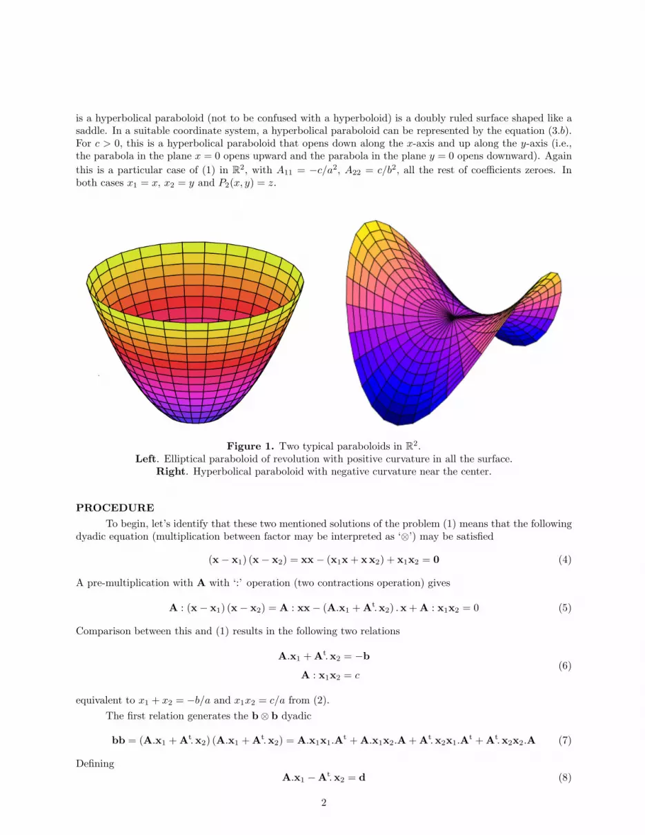
is a hyperbolical paraboloid (not to be confused with a hyperboloid) is a doubly ruled surface shaped like asaddle. In a suitable coordinate system, a hyperbolical paraboloid can be represented by the equation (3.b).For c > 0, this is a hyperbolical paraboloid that opens down along the x-axis and up along the y-axis (i.e.,the parabola in the plane x = 0 opens upward and the parabola in the plane y = 0 opens downward). Againthis is a particular case of (1) in R2, with A11 = −c/a2, A22 = c/b2, all the rest of coefficients zeroes. Inboth cases x1 = x, x2 = y and P2(x, y) = z.

Figure 1. Two typical paraboloids in R2.Left. Elliptical paraboloid of revolution with positive curvature in all the surface.

Right. Hyperbolical paraboloid with negative curvature near the center.

PROCEDURETo begin, let’s identify that these two mentioned solutions of the problem (1) means that the following

dyadic equation (multiplication between factor may be interpreted as ‘⊗’) may be satisfied

(x − x1) (x − x2) = xx − (x1x + xx2) + x1x2 = 0 (4)

A pre-multiplication with A with ‘:’ operation (two contractions operation) gives

A : (x − x1) (x − x2) = A : xx − (A.x1 + At.x2) .x + A : x1x2 = 0 (5)

Comparison between this and (1) results in the following two relations

A.x1 + At.x2 = −b

A : x1x2 = c(6)

equivalent to x1 + x2 = −b/a and x1x2 = c/a from (2).The first relation generates the b⊗ b dyadic

bb = (A.x1 + At.x2) (A.x1 + At.x2) = A.x1x1.At + A.x1x2.A + At.x2x1.At + At.x2x2.A (7)

DefiningA.x1 − At.x2 = d (8)

2

a dyadic of d may also be obtained in a similar manner

dd = (A.x1 − At.x2) (A.x1 − At.x2) = A.x1x1.At − A.x1x2.A − At.x2x1.At + At.x2x2.A (9)

The subtraction between bb and dd results in

∆ = dd = bb − 2 (A.x1x2.A + At.x2x1.At ) (10)

the equivalent to ∆ = b2 − 4ac in (2).

RESOLVENT

The following expressions come from the second relation (6.b)

A .x1 = cx2

‖x2‖2At.x2 = c

x1

‖x1‖2‖xi‖2 = xi .xi (11)

with ‖ · ‖ the euclidean 2-norm ‖ · ‖2 of a vector (no sum on ‘ i ’, i = 1, 2). Substitution in the last twoterms of (10) results in

A.x1x2.A + At.x2x1.At = c2 x2x1 + x1x2

‖x1‖2 ‖x2‖2(12)

Multiplication with A with operation ‘ : ’ to (10), after substitution of (12), gives the expression

A : dd = A : bb − 4 c3

‖x1‖2 ‖x2‖2(13)

which may be taken to obtain d, the equivalent to√

∆ in (2). Once d is obtained two solutions of (1) maybe calculated by the semi-summation and semi-subtraction of (6.a) and (8)

x1 = − 12 A−1. (b − d ) x2 = − 1

2 A−t. (b + d ) (14)

The dyadic dd may be seen as a discriminant, like ∆ in (2). When dd = O, d = 0 with A symmetrical,we obtain only one solution, and x1 = x2 is only one closed curve. In other case, it depends on the valueof d =

√d.d (a contraction in ∆ = dd is necessary). If d ∈ Rn is a negative vector (partial or totally),

d.d = ‖d‖2 is always positive by definition. If d ∈ Cn, d.d may be negative, for instance, in the imaginarycase. The result A : dd negative is imposible, because the initial restriction of A was to be a definite positiveform A : xx ≥ 0 ∀x. We shall come back to (13) later in order to obtain d.

The problem with this procedure is that it states a vicious circle. We need ‖xi‖ to obtain d and thusobtain xi. This vicious circle may be interrupted declaring s = ‖xi‖ as a parameter of the curves xi(s), andthen the resolvent (14) becomes the solution of obtaining the interception of those curves with this lengthdistance s (the parameter s should be the radius in polar coordinates of the curve) to the origin in theP2(x) = 0 hyperplane.

This parameter s is related by

s4 = ‖x1‖2 ‖x2‖2 =4 c3

A : (bb− dd )≥ ( ‖b‖2 + ‖d‖2 )2 − 4 (b.d )2

16 ‖A‖4(15)

where the middle member is obtained from the norms of (14)

4 ‖A‖2 ‖x1‖2 ≥ ‖b‖2 + ‖d‖2 − 2b.d 4 ‖A‖2 ‖x2‖2 ≥ ‖b‖2 + ‖d‖2 + 2b.d (16)

3

The norm used for both vectors and matrixes (subordinated to the vectors) is the euclidean 2-norm (see [1]for instance)

‖A‖2 =√

ρ(At.A) ‖x‖2 =√

x.x ‖A.x‖2 = ‖A‖2 ‖x‖2 ‖At‖2 = ‖A‖2 (17)

The operator ρ is the spectral radius of matrix A defined on its eigenvalues λk.When c = 0 then d = b according to (13) and the solutions according with (14) are x1 = 0, the vertex

of the paraboloid, and x2 = −A−t. b.

EIGENVALUESSummarized definitions of eigenvalues λ and eigenvectors e are presented by (see [2] for instance)

A.e = λ e P (λ) = det(A − λI) = 0 ρ(A) = max1≤i≤k

|λi|λ = α + iβ

|λ| =√

α2 + β2(18)

P (λ) is the characteristic polynomial whose roots are the eigenvalues. ρ is the spectral radius. The multiplicitydk of the eigenvalue λk originate several subspaces Wk, whose union is the complete space V = Rn

P (λ) =k∏

i=1

(λ − λi)di

k∑i=1

dim Wi = dim V = n dim Wi = di (19)

Define the matrix S with columns being the eigenvectors ei,j (j ≤ di, it can be more than one eigenvectorfor each eigenvalue) that generate subspace Wi for each eigenvalue λi (1 ≤ i ≤ k ≤ n)

(A − λi I) .x = 0 S = [S1,S2, . . . ,Sk ] = [ IB1, IB2, . . . , IBk ] (20)

The linear system (20.a) serves to obtain the components of each eigenvector ei,j in the construction of S.Each base IBi contents the number di of eigenvectors that generate the subspace Wi. Then, the matrix Sdiagonalizes A in this manner

A .S = Λ.S = S.Λ S−1.A .S = Λ = diag{λ1, λ2, . . . , λk } (21)

The value λi may be repeated in matrix Λ depending on di. The matrixes A and Λ (over F = R) aresimilar and matrixes S and Λ permute. When matrix A is symmetrical (or hermitic in the complex case) alleigenvalues are real, transformation S is also orthogonal (when eigenvectors are normalized), and A and Λ(over F = R) are also congruent.

TRANSFORMATIONSNow we get back to the equation (13). We may find a transformation Q, such that

x = Q.x A = Qt.A.Q = I (22)

No matter there may be some complex (imaginary) components of the matrix in the case of some negativeeigenvalues. But this matrix is not necessarily hermitian or unitary. With the help of this transformationthe vector d may be obtained as

A : dd = A : dd = A : dd = d.d ‖d‖′ =√

d.d =√

A : dd d = ‖d‖′ e d = Q.d (23)

with d an intermediate transformation (x = S.x). This complete the resolvent (14). Although d may haveimaginary components when negative eigenvalues, ‖d‖′ in (23.b) has been calculated as it would not becomplex (this is why the ‘ ′ ’ mark), however, the norm ‖e‖ =

√e∗.e = 1 make it general, e may be complex

4

or not. Then redefine e′ = e/‖e‖′, where ‖e‖′ =√|e.e| = 0, and use it in the place of e in (23.c) (when

|e.e| = 0 or d ∈ Rn avoid this and the ‘ ′ ’ mark has not importance). This last procedure revert the differencebetween d and e norms calculation, if e is selected with ‖e‖ = 1.

For the purpose of (23.a) through (22) transformation (The matrix S should also be seen as a lineartransformation, when A is symmetrical, also S is orthogonal S−1 = St, rigid transformation, if the eigenvec-tors, normalized as e = e/‖e‖, are also orthogonal between them), this transformation matrix Q is calculatedby

d = L−1. d =√

Λ . d =√

Λ .S−1.d = Q−1.d Q = S .(√

Λ)−1 = S.L (24)

where it may be taken into account these definitions

A = S−1.A .S = Λ d = S.d L = (√

Λ)−1 A = Lt. A .L = Qt.A .Q (25)

which complete (23.a). The last relation (25.d) only have sense when S is orthogonal. With these transfor-mations the equation (1) becomes

P2(x) = Λ : xx + b.x + c = x.x + b.x + c = 0 (26)

where x = S.x = Q.x , b = St.b and b = Qt.b. This last conversion facilitates the solving in any manner.

The matrixes A, A = Λ (over F = R), and A = I (over F = C) are all congruent. The matrices A andA = I (over F = C) are only congruent, but A = Λ (over F = R) is additionally similar only in the case whenA is symmetrical. Exclusively, the operation ‘ : ’ in the first term of (1) accepts only congruent matrixes (see(23.a) where the transformations are in cascade), that is why is important to define A symmetrical and thetransformation S orthogonal (this is obtained when eigenvectors are an orthonormal base).

The sequence of transformations may be seen as x = Q.x is equivalent to x = S.x and x = L.x.The square root and inversion of a matrix do not commutate over Λ for some λi imaginary. The followingexpression justify this: The quantities

√1/i =

√−i = i√

i and 1/√

i =√

i/i = −i√

i are not the same unlessthey are squared.

At this level, a residuary problem to solve x is to obtain e in (23.c). This is made by taken, for examplein R2 all eigenvalues positive, the vector {e} = {cos θ, sin θ} (when any of the eigenvalue is negative the valueof e should be consistent to give a value d = Q.d in Rn. A convenient imaginary “−i ” in the places ofthe negative eigenvalues is enough to cancel the effect of (

√Λ)−1 in Q within (24.b)), and when any of the

solutions (14) coincide their norm ‖x‖ with s, the solution is the correct and the value of θ is the adequate.In the general case Rn, the vector e = e(θ) is a function of θ, where θ ∈ Rn−1 are the combination of (n− 1)rotations with angles θ1, . . . , θn−1, around (n − 1) different axes x2, . . . , xn, that makes to coincide axis x1

direction with changing radius vector x = e direction, in the (n-dimensional) sphere Sn(0, 1) of unit radiusand centred in x = 0. In the space of x ∈ Rn, is equivalent to change the coordinates from {x} to {s, θ}, forexample in R3, the cartesian coordinates {x} = {x1, x2, x3} in the spherical coordinates are {x} = {s, θ1, θ2},where s = ‖x‖, θ1 is the zenithal angle and θ2 is the azimuthal angle. All these changes of coordinates areisomorphic, and there is an unique correspondence between θ and θ.

Remember that s = ‖x1‖ = ‖x2‖ and ‖d‖ ≤ ‖Q‖ ‖d‖. As it will be seen below, s changes from themajor to the minor ‖x‖ =

√|c/λi|, when eigenvalues λi are ordered from the minor to the major absolutevalues. Until now we have taken s = ‖x1‖ = ‖x2‖, but we can take s = ‖x1‖ and t = ‖x2‖ in (13) so we havetwo procedures

A : dd = A : bb− 4 c3

s4A : dd = A : bb − 4 c3

s2 t2(27)

At the left the standard prime proposed solution procedure, at the right a new procedure where may use thetendencies t → 0 and s → ∞ in the case of the hyperbola type solution with mixed positive and negative

5

eigenvalues of A. One may fix t and evolves s maintaining A : ∆ = A : dd > 0. The parameter t ∈ (0, tmax]is an auxiliary value that changes the discriminant ∆ = dd in (27.b) and permits to obtain the hyperbolatype solution on the parameter s = ‖x‖ ∈ [smin,∞). The value smin = tmax =

√|c/λi|, being |λi| themajor absolute eigenvalue, is the only value where t and s coincide, and they are respectively the minoraxis points in ellipses of figures 2, 3 right and the vertex points in hyperbolas of figures 4, 5 right, in theexamples below. Then s = ‖x1‖ and ‖x2‖ (not t) are two open curves depending on parameter s, for tvalues in its range. A precise combinations of s and t are necessary to obtain the solutions and there is anunique correspondence between them. Imagine θ is a tuner (of one turn θ ∈ (−π, π] for R2) that modules s,for one of the two procedures (27), until s and ‖xi‖ coincide. Expression (27.a) for the case of all positiveeigenvalues, expression(27.b) for the case of some negative eigenvalues. Despite this tuner may be consideredso fine (with 6000 or 12000 selections for ∆‖x‖ of 10−2 or 10−4), tolerances εmax and δmax must be imposedon absolute errors ε = |s−‖x‖| and absolute deviations δ = |P2(x)| (with values 0.35 and 0.40, respectively).

For b = 0 and A symmetrical, the solutions are opposite x1 = −x2 in a centred paraboloid as we shallsee in the next section. The limits

√|c/λi| for t and s intervals in the previous paragraph will be justifiedthere.

CENTRED

The vertex of a paraboloid is the point xv = −A−1.b/2 (also with A−t instead A−1). A paraboloidwith b = 0 has xv = 0 and is said to be centred, like the unidimensional situation where the vertex positionxv = −b/(2a) is centred in x = 0, the parabola has a minimum or maximum value P2(xv) = c − b2/(4a) inthe vertex, according a > 0 or a < 0, respectively, and the solutions x1,2 = ±√−c/a are opposite. This isthe case for opposite solutions x1 = −x2 with symmetrical A. The general solutions from (14) for centredparaboloid (i.e. non symmetrical A) are

x1 = 12 A−1. d x2 = − 1

2 A−t. d (28)

This procedure is the same as decribed above.Another alternative is based in this analysis. With b = 0, we shall use (1) without the central term

(without any loss of generality we changed the sign of c)

A : xx = (A.x).x = c A.x =c

‖x‖2x (29)

and recalling (18.a) we find

A.e = λ e λ =c

‖x‖2‖x‖ =

√c/λ x = ‖x‖ e (30)

that is the solution through the eigenvalues λ and eigenvectors e (the sign of the value of λ must be takenas the sign of the value of c to be solvable). We obtain several solutions as eigenvectors ei we have for eacheigenvalue λi > 0. For negative eigenvalues, the comparison (30.b) is already not valid for c > 0, and viceversa. The linear combinations of these will give any of the solutions (28).

One way to obtain t in this case (A symmetrical and b = 0) is by (27.b) and (28) as

s t =√| c3/x.A3.x | A3 = At.A.A or A3 = A.A.At (31)

for every x and s = ‖x‖. For the instance of A non symmetrical, the A3 in the previous equation becomesone of the last two expressions according we deal with x = x1 or x = x2.

The solution of non-centred problem will be displaced respect to the centred one in ∆x = − 12A

−1.b(A symmetrical) according to (14).

6

EXAMPLESFor R2 the general equation (1), with x1 = x, x2 = y and P2(x, y) = 0 gives an ellipse ∆ < 0, a

hyperbola ∆ > 0 or a parabola ∆ = 0 (∆ = B2 − 4AC, A = A11, B = 2A12 = 2A21, C = A22). For R3

with z = P2(x) the surface are called elliptical or hyperbolical paraboloids according to ∆ < 0 or ∆ > 0,respectively.

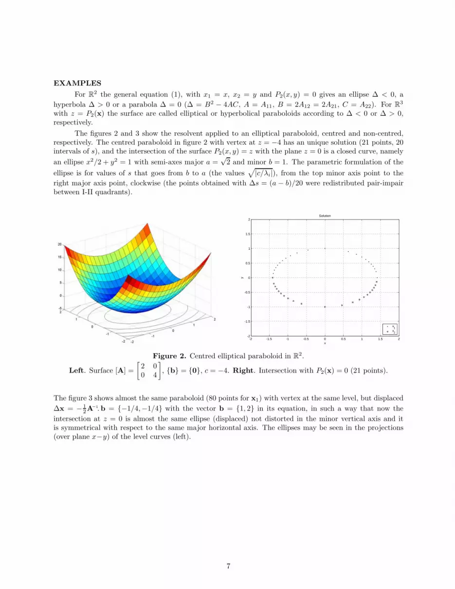
The figures 2 and 3 show the resolvent applied to an elliptical paraboloid, centred and non-centred,respectively. The centred paraboloid in figure 2 with vertex at z = −4 has an unique solution (21 points, 20intervals of s), and the intersection of the surface P2(x, y) = z with the plane z = 0 is a closed curve, namelyan ellipse x2/2 + y2 = 1 with semi-axes major a =

√2 and minor b = 1. The parametric formulation of the

ellipse is for values of s that goes from b to a (the values√|c/λi|), from the top minor axis point to the

right major axis point, clockwise (the points obtained with ∆s = (a − b)/20 were redistributed pair-impairbetween I-II quadrants).

-2 -1.5 -1 -0.5 0 0.5 1 1.5 2-2

-1.5

-1

-0.5

0

0.5

1

1.5

2

y

x

Solution

x1

x2

Figure 2. Centred elliptical paraboloid in R2.

Left. Surface [A] =[

2 00 4

], {b} = {0}, c = −4. Right. Intersection with P2(x) = 0 (21 points).

The figure 3 shows almost the same paraboloid (80 points for x1) with vertex at the same level, but displaced∆x = − 1

2A−1.b = {−1/4,−1/4} with the vector b = {1, 2} in its equation, in such a way that now the

intersection at z = 0 is almost the same ellipse (displaced) not distorted in the minor vertical axis and itis symmetrical with respect to the same major horizontal axis. The ellipses may be seen in the projections(over plane x−y) of the level curves (left).

7

-2 -1.5 -1 -0.5 0 0.5 1 1.5 2-2

-1.5

-1

-0.5

0

0.5

1

1.5

2

y

x

Solution

x1

x2

Figure 3. Non centred elliptical paraboloid in R2.

Left. Surface [A] =[

2 00 4

], {b} =

{12

}, c = −4. Right. Intersection with P2(x) = 0 (21 points).

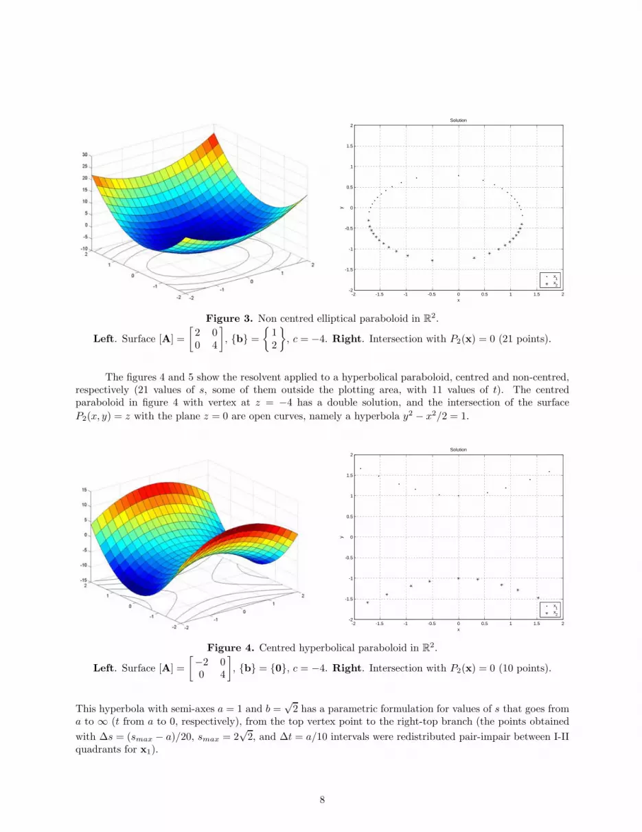
The figures 4 and 5 show the resolvent applied to a hyperbolical paraboloid, centred and non-centred,respectively (21 values of s, some of them outside the plotting area, with 11 values of t). The centredparaboloid in figure 4 with vertex at z = −4 has a double solution, and the intersection of the surfaceP2(x, y) = z with the plane z = 0 are open curves, namely a hyperbola y2 − x2/2 = 1.

-2 -1.5 -1 -0.5 0 0.5 1 1.5 2-2

-1.5

-1

-0.5

0

0.5

1

1.5

2

y

x

Solution

x1

x2

Figure 4. Centred hyperbolical paraboloid in R2.

Left. Surface [A] =[−2 0

0 4

], {b} = {0}, c = −4. Right. Intersection with P2(x) = 0 (10 points).

This hyperbola with semi-axes a = 1 and b =√

2 has a parametric formulation for values of s that goes froma to ∞ (t from a to 0, respectively), from the top vertex point to the right-top branch (the points obtainedwith ∆s = (smax − a)/20, smax = 2

√2, and ∆t = a/10 intervals were redistributed pair-impair between I-II

quadrants for x1).

8

-2 -1.5 -1 -0.5 0 0.5 1 1.5 2-2

-1.5

-1

-0.5

0

0.5

1

1.5

2

y

x

Solution

x1

x2

Figure 5. Non centred hyperbolical paraboloid in R2.

Left. Surface [A] =[−2 0

0 4

], {b} =

{12

}, c = −4. Right. Intersection with P2(x) = 0 (17 points).

The branches of the centred hyperbola open vertically upward and downward with tangent lines y =±(a/b)x = ± tan β x (asymptotes). This tangent lines or asymptotes may be seen as an oblique systemof coordinates with basis (covariant) ei′ ={±b, a}/√a2 + b2 = {± cosβ, sin β} = {±√

6/3,√

3/3} and coordi-nates (contravariant)

x′ = ssin(θ′ + 2β)

sin 2β= t

sin 2β

sin θ′→ s y′ = s

sin θ′

sin 2β= t

sin 2β

sin(θ′ + 2β)→ t x′y′ = k2 (32)

that satisfy the last expression (32.c) of inverse proportionality ( s t = k2, k =√

a2 + b2/2 =√

3/2, cos θ′ =x.ex′/s ). The vertexes are vertically separated a distance 2a. The figure 5 shows almost the same paraboloidwith vertex at the same level, but displaced ∆x = − 1

2A−1.b = {1/4,−1/4} with the vector b = {1, 2} in

its equation, in such a way that now the intersection at z = 0 is almost (displaced) the same hyperbola notdistorted in the minor axis and it is symmetrical with respect to the same major vertical axis. The hyperbolasmay be seen in the projections (over plane x−y) of the level curves (left).

The figure 6 contains the results of obtaining t by two methods. This exercise was made only forcentred paraboloid (b = 0) in order to obtain the unique analytical correspondence between s and t. Butit was unsuccessful as it can be seen. We obtain td by the method proposed by equations (31) and th bythe method proposed by equations (32). The results are shown in figure 6 and exists a significant difference.The values td obtained with the discriminant d are the actual value that corresponds with the curve of thehyperbola, whereas the value th is the proposed formulation. Although the tendency is the same, there is asubstantial discrepancy when θ′ → 0 in the extreme of the hyperbola branch and the dependence of (32.a, b)with respect to t is invalid. The dependence with respect to s is valid anyway. The tendency st → k2 is alsowrong and it is better to use (31) s t =

√| c3/x.A3.x | =√

(1 + 3x2/8)−1 with x = {x, a√

1 + (x/b)2} and

s = ‖x‖ = a√

1 + (a2 + b2)x2/(a2b2) =√

1 + 1.5 x2, curve for td in figure 6, rather than th.

9

0 2 4 6 8 10 12 14 16 18 200

0.1

0.2

0.3

0.4

0.5

0.6

0.7

0.8

0.9

1

t ,

y / 1

0

x

Parameter , Distance

td (discr.)

th (hyper.)

HyperbolaAsymptote

Figure 6. Parameter t calculated by two methods.

In practice, we modulated θ for each combination of s and t and when the result of x is adequate inerror ε and deviation δ (within tolerances) these values are conserved and the result is printed graphically,otherwise the seeking is continued for the next combination. This only occur when there is a negativeeigenvalue. For all positive eigenvalue the modulation is only for seeking s. Finally, the results are eloquentas it may be seen in figure 4 and 5.

REFERENCES[1] Burden, R. L.; Faires, J. D. Numerical Analysis, 9th Edition. Brooks/Cole, Cengage Learning,

Boston, 2011.

[2] Hoffman, K.; Kunze, R. Linear Algebra, 2nd Edition. Prentice-Hall, Englewood Cliff, New Jersey,1971.

10