�����������������

Citation: Le Quilleuc, A.; Collin, A.;

Jasinski, M.F.; Devillers, R. Very

High-Resolution Satellite-Derived

Bathymetry and Habitat Mapping

Using Pleiades-1 and ICESat-2.

Remote Sens. 2022, 14, 133. https://

doi.org/10.3390/rs14010133

Academic Editors: Simona Niculescu,

Junshi Xia and Dar Roberts

Received: 1 November 2021

Accepted: 22 December 2021

Published: 29 December 2021

Publisher’s Note: MDPI stays neutral

with regard to jurisdictional claims in

published maps and institutional affil-

iations.

Copyright: © 2021 by the authors.

Licensee MDPI, Basel, Switzerland.

This article is an open access article

distributed under the terms and

conditions of the Creative Commons

Attribution (CC BY) license (https://

creativecommons.org/licenses/by/

4.0/).

remote sensing

Article

Very High-Resolution Satellite-Derived Bathymetry andHabitat Mapping Using Pleiades-1 and ICESat-2Alyson Le Quilleuc 1,*, Antoine Collin 2,3 , Michael F. Jasinski 4 and Rodolphe Devillers 5

1 ENSTA Bretagne Engineering School, 29200 Brest, France2 Section des Sciences de la Vie et de la Terre, EPHE-PSL University, CNRS LETG, 35800 Dinard, France;

antoine.collin@ephe.psl.eu3 LabEx CORAIL, BP 1013, 98729 Papetoai, French Polynesia4 NASA, Goddard Space Flight Center, Greenbelt, MD 20771, USA; michael.f.jasinski@nasa.gov5 Espace-Dev (IRD-UM-UG-UR-UA-UNC), 34934 Montpellier, France; rodolphe.devillers@ird.fr* Correspondence: alyson.le_quilleuc@ensta-bretagne.org

Abstract: Accurate and reliable bathymetric data are needed for a wide diversity of marine researchand management applications. Satellite-derived bathymetry represents a time saving method tomap large shallow waters of remote regions compared to the current costly in situ measurementtechniques. This study aims to create very high-resolution (VHR) bathymetry and habitat mapping inMayotte island waters (Indian Ocean) by fusing 0.5 m Pleiades-1 passive multispectral imagery andactive ICESat-2 LiDAR bathymetry. ICESat-2 georeferenced photons were filtered to remove noiseand corrected for water column refraction. The bathymetric point clouds were validated using theFrench naval hydrographic and oceanographic service Litto3D® dataset and then used to calibratethe multispectral image to produce a digital depth model (DDM). The latter enabled the creation of adigital albedo model used to classify benthic habitats. ICESat-2 provided bathymetry down to 15 mdepth with a vertical accuracy of bathymetry estimates reaching 0.89 m. The benthic habitats mapproduced using the maximum likelihood supervised classification provided an overall accuracy of96.62%. This study successfully produced a VHR DDM solely from satellite data. Digital models ofhigher accuracy were further discussed in the light of the recent and near-future launch of higherspectral and spatial resolution satellites.

Keywords: bathymetry; Mayotte; marine habitat; coral reefs; ICESat-2; Pleiades-1; LiDAR; VHRmultispectral imagery

1. Introduction

Mapping coastal areas is essential to tackle a broad range of environmental and socialissues [1–3]. Therefore, a wide variety of scientific research disciplines could benefit from abetter knowledge of this interface, especially regarding the monitoring and protection ofcoral reefs in archipelagos or the production of navigational charts [4].

Numerous reliable and accurate techniques exist to acquire bathymetric soundings.Data are often obtained through marine surveys equipped with multibeam or single-beamechosounders [5]. However, these approaches are usually impracticable in remote andshallow areas as well as time consuming and limited in terms of spatial coverage, andtherefore remain costly. As an alternative, remote sensing is increasingly used to retrievecoastal bathymetry. Airborne data acquired with bathymetric LiDAR are useful to maplarger areas but remain costly and limited spatially [6,7].

Over the past few years, satellite-derived bathymetry (SDB) has been increasinglyused as it offers a more affordable and time saving alternative. Scientific studies havedemonstrated the possibility of obtaining reliable bathymetric data through hyperspectraland multispectral (MS) imagery at various spatial resolutions, due to a correlation betweenwater depth and reflectance data [8–11]. Nevertheless, SDB mostly relies on passive imagery,

Remote Sens. 2022, 14, 133. https://doi.org/10.3390/rs14010133 https://www.mdpi.com/journal/remotesensing

Remote Sens. 2022, 14, 133 2 of 23

which strongly constrains its use to clear and shallow water areas [12,13]. Depth can beretrieved from satellite MS imagery using physics-based or empirical models. Physics-based models rely on the physics or the radiative transfer of light in the water column andthe physical properties of the water constituents that can be estimated with or without fieldmeasurements of depth for calibration. Some physics-based models are entirely based onthe inversion of the radiative transfer model, such as WASI and BOMBER, but they canbe complex to implement [14–16]. On the other hand, empirical models are limited by theneed to calibrate the MS imagery with in situ measurements [17,18].

There is a real need for producing bathymetric data solely from satellite images. Inthis context, the launch of the NASA Ice, Cloud, and Land Elevation Satellite-2 (ICESat-2)in September 2018 offered new prospects [19]. This satellite aims to monitor the cryosphereand terrestrial biosphere using the green 532 nm LiDAR with photon-counting capability.Pre-launch studies highlighted its potential to penetrate the upper part of the water columnand reach the bottom [20]. A pioneer study has recently validated accurate ICESat-2bathymetry retrieval at 38 m depth in very clear waters [21]. A second relevant studyused ICESat-2 bathymetric measurements, down to 18 m depth, to calibrate and validateSentinel-2 imagery at 10 m pixel size [17]. This spatial resolution nonetheless remainslimiting for some applications (e.g., marine ecology, navigation).

Our paper aims to create a higher resolution digital depth model (DDM) by fusingactive ICESat-2 bathymetric soundings and 0.5 m Pleiades-1 passive MS imagery in orderto provide very high-resolution (VHR) satellite-based bathymetry and habitat maps of thecoral reefscapes in Mayotte. First, a density-based algorithm was implemented on ICESAt-2ATL03 L2 dataset to remove the noise in photon data and detect the water surface. The noisearises from several sources, including the laser pulse being scattered by the atmosphere,the solar background noise effects, and the detector dark noise. In our study, the main noisesource is associated with photons that are scattered by particles in the water column [22].Based on this first clustering, photons from the seabed were identified and corrected for therefraction effect occurring at the air-water interface. Producing bathymetric maps requiresfinding a function that describes the relationship between bathymetry measurements andthe remotely sensed spectral values of the satellite image [8]. In this study, we used the bandratio model developed by [23]. First, we derived the above water surface reflectance logratio of two spectral bands. Then, we characterized the relationship between the ratio andICESat-2 water depth measurements [17]. Therefore, this study innovatively produces aVHR DDM and VHR benthic habitats map of the area from satellite data without a need forin situ measurements. Bathymetric data were used to remove the effect of the water columnand generate a digital albedo model (DAM) to classify benthic habitats [24–27]. Finally, thevertical accuracy of the predicted depths was assessed by comparing the bathymetric datato the French naval hydrographic and oceanographic service SHOM bathymetric LiDARand multibeam echosounder reference dataset (Litto3D®). Classification performanceswere evaluated using a confusion matrix.

2. Materials and Methods2.1. Study Site and Data2.1.1. Study Site

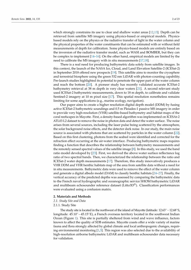
The study site is located in the northwest of the island of Mayotte (latitude: 12.63◦−12.68◦S,longitude: 45.10◦−45.15◦E), a French overseas territory located in the southwest IndianOcean (Figure 1). This site is partially sheltered from wind and wave influence, factorsknown to affect the quality of SDB estimates. Mayotte coasts offer a wide variety of marinefauna and flora strongly affected by global climate and local anthropogenic changes, requir-ing environmental monitoring [1,3]. This region was also selected due to the availability ofhigh-resolution airborne bathymetric LiDAR and multibeam echosounder data necessaryfor validation.

Remote Sens. 2022, 14, 133 3 of 23

Remote Sens. 2021, 13, x FOR PEER REVIEW 3 of 24

due to the availability of high-resolution airborne bathymetric LiDAR and multibeam echosounder data necessary for validation.

Water clarity is a key parameter in SDB estimation. Clarity is related to light ray pen-etration in the water column, thus impacting the quality and quantity of the available bathymetric soundings [27–31]. This variable can be estimated using a diffuse attenuation coefficient of 490 nm measured at 4 km resolution by the moderate-resolution imaging spectroradiometer (MODIS-Aqua, publicly accessible from https://ocean-color.gsfc.nasa.gov/l3/, last accessed: 28 December 2021) [32]. A diffuse attenuation coef-ficient value of 0.0615 m−1 was obtained for the month of May 2020 for the study site, indicating a very clear water type. Previous studies using ICESat-2 for bathymetric esti-mations had a diffuse attenuation coefficient ranging from 0.032 m−1 for the Virgin Island to 0.123 m−1 for the Bahamas, both known to be areas with very clear water [21,33].

Figure 1. Map of the ground tracks of ICESat-2 over Mayotte collected on 14 May 2020. The satellite multispectral imagery was acquired by Pleiades-1A on 25 May 2020. The red square identifies the study area.

2.1.2. Litto3D® Reference Dataset The French Oceanographic and Hydrographic Marine Service (SHOM) and the

French National Institute for Geographical and Forest Information (IGN) conducted a joint altimetric and hydrographic survey of Mayotte from 2003 to 2010. Most of the island was mapped using the airborne topographic and bathymetric LiDAR and multibeam echosounder. The resulting Litto3D® product provides soundings located in a three-di-mensional geometric reference system with high spatial resolution and a land-sea contin-uum (data are available for free from https://diffusion.shom.fr/, last accessed: 28 Decem-ber 2021). Data extracted from this dataset, corresponding to the ICESat-2 ground track, and used for comparison, include bathymetric points acquired using the bathymetric Li-DAR and multibeam echosounder.

Litto3D® soundings are provided in a cartesian coordinate system in the horizontal plane and with orthometric heights. The point cloud density is constrained by the acqui-sition method over a specific area and the gridded model is provided with a spatial spac-ing of either 1 m or 5 m. Specification regarding the positioning and the geodesy of the

Figure 1. Map of the ground tracks of ICESat-2 over Mayotte collected on 14 May 2020. The satellitemultispectral imagery was acquired by Pleiades-1A on 25 May 2020. The red square identifies thestudy area.

Water clarity is a key parameter in SDB estimation. Clarity is related to light raypenetration in the water column, thus impacting the quality and quantity of the availablebathymetric soundings [27–31]. This variable can be estimated using a diffuse attenuationcoefficient of 490 nm measured at 4 km resolution by the moderate-resolution imagingspectroradiometer (MODIS-Aqua, publicly accessible from https://oceancolor.gsfc.nasa.gov/l3/, last accessed: 28 December 2021) [32]. A diffuse attenuation coefficient value of0.0615 m−1 was obtained for the month of May 2020 for the study site, indicating a veryclear water type. Previous studies using ICESat-2 for bathymetric estimations had a diffuseattenuation coefficient ranging from 0.032 m−1 for the Virgin Island to 0.123 m−1 for theBahamas, both known to be areas with very clear water [21,33].

2.1.2. Litto3D® Reference Dataset

The French Oceanographic and Hydrographic Marine Service (SHOM) and the FrenchNational Institute for Geographical and Forest Information (IGN) conducted a joint altimet-ric and hydrographic survey of Mayotte from 2003 to 2010. Most of the island was mappedusing the airborne topographic and bathymetric LiDAR and multibeam echosounder. Theresulting Litto3D® product provides soundings located in a three-dimensional geometricreference system with high spatial resolution and a land-sea continuum (data are availablefor free from https://diffusion.shom.fr/, last accessed: 28 December 2021). Data extractedfrom this dataset, corresponding to the ICESat-2 ground track, and used for compari-son, include bathymetric points acquired using the bathymetric LiDAR and multibeamechosounder.

Litto3D® soundings are provided in a cartesian coordinate system in the horizontalplane and with orthometric heights. The point cloud density is constrained by the ac-quisition method over a specific area and the gridded model is provided with a spatialspacing of either 1 m or 5 m. Specification regarding the positioning and the geodesy ofthe Litto3D® dataset are presented in Table 1 [34]. A local geoid, RGM04, was used as areference for this dataset.

Remote Sens. 2022, 14, 133 4 of 23

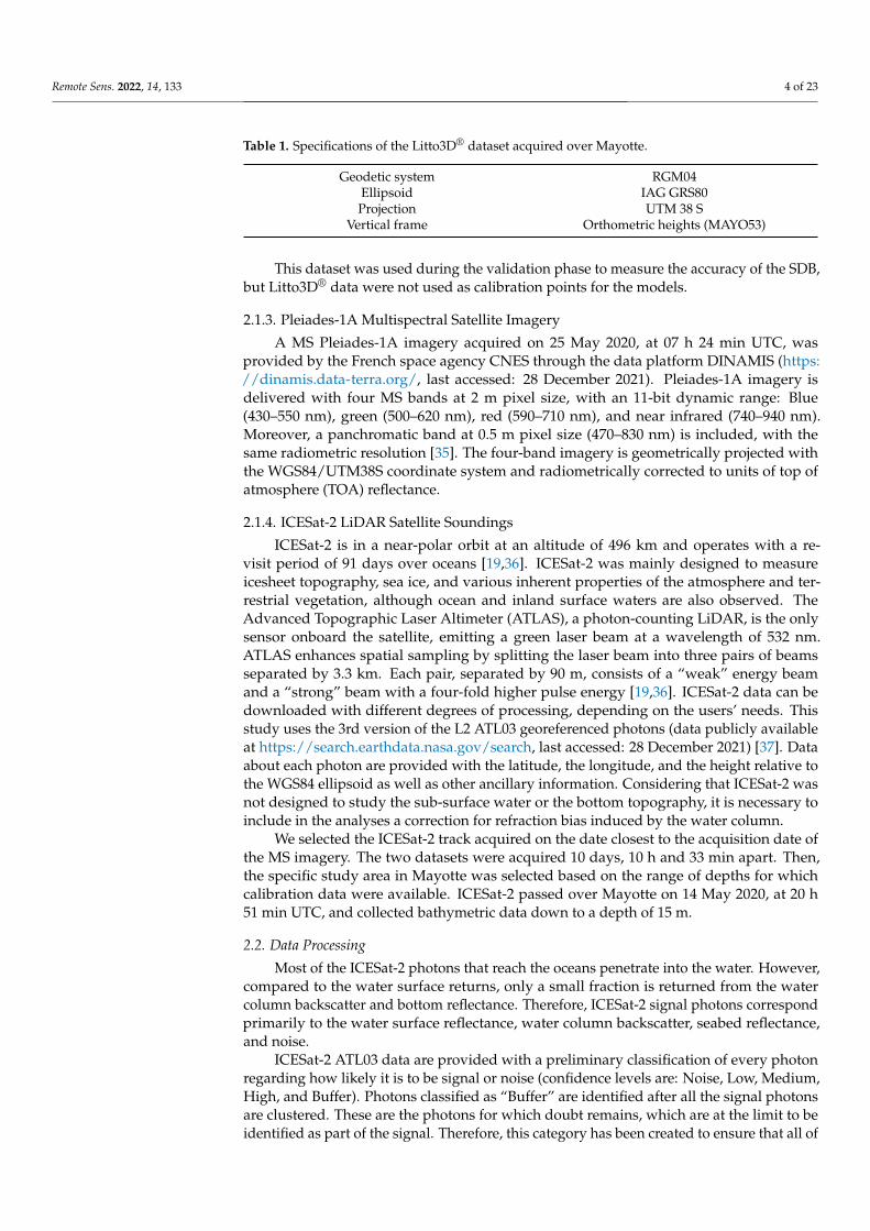
Table 1. Specifications of the Litto3D® dataset acquired over Mayotte.

Geodetic system RGM04Ellipsoid IAG GRS80Projection UTM 38 S

Vertical frame Orthometric heights (MAYO53)

This dataset was used during the validation phase to measure the accuracy of the SDB,but Litto3D® data were not used as calibration points for the models.

2.1.3. Pleiades-1A Multispectral Satellite Imagery

A MS Pleiades-1A imagery acquired on 25 May 2020, at 07 h 24 min UTC, wasprovided by the French space agency CNES through the data platform DINAMIS (https://dinamis.data-terra.org/, last accessed: 28 December 2021). Pleiades-1A imagery isdelivered with four MS bands at 2 m pixel size, with an 11-bit dynamic range: Blue(430–550 nm), green (500–620 nm), red (590–710 nm), and near infrared (740–940 nm).Moreover, a panchromatic band at 0.5 m pixel size (470–830 nm) is included, with thesame radiometric resolution [35]. The four-band imagery is geometrically projected withthe WGS84/UTM38S coordinate system and radiometrically corrected to units of top ofatmosphere (TOA) reflectance.

2.1.4. ICESat-2 LiDAR Satellite Soundings

ICESat-2 is in a near-polar orbit at an altitude of 496 km and operates with a re-visit period of 91 days over oceans [19,36]. ICESat-2 was mainly designed to measureicesheet topography, sea ice, and various inherent properties of the atmosphere and ter-restrial vegetation, although ocean and inland surface waters are also observed. TheAdvanced Topographic Laser Altimeter (ATLAS), a photon-counting LiDAR, is the onlysensor onboard the satellite, emitting a green laser beam at a wavelength of 532 nm.ATLAS enhances spatial sampling by splitting the laser beam into three pairs of beamsseparated by 3.3 km. Each pair, separated by 90 m, consists of a “weak” energy beamand a “strong” beam with a four-fold higher pulse energy [19,36]. ICESat-2 data can bedownloaded with different degrees of processing, depending on the users’ needs. Thisstudy uses the 3rd version of the L2 ATL03 georeferenced photons (data publicly availableat https://search.earthdata.nasa.gov/search, last accessed: 28 December 2021) [37]. Dataabout each photon are provided with the latitude, the longitude, and the height relative tothe WGS84 ellipsoid as well as other ancillary information. Considering that ICESat-2 wasnot designed to study the sub-surface water or the bottom topography, it is necessary toinclude in the analyses a correction for refraction bias induced by the water column.

We selected the ICESat-2 track acquired on the date closest to the acquisition date ofthe MS imagery. The two datasets were acquired 10 days, 10 h and 33 min apart. Then,the specific study area in Mayotte was selected based on the range of depths for whichcalibration data were available. ICESat-2 passed over Mayotte on 14 May 2020, at 20 h51 min UTC, and collected bathymetric data down to a depth of 15 m.

2.2. Data Processing

Most of the ICESat-2 photons that reach the oceans penetrate into the water. However,compared to the water surface returns, only a small fraction is returned from the watercolumn backscatter and bottom reflectance. Therefore, ICESat-2 signal photons correspondprimarily to the water surface reflectance, water column backscatter, seabed reflectance,and noise.

ICESat-2 ATL03 data are provided with a preliminary classification of every photonregarding how likely it is to be signal or noise (confidence levels are: Noise, Low, Medium,High, and Buffer). Photons classified as “Buffer” are identified after all the signal photonsare clustered. These are the photons for which doubt remains, which are at the limit to beidentified as part of the signal. Therefore, this category has been created to ensure that all of

Remote Sens. 2022, 14, 133 5 of 23

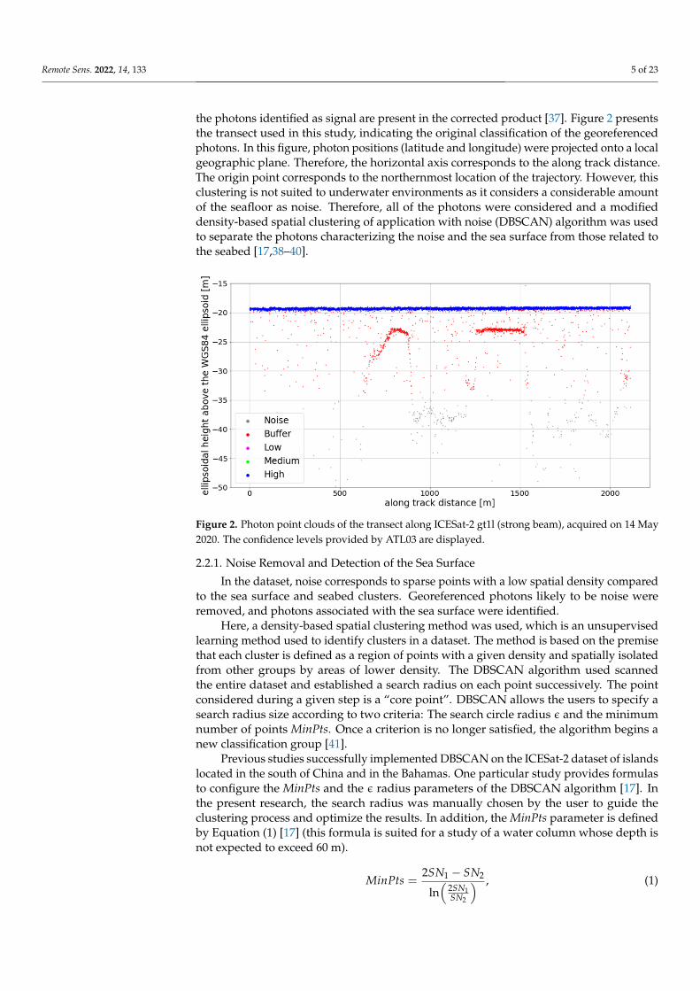
the photons identified as signal are present in the corrected product [37]. Figure 2 presentsthe transect used in this study, indicating the original classification of the georeferencedphotons. In this figure, photon positions (latitude and longitude) were projected onto a localgeographic plane. Therefore, the horizontal axis corresponds to the along track distance.The origin point corresponds to the northernmost location of the trajectory. However, thisclustering is not suited to underwater environments as it considers a considerable amountof the seafloor as noise. Therefore, all of the photons were considered and a modifieddensity-based spatial clustering of application with noise (DBSCAN) algorithm was usedto separate the photons characterizing the noise and the sea surface from those related tothe seabed [17,38–40].

Remote Sens. 2021, 13, x FOR PEER REVIEW 5 of 24

ICESat-2 ATL03 data are provided with a preliminary classification of every photon regarding how likely it is to be signal or noise (confidence levels are: Noise, Low, Medium, High, and Buffer). Photons classified as “Buffer” are identified after all the signal photons are clustered. These are the photons for which doubt remains, which are at the limit to be identified as part of the signal. Therefore, this category has been created to ensure that all of the photons identified as signal are present in the corrected product [37]. Figure 2 pre-sents the transect used in this study, indicating the original classification of the georefer-enced photons. In this figure, photon positions (latitude and longitude) were projected onto a local geographic plane. Therefore, the horizontal axis corresponds to the along track distance. The origin point corresponds to the northernmost location of the trajectory. However, this clustering is not suited to underwater environments as it considers a con-siderable amount of the seafloor as noise. Therefore, all of the photons were considered and a modified density-based spatial clustering of application with noise (DBSCAN) al-gorithm was used to separate the photons characterizing the noise and the sea surface from those related to the seabed [17,38–40].

Figure 2. Photon point clouds of the transect along ICESat-2 gt1l (strong beam), acquired on 14 May 2020. The confidence levels provided by ATL03 are displayed.

2.2.1. Noise Removal and Detection of the Sea Surface In the dataset, noise corresponds to sparse points with a low spatial density com-

pared to the sea surface and seabed clusters. Georeferenced photons likely to be noise were removed, and photons associated with the sea surface were identified.

Here, a density-based spatial clustering method was used, which is an unsupervised learning method used to identify clusters in a dataset. The method is based on the premise that each cluster is defined as a region of points with a given density and spatially isolated from other groups by areas of lower density. The DBSCAN algorithm used scanned the entire dataset and established a search radius on each point successively. The point con-sidered during a given step is a “core point”. DBSCAN allows the users to specify a search radius size according to two criteria: The search circle radius ϵ and the minimum number of points MinPts. Once a criterion is no longer satisfied, the algorithm begins a new clas-sification group [41].

Previous studies successfully implemented DBSCAN on the ICESat-2 dataset of is-lands located in the south of China and in the Bahamas. One particular study provides formulas to configure the MinPts and the ϵ radius parameters of the DBSCAN algorithm [17]. In the present research, the search radius was manually chosen by the user to guide

Figure 2. Photon point clouds of the transect along ICESat-2 gt1l (strong beam), acquired on 14 May2020. The confidence levels provided by ATL03 are displayed.

2.2.1. Noise Removal and Detection of the Sea Surface

In the dataset, noise corresponds to sparse points with a low spatial density comparedto the sea surface and seabed clusters. Georeferenced photons likely to be noise wereremoved, and photons associated with the sea surface were identified.

Here, a density-based spatial clustering method was used, which is an unsupervisedlearning method used to identify clusters in a dataset. The method is based on the premisethat each cluster is defined as a region of points with a given density and spatially isolatedfrom other groups by areas of lower density. The DBSCAN algorithm used scannedthe entire dataset and established a search radius on each point successively. The pointconsidered during a given step is a “core point”. DBSCAN allows the users to specify asearch radius size according to two criteria: The search circle radius ε and the minimumnumber of points MinPts. Once a criterion is no longer satisfied, the algorithm begins anew classification group [41].

Previous studies successfully implemented DBSCAN on the ICESat-2 dataset of islandslocated in the south of China and in the Bahamas. One particular study provides formulasto configure the MinPts and the ε radius parameters of the DBSCAN algorithm [17]. Inthe present research, the search radius was manually chosen by the user to guide theclustering process and optimize the results. In addition, the MinPts parameter is definedby Equation (1) [17] (this formula is suited for a study of a water column whose depth isnot expected to exceed 60 m).

MinPts =2SN1 − SN2

ln(

2SN1SN2

) , (1)

Remote Sens. 2022, 14, 133 6 of 23

where SN1 is the number of expected photons corresponding to signal and noise anddefined by Equation (2):

SN1 =πε2N1

hl, (2)

where N1 is the total number of photons (both signal and noise), h is the vertical range andl is the along track range. SN2 is the expected noise photons number and is defined byEquation (3):

SN2 =πε2N2

h2l, (3)

where N2 corresponds to the number of photons in the layer with the fewer bathymetricphotons, while h2 is the height of the corresponding layer [17].

The variable MinPts is constrained to a value no lower than 3. If the previous formulaprovides a value lower than this threshold, then MinPts was set to 3 [17]. This algorithmmight not be optimal in the present situation, since the dataset contains isolated photonsfrom the seabed which could be identified as noise. Considering the small number ofphotons from the seabed, it was decided not to optimize the noise cleaning process, even ifit meant that some manual cleaning had to be done. Therefore, the remaining noise pointswere removed manually using GlobalMapper software 22.1.0 (Blue Marble Geographics,Hallowell, ME, USA).

2.2.2. Detection of the Seabed

The sea surface is the cluster with the highest number of photons. It is a high-densitygroup of photons spread over a continuous line, depending on the state of the sea. The seasurface cluster is clearly visible in blue in Figure 2.

According to [17], after removing the noise, the seabed is defined as every signalphoton below a threshold value underneath the water surface. Therefore, every photonwhose elevation is lower than LMS-3SV (where LMS is the Local Mean Sea level and SVthe Surface Variance), was identified as a return signal from the seabed [17].

2.2.3. Correction for the Refraction Bias

Geolocated signal photons located below the water surface are not corrected for therefraction effect that redirects the light, and thus the LiDAR beams. It induces a positioningbias for photons in the water layer that would impact the bathymetry estimate.

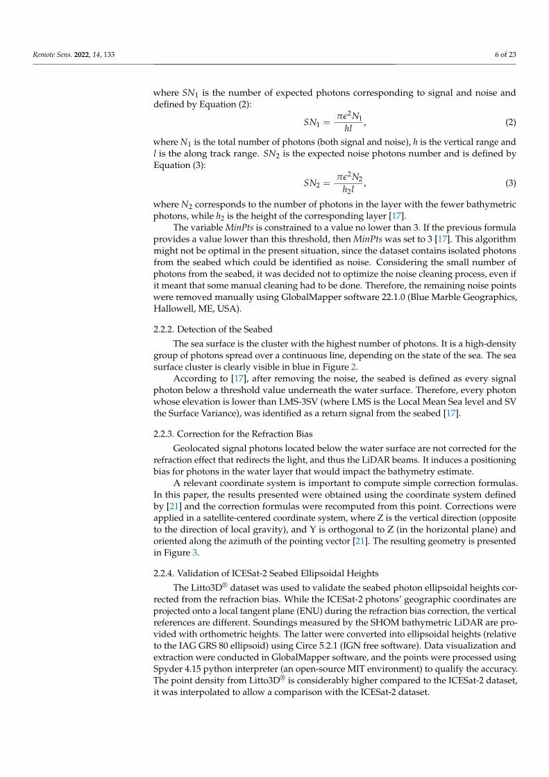
A relevant coordinate system is important to compute simple correction formulas.In this paper, the results presented were obtained using the coordinate system definedby [21] and the correction formulas were recomputed from this point. Corrections wereapplied in a satellite-centered coordinate system, where Z is the vertical direction (oppositeto the direction of local gravity), and Y is orthogonal to Z (in the horizontal plane) andoriented along the azimuth of the pointing vector [21]. The resulting geometry is presentedin Figure 3.

2.2.4. Validation of ICESat-2 Seabed Ellipsoidal Heights

The Litto3D® dataset was used to validate the seabed photon ellipsoidal heights cor-rected from the refraction bias. While the ICESat-2 photons’ geographic coordinates areprojected onto a local tangent plane (ENU) during the refraction bias correction, the verticalreferences are different. Soundings measured by the SHOM bathymetric LiDAR are pro-vided with orthometric heights. The latter were converted into ellipsoidal heights (relativeto the IAG GRS 80 ellipsoid) using Circe 5.2.1 (IGN free software). Data visualization andextraction were conducted in GlobalMapper software, and the points were processed usingSpyder 4.15 python interpreter (an open-source MIT environment) to qualify the accuracy.The point density from Litto3D® is considerably higher compared to the ICESat-2 dataset,it was interpolated to allow a comparison with the ICESat-2 dataset.

Remote Sens. 2022, 14, 133 7 of 23Remote Sens. 2021, 13, x FOR PEER REVIEW 7 of 24

(a) (b) (c)

Figure 3. (a) Schematic diagram for the change of coordinate systems and the computation of the refraction bias in the horizontal plane; (b) in the vertical plane (figure adapted from [21]); and (c) correction formulas.

2.2.4. Validation of ICESat-2 Seabed Ellipsoidal Heights The Litto3D® dataset was used to validate the seabed photon ellipsoidal heights cor-

rected from the refraction bias. While the ICESat-2 photons’ geographic coordinates are projected onto a local tangent plane (ENU) during the refraction bias correction, the ver-tical references are different. Soundings measured by the SHOM bathymetric LiDAR are provided with orthometric heights. The latter were converted into ellipsoidal heights (rel-ative to the IAG GRS 80 ellipsoid) using Circe 5.2.1 (IGN free software). Data visualization and extraction were conducted in GlobalMapper software, and the points were processed using Spyder 4.15 python interpreter (an open-source MIT environment) to qualify the accuracy. The point density from Litto3D® is considerably higher compared to the ICESat-2 dataset, it was interpolated to allow a comparison with the ICESat-2 dataset.

2.3. Satellite-Derived Bathymetry 2.3.1. Ratio Transform Method

The SDB ratio transform algorithm provided by ENVI 5.3 (L3Harris Geospatial Solu-tions, Broomfield, CO, USA) was used to retrieve the relative DDM of the study area. The DDM is based on the relationship between reflectance and bathymetry, which is described by [23]. The semi-empirical model provides values of relative bathymetry by computing the logarithmic ratio of the reflectance of two spectral bands from a MS imagery. First, the 2 m pixel size imagery was converted into TOA reflectance values and was geometrically projected to the WGS84/UTM38S. At this point, the spatial resolution was enhanced using the Gram-Schmidt pan-sharpening method [42,43]. Second, the MS image was cropped with a spatial subset tool to isolate the geographical area of interest. Finally, the ratio transform was implemented with the algorithm developed by [23]. A map of the relative water depth (i.e., log ratio of the spectral bands) was derived from the log ratio between the green and blue spectral bands [44–49].

This method is one of the most commonly used methods in SDB studies, as it proved to provide accurate results and does not require many points for the calibration phase [18,23]. The advantages are that only two parameters need to be set and it works on all types of albedos. This method is also mainly suited for clear case 1 water, which is the case in this study [18,23].

Working with spectral band ratios is a way to compensate for the variability of ocean bottom type, since changes in the albedo values will affect approximately equally both

Figure 3. (a) Schematic diagram for the change of coordinate systems and the computation of therefraction bias in the horizontal plane; (b) in the vertical plane (figure adapted from [21]); and(c) correction formulas.

2.3. Satellite-Derived Bathymetry2.3.1. Ratio Transform Method

The SDB ratio transform algorithm provided by ENVI 5.3 (L3Harris Geospatial Solu-tions, Broomfield, CO, USA) was used to retrieve the relative DDM of the study area. TheDDM is based on the relationship between reflectance and bathymetry, which is describedby [23]. The semi-empirical model provides values of relative bathymetry by computingthe logarithmic ratio of the reflectance of two spectral bands from a MS imagery. First, the2 m pixel size imagery was converted into TOA reflectance values and was geometricallyprojected to the WGS84/UTM38S. At this point, the spatial resolution was enhanced usingthe Gram-Schmidt pan-sharpening method [42,43]. Second, the MS image was croppedwith a spatial subset tool to isolate the geographical area of interest. Finally, the ratiotransform was implemented with the algorithm developed by [23]. A map of the relativewater depth (i.e., log ratio of the spectral bands) was derived from the log ratio betweenthe green and blue spectral bands [44–49].

This method is one of the most commonly used methods in SDB studies, as it proved toprovide accurate results and does not require many points for the calibration phase [18,23].The advantages are that only two parameters need to be set and it works on all types ofalbedos. This method is also mainly suited for clear case 1 water, which is the case in thisstudy [18,23].

Working with spectral band ratios is a way to compensate for the variability of oceanbottom type, since changes in the albedo values will affect approximately equally bothspectral bands. On the contrary, a variation of depth has a higher impact on the spectralband, which is the most intensely absorbed in the water column. Therefore, depth isexpected to be retrieved by this method independently of bottom albedo and can beobtained by inverting the radiative transfer equation as follows [23]:

z = m1ln(nRw

(λj))

ln(nRw(λi))− m0, (4)

where z is the depth, n is a constant needed for the ratio to stay positive, Rw is the reflectanceof the water, m0 is the offset for a depth of 0 m, and m1 is the gain coefficient.

Remote Sens. 2022, 14, 133 8 of 23

Each pixel of the MS imagery was assigned a value between 0 and 1. The finalDDM was obtained by calibrating the relative bathymetry product with field-based depthmeasurements.

The final DDM was produced by finding the equation that best fits (i.e., lowest RMSEand higher R2 with a simple equation formula) the relationship between the relativebathymetric values and the ground truth depth measurements. If bathymetric sound-ings measured by ICESat-2 are reliable and accurate enough, they could be used as acalibration/validation dataset to produce bathymetry solely from satellite observations.

2.3.2. Calibration with ICESat-2 Soundings

During the calibration phase, pixels from the relative DDM were matched to bathy-metric points measured by ICESat-2.

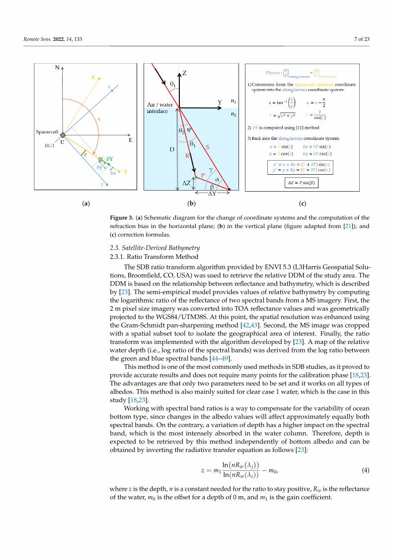
To produce a DDM, i.e., a map of the water height at the acquisition date of the satelliteMS imagery, ICESat-2 vertical heights were converted into the appropriate datum. First,the ellipsoidal heights measured by the ICESat-2 satellite were referenced to the IAG GRS80 ellipsoid and had to be referenced to the chart datum. The SHOM (https://data.shom.fr/,last accessed: 28 December 2021) provides accurate altimetric information over Mayotteisland, including the distance between the ellipsoid and the chart datum in Dzaoudzilocality (distance of −21.74 m). Second, the water height above the chart datum, at theacquisition time of the MS satellite imagery, was added. The closest tide gauge from thestudy site was also located at Dzaoudzi and the measurements were available from theSHOM website. The tide gauge recorded a water height of 1.02 m above the chart datumon 25 May 2020, at 07 h 24 min UTC. Figure 4 illustrates the different variables involved tocompute the bathymetry from ICESat-2 ellipsoidal heights.

Remote Sens. 2021, 13, x FOR PEER REVIEW 8 of 24

spectral bands. On the contrary, a variation of depth has a higher impact on the spectral band, which is the most intensely absorbed in the water column. Therefore, depth is ex-pected to be retrieved by this method independently of bottom albedo and can be ob-tained by inverting the radiative transfer equation as follows [23]: 𝑧 = 𝑚 ( ) ( ( )) − 𝑚 , (4)

where z is the depth, n is a constant needed for the ratio to stay positive, Rw is the reflec-tance of the water, m0 is the offset for a depth of 0 m, and m1 is the gain coefficient.

Each pixel of the MS imagery was assigned a value between 0 and 1. The final DDM was obtained by calibrating the relative bathymetry product with field-based depth meas-urements.

The final DDM was produced by finding the equation that best fits (i.e., lowest RMSE and higher R2 with a simple equation formula) the relationship between the relative bath-ymetric values and the ground truth depth measurements. If bathymetric soundings measured by ICESat-2 are reliable and accurate enough, they could be used as a calibra-tion/validation dataset to produce bathymetry solely from satellite observations.

2.3.2. Calibration with ICESat-2 Soundings During the calibration phase, pixels from the relative DDM were matched to bathy-

metric points measured by ICESat-2. To produce a DDM, i.e., a map of the water height at the acquisition date of the sat-

ellite MS imagery, ICESat-2 vertical heights were converted into the appropriate datum. First, the ellipsoidal heights measured by the ICESat-2 satellite were referenced to the IAG GRS 80 ellipsoid and had to be referenced to the chart datum. The SHOM (https://data.shom.fr/, last accessed: 28 December 2021) provides accurate altimetric infor-mation over Mayotte island, including the distance between the ellipsoid and the chart datum in Dzaoudzi locality (distance of −21.74 m). Second, the water height above the chart datum, at the acquisition time of the MS satellite imagery, was added. The closest tide gauge from the study site was also located at Dzaoudzi and the measurements were available from the SHOM website. The tide gauge recorded a water height of 1.02 m above the chart datum on 25 May 2020, at 07 h 24 min UTC. Figure 4 illustrates the different variables involved to compute the bathymetry from ICESat-2 ellipsoidal heights.

Figure 4. Variables involved in the process of retrieving ICESat-2 bathymetry at the acquisition time of Pleiades-1A.

Relative bathymetry points from the MS imagery were collected at the exact same location as the measurement points of ICESat-2 and an equation linking the two datasets

Figure 4. Variables involved in the process of retrieving ICESat-2 bathymetry at the acquisition timeof Pleiades-1A.

Relative bathymetry points from the MS imagery were collected at the exact samelocation as the measurement points of ICESat-2 and an equation linking the two datasetswas determined. Finally, the equation was applied to the relative DDM using the ENVIband math tool to generate the final DDM.

2.3.3. Digital Depth Model Validation

We compared different regression models. The aim was to find the model that bestmatches the bathymetry measurements of ICESat-2 with the remotely sensed spectralvalues of Pleiades-1A. The best regression was chosen based on the RMSE and basedon the coefficient of determination, R2. The final DDM was validated in comparison tothe Litto3D® reference dataset by computing the root mean square error (RMSE) and themaximum absolute error (MAE) statistical indicators.

Remote Sens. 2022, 14, 133 9 of 23

2.4. Benthic Habitats Mapping2.4.1. Processing of the Multispectral Imagery

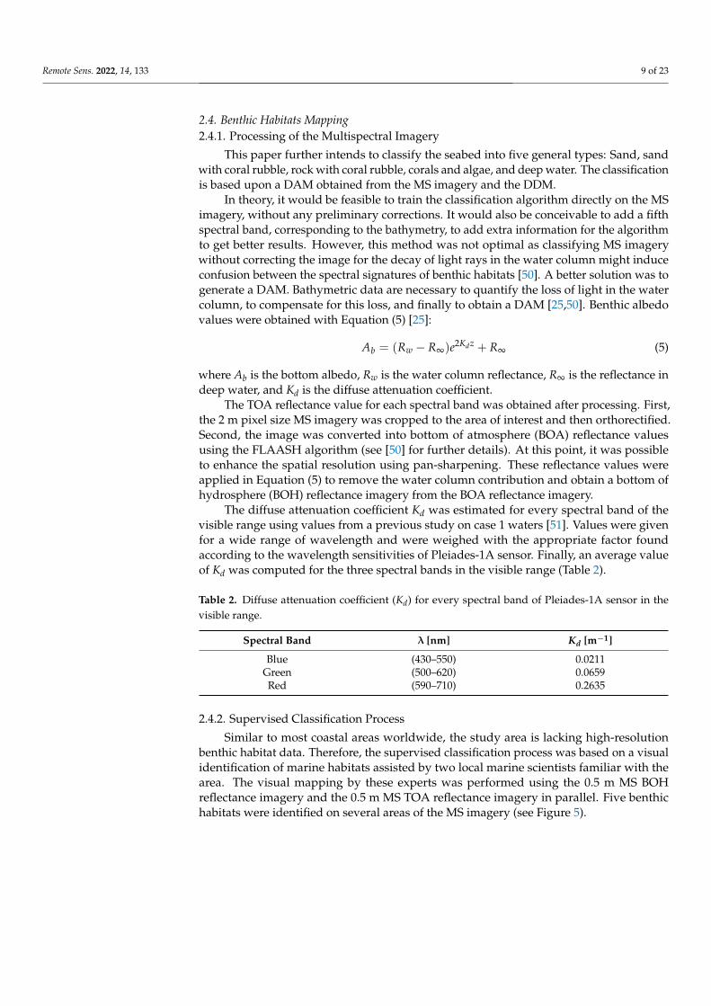
This paper further intends to classify the seabed into five general types: Sand, sandwith coral rubble, rock with coral rubble, corals and algae, and deep water. The classificationis based upon a DAM obtained from the MS imagery and the DDM.

In theory, it would be feasible to train the classification algorithm directly on the MSimagery, without any preliminary corrections. It would also be conceivable to add a fifthspectral band, corresponding to the bathymetry, to add extra information for the algorithmto get better results. However, this method was not optimal as classifying MS imagerywithout correcting the image for the decay of light rays in the water column might induceconfusion between the spectral signatures of benthic habitats [50]. A better solution was togenerate a DAM. Bathymetric data are necessary to quantify the loss of light in the watercolumn, to compensate for this loss, and finally to obtain a DAM [25,50]. Benthic albedovalues were obtained with Equation (5) [25]:

Ab = (Rw − R∞)e2Kdz + R∞ (5)

where Ab is the bottom albedo, Rw is the water column reflectance, R∞ is the reflectance indeep water, and Kd is the diffuse attenuation coefficient.

The TOA reflectance value for each spectral band was obtained after processing. First,the 2 m pixel size MS imagery was cropped to the area of interest and then orthorectified.Second, the image was converted into bottom of atmosphere (BOA) reflectance valuesusing the FLAASH algorithm (see [50] for further details). At this point, it was possibleto enhance the spatial resolution using pan-sharpening. These reflectance values wereapplied in Equation (5) to remove the water column contribution and obtain a bottom ofhydrosphere (BOH) reflectance imagery from the BOA reflectance imagery.

The diffuse attenuation coefficient Kd was estimated for every spectral band of thevisible range using values from a previous study on case 1 waters [51]. Values were givenfor a wide range of wavelength and were weighed with the appropriate factor foundaccording to the wavelength sensitivities of Pleiades-1A sensor. Finally, an average valueof Kd was computed for the three spectral bands in the visible range (Table 2).

Table 2. Diffuse attenuation coefficient (Kd) for every spectral band of Pleiades-1A sensor in thevisible range.

Spectral Band λ [nm] Kd [m−1]

Blue (430–550) 0.0211Green (500–620) 0.0659Red (590–710) 0.2635

2.4.2. Supervised Classification Process

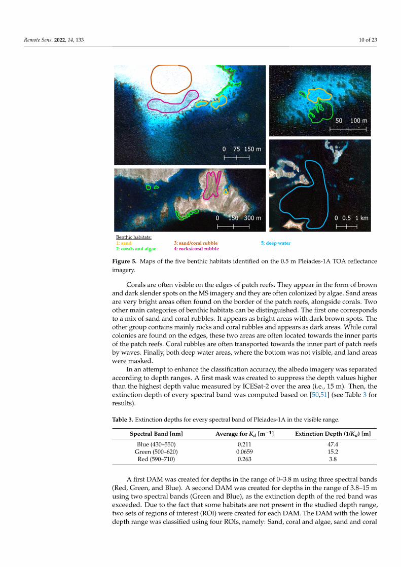
Similar to most coastal areas worldwide, the study area is lacking high-resolutionbenthic habitat data. Therefore, the supervised classification process was based on a visualidentification of marine habitats assisted by two local marine scientists familiar with thearea. The visual mapping by these experts was performed using the 0.5 m MS BOHreflectance imagery and the 0.5 m MS TOA reflectance imagery in parallel. Five benthichabitats were identified on several areas of the MS imagery (see Figure 5).

Remote Sens. 2022, 14, 133 10 of 23

Remote Sens. 2021, 13, x FOR PEER REVIEW 10 of 24

area. The visual mapping by these experts was performed using the 0.5 m MS BOH reflec-tance imagery and the 0.5 m MS TOA reflectance imagery in parallel. Five benthic habitats were identified on several areas of the MS imagery (see Figure 5).

Figure 5. Maps of the five benthic habitats identified on the 0.5 m Pleiades-1A TOA reflectance im-agery.

Corals are often visible on the edges of patch reefs. They appear in the form of brown and dark slender spots on the MS imagery and they are often colonized by algae. Sand areas are very bright areas often found on the border of the patch reefs, alongside corals. Two other main categories of benthic habitats can be distinguished. The first one corre-sponds to a mix of sand and coral rubbles. It appears as bright areas with dark brown spots. The other group contains mainly rocks and coral rubbles and appears as dark areas. While coral colonies are found on the edges, these two areas are often located towards the inner parts of the patch reefs. Coral rubbles are often transported towards the inner part of patch reefs by waves. Finally, both deep water areas, where the bottom was not visible, and land areas were masked.

In an attempt to enhance the classification accuracy, the albedo imagery was sepa-rated according to depth ranges. A first mask was created to suppress the depth values higher than the highest depth value measured by ICESat-2 over the area (i.e., 15 m). Then, the extinction depth of every spectral band was computed based on [50,51] (see Table 3 for results).

Figure 5. Maps of the five benthic habitats identified on the 0.5 m Pleiades-1A TOA reflectanceimagery.

Corals are often visible on the edges of patch reefs. They appear in the form of brownand dark slender spots on the MS imagery and they are often colonized by algae. Sand areasare very bright areas often found on the border of the patch reefs, alongside corals. Twoother main categories of benthic habitats can be distinguished. The first one correspondsto a mix of sand and coral rubbles. It appears as bright areas with dark brown spots. Theother group contains mainly rocks and coral rubbles and appears as dark areas. While coralcolonies are found on the edges, these two areas are often located towards the inner partsof the patch reefs. Coral rubbles are often transported towards the inner part of patch reefsby waves. Finally, both deep water areas, where the bottom was not visible, and land areaswere masked.

In an attempt to enhance the classification accuracy, the albedo imagery was separatedaccording to depth ranges. A first mask was created to suppress the depth values higherthan the highest depth value measured by ICESat-2 over the area (i.e., 15 m). Then, theextinction depth of every spectral band was computed based on [50,51] (see Table 3 forresults).

Table 3. Extinction depths for every spectral band of Pleiades-1A in the visible range.

Spectral Band [nm] Average for Kd [m−1] Extinction Depth (1/Kd) [m]

Blue (430–550) 0.211 47.4Green (500–620) 0.0659 15.2Red (590–710) 0.263 3.8

A first DAM was created for depths in the range of 0–3.8 m using three spectral bands(Red, Green, and Blue). A second DAM was created for depths in the range of 3.8–15 musing two spectral bands (Green and Blue), as the extinction depth of the red band wasexceeded. Due to the fact that some habitats are not present in the studied depth range,two sets of regions of interest (ROI) were created for each DAM. The DAM with the lowerdepth range was classified using four ROIs, namely: Sand, coral and algae, sand and coral

Remote Sens. 2022, 14, 133 11 of 23

rubble, and rocks and coral rubble. The DAM with the higher depth range was classifiedusing three ROIs, namely: Sand, coral and algae, and deep water.

Moreover, a choice of three morphological predictors was made to complement the MSbands of the DAM in order to enhance the classification results. The first predictor addedwas the slope before adding the aspect and the profile convexity all together. Classificationswere computed using a 3 × 3 pixel kernel size.

Three classification algorithms were compared in this study: Neural network (NN),maximum likelihood (ML), and support vector machine (SVM).

2.4.3. Validation of the Supervised Classification

A validation dataset based on the MS imagery was produced with the same knowledgeas for the calibration phase. A post-classification accuracy assessment using a confusionmatrix provided information on overall accuracy (OA) and the kappa coefficient (κ) [52,53].

The ML and the SVM classifiers were set with the default parameters. A neuralnetwork classification was implemented with one and three hidden neurons in one hiddenlayer, in order to test the depth of the neuronal architecture.

3. Results3.1. DDM3.1.1. Correction of ICESat-2 Dataset

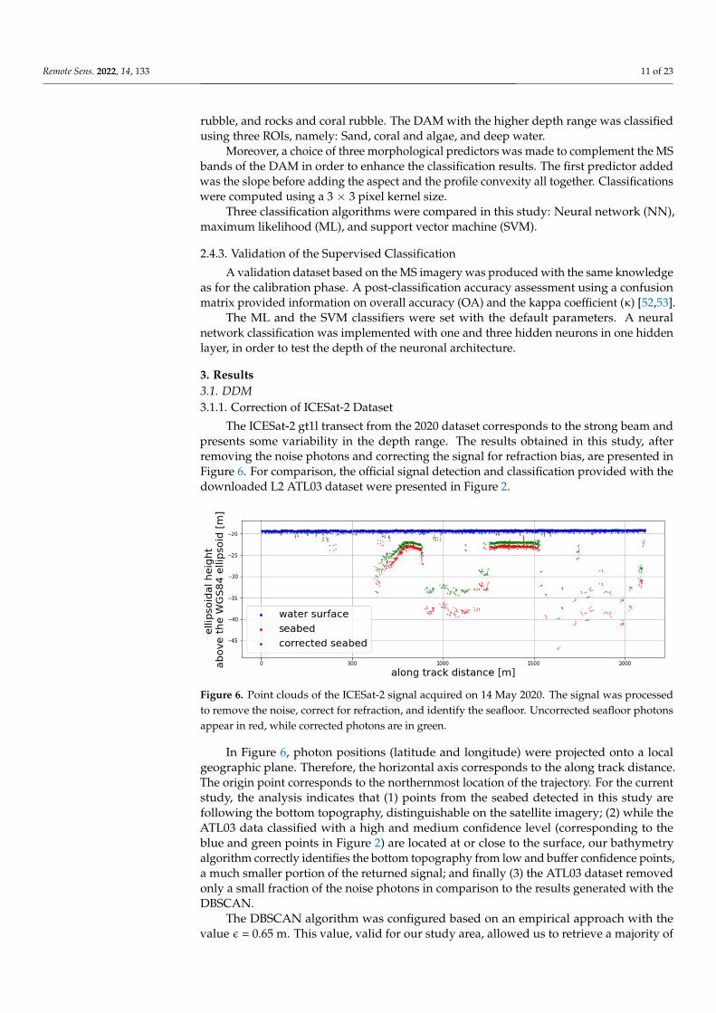
The ICESat-2 gt1l transect from the 2020 dataset corresponds to the strong beam andpresents some variability in the depth range. The results obtained in this study, afterremoving the noise photons and correcting the signal for refraction bias, are presented inFigure 6. For comparison, the official signal detection and classification provided with thedownloaded L2 ATL03 dataset were presented in Figure 2.

Remote Sens. 2021, 13, x FOR PEER REVIEW 11 of 24

Table 3. Extinction depths for every spectral band of Pleiades-1A in the visible range.

Spectral Band [nm] Average for Kd [m−1] Extinction Depth (1/Kd) [m] Blue (430–550) 0.211 47.4

Green (500–620) 0.0659 15.2 Red (590–710) 0.263 3.8

A first DAM was created for depths in the range of 0–3.8 m using three spectral bands (Red, Green, and Blue). A second DAM was created for depths in the range of 3.8–15 m using two spectral bands (Green and Blue), as the extinction depth of the red band was exceeded. Due to the fact that some habitats are not present in the studied depth range, two sets of regions of interest (ROI) were created for each DAM. The DAM with the lower depth range was classified using four ROIs, namely: Sand, coral and algae, sand and coral rubble, and rocks and coral rubble. The DAM with the higher depth range was classified using three ROIs, namely: Sand, coral and algae, and deep water.

Moreover, a choice of three morphological predictors was made to complement the MS bands of the DAM in order to enhance the classification results. The first predictor added was the slope before adding the aspect and the profile convexity all together. Clas-sifications were computed using a 3 × 3 pixel kernel size.

Three classification algorithms were compared in this study: Neural network (NN), maximum likelihood (ML), and support vector machine (SVM).

2.4.3. Validation of the Supervised Classification A validation dataset based on the MS imagery was produced with the same

knowledge as for the calibration phase. A post-classification accuracy assessment using a confusion matrix provided information on overall accuracy (OA) and the kappa coeffi-cient (κ) [52,53].

The ML and the SVM classifiers were set with the default parameters. A neural net-work classification was implemented with one and three hidden neurons in one hidden layer, in order to test the depth of the neuronal architecture.

3. Results 3.1. DDM 3.1.1. Correction of ICESat-2 Dataset

The ICESat-2 gt1l transect from the 2020 dataset corresponds to the strong beam and presents some variability in the depth range. The results obtained in this study, after re-moving the noise photons and correcting the signal for refraction bias, are presented in Figure 6. For comparison, the official signal detection and classification provided with the downloaded L2 ATL03 dataset were presented in Figure 2.

Figure 6. Point clouds of the ICESat-2 signal acquired on 14 May 2020. The signal was processedto remove the noise, correct for refraction, and identify the seafloor. Uncorrected seafloor photonsappear in red, while corrected photons are in green.

In Figure 6, photon positions (latitude and longitude) were projected onto a localgeographic plane. Therefore, the horizontal axis corresponds to the along track distance.The origin point corresponds to the northernmost location of the trajectory. For the currentstudy, the analysis indicates that (1) points from the seabed detected in this study arefollowing the bottom topography, distinguishable on the satellite imagery; (2) while theATL03 data classified with a high and medium confidence level (corresponding to theblue and green points in Figure 2) are located at or close to the surface, our bathymetryalgorithm correctly identifies the bottom topography from low and buffer confidence points,a much smaller portion of the returned signal; and finally (3) the ATL03 dataset removedonly a small fraction of the noise photons in comparison to the results generated with theDBSCAN.

The DBSCAN algorithm was configured based on an empirical approach with thevalue ε = 0.65 m. This value, valid for our study area, allowed us to retrieve a majority of

Remote Sens. 2022, 14, 133 12 of 23

the seabed signal while eliminating most of the noise photons. The remaining noise pointscan be manually removed during the validation phase.

3.1.2. Validation of ICESat-2 Data

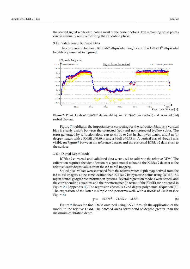
The comparison between ICESat-2 ellipsoidal heights and the Litto3D® ellipsoidalheights is presented in Figure 7.

Remote Sens. 2021, 13, x FOR PEER REVIEW 12 of 24

Figure 6. Point clouds of the ICESat-2 signal acquired on 14 May 2020. The signal was processed to remove the noise, correct for refraction, and identify the seafloor. Uncorrected seafloor photons ap-pear in red, while corrected photons are in green.

In Figure 6, photon positions (latitude and longitude) were projected onto a local geographic plane. Therefore, the horizontal axis corresponds to the along track distance. The origin point corresponds to the northernmost location of the trajectory. For the current study, the analysis indicates that (1) points from the seabed detected in this study are fol-lowing the bottom topography, distinguishable on the satellite imagery; (2) while the ATL03 data classified with a high and medium confidence level (corresponding to the blue and green points in Figure 2) are located at or close to the surface, our bathymetry algorithm correctly identifies the bottom topography from low and buffer confidence points, a much smaller portion of the returned signal; and finally (3) the ATL03 dataset removed only a small fraction of the noise photons in comparison to the results generated with the DBSCAN.

The DBSCAN algorithm was configured based on an empirical approach with the value ϵ = 0.65 m. This value, valid for our study area, allowed us to retrieve a majority of the seabed signal while eliminating most of the noise photons. The remaining noise points can be manually removed during the validation phase.

3.1.2. Validation of ICESat-2 Data The comparison between ICESat-2 ellipsoidal heights and the Litto3D® ellipsoidal

heights is presented in Figure 7.

Figure 7. Point clouds of Litto3D® dataset (blue), and ICESat-2 raw (yellow) and corrected (red) seabed photons.

Figure 7 highlights the importance of correcting for the refraction bias, as a vertical bias is clearly visible between the corrected (red) and non-corrected (yellow) data. The error generated by refraction alone can reach up to 2 m in shallower waters and 5 m for deeper waters with a RMSE of 0.89 m and a MAE of 0.73 m. A vertical bias of about 1 m is visible on Figure 7 between the reference dataset and the corrected ICESat-2 data close to the surface.

3.1.3. Digital Depth Model ICESat-2 corrected and validated data were used to calibrate the relative DDM. The

calibration required the identification of a good model to bound the ICESat-2 dataset to the relative water depth values from the 0.5 m MS imagery.

Scaled pixel values were extracted from the relative water depth map derived from the 0.5 m MS imagery at the same location than ICESat-2 bathymetric points using QGIS 3.18.3 (open-source geographic information system). Several regression models were

Figure 7. Point clouds of Litto3D® dataset (blue), and ICESat-2 raw (yellow) and corrected (red)seabed photons.

Figure 7 highlights the importance of correcting for the refraction bias, as a verticalbias is clearly visible between the corrected (red) and non-corrected (yellow) data. Theerror generated by refraction alone can reach up to 2 m in shallower waters and 5 m fordeeper waters with a RMSE of 0.89 m and a MAE of 0.73 m. A vertical bias of about 1 m isvisible on Figure 7 between the reference dataset and the corrected ICESat-2 data close tothe surface.

3.1.3. Digital Depth Model

ICESat-2 corrected and validated data were used to calibrate the relative DDM. Thecalibration required the identification of a good model to bound the ICESat-2 dataset to therelative water depth values from the 0.5 m MS imagery.

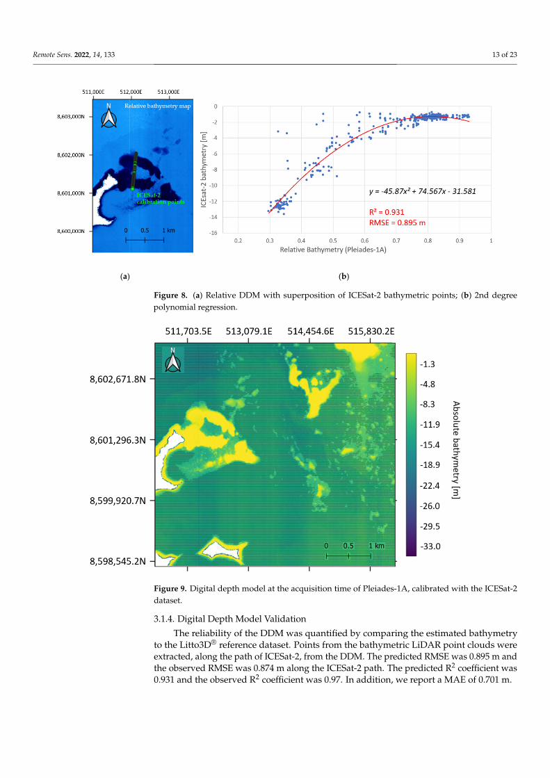
Scaled pixel values were extracted from the relative water depth map derived from the0.5 m MS imagery at the same location than ICESat-2 bathymetric points using QGIS 3.18.3(open-source geographic information system). Several regression models were tested, andthe corresponding equations and their performance (in terms of the RMSE) are presented inFigure A1 (Appendix A). The regression chosen is a 2nd degree polynomial (Equation (6)).The expression of the latter is simple and performs well, with a RMSE of 0.895 m (seeFigure 8).

y = −45.87x2 + 74.567x − 31.581 (6)

Figure 9 shows the final DDM obtained using ENVI through the application of themodel to the relative DDM. The hatched areas correspond to depths greater than themaximum calibration depth.

Remote Sens. 2022, 14, 133 13 of 23

Remote Sens. 2021, 13, x FOR PEER REVIEW 13 of 24

tested, and the corresponding equations and their performance (in terms of the RMSE) are presented in Figure A1 (Appendix A). The regression chosen is a 2nd degree polynomial (Equation (6)). The expression of the latter is simple and performs well, with a RMSE of 0.895 m (see Figure 8). y = −45.87x² + 74.567x − 31.581 (6)

(a) (b)

Figure 8. (a) Relative DDM with superposition of ICESat-2 bathymetric points; (b) 2nd degree polynomial regression.

Figure 9 shows the final DDM obtained using ENVI through the application of the model to the relative DDM. The hatched areas correspond to depths greater than the max-imum calibration depth.

Figure 8. (a) Relative DDM with superposition of ICESat-2 bathymetric points; (b) 2nd degreepolynomial regression.

Remote Sens. 2021, 13, x FOR PEER REVIEW 13 of 24

tested, and the corresponding equations and their performance (in terms of the RMSE) are presented in Figure A1 (Appendix A). The regression chosen is a 2nd degree polynomial (Equation (6)). The expression of the latter is simple and performs well, with a RMSE of 0.895 m (see Figure 8). y = −45.87x² + 74.567x − 31.581 (6)

(a) (b)

Figure 8. (a) Relative DDM with superposition of ICESat-2 bathymetric points; (b) 2nd degree polynomial regression.

Figure 9 shows the final DDM obtained using ENVI through the application of the model to the relative DDM. The hatched areas correspond to depths greater than the max-imum calibration depth.

Figure 9. Digital depth model at the acquisition time of Pleiades-1A, calibrated with the ICESat-2dataset.

3.1.4. Digital Depth Model Validation

The reliability of the DDM was quantified by comparing the estimated bathymetryto the Litto3D® reference dataset. Points from the bathymetric LiDAR point clouds wereextracted, along the path of ICESat-2, from the DDM. The predicted RMSE was 0.895 m andthe observed RMSE was 0.874 m along the ICESat-2 path. The predicted R2 coefficient was0.931 and the observed R2 coefficient was 0.97. In addition, we report a MAE of 0.701 m.

Remote Sens. 2022, 14, 133 14 of 23

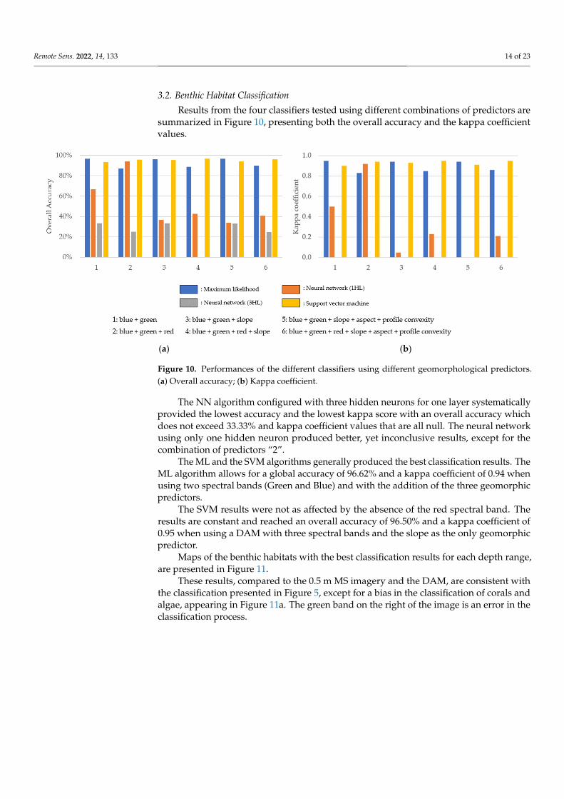
3.2. Benthic Habitat Classification

Results from the four classifiers tested using different combinations of predictors aresummarized in Figure 10, presenting both the overall accuracy and the kappa coefficientvalues.

Remote Sens. 2021, 13, x FOR PEER REVIEW 14 of 24

Figure 9. Digital depth model at the acquisition time of Pleiades-1A, calibrated with the ICESat-2 dataset.

3.1.4. Digital Depth Model Validation The reliability of the DDM was quantified by comparing the estimated bathymetry

to the Litto3D® reference dataset. Points from the bathymetric LiDAR point clouds were extracted, along the path of ICESat-2, from the DDM. The predicted RMSE was 0.895 m and the observed RMSE was 0.874 m along the ICESat-2 path. The predicted R2 coefficient was 0.931 and the observed R2 coefficient was 0.97. In addition, we report a MAE of 0.701 m.

3.2. Benthic Habitat Classification Results from the four classifiers tested using different combinations of predictors are

summarized in Figure 10, presenting both the overall accuracy and the kappa coefficient values.

(a) (b)

Figure 10. Performances of the different classifiers using different geomorphological predictors. (a) Overall accuracy; (b) Kappa coefficient.

The NN algorithm configured with three hidden neurons for one layer systematically provided the lowest accuracy and the lowest kappa score with an overall accuracy which does not exceed 33.33% and kappa coefficient values that are all null. The neural network using only one hidden neuron produced better, yet inconclusive results, except for the combination of predictors “2”.

The ML and the SVM algorithms generally produced the best classification results. The ML algorithm allows for a global accuracy of 96.62% and a kappa coefficient of 0.94 when using two spectral bands (Green and Blue) and with the addition of the three geo-morphic predictors.

The SVM results were not as affected by the absence of the red spectral band. The results are constant and reached an overall accuracy of 96.50% and a kappa coefficient of 0.95 when using a DAM with three spectral bands and the slope as the only geomorphic predictor.

Maps of the benthic habitats with the best classification results for each depth range, are presented in Figure 11.

Figure 10. Performances of the different classifiers using different geomorphological predictors.(a) Overall accuracy; (b) Kappa coefficient.

The NN algorithm configured with three hidden neurons for one layer systematicallyprovided the lowest accuracy and the lowest kappa score with an overall accuracy whichdoes not exceed 33.33% and kappa coefficient values that are all null. The neural networkusing only one hidden neuron produced better, yet inconclusive results, except for thecombination of predictors “2”.

The ML and the SVM algorithms generally produced the best classification results. TheML algorithm allows for a global accuracy of 96.62% and a kappa coefficient of 0.94 whenusing two spectral bands (Green and Blue) and with the addition of the three geomorphicpredictors.

The SVM results were not as affected by the absence of the red spectral band. Theresults are constant and reached an overall accuracy of 96.50% and a kappa coefficient of0.95 when using a DAM with three spectral bands and the slope as the only geomorphicpredictor.

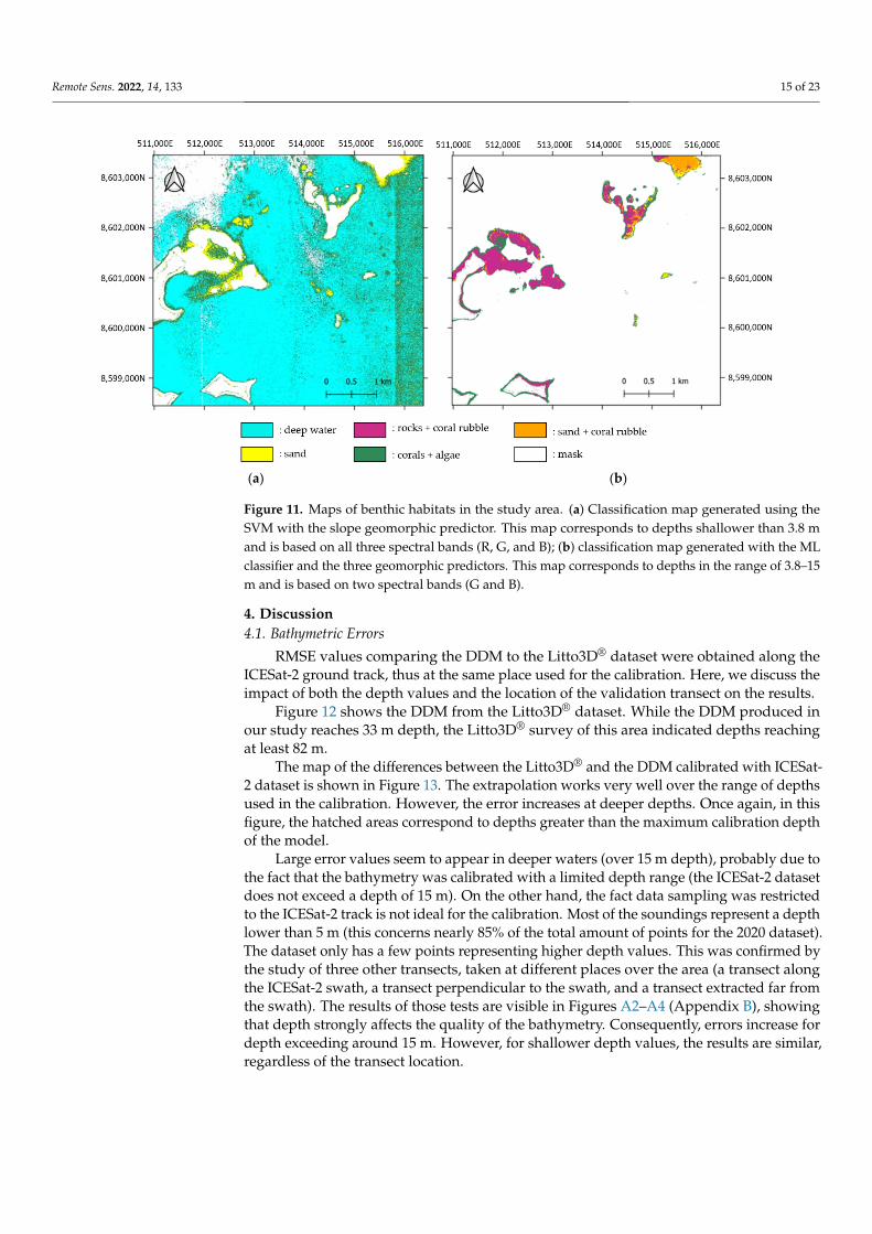
Maps of the benthic habitats with the best classification results for each depth range,are presented in Figure 11.

These results, compared to the 0.5 m MS imagery and the DAM, are consistent withthe classification presented in Figure 5, except for a bias in the classification of corals andalgae, appearing in Figure 11a. The green band on the right of the image is an error in theclassification process.

Remote Sens. 2022, 14, 133 15 of 23Remote Sens. 2021, 13, x FOR PEER REVIEW 15 of 24

(a) (b)

Figure 11. Maps of benthic habitats in the study area. (a) Classification map generated using the SVM with the slope geomorphic predictor. This map corresponds to depths shallower than 3.8 m and is based on all three spectral bands (R, G, and B); (b) classification map generated with the ML classifier and the three geomorphic predictors. This map corre-sponds to depths in the range of 3.8–15 m and is based on two spectral bands (G and B).

These results, compared to the 0.5 m MS imagery and the DAM, are consistent with the classification presented in Figure 5, except for a bias in the classification of corals and algae, appearing in Figure 11a. The green band on the right of the image is an error in the classification process.

4. Discussion 4.1. Bathymetric Errors

RMSE values comparing the DDM to the Litto3D® dataset were obtained along the ICESat-2 ground track, thus at the same place used for the calibration. Here, we discuss the impact of both the depth values and the location of the validation transect on the re-sults.

Figure 12 shows the DDM from the Litto3D® dataset. While the DDM produced in our study reaches 33 m depth, the Litto3D® survey of this area indicated depths reaching at least 82 m.

Figure 11. Maps of benthic habitats in the study area. (a) Classification map generated using theSVM with the slope geomorphic predictor. This map corresponds to depths shallower than 3.8 mand is based on all three spectral bands (R, G, and B); (b) classification map generated with the MLclassifier and the three geomorphic predictors. This map corresponds to depths in the range of 3.8–15m and is based on two spectral bands (G and B).

4. Discussion4.1. Bathymetric Errors

RMSE values comparing the DDM to the Litto3D® dataset were obtained along theICESat-2 ground track, thus at the same place used for the calibration. Here, we discuss theimpact of both the depth values and the location of the validation transect on the results.

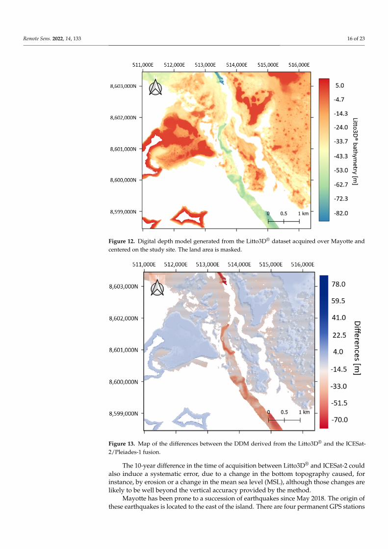
Figure 12 shows the DDM from the Litto3D® dataset. While the DDM produced inour study reaches 33 m depth, the Litto3D® survey of this area indicated depths reachingat least 82 m.

The map of the differences between the Litto3D® and the DDM calibrated with ICESat-2 dataset is shown in Figure 13. The extrapolation works very well over the range of depthsused in the calibration. However, the error increases at deeper depths. Once again, in thisfigure, the hatched areas correspond to depths greater than the maximum calibration depthof the model.

Large error values seem to appear in deeper waters (over 15 m depth), probably due tothe fact that the bathymetry was calibrated with a limited depth range (the ICESat-2 datasetdoes not exceed a depth of 15 m). On the other hand, the fact data sampling was restrictedto the ICESat-2 track is not ideal for the calibration. Most of the soundings represent a depthlower than 5 m (this concerns nearly 85% of the total amount of points for the 2020 dataset).The dataset only has a few points representing higher depth values. This was confirmed bythe study of three other transects, taken at different places over the area (a transect alongthe ICESat-2 swath, a transect perpendicular to the swath, and a transect extracted far fromthe swath). The results of those tests are visible in Figures A2–A4 (Appendix B), showingthat depth strongly affects the quality of the bathymetry. Consequently, errors increase fordepth exceeding around 15 m. However, for shallower depth values, the results are similar,regardless of the transect location.

Remote Sens. 2022, 14, 133 16 of 23Remote Sens. 2021, 13, x FOR PEER REVIEW 16 of 24

Figure 12. Digital depth model generated from the Litto3D® dataset acquired over Mayotte and centered on the study site. The land area is masked.

The map of the differences between the Litto3D® and the DDM calibrated with ICE-Sat-2 dataset is shown in Figure 13. The extrapolation works very well over the range of depths used in the calibration. However, the error increases at deeper depths. Once again, in this figure, the hatched areas correspond to depths greater than the maximum calibra-tion depth of the model.

Figure 13. Map of the differences between the DDM derived from the Litto3D® and the ICESat-2/Pleiades-1 fusion.

Figure 12. Digital depth model generated from the Litto3D® dataset acquired over Mayotte andcentered on the study site. The land area is masked.

Remote Sens. 2021, 13, x FOR PEER REVIEW 16 of 24

Figure 12. Digital depth model generated from the Litto3D® dataset acquired over Mayotte and centered on the study site. The land area is masked.

The map of the differences between the Litto3D® and the DDM calibrated with ICE-Sat-2 dataset is shown in Figure 13. The extrapolation works very well over the range of depths used in the calibration. However, the error increases at deeper depths. Once again, in this figure, the hatched areas correspond to depths greater than the maximum calibra-tion depth of the model.

Figure 13. Map of the differences between the DDM derived from the Litto3D® and the ICESat-2/Pleiades-1 fusion. Figure 13. Map of the differences between the DDM derived from the Litto3D® and the ICESat-2/Pleiades-1 fusion.

The 10-year difference in the time of acquisition between Litto3D® and ICESat-2 couldalso induce a systematic error, due to a change in the bottom topography caused, forinstance, by erosion or a change in the mean sea level (MSL), although those changes arelikely to be well beyond the vertical accuracy provided by the method.

Mayotte has been prone to a succession of earthquakes since May 2018. The origin ofthese earthquakes is located to the east of the island. There are four permanent GPS stations

Remote Sens. 2022, 14, 133 17 of 23

in Mayotte and their rigorous monitoring has allowed experts to observe a displacementof all the stations by several centimeters towards the East and a subsidence of severalcentimeters since the beginning of the events [54–56].

In addition, the conversion of datums, using CIRCE software, could be a source oferror. The grid used for the calculation is the GGM04V1 and the resulting vertical accuracyis estimated by the software at 10/20 cm.

On the other hand, during the correction of the refraction effect, n1 and n2 refractiveindices were assumed and could therefore contribute to a small bias.

The method used to retrieve the map of the relative water depth could be improved toobtain more accurate DDM by implementing more recent and innovative approaches, suchas IMBR, OBRA, MODPA or SMART-SDB [11,24,57–59].

4.2. Impact of the Spatial Resolution of the Multispectral Imagery

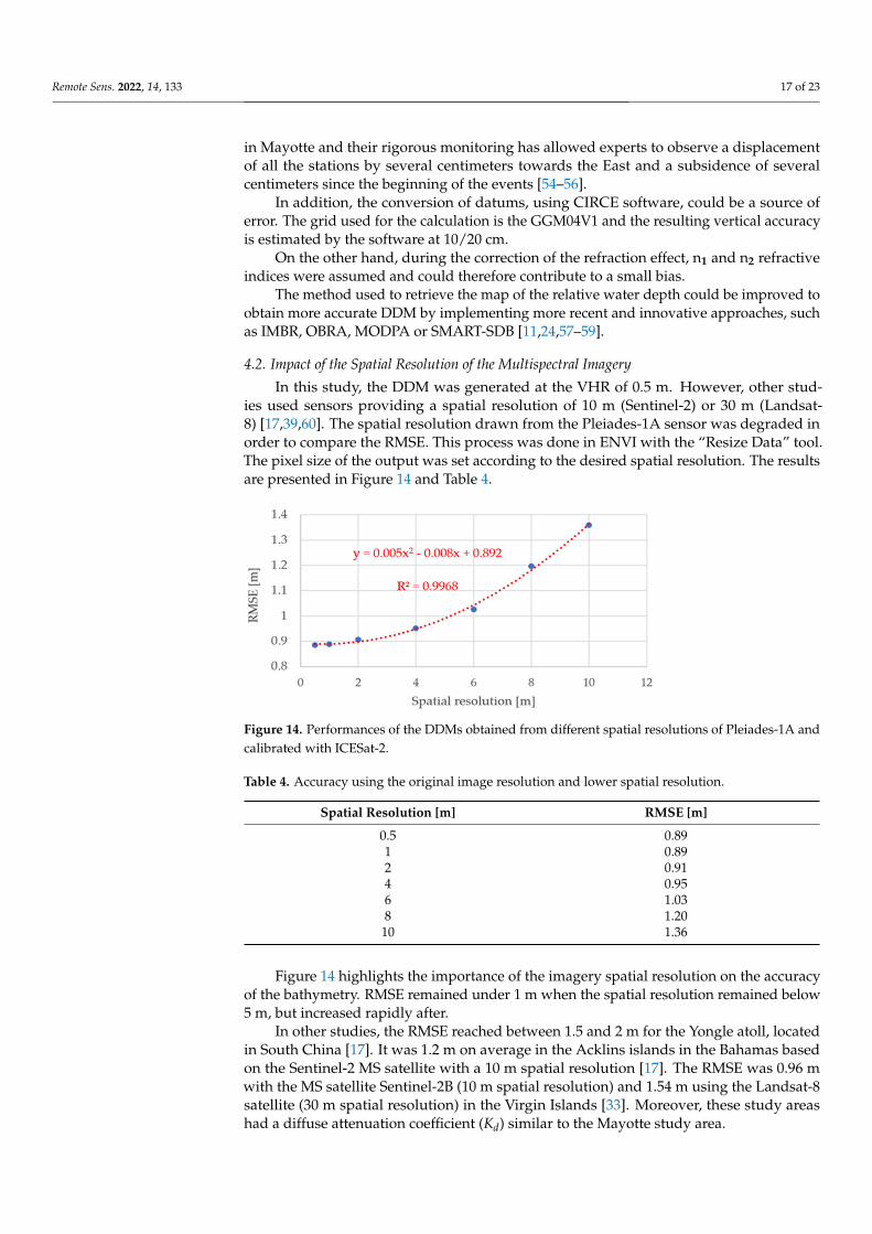
In this study, the DDM was generated at the VHR of 0.5 m. However, other stud-ies used sensors providing a spatial resolution of 10 m (Sentinel-2) or 30 m (Landsat-8) [17,39,60]. The spatial resolution drawn from the Pleiades-1A sensor was degraded inorder to compare the RMSE. This process was done in ENVI with the “Resize Data” tool.The pixel size of the output was set according to the desired spatial resolution. The resultsare presented in Figure 14 and Table 4.

Remote Sens. 2021, 13, x FOR PEER REVIEW 17 of 24

Large error values seem to appear in deeper waters (over 15 m depth), probably due to the fact that the bathymetry was calibrated with a limited depth range (the ICESat-2 dataset does not exceed a depth of 15 m). On the other hand, the fact data sampling was restricted to the ICESat-2 track is not ideal for the calibration. Most of the soundings rep-resent a depth lower than 5 m (this concerns nearly 85% of the total amount of points for the 2020 dataset). The dataset only has a few points representing higher depth values. This was confirmed by the study of three other transects, taken at different places over the area (a transect along the ICESat-2 swath, a transect perpendicular to the swath, and a transect extracted far from the swath). The results of those tests are visible in Figures A2–A4 (Ap-pendix B), showing that depth strongly affects the quality of the bathymetry. Conse-quently, errors increase for depth exceeding around 15 m. However, for shallower depth values, the results are similar, regardless of the transect location.

The 10-year difference in the time of acquisition between Litto3D® and ICESat-2 could also induce a systematic error, due to a change in the bottom topography caused, for instance, by erosion or a change in the mean sea level (MSL), although those changes are likely to be well beyond the vertical accuracy provided by the method.

Mayotte has been prone to a succession of earthquakes since May 2018. The origin of these earthquakes is located to the east of the island. There are four permanent GPS sta-tions in Mayotte and their rigorous monitoring has allowed experts to observe a displace-ment of all the stations by several centimeters towards the East and a subsidence of several centimeters since the beginning of the events [54–56].

In addition, the conversion of datums, using CIRCE software, could be a source of error. The grid used for the calculation is the GGM04V1 and the resulting vertical accuracy is estimated by the software at 10/20 cm.

On the other hand, during the correction of the refraction effect, n1 and n2 refractive indices were assumed and could therefore contribute to a small bias.

The method used to retrieve the map of the relative water depth could be improved to obtain more accurate DDM by implementing more recent and innovative approaches, such as IMBR, OBRA, MODPA or SMART-SDB [11,24,57–59].

4.2. Impact of the Spatial Resolution of the Multispectral Imagery In this study, the DDM was generated at the VHR of 0.5 m. However, other studies

used sensors providing a spatial resolution of 10 m (Sentinel-2) or 30 m (Landsat-8) [17,39,60]. The spatial resolution drawn from the Pleiades-1A sensor was degraded in or-der to compare the RMSE. This process was done in ENVI with the “Resize Data” tool. The pixel size of the output was set according to the desired spatial resolution. The results are presented in Figure 14 and Table 4.

Figure 14. Performances of the DDMs obtained from different spatial resolutions of Pleiades-1A and calibrated with ICESat-2.

Figure 14. Performances of the DDMs obtained from different spatial resolutions of Pleiades-1A andcalibrated with ICESat-2.

Table 4. Accuracy using the original image resolution and lower spatial resolution.

Spatial Resolution [m] RMSE [m]

0.5 0.891 0.892 0.914 0.956 1.038 1.2010 1.36

Figure 14 highlights the importance of the imagery spatial resolution on the accuracyof the bathymetry. RMSE remained under 1 m when the spatial resolution remained below5 m, but increased rapidly after.

In other studies, the RMSE reached between 1.5 and 2 m for the Yongle atoll, locatedin South China [17]. It was 1.2 m on average in the Acklins islands in the Bahamas basedon the Sentinel-2 MS satellite with a 10 m spatial resolution [17]. The RMSE was 0.96 mwith the MS satellite Sentinel-2B (10 m spatial resolution) and 1.54 m using the Landsat-8satellite (30 m spatial resolution) in the Virgin Islands [33]. Moreover, these study areashad a diffuse attenuation coefficient (Kd) similar to the Mayotte study area.

Remote Sens. 2022, 14, 133 18 of 23

One of these studies obtained different results using Sentinel-2 observations andICESat-2 observations from multiple swaths [60]. The DDM was produced with an extrap-olation process conducted over the entire area with a RMSE of 3.36 m. However, whenthe study area was constrained between the two ICESat-2 swaths, the RMSE decreased to0.35 m. This study area had a higher turbidity of Kd = 1.68 m−1 [60].

During the acquisition time of some of these studies, meteorological events such ashurricanes occurred and could have impacted the topography of the bottom and affectedthe results. However, the evaluation of possible episodic events was not reported for thisstudy or investigated.

4.3. Benthic Classification

Classification algorithms performed very differently. It is difficult to assess the impactof the geomorphic predictors on the results. It seems that adding extra information didnot impact the SVM and ML classifications, but could have degraded the NN (+1HL)classification. A large amount information could have undermined the results due to aredundancy in the information. The major change seems to be related to the use of the redspectral band. The results were sometimes better without the red spectral band, probablydue to the fact that the corresponding maps were in the depth range of 3.7–15 m, for whichbenthic classes, such as sand and coral rubble and rocks and coral rubble, are not present.A reduced number of groups tends to enhance the algorithm performance.

The benthic classification is based on a visual recognition of general benthic classesbased on experts’ knowledge. Although, commonly done, identifying benthic classes onMS imagery is not as reliable as direct underwater observations. Living corals could havebeen confused for dead corals colonized by algae. As a matter of fact, the classificationpresented in Figure 11a presented very good results, while having a major bias in theclassification of coral and algae in areas of deep water. Some regions selected both to trainthe algorithm and for further validation presented corals which were distinguishable butvery dark, due to the depth. Those were confused with deep and dark water areas.

Moreover, Mayotte is a complex area. The tidal range reaches 4 m. Therefore, whenthe tide is the lowest, corals can be above the water surface and bleached. Dead corals aretheoretically recognizable by their bright color, but they can get darker as they are oftencolonized by algae. The winds and the waves have the effect to break coral colonies and tocreate coral rubble areas which are difficult to identify, as they get mixed with sand androcks and can be mixed up with areas of isolated corals.

5. Conclusions

This study aimed to evaluate the quality of VHR DDM and DAM generated fromsatellite data. A DDM calibrated with data from the satellite ICESat-2 presented a RMSEof 0.89 m along ICESat-2 ground track, i.e., around 6% of the maximum depth retrievedby ICESat-2. Bathymetric results were generally satisfying down to a depth of around15 m, which is close to the maximum depth of the calibration data used. Marine habitatclassification results were very heterogeneous, depending on the number of predictorsused, the type of predictors, and the algorithm used. However, some combinations ofparameters provided satisfactory results. The classification with the ML classification usingBlue and Green spectral bands with the three geomorphic predictors provided an overallaccuracy of 96.62% and a κ coefficient of 0.94. In addition, the SVM classification usingBlue, Green, and Red spectral bands with the addition of the slope geomorphic predictorpresented an overall accuracy of 96.50% and a κ coefficient of 0.95. This approach can be ofstrong interest to map coastal areas lacking bathymetry and marine habitat maps and forwhich field observations are difficult.

While the quality of the results obtained in this study can support coastal managementand conservation, the accuracy of bathymetry predictions remains limited for applications,such as navigation, that require higher spatial accuracy. It would be interesting to pursuethis research to get more accurate DDMs.

Remote Sens. 2022, 14, 133 19 of 23

Further work, implementing this method on diverse study sites, would confirm therobustness of the method implemented. In the prospect of future studies, it would berelevant to consider several ICESat-2 ground tracks from the area of interest and even toadd the points from other times that ICESat-2 surveyed the area. This would provide abetter variability of depths and a better spatial distribution of the data for the calibrationprocess. Moreover, this increase in the number of points opens prospects for the use ofdeep learning methods to generate DDMs.

Developing an algorithm dedicated to the processing of seafloor data generated fromICESat-2 datasets would be important. The correction for the refraction effect has provennecessary and reliable, but could be further enhanced. The water column properties arechanging with depth and the refraction correction should also adapt according to the watercolumn properties.

It would be relevant to also improve the seabed signal correction by considering thestate of the sea (for instance, presence of waves on the water surface), in helping to developa method that could be used in less sheltered areas [17].

In this study, the results presented were obtained using a MS imagery acquired by thePleiades-1A sensor with four spectral bands and a VHR of 0.5 m using the panchromaticband. The correlation between spatial resolution and the quality of the resulting bathymetryhas been demonstrated in this paper. Therefore, future studies could consider generatingbetter quality DDMs using the WV3 sensor (eight spectral bands at 0.30 m using thepanchromatic band) or even the sensor of the new Pleiades Neo constellation launched inearly 2021 (six spectral bands at 0.3 m with the panchromatic band).

The ICESat-2 products produced by NASA are constantly enhanced and one can bevery optimistic regarding the future quality of DDMs and by-products obtained usingICESat-2 measurements.

Author Contributions: Conceptualization, A.L.Q., A.C. and R.D.; methodology, A.L.Q., A.C. andM.F.J.; software, A.L.Q. and A.C.; validation, A.L.Q., A.C., M.F.J. and R.D.; formal analysis, A.L.Q.,A.C., M.F.J. and R.D.; investigation, A.L.Q., A.C., M.F.J. and R.D.; resources, A.L.Q., A.C., M.F.J. andR.D.; data curation, A.C.; writing—original draft preparation, A.L.Q.; writing—review and editing,A.C., M.F.J. and R.D.; supervision, A.C. and R.D.; project administration, A.C. and R.D.; fundingacquisition, R.D. All authors have read and agreed to the published version of the manuscript.

Funding: With the support of Montpellier Université d’Excellence (MUSE) KIM Sea and Coastprogram for funding the PhotonExplorer project.

Institutional Review Board Statement: Not applicable.

Informed Consent Statement: Not applicable.

Data Availability Statement: The Pleiades-1A imagery provided by CNES-AIRBUS through theDINAMIS platform is not publicly available. The ICESat-2 L2 ATL03 geolocated photons analyzedduring this study are publicly available at https://search.earthdata.nasa.gov/search, last accessed: 28December 2021. The Litto3D® dataset used for validation is publicly available from https://diffusion.shom.fr/, last accessed: 28 December 2021. The diffuse attenuation coefficient of 490 nm measuredat 4 km resolution by MODIS is available publicly from https://oceancolor.gsfc.nasa.gov/l3/, lastaccessed: 28 December 2021. Altimetric information over Mayotte island are available from theSHOM website, https://data.shom.fr/, last accessed: 25 October 2021.

Acknowledgments: The authors gratefully thank the NASA for distributing the ICESat-2 data andfor the support of the ICESat-2 Applied Users group, and the SHOM for providing us with theairborne LiDAR survey data. The authors would like to thank the DINAMIS platform for accessto the Pleiades images and, the CNES “Pléiades © CNES 2020, Distribution Airbus DS”. Pleiades-1imagery is a courtesy from CNES-AIRBUS. Thank you to Thomas Claverie (UMR Marbec) and AlineAubry (UMR Espace-Dev) from CUFR Mayotte for providing expert knowledge used for habitatmapping. The authors would also like to thank the reviewers for improving the manuscript withtheir comments and corrections.

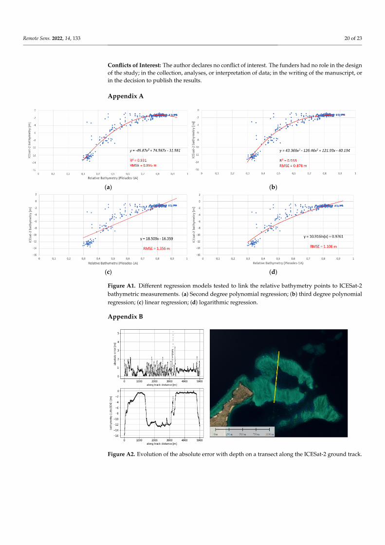
Remote Sens. 2022, 14, 133 20 of 23

Conflicts of Interest: The author declares no conflict of interest. The funders had no role in the designof the study; in the collection, analyses, or interpretation of data; in the writing of the manuscript, orin the decision to publish the results.

Appendix A

Remote Sens. 2021, 13, x FOR PEER REVIEW 20 of 24

Informed Consent Statement: Not applicable.

Data Availability Statement: The Pleiades-1A imagery provided by CNES-AIRBUS through the DINAMIS platform is not publicly available. The ICESat-2 L2 ATL03 geolocated photons analyzed during this study are publicly available at https://search.earthdata.nasa.gov/search, last accessed: 28 December 2021. The Litto3D® dataset used for validation is publicly available from https://diffu-sion.shom.fr/, last accessed: 28 December 2021. The diffuse attenuation coefficient of 490 nm meas-ured at 4 km resolution by MODIS is available publicly from https://oceancolor.gsfc.nasa.gov/l3/, last accessed: 28 December 2021. Altimetric information over Mayotte island are available from the SHOM website, https://data.shom.fr/, last accessed: 25 October 2021.

Acknowledgments: The authors gratefully thank the NASA for distributing the ICESat-2 data and for the support of the ICESat-2 Applied Users group, and the SHOM for providing us with the air-borne LiDAR survey data. The authors would like to thank the DINAMIS platform for access to the Pleiades images and, the CNES “Pléiades © CNES 2020, Distribution Airbus DS”. Pleiades-1 im-agery is a courtesy from CNES-AIRBUS. Thank you to Thomas Claverie (UMR Marbec) and Aline Aubry (UMR Espace-Dev) from CUFR Mayotte for providing expert knowledge used for habitat mapping. The authors would also like to thank the reviewers for improving the manuscript with their comments and corrections.

Conflicts of Interest: The author declares no conflict of interest. The funders had no role in the design of the study; in the collection, analyses, or interpretation of data; in the writing of the manu-script, or in the decision to publish the results.

Appendix A

(a) (b)

(c) (d)

Figure A1. Different regression models tested to link the relative bathymetry points to ICESat-2 bathymetric measurements. (a) Sec-ond degree polynomial regression; (b) third degree polynomial regression; (c) linear regression; (d) logarithmic regression.

Figure A1. Different regression models tested to link the relative bathymetry points to ICESat-2bathymetric measurements. (a) Second degree polynomial regression; (b) third degree polynomialregression; (c) linear regression; (d) logarithmic regression.

Appendix B

Remote Sens. 2021, 13, x FOR PEER REVIEW 21 of 24

Appendix B

Figure A2. Evolution of the absolute error with depth on a transect along the ICESat-2 ground track.

Figure A3. Evolution of the absolute error with depth on a transect across the ICESat-2 ground track.

Figure A4. Evolution of the absolute error with depth on a transect far from the ICESat-2 ground track.

Figure A2. Evolution of the absolute error with depth on a transect along the ICESat-2 ground track.

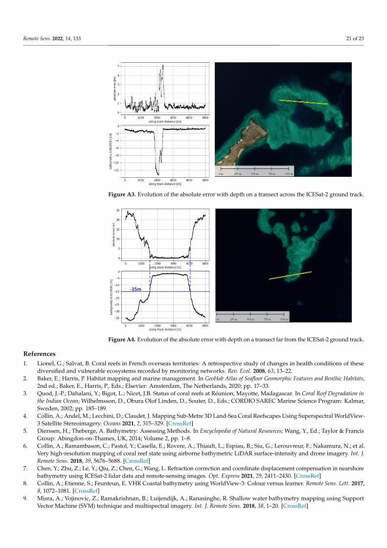
Remote Sens. 2022, 14, 133 21 of 23

Remote Sens. 2021, 13, x FOR PEER REVIEW 21 of 24

Appendix B

Figure A2. Evolution of the absolute error with depth on a transect along the ICESat-2 ground track.

Figure A3. Evolution of the absolute error with depth on a transect across the ICESat-2 ground track.

Figure A4. Evolution of the absolute error with depth on a transect far from the ICESat-2 ground track.

Figure A3. Evolution of the absolute error with depth on a transect across the ICESat-2 ground track.

Remote Sens. 2021, 13, x FOR PEER REVIEW 21 of 24

Appendix B

Figure A2. Evolution of the absolute error with depth on a transect along the ICESat-2 ground track.

Figure A3. Evolution of the absolute error with depth on a transect across the ICESat-2 ground track.

Figure A4. Evolution of the absolute error with depth on a transect far from the ICESat-2 ground track.

Figure A4. Evolution of the absolute error with depth on a transect far from the ICESat-2 ground track.

References1. Lionel, G.; Salvat, B. Coral reefs in French overseas territories: A retrospective study of changes in health conditions of these

diversified and vulnerable ecosystems recorded by monitoring networks. Rev. Ecol. 2008, 63, 13–22.2. Baker, E.; Harris, P. Habitat mapping and marine management. In GeoHab Atlas of Seafloor Geomorphic Features and Benthic Habitats,

2nd ed.; Baker, E., Harris, P., Eds.; Elsevier: Amsterdam, The Netherlands, 2020; pp. 17–33.3. Quod, J.-P.; Dahalani, Y.; Bigot, L.; Nicet, J.B. Status of coral reefs at Réunion, Mayotte, Madagascar. In Coral Reef Degradation in

the Indian Ocean; Wilhelmsson, D., Obura Olof Linden, D., Souter, D., Eds.; CORDIO SAREC Marine Science Program: Kalmar,Sweden, 2002; pp. 185–189.

4. Collin, A.; Andel, M.; Lecchini, D.; Claudet, J. Mapping Sub-Metre 3D Land-Sea Coral Reefscapes Using Superspectral WorldView-3 Satellite Stereoimagery. Oceans 2021, 2, 315–329. [CrossRef]

5. Dierssen, H.; Theberge, A. Bathymetry: Assessing Methods. In Encyclopedia of Natural Resources; Wang, Y., Ed.; Taylor & FrancisGroup: Abingdon-on-Thames, UK, 2014; Volume 2, pp. 1–8.

6. Collin, A.; Ramambason, C.; Pastol, Y.; Casella, E.; Rovere, A.; Thiault, L.; Espiau, B.; Siu, G.; Lerouvreur, F.; Nakamura, N.; et al.Very high-resolution mapping of coral reef state using airborne bathymetric LiDAR surface-intensity and drone imagery. Int. J.Remote Sens. 2018, 39, 5676–5688. [CrossRef]

7. Chen, Y.; Zhu, Z.; Le, Y.; Qiu, Z.; Chen, G.; Wang, L. Refraction correction and coordinate displacement compensation in nearshorebathymetry using ICESat-2 lidar data and remote-sensing images. Opt. Express 2021, 29, 2411–2430. [CrossRef]

8. Collin, A.; Etienne, S.; Feunteun, E. VHR Coastal bathymetry using WorldView-3: Colour versus learner. Remote Sens. Lett. 2017,8, 1072–1081. [CrossRef]

9. Misra, A.; Vojinovic, Z.; Ramakrishnan, B.; Luijendijk, A.; Ranasinghe, R. Shallow water bathymetry mapping using SupportVector Machine (SVM) technique and multispectral imagery. Int. J. Remote Sens. 2018, 38, 1–20. [CrossRef]

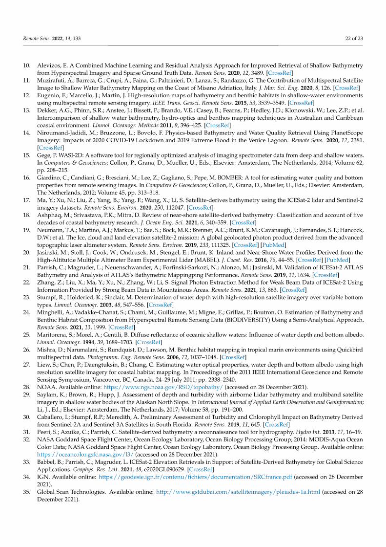
Remote Sens. 2022, 14, 133 22 of 23

10. Alevizos, E. A Combined Machine Learning and Residual Analysis Approach for Improved Retrieval of Shallow Bathymetryfrom Hyperspectral Imagery and Sparse Ground Truth Data. Remote Sens. 2020, 12, 3489. [CrossRef]

11. Muzirafuti, A.; Barreca, G.; Crupi, A.; Faina, G.; Paltrinieri, D.; Lanza, S.; Randazzo, G. The Contribution of Multispectral SatelliteImage to Shallow Water Bathymetry Mapping on the Coast of Misano Adriatico, Italy. J. Mar. Sci. Eng. 2020, 8, 126. [CrossRef]

12. Eugenio, F.; Marcello, J.; Martin, J. High-resolution maps of bathymetry and benthic habitats in shallow-water environmentsusing multispectral remote sensing imagery. IEEE Trans. Geosci. Remote Sens. 2015, 53, 3539–3549. [CrossRef]

13. Dekker, A.G.; Phinn, S.R.; Anstee, J.; Bissett, P.; Brando, V.E.; Casey, B.; Fearns, P.; Hedley, J.D.; Klonowski, W.; Lee, Z.P.; et al.Intercomparison of shallow water bathymetry, hydro-optics and benthos mapping techniques in Australian and Caribbeancoastal environment. Limnol. Oceanogr. Methods 2011, 9, 396–425. [CrossRef]

14. Niroumand-Jadidi, M.; Bruzzone, L.; Bovolo, F. Physics-based Bathymetry and Water Quality Retrieval Using PlanetScopeImagery: Impacts of 2020 COVID-19 Lockdown and 2019 Extreme Flood in the Venice Lagoon. Remote Sens. 2020, 12, 2381.[CrossRef]

15. Gege, P. WASI-2D: A software tool for regionally optimized analysis of imaging spectrometer data from deep and shallow waters.In Computers & Geosciences; Collon, P., Grana, D., Mueller, U., Eds.; Elsevier: Amsterdam, The Netherlands, 2014; Volume 62,pp. 208–215.

16. Giardino, C.; Candiani, G.; Bresciani, M.; Lee, Z.; Gagliano, S.; Pepe, M. BOMBER: A tool for estimating water quality and bottomproperties from remote sensing images. In Computers & Geosciences; Collon, P., Grana, D., Mueller, U., Eds.; Elsevier: Amsterdam,The Netherlands, 2012; Volume 45, pp. 313–318.

17. Ma, Y.; Xu, N.; Liu, Z.; Yang, B.; Yang, F.; Wang, X.; Li, S. Satellite-derives bathymetry using the ICESat-2 lidar and Sentinel-2imagery datasets. Remote Sens. Environ. 2020, 250, 112047. [CrossRef]

18. Ashphaq, M.; Srivastava, P.K.; Mitra, D. Review of near-shore satellite-derived bathymetry: Classification and account of fivedecades of coastal bathymetry research. J. Ocean Eng. Sci. 2021, 6, 340–359. [CrossRef]

19. Neumann, T.A.; Martino, A.J.; Markus, T.; Bae, S.; Bock, M.R.; Brenner, A.C.; Brunt, K.M.; Cavanaugh, J.; Fernandes, S.T.; Hancock,D.W.; et al. The Ice, cloud and land elevation satellite-2 mission: A global geolocated photon product derived from the advancedtopographic laser altimeter system. Remote Sens. Environ. 2019, 233, 111325. [CrossRef] [PubMed]

20. Jasinski, M.; Stoll, J.; Cook, W.; Ondrusek, M.; Stengel, E.; Brunt, K. Inland and Near-Shore Water Profiles Derived from theHigh-Altitutde Multiple Altimeter Beam Experimental Lidar (MABEL). J. Coast. Res. 2016, 76, 44–55. [CrossRef] [PubMed]

21. Parrish, C.; Magruder, L.; Neuenschwander, A.; Forfinski-Sarkozi, N.; Alonzo, M.; Jasinski, M. Validation of ICESat-2 ATLASBathymetry and Analysis of ATLAS’s Bathymetric Mappingping Performance. Remote Sens. 2019, 11, 1634. [CrossRef]

22. Zhang, Z.; Liu, X.; Ma, Y.; Xu, N.; Zhang, W.; Li, S. Signal Photon Extraction Method for Weak Beam Data of ICESat-2 UsingInformation Provided by Strong Beam Data in Mountainous Areas. Remote Sens. 2021, 13, 863. [CrossRef]

23. Stumpf, R.; Holderied, K.; Sinclair, M. Determination of water depth with high-resolution satellite imagery over variable bottomtypes. Limnol. Oceanogr. 2003, 48, 547–556. [CrossRef]

24. Minghelli, A.; Vadakke-Chanat, S.; Chami, M.; Guillaume, M.; Migne, E.; Grillas, P.; Boutron, O. Estimation of Bathymetry andBenthic Habitat Composition from Hyperspectral Remote Sensing Data (BIODIVERSITY) Using a Semi-Analytical Approach.Remote Sens. 2021, 13, 1999. [CrossRef]

25. Maritorena, S.; Morel, A.; Gentili, B. Diffuse reflectance of oceanic shallow waters: Influence of water depth and bottom albedo.Limnol. Oceanogr. 1994, 39, 1689–1703. [CrossRef]

26. Mishra, D.; Narumalani, S.; Rundquist, D.; Lawson, M. Benthic habitat mapping in tropical marin environments using Quickbirdmultispectral data. Photogramm. Eng. Remote Sens. 2006, 72, 1037–1048. [CrossRef]

27. Liew, S.; Chen, P.; Daengtuksin, B.; Chang, C. Estimating water optical properties, water depth and bottom albedo using highresolution satellite imagery for coastal habitat mapping. In Proceedings of the 2011 IEEE International Geoscience and RemoteSensing Symposium, Vancouver, BC, Canada, 24–29 July 2011; pp. 2338–2340.

28. NOAA. Available online: https://www.ngs.noaa.gov/RSD/topobathy/ (accessed on 28 December 2021).29. Saylam, K.; Brown, R.; Hupp, J. Assessment of depth and turbidity with airborne Lidar bathymetry and multiband satellite

imagery in shallow water bodies of the Alaskan North Slope. In International Journal of Applied Earth Observation and Geoinformation;Li, J., Ed.; Elsevier: Amsterdam, The Netherlands, 2017; Volume 58, pp. 191–200.

30. Caballero, I.; Stumpf, R.P.; Meredith, A. Preliminary Assessment of Turbidity and Chlorophyll Impact on Bathymetry Derivedfrom Sentinel-2A and Sentinel-3A Satellites in South Florida. Remote Sens. 2019, 11, 645. [CrossRef]

31. Peeri, S.; Azuike, C.; Parrish, C. Satellite-derived bathymetry a reconnaissance tool for hydrography. Hydro Int. 2013, 17, 16–19.32. NASA Goddard Space Flight Center, Ocean Ecology Laboratory, Ocean Biology Processing Group; 2014: MODIS-Aqua Ocean

Color Data; NASA Goddard Space Flight Center, Ocean Ecology Laboratory, Ocean Biology Processing Group. Available online:https://oceancolor.gsfc.nasa.gov/l3/ (accessed on 28 December 2021).

33. Babbel, B.; Parrish, C.; Magruder, L. ICESat-2 Elevation Retrievals in Support of Satellite-Derived Bathymetry for Global ScienceApplications. Geophys. Res. Lett. 2021, 48, e2020GL090629. [CrossRef]

34. IGN. Available online: https://geodesie.ign.fr/contenu/fichiers/documentation/SRCfrance.pdf (accessed on 28 December2021).

35. Global Scan Technologies. Available online: http://www.gstdubai.com/satelliteimagery/pleiades-1a.html (accessed on 28December 2021).

Remote Sens. 2022, 14, 133 23 of 23

36. ESA. Available online: https://earth.esa.int/web/eoportal/satellite-missions/i/icesat-2 (accessed on 28 December 2021).37. Neumann, T.A.; Brenner, A.; Hancock, D.; Robbins, J.; Saba, J.; Harbeck, K.; Gibbons, A.; Lee, J.; Luthcke, S.B.; Rebold, T.; et al.

ATLAS/ICESat-2 L2A Global Geolocated Photon Data, Version 3. [ATL03]; NASA National Snow and Ice Data Center DistributedActive Archive Center: Boulder, CO, USA, 2020.

38. Ester, M.; Kriegel, H.-P.; Sander, J.; Xu, X. A density-based algorithm for discovering clusters in large spatial databases with noise.In Proceedings of the Second International Conference on Knowledge Discovery and Data Mining (KDD’96), Portland, OR, USA,2–4 August 1996; AAAI Press: Palo Alto, CA, USA, 1996; pp. 226–231.

39. Xie, C.; Chen, P.; Pan, D.; Zhong, C.; Zhang, Z. Improved Filtering of ICESat-2 Lidar Data for Nearshore Bathymetry EstimationUsing Sentinel-2 Imagery. Remote Sens. 2021, 13, 4303. [CrossRef]

40. Xun, N.; Ma, X.; Ma, Y.; Zhao, P.; Yang, J.; Wang, H. Deriving Highly Accurate Shallow Water Bathymetry From Sentinel-2 andICESat-2 Datasets by a Multitemporal Stacking Method. IEEE J. Sel. Top. Appl. Earth Obs. Remote Sens. 2021, 14, 6677–6685.

41. Khater, I.; Nabi, I.R.; Hamarneh, G. A Review of Super-Resolution Single-Molecule Localization Microscopy Cluster Analysis andQuantification Methods. Patterns 2020, 1, 100038. [CrossRef] [PubMed]

42. Randazzo, G.; Barreca, G.; Cascio, M.; Crupi, A.; Fontana, M.; Gregorio, F.; Lanza, S.; Muzirafuti, A. Analysis of Very High SpatialResolution Images for Automatic Shoreline Extraction and Satellite-Derived Bathymetry Mapping. Geosciences 2020, 10, 172.[CrossRef]

43. Gabr, B.; Ahmed, M.; Marmoush, Y. PlanetScope and Landsat 8 Imageries for Bathymetry Mapping. J. Mar. Sci. Eng. 2020, 8, 143.[CrossRef]

44. Pe’eri, S.; Parrish, C.; Azuike, C.; Alexander, L.; Armstrong, A. Satellite Remote Sensing as a Reconnaissance Tool for AssessingNautical Chart Adequacy and Completeness. Mar. Geodesy 2014, 37, 293–314. [CrossRef]

45. Poppenga, S.; Palaseanu-Lovejoy, M.; Gesch, D.; Danielson, J.; Tyler, D. Evaluating the Potential for Near-Shore Bathymetry on theMajuro Atoll, Republic of the Marshall Islands, Using Landsat 8 and WorldView-3 Imagery; Scientific Investigations Report 2018-5024;U.S. Geological Survey: Reston, VA, USA, 2018.

46. Favoretto, F.; Morel, Y.; Waddington, A.; Lopez-Calderon, J.; Cadena-Roa, M.; Blanco-Jarvio, A. Testing of the 4SM Method inthe Gulf of California Suggests Field Data Are not Needed to Derive Satellite Bathymetry. Sensors 2017, 17, 2248. [CrossRef][PubMed]

47. Nur, H.; Othman, Y.; Wiwin, W.; Saiful, S. Integration of Satellite-Derived Bathymetry and Sounding Data in Providing Continuousand Detailed Bathymetric Information. In IOP Conference Series: Earth and Environmental Science, Proceedings of the 2nd MaritimeScience and Advanced Technology; Marine Science and Technology in Framework of The Sustainable Development Goals, Makassar, Indonesia,7–8 August 2019; IOP Publishing Ltd.: Bristol, UK, 2020; Volume 618, p. 012018.

48. Yakup, D.; Zeliha, S.; Bulent, S.; Mehmet, A.; Dagdeviren, M. Determination of sediment deposition of Hasanlar Dam usingbathymetric and remote sensing studies. Nat. Hazards 2019, 97, 211–227.

49. Monteys, X.; Harris, P.; Caloca, S.; Cahalane, C. Spatial Prediction of Coastal Bathymetry Based on Multispectral Satellite Imageryand Multibeam Data. Remote Sens. 2015, 7, 13782–13806. [CrossRef]

50. Collin, A.; Planes, S. Enhancing Coral Health Detection Using Spectral Diversity Indices from WorldView-2 Imagery and MachineLearners. Remote Sens. 2012, 4, 3244–3264. [CrossRef]

51. Morel, A.; Maritorena, S. Bio-optical properties of oceanic waters: A reappraisal. J. Geophys. Res. 2001, 106, 7163–7180. [CrossRef]52. Mogstad, A.; Johnsen, G.; Ludvigsen, M. Shallow-Water Habitat Mapping using Underwater Hyperspectral Imaging from an

Unmanned Surface Vehicle: A Pilot Study. Remote Sens. 2019, 11, 685. [CrossRef]53. Story, M.; Congalton, R.G. Accuracy assessment: A user’s perspective. Photogramm. Eng. Remote Sens. 1986, 52, 397–399.54. Lemoine, A.; Briole, P.; Bertil, D.; Roullé, A.; Foumelis, M.; Thinon, I.; Raucoules, D.; de Michele, M.; Valty, P.; Hoste Colomer,

R. The 2018–2019 seismo-volcanic crisis east of Mayotte, Comoros islands: Seismicity and ground deformation markers of anexceptional submarine eruption. Geophys. J. Int. 2020, 223, 22–44. [CrossRef]

55. Cesca, S.; Letort, J.; Razafindrakoto, H.N.T.; Heimann, S.; Rivalta, E.; Isken, M.P.; Nikkhoo, M.; Passarelli, L.; Petersen, G.L.;Cotton, F.; et al. Drainage of a deep magma reservoir near Mayotte inferred from seismicity and deformation. Nat. Geosci. 2020,13, 87–93. [CrossRef]

56. Feuillet, N.; Jorry, S.; Crawford, W.; Deplus, C.; Thinon, I.; Jacques, E.; Van der Woerd, J. Birth of a large volcanic edifice throughlithosphere-scale dyking offshore Mayotte (Indian Ocean). Nat. Geosci 2021. under review. [CrossRef]

57. Amrari, S.; Bourassin, E.; Andréfouët, S.; Soulard, B.; Lemonnier, H.; Le Gendre, R. Shallow Water Bathymetry Retrieval Using aBand-Optimization Iterative Approach: Application to New Caledonia Coral Reef Lagoons Using Sentinel-2 Data. Remote Sens.2021, 13, 4108. [CrossRef]

58. Niroumand-Jadidi, M.; Vitti, A.; Lyzenga, D.R. Multiple Optimal Depth Predictors Analysis (MODPA) for river bathymetry:Findings from spectroradiometry, simulations, and satellite imagery. Remote Sens. Environ. 2018, 218, 132–147. [CrossRef]

59. Niroumand-Jadidi, M.; Bovolo, F.; Bruzzone, L. SMART-SDB: Sample-specific multiple band ratio technique for satellite-derivedbathymetry. Remote Sens. Environ. 2020, 251, 112091. [CrossRef]

60. Albright, A.; Glennie, C. Nearshore Bathymetry From Fusion of Sentinel-2 and ICESat-2 Observations. IEEE Geosci. Remote Sens.Lett. 2021, 18, 900–904. [CrossRef]