Embed Size (px)
Citation preview
2420 J. Opt. Soc. Am. A/Vol. 14, No. 9 /September 1997 Burgess et al.
Visual signal detectability with two noisecomponents: anomalous masking effects
Arthur E. Burgess
Brigham and Women’s Hospital, Harvard Medical School, Boston, Massachusetts 02115
Xing Li
Xerox Webster Research Laboratories, Webster, New York 14580
Craig K. Abbey
Department of Radiology, University of Arizona, Tucson, Arizona 85724
Received September 16, 1996; revised manuscript received March 17, 1997; accepted March 18, 1997
We measured human observers’ detectability of aperiodic signals in noise with two components (white andlow-pass Gaussian). The white-noise component ensured that the signal detection task was always noise lim-ited rather than contrast limited (i.e., image noise was always much larger than observer internal noise). Thelow-pass component can be considered to be a statistically defined background. Contrast threshold elevationwas not linearly related to the rms background contrast. Our results gave power-law exponents near 0.6,similar to that found for deterministic masking. The Fisher–Hotelling linear discriminant model assessed byRolland and Barrett [J. Opt. Soc. Am. A 9, 649 (1992)] and the modified nonprewhitening matched filter modelsuggested by Burgess [J. Opt. Soc. Am. A 11, 1237 (1994)] for describing signal detection in statistically definedbackgrounds did not fit our more precise data. We show that it is not possible to find any nonprewhiteningmodel that can fit our data. We investigated modified Fisher–Hotelling models by using spatial-frequencychannels, as suggested by Myers and Barrett [J. Opt. Soc. Am. A 4, 2447 (1987)]. Two of these models did givegood fits to our data, which suggests that we may be able to do partial prewhitening of image noise. © 1997Optical Society of America [S0740-3232(97)04009-X]
1. INTRODUCTIONThe purpose of the work described here was to investigatehuman observer signal detection performance in imageswith two noise components and to evaluate the agreementwith a number of observer models based on statistical de-cision theory. In the experiments one noise componentwas uncorrelated noise to simulate image noise, while theother was low-pass-filtered noise designed to simulatespatially varying structure (statistically defined back-ground). Four different experiments will be described:The purpose is to provide a variety of tests for the ob-server models. (a) The first experiment demonstratesthe effect of background correlation distance variation onsignal detectability. For the other three experiments,the background correlation distances were larger thansignal dimensions to give the maximum possible differ-ences between model predictions. (b) In the second typeof experiment, detectability of several aperiodic signalswas evaluated over a wide range of background spectraldensities at three fixed background correlation distances.This approach evaluates models along one direction in thespace of background parameters. (c) In the third type ofexperiment, the effect of observer viewing distance wasmeasured over the range from 0.5 to 2.5 m for two signals.(d) In the final experiment, signal detectability was mea-sured with the same background sample in each of the
0740-3232/97/0902420-23$10.00 ©
two alternative images. The purpose of this experimentwas to attempt to separate background uncertainty (dueto statistical variation) from masking effects caused bythe background structure.
Most previous experiments investigating human signaldetection performance with noise-limited images havebeen done by use of the signal-known-exactly (SKE) andthe background-known-exactly (BKE) paradigms withone noise component. The advantage of the combinedSKE–BKE approach is that human performance can becompared with that for the ideal Bayesian observer doingthe same task.1,2 These experiments were interestingand informative about fundamental properties of the hu-man visual system performance. However, they were farremoved from the complex visual tasks performed by ex-pert image analysts or interpreters who attempt to detectand identify a large variety of signals in a large variety ofbackground structures or clutter. The signals and thebackgrounds in these types of images are defined only in astatistical sense. This has led to investigation of humanperformance of noise-limited detection tasks with simplestatistically defined (lumpy) additive backgrounds byRolland and Barrett3 and by Burgess.4 Eckstein andWhiting5 have recently done experiments with patient-structured backgrounds but have not investigated the ef-fect of changing the relative contributions of image noise
1997 Optical Society of America
Burgess et al. Vol. 14, No. 9 /September 1997 /J. Opt. Soc. Am. A 2421
and patient structure to threshold elevation. In this pa-per we use the term background to refer to spatial varia-tions that are slowly varying in comparison with the sig-nal size, while we use the term noise to refer to rapidlyvarying spatial variations. Note that the signals and thenoise are added to backgrounds in our tasks, so the recentresearch efforts on nonoverlapping backgrounds by Javidiand Wang6 and by Kober and Campos7 do not apply.There are a number of reasons for investigating humanperformance for statistically defined additive back-grounds.
One reason is that predictions of observer performancebased on the Bayesian observer doing combined SKE–BKE tasks do not agree with clinical experience innuclear medicine imaging. This was pointed by Tsuiet al.,8 who did experiments with synthetic signals (le-sions) added to clinical nuclear medicine images. Theclassical signal detection theory approach that uses amatched filter (based on SKE–BKE assumptions) pre-dicted monotonically increasing detectability as imagingaperture size increased. The same photon-limited ap-proach was used by Wagner et al.9 to investigate perfor-mance of the ideal Bayesian observer for the Raleigh task(discrimination between a single Gaussian signal and aseparated pair of Gaussian signals) on a known back-ground. They found improving performance with in-creasing aperture diameter and no optimum size. Usingstatistically defined backgrounds, Myers et al.10 showedthat a linear discriminant observer model did lead to theprediction of a specific optimum imaging aperture size.Improved models for predicting human performancewould be valuable for design and optimization of nuclearmedicine imaging systems.
A second reason for this investigation is that it is wellknown that detectability of signals depends on the com-plexity of the background in the local vicinity of the sig-nal. This is a natural feature of most image analysistasks. Revesz et al. referred to this problem as ‘‘detec-tion in structured noise.’’ 11 The term conspicuity12 isalso used to describe the relationship between the ease ofdetection of an object and local background complexity.This problem has led to development of a variety of back-ground suppression techniques in medical imaging, in-cluding tomography and dual-energy imaging. Onceagain, the absence of a human observer model for complextasks does not allow one to predict, a priori, how muchperformance loss there is due to the conspicuity problemand hence how much improvement is needed for the back-ground suppression techniques to be feasible.
Our results also show an interesting departure from ageneral observation that described the effects of imagenoise on signal detectability for all previous research.One way to think about the effects of noise and a statis-tically defined background is in terms of signal detectionthreshold elevation. In many papers this is referred toas ‘‘masking.’’ The terminology is somewhat confused be-cause, while some authors use the term only for determin-istic processes, others use it for both deterministic andstochastic processes. To the best of our knowledge, allprevious evaluations of threshold elevation due to noisehave shown that the signal energy threshold is linearly
related to the noise spectral density. As can be seen be-low, our results show a nonlinear (power-law) dependenceon background spectral density with an exponent near0.6. However, in all the previous experiments fixed fil-ters were used to produce the noise. As is shown below,all reasonable observer models predict such a linear effectfor a fixed noise spectral shape as noise amplitude is var-ied. In our experiments the white-noise component washeld at a fixed spectral density, giving an rms luminancecontrast variation of 15.8% (20/127 gray levels). The low-pass background component also had a fixed bandwidthfilter, but the spectral density was scaled to give a rangeof rms luminance contrast variation from 0.8% to 25%(1–32 gray levels). The combined noise power spectrumwill therefore change shape as the background componentis increased. The predicted threshold elevation for thiscase depends on whether the observer is able to compen-sate for the spectral changes (prewhiten the total noise).Nonprewhitening models will show a linear energythreshold elevation as background spectral density in-creases, while models that can perform partial or com-plete prewhitening will show other threshold elevation ef-fects.
Myers et al.10 considered two model observers in a the-oretical analysis of signal detection with Poisson noiseand a lumpy background produced by a Poisson randomprocess. One model was the best linear observer, also re-ferred to as the Hotelling observer or the Fisher–Hotelling (FH) observer,13,14 first proposed by Fieteet al.15 for use as a model of human observer performancefor noise-limited signal detection tasks. The other modelwas the nonprewhitening matched filter observer (NPW)model, which does not do background estimation. TheFH model has, in essence, an infinite number of infinitesi-mally narrow spatial-frequency channels and can adjustfrequency response to decorrelate (prewhiten) all the in-put noise and can match the signal spectrum after thisprewhitening filtration. The NPW model has, in effect, asingle channel that can adapt to match the input signalspectrum but cannot decorrelate input noise. Rollandand Barrett3 reported results of psychophysical experi-ments that simulated imaging of a two-dimensional (2D)Gaussian signal superimposed on an inhomogeneousbackground through a pinhole aperture. AppropriatePoisson noise was added to the resulting images. Theyfound that the variation of human observer performancewith respect to aperture size and imaging time was wellpredicted by the FH model. The predictions of the NPWmodel did not agree with their human observer results.Burgess4 showed that a modified NPW model could fit theRolland–Barrett data. The model included a linear filterwith no zero frequency (dc) response and a shape similarto that of the human contrast sensitivity function. Weshall refer to this as the NPWE model. The Rolland–Barrett data were not sufficiently precise to allow one tofavor either the FH model or the NPWE model.
The experiments described in this paper were designedto do more stringent tests of the two models. The observ-er’s task was to detect compact aperiodic 2D signals in im-ages with two noise components (white and filtered).The low-pass noise components were created from whitenoise by use of a Gaussian linear filter. The correlation
2422 J. Opt. Soc. Am. A/Vol. 14, No. 9 /September 1997 Burgess et al.
distances (spatial standard deviations) of the filters werechosen to be large compared with signal dimensions andto therefore maximize differences in predictions of thevarious models. The experimental results presented be-low demonstrate that neither of the two previous models(FH and NPWE) provides a good fit to human observerperformance over the full range of lumpy background am-plitudes investigated. The performance of a variety ofFH models with spatial-frequency channels is also evalu-ated in this paper. These include the circularly symmet-ric channelized FH model of Myers and Barrett16 with dcremoval by an arbitrary low-frequency cutoff. This is re-ferred to as the FHCMB model. Barrett et al.17 foundgood agreement between a variety of human observer re-sults and predictions of the FHCMB model. This modelcan be described as having the ability to only partiallycompensate for noise correlations (prewhiten), since noisewithin a channel is irretrievably mixed by the channel in-tegration process. However, the observer model can ad-just the weights of individual channel outputs to achievethe best possible performance subject to the finite channelbandwidths (i.e., partial prewhitening). The smaller thechannel bandwidth, the more effective this procedure be-comes. In the limit of infinitesimal channel bandwidth,the model becomes the ideal observer model. Otherchannelized FH models are investigated here. Onemodel, FHCavg, has circular symmetry for the channels,an eye filter plus internal noise, and averaging of thechannel start frequencies. The final model, FHCDOM,has a circularly symmetric eye filter, overlapping spatial-frequency channels of the type described by Daly,18 andinternal noise. It is shown that these models give im-proved fits to the observer data. Finally, a simple equa-tion is given that fits the data but has no known theoret-ical significance.
2. THEORYThe images used in these experiments are of the form
i~x, y ! 5 s~x 2 x0 , y 2 y0! 1 n~x, y ! 1 b~x, y ! 1 C,(1)
where s(x 2 x0 , y 2 y0) is the signal spatial functioncentered at position (x0 , y0), with white Gaussian noisen(x, y), a spatially varying background b(x, y), and aconstant level C. The white noise has constant spectraldensity N0 and zero mean. The lumpy backgrounds wereproduced by low-pass filtering of zero mean Gaussiannoise with spectral density W0 . The constant C was setat 127 to center the image data in the 0–255 range of dis-play memory.
Since the noise and the background used in our experi-ments are independent stationary Gaussian random pro-cesses, their sum will also be a stationary Gaussian ran-dom process.19 Hence the optimum Bayesian observermodel for our experiments is linear. Note that this is dif-ferent from the experimental situation of Rolland andBarrett, who used Poisson noise and backgrounds createdwith a Poisson random process. The ideal observer deci-sion process would be nonlinear for that case. Math-ematical considerations restricted them to linear observer
models. The optimum linear observer goes by a numberof names. It is often referred to as the Fisher linear dis-criminant in the pattern recognition literature.20 Bar-rett and co-workers17 refer to the model as the Hotellingobserver. The two-class separation that arises is some-times called the Mahalanobis distance.20 The distinctionamong names is frequently based on whether the meansand the variances of the classes are sample estimates orpopulation values. We refer to this optimum linear dis-criminant function approach as the FH model. Since weare using Gaussian noise and background, the FH modelalso is the ideal Bayesian observer.
In this paper a variety of observer models are comparedwith human observer results. The models shall now beintroduced. A summary of model properties is given inTable 1.
A. Fisher–Hotelling ModelThe FH observer performs the detection task by cross cor-relation of the image data and a template, t(x 2 x0 , y2 y0), centered at the expected signal locations. Thetemplate spatial function is calculated10 with the exactlyknown signal function and the covariance matrix of thedata and serves, simultaneously, to compensate for noisecorrelations (prewhiten), estimate the background, anddetect the signal. The signal has the amplitude spec-trum, S(u, v), the noise has the power spectrum,N(u, v), and the statistically defined background has thepower spectrum, W(u, v). The FH observer perfor-mance for the images used in this study is described bythe detectability index, d8, in Eq. (2). The derivation ofthis equation is described in Myers et al.10:
~dFH8 !2 5 EE F uS~u, v !u2
N~u, v ! 1 W~u, v !Gdudv. (2)
B. Modified Nonprewhitening Matched Filter ModelThe NPW model has a long history. The NPW model wasfirst presented by Wagner and Weaver.21 The NPWmodel uses the filtered signal as a template for cross cor-
Table 1. Summary of Descriptions and Propertiesof Models Used in This Papera
AcronymNumber ofChannels Eye Filter
InternalNoise
FilterOverlap
NPWEb 1 yes yes N/AFHc infinite no no noFHN
d infinite yes yes noFHCMB
e 5 no no noFHCavg
f 8 yes yes noFHCDOM
g 6 or 11 yes yes yes
a The number of channels listed is for the radial direction only andranges from 0 to 50 c/deg.
b NPWE, NPW model with eye filter.c FH, Fisher–Hotelling linear discriminator (also ideal observer for this
study).d FHN , FH model with an eye filter and internal noise.e FHCMB, FH model with nonoverlapping (rect) channels above initial
frequency.f FHCavg, FH model with 1-octave rect channels and boundary fre-
quency averaging.g FHCDOM, FH model with difference-of-mesa filter channels.
Burgess et al. Vol. 14, No. 9 /September 1997 /J. Opt. Soc. Am. A 2423
relation and has no way of estimating the background.Myers et al.22 demonstrated that this model gave a goodfit to human signal detection results for a variety of imagenoise power spectra for the case of uniform backgrounds.Rolland and Barrett3 showed that a NPW model, whichincludes a dc response, gave very poor agreement withhuman signal detection results for statistically definedbackgrounds. The NPW model was modified by Burgesset al.1 and by Ishida et al.23 to include an eye filter andobserver internal noise. The combination of the signaland the eye filter is equivalent to a template that is par-tially adaptive in that it is influenced by signal size,shape, and location, but not by the covariance matrices ofthe noise or the lumpy background. The eye filter,E(u, v), has a spatial-frequency response similar to thecontrast sensitivity function of the human visual system,where u and v are spatial frequencies. This observerhas, in effect, a single channel with frequency responseC1(u, v) 5 S(u, v)E(u, v). We assume that the ob-server has internal noise with a spectral density Ni(u, v)that may depend on the input signal and noise spectra.The detectability index for this NPWE model is given bythe equation4
~dNPWE8 !2 5
F EE uS~u, v !u2uE~u, v !u2dudv G2
EE @N~u, v ! 1 W~u, v !#uS~u, v !u2uE~u, v !u4dudv 1 EE Ni~u, v !dudv. (3)
It is necessary to select a model of the eye filter, and avery desirable feature is a filter that allows subtraction ofa local estimate of the background. Such a filter willhave no dc (zero-frequency) response, which therefore re-moves some of the random variation in the amplitude ofthe local background on which the signal sits. If this lo-cal background estimation were not done, then the ob-server would include this variable offset in templatecross-correlation results and would make many addi-tional decision errors. The human visual system appearsto be able to estimate and compensate for local back-ground and is often described by a contrast sensitivityfunction with zero dc response. We considered severaleye filter models. The equation E( f ) 5 f1.3 exp(2bf ), forradial frequency f, was used in the modified NPW modelby Burgess4 to fit the experimental results obtained byRolland and Barrett.3 The Barten model24 has beenshown to fit a large variety of human contrast sensitivityresults. The E( f ) 5 f exp(2cf ) filter equation is asimple approximation to the Barten model. We foundlittle difference among model predictions when using thethree filters and therefore restrict ourselves to using thef exp(2cf ) model.
Given the large number of possible eye filter models, wedeveloped a method of determining whether the NPWEmodel with any fixed eye filter function could fit our ex-perimental results. As is shown below and in AppendixA, Section 2, the detectability index equation for theNPWE model can be changed to the equivalent forms
Ct2 2 Ct0
2 5 aW0 , ~d08/d8!2 2 1 5 bW0 /N0 , (4)
where Ct and Ct0 are contrast thresholds with and with-out a lumpy background, respectively; W0 is the dc valueof W(u, v); and d08 is the signal detectability for a uni-form background (W0 5 0). The parameters a and b areconstants for a given signal, eye filter, and lumpy back-ground correlation distance. If one plots data for eitherequation in log-log form, any NPWE model predicts aslope of unity. It is shown below that Eqs. (4) are notvalid for our human observer results but that a more gen-eral form with W0 raised to approximately the 0.6 powergives a good fit. This is a completely empirical observa-tion with no known theoretical significance. The deriva-tion of Eqs. (4) is as follows. Let the signal amplitudespectrum be given by S(u, v) 5 CF(u, v), where C is acontrast scaling factor. Let the white-noise spectrum begiven by N(u, v) 5 N0H2(u, v). For the uniform back-ground case (W0 5 0) Eq. (3) becomes (at contrastthreshold value, Ct0)
~dNPWE8 !2 5 ACt02/~N0B 1 C !,
where
A 5 F EE uF~u, v !u2uE~u, v !u2dudv G2
,
B 5 EE H2~u, v !uF~u, v !u2uE~u, v !u4dudv,
C 5 EE Ni~u, v !dudv. (5)
With the use of d8 of unity to define a threshold, the con-trast threshold equation becomes (Ct0)2 5 (N0B1 C)/A. Similarly, let the lumpy background spectrumbe given by W(u, v) 5 W0K2(u, v), and let D be thebackground variance integral analogous to B in Eqs. (5).Then the contrast threshold equation becomes (Ct)
2
5 (N0B 1 W0D 1 C)/A 5 (Ct0)2 1 W0D/A 5 (Ct0)2
1 aW0 . Hence one obtains the first relation of Eqs. (4).One obtains the second relation in a similar manner bysolving for the d8 ratio at a particular contrast.
C. Fisher–Hotelling Model with Eye Filter and InternalNoise (FHN)The FH model can be modified to resemble the human ob-server more closely by inclusion of a circularly symmetriceye filter function, E( f ), for radial spatial frequency, f,and internal noise. The signal and background spectraused in our experiments also had circular symmetry.The white internal noise, Ni , is added after the filter butbefore the linear discriminator. The detectability indexfor this model (which we shall refer to as FHN , with N
2424 J. Opt. Soc. Am. A/Vol. 14, No. 9 /September 1997 Burgess et al.
denoting internal noise) can be obtained by a simplemodification of Eq. (2), giving (for circular symmetry)
~dFHN8 !2 5 2pE
0
`H E~ f !2S~ f !2
E~ f !2@N0 1 W~ f !# 1 NifdfJ . (6)
One can, of course, divide the numerator and the denomi-nator by E2( f ) if it never goes to zero. The resulting ex-pression, Ni /E2( f ), is simply the internal noise referredback to the input.25
D. Fisher–Hotelling Model with Myers–BarrettChannels (FHCMB)Myers and Barrett16 showed that, when the FH modelwas modified to include nonoverlapping (rect function)spatial-frequency channels, it predicted human observerperformance for detection of signals in anticorrelatednoise with a uniform background. We shall refer to thisas the FHCMB model. Myers and Barrett used circularsymmetric channels with sharp boundaries, kept the ratioof the channel bandwidth and center frequency constant(constant Q), and used a low-frequency cutoff, fc . Therewas no filter response below the cutoff frequency to en-sure no dc response. Boundaries between subsequentchannels were given by the relation fn 5 anfc . Myersand Barrett tried the four combinations of two differentcutoff frequencies [ fc ' 0.6, 0.87 cycles per degree (c/deg)]and two values of a (1.5, 2.0). They found little differ-ence in performance for the various combinations of chan-nel parameters. Their observers were not constrained toa particular viewing distance, so the values of fc are onlyan estimate of average values. The use of discrete, non-overlapping channels was based on the desire for math-ematical simplicity. Physiology and psychophysics, incontrast, suggest that there are many overlapping chan-nels with a bandwidth of 1 octave (a 5 2).26 The FHCMBmodel is, in effect, an N-channel model in which the noisespectrum within a given channel spatial-frequency re-sponse range, Ri , cannot be prewhitened but in which thechannel outputs can be weighted to attempt to flatten theoverall channel response to total noise (including thelumpy background). The detectability index for theFHCMB model is determined by the sum of outputs, Vi ,with the following equations16:
~dFHCMB8 !2 5 (
i51
N
Vi , (7)
where
Vi 5 F2p ERi
S~ f !fd fG2Y 2p ERi
@N0 1 W~ f !#fdf.
E. Fisher–Hotelling Model with Rect FunctionChannels and Averaging (FHCavg)One can argue that the choice of the low-frequency cutoffvalue is arbitrary. Therefore we considered a slightlymodified version of the Myers–Barrett channelized modelthat included an eye filter (with no dc response), had thefirst channel extended to zero frequency, and included ob-server internal noise. The individual channel responsesfor this model are given by
Vi 5 F2p ERi
S~ f !E~ f !fdfG2Y 2p
3 ERi
$E2~ f !@N0 1 W~ f !# 1 Ni~ f !%fdf. (8)
The discrete nonoverlapping channels cause the sameanomalous predictions that can be seen below for theFHCMB model. Since there is no compelling reason topick a particular value for the first spatial-frequencyboundary, this model uses 1-octave-wide channels, andperformance is calculated by averaging of performance re-sults over a 1-octave range of starting frequencies (0.25–0.5 c/deg). Another way to justify averaging is that, evenif there were well-defined channel boundaries, observersdo not normally maintain a fixed viewing distance, sothere is a natural variation in angular extent of signalsand noise parameters in images.
F. Fisher–Hotelling Model with Difference-of-MesaFilter Channels (FHCDOM)Finally, we investigated one other channelized FH model,using an eye filter and overlapping 2D channels based onDaly’s model.18 The 2D channel response functions,Cmn , are separable functions in polar frequency coordi-nates of the form Cmn( f, u) 5 Dm( f )Fn(u). The mth ra-dial frequency response function, Dm( f ), is calculatedfrom differences between low-pass filters to ensure thatthe total filter response sums to unity. Summing tounity is an irrelevant constraint given the decorrelationstage in the FH model, but we used it to be consistentwith Daly’s filter model. The low-pass filter has three re-gions: a flat passband with unit response for frequenciesless than f1/2 2 w, a transition region modeled by a Han-ning window function of width w, and a stop band withzero response for frequencies greater than f1/2 1 w.Daly refers to this as a mesa filter. The transition regionresponse function is
H~f, f1/2! 512 H 1 1 cosFp~ f 2 f1/2 1 w/2!
w G J . (9)
The difference-of-mesa (DOM) channel response is calcu-lated by use of the difference between adjacent mesa low-pass filters. We also followed Daly in using a truncatedGaussian function with no angular dependence for thelowest-frequency base band. The angular filters for non-zero radial center frequencies, An(u, uc), were also Han-ning functions of active width uw centered at angle ucwith zero response outside the active width and the form
An~u, uw! 512 H 1 1 cosFp~u 2 uc!
uwG J . (10)
We used the value p/6 for uw and np/6 for uc , as well asa variety of DOM filter radial base widths (w) and peakfrequency ratios, as discussed below.
Each channel consists of a filter and an integrator. Tosimplify notation, let us use a single index number, m, toidentify a particular channel that has some radial centerfrequency, fm , and angular center frequency, um . Givenan input image spectrum, I( f, u), the mth channel filteroutput is Um( f, u) 5 Cm( f 2 fm , u 2 um)E( f )I( f, u).
Burgess et al. Vol. 14, No. 9 /September 1997 /J. Opt. Soc. Am. A 2425
Since the signals and the lumpy background spectra usedin our work are radially symmetric, the channel output,after integration, is given by
Vm 5 V int 1 E0
`E0
2p
Cm~ f, u!I~ f, u!E~ f !fdfdu
5 V int 1 E0
`
Dm~ f !I~ f !E~ f !fd fE0
2p
Am~u!du.
(11)
The V int term represents observer internal noise as an ad-ditional variance for each channel, with no correlation be-tween channels. The value of V int was scaled to accountfor 2D bandwidth increases as channel center frequencyincreased. The values of V int were selected to be consis-tent with Pelli’s27 finding of a flat power spectrum and anoverall spectral density of 0.02N0 , as described below.The outputs of channels with overlapping channels arecorrelated, so the FH linear discriminator device will in-clude a decorrelation step. The detectability index forthis observer is calculated with28 (d8)2 5 VTS21V, whereV is the mean channels-output vector with componentsgiven by the expectation values ^Vm& and S is thechannels-output covariance matrix with components^VmVm8&. The inverse of the covariance matrix is used todecorrelate the outputs of the channels. The matrix cal-culations used to determine d8 can be done by standardmethods29 because the spatial-frequency channels reducethe dimensionality of the problem. The method of calcu-lating the mean output vector and covariance matrix ele-ments is described in Appendix C.
3. EXPERIMENTAL METHODSThe experiments were done by the two-alternative forced-choice (2AFC) method with simultaneous, side-by-sidepresentation of the two-alternative image fields. Eachfield consisted of a signal at the center (if present), uncor-related noise, and a sample background from the en-semble of lumpy backgrounds. The two noise fields andthe two lumpy backgrounds used in a particular decisiontrial were uncorrelated. Examples of the signal to be de-tected were always displayed above the noise fields.There was no restriction on viewing time for each decisiontrial, and observers were given feedback about whethertheir decision was correct.
Three signals were used. Two signals were sharp-edged disks with radii, R, of 4 and 8 pixels, respectively.The other signal had a 2D Gaussian profile with a spatialstandard deviation, s, of 3 pixels. During a block of 256trials the signal profile was fixed, but three different am-plitudes were randomly interspersed. The amplitudeswere selected, on the basis of preliminary experiments, togive detectability indices in the vicinity of 2. This en-sured that the coefficient of variation of d8 (standarderror/mean) was near its minimum value.30 The ob-server models (see Table 1) are not bothered by randomlyvarying signal amplitude, since the template amplitudescaling factor cancels out in the likelihood ratio calcula-tion for 2AFC trials. We checked human observer perfor-mance with known and random signal amplitudes. Iden-
tical psychometric functions are obtained for the twocases. The values of detectability index normalized bysignal-to-noise ratio (SNR), d8/SNR, for the three ampli-tudes were averaged over all the blocks of trials (usuallythree) for each observer and experimental condition. Foraperiodic signals, the relationship between d8 and SNR islinear for d8 above 0.5, and the SNR intercept is small.The estimates of d8/SNR that were obtained by averagingwere checked against values determined by linear regres-sion of d8 versus SNR. The estimate means determinedby the two methods agreed within 0.5%. The averagerms difference in estimates was approximately 1.5%.
The strategy for most experiments was to keep thewhite-noise spectral density, N0 , fixed and to vary thelumpy background parameters. A white-noise standarddeviation of 20 gray levels (rms contrast of 15.8%) was se-lected to ensure that image noise was much greater thanobserver internal noise,27,31 and that the relative effectsof external white noise and internal noise did not varyacross experimental conditions. White noise was pro-duced as follows. Pseudorandom numbers with a rectan-gular probability density function (PDF) were generatedwith the RAN1 algorithm29 and were transformed to ap-proximate a Gaussian PDF.29
The lumpy background images were produced by low-pass filtering of white Gaussian noise in the frequency do-main by use of a rotationally symmetric Gaussian low-pass filter to give a power spectrum, W( f )5 W0 exp(24p2sb2 f 2), where W0 is the dc spectral den-sity, sb is the spatial standard deviation (correlation dis-tance), and f is radial spatial frequency. The backgroundamplitude variance after filtering, (sb)2, is given by theequation (sb)2 5 W04p(sb)2. Six different pixel ampli-tude standard deviations (1, 2, 4, 8, 16, and 32) were usedfor each correlation distance (4, 8, and 16 pixels). The re-sulting lumpy background image pixel amplitudes werescaled to give the desired amplitude standard deviationand were converted to integer form by rounding for dis-play. Images with the first two correlation distances (4and 8 pixels) were 128 3 128 pixels. We took care toavoid aliasing problems when doing the fast Fouriertransforms of the backgrounds with the 16-pixel correla-tion distance. In this case we used only the central 1283 128 pixel region of a filtered 256 3 256 pixel image.Each 128 3 128 pixel background image was then di-vided into 16 segments of 32 3 32 pixels or 4 segments of64 3 64 pixels. Segments used in a 2AFC pair were al-ways selected from different background images to ensurethat they were uncorrelated. Each background and noisefile gave 2048 small fields (32 3 32 pixels) or 512 largefields (64 3 64 pixels). For a given 2AFC trial, two noisefields were randomly selected from the noise file, and twobackgrounds were randomly selected from the back-ground file.
On a given display trial the signal, the white noise, thebackground, and the dc offset were added together [seeEq. (1)] in computer memory. The upper limits to thewhite-noise and lumpy background variances were re-stricted by the need to ensure that the combination of sig-nal, noise, and background variation would rarely drivethe image data outside the 8-bit dynamic range of the dis-play memory. All the data values in an image were
2426 J. Opt. Soc. Am. A/Vol. 14, No. 9 /September 1997 Burgess et al.
checked before loading into the display memory, and anyvalues outside the 0–255 range were set to either 0 or 255as appropriate. This happens in roughly 1 pixel in 1000,so has little effect on the Gaussian probability distribu-tion of the background plus noise.
The images were displayed with a DEC VAX computer,a Peritek VCU-Q display board, and a Tektronix 634monitor with a flat cathode-ray tube. The display was240 3 320 pixels at a 60-Hz (noninterlaced) refresh rate.The monitor had a mean luminance of 150 cd/m2. Theviewing distance for most experiments was fixed at 1 mby use of a chair with a headrest, and each pixel in thedisplay subtended an angle of 0.55 mrad (0.01 deg). Fourobservers took part in the experiments: Two were au-thors, and the two others were naıve as to the detailedpurpose of the study. Two observers (authors) took partin a supplementary experiment in which the viewing dis-tance was varied between 0.5 and 2.5 m. All the observ-ers were well trained by doing at least 512 practice trialsfor each experimental condition before the data collectionbegan. A total of 768 trials were used for each observerand experimental condition. This gave a standard errorof approximately 5% of the mean value for each datum.
The role of the lumpy background on observer perfor-mance is determined, for a given background correlationdistance, by the ratio of the background and noise dc spec-tral densities, (W0 /N0), so the logarithm of this param-eter was used as the independent variable for analysis ofresults.
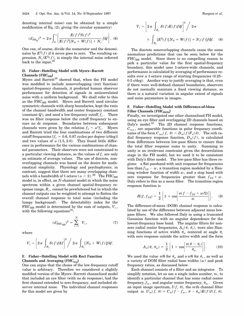
4. OBSERVER MODEL PERFORMANCECALCULATIONSThe integrals related to observer model performance werecalculated numerically by Simpson’s rule. Example re-sults for the FH and the NPWE models are shown in Fig.1(a) for the Gaussian signal and a range of backgroundspectral density scales (W0). In this and subsequent fig-ures the data for detectability, d8, will be normalized bythe SNR0 for the uniform background case (W0 5 0).This has the effect of dividing d8 by a constant for a givensignal and a given white-noise level. We chose to usenormalization by SNR0 rather than by a value SNRtot thatincluded the effects of both the white-noise and the back-ground component noise. The SNRtot calculation wouldhave implicitly included the FH model in the normaliza-tion, would have removed some of the variation from theW0 parameter change from all the other data, and wouldhave made it more difficult for the reader to interpret theresults. The observer d8 values for the uniform back-ground case are plotted at log(W0 /N0) equal to 21.8rather than at negative infinity, for convenience. It canbe seen that the FH model observer is ideal (d8/SNR05 1) for the uniform background case (W0 5 0), whilethe efficiency, (d8/SNR0)
2, of the NPWE model is approxi-mately 72% [d8/SNR 5 0.85 (Ref. 2)]. The reduced effi-ciency of the NPWE model is due to attenuation by thebandpass eye filter. The two models are almost equal inperformance over a small range of background spectraldensities near log(W0 /N0) equal to 1.5, and the perfor-mance of the NPWE model drops rapidly at higher ratios.We expect, on the basis of many previous experiments,
the value of d8/SNR0 to be approximately 0.7, correspond-ing to 50% human observer efficiency.2 Hence observermodel results must be scaled in some manner to fit hu-man observer results.
One approach is to simply scale model detectability in-dex data vertically by a multiplicative factor to fit humanobserver results. This cannot be done satisfactorily be-cause none of the equations describing model observerperformance is mathematically separable. Instead, scal-ing is done by introduction of known sources of ineffi-ciency directly into the equations of the models. Weknow that a major part of the reduction in efficiency canbe explained by a form of induced (evoked) internal
Fig. 1. (a) Absolute detectability index, d8, results for twomodel observers: Fisher–Hotelling (FH, which is ideal); and themodified nonprewhitening matched filter (NPWE). The Gauss-ian signal, g3, (s 5 3 pixels) is added to white noise (spectraldensity, N0) and to a statistically defined background, L8, withdc spectral density, W0 , and a correlation distance of 8 pixels.Note that, in the limit of no lumpy background, the value of d8for the FH model equals the SNR0 value. (b) Demonstration oftwo methods of adjusting the models shown in (a) to fit humanobserver results at W0 5 0 (uniform background with human av-erage d8/SNR of roughly 0.7). The solid and the dashed curvesshow results of the preferred method of including the two com-ponents of observer internal noise in the models [FHN , with Eq.(6); and NPWE, with Eq. (3)]. The unconnected symbols (1, 3)show the results of multiplicative scaling.
Burgess et al. Vol. 14, No. 9 /September 1997 /J. Opt. Soc. Am. A 2427
noise,31 so that the apparent display noise spectral den-sity is approximately 1.6 times the actual spectral den-sity, N0 , which sets an upper limit of roughly 60% for hu-man efficiency. This can be accounted for byreplacement of N0 with the term (1 1 BN)N0 in all theequations describing model detectability indices. Foreach experimental condition, we determined the averagehuman performance for the case in which there was nolumpy background and adjusted BN so that the model un-der consideration fitted this value. This gave estimatedvalues of B in the range from 0.6 to 1.0 for the differentsignal and background conditions, consistent with previ-ous estimates.31 It might seem reasonable to assumethat the lumpy background also induces internal noiseand that a similar (1 1 BW) factor might apply to W0 .We report measurements done with the same lumpybackgrounds in both alternative noise fields. These re-sults indicate that such an induced noise effect may bepresent for lumpy backgrounds, but the parameter BW isonly approximately 0.1.
Some of the models included constant observer internalnoise, which appears to have a nearly flat powerspectrum27 that depends on display luminance. At theluminance used in this experiment the internal noisespectral density corresponds to roughly Ni 5 0.02N0D2,where N0 is the image white-noise spectral density and Dis the viewing distance in meters. The value of 0.02 isestimated from summaries27,31 of published observer in-ternal noise spectral densities. At the display luminanceand the 1-m viewing distance used in these experiments,the internal noise spectral density is approximately5 3 1028 s deg2, and the white-noise spectral density isapproximately 2 3 1026 s deg2. The results of scaling byboth methods (simple multiplication and including inter-nal noise) are shown in Fig. 1(b). Note that the internalnoise scaling method shifts the theoretical curves to theright as well as down because of the (1 1 BN)N0 term.The shift downward is due to the reduced observer effi-ciency. The cause of the shift to the right is more subtle.With the use of the evoked internal noise the nominal de-pendent variable for the graph is log(W0 /N0), while theactual value in the models is log$W0@(1 1 BN)N0#%, whichcauses the function to be shifted. Since the Ni /N0 ratiowas not measured, we evaluated the sensitivity of modelsto the selected value for this ratio by using the range(0.01, 0.02, 0.05, and 0.1) and found that the sensitivity tothe selected fixed internal noise value was low. There-fore we used a ratio of 0.02 for all the comparisons. Thisinternal noise corresponds to white noise of roughly 3gray levels (rms) for our display.
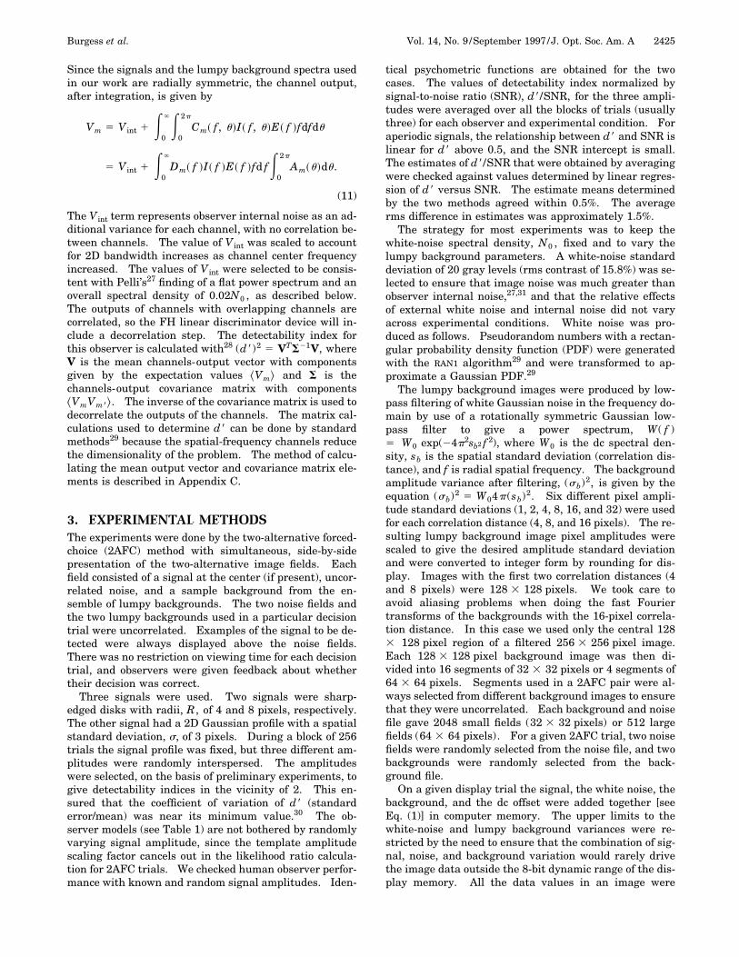
5. EXPERIMENTAL RESULTSA. Background Field SizeThe variation of human performance (d8/SNR) in detect-ing a disk signal (R 5 4) as a function of image field sizeis shown in Fig. 2(a). Our previous experience with uni-form backgrounds had shown that performance decreaseswith increasing noise field size. This is due to that factthat, while signal location is specified, the observers findit increasingly difficult to use this location information
precisely as field size increases. It was possible that thesituation might be different for lumpy backgrounds be-cause increased field size might give the observer a betteropportunity to become familiar with the statistical prop-erties of the backgrounds. The purpose of this experi-ment was to determine whether this hypothesis was true.As Fig. 2 demonstrates, the hypothesis was incorrect.Therefore a field size of 32 3 32 pixels was used for thesmall signals, and a field size of 64 3 64 pixels was usedfor the large disk signal (R 5 8 pixels) in all the subse-quent experiments—to give observers the best possibleopportunity to use signal location information.
Fig. 2. (a) Field size dependence of results for detecting a disksignal (R 5 4) in white noise added to a uniform backgroundand a lumpy background (correlation distance of 8 pixels).Three observers (XL, MS, and FC) did 768 trials per datum witha standard error of roughly 5% of the mean data values. Detect-ability decreases as field size increases because of increased dif-ficulty in precisely using the known signal location (dia., diam-eter). (b) Amplitude threshold variation as a function of thespatial standard deviation (correlation distance) of the back-ground (bkgd corr dist). The signal is a 2D Gaussian with a spa-tial standard deviation of 3 pixels. The background was pro-duced with a Gaussian low-pass filter. Observer AB was veryexperienced, and observer PN was both naıve as to the purpose ofthe experiment and newly trained in signal detection tasks.Predictions of three observer models (FHN , FHCavg, and NPWE)are shown.
2428 J. Opt. Soc. Am. A/Vol. 14, No. 9 /September 1997 Burgess et al.
B. Background Correlation Distance Effects (at FixedRoot-Mean-Square Contrast)The purpose of this experiment was to compare model andhuman performance over a wide range of correlation dis-tances with a fixed background rms contrast. This infor-mation was needed to select appropriate background cor-relation distances for evaluation of observer models. Theexperiment was done with a fixed rms contrast (8 graylevels) for the white-noise component. This value was se-lected to give noise that was easily visible and well abovethe estimated observer internal noise level correspondingto roughly 3 gray levels for these display conditions. Thebackground rms contrast was fixed at 16 gray levels to en-sure that the combination of signal, noise, and back-ground values would rarely give a sum outside the 0–255dynamic range of display memory—very large signal am-plitudes (up to 50 gray levels) were needed for some back-ground correlation distances. The signal was a 2DGaussian with a spatial standard deviation of 3 pixels.The background was produced by use of a Gaussian low-pass filter with a range of spatial standard deviations(correlation distances) from 0 to 11 pixels. Results basedon 512 trials per datum (7% coefficient of variation) areshown in Fig. 2(b). The dependent variable is the signalamplitude required for the human observer to achieve92% correct (d8 5 2) for 2AFC detection. The observermodel predictions were scaled to fit the human observerresults for the white-noise case (background componentcorrelation distance equal to zero) in which average hu-man observer d8/SNR was roughly 0.7 and absolute effi-ciency was approximately 50%. The most obvious fea-ture of the graph is that amplitude thresholds are highestwhen correlation distance is roughly equal to signal size.This was expected because signal detection is most diffi-cult when the background has features very similar to thesignals. It is clear from Fig. 2(b) that model predictionsare nearly identical for background correlation distancesless than the signal size—after adjustment for observerefficiency. The figure also demonstrates that the largestmodel performance ratios occur when the ratio of signalsize to background correlation distance is roughly 3.Hence this region is the best choice for evaluation of mod-els. The results suggest that the NPWE model gives apoor fit to human observer results, the FH model gives afair fit, and the channelized FHCavg model gives a verygood fit. Amplitude threshold, rather than SNR thresh-old, was used to demonstrate the wide range of signal am-plitudes required. Since both noise components hadGaussian PDF’s the calculation of ideal observer SNRtot ,including effects of both noise components, is straightfor-ward (the FH observer is ideal for this case). A plot ofhuman observer d8/SNRtot would be nearly constant andwould have hidden the dramatic amplitude variation inthe SNR calculation.
C. Background Root-Mean-Square Contrast Effects (atFixed Correlation Distances)The purpose of these experiments was to determine theeffect of varying the background rms contrast on signaldetectability and to compare human observer results tomodel predictions. The background correlation distanceswere selected to be large compared with signal size and to
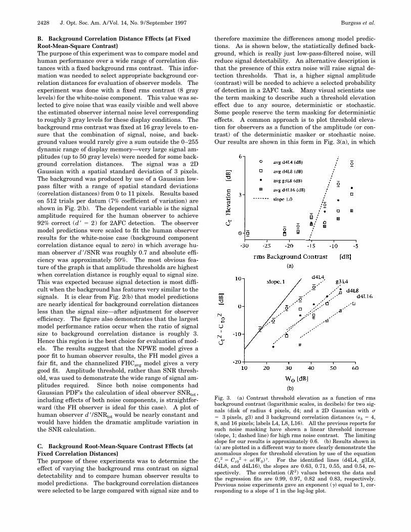
therefore maximize the differences among model predic-tions. As is shown below, the statistically defined back-ground, which is really just low-pass-filtered noise, willreduce signal detectability. An alternative description isthat the presence of this extra noise will raise signal de-tection thresholds. That is, a higher signal amplitude(contrast) will be needed to achieve a selected probabilityof detection in a 2AFC task. Many visual scientists usethe term masking to describe such a threshold elevationeffect due to any source, deterministic or stochastic.Some people reserve the term masking for deterministiceffects. A common approach is to plot threshold eleva-tion for observers as a function of the amplitude (or con-trast) of the deterministic masker or stochastic noise.Our results are shown in this form in Fig. 3(a), in which
Fig. 3. (a) Contrast threshold elevation as a function of rmsbackground contrast (logarithmic scales, in decibels) for two sig-nals (disk of radius 4 pixels, d4; and a 2D Gaussian with s5 3 pixels, g3) and 3 background correlation distances (sb 5 4,8, and 16 pixels; labels L4, L8, L16). All the previous reports forsuch noise masking have shown a linear threshold increase(slope, 1; dashed line) for high rms noise contrast. The limitingslope for our results is approximately 0.6. (b) Results shown in(a) are plotted in a different way to more clearly demonstrate theanomalous slopes for threshold elevation by use of the equationCt
2 5 Ct02 1 a(W0)g. For the identified lines (d4L4, g3L8,
d4L8, and d4L16), the slopes are 0.63, 0.71, 0.55, and 0.54, re-spectively. The correlation (R2) values between the data andthe regression fits are 0.99, 0.97, 0.82 and 0.83, respectively.Previous noise experiments gave an exponent (g) equal to 1, cor-responding to a slope of 1 in the log-log plot.
Burgess et al. Vol. 14, No. 9 /September 1997 /J. Opt. Soc. Am. A 2429
we plot the contrast threshold elevation, averaged for fourobservers, as a function of the rms contrast of the lumpybackgrounds. Contrast thresholds are normalized to avalue of 1 for the uniform background case, and rms con-trast is defined as the amplitude standard deviation of thelumpy background divided by the mean (dc) value of 127gray levels. Both quantities are plotted in logarithmicform, with 10 dB equal to a factor of 10 in contrast ampli-tude, and the uniform background results are artificiallyplaced at 228 dB rather than at negative infinity. Notethat the vertical and the horizontal scales are different inFig. 3, so that the line indicating a slope of unity is not at45 deg. The most striking aspect of the data is that theydo not reach a limiting slope of 1 for large backgroundrms contrast values, as would be expected from Eqs. (4)for the NPWE observer. All the previous human ob-server experiments have shown a limiting slope ofunity.27 However, one might argue that the curves havenot yet reached limiting slopes. The issue is more clearlydemonstrated by transformation of the Fig. 3(a) results tothe form shown in Fig. 3(b). Using Eqs. (4), one obtainsthe predicted result that the difference in squared thresh-olds, (Ct
2 2 Ct02), should be proportional to the back-
ground spectral density value at zero frequency, W0 .The Fig. 3(b) log-log plot of (Ct
2 2 Ct02) versus W0 shows
that proportionality definitely does not occur. Both axesare in decibel scales—with Ct0 being arbitrarily set equalto 1 and with W0 in arbitrary units. The line of unitslope is shown together with linear-regression fits to thehuman observer data that give slopes in the range from0.54 to 0.71. To the best of our knowledge, this is thefirst time nonunit threshold elevation slopes have beenfound for noise. This point is discussed in detail below.As was shown above, the NPWE detectability index equa-tion can be transformed to Eqs. (4) so that the observerdata should fall on a straight line with unit slope if anyNPWE model is valid. Our results demonstrate thatthere is no modified NPW model that could possibly fit thehuman observer data, since all such models would give aslope of 1. Changing the eye filter model will change thevalue of b in Eq. (3) and hence the intercept [log(b)]shown in Fig. 3(b), but the slope of line will remain unity.The observer detectability results can be fitted with thead hoc equation
~d8/d08 !2 2 1 5 a~W0 /N0!g. (12)
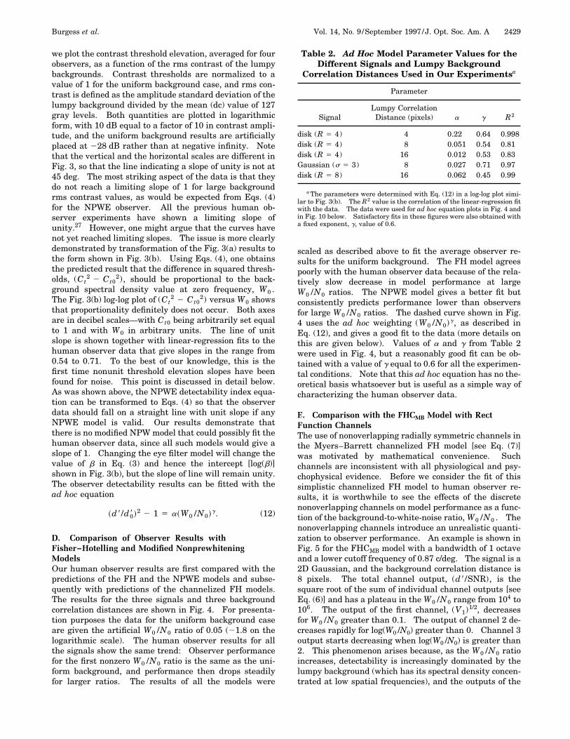
D. Comparison of Observer Results withFisher–Hotelling and Modified NonprewhiteningModelsOur human observer results are first compared with thepredictions of the FH and the NPWE models and subse-quently with predictions of the channelized FH models.The results for the three signals and three backgroundcorrelation distances are shown in Fig. 4. For presenta-tion purposes the data for the uniform background caseare given the artificial W0 /N0 ratio of 0.05 (21.8 on thelogarithmic scale). The human observer results for allthe signals show the same trend: Observer performancefor the first nonzero W0 /N0 ratio is the same as the uni-form background, and performance then drops steadilyfor larger ratios. The results of all the models were
scaled as described above to fit the average observer re-sults for the uniform background. The FH model agreespoorly with the human observer data because of the rela-tively slow decrease in model performance at largeW0 /N0 ratios. The NPWE model gives a better fit butconsistently predicts performance lower than observersfor large W0 /N0 ratios. The dashed curve shown in Fig.4 uses the ad hoc weighting (W0 /N0)g, as described inEq. (12), and gives a good fit to the data (more details onthis are given below). Values of a and g from Table 2were used in Fig. 4, but a reasonably good fit can be ob-tained with a value of g equal to 0.6 for all the experimen-tal conditions. Note that this ad hoc equation has no the-oretical basis whatsoever but is useful as a simple way ofcharacterizing the human observer data.
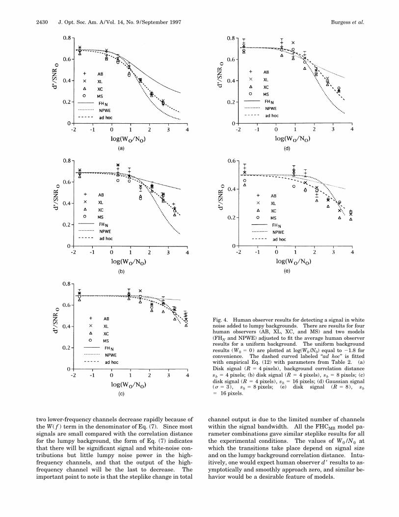
E. Comparison with the FHCMB Model with RectFunction ChannelsThe use of nonoverlapping radially symmetric channels inthe Myers–Barrett channelized FH model [see Eq. (7)]was motivated by mathematical convenience. Suchchannels are inconsistent with all physiological and psy-chophysical evidence. Before we consider the fit of thissimplistic channelized FH model to human observer re-sults, it is worthwhile to see the effects of the discretenonoverlapping channels on model performance as a func-tion of the background-to-white-noise ratio, W0 /N0 . Thenonoverlapping channels introduce an unrealistic quanti-zation to observer performance. An example is shown inFig. 5 for the FHCMB model with a bandwidth of 1 octaveand a lower cutoff frequency of 0.87 c/deg. The signal is a2D Gaussian, and the background correlation distance is8 pixels. The total channel output, (d8/SNR), is thesquare root of the sum of individual channel outputs [seeEq. (6)] and has a plateau in the W0 /N0 range from 104 to106. The output of the first channel, (V1)1/2, decreasesfor W0 /N0 greater than 0.1. The output of channel 2 de-creases rapidly for log(W0 /N0) greater than 0. Channel 3output starts decreasing when log(W0 /N0) is greater than2. This phenomenon arises because, as the W0 /N0 ratioincreases, detectability is increasingly dominated by thelumpy background (which has its spectral density concen-trated at low spatial frequencies), and the outputs of the
Table 2. Ad Hoc Model Parameter Values for theDifferent Signals and Lumpy Background
Correlation Distances Used in Our Experimentsa
Parameter
SignalLumpy Correlation
Distance (pixels) a g R2
disk (R 5 4) 4 0.22 0.64 0.998disk (R 5 4) 8 0.051 0.54 0.81disk (R 5 4) 16 0.012 0.53 0.83Gaussian (s 5 3) 8 0.027 0.71 0.97disk (R 5 8) 16 0.062 0.45 0.99
a The parameters were determined with Eq. (12) in a log-log plot simi-lar to Fig. 3(b). The R2 value is the correlation of the linear-regression fitwith the data. The data were used for ad hoc equation plots in Fig. 4 andin Fig. 10 below. Satisfactory fits in these figures were also obtained witha fixed exponent, g, value of 0.6.
2430 J. Opt. Soc. Am. A/Vol. 14, No. 9 /September 1997 Burgess et al.
Fig. 4. Human observer results for detecting a signal in whitenoise added to lumpy backgrounds. There are results for fourhuman observers (AB, XL, XC, and MS) and two models(FHN and NPWE) adjusted to fit the average human observerresults for a uniform background. The uniform backgroundresults (W0 5 0) are plotted at log(W0 /N0) equal to 21.8 forconvenience. The dashed curved labeled ‘‘ad hoc’’ is fittedwith empirical Eq. (12) with parameters from Table 2. (a)Disk signal (R 5 4 pixels), background correlation distancesb 5 4 pixels; (b) disk signal (R 5 4 pixels), sb 5 8 pixels; (c)disk signal (R 5 4 pixels), sb 5 16 pixels; (d) Gaussian signal(s 5 3), sb 5 8 pixels; (e) disk signal (R 5 8), sb5 16 pixels.
two lower-frequency channels decrease rapidly because ofthe W( f ) term in the denominator of Eq. (7). Since mostsignals are small compared with the correlation distancefor the lumpy background, the form of Eq. (7) indicatesthat there will be significant signal and white-noise con-tributions but little lumpy noise power in the high-frequency channels, and that the output of the high-frequency channel will be the last to decrease. Theimportant point to note is that the steplike change in total
channel output is due to the limited number of channelswithin the signal bandwidth. All the FHCMB model pa-rameter combinations gave similar steplike results for allthe experimental conditions. The values of W0 /N0 atwhich the transitions take place depend on signal sizeand on the lumpy background correlation distance. Intu-itively, one would expect human observer d8 results to as-ymptotically and smoothly approach zero, and similar be-havior would be a desirable feature of models.
Burgess et al. Vol. 14, No. 9 /September 1997 /J. Opt. Soc. Am. A 2431
The human observer results for two experimental con-ditions shown in Fig. 4 are compared in Figs. 6(a) and6(b), respectively, with the Myers–Barrett model,FHCMB, with nonoverlapping channels. We evaluatedall the cases shown in Fig. 4 with the parameter valuesused by Myers and Barrett16: two bandwidths (a5 1.5, 2), and two low-frequency cutoffs ( fc5 0.66, 0.87 c/deg). Only two signal–background com-binations d4L8 and g3L8) with 1-octave bandwidth areshown, for purposes of illustration, in Fig. 6. The FHCMBmodel predictions are sensitive to channel parameter se-lection and do not show any consistent agreement withhuman observer performance. It was possible to adjustchannel parameters to obtain a good fit for any given ex-perimental condition (signal and background correlationdistance), but quite different parameter values wereneeded to fit different experimental conditions. As isshown in Section 6, the FHCMB model also gave pooragreement with a viewing distance experiment.
F. Comparison with the FHCavg Channel ParameterAveraging ModelWe evaluated the FHCavg channels model by using Eq.(8). The model included an eye filter, internal noise, alow-frequency (dc) channel that extended to zero fre-quency, and a sequence of 1-octave-wide rect functionbandpass channels. Both the dc channel and the firstbandpass channel had bandwidths of Df1 . The band-width of each subsequent bandpass channel was a factorof 2 larger than that of the previous channel. We calcu-lated performance for the model by using eight values ofDf1 , evenly spaced on a logarithmic scale from 0.125 to0.25 c/deg, and averaged the results. We also used therange from 0.25 to 0.5 for Df1 and obtained identical re-sults. We found that it made little difference (less than1% variation) whether we first averaged individual chan-nel outputs, Vi in Eq. (7), for a given log(W0 /N0) ratio overthe ensemble of Df1 values and then calculated d8 or
Fig. 5. Demonstration of quantization effects as a function ofthe lumpy background spectral density for the FHCMB modelwith the discrete, nonoverlapping channels used by Myers andBarrett. Total output (d8/SNR0) and individual channel out-puts, (Vi)
1/2, calculated with Eq. (7), are shown for one param-eter selection ( fc 5 0.87 c/deg and a 5 2). The signal is a 2DGaussian (s 5 3), and the lumpy background correlation dis-tance is 8 pixels.
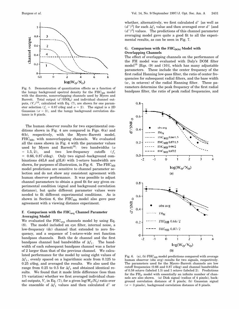
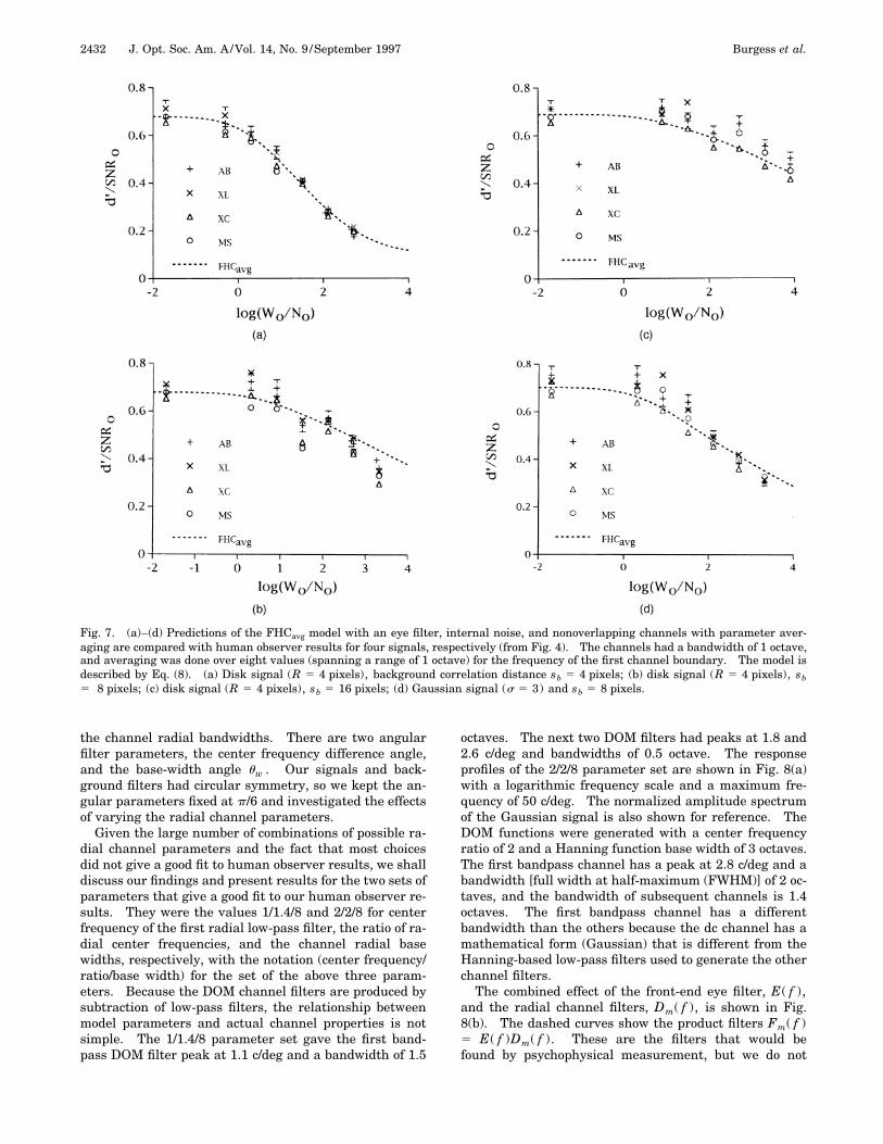
whether, alternatively, we first calculated d8 [as well as(d8)2] for each Df1 value and then averaged over d8 [and(d8)2] values. The predictions of this channel parameteraveraging model gave quite a good fit to all the experi-mental results, as can be seen in Fig. 7.
G. Comparison with the FHCDOM Model withOverlapping ChannelsThe effect of overlapping channels on the performance ofthe FH model was evaluated with Daly’s DOM filtermodel18 [Eqs. (9) and (10)], which has many adjustableparameters. These include the center frequency of thefirst radial Hanning low-pass filter, the ratio of center fre-quencies for subsequent radial filters, and the base width(w, in octaves) of the radial Hanning filter. These pa-rameters determine the peak frequency of the first radialbandpass filter, the ratio of peak radial frequencies, and
Fig. 6. (a), (b) FHCMB model predictions compared with averagehuman observer (obs avg) results for two signals, respectively.The parameters used for the Myers–Barrett channels are lowcutoff frequencies (0.66 and 0.87 c/deg) and channel bandwidthsof 0.58 octave (labeled 1.5) and 1 octave (labeled 2). Predictionsfor the FHN model with essentially an infinite number of chan-nels are also shown. (a) Disk signal (radius of 4 pixels), back-ground correlation distance of 8 pixels; (b) Gaussian signal(s 5 3 pixels), background correlation distance of 8 pixels.
2432 J. Opt. Soc. Am. A/Vol. 14, No. 9 /September 1997 Burgess et al.
Fig. 7. (a)–(d) Predictions of the FHCavg model with an eye filter, internal noise, and nonoverlapping channels with parameter aver-aging are compared with human observer results for four signals, respectively (from Fig. 4). The channels had a bandwidth of 1 octave,and averaging was done over eight values (spanning a range of 1 octave) for the frequency of the first channel boundary. The model isdescribed by Eq. (8). (a) Disk signal (R 5 4 pixels), background correlation distance sb 5 4 pixels; (b) disk signal (R 5 4 pixels), sb5 8 pixels; (c) disk signal (R 5 4 pixels), sb 5 16 pixels; (d) Gaussian signal (s 5 3) and sb 5 8 pixels.
the channel radial bandwidths. There are two angularfilter parameters, the center frequency difference angle,and the base-width angle uw . Our signals and back-ground filters had circular symmetry, so we kept the an-gular parameters fixed at p/6 and investigated the effectsof varying the radial channel parameters.
Given the large number of combinations of possible ra-dial channel parameters and the fact that most choicesdid not give a good fit to human observer results, we shalldiscuss our findings and present results for the two sets ofparameters that give a good fit to our human observer re-sults. They were the values 1/1.4/8 and 2/2/8 for centerfrequency of the first radial low-pass filter, the ratio of ra-dial center frequencies, and the channel radial basewidths, respectively, with the notation (center frequency/ratio/base width) for the set of the above three param-eters. Because the DOM channel filters are produced bysubtraction of low-pass filters, the relationship betweenmodel parameters and actual channel properties is notsimple. The 1/1.4/8 parameter set gave the first band-pass DOM filter peak at 1.1 c/deg and a bandwidth of 1.5
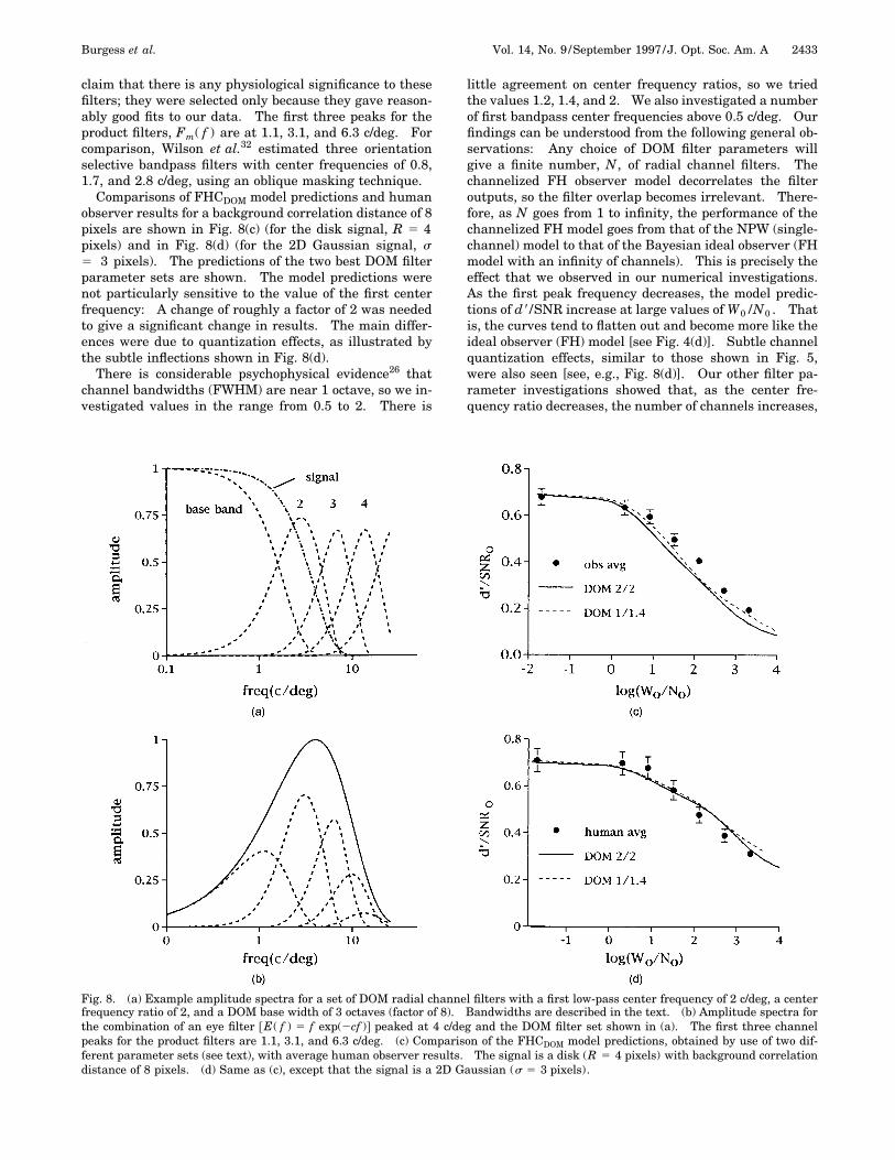
octaves. The next two DOM filters had peaks at 1.8 and2.6 c/deg and bandwidths of 0.5 octave. The responseprofiles of the 2/2/8 parameter set are shown in Fig. 8(a)with a logarithmic frequency scale and a maximum fre-quency of 50 c/deg. The normalized amplitude spectrumof the Gaussian signal is also shown for reference. TheDOM functions were generated with a center frequencyratio of 2 and a Hanning function base width of 3 octaves.The first bandpass channel has a peak at 2.8 c/deg and abandwidth [full width at half-maximum (FWHM)] of 2 oc-taves, and the bandwidth of subsequent channels is 1.4octaves. The first bandpass channel has a differentbandwidth than the others because the dc channel has amathematical form (Gaussian) that is different from theHanning-based low-pass filters used to generate the otherchannel filters.
The combined effect of the front-end eye filter, E( f ),and the radial channel filters, Dm( f ), is shown in Fig.8(b). The dashed curves show the product filters Fm( f )5 E( f )Dm( f ). These are the filters that would befound by psychophysical measurement, but we do not
Burgess et al. Vol. 14, No. 9 /September 1997 /J. Opt. Soc. Am. A 2433
claim that there is any physiological significance to thesefilters; they were selected only because they gave reason-ably good fits to our data. The first three peaks for theproduct filters, Fm( f ) are at 1.1, 3.1, and 6.3 c/deg. Forcomparison, Wilson et al.32 estimated three orientationselective bandpass filters with center frequencies of 0.8,1.7, and 2.8 c/deg, using an oblique masking technique.
Comparisons of FHCDOM model predictions and humanobserver results for a background correlation distance of 8pixels are shown in Fig. 8(c) (for the disk signal, R 5 4pixels) and in Fig. 8(d) (for the 2D Gaussian signal, s5 3 pixels). The predictions of the two best DOM filterparameter sets are shown. The model predictions werenot particularly sensitive to the value of the first centerfrequency: A change of roughly a factor of 2 was neededto give a significant change in results. The main differ-ences were due to quantization effects, as illustrated bythe subtle inflections shown in Fig. 8(d).
There is considerable psychophysical evidence26 thatchannel bandwidths (FWHM) are near 1 octave, so we in-vestigated values in the range from 0.5 to 2. There is
little agreement on center frequency ratios, so we triedthe values 1.2, 1.4, and 2. We also investigated a numberof first bandpass center frequencies above 0.5 c/deg. Ourfindings can be understood from the following general ob-servations: Any choice of DOM filter parameters willgive a finite number, N, of radial channel filters. Thechannelized FH observer model decorrelates the filteroutputs, so the filter overlap becomes irrelevant. There-fore, as N goes from 1 to infinity, the performance of thechannelized FH model goes from that of the NPW (single-channel) model to that of the Bayesian ideal observer (FHmodel with an infinity of channels). This is precisely theeffect that we observed in our numerical investigations.As the first peak frequency decreases, the model predic-tions of d8/SNR increase at large values of W0 /N0 . Thatis, the curves tend to flatten out and become more like theideal observer (FH) model [see Fig. 4(d)]. Subtle channelquantization effects, similar to those shown in Fig. 5,were also seen [see, e.g., Fig. 8(d)]. Our other filter pa-rameter investigations showed that, as the center fre-quency ratio decreases, the number of channels increases,
Fig. 8. (a) Example amplitude spectra for a set of DOM radial channel filters with a first low-pass center frequency of 2 c/deg, a centerfrequency ratio of 2, and a DOM base width of 3 octaves (factor of 8). Bandwidths are described in the text. (b) Amplitude spectra forthe combination of an eye filter @E( f ) 5 f exp(2cf )# peaked at 4 c/deg and the DOM filter set shown in (a). The first three channelpeaks for the product filters are 1.1, 3.1, and 6.3 c/deg. (c) Comparison of the FHCDOM model predictions, obtained by use of two dif-ferent parameter sets (see text), with average human observer results. The signal is a disk (R 5 4 pixels) with background correlationdistance of 8 pixels. (d) Same as (c), except that the signal is a 2D Gaussian (s 5 3 pixels).
2434 J. Opt. Soc. Am. A/Vol. 14, No. 9 /September 1997 Burgess et al.
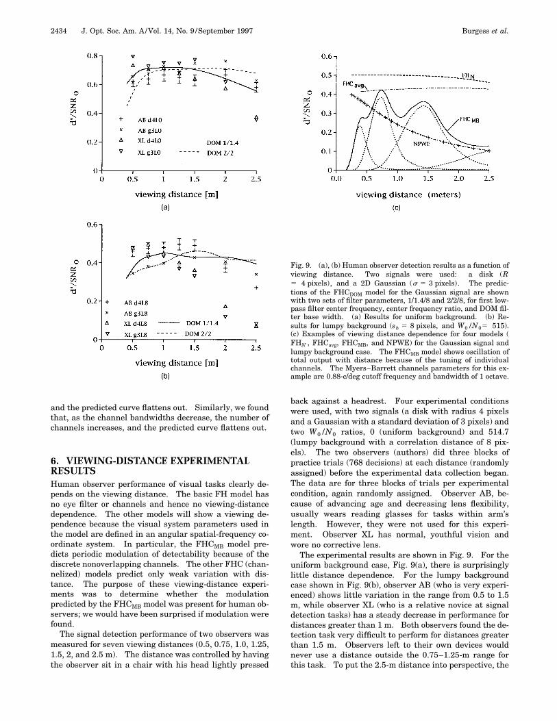
Fig. 9. (a), (b) Human observer detection results as a function ofviewing distance. Two signals were used: a disk (R5 4 pixels), and a 2D Gaussian (s 5 3 pixels). The predic-tions of the FHCDOM model for the Gaussian signal are shownwith two sets of filter parameters, 1/1.4/8 and 2/2/8, for first low-pass filter center frequency, center frequency ratio, and DOM fil-ter base width. (a) Results for uniform background. (b) Re-sults for lumpy background (sb 5 8 pixels, and W0 /N05 515).(c) Examples of viewing distance dependence for four models (FHN , FHCavg, FHCMB, and NPWE) for the Gaussian signal andlumpy background case. The FHCMB model shows oscillation oftotal output with distance because of the tuning of individualchannels. The Myers–Barrett channels parameters for this ex-ample are 0.88-c/deg cutoff frequency and bandwidth of 1 octave.
and the predicted curve flattens out. Similarly, we foundthat, as the channel bandwidths decrease, the number ofchannels increases, and the predicted curve flattens out.
6. VIEWING-DISTANCE EXPERIMENTALRESULTSHuman observer performance of visual tasks clearly de-pends on the viewing distance. The basic FH model hasno eye filter or channels and hence no viewing-distancedependence. The other models will show a viewing de-pendence because the visual system parameters used inthe model are defined in an angular spatial-frequency co-ordinate system. In particular, the FHCMB model pre-dicts periodic modulation of detectability because of thediscrete nonoverlapping channels. The other FHC (chan-nelized) models predict only weak variation with dis-tance. The purpose of these viewing-distance experi-ments was to determine whether the modulationpredicted by the FHCMB model was present for human ob-servers; we would have been surprised if modulation werefound.
The signal detection performance of two observers wasmeasured for seven viewing distances (0.5, 0.75, 1.0, 1.25,1.5, 2, and 2.5 m). The distance was controlled by havingthe observer sit in a chair with his head lightly pressed
back against a headrest. Four experimental conditionswere used, with two signals (a disk with radius 4 pixelsand a Gaussian with a standard deviation of 3 pixels) andtwo W0 /N0 ratios, 0 (uniform background) and 514.7(lumpy background with a correlation distance of 8 pix-els). The two observers (authors) did three blocks ofpractice trials (768 decisions) at each distance (randomlyassigned) before the experimental data collection began.The data are for three blocks of trials per experimentalcondition, again randomly assigned. Observer AB, be-cause of advancing age and decreasing lens flexibility,usually wears reading glasses for tasks within arm’slength. However, they were not used for this experi-ment. Observer XL has normal, youthful vision andwore no corrective lens.
The experimental results are shown in Fig. 9. For theuniform background case, Fig. 9(a), there is surprisinglylittle distance dependence. For the lumpy backgroundcase shown in Fig. 9(b), observer AB (who is very experi-enced) shows little variation in the range from 0.5 to 1.5m, while observer XL (who is a relative novice at signaldetection tasks) has a steady decrease in performance fordistances greater than 1 m. Both observers found the de-tection task very difficult to perform for distances greaterthan 1.5 m. Observers left to their own devices wouldnever use a distance outside the 0.75–1.25-m range forthis task. To put the 2.5-m distance into perspective, the
Burgess et al. Vol. 14, No. 9 /September 1997 /J. Opt. Soc. Am. A 2435
disk signal (diameter of 8 pixels) subtends a visual angleof roughly 1.8 mrad (0.03 deg) at this distance—only twicethe size of the optical point-spread function of the eye.The predictions of the FHCDOM model for the 2D Gauss-ian signal with the two best sets of the three parameters(1/1.4/8 and 2/2/8) are also shown in Figs. 9(a) and 9(b),respectively. They show a significant decrease in perfor-mance at short distances but little dependence at long dis-tances.
Figure 9(c) shows the calculated performance for theGaussian signal and lumpy background case as a functionof viewing distance for three models. Performance forthe FHN and the FHCavg models shows little distance de-pendence. The NPWE model predicts a rapid decrease asdistance increases. The FHCMB model with nonoverlap-ping channels (a bandwidth of 1 octave and a cutoff fre-quency of 0.87 c/deg are used here as an example) showsan oscillatory distance dependence. The total output ofthe FHCMB model (solid curve) is due to contributionsfrom individual channels (dashed curves) that place eachpeak at a particular distance. This distance tuning
arises because of the limited bandwidth of the channels.The very low performance of the FHCMB (below 0.25 m isdue to complete lack of visual response for the model be-low 0.87 c/deg). All versions of the FHCMB model showedsimilar oscillatory behavior.
7. DETERMINISTIC BACKGROUNDEXPERIMENTAL RESULTSThe following experiments were done with the same seg-ment of lumpy background in both 2AFC test fields (side-by-side display with no time limit). However, a newlumpy background segment was randomly selected foreach decision trial. The purpose of these experimentswas to determine the relative effects of uncertainty aboutbackground spatial variation (present only when differentbackground samples are used for the two alternative im-age fields) and masking due only to background structure(when the same background samples are used). Whenthe same background segment is used in both fields it no
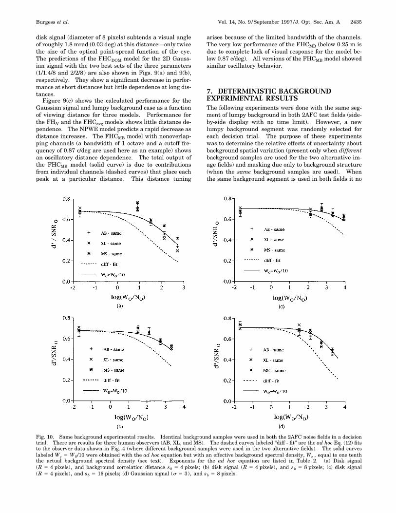
Fig. 10. Same background experimental results. Identical background samples were used in both the 2AFC noise fields in a decisiontrial. There are results for three human observers (AB, XL, and MS). The dashed curves labeled ‘‘diff - fit’’ are the ad hoc Eq. (12) fitsto the observer data shown in Fig. 4 (where different background samples were used in the two alternative fields). The solid curveslabeled We 5 W0/10 were obtained with the ad hoc equation but with an effective background spectral density, We , equal to one tenththe actual background spectral density (see text). Exponents for the ad hoc equation are listed in Table 2. (a) Disk signal(R 5 4 pixels), and background correlation distance sb 5 4 pixels; (b) disk signal (R 5 4 pixels), and sb 5 8 pixels; (c) disk signal(R 5 4 pixels), and sb 5 16 pixels; (d) Gaussian signal (s 5 3), and sb 5 8 pixels.
2436 J. Opt. Soc. Am. A/Vol. 14, No. 9 /September 1997 Burgess et al.
longer represents noise for the Bayesian observer models.These observers would just subtract one image field fromthe other, leaving a simple 2AFC signal-polarity detectionproblem with white noise and a uniform background.Hence we shall refer to this as a deterministic (predict-able) background case. The situation is different for hu-man observers. It has been shown in many experimentsthat deterministic maskers can significantly decrease de-tectability of signals. It is usually found that increasedsimilarity of the signal and masker leads to decreased ob-server performance.
For simplicity, we shall refer to our deterministicmethod as using the same background, whereas the pre-vious stochastic method will be referred to as the differentbackground case. We did the same background experi-ments, using the two small signals [disk (R 5 4) andGaussian] and the full range of background correlationdistances (4, 8, and 16 pixels). Three experienced observ-ers (AB, XL, and MS), who had previously done the dif-ferent background experiments, did this experiment. Atotal of 512 practice trials and 768 data-acquisition trialswere done for each experimental condition. The resultsof our same background experiments are shown in Fig.10. The dashed curves labeled ‘‘diff - fit’’ are the bestad hoc Eq. (12) fits to the average human observer resultsshown in Fig. 4 for the different background condition.The fits were done by use of the equation (d8/d08)2 2 15 a(We /N0)g, with parameters from Table 2. The ob-server results for the same background condition ap-peared to be shifted versions of the results for the differ-ent background condition. This was confirmed by thefact that we were able to fit the results for the same back-ground condition, using the ad hoc Eq. (12) with identicalvalues of a and g but with an effective background spec-tral density parameter We that was found to be approxi-mately equal to W0/10. This value is considerablysmaller than the effective noise spectral density, Ne5 0.6N0 , found by Burgess and Colborne31 when thesame white-noise sample was used in both alternativefields. They interpreted their result in terms of an in-duced or evoked internal noise because the identical fac-tor was found in experiments on observer decision consis-tency. The same lumpy background results suggest thatthe background spatial variation has a rather small effecton observer decision variability (internal noise).
8. DISCUSSION AND CONCLUSIONSRolland and Barrett3 presented human observer resultsfor detecting a 2D Gaussian signal in a combination ofPoisson noise and statistically defined backgrounds basedon Poisson statistics. Their results were consistent withthe FH observer model but not with the standard nonpre-whitening matched filter observer (NPW) model withoutan eye filter. Burgess4 showed that their results wereconsistent with a modified NPW observer (NPWE) modelthat included an eye filter and pointed out that the ex-perimental data were not precise enough to allow dis-crimination between the predictions of the FH and theNPWE models. There are a number of significant differ-ences between the Rolland–Barrett experiments andthose presented here. Their motivation was to evaluate
the effect of varying two parameters that have particularimportance in nuclear medicine experiments: exposuretime, and imaging system aperture. Both experimentswere, in effect, done with fixed lumpy background spec-tral densities and variable white-noise spectral densities.The variable aperture experiment also led to variable spa-tial filtering of the signal and the lumpy background.This meant that human observer internal noise may havebecome important for long exposure times or large aper-tures. Of course, this would also happen in the clinicalimaging situation being simulated and hence was a veryreasonable experimental design, given their aim. But itdid have the effect of introducing another variable andcomplicating analysis of results. By contrast, we keptthe white-noise level constant and well above the humaninternal noise level in our experiments to control for thiseffect. There were important differences in methods.We used the 2AFC method, while Rolland and Barrettused single images with 50% probability of a signal’s be-ing present and the receiver operating characteristicrating-scale response method. We also used many moreimages per experimental condition (typically 768 com-pared with 70) because we knew that much higher preci-sion would be needed to distinguish between the two can-didate models (FH and NPWE). In addition, there wasthe difference in PDF’s for the noise and the backgrounds(Poisson for Rolland and Barrett, and Gaussian here).
Our human observer results clearly cannot be de-scribed by the ideal observer (FH) model even after inclu-sion of an eye filter and of the two sources of internalnoise. We have also shown that it is not possible to finda NPWE model that will fit our data. Our results (Fig. 4)suggest that the two limiting spatial-frequency channelcases do not apply to human observers. One limit (theFH model) is an infinite number of spatial-frequencychannels followed by decorrelation and prewhitening.The other limit (NPWE) has a single spatial-frequencychannel tuned to the filtered signal and does not pre-whiten the noise. The Myers–Barrett FH model withnonoverlapping channels has provided fairly goodagreement17 with less precise data in a variety of decisiontasks. This provides strong support for the view that hu-mans can make effective use of the combined output of arelatively small number of spatial-frequency channelsthat are selected appropriately for the known signal pro-file, known noise correlation properties, and known pos-sible signal locations. Effective use also requires somecompensation for background correlations. The Myers–Barrett FH model uses nonoverlapping channels formathematical convenience, but the lack of overlap isclearly inconsistent with a large body of physiological andpsychophysical evidence. The lack of channel overlapleads to prediction of quantization effects for the d8 varia-tions, as a function of both background spectral densityand viewing distance, that are inconsistent with our ob-server results (Figs. 4, 5, and 9). The quantization ef-fects, when examined in detail, are very sensitive to theselection of channel boundaries.
We did find that our results could be fitted by two chan-nelized FH models. One, FHCavg, involved averagingover channel parameters by use of a slightly modified ver-sion of the Myers–Barrett, FHCMB, model. This ap-
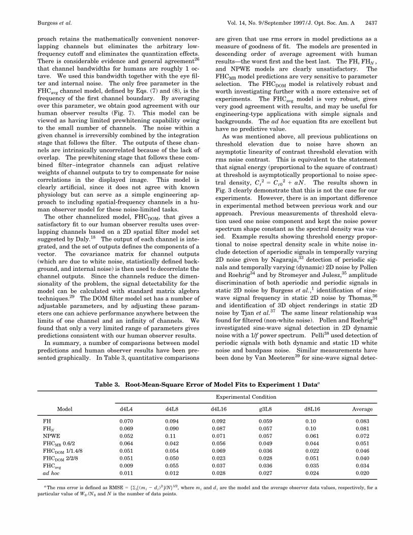
Burgess et al. Vol. 14, No. 9 /September 1997 /J. Opt. Soc. Am. A 2437
proach retains the mathematically convenient nonover-lapping channels but eliminates the arbitrary low-frequency cutoff and eliminates the quantization effects.There is considerable evidence and general agreement26
that channel bandwidths for humans are roughly 1 oc-tave. We used this bandwidth together with the eye fil-ter and internal noise. The only free parameter in theFHCavg channel model, defined by Eqs. (7) and (8), is thefrequency of the first channel boundary. By averagingover this parameter, we obtain good agreement with ourhuman observer results (Fig. 7). This model can beviewed as having limited prewhitening capability owingto the small number of channels. The noise within agiven channel is irreversibly combined by the integrationstage that follows the filter. The outputs of these chan-nels are intrinsically uncorrelated because of the lack ofoverlap. The prewhitening stage that follows these com-bined filter–integrator channels can adjust relativeweights of channel outputs to try to compensate for noisecorrelations in the displayed image. This model isclearly artificial, since it does not agree with knownphysiology but can serve as a simple engineering ap-proach to including spatial-frequency channels in a hu-man observer model for these noise-limited tasks.
The other channelized model, FHCDOM, that gives asatisfactory fit to our human observer results uses over-lapping channels based on a 2D spatial filter model setsuggested by Daly.18 The output of each channel is inte-grated, and the set of outputs defines the components of avector. The covariance matrix for channel outputs(which are due to white noise, statistically defined back-ground, and internal noise) is then used to decorrelate thechannel outputs. Since the channels reduce the dimen-sionality of the problem, the signal detectability for themodel can be calculated with standard matrix algebratechniques.29 The DOM filter model set has a number ofadjustable parameters, and by adjusting these param-eters one can achieve performance anywhere between thelimits of one channel and an infinity of channels. Wefound that only a very limited range of parameters givespredictions consistent with our human observer results.
In summary, a number of comparisons between modelpredictions and human observer results have been pre-sented graphically. In Table 3, quantitative comparisons
are given that use rms errors in model predictions as ameasure of goodness of fit. The models are presented indescending order of average agreement with humanresults—the worst first and the best last. The FH, FHN ,and NPWE models are clearly unsatisfactory. TheFHCMB model predictions are very sensitive to parameterselection. The FHCDOM model is relatively robust andworth investigating further with a more extensive set ofexperiments. The FHCavg model is very robust, givesvery good agreement with results, and may be useful forengineering-type applications with simple signals andbackgrounds. The ad hoc equation fits are excellent buthave no predictive value.
As was mentioned above, all previous publications onthreshold elevation due to noise have shown anasymptotic linearity of contrast threshold elevation withrms noise contrast. This is equivalent to the statementthat signal energy (proportional to the square of contrast)at threshold is asymptotically proportional to noise spec-tral density, Ct
2 5 Ct02 1 aN. The results shown in
Fig. 3 clearly demonstrate that this is not the case for ourexperiments. However, there is an important differencein experimental method between previous work and ourapproach. Previous measurements of threshold eleva-tion used one noise component and kept the noise powerspectrum shape constant as the spectral density was var-ied. Example results showing threshold energy propor-tional to noise spectral density scale in white noise in-clude detection of aperiodic signals in temporally varying2D noise given by Nagaraja,33 detection of periodic sig-nals and temporally varying (dynamic) 2D noise by Pollenand Roehrig34 and by Stromeyer and Julesz,35 amplitudediscrimination of both aperiodic and periodic signals instatic 2D noise by Burgess et al.,1 identification of sine-wave signal frequency in static 2D noise by Thomas,36
and identification of 3D object renderings in static 2Dnoise by Tjan et al.37 The same linear relationship wasfound for filtered (non-white noise). Pollen and Roehrig34
investigated sine-wave signal detection in 2D dynamicnoise with a 1/f power spectrum. Pelli38 used detection ofperiodic signals with both dynamic and static 1D whitenoise and bandpass noise. Similar measurements havebeen done by Van Meeteren39 for sine-wave signal detec-
Table 3. Root-Mean-Square Error of Model Fits to Experiment 1 Dataa
Model
Experimental Condition
d4L4 d4L8 d4L16 g3L8 d8L16 Average
FH 0.070 0.094 0.092 0.059 0.10 0.083FHN 0.069 0.090 0.087 0.057 0.10 0.081NPWE 0.052 0.11 0.071 0.057 0.061 0.072FHCMB 0.6/2 0.064 0.042 0.056 0.049 0.044 0.051FHCDOM 1/1.4/8 0.051 0.054 0.069 0.036 0.022 0.046FHCDOM 2/2/8 0.051 0.050 0.023 0.028 0.051 0.040FHCavg 0.009 0.055 0.037 0.036 0.035 0.034ad hoc 0.011 0.012 0.028 0.027 0.024 0.020
a The rms error is defined as RMSE 5 $( i@(mi 2 di)2#/N%1/2, where mi and di are the model and the average observer data values, respectively, for a
particular value of W0 /N0 and N is the number of data points.
2438 J. Opt. Soc. Am. A/Vol. 14, No. 9 /September 1997 Burgess et al.
tion in static low-pass noise. Pavel et al.40 showed thatthe relationship also held for identification of visually pre-sented American Sign Language in dynamic 2D whitenoise.
The slope of roughly 0.6 relating threshold elevationand noise scale that we found in our experiments is closeto the results for deterministic masking described byLegge and Foley,41 by Legge,42 and by others (see Swiftand Smith43 for a summary). The origin of the 0.6 slopeis, of course, quite different for the two types of experi-ments, and comparison based only on slopes would beboth simplistic and misleading. Our experiments havetwo noise (masking) components, while the previousmasking experiments have one component. In fact, oneof the implications of Fig. 2(b) is that the slope of thethreshold elevation curves [like Fig. 3(a)] for two-component noise experiments will have a range of values.When the correlation distances of both components aresmall compared with signal size, the NPWE model willstill hold, and the slope will be unity. When the modelpredictions diverge at background correlation distancesnear signal size, as shown in Fig. 2(b), one would expectthe threshold elevation slope to decrease as correlationdistance increases.
In deterministic masking experiments the observerusually tries to detect a sinusoidal signal of one orienta-tion and frequency in the presence of a second (masking)sinusoid with a different orientation or frequency. Mod-els of deterministic masking are still controversial.Nachmias44 discusses the standard masking models thatinclude linear bandpass filters followed by a nonlineartransducer function for each filter and finally nonlinearpooling of transducer outputs by a method such as prob-ability summation. In the standard model, the criticaldecision variable is usually determined by the output ofthe single channel tuned to the signal. Nachmias44 pre-sents new results indicating that this type of model is in-adequate and suggests two alternative approaches for de-velopment of an improved model based on recent work inpsychoacoustics. One approach might include proce-dures analogous to profile analysis,45 which uses changesin the pattern of spatial-frequency channels in the deci-sion task combined with gain control.46 The second ap-proach suggested by Nachmias is that the signal might bedetected by changes in local spatial features in the ap-pearance of the masker. Both these approaches aremultiple-channel models. Foley47 suggested modifica-tions to the standard model by including nonlinear chan-nel response inhibition due to excitation of other chan-nels, but the model still retains the strength of the outputof the single channel tuned to the sinusoidal test signal asthe crucial decision variable. The channelized FH mod-els used in this paper are Bayesian pattern analysis mod-els, which, in essence, compare the decorrelated outputsof all the spatial-frequency channels with the expectedoutputs based on the known signal shape and location.Given the spatially localized nature of the pattern analy-sis needed for detection of the aperiodic signals used ourexperiments (with known signal location), the channel-ized FH models could also be referred to as local featureanalyzer models.
Smith and Swift43,48 presented interesting contrast
threshold elevation results by using the same noise fieldin both alternatives of a 2AFC signal detection task.They found that the slope of the threshold signal contrastversus masker rms contrast depended on learning effects.Note that in this case the masker is not really noise be-cause a detection procedure that included subtraction ofone alternative from the other (see Green and Swets49)would eliminate the noise field, and the signal would al-ways be detectable. In one experiment observers had theopportunity to become very familiar with one particularnoise field. When the same noise image was used forboth 2AFC images and that noise image was also used re-peatedly for all the decision trials, the slope for a block oftrials eventually decreased from 1.0 to roughly 0.65.When they used a new noise field for the two alternativesin each decision trial, the slope remained equal to 1 insuccessive blocks of trials and was consistent with experi-ments in which noise was used. They concluded that ob-server familiarity with the masker is an important con-sideration.
Daly18 made the distinction between phase-coherentand phase-incoherent masking. Sine waves whose fre-quency or orientation is different from the signal to be de-tected represent phase-coherent masking, while randomnoise represents phase-incoherent masking. While dis-cussing the Smith–Swift results, Daly suggested that thesource of the difference in slopes is not inherent in thenoise or in the sinusoidal wave forms but rather in theuncertainty caused by the masking pattern and that thisuncertainty can be reduced through learning. Differentassumptions about spatial-frequency channels andmechanisms for combining outputs of these channels pre-dict a slope of unity when the noise spectrum shape isfixed.
Burgess and Colborne31 did 2AFC signal detection ex-periments by using the same two white-noise fields.They found no evidence for a threshold elevation slope ofless than unity for this case. Their results were com-pared with observer consistency measurements for 2AFCexperiments in which different alternative noise fieldswere used. Both methods gave results consistent with aninduced internal noise spectral density of approximately80% of the external noise spectral density, N0 . Ex-pressed in equivalent noise terms, when the same noisefield was used in both alternatives the effective noisespectral density was roughly Ne 5 0.6N0 . This propor-tionality factor is considerably higher than the factor of0.1 that we found here for the lumpy background case.
Our experimental results suggest that our data are notconsistent with a single-channel, and hence nonprewhit-ening, model in which detection is mediated by a spatial-frequency channel tuned to the signal. They also suggestthat our data are not consistent with the other extremecase of the ideal observer model, which has an infinitenumber of channels combined with channel decorrelationand spectral prewhitening capabilities. Furthermore,the comparison of our observer data with the predictionsof the (FH) prewhitening model with overlapping chan-nels suggests that we may be able to make very effectiveuse of only a small number of channels for a given task.An observer with such channel mechanisms would have alimited capability to compensate for noise correlations in
Burgess et al. Vol. 14, No. 9 /September 1997 /J. Opt. Soc. Am. A 2439
images. Finally, our results suggest that two models,FHCavg and FHCDOM , with a limited number of spatial-frequency channels can be used to model human observ-ers. It is clearly necessary to investigate these modelsfor a larger variety of signals and background conditions.
APPENDIX A: THRESHOLD ELEVATION1. Fixed Noise Spectral ShapeLet the noise power spectrum be N(u, v)5 N0H2(u, v), where H(u, v) is an arbitrary filter func-tion that is fixed, while the noise scaling factor, N0 , isvaried during an experiment. We select some perfor-mance level d8 equal to 2, for example, to define a decisionthreshold and assume that the observer requires a signalenergy, Et , to achieve threshold performance. We thenadjust the signal amplitude (contrast) for the human ob-server so that the signal spectrum at the human thresh-old is St(u, v) 5 CtP(u, v), where Ct is the signal con-trast at threshold and P(u, v) is the normalized spectralprofile selected to give a signal energy of unity. Signalcontrast energy can be defined in either the spatial do-main or the frequency domain (because of Parseval’s theo-rem). In the frequency domain the definition is
E 5 E2`
` E2`
` FS~u, v !
I0G2
dudv, (A1)
where I0 is the average uniform luminance due to theconstant offset described in Eq. (1). Since I0 would alsoappear in the noise contrast definition, it plays no role inour calculations and will be set to unity for convenience.
Consider first the ideal, prewhitening observer model[Eq. (2)]. The relationship between threshold contrastand noise spectral density scale can easily be shown to begiven by
Ct2 5 aN0 , where a21 5 EE F P~u, v !2
H~u, v !2Gdudv.
(A2)
The parameter a will be constant if the functions H(u, v)and P(u, v) are fixed.
Next consider the prewhitening observer model with aneye filter and internal noise [Eq. (6)]. The relationshipbetween threshold contrast and noise spectral densityscale is given by
Ct2 5 aN0 , where
a21 5 EE F E~u, v !2P~u, v !2
E~ f !2H~ f !2 1 Ni~u, v !/N0Gdudv.
(A3)
Again, the parameter a will be constant as long as thefunctions E(u, v), H(u, v), Ni(u, v), and P(u, v) arefixed. In the limit of zero external noise, the contrastthreshold is determined by the internal noise. When ex-ternal noise is large compared with internal noise at allthe frequencies, the value of (Ct)
2 is proportional to N0 .Similarly, the contrast threshold for the Myers–Barrett
FH model [Eq. (7)] with radial, nonoverlapping channels,each with frequency response range Ri , is given by
Ct2 5 aN0 , where
a21 5 (i50
M H F ERi
P~ f !2fd fG2Y ERi
H~ f !2fd fJ . (A4)
The threshold contrast for the NPWE model [if we use Eq.(3) and neglect observer internal noise] is given by
Ct2 5 aN0 , where
a 5
EE uH~u, v !u2uuP~u, v !u2uE~u, v !u4dudv
F EE uP~u, v !u2uE~u, v !u2dudv G2 .
(A5)
Note that all the equations relating contrast thresholdand noise spectral scaling factor have the same formwhen external noise is large compared with internalnoise, (Ct)
2 5 aN0 . The value of the parameter a ineach equation is constant if the normalized signal andnoise spectra and the eye filter do not change. The dif-ferences among models are due to the methods of calcu-lating the value of the parameter a.
2. Linear Combination of Two Noise ComponentsLet the total noise be given by N(u, v) 5 N1@H1(u, v)#2
1 N2@H2(u, v)#2, where the filters H1(u, v), H2(u, v)are fixed and different; one spectral scaling factor (e.g.,N1) is fixed, and one scaling factor (say, N2) is variable.For purposes of illustration we assume that observer in-ternal noise is small compared with N1 and can be ig-nored.
The relationship between threshold contrast and noisespectral density scale for the ideal, prewhitening observermodel is given by
Ct2 5 bN2 , where
b21 5 EE F uP~u, v !u2
~N1 /N2!uH1~u, v !u2 1 uH2~u, v !u2Gdudv.
(A6)
Since the parameter b is a function of N2 , there is onlyone way that it can be constant as N2 is varied, as long asthere is validity to the assumption that the low-pass filterfunctions H1 and H2 in the integral are nonzero andfixed. The parameter b can be approximately constant inthe limiting case of the bandwidths’ of H1 and H2 beingmuch larger than the signal bandwidth. This situationoccurs when the correlation lengths of both noise compo-nents are small compared with signal size.
The situation is different for the NPWE model. Thetwo-noise-component contrast threshold is given by
Ct2 5 b1N1 1 b2N2 , where
bk 5
EE uHk~u, v !u2uuP~u, v !u2uE~u, v !u4dudv
F EE uP~u, v !u2uE~u, v !u2dudv G2 .
(A7)
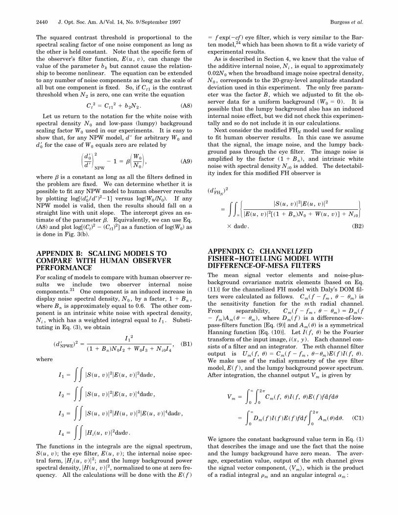
2440 J. Opt. Soc. Am. A/Vol. 14, No. 9 /September 1997 Burgess et al.
The squared contrast threshold is proportional to thespectral scaling factor of one noise component as long asthe other is held constant. Note that the specific form ofthe observer’s filter function, E(u, v), can change thevalue of the parameter bk but cannot cause the relation-ship to become nonlinear. The equation can be extendedto any number of noise components as long as the scale ofall but one component is fixed. So, if Ct1 is the contrastthreshold when N2 is zero, one can write the equation
Ct2 5 Ct1
2 1 b2N2 . (A8)
Let us return to the notation for the white noise withspectral density N0 and low-pass (lumpy) backgroundscaling factor W0 used in our experiments. It is easy toshow that, for any NPW model, d8 for arbitrary W0 andd08 for the case of W0 equals zero are related by
S d08
d8D
NPW
2
2 1 5 bS W0
N0D , (A9)
where b is a constant as long as all the filters defined inthe problem are fixed. We can determine whether it ispossible to fit any NPW model to human observer resultsby plotting log@(d08 / d8)221# versus log(W0 /N0). If anyNPW model is valid, then the results should fall on astraight line with unit slope. The intercept gives an es-timate of the parameter b. Equivalently, we can use Eq.(A8) and plot log@(Ct)
2 2 (Ct1)2# as a function of log(W0) as
is done in Fig. 3(b).
APPENDIX B: SCALING MODELS TOCOMPARE WITH HUMAN OBSERVERPERFORMANCEFor scaling of models to compare with human observer re-sults we include two observer internal noisecomponents.31 One component is an induced increase indisplay noise spectral density, N0 , by a factor, 1 1 Bn ,where Bn is approximately equal to 0.6. The other com-ponent is an intrinsic white noise with spectral density,Ni , which has a weighted integral equal to I1 . Substi-tuting in Eq. (3), we obtain
~dNPWE8 !2 5I1
2
~1 1 Bn!N0I2 1 W0I3 1 Ni0I4, (B1)
where
I1 5 EE uS~u, v !u2uE~u, v !u2dudv,
I2 5 EE uS~u, v !u2uE~u, v !u4dudv,
I3 5 EE uS~u, v !u2uH~u, v !u2uE~u, v !u4dudv,
I4 5 EE uHi~u, v !u2dudv.
The functions in the integrals are the signal spectrum,S(u, v); the eye filter, E(u, v); the internal noise spec-tral form, uHi(u, v)u2; and the lumpy background powerspectral density, uH(u, v)u2, normalized to one at zero fre-quency. All the calculations will be done with the E( f )
5 f exp(2cf ) eye filter, which is very similar to the Bar-ten model,24 which has been shown to fit a wide variety ofexperimental results.
As is described in Section 4, we knew that the value ofthe additive internal noise, Ni , is equal to approximately0.02N0 when the broadband image noise spectral density,N0 , corresponds to the 20-gray-level amplitude standarddeviation used in this experiment. The only free param-eter was the factor B, which we adjusted to fit the ob-server data for a uniform background (W0 5 0). It ispossible that the lumpy background also has an inducedinternal noise effect, but we did not check this experimen-tally and so do not include it in our calculations.
Next consider the modified FHN model used for scalingto fit human observer results. In this case we assumethat the signal, the image noise, and the lumpy back-ground pass through the eye filter. The image noise isamplified by the factor (1 1 Bn), and intrinsic whitenoise with spectral density Ni0 is added. The detectabil-ity index for this modified FH observer is
~dFHN8 !2
5 EE H uS~u, v !u2uE~u, v !u2
uE~u, v !u2@~1 1 Bn!N0 1 W~u, v !# 1 Ni0J
3 dudv. (B2)
APPENDIX C: CHANNELIZEDFISHER–HOTELLING MODEL WITHDIFFERENCE-OF-MESA FILTERSThe mean signal vector elements and noise-plus-background covariance matrix elements [based on Eq.(11)] for the channelized FH model with Daly’s DOM fil-ters were calculated as follows. Cm( f 2 fm , u 2 um) isthe sensitivity function for the mth radial channel.From separability, Cm( f 2 fm , u 2 um) 5 Dm( f2 fm)Am(u 2 um), where Dm( f ) is a difference-of-low-pass-filters function [Eq. (9)] and Am(u) is a symmetricalHanning function [Eq. (10)]. Let I( f, u) be the Fouriertransform of the input image, i(x, y). Each channel con-sists of a filter and an integrator. The mth channel filteroutput is Um( f, u) 5 Cm( f 2 fm , u2um)E( f )I( f, u).We make use of the radial symmetry of the eye filtermodel, E( f ), and the lumpy background power spectrum.After integration, the channel output Vm is given by
Vm 5 E0
`E0
2p
Cm~ f, u!I~ f, u!E~ f !fd fdu
5 E0
`
Dm~ f !I~ f !E~ f !fd fE0
2p
Am~u!du. (C1)
We ignore the constant background value term in Eq. (1)that describes the image and use the fact that the noiseand the lumpy background have zero mean. The aver-age, expectation value, output of the mth channel givesthe signal vector component, ^Vm&, which is the productof a radial integral rm and an angular integral am :
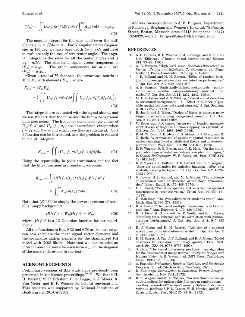
Burgess et al. Vol. 14, No. 9 /September 1997 /J. Opt. Soc. Am. A 2441
^Vm& 5 E0
`
Dm~ f !S~ f !E~ f !fd fE0
2p
Am~u!du 5 rmam .
(C2)
The angular integral for the base band (over the half-plane) is a0 5 *0
pdu 5 p. For N angular center frequen-cies in 180 deg, we have base width uW 5 p/N and needto evaluate only the case of zero center angle. The angu-lar integral is the same for all the center angles and isa1 5 p/N. The base-band signal vector component is^V1& 5 a0r1 . The other components for m . 1 are^Vm& 5 a1rm .
Given a total of M channels, the covariance matrix isM 3 M, with elements Knm , where
Kmn 5 ^VmVn&
5 K EE Um~ f, u!fd fduEE Un~ f1 , u1!f1d f1du1L .
(C3)
The integrals are evaluated with the signal absent, andwe use the fact that the noise and the lumpy backgroundhave zero mean. The frequency-domain sample values ofUm( f, u) and Um( f1 , u1) are uncorrelated except whenf 5 f1 and u 5 u1 , in which case they are identical. So ad function can be introduced, and the problem is reducedto one 2D integral:
Kmn 5 EE ^Um~ f, u!Un~ f, u!&fd fdu. (C4)
Using the separability in polar coordinates and the factthat the filter functions are constant, we obtain
Kmn 5 E0
`
^R2~ f !&Dm~ f !Dn~ f !E2~ f !fd f
3 E0
2p
Am~u!An~u!du. (C5)
Note that ^R2( f )& is simply the power spectrum of noiseplus lumpy background.
^R2~ f !& 5 W0uH~ f !u2 1 N0 , (C6)
where uH( f )u2 is a 2D Gaussian function for our experi-ments.
All the functions in Eqs. (C2) and (C5) are known, so wecan now calculate the mean signal vector elements andthe covariance matrix elements for the channelized FHmodel with DOM filters. Note that we also included aninternal noise variance for each term Knn on the diagonalof the matrix (described in the text).
ACKNOWLEDGMENTSPreliminary versions of this study have previously beenpresented in conference proceedings.50–52 We thank H.H. Barrett, M. P. Eckstein, G. E. Legge, K. J. Myers, R.Van Meter, and R. F. Wagner for helpful conversations.This research was supported by National Institutes ofHealth grant R01-CA58302.
Address correspondence to A. E. Burgess, Departmentof Radiology, Brigham and Women’s Hospital, 75 FrancisStreet, Boston, Massachusetts 02115 [telephone: (617)732-6329, e-mail: [email protected]].
REFERENCES1. A. E. Burgess, R. F. Wagner, R. J. Jennings, and H. B. Bar-
low, ‘‘Efficiency of human visual discrimination,’’ Science214, 93–94 (1981).
2. A. E. Burgess, ‘‘High level visual decision efficiencies,’’ inVision: Coding and Efficiency, C. Blakemore, ed. (Cam-bridge U. Press, Cambridge, 1990), pp. 431–440.
3. J. P. Rolland and H. H. Barrett, ‘‘Effect of random back-ground inhomogeneity on observer detection performance,’’J. Opt. Soc. Am. A 9, 649–658 (1992).
4. A. E. Burgess, ‘‘Statistically defined backgrounds: perfor-mance of a modified nonprewhitening matched filtermodel,’’ J. Opt. Soc. Am. A 11, 1237–1242 (1994).
5. M. P. Eckstein and J. S. Whiting, ‘‘Visual signal detectionin structured backgrounds. I. Effect of number of pos-sible spatial locations and signal contrast,’’ J. Opt. Soc. Am.A 13, 1777–1787 (1996).
6. B. Javidi and J. Wang, ‘‘Design of filters to detect a noisytarget in nonoverlapping background noise,’’ J. Opt. Soc.Am. A 11, 2604–2612 (1994).
7. V. Kober and J. Campos, ‘‘Accuracy of location measure-ment of a noisy target in a nonoverlapping background,’’ J.Opt. Soc. Am. A 13, 1653–1665 (1996).
8. B. M. W. Tsui, C. E. Metz, F. B. Atkins, S. J. Starr, and R.N. Beck, ‘‘A comparison of optimum spatial resolution innuclear imaging based on statistical theory and on observerperformance,’’ Phys. Med. Biol. 23, 654–676 (1978).
9. R. F. Wagner, D. G. Brown, and C. E. Metz, ‘‘On the multi-plex advantage of coded source/aperture photon imaging,’’in Digital Radiography, W. R. Brody, ed., Proc. SPIE 314,72–76 (1981).
10. K. J. Myers, J. P. Rolland, H. H. Barrett, and R. F. Wagner,‘‘Aperture optimization for emission imaging: effect of aspatially varying background,’’ J. Opt. Soc. Am. A 7, 1279–1293 (1990).
11. G. Revesz, H. L. Kundel, and M. A. Graber, ‘‘The influenceof structured noise on detection of radiologic abnormali-ties,’’ Invest. Radiol. 9, 479–486 (1974).
12. F. L. Engel, ‘‘Visual conspicuity and selective backgroundinterference in eccentric vision,’’ Vision Res. 14, 459–471(1973).
13. H. Hotelling, ‘‘The generalization of student’s ratio,’’ Ann.Math. Stat. 2, 360–378 (1931).
14. R. A. Fisher, ‘‘The use of multiple measurements in taxonicproblems,’’ Ann. Eugenics 7, 179–188 (1936).
15. R. D. Fiete, H. H. Barrett, W. E. Smith, and K. J. Myers,‘‘Hotelling trace criterion and its correlation with human-observer performance,’’ J. Opt. Soc. Am. A 4, 945–953(1987).
16. K. J. Myers and H. H. Barrett, ‘‘Addition of a channelmechanism to the ideal-observer model,’’ J. Opt. Soc. Am. A4, 2447–2457 (1987).
17. H. H. Barrett, J. Yao, J. P. Rolland, and K. J. Myers, ‘‘Modelobservers for assessment of image quality,’’ Proc. Natl.Acad. Sci. USA 90, 9758–9765 (1993).
18. S. Daly, ‘‘The visual differences predictor: an algorithmfor the assessment of image fidelity,’’ in Digital Images andHuman Vision, A. B. Watson., ed. (MIT Press, Cambridge,Mass., 1993), pp. 179–206.
19. A. Papoulis, Probability, Random Variables, and StochasticProcesses, 3rd ed. (McGraw-Hill, New York, 1990).
20. K. Fukunaga, Introduction to Statistical Pattern Recogni-tion (Academic, New York, 1972).
21. R. F. Wagner and K. E. Weaver, ‘‘An assortment of imagequality indices for radiographic film-screen combinations—can they be resolved?’’ in Application of Optical Instrumen-tation in Medicine I, P. L. Carson, W. R. Hendee, and W. C.Zarnstorff, eds., Proc. SPIE 35, 83–94 (1972).
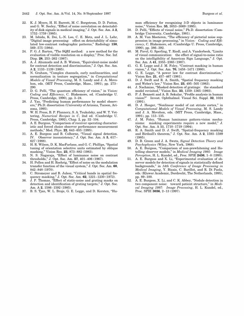
2442 J. Opt. Soc. Am. A/Vol. 14, No. 9 /September 1997 Burgess et al.
22. K. J. Myers, H. H. Barrett, M. C. Borgstrom, D. D. Patton,and G. W. Seeley, ‘‘Effect of noise correlation on detectabil-ity of disk signals in medical imaging,’’ J. Opt. Soc. Am. A 2,1752–1759 (1985).
23. M. Ishida, K. Doi, L.-N. Loo, C. E. Metz, and J. L. Lehr,‘‘Digital image processing: effect on detectability of simu-lated low-contrast radiographic patterns,’’ Radiology 150,569–575 (1984).
24. P. G. J. Barten, ‘‘The SQRI method: a new method for theevaluation of visible resolution on a display,’’ Proc. Soc. Inf.Disp. 28, 253–262 (1987).
25. A. J. Ahumada and A. B. Watson, ‘‘Equivalent-noise modelfor contrast detection and discrimination,’’ J. Opt. Soc. Am.A 2, 1133–1139 (1985).
26. N. Graham, ‘‘Complex channels, early nonlinearities, andnormalization in texture segregation,’’ in ComputationalModels of Visual Processing, M. S. Landy and J. A. Movs-hon, eds. (MIT Press, Cambridge, Mass., 1991), pp. 273–290.
27. D. G. Pelli, ‘‘The quantum efficiency of vision,’’ in Vision:Coding and Efficiency, C. Blakemore, ed. (Cambridge U.Press, Cambridge, 1990), pp. 3–24.
28. J. Yao, ‘‘Predicting human performance by model observ-ers,’’ Ph.D. dissertation (University of Arizona, Tucson, Ari-zona, 1995).
29. W. H. Press, B. P. Flannery, S. A. Teukolsky, and W. T. Vet-tering, Numerical Recipes in C, 2nd ed. (Cambridge U.Press, Cambridge, 1992), Chap. 2, pp. 32–104.
30. A. E. Burgess, ‘‘Comparison of receiver operating character-istic and forced choice observer performance measurementmethods,’’ Med. Phys. 22, 643–655 (1995).
31. A. E. Burgess and B. Colborne, ‘‘Visual signal detection.IV. Observer inconsistency,’’ J. Opt. Soc. Am. A 5, 617–627 (1988).
32. H. R. Wilson, D. K. MacFarlane, and G. C. Phillips, ‘‘Spatialtuning of orientation selective units estimated by obliquemasking,’’ Vision Res. 23, 873–882 (1983).
33. N. S. Nagaraja, ‘‘Effect of luminance noise on contrastthresholds,’’ J. Opt. Soc. Am. 57, 401–406 (1967).
34. H. Pollen and H. Roehrig, ‘‘Effect of noise on the modulationtransfer function of the visual system,’’ J. Opt. Soc. Am. 60,842–848 (1970).
35. C. Stromeyer and B. Julesz, ‘‘Critical bands in spatial fre-quency masking,’’ J. Opt. Soc. Am. 62, 1221–1230 (1972).
36. J. P. Thomas, ‘‘Effect of static-noise and grating masks ondetection and identification of grating targets,’’ J. Opt. Soc.Am. A 2, 1586–1592 (1985).
37. B. S. Tjan, W. L. Braje, G. E. Legge, and D. Kersten, ‘‘Hu-
man efficiency for recognizing 3-D objects in luminancenoise,’’ Vision Res. 35, 3053–3069 (1995).
38. D. Pelli, ‘‘Effects of visual noise,’’ Ph.D. dissertation (Cam-bridge University, Cambridge, 1981).
39. A. M. Van Meeteren, ‘‘The efficiency of pictorial noise sup-pression in image processing,’’ in Vision: Coding and Effi-ciency, C. Blakemore, ed. (Cambridge U. Press, Cambridge,1990), pp. 386–392.
40. M. Pavel, G. Sperling, T. Riedl, and A. Vanderbeek, ‘‘Limitsof visual communication: the effect of signal-to-noise ratioon the intelligibility of American Sign Language,’’ J. Opt.Soc. Am. A 41, 2355–2365 (1987).
41. G. E. Legge and J. M. Foley, ‘‘Contrast masking in humanvision,’’ J. Opt. Soc. Am. 70, 1458–1471 (1980).
42. G. E. Legge, ‘‘A power law for contrast discrimination,’’Vision Res. 21, 457–467 (1981).
43. D. J. Swift and R. A. Smith, ‘‘Spatial frequency maskingand Weber’s law,’’ Vision Res. 23, 495–505 (1983).
44. J. Nachmias, ‘‘Masked detection of gratings: the standardmodel revisited,’’ Vision Res. 33, 1359–1365 (1993).
45. P. J. Bennett and A. B. Sekular, ‘‘Profile analysis in humanvision?’’ Invest. Ophthalmol. Visual Sci. Suppl. 32, 1024(1991).
46. D. J. Heeger, ‘‘Nonlinear model of cat striate cortex,’’ inComputational Models of Visual Processing, M. S. Landyand J. A. Movshon, eds. (MIT Press, Cambridge, Mass.,1991), pp. 113–135.
47. J. M. Foley, ‘‘Human luminance pattern-vision mecha-nisms: masking experiments require a new model,’’ J.Opt. Soc. Am. A 11, 1710–1719 (1994).
48. R. A. Smith and D. J. Swift, ‘‘Spatial-frequency maskingand Birdsall’s theorem,’’ J. Opt. Soc. Am. A 2, 1593–1599(1985).
49. D. B. Green and J. A. Swets, Signal Detection Theory andPsychophysics (Wiley, New York, 1968).
50. A. E. Burgess, ‘‘Comparison of non-prewhitening and Ho-telling observer models,’’ in Medical Imaging 1995: ImagePerception, H. L. Kundel, ed., Proc. SPIE 2436, 1–8 (1995).
51. A. E. Burgess and X. Li, ‘‘Experimental evaluation of ob-server models for detection of signals in statistically definedbackgrounds,’’ in 14th Conference of Image Processing inMedical Imaging, Y. Bizais, C. Barillot, and R. Di Paola,eds. (Kluwer Academic, Dordrecht, The Netherlands, 1995),pp. 89–100.
52. A. E. Burgess, X. Li, and C. K. Abbey, ‘‘Nodule detection intwo component noise: toward patient structure,’’ in Medi-cal Imaging 1997: Image Processing, H. L. Kundel, ed.,Proc. SPIE 3036, 2–13 (1997).


