Vlasov-code simulations of collisionless plasmas

Ilya SilinJörg BüchnerMax-Planck Institut für AeronomieKatlenburg-Lindau

A Vlasov-code is a numerical scheme for simulations of rarefied plasmas,e.g. in the interplanetary and interstellar medium, where particle collisionscan be neglected. In this method the self-consistent evolution of plasma isdescribed by Maxwell equations for electromagnetic fields and Vlasov equa-tions for particle distribution functions. Due to the necessary detailed sam-pling of the velocity space Vlasov-code simulations pose high memory re-quirements. Consequently, they challenge huge calculational resources. Forsix-dimensional calculations (3D in the configuration and 3D in the veloc-ity space) the only solution is to carry out the simulations on a parallel ma-chine with considerably large memory resources and a large number of CPUs.In this paper we describe the numerical scheme and the parallelization ar-chitectures used for the MPAe Vlasov-code simulation at GWDG facilities.The code is written in ANSI C language and is parallelized using standardmessage-passing interface (MPI) and/or OpenMP libraries which makes thecode portable as it is on any hardware.

1

Vlasov-code numerical scheme

The main feature which distinguishes the Vlasov-code simulations from othernumerical methods of plasma simulation, such as magneto-hydro-dynamic(MHD), hybrid and particle-in-cell (PIC) codes, is that plasma is representedby particle distribution functions. For comparison, in MHD codes plasma isconsidered as fluid, in PIC-codes as an ensemble of so-called super-particles,in hybrid codes - ions are represented by super-particles and electrons byfluid. MHD-codes allow diagnostics only of the mean local velocity of plasma.In PIC-codes, the number of super-particles per cell usually does not exceed100. In case of inhomogeneous plasmas, the number of particles in low-density regions even turns to zero. Thus, information about particle distribu-tion in the velocity space is available only in dense plasma regions. But eventhere the particle distribution function is resolved by only

����������� �points

in every velocity dimension.The advantage of the Vlasov approach is the detailed information about

the distribution of particles in the velocity space. This allows investigationswhich cannot be carried out in MHD or PIC approaches, e.g. of resonantwave-particle interactions. The distribution functions have to be sampled byat least 15 - 20 points in every velocity dimension. Besides, the local plasmadensity changes only the amplitude of the distribution and does not affectthe velocity space resolution and range. Theoretically, such simulation corre-sponds to using a PIC code with 3400 - 8000 super-particles in every cell.

There are, however, limits of application of Vlasov-code simulations. First,the classical Vlasov equation describes only collisionless plasmas, i.e. veryhot and rarefied gas. It cannot be directly applied to simulations of laboratoryand stellar plasmas, where collisions are important. Also, the classical Vlasovequation is valid only for non-relativistic interactions. In order to describevery hot plasmas or energetic tails of particle distributions one has to usegeneralized relativistic Vlasov equations.

The MPAe Vlasov code has been applied to investigation of instabilitiesin thin current sheets in space plasmas. The code consists of four sepa-rate blocks. First, the particle distribution functions are initialized as drift-Maxwellians:������������ ���������� �����"! ��$#&% �(')"*,+ � � �-� '/.�0�132�4

� '576 � �,8 4:9 � � ' 6 � ';# � ')"*,+ � < � (1)

where = �?>-�@ for ions and electrons, respectively.Then, the charge and current densities are integrated (zero- and first-order

moments of the distribution function):

AB�DC � @ �FEG�H�HIJ��

2

�= � C � @ �FE �� �H�HIJ�� � (2)

Further, the Maxwell equations for electromagnetic fields are solved. Inour version of the code the electromagnetic fields are expressed in terms ofelectrostatic and vector-potentials:

�� � 4 ���� 4 �� ���� ��� � �� �� � (3)

The potentials can be found by solving the Poisson and D’Alambert equations� � � 4 � % A� �� 4�� ' � '

��� � ' � 4� %� �= � (4)

Notice, that a part of displacement current� � � �� � � � � � is neglected in the

second Equation (4). This way the propagation of electromagnetic waves issuppressed and subsequent heating of plasma is avoided.

Finally, the electromagnetic fields are used to solve the Vlasov equationsin order to update the particle distribution functions:� �H�� � 6 ���� � �H�� �� 6 @ �� � � �� 6 �� �� ���� � � �H�� �� � � � (5)

From this step the program returns to Equation (2) and the cycle repeats.This is the main program loop. The numerical analogues of Equations (2-5)are obtained by direct substitution of derivatives and integrals by the time-and grid-centered numerical expressions, e.g. Equation (5) takes the form

fnew[i]=fold[i]-2.*dt*(vx[ivx]*dfx+vy[ivy]*dfy+vz[ivz]*dfz+Fx*dfvx+Fy*dfvy+Fz*dfvz),

where� @���� >�� is the value of distribution function at time step � 6 � � and

phase-space location > , ��� �"I � >�� is the value of this distribution at the moment� 4 � � , I � is the time increment, ��� , ��� and � ! are the velocity-space coordi-nates corresponding to the phase-space coordinate > , I � � ,

I � � andI � !

are thedifferences of distribution function values along the x, y and z-coordinatesaround the location > , � � , � � and � ! are local values of the Lorentz forceand

I � ��� ,I � ��� and

I � � ! are the differences of distribution function alongthe velocity axes around location > .

The only equation which requires more complicated methods is the Pois-son equation 4. It is solved iteratively by the Gauss-Seidel method [1, 2]. The

3

numerical scheme for the one-dimensional poisson equation is as follows:� 5 � � 4 # � 5 6 � 5�� �� � � � ' � 4 � % A 5 � (6)

From this equation one can express the value of electrostatic potential at thegiven location � as

� 5 � #&% A 5 � � � � ' � 6 �# � � 5 � � 6 � 5�� � � � (7)

The corresponding passage from the three-dimensional simulation is givenbelow:

potential[ir]=alpha*(h2x*(potential[ir-nynz]+A0[ir+nynz])+ h2y*(potential[ir-nz]+A0[ir+nz])+h2z*(potential[ir-1]+A0[ir+1])+c[ir]);

Here � � ��� � ,��# � ,

��# � and��#,!

are dimensional factors� � �$#�� � � ' 6 � � ' 6� ! ' ��� , � � � � ' , � � � � ' , and

� � � ! ' , � � > ��� is the� % A�� > ��� . The array

� � ��@ � > � �contains the values of the electrostatic potential

�to the left and the array� �

consists of the approximate values of�

from the previous iteration tothe right of the considered point > � . At the first iteration the

� �set is as-

signed some values and the� � ��@ � > � � array is updated. Then, the square

error �� � � � � >�� 4 � � ��@ � > � � � >�� � ' is estimated and the iterations continue untilthe average error gets less than

���� � �. In the shared memory task this does

not present any serious problem, only that the innermost loop of the solveritself cannot be parallelized. However, as we shall demonstrate later, on thedistributed memory machines this iterative method requires particular treat-ment.

Parallelization architectures

OpenMP

One of the simplest parallelization standards is the OpenMP library (for de-tails see www.openmp.org and ”Scientific Applications in RS6000 SP Envi-ronments” at www.redbooks.ibm.com). On a machine with shared memorysuch as IBM p690 the parallelization is straightforward. The code is exe-cuted in a usual sequential manner and only the massive calculation loops areparallelized. Within each parallel loop the array of data is shared between dif-ferent CPUs. The domain decomposition of the data array and the so-called”fork-join” execution of the code in the parallel region is shown schemati-cally in Figure 1. In all our parallel simulations the domain decomposition

4

Fig. 1: Schematic data-array decomposition between CPUs (left panel) and fork-join executionscheme (right panel) in parallel OpenMP region.

was carried out along the spatial � -coordinate. For the best performance onehas to make sure that the size of the decomposed array, i.e. the number ofgrid-points in the � -dimension, is proportional to the number of CPUs used.Then the job will be shared equally between all CPUs and the time losses forsynchronization will be minimized.

The use of OpenMP is enabled by including the header file

#include <omp.h>

and by appropriate comments in the makefile during compilation and linking

mpcc_r -c -O3 -qsmp=omp ...

and

mpcc_r -lm -o vlasov -qsmp=omp ...

With the option 4 ��� � � � � 9 � � every loop in the program will be paral-lelized automatically, which often leads to a less efficient execution of therun. With the option 4 ��� � � � � � � only the loops which are provided witha preprocessor header, e.g.

#pragma omp parallel for private(i)

will be executed in parallel. This allows to efficiently share the massive cal-culations between the CPUs and at the same time avoid the time losses duringparallelization of the small loops, where the calculation time is comparableor smaller than the parallelization and synchronization time.

MPI

On parallel machines with distributed memory where each CPU has accessto its own block of memory the OpenMP parallelization looses sense. In-stead, one has to use the message-passing interface (MPI) library (details un-der www.mpi-forum.org and ”RS6000 SP: Practical MPI Programming” at

5

Fig. 2: Schematic domain decomposition between nodes (left panel) and parallel executionscheme (right panel) of an MPI code.

www.redbooks.ibm.com). Being probably the most wide-spread paralleliza-tion library, MPI has the only disadvantage that it must be explicitly pro-grammed in the code. The MPI library is activated by listing the header file

#include <mpi.h>

The parallel environment is launched by the commands

MPI_Init (&argc, &argv);MPI_Comm_size (MPI_COMM_WORLD, &nprocs);MPI_Comm_rank (MPI_COMM_WORLD, &npid);

where � � � � � and � > I correspond to the total number of MPI-tasks and theprivate id-number of a given task. The aim of parallelization is to decreasethe calculation time or to bind together separated memory resources. Fromthis point of view it is worth to initialize only one task on every CPU/memoryblock, although technically it is possible to launch more than one task onevery CPU. Now, the domain decomposition is carried out in the same man-ner as in the shared-memory case, with the only exception that each CPU”knows” only its own part of the data and ”does not know” anything aboutthe rest of the field. The domain decomposition and the execution scheme areillustrated in Figure 2.

In every calculation loop corresponding to a differential equation, eachCPU needs the parts of the data-arrays from its neighbours directly adjacentto it. In the Equations (2- 5) we encounter the following spatial derivativesalong the x-axis:

� � � � � ,��� 5 � � � ,

��� 8 � � � ,��� ; � � � ,

� � � � � � and� �

�

� � � .It means that the layers of arrays containing

�,� 5 ,

� 8 , � ; , � � and�

� mustbe sent from each CPU to its neighbours. In a typical production run the sizeof such data blocks can reach up to 16 Kbytes for the potentials and up to60 Mbytes for the distribution functions. Such volumes of data do not causeany significant time delays on machines connected by Gigabit Ethernet or onIBM RS6000-SP with high performance switch. An example of distributionfunction layers exchanged between different MPI-tasks is given below:

Vlasov_solver(...);

6

for(ip=0;ip<nprocs;ip++){if(npid==ip){if(ip==0){for(i=0;i<sx;i++){right[i]=fi[sall-2*sx+i];}istat=MPI_Send(&right[0],sx,MPI_FLOAT,ip+1,0,MPI_COMM_WORLD);

}if(ip>0 && ip<nprocs-1){istat=MPI_Recv(&right[0],sx,MPI_FLOAT,ip-1,0,MPI_COMM_WORLD,&status);Vlasov_bound(...);for(i=0;i<sx;i++){right[i]=fi[sall-2*sx+i];}istat=MPI_Send(&right[0],sx,MPI_FLOAT,ip+1,0,MPI_COMM_WORLD);

}if(ip==nprocs-1){istat=MPI_Recv(&right[0],sx,MPI_FLOAT,ip-1,0,MPI_COMM_WORLD,&status);Vlasov_bound(...);

}}

}istat=MPI_Barrier(MPI_COMM_WORLD);

for(ip=0;ip<nprocs;ip++){if(npid==ip){if(ip>0){for(i=0;i<sx;i++){left[i]=fhelp[i];}istat=MPI_Send(&left[0],sx,MPI_FLOAT,ip-1,0,MPI_COMM_WORLD);

}if(ip<nprocs-1){istat=MPI_Recv(&left[0],sx,MPI_FLOAT,ip+1,0,MPI_COMM_WORLD,&status);Vlasov_bound(...);

}}

}istat=MPI_Barrier(MPI_COMM_WORLD);

In this code passage first the Vlasov equation is solved in the inner volumeof each domain. Then, every MPI-task with id-number � > I first sends its

7

right part of the array� � @ � � consisting of � � elements of size

�����_ ����� ��

to its right neighbour with id-number � > I 6 �. Then each task receives the

parcel and solves Vlasov equation at the left-most boundary of the domain.The thread corresponding to the left-most domain ( � > I � � �

) only sendsthe parcel and the thread corresponding the right-most domain ( � > I � � � � � � � 4 �

) only receives the parcel. Then, the left-most boundaries of allthreads are exchanged in the similar manner. Afterwards the left-most layerfrom the left-most node � > I � � �

is sent to the right-most node and, vice-versa, the right-most node sends the right-most part of its distribution func-tions arrays to the left-most node in order to satisfy the periodic boundaryconditions.

A particularly tricky situation occurs with the iterative Gauss-Seidel solverfor the potentials. The point is that this loop carries out the differentiationmany times per cycle. In this case transmitting/receiving even small packagesof data is too costly. In order to avoid it we gather the arrays of charge and cur-rent densities from all MPI-tasks on the Master and solve the iterative routinelocally on the Master-thread. Then, the necessary domains of the resultingpotentials are redistributed among all the threads. Compared to jobs par-allelized with OpenMP architecture, the productivity of MPI-runs increasesslower with the increasing number of CPUs, because the inter-processor traf-fic (the number of communication commands and the volume of data sent)increases proportionally.

Hybrid

The most general case of parallel architecture is the ”hybrid” one when MPIand OpenMP libraries are combined (recommended reading ”Scientific Ap-plications in RS6000 SP Environments” at www.redbooks.ibm.com). Thisarchitecture has been successfully employed for

# �' Vlasov simulationson the IBM RS6000-SP machine at GWDG. On this machine four proces-sors have access to a common 2 Gbytes memory block. This unit is calleda node. The nodes are connected between each other by the IBM high-performance switch, which enables high-rate data traffic between the nodes.Thus, it makes sense to start a single MPI task on each node to avoid the MPI-communications within the single memory block and keep only the necessarydata traffic between the isolated domains. At the same time the processing ofthe data in each domain is carried out by all the CPUs which have access toit, i.e. under the OpenMP parallelization. This architecture uses the advan-tages of both standards in the most rational way. It is also portable as is onany other hardware, e.g. several IBM Regatta machines connected by Eth-ernet. The domain decomposition and the execution line are schematicallyillustrated in Figure 3.

8

Fig. 3: Schematic domain decomposition between nodes and CPUs (left panel) and executionscheme (right panel) of a code with hybrid parallel architecture.

An example of hybrid parallel code is given below.

#ifdef _OPENMP#pragma omp parallel for private(i)#endiffor(i=0;i<nxnz;i++){glsigma[npid*(nxnz-nz)+i]=sigma[i];

}for(ip=0;ip<nprocs;ip++){if(npid==ip){if(ip==0){for(i=1;i<nprocs;i++){istat=MPI_Recv(&glsigma[i*(nxnz-nz)],nxnz,MPI_DOUBLE,i,0,MPI_COMM_WORLD,&status);}

}if(ip>0){istat=MPI_Send(&glsigma[ip*(nxnz-nz)],nxnz,MPI_DOUBLE,0,0,MPI_COMM_WORLD);

}}

}istat=MPI_Barrier(MPI_COMM_WORLD);

for(ip=0;ip<nprocs;ip++){if(npid==ip){if(ip==0){Poisson(glsigma,glphi,schritt);

}}

}istat=MPI_Barrier(MPI_COMM_WORLD);

9

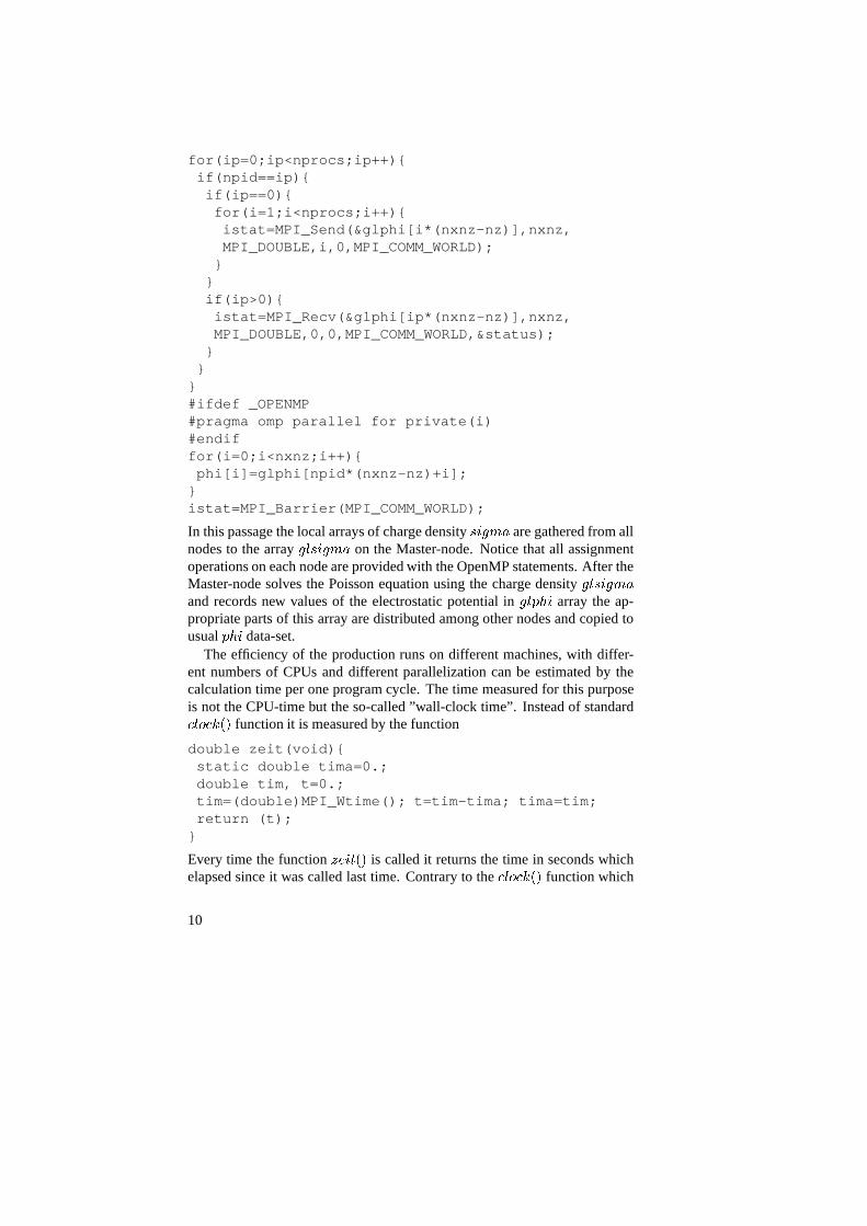
for(ip=0;ip<nprocs;ip++){if(npid==ip){if(ip==0){for(i=1;i<nprocs;i++){istat=MPI_Send(&glphi[i*(nxnz-nz)],nxnz,MPI_DOUBLE,i,0,MPI_COMM_WORLD);}

}if(ip>0){istat=MPI_Recv(&glphi[ip*(nxnz-nz)],nxnz,MPI_DOUBLE,0,0,MPI_COMM_WORLD,&status);

}}

}#ifdef _OPENMP#pragma omp parallel for private(i)#endiffor(i=0;i<nxnz;i++){phi[i]=glphi[npid*(nxnz-nz)+i];

}istat=MPI_Barrier(MPI_COMM_WORLD);

In this passage the local arrays of charge density �H>�� � � are gathered from allnodes to the array � � �H>�� � � on the Master-node. Notice that all assignmentoperations on each node are provided with the OpenMP statements. After theMaster-node solves the Poisson equation using the charge density � � �H>�� � �and records new values of the electrostatic potential in � � ��� > array the ap-propriate parts of this array are distributed among other nodes and copied tousual

��� > data-set.The efficiency of the production runs on different machines, with differ-

ent numbers of CPUs and different parallelization can be estimated by thecalculation time per one program cycle. The time measured for this purposeis not the CPU-time but the so-called ”wall-clock time”. Instead of standard� � � ��� � � function it is measured by the function

double zeit(void){static double tima=0.;double tim, t=0.;tim=(double)MPI_Wtime(); t=tim-tima; tima=tim;return (t);

}

Every time the function! @�> � � � is called it returns the time in seconds which

elapsed since it was called last time. Contrary to the � � � ��� � � function which

10

10 20 30 40 50 60Number of CPUs

-1

0

1

2

3

4

Log

HTimepe

rcyc

leL

Fig. 4: Logarithm of wall-clock time per one program cycle (logaritmic scale) of OpenMP (redgreen and cyan lines) on IBM p690 and hybrid parallelization techniques on IBM RS6000-SP(blue lines) for different numbers of CPUs used. Solid lines show the full program cycle duration,dashed lines correspond to fully parallel part of the cycle. The cyan lines are drawn for the runwith 30 Gbytes memory block, the green - 8 Gbytes, red and blue - 800 Mbytes.

has different values on different CPUs, the�����

_� � > � @ � � function is uniquely

defined on all CPUs/MPI tasks.The time required for one program cycle depends on the number of CPUs

involved can be estimated as approximately� � � ������� ���� � 6 ��� 8���� ���� � � (8)

where ������� � is the total calculation time and ��� 8���� is the time needed forsynchronization, parallelization and communication. The first term ������� � isusually proportional to the size of the memory block used by the program,while the other, ��� 8���� , is constant. Thus, it is impossible to separate the di-agnostics of the program efficiency from its memory consumption. Figure 4demonstrates this effect. In this figure we compare relative calculation time(in seconds, logarithmic scaling) of a

#F�' Vlasov-code test-run with ap-proximately 800 Mbytes on IBM RS6000-SP with hybrid architecture (bluelines) and OpenMP version with 800 Mbytes, 8 Gbytes and 30 Gbytes (red,green and cyan lines, respectively) memory on IBM p690 machine. The solidlines correspond to the total program cycle (integration of distribution func-tion moments, calculation of potentials and electromagnetic fields and solvingthe Vlasov equation), while the dashed lines show only the fully-parallelizedpart of the cycle (without iterative Gauss-Seidel solver). For the 800-Mbytesmemory test-run the amount of calculations is rather small and the synchro-nization and communication time with the increasing number of CPUs be-come comparable to the calculation duration. Hence, the strong saturation

11

-10-5 0 510

x�Lz

-10

-5

0

510

y�Lz

-202

z�Lz-202

z�Lz

Fig. 5: Constant-level plot of plasma density exhibiting the wave profile in the current directionafter 25 ion gyroperiods of simulation.

tendency in both red and blue dashed curves. The solid red and blue curveseven show the increase of the calculation time because they include a se-quential part which is not accelerated by the use of more processors, but thesynchronization and traffic duration before and after it increase. However,for massive production runs with large memory the amount of calculationwork exceeds significantly the synchronization and communication part andthe time gain with more CPUs is very efficient. Thus, one can see, that ittakes longer to execute a small-memory job on 32 or 64 CPUs than on 16,while the high-memory jobs may still run faster on an even larger number ofprocessors.

Simulation results

The results obtained with the Vlasov-code described in this paper reveal im-portant processes which have been missed by other plasma simulation tech-niques. It has been known from linear theory and experiments that in theregions of magnetic field and plasma density gradients the unstable lower-hybrid-drift (LHD) waves are excited. These waves are localized at the re-gions of maximum density gradient outside thin current sheets and propa-gate perpendicularly to the magnetic field direction with the group velocityapproximately equal to ion thermal speed. These waves can consequentlyinteract with the particle flows through the direct and inverse Landau damp-ing [3, 4]. As a result, in thin current sheets the LHD waves are resonantly

12

0 2 4 6 8 10 12tW0

-4

-2

0

2

4

z

log E`

0.00294

0.

Fig. 6: The time versus z-coordinate plot of the Fourier amplitude of the dominant current alignedelectric field

���. One sees that the first perturbations occur at ������� �� at ��������� .

amplified by ions and damped by electrons. This effect is achieved in Vlasovsimulations due to the detailed particle distribution functions resolution inthe velocity space. As the waves grow they expand from the edges of thecurrent sheet towards the center and trigger global oscillations of the currentsheet [5, 6]. An example of such instability is demonstrated in Figure 5. Inour setup the X-axis coincides with the magnetic-field direction, current flowsalong the Y-axis and Z-axis is perpendicular to the current sheet plane. Onesees that the constant-level contours of plasma density shaping the currentsheet exhibit wave-like profile in the current-flow direction. The sequence ofsuch pictures shows that this wave in fact propagates with approximately ionthermal velocity in the ion drift direction. The wavelength and oscillation fre-quency of the wave scale with typical LHD properties. However, the growthrate of this instability is slower than that of LHD and scales with ion gyrofre-quency. This means that the oscillations, group velocity and wavelength areinherited from the LHD waves while the growth of this global instability isdue to the ion dynamics, namely due to the inverse Landau damping.

This mechanism solves the problem of current sheet stability against thelinear global current-aligned modes [7, 8]. Indeed, the Fourier analysis of thedominant modes in the current-aligned electric field shows that the wave firstappears at the periphery of the current sheet and gradually expands in spaceand exponentially grows in amplitude (Figure 6).

In the full three-dimensional configuration space these waves form theso-called ”cigar-like structures” [4] stretched along the local magnetic field

13

-10-5

05

10x�Lz

-10

-5

0

5

10

y�Lz

-202

z�Lz

-10-5

05

10x�Lz

Fig. 7: The spatial domains of maximum positive (red) and minimum negative (blue) current-aligned electric field

���at ��� ������ .

shown in Figure 7. At the same time, the magnetic field perturbations containthe wave-like profile in the current direction and the change of sign in themagnetic field direction, thus showing some tearing-mode instability. Fig-ure 8 demonstrates the maximum and minimum domains of the reconnectednormal magnetic field

� ; in the 3D Vlasov-code simulations. The three-dimensional Vlasov-code simulations revealed that these wave modes can di-rectly couple to the aperiodic tearing-mode instability which slowly grows inthe orthogonal direction and enhance its growth rate. Indeed, the structure ofthe reconnected fields is such that if the amplitude of the maxima and min-ima increases due to the fast-growing wave-mode in the current direction itsubsequently increases also in the orthogonal tearing-mode direction.

Acknowledgements

I.S. acknowledges the support of Deutscher Akademischer Austauschdienst(DAAD) during his Ph.D. thesis preparation in Germany.

References

[1] W. H. Press, S. A. Teukolsky, W. T. Vetterling, and B. P. Flannery, Numerical recipes inC (Cambridge University Press, Cambridge, New York, Port Chester, Melbourne, Sydney,1988).

14

-10-5

05

10x�Lz

-10

-5

0

5

10

y�Lz

-202

z�Lz

-10-5

05

10x�Lz

Fig. 8: The spatial domains of maximum positive (red) and minimum negative (blue) reconnectedmagnetic field

���at ��� � � �� .

[2] R. W. Hockney and J. W. Eastwood, Computer Simulation Using Particles (Adam Hilger,Bristol and Philadelphia, 1988).

[3] V. L. Ginzburg, The Propagation of Electromagnetic Waves in Plasmas (Pergamon Press,Oxford, New York, Toronto, Sydney, Braunschweig, 1988).

[4] V. Tsytovich, Lectures on non-linear plasma kinetics (Springer, Berlin, Heidelberg, NewYork, 1995), pp. 349–353.

[5] I. Silin and J. Büchner, “Kinetic instabilities of thin current sheets. Results of 2 1/2D Vlasovcode simulations,” Phys. Plasmas 10, 1299 – 1307 (2003).

[6] I. Silin and J. Büchner, “Nonlinear instability of thin current sheets in antiparallel andguided magnetic fields,” in print, Phys. Plasmas 10 (2003).

[7] W. Daughton, “Kinetic theory of the drift kink instability in a current sheet,” J. Geophys.Res. 103, 29429 (1998).

[8] I. Silin, J. Büchner, and L. M. Zelenyi, “Instabilities of collisionless current sheets: Theoryand simulations,” Phys. Plasmas 9, 1104 (2002).

15