Embed Size (px)
Citation preview

Volume 43 Number 2 June 2019
1977

Editorial BoardsInformatica is a journal primarily covering intelligent systems inthe European computer science, informatics and cognitive com-munity; scientific and educational as well as technical, commer-cial and industrial. Its basic aim is to enhance communicationsbetween different European structures on the basis of equal rightsand international refereeing. It publishes scientific papers ac-cepted by at least two referees outside the author’s country. In ad-dition, it contains information about conferences, opinions, criti-cal examinations of existing publications and news. Finally, majorpractical achievements and innovations in the computer and infor-mation industry are presented through commercial publications aswell as through independent evaluations.
Editing and refereeing are distributed. Each editor from theEditorial Board can conduct the refereeing process by appointingtwo new referees or referees from the Board of Referees or Edi-torial Board. Referees should not be from the author’s country. Ifnew referees are appointed, their names will appear in the list ofreferees. Each paper bears the name of the editor who appointedthe referees. Each editor can propose new members for the Edi-torial Board or referees. Editors and referees inactive for a longerperiod can be automatically replaced. Changes in the EditorialBoard are confirmed by the Executive Editors.
The coordination necessary is made through the Executive Edi-tors who examine the reviews, sort the accepted articles and main-tain appropriate international distribution. The Executive Boardis appointed by the Society Informatika. Informatica is partiallysupported by the Slovenian Ministry of Higher Education, Sci-ence and Technology.
Each author is guaranteed to receive the reviews of his article.When accepted, publication in Informatica is guaranteed in lessthan one year after the Executive Editors receive the correctedversion of the article.
Executive Editor – Editor in ChiefMatjaž GamsJamova 39, 1000 Ljubljana, SloveniaPhone: +386 1 4773 900, Fax: +386 1 251 93 [email protected]://dis.ijs.si/mezi/matjaz.html
Editor EmeritusAnton P. ŽeleznikarVolariceva 8, Ljubljana, [email protected]://lea.hamradio.si/˜s51em/
Executive Associate Editor - Deputy Managing EditorMitja Luštrek, Jožef Stefan [email protected]
Executive Associate Editor - Technical EditorDrago Torkar, Jožef Stefan InstituteJamova 39, 1000 Ljubljana, SloveniaPhone: +386 1 4773 900, Fax: +386 1 251 93 [email protected]
Contact Associate EditorsEurope, Africa: Matjaz GamsN. and S. America: Shahram RahimiAsia, Australia: Ling FengOverview papers: Maria Ganzha, Wiesław Pawłowski,
Aleksander Denisiuk
Editorial BoardJuan Carlos Augusto (Argentina)Vladimir Batagelj (Slovenia)Francesco Bergadano (Italy)Marco Botta (Italy)Pavel Brazdil (Portugal)Andrej Brodnik (Slovenia)Ivan Bruha (Canada)Wray Buntine (Finland)Zhihua Cui (China)Aleksander Denisiuk (Poland)Hubert L. Dreyfus (USA)Jozo Dujmovic (USA)Johann Eder (Austria)George Eleftherakis (Greece)Ling Feng (China)Vladimir A. Fomichov (Russia)Maria Ganzha (Poland)Sumit Goyal (India)Marjan Gušev (Macedonia)N. Jaisankar (India)Dariusz Jacek Jakóbczak (Poland)Dimitris Kanellopoulos (Greece)Samee Ullah Khan (USA)Hiroaki Kitano (Japan)Igor Kononenko (Slovenia)Miroslav Kubat (USA)Ante Lauc (Croatia)Jadran Lenarcic (Slovenia)Shiguo Lian (China)Suzana Loskovska (Macedonia)Ramon L. de Mantaras (Spain)Natividad Martínez Madrid (Germany)Sando Martincic-Ipišic (Croatia)Angelo Montanari (Italy)Pavol Návrat (Slovakia)Jerzy R. Nawrocki (Poland)Nadia Nedjah (Brasil)Franc Novak (Slovenia)Marcin Paprzycki (USA/Poland)Wiesław Pawłowski (Poland)Ivana Podnar Žarko (Croatia)Karl H. Pribram (USA)Luc De Raedt (Belgium)Shahram Rahimi (USA)Dejan Rakovic (Serbia)Jean Ramaekers (Belgium)Wilhelm Rossak (Germany)Ivan Rozman (Slovenia)Sugata Sanyal (India)Walter Schempp (Germany)Johannes Schwinn (Germany)Zhongzhi Shi (China)Oliviero Stock (Italy)Robert Trappl (Austria)Terry Winograd (USA)Stefan Wrobel (Germany)Konrad Wrona (France)Xindong Wu (USA)Yudong Zhang (China)Rushan Ziatdinov (Russia & Turkey)

https://doi.org/10.31449/inf.v43i2.2179 Informatica 43 (2019) 151–159 151
A Review on CT and X-Ray Images Denoising Methods
Dang N. H. Thanh
Department of Information Technology, Hue College of Industry, Hue 530000 Vietnam
E-mail: [email protected]
V. B. Surya Prasath
Division of Biomedical Informatics, Cincinnati Children’s Hospital Medical Center, Cincinnati OH 45229 USA
Department of Biomedical Informatics, College of Medicine, University of Cincinnati, Cincinnati OH 45267 USA
Department of Electrical Engineering and Computer Science, University of Cincinnati, Cincinnati OH 45221 USA
E-mail: [email protected], [email protected]
Le Minh Hieu
Department of Economics, University of Economics, The University of Danang, Danang 550000 Vietnam
E-mail: [email protected]
Overview paper
Keywords: poisson noise, medical imaging, image processing, medical image processing, denoising
Received: February 6, 2018
In medical imaging systems, denoising is one of the important image processing tasks. Automatic noise
removal will improve the quality of diagnosis and requires careful treatment of obtained imagery. Com-
puted tomography (CT) and X-Ray imaging systems use the X radiation to capture images and they are
usually corrupted by noise following a Poisson distribution. Due to the importance of Poisson noise re-
moval in medical imaging, there are many state-of-the-art methods that have been studied in the image
processing literature. These include methods that are based on total variation (TV) regularization, wave-
lets, principal component analysis, machine learning etc. In this work, we will provide a review of the
following important Poisson removal methods: the method based on the modified TV model, the adaptive
TV method, the adaptive non-local total variation method, the method based on the higher-order natural
image prior model, the Poisson reducing bilateral filter, the PURE-LET method, and the variance stabi-
lizing transform-based methods. Our task focuses on methodology overview, accuracy, execution time and
their advantage/disadvantage assessments. The goal of this paper is to provide an apt choice of denoising
method that suits to CT and X-ray images. The integration of several high-quality denoising methods in
image processing software for medical imaging systems will be always excellent option and help further
image analysis for computer-aided diagnosis.
Povzetek: Pregledni članek opisuje metode za čiščenje slike, narejene z rentgenom ali CT.
1 Introduction Image denoising and noise removal with structure preser-
vation is one of important tasks that are integrated in med-
ical diagnostic imaging system, such as X-Ray, computed
tomography (CT). X-ray and CT images are formed when
an area under consideration of a patient is exposed under
X-ray/CT and resulting attenuation is captured [1]. The
noise density in these systems follows by the Poisson dis-
tribution and well known as the Poisson noise, shot noise,
photon noise, Schott noise or quantum noise. Although
Poisson noise does not depend on temperature and fre-
quency, it depends on photon counters. Poisson noise
strength is proportional with the pixel intensity growth:
Poisson noise at higher intensity pixel is greater than one
at less intensity pixel [2].
Nowadays, digitization is an important technique to
improve image quality in medical imaging systems and
the Poisson noise characteristics needs to be considered to
remove it effectively [1]. Because the Poisson noise is a
type of signal dependent noises, applying the usual de-
noising methods like for additive noises is ineffective, we
need to design specific methods based on its characteris-
tics.
There are many approaches were used to remove the
Poisson noise, including total variation, mathematical
transforms (wavelets, etc.), Markov random field, princi-
pal component analysis (PCA), machine learning etc. This
paper mainly focuses on non-learning-based methods,
learning technique is just a tiny part of this review that re-
lates to the field of expert image prior model.
The approach that has been widely studied in the past
few year and earn many achievements is regularization by
total variation. This approach based on the regularization
that was developed long time ago. Rudin et al. [3] used
the total variation regularization to remove noise on digital
images. Basically, they minimized an energy functional
based on L2 norm of image gradient with fixed constraint
152 Informatica 43 (2019) 151–159 D.N.H. Thanh et al.
for noise variance. The proposed model was also known
as ROF (Rudin-Osher-Fatemi) model. This work is well-
known and was cited by tens of thousands of times. How-
ever, the ROF model focuses on restoring images that are
degraded by Gaussian noise. This model is ineffective to
process Poisson noise: in the resulting image, the edge is
not well preserved; if regularization strength is decreased,
the noise in higher intensity-region still remains.
To pass over those limitations of the ROF model, Triet
et al. [2] proposed an improved version that can process
the Poisson noise well. This model is known as modified
ROF model (MROF). However, both of original methods
that based on ROF and MROF create an effect: artificial
artifacts [1]. The artificial artifacts on digital images are
misrepresentations of image processing. This effect makes
some regions of images get unnatural [4]. The artifacts
have many types, such as: staircasing, star, halo etc. In
medical imaging, these artifacts can cause doctors to mis-
take for actual pathology. Usually, they need to learn to
recognize these artifacts to avoid mistaking. So, during the
processing, these artificial regions should not to be cre-
ated. Prasath [1] proposed an adaptive version of MROF
to remove this effect. This method is known as the adap-
tive total variation method (ATV).
A common problem of both MROF and ATV methods
is ineffective to process on photon-limited image. To en-
hance quality of this type of image in denoising process,
Salmon et al. [5] proposed the non-local PCA method.
Thereafter, Liu et al. [6] proposed another adaptive non-
local total variation method (ANLTV). This method in-
creases the information structure of image and gives the
better denoising result on photon-limited images.
Non-local approaches like ANLTV are state-of-the-
art. However, if the local models are combined with train-
ing process, we can get the result that is not inferior to
other state-of-the-art non-local models. Wensen et al. [7]
proposed a local variational model that incorporates the
fields of expert prior image that is widely used in image
prior and regularization model. This model is known as
the higher-order natural image prior model (HNIPM). The
HNIPM can remove Poisson noise on both high and low
peak images. Although this model is local, since the model
is trained on the Anscombe transform domain (very effec-
tive for Poisson denoising), it is also a competitive model
to compare to other state-of-the-art Poisson denoising
models.
However, above methods are performed on iteration
and this requires more execution time to remove noise.
Kirti et al. [8] proposed a spatial domain filter by modi-
fying bilateral filter framework to remove Poisson noise.
The Poisson reducing bilateral filter (PRBF) is non-itera-
tive nature. So, it can treat Poisson noise faster than itera-
tive based approaches.
Another approach is highly expected – wavelet and its
modifications. Thierry et al. proposed a denoising method
based on image-domain minimization of Poisson unbiased
risk estimation: PURE-LET (Poisson Unbiased Risk Esti-
mation – Linear Expansion of Thresholds) [9]. This
method is performed in a transformed domain: undeci-
mated discrete wavelet transform and can be extended
with some other transforms. Zhang et al. [10] also pro-
posed a multiscale variance stabilizing transform (MS-
VST) that can be deemed as an extension of Anscombe
transform. This transform also can be combined with
wavelet, ridgelet, and curvelet [10]. Both PURE-LET and
MS-VST are competitive relative to many existing de-
noising methods, in which, the VST based methods are
new research trend for CT and X-Ray images denoising
[11] [12] [13] [14], because of using VST, Poisson noise
can be treated as the additive Gaussian noise. Hence, re-
searchers can reuse the existing Gaussian denoising meth-
ods, that get many achievements and it is unnecessary to
develop a partial denoising method to treat Poisson noise.
Our paper is organized as follows: in Section 2, a de-
tail about image formation on CT/X-Ray imaging systems
and characteristics of Poisson noise are provided; in Sec-
tion 3, methodology of Poison denoising methods are cov-
ered shortly; Section 4 and Section 5 present the discus-
sion about accuracy, performance, advantages/disad-
vantages of methods and the conclusion.
2 Image formation in medical imag-
ing systems and Poisson noise In CT and X-Ray imaging systems, to produce a radio-
graphic image, X-Ray photons must pass through tissue
and interact with an image receptor. The process of image
formation is a result of differential absorption of the X-
Ray beam as it interacts with the anatomic tissue [15]. Dif-
ferential absorption is a process whereby some of the X-
Ray beam is absorbed in the tissue and some passes
through the anatomic part. Because varying anatomic
parts do not absorb the primary beam to the same degree,
anatomic parts composed of bone absorb more X-Ray
photons than parts filled with air. Differential absorption
of the primary X-Ray beam creates an image that structur-
ally represents the anatomic area of interest.
a
b
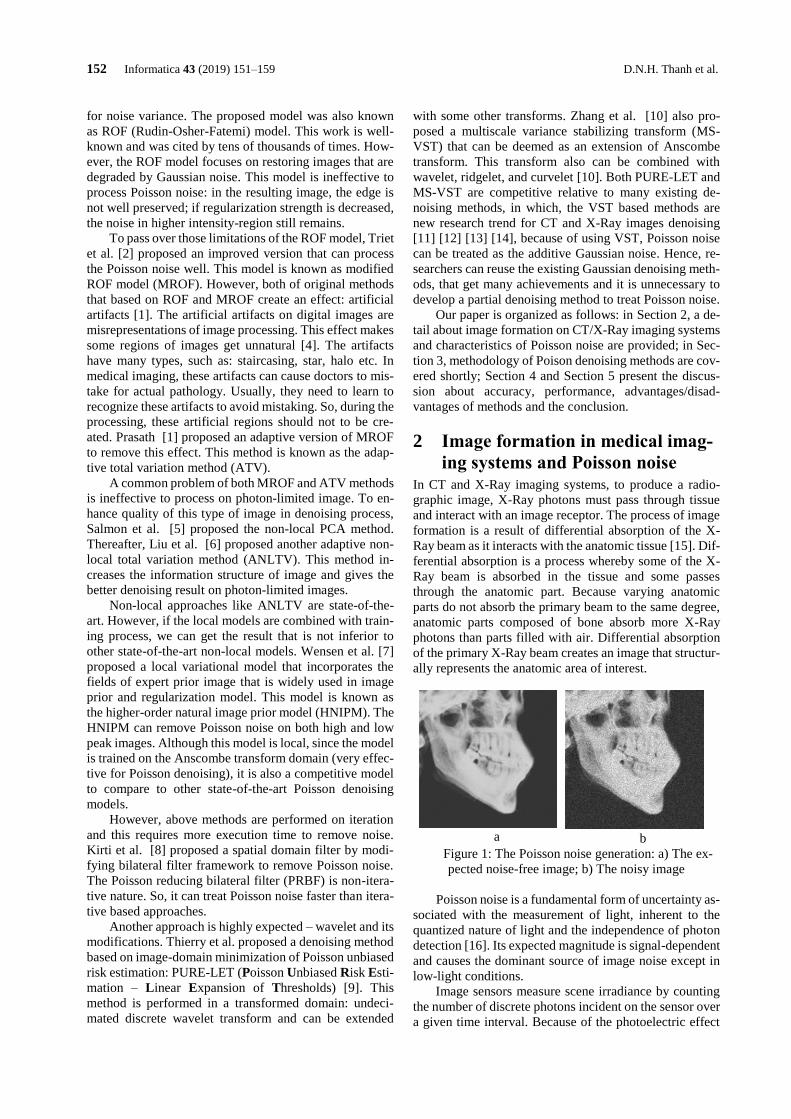
Figure 1: The Poisson noise generation: a) The ex-
pected noise-free image; b) The noisy image
Poisson noise is a fundamental form of uncertainty as-
sociated with the measurement of light, inherent to the
quantized nature of light and the independence of photon
detection [16]. Its expected magnitude is signal-dependent
and causes the dominant source of image noise except in
low-light conditions.
Image sensors measure scene irradiance by counting
the number of discrete photons incident on the sensor over
a given time interval. Because of the photoelectric effect

A Review on CT and X-Ray Images Denoising Methods Informatica 43 (2019) 151–159 153
in digital sensors, photons are converted into electrons,
whereas film-based sensors rely on photo-sensitive chem-
ical reaction. Then, the random individual photon arrival
leads to Poisson noise.
Individual photon detections can be considered as in-
dependent events that follow a random temporal distribu-
tion. The photon counting is a Poisson process, and the
number of photons 𝑘 measured by a given sensor element
over a time interval 𝑡 is described by the discrete proba-
bility distribution
𝑃(𝑘) =𝑒−𝜆𝑡(𝜆𝑡)𝑘
𝑘!,
where 𝜆 – expected number of photons per unit time inter-
val, which is proportional to the incident scene irradiance.
Since the Poisson noise is derived from the nature of
signal itself, it provides a lower bound on the uncertainty
of measuring light. Any measurement would relate to
Poisson noise, even under the ideal conditions of free-
noise sources. When Poisson noise is the only significant
source of uncertainty, as commonly occurs in bright pho-
ton-rich environments, imaging is called photon-limited
[16]. By the Poisson distribution, to reduce the Poisson
noise, need to capture more photons. This requires longer
exposures times or increasing the X-Ray intensity beam.
However, the number of photons captured in a single shot
is limited by the full well capacity of the sensor. Moreo-
ver, increasing exposures times or photon intensity beam
would be harmful for health of patients. Since this limita-
tion of technology, it is necessary to reduce the Poisson
noise by image processing algorithms.
Figure 1 simulates the Poisson noise generation on
image. We use the built-in imnoise function of MATLAB
to generate the Poisson noise on skull image [17]. The
Poisson noise in the higher intensity regions is greater than
one of the lower intensity regions.
3 Denoising methods on CT and X-
Ray images
3.1 The modified ROF model
Suppose that 𝑓 – a given grayscale image on Ω (a bounded
open subset of ℝ2, i.e. Ω ⊂ ℝ2), 𝑢 – an expected denoising
image that closely matches to observed image, 𝑥 =(𝑥1, 𝑥2) ∈ Ω – pixels.
By using total variation regularization, Triet et al. con-
vert the Poisson denoising problem to the following mini-
mization problem:
𝑢 = argmin𝑢
(∫ (𝑢 − 𝑓. 𝑙𝑛(𝑢))𝑑𝑥Ω
+𝛽 ∫ |∇𝑢|𝑑𝑥Ω
) (1)
where, 𝛽 > 0 – regularization parameter.
To solve this problem, Triet et al. used the gradient
descent method that replaces the regularization parameter
by function that is suitable to process noise on image re-
gions with both low and high intensity. This manner ex-
actly suits the signal-dependent nature of Poisson noise.
3.2 The adaptive Total variation method
The adaptive total variation method is similar with above
method. However, the second term in (1) is replaced by an
adaptive total variation:
𝑢 = argmin𝑢
(∫ (𝑢 − 𝑓. 𝑙𝑛(𝑢))𝑑𝑥Ω
+ ∫ 𝜔(𝑥)|∇𝑢|𝑑𝑥Ω
) (2)
where,
𝜔(𝑥) =1
1 + 𝑘|𝐺𝜎 ∗ ∇𝑢|,
𝐺𝜎 – the Gaussian kernel for smoothing with 𝜎 variance,
𝑘 > 0 – contrast parameter, operator ∗ is convolution.
In order avoid staircasing artifacts, Prasath [1] pro-
posed the generalized inverse gradient term incorporating
to the local statistics with patches extracted from image.
The detail about this term is presented below.
Let 𝒩𝑥,𝑟 be the local region centered at 𝑥 with radius
𝑟. Consider the local histogram of a pixel 𝑥 ∈ Ω and its
corresponding cumulative distribution function [18]:
𝐻𝑥(𝑦) =|{𝑧 ∈ 𝒩𝑥,𝑟 ∩ Ω|𝑢(𝑧) = 𝑦|}|
|𝒩𝑥,𝑟 ∩ Ω|,
𝐶𝑥(𝑦) =|{𝑧 ∈ 𝒩𝑥,𝑟 ∩ Ω|𝑢(𝑧) ≤ 𝑦|}|
|𝒩𝑥,𝑟 ∩ Ω|,
Where 0 ≤ 𝑦 ≤ 𝐿, 𝐿 – maximum possible pixel value of
the image, |∙| – the number of elements of set (cardinality).
The local histogram quantity to quantify local regions
of given image is:
𝒬(𝑥) = ∫ 𝐶𝑥(𝑦)𝑑𝑦𝐿
0
.
Finally, the adaptive weight in (2) is defined as:
𝜔(𝑥) =1
1 + 𝑘(|𝐺𝜎 ∗ ∇𝑢(𝑥)|/𝒬(𝑥))2
The alternating direction method of multipliers [1] is
provided to solve the problem (2). This iterative manner
also gives good performance.
3.3 The adaptive non-local Total Variation
method
In the case of photon-limited image, a lot of useful struc-
ture information of original image has been lost. So, the
corrupted image is close to the binary image. If we only
apply the denoising methods, such as the modified ROF
model or the adaptive total variation, the denoising result
is not really effective.
For this type of images, firstly, we need to enhance
image (improve light, contrast, etc.) and after that, per-
form the denoising process.
The method that Liu et al. [6] proposed is similar with
above idea. For first step, they enhance the image detail
by using Euler’s elastica. In second step, they remove
noise by using non-local total variation to aim to preserve
the structure information.
The Euler’s elastica-based noise image enhancement
model is proposed hereafter:
154 Informatica 43 (2019) 151–159 D.N.H. Thanh et al.
𝑢 = argmin𝑢
(∫ 𝑢 − 𝑓. 𝑙𝑛(𝑢)𝑑𝑥Ω
+𝜆 ∫ (𝑎 + 𝑏 (∇.∇𝑢
|∇𝑢|)
2
) |∇𝑢|𝑑𝑥Ω
) (3)
where 𝜆 > 0 – regularization parameter, 𝑎 > 0, 𝑏 > 0 –
weight parameters.
The Poisson denoising model based on non-local total
variation is provided as follows:
𝑈 = argmin𝑢
(∫ (𝑢 − 𝑈)2𝑑𝑥Ω
+𝛼 ∫ |∇NL𝑢|𝑑𝑥Ω
), (4)
where
∫ |∇NL𝑢|𝑑𝑥Ω
= ∫ √∫ (𝑢(𝑥) − 𝑢(𝑦))2
𝜔(𝑥, 𝑦)𝑑𝑦Ω
𝑑𝑥Ω
– is non-local total variation, 𝜔(𝑥, 𝑦) – the non-local
weight to measure the similarity of patches centered at the
pixels 𝑥 and 𝑦. The denoised version will be restored from
(4) by using an inverse Anscombe transform as bellow:
𝑢 = (𝑈
2)
2
−3
8.
The alternating direction method of multipliers is also
recommended to solve the models (3) and (4).
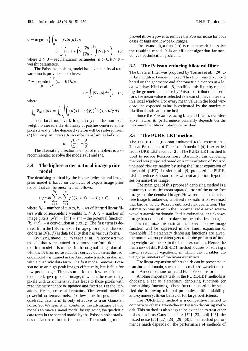
3.4 The higher-order natural image prior
model
The denoising method by the higher-order natural image
prior model is based on the fields of expert image prior
model that can be presented as follows:
argmin𝑢
∑ 𝛼𝑖 ∑ 𝜌((𝑘𝑖 ∗ 𝑢)𝑝)
𝑁
𝑝=1
𝑁𝑓
𝑖=1
+ 𝐷(𝑢, 𝑓), (5)
where 𝑁𝑓 – number of filters, 𝑘𝑖 – set of learned linear fil-
ters with corresponding weights 𝛼𝑖 > 0, 𝑁 – number of
image pixels, 𝜌(𝑧) = ln (1 + 𝑧2) – the potential function, (𝑘𝑖 ∗ 𝑢)𝑝 – a convolution at pixel 𝑝. The first term is de-
rived from the fields of expert image prior model, the sec-
ond term 𝐷(𝑢, 𝑓) is data fidelity that has various forms.
By using model (5), Wensen et al. [7] proposed two
models that were trained in various transform domains:
the first model – is trained in the original image domain
with the Poisson noise statistics derived data term; the sec-
ond model – is trained in the Anscombe transform domain
with a quadratic data term. The first model removes Pois-
son noise on high peak images effectively, but it fails for
low peak image. The reason is for the low peak image,
there are large regions of image, in which, there are many
pixels with zero intensity. This leads to those pixels with
zero intensity cannot be updated and fixed at 0 in the iter-
ations. Hence, noise still remains. The second model is
powerful to remove noise for low peak images, but the
quadratic data term is only effective to treat Gaussian
noise. So, Wensen et al. combined the advantages of two
models to make a novel model by replacing the quadratic
data term in the second model by the Poisson noise statis-
tics of data term in the first model. The resulting model
proved its own power to remove the Poisson noise for both
cases of high and low peak images.
The iPiano algorithm [19] is recommended to solve
the resulting model. It is an efficient algorithm for non-
convex optimization problems.
3.5 The Poisson reducing bilateral filter
The bilateral filter was proposed by Tomasi et al. [20] to
reduce additive Gaussian noise. This filter was developed
based on the geometric and photometric distances in a lo-
cal window. Kirti et al. [8] modified this filter by replac-
ing the geometric distance by Poisson distribution. There-
fore, the mean value is selected as mean of image intensity
in a local window. For every mean value in the local win-
dow, the expected value is estimated by the maximum
likelihood estimation method.
Since the Poisson reducing bilateral filter is non-iter-
ative nature, its performance primarily depends on the
maximum likelihood estimation method.
3.6 The PURE-LET method
The PURE-LET (Poisson Unbiased Risk Estimation –
Linear Expansion of Thresholds) method [9] is extended
from SURE-LET method [21]. The PURE-LET method is
used to reduce Poisson noise. Basically, this denoising
method was proposed based on a minimization of Poisson
unbiased risk estimation by using the linear expansion of
thresholds (LET). Luisier et al. [9] proposed the PURE-
LET to reduce Poisson noise without any priori hypothe-
ses on noise-free image.
The main goal of this proposed denoising method is a
minimization of the mean squared error of the noise-free
image and the denoised image. However, since the noise-
free image is unknown, unbiased risk estimation was used
that known as the Poisson unbiased risk estimation. This
estimation was given in the unnormalized-Haar-discrete-
wavelet-transform domain. In this estimation, an unknown
image function used to replace for the noise-free image.
To minimize this estimation, above unknow image
function will be expressed in the linear expansion of
thresholds. If elementary denoising functions are given,
the minimization problem gets to be the problem of find-
ing weight parameters in the linear expansion. Hence, the
main task of this PURE-LET method focuses on solving a
linear system of equations, in which the variables are
weight parameters of the linear expansion.
The linear expansion of thresholds can be presented in
transformed domain, such as unnormalized wavelet trans-
form, Anscombe transform and Haar-Fisz transform.
Another important task in the PURE-LET methods is
choosing a set of elementary denoising functions (or
thresholding functions). These functions need to be satis-
fied the following minimal properties: differentiability,
anti-symmetry, linear behavior for large coefficients.
The PURE-LET method is a competitive method to
compare to other state-of-the-art Poisson denoising meth-
ods. This method is also easy to be extended to treat other
noises, such as Gaussian noise [22] [23] [24] [25], the
mixed noise [26] [27] [28] [29] [30]. The method perfor-
mance much depends on the performance of methods of
A Review on CT and X-Ray Images Denoising Methods Informatica 43 (2019) 151–159 155
solving linear system of equations, for example, the
Gauss-Seidel method.
3.7 The multiscale variance stabilizing
transform method
The multiscale variance stabilizing transform method is
proposed by Zhang et al. [10] to reduce Poisson noise on
photon-limited image. This method is based on the vari-
ance stabilizing transform (VST) that is incorporated
within the multiscale framework offered by the undeci-
mated wavelet transform (UWT). This transform is used
because of its translation-invariant denoising. The de-
noising task comes to finding coefficients of the mul-
tiscale variance stabilizing transform. By using these co-
efficients, we can estimate the noise-free image.
The denoising method involves in the following steps:
transformation – computation of UWT in conjunction with
MS-VST; detection – detection of significant detail coef-
ficients by hypotheses test; estimation – reconstruction of
the final estimate by using the knowledge of the detected
coefficients. Since the signal reconstruction requires in-
verting the MS-VST-combined UWT, this reconstruction
process is formulated as a convex sparsity-promotion op-
timization problem. This optimization problem can be
solved by many iterative methods, such as the iterative hy-
brid steepest descent method.
The MS-VST method can be combined with wavelet,
as well as ridgelet (wavelet analysis in Radon domain) or
curvelet. Further, this method can also to be extended to
reduce other types of noise.
3.8 Adaptive variance stabilizing trans-
form based methods
The Poisson denoising methods by VST-based approach
is often performed by three steps: applying the variance
stabilizing transform, such as Anscombe transform; apply-
ing the denoising methods to resulting image, in which the
denoising methods are the one for additive Gaussian
noise; using inverse transformation to denoised image to
get the Poisson denoised image.
Hence, VST-based methods can use state-of-the-art
Gaussian denoising methods. By this idea, there are some
very effective methods, such as BM3D [31], SAFIR [32],
BLS-GSM [33].
For VST-based methods, the choice of inverse trans-
formation is very important. Makitalo and Foi [11] pro-
posed the optimal inverse Anscombe transform. The adap-
tive variance stabilizing transform-based method of
Makitalo et al. can be covered as follows:
Step 1: Apply the Anscombe transform to Poisson
noisy image to get asymptotically additive Gaussian noisy
image. For 𝑧 – the observed pixel values obtained through
an image acquisition device, the Anscombe transform is
𝑓(𝑧) = 2√𝑧 +3
8, 𝑧 = (𝑧1, … , 𝑧𝑁), 𝑁 − pixel numbers.
Step 2: Denoise the transformed images by additive
Gaussian denoising method.
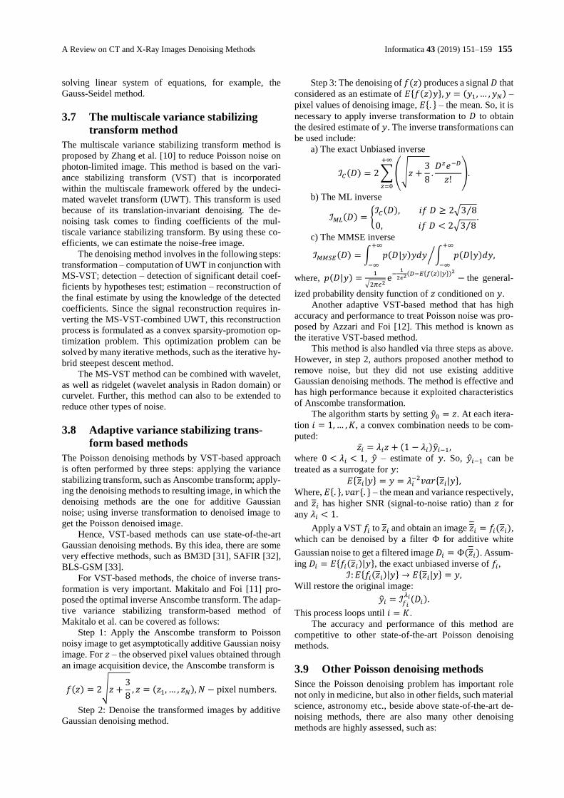
Step 3: The denoising of 𝑓(𝑧) produces a signal 𝐷 that
considered as an estimate of 𝐸{𝑓(𝑧)𝑦}, 𝑦 = (𝑦1, … , 𝑦𝑁) –
pixel values of denoising image, 𝐸{. } – the mean. So, it is
necessary to apply inverse transformation to 𝐷 to obtain
the desired estimate of 𝑦. The inverse transformations can
be used include:
a) The exact Unbiased inverse
ℐ𝐶(𝐷) = 2 ∑ (√𝑧 +3
8.𝐷𝑧𝑒−𝐷
𝑧!)
+∞
𝑧=0
.
b) The ML inverse
ℐ𝑀𝐿(𝐷) = {ℐ𝐶(𝐷), 𝑖𝑓 𝐷 ≥ 2√3 8⁄
0, 𝑖𝑓 𝐷 < 2√3 8⁄.
c) The MMSE inverse
ℐ𝑀𝑀𝑆𝐸(𝐷) = ∫ 𝑝(𝐷|𝑦)𝑦𝑑𝑦+∞
−∞
∫ 𝑝(𝐷|𝑦)𝑑𝑦+∞
−∞
⁄ ,
where, 𝑝(𝐷|𝑦) =1
√2𝜋𝜖2e
−1
2𝜖2(𝐷−𝐸{𝑓(𝑧)|𝑦})2
− the general-
ized probability density function of 𝑧 conditioned on 𝑦.
Another adaptive VST-based method that has high
accuracy and performance to treat Poisson noise was pro-
posed by Azzari and Foi [12]. This method is known as
the iterative VST-based method.
This method is also handled via three steps as above.
However, in step 2, authors proposed another method to
remove noise, but they did not use existing additive
Gaussian denoising methods. The method is effective and
has high performance because it exploited characteristics
of Anscombe transformation.
The algorithm starts by setting ��0 = 𝑧. At each itera-
tion 𝑖 = 1, … , 𝐾, a convex combination needs to be com-
puted:
𝑧�� = 𝜆𝑖𝑧 + (1 − 𝜆𝑖)��𝑖−1, where 0 < 𝜆𝑖 < 1, �� – estimate of 𝑦. So, ��𝑖−1 can be
treated as a surrogate for 𝑦:
𝐸{𝑧𝑖|𝑦} = 𝑦 = 𝜆𝑖−2𝑣𝑎𝑟{𝑧𝑖|𝑦},
Where, 𝐸{. }, 𝑣𝑎𝑟{. } – the mean and variance respectively,
and 𝑧𝑖 has higher SNR (signal-to-noise ratio) than 𝑧 for
any 𝜆𝑖 < 1.
Apply a VST 𝑓𝑖 to 𝑧𝑖 and obtain an image 𝑧𝑖 = 𝑓𝑖(𝑧𝑖),
which can be denoised by a filter Φ for additive white
Gaussian noise to get a filtered image 𝐷𝑖 = Φ(𝑧𝑖). Assum-
ing 𝐷𝑖 = 𝐸{𝑓𝑖(𝑧𝑖)|𝑦}, the exact unbiased inverse of 𝑓𝑖,
ℐ: 𝐸{𝑓𝑖(𝑧𝑖)|𝑦} → 𝐸{𝑧𝑖|𝑦} = 𝑦, Will restore the original image:
��𝑖 = ℐ𝑓𝑖
𝜆𝑖(𝐷𝑖).
This process loops until 𝑖 = 𝐾.
The accuracy and performance of this method are
competitive to other state-of-the-art Poisson denoising
methods.
3.9 Other Poisson denoising methods
Since the Poisson denoising problem has important role
not only in medicine, but also in other fields, such material
science, astronomy etc., beside above state-of-the-art de-
noising methods, there are also many other denoising
methods are highly assessed, such as:
156 Informatica 43 (2019) 151–159 D.N.H. Thanh et al.
The adaptive BLS-GSM method of Li et al. [34].
They proposed this method based on Bayesian least
squares method. Basically, this Poisson denoising method
is a term of VST-based approach.
The optimized anisotropic Poisson denoising method
of Radow et al. [35]. This method is proposed based on
variational approach and anisotropic regulariser in the
spirit of anisotropic diffusion. This method can be consid-
ered as a part of the total variation regularization.
The Poisson denoising based on greedy approach of
Dupe and Anthoine [36]. The goal of this method is com-
bination of a greedy method with Moreau-Yosida regular-
ization of the Poisson likelihood.
The Poisson reduction based on region classification
and response median filtering of Kirti et al [37]. Their con-
tribution is usage of modified Harris corner point detector
to predict noisy pixels and responsive median filtering in
spatial domain.
The primal-dual hybrid gradient algorithm [38] is a
Poisson denoising method that should be also noticed.
This method is based on total variation regularization and
primal-dual hybrid gradient. So, this method has very
good performance.
4 Discussion Firstly, we will discuss on the accuracy of Poisson de-
noising methods. The MROF, ATV, ANLTV and HNIPM
methods based on regularization, their accuracy is good
enough to perform in medical imaging systems. Since the
HNIPM method is trained on Anscombe transform do-
main, regardless of its localization, its accuracy is compet-
itive enough to other methods. If we combine the MROF,
ATV, ANLTV methods with training process to select op-
timal parameters in iterative manners, their accuracy
might be so far better than the HNIPM method, especially,
for the ANLTV method, because it does not change the
information structure of image in denoising process.
An effect that reduces the accuracy in denoising pro-
cess is artificial artifacts. Almost of local methods usually
create this effect. So, we need to perform some techniques
to avoid adding artifacts to images, such in the case of the
ATV method. For non-local methods, since the infor-
mation structure of image is preserved, the artifacts will
be seldom added. The PRBF method has the lowest accu-
racy to compare to other denoising methods, including the
PURE-LET, MS-VST and adaptive VST-based methods.
When filter noise by PRBF, the hallo artifacts will appear
in resulting images and the artifacts strength depends on
filter parameters. Although we can control these parame-
ters to reduce the hallo artifacts, it is very hard to select
optimal values. There are some methods were developed
to reduce this type of artifacts [39] [40], but it is still un-
finished, especially, on Poisson noise reduction process by
bilateral filter. For the PURE-LET, MS-VST and adaptive
VST-based methods, the accuracy might be better than lo-
cal variational based methods without training process,
particularly, for the photon-limited images. However, the
PURE-LET method is usually unstable. In our test, the de-
noising result by the PURE-LET method is slightly differ-
ent in every execution, regardless of unchangeable input
setting of parameters and configuration. When we com-
pare the MS-VST method to the PURE-LET method, the
MS-VST method has better accuracy, especially, for pho-
ton-limited images [10]. The adaptive VST-based meth-
ods have better accuracy and performance to compare to
MS-VST method [11] [12]. Both the PURE-LET and MS-
VST cause the artifacts. For the adaptive VST-based
methods, appearance of the artifacts depends on selection
of Gaussian denoising methods.
Secondly, we focus on method performance by as-
sessing the execution time. Poisson denoising methods,
such as MROF, ATV, ANLTV, PURE-LET, MS-VST and
adaptive VST-based methods are designed on iterative
manner, so their execution time is longer than one of the
PRBF method. The PRBF method is very fast and this is
proven in processing large images. Execution time of both
of PURE-LET, MS-VST and adaptive VST-based meth-
ods also depends on computation time of transforms. Oth-
erwise, for the PURE-LET method, it also depends on ex-
ecution time of solving system of linear equations, and for
the MS-VST method – depends on performance of method
to solve convex optimization problem, such as the hybrid
steepest decent method, and for adaptive VST-based
methods – depends on performance of selective Gaussian
denoising methods. For other methods: MROF, ATV,
ANLTV, HNIPM, execution time much depend on perfor-
mance of method to solve optimization problem (convex
optimization for the MROF, ATV, ANLTV methods and
nonconvex optimization for the HNIPM method). There
were some methods are recommended in their proposed
works to solve these optimization problems: the gradient
descent method, the alternating direction method of mul-
tipliers for convex optimization; iPiano for non-convex
optimization. However, for the convex optimization, we
can use other faster methods, such as: the primal-dual
modified extragradient method, the primal-dual Arrow-
Hurwitz method, the graph-cut method [41]. In work [41],
Chambolle et al. showed comparison of execution time of
above methods with the alternating direction method of
multipliers. Among of these methods, the primal-dual Ar-
row-Hurwitz method is the fastest, but proof of its conver-
gence is open problem. The primal-dual modified extra-
gradient method is certainly convergent and it is easy to
parallelize on GPU. The graph-cut method is very fast and
give exact discrete solutions, but an efficient paralleliza-
tion on GPU is still open problem. For the non-convex op-
timization, the iPiano method is state-of-the-art algorithm
and fast enough to applied in this situation. Parallelization
of the iPiano method is still open problem. Hence, the ex-
ecution time problem of all above methods can be solved
by combining with higher performance algorithms and/or
parallel processing.
Finally, about methodology, the MROF, ATV,
ANLTV and PRBF methods are simple and easy to under-
stand and easy to write program. The HNIPM is slightly
more complex and requires the training process. Both of
PURE-LET, MS-VST and adaptive VST-based methods
are the most complex. They are performed in various
transform domains. Their accuracy and performance also
depend on calculation of these transforms.
A Review on CT and X-Ray Images Denoising Methods Informatica 43 (2019) 151–159 157
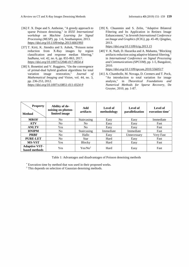
To choose suitable method for Poisson denoising in
specific cases, we need to know their advantages and dis-
advantages. These advantages and disadvantages are listed
in Table 1 in terms of denoising capabilities of the re-
viewed denoising methods here. After decades of de-
noising research there are no universal denoising method
even in the case of additive Gaussian noise. However, by
concentrating on the state of the art denoising methods
with emphasize of domain specific techniques will pave
the way for choosing an optimal denoising method. We
believe the overview of Poisson denoising methods based
on mathematically well-defined techniques studied here
can be used by researchers in developing and utilizing
these in various domains.
5 Conclusion The denoising on CT/X-Ray images is still a challenge in
medical image processing, especially, on the photon-lim-
ited images. The state-of-the-art methods cannot solve
simultaneously the following tasks: high accuracy on both
photon-limited and photon-unlimited images, avoid add-
ing artificial artifacts and the performance. The goal to de-
velop an effective universal method that reduces multiple
types of noise is even more difficult challenge.
In this paper, we reviewed on the following methods:
MROF, ATV, ANLTV, HNIPM, PRBF, PURE-LET and
MS-VST. The PRBF is excellent choice if the execution
time is the most important. However, if the accuracy is
priority, non-local methods are recommended. If we need
to process the photon-limited images, the ANLTV, MS-
VST and adaptive VST-based methods are very good
choices. If we want to exploit the existing Gaussian de-
noising methods, we can use adaptive VST-based meth-
ods, including MS-VST.
During denoising process is performed, it is necessary
to avoid adding artificial structures, and one can choose
ATV or ANLTV methods that provide good denoising
performance without introducing discernible artifacts. In
this case, the VST-based methods can be used if they are
combined to the image structure preservation Gaussian de-
noising methods, such as BM3D [31], SAFIR [32] etc.
By the research trend, the VST-based approach is a
novel option by the criteria to create an “universal”
method to remove multiple type of noises. This approach
has potential if it is possible to expand the VST-based ap-
proach to apply to other signal dependent noises.
6 References
[1] V. B. S. Prasath, "Quantum Noise Removal in X-
Ray Images with Adaptive Total Variation
Regularization," Informatica, vol. 28, no. 3, pp.
505-515, 2017.
http://dx.doi.org/10.15388/Informatica.2017.141
[2] L. Triet, C. Rick and J. A. Thomas, "A Variational
Approach to Reconstructing Images Corrupted by
Poisson Noise," Journal of Mathematical Imaging
and Vision, vol. 27, no. 3, pp. 257-263, 2007.
https://doi.org/10.1007/s10851-007-0652-y
[3] I. R. Leonid, O. Stanley and F. Emad, "Nonlinear
total variation based noise removal algorithms,"
Physica D: Nonlinear phenomena, vol. 60, no. 1-4,
pp. 259-268, 1992.
https://doi.org/10.1016/0167-2789(92)90242-F
[4] W. Zhifeng, L. Si, Z. Xueying, X. Yuesheng and K.
Andrzej, "Reducing staircasing artifacts in spect
reconstruction by an infimal convolution
regularization," Journal of Computational
Mathematics, vol. 34, no. 6, pp. 626-647, 2016.
https://doi.org/10.4208/jcm.1607-m2016-0537
[5] S. Joseph, H. Zachary, D. Charles-Alban and W.
Rebecca, "Poisson Noise Reduction with Non-local
PCA," Journal of Mathematical Imaging and
Vision, vol. 48, no. 2, pp. 279-294, 2014.
https://doi.org/10.1007/s10851-013-0435-6
[6] H. Liu, Z. Zhang, L. Xiao and Z. Wei, "Poisson
noise removal based on non-local total variation
with Euler's elastica pre-processing," Journal of
Shanghai Jiao Tong University, vol. 22, no. 5, pp.
609-614, 2017.
https://doi.org/10.1007/s12204-017-1878-5
[7] F. Wensen, Q. Hong and C. Yunjin, "Poisson noise
reduction with higher-order natural image prior
model," SIAM journal on imaging sciences, vol. 9,
no. 3, pp. 1502-1524, 2016.
https://doi.org/10.1137/16m1072930
[8] V. T. Kirti, H. D. Omkar and M. S. Ashok, "Poisson
noise reducing Bilateral filter," Procedia Computer
Science, vol. 79, pp. 861-865, 2016.
https://doi.org/10.1016/j.procs.2016.03.087
[9] F. Luisier, C. Vonesch, T. Blu and M. Unser, "Fast
Interscale Wavelet Denoising of Poisson-corrupted
Images," Signal Processing, vol. 90, pp. 415-427,
2010.
https://doi.org/10.1016/j.sigpro.2009.07.009
[10] Z. Bo, M. F. Jalal and S. Jean-Luc, "Wavelets
ridgelets and curvlets for Poisson noise removal,"
IEEE Transaction on image processing, vol. 17, no.
7, pp. 1093-1108, 2008.
https://doi.org/10.1109/tip.2008.924386
[11] M. Markku and F. Alessandro, "Optimal Inversion
of the Anscombe Transformation in Low-Count
Poisson Image Denoising," IEEE Transactions on
Image Processing, vol. 20, no. 1, pp. 99-109, 2011.
https://doi.org/10.1109/tip.2010.2056693
[12] A. Lucio and F. Alessandro, "Variance Stabilization
for Noisy+Estimate Combination in Iterative
Poisson Denoising," IEEE Signal Processing
Letters, vol. 23, no. 8, pp. 1086-1090, 2016.
https://doi.org/10.1109/lsp.2016.2580600
[13] M. Niklas, B. Peter, D. Wolfgang, M. V. Paul and
B. Y. Andrew, "Poisson noise removal from high-
resolution STEM images based on periodic block
matching," Advanced Structural and Chemical
Imaging, vol. 1, no. 3, pp. 1-19, 2015.
https://doi.org/10.1186/s40679-015-0004-8

158 Informatica 43 (2019) 151–159 D.N.H. Thanh et al.
[14] A. S. Sid, Z. Messali, F. Poyer, R. L. Lumbroso-Le,
L. Desjardins, T. C. D. Cassoux N., S. Marco and S.
Lemaitre, "Iterative Variance Stabilizing
Transformation Denoising of Spectral Domain
Optical Coherence Tomography Images Applied to
Retinoblastoma," Ophthalmic Research, vol. 59, pp.
164-169, 2018.
https://doi.org/10.1159/000486283
[15] T. L. Fauber, Radiographic Imaging and Exposure,
Missouri: Elsevier, 2017.
[16] S. W. Hasinoff, "Photon, Poisson Noise," in
Computer Vision: A Reference Guide, Boston, MA,
Springer US, 2014, pp. 608-610.
https://doi.org/10.1007/978-0-387-31439-6_482
[17] N. Veasey, "X-ray of skull showing brain and
neurons," Getty Images.
[18] V. B. S. Prasath and R. Delhibabu, "Automatic
contrast parameter estimation in anisotropic
diffusion for image restoration," in International
Conference on Analysis of Images, Social Networks
and Texts, p. 198-206, Yekaterinburg, 2014.
https://doi.org/10.1007/978-3-319-12580-0_20
[19] O. Peter, C. Yunjin, B. Thomas and P. Thomas,
"iPiano: Inertial Proximal Algorithm for Nonconvex
Optimization," SIAM Journal on Imaging Sciences,
vol. 7, no. 2, p. 1388–1419, 2014.
https://doi.org/10.1137/130942954
[20] C. Tomasi and R. Manuchi, "Bilateral filtering for
gray and color images," in Sixth International
Conference on Computer Vision, Bombay, 1998.
https://doi.org/10.1109/iccv.1998.710815
[21] B. Thierry and L. Florian, "The SURE-LET
approach to image denoising," IEEE transaction on
image processing, vol. 16, no. 11, pp. 2778-2786,
2007.
https://doi.org/10.1109/tip.2007.906002
[22] V. B. S. Prasath, D. N. H. Thanh, N. H. Hai and N.
X. Cuong, "Image Restoration With Total Variation
and Iterative Regularization Parameter Estimation,"
in Proceedings of the Eighth International
Symposium on Information and Communication
Technology, pp. 378-384, Nha Trang, 2017.
https://doi.org/10.1145/3155133.3155191
[23] V. B. S. Prasath and D. Vorotnikov, "On a System
of Adaptive Coupled PDEs for Image Restoration,"
Journal of Mathematical Imaging and Vision, vol.
48, no. 1, pp. 35-52, 2014.
https://doi.org/10.1007/s10851-012-0386-3
[24] V. B. S. Prasath and A. Singh, "A hybrid convex
variational model for image restoration," Applied
Mathematics and Computation, vol. 215, no. 10, pp.
3655-3664, 2010.
https://doi.org/10.1016/j.amc.2009.11.003
[25] V. B. S. Prasath, D. Vorotnikov, P. Rengarajan, S.
Jose, G. Seetharaman and K. Palaniappan,
"Multiscale Tikhonov-Total Variation Image
Restoration Using Spatially Varying Edge
Coherence Exponent," IEEE Transactions on Image
Processing, vol. 24, no. 12, pp. 5220 - 5235, 2015.
https://doi.org/10.1109/tip.2015.2479471
[26] D. N. H. Thanh and S. D. Dvoenko, "A method of
total variation to remove the mixed Poisson-
Gaussian noise," Pattern Recognition and Image
Analysis, vol. 26, no. 2, pp. 285-293, 2016.
https://doi.org/10.1134/s1054661816020231
[27] D. N. H. Thanh and S. D. Dvoenko, "A Mixed Noise
Removal Method Based on Total Variation,"
Informatica, vol. 26, no. 2, pp. 159-167, 2016.
[28] D. N. H. Thanh and S. D. Dvoenko, "A Variational
Method to Remove the Combination of Poisson and
Gaussian Noises," in Proceedings of the 5th
International Workshop on Image Mining. Theory
and Applications (IMTA-5-2015) in conjunction
with VISIGRAPP 2015, pp. 38-45, Berlin, 2015.
https://doi.org/10.5220/0005460900380045
[29] D. N. H. Thanh and S. D. Dvoenko, "Image noise
removal based on total variation," Computer Optics,
vol. 39, no. 4, pp. 564-571, 2015.
https://doi.org/10.18287/0134-2452-2015-39-4-
564-571
[30] D. N. H. Thanh, S. D. Dvoenko and D. V. Sang, "A
Denoising Method Based on Total Variation," in
Proceedings of the Sixth International Symposium
on Information and Communication Technology,
pp. 223-230, Hue, 2015.
https://doi.org/10.1145/2833258.2833281
[31] K. Makitalo and A. Foi, "On the inversion of the
Anscombe transformation in low-count Poisson
image denoising," in Workshop Local and Non-
Local approximation Image Processing, pp. 26-32,
Tuusula, 2009.
https://doi.org/10.1109/lnla.2009.5278406
[32] J. Boulanger, J. B. Sibarita, C. Kervrann and P.
Bouthemy, "Non-parametric regression for patch-
based fluorescence microscopy image sequence
denoising," in Fifth IEEE International symposium
on Biomedical Imaging, Paris, 2008.
https://doi.org/10.1109/isbi.2008.4541104
[33] J. Portilla, V. Strela, M. J. Wainwright and E. P.
Simoncelli, "Image denoising using scale mixtures
of Gaussian in the wavelet domain," IEEE Trans.
Image Process., vol. 12, no. 11, pp. 1338-1351,
2003.
https://doi.org/10.1109/tip.2003.818640
[34] L. Li, N. Kasabov, J. Yang, L. Yao and Z. Jia,
"Poisson Image Denoising Based on BLS-GSM
Method," in International conference on Neural
Information Processing, pp. 513-522, Istanbul,
2015.
https://doi.org/10.1007/978-3-319-26561-2_61
[35] G. Radow, M. Breub, L. Hoeltgen and T. Fischer,
"Optimised Anisotropic Poisson Denoising," in
Scandinavian conference on Image Analysis, pp.
502-514, Tromso, 2017.
https://doi.org/10.1007/978-3-319-59126-1_42
A Review on CT and X-Ray Images Denoising Methods Informatica 43 (2019) 151–159 159
[36] F. X. Dupe and S. Anthoine, "A greedy approach to
sparse Poisson denoising," in IEEE International
workshop on Machine Learning for Signal
Processing (MLSP), pp. 1-6, Southampton, 2013.
https://doi.org/10.1109/mlsp.2013.6661993
[37] T. Kirti, K. Jitendra and S. Ashok, "Poisson noise
reduction from X-Ray images by region
classification and response median filtering,"
Sadhana, vol. 42, no. 6, pp. 855-863, 2017.
https://doi.org/10.1007/s12046-017-0654-4
[38] S. Bonettini and V. Ruggiero, "On the convergence
of primal-dual hybrid gradient algorithms for total
variation image restoration," Journal of
Mathematical Imaging and Vision, vol. 44, no. 3,
pp. 236-253, 2012.
https://doi.org/10.1007/s10851-011-0324-9
[39] X. Chuanmin and S. Zelin, "Adaptive Bilateral
Filtering and Its Application in Retinex Image
Enhancement," in Seventh International Conference
on Image and Graphics (ICIG), pp. 45-49, Qingdao,
2013.
https://doi.org/10.1109/icig.2013.15
[40] V. K. Nath, D. Hazarika and A. Mahanta, "Blocking
artifacts reduction using adaptive bilateral filtering,"
in International Conference on Signal Processing
and Communications (SPCOM), pp. 1-5, Bangalore,
2010.
https://doi.org/10.1109/spcom.2010.5560517
[41] A. Chambolle, M. Novaga, D. Cremers and T. Pock,
"An introduction to total variation for image
analysis," in Theoretical Foundations and
Numerical Methods for Sparse Recovery, De
Gruyter, 2010, pp. 1-87.
Property
Method
Ability of de-
noising on photon-
limited image
Add
artifacts
Level of
methodology
Level of
parallelization
Level of
execution time*
MROF No Staircasing Easy Easy Immediate
ATV No No Easy Easy Fast
ANLTV Yes No Easy Easy Fast
HNIPM No Staircasing Immediate Immediate Fast
PRBF No Hallo Easy Unnecessary Very Fast
PURE-LET No Star Hard Easy Fast
MS-VST Yes Blocky Hard Easy Fast
Adaptive VST-
based methods Yes Yes/No† Hard Easy Fast
Table 1: Advantages and disadvantages of Poisson denoising methods
* Execution time by method that was used in their proposed works. † This depends on selection of Gaussian denoising methods.

160 Informatica 43 (2019) 151–159 D.N.H. Thanh et al.
https://doi.org/10.31449/inf.v43i2.1617 Informatica 43 (2019) 161–175 161
On the Properties of Epistemic and Temporal Epistemic Logics ofAuthentication
Sharar Ahmadi and Mehran S. FallahDepartment of Computer Engineering and Information TechnologyAmirkabir University of Technology (Tehran Polytechnic), Hafez Ave., Tehran, IranE-mail: [email protected], [email protected]
Massoud PourmahdianDepartment of Mathematics and Computer ScienceAmirKabir University of Technology (Tehran Polytechnic), Hafez Ave., Tehran, IranE-mail: [email protected]
Overview paper
Keywords: epistemic logic, temporal epistemic logic, formal verification, authentication protocol
Received: May 2, 2017
The authentication properties of a security protocol are specified based on the knowledge gained by theprincipals that exchange messages with respect to the steps of that protocol. As there are many successfulattacks on authentication protocols, different formal systems, in particular epistemic and temporal epis-temic logics, have been developed for analyzing such protocols. However, such logics may fail to detectsome attacks. To promote the specification and verification power of these logics, researchers may try toconstruct them in such a way that they preserve some properties such as soundness, completeness, beingomniscience-free, or expressiveness. The aim of this paper is to provide an overview of the epistemic andtemporal epistemic logics which are applied in the analysis of authentication protocols to find out how farthese logical properties may affect analyzing such protocols.
Povzetek: V preglednem prispevku je prestavljena epistemska in casovna epistemska logika overitvenegapostopka z namenom izboljšave delovanja.
1 Introduction
The principals communicating in a network need to be as-sured that they are sending/receiving messages to/from theintended principals as otherwise an attacker may imperson-ate an authorized principal and gain access to confidentialinformation. To prevent this, the principals use authenti-cation protocols, which are built on cryptography, for ex-changing messages [13]. Since there are many successfulattacks on authentication protocols [47, 60, 49, 35, 37, 33],different formal sytems have been developed for analyzingsuch protocols. Many of these systems are logical and areknown as logics of authentication [14, 8, 7, 36, 38].
The first formal system designated for the specificationand verification of authentication protocols is an epistemiclogic - called BAN [14]. Although BAN can safely ver-ify some protocols, it does not verify some other onessuccessfully, e.g., it proved that the Needham-SchroederPublic Key protocol (NSPK for short) was secure butlater it was shown that NSPK was vulnerable to man-in-the-middle attack [46]. To promote the verificationpower of BAN, some extensions of it have been developed[27, 3, 60, 62, 61, 17, 4]. Moreover, researchers have devel-oped some other logics of authentication that are not BAN-
like, but are inherited from standard logics. Many of theselogics are epistemic and temporal epistemic ones that canmodel different runs of a protocol or can be applied to in-vestigate the knowledge acquired by principals at differentinstants in protocol runs [16, 45, 50, 52, 8, 53]. For ex-ample, a principal may find out who originated a receivedmessage at specific step of a protocol run and may agreewith the sender on the received information.
There are also dynamic epistemic logics that are usefulfor modeling knowledge protocols, which model higher-order information and uncertainties in terms of agents’knowledge about each other. However, since these logicsare inconvenient in a cryptographic setting for generatingequivalence relations among messages, we do not considerthem in this paper [21].
Although the proposed epistemic and temporal epistemiclogics have significantly improved the analysis of authen-tication protocols, every now and then a problem is foundand we need to improve the logics to solve that problem.For example, an attack may be detected by an omniscience-free logic while it is ignored by another logic that is notomniscience-free. Similarly, an authentication protocol canbe specified by a temporal epistemic logic while it can-not be specified by a logic whose modalities are only epis-
162 Informatica 43 (2019) 161–175 S. Ahmadi et al.
temic ones. Such issues encourage researchers to find outif logics of authentication should preserve specific logicalproperties. The properties that are usually discussed in thiscontext are soundness, completeness, expressiveness, andbeing omniscience-free. Moreover, since a powerful at-tacker is traditionally modeled as the well-known Dolev-Yao message deduction system [24], it is valuable to seeif these logics can model such a system. In this way, ifa logic of authentication proves a security goal about anauthentication protocol, one can trust that the result is in-deed valid in the presence of a powerful attacker who caneavesdrop all communications, drop, manipulate and re-play messages, and perform cryptographic operations usinghis known keys and messages.
The aim of this paper is not to compare epistemic log-ics of authentication to alternative security protocol analy-sis, such as applied pi calculus and other process calculi,strands, multiset and other forms of rewriting. The aim ofthis paper is to provide an overview of the epistemic andtemporal epistemic logics of authentication to find out howfar some of their logical properties such as soundness, com-pleteness, being omniscience-free, and expressiveness mayaffect analyzing authentication protocols. To do so, we dis-cuss not only the conditions under which these logics sup-port the Dolev-Yao message deduction, but also the logicalproperties that encourage us to trust the derived judgementsabout the authentication protocols.
The rest of the paper is as follows: In Section 2, we pro-vide an overview of the notions of cryptography, Kripkesemantics, and epistemic logics of authentication. In Sec-tion 3, we compare epistemic and temporal epistemic log-ics of authentication and show how far some of their logicalproperties may affect them in analyzing authentication pro-tocols. Section 4 concludes the paper.
2 Basic notions
Authentication protocols are rules built on cryptographicprimitives that help principals authenticate each other whilecommunicating in a hostile environment [13]. An authen-tication goal can be expressed in terms of a knowledge no-tion, e.g., the sender authentication can be read as “the re-ceiver knows the sender of a received message”. Considerthe NSPK protocol shown in Figure 1. Every principal inthis protocol has a public key and a private key such thatthe public key of any principal A is known to everyone butonly A has the corresponding private key.
In this protocol, principal A generates a nonce na, pairsna with its name A, encrypts na.A with principal B’spublic-key pk(B) so that only B can decrypt it by his pri-vate key, and sends {na.A}pk(B) to B. By receiving thismessage, B decrypts it and sends na back along with hisnonce nb in an encrypted message so that only A can de-crypt it. Then, A sends nb back to B. The goal of theNSPK protocol is that both A and B can be assured thatthey are talking to each other and not to an attacker. BAN
logic proved that the NSPK protocol was safe [14], whereasLowe showed that it was vulnerable to the man-in-the-middle attack [46]. Although such a result seems confus-ing, it is suggested by the well-known fact that the NSPKprotocol is safe assuming that no compliant initiator willever select a non-compliant responder for a session. Need-ham and Schroeder assumed this fact about the principals.However, it was certainly no longer a reasonable assump-tion when cryptographic protocols were beginning to beused on the open internet and Lowe outlined the man-in-the-middle attack.
The man-in-the-middle attack, shown in Figure. 1, con-sists of two interleaved sessions of the NSPK protocol. Af-ter A initiates a protocol run with I , the intruder I extractsthe message, impersonates A, and sends na to B. When Breplies, I forwards this message to A and misuses A to ob-tain nb. Then, I sends nb back toB. Thus,B is deceived tobelieve that he is talking to A while he is in fact communi-cating with I . This attack shows that the result of analyzingthe NSPK protocol using BAN logic is questionable. Sincethe original BAN did not have formal semantics, findingsuch a semantics that could model the above attack becamean important topic of research.
As said earlier, the formal analysis of an authenticationprotocol using epistemic logics depends on the knowledgegained by the principals executing that protocol. There aretwo main ways to formalize such knowledge. Assume thestatement: “B has sentm”, where the underlying semanticsof a logic of authentication interprets this statement as fol-lows: “B is engaging in an event of a protocol sending mes-sage m”. If we formalize this statement with a logical for-mula φ, A knows φ means: “A knows that B has sent m".This is called propositional knowledge which is implicitand does not care about the details of computation [58].There is also algorithmic knowledge formalizing the exactmodels of principals’ knowledge such that if a principalhas some bit strings, he can apply cryptographic operatorsto compute more strings using some predefined algorithms[30]. In this paper, we consider both of these knowledgeformalizations, but first we need to explain some primitivenotions.
Assume that θ is a set of principals exchanging messagesby executing an authentication protocol. We may use a log-ical language L to specify not only the steps of such a pro-tocol, but also the intended authentication properties thatwe want to prove about that protocol. To do so, we need toformalize exchanged messages as message terms in L be-cause protocols are a type of messages passing multi-agentsystems [26]. A message may be a plain term c or a com-pound one constructed by encryption or pairing such that{m}k is the encryption of message m with the key k andm.m′ is the pairing of messagesm andm′. There is a needfor a derivation system to derive new messages from knownones using cryptographic functions. In this paper, we usethe well-known Dolev-Yao message deduction system [24]as follows: m.m′ is a message if and only if bothm andm′
are messages. If {m}k and k are messages, then so is m.

On the Properties of Epistemic. . . Informatica 43 (2019) 161–175 163
Figure 1: NSPK protocol and the man-in-the-middle attack
Finally, if m and k are messages, then so is {m}k. Given aset of message terms τ and a finite set of Dolev-Yao mes-sage deduction rules σ, we say that m is derivable from τif either m ∈ τ or m is derivable from τ by applying therules in σ. Assuming a set of message terms τ , there aretwo interpretations for knowledge.
The first interpretation says that a principal i knows aformula φ if he is aware of φ and φ is true in all the worldshe considers possible. In this case, a set of formulas, de-noted by Ai(w), is associated to every possible world wsuch that i is aware of every formula in Ai(w) [31]. Theintuition behind such an interpretation is that a principalneeds to be aware of a formula before he can know it. Forinstance, a principal i may be aware of an encrypted mes-sage {m}k that he receives without being aware of messagem. In this way, i may know that he receives {m}k if thismessage holds in all the worlds that are possible to himwhile he may not know that he receives m. In the contextof verifying security protocols, Ai(w) is implemented asan algorithm that says "YES" for the formulas that agent iis aware of in his local state in w. In this way, we say that iknows φ explicitly using algorithmic knowledge [45].
The second interpretation says that a principal i knows aformula φ implicitly, shown by an epistemic formula Kiφ,if i knows that φ is true. The set F of L-formulas then,comprises not only atomic formulas about sending or re-ceiving messages, but also compound formulas built induc-tively as follows: For every φ, ψ ∈ F , i ∈ θ, and m ∈ τ ,we have φ ∧ ψ, ¬φ, Ki φ, and Aiφ are in F .
The authentication protocols and goals formalized byformulas in F need to be interpreted in a proper formalsemantics. Since an authentication protocol can be seenas a multi-agent system and it is known that an interpretedsystem 1 (IS for short) is a standard semantics for a multi-
1Assume that θ = {i1, . . . , in, e} is a set of principals such that “e”denotes a specific principal called the environment. For each i ∈ θ, thereis a finite set Li of local states, a finite set ai of local actions, and alocal protocol pi : Li → 2ai . The transition relation ti : Li × a1 ×. . . × an → Li is then defined to return the next local state of i afterall the principals perform their actions at the local state. Consider a setof global states G ⊆ L1 × . . . Ln × Le, a set of joint actions a =a1 × . . .× an × ae, a joint protocol p :
(p1, . . . , pn, pe), and a global
transition relation t = (t1, . . . , tn, te), which operates on global statesby composing all local and environmental transition relations. An IS isthen a tuple
(G, I0, t, {∼i}i∈A, π
), whereG is the set of all global states
accessible from any initial global state in I0 via the transition relation t.For each i ∈ θ, there is an accessibility relation ∼i⊆ G × G such that
agent system, authentication protocols can be modeled byinterpreted systems too. This can build a foundation forconstructing Kripke semantics for epistemic logics of au-thentication as follows [26].
A Kripke model of an epistemic logic of authenticationcan reflect an authentication protocol. Such a model has aset of possible worlds that can be defined as W = R × N,where R is the set of all runs of that protocol and N is theset of natural numbers. Thus, a pair 〈r, n〉 - called a point- represents a run r at a time instant t. Such a point can beassociated to a set of formulas that hold (are true) in thatpoint. A Kripke model is then a tuple of the form M =(W, {∼i}i∈A, π
)where W is the set of all possible points
of the protocol. Moreover, the accessibility relation ∼i canbe interpreted in different ways.
In one interpretation, for every w1, w2 ∈ W , w1 ∼i w2
holds if and only if the local states of a principal i are thesame in w1 and w2. For example, the local states of Bat the end of both runs of the NSPK protocol shown inFigure. 1 are the same because B sends and receives thesame messages by completing the execution of these tworuns. In another interpretation, for every w1, w2 ∈ W ,w1 ∼i w2 holds if and only if the local states of a princi-pal i are indistinguishable in w1 and w2. For example, as-sume that there is a protocol P such that w1 = 〈r1, t1〉 andw2 = 〈r2, t2〉 are two possible worlds of a Kripke modelthat reflects P. Principals A and B participate in two runsof P, denoted by r1 and r2, and formulas A sends {m}Kand A sends {m′}k′ hold in w1 and w2, respectively. As-sume that B does not know the proper decryption keys todecrypt these messages, so he cannot distinguish formu-las A sends {m}K and A sends {m′}k′ because he sees{m}k and {m′}k′ as two random messages. In this way,he considers both of the formulas the same. If all of theother formulas that hold in w1 and w2 are equal, B cannotdistinguish between w1 and w2 even if {m}k 6= {m′}k′ ,i.e., we have: w1 ∼B w2
2. In this model, Ki φ is trueat w ∈ W if φ is true at every w′ ∈ W that is accessiblefrom w in A’s view. Moreover, Aiφ is true in w ∈ W if φcan be computed by an awareness algorithmAi in w. Such
g ∼i g′ if and only if li(g) = li(g
′), where li : G → Li(g) returns i’slocal state in the global state g, and π : G× Atom→ {true, false} isan interpretation function [26].
2There are also some other interpretations for the accessibility relation.We refer the interested reader to Ref. [17, 8].
164 Informatica 43 (2019) 161–175 S. Ahmadi et al.
an algorithm is defined specifically for every protocol andfor computing intended formulas [30]. The truth of othernon-atomic formulas is defined in a standard way and theatomic formulas are interpreted by the interpretation func-tion π [15].
Assume thatM =(W, {∼i}i∈A, π
)is a Kripke model
that models a protocol P, and AuthR is an authenticationrequirement formalized by a logical formula φ. We saythat φ is satisfiable with respect toM when there is a w ∈W such that φ is true in w, i.e., AuthR holds in a runof P that is associated to w. We say that φ is valid withrespect toM if φ is true in every w ∈W i.e. AuthR holdsin all runs of P. We discuss authentication and formalizingauthentication in more detail below.
2.1 Formalizing authentication
Most of the security protocols have been designated for at-taining authentication i.e. one principal should be assuredof the identity of another principal. A protocol designermay assign different roles such as initiator, responder, orserver to principals. Authentication protocols can be clas-sified into two categories with respect to these roles: theprotocols that try to authenticate a responder B to an initia-tor A, and the protocols that try to authenticate an initiatorA to a responder B.
The notion of authentication does not have a clear con-sensus definition in the academic literature. However, themost clear and hierarchical definition for authentication hasbeen devised by Lowe. In this definition, authenticationrequirements depend on the use to which the security pro-tocol is put. These requirements can then be classified asaliveness, weak agreement, non-injective agreement, andagreement [46]. A protocol guarantees to a principal A“aliveness” of another principal B if the following condi-tion holds: whenever the initiator A completes a run of theprotocol, apparently with the responder B, then B has pre-viously been running the protocol. Aliveness can be ex-tended to “weak agreement” if B has previously been run-ning the protocol with A. “Weak agreement" can be ex-tended to non-injective agreement on a set of data items(where V is a set of free variables of the protocol) if B haspreviously been running the protocol with A, B was actingas responder in his run, and the two principals agreed onthe values of all the variables in V . Weak agreement canbe extended to “agreement" if each such a run of A corre-sponds to a unique run of B [46].
There are many attacks that occur due to parallel runs ofa protocol [47]. The definition of weak agreement for au-thentication guarantees a one to one relationship betweenthe runs of two principals as follows: a protocol authen-ticates a responder to an initiator, whenever a principal Astarts j runs of the protocol as an initiator and l runs as aresponder all in parallel; and completes k ≤ j runs of theprotocol acting as initiator apparently with a responder B,then B has recently been running k runs acting as respon-der in parallel, apparently with A. Moreover, A protocol
authenticates an initiator to a responder, whenever a princi-pal B starts j runs of the protocol as a responder and l runsas an initiator, all in parallel; and completes k ≤ j runs ofthe protocol acting as responder, apparently with initiatorA, then A has recently been running k runs acting as ini-tiator in parallel, apparently with B [59]. In the followingexample, we explain the definition of agreement in moredetail.
Example 2.1. Consider the following challenge-responseprotocol that aims to authenticate an initiator A to aresponder B, and to authenticate a responder B to aninitiator A. In this protocol, kab is a shared key between Aand B. Moreover, na and nb are two nonces generated byA and B, respectively.
A→ B : naB → A : {na}kab
.nbA→ B : {nb}kab
There is the following reflection attack on the protocolthat consists of two sessions of the protocol executed inparallel. In this attack, B has the responder role and I(A)denotes an intruder who impersonates A:
1. I(A)→ B : na2. B → I(A) : {na}kab
.nb1′. I(A)→ B : nb2′. B → I(A) : {nb}kab
.n′b3. I(A)→ B : {nb}kab
B starts two runs of the protocol as a responder to A,but it completes only one run (lines: 1, 2, and 3) with I(A)while A does not participate in these runs. So, the protocolfails to aim the agreement requirement.
In the next example, we show how we can formalize anauthentication requirement.
Example 2.2. Consider the NSPK protocol, shown in Fig-ure 1. We want to formalize the non-injective agreementauthentication requirement. To do so, we use epistemicmodalities as follows:
KB KA msg na.nb
This formula can be read as follows: “B knows that Aknows the message na.nb". If this formula can be provenfor the NSPK protocol, then we say that the protocol guar-antees “non-injective agreement” toB, where {na.nb} ap-pears as the set of data items that the two principals agreeon their value. Since B encrypts nb with A’s public-keyand sends {na.nb}pk(A) to A, whenever B receives a mes-sage containing nb, he concludes that A has previouslybeen running the protocol with B because A is the onlyprincipal who has A’s private key to decrypt {na.nb}pk(A)
in order to extract nb. The man-in-the-middle attack de-ceives B to believe that he is talking to A while he is infact talking to I , who is an intruder. All BAN-like logics
On the Properties of Epistemic. . . Informatica 43 (2019) 161–175 165
proved the above formula for the NSPK protocol, whereasan omniscience-free epistemic BAN-like logic, that is re-ferred to WS5 throughout this paper, could identify this in-sider attack [17]. In fact, being omniscience-free enabledWS5 to model the Dolev-Yao message deduction properly.We will explain this logic in detail at next sections.
3 Logical properties
In this section, we investigate how far some properties ofepistemic and temporal epistemic logics of authenticationmay affect the analysis of authentication protocols. Theproperties that we investigate are soundness, completeness,being omniscience-free, and expressiveness.
3.1 Soundness and completeness
Beside syntax and semantics, every logic may have a proofsystem X consisting of some axioms and rules where theaxioms are valid with respect to the logic’s semantics andthe rules preserve validity i.e. if the premise of a rule isvalid, the result of it is also valid. Let X be a proof systemof a logic of authentication that is based on the Dolev-Yaodeduction system. Moreover, let the following statement bean authentication property: “principals i and j know thatthey are talking to each other”, where i and j are engagingonly in one session and both peers has received certain mes-sages as common knowledge to authenticate each other. Inthis case, proving φ in X means that i and j know that theyare indeed talking to each other even in an environmentwhere there are attackers who can derive messages due tothe Dolev-Yao deduction system.
The proof system X may have some interesting proper-ties, two of which are soundness and completeness: X issound if every derivable formula φ in X is also valid. X iscomplete if every valid formula φ is provable in X . This isalso called “weak completeness” by some researchers [15].Logical analysis of security protocols relies on formal mod-els of cryptography where cryptographic operations and se-curity properties are defined as formal expressions. Suchmodels ignore the details of encryption and focus on anabstract high-level specification and analysis of a system[1, 14, 24, 28].
Proving the soundness and completeness of a logic of au-thentication gives a strong intuition that the formal seman-tics of that logic is defined properly and it is working asexpected. So, the logic can be applied safely in analyzingauthentication protocols. For formal verification of a secu-rity protocol, there is a need for a formal model to reflectthat protocol appropriately i.e. there is a need for a soundformal model for that protocol. Using a logical model, theverification is then dependent on the following parameters:first, the protocol must be described in the language of thelogic. This description will be a part of a trust theory whichconsists of correct and acceptable propositions used in de-ducing security requirements. Even with a bad description
of a protocol and its initial assumptions, the logic shouldconsider all possible runs of that protocol.
To discuss the second parameter for defining a sound for-mal model, we first provide an overview of the Dolev-Yaoindistinguishability relation. The intuitive idea for defin-ing this relation is the fact that two messages are indis-tinguishable if any test - based on a limited set of opera-tions on messages - gives the same result about the config-uration of those messages. The Dolev-Yao indistinguisha-bility relation can be related to cryptographic computingmodels. In this case, a formal model is said to be com-putationally sound. This is expressed for static equiva-lence, which is a general form of indistinguishability, ex-plicitly: two local states are static equivalents if they sat-isfy the same equivalence tests. For a given theory ofequation, static equivalence is based on a computable ef-ficient set of operations such as symmetric and asymmet-ric encryption and decryption. For example, consider thesimplest equivalence theory satisfying an equation of theform dec(enc(m, pk), pr) = m, where pk, pr, and m area public key, a private key, and a message, respectively.Moreover, enc is an asymmetric encryption operator thatencrypts m with pk and dec is an asymmetric decryptionoperator that decrypts an encrypted message with pr [2].
There is also another parameter for defining a sound for-mal model. Assume that there is a specification of an au-thentication protocol P and some initial assumptions usinga logic of authentication L. We need to show whatever isdeduced in L about P should be consistent with what theprincipals involved in executions of P actually infer. As-sume that Γ is a finite set of logical formulas including thespecification of P and its initial assumptions. Moreover,assume that the desired security goal is formalized by aformula φ that can be proven by applying the formuals in Γand the axioms and rules of L’s proof system. If L is log-ically sound andM is its model that satisfies the formulasin Γ, M also satisfies φ. If we show that M considersall possible runs of P , including those that attackers mayparticipate in, the model reflects P properly.
As said earlier, the other theorem that is usually inves-tigated for every logic is completeness. All valid formu-las of a complete logic are also provable in its proof sys-tem. This motivates researchers to provide provers for theanalysis of security protocols [22, 52, 51, 29]. If such alogic is also sound, the derived statements are more trustedsince completeness shows that the formal semantics workas expected. Completeness may be a result of another prop-erty. As an example, the completeness of BAN-like logicshas been an open problem for many years because someof them do not have any formal semantics and some otherones have inaccurate formal semantics. So, the logics couldnot model some possible runs executed by a Dolev-Yao at-tacker. However, it has been shown that the completenessof BAN-like logics can be proven by presenting a formalsemantics that avoids logical omniscience [18]. We willdiscuss logical omniscience in more details later.
There is also another line of research that proves com-
166 Informatica 43 (2019) 161–175 S. Ahmadi et al.
pleteness for monadic fragments of a first-order temporalepistemic logic with respect to their corresponding classesof quantified interpreted systems. Such systems may havethe following typical properties: synchronicity, perfect re-call, no learning, and unique initial state. In contrast tomost of the logics of authentication, such a logic has someaxioms and rules that explore the relationship between itstime and knowledge modalities [5, 6].
3.2 Logical omniscienceThe semantics of a logic of authentication can be definedbased on the standard Kripke structure. Such a semanticsmay lead to the logical omniscience problem where princi-pals know all logical truths i.e. they know all consequencesof what they know [31]. In fact, the problem bypasses thelimitations placed on the knowledge of a principal who re-ceives an encrypted message but does not have the rightkey to decrypt that message. Assume that L is an epistemiclogic of authentication, which has a formal semantics builton the standard Kripke structure, and Γ is a set of logicalformulas in L. Moreover, assume that a formula φ can bederived from Γ in L’s proof system and an agent i knowsall of the formulas in Γ. Then, the formal semantics of Lleads to the logical omniscience where i knows φ. This factis an immediate result of the interpretation of the knowl-edge modality of L with respect to the underlying standardKripke semantics. In this way, a formula Kiφ is true in astate (possible world)w if and only if φ is true in every statethat is indistinguishable (accessible) from w in i’s view.
For example, assume that the following formula is truein all possible runs of a protocol,
i sent msg {m}k → submsg(m)
where submsg(m) is read as m is a sub-message i.e. m isa sub-message of {m}k. Using the standard Kripke seman-tics and for every principal j, the following formula is alsotrue in all runs of that protocol:
Kj i sent msg {m}k → Kj submsg(m)
Now, assume that the anonymity of i fails and the formulaKj i sent msg {m}k is valid. Therefore, Kj submsg(m)can be deduced by applying modus ponens. But in fact,this judgment is true only if j knows the symmetric keyk to decrypt {m}k. Thus, logical omniscience should beavoided in order to restrict principals’ knowledge to whatthey can compute from their known facts, messages, andkeys.
There are different approaches for solving the logicalomniscience problem in the analysis of security protocols.In Ref. [19], the problem is solved by presenting a gen-eralized Kripke semantics based on a permutation-basedIS. Such a semantics results in a weakened necessitationrule for a logic faithful to BAN. Hence the logic becomesan omniscience-free weakened S5. Such a logic formal-izes an implicit form of knowledge that results in abstracthigh-level reasoning of security protocols [17]. The logical
omniscience problem can also be avoided by exact mod-els of knowledge that a principal acquires during protocolruns. For example, such models are applied by a logic -called TDL [45]. So, a part of the logic that links epistemicmodalities to awareness algorithms becomes omniscience-free. In this way, a principal knows a fact if he is aware ofthat fact. The idea of using awareness algorithms in formalsecurity was originated in Ref. [30]. We will talk about thelogics that use such algorithms at the end of this section.
3.3 Expressiveness
Epistemic logics of authentication usually have three dif-ferent operators besides the standard ones of propositionallogics. These operators are temporal, epistemic, and aware-ness. Hybrid systems may also have some other operatorssuch as type operators or algebraic operators, but we do notconsider hybrid systems in this paper and refer the inter-ested reader to Ref. [39]. Temporal modalities formalizeprecedence of actions, time intervals, etc., such as “next”and “in a time interval [t1, t2]". Epistemic modalities for-malize the knowledge of principals. Awareness operatorsshow the algorithms that principals use to become aware offacts. The expressiveness of epistemic logics of authentica-tion relies on their logical order and modalities. Moreover,if a logic has temporal operators, its expressiveness also re-lies on the method that the epistemic core is augmented bytemporal modalities.
There are three approaches for adding temporal modali-ties to an epistemic core of a logic of authentication. Thefirst approach, which makes the resulting temporal epis-temic logic very expressive, is the fusion approach whereepistemic and temporal modalities may appear in eachother’s scope without any restrictions. Moreover, the re-sulting logic may have axioms and rules that explore inter-actions between time and knowledge [5, 8, 23, 4]. Thisapproach has been used in developing logics applied inanalyzing a wide range of security protocols. Two ex-amples of these protocols are classical authentication pro-tocols such as NSPK and stream authentication protocolssuch as TESLA [57], which is used for sending streams ofmessages: videos, audios, etc.
The second approach is to use fibring technique wheretemporal and epistemic modalities may appear in eachother’s scope without any restrictions. But, the time andknowledge dimensions of a fibred logic are orthogonal. So,such a logic has no axioms and rules to explore the rela-tionship between time and knowledge. Fibring techniquedoes not model the knowledge which is obtained as a con-sequence of a particular event. Thus, a fibred logic is lessintuitive for modeling security protocols and less expres-sive in comparison with other logics built on the fusion ap-proach. However, theorems such as soundness and com-pleteness may be easily proven for a fibred logic if its con-stituent logics are sound and complete. Moreover, a provercan be easily constructed for a fibred logic if its constituentlogics have provers. Such a logic has been developed for
On the Properties of Epistemic. . . Informatica 43 (2019) 161–175 167
the analysis of the TESLA protocol [56].Finally, the last approach for adding temporal modalities
to an epistemic core of a logic of authentication is using thetemporalization technique. This technique operates in a hi-erarchical way such that the temporal modalities can neverappear in the scope of epistemic modalities i.e. the result-ing logic does not have any formula of the form Ki © φ,which can be read as follows: agent i knows that at thenext step φ holds. This approach has been used for verify-ing different protocols such as TESLA and WMF [53, 52].
In Figure 2, we compare some important epistemic andtemporal epistemic logics of authentication against theabove properties where every row of the figure is dedicatedto a specific logic. The 1st column of each row showsthe logic name. The 2nd column shows if the logic or-der is “propositional” or “first-order”, denoted by “PR” and“FO”, respectively. The 3rd column shows the type of op-erators used in the logic where “E”, “A”, and “T” denote“epistemic”, “awareness”, and “temporal”, in order. The4th column shows if the logic has a proof system, modelchecker, tableau . . .. The 5–7th columns show if the logicis sound, complete, or omniscience-free, respectively. If alogic is sound, complete, or omniscience-free, we show thisby a “X” symbol. If any of these properties does not hold,we show this by a “×” symbol. If a logic does not have aproof system, it has no soundness and completeness theo-rems. In this case, we use a “−” symbol. Finally in the lastcolumn, “EXP ” denotes that the explicit part of the logicis omniscience-free. Some of the security protocols ana-lyzed by these logics are shown in Figure 3. The attackermodels of these logics are also summarized in Figure 4.In what follows, we explain the above logical properties inmore detail.
3.4 Inside the logics
In 1989 BAN logic was proposed as the first formal sys-tem for the specification and verification of authenticationprotocols [14]. This is a simple intuitive propositional epis-temic logic named after its developers Burrows, Abadi, andNeedham. The syntax of BAN consists of inference rulesabout principals’ beliefs and their actions. This syntax en-ables BAN not only to specify the steps of an authentica-tion protocol and its security goals, but also to derive theintended goals about that protocol. The first step of ap-plying BAN is to idealize a protocol into an abstraction. Inthe second step, one should translate the initial assumptionsand the security goals into BAN language, relate each ide-alized step of the protocol to a BAN formula, and then useBAN inference rules to derive intended goals.
The soundness and completeness theorems cannot beproven for BAN because it has no formal semantics. Thislogic has only epistemic modalities and it is not expressiveenough to specify or verify highly time-dependent proto-cols such as stream authentication protocols [29]. This,along with BAN’s propositional order, results in its lowspecification power. BAN has no formal attacker model
but the capabilities of attackers are somehow embedded inits proof system.
For example, BAN has a rule - called the message-meaning rule - which has two premises. Assume thatP and Q are two agents, m is a message, k is a key,and {m}k denotes that m is encrypted with k. The firstpremise of this rule says that P believes that k is a sharedkey between P and Q. This is formalized as follows:P Believes P ↔k Q. The second premise says that some-one has sent a message which contains {m}k to P . This isshown as follows: P sees {m}k. The conclusion of thisrule is that P believes that at some time Q sent a messagewhich contains m. This is formalized by the following for-mula: P Believes Q said {m}k. As k is a shared keybetween P and Q, only these two agents can use k to en-crypt m and no other agent can create {m}k. Thus, whenP receives {m}k it concludes that at some time Q has senta message which contains {m}k. In this way, even if anattacker has sent a message containing {m}k to P , P be-lieves that this message has not been originated by Q [14].As an example of formalizing authentication in BAN, wesay that authentication is complete for the NSPK protocolif there are nonces na and nb, generated by A and B, re-spectively, such that the following statements hold:
A Believes A↔na.nb BB Believes A↔na.nb B.
The above formalizations can be classified as non-injective agreement. However, other weaker formalizationscan be presented too.
As said earlier, BAN has some problems while verify-ing authentication protocols. Many extensions of this logichave been developed to resolve its problems. One of theseextensions is GNY developed in 1990 for verifying a widerrange of authentication protocols. GNY emphasizes sepa-rating the content and meaning of messages while it followsthe same method as BAN for formalizing authentication.This logic is named after its developers Gong, Needham,and Yahalom. Although GNY can be applied in verifyinga sample voting protocol successfully, the logic still suf-fers the same problems as its predecessor. Neither BANnor GNY preserves the properties discussed in Subsections3.1, 3.2, and 3.3. Thus, their derivations are not trustwor-thy. Moreover, these logics cannot analyze highly time-dependent protocols such as the TESLA protocol.
The first attempt for developing a formal semantics forBAN was in 1991 when Abadi and Tuttle improved the syn-tax and inference rules of BAN and also presented a formalsemantics - called AT - for BAN [3]. This semantics isbased on the standard Kripke structure constructed frominterpreted systems. In this model, a principal i knows aformula φ if we have: “i knows φ” is true at a point 〈r, k〉if it is true in every point 〈r′, k′〉 that is indistinguishablefrom 〈r, k〉 in i’s view. This extension of BAN - called ATlogic - is sound with respect to the AT semantics. Thus,the proofs in this logic are more trustworthy. However, thecompleteness of AT remained an open problem for years
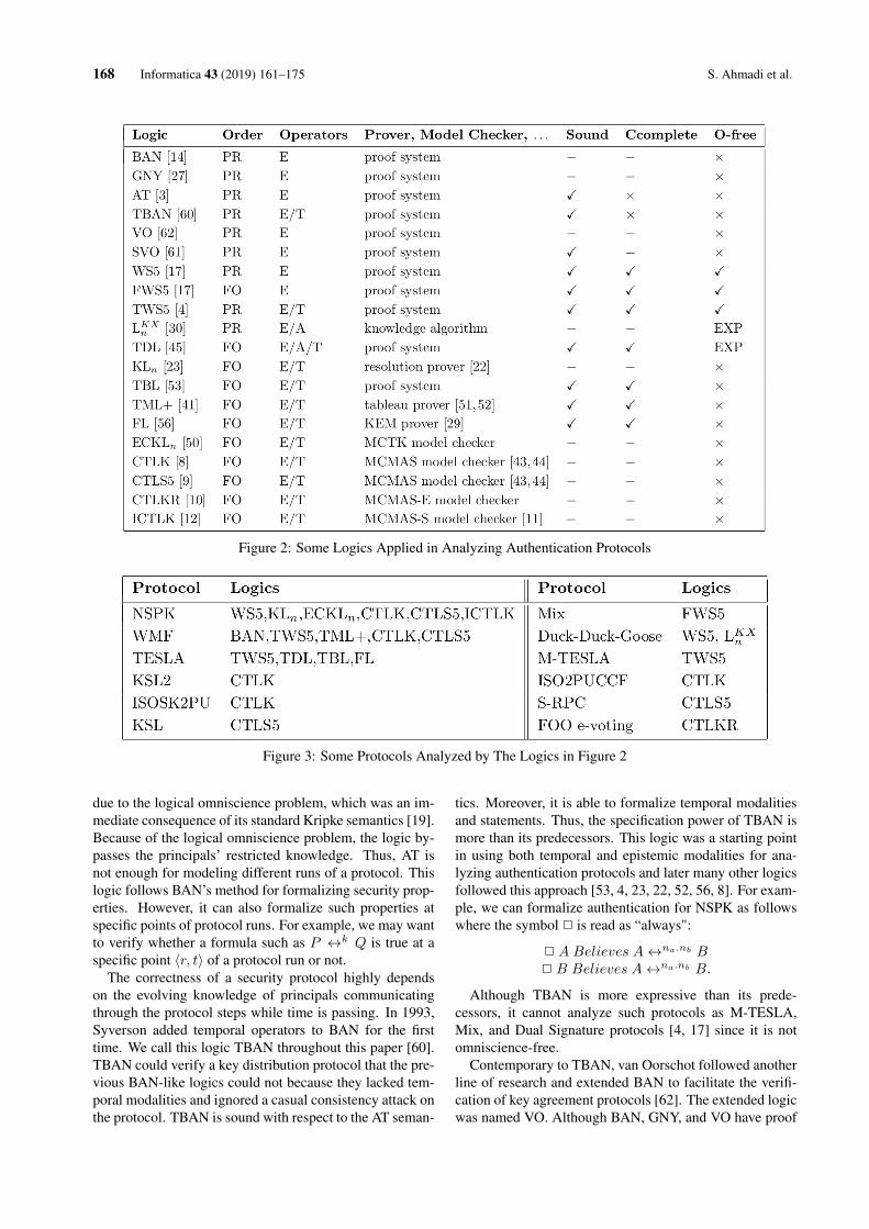
168 Informatica 43 (2019) 161–175 S. Ahmadi et al.
Figure 2: Some Logics Applied in Analyzing Authentication Protocols
Figure 3: Some Protocols Analyzed by The Logics in Figure 2
due to the logical omniscience problem, which was an im-mediate consequence of its standard Kripke semantics [19].Because of the logical omniscience problem, the logic by-passes the principals’ restricted knowledge. Thus, AT isnot enough for modeling different runs of a protocol. Thislogic follows BAN’s method for formalizing security prop-erties. However, it can also formalize such properties atspecific points of protocol runs. For example, we may wantto verify whether a formula such as P ↔k Q is true at aspecific point 〈r, t〉 of a protocol run or not.
The correctness of a security protocol highly dependson the evolving knowledge of principals communicatingthrough the protocol steps while time is passing. In 1993,Syverson added temporal operators to BAN for the firsttime. We call this logic TBAN throughout this paper [60].TBAN could verify a key distribution protocol that the pre-vious BAN-like logics could not because they lacked tem-poral modalities and ignored a casual consistency attack onthe protocol. TBAN is sound with respect to the AT seman-
tics. Moreover, it is able to formalize temporal modalitiesand statements. Thus, the specification power of TBAN ismore than its predecessors. This logic was a starting pointin using both temporal and epistemic modalities for ana-lyzing authentication protocols and later many other logicsfollowed this approach [53, 4, 23, 22, 52, 56, 8]. For exam-ple, we can formalize authentication for NSPK as followswhere the symbol 2 is read as “always":
2 A Believes A↔na.nb B2 B Believes A↔na.nb B.
Although TBAN is more expressive than its prede-cessors, it cannot analyze such protocols as M-TESLA,Mix, and Dual Signature protocols [4, 17] since it is notomniscience-free.
Contemporary to TBAN, van Oorschot followed anotherline of research and extended BAN to facilitate the verifi-cation of key agreement protocols [62]. The extended logicwas named VO. Although BAN, GNY, and VO have proof
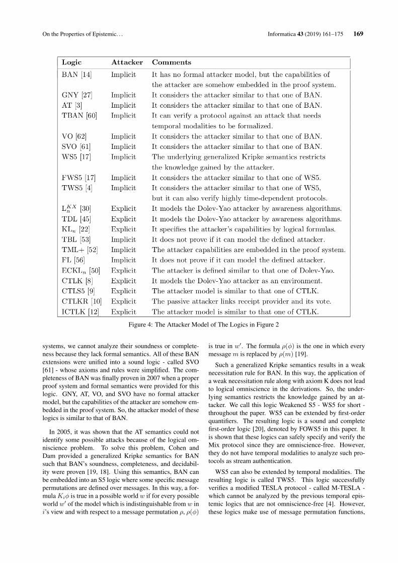
On the Properties of Epistemic. . . Informatica 43 (2019) 161–175 169
Figure 4: The Attacker Model of The Logics in Figure 2
systems, we cannot analyze their soundness or complete-ness because they lack formal semantics. All of these BANextensions were unified into a sound logic - called SVO[61] - whose axioms and rules were simplified. The com-pleteness of BAN was finally proven in 2007 when a properproof system and formal semantics were provided for thislogic. GNY, AT, VO, and SVO have no formal attackermodel, but the capabilities of the attacker are somehow em-bedded in the proof system. So, the attacker model of theselogics is similar to that of BAN.
In 2005, it was shown that the AT semantics could notidentify some possible attacks because of the logical om-niscience problem. To solve this problem, Cohen andDam provided a generalized Kripke semantics for BANsuch that BAN’s soundness, completeness, and decidabil-ity were proven [19, 18]. Using this semantics, BAN canbe embedded into an S5 logic where some specific messagepermutations are defined over messages. In this way, a for-mulaKiφ is true in a possible world w if for every possibleworld w′ of the model which is indistinguishable from w ini’s view and with respect to a message permutation ρ, ρ(φ)
is true in w′. The formula ρ(φ) is the one in which everymessage m is replaced by ρ(m) [19].
Such a generalized Kripke semantics results in a weaknecessitation rule for BAN. In this way, the application ofa weak necessitation rule along with axiom K does not leadto logical omniscience in the derivations. So, the under-lying semantics restricts the knowledge gained by an at-tacker. We call this logic Weakened S5 - WS5 for short -throughout the paper. WS5 can be extended by first-orderquantifiers. The resulting logic is a sound and completefirst-order logic [20], denoted by FOWS5 in this paper. Itis shown that these logics can safely specify and verify theMix protocol since they are omniscience-free. However,they do not have temporal modalities to analyze such pro-tocols as stream authentication.
WS5 can also be extended by temporal modalities. Theresulting logic is called TWS5. This logic successfullyverifies a modified TESLA protocol - called M-TESLA -which cannot be analyzed by the previous temporal epis-temic logics that are not omniscience-free [4]. However,these logics make use of message permutation functions,
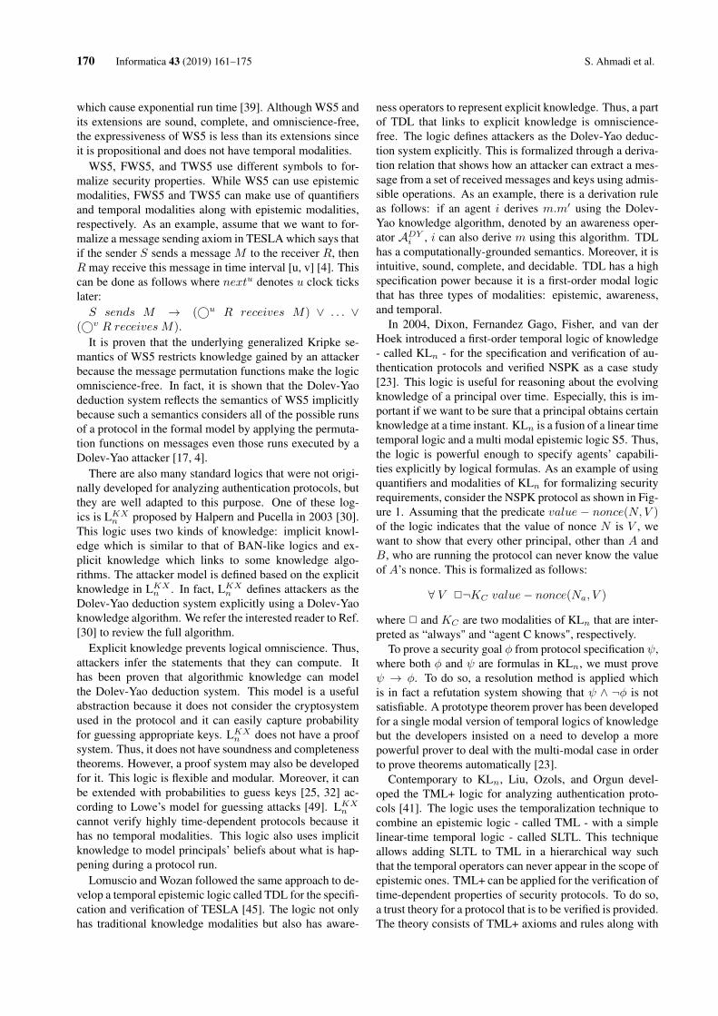
170 Informatica 43 (2019) 161–175 S. Ahmadi et al.
which cause exponential run time [39]. Although WS5 andits extensions are sound, complete, and omniscience-free,the expressiveness of WS5 is less than its extensions sinceit is propositional and does not have temporal modalities.
WS5, FWS5, and TWS5 use different symbols to for-malize security properties. While WS5 can use epistemicmodalities, FWS5 and TWS5 can make use of quantifiersand temporal modalities along with epistemic modalities,respectively. As an example, assume that we want to for-malize a message sending axiom in TESLA which says thatif the sender S sends a message M to the receiver R, thenR may receive this message in time interval [u, v] [4]. Thiscan be done as follows where nextu denotes u clock tickslater:S sends M → (©u R receives M) ∨ . . . ∨
(©v R receives M).It is proven that the underlying generalized Kripke se-
mantics of WS5 restricts knowledge gained by an attackerbecause the message permutation functions make the logicomniscience-free. In fact, it is shown that the Dolev-Yaodeduction system reflects the semantics of WS5 implicitlybecause such a semantics considers all of the possible runsof a protocol in the formal model by applying the permuta-tion functions on messages even those runs executed by aDolev-Yao attacker [17, 4].
There are also many standard logics that were not origi-nally developed for analyzing authentication protocols, butthey are well adapted to this purpose. One of these log-ics is LKXn proposed by Halpern and Pucella in 2003 [30].This logic uses two kinds of knowledge: implicit knowl-edge which is similar to that of BAN-like logics and ex-plicit knowledge which links to some knowledge algo-rithms. The attacker model is defined based on the explicitknowledge in LKXn . In fact, LKXn defines attackers as theDolev-Yao deduction system explicitly using a Dolev-Yaoknowledge algorithm. We refer the interested reader to Ref.[30] to review the full algorithm.
Explicit knowledge prevents logical omniscience. Thus,attackers infer the statements that they can compute. Ithas been proven that algorithmic knowledge can modelthe Dolev-Yao deduction system. This model is a usefulabstraction because it does not consider the cryptosystemused in the protocol and it can easily capture probabilityfor guessing appropriate keys. LKXn does not have a proofsystem. Thus, it does not have soundness and completenesstheorems. However, a proof system may also be developedfor it. This logic is flexible and modular. Moreover, it canbe extended with probabilities to guess keys [25, 32] ac-cording to Lowe’s model for guessing attacks [49]. LKXncannot verify highly time-dependent protocols because ithas no temporal modalities. This logic also uses implicitknowledge to model principals’ beliefs about what is hap-pening during a protocol run.
Lomuscio and Wozan followed the same approach to de-velop a temporal epistemic logic called TDL for the specifi-cation and verification of TESLA [45]. The logic not onlyhas traditional knowledge modalities but also has aware-
ness operators to represent explicit knowledge. Thus, a partof TDL that links to explicit knowledge is omniscience-free. The logic defines attackers as the Dolev-Yao deduc-tion system explicitly. This is formalized through a deriva-tion relation that shows how an attacker can extract a mes-sage from a set of received messages and keys using admis-sible operations. As an example, there is a derivation ruleas follows: if an agent i derives m.m′ using the Dolev-Yao knowledge algorithm, denoted by an awareness oper-ator ADYi , i can also derive m using this algorithm. TDLhas a computationally-grounded semantics. Moreover, it isintuitive, sound, complete, and decidable. TDL has a highspecification power because it is a first-order modal logicthat has three types of modalities: epistemic, awareness,and temporal.
In 2004, Dixon, Fernandez Gago, Fisher, and van derHoek introduced a first-order temporal logic of knowledge- called KLn - for the specification and verification of au-thentication protocols and verified NSPK as a case study[23]. This logic is useful for reasoning about the evolvingknowledge of a principal over time. Especially, this is im-portant if we want to be sure that a principal obtains certainknowledge at a time instant. KLn is a fusion of a linear timetemporal logic and a multi modal epistemic logic S5. Thus,the logic is powerful enough to specify agents’ capabili-ties explicitly by logical formulas. As an example of usingquantifiers and modalities of KLn for formalizing securityrequirements, consider the NSPK protocol as shown in Fig-ure 1. Assuming that the predicate value − nonce(N,V )of the logic indicates that the value of nonce N is V , wewant to show that every other principal, other than A andB, who are running the protocol can never know the valueof A’s nonce. This is formalized as follows:
∀ V 2¬KC value− nonce(Na, V )
where 2 and KC are two modalities of KLn that are inter-preted as “always" and “agent C knows", respectively.
To prove a security goal φ from protocol specification ψ,where both φ and ψ are formulas in KLn, we must proveψ → φ. To do so, a resolution method is applied whichis in fact a refutation system showing that ψ ∧ ¬φ is notsatisfiable. A prototype theorem prover has been developedfor a single modal version of temporal logics of knowledgebut the developers insisted on a need to develop a morepowerful prover to deal with the multi-modal case in orderto prove theorems automatically [23].
Contemporary to KLn, Liu, Ozols, and Orgun devel-oped the TML+ logic for analyzing authentication proto-cols [41]. The logic uses the temporalization technique tocombine an epistemic logic - called TML - with a simplelinear-time temporal logic - called SLTL. This techniqueallows adding SLTL to TML in a hierarchical way suchthat the temporal operators can never appear in the scope ofepistemic ones. TML+ can be applied for the verification oftime-dependent properties of security protocols. To do so,a trust theory for a protocol that is to be verified is provided.The theory consists of TML+ axioms and rules along with
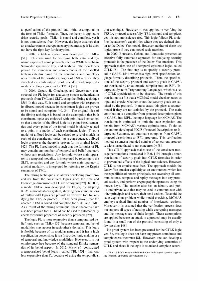
On the Properties of Epistemic. . . Informatica 43 (2019) 161–175 171
a specification of the protocol and initial assumptions inthe form of TML+ formulas. Then, the theory is applied todrive security goals. TML+ is sound and complete, yet itis not omniscience-free. However, the logic assumes thatan attacker cannot decrypt an encrypted message if he doesnot have the right key for decryption.
In 2007, a tableau system was developed for TML+[51]. This was used for verifying both static and dy-namic aspects of some protocols such as WMF, Needham-Schroeder symmetric key, and Kerbros. The developersproved the soundness and completeness of the labelledtableau calculus based on the soundness and complete-ness results of the constituent logics of TML+. Then, theysketched a resolution-type proof procedure and proposed amodel checking algorithm for TML+ [51].
In 2006, Orgun, Ji, Chuchang, and Governatori con-structed the FL logic for analyzing stream authenticationprotocols from TML and SLTL using the fibring technique[56]. In this way, FL is sound and complete with respect toits fibered model because its constituent logics are provento be sound and complete [40, 34]. The original idea ofthe fibring technique is based on the assumption that bothconstituent logics are endowed with point-based semanticsso that a model of the fibred logic is a point-based seman-tics and every point of the fibred model is closely relatedto a point in a model of each constituent logic. Thus, amodel of a fibred logic can be related to several models ineach of the constituent logics. As a consequence, a fibredlogic preserves the theorems proven for its original logics[42]. The FL fibred model is such that the formulas of FLmay contain any number of temporal and belief operatorswithout any restrictions. Any formula whose main opera-tor is a temporal modality, is interpreted by referring to theSLTL semantics and any formula whose main operator isa belief modality, is interpreted by referring to the Kripkesemantics of TML.
The fibring technique also allows developing proof pro-cedures from the constituent logics since the time andknowledge dimensions of FL are orthogonal[29]. In 2008,a modal tableau was developed for FL[29] by adaptingKEM, a modal tableau system, showing how combinationsof multi-modal logics can provide an effective tool for ver-ifying the TESLA protocol. It has been proven that theadapted KEM is sound and complete for SLTL and TML.As a result of the fibring technique, these theorems havealso been proven for FL. KEM can be used to automaticallycheck for formal properties of security protocols [29].
The logic FL is more expressive than a temporalised be-lief logic such as TML+ [52] because temporal and beliefmodalities may appear in each other’s domains. This logicis flexible because of its modular nature and it has a highspecification power since it is a first-order logic making useof temporal and knowledge modalities. However, it is notomniscience-free because of the standard Kripke seman-tics of its belief aspect. In 2012, Ma et al. constructeda temporalized belief logic - called TBL [53] - that wasless expressive than FL because of using the temporaliza-
tion technique. However, it was appllied in verifying theTESLA protocol successfully. TBL is sound and complete,yet it is not omniscience-free. This logic follows FL to de-fine the attacker’s capabilities where they are defined simi-lar to the Dolev-Yao model. However, neither of these twologics prove if they can model such attackers.
In 2009, Boureanu, Cohen, and Lomuscio presented aneffective fully automatic approach for analyzing securityprotocols in the presence of the Dolev-Yao attackers. Thisapproach makes use of a temporal epistemic logic, calledCTLK [8]. The first step is to specify a security proto-col in CAPSL [54], which is a high-level specification lan-guage formally describing protocols. Then, the specifica-tions of the security protocol and security goals in CAPSLare translated by an automatic compiler into an ISPL (In-terpreted Systems Programming Language), which is a setof CTLK specifications to be checked. The result of thistranslation is a file that a MCMAS model checker3 takes asinput and checks whether or not the security goals are sat-isfied by the protocol. In most cases, this gives a counter-model if they are not satisfied by the protocol. The maincontribution is a compiler from protocol descriptions givenin CAPSL into ISPL, the input language for MCMAS. Thetranslation is optimised to limit the state explosion andbenefit from MCMAS’s various optimisations. To do so,the authors developed PD2IS (Protocol Descriptions to In-terpreted Systems), an automatic compiler from CAPSLprotocol descriptions to ISPL programs. This verificationmethod assumes a bounded number of concurrent protocolsessions instantiated to run concurrently [8].
This CTLK approach makes use of the consistent mes-sage permutations introduced in Ref. [19] through a smarttranslation of security goals into CTLK formulas in orderto prevent bad effects of the logical omniscience. However,CTLK is not omniscience-free. The approach models theDolev-Yao attacker explicitly as an environment which hasthe capabilities of honest principals, can eavesdrop all com-munications, compose and replay messages into any proto-col session, and perform cryptographic operators using hisknown keys. The attacker also has an identity and pub-lic and private keys that may be used to communicate withother principals and record their send actions. To avoid thestate-explosion problem while model checking, MCMASemploys a fixed limited number of interleaved sessions.Moreover, it is assumed that the verification process doesnot support all types of nesting while encrypting messagesand the messages are of finite-length. These assumptionsare applied because an attack to a protocol may be usuallyfound in a small run of the protocol consisting of only afew sessions [48].
No proof system has been presented for the CTLK logicyet. So, this logic does not have any proven soundness andcompleteness theorems [8]. However, one can develop aproof system with respect to the underlying semantics ofCTLK and check if the logic is sound and complete accord-
3This is a BDD-based model checker for multi-agent systems support-ing temporal-epistemic specifications [43]
172 Informatica 43 (2019) 161–175 S. Ahmadi et al.
ing to that proof system. CTLK is powerful and flexibleenough to be extended. As a variant of this logic, CTLS5nhas been developed to model-check detectability of attacksin multi-agent systems that are automatically generated forsecurity protocols [9]. As another extension of CTLK,CTLKR has been developed for the analysis of an e-votingprotocol - called Foo - with a passive attacker model whocan link the receipt-providing principal and its vote [10].Finally, ICTLK [12] has been developed for analyzing anunbounded number of concurrent protocol sessions. Theseextensions of CTLK use the same tools for verifying secu-rity protocols automatically. Contemporary to CTLK, Luoet al. provided a temporal epistemic logic - called ECKLn- that was applied in verifying the NSPK protocol usingmodel checking techniques similarly. To do so, the authorsimplemented and automatically verified security protocolsin a model checker for multiagent systems [9].
4 Conclusions
One of the main approaches for formal analysis of authen-tication protocols is using epistemic or temporal epistemiclogics. The semantics of such logics should be able tomodel the protocol runs, including those executed by at-tackers. Then, theorem provers or model checkers are builton these logics to analyze the protocols against intendedproperties. Comparing the logics in Figure 2, it seems thatWS5 and its extensions are the best choices for protocolanalysis since they are sound, complete, and omniscience-free. However, Figures 3 and 4 show that CTLK and itsextensions are very powerful in security protocol analysis,make use of automatic compilers and model checkers, andprevent bad effects of logical omniscience while modelingthe Dolev-Yao message deduction.
It has been shown that it is an undecidable problem tofind whether a security protocol is indeed secure or not[55]. Thus, it is practical to use trusted security protocolsanalyzed by different formal methods to provide fast solu-tions for existing problems of real life systems. At the sametime, it is practical to move toward the best formal systemfor verifying authentication protocols. A good measure forfinding such a formal system for security protocol analysisis to prove that it can model the Dolev-Yao message deduc-tion. In this line, we investigated the epistemic and tempo-ral epistemic logics and showed how far their propertiessuch as soundness, completeness, being omniscience-free,and expressiveness may affect the analysis of authentica-tion protocols. Some of these logics have no proof sys-tem, thus they have no soundness or completeness theo-rems. However, they may apply model checkers for analy-sis and use awareness algorithms for preventing the logicalomniscience problem while modeling the Dolev-Yao mes-sage deduction explicitly [30, 45, 8]. Preventing the logi-cal omniscience or avoiding its bad effects restricts a prin-cipal’s knowledge to what he can compute or derive withhis known keys and messages. Some other epistemic log-
ics have proof systems, are omniscience-free, and modelthe attacker capabilities implicitly [19, 20, 4]. If such log-ics are logically sound, their derived judgments are moretrustworthy. If they are complete, they may make use ofautomatic provers.
Comparing Figures 2 and 4, the epistemic logicsmodeling the Dolev-Yao message deduction are eitheromniscience-free or prevent the bad effects of omniscience.In fact, provers are usually built on logics that preserveproperties such as soundness, completeness, and beingomniscience-free so that one can trust their output. At thesame time, model checkers deal with the state explosionproblem by imposing some assumptions so that they canverify security protocols within an acceptable time. How-ever, such assumptions may not stop us from using modelcheckers since they cover a wide range of security proto-cols and use existing tools. Finally, the expressiveness ofsuch logics makes them powerful enough to both formal-ize attacker’s capabilities by logical formulas and analyzedifferent classes of authentication protocols. Specifically, ifthe logic has both temporal and epistemic modalities, it cananalyze highly time-dependent protocols such as streamauthentication protocols.
Although it has been shown that logics using algorith-mic knowledge can model the Dolev-Yao message deduc-tive explicitly [30], to the best of our knowledge it has notbeen proven if a temporal epistemic logic of authenticationcan model such an attacker implicitly using permutation-based generalized Kripke semantics. This can be a topic forfurther research. As seen in this paper, all of the logics thatmodel the attacker capabilities implicitly are omniscience-free. Thus, this can be a starting point for this topic of re-search. Finally, it would be beneficial if such an overviewextends to the use of epistemic and temporal epistemic log-ics in analyzing other security/privacy properties.
References[1] M. Abadi and A.D. Gordon (1999) A calculus for
cryptographic protocols: The spi calculus, Infor-mation and computation, Elsevier, 148(1): 1–70.https://doi.org/10.1006/inco.1998.2740
[2] M. Abadi and P. Rogaway (2002) Reconciling twoviews of cryptography (the computational sound-ness of formal encryption), Journal of cryptol-ogy, Springer, 15(2): 103–127. http://dx.doi.org/10.1007/s00145-007-0203-0
[3] M. Abadi and M.R. Tuttle (1991), A semantics fora logic of authentication, Proceedings of the tenthannual ACM symposium on Principles of distributedcomputing, ACM, 201–216. https://doi.org/10.1145/112600.112618
[4] S. Ahmadi and M.S. Fallah (2018) An Omniscience-Free Temporal Logic of Knowledge for Verify-
On the Properties of Epistemic. . . Informatica 43 (2019) 161–175 173
ing Authentication Protocols, Bulletin of the Ira-nian Mathematical Society, Springer, 44(5): 1–23.https://doi.org/10.1007/s41980-018-0087-9
[5] F. Belardinelli and A. Lomuscio (2010) Interactionsbetween time and knowledge in a first-order logic formulti-agent systems, Proceedings of the Twelfth In-ternational Conference on the Principles of Knowl-edge Representation and Reasoning, AAAI Press,38–48.
[6] F. Belardinelli and A. Lomuscio (2012) Interactionsbetween time and knowledge in a first-order logic formulti-agent systems: completeness results, Journal ofArtificial Intelligence Research, AI Access Founda-tion, 1–45. https://doi.org/10.1613/jair.3547
[7] B. Blanchet, B. Smyth, and V. Cheval (2015) ProVerif1.90: Automatic Cryptographic Protocol Verifier,User Manual and Tutorial.
[8] , I. Boureanu, M. Cohen, and A. Lomuscio (2009)Automatic verification of temporal-epistemic proper-ties of cryptographic protocols, Journal of AppliedNon-Classical Logics, Taylor & Francis, 19(4): 463–487. https://doi.org/10.3166/jancl.19.463-487
[9] I. Boureanu, M. Cohen, and A. Lomuscio (2010)Model checking detectability of attacks in multiagentsystems, Proceedings of the 9th International Confer-ence on Autonomous Agents and Multiagent Systems,International Foundation for Autonomous Agents andMultiagent Systems, 1: 691–698.
[10] I. Boureanu, A.V. Jones, and A. Lomuscio (2012)Automatic verification of epistemic specifications un-der convergent equational theories, Proceedings ofthe 11th International Conference on AutonomousAgents and Multiagent Systems-Volume 2, Interna-tional Foundation for Autonomous Agents and Mul-tiagent Systems, 1141–1148.
[11] I. Boureanu, P. Kouvaros, and A. Lomuscio (2016)MCMAS-S- An experimental model checker orthe verification of security properties in unboundedmulti-agent systems. https://vas.doc.ic.ac.uk/software/mcmas-extensions/
[12] I. Boureanu, P. Kouvaros, and A. Lomuscio (2016)Verifying Security Properties in Unbounded Multia-gent Systems, Proceedings of the 2016 InternationalConference on Autonomous Agents & MultiagentSystems, International Foundation for AutonomousAgents and Multiagent Systems,1209–1217.
[13] C. Boyd and A. Mathuria (2013)Protocols for authen-tication and key establishment, Springer Science &Business Media, 2013. https://doi.org/10.1007/978-3-662-09527-0
[14] M. Burrows, M. Abadi, and R.M. Needham (1989) Alogic of authentication, Proceedings of the Royal So-ciety of London A: Mathematical, Physical and En-gineering Sciences, The Royal Society, 426(1871):233–271.
[15] C.C. Chang and H.J. Keisler (1990) Model theory,North Holland, 73.
[16] L. Chao, L. Hui, and M. Jianfeng (2009) Analy-sis the Properties of TLS Based on Temporal Logicof Knowledge, Proceedings of the 5th InternationalConference on Information Assurance and Security,IEEE, 2: 19–22. https://doi.org/10.1109/ias.2009.49
[17] M. Cohen (2007) Logics of Knowledge and Cryptog-raphy: Completeness and Expressiveness, PhD The-sis, KTH, Stockholm, Sweden.
[18] M. Cohen and M. Dam (2005) A completeness resultfor BAN logic, Prococeedings of Methods for Modal-ities, 4.
[19] M. Cohen and M. Dam (2005) Logical omniscience inthe semantics of BAN logic, Proceedings of the Foun-dations of Computer Security, 121–132.
[20] M. Cohen and M. Dam (2007) A complete axiom-atization of knowledge and cryptography, Proceed-ings of the 22nd Annual IEEE Symposium on Logicin Computer Science, IEEE, 77–88.
[21] F. Dechesne and Y. Wang (2010) To know or not toknow: epistemic approaches to security protocol ver-ification, Synthese, Springer, 177(1): 51–76. https://doi.org/10.1007/s11229-010-9765-8
[22] C. Dixon, M.C. Fernández Gago, M. Fisher, andW. van der Hoek (2007) Temporal logics of knowl-edge and their applications in security, ElectronicNotes in Theoretical Computer Science, Elsevier,186: 27–42. https://doi.org/10.1016/j.entcs.2006.11.043
[23] C. Dixon, M.C.F. Gago, M. Fisher, and W. Van DerHoek (2004) Using temporal logics of knowledge inthe formal verification of security protocols, Proceed-ings of the 11th International Symposium on Tempo-ral Representation and Reasoning, IEEE,148–151.
[24] D. Dolev and A. Yao (1983) On the security of publickey protocols, Proceedings of the IEEE Transactionson Information Theory, IEEE, 29(2):198–208.
[25] R. Fagin and J.Y. Halpern (1994) Reason-ing about knowledge and probability, Jour-nal of the ACM, ACM, 41(2):340–367.https://doi.org/10.1145/273865.274429
174 Informatica 43 (2019) 161–175 S. Ahmadi et al.
[26] R. Fagin, Y. Moses, J.Y. Halpern, and M.Y. Vardi(2003) Reasoning about knowledge, The MIT Press.https://doi.org/10.7551/mitpress/5803.001.0001
[27] L. Gong, R. Needham, and R. Yahalom (1990)Reasoning about belief in cryptographic proto-cols, Proceedings of the IEEE Computer SocietySymposium on Research in Security and Privacy,IEEE, 234–248. https://doi.org/10.1109/risp.1990.63854
[28] A.D. Gordon and A. Jeffrey (2003) Authenticity bytyping for security protocols, Journal of computer se-curity, IOS Press, 11(4): 451–519. https://doi.org/10.3233/jcs-2003-11402
[29] G. Governatori, A.M. Orgun, and C. Liu (2008)Modal tableaux for verifying stream authenticationprotocols, Journal of Autonomous Agents and MultiAgent Systems. https://doi.org/10.1007/s10458-007-9027-4
[30] J.Y. Halpern and R. Pucella (2003) Modelingadversaries in a logic for security protocolanalysis, Formal Aspects of Security, Springer,115–132. https://doi.org/10.1007/978-3-540-40981-6_11
[31] J.Y. Halpern and R. Pucella (2011) Dealing withlogical omniscience: Expressiveness and pragmatics,Artificial intelligence, Elsevier, 175(1): 220–235.https://doi.org/10.1016/j.artint.2010.04.009
[32] J.Y. Halpern and M.R. Tuttle (1993) Knowl-edge, probability, and adversaries, Journal of theACM, ACM,40(4):917–960. https://doi.org/10.1145/153724.153770
[33] J. Heather, G. Lowe, and S. Schneider (2003)How to prevent type flaw attacks on security pro-tocols, Journal of Computer Security, IOS Press,11(2): 217–244. https://doi.org/10.3233/jcs-2003-11204
[34] G.E. Hughes and M.J. Cresswell (2012) A new intro-duction to modal logic, Routledge. https://doi.org/10.4324/9780203028100
[35] G. Jakubowska, P. Dembinski, W. Penczek, and M.Szreter (2009) Simulation of Security Protocols basedon Scenarios of Attacks, Fundamenta Informaticae,93(1): 185-203.
[36] A. Jurcut, T. Coffey, and R. Dojen (2013) Establish-ing and fixing security protocols weaknesses usinga logic-based verification tool, Journal of Communi-cation, 8(11): 795–806. https://doi.org/10.12720/jcm.8.11.795-805
[37] A.D. Jurcut, T. Coffey, and R. Dojen (2014) De-sign guidelines for security protocols to prevent re-play & parallel session attacks, computers & secu-rity, Elsevier, 45: 255–273. https://doi.org/10.1016/j.cose.2014.05.010
[38] F. Kammuller and C.W. Probst (2015) Mod-eling and verification of insider threats usinglogical analysis, IEEE Systems Journal, IEEE,11(2): 534–545. https://doi.org/10.1109/jsyst.2015.2453215
[39] S. Kramer (2007) Logical concepts in cryptography,PhD Thesis, École Polytechnique Fédérale de Lau-sanne.
[40] C. Liu and M. Orgun (1996) Dealing with multi-ple granularity of time in temporal logic program-ming, Journal of Symbolic Computation, Elsevier,22(5): 699–720. https://doi.org/10.1006/jsco.1996.0072
[41] C. Liu, M.A. Ozols, and M. Orgun (2004) A tem-poralised belief logic for specifying the dynamics oftrust for multi-agent systems Advances in ComputerScience-ASIAN 2004. Higher-Level Decision Mak-ing, Springer, 142–156. https://doi.org/10.1007/978-3-540-30502-6_10
[42] C. Liu, M. Ozols, and M. Orgun (2005) A fibred be-lief logic for multi-agent systems, AI 2015: Advancesin Artificial Intelligence, Springer, 29–38. https://doi.org/10.1007/11589990_6
[43] A. Lomuscio, H. Qu, and F. Raimondi (2009)MCMAS: A model checker for the verificationof multi-agent systems, Computer Aided Verifica-tion, Springer, 682–688. https://doi.org/10.1007/978-3-642-02658-4_55
[44] A. Lomuscio, H. Qu, and F. Raimondi (2015) MC-MAS: an open-source model checker for the veri-fication of multi-agent systems International Jour-nal on Software Tools for Technology Transfer,Springer, 19(1): 9–30. https://doi.org/10.1007/s10009-015-0378-x
[45] A. Lomuscio and B. Wozna (2006) A complete anddecidable security-specialised logic and its applica-tion to the TESLA protocol, Proceedings of the 5thinternational joint conference on Autonomous agentsand multiagent systems, ACM, 145–152. https://doi.org/10.1145/1160633.1160658
[46] G. Lowe (1995) An attack on the Needham-Schroeder public-key authentication protocol,Information processing letters, Elsevier, 56(3):131–133. https://doi.org/10.1016/0020-0190(95)00144-2
On the Properties of Epistemic. . . Informatica 43 (2019) 161–175 175
[47] G. Lowe (1997) A family of attacks upon authentica-tion protocols, epartment of Mathematics and Com-puter Science, University of Leicester.
[48] G. Lowe (1998) Casper: A Compiler for the Anal-ysis of Security Protocols, Journal of Computer Se-curity, IOS Press, 6(1-2): 53–84. https://doi.org/10.3233/jcs-1998-61-204
[49] G. Lowe (2004) Analysing protocols subject to guess-ing attacks, Journal of Computer Security, IOS Press,12(1): 83–97. https://doi.org/10.3233/jcs-2004-12104
[50] X. Luo, Y. Chen, M. Gu, and L. Wu (2009)Model Checking Needham-Schroeder Security Pro-tocol Based on Temporal Logic of Knowledge, Pro-ceedings of the NSWCTC’09. International Confer-ence on Networks Security, Wireless Communicationsand Trusted Computing, IEEE, 2: 551–554. https://doi.org/10.1109/nswctc.2009.384
[51] J. Ma, M.A. Orgun, and K. Adi (2011) Ananalytic tableau calculus for a temporalised be-lief logic, Journal of Applied Logic, Elsevier,9(4): 289–304. https://doi.org/10.1016/j.jal.2011.08.003
[52] J. Ma, M.A. Orgun, and A. Sattar (2009) Analysis ofauthentication protocols in agent-based systems us-ing labeled tableaux IEEE Transactions on Systems,Man, and Cybernetics, Part B: Cybernetics, IEEE,39(4): 889–900. https://doi.org/10.1109/tsmcb.2009.2019263
[53] J. Ma and K. Schewe (2012) A TemporalisedBelief Logic for Reasoning about AuthenticationProtocols, Proceedings of the IEEE 11th Inter-national Conference on Trust, Security and Pri-vacy in Computing and Communications (Trust-Com), IEEE, 1721–1728. https://doi.org/10.1109/trustcom.2012.59
[54] J.K. Millen (1996) CAPSL: Common AuthenticationProtocol Specification Language, Proceedings of the1996 workshop on New security Paradigms (NSPW),ACM, 96: 132. https://doi.org/10.1145/304851.304879
[55] J. Mitchell, A. Scedrov, N. Durgin, and P. Lincoln(1999) Undecidability of bounded security protocols,Proceedings of the Workshop on Formal Methods andSecurity Protocols.
[56] M.A. Orgun, J. Ma, C. Liu, and G. Governatori(2006) Analysing stream authentication protocols inautonomous agent-based systems2nd IEEE Interna-tional Symposium on, Proceedings of the 2nd IEEEInternational Symposium on Dependable, Autonomicand Secure Computing, IEEE, 325–332. https://doi.org/10.1109/dasc.2006.19
[57] A. Perrig, R. Canetti, J.D. Tygar, and D. Song(2000) Efficient authentication and signing of mul-ticast streams over lossy channels, Proceedingsof the IEEE Symposium on Security and Pri-vacy, IEEE, 56–73. https://doi.org/10.1109/secpri.2000.848446
[58] R. Ramanujam and S.P. Suresh (2005) Decidingknowledge properties of security protocols, Proceed-ings of the 10th conference on theoretical aspectsof rationality and knowledge, National University ofSingapore, 219–235.
[59] R. Ramezanian (2015) Process Algebraic Model-ing of Authentication Protocols for Analysis of Par-allel Multi-Session Executions, The ISC Interna-tional Journal of Information Security, Iranian So-ciety of Cryptology, 1(1): 55-67. https://doi.org/10.22042/isecure.2015.1.1.6
[60] P.F. Syverson (1993) Adding time to a logic ofauthentication, Proceedings of the 1st ACM con-ference on Computer and communications security,ACM, 97–101. https://doi.org/10.1145/168588.168600
[61] P.F. Syverson and P.C. Van Oorschot (1994) On uni-fying some cryptographic protocol logics, Proceed-ings of the IEEE Computer Society Symposium onResearch in Security and Privacy, IEEE, 14–28.https://doi.org/10.21236/ada465512
[62] P. van Oorschot (1993) Extending cryptographic log-ics of belief to key agreement protocols, Proceed-ings of the 1st ACM Conference on Computer andCommunications Security, ACM, 232–243. https://doi.org/10.1145/168588.168617

176 Informatica 43 (2019) 161–175 S. Ahmadi et al.

https://doi.org/10.31449/inf.v43i2.2678 Informatica 43 (2019) 177–186 177
Benchmark Problems for Exhaustive Exact Maximum Clique SearchAlgorithms
Sándor SzabóInstitute of Mathematics and Informatics, University of PécsIfjuság utja 6, H-7624 Pécs, HungaryE-mail: [email protected]
Bogdán ZaválnijAlfréd Rényi Institute of Mathematics, Hungarian Academy of SciencesReáltanoda u. 13–15, H-1053 Budapest, HungaryE-mail: [email protected]
Keywords: clique, maximal clique, maximum clique, graph coloring, random graph, Mycielski graph
Received: February 12, 2019
There are well established widely used benchmark tests to assess the performance of practical exact cliquesearch algorithms. In this paper a family of further benchmark problems is proposed mainly to test exhaus-tive clique search procedures.
Povzetek: Podanih je nekaj novih standardnih problemov za testiranje algoritmov za iskanje klik.
1 PreliminariesLet G = (V,E) be a finite simple graph. Here V is theset of vertices of G and E is the set of edges of G. Thefiniteness of G means that G has finitely many nodes andfinitely many vertices, that is, |V | < ∞, |E| < ∞. Thesimplicity of G means that G does not have any loop and itdoes not have double edges.
Let C be a subset of V . If two distinct nodes in C arealways adjacent in G, then C is called a clique in G. WhenC has k elements, then we talk about a k-clique. We in-clude the cases k = 0 and k = 1 as well when |C| = 0 and|C| = 1, respectively. Though in these cases C does nothave two distinct elements.
A clique is maximal in G if it is not part of any largerclique in G. In other words a clique is maximal clique ofthe graph G if it cannot be extended to a larger clique byadding a new node of the graph G. A k-clique is a maxi-mum clique in G if G does not contain any (k + 1)-clique.All the maximum cliques of a graph G have the same num-ber of nodes. We call this well defined number the cliquenumber of G and we denote it by ω(G).
A number of problems is referred as clique search prob-lems [1].
Problem 1. Given a finite simple graph G. List all maxi-mal cliques of G without repetition.
Problem 2. Given a finite simple graphG and given a pos-itive integer k. Decide if G has a k-clique.
Problem 3. Given a finite simple graph G. Determineω(G).
Problem 4. Given a finite simple graph G. List all maxi-mum cliques of G without repetition.
An algorithm to solve Problem 1 can be found in [2].The algorithm is commonly known as Bron-Kerbosch al-gorithm. Obviously, the Bron-Kerbosch algorithm can beused to solve Problems 2, 3 and 4. A more efficient algo-rithm to solve these problems was first given in [3]. Thealgorithm is known under the name Caraghan-Pardalos al-gorithm. The Bron-Kerbosch and Carraghan-Pardalos al-gorithms are the classical algorithms that form the base ofmany further clique search procedures. These algorithmsare presented in [14], [26], [24], [10], [9]. But this list isnot intended to be complete.
The complexity theory of the algorithm tells us thatProblem 2 is in the NP-complete complexity class. (See forinstance [6].) Consequently, Problem 3 must be NP-hard.
We color the vertices of G such that the following con-ditions are satisfied.
(1) Each vertex of G is colored with exactly one color.
(2) Vertices of G connected by an edge receive distinctcolors.
A coloring of the nodes of G that satisfies conditions (1),(2) is called a legal coloring or well coloring of the nodesof G.
Suppose that the nodes ofG can be colored legally usingk colors. We may use a map f : V → {1, . . . , k} to de-scribe a coloring of the nodes of G. The numbers 1, . . . , kplay the roles of the colors and f(v) is the color of the ver-tex v for each v ∈ V . If for adjacent nodes u and v of G

178 Informatica 43 (2019) 177–186 S. Szabo et al.
the equation f(u) = f(v) implies u = v, then the coloringdefined by the map f is a legal coloring.
There is a number of the colors k such that the nodesof G can be colored legally using k colors and the nodesof G cannot be colored legally using k − 1 colors. Thiswell defined number k is called the chromatic number ofthe graph G and it is denoted by χ(G).
Graph coloring is a vast subject and we cannot make jus-tice to this venerable field. In this paper we take a verynarrow view. We are interested in only one particular ap-plication. Note that ω(G) ≤ χ(G) holds for each finitesimple graph G and so coloring of the nodes can be used toestimate the size of a maximum clique. However, the gapbetween ω(G) and χ(G) can be arbitrarily large. J. Myciel-ski [13] exhibited a graph M (k) for which ω(M (k)) = 2and χ(M (k)) = k for each integer k ≥ 2.
In order to find bounds for ω(G) the following node col-oring was proposed in [21]. Let us choose an integer s ≥ 2and consider a coloring of the nodes of G that satisfies thefollowing conditions.
(1′) Each vertex of G is colored with exactly one color.
(2′) If the vertices v1, . . . , vs are vertices of a clique in G,then all the vertices v1, . . . , vs cannot receive the samecolor.
A coloring of the nodes of G satisfying the conditions (1′),(2′), is called a monochrome s-clique free coloring. Inshort we will talk about s-clique free coloring. For s = 2the monochrome s-clique free coloring of the nodes givesback the legal coloring of the nodes. There is a well de-fined minimum number k such that the nodes of G have ans-clique free coloring using k colors. This k is referred toas the the s-clique free chromatic number of G and it is de-noted by χ(s)(G). The inequality ω(G) ≤ (s− 1)χ(s)(G)shows that s-clique free coloring of the nodes can be usedto establish upper bound for the clique number.
A number of problems is considered in connection withcoloring the nodes of a graph customarily.
Problem 5. Given a finite simple graphG and given a pos-itive integer k. Decide whether the nodes ofG admit a legalcoloring using k colors.
Problem 6. Given a finite simple graph G. Determineχ(G).
It is a well known result of the complexity theory of al-gorithms that Problem 5 belongs to the P complexity classfor k = 2 and it belongs to the NP-complete complexityclass for k ≥ 3. (See for example [15].) It follows that fork ≥ 3 Problem 6 is NP-hard.
Problem 7. Given a finite simple graphG and two positiveintegers s, k. Decide if the nodes ofG have a legal s-cliquefree coloring with k colors.
It was established in [23] that for k = 3, s ≥ 3 Problem7 is NP-complete.
2 A Mycielski type resultAs we have already mentioned the chromatic number canbe a poor upper estimate of the clique number. By My-cielski’s construction there are 3-clique free graphs witharbitrarily large chromatic number. P. Erdos [5] general-ized this result. Let us call the length of a shortest cordlesscircle in a graph the girth of the graph. Clearly, the girth ofa 3-clique free graph must be at least 4. Erdos has provedthat for given positive integers k and l, there is a finite sim-ple graph G with girth(G) ≥ l, χ(G) ≥ k. Erdos’s proofis not constructive and so it is not at all straight forwardhow the resulting graphs could be used in constructing testinstances.
In this section we present another extension of Myciel-ski’s result. We replace the legal coloring of the nodes of agraph by a legal s-clique free coloring of the nodes of thegraph. Consequently, the s-clique free chromatic numberχ(s)(G) will play the role of the chromatic number χ(G).
The result is motivated by the fact that one might tryto construct clique search test instances by replacing theMycielski graph by the graph emerging from the proof thegeneralized version.
Theorem 1. Let us choose two positive integers s and kwith s ≥ 3 and k ≥ 2(s−1)/(s − 1). There is a finitesimple graph L(s,k) such that ω(L(s,k)) ≤ 2(s−1) andχ(s)(L(s,k)) ≥ k.
The reader may notice that the graph L(2,k) is isomor-phic to the Mycielski graph M (k).Proof. The proof will be constructive. We start with thespecial case s = 3. We choose an integer k for whichk ≥ 2(3−1)/(3− 1) = 2. Let M (k) be the Mycielski graphwith parameter k. Let u1, . . . , un be the nodes of M (k).We substitute the node ui of M (k) by an isomorphic copyM
(k)i of the Mycielski graph for each i, 1 ≤ i ≤ n. Let
vi,1,, . . . , vi,n be the nodes of M (k)i . We assume that the
nodesv1,1, . . . , v1,n, . . . , vn,1, . . . , vn,n
are pair-wise distinct. These nodes will be the nodes of thegraph L(3,k).
The edges of M (k)i are going to be edges of L(3,k) for
each i, 1 ≤ i ≤ n. Further, whenever the unorderedpair {ui, uj} is an edge of M (k), then we add the edge{vi,α, vj,β} to L(3,k) for each α, β, 1 ≤ α, β ≤ n.
The dedicated reader will not fail to notice that the con-struction we just presented is the so called lexicographicproduct of the graphs M (k) and M (k).
We claim that ω(L(3,k)) ≤ 4.In order to verify the claim we assume on the con-
trary that ω(L(3,k)) ≥ 5. Let C be a 5-clique in L(3,k).Set Vi = {vi,1,, . . . , vi,n}. Note that the set Vi inducesM
(k)i in L(3,k) as a subgraph of L(3,k). From the fact that
ω(M(k)i ) ≤ 2 it follows that C may have at most 2 nodes
in Vi for each i, 1 ≤ i ≤ n. Therefore C has nodes in someM
(k)i for at least 3 distinct values of i.

Benchmark Problems for Exhaustive Exact. . . Informatica 43 (2019) 177–186 179
Suppose that i and j are distinct numbers in the set{1, . . . , n}. A node in M (k)
i and a node in M (k)j can be
adjacent only if the unordered pair {ui, uj} is an edge ofM (k). This means thatM (k) contains a 3-clique. ButM (k)
does not contain any 3-clique. This contradiction com-pletes the verification of the claim.
We claim that χ(3)(L(3,k)) ≥ k.In order to prove the claim let us assume on the contrary
that χ(3)(L(3,k)) ≤ k − 1. Set
V = V1 ∪ · · · ∪ Vn= {v1,1, . . . , v1,n, . . . , vn,1, . . . , vn,n}.
Suppose that the map f : V → {1, . . . , k − 1} defines a3-clique free coloring of the nodes of L(3,k).
The restriction of f to the set Vi is a map gi : Vi →{1, . . . , k − 1}. Clearly, the map gi defines a coloring ofthe nodes of the graphM (k)
i . From the fact that χ(M(k)i ) ≥
k it follows that there are two distinct adjacent nodes ofM
(k)i such that the two nodes receive the same color ci.
Set U = {u1, . . . , un}. Using the color ci we define a maph : U → {1, . . . , k − 1}. We set h(ui) = ci for each i,1 ≤ i ≤ n.
Note that the map h defines a legal coloring of the nodesof the graphM (k). The only thing which needs verificationis that if ui and uj are distinct adjacent nodes ofM (k), thenci 6= cj .
Let us assume on the contrary that ui and uj are distinctadjacent nodes of M (k) and ci = cj . The graph M (k)
i hastwo distinct adjacent nodes vi,i(1) and vi,i(2) such that
f(vi,i(1)) = f(vi,i(2)) = ci.
Similarly, the graph M (k)j has two distinct adjacent nodes
vj,j(1) and vj,j(2) such that
f(vj,j(1)) = f(vj,j(2)) = cj .
Note that the nodes vi,i(1), vi,i(2), vj,j(1), vj,j(2) are thenodes of a 4-clique in L(3,k). This means that the coloringdefined by the map f is not a 3-clique free coloring of thenodes of L(3,k). This shows that the coloring defined bythe map h is a legal coloring of the nodes of M (k).
The coloring defined by h is using at most k − 1 colors.This contradicts the fact that χ(M (k)) ≥ k. Thus we mayconclude that χ(3)(L(3,k)) ≥ k as we claimed.
Let us turn to the special case s = 4. We choose a integerk for which k ≥ 2(4−1)/(4 − 1), that is, k ≥ 3. Let M (k)
be the Mycielski graph with parameter k. Let u1, . . . , unbe the nodes of M (k). We substitute the node ui of M (k)
by an isomorphic copy L(3,k)i of the graph L(3,k) for each
i, 1 ≤ i ≤ n. Let vi,1,, . . . , vi,m be the nodes of L(3,k)i . We
assume that the nodes
v1,1, . . . , v1,m, . . . , vn,1, . . . , vn,m
are pair-wise distinct. These nodes will be the nodes of thegraph L(4,k).
The edges of L(3,k)i are going to be edges of L(4,k) for
each i, 1 ≤ i ≤ n. Further, whenever the unorderedpair {ui, uj} is an edge of M (k), then we add the edge{vi,α, vj,β} to L(4,k) for each α, β, 1 ≤ α, β ≤ m.
We claim that ω(L(4,k)) ≤ 8.In order to verify the claim we assume on the contrary
that ω(L(4,k)) ≥ 9. Let C be a 9-clique in L(4,k). Notethat the set Vi = {vi,1,, . . . , vi,m} induces L(3,k)
i in L(4,k)
as a subgraph of L(4,k). From the fact that ω(L(3,k)i ) ≤ 4
it follows that C may have at most 4 nodes in Vi for eachi, 1 ≤ i ≤ n. Therefore C has nodes in some L(3,k)
i for atleast 3 distinct values of i.
Suppose that i and j are distinct numbers in the set{1, . . . , n}. A node in L
(3,k)i and a node in L
(3,k)j can
be adjacent only if the unordered pair {ui, uj} is an edgeof M (k). This means that M (k) contains a 3-clique. ButM (k) does not contain any 3-clique. This contradictioncompletes the proof of the claim.
We claim that χ(4)(L(4,k)) ≥ k.In order to prove the claim let us assume on the contrary
that χ(4)(L(4,k)) ≤ k − 1. Set
V = V1 ∪ · · · ∪ Vn= {v1,1, . . . , v1,n, . . . , vn,1, . . . , vn,n}.
Suppose that the map f : V → {1, . . . , k − 1} defines a4-clique free coloring of the nodes of L(4,k).
The restriction of f to the set Vi is a map gi : Vi →{1, . . . , k − 1}. Clearly, the map gi defines a coloringof the nodes of the graph L
(3,k)i . From the fact that
χ(3)(L(3,k)i ) ≥ k it follows that there is a 3-clique in L(3,k)
i
such that the 3 nodes of the clique receive the same colorci. Set U = {u1, . . . , un}. Using the color ci we define amap h : U → {1, . . . , k − 1}. We set h(ui) = ci for eachi, 1 ≤ i ≤ n.
Note that the map h defines a legal coloring of the nodesof the graphM (k). The only thing which needs verificationis that if ui and uj are distinct adjacent nodes ofM (k), thenci 6= cj .
Let us assume on the contrary that ci = cj . The graphL(3,k)i has 3 distinct pair-wise adjacent nodes vi,i(1), vi,i(2),
vi,i(3) such that
f(vi,i(1)) = f(vi,i(2)) = f(vi,i(2)) = ci.
Similarly, the graph L(3,k)i has 3 distinct pair-wise adjacent
nodes vj,j(1), vj,j(2), vj,j(2) such that
f(vj,j(1)) = f(vj,j(2)) = f(vj,j(3)) = cj .
Note that the nodes
vi,i(1), vi,i(2), vi,i(3), vj,j(1), vj,j(2), vj,j(3)
are the nodes of a 6-clique in L(4,k). This means that thecoloring defined by the map f is not a 4-clique free coloringof the nodes of L(4,k). This shows that the coloring definedby the map h is a legal coloring of the nodes of M (k).
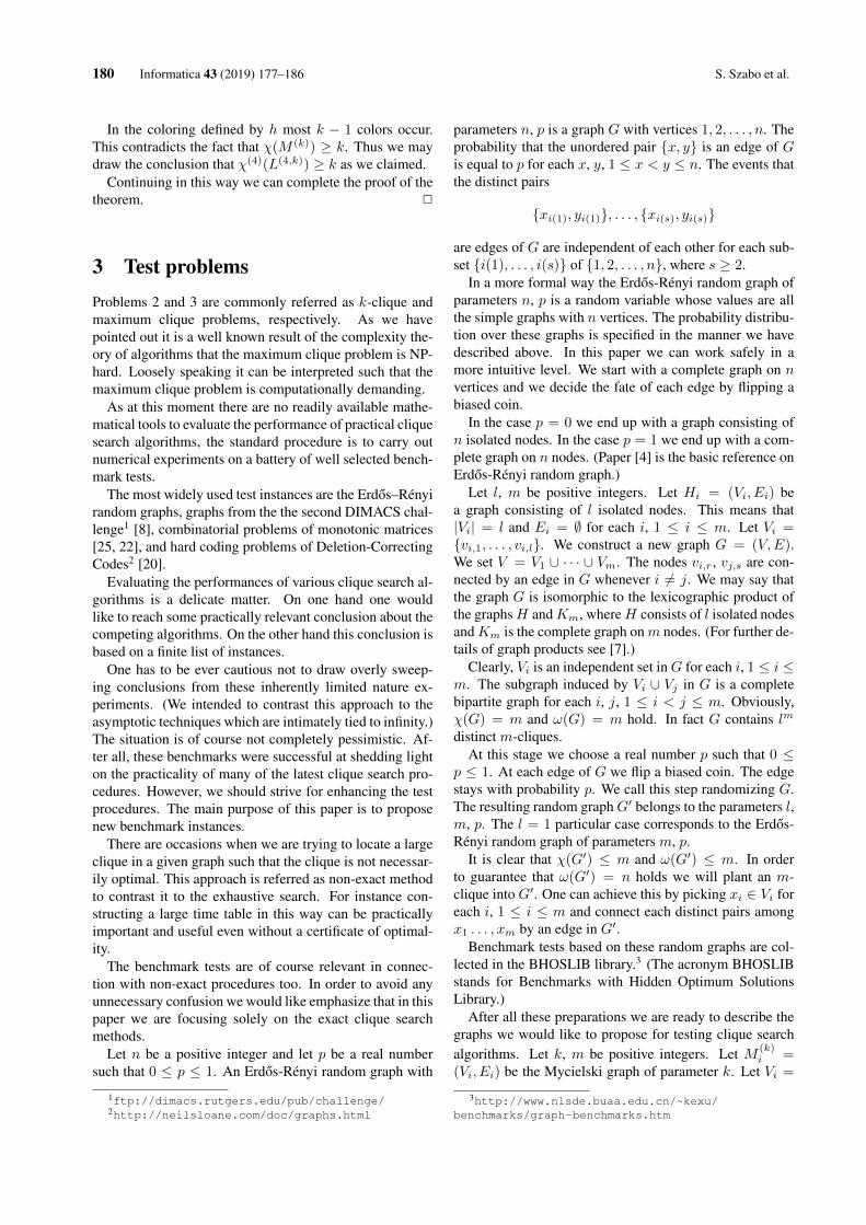
180 Informatica 43 (2019) 177–186 S. Szabo et al.
In the coloring defined by h most k − 1 colors occur.This contradicts the fact that χ(M (k)) ≥ k. Thus we maydraw the conclusion that χ(4)(L(4,k)) ≥ k as we claimed.
Continuing in this way we can complete the proof of thetheorem. 2
3 Test problemsProblems 2 and 3 are commonly referred as k-clique andmaximum clique problems, respectively. As we havepointed out it is a well known result of the complexity the-ory of algorithms that the maximum clique problem is NP-hard. Loosely speaking it can be interpreted such that themaximum clique problem is computationally demanding.
As at this moment there are no readily available mathe-matical tools to evaluate the performance of practical cliquesearch algorithms, the standard procedure is to carry outnumerical experiments on a battery of well selected bench-mark tests.
The most widely used test instances are the Erdos–Rényirandom graphs, graphs from the the second DIMACS chal-lenge1 [8], combinatorial problems of monotonic matrices[25, 22], and hard coding problems of Deletion-CorrectingCodes2 [20].
Evaluating the performances of various clique search al-gorithms is a delicate matter. On one hand one wouldlike to reach some practically relevant conclusion about thecompeting algorithms. On the other hand this conclusion isbased on a finite list of instances.
One has to be ever cautious not to draw overly sweep-ing conclusions from these inherently limited nature ex-periments. (We intended to contrast this approach to theasymptotic techniques which are intimately tied to infinity.)The situation is of course not completely pessimistic. Af-ter all, these benchmarks were successful at shedding lighton the practicality of many of the latest clique search pro-cedures. However, we should strive for enhancing the testprocedures. The main purpose of this paper is to proposenew benchmark instances.
There are occasions when we are trying to locate a largeclique in a given graph such that the clique is not necessar-ily optimal. This approach is referred as non-exact methodto contrast it to the exhaustive search. For instance con-structing a large time table in this way can be practicallyimportant and useful even without a certificate of optimal-ity.
The benchmark tests are of course relevant in connec-tion with non-exact procedures too. In order to avoid anyunnecessary confusion we would like emphasize that in thispaper we are focusing solely on the exact clique searchmethods.
Let n be a positive integer and let p be a real numbersuch that 0 ≤ p ≤ 1. An Erdos-Rényi random graph with
1ftp://dimacs.rutgers.edu/pub/challenge/2http://neilsloane.com/doc/graphs.html
parameters n, p is a graph G with vertices 1, 2, . . . , n. Theprobability that the unordered pair {x, y} is an edge of Gis equal to p for each x, y, 1 ≤ x < y ≤ n. The events thatthe distinct pairs
{xi(1), yi(1)}, . . . , {xi(s), yi(s)}
are edges of G are independent of each other for each sub-set {i(1), . . . , i(s)} of {1, 2, . . . , n}, where s ≥ 2.
In a more formal way the Erdos-Rényi random graph ofparameters n, p is a random variable whose values are allthe simple graphs with n vertices. The probability distribu-tion over these graphs is specified in the manner we havedescribed above. In this paper we can work safely in amore intuitive level. We start with a complete graph on nvertices and we decide the fate of each edge by flipping abiased coin.
In the case p = 0 we end up with a graph consisting ofn isolated nodes. In the case p = 1 we end up with a com-plete graph on n nodes. (Paper [4] is the basic reference onErdos-Rényi random graph.)
Let l, m be positive integers. Let Hi = (Vi, Ei) bea graph consisting of l isolated nodes. This means that|Vi| = l and Ei = ∅ for each i, 1 ≤ i ≤ m. Let Vi ={vi,1, . . . , vi,l}. We construct a new graph G = (V,E).We set V = V1 ∪ · · · ∪ Vm. The nodes vi,r, vj,s are con-nected by an edge in G whenever i 6= j. We may say thatthe graph G is isomorphic to the lexicographic product ofthe graphsH andKm, whereH consists of l isolated nodesandKm is the complete graph onm nodes. (For further de-tails of graph products see [7].)
Clearly, Vi is an independent set inG for each i, 1 ≤ i ≤m. The subgraph induced by Vi ∪ Vj in G is a completebipartite graph for each i, j, 1 ≤ i < j ≤ m. Obviously,χ(G) = m and ω(G) = m hold. In fact G contains lm
distinct m-cliques.At this stage we choose a real number p such that 0 ≤
p ≤ 1. At each edge of G we flip a biased coin. The edgestays with probability p. We call this step randomizing G.The resulting random graphG′ belongs to the parameters l,m, p. The l = 1 particular case corresponds to the Erdos-Rényi random graph of parameters m, p.
It is clear that χ(G′) ≤ m and ω(G′) ≤ m. In orderto guarantee that ω(G′) = n holds we will plant an m-clique into G′. One can achieve this by picking xi ∈ Vi foreach i, 1 ≤ i ≤ m and connect each distinct pairs amongx1 . . . , xm by an edge in G′.
Benchmark tests based on these random graphs are col-lected in the BHOSLIB library.3 (The acronym BHOSLIBstands for Benchmarks with Hidden Optimum SolutionsLibrary.)
After all these preparations we are ready to describe thegraphs we would like to propose for testing clique searchalgorithms. Let k, m be positive integers. Let M (k)
i =(Vi, Ei) be the Mycielski graph of parameter k. Let Vi =
3http://www.nlsde.buaa.edu.cn/~kexu/benchmarks/graph-benchmarks.htm
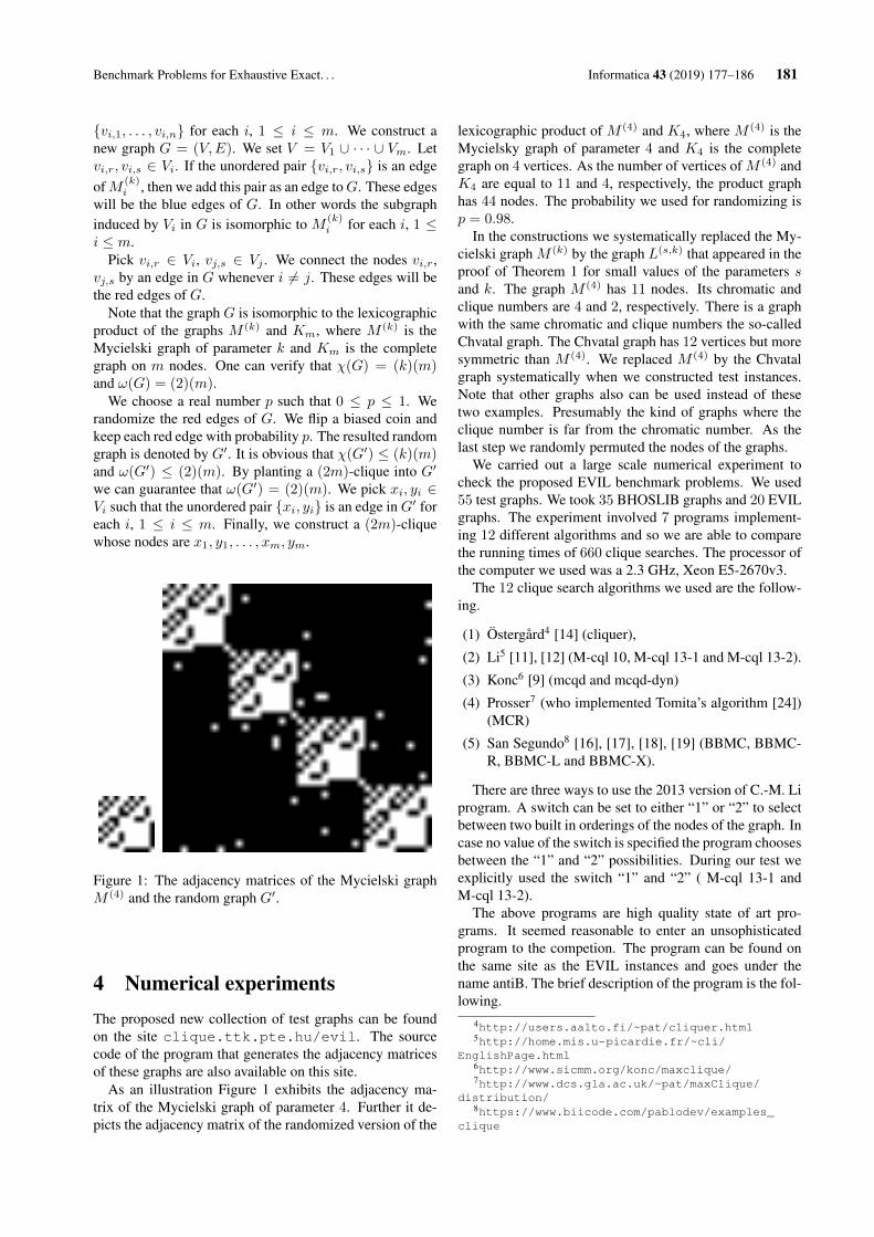
Benchmark Problems for Exhaustive Exact. . . Informatica 43 (2019) 177–186 181
{vi,1, . . . , vi,n} for each i, 1 ≤ i ≤ m. We construct anew graph G = (V,E). We set V = V1 ∪ · · · ∪ Vm. Letvi,r, vi,s ∈ Vi. If the unordered pair {vi,r, vi,s} is an edgeofM (k)
i , then we add this pair as an edge toG. These edgeswill be the blue edges of G. In other words the subgraphinduced by Vi in G is isomorphic to M (k)
i for each i, 1 ≤i ≤ m.
Pick vi,r ∈ Vi, vj,s ∈ Vj . We connect the nodes vi,r,vj,s by an edge in G whenever i 6= j. These edges will bethe red edges of G.
Note that the graph G is isomorphic to the lexicographicproduct of the graphs M (k) and Km, where M (k) is theMycielski graph of parameter k and Km is the completegraph on m nodes. One can verify that χ(G) = (k)(m)and ω(G) = (2)(m).
We choose a real number p such that 0 ≤ p ≤ 1. Werandomize the red edges of G. We flip a biased coin andkeep each red edge with probability p. The resulted randomgraph is denoted by G′. It is obvious that χ(G′) ≤ (k)(m)and ω(G′) ≤ (2)(m). By planting a (2m)-clique into G′
we can guarantee that ω(G′) = (2)(m). We pick xi, yi ∈Vi such that the unordered pair {xi, yi} is an edge in G′ foreach i, 1 ≤ i ≤ m. Finally, we construct a (2m)-cliquewhose nodes are x1, y1, . . . , xm, ym.
Figure 1: The adjacency matrices of the Mycielski graphM (4) and the random graph G′.
4 Numerical experimentsThe proposed new collection of test graphs can be foundon the site clique.ttk.pte.hu/evil. The sourcecode of the program that generates the adjacency matricesof these graphs are also available on this site.
As an illustration Figure 1 exhibits the adjacency ma-trix of the Mycielski graph of parameter 4. Further it de-picts the adjacency matrix of the randomized version of the
lexicographic product of M (4) and K4, where M (4) is theMycielsky graph of parameter 4 and K4 is the completegraph on 4 vertices. As the number of vertices of M (4) andK4 are equal to 11 and 4, respectively, the product graphhas 44 nodes. The probability we used for randomizing isp = 0.98.
In the constructions we systematically replaced the My-cielski graph M (k) by the graph L(s,k) that appeared in theproof of Theorem 1 for small values of the parameters sand k. The graph M (4) has 11 nodes. Its chromatic andclique numbers are 4 and 2, respectively. There is a graphwith the same chromatic and clique numbers the so-calledChvatal graph. The Chvatal graph has 12 vertices but moresymmetric than M (4). We replaced M (4) by the Chvatalgraph systematically when we constructed test instances.Note that other graphs also can be used instead of thesetwo examples. Presumably the kind of graphs where theclique number is far from the chromatic number. As thelast step we randomly permuted the nodes of the graphs.
We carried out a large scale numerical experiment tocheck the proposed EVIL benchmark problems. We used55 test graphs. We took 35 BHOSLIB graphs and 20 EVILgraphs. The experiment involved 7 programs implement-ing 12 different algorithms and so we are able to comparethe running times of 660 clique searches. The processor ofthe computer we used was a 2.3 GHz, Xeon E5-2670v3.
The 12 clique search algorithms we used are the follow-ing.
(1) Östergård4 [14] (cliquer),
(2) Li5 [11], [12] (M-cql 10, M-cql 13-1 and M-cql 13-2).
(3) Konc6 [9] (mcqd and mcqd-dyn)
(4) Prosser7 (who implemented Tomita’s algorithm [24])(MCR)
(5) San Segundo8 [16], [17], [18], [19] (BBMC, BBMC-R, BBMC-L and BBMC-X).
There are three ways to use the 2013 version of C.-M. Liprogram. A switch can be set to either “1” or “2” to selectbetween two built in orderings of the nodes of the graph. Incase no value of the switch is specified the program choosesbetween the “1” and “2” possibilities. During our test weexplicitly used the switch “1” and “2” ( M-cql 13-1 andM-cql 13-2).
The above programs are high quality state of art pro-grams. It seemed reasonable to enter an unsophisticatedprogram to the competion. The program can be found onthe same site as the EVIL instances and goes under thename antiB. The brief description of the program is the fol-lowing.
4http://users.aalto.fi/~pat/cliquer.html5http://home.mis.u-picardie.fr/~cli/
EnglishPage.html6http://www.sicmm.org/konc/maxclique/7http://www.dcs.gla.ac.uk/~pat/maxClique/
distribution/8https://www.biicode.com/pablodev/examples_
clique
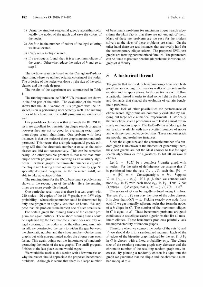
182 Informatica 43 (2019) 177–186 S. Szabo et al.
1) Using the simplest sequential greedy algorithm colorlegally the nodes of the graph and save the colors ofthe nodes.
2) Set k to be the number of colors of the legal coloringwe have located.
3) Carry out a k-clique search.
4) If a k-clique is found, then it is a maximum clique ofthe graph. Otherwise reduce the value of k and go tostep 3.
The k-clique search is based on the Carraghan-Pardalosalgorithm, where we utilized original coloring of the nodes.The ordering of the nodes was done by the size of the colorclasses and the node degrees.
The results of the experiment are summarized in Table1.
The running times on the BHOSLIB instances are shownin the first part of the table. The evaluation of the resultsshows that the 2013 version of Li’s program with the “2”switch is on is performing unexpectedly well. The runningtimes of he cliquer and the antiB programs are outliers aswell.
Our possible explanation is that although the BHOSLIBtests are excellent for heuristic big clique search programshowever they are not so good for evaluating exact maxi-mum clique search algorithms. One problem with theseinstances is that the nodes of these graphs are not randomlypermuted. This means that a simple sequential greedy col-oring will find the chromatic number at once, as the colorclasses are laid out consecutively. This can be remediedeasily. An other possible problem is that most maximumclique search programs use coloring as an auxiliary algo-rithm. For these graphs the chromatic number is equal tothe clique size leaving a zero optimality or duality gap. Sospecially designed programs, as the presented antiB, areable to take advantage of this.
The running times for the EVIL benchmark problems areshown in the second part of the table. Here the runningtimes are more evenly distributed.
One particular result was that there is a test graph with220 nodes – 20 copies of the M (4) graph, p = 98% edgeprobability – whose clique number could be determined byonly one program in slightly less than 12 hours. We sup-pose that this problem is the hardest one of such small size.
For certain graph the running times of the cliquer pro-gram are again outliers. These short running times couldbe explained by the fact that the cliquer does not rely onlegal coloring of the nodes as do the other programs. Af-ter all, we constructed the tests to widen the gap betweenthe chromatic number and the clique number. On the samegraphs but with non-permuted nodes the cliquer runs evenfaster. This again points out the importance of randomlypermuting the nodes of the test graphs. The antiB programfinishes at the last place as one would expect.
We would like to close this section with a few remarks onwhy the reader should appreciate the proposed benchmarkproblems. Although it seems that there is a large number
of benchmark problems for maximum clique search algo-rithms the plain fact is that there are not enough of them.Many of these test problems are too easy for the modernsolvers as the sizes of these problems are small. On theother hand there are test instances that are overly hard forthe contemporary clique solvers. The proposed EVIL testgraphs are forming parameterized families. The parameterscan be tuned to produce benchmark problems in various de-grees of difficulty.
5 A historical thread
The graphs that are used for benchmarking clique search al-gorithms are coming from various walks of discrete math-ematics and its applications. In this section we will followa particular thread in order to shed some light on the forcesand demands that shaped the evolution of certain bench-mark problems.
By the lack of other possibilities the performance ofclique search algorithms are commonly evaluated by car-rying out large scale numerical experiments. Historicallythe first clique search procedures were tested almost exclu-sively on random graphs. The Erdos-Rényi random graphsare readily available with any specified number of nodesand with any specified edge densities. These random graphare popular and useful test instances.
Since the clique size and the chromatic number of a ran-dom graph is unknown at the moment of generating them,these test graphs are not the ideal choices to test k-cliquesearch algorithms or for algorithms to list all maximumcliques.
Let G = (V,E) be a complete k-partite graph withn nodes. For the sake of definiteness we assume that Vis partitioned into the sets V1, . . . , Vk such that |V1| =· · · = |Vk| = s. Consequently n = ks. SupposeVi = {vi,1, . . . , vi,s}. If i 6= j, then we connect eachnode vi,α in Vi with each node vj,β in Vj . Thus G has(1/2)k(k − 1)s2 edges, that is, |E| = (1/2)k(k − 1)s2.
The nodes of G can be legally colored using k colors.The sets V1, . . . , Vk can play the roles of the color classes.It is clear that ω(G) = k. Picking exactly one node fromeach Vi we get mutually adjacent nodes that form the nodesof a k-clique in G. The number of the maximum cliquesin G is equal to sk. These benchmark problems are goodcandidates to test clique search algorithms that list all max-imum cliques. These benchmark problems painfully lackthe unpredictability of random graphs.
Therefore when we connect the nodes of the sets Vi andVj we should do it in a randomized manner. Each of thes2 edges of the bipartite graph induced by the set Vi ∪ Vjin G is chosen with a fixed probability pi,j . The cliquesize of the resulting random graph may decrease and thechromatic number of the resulting random graph may in-crease. By planting a randomly chosen k-clique into thegraph we guarantee that the clique and the chromatic num-ber are equal to k.

Benchmark Problems for Exhaustive Exact. . . Informatica 43 (2019) 177–186 183
These graphs are the BHOSLIB instances. The develop-ment of these graphs greatly enhanced the utility of randomgraphs in testing clique search algorithms.
A graph whose chromatic number is equal to its cliquenumber is by no means is a typical graph. This is why wepropose a family of test graphs that have all the desiredproperties of the BHOSLIB graph and in the same time thegap between the clique and chromatic numbers can be setin a more flexible manner.
Let G = (V,E) be the graph we intend to construct.Let us start with a graph M = (W,F ) such that ω(M) =r, χ(M) = s are known. Suppose W = {w1, . . . , wm}.We consider k isomorphic copies M1, . . . ,Mk of M . LetMi = (Wi, Fi), where Wi = {wi,1, . . . , wi,m}.
In order to construct the graph G we set V = W1 ∪· · · ∪Wk. Here we assume that the sets W1, . . . ,Wk arepair-wise disjoint. Consequently G has km nodes. Let uspick two distinct Wi and Wj . We connect wiα and wj,βfor each α, β, 1 ≤ α, β ≤ m. The resulting graph G haskm nodes and k|F | + (1/2)k(k − 1)m2 edges. Clearly,ω(G) = kω(M) = kr and χ(G) = kχ(M) = ks.
As a next step we randomize G. Namely, we pick eachof the m2 edges running between Wi and Wj with a fixedprobability pi,j . (In many cases we choose all pi,j to beequal.) Because we drop edges from the graphG, the quan-tities ω(G), χ(G) may change. By planting a random (kr)-clique we may restore the original ω(G). The chromaticnumber of the new random graph may decrease. If theprobability pi,j is close to one then most likely the decreasein the chromatic number is small. When we choose a graphM for which ω(M) is much smaller than χ(M), then forthe resulted random graph the gap between the clique andchromatic numbers most likely does not disappear.
The resulting random graphs are the test instances pro-posed in this paper.
The Szemerédi regularity lemma teaches us that a largedense graph can be transformed into a form which is verymuch similar to our proposed graph. So the proposed graphin a sense is not overly artificial.
6 Reducing the number of nodes
We use the graphs L(s,k) defined in the proof of Theorem1 to construct benchmark instances. It is imperative to con-struct hard benchmark instances with as few nodes as possi-ble. In this section we will show that with a little extra carewe can reduce the number of the nodes and still get a graphwhich has the required properties of the graphs L(s,k). Forthe sake of simplicity we will restrict our attention to thespecial case s = 3.
Let G = (V,E) be a finite simple graph. A subset C ofV is called an edge covering set of G if each edge of G hasat least one end point in C.
Let µ(k) be the number of the nodes of the Mycielskigraph M (k) of parameter k. The Mycielski graph M (3) isa circle consisting of 5 nodes and 5 edges. Thus µ(3) =
5. The Mycielski graph M (k+1) is constructed from theMycielski graph M (k) in the following way.
Suppose U = {u1, . . . , un} is the set of nodes of M (k).Here of course n = µ(k). In order to construct M (k+1)
from M (k) we add new nodes v1, . . . , vn to the existingnodes u1, . . . , un. We set V = {v1, . . . , vn}. We assumethat the nodes u1, . . . , un and v1, . . . , vn are pair-wise dis-tinct. In other words we assume that U ∩ V = ∅. We drawan edge between the node vi and each neighbor of the nodeui for each i, 1 ≤ i ≤ n. Finally we add a new node w tothe set of nodes U ∪V and draw an edge between the nodew and vi for each i, 1 ≤ i ≤ n.
Note that the equation µ(k + 1) = 2µ(k) + 1 holds andusing µ(3) = 5 one can compute the number of nodes ofthe Mycielski graph M (k).
Lemma 1. The Mycielski graph M (k) has an edge cover-ing set of size µ(k − 1) + 1 for each k ≥ 3.
Proof. For k = 3 the Mycielski graph is a circle consistingof 5 vetices and 5 edges. Two adjacent nodes x, y and anode z that is not adjacent to any of x, y form an edgecovering set in M (3). This proves the lemma in the specialcase k = 3.
For the remaining part of the proof we may assume thatk ≥ 4. We proceed by an induction on k. The My-cielski graph M (k) has some nodes u1, . . . , un such thatn = µ(k − 1) and the subset U = {u1, . . . , un} induces asubgraph that is isomorphic to M (k−1).
The Mycielski graph M (k) has some nodes v1, . . . , vnsuch that vi is adjacent to each neighbor of ui for each i,1 ≤ i ≤ n. Finally, M (k) has a node w which is adjacentto vi for each i, 1 ≤ i ≤ n.
The set C = U ∪ {w} is an edge covering set in M (k).This completes the proof of the lemma. 2
We do not claim that this edge covering set has the smallestpossible number of nodes.
Lemma 2. For each integer k ≥ 3 there is a graph N (k)
such that it has [µ(k − 1) + 1]µ(k) + µ(k − 1) nodesω(N (k)) ≤ 4 and χ(3)(N (k)) ≥ k.
Proof. We start the construction ofN (k) with the Mycielskigraph M (k). We assume that U = {u1, . . . , un} is the setof nodes of M (k). By Lemma 1, the graph M (k) has anedge covering set C, where n = µ(k) and |C| = µ(k −1) + 1.
We will assign a subgraph Li to the node ui of the graphM (k) for each i, 1 ≤ i ≤ n. The graph Li is either a graphconsisting of one single node vi,1 or Li is an isomorphiccopy of the Mycielski graph M (k). In this second case theset of nodes of Li is equal to Vi = {vi,1, . . . , vi,r}, wherer = µ(k).
If ui 6∈ C, then to the node ui we assign the graph Liwhich consists of a single node. If ui ∈ C, then to the nodeui we assign the graph Li which has µ(k) nodes.
Let us suppose that the unordered pair {ui, uj} is anedge of the graphM (k). We draw edges between each node

184 Informatica 43 (2019) 177–186 S. Szabo et al.
of Li and each node of Lj . The result of repeating this pro-cedure for each edges of the graph M (k) will be the graphN (k). Clearly, N (k) has
[µ(k − 1) + 1]µ(k) + µ(k)− µ(k − 1)− 1 =
[µ(k − 1) + 1]µ(k) + 2µ(k − 1) + 1− µ(k − 1)− 1 =
[µ(k − 1) + 1]µ(k) + µ(k − 1)
nodes. It remains to show that ω(N (k)) ≤ 4 andχ(3)(N (k)) ≥ k.
In order to prove that ω(N (k)) ≤ 4 we assume on thecontrary that ω(N (k)) ≥ 5. Let ∆ be a 5-clique in N (k).Note that
ω(Li) =
{1, if |Vi| = 1,2, if |Vi| = µ(k).
The clique ∆ may contain at most one node from Li forwhich |Vi| = 1. The clique ∆ may contain at most twonodes from Li when |Vi| = µ(k). It follows that theremust be at least three distinct values of i for which thegraph Li contains a node from the 5-clique ∆. This givesat least three distinct values of i for which the nodes uipair-wise adjacent. But M (k) does not have any 3-cliqueas ω(M (k)) ≤ 2.
In order to prove that χ(3)(N (k)) ≥ k we assume on thecontrary that χ(3)(N (k)) ≤ k−1. Let V = V1∪· · ·∪Vn bethe set of nodes ofN (k) and let f : V → {1, . . . , k−1} be amap that describes the monochrome 3-clique free coloringof the nodes of N (k).
Consider a subgraph Li of N (k). Let gi be the re-striction of f to Vi = {vi,1, . . . , vi,r}. Plainly, the mapgi : Vi → {1, . . . , k − 1} describes a coloring of the nodesof the graph Li. Using the facts that Li is isomorphic toM (k) and χ(M (k)) ≥ k we can draw the conclusion thatthere must be two distinct adjacent nodes of M (k) that re-ceive the same color.
Remember that U = {u1, . . . , un} is the set of nodes ofthe Mycielski graph M (k) we used in the construction ofN (k). We define a map h : U → {1, . . . , k − 1}.
If the subgraph Li of N (k) has only one node, then weset h(ui) to be f(vi,1). In plain English we assign the colorof the only node of the graph Li to the node ui of the graphM (k).
If the subgraphLi ofN (k) has µ(k) nodes, then there aretwo distinct adjacent nodes of Li, say vi,i(1), vi,i(2) suchthat f(vi,i(1)) = f(vi,i(2)). In this case we set h(ui) to bef(vi,i(1)). In simple English assign the common color ofthe adjacent nodes vi,i(1), vi,i(2) of N (k) to the node ui ofM (k).
We claim that the map h : U → {1, . . . , k−1} describesa legal coloring of the nodes of M (k). The only thing weshould check is that if ui, uj are distinct adjacent nodes ofM (k), then h(ui) 6= h(uj) must hold.
Let us start with the case when ui 6∈ C, uj 6∈ C. Theassumption that ui, uj are distinct adjacent nodes of M (k)
contradicts the fact that C is an edge covering set in M (k).Therefore this case cannot occur.
If ui ∈ C, uj ∈ C, then the subgraphs Li, Lj of N (k)
both have µ(k) nodes. There are distinct adjacent nodesvi,i(1), vi,i(2) in Li such that f(vi,i(1)) = f(vi,i(2)) =h(ui). Similarly, there are distinct adjacent nodes vj,j(1),vj,j(2) in Lj such that f(vj,j(1)) = f(vj,j(2)) = h(uj).Here h(ui) 6= h(uj) must hold since otherwise we have a4-clique in N (k) whose nodes receive the same color. Thiscannot happen as the map f : V → {1, . . . , k − 1} de-scribes a monochrome 3-clique free coloring of the nodesof N (k).
If ui 6∈ C, uj ∈ C, then the subgraph Li of N (k)
has only one node and the subgraph Lj of N (k) hasµ(k) nodes. Now f(vi,1) = h(ui). There are dis-tinct adjacent nodes vj,j(1), vj,j(2) in Lj such thatf(vj,j(1)) = f(vj,j(2)) = h(uj). This time h(ui) 6= h(uj)
must hold since otherwise we have a 3-clique in N (k)
whose nodes receive the same color. This cannot happen asthe map f : V → {1, . . . , k − 1} describes a monochrome3-clique free coloring of the nodes of N (k). 2
AcknowledgmentsThis research was supported by National Research, Devel-opment and Innovation Office – NKFIH Fund No. SNN-117879.
References[1] I. M. Bomze, M. Budinich, P. M. Pardalos, M. Pelillo
(1999) The Maximum Clique Problem, Handbookof Combinatorial Optimization Vol. 4, Kluwer Aca-demic Publisher. https://doi.org/10.1007/978-1-4757-3023-4_1
[2] C. Bron and J. Kerbosch (1973) Finding allcliques of an undirected graph, Communicationsof ACM 16, 575–577. https://doi.org/10.1145/362342.362367
[3] R. Carraghan, P. M. Pardalos (1990) An exact al-gorithm for the maximum clique problem, Opera-tion Research Letters 9, 375–382. https://doi.org/10.1016/0167-6377(90)90057-C
[4] P. Erdos, A. Rényi (1960) On the evolution of randomgraphs, Magyar Tud. Akad. Mat. Kutató Int. Közl. 5,17–61.
[5] P. Erdos (1959), Graph theory and probability, Canad.J. Math. 11, 34–38.
[6] M. R. Garey and D. S. Johnson (2003), Computersand Intractability: A Guide to the Theory of NP-completeness, Freeman, New York.
[7] R. Hammack, W. Imrich, S. Klavžar (2011) Hand-book of Product Graphs, CRC Press, Boca Raton, FL.
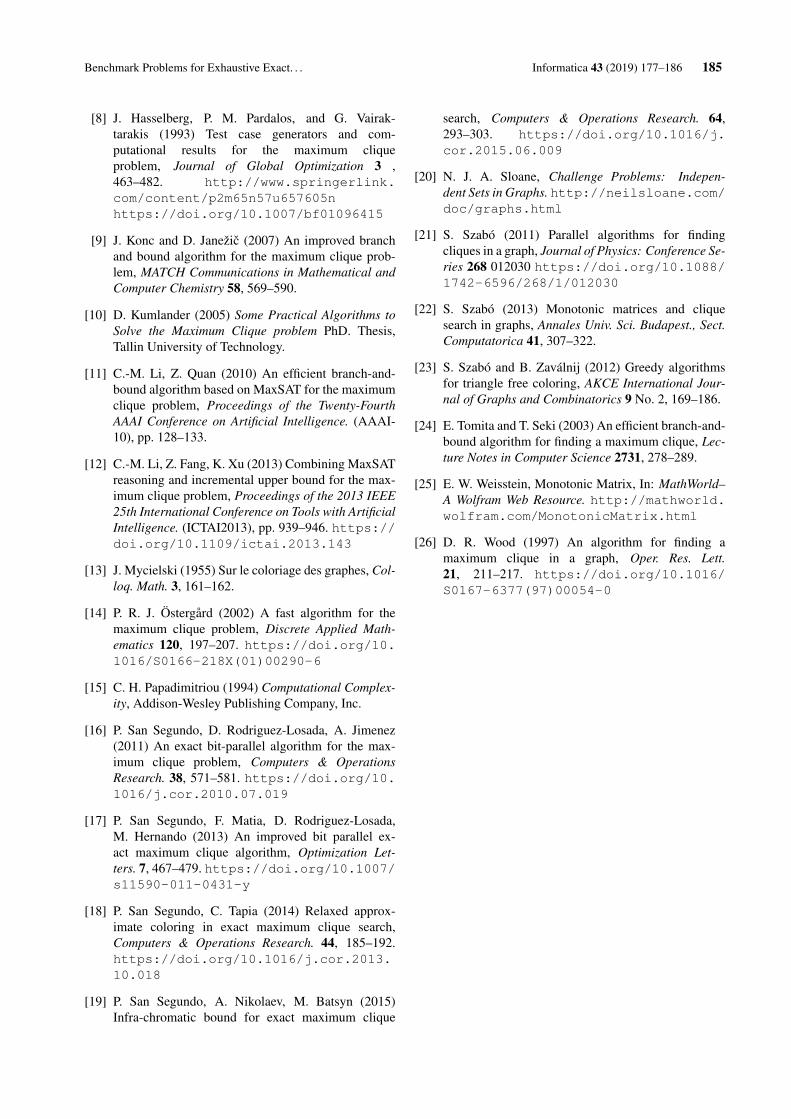
Benchmark Problems for Exhaustive Exact. . . Informatica 43 (2019) 177–186 185
[8] J. Hasselberg, P. M. Pardalos, and G. Vairak-tarakis (1993) Test case generators and com-putational results for the maximum cliqueproblem, Journal of Global Optimization 3 ,463–482. http://www.springerlink.com/content/p2m65n57u657605nhttps://doi.org/10.1007/bf01096415
[9] J. Konc and D. Janežic (2007) An improved branchand bound algorithm for the maximum clique prob-lem, MATCH Communications in Mathematical andComputer Chemistry 58, 569–590.
[10] D. Kumlander (2005) Some Practical Algorithms toSolve the Maximum Clique problem PhD. Thesis,Tallin University of Technology.
[11] C.-M. Li, Z. Quan (2010) An efficient branch-and-bound algorithm based on MaxSAT for the maximumclique problem, Proceedings of the Twenty-FourthAAAI Conference on Artificial Intelligence. (AAAI-10), pp. 128–133.
[12] C.-M. Li, Z. Fang, K. Xu (2013) Combining MaxSATreasoning and incremental upper bound for the max-imum clique problem, Proceedings of the 2013 IEEE25th International Conference on Tools with ArtificialIntelligence. (ICTAI2013), pp. 939–946. https://doi.org/10.1109/ictai.2013.143
[13] J. Mycielski (1955) Sur le coloriage des graphes, Col-loq. Math. 3, 161–162.
[14] P. R. J. Östergård (2002) A fast algorithm for themaximum clique problem, Discrete Applied Math-ematics 120, 197–207. https://doi.org/10.1016/S0166-218X(01)00290-6
[15] C. H. Papadimitriou (1994) Computational Complex-ity, Addison-Wesley Publishing Company, Inc.
[16] P. San Segundo, D. Rodriguez-Losada, A. Jimenez(2011) An exact bit-parallel algorithm for the max-imum clique problem, Computers & OperationsResearch. 38, 571–581. https://doi.org/10.1016/j.cor.2010.07.019
[17] P. San Segundo, F. Matia, D. Rodriguez-Losada,M. Hernando (2013) An improved bit parallel ex-act maximum clique algorithm, Optimization Let-ters. 7, 467–479. https://doi.org/10.1007/s11590-011-0431-y
[18] P. San Segundo, C. Tapia (2014) Relaxed approx-imate coloring in exact maximum clique search,Computers & Operations Research. 44, 185–192.https://doi.org/10.1016/j.cor.2013.10.018
[19] P. San Segundo, A. Nikolaev, M. Batsyn (2015)Infra-chromatic bound for exact maximum clique
search, Computers & Operations Research. 64,293–303. https://doi.org/10.1016/j.cor.2015.06.009
[20] N. J. A. Sloane, Challenge Problems: Indepen-dent Sets in Graphs. http://neilsloane.com/doc/graphs.html
[21] S. Szabó (2011) Parallel algorithms for findingcliques in a graph, Journal of Physics: Conference Se-ries 268 012030 https://doi.org/10.1088/1742-6596/268/1/012030
[22] S. Szabó (2013) Monotonic matrices and cliquesearch in graphs, Annales Univ. Sci. Budapest., Sect.Computatorica 41, 307–322.
[23] S. Szabó and B. Zaválnij (2012) Greedy algorithmsfor triangle free coloring, AKCE International Jour-nal of Graphs and Combinatorics 9 No. 2, 169–186.
[24] E. Tomita and T. Seki (2003) An efficient branch-and-bound algorithm for finding a maximum clique, Lec-ture Notes in Computer Science 2731, 278–289.
[25] E. W. Weisstein, Monotonic Matrix, In: MathWorld–A Wolfram Web Resource. http://mathworld.wolfram.com/MonotonicMatrix.html
[26] D. R. Wood (1997) An algorithm for finding amaximum clique in a graph, Oper. Res. Lett.21, 211–217. https://doi.org/10.1016/S0167-6377(97)00054-0

186 Informatica 43 (2019) 177–186 S. Szabo et al.
antiB BBMC BBMC BBMC BBMC M-clq M-clq M-clq mcqd mcqd MCR cliquername |V | % ω(G) -R -L -X 10 13-1 13-2 -dyn
frb30-15-1.clq 450 82 30 0 1611 1645 1694 1613 575 629 0 2735 2541 3673 21frb30-15-2.clq 450 82 30 0 1010 1094 1191 1047 921 990 0 3329 4155 905 43frb30-15-3.clq 450 82 30 0 602 581 623 556 432 429 0 1305 2767 300 194frb30-15-4.clq 450 82 30 0 1855 1768 1901 1676 1154 617 0 5763 4996 2698 2frb30-15-5.clq 450 82 30 0 1273 1213 1437 1154 726 1110 0 1997 4536 1355 0frb35-17-1.clq 595 84 35 1 – – – – – – 1 – – 34983 18frb35-17-2.clq 595 84 35 1 – – – – – – 1 – – – 104frb35-17-3.clq 595 84 35 2 – – – – – – 0 – – 22607 14493frb35-17-4.clq 595 84 35 1 – – – – 27231 42219 0 – – 5249 7923frb35-17-5.clq 595 84 35 5 – – – – – – 0 – – – 181frb40-19-1.clq 760 86 40 0 – – – – – – 1 – – 11589 –frb40-19-2.clq 760 86 40 1 – – – – – – 0 – – – –frb40-19-3.clq 760 86 40 8 – – – – – – 0 – – – 353frb40-19-4.clq 760 86 40 38 – – – – – – 7 – – – 2296frb40-19-5.clq 760 86 40 10 – – – – – – 5 – – – 78frb45-21-1.clq 945 87 45 0 – – – – – – 119 – – – –frb45-21-2.clq 945 87 45 118 – – – – – – 72 – – – –frb45-21-3.clq 945 87 45 122 – – – – – – 44 – – – –frb45-21-4.clq 945 87 45 218 – – – – – – 36 – – – –frb45-21-5.clq 945 87 45 475 – – – – – – 203 – – – –frb50-23-1.clq 1150 88 50 16385 – – – – – – 764 – – – –frb50-23-2.clq 1150 88 50 10145 – – – – – – 363 – – – –frb50-23-3.clq 1150 88 50 12585 – – – – – – 7938 – – – –frb50-23-4.clq 1150 88 50 501 – – – – – – 17 – – – 2754frb50-23-5.clq 1150 88 50 18256 – – – – – – 221 – – – –frb53-24-1.clq 1272 88 53 73 – – – – – – 4771 – – – –frb53-24-2.clq 1272 88 53 – – – – – – – 190 – – – –frb53-24-3.clq 1272 88 53 2910 – – – – – – 2091 – – – –frb53-24-4.clq 1272 88 53 29815 – – – – – – 4022 – – – –frb53-24-5.clq 1272 88 53 27671 – – – – – – 1071 – – – –frb59-26-1.clq 1534 89 59 – – – – – – – – – – – –frb59-26-2.clq 1534 89 59 42408 – – – – – – – – – – –frb59-26-3.clq 1534 89 59 – – – – – – – – – – – –frb59-26-4.clq 1534 89 59 – – – – – – – – – – – –frb59-26-5.clq 1534 89 59 – – – – – – – 11661 – – – –chv12x10.clq 120 92 20 – 4 5 4 1 1 8 0 4759 48 700 0myc5x24.clq 120 97 48 14536 0 0 0 0 0 0 0 2 1 4 112
myc11x11.clq 121 93 22 – 8 12 7 2 1 7 0 1097 85 1081 239s3m25x5.clq 125 89 20 5440 6 8 6 5 1 1 0 5 6 9 0myc23x6.clq 138 87 12 1681 2 3 2 2 2 57 0 4 7 56 699myc5x30.clq 150 97 60 – 1 1 1 0 0 0 0 10 2 47 42042s3m25x6.clq 150 90 24 – 192 278 195 186 4 12 8 64 92 128 0
myc11x14.clq 154 94 28 – 486 566 422 66 33 235 23 – 11563 – –chv12x15.clq 180 94 30 – 26019 34161 26045 7796 1235 26798 184 – – – 0myc5x36.clq 180 97 72 – 3 2 3 2 0 0 0 17 6 118 –myc23x8.clq 184 90 16 – 115 165 112 88 215 23434 90 1138 1390 – –
myc11x17.clq 187 95 34 – 40109 – 33957 5056 2378 43935 2375 – – – 3159s3m25x8.clq 200 92 32 – 46253 – 44843 38987 181 1206 478 22778 18148 40089 0myc5x42.clq 210 98 84 – 26 15 25 4 0 0 0 443 36 1414 –
myc11x20.clq 220 95 40 – – – – – – – 38519 – – – –myc23x10.clq 230 91 20 – – – – 38104 26210 – 7545 – – – –chv12x20.clq 240 95 40 – – – – – – – – – – – –myc5x48.clq 240 97 96 – 23 22 25 13 0 0 0 319 39 3316 –
s3m25x10.clq 250 93 40 – – – – – 6980 44122 – – – – 18myc11x23.clq 253 95 46 – – – – – – – – – – – –
Table 1: Running time results in seconds for the BHOSLIB and EVIL instances. The “–” sign indicates that the runningtimes are exceeding the 12 hour limit.
https://doi.org/10.31449/inf.v43i2.1621 Informatica 43 (2019) 187–198 187
Mutual Information Based Feature Selection for Fingerprint
Identification
Ahlem Adjimi and Abdenour Hacine-Gharbi
LMSE laboratory, University of Bordj Bou Arreridj, Elanasser, 34030 Bordj Bou Arreridj, Algeria
E-mail: [email protected], [email protected]
Philippe Ravier
PRISME laboratory, University of Orleans, 12 rue de Blois, 45067 Orléans, France
E-mail: [email protected], +0033238494863
Messaoud Mostefai
LMSE laboratory, University of Bordj Bou Arreridj, Elanasser, 34030 Bordj Bou Arreridj, Algeria
E-mail: [email protected]
Keywords: fingerprint identification, feature selection, dimensionality reduction, mutual information, local binary
patterns, local phase quantization, histogram of gradients, binarized statistical image features
Received: May 3, 2017
In the field of fingerprint identification, local histograms coding is one of the most popular techniques
used for fingerprint representation, due to its simplicity. This technique is based on the concatenation of
the local histograms resulting in a high dimension histogram, which causes two problems. First, long
computing time and big memory capacities are required with databases growing. Second, the recognition
rate may be degraded due to the curse of dimensionality phenomenon. In order to resolve these problems,
we propose to reduce the dimensionality of histograms by choosing only the pertinent bins from them
using a feature selection approach based on the mutual information computation. For fingerprint features
extraction we use four descriptors: Local Binary Patterns (LBP), Histogram of Gradients (HoG), Local
Phase Quantization (LPQ) and Binarized Statistical Image Features (BSIF). As mutual information based
selection methods, we use four strategies: Maximization of Mutual Information (MIFS), minimum
Redundancy and Maximal Relevance (mRMR), Conditional Info max Feature Extraction (CIFE) and Joint
Mutual Information (JMI). We compare results in terms of recognition rates and number of selected
features for the investigated descriptors and selection strategies. Our results are conducted on the four
FVC 2002 datasets which present different image qualities. We show that the combination of mRMR or
CIFE feature selection methods with HoG features gives the best results. We also show that the selection
of useful fingerprint features can surely improve the recognition rate and reduce the complexity of the
system in terms of computation cost. The feature selection algorithms may reach 98% of time reduction
by considering only 20% of the total number of features while also improving the recognition rate of about
2% by avoiding the curse of dimensionality phenomena.
Povzetek: Analizirani so različni načini opisa in preiskovanja pri histogramskem kodiranju identifikacije
prstnih odtisov.
1 Introduction Biometric recognition has gained a considerable interest
in the recent years because of the various applications in
the large field of security. Security can be categorized in
data access security (computer and mobile access, USB
key, bank cards) or in person access security (forensic
identification, ID access). Many technological solutions
exist relying on distinctive biometric identifiers (e.g.
fingerprints, face, iris or speech) each one having its own
qualities. However, the most used biometric identifiers are
the fingerprints due to their uniqueness, persistence,
simplicity of acquisition and the availability of the
electronic acquisition devices [1]. Indeed, the fingerprints
are single to each person and they remain unchanged
during all the life of the person.
Fingerprint recognition systems can be categorized into
three main approaches: minutiae-based systems, image-
based correlation systems and image-based distance
systems [2]. For the first category, the fingerprint image
must pass through several preprocessing steps to detect
and extract some points of interest called minutiae:
smoothing, local ridge orientation estimation,
binarization, thinning, and minutia detection. The second
category directly estimates the similarity between a test
and a reference fingerprint pattern by the autocorrelation
method. For the third category, global or local features are
extracted from the fingerprint image such that the features
also called descriptors retain most of the pertinent
information representing the fingerprint. This kind of
188 Informatica 43 (2019) 188–198 A. Adjimi et al.
fingerprint recognition systems is preferred in the case of
low quality images, because it is difficult to extract
reliable minutiae sets in this case [3]. A distance measure
between a test and a reference fingerprint pattern or any
other classifier are finally used for making a matching
decision [3].
Within this last category, many descriptors have been
proposed. These descriptors can be principally grouped
into histogram-based features or linear transformed
features. The descriptors of the first group exploit some
statistical characteristics of the fingerprint by
transforming the image into a histogram of fixed length
like Local Binary Patterns (LBP), Gabor filter with Local
Binary Patterns (GLBP) hybrid method [4], Local Phase
Quantization (LPQ) [5], Histogram of Gradients [6] or
Binarized Statistical Image Features (BSIF) [7] or Scale
Invariant Feature Transform (SIFT) [8][9]. In the second
group, the fingerprint image is transformed into a vector
of different features extracted from the fingerprint image
such as Discrete Cosine Transform (DCT) features [10],
Gabor filters based descriptors [11][12] and Discrete
Wavelet Transform (DWT) features [13][14][15][16].
In this work, we focus on the histogram-based
fingerprint representation techniques such as LBP, LPQ,
HoG and BSIF. Indeed, these techniques are very used for
fingerprint recognition due to their simplicity. These
techniques are based on the concatenation of the local
histograms leading to a histogram of great dimension
(e.g.1024 features for each fingerprint in the case of LBP),
which requires long computing time, big memory capacity
and requires a huge training dataset to model the classes.
Practically, it has been observed that features addition can
cause a performance degradation of the classifier if the
number of data used for the classifier designing is too low
relatively to the number of features [17][18]. This
phenomenon called the curse of dimensionality leads to
the phenomenon of "peaking" [19]. So it is desirable to
keep the number of features as small as possible which is
also of benefit for reducing computational cost in the
fingerprint identification task and for avoiding memory
obstruction too. Keeping a small number of features is a
dimensionality reduction operation, which can be done
with two approaches: the first approach is a features
transformation in which the initial features set is replaced
by a new reduced set using transformation algorithm like
PCA (Principal Component Analysis), LDA (Linear
Discriminant Analysis)…. The second approach is a
features selection which selects the relevant features from
the initial features set [20]. However, using a reduced set
of features by transformation needs greater memory
capacity and more computing time in the testing phase
compared to using a reduced set of features obtained by
selection algorithms [20] because the former requires
computation of all the features before reduction. So, in the
present work, we have considered the features selection
algorithms to select the relevant bins of histograms for the
histogram-based fingerprint representation techniques.
The feature selection methods are also divided into two
categories, which are “wrapper” or “filter”. In “wrapper”
methods, the relevance measure for a features subset is the
training/testing recognition rate of the used classifier.
Consequently, the wrapper selection procedure makes the
computational cost rapidly increase, because a new
classifier has to be built with training and testing phases
each time a features subset is tested. Moreover, the
features selected by wrapper methods are adapted to the
used classifier, so their performance results are dependent
on the type of classifier. In contrast, “filter” methods
evaluate the features subset relevance independently of the
classifier, so the selected features can be used for any
classifier modelling [20][21]. For all these reasons, we
have chosen the “filter” methods, which are the preferable
methods in the case of high dimensionality and large
datasets for computational reasons. The “filter” methods use a selection criterion typically
based on information theory tools like Mutual Information
(MI) useful for measuring the quantity of information that
features may have for describing the data. To our
knowledge, only few works have investigated the MI
based criteria in the field of biometric identification.
In [22], an efficient code selection method for face
recognition is presented and compact LBP codes are
obtained. The code selection is based on the maximization
of mutual information (MMI) between features (LBP
codes) and class labels. Applying this principle for
selection is achieved by using the max-relevance and min-
redundancy (mRMR) criterion. The method proposed
consists of transforming the face images into LBP
histograms, then selecting the relevant codes from these
histograms using the maximization of the mutual
information. In this work the authors have used the chi-
square formula for measuring the distance between the
histograms of the reference and the test templates.
In [23], the BSIF features have been investigated in the
frame of a fingerprint recognition system, with
preliminary results of feature selection using the FVC2002
fingerprint dataset [24]. The experiments have shown that
an increasing number of extracted sub-images leads to an
increasing recognition rate, but also leads to higher
dimension histograms which decreased accordingly
performance of the system regarding computing time and
memory capacity. This motivated the use of MI feature
selection strategy, namely interaction capping (ICAP).
In this work, we extend the fingerprint recognition
system proposed in [23] by considering more datasets
within the FVC2002 fingerprint database, more descriptor
types and by investigating several other feature selection
strategies, all based on mutual information computation to
select the relevant bins of histograms that are extracted
from the fingerprint images. The present study will focus
on robustness of the fingerprint system regarding various
descriptors and noisy datasets. The main aim of this work
is to find a combination of feature selection method with
a pertinent descriptor type in a larger context than in study
[23]. To that aim, next section introduces the former
developments of [23] and explains the novelty of the
present paper comparatively. Section 3 proposes a brief
review of all the descriptors used in this paper. Section 4
describes the feature selection methods based on mutual
information. In section 5 we present the experimental
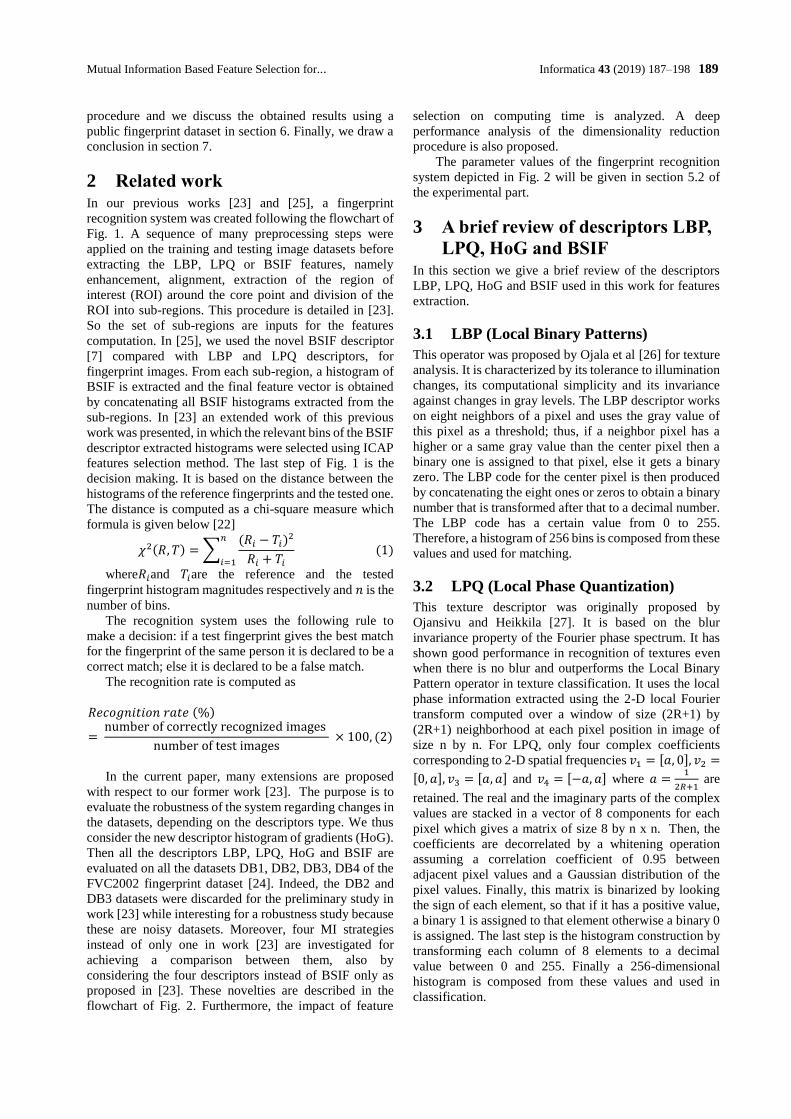
Mutual Information Based Feature Selection for... Informatica 43 (2019) 187–198 189
procedure and we discuss the obtained results using a
public fingerprint dataset in section 6. Finally, we draw a
conclusion in section 7.
2 Related work In our previous works [23] and [25], a fingerprint
recognition system was created following the flowchart of
Fig. 1. A sequence of many preprocessing steps were
applied on the training and testing image datasets before
extracting the LBP, LPQ or BSIF features, namely
enhancement, alignment, extraction of the region of
interest (ROI) around the core point and division of the
ROI into sub-regions. This procedure is detailed in [23].
So the set of sub-regions are inputs for the features
computation. In [25], we used the novel BSIF descriptor
[7] compared with LBP and LPQ descriptors, for
fingerprint images. From each sub-region, a histogram of
BSIF is extracted and the final feature vector is obtained
by concatenating all BSIF histograms extracted from the
sub-regions. In [23] an extended work of this previous
work was presented, in which the relevant bins of the BSIF
descriptor extracted histograms were selected using ICAP
features selection method. The last step of Fig. 1 is the
decision making. It is based on the distance between the
histograms of the reference fingerprints and the tested one.
The distance is computed as a chi-square measure which
formula is given below [22]
𝜒2(𝑅, 𝑇) = ∑(𝑅𝑖 − 𝑇𝑖)2
𝑅𝑖 + 𝑇𝑖
𝑛
𝑖=1 (1)
where𝑅𝑖and 𝑇𝑖are the reference and the tested
fingerprint histogram magnitudes respectively and 𝑛 is the
number of bins.
The recognition system uses the following rule to
make a decision: if a test fingerprint gives the best match
for the fingerprint of the same person it is declared to be a
correct match; else it is declared to be a false match.
The recognition rate is computed as
𝑅𝑒𝑐𝑜𝑔𝑛𝑖𝑡𝑖𝑜𝑛 𝑟𝑎𝑡𝑒 (%)
= number of correctly recognized images
number of test images × 100, (2)
In the current paper, many extensions are proposed
with respect to our former work [23]. The purpose is to
evaluate the robustness of the system regarding changes in
the datasets, depending on the descriptors type. We thus
consider the new descriptor histogram of gradients (HoG).
Then all the descriptors LBP, LPQ, HoG and BSIF are
evaluated on all the datasets DB1, DB2, DB3, DB4 of the
FVC2002 fingerprint dataset [24]. Indeed, the DB2 and
DB3 datasets were discarded for the preliminary study in
work [23] while interesting for a robustness study because
these are noisy datasets. Moreover, four MI strategies
instead of only one in work [23] are investigated for
achieving a comparison between them, also by
considering the four descriptors instead of BSIF only as
proposed in [23]. These novelties are described in the
flowchart of Fig. 2. Furthermore, the impact of feature
selection on computing time is analyzed. A deep
performance analysis of the dimensionality reduction
procedure is also proposed.
The parameter values of the fingerprint recognition
system depicted in Fig. 2 will be given in section 5.2 of
the experimental part.
3 A brief review of descriptors LBP,
LPQ, HoG and BSIF In this section we give a brief review of the descriptors
LBP, LPQ, HoG and BSIF used in this work for features
extraction.
3.1 LBP (Local Binary Patterns)
This operator was proposed by Ojala et al [26] for texture
analysis. It is characterized by its tolerance to illumination
changes, its computational simplicity and its invariance
against changes in gray levels. The LBP descriptor works
on eight neighbors of a pixel and uses the gray value of
this pixel as a threshold; thus, if a neighbor pixel has a
higher or a same gray value than the center pixel then a
binary one is assigned to that pixel, else it gets a binary
zero. The LBP code for the center pixel is then produced
by concatenating the eight ones or zeros to obtain a binary
number that is transformed after that to a decimal number.
The LBP code has a certain value from 0 to 255.
Therefore, a histogram of 256 bins is composed from these
values and used for matching.
3.2 LPQ (Local Phase Quantization)
This texture descriptor was originally proposed by
Ojansivu and Heikkila [27]. It is based on the blur
invariance property of the Fourier phase spectrum. It has
shown good performance in recognition of textures even
when there is no blur and outperforms the Local Binary
Pattern operator in texture classification. It uses the local
phase information extracted using the 2-D local Fourier
transform computed over a window of size (2R+1) by
(2R+1) neighborhood at each pixel position in image of
size n by n. For LPQ, only four complex coefficients
corresponding to 2-D spatial frequencies 𝑣1 = [𝑎, 0], 𝑣2 =
[0, 𝑎], 𝑣3 = [𝑎, 𝑎] and 𝑣4 = [−𝑎, 𝑎] where 𝑎 =1
2𝑅+1 are
retained. The real and the imaginary parts of the complex
values are stacked in a vector of 8 components for each
pixel which gives a matrix of size 8 by n x n. Then, the
coefficients are decorrelated by a whitening operation
assuming a correlation coefficient of 0.95 between
adjacent pixel values and a Gaussian distribution of the
pixel values. Finally, this matrix is binarized by looking
the sign of each element, so that if it has a positive value,
a binary 1 is assigned to that element otherwise a binary 0
is assigned. The last step is the histogram construction by
transforming each column of 8 elements to a decimal
value between 0 and 255. Finally a 256-dimensional
histogram is composed from these values and used in
classification.
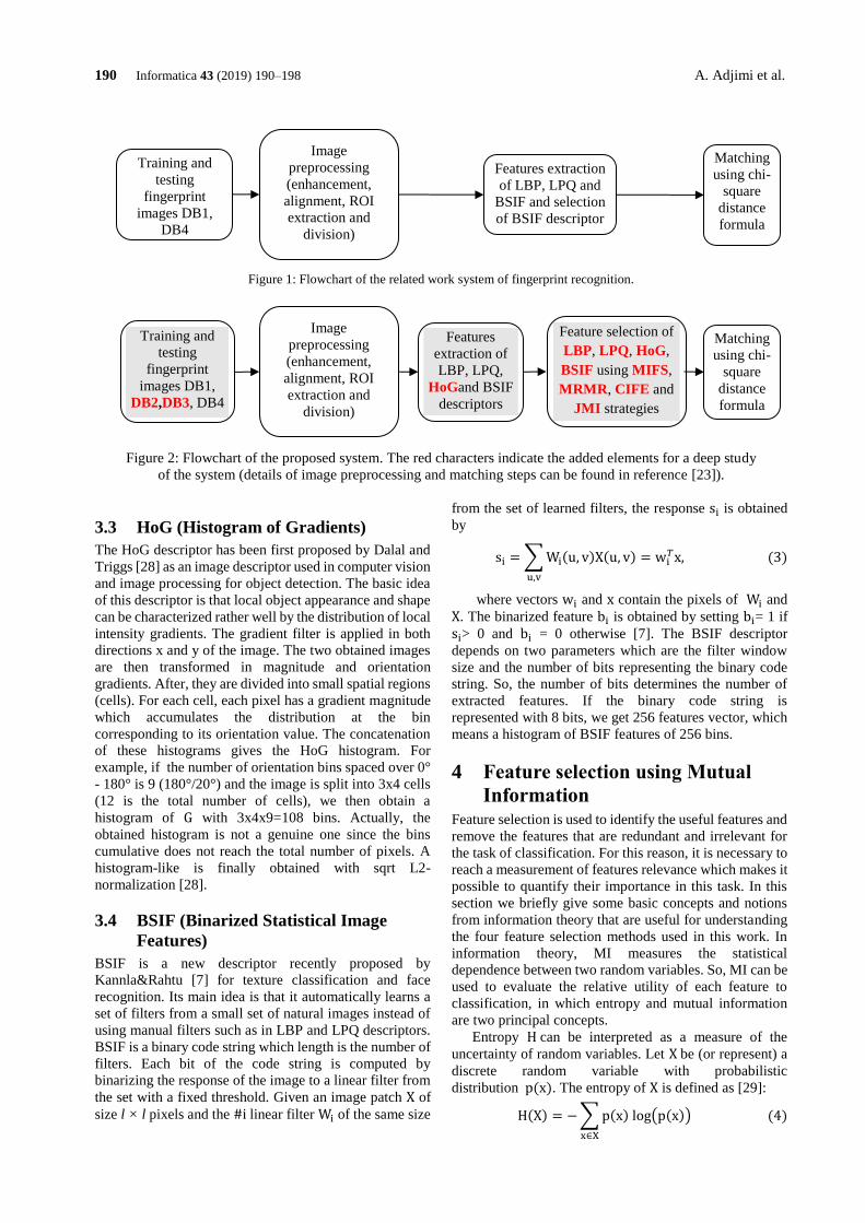
190 Informatica 43 (2019) 190–198 A. Adjimi et al.
Figure 1: Flowchart of the related work system of fingerprint recognition.
Figure 2: Flowchart of the proposed system. The red characters indicate the added elements for a deep study
of the system (details of image preprocessing and matching steps can be found in reference [23]).
3.3 HoG (Histogram of Gradients)
The HoG descriptor has been first proposed by Dalal and
Triggs [28] as an image descriptor used in computer vision
and image processing for object detection. The basic idea
of this descriptor is that local object appearance and shape
can be characterized rather well by the distribution of local
intensity gradients. The gradient filter is applied in both
directions x and y of the image. The two obtained images
are then transformed in magnitude and orientation
gradients. After, they are divided into small spatial regions
(cells). For each cell, each pixel has a gradient magnitude
which accumulates the distribution at the bin
corresponding to its orientation value. The concatenation
of these histograms gives the HoG histogram. For
example, if the number of orientation bins spaced over 0°
- 180° is 9 (180°/20°) and the image is split into 3x4 cells
(12 is the total number of cells), we then obtain a
histogram of G with 3x4x9=108 bins. Actually, the
obtained histogram is not a genuine one since the bins
cumulative does not reach the total number of pixels. A
histogram-like is finally obtained with sqrt L2-
normalization [28].
3.4 BSIF (Binarized Statistical Image
Features)
BSIF is a new descriptor recently proposed by
Kannla&Rahtu [7] for texture classification and face
recognition. Its main idea is that it automatically learns a
set of filters from a small set of natural images instead of
using manual filters such as in LBP and LPQ descriptors.
BSIF is a binary code string which length is the number of
filters. Each bit of the code string is computed by
binarizing the response of the image to a linear filter from
the set with a fixed threshold. Given an image patch X of
size l × l pixels and the #i linear filter Wi of the same size
from the set of learned filters, the response si is obtained
by
si = ∑ Wi(u, v)X(u, v) = wi𝑇x, (3)
u,v
where vectors wi and x contain the pixels of Wi and
X. The binarized feature bi is obtained by setting bi= 1 if
si> 0 and bi = 0 otherwise [7]. The BSIF descriptor
depends on two parameters which are the filter window
size and the number of bits representing the binary code
string. So, the number of bits determines the number of
extracted features. If the binary code string is
represented with 8 bits, we get 256 features vector, which
means a histogram of BSIF features of 256 bins.
4 Feature selection using Mutual
Information Feature selection is used to identify the useful features and
remove the features that are redundant and irrelevant for
the task of classification. For this reason, it is necessary to
reach a measurement of features relevance which makes it
possible to quantify their importance in this task. In this
section we briefly give some basic concepts and notions
from information theory that are useful for understanding
the four feature selection methods used in this work. In
information theory, MI measures the statistical
dependence between two random variables. So, MI can be
used to evaluate the relative utility of each feature to
classification, in which entropy and mutual information
are two principal concepts.
Entropy H can be interpreted as a measure of the
uncertainty of random variables. Let X be (or represent) a
discrete random variable with probabilistic
distribution p(x). The entropy of X is defined as [29]:
H(X) = − ∑ p(x) log(p(x))
x∈X
(4)
Training and
testing
fingerprint
images DB1,
DB4
Image
preprocessing
(enhancement,
alignment, ROI
extraction and
division)
Features extraction
of LBP, LPQ and
BSIF and selection
of BSIF descriptor
Matching
using chi-
square
distance
formula
Training and
testing
fingerprint
images DB1,
DB2,DB3, DB4
Image
preprocessing
(enhancement,
alignment, ROI
extraction and
division)
Features
extraction of
LBP, LPQ,
HoGand BSIF
descriptors
Matching
using chi-
square
distance
formula
Feature selection of
LBP, LPQ, HoG,
BSIF using MIFS,
MRMR, CIFE and
JMI strategies

Mutual Information Based Feature Selection for... Informatica 43 (2019) 187–198 191
The mutual information MI between two discrete
variables X and Y is defined using their joint probabilistic
distribution p(x, y) and their respective marginal
probabilities p(x) and p(y) as:
MI(X; Y) = ∑ p(x, y) logp(x, y)
p(x)p(y)(5)
x∈X y∈Y
The objective of using MI is to select a subset S of
relevant features from a set F of features, which share the
most information with the class variable. The treatment of
each feature needs a very big number of possible subsets
(combination Ckn), this leads to the iterative "greedy"
algorithms which select the relevant features one by one
(sequential forward selection) or deletes the unneeded
features (sequential backward selection). The use of the
greedy forward selection procedure with the MI based
relevance criterion is generally a good choice of feature
selection procedure [30].
The Forward ‘‘greedy’’ algorithm based on MI is
presented as follows [31][32]:
1) (Initialization) set F ←“initial set of n features”; S ←
“empty subset”
2) (Calculation of MI), ∀fi ∈ F , calculateMI(C; fi). 3) (Choose the first feature fs1
), find the feature that
maximizes MI(C; fi), affect F ← F − {fs1}, S ←
{fs1}.
4) (Greedy selection), repeat until the desired number of
features:
a. (Compute MI between features), ∀fi ∈ F , compute MI(C; S, fi).
b. (Select the next feature fsj), choose the feature
fi ∈ F that maximizes MI(C; S, fi) at the step j,
affect F ← F − {fsj}, S ← S ∪ {fsj
}.
5) Take out the subset S of the selected features.
Practically, it is difficult to compute MI(C; S, fi) when
the cardinal of the subset S increases because it requires
an estimation of high dimension probability density
functions, which cannot be correctly estimated with a
limited number of samples [20]. So the majority of the
algorithms use measurements which are maximally based
on three variables: two features plus the class index. For
this reason, many proposed criteria based on MI are
heuristic [32][33]. As previously stated, “filter”methods are preferred to
wrapper ones. These methods are defined by a criterion J, also called relevance index or scoring criterion, which is
planned to measure the relevance of a feature or a feature
subset for the task of classification. The simplest feature-
scoring criterion is referred as MIM (Mutual Information
Maximization) [21]:
Jmim(fi ) = MI(C; fi ) (6)
The Jmim criterion does not include the features
already selected which leads to selecting redundant
features (sharing the same information with the class
index C) that must be eliminated. Numerous
“filter”criteria have been proposed taking into account the
redundancy [33][32]. We use four criteria in this work:
MIFS, mRMR, CIFE and JMI [21].
4.1 Mutual Information Feature Selection
strategy (MIFS)
Proposed by Battiti [31], it is very useful in feature
selection problems and classifying systems due to its
simplicity. MIFS selects the feature that maximizes the
information about the class label C, and subtract the MI
between features fi and the already selected variable fj to
achieve the minimum redundancy:
Jmifs(fi ) = MI(C; fi ) − β ∑ MI(
fj∈S
fi ; fj) (7)
In this latter expression, S stands for the set of already
selected features.
The parameter β is a configurable parameter that
determines the degree of redundancy checking within
MIFS. It must be set experimentally [21][34]. The
performance of MIFS degrades if there are many
irrelevant and redundant features because it penalizes
redundancy too much.
4.2 Minimum Redundancy and Maximal
Relevance strategy (mRMR)
Proposed by Peng et al [35], it is equivalent to MIFS with
β =1
|S| where |S| = card(S) is the number of already
selected features. It finds a balance between the relevance,
which is the dependence between the features and the
class, and the redundancy of features with respect to the
subset of previously selected features. The criterion can be
written as:
Jmrmr(fi ) = MI(C; fi ) −1
|S|∑ MI(
fj∈S
fi ; fj). (8)
With the minimum redundancy criterion of mRMR
method, we can get more representative features of the
class variable, which are maximally dissimilar to already
selected ones, so it gives a small number of features which
effectively covers the same space as a larger number of
features.
4.3 Conditional Infomax Feature
Extraction strategy (CIFE)
Lin and Tang [36] proposed a criterion, called Conditional
Infomax Feature Extraction, in which the joint class-
relevant information is maximized by explicitly reducing
the class-relevant redundancies among features [33]. Note
that this criterion has been proposed by several authors in
different ways [20][32][33][37]:
Jcife(fi ) = MI(C; fi )
− ∑ MI(fi ; fj)
fj∈S
+ ∑ MI(fi ; fj|C). (9)
fj∈S
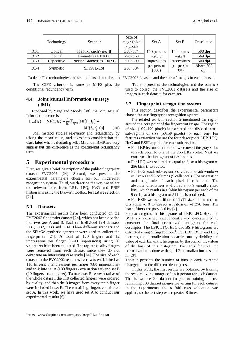
192 Informatica 43 (2019) 192–198 A. Adjimi et al.
The CIFE criterion is same as MIFS plus the
conditional redundancy term.
4.4 Joint Mutual Information strategy
(JMI)
Proposed by Yang and Moody [38], the Joint Mutual
Information score is
Jjmi(fi ) = MI(C; fi ) −1
|S|∑ [MI(fi ; fj ) −fj∈S
MI(fi ; fj|C)] (10)
JMI method studies relevancy and redundancy by
taking the mean value, and takes into consideration the
class label when calculating MI. JMI and mRMR are very
similar but the difference is the conditional redundancy
term.
5 Experimental procedure First, we give a brief description of the public fingerprint
dataset FVC2002 [24]. Second, we present the
experimental parameters chosen for our fingerprint
recognition system. Third, we describe the way we select
the relevant bins from LBP, LPQ, HoG and BSIF
histograms using the Brown’s toolbox for feature selection
[21].
5.1 Datasets
The experimental results have been conducted on the
FVC2002 fingerprint dataset [24], which has been divided
into two sets A and B. Each set is divided in 4 datasets
DB1, DB2, DB3 and DB4. Three different scanners and
the SFinGe synthetic generator were used to collect the
fingerprints [24]. A total of 120 fingers and 12
impressions per finger (1440 impressions) using 30
volunteers have been collected. The top-ten quality fingers
were removed from each dataset since they do not
constitute an interesting case study [24]. The size of each
dataset in the FVC2002 test, however, was established as
110 fingers, 8 impressions per finger (880 impressions)
and split into set A (100 fingers - evaluation set) and set B
(10 fingers - training set). To make set B representative of
the whole dataset, the 110 collected fingers were ordered
by quality, and then the 8 images from every tenth finger
were included in set B. The remaining fingers constituted
set A. In this work, we have used set A to conduct our
experimental results [6].
1https://www.dropbox.com/s/wregrs3ah0qcfdd/SIfing.rar
Table 1 presents the technologies and the scanners
used to collect the FVC2002 datasets and the size of
images in each dataset for each set.
5.2 Fingerprint recognition system
This section describes the experimental parameters
chosen for our fingerprint recognition system.
The related work in section 2 mentioned the region
around the core point of the fingerprint image. The region
of size (100x100 pixels) is extracted and divided into 4
sub-regions of size (50x50 pixels) for each one. For
features extraction we use the four descriptors LBP, LPQ,
HoG and BSIF applied for each sub-region.
• For LBP features extraction, we convert the gray value
of each pixel to one of the 256 LBP codes. Next we
construct the histogram of LBP codes.
• For LPQ we use a radius equal to 3, so a histogram of
256 bins is extracted.
• For HoG, each sub-region is divided into sub windows
of 3 rows and 3 columns (9 cells total). The orientation
and magnitude of each pixel is calculated. The
absolute orientation is divided into 9 equally sized
bins, which results in a 9-bin histogram per each of the
9 cells, so a histogram of 81 bins is produced.
• For BSIF we use a filter of 11x11 size and number of
bits equal to 8 to extract a histogram of 256 bins. The
learnt filters are provided by [7].
For each region, the histograms of LBP, LPQ, HoG and
BSIF are extracted independently and concatenated to
construct the final normalized histogram for each
descriptor. The LBP, LPQ, HoG and BSIF histograms are
extracted using SIfingToolbox1. For LBP, BSIF and LPQ
features, the normalization is carried out by dividing the
value of each bin of the histogram by the sum of the values
of the bins of this histogram. For HoG features, the
normalization is done with sqrt L2-normalization as stated
in [28].
Table 2 presents the number of bins in each extracted
histogram for the different descriptors.
In this work, the first results are obtained by training
the system over 7 images of each person for each dataset.
That is, we use 700 dataset images for training and use
remaining 100 dataset images for testing for each dataset.
In the experiments, the 8 fold-cross validation was
applied, so the test step was repeated 8 times.
Technology Scanner
Size of
image (pixel
× pixel)
Set A Set B Resolution
DB1 Optical IdentixTouchView II 388×374 100 persons
with 8
impressions
per person
(800)
10 persons
with 8
impressions
per person
(80)
500 dpi
DB2 Optical Biometrika FX2000 296×560 569 dpi
DB3 Capacitive Precise Biometrics 100 SC 300×300 500 dpi
DB4 Synthetic SFinGEv2.51 288×384 About 500
dpi
Table 1: The technologies and scanners used to collect the FVC2002 datasets and the size of images in each dataset.
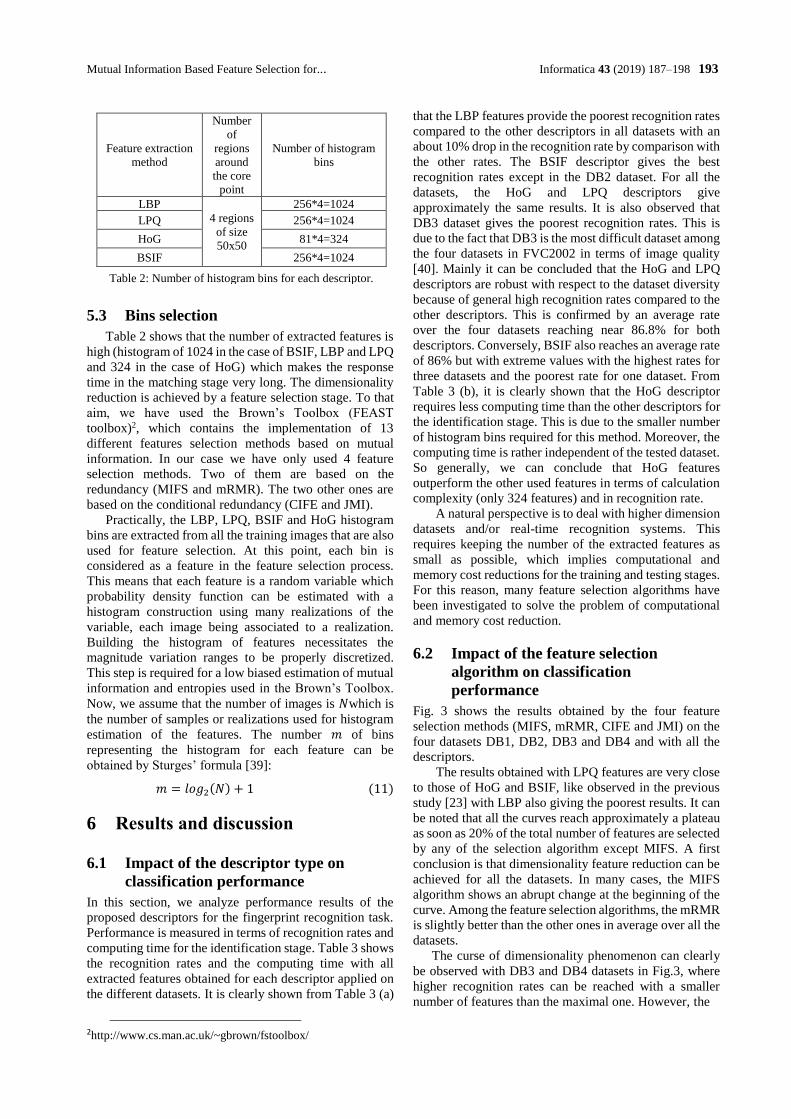
Mutual Information Based Feature Selection for... Informatica 43 (2019) 187–198 193
5.3 Bins selection
Table 2 shows that the number of extracted features is
high (histogram of 1024 in the case of BSIF, LBP and LPQ
and 324 in the case of HoG) which makes the response
time in the matching stage very long. The dimensionality
reduction is achieved by a feature selection stage. To that
aim, we have used the Brown’s Toolbox (FEAST
toolbox)2, which contains the implementation of 13
different features selection methods based on mutual
information. In our case we have only used 4 feature
selection methods. Two of them are based on the
redundancy (MIFS and mRMR). The two other ones are
based on the conditional redundancy (CIFE and JMI).
Practically, the LBP, LPQ, BSIF and HoG histogram
bins are extracted from all the training images that are also
used for feature selection. At this point, each bin is
considered as a feature in the feature selection process.
This means that each feature is a random variable which
probability density function can be estimated with a
histogram construction using many realizations of the
variable, each image being associated to a realization.
Building the histogram of features necessitates the
magnitude variation ranges to be properly discretized.
This step is required for a low biased estimation of mutual
information and entropies used in the Brown’s Toolbox.
Now, we assume that the number of images is 𝑁which is
the number of samples or realizations used for histogram
estimation of the features. The number 𝑚 of bins
representing the histogram for each feature can be
obtained by Sturges’ formula [39]:
𝑚 = 𝑙𝑜𝑔2(𝑁) + 1 (11)
6 Results and discussion
6.1 Impact of the descriptor type on
classification performance
In this section, we analyze performance results of the
proposed descriptors for the fingerprint recognition task.
Performance is measured in terms of recognition rates and
computing time for the identification stage. Table 3 shows
the recognition rates and the computing time with all
extracted features obtained for each descriptor applied on
the different datasets. It is clearly shown from Table 3 (a)
2http://www.cs.man.ac.uk/~gbrown/fstoolbox/
that the LBP features provide the poorest recognition rates
compared to the other descriptors in all datasets with an
about 10% drop in the recognition rate by comparison with
the other rates. The BSIF descriptor gives the best
recognition rates except in the DB2 dataset. For all the
datasets, the HoG and LPQ descriptors give
approximately the same results. It is also observed that
DB3 dataset gives the poorest recognition rates. This is
due to the fact that DB3 is the most difficult dataset among
the four datasets in FVC2002 in terms of image quality
[40]. Mainly it can be concluded that the HoG and LPQ
descriptors are robust with respect to the dataset diversity
because of general high recognition rates compared to the
other descriptors. This is confirmed by an average rate
over the four datasets reaching near 86.8% for both
descriptors. Conversely, BSIF also reaches an average rate
of 86% but with extreme values with the highest rates for
three datasets and the poorest rate for one dataset. From
Table 3 (b), it is clearly shown that the HoG descriptor
requires less computing time than the other descriptors for
the identification stage. This is due to the smaller number
of histogram bins required for this method. Moreover, the
computing time is rather independent of the tested dataset.
So generally, we can conclude that HoG features
outperform the other used features in terms of calculation
complexity (only 324 features) and in recognition rate.
A natural perspective is to deal with higher dimension
datasets and/or real-time recognition systems. This
requires keeping the number of the extracted features as
small as possible, which implies computational and
memory cost reductions for the training and testing stages.
For this reason, many feature selection algorithms have
been investigated to solve the problem of computational
and memory cost reduction.
6.2 Impact of the feature selection
algorithm on classification
performance
Fig. 3 shows the results obtained by the four feature
selection methods (MIFS, mRMR, CIFE and JMI) on the
four datasets DB1, DB2, DB3 and DB4 and with all the
descriptors.
The results obtained with LPQ features are very close
to those of HoG and BSIF, like observed in the previous
study [23] with LBP also giving the poorest results. It can
be noted that all the curves reach approximately a plateau
as soon as 20% of the total number of features are selected
by any of the selection algorithm except MIFS. A first
conclusion is that dimensionality feature reduction can be
achieved for all the datasets. In many cases, the MIFS
algorithm shows an abrupt change at the beginning of the
curve. Among the feature selection algorithms, the mRMR
is slightly better than the other ones in average over all the
datasets.
The curse of dimensionality phenomenon can clearly
be observed with DB3 and DB4 datasets in Fig.3, where
higher recognition rates can be reached with a smaller
number of features than the maximal one. However, the
Feature extraction
method
Number
of
regions
around
the core
point
Number of histogram
bins
LBP
4 regions
of size
50x50
256*4=1024
LPQ 256*4=1024
HoG 81*4=324
BSIF 256*4=1024
Table 2: Number of histogram bins for each descriptor.
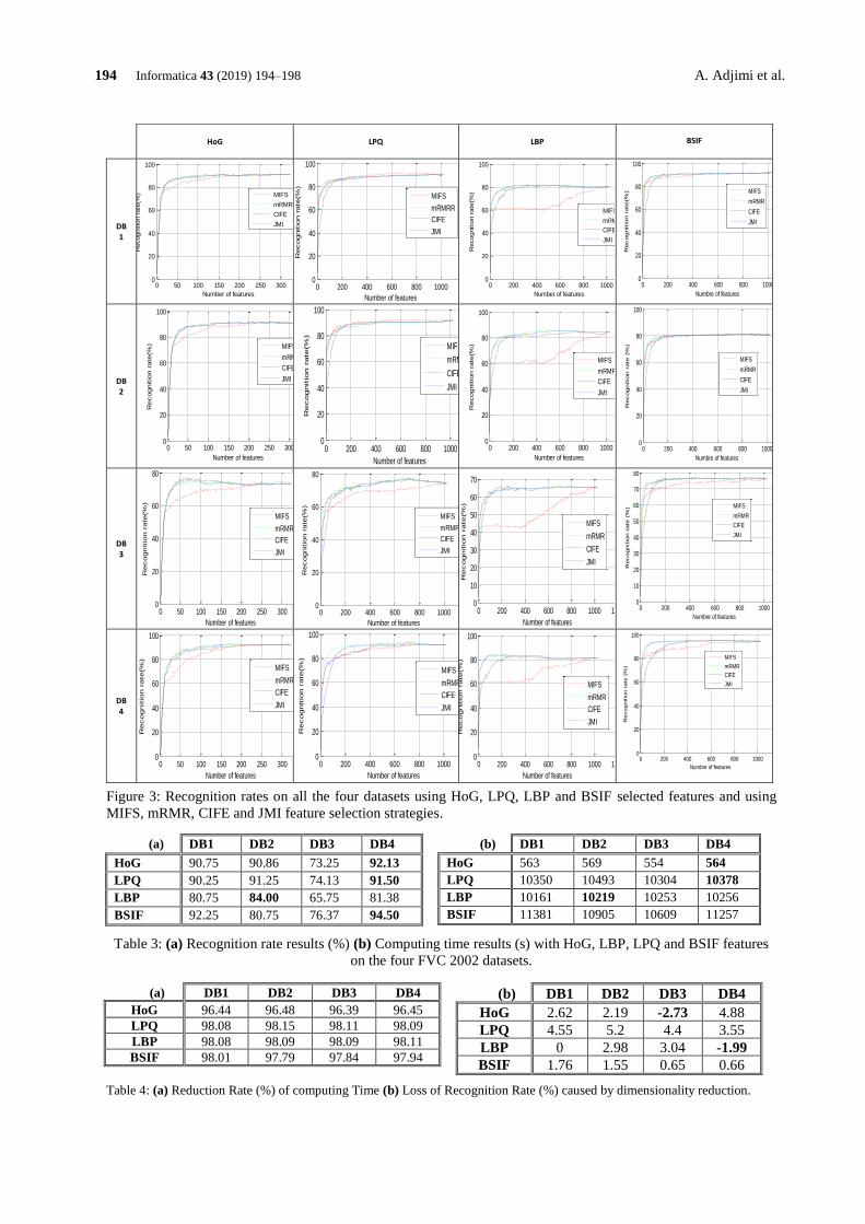
194 Informatica 43 (2019) 194–198 A. Adjimi et al.
HoG LPQ LBP
BSIF
DB1
DB2
DB3
DB4
Figure 3: Recognition rates on all the four datasets using HoG, LPQ, LBP and BSIF selected features and using
MIFS, mRMR, CIFE and JMI feature selection strategies.
(a) DB1 DB2 DB3 DB4
HoG 90.75 90.86 73.25 92.13
LPQ 90.25 91.25 74.13 91.50
LBP 80.75 84.00 65.75 81.38
BSIF 92.25 80.75 76.37 94.50
(b) DB1 DB2 DB3 DB4
HoG 563 569 554 564
LPQ 10350 10493 10304 10378
LBP 10161 10219 10253 10256
BSIF 11381 10905 10609 11257
Table 3: (a) Recognition rate results (%) (b) Computing time results (s) with HoG, LBP, LPQ and BSIF features
on the four FVC 2002 datasets.
(a) DB1 DB2 DB3 DB4
HoG 96.44 96.48 96.39 96.45
LPQ 98.08 98.15 98.11 98.09
LBP 98.08 98.09 98.09 98.11
BSIF 98.01 97.79 97.84 97.94
(b) DB1 DB2 DB3 DB4
HoG 2.62 2.19 -2.73 4.88
LPQ 4.55 5.2 4.4 3.55
LBP 0 2.98 3.04 -1.99
BSIF 1.76 1.55 0.65 0.66
Table 4: (a) Reduction Rate (%) of computing Time (b) Loss of Recognition Rate (%) caused by dimensionality reduction.
0 50 100 150 200 250 300 3500
20
40
60
80
100
Number of features
Recognitio
n r
ate
(%)
MIFS
mRMR
CIFE
JMI
0 200 400 600 800 1000 12000
20
40
60
80
100
Number of featuresR
ecognitio
n r
ate
(%)
MIFS
mRMRR
CIFE
JMI
0 200 400 600 800 1000 12000
20
40
60
80
100
Number of features
Recognitio
n r
ate
(%)
MIFS
mRMR
CIFE
JMI
0 200 400 600 800 1000 12000
20
40
60
80
100
Numbre of features
Recognitio
n r
ate
(%)
MIFS
mRMR
CIFE
JMI
0 50 100 150 200 250 300 3500
20
40
60
80
100
Number of features
Recognitio
n r
ate
(%)
MIFS
mRMR
CIFE
JMI
0 200 400 600 800 1000 12000
20
40
60
80
100
Number of features
Recognitio
n r
ate
(%)
MIFS
mRMR
CIFE
JMI
0 200 400 600 800 1000 12000
20
40
60
80
100
Number of features
Recognitio
n r
ate
(%)
MIFS
mRMR
CIFE
JMI
0 200 400 600 800 1000 12000
20
40
60
80
100
Numbre of features
Recognitio
n r
ate
(%
)
MIFS
mRMR
CIFE
JMI
0 50 100 150 200 250 300 3500
20
40
60
80
Number of features
Recognitio
n r
ate
(%)
MIFS
mRMR
CIFE
JMI
0 200 400 600 800 1000 12000
20
40
60
80
Number of features
Recognitio
n r
ate
(%)
MIFS
mRMR
CIFE
JMI
0 200 400 600 800 1000 12000
10
20
30
40
50
60
70
Number of features
Recognitio
n r
ate
(%)
MIFS
mRMR
CIFE
JMI
0 200 400 600 800 1000 12000
10
20
30
40
50
60
70
80
Numbre of features
Recognitio
n r
ate
(%
)
MIFS
mRMR
CIFE
JMI
0 50 100 150 200 250 300 3500
20
40
60
80
100
Number of features
Recognitio
n r
ate
(%)
MIFS
mRMR
CIFE
JMI
0 200 400 600 800 1000 12000
20
40
60
80
100
Number of features
Recognitio
n r
ate
(%)
MIFS
mRMR
CIFE
JMI
0 200 400 600 800 1000 12000
20
40
60
80
100
Number of features
Recognitio
n r
ate
(%)
MIFS
mRMR
CIFE
JMI
0 200 400 600 800 1000 12000
20
40
60
80
100
Numbre of features
Recognitio
n r
ate
(%
)
MIFS
mRMR
CIFE
JMI
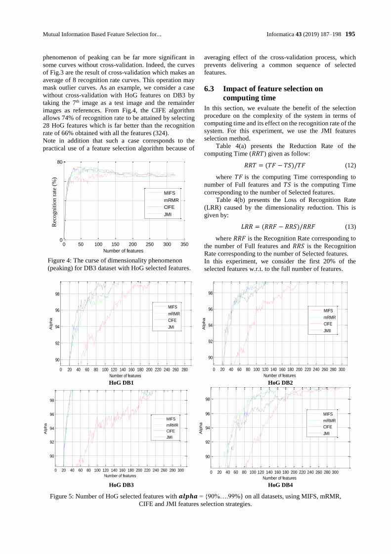
Mutual Information Based Feature Selection for... Informatica 43 (2019) 187–198 195
phenomenon of peaking can be far more significant in
some curves without cross-validation. Indeed, the curves
of Fig.3 are the result of cross-validation which makes an
average of 8 recognition rate curves. This operation may
mask outlier curves. As an example, we consider a case
without cross-validation with HoG features on DB3 by
taking the 7th image as a test image and the remainder
images as references. From Fig.4, the CIFE algorithm
allows 74% of recognition rate to be attained by selecting
28 HoG features which is far better than the recognition
rate of 66% obtained with all the features (324).
Note in addition that such a case corresponds to the
practical use of a feature selection algorithm because of
averaging effect of the cross-validation process, which
prevents delivering a common sequence of selected
features.
6.3 Impact of feature selection on
computing time
In this section, we evaluate the benefit of the selection
procedure on the complexity of the system in terms of
computing time and its effect on the recognition rate of the
system. For this experiment, we use the JMI features
selection method.
Table 4(a) presents the Reduction Rate of the
computing Time (𝑅𝑅𝑇) given as follow:
𝑅𝑅𝑇 = (𝑇𝐹 − 𝑇𝑆)/𝑇𝐹 (12)
where 𝑇𝐹 is the computing Time corresponding to
number of Full features and 𝑇𝑆 is the computing Time
corresponding to the number of Selected features.
Table 4(b) presents the Loss of Recognition Rate
(LRR) caused by the dimensionality reduction. This is
given by:
𝐿𝑅𝑅 = (𝑅𝑅𝐹 − 𝑅𝑅𝑆)/𝑅𝑅𝐹 (13)
where 𝑅𝑅𝐹 is the Recognition Rate corresponding to
the number of Full features and 𝑅𝑅𝑆 is the Recognition
Rate corresponding to the number of Selected features.
In this experiment, we consider the first 20% of the
selected features w.r.t. to the full number of features.
HoG DB1 HoG DB2
HoG DB3 HoG DB4
Figure 5: Number of HoG selected features with 𝒂𝒍𝒑𝒉𝒂 = {90%….99%} on all datasets, using MIFS, mRMR,
CIFE and JMI features selection strategies.
0 20 40 60 80 100 120 140 160 180 200 220 240 260 280
90
92
94
96
98
Number of features
Alp
ha
MIFS
mRMR
CIFE
JMI
0 20 40 60 80 100 120 140 160 180 200 220 240 260 280 300
90
92
94
96
98
Number of features
Alp
ha
MIFS
mRMR
CIFE
JMII
0 20 40 60 80 100 120 140 160 180 200 220 240 260 280 300
90
92
94
96
98
Number of features
Alp
ha
MIFS
mRMR
CIFE
JMI
0 20 40 60 80 100 120 140 160 180 200 220 240 260 280 300
90
92
94
96
98
Number of features
Alp
ha
MIFS
mRMR
CIFE
JMI
Figure 4: The curse of dimensionality phenomenon
(peaking) for DB3 dataset with HoG selected features.
0 50 100 150 200 250 300 3500
20
40
60
80
Number of features
Accura
cy(%
)
MIFS
mRMR
CIFE
JMI
Rec
ogn
itio
n r
ate
(%)
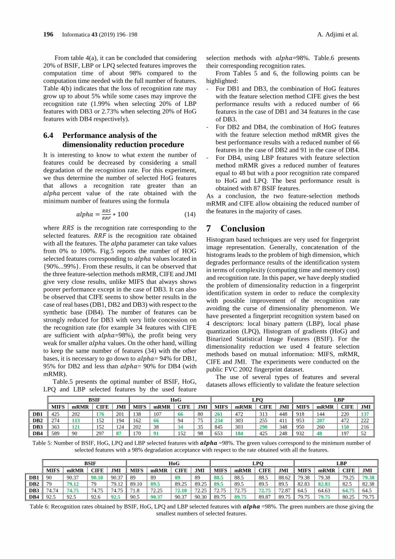
196 Informatica 43 (2019) 196–198 A. Adjimi et al.
From table 4(a), it can be concluded that considering
20% of BSIF, LBP or LPQ selected features improves the
computation time of about 98% compared to the
computation time needed with the full number of features.
Table 4(b) indicates that the loss of recognition rate may
grow up to about 5% while some cases may improve the
recognition rate (1.99% when selecting 20% of LBP
features with DB3 or 2.73% when selecting 20% of HoG
features with DB4 respectively).
6.4 Performance analysis of the
dimensionality reduction procedure
It is interesting to know to what extent the number of
features could be decreased by considering a small
degradation of the recognition rate. For this experiment,
we thus determine the number of selected HoG features
that allows a recognition rate greater than an
𝑎𝑙𝑝ℎ𝑎 percent value of the rate obtained with the
minimum number of features using the formula
𝑎𝑙𝑝ℎ𝑎 =𝑅𝑅𝑆
𝑅𝑅𝐹∗ 100 (14)
where 𝑅𝑅𝑆 is the recognition rate corresponding to the
selected features. 𝑅𝑅𝐹 is the recognition rate obtained
with all the features. The alpha parameter can take values
from 0% to 100%. Fig.5 reports the number of HOG
selected features corresponding to 𝑎𝑙𝑝ℎ𝑎 values located in
{90%...99%}. From these results, it can be observed that
the three feature-selection methods mRMR, CIFE and JMI
give very close results, unlike MIFS that always shows
poorer performance except in the case of DB3. It can also
be observed that CIFE seems to show better results in the
case of real bases (DB1, DB2 and DB3) with respect to the
synthetic base (DB4). The number of features can be
strongly reduced for DB3 with very little concession on
the recognition rate (for example 34 features with CIFE
are sufficient with 𝑎𝑙𝑝ℎ𝑎=98%), the profit being very
weak for smaller 𝑎𝑙𝑝ℎ𝑎 values. On the other hand, willing
to keep the same number of features (34) with the other
bases, it is necessary to go down to 𝑎𝑙𝑝ℎ𝑎= 94% for DB1,
95% for DB2 and less than 𝑎𝑙𝑝ℎ𝑎= 90% for DB4 (with
mRMR).
Table.5 presents the optimal number of BSIF, HoG,
LPQ and LBP selected features by the used feature
selection methods with 𝑎𝑙𝑝ℎ𝑎=98%. Table.6 presents
their corresponding recognition rates.
From Tables 5 and 6, the following points can be
highlighted:
- For DB1 and DB3, the combination of HoG features
with the feature selection method CIFE gives the best
performance results with a reduced number of 66
features in the case of DB1 and 34 features in the case
of DB3.
- For DB2 and DB4, the combination of HoG features
with the feature selection method mRMR gives the
best performance results with a reduced number of 66
features in the case of DB2 and 91 in the case of DB4.
- For DB4, using LBP features with feature selection
method mRMR gives a reduced number of features
equal to 48 but with a poor recognition rate compared
to HoG and LPQ. The best performance result is
obtained with 87 BSIF features.
As a conclusion, the two feature-selection methods
mRMR and CIFE allow obtaining the reduced number of
the features in the majority of cases.
7 Conclusion Histogram based techniques are very used for fingerprint
image representation. Generally, concatenation of the
histograms leads to the problem of high dimension, which
degrades performance results of the identification system
in terms of complexity (computing time and memory cost)
and recognition rate. In this paper, we have deeply studied
the problem of dimensionality reduction in a fingerprint
identification system in order to reduce the complexity
with possible improvement of the recognition rate
avoiding the curse of dimensionality phenomenon. We
have presented a fingerprint recognition system based on
4 descriptors: local binary pattern (LBP), local phase
quantization (LPQ), Histogram of gradients (HoG) and
Binarized Statistical Image Features (BSIF). For the
dimensionality reduction we used 4 feature selection
methods based on mutual information: MIFS, mRMR,
CIFE and JMI. The experiments were conducted on the
public FVC 2002 fingerprint dataset.
The use of several types of features and several
datasets allows efficiently to validate the feature selection
BSIF HoG LPQ LBP
MIFS mRMR CIFE JMI MIFS mRMR CIFE JMI MIFS mRMR CIFE JMI MIFS mRMR CIFE JMI
DB1 425 202 176 201 138 107 66 80 261 472 313 448 918 144 220 137
DB2 274 113 152 194 162 66 94 75 234 303 255 411 953 207 472 222
DB3 363 121 152 124 202 38 34 35 845 303 290 348 950 260 150 216
DB4 589 90 297 87 170 91 152 98 653 184 425 248 932 48 197 52
Table 5: Number of BSIF, HoG, LPQ and LBP selected features with 𝒂𝒍𝒑𝒉𝒂 =98%. The green values correspond to the minimum number of
selected features with a 98% degradation acceptance with respect to the rate obtained with all the features.
BSIF HoG LPQ LBP
MIFS mRMR CIFE JMI MIFS mRMR CIFE JMI MIFS mRMR CIFE JMI MIFS mRMR CIFE JMI
DB1 90 90.37 90.10 90.37 89 89 89 89 88.5 88.5 88.5 88.62 79.38 79.38 79.25 79.38
DB2 79 79.12 79 79.12 89.10 89.5 89.25 89.25 89.5 89.5 89.5 89.5 82.83 82.83 82.5 82.38
DB3 74.74 74.75 74.75 74.75 71.8 72.25 72.10 72.25 72.75 72.75 72.75 72.87 64.5 64.63 64.75 64.5
DB4 92.5 92.5 92.6 92.5 90.5 90.37 90.37 90.30 89.75 89.75 89.87 89.75 79.75 79.75 80.25 79.75
Table 6: Recognition rates obtained by BSIF, HoG, LPQ and LBP selected features with 𝒂𝒍𝒑𝒉𝒂 =98%. The green numbers are those giving the
smallest numbers of selected features.
Mutual Information Based Feature Selection for... Informatica 43 (2019) 187–198 197
techniques and to choose the best combination (type of
features/feature selection method) for the task of
fingerprint identification. From all the results we can
conclude that the use of feature selection methods can
reduce the number of features whatever the type of
features and whatever the dataset, except in the case of
using MIFS with LBP features that present bad
performance result. We can conclude also that the feature
selection techniques can reduce the curse of
dimensionality phenomenon and probably improve the
recognition rate of the identification system. The
combination of HoG features with CIFE or mRMR gives
the best performance in terms of recognition rate,
robustness and complexity of the system. In terms of
complexity, a huge computation time reduction (98%) is
obtained by considering only 20% of the total number of
features without much affecting the recognition rate.
In definitive, employing feature selection algorithms
will always provide a benefit when compared to no
selection since higher or equal identification performance
can be obtained and at the same time the computation
complexity for the identification stage can be reduced. As
perspective, we plan to investigate other descriptors and
biometric modalities.
References [1] D. Maio, D. Maltoni, A. K. Jain and S. Prabhakar, "
Handbook of fingerprint recognition," Springer,
New York, NY, 2003.
https://doi.org/10.1007/b97303
[2] K. S. Sunil, "A Review of Image Based Fingerprint
Authentication Algorithms," International Journal
of Advanced Research in Computer Science and
Software Engineering, vol. 3, no. 6, pp. 553-556,
2013.
[3] Y. Jucheng, "Non-minutiae based fingerprint
descriptor," in Biometrics, Nanchang, In Tech, 2012,
pp. 80-98.
https://doi.org/10.5772/21642
[4] N. Nanni and A. Lumini, "Local Binary Patterns for
a hybrid fingerprint matcher," Pattern Recognition,
vol. 41, no. 11, pp. 3461-3466, 2008.
https://doi.org/10.1016/j.patcog.2008.05.013
[5] S. Brahnam, C. Casanova, L. Nanni and A. Lumini,
"A Hybrid Fingerprint Multimatcher," in 16th
International Conference on Image Processing,
Computer Vision, and Pattern Recognition, Las
Vegas, Nevada, USA, pp. 877-882, 2012.
[6] L. Nanni and A. Lumini, "Descriptors for image-
based fingerprint matchers," Expert Systems With
Applications, vol. 36, no. 10, pp. 12414-12422,
2009.
https://doi.org/10.1016/j.eswa.2009.04.041
[7] J. Kanala and E. Rahtu, "BSIF: binarized statistical
image features", 21st International Conference on
Pattern Recognition (ICPR 2012)," IEEE, Tsukuba,
Japan, pp. 1363-1366, 2012.
[8] A I Awad and K Baba, "Evaluation of a fingerprint
identification algorithm with SIFT features," in IIAI
International Conference on Advanced Applied
Informatics, Fukuoka, 2012, pp. 129-132.
https://doi.org/10.1109/iiai-aai.2012.34
[9] S Egawa, A I Awad, and K Baba, "Evaluation of
acceleration algorithm for biometric identification,"
Network Digital Technologies NDT 2012.
Communications in Computer and Information
Science. Springer, Berlin, Heidelberg, vol. 294, pp.
231-242, 2012.
https://doi.org/10.1007/978-3-642-30567-2_19
[10] T. Amornraksa and S. Tachaphetpiboon,
"Fingerprint recognition using DCT features,"
Electronic Letters, vol. 42, no. 9, pp. 522–523, 2006.
https://doi.org/10.1049/el:20064330
[11] A. K. Jain, S. Prabhakar, L. Hong and S. Pankanti,
"Filterbank-based fingerprint matching," Image
Processing, IEEE Transactions, vol. 9, no. 5, pp.
846-859, 2000.
https://doi.org/10.1109/83.841531
[12] S. Lifeng, Z. Feng and T. Xiaoou, "Improved
fingercode for filterbank-based fingerprint
matching," In International Conference on Image
Processing , vol. 2, no. 2, pp. 895-898, 2003.
https://doi.org/10.1109/icip.2003.1246825
[13] R. Kumar, P. Chandra and M. Hanmandlu,
"Fingerprint Matching Based on Texture Feature,"
In Mobile Communication and Power Engineering,
Springer-Verlag Berlin, vol. 296, pp. 86-91, 2013.
https://doi.org/10.1007/978-3-642-35864-7_12
[14] M. Saha, J. Chaki and R. Parekh, "Fingerprint
Recognition using Texture Features," International
Journal of Science and Research, vol. 2, no. 12, pp.
2319-7064, 2013.
[15] K. Tewari and R. L. Kalakoti, "Fingerprint
Recognition Using Transform Domain Techniques,"
in International Technological Conference, pp.136-
140, 2014.
[16] M. W. Zin and M. M. Sein, "Texture feature based
fingerprint recognition for low quality
imagesTexture Feature based Fingerprint
Recognition for Low Quality Images," in Micro-
NanoMechatronics and Human Science (MHS),
International Symposium, IEEE, Nagoya, Japan, pp.
333–338, 2011.
https://doi.org/10.1109/mhs.2011.6102204
[17] C. M. Bishop, Neural Networks for Pattern
Recognition, Oxford University Press, 1995.
[18] A. K. Jain and B. Chandrasekaran, "Dimensionality
and Sample Size Considerations in Pattern
Recognition Practice," in Handbook of Statistics,
Amsterdam, 1982, pp. 835-855.
https://doi.org/10.1016/s0169-7161(82)02042-2
[19] A. K. Jain, R. P. Duin and J. Mao, "Statistical
Pattern Recognition: A Review," IEEE Transaction
on Pattern Analysis and Machine Intelligence, vol.
22, no. 1, pp. 4-37, 2000.
https://doi.org/10.1109/34.824819
[20] A. Hacine-Gharbi, M. Deriche, P. Ravier and T.
Mohamadi, "A new histogram-based estimation
198 Informatica 43 (2019) 198–198 A. Adjimi et al.
technique of entropy and mutual information using
mean squared error minimization," Computers &
Electrical Engineering, vol. 39, no. 3, pp. 918-933,
2013.
https://doi.org/10.1016/j.compeleceng.2013.02.010
[21] G. Brown, A. Pocock, M. Lujan and M. J.Zhao,
"Conditional Likelihood Maximisation: A Unifying
Framework for Information Theoretic Feature
Selection," Journal of Machine Learning Research,
vol. 13, pp. 27-66, 2012.
[22] B. Jun, T. Kim and D. Kim, "A compact local
binary pattern using maximization of mutual
information for face analysis Pattern Recognition,"
Pattern Recognition, vol. 44, pp. 532–543, 2011.
https://doi.org/10.1016/j.patcog.2010.10.008
[23] A. Adjimi, A. Hacine-Gharbi, P. Ravier and M.
Mostefai, "Extraction and selection of binarised
statistical image features for fingerprint
recognition," Int. J. Biometrics, vol. 9, no. 1, p. 67–
80., 2017.
https://doi.org/10.1504/ijbm.2017.10005054
[24] D. Maio, D. Maltoni, R. Cappelli, J. L. Wayman and
A. K. Jain, "FVC2002: Second Fingerprint
Verification Competition," in 16 th international
conference in Pattern Recognition, 2002.
[25] A. Adjimi, A. Hacine-Gharbi and M. Mostefai,
"Application of Binarized Statistical Image
Features for Fingerprint Recognition," in SIVA
2015, 3rd international conference signal image
vision and their applications, Guelma, Algeria,
2015.
[26] T. Ojala, M. Pietikainen and T. Maenpaa,
"Multiresolution gray-scale and rotation invariant
texture classification with local binary patterns,"
Pattern Analysis and Machine Intelligence, IEEE
Transactions, vol. 24, no. 7, pp. 971-987, 2002.
https://doi.org/10.1109/tpami.2002.1017623
[27] T. Ojala, M. Pietikainen and D. Harwood, "A
comparative study of texture measures with
classification based on feature distributions,"
Pattern Recognition, vol. 29, pp. 51–59, 1996.
https://doi.org/10.1016/0031-3203(95)00067-4
[28] N. Dalal and B. Triggs, "Histograms of oriented
gradients for human detection," in IEEE Computer
Society Conference on Computer Vision and
Pattern Recognition (CVPR'05), San Diego, USA,
p. 886-893, 2005.
https://doi.org/10.1109/CVPR.2005.177
[29] T. Cover and J. Thomas, Elements of information
theory, 2e édition ed., Canada: John Wiley & Sons,
2006.
https://doi.org/10.1002/047174882x
[30] D. François, F. Rossi, V. Wertz and M. Verleysen,
"Resampling methods for parameter-free and robust
feature selection with mutual information,"
Neurocomputing, vol. 70, pp. 1276–1288, 2007.
https://doi.org/10.1016/j.neucom.2006.11.019
[31] R. Battiti, "Using mutual information for selecting
features in supervised neural net learning," IEEE
Trans. Neural Networks, vol. 5, no. 4, pp. 537–550,
1994.
https://doi.org/10.1109/72.298224
[32] A. Hacine-Gharbi, P. Ravier and T. Mohamadi, "Une
nouvelle méthode de sélection des paramètres
pertinents : application en reconnaissance de la
parole," in conférence TAIMA, Hammamet, Tunisie,
pp. 399-407, 2009.
[33] G. Brown, "A new perspective for information
theoretic feature selection," in International
Conference on Artificial Intelligence and Statistics,
Florida, USA, pp, 49-56, 2009.
[34] N. Kwak and C. H. Choi, "Input feature selection
for classification problems," IEEE Transactions on
Neural Networks, vol. 13, no. 1, pp. 143–159, 2002.
https://doi.org/10.1109/72.977291
[35] H. Peng, F. Long and C. Ding, "Feature selection
based on mutual information: Criteria of max
dependency, max-relevance, and min-redundancy,"
IEEE Transactions on Pattern Analysis and
Machine Intelligence, vol. 27, no. 8, pp. 1226–
1238, 2005.
https://doi.org/10.1109/tpami.2005.159
[36] D. Lin and X. Tang, "Conditional infomax learning:
An integrated framework for feature extraction and
fusion," in European Conference on Computer
Vision, Springer-Verlag Berlin, Graz, Austria, pp.
68-82 , 2006.
https://doi.org/10.1007/11744023_6
[37] I. Kojadinovic, "Relevance measures for subset
variable selection in regression problems based on
k-additive mutual information," Comput. Statist.
Data Anal., vol. 49, pp. 1205–1227, 2005.
https://doi.org/10.1016/j.csda.2004.07.026
[38] H. Yang and J. Moody, "Data Visualization and
Feature Selection: New Algorithms for Non
Gaussian Data," Advances in Neural Information
Processing Systems, MIT Press, pp. 688-695, 1999.
[39] H. Sturges, "The choice of a class-interval," J.
Amer. Statist. Assoc, vol. 21, pp. 65–66, 1926.
https://doi.org/10.1080/01621459.1926.10502161
[40] Y. Chen, S. C. Dass and A. K. Jain, "Fingerprint
Quality Indices for Predicting Authentication
Performance," in Audio- and Video-Based
Biometric Person Authentication, Springer-Verlag
Berlin Heidelberg, Hilton Rye Town, USA, pp.
160-170, 2005.
https://doi.org/10.1007/11527923_17
https://doi.org/10.31449/inf.v43i2.2687 Informatica 43 (2019) 199–207 199
Some Remarks and Tests on the DH1 Cryptosystem Based on AutomataCompositions
Pál DömösiInstitute of Mathematics and Informatics, University of NyíregyházaH-4400 Nyíregyháza, Sóstói út 31/B, Hungary
Faculty of Informatics, University of DebrecenH-4028 Debrecen, Kassai út 26, HungaryE-mail: [email protected]
József Gáll, Géza HorváthFaculty of Informatics, University of DebrecenH-4028 Debrecen, Kassai út 26, HungaryE-mail: [email protected], [email protected]
Norbert TihanyiFaculty of Informatics, Eötvös Loránd UniversityH-1117 Budapest, Pázmány Péter sétány 1/C, HungaryE-mail: [email protected]
Keywords: automata network, NIST test, block cipher, statistics
Received: February 17, 2019
In this paper we discuss NIST test results of a previously introduced cryptosystem based on automatacompositions. We conclude that the requirements of NIST test are all fulfilled by the cryptosystem.
Povzetek: Analiziran je kriptirni sistem DH1 na osnovi koncnih avtomatov s testom NIST.
1 Introduction and problemstatement
Dömösi and Horváth in their previousworks (see [Dömösi and Horváth, 2015a] and[Dömösi and Horváth, 2015b]) introduced new blockciphers based on Gluškov-type product of automata.In what follows we will refer to the cipher in[Dömösi and Horváth, 2015a] as the first Dömösi-Horváth cryptosystem, or in short, DH1-cipher, whereas tothe cipher in [Dömösi and Horváth, 2015b] as the secondDömösi-Horváth cryptosystem, or in short, DH2-cipher.In this paper we investigate some properties of the DH1-cipher. However, we do not discuss all details of definitionand motivation regarding DH1-chipers in this paper.
Both systems use the following simple idea: considera giant-size permutation automaton such that the set ofstates and the set of inputs consisting of all given lengthof strings over a non-trivial alphabet as all possible plain-text/ciphertext blocks. Moreover consider a cryptograph-ically secure pseudo random number generator with largeperiodicity having the property that, getting its really ran-dom kernel, it serves a sequence of pseudo random stringsas inputs for the automaton. For each plaintext block thesystem calculates the new state into which the actual pseu-dorandom string takes the automaton from the state which
is identified as the actual plaintext block. The string –identified as the new state– will be the ciphertext blockordered to the considered plaintext block. Of course, theciphertext will be the concatenation of the generated ci-phertext blocks. The giant size of the automaton makesit infeasible to break the system by brute-force method.
For all notions and notations not defined in this paperwe refer to the monographs [Dömösi and Nehaniv, 2005,Mezenes and Vanstone, 1996]. The cryptosystem dis-cussed here is a block cipher. Since the key automaton isa permutation automaton, for every ciphertext there existsexactly one plaintext making the encryption and decryptionunambiguous. Moreover, there is a huge number of corre-sponding encoded messages to each plaintext so that sev-eral encryptions of the same plaintext yield several distinctciphertexts.
Given the cryptosystem DH1-cipher described above anatural question is the investigation of the statistical prop-erties of the system from many perspectives. For in-stance, the avalanche effect of the system –as a natu-ral property required in the profession– may be tested byseveral classical hypothesis tests. Some early results aregiven in [Dömösi et al., 2017] where they confirm that theavalanche effect is fulfilled. However, further tests can andshould also be used, in particular the ones used for testingwhether the output of it can be distinguished from ’true’random sources. That is why we turned to the well known
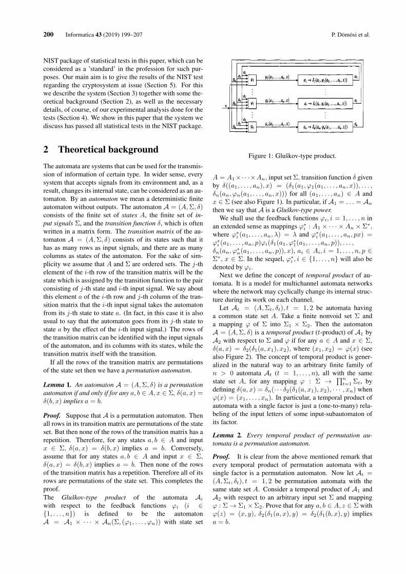
200 Informatica 43 (2019) 199–207 P. Dömösi et al.
NIST package of statistical tests in this paper, which can beconsidered as a ’standard’ in the profession for such pur-poses. Our main aim is to give the results of the NIST testregarding the cryptosystem at issue (Section 5). For thiswe describe the system (Section 3) together with some the-oretical background (Section 2), as well as the necessarydetails, of course, of our experimental analysis done for thetests (Section 4). We show in this paper that the system wediscuss has passed all statistical tests in the NIST package.
2 Theoretical backgroundThe automata are systems that can be used for the transmis-sion of information of certain type. In wider sense, everysystem that accepts signals from its environment and, as aresult, changes its internal state, can be considered as an au-tomaton. By an automaton we mean a deterministic finiteautomaton without outputs. The automaton A = (A,Σ, δ)consists of the finite set of states A, the finite set of in-put signals Σ, and the transition function δ, which is oftenwritten in a matrix form. The transition matrix of the au-tomaton A = (A,Σ, δ) consists of its states such that ithas as many rows as input signals, and there are as manycolumns as states of the automaton. For the sake of sim-plicity we assume that A and Σ are ordered sets. The j-thelement of the i-th row of the transition matrix will be thestate which is assigned by the transition function to the pairconsisting of j-th state and i-th input signal. We say aboutthis element a of the i-th row and j-th column of the tran-sition matrix that the i-th input signal takes the automatonfrom its j-th state to state a. (In fact, in this case it is alsousual to say that the automaton goes from its j-th state tostate a by the effect of the i-th input signal.) The rows ofthe transition matrix can be identified with the input signalsof the automaton, and its columns with its states, while thetransition matrix itself with the transition.
If all the rows of the transition matrix are permutationsof the state set then we have a permutation automaton.
Lemma 1. An automaton A = (A,Σ, δ) is a permutationautomaton if and only if for any a, b ∈ A, x ∈ Σ, δ(a, x) =δ(b, x) implies a = b.
Proof. Suppose that A is a permutation automaton. Thenall rows in its transition matrix are permutations of the stateset. But then none of the rows of the transition matrix has arepetition. Therefore, for any states a, b ∈ A and inputx ∈ Σ, δ(a, x) = δ(b, x) implies a = b. Conversely,assume that for any states a, b ∈ A and input x ∈ Σ,δ(a, x) = δ(b, x) implies a = b. Then none of the rowsof the transition matrix has a repetition. Therefore all of itsrows are permutations of the state set. This completes theproof.The Gluškov-type product of the automata Aiwith respect to the feedback functions ϕi (i ∈{1, . . . , n}) is defined to be the automatonA = A1 × · · · × An(Σ, (ϕ1, . . . , ϕn)) with state set
Figure 1: Gluškov-type product.
A = A1×· · ·×An, input set Σ, transition function δ givenby δ((a1, . . . , an), x) = (δ1(a1, ϕ1(a1, . . . , an, x)), . . . ,δn(an, ϕn(a1, . . . , an, x))) for all (a1, . . . , an) ∈ A andx ∈ Σ (see also Figure 1). In particular, if A1 = . . . = Anthen we say that A is a Gluškov-type power.
We shall use the feedback functions ϕi, i = 1, . . . , n inan extended sense as mappings ϕ∗i : A1 × · · · × An × Σ∗,where ϕ∗i (a1, . . . , an, λ) = λ and ϕ∗i (a1, . . . , an, px) =ϕ∗i (a1, . . . , an, p)ϕi(δ1(a1, ϕ
∗1(a1, . . . , an, p)), . . . ,
δn(an, ϕ∗n(a1, . . . , an, p)), x), ai ∈ Ai, i = 1, . . . , n, p ∈
Σ∗, x ∈ Σ. In the sequel, ϕ∗i , i ∈ {1, . . . , n} will also bedenoted by ϕi.
Next we define the concept of temporal product of au-tomata. It is a model for multichannel automata networkswhere the network may cyclically change its internal struc-ture during its work on each channel.
Let At = (A,Σt, δt), t = 1, 2 be automata havinga common state set A. Take a finite nonvoid set Σ anda mapping ϕ of Σ into Σ1 × Σ2. Then the automatonA = (A,Σ, δ) is a temporal product (t-product) of A1 byA2 with respect to Σ and ϕ if for any a ∈ A and x ∈ Σ,δ(a, x) = δ2(δ1(a, x1), x2), where (x1, x2) = ϕ(x) (seealso Figure 2). The concept of temporal product is gener-alized in the natural way to an arbitrary finite family ofn > 0 automata At (t = 1, . . . , n), all with the samestate set A, for any mapping ϕ : Σ →
∏nt=1 Σt, by
defining δ(a, x) = δn(· · · δ2(δ1(a, x1), x2), · · · , xn) whenϕ(x) = (x1, . . . , xn). In particular, a temporal product ofautomata with a single factor is just a (one-to-many) rela-beling of the input letters of some input-subautomaton ofits factor.
Lemma 2. Every temporal product of permutation au-tomata is a permutation automaton.
Proof. It is clear from the above mentioned remark thatevery temporal product of permutation automata with asingle factor is a permutation automaton. Now let At =(A,Σt, δt), t = 1, 2 be permutation automata with thesame state set A. Consider a temporal product of A1 andA2 with respect to an arbitrary input set Σ and mappingϕ : Σ→ Σ1 ×Σ2. Prove that for any a, b ∈ A, z ∈ Σ withϕ(z) = (x, y), δ2(δ1(a, x), y) = δ2(δ1(b, x), y) impliesa = b.
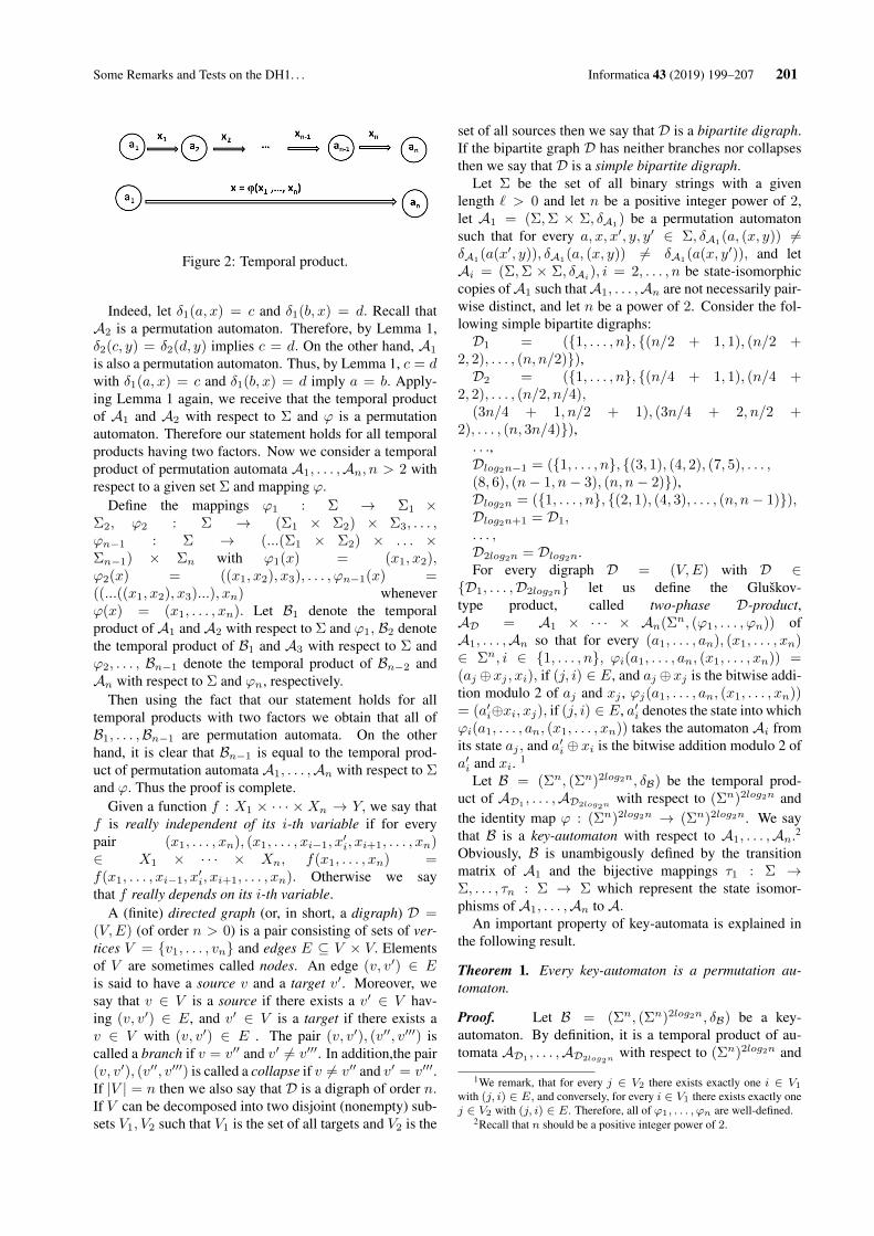
Some Remarks and Tests on the DH1. . . Informatica 43 (2019) 199–207 201
Figure 2: Temporal product.
Indeed, let δ1(a, x) = c and δ1(b, x) = d. Recall thatA2 is a permutation automaton. Therefore, by Lemma 1,δ2(c, y) = δ2(d, y) implies c = d. On the other hand, A1
is also a permutation automaton. Thus, by Lemma 1, c = dwith δ1(a, x) = c and δ1(b, x) = d imply a = b. Apply-ing Lemma 1 again, we receive that the temporal productof A1 and A2 with respect to Σ and ϕ is a permutationautomaton. Therefore our statement holds for all temporalproducts having two factors. Now we consider a temporalproduct of permutation automata A1, . . . ,An, n > 2 withrespect to a given set Σ and mapping ϕ.
Define the mappings ϕ1 : Σ → Σ1 ×Σ2, ϕ2 : Σ → (Σ1 × Σ2) × Σ3, . . . ,ϕn−1 : Σ → (...(Σ1 × Σ2) × . . . ×Σn−1) × Σn with ϕ1(x) = (x1, x2),ϕ2(x) = ((x1, x2), x3), . . . , ϕn−1(x) =((...((x1, x2), x3)...), xn) wheneverϕ(x) = (x1, . . . , xn). Let B1 denote the temporalproduct of A1 and A2 with respect to Σ and ϕ1, B2 denotethe temporal product of B1 and A3 with respect to Σ andϕ2, . . . , Bn−1 denote the temporal product of Bn−2 andAn with respect to Σ and ϕn, respectively.
Then using the fact that our statement holds for alltemporal products with two factors we obtain that all ofB1, . . . ,Bn−1 are permutation automata. On the otherhand, it is clear that Bn−1 is equal to the temporal prod-uct of permutation automata A1, . . . ,An with respect to Σand ϕ. Thus the proof is complete.
Given a function f : X1 × · · · × Xn → Y, we say thatf is really independent of its i-th variable if for everypair (x1, . . . , xn), (x1, . . . , xi−1, x
′i, xi+1, . . . , xn)
∈ X1 × · · · × Xn, f(x1, . . . , xn) =f(x1, . . . , xi−1, x
′i, xi+1, . . . , xn). Otherwise we say
that f really depends on its i-th variable.A (finite) directed graph (or, in short, a digraph) D =
(V,E) (of order n > 0) is a pair consisting of sets of ver-tices V = {v1, . . . , vn} and edges E ⊆ V × V. Elementsof V are sometimes called nodes. An edge (v, v′) ∈ Eis said to have a source v and a target v′. Moreover, wesay that v ∈ V is a source if there exists a v′ ∈ V hav-ing (v, v′) ∈ E, and v′ ∈ V is a target if there exists av ∈ V with (v, v′) ∈ E . The pair (v, v′), (v′′, v′′′) iscalled a branch if v = v′′ and v′ 6= v′′′. In addition,the pair(v, v′), (v′′, v′′′) is called a collapse if v 6= v′′ and v′ = v′′′.If |V | = n then we also say that D is a digraph of order n.If V can be decomposed into two disjoint (nonempty) sub-sets V1, V2 such that V1 is the set of all targets and V2 is the
set of all sources then we say that D is a bipartite digraph.If the bipartite graph D has neither branches nor collapsesthen we say that D is a simple bipartite digraph.
Let Σ be the set of all binary strings with a givenlength ` > 0 and let n be a positive integer power of 2,let A1 = (Σ,Σ × Σ, δA1
) be a permutation automatonsuch that for every a, x, x′, y, y′ ∈ Σ, δA1(a, (x, y)) 6=δA1(a(x′, y)), δA1(a, (x, y)) 6= δA1(a(x, y′)), and letAi = (Σ,Σ × Σ, δAi
), i = 2, . . . , n be state-isomorphiccopies ofA1 such thatA1, . . . ,An are not necessarily pair-wise distinct, and let n be a power of 2. Consider the fol-lowing simple bipartite digraphs:D1 = ({1, . . . , n}, {(n/2 + 1, 1), (n/2 +
2, 2), . . . , (n, n/2)}),D2 = ({1, . . . , n}, {(n/4 + 1, 1), (n/4 +
2, 2), . . . , (n/2, n/4),(3n/4 + 1, n/2 + 1), (3n/4 + 2, n/2 +
2), . . . , (n, 3n/4)}),. . .,Dlog2n−1 = ({1, . . . , n}, {(3, 1), (4, 2), (7, 5), . . . ,(8, 6), (n− 1, n− 3), (n, n− 2)}),Dlog2n = ({1, . . . , n}, {(2, 1), (4, 3), . . . , (n, n− 1)}),Dlog2n+1 = D1,. . . ,D2log2n = Dlog2n.For every digraph D = (V,E) with D ∈
{D1, . . . ,D2log2n} let us define the Gluškov-type product, called two-phase D-product,AD = A1 × · · · × An(Σn, (ϕ1, . . . , ϕn)) ofA1, . . . ,An so that for every (a1, . . . , an), (x1, . . . , xn)∈ Σn, i ∈ {1, . . . , n}, ϕi(a1, . . . , an, (x1, . . . , xn)) =(aj ⊕xj , xi), if (j, i) ∈ E, and aj ⊕xj is the bitwise addi-tion modulo 2 of aj and xj , ϕj(a1, . . . , an, (x1, . . . , xn))= (a′i⊕xi, xj), if (j, i) ∈ E, a′i denotes the state into whichϕi(a1, . . . , an, (x1, . . . , xn)) takes the automaton Ai fromits state aj , and a′i ⊕ xi is the bitwise addition modulo 2 ofa′i and xi. 1
Let B = (Σn, (Σn)2log2n, δB) be the temporal prod-uct of AD1 , . . . ,AD2log2n
with respect to (Σn)2log2n andthe identity map ϕ : (Σn)2log2n → (Σn)2log2n. We saythat B is a key-automaton with respect to A1, . . . ,An.2
Obviously, B is unambigously defined by the transitionmatrix of A1 and the bijective mappings τ1 : Σ →Σ, . . . , τn : Σ → Σ which represent the state isomor-phisms of A1, . . . ,An to A.
An important property of key-automata is explained inthe following result.
Theorem 1. Every key-automaton is a permutation au-tomaton.
Proof. Let B = (Σn, (Σn)2log2n, δB) be a key-automaton. By definition, it is a temporal product of au-tomata AD1
, . . . ,AD2log2nwith respect to (Σn)2log2n and
1We remark, that for every j ∈ V2 there exists exactly one i ∈ V1with (j, i) ∈ E, and conversely, for every i ∈ V1 there exists exactly onej ∈ V2 with (j, i) ∈ E. Therefore, all of ϕ1, . . . , ϕn are well-defined.
2Recall that n should be a positive integer power of 2.
202 Informatica 43 (2019) 199–207 P. Dömösi et al.
the identity map ϕ : (Σn)2log2n → (Σn)2log2n as definedabove. By Lemma 2, it is enough to prove that each ofAD1 , . . . ,AD2log2n
is a permutation automaton.Consider an automaton AD = (Σn,Σn, δD) with AD ∈
{AD1, . . . ,AD2log2n
} and the simple bipartite digraphD =(V,E) assigned toAD. Let V1 denote the set of targets andV2 denote the set of sources of D as before.
By Lemma 1 it is enough to prove thatfor any states (a1, . . . , an), (a′1, . . . , a
′n)
∈ Σn and input (x1, . . . , xn) ∈Σn, δD((a1, . . . , an), (x1, . . . , xn))= δD((a′1, . . . , a
′n), (x1, . . . , xn)) implies (a1, . . . , an) =
(a′1, . . . , a′n).
Suppose δD((a1, . . . , an), (x1, . . . , xn)) =δD((a′1, . . . , a
′n), (x1, . . . , xn)) = (b1, . . . , bn) for
some state (b1, . . . , bn) of AD and let (i, j) ∈ E. Observethat for every i ∈ V1 there exists exactly one j ∈ V2 with(j, i) ∈ E, and vice versa, for every j ∈ V2 there existsexactly one i ∈ V1 with (j, i) ∈ E. This means that thetransitions in the i-th and j-th component automata dependonly on the i-th and j-th state and input components.
Then, by the effect of its input (aj⊕xj , xi) the i-th com-ponent of AD goes from its state ai into state bi, and sim-ilarly, by the effect of its input (bi ⊕ xi, xj) the j-th com-ponent of AD goes from its state aj into state bj .
But then by the effect of its input (a′j ⊕ xj , xi), the i-thcomponent of AD goes from its state a′i into state bi, andsimilarly, by the effect of its input (bi ⊕ xi, xj), the j-thcomponent of AD goes from its state a′j into state bj .
Recall that Aj is a permutation automaton. Therefore,applying Lemma 1, aj = a′j . Therefore, using our previousassumptions we can derive that by the effect of its input(aj ⊕ xj , xi) the i-th component of AD goes from its statea′i into state bi. On the other hand, we assumed that by theeffect of its input (aj ⊕ xj , xi), the i-th component of ADgoes from its state ai into state bi.Applying Lemma 1 againwe obtain that ai = a′i.
Applying the above treatment to ev-ery (i, j) ∈ E, we receive (a1, . . . , an)= (a′1, . . . , a
′n). This completes the proof.
The basic idea of DH1 cryptosystem is to use a fi-nite automaton and a pseudo random generator. The setof states of the automaton consists of all possible plain-text/cyphertext blocks and the input set of the automatoncontains all possible pseudo random blocks. The size of thepseudo random blocks are the same as the size of the plain-text/cyphertext blocks. For each plaintext block the pseudorandom generator generates the next pseudo random blockand the automaton transforms the plaintext block into acyphertext block by the effect of the pseudo random block.The key is the transformation matrix of the automaton.
It is easy to see that the key must be a permutation au-tomaton, since this property grants an unambiguous de-cryption. This condition is satisfied by Theorem 1.
On the other hand we can have more than one cor-responding ciphertext for each plaintext even if we usethe same key-automaton. The reason for this is that we
can change the pseudo random numbers generated by thepseudo random generator. We can save a secret number n–as a part of the key– and before encryption we can choosea (public) random number m. This number m will be thefirst block of the ciphertext, and before encryption and de-cryption, the seed of the pseudo random number generatorcan be calculated with an XOR operation from n and m(n ⊕m). This way each encryption process uses differentpseudo random numbers and results different ciphertext forthe same plaintext.
The problem with this idea is the following. Modernblock ciphers operate on fixed-length groups of bits calledblocks. The size of the blocks is at least 128 bits (16 bytes),so the size of the transition matrix of the automaton is huge,namely 2128 × 2128 × 16 bytes, which is impossible to bestored in the memory or on a hard disk. The solution isto use an automata network. Gluškov-type product of au-tomata consists of smaller component automata and it isable to simulate the operation of a huge automaton. In thiscase we should store only the transition matrix of the iso-morphic component-automata, the structure of the compo-sition and the secret number n to calculate the seed of thepseudo random number generator.
3 Encryption and decryptionA symmetric cryptosystem consists of the following:
– a set of plaintexts P ,
– a set of ciphertexts C,
– a key space K,
– an encryption function e : P ×K → C, and
– a decryption function d : C × K → P .
Furthermore, the following property must hold for eachx ∈ P and k ∈ K: d((e(x, k), k) = x. Moreover, the cryp-tosystem is called approved block cipher if and only if theelements of the set of plaintexts and the set of ciphertextsare at least 128 bit long (|P| ≥ 2128 and |C| ≥ 2128).
Our cryptosystem is a block cipher one. Both of the en-cryption and decryption apparatus have a pseudo randomgenerator and a key-automaton.
The encryption procedure is the following. Before theencryption procedure, the pseudo random generator gets itsinitialization vector as a true random string r1 . . . rn ∈ Σn,where the pseudo random alphabet Σ is also the plaintextand the ciphertext alphabet simultaneously. This initializa-tion vector will also be the first block of the ciphertext.
Then the apparatus reads the plaintext block-by-blockand, after reading the next plaintext block a1 · · · an ∈ Σn
(the first block first), it generates the second, third, and thefurther blocks of the ciphertext in the following way.
The apparatus takes the key-automaton B =(Σn, (Σn)2log2n, δB) into the state a1 · · · an ∈ Σn
Some Remarks and Tests on the DH1. . . Informatica 43 (2019) 199–207 203
which coincides with the actual one, i.e. the last receivedplaintext block.
Next the pseudo random number generator gener-ates a 2log2n long number of pseudo random se-quences w1, . . . , w2log2n ∈ Σn such that each of themtakes the next temporal component (the first one first)AD = (Σn,Σn, δD) (AD ∈ {AD1
, . . . ,AD2log2n})
of the key automaton into the state ak,1 · · · ak,n= δD(ak−1,1 · · · ak−1,n, wk), k = 1, . . . , 2log2n, wherea0,1 · · · a0,n denotes the actual plaintext block.
The last state a2log2n,1 · · · a2log2n,n will be the generatedciphertext block of the plaintext block a1 · · · an.
The i-th transition ai,1 · · · ai,n =δD(ai−1,1 · · · ai−1,n, wi) will be performed in thefollowing way.
Recall that D is a Gluškov product AD = A1 ×· · ·×An(Σn, (ϕ1, . . . , ϕn)) of appropriate permutation au-tomata Am = (Σ,Σ2, δm),m = 1, . . . , n that are stateisomorphic to each other so that for an appropriate bipar-tite digraph D = (V,E) with the set V1 of targets and V2of sources we have as follows:δi(ak−1,i, ϕi(ak−1,1, · · · , ak−1,n, (x1, . . . , xn)) =
ak,i, where ak,i = δi(ak−1,i, (ak−1,j ⊕ xj , xi)), if(j, i) ∈ E, and ak,i = δi(ak−1,i, (ak,j ⊕ xj , xi)), if(i, j) ∈ E, and ak,j = δi(ak−1,i, (ak−1,j ⊕ xj , xi)),
(1)
where wm = x1 · · ·xn ∈ Σn is the actual pseudo ran-dom string. Obviously, using the transition matrix of Ai,from ak−1,i, ak−1,j , xi, xj we can determine ak,i for ev-ery i ∈ V1, (j, i) ∈ E. Moreover, after calculatingthe values ai(i ∈ V1), using the transition table of Ai,from ak−1,j , ak,i, xi, xj we can determine ak,j for everyi ∈ V2, (i, j) ∈ E.
Then, concatenating the calculated blocks, we will getthe ciphertext.
The decryption procedure is the following. Similarly asbefore, before the decryption procedure the pseudo randomgenerator gets the first ciphertext block as its initializationvector r1 . . . rn ∈ Σn.
Then the apparatus reads the ciphertext block-by-blockand, after reading the next ciphertext block c1 · · · cn ∈ Σn
(the first block first), it generates the second, third and thefurther blocks of the plaintext in the following way.
The apparatus determines the statea1 · · · an ∈ Σn of key-automatonB = (Σn, (Σn)2log2n, δB) into which the automatonB is taken from the state a1 · · · an ∈ Σn by the effect of2log2n consecutive strings in Σn generated by the pseudorandom generator.
Thus the pseudo random generator should generatea 2log2n -long number of pseudo random sequencesw1, . . . , w2log2n ∈ Σn and going back from the last mem-ber w2log2n to the first one w1 the following procedure isperformed.
Each of them takes the next temporal com-ponent (in opposite direction, i.e., the last one
first and the first one last) AD = (Σn,Σn, δD)(AD ∈ {AD1
, . . . ,AD2log2n}) of the key automa-
ton into the state ak−1,1 · · · ak−1,n back from thestate ak,1 · · · ak,n = δD(ak−1,1 · · · ak−1,n, wk), k =1, . . . , 2log2n, where a2log2n,1 · · · a2log2n,n denotes theactual ciphertext block c1 · · · cn.
The last state a0,1 · · · a0,n will be the generated plaintextblock of the ciphertext block c1 · · · cn.
The state ai−1,1 · · · ai−1,n obtainedfrom the i-th state transition ai,1 · · · ai,n= δD(ai−1,1 · · · ai−1,n, wi) will be performed in thefollowing way.
Recall again that D is a Gluškov productAD = A1 × · · · × An(Σn, (ϕ1, . . . , ϕn)) of appro-priate permutation automata Am = (Σ2,Σ, δm),m =1, . . . , n that are state isomorphic to each otherso that for an appropriate bipartite digraphD = (V,E) with the set V1 of targets and V2 ofsources, we conclude as in (1).
Recall also that all of A1, . . . ,An are permutationautomata. Therefore, for every ak,i, ak,j , xi, xj , j ∈V2, (j, i) ∈ E, there exists only one ak−1,j with ak,j =δi(ak−1,j , (ak,i ⊕ xi, xj)). Thus, using the transitiontable we can unambiguously determine ak−1,j for ev-ery j ∈ V2. Moreover, for every ak,i, ak−1,j , xi, xj ,i ∈ V1, (j, i) ∈ E, there exists exactly one ak−1,i with ak,i= δi(ak−1,i, (ak−1,j ⊕ xj , xi)). Therefore, using the tran-sition table again we can unambiguously determine ak−1,ias well for every i ∈ V1.
Then by concatenating the determined plaintext blockswe will get the plaintext back.
To sum up, the discussed cryptosys-tem is a block cipher. Because ofTheorem 1, for every ciphertext there exists exactlyone plaintext making the encryption and decryptionunambiguous. Moreover, there is a huge number ofcorresponding encoded messages to each plaintext so thatseveral encryptions of the same plaintext yield severaldistinct ciphertexts.
4 Experimental resultsThe practical test was done using 16 byte (128 bit) long in-put blocks, output blocks and pseudo random blocks. Firstwe present the size of the keyspace, then we continue ourinvestigation with the test results of the the speed of thealgorithm, and finally the effectiveness of the avalanche ef-fect.
Using the above mentioned parameters with 256 possi-ble states (1 byte long states) we need 16 automata havinga transition matrix of 216 = 65536 lines and 28 = 256columns. Each cell of the automaton contains 1 byte longdata (One state). The size of the matrix is 16 megabytesand the number of possible matrices is 256!65536, where theexclamation mark means the factorial operation. This pro-tection is much more than good enough against brute-force
204 Informatica 43 (2019) 199–207 P. Dömösi et al.
attacks. When we use isomorphic automata this huge num-ber should be further increased to have 256!65536∗256!15 =256!65551 possible keys. Using the above mentioned pa-rameters with half byte (4bits) long states, we need 32 au-tomata having a transition matrix of 28 = 256 lines and24 = 16 columns and each cell of the automaton containshalf byte long data. In this case the size of the matrix isonly 2 kilobytes and the number of possible matrices is16!256. Using permutation automata this can be increasedto 16!287 possible keys, which is still more than enoughagainst brute-force attacks. However, we recommend the 8bit version, because the number of calculations during theencoding and decoding process is less and the effectivenessof the avalanche effect is better.
The practical test of the encoding and decoding algo-rithm was done on an average desktop PC, (3,1 GHz IntelCore I3-2100 processor, 4 Gigabyte RAM). The programwe used was a well written C# implementation. The resultsof the speed tests of the 8 bit version can be seen in Table1.
The results of the speed tests show that using an averagePC the encoding time is more than 4 megabytes per second,and decoding time is about the same.
The avalanche effect is a very important property ofblock ciphers. The block cipher is said to have avalancheeffect when a small change in the plaintext block results ina significant change in the corresponding ciphertext block,further, a small change in the ciphertext block results in asignificant change in the corresponding plaintext block. Wetested the avalanche effect in the following way. We chose1000000 random plaintext blocks, encoded them and thenwe changed 1 bit in each plaintext block, encoded again,then we calculated the number of different bytes in the ci-phertext blocks pair-wise. We also tested the opposite case,namely, we chose 1000000 random ciphertext blocks, de-coded them and then we changed 1 bit in each ciphertextblock, decoded again and calculated the number of differ-ent bytes in each plaintext block pair-wise. During the firsttest we used just the first two rounds of encoding and de-coding. The results can be seen in Table 2. When wechange only one bit in the plaintext block the differencebetween the corresponding ciphertext blocks will be reallyhuge in the majority of cases. The same effect can be seenin the opposite case: changing one bit in the ciphertextblock results in a huge difference in the plaintext block aswell. Although it was a good result, we also made a fur-ther test with the full 4-round algorithm. The results can beseen in Table 3.
Furthermore, we calculated the optimal avalanche effect.For this, we chose 2×1000000 completely random blocksand then calculated the difference between them pair-wise.The results are in Table 4
We can assume that using the 8-bit version of the algo-rithm with 128 bit long blocks and 4 rounds the algorithmhas the maximal avalanche effect and an appropriate speed(4 megabyte/s). Of course the speed of the algorithm de-pends on the hardware, the programming language and the
actual program code as well.
5 The NIST test
The National Institute of Standards and Technology (NIST)published a statistical package consisting of 15 statisticaltests that were developed to test the randomness of arbi-trarily long binary sequences produced by either hardwareor software based cryptographic random or pseudo randomnumber generators. In case of each statistical test a set ofP-values was produced. Given a significance level α, if theP-value is less than or equal to α then test suggests thatthe observed data is inconsistent with our null hypothesis,i.e. the ’hypothesis of randomness’, so we reject it. Weused α = 0.01 as it is common in such problems in cryp-tography. An α of 0.01 indicates that one would expect1 sequence in 100 sequences to be rejected under the nullhypothesis. Hence a P-value exceeding 0.01 would meanthat the sequence would be considered to be random, andP-value less than or equal to 0.01 would lead to the conclu-sion that the sequence is non-random.
One of the criteria used to evaluate the AES candidatealgorithms was their demonstrated suitability as randomnumber generators. That is, the evaluation of their out-put utilizing statistical tests should not provide any meansby which to distinguish them computationally from a trulyrandom source. Randomness testing was performed usingthe same parameters as for the AES candidates in orderto achieve the most reliable and comparable results. Firstthe input parameters –such as the sequence length, samplesize, and significance level– were fixed. Namely, these pa-rameters were set at 220 bits, 300 binary sequences, andα = 0.01, respectively. Furthermore, Table 5 shows thelength parameters we used.
In order to analyze the output of the algorithmwe encrypted the Rockyou database, which containsmore than 32 millions of cleartext passwords (see e.g:[Tihanyi et al., 2015]). Applying the NIST test for the en-crypted file it has turned out that the output of the algo-rithm can not be distinguished in polynomial time fromtrue random sources by statistical tests. The exact p-valuesof the evaluation of the ciphertext are shown in Table (6).We also tested the uniformity of the distribution of the p-values obtained by the statistical tests included in NIST,which is a usual requirement in the literature (see e.g.[Rukhin et al., 2010]). The uniformity of p-values provideno additional information about the type of the cryptosys-tem. We have also shown that the proportions of binarysequences which passed the 0.01 level lie in the requiredconfidence interval (see e.g. [Rukhin et al., 2010]).
6 Conclusions
The output of our crypto algorithm has passed all statisti-cal tests of the NIST suite we performed and we were not

Some Remarks and Tests on the DH1. . . Informatica 43 (2019) 199–207 205
Table 1: Encoding and decoding spped test.
Type of the plaintext Size Encoding time Decoding time Encoded bytes per secondImage:JPG 205216 00:00.0470960 00:00.0456500 4357397.6558519
Document:PDF 204768 00:00.0459240 00:00.0454752 4458845.0483407Text:TXT 204848 00:00.0467470 00:00.0461294 4382056.6025627
Compressed:RAR 204848 00:00.0471470 00:00.0454830 4344878.7833796Compressed:RAR 104883392 00:25.9539778 00:27.2784568 4041129.7569962Compressed:RAR 524613552 02:10.6843636 02:08.6140492 4014355.9454882Compressed:RAR 1102971104 04:28.121944 04:08.2624464 4442762.5683785
Table 2: Character differences after 2 rounds of encoding.
different characters in one block encoding decoding0 0 01 0 02 1 13 0 04 36 405 3 16 72 897 125 1368 5574 55949 11 4
10 179 22511 410 39612 11050 1106413 880 92114 22670 2239715 43064 4271016 915924 916422
Table 3: Character differences after 4 rounds of encoding.
different characters in one block encoding decoding0-12 0 013 37 2814 1717 174615 59403 5914516 938842 939081
Table 4: Optimal avalanche effect.
different characters in one block0-12 013 3214 169315 5868116 939594
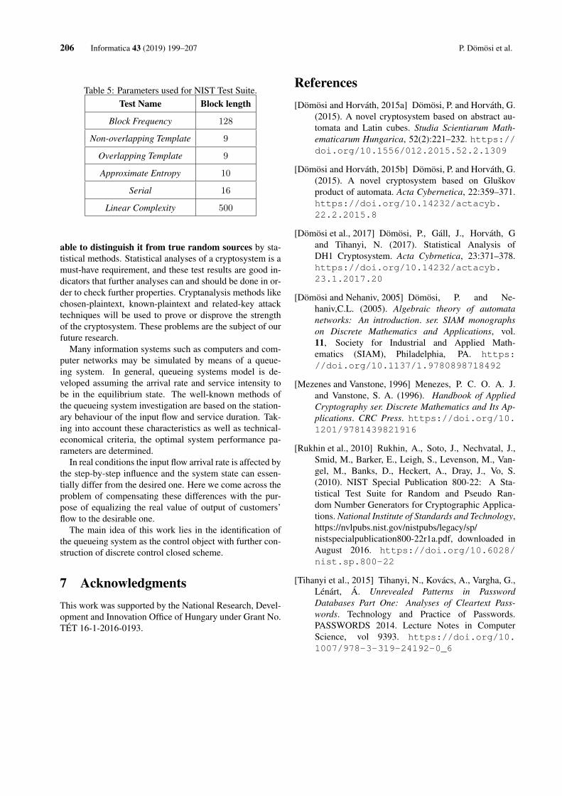
206 Informatica 43 (2019) 199–207 P. Dömösi et al.
Table 5: Parameters used for NIST Test Suite.Test Name Block length
Block Frequency 128
Non-overlapping Template 9
Overlapping Template 9
Approximate Entropy 10
Serial 16
Linear Complexity 500
able to distinguish it from true random sources by sta-tistical methods. Statistical analyses of a cryptosystem is amust-have requirement, and these test results are good in-dicators that further analyses can and should be done in or-der to check further properties. Cryptanalysis methods likechosen-plaintext, known-plaintext and related-key attacktechniques will be used to prove or disprove the strengthof the cryptosystem. These problems are the subject of ourfuture research.
Many information systems such as computers and com-puter networks may be simulated by means of a queue-ing system. In general, queueing systems model is de-veloped assuming the arrival rate and service intensity tobe in the equilibrium state. The well-known methods ofthe queueing system investigation are based on the station-ary behaviour of the input flow and service duration. Tak-ing into account these characteristics as well as technical-economical criteria, the optimal system performance pa-rameters are determined.
In real conditions the input flow arrival rate is affected bythe step-by-step influence and the system state can essen-tially differ from the desired one. Here we come across theproblem of compensating these differences with the pur-pose of equalizing the real value of output of customers’flow to the desirable one.
The main idea of this work lies in the identification ofthe queueing system as the control object with further con-struction of discrete control closed scheme.
7 AcknowledgmentsThis work was supported by the National Research, Devel-opment and Innovation Office of Hungary under Grant No.TÉT 16-1-2016-0193.
References[Dömösi and Horváth, 2015a] Dömösi, P. and Horváth, G.
(2015). A novel cryptosystem based on abstract au-tomata and Latin cubes. Studia Scientiarum Math-ematicarum Hungarica, 52(2):221–232. https://doi.org/10.1556/012.2015.52.2.1309
[Dömösi and Horváth, 2015b] Dömösi, P. and Horváth, G.(2015). A novel cryptosystem based on Gluškovproduct of automata. Acta Cybernetica, 22:359–371.https://doi.org/10.14232/actacyb.22.2.2015.8
[Dömösi et al., 2017] Dömösi, P., Gáll, J., Horváth, Gand Tihanyi, N. (2017). Statistical Analysis ofDH1 Cryptosystem. Acta Cybrnetica, 23:371–378.https://doi.org/10.14232/actacyb.23.1.2017.20
[Dömösi and Nehaniv, 2005] Dömösi, P. and Ne-haniv,C.L. (2005). Algebraic theory of automatanetworks: An introduction. ser. SIAM monographson Discrete Mathematics and Applications, vol.11, Society for Industrial and Applied Math-ematics (SIAM), Philadelphia, PA. https://doi.org/10.1137/1.9780898718492
[Mezenes and Vanstone, 1996] Menezes, P. C. O. A. J.and Vanstone, S. A. (1996). Handbook of AppliedCryptography ser. Discrete Mathematics and Its Ap-plications. CRC Press. https://doi.org/10.1201/9781439821916
[Rukhin et al., 2010] Rukhin, A., Soto, J., Nechvatal, J.,Smid, M., Barker, E., Leigh, S., Levenson, M., Van-gel, M., Banks, D., Heckert, A., Dray, J., Vo, S.(2010). NIST Special Publication 800-22: A Sta-tistical Test Suite for Random and Pseudo Ran-dom Number Generators for Cryptographic Applica-tions. National Institute of Standards and Technology,https://nvlpubs.nist.gov/nistpubs/legacy/sp/nistspecialpublication800-22r1a.pdf, downloaded inAugust 2016. https://doi.org/10.6028/nist.sp.800-22
[Tihanyi et al., 2015] Tihanyi, N., Kovács, A., Vargha, G.,Lénárt, Á. Unrevealed Patterns in PasswordDatabases Part One: Analyses of Cleartext Pass-words. Technology and Practice of Passwords.PASSWORDS 2014. Lecture Notes in ComputerScience, vol 9393. https://doi.org/10.1007/978-3-319-24192-0_6

Some Remarks and Tests on the DH1. . . Informatica 43 (2019) 199–207 207
Table 6: Results for the uniformity of p-values and the proportion of passing sequences.
C1 C2 C3 C4 C5 C6 C7 C8 C9 C10 P-value PRO- STATISTICAL TEST
PORTION
28 35 23 33 43 34 32 23 26 23 0.162606 296/300 Frequency
25 29 35 38 27 23 26 27 31 39 0.407091 298/300 BlockFrequency
28 37 26 37 32 28 25 36 25 26 0.574903 297/300 CumulativeSums
26 30 31 30 33 27 24 38 28 33 0.840081 295/300 CumulativeSums
33 20 33 26 32 28 44 25 30 29 0.205897 297/300 Runs
23 33 40 24 31 22 31 29 38 29 0.284959 297/300 LongestRun
24 28 40 32 24 30 30 27 37 28 0.527442 297/300 Rank
34 35 23 33 30 35 27 34 23 26 0.623240 298/300 FFT
35 31 30 29 30 29 32 28 23 33 0.958773 295/300 NonOverlapping−
Template
. . . . . . . . . . . . .
· · · · · · · · · · · · · · · · · · · · · · · · · · · · · · · · · · · · · · ·
25 27 25 29 40 39 29 33 26 27 0.419021 299/300 OverlappingTemplate
32 29 21 20 29 37 34 28 30 40 0.220931 298/300 Universal
35 33 28 34 26 26 27 30 33 28 0.935716 299/300 ApproximateEntropy
21 17 24 23 15 15 18 12 15 17 0.516465 171/177 RandomExcursions
. . . . . . . . . . . . .
· · · · · · · · · · · · · · · · · · · · · · · · · · · · · · · · · · · · · · ·
23 16 15 16 14 26 12 18 18 19 0.384836 172/177 RandomExcursions−
V ariant
. . . . . . . . . . . . .
· · · · · · · · · · · · · · · · · · · · · · · · · · · · · · · · · · · · · · ·
23 27 38 25 27 43 41 24 24 28 0.042808 298/300 Serial
28 28 25 24 45 32 32 33 28 25 0.253551 296/300 Serial
32 25 33 34 40 20 31 35 15 35 0.039244 295/300 LinearComplexity

208 Informatica 43 (2019) 199–207 P. Dömösi et al.
https://doi.org/10.31449/inf.v43i2.1888 Informatica 43 (2019) 209–219 209
Agent-Based Modeling of Society Resistance against Unpopular Norms
Kashif Zia, Dinesh Kumar Saini and Arshad MuhammadFaculty of Computing and Information Technology, Sohar University, Sohar, OmanE-mail: [email protected], [email protected], [email protected]
Umar FarooqUniversity of Science and Technology Bannu, Khyber Pakhtunkhwa, PakistanE-mail: [email protected]
Keywords: agent-based modeling and simulation, unpopular norms, emperor’s dilemma, norm aversion
Received: June 24, 2017
People lives in a society adhering to different types of norms, and some of these norms are unpopular.This paper proposes an agent-based model for unpopular norm aversion. The proposed model is simulatedasking important “what-if” questions to elaborate on the conditions and reasons behind the emergence,spreading and aversion of unpopular norms. Such conditions can thus be analyzed and mapped onto thebehavioral progression of real people and patterns of their interactions to achieve improved societal traitsparticularly using the new social landscape dominated by digital content and social networking. Hence, itcan be argued that careful amalgamation of social media content can not only educate the people but alsohelp them in an aversion of undesirable behaviors such as retention and spreading of unpopular norms.Simulation results revealed that to achieve a dominant norm aversion, an agent population must incorpo-rate a rational model, besides, active participation of agents in averting unpopular norms.
Povzetek: Razvit je agentni sistem obnašanja množic, ki omogoca analizo odpora proti nezaželenim nor-mam.
1 IntroductionSocial norms are concepts and practices prevalent in a soci-ety [7]. Formally, “Norms are practical prescriptions, per-missions, or prohibitions, accepted by members of particu-lar groups, organizations, or societies, and capable of guid-ing the actions of those individuals” [21].
Norms are accepted which means that their existence isevident from empirical inquiry. However, there is a con-tradiction in the viewpoint of the notion of existence. Oneview of norms existence (acceptance) is internalized thatincorporates it into individuals’ identity [21, 1]. The otherview uses the intentions of individuals’ as the criterion fornorm acceptance instead of the identity of individuals [21].Therefore, conforming/accepting a norm corresponds tothe first view while following a norm relates to the sec-ond view [3]. This distinction allows thinking of a normeven without accepting it [21]. Norms describe a collectivebehavior of groups, organizations, or societies but they arethe collective outcome of individuals’ cognition.
Norms have the power to transform into actions. Thiscan lead to norm transformation as well. Brennan et al[3] have distinguished between conforming and comply-ing (following) with norms. Similarly, they differentiatedbetween avoiding and acting opposite to norms. These ac-tions are norm guided and in the absence of a norm, anaction would not be performed or it would be performedbut not in a similar fashion [21].
Norms play an important role in the development of so-
cial order [30]. They can change, create and affect behav-iors. On the other hand, behaviors are capable of chang-ing, creating and affecting norms [15]. Individual behavioraffects the behavior of other individuals in its range of in-fluence [8]. The process is often defined as norm being“externalized”. These externalities are able to reproduce aregulatory impact on individuals’ behavior [12]. Accordingto Christine Horne, a higher degree of norm enforcementhave large sanctioning benefits [9]. She designed a normenforcement theory with the following features. In the caseof group welfare, sanctioning benefits have a positive effecton norm and metanorm enforcement. However, the sanc-tioning cost has a negative effect on norm enforcement. Inthe case of social relations, interdependence has a positiveeffect on norm enforcement. Similarly, sanctioning costand interdependence have a positive effect on metanormenforcement. Meta-norms are a particular type of normsthat regulate enforcement. Interdependence means the ex-tent to which individuals value their relations. The experi-mental analysis of the theory of enforcement has revealedthat theories that do not consider social relational contactmay produce faulty predictions.
Generally, an individual in a society is expected to be-have according to societal norms. However, the equation isnot that simple. Following a societal norm does not meanthat an individual is accepting it. There may be a num-ber of conditions and incentives that force an individualto follow a social norm [21]. This clearly distinguishes
210 Informatica 43 (2019) 209–219 K. Zia et al.
the distinction between following and conforming to thenorm. If a norm is not confirmed or accepted from theinside of an individual, just following it as a visible traitis of weaker intensity. Hence, in the case of an individ-ual, a norm can be followed as a result of social pressure,but not accepted, if the individual’s personal belief doesnot correspond to it. Contrarily, an individual may ac-cept/conform to a norm, if personal belief corresponds tofollowing it. Christine Horne [10] has emphasized on re-lationships, which are more important than individual per-ception about norms. She argues that these relationshipscan even persuade an individual to enforce a norm, even ifthere is no apparent benefit of doing it. This situation be-comes interesting when a particular norm is unpopular innature.
Unpopular social norms are those norms with which themajority of people do not agree or believe in it internally. Infact, people personally do not agree with unpopular normsbut still stick to them. Individuals’ may even unintention-ally enforce others to follow them. Such cases in sociologyare dealt through a dilemma called, Emperor’s Dilemma,as illustrated by Nkomo in [24]. Emperor’s dilemma re-lates to a tale in which everyone shows fake admiration fora new gown worn by an emperor even though the emperorwas naked. The cunning gown designers announced thatthe (non-existent) gown would not be visible to those whoare not loyal to the emperor or who are really dumb. Thefear of being punished and of being identified as having in-ferior societal traits, no one spoke the truth. The truth thatthe emperor was in fact naked.
It is evident that the Emperor’s Dilemma is demonstratedin many places around the world in one way or the other.Whether it is foot-binding in neo-Confucian China or inter-cousin marriages and dowry in Asia (indicated by Blakein [2] and Hughes in [11], respectively), the nature of thethought process is the same. People do not reveal what theyreally believe from the fear of being identified as ignorantor anti-social.
It is not that harmful if unpopular norms are followedat an individual level. However, when a large populationadopts unpopular norms, following it becomes a kind ofdefault behavior that might influence the neutral part of thepopulation. As a consequence, it has been observed thatpeople even start enforcing unpopular norm which they dis-approve in private. This behavior is generally termed asfalse enforcement. Willer et al. in [29] focused on findingout the reasons for false enforcement. According to them,people falsely enforce unpopular norms to create an illu-sion of sincerity rather than conviction. They performedexperiments using two scenarios, namely, wine tasting andtext evaluation. Experimental results revealed that peoplewho enforced a norm even against their actual belief, infact, criticized different alternate variations of an unpop-ular norm. In short, their outcomes indicate that how so-cial pressure can lead to false enforcement of an unpopularnorm.
Un-popular Norms (UNs) could have an adverse impact
on society and it is, therefore, sometimes necessary to op-pose and possibly avert them. To achieve this goal, it is im-portant to know the conditions which enable the persistenceof unpopular norms and models that support possible aver-sion of these norms. This study attempts to elaborate onthe conditions and reasons behind the emergence, spread-ing and aversion of unpopular norms in a society, using atheory-driven agent-based simulation.
The rest of the paper is structured as follows. Section 1introduced the research work presented in this work. Re-lated work is provided in section 2. The current modelsand then the proposed model is presented in section 3. De-tailed analysis and comparison are provided in 4. Section5 ends this paper with conclusions and future direction ofthis work.
2 Related work
The propagation and transformation of norms co-evolvewith each other. Norms propagate through diffused influ-ence. Since the subjects being influenced may have theirown perspective, they may decide to adhere or reject it.As a result, the reciprocating influence of the subjects maytransform the norm itself. According to Macy and Flache,exploration of scenarios of such a nature has been a sub-ject of complex adaptive systems and they are investigatedby developing agent-based models [18]. Understanding theemergence of norms in a society of agents is a challengeand an area of ongoing research [27].
Studying norms in society have been one of the researchfocus of agent-based modeling community. Theoreticalstudies on norms such as those conducted by Conte andCastelfranchi [6] and Meneguzzi et al. [20] explored thatagent are supposed to comply with social norms. Thesense of punishment from the society is evident as the pre-dominant factor behind compliance of norms [4]. Stud-ies conducted by Sanchez-Anguix et al. [25] and Sato andHashimoto [26] focused on the emergence of norms andthey described strategies showing how norms prevail in asociety. This is basically governed by societal influence.Agents set their goals and frequently change their behav-ior based on societal influence until a global equilibrium inachieved [27]. Though lots of work has been done on theemergence and prevalence of norms, very limited is car-ried out for the aversion of unpopular norms. To the best,our knowledge, our previous work [31, 22, 23] is the onlyagent-based study on this exciting research area. Willer etal. have pointed out many “empirical cases in which in-dividuals are persuaded to publicly support behaviors orbeliefs that they privately question” [29]. The term, Prefer-ence falsification, coined by Kuran [17] is defined as “theact of misrepresenting one’s genius wants under perceivedsocial pressures”. According to him, an equilibrium is thesum of three utilities namely, intrinsic, expressive, and rep-utation. The intrinsic utility is about an individual’s per-sonal satisfaction being part of the society. The expressive
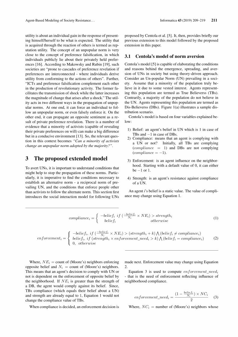
Agent-Based Modeling of Society Resistance. . . Informatica 43 (2019) 209–219 211
utility is about an individual gain in the response of present-ing himself/herself to be what is expected. The utility thatis acquired through the reaction of others is termed as rep-utation utility. The concept of an unpopular norm is veryclose to the concept of preference falsification, in whichindividuals publicly lie about their privately held prefer-ences [16]. According to Makowsky and Rubin [19], suchsocieties are “prone to cascades of preference revelation ifpreferences are interconnected - where individuals deriveutility from conforming to the actions of others”. Further,“ICTs and preference falsification complement each otherin the production of revolutionary activity. The former fa-cilitates the transmission of shock while the latter increasesthe magnitude of change that arises after a shock.” The util-ity acts in two different ways in the propagation of unpop-ular norms. At one end, it can force an individual to fol-low an unpopular norm, or even falsely enforce it. On theother end, it can propagate an opposite sentiment as a re-sult of private preference revelation. There is a number ofevidence that a minority of activists (capable of revealingtheir private preferences on will) can make a big differencebut in a conducive environment [13]. So, the relevant ques-tion in this context becomes “Can a minority of activistschange an unpopular norm adopted by the majority?”.
3 The proposed extended modelTo avert UNs, it is important to understand conditions thatmight help to stop the propagation of these norms. Partic-ularly, it is imperative to find the conditions necessary toestablish an alternative norm - a reciprocal norm of pre-vailing UN, and the conditions that enforce people otherthan activists to follow the alternate norm. This section firstintroduces the social interaction model for following UNs
proposed by Centola et al. [5]. It, then, provides briefly ourprevious extension to this model followed by the proposedextension in this paper.
3.1 Centola’s model of norm aversionCentola’s model [5] is capable of elaborating the conditionsand reasons behind the emergence, spreading, and aver-sion of UNs in society but using theory-driven approach.Consider an Un-popular Norm (UN) prevailing in a soci-ety. Assume that a minority of the population truly be-lieve in it due to some vested interest. Agents represent-ing this population are termed as True Believerss (TBs).Contrarily, a majority of the population do not believe inthe UN. Agents representing this population are termed asDis-Believerss (DBs). Figure 1(a) illustrates a sample dis-tribution scenario.
Centola’s model is based on four variables explained be-low:
1) Belief: an agent’s belief in UN which is 1 in case ofTBs and −1 in case of DBs.
2) Compliance: means that an agent is complying witha UN or not? Initially, all TBs are complying(compliance = 1) and DBs are not complying(compliance = −1).
3) Enforcement: is an agent influence on the neighbor-hood. Starting with a default value of 0, it can eitherbe −1 or 1.
4) Strength: is an agent’s resistance against complianceof a UN.
An agent i’s belief is a static value. The value of compli-ance may change using Equation 1.
compliancei =
{−beliefi if (−beliefiNi
×NEi) > strengthibeliefi otherwise
(1)
enforcementi =
−beliefi, if (−beliefiNi×NEi) > (strengthi + k)
∧(beliefi 6= compliancei)
beliefi, if (strengthi × enforcement_needi > k)∧
(beliefi = compliancei)0, otherwise
(2)
Where, NEi = count of (Moore’s) neighbors enforcingopposite belief and Ni = count of (Moore’s) neighbors.This means that an agent’s decision to comply with UN ornot is dependent on the enforcement of opposite belief bythe neighborhood. If NEi is greater than the strength ofa DB, the agent would comply against its belief. Since,TBs compliance (which equals their belief about a UN)and strength are already equal to 1, Equation 1 would notchange the compliance value of TBs.
When compliance is decided, an enforcement decision is
made next. Enforcement value may change using Equation2.
Equation 3 is used to compute enforcement_needi- that is the need of enforcement reflecting influence ofneighborhood compliance.
enforcement_needi =(1− beliefi
Ni)×NCi
2(3)
Where, NCi = number of (Moore’s) neighbors whose
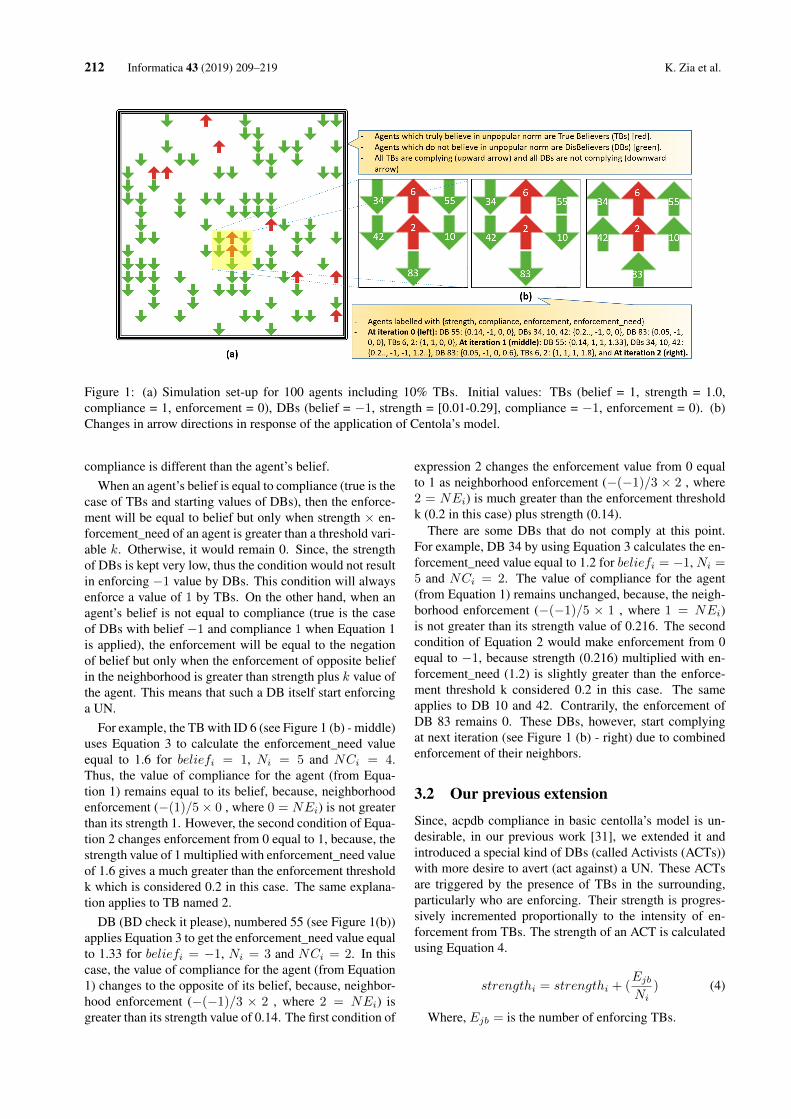
212 Informatica 43 (2019) 209–219 K. Zia et al.
Figure 1: (a) Simulation set-up for 100 agents including 10% TBs. Initial values: TBs (belief = 1, strength = 1.0,compliance = 1, enforcement = 0), DBs (belief = −1, strength = [0.01-0.29], compliance = −1, enforcement = 0). (b)Changes in arrow directions in response of the application of Centola’s model.
compliance is different than the agent’s belief.When an agent’s belief is equal to compliance (true is the
case of TBs and starting values of DBs), then the enforce-ment will be equal to belief but only when strength × en-forcement_need of an agent is greater than a threshold vari-able k. Otherwise, it would remain 0. Since, the strengthof DBs is kept very low, thus the condition would not resultin enforcing −1 value by DBs. This condition will alwaysenforce a value of 1 by TBs. On the other hand, when anagent’s belief is not equal to compliance (true is the caseof DBs with belief −1 and compliance 1 when Equation 1is applied), the enforcement will be equal to the negationof belief but only when the enforcement of opposite beliefin the neighborhood is greater than strength plus k value ofthe agent. This means that such a DB itself start enforcinga UN.
For example, the TB with ID 6 (see Figure 1 (b) - middle)uses Equation 3 to calculate the enforcement_need valueequal to 1.6 for beliefi = 1, Ni = 5 and NCi = 4.Thus, the value of compliance for the agent (from Equa-tion 1) remains equal to its belief, because, neighborhoodenforcement (−(1)/5× 0 , where 0 = NEi) is not greaterthan its strength 1. However, the second condition of Equa-tion 2 changes enforcement from 0 equal to 1, because, thestrength value of 1 multiplied with enforcement_need valueof 1.6 gives a much greater than the enforcement thresholdk which is considered 0.2 in this case. The same explana-tion applies to TB named 2.
DB (BD check it please), numbered 55 (see Figure 1(b))applies Equation 3 to get the enforcement_need value equalto 1.33 for beliefi = −1, Ni = 3 and NCi = 2. In thiscase, the value of compliance for the agent (from Equation1) changes to the opposite of its belief, because, neighbor-hood enforcement (−(−1)/3 × 2 , where 2 = NEi) isgreater than its strength value of 0.14. The first condition of
expression 2 changes the enforcement value from 0 equalto 1 as neighborhood enforcement (−(−1)/3 × 2 , where2 = NEi) is much greater than the enforcement thresholdk (0.2 in this case) plus strength (0.14).
There are some DBs that do not comply at this point.For example, DB 34 by using Equation 3 calculates the en-forcement_need value equal to 1.2 for beliefi = −1, Ni =5 and NCi = 2. The value of compliance for the agent(from Equation 1) remains unchanged, because, the neigh-borhood enforcement (−(−1)/5 × 1 , where 1 = NEi)is not greater than its strength value of 0.216. The secondcondition of Equation 2 would make enforcement from 0equal to −1, because strength (0.216) multiplied with en-forcement_need (1.2) is slightly greater than the enforce-ment threshold k considered 0.2 in this case. The sameapplies to DB 10 and 42. Contrarily, the enforcement ofDB 83 remains 0. These DBs, however, start complyingat next iteration (see Figure 1 (b) - right) due to combinedenforcement of their neighbors.
3.2 Our previous extension
Since, acpdb compliance in basic centolla’s model is un-desirable, in our previous work [31], we extended it andintroduced a special kind of DBs (called Activists (ACTs))with more desire to avert (act against) a UN. These ACTsare triggered by the presence of TBs in the surrounding,particularly who are enforcing. Their strength is progres-sively incremented proportionally to the intensity of en-forcement from TBs. The strength of an ACT is calculatedusing Equation 4.
strengthi = strengthi + (EjbNi
) (4)
Where, Ejb = is the number of enforcing TBs.
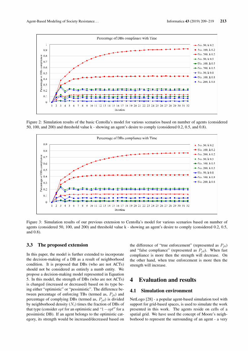
Agent-Based Modeling of Society Resistance. . . Informatica 43 (2019) 209–219 213
Figure 2: Simulation results of the basic Centolla’s model for various scenarios based on number of agents (considered50, 100, and 200) and threshold value k - showing an agent’s desire to comply (considered 0.2, 0.5, and 0.8).
Figure 3: Simulation results of our previous extension to Centolla’s model for various scenarios based on number ofagents (considered 50, 100, and 200) and threshold value k - showing an agent’s desire to comply (considered 0.2, 0.5,and 0.8).
3.3 The proposed extension
In this paper, the model is further extended to incorporatethe decision-making of a DB as a result of neighborhoodcondition. It is proposed that DBs (who are not ACTs)should not be considered as entirely a numb entity. Wepropose a decision-making model represented in Equation5. In this model, the strength of DBs (who are not ACTs)is changed (increased or decreased) based on its type be-ing either “optimistic” or “pessimistic”. The difference be-tween percentage of enforcing TBs (termed as, Pjb) andpercentage of complying DBs (termed as, Pjd) is dividedby neighborhood density (Ni) times the fraction of DBs ofthat type (consider opt for an optimistic and “1−opt′′ for apessimistic DB). If an agent belongs to the optimistic cat-egory, its strength would be increased/decreased based on
the difference of “true enforcement” (represented as Pjb)and “false compliance” (represented as Pjd). When fastcompliance is more then the strength will decrease. Onthe other hand, when true enforcement is more then thestrength will increase.
4 Evaluation and results
4.1 Simulation environment
NetLogo [28] - a popular agent-based simulation tool withsupport for grid-based spaces, is used to simulate the workpresented in this work. The agents reside on cells of aspatial grid. We have used the concept of Moore’s neigh-borhood to represent the surrounding of an agent - a very
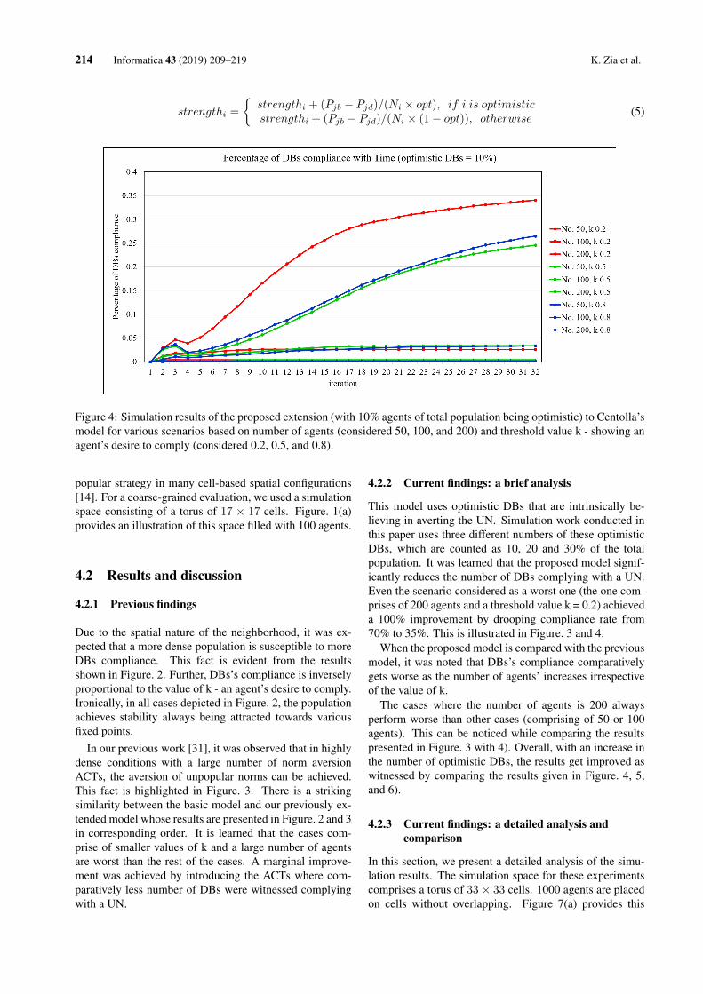
214 Informatica 43 (2019) 209–219 K. Zia et al.
strengthi =
{strengthi + (Pjb − Pjd)/(Ni × opt), if i is optimisticstrengthi + (Pjb − Pjd)/(Ni × (1− opt)), otherwise (5)
Figure 4: Simulation results of the proposed extension (with 10% agents of total population being optimistic) to Centolla’smodel for various scenarios based on number of agents (considered 50, 100, and 200) and threshold value k - showing anagent’s desire to comply (considered 0.2, 0.5, and 0.8).
popular strategy in many cell-based spatial configurations[14]. For a coarse-grained evaluation, we used a simulationspace consisting of a torus of 17 × 17 cells. Figure. 1(a)provides an illustration of this space filled with 100 agents.
4.2 Results and discussion
4.2.1 Previous findings
Due to the spatial nature of the neighborhood, it was ex-pected that a more dense population is susceptible to moreDBs compliance. This fact is evident from the resultsshown in Figure. 2. Further, DBs’s compliance is inverselyproportional to the value of k - an agent’s desire to comply.Ironically, in all cases depicted in Figure. 2, the populationachieves stability always being attracted towards variousfixed points.
In our previous work [31], it was observed that in highlydense conditions with a large number of norm aversionACTs, the aversion of unpopular norms can be achieved.This fact is highlighted in Figure. 3. There is a strikingsimilarity between the basic model and our previously ex-tended model whose results are presented in Figure. 2 and 3in corresponding order. It is learned that the cases com-prise of smaller values of k and a large number of agentsare worst than the rest of the cases. A marginal improve-ment was achieved by introducing the ACTs where com-paratively less number of DBs were witnessed complyingwith a UN.
4.2.2 Current findings: a brief analysis
This model uses optimistic DBs that are intrinsically be-lieving in averting the UN. Simulation work conducted inthis paper uses three different numbers of these optimisticDBs, which are counted as 10, 20 and 30% of the totalpopulation. It was learned that the proposed model signif-icantly reduces the number of DBs complying with a UN.Even the scenario considered as a worst one (the one com-prises of 200 agents and a threshold value k = 0.2) achieveda 100% improvement by drooping compliance rate from70% to 35%. This is illustrated in Figure. 3 and 4.
When the proposed model is compared with the previousmodel, it was noted that DBs’s compliance comparativelygets worse as the number of agents’ increases irrespectiveof the value of k.
The cases where the number of agents is 200 alwaysperform worse than other cases (comprising of 50 or 100agents). This can be noticed while comparing the resultspresented in Figure. 3 with 4). Overall, with an increase inthe number of optimistic DBs, the results get improved aswitnessed by comparing the results given in Figure. 4, 5,and 6).
4.2.3 Current findings: a detailed analysis andcomparison
In this section, we present a detailed analysis of the simu-lation results. The simulation space for these experimentscomprises a torus of 33× 33 cells. 1000 agents are placedon cells without overlapping. Figure 7(a) provides this
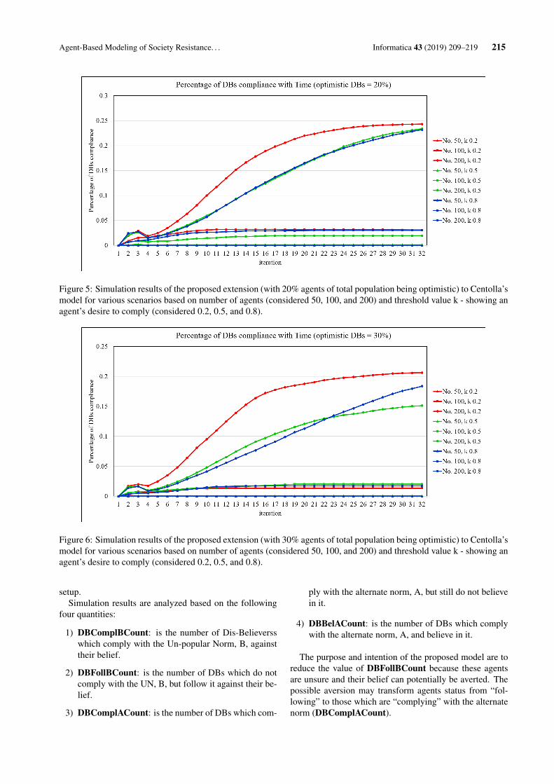
Agent-Based Modeling of Society Resistance. . . Informatica 43 (2019) 209–219 215
Figure 5: Simulation results of the proposed extension (with 20% agents of total population being optimistic) to Centolla’smodel for various scenarios based on number of agents (considered 50, 100, and 200) and threshold value k - showing anagent’s desire to comply (considered 0.2, 0.5, and 0.8).
Figure 6: Simulation results of the proposed extension (with 30% agents of total population being optimistic) to Centolla’smodel for various scenarios based on number of agents (considered 50, 100, and 200) and threshold value k - showing anagent’s desire to comply (considered 0.2, 0.5, and 0.8).
setup.Simulation results are analyzed based on the following
four quantities:
1) DBComplBCount: is the number of Dis-Believersswhich comply with the Un-popular Norm, B, againsttheir belief.
2) DBFollBCount: is the number of DBs which do notcomply with the UN, B, but follow it against their be-lief.
3) DBComplACount: is the number of DBs which com-
ply with the alternate norm, A, but still do not believein it.
4) DBBelACount: is the number of DBs which complywith the alternate norm, A, and believe in it.
The purpose and intention of the proposed model are toreduce the value of DBFollBCount because these agentsare unsure and their belief can potentially be averted. Thepossible aversion may transform agents status from “fol-lowing” to those which are “complying” with the alternatenorm (DBComplACount).
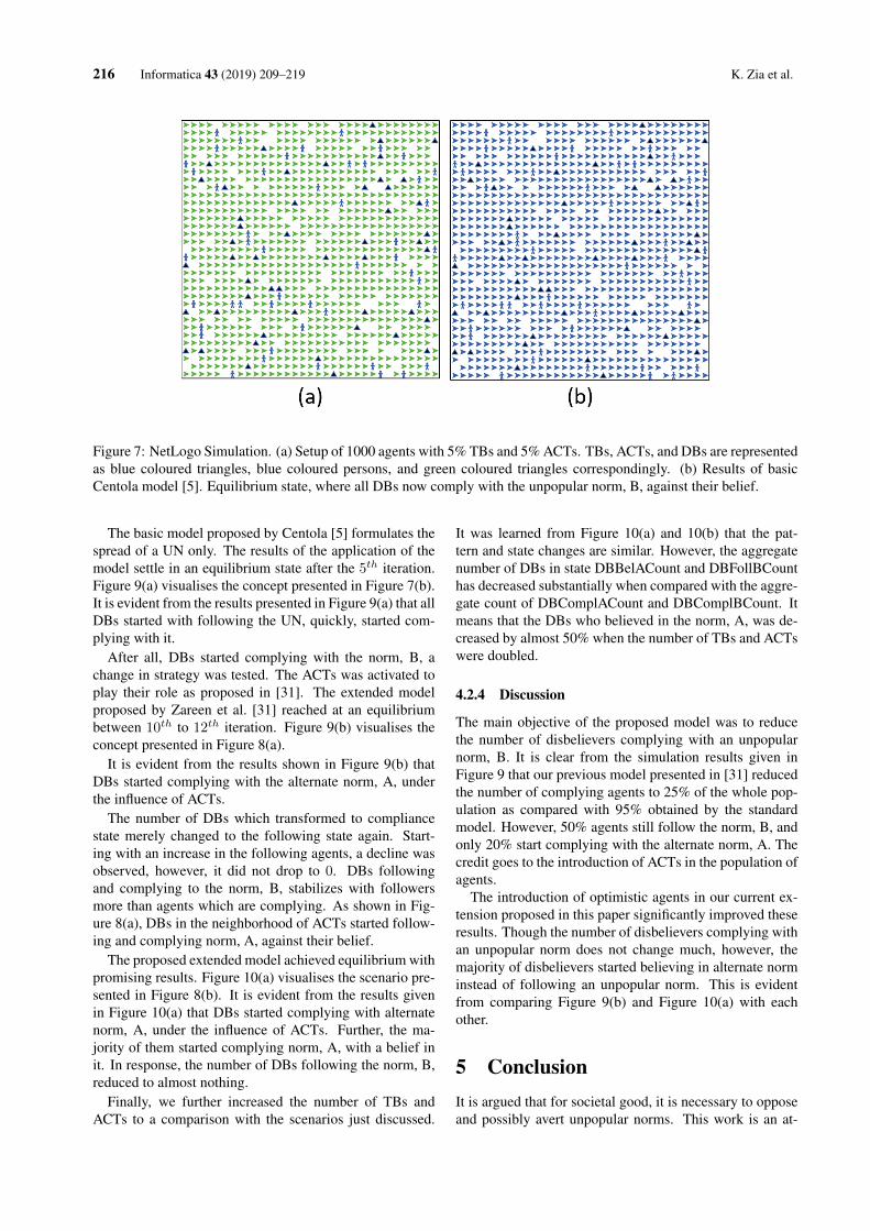
216 Informatica 43 (2019) 209–219 K. Zia et al.
Figure 7: NetLogo Simulation. (a) Setup of 1000 agents with 5% TBs and 5% ACTs. TBs, ACTs, and DBs are representedas blue coloured triangles, blue coloured persons, and green coloured triangles correspondingly. (b) Results of basicCentola model [5]. Equilibrium state, where all DBs now comply with the unpopular norm, B, against their belief.
The basic model proposed by Centola [5] formulates thespread of a UN only. The results of the application of themodel settle in an equilibrium state after the 5th iteration.Figure 9(a) visualises the concept presented in Figure 7(b).It is evident from the results presented in Figure 9(a) that allDBs started with following the UN, quickly, started com-plying with it.
After all, DBs started complying with the norm, B, achange in strategy was tested. The ACTs was activated toplay their role as proposed in [31]. The extended modelproposed by Zareen et al. [31] reached at an equilibriumbetween 10th to 12th iteration. Figure 9(b) visualises theconcept presented in Figure 8(a).
It is evident from the results shown in Figure 9(b) thatDBs started complying with the alternate norm, A, underthe influence of ACTs.
The number of DBs which transformed to compliancestate merely changed to the following state again. Start-ing with an increase in the following agents, a decline wasobserved, however, it did not drop to 0. DBs followingand complying to the norm, B, stabilizes with followersmore than agents which are complying. As shown in Fig-ure 8(a), DBs in the neighborhood of ACTs started follow-ing and complying norm, A, against their belief.
The proposed extended model achieved equilibrium withpromising results. Figure 10(a) visualises the scenario pre-sented in Figure 8(b). It is evident from the results givenin Figure 10(a) that DBs started complying with alternatenorm, A, under the influence of ACTs. Further, the ma-jority of them started complying norm, A, with a belief init. In response, the number of DBs following the norm, B,reduced to almost nothing.
Finally, we further increased the number of TBs andACTs to a comparison with the scenarios just discussed.
It was learned from Figure 10(a) and 10(b) that the pat-tern and state changes are similar. However, the aggregatenumber of DBs in state DBBelACount and DBFollBCounthas decreased substantially when compared with the aggre-gate count of DBComplACount and DBComplBCount. Itmeans that the DBs who believed in the norm, A, was de-creased by almost 50% when the number of TBs and ACTswere doubled.
4.2.4 Discussion
The main objective of the proposed model was to reducethe number of disbelievers complying with an unpopularnorm, B. It is clear from the simulation results given inFigure 9 that our previous model presented in [31] reducedthe number of complying agents to 25% of the whole pop-ulation as compared with 95% obtained by the standardmodel. However, 50% agents still follow the norm, B, andonly 20% start complying with the alternate norm, A. Thecredit goes to the introduction of ACTs in the population ofagents.
The introduction of optimistic agents in our current ex-tension proposed in this paper significantly improved theseresults. Though the number of disbelievers complying withan unpopular norm does not change much, however, themajority of disbelievers started believing in alternate norminstead of following an unpopular norm. This is evidentfrom comparing Figure 9(b) and Figure 10(a) with eachother.
5 ConclusionIt is argued that for societal good, it is necessary to opposeand possibly avert unpopular norms. This work is an at-
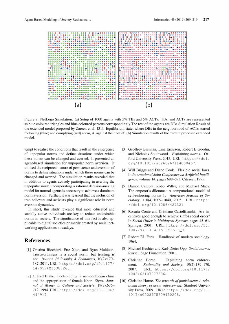
Agent-Based Modeling of Society Resistance. . . Informatica 43 (2019) 209–219 217
Figure 8: NetLogo Simulation. (a) Setup of 1000 agents with 5% TBs and 5% ACTs. TBs, and ACTs are representedas blue coloured triangles and blue coloured persons correspondingly.The rest of the agents are DBs.Simulation Result ofthe extended model proposed by Zareen et al. [31]. Equilibrium state, where DBs in the neighborhood of ACTs startedfollowing (blue) and complying (red) norm, A, against their belief. (b) Simulation results of the current proposed extendedmodel.
tempt to realise the conditions that result in the emergenceof unpopular norms and define situations under whichthese norms can be changed and averted. It presented anagent-based simulation for unpopular norm aversion. Itutilised the reciprocal nature of persistence and aversion ofnorms to define situations under which these norms can bechanged and averted. The simulation results revealed thatin addition to agents actively participating in averting theunpopular norm, incorporating a rational decision-makingmodel for normal agents is necessary to achieve a dominantnorm aversion. Further, it was learned that the inclusion oftrue believers and activists play a significant role in normaversion dynamics.
In short, this study revealed that more educated andsocially active individuals are key to reduce undesirablenorms in society. The significance of this fact is also ap-plicable to digital societies primarily created by social net-working applications nowadays.
References[1] Cristina Bicchieri, Erte Xiao, and Ryan Muldoon.
Trustworthiness is a social norm, but trusting isnot. Politics, Philosophy & Economics, 10(2):170–187, 2011. URL: https://doi.org/10.1177/1470594X10387260.
[2] C Fred Blake. Foot-binding in neo-confucian chinaand the appropriation of female labor. Signs: Jour-nal of Women in Culture and Society, 19(3):676–712, 1994. URL: https://doi.org/10.1086/494917.
[3] Geoffrey Brennan, Lina Eriksson, Robert E Goodin,and Nicholas Southwood. Explaining norms. Ox-ford University Press, 2013. URL: https://doi.org/10.1017/s0266267114000467.
[4] Will Briggs and Diane Cook. Flexible social laws.In International Joint Conference on Artificial Intelli-gence, volume 14, pages 688–693. Citeseer, 1995.
[5] Damon Centola, Robb Willer, and Michael Macy.The emperor’s dilemma: A computational model ofself-enforcing norms 1. American Journal of So-ciology, 110(4):1009–1040, 2005. URL: https://doi.org/10.1086/427321.
[6] Rosaria Conte and Cristiano Castelfranchi. Are in-centives good enough to achieve (info) social order?In Social Order in Multiagent Systems, pages 45–61.Springer, 2001. URL: https://doi.org/10.1007/978-1-4615-1555-5_3.
[7] Robert EL Faris. Handbook of modern sociology.1964.
[8] Michael Hechter and Karl-Dieter Opp. Social norms.Russell Sage Foundation, 2001.
[9] Christine Horne. Explaining norm enforce-ment. Rationality and Society, 19(2):139–170,2007. URL: https://doi.org/10.1177/1043463107077386.
[10] Christine Horne. The rewards of punishment: A rela-tional theory of norm enforcement. Stanford Univer-sity Press, 2009. URL: https://doi.org/10.1017/s0003975609990208.
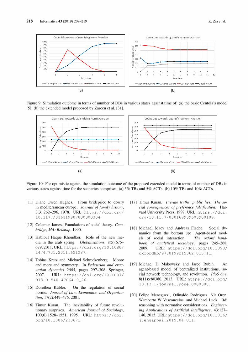
218 Informatica 43 (2019) 209–219 K. Zia et al.
Figure 9: Simulation outcome in terms of number of DBs in various states against time of: (a) the basic Centola’s model[5]. (b) the extended model proposed by Zareen et al. [31].
Figure 10: For optimistic agents, the simulation outcome of the proposed extended model in terms of number of DBs invarious states against time for the scenarios comprises: (a) 5% TBs and 5% ACTs. (b) 10% TBs and 10% ACTs.
[11] Diane Owen Hughes. From brideprice to dowryin mediterranean europe. Journal of family history,3(3):262–296, 1978. URL: https://doi.org/10.1177/036319907800300304.
[12] Coleman James. Foundations of social theory. Cam-bridge, MA: Belknap, 1990.
[13] Habibul Haque Khondker. Role of the new me-dia in the arab spring. Globalizations, 8(5):675–679, 2011. URL: https://doi.org/10.1080/14747731.2011.621287.
[14] Tobias Kretz and Michael Schreckenberg. Mooreand more and symmetry. In Pedestrian and evac-uation dynamics 2005, pages 297–308. Springer,2007. URL: https://doi.org/10.1007/978-3-540-47064-9_26.
[15] Dorothea Kübler. On the regulation of socialnorms. Journal of Law, Economics, and Organiza-tion, 17(2):449–476, 2001.
[16] Timur Kuran. The inevitability of future revolu-tionary surprises. American Journal of Sociology,100(6):1528–1551, 1995. URL: https://doi.org/10.1086/230671.
[17] Timur Kuran. Private truths, public lies: The so-cial consequences of preference falsification. Har-vard University Press, 1997. URL: https://doi.org/10.1177/000169939603900109.
[18] Michael Macy and Andreas Flache. Social dy-namics from the bottom up: Agent-based mod-els of social interaction. The oxford hand-book of analytical sociology, pages 245–268,2009. URL: https://doi.org/10.1093/oxfordhb/9780199215362.013.11.
[19] Michael D Makowsky and Jared Rubin. Anagent-based model of centralized institutions, so-cial network technology, and revolution. PloS one,8(11):e80380, 2013. URL: https://doi.org/10.1371/journal.pone.0080380.
[20] Felipe Meneguzzi, Odinaldo Rodrigues, Nir Oren,Wamberto W Vasconcelos, and Michael Luck. Bdireasoning with normative considerations. Engineer-ing Applications of Artificial Intelligence, 43:127–146, 2015. URL: https://doi.org/10.1016/j.engappai.2015.04.011.
Agent-Based Modeling of Society Resistance. . . Informatica 43 (2019) 209–219 219
[21] Paul Morrow. The thesis of norm transformation inthe theory of mass atrocity. Genocide Studies andPrevention: An International Journal, 9(1):8, 2015.
[22] Arshad Muhammad, Kashif Zia, and Dinesh KumarSaini. Agent-based simulation of socially-inspiredmodel of resistance against unpopular norms. In 10thInternational Conference on Agents and Artificial In-telligence, pages 133–139, 2018. URL: https://doi.org/10.5220/0006735501330139.
[23] Arshad Muhammad, Kashif Zia, and Dinesh Ku-mar Saini. Population dynamics necessary to avertunpopular norms. In Agents and Artificial Intelli-gence, pages 64–75. Springer International Publish-ing, 2019. URL: https://doi.org/10.1007/978-3-030-05453-3_4.
[24] Stella M Nkomo. The emperor has no clothes:Rewriting “race in organizations”. Academy ofManagement Review, 17(3):487–513, 1992. URL:https://doi.org/10.5465/amr.1992.4281987.
[25] Victor Sanchez-Anguix, Vicente Julian, VicenteBotti, and Ana García-Fornes. Tasks for agent-basednegotiation teams: Analysis, review, and challenges.Engineering Applications of Artificial Intelligence,26(10):2480–2494, 2013. URL: https://doi.org/10.1016/j.engappai.2013.07.006.
[26] Takashi Sato and Takashi Hashimoto. Dynamic socialsimulation with multi-agents having internal dynam-ics. In New Frontiers in Artificial Intelligence, pages237–251. Springer, 2007. URL: https://doi.org/10.1007/978-3-540-71009-7_21.
[27] George A Vouros. The emergence of norms via con-textual agreements in open societies. In Advancesin Social Computing and Multiagent Systems, pages185–201. Springer, 2015.
[28] Uri Wilensky and William Rand. An introduc-tion to agent-based modeling: modeling natural, so-cial, and engineered complex systems with NetLogo.MIT Press, 2015. URL: https://doi.org/10.1063/pt.3.2884.
[29] Robb Willer, Ko Kuwabara, and Michael W Macy.The false enforcement of unpopular norms. AmericanJournal of Sociology, 115(2):451–490, 2009. URL:https://doi.org/10.1086/599250.
[30] H Peyton Young. Social norms. 2007.
[31] Zoofishan Zareen, Muzna Zafar, and Kashif Zia. Con-ditions facilitating the aversion of unpopular norms:An agent-based simulation study. International Jour-nal of Advanced Computer Science and Applica-tions, 7(7), 2016. URL: https://doi.org/10.14569/ijacsa.2016.070769.

220 Informatica 43 (2019) 209–219 K. Zia et al.
https://doi.org/10.31449/inf.v43i2.2217 Informatica 43 (2019) 221–234 221
A New Ensemble Semi-supervised Self-labeled Algorithm
Ioannis LivierisDepartment of Computer & Informatics EngineeringTechnological Educational Institute of Western Greece, Greece, GR 263-34E-mail: [email protected]
Keywords: semi-supervised methods, self-labeled, ensemble methods, classification, voting
Received: March 13, 2018
As an alternative to traditional classification methods, semi-supervised learning algorithms have become ahot topic of significant research, exploiting the knowledge hidden in the unlabeled data for building pow-erful and effective classifiers. In this work, a new ensemble-based semi-supervised algorithm is proposedwhich is based on a maximum-probability voting scheme. The reported numerical results illustrate theefficacy of the proposed algorithm outperforming classical semi-supervised algorithms in term of classifi-cation accuracy, leading to more efficient and robust predictive models.
Povzetek: Razvit je nov delno nadzorovani ucni algoritem s pomocjo ansamblov in glasovalno shemo naosnovi najvecje verjetnosti.
1 Introduction
The development of a powerful and accurate classifier isconsidered as one of the most significant and challeng-ing tasks in machine learning and data mining [3]. Nev-ertheless, it is generally recognized that the key to recog-nition problems does not lie wholly in any particular solu-tion since no single model exists for all pattern recognitionproblems [28, 15].
During the last decades, in the area of machine learn-ing the development of an ensemble of classifiers has beenproposed as a new direction for improving the classifica-tion accuracy. The basic idea of ensemble learning is thecombination of a set of diverse prediction models, each ofwhich solves the same original task, in order to obtain a bet-ter composite global model with more accurate and reliableestimates or decisions than can be obtained from using asingle model [9, 28]. Therefore, several prediction modelshave been proposed based on ensembles techniques whichhave been successfully utilized to tackle difficult real-worldproblems [31, 14, 32, 30, 23, 27, 11]. Traditional ensemblemethods usually combine the individual predictions of su-pervised algorithms which utilize only labeled data as train-ing set. However, in most real-world classification prob-lems, the acquisition of sufficient labeled samples is cum-bersome and expensive and frequently requires the effortsof domain experts. On the other hand, unlabeled data arefairly easy to obtain and require less effort of experiencedhuman annotators.
Semi-supervised learning algorithms constitute the ap-propriate and effective machine learning methodologyfor extracting useful knowledge from both labeled andunlabeled data. In contrast to traditional classificationapproaches, semi-supervised algorithms utilize a largeamount of unlabeled samples to either modify or reprior-
itize the hypothesis obtained from labeled samples in or-der to build an efficient and accurate classifier. The gen-eral assumption of these algorithms is to leverage the largeamount of unlabeled data in order to reduce data sparsityin the labeled training data and boost the classifier per-formance, particularly focusing on the setting where theamount of available labeled data is limited. Hence, thesemethods have received considerable attention due to theirpotential for reducing the effort of labeling data while stillpreserving competitive and sometimes better classificationperformance (see [18, 6, 7, 38, 17, 16, 21, 20, 22, 44, 45,46, 43] and the references therein). The main issue insemi-supervised learning is how to exploit the informationhidden in the unlabeled data. In the literature, several ap-proaches have been proposed each with different philoso-phy related to the link between the distribution of labeledand unlabeled data [46, 4, 36].
Self-labeled methods constitute semi-supervised meth-ods which address the shortage of labeled data via a self-learning process based on supervised prediction models.The main advantages of this class of methods are their sim-plicity and their wrapper-based philosophy. The former isrelated to the facility/comodity of application and imple-mentation while the latter refers to the fact that any super-vised classifier can be utilized, independent of its complex-ity [35]. In the literature, self-labeled methods are dividedinto self-training [41] and co-training [4]. Self-trainingconstitutes an efficient semi-supervised method which iter-atively enlarges the labeled training set by adding the mostconfident predictions of the utilized supervised classifier.The standard co-training method splits the feature spaceinto two different conditionally independent views. Sub-sequently, it trains one classifier in each specific view andthe classifiers teach each other the most confidently pre-dicted examples. More sophisticated and advanced variants
222 Informatica 43 (2019) 221–234 I.E. Livieris
of this method do not require explicit feature splits or the it-erative mutual-teaching procedure imposed by co-training,as they are commonly based on disagreement-based classi-fiers [44, 12, 36, 46, 45]
By taking these into consideration, ensemble methodsand semi-supervised methods constitute two significantclasses of methods. The former attempt to achieve strongclassification performance by combining individual classi-fiers while the later attempt to enhance the performance ofa classifier by exploiting the information in the unlabeleddata. Although both methodologies have been efficientlyapplied to a variety of real-world problems during the lastdecade, they were almost developed separately. In this con-text, Zhou [43] advocated that ensemble learning and semi-supervised learning are indeed beneficial to each other andstronger learning machines can be generated by leverag-ing unlabeled data with the combination of diverse classi-fiers. More specifically, ensemble learning could be usefulto semi-supervised learning since an ensemble of classifierscould be more accurate than an individual classifier. Ad-ditionally, semi-supervised learning could assist ensemblelearning since unlabeled data can enhance the diversity ofthe base learner which constitute the ensemble and increasethe ensemble’s classification accuracy.
In this work, a new ensemble semi-supervised self-labeled learning algorithm is proposed. The proposed al-gorithm combines the individual predictions of three ofthe most representative SSL algorithms: Self-training, Co-training and Tri-training via a maximum-probability votingscheme. The efficiency of the proposed algorithm is eval-uated on various standard benchmark datasets and the re-ported experimental results illustrate its efficacy in termsof classification accuracy, leading to more efficient and ro-bust prediction models.
The remainder of this paper is organized as follows: Sec-tion 3 presents some elementary semi-supervised learningdefinitions and Section 4 presents a detailed description ofthe proposed algorithm. Section 5 presents the experimen-tal results of the comparison of the proposed algorithm withthe most popular semi-supervised classification methods onstandard benchmark datasets. Finally, Section 6 discussesthe conclusions and some research topics for future work.
2 Related work
Semi-Supervised Learning (SSL) and Ensemble Learning(EL) constitute machine learning techniques which wereindependently developed to improve the performance ofexisting learning methods, though from different perspec-tives and methodologies. SSL provides approaches to im-prove model generalization performance by exploiting un-labeled data; while EL explores the possibility of achiev-
ing the same objective by aggregating a group of learn-ers. Zhou [43] presented an extensive analysis of howsemi-supervised learning and ensemble learning can be ef-ficiently fuse for the development of efficient predictionmodels. A number of rewarding studies which fuse and ex-ploit their advantages have been carried out in recent years;some useful outcomes of them are briefly presented below.
Zhou and Goldman [42] have adopted the idea of en-semble learning and majority voting and proposed a newSSL algorithm which is based on the multi-learning ap-proach. More specifically, this algorithm utilizes multiplealgorithms for producing the necessary information and en-dorses a voted majority process for the final decision, in-stead of asking for more than one views of the correspond-ing data.
Along this line, Li and Zhou [17] proposed another al-gorithm, in which a number of Random trees are trainedon bootstrap data from the dataset, named Co-Forest. Themain idea of this algorithm is the assignment of a few un-labeled examples to each Random tree during the trainingprocess. Eventually, the final decision is composed by asimple majority voting. Notice that the utilization of Ran-dom Tree classifier for random samples of the collected la-beled data is the main reason why the behavior Co-Forestis efficient and robust although the number of the availablelabeled examples is reduced. Xu et al. [40] applied thismethod for the predictions of protein subcellular localiza-tion providing some promising results.
Sun and Zhang [34] attempted to combine the ad-vantages of multiple-view learning and ensemble learn-ing for semi-supervised learning. They proposed anovel multiple-view multiple-learner framework for semi-supervised learning which adopted a co-training basedlearning paradigm in enlarging labeled data from a muchlarger set of unlabeled data. Their motivation is based onthe fact that the use of multiple views is promising to pro-mote performance compared with single-view learning be-cause information is more effectively exploited; while atthe same time, as an ensemble of classifiers is learned fromeach view, predictions with higher accuracies can be ob-tained than solely adopting one classifier from the sameview. The experiments conduced on several datasets pre-sented some encouraging results, illustrating the efficacyof the proposed method.
Roy et al. [29] presented a novel approach by utilizinga multiple classifier system in the SSL framework insteadof using a single weak classifier for change detection in re-motely sensed images. The proposed algorithm during theiterative learning process uses the agreement between allthe classifiers which constitute the ensemble for collectingthe most confident labeled patterns. The effectiveness ofthe proposed technique was presented by a variety of ex-periments carried out on multi-temporal and multi-spectral
A New Ensemble Semi-supervised Self-labeled Algorithm Informatica 43 (2019) 221–234 223
datasets.In more recent works, Livieris et al. [21] proposed a new
ensemble-based semi-supervised method for the prognosisof students’ performance in the final examinations. Theyincorporated a ensemble of classifiers as base learner in thesemi-supervised framework. Based on their numerical ex-periments, the authors concluded that ensemble methodsand semi-supervised methodologies could efficiently com-bined to develop efficient prediction models. Motivatedby the previous work, Livieris et al. [22] presented a newensemble-based semi-supervised learning algorithm for theclassification of chest X-rays of tuberculosis, presentingsome encouraging results.
3 A review on semi-supervisedself-labeled classification
In this section, we present a formal definition of the semi-supervised classification problem and briefly describe themost relevant self-labeled approaches proposed in the lit-erature. Let xp = (xp1, xp2, . . . , xpD, y) be an example,where xp belongs to a class y and aD-dimensional space inwhich xpi is the i-th attribute of the p-th sample. SupposeL is a labeled set of NL instances xp with y known and Uis an unlabeled set ofNU instance xq with y unknown. No-tice that the set L ∪ U consists the training set. Moreover,there exists a test set T of NT unseen instances where y isunknown, which has not been utilized in the training stage.Notice that the aim of the semi-supervised classification isto obtain an accurate and robust learning hypothesis withthe use of the training set.
Self-labeled techniques constitute a significant family ofclassification methods which progressively classify unla-beled data based on the most confident predictions andutilize them to modify the hypothesis learned from la-beled samples. Therefore, the methods of this class ac-cept that their own predictions tend to be correct, with-out making any specific assumptions about the input data.In the literature, a variety of self-labeled methods hasbeen proposed each with different philosophy and method-ology on exploiting the information hidden in the unla-beled data. In this work, we focus our attention to Self-training, Co-training and Tri-training which constitute themost efficient and commonly used self-labeled methods[21, 20, 22, 35, 37, 36].
3.1 Self-TrainingSelf-training [41] is generally considered as the simplestand one of the most efficient SSL algorithms. This algo-rithm is a wrapper based SSL approach which constitutes
an iterative procedure of self-labeling unlabeled data. Ac-cording to Ng and Cardie [25] “self-training is a single-view weakly supervised algorithm” which is based on itsown predictions on unlabeled data to teach itself. Firstly, anarbitrary classifier is initially trained with a small amountof labeled data, constituting its training set which is itera-tively augmented using its own most confident predictionsof the unlabeled data. More analytically, each unlabeledinstance which has achieved a probability over a specificthreshold ConLev is considered sufficiently reliable to beadded to the labeled training set and subsequently the clas-sifier is retrained.
Clearly, the success of Self-training is heavily dependedon the newly-labeled data based on its own predictions,hence its weakness is that erroneous initial predictionswill probably lead the classifier to generate incorrectlylabeled data [46]. A high-level description of Self-trainingalgorithm is presented in Algorithm 1.
Algorithm 1: Self-training
Input: L − Set of labeled instances.U − Set of unlabeled instances.ConLev − Confidence level.C − Base learner.
Output: Trained classifier.
1 : repeat
2 : Train C on L.
3 : Apply C on U .
4 : Select instances with a predicted probability more than ConLev
per iteration (xMCP).
5 : Remove xMCP from U and add to L.
6 : until some stopping criterion is met or U is empty.
3.2 Co-trainingCo-training [4] is a SSL algorithm which utilizes two clas-sifiers, each trained on a different view of the labeled train-ing set. The underlying assumptions of the Co-training ap-proach is that feature space can be split into two differentconditionally independent views and that each view is ableto predict the classes perfectly [33]. Under these assump-tions, two classifiers are trained separately for each viewusing the initial labeled set and then iteratively the classi-fiers augment the training set of the other with the mostconfident predictions on unlabeled examples.

224 Informatica 43 (2019) 221–234 I.E. Livieris
Essentially, Co-training is a “two-view weakly super-vised algorithm” since it uses the self-training approach oneach view [25]. Blum and Mitchell [4] have extensivelystudied the efficacy of Co-training and they concludedthat if the two views are conditionally independent, thenthe use of unlabeled data can significantly improve thepredictive accuracy of a weak classifier. Nevertheless,the assumption about the existence of sufficient andredundant views is a luxury hardly met in most real worldscenarios. Algorithm 2 presents a high-level description ofCo-training algorithm.
Algorithm 2: Co-training
Input: L − Set of labeled instances.U − Set of unlabeled instances.Ci − Base learner (i = 1, 2).
Output: Trained classifier.
1: Create a pool U ′ of u examples by randomly choosing from U .
2: repeat
3: Train C1 on L(V1).
4: Train C2 on L(V2).
5: for each classifier Ci do (i = 1, 2)
6: Ci chooses p samples (P ) that it most confidently labels as
positive and n instances (N ) that it most confidently labels
as negative from U .
7: Remove P and N from U ′.
8: Add P and N to L.
9: end for
10: Refill U ′ with examples from U to keep U ′ at constant size of u
examples.
11: until some stopping criterion is met or U is empty.
Remark: V1 and V2 are two feature conditionally independent views of instances.
3.3 Tri-TrainingTri-Training [44] consists of an improved version of Co-Training which overcomes the requirements for multiplesufficient an redundant feature sets. This algorithm consti-tutes a bagging ensemble of three classifiers, trained on thedata subsets generated through bootstrap sampling from theoriginal labeled training set. In case two of the three clas-sifiers agree on the categorization of an unlabeled instance,then this is considered to be labeled and augment the thirdclassifier with the newly labeled example. The efficiency ofthe training process is based on the strategy the “majorityteach minority” which avoids the use of a complicated timeconsuming approach to explicit measure the predictive con-fidence, serving as an implicit confidence measurement,
In contrast to several SSL algorithms, Tri-trainingdoes not require different supervised algorithms as baselearners which leads to greater applicability in many realworld classification problems [12, 46, 19]. A high-leveldescription of Tri-training is presented in Algorithm 3.
Algorithm 3: Tri-training algorithm
Input: L − Set of labeled instances.U − Set of unlabeled instances.Ci − Base learner (i = 1, 2, 3).
Output: Trained classifier.
1: for i = 1, 2, 3 do
2: Si = BootstrapSample(L).
3: Train Ci on Si.
4: end for
5: repeat
6: for i = 1, 2, 3 do
7: Li = ∅.8: for u ∈ U do
9: if Cj(u) = Ck(u) then (j, k 6= i)
10: Li = Li ∪ (u,Cj(u)).
11: end if
12: end for
13: end for
14: for i = 1, 2, 3 do
15: Train Ci on Si.
17: end for
18: until some stopping criterion is met or U is empty.
4 An ensemble semi-supervisedself-labeled algorithm
In this section, the proposed ensemble SSL algorithm ispresented which is based on the hybridization of ensem-ble learning with semi-supervised learning. Generally, thedevelopment of an ensemble of classifiers consists of twomain steps: selection and combination.
The selection of the appropriate component classifierswhich constitute the ensemble is considered essential forits efficiency and the key points for its efficacy is based onthe diversity and the accuracy the component classifiers. Acommonly and widely utilized approach is to apply diverseclassification algorithms (with heterogeneous model repre-sentations) to a single dataset [24]. Moreover, the combina-tion of the individual predictions of the classification algo-rithms takes place through several methodologies and tech-niques with different philosophy and performance [28, 9].
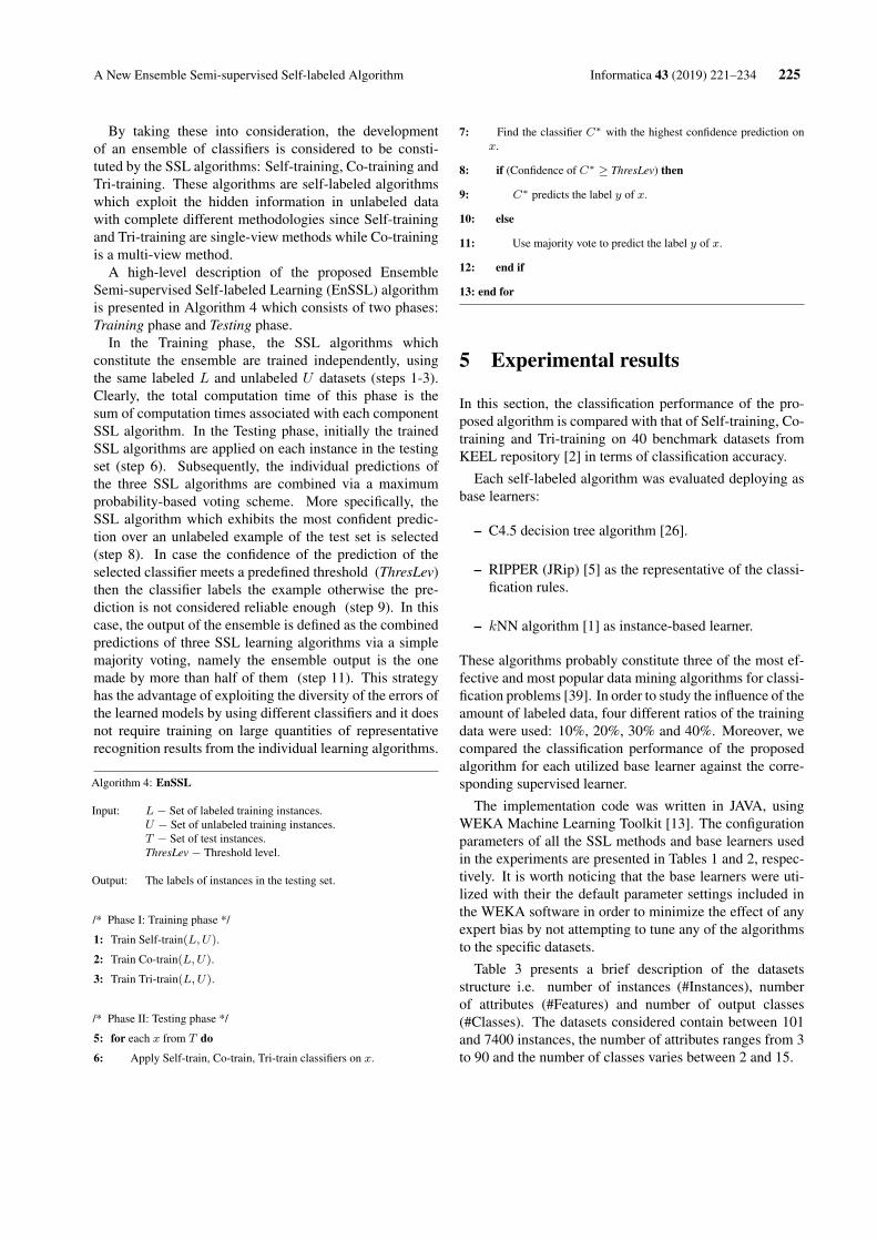
A New Ensemble Semi-supervised Self-labeled Algorithm Informatica 43 (2019) 221–234 225
By taking these into consideration, the developmentof an ensemble of classifiers is considered to be consti-tuted by the SSL algorithms: Self-training, Co-training andTri-training. These algorithms are self-labeled algorithmswhich exploit the hidden information in unlabeled datawith complete different methodologies since Self-trainingand Tri-training are single-view methods while Co-trainingis a multi-view method.
A high-level description of the proposed EnsembleSemi-supervised Self-labeled Learning (EnSSL) algorithmis presented in Algorithm 4 which consists of two phases:Training phase and Testing phase.
In the Training phase, the SSL algorithms whichconstitute the ensemble are trained independently, usingthe same labeled L and unlabeled U datasets (steps 1-3).Clearly, the total computation time of this phase is thesum of computation times associated with each componentSSL algorithm. In the Testing phase, initially the trainedSSL algorithms are applied on each instance in the testingset (step 6). Subsequently, the individual predictions ofthe three SSL algorithms are combined via a maximumprobability-based voting scheme. More specifically, theSSL algorithm which exhibits the most confident predic-tion over an unlabeled example of the test set is selected(step 8). In case the confidence of the prediction of theselected classifier meets a predefined threshold (ThresLev)then the classifier labels the example otherwise the pre-diction is not considered reliable enough (step 9). In thiscase, the output of the ensemble is defined as the combinedpredictions of three SSL learning algorithms via a simplemajority voting, namely the ensemble output is the onemade by more than half of them (step 11). This strategyhas the advantage of exploiting the diversity of the errors ofthe learned models by using different classifiers and it doesnot require training on large quantities of representativerecognition results from the individual learning algorithms.
Algorithm 4: EnSSL
Input: L − Set of labeled training instances.U − Set of unlabeled training instances.T − Set of test instances.ThresLev − Threshold level.
Output: The labels of instances in the testing set.
/* Phase I: Training phase */
1: Train Self-train(L,U).
2: Train Co-train(L,U).
3: Train Tri-train(L,U).
/* Phase II: Testing phase */
5: for each x from T do
6: Apply Self-train, Co-train, Tri-train classifiers on x.
7: Find the classifier C∗ with the highest confidence prediction onx.
8: if (Confidence of C∗ ≥ ThresLev) then
9: C∗ predicts the label y of x.
10: else
11: Use majority vote to predict the label y of x.
12: end if
13: end for
5 Experimental results
In this section, the classification performance of the pro-posed algorithm is compared with that of Self-training, Co-training and Tri-training on 40 benchmark datasets fromKEEL repository [2] in terms of classification accuracy.
Each self-labeled algorithm was evaluated deploying asbase learners:
– C4.5 decision tree algorithm [26].
– RIPPER (JRip) [5] as the representative of the classi-fication rules.
– kNN algorithm [1] as instance-based learner.
These algorithms probably constitute three of the most ef-fective and most popular data mining algorithms for classi-fication problems [39]. In order to study the influence of theamount of labeled data, four different ratios of the trainingdata were used: 10%, 20%, 30% and 40%. Moreover, wecompared the classification performance of the proposedalgorithm for each utilized base learner against the corre-sponding supervised learner.
The implementation code was written in JAVA, usingWEKA Machine Learning Toolkit [13]. The configurationparameters of all the SSL methods and base learners usedin the experiments are presented in Tables 1 and 2, respec-tively. It is worth noticing that the base learners were uti-lized with their the default parameter settings included inthe WEKA software in order to minimize the effect of anyexpert bias by not attempting to tune any of the algorithmsto the specific datasets.
Table 3 presents a brief description of the datasetsstructure i.e. number of instances (#Instances), numberof attributes (#Features) and number of output classes(#Classes). The datasets considered contain between 101and 7400 instances, the number of attributes ranges from 3to 90 and the number of classes varies between 2 and 15.
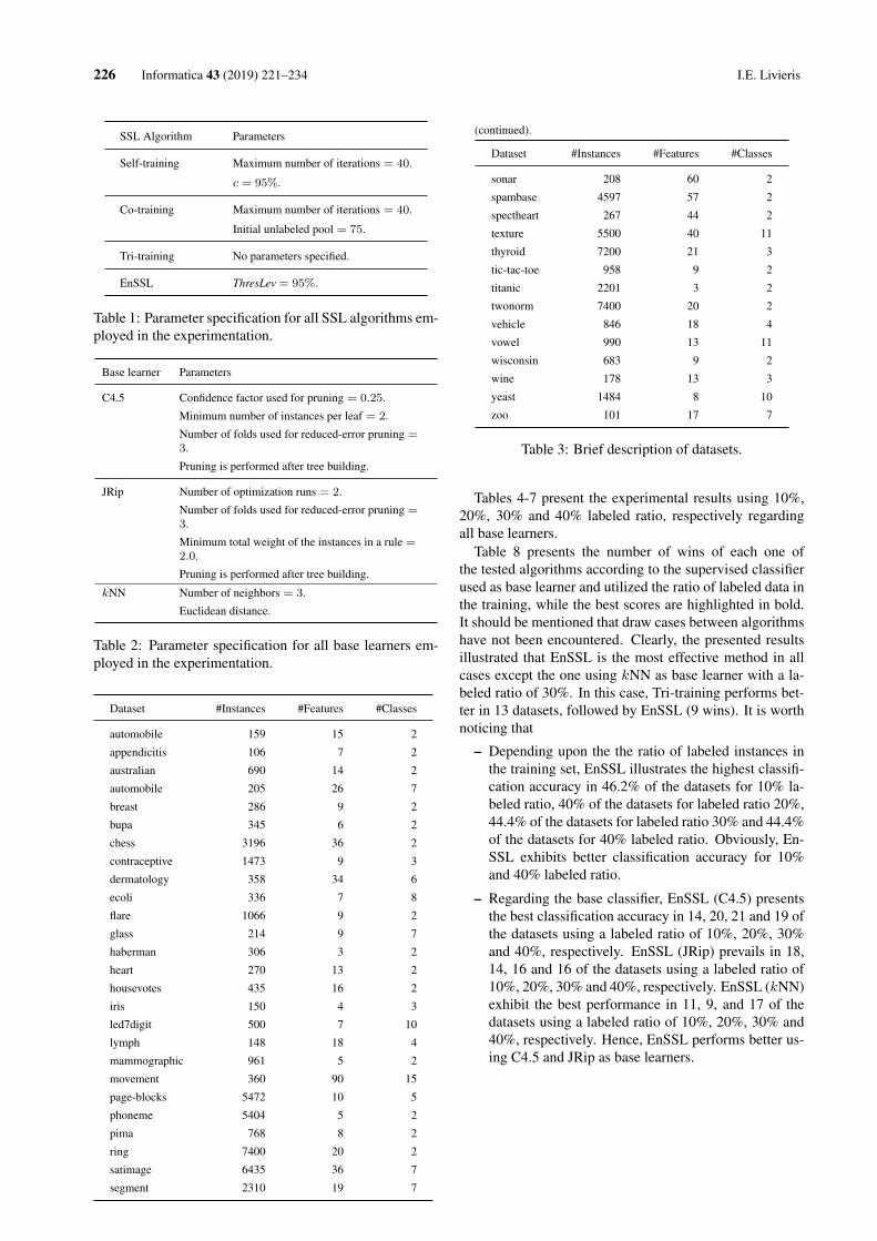
226 Informatica 43 (2019) 221–234 I.E. Livieris
SSL Algorithm Parameters
Self-training Maximum number of iterations = 40.
c = 95%.
Co-training Maximum number of iterations = 40.
Initial unlabeled pool = 75.
Tri-training No parameters specified.
EnSSL ThresLev = 95%.
Table 1: Parameter specification for all SSL algorithms em-ployed in the experimentation.
Base learner Parameters
C4.5 Confidence factor used for pruning = 0.25.
Minimum number of instances per leaf = 2.
Number of folds used for reduced-error pruning =3.
Pruning is performed after tree building.
JRip Number of optimization runs = 2.
Number of folds used for reduced-error pruning =3.
Minimum total weight of the instances in a rule =2.0.
Pruning is performed after tree building.
kNN Number of neighbors = 3.
Euclidean distance.
Table 2: Parameter specification for all base learners em-ployed in the experimentation.
Dataset #Instances #Features #Classes
automobile 159 15 2
appendicitis 106 7 2
australian 690 14 2
automobile 205 26 7
breast 286 9 2
bupa 345 6 2
chess 3196 36 2
contraceptive 1473 9 3
dermatology 358 34 6
ecoli 336 7 8
flare 1066 9 2
glass 214 9 7
haberman 306 3 2
heart 270 13 2
housevotes 435 16 2
iris 150 4 3
led7digit 500 7 10
lymph 148 18 4
mammographic 961 5 2
movement 360 90 15
page-blocks 5472 10 5
phoneme 5404 5 2
pima 768 8 2
ring 7400 20 2
satimage 6435 36 7
segment 2310 19 7
(continued).
Dataset #Instances #Features #Classes
sonar 208 60 2
spambase 4597 57 2
spectheart 267 44 2
texture 5500 40 11
thyroid 7200 21 3
tic-tac-toe 958 9 2
titanic 2201 3 2
twonorm 7400 20 2
vehicle 846 18 4
vowel 990 13 11
wisconsin 683 9 2
wine 178 13 3
yeast 1484 8 10
zoo 101 17 7
Table 3: Brief description of datasets.
Tables 4-7 present the experimental results using 10%,20%, 30% and 40% labeled ratio, respectively regardingall base learners.
Table 8 presents the number of wins of each one ofthe tested algorithms according to the supervised classifierused as base learner and utilized the ratio of labeled data inthe training, while the best scores are highlighted in bold.It should be mentioned that draw cases between algorithmshave not been encountered. Clearly, the presented resultsillustrated that EnSSL is the most effective method in allcases except the one using kNN as base learner with a la-beled ratio of 30%. In this case, Tri-training performs bet-ter in 13 datasets, followed by EnSSL (9 wins). It is worthnoticing that
– Depending upon the the ratio of labeled instances inthe training set, EnSSL illustrates the highest classifi-cation accuracy in 46.2% of the datasets for 10% la-beled ratio, 40% of the datasets for labeled ratio 20%,44.4% of the datasets for labeled ratio 30% and 44.4%of the datasets for 40% labeled ratio. Obviously, En-SSL exhibits better classification accuracy for 10%and 40% labeled ratio.
– Regarding the base classifier, EnSSL (C4.5) presentsthe best classification accuracy in 14, 20, 21 and 19 ofthe datasets using a labeled ratio of 10%, 20%, 30%and 40%, respectively. EnSSL (JRip) prevails in 18,14, 16 and 16 of the datasets using a labeled ratio of10%, 20%, 30% and 40%, respectively. EnSSL (kNN)exhibit the best performance in 11, 9, and 17 of thedatasets using a labeled ratio of 10%, 20%, 30% and40%, respectively. Hence, EnSSL performs better us-ing C4.5 and JRip as base learners.

A New Ensemble Semi-supervised Self-labeled Algorithm Informatica 43 (2019) 221–234 227
Dataset C4.5 Self(C4.5)
Co(C4.5)
Tri(C4.5)
EnSSL(C4.5)
JRip Self(JRip)
Co(JRip)
Tri(JRip)
EnSSL(JRip)
kNN Self(kNN)
Co(kNN)
Tri(kNN)
EnSSL(kNN)
automobile 64,21% 71,63% 71,58% 66,46% 69,79% 64,88% 69,08% 70,33% 64,63% 65,33% 61,75% 72,29% 64,13% 69,00% 74,13%
appendicitis 76,27% 81,09% 83,00% 82,00% 82,00% 83,91% 82,09% 81,00% 83,09% 83,09% 82,00% 85,82% 85,82% 85,82% 85,82%
australian 84,20% 85,80% 85,65% 87,10% 86,67% 85,22% 85,65% 85,36% 86,23% 86,38% 83,19% 83,91% 85,36% 83,77% 84,93%
banana 74,40% 74,58% 74,85% 75,00% 74,85% 73,19% 72,89% 73,15% 73,25% 73,30% 72,38% 72,89% 73,15% 73,25% 73,30%
breast 70,22% 75,87% 75,54% 73,82% 75,54% 68,45% 69,91% 67,81% 73,12% 69,56% 73,03% 72,41% 73,09% 73,45% 73,45%
bupa 56,24% 57,98% 57,96% 57,96% 58,57% 56,24% 58,57% 57,96% 57,96% 57,96% 56,24% 58,57% 57,96% 57,96% 57,96%
chess 98,97% 99,41% 97,62% 99,44% 99,41% 97,97% 99,09% 97,68% 99,09% 99,19% 93,90% 96,34% 90,02% 96,56% 96,40%
contraceptive 48,75% 49,69% 50,98% 50,37% 50,30% 43,04% 43,65% 46,64% 46,57% 46,77% 48,95% 50,84% 51,12% 51,59% 51,12%
dermatology 92,60% 94,54% 90,17% 94,54% 95,36% 85,76% 87,15% 86,06% 89,61% 91,00% 94,79% 97,25% 94,53% 97,24% 96,97%
ecoli 79,77% 80,37% 74,99% 80,97% 79,78% 78,83% 77,99% 75,88% 79,48% 78,88% 80,93% 80,97% 77,37% 82,15% 82,15%
flare 72,23% 74,66% 71,76% 73,73% 74,10% 68,38% 71,20% 67,18% 70,44% 70,36% 72,04% 74,95% 63,32% 73,92% 74,20%
glass 63,51% 67,81% 62,73% 64,48% 67,32% 61,21% 68,25% 62,64% 55,30% 64,09% 64,03% 72,51% 71,56% 72,97% 73,44%
haberman 71,90% 72,24% 70,24% 70,24% 70,24% 70,91% 71,57% 70,26% 70,56% 70,90% 71,55% 70,89% 73,88% 74,20% 74,20%
heart 78,54% 78,57% 76,89% 80,53% 81,52% 78,92% 80,89% 80,23% 80,90% 81,23% 80,87% 79,88% 80,86% 81,19% 80,20%
housevotes 96,52% 96,56% 94,84% 93,51% 95,69% 96,96% 96,56% 96,58% 93,51% 95,69% 91,34% 91,85% 91,85% 91,85% 91,85%
iris 92,67% 94,00% 95,33% 94,67% 94,00% 92,00% 93,33% 91,33% 90,00% 94,00% 92,67% 93,33% 93,33% 95,33% 94,67%
led7digit 69,80% 71,80% 58,60% 53,20% 69,40% 68,00% 70,60% 69,00% 34,20% 69,80% 72,60% 73,00% 56,00% 53,00% 69,40%
lymph 70,95% 74,38% 73,76% 73,71% 73,71% 72,90% 74,29% 75,05% 72,29% 74,38% 76,95% 78,48% 80,57% 81,19% 80,48%
mammographic 82,41% 83,49% 83,01% 84,22% 84,34% 82,41% 83,25% 82,29% 83,86% 83,73% 82,05% 82,65% 82,29% 83,73% 83,25%
movement 40,28% 56,94% 50,00% 35,83% 52,78% 29,44% 56,94% 49,17% 31,94% 48,89% 40,28% 65,00% 56,94% 59,72% 65,56%
page-blocks 95,39% 96,58% 95,71% 96,49% 96,71% 95,96% 96,09% 95,65% 96,36% 96,47% 96,05% 96,27% 95,34% 96,27% 96,16%
phoneme 80,33% 81,79% 80,13% 81,24% 81,98% 79,40% 81,35% 80,16% 80,46% 81,46% 80,26% 82,27% 81,25% 81,87% 82,14%
pima 74,47% 73,81% 73,81% 74,46% 74,20% 74,47% 73,29% 72,90% 73,81% 73,16% 72,69% 72,38% 73,03% 73,15% 73,54%
ring 80,41% 80,82% 80,91% 81,20% 83,54% 91,84% 92,47% 92,62% 92,61% 93,08% 62,15% 61,66% 60,51% 62,19% 61,05%
satimage 83,20% 84,38% 83,98% 84,65% 85,39% 83,31% 83,62% 84,15% 83,43% 84,80% 88,48% 89,25% 88,47% 89,03% 89,46%
segment 92,55% 94,42% 90,30% 93,90% 94,89% 91,82% 90,87% 86,15% 90,09% 92,77% 93,33% 93,12% 90,52% 93,29% 93,77%
sonar 67,43% 73,57% 68,67% 71,19% 71,19% 68,86% 77,05% 72,69% 74,71% 76,12% 70,69% 78,95% 74,10% 73,67% 76,05%
spambase 91,55% 92,72% 91,13% 92,79% 92,89% 90,68% 92,37% 91,55% 91,89% 92,83% 92,39% 93,02% 92,33% 93,22% 93,31%
spectheart 67,50% 68,75% 70,00% 70,00% 70,00% 63,75% 72,50% 70,00% 71,25% 71,25% 63,75% 66,25% 68,75% 68,75% 68,75%
texture 84,55% 87,87% 86,02% 86,65% 88,95% 84,73% 86,91% 86,33% 86,20% 89,64% 94,75% 96,07% 95,13% 95,78% 96,22%
thyroid 99,17% 99,32% 98,72% 99,24% 99,28% 98,89% 99,17% 98,42% 99,17% 99,24% 98,43% 98,76% 98,53% 98,69% 98,87%
tic-tac-toe 81,73% 83,60% 85,70% 85,27% 85,38% 97,08% 97,49% 97,91% 97,60% 97,49% 97,29% 99,06% 98,75% 98,64% 98,96%
titanic 77,15% 76,83% 77,60% 77,65% 77,82% 77,06% 77,19% 76,92% 77,65% 77,69% 77,06% 76,83% 77,69% 77,60% 77,65%
twonorm 78,99% 79,54% 79,50% 79,51% 82,19% 83,99% 84,82% 84,39% 84,19% 86,61% 93,39% 93,59% 93,69% 93,70% 94,61%
vehicle 66,55% 70,33% 66,78% 68,66% 70,44% 62,17% 60,87% 60,04% 61,34% 60,99% 64,90% 70,69% 67,97% 69,38% 70,33%
vowel 97,27% 98,28% 97,57% 98,28% 98,28% 96,96% 98,18% 97,17% 98,28% 98,28% 95,85% 97,57% 95,85% 97,47% 97,57%
wisconsin 94,57% 94,56% 93,57% 94,13% 94,56% 93,99% 95,85% 93,84% 94,98% 95,12% 96,42% 96,70% 96,28% 96,70% 96,70%
wine 84,28% 89,90% 78,01% 88,79% 89,90% 86,44% 89,28% 86,41% 89,87% 90,98% 93,20% 95,52% 94,97% 95,52% 95,52%
yeast 75,13% 74,93% 74,86% 74,86% 74,86% 75,07% 74,19% 75,74% 75,13% 75,20% 75,21% 74,19% 75,07% 75,27% 75,14%
zoo 93,09% 92,09% 89,18% 92,09% 92,09% 84,09% 86,09% 87,09% 86,09% 86,09% 90,09% 95,09% 84,27% 95,09% 95,09%
Table 4: Classification accuracy (labeled ratio 10%).

228 Informatica 43 (2019) 221–234 I.E. Livieris
Dataset C4.5 Self(C4.5)
Co(C4.5)
Tri(C4.5)
EnSSL(C4.5)
JRip Self(JRip)
Co(JRip)
Tri(JRip)
EnSSL(JRip)
kNN Self(kNN)
Co(kNN)
Tri(kNN)
EnSSL(kNN)
automobile 66,08% 77,29% 62,75% 73,50% 76,00% 65,42% 69,67% 64,67% 71,50% 74,04% 64,17% 68,46% 65,92% 72,25% 74,08%
appendicitis 80,09% 81,09% 83,00% 82,91% 82,91% 83,91% 82,09% 82,00% 82,91% 82,00% 83,09% 86,82% 86,73% 85,82% 85,82%
australian 86,09% 86,67% 86,23% 87,10% 87,68% 85,51% 86,09% 85,80% 86,23% 86,09% 84,93% 85,94% 83,04% 84,06% 85,07%
banana 74,62% 74,57% 75,23% 75,08% 78,26% 73,36% 72,75% 74,21% 73,79% 75,13% 74,55% 72,75% 74,21% 73,79% 75,13%
breast 70,23% 74,16% 71,31% 75,54% 75,64% 69,24% 72,07% 68,51% 71,70% 71,01% 73,12% 70,68% 71,69% 72,75% 72,75%
bupa 57,41% 58,27% 57,96% 57,96% 58,57% 57,10% 58,27% 57,96% 57,96% 57,96% 57,10% 57,41% 57,96% 57,96% 57,96%
chess 99,00% 99,41% 98,18% 99,37% 99,41% 98,87% 99,09% 98,15% 99,03% 99,06% 94,90% 95,99% 91,02% 96,71% 96,40%
contraceptive 50,44% 50,17% 50,84% 50,44% 50,71% 43,04% 42,57% 46,64% 46,36% 45,75% 50,51% 50,37% 51,93% 49,83% 50,71%
dermatology 93,41% 92,63% 89,32% 93,99% 94,81% 85,77% 88,52% 85,49% 89,05% 91,52% 94,79% 96,97% 95,32% 96,97% 97,24%
ecoli 80,02% 79,48% 76,79% 79,19% 80,06% 80,62% 78,89% 77,66% 78,01% 78,58% 80,94% 79,20% 80,07% 81,29% 81,58%
flare 73,17% 75,42% 72,70% 73,35% 74,29% 68,95% 73,17% 72,70% 71,85% 73,73% 72,51% 74,29% 68,48% 73,36% 73,45%
glass 65,52% 67,34% 63,70% 64,96% 70,24% 63,12% 64,94% 65,02% 62,21% 66,47% 67,81% 66,84% 71,58% 69,13% 72,97%
haberman 72,24% 70,24% 70,24% 70,24% 70,24% 71,27% 70,24% 70,27% 69,91% 70,24% 71,87% 70,59% 73,56% 73,56% 73,24%
heart 79,25% 77,89% 77,60% 79,22% 80,20% 80,88% 78,58% 76,89% 79,56% 79,57% 80,92% 81,53% 82,86% 80,86% 81,52%
housevotes 96,52% 96,56% 95,69% 93,51% 95,69% 96,96% 96,99% 96,99% 93,08% 94,38% 91,79% 91,85% 91,85% 91,85% 91,85%
iris 94,00% 94,00% 93,33% 93,33% 93,33% 93,33% 93,33% 91,33% 93,33% 93,33% 93,33% 93,33% 94,00% 93,33% 94,67%
led7digit 70,40% 71,00% 65,60% 68,00% 70,20% 69,60% 70,00% 70,80% 58,80% 70,40% 73,00% 73,80% 67,00% 69,40% 71,20%
lymph 71,57% 75,71% 72,43% 74,43% 76,43% 74,48% 72,43% 76,38% 73,76% 75,10% 79,19% 79,81% 83,24% 81,19% 81,14%
mammographic 83,61% 82,65% 82,65% 84,10% 83,37% 83,25% 83,37% 82,89% 83,73% 83,61% 83,01% 83,49% 82,29% 83,98% 83,25%
movement 50,00% 59,17% 47,50% 47,22% 57,50% 43,33% 54,17% 51,94% 21,39% 45,83% 57,22% 63,06% 55,83% 61,11% 65,00%
page-blocks 96,36% 96,75% 96,02% 96,58% 96,78% 96,22% 96,49% 95,74% 96,55% 96,71% 96,13% 96,40% 95,69% 96,18% 96,16%
phoneme 80,51% 81,33% 80,00% 81,20% 81,79% 79,94% 81,12% 80,11% 81,05% 81,55% 81,25% 82,12% 81,49% 81,81% 82,35%
pima 74,48% 74,33% 73,15% 73,29% 73,81% 74,62% 74,73% 73,41% 73,28% 73,67% 73,47% 74,07% 73,54% 73,68% 73,67%
ring 81,00% 80,69% 81,12% 80,91% 83,76% 92,28% 92,62% 92,16% 93,01% 93,14% 62,20% 61,36% 60,58% 62,38% 61,04%
satimage 83,29% 84,57% 84,27% 84,15% 84,90% 83,40% 83,23% 83,00% 83,73% 84,55% 88,90% 89,28% 88,50% 89,42% 89,65%
segment 93,46% 94,37% 91,17% 94,03% 94,59% 92,16% 91,21% 88,96% 90,48% 92,47% 92,34% 92,90% 91,21% 93,64% 93,55%
sonar 70,76% 71,24% 73,12% 73,62% 76,07% 70,71% 69,81% 75,07% 70,26% 69,83% 74,50% 75,98% 74,64% 78,86% 79,88%
spambase 92,28% 92,89% 91,87% 92,81% 92,85% 90,94% 92,55% 91,78% 92,52% 92,89% 92,85% 93,18% 92,81% 93,39% 93,70%
spectheart 71,25% 68,75% 71,25% 70,00% 68,75% 65,00% 71,25% 70,00% 71,25% 71,25% 66,25% 66,25% 66,25% 67,50% 68,75%
texture 86,36% 87,29% 86,29% 87,42% 88,76% 85,33% 86,53% 86,13% 86,51% 89,31% 94,49% 96,27% 95,58% 96,05% 96,56%
thyroid 99,21% 99,32% 98,96% 99,25% 99,31% 99,01% 99,17% 98,54% 99,13% 99,19% 98,58% 98,65% 98,96% 98,58% 98,79%
tic-tac-toe 82,36% 86,11% 85,28% 84,96% 87,47% 97,39% 97,70% 98,02% 98,01% 97,91% 98,12% 98,12% 97,07% 98,64% 98,33%
titanic 77,19% 77,06% 77,19% 77,65% 77,24% 77,15% 77,46% 75,69% 77,65% 77,65% 77,15% 76,92% 77,06% 77,33% 76,96%
twonorm 79,74% 79,58% 79,39% 79,64% 82,70% 84,11% 83,72% 84,16% 84,07% 86,62% 93,50% 93,73% 93,61% 93,73% 94,69%
vehicle 68,56% 71,26% 66,78% 70,09% 71,62% 62,54% 60,17% 59,92% 61,11% 60,63% 65,37% 67,50% 67,73% 70,21% 69,97%
vowel 97,87% 98,08% 98,48% 98,38% 98,58% 97,77% 98,18% 98,08% 98,18% 98,18% 96,76% 96,86% 96,66% 97,17% 97,47%
wisconsin 94,70% 94,28% 94,57% 94,13% 94,42% 94,42% 95,71% 95,56% 95,99% 95,70% 96,42% 96,85% 96,56% 96,85% 96,70%
wine 88,82% 89,90% 87,61% 85,42% 87,68% 89,90% 88,76% 84,15% 89,93% 89,90% 93,24% 95,52% 94,41% 95,52% 95,52%
yeast 75,34% 76,07% 74,39% 75,00% 74,73% 75,20% 75,80% 75,14% 74,80% 75,20% 75,47% 74,86% 75,34% 75,41% 75,20%
zoo 94,00% 92,09% 82,18% 89,09% 91,09% 86,09% 84,18% 89,00% 86,09% 86,09% 92,09% 95,09% 81,27% 94,18% 94,18%
Table 5: Classification accuracy (labeled ratio 20%).

A New Ensemble Semi-supervised Self-labeled Algorithm Informatica 43 (2019) 221–234 229
Dataset C4.5 Self(C4.5)
Co(C4.5)
Tri(C4.5)
EnSSL(C4.5)
JRip Self(JRip)
Co(JRip)
Tri(JRip)
EnSSL(JRip)
kNN Self(kNN)
Co(kNN)
Tri(kNN)
EnSSL(kNN)
automobile 74,21% 73,46% 72,92% 77,29% 79,21% 67,92% 63,42% 70,38% 71,54% 72,83% 65,50% 61,63% 69,17% 70,96% 70,33%
appendicitis 82,00% 83,09% 83,00% 84,82% 84,00% 83,91% 83,91% 84,82% 83,82% 83,82% 85,73% 86,73% 86,73% 84,91% 86,73%
australian 85,94% 86,52% 85,80% 86,81% 86,67% 85,65% 85,94% 85,65% 85,80% 85,51% 84,20% 83,91% 85,07% 84,06% 85,64%
banana 74,70% 74,58% 75,36% 74,70% 78,81% 73,45% 72,89% 73,70% 73,11% 76,11% 74,66% 72,89% 73,70% 73,11% 76,11%
breast 70,32% 75,20% 74,16% 75,54% 75,74% 69,54% 75,17% 69,95% 71,32% 72,03% 73,23% 73,09% 71,69% 73,09% 72,75%
bupa 57,10% 57,98% 57,96% 57,96% 58,57% 57,41% 57,98% 55,67% 57,96% 57,96% 57,41% 55,92% 57,96% 57,96% 57,96%
chess 99,12% 99,41% 98,28% 99,41% 99,44% 98,90% 99,00% 98,12% 99,22% 99,31% 94,96% 94,15% 92,49% 96,71% 95,93%
contraceptive 50,85% 49,82% 50,91% 50,17% 51,72% 46,50% 44,60% 47,39% 46,98% 46,43% 51,39% 49,21% 51,66% 52,20% 51,11%
dermatology 94,80% 93,15% 90,97% 94,53% 95,08% 87,67% 88,81% 86,35% 87,40% 89,08% 95,88% 96,43% 96,15% 97,24% 96,97%
ecoli 80,06% 79,15% 77,07% 78,87% 78,57% 80,66% 79,51% 79,79% 76,53% 77,12% 81,24% 79,80% 80,37% 80,70% 80,70%
flare 73,63% 74,48% 74,20% 73,45% 73,73% 69,13% 71,00% 70,64% 70,55% 71,95% 72,61% 73,35% 71,57% 74,11% 73,73%
glass 66,47% 61,19% 65,95% 69,74% 70,15% 63,16% 63,66% 65,06% 67,40% 68,83% 69,70% 63,68% 60,80% 71,99% 70,65%
haberman 72,24% 71,86% 70,24% 70,24% 70,24% 71,91% 71,86% 70,90% 70,24% 70,24% 72,89% 70,91% 72,57% 73,54% 72,56%
heart 79,90% 76,27% 79,87% 78,88% 80,22% 81,23% 79,59% 79,22% 82,22% 81,87% 82,22% 80,19% 83,84% 81,52% 81,84%
housevotes 96,52% 96,56% 96,99% 96,56% 96,56% 96,96% 96,99% 96,56% 96,99% 96,99% 92,21% 91,85% 91,85% 92,26% 91,85%
iris 94,00% 94,00% 94,00% 93,33% 94,00% 93,33% 93,33% 92,00% 94,00% 93,33% 93,33% 94,00% 94,00% 92,00% 93,33%
led7digit 71,20% 70,40% 69,20% 71,00% 71,00% 70,40% 69,20% 71,60% 69,00% 71,00% 73,20% 73,60% 70,80% 70,80% 71,80%
lymph 76,33% 73,62% 76,43% 72,38% 71,71% 74,90% 75,76% 79,76% 75,86% 77,14% 79,81% 79,14% 77,86% 81,19% 80,52%
mammographic 83,73% 83,98% 82,05% 84,22% 84,10% 83,61% 84,10% 82,29% 84,10% 84,22% 83,37% 83,86% 82,53% 83,73% 83,96%
movement 55,28% 58,89% 51,67% 50,56% 61,39% 51,39% 54,44% 50,00% 38,33% 53,06% 59,11% 63,06% 54,44% 58,06% 63,61%
page-blocks 96,38% 96,47% 96,38% 96,69% 96,87% 96,29% 96,36% 96,11% 96,38% 96,60% 96,20% 96,20% 95,92% 96,33% 96,34%
phoneme 81,05% 81,01% 80,11% 81,31% 81,42% 80,61% 80,55% 80,64% 80,88% 81,44% 81,68% 81,98% 81,35% 82,20% 82,14%
pima 75,53% 74,84% 73,68% 74,72% 75,24% 75,25% 73,80% 72,65% 72,37% 73,02% 74,48% 74,51% 74,20% 72,76% 74,71%
ring 81,23% 80,30% 81,43% 81,03% 83,15% 92,59% 92,88% 91,80% 92,59% 92,88% 62,36% 61,15% 60,65% 62,26% 60,80%
satimage 84,29% 84,48% 84,41% 84,69% 85,18% 83,43% 83,39% 83,36% 83,56% 84,91% 88,90% 89,08% 88,98% 89,45% 89,76%
segment 93,68% 94,03% 91,73% 94,37% 94,76% 92,64% 91,13% 87,88% 90,30% 92,77% 92,55% 92,51% 90,82% 93,55% 93,55%
sonar 72,62% 71,69% 74,57% 76,10% 74,17% 74,55% 74,14% 71,69% 74,10% 76,50% 74,52% 77,50% 76,43% 72,21% 74,10%
spambase 92,70% 92,70% 92,13% 92,92% 92,87% 92,15% 91,78% 91,83% 92,31% 92,44% 92,98% 92,55% 92,94% 93,37% 93,26%
spectheart 71,25% 71,25% 68,75% 67,50% 68,75% 68,75% 70,00% 71,25% 71,25% 71,25% 70,00% 71,25% 68,75% 67,50% 68,75%
texture 86,44% 87,80% 86,73% 86,76% 88,85% 86,25% 86,44% 87,45% 86,56% 88,95% 95,64% 95,89% 95,85% 96,16% 96,40%
thyroid 99,25% 99,17% 99,22% 99,32% 99,28% 99,07% 99,04% 99,17% 99,00% 99,13% 98,61% 98,33% 98,68% 98,63% 98,64%
tic-tac-toe 83,30% 84,96% 85,80% 85,38% 88,41% 97,81% 97,70% 97,60% 98,02% 97,70% 98,54% 96,45% 97,07% 98,85% 98,85%
titanic 77,15% 77,28% 77,46% 77,10% 77,24% 77,24% 77,24% 77,46% 77,51% 77,24% 77,17% 77,19% 77,46% 77,19% 77,06%
twonorm 79,85% 79,53% 79,68% 81,18% 83,59% 84,82% 83,93% 84,73% 84,91% 87,38% 93,72% 93,88% 93,73% 93,93% 94,89%
vehicle 68,68% 70,45% 69,15% 69,74% 71,75% 62,77% 58,52% 60,64% 60,76% 60,76% 67,73% 66,20% 67,86% 70,21% 69,04%
vowel 97,87% 97,47% 97,67% 97,98% 97,87% 97,77% 97,57% 97,98% 98,38% 98,28% 97,07% 96,86% 96,05% 97,97% 97,77%
wisconsin 94,99% 94,99% 94,13% 94,42% 94,85% 95,28% 96,42% 94,41% 94,99% 94,98% 96,57% 96,70% 96,56% 96,70% 96,70%
wine 89,35% 88,79% 87,61% 91,57% 91,57% 91,57% 87,58% 88,73% 88,79% 88,17% 94,35% 96,08% 96,63% 95,52% 96,08%
yeast 75,41% 74,73% 75,20% 75,20% 75,54% 76,08% 75,13% 75,00% 75,54% 76,21% 75,68% 74,53% 74,59% 75,20% 75,07%
zoo 94,00% 93,09% 88,09% 94,00% 95,00% 87,09% 87,09% 81,18% 86,09% 86,09% 93,01% 94,09% 88,27% 93,09% 93,09%
Table 6: Classification accuracy (labeled ratio 30%).

230 Informatica 43 (2019) 221–234 I.E. Livieris
Dataset C4.5 Self(C4.5)
Co(C4.5)
Tri(C4.5)
EnSSL(C4.5)
JRip Self(JRip)
Co(JRip)
Tri(JRip)
EnSSL(JRip)
kNN Self(kNN)
Co(kNN)
Tri(kNN)
EnSSL(kNN)
automobile 74,25% 72,33% 77,33% 75,46% 81,13% 70,88% 59,71% 68,46% 70,96% 71,58% 67,92% 65,33% 64,75% 67,21% 69,75%
appendicitis 83,82% 81,09% 85,73% 82,00% 82,00% 83,91% 81,09% 83,82% 83,00% 83,00% 85,81% 82,09% 85,82% 84,91% 85,82%
australian 86,23% 85,80% 86,09% 87,54% 87,10% 85,65% 85,36% 85,94% 86,38% 85,36% 85,38% 84,93% 84,06% 84,20% 86,78%
banana 74,79% 74,66% 75,77% 74,72% 80,53% 73,47% 72,74% 73,55% 72,81% 75,70% 74,94% 72,74% 73,55% 72,81% 75,70%
breast 70,95% 71,34% 75,20% 75,16% 75,16% 70,41% 70,68% 70,33% 71,70% 70,67% 73,04% 72,73% 72,38% 72,75% 73,08%
bupa 58,04% 54,75% 57,67% 57,96% 58,57% 57,44% 54,75% 57,67% 55,67% 57,96% 57,54% 55,34% 57,67% 57,96% 57,96%
chess 99,22% 99,25% 99,03% 99,41% 99,41% 99,00% 99,19% 98,62% 99,12% 99,16% 95,71% 93,55% 93,30% 96,65% 95,96%
contraceptive 51,41% 48,00% 51,73% 50,03% 51,52% 46,87% 42,84% 46,98% 47,05% 46,88% 51,96% 47,93% 51,11% 52,07% 51,93%
dermatology 95,08% 93,46% 92,05% 94,26% 95,38% 87,71% 87,98% 88,25% 89,08% 90,17% 96,14% 96,43% 95,59% 97,24% 97,24%
ecoli 81,84% 77,67% 80,63% 79,48% 80,34% 81,22% 79,49% 77,69% 80,37% 79,80% 82,04% 80,96% 79,46% 80,69% 82,47%
flare 73,82% 73,63% 73,07% 74,29% 74,10% 69,23% 68,86% 71,76% 69,79% 70,64% 73,27% 73,17% 72,32% 73,64% 73,36%
glass 70,65% 61,58% 67,38% 68,72% 72,01% 66,76% 55,13% 67,79% 61,77% 67,79% 73,42% 62,19% 70,17% 73,40% 74,78%
haberman 73,53% 73,53% 71,90% 70,24% 70,24% 72,20% 72,86% 70,94% 69,27% 69,27% 72,91% 72,22% 73,87% 74,20% 74,20%
heart 80,23% 74,94% 77,95% 77,90% 80,88% 81,55% 80,26% 82,47% 82,22% 83,52% 82,87% 81,53% 82,52% 80,86% 82,49%
housevotes 96,56% 94,82% 96,12% 96,56% 96,56% 96,96% 96,99% 96,56% 96,56% 96,56% 92,23% 91,85% 92,26% 91,85% 91,85%
iris 94,00% 94,00% 93,33% 93,33% 93,33% 94,00% 94,00% 86,67% 93,33% 93,33% 94,00% 94,00% 94,00% 92,67% 93,33%
led7digit 71,40% 68,60% 68,40% 70,40% 70,80% 70,80% 69,60% 68,80% 70,80% 71,00% 73,40% 74,00% 72,00% 71,80% 72,20%
lymph 76,33% 75,10% 74,29% 75,05% 75,05% 76,24% 76,43% 77,86% 75,76% 77,24% 80,52% 76,43% 79,81% 81,86% 81,86%
mammographic 83,73% 83,61% 82,29% 84,10% 84,10% 83,86% 83,61% 82,89% 84,22% 83,49% 83,37% 82,29% 82,29% 83,61% 83,13%
movement 55,83% 58,89% 51,11% 55,00% 59,17% 52,44% 50,28% 50,00% 49,17% 52,78% 61,39% 53,89% 58,89% 65,28% 62,78%
page-blocks 96,42% 96,56% 96,36% 96,77% 96,91% 96,34% 96,34% 96,29% 96,24% 96,34% 96,31% 96,27% 96,05% 96,31% 96,40%
phoneme 81,11% 80,51% 80,66% 81,20% 81,25% 80,90% 80,05% 80,48% 81,03% 81,18% 82,14% 81,61% 81,53% 82,11% 82,20%
pima 74,87% 73,54% 74,33% 73,16% 74,20% 76,05% 73,80% 73,81% 73,16% 74,33% 74,57% 74,19% 74,34% 73,02% 74,84%
ring 82,45% 80,91% 80,97% 81,16% 83,32% 92,69% 92,96% 91,64% 92,74% 93,19% 62,72% 60,47% 60,47% 62,32% 60,49%
satimage 84,38% 84,34% 84,55% 84,24% 85,10% 83,74% 84,48% 83,71% 83,73% 85,00% 88,92% 88,81% 89,20% 89,45% 89,73%
segment 94,20% 93,46% 92,03% 93,72% 94,20% 93,03% 90,35% 90,87% 90,26% 91,82% 92,99% 92,08% 92,12% 93,42% 93,07%
sonar 73,17% 71,74% 72,71% 72,69% 73,67% 76,00% 70,81% 72,71% 71,29% 76,26% 75,02% 77,00% 74,14% 75,57% 77,50%
spambase 92,81% 92,41% 92,11% 92,72% 92,76% 92,26% 91,87% 91,87% 92,05% 92,37% 93,02% 92,65% 93,22% 93,18% 93,41%
spectheart 72,50% 66,25% 71,25% 68,75% 68,75% 68,75% 72,50% 70,00% 70,00% 71,25% 70,00% 67,50% 70,00% 68,75% 68,75%
texture 87,05% 87,85% 87,05% 87,56% 88,89% 86,89% 86,42% 86,45% 87,24% 89,16% 95,91% 95,69% 95,84% 96,09% 96,31%
thyroid 99,25% 99,08% 99,25% 99,22% 99,25% 99,17% 99,07% 99,07% 99,17% 99,18% 98,69% 98,50% 98,54% 98,63% 98,78%
tic-tac-toe 83,51% 84,34% 85,90% 85,70% 88,93% 98,02% 97,49% 97,60% 97,70% 97,81% 98,64% 93,73% 97,29% 98,85% 98,43%
titanic 77,60% 77,46% 77,87% 77,51% 77,92% 77,60% 77,46% 77,96% 77,92% 77,92% 77,60% 77,65% 77,96% 77,19% 78,01%
twonorm 80,11% 80,04% 80,19% 80,22% 82,82% 84,89% 83,65% 84,18% 83,95% 86,07% 94,11% 94,03% 93,91% 93,84% 95,03%
vehicle 70,34% 69,25% 69,40% 68,45% 70,68% 64,88% 57,68% 60,88% 60,05% 60,88% 68,20% 67,60% 68,08% 70,09% 69,38%
vowel 98,08% 97,77% 97,98% 98,28% 98,18% 97,98% 98,28% 97,87% 98,18% 98,18% 97,57% 96,36% 97,67% 97,47% 97,37%
wisconsin 94,99% 94,28% 94,85% 94,99% 94,99% 95,99% 95,56% 94,70% 95,27% 95,27% 97,42% 96,42% 96,99% 96,70% 96,70%
wine 90,39% 88,79% 88,24% 88,79% 90,49% 91,57% 88,20% 85,39% 90,36% 88,73% 94,87% 94,97% 95,52% 95,52% 95,52%
yeast 75,35% 74,66% 75,20% 75,27% 75,60% 76,08% 73,91% 75,34% 74,93% 76,27% 76,08% 73,85% 75,40% 75,34% 75,40%
zoo 95,00% 90,09% 91,09% 93,00% 92,00% 87,09% 87,09% 85,09% 87,09% 87,09% 93,01% 90,18% 92,09% 92,09% 93,09%
Table 7: Classification accuracy (labeled ratio 40%).
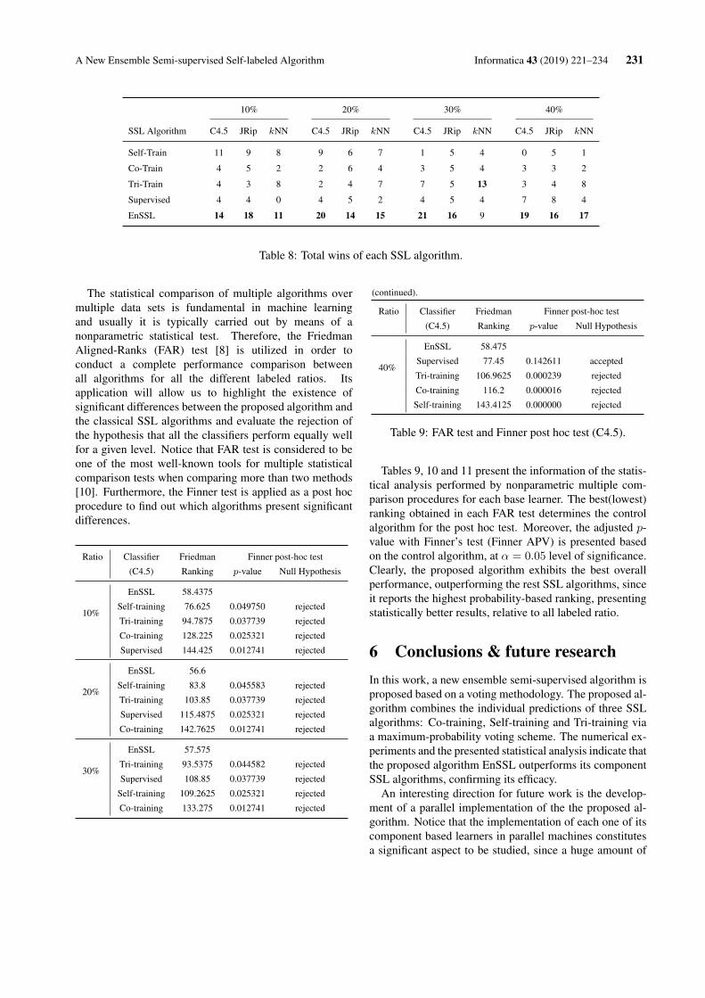
A New Ensemble Semi-supervised Self-labeled Algorithm Informatica 43 (2019) 221–234 231
10% 20% 30% 40%
SSL Algorithm C4.5 JRip kNN C4.5 JRip kNN C4.5 JRip kNN C4.5 JRip kNN
Self-Train 11 9 8 9 6 7 1 5 4 0 5 1
Co-Train 4 5 2 2 6 4 3 5 4 3 3 2
Tri-Train 4 3 8 2 4 7 7 5 13 3 4 8
Supervised 4 4 0 4 5 2 4 5 4 7 8 4
EnSSL 14 18 11 20 14 15 21 16 9 19 16 17
Table 8: Total wins of each SSL algorithm.
The statistical comparison of multiple algorithms overmultiple data sets is fundamental in machine learningand usually it is typically carried out by means of anonparametric statistical test. Therefore, the FriedmanAligned-Ranks (FAR) test [8] is utilized in order toconduct a complete performance comparison betweenall algorithms for all the different labeled ratios. Itsapplication will allow us to highlight the existence ofsignificant differences between the proposed algorithm andthe classical SSL algorithms and evaluate the rejection ofthe hypothesis that all the classifiers perform equally wellfor a given level. Notice that FAR test is considered to beone of the most well-known tools for multiple statisticalcomparison tests when comparing more than two methods[10]. Furthermore, the Finner test is applied as a post hocprocedure to find out which algorithms present significantdifferences.
Ratio Classifier Friedman Finner post-hoc test
(C4.5) Ranking p-value Null Hypothesis
10%
EnSSL 58.4375
Self-training 76.625 0.049750 rejected
Tri-training 94.7875 0.037739 rejected
Co-training 128.225 0.025321 rejected
Supervised 144.425 0.012741 rejected
20%
EnSSL 56.6
Self-training 83.8 0.045583 rejected
Tri-training 103.85 0.037739 rejected
Supervised 115.4875 0.025321 rejected
Co-training 142.7625 0.012741 rejected
30%
EnSSL 57.575
Tri-training 93.5375 0.044582 rejected
Supervised 108.85 0.037739 rejected
Self-training 109.2625 0.025321 rejected
Co-training 133.275 0.012741 rejected
(continued).
Ratio Classifier Friedman Finner post-hoc test
(C4.5) Ranking p-value Null Hypothesis
40%
EnSSL 58.475
Supervised 77.45 0.142611 accepted
Tri-training 106.9625 0.000239 rejected
Co-training 116.2 0.000016 rejected
Self-training 143.4125 0.000000 rejected
Table 9: FAR test and Finner post hoc test (C4.5).
Tables 9, 10 and 11 present the information of the statis-tical analysis performed by nonparametric multiple com-parison procedures for each base learner. The best(lowest)ranking obtained in each FAR test determines the controlalgorithm for the post hoc test. Moreover, the adjusted p-value with Finner’s test (Finner APV) is presented basedon the control algorithm, at α = 0.05 level of significance.Clearly, the proposed algorithm exhibits the best overallperformance, outperforming the rest SSL algorithms, sinceit reports the highest probability-based ranking, presentingstatistically better results, relative to all labeled ratio.
6 Conclusions & future researchIn this work, a new ensemble semi-supervised algorithm isproposed based on a voting methodology. The proposed al-gorithm combines the individual predictions of three SSLalgorithms: Co-training, Self-training and Tri-training viaa maximum-probability voting scheme. The numerical ex-periments and the presented statistical analysis indicate thatthe proposed algorithm EnSSL outperforms its componentSSL algorithms, confirming its efficacy.
An interesting direction for future work is the develop-ment of a parallel implementation of the the proposed al-gorithm. Notice that the implementation of each one of itscomponent based learners in parallel machines constitutesa significant aspect to be studied, since a huge amount of

232 Informatica 43 (2019) 221–234 I.E. Livieris
Ratio Classifier Friedman Finner post-hoc test
(JRip) Ranking p-value Null Hypothesis
10%
EnSSL 62.2625
Self-training 81.5375 0.136404 accepted
Tri-training 100.2625 0.004429 rejected
Co-training 121.0125 0.136404 rejected
Supervised 137.425 0.000000 rejected
20%
EnSSL 69.25
Self-training 95.225 0.044749 rejected
Tri-training 102.35 0.014031 rejected
Supervised 116.7 0.000492 rejected
Co-training 118.975 0.000488 rejected
30%
EnSSL 66.225
Supervised 99.9625 0.009140 rejected
Tri-training 104.175 0.004484 rejected
Self-training 109.25 0.001771 rejected
Co-training 122.8875 0.000048 rejected
40%
EnSSL 64.925
Supervised 76.1 0.387887 accepted
Tri-training 107.875 0.001206 rejected
Co-training 121.175 0.000028 rejected
Self-training 132.425 0.000001 rejected
Table 10: FAR test and Finner post hoc test (JRip).
data can be processed in significantly less computationaltime. Since the experimental results are quite encourag-ing, a next step could be the evaluation of the proposedalgorithm in specific scientific fields applying real worlddatasets, such as the educational, health care, etc.
References[1] David W. Aha. Lazy Learning. Dor-
drecht: Kluwer Academic Publishers, 1997.https://doi.org/10.1007/978-94-017-2053-3
[2] Jesús Alcalá-Fdez, Alberto Fernández, Julián Lu-engo, Joaquín Derrac, Salvador García, LucianoSánchez, and Francisco Herrera. Keel data-miningsoftware tool: data set repository, integration of algo-rithms and experimental analysis framework. Jour-nal of Multiple-Valued Logic & Soft Computing, 17,2011. https://doi.org/10.1109/nwesp.2011.6088224
[3] Ethem Alpaydin. Introduction to Machine Learn-ing. MIT Press, Cambridge, 2nd edition, 2010.https://doi.org/10.1017/s0269888906220745
[4] Avrim Blum and Tom Mitchell. Combininglabeled and unlabeled data with co-training.
Ratio Classifier Friedman Finner post-hoc test
(kNN) Ranking p-value Null Hypothesis
10%
EnSSL 59.65
Tri-training 73.825 0.273404 accepted
Self-training 89.3375 0.028959 rejected
Co-training 129.8375 0.00000 rejected
Supervised 149.85 0.00000 accepted
20%
EnSSL 59.5125
Tri-training 79.1625 0.128941 accepted
Self-training 103.55 0.00089 rejected
Co-training 130.075 0.00000 rejected
Supervised 130.2 0.00000 accepted
30%
EnSSL 70.9625
Tri-training 86.9875 0.045642 rejected
Supervised 101.175 0.026013 rejected
Self-training 117.8625 0.000581 rejected
Co-training 125.5125 0.0001 rejected
40%
EnSSL 61.9875
Supervised 74.3375 0.33996 accepted
Tri-training 92.2625 0.02568 rejected
Co-training 124.225 0.000003 rejected
Self-training 149.6875 0.000000 rejected
Table 11: FAR test and Finner post hoc test (kNN).
In 11th annual conference on Computationallearning theory, pages 92–100. ACM, 1998.https://doi.org/10.1109/icdm.2001.989574
[5] William W. Cohen. Fast effective rule induction.In International Conference on Machine Learning,pages 115–123, 1995. https://doi.org/10.1016/b978-1-55860-377-6.50023-2
[6] Bozidara Cvetkovic, Boštjan Kaluza, Mitja Luštrek,and Matjaz Gams. Semi-supervised learning foradaptation of human activity recognition classifier tothe user. In Proceddings of International Joint Con-ference on Artificial Intelligence, pages 24–29, 2011.
[7] Asif Ekbal and Sivaji Bandyopadhyay. Named entityrecognition using appropriate unlabeled data, post-processing and voting. Informatica, 34(1), 2010.
[8] Helmut Finner. On a monotonicity problem in step-down multiple test procedures. Journal of the Amer-ican Statistical Association, 88(423):920–923, 1993.https://doi.org/10.2307/2290782
[9] Matjaž Gams. Weak intelligence: through the prin-ciple and paradox of multiple knowledge. Nova Sci-ence, 2001.
A New Ensemble Semi-supervised Self-labeled Algorithm Informatica 43 (2019) 221–234 233
[10] Salvador García, Alberto Fernández, Julián Lu-engo, and Francisco Herrera. Advanced nonpara-metric tests for multiple comparisons in the de-sign of experiments in computational intelligenceand data mining: Experimental analysis of power.Information Sciences, 180(10):2044–2064, 2010.https://doi.org/10.1016/j.ins.2009.12.010
[11] Hristijan Gjoreski, Boštjan Kaluža, Matjaž Gams,Radoje Milic, and Mitja Luštrek. Context-based en-semble method for human energy expenditure esti-mation. Applied Soft Computing, 37:960–970, 2015.https://doi.org/10.1016/j.asoc.2015.05.001
[12] Tao Guo and Guiyang Li. Improved tri-training withunlabeled data. Software Engineering and KnowledgeEngineering: Theory and Practice, pages 139–147,2012. https://doi.org/10.1007/978-3-642-25349-2 19
[13] Mark Hall, Eibe Frank, Geoffrey Holmes, Bern-hard Pfahringer, Peter Reutemann, and Ian H. Wit-ten. The WEKA data mining software: An update.SIGKDD Explorations Newsletters, 11:10–18, 2009.https://doi.org/10.1145/1656274.1656278
[14] Kyaw Kyaw Htike. Hidden-layer ensemble fusion ofMLP neural networks for pedestrian detection. Infor-matica, 41(1), 2017.
[15] Ludmila I. Kuncheva. Combining Pattern Clas-sifiers: Methods and Algorithms. McGraw Hill,John Wiley & Sons, Inc., second edition, 2014.https://doi.org/10.1002/9781118914564
[16] Jurica Levatic, Sašo Džeroski, Fran Supek, andTomislav Šmuc. Semi-supervised learning for quanti-tative structure-activity modeling. Informatica, 37(2),2013.
[17] Ming Li and Zhi-Hua Zhou. Improve computer-aided diagnosis with machine learning techniquesusing undiagnosed samples. IEEE Transac-tions on Systems, Man, and Cybernetics-Part A:Systems and Humans, 37(6):1088–1098, 2007.https://doi.org/10.1109/tsmca.2007.904745
[18] Chang Liu and Pong C. Yuen. A boostedco-training algorithm for human action recogni-tion. IEEE transactions on circuits and sys-tems for video technology, 21(9):1203–1213, 2011.https://doi.org/10.1109/tcsvt.2011.2130270
[19] Ioannis E. Livieris, Ioannis Dimopoulos, ThedoreKotsilieris, and Panagiotis Pintelas. Predicting lengthof stay in hospitalized patients using ssl algorithms.In ACM 8th International Conference on Software
Development and Technologies for Enhancing Acces-sibility and Fighting Infoexclusion, pages 1–8, 2018.https://doi.org/10.1145/3218585.3218588
[20] Ioannis E. Livieris, Konstantina Drakopoulou, Vas-silis Tampakas, Tassos Mikropoulos, and Panagio-tis Pintelas. Predicting secondary school students’performance utilizing a semi-supervised learning ap-proach. Journal of Educational Computing Research,2018. https://doi.org/10.1177/0735633117752614
[21] Ioannis E. Livieris, Konstantina Drakopoulou, Vas-silis Tampakas, Tassos Mikropoulos, and PanagiotisPintelas. Research on e-Learning and ICT in Edu-cation, chapter An ensemble-based semi-supervisedapproach for predicting students’ performance, page25-42. Springer, 2018. https://doi.org/10.1007/978-3-319-95059-4 2
[22] Ioannis E. Livieris, Andreas Kanavos, VassilisTampakas, and Panagiotis Pintelas. An ensem-ble SSL algorithm for efficient chest x-ray imageclassification. Journal of Imaging, 4(7), 2018.https://doi.org/10.3390/jimaging4070095
[23] Ioannis E. Livieris, Tassos Mikropoulos, and Panagi-otis Pintelas. A decision support system for predictingstudents’ performance. Themes in Science and Tech-nology Education, 9:43–57, 2016.
[24] Christopher J. Merz. Using correspondence analysisto combine classifiers. Machine Learning, 36:33–58,1999. https://doi.org/10.1023/A:1007559205422
[25] Vincent Ng and Claire Cardie. Weakly su-pervised natural language learning without redun-dant views. In Proceedings of the 2003 Confer-ence of the North American Chapter of the As-sociation for Computational Linguistics on Hu-man Language Technology-Volume 1, pages 94–101.Association for Computational Linguistics, 2003.https://doi.org/10.3115/1073445.1073468
[26] J. Ross Quinlan. C4.5: Programs for machinelearning. Morgan Kaufmann, San Francisco, 1993.https://doi.org/10.1007/BF00993309
[27] Matteo Re and Giorgio Valentini. Advancesin Machine Learning and Data Mining for As-tronomy, chapter Ensemble methods: A re-view, pages 563–594. Chapman & Hall, 2012.https://doi.org/10.1201/b11822-34
[28] Lior Rokach. Pattern Classification Using Ensem-ble Methods. World Scientific Publishing Company,2010. https://doi.org/10.1142/7238
234 Informatica 43 (2019) 221–234 I.E. Livieris
[29] Moumita Roy, Susmita Ghosh, Ashish Ghosh. Anovel approach for change detection of remotelysensed images using semi-supervised multiple classi-fier system. Information Sciences, 269:35–47, 2014.https://doi.org/10.1016/j.ins.2014.01.037
[30] S.K. Satapathy, A.K. Jagadev, and S. Dehuri. Anempirical analysis of different machine learning tech-niques for classification of EEG signal to detectepileptic seizure. Informatica, 41(1), 2017.
[31] Sandeep Kumar Satapathy, Alok Kumar Jagadev, andSatchidananda Dehuri. Weighted majority votingbased ensemble of classifiers using different machinelearning techniques for classification of EEG signal todetect epileptic seizure. Informatica, 41(1):99, 2017.
[32] Gasper Slapnicar, Mitja Luštrek, and Matej Marinko.Continuous blood pressure estimation from PPG sig-nal. Informatica, 42(1), 2018.
[33] Shiliang Sun and Feng Jin. Robust co-training.International Journal of Pattern Recognition andArtificial Intelligence, 25(07):1113–1126, 2011.https://doi.org/10.1142/s0218001411008981
[34] Shiliang Sun and Qingjiu Zhang. Multiple-view multiple-learner semi-supervised learn-ing. Neural processing letters, 34(3):229, 2011.https://doi.org/10.1007/s11063-011-9195-8
[35] Isaac Triguero, Salvador García, and FranciscoHerrera. SEG-SSC: A framework based onsynthetic examples generation for self-labeledsemi-supervised classification. IEEE Trans-actions on Cybernetics, 45:622–634, 2014.https://doi.org/10.1109/tcyb.2014.2332003
[36] Isaac Triguero, Salvador García, and Francisco Her-rera. Self-labeled techniques for semi-supervisedlearning: taxonomy, software and empirical study.Knowledge and Information Systems, 42(2):245–284,2015. https://doi.org/10.1007/s10115-013-0706-y
[37] Isaac Triguero, José A. Sáez, Julián Luengo,Salvador García, and Francisco Herrera. Onthe characterization of noise filters for self-training semi-supervised in nearest neighborclassification. Neurocomputing, 132:30–41, 2014.https://doi.org/10.1016/j.neucom.2013.05.055
[38] Julius Venskus, Povilas Treigys, JolitaBernataviciene, Viktor Medvedev, Miroslav Voz-nak, Mindaugas Kurmis, and Violeta Bulbenkiene.Integration of a self-organizing map and a virtual
pheromone for real-time abnormal movement detec-tion in marine traffic. Informatica, 28(2):359–374,2017.
[39] Xindong Wu, Vipin Kumar, J. Ross Quinlan, Joy-deep Ghosh, Qiang Yang, Hiroshi Motoda, GeoffreyJ. McLachlan, Angus Ng, Bing Liu, and Philip S. Yu,Zhi-Hua Zhou, Michael Steinbach, David J. Hand,and Dan Steinberg Top 10 algorithms in data min-ing. Knowledge and information systems, 14(1):1–37,2008. https://doi.org/10.1201/9781420089653
[40] Qian Xu, Derek Hao Hu, Hong Xue, Weichuan Yu,and Qiang Yang. Semi-supervised protein subcellularlocalization. BMC bioinformatics, 10(1):S47, 2009.https://doi.org/10.1186/1471-2105-10-s1-s47
[41] David Yarowsky. Unsupervised word sense disam-biguation rivaling supervised methods. In Proceed-ings of the 33rd annual meeting of the associationfor computational linguistics, pages 189–196, 1995.https://doi.org/10.3115/981658.981684
[42] Yan Zhou and Sally Goldman. Democraticco-learning. In 16th IEEE InternationalConference on Tools with Artificial Intelli-gence (ICTAI), pages 594–602. IEEE, 2004.https://doi.org/10.1109/ictai.2004.48
[43] Zhi-Hua Zhou. When semi-supervised learning meetsensemble learning. In Frontiers of Electrical andElectronic Engineering in China, volume 6, pages 6–16. Springer, 2011. https://doi.org/10.1007/s11460-011-0126-2
[44] Zhi-Hua Zhou and Ming Li. Tri-training:Exploiting unlabeled data using three classi-fiers. IEEE Transactions on Knowledge andData Engineering, 17(11):1529–1541, 2005.https://doi.org/10.1109/tkde.2005.186
[45] Xiaojin Zhu. Semi-supervised learning. In Encyclo-pedia of Machine Learning, pages 892–897. Springer,2011.
[46] Xiaojin Zhu and Andrew B. Goldberg Intro-duction to semi-supervised learning. Syn-thesis lectures on artificial intelligenceand machine learning, 3(1):1–130, 2009.https://doi.org/10.2200/s00196ed1v01y200906aim006
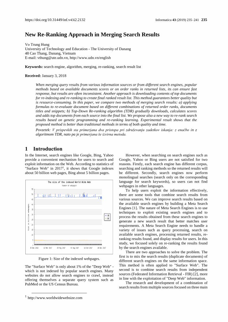
https://doi.org/10.31449/inf.v43i2.2132 Informatica 43 (2019) 235–241 235
New Re-Ranking Approach in Merging Search Results
Vo Trung Hung
University of Technology and Education - The University of Danang
48 Cao Thang, Danang, Vietnam
E-mail: [email protected], http://www.udn.vn/english
Keywords: search engine, algorithm, merging, re-ranking, search result list
Received: January 3, 2018
When merging query results from various information sources or from different search engines, popular
methods based on available documents scores or on order ranks in returned lists, its can ensure fast
response, but results are often inconsistent. Another approach is downloading contents of top documents
for re-indexing and re-ranking to create final ranked result list. This method guarantees better quality but
is resource-consuming. In this paper, we compare two methods of merging search results: a) applying
formulas to re-evaluate document based on different combinations of returned order ranks, documents
titles and snippets; b) Top-Down Re-ranking algorithm (TDR) gradually downloads, calculates scores
and adds top documents from each source into the final list. We propose also a new way to re-rank search
results based on genetic programming and re-ranking learning. Experimental result shows that the
proposed method is better than traditional methods in terms of both quality and time.
Povzetek: V prispevkih sta primerjana dva pristopa pri združevanju zadetkov iskanja: z enačbo in z
algoritmom TDR, nato pa je primerjana še izvirna metoda.
1 Introduction In the Internet, search engines like Google, Bing, Yahoo
provide a convenient mechanism for users to search and
exploit information on the Web. According to statistics of
"Surface Web" in 20171, it shows that Google indexes
about 50 billion web pages, Bing about 5 billion pages.
Figure 1: Size of the indexed webpages.
The "Surface Web" is only about 1% of the "Deep Web" -
which is not indexed by popular search engines. Many
websites do not allow search engines to crawl, instead
offering themselves a separate query system such as
PubMed or the US Census Bureau.
1 http://www.worldwidewebsize.com
However, when searching on search engines such as
Google, Yahoo or Bing users are not satisfied for two
reasons. Firstly, each search engine has different corpus,
searching and ranking methods so the returned results will
be different. Secondly, search engines now perform
monolingual searches (search only on the corresponding
language for search keywords), so users can not find
webpages in other languages.
To help users exploit the information effectively,
there are some tools that combine search results from
various sources. We can improve search results based on
the available search engines by building a Meta Search
Engines [1]. The nature of Meta Search Engines is to use
techniques to exploit existing search engines and to
process the results obtained from these search engines to
generate a new search result that better matches user
requirements. A Meta Search Engine needs to handle a
variety of issues such as query processing, search on
available search engines, processing returned results, re-
ranking results found, and display results for users. In this
study, we focused solely on re-ranking the results found
by the search engines available.
There are two approaches to solve the problem. The
first is to mix the search results (duplicate documents) of
different search engines on the same information space.
This method is often applied to "Surface Web". The
second is to combine search results from independent
sources (Federated Information Retrieval - FIR) [2], more
in line with the exploitation of "Deep Web" information.
The research and development of a combination of
search results from multiple sources focused on three main
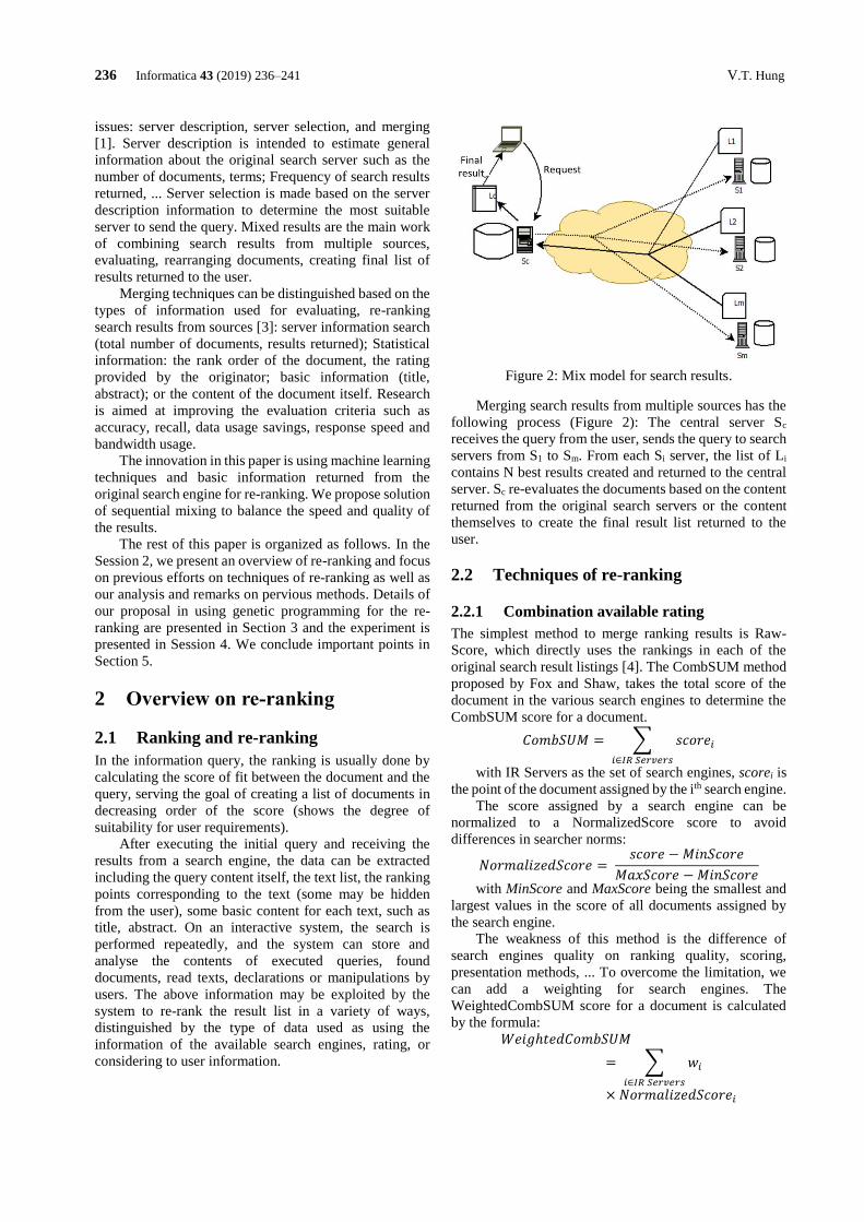
236 Informatica 43 (2019) 236–241 V.T. Hung
issues: server description, server selection, and merging
[1]. Server description is intended to estimate general
information about the original search server such as the
number of documents, terms; Frequency of search results
returned, ... Server selection is made based on the server
description information to determine the most suitable
server to send the query. Mixed results are the main work
of combining search results from multiple sources,
evaluating, rearranging documents, creating final list of
results returned to the user.
Merging techniques can be distinguished based on the
types of information used for evaluating, re-ranking
search results from sources [3]: server information search
(total number of documents, results returned); Statistical
information: the rank order of the document, the rating
provided by the originator; basic information (title,
abstract); or the content of the document itself. Research
is aimed at improving the evaluation criteria such as
accuracy, recall, data usage savings, response speed and
bandwidth usage.
The innovation in this paper is using machine learning
techniques and basic information returned from the
original search engine for re-ranking. We propose solution
of sequential mixing to balance the speed and quality of
the results.
The rest of this paper is organized as follows. In the
Session 2, we present an overview of re-ranking and focus
on previous efforts on techniques of re-ranking as well as
our analysis and remarks on pervious methods. Details of
our proposal in using genetic programming for the re-
ranking are presented in Section 3 and the experiment is
presented in Session 4. We conclude important points in
Section 5.
2 Overview on re-ranking
2.1 Ranking and re-ranking
In the information query, the ranking is usually done by
calculating the score of fit between the document and the
query, serving the goal of creating a list of documents in
decreasing order of the score (shows the degree of
suitability for user requirements).
After executing the initial query and receiving the
results from a search engine, the data can be extracted
including the query content itself, the text list, the ranking
points corresponding to the text (some may be hidden
from the user), some basic content for each text, such as
title, abstract. On an interactive system, the search is
performed repeatedly, and the system can store and
analyse the contents of executed queries, found
documents, read texts, declarations or manipulations by
users. The above information may be exploited by the
system to re-rank the result list in a variety of ways,
distinguished by the type of data used as using the
information of the available search engines, rating, or
considering to user information.
Figure 2: Mix model for search results.
Merging search results from multiple sources has the
following process (Figure 2): The central server Sc
receives the query from the user, sends the query to search
servers from S1 to Sm. From each Si server, the list of Li
contains N best results created and returned to the central
server. Sc re-evaluates the documents based on the content
returned from the original search servers or the content
themselves to create the final result list returned to the
user.
2.2 Techniques of re-ranking
2.2.1 Combination available rating
The simplest method to merge ranking results is Raw-
Score, which directly uses the rankings in each of the
original search result listings [4]. The CombSUM method
proposed by Fox and Shaw, takes the total score of the
document in the various search engines to determine the
CombSUM score for a document.
𝐶𝑜𝑚𝑏𝑆𝑈𝑀 = ∑ 𝑠𝑐𝑜𝑟𝑒𝑖
𝑖∈𝐼𝑅 𝑆𝑒𝑟𝑣𝑒𝑟𝑠
with IR Servers as the set of search engines, scorei is
the point of the document assigned by the ith search engine.
The score assigned by a search engine can be
normalized to a NormalizedScore score to avoid
differences in searcher norms:
𝑁𝑜𝑟𝑚𝑎𝑙𝑖𝑧𝑒𝑑𝑆𝑐𝑜𝑟𝑒 = 𝑠𝑐𝑜𝑟𝑒 − 𝑀𝑖𝑛𝑆𝑐𝑜𝑟𝑒
𝑀𝑎𝑥𝑆𝑐𝑜𝑟𝑒 − 𝑀𝑖𝑛𝑆𝑐𝑜𝑟𝑒
with MinScore and MaxScore being the smallest and
largest values in the score of all documents assigned by
the search engine.
The weakness of this method is the difference of
search engines quality on ranking quality, scoring,
presentation methods, ... To overcome the limitation, we
can add a weighting for search engines. The
WeightedCombSUM score for a document is calculated
by the formula:
𝑊𝑒𝑖𝑔ℎ𝑡𝑒𝑑𝐶𝑜𝑚𝑏𝑆𝑈𝑀
= ∑ 𝑤𝑖
𝑖∈𝐼𝑅 𝑆𝑒𝑟𝑣𝑒𝑟𝑠
× 𝑁𝑜𝑟𝑚𝑎𝑙𝑖𝑧𝑒𝑑𝑆𝑐𝑜𝑟𝑒𝑖
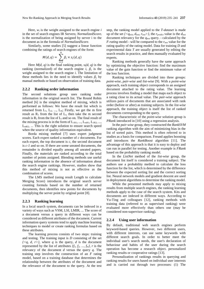
New Re-Ranking Approach in Merging Search Results Informatica 43 (2019) 235–241 237
Here, wi is the weight assigned to the search engine i
in the set of search engines IR Servers; NormalizedScorei
is the normalization of being assigned by server i to the
document as in the formula of NormalizedScore.
Similarly, some studies [5] suggest a linear function
combining the ratings of search engines of the form:
𝑀(𝑑, 𝑞) = ∑ 𝛽𝑖
𝑛
𝑖=1
× 𝑠𝑖(𝑑, 𝑞)
Here M(d, q) is the final ranking point, si(d, q) is the
ranking (normalized) of the search engine i, 𝛽𝑖 is the
weight assigned to the search engine i. The limitation of
these methods lies in the need to identify values 𝛽𝑖 by
manual methods or based on observation of training data.
2.2.2 Ranking order information
The second solutions group uses ranking order
information in the original search list. The Round Robin
method [6] is the simplest method of mixing, which is
performed as follows: We have the result list which is
returned from L1, L2, ..., Lm; Firstly, we get the m first
result as R1 from the list of Li, then take the m second
result is R2 from the list of Li and so on. The final result of
the mixing process is in the form of L1R1, ..., LmR1, L1R2, ...,
LmR2, ... This is the right solution to ensure search speed
when the source of quality information equivalent.
Borda mixing method [7] uses expert judgment
scores. Each expert ranked a number of c documents. For
each expert, the top document is c, the second document
is c-1 and so on. If there are some unrated documents, the
remainder is divided equally among all unrated papers.
Finally, the materials are ranked according to the total
number of points assigned. Blending methods use useful
ranking information in the absence of information about
the search engine rankings. However, studies show that
this method of mixing is not as effective as the
combination of scores.
The LMS method (using result Length to calculate
Merging Score) introduces the original search server
counting formula based on the number of returned
documents, then identifies new points for documents by
multiplying the server point by original point [8].
2.2.3 Ranking learning
In a local search system, documents can be indexed in a
variety of ways such as VSM, LSI, LMIR, ... The score of
a document versus a query in different ways can be
considered as different attributes of the document. Current
information query systems tend to apply machine learning
techniques to model or create ranking formulas based on
these attributes.
The learning process consists of two steps: training
and testing. The training input is D consisting of the set
{<q, d, r>}, where q is the query, d is the document
represented by the list of attributes {f1, f2, ..., fm}, r is the
relevancy of the document d versus the query q. The
training step involves the construction of an F rating
model, based on a training database that determines the
relationship between the attributes of the document and
the relevance of the document to the query. At the test
step, the ranking model applied to the T-dataset is made
up of the set {<qtest, dtest, rtest>}, the rpredict value is the dtest
document relevancy for the qtest query. - calculated by the
F-rating model - will be compared to the rtest value for the
rating quality of the rating model. Data for training D and
experimental data T are usually generated by editing the
search results in practice, and then manually evaluated by
experts.
Ranking methods generally have the same approach
by optimizing the objective function: find the maximum
value of the gain function or find the minimum value of
the loss function.
Ranking techniques are divided into three groups:
point-wise, pair-wise and list-wise [9]. With a point-wise
approach, each training object corresponds to an assigned
document attached to the rating value. The learning
process involves finding a model that maps each object to
a rating close to its actual value. The pair-wise approach
utilizes pairs of documents that are associated with rank
order (before or after) as training subjects. In the list-wise
approach, the training object is itself the list of ranked
documents corresponding to the query.
The characteristic of the point-wise solution group is
PRank introduced in [10] using a regression analysis.
In the pair-wise group, they constructed the RankSVM
ranking algorithm with the aim of minimizing bias in the
list of sorted pairs. This method is often referred to in
studies as a basis for comparison. Freund applies boosting
and introduces the RankBoost algorithm [11]. The
advantage of this approach is that it is easy to deploy and
can run in parallel for testing. Another example is FRank
based on the probability ranking model.
In the ListNet method of the list-wise group, the
document list itself is considered a training subject. The
authors use a probability method to calculate the loss
function for the list, which is determined by the difference
between the expected sorting list and the correct sorting
list. Neural network models and gradient descent are used
in deployment algorithms to determine the ranking model.
While the presented methods may apply to mixing
results from multiple search engines, the ranking learning
methods apply to the case of the search system. Kits and
documents are indexed in different ways. According to
Yu-Ting and colleagues [12], ranking methods with
training data (referred to as supervised ranking) were
evaluated more effectively than others one (may be
considered non-supervisor ranking).
2.2.4 Using user information
By default, traditional web search engines perform
keyword-based queries. However, two different users,
with different interests, can use same keywords with
different search goals. In order to better meet the
individual user's search needs, the user's declaration of
behaviour and habits of the user during the search
operation has become a research object. personalized
ranking results or cooperative ratings [13].
Personalization of rankings results in querying and
ranking results for users based on individual user interests
and is carried out through two processes: (1) The
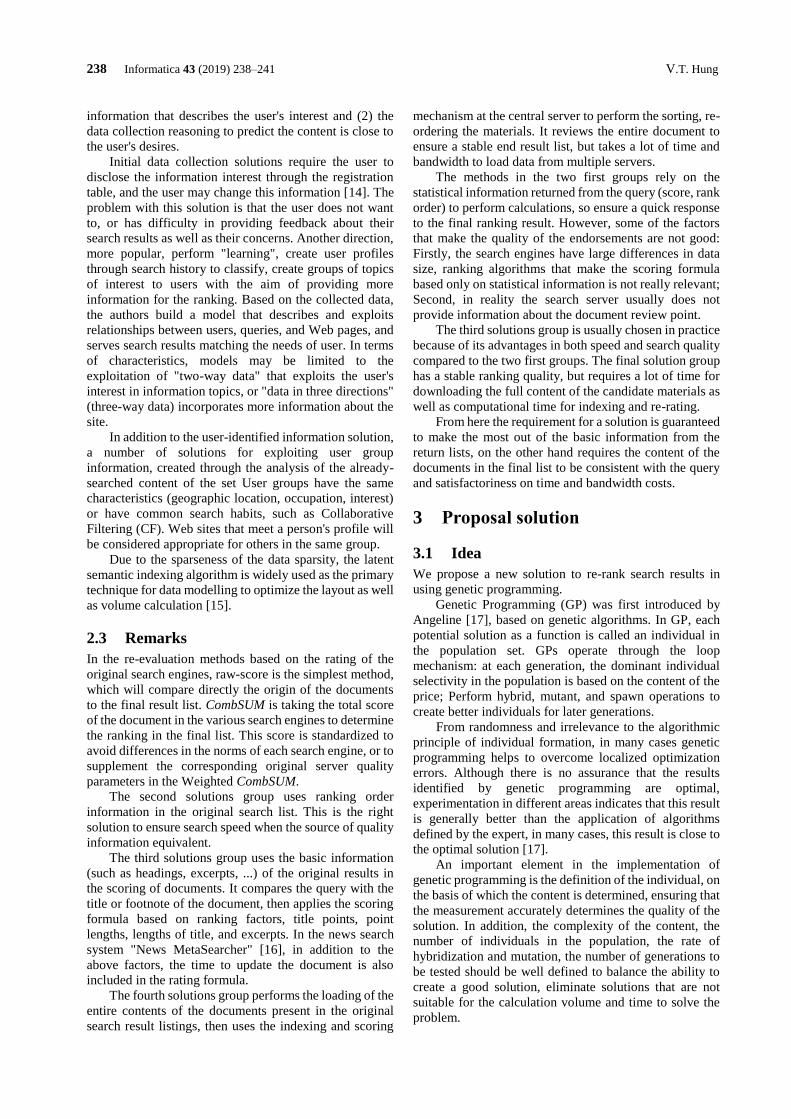
238 Informatica 43 (2019) 238–241 V.T. Hung
information that describes the user's interest and (2) the
data collection reasoning to predict the content is close to
the user's desires.
Initial data collection solutions require the user to
disclose the information interest through the registration
table, and the user may change this information [14]. The
problem with this solution is that the user does not want
to, or has difficulty in providing feedback about their
search results as well as their concerns. Another direction,
more popular, perform "learning", create user profiles
through search history to classify, create groups of topics
of interest to users with the aim of providing more
information for the ranking. Based on the collected data,
the authors build a model that describes and exploits
relationships between users, queries, and Web pages, and
serves search results matching the needs of user. In terms
of characteristics, models may be limited to the
exploitation of "two-way data" that exploits the user's
interest in information topics, or "data in three directions"
(three-way data) incorporates more information about the
site.
In addition to the user-identified information solution,
a number of solutions for exploiting user group
information, created through the analysis of the already-
searched content of the set User groups have the same
characteristics (geographic location, occupation, interest)
or have common search habits, such as Collaborative
Filtering (CF). Web sites that meet a person's profile will
be considered appropriate for others in the same group.
Due to the sparseness of the data sparsity, the latent
semantic indexing algorithm is widely used as the primary
technique for data modelling to optimize the layout as well
as volume calculation [15].
2.3 Remarks
In the re-evaluation methods based on the rating of the
original search engines, raw-score is the simplest method,
which will compare directly the origin of the documents
to the final result list. CombSUM is taking the total score
of the document in the various search engines to determine
the ranking in the final list. This score is standardized to
avoid differences in the norms of each search engine, or to
supplement the corresponding original server quality
parameters in the Weighted CombSUM.
The second solutions group uses ranking order
information in the original search list. This is the right
solution to ensure search speed when the source of quality
information equivalent.
The third solutions group uses the basic information
(such as headings, excerpts, ...) of the original results in
the scoring of documents. It compares the query with the
title or footnote of the document, then applies the scoring
formula based on ranking factors, title points, point
lengths, lengths of title, and excerpts. In the news search
system "News MetaSearcher" [16], in addition to the
above factors, the time to update the document is also
included in the rating formula.
The fourth solutions group performs the loading of the
entire contents of the documents present in the original
search result listings, then uses the indexing and scoring
mechanism at the central server to perform the sorting, re-
ordering the materials. It reviews the entire document to
ensure a stable end result list, but takes a lot of time and
bandwidth to load data from multiple servers.
The methods in the two first groups rely on the
statistical information returned from the query (score, rank
order) to perform calculations, so ensure a quick response
to the final ranking result. However, some of the factors
that make the quality of the endorsements are not good:
Firstly, the search engines have large differences in data
size, ranking algorithms that make the scoring formula
based only on statistical information is not really relevant;
Second, in reality the search server usually does not
provide information about the document review point.
The third solutions group is usually chosen in practice
because of its advantages in both speed and search quality
compared to the two first groups. The final solution group
has a stable ranking quality, but requires a lot of time for
downloading the full content of the candidate materials as
well as computational time for indexing and re-rating.
From here the requirement for a solution is guaranteed
to make the most out of the basic information from the
return lists, on the other hand requires the content of the
documents in the final list to be consistent with the query
and satisfactoriness on time and bandwidth costs.
3 Proposal solution
3.1 Idea
We propose a new solution to re-rank search results in
using genetic programming.
Genetic Programming (GP) was first introduced by
Angeline [17], based on genetic algorithms. In GP, each
potential solution as a function is called an individual in
the population set. GPs operate through the loop
mechanism: at each generation, the dominant individual
selectivity in the population is based on the content of the
price; Perform hybrid, mutant, and spawn operations to
create better individuals for later generations.
From randomness and irrelevance to the algorithmic
principle of individual formation, in many cases genetic
programming helps to overcome localized optimization
errors. Although there is no assurance that the results
identified by genetic programming are optimal,
experimentation in different areas indicates that this result
is generally better than the application of algorithms
defined by the expert, in many cases, this result is close to
the optimal solution [17].
An important element in the implementation of
genetic programming is the definition of the individual, on
the basis of which the content is determined, ensuring that
the measurement accurately determines the quality of the
solution. In addition, the complexity of the content, the
number of individuals in the population, the rate of
hybridization and mutation, the number of generations to
be tested should be well defined to balance the ability to
create a good solution, eliminate solutions that are not
suitable for the calculation volume and time to solve the
problem.

New Re-Ranking Approach in Merging Search Results Informatica 43 (2019) 235–241 239
Previously, the practice of ranking methods was
conducted independently, on different sets of data. This
does not allow comparison of methods and hinders
research. In 2007, Microsoft introduced the LETOR
(LEARNING TO Rank) data set for the study of
techniques in text search. In version 3.0 [18], the
OHSUMED collection is edited from MEDLINE - a
database of medical publications - for academic rankings.
From the data of 106 queries, three files are created: the
trainset contains 63 queries, the validation set contains 21
queries, and the testing set contains 22 queries. Each file
contains records in the following format:
<lb> qid:<q> 1:<v1> 2:<v2> . ... 45:<v45>
where <lb> is the value of relevance; <q> is the
query number; <v1>, ... <v45> are values that correspond
to the features of the documents, which are calculated on
the basis of common rankings for search. Some examples
of attributes used include:
ID Formula
1 ∑ 𝑐(𝑞𝑖 , 𝑑)𝑞𝑖∈𝑞∩𝑑 in the titles
5 ∑ log (𝐶
𝑑𝑓(𝑞𝑖))𝑞𝑖∈𝑞∩𝑑 in the titles
11 BM25 of the title 14 LMIR.JM of the title
16 ∑ 𝑐(𝑞𝑖 , 𝑑)𝑞𝑖∈𝑞∩𝑑 in the compendium
26 BM25 of the compendium
28 LMIR.JM of the compendium
Table 1: Example attribute of the OHSUMED collection.
In the above formulas, qi is the query keyword ith in
the query q, d is the document, c(qi, d) is the number of
occurrences of qi in the document d; C is the total number
of documents in the corpus, df(qi) is the number of
documents containing the keyword qi. The BM25 and
LMIR.JM scores are documented using the BM25 rating
model and the Jelinek - Mercer smoothing language model
[19].
3.2 Modelling application of genetic
programming
The GP application solution for rating learning is as
following model:
- Input 1: Training data set D with recording records
in the form of the OHSUMED collection;
- Input 2: Parameters Ng is the number of generations,
Np is the number of individuals per generation, Nc is the
hybrid speed, Nm is the speed of the mutation.
- Output: The rank function F(q, d), which sets the
value to a real number, corresponds to the relevance of the
document d to the query q.
The training process consists of five steps as follows:
- Step 1: Randomly identify first generation
individuals;
- Step 2: Determine the value of the content for each
individual;
- Step 3: Perform hybrid and mutation operations;
2 http://pyevolve.sourceforge.net (access on 15/01/2016)
- Step 4: Create a new generation and repeat steps
from 2 to 4 until you have enough Ng;
- Step 5: Choose the best individual result.
Each individual (gene) is defined as a function f(q, d)
that measures the relevance of the document to the query,
with the following options:
- Option 1: The linear function uses 45 attributes:
𝑇𝐹 − 𝐴𝐹 = 𝑎1 × 𝑓1 + 𝑎2 × 𝑓2 + ⋯ + 𝑎45 × 𝑓45
- Option 2: Linear function, using only a selective
random attribute:
𝑇𝐹 − 𝑅𝐹 = 𝑎𝑖1 × 𝑓𝑖1 + 𝑎𝑖2 × 𝑓𝑖2 + ⋯ + 𝑎𝑖𝑛 × 𝑓𝑖𝑛
- Option 3: Apply function to attributes. Limit the use
of functions x, 1/x, sin(x), log(x), and 1/(1+ex).
𝑇𝐹 − 𝐹𝐹 = 𝑎1 × ℎ1(𝑓1) + 𝑎2 × ℎ2(𝑓2) + ⋯+ 𝑎45 × ℎ45(𝑓45)
- Option 4: Create a TF-GF function similar to the one
presented in [20], but retain the evaluation of non-linear
functions. The function is binary tree, with inner vertices
being operators, leaf vertices are constants or variables.
In the formulas, ai are the parameters, fi are the
attribute values of the document, hi are the function.
In options 1, 2 and 3, to hybridize two individuals f1(q,
d) and f2(q, d), a random list of parameters has the same
index of functions to be exchanged. The mutation
operation for the individual, f(q,d), is performed by
swapping two random parameters of the function f(q, d).
Comparison of search and ranking solutions is usually
based on the measures P@k, MAP, NDCG@k [20] that is
used to determine the value of the content. Here, we test
the fitness function corresponding to the MAP value.
In the first two options, Ng, Np, Nc, Nm are respectively
100, 100, 0.9, 0.1. For option 3, Ng, Np are defined as
200,400. In option 4, Ng, Np, Nc, Nm are respectively 1000,
100, 0.9 and 0.2. These values are determined by
experiment. The Ng value, given in alternatives 3 and 4, is
greater due to the complexity and diversity of individuals
- the ranking function.
4 Experiment The TF-Ranking experimental software, built on the basis
of the PyEvolve library, was developed by Christian S.
Perone2, which enables the development of a genetic
algorithm for development in the Python language.
In the OHSUMED collection, the data is divided into
five directories, each containing the train.txt, vali.txt and
test.txt files for training, re-evaluation, and
experimentation. According to each directory, the training
and experiment steps are as follows:
- The training module reads data from train.txt for best
pbest selection, applying the scoring function to the text in
test.txt.
- Microsoft's Eval-Score-3.0.pl tool is used to
generate P@k, MAP, NDCG@k values (k = 1,2,5,100),
evaluating the effect of the generated point function.
For each option, the mean value for each of the P@k,
MAP, NDCG@k scores of the five directories was taken
as the scores for the experimental option. The
implementation of training and experiment was done 5
240 Informatica 43 (2019) 240–241 V.T. Hung
times, the average value for comparison and evaluation of
results.
Table 2, Table 3 and Table 4 compare MAP, P@k and
NDCG@k (with k = 1, 2, 5, 10) of the proposed solution
against the baseline method, published in website of the
LETOR3 assessment data set. Bold cells contain the
highest values in the corresponding column.
Method MAP
Regression 0.4220
RankSVM 0.4334
RankBoost 0.4411
ListNet 0.4457
FRank 0.4439
TF-AF 0.4456
TF-RF 0.4467
TF-FF 0.4468
TF-GF 0.4427
Table 2: Comparison of MAP values
Method K=1 K=2 K=5 K=10
Regression 0.4456 0.4532 0.4278 0.4110
RankSVM 0.4958 0.4331 0.4164 0.4140
RankBoost 0.4632 0.4504 0.4494 0.4302
ListNet 0.5326 0.481 0.4432 0.441
FRank 0.5300 0.5008 0.4588 0.4433
TF-AF 0.5506 0.4789 0.4476 0.4348
TF-RF 0.5545 0.4835 0.4633 0.4404
TF-FF 0.5294 0.4957 0.4600 0.4437
TF-GF 0.4997 0.4760 0.4507 0.4372
Table 3: Comparison of NDCG@k values
Table 4: Comparison of P@k values
Experimental results show that the TF-AF, TF-RF
alternatives are good. MAP, NDCG @ k and P @ k values
outperformed the corresponding Regression, RankSVM,
and RankBoost methods, which were equivalent and
slightly better than the ListNet and FRank methods. The
TF-GF method was not very good: Despite the good
results on the training set, the results on the experimental
set were just average, sign of overfitting.
One-time training for 5 directories with TF-AF, TF-
TF, TF-FF, and TF-GF options takes 150 minutes, 70
minutes, 200 minutes and 10 hours respectively on a dual-
3 http://research.microsoft.com/
CPU computer. Core 3.30 GHz, 4 GB RAM installed
Windows 7.
This result shows that the use of linear functions for
ranking assures efficiency, both in terms of experimental
quality and duration of training.
5 Conclusion The paper introduces an overview on re-ranking. It
evaluates the application of methods of mixing
information retrieval results from multiple sources by re-
calculating the scores based on the basic information
returned from the original search engine and proposing a
re-ranking method. sequentially, progressively download
the best documents to create the final result list.
The innovation of this proposal is applying the
machine learning method in using genetic programming.
We experimented proposal solution on the LETOR
experimental data set to develop a new ranking system
with the objective of evaluating the effectiveness of this
learning methodology. Experimental results suggest that
the proposed method is better than traditional methods in
terms of both quality and time.
Our next research is to integrate this re-ranking tool in
multi-language and cross-language search systems. The
systems are intended to allow users to find documents in
languages other than the language of the search keywords.
Acknowledgement
This research is funded by Funds for Science and
Technology Development of the University of Danang
under project number B2019-DN06-18.
References [1] Kurt I. Munson (2000), Internet Search Engines:
Understanding Their Design to Improve Information
Retrieval, Journal of Library Metadata, Volume 2,
p.p. 47-60.
https://doi.org/10.1300/J141v02n03_04
[2] M. Shokouhi and L. Si (2011), Foundations and
Trends® in Information Retrieval, Federated
Search, Volume 5 (No. 1), p.p. 101-107.
https://doi.org/10.1561/1500000010
[3] J. Callan (2002), Distributed information retrieval,
The Information Retrieval Series: Springer, INRE,
Volume 7, p.p. 127-150.
https://doi.org/10.1007/0-306-47019-5_5
[4] S. Wu, F. Crestani, Y. Bi (2006), Evaluating Score
Normalization Methods in Data Fusion, Information
Retrieval Technology, Proceedings of 3rd Asia
Information Retrieval Symposium, AIRS 2006,
Singapore, p.p. 642-648.
https://doi.org/10.1007/11880592_57
[5] W. Shengli, B. Yaxin, Z. Xiaoqin (2011), The linear
combination data fusion method in information
retrieval, Lecture Notes in Computer Science book
series (LNCS, volume 6861), pp. 219–233.
https://doi.org/10.1007/978-3-642-23091-2_20
Method P@1 P@2 P@5 P@10
Regression 0.5965 0.6006 0.5337 0.4666
RankSVM 0.5974 0.5494 0.5319 0.4864
RankBoost 0.5576 0.5481 0.5447 0.4966
ListNet 0.6524 0.6093 0.5502 0.4975
FRank 0.6429 0.6195 0.5638 0.5016
TF-AF 0.6691 0.6167 0.5499 0.4955
TF-RF 0.6642 0.6020 0.5653 0.4954
TF-FF 0.6619 0.6279 0.5612 0.4983
TF-GF 0.6220 0.6058 0.5520 0.4969
New Re-Ranking Approach in Merging Search Results Informatica 43 (2019) 235–241 241
[6] S. Wu, S. McClean (2005), Data Fusion with
Correlation Weights, Lecture Notes in Computer
Science, Volume 3408/2005, p.p. 275-286.
https://doi.org/10.1007/978-3-540-31865-1_20
[7] B. Xu, S. Luo, K. Sun (2012), Towards Multimodal
Query in Web Service Search, 19th International
Conference on Web Services, IEEE.
https://doi.org/10.1109/icws.2012.42
[8] Y. Rasolofo, F. Abbaci, J. Savoy (2001), Approaches
to collection selection and results merging for
distributed information retrieval, CIKM'01
Proceedings of the 10th international conference on
Information and knowledge management, ACM, p.p.
191 - 198.
https://doi.org/10.1145/502585.502618
[9] L. Hang (2011), Learning to Rank for Information
Retrieval and Natural Language Processing,
Synthesis Lectures on Human Language
Technologies, Morgan & Claypool Publishers, p.p.
1-113.
https://doi.org/10.2200/s00348ed1v01y201104hlt012
[10] C. Koby, S. Yoram (2002), Pranking with Ranking,
Advances in Neural Information Processing Systems
14, Volume 14, p.p. 641-647.
https://doi.org/10.7551/mitpress/1120.003.0087
[11] M.R. Yousefi, T.M. Breuel (2012), Gated Boosting:
Efficient Classifier Boosting and Combining,
Lecture Notes in Computer Science, p.p. 262-265.
https://doi.org/10.1007/978-3-642-33347-7_28
[12] L. Yu-Ting, L. Tie-Yan, Q. Tao, M. Zhi-Ming, L.
Hang (2007), Supervised rank aggregation,
Proceedings of the 16th international conference on
World Wide Web - WWW ’07, p.p. 481–490.
https://doi.org/10.1145/1242572.1242638
[13] K. Veningston, R. Shanmugalakshmi (2012),
Enhancing personalized web search re-ranking
algorithm by incorporating user profile, Third
International Conference on Computing,
Communication and Networking Technologies
(ICCCNT'12).
https://doi.org/10.1109/icccnt.2012.6396036
[14] P.A. Chirita, W. Nejdl, R. Paiu, C. Kohlschütter
(2005), Using ODP metadata to personalize search,
Proceedings of the 28th annual international ACM
SIGIR conference on Research and development in
information retrieval - SIGIR '05, p.p. 178--185.
https://doi.org/10.1145/1076034.1076067
[15] T. Nasrin, H. Faili (2016), Automatic Wordnet
Development for Low-Resource Languages using
Cross-Lingual WSD, Journal of Artificial
Intelligence Research, Volume 56, p.p. 61–87.
https://doi.org/10.1613/jair.4968
[16] Y. Rasolofo, D. Hawking, J. Savoy (2003), Result
Merging Strategies for a Current News
MetaSearcher, Information Processing &
Management, No 39(4), p.p. 581–609.
https://doi.org/10.1016/s0306-4573(02)00122-x
[17] P.J. Angeline (1994), Genetic programming: On the
programming of computers by means of natural
selection, Biosystems, MIT Press Cambridge, p.p.
69-73.
https://doi.org/10.1016/0303-2647(94)90062-0
[18] Q. Tao, L.T. Yan, X. Jun, L. Hang (2010), LETOR:
A benchmark collection for research on learning to
rank for information retrieval, Information Retrieval,
Volume 13, No. 4, p.p. 346–374.
https://doi.org/10.1007/s10791-009-9123-y
[19] C. Zhai, J. Lafferty (2001), A study of smoothing
methods for language models applied to Ad Hoc
information retrieval, Proceedings of the 24th annual
international ACM SIGIR conference on Research
and development in information retrieval - SIGIR
’01, p.p. 334–342.
https://doi.org/10.1145/383952.384019
[20] T.G. Lam, T.H. Vo, C.P. Huynh (2015), Building
Structured Query in Target Language for
Vietnamese – English Cross Language Information
Retrieval Systems, International Journal of
Engineering Research & Technology (IJERT),
Volume 4, No. 04, p.p. 146–151.
https://doi.org/10.17577/ijertv4is040317

242 Informatica 43 (2019) 235–241 V.T. Hung
https://doi.org/10.31449/inf.v43i2.1823 Informatica 43 (2019) 243–252 243
Physical Match
Aaron E. Naiman, Eliav Farber and Yossi SteinDepartment of Applied Mathematics, Jerusalem College of Technology-Machon Lev, Jerusalem, IsraelE-mail: [email protected]
Keywords: physical match, curve matching, pattern recognition, edge pixels, image processing, curve fitting, cyclic,longest common subsequence
Received: September 13, 2017
We present an approach to solving the problem of “physical match,” i.e., reconnecting back together brokenor ripped pieces of material. Our method involves correlating the jagged edges of the pieces, using amodified version of the longest common subsequence algorithm.
Povzetek: Predstavljena je izvirna metoda sestavljanja razbitih fizicnih predmetov.
1 Introduction
The problem of “physical match” spans many different ap-plications, from whimsical (jigsaw) puzzle solving [9, 19,20], to 3-D archeology [17, 14, 7, 6] (sometimes utilizinga priori shape knowledge, or rotational symmetry), to theforensic sciences [15, 16]. In the present paper we restrictourselves to the 2-D problem, and the particular aspects ofone-dimensional border which one can take advantage of,for this flat case, but not resorting to the rich information of3-D surface-to-surface matching. Therefore, given a singlepiece of material, be it paper, clothing, glass, etc., once it isripped or broken into many pieces, the challenge is to pieceback together the parts, to the original shape.
Sometimes one can take advantage of text [18], color[9], orientation (e.g., lined paper), images [20, 10, 4], spe-cific shapes (e.g., machine-shredded paper [18], or the jig-saw puzzle problem [19]) and/or texture. A survey of suchmethods can be found in [8]. We are making none of theseassumptions, and therefore matching via shape alone.
Some approach this problem with gross polygon approx-imations of the pieces [1], whereas others solve with a mul-tiscale of resolutions [3]. Our method is based on cor-relating the changes of direction along the edges of thepieces. In [21], the same information is used, however,whereas they build histograms of these changes of direc-tion, we compare them directly, retaining their order, asdescribed below. Finally, [16] present statistical findings(for the plausibility of the Daubert ruling in the court oflaw) for three different types of material. Our analysis isfor generic materials, and we concentrate more on the al-gorithms involved.
2 Background and problem
We have chosen to, at least initially, model the pieces onthe computer, rather than work with actually torn material.The reason for this is in order to steer away from possi-
ble parameter fixing based on a few physical cases, andinstead deriving statistics and parameter values, based onthousands of computer-modeled Monte-Carlo simulations.
In order to accurately match along the edges of thepieces, we start by scanning in the pieces to determinethe location of all of the edges. This has to be done withenough resolution to pick up the unique characteristics ofeach segment of the edge, and minimize the effects of thejagged nature of digitization of the edge pixel positions. Onthe other hand, the resolution cannot be too high, lest thecomputations be inordinately expensive.
Once the edges have been located, the edge slopes haveto be calculated in such a fashion so that they can be com-pared to each other. The slope calculations require an or-dering of the pixels, which is accomplished together withthe previous step of locating the edge pixels. This is donefor all of the edges of all of the pieces. Since the pieceshave been translated and rotated with respect to each other,we actually stored away in arrays, one for each piece, theinvariant changes in direction along the edge. This we areable to accomplish, as we “travel” along the edges (ex-plained below), recording the rotations.
After the edges have been characterized, the core of oursystem is to find where the turns of the edges of separatepieces correctly match up. We use a modified version ofthe longest common subsequence (LCS) algorithm [5], ad-justed to be appropriate for problems where the startingpoints of the sequences are not known.
Finally, the last step is to calculate from the matchingturns, where exactly to “sew” the pieces back together. Thisstage requires further filtering of the matching algorithm, todispose of spurious matches along the edges.
To summarize, the following algorithms are needed forus to model and verify our physical match system:
1) modeling original, non-trivial pieces of material, andbreaking them further into pieces,
2) accurately scanning in the (edges of) the pieces, at the

244 Informatica 43 (2019) 243–252 A.E. Naiman et al.
required resolution, to locate and order the edge pix-els,
3) calculating the edge slopes,
4) correlating the edge slope deviations to find the cor-rect matches and
5) sewing the pieces back together.
3 Modeling random-shaped piecesand breaking them
For simplicity’s sake, we start with pieces which are basi-cally circular in shape, but we perturb the edge to obtain apolygon. Beginning with a center, we randomly choosea sequence of angles, as well as radii, ranging betweentwo given extrema. These points are then connected withstraight lines to obtain the polygon. See an example of thisin Figure 1. A less-simple shape would be to connect thesame points with splines, as seen in Figure 2. The ramifi-
Figure 1: Polygonal edge
Figure 2: Spline edge
cations of such a shape on the subsequent algorithms, willbe the subject of future analysis.
Given polygon, we must now simulate “breaking” it intosmaller pieces. Starting at an interior point, we proceed ina straight line, randomizing both the direction and lengthof the step. This is repeated until a step exits the polygon,as seen in Figure 3. Continuing in the opposite direction,we can create the entire crack, defining our two sub-pieces,as in Figure 4.
Figure 3: Break exiting polygon
Figure 4: Two pieces
Treating each sub-piece separately, we can now recurse,breaking each piece further and further. Examples of 3pieces and 100 pieces are shown in Figures 5 and 6.
When determining the values of the extrema, both forthe random direction and the random length of the step wetake, it is important to generate a break with similar “turn”characteristics to the original polygon edge.
The reason for this is the following. While it is truethat, e.g., for a simply-shaped piece of material, the breakmay actually generate a different kind of edge, we are look-ing for a worst-case scenario, where we cannot easily tellwhere the ripped part is, and where the original polygonaledge is. Two counterexamples can be seen in Figures 7 and8.
We note that calculating when the break “leaves” thepiece, in not trivial. We cannot simply check whether thefinal end of the current “step” segment falls out of the poly-
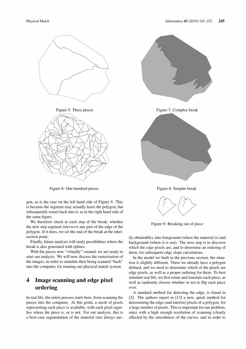
Physical Match Informatica 43 (2019) 243–252 245
Figure 5: Three pieces
Figure 6: One hundred pieces
gon, as is the case on the left hand side of Figure 9. Thisis because the segment may actually leave the polygon, butsubsequently return back into it, as in the right hand side ofthe same figure.
We therefore check at each step of the break, whetherthe new step segment intersects any part of the edge of thepolygon. If it does, we set the end of the break at the inter-section point.
Finally, future analysis will study possibilities where thebreak is also generated with splines.
With the pieces now “virtually” created, we are ready tostart our analysis. We will now discuss the rasterization ofthe images, in order to simulate their being scanned “back”into the computer, for running our physical match system.
4 Image scanning and edge pixelordering
In real life, the entire process starts here, from scanning thepieces into the computer. At this point, a mesh of pixelsrepresenting each piece is available, with each pixel signi-fies where the piece is, or is not. For our analysis, this isa best-case segmentation of the material (not always eas-
Figure 7: Complex break
Figure 8: Simpler break
Figure 9: Breaking out of piece
ily obtainable), into foreground (where the material is) andbackground (where it is not). The next step is to discoverwhich the edge pixels are, and to determine an ordering ofthem, for subsequent edge slope calculations.
In the model we built in the previous section, the situa-tion is slightly different. There we already have a polygondefined, and we need to determine which of the pixels areedge pixels, as well as a proper ordering for them. To bestsimulate real life, we first rotate and translate each piece, aswell as randomly choose whether or not to flip each pieceover.
A standard method for detecting the edge, is found in[2]. The authors report in [13] a new, quick method fordetermining the edge (and interior) pixels of a polygon, fora large number of pixels. This is important for our problem,since with a high enough resolution of scanning (clearlyeffected by the smoothness of the curves, and in order to
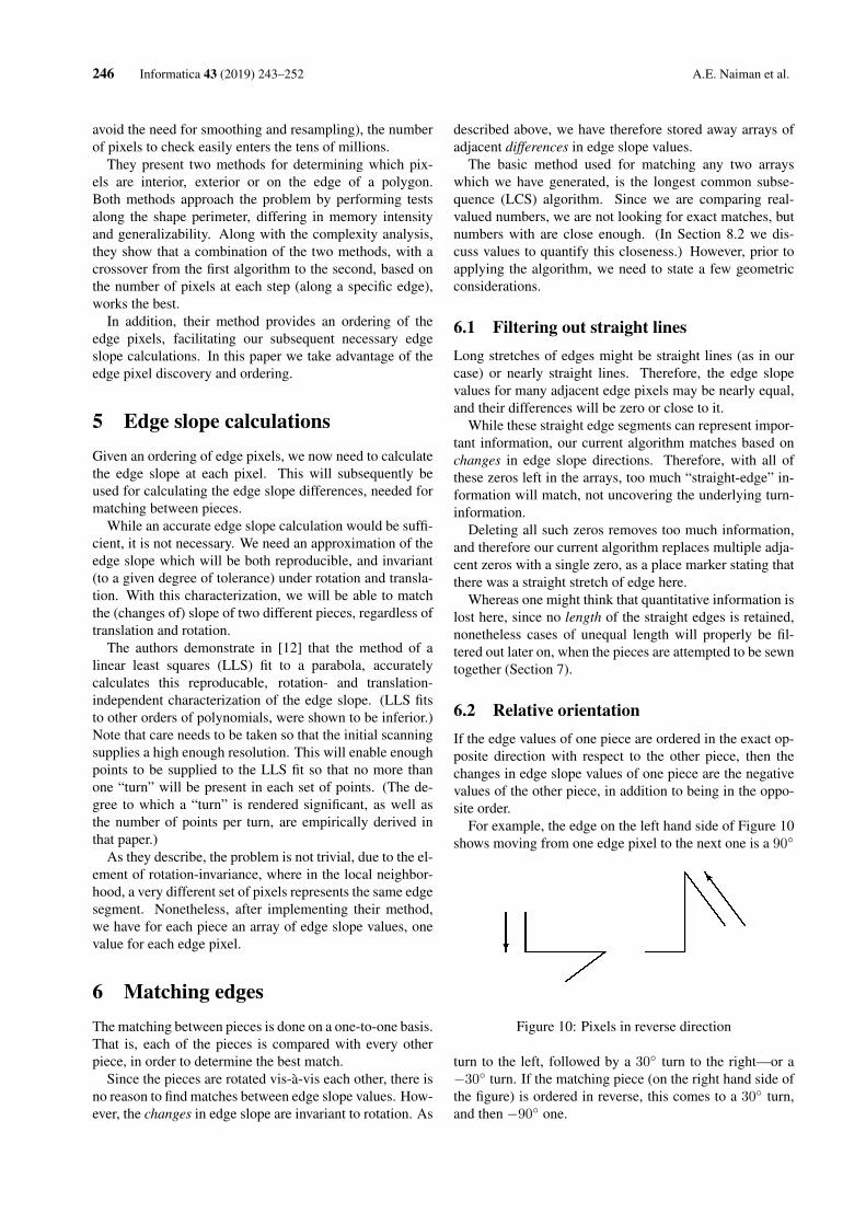
246 Informatica 43 (2019) 243–252 A.E. Naiman et al.
avoid the need for smoothing and resampling), the numberof pixels to check easily enters the tens of millions.
They present two methods for determining which pix-els are interior, exterior or on the edge of a polygon.Both methods approach the problem by performing testsalong the shape perimeter, differing in memory intensityand generalizability. Along with the complexity analysis,they show that a combination of the two methods, with acrossover from the first algorithm to the second, based onthe number of pixels at each step (along a specific edge),works the best.
In addition, their method provides an ordering of theedge pixels, facilitating our subsequent necessary edgeslope calculations. In this paper we take advantage of theedge pixel discovery and ordering.
5 Edge slope calculationsGiven an ordering of edge pixels, we now need to calculatethe edge slope at each pixel. This will subsequently beused for calculating the edge slope differences, needed formatching between pieces.
While an accurate edge slope calculation would be suffi-cient, it is not necessary. We need an approximation of theedge slope which will be both reproducible, and invariant(to a given degree of tolerance) under rotation and transla-tion. With this characterization, we will be able to matchthe (changes of) slope of two different pieces, regardless oftranslation and rotation.
The authors demonstrate in [12] that the method of alinear least squares (LLS) fit to a parabola, accuratelycalculates this reproducable, rotation- and translation-independent characterization of the edge slope. (LLS fitsto other orders of polynomials, were shown to be inferior.)Note that care needs to be taken so that the initial scanningsupplies a high enough resolution. This will enable enoughpoints to be supplied to the LLS fit so that no more thanone “turn” will be present in each set of points. (The de-gree to which a “turn” is rendered significant, as well asthe number of points per turn, are empirically derived inthat paper.)
As they describe, the problem is not trivial, due to the el-ement of rotation-invariance, where in the local neighbor-hood, a very different set of pixels represents the same edgesegment. Nonetheless, after implementing their method,we have for each piece an array of edge slope values, onevalue for each edge pixel.
6 Matching edgesThe matching between pieces is done on a one-to-one basis.That is, each of the pieces is compared with every otherpiece, in order to determine the best match.
Since the pieces are rotated vis-à-vis each other, there isno reason to find matches between edge slope values. How-ever, the changes in edge slope are invariant to rotation. As
described above, we have therefore stored away arrays ofadjacent differences in edge slope values.
The basic method used for matching any two arrayswhich we have generated, is the longest common subse-quence (LCS) algorithm. Since we are comparing real-valued numbers, we are not looking for exact matches, butnumbers with are close enough. (In Section 8.2 we dis-cuss values to quantify this closeness.) However, prior toapplying the algorithm, we need to state a few geometricconsiderations.
6.1 Filtering out straight linesLong stretches of edges might be straight lines (as in ourcase) or nearly straight lines. Therefore, the edge slopevalues for many adjacent edge pixels may be nearly equal,and their differences will be zero or close to it.
While these straight edge segments can represent impor-tant information, our current algorithm matches based onchanges in edge slope directions. Therefore, with all ofthese zeros left in the arrays, too much “straight-edge” in-formation will match, not uncovering the underlying turn-information.
Deleting all such zeros removes too much information,and therefore our current algorithm replaces multiple adja-cent zeros with a single zero, as a place marker stating thatthere was a straight stretch of edge here.
Whereas one might think that quantitative information islost here, since no length of the straight edges is retained,nonetheless cases of unequal length will properly be fil-tered out later on, when the pieces are attempted to be sewntogether (Section 7).
6.2 Relative orientationIf the edge values of one piece are ordered in the exact op-posite direction with respect to the other piece, then thechanges in edge slope values of one piece are the negativevalues of the other piece, in addition to being in the oppo-site order.
For example, the edge on the left hand side of Figure 10shows moving from one edge pixel to the next one is a 90◦
Figure 10: Pixels in reverse direction
turn to the left, followed by a 30◦ turn to the right—or a−30◦ turn. If the matching piece (on the right hand side ofthe figure) is ordered in reverse, this comes to a 30◦ turn,and then −90◦ one.

Physical Match Informatica 43 (2019) 243–252 247
Similarly, if one piece is flipped over as compared to theother piece, then the values will be either in the oppositeorder (−30◦, 90◦), as in Figure 11, or with reversed signs
Figure 11: Flipped piece with opposite order
(90◦, −30◦), as seen in Figure 12.
Figure 12: Flipped piece with reversed signs
Therefore, we need to compare the two array in four dif-ferent fashions:
1) as is,
2) with one of the arrays reversed,
3) with one of the arrays with opposite signs and
4) with one of the arrays reversed and with oppositesigns.
6.3 Cyclic correlation
Recall that each array represents the changes of edge slopevalues for the perimeter of a given piece. Since we ran-domly choose where along an edge to start the array, we donot know where a matching segment is for any two pieces.It could be that the match is in the middle of array A, butfor array B, it is at the end of the array, and finishes subse-quently back around at the beginning of the array.
The authors in [11] deal with this issue at length anddemonstrate that initially four LCS algorithm invocationsare necessary:
1) as is,
2) with one array rotated by 50%,
3) with the other array rotated by 50% and
4) with both arrays rotated by 50%.
(Rotating the array amounts to choosing a different start-ing point along the piece’s edge.) Padding the array withthe same content was avoided, in order to avoid possiblespurious artifacts.
Note that these four possibilities are in addition to thefour permutations mentioned previously in Section 6.2,with reversed arrays and negative values. Therefore, thecomposite set of possibilities includes a total of 16 pos-sibilities. The best LCS (of the 16) is found, and then ifdeemed necessary, one or both arrays are reversed, sign-changed and 50% rotated.
In the same paper, the authors show that once the bestLCS (so far) is found, and after performing a centeringtechnique they devised, an additional invocation of the LCSalgorithm is necessary to extract the LCS. They establishthat for cases where the LCS in the two sequences areknown to be clustered within the sequences, this final cen-tering and subsequent LCS algorithm step provide optimalLCS results.
Our problem indeed exhibits this clustering behavior, astwo pieces generally match along the adjacent side, and notall the way around. (A degenerate case is when one piecesits totally within another.)
With the two LCSs lined up and centered within theirsequences, we are ready to proceed with the final stage of“reconnecting” the two pieces back together.
7 Sewing edgesAs was noted in the previous section, a final invocation ofthe LCS algorithm was used in order to extract an LCSas long as possible. However, even with optimal resultsof obtaining the entire, appropriate LCS, we still need toconcern ourselves with spurious, random matches whichmay enter the LCS.
7.1 Filtering random matchesConsider Figure 13. We see that although we have a good
Figure 13: With spurious matches - both sides
match overall, if we are to consider the extra, spurious cir-cled matches which are outside of our match, this might se-riously degrade our subsequent calculations for reconnect-ing the pieces.
Note that random matches can occur within the LCSspans as well, although they would less effect the “sewing”process (described below), since in general they are geo-metrically closer to each other.

248 Informatica 43 (2019) 243–252 A.E. Naiman et al.
To dispose of the circled mis-matches, we return to thecentering process mentioned in the previous section, re-garding the final LCS algorithm invocation. We reusethis center to throw our support behind the 20–30% of thematches which are closest to the center, and discard the re-maining matches.
Note as well, that the LCS algorithm only “rewards” formatches, and does not penalize for mismatches. Thesemismatches are possibly due to missing material along amatching edge, leading to intervening unmatching pairs.If the type of the material and/or situation are such thatworn or missing pieces are unlikely, then penalties for mis-matches can be considered as well.
7.2 Moving and rotatingWe must first move the two pieces next to each other, inorder to enable the final stitching. For simplicity’s sake,we assume one piece to be stationary, and the other willbe matched up to it. Since this second piece is both trans-lated away, and rotated from the first piece, the followingmaneuver will return its coordinates [x y]
T to their correctlocations:(
cosα sinα− sinα cosα
)(xy
)+
(∆x∆y
)The challenge, therefore, is to find the optimal values of α,∆x and ∆y, to juxtapose the two pieces.
Even though we have already established our matchingpositions within the arrays, along with their (x, y) coor-dinates, we acknowledge sources of initial measurementerrors in the scanning, as well as possible internal mis-matches, mentioned above. We therefore use a nonlinearleast squares (LSQ) solver (in MATLAB: lsqnonlin)to find the triad of values which minimizes the sum ofthe square distances between our remaining LCS matches.Note: as many nonlinear solvers require, we initially seedthe solver with a seat-of-the-pants approximation given thegeometry and any three matching pairs. Also, it was cru-cial to adjust the maximum number of iterations allowed(in MATLAB: MaxIter) and the termination tolerance onx (MATLAB: TolX) in order to converge properly to thedesired results.
7.3 Micro-stitchingWith our two pieces lined up next to each other, we havethe situation shown in Figure 14. We need to find the en-tire “seam” in order to properly stitch the two pieces to-gether. A proper stitching is crucial for the success of fur-ther matching to more pieces. Note that now we would liketo find the most number of pixels which can be consideredpart of the seam, with the remaining pixels comprising theedge of the combined piece. Therefore, matching betweenpixels of the two pieces:
1) entails geometric proximity, instead of matchingslopes as before, and
Figure 14: Pre-stitch
2) is done for all of the candidate pixels along the seam,and not only the LCS matches.
Starting from the LCS center, the algorithm proceeds inboth directions along the seam, by adding the closest pixels(to each other) from the two pieces, as long as their distanceis 0.4 of the average mean distance (calculated earlier inthe nonlinear least squares procedure). We allow skippingpixels, as long as subsequent ones are part of the seam.When we hit three consecutive pairs which are too far apart,we consider the seam ended (in that direction). Note thatthe 0.4 value and the count of three consecutive pairs, wereempirically derived.
7.4 Goodness of fitDue to the digitized nature of the problem, we need metricsto measure the quality of the matches. The minimized sumsquared error calculated to translate and rotate the piecesgives us one measure, but that was prior to the stitching.
We therefore measure the overlap between the twopieces, as well as gaps which may have been uncovered.See, e.g., in Figure 15, where the dark gray area near the
Figure 15: Overlap and gap
top shows us the overlap, and the thin light gray strip to-wards the bottom—where neither piece covers.
One way to quantify these values is to rescan the entirestitched area of the union of the two pieces. However, thisprocess takes quite a bit of computation time, and is notnecessary. Instead, we take a much quicker approach byanalyzing the seam only. Starting at one end, we travelalong the two edges, calculating where there are crossoversbetween the two pieces. At these points, we go from over-laps to gaps, or vice versa; we sum each of these separately.
There is one case where an entire scan of the union of thetwo pieces is helpful—and necessary. On the left hand side

Physical Match Informatica 43 (2019) 243–252 249
of Figure 16 we see that although our eyes solve the prob-
Figure 16: Reconfigurable pieces
lem easily, moving the two pieces together, another pos-sibility can be seen as well, on the right hand side of thefigure. Note that the latter possibility suffers no overlaps orgaps, along the seam.
Clearly this is not the desired result. We therefore run aquick, low-resolution scan of the union of the two pieces,discarding this possibility by comparing the total area be-fore and after stitching. Note that one cannot decide ona consistent ordering of the edge pixels based on concav-ity/convexity of the pieces, as even along matching edges,part of the shared edge might be concave, and part convex.
One final measure of fit, is the length of the seam. Thisis needed, as, e.g., if two pieces meet at just one point,then the sum squared error will be zero, there will be nooverlap nor gap areas, and the area of the union will beexactly equal to the sum of the individual areas. However,the seam length will be zero too, indicating that no matchat all occurred.
The gross overlap demonstrated in Figure 16, and theextremely short length of the seam, are not used statisticallywith the first two metrics, i.e., the lengths of overlaps andgaps. These last two measures of fit used in a binary fashionto throw away possible matches.
8 ResultsWe present here some sample cases, together withempirically-drawn heuristics regarding system parametervalues.
8.1 More than two piecesWhen we start with more than two pieces, we compare ev-ery piece to every other one. We take the “greedy” ap-proach of choosing the candidate pairs which maximizethe number of possible “sewings,” for this round of thephysical match. Others [10, 4] approach this by buildinggraphs of matches, subsequently redivided into subgraphsby spectral clustering.) E.g., if the following pairs havebeen discovered: (1,2), (2,3) and (3,4), we will ignore the(2,3) match, first working with the other two pairs. Oncethat is finished, we iterate until all possible matches havebeen found. See Figures 17–21.
8.2 System parameter valuesOur entire approach is subject to a number of interdepen-dent, system-level parameters which need to be set to the
Figure 17: 8 pieces
Figure 18: 8 pieces stitched
correct values. We demonstrate below what can happenwith the wrong set of values.
The parameters of interest are:
Resolution This is the scanning resolution of the variouspieces into the computer, in MATLAB pixels. As men-tioned in Section 5, care needs to be taken so thatthe resolution is high enough to capture the twists andturns of the edge, but not too high, as to make the com-putation inordinately long. Sample values (in MAT-LAB coordinates): 100, 200.
Edge characterization points Again, as discussed in thesame section, this needs to be large enough to supplythe linear least squares fit to a parabola algorithm withenough information to characterize the edge slope, butnot too large, so that no more than one turn is presentin the set of points. Sample values: 23–29 (resolutionof 100), 31–37 (resolution of 200).
Straight corner maximum This determines the maxi-mum value of change of direction at a pixel, such thatwe still consider there to be no change, as if a straightline was passing through. We addressed this in Sec-tion 6.1 to filter out straight lines. Sample values: 0.2–0.8.

250 Informatica 43 (2019) 243–252 A.E. Naiman et al.
Figure 19: 4 pieces
Figure 20: 4 pieces stitched
Figure 21: 2 pieces
LCS maximum match In the LCS matching algorithm,we stated in Section 6 that when comparing changesof slope, we are willing to have these numbers be dif-ferent, up to this maximum value. Sample values:0.1–0.4.
LSQ confidence in matches This value is used in Sec-tion 7.2 to supply the nonlinear least squares fit withmatches, to translate and rotate the pieces together. Itis a fraction of the matches in each direction, startingfrom the center of the LCS. Sample values: 0.10–0.25.
In addition to the conclusions we derive below, we found:
1) Overall it makes sense to scan at a resolution of 200, inorder to obtain better fit statistics (preventing overlapsand gaps), which in turn provides better conditions forsubsequent matches to other pieces.
2) The LSQ confidence in matches parameter was lessimportant.
3) Of the three remaining parameter: edge characteriza-tion points, straight corner maximum and LCS max-
imum match, as long as at least two of them werewithin the nominal bounds prescribed below, thenmatching was successful approximately 80% of thetime. If only one of them was within the nominalbounds (particularly, one of the first two parameters),then successful matching was achieved in about 50%of the cases.
4) The two parameters: straight corner maximum andLCS maximum match, were not particularly depen-dent on the resolution, as long as they were within thenominal bounds prescribed below.
8.3 Optimal valuesIn general, the values in Table 1 worked optimally for a
resolution of 100edge characterization points 27, 29
straight corner maximum 0.4–0.8LCS maximum match 0.2–0.4
LSQ confidence in matches 0.10–0.25
Table 1: Resolution of 100 — optimal values
scanning resolution value of 100. We show in Table 2 the
resolution of 200edge characterization points 35, 37
straight corner maximum 0.4–0.8LCS maximum match 0.2–0.4
LSQ confidence in matches 0.10–0.25
Table 2: Resolution of 200 — optimal values
optimal valus for a scanning resolution value of 200.We present here a specific case, in order to illustrate what
happens when the system parameters stray too far from thenominal values. In Table 3 are the system parameter val-
resolution of 100edge characterization points 25
straight corner maximum 0.8LCS maximum match 0.2
LSQ confidence in matches 0.20
Table 3: Nominal values
ues for this specific case. The subsequent matches are dis-played in Figure 22, showing a good match up between thetwo pieces.
If, however, the edge characterization points parameteris set too low, to 17, then the edge slope values are notproperly calculated, and just low values of changes in theslope direction are matched. This can be seen in Figure 23,where we see that the matches are also not only along the

Physical Match Informatica 43 (2019) 243–252 251
Figure 22: Nominal values
Figure 23: Edge characterization points too low
correct seam, but all around the edges.Another problematic case is if the straight corner maxi-
mum is set too low. In Figure 24, with the value set to 0.3,we see that only very straight corners are considered to bemodeling straight lines, and therefore we have a huge num-ber of matches. The information at the corners of interestis lost in the noise.
Finally, we demonstrate what happens if the LCS max-imum match system parameter is set too low. A value of0.01 is too stringent to allow edge slope changes of the twopieces to match up with each other. This is seen in Fig-ure 25, where very few matches have been established.
Figure 24: Straight corner maximum too low
Figure 25: LCS maximum match too low
9 Future researchWe list here a number of future directions for this research.
1) As mentioned in Section 3, we would like to build theinitial piece, as well as generate the breaks, using themore general splines, instead of straight lines.
2) Clearly we would like to run the analysis for actualpieces of broken/torn material, in order to verify theoptimal system parameter values.
3) “Holes” in the material might be due to missingpieces. How do the holes effect this process? Canthe stitching algorithm of Section 7.3 easily be modi-fied so as to be able to “jump” over such holes? Notethat previous work of automating jigsaw puzzle recon-struction rarely addressed this.
4) In addition, we would like to understand how varioustypes of material (glass, pottery, plastic, rubber, etc.)effect the system parameter values of choice.
5) Specifically, paper has more characteristics, due to thefibers jutting out along the torn edge. Can we takeadvantage of these? Are they “in the way?” Can weremove them, without effecting the success of the sub-sequent matching?
6) On the issue of paper, how does the fact that it is usu-ally multi-ply, effect the analysis? Can we analyzeeach ply, and match on the composite picture?
7) This also brings us to the exciting extension to 3-Dphysical match, with applications to archeology andexploded object reconstruction.
8) Finally, there is the area of forensics. In order toclaim: “This piece came from this object.” and havethis be admissable in court, we have to answer ques-tions regarding confidence levels of the fit, as well asstatistical probability that no other piece could likelyfit there.
10 SummaryWe have presented a method for solving the problem ofphysical match. The algorithm involves finding the edgepixels, ordering them, and using their positions to char-acterize the edge slope. The turns along the edges arethen matched to each other using a modified version of thelongest common subsequence algorithm.
Finally, the various pieces are translated, rotated andflipped (if necessary), and then stitched together for furthermatching to other pieces.
We discussed future directions for the research, particu-larly in the arena of extending the analysis to 3-D shapesand breaks.
References[1] F. BORTOLOZZI, Document reconstruction based on
feature matching, in 18th Brazilian Symposium onComputer Graphics and Image Processing, Oct. 2005,pp. 163–170.
252 Informatica 43 (2019) 243–252 A.E. Naiman et al.
[2] J. CANNY, A computational approach to edge de-tection, Pattern Analysis and Machine Intelligence,IEEE Transactions on, 8 (1986), pp. 679–698.
[3] H. C. DA GAMA LEITAO AND J. STOLFI, A multi-scale method for the reassembly of two-dimensionalfragmented objects, IEEE Transactions on Pat-tern Analysis and Machine Intelligence, 24 (2002),pp. 1239–1251.
[4] A. C. GALLAGHER, Jigsaw puzzles with pieces ofunknown orientation, in Computer Vision and Pat-tern Recognition (CVPR), 2012 IEEE Conference on,IEEE, 2012, pp. 382–389.
[5] M. R. GAREY AND D. S. JOHNSON, Computersand Intractability: A Guide to the Theory of NP-Completeness, W. H. Freeman, 1979.
[6] Q.-X. HUANG, S. FLÖRY, N. GELFAND,M. HOFER, AND H. POTTMANN, Reassemblingfractured objects by geometric matching, in ACMTransactions on Graphics (TOG), vol. 25, ACM,2006, pp. 569–578.
[7] M. KAMPEL AND R. SABLATNIG, 3d puzzling ofarcheological fragments, in Proc. of 9th ComputerVision Winter Workshop, vol. 2, Slovenian PatternRecognition Society, 2004, pp. 31–40.
[8] F. KLEBER AND R. SABLATNIG, A survey of tech-niques for document and archaeology artefact recon-struction, in Document Analysis and Recognition,2009. ICDAR’09. 10th International Conference on,IEEE, 2009, pp. 1061–1065.
[9] D. A. KOSIBA, P. M. D. AND. S. BALASUBRAMA-NIAN, T. L. GANDHI, AND K. KASTURI, An auto-matic jigsaw puzzle solver, in Proceedings of the 12thIAPR International Conference on Pattern Recogni-tion - Conference A: Computer Vision & Image Pro-cessing, vol. 1, 1994, pp. 616–618.
[10] H. LIU, S. CAO, AND S. YAN, Automated assemblyof shredded pieces from multiple photos, Multimedia,IEEE Transactions on, 13 (2011), pp. 1154–1162.
[11] A. E. NAIMAN, E. FARBER, AND Y. STEIN, CLCS—cyclic longest common subsequence, 2018. submit-ted.
[12] , Edge characterization of digitized images,Oct. 2018. submitted.
[13] , EdgeTrek—interior and boundary pixels forlarge regions, Oct. 2018. submitted.
[14] G. PAPAIOANNOU AND E.-A. KARABASSI, Onthe automatic assemblage of arbitrary broken solidartefacts, Image and Vision Computing, 21 (2003),pp. 401–412.
[15] SCIENTIFIC WORKING GROUP FOR MATERIALSANALYSIS, Glass fractures, Forensic Science Com-munications, 7 (2005).
[16] Y. SHOR, Y. YEKUTIELI, S. WIESNER, ANDT. TSACH, Physical Match, Elsevier, AcademicPress, 2 ed., 2013, pp. 54–59. Encyclopedia of Foren-sic Sciences, ed.: Jay A. Siegel, Pekka J. Saukko,Max M. Houck.
[17] G. ÜÇOLUK AND I. HAKKI TOROSLU, Automaticreconstruction of broken 3-d surface objects, Com-puters & Graphics, 23 (1999), pp. 573–582.
[18] A. UKOVICH, G. RAMPONI, H. DOULAVERAKIS,Y. KOMPATSIARIS, AND M. G. STRINTZIS, Shred-ded document reconstruction using MPEG-7 stan-dard descriptors, in Proceedings of the Fourth IEEEInternational Symposium on Signal Processing andInformation Technology, Dec. 2004, pp. 334–337.
[19] H. WOLFSON, E. SCHONBERG, A. KALVIN1, ANDY. LAMDAN, Solving jigsaw puzzles by computer,Annals of Operations Research, 12 (1988), pp. 51–64.
[20] F.-H. YAO AND G.-F. SHAO, A shape and imagemerging technique to solve jigsaw puzzles, PatternRecognition Letters, 24 (2003), pp. 1819–1835.
[21] L. ZHU, Z. ZHOU, J. ZHANG, AND D. HU, A par-tial curve matching method for automatic reassemblyof 2d fragments, in Intelligent Computing in SignalProcessing and Pattern Recognition, Springer, 2006,pp. 645–650.
https://doi.org/10.31449/inf.v43i2.2090 Informatica 43 (2019) 253–262 253
The Permutable k-means for the Bi-partial Criterion
Sergey Dvoenko
Tula State University, 92 Lenin Ave., Tula, Russian Federation
E-mail: [email protected]
Jan Owsinski
Systems Research Institute, Polish Academy of Sciences, 6 Newelska, 01 447 Warsaw, Poland
E-mail: [email protected], http://www.ibspan.waw.pl/glowna/en /
Keywords: distance, similarity, dissimilarity, cluster, k-means, objective function
Received: December 18, 2017
The bi-partial criterion for clustering problem consists of two parts, where the first one takes into account intra-
cluster relations, and the second – inter-cluster ones. In the case of k-means algorithm, such bi-partial criterion
combines intra-cluster dispersion with inter-cluster similarity, to be jointly minimized. The first part only of such
objective function provides the “standard” quality of clustering based on distances between objects (the well-
known classical k-means). To improve the clustering quality based on the bi-partial objective function, we de-
velop the permutable version of k-means algorithm. This paper shows that the permutable k-means appears to
be a new type of a clustering procedure.
Povzetek: Študija se ukvarja z gručenjem znotraj in med gručami, pri čemer izvirna metoda uporablja
permutirano verzijo običajnega algoritma za gručenje.
1 Introduction and related works
1.1 Clustering by k-means
According to the basic idea of the classical k-means algo-
rithm [1-5], a set 1{ ,... }N = of N elements is di-
vided into clusters k , 1,...k K= , represented in a fea-
ture space by their “representative” objects kx , and/or
“mean” objects kx (centers), where 1( ,... )T
nx x=x is a
vector in the n− dimensional space.
In this paper, we consider means as representatives and
calculate new means as in the classical procedure.
The well-known respective clustering criterion mini-
mizes average of squared distances to cluster centers
2 2
1 1
1( )
K Kk
k k k
k k
NJ K N
N N
= =
= = , (1)
2 2 2
1 1
1 1|| || ( , )
k kN N
k i k i k
i ik k
dN N
= =
= − = x x x x ,
where 2
k is the dispersion of the cluster k having size
kN , and ( , )d x y is the Euclidean distance between vec-
tors x and y .
As it is well-known [6–10], cluster dispersions can be
calculated without direct use of cluster means, based on
pairwise distances between vectors
2 2 2
2 21 1 1 1
1 1|| || ( , )
2 2
k k k kN N N N
k i j i j
i j i jk k
dN N= = = =
= − = x x x x . (2)
Empirical data often appear in the form of a matrix of
pairwise comparisons of elements of the set. Such com-
parisons can be nonnegative values of dissimilarity or sim-
ilarity of objects from the set [11].
This is important for our approach, since the permuta-
ble k-means, developed in this paper, uses only distance
𝐷(𝑁,𝑁) or similarity 𝑆(𝑁, 𝑁) matrices. Therefore, cluster
means are not presented in them, and we need to develop
equivalent forms of (1) and (2).
The basis of our approach is the Torgerson’s idea of
the “gravity center”, developed for multidimensional scal-
ing problem [6] in the method of double centering for prin-
cipal projections to get the appropriate feature space with
the raw distance matrix, immersed in it.
Our goal is different: we do not want to restore a fea-
ture space itself, since it is sufficient to suppose that ob-
jects are immersed in some metric (more closely, Euclid-
ean) space, as we show this later on.
Naturally, the two-component criteria, similar to the
bi-partial one (Dunn, Calinski-Harabasz, Xie-Beni etc.),
are used in cluster-analysis [9, 12]. They are mainly used
to assess the proper number of clusters K. Such criteria are
usually heuristic constructions, used to assess the results
of some algorithms of quite different origins and proper-
ties.
Here we are interested in improving the results of the
classical clustering problem with a predefined number of
clusters K. Namely, we try to develop here the bi-partial
objective function to build a homogeneous and strict met-
ric criterion for standard k-means algorithm only for a pre-
defined number K, and not to use any other idea of proce-
dure than that of k-means.
1.2 The bi-partial criterion
In order to introduce here a general bi-partial objective
function, we refer to an illustrative problem of dividing a
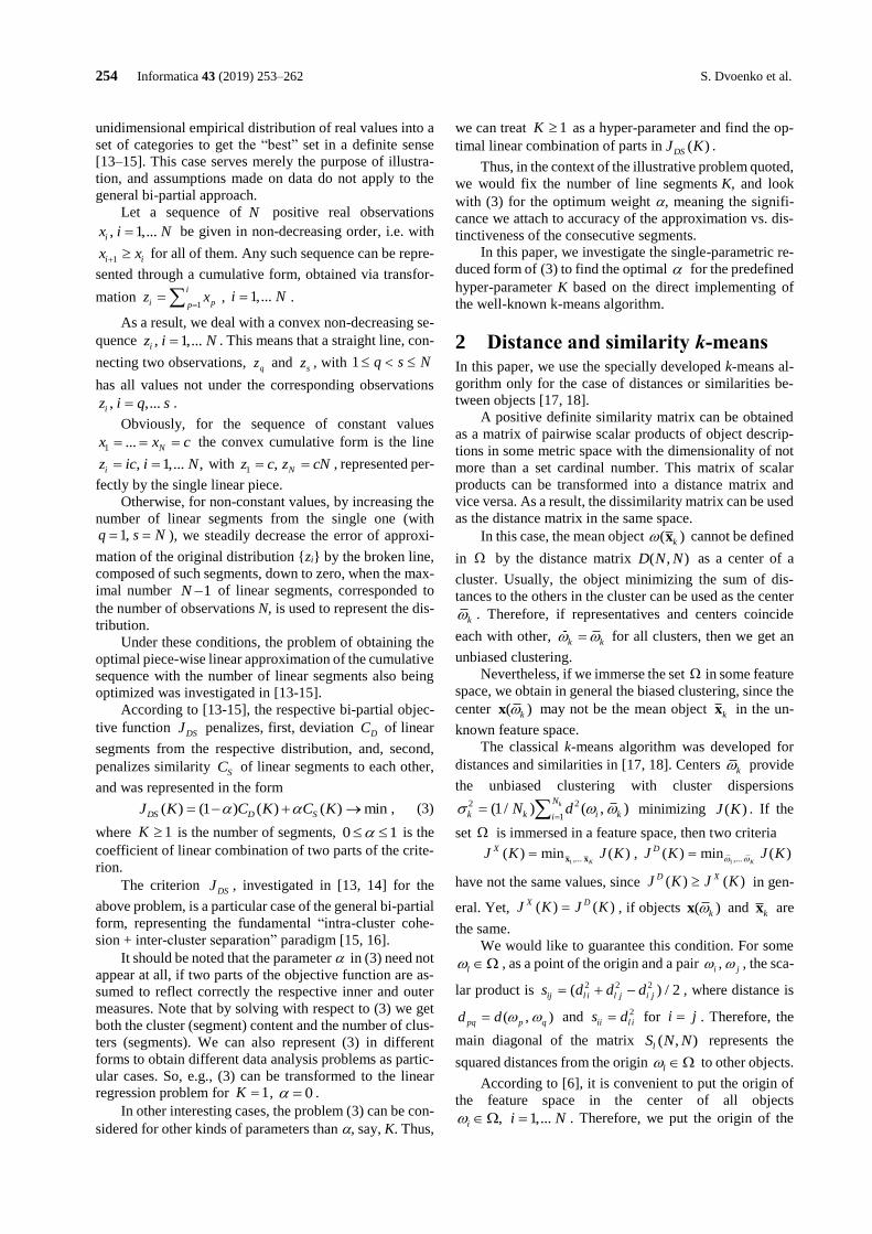
254 Informatica 43 (2019) 253–262 S. Dvoenko et al.
unidimensional empirical distribution of real values into a
set of categories to get the “best” set in a definite sense
[13–15]. This case serves merely the purpose of illustra-
tion, and assumptions made on data do not apply to the
general bi-partial approach.
Let a sequence of N positive real observations
, 1,...ix i N= be given in non-decreasing order, i.e. with
1i ix x+ for all of them. Any such sequence can be repre-
sented through a cumulative form, obtained via transfor-
mation 1
i
i ppz x
== , 1,...i N= .
As a result, we deal with a convex non-decreasing se-
quence , 1,...iz i N= . This means that a straight line, con-
necting two observations, qz and
sz , with 1 q s N
has all values not under the corresponding observations
, ,...iz i q s= .
Obviously, for the sequence of constant values
1 ... Nx x c= = = the convex cumulative form is the line
, 1,... ,iz ic i N= = with
1 , Nz c z cN= = , represented per-
fectly by the single linear piece.
Otherwise, for non-constant values, by increasing the
number of linear segments from the single one (with 1,q s N= = ), we steadily decrease the error of approxi-
mation of the original distribution {zi} by the broken line,
composed of such segments, down to zero, when the max-
imal number 1N − of linear segments, corresponded to
the number of observations N, is used to represent the dis-
tribution.
Under these conditions, the problem of obtaining the
optimal piece-wise linear approximation of the cumulative
sequence with the number of linear segments also being
optimized was investigated in [13-15].
According to [13-15], the respective bi-partial objec-
tive function DSJ penalizes, first, deviation
DC of linear
segments from the respective distribution, and, second,
penalizes similarity SC of linear segments to each other,
and was represented in the form
( ) (1 ) ( ) ( ) minDS D SJ K C K C K = − + → , (3)
where 1K is the number of segments, 0 1 is the
coefficient of linear combination of two parts of the crite-
rion.
The criterion DSJ , investigated in [13, 14] for the
above problem, is a particular case of the general bi-partial
form, representing the fundamental “intra-cluster cohe-
sion + inter-cluster separation” paradigm [15, 16].
It should be noted that the parameter in (3) need not
appear at all, if two parts of the objective function are as-
sumed to reflect correctly the respective inner and outer
measures. Note that by solving with respect to (3) we get
both the cluster (segment) content and the number of clus-
ters (segments). We can also represent (3) in different
forms to obtain different data analysis problems as partic-
ular cases. So, e.g., (3) can be transformed to the linear
regression problem for 1K = , 0 = .
In other interesting cases, the problem (3) can be con-
sidered for other kinds of parameters than , say, K. Thus,
we can treat 1K as a hyper-parameter and find the op-
timal linear combination of parts in ( )DSJ K .
Thus, in the context of the illustrative problem quoted,
we would fix the number of line segments K, and look
with (3) for the optimum weight , meaning the signifi-
cance we attach to accuracy of the approximation vs. dis-
tinctiveness of the consecutive segments.
In this paper, we investigate the single-parametric re-
duced form of (3) to find the optimal for the predefined
hyper-parameter K based on the direct implementing of
the well-known k-means algorithm.
2 Distance and similarity k-means In this paper, we use the specially developed k-means al-
gorithm only for the case of distances or similarities be-
tween objects [17, 18].
A positive definite similarity matrix can be obtained
as a matrix of pairwise scalar products of object descrip-
tions in some metric space with the dimensionality of not
more than a set cardinal number. This matrix of scalar
products can be transformed into a distance matrix and
vice versa. As a result, the dissimilarity matrix can be used
as the distance matrix in the same space.
In this case, the mean object ( )k x cannot be defined
in by the distance matrix ( , )D N N as a center of a
cluster. Usually, the object minimizing the sum of dis-
tances to the others in the cluster can be used as the center
k . Therefore, if representatives and centers coincide
each with other, k k = for all clusters, then we get an
unbiased clustering.
Nevertheless, if we immerse the set in some feature
space, we obtain in general the biased clustering, since the
center ( )kx may not be the mean object kx in the un-
known feature space.
The classical k-means algorithm was developed for
distances and similarities in [17, 18]. Centers k provide
the unbiased clustering with cluster dispersions 2 2
1(1/ ) ( , )
kN
k k i kiN d
== minimizing ( )J K . If the
set is immersed in a feature space, then two criteria
1 ,...( ) min ( )K
XJ K J K= x x , 1 ,...( ) min ( )
K
DJ K J K =
have not the same values, since ( ) ( )D XJ K J K in gen-
eral. Yet, ( ) ( )X DJ K J K= , if objects ( )kx and kx are
the same.
We would like to guarantee this condition. For some
l , as a point of the origin and a pair ,i j , the sca-
lar product is 2 2 2( ) / 2ij l i l j i js d d d= + − , where distance is
( , )pq p qd d = and 2
ii l is d= for i j= . Therefore, the
main diagonal of the matrix ( , )lS N N represents the
squared distances from the origin l to other objects.
According to [6], it is convenient to put the origin of
the feature space in the center of all objects
, 1,...i i N = . Therefore, we put the origin of the

The Permutable k-means for the Bi-partial Criterion Informatica 43 (2019) 253–262 255
feature space, cluster by cluster, in each center k to rep-
resent it by its distances to all other objects in the unknown
feature space (kN is the number of objects in
k ,
,p q k ):
2 2 2
21 1 1
1 1( , )
2
k k kN N N
i k ip pq
p p qk k
d d dN N
= = =
= − , (4)
where, according to (1), (4), the cluster dispersion is
2 2 2
21 1 1 1
2
21 1
1 1 1
2
1.
2
k k k k
k k
N N N N
k ip pq
i p p qk k k
N N
pq
p qk
d dN N N
dN
= = = =
= =
= − =
(5)
Hence, we develop the distance k-means algorithm
based on the classical principle of the “minimum distance
to a cluster center”:
(a) Step 0. Determine in some way K centers 1
k and put
them as representatives 1 1 , 1,... ;k k k K = = 1s = .
Step s. Reallocate all objects between clusters:
1. s
i k , if 𝑑(𝜔𝑖 , ��𝑘𝑠) ≤ 𝑑(𝜔𝑖 , ��𝑗
𝑠) for s
i j k ,
1,... ,j K= 1,... .i N=
2. Recalculate centers , 1,... ,s
k k K = represented by
distances ( , ), 1,... .s
i kd i N =
3. Stop, if s s
k k = , 1,... ,k K=
else 1s s
k k + = , 1s s
k k + = , 1,... ;k K=
1s s= + .
Based on the direct recalculation of the criterion (1),
the equivalent realization is:
(b) Step 0. Determine in some way K centers 1
k and put
them as representatives 1 1 , 1,... ;k k k K = = calcu-
late 1 1 ( )J J K= and put
1 1 1( )J J K J= = relative to rep-
resentatives; 1s = .
Step s. Reallocate all objects between clusters:
1. s
i k , if 𝐽𝑖𝑘𝑠 ≤ 𝐽𝑖𝑝
𝑠 for s
i p k , 1,... ,p K=
1,... .i N=
2. Recalculate centers , 1,... ,s
k k K = represented by
distances ( , ), 1,... ;s
i kd i N = recalculate .sJ
3. Stop, if s sJ J= , else 1s sJ J+ = , 1s sJ J+ = ;
1s s= + .
A positive definite similarity matrix ( , )S N N with el-
ements ( , ) 0ij i js s = can be obtained as a matrix of
scalar products in the positive quadrant of the feature
space. Relative to some point k as the origin,
with 2 2 2( ) / 2ij ki kj ijs d d d= + − ,
2
ii kis d= , distances are de-
fined as 2 2ij ii jj ijd s s s= + − . The cluster center k is rep-
resented by its similarities with other objects
1
1( , )
kN
i k ip
pk
s sN
=
= , p k , , 1,...i i N = . (6)
The cluster compactness is the mean similarity of the
cluster center with respect to other objects (6):
1
1( , )
kN
k i k
ik
sN
=
= = 21 1
1 k kN N
ip
i pk
sN = =
; ,i p k .
The unbiased clustering minimizes the cluster disper-
sion 2
k and maximizes the compactness k according to
(5):
2
21 1
1( 2 )
2
k kN N
k ii jj ij
i jk
s s sN
= =
= + − =1
1 kN
ii k
ik
sN
=
− ,
and for all clusters:
2
1
( )K
kk
k
NJ K
N
=
= =1 1
1( )
N Kk
ii k
i k
Ns C I K
N N
= =
− = − .
For similarity clustering, we maximize compactness
( )I K , with ( ) ( )I K C J K= − . The similarity k-means al-
gorithm is the analogue of algorithms (a) and (b) relative
to ( )I K .
3 The bi-partial criterion for clustering
In this paper, we develop the bi-partial objective function
like (3) for the dissimilarity k-means
( ) (1 ) ( ) ( )J K J K K = − + , (7)
so as to combine ( )J K for intra-cluster distances with the
inter-cluster similarity ( )K . We define the inter-cluster
similarity 01( ) (1 / ) ( , )
K
kkK K s
== relative to the
center of the whole set, being the object 0 , represented
by its similarities with respect to all other centers
0 1( , ) (1 / ) ( , )
K
k k pps K s
== ; , 1,...k k K = :
2
1 1
1( ) ( , )
K K
k l
k l
K sK
= =
= . (8)
Unfortunately, the bi-partial criterion ( )J K , as de-
fined here, does not work for the classical k-means (b),
since (8), as the second part of ( )J K in (7), cannot be
changed for constant centers while attempting to transfer
objects in step s.
Therefore, for any 0 1 , the clustering results are
the same as for the classical case with 0 = . And the al-
gorithm does not work properly with 1 = .
We develop here the new “permutable” version of the
classical k-means (b) without direct calculation of cluster
centers. Here, the new permutable k-means is the meanless
clustering for the classical k-means (b).
As we can see in (5), the cluster dispersion is half of
the average of squared distances between objects in the
cluster. This representation does not contain centers them-
selves, and we calculate the criterion (1) without centers
in the form
2 2
1 1 1 1
1 1( )
2
k kN NK Kk
k pq
k k p qk
NJ K d
N N N
= = = =
= = . (9)
Next, we would like to calculate the similarity
( , )k ls between cluster centers in (8). According to (6),

256 Informatica 43 (2019) 253–262 S. Dvoenko et al.
the average similarity of the center k with the objects
from the other cluster i l is
1 1 1
1 1( , ) ( , )
l l kN N N
l k i k ip
i i pl l k
s s sN N N
= = =
= = , p k .
It is evident that ( , ) ( , )l k k ls s = , as ij jis s= .
Therefore, we can use the suitable notation
( , ) ( , ) ( , ) ( , )l k k l l k l ks s s s = = = . Hence,
(8) is converted into (p k ,
q l ):
2
1 1 1 1
1 1( ) .
k lN NK K
pq
k l p qk l
K sN NK
= = = =
= (10)
The goal of ( )J K is to produce clusters with possibly
low dispersion and possibly dissimilar centers. We note
that (10) is in a way an inconsistent function, since for
k l= it contains the cluster compactness k . Hence, we
modify (10) to get the inter-cluster similarities only and
take into account the symmetry
1 1, 1 1
1 1( ) ,
2 ( 1)
k lN NK K
pq
k l l k p qk l
K sK K N N
= = = =
=− (11)
for , .p k q l
We develop here the classical k-means (b) in the new
form of the permutable k-means based on (9)–(11):
(c) Step 0. Determine in some way the sets 1, 1,...l l K = ;
define , calculate 1 1 ( )J J K= ; 1s = .
Step s. Reallocate all objects between clusters:
1. Remember, but do not move: s
i k , if 𝐽𝑖𝑘𝑠 ≤ 𝐽𝑖𝑝
𝑠 for
s
i p k , 1,... ,p K= 1,... .i N=
2. Reallocate all objects , 1,...i i N = at once;
calculate 1sJ + .
3. If 1s sJ J+ = then stop;
If 1s sJ J+ then: cancel last reallocations, 1s sJ J+ = ,
stop;
If 1s sJ J+ then: 1 ,s sJ J+ = 1s s= + .
As we can see, in the step (s.1) we recalculate the cri-
terion sJ in order to get its modified value s
ipJ . Let
s
i j . When trying to move i from
s
j to some other
s
p , we try to change the respective sets to \s
j i and to
s
p i . Changes in the sets result in implicit changes of
their centers, even though we do not calculate them. Con-
sequently, this action differs from the same one in algo-
rithms (a) and (b) for constant centers.
Algorithm (c) appears to be a new type of clustering
procedures, since its result differs, in general, from those
of the classical (a) and (b) procedures, both for the classi-
cal ( 0) = and the proper bi-partial ( 0) cases. In ad-
dition, we can use some optimal initial clusters to enhance
the quality of results, and optimal recalculations to im-
prove performance of permutations.
As we can see, the algorithm (c) is the same as the clas-
sical ones (a) and (b) for the standard criterion ( )J K and
differs (sometimes subtly and finely) from them for the bi-
partial criterion ( )J K .
It is clear that the new algorithm gives the classical re-
sult for non-intersecting clusters. Nevertheless, its result
can be improved for intersecting clusters, since by means
of the criterion ( )J K a cluster center can be shifted in
some vicinity without changing the cluster itself. Such
possibility depends on the gaps between real points in con-
tinuous feature space and the discrete cluster structure su-
perimposed.
4 Redistribution of data dispersion by
the bi-partial criterion Here, we explain why by means of the criterion (7) it is
possible to improve the classical clustering of k-means.
Consider the classical case. Let the set of size N be
divided into K subsets (clusters). In our perspective, we
consider balancing of total dispersion between its intra-
and inter- parts. We know [19, 20] that T W BS S S= + ,
where TS is the total scatter matrix,
WS is the intra-cluster
and BS is the inter-cluster scatter matrices. Therefore,
T W BtrS trS trS= + for diagonal elements only. Since
2
T TtrS N= , 2
W WtrS N= , and 2
B BtrS N= , then finally
2 2 2
T W B = + .
Let the set 1{ ,... }N= be immersed in some met-
ric space and represented by the distance matrix ( , )D N N
only with elements ( , ) 0ij i jd d= . Let be split
into groups , 1,...k k K = . Based on the Torgerson’s for-
mula, we define the following:
for single group dispersions
2 2
21 1
1( , ), 1,...
2
k kN N
k p q
p qk
d k KN = =
= = ;
for the intra-group dispersion
2 2 2
21 1 1 1
2
1 1 1
1( , )
2
1 1( , ) ;
2
k k
k k
N NK Kk k
W k p q
k k p qk
N NK
p q
k p qk
N Nd
N N N
dN N
= = = =
= = =
= = =
for the total dispersion
2 2
21 1
2
21 1 1 1
1( , )
2
1( , ) ;
2
k l
N N
T p q
p q
N NK K
p q
k l p q
dN
dN
= =
= = = =
= =
for the inter-center dispersion
2 2 2
0 21 1 1
1 1( , ) ( , )
2
K K K
IC k p q
k p q
d dK K= = =
= = ,
where the center 0 of the set is represented by its
distances to other centers k through
2 2 2
0
1
1( , ) ( , )
K
k k p IC
p
d dK =
= − .
We remark that the classical inter-group dispersion is
not given by the Torgerson’s formula
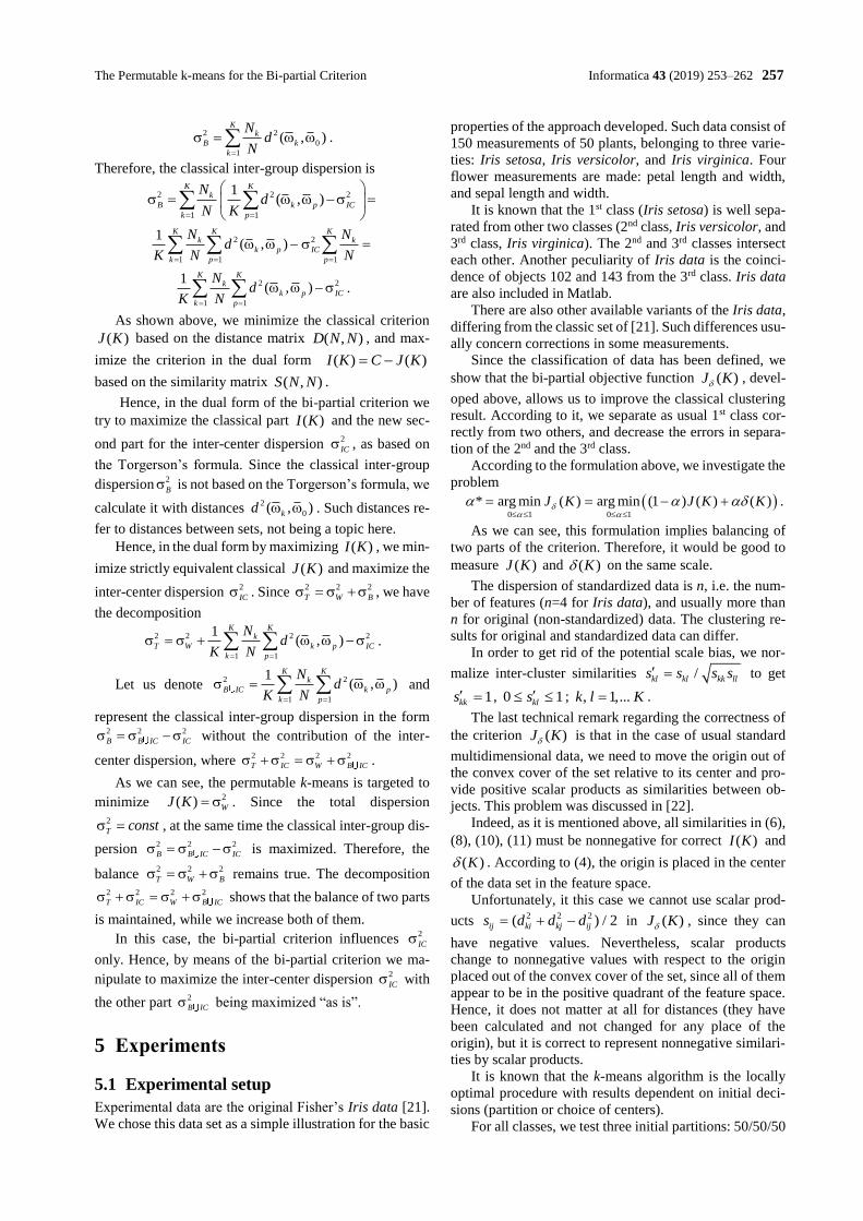
The Permutable k-means for the Bi-partial Criterion Informatica 43 (2019) 253–262 257
2 2
0
1
( , )K
k
B k
k
Nd
N=
= .
Therefore, the classical inter-group dispersion is
2 2 2
1 1
1( , )
K Kk
B k p IC
k p
Nd
N K= =
= − =
2 2
1 1 1
1( , )
K K Kk k
k p IC
k p p
N Nd
K N N= = =
− =
2 2
1 1
1( , )
K Kk
k p IC
k p
Nd
K N= =
− .
As shown above, we minimize the classical criterion
( )J K based on the distance matrix ( , )D N N , and max-
imize the criterion in the dual form ( ) ( )I K C J K= −
based on the similarity matrix ( , )S N N .
Hence, in the dual form of the bi-partial criterion we
try to maximize the classical part ( )I K and the new sec-
ond part for the inter-center dispersion 2
IC , as based on
the Torgerson’s formula. Since the classical inter-group
dispersion2
B is not based on the Torgerson’s formula, we
calculate it with distances 2
0( , )kd . Such distances re-
fer to distances between sets, not being a topic here.
Hence, in the dual form by maximizing ( )I K , we min-
imize strictly equivalent classical ( )J K and maximize the
inter-center dispersion 2
IC . Since 2 2 2
T W B = + , we have
the decomposition
2 2 2 2
1 1
1( , )
K Kk
T W k p IC
k p
Nd
K N= =
= + − .
Let us denote 2 2
1 1
1( , )
K Kk
B IC k p
k p
Nd
K N= =
= and
represent the classical inter-group dispersion in the form 2 2 2
B B IC IC = − without the contribution of the inter-
center dispersion, where 2 2 2 2
T IC W B IC + = + .
As we can see, the permutable k-means is targeted to
minimize 2( ) WJ K = . Since the total dispersion
2
T const = , at the same time the classical inter-group dis-
persion 2 2 2
B B IC IC = − is maximized. Therefore, the
balance 2 2 2
T W B = + remains true. The decomposition
2 2 2 2
T IC W B IC + = + shows that the balance of two parts
is maintained, while we increase both of them.
In this case, the bi-partial criterion influences 2
IC
only. Hence, by means of the bi-partial criterion we ma-
nipulate to maximize the inter-center dispersion 2
IC with
the other part 2
B IC being maximized “as is”.
5 Experiments
5.1 Experimental setup
Experimental data are the original Fisher’s Iris data [21].
We chose this data set as a simple illustration for the basic
properties of the approach developed. Such data consist of
150 measurements of 50 plants, belonging to three varie-
ties: Iris setosa, Iris versicolor, and Iris virginica. Four
flower measurements are made: petal length and width,
and sepal length and width.
It is known that the 1st class (Iris setosa) is well sepa-
rated from other two classes (2nd class, Iris versicolor, and
3rd class, Iris virginica). The 2nd and 3rd classes intersect
each other. Another peculiarity of Iris data is the coinci-
dence of objects 102 and 143 from the 3rd class. Iris data
are also included in Matlab.
There are also other available variants of the Iris data,
differing from the classic set of [21]. Such differences usu-
ally concern corrections in some measurements.
Since the classification of data has been defined, we
show that the bi-partial objective function ( )J K , devel-
oped above, allows us to improve the classical clustering
result. According to it, we separate as usual 1st class cor-
rectly from two others, and decrease the errors in separa-
tion of the 2nd and the 3rd class.
According to the formulation above, we investigate the
problem
( )0 1 0 1
* arg min ( ) arg min (1 ) ( ) ( )J K J K K
= = − + .
As we can see, this formulation implies balancing of
two parts of the criterion. Therefore, it would be good to
measure ( )J K and ( )K on the same scale.
The dispersion of standardized data is n, i.e. the num-
ber of features (n=4 for Iris data), and usually more than
n for original (non-standardized) data. The clustering re-
sults for original and standardized data can differ.
In order to get rid of the potential scale bias, we nor-
malize inter-cluster similarities /kl kl kk lls s s s = to get
1kks = , 0 1kls ; , 1,...k l K= .
The last technical remark regarding the correctness of
the criterion ( )J K is that in the case of usual standard
multidimensional data, we need to move the origin out of
the convex cover of the set relative to its center and pro-
vide positive scalar products as similarities between ob-
jects. This problem was discussed in [22].
Indeed, as it is mentioned above, all similarities in (6),
(8), (10), (11) must be nonnegative for correct ( )I K and
( )K . According to (4), the origin is placed in the center
of the data set in the feature space.
Unfortunately, it this case we cannot use scalar prod-
ucts 2 2 2( ) / 2ij ki kj ijs d d d= + − in ( )J K , since they can
have negative values. Nevertheless, scalar products
change to nonnegative values with respect to the origin
placed out of the convex cover of the set, since all of them
appear to be in the positive quadrant of the feature space.
Hence, it does not matter at all for distances (they have
been calculated and not changed for any place of the
origin), but it is correct to represent nonnegative similari-
ties by scalar products.
It is known that the k-means algorithm is the locally
optimal procedure with results dependent on initial deci-
sions (partition or choice of centers).
For all classes, we test three initial partitions: 50/50/50

258 Informatica 43 (2019) 253–262 S. Dvoenko et al.
(plant varieties as classes), 50/70/30 (20 plants from the
3rd class are wrongly placed in the 2nd class), 50/30/70 (20
plants from the 2nd class are wrongly placed in the 3rd
class).
For just two intersecting classes (2nd and 3rd) we test
also three initial partitions: 50/50 (plant varieties as clas-
ses), 70/30 (20 plants from the 3rd class are wrongly placed
in the 2nd class), 30/70 (20 plants from the 2nd class are
wrongly placed in the 3rd class).
In yet another case we investigate two classes of the
entire set, organized as the small one (1st class) and the big
one (2nd and 3rd classes). We test three initial partitions:
50/100 (plants from the 1st class versus all plants from the
2nd and 3rd classes together), 100/50 (all plants from the 1st
and the 2nd classes together versus plants from the 3rd
class), 30/120 (only first 30 plants from the 1st class versus
all others).
In all experiments, we first get the classical result with 0 = , starting from the predefined initial partitions as
above. Second, starting, as well, from the predefined ini-
tial partitions characterized above, we vary the parameter
0 1 with increment 0.01 to find the optimal *
among the tested 100 points.
5.2 Results and discussion
In the first experiment with original Iris data for all initial
partitions for three classes, we correctly separate the 1st
class and decrease errors in separation of intersecting 2nd
and 3rd classes (Table 1, Fig.1). For two intersecting clas-
ses only, we decrease errors in the separation of the 2nd and
3rd classes, too (Table 1, Fig. 2, 3). It can be seen that the
optimal intervals for * depend on the number of clusters
(Table 1), hence on data dispersion, and can slightly differ
for different initial partitions. Error diagrams are not mon-
otonic functions (Fig. 1–3).
As we can see, original Iris data are some sort of “well
structured” data, since for different initial partitions we get
the same 16 misclassified objects for the classical ( 0) =
criterion and the same 15 misclassified objects for the bi-
partial ( *) criterion (Table 1). For the classical criterion,
misclassified objects are generally from the 3rd class (Ta-
ble 2). The object 135 is well classified and shown here,
since it is misclassified for the bi-partial criterion.
Misclassified objects for the bi-partial criterion are
from the 3rd class, too (Table 3). Here, objects 53 and 78
are well classified, and the object 135 is misclassified.
We repeat this experiment for standardized data (Ta-
ble 4). Such data are more complicated. As we know, Iris
classes are not so spherical ones in the original feature
space, and that is why the k-means type of approach is not
the best suited for them.
After data standardization, classes appear to be more
spherical and contain more “mixed” objects from inter-
secting classes, usually giving more misclassifications in
the classical case (Table 4).
Hence, for the classical criterion ( 0) = for standard-
ized data, 25 misclassified objects are from two intersect-
ing classes, 2nd and 3rd, with well classified all objects
from the 1st class (Table 5). Objects 104, 109, 112, 126,
129 are well classified and shown too, since they are mis-
classified for the bi-partial criterion.
Misclassified objects for the bi-partial criterion are
mainly from the 3rd class again (Table 6). Here, objects 52,
57, 66, 71, 76, 86, 87 are well classified and objects 104,
109, 112, 128, 129 are misclassified.
Table 1: Clustering results of original Iris data.
Initial
partitions
Errors
( 0) = *
Errors
( *) Diagrams
50/50/50 16 0.6 ÷ 0.75 15
Fig. 1 50/70/30 16 0.6 ÷ 0.75 15
50/30/70 16 0.6 ÷ 0.75 15
50/50 16 0.81 ÷ 0.92 15 Fig. 2
70/30 16 0.81 ÷ 0.92 15
30/70 16 0.81 ÷ 0.91 15 Fig. 3
Table 2: Classical 16 misclassifications
of original Iris data.
0 =
50/50/50 50/50
50/70/30 70/30
50/30/70 30/70
2nd cluster 3rd cluster
Iris versicolor
2nd class (51-100)
53
78
Iris virginica
3rd class (101-150)
102 120 128 147
107 122 134 150
114 124 139
115 127 143
Correct: 135
Table 3: Bi-partial 15 misclassifications of
original Iris data.
*
50/50/50 50/50
50/70/30 70/30
50/30/70 30/70
2nd cluster 3rd cluster
Iris versicolor
2nd class (51-100)
53
78
Iris virginica
3rd class (101-150)
102 120 128 147
107 122 134 150
114 124 139_
115 127 143
135_
Table 4: Clustering results of standardized Iris data.
Initial
partitions
Errors
( 0) = *
Errors
( *) Diagrams
50/50/50 25 0.85 22
Fig. 4 50/70/30 25 0.85 22
50/30/70 25 0.85 22
50/50 17 0.94 ÷ 0.97 15 Fig. 5
70/30 17 0.92 ÷ 0.97 15 Fig. 6
30/70 17 0.83 ÷ 0.95 14 Fig. 7
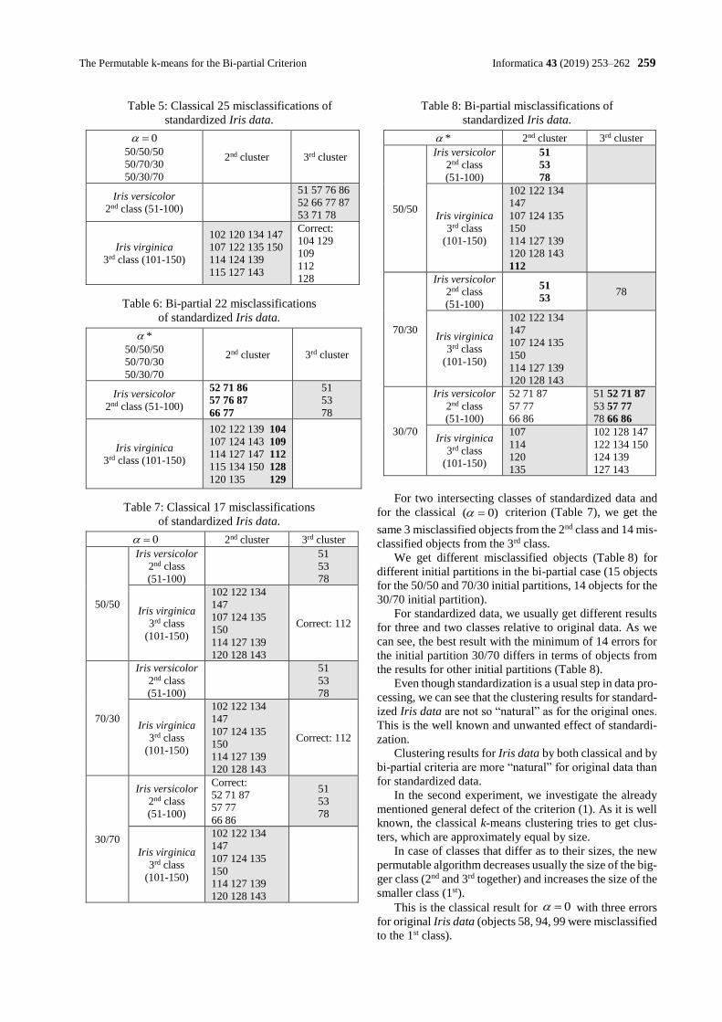
The Permutable k-means for the Bi-partial Criterion Informatica 43 (2019) 253–262 259
Table 5: Classical 25 misclassifications of
standardized Iris data.
0 =
50/50/50
50/70/30
50/30/70
2nd cluster 3rd cluster
Iris versicolor
2nd class (51-100)
51 57 76 86
52 66 77 87
53 71 78
Iris virginica
3rd class (101-150)
102 120 134 147
107 122 135 150
114 124 139
115 127 143
Correct:
104 129
109
112
128
Table 6: Bi-partial 22 misclassifications
of standardized Iris data.
*
50/50/50
50/70/30
50/30/70
2nd cluster 3rd cluster
Iris versicolor
2nd class (51-100)
52 71 86
57 76 87
66 77
51
53
78
Iris virginica
3rd class (101-150)
102 122 139 104
107 124 143 109
114 127 147 112
115 134 150 128
120 135 129
Table 7: Classical 17 misclassifications
of standardized Iris data.
0 = 2nd cluster 3rd cluster
50/50
Iris versicolor
2nd class
(51-100)
51
53
78
Iris virginica
3rd class
(101-150)
102 122 134
147
107 124 135
150
114 127 139
120 128 143
Correct: 112
70/30
Iris versicolor
2nd class
(51-100)
51
53
78
Iris virginica
3rd class
(101-150)
102 122 134
147
107 124 135
150
114 127 139
120 128 143
Correct: 112
30/70
Iris versicolor
2nd class
(51-100)
Correct:
52 71 87
57 77
66 86
51
53
78
Iris virginica
3rd class
(101-150)
102 122 134
147
107 124 135
150
114 127 139
120 128 143
Table 8: Bi-partial misclassifications of
standardized Iris data.
* 2nd cluster 3rd cluster
50/50
Iris versicolor
2nd class
(51-100)
51
53
78
Iris virginica
3rd class
(101-150)
102 122 134
147
107 124 135
150
114 127 139
120 128 143
112
70/30
Iris versicolor
2nd class
(51-100)
51
53 78
Iris virginica
3rd class
(101-150)
102 122 134
147
107 124 135
150
114 127 139
120 128 143
30/70
Iris versicolor
2nd class
(51-100)
52 71 87
57 77
66 86
51 52 71 87
53 57 77
78 66 86
Iris virginica
3rd class
(101-150)
107
114
120
135
102 128 147
122 134 150
124 139
127 143
For two intersecting classes of standardized data and
for the classical ( 0) = criterion (Table 7), we get the
same 3 misclassified objects from the 2nd class and 14 mis-
classified objects from the 3rd class.
We get different misclassified objects (Table 8) for
different initial partitions in the bi-partial case (15 objects
for the 50/50 and 70/30 initial partitions, 14 objects for the
30/70 initial partition).
For standardized data, we usually get different results
for three and two classes relative to original data. As we
can see, the best result with the minimum of 14 errors for
the initial partition 30/70 differs in terms of objects from
the results for other initial partitions (Table 8).
Even though standardization is a usual step in data pro-
cessing, we can see that the clustering results for standard-
ized Iris data are not so “natural” as for the original ones.
This is the well known and unwanted effect of standardi-
zation.
Clustering results for Iris data by both classical and by
bi-partial criteria are more “natural” for original data than
for standardized data.
In the second experiment, we investigate the already
mentioned general defect of the criterion (1). As it is well
known, the classical k-means clustering tries to get clus-
ters, which are approximately equal by size.
In case of classes that differ as to their sizes, the new
permutable algorithm decreases usually the size of the big-
ger class (2nd and 3rd together) and increases the size of the
smaller class (1st).
This is the classical result for 0 = with three errors
for original Iris data (objects 58, 94, 99 were misclassified
to the 1st class).
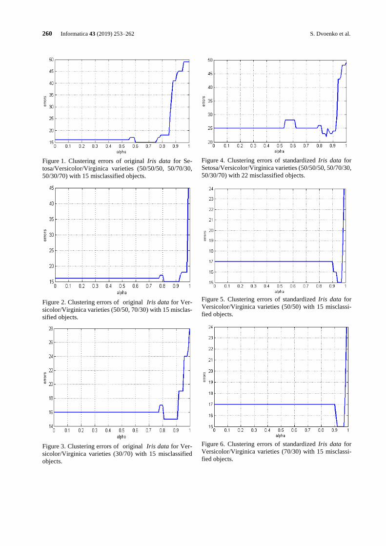
260 Informatica 43 (2019) 253–262 S. Dvoenko et al.
Figure 1. Clustering errors of original Iris data for Se-
tosa/Versicolor/Virginica varieties (50/50/50, 50/70/30,
50/30/70) with 15 misclassified objects.
Figure 2. Clustering errors of original Iris data for Ver-
sicolor/Virginica varieties (50/50, 70/30) with 15 misclas-
sified objects.
Figure 3. Clustering errors of original Iris data for Ver-
sicolor/Virginica varieties (30/70) with 15 misclassified
objects.
Figure 4. Clustering errors of standardized Iris data for
Setosa/Versicolor/Virginica varieties (50/50/50, 50/70/30,
50/30/70) with 22 misclassified objects.
Figure 5. Clustering errors of standardized Iris data for
Versicolor/Virginica varieties (50/50) with 15 misclassi-
fied objects.
Figure 6. Clustering errors of standardized Iris data for
Versicolor/Virginica varieties (70/30) with 15 misclassi-
fied objects.
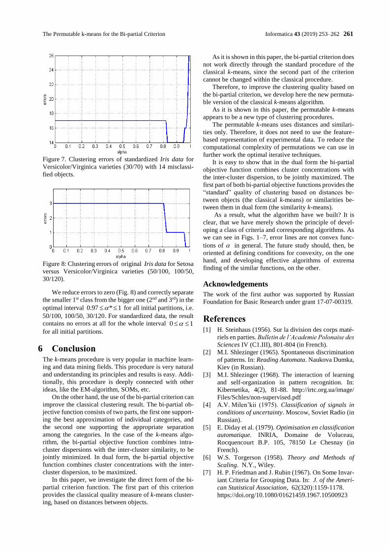
The Permutable k-means for the Bi-partial Criterion Informatica 43 (2019) 253–262 261
Figure 7. Clustering errors of standardized Iris data for
Versicolor/Virginica varieties (30/70) with 14 misclassi-
fied objects.
Figure 8: Clustering errors of original Iris data for Setosa
versus Versicolor/Virginica varieties (50/100, 100/50,
30/120).
We reduce errors to zero (Fig. 8) and correctly separate
the smaller 1st class from the bigger one (2nd and 3rd) in the
optimal interval 0.97 * 1 for all initial partitions, i.e.
50/100, 100/50, 30/120. For standardized data, the result
contains no errors at all for the whole interval 0 1
for all initial partitions.
6 Conclusion The k-means procedure is very popular in machine learn-
ing and data mining fields. This procedure is very natural
and understanding its principles and results is easy. Addi-
tionally, this procedure is deeply connected with other
ideas, like the EM-algorithm, SOMs, etc.
On the other hand, the use of the bi-partial criterion can
improve the classical clustering result. The bi-partial ob-
jective function consists of two parts, the first one support-
ing the best approximation of individual categories, and
the second one supporting the appropriate separation
among the categories. In the case of the k-means algo-
rithm, the bi-partial objective function combines intra-
cluster dispersions with the inter-cluster similarity, to be
jointly minimized. In dual form, the bi-partial objective
function combines cluster concentrations with the inter-
cluster dispersion, to be maximized.
In this paper, we investigate the direct form of the bi-
partial criterion function. The first part of this criterion
provides the classical quality measure of k-means cluster-
ing, based on distances between objects.
As it is shown in this paper, the bi-partial criterion does
not work directly through the standard procedure of the
classical k-means, since the second part of the criterion
cannot be changed within the classical procedure.
Therefore, to improve the clustering quality based on
the bi-partial criterion, we develop here the new permuta-
ble version of the classical k-means algorithm.
As it is shown in this paper, the permutable k-means
appears to be a new type of clustering procedures.
The permutable k-means uses distances and similari-
ties only. Therefore, it does not need to use the feature-
based representation of experimental data. To reduce the
computational complexity of permutations we can use in
further work the optimal iterative techniques.
It is easy to show that in the dual form the bi-partial
objective function combines cluster concentrations with
the inter-cluster dispersion, to be jointly maximized. The
first part of both bi-partial objective functions provides the
“standard” quality of clustering based on distances be-
tween objects (the classical k-means) or similarities be-
tween them in dual form (the similarity k-means).
As a result, what the algorithm have we built? It is
clear, that we have merely shown the principle of devel-
oping a class of criteria and corresponding algorithms. As
we can see in Figs. 1–7, error lines are not convex func-
tions of in general. The future study should, then, be
oriented at defining conditions for convexity, on the one
hand, and developing effective algorithms of extrema
finding of the similar functions, on the other.
Acknowledgements
The work of the first author was supported by Russian
Foundation for Basic Research under grant 17-07-00319.
References [1] H. Steinhaus (1956). Sur la division des corps maté-
riels en parties. Bulletin de l’Academie Polonaise des
Sciences IV (C1.III), 801-804 (in French).
[2] M.I. Shlezinger (1965). Spontaneous discrimination
of patterns. In: Reading Automata. Naukova Dumka,
Kiev (in Russian).
[3] M.I. Shlezinger (1968). The interaction of learning
and self-organization in pattern recognition. In:
Kibernetika, 4(2), 81-88. http://irtc.org.ua/image/
Files/Schles/non-supervised.pdf
[4] A.V. Milen’kii (1975). Classification of signals in
conditions of uncertainty. Moscow, Soviet Radio (in
Russian).
[5] E. Diday et al. (1979). Optimisation en classification
automatique. INRIA, Domaine de Voluceau,
Rocquencourt B.P. 105, 78150 Le Chesnay (in
French).
[6] W.S. Torgerson (1958). Theory and Methods of
Scaling. N.Y., Wiley.
[7] H. P. Friedman and J. Rubin (1967). On Some Invar-
iant Criteria for Grouping Data. In: J. of the Ameri-
can Statistical Association, 62(320):1159-1178.
https://doi.org/10.1080/01621459.1967.10500923
262 Informatica 43 (2019) 253–262 S. Dvoenko et al.
[8] H. Späth (1983). Cluster-formation und -analyse:
Theorie, FORTRAN-Programme und Beispiele.
R. Oldenbourg-Verlag, München — Wien.
[9] S.A. Aivazyan, et al. (1989). Applied Statistics.
Classification and reduction of dimensionality
(Ch. 5. Basic concepts and definitions used in classi-
fication without training. 5.4. Classification quality
functionals and extremal approach to cluster analy-
sis problems). Finansy i statistika, Moscow (in Rus-
sian)
[10] H.-J. Mucha, U. Simon, R. Brüggemann (2002).
Model-based Cluster Analysis Applied to Flow Cy-
tometry Data of Phytoplankton. Tech. Report, Ber-
lin. http://www.wias-berlin.de/techreport/5/
wias_technicalreports_5.pdf
[11] E. Pekalska, R.P.W. Duin (2005). The Dissimilarity
Representation for Pattern Recognition. Founda-
tions and Applications. W.S. Singapore.
[12] A.W.F. Edwards, L.L. Cavalli-Sforza (1965). A
Method for Cluster Analysis. In: Biometrics, 21,
362–375. https://www.jstor.org/stable/ 2528096
?seq=1#page_scan_tab_contents
[13] Jan W. Owsinski (2012). On the optimal division of
an empirical distribution (and some related prob-
lems). In: Przegląd Statystyczny, special issue, 1,
109-122.
[14] Jan W. Owsinski (2013). On dividing an empirical
distribution into optimal segments. http://new.sis-
statistica.org/wp-content/uploads/ 2013/09/RS12-
On-Dividing-an-Empirical-Distribution-into.pdf
[15] Jan W. Owsinski (2011). The bi-partial approach in
clustering and ordering: the model and the algo-
rithms. In: Statistica & Applicazioni. Special Issue,
43–59.
[16] Jan W. Owsinski (1990). On a new naturally indexed
quick clustering method with a global objective
function. In: Applied Stochastic Models and Data
Analysis, 6(3), 157-171.
https://doi.org/10.1002/asm.3150060303
[17] S.D. Dvoenko (2009). Clustering and separating of a
set of members in terms of mutual distances and sim-
ilarities. In: Transactions on MLDM. IBaI Publish-
ing 2, 2 (Oct. 2009), 80-99.
[18] S. Dvoenko (2014). Meanless k-means as k-meanless
clustering with the bi-partial approach. In: Proc. of
12th Int. Conf. on Pattern Recognition and Image
Processing (PRIP’2014). UIIP NASB, Minsk, Bela-
rus, 50-54.
[19] R.O. Duda, P.E. Hart (1973). Pattern Classification
and Scene Analysis. N.Y., Wiley.
[20] R.O. Duda, P.E. Hart, D.G.Stork (2000). Pattern
Classification. Wiley-Interscience New York, NY.
[21] R.A. Fisher (1936). The use of multiple measure-
ments in taxonomic problems. In Ann. Eugenics. 7,
2 (Sept. 1936), 179-188.
https://doi.org/10.1111/j.1469-1809.1936.tb02137.x
[22] S. D. Dvoenko, D.O. Pshenichny (2016). A recov-
ering of violated metric in machine learning. In: Pro-
ceedings of 8th Int. Symposium on Information and
Communication Technology (SoICT’2016). ACM
NY, 15-21.
https://doi.org/10.1145/3011077.3011084
https://doi.org/10.31449/inf.v43i2.2019 Informatica 43 (2019) 263–279 263
A CLR Virtual Machine Based Execution Framework for IEC 61131-3
Applications
Salvatore Cavalieri and Marco Scroppo
University of Catania, Department of Electrical Electronic and Computer Engineering (DIEEI), Italy
E-mail: [email protected], [email protected]
Keywords: IEC61131-3, PLC, CLR VM, real-time industrial applications
Received: November 13, 2017
The increased need of flexibility of automation systems and the increased capabilities of sensors and
actuators paired with more capable bus systems, pave the way for the reallocation of IEC 61131-3
applications away from the field level into so-called compute pools. Such compute pools are decentralised
with enough compute power for a large number of applications, while providing the required flexibility
to quickly adapt to changes of the applications requirements. The paper proposes a framework able to
deploy IEC 61131-3 applications to multiple computing platforms based on CLR VM; it uses C# language
as intermediate code. The software solution proposed by the authors does not require any modifications
of the IEC 61131-3 applications. Current literature does not provide solutions like that here presented;
due to the spread current use of C# language in the development of industrial applications, adoption of
the proposed solution seems very attractive. The paper will deeply describe the software implementation
and will also present an analysis about the capability of the proposed framework to respect real-time
constraints of the industrial processes, mainly focusing on the periodic ones.
Povzetek: Prispevek predlaga okvir, ki omogoča uporabo aplikacij IEC 61131-3 za več računalniških
platform, ki temeljijo na CLR VM.
1 Introduction Programmable Logic Controllers (PLCs) are widely used
for the control of automation systems. The standard IEC
61131-3 defines the execution model as well as
programming languages for such systems [1]. According
to IEC 61131-3, software development becomes
independent of process mapping and device specific
configuration files. Programmers can focus on the
algorithm and control development. Device specific
knowledge is outsourced into the block library and can be
substituted, every time a new target PLC device should be
programmed.
During these last years, the need to deploy IEC
61131-3 – based applications addressing multiple target
platforms (also different from PLCs, e.g. based on general
purpose computing architectures) became more and more
urgent for the reason explained in the following. In a
common factory automation scenario, actuators and
sensors connect to the PLCs via automation buses;
traditionally, bus based systems dominated the automation
industry. Nowadays, more powerful and flexible
automation networks appear and allow the connection of
thousands of actuators and sensors to the same network,
while still obtaining the required timing performance;
interested readers are referred to [2] for a detailed
overview.
Those changes in the communication technologies
opens possibilities of computation further away from the
field level, compared to how it is done in today’s
automation systems. On the other hand, many sensors and
actuators are equipped with small microcontrollers,
allowing them to do basic data processing; furthermore,
they are able to connect directly to the new bus
technologies.
Having basic data processing done at the lowest level
(i.e., at the field level directly on sensors and actuators)
and a connection to capable networks, allows the
reallocation of applications away from the field level into
so-called compute pools [3] [4]. Such compute pools are
decentralised with enough compute power for a large
number of applications, while providing the required
flexibility to quickly adapt to changes of the applications
requirements. This has several benefits. Changing control
applications becomes merely a problem of reconfiguration
in the compute pool. Costs will decrease as well as the
need for physical PLCs will be decreased; in this new
scenario, the PLC is migrated to the computing pool and
can be also realised by general purpose computer
architectures (e.g., a server or a cluster of servers).
Several requirements must be satisfied in order to
reach this goal. The first one is the guarantee of the total
compliance with IEC 61131-3; it is clear that moving an
IEC 61131-3 application on a compute pool must be
realised without any changes in the same application.
Then, respect of real-time constraints of the IEC 61131-3
control applications must occur when migrating the
application to the compute pool. Particular cares must be
reserved for real-time applications requiring periodic
executions; in these cases, executions of each process
must occur exactly with the requested period.
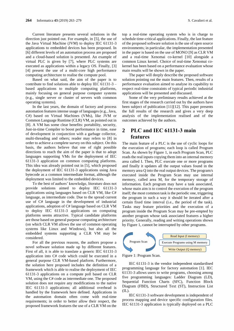
264 Informatica 43 (2019) 263–279 S. Cavalieri et al.
Current literature presents several solutions in the
direction just pointed out. For example, in [5], the use of
the Java Virtual Machine (JVM) to deploy IEC 61131-3
applications to embedded devices has been proposed. In
[6] different levels of an automation process are proposed
and a cloud-based solution is presented. An example of
virtual PLC is given by [7], where PLC systems are
executed as applications within a legacy OS. Finally, [3]
[4] present the use of a multi-core high performance
computing architecture to realise the compute pool.
Based on what said, the aim of the paper is to
contribute to find solutions able to deploy IEC 61131-3 –
based applications to multiple computing platforms,
mainly focusing on general purpose computer systems
(e.g., single server or cluster of servers with common
operating systems).
In the last years, the domain of factory and process
automation features intense usage of languages (e.g., Java,
C#) based on Virtual Machines (VMs), like JVM or
Common Language Runtime (CLR) VM, as pointed out in
[8]. A VM has some clear benefits: portability, security,
Just-in-time Compiler to boost performance in time, ease
of development in conjunction with a garbage collector,
multi-threading and others; reader may refers to [8] in
order to achieve a complete survey on this subject. On this
basis, the authors believe that one of right possible
directions to reach the aim of the paper is that to adopt
languages supporting VMs for the deployment of IEC
61131-3 application on common computing platforms.
This idea was already pointed out in [5], which proposed
the deployment of IEC 61131-3 applications using Java
bytecode as a common intermediate format, although the
deployment was limited to the embedded devices.
To the best of authors’ knowledge, literature does not
provide solutions aimed to deploy IEC 61131-3
applications using languages based on CLR VM, like C#
language, as intermediate code. Due to the spread current
use of C# language in the development of industrial
applications, adoption of C# language based on CLR VM
to deploy IEC 61131-3 applications on computing
platforms seems attractive. Typical candidate platforms
are those based on general purpose computing architecture
(on which CLR VM allows the use of common operating
systems like Linux and Windows), but also all the
embedded systems supporting a CLR VM may be
considered.
For all the previous reasons, the authors propose a
novel software solution made up by different features.
First of all, it is able to translate a generic IEC 61131-3
application into C# code which could be executed in a
general purpose CLR VM-based platform. Furthermore,
the solution here proposed includes the definition of a
framework which is able to realise the deployment of IEC
61131-3 applications on a compute poll based on CLR
VM, using the C# code as intermediate one. The proposed
solution does not require any modifications to the native
IEC 61131-3 applications; all additional overhead is
handled by the framework here defined. Applications in
the automation domain often come with real-time
requirements; in order to better allow their respect, the
proposed framework features the use of a CLR VM on the
top a real-time operating system who is in charge to
schedule time-critical applications. Finally, the last feature
of the proposed software solution is the use of open source
environments; in particular, the implementation presented
in the paper is based on the use of MONO [9] as CLR VM
and a real-time Xenomai co-kernel [10] alongside a
common Linux kernel. Choice of real-time Xenomai co-
kernel has been based on a performance evaluation whose
main results will be shown in the paper.
The paper will deeply describe the proposed software
solution pointing out the main features. Then, results of a
performance evaluation aimed to analyse its capability to
respect real-time constraints of typical periodic industrial
applications will be presented and discussed.
Some of the very preliminary results achieved at the
first stages of the research carried out by the authors have
been subject of publication [11][12]. This paper presents
the full results of the research and gives a very deep
analysis of the implementation realised and of the
outcomes achieved by the authors.
2 PLC and IEC 61131-3 main
features The main feature of a PLC is the use of cyclic loops for
the execution of programs; each loop is called Program
Scan. As shown by Figure 1, in each Program Scan, PLC
reads the real inputs copying them into an internal memory
area called I. Then, PLC execute one or more programs
and finally it updates all the output values found in the
memory area Q into the real output devices. The program/s
executed inside the Program Scan may use internal
memory, called area M, for the temporary storage of
information. Each program may have a task associated,
whose main aim is to control the execution of the program
itself; the most common task is the periodic one, triggering
the program in such a way it should be iterated after a
certain fixed time interval (i.e., the period of the task).
Tasks may feature priorities and the execution of a
program inside the Program Scan may be pre-empted by
another program whose task associated features a higher
priority. Generally, reading and writing operations shown
by Figure 1, cannot be interrupted by other programs.
Figure 1: Program Scan.
IEC 61131-3 is the vendor independent standardised
programming language for factory automation [1]. IEC
61131-3 allows users to write programs, choosing among
five programming languages: Ladder Diagram (LD),
Sequential Function Charts (SFC), Function Block
Diagram (FBD), Structured Text (ST), Instruction List
(IL).
IEC 61131-3 software development is independent of
process mapping and device specific configuration files.
IEC 61131-3 application is typically deployed on a PLC
Read Input (I memory)
Execute Programs using M memory Program Scan
Write Output (Q memory)
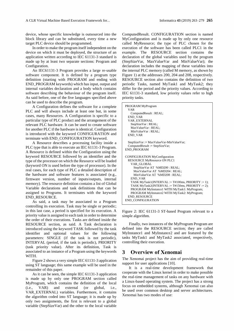
A CLR Virtual Machine Based Execution Framework for... Informatica 43 (2019) 263–279 265
device, whose specific knowledge is outsourced into the
block library and can be substituted, every time a new
target PLC device should be programmed.
In order to make the program itself independent on the
device on which it must be deployed, the structure of an
application written according to IEC 61131-3 standard is
made up by at least two separate sections: Program and
Configuration.
An IEC61131-3 Program provides a large re-usable
software component. It is defined by a program type
definition (starting with PROGRAM and ending with
END_PROGRAM keywords) which has input, output and
internal variables declaration and a body which contains
software describing the behaviour of the program itself.
As said before, one of the five languages specified above
can be used to describe the program.
A Configuration defines the software for a complete
PLC and will always include at least one but, in some
cases, many Resources. A Configuration is specific to a
particular type of PLC product and the arrangement of the
relevant PLC hardware. It can be used to create software
for another PLC if the hardware is identical. Configuration
is introduced with the keyword CONFIGURATION and
terminate with END_CONFIGURATION keyword.
A Resource describes a processing facility inside a
PLC type that is able to execute an IEC 61131-3 Program.
A Resource is defined within the Configuration using the
keyword RESOURCE followed by an identifier and the
type of the processor on which the Resource will be loaded
(keyword ON is used before the type of processor). In the
real cases, for each type of PLC a detailed description of
the hardware and software features is associated (e.g.,
firmware version, number of inputs/outputs, internal
memory). The resource definition contains a list of Global
Variable declarations and task definitions that can be
assigned to Programs. It terminates with the keyword
END_RESOURCE.
As said, a task may be associated to a Program
controlling its execution. Task may be single or periodic;
in this last case, a period is specified for its execution. A
priority value is assigned to each task in order to determine
the order of their executions. Tasks are defined inside the
RESOURCE section, as said. A Task declaration is
introduced using the keyword TASK followed by the task
identifier and optional values for the following
parameters: SINGLE (if the task is not periodic),
INTERVAL (period, if the task is periodic), PRIORITY
(task priority value). After its definition, Task is
associated to an instance of a Program using the keywords
WITH.
Figure 2 shows a very simple IEC 61131-3 application
using ST language; this same example will be used in the
remainder of this paper.
As it can be seen, the simple IEC 61131-3 application
is made up by only one PROGRAM section called
MyProgram, which contains the definition of the local
(i.e., VAR) and external (or global, i.e.,
VAR_EXTERNAL) variables. Furthermore, it contains
the algorithm coded into ST language; it is made up by
only two assignments, the first is relevant to a global
variable (StepSizeVar) and the other to the local variable
ComputedResult. CONFIGURATION section is named
MyConfiguration and is made up by only one resource
called MyResource; the type of PLC chosen for the
execution of the software has been called PLC1 in the
example. The RESOURCE section contains the
declaration of the global variables used by the program
(StepSizeVar, MaxValueVar and MinValueVar); the
declaration includes the mapping of these variables into
the internal PLC memory (called M memory, as shown by
Figure 1) at the addresses 200, 204 and 208, respectively.
RESOURCE section also contains the definition of two
periodic Tasks, named MyTask1 and MyTask2; they
differ for the period and the priority values. According to
IEC 61131-3 standard, low priority values refer to high
priority tasks.
Figure 2: IEC 61131-3 ST-based Program relevant to a
simple algorithm.
Finally, two instances of the MyProgram Program are
defined into the RESOURCE section; they are called
MyInstance1 and MyInstance2 and are featured by the
tasks MyTask1 and MyTask2 associated, respectively,
controlling their execution.
3 Overview of Xenomai The Xenomai project has the aim of providing real-time
support for user applications [10].
It is a real-time development framework that
cooperate with the Linux kernel in order to make possible
the real-time management of tasks on any hardware with
a Linux-based operating system. The project has a strong
focus on embedded systems, although Xenomai can also
be used over common desktop and server architectures.
Xenomai has two modes of use:
PROGRAM MyProgram
VAR ComputedResult : REAL;
END_VAR
VAR_EXTERNAL StepSizeVar : REAL;
MaxValueVar : REAL;
MinValueVar : REAL; END_VAR
StepSizeVar := MaxValueVar-MinValueVar; ComputedResult := StepSizeVar;
END_PROGRAM
CONFIGURATION MyConfiguration
RESOURCE MyResource ON PLC1
VAR_GLOBAL StepSizeVar AT %MD200 : REAL;
MaxValueVar AT %MD204 : REAL;
MinValueVar AT %MD208 : REAL; END_VAR
TASK MyTask1(INTERVAL := T#100ms, PRIORITY := 1);
TASK MyTask2(INTERVAL := T#150ms, PRIORITY := 2); PROGRAM MyInstance1 WITH MyTask1: MyProgram;
PROGRAM MyInstance2 WITH MyTask2: MyProgram;
END_RESOURCE
END_CONFIGURATION
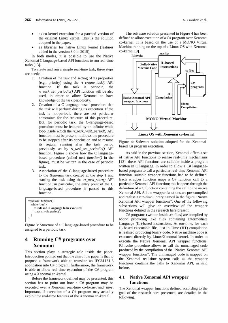
266 Informatica 43 (2019) 263–279 S. Cavalieri et al.
• as co-kernel extension for a patched version of
the original Linux kernel. This is the solution
adopted in the paper.
• as libraries for native Linux kernel (features
added in the version 3.0 in 2015)
In both modes, it is possible to use the Native
Xenomai C language-based API functions to run real-time
tasks [13].
To create and run a simple real-time task, three steps
are needed:
1. Creation of the task and setting of its properties
(e.g., priority) using the rt_create_task() API
function. If the task is periodic, the
rt_task_set_periodic() API function will be also
used, in order to allow Xenomai to have
knowledge of the task periodicity.
2. Creation of a C language-based procedure that
the task will perform during its execution. If the
task is not-periodic there are not particular
constraints for the structure of this procedure.
But, for periodic task, the C-language-based
procedure must be featured by an infinite while
loop inside which the rt_task_wait_period() API
function must be present; it allows the procedure
to be stopped after its conclusion and to resume
its regular running after the task period
previously set by rt_task_set_periodic() API
function. Figure 3 shows how the C language-
based procedure (called task_function() in the
figure), must be written in the case of periodic
task.
3. Association of the C language-based procedure
to the Xenomai task created at the step 1 and
starting the task using the rt_task_start() API
function; in particular, the entry point of the C
language-based procedure is passed to this
function.
Figure 3: Structure of a C language-based procedure to be
assigned to a periodic task.
4 Running C# programs over
Xenomai This section plays a strategic role inside the paper.
Introduction pointed out that the aim of the paper is that to
propose a framework able to translate an IEC61131-3
application into C# program; furthermore, the framework
is able to allow real-time execution of the C# program
using a Xenomai co-kernel.
Before the framework defined may be presented, this
section has to point out how a C# program may be
executed over a Xenomai real-time co-kernel and, most
important, if execution of a C# program may actually
exploit the real-time features of the Xenomai co-kernel.
The software solution presented in Figure 4 has been
defined to allow execution of a C# program over Xenomai
co-kernel. It is based on the use of a MONO Virtual
Machine running on the top of a Linux OS with Xenomai
co-kernel [9].
Figure 4: Software solution adopted for the Xenomai-
based C# program execution.
As said in the previous section, Xenomai offers a set
of native API functions to realise real-time mechanisms
[13]; these API functions are callable inside a program
written in C language. In order to allow a C# language-
based program to call a particular real-time Xenomai API
function, suitable wrapper functions had to be defined.
Each wrapper function maps a C# function call to a
particular Xenomai API function; this happens through the
definition of a C function containing the call to the native
Xenomai API. All the wrapper functions are pre-compiled
and realise a run-time library named in the figure “Native
Xenomai API wrapper functions”. One of the following
subsections will give an overview of the wrapper
functions defined in the research here present.
C# programs (written inside .cs files) are compiled by
Mono producing .exe files containing Intermediate
Language (IL)-based instructions. At run-time, for each
IL-based executable file, Just-In-Time (JIT) compilation
is realised producing binary code. Native machine code is
executed directly by Linux/Xenomai kernel. In order to
execute the Native Xenomai API wrapper functions,
P/Invoke procedure allows to call the unmanaged code
produced by the compilation of the “Native Xenomai API
wrapper functions”. The unmanaged code is mapped on
the Xenomai real-time system calls as the wrapper
functions contains the calls to Xenomai API, as said
before.
4.1 Native Xenomai API wrapper
functions
The Xenomai wrapper functions defined according to the
goal of the research here presented, are detailed in the
following.
.cs files
Linux OS with Xenomai co-kernel
.exe file
Mono
Compilation
JIT
Compilation
P/Invoke
Fully-Native
Machine Code
Native Xenomai API
wrapper functions
MONO Virtual Machine
C#
program
IL-based
instructions
void task_function(){
while (true) {
//Code in C Language to be executed
rt_task_wait_period();
}
}
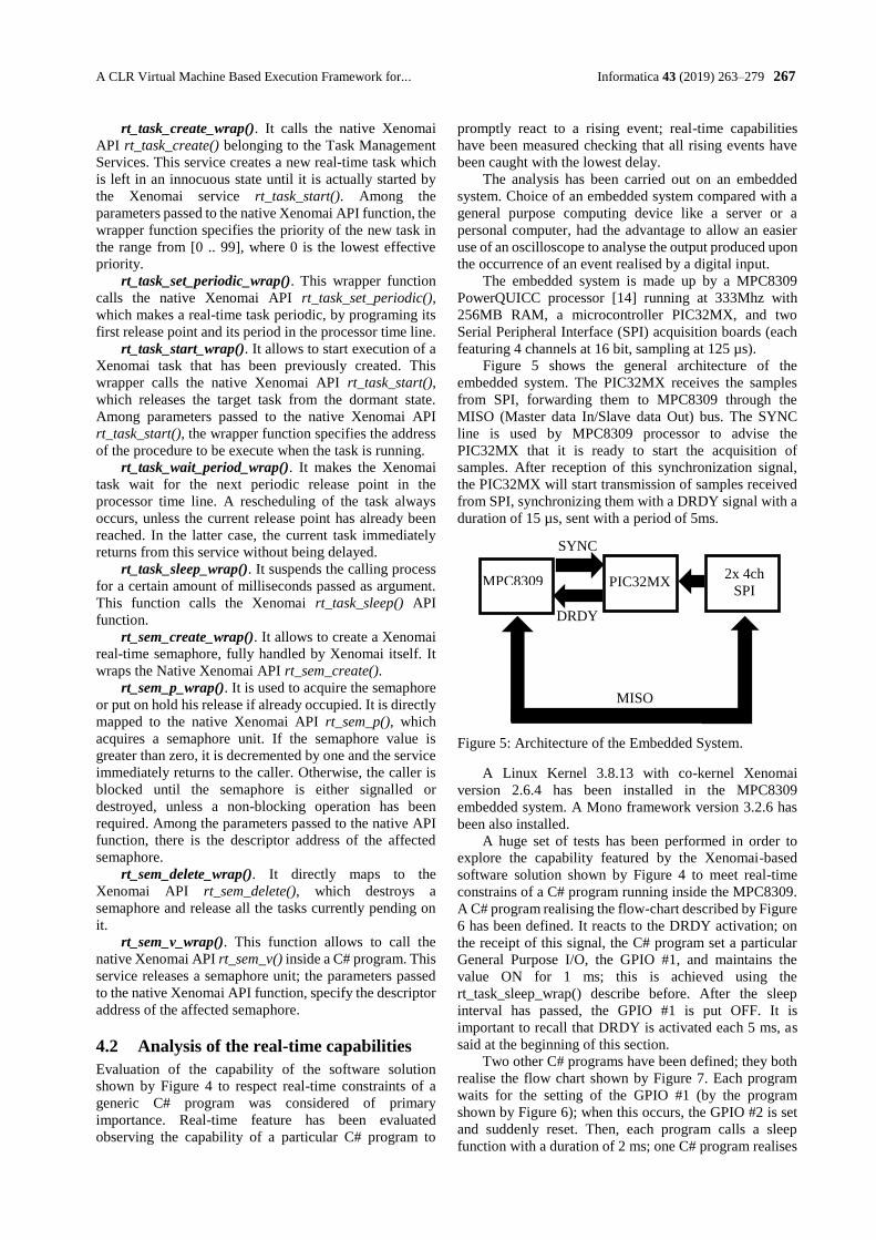
A CLR Virtual Machine Based Execution Framework for... Informatica 43 (2019) 263–279 267
rt_task_create_wrap(). It calls the native Xenomai
API rt_task_create() belonging to the Task Management
Services. This service creates a new real-time task which
is left in an innocuous state until it is actually started by
the Xenomai service rt_task_start(). Among the
parameters passed to the native Xenomai API function, the
wrapper function specifies the priority of the new task in
the range from [0 .. 99], where 0 is the lowest effective
priority.
rt_task_set_periodic_wrap(). This wrapper function
calls the native Xenomai API rt_task_set_periodic(),
which makes a real-time task periodic, by programing its
first release point and its period in the processor time line.
rt_task_start_wrap(). It allows to start execution of a
Xenomai task that has been previously created. This
wrapper calls the native Xenomai API rt_task_start(),
which releases the target task from the dormant state.
Among parameters passed to the native Xenomai API
rt_task_start(), the wrapper function specifies the address
of the procedure to be execute when the task is running.
rt_task_wait_period_wrap(). It makes the Xenomai
task wait for the next periodic release point in the
processor time line. A rescheduling of the task always
occurs, unless the current release point has already been
reached. In the latter case, the current task immediately
returns from this service without being delayed.
rt_task_sleep_wrap(). It suspends the calling process
for a certain amount of milliseconds passed as argument.
This function calls the Xenomai rt_task_sleep() API
function.
rt_sem_create_wrap(). It allows to create a Xenomai
real-time semaphore, fully handled by Xenomai itself. It
wraps the Native Xenomai API rt_sem_create().
rt_sem_p_wrap(). It is used to acquire the semaphore
or put on hold his release if already occupied. It is directly
mapped to the native Xenomai API rt_sem_p(), which
acquires a semaphore unit. If the semaphore value is
greater than zero, it is decremented by one and the service
immediately returns to the caller. Otherwise, the caller is
blocked until the semaphore is either signalled or
destroyed, unless a non-blocking operation has been
required. Among the parameters passed to the native API
function, there is the descriptor address of the affected
semaphore.
rt_sem_delete_wrap(). It directly maps to the
Xenomai API rt_sem_delete(), which destroys a
semaphore and release all the tasks currently pending on
it.
rt_sem_v_wrap(). This function allows to call the
native Xenomai API rt_sem_v() inside a C# program. This
service releases a semaphore unit; the parameters passed
to the native Xenomai API function, specify the descriptor
address of the affected semaphore.
4.2 Analysis of the real-time capabilities
Evaluation of the capability of the software solution
shown by Figure 4 to respect real-time constraints of a
generic C# program was considered of primary
importance. Real-time feature has been evaluated
observing the capability of a particular C# program to
promptly react to a rising event; real-time capabilities
have been measured checking that all rising events have
been caught with the lowest delay.
The analysis has been carried out on an embedded
system. Choice of an embedded system compared with a
general purpose computing device like a server or a
personal computer, had the advantage to allow an easier
use of an oscilloscope to analyse the output produced upon
the occurrence of an event realised by a digital input.
The embedded system is made up by a MPC8309
PowerQUICC processor [14] running at 333Mhz with
256MB RAM, a microcontroller PIC32MX, and two
Serial Peripheral Interface (SPI) acquisition boards (each
featuring 4 channels at 16 bit, sampling at 125 µs).
Figure 5 shows the general architecture of the
embedded system. The PIC32MX receives the samples
from SPI, forwarding them to MPC8309 through the
MISO (Master data In/Slave data Out) bus. The SYNC
line is used by MPC8309 processor to advise the
PIC32MX that it is ready to start the acquisition of
samples. After reception of this synchronization signal,
the PIC32MX will start transmission of samples received
from SPI, synchronizing them with a DRDY signal with a
duration of 15 µs, sent with a period of 5ms.
Figure 5: Architecture of the Embedded System.
A Linux Kernel 3.8.13 with co-kernel Xenomai
version 2.6.4 has been installed in the MPC8309
embedded system. A Mono framework version 3.2.6 has
been also installed.
A huge set of tests has been performed in order to
explore the capability featured by the Xenomai-based
software solution shown by Figure 4 to meet real-time
constrains of a C# program running inside the MPC8309.
A C# program realising the flow-chart described by Figure
6 has been defined. It reacts to the DRDY activation; on
the receipt of this signal, the C# program set a particular
General Purpose I/O, the GPIO #1, and maintains the
value ON for 1 ms; this is achieved using the
rt_task_sleep_wrap() describe before. After the sleep
interval has passed, the GPIO #1 is put OFF. It is
important to recall that DRDY is activated each 5 ms, as
said at the beginning of this section.
Two other C# programs have been defined; they both
realise the flow chart shown by Figure 7. Each program
waits for the setting of the GPIO #1 (by the program
shown by Figure 6); when this occurs, the GPIO #2 is set
and suddenly reset. Then, each program calls a sleep
function with a duration of 2 ms; one C# program realises
MPC8309 PIC32MX 2x 4ch
SPI
SYNC
DRDY
MISO
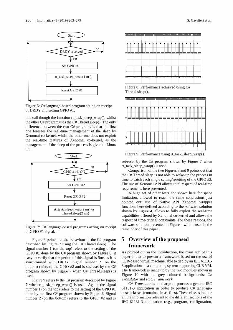
268 Informatica 43 (2019) 263–279 S. Cavalieri et al.
this call though the function rt_task_sleep_wrap(), whilst
the other C# program uses the C# Thread.sleep(). The only
difference between the two C# programs is that the first
one foresees the real-time management of the sleep by
Xenomai co-kernel, whilst the other one does not exploit
the real-time features of Xenomai co-kernel, as the
management of the sleep of the process is given to Linux
OS.
Figure 7: C# language-based programs acting on receipt
of GPIO #1 signal.
Figure 8 points out the behaviour of the C# program
described by Figure 7 using the C# Thread.sleep(). The
signal number 1 (on the top) refers to the setting of the
GPIO #1 done by the C# program shown by Figure 6; it
easy to verify that the period of this signal is 5ms as it is
synchronised with DRDY. Signal number 2 (on the
bottom) refers to the GPIO #2 and is set/reset by the C#
program shown by Figure 7 when C# Thread.sleep() is
used.
Figure 9 refers to the C# program described by Figure
7 when rt_task_sleep_wrap() is used. Again, the signal
number 1 (on the top) refers to the setting of the GPIO #1
done by the first C# program shown by Figure 6. Signal
number 2 (on the bottom) refers to the GPIO #2 and is
set/reset by the C# program shown by Figure 7 when
rt_task_sleep_wrap() is used.
Comparison of the two Figures 8 and 9 points out that
the C# Thread.sleep is not able to wake-up the process in
time to catch each single setting/resetting of the GPIO #2.
The use of Xenomai API allows total respect of real-time
requirements here presented.
A huge set of other tests not shown here for space
limitation, allowed to reach the same conclusions just
pointed out: use of Native API Xenomai wrapper
functions here defined according to the software solution
shown by Figure 4, allows to fully exploit the real-time
capabilities offered by Xenomai co-kernel and allows the
respect of time-critical constraints. For these reasons, the
software solution presented in Figure 4 will be used in the
remainder of this paper.
5 Overview of the proposed
framework As pointed out in the Introduction, the main aim of this
paper is that to present a framework based on the use of
CLR-based virtual machine, able to deploy an IEC 61131-
3 application on a computing system supporting CLR VM.
The framework is made up by the two modules shown in
Figure 10 with the grey coloured backgrounds: C#
Translator and PLC Framework.
C# Translator is in charge to process a generic IEC
61131-3 application in order to produce C# language-
based classes (contained in .cs files). These classes include
all the information relevant to the different sections of the
IEC 61131-3 application (e.g., program, configuration,
DRDY received
yes
no
Set GPIO #1
Reset GPIO #1
rt_task_sleep_wrap(1 ms)
Start
GPIO #1 is ON
yes
no
Set GPIO #2
rt_task_sleep_wrap(2 ms) or
Thread.sleep(2 ms)
Reset GPIO #2
Start
Figure 6: C# language-based program acting on receipt
of DRDY and setting GPIO #1.
Figure 8: Performance achieved using C#
Thread.sleep().
Figure 9: Performance using rt_task_sleep_wrap().
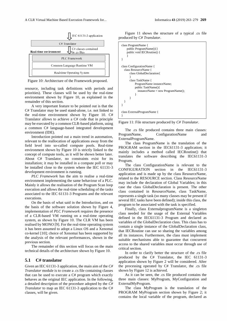
A CLR Virtual Machine Based Execution Framework for... Informatica 43 (2019) 263–279 269
resource, including task definitions with periods and
priorities). These classes will be used by the real-time
environment shown by Figure 10, as explained in the
remainder of this section.
A very important feature to be pointed out is that the
C# Translator may be used stand-alone, i.e. not linked to
the real-time environment shown by Figure 10. C#
Translator allows to achieve a C# code that in principle
may be executed by a common CLR-based platform, using
a common C# language-based integrated development
environment (IDE).
Introduction pointed out a main trend in automation,
relevant to the reallocation of applications away from the
field level into so-called compute pools. Real-time
environment shown by Figure 10 is strictly linked to the
concept of compute tools, as it will be shown better later.
About C# Translator, no constraints exist for its
installation; it may be installed in a compute poll or may
be installed close to the system where the IEC 61131-3
development environment is running.
PLC Framework has the aim to realise a real-time
environment implementing the same behaviour of a PLC.
Mainly it allows the realisation of the Program Scan loop
execution and allows the real-time scheduling of the tasks
associated to the IEC 61131-3 Programs and the relevant
executions.
On the basis of what said in the Introduction, and on
the basis of the software solution shown by Figure 4,
implementation of PLC Framework requires the presence
of a CLR-based VM running on a real-time operating
system, as shown by Figure 10. The CLR VM has been
realised by MONO [9]. For the real-time operating system
it has been assumed to adopt a Linux OS and a Xenomai
co-kernel [10]; choice of Xenomai has been supported by
the analysis of the relevant performances, shown in the
previous section.
The remainder of this section will focus on the main
technical details of the architecture shown by Figure 10.
5.1 C# translator
Given an IEC 61131-3 application, the main aim of the C#
Translator module is to create a .cs file containing classes
that can be used to execute a C# program which exactly
behaves as the original IEC application. In the following,
a detailed description of the procedure adopted by the C#
Translator to map an IEC 61131-3 application to the C#
classes, will be given.
Figure 11 shows the structure of a typical .cs file
produced by C# Translator.
Figure 11: File structure produced by C# Translator.
The .cs file produced contains three main classes:
ProgramName, ConfigurationName and
ExternalProgramName.
The class ProgramName is the translation of the
PROGRAM section in the IEC61131-3 application; it
mainly includes a method called IECRoutine() that
translates the software describing the IEC61131-3
Program.
The class ConfigurationName is relevant to the
CONFIGURATION section in the IEC61131-3
application and is made up by the class ResourceName,
related to the RESOURCE section. Class ResourceName
may include the declaration of Global Variables; in this
case the class GlobalDeclaration is present. The other
class contained in ResourceName, class TaskName,
represents a single task (so many classes may be present if
several IEC tasks have been defined); inside this class, the
program to be associated with the task is specified.
Finally, class ExternalprogramName is a singleton
class needed for the usage of the External Variables
defined in the IEC61131-3 Program and declared as
variables of the GlobalDeclaration class. This class has to
contain a single instance of the GlobalDeclaration class,
that IECRoutine can use so sharing the variables among
all its instances. Furthermore, the class must implement
suitable mechanisms able to guarantee that concurrent
access to the shared variables must occur through use of
critical section.
In order to clarify better the structure of the .cs file
produced by the C# Translator, the IEC 61131-3
application shown by Figure 2 will be considered. After
the processing operated by C# Translator, the .cs file
shown by Figure 12 is achieved.
As it can be seen, the .cs file produced contains the
three main classes: MyProgram, MyConfiguration and
ExternalMyProgram.
The class MyProgram is the translation of the
PROGRAM MyProgram section shown by Figure 2; it
contains the local variable of the program, declared as
class ProgramName { public ProgramName(){}
public void IECRoutine() {
} }
class ConfigurationName { class ResourceName {
class GlobalDeclaration{
} class TaskName {
ProgramName instanceName;
public TaskName(){ instanceName = new ProgramName();
}
}
}
}
class ExternalProgramName {
}
Figure 10: Architecture of the Framework proposed.
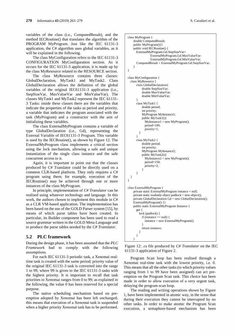
270 Informatica 43 (2019) 263–279 S. Cavalieri et al.
variables of the class (i.e., ComputedResult), and the
method IECRoutine() that translates the algorithm of the
PROGRAM MyProgram. Just like the IEC 61131-3
application, the C# algorithm uses global variables, as it
will be explained in the following.
The class MyConfiguration refers to the IEC 61131-3
CONFIGURATION MyConfiguration section. As it
occurs for the IEC 61131-3 application, it is made up by
the class MyResource related to the RESOURCE section.
The class MyResource contains three classes:
GlobalDeclaration, MyTask1 and MyTask2. Class
GlobalDeclaration allows the definition of the global
variables of the original IEC61131-3 application (i.e.,
StepSizeVar, MaxValueVar and MinValueVar). The
classes MyTask1 and MyTask2 represent the IEC 61131-
3 Tasks: inside these classes there are the variables that
indicate the properties of the tasks as period and priority,
a variable that indicates the program associated with the
task (MyProgram) and a constructor with the aim of
initializing these variables.
The class ExternalMyProgram contains a variable of
type GlobalDeclaration (i.e., Gd), representing the
External Variable of IEC61131-3 Program. This variable
is used by the IECRoutine(), as shown by Figure 12. The
ExternalMyProgram class implements a critical section
using the lock mechanism, allowing a safe and unique
instantiation of the single class instance and the safe
concurrent access to it.
Again, it is important to point out that the classes
produced by C# Translator could be directly used on a
common CLR-based platform. They only requires a C#
program using them; for example, execution of the
IECRoutine() may be achieved through one or more
instances of the class MyProgram.
In principle, implementation of C# Translator can be
realised using whatever technology and language. In this
work, the authors chosen to implement this module in C#
as a CLR VM-based application. The implementation has
been based on the use of the GOLD Parser system [15], by
means of which parse tables have been created. In
particular, its Builder component has been used to read a
source grammar written in the GOLD Meta-Language and
to produce the parse tables needed by the C# Translator.
5.2 PLC framework
During the design phase, it has been assumed that the PLC
Framework had to comply with the following
assumptions.
For each IEC 61131-3 periodic task, a Xenomai real-
time task is created with the same period; priority value of
the original IEC 61131-3 task is converted into the range
1 to 99, where 99 is given to the IEC 61131-3 tasks with
the highest priority. It is important to recall that task
priorities in Xenomai ranges from 0 to 99; as explained in
the following, the value 0 has been reserved for a special
purpose.
The native scheduling mechanism based on pre-
emption adopted by Xenomai has been left unchanged;
this means that execution of a Xenomai task is suspended
when a higher priority Xenomai task has to be performed.
Program Scan loop has been realised through a
Xenomai real-time task with the lowest priority, i.e. 0.
This means that all the other tasks (to which priority values
ranging from 1 to 99 have been assigned) can act pre-
emption on the Program Scan task. This choice has been
made in order to allow execution of a very urgent task,
delaying the program scan loop.
The reading and writing operations shown by Figure
1, have been implemented in atomic way, in the sense that
during their execution they cannot be interrupted by no
other tasks. In order to make atomic the Program Scan
execution, a semaphore-based mechanism has been
Figure 12: .cs file produced by C# Translator on the IEC
61131-3 application of Figure 2.
class MyProgram { double ComputedResult;
public MyProgram(){}
public void IECRoutine() { ExternalMyProgram.Gd.StepSizeVar=
ExternalMyProgram.Gd.MaxValueVar-
ExternalMyProgram.Gd.MinValueVar; ComputedResult = ExternalMyProgram.Gd.StepSizeVar;
}
}
class MyConfiguration {
class MyResource { class GlobalDeclaration{
double StepSizeVar;
double MaxValueVar; double MinValueVar;
}
class MyTask1 { double period;
int priority;
MyProgram MyInstance1; public MyTask1(){
MyInstance1 = new MyProgram();
period=100; priority=1;
}
} class MyTask2 {
double period;
int priority; MyProgram MyInstance2;
public MyTask2(){
MyInstance2 = new MyProgram(); period=150;
priority=2;
} }
} }
class ExternalMyProgram { private static ExternalMyProgram instance = null;
private static readonly object padlock = new object();
private GlobalDeclaration Gd = new GlobalDeclaration();
ExternalMyProgram() {}
public static ExternalMyProgram Instance {
get { lock (padlock) {
if (instance == null) {
instance = new ExternalMyProgram(); }
return instance;
} }
}
}
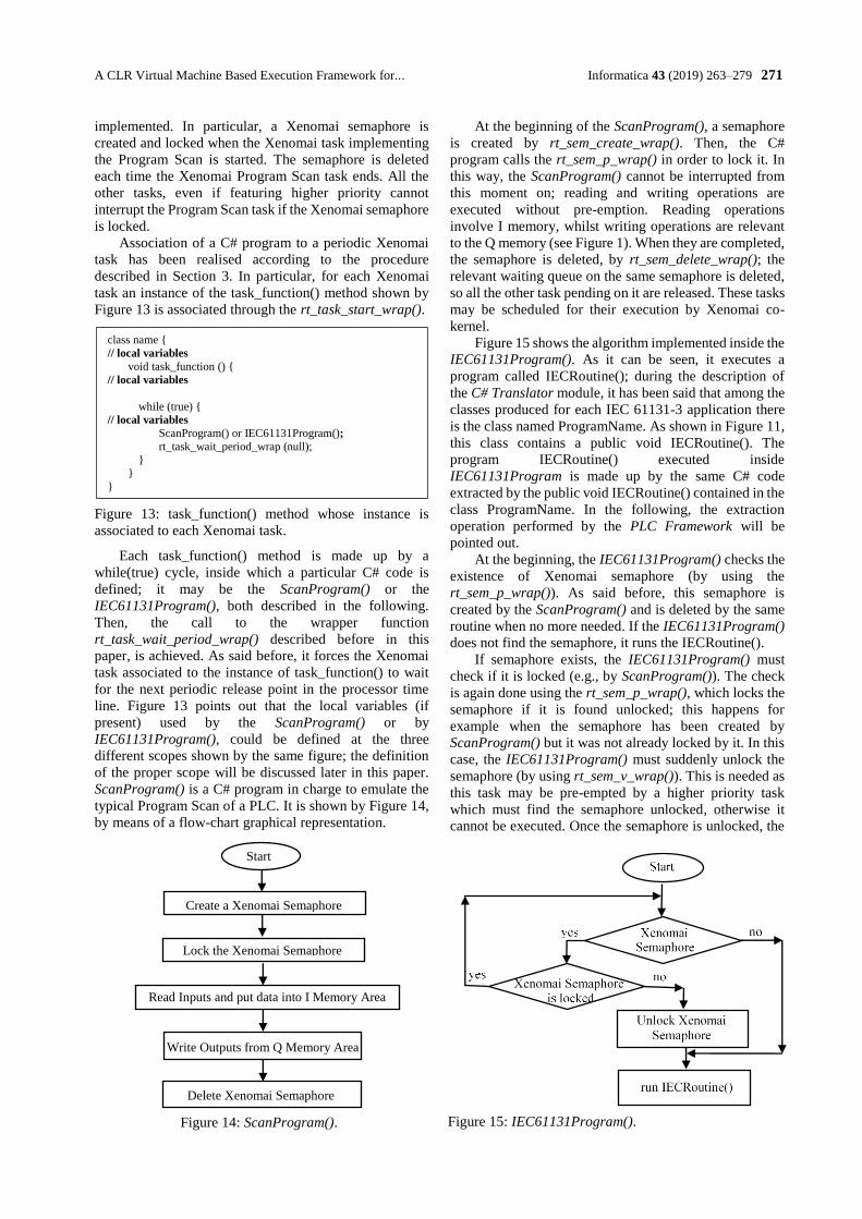
A CLR Virtual Machine Based Execution Framework for... Informatica 43 (2019) 263–279 271
implemented. In particular, a Xenomai semaphore is
created and locked when the Xenomai task implementing
the Program Scan is started. The semaphore is deleted
each time the Xenomai Program Scan task ends. All the
other tasks, even if featuring higher priority cannot
interrupt the Program Scan task if the Xenomai semaphore
is locked.
Association of a C# program to a periodic Xenomai
task has been realised according to the procedure
described in Section 3. In particular, for each Xenomai
task an instance of the task_function() method shown by
Figure 13 is associated through the rt_task_start_wrap().
Figure 13: task_function() method whose instance is
associated to each Xenomai task.
Each task_function() method is made up by a
while(true) cycle, inside which a particular C# code is
defined; it may be the ScanProgram() or the
IEC61131Program(), both described in the following.
Then, the call to the wrapper function
rt_task_wait_period_wrap() described before in this
paper, is achieved. As said before, it forces the Xenomai
task associated to the instance of task_function() to wait
for the next periodic release point in the processor time
line. Figure 13 points out that the local variables (if
present) used by the ScanProgram() or by
IEC61131Program(), could be defined at the three
different scopes shown by the same figure; the definition
of the proper scope will be discussed later in this paper.
ScanProgram() is a C# program in charge to emulate the
typical Program Scan of a PLC. It is shown by Figure 14,
by means of a flow-chart graphical representation.
Figure 14: ScanProgram().
At the beginning of the ScanProgram(), a semaphore
is created by rt_sem_create_wrap(). Then, the C#
program calls the rt_sem_p_wrap() in order to lock it. In
this way, the ScanProgram() cannot be interrupted from
this moment on; reading and writing operations are
executed without pre-emption. Reading operations
involve I memory, whilst writing operations are relevant
to the Q memory (see Figure 1). When they are completed,
the semaphore is deleted, by rt_sem_delete_wrap(); the
relevant waiting queue on the same semaphore is deleted,
so all the other task pending on it are released. These tasks
may be scheduled for their execution by Xenomai co-
kernel.
Figure 15 shows the algorithm implemented inside the
IEC61131Program(). As it can be seen, it executes a
program called IECRoutine(); during the description of
the C# Translator module, it has been said that among the
classes produced for each IEC 61131-3 application there
is the class named ProgramName. As shown in Figure 11,
this class contains a public void IECRoutine(). The
program IECRoutine() executed inside
IEC61131Program is made up by the same C# code
extracted by the public void IECRoutine() contained in the
class ProgramName. In the following, the extraction
operation performed by the PLC Framework will be
pointed out.
At the beginning, the IEC61131Program() checks the
existence of Xenomai semaphore (by using the
rt_sem_p_wrap()). As said before, this semaphore is
created by the ScanProgram() and is deleted by the same
routine when no more needed. If the IEC61131Program()
does not find the semaphore, it runs the IECRoutine().
If semaphore exists, the IEC61131Program() must
check if it is locked (e.g., by ScanProgram()). The check
is again done using the rt_sem_p_wrap(), which locks the
semaphore if it is found unlocked; this happens for
example when the semaphore has been created by
ScanProgram() but it was not already locked by it. In this
case, the IEC61131Program() must suddenly unlock the
semaphore (by using rt_sem_v_wrap()). This is needed as
this task may be pre-empted by a higher priority task
which must find the semaphore unlocked, otherwise it
cannot be executed. Once the semaphore is unlocked, the
class name {
// local variables
void task_function () {
// local variables
while (true) { // local variables
ScanProgram() or IEC61131Program();
rt_task_wait_period_wrap (null); }
}
}
Read Inputs and put data into I Memory Area
Delete Xenomai Semaphore
Create a Xenomai Semaphore
Write Outputs from Q Memory Area
Start
Lock the Xenomai Semaphore
Figure 15: IEC61131Program().
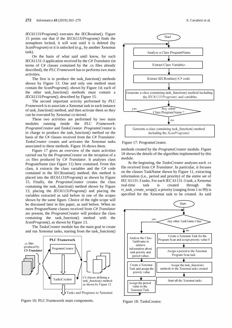
272 Informatica 43 (2019) 263–279 S. Cavalieri et al.
IEC61131Program() executes the IECRoutine(). Figure
15 points out that if the IEC61131Program() finds the
semaphore locked, it will wait until it is deleted (by
ScanProgram) or it is unlocked (e.g., by another Xenomai
task).
On the basis of what said until know, for each
IEC61131-3 application received by the C# Translator (in
terms of C# classes contained by the .cs files already
described), the PLC Framework has to performs two main
activities.
The first is to produce the task_function() methods
shown by Figure 13. One and only one method must
contain the ScanProgram(), shown by Figure 14; each of
the other task_function() methods must contain a
IEC61131Program(), described by Figure 15.
The second important activity performed by PLC
Framework is to associate a Xenomai task to each instance
of task_function() method, and then activate them so they
can be executed by Xenomai co-kernel.
These two activities are performed by two main
modules running inside the PLC Framework:
ProgramsCreator and TasksCreator. ProgramsCreator is
in charge to produce the task_function() method on the
basis of the C# classes received from the C# Translator.
TasksCreator creates and activates the Xenomai tasks
associated to these methods. Figure 16 shows them.
Figure 17 gives an overview of the main activities
carried out by the ProgramsCreator on the reception of a
.cs files produced by C# Translator. It analyses class
ProgramName (see Figure 11) here contained. From this
class, it extracts the class variables and the C# code
contained in the IECRoutine() method; this method is
placed into the IEC61131Program() as shown by Figure
15. Finally, the ProgramsCreator creates the class
containing the task_function() method shown by Figure
13, placing the IEC61131Program() and placing the
variables extracted as said before in one of the scopes
shown by the same figure. Choice of the right scope will
be discussed later in this paper, as said before. When no
more ProgramName classes received from C# Translator
are present, the ProgramsCreator will produce the class
containing the task_function() method with the
ScanProgram(), as shown by Figure 13.
The TasksCreator module has the main goal to create
and run Xenomai tasks, starting from the task_function()
methods created by the ProgramsCreator module. Figure
18 shows the details of the algorithm implemented by this
module.
At the beginning, the TasksCreator analyses each .cs
file received from C# Translator. In particular, it focuses
on the classes TaskName shown by Figure 11, extracting
information (i.e., period and priority) of the entire set of
IEC 61131-3 tasks. For each IEC 61131-3 task, a Xenomai
real-time task is created through the
rt_task_create_wrap(); a priority (ranging from 1 to 99) is
specified for the Xenomai task to be created. As said
Figure 17: ProgramsCreator.
Figure 16: PLC Framework main components.
Figure 18: TasksCreator.
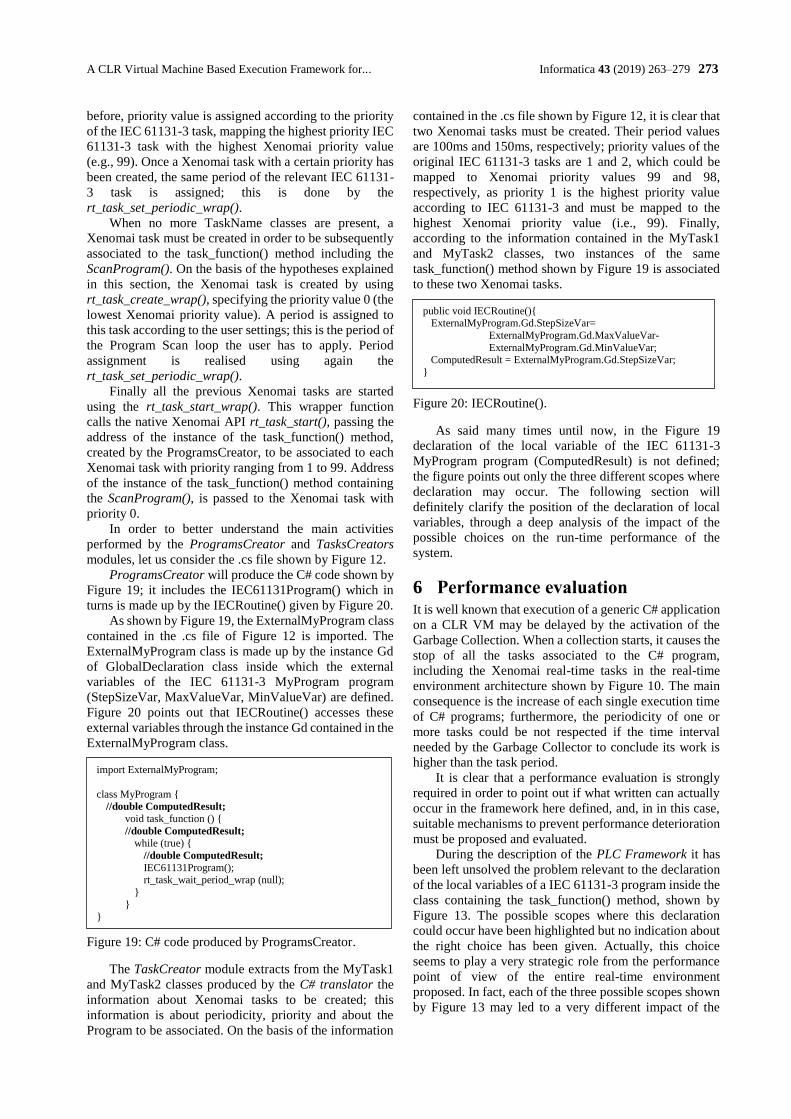
A CLR Virtual Machine Based Execution Framework for... Informatica 43 (2019) 263–279 273
before, priority value is assigned according to the priority
of the IEC 61131-3 task, mapping the highest priority IEC
61131-3 task with the highest Xenomai priority value
(e.g., 99). Once a Xenomai task with a certain priority has
been created, the same period of the relevant IEC 61131-
3 task is assigned; this is done by the
rt_task_set_periodic_wrap().
When no more TaskName classes are present, a
Xenomai task must be created in order to be subsequently
associated to the task_function() method including the
ScanProgram(). On the basis of the hypotheses explained
in this section, the Xenomai task is created by using
rt_task_create_wrap(), specifying the priority value 0 (the
lowest Xenomai priority value). A period is assigned to
this task according to the user settings; this is the period of
the Program Scan loop the user has to apply. Period
assignment is realised using again the
rt_task_set_periodic_wrap().
Finally all the previous Xenomai tasks are started
using the rt_task_start_wrap(). This wrapper function
calls the native Xenomai API rt_task_start(), passing the
address of the instance of the task_function() method,
created by the ProgramsCreator, to be associated to each
Xenomai task with priority ranging from 1 to 99. Address
of the instance of the task_function() method containing
the ScanProgram(), is passed to the Xenomai task with
priority 0.
In order to better understand the main activities
performed by the ProgramsCreator and TasksCreators
modules, let us consider the .cs file shown by Figure 12.
ProgramsCreator will produce the C# code shown by
Figure 19; it includes the IEC61131Program() which in
turns is made up by the IECRoutine() given by Figure 20.
As shown by Figure 19, the ExternalMyProgram class
contained in the .cs file of Figure 12 is imported. The
ExternalMyProgram class is made up by the instance Gd
of GlobalDeclaration class inside which the external
variables of the IEC 61131-3 MyProgram program
(StepSizeVar, MaxValueVar, MinValueVar) are defined.
Figure 20 points out that IECRoutine() accesses these
external variables through the instance Gd contained in the
ExternalMyProgram class.
Figure 19: C# code produced by ProgramsCreator.
The TaskCreator module extracts from the MyTask1
and MyTask2 classes produced by the C# translator the
information about Xenomai tasks to be created; this
information is about periodicity, priority and about the
Program to be associated. On the basis of the information
contained in the .cs file shown by Figure 12, it is clear that
two Xenomai tasks must be created. Their period values
are 100ms and 150ms, respectively; priority values of the
original IEC 61131-3 tasks are 1 and 2, which could be
mapped to Xenomai priority values 99 and 98,
respectively, as priority 1 is the highest priority value
according to IEC 61131-3 and must be mapped to the
highest Xenomai priority value (i.e., 99). Finally,
according to the information contained in the MyTask1
and MyTask2 classes, two instances of the same
task_function() method shown by Figure 19 is associated
to these two Xenomai tasks.
Figure 20: IECRoutine().
As said many times until now, in the Figure 19
declaration of the local variable of the IEC 61131-3
MyProgram program (ComputedResult) is not defined;
the figure points out only the three different scopes where
declaration may occur. The following section will
definitely clarify the position of the declaration of local
variables, through a deep analysis of the impact of the
possible choices on the run-time performance of the
system.
6 Performance evaluation It is well known that execution of a generic C# application
on a CLR VM may be delayed by the activation of the
Garbage Collection. When a collection starts, it causes the
stop of all the tasks associated to the C# program,
including the Xenomai real-time tasks in the real-time
environment architecture shown by Figure 10. The main
consequence is the increase of each single execution time
of C# programs; furthermore, the periodicity of one or
more tasks could be not respected if the time interval
needed by the Garbage Collector to conclude its work is
higher than the task period.
It is clear that a performance evaluation is strongly
required in order to point out if what written can actually
occur in the framework here defined, and, in in this case,
suitable mechanisms to prevent performance deterioration
must be proposed and evaluated.
During the description of the PLC Framework it has
been left unsolved the problem relevant to the declaration
of the local variables of a IEC 61131-3 program inside the
class containing the task_function() method, shown by
Figure 13. The possible scopes where this declaration
could occur have been highlighted but no indication about
the right choice has been given. Actually, this choice
seems to play a very strategic role from the performance
point of view of the entire real-time environment
proposed. In fact, each of the three possible scopes shown
by Figure 13 may led to a very different impact of the
import ExternalMyProgram;
class MyProgram { //double ComputedResult;
void task_function () {
//double ComputedResult;
while (true) {
//double ComputedResult;
IEC61131Program(); rt_task_wait_period_wrap (null);
}
}
}
public void IECRoutine(){ ExternalMyProgram.Gd.StepSizeVar=
ExternalMyProgram.Gd.MaxValueVar-
ExternalMyProgram.Gd.MinValueVar; ComputedResult = ExternalMyProgram.Gd.StepSizeVar;
}
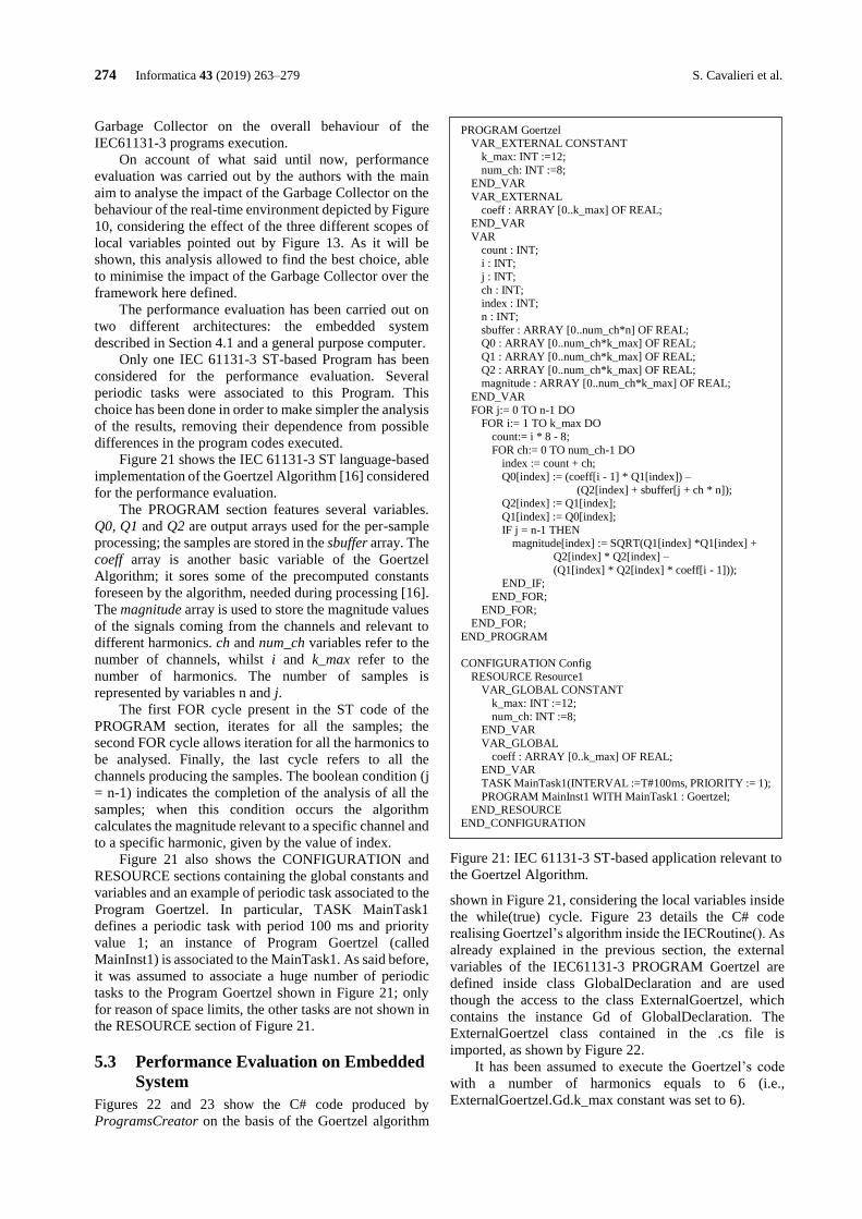
274 Informatica 43 (2019) 263–279 S. Cavalieri et al.
Garbage Collector on the overall behaviour of the
IEC61131-3 programs execution.
On account of what said until now, performance
evaluation was carried out by the authors with the main
aim to analyse the impact of the Garbage Collector on the
behaviour of the real-time environment depicted by Figure
10, considering the effect of the three different scopes of
local variables pointed out by Figure 13. As it will be
shown, this analysis allowed to find the best choice, able
to minimise the impact of the Garbage Collector over the
framework here defined.
The performance evaluation has been carried out on
two different architectures: the embedded system
described in Section 4.1 and a general purpose computer.
Only one IEC 61131-3 ST-based Program has been
considered for the performance evaluation. Several
periodic tasks were associated to this Program. This
choice has been done in order to make simpler the analysis
of the results, removing their dependence from possible
differences in the program codes executed.
Figure 21 shows the IEC 61131-3 ST language-based
implementation of the Goertzel Algorithm [16] considered
for the performance evaluation.
The PROGRAM section features several variables.
Q0, Q1 and Q2 are output arrays used for the per-sample
processing; the samples are stored in the sbuffer array. The
coeff array is another basic variable of the Goertzel
Algorithm; it sores some of the precomputed constants
foreseen by the algorithm, needed during processing [16].
The magnitude array is used to store the magnitude values
of the signals coming from the channels and relevant to
different harmonics. ch and num_ch variables refer to the
number of channels, whilst i and k_max refer to the
number of harmonics. The number of samples is
represented by variables n and j.
The first FOR cycle present in the ST code of the
PROGRAM section, iterates for all the samples; the
second FOR cycle allows iteration for all the harmonics to
be analysed. Finally, the last cycle refers to all the
channels producing the samples. The boolean condition (j
= n-1) indicates the completion of the analysis of all the
samples; when this condition occurs the algorithm
calculates the magnitude relevant to a specific channel and
to a specific harmonic, given by the value of index.
Figure 21 also shows the CONFIGURATION and
RESOURCE sections containing the global constants and
variables and an example of periodic task associated to the
Program Goertzel. In particular, TASK MainTask1
defines a periodic task with period 100 ms and priority
value 1; an instance of Program Goertzel (called
MainInst1) is associated to the MainTask1. As said before,
it was assumed to associate a huge number of periodic
tasks to the Program Goertzel shown in Figure 21; only
for reason of space limits, the other tasks are not shown in
the RESOURCE section of Figure 21.
5.3 Performance Evaluation on Embedded
System
Figures 22 and 23 show the C# code produced by
ProgramsCreator on the basis of the Goertzel algorithm
shown in Figure 21, considering the local variables inside
the while(true) cycle. Figure 23 details the C# code
realising Goertzel’s algorithm inside the IECRoutine(). As
already explained in the previous section, the external
variables of the IEC61131-3 PROGRAM Goertzel are
defined inside class GlobalDeclaration and are used
though the access to the class ExternalGoertzel, which
contains the instance Gd of GlobalDeclaration. The
ExternalGoertzel class contained in the .cs file is
imported, as shown by Figure 22.
It has been assumed to execute the Goertzel’s code
with a number of harmonics equals to 6 (i.e.,
ExternalGoertzel.Gd.k_max constant was set to 6).
PROGRAM Goertzel VAR_EXTERNAL CONSTANT
k_max: INT :=12;
num_ch: INT :=8; END_VAR
VAR_EXTERNAL
coeff : ARRAY [0..k_max] OF REAL; END_VAR
VAR
count : INT; i : INT;
j : INT;
ch : INT; index : INT;
n : INT;
sbuffer : ARRAY [0..num_ch*n] OF REAL; Q0 : ARRAY [0..num_ch*k_max] OF REAL;
Q1 : ARRAY [0..num_ch*k_max] OF REAL;
Q2 : ARRAY [0..num_ch*k_max] OF REAL;
magnitude : ARRAY [0..num_ch*k_max] OF REAL;
END_VAR
FOR j:= 0 TO n-1 DO FOR i:= 1 TO k_max DO
count:= i * 8 - 8;
FOR ch:= 0 TO num_ch-1 DO index := count + ch;
Q0[index] := (coeff[i - 1] * Q1[index]) –
(Q2[index] + sbuffer[j + ch * n]); Q2[index] := Q1[index];
Q1[index] := Q0[index];
IF j = n-1 THEN magnitude[index] := SQRT(Q1[index] *Q1[index] +
Q2[index] * Q2[index] –
(Q1[index] * Q2[index] * coeff[i - 1])); END_IF;
END_FOR;
END_FOR; END_FOR;
END_PROGRAM
CONFIGURATION Config
RESOURCE Resource1 VAR_GLOBAL CONSTANT
k_max: INT :=12;
num_ch: INT :=8; END_VAR
VAR_GLOBAL
coeff : ARRAY [0..k_max] OF REAL; END_VAR
TASK MainTask1(INTERVAL :=T#100ms, PRIORITY := 1);
PROGRAM MainInst1 WITH MainTask1 : Goertzel; END_RESOURCE END_CONFIGURATION
Figure 21: IEC 61131-3 ST-based application relevant to
the Goertzel Algorithm.
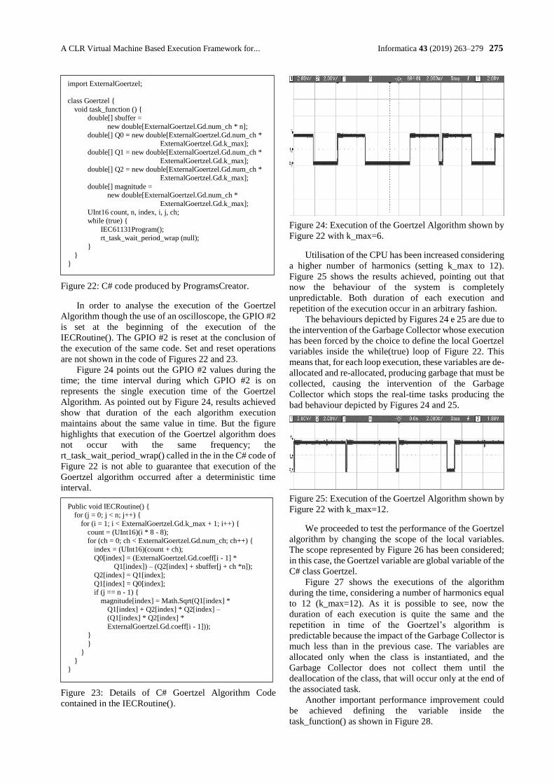
A CLR Virtual Machine Based Execution Framework for... Informatica 43 (2019) 263–279 275
In order to analyse the execution of the Goertzel
Algorithm though the use of an oscilloscope, the GPIO #2
is set at the beginning of the execution of the
IECRoutine(). The GPIO #2 is reset at the conclusion of
the execution of the same code. Set and reset operations
are not shown in the code of Figures 22 and 23.
Figure 24 points out the GPIO #2 values during the
time; the time interval during which GPIO #2 is on
represents the single execution time of the Goertzel
Algorithm. As pointed out by Figure 24, results achieved
show that duration of the each algorithm execution
maintains about the same value in time. But the figure
highlights that execution of the Goertzel algorithm does
not occur with the same frequency; the
rt_task_wait_period_wrap() called in the in the C# code of
Figure 22 is not able to guarantee that execution of the
Goertzel algorithm occurred after a deterministic time
interval.
Figure 23: Details of C# Goertzel Algorithm Code
contained in the IECRoutine().
Figure 24: Execution of the Goertzel Algorithm shown by
Figure 22 with k_max=6.
Utilisation of the CPU has been increased considering
a higher number of harmonics (setting k_max to 12).
Figure 25 shows the results achieved, pointing out that
now the behaviour of the system is completely
unpredictable. Both duration of each execution and
repetition of the execution occur in an arbitrary fashion.
The behaviours depicted by Figures 24 e 25 are due to
the intervention of the Garbage Collector whose execution
has been forced by the choice to define the local Goertzel
variables inside the while(true) loop of Figure 22. This
means that, for each loop execution, these variables are de-
allocated and re-allocated, producing garbage that must be
collected, causing the intervention of the Garbage
Collector which stops the real-time tasks producing the
bad behaviour depicted by Figures 24 and 25.
Figure 25: Execution of the Goertzel Algorithm shown by
Figure 22 with k_max=12.
We proceeded to test the performance of the Goertzel
algorithm by changing the scope of the local variables.
The scope represented by Figure 26 has been considered;
in this case, the Goertzel variable are global variable of the
C# class Goertzel.
Figure 27 shows the executions of the algorithm
during the time, considering a number of harmonics equal
to 12 (k_max=12). As it is possible to see, now the
duration of each execution is quite the same and the
repetition in time of the Goertzel’s algorithm is
predictable because the impact of the Garbage Collector is
much less than in the previous case. The variables are
allocated only when the class is instantiated, and the
Garbage Collector does not collect them until the
deallocation of the class, that will occur only at the end of
the associated task.
Another important performance improvement could
be achieved defining the variable inside the
task_function() as shown in Figure 28.
Public void IECRoutine() { for (j = 0; j < n; j++) {
for (i = 1; i < ExternalGoertzel.Gd.k_max + 1; i++) {
count = (UInt16)(i * 8 - 8); for (ch = 0; ch < ExternalGoertzel.Gd.num_ch; ch++) {
index = (UInt16)(count + ch);
Q0[index] = (ExternalGoertzel.Gd.coeff[i - 1] * Q1[index]) – (Q2[index] + sbuffer[j + ch *n]);
Q2[index] = Q1[index];
Q1[index] = Q0[index]; if (j == n - 1) {
magnitude[index] = Math.Sqrt(Q1[index] * Q1[index] + Q2[index] * Q2[index] –
(Q1[index] * Q2[index] *
ExternalGoertzel.Gd.coeff[i - 1])); }
}
} }
}
import ExternalGoertzel;
class Goertzel {
void task_function () { double[] sbuffer =
new double[ExternalGoertzel.Gd.num_ch * n];
double[] Q0 = new double[ExternalGoertzel.Gd.num_ch * ExternalGoertzel.Gd.k_max];
double[] Q1 = new double[ExternalGoertzel.Gd.num_ch *
ExternalGoertzel.Gd.k_max]; double[] Q2 = new double[ExternalGoertzel.Gd.num_ch *
ExternalGoertzel.Gd.k_max];
double[] magnitude = new double[ExternalGoertzel.Gd.num_ch *
ExternalGoertzel.Gd.k_max];
UInt16 count, n, index, i, j, ch; while (true) {
IEC61131Program();
rt_task_wait_period_wrap (null);
}
}
}
Figure 22: C# code produced by ProgramsCreator.
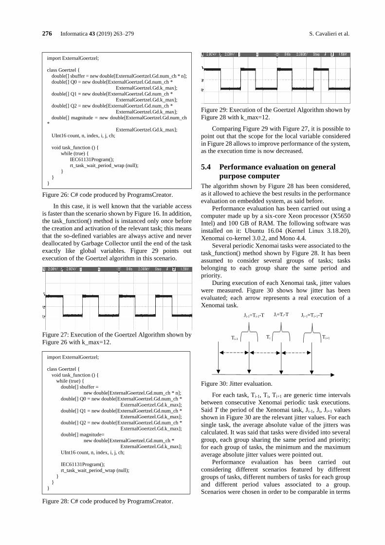
276 Informatica 43 (2019) 263–279 S. Cavalieri et al.
Figure 26: C# code produced by ProgramsCreator.
In this case, it is well known that the variable access
is faster than the scenario shown by Figure 16. In addition,
the task_function() method is instanced only once before
the creation and activation of the relevant task; this means
that the so-defined variables are always active and never
deallocated by Garbage Collector until the end of the task
exactly like global variables. Figure 29 points out
execution of the Goertzel algorithm in this scenario.
Figure 27: Execution of the Goertzel Algorithm shown by
Figure 26 with k_max=12.
Figure 28: C# code produced by ProgramsCreator.
Figure 29: Execution of the Goertzel Algorithm shown by
Figure 28 with k_max=12.
Comparing Figure 29 with Figure 27, it is possible to
point out that the scope for the local variable considered
in Figure 28 allows to improve performance of the system,
as the execution time is now decreased.
5.4 Performance evaluation on general
purpose computer
The algorithm shown by Figure 28 has been considered,
as it allowed to achieve the best results in the performance
evaluation on embedded system, as said before.
Performance evaluation has been carried out using a
computer made up by a six-core Xeon processor (X5650
Intel) and 100 GB of RAM. The following software was
installed on it: Ubuntu 16.04 (Kernel Linux 3.18.20),
Xenomai co-kernel 3.0.2, and Mono 4.4.
Several periodic Xenomai tasks were associated to the
task_function() method shown by Figure 28. It has been
assumed to consider several groups of tasks; tasks
belonging to each group share the same period and
priority.
During execution of each Xenomai task, jitter values
were measured. Figure 30 shows how jitter has been
evaluated; each arrow represents a real execution of a
Xenomai task.
Figure 30: Jitter evaluation.
For each task, Ti-1, Ti, Ti+1 are generic time intervals
between consecutive Xenomai periodic task executions.
Said T the period of the Xenomai task, Ji-1, Ji, Ji+1 values
shown in Figure 30 are the relevant jitter values. For each
single task, the average absolute value of the jitters was
calculated. It was said that tasks were divided into several
group, each group sharing the same period and priority;
for each group of tasks, the minimum and the maximum
average absolute jitter values were pointed out.
Performance evaluation has been carried out
considering different scenarios featured by different
groups of tasks, different numbers of tasks for each group
and different period values associated to a group.
Scenarios were chosen in order to be comparable in terms
import ExternalGoertzel;
class Goertzel {
double[] sbuffer = new double[ExternalGoertzel.Gd.num_ch * n]; double[] Q0 = new double[ExternalGoertzel.Gd.num_ch *
ExternalGoertzel.Gd.k_max];
double[] Q1 = new double[ExternalGoertzel.Gd.num_ch * ExternalGoertzel.Gd.k_max];
double[] Q2 = new double[ExternalGoertzel.Gd.num_ch *
ExternalGoertzel.Gd.k_max]; double[] magnitude = new double[ExternalGoertzel.Gd.num_ch
*
ExternalGoertzel.Gd.k_max]; UInt16 count, n, index, i, j, ch;
void task_function () { while (true) {
IEC61131Program();
rt_task_wait_period_wrap (null);
}
}
}
import ExternalGoertzel;
class Goertzel {
void task_function () { while (true) {
double[] sbuffer =
new double[ExternalGoertzel.Gd.num_ch * n]; double[] Q0 = new double[ExternalGoertzel.Gd.num_ch *
ExternalGoertzel.Gd.k_max];
double[] Q1 = new double[ExternalGoertzel.Gd.num_ch * ExternalGoertzel.Gd.k_max];
double[] Q2 = new double[ExternalGoertzel.Gd.num_ch * ExternalGoertzel.Gd.k_max];
double[] magnitude=
new double[ExternalGoertzel.Gd.num_ch * ExternalGoertzel.Gd.k_max];
UInt16 count, n, index, i, j, ch;
IEC61131Program();
rt_task_wait_period_wrap (null);
} }
}
Ti-1 Ti Ti+1
Ji-1=Ti-1-T Ji=Ti-T Ji+1=Ti+1-T

A CLR Virtual Machine Based Execution Framework for... Informatica 43 (2019) 263–279 277
of bandwidth utilisation, otherwise comparison between
their performances was meaningless.
For each group of tasks, the bandwidth utilisation has
been defined by:
𝑏𝑎𝑛𝑑𝑤𝑖𝑑𝑡ℎ 𝑢𝑡𝑖𝑙𝑖𝑠𝑎𝑡𝑖𝑜𝑛 =1
𝑇∗ 𝑛 ∗ 𝑡 (1)
where n is the number of tasks belonging to the group
and sharing the same period T, and t is the execution time
of the Program associated to the task.
Use of the parameter given by (1) allowed to compare
scenarios featured by the same bandwidth utilisation,
during the performance evaluation carried out.
Tables 1 and 2 show two of the scenarios considered.
Three groups of tasks have been considered for each
scenario. Inside each scenario, the groups differs for the
number of tasks and the relevant period. Comparing the
different scenarios, they feature groups with the same
bandwidth utilisation.
Tables 3 and 4 presents some of the results achieved.
They show the minimum and maximum average absolute
jitter values for each scenario and for each of the three
groups. As it can be seen, the average absolute jitter values
are always very close to zero.
Table 1: Scenario 1: Groups of Tasks with Period,
Number of Tasks and Bandwidth Utilisation.
Group Period
(ms)
Number of
Tasks
Bandwidth
Utilisation
1 50 100 30%
2 30 100 50%
3 25 100 60%
Table 2: Scenario 2: Groups of Tasks with Period,
Number of Tasks and Bandwidth Utilisation.
Group Period
(ms)
Number of
Tasks
Bandwidth
Utilisation
1 25 50 30%
2 15 50 50%
3 12.5 50 60%
Table 3: Scenario 1: Minimum and Maximum Average
Absolute Jitters.
Group Period (ms) Min (ms) Max (ms)
1 50 6.58 E-05 3.40 E-04
3 30 5.03 E-05 3.59 E-04
4 25 5.89 E-05 6.45 E-04
Table 4: Scenario 2: Minimum and Maximum Average
Absolute Jitters.
Group Period (ms) Min (ms) Max (ms)
1 25 5.27 E-05 1.89 E-04
2 15 5.39 E-05 3.41 E-04
3 12.5 5.86 E-05 6.96 E-04
These results seem to demonstrate that Garbage
Collector does not affect at all the performance of the
system. They confirm the same results achieved through
the experiments carried out by the embedded system and
shown in the previous subsection.
In order to verify this result, in the following an
analysis will be presented in order to point out what could
occur when the Garbage Collector intervenes. The C#
code shown by Figure 22 has been considered. As said, in
this scenario the local variables are mapped inside the
while(true) cycle; this means that the entire set of variables
are re-located for each cycle. This affects the heap
memory capacity, going to fill it and forcing the Garbage
Collector to intervene to free the unused variables, as each
cycle uses another set of the same local variables.
Tables 5 and 6 show the minimum and maximum
average absolute jitter values for the same scenarios seen
before. It is important to point out the higher values of the
jitter. Furthermore, it is important to compare the
maximum average absolute jitter values with the period of
each group; in some cases, the values are close to the same
periods, pointing out the very bad performance achieved.
Time instants of each Xenomai task execution have
been recorded during the performance evaluation,
considering again the C# code shown by Figure 22. The
entire set of the execution times for the tasks belonging to
each group has been carefully analysed. Analysis pointed
out that Xenomai task executions sometimes featured the
behaviour depicted by Figure 31. Each vertical arrow in
the figure represents a real execution; Ti is the time
interval between two consecutive executions, and the
dotted vertical arrows represents the instant at which a
periodic execution is expected but does not occur.
Table 5: Scenario 1: Minimum and Maximum Average
Absolute Jitters.
Group Period (ms) Min (ms) Max (ms)
1 50 9.38 11.30
2 30 5.62 11.12
3 25 4.77 12.56
Table 6: Scenario 2: Minimum and Maximum Average
Absolute Jitters.
Group Period (ms) Min (ms) Max (ms)
1 25 2.12 2.56
2 15 1.30 2.49
3 12.5 1.10 2.62
As shown by Figure 31, during a task execution, jitter
values greater than a multiple value of the task period may
occur. It has been observed that the generic Ti may be
greater than two or three times the task period, in the worst
cases. The only event which could cause this behaviour is
the running of Garbage Collector causing the stop of the
Figure 31: Xenomai task executions.
Ti
Ti
Ti
278 Informatica 43 (2019) 263–279 S. Cavalieri et al.
Xenomai tasks. Values of the time interval Ti clearly
depends on the execution times of the Garbage Collector
needed to collect all the garbage produced by the
programs.
7 Final remarks Paper has presented a software solution allowing the
execution of IEC 61131-3 applications into computing
systems based on a CLR VM. The software solution is
made up by two main components.
The first component is a software able to realise
translation of a generic IEC 61313-3 application into C#
code. For each IEC 61131-3 application a .cs file is
produced containing several classes relevant to the
original IEC 61131-3 sections; these classes may be
directly instantiated and used in a generic C# program
running inside a CLR VM. Otherwise, the output
produced may be passed to the second component here
presented, which is a real-time execution environment. It
is a framework able to realise the exact behaviour of a PLC
(e.g., Program Scan loops and real-time task scheduling).
It requires the presence of a CLR VM running on the top
of a real-time operating system. The framework receives
the C# classes produced by the first component described
before, achieved for an IEC 61131-3 application. On the
basis of these classes, it produces suitable C# programs
and real-time tasks associated to the programs to be
submitted to the underlying real-time operating system. In
this paper, use of Xenomai real-time co-kernel has been
presented.
After a description of both the software components,
the paper focused on a performance evaluation of
capability of the real-time environment to respect the
periodic constraints of real-time tasks. As known, in a
CLR VM-based environment, execution of a generic C#
program may be delayed by the activation of the Garbage
Collection. When a collection starts, it may cause the stop
of all the tasks associated to the C# program and the
increase of their execution time. The periodicity of one or
more tasks could be not respected for the same reason. The
results of the performance evaluation carried out by the
authors, pointed out that although Garbage Collector may
be a cause of performance degradation, its impact on the
performance of the system may be drastically limited. This
can be achieved by realising the right mapping between
the IEC 61131-3 original local variables defined inside
IEC 61131-3 PROGRAM section and the variables used
by the C# classes generated by the real-time environment.
Results presented in the paper, pointed out that the
mapping choices operated by the authors avoid the
intervention of the Garbage Collector. Under their
adoption, performance evaluation allowed to demonstrate
the capability of the real-time environment here presented
to respect real-time constraints of periodic tasks.
To the best of authors’ knowledge, current literature
does not provide solutions aimed to deploy IEC 61131-3
applications on CLR VM, using C# language as
intermediate code. Due to the spread current use of C#
language in the development of industrial applications,
adoption of the software solutions here presented seems
attractive. Typical candidate platforms on which
deployment may be achieved, are those based on general
purpose computer architecture (on which CLR VM allows
the use of common operating systems like Linux and
Windows), but also all the embedded systems supporting
a CLR VM may be considered.
Furthermore, the paper gives a contribution to a very
spread research field currently present in literature; in
particular it introduces a solution able to move
computation further away from the field level into the so-
called compute pools, which are decentralised and may be
also realised inside cloud computing solutions. In the
scenario proposed, the PLC is migrated to the compute
pool which can be realised by a computer architectures
based on CLR VM, as demonstrated by the research
presented in the paper.
Although the paper has been presented considering
Just-in-Time compilation, it is important to point out that
the procedures presented in the paper and aimed to
translate original IEC 61131-3 language-based programs
may be applied also into the case the Ahead-of-Time
(AOT) compilation was adopted.
References [1] R.W.Lewis (1998). Programming Industrial Control
Systems Using IEC 1131-3, IEE, ISBN-13: 978-
0852969502, 1998.
[2] J. D. Decotignie (2009). The many faces of industrial
ethernet [past and present]. IEEE Industrial
Electronics Magazine, vol. 3, no. 1, pp. 8–19.
https://doi.org/10.1109/mie.2009.932171
[3] M. Becker, K. Sandstrom, M. Behnam, T. Nolte
(2015). A many-core based execution framework for
IEC 61131-3. Proceedings of 41st IEEE Annual
Conference IECON 2015, pp.4525-4530,
https://doi.org/10.1109/IECON.2015.7392805.
[4] S. Mubeen, M. Becker, X. Zhao, L. Gan, M.
Behnam, T. Nolte (2016). Towards automated
deployment of IEC 61131-3 applications on multi-
core systems. Proceedings of IEEE World
Conference on Factory Communication Systems
(WFCS 2016), pp.1-4,
https://doi.org/10.1109/WFCS.2016.7496531.
[5] M. Simros, S. Theurich and M. Wollschlaeger
(2012). Programming Embedded Devices in IEC
61131-Languages with Industrial PLC Tools using
PLCOPEN XML. Proceedings of 10th Portuguese
Conference on Automatic Control (2012), pp.51-56.
[6] O. Givehchi, H. Trsek, and J. Jasperneite (2013).
Cloud computing for industrial automation systems
- a comprehensive overview. Proceedings of IEEE
18th Conference on Emerging Technologies Factory
Automation (ETFA 2013), pp.1–4.
https://doi.org/10.1109/etfa.2013.6648080
[7] O. Givehchi, J. Imtiaz, H. Trsek, and J. Jasperneite
(2014). Control-as-a-service from the cloud: A case
study for using virtualized PLCs. Proceedings of
10th IEEE Workshop on Factory Communication
Systems (WFCS 2014), pp.1–4.
https://doi.org/10.1109/wfcs.2014.6837587
A CLR Virtual Machine Based Execution Framework for... Informatica 43 (2019) 263–279 279
[8] I. Kühl and A. Fay (2011). A Middleware for
Software Evolution of Automation Software.
Proceedings of IEEE 16th Conference on Emerging
Technologies and Factory Automation (ETFA 2011),
pp.1-9.
https://doi.org/10.1109/etfa.2011.6059109
[9] Mono official website, available on
http://www.mono-project.com/
[10] Xenomai official website, available on
https://xenomai.org
[11] S. Cavalieri, L. Galvagno, M.S.Scroppo (2016). A
Framework based on CLR Virtual Machine to
deploy IEC 61131-3 programs. Proceedings of 14th
International Conference on Industrial Informatics
(INDIN 2016), University of Poitiers, Poitiers,
France,pp.126–131,
https://doi.org/10.1109/INDIN.2016.7819146.
[12] S. Cavalieri, L. Galvagno, G. Puglisi, M.S. Scroppo
(2016). Moving IEC 61131-3 applications to a
computing framework based on CLR Virtual
Machine. Proceedings of 21th International
Conference on Emerging Technologies and Factory
Automation (ETFA 2016), Berlin, Germany, pp.1-8,
https://doi.org/10.1109/ETFA.2016.7733632.
[13] Xenomai official API reference website, available on
https://xenomai.org/api-reference/
[14] Freescale Semiconductor, MPC8309 (2014).
PowerQUICC II Pro Integrated Communications
Processor Family Hardware Specifications, Data
Sheet. Document Number MPC8309EC, Rev 4,
12/2014. Available on http://www.nxp.com/
[15] Gold parsing system official website, available on
http://www.goldparser.org/
[16] G. Goertzel (1958). An algorithm for the evaluation
of finite trigonometric series. American
Mathematical Monthly, Vol. 65, No. 1, pp. 34-35,
https://doi.org/10.2307/2310304

280 Informatica 43 (2019) 263–279 S. Cavalieri et al.
https://doi.org/10.31449/inf.v43i2.2133 Informatica 43 (2019) 281–289 281
A Comparative Study of Automatic Programming Techniques
Sibel Arslan and Celal Öztürk
Erciyes University, Engineering Faculty, Computer Engineering Department, Kayseri, Turkey
E-mail: [email protected], [email protected]
Keywords: automatic programming, genetic programming, artificial bee colony programming, symbolic regression,
prediction, feature selection
Received: January 3, 2018
Automatic programming, an evolutionary computing technique, forms the programs automatically and is
based on higher level features that can be easily specified than normal programming languages. Genetic
Programming (GP) is the first and best-known automatic programming technique that is applied to solve
many practical problems. Artificial Bee Colony Programming (ABCP) is one of the latest proposed
automatic programming method that combines evolutionary approach with swarm intelligence. GP is an
extension version of Genetic Algorithm (GA) and ABCP is based on Artificial Bee Colony (ABC)
algorithm. The main differences of these automatic programing techniques and their conventional
algorithms (GA and ABC) are modeling solution. In ABC same as GA, the solutions are represented fixed
code blocks. In GP and ABCP, the positions of food sources are expressed in tree structure that is
composed of different combinations of terminals and functions that are specifically defined as problems.
This paper presents a review on GP and ABCP and they are worked in symbolic regression, prediction
and feature selection problems which are widely tackled by researchers. The results of the ABCP
compared with results of GP show that this algorithm is a powerful optimization technique for structural
design.
Povzetek: Predstavljena je primerjalna analiza tehnik avtomatskega programiranja.
1 Introduction Computer programming is the process of obtaining a
program that can be executed machine to use the necessary
information to perform a task. Automatic programming is
a computer programming technique which automatically
generates the program code [1]. It provides practical
solutions for many machine learning methods such as
Artificial Neural Network (ANN), Decision Trees (DT),
Support Vector Machines (SVM), Genetic Programming
(GP), Artificial Bee Colony Programming (ABCP). GP,
most well-known automatic programming method, was
developed by Koza [2]. GP is an extension of Genetic
Algorithm (GA) and the basic steps for the GP algorithm
are similar to the steps of GA. ABCP is recently proposed
automatic programming technique which is based on the
Artificial Bee Colony Algorithm (ABC) [3]. The goal of
this paper is to evaluate the success of the models obtained
from these automatic programming methods in symbolic
regression, prediction and feature selection problems and
review papers related to the problems.
Symbolic regression is a type of regression problem
aimed at finding the most appropriate mathematical model
in terms of accuracy and complexity of data. There are
works investigating the problem of symbolic regression
with automatic programing techniques, mostly with GP
[3-10]. ABCP was proposed for the first time as a new
method for the symbolic regression problem and
compared with GP [3]. Faris proposed solving the
symbolic regression problem using GP model was
compared to least square estimation, GA and particle
swarm intelligence models based on estimating the
parameters of the nonlinear regressive curve of the cutting
tool [4]. According to the benchmarks in the paper, GP
was found to be superior performance. In [5], two versions
of GP (standard GP and multi-population GP) were
compared with ANN on pharmaceutical formulation
symbolic regression problem. Compared to successful
ANN models, GP models provided a significant
advantage, parametric equations that can be interpreted
and analyzed more easily. Gene Expression Programming
(GEP) [6], Immune Programming (IP) [7], Ant Colony
Programming (ACP) [8-10] are other automated
programming techniques that used in the problem of
symbolic regression. GEP, proposed on both GA and GP,
is flexible at genetic operations due to its linear code
blocks and its parse trees [6]. IP is based on Artificial
Immune System (AIS) and is a domain-independent
approach [7] where antigens can be represented in the tree
structure express solutions similar to GP. ACP [8, 9] and
Dynamic Ant Colony Programming (DAP) which
dynamic version of ACP [10] are the main ACP examples
that are inspired on ant colony algorithm.
Automatic programming techniques have been solved
prediction problems where most of applications are based
on evolutionary optimization techniques [11-19]. Seidy
proposed a new stock market prediction model using the
Particle Swarm Optimization with Center of Mass
Technique (PSOCoM) which was more successful results
than the particle swarm optimization based models
according to the prediction accuracy [11]. Manjusha et al.
used Naive Bayes and J48 algorithms to diagnose
potentially fatal dermatological diseases with similar
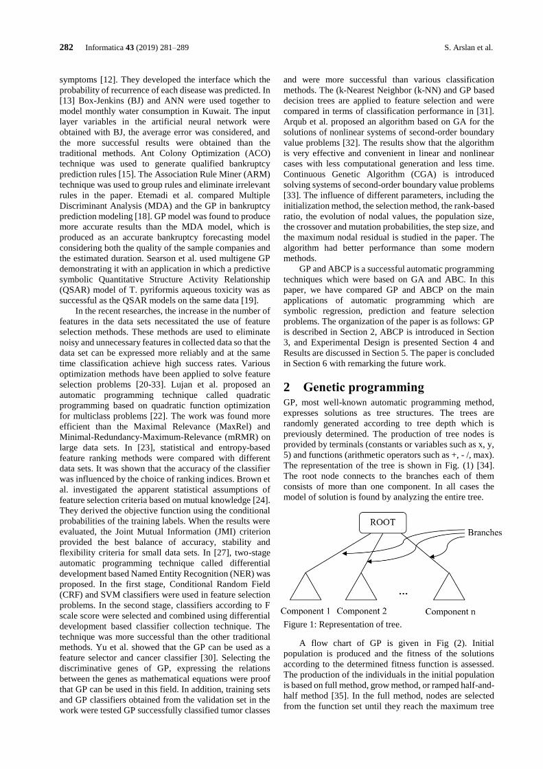
282 Informatica 43 (2019) 281–289 S. Arslan et al.
symptoms [12]. They developed the interface which the
probability of recurrence of each disease was predicted. In
[13] Box-Jenkins (BJ) and ANN were used together to
model monthly water consumption in Kuwait. The input
layer variables in the artificial neural network were
obtained with BJ, the average error was considered, and
the more successful results were obtained than the
traditional methods. Ant Colony Optimization (ACO)
technique was used to generate qualified bankruptcy
prediction rules [15]. The Association Rule Miner (ARM)
technique was used to group rules and eliminate irrelevant
rules in the paper. Etemadi et al. compared Multiple
Discriminant Analysis (MDA) and the GP in bankruptcy
prediction modeling [18]. GP model was found to produce
more accurate results than the MDA model, which is
produced as an accurate bankruptcy forecasting model
considering both the quality of the sample companies and
the estimated duration. Searson et al. used multigene GP
demonstrating it with an application in which a predictive
symbolic Quantitative Structure Activity Relationship
(QSAR) model of T. pyriformis aqueous toxicity was as
successful as the QSAR models on the same data [19].
In the recent researches, the increase in the number of
features in the data sets necessitated the use of feature
selection methods. These methods are used to eliminate
noisy and unnecessary features in collected data so that the
data set can be expressed more reliably and at the same
time classification achieve high success rates. Various
optimization methods have been applied to solve feature
selection problems [20-33]. Lujan et al. proposed an
automatic programming technique called quadratic
programming based on quadratic function optimization
for multiclass problems [22]. The work was found more
efficient than the Maximal Relevance (MaxRel) and
Minimal-Redundancy-Maximum-Relevance (mRMR) on
large data sets. In [23], statistical and entropy-based
feature ranking methods were compared with different
data sets. It was shown that the accuracy of the classifier
was influenced by the choice of ranking indices. Brown et
al. investigated the apparent statistical assumptions of
feature selection criteria based on mutual knowledge [24].
They derived the objective function using the conditional
probabilities of the training labels. When the results were
evaluated, the Joint Mutual Information (JMI) criterion
provided the best balance of accuracy, stability and
flexibility criteria for small data sets. In [27], two-stage
automatic programming technique called differential
development based Named Entity Recognition (NER) was
proposed. In the first stage, Conditional Random Field
(CRF) and SVM classifiers were used in feature selection
problems. In the second stage, classifiers according to F
scale score were selected and combined using differential
development based classifier collection technique. The
technique was more successful than the other traditional
methods. Yu et al. showed that the GP can be used as a
feature selector and cancer classifier [30]. Selecting the
discriminative genes of GP, expressing the relations
between the genes as mathematical equations were proof
that GP can be used in this field. In addition, training sets
and GP classifiers obtained from the validation set in the
work were tested GP successfully classified tumor classes
and were more successful than various classification
methods. The (k-Nearest Neighbor (k-NN) and GP based
decision trees are applied to feature selection and were
compared in terms of classification performance in [31].
Arqub et al. proposed an algorithm based on GA for the
solutions of nonlinear systems of second-order boundary
value problems [32]. The results show that the algorithm
is very effective and convenient in linear and nonlinear
cases with less computational generation and less time.
Continuous Genetic Algorithm (CGA) is introduced
solving systems of second-order boundary value problems
[33]. The influence of different parameters, including the
initialization method, the selection method, the rank-based
ratio, the evolution of nodal values, the population size,
the crossover and mutation probabilities, the step size, and
the maximum nodal residual is studied in the paper. The
algorithm had better performance than some modern
methods.
GP and ABCP is a successful automatic programming
techniques which were based on GA and ABC. In this
paper, we have compared GP and ABCP on the main
applications of automatic programming which are
symbolic regression, prediction and feature selection
problems. The organization of the paper is as follows: GP
is described in Section 2, ABCP is introduced in Section
3, and Experimental Design is presented Section 4 and
Results are discussed in Section 5. The paper is concluded
in Section 6 with remarking the future work.
2 Genetic programming GP, most well-known automatic programming method,
expresses solutions as tree structures. The trees are
randomly generated according to tree depth which is
previously determined. The production of tree nodes is
provided by terminals (constants or variables such as x, y,
5) and functions (arithmetic operators such as +, - /, max).
The representation of the tree is shown in Fig. (1) [34].
The root node connects to the branches each of them
consists of more than one component. In all cases the
model of solution is found by analyzing the entire tree.
Figure 1: Representation of tree.
A flow chart of GP is given in Fig (2). Initial
population is produced and the fitness of the solutions
according to the determined fitness function is assessed.
The production of the individuals in the initial population
is based on full method, grow method, or ramped half-and-
half method [35]. In the full method, nodes are selected
from the function set until they reach the maximum tree
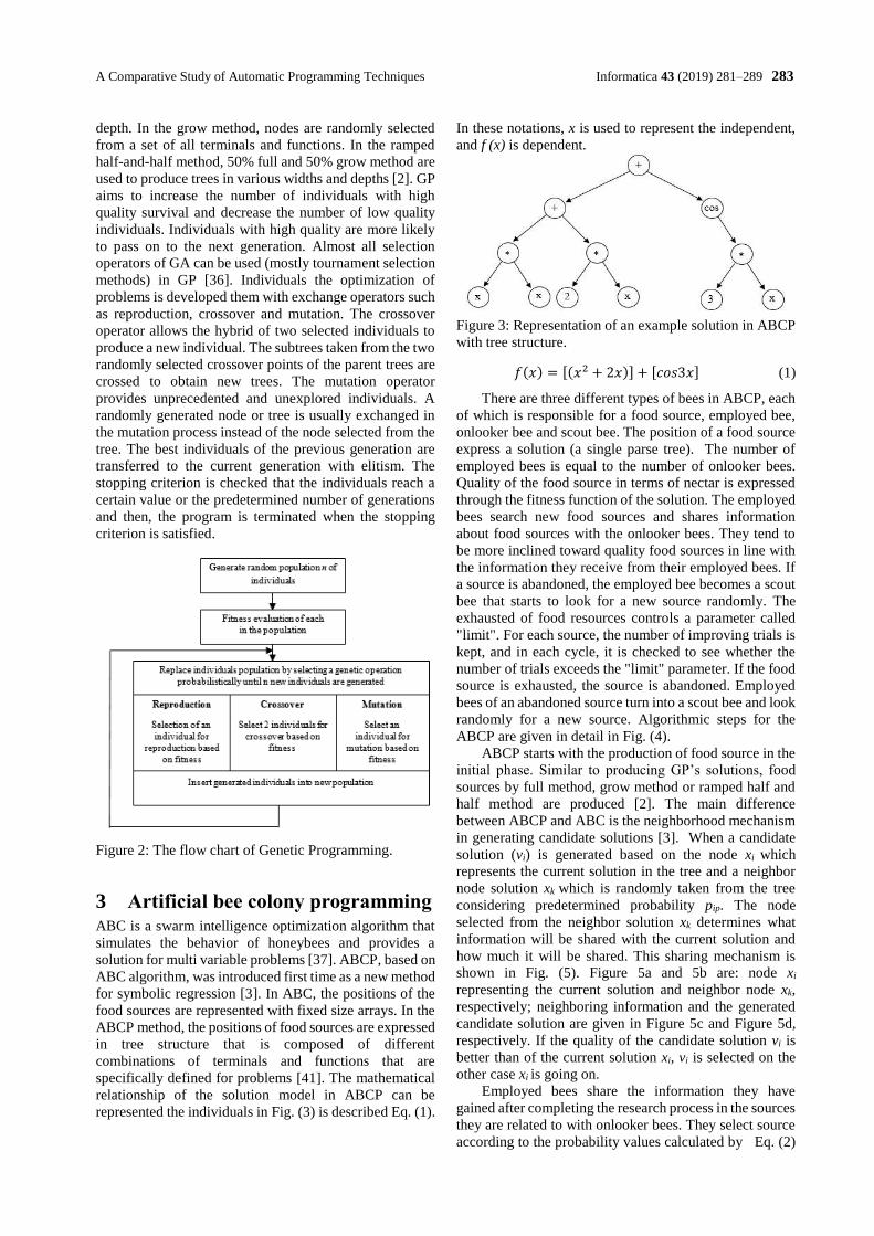
A Comparative Study of Automatic Programming Techniques Informatica 43 (2019) 281–289 283
depth. In the grow method, nodes are randomly selected
from a set of all terminals and functions. In the ramped
half-and-half method, 50% full and 50% grow method are
used to produce trees in various widths and depths [2]. GP
aims to increase the number of individuals with high
quality survival and decrease the number of low quality
individuals. Individuals with high quality are more likely
to pass on to the next generation. Almost all selection
operators of GA can be used (mostly tournament selection
methods) in GP [36]. Individuals the optimization of
problems is developed them with exchange operators such
as reproduction, crossover and mutation. The crossover
operator allows the hybrid of two selected individuals to
produce a new individual. The subtrees taken from the two
randomly selected crossover points of the parent trees are
crossed to obtain new trees. The mutation operator
provides unprecedented and unexplored individuals. A
randomly generated node or tree is usually exchanged in
the mutation process instead of the node selected from the
tree. The best individuals of the previous generation are
transferred to the current generation with elitism. The
stopping criterion is checked that the individuals reach a
certain value or the predetermined number of generations
and then, the program is terminated when the stopping
criterion is satisfied.
Figure 2: The flow chart of Genetic Programming.
3 Artificial bee colony programming ABC is a swarm intelligence optimization algorithm that
simulates the behavior of honeybees and provides a
solution for multi variable problems [37]. ABCP, based on
ABC algorithm, was introduced first time as a new method
for symbolic regression [3]. In ABC, the positions of the
food sources are represented with fixed size arrays. In the
ABCP method, the positions of food sources are expressed
in tree structure that is composed of different
combinations of terminals and functions that are
specifically defined for problems [41]. The mathematical
relationship of the solution model in ABCP can be
represented the individuals in Fig. (3) is described Eq. (1).
In these notations, x is used to represent the independent,
and f (x) is dependent.
Figure 3: Representation of an example solution in ABCP
with tree structure.
𝑓(𝑥) = [(𝑥2 + 2𝑥)] + [𝑐𝑜𝑠3𝑥] (1)
There are three different types of bees in ABCP, each
of which is responsible for a food source, employed bee,
onlooker bee and scout bee. The position of a food source
express a solution (a single parse tree). The number of
employed bees is equal to the number of onlooker bees.
Quality of the food source in terms of nectar is expressed
through the fitness function of the solution. The employed
bees search new food sources and shares information
about food sources with the onlooker bees. They tend to
be more inclined toward quality food sources in line with
the information they receive from their employed bees. If
a source is abandoned, the employed bee becomes a scout
bee that starts to look for a new source randomly. The
exhausted of food resources controls a parameter called
"limit". For each source, the number of improving trials is
kept, and in each cycle, it is checked to see whether the
number of trials exceeds the "limit" parameter. If the food
source is exhausted, the source is abandoned. Employed
bees of an abandoned source turn into a scout bee and look
randomly for a new source. Algorithmic steps for the
ABCP are given in detail in Fig. (4).
ABCP starts with the production of food source in the
initial phase. Similar to producing GP’s solutions, food
sources by full method, grow method or ramped half and
half method are produced [2]. The main difference
between ABCP and ABC is the neighborhood mechanism
in generating candidate solutions [3]. When a candidate
solution (vi) is generated based on the node xi which
represents the current solution in the tree and a neighbor
node solution xk which is randomly taken from the tree
considering predetermined probability pip. The node
selected from the neighbor solution xk determines what
information will be shared with the current solution and
how much it will be shared. This sharing mechanism is
shown in Fig. (5). Figure 5a and 5b are: node xi
representing the current solution and neighbor node xk,
respectively; neighboring information and the generated
candidate solution are given in Figure 5c and Figure 5d,
respectively. If the quality of the candidate solution vi is
better than of the current solution xi, vi is selected on the
other case xi is going on.
Employed bees share the information they have
gained after completing the research process in the sources
they are related to with onlooker bees. They select source
according to the probability values calculated by Eq. (2)
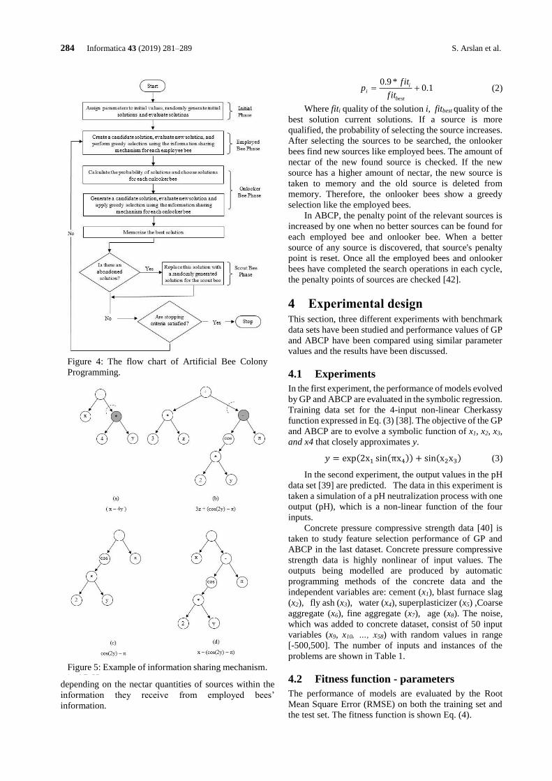
284 Informatica 43 (2019) 281–289 S. Arslan et al.
depending on the nectar quantities of sources within the
information they receive from employed bees’
information.
1.0*9.0
+=best
ii
f it
f itp (2)
Where fiti quality of the solution i, fitbest quality of the
best solution current solutions. If a source is more
qualified, the probability of selecting the source increases.
After selecting the sources to be searched, the onlooker
bees find new sources like employed bees. The amount of
nectar of the new found source is checked. If the new
source has a higher amount of nectar, the new source is
taken to memory and the old source is deleted from
memory. Therefore, the onlooker bees show a greedy
selection like the employed bees.
In ABCP, the penalty point of the relevant sources is
increased by one when no better sources can be found for
each employed bee and onlooker bee. When a better
source of any source is discovered, that source's penalty
point is reset. Once all the employed bees and onlooker
bees have completed the search operations in each cycle,
the penalty points of sources are checked [42].
4 Experimental design This section, three different experiments with benchmark
data sets have been studied and performance values of GP
and ABCP have been compared using similar parameter
values and the results have been discussed.
4.1 Experiments
In the first experiment, the performance of models evolved
by GP and ABCP are evaluated in the symbolic regression.
Training data set for the 4-input non-linear Cherkassy
function expressed in Eq. (3) [38]. The objective of the GP
and ABCP are to evolve a symbolic function of x1, x2, x3,
and x4 that closely approximates y.
𝑦 = exp(2x1 sin(πx4)) + sin(x2x3) (3)
In the second experiment, the output values in the pH
data set [39] are predicted. The data in this experiment is
taken a simulation of a pH neutralization process with one
output (pH), which is a non-linear function of the four
inputs.
Concrete pressure compressive strength data [40] is
taken to study feature selection performance of GP and
ABCP in the last dataset. Concrete pressure compressive
strength data is highly nonlinear of input values. The
outputs being modelled are produced by automatic
programming methods of the concrete data and the
independent variables are: cement (x1), blast furnace slag
(x2), fly ash (x3), water (x4), superplasticizer (x5) ,Coarse
aggregate (x6), fine aggregate (x7), age (x8). The noise,
which was added to concrete dataset, consist of 50 input
variables (x9, x10, …, x58) with random values in range
[-500,500]. The number of inputs and instances of the
problems are shown in Table 1.
4.2 Fitness function - parameters
The performance of models are evaluated by the Root
Mean Square Error (RMSE) on both the training set and
the test set. The fitness function is shown Eq. (4).
Figure 4: The flow chart of Artificial Bee Colony
Programming.
Figure 5: Example of information sharing mechanism.
in ABCP.

A Comparative Study of Automatic Programming Techniques Informatica 43 (2019) 281–289 285
𝑓𝑖𝑡𝑛𝑒𝑠𝑠 = √∑ (𝑦𝑝𝑟𝑒𝑑−𝑦𝑎𝑐𝑡𝑢𝑎𝑙)
2𝑛𝑡=1
𝑛 (4)
Where n define the data size, yactual is y values from
data set, ypred is the predicted y value by obtained solution.
The complexity of the solution is calculated as in Eq.
(5) in proportion to the depth of the tree and the number
of nodes.
𝐶 = ∑ 𝑛 ∗ 𝑘𝑑𝑘=1 (5)
Where C is tree complexity, d is the depth of the
solution, and n is the number of nodes at depth. The
parameters for GP and ABCP are summarized in Table 2.
The add3 function is the sum of three variables (𝑥1+
𝑥2+ 𝑥3) and the mult3 function is the multiplication of
three variables (𝑥1* 𝑥2* 𝑥3). If the divisor value is equal
to zero, the result is 1, otherwise the normal division is
performed in the rdivide function. The ifbte and the iflte
indicates the condition of the nodes. Eq. (6) and Eq. (7)
describe how the functions operate condition expressions.
𝑋 = 𝑖𝑓𝑏𝑡𝑒(𝐴, 𝐵, 𝐶, 𝐷) 𝑖𝑓(𝐴 ≥ 𝐵)𝑡ℎ𝑒𝑛 𝑋 = 𝐶 𝑒𝑙𝑠𝑒 𝑋 = 𝐷 (6)
𝑋 = 𝑖𝑓𝑙𝑡𝑒(𝐴, 𝐵, 𝐶, 𝐷) 𝑖𝑓(𝐴 < 𝐵)𝑡ℎ𝑒𝑛 𝑋 = 𝐶 𝑒𝑙𝑠𝑒 𝑋 = 𝐷 (7)
The population size was taken high value according to the
curse of the data sets in the literature. When experiments
are evaluated, it is observed that the optimum results were
obtained where population/ colony size was set to 100 for
Cherkassy, 200 for pH and 300 for Concrete. Therefore,
other parameters like generation number and maximum
tree depth values was set to make fair test with same
parameters like in the literature. In this work, the stop
criterion is decided by using the maximum generation
number for both GP and ABCP.
5 Results & discussions This section demonstrate symbolic regression, prediction
and feature selection abilities of ABCP and GP, set of
experiments conducted.
5.1 Simulation Results
The experiments are run 30 times independently for
ABCP and GP and the obtained results are demonstrated
in Table 3 for the problems. The R2 values of the best
cases of GP and ABCP are also presented in the table for
training and test sets.
Metric Criteria
Problems
Cherkassy pH Concrete
GP ABCP GP ABCP GP ABCP
Mean RMSE 0.07 0.03 0.92 0.77 11.64 10.50
Std RMSE 0.03 0.02 0.14 0.07 2.38 1.51
Best RMSE 0.02 0.01 0.60 0.59 8.83 8.26
Worst RMSE 0.11 0.09 12.60 0.88 16.77 14.57
Best 𝑅𝑡𝑟𝑎𝑖𝑛2 0.97 1.00 0.90 0.96 0.72 0.76
Best 𝑅𝑡𝑒𝑠𝑡2 0.98 1.00 0.91 0.96 0.70 0.73
Table 3. Obtained results of GP and ABCP.
While obtaining the results of GP on symbolic
regression problem, the GPTIPS (an open source symbolic
regression solution toolbox) [39] is modified and used in
this work. It indicates ABCP has much better training
Nam
e
#In
pu
ts
#To
tal I
nst
ance
s
#Tra
inin
g In
stan
ces
#Te
st In
stan
ces
No
ise
Cherkassy 4 500 400 100 -
pH 4 990 700 299 -
Concrete 8 1030 773 257 50 input variables
[-500,500]
Table 1: Benchmark Problems.
Parameters
Problems
Cherkassy pH Concrete
GP ABCP GP ABCP GP ABCP
Population /
Colony size 100 100 200 200 300 300
Iteration size 100 100 200 200 500 500
Maximum tree
depth 12 12 12 12 12 12
Tournament
size 6 - 25 - 15 -
Mutation ratio 0.14 - 0.14 - 0.14 -
Crossover ratio 0.84 - 0.84 - 0.84 -
Direct
reproduction
ratio
0.02 - 0.02 - 0.02 -
Functions
+,-, *, tan, sin,
cos, square, max, min, exp,
ifbte, iflte
+, -, *, tanh, add3, mult3
+,-
,*,rdivide,sin, cos,exp,rlog,
add3,mult3
Constans [-10,10] [-10,10] [-10,10]
Table 2: Parameters for GP and ABCP.
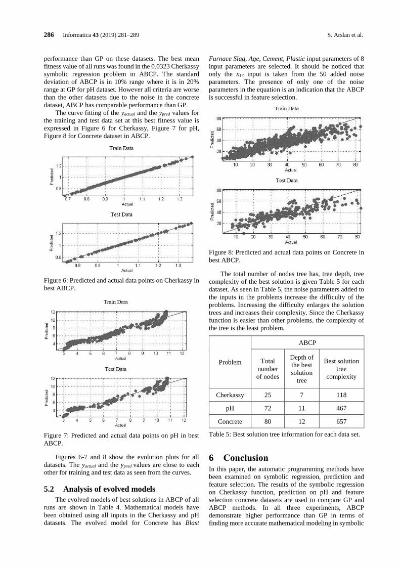
286 Informatica 43 (2019) 281–289 S. Arslan et al.
performance than GP on these datasets. The best mean
fitness value of all runs was found in the 0.0323 Cherkassy
symbolic regression problem in ABCP. The standard
deviation of ABCP is in 10% range where it is in 20%
range at GP for pH dataset. However all criteria are worse
than the other datasets due to the noise in the concrete
dataset, ABCP has comparable performance than GP.
The curve fitting of the yactual and the ypred values for
the training and test data set at this best fitness value is
expressed in Figure 6 for Cherkassy, Figure 7 for pH,
Figure 8 for Concrete dataset in ABCP.
Figure 6: Predicted and actual data points on Cherkassy in
best ABCP.
Figure 7: Predicted and actual data points on pH in best
ABCP.
Figures 6-7 and 8 show the evolution plots for all
datasets. The yactual and the ypred values are close to each
other for training and test data as seen from the curves.
5.2 Analysis of evolved models
The evolved models of best solutions in ABCP of all
runs are shown in Table 4. Mathematical models have
been obtained using all inputs in the Cherkassy and pH
datasets. The evolved model for Concrete has Blast
Furnace Slag, Age, Cement, Plastic input parameters of 8
input parameters are selected. It should be noticed that
only the x17 input is taken from the 50 added noise
parameters. The presence of only one of the noise
parameters in the equation is an indication that the ABCP
is successful in feature selection.
Figure 8: Predicted and actual data points on Concrete in
best ABCP.
The total number of nodes tree has, tree depth, tree
complexity of the best solution is given Table 5 for each
dataset. As seen in Table 5, the noise parameters added to
the inputs in the problems increase the difficulty of the
problems. Increasing the difficulty enlarges the solution
trees and increases their complexity. Since the Cherkassy
function is easier than other problems, the complexity of
the tree is the least problem.
Problem
ABCP
Total
number
of nodes
Depth of
the best
solution
tree
Best solution
tree
complexity
Cherkassy 25 7 118
pH 72 11 467
Concrete 80 12 657
Table 5: Best solution tree information for each data set.
6 Conclusion In this paper, the automatic programming methods have
been examined on symbolic regression, prediction and
feature selection. The results of the symbolic regression
on Cherkassy function, prediction on pH and feature
selection concrete datasets are used to compare GP and
ABCP methods. In all three experiments, ABCP
demonstrate higher performance than GP in terms of
finding more accurate mathematical modeling in symbolic
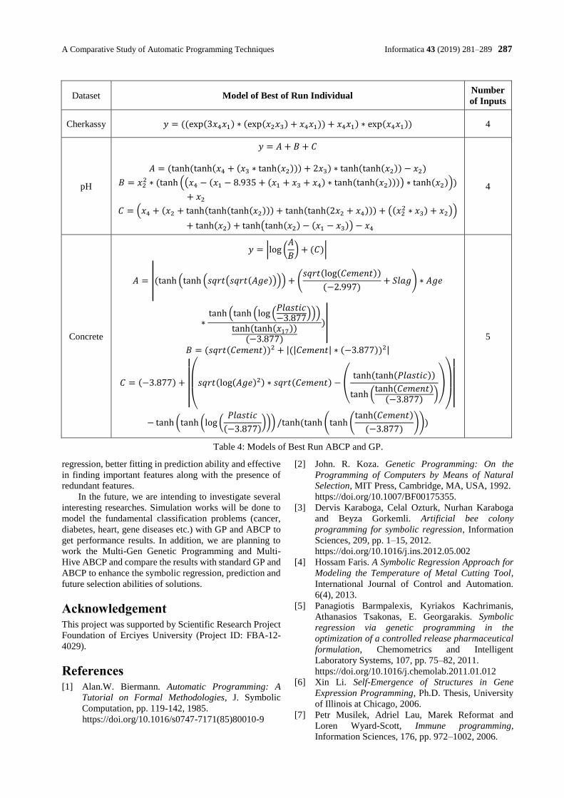
A Comparative Study of Automatic Programming Techniques Informatica 43 (2019) 281–289 287
regression, better fitting in prediction ability and effective
in finding important features along with the presence of
redundant features.
In the future, we are intending to investigate several
interesting researches. Simulation works will be done to
model the fundamental classification problems (cancer,
diabetes, heart, gene diseases etc.) with GP and ABCP to
get performance results. In addition, we are planning to
work the Multi-Gen Genetic Programming and Multi-
Hive ABCP and compare the results with standard GP and
ABCP to enhance the symbolic regression, prediction and
future selection abilities of solutions.
Acknowledgement This project was supported by Scientific Research Project
Foundation of Erciyes University (Project ID: FBA-12-
4029).
References [1] Alan.W. Biermann. Automatic Programming: A
Tutorial on Formal Methodologies, J. Symbolic
Computation, pp. 119-142, 1985.
https://doi.org/10.1016/s0747-7171(85)80010-9
[2] John. R. Koza. Genetic Programming: On the
Programming of Computers by Means of Natural
Selection, MIT Press, Cambridge, MA, USA, 1992.
https://doi.org/10.1007/BF00175355.
[3] Dervis Karaboga, Celal Ozturk, Nurhan Karaboga
and Beyza Gorkemli. Artificial bee colony
programming for symbolic regression, Information
Sciences, 209, pp. 1–15, 2012.
https://doi.org/10.1016/j.ins.2012.05.002
[4] Hossam Faris. A Symbolic Regression Approach for
Modeling the Temperature of Metal Cutting Tool,
International Journal of Control and Automation.
6(4), 2013.
[5] Panagiotis Barmpalexis, Kyriakos Kachrimanis,
Athanasios Tsakonas, E. Georgarakis. Symbolic
regression via genetic programming in the
optimization of a controlled release pharmaceutical
formulation, Chemometrics and Intelligent
Laboratory Systems, 107, pp. 75–82, 2011.
https://doi.org/10.1016/j.chemolab.2011.01.012
[6] Xin Li. Self-Emergence of Structures in Gene
Expression Programming, Ph.D. Thesis, University
of Illinois at Chicago, 2006.
[7] Petr Musilek, Adriel Lau, Marek Reformat and
Loren Wyard-Scott, Immune programming,
Information Sciences, 176, pp. 972–1002, 2006.
Dataset Model of Best of Run Individual Number
of Inputs
Cherkassy 𝑦 = ((exp(3𝑥4𝑥1) ∗ (exp(𝑥2𝑥3) + 𝑥4𝑥1)) + 𝑥4𝑥1) ∗ exp(𝑥4𝑥1)) 4
pH
𝑦 = 𝐴 + 𝐵 + 𝐶
𝐴 = (tanh (tanh(𝑥4 + (𝑥3 ∗ tanh(𝑥2))) + 2𝑥3) ∗ tanh(tanh(𝑥2)) − 𝑥2)
𝐵 = 𝑥22 ∗ (tanh ((𝑥4 − (𝑥1 − 8.935 + (𝑥1 + 𝑥3 + 𝑥4) ∗ tanh(tanh(𝑥2)))) ∗ tanh(𝑥2)))
+ 𝑥2
𝐶 = (𝑥4 + (𝑥2 + tanh(tanh(tanh(𝑥2))) + tanh(tanh(2𝑥2 + 𝑥4))) + ((𝑥22 ∗ 𝑥3) + 𝑥2))
+ tanh(𝑥2) + tanh(tanh(𝑥2) − (𝑥1 − 𝑥3)) − 𝑥4
4
Concrete
𝑦 = |log (𝐴
𝐵) + (𝐶)|
𝐴 = |(tanh (tanh (𝑠𝑞𝑟𝑡(𝑠𝑞𝑟𝑡(𝐴𝑔𝑒)))) + (𝑠𝑞𝑟𝑡(log(𝐶𝑒𝑚𝑒𝑛𝑡))
(−2.997)+ 𝑆𝑙𝑎𝑔) ∗ 𝐴𝑔𝑒
∗tanh (tanh (log (
𝑃𝑙𝑎𝑠𝑡𝑖𝑐−3.877
)))
tanh(tanh(𝑥17))(−3.877)
)|
𝐵 = (𝑠𝑞𝑟𝑡(𝐶𝑒𝑚𝑒𝑛𝑡))2 + |(|𝐶𝑒𝑚𝑒𝑛𝑡| ∗ (−3.877))2|
𝐶 = (−3.877) + ||
(
𝑠𝑞𝑟𝑡(log(𝐴𝑔𝑒)2) ∗ 𝑠𝑞𝑟𝑡(𝐶𝑒𝑚𝑒𝑛𝑡) − (
tanh(tanh(𝑃𝑙𝑎𝑠𝑡𝑖𝑐))
tanh (tanh(𝐶𝑒𝑚𝑒𝑛𝑡)(−3.877)
))
)
||
− tanh (tanh (log (𝑃𝑙𝑎𝑠𝑡𝑖𝑐
(−3.877)))) /tanh (tanh (tanh (
tanh(𝐶𝑒𝑚𝑒𝑛𝑡)
(−3.877))))
5
Table 4: Models of Best Run ABCP and GP.
288 Informatica 43 (2019) 281–289 S. Arslan et al.
https://doi.org/10.1016/j.ins.2005.03.009.
[8] Mariusz Boryczka, Ant colony programming:
application of ant colony system to function
approximation, Intelligent Systems for Automated
Learning and Adaptation: Emerging Trends and
Applications, pp. 248–272, 2010.
https://doi.org/10.4018/978-1-60566-798-0.ch011.
[9] Olivier Roux, Cyril Fonlupt . Ant programming or,
how to use ants for automatic programming,
Proceedings of ANTS’2000, pp. 121– 129, 2000.
[10] Shinichi Shirakawa, Shintaro Ogino, Tomoharu
Nagao. T. Nagao, Dynamic ant programming for
automatic construction of programs, IEEE
Transactions on Electrical and Electronic
Engineering, pp. 540–548, 2008.
https://doi.org/10.1002/tee.20311.
[11] Essam.El. Seidy. A New Particle Swarm
Optimization Based Stock Market Prediction
Technique, International Journal of Advanced
Computer Science and Applications (IJACSA), Vol.
7, No. 4, 2016.
https://doi.org/10.14569/ijacsa.2016.070442.
[12] K.K. Manjusha, K. Sankaranayanan, P. Seena. Data
Mining in Dermatological Diagnosis: A Method for
Severity Prediction, International Journal of
Computer Applications, (0975 – 8887) Vol. 117 –
No.11, 2015.
[13] Sana BuHamra, Nejib Smaoui, Mahmoud Gabr. The
Box–Jenkins analysis and neural networks:
prediction and time series modelling, Applied
Mathematical Modelling, Vol: 27,pp. 805–815,
2003.
https://doi.org/10.1016/s0307-904x(03)00079-9.
[14] Gianluca Bontempi. Machine Learning Strategies
for Time Series Prediction, Machine Learning
Group, Computer Science Department Boulevard de
Triomphe - CP 212, Hammamet, 2013.
Retrieved from: http://www.ulb.ac.be/di.
[15] A. Martin, V. Aswathy, V.Prasanna Venkatesan.
Framing Qualitative Bankruptcy Prediction Rules
Using Ant Colony Algorithm, International Journal
of Computer Applications, 0975 – 8887 ,Volume
41– No.21, 2012.
https://doi.org/10.5120/5827-8143.
[16] Shuzhan Wan, Shengwu. Xiong and Yi Liu,
Prediction based multi-strategy differential
evolution algorithm for dynamic environments,
Evolutionary Computation (CEC), 2012 IEEE
Congress, pp. 10-15, 2012.
https://doi.org/10.1109/cec.2012.6256628.
[17] Dandan .Li, Wanxin. Xue, Yilei Pei . A high-
precision prediction model using Ant Colony
Algorithm and neural network, International
Conference on Logistics, Informatics and Service
Sciences (LISS), 2015.
https://doi.org/10.1109/liss.2015.7369696.
[18] Hossein Etemadi, Ali Asghar Anvary Rostamy,
Hossan Farajzadeh Dehkordi . A genetic
programming model for bankruptcy prediction:
Empirical evidence from Iran, Expert Systems with
Applications, Vol: 36, pp. 3199–3207, 2009.
https://doi.org/10.1016/j.eswa.2008.01.012.
[19] Pamela Dominic, David Edward Leahy, Mark J.
Willis. Predicting the toxicity of chemical
compounds using GPTIPS: a free open source
genetic programming toolbox for MATLAB,
Intelligent Control and Computer Engineering,
Lecture Notes in Electrical Engineering, Vol. 70,
Springer, pp. 83-93, 2011.
https://doi.org/10.1007/978-94-007-0286-8_8.
[20] Yudong Zhang, Shuihua Wanga, Preetha Phillips,
Genlin Ji. Binary PSO with mutation operator for
feature selection using decision tree applied to spam
detection, Knowledge-Based Systems, Vol: 64, pp.
22–31,2014.
https://doi.org/10.1016/j.knosys.2014.03.015.
[21] Mark A. Hall , Correlation-based Feature Selection
for Machine Learning, PhD Thesis, The University
of Waikato, 1999.
[22] Irene Rodriguez Lujan, Ramon Huerta, Charles
Elkan, Carlos Santa Cruz. Quadratic Programming
Feature Selection, Journal of Machine Learning
Research, 11, pp. 1491-1516, 2010.
[23] Jasmina Novakovıć, Perica Strbac, Dusan Bulatovıć.
Toward Optimal Feature Selection Using Ranking
Methods And Classification Algorithms, Yugoslav
Journal of Operations Research, Vol: 21, Number 1,
pp. 119-135, 2011.
https://doi.org/10.2298/yjor1101119n.
[24] Gavin Brown, Adam Pocock, Ming-Jie Zhao, Mikel
Luj´an. Conditional Likelihood Maximisation: A
Unifying Framework for Information Theoretic
Feature Selection, Journal of Machine Learning
Research, Vol: 13, pp. 27-66, 2012.
[25] Riyaz Sikora, Selwyn Piramuthu . Framework For
Efficient Feature Selection In Genetic Algorithm
Based Data Mining, European Journal of
Operational Research, Vol:180, pp. 723–737, 2007.
https://doi.org/10.1016/j.ejor.2006.02.040.
[26] Shital C. Shah, Andrew Kusiak. Data mining and
genetic algorithm based gene/SNP selection,
Artificial Intelligence in Medicine, Vol: 31, pp.
183—196, 2004.
https://doi.org/10.1016/j.artmed.2004.04.002.
[27] Utpal Kumar Sikdar, Asif Ekbal, Sriparna Saha.
Differential Evolution based Feature Selection and
Classifier Ensemble for Named Entity Recognition,
Proceedings of COLING 2012: Technical Papers.
COLING 2012, Mumbai, December, pp. 2475–
2490, 2012.
https://doi.org/10.1007/s10032-011-0155-7.
[28] Yuanning Liu, Gang Wang, Huiling Chen, Hao
Dong, X.iaodong Zhu, Sujing Wang . An Improved
Particle Swarm Optimization for Feature Selection,
Journal of Bionic Engineering, Vol: 8, 2011.
https://doi.org/10.1016/s1672-6529(11)60020-6.
[29] Bing Xue, Mengijie Zhang, Will N. Browne.
Particle Swarm Optimization for Feature Selection
in Classification: A Multi-Objective Approach, IEEE
Transactıons on Cybernetıcs, Vol. 43, No. 6, 2013.
https://doi.org/10.1109/tsmcb.2012.2227469.
A Comparative Study of Automatic Programming Techniques Informatica 43 (2019) 281–289 289
[30] Jianjun Yu, Jindan Yu, Arpit A. Almal, Saravana
M.Dhanasekaran ,Debashis Ghosh, William
P.Worzel, Arul M.Chinnaiyan. Feature Selection
and Molecular Classification of Cancer Using
Genetic Programming, Neoplasia, Vol. 9, No:4, pp.
292 – 303, 2007.
https://doi.org/10.1593/neo.07121.
[31] Jacques-Andre Landry, Luis Da Costa and Thomas
Bernier. Discriminant Feature Selection by Genetic
Programming: Towards a domain independent
multi-class object detection system, Systemics
Cybernetics and Informatics, Vol: 3(1), pp. 76-81,
2006.
[32] Omer Abu-Arqub, Zaer Abo-Hammour, Shaher
Mohammad Momani. Application of Continuous
Genetic Algorithm for Nonlinear System of Second-
Order Boundary Value Problems, Applied
Mathematics& Information Sciences, 8, No.1, pp.
235-248, 2014.
https://doi.org/10.12785/amis/080129.
[33] Omer Abu-Arqub, Zaer Abo-Hammour. Numerical
solution of systems of second-order boundary value
problems using continuous genetic algorithm,
Information Sciences, Vol: 279, pp. 396-415, 2014.
https://doi.org/10.1016/j.ins.2014.03.128.
[34] Riccardo Poli, William B. Langdon, Nicholas F.
McPhee, John R. Koza, A Field Guide to Genetic
Programming, 2016.
http://cswww.essex.ac.uk/staff/rpoli/gp-field-guide/.
[35] Zhaohui Gan, Tommy W.SChow, W.N.Chau. Clone
selection programming and its application to
symbolic regression, Expert Systems with
Applications, Vol: 36, 2009, pp. 3996–4005, 2009.
https://doi.org/10.1016/j.eswa.2008.02.030.
[36] Hajira Jabeen, Abdul Rauf Baig. Review of
Classification Using Genetic Programming,
International Journal of Engineering Science and
Technology, Vol: 2, pp. 94-103, 2010.
[37] Beyza Gorkemli. Study of Artificial Bee Colony
Programming (ABCP) to Symbolic Regression
Problems, PhD Thesis, Erciyes University,
Engineering Faculty, Computer Engineering
Department, 2015.
[38] Vladimir Cherkassky, Don Gehring, Filip Mulier.
Comparison of adaptive methods for function
estimation from samples, IEEE Transactions on
Neural Networks, Vol: 7 (4), 1996, pp. 969- 984,
1996.
https://doi.org/10.1109/72.508939
[39] Dominic P. Searson, GPTIPS 2: an open-source
software platform for symbolic data mining. Chapter
22 in Handbook of Genetic Programming
Applications, A.H. Gandomi et al., (Eds.), Springer,
New York, NY, 2015., https://
sites.google.com/site/gptips4matlab/file-cabinet.
https://doi.org/10.1007/978-3-319-20883-1_22
[40] UCI, Machine Learning Repository, Concrete
Compressive Strength Data Set.
https://archive.ics.uci.edu/ml/datasets/Concrete+Co
mpressive+Strength, Access Date: 15.10.2016.
[41] Sibel Arslan, Celal Ozturk, Multi Hive Artificial Bee
Colony Programming for high dimensional symbolic
regression with feature selection, Applied Soft
Computing Journal 78, 515–527, 2019.
https://doi.org/10.1016/j.asoc.2019.03.014.
[42] Sibel Arslan, Celal Ozturk, Artificial Bee Colony
Programming Descriptor for Multi-Class Texture
Classification, Applied Sciences, 9(9), 2019.
https://doi.org/10.3390/app9091930.

290 Informatica 43 (2019) 281–289 S. Arslan et al.
https://doi.org/10.31449/inf.v43i2.2303 Informatica 43 (2019) 291–298 291
Evolving Neural Network CMAC and its Applications
Oleg Rudenko, Oleksandr Bessonov and Oleksandr Dorokhov
Kharkiv National University of Economics, Nauka Ave 9a, 61166 Kharkiv, Ukraine
E-mail: [email protected]
Keywords: neural network, training, nonlinear object, identification, adaptive control
Received: April 21, 2018
The conventional neural network (NN) CMAC (Cerebellar Model Articulation Controller) can be
applied in many real-world applications thanks to its high learning speed and good generalization
capability. In this paper, it is proposed to utilize a neuro-evolutional approach to adjust CMAC
parameters and construct mathematical models of nonlinear objects in the presence of the Gaussian
noise. The general structure of the evolving NN CMAC (ECMAC) is considered. The paper
demonstrates that the evolving NN CMAC can be used effectively for the identification of nonlinear
dynamical systems. The simulation of the proposed approach for various nonlinear objects is performed.
The results proved the effectiveness of the developed methods.
Povzetek: Razvit je postopek za evolucijsko iskanje najbolj prilagojene CMAC (Cerebellar Model
Articulation Controller) nevronske mreže za probleme z Gaussovim šumom.
1 Introduction Using a mathematical model of the cerebellar cortex
developed by D. Marr [1] in 1975 J. Albus proposed a
model describing the motion control processes that occur
in the cerebellum, which was subsequently implemented
in the neural network controller for controlling the robot
- arm, which he called CMAC - Cerebellar Model
Articulation Controller [2, 3]. Ease of implementation
and a good network of approximating properties have
ensured its wide usage not only in the tasks of controlling
the robotic arm in real time, but also to solve many other
practical problems [4-14].
However, it should be noted that in designing a
network CMAC a number of difficulties in the selection
of parameters such as the number of levels and the
quantization levels, the shape of the receptive field, the
type of applied information hashing algorithm and
training. These parameters have a significant impact on
the accuracy and speed of CMAC network, and
therefore, the determination of the optimal values of
these parameters is an important practical problem. In
this article, for eliminating the drawbacks of traditional
methods of synthesis and functioning ANN CMAC we
provide the use of a new class of networks - evolving
ANN (EANN) in which, in addition to traditional
learning it is used another fundamental form of
adaptation - evolution, realized by applying the
evolutionary computation [15-18].
The use of two forms of adaptation in EANN -
evolution, and training, allowing to change the network
structure, its parameters and learning algorithms without
external intervention, make the network data most
suitable for work in non-stationary conditions and
uncertainty about the properties of the object under study
and the conditions of its functioning.
The main advantage of using evolutionary
algorithms (EA) as learning algorithms is that many
ANN parameters can be encoded in the genome and
determined in parallel. Moreover, unlike most
optimization algorithms designed to solve a problem, EA
operate with a multitude of solutions - the population,
which allows reaching a global minimum, without
getting stuck in the local ones. In this case, information
about each individual of the population is encoded in a
chromosome (genotype), and the solution (phenotype) is
obtained after evolution (selection, crossing, mutation)
by decoding.
Among EAs that are stochastic and include
evolutionary programming, evolutionary strategies,
genetic algorithms, genetic programming, in particular,
programming with gene expression, genetic algorithms
(GA) are the most common [19,20]. GA abstract the
fundamental processes of Darwinian evolution: natural
selection and genetic changes due to recombination and
mutation.
2 Neural network CMAC The modification of the network proposed by Albus is
shown in Figure 1. The network consists of the input,
hidden and output layers, labeled L1, L2, L3,
respectively, and uses two basic conversions:
S: XA, (1)
P: Ay, (2)
where X - N-dimensional space of continuous input
signals; A - n-dimensional space associations; y - a one-
dimensional output.
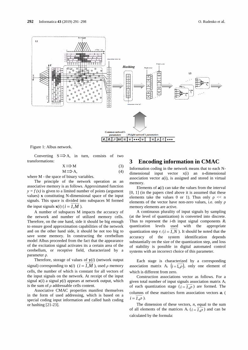
292 Informatica 43 (2019) 291–298 O. Rudenko et al.
Converting SA, in turn, consists of two
transformations:
XM (3)
MA, (4)
where M - the space of binary variables.
The principle of the network operation as an
associative memory is as follows. Approximated function
y = f (x) is given to a limited number of points (argument
values) x constituting N-dimensional space of the input
signals. This space is divided into subspaces M formed
the input signals x(i) ( M,1i = ).
A number of subspaces M impacts the accuracy of
the network and number of utilized memory cells.
Therefore, on the one hand, side it should be big enough
to ensure good approximation capabilities of the network
and on the other hand side, it should be not too big to
save some memory. In constructing the cerebellum
model Albus proceeded from the fact that the appearance
of the excitation signal activates its a certain area of the
cerebellum, or receptive field, characterized by a
parameter ρ.
Therefore, storage of values of y(i) (network output
signal) corresponding to x(i) ( M,1i = ), used ρ memory
cells, the number of which is constant for all vectors of
the input signals on the network. At receipt of the input
signal x(i) a signal y(i) appears at network output, which
is the sum of ρ addressable cells content.
Associative CMAC properties manifest themselves
in the form of used addressing, which is based on a
special coding input information and called hash coding
or hashing [21-23].
3 Encoding information in CMAC Information coding in the network means that to each N-
dimensional input vector x(i) an n-dimensional
association vector a(i), is assigned and stored in virtual
memory.
Elements of a(i) can take the values from the interval
[0, 1] (in the papers cited above it is assumed that these
elements take the values 0 or 1). Thus only ρ << n
elements of the vector have non-zero values, i.e. only ρ
memory elements are active.
A continuous plurality of input signals by sampling
(at the level of quantization) is converted into discrete.
Thus to represent the i-th input signal components Ri
quantization levels used with the appropriate
quantization step ri ( ). It should be noted that the
accuracy of the system identification depends
substantially on the size of the quantization step, and loss
of stability is possible in digital automated control
systems with an incorrect choice of this parameter.
Each stage is characterized by a corresponding
association matrix Ai , only one element of
which is different from zero.
Construction associations vector as follows. For a
given total number of input signals association matrix Ai
of each quantization stage ( ) are formed. The
columns of these matrixes form association vectors ai (
).
The dimension of these vectors, n, equal to the sum
of all elements of the matrices Ai ( ) and can be
calculated by the formula:
N,1i =
( ),1=i
,1i =
,1i =
,1i =
Figure 1: Albus network.

Evolving Neural Network CMAC and... Informatica 43 (2019) 291–298 293
+
−=
N
11R
n
, (5)
where R - the number of used levels for quantizing input
signals; N - the dimension of the input vector; - means
rounded to the nearest whole number.
Since all ρ matrices Ai ( ,1i = ) have only one non-
zero element, from the n components of the vector a(i)
only ρ are non-zero.
The quantization region is arranged in such a way,
that any of them relating to the adjacent stages have not
more than (ρ - 1)-th connection. This corresponds to a
restriction on the maximum total number of cells equal to
(ρ - 1) used for storing two different vectors of the input
signals in which their recognition is still possible.
4 Selecting the basic functions of
neurons Selecting the basic functions of neurons in L1 layer
significantly affects the approximating properties of
CMAC network.
As already noted, the traditional CMAC performs
piecewise constant approximation, that is a consequence
of the usage of neurons with a rectangular activation
function.
When choosing rectangular basis functions
computational cost will be minimal. Also, CMAC
networks widely use B-splines as basis functions.
B-splines undoubted advantage is the possibility of
recurrent calculating in both the splines in accordance
with the formula [24-27]:
)()()( ,1
1
1,1
1
, xBx
xBx
xB jn
njj
j
jn
njj
nj
jn −
+−
−−
−−
−
−
−+
−
−=
(6)
and their derivatives -order:
( )
( )
, 1, 1
1
( 1)( ) ( )
( 1)
j n
n j n j
j j n
xnB x B x
n
−
− −
− −
−−= +
− − −
( )
1,
1
( 1)( )
( 1)
j
n j
j j n
xnB x
n
−
− +
−−+
− − −
(7)
Here:
)
= −
otherwise; ,0
;, xif ,1)( 1,0
jjj xB
)
= −
otherwise; ,0
;, xif ,1)( 1,0
)0(jj
j xB
−−
−=
+−
−
−
−−
−−
−
1
,1
)1(
1
1,1
)1(
,
)()()(
)(njj
jn
njj
jn
jn
xBxBxB
(8)
where j - j-th spline’s node (center of the quantization
field).
Thus, after determining the active slot ],( 1 jj − for
the zero order B-spline, these expressions can be used to
obtain the values of all nonzero B-spline of higher order
and, if appropriate, their derivatives. Note that traditional СМАС uses zero order B-
spline. Selection of the first order B-spline leads to the
triangular membership function, and selection of the
fourth-order B-spline leads to membership function
similar to the Gaussian.
The CMAC network also uses Gaussian activation
function of the form:
−−=
2
2)exp)(
i
ji xФμ(x j (9)
As a basis one can use trigonometric functions, for
example, cosine:
( )
+−
−
=
otherwise, 0
];2
r,
2
r( хif
rcos
)(jj
jj
iiij
ji
xxФ
(10)
where - i-th center of the quantization field; rj -
quantization step of j-th component of the input signal.
However, it should be noted that although the most
commonly used Gaussian membership functions also
allow a very simple calculation of derivatives and have
the property of a local activation, it is difficult to allocate
clearly enough their activation boundary, which is often
important for the implementation of the network that
used, for example, scaling basis functions.
In order to eliminate this disadvantage, one can use a
modified Gaussian function that has the following form:
−−
−−
=
otherwise. 0
);,( хif ))((
4/)(exp
)( 2121
21
xxxФi
2 (11)
As seen from the expression (11), the function is
strictly defined in the range (λ1, λ2), which simplifies the
process of scaling basis functions when the network
parameters such as R and ρ are changing.
5 Network training
Defining the network parameters, i.e. in the general case
defining a vector ( )k , that includes all network
parameters (weights, parameters of basis functions, etc.)
is accomplished by training with the teacher.
The training criterion can be presented as follows:
( )=
=k
i
iekeF1
)()( , (12)
where ( ))(ie - some loss function.
•
i

294 Informatica 43 (2019) 291–298 O. Rudenko et al.
Gradient network training algorithm has the
following form:
( ( ))ˆ ˆ( ) ( 1) ( )j
F e kk k k
= − +
, (13)
or
( )( )ˆ ˆ( ) ( 1) ( ) ( )
j
e kk k k e k
= − +
(14)
where 0 – parameter that affects the training speed
and which can be selected differently for different
network parameters.
Training of traditional CMAC that uses
( ) 2( ) 0,5 ( )e i e i = and rectangular basis functions,
occurs on each step after the presentation of training
pairs )}(),({ kykx , where )(ky – function’s value,
that corresponds )(kx , and consists in the correction of
only those of its weights that correspond to the single
components of the association vector for a given vector
)(kx .
In this case, the training algorithm for all i , j , for
which 1)()( == kaka ji , is the following:
1
1( 1) ( ) ( ) ( ) ,
n
j j i
i
w k w k y k w k =
+ = + −
(15)
where ]1,0( – parameter that affects the speed of
training.
When membership functions with a form other than
rectangular are used, this algorithm can be written as
follows:
,)()()()(
)()()()()()()1(
2
−+=+ kax
kax
kwxkakykkwkw
T
(16)
where )(k - in general case a variable parameter.
Multistep network training algorithms were
considered in [7,8].
6 Evolving ANN CMAC During switching from ANN to EANN for all types of
networks the common evolutionary procedure
(initialization population, an estimation of the
population, selection, cross-breeding, mutations) is used.
Differences are only in the method of encoding the
structure and parameters of a particular form of ANN in
the chromosome.
At the beginning of EA functioning, a population 0P
that consisting of N individuals (ANN):
NHHHP ,,..., 210 = is randomly initialized. The
proper choice of the N’s value is very important as this
parameter significantly affects the speed of the algorithm
and its selection is critical for real-time systems.
Each individual in the population at the same time
gets its own unique description, encoded in the
chromosome Ljjjj hhhH ,..., 21=,
which consists
of L gene, wherein maxmin wwhij - i-th value of j-
gene chromosome (minw - the minimum and
maxw -
maximum allowable values, respectively).
Figure 1 shows an example ECMAC chromosome’s
format and the correspondence between genes and
network parameters stored in the chromosome. It should
be noted that chromosome length depends on the
dimensionality of the problem and the maximum amount
of memory.
As seen from the drawing, it consists of a
chromosome gene in which information about
corresponding network parameters is stored. At the
beginning of the chromosome, there are genes that
contain information about the parameters of the noise
and they are active only in case of the noisy
measurements. Next gene’s block encodes the number of
levels and the quantization steps, the shape of the
receptive field of neurons and type of algorithm that is
used for hashing information.
Due to the large amount of the BF that can be used in
CMAC, there is a special gene in its chromosome BF,
that is responsible for coding the type of the used
functions. There is also a gene H in the chromosome, that
encodes a type of the hashing algorithm (If its value is set
to 0 then hashing is not used).
Then, in the chromosome, there is a group of genes
encoding weighting parameters directly relevant to the
associative neurons. During the initialization phase,
initial values are assigned to all these parameters by
using a random number generator.
Since during evolution mutation may occur in the
parameters affecting the amount of used associative
neurons, the length of the chromosome can vary. The use
of variable length chromosomes occur individuals with
specific genetic code segments (introns) which are not
used for coding characteristics [28-29].
Typically, introns are used in the EA:
- as noncoding bits that are uniformly added to the
genetic code (in this case, introns only fill the space
between the active genes of the chromosome);
- as the nonfunctional parts of the genetic code, i.e.,
parts of the decision which do not actually do anything,
thus not affect the fitness of the chromosome (this
usually occurs in the genetic programming and in the
chromosomes, which are subject to the cycle of
development after birth);
-as posterior useless part of the chromosome, which
do not participate in the calculation of its fitness (usually
it manifests itself in some types of competitive-trained
neural networks, in which only neurons-winners in
contrast to other neurons that are a posteriori useless
affect network performance results).
Introns appear in other types of neural networks,
where they are called potentially useful waste.
The control of introns amount in the population
carried out by:
- the use of special operators, that alter the length of
the chromosome and add or remove introns
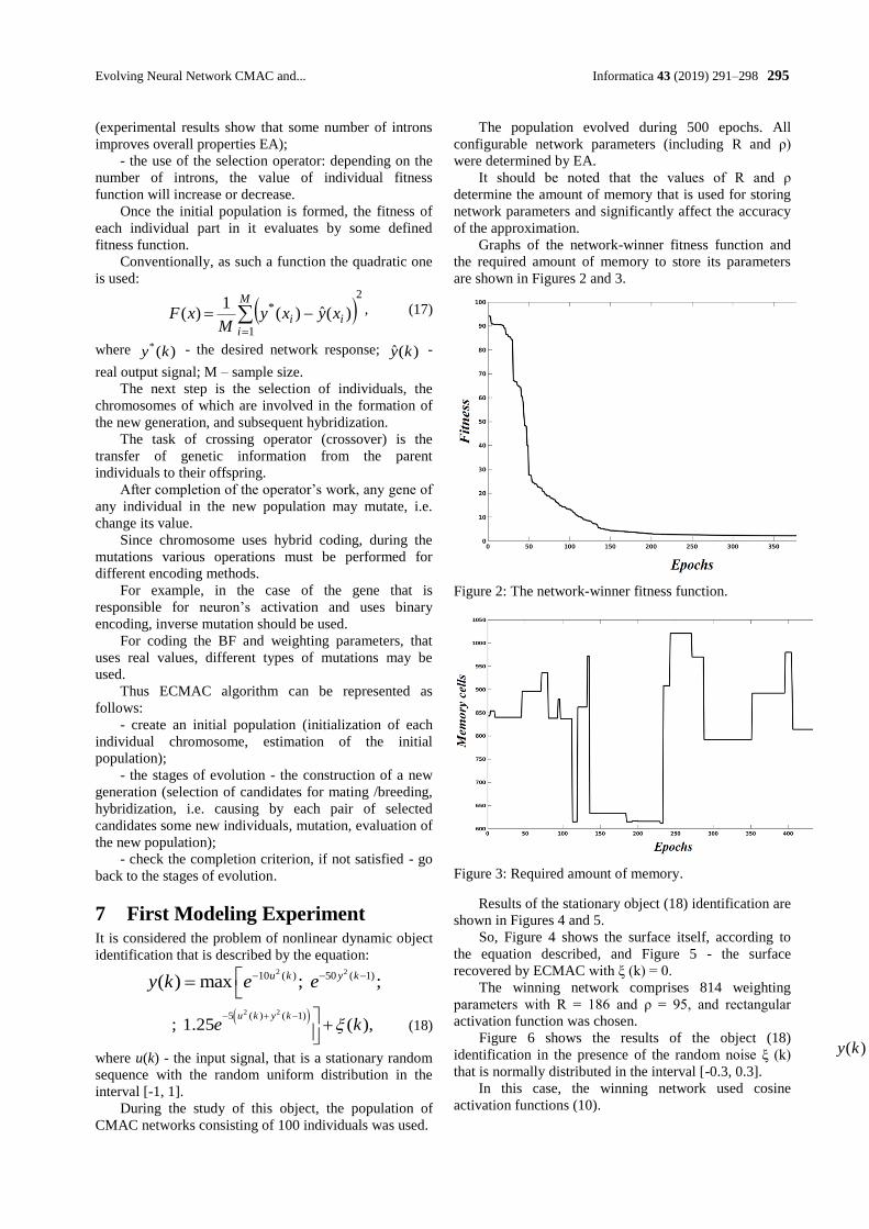
Evolving Neural Network CMAC and... Informatica 43 (2019) 291–298 295
(experimental results show that some number of introns
improves overall properties EA);
- the use of the selection operator: depending on the
number of introns, the value of individual fitness
function will increase or decrease.
Once the initial population is formed, the fitness of
each individual part in it evaluates by some defined
fitness function.
Conventionally, as such a function the quadratic one
is used:
( )2
1
* )(ˆ)(1
)( =
−=M
iii xyxy
MxF , (17)
where )(* ky - the desired network response; )(ˆ ky -
real output signal; M – sample size.
The next step is the selection of individuals, the
chromosomes of which are involved in the formation of
the new generation, and subsequent hybridization.
The task of crossing operator (crossover) is the
transfer of genetic information from the parent
individuals to their offspring.
After completion of the operator’s work, any gene of
any individual in the new population may mutate, i.e.
change its value.
Since chromosome uses hybrid coding, during the
mutations various operations must be performed for
different encoding methods.
For example, in the case of the gene that is
responsible for neuron’s activation and uses binary
encoding, inverse mutation should be used.
For coding the BF and weighting parameters, that
uses real values, different types of mutations may be
used.
Thus ECMAC algorithm can be represented as
follows:
- create an initial population (initialization of each
individual chromosome, estimation of the initial
population);
- the stages of evolution - the construction of a new
generation (selection of candidates for mating /breeding,
hybridization, i.e. causing by each pair of selected
candidates some new individuals, mutation, evaluation of
the new population);
- check the completion criterion, if not satisfied - go
back to the stages of evolution.
7 First Modeling Experiment It is considered the problem of nonlinear dynamic object
identification that is described by the equation: 2 210 ( ) 50 ( 1)( ) max ; ;u k y ky k e e− − −=
( )2 25 ( ) ( 1); 1.25 ( ),
u k y ke k− + − +
(18)
where u(k) - the input signal, that is a stationary random
sequence with the random uniform distribution in the
interval [-1, 1].
During the study of this object, the population of
CMAC networks consisting of 100 individuals was used.
The population evolved during 500 epochs. All
configurable network parameters (including R and ρ)
were determined by EA.
It should be noted that the values of R and ρ
determine the amount of memory that is used for storing
network parameters and significantly affect the accuracy
of the approximation.
Graphs of the network-winner fitness function and
the required amount of memory to store its parameters
are shown in Figures 2 and 3.
Figure 2: The network-winner fitness function.
Figure 3: Required amount of memory.
Results of the stationary object (18) identification are
shown in Figures 4 and 5.
So, Figure 4 shows the surface itself, according to
the equation described, and Figure 5 - the surface
recovered by ECMAC with ξ (k) = 0.
The winning network comprises 814 weighting
parameters with R = 186 and ρ = 95, and rectangular
activation function was chosen.
Figure 6 shows the results of the object (18)
identification in the presence of the random noise ξ (k)
that is normally distributed in the interval [-0.3, 0.3].
In this case, the winning network used cosine
activation functions (10).
)(ky
)(ku )1( −ky
k
)(ky
)(ky
)(ky
k
k
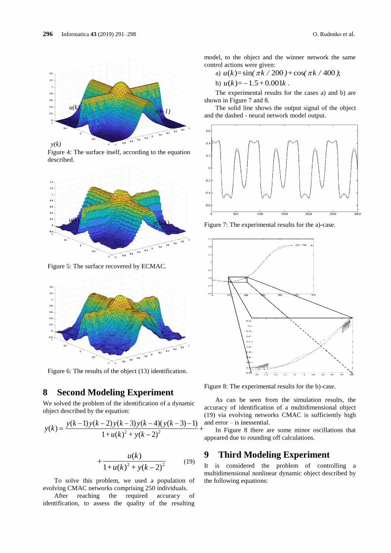
296 Informatica 43 (2019) 291–298 O. Rudenko et al.
8 Second Modeling Experiment We solved the problem of the identification of a dynamic
object described by the equation:
2 2
( 1) ( 2) ( 3) ( 4)( ( 3) 1)( )
1 ( ) ( 2)
y k y k y k y k y ky k
+u k + y k
− − − − − −= +
−
2 2
( )
1 ( ) ( 2)
u k
+u k + y k+
− (19)
To solve this problem, we used a population of
evolving CMAC networks comprising 250 individuals.
After reaching the required accuracy of
identification, to assess the quality of the resulting
model, to the object and the winner network the same
control actions were given:
a) ( )=sin 200 cos 400 ;u k ( k / )+ ( k / )
b) ( )= 1 5 0 001u k . + . k− .
The experimental results for the cases a) and b) are
shown in Figure 7 and 8.
The solid line shows the output signal of the object
and the dashed - neural network model output.
Figure 7: The experimental results for the a)-case.
Figure 8: The experimental results for the b)-case.
As can be seen from the simulation results, the
accuracy of identification of a multidimensional object
(19) via evolving networks CMAC is sufficiently high
and error – is inessential.
In Figure 8 there are some minor oscillations that
appeared due to rounding off calculations.
9 Third Modeling Experiment It is considered the problem of controlling a
multidimensional nonlinear dynamic object described by
the following equations:
Figure 4: The surface itself, according to the equation
described.
Figure 5: The surface recovered by ECMAC.
Figure 6: The results of the object (13) identification.
u(k) y(k-1)
u(k) y(k-1)
y(k)
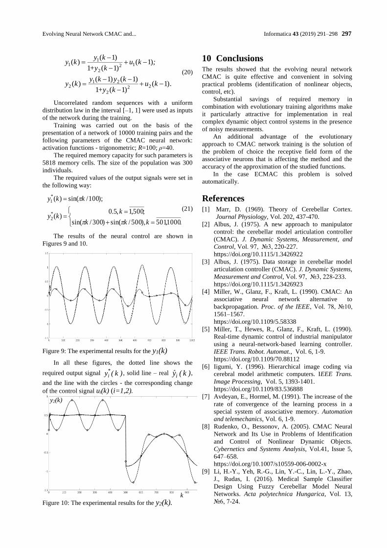
Evolving Neural Network CMAC and... Informatica 43 (2019) 291–298 297
).1()1(1
)1()1()(
)1()1(1
)1()(
222
212
122
11
−+−
−−=
−+−
−=
kuk+y
kykyky
;kuk+y
kyky
(20)
Uncorrelated random sequences with a uniform
distribution law in the interval [–1, 1] were used as inputs
of the network during the training.
Training was carried out on the basis of the
presentation of a network of 10000 training pairs and the
following parameters of the CMAC neural network:
activation functions - trigonometric; R=100; ρ=40.
The required memory capacity for such parameters is
5818 memory cells. The size of the population was 300
individuals.
The required values of the output signals were set in
the following way:
=+
==
=
.1000,501),500/sin()300/sin(
;500,1,5.0)(
);100/sin()(
*2
*1
kkk
kky
kky
(21)
The results of the neural control are shown in
Figures 9 and 10.
Figure 9: The experimental results for the y1(k)
In all these figures, the dotted line shows the
required output signal )k(y*i
, solid line – real )k(yi,
and the line with the circles - the corresponding change
of the control signal ui(k) (i=1,2).
Figure 10: The experimental results for the y2(k).
10 Conclusions The results showed that the evolving neural network
CMAC is quite effective and convenient in solving
practical problems (identification of nonlinear objects,
control, etc).
Substantial savings of required memory in
combination with evolutionary training algorithms make
it particularly attractive for implementation in real
complex dynamic object control systems in the presence
of noisy measurements.
An additional advantage of the evolutionary
approach to CMAC network training is the solution of
the problem of choice the receptive field form of the
associative neurons that is affecting the method and the
accuracy of the approximation of the studied functions.
In the case ECMAC this problem is solved
automatically.
References [1] Marr, D. (1969). Theory of Cerebellar Cortex.
Journal Physiology, Vol. 202, 437-470.
[2] Albus, J. (1975). A new approach to manipulator
control: the cerebellar model articulation controller
(CMAC). J. Dynamic Systems, Measurement, and
Control, Vol. 97, №3, 220-227.
https://doi.org/10.1115/1.3426922
[3] Albus, J. (1975). Data storage in cerebellar model
articulation controller (CMAC). J. Dynamic Systems,
Measurement and Control, Vol. 97, №3, 228-233.
https://doi.org/10.1115/1.3426923
[4] Miller, W., Glanz, F., Kraft, L. (1990). CMAC: An
associative neural network alternative to
backpropagation. Proc. of the IEEE, Vol. 78, №10,
1561–1567.
https://doi.org/10.1109/5.58338
[5] Miller, T., Hewes, R., Glanz, F., Kraft, L. (1990).
Real-time dynamic control of industrial manipulator
using a neural-network-based learning controller.
IEEE Trans. Robot. Automat., Vol. 6, 1-9.
https://doi.org/10.1109/70.88112
[6] Iigumi, Y. (1996). Hierarchical image coding via
cerebral model arithmetic computers. IEEE Trans.
Image Processing, Vol. 5, 1393-1401.
https://doi.org/10.1109/83.536888
[7] Avdeyan, E., Hormel, M. (1991). The increase of the
rate of convergence of the learning process in a
special system of associative memory. Automation
and telemechanics, Vol. 6, 1-9.
[8] Rudenko, O., Bessonov, A. (2005). CMAC Neural
Network and Its Use in Problems of Identification
and Control of Nonlinear Dynamic Objects.
Cybernetics and Systems Analysis, Vol.41, Issue 5,
647–658.
https://doi.org/10.1007/s10559-006-0002-x
[9] Li, H.-Y., Yeh, R.-G., Lin, Y.-C., Lin, L.-Y., Zhao,
J., Rudas, I. (2016). Medical Sample Classifier
Design Using Fuzzy Cerebellar Model Neural
Networks. Acta polytechnica Hungarica, Vol. 13,
№6, 7-24.
y2(k)
k
298 Informatica 43 (2019) 291–298 O. Rudenko et al.
https://doi.org/10.12700/aph.13.6.2016.6.1
[10] Shafik, A., Abdelhameed, M., Kassem ,A. (2014).
CMAC Based Hybrid Control System for Solving
Electrohydraulic System Nonlinearities. Int. Journal
of Manufacturing, Materials, and Mechanical
Engineering, Vol.4(2), 20-26.
https://doi.org/10.4018/ijmmme.2014040104
[11] Lee, C.-H., Chang, F.-Y. (2014). An Efficient
Interval Type-2 Fuzzy CMAC for Chaos Time-
Series Prediction and Synchronization. IEEE
Transactions on Cybernetics, Vol. 44, №3, 329-341.
https://doi.org/10.1109/tcyb.2013.2254113
[12] Chung, C.-C., Lin, C.-C. (2015). Fuzzy Brain
Emotional Cerebellar Model Articulation Control
System Design for Multi-Input Multi-Output
Nonlinear. Acta Polytechnica Hungarica, Vol. 12,
№ 4. 39-58.
https://doi.org/10.12700/aph.12.4.2015.4.3
[13] Dorokhov, O., Chernov, V., Dorokhova, L.,
Streimkis, J. (2018). Multi-criteria choice of
alternatives under fuzzy information,
Transformations in Business and Economics, Vol. 2,
95-106.
[14] Маlyarets L., Dorokhov, O., Dorokhova L. (2018).
Method of constructing the fuzzy regression model
of bank сompetitiveness. Journal of Central Banking
Theory and Practice, Vol. 7, №2, 139–164.
https://doi.org/10.2478/jcbtp-2018-0016
[15] Xu, S., Jing, Y. (2016). Research and Application
of the Pellet Grate Thickness Control System Base
on Improved CMAC Neural Network Algorithm.
Journal of Residuals Science & Technology, Vol. 13,
№ 6, 1501-1509.
[16] Floreano, D., Mattiussi, C. (2008). Bio-Inspired
Artificial Intelligence Theories, Methods, and
Technologies. The MIT Press Cambridge,
Massachusetts-London, England.
[17] Andries, P. (1997). Engelbrecht Computational
Intelligence An Introduction. John Wiley & Sons.
[18] Yao, X. (1993). A Review of Evolutionary
Artificial Neural Networks. Int. J. Intell. Syst., №8
(4), 539-567.
[19] Yao, X. (1999). Evolving Artificial Neural
Networks. Proc. of the IEEE, Vol. 87, №9,1423-
1447.
https://doi.org/10.1109/5.784219
[20] Holland, J. (1975). Adaptation in Natural and
Artificial Systems. An Introductory Analysis With
Application to Biology, Control and Artificial
Intelligence. University of Michigan.
[21] Goldberg, D. (1989). Genetic Algorithms in Search,
Optimization and Machine Learning. Addison-
Wesley, MA.
[22] Knuth, D. (1973). Sorting and Searching, in the Art
of Computer Programming. Menlo Park, Calif.,
Addison Wesley.
[23] Wang, Z.-Q., Schiano, J., Ginsberg, M. (1996).
Hash-Coding in CMAC Neural Networks. IEEE Int.
Conf. on Neural Networks, Vol. 3, 1698-1703.
https://doi.org/10.1109/icnn.1996.549156
[24] Rudenko, O., Bessonov, O.(2004). Hashing
information in a neural network СМАС. Control
Systems and Machines, №5, 67-73.
[25] Chiang, C.-T., Lin, C.-S. (1996). CMAC with
General Basis Functions. Neural Networks, Vol. 7,
№7, 1199-1211.
[26] Lane, S., Handelman, D., Gelfand, J. (1992). Theory
and Development of Higher-Order CMAC Neural
Networks. IEEE Control Systems, Vol. 12, № 2, 23-
30.
https://doi.org/10.1109/37.126849
[27] Rudenko, O., Bessonov, O. (2004). On the Choice
of Basis Functions in a Neural Network СМАС.
Problems of Control and Informatics, № 2, 143–154.
[28] Wu, A.(1995). Empirical Studies of the Genetic
Algorithm with Non-Coding Segments.
Evolutionary Computation, Vol. 3(2), 121-147.
[29] Castellano, J. (2001). Scrapping or Recycling: the
Role of Chromosome Length-Altering Operators in
Genetic Algorithms. GeNeura Group, Department of
Architecture and Computer Technology, University
of Granada. (2001).

https://doi.org/10.31449/inf.v43i2.2783 Informatica 43 (2019) 299–303 299
Design of Intelligent English Writing Self-evaluation Auxiliary System
Man Liu
School of Foreign Languages, Changchun Institute of Technology, Changchun, Jilin 130012, China
E-mail: [email protected]
Keywords: English writing, self-evaluation, auxiliary system, writing teaching
Received: May 23, 2019
Since the reform and opening up, the exchanges between China and the world have become more and
more frequent. English, as a widely used international language, plays an important role in international
exchanges. English teaching includes five aspects, listening, speaking, reading, writing and translation.
Writing teaching is very important but difficult. In order to improve students' autonomous writing ability,
this paper briefly introduced the real-time multi-writing teaching mode and designed an automatic scoring
algorithm of writing self-evaluation auxiliary system, random sampling based Bayesian classification and
combinational algorithm. One thousand CET-4 and CET-6 compositions from Chinese Learner English
Corpus (CLEC) were evaluated, and the scoring effect of Bayesian classification algorithm was also
tested. The results showed that the accuracy rate, recall rate and F value of the proposed algorithm was
better than that of Bayesian classification algorithm under 150 feature extraction dimensions, the two
algorithms had improved scoring effect under the optimal feature extraction dimensions, and the
improvement amplitude of the algorithm proposed in this study was larger. In summary, the random
sampling based Bayesian classification and combinational algorithm is effective and feasible as an
automatic scoring algorithm of writing self-evaluation auxiliary system.
Povzetek: Za boljše učenje angleščine je za kitajske študente razvita vrsta pripomočkov v obliki
informacijskih storitev.
1 Introduction As the economic globalization deepens, the
communication between China and other countries is
more and more frequent, and the most frequently used
language is English. English teaching includes five
aspects, listening, speaking, reading, writing and
translation, among which writing teaching is the most
important and difficult part [1]. English writing ability can
be improved through a large number of writing exercises
and comments of teachers. However, the ratio of the
number of teachers to the number of students is very small
in China. Teachers can not provide guidance to all
students. If students lack guidance about writing exercises,
the improvement effect will be greatly reduced. Because
of the rapid development of computer and natural
language research, a computer intelligence based self-
correction system has been developed [2]. Despite the fact
that the writing language is changeable and the effect is
not ideal in practice, it is still of great help to lighten the
burden on teachers and improve students' English writing
level. Deng [3] put forward a design method of cloud
service platform based intelligent English writing
auxiliary teaching system, constructed the overall design
model of English writing teaching system, improved the
intelligence level of the English writing teaching system
using Cloud-P2P fusion model, and found that the English
writing teaching system had favourable adaptability,
learning ability and reliability. Li [4] selected two parallel
classes as the object, one was taught by the traditional
business English writing teaching mode and the other was
guided by computer assisted technology. The teaching
quality was evaluated after one academic term, and it was
found that computer assisted technology had positive
effect on business English writing. Tsai [5] applied the
blackboard course management system in English essay
writing teaching and found that the teaching result of the
experimental group was superior to that of the control
group after two academic years. The questionnaire result
suggested that most of the students had positive learning
result, indicating the teaching mode could improve the
effectiveness of English writing learning. This paper
briefly introduced the real-time multi-writing teaching
mode and designed the automatic scoring algorithm of the
writing self-evaluation assistant system. One thousand
CET-4 and CET-6 compositions from Chinese Learner
English Corpus (CLEC) were scored. The scoring effect
of the Bayesian classification algorithm was also tested
and compared with the automatic scoring algorithm.
2 English writing teaching mode The traditional teaching mode in China is mostly “duck-
stuffing”, which is similar to assembly line. Most colleges
and universities regard English writing teaching as a part
of English teaching, or as a subsidiary part, and moreover
it is not paid much attentions to because of time and
energy waste. The traditional teaching of English writing
is usually conducted in the classroom, but teachers usually
do not pay attention to whether students understand or not
and only provide students with template sentences and
simple explanation [6].
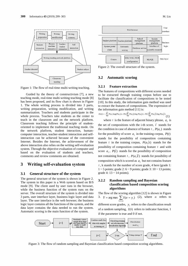
300 Informatica 43 (2019) 299–303 M. Liu
Figure 1: The flow of real-time multi-writing teaching.
Guided by the theory of constructivism [7], a new
teaching mode, real-time multi-writing teaching mode [8]
has been proposed, and its flow chart is shown in Figure
1. The whole writing process is divided into 3 parts,
writing preparation, writing modification, and writing
summarization. Teachers and students participate in the
whole process. Teachers take students as the center to
teach in the classroom and on the network platform.
Classroom teaching follows the principle of student-
oriented to implement the traditional teaching mode. On
the network platform, student interaction, human-
computer interaction, teacher-student interaction and self-
interaction can be achieved because of the convenient
Internet. Besides the Internet, the achievement of the
above interaction also relies on the writing self-evaluation
system. Through the objective evaluation of computer and
based on the evaluation of students and teachers,
comments and review comments are obtained.
3 Writing self-evaluation system
3.1 General structure of the system
The general structure of the system is shown in Figure 2.
The system in this paper is a Web system based on B/S
mode [9]. The client used by user runs in the browser,
while the business function of the system runs on the
server. The overall structure of the system is divided into
3 parts, user interface layer, business logic layer and data
layer. The user interface is the web browser; the business
logic layer contains all the functions of the system, and the
data layer contains the data needed to run the system.
Automatic scoring is the main function of the system.
Figure 2: The overall structure of the system.
3.2 Automatic scoring
3.2.1 Feature extraction
The features of compositions with different scores needed
to be extracted through training corpus before use to
facilitate the classification of compositions to be tested
[10]. In this study, the information gain method was used
to extract the features of compositions. The expression of
the information gain method [11] is:
===
++−=k
i
ii
k
i
iii
k
i
i taPtaPtPtaPtaPtPaPaPtIG111
)(log)()()(log)()())(log()()(
(1)
where t is the feature of adjacent binary phrase, ia is
the set of compositions with the i-th score, t stands for
the condition in case of absence of feature t , )( iaP stands
for the possibility of score ia in the training corpus, )(tP
stands for the possibility of composition containing
feature t in the training corpus, )( taP i stands for the
possibility of composition containing feature t and with
score ia , )(tP stands for the possibility of composition
not containing feature t , )( taP i stands for possibility of
composition which is scored as ia but not contains feature
t , k stands for the number of score grade, 4 here (grade 1:
1 ~ 5 points; grade 2: 6 ~ 9 points; grade 3: 10 ~ 13 points;
grade 4: 13 ~ 14 points).
3.2.2 Random sampling and Bayesian
classification based composition scoring
algorithms
The flow of the scoring algorithm [12] is shown in Figure
3.
==mi
iyIY1
)(maxarg (2), where α refers to
different score grades, iy refers to the classification result
of a random sampling, )•(I refers to indicator function, 1
if the parameter is true and 0 if not.
Figure 3: The flow of random sampling and Bayesian classification based composition scoring algorithms.

Design of Intelligent English Writing Self-evaluation... Informatica 43 (2019) 299–303 301
The calculation formula of Bayesian classification
based algorithm [13] is:
=
=V
k k
Nik
iN
aPabP
k
1 !
)()(
(3)
VN
NaP
ia
ji
ij+
+=
1)(
(4)
where b refers to the spatial vector of an English
composition, mib ,,,, 21= , m refers to the
number of features of adjacent binary phrase, iθ refers to
the weight of the i-th feature in composition b, V refers to
the number of binary phase features, kN refers to the
number of times of the k-th feature appearing in b,
)( iabP refers to the possibility of a composition
obtaining some score, )( ij aθP refers to the possibility of
feature jθ in a composition which is scored as ia , jiN
refers to the number of times of the j-th feature appearing
in a composition which is scored as the j-th feature, and
iaN refers to the number of all the features of a
composition which is scored as ia .
4 Automatic scoring test of the
writing self-evaluation system
4.1 Testing method
Five hundred of CET-4 compositions which involved two
themes and 500 CET-6 compositions with which involved
two themes were selected from CLEC [14]. Before the
test, the compositions were scored and classified into four
score grades according to the scoring criteria of CET-4
and CET-6 compositions. Based on the binary phrase
features, the compositions which involved four themes
were scored under 150 feature extraction dimensions, i.e.,
the 1000 compositions were classified into four score
grades using the algorithm proposed in this study. Then
the compositions were scored after the automatic
calculation of optimal feature dimensions. The whole
system program ran on a server in a lab. The server was
configured with Windows 7 system, I7 processor and 16G
memory. In order to increase the persuasiveness of the
results, the test results of the Bayesian classification
algorithm based scoring system was selected for
comparison. The test method was the same as the system
proposed in this study.
4.2 Evaluation criteria
The automatic scoring effect of the writing self-evaluation
system was evaluated in the aspects of accuracy rate, recall
rate and F value [15]. The accuracy rate could be
calculated using the following formula: the accuracy rate
= correctly recognized number/total recognized number,
where correctly recognized number is the number of
correctly classified compositions based on above scoring
algorithm and the total recognized number is the total
number of compositions identified by the scoring
algorithm.
The recall rate could be calculated using the following
formula: recall rate = correctly recognized
number/actually existed number, where actually existed
number refers to the number of compositions which
actually existed and ought to be recognized.
F value (comprehensive evaluation index) could be
calculated using the follow formula: F value = 2 ×
accuracy rate × recall rate /(accuracy rate + recall rate).
4.3 Testing results
As shown in Table 1, the accuracy rate, recall rate and F
value of the scoring algorithm were about 14%, 28% and
22% higher than those of Bayesian classification
algorithm in scoring different themes of compositions.
The accuracy rate, recall rate and F value of the Bayesian
classification algorithm were 0.739, 0.661 and 0.690
respectively; the accuracy rate, recall rate and F value of
the algorithm proposed in this study were 0.845, 0.850 and
0.844 respectively. It indicated that the algorithm
proposed in this study was superior to the Bayesian
classification algorithm in scoring compositions, and all
Theme Bayesian classification algorithm Random sampling based Bayesian
classification algorithm
Accuracy
rate (P)
Recall rate
(R)
F value Accuracy
rate (P)
Recall rate
(R)
F value
Theme 1
(CET-4) 0.719 0.626 0.660 0.849 0.881 0.862
Theme 2
(CET-4) 0.750 0.679 0.708 0.838 0.833 0.832
Theme 3
(CET-6) 0.759 0.710 0.730 0.836 0.831 0.831
Theme 4
(CET 6) 0.726 0.630 0.661 0.857 0.853 0.851
Average
value 0.739 0.661 0.690 0.845 0.850 0.844
Table 1: The scoring test results of the two algorithms under 150 feature extraction dimensions.
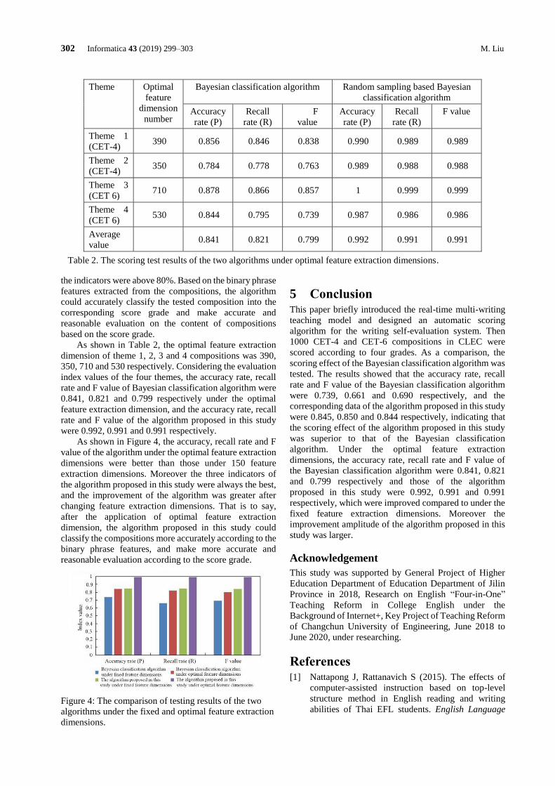
302 Informatica 43 (2019) 299–303 M. Liu
the indicators were above 80%. Based on the binary phrase
features extracted from the compositions, the algorithm
could accurately classify the tested composition into the
corresponding score grade and make accurate and
reasonable evaluation on the content of compositions
based on the score grade.
As shown in Table 2, the optimal feature extraction
dimension of theme 1, 2, 3 and 4 compositions was 390,
350, 710 and 530 respectively. Considering the evaluation
index values of the four themes, the accuracy rate, recall
rate and F value of Bayesian classification algorithm were
0.841, 0.821 and 0.799 respectively under the optimal
feature extraction dimension, and the accuracy rate, recall
rate and F value of the algorithm proposed in this study
were 0.992, 0.991 and 0.991 respectively.
As shown in Figure 4, the accuracy, recall rate and F
value of the algorithm under the optimal feature extraction
dimensions were better than those under 150 feature
extraction dimensions. Moreover the three indicators of
the algorithm proposed in this study were always the best,
and the improvement of the algorithm was greater after
changing feature extraction dimensions. That is to say,
after the application of optimal feature extraction
dimension, the algorithm proposed in this study could
classify the compositions more accurately according to the
binary phrase features, and make more accurate and
reasonable evaluation according to the score grade.
Figure 4: The comparison of testing results of the two
algorithms under the fixed and optimal feature extraction
dimensions.
5 Conclusion This paper briefly introduced the real-time multi-writing
teaching model and designed an automatic scoring
algorithm for the writing self-evaluation system. Then
1000 CET-4 and CET-6 compositions in CLEC were
scored according to four grades. As a comparison, the
scoring effect of the Bayesian classification algorithm was
tested. The results showed that the accuracy rate, recall
rate and F value of the Bayesian classification algorithm
were 0.739, 0.661 and 0.690 respectively, and the
corresponding data of the algorithm proposed in this study
were 0.845, 0.850 and 0.844 respectively, indicating that
the scoring effect of the algorithm proposed in this study
was superior to that of the Bayesian classification
algorithm. Under the optimal feature extraction
dimensions, the accuracy rate, recall rate and F value of
the Bayesian classification algorithm were 0.841, 0.821
and 0.799 respectively and those of the algorithm
proposed in this study were 0.992, 0.991 and 0.991
respectively, which were improved compared to under the
fixed feature extraction dimensions. Moreover the
improvement amplitude of the algorithm proposed in this
study was larger.
Acknowledgement
This study was supported by General Project of Higher
Education Department of Education Department of Jilin
Province in 2018, Research on English “Four-in-One”
Teaching Reform in College English under the
Background of Internet+, Key Project of Teaching Reform
of Changchun University of Engineering, June 2018 to
June 2020, under researching.
References [1] Nattapong J, Rattanavich S (2015). The effects of
computer-assisted instruction based on top-level
structure method in English reading and writing
abilities of Thai EFL students. English Language
Theme Optimal
feature
dimension
number
Bayesian classification algorithm Random sampling based Bayesian
classification algorithm
Accuracy
rate (P)
Recall
rate (R)
F
value
Accuracy
rate (P)
Recall
rate (R)
F value
Theme 1
(CET-4) 390 0.856 0.846 0.838 0.990 0.989 0.989
Theme 2
(CET-4) 350 0.784 0.778 0.763 0.989 0.988 0.988
Theme 3
(CET 6) 710 0.878 0.866 0.857 1 0.999 0.999
Theme 4
(CET 6) 530 0.844 0.795 0.739 0.987 0.986 0.986
Average
value 0.841 0.821 0.799 0.992 0.991 0.991
Table 2. The scoring test results of the two algorithms under optimal feature extraction dimensions.
Design of Intelligent English Writing Self-evaluation... Informatica 43 (2019) 299–303 303
Teaching, 8(11), pp. 231.
https://doi.org/10.5539/elt.v8n11p231
[2] Xia M, Zhang Y, Zhang C (2017). A TAM-based
approach to explore the effect of online experience
on destination image: A smartphone user's
perspective. Journal of Destination Marketing &
Management.
https://doi.org/10.1016/j.jdmm.2017.05.002
[3] Deng L (2018). Design of English writing assisted
instruction teaching system based on intelligent
cloud service platform. International Conference on
Intelligent Transportation, Big Data & Smart City.
IEEE Computer Society, pp. 287-290.
https://doi.org/10.1109/ICITBS.2018.00080
[4] Li X (2018) Influence of computer-aided instruction
model on business English writing teaching effect.
International Journal of Emerging Technologies in
Learning, 13(3), pp. 197.
[5] Tsai Y R (2015). Applying the technology
acceptance model (TAM) to explore the effects of a
course management system (CMS)-assisted EFL
writing instruction. Calico Journal, 32(1).
https://doi.org/10.1558/cj.v32i1.153-171
[6] Tarhini A, Hassouna M, Abbasi M S, et al. (2015).
Towards the acceptance of RSS to support learning:
an empirical study to validate the technology
acceptance model in Lebanon. Electronic Journal of
e-Learning, 13(1), pp. 30-41.
[7] Li L (2016). Design and implementation of higher
vocational English writing and training testing
system. International Conference on Materials
Engineering, Manufacturing Technology and
Control.
[8] Chapela M E G (2016). A corpus-based analysis of
post-auxiliary ellipsis in modern English:
methodological and theoretical issues.
[9] Ohta R (2017). The impact of an automated
evaluation system on student-writing performance.
Kate Bulletin, 22, pp. 23-33.
[10] Ahsen M E, Ayvaci M, Raghunathan S (2017).
When algorithmic predictions use human-generated
data: a bias-aware classification algorithm for breast
cancer diagnosis. Social Science Electronic
Publishing. https://doi.org/10.2139/ssrn.3087467
[11] Alcázar V, Fernández S, Borrajo D, et al. (2015).
Using random sampling trees for automated
planning. Ai Communications, 28(4), pp. 665-681.
[12] Myttenaere A D, Golden B, Grand B L, et al. (2015).
Study of a bias in the offline evaluation of a
recommendation algorithm. Computer Science,
79(3), pp. 263-72. https://doi.org/10.1016/0002-
9416(81)90074-9
[13] Hao J, Niu K, Meng Z, et al. (2017). A collaborative
filtering recommendation algorithm based on score
classification. International Conference on Security,
Privacy and Anonymity in Computation,
Communication and Storage. Springer, Cham, pp.
435-445. https://doi.org/10.1007/978-3-319-72395-
2_40
[14] Santos D P D, André C P L F D C (2017). Automatic
selection of learning bias for active sampling.
Intelligent Systems. IEEE, Recife, Brazil, pp. 55-60.
https://doi.org/10.1109/BRACIS.2016.021
[15] Zoph B, Yuret D, May J, et al. (2016). Transfer
learning for low-resource neural machine
translation. Conference on Empirical Methods in
Natural Language Processing, pp. 1568-1575.

304 Informatica 43 (2019) 299–303 M. Liu

Informatica 43 (2019) 305–305 305
JOŽEF STEFAN INSTITUTE
Jožef Stefan (1835-1893) was one of the most prominentphysicists of the 19th century. Born to Slovene parents,he obtained his Ph.D. at Vienna University, where he waslater Director of the Physics Institute, Vice-President of theVienna Academy of Sciences and a member of several sci-entific institutions in Europe. Stefan explored many areasin hydrodynamics, optics, acoustics, electricity, magnetismand the kinetic theory of gases. Among other things, heoriginated the law that the total radiation from a blackbody is proportional to the 4th power of its absolute tem-perature, known as the Stefan–Boltzmann law.
The Jožef Stefan Institute (JSI) is the leading indepen-dent scientific research institution in Slovenia, covering abroad spectrum of fundamental and applied research in thefields of physics, chemistry and biochemistry, electronicsand information science, nuclear science technology, en-ergy research and environmental science.
The Jožef Stefan Institute (JSI) is a research organisationfor pure and applied research in the natural sciences andtechnology. Both are closely interconnected in research de-partments composed of different task teams. Emphasis inbasic research is given to the development and education ofyoung scientists, while applied research and developmentserve for the transfer of advanced knowledge, contributingto the development of the national economy and society ingeneral.
At present the Institute, with a total of about 900 staff,has 700 researchers, about 250 of whom are postgraduates,around 500 of whom have doctorates (Ph.D.), and around200 of whom have permanent professorships or temporaryteaching assignments at the Universities.
In view of its activities and status, the JSI plays the roleof a national institute, complementing the role of the uni-versities and bridging the gap between basic science andapplications.
Research at the JSI includes the following major fields:physics; chemistry; electronics, informatics and computersciences; biochemistry; ecology; reactor technology; ap-plied mathematics. Most of the activities are more orless closely connected to information sciences, in particu-lar computer sciences, artificial intelligence, language andspeech technologies, computer-aided design, computer ar-chitectures, biocybernetics and robotics, computer automa-tion and control, professional electronics, digital communi-cations and networks, and applied mathematics.
The Institute is located in Ljubljana, the capital of the in-dependent state of Slovenia (or S♥nia). The capital todayis considered a crossroad between East, West and Mediter-
ranean Europe, offering excellent productive capabilitiesand solid business opportunities, with strong internationalconnections. Ljubljana is connected to important centerssuch as Prague, Budapest, Vienna, Zagreb, Milan, Rome,Monaco, Nice, Bern and Munich, all within a radius of 600km.
From the Jožef Stefan Institute, the Technology park“Ljubljana” has been proposed as part of the national strat-egy for technological development to foster synergies be-tween research and industry, to promote joint ventures be-tween university bodies, research institutes and innovativeindustry, to act as an incubator for high-tech initiatives andto accelerate the development cycle of innovative products.
Part of the Institute was reorganized into several high-tech units supported by and connected within the Technol-ogy park at the Jožef Stefan Institute, established as thebeginning of a regional Technology park "Ljubljana". Theproject was developed at a particularly historical moment,characterized by the process of state reorganisation, privati-sation and private initiative. The national Technology Parkis a shareholding company hosting an independent venture-capital institution.
The promoters and operational entities of the project arethe Republic of Slovenia, Ministry of Higher Education,Science and Technology and the Jožef Stefan Institute. Theframework of the operation also includes the University ofLjubljana, the National Institute of Chemistry, the Institutefor Electronics and Vacuum Technology and the Institutefor Materials and Construction Research among others. Inaddition, the project is supported by the Ministry of theEconomy, the National Chamber of Economy and the Cityof Ljubljana.
Jožef Stefan InstituteJamova 39, 1000 Ljubljana, SloveniaTel.:+386 1 4773 900, Fax.:+386 1 251 93 85WWW: http://www.ijs.siE-mail: [email protected] relations: Polona Strnad

Informatica 43 (2019)
INFORMATICAAN INTERNATIONAL JOURNAL OF COMPUTING AND INFORMATICS
INVITATION, COOPERATION
Submissions and Refereeing
Please register as an author and submit a manuscript at:http://www.informatica.si. At least two referees outside the au-thor’s country will examine it, and they are invited to make asmany remarks as possible from typing errors to global philosoph-ical disagreements. The chosen editor will send the author theobtained reviews. If the paper is accepted, the editor will alsosend an email to the managing editor. The executive board willinform the author that the paper has been accepted, and the authorwill send the paper to the managing editor. The paper will be pub-lished within one year of receipt of email with the text in Infor-matica MS Word format or Informatica LATEX format and figuresin .eps format. Style and examples of papers can be obtained fromhttp://www.informatica.si. Opinions, news, calls for conferences,calls for papers, etc. should be sent directly to the managing edi-tor.
SUBSCRIPTIONPlease, complete the order form and send it to Dr. Drago Torkar,Informatica, Institut Jožef Stefan, Jamova 39, 1000 Ljubljana,Slovenia. E-mail: [email protected]
Since 1977, Informatica has been a major Slovenian scientificjournal of computing and informatics, including telecommunica-tions, automation and other related areas. In its 16th year (morethan twentyfive years ago) it became truly international, althoughit still remains connected to Central Europe. The basic aim of In-formatica is to impose intellectual values (science, engineering)in a distributed organisation.
Informatica is a journal primarily covering intelligent systems inthe European computer science, informatics and cognitive com-munity; scientific and educational as well as technical, commer-cial and industrial. Its basic aim is to enhance communicationsbetween different European structures on the basis of equal rightsand international refereeing. It publishes scientific papers ac-cepted by at least two referees outside the author’s country. In ad-dition, it contains information about conferences, opinions, criti-cal examinations of existing publications and news. Finally, majorpractical achievements and innovations in the computer and infor-mation industry are presented through commercial publications aswell as through independent evaluations.
Editing and refereeing are distributed. Each editor can conductthe refereeing process by appointing two new referees or refereesfrom the Board of Referees or Editorial Board. Referees shouldnot be from the author’s country. If new referees are appointed,their names will appear in the Refereeing Board.
Informatica web edition is free of charge and accessible athttp://www.informatica.si.Informatica print edition is free of charge for major scientific, ed-ucational and governmental institutions. Others should subscribe.

Informatica WWW:
http://www.informatica.si/
Referees from 2008 on:
A. Abraham, S. Abraham, R. Accornero, A. Adhikari, R. Ahmad, G. Alvarez, N. Anciaux, R. Arora, I. Awan, J.Azimi, C. Badica, Z. Balogh, S. Banerjee, G. Barbier, A. Baruzzo, B. Batagelj, T. Beaubouef, N. Beaulieu, M. terBeek, P. Bellavista, K. Bilal, S. Bishop, J. Bodlaj, M. Bohanec, D. Bolme, Z. Bonikowski, B. Boškovic, M. Botta,P. Brazdil, J. Brest, J. Brichau, A. Brodnik, D. Brown, I. Bruha, M. Bruynooghe, W. Buntine, D.D. Burdescu, J.Buys, X. Cai, Y. Cai, J.C. Cano, T. Cao, J.-V. Capella-Hernández, N. Carver, M. Cavazza, R. Ceylan, A. Chebotko,I. Chekalov, J. Chen, L.-M. Cheng, G. Chiola, Y.-C. Chiou, I. Chorbev, S.R. Choudhary, S.S.M. Chow, K.R.Chowdhury, V. Christlein, W. Chu, L. Chung, M. Ciglaric, J.-N. Colin, V. Cortellessa, J. Cui, P. Cui, Z. Cui, D.Cutting, A. Cuzzocrea, V. Cvjetkovic, J. Cypryjanski, L. Cehovin, D. Cerepnalkoski, I. Cosic, G. Daniele, G.Danoy, M. Dash, S. Datt, A. Datta, M.-Y. Day, F. Debili, C.J. Debono, J. Dedic, P. Degano, A. Dekdouk, H.Demirel, B. Demoen, S. Dendamrongvit, T. Deng, A. Derezinska, J. Dezert, G. Dias, I. Dimitrovski, S. Dobrišek,Q. Dou, J. Doumen, E. Dovgan, B. Dragovich, D. Drajic, O. Drbohlav, M. Drole, J. Dujmovic, O. Ebers, J. Eder,S. Elaluf-Calderwood, E. Engström, U. riza Erturk, A. Farago, C. Fei, L. Feng, Y.X. Feng, B. Filipic, I. Fister, I.Fister Jr., D. Fišer, A. Flores, V.A. Fomichov, S. Forli, A. Freitas, J. Fridrich, S. Friedman, C. Fu, X. Fu, T.Fujimoto, G. Fung, S. Gabrielli, D. Galindo, A. Gambarara, M. Gams, M. Ganzha, J. Garbajosa, R. Gennari, G.Georgeson, N. Gligoric, S. Goel, G.H. Gonnet, D.S. Goodsell, S. Gordillo, J. Gore, M. Grcar, M. Grgurovic, D.Grosse, Z.-H. Guan, D. Gubiani, M. Guid, C. Guo, B. Gupta, M. Gusev, M. Hahsler, Z. Haiping, A. Hameed, C.Hamzaçebi, Q.-L. Han, H. Hanping, T. Härder, J.N. Hatzopoulos, S. Hazelhurst, K. Hempstalk, J.M.G. Hidalgo, J.Hodgson, M. Holbl, M.P. Hong, G. Howells, M. Hu, J. Hyvärinen, D. Ienco, B. Ionescu, R. Irfan, N. Jaisankar, D.Jakobovic, K. Jassem, I. Jawhar, Y. Jia, T. Jin, I. Jureta, Ð. Juricic, S. K, S. Kalajdziski, Y. Kalantidis, B. Kaluža,D. Kanellopoulos, R. Kapoor, D. Karapetyan, A. Kassler, D.S. Katz, A. Kaveh, S.U. Khan, M. Khattak, V.Khomenko, E.S. Khorasani, I. Kitanovski, D. Kocev, J. Kocijan, J. Kollár, A. Kontostathis, P. Korošec, A.Koschmider, D. Košir, J. Kovac, A. Krajnc, M. Krevs, J. Krogstie, P. Krsek, M. Kubat, M. Kukar, A. Kulis, A.P.S.Kumar, H. Kwasnicka, W.K. Lai, C.-S. Laih, K.-Y. Lam, N. Landwehr, J. Lanir, A. Lavrov, M. Layouni, G. Leban,A. Lee, Y.-C. Lee, U. Legat, A. Leonardis, G. Li, G.-Z. Li, J. Li, X. Li, X. Li, Y. Li, Y. Li, S. Lian, L. Liao, C. Lim,J.-C. Lin, H. Liu, J. Liu, P. Liu, X. Liu, X. Liu, F. Logist, S. Loskovska, H. Lu, Z. Lu, X. Luo, M. Luštrek, I.V.Lyustig, S.A. Madani, M. Mahoney, S.U.R. Malik, Y. Marinakis, D. Marincic, J. Marques-Silva, A. Martin, D.Marwede, M. Matijaševic, T. Matsui, L. McMillan, A. McPherson, A. McPherson, Z. Meng, M.C. Mihaescu, V.Milea, N. Min-Allah, E. Minisci, V. Mišic, A.-H. Mogos, P. Mohapatra, D.D. Monica, A. Montanari, A. Moroni, J.Mosegaard, M. Moškon, L. de M. Mourelle, H. Moustafa, M. Možina, M. Mrak, Y. Mu, J. Mula, D. Nagamalai,M. Di Natale, A. Navarra, P. Navrat, N. Nedjah, R. Nejabati, W. Ng, Z. Ni, E.S. Nielsen, O. Nouali, F. Novak, B.Novikov, P. Nurmi, D. Obrul, B. Oliboni, X. Pan, M. Pancur, W. Pang, G. Papa, M. Paprzycki, M. Paralic, B.-K.Park, P. Patel, T.B. Pedersen, Z. Peng, R.G. Pensa, J. Perš, D. Petcu, B. Petelin, M. Petkovšek, D. Pevec, M.Piculin, R. Piltaver, E. Pirogova, V. Podpecan, M. Polo, V. Pomponiu, E. Popescu, D. Poshyvanyk, B. Potocnik,R.J. Povinelli, S.R.M. Prasanna, K. Pripužic, G. Puppis, H. Qian, Y. Qian, L. Qiao, C. Qin, J. Que, J.-J.Quisquater, C. Rafe, S. Rahimi, V. Rajkovic, D. Rakovic, J. Ramaekers, J. Ramon, R. Ravnik, Y. Reddy, W.Reimche, H. Rezankova, D. Rispoli, B. Ristevski, B. Robic, J.A. Rodriguez-Aguilar, P. Rohatgi, W. Rossak, I.Rožanc, J. Rupnik, S.B. Sadkhan, K. Saeed, M. Saeki, K.S.M. Sahari, C. Sakharwade, E. Sakkopoulos, P. Sala,M.H. Samadzadeh, J.S. Sandhu, P. Scaglioso, V. Schau, W. Schempp, J. Seberry, A. Senanayake, M. Senobari,T.C. Seong, S. Shamala, c. shi, Z. Shi, L. Shiguo, N. Shilov, Z.-E.H. Slimane, F. Smith, H. Sneed, P. Sokolowski,T. Song, A. Soppera, A. Sorniotti, M. Stajdohar, L. Stanescu, D. Strnad, X. Sun, L. Šajn, R. Šenkerík, M.R.Šikonja, J. Šilc, I. Škrjanc, T. Štajner, B. Šter, V. Štruc, H. Takizawa, C. Talcott, N. Tomasev, D. Torkar, S.Torrente, M. Trampuš, C. Tranoris, K. Trojacanec, M. Tschierschke, F. De Turck, J. Twycross, N. Tziritas, W.Vanhoof, P. Vateekul, L.A. Vese, A. Visconti, B. Vlaovic, V. Vojisavljevic, M. Vozalis, P. Vracar, V. Vranic, C.-H.Wang, H. Wang, H. Wang, H. Wang, S. Wang, X.-F. Wang, X. Wang, Y. Wang, A. Wasilewska, S. Wenzel, V.Wickramasinghe, J. Wong, S. Wrobel, K. Wrona, B. Wu, L. Xiang, Y. Xiang, D. Xiao, F. Xie, L. Xie, Z. Xing, H.Yang, X. Yang, N.Y. Yen, C. Yong-Sheng, J.J. You, G. Yu, X. Zabulis, A. Zainal, A. Zamuda, M. Zand, Z. Zhang,Z. Zhao, D. Zheng, J. Zheng, X. Zheng, Z.-H. Zhou, F. Zhuang, A. Zimmermann, M.J. Zuo, B. Zupan, M.Zuqiang, B. Žalik, J. Žižka,

InformaticaAn International Journal of Computing and Informatics
Web edition of Informatica may be accessed at: http://www.informatica.si.
Subscription Information Informatica (ISSN 0350-5596) is published four times a year in Spring, Summer,Autumn, and Winter (4 issues per year) by the Slovene Society Informatika, Litostrojska cesta 54, 1000 Ljubljana,Slovenia.The subscription rate for 2019 (Volume 43) is– 60 EUR for institutions,– 30 EUR for individuals, and– 15 EUR for studentsClaims for missing issues will be honored free of charge within six months after the publication date of the issue.
Typesetting: Borut Žnidar, [email protected]: ABO grafika d.o.o., Ob železnici 16, 1000 Ljubljana.
Orders may be placed by email ([email protected]), telephone (+386 1 477 3900) or fax (+386 1 251 93 85). Thepayment should be made to our bank account no.: 02083-0013014662 at NLB d.d., 1520 Ljubljana, Trg republike2, Slovenija, IBAN no.: SI56020830013014662, SWIFT Code: LJBASI2X.
Informatica is published by Slovene Society Informatika (president Niko Schlamberger) in cooperation with thefollowing societies (and contact persons):Slovene Society for Pattern Recognition (Vitomir Štruc)Slovenian Artificial Intelligence Society (Mitja Luštrek)Cognitive Science Society (Olga Markic)Slovenian Society of Mathematicians, Physicists and Astronomers (Marej Brešar)Automatic Control Society of Slovenia (Nenad Muškinja)Slovenian Association of Technical and Natural Sciences / Engineering Academy of Slovenia (Mark Pleško)ACM Slovenia (Borut Žalik)
Informatica is financially supported by the Slovenian research agency from the Call for co-financing of scientificperiodical publications.
Informatica is surveyed by: ACM Digital Library, Citeseer, COBISS, Compendex, Computer & InformationSystems Abstracts, Computer Database, Computer Science Index, Current Mathematical Publications, DBLPComputer Science Bibliography, Directory of Open Access Journals, InfoTrac OneFile, Inspec, Linguistic andLanguage Behaviour Abstracts, Mathematical Reviews, MatSciNet, MatSci on SilverPlatter, Scopus, ZentralblattMath

Volume 43 Number 2 June 2019 ISSN 0350-5596
A Review on CT and X-Ray Images DenoisingMethods
D. Thanh, P. Surya,L.M. Hieu
151
On the Properties of Epistemic and TemporalEpistemic Logics of Authentication
S. Ahmadi, M.S. Fallah,M. Pourmahdian
161
Benchmark Problems for Exhaustive ExactMaximum Clique Search Algorithms
S. Szabó, B. Zavalnij 177
Mutual Information Based Feature Selection forFingerprint Identification
A. Adjimi,A. Hacine-Gharbi,P. Ravier, M. Mostefai
187
Some Remarks and Tests on the DH1 CryptosystemBased on Automata Compositions
P. Dömösi, J. Gáll,G. Horváth, N. Tihanyi
199
Agent-Based Simulation of Socially-Inspired Modelof Resistance against Unpopular Norms
K. Zia, D.K. Saini,A. Muhammad, U. Farooq
209
A New Ensemble Semi-supervised Self-labeledAlgorithm
I.E. Livieris 221
New Re-Ranking Approach in Merging SearchResults
H.T. Vo 235
Physical Match A.E. Naiman, Y. Stein,E. Farber
243
The Permutable k-means for the Bi-Partial Criterion S.D. Dvoenko,J.W. Owsinski
253
A CLR Virtual Machine Based Execution frameworkfor IEC 61131-3 Applications
S. Cavalieri, M.S. Scroppo 263
A Comparative Study of Automatic ProgrammingTechniques
S. Arslan, C. Öztürk 281
Evolving Neural Network CMAC and itsApplications
O. Rudenko, O. Bessonov,O. Dorokhov
291
Design of Intelligent English Writing Self-evaluationAuxiliary System
M.M. Liu 299

Informatica 43 (2019) Number 2, pp. 151–305