國國國國國國國國國國國國國國國

國國國國Department of Economics

College of Social Sciences

National Taiwan University

Master Thesis

國國國國國國國 國國國國國國國國國國國：

Volume-Driven Random Walk

of Speculative Prices

國國國

Yen-Lin Chiu

國國國國 國國國 國國：

國國國 國國

Advisor: Ray-Yeutien Chou, Ph.D.

Jau-er Chen, Ph.D.

國國國國 102 國 6 國

June 2013

2

國國國國國國國國國國國國國國國國國國國國

國國國國國國國 國國國國國國國國國國國：Volume-Driven Random Walk

of Speculative Prices

國國國國國國國國（ R99323035 國國國國國國國國國國國國 國國國國國國國國國國國 國國國）、， 102 國 06 國 27 國國國國國國國國國國國國國國國國國國國國國，

國國國國： 國國國國國（）

國國國國國（）

i

摘摘

國國國國國Clark, P. K. (1973)國國國國國國國國國 國國國國國，(Q)國國國國國國(operational time)國國國 國國國 國國國國國。，

(r)國國國國國國國國國國國國國國國國國國國(random walk) 國國國國國國國國國國國國國國國國國國國國 國國國國國國國國國國國國國國國國國國國國國國國國國 國國國國國 國國國國國國國國國國國 國國國國國國國國。，。，， 150 國國國 國國國國國國國國國國國國國國國國國國國國國國國國國國國國國國國國國國，－，

√Q 國國國國國國國國國國國國國國國。

國國國國國國國國國國國。

國國國: 國國國國國, 國國國國, 國國國國.

ii

Abstract

This thesis proposes a model for speculative price that

modifies the classic stochastic model of Clark, P. K.

(1973) by simply adapting trading volume, Q, as the

operational time. It suggests return is a random walk

driven by trading volume. Not only can this model be

derived from two intuitive assumptions, but also can

several stylized facts of speculative price be derived

from a few further assumptions that are supported by

empirical evidences. Empirical evidence is examined for

the most representative 150 companies in Taiwan stock

market: A linear equation of trading volume and return

conditional variance is confirmed to describe the real

data well. After divided by √Q, return tends to be

normally distributed.

iii

Keywords: Speculative Price, Stochastic Volatility,

Random Walk.

iv

Content

國國.....................................................iiAbstract..............................................iii

Content.............................................ivList of Tables..........................................vList of Figures........................................viI. Introduction.........................................1II. Literature Review................................3III. Model............................................6IV. Empirical Evidence..............................12

1. Data............................................122. Methodology.....................................13

A. Normality Test...............................13B. Linear Conditional Variance..................14

3. Analysis Results................................17Appendix...............................................26

A. Proof...........................................26B. Component List..................................29C. Figures & Tables................................33

Reference.......................................65

v

List of Tables

Table 1: Price Change and Kurtosis by Turnover Class.....................................15

Table 2: The Number of Companies That Has Minimal Percentage Rejection of Normality Test OccurredWhen a is around 0.5.........................18

Table 3: Regression Results of Conditional Varianceon Volume and Rejection Rate of Normality on Adjusted Return for Taiwan 50................19

Table 4 : Results of t-test for Significance of Intercept Term...............................24

Table 5: List of Taiwan 50 Index component at 5.17.2013....................................29

Table 6: List of Taiwan Mid-Cap 100 Index componentat 5.17.2013.................................30

Table 7: Regression Results of Conditional Varianceon Volume and Rejection Rate of Normality on Adjusted Return for Taiwan Mid-Cap 100.......59

vi

List of Figures

Figure 1: Selected Graphical Results for Tests. .18Figure 2: Autocorrelation ACF plots for 2330 (TSMC)

.............................................23Figure 3: Graphical Results of Tests on Taiwan 5034Figure 4: Graphical Results of Tests on Taiwan Mid-

Cap 100......................................47

vii

I. Introduction

A classical result in financial economics is that

no arbitrage condition makes the asset price become a

martingale under a certain measure, which further

makes the price follow a time-changed Brownian motion

(Bachelier, L. 1900, Monroe, I. 1978). However,

Samuelso.Pa (1973) pointed out that the absolute

Brownian motion model contradicts the limited

liability feature of modern stocks and bonds as it

leads speculative price to be negative with

probability 1/2 in future. He and Osborne, M. F.

(1959) advocated geometric Brownian motion as a better

alternative for speculative price. The speculative

price theory based on Brownian motion has inspired

great works such as the option pricing formula in

Black, F. and M. Scholes (1973). The convenience that

Brownian motion brings due to its three properties

(continuity, stationarity and independence increment)

also makes it a widely accepted assumption in

economics.

Nevertheless, several studies have found that

return does not obey the basic laws of Brownian

motion. For continuity, many models now include jumps

and found it is more capable to describe the data

(Jorion, P. 1988, Merton, R. C. 1976). For

1

stationarity, it is found the volatility of return is

time-varying and the GARCH effect plays a significant

role (Bollerslev, T. 1986, Bollerslev, T., R. Y. Chou

and K. F. Kroner 1992, Engle, R. F. 1982). For the

other, both the high-frequency and low-frequency data

exhibit strong autocorrelation on the amplitude of

return (Ané, T. and L. Ureche-Rangau 2008, Bollerslev,

T. 1986).

Scholars have attempted to bridge the gap between

classic theory and the empirical evidences. One of the

competing schools begins with Clark, P. K. (1973). He

hypothesized price return is a subordinated Brownian

motion to account for its time-varying volatility and

connected it with trading volume as the proxy for

information arrival:

r (t)=B (v (t))≅∑1

v(t)

εi ,

where {εi } normal (0,1),v (t )≅Q2, and Q is trading volume.

This is later named “Mixture Distribution Hypothesis” and

since then, many empirical researches have proven in

favor of this hypothesis. Andersen, T. G., T. Bollerslev,

F. X. Diebold and H. Ebens (2001) found the distribution

realized volatility is closed to log Normal in high

frequency data, which coincides with Clark’s hypothesis

based on daily data that trading volume is log normal

2

distributed and equivalent to volatility.

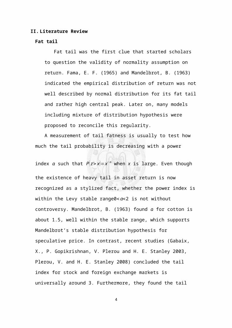
This thesis is motivated by the above, mainly by

Clark, to investigate whether there is a better model

to provide accurate description to empirical evidences

that have been found so far. It turns out the return

process under this model is extremely simple:

r (t,∆t )≡logP (t+∆t)−logP (t )= ∑i=1

Q(t,∆t)

εi , (1)

where Q(t,∆t) and r (t,∆t ) are trading volume and return

in a time interval (t,t+∆t ), εiis i.i.d. random variable

with 4th moment finite. Readers can note it is a random

walk driven by volume. We will later show the readers how

formula (1) can be derived from two intuitive

assumptions.

3

II. Literature Review

Fat tail

Fat tail was the first clue that started scholars

to question the validity of normality assumption on

return. Fama, E. F. (1965) and Mandelbrot, B. (1963)

indicated the empirical distribution of return was not

well described by normal distribution for its fat tail

and rather high central peak. Later on, many models

including mixture of distribution hypothesis were

proposed to reconcile this regularity.

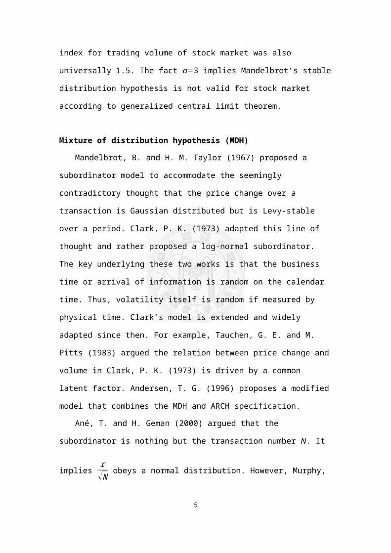
A measurement of tail fatness is usually to test how

much the tail probability is decreasing with a power

index α such that P (r>x)=x−α when x is large. Even though

the existence of heavy tail in asset return is now

recognized as a stylized fact, whether the power index is

within the Levy stable range0<α<2 is not without

controversy. Mandelbrot, B. (1963) found α for cotton is

about 1.5, well within the stable range, which supports

Mandelbrot’s stable distribution hypothesis for

speculative price. In contrast, recent studies (Gabaix,

X., P. Gopikrishnan, V. Plerou and H. E. Stanley 2003,

Plerou, V. and H. E. Stanley 2008) concluded the tail

index for stock and foreign exchange markets is

universally around 3. Furthermore, they found the tail

4

index for trading volume of stock market was also

universally 1.5. The fact α=3 implies Mandelbrot’s stable

distribution hypothesis is not valid for stock market

according to generalized central limit theorem.

Mixture of distribution hypothesis (MDH)

Mandelbrot, B. and H. M. Taylor (1967) proposed a

subordinator model to accommodate the seemingly

contradictory thought that the price change over a

transaction is Gaussian distributed but is Levy-stable

over a period. Clark, P. K. (1973) adapted this line of

thought and rather proposed a log-normal subordinator.

The key underlying these two works is that the business

time or arrival of information is random on the calendar

time. Thus, volatility itself is random if measured by

physical time. Clark’s model is extended and widely

adapted since then. For example, Tauchen, G. E. and M.

Pitts (1983) argued the relation between price change and

volume in Clark, P. K. (1973) is driven by a common

latent factor. Andersen, T. G. (1996) proposes a modified

model that combines the MDH and ARCH specification.

Ané, T. and H. Geman (2000) argued that the

subordinator is nothing but the transaction number N. It

implies r√N obeys a normal distribution. However, Murphy,

5

A. and M. Izzeldin (2006) and Gillemot, L., J. D. Farmer

and F. Lillo (2006) disagreed with the results provided

by Ané, T. and H. Geman (2000). Heyde, C. C. (2010)

suggests Brownian motion with an auto-correlated and

fractal subordinator as a mixture distribution model for

speculative prices. In this thesis, we can regard trading

volume as the subordinator suggested by Heyde.

Autocorrelation and Long-Memory

In the work of Bachelier or geometric Brownian

motion, the return of each non-overlapping period is

independent because it is believed speculator will

exploit every possible chance and information

instantly and it leads price change is independent to

any past information. The convenience it brings in

modeling also makes independence an usual assumption.

However, statistical results indicates return is

approximately serial uncorrelated but not is the

amplitude (volatility). Ding, Z., C. W. Granger and R.

F. Engle (1993) shows the period for amplitude to be

correlated is surprisingly long and robust to power

transformation of amplitude. Its autocorrelation

decays as a hyperbolic function of time instead of

exponential function predicted by GARCH model.

The long memory of autocorrelation does not only

6

appear in amplitude but also in trading

volume.Bollerslev, T. and D. Jubinski (1999),Lobato,

I. N. and C. Velasco (2000) , Fleming, J. and C. Kirby

(2011) show volatility and volume exhibit the same

degree of autocorrelation although they may not share

the same memory component.

Volume-volatility relation

The positive relation between volume and magnitude

of price change has long been recognized as a stylized

fact. For qualitative studies, Karpoff, J. M. (1987)

surveyed a series of studies and concluded a

supportive answer to the positive relation. In

addition, Lamoureux, C. G. and W. D. Lastrapes (1990)

argued that GARCH effect tends to lose its

significance when trading volume is included in the

regression equation, which implies the importance of

volume to volatility. However, the source of the

volume-volatility relation is controversial. Jones, C.

M., G. Kaul and M. L. Lipson (1994) casts doubts on

the information content of volume than transaction

number. Chan, K. and W.-M. Fong (2000) responds that

the answer is positive.

For quantitative investigation, Hasbrouck, J.

(1991) suggests the impact of volume on price change

7

should be concave. An analytic answer begins with

Gabaix, X., P. Gopikrishnan, V. Plerou and H. E.

Stanley (2003). They studied the high frequency data

in stock market and found a linear relation with high

R-square (about 90%) whenever volume is large:

E (r2∨Q)≅a+bQ (2)

Their finding is an important inspiration to this thesis.

8

III. Model

We start our model by the assumptions below. The proof

for following propositions is placed in Appendix:

Assumption 1 (identical distribution)

If the trading volumes are equal, the return rates

of two separate periods are identical in distribution

with 0 mean and finite 4th moments.

Assumption 2 (conditional independent)

The price impacts of a transaction are independent

conditional on corresponding trading volumes.

Assumption 3

Trading volume of each transaction, q, is

independently and identically distributed with E (q2 )<∞.

Assumptions 3 is based on the empirical research of

Gopikrishnan, P., V. Plerou, X. Gabaix and H. E.

Stanley (2000). They find a weak autocorrelation in

volume of individual trade. Readers may wonder if

assumption 3 is reasonable since empirical evidences

show cumulative trading volumes across times of “a

given length” are strongly correlated. From the proof

of proposition 3, readers will soon realize the

cumulative volume inherits the autocorrelation of

9

transaction number even though the individual trading

volume is independent.

Assumption 4

The law of large number for transaction number

holds. That is,

limT→∞

N(t,T)

T >0∧∃,

where N(t, T) is transaction number in time t to

t+T.

Assumption 5

N(ti,∆t) is 2nd order stationary with long memory,

that is,

Corr (N(ti,∆t),N(tj,∆t))=C∗(ti−tj)h,forsomeh>0,

where C is a positive constant.

Assumption 5 is the source that makes variables we

concerned about to have long-memory (trading volume

and return amplitude). This feature is noticed in

Gopikrishnan, P., V. Plerou, X. Gabaix and H. E.

Stanley (2000) as they found the autocorrelation of

transaction number is extremely strong. There are

several ways to model transaction number so as to

induce long memory. For example, ARFIMA or fractional

10

Brownian motion. Another ideal way to model long

memory in transaction is to assume large return induce

people to trade because of risk aversion or

information revelation, which induce large volatility

in later period and so on. We omit modeling long

memory of transaction number and make it an assumption

to focus on its effect on volume and return.

Proposition 1 (Volume-driven random walk)

The representation of return rate during a period

(t,t+∆t )is of form (1) that is time invariant:

r (t,∆t )≡logP (t+∆t)−logP (t )d⇒

∑i=1

Q(t,∆t)

εi(3)

where Q(t,∆t) is trading volume occurred in (t,t+∆t ), εi

is independent and identical random variable with

E(ε¿¿i)=0¿ and finite 4th moment. d⇒ denotes equal in

distribution. For convenience, we denote σ2≡E(ε¿¿i2)¿.

The intuition behind this formula is that every

share traded is always in a transaction initiated by

either a buyer or seller. Whenever the number of

transaction is huge and the volume of each transaction

11

is independent, assuming the fraction of buyer

initiated transaction is fixed, p, the magnitude of

order imbalance will be about√p(1−p)Q by the property

of binomial distribution. The reader will note the

magnitude of imbalance is the same as implied by

equation (1).

In addition, Assumptions 1 and 2 are actually

sufficient and necessary conditions of proposition 1.

Proposition 2 (heterogeneous Q-linear variance)

The conditional variance of return on volume is

Var ((r (t,∆t)¿|Q (t,∆t) )=E ((r (t,∆t )2¿|Q (t,∆t ))=σ2Q (t,∆t ),

where σ2=Var (εi).

To understand the essence of proposition 2,

consider a partition of time during a given trading

period (0, T):

0=t0<t1<t2<…<tn=T.

Since it is well known that return is serial

uncorrelated,

var (r (0,T) )=∑i=0

n−1var (r (ti,∆ti)) where ∆ti=ti+1−ti

If the variance of return is a function of a specific

12

quantity at the spot time, or var (r (ti,∆ti))=x (ti,∆ti ), the

above equation implies x (0,T )=∑i=0

n−1x (ti,∆ti ) and x is non-

negative, increasing in length of time. As partition is

arbitrary, it indicates x can only be a quantity that is

invariant in addition under different partition. Hence, x

is a linear function of some additive, non-negative

quantity. Our model implies the specific quantity is

trading volume.

Proposition 3 (autocorrelation and long memory)

1. Trading volume is auto-correlated and has long

memory as trading number:

Corr (Q (t,∆t ),Q (s,∆s) )=C'∗|t−s|h,

where 0<C'<C.

2. The serial correlation of return is 0 but the

square of return is auto-correlated and has long

memory:

Corr (r (t,∆t ),r (s,∆s ))=0

and

Corr (r2 (t,∆t),r2 (s,∆s))=C''∗|t−s|h,

where 0<C''<C'<C and (t,t+∆t) does not overlap with

(s,s+∆s).

13

3. Trading volume is positive correlated with square

of return:

Corr (Q (t,∆t ),r2 (t,∆t) )>0.

These three results are derived for proving the

empirically found evidence is consistent with our

model. The first part shows cumulative trading volumes

exhibit long memory although trading volumes in

individual transaction is assumed independent. The

second part shows not only trading volume but also

absolute return has long memory whereas return is

uncorrelated. The noteworthy part is the model

predicts0<C''<C'<C. It implies that the strength of

autocorrelation of transaction number is strongest and

the one of square return is weakest, while the one of

trading volume is in the middle. This prediction is

also consistent with empirical findings. The third

part is show the volatility of return positively

correlated with trading volume as shown in Karpoff, J.

M. (1987).

Proposition 4 (asymptotical normality)

If trading volume goes infinity as time approaches

infinity, then

14

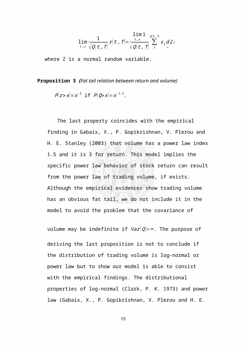
limT→∞

1√Q (t,T )

r (t,T)=limT→∞

1

√Q (t,T)∑1

Q (t,T)

εid⇒Z,

where Z is a normal random variable.

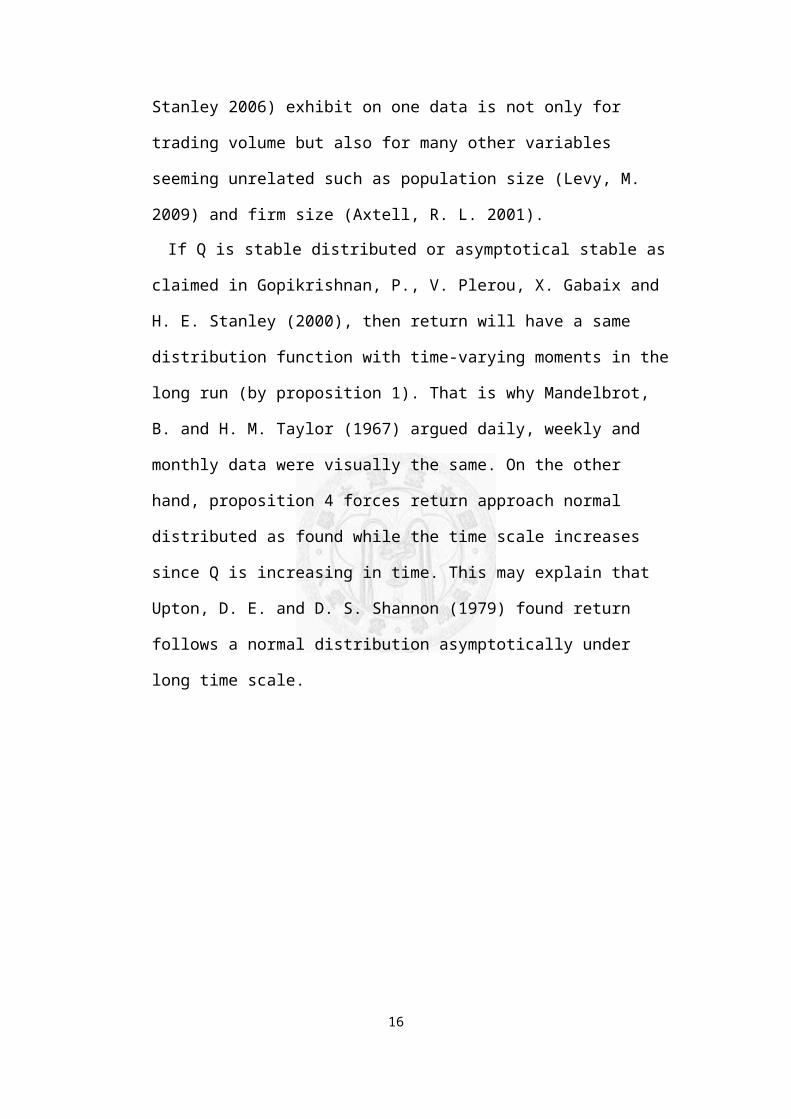
Proposition 5 (Fat tail relation between return and volume)

P (r>x)=x−3 if P (Q>x )=x−1.5.

The last property coincides with the empirical

finding in Gabaix, X., P. Gopikrishnan, V. Plerou and

H. E. Stanley (2003) that volume has a power law index

1.5 and it is 3 for return. This model implies the

specific power law behavior of stock return can result

from the power law of trading volume, if exists.

Although the empirical evidences show trading volume

has an obvious fat tail, we do not include it in the

model to avoid the problem that the covariance of

volume may be indefinite if Var (Q)=∞. The purpose of

deriving the last proposition is not to conclude if

the distribution of trading volume is log-normal or

power law but to show our model is able to consist

with the empirical findings. The distributional

properties of log-normal (Clark, P. K. 1973) and power

law (Gabaix, X., P. Gopikrishnan, V. Plerou and H. E.

15

Stanley 2006) exhibit on one data is not only for

trading volume but also for many other variables

seeming unrelated such as population size (Levy, M.

2009) and firm size (Axtell, R. L. 2001).

If Q is stable distributed or asymptotical stable as

claimed in Gopikrishnan, P., V. Plerou, X. Gabaix and

H. E. Stanley (2000), then return will have a same

distribution function with time-varying moments in the

long run (by proposition 1). That is why Mandelbrot,

B. and H. M. Taylor (1967) argued daily, weekly and

monthly data were visually the same. On the other

hand, proposition 4 forces return approach normal

distributed as found while the time scale increases

since Q is increasing in time. This may explain that

Upton, D. E. and D. S. Shannon (1979) found return

follows a normal distribution asymptotically under

long time scale.

16

IV. Empirical Evidence

In attempting to judge the success of this theory,

we have to examine the degree of agreement between the

conclusion of the theory and reality. As Proposition 3

and 5 are well documented in literatures, we are left

with Proposition 1, 2, and 4 to verify. Proposition 1

and 4 can be examined together by the first empirical

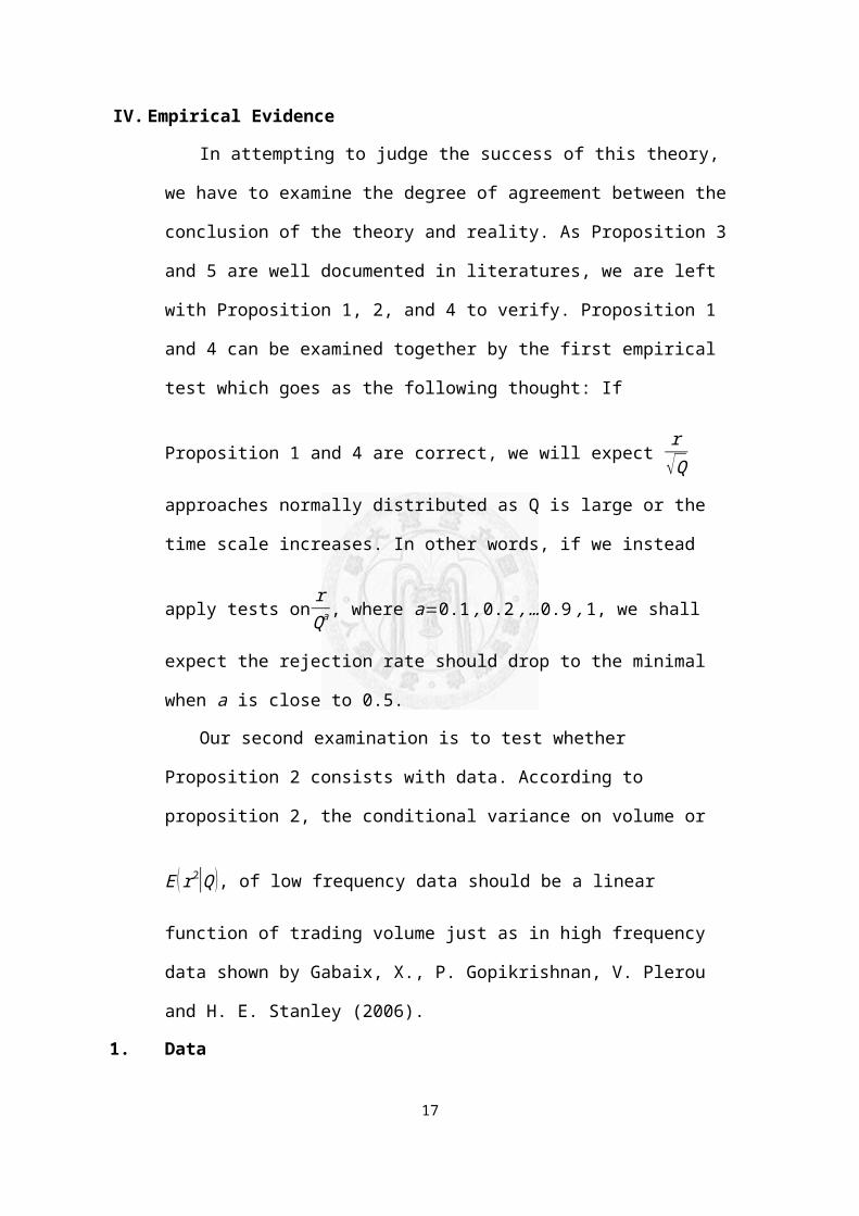
test which goes as the following thought: If

Proposition 1 and 4 are correct, we will expect r√Q

approaches normally distributed as Q is large or the

time scale increases. In other words, if we instead

apply tests on rQa, where a=0.1,0.2,…0.9,1, we shall

expect the rejection rate should drop to the minimal

when a is close to 0.5.

Our second examination is to test whether

Proposition 2 consists with data. According to

proposition 2, the conditional variance on volume or

E (r2|Q ), of low frequency data should be a linear

function of trading volume just as in high frequency

data shown by Gabaix, X., P. Gopikrishnan, V. Plerou

and H. E. Stanley (2006).

1. Data

17

Daily data are chosen as the time scale for the

tradeoff between number of data points and power of

test. Although high frequency data has the advantage

of being plentiful in number, the volume for each

point (one transaction) is not large enough for

central limit theorem to work.

The data source for stocks in Taiwan is TEJ’s

database and the period is last 10 years from

5/15/2003 to 5/15/2013. While most companies have data

points of 2488 in this period, some companies in our

sample do not since their date of I.P.O. occurred

later than 5/15/2003 or just recently.

Return is defined as log difference of price and

adjusted from dividend and split. The objects tested

are the chosen from Taiwan 50 and Taiwan Mid-Cap 100

for they represent nearly 90% of Taiwan stock market1.

For the detail list of all companies please refer to

Table 5 and Table 6 in Appendix B.

2. Methodology

A. Normality Test

To ensure our results are robust, I apply 4 tests

1 FTSE TWSE Taiwan 50 Index: 50 of the most highly capitalised blue chip stocks and represent nearly 70% of the Taiwanese market. FTSE TWSE Taiwan Mid-Cap 100 Index: The next 100 constituents ranked by market capitalisation after the FTSE TWSE Taiwan 50 Index. The index predominantly measures growth sectors and represents nearly 20%of the market.

18

for normality test. They are J-B test, Shapiro-Wilk

test, Anderson-Darling test, Lilliefors test. It turns

out robust to whatever test applied; therefore, I show

the results of Shapiro-Wilk test because Razali, N. M.

and Y. B. Wah (2011) concludes that Shapiro-Wilk has

the best power for a given significance, followed

closely by Anderson-Darling when comparing the

Shapiro-Wilk, Kolmogorov-Smirnov, Lilliefors, and

Anderson-Darling tests. A brief description of other

tests is in appendix. Critical P-value is 5% for all

tests.

For each company, data is divided into subsamples,

which contain consecutive 50 data points and there is no

overlapping in period.

The description of Shapiro–Wilk test is as follows:

Shapiro–Wilk test2

In statistics, the Shapiro–Wilk test tests the null

hypothesis that a sample x1,x2,x3,…,xn came from

a normally distributed population. See Shapiro, S. S. andM. B. Wilk (1965).

The test statistic is:

2 http://en.wikipedia.org/wiki/Shapiro%E2%80%93Wilk_test19

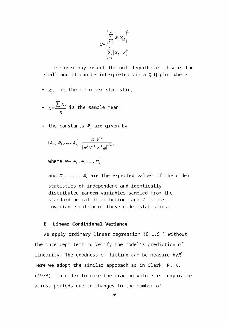
W=(∑i=1

naix(i))

2

∑i=1

n

(xi−x )2

The user may reject the null hypothesis if W is toosmall and it can be interpreted via a Q-Q plot where:

x(i)  is the ith order statistic;

x≡∑xi

n is the sample mean;

the constants ai are given by

(a1,a2,…,an )= m⊺V−1

(m⊺V−1V−1m)1/2,

where m=(m1,m2,…,mn )

and m1, ..., mn are the expected values of the order

statistics of independent and identically distributed random variables sampled from the standard normal distribution, and V is the covariance matrix of those order statistics.

B. Linear Conditional Variance

We apply ordinary linear regression (O.L.S.) without

the intercept term to verify the model’s prediction of

linearity. The goodness of fitting can be measure byR2.

Here we adopt the similar approach as in Clark, P. K.

(1973). In order to make the trading volume is comparable

across periods due to changes in the number of 20

outstanding shares, we will replace trading volume by

turnover in the two analyses3. We group the data points by

increasing turnover into groups of 50 each and then

calculate arithmetic average of square return and

geometric average4 of turnover multiplied by 1000 within

each group as E(r2∨V) and V respectively. Therefore, the

O.L.S. equation becomes

E (r2|V )=ω∗V,

whereV=turnover∗103= volume∗103outstanding

Note that estimating ω is equivalent to estimating σ2 in

our model.

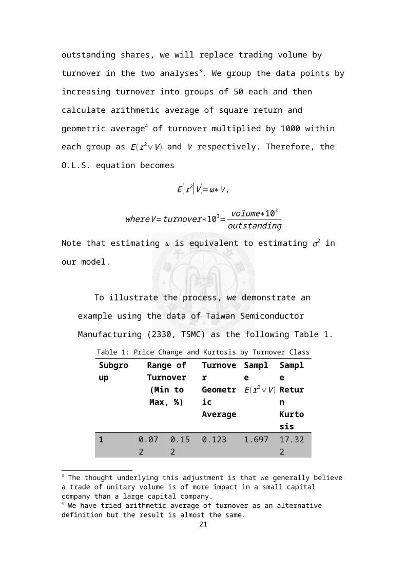
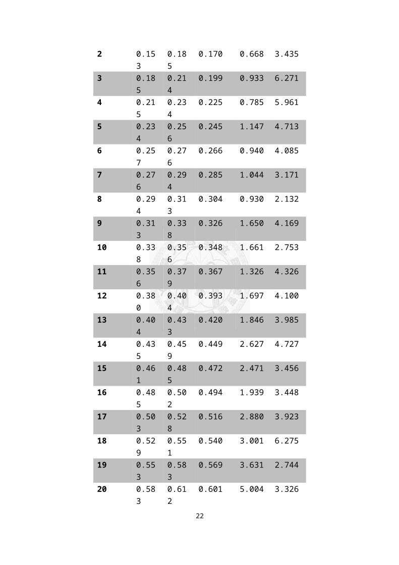
To illustrate the process, we demonstrate an

example using the data of Taiwan Semiconductor

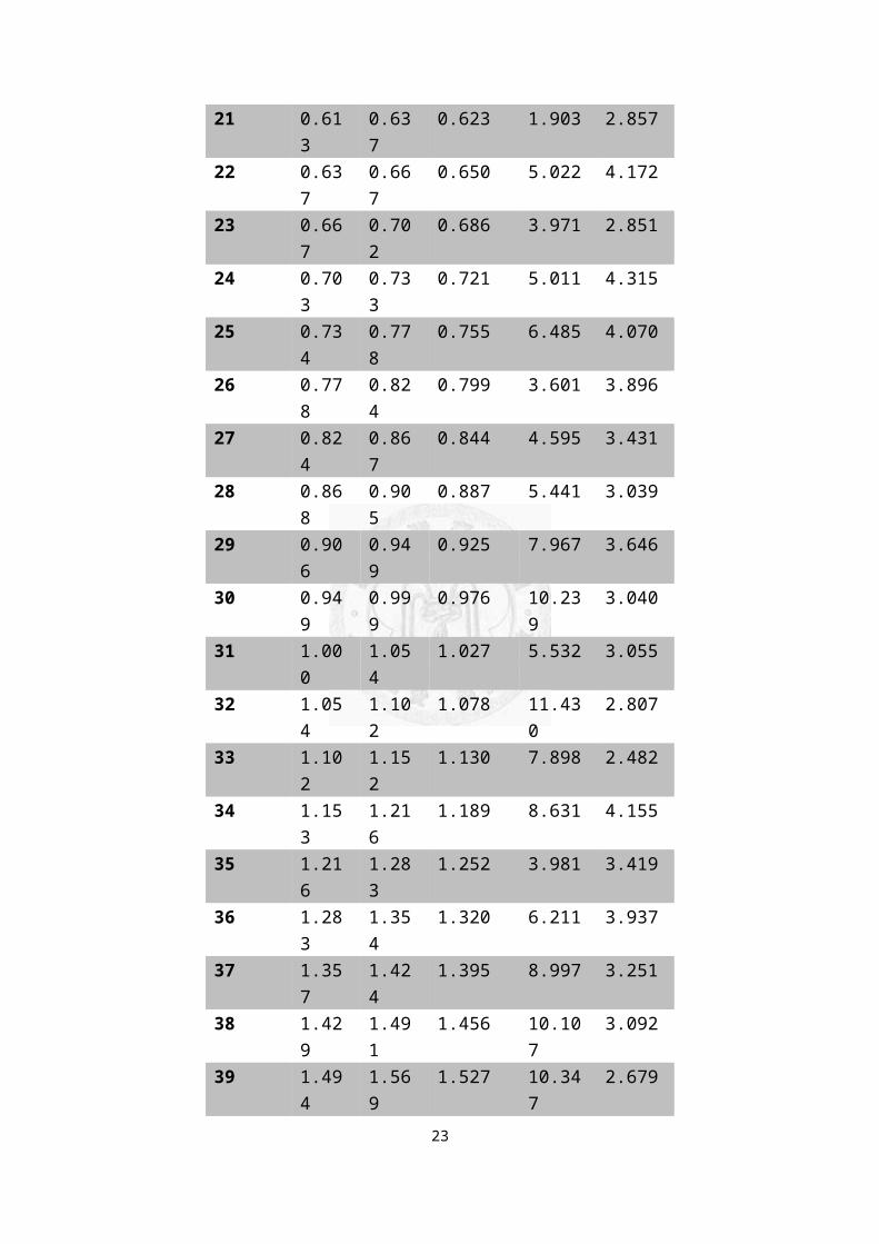
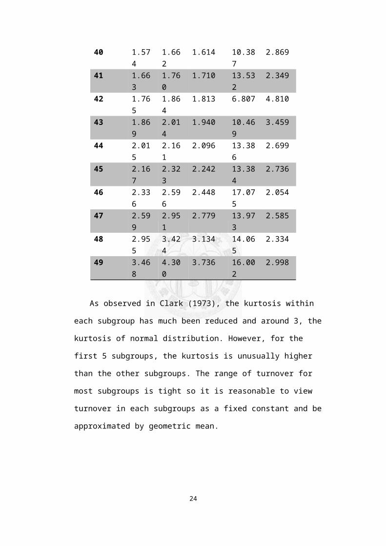
Manufacturing (2330, TSMC) as the following Table 1.

Table 1: Price Change and Kurtosis by Turnover ClassSubgroup

Range ofTurnover(Min toMax, %)

Turnover Geometric Average

SampleE(r2∨V)

Sample Return Kurtosis

1 0.072

0.152

0.123 1.697 17.322

3 The thought underlying this adjustment is that we generally believea trade of unitary volume is of more impact in a small capital company than a large capital company.4 We have tried arithmetic average of turnover as an alternative definition but the result is almost the same.

21

2 0.153

0.185

0.170 0.668 3.435

3 0.185

0.214

0.199 0.933 6.271

4 0.215

0.234

0.225 0.785 5.961

5 0.234

0.256

0.245 1.147 4.713

6 0.257

0.276

0.266 0.940 4.085

7 0.276

0.294

0.285 1.044 3.171

8 0.294

0.313

0.304 0.930 2.132

9 0.313

0.338

0.326 1.650 4.169

10 0.338

0.356

0.348 1.661 2.753

11 0.356

0.379

0.367 1.326 4.326

12 0.380

0.404

0.393 1.697 4.100

13 0.404

0.433

0.420 1.846 3.985

14 0.435

0.459

0.449 2.627 4.727

15 0.461

0.485

0.472 2.471 3.456

16 0.485

0.502

0.494 1.939 3.448

17 0.503

0.528

0.516 2.880 3.923

18 0.529

0.551

0.540 3.001 6.275

19 0.553

0.583

0.569 3.631 2.744

20 0.583

0.612

0.601 5.004 3.326

22

21 0.613

0.637

0.623 1.903 2.857

22 0.637

0.667

0.650 5.022 4.172

23 0.667

0.702

0.686 3.971 2.851

24 0.703

0.733

0.721 5.011 4.315

25 0.734

0.778

0.755 6.485 4.070

26 0.778

0.824

0.799 3.601 3.896

27 0.824

0.867

0.844 4.595 3.431

28 0.868

0.905

0.887 5.441 3.039

29 0.906

0.949

0.925 7.967 3.646

30 0.949

0.999

0.976 10.239

3.040

31 1.000

1.054

1.027 5.532 3.055

32 1.054

1.102

1.078 11.430

2.807

33 1.102

1.152

1.130 7.898 2.482

34 1.153

1.216

1.189 8.631 4.155

35 1.216

1.283

1.252 3.981 3.419

36 1.283

1.354

1.320 6.211 3.937

37 1.357

1.424

1.395 8.997 3.251

38 1.429

1.491

1.456 10.107

3.092

39 1.494

1.569

1.527 10.347

2.679

23

40 1.574

1.662

1.614 10.387

2.869

41 1.663

1.760

1.710 13.532

2.349

42 1.765

1.864

1.813 6.807 4.810

43 1.869

2.014

1.940 10.469

3.459

44 2.015

2.161

2.096 13.386

2.699

45 2.167

2.323

2.242 13.384

2.736

46 2.336

2.596

2.448 17.075

2.054

47 2.599

2.951

2.779 13.973

2.585

48 2.955

3.424

3.134 14.065

2.334

49 3.468

4.300

3.736 16.002

2.998

As observed in Clark (1973), the kurtosis within

each subgroup has much been reduced and around 3, the

kurtosis of normal distribution. However, for the

first 5 subgroups, the kurtosis is unusually higher

than the other subgroups. The range of turnover for

most subgroups is tight so it is reasonable to view

turnover in each subgroups as a fixed constant and be

approximated by geometric mean.

24

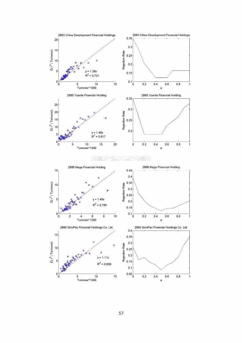
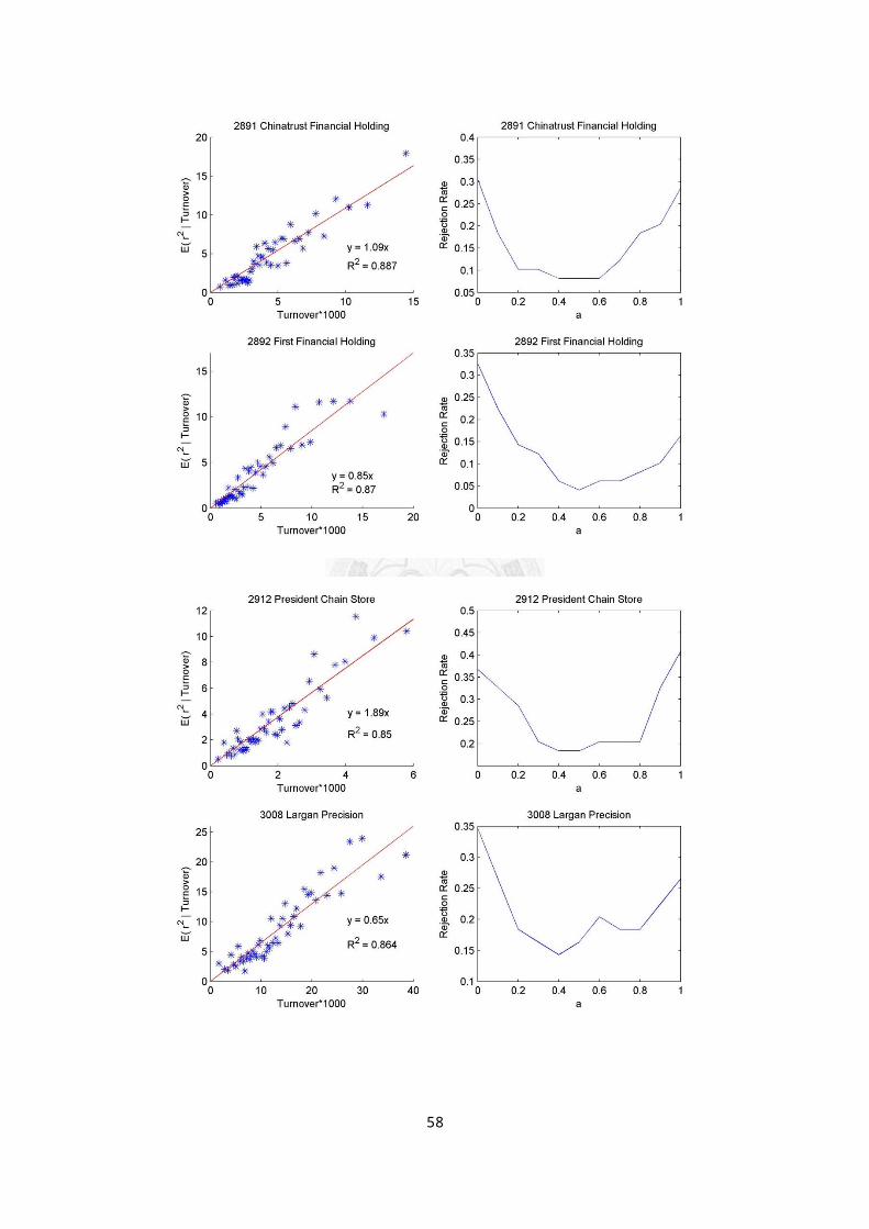
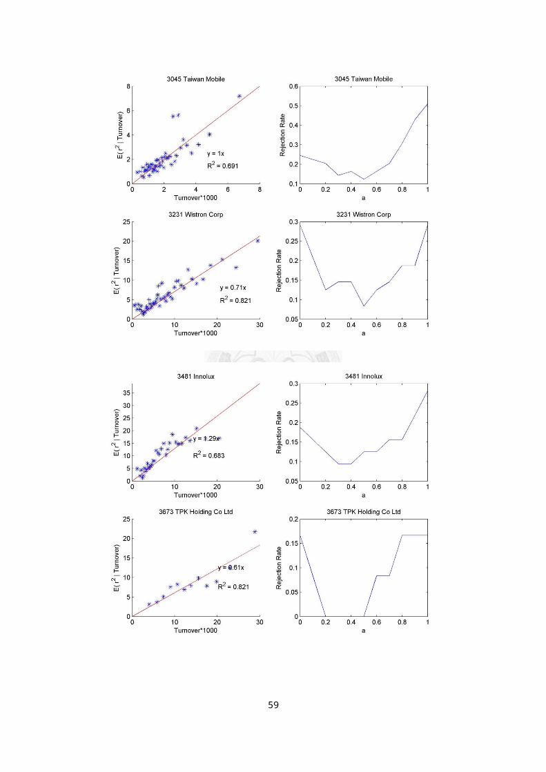
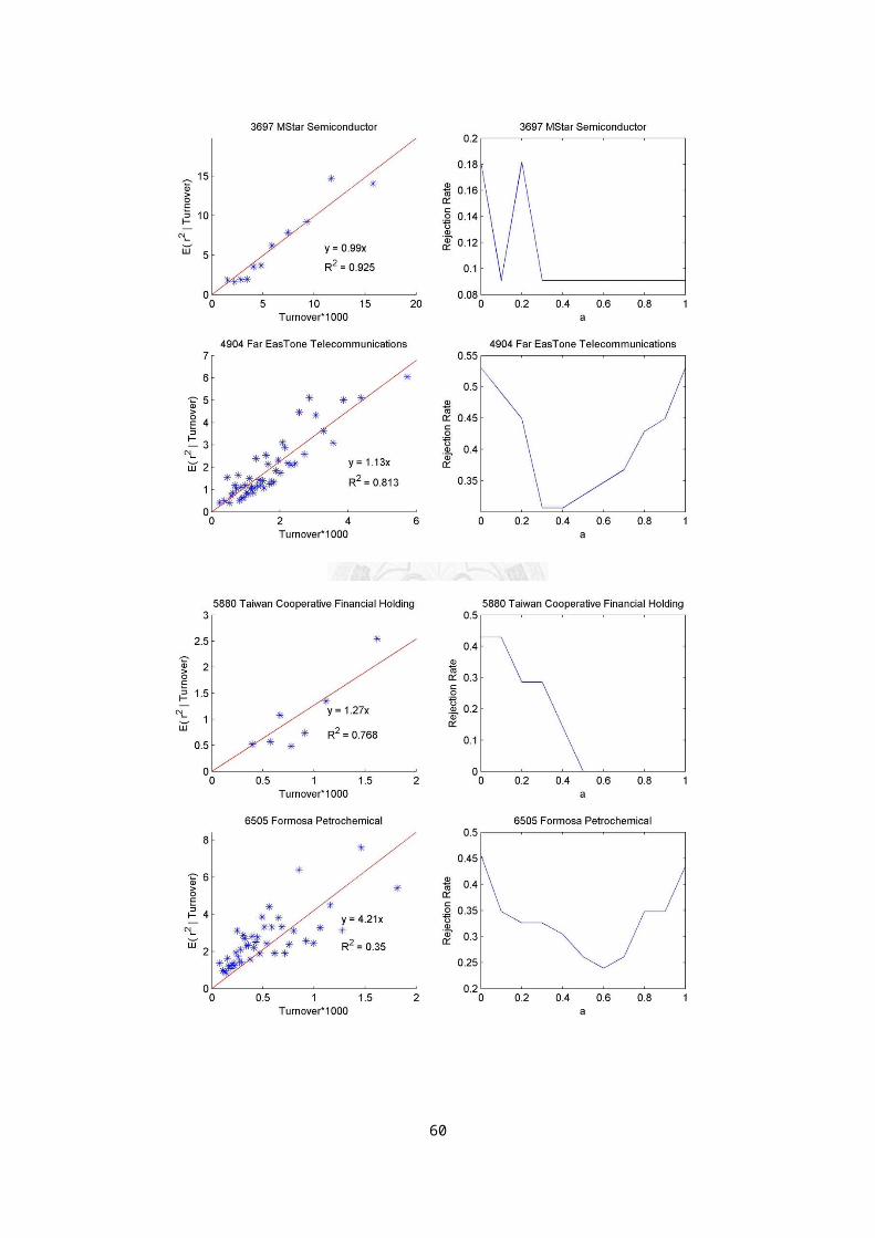
3. Analysis Results

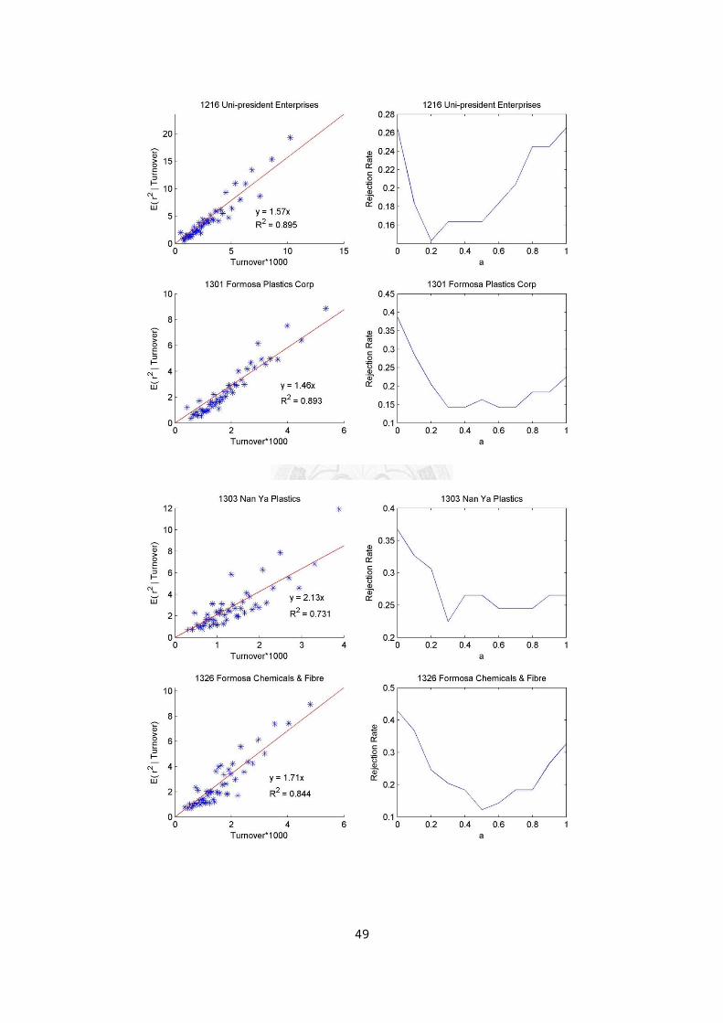
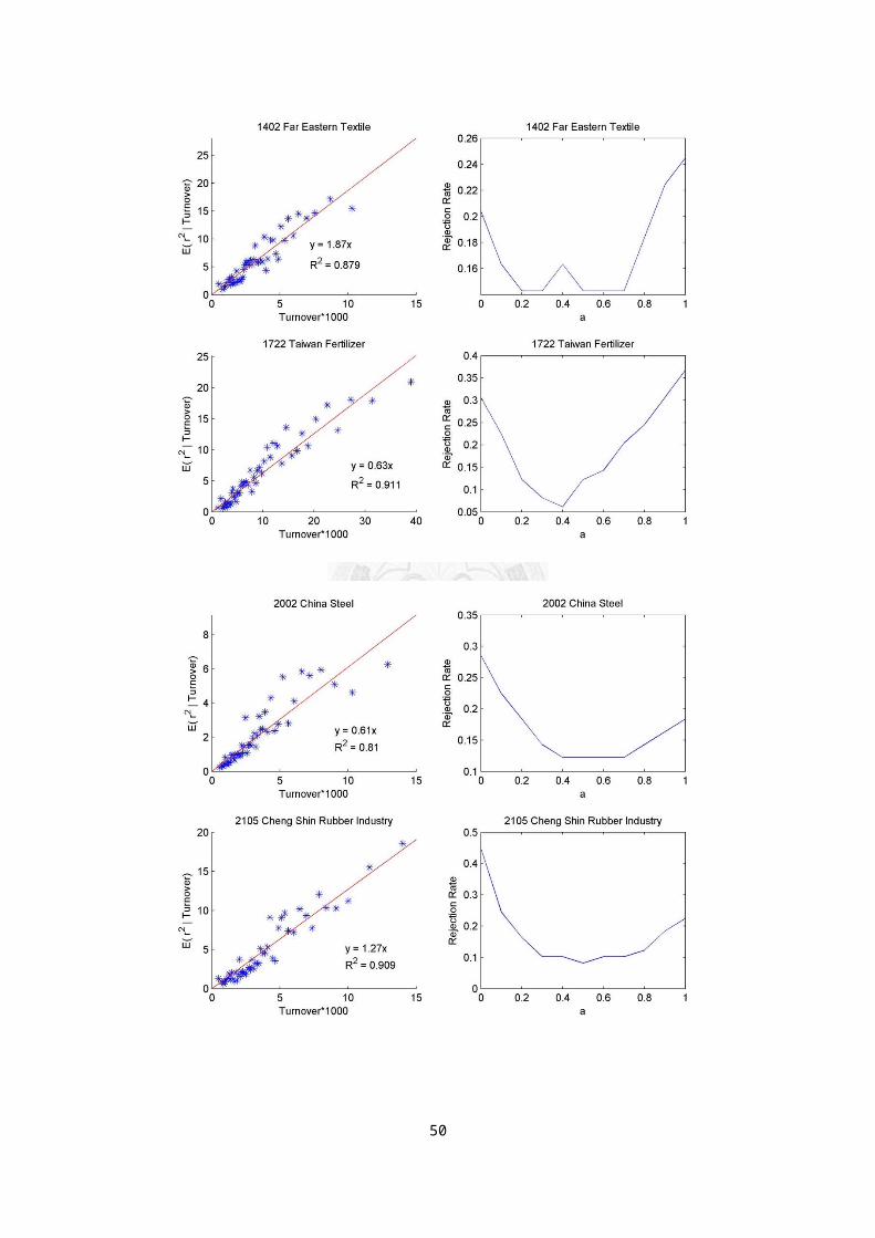
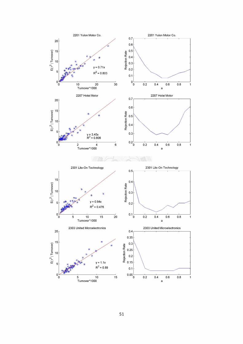
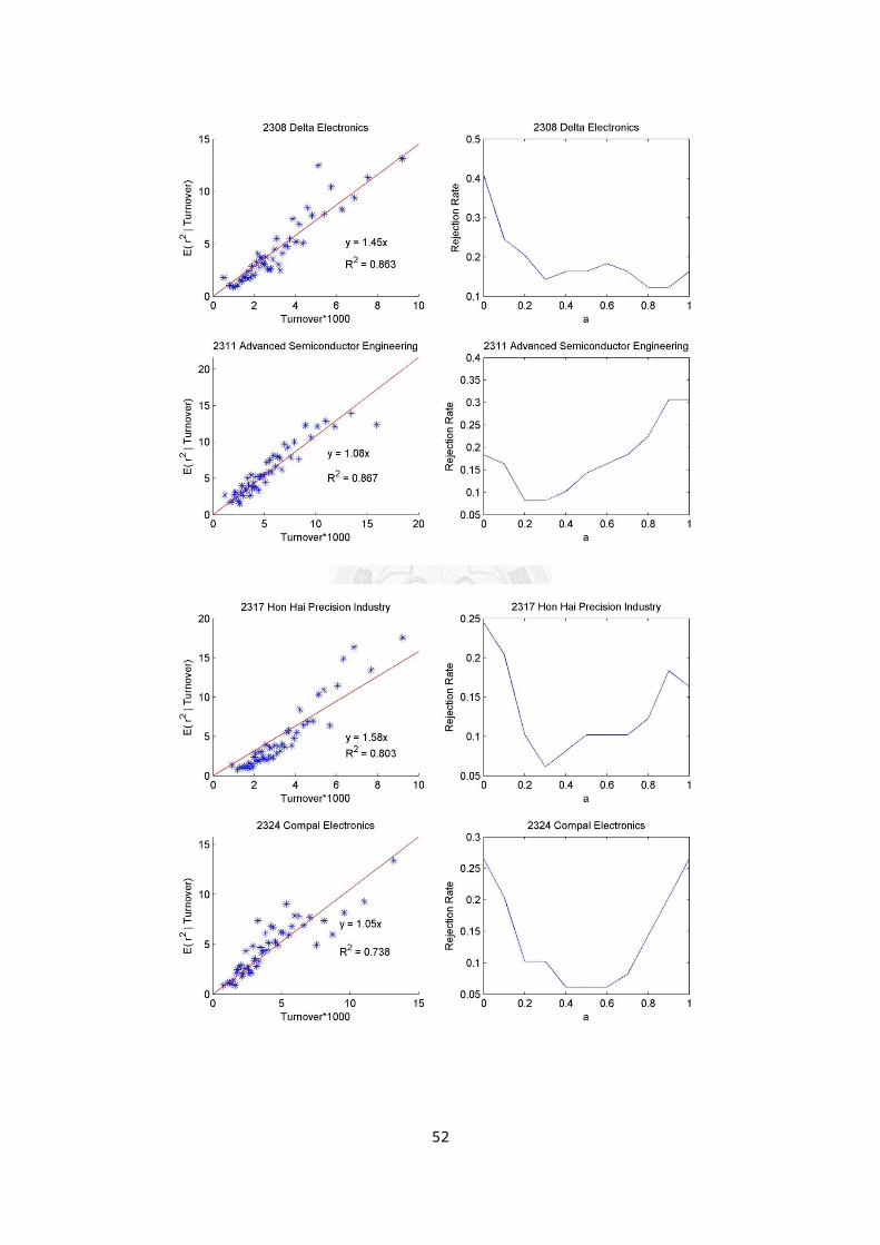
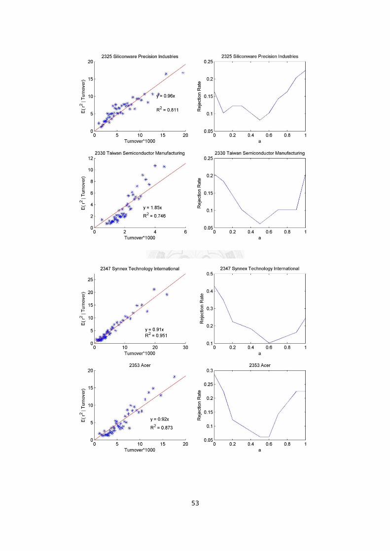
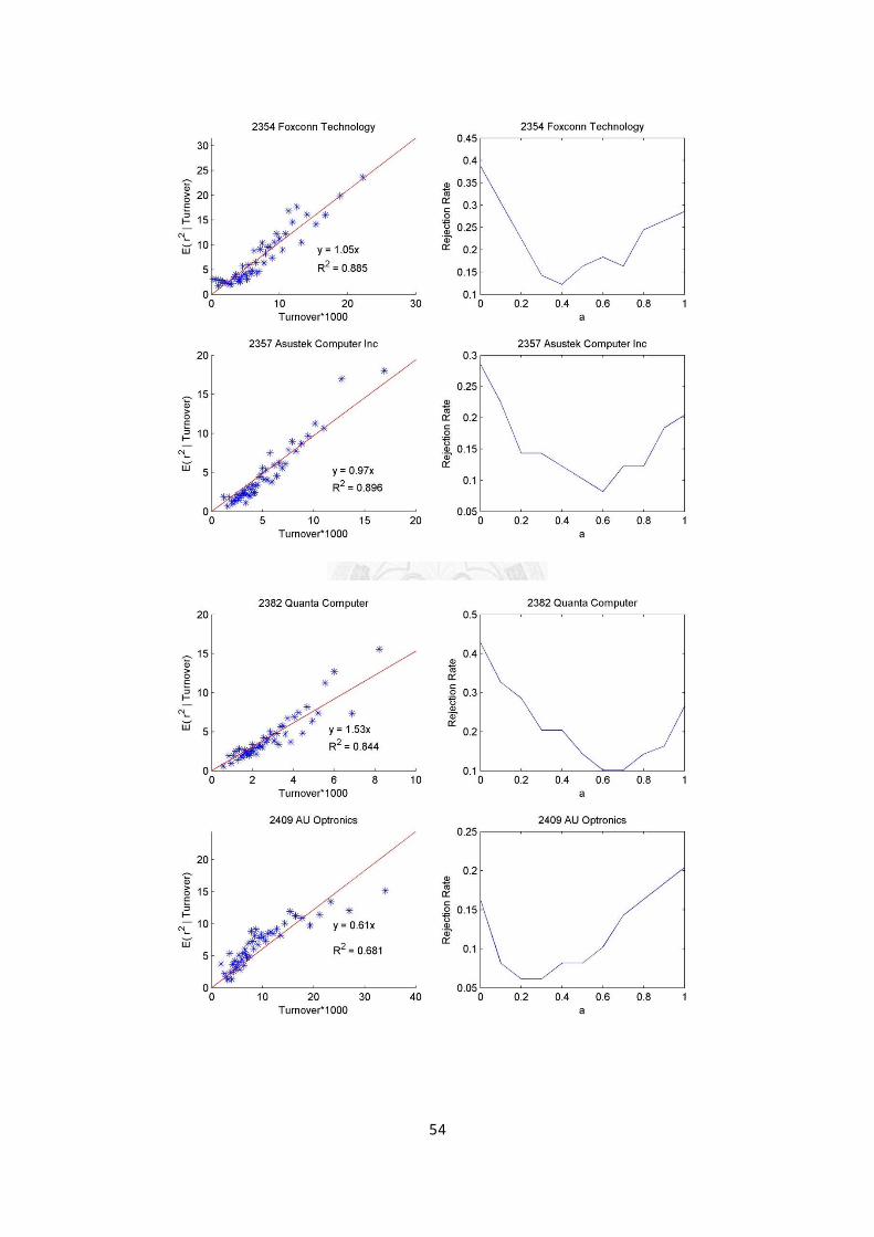
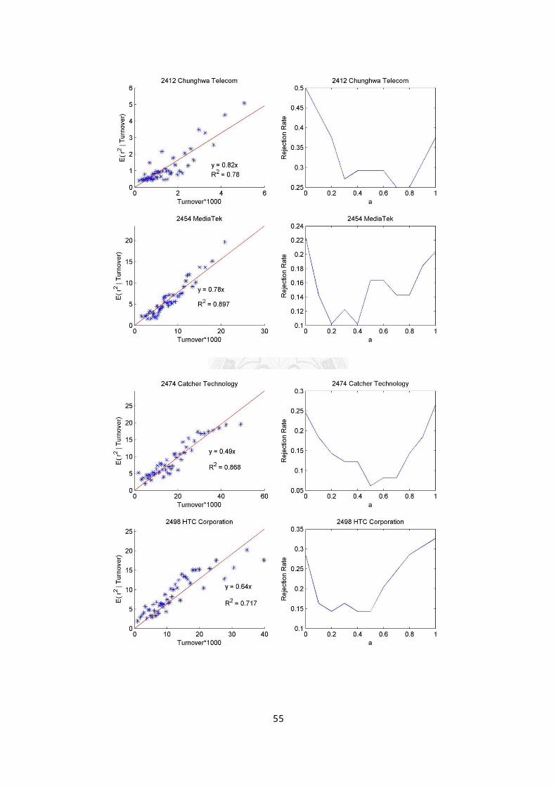
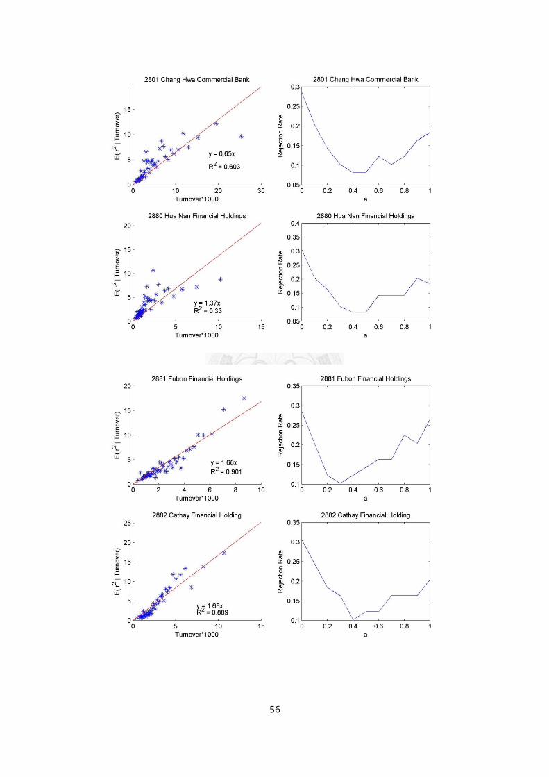
Figure 1 demonstrates the test results for 4

companies selected from the sample. For extensive

results for all companies, please refer to appendix.

The normality test and the scatter plot with fitting

equation and R2 of each company are shown. As we can

observe from the figures below, the rejection rate

tends to reach a minimal for 0<a<1 whereas the

rejection rate is about twice when the data is not

adjusted by volume for most companies. In Table 2, the

number of companies among 50 and Mid-Cap 100 that have

minimal at a=0.5 is 28 of 50 and 48 of 100, while the

number increases to 42 of 50 and 84 of 100 if we count

in the cases for a=0.4 and 0.6, implying √Q plays an important role in return. Although the result is far

from perfect since the rejection rates at a=0.4, 0.5

or 0.6 for most companies are still higher than the

critical threshold 5%, it is fair to conclude the

proposed model is a good approximation at this level

of analysis.

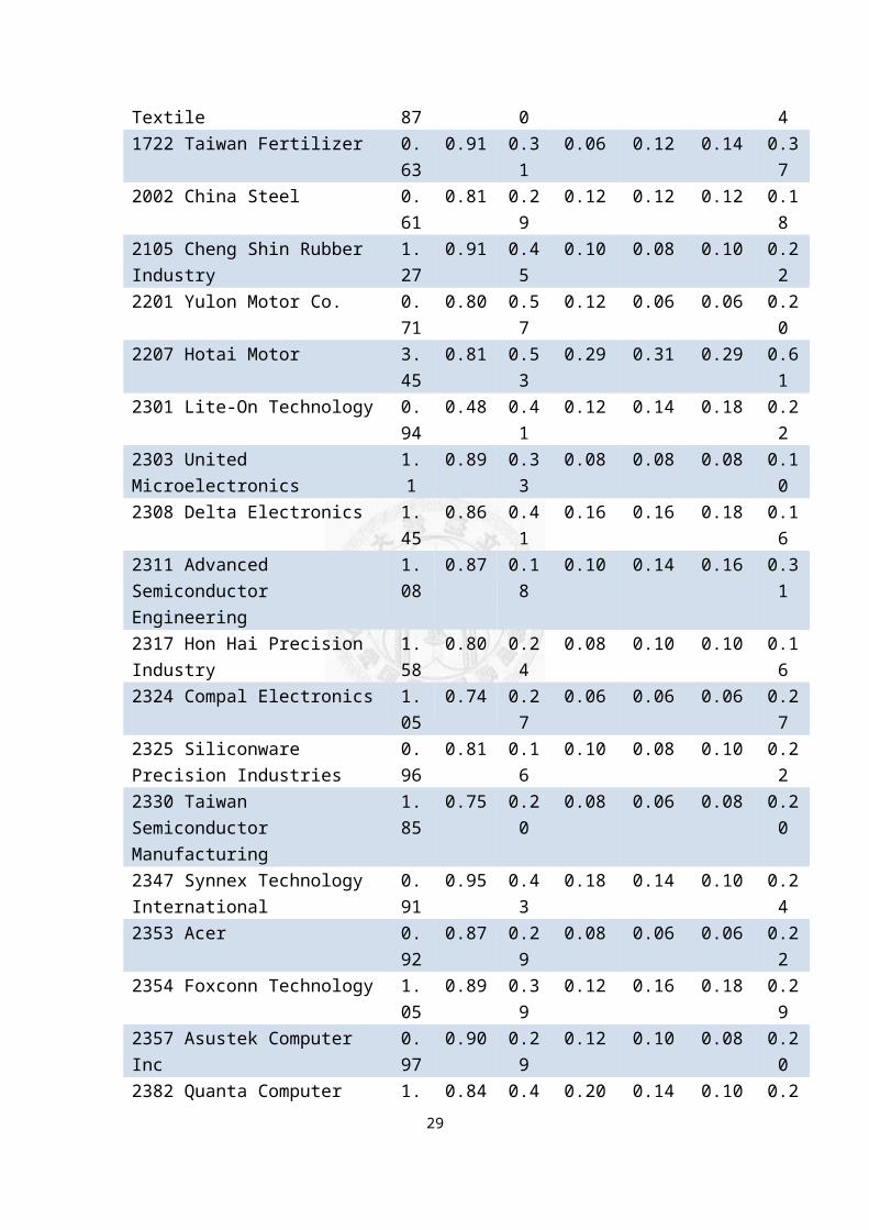
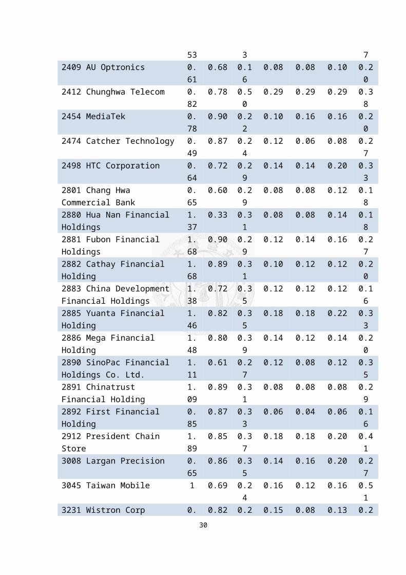
For the second examination, the results are

combined with the normal test below. Table 3:

Regression Results of Conditional Variance on Volume

25

and Rejection Rate of Normality on Adjusted Return for

Taiwan 50. and Table 7: Regression Results of

Conditional Variance on Volume and Rejection Rate of

Normality on Adjusted Return for Taiwan Mid-Cap 100

shows the summary of results. The linear function fits

the conditional variance well for most companies with

highR2, a great agreement to the model’s prediction. A

few (6% for Taiwan 50, 20% for Mid-Cap 100) companies

are with R2 less than 60%. The conditional variance

among those companies shows a tendency of concavity

systematically. This is consistent with the fact that

those companies touch minimal in normal test ata<0.5.

26

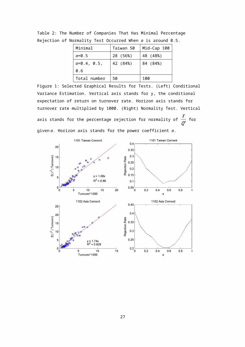
Table 2: The Number of Companies That Has Minimal Percentage Rejection of Normality Test Occurred When a is around 0.5.

Minimal Taiwan 50 Mid-Cap 100a=0.5 28 (56%) 48 (48%)a=0.4, 0.5, 0.6

42 (84%) 84 (84%)

Total number 50 100Figure 1: Selected Graphical Results for Tests. (Left) Conditional Variance Estimation. Vertical axis stands for y, the conditional expectation of return on turnover rate. Horizon axis stands for turnover rate multiplied by 1000. (Right) Normality Test. Vertical

axis stands for the percentage rejection for normality of rQa for

given a. Horizon axis stands for the power coefficient a.

27

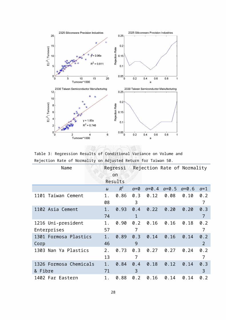
Table 3: Regression Results of Conditional Variance on Volume and Rejection Rate of Normality on Adjusted Return for Taiwan 50.

Name Regression

Results

Rejection Rate of Normality

ω R2 a=0 a=0.4 a=0.5 a=0.6 a=11101 Taiwan Cement 1.

080.86 0.3

30.12 0.08 0.10 0.2

71102 Asia Cement 1.

740.93 0.4

10.22 0.20 0.20 0.3

71216 Uni-president Enterprises

1.57

0.90 0.27

0.16 0.16 0.18 0.27

1301 Formosa Plastics Corp

1.46

0.89 0.39

0.14 0.16 0.14 0.22

1303 Nan Ya Plastics 2.13

0.73 0.37

0.27 0.27 0.24 0.27

1326 Formosa Chemicals & Fibre

1.71

0.84 0.43

0.18 0.12 0.14 0.33

1402 Far Eastern 1. 0.88 0.2 0.16 0.14 0.14 0.2

28

Textile 87 0 41722 Taiwan Fertilizer 0.

630.91 0.3

10.06 0.12 0.14 0.3

72002 China Steel 0.

610.81 0.2

90.12 0.12 0.12 0.1

82105 Cheng Shin Rubber Industry

1.27

0.91 0.45

0.10 0.08 0.10 0.22

2201 Yulon Motor Co. 0.71

0.80 0.57

0.12 0.06 0.06 0.20

2207 Hotai Motor 3.45

0.81 0.53

0.29 0.31 0.29 0.61

2301 Lite-On Technology 0.94

0.48 0.41

0.12 0.14 0.18 0.22

2303 United Microelectronics

1.1

0.89 0.33

0.08 0.08 0.08 0.10

2308 Delta Electronics 1.45

0.86 0.41

0.16 0.16 0.18 0.16

2311 Advanced Semiconductor Engineering

1.08

0.87 0.18

0.10 0.14 0.16 0.31

2317 Hon Hai Precision Industry

1.58

0.80 0.24

0.08 0.10 0.10 0.16

2324 Compal Electronics 1.05

0.74 0.27

0.06 0.06 0.06 0.27

2325 Siliconware Precision Industries

0.96

0.81 0.16

0.10 0.08 0.10 0.22

2330 Taiwan Semiconductor Manufacturing

1.85

0.75 0.20

0.08 0.06 0.08 0.20

2347 Synnex Technology International

0.91

0.95 0.43

0.18 0.14 0.10 0.24

2353 Acer 0.92

0.87 0.29

0.08 0.06 0.06 0.22

2354 Foxconn Technology 1.05

0.89 0.39

0.12 0.16 0.18 0.29

2357 Asustek Computer Inc

0.97

0.90 0.29

0.12 0.10 0.08 0.20

2382 Quanta Computer 1. 0.84 0.4 0.20 0.14 0.10 0.229

53 3 72409 AU Optronics 0.

610.68 0.1

60.08 0.08 0.10 0.2

02412 Chunghwa Telecom 0.

820.78 0.5

00.29 0.29 0.29 0.3

82454 MediaTek 0.

780.90 0.2

20.10 0.16 0.16 0.2

02474 Catcher Technology 0.

490.87 0.2

40.12 0.06 0.08 0.2

72498 HTC Corporation 0.

640.72 0.2

90.14 0.14 0.20 0.3

32801 Chang Hwa Commercial Bank

0.65

0.60 0.29

0.08 0.08 0.12 0.18

2880 Hua Nan Financial Holdings

1.37

0.33 0.31

0.08 0.08 0.14 0.18

2881 Fubon Financial Holdings

1.68

0.90 0.29

0.12 0.14 0.16 0.27

2882 Cathay Financial Holding

1.68

0.89 0.31

0.10 0.12 0.12 0.20

2883 China Development Financial Holdings

1.38

0.72 0.35

0.12 0.12 0.12 0.16

2885 Yuanta Financial Holding

1.46

0.82 0.35

0.18 0.18 0.22 0.33

2886 Mega Financial Holding

1.48

0.80 0.39

0.14 0.12 0.14 0.20

2890 SinoPac Financial Holdings Co. Ltd.

1.11

0.61 0.27

0.12 0.08 0.12 0.35

2891 Chinatrust Financial Holding

1.09

0.89 0.31

0.08 0.08 0.08 0.29

2892 First Financial Holding

0.85

0.87 0.33

0.06 0.04 0.06 0.16

2912 President Chain Store

1.89

0.85 0.37

0.18 0.18 0.20 0.41

3008 Largan Precision 0.65

0.86 0.35

0.14 0.16 0.20 0.27

3045 Taiwan Mobile 1 0.69 0.24

0.16 0.12 0.16 0.51

3231 Wistron Corp 0. 0.82 0.2 0.15 0.08 0.13 0.230

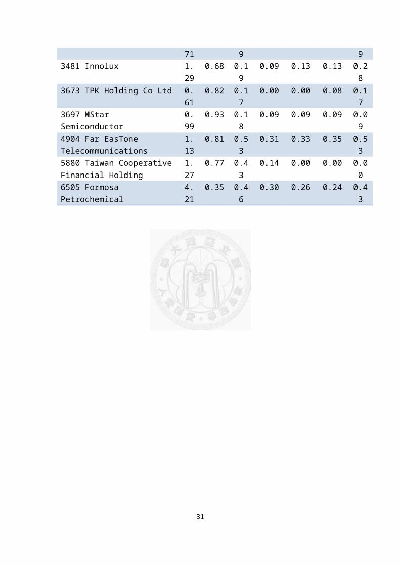
71 9 93481 Innolux 1.

290.68 0.1

90.09 0.13 0.13 0.2

83673 TPK Holding Co Ltd 0.

610.82 0.1

70.00 0.00 0.08 0.1

73697 MStar Semiconductor

0.99

0.93 0.18

0.09 0.09 0.09 0.09

4904 Far EasTone Telecommunications

1.13

0.81 0.53

0.31 0.33 0.35 0.53

5880 Taiwan CooperativeFinancial Holding

1.27

0.77 0.43

0.14 0.00 0.00 0.00

6505 Formosa Petrochemical

4.21

0.35 0.46

0.30 0.26 0.24 0.43

31

DiscussionAlthough the above two tests have shown trading

volume plays an important role in return’s behavior

and moments (variance, skewness, and kurtosis), volume

alone is not fully able to deduce return to be normal

distributed. As we can see from the rejection rate of

Table 3: Regression Results of Conditional Variance on

Volume and Rejection Rate of Normality on Adjusted

Return for Taiwan 50. and Table 7: Regression Results

of Conditional Variance on Volume and Rejection Rate

of Normality on Adjusted Return for Taiwan Mid-Cap 100,

the rejection rate drops significantly but is above

5%, the critical P-value, for most cases. It implies

there is at least one factor other than volume

influencing return. The concavity of variance from

companies that do not have rejection minimal at a=0.5

is also obvious. Price limits to volatility in Taiwan

stock market may be one cause to the concavity of

variance conditional on volume. To sum up, a few can

be noted directly:

The first is that the variance of adjusted return

is not constant but time varying; that is, Var (rt

√Qt

)=σt2

. The slope of conditional variance on volume for

different period is significantly different. For 32

example, the estimated average slope is 1.854 for

Taiwan Semiconductor Manufacturing (2330, TSMC) in

2003-2013, while it is 1.198 in 1993-2003. The second

is that long memory still exists in the adjusted

return , which implies there is a long memory

component other than volume in the adjusted return or

σt. Take TSMC as example again. The reader can observe

this from Figure 2. The autocorrelation function of

absolute value of return is visually the same as the

one of | r√Q| . These are consistent with Gillemot, L., J. D. Farmer and F. Lillo (2006) that states trading

volume may not be the only source of price fluctuation

and the long-memory component of return differs from

the one of volume Bollerslev, T. and D. Jubinski

(1999).

33

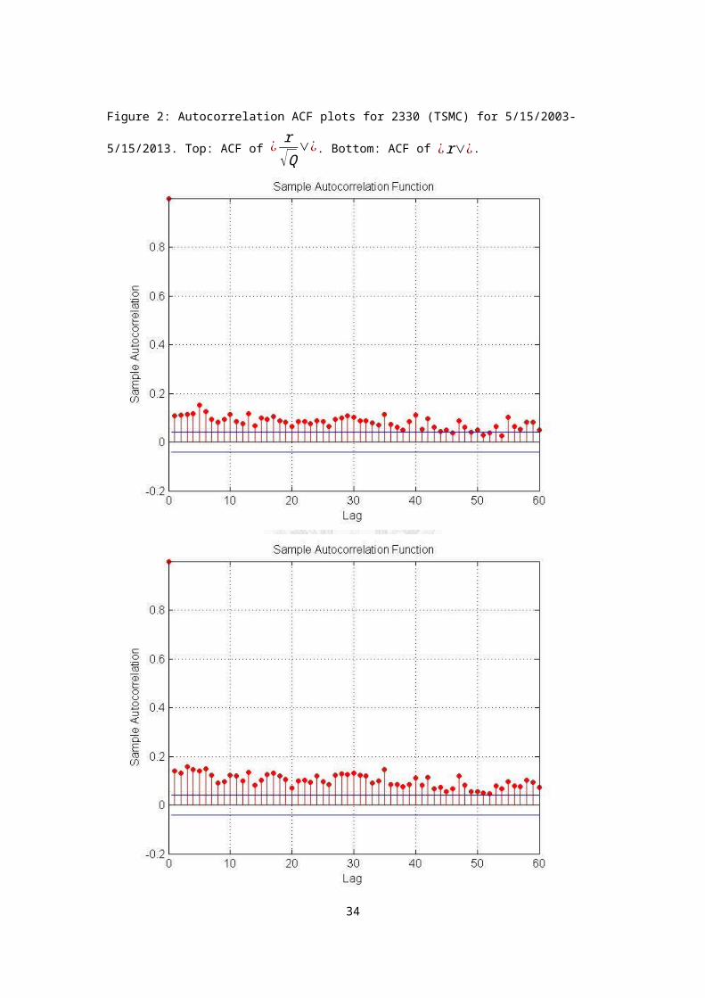
Figure 2: Autocorrelation ACF plots for 2330 (TSMC) for 5/15/2003-

5/15/2013. Top: ACF of ¿r√Q

∨¿. Bottom: ACF of ¿r∨¿.

34

Moreover, Proposition 2 implies the intercept term

in the linear equation between E(r2∨Q) and Q should be

0 or insignificant. If this proposition is perfectly

right, we shall not be able to observe any

significance in tests. However, the empirical evidence

indicates although the goodness of fit of E (r2|V )=ω∗V

is high, it is not without problems. We apply t-test

to test the null-hypothesis: H0: μ=0 against H1: μ≠0

for the following linear regression:

E (r2|V )=μ+ω∗V

It is obvious H0 is equivalent to proposition 2.

Table 4 shows the null hypothesis μ=0 is rejected

for 24 companies among 50 and for 66 companies among

Mid-Cap 100 in level of 1% significance. Also, the

estimated μ is not positive for each company all the

times. There are 9 companies among both Taiwan 50 and

Mid-Cap 100 whose intercept term is 1% significant and

negative. This implies, for these companies, the

estimated conditional variance will reduce to be

negative whenever turnover rate is small enough, which

is not possible since variance is always non-negative

by its definition. The significance of intercept term

is able to explain why the calculated R2 is negative

35

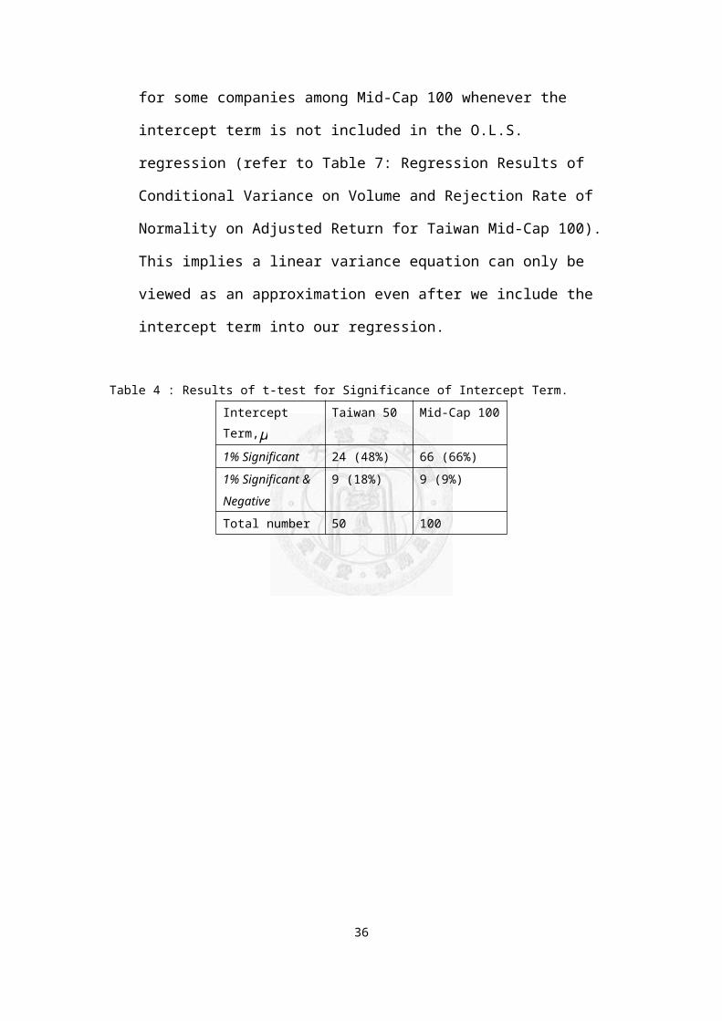
for some companies among Mid-Cap 100 whenever the

intercept term is not included in the O.L.S.

regression (refer to Table 7: Regression Results of

Conditional Variance on Volume and Rejection Rate of

Normality on Adjusted Return for Taiwan Mid-Cap 100).

This implies a linear variance equation can only be

viewed as an approximation even after we include the

intercept term into our regression.

Table 4 : Results of t-test for Significance of Intercept Term.Intercept Term,μ

Taiwan 50 Mid-Cap 100

1% Significant 24 (48%) 66 (66%)1% Significant & Negative

9 (18%) 9 (9%)

Total number 50 100

36

Conclusion

In this study, we propose a model based on some

assumptions. This model emphasizes the role of trading

volume in the behavior of speculative price and

provides a definite and quantitative description. The

assumptions are either intuitive or supported by

empirical evidences found before. The features of the

model are that the derived return formula is

invariance under time scales and simple: it is a

random walk with trading volume as its driving steps.

The properties of this model are also consistent with

most empirical findings so far.

To empirically examine whether this model captures

the essence of the mechanism of stock return, we apply

two approaches for Taiwan stock market. First we apply

normal tests to return adjusted by different power

transformation of volume. The results show the

rejection rate of normal test drops significantly

around power of 0.5. However, this model is not

without shortcomings: the rejection rate for normality

hardly drops to the 5% significant level. Also,

Var (r√Q

) is time-varying and | r√Q| is still auto-correlated and has long-memory as |r|. In addition,

37

Proposition 2 asserts the intercept term in the linear

variance equation is 0 while the empirical t-test

shows the intercept term is significantly away from 0

and can be negative for some companies.

Overall, the success of its empirical prediction

indicates the model reflects fundamental attributes of

speculative prices while the failure to provide an

accurate description to the autocorrelation of | r√Q| and the conditional variance of return suggests the

need to plague much work on the theoretical

development. The author hopes this model may become a

platform to further theory building for its

simplicity.

38

Appendix

A. Proof

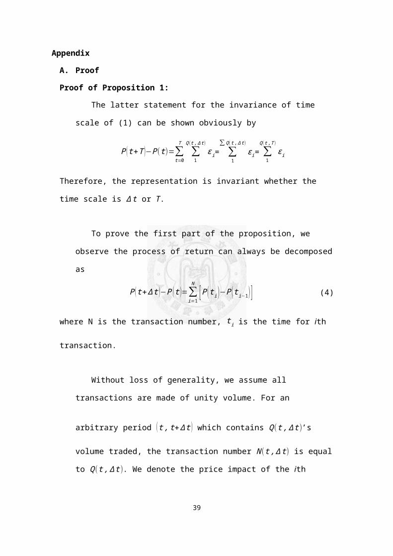
Proof of Proposition 1:

The latter statement for the invariance of time

scale of (1) can be shown obviously by

P (t+T )−P(t)=∑t=0

T

∑1

Q (t,∆t)

εi= ∑1

∑ Q(t,∆t)

εi= ∑1

Q(t,T )

εi

Therefore, the representation is invariant whether the

time scale is ∆t or T.

To prove the first part of the proposition, we

observe the process of return can always be decomposed

as

P (t+∆t )−P (t )=∑i=1

N

[P (ti )−P (ti−1) ] (4)

where N is the transaction number, ti is the time for ith

transaction.

Without loss of generality, we assume all

transactions are made of unity volume. For an

arbitrary period (t,t+∆t ) which contains Q(t,∆t)’s

volume traded, the transaction number N(t,∆t) is equal

to Q(t,∆t). We denote the price impact of the ith

39

transaction as εi. Assumption 1 implies

εi≡P (ti )−P (ti−1 )=εj≡P (tj )−P (tj−1 )∈distribution∀i≠j.

Moreover, the impact of each transaction is independent

by Assumption 2.

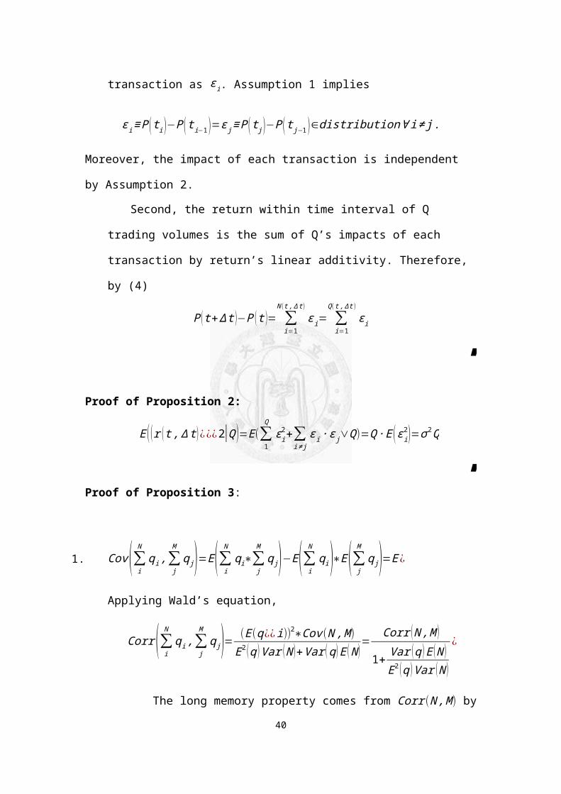
Second, the return within time interval of Q

trading volumes is the sum of Q’s impacts of each

transaction by return’s linear additivity. Therefore,

by (4)

P (t+∆t )−P (t )= ∑i=1

N (t,∆t)

εi= ∑i=1

Q(t,∆t )

εi

∎

Proof of Proposition 2:

E ((r (t,∆t)¿¿¿2|Q )=E(∑1

Qεi2+∑

i≠jεi∙εj∨Q)=Q∙E (εi

2)=σ2Q

∎

Proof of Proposition 3:

1. Cov(∑iNqi,∑

j

Mqj)=E(∑i

Nqi∗∑

j

Mqj)−E(∑i

Nqi)∗E(∑j

Mqj)=E ¿

Applying Wald’s equation,

Corr (∑iNqi,∑

j

Mqj)= (E(q¿¿i))2∗Cov(N,M)

E2 (q )Var (N )+Var (q)E (N)=

Corr (N,M )

1+Var (q )E (N )E2 (q )Var (N )

¿

The long memory property comes from Corr (N,M) by

40

Assumption 5∎

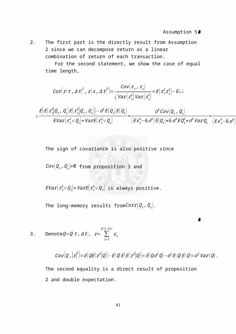
2. The first part is the directly result from Assumption 2 since we can decompose return as a linear combination of return of each transaction.

For the second statement, we show the case of equaltime length,

Cor (r (t,∆t)2,r (s,∆t)2 )= Cov (rt,rs )√Var (rt

2)Var (rs2)=E (rt

2rs2 )−E¿¿

¿E(E (rt

2|Qt,Qs)E (rs2|Qt,Qs))−σ4E (Qt )E (Qt )

EVar (rt2∨Qt)+VarE (rt

2∨Qt )=

σ4Cov (Qt,Qs )(Eεi

4−6σ4)E (Qt )+6σ4EQt2+σ4VarQt

=σ4Cov (Qt,Qs)

(Eεi4−6σ4 )E (Qt )−6σ4 (EQt )2+7σ4VarQt

=Corr (Qt,Qs )

(Eεi4

σ4 −6)E (Qt)−6 (EQt )2

VarQt+7

=Corr (Qt,Qs )constant

The sign of covariance is also positive since

Cov (Qt,Qs )>0 from proposition 3 and

EVar (rt2∨Qt)+VarE(rt

2∨Qt) is always positive.

The long-memory results fromCorr (Qt,Qs ).

∎

3. DenoteQ=Q (t,∆t ), r= ∑i=1

Q (t,∆t )

εi

Cov (Q,|r|2)=E (QE (r2|Q ))−E (Q)E (E (r2|Q ))=E (Qσ2Q )−σ2E (Q)E (Q )=σ2Var(Q).

The second equality is a direct result of proposition

2 and double expectation.

41

∴Corr (Q,|r|2)= Cov (Q,|r|2)√Var (Q )Var (r2 )

=σ2Var (Q )

√Var (Q ) [(Eεi4−6σ4 )E (Q )+6σ4EQ2+σ4VarQ ]

=1

√ [(Eεi4

σ4 −6)E (Q)+6EQ2]Var (Q )

+1

>0

∎

Proof of Proposition 4This is a direct result from Rényi, A. (1960) for randomsums of random variables as we have Assumption 4 and i.i.d. conditions of proposition 1.

∎

Proof of Proposition 5

r= ∑i=1

Q (t,∆t )

εi=√Q (t,∆t ) 1√Q (t,∆t )

∑i=1

Q (t,∆t )

εi=√Q (t,∆t )U,

where U=1

√Q (t,∆t )∑i=1

Q(t,∆t )

εi.

Var (U )=E[Var( 1√Q (t,∆t )

∑i=1

Q (t,∆t )

εi|Q)]+Var [E( 1√Q (t,∆t )

∑i=1

Q(t,∆t)

εi|Q)]=1∴ If U has finite power law index γU, then γU≥2

∴P (r>x)=x−3 whenever x is large because power index of

√Q (t,∆t)is 3.

∎

42

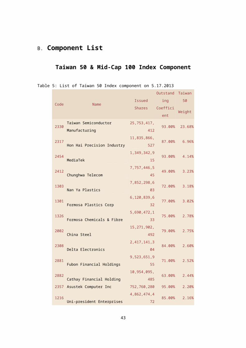
B. Component List

Taiwan 50 & Mid-Cap 100 Index Component

Table 5: List of Taiwan 50 Index component on 5.17.2013

Code NameIssuedShares

Outstanding

Taiwan50

Coefficient

Weight

2330Taiwan Semiconductor Manufacturing

25,753,417,412

93.00% 23.68%

2317Hon Hai Precision Industry

11,835,866,527

87.00% 6.96%

2454MediaTek

1,349,342,915

93.00% 4.14%

2412Chunghwa Telecom

7,757,446,545

49.00% 3.23%

1303Nan Ya Plastics

7,852,298,603

72.00% 3.18%

1301Formosa Plastics Corp

6,120,839,632

77.00% 3.02%

1326Formosa Chemicals & Fibre

5,690,472,133

75.00% 2.78%

2002China Steel

15,271,902,492

79.00% 2.75%

2308Delta Electronics

2,417,141,304

84.00% 2.60%

2881Fubon Financial Holdings

9,523,651,955

71.00% 2.52%

2882Cathay Financial Holding

10,954,095,485

63.00% 2.44%

2357 Asustek Computer Inc 752,760,280 95.00% 2.20%

1216Uni-president Enterprises

4,862,474,472

85.00% 2.16%

43

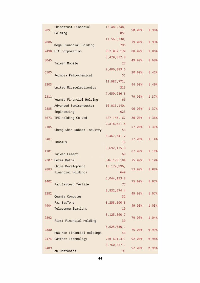
2891Chinatrust Financial Holding

13,483,748,051

90.00% 1.96%

2886Mega Financial Holding

11,563,730,796

79.00% 1.93%

2498 HTC Corporation 852,052,170 88.00% 1.86%

3045Taiwan Mobile

3,420,832,827

49.00% 1.69%

6505Formosa Petrochemical

9,486,083,651

20.00% 1.42%

2303United Microelectronics

12,987,771,315

94.00% 1.40%

2311Yuanta Financial Holding

7,650,986,866

79.00% 1.37%

2885Advanced Semiconductor Engineering

10,016,140,025

96.00% 1.37%

3673 TPK Holding Co Ltd 327,140,167 80.00% 1.36%

2105Cheng Shin Rubber Industry

2,818,621,453

57.00% 1.31%

3481Innolux

8,467,041,216

77.00% 1.14%

1101Taiwan Cement

3,692,175,869

87.00% 1.11%

2207 Hotai Motor 546,179,184 75.00% 1.10%

2883China Development Financial Holdings

15,172,996,640

93.00% 1.08%

1402Far Eastern Textile

5,044,133,877

75.00% 1.07%

2382Quanta Computer

3,832,574,432

49.99% 1.07%

4904Far EasTone Telecommunications

3,258,500,810

49.00% 1.05%

2892First Financial Holding

8,125,360,730

79.00% 1.04%

2880Hua Nan Financial Holdings

8,625,030,143

75.00% 0.99%

2474 Catcher Technology 750,691,371 92.00% 0.98%

2409AU Optronics

8,760,837,191

92.00% 0.95%

44

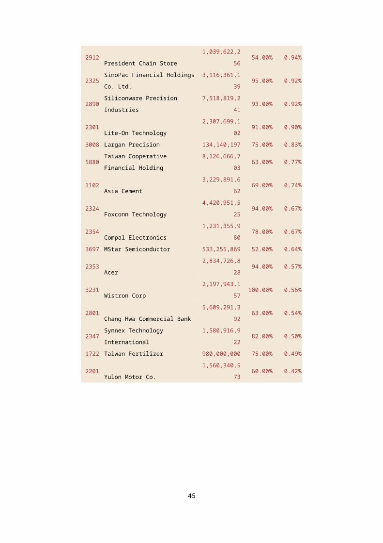
2912President Chain Store

1,039,622,256

54.00% 0.94%

2325SinoPac Financial HoldingsCo. Ltd.

3,116,361,139

95.00% 0.92%

2890Siliconware Precision Industries

7,518,819,241

93.00% 0.92%

2301Lite-On Technology

2,307,699,102

91.00% 0.90%

3008 Largan Precision 134,140,197 75.00% 0.83%

5880Taiwan Cooperative Financial Holding

8,126,666,703

63.00% 0.77%

1102Asia Cement

3,229,891,662

69.00% 0.74%

2324Foxconn Technology

4,420,951,525

94.00% 0.67%

2354Compal Electronics

1,231,355,980

78.00% 0.67%

3697 MStar Semiconductor 533,255,869 52.00% 0.64%

2353Acer

2,834,726,828

94.00% 0.57%

3231Wistron Corp

2,197,943,157

100.00% 0.56%

2801Chang Hwa Commercial Bank

5,609,291,392

63.00% 0.54%

2347Synnex Technology International

1,580,916,922

82.00% 0.50%

1722 Taiwan Fertilizer 980,000,000 75.00% 0.49%

2201Yulon Motor Co.

1,560,340,573

60.00% 0.42%

45

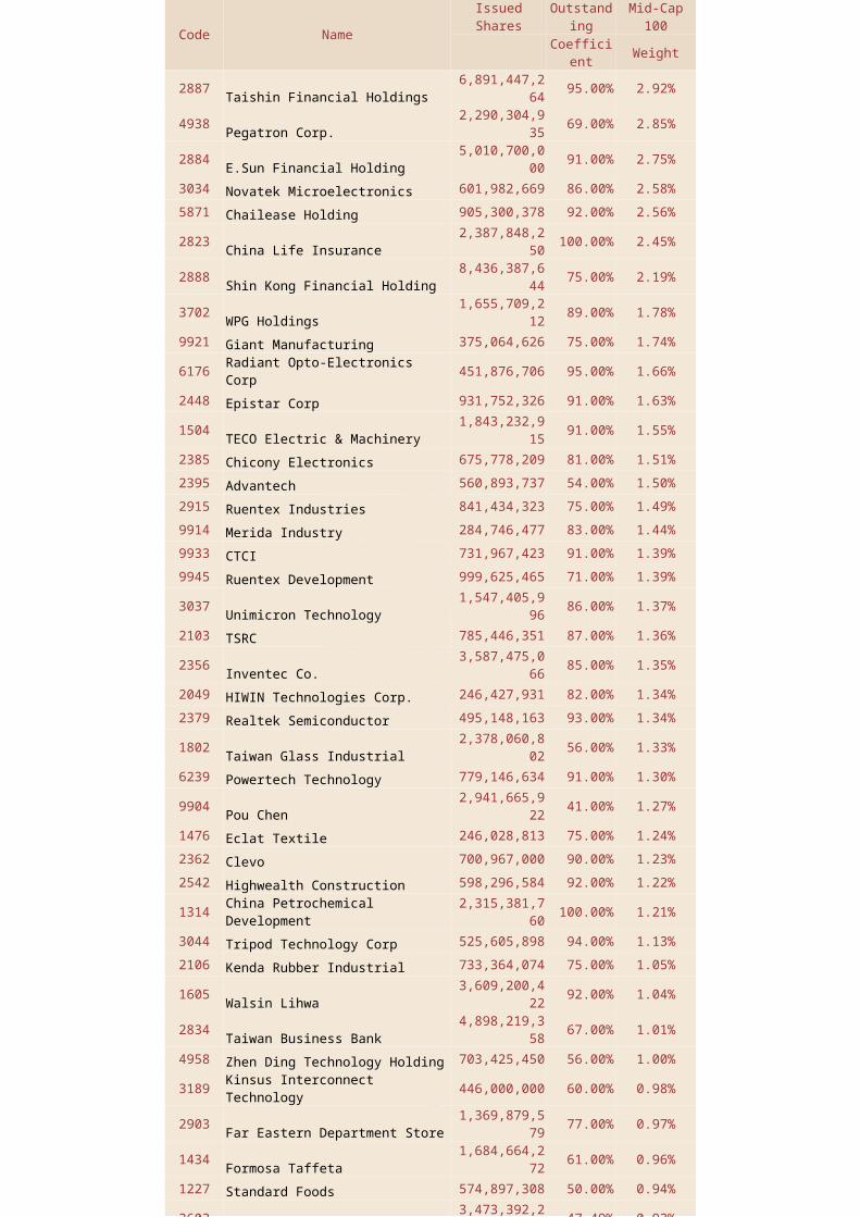
Table 6: List of Taiwan Mid-Cap 100 Index component on 5.17.2013

46

47

Code Name

IssuedShares

Outstanding

Mid-Cap100

Coefficient Weight

2887 Taishin Financial Holdings6,891,447,2

64 95.00% 2.92%

4938 Pegatron Corp.2,290,304,9

35 69.00% 2.85%

2884 E.Sun Financial Holding5,010,700,0

00 91.00% 2.75%

3034 Novatek Microelectronics 601,982,669 86.00% 2.58%5871 Chailease Holding 905,300,378 92.00% 2.56%

2823 China Life Insurance2,387,848,2

50 100.00% 2.45%

2888 Shin Kong Financial Holding8,436,387,6

44 75.00% 2.19%

3702 WPG Holdings1,655,709,2

12 89.00% 1.78%

9921 Giant Manufacturing 375,064,626 75.00% 1.74%

6176 Radiant Opto-Electronics Corp 451,876,706 95.00% 1.66%

2448 Epistar Corp 931,752,326 91.00% 1.63%

1504 TECO Electric & Machinery1,843,232,9

15 91.00% 1.55%

2385 Chicony Electronics 675,778,209 81.00% 1.51%2395 Advantech 560,893,737 54.00% 1.50%2915 Ruentex Industries 841,434,323 75.00% 1.49%9914 Merida Industry 284,746,477 83.00% 1.44%9933 CTCI 731,967,423 91.00% 1.39%9945 Ruentex Development 999,625,465 71.00% 1.39%

3037 Unimicron Technology1,547,405,9

96 86.00% 1.37%

2103 TSRC 785,446,351 87.00% 1.36%

2356 Inventec Co.3,587,475,0

66 85.00% 1.35%

2049 HIWIN Technologies Corp. 246,427,931 82.00% 1.34%2379 Realtek Semiconductor 495,148,163 93.00% 1.34%

1802 Taiwan Glass Industrial2,378,060,8

02 56.00% 1.33%

6239 Powertech Technology 779,146,634 91.00% 1.30%

9904 Pou Chen2,941,665,9

22 41.00% 1.27%

1476 Eclat Textile 246,028,813 75.00% 1.24%2362 Clevo 700,967,000 90.00% 1.23%2542 Highwealth Construction 598,296,584 92.00% 1.22%

1314 China Petrochemical Development

2,315,381,760 100.00% 1.21%

3044 Tripod Technology Corp 525,605,898 94.00% 1.13%2106 Kenda Rubber Industrial 733,364,074 75.00% 1.05%

1605 Walsin Lihwa3,609,200,4

22 92.00% 1.04%

2834 Taiwan Business Bank4,898,219,3

58 67.00% 1.01%

4958 Zhen Ding Technology Holding 703,425,450 56.00% 1.00%

3189 Kinsus Interconnect Technology 446,000,000 60.00% 0.98%

2903 Far Eastern Department Store1,369,879,5

79 77.00% 0.97%

1434 Formosa Taffeta1,684,664,2

72 61.00% 0.96%

1227 Standard Foods 574,897,308 50.00% 0.94%

2603 3,473,392,2 47.49% 0.93%

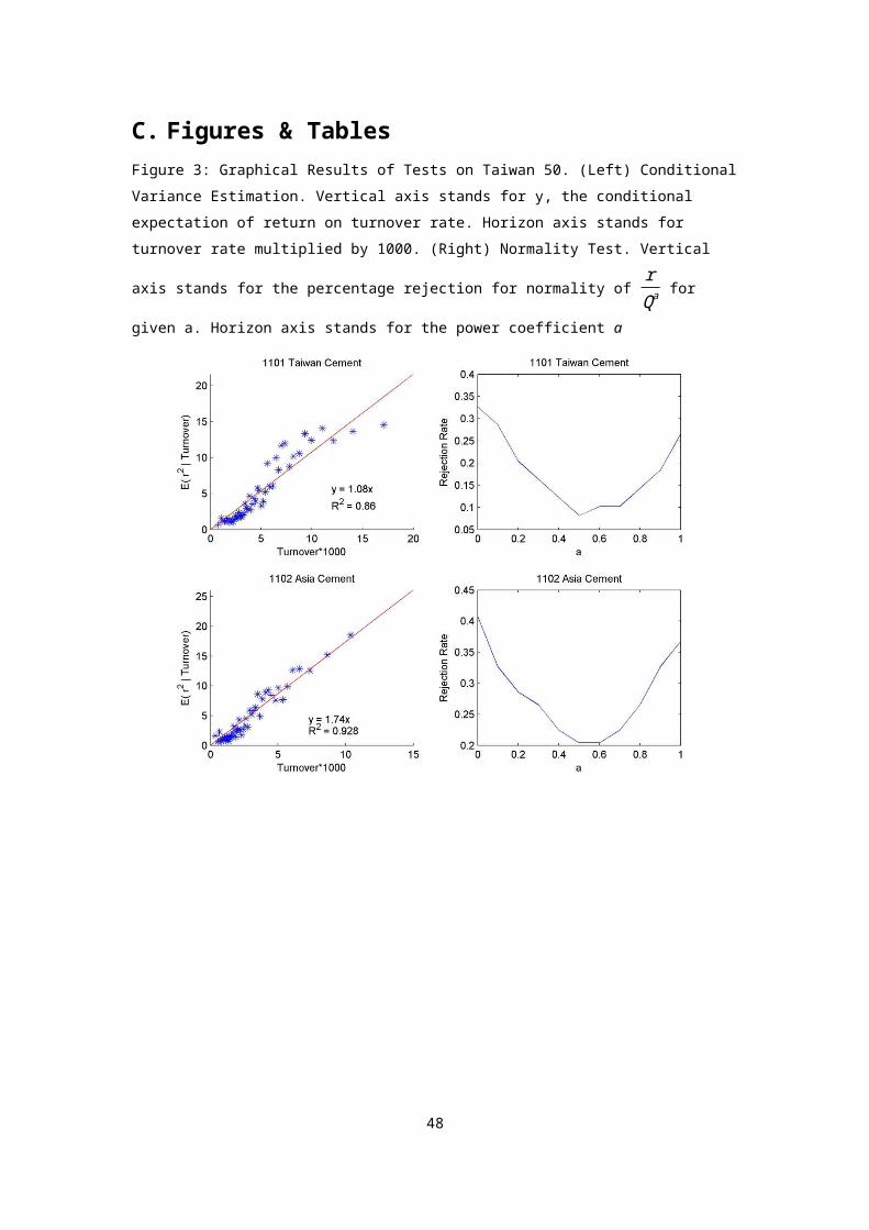
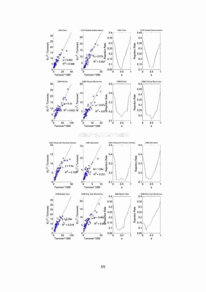
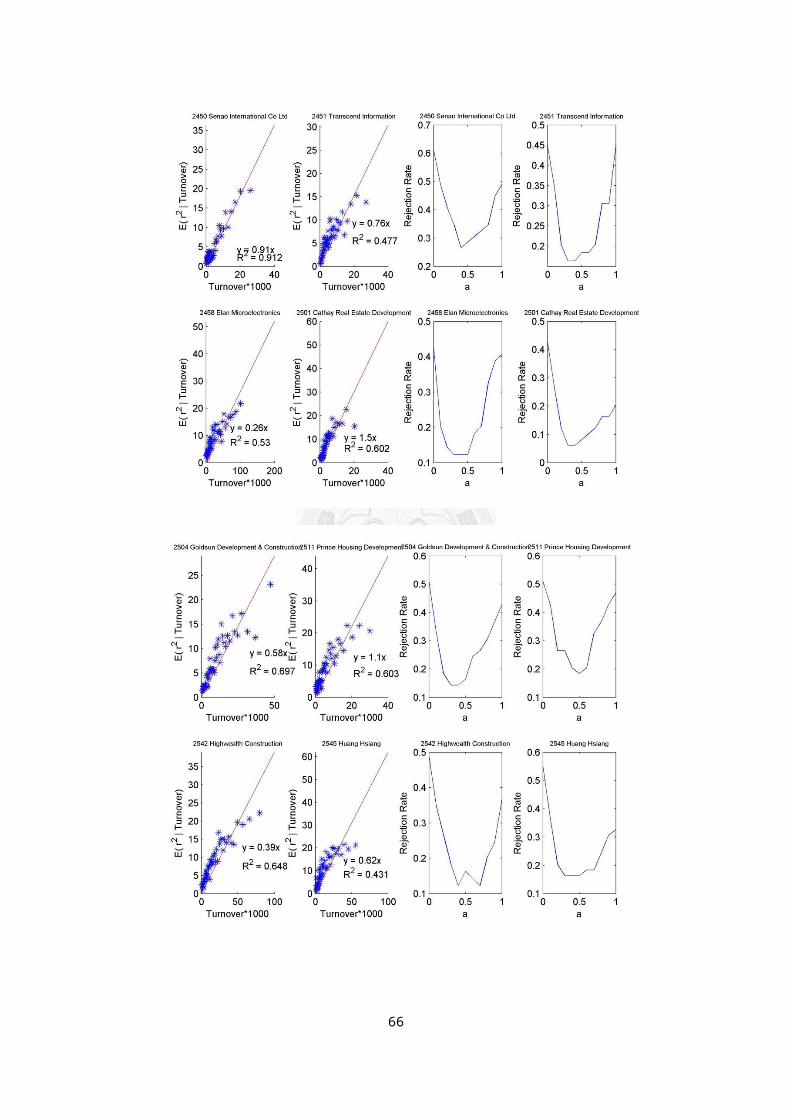
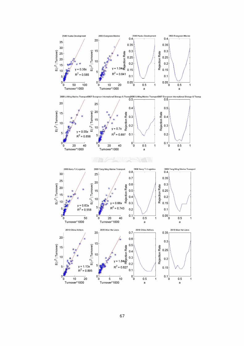
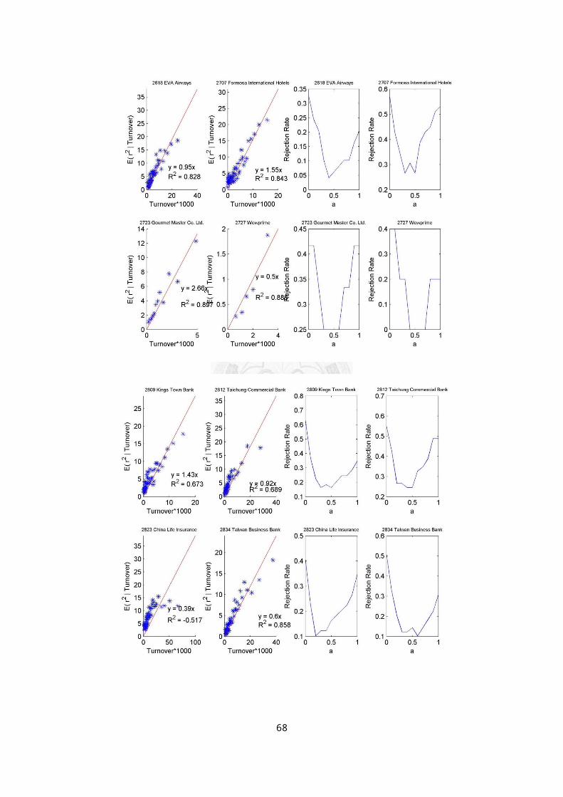
C. Figures & TablesFigure 3: Graphical Results of Tests on Taiwan 50. (Left) ConditionalVariance Estimation. Vertical axis stands for y, the conditional expectation of return on turnover rate. Horizon axis stands for turnover rate multiplied by 1000. (Right) Normality Test. Vertical

axis stands for the percentage rejection for normality of rQa for

given a. Horizon axis stands for the power coefficient a

48

49

50

51

52

53

54

55

56

57

58

59

60

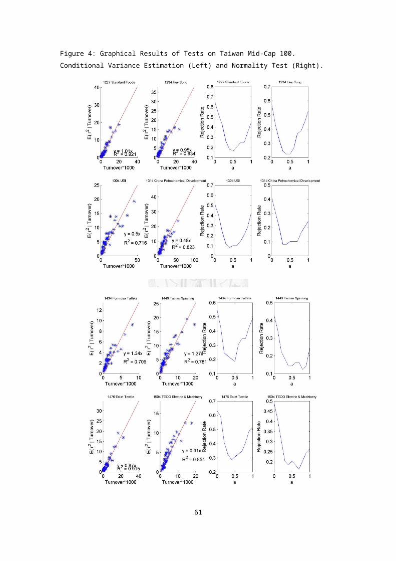
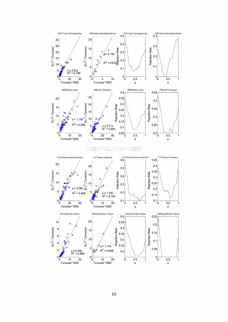
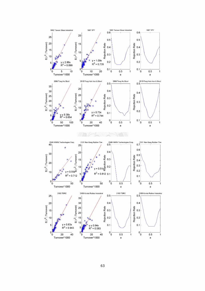
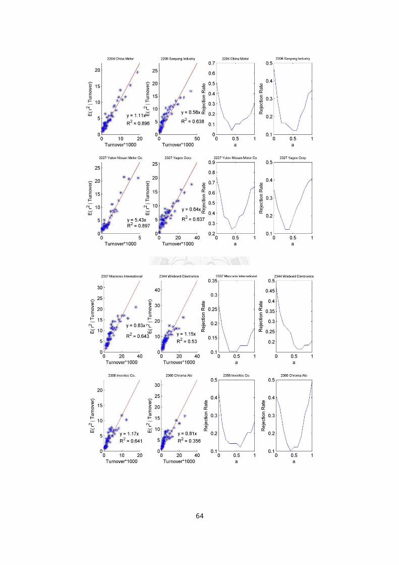
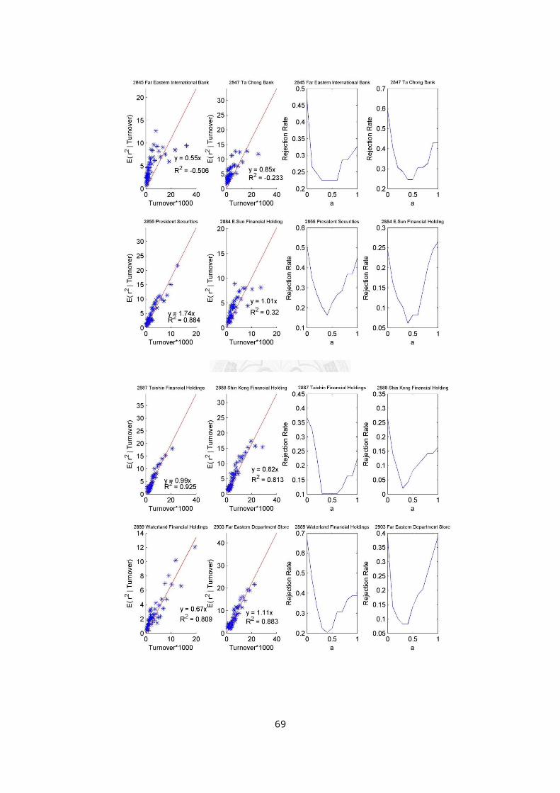
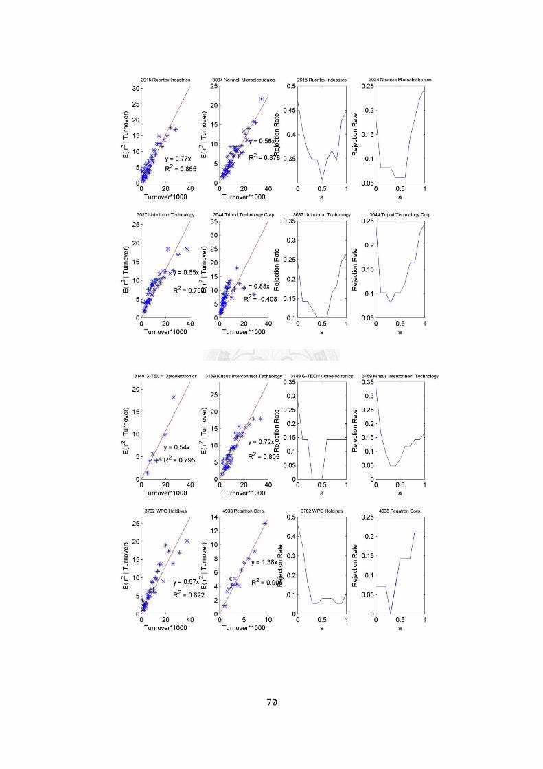
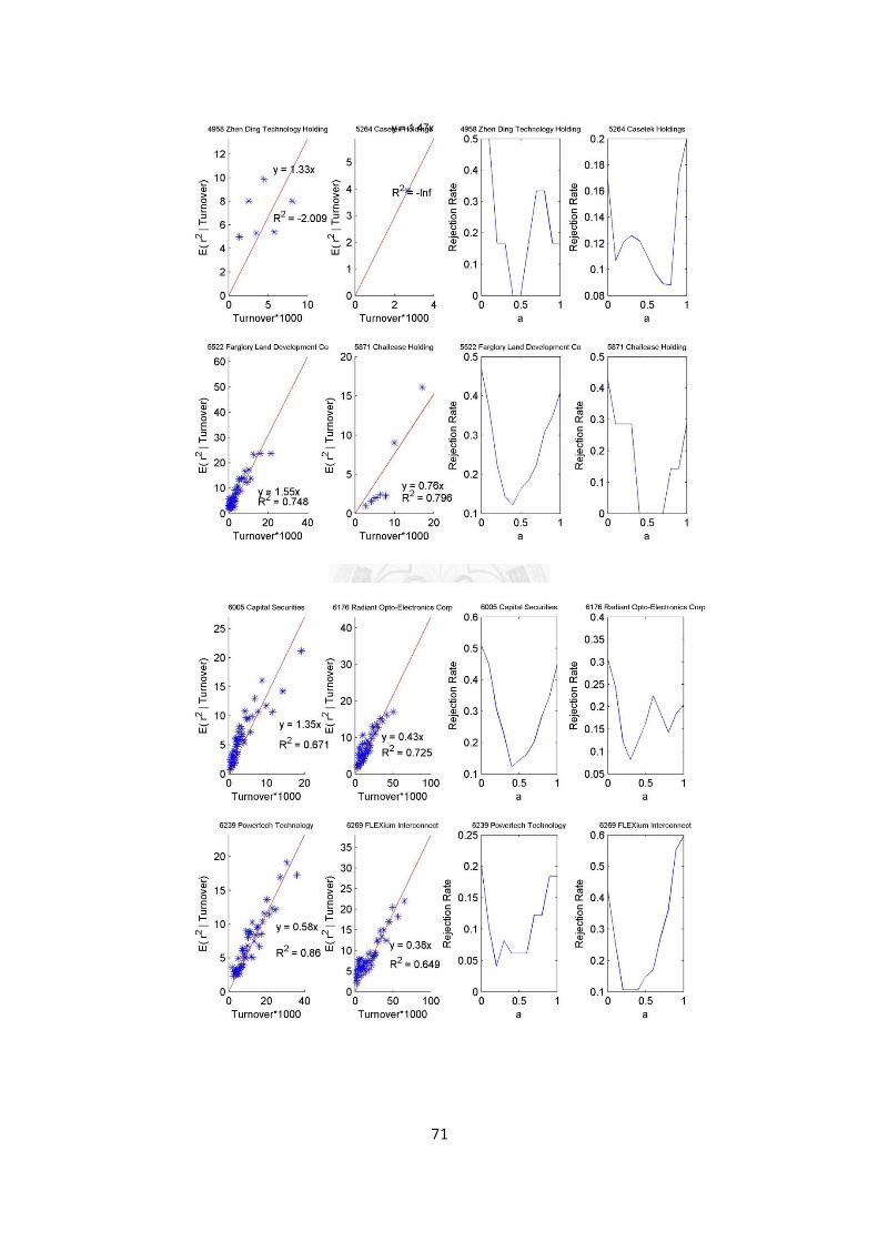
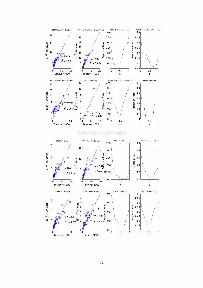
Figure 4: Graphical Results of Tests on Taiwan Mid-Cap 100. Conditional Variance Estimation (Left) and Normality Test (Right).

61

62

63

64

65

66

67

68

69

70

71

72

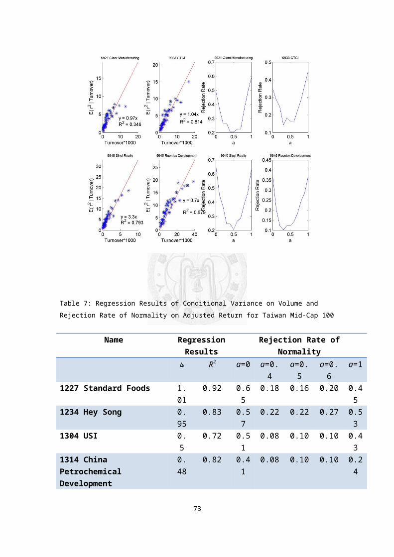
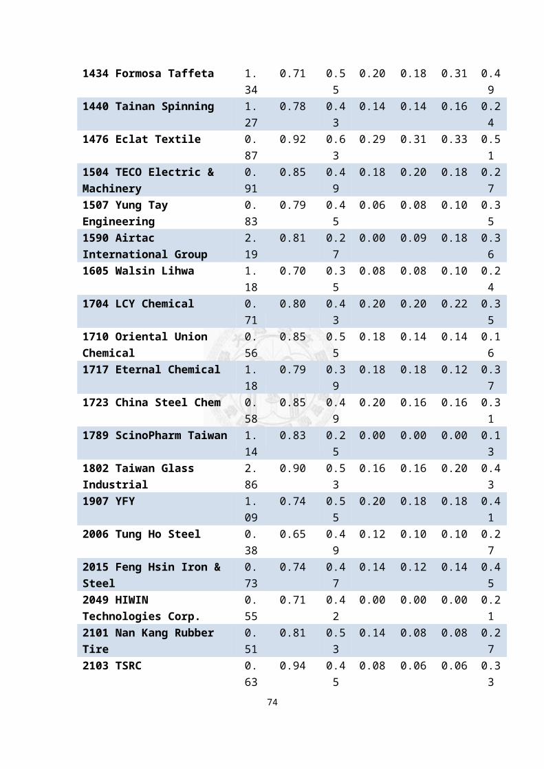
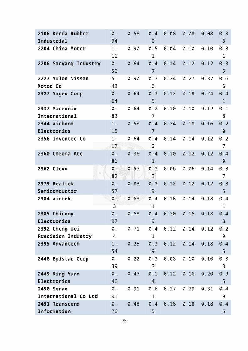
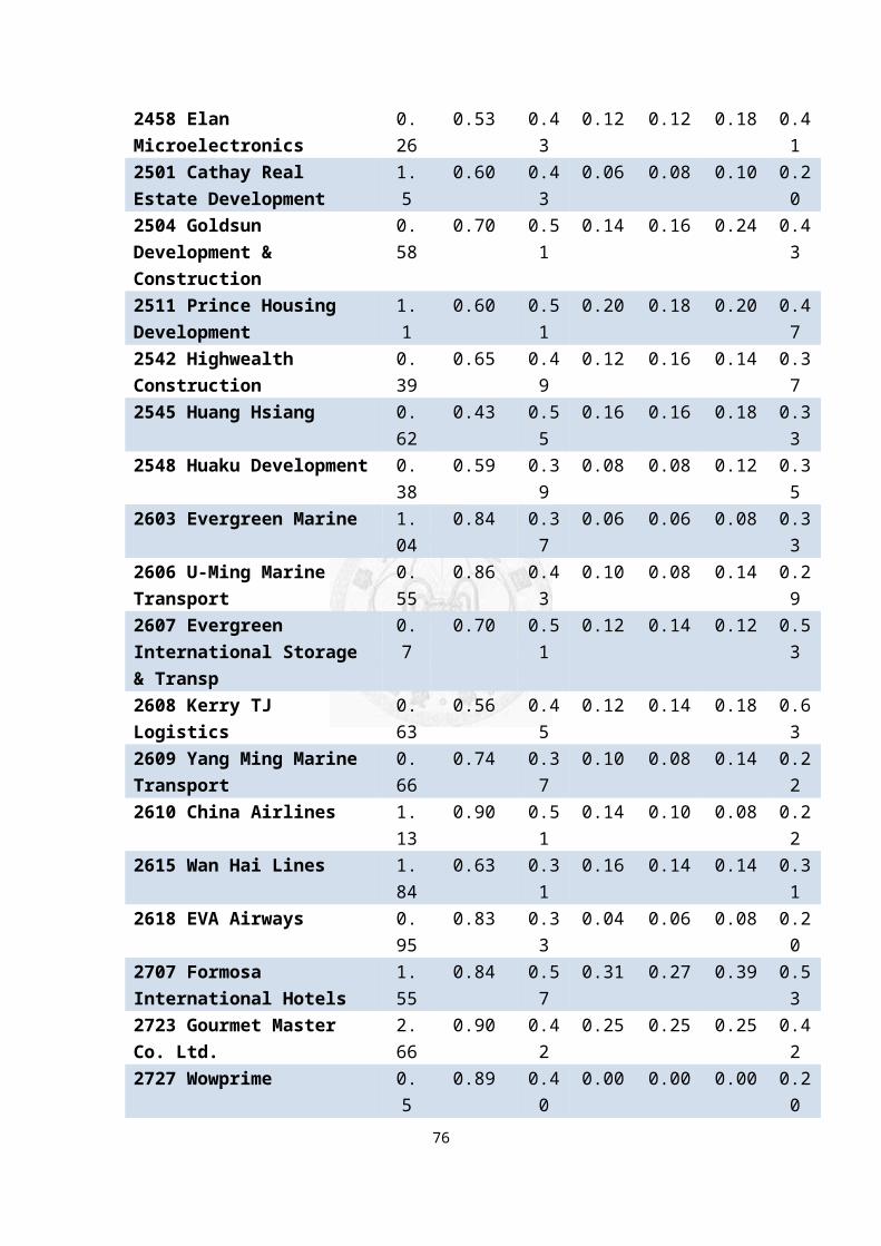
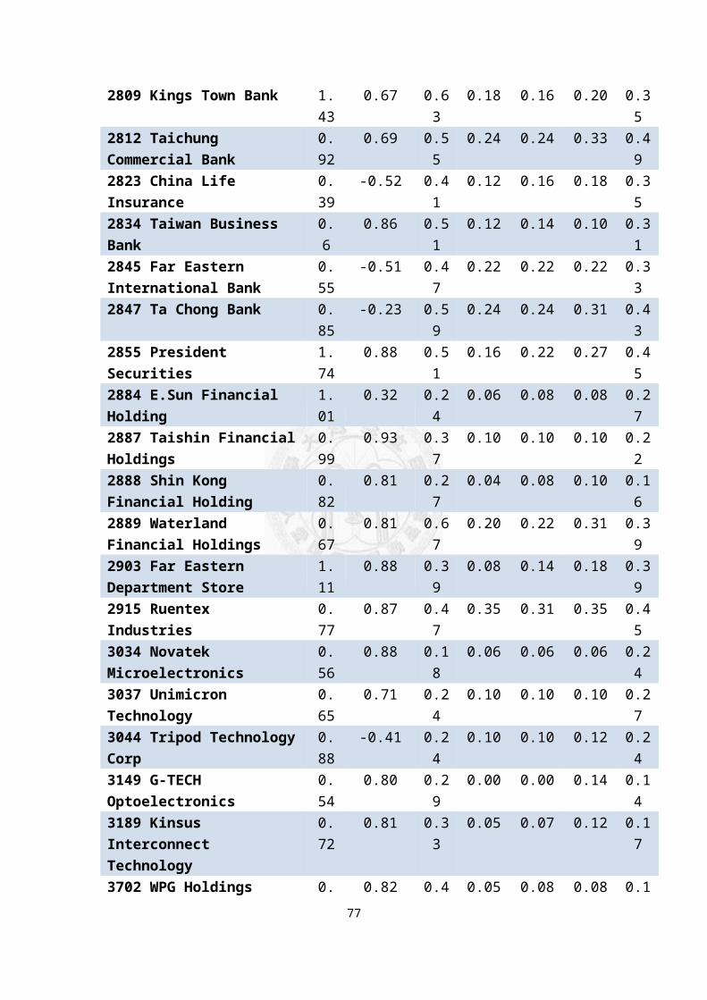
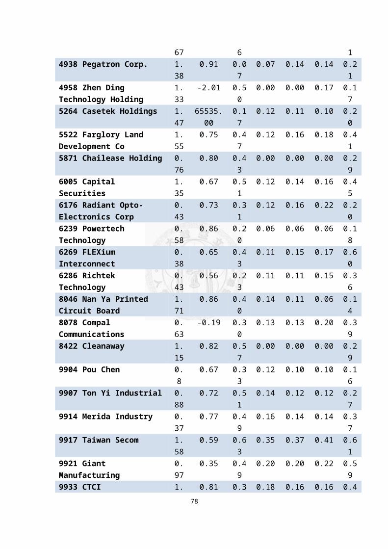
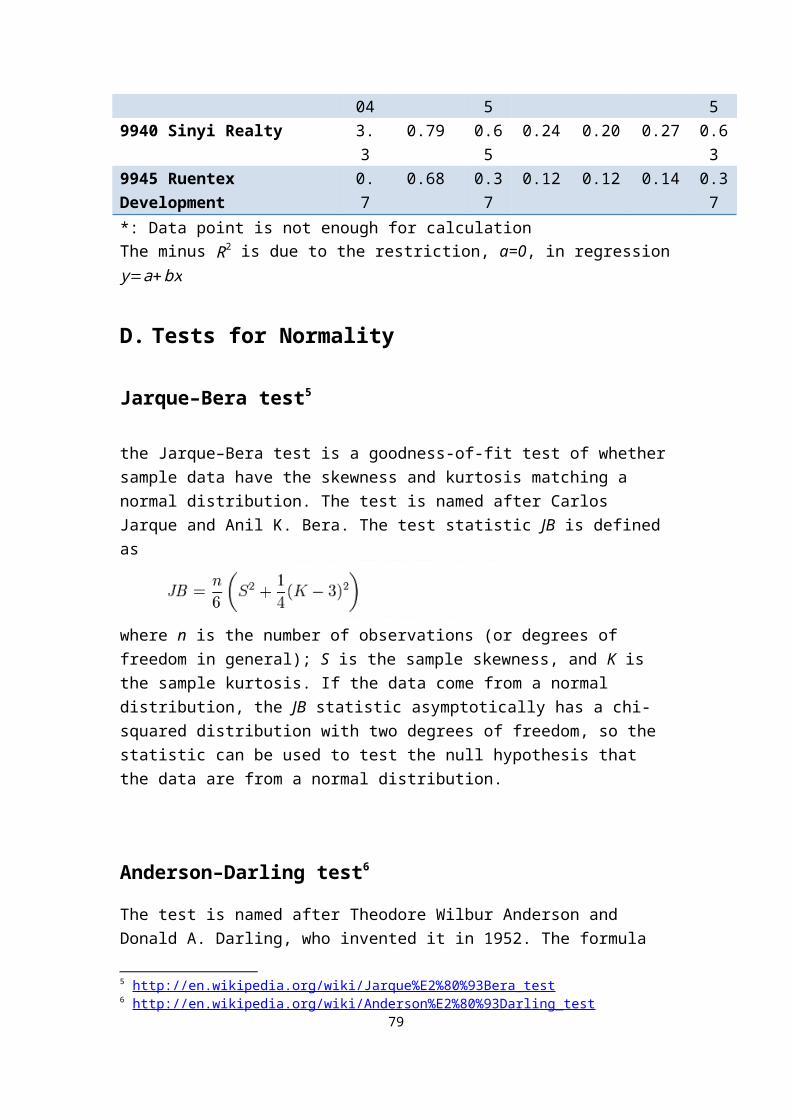
Table 7: Regression Results of Conditional Variance on Volume and Rejection Rate of Normality on Adjusted Return for Taiwan Mid-Cap 100

Name RegressionResults

Rejection Rate ofNormality

ω R2 a=0 a=0.4

a=0.5

a=0.6

a=1

1227 Standard Foods 1.01

0.92 0.65

0.18 0.16 0.20 0.45

1234 Hey Song 0.95

0.83 0.57

0.22 0.22 0.27 0.53

1304 USI 0.5

0.72 0.51

0.08 0.10 0.10 0.43

1314 China Petrochemical Development

0.48

0.82 0.41

0.08 0.10 0.10 0.24

73

1434 Formosa Taffeta 1.34

0.71 0.55

0.20 0.18 0.31 0.49

1440 Tainan Spinning 1.27

0.78 0.43

0.14 0.14 0.16 0.24

1476 Eclat Textile 0.87

0.92 0.63

0.29 0.31 0.33 0.51

1504 TECO Electric & Machinery

0.91

0.85 0.49

0.18 0.20 0.18 0.27

1507 Yung Tay Engineering

0.83

0.79 0.45

0.06 0.08 0.10 0.35

1590 Airtac International Group

2.19

0.81 0.27

0.00 0.09 0.18 0.36

1605 Walsin Lihwa 1.18

0.70 0.35

0.08 0.08 0.10 0.24

1704 LCY Chemical 0.71

0.80 0.43

0.20 0.20 0.22 0.35

1710 Oriental Union Chemical

0.56

0.85 0.55

0.18 0.14 0.14 0.16

1717 Eternal Chemical 1.18

0.79 0.39

0.18 0.18 0.12 0.37

1723 China Steel Chem 0.58

0.85 0.49

0.20 0.16 0.16 0.31

1789 ScinoPharm Taiwan 1.14

0.83 0.25

0.00 0.00 0.00 0.13

1802 Taiwan Glass Industrial

2.86

0.90 0.53

0.16 0.16 0.20 0.43

1907 YFY 1.09

0.74 0.55

0.20 0.18 0.18 0.41

2006 Tung Ho Steel 0.38

0.65 0.49

0.12 0.10 0.10 0.27

2015 Feng Hsin Iron & Steel

0.73

0.74 0.47

0.14 0.12 0.14 0.45

2049 HIWIN Technologies Corp.

0.55

0.71 0.42

0.00 0.00 0.00 0.21

2101 Nan Kang Rubber Tire

0.51

0.81 0.53

0.14 0.08 0.08 0.27

2103 TSRC 0.63

0.94 0.45

0.08 0.06 0.06 0.33

74

2106 Kenda Rubber Industrial

0.94

0.58 0.49

0.08 0.08 0.08 0.33

2204 China Motor 1.11

0.90 0.51

0.04 0.10 0.10 0.31

2206 Sanyang Industry 0.56

0.64 0.47

0.14 0.12 0.12 0.35

2227 Yulon Nissan Motor Co

5.43

0.90 0.76

0.24 0.27 0.37 0.66

2327 Yageo Corp 0.64

0.64 0.35

0.12 0.18 0.24 0.41

2337 Macronix International

0.83

0.64 0.27

0.10 0.10 0.12 0.18

2344 Winbond Electronics

1.15

0.53 0.47

0.24 0.18 0.16 0.20

2356 Inventec Co. 1.17

0.64 0.43

0.14 0.14 0.12 0.27

2360 Chroma Ate 0.81

0.36 0.41

0.10 0.12 0.12 0.49

2362 Clevo 0.82

0.57 0.33

0.06 0.06 0.14 0.37

2379 Realtek Semiconductor

0.57

0.83 0.39

0.12 0.12 0.12 0.35

2384 Wintek 0.3

0.63 0.41

0.16 0.14 0.18 0.41

2385 Chicony Electronics

0.97

0.68 0.49

0.20 0.16 0.18 0.43

2392 Cheng Uei Precision Industry

0.4

0.71 0.41

0.12 0.14 0.12 0.29

2395 Advantech 1.54

0.25 0.39

0.12 0.14 0.18 0.45

2448 Epistar Corp 0.39

0.22 0.33

0.08 0.10 0.10 0.33

2449 King Yuan Electronics

0.46

0.47 0.14

0.12 0.16 0.20 0.35

2450 Senao International Co Ltd

0.91

0.91 0.61

0.27 0.29 0.31 0.49

2451 Transcend Information

0.76

0.48 0.45

0.16 0.18 0.18 0.45

75

2458 Elan Microelectronics

0.26

0.53 0.43

0.12 0.12 0.18 0.41

2501 Cathay Real Estate Development

1.5

0.60 0.43

0.06 0.08 0.10 0.20

2504 Goldsun Development & Construction

0.58

0.70 0.51

0.14 0.16 0.24 0.43

2511 Prince Housing Development

1.1

0.60 0.51

0.20 0.18 0.20 0.47

2542 Highwealth Construction

0.39

0.65 0.49

0.12 0.16 0.14 0.37

2545 Huang Hsiang 0.62

0.43 0.55

0.16 0.16 0.18 0.33

2548 Huaku Development 0.38

0.59 0.39

0.08 0.08 0.12 0.35

2603 Evergreen Marine 1.04

0.84 0.37

0.06 0.06 0.08 0.33

2606 U-Ming Marine Transport

0.55

0.86 0.43

0.10 0.08 0.14 0.29

2607 Evergreen International Storage & Transp

0.7

0.70 0.51

0.12 0.14 0.12 0.53

2608 Kerry TJ Logistics

0.63

0.56 0.45

0.12 0.14 0.18 0.63

2609 Yang Ming Marine Transport

0.66

0.74 0.37

0.10 0.08 0.14 0.22

2610 China Airlines 1.13

0.90 0.51

0.14 0.10 0.08 0.22

2615 Wan Hai Lines 1.84

0.63 0.31

0.16 0.14 0.14 0.31

2618 EVA Airways 0.95

0.83 0.33

0.04 0.06 0.08 0.20

2707 Formosa International Hotels

1.55

0.84 0.57

0.31 0.27 0.39 0.53

2723 Gourmet Master Co. Ltd.

2.66

0.90 0.42

0.25 0.25 0.25 0.42

2727 Wowprime 0.5

0.89 0.40

0.00 0.00 0.00 0.20

76

2809 Kings Town Bank 1.43

0.67 0.63

0.18 0.16 0.20 0.35

2812 Taichung Commercial Bank

0.92

0.69 0.55

0.24 0.24 0.33 0.49

2823 China Life Insurance

0.39

-0.52 0.41

0.12 0.16 0.18 0.35

2834 Taiwan Business Bank

0.6

0.86 0.51

0.12 0.14 0.10 0.31

2845 Far Eastern International Bank

0.55

-0.51 0.47

0.22 0.22 0.22 0.33

2847 Ta Chong Bank 0.85

-0.23 0.59

0.24 0.24 0.31 0.43

2855 President Securities

1.74

0.88 0.51

0.16 0.22 0.27 0.45

2884 E.Sun Financial Holding

1.01

0.32 0.24

0.06 0.08 0.08 0.27

2887 Taishin FinancialHoldings

0.99

0.93 0.37

0.10 0.10 0.10 0.22

2888 Shin Kong Financial Holding

0.82

0.81 0.27

0.04 0.08 0.10 0.16

2889 Waterland Financial Holdings

0.67

0.81 0.67

0.20 0.22 0.31 0.39

2903 Far Eastern Department Store

1.11

0.88 0.39

0.08 0.14 0.18 0.39

2915 Ruentex Industries

0.77

0.87 0.47

0.35 0.31 0.35 0.45

3034 Novatek Microelectronics

0.56

0.88 0.18

0.06 0.06 0.06 0.24

3037 Unimicron Technology

0.65

0.71 0.24

0.10 0.10 0.10 0.27

3044 Tripod TechnologyCorp

0.88

-0.41 0.24

0.10 0.10 0.12 0.24

3149 G-TECH Optoelectronics

0.54

0.80 0.29

0.00 0.00 0.14 0.14

3189 Kinsus Interconnect Technology

0.72

0.81 0.33

0.05 0.07 0.12 0.17

3702 WPG Holdings 0. 0.82 0.4 0.05 0.08 0.08 0.177

67 6 14938 Pegatron Corp. 1.

380.91 0.0

70.07 0.14 0.14 0.2

14958 Zhen Ding Technology Holding

1.33

-2.01 0.50

0.00 0.00 0.17 0.17

5264 Casetek Holdings 1.47

65535.00

0.17

0.12 0.11 0.10 0.20

5522 Farglory Land Development Co

1.55

0.75 0.47

0.12 0.16 0.18 0.41

5871 Chailease Holding 0.76

0.80 0.43

0.00 0.00 0.00 0.29

6005 Capital Securities

1.35

0.67 0.51

0.12 0.14 0.16 0.45

6176 Radiant Opto-Electronics Corp

0.43

0.73 0.31

0.12 0.16 0.22 0.20

6239 Powertech Technology

0.58

0.86 0.20

0.06 0.06 0.06 0.18

6269 FLEXium Interconnect

0.38

0.65 0.43

0.11 0.15 0.17 0.60

6286 Richtek Technology

0.43

0.56 0.23

0.11 0.11 0.15 0.36

8046 Nan Ya Printed Circuit Board

1.71

0.86 0.40

0.14 0.11 0.06 0.14

8078 Compal Communications

0.63

-0.19 0.30

0.13 0.13 0.20 0.39

8422 Cleanaway 1.15

0.82 0.57

0.00 0.00 0.00 0.29

9904 Pou Chen 0.8

0.67 0.33

0.12 0.10 0.10 0.16

9907 Ton Yi Industrial 0.88

0.72 0.51

0.14 0.12 0.12 0.27

9914 Merida Industry 0.37

0.77 0.49

0.16 0.14 0.14 0.37

9917 Taiwan Secom 1.58

0.59 0.63

0.35 0.37 0.41 0.61

9921 Giant Manufacturing

0.97

0.35 0.49

0.20 0.20 0.22 0.59

9933 CTCI 1. 0.81 0.3 0.18 0.16 0.16 0.478

04 5 59940 Sinyi Realty 3.

30.79 0.6

50.24 0.20 0.27 0.6

39945 Ruentex Development

0.7

0.68 0.37

0.12 0.12 0.14 0.37

*: Data point is not enough for calculationThe minus R2 is due to the restriction, a=0, in regressiony=a+bx

D. Tests for Normality

Jarque–Bera test5

the Jarque–Bera test is a goodness-of-fit test of whethersample data have the skewness and kurtosis matching a normal distribution. The test is named after Carlos Jarque and Anil K. Bera. The test statistic JB is defined as

where n is the number of observations (or degrees of freedom in general); S is the sample skewness, and K is the sample kurtosis. If the data come from a normal distribution, the JB statistic asymptotically has a chi-squared distribution with two degrees of freedom, so the statistic can be used to test the null hypothesis that the data are from a normal distribution.

Anderson–Darling test6

The test is named after Theodore Wilbur Anderson and Donald A. Darling, who invented it in 1952. The formula

5 http://en.wikipedia.org/wiki/Jarque%E2%80%93Bera_test6 http://en.wikipedia.org/wiki/Anderson%E2%80%93Darling_test

79

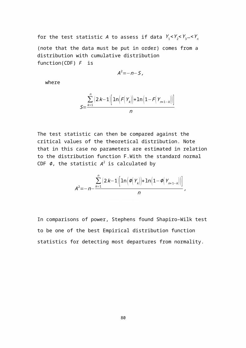
for the test statistic A to assess if data Y1<Y2<Y3…<Yn 

(note that the data must be put in order) comes from a distribution with cumulative distribution function(CDF) F  is

A2=−n−S,where

S=∑k=1

n(2k−1 )[ln(F (Yk ))+ln (1−F (Yn+1−k ))]

n

The test statistic can then be compared against the critical values of the theoretical distribution. Note that in this case no parameters are estimated in relationto the distribution function F.With the standard normal CDF Φ, the statistic A2 is calculated by

A2=−n−∑k=1

n(2k−1 )[ln (Φ (Yk ))+ln(1−Φ (Yn+1−k ))]

n ,

In comparisons of power, Stephens found Shapiro–Wilk test

to be one of the best Empirical distribution function

statistics for detecting most departures from normality.

80

Reference

ANÉ, T., and H. GEMAN (2000): "Order Flow, Transaction Clock, and Normality of Asset Returns," The Journal of Finance, 55, 2259-2284.

ANÉ, T., and L. URECHE-RANGAU (2008): "Does Trading Volume Really Explain Stock Returns Volatility?," Journal of International Financial Markets, Institutions and Money, 18, 216-235.

ANDERSEN, T. G. (1996): "Return Volatility and Trading Volume: An Information Flow Interpretation of Stochastic Volatility," Journal of Finance, 51, 169-204.

ANDERSEN, T. G., T. BOLLERSLEV, F. X. DIEBOLD, and H. EBENS (2001): "The Distribution of Realized Stock Return Volatility," Journal of Financial Economics, 61, 43-76.

AXTELL, R. L. (2001): "Zipf Distribution of Us Firm Sizes," Science, 293, 1818-1820.

BACHELIER, L. (1900): Théorie De La Spéculation. Gauthier-Villars.

BLACK, F., and M. SCHOLES (1973): "The Pricing of Options and Corporate Liabilities," The journal of political economy, 637-654.

BOLLERSLEV, T. (1986): "Generalized Autoregressive Conditional Heteroskedasticity," Journal of Econometrics, 31, 307-327.

BOLLERSLEV, T., R. Y. CHOU, and K. F. KRONER (1992): "Arch Modeling in Finance - a Review of the Theory and Empirical-Evidence," Journal of Econometrics, 52, 5-59.

BOLLERSLEV, T., and D. JUBINSKI (1999): "Equity Trading Volume and Volatility: Latent Information Arrivals and Common Long-Run Dependencies," Journal of Business & Economic Statistics, 17, 9-21.

81

CHAN, K., and W.-M. FONG (2000): "Trade Size, Order Imbalance, and the Volatility–Volume Relation," Journal of Financial Economics, 57, 247-273.

CLARK, P. K. (1973): "A Subordinated Stochastic Process Model with Finite Variance for Speculative Prices," Econometrica: Journal of the Econometric Society, 135-155.

DING, Z., C. W. GRANGER, and R. F. ENGLE (1993): "A Long Memory Property of Stock Market Returns and a New Model," Journal of empirical finance, 1, 83-106.

ENGLE, R. F. (1982): "Autoregressive Conditional Heteroscedasticity with Estimates of the Variance ofUnited-Kingdom Inflation," Econometrica, 50, 987-1007.

FAMA, E. F. (1965): "The Behavior of Stock-Market Prices,"Journal of Business, 38, 34-105.

FLEMING, J., and C. KIRBY (2011): "Long Memory in Volatility and Trading Volume," Journal of Banking & Finance, 35, 1714-1726.

GABAIX, X., P. GOPIKRISHNAN, V. PLEROU, and H. E. STANLEY (2003): "A Theory of Power-Law Distributions in Financial Market Fluctuations," Nature, 423, 267-70.

— (2006): "Institutional Investors and Stock Market Volatility," Quarterly Journal of Economics, 121, 461-504.

GILLEMOT, L., J. D. FARMER, and F. LILLO (2006): "There's More to Volatility Than Volume," Quantitative Finance, 6,371-384.

GOPIKRISHNAN, P., V. PLEROU, X. GABAIX, and H. E. STANLEY (2000): "Statistical Properties of Share Volume Traded in Financial Markets," Physical Review E, 62, R4493-R4496.

HASBROUCK, J. (1991): "Measuring the Information-Content ofStock Trades," Journal of Finance, 46, 179-207.

HEYDE, C. C. (2010): "A Risky Asset Model with Strong Dependence through Fractal Activity Time," in Selected Works of Cc Heyde: Springer, 432-437.

JONES, C. M., G. KAUL, and M. L. LIPSON (1994): "Transactions, Volume, and Volatility," Review of Financial Studies, 7, 631-651.

JORION, P. (1988): "On Jump Processes in the Foreign 82

Exchange and Stock Markets," Review of Financial Studies, 1, 427-445.

KARPOFF, J. M. (1987): "The Relation between Price Changesand Trading Volume - a Survey," Journal of Financial and Quantitative Analysis, 22, 109-126.

LAMOUREUX, C. G., and W. D. LASTRAPES (1990): "Heteroskedasticity in Stock Return Data - Volume Versus Garch Effects," Journal of Finance, 45, 221-229.

LEVY, M. (2009): "Gibrat's Law for (All) Cities: Comment,"American Economic Review, 99, 1672-1675.

LOBATO, I. N., and C. VELASCO (2000): "Long Memory in Stock-Market Trading Volume," Journal of Business & Economic Statistics, 18, 410-427.

MANDELBROT, B. (1963): "The Variation of Certain Speculative Prices," The Journal of Business, 36, 394-419.

MANDELBROT, B., and H. M. TAYLOR (1967): "On the Distribution of Stock Price Differences," Operations research, 15, 1057-1062.

MERTON, R. C. (1976): "Option Pricing When Underlying Stock Returns Are Discontinuous," Journal of Financial Economics, 3, 125-144.

MONROE, I. (1978): "Processes That Can Be Embedded in Brownian-Motion," Annals of Probability, 6, 42-56.

MURPHY, A., and M. IZZELDIN (2006): "Order Flow, TransactionClock, and Normality of Asset Returns: A Comment on Ané and Geman (2000)."

OSBORNE, M. F. (1959): "Brownian Motion in the Stock Market," Operations research, 7, 145-173.

PLEROU, V., and H. E. STANLEY (2008): "Stock Return Distributions: Tests of Scaling and Universality from Three Distinct Stock Markets," Phys Rev E Stat NonlinSoft Matter Phys, 77, 037101.

RAZALI, N. M., and Y. B. WAH (2011): "Power Comparisons of Shapiro-Wilk, Kolmogorov-Smirnov, Lilliefors and Anderson-Darling Tests," Journal of Statistical Modeling and Analytics, 2, 21-33.

SAMUELSO.PA (1973): "Mathematics of Speculative Price," Siam Review, 15, 1-42.

83

SHAPIRO, S. S., and M. B. WILK (1965): "An Analysis of Variance Test for Normality (Complete Samples)," Biometrika, 52, 591-&.

TAUCHEN, G. E., and M. PITTS (1983): "The Price Variability-Volume Relationship on Speculative Markets," Econometrica, 51, 485-505.

UPTON, D. E., and D. S. SHANNON (1979): "The Stable Paretian Distribution, Subordinated Stochastic Processes, and Asymptotic Lognormality: An EmpiricalInvestigation," The Journal of Finance, 34, 1031-1039.

84