Embed Size (px)
Citation preview

NEURAL NETWORK MODELLING AND PREDICTION OF THE FLOTATION DEINKING BEHAVIOUR OF COMPLEX RECYCLED
PAPER MIXES
by
W. J. Pauck
Submitted in fulfilment of the academic requirements for the degree of Doctor of Philosophy in the Faculty of Engineering, University of KwaZulu Natal, Durban.
October 2011
Supervisor: Dr. J Pocock

ii
As the candidate’s Supervisor, I agree/do not agree to the submission of this
thesis.
Name:...........................................Signature: …………………… Date.................
Declaration
The experimental work described in this dissertation was carried out in the laboratories
of the Forest and Forest Products Research Centre, from January 2009 to December
2011, under the supervision of Dr. J Pocock.
i. The research reported in this thesis, except where otherwise indicated, is my
original work.
ii. This thesis has not been submitted for any degree or examination at any other
university.
iii. This thesis does not contain other persons’ writing, unless specifically
acknowledged as being sourced from other researchers. Where other written
sources have been quoted, then:
a) Their words have been re-written but the general information attributed
to them has been referenced;
b) Where their exact words have been used, their writing has been placed
inside quotation marks, and referenced.
iv. Where I have reproduced a publication of which I am an author, co-editor or
editor, I have indicated in detail which part of the publication was written by
myself alone and have fully referenced such publications.
v. This thesis does not contain text; graphics or tables copied and pasted form the
Internet unless specifically acknowledged, and the source being detailed in the
thesis Reference section.
Signature: ………………………… Date:…………………...

iii
ACKNOWLEDGEMENTS
I would like to thank Dr. Jon Pocock and Dr. Richard Venditti for their guidance
and supervision of this thesis.
In addition, I am indebted to the following people and organisations for their
invaluable assistance in the execution of this work:
Mr. Jerome Andrew for managing the project financially.
Mr. Hoosain Adam and the laboratory staff of the Forest Products
Research Centre for the flotation work and analysis.
Mrs. Priya Govender (Mondi Paper Company) and Mr. Jack Steyn
(Nampak) for allowing me free access to their process information and
operations.
I would like to thank Mrs. Jane Molony (CEO of the Paper Manufacturers
Association of South Africa) for her enthusiastic support and finally the Council
for Scientific and Industrial Research for their financial support for this work.

iv
ABSTRACT
In the absence of any significant legislation, paper recycling in South Africa has grown
to a respectable recovery rate of 43% in 2008, driven mainly by the major paper
manufacturers. Recently introduced legislation will further boost the recovery rate of
recycled paper. Domestic household waste represents the major remaining source of
recycled paper. This source will introduce greater variability into the paper streams
entering the recycling mills, which will result in greater process variability and operating
difficulties. This process variability manifests itself as lower average brightness or
increased bleaching costs. Deinking plants will require new techniques to adapt to the
increasingly uncertain composition of incoming recycled paper streams. As a
developing country, South Africa is still showing growth in the publication paper and
hygiene paper markets, for which recycled fibre is an important source of raw material.
General deinking conditions pertaining to the South African tissue and newsprint
deinking industry were obtained through field surveys of the local industry and
assessment of the current and future requirements for deinking of differing quality
materials.
A large number of operating parameters ranging from waste mixes, process variables
and process chemical additions, typically affect the recycled paper deinking process.
In this study, typical newsprint and fine paper deinking processes were investigated
using the techniques of experimental design to determine the relative effects of
process chemical additions, pH, pulping and flotation times, pulping and flotation
consistencies and pulping and flotation temperatures on the final deinked pulp
properties.
Samples of recycled newsprint, magazines and fine papers were pulped and deinked
by flotation in the laboratory. Handsheets were formed and the brightness, residual ink
concentration and the yield were measured. It was determined that the type of
recycled paper had the greatest influence on final brightness, followed by bleaching
conditions, flotation cell residence time and flotation consistency. The residual ink
concentration and yield were largely determined by residence time and consistency in
the flotation cell.

v
The laboratory data generated was used to train artificial neural networks which
described the laboratory data as a multi-dimensional mathematical model. It was found
that regressions of approximately 0.95, 0.84 and 0.72 were obtained for brightness,
residual ink concentration and yield respectively.
Actual process data from three different deinking plants manufacturing seven different
grades of recycled pulp was gathered. The data was aligned to the laboratory
conditions to take into account the different process layouts and efficiencies and to
compensate for the differences between laboratory and plant performance. This data
was used to validate the neural networks and select the models which best described
the overall deinking performances across all of the plants. It was found that the
brightness and residual ink concentration could be predicted in a commercial operation
with correlations in excess of 0.9. Lower correlations of ca. 0.5 were obtained for yield.
It is intended to use the data and models to develop a predictive model to facilitate the
management and optimization of a commercial flotation deinking processes with
respect to waste input and process conditions.

vi
TABLE OF CONTENTS
PREFACE ii
ACKNOWLEDGEMENTS iii
ABSTRACT iv
TABLE OF CONTENTS vi
LIST OF TABLES xiv
LIST OF FIGURES xvi
GLOSSARY OF ABBREVIATIONS AND TERMS xxi
1 GENERAL INTRODUCTION
1
1.1 A global overview of paper recycling 1
1.2 Paper recycling in South Africa 3
1.3 Problem statement 5
1.4 Scope and delimitation 5
1.5 Objectives and anticipated benefits 6
2 REVIEW OF UNIT OPERATIONS IN PAPER RECYCLING
7
2.1 Introduction 7
2.2 Pulping or slushing 8
2.2.1 Introduction 8
2.2.2 Process parameters 9
2.2.3 Models and fundamentals 10
2.2.3.1 Defibering or deflaking 10
2.2.3.2 Ink detachment 12
2.2.3.3 Particle fragmentation and redeposition 12
2.2.4 Conclusion 14
2.3 Centrifugal cleaning 15
2.4 Screening and fractionation 15
2.5 Flotation 16
2.5.1 Introduction 16
2.5.2 Process equipment and parameters 16
2.5.3 Theoretical models and fundamentals 17
2.5.3.1 Introduction 17
2.5.3.2 Multistage probability process models 19
2.5.3.3 Reaction rate models 23
2.5.3.4 Population balance models 23
2.5.3.5 Hydrodynamic models 25
2.5.3.6 Transport phenomena models 26
2.5.3.7 Statistical models 29
2.5.3.8 Practical models 29

vii
2.5.4 Conclusions 29
2.6 Washing 29
2.7 Dewatering 31
2.8 Dispersing 32
2.9 Bleaching 33
2.10 Process control of deinking plants 34
3 REVIEW OF CHEMISTRY OF DEINKING
35
3.1 Printing inks 35
3.2 The chemistry in the pulper 38
3.2.1 Chemicals added into the pulper 38
3.2.2 The effect of temperature 40
3.2.3 Sodium hydroxide 40
3.2.4 Hydrogen peroxide 41
3.2.5 Sodium silicate 43
3.2.6 Surfactants 44
3.2.7 Pulping pH 45
3.2.8 Conclusion 47
3.3 Chemistry in the flotation cell 47
3.3.1 Surface chemical mechanisms of flotation 47
3.3.2 The soap and surfactants 52
3.3.3 Temperature, pH and surface tension 54
3.3.4 The role of the calcium ion 55
3.3.5 Fillers 56
3.3.6 Sodium silicate 58
3.3.6.1 The general chemistry and properties of soluble silicates 58
3.3.6.2 The effects of sodium silicate in deinking 59
3.4 Final bleaching 61
3.5 Measurement of deinking efficiency 62
3.5.1 Yield 63
3.5.2 Brightness 63
3.5.3 Colour 64
3.5.4 Dirt content 64
3.5.5 Effective residual ink concentration 65
3.5.6 Conclusion 66
4 REVIEW OF ARTIFICIAL NEURAL NETWORKS
67
4.1 Introduction 67
4.2 Structure of biological networks 67
4.3 Structure of artificial neural networks 68
4.4 Mathematical basis of neural networks 70
4.4.1 Early history 70
4.4.2 Multi-layer networks and error back-propagation 71
4.4.3 Network training 75

viii
4.4.4 Other techniques 76
4.5 Application and feasibility of neural networks
77
4.5.1 Introduction 77
4.5.2 Hardware and software requirement 78
4.5.3 Data collection and preparation 78
4.5.4 Quality of data required 79
4.5.5 Quantity of data required 79
4.6 Design, training and testing 80
4.6.1 Introduction 80
4.6.2 Pre-processing of data 80
4.6.3 Selecting the type of neural network 81
4.6.4 Training process 81
4.6.4.1 Partitioning 81
4.6.4.2 Training 81
4.6.4.3 Selecting the optimum network 83
4.6.4.4 Testing the network 83
4.6.4.5 Over training 83
4.7 Review of applications of neural networks in flotation and in the paper industry
84
4.7.1 Introduction 84
4.7.2 The use of neural networks in flotation processes 84
4.7.3 The use of neural networks in the pulp and paper industry 85
4.7.4 Neural networks in combination with other techniques 87
4.8 Conclusions 87
5 METHODOLOGY
88
5.1 Introduction – overview of methodology 88
5.2 Review of deinking conditions in newsprint and tissue manufacture
89
5.2.1 Grades of recycled paper 90
5.2.2 Newsprint deinking conditions 92
5.2.2.1 Process configuration 92
5.2.2.2 Raw materials 92
5.2.2.3 Process conditions 93
5.2.2.4 Process control philosophy 94
5.2.3 Recycled office paper deinking conditions – double loop process 94
5.2.3.1 Process configuration 94
5.2.3.2 Raw materials 94
5.2.3.3 Process conditions 95
5.2.3.4 Process control philosophy 97
5.2.4 Recycled office paper deinking conditions – single loop process
97
5.2.4.1 Process configuration 97
5.2.4.2 Raw materials 97

ix
5.2.4.3 Process conditions 98
5.2.4.4 Process control philosophy 99
5.3 Process control of deinking plants 99
5.4 Determination of potential control parameters 100
5.4.1 Pulper consistency 100
5.4.2 Pulper pH 101
5.4.3 Pulping time 101
5.4.4 Pulping temperature 101
5.4.5 Addition of hydrogen peroxide 101
5.4.6 Addition of sodium hydroxide 102
5.4.7 Addition of chelating agent 102
5.4.8 Addition of sodium silicate 102
5.4.9 Addition of surfactant 102
5.4.10 Flotation temperature 103
5.4.11 Flotation conditions 103
5.4.12 Flotation pH 105
5.4.13 Calcium concentration 105
5.4.14 Washing efficiency 105
5.4.15 Dispersion 106
5.4.16 Final bleaching 106
5.4.17 Grade of recycled paper 106
5.4.18 In summary 106
5.5 Measurement of effects of control variables 108
5.6 Screening of potential control variables 108
5.6.1 Pulping and flotation methods 108
5.6.1.1 Recycled paper sample preparation 108
5.6.1.2 Laboratory pulping procedure 109
5.6.1.3 Flotation method 110
5.6.1.4 Equipment and test methods 111
5.6.2 Experimental design 114
6 RESULTS OF SCREENING RUNS
118
6.1 Introduction 118
6.2 Results of screening runs – general trends 118
6.2.1 Dependence of brightness on flotation time 118
6.2.2 Dependence of ERIC on flotation time 119
6.2.3 Dependence of yield in flotation time 120
6.2.4 Variation of brightness and ERIC with processing stage 120
6.2.5 The relationship between ERIC and brightness 122
6.3 Variability and drift 125
6.4 Correlation between UV included and UV excluded brightness
125
6.5 Results of screening runs – net effect of variables 126
6.5.1 Newsprint 126
6.5.2 Magazines 128
6.5.3 Heavy letter 1 130

x
6.5.4 Heavy letter 2
132
6.6 Selection of control variables 134
7 GENERATION OF LABORATORY DATA 136
7.1 Introduction 136
7.1 Methodology 136
7.3 Results 140
7.4 Conclusions 142
8 NEURAL NETWORK MODELLING OF LABORATORY DATA
144
8.1 Introduction 144
8.2 Software 144
8.3 Training using MATLAB 145
8.3.1 General methodology 145
8.3.2 Specific training options used 149
8.3.2.1 Network initialisation 149
8.3.2.2 The number of neurons and layers 149
8.3.2.3 Addition of data 150
8.3.2.4 The number of input values 150
8.3.2.5 the ratio of data in training, validation and test sets 150
8.3.2.6 Learning and training algorithms 150
8.3.2.7 Pre-processing 152
8.4 Problems with backpropagation 152
8.5 Evaluation neural network performance 153
8.6 Specific methodology and results 153
8.6.1 Selection of output variables 153
8.6.2 Final selection of input variables by sensitivity analysis 153
8.7 Discussion 158
8.8 Further work 159
9 PLANT TESTING OF NEURAL NETWORK MODELS 160
9.1 Introduction 160
9.2 Alignment of plant and Laboratory processes 160
9.3 Data collection 163
9.3.1 Single-loop newsprint deinking mill 164
9.3.1.1 Recycled paper inputs 164
9.3.1.2 Chemical additions 164
9.3.1.3 Pulping conditions 165
9.3.1.4 Flotation conditions 166

xi
9.3.1.5 Laboratory-plant flotation alignment 166
9.3.1.6 Deinked fibre properties 167
9.3.1.7 Yield 170
9.3.2 Double-loop office paper deinking plant 171
9.3.2.1 Recycled paper inputs 172
9.3.2.2 Chemical additions 174
9.3.2.3 Pulping conditions 174
9.3.2.4 Flotation conditions 175
9.3.2.5 Pulp bleaching conditions 176
9.3.2.6 Deinked fibre properties 178
9.3.2.7 Yield 179
9.3.3 Single-loop office paper deinking plant 179
9.3.3.1 Recycled paper inputs 180
9.3.3.2 Chemical additions 182
9.3.3.3 Pulping conditions 182
9.3.3.4 Flotation conditions 184
9.3.3.5 Pulp bleaching conditions 184
9.3.3.6 Deinked fibre properties 185
9.3.3.7 Yield 186
9.4 Results of model testing and discussion 187
9.4.1 Brightness 187
9.4.2 Residual ink concentration 193
9.4.3 Yield 197
10 FINAL CONCLUSIONS AND FURTHER WORK
202
10.1 Review of work done 202
10.2 Conclusions 203
10.2.1 Screening of control variables 203
10.2.2 Data generation 204
10.2.3 Generation of neural networks 204
10.2.4 Prediction of neural networks 205
10.3 Applications 206
10.3.1 Process optimisations 206
10.3.2 Raw material changes 207
10.4 Future work 207
10.4.1 Unresolved questions 207
10.4.2 Extensions of the model to other parameters 208
10.4.3 Practical implementation 209
10.4.3.1 Implement the prototype on customer hardware and software 209
10.4.3.2 Acceptance testing 209
10.4.3.3 Handover and training 209
10.4.3.4 Maintenance
210

xii
REFERENCES
APPENDICES
APPENDIX 1A(i): PLACKETT-BURMAN DESIGN AND RESULTS FOR NEWSPRINT
APPENDIX 1A(ii): NET EFFECTS FOR 12-RUN AND 24-RUN REFLECTED DESIGN - NEWSPRINT
APPENDIX 1B(i) – PLACKETT-BURMAN DESIGN AND RESULTS FOR MAGAZINES
APPENDIX 1B(ii): NET EFFECTS FOR 12-RUN AND 24-RUN REFLECTED DESIGN - MAGAZINES
APPENDIX 1C(i) – PLACKETT-BURMAN DESIGN AND RESULTS FOR HEAVY LETTER 1
APPENDIX 1C(ii): NET EFFECTS FOR 12-RUN AND 24-RUN REFLECTED DESIGN – HEAVY LETTER 1
APPENDIX 1D(i)– PLACKETT-BURMAN DESIGN AND RESULTS FOR HEAVY LETTER 2
APPENDIX 1D(ii): NET EFFECTS FOR 12-RUN AND 24-RUN REFLECTED DESIGN – HEAVY LETTER 2
APPENDIX 2 – FACTOR RANK ANALYSIS
APPENDIX 3: DEINKING TRAINING DATA
APPENDIX 4A: TRAINING RESULTS FOR BRIGHTNESS
APPENDIX 4B: TRAINING RESULTS FOR ERIC
APPENDIX 4C: TRAINING RESULTS FOR YIELD
APPENDIX 5A: NEURAL NETWORK SENSITIVITY ANALYSIS - BRIGHTNESS
APPENDIX 5B: NEURAL NETWORK SENSITIVITY ANALYSIS - ERIC
APPENDIX 5C: NEURAL NETWORK SENSITIVITY ANALYSIS - YIELD
APPENDIX 6A: FLOTATION ALIGNMENT - NEWSPRINT
APPENDIX 6B: FLOTATION ALIGNMENT - DOUBLE LOOP

xiii
TISSUE
APPENDIX 6C: FLOTATION ALIGNMENT SINGLE - LOOP TISSUE
APPENDIX 7: PROCESSED PLANT DATA
APPENDIX 8A(i): PERFORMANCE OF NEURAL NETWORKS FOR THE PREDICTION OF BRIGHTNESS
APPENDIX 8A(ii): MEAN PREDICTED BRIGHTNESS OF NEURAL NETWORKS COMPARED TO PLANT BRIGHTNESS, BY PAPER GRADE
APPENDIX 8B(i): PERFORMANCE OF NEURAL NETWORKS FOR THE PREDICTION OF ERIC
APPENDIX 8B(ii): MEAN PREDICTED ERIC OF NEURAL NETWORKS COMPARED TO PLANT ERIC, BY PAPER GRADE
APPENDIX 8C(i): PERFORMANCE OF NEURAL NETWORKS FOR THE PREDICTION OF YIELD
APPENDIX 8C(ii): MEAN PREDICTED YIELD OF NEURAL NETWORKS COMPARED TO PLANT YIELD, BY PAPER GRADE
APPENDIX 9: MATLAB CODE
APPENDIX 10: NEURAL NETWORK STRUCTURES

xiv
LIST OF TABLES
1.1 Utilisation rates, process yields and amount of recycled fibre in different grades of paper, Germany, 1998
2
1.2 Utilisation rates in the USA, 2005 2
1.3 Annual production of pulp in South Africa 4
2.1 Efficiency ranges for the main separation processes after pulping 8
2.2 Comparison of deinking and mineral flotation 18
2.3 Typical size ranges of particles 30
3.1 Typical composition and applications of printing inks. Deinking behaviour relative to unprinted paper
36
3.2 Comparison of deinking agents 45
3.3 Role, nature and effects of surfactants in deinking 52
3.4 Comparison of reductive bleaching agents 62
5.1 Paper Recycling in South Africa 89
5.2 Recovery of recycled paper in South Africa 90
5.3 Overview of recovered paper specifications 91
5.4 Process conditions and control of a newsprint deinking plant 93
5.5 Percentage additions of recycled paper in various towelling tissue grades 95
5.6 Process conditions and control of a double loop office paper deinking plant 96
5.7 Percentage additions of recycled paper in various towelling tissue grades 98
5.8 Process conditions and control of the single loop office paper deinking plant 98
5.9 Summary of screening of control variables 107
5.10 A 12 run Plackett-Burman design, with reflection 115
5.11 Screening experimental design for control variables 116
xv
7.1 Waste mixture experimental design 138
7.2 Modified ranges of deinking parameters with reasons for changes 139
7.3 Statistics for the midpoints of the base grades 143
8.1 Symbols and descriptors of response surfaces 155
8.2 Assessment of response surfaces in Figure 8.4 156
8.3 Summary of neural network model % responses to process parameters 157
8.4 Summary of best Neural Network performance 159
9.1 Raw material breakdown for double-loop office waste deinking plant 174
9.2 Monthly flotation yield calculation for recycling plant 179
9.3 Raw material breakdown for single-loop office paper deinking plant 180
9.4 Estimation of yield losses 187
10.1 Summary of neural network performance 205

xvi
LIST OF FIGURES 1.1 Grade mix of recovered papers 5
2.1 Approach of ink particle and air bubble 19
2.2 Schematic of probability of attachment by sliding Pasl 20
2.3 Formation of three-phase contact angle 21
2.4 Stabilising and destabilizing forces on a particle-bubble aggregate 22
2.5 Photograph of rising air bubble with attached ink particles 22
2.6 Flotation efficiency as a function of flotation time and particle size 24
2.7 Schematic of combination of transport equations to simulate a flotation cell
28
2.8 Effect of consistency on theoretical washing efficiency, as measured by ash removal
31
3.1 Brightness dependence on H2O2/NaOH ratio 42
3.2 Effect of sodium silicate on deinking brightness 44
3.3 Collecting mechanism of calcium soap 49
3.4 Mechanism of ink agglomeration and flotation 51
4.1 Schematic of a biological nerve cell 67
4.2 A processing unit in an artificial neural network 68
4.3 Interconnection of artificial processing units 69
4.4 Schematic of an artificial neuron 70
4.5 Nonlinear model of a neuron 71
4.6 The sigmoid function 73
4.7 A two-layer perceptron structure 74
4.8 Comparison of training error and validation error during training 82
4.9 Good and poor generalisation 83
xvii
5.1 Process flow diagram – single-loop newsprint deinking plant 92
5.2 Process flow diagram – double loop office waste deinking plant 94
5.3 Process flow diagram – single loop office waste deinking plant 97
5.4 External and internal view of laboratory pulper 111
5.5 View of pulping action, demonstrating good mixing action 111
5.6 Laboratory flotation cell 112
5.7 Laboratory flotation cell froth generation 112
6.1 Variation of brightness as a function of flotation time 119
6.2 Variation of ERIC as a function of flotation time 119
6.3 Variation of yield as a function of flotation time 120
6.4 Effect of processing stage on brightness 121
6.5 Effect of processing stage on ERIC 122
6.6 Cluster plot of brightness vs. ERIC for newsprint 123
6.7 Cluster plot of brightness vs. ERIC for magazines 123
6.8 Cluster plot of brightness vs. ERIC for heavy letter 1 124
6.9 Cluster plot of brightness vs. ERIC for heavy letter 2 124
6.10 Variability and drift of final brightness 125
6.11 Correlation between final washed UVin and UVex for HL1, HL2 and OMG 126
6.12 Net effect of variables on the washed brightness of newsprint 127
6.13 Net effect of variables on washed ERIC of newsprint 128
6.14 Net effect of variables on the yield of newsprint 128
6.15 Net effect of variables on the washed brightness of magazine papers 129
6.16 Net effect of variables on the washed ERIC of magazine papers 129
6.17 Net effect of variables on the yield of magazine papers 130
6.18 Net effect of variables on the washed brightness of HL1 130
6.19 Net effect of variables on the washed ERIC of HL1 131

xviii
6.20 Net effect of variables on the yield of HL1 131
6.21 Net effect of variables on the washed brightness of HL2 132
6.22 Net effect of variables on the washed ERIC of HL2 133
6.23 Net effect of variables on the yield of HL2 133
6.24 Ranking of control variables – greatest influence-MEAN-least influence 134
7.1 Mixture space for four recycled paper grades 137
7.2 Variability and drift in ONP results 140
7.3 Variability and drift in OMG results 141
7.4 Variability and drift in HL1results 141
7.5 Variability and drift in HL2 results 142
8.1 MATLAB training window, showing training parameters 146
8.2 Example of plot of performance of training, validation and test sets, demonstrating early stopping
147
8.3 Example of plots of regression of a training session 148
8.4 Response surface of brightness to selected variables 156
9.1 Brightness development vs solids losses for a ONP/OMG mix 161
9.2 Brightness development for a ONP/OMG mixture vs time 162
9.3 Brightness development vs. number of cells for a ONP/OMG mix 162
9.4 Process flow diagram – single-loop alkaline newsprint deinking plant 165
9.5 Comparison of brightness, ERIC and yield for laboratory to single-loop newsprint deinking plant flotation
167
9.6 Correlation of laboratory and plant brightness measurements 168
9.7 Correlation of laboratory washed and plant floated brightness measurements
169
9.8 Linear correlation between laboratory and plant measured ERIC 169
9.9 Prediction of ERIC after washing from plant ERIC after flotation 170

xix
9.10 Yield relationships in newsprint deinking plant 171
9.11 Process flow diagram – double-loop neutral office waste deinking plant 173
9.12 Comparison of brightness, ERIC and yield for laboratory to double-loop deinking plant flotation
176
9.13 Comparative case studies of various office waste bleaching agents 177
9.14 Correlation of laboratory and plant brightness measurements 178
9.15 Process flow diagram – single-loop office paper deinking plant 181
9.16 Comparison of brightness, ERIC and yield for laboratory to single-loop office paper deinking plant flotation
184
9.17 Correlation of laboratory and plant brightness measurements 185
9.18 Correlation between washed brightness and floated brightness 186
9.19 Brightness prediction performance of top, second and 10th ranked neural networks with reduced inputs
188
9.20 Brightness prediction performance of top, second and 10th ranked neural networks with full set of inputs
189
9.21 Brightness prediction performance of neural network Bright_FinalA_20_2 for different grades and plants
190
9.22 Network brightness response surface for a mixture of all grades 191
9.23 Network brightness response surface for a mixture of ONP and OMG grades
192
9.24 Network brightness response surface for a mixture of HL1 and HL2 grades
192
9.25 ERIC prediction performance of top ranked neural networks with different variable data sets
194
9.26 ERIC prediction performance of network ERIC_FinalC_17_3 for different paper grades and processing plants
194
9.27 Eric_FinalC_17_3 network ERIC response surface for a mixture of all grades
195
9.28 Eric_FinalC_17_3 network ERIC response surface for a mixture of ONP and OMG grades
196
9.29 Network ERIC response surface for a mixture of HL1 and HL2 grades 196
9.30 Yield prediction performance of top ranked neural networks for different variable data sets
198
9.31 Yield prediction performance of top neural network (Yield_FinalC_8_4) 199

xx
for different paper grades and processing plants
9.32 Network Yield response surface for a mixture of all grades 200
9.33 Network Yield response surface for a mixture of ONP and OMG grades 200
9.34 Network Yield response surface for a mixture of HL1 And HL2 grades 201

xxi
GLOSSARY OF TERMS AND ABBREVIATIONS ANN Artificial neural network
Board A paper typically of high thickness and high grammage
Brightness Spectral reflectance at 457 nanometres.
Chemical pulp Pulp fibres produced by chemical degradation of lignin.
Chromophore A chemical structure which exhibits colour in the visible region of the
electromagnetic spectrum.
COD Chemical oxygen demand.
Consistency Mass percent of solids in an aqueous pulp suspension.
Defibering Separation of paper or paperboard into individual fibres.
Dissolving pulp A chemical pulp with a high cellulose content.
ERIC Effective residual ink concentration, measured by reflectance at 950
nanometres.
Filler
Minerals such as clay (kaolin) or calcium carbonate, which are added
to a sheet of paper during manufacture to enhance the optical
properties of the paper and to reduce the raw material cost.
Fines Very small fragments of fibre and colloidal material, which occur in
paper and pulp mill process water circuits.
Flakes Small pieces of recycled paper that have not been completely
disintegrated into fibres.
Furnish The fibre and fillers that constitute the raw materials of a sheet of
paper.
Grammage The basis weight of a sheet of paper, expressed as grams/m2, or gsm.
Lignin Lignin is the substance that binds the fibre cells together in wood. It is
an amorphous, glassy polymer of uncertain structure, comprising
mainly phenolic monomeric units.
Lumen The hollow centre of a fibrous wood cell.
Mechanical pulp Pulp fibres produced by mechanical degradation of wood. Refer to
“wood containing”.
nm Nanometers, or 10-9 meter.

xxii
Pareto analysis Statistical analysis technique that uses the 80/20 Pareto Principle.
Pits Small apertures in the cell wall of a wood fibre, to facilitate the
transport of fluids from cell to cell.
ppm Parts per million.
Pulp A variably used term in the industry, referring to an aqueous
suspension of wood fibres, but can also refer to the wood fibres
themselves.
rpm Revolutions per minute.
Reynolds number A dimensionless number used in fluid mechanics to express the ratio
of inertial forces to viscous forces.
SEM Scanning electron microscope.
Shives Small bundles of unseparated fibres, usually arising when wood is
incompletely separated into fibres during pulping.
Specific energy The ratio of energy input to mass flow of fibres. Common units are
kWh/ton.
Stickies Stickies arise when waste paper is recycled, and are formed from the
resins and adhesives that are used in the manufacture of paper or
board products.
Stokes number A dimensionless number used in fluid mechanics to express the
behaviour of particles suspended in a flowing fluid.
Utilisation rate The percentage of recovered paper used as a raw material in paper
production.
Virgin pulp/fibre Fibre made from wood or other plant material, as opposed to recycled
fibres.
Wood free Refers to paper made from chemical pulps, essentially means that
there is no lignin remaining in the fibres.
Wood containing Refers to paper made wholly or in part from mechanical pulps, thus
containing lignin.

Chapter 1: General Introduction Page 1
CHAPTER 1: GENERAL INTRODUCTION
1.1 A global overview of paper recycling
In 2000 the global paper industry used an estimated 145 million tons of recycled fibre,
only slightly less than the estimated 185 million tons of wood and non-wood pulp
produced (World trade in waste paper, 2001). In 2007, 208 million tons of paper were
recovered as opposed to an estimated total pulp production of 188 million tons (RISI,
2008a & 2008b). These figures show that today, recycled fibre constitutes a major
proportion of the fibre used in the paper industry. In many parts of the developed
world the paper industry would not exist without this valuable fibre resource. Even in
countries which have abundant natural forest resources, recycled fibres are used in
combination with virgin pulps in the production of many grades of paper. In the 1990’s,
the consumption of recovered paper grew at an annual rate of 6%, compared to the
3% annual growth in paper production and the 2% growth in the production of
chemical pulp and mechanical pulp. (Goettsching & Pakarinen, 2000: 12-22)
This growth in the usage of recycled fibres has been encouraged by the growth in
environmental awareness in the industrialised nations, coupled with stringent
environmental legislation. The use of recycled fibre has been most successful in the
densely populated developed countries, where recycling and collection efficiencies
make recycled fibre a cost effective alternative to virgin fibre.
In developed countries, environmental awareness by the general public has driven the
promulgation of environmental legislation, which aims to limit the amount of waste
produced by domestic households and industrial operations. This has been necessary
because of the growing mountains of waste material and limited landfill capacity,
which has increased the costs and environmental burdens of waste disposal.
In the late 1950’s the first flotation deinking plant was installed in the United States.
Since then the production capacity has grown to exceed 30 million tons per annum in
2000. Most of this capacity growth has been in Europe (44%), with 25% each in the
United States and Asia. The remaining 6% growth has occurred in South America,
Africa and Oceania (Goettsching & Pakarinen, 2000: 12-22).
The amount of recovered paper used as a raw material is called the utilisation rate.
This varies widely according to region and the grade of paper manufactured. In

Chapter 1: General Introduction Page 2
addition, the yields of the deinking processes also depend on the grade of paper
produced. This yield loss is a consequence of the differing quality requirements of the
end products. Based on statistics and estimates given by Goettsching & Pakarinen
(2000: 12-22), the amount of recycled fibre in the different grades of paper in
Germany in 1998 has been estimated in Table 1.1.
Table 1.1 Utilisation rates, process yields and amount of recycled fibre in different grades of paper, Germany, 1998.
Paper Grade Utilisation rate %
Estimated yield of
deinking process
%
Estimated % recovered fibre in
final product
Packaging and cardboard 96 90-95 86-91
Hygiene papers 70 60-75 42-52
Specialty papers 48 70-95 34-46
Graphic papers (including
newsprint)
37 65-85 24-31
Newsprint 115 65-85 75-98
By contrast, the utilisation rates in the United States of America differ somewhat, as
Table 1.2 shows.
Table 1.2: Utilisation rates in the USA, 2005. (Roberts, 2007)
Paper Sector % Utilisation
Tissue 46
Boxboard 38
Newsprint 33
Container boards 24
Printing & writings 7
.
As can be seen from Tables 1.1 and 1.2, the highest levels of recycled fibre are used
in packaging papers and cardboard. For economic and technical reasons, the dark
grey or brown colours of the final product do not require ink removal. The level of
recycled fibre in tissue papers is more moderate, due to high yield losses in the
recycling process. The average recycled fibre content of printing and writing papers is
much lower, due to the high brightness requirements of many of the grades. In
particular, Xerographic photocopy papers and other high quality grades do not allow
high levels of recycled fibre addition. By contrast, the utilisation rates of newsprint

Chapter 1: General Introduction Page 3
have reached a very high level. This has been driven by the economic constraints on
newsprint production and the development of deinking processes that produce an
acceptable quality fibre that can be re-used at high levels.
The average global waste paper utilisation rate was projected to grow further, but at a
lower rate. It was expected that a balanced utilisation rate of about 50% would be
achieved by the year 2010 (Goettsching & Pakarinen, 2000 7: 12-22). This means that
the average recycled fibre content of a paper or board product would be about 42.5%
after recycling losses have been taken into account. However, recent figures have
suggested that in Europe and America the waste utilisation rates have exceeded
these expectations. In 2007, the recycling rate in Europe reached 64.3%, and the
industry has set itself a target of 66% by 2010 (“European Declaration on Paper
Recycling 2006 – 2010. Monitoring Report”, 2007). In the United States of America,
the recovery rate has increased from 33.5% in 1990 to 53.4% in 2006 (“2006
Recovered Paper Annual Statistics”, 2006), with a goal of 55% by 2012 (“2007
Recovered Paper Annual Statistics”, 2007). The international economic recession of
2008 to 2009 has impacted negatively on these projections, but indications are that
the pre-recession momentum would be regained (Bureau of International Recycling,
2009).
1.2 Paper recycling in South Africa
In South Africa the situation is a little different from the rest of the world. There has
historically been no legislation governing the re-use of recycled paper. With no
supporting legislation, the major paper manufacturers have increased collections by
aggressive promotion of recycling practices and the paying of good prices for recycled
paper.
However, the National Environmental Management: Waste Act 59 of 2008 has been
promulgated. This bill will change the way waste is managed in South Africa. Any
material that can be recycled will not be classified as a waste, and will thus not be
allowed to be dumped in landfill sites. The bill has set a target of a 70% reduction in
waste dumped in landfills by 2022. This bill will thus boost the supply of recycled
paper in South Africa (Pamsa, 2007).
Despite the lack of legislation, the recovery rate of recycled paper has grown from
29% in 1984 to 50% in the year 2003. Since then the recovery rate has fallen back to

Chapter 1: General Introduction Page 4
ca. 43% in 2008, with another increase expected in the years ahead. (South African
Paper Recovery Information for 2008). The 2008 figure of 43% corresponds to about
1030 000 tons per annum. This indicates that the amount of paper recovered has
increased considerably, even though its percentage of the total paper manufactured
as decreased a little.
Table 1.3 compares the tonnages of the various types of pulps produced in South
Africa. Recycled fibre is the second most important source of fibre in South Africa.
Table 1.3: Annual production of pulp in South Africa. (Pamsa, 2007)
An analysis for 2009 by the Paper Recycling Association of South Africa (PRASA,
2009), showed that the total amount of paper available for recovery was about 1,639
000 tons. Of this amount, only about 943 000 tons (or 57.6%) was recovered. The
remaining 43% consists of paper originating from domestic households. This
represents the last available source of paper for recycling. Besides the difficulties
associated with the collection of this paper, it will need extensive sorting into useable
fractions. Even with sorting processes, the resultant grades of recycled paper are not
uniform and will present challenges to the waste recycling plants, in terms of ever
increasing variability of incoming raw material.
Figure 1.1 below represents an analysis by Hunt (2008) on the collection and use of
recycled paper in South Africa. With the industry having to resort more and more to
recovering household waste, which is a mixture of newsprint, magazines, office papers
and packaging papers, it is evident that the grades of sorted waste available to
recyclers in the future will be more variable.
It seems likely that newsprint manufacturers will have to take increasing quantities of
mixed waste, and tissue (sanitary) manufacturers will have to take an increasing
PULP GRADE TONS PRODUCED (000’S)
Mechanical pulp 238
Semi-chemical pulp 135
Chemical pulp 1489
Dissolving pulp 543
Recycled fibre 946
Total 3351

Chapter 1: General Introduction Page 5
newsprint component in their waste mix. Packaging papers will also be a small
component of these recycled streams.
Figure 1.1: Grade mix of recovered papers. (Hunt, 2008)
1.3 Problem statement
A survey administered by the Forest and Forest Products Research Centre (FFPRC, a
division of the Council for Scientific and Industrial Research) amongst the recycling
industry in SA, indicated that most companies which engaged in deinking felt that the
efficiency of their deinking processes needed to be improved. Accordingly funds were
obtained to address this problem. (Andrew, 2007)
Discussions with the industry managers (Govender, 2008; Steyn, 2008) revealed that
the performance of their processes was not adequate. This was attributed to the fact
that the “quality” of the recycled paper supply had deteriorated over the years. It
should be noted that poor “quality” referred to the variability in composition of the
incoming recycled paper, rather than adherence to any particular property.
1.4 Scope and delimitation
The scope of this study was limited to the process conditions and raw materials used
by a newsprint manufacturer (Mondi Shanduka Newsprint Ltd. Merebank mill) and a
tissue manufacturer (Nampak Tissue) in South Africa.

Chapter 1: General Introduction Page 6
1.5 Objectives and anticipated benefits
The objective of this project was to investigate the factors affecting the deinking
processes at local plants with a range of recycled paper materials, with a view to
developing an Artificial Intelligence based model for management control of such
processes. This would allow for optimal adaption of deinking processes in response to
changing incoming waste paper conditions.
This was accomplished by physically modelling the processes on a laboratory scale
and then mathematically modelling the laboratory process, using an Artificial Neural
Network technique. The laboratory based neural network model was then validated
against plant data. The models developed in this work were consciously based on
laboratory data, as it was not feasible to collect plant data over a wide enough range of
operating values to successfully train a neural network. The plants have stringent
quality and production targets with little room for experimentation. This situation also
pertains in other parts of the world (Moe & RØring, 2001). Moe & RØring (2001) were
able to monitor and model process conditions during the start-up phase of a new plant,
where process conditions naturally varied to a greater extent than in an established
plant.
It is intended to later use the validated model to develop a practical predictive model.
This model would enable plant personnel to adapt to changing recycled paper
composition and quality in a proactive manner. They would not have to rely on the
usual method of process control by reacting to out-of-specification events. Better
process control and more consistent final product quality would provide economic
benefits to South African producers as they seek to compete in a globally very
competitive industry.

Chapter 2: Review of unit operations Page 7
CHAPTER 2: REVIEW OF UNIT OPERATIONS IN PAPER
RECYCLING
2.1 Introduction
The major raw material for deinking processes consists of recycled paper. In addition
to cellulose fibres, recycled paper consists of a wide variety of additional components
necessary to manufacture paper products. These are typically substances such as:
- Additives used in the production of paper, which will include mineral fillers,
coating components, dyes, sizing agents and process chemicals.
- Printing inks, adhesives, binders, plastic films and coatings.
- Miscellaneous foreign materials such as wire, stones, paper clips, staples and
string.
It is important that the collection and storage processes do not further contaminate the
collected paper. Recycled paper should be stored under cover and protected from the
elements and should not be allowed to age for too long in storage. It has been found
that as time passes, certain types of printing inks undergo ageing. These are oxidation
processes induced by sunlight and atmospheric oxygen, which lead to further
crosslinking of the ink binders. This makes them more difficult to remove from the
paper, thus negatively impacting on deinking processes. This process has been called
the “summer effect” (Haynes, 2008; Merza & Haynes, 2001).
High quality usable fibres must be separated from this complex mixture of materials
described above and various waste streams need to be eliminated from the system. A
variety of separation processes can be employed. These processes separate contrary
materials based on their particle size, particle shape, particle deformability and
surface chemistry. The main separation processes which are available to remove
contaminants perform best in particular particle size ranges. These are summarised in
Table 2.1 (Goettsching & Pakarinen, 2000: 91-94; Dash & Patel, 1997).
There is some overlap in the optimum efficiency ranges of the various separating
processes. These processes make use of different particle properties to achieve
separation. The flotation process relies on the surface chemical properties, whereas
all of the other processes use physical properties such as particle size and density to
achieve separation. However, surface chemistry does play a small role in the washing
process. In addition, a number of secondary unit operations, such as pulping,
dispersing, dewatering and bleaching are necessary to achieve adequate separation.
Chapter 2: Review of unit operations Page 8
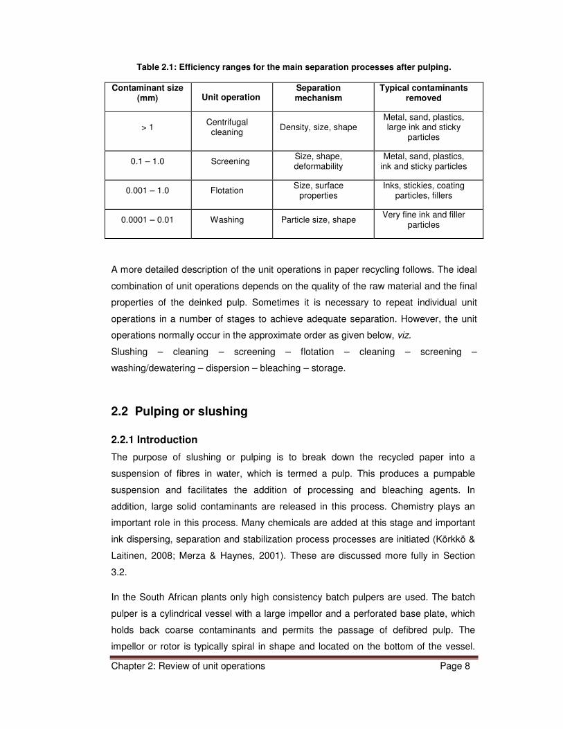
Table 2.1: Efficiency ranges for the main separation processes after pulping.
Contaminant size (mm) Unit operation
Separation mechanism
Typical contaminants removed
> 1 Centrifugal cleaning
Density, size, shape Metal, sand, plastics, large ink and sticky
particles
0.1 – 1.0 Screening Size, shape, deformability
Metal, sand, plastics, ink and sticky particles
0.001 – 1.0 Flotation Size, surface
properties Inks, stickies, coating
particles, fillers
0.0001 – 0.01 Washing Particle size, shape Very fine ink and filler
particles
A more detailed description of the unit operations in paper recycling follows. The ideal
combination of unit operations depends on the quality of the raw material and the final
properties of the deinked pulp. Sometimes it is necessary to repeat individual unit
operations in a number of stages to achieve adequate separation. However, the unit
operations normally occur in the approximate order as given below, viz.
Slushing – cleaning – screening – flotation – cleaning – screening –
washing/dewatering – dispersion – bleaching – storage.
2.2 Pulping or slushing
2.2.1 Introduction
The purpose of slushing or pulping is to break down the recycled paper into a
suspension of fibres in water, which is termed a pulp. This produces a pumpable
suspension and facilitates the addition of processing and bleaching agents. In
addition, large solid contaminants are released in this process. Chemistry plays an
important role in this process. Many chemicals are added at this stage and important
ink dispersing, separation and stabilization process processes are initiated (Körkkö &
Laitinen, 2008; Merza & Haynes, 2001). These are discussed more fully in Section
3.2.
In the South African plants only high consistency batch pulpers are used. The batch
pulper is a cylindrical vessel with a large impellor and a perforated base plate, which
holds back coarse contaminants and permits the passage of defibred pulp. The
impellor or rotor is typically spiral in shape and located on the bottom of the vessel.

Chapter 2: Review of unit operations Page 9
Water, recycled paper and process chemicals are charged into the pulper and the
rotating impellor breaks the paper down into fibres, in a process termed defibering. It
is necessary to wet paper fibres and to overcome the hydrogen bonding forces that
bond the fibres together in the dry state (Körkkö & Laitinen, 2008).
2.2.2 Process parameters
The important process parameters for pulping are specific energy consumption,
pulping time, temperature, pH or alkalinity and consistency. The extent of the pulping
process is measured by the flake content. A flake is a small piece of undisintegrated
paper. Deflaking rates of 98% are possible (Pescantin, Gu & Edwards, 1999).
The specific energy demand of the pulping process can vary from ca. 30 kWh/t in the
case of high consistency pulping to over 100 kWh/t for low consistency pulping.
Historically, batch pulpers have been favoured because of operating flexibility and the
ability to put more energy into the slushing process (Merza & Haynes, 2001).
The time taken to completely deflake the recycled paper depends on the nature of the
paper. Papers with a high wet strength require more energy and time to deflake.
Typical pulping times for high consistency pulpers are in the region of 10 to 15
minutes, but can be as high as 55 minutes for wet strength grades (Pescantin, Gu &
Edwards, 1999). Whilst long pulping times favour the complete disintegration of the
waste paper, they also contribute to excessive ink fragmentation and lead to ink
redeposition. One such redeposition process is lumen loading, whereby tiny ink
particles enter the fibre cells through the pits, and reside permanently in the lumen,
making it impossible to remove the ink particle. It is generally recommended to
minimize the pulping time, consistent with efficient deflaking. (Körkkö & Laitinen, 2008;
Merza & Haynes, 2001)
Pulping temperatures are typically in the region of 45oC, but can be as high as 85oC
for certain grades. Increasing pulping temperature can increase the rate of defibering.
However, this effect moderates at temperatures over 40ºC, with no practical benefits
over 60ºC (Körkkö & Laitinen, 2008).
Pulping is normally carried out at high pH’s. High pH is achieved by the addition of
sodium hydroxide and/or sodium silicate. The high pH facilitates fibre swelling and ink
removal (Körkkö & Laitinen, 2008), but also enhances the extraction of soluble and
colloidal materials, which contribute to high chemical oxygen demand (COD) and
hence water pollution. (Brouillette, Daneault & Dorris, 2001; Goettsching & Pakarinen

Chapter 2: Review of unit operations Page 10
2000: 95-105). High pH pulping is the norm for wood-containing papers (newsprint
and magazines), but neutral pulping is more usual for wood-free papers (Körkkö &
Laitinen, 2008; Brouillette, Daneault & Dorris, 2001).
The initial repulping pH has a great effect on the wet tensile strength of the paper, and
hence on the deflaking rate, as expressed in Equation (2) below (Brouillette, Daneault
& Dorris, 2001).
Seasonal differences in deinking, known as the “summer effect”, have been widely
reported on in the northern Hemisphere (Haynes, 2008; Merza & Haynes, 2001). As a
result of the higher temperatures in the summer months, accelerated thermal drying of
newsprint inks occurs. This leads to embrittlement of the ink and stronger attachment
to the fibres. When pulped, greater ink fragmentation and redeposition occurs, with
attendant deinking difficulties. These have been overcome by adding increased levels
of sodium hydroxide and decreasing pulping times during the warmer months.
However, this has not been reported to be a problem in South Africa, because of the
milder climate and smaller differences in Summer and Winter temperatures.
Currently, high consistency pulping (13-18%) is almost exclusively used in the modern
deinking process. High consistency offers better and faster deflaking, lower energy
consumption and a higher deinking chemicals concentration for the same dry fibre
mass addition rate (Körkkö & Laitinen, 2008). High consistency pulping can be
achieved in a continuous drum pulper or in a batch pulper. Batch pulpers offer better
opportunities to control the ink fragmentation through variations in consistency and
pulping time (Merza & Haynes, 2001). Drum pulpers have a gentler defibering action,
with resultant reduced fragmentation of contaminants. This allows the larger
contaminants to be more easily removed in the screening stages (Merza & Haynes,
2001; Goettsching & Pakarinen, 2000: 106).
2.2.3 Models and fundamentals
The study of the mechanisms of the pulping process only started in the 1980’s, with
significant work only being published after 1998 (Fabry, Carre & Galland, 2005). The
pulping process can be divided into three distinct mechanisms: defibering, ink
detachment and particle fragmentation (Körkkö & Laitinen, 2008).
2.2.3.1 Defibering or deflaking
Recycled paper, chemicals and water are charged to the pulper. Within about two
minutes wetting occurs and the inter-fibre bonding forces are weakened considerably

Chapter 2: Review of unit operations Page 11
(Goettsching & Pakarinen, 2000: 94). The input of mechanical energy via a rotor
separates the paper into individual fibres. Higher strength papers generally need
more energy to defibre, and pulping times approaching 60 minutes could be required
for strong boards and wet-strength papers. Increasing pulping temperature increases
the defibering rate (or reduces the pulping time). However, above about 40 oC, no
substantial improvements have been noted (Körkkö & Laitinen, 2008). The addition of
alkalinity (in the form of sodium hydroxide alone or in combination with sodium
silicate) leads to fibre swelling and accelerated defibering. Rao et al. (1998) state that
both mechanical forces (comprising shear and vibration) as well as chemical forces
are required to efficiently detach and stabilise ink particles.
Bennington, Sui & Smith (1998) studied the kinetics of the defibering of recycled paper
in repulpers. Defibering was found to obey a first order kinetic model of the form:
���� � ��� (1)
Where F is the TAPPI flake content, t is time and k is the rate constant.
The rate of deflaking was found to be dependent on the cumulative contact area
between the pulp fibres and the rotor blades. By expressing the rate constant in terms
of practical pulping parameters, Bennington et al. (1998) developed the following
expressions:
���� � ���� . ��� � �����
�������� � . � (2)
Where k’ is the intrinsic rate constant, C is the volumetric concentration of fibre
suspension, B is the number of impellor vanes, N is the impellor rotational speed, G is
the area swept by a rotor vane, T is the wet tensile strength of the paper, H is the
impellor height, K is a constant, Np is the impellor power number, D is the impellor
diameter, and is the density, all in S.I. units.
For a given installation with fixed geometry and defined operating conditions, this
expression simplifies to:
���� � ��!��� "���# $ . � (3)
Where �!and %! are machine efficiency constants.

Chapter 2: Review of unit operations Page 12
Equation (3) shows that the rate of deflaking in a practical situation depends on the
wet tensile of the paper, viz. the type of paper being pulped. This model was shown to
hold for a number of industrial rotors, operating speeds, consistencies and paper
types. Validation of this model in industrial scale pulpers showed that almost complete
deflaking had occurred after about 2 minutes. This suggests that most industrial
pulping sequences are too long.
Fabry & Carré (2004) have demonstrated that the rate of defibering can be well
explained by the volume energy consumption (the electrical energy input per volume
of pulp, kWhm-3) for a given type of pulper and initial chemical conditions. Similarly,
Rao et al. (1998) have shown that the amount of energy inputted in the stirring system
determines the initial rate of detachment. They also reported that the addition of
alkaline chemicals increases the defibering rate and reduces the energy requirement.
2.2.3.2 Ink detachment
Ink detachment occurs simultaneously with defibering. Generally, more energy is
required to detach ink particles, as the chemical bonding forces between ink and
paper are higher than the hydrogen bonding forces between paper fibres. It is thought
that fibre swelling, induced by high pH also facilitates ink detachment. In addition,
chemicals such as sodium hydroxide and hydrogen peroxide could chemically break
down ink binders, further enhancing ink detachment (Körkkö & Laitinen, 2008; Fabry &
Carre, 2004; Carré, Galland & Julien Saint Amand, 1994).
Whilst ink detachment is a complex function of rotor speed, pulping time and
chemistry (Rao et al., 1998), Fabry & Carré (2004) found that the volume energy
consumption well describes the detachment phenomenon. The volume energy
consumption effectively summarises the forces involved in pulping, viz. the pulping
time, rotor speed, consistency and the type of pulping device.
2.2.3.3 Particle fragmentation and redeposition
The continuing input of mechanical energy leads to further comminution of ink
particles. Rao et al. (1998) found that non-ionic surfactants assist in the comminution
process, whereas the soap/calcium system tends to agglomerate the ink particles.
The production of large quantities of fine ink particles will lead to redeposition onto the
fibre surface. The mechanical action also smears ink onto fibre surfaces (Carré &
Galland, 2007), or even results in ink penetration into the fibre lumens via the pits,
known as lumen loading. (Haynes, 2000).

Chapter 2: Review of unit operations Page 13
Similarly, Fabry & Carré (2004) found that ink fragmentation depended on rotor speed,
pulping time and chemistry, and reported that the volume energy consumption also
describes the detachment phenomenon, although it does not predict the ink
redeposition process.
Redeposition and lumen loading lead to irreversible brightness loss. This can be
mitigated by the addition of surfactants, which stabilise the fine ink particles by
rendering them hydrophilic (Körkkö & Laitinen, 2008).
In similar deflaking rate studies, Bennington & Wang (2001) also found that the rate of
ink detachment followed first order kinetics, and depended on fibre suspension
consistency and the cumulative contact area between rotor and suspension. Whilst
the consistency affected the rate of ink detachment, it did not influence the final level
of detachment.
Bennington & Wang (2001) found that after some time ink redeposition started setting
in. Ink redeposition also followed first order kinetics, increasing as the concentration of
detached ink increased.
The net effect of these two competing processes was that the residual ink
concentration on fibres decreased with repulping time to a minimum at about 15
minutes, and thereafter increased steadily as ink redeposition started gaining
momentum.
A comprehensive study of the effects of pulping parameters on deflaking, ink
detachment and ink removal by flotation was carried out by Fabry, Carré & Crémon
(2001). They found that the rate of defibering was accelerated by consistency,
temperature, rotor speed and the introduction of chemicals conventionally used in
pulping. The results suggested that the pulping times conventionally used in industrial
pulpers were way too long. On the other hand, the effect of rotor speed, consistency
and temperature on the residual ink concentration all showed minima with respect to
the pulping time. This confirms the observations of Bennington & Wang (2001) that
the rate of both ink detachment and ink redeposition are accelerated at the same time,
resulting in an optimum repulping time. Continually increasing pulping times also lead
to continually increasing ink fragmentation. The use of conventional pulping
chemicals (viz. sodium hydroxide, sodium silicate, hydrogen peroxide and surfactants)
greatly accelerated the deflaking and ink detachment and retarded the ink

Chapter 2: Review of unit operations Page 14
redeposition. Nevertheless, increasing pulping times still resulted in increasing ink
redeposition with time (Fabry, Carré & Crémon, 2001).
The net effect of the abovementioned pulping conditions on ink removal by flotation
was found to be as follows: longer pulping times, higher consistencies, higher
temperatures lead to greater ink fragmentation and consequently to inferior ink
removal by flotation. The use of conventional pulping chemicals also lead to a slightly
lower ink removal (ERIC, see Section 3.5.5) by flotation (Fabry, Carré & Crémon,
2001).
In another study on the effect of pulping variables on ink removal from thermally aged
newsprint, Haynes (2000) found that ink fragmentation increased (viz. Eric increased)
with decreasing temperature, increasing pulping time, decreasing alkali charge, and
increasing ratio of sodium silicate to sodium hydroxide. These results are at odds with
those reported by Fabry, Carré & Crémon (2001) with respect to temperature, perhaps
due to different types of ink.
2.2.4 Conclusion
The pulping process represents a compromise between two opposing processes:
fragmentation processes (defibering, ink detachment and ink fragmentation) and
redeposition processes. Too much fragmentation can result in ink particles being too
fine for effective removal by flotation, and excessive redeposition results in lumen
loading with very little possibility of ever removing the ink from the lumens. After
defibering and detachment, the fragmentation and redeposition processes occur
simultaneously. All of these processes are influenced by consistency, chemistry,
temperature, and energy input. The ideal pulping conditions represent a compromise
between the abovementioned processes. Thus, pulping is a process which must be
optimised for each item of equipment and set of conditions As a result, various
authors (Fabry, Carré & Galland, 2005) have recommended to drastically reduce the
pulping times of 15 to 20 minutes normally employed in commercial deinking lines to
only a few minutes.
The above conclusions apply mainly to recycled newsprint and magazine furnishes.
In a study of the defibering-detachment-fragmentation-redeposition dynamics in wood-
free recovered papers intended for tissue manufacture, Fabry, Carre & Galland (2005)
found that ink redeposition was not a major negative factor, and that extended pulping
times marginally improved ink removal by flotation. In recycled paper mixes of wood

Chapter 2: Review of unit operations Page 15
containing and wood free papers, it could be expected that ink redeposition would
again appear as a negative effect.
2.3 Centrifugal Cleaning
Cleaners or hydrocyclones make use of centrifugal force and differences in relative
density to separate undesirable particles from the water. Thus, dense particles such
as sand and metal, and light particles such as shives and plastic material are easily
removed by a cleaner. According to Table 2.1, cleaners are most effective at
removing large, dense particles. (Goettsching & Pakarinen, 2000: 134-137).
Ink particles have densities close to that of water, and are not normally separated by
cleaners. However, cleaners are known to remove very small dense particles of the
type typically found in fillers (Goettsching & Pakarinen, 2000: 134-137). Fillers have
different brightness to fibres, and their removal could influence the final, measured
brightness.
Centrifugal cleaners are usually connected in a cascade arrangement, and are
normally used in combination with screening to effect removal of contrary materials in
a recycling system.
2.4 Screening and fractionation
The recycled fibre pulp is passed through a screen plate perforated with small holes or
slots. A rotating rotor within the screen body produces pulsations and a pressure drop
across the screen plate, thereby ensuring throughput and preventing fouling. Debris
such as shives, coarse fibre, stickies and fragments of plastic are removed from the
pulp stream on the basis of size, although particle shape and flexibility also play a
role. Flexible or conformable particles will force themselves through even fine
perforations.
Typical screen plate hole sizes are 1.2 to 1.6 mm in the primary screens, and slot
widths as low as 0.1 mm are commonly used in the final stages. Screen design factors
(screen profiles and rotor geometries) play a large role in the performance and
efficiency of the screens. It is not possible to remove all the debris in one screening
stage, and fibre losses always accompany screening. In order to optimise the

Chapter 2: Review of unit operations Page 16
screening efficiencies, multiple stage screening in a cascade arrangement is usually
employed. (Goettsching & Pakarinen, 2000: 110-132).
Cleaning and screening removes high density and large solid materials, and do not
remove significant quantities of ink. Pulping, flotation and washing have the overriding
influence on ink removal (Beneventi, Deluca & Carré, 2004) Thus, it was assumed for
the purposes of this modelling work that the change in brightness or ERIC was solely
due to the pulping, flotation and washing processes.
2.5 Flotation
2.5.1 Introduction
The flotation process is one of two methods for removing ink from a recycled paper
pulp. Fine air bubbles are injected into the fibrous pulp. The bubbles move upwards to
the surface, and in the process attach to themselves hydrophobic particles such as
ink, stickies, fillers and coating components. Typically, particles in the size range of
10-250 microns form stable structures with the air bubbles and are successfully
removed. On the surface, the bubbles form a stable foam layer comprising the ink and
other floated material. This foam bed is removed physically from the fibre suspension
below (Goettsching & Pakarinen, 2000: 153-154).
2.5.2 Process equipment and parameters
Early deinking flotation cells were based on designs borrowed from the mineral
flotation industry. Hines (Hines, P.R. 1933. US Pat. No. 2,005,742) was granted a
patent for flotation deinking in 1935, but it was only in the early 1950’s that the Denver
cell, originally designed for mineral flotation, was first used in a deinking flotation
installation in North America (Kemper, 1999). Only in the 1980’s did waste paper
recycling and flotation deinking come into common use. Since then a large amount of
effort by many manufacturers has gone into the design of specialized deinking
equipment. Flotation cell designs can be square, rectangular, cylindrical (horizontal or
vertical), or elliptical, and some cells are even pressurised. High speed impellors
provide agitation and fine air bubbles are introduced by aspiration or pumped in
through fine nozzles. (Goettsching & Pakarinen, 2000: 158-165; McCool, 1993).
Multiple flotation stages are necessary to achieve the desired pulp quality in modern
installations.

Chapter 2: Review of unit operations Page 17
Of interest in the South African market are the flotation cells produced by Sulzer
Escher Wyss (CF/CFC), and the Voith E-cell and Voith Sulzer Eco-Cell. The details of
these cells are discussed later in Chapter 9.
Flotation systems are generally operated at consistencies of 0.8%-1.5%, temperatures
of 40°C-70°C, and pH’s in the range of 7-9. A water hardness of about 200 ppm as
calcium carbonate is required when using fatty acid surfactants as collectors. With
surfactants other than fatty acid soaps, hardness is not required. The relative air
volume (expressed as total air volume flow per total stock volume flow) is typically
300%, with some flotation systems operating at relative air volumes up to 1000% A
secondary flotation stage is commonly used. The flotation foam removed from the
primary stages is refloated in a secondary stage. The secondary stage further
removes contaminants (ink, fillers, stickies), and the remaining fibres are returned to
the inlet of the primary flotation cells. In this way the fibre losses are reduced.
(Goettsching & Pakarinen, 2000: 153-158)
2.5.3 Theoretical models and fundamentals
2.5.3.1 Introduction
The physical flotation processes have been described using hydrodynamic and
probability processes by various authors (Heindel, 1999; McCool, 1993; Schulze,
1991). The flotation process has been described as a combination of three main
physical processes (McCool, 1993):
a. The probability of collision - dependent on the number and size of the air
bubbles and ink particles.
b. The probability of attachment of air bubbles and ink particles - dependent
on the surface chemistry of the various particles.
c. The probability of removal of the air bubble-particle complex from the
system – dependant on the stability of the bubble-particle complex.
Steps a. and c. depend on process equipment design and process conditions such as
consistency, temperature, agitation, retention time and flotation cell design. A more
detailed treatment of theoretical models for the flotation process follows.
Flotation deinking processes have drawn many of the concepts and practices from the
mineral flotation industry. However, the flotation of ink from a cellulose fibre slurry

Chapter 2: Review of unit operations Page 18
differs in many fundamental aspects from that of mineral flotation. These similarities
and differences are summarized in Table 2.2:
Table 2.2: Comparison of deinking and mineral flotation. (Julien Saint Amand, 1999;
Heindel, 1997; Pan et al., 1996)
PROCESS PARAMETER
FLOTATION DEINKING MINERAL FLOTATION
Particle surface energy Varies from low energy hydrophobic adhesives and inks to high energy hydrophilic fibres and fillers.
More uniform, generally high energy hydrophilic minerals.
Particle size and shape Broad distribution, 1 micron to 1 mm. spherical to fibrous to large flat.
Broad distribution, irregular and granular.
Particle density Less than or equal to water, filler particles greater than water, very fine.
Generally higher than water.
Particle liberation Slushing in the presence of a mix of chemicals.
Size reduction by grinding.
Pulp properties Heterogeneous fibre network which tends to flocculate above 1% consistency, at relatively high temperature 40-60
oC. A blend of
dissolved, colloidal and suspended particles.
More homogeneous 2-phase system with simpler rheology, lower temperature.
Characterization of final product
Qualitative or semi-quantitative brightness, dirt and adhesive content. Indirect measurement of ink content using a spectrophotometer.
Quantitative chemical analysis.
Impact of low efficiency on downstream plant
Reduced product quality, contamination of downstream equipment
Effects are mainly economic.
The net result of these differences is the lower separation efficiency of flotation
deinking. Nevertheless, it is assumed that the fundamental processes occurring are
very similar. Particle inertia effects are typically disregarded in flotation deinking,
because of the lower density of particles involved. The modelling of flotation separation
processes has tended to be grouped into a number of different approaches, as
outlined below.

Chapter 2: Review of unit operations Page 19
2.5.3.2 Multistage probability process models (Bloom and Heindel, 1997; Heindel,
1997)
In these models, the basic philosophy is that the overall flotation process consists of a
number of sub-processes, each with their associated probabilities. The basic
assumptions are: bubbles and particles are spherical, one particle interacts with one
bubble, a non-turbulent flow environment is assumed, and the air bubbles are
assumed to be “stiff”, or inelastic.
The sub-processes are:
Step 1: Approach of particle and air bubble
As depicted in Figure 2.1, it is assumed that the particle is intercepted by the bubble
within a capture radius Rc. Because of the low density of ink particles, inertial effects
are neglected and it is assumed that the particle moves along a fluid streamline.
Figure 2.1: Approach of ink particle and air bubble. (Bloom and Heindel, 1997; Heindel,
1997)
Step 2: Interception of particle by the bubble
By taking into account the Reynolds number (ReB) and Stokes number pertaining in a
typical flotation cell, an expression for the probability of particle capture, Pc, has been
derived (Bloom and Heindel, 1997; Heindel, 1997):
&' � ()*+ ,-./0.1�23 4 "-�-/$*
(4)

Chapter 2: Review of unit operations Page 20
Step 3: Attachment by sliding
The particles slides along the interface for some distance before attachment takes
place. With reference to Figure 2.2, the probability of attachment by sliding, Pasl, can
be expressed as:
Figure 2.2: Schematic of probability of attachment by sliding Pasl (Bloom and Heindel,
1997; Heindel, 1997)
&567 � -89:;�<-/=->?� (5)
where @'AB� is the limiting radius associated with the touching angle C'AB� D . Various expressions have been derived for this term, but its determination still
depends on a number of immeasurable quantities. (Bloom and Heindel, 1997; Heindel,
1997)
Step 4: Film rupture and formation of three-phase contact angle
Once a particle is attached to an air liquid film, the film must rupture and a three-phase
contact configuration must form. This is illustrated schematically in Figure 2.3.
It has been widely assumed that this probability is close to 1. Thus, the probability of
three-phase contact Ptpc = 1 (Bloom and Heindel, 1997; Heindel, 1997).

Chapter 2: Review of unit operations Page 21
Figure 2.3: Formation of three-phase contact angle. (Bloom and Heindel, 1997; Heindel,
1997)
Step 5: Stabilisation of the particle-bubble complex and transport to the froth layer.
The particle-air bubble aggregate must remain stable as it is transported up to the froth
layer. As it rises, the air bubble will experience stresses, which tend to destabilise the
particle-bubble aggregate. A schematic of this situation is given in Figure 2.4:
Figure 2.4 can be a little misleading. In practice, as a bubble rises to the surface, the
ink particles will most probably slide to the bottom of the bubble, as shown in Figure
2.5.
These forces are identified as gravitation Fg, buoyancy Fb, detachment by fluid drag Fd,
force due to capillary pressure in the gas bubble Fσ, capliiary force Fca, and the
hydrostatic pressure force Fhyd. The net balance of these forces B is defined as:
� � �EF;G8HIFJ;�G;;G8HIFJ; =
�K��L=�E=�M�8G=�HNE (6)
and the probability of stabilisation &6�5O is:
&6�5O � 1 � exp <1 � 2�? (7)
Once again, expressions have been derived for the force balance (Bloom & Heindel,
1997; Heindel, 1997).
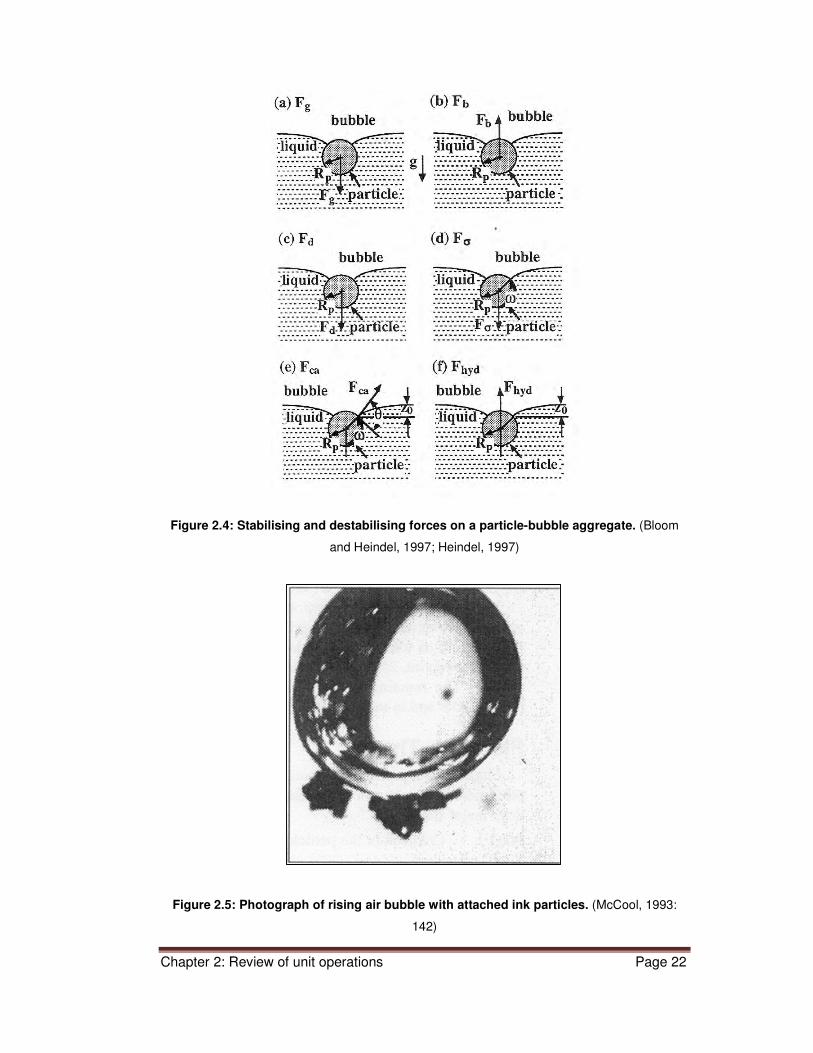
Chapter 2: Review of unit operations Page 22
Figure 2.4: Stabilising and destabilising forces on a particle-bubble aggregate. (Bloom
and Heindel, 1997; Heindel, 1997)
Figure 2.5: Photograph of rising air bubble with attached ink particles. (McCool, 1993:
142)

Chapter 2: Review of unit operations Page 23
By assuming that the individual micro process probabilities are not correlated, the
overall probability of separation by flotation becomes:
&TU.A577 � &'&567&�V'&6�5O � &'&567&6�5O approximately (8)
where &' is the probability of particle capture, &567 is the probability of attachment by
sliding, &�V' is the probability of three-phase contact (assumed to be ca. 1) and &6�5O is
the probability of stabilisation.
The calculation of these probabilities involves a large number of difficult-to-measure
variables. As a result, the use of such models in practice is limited.
2.5.3.3 Reaction rate models
Another way of describing the flotation process is to consider it analogous to a first-
order chemical reaction:
X(particles) + Y(bubbles) → Z(floated particles) (9)
where X, Y and Z are the number of objects. Assuming the concentration of the
bubbles is constant and that the volume of the removed particles is negligible, the rate
expression becomes:
�'�� � ��[ (10)
where c is particle concentration and k is a rate constant.
Depending on the system studied, many different expressions have been developed
for k (Heindel, 1997).
2.5.3.4 Population balance models
The basic kinetic model above has been extended by Bloom (1996), Heindel (1997)
and Bloom and Heindel (1997) to a population balance model of the form:
�\�]�� � -k1 npf nBf + k2 nBa (11)
where npf = number of free particles per unit volume available for attachment,
nBf = number of bubbles per unit volume available for attachment, and

Chapter 2: Review of unit operations Page 24
nBa = number of bubbles with particles attached.
Thus the term -k1 npf nB
f represents the probability of attachment and k2 nBa represents
the probability of particle-bubble aggregates splitting to become unattached particles
again.
This approach thus ties in with the probabilistic approach, where:
k1 � Z PcPaslPtpcPstab (12)
and
k2 � 1 - Pstab (13)
Solving these equations (Bloom and Heindel, 1997) yields the predicted flotation
efficiency as a function of particle size for various particle diameters Rp, as shown in
Figure 2.6. For particle diameters greater than 200 microns, the theory predicts that
Pstab < 0. In this case Poverall (equation 8) will be less than zero and flotation will not
occur. In addition, very small particles (1 to 10 microns) will take an impractically long
time to float.
Figure 2.6: Flotation efficiency as a function of flotation time and particle size. (Bloom
and Heindel, 1997; Heindel, 1997)

Chapter 2: Review of unit operations Page 25
The findings of this model concur with what is known in practice: large particles of ink,
as generated by electrographic inks, do not float well and very fine ink particles are
also not removed by flotation.
The models outlined above were partially validated experimentally (Bloom, 2006), with
the conclusions that the models showed “great promise” if the measurement of bubble
particle size, stability parameters and the relationship between consistency and
viscosity could be determined.
2.5.3.5 Hydrodynamic models
As above, the flotation process can be considered as a first order kinetic process:
nopnq � -zNpNbPcPaPs (14)
where Np and Nb are the number of particles and bubbles per unit volume, Pc, Pa and
Ps are the probabilities of collision, attachment and stabilization respectively. Julian
Saint Amand (1999) has taken a slightly different approach to the modelling of the
flotation process. Equation 14 can be written as follows:
toptq � -zNpNbPcPaPs � -kNp (15)
where k is a flotation rate constant.
In order to increase the generality of such models it is useful to consider the concept of
volume of air to pulp ratio, instead of flotation time to define rate constants. Thus, let
air ratio = T and ∆T = Nb(πd3/6), where d is the bubble diameter. An equation similar
to Equation 15 can now be written:
toptu � �%�� or
v���� � �%wx (16)
where K is a flotation rate constant.
For small variations of topop and wx and after integration, one gets
ln ����y� -KT (17)
The flotation efficiency as a function of air ratio is given by:

Chapter 2: Review of unit operations Page 26
E � 1 - ����y � 1 – ���� (18)
Laboratory deinking studies, where loge (number of particles per litre of pulp) is plotted
against T, have confirmed this linear relationship for different ink particle sizes (Julian
Saint Amand, 1999). An investigation into the effects of particle size, bubble size and
turbulence agreed with the established theory for mineral flotation (Julian Saint
Amand, 1999), viz:
• High ink removal efficiencies and high flotation losses are achieved with high
air ratios,
• Lower flotation efficiencies for microscopic ink particles,
• Small bubbles are more efficient at removing particles.
2.5.3.6 Transport phenomena models
Beneventi, Benesse, Carré, Julien Saint Amand & Salgueiro (2007) started from a
similar rate equation as above (Equation 14):
nopnq � -ZpbPcPaPs (19)
where Np is the number of particles per unit volume, Pc, Pa and Ps are the probabilities
of collision, attachment and stabilization respectively and Zpb is the particle-bubble
collision rate. They considered particle and water transport phenomena in terms of
semi-empirical equations for the three sub-processes of flotation, entrainment and
drainage, thus:
Flotation rate
It has been shown that (Koh & Schwartz, 2003):
Zpb � NpNb<√����23� ?<
n� = n�* ?3 (20)
where Zpb is the particle-bubble collision rate, Np is the particle number concentration,
Nb is the bubble number concentration, ET is the turbulent dissipation rate, v is
kinematic viscosity, dp and db are particle and bubble diameters.
The bubble number concentration Nb is given by:

Chapter 2: Review of unit operations Page 27
Nb � 6Qgtg/πdb3Svb (21)
where Qg is the injected gas flow, tg is the gas retention time and S is the cross-
sectional area of the cell, db is the bubble diameter, vb is the bubble rising velocity.
By combining the above equations, the rate of particle removal reduces to:
nopnq � �<���
� ? Np, where % � 6 �8�G���KUL � ���
23�U "�� = �L*�L $) (22)
In practice it has been found necessary to modify the equation slightly, by
incorporating an empirical correction factor α:
nopnq � �<����
� ? Np (23)
This equation has been used to simulate industrial flotation systems.
Particle entrainment
Hydrophilic particles such as fibre fines, fibres and fillers, whilst not adhering to the
surface of air bubbles, can nevertheless be dragged up or entrained into the froth
phase by the rising air bubbles. The transport rate of hydrophilic particles can be
described by:
nopnq � �<����� ? Np (24)
where φ is the particle entrainment co-efficient and Q�� the water upward flow in the
froth without drainage, and V is the pulp volume in the flotation cell.
Drainage from the froth
The froth structure is very dynamic. Particles and water drain back into the pulp slurry,
and bubbles can coalesce or burst. This can result in particle fractionation in the froth
layer. An empirical equation for the water volume fraction in the froth ε, has been
developed to describe the water drainage behaviour:
ε � εo�� ¡q¢ (25)
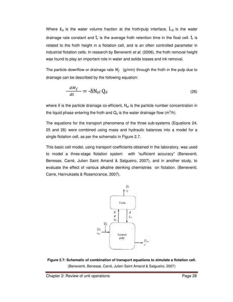
Chapter 2: Review of unit operations Page 28
Where εo is the water volume fraction at the froth/pulp interface, Ld is the water
drainage rate constant and tr is the average froth retention time in the float cell. tr is
related to the froth height in a flotation cell, and is an often controlled parameter in
industrial flotation cells. In research by Beneventi et al. (2006), the froth removal height
was found to play an important role in water and solids losses and ink removal.
The particle downflow or drainage rate £¤ (g/min) through the froth in the pulp due to
drainage can be described by the following equation:
�¥] �� � -δNpf Qd (26)
where δ is the particle drainage co-efficient, Npf is the particle number concentration in
the liquid phase entering the froth and Qd is the water drainage flow (m3/h).
The equations for the transport phenomena of the three sub-systems (Equations 24,
25 and 26) were combined using mass and hydraulic balances into a model for a
single flotation cell, as per the schematic in Figure 2.7.
This basic cell model, using transport coefficients obtained in the laboratory, was used
to model a three-stage flotation system with “sufficient accuracy” (Beneventi,
Benesse, Carré, Julien Saint Amand & Salgueiro, 2007), and in another study, to
evaluate the effect of various alkaline deinking chemistries on flotation. (Beneventi,
Carre, Hannuksela & Rosencrance, 2007).
Figure 2.7: Schematic of combination of transport equations to simulate a flotation cell.
(Beneventi, Benesse, Carré, Julien Saint Amand & Salgueiro, 2007)

Chapter 2: Review of unit operations Page 29
2.5.3.7 Statistical models
Pan et al. (1996 & 1994) proposed a very simple “Global Model” to predict the
outcome of deinking flotation processes. It has only two parameters:
• The capture radius, which is the distance between centres of an air bubble and
an ink particle, within which a particle will stick to an air bubble, and
• The bubble flux or flotation time.
The output of this model is defined as the flotation efficiency, which is the ratio of
particles captured to the number originally present. The workers constructed various
model systems in the laboratory, and report “excellent general agreement” with the
global model (Pan et al., 1996). Unfortunately, the exact mathematical nature of the
model was not disclosed in the publication.
2.5.3.8 Practical models
Scheldorf and Strand (1996) simulated ink removal in a newsprint deinking facility by
using a combination of an existing modular simulation program known as WinGEMS
with additional calculation blocks which were termed SPECSEP, BRIGHT and
CONINK. SPECSEP was a model of the particle size distribution of ink removed in
the pulper, BRIGHT was a model for the calculation of brightness from the Kubelka-
Munk theory and the fractional composition of the pulp slurry, and CONINK converted
a measured ink size distribution into an ink solids fraction. The results were described
by the authors as “promising”.
2.5.4 Conclusions
Consideration of the overview of theoretical models presented above demonstrate that
the modelling of a flotation system is extremely complex. Most of the attempts at
modelling have been focused on the flotation process, although some models have
been developed for the pulping process. It is probably not possible to develop a global
first-principles model for the combined pulping and flotation processes, as they rely on
fundamentally different physical processes, and the measurement of ink is not
quantitative. An attempt will be made in this work to use artificial intelligence
techniques to develop a global model for a deinking system.
2.6 Washing
Washing is a process of removing solid contaminants (including ink particles) by high
dilution and filtration. The washing filtrate contains the contraries in the form of very

Chapter 2: Review of unit operations Page 30
finely dispersed particles such as fillers, fibre fines, stickies, fine ink particles, colloidal
particles and dissolved organics. Washing is less selective with respect to ink particles
than the flotation process, but removes a wider variety of contaminants (Goettsching &
Pakarinen, 2000:176). Typical size ranges of particles encountered in a deinking
system are listed in Table 2.3 (Goettsching & Pakarinen, 2000:176; Dobias, Klar &
Schwinger, 1992).
Table 2.3: Typical size ranges of particles.
Solid particle Size in microns
China clay 1-2
Kaolin 0.3-5
Calcium Carbonate 0.5-5
Titanium dioxide 0.2-0.5
Coating grit <60
Ink particles 0.5-500
Fibre fines <200
Short fibre fraction (length) 120-400
Long fibre fraction (length) >400
The pore size of a fibre mat is initially that of the wire mesh on which the filtration is
taking place (ca. 500 microns), but decreases down to about 10 microns as the fibre
mat builds up and consolidates on the filtration mesh. In practice, only particles
smaller than 30 microns are successively removed by washing. Larger particles tend
to become mechanically or electrokinetically entrained in the fibre mat during the
filtration process (Goettsching & Pakarinen, 2000:176-180). The theoretical efficiency
of a washing machine depends to a large extent on the consistency entering and
leaving the washing unit, as shown in Figure 2.8.
Washing and flotation are often used in combination in many commercial deinking
plants (McCool, 1993). Washing is more often targeted at removing fillers and fines,
whilst flotation is used to selectively remove inks. For very finely dispersed
flexographic inks, washing is the only practical means of ink separation.

Chapter 2: Review of unit operations Page 31
Figure 2.8: Effect of consistency on theoretical washing efficiency, as measured by ash
removal. (Goettsching & Pakarinen, 2000:176)
Washing is normally carried out in dewatering machines, as described below.
(Goettsching & Pakarinen, 2000:176-181)
2.7 Dewatering
Dewatering is a distinct unit operation in the processing of recycled fibres. Dewatering
is the process of removing the water and water-soluble components of a fibre pulp
from the solid (usually fibre) components.
Dewatering is usually done to adjust the consistency of a process into a range which
is most efficient or cost effective. For example bleaching processes are more effective
and use fewer chemicals at higher consistencies, and smaller storage volumes are
required for high consistency pulp.
Dewatering allows for the removal of excess water in one area of the process to be
utilised in other stages of the process in order to conserve process chemicals or
process heat. Dewatering is also used to separate water systems. For example, an
alkaline process could be separated from an acidic one, thereby eliminating expensive
neutralisation steps.
Dewatering is essentially a filtration process carried out using belt, drum or disc filters.
These machines can be vacuum or pressure assisted. The pulp feed consistency is
typically 2-3.5% and water is removed to produce a fibre cake with a consistency
Chapter 2: Review of unit operations Page 32
ranging from 5% to 25%, depending on the machine (Figure 2.8). The resulting filtrate
normally contains small quantities of fibre fines, colloidal and soluble materials. A
filtrate consistency of 100 – 1000 ppm is typical. (Goettsching & Pakarinen, 2000:
168-175.)
The filtrate water from dewatering systems is recirculated for use at various points in
the process. This is termed “back-water” in the industry. The result of this is that
contaminants and process chemicals are cycled up and concentrated, which can have
a significant disturbing effect on the process. It is advisable to remove such fines and
colloidal matter from filtrate waters. This is usually done by using dissolved air flotation
techniques.
2.8 Dispersing
Dispersing breaks up remaining ink and dirt specks into particles that are the correct
size for further flotation or washing. In addition, it can also serve to disintegrate dirt
specs until they are too small to be detected visually, thereby improving the
appearance of the final paper. The visual detection limit for dirt specks is widely
considered to be about 50 microns. In addition, dispersion can assist in removing ink
particles still attached to the fibres and conditioning them for papermaking. In the
dispersion process, high shear forces, which are in excess of the shear strength of the
particles to be dispersed are applied to the stock. This is usually only achievable at
high stock consistencies, of 20-30%. Dispersing can be carried out in disk dispergers
or kneading dispergers. Disk dispergers are similar to pulp refiners, with specialised
plates containing intermeshing teeth mounted on a static stator and a rotating rotor.
The amount of energy, and hence the applied shear force is regulated by changing
the axial spacing of the plates. Typical applied energy is in the range 50-80 kWh/t.
Kneading is performed in tubular machines containing rotating shafts with specially
shaped flights or impellors. The energy input into a kneader can be regulated by
throttling the discharge from the machine. Energy inputs can range from 30-80 kWh/t.
Dispersion is usually carried out at elevated temperatures of 60-130 ºC for disk
dispergers and 40-95 ºC for kneaders. Disk dispergers are more effective at reducing
dirt particle size, but also tend to affect fibre strengths and freeness. Kneading is
gentler on the fibres. (Goettsching & Pakarinen, 2000: 185-192)
Chapter 2: Review of unit operations Page 33
2.9 Bleaching
Bleaching in deinking involves the removal of yellowness of the fibres or other
coloured components originating from printing inks. Bleaching chemicals can be
added at various stages of the process. The chemistry of hydrogen peroxide
bleaching is discussed in the Section 3.2.
The pulp bleaching industry has available to it a wide variety of bleaching agents. The
commonly used oxidative bleaching agents include hydrogen peroxide (P), ozone (Z),
oxygen (O), chlorine dioxide (D) and sodium hypochloride (H). The range of available
reductive bleaching agents is more limited, and consists of sodium hydrosulphite (Y)
and formamidine sulphinic (FAS) acid.
All of the oxidative bleaching agents can be used to bleach pulps which do not contain
mechanical fibres. Chlorine dioxide gave the best destruction of fluorescent whitening
agents (FWA), followed by potassium permonosulphate and peracetic acid. The
reducing agents gave the best colour removal, followed by ozone, chlorine dioxide
and sodium hypochlorite (Magnin, Angelier & Galland, 2000). Goettsching &
Pakarinen (2000): 307 state that ozone is also very effective in removing FWA’s.
However, the oxidative bleaching agents, with the exception of hydrogen peroxide, are
not suitable in applications which contain mechanical pulps, as oxidative degradation
of lignin occurs. This necessitates additional pulp washing stages and results in
effluents high in COD. Thus in practice hydrogen peroxide and the reductive bleaching
agents are used. These have the advantage that bleaching can be carried out in
existing tanks and chests, without requiring dedicated bleaching and pulp washing
plant. The reductive bleaches are most effective for colour stripping (removing the
colour from dyes emanating from coloured papers and inkjet inks) and hydrogen
peroxide is effective for the removal of fibre yellowing (Goettsching & Pakarinen,
2000: 308; Magnin, Angelier & Galland, 2000; Hach & Joachimides, 1991).
As a first bleaching stage, hydrogen peroxide is added into the pulper to counteract
the propensity of fibres to yellow in an alkaline environment. A final, or post bleaching
stage can also be applied at the end of the process in the storage chest. However, if
really high brightness is required, a dedicated bleach plant might be necessary. The
final bleaching is usually reductive bleaching with sodium hydrosulphite or
formamidine sulphinic acid (FAS). If the highest possible final brightness is desired,

Chapter 2: Review of unit operations Page 34
then a multistage peroxide/hydrosulphite bleaching sequence is necessary (Hach &
Joachimides, 1991).
Interstage bleaching with hydrogen peroxide has also been investigated by Carré,
Galland, Vernac & Suty (1996). Peroxide bleaching can be performed in a kneading
stage between two flotation stages, with similar results to that obtained by bleaching in
the pulper. Similarly, pseudo-neutral pulping, followed by bleaching in the interstage
kneader produced comparable results.
2.10 Process control of deinking plants
Paper recycling plants are typically controlled by measuring the final optical properties
of the pulp. In particular the brightness is routinely measured, but the residual ink
concentration and dirt concentration can also serve as secondary measures of
deinking. The overall process yield is also monitored. These properties are discussed
in more detail in Section 3.5.
These properties are usually measured by manual sampling at regular intervals and
determining the optical properties in the laboratory. On-line measuring devices have
come on the market in recent years to measure brightness (Gehr, Reinholdt & Koberi,
2000), specks (Julien Saint Amand, Perrin & Sabater, 1993), residual ink (ERIC) and
fine ink particles (Carré & Galland, 2007). These devices aid in the control of the plants
by providing timeous information to allow changes to be made to process parameters.
Waste recycling plants are normally set up to run at a standard set of conditions, which
by experience have been shown to produce the desired final quality. Process
parameters are not normally varied in response to changes in output quality or
changes in raw material composition. The processes essentially fluctuate naturally
about a process mean. The biggest challenge is that the improvements in brightness
that can be achieved by manipulation of process parameters are always
overshadowed by the effect of quality variations in the recycled paper feed (Carré &
Galland, 2007).
Thus, the usual response is to change the recycled paper mix fed to the plant.
However, the increasing variability of the recycled paper as foreseen in Chapter 1
makes this approach less viable in the future, and alternate control strategies are
needed.

Chapter 3: Review of deinking chemistry Page 35
CHAPTER 3: REVIEW OF CHEMISTRY OF DEINKING
The main components of a typical deinking system are the fibres, water which
functions as the carrier phase, the printing inks, the mineral fillers and various other
process chemicals that are required to achieve deinking. A deinking system is very
complex, because these components can interact with each other in difficult to predict
ways. The various components will be considered:
3.1 Printing Inks
The main printing processes in use today are offset lithography, rotogravure and the
flexographic processes. Offset lithography is commonly used for printing mass
circulation newspapers, due to the high print quality and good economics of the
process. The old letterpress process is no longer widely used. The rotogravure
process is mainly used in the printing of high quality work, such as mass circulation
magazines on coated or supercalendered paper. Flexographic printing of newsprint is
used to a limited extent in countries such as the United States of America, England
and Italy (Carré et al., 2000), but not in South Africa. Flexographic printing is the most
commonly used process for the printing of packaging papers (Goettsching &
Pakarinen, 2000: 283 – 293; Aspler, 1991).
A printing ink consists of a vehicle, a binder, a colorant (pigment or dyestuff) and a
variety of additives. The vehicle is a solvent that dissolves the binder and disperses
the pigment. The binder is a polymeric material that on drying forms a film on the
surface of the paper, thereby enveloping and adhering the pigments to the substrate.
The colorants impart colour to the ink. The dominant pigment is carbon black as most
inks are black, although coloured pigments (cyan, magenta and yellow) are used in
colour printing. The compositions of printing ink vary, as printing inks are formulated
according to the printing process used (Dobias et al., 1992).
Typical compositions, applications and deinking behaviour of various types of ink are
summarised in Table 3.1. (Carré & Magnin, 2004; Carré, Magnin & Galland, 2003;
Carré et al., 2000; Goettsching & Pakarinen, 2000:270-282; Dobias et al., 1992).

Chapter 3: Review of deinking chemistry Page 36
Table 3.1: Typical composition and applications of printing inks. Deinking behaviour
relative to unprinted paper.
Printing
process Application Binders Carriers
Deinking
behaviour
Web-fed cold-set Offset
Newsprint, mass circulation papers.
Hydrocarbon resins Mineral oil Deinks well, ca.
15% ISO brightness drop
Offset
High quality printing on coated stock,
forms, magazines, inserts etc.
Drying oils, alkyd resins, colophony
resins, hydrocarbon resins
Mineral oil
Deinks well, ca. 15% brightness drop. Affected negatively by
ageing
Rotogravure Mass circulation
high quality work eg. magazines, inserts
Colophony resins, hydrocarbon resins
Toluene
Deinks better than offset inks,
especially on coated papers
Flexographic and
rotogravure Packaging printing
Cellulose nitrate, polyvinyl acetate,
polyamides
Alcohols, ethyl acetate, benzene
Not deinked
Water-based flexographic
Newsprint (UK, Italy, USA)
and packaging
Acrylic resin dispersions
Water
Poor, ca. 30% ISO brightness loss.
Better removed by washing & neutral
deinking
Non-impact or electrostatic
(Xerographic)
Office copiers and printers, using toner
inks
Styrene acrylic, styrene butadiene, polyester or epoxy
resins
Toner inks do not contain
solvents
Form large ink particles not easy to float – specks in
the sheet
Ink-jet printing Home/office printers,
text and colour graphic prints
Azo dyes bound by soluble polymers
Water ethylene glycols
Not floatable, dye-based inks can be
colour stripped.
In the printing process the ink is applied to the surface of the paper. The vehicle
evaporates and penetrates into the paper, allowing the binder to form a tightly
adhering film on the paper surface. The drying process is a purely physical process for
binders such as high-boiling hydrocarbon resins or colophony resins. Such resins
never harden or dry, but remain adhering to the paper surface. On the other hand,
binders such as alkyd resins and drying oils undergo chemical cross-linking and
solidifying reactions to form hard, brittle and tightly adhering films on the paper
surface. The cross-linking processes can be either oxidative drying or initiated by
heat, UV light or electron beams. The nature of the drying processes and the chemical
nature of the printing ink binders and pigments determine the ease with which the ink
can be removed. It has been found that binders and solvents that are covalently
bonded; uncrosslinked; alkaline insoluble and wet pigments are easy to remove. In
contrast, solvents and binders that are polar; crosslinked; alkaline soluble and wet
pigments poorly are difficult to deink (Goettsching & Pakarinen, 2000: 274). This

Chapter 3: Review of deinking chemistry Page 37
second class of inks do not fragment well on repulping and typically form large
coherent ink particles which can’t be easily emulsified and hence removed (Read,
1986).
With the passing of time and the action of heat and oxygen, the binders crosslink, thus
becoming more brittle and firmly attached to the fibres. These inks are more difficult to
remove from the fibres and fragment more during processing, both resulting in greater
deinking difficulties. This is referred to as the “Summer effect” in the northern
Hemisphere. (Carré, Magnin & Galland, 2003; Le Ny et al., 2001; Goettsching &
Pakarinen, 2000: 293; Olson & Letscher, 1992).
Water-based flexographic inks, which are bound by acrylic resin dispersions, form
very fine particles when pulped. These particles are too small for removal by flotation,
and are best removed by washing (Carré & Magnin, 2004).
The inks used in office copiers and printers (electrophotographic or “Xerographic”
printing processes) do not contain a carrier. These “dry” inks are termed toners. The
dry toner ink (consisting of fine plastic particles (ca. 20 microns) and carbon black
pigment) is applied electrostatically to the paper surface and then fused at elevated
temperatures onto the paper. The fused particles adhere tightly to the paper surface.
(Johnson & Thompson, 1995)
Toners can be detached from fibre surfaces in the pulping process, but tend to break
down into a wide range of particle sizes, varying from 10-20 microns up to large
particles of around 500 microns. A large number of toner particles remain attached to
fibres, forming “hairy particles” (Berg, Johnson & Thompson, 1997; Johnson &
Thompson, 1995). These larger particles are difficult to remove by flotation, and
impossible to remove by washing. This results in a bright pulp with visible (> 50
microns) dirt specks. Additional energy has to be applied to break down the large
particles into floatable sizes (Carré & Magnin, 2004; Goettsching & Pakarinen, 2000:
278). The particles are broken down using kneaders or dispersers, usually at elevated
temperatures. Kneaders can successfully break down particles into the 20-100 micron
range, which can then be successfully removed by subsequent flotation stages
(Borchardt & Lott, 1996). As was the case for offset inks, the conditions under which
the office papers were printed affect the deinkability of toner inks. A study by Hladnik
et al. (2006) showed that the printing drum voltage had by far the greatest effect on
the deinkability of digitally printed papers.

Chapter 3: Review of deinking chemistry Page 38
The other main type of printing in the office environment is ink-jet printing. The inks
used in ink-jet printing are essentially solutions of water soluble dyes which dry onto
the fibre surfaces. They detach from the fibres as very small particles, which are
difficult to remove by flotation or even by washing. However, they can be removed by
“colour stripping” using reductive bleaching agents (Carré & Magnin, 2004;
Goettsching & Pakarinen, 2000:281).
As a recent development, pigment based ink-jet inks are finding more and more
applications. These are proving to be almost impossible to deink, as the very fine
particles behave similarly to water-based flexographic inks. Also, the pigment particles
cannot be decolourised by bleaching (Carré & Magnin, 2004).
Ink particles in a deinking system are actually agglomerates of the pigment and the
binder system used to manufacture the ink. As the binder envelopes the pigments, it is
actually the nature of the binder that determines the surface chemistry of the ink
particle, the ultimate particle size distribution and consequently the ease with which it
can be removed (Read, 1991 & 1986).
In order to be recycled, the paper must be re-pulped and the ink must be separated
from the fibre substrate. This takes place in the first stage of the deinking process, the
pulper. The subsequent separation of ink particles from the fibre slurry takes place in
the flotation or washing processes.
3.2 The chemistry in the pulper
3.2.1 Chemicals added into the pulper
The pulping process consists of charging water, recycled paper and a variety of
chemicals to the pulper and mixing together for 4 to 60 minutes, at temperatures of 45
oC to 60 oC and a pH of 9.5 to 10.5. The higher temperatures ensure faster reactions
and increased solubility of the process chemicals (McCormick, 1990).
The water used to repulp the recycled paper is filtrate normally drawn from one of the
dewatering stages downstream in the process. This means that colloidal matter, salts,
surfactants and other process chemicals and containments in the filtrates are
recycled, unless they have been removed by some filtrate cleaning process such as
dissolved air flotation.

Chapter 3: Review of deinking chemistry Page 39
The pulping process has to fulfil a number of functions: convert the recycled paper into
a pumpable fibrous suspension, separate the ink from the fibres and finally stabilise
the ink particles to prevent their re-deposition onto the fibres. The separation of the ink
is essential for successful deinking. If the ink is not separated from the fibre or re-
deposits onto the fibre, its subsequent removal by flotation will not be possible.
Ink can redeposit onto the fibres in three ways:
• In lumen loading tiny ink particles migrate through the pits in the fibre wall into
the hollow centre of the wood fibre, known as the lumen. Once in the lumen,
the ink particles can never be removed (Ben & Dorris, 2000).
• Ink particles can be re-adsorbed via surface chemical interactions onto the
fibre surfaces in a process termed chemical redeposition.
• Ink particles can be mechanically entrapped by irregularities on the fibre
surface.
In order to prevent redeposition from occurring, both the fibres and the ink particles
must be stabilised by ensuring that their surfaces are hydrophilic. Hydrophobic
surfaces will lead to immediate re-deposition (Goettsching & Pakarinen, 2000:244;
Section 2.2.3).
The separation of the ink from the fibres is brought about by fibre-to-fibre friction and
mechanical action in the pulper (Rao et al., 1998; Borchardt, 1997 & 1993; Schriver,
1990). The ink removal mechanism has been likened to a laundering process.
Laundering is facilitated by high alkalinity and the presence of surfactants and
complexing agents (Borchardt, 1993; Larsson, 1987).
The chemicals that are commonly added to a newsprint/magazine deinking system
are: sodium hydroxide (NaOH), hydrogen peroxide (H2O2), chelating agents, sodium
silicate, surfactants and collectors. This mixture has a pH in the region of 9 to 11. On
the other hand, the deinking of mixed office waste is normally undertaken under true
neutral or low alkali conditions (Hannuksela & Rosencrance n.d.). Under true neutral
conditions the pH is 6.8-7.2, and sodium hydroxide, sodium silicate and hydrogen
peroxide are not added. Under low alkali or pseudo-neutral conditions the pH is 7.2-
8.8, with a low addition rate of chemicals.
Tayler et al. (2006) have reported on the successful use of sodium sulphite in a near-
neutral environment to deink newsprint. The final ERIC values were similar but the
brightness values were slightly lower.

Chapter 3: Review of deinking chemistry Page 40
3.2.2 The effect of temperature
In addition to the hydrodynamic effects of temperature, discussed in Section 2.2,
temperature also has an effect on the chemistry of the pulping process. The pulping
temperature should be close to the cloud point of the non-ionic surfactant in use
(Pirttinen & Stenius, 2000). Borchardt & Lott (1996) found that pulping temperature
had some influence on the deinking results, but the trends were unclear. Renders,
Chauveheid & Dionne (1996) reported a small negative trend of brightness as a
function of temperature for newsprint/magazine mixes and a small positive trend for
mixed office waste furnishes. Pulping temperature will also affect the rate of the
bleaching reactions.
3.2.3 Sodium hydroxide
Sodium hydroxide is commonly used to adjust the pH of the pulping system into the
alkaline region of 9.5 to 10.5. At high pH’s the fibres swell by absorbing water and
they become more flexible. This swelling action assists in detaching the ink from the
fibres. Printing ink binders containing drying oils or alkyd resins are thought to be
partially saponified in this alkaline environment (Ferguson, 1992a; McCormick, 1990)
according to reaction (1):
R-CO-O-R’ + NaOH = R-CO- O-Na++ R’-OH (1)
The saponified ink resins have enhanced alkaline solubility and would carry a negative
charge in solution. However, this was contested by Johansson & Ström (1999), who
found that very little saponification of the ester group occurred. Only minor oxidation
and limited polymerisation of the fatty acid chains was found to take place.
Cellulose fibres exposed to a high pH environment tend to yellow or darken in a
process known as ‘’alkali darkening’’ (Ferguson, 1991 & 1992a). Alkali darkening is
caused by the formation of chromophores in the lignin molecules remaining in the
fibres. The yellowing effect increases as more caustic soda is added, and is more
pronounced in fibres originating from mechanical pulping. Ferguson (1991) reported
that at a pH in excess of 10.2 the pulper brightness of a 70:30 newsprint/magazine
furnish started to deteriorate.
Another side effect of high pH is the softening of adhesive materials such as stickies.
This makes their removal by mechanical screening more difficult, as discussed in
Section 2.4.

Chapter 3: Review of deinking chemistry Page 41
3.2.4 Hydrogen peroxide
As a consequence of alkali darkening, it is necessary to add the bleaching agent
hydrogen peroxide to the pulper. Caustic soda is used to “activate” the hydrogen
peroxide. The activation reaction with caustic soda at pH 10.0-11.5 and 40-80 oC is:
H2O2 + NaOH = HOO- + Na+ + H2O (2)
The perhydroxyl anion (HOO-) is the active species in the bleaching reaction
(Ferguson 1992a). The concentration of NaOH can influence the concentration of the
perhydroxyl anion (reaction 2) and hence the bleaching reaction. Thus, the
concentrations of both sodium hydroxide and hydrogen peroxide need to be optimised
for effective bleaching (Ferguson, 1992a). Goettsching & Pakarinen (2000) suggest
an optimum ratio of hydrogen peroxide to sodium hydroxide, dependant on the level of
hydrogen peroxide (Figure 3.1). Renders (1993) suggested that an optimal alkalinity
level is 0.5% on dry fibre, independent of the amount of sodium silicate added. The
optimum alkalinity was however dependent on the addition level of hydrogen peroxide
(Renders, Chauveheid & Dionne 1996). Alkalinity was defined as:
%TA = [NaOH] + 0.112[Silicate] (3)
Where NaOH is as 100%, sodium silicate as 38ºBé (see Section 3.3.6.1), all
concentrations as % on dry fibre.
This optimum alkalinity manifested as a pH in the pulp of 8.5 to 9 (Renders,
Chauveheid & Dionne, 1996). A 10% excess of hydrogen peroxide must be present to
prevent reversion or yellowing. Increasing addition levels of hydrogen peroxide result
in increasing brightness levels, up to a maximum of about 3%. In addition, increasing
levels of bleaching agent will increase the COD of the process effluent. Thus, a 2%
addition rate is considered economical (Goettsching & Pakarinen, 2000:315).
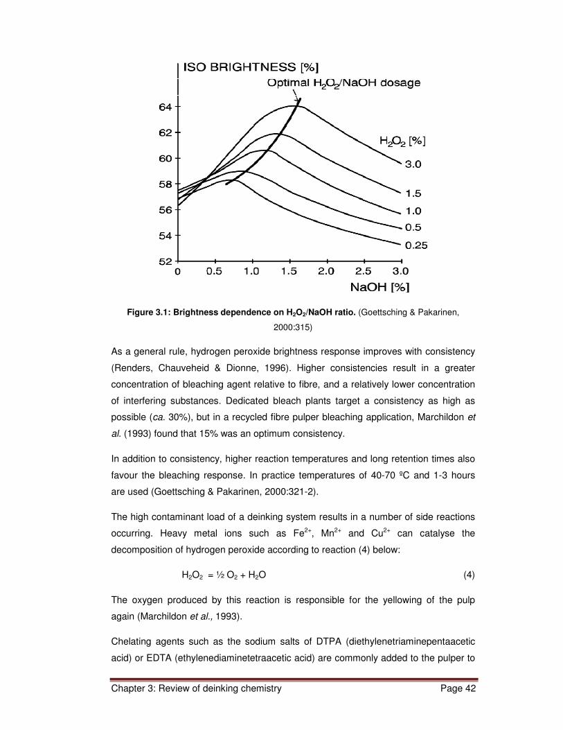
Chapter 3: Review of deinking chemistry Page 42
Figure 3.1: Brightness dependence on H2O2/NaOH ratio. (Goettsching & Pakarinen,
2000:315)
As a general rule, hydrogen peroxide brightness response improves with consistency
(Renders, Chauveheid & Dionne, 1996). Higher consistencies result in a greater
concentration of bleaching agent relative to fibre, and a relatively lower concentration
of interfering substances. Dedicated bleach plants target a consistency as high as
possible (ca. 30%), but in a recycled fibre pulper bleaching application, Marchildon et
al. (1993) found that 15% was an optimum consistency.
In addition to consistency, higher reaction temperatures and long retention times also
favour the bleaching response. In practice temperatures of 40-70 ºC and 1-3 hours
are used (Goettsching & Pakarinen, 2000:321-2).
The high contaminant load of a deinking system results in a number of side reactions
occurring. Heavy metal ions such as Fe2+, Mn2+ and Cu2+ can catalyse the
decomposition of hydrogen peroxide according to reaction (4) below:
H2O2 = ½ O2 + H2O (4)
The oxygen produced by this reaction is responsible for the yellowing of the pulp
again (Marchildon et al., 1993).
Chelating agents such as the sodium salts of DTPA (diethylenetriaminepentaacetic
acid) or EDTA (ethylenediaminetetraacetic acid) are commonly added to the pulper to
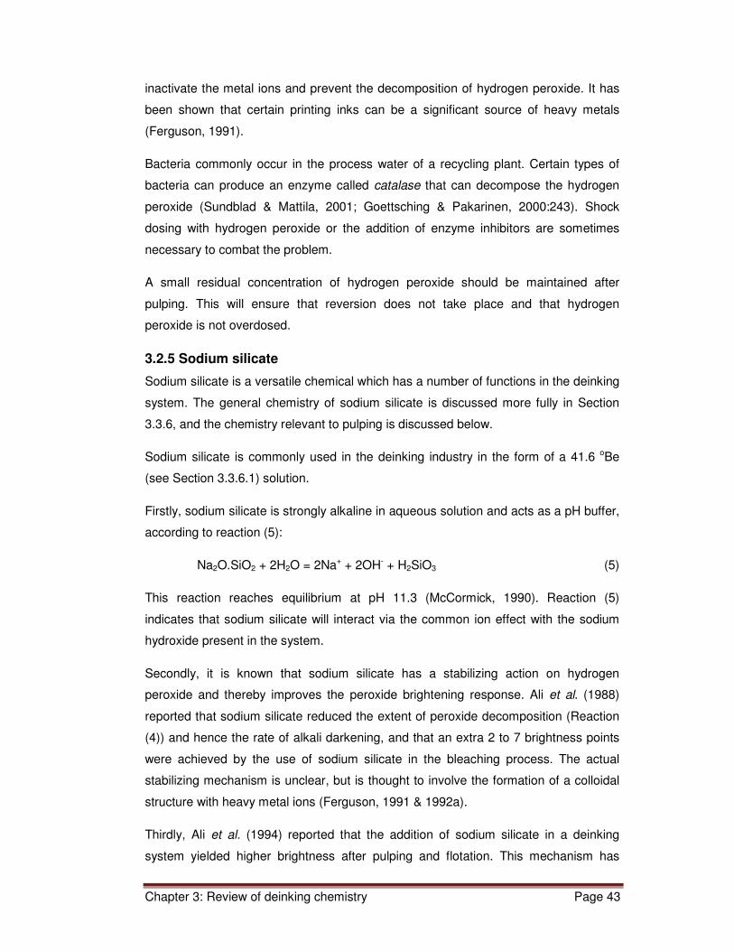
Chapter 3: Review of deinking chemistry Page 43
inactivate the metal ions and prevent the decomposition of hydrogen peroxide. It has
been shown that certain printing inks can be a significant source of heavy metals
(Ferguson, 1991).
Bacteria commonly occur in the process water of a recycling plant. Certain types of
bacteria can produce an enzyme called catalase that can decompose the hydrogen
peroxide (Sundblad & Mattila, 2001; Goettsching & Pakarinen, 2000:243). Shock
dosing with hydrogen peroxide or the addition of enzyme inhibitors are sometimes
necessary to combat the problem.
A small residual concentration of hydrogen peroxide should be maintained after
pulping. This will ensure that reversion does not take place and that hydrogen
peroxide is not overdosed.
3.2.5 Sodium silicate
Sodium silicate is a versatile chemical which has a number of functions in the deinking
system. The general chemistry of sodium silicate is discussed more fully in Section
3.3.6, and the chemistry relevant to pulping is discussed below.
Sodium silicate is commonly used in the deinking industry in the form of a 41.6 oBe
(see Section 3.3.6.1) solution.
Firstly, sodium silicate is strongly alkaline in aqueous solution and acts as a pH buffer,
according to reaction (5):
Na2O.SiO2 + 2H2O = 2Na+ + 2OH- + H2SiO3 (5)
This reaction reaches equilibrium at pH 11.3 (McCormick, 1990). Reaction (5)
indicates that sodium silicate will interact via the common ion effect with the sodium
hydroxide present in the system.
Secondly, it is known that sodium silicate has a stabilizing action on hydrogen
peroxide and thereby improves the peroxide brightening response. Ali et al. (1988)
reported that sodium silicate reduced the extent of peroxide decomposition (Reaction
(4)) and hence the rate of alkali darkening, and that an extra 2 to 7 brightness points
were achieved by the use of sodium silicate in the bleaching process. The actual
stabilizing mechanism is unclear, but is thought to involve the formation of a colloidal
structure with heavy metal ions (Ferguson, 1991 & 1992a).
Thirdly, Ali et al. (1994) reported that the addition of sodium silicate in a deinking
system yielded higher brightness after pulping and flotation. This mechanism has

Chapter 3: Review of deinking chemistry Page 44
been the subject of much debate (Section 3.3.6), but has been attributed to the
dispersing action of sodium silicate (Ferguson 1991). This mechanism has been
investigated by Pauck (2003), whose research suggested that sodium silicate
influenced the chemistry through its sequestering effect on calcium and hence
increasing the activity of the soap. Whatever the mechanism might be, the net result is
that sodium silicate improves the brightness, as shown in Figure 3.2.
Figure 3.2: Effect of sodium silicate on deinking brightness.
(Goettsching & Pakarinen 2000: 317)
Sodium silicate should not be overused, as this will lead to a build up of silicates in
solution. High levels of silicate can interfere with paper machine retention aid systems
(McCormick, 1990) and cause deposits and scale formation on process equipment.
3.2.6 Surfactants
The mechanical action of the pulper impellor alone will not completely detach all ink
from to the fibres (Rao & Stenius, 1998; Section 2.2.3). Surfactants are commonly
added to a pulping system to assist with the wetting of the recovered paper, the
dispersion of ink and the stabilisation of ink particles (Schriver, 1990). The surfactants
used are usually non-ionic ethylene oxide - propylene oxide block copolymers (Rao et
al., 1999; Ferguson, 1991), discussed more fully in Section 3.3.2. Surfactants, if used
in combination with the soap/calcium flotation system, will tend to stabilise the
calcium-soap particles and ink particles and thereby reduce the flotation efficiency

Chapter 3: Review of deinking chemistry Page 45
(Johansson & Ström, 1999). Table 3.2 summarises various aspects of the numerous
deinking agents the can be added into pulpers.
Table 3.2: Comparison of deinking agents. (Merza & Haynes, 2001)
Fatty acids Surfactants
Fatty
acid/surfactant
emulsions
Surfactant/fatty acid
blends
Poor detergency Strong detergency, over disperse inks
Combined effect Combined effect
Good ink collector Average collector,
prevent ink redeposition
Combined effect Combined effect
Make-down equipment required
Liquid – easy handling
Liquid – easy handling
Make-down equipment required
High dosage 0.5-0.7%
Low dosage 0.1-0.25%
Medium dosage 0.3-0.5%
Depends on process
Requires 150-200 ppm hardness
No hardness required
Requires 80+ ppm hardness
Requires 150-200 ppm hardness
Fatty acids have a similar ink dispersing action to the non-ionic dispersants (Rao &
Stenius, 1998; Borchardt, 1997; McCormick, 1990). However, the fatty acid soap will
only be effective as a dispersant if there are an excess for free soap anions, which will
depend on the pH of the solution (reaction 6) and the concentration of calcium in the
pulper (Rao & Stenius, 1998). High hardness in the pulper will precipitate the free fatty
acid, rendering it ineffective as a dispersant (Pauck, 2003; Weigl et al., 1987). This
could lead to an increase in the ink particle size by agglomeration in the pulper
(Pirttinen & Stenius, 2000).
3.2.7 Pulping pH
Alkaline deinking has been found to be essential for the successful deinking of offset
printing inks, particularly if the printing ink has aged somewhat. Caustic soda in the
pulper has been found to improve ink detachment and reduce ink fragmentation, but
hydrogen peroxide has no effect on ink detachment. The negative effect of alkaline
pulping is the increase in soluble organic materials in the process water, which
manifests as high levels of chemical oxygen demand (COD). High COD’s have
implications for effluent water treatment and discharge (Galland, Vernac and Carré,

Chapter 3: Review of deinking chemistry Page 46
1997a). Ackermann, Putz & Goettsching (1999) have also found that neutral deinking
results in inferior quality of deinked offset papers.
In neutral deinking, the amount of sodium hydroxide in the pulper is greatly reduced,
and sodium silicate and hydrogen peroxide are eliminated. For newsprint and
magazine blends, this results in less alkaline yellowing but also reduced ink release
and more ink fragmentation, with resultant reduced ink removal efficiency and lower
consequent brightness. This can be overcome by more aggressive post-flotation
bleaching, which however has to be done under alkaline conditions, therefore
negating the previous benefits. The net effect is reduced chemical consumption and
lower COD loading of the effluent, but reduced output quality. (Vahlroos, Körkkö,
Rosencrance & Niinimaki, 2007; Moe & RØring, 1998).
Azevedo, Drelich & Miller (1999) found that mixed office waste pulped under alkaline
conditions resulted in larger ink particles and inferior flotation removal. Neutral pulping
resulted in a toner particle size more amenable to removal by flotation, together with
the simultaneous flotation of filler particles. The neutral deinking of newsprint has
been investigated by Lakshmana Reddy, Nayak & Vasanthakumar Pai (2008) using a
new deinking surfactant. The results were comparable to that of alkaline deinking, with
reduced COD load in the effluent.
On the other hand, water based inks, such as flexographic inks, become highly
dispersed and fragmented in alkaline pulping systems, resulting in them being very
difficult to remove. Neutral pulping results in less fragmentation and some success
can be achieved with removal by flotation. The advantage of neutral deinking is that
much lower levels of COD are produced in the process water. Thus, for the deinking
of mixtures of different recycled paper grades, multistage processes are often
essential. A neutral first stage followed by an alkaline second stage has been found to
be effective. (Galland, Vernac and Carré, 1997a)
In the neutral deinking of recycled office papers, the reduced ink fragmentation is
actually an advantage, allowing the easier removal of toner inks by flotation. Better
stickies control and lower chemical costs are also advantages of neutral deinking.
(Vahlroos et al., 2007; Moe & RØring, 1998).
The deinking of recycled office papers to produce high quality recycled pulp also
requires a multistage process. In this case a neutral first stage followed by either

Chapter 3: Review of deinking chemistry Page 47
neutral or alkaline second stage is effective. Interstage bleaching with hydrogen
peroxide or reductive bleaches further enhances the brightness (Galland, Vernac and
Carré, 1997b).
3.2.8 Conclusion
At the conclusion of the pulping process, the fibres should be well dispersed in the
process solution with no flakes remaining. The ink particles should be separated from
the fibre and well dispersed and stabilised to ensure that no re-deposition occurs. The
yellowing that was induced by the high pH environment has been reversed by the
hydrogen peroxide.
This pulp is now passed through various physical screening and cleaning processes
(as described in Sections 2.3 and 2.4 above) before it is pumped to the flotation cell.
The physical separation processes tend to remove larger and denser or lighter
particles, which tend not to affect the brightness of the pulp. Prior to flotation the fibre
suspension is diluted with backwater to a consistency of ca. 1% and the pH is
adjusted to the required level. If a soap/calcium system is being employed, then at this
point collector soap and sufficient calcium chloride to obtain a calcium hardness of ca.
250 ppm as CaCO3 is added. In the flotation cell air in the form of fine bubbles is
forced through the fibre suspension. The air rises to the surface and forms a layer of
foam on the surface of the pulp. This layer of foam, laden with ink particles, fibres,
fines and filler is mechanically removed from the system.
3.3 Chemistry in the flotation cell
3.3.1 Surface chemical mechanisms of flotation
The pulping process is a process based on fragmentation and dispersing actions. In
contrast, flotation processes require the agglomeration of dispersed inks to an ideal
particle size range of 10 to 100 microns. In order for agglomeration to occur, the ink
particles must be hydrophobic (Ferguson, 1992b). Opinions vary as to the ideal size
range of the ink particles. Goettsching & Pakarinen (2000: 245) state that 20-40
microns is ideal, whilst Borchardt (1997) quotes a range of 30-80 microns.
Hydrodynamic studies by Julien Saint Amand (1999) suggest an upper limit of 100
microns for the ink particle size.
The ink particle of correct size must then attach itself to an air bubble that is rising
through the fibre slurry. To facilitate this attachment, it is necessary to add chemicals

Chapter 3: Review of deinking chemistry Page 48
called collectors. The collectors most widely used in newsprint deinking systems are
commercial fatty acids. The fatty acids are available in a number forms: solid soap
pellets, liquid soap or the free fatty acid. A certain amount of preparation is needed to
enable the fatty acid to be conveniently added into the system (Section 3.3.2). The
soap must be converted to the calcium salt of the fatty acid according to reactions (6)
and (7) below, for it to function as a collector. (Johansson & Ström, 1999; Johansson
et al., 1996; Ferguson, 1992b)
RCOOH + NaOH = RCOONa + H2O (6)
Fatty acid Sodium soap
2RCOONa + CaCl2 = (RCOO)2Ca + 2NaCl (7)
Sodium soap Calcium soap
The sodium soap is sparingly soluble in water at low concentrations. The calcium
soap on the other hand is insoluble, and precipitates out of solution as a fine white
precipitate. Above pH 7, the concentration of free sodium oleate has been estimated
to be only ca. 2 x 10⁻⁷ M (Rao et al., 1998). The calcium level required for effective
collector activity is widely accepted to be about 200 ppm of calcium hardness (CaCO3)
(Ferguson, 1992b).
The calcium is added to the system as a calcium chloride solution. The addition of
extra calcium might not be necessary in areas where the water is naturally hard or the
recycled paper contains large amounts of calcium carbonate filler.
There are many schools of thought as to the mechanisms of interaction between ink
particles, surfactants and air bubbles. Beneventi & Carré (2000) have reviewed
mechanisms by Schweizer (Schweizer, G. 1965. Wochenblatt fuer papier Fabrikation
93(19):823-880), Bechstein (Bechstein, G. 1975. Oesterr. Papier 12(4):16-19), Ortner
(Ortner, H.E. 1981. Tappi Press. Atlanta, GA), Hornfeck (Hornfeck, K. 1982.
Wochenblatt fuer Papier Fabrication. 110(5):542-544), Larsson (Larsson, A., Stenius,
P., Odberg, L. 1984. Svensk Papperstidning No. 18, pp158-164) and Putz (Putz,
Schaffrath & Goettsching 1993).
Goettsching & Pakerinin (2000), Linck (1990), McCool (1993) and Schriver (1990)
also refer to the work of Larsson et al. (Larsson, A., Stenius, P., Odberg, L. Sv.
Papperstidning 88(3),R2(1985) and 87(18),R165(1984)).

Chapter 3: Review of deinking chemistry Page 49
The Larsson mechanism is considered by Beneventi & Carré (2000) to be “state of the
art”, and is discussed below as an example. The Larsson theory suggests that in
alkaline medium, the ionised fatty acids stabilise the ink particles. Calcium ions will
precipitate the soap according to reaction (7) as very small particles, or micro-
precipitates (Ferguson, 1992b) onto the surface of the ink particles. Larsson (1987)
reported that this layer of sub-micron calcium soap particles was visible under a
scanning electron microscope. This layer of calcium soap precipitate will render the
ink more hydrophobic and leads to agglomeration of the ink into larger particles. The
soap-coated particles also enhance the adhesion of the ink to the air bubbles and
facilitate their removal from solution. Figure 3.3 depicts this process:
Figure 3.3: Collecting mechanism of calcium soap. (Larsson et al., 1987)
McCormick (1991) has proposed an alternate theory: The soap molecules are
adsorbed onto the surface of the dispersed ink particle, and impart a negative charge
to the ink surface. The calcium ions react with the soap molecules according to
reaction (7). The negative charge on the soap particle has now been neutralised and
the ink particle is more hydrophobic. However, because the soap molecules are
adsorbed onto the surface of the ink particle, the soap/calcium salt takes on a strained
configuration. When two ink particles collide, a re-arrangement of the adsorbed
calcium soap molecule takes place, and the calcium ion now acts as a bridge between
two ink particles. This process can repeat itself to form larger and larger ink
agglomerates. In a similar way, the calcium soap stabilises the air bubbles by
adsorbing at the interface between air and water. When such a stabilised air bubble
collides with an ink particle, a similar calcium soap re-arrangement takes place and
the ink particle is attached to an air bubble, via the calcium link. This mechanism is
shown in pictorial form in Figure 3.4.
O
Ca2+
Ca2+
Air bubble
Dispersed ink
particles
Precipitated calcium
soap particles
Calcium soap attaches
air bubbles to ink
particles

Chapter 3: Review of deinking chemistry Page 50
Putz, Schaffrath & Goettsching (1993) have postulated that a “hydrate cover” acts as
a barrier between the ink particles and the air bubbles. Surfactants adsorb onto the
surface of the ink particle and disrupt the ‘’hydrate cover’’. The removal of this hydrate
cover facilitates the attachment of the ink particle to the air bubble and ink removal by
flotation can take place.
Based on studies of the equilibrium concentrations of the oleate-calcium system and
agglomeration kinetics, Rao et al. (1998) have concluded that the agglomeration of ink
particles is preceded by the agglomeration of calcium soap particles. This lends
support to the Larsson mechanism, and they suggest that there is no evidence to
support the bridging mechanisms of Ortner and McCormic.
The models are all confusingly similar, and mostly refer to the calcium – soap system.
In essence, they all seek to describe the complex interactions occurring between
soap, ink particle and air-water interface.
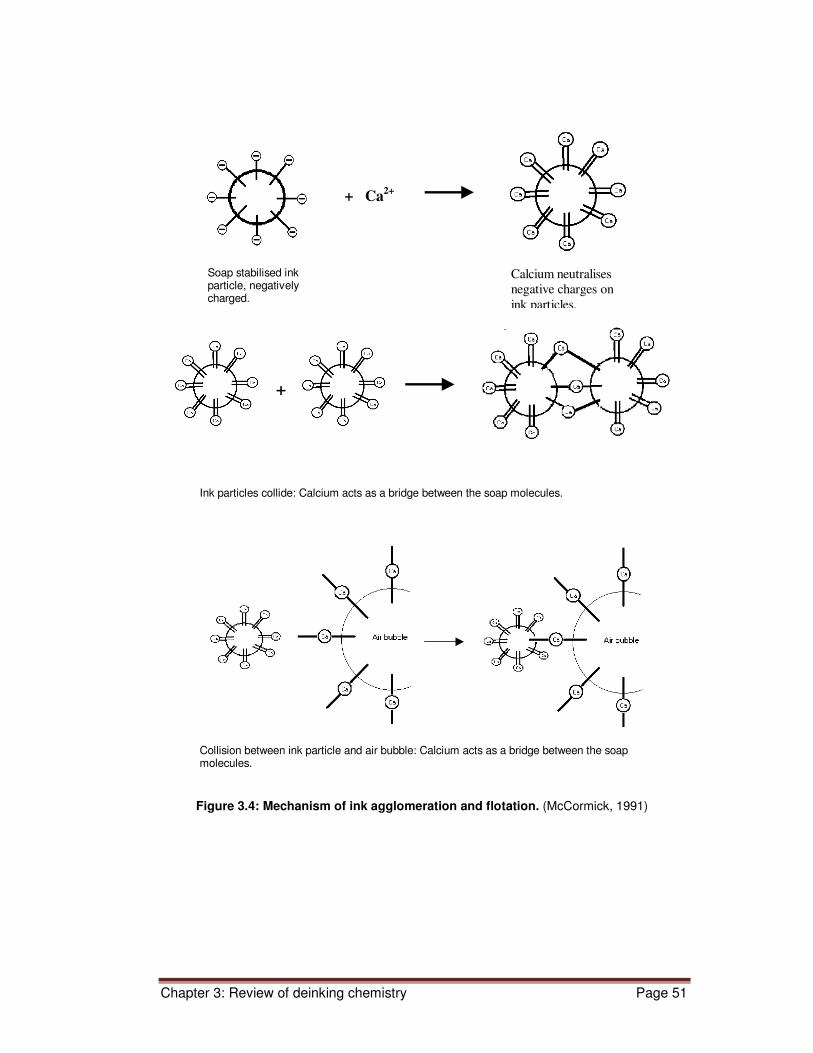
Chapter 3: Review of deinking chemistry Page 51
Figure 3.4: Mechanism of ink agglomeration and flotation. (McCormick, 1991)
Ink particles collide: Calcium acts as a bridge between the soap molecules.
Collision between ink particle and air bubble: Calcium acts as a bridge between the soap molecules.
+ Ca2+
+
Soap stabilised ink particle, negatively charged.
Calcium neutralises
negative charges on
ink particles.

Chapter 3: Review of deinking chemistry Page 52
3.3.2 The soap and surfactants
Surfactants play three main roles in the flotation process, summarised in Table 3.3:
Table 3.3: Role, nature and effects of surfactants in deinking. (Zhao, Deng & Zhu 2004)
Surfactant role
Typical surfactants Effect in the process
Dispersant
Non-ionics such as alcohol ethoxylates, alkyl phenol ethoxylates, fatty acid ethoxylates, and polyethylene oxide alkyl ethers.
Liberation of ink from fibres, dispersion and stabilisation of ink particles.
Collectors Fatty acid soaps, polyethylene oxide-polypropylene oxide copolymers, ethoxylated fatty acids.
Agglomeration and aggregation of small ink particles into ideal particle size ranges for flotation (10-100 microns)
Frothers Non-ionic surfactants Generate a stable foam layer to carry and remove ink particles.
Most surfactants however can play multiple roles and can interact in complex ways
with other components of the deinking system. Surfactants are characterised by their
hydrophile-lipophile balance (HLB value), their cloud-point (non-ionic surfactants) or
Krafft point (ionic surfactants) and the critical micelle concentration (CMC). The cloud
point should be at least 5ºC higher than the flotation temperature, and an HLB value
of 14-15.5 has been found to be optimum. However, there are many other factors
influencing the performance of surfactants in deinking, so these factors should not be
the sole basis of surfactant selection. The selection of surfactant depends greatly on
the conditions prevailing in any one deinking plant (Theander & Pugh, 2004; Zhao,
Deng & Zhu, 2004).
Fatty acids are the most commonly used surfactants in the deinking of newsprint.
They have good dispersing and foaming properties and are easily biodegradable
(Goettsching & Pakarinen, 2000: 254). Fatty acid soaps are sensitive to water
hardness and pH, according to reaction (7). However, as outlined in Section 3.3.1,
hardness is an integral part of the collecting mechanism.
The optimum fatty acid chain length for newsprint flotation is reported to be C16 (Mak
& Stevens, 1993). The ideal degree of unsaturation depends on the water hardness.
Fatty acids with higher iodine values need higher water hardness to perform well (Mak
& Stevens, 1993). The flotation efficiency of fatty acids decreases in the order
stearate>palmitate>oleate (Rao et al.,1998).

Chapter 3: Review of deinking chemistry Page 53
Commercial fatty acids are blends of C16 to C18 saturated and unsaturated carboxylic
acids such as stearic (C18:0), oleic (C18:1), palmitic (C16:0), linoleic (C18:2), linolenic
(C18:3) and palmitoleic acids (C16:1).
Fatty acid soaps are waxy solids at room temperature. They need special preparation
and storage measures to convert them to liquid form to effectively dose them into a
system. The free fatty acid is liquid but would need to be converted to the soap in situ.
Liquid solutions need to be kept hot and constantly stirred. In order to avoid these
practical difficulties and associated housekeeping issues (Turvey, 1990), a number of
synthetic surfactants or fatty acid/surfactant blends have been developed, which allow
easy handling and are not sensitive to water hardness (Table 3.2).
Synthetic collectors commonly used in the industry are the non-ionic surfactants of the
following types: ethylene oxide (EO) propylene oxide (PO) copolymers, ethoxylated
fatty alcohols and ethoxylated fatty acids. Anionic surfactants have higher solubilities
than non-ionics, and tend to cycle up in process water systems, resulting in higher
yield losses due to high foaming tendencies. The poor biodegradability of particularly
the ethoxylated nonyl-phenols has precluded their use in recent years (Goettsching
and Pakarinen, 2000: 255; Dash & Patel, 1997). In order to address the concerns
about biodegradability and renewability, researches have investigated surfactants
based on natural sources, such as sugars and proteins. These have proven to be
viable replacements for conventional petroleum based surfactants (Spence, Venditti &
Rojas, 2009).
Fatty acid ethoxylates are thought to work by means of a hydrolysis mechanism. In
the esterified form (mid to lower pH ranges) they function as dispersants, and disperse
the inks. After some time in alkaline conditions they hydrolyse to fatty acids, and then
function as collectors via the fatty acid-calcium coagulation mechanisms discussed in
Section 3.3.1 (Theander & Pugh, 2004).
In a comparative study of a number of different surfactants, it was found that fatty acid
based systems out-performed all other types (Mak & Stevens, 1993). In order to
combine the superior collecting properties of fatty acids and the handling properties of
synthetic surfactants, semi-synthetic fatty acid emulsion products have been
developed. The final choice of surfactant for deinking is determined by many practical
factors, which might outweigh the considerations of deinking efficiency alone.

Chapter 3: Review of deinking chemistry Page 54
Kanhekar et al. (2005) found that, depending on the nature of the soap/surfactant, ink
removal either reaches an optimum and then decreases, or it increases steadily with
surfactant dosage. Licht & Leighton (1991) found that the deinking reagent did not
have a significant effect on brightness. On the other hand, Spence, Venditti & Rojas
(2009) found a definite positive correlation between surfactant addition and ink
removal efficiency.
3.3.3 Temperature, pH and surface tension
The pH of the solution has a profound effect on the calcium soap equilibrium, and the
maximum efficiency of flotation of both mineral-oil and vegetable-oil based offset inks
occurs between pH 7 and 11 (Rao et al., 1998). In a review of flotation chemistry,
Theander & Pugh (2004) state that a pH range of 8 to 10 is optimal for flotation.
Flotation efficiency falls off above pH 10. This can be ascribed in part due to the more
negative surface charges (zeta potentials) and hence greater repulsive forces at
higher pH.
Substances naturally occurring in pulps or used in the paper making process, such as
lignosulphonates, starch, carboxymethyl cellulose (CMC) or additives to coating
mixes, tend to act as dispersing agents in a deinking system. Such materials all have
a negative effect on flotation. (Rao et al., 1998)
The hydrodynamics of flotation discussed in Section 2 showed the importance of air
bubble size. From a surface chemistry point of view, the size of a stable air bubble
depends on the surface tension of the liquid, according to the Young-Laplace equation
(8):
∆� � ��� (8)
Where ∆P is the pressure difference between bubble gas and solution, is the surface
tension and is the bubble radius. The nature of the surfactant, including its
hydrophilic/lipophilic balance and concentration will determine the surface tension and
hence the stable bubble size (Rao et al., 1998). The creation and destruction of air
bubbles in a flotation system is a very dynamic process, often taking place within very
short periods of time. Hence, the diffusion rate of surfactant molecules to the surface
can also play an overriding role in determining the surface tension (Theander & Pugh,
2004).

Chapter 3: Review of deinking chemistry Page 55
Practically, flotation deinking processes run at temperatures ranging between 40 and
60ºC, although office paper recycling plants sometimes run at temperatures up to
90ºC. The work of Pletka et al. (2000) clearly showed an increase in brightness as the
flotation temperature exceeded 60ºC. However, researchers are not unanimous on
the effect of temperature on deinking, some reporting better ink removal at higher
temperatures and others reporting the opposite. Many secondary parameters such as
surfactant solubility, bubble size, froth structure and solution viscosity are affected by
temperature, so that it is very difficult to isolate the effect of temperature alone
(Theander & Pugh, 2004).
3.3.4 The role of the calcium Ion
The important role that the calcium ion plays in the ink collecting mechanism has been
discussed in Section 3.3.1. The calcium ion also interacts with other components of a
deinking system.
The hardness of a flotation system influences the amount of fibre that is lost during
flotation (Turvey, 1987; 1990 & 1991). Fibre loss constitutes a loss of yield in the
process, with negative economic consequences. Turvey (1990) reported a fibre loss of
7 -10% at a hardness of ca. 280 ppm calcium, which suggested that the calcium ions
can interact with the fibres in some way. Schwinger & Dobias (1991) reported that the
calcium cation adsorbs onto the surface of the fibre. Cellulose fibres normally exhibit a
negative charge in solution, and adsorbed calcium ions reduce the negative surface
charge to almost neutral. This renders the fibres hydrophobic and thus floatable.
Turvey (1991) suggests that the calcium cations are held onto the fibre surface by the
carboxylic acid groups that occur on a fibre surface in an alkaline environment, as per
reaction (9). Furthermore, Turvey (1991) suggested that small ink particles are
capable of interacting with calcium ions, and will deposit onto a fibre via the calcium
half-salt reaction (9).
Fibre-COO- + Ca2+ = Fibre-COOCa+ (9)
It could be expected that free calcium ions could precipitate as calcium hydroxide in
the alkaline deinking environment, as per reaction (10).
Chapter 3: Review of deinking chemistry Page 56
Ca2+ + 2OH- = Ca(OH)2 (10)
However, Oliveira & Torem (1996) and Froass et al. (1997) state that this reaction
does not occur to any extent below pH 12.
Calcium will also react with sodium silicate to form insoluble calcium silicate, as in
reaction (11).
Ca2+ + Na2O.SiO2 = CaSiO3 + 2Na+ (11)
Froass et al. (1997) have determined that the critical precipitation concentration for
calcium in a silicate solution corresponds to ca. 56 ppm of calcium at pH 9.2, 60oC
and ca. 2340 ppm SiO2. Thus, a 1% (10 000 ppm) addition of sodium silicate would
exceed these values, indicating that such reactions are probable. These calcium
silicates are known to form deposits on process equipment.
However, Turvey (1991) reports that the adsorption of calcium onto the fibre
predominates the above reactions under alkaline conditions, and is responsible for the
flotation of fibres.
Mineral fillers such as kaolin (aluminium silicates) usually carry a negative surface
charge. Calcium ions adsorb onto the surface of the mineral filler, partially neutralising
the negative charge (Liphard et al., 1991).
3.3.5 Fillers
Fillers are commonly used in the manufacture of various grades of paper. Newsprint
can contain from less than 5% to over 10% filler, depending on world region
(Brouillette et al., 2010). Office papers can contain ca. 20 % filler, as can uncoated
and coated magazine papers. Thus, one of the major components in a deinking
system will be the mineral filler. The filler most commonly used in making paper is clay
or kaolin, although talc and calcium carbonate are also used (McCormick, 1991).
Kaolin will originate from the magazine papers and the recycled office paper will
contribute calcium carbonate to the recovered paper mix. The use of calcium
carbonate has increased in recent years with the rise in alkaline paper making.
Although calcium carbonate is not used in newsprint or magazine furnishes, it is
Chapter 3: Review of deinking chemistry Page 57
increasingly being used as a pigment in coating formulations, so it too can find its way
into newsprint/magazine deinking systems.
Newsprint is usually deinked in combination with recovered magazine papers in a
typical blending ratio of 70% newsprint to 30% magazine, although this can vary
depending on geographical region and availability. This is primarily to boost the
brightness, but it has also been found that it is difficult to deink newsprint on its own
(Schriver et al., 1990; Zabala & McCool, 1988). Some newsprint-only deinking
operations have reportedly been adding fillers to the deinking cell to improve the
deinking efficiency (Schriver et al., 1990; Zabala & McCool, 1988).
Clay particles normally exhibit a plate-like structure with a negative surface charge,
and Zabala & McCool (1988) have hypothesised that the ink particles adsorb onto the
surface of the filler, thereby producing larger, more easily floatable particles. Liphard
et al. (1991) and McCormick (1991) have suggested that the negatively charged clay
particles will associate with the weak positive surface charge of the calcium on the ink
particle surface, thereby forming a protective filler layer.
Similarly, Grant & Blain (1995) have shown that filler clays or talc absorb ink mineral
oils and go on to form ink-coated mineral particles. These particles are stable to shear
forces and adhere well to air bubbles, and will thus float well. Shen, Abubakr &
Springer et al. (1995) found that the addition of clay to a laboratory flotation cell
significantly reduced the fibre losses from the cell, without negatively affecting the
flotation deinking performance.
Schriver et al. (1990) have shown that the best fatty acid-based deinking performance
was obtained from calcined filler clay, followed by talc and a low surface area zeolite.
A scavenging mechanism was proposed. In contrast, calcium carbonate did not
appear to enhance deinking.
However, Letcher & Sutman (1991) and Mahagaonkar, Stack & Banham (1998) found
no evidence to support the theory that fillers assists ink removal.
It is sometimes necessary to remove the fillers in addition to inks, in cases where the
final product does not require fillers, eg. newsprint or tissue paper. It has been found
that fatty acid collectors remove a small quantity of filler, but special collectors are

Chapter 3: Review of deinking chemistry Page 58
necessary to remove the fillers efficiently. This is normally accomplished in a
dedicated second flotation stage (Liphard et al., 1991).
3.3.6 Sodium silicate
The final major chemical additive to an alkaline deinking system is sodium silicate.
Sodium silicate is used in a number of different fields, such as detergents, oil drilling,
mineral flotation and bleaching. The chemistry of the soluble silicates relevant to
deinking is discussed below:
3.3.6.1 The general chemistry and properties of soluble silicates
The soluble silicates are a combination of silica and an alkali metal oxide. The general
formula can be written: x SiO2:M2O, where M is Na, K or Li, and x is the molar ratio.
Molar ratios of 2:1 are termed ‘’alkaline’’ and ratios of 3.3:1 are referred to as
‘’neutral’’. The sodium silicates find general application, whereas the lithium and
potassium salts are used in specialised fields.
The sodium silicates are commercially available as solid powders or as viscous
aqueous solutions. For reasons of convenience, solutions are used in the industry.
The density of such solutions is expressed as degrees Baume’ (oBé) or degrees
Twaddle (oTw) at 20 oC. These are defined in terms of the specific gravity (SG)
according to equation (12):
oBé = 145(1 – 1/SG) and oTw = 200(SG – 1) (12)
The specific gravity and viscosity depend on the molar ratio and the concentration in
solution (Crosfield, 1993). Conventionally, 3.3:1 molar ratio, 38% solids, 79 oTw (oBé
41) sodium silicates are used in deinking.
As already mentioned, solutions of sodium silicate are strongly alkaline (reaction 5),
with a buffering ability similar to that of sodium hydroxide, but at a lower pH.
Na2O. SiO2 + 2H2O = 2Na2+ + 2OH- + H2SiO3,
or Na2O + H2O = 2NaOH (5)
At high concentrations, the silicates form insoluble silicate complexes with multivalent
metal ions such as calcium, aluminium and magnesium to. At lower concentrations the
silicates can sequester iron and manganese ions. This sequestering action is

Chapter 3: Review of deinking chemistry Page 59
employed in water treatment processes and in the detergent industry, where silicates
react with the calcium and magnesium ions to reduce their activity and enhance
surfactant performance (Crosfield, 1993; Falcone, 1982).
The high alkalinity of silicate solutions will saponify the ester bonds in organic oils and
fats. The soluble sodium soaps thus formed contribute to the overall detergent action
of the silicate. The silicates are more efficient emulsifiers than conventional alkalis
such as sodium hydroxide (Crosfield, 1993).
The silicate solutions are only stable at high pH. At pH’s below about 9, insoluble silica
gels are formed. This occurs rapidly in a concentrated solution, but can take many
hours in dilute (less that 1% SiO2) solutions. (Crosfield, 1993)
3.3.6.2 The effects of sodium silicate in deinking
The effects of including sodium silicate in a deinking formulation have been
investigated by a number of researchers. In this section the results and conclusions of
the various workers are summarised.
In a comprehensive study by Ali et al. (1994) of a 70/30 blend of newsprint and
magazine, deinked by washing and flotation and measurement of brightness,
lightness (L*), yellowness (b*) and particle size distribution by image analysis, it was
reported that:
• The brightness of the final pulp increased as sodium silicate dosage increased
from 0% to 5%.
• Silicate enhanced the removal of ink by forming larger, more floatable
particles.
• Sodium silicate appeared to prevent suspended ink particles from re-
depositing on the fibre surface.
• Sodium silicate had a stabilising action on hydrogen peroxide.
• Sodium silicate removed more ink than caustic soda alone.
• Sodium silicate reduced alkali yellowing of the pulp.
Numerous other researchers (Mahagaonkar et al., 1997; Mahagaonkar et al., 1996;
Borchardt, 1995; Ferguson, 1992a and Read, 1991) have reported on experimental
work that demonstrates that sodium silicate leads to higher brightness and reduced
ink speck counts when used in the deinking of newsprint. The reasons advanced were
Chapter 3: Review of deinking chemistry Page 60
that sodium silicate demonstrates wetting, detergency, peptization, ink dispersion,
alkalinity, pH buffering, peroxide stabilisation and sequestering actions.
In contrast to the proposed dispersing action of sodium silicate, a number of
researchers have presented evidence that sodium silicate actually has an
agglomerating or collecting action. (Santos et al.,1996; Renders et al., 1996; Renders,
1993 & Dionne, 1994)
The sequestering action of sodium silicate is utilised in detergent formulations, where
it complexes water hardness salts and protects the surfactants. In the field of crude oil
recovery, Krumrine (1982) reports that sodium silicates enhance recovery yields
relative to sodium hydroxide due to the interaction of the silicate with hardness ions.
The sequestering action of sodium silicate has support in the deinking field
(McCormick, 1990). Weigl (1987) reports that the precipitation of fatty acid soap by
calcium ions in the pulper leads to higher surface tensions and reduced emulsification
of inks, with resultant increased ink redeposition. Research by Pauck (2003) supports
the view that sodium silicate sequesters calcium in the pulper and enhances soap
activity.
Mathur (1991) discounts the role that the surface active properties of sodium silicate
play in ink removal. Instead, he ascribes the higher brightness observed with the use
of sodium silicate to the chelation of metal ions such as Fe2+, Mg2+, and Cu2+, and the
attendant stabilisation of hydrogen peroxide.
Mak & Stevens (1993) studied the characteristics of fatty acids in deinking, and found
that sodium silicate did not have a significant influence on deinking performance.
Zabala & McCool (1988) were able to replace sodium silicate with a metal chelant in a
commercial deinking system with no negative effects on brightness.
Other effects of sodium silicate have also been reported. Sodium silicate has been
shown to reduce the fibre losses during deinking (Ackermann et al., 1999; Liphard et
al., 1991) and to suppress the flotation of fillers (Ackermann et al., 1999; Mathur,
1994). This mirrors the function of sodium silicate as a suppressant in the flotation of
minerals such as chromium, copper, tin, fluorspar and phosphates, where it
selectively adsorbes onto the surface of unwanted gangue minerals such as silica or
iron oxide, thereby rendering them hydrophilic and depressing their flotation.
(Crosfield, 1993)

Chapter 3: Review of deinking chemistry Page 61
Observations of the effect of sodium silicate in a South African newsprint deinking
operation showed that attempts to eliminate sodium silicate from the process resulted
in an immediate fall-off in deinking efficiency and loss of brightness (Crosby 1999).
In order to consolidate the divergent views on the role of sodium silicate, a summary is
presented below.
• pH Buffering action and saponification
• Peroxide stabilisation
• Prevention of yellowing
• Ink agglomerator or collector
• Ink dispersant
• Calcium sequestering action
3.4 Final bleaching
The final bleaching of pulp, after all ink removal processes have taken place, is also
called post-bleaching. After deinking, the pulp is dewatered and stored in a storage
chest. If a second stage of hydrogen peroxide bleaching is required, the pulp is
thickened to as high a consistency as possible (30-40%) and subjected to similar
chemical additions and process conditions as discussed in the Section 3.2 on pulper
chemistry.
Post-bleaching can also be achieved using reductive bleaching alone, depending on
the final brightness required. The two commonly available reducing agents are sodium
dithionite (a.k.a. sodium hydrosulphite) and formamidine sulphinic acid (FAS). A
tabulated comparison of the practical bleaching conditions of the two reductive
bleaching agents is given in Table 3.4. The factors mentioned in the table naturally
interact, so optimisation for each plant is necessary.
Both reducing agents are susceptible to decomposition by oxygen in solution, so
practical steps need to be taken to reduce aeration of the pulp and bleaching
solutions. The bleaching times are quite short, so bleaching can be accomplished in
storage chests or even “in pipe”.
Post-bleaching in a tower has been shown to be more efficient than pulper bleaching.
This is because of the higher consistencies that can be achieved in a post-bleaching

Chapter 3: Review of deinking chemistry Page 62
operation and the presence of fewer contaminants that could be involved in side
reactions with hydrogen peroxide (Renders, Chauveheid & Dionne, 1996).
Table 3.4: Comparison of reductive bleaching agents. (Goettsching & Pakarinen 2000:326-
334)
Property Sodium dithionite FAS
Chemical formula Na2S2O4 C(NH2)(NH) – SO(OH)
Reduction bleaching reaction
Na2S2O4 + H2O → NaHSO2 + NaHSO3
(active agent in bold)
C(NH2)(NH) – SO(OH) + NaOH → CO(NH2)2 + NaHSO3
(active agent in bold)
Bleaching consistency
3 – 5% 5 – 20% (C)
Bleaching time 5 - 10 mins 15 – 60 mins
Bleaching temperature
Ca. 60 ºC 40 - 90 ºC (T)
pH 6 - 7 Ca. 9
Addition rate 0.5 – 1.0% 0.2 – 0.8% (F)
Typical brightness increase
4% - 7% ISO R457 = 55.05+0.08T-0.12C+5.7F-F
2
for wood containing pulps
Additional bleaching can also be performed in dispersers or kneaders. Dispersers are
placed in deinking lines after flotation and washing but before final storage.
Temperatures and consistencies are high in dispersing units, and they thus provide
ideal conditions for bleaching. The brightness naturally drops through the dispersion
process, due to the further break up of ink particles. Hence, addition of bleach into the
disperser can counteract this brightness drop. (Renders, Chauveheid & Dionne, 1996)
3.5 Measurement of deinking efficiency
The main criteria of deinking efficiency are the optical properties of the pulp and the
yield or output of the process. There are three aspects to the optical properties: the
brightness, the colour and the dirt content, which together determine the appearance
of the final pulp to the human eye (Haynes, 2000). In a practical situation, pulp
strength is also important for the final application of the pulp in the making of paper.
However, pulp strength cannot be influenced by the recycling process, other than by
varying the incoming recycled paper mix, so it is not normally considered as
something to be monitored in a recycling plant.

Chapter 3: Review of deinking chemistry Page 63
3.5.1 Yield
The efficiency of the deinking process can be measured in two ways. Firstly, the
efficiency of the process is determined by measuring the yield, which is defined as:
% � ��� � �1 � ������� ��������� ���� ! 100 (13)
viz. pulp mass remaining after the deinking process as a percentage of the mass of
recovered paper fed to the process.
It has been estimated that ink constitutes ca 2-5% and filler 10-40% of the recycled
stock (Hannuksela & Rosencrance, n.d). The deinking process typically removes ink,
some fibres, and mineral fillers such as clay or calcium carbonate. A single flotation
deinking stage normally has a yield of about 85-90%, and a single washing stage has
a yield of 75-85% (Goettsching & Pakarinen 2000: 295). Spence, Venditti & Rojas
(2009) reported lower yields with increasing ink removal efficiency (coupled with
increasing surfactant addition). Thus, a lower yield generally means a higher quality
final product due to better deinking, but with negative economic implications. The yield
is therefore a compromise between quality and cost as it is very difficult to achieve
both high yield and high ink removal efficiency (Le Ny, Haveri & Pakarinen, 2001). In
addition, in a commercial operation other solid contaminants such as plastic, staples,
grit etc. will also be removed. This is also a yield loss, but has nothing to do with the
flotation yield. Flotation deinking plants are designed to optimise both these factors.
Another way of looking at the efficiency of the deinking process is to consider the
reject rate. The reject rate is the amount of material rejected by the deinking process
relative to the amount of feed, and is really the converse of the yield as discussed
above.
3.5.2 Brightness
The brightness of the pulp is defined as the spectral reflectance at 457 nanometers
(R457), relative to a magnesium oxide standard. The two main methods are the TAPPI
standard method and the ISO standard. The TAPPI method utilises an incident beam
at 450, and the ISO method uses diffuse incident light. The methods give similar
results (Goettsching & Pakarinen, 2000: 296).

Chapter 3: Review of deinking chemistry Page 64
The brightness is the standard and widely used method to measure the efficiency of
deinking systems, but it has some limitations which need to be taken into account
when interpreting brightness data. The brightness of a sheet of recycled paper is the
composite effect of the intrinsic brightness of the fibres, the brightness of fillers and
the amount and particle size distribution of the ink. The reflectance at 457 nm of ink is
low, and fillers and bleached fibres have high brightness. The removal of ink will result
in an increase in brightness, but the removal of filler may result in a decrease in
brightness, even though ink has been removed as well. In addition, bleaching of a
recycled pulp will result in a higher measured brightness, even if no ink has been
removed. Thus there is no direct correlation between brightness and ink content, and
small ink particles have a lower brightness than an equivalent amount of larger ink
particles (Carré, Galland & Julien Saint Amand, 1994; McCool, 1993).
3.5.3 Colour
Reflectance at 457 nm is measured in the blue region of the visible spectrum, and will
not describe the optical appearance of a coloured sheet of paper. The response of the
human eye to colour has been simulated and quantified in a system called the
CIELAB colour system. This system makes use of a set of three colour co-ordinates in
a three dimensional colour space to describe a colour. The co-ordinates are L* which
denotes the lightness, a* denotes the red-green axis and b* denotes the yellow-blue
axis. (Goettsching & Pakarinen, 2000: 296)
In practice the colour is not used to assess the degree of deinking of a recycled pulp,
but can however be useful in measuring the effectiveness of bleaching or colour
stripping operations.
3.5.4 Dirt content
The human eye cannot detect particles less than 50 microns in diameter (Goettsching
& Pakarinen, 2000: 269). Particles greater than this are detected as individual
specks. This is commonly referred to as “dirt” or conversely “cleanliness” in the
recycling industry. Particles below the visibility limit, whilst not individually visible
produce a grey appearance in the pulp.
The ink size population between 10 and 100 microns has little impact on brightness or
ERIC (particles too big) or on final paper cleanliness (particles too small). With the
help of image analysis techniques, the number of ink specks in this size range can be

Chapter 3: Review of deinking chemistry Page 65
analysed quantitatively and the efficiency of deinking can be measured more directly
(Haynes, 2000; Anderson, 1993; McCool, 1993). However, each image analysis
system has a lower size limit below which it can’t detect ink particles. This is usually
about 2-3 microns (Carré, Galland & Julien Saint Amand, 1994; McCool, 1993). In
addition, image analysis as a technique is complex to perform with high repeatability.
Carré, Galland & Julien Saint Amand (1994) reported an accuracy of about 25% only,
with a large number of measurements being required. Image analysis is thus not
routinely used to control process plants.
3.5.5 Effective residual ink concentration (ERIC)
This technique was introduced by Jordan and Popson (1994), and involves the
measurement of the reflectance of a sample pad of pulp in the infrared region (950
nanometers) of the spectrum, where only the black printing inks absorb light
(Goettsching & Pakarinen, 2000:268). This measurement is thus not sensitive to the
influences of bleaching or other coloured materials (Carré, Galland & Julien Saint
Amand, 1994). The attenuation of the incident beam gives a direct measure of the
amount of printing ink on the surface of the pulp pad. The measurement is expressed
as ppm. However, the variability of the method is greater than that of brightness
determination. In a comparative study of ink measuring methods, Carré, Galland &
Julien Saint Amand (1994) reported a coefficient of variation of 4% for ERIC
measurements, compared to less than 2% for brightness. In another study, Carré,
Galland, Vernac & Suty (1996) found comparative variability of 5% and 2%
respectively.
As for the brightness, the ERIC measurement is a spectrophotometric method, and is
thus also dependent on the particle size distribution of the ink (Carré, Galland, Vernac
& Suty, 1996). Sub-visible ink particles, less than ca. 10 microns in diameter have the
greatest effect on the ERIC measurement. On the other hand, ink particles greater
than 10 microns and coloured inks have a negligible effect on the measured ERIC.
Thus ERIC is a direct measurement of the ink particle size range that also determines
brightness (Haynes, 2000).
Moreover, one cannot obtain a direct correlation between ERIC and brightness, as
brightness is also influenced by the underlying brightness of the fibres. Thus a
deinked newsprint pulp and a deinked office paper pulp might have the same residual
ink concentration, but would have vastly different brightness, as the office paper
contains no mechanical pulp and is inherently much brighter than newsprint.

Chapter 3: Review of deinking chemistry Page 66
Correlations between ERIC and brightness will only exist for a particular grade of
recycled paper and bleaching conditions.
.
3.5.6 Conclusion
Depending on the requirements of the deinked pulp, the above methods can be used
alone or in combination to evaluate the final appearance of the deinked pulp.
Therefore, the brightness could be used as an overall measure of deinking efficiency,
and ERIC or image analysis could be used to determine more specifically the amount
of ink removed. (Haynes, 2000)

Chapter 4: Review of Artificial Neural Networks Page 67
CHAPTER 4: REVIEW OF ARTIFICIAL NEURAL NETWORKS
4.1 Introduction
Artificial Neural Networks (ANN’s) were inspired by the vast interconnected network
structure of nerve cells found in the human brain. ANN’s were initially developed in an
attempt to understand the structure and functioning of the brain, but have developed to
become useful tools in scientific and engineering applications such as pattern
recognition and classification. Typical pattern recognition applications include visual
image classification, speech recognition and medical diagnosis. Classification
applications would include the modelling of complex process systems. (Dayhoff, 1990)
4.2 Structure of biological networks
Traditional computing applications rely on sequential or serial processing. A silicon
chip operates in the nanosecond range (Haykin, 1994:1), and a computer CPU can
perform millions of operations (adding, subtracting, loading, shifting etc.) per second.
These operations are performed one at a time, in sequence. By contrast, a Neural
Network is a highly interconnected parallel processing structure. Relatively few
operations are performed within this structure, but because of its interconnectedness,
it is able to perform complex modelling functions (Dayhoff, 1990: Chapter 1). A
schematic of a typical biological nerve cell, also known as a neuron, as found in the
human brain is shown in Figure 4.1.
Figure 4.1: Schematic of a biological nerve cell. (Dayhoff 1990: Chapter 1)

Chapter 4: Review of Artificial Neural Networks Page 68
A neuron receives a series of inputs from the axons of preceding neurons, through
interconnecting fibres called synapses. Based on the inputs received, the neuron will
fire an impulse down its own axon to other neurons downstream. Information
processing speed in biological neurons is in the millisecond range (Haykin, 1994:1),
much slower than that of a silicone junction. However the brain is a network of millions
of interconnected neurons, viz. a massively interconnected parallel processing
structure. It has been estimated that the brain contains 100 billion neurons, and each
neuron is connected to ca. 10000 other cells. Thus the human brain has an estimated
storage capacity of 1014 interconnects and a processing speed of 1016 interconnects
per second. (Dayhoff, 1990: Chapter 1).
4.3 Structure of artificial neural networks
The structure of artificial neural networks (ANN’s) has been modeled on that of the
biological systems. Haykin (1994:2) defines an artificial neural network as “…..a
massively parallel distributed processor that has a natural propensity for storing
experiential knowledge and making it available for use. It resembles the brain in two
respects:
1. Knowledge is acquired by the network through a learning process.
2. Interneuron connection strengths known as synaptic weights are used to store
the knowledge.”
The structure of a typical processing unit in an ANN, also called an artificial neuron or
peceptron, (Tarasenko, 1998), is shown in Figure 4.2.
Figure 4.2: A processing unit in an artificial neural network. (Dayhoff 1990: Chapter 1)
Multiple inputs, each with its associated connection strength or weighting (wji), are fed
into the processing unit, or neuron. The neuron sums the weighted inputs and

Chapter 4: Review of Artificial Neural Networks Page 69
computes an output via a threshold function f(∑). The output is then sent on to the
target neurons. These processing units are interconnected to other, similar units in the
manner shown in Figure 4.3.
Figure 4.3: Interconnection of artificial processing units. (Dayhoff, 1990: Chapter 1)
Figure 4.3 depicts a network which has three layers. The first layer consists of input
units. Data is inputted into the network in the form of an input vector. The inputs can
take the form of images, speech patterns, financial data, diagnostic information, sensor
outputs or process data. The input layer takes on the values of the input vector. The
middle or hidden layer takes on the features of the input layer. There is sometimes
more than one hidden layer, depending on the complexity of the input pattern. The last
layer forms the output of the network. As is evident from the diagram, each input
neuron is connected to every middle layer neuron, and every middle layer neuron is
connected to every output neuron. Each connection is characterized by a weighting, or
connection strength. These weightings are summed and operated on by the threshold
function, before being passed on to the next layer. The values of the connection
weights are obtained by the process of training the network. In supervised training, the
network is presented with a series of input vectors and associated target answers. In
response to the inputs and target outputs, various mathematical techniques are
applied (see Section 4.4.2) in which the internal parameters are adjusted so that the
output of the network matches or closely approximates the target answers. In this way
a neural network learns by example. In the process of training the network, choices
have to be made with respect to the internal size and structure of the network, viz. the
number of processing units and the nature of their interconnections. The process of

Chapter 4: Review of Artificial Neural Networks Page 70
learning involves the adjustment and optimization of these internal structures. Various
learning paradigms have been developed to achieve this, depending on the
application: back error propagation, competitive learning, Kohonen feature maps, and
counter propagation. If no target answers are available, a process of unsupervised
training occurs, in which the network classifies the inputs into similarity categories.
(Tarassenko, 1998: Chapter 2)
4.4 Mathematical basis of neural networks
4.4.1 Early history
An artificial neuron, or perceptron, was defined mathematically, with reference to the
schematic in Figure 4.4, by equation (1), as follows:
Figure 4.4: Schematic of an artificial neuron. (Tarasenko, 1998:7)
� � �(∑ � ��� ��) (1)
In the early perceptrons, the activation function � was a hard-limiting function which
gave an output of +1 whenever ∑ wi xi was greater than some threshold value
(usually 0), or -1 whenever the sum was less than or equal to the threshold value.
Learning was the process of adjusting the values of wi until the neuron performed the

Chapter 4: Review of Artificial Neural Networks Page 71
classification successfully. More complex patterns were solved by using a number of
neurons in parallel.
Returning to the analogy with biological systems, the weights wi would be referred to
as synaptic weights. However, the structure of the neurons, as well as the learning
processes are gross over-simplifications of the biological systems.
In the early years of study, ANN’s were applied to pattern recognition problems.
However, the perceptron structures as detailed above were not able to learn the
simple task of how to determine the parity of a binary input pattern viz: to return a
value of +1 for an odd number of 1’s and -1 for an even number of 1’s. It was
eventually found that the problem could be solved by construction of a multi-layer
perceptron, but no learning algorithms for multi-layer structures were available at the
time. It took a few decades and the development of modern computing power to
achieve viable learning algorithms. Currently, ANN’s find use in applications of pattern
classification, regression (prediction of continuous variables from input vectors) and
time series prediction. In this work, an ANN will be used in the role of regression.
(Tarassenko, 1998: Chapter 2)
4.4.2 Multi-layer networks and error back-propagation
A more modern model of a neuron is shown in Figure 4.5.
X1
X2
Xn
wk1
wk2
wkn
∑
wk0
Xk0
Input pattern
Variable weights
Bias weight
and
input
Activation function
ffffhhhh Output
y
∑
Target value, t
Error
+
-
vk
Figure 4.5: Nonlinear model of a neuron.
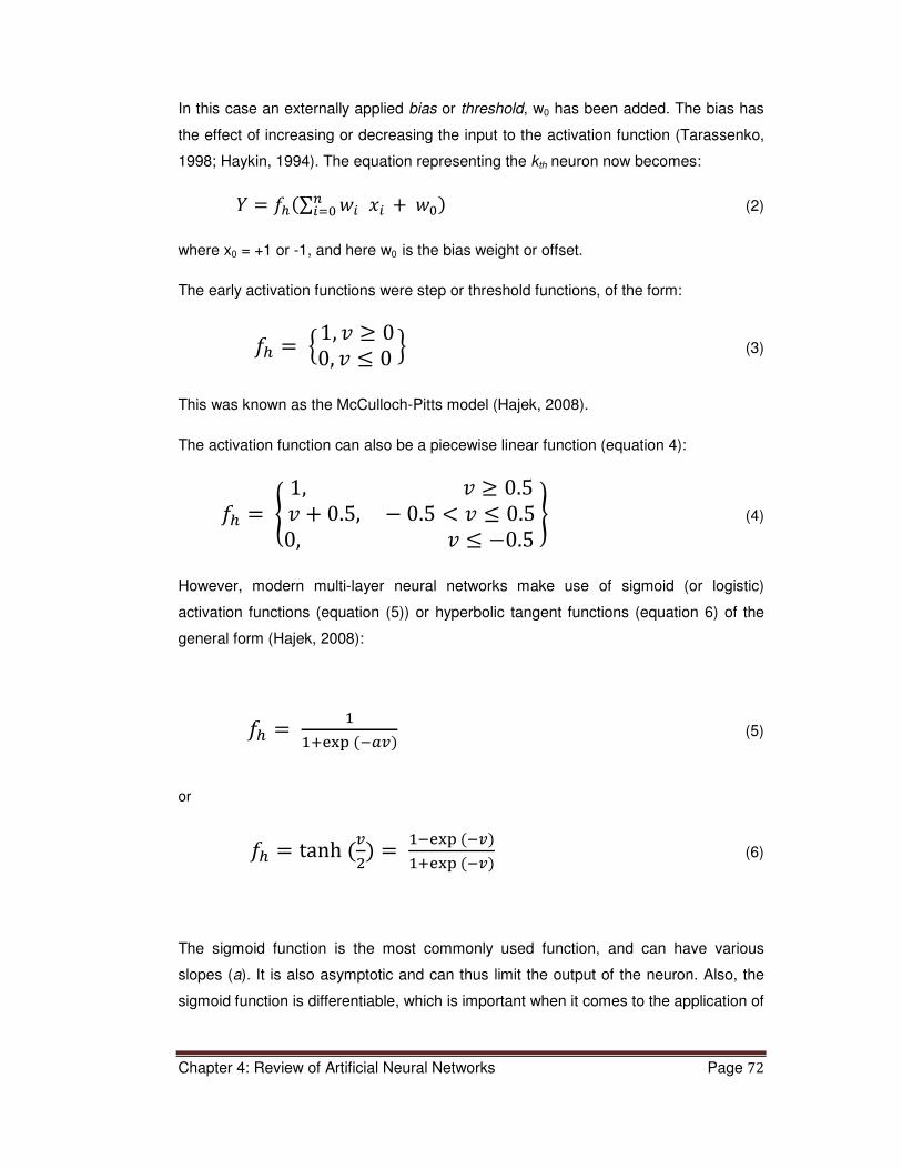
Chapter 4: Review of Artificial Neural Networks Page 72
In this case an externally applied bias or threshold, w0 has been added. The bias has
the effect of increasing or decreasing the input to the activation function (Tarassenko,
1998; Haykin, 1994). The equation representing the kth neuron now becomes:
� � �(∑ � ��� �� � �� (2) where x0 = +1 or -1, and here w0 is the bias weight or offset.
The early activation functions were step or threshold functions, of the form:
� � �1, � � 00, � � 0 � (3)
This was known as the McCulloch-Pitts model (Hajek, 2008).
The activation function can also be a piecewise linear function (equation 4):
� � 1, � � 0.5� � 0.5, " 0.5 # � � 0.50, � � "0.5 $ (4)
However, modern multi-layer neural networks make use of sigmoid (or logistic)
activation functions (equation (5)) or hyperbolic tangent functions (equation 6) of the
general form (Hajek, 2008):
� � %%&'() �*+,� (5)
or
� � tanh �,/� � %*'() �*,�%&'() �*,� (6)
The sigmoid function is the most commonly used function, and can have various
slopes (a). It is also asymptotic and can thus limit the output of the neuron. Also, the
sigmoid function is differentiable, which is important when it comes to the application of

Chapter 4: Review of Artificial Neural Networks Page 73
minimization of squared error criteria as the basis for the multi-layer learning
algorithms, as discussed below (Haykin, 1994:12).
A sigmoid function (g) is depicted in Figure 4.6.
Figure 4.6: The sigmoid function. (Tarassenko, 1998:14)
With reference to figure 4.5, the output of a neuron can be compared to a target value,
and an error function can be defined as some difference between the output and
actual (target) value. In practice, the square of the error is more convenient, to
eliminate negative values. Thus, a sum-of-squares error function can be defined as
follows:
0 � 1/2 ∑ �2 3 " 43�/53�% (3)
where 2 3 is the output of a multi-layer network for an input pattern p and 43 is the
corresponding target value (Tarassenko, 1998:13)
The error function E is minimized by gradient descent by differentiating it with respect
to every weight wi in the network (Tarassenko 1998: Chapter 2). For an individual
weight wi, the weight update (or change in weight) is thus given by:
6 � � " 7 898:; (4)

Chapter 4: Review of Artificial Neural Networks Page 74
In order to achieve this differentiation, a continuous differentiable function such as a
sigmoid function as shown in Figure 4.6 must be used.
Specifically:
2� � <=>?@ � %% & ABC (5)
where >? � ∑ �?�� ��%
Let us now consider the case of a two-layer perceptron, structure as depicted in Figure
4.7.
Figure 4.7: A two-layer perceptron structure. (Tarassenko, 1998:15)
The “two” refers to the number of layers of weights, not the number of layers of units.
In addition, the terminology of I = number of input parameters (five in this example), J
= number of hidden units (three) and K = number of output units (three). For this K
class problem, the error function now becomes:
0 � %/ ∑ ∑ =2D3 " 4D3@/ � %
/ ∑ ∑ =<∑ ?D2?3 " 4D3? @ED�%53�%ED�%53�%/
(6)
Which expands to:
0 � %/ ∑ ∑ =<∑ ?D<=∑ �?��3� @? " 4D3@/ D3 (7)

Chapter 4: Review of Artificial Neural Networks Page 75
In this form E can now be differentiated with respect to each weight to calculate the
gradient of the error function. The error back propagation algorithm thus arises and is
used to update the weights in a multi-layer network. The update equations have been
derived (Tarassenko, 1998:15) thus:
For the input - to - hidden layer:
6 �? � " 7 898:;C � " 7F?2�
where F? � 898+C � ∑ FD ?D 2?=1 " 2?@D , (8)
And for the hidden-to-output layer:
6 ?D � " 7 898:CG � " 7FD2?
where FD � 898+G � =2D – 4D@2D=1 – 2D@ (9)
The error back propagation algorithm derives its name from the fact the errors (FD ’s ) of
the output layer need to be calculated first, as they are required in the calculation on
the input layer updates.
It has been shown (Tarassenko 1998:16, quoting Cybenko, G. 1989. Approximation by
superpositions of a sigmoidal function. Math. Control, Signals & Systems. 2: 304-314.,
and Hornik, K., Stinchcombe, M. and White, H. 1989. Multilayer feedforward networks
are universal approximators. Neural Networks. 2: 359-366) that a two-layer multilayer
perceptron with sigmoid transfer functions is able to approximate any function, given
the correct selection of the network architecture, in particular the number of hidden
units. It is even possible to over-fit a function to available data, as discussed in Section
4.6.4.5.
4.4.3 Network training
The training process consists of finding the optimum number of hidden units, j, with the
associated first-layer weights wij and second-layer weights wjk. Network training
normally occurs in three distinct steps, each requiring its own data. (Tarassenko,
1998:17)

Chapter 4: Review of Artificial Neural Networks Page 76
Step 1: Training: present the network with input-output data, which is used to
determine wij and wjk.
Step 2 – Validation: the validation set is presented to the network not to further adjust
wij or wjk but to determine the error of the output. Training is stopped when the error is
at a minimum, and the weights are fixed.
Step 3 – Testing: the generalisation of the network is assessed by applying a test set.
The three steps mentioned above refer to a process of supervised learning. In
supervised learning, a target/output value or answer is available for each input vector.
In many real world problems, output values are not readily available. Nevertheless it is
still possible to train a neural network using clustering algorithms, discussed below.
Training methodology is discussed more fully in Section 4.6.
4.4.4 Other techniques
A number of other mathematical techniques have found application in neural networks
(Tarassenko, 1998: Chapter 2):
• Cluster analysis and the use of clustering algorithms as a means of grouping
input patterns with similar characteristics.
• A clustering technique called a “Kohonen’s feature map” is a technique to
represent complex multi-dimensional data in a 2-dimensional representation.
• Radial Basis Function (RBF) networks make use of clustered input vectors and
non-normalised Gaussian functions as activation functions. RBF networks offer
some simplifications in the training process.
• Auto-associative neural networks have the same dimensionality in inputs and
outputs. viz. the target data is the same as the input data. These are typically
used in data compression algorithms. A two-layer neural network trained in this
manner essentially performs linear principal component analysis.
• Recurrent networks: All of the abovementioned networks are exclusively
feedforward networks. In Recurrent Networks, feedforward as well as feedback
connections are used. Such networks are very complex and dynamic in nature,
and often do not settle down to a stable state. Such networks are used mainly
in time series prediction applications.
The abovementioned structures were not required in this work, and are thus not
discussed further.

Chapter 4: Review of Artificial Neural Networks Page 77
4.5 Application and feasibility of neural networks
4.5.1 Introduction
Neural Networks have several key attributes, which make them effective candidates to
model a complex system such as a deinking flotation process (Tarassenko, 1998;
Haykin, 1994:4):
• ANN’s can learn from “experience” and interpolate responses from data not
previously encountered. This is also known as the ability to generalize data.
They have the capability to adapt to changing conditions by simply retraining.
• If enough data is available ANN’s can produce solutions in a comparatively
short space of time, when compared to traditional methods. However, some
experience of the area of application is necessary in order to select the optimal
network design.
• Although a considerable amount of computational power is required to train a
ANN, once it has been trained, it can act on input data rapidly to produce an
output.
• ANN’s are particularly suitable for dealing with complex, non-linear systems, as
typically found in real-world problems.
• ANN’s are robust, and can tolerate noise, distortions and partially incorrect
input data (Rudd, 1991).
Tarassenko (1998: 50) lists three criteria which determine if data is suitable for
representation by neural networks:
Criterion 1: “The solution to the problem cannot be explicitly described by an algorithm
or set of equations or a set of rules”.
Attempts have been made to develop first-principle hydrodynamic models, reviewed in
Chapter 2 in this work. However, these models are complex and are usually limited to
only the physical processes in the flotation stage of the deinking process. The
complexity of these models is such that they will find limited application in the everyday
operational environment of a deinking plant.
Thus from a practical point of view, the development of a neural network model is
more feasible.

Chapter 4: Review of Artificial Neural Networks Page 78
Criterion 2: “There is evidence that input-output mapping exists such that y = f(x),
where the form of f is unknown”.
Many studies have been reported in the literature (Chapters 2 & 3) on the effects of the
parameters of the deinking process on the outputs (ink removal and yield). The
relationships between inputs and output appear in the majority of cases to be
curvilinear in nature. The limitation of these studies is that, as for most laboratory type
investigations, one variable is changed while all other are kept constant. This approach
unfortunately does not provide an overall response surface to all the variables. As a
result, many studies have shown conflicting results, as discussed in Chapter 3. It is
expected that by identifying viable control parameters and modeling them with a neural
network, a complete picture can be obtained of the behavior of a deinking system.
Criterion 3: There is a large amount of data available to train the network.
In this study, the data required to develop a practical neural network was generated in
the laboratory. In this way it was possible to gather many data points over a wide
range of conditions. On the other hand, data gathered directly from plant processes
would have been limited in range, and hence the predictability of the ANN models
would be limited.
In recent years, a large number of successful neural network applications in fields as
diverse as fault diagnosis and condition monitoring, financial forecasting, signal and
image analysis, pattern detection and process control have been reported
(Tarassenko, 1998:52). In addition, a number of more specific applications in the pulp
and paper industry are discussed in Section 4.7.
4.5.2 Hardware and software requirement
Many of the earlier challenges with neural network processing have now been
overcome with the development of modern computing power. A commercial package
MATLAB with a neural network toolbox was used in this work.
4.5.3 Data collection and preparation (Tarassenko, 1998: Chapter 6)
Neural networks are very much driven by the data that is inputted into them. Good
quality data in sufficient quantity is essential. One of the advantages of neural
networks is that they allow the fusion of data, viz. different types of data (quantitative
and qualitative or descriptive) can be inputted or outputted together.
It is not necessary to know the nature of the relationship between input and output
data, but as discussed in Section 4.5.1, such a relationship must exist.

Chapter 4: Review of Artificial Neural Networks Page 79
4.5.4 Quality of data required
As a first approximation, the training of a neural network can be considered similar to
that of fitting a polynomial curve to a set of points. Neural networks can only generalize
reliably by interpolation. Any extrapolation required will be guesswork, and
consequently unreliable. Thus, the network must be trained with the full range of
process conditions likely to be encountered to avoid having to extrapolate. Also, the
data sets used for training should contain examples of both normal and abnormal
operating conditions.
4.5.5 Quantity of data required
By further analogy with polynomials, the number of input vectors (viz. a set of input
values) should be of the same magnitude as the number of unknowns in the network,
which corresponds to the number of weights wij and wjk. If I = number of inputs, J = the
number of hidden units and K = the number of outputs or output classes, then the
number of weights W for a two-layer perceptron is given by:
I � J � �K � 1�L � �L � 1�M (10)
W thus corresponds to the minimum number of input vectors P required.
A term called network capacity, defined as
NE (11)
has been suggested, with the recommendation that the number of input vectors P be
considerably more than the network capacity (Tarassenko, 1998:70). viz:
I O NE (12)
An alternative suggestion has been the use of an “accuracy parameter”, ε, defined as
the proportion of input vectors that are incorrectly classified, be taken into account
(Tarassenko, 1998:70). Thus ε = 0.1 for a 90% data accuracy and
I � NP (13)
Taking the above arguments into account, the ideal number of input vectors would lie
between W and 10W.

Chapter 4: Review of Artificial Neural Networks Page 80
It is obvious that the network architecture (viz. J in equation above) plays a large role
in determining P. As a rough guide (Tarassenko, 1998:70):
L � √KM (14)
I and K are determined by the physical system to be modeled, J can be calculated
(equation (14)), and hence the number of data vectors required can be estimated from
equation (10).
4.6 Design, training and testing (Tarassenko, 1998: Chapter 7)
4.6.1 Introduction
The process of designing a neural network is an iterative one. Trial and error and
experimentation will be required to obtain a network with good generalization
properties (Hajek, 2010). It might be necessary to apply a blend of different techniques
to achieve an overall model that is practical (Tarassenko, 1998: 77).
When designing a neural network, a thorough knowledge of the subject domain is
necessary in order to achieve a workable model.
4.6.2 Pre-processing of data
Depending on the nature of the input data, a certain amount of pre-processing of the
data might be required. In particular, reducing the dimensionality of the data is usually
essential, to limit the size of the network and consequently the required amount of
training data. Typical techniques that could be applied here are Principle Component
Analysis, signal processing by Fast Fourier Transforms or encoding of non-numerical
data into numerical form. In this work, a process of screening experimental design was
used to eliminate control variables (viz. adjustable operating conditions) that have little
influence on the final outputs. It emerged that only about seven to ten control variables
would be needed to produce a good model.
Continuous input variables normally can be inputted as they stand, except perhaps for
the normalization of data which have vastly differing dynamic ranges (Tarassenko
1998:Chapter 7). The linear normalization commonly applied is the zero-mean unit-
variance transformation, equation (15):
��R � S;* T;U;
(15)

Chapter 4: Review of Artificial Neural Networks Page 81
where V� is the mean and W� is the standard deviation.
In this work, all of the input variables are continuous, with magnitude ranging from 0 up
to 1000.
4.6.3 Selecting the type of neural network
In this work a supervised training methodology was used. This is because
experimental outputs are available for each set of inputs. Furthermore, a multi-layer
perceptron (MLP) architecture has been applied, as it has been demonstrated that a
two-layer MLP can approximate any function (Tarassenko, 1998:89). Radial basis
function (RBF) networks have similar, to slightly inferior generalisation properties and
lower training times (Tarassenko, 1998:88). Training times were not a limitation in this
work.
4.6.4 Training process
The generalized procedure for the training of a MLP involves the following steps:
4.6.4.1 Partitioning
As discussed in Section 4.4.3 above, before training the available data is randomly
partitioned (equally if possible) into training, validation and test data sets.
4.6.4.2 Training
Initialising
In this process, the weights must be initialized by random setting to values, typically
between -0.01 and +0.01. If the initialization values are too large, the sigmoid
activation functions will be in the saturated zone, and incremental changes will be
small, resulting in very low learning rates. In extreme cases, neurons could get stuck at
values close to 0 or 1.0
Training
Thereafter the network is repeatedly presented with training vectors, in random order.
The output is calculated, compared to the target and the error, E, is computed. The
back-propagation algorithm is then employed to calculate the weight updates (Section
4.4.2). Additional parameters, known as the learning rate (7) and the momentum (X)
have been introduced to speed up the learning processes. Equations (8) and (9) now
become
∆?D � ?D(4 � 1� " ?D�4� � " 7FD2� � X Z?D�4� " ?D�4 " 1�[ (16)
and

Chapter 4: Review of Artificial Neural Networks Page 82
∆�D � �D�4 � 1� " �D�4� � " 7F?2� � X Z�?�4� " �?�4 " 1�[ (17)
where δ, y and w are as defined in Section 4.4.2.
7 is typically between 0.01 and 0.1, and X lies between 0.5 and 0.99. Learning with
momentum prevents the learning process from terminating in small local minima.
The data vectors can be applied to the network in batch or sequential fashion. In batch
learning the weight updates are averaged across all the training patterns, whereas in
sequential learning the weights are updated after each pattern has been presented.
Sequential learning is preferred in practice (Tarassenko, 1998: 91).
Stopping
The network is trained subject to a stopping criterion. The network is repeatedly
presented with training vectors until the classification error (mean square error (MSE)
of the validation set, eval) has reached a minimum and starts to increase again (Figure
4.8). At this minimum point, the (eval)min and the corresponding set of weights are saved
and taken to be the best solution. It is typical for the training error (etr) to continue
decreasing beyond this optimum point. Figure 4.9 demonstrates how the training error
(etr) continues to decrease as the network more closely approximates the data points
(Figure 4.9b), whilst the validation error (eval) increases again as generalisation is
compromised (Figure 4.9a).
Figure 4.8: Comparison of training error and validation error during training.
(Tarassenko, 1998:93)

Chapter 4: Review of Artificial Neural Networks Page 83
4.6.4.3 Selecting the optimum network
During the training process, a number of different network structures (different I-J-K
configurations) are presented with the training data, and (eval)min is calculated for each
structure. On the basis of the lowest MSE’s, the m best network structures are
selected. These m structures are then presented with the test data sets, and the best
network is selected (viz. the network that produces the lowest (eval)min) on the basis of
the test set. The test data set must not be part of the training data, and should be
separate from the training and validation sets. The test set is nevertheless still part of
the original data set, and might still not represent the real world situation.
4.6.4.4 Testing the network
Previously unseen data from the real world are presented to the network, to test the
generalization performance of the network.
4.6.4.5 Over training
Common problems that can arise in the process include stuck units (refer to Section
4.6.3.2), poor generalization, insufficient or unbalanced data, over-fitting, over-training
and extrapolation. The problem of over fitting or poor generalisation is illustrated in
Figure 4.9. Figure 4.9a represents a curve that generalizes the data well, viz. the
underlying trends are well captured. Figure 4.9b represents a network that is over
fitted. The network has memorized the data, but not the underlying behaviour. This is
usually caused by having too many hidden neurons.
Figure 4.9: (a) Good generalisation. (b) Over fitted data – poor generalisation ( x =
training data, o = test point) (Tarassenko, 1998:17)

Chapter 4: Review of Artificial Neural Networks Page 84
4.7 Review of applications of neural networks in flotation and
in the paper industry
4.7.1 Introduction
The effects of various separation unit operations, process chemicals and waste types
have been extensively studied by many researchers and reviewed in Chapters 2 and
3. These findings have generally been well applied in the industry. Our understanding
of the fundamental physical and chemical processes underlying the deinking
processes is growing. But, due to the great variability of the raw material as well as the
complexity of the physical processes which occur at the micro level, processing
problems and process instability remain as challenges.
The large number of flotation models that have been developed highlights the
uncertainty around what exactly happens in a flotation cell (Labidi et al., 2007).
Attempts have been made (Beneventi et al., 2006; Bloom, 2006; Heindel, 1999; Julian
Saint Amand, 1999; Bloom & Heindel, 1997) to model these processes from first
principles, in terms of the collision probabilities of ink particles and bubbles. These
models are however highly complex and somewhat removed from the daily experience
of those who operate deinking plants. Such challenges have also been expressed by
Hodouin et al. (2001) in the related field of mineral ore processing.
As a result of the abovementioned difficulties, attempts have been made to use
Artificial Intelligence based systems to model and control modern flotation plants, in
both the fields of mineral flotation, and to a much lesser extent in deinking flotation.
The following techniques have been successfully used singly or in combination in
trying to address the problems of process control in highly complex and ill-defined
systems.
4.7.2 The use of neural networks in flotation processes
In a review article, Hodouin et al. (2002) outlines the state of the art and challenges in
the control of mineral flotation plants. There are many similarities to the problems
faced in flotation deinking plants, viz. complexity of raw material, measurement
difficulties, complex physical processes and a small number of outputs measuring the
process, but a large number of inputs, many of which interact. These conditions make
it difficult to develop mathematical models.
Singh et al. (2003) in their description of the control difficulties experienced in mineral
flotation plants, describe a very similar picture to that experienced in deinking flotation
plants: difficult control, interactive circuits, unstable plants, and changing feed

Chapter 4: Review of Artificial Neural Networks Page 85
conditions. They say that an ideal is to have an algorithm or strategy to find new
optimum conditions, rather than an “unguided hunt” for the new conditions. This is
essentially the objective of the current work: to develop an algorithm which will guide
operations management in the appropriate strategies to adapt to changing raw
material conditions.
An ANN model of a copper/lead flotation plant was developed by Forouzi & Meech
(1999), and used to predict the assays of the concentrate streams. The model was
incorporated into the process control system, and was adaptive in nature, viz. it was
retrained whenever the prediction efficiency decreased to a pre-determined level.
Cubillos & Lima (1997 & 1998) used a combination of a physical model (mass, energy,
momentum) and an ANN model. The ANN was used to predict certain process
parameters, which then become inputs into the physical model.
In another hybrid approach, Gupta et al. (1999) developed an ANN to predict flotation
rate constants from operating variables, and thereafter used these constants in a first
principles model to predict the performance of a phosphate flotation column.
Amongst the earliest fields of application of neural networks was in the field of pattern
recognition and image processing. This was also applied into the flotation industry.
Rughooputh & Rughooputh (2002) describe the application of ANN’s to the complex
task of analyzing the visual attributes of the froth in a flotation cell to make deductions
about the state of flotation process. The system that was developed was reported to
be highly reliable.
4.7.3 The use of neural networks in the pulp and paper industry
Labidi et. al. (2007) studied the effects of flotation consistency, airflow rate and
agitation speed, at various flotation times, on the rate of ink removal. Ink removal was
measured by the increase in brightness and the change in ERIC. Kinetically, ink
removal was considered as a first order kinetic process defined by
logA Zabc*adabc*ac[ � efg�hi Ajj 4 (18)
where BBF = brightness of unprinted paper, BD = disintegration brightness, and BF =
floated brightness of printed paper. Similar expressions were developed for ERIC. An
ANN was developed which effectively modelled the brightness and ERIC out of the

Chapter 4: Review of Artificial Neural Networks Page 86
flotation cell. The outputs of the ANN correlated closely with the experimental results.
They found that ink removal was enhanced by higher consistency and airflow rates.
In a review of the applications of neural networks in the pulp and paper industry,
Laperriere & Wasik (2001) found that ANN’s have compared well with deterministic
models, in particular the modelling of a Kraft digester. In another study, Rughooputh &
Rughooputh (2002) compared a deterministic model and a ANN model to simulate the
pulping process in a Kraft digester. They were found to produce similar results.
Rudd (1991) relates the use of an ANN to model and control a brownstock washer
system. It was found that the percentage errors achieved by the ANN were superior to
those achieved by traditional regression techniques.
Figueiredo et al. (2008) reported that the output of a causticising process was
successfully predicted by an ANN.
In addition, ANN models have also been successful in the more complex field of
predicting functional pulp or paper properties and diagnosing web breaks. Edwards et
al. (1999) described the use of an ANN to classify and predict paper curl. Curl is an
important quality characteristic, which can only be measured off-line, after the paper
has been manufactured. It was found that the ANN was successful in the classification
tasks to a level of confidence of 68%.
In a practical plant study, Smith & Broeren (1996) reported on the use of an ANN to
analyse and optimise a newsprint deinking facility, which recycled a mixture of old
newsprint and magazines. Time-stamped plant operating data was acquired and fed
into an ANN. An input vector of 66 variables was inputted, and the influence of a large
number of process variables was analysed and ranked in order of influence. As a
result, large cost saving were achieved in terms of reduced pulper chemical additions.
ANN’s have found extensive application in the field of image analysis. Verikas et al.
(2000) used an ANN, together with Fuzzy Logic to analyse the colour of dirt specs in a
sheet of recycled paper.
As examples from completely different fields, Zhang & Stanley (1999) reported on the
use of an ANN to model a water treatment process. On-line parameters were used to
train and test the model, which was incorporated into a real-time process control
scheme. Schlang et al. (2001) reviewed the extensive use of hybrid ANN models for
the control of rolling strip mills in the steel industry.

Chapter 4: Review of Artificial Neural Networks Page 87
4.7.4 Neural networks in combination with other techniques
Neural networks can be used in combination with other Artificial Intelligence
techniques. In a review article, Huang & Zhang (1995) reviewed the synthesis of ANN
and expert systems and their applications in manufacturing. They maintain that the
strengths of the two techniques have been found to complement each other in the
solving of complex manufacturing problems.
ANN’s have also been used together with Fuzzy Logic systems in a number of
applications. Verikas et al. (2000) used an ANN, together with Fuzzy Logic to analyse
the colour of dirt specs in a sheet of recycled paper. Bergh & Yianatos (2002), in their
review article state that Fuzzy Logic and ANN’s have proven to be powerful
components in expert supervisory systems.
Multivariate data processing has been used by various workers to analyse the
complexities of flotation processes. Eriksson et al. (2001) and Wold et al. (2001) report
on the use of multivariate regression in the prediction of inter alia the COD load of an
effluent resulting from the deinking of recycled paper. These applications could well
have been tackled with neural networks, with similar results.
4.8 Conclusions
The successful use of artificial neural networks in the field of flotation monitoring and
control has been demonstrated. It is the intention of this work to model the effect of
variable raw material conditions on the outcome of a laboratory-based deinking
process, with a view to developing a predictive model, which could help plant
management to cope with unexpected raw material changes.

Chapter 5: Methodology Page 88
CHAPTER 5: METHODOLOGY
5.1 Introduction – overview of methodology
The objective of this research was to model the combined processes of pulping,
deinking and washing with respect to raw material changes and process parameters.
The output parameters that were modelled are ISO brightness, ERIC, and yield. The
proposed methodology was as follows:
1) Firstly, establish general deinking conditions in the South African tissue and
newsprint deinking industry. This was done through field surveys of the local
industry and assessment of the current and future requirements for deinking of
different quality materials.
2) Secondly, to model the industrial processes in the laboratory. Experimental
work was done in the laboratory to establish the best process control
parameters. A distinction was made between control parameters and
optimisation parameters. Optimisation parameters are parameters which, whilst
important for the overall efficiency of the process, are not suitable to control
short term variations. On the other hand, control parameters are those which
are suitable to change and thus to control the short term variations in the
process. Once the control parameters were established, experimental work
was performed with a wide blend of different recycled paper raw materials and
control parameters to generate data to train a neural network.
3) Model the laboratory processes mathematically, using neural networks. The
pulping, flotation and washing processes as well as the effects of a range of
variables on the efficiency of deinking were modeled. Neural networks were
selected as the potential best method due to the number of potential variables
and non-linearities which could be encountered.
4) Test the model on an industrial scale. This would involve inputting plant data
into the mathematical model to determine how well the model generalizes and
predicts outputs on a plant scale.
5) The model’s purpose would be to enable process operators to adapt to
changing recycled paper raw material conditions using predictive model-based
control methods.

Chapter 5: Methodology Page 89
5.2 Review of deinking conditions in newsprint and tissue manufacture The three main companies involved in deinking operations in South Africa are Mondi
Shanduka Newsprint - Merebank mill, Nampak Tissue, which has deinking mills in
Belville - Cape Town and Klipriver - Johannesburg, and Kimberly Clark - Enstra mill.
Two mills, namely Mondi Shanduka Merebank mill and Nampak Klipriver mill were the
initial participants in this study. It is from these two mills that the ranges for the
modelling parameters were determined. As the study progressed, the Nampak Belville
mill was included in the model testing exercise. Executives and process personnel
from both companies were interviewed, and readily provided information. Table 5.1
below summarizes the range of process conditions of paper recycling in SA.
Table 5.1: Paper Recycling in South Africa.
PROCESS PAPER GRADE USED
(refer to Section 7.2.1 for definitions)
PROCESS CONDITIONS
Newsprint deinking ONP, SBM
Alkaline slushing in presence of H2O2, deinking flotation with
displector system, washing, dispersion, bleaching
Tissue manufacture HL1, HL2, mixed office paper Neutral slushing, deinking
without chemicals, dispersion, bleaching
Linerboard and carton board manufacture
K3, K4 Slushing, no deinking,
cleaning (hydrocyclones), screening, dispersion
As can be seen in Table 5.1, deinking is only carried out by the newsprint and tissue
manufacturers. The largest volume of recycled paper is processed by the
manufacturers of packaging papers and boards (Table 7.2), but no deinking is carried
out in these processes. It can also be seen from Table 5.1 that quite different process
regimes apply to the different recycled paper grades.

Chapter 5: Methodology Page 90
5.2.1 Grades of recycled paper
Table 5.2 depicts the quantities of the various grades of paper recovered in South
Africa.
Table 5.2: Recovery of recycled paper in South Africa. (Pamsa, 2007).
DESCRIPTION RECYCLED PAPER GRADE
DESIGNATION (refer to Table 7.3 for
definitions)
2007 CONSUMPTION (tpa)
Newspapers FN, SN 105 922
Magazines SBM or OMG 40 617
Corrugated & kraft papers K1, K2, K3, K4 512 705
Office, graphic papers HL1, HL2, Supermix 168 132
Other, mixed papers CMW 119 001
Recycled paper is broadly classified in pre-consumer and post-consumer waste. Pre-
consumer waste is paper that has been processed but has not fulfilled its function, for
example, an over-run of issues of a daily newspaper. The paper has been printed but
the newspapers have not been sold. They are returned to the recycler as pre-
consumer waste. On the other hand, if the newspaper had been purchased, read and
discarded, it would have to be recovered from the domestic waste stream. This is
termed post-consumer waste.
Pre-consumer waste is relatively clean and uniform in its composition. Post-consumer
waste has a very much more varied composition, and extensive sorting is invariably
required. It is thus more costly to collect and commands a lower price in the market.
The designations and the respective specifications for recycled paper collected in
South Africa, as detailed in Table 5.3, are relevant to this work:

Chapter 5: Methodology Page 91
Table 5.3: Overview of recovered paper specifications. (Harper, 2009, Steyn, 2009, South
African Standard Grade Definitions for Recovered Paper, 2009)
DESIGNATION SPECIFICATION COMMENTS
SBM or OMG
“sorted books & magazines”
Books and magazines, all types including ledgers, invoice books
etc., free of covers and other contaminants.
Pre-consumer waste, includes light weight coated (LWC),
supercalendered (SC), wood-free coated paper, advertising
inserts. Contains 5-10% mechanical grades.
FN
“Flat News”
Newspaper – over issues and once-read newspapers.
Pre-consumer newsprint and over-issues. Newspapers, including advertisement
inserts. No flexographic prints.
SN
“Special News”
Post-consumer, kerbside collection of newsprint
Newspaper includes ca. 10% magazines, 5% letter, no
packaging or brown paper.
HL1
“Heavy Letter 1”
White heavy letters such as woodfree letter papers, office records, with a maximum1 of
mechanical papers and written-on papers, free of covers, bindings
etc.
White base papers – includes office papers, carbonless copy paper, ledger, white boards,
some colour printing.
HL2
“Heavy Letter 2”
Pastel coloured heavy letters such as white or coloured writing papers, office records, containing
a maximum of mechanical or written-on papers, free of covers,
etc.
As for HL1 but contains coloured and pastel base
papers.
No heavily printed or coloured stock.
SUPERMIX A 50/50 blend of HL1 And HL2
CMW
“common mixed waste”
Any mixture of acceptable paper for pulping, free of extraneous
matter.
Various grades of paper and board.
Note 1: Specified by individual customers, usually ca. 10%.
Old newsprint (ONP) is a collective designation for Flat News and Special News.
There are many more grades of paper collected in South Africa, but they are not
relevant to this study, so will not be discussed further.

Chapter 5: Methodology Page 92
5.2.2 Newsprint deinking conditions
5.2.2.1 Process configuration
Figure 5.1 gives a self explanatory overview of the process flow of the newsprint
deinking facility. The plant is a common single-loop flotation process with Voith
EcoCell’s ®
Figure 5.1: Process flow diagram – single-loop newsprint deinking plant. (Refer to Figure
9.4 for greater clarity)
5.2.2.2 Raw materials
The mill uses a mixture of ONP and SBM in the approximate bale ratio of 75:25.
Depending on availability, the ratio of Flat News and Special News varies to make up
the 75%. The SBM is essential to achieve the brightness targets, so its use is
optimized depending on availability and cost constraints. The paper is stored under
cover and is less than six months old.

Chapter 5: Methodology Page 93
5.2.2.3 Process conditions
The process conditions pertaining to pulping, flotation and washing are presented in
Table 5.4. The parameters that are used to monitor and control the process are also
detailed:
Table 5.4: Process conditions and control of a newsprint deinking plant.
PROCESS STANDARD CONDITIONS MONITORING & CONTROL
Pulping
Consistency 14-20% Monitored
pH 9-10 Controlled to 9.5-9.7
Pulping time 13.3 mins. Kept constant
Temperature 50oC Monitored
H2O2 , 0.48-0.52 %[1] A small residual is maintained
NaOH 0.55-0.6 %
Pulper brightness monitored >40,
Pulper ERIC 300-800
Chelant – nil
Sodium silicate 0.38-0.4 %
Surfactant 0.085-0.1%
Flotation
Temperature 42˚C Control weir level in flotation cell
Consistency 1.2-1.4% Monitor- brightness out >50
pH 7.5-8.0 Monitor- ERIC out 200-400
Calcium hardness ca. 240ppm
CaCO3
Monitored – Calcium collector not
used. An average of ca. 210 ppm.
Washing-disc
filter Consistency in: 0.9%, out:4.7% Monitored
Washing – wash
press Consistency in: 4.7%, out:28%
Consistency monitored.
Brightness out >50
ERIC out <250
Dispersion
Brightness out 57-58
ERIC out <250
Final after
bleaching
Brightness >58
ERIC 150-300
pH 5.5-6.5
Exit specification
Note 1: Addition rates are quoted as % active material per dry mass of paper.

Chapter 5: Methodology Page 94
5.2.2.4 Process control philosophy
If a process upset or out-of-specification event occurs, the control strategy is to restore
standard conditions and increase the level of SBM relative to ONP to increase the
brightness. Water is purged from the filtrate water chests to reduce the fines and
colloidal load of the system. The yield of the process is an issue as it has economic
consequences.
5.2.3 Recycled office paper deinking conditions – double loop process
5.2.3.1 Process configuration
Figure 5.2 below gives an overview of the process flow of a office paper deinking
facility, which produces a variety of toweling tissue grades. The flotation cells are
Escher Wyss CS cells.
Figure 5.2: Process flow diagram – double loop office waste deinking plant. (Refer to
Figure 9.11 for greater clarity)
5.2.3.2 Raw materials
The mill uses a mixture of HL1, HL2, SUPERMIX, ONP and SBM in various ratios,
depending on the quality of tissue made. The percentage mixing ratios are given in the
Table 5.5. In practice, the use of HL2 has been dwindling over the last few years, due
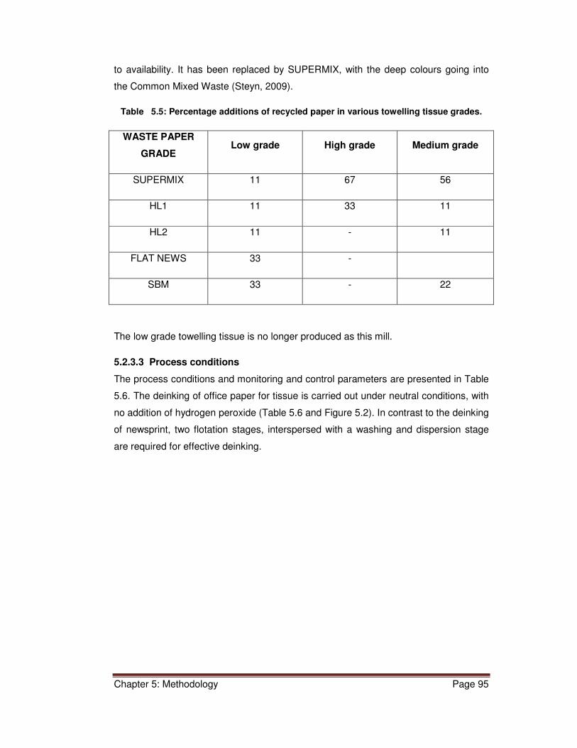
Chapter 5: Methodology Page 95
to availability. It has been replaced by SUPERMIX, with the deep colours going into
the Common Mixed Waste (Steyn, 2009).
Table 5.5: Percentage additions of recycled paper in various towelling tissue grades.
WASTE PAPER
GRADE Low grade High grade Medium grade
SUPERMIX 11 67 56
HL1 11 33 11
HL2 11 - 11
FLAT NEWS 33 -
SBM 33 - 22
The low grade towelling tissue is no longer produced as this mill.
5.2.3.3 Process conditions
The process conditions and monitoring and control parameters are presented in Table
5.6. The deinking of office paper for tissue is carried out under neutral conditions, with
no addition of hydrogen peroxide (Table 5.6 and Figure 5.2). In contrast to the deinking
of newsprint, two flotation stages, interspersed with a washing and dispersion stage
are required for effective deinking.

Chapter 5: Methodology Page 96
Table 5.6: Process conditions and control of a double loop office paper deinking plant.
PROCESS STANDARD CONDITIONS MONITORING & CONTROL
Pulping
Consistency 16-18% Monitored
pH 7-8 monitored
Pulping time 16 mins. Kept constant
Temperature 35-40oC Monitored
H2O2 0 %
NaOH 0 %
Pulper brightness monitored 61-68%
Chelant – nil
Sodium silicate 0 %
Surfactant 0.1%[1]
Flotation I
pH Monitored
Consistency 0.8-1% Monitor- brightness out >50
Monitor ash content
Monitor air flow to float cell
Washing-Vario I Consistency out 10-12% Monitor consistency and pH
Brightness out boosted by bleach
addition [2]
Washing – wash
press I Consistency out 25-35%
Dispersion
Temperature 75-80oC
Consistency 25-30% Monitor
Flotation II Consistency 0.8-1.2% Monitor consistency, pH, brightness
Washing – Vario
II Consistency out 10-12% Monitor
Washing – wash
press II Consistency out 25-35% Monitor
HD storage
Final after
bleaching
Brightness >80 high grade,
74-78 medium grade
Exit specification
Note: 1. Addition rates are quoted as % active material per dry mass of paper. 2. Bleaching with formamidine sulfinic acid (FAS)

Chapter 5: Methodology Page 97
5.2.3.4 Process control philosophy
The most important quality requirement for tissue manufacture is the softness. This
parameter is however not affected by the recycling process. Secondly, visual
properties, viz. cleanliness (no dirt specs) and brightness are important. Brightness is
adjusted by varying the amount of HL1.
5.2.4 Recycled office paper deinking conditions – single loop process
5.2.4.1 Process configuration
Figure 5.3 gives an overview of the process flow of the single loop deinking facility,
which produces a variety of toweling tissue grades. The flotation cells were supplied by
Voith, and comprise a mixing cell, five flotation cells in series and a secondary cell for
the flotation of the rejects from the first five stages. The cells are circular in cross-
section with an estimated volume by calculation of 42.4 m3 for the 5 primary cells. The
overall process flow is shown in Figure 5.3.
Figure 5.3: Process flow diagram – single loop office waste deinking plant
(See Figure 9.15 for greater clarity)
5.2.4.2 Raw materials
The mill uses a mixture of HL1, HL2, SUPERMIX, ONP and SBM in various ratios,
depending on the quality of tissue made. The percentage mixing ratios are given in the
Table 5.7.

Chapter 5: Methodology Page 98
Table 5.7: Percentage additions of recycled paper in various towelling tissue grades.
WASTE PAPER GRADE
Low grade (D)
High grade (Industrial
wipes)
Medium grade (A)
Very High
grade
SUPERMIX 40 100 85 0
HL1 0 0 0 100
HL2 0 0 0 0
FLAT NEWS 30 0 0 0
SBM 30 0 15 0
.
5.2.4.3 Process conditions
The process conditions and monitoring and control parameters are presented in Table
5.8. In this case, the deinking of office paper for tissue is also carried out under neutral
conditions, with no addition of hydrogen peroxide, alkaline chemicals or even
surfactant.
Table 5.8: Process conditions and control of the single loop office paper deinking plant.
PROCESS STANDARD CONDITIONS MONITORING & CONTROL
Pulping
Consistency 16-18% Monitored
pH 7-7.5 Monitored Pulping time 16-20 mins. Kept constant
Temperature setpoint 85oC, actual 60 oC.
Monitored
H2O2 - 0 % NaOH - 0 %
Pulper brightness monitored 60-70%
Chelant – nil Sodium silicate - 0 %
Surfactant 0%[1]
Flotation
pH ca. 7-7.5 Monitored Consistency 0.6-0.8% Monitored
Temperature setpoint 50 - 55oC, actual 48-50 oC.
Brightness into float cell, brightness after float cell
Washing-Vario split
Consistency out 10-(12)-16% Monitor consistency and pH
Thickening Consistency out 18%
Bleaching Temperature setpoint 80oC Consistency 15%
Brightness after bleaching.[2]
Final after bleaching
Brightness >80 high grade, >75 low grade
Exit specification
Note: 1. Addition rates are quoted as % active material per dry mass of paper. 2. Bleaching with Direct Borol Injection.

Chapter 5: Methodology Page 99
In contrast to the double loop plant, there is only one flotation stage, followed by
cleaning and screening, washing, thickening and bleaching.
5.2.4.4 Process control philosophy
The most important quality requirement for tissue manufacture is the softness. This
parameter is however not affected by the recycling process. Secondly, visual
properties, viz. cleanliness (no dirt specs) and brightness are important. Brightness is
adjusted by varying the amount of bleaching solution. The brightness’s are generally
within specification, but ad.hoc. additions of bleach solution are used to bring the
brightness into specification.
5.3 Process control of deinking plants
The deinking processes are such that there are few opportunities to make adjustments
to the process if the quality of the output changed. In particular the setup of the
flotation cells offers no flexibility. The aeration air is aspirated into the cell through a
fixed aperture, so the air flow can’t be adjusted. The level in the float cell can be
controlled, so in theory one could adjust the froth height. In practice however the float
cell level or froth height is maintained at a set point and not varied in response to
changing conditions. Even so it is very difficult to consistently control the height at this
set point. The construction of the cells does not offer a great height difference to adjust
this parameter. It is of course possible to adjust the level of addition of process
chemicals, but with the exception of the final bleaching chemicals, this is not done.
The general strategy is to check the quality of the incoming recycled paper as a first
step. Thereafter, adjustment in process chemicals might be attempted. Such
adjustments are in the main ad-hoc and experience based (Crosby, 2008). Thus, the
main driver of quality in a paper recycling plant is the variability of the incoming
recycled paper, with little possibility to remedy poor paper quality in the process.
Certain grades of recycled paper, depending on the process, are known as “brightness
boosters”, and are employed as such to control the final brightness. For example,
OMG is used to boost brightness in newsprint deinking and HL1 boosts the brightness
in tissue deinking. However, this approach is becoming less viable due to constrained
availability of such high quality feedstocks. The deinking mills are having to make use
of lower grade and mixed paper.

Chapter 5: Methodology Page 100
5.4 Determination of potential control parameters
With reference to Tables 5.4, 5.6 and 5.8, the list of possible control variables in the
combined pulping, flotation and washing processes totals about 15 variables.
Processes such as dispersion and final bleaching were not modelled, as they differ for
the newsprint and tissue deinking processes and would not be accommodated in a
global model. In addition, dispersion can at this point in time not be replicated in the
laboratory.
It was desirable that the list of 15 possible control variables be reduced, to avoid
having to build a large and complex neural network model requiring vast amounts of
training data. In order to screen the large number of possible variables in a reasonable
amount of time, it was necessary to use experimental design techniques. For example,
to investigate all possible combinations of 15 factors at only two levels would require
215 or 32768 experiments. Plackett-Burman fractional factorial designs have been
found to be effective in investigating large numbers of experimental variables with a
minimum number of experimental runs (Barrentine, 1999: 39).
The list of possible control variables can also be reduced by eliminating variables that
from a process plant point of view are not practical control variables. A good control
variable is one that can be easily changed or adjusted without throwing the process
out of balance, reducing the capacity of the plant or requiring considerable operating or
capital expenditure. On the other hand a variable which has a significant effect on the
process but is not a practical control variable would still need to be optimized. Such a
variable would be considered to be an optimisation variable. The conditions listed in
Tables 5.4, 5.6 and 5.8 were considered in the light of these requirements as possible
practical control variables.
5.4.1 Pulper consistency
The effect of the consistency in the pulper on the deinking process has been studied
(Section 2.2.2). Bennington et al. (1998) found that pulping time and pulping
consistency were not major influencing factors, as the ink was released very rapidly
from the fibres, and that continued pulping tended to redeposit ink on the fibres. On the
other hand, Ackerman et al. (1999) reported that pulping consistencies and alkalinities
interacted to influence the final deinked brightness.
A pulper designed to operate at for example 14-20% consistency would not slush pulp
effectively at 5% consistency. Similarly, a low consistency pulper would not be able to
pulp at high consistency. In addition, a reduction of pulping consistency from 14% to

Chapter 5: Methodology Page 101
5% at the same hydraulic throughput would constitute a 280% reduction in plant
throughput, in terms of dry fibre processed. Thus the consistency in the pulper is not a
practical control variable, although the exact level of pulping consistency could be
optimized. In the laboratory, the pulper could not effectively deflake the recycled paper
at a consistency of 5%, but deflaked effectively in the 8 to 10% consistency range. At
consistencies above 10%, poor movement (and thus mixing) of the stock occurred.
Thus 8-10% consistency was chosen as the practical range for the laboratory
experiments.
5.4.2 Pulper pH
The pH is the result of the addition of chemicals such as sodium hydroxide and sodium
silicate, whose addition in turn is determined by the level of hydrogen peroxide
required (Ferguson, 1992). The pH was thus not considered to be a control variable,
but rather a variable to be monitored as an indication of the level of addition of other
chemicals.
5.4.3 Pulping time
The pulping time has also been studied by a variety of researchers. Bennington et al.
(1998) found that pulping time was not a major influencing factor, but Ali et al. (1988)
found that pulping time interacted with pulping temperature and the level of addition of
bleaching chemicals to influence the final bleaching, and hence brightness. The
pulping time is easy to manipulate on a plant, although it could have throughput
implications. Pulping time was thus considered as a possible control variable.
5.4.4 Pulping temperature
In addition to the pulping time discussed above, the temperature could be considered
as a possible control variable. Borchardt (1997) says that typical pulping temperatures
are 40 oC to 60oC, with 50-90 oC more usual for office paper. High pulping
temperatures can soften adhesive components in the pulper and lead to stickies
problems. Increasing temperature can have energy use implications but it is a
relatively easy parameter to increase with the direct injection of steam. Temperature
was considered as a possible control variable.
5.4.5 Addition of hydrogen peroxide
Hydrogen peroxide is a bleaching agent added into the pulper to overcome the
yellowing associated with the alkaline environment. Hydrogen peroxide thus has a
direct effect on the final brightness and can be added to overcome the effects of lower

Chapter 5: Methodology Page 102
grade raw materials. The level of addition of hydrogen peroxide is easy to manipulate,
and was thus considered an important control variable.
5.4.6 Addition of sodium hydroxide
The addition of sodium hydroxide is necessary to provide the alkaline environment
necessary for the effective functioning of hydrogen peroxide and the fragmentation of
ink particles (Section 2.2). The amount of sodium hydroxide necessary relative to
hydrogen peroxide has been the subject of a number of studies (Azevedo, 1999;
Dionne, 1994; Renders, 1993; Section 3.2.4). These studies have suggested various
ratios as being optimum. However, the effect of the independent addition of sodium
hydroxide was studied to determine the potential of sodium hydroxide as a control
variable.
5.4.7 Addition of chelating agent
Chelating agents are added in order to complex heavy metal ions which might
decompose the hydrogen peroxide. Studies by Renders (1993), Mathur (1991) and
Ferguson (1991) on the effects of chelating agents on the deinking process have
shown that levels of about 0.2% to 0.5% assist in achieving the brightness targets.
Chelant is thus a necessary additive to be optimized, but does not influence the
process to such an extent to show any control effect on the process.
5.4.8 Addition of sodium silicate
The role of sodium silicate is multi-faceted and has been shown to play a role in both
pulping and flotation (Section 3.2.5). Its efficacy as an agent of process control
independent of sodium hydroxide needed to be established. Optimum addition levels
are said to be ca. 2.5% (Borchardt, 1997; Dionne, 1993), although it can be added at
levels of up to 5%.
5.4.9 Addition of surfactant
The surfactant is responsible for the dispersion and stabilization of ink particles in the
pulper and the generation of the froth in the flotation cell. It has been shown to
influence both flotation efficiency and yield (Sections 3.2.6 & 3.3.2). The addition rate
of surfactant is easy to change and it was thus an obvious choice as a control variable.
On the other hand, the type of surfactant system chosen for a process is more a
question of optimisation.
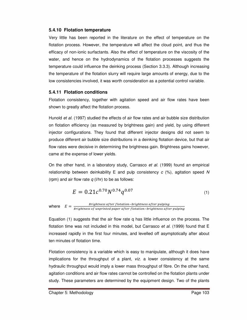
Chapter 5: Methodology Page 103
5.4.10 Flotation temperature
Very little has been reported in the literature on the effect of temperature on the
flotation process. However, the temperature will affect the cloud point, and thus the
efficacy of non-ionic surfactants. Also the effect of temperature on the viscosity of the
water, and hence on the hydrodynamics of the flotation processes suggests the
temperature could influence the deinking process (Section 3.3.3). Although increasing
the temperature of the flotation slurry will require large amounts of energy, due to the
low consistencies involved, it was worth consideration as a potential control variable.
5.4.11 Flotation conditions
Flotation consistency, together with agitation speed and air flow rates have been
shown to greatly affect the flotation process.
Hunold et al. (1997) studied the effects of air flow rates and air bubble size distribution
on flotation efficiency (as measured by brightness gain) and yield, by using different
injector configurations. They found that different injector designs did not seem to
produce different air bubble size distributions in a deinking flotation device, but that air
flow rates were decisive in determining the brightness gain. Brightness gains however,
came at the expense of lower yields.
On the other hand, in a laboratory study, Carrasco et al. (1999) found an empirical
relationship between deinkability E and pulp consistency c (%), agitation speed N
(rpm) and air flow rate q (l/hr) to be as follows:
� � 0.21��.��.���.� (1)
where � � ���������� ����� �������������������� ����� �������
���������� �� ��������� ����� ����� �������������������� ����� �������
Equation (1) suggests that the air flow rate q has little influence on the process. The
flotation time was not included in this model, but Carrasco et al. (1999) found that E
increased rapidly in the first four minutes, and levelled off asymptotically after about
ten minutes of flotation time.
Flotation consistency is a variable which is easy to manipulate, although it does have
implications for the throughput of a plant, viz. a lower consistency at the same
hydraulic throughput would imply a lower mass throughput of fibre. On the other hand,
agitation conditions and air flow rates cannot be controlled on the flotation plants under
study. These parameters are determined by the equipment design. Two of the plants

Chapter 5: Methodology Page 104
use flotation cells supplied by Voith, which aspirate air through a venturi effect, and the
third plant uses Escher Wyss cells in which the air flow is regulated by pressure. In this
case it would be possible to adjust the air flow, but in practice this is not done. In
addition, these conditions are difficult to duplicate in the laboratory equipment
available.
Peters et al. (2007) treated the subject of the interaction of flotation cell variables in a
similar way. They stated that the Specific Air Volume (SAV, Litres air/kg solids),
defined as the volume of air applied to a flotation line per kilogram of solids in the feed
determines the flotation efficiency. Thus for a laboratory batch cell:
!"��� � #�$
%& (2)
where V = cell volume, c = consistency, q = air flow rate, tf = flotation time.
In the laboratory cell, the agitation speed was maintained constant between 1500 and
1600 rpm. Thus the q would be constant and the equation reduces to one of the form
!"��� � ' ��()� (3)
where L is a constant.
Similarly, for a continuous flotation cell, where Qs is the flow rate of the stock
!"����� � #
&+, (4)
But, aspirated air flow per cell (q) depends on the stock flow Qs
� � -./� � -0)�/� (5)
where d and -0 are constants, n = number of float cells in series, and because tf is
proportional to n
Substituting into equation (4) and rearranging reduces to an equation of the general
form of equation (3), with a different constant P:
!"����� � 4 ��()� (6)

Chapter 5: Methodology Page 105
The two different empirical approaches discussed above confirm that flotation
residence time and consistency are important control parameters.
Flotation time and consistency, through their influence on the SAV (Peters et al.,
2007), will affect the yield of the process, and changes in flotation time will obviously
have an effect on plant throughput rates. Thus, flotation time and consistency are two
variables central to the performance of a deinking plant.
5.4.12 Flotation pH
As discussed in Section 3.2.7, pulping pH and flotation pH play a significant role in
flotation deinking. In particular lower pH’s favoured the deinking of office papers. In
addition, the pH of flotation will affect the function of surfactants, particularly the fatty
acid soaps, and could potentially be an important control parameter.
5.4.13 Calcium concentration
The calcium concentration, or calcium hardness, has been shown to affect the
performance of deinking systems, both in terms of deinking and yield (Section 3.3.4).
This is particularly true for soap-based deinking systems, where the calcium acts as a
collector. However, in the processes under study, fatty acid soaps are not used and
the calcium hardness is monitored but not controlled. Also large amounts of calcium
enter the deinking system in the form of calcium carbonate fillers. The calcium
concentration in solution will thus be determined by the ambient pH and solubility
equilibria and any attempt to control this will be futile. Thus the calcium concentration
of the process water was maintained at an ambient level of ca. 200 ppm, but was not
considered as a control variable.
5.4.14 Washing efficiency
Washing as a process consists of dilution followed by filtration and is commonly
carried out in deinking plants. It serves to remove fine particles and fillers. The
washing process generally occurs within certain dilution ranges. The fibrous slurry
after flotation (typically at ca. 1% consistency) is dewatered in stages up to ca. 30%
consistency. The efficiency of washing is determined by the consistency increase
across the dewatering equipment (Section 2.6) and the particle size distribution of the
fine materials, which turn have been determined by conditions in the pulper and
flotation cells. Washing can thus not be independently controlled. In this work, washing
was simulated by the process of making hand sheets. In this process, the fibrous
sample is diluted to a consistency of about 0.3% and dewatered on a 150 micron mesh
to form a hand sheet of approximately 20% consistency.

Chapter 5: Methodology Page 106
5.4.15 Dispersion
The equipment required to simulate this process was not available in the laboratory.
This was not modelled in this work.
5.4.16 Final bleaching
Final adjustment of the brightness is carried out by bleaching, sometimes in a
specialised bleach plant, but most often in the storage chests prior to utilization by the
paper making process. This is achieved either oxidatively using hydrogen peroxide or
reductively using strong reducing agents such as sodium dithionite. Combinations of
the two processes are also possible (Sections 3.4). This is a separate process, carried
out after deinking, and was excluded from the modelling exercise.
5.4.17 Grade of recycled paper
Lastly, the grade of paper being recycled is one of the major determinants of the
output of a recycling plant. The process plants under consideration in this work use
four basic grades of recycled paper as raw material: newsprint (ONP), magazines
(OMG), white office papers (HL1) and pastel coloured office papers (HL2). Some of
the recycled grades of paper being used are blends of the four basic grades. For
example, SUPERMIX is a 50/50 blend of HL1 and HL2, and Special News (SN)
consists of newsprint with some magazine and office papers (Table 5.3). Nevertheless,
it is possible to describe the raw material mix of any of the plants in terms of ratios of
the four basic grades.
5.4.18 In summary
The parameters that were considered as possible control variables are summarized in
Table 5.9. The levels that were chosen for the screening process, designated as LOW
and HIGH in Table 5.9, encompassed the range in practical use by the participating
mills.

Chapter 5: Methodology Page 107
Table 5.9: Summary of screening of control variables.
PARAMETER
LEVELS IN NEWSPRINT
DEINKING
LEVELS IN TISSUE
DEINKING
LEVELS IN LABORATORY
MODELING [Low-High]
COMMENTS
PULPING % Pulping consistency
14-16 16-18 8-10 Not a control variable
pH 9.5-9.8 7.0-8.0 Monitored Not a control variable
%NaOH 0.55 -0.6 0 0 - 0.67 Control variable % Sodium silicate
0.38-0.4 0 0 - 2 Control variable
%H2O2 0.48-0.52 0 0 – 1 Control variable
% Dispersant %Surf-p
0.085-0.1 0.1 0.25 - 0.75 Higher levels needed in laboratory to achieve frothing
Pulping time, tp mins
13.3 16 5 – 15 Control variable
Temperature, Tp oC
50 35 – 40 35 – 50 Control variable
Chelant 0 0 0.2 EDTA, keep constant
FLOTATION
Temperature, Tf oC
42 30 – 45 Control variable
% Consistency 1.2 – 1.4 0.8 – 1.2 0.8 – 1.3 Control variable
pH 7.5 – 8.0 8 - 10 Control variable
Hardness, ppm CaCO3
240 200 200 Add CaCl2 to a level of 200 ppm CaCO3
Flotation time, tf mins
See Chapter 9
See Chapter 9
5 – 20 Control variable
% Dispersant %Surf-f
0 added 0 added 0 – 0.5 Higher levels needed in laboratory to achieve frothing

Chapter 5: Methodology Page 108
5.5 Measurement of effects of control variables
The effects of the selected control variables in Table 5.6 were measured by
determining the final brightness (R457) and the final residual ink concentration (ERIC)
after the washing process.
The yield, calculated on a dry basis and defined as follows:
%6789- � :��� �� ������ ����� ���������
:��� �� ������ ������ ��������� ; 100 (7)
was used as a measure of losses to the process. This corresponds to the total solids
yield, as the pulp pad would include any filler present.
5.6 Screening of potential control variables
5.6.1 Pulping and flotation methods
After a process of trial and error, based on previous experience (Pauck, 2003), the
following laboratory pulping and flotation procedures were used:
5.6.1.1 Recycled paper sample preparation
In order to standardise on the recycled paper raw materials used in the laboratory
work, the follow compositions were used to represent the basic grades. These blends
were obtained by visual estimation of the composition of recycled paper in the
warehouses of the participating mills.
Newsprint (ONP)
Local newspapers less than 6 months old were used. The inserts were removed.
Magazines (OMG)
A blend of 33% (by weight) of heavy-weight glossy coated magazines with 67%
supercalendered and light-weight coated grades (magazines and inserts) was made
to represent this grade of recycled paper.
Heavy letter 1 (HL1)
A blend of 80% Xerographic printed paper (laser printer and photocopier) and 20%
inkjet printed paper was used to represent this grade.
Heavy letter 2 (HL2)
This comprised 44% white or grey papers and the balance a blend of yellow, green,
blue and red pastel shades of paper.

Chapter 5: Methodology Page 109
In each case, enough paper for about 30 runs was torn into short strips, mixed well
and stored in cardboard box under standard paper laboratory conditions.
5.6.1.2 Laboratory pulping procedure
1. Add the following chemicals in order into the pulper, in the quantities specified
in the experimental design:
• Water at 5 oC above the pulping temperature.
• Caustic soda 35% solution
• Sodium silicate 38% solution
• Chelating agent (EDTA powder)
• Calcium chloride (CaCl2.2H2O) powder
• Surfactant
2. Agitate briefly in the pulper to dissolve.
3. Add the paper, torn into strips, into the pulper. Allow the paper to wet out and
leave to soak for 10 mins.
4. Start the pulper motor and allow to mix until the paper has started to
disintegrate (about 30 seconds).
5. Then add hydrogen peroxide 30% solution (if required) and start the pulping
timer.
6. Allow to pulp for the specified time and temperature. Make sure that the pulp is
mixing well by “rolling over” in the pulper.
7. Take a sample and test the temperature, consistency, pH, hardness and
residual peroxide according to standard methods, as required in the recipe.
8. Make two pulper pads on the Rapid-Koethen sheet former as follows:
a) take a sample of pulp. [Mass of sample = 6.3/consistency x 100], about 80
grams of sample at ca. 8-10% consistency.
b) dilute the sample to 500ml and stir to disperse;
c) fill the former to 2 litres, introduce air agitation and pour in the sample,
allow to agitate for 15 seconds and then commence draining,
d) form a pad. The pad will have a mass of approximately 200 g/m2
e) couch off the pad in the standard manner;
f) dry the pad in the sheet dryer in the standard manner.

Chapter 5: Methodology Page 110
5.6.1.3 Flotation method
One hour after the paper had been pulped; the flotation is commenced, according to
the method below. The laboratory flotation cell has a working volume of 15 litres.
1. Add into a bucket, in the following order:
• 12 litres of water, at 5 oC above the specified flotation temperature;
• The required quantity of pulp, from the pulper at ca. 8-10%;
• Calcium chloride (CaCl2.2H2O) powder;
• Surfactant (if required).
2. Adjust the pH drop-wise to the required level while stirring, using 10% NaOH
or 10% H2SO4 solution.
3. Transfer the pulp to the flotation cell, make up with water to achieve the
required starting temperature.
4. Switch on the agitator, and float at 1550 to 1600 rpm for the specified time.
Maintain the level in the float cell by making up with water at the correct
temperature from time to time.
5. Scrape off the froth in a steady and repeatable manner.
6. When the float is complete, stop the motor and drain the entire contents of the
cell quantitatively into a tared bucket.
7. Weigh the contents of the bucket and determine the consistency of the floated
pulp. Be sure to stir the bucket very well before drawing the samples.
Calculate the %Yield as per equation (7).
8. Prepare the following samples:
• 600 grams of sample for consistency test, in duplicate;
• Two floated pulp pads, as per Section 5.6.1.2(8) above, but using the
following mass of sample: Mass of sample = 6.3/consistency x 100;
• Six 60g/m2 handsheets, as per the standard method (Formation of
handsheets for physical tests of pulp. CSIR Methods Manual no. FFP_15,
based on Tappi T 205 sp-95 and ISO 5269-1:1998(E)), formed on a Rapid-
Koethen sheet former.
9. Perform the following measurements on the pads and handsheets:
a. Brightness, L*, a*, b*, measured on the top-side and wire-side, 4
measurements per pad or sheet (1 in each quadrant).
b. ERIC, 4 measurements (one in each quadrant) on the pulper and flotation
pads, and one on each of the handsheets. Top-side and wire-side to be
measured.
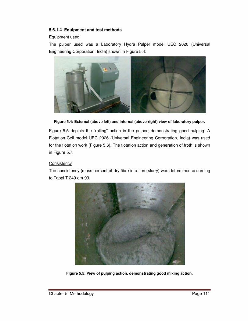
Chapter 5: Methodology Page 111
5.6.1.4 Equipment and test methods
Equipment used
The pulper used was a Laboratory Hydra Pulper model UEC 2020 (Universal
Engineering Corporation, India) shown in Figure 5.4:
Figure 5.4: External (above left) and internal (above right) view of laboratory pulper.
Figure 5.5 depicts the “rolling” action in the pulper, demonstrating good pulping. A
Flotation Cell model UEC 2026 (Universal Engineering Corporation, India) was used
for the flotation work (Figure 5.6). The flotation action and generation of froth is shown
in Figure 5.7.
Consistency
The consistency (mass percent of dry fibre in a fibre slurry) was determined according
to Tappi T 240 om-93.
Figure 5.5: View of pulping action, demonstrating good mixing action.

Chapter 5: Methodology Page 112
Figure 5.6: Laboratory flotation cell.
Figure 5.7: Laboratory flotation cell froth generation.
Pulp pads
Pulp pads were formed to determine the brightness of the pulped paper before
flotation (referred to as pulper pads) and after flotation (referred to as floated pads).
The pads were formed on the Rapid-Koethen sheet former, with the modification that
less dilution water was added (2 litres instead of 7 litres). This was based on the
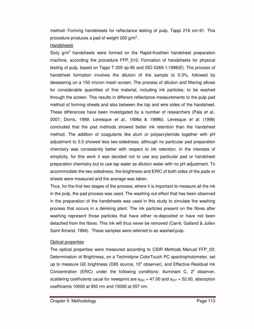
Chapter 5: Methodology Page 113
method: Forming handsheets for reflectance testing of pulp, Tappi 218 om-91. This
procedure produces a pad of weight 200 g/m2.
Handsheets
Sixty g/m2 handsheets were formed on the Rapid-Koethen handsheet preparation
machine, according the procedure FFP_015: Formation of handsheets for physical
testing of pulp, based on Tappi T 205 sp-95 and ISO 5269-1:1998(E). The process of
handsheet formation involves the dilution of the sample to 0.3%, followed by
dewatering on a 150 micron mesh screen. The process of dilution and filtering allows
for considerable quantities of fine material, including ink particles, to be washed
through the screen. This results in different reflectance measurements to the pulp pad
method of forming sheets and also between the top and wire sides of the handsheet.
These differences have been investigated by a number of researchers (Pala et al.,
2007; Dorris, 1999; Levesque et al., 1998a & 1998b). Levesque et al. (1998)
concluded that the pad methods showed better ink retention than the handsheet
method. The addition of coagulants like alum or polyacrylamide together with pH
adjustment to 5.5 showed less two-sidedness, although no particular pad preparation
chemistry was consistently better with respect to ink retention. In the interests of
simplicity, for this work it was decided not to use any particular pad or handsheet
preparation chemistry but to use tap water as dilution water with no pH adjustment. To
accommodate the two-sidedness, the brightness and ERIC of both sides of the pads or
sheets were measured and the average was taken.
Thus, for the first two stages of the process, where it is important to measure all the ink
in the pulp, the pad process was used. The washing out effect that has been observed
in the preparation of the handsheets was used in this study to simulate the washing
process that occurs in a deinking plant. The ink particles present on the fibres after
washing represent those particles that have either re-deposited or have not been
detached from the fibres. This ink will thus never be removed (Carré, Galland & Julien
Saint Amand, 1994). These samples were referred to as washed pulp.
Optical properties
The optical properties were measured according to CSIR Methods Manual FFP_03:
Determination of Brightness, on a Technidyne ColorTouch PC spectrophotometer, set
up to measure GE brightness (D65 source, 10o observer), and Effective Residual Ink
Concentration (ERIC) under the following conditions: illuminant C, 2o observer,
scattering coefficients usual for newsprint are s950 = 47.00 and s557 = 52.00, absorption
coefficients 10000 at 950 nm and 15000 at 557 nm.

Chapter 5: Methodology Page 114
The full range of optical properties were recorded on the pulped, floated and washed
pulps viz. brightness (UVex), UV brightness (UVin), lightness (L*), b* (blue-yellow) and
a* (red-green) and ERIC. However, only the brightness and ERIC on the final washed
pulp were used to generate the models, as this is the final output of the process.
There is a distinction between brightness and UV brightness. In the measurement of
UV brightness, the illuminant in the spectrophotometer has an ultraviolet light
component which fluoresces as blue light, thereby boosting the perceived brightness.
The UV brightness is thus always higher than the non-UV brightness if the paper
contains fluorescent whitening agents. However, the UV brightness is what the user of
a paper product will actually see and perceive, and was thus the brightness which was
modelled in this study.
5.6.2 Experimental design
When confronted with a large number of factors which could potentially influence a
process, it is essential to perform screening runs, in order to sift through the many
factors and eliminate those that have little or no influence on the process. In particular,
Plackett-Burman experimental designs have proven themselves to be efficient ways of
screening large numbers of variables in relatively few experimental runs. An 11-factor,
12-run Plackett-Burman design is depicted in Table 5.10. This design was adapted
from Barrentine (1999: 56). In this table, a “1” represents the high value of a variable,
and a “-1” represents the low value.

Chapter 5: Methodology Page 115
Table 5.10: A 12 run Plackett-Burman design, with reflection.
FACTORS OUTPUT
RUN NO. A B C D E F G H I J K Y S2
1 1 -1 1 -1 -1 -1 1 1 1 -1 1
2 1 1 -1 1 -1 -1 -1 1 1 1 -1
3 -1 1 1 -1 1 -1 -1 -1 1 1 1
4 1 -1 1 1 -1 1 -1 -1 -1 1 1
5 1 1 -1 1 1 -1 1 -1 -1 -1 1
6 1 1 1 -1 1 1 -1 1 -1 -1 -1
7 -1 1 1 1 -1 1 1 -1 1 -1 -1
8 -1 -1 1 1 1 -1 1 1 -1 1 -1
9 -1 -1 -1 1 1 1 -1 1 1 -1 1
10 1 -1 -1 -1 1 1 1 -1 1 1 -1
11 -1 1 -1 -1 -1 1 1 -1 -1 1 1
12 -1 -1 -1 -1 -1 -1 -1 1 -1 -1 -1
13 -1 1 -1 1 1 1 -1 -1 -1 1 -1
14 -1 -1 1 -1 1 1 1 -1 -1 -1 1
15 1 -1 -1 1 -1 1 1 1 -1 -1 -1
16 -1 1 -1 -1 1 -1 1 1 1 -1 -1
17 -1 -1 1 -1 -1 1 -1 1 1 1 -1
18 -1 -1 -1 1 -1 -1 1 -1 1 1 1
19 1 -1 -1 -1 1 -1 -1 1 -1 1 1
20 1 1 -1 -1 -1 1 -1 -1 1 -1 1
21 1 1 1 -1 -1 -1 1 -1 -1 1 -1
22 -1 1 1 1 -1 -1 -1 1 -1 -1 1
23 1 -1 1 1 1 -1 -1 1 1 -1 -1
24 1 1 1 1 1 1 1 -1 1 1 1
ΣY+
ΣY-
Yavg+
Yavg-
NET EFFECT
S+2 AVG
S-2 AVG
F
The runs 13 to 24, shaded in Table 5.10 are the “reflection” or inverse of the first 12
runs. Reflection makes it possible to determine the effect of the main variables free
from two-factor interactions (Barrentine, 1999:46). The control variables and
associated high and low values identified in Table 5.9 now become the experimental
design depicted in Table 5.11:

Chapter 5: Methodology Page 116
Table 5.11: Screening experimental design for control variables.
PULPING FLOTATION OUTPUT
A B C D E F G H I J K Y
RUN
NO. %
NaO
H
% S
od
S
ilic
ate
%H
2O
2
% S
urf
-p
t p,
min
Tp, d
eg
C
Tf, d
eg
C
% c
on
s
pH
% S
urf
-f
t f, m
in
1 0.67 0 1 0.25 5 35 45 1.3 10 0 20
2 0.67 2 0 0.75 5 35 30 1.3 10 0.5 5
3 0 2 1 0.25 15 35 30 0.8 10 0.5 20
4 0.67 0 1 0.75 5 50 30 0.8 8 0.5 20
5 0.67 2 0 0.75 15 35 45 0.8 8 0 20
6 0.67 2 1 0.25 15 50 30 1.3 8 0 5
7 0 2 1 0.75 5 50 45 0.8 10 0 5
8 0 0 1 0.75 15 35 45 1.3 8 0.5 5
9 0 0 0 0.75 15 50 30 1.3 10 0 20
10 0.67 0 0 0.25 15 50 45 0.8 10 0.5 5
11 0 2 0 0.25 5 50 45 1.3 8 0.5 20
12 0 0 0 0.25 5 35 30 0.8 8 0 5
13 0 2 0 0.75 15 50 30 0.8 8 0.5 5
14 0 0 1 0.25 15 50 45 0.8 8 0 20
15 0.67 0 0 0.75 5 50 45 1.3 8 0 5
16 0 2 0 0.25 15 35 45 1.3 10 0 5
17 0 0 1 0.25 5 50 30 1.3 10 0.5 5
18 0 0 0 0.75 5 35 45 0.8 10 0.5 20
19 0.67 0 0 0.25 15 35 30 1.3 8 0.5 20
20 0.67 2 0 0.25 5 50 30 0.8 10 0 20
21 0.67 2 1 0.25 5 35 45 0.8 8 0.5 5
22 0 2 1 0.75 5 35 30 1.3 8 0 20
23 0.67 0 1 0.75 15 35 30 0.8 10 0 5
24 0.67 2 1 0.75 15 50 45 1.3 10 0.5 20
ΣY+
ΣY-
Yavg+
Yavg-
NET EFFECT
For each run under the specified conditions, the outputs “Y” are the washed
brightness, washed ERIC and Yield. Ideally, a number of replicates of a design should
be carried out to determine the S2 for each run and each variable. This makes it
possible to calculate the statistical significance of the differences observed. However,

Chapter 5: Methodology Page 117
because of the large number of runs required for this project, replicates of the
screening designs were not performed. Instead, a number of midpoints were run, using
the average of the low and high values of the variables. The variance for the midpoint
runs gives an indication of the variability of the runs. The midpoints were also run at
intervals through each screening run, to detect any significant drift in the processes.

Chapter 6: Results of screening runs Page 118
CHAPTER 6: RESULTS OF SCREENING RUNS
6.1 Introduction
In the previous section, the possible control variables were summarised in Table 5.9.
As discussed in Section 5.6.2, a statistical experimental design procedure was used to
drastically reduce the number of experimental runs required to obtain meaningful
information on the independent effect of many different process parameters.
6.2 Results of screening runs – general trends
The general results of the screening runs are presented. Flotation time (tf) emerged
from the Plackett-Burman screening trials as one of the major determinants of overall
performance. Accordingly, the brightnesses, ERIC and yield as a function of flotation
time for the different grades are shown in Figures 6.1, 6.2 and 6.3 respectively. A
flotation time of zero was assigned to the brightnesses of the pulper sample. The
average brightness, ERIC and yield for all 24 runs of the Plackett-Burman design is
reported, at 5 minutes and 20 minutes flotation time. There was obviously a large
variability in the results, due to the high-low pattern in the experimental design.
Therefore, the averages only are reported for simplicity and the variability is depicted
by error bars showing plus and minus one standard deviation.
6.2.1 Dependence of brightness on flotation time
The large variability is a result of the high-low nature of the experimental design, but
serves to demonstrate the magnitude of the variability induced by the process
conditions as compared to that induced by paper grade, flotation time or processing
stage. The variability can be further appreciated in the cluster plots, Figures 6.6 to 6.9.
The brightness increased rapidly with flotation time (Figure 6.1), with the major
proportion of the ink was removed after 5 minutes. In the case of the heavy letter
grades, the increase in brightness was very small. The heavy letter grades nowadays
contain large proportions of lightly printed electrographic material (photocopy and laser
printed). It is well known that toner inks form large ink particles, which do not float very
well, unless they are reduced in size by further processing (usually dispersion) and
removed in a second flotation stage (Goettsching & Pakarinen, 2000:276). This was
observed on the laboratory hand sheets; the toner inks had agglomerated into large
dirt specks.

Chapter 6: Results of screening runs Page 119
Figure 6.1: Variation of brightness as a function of flotation time (Average of 24 Plackett-
Burman runs reported).
6.2.2 Dependence of ERIC on flotation time
The dependence of the 24 run average ERIC values on flotation time is shown in
Figure 6.2. The ERIC values for ONP and OMG undergo large changes and show
greater variability than those for HL1 and HL2, probably due to the fact that ONP and
OMG are more heavily printed than the office grades.
Figure 6.2: Variation of ERIC as a function of flotation time (Average of 24 Plackett-
Burman runs reported).
30
40
50
60
70
80
90
100
110
0 5 10 15 20 25
% B
RIG
HT
NE
SS
FLOTATION TIME t f (mins)
ONP
OMG
HL2
HL1
10
100
1000
0 5 10 15 20 25
ER
IC
FLOTATION TIME tf (mins)
ONP
OMG
HL2
HL1

Chapter 6: Results of screening runs Page 120
6.2.3 Dependence of yield on flotation time
The 24 run average yield decreased rapidly with flotation time (Figure 6.3), and
continued to decrease after about 5 minutes flotation time with no great improvement
in brightness.
Figure 6.3: Variation of yield as a function of flotation time (Average of 24 Plackett-
Burman runs reported) .
Yield and optical properties represent the trade-off between economy and quality that
has to take place in every deinking operation. The yield losses were highest for OMG,
due to the high level of filler both in the paper and as a component of the coatings
(Borchardt, 2003).
6.2.4 Variation of brightness and ERIC with processing stage.
As outlined in the experimental procedure, the waste was first pulped, then floated and
washed, in sequence. The brightness of all grades increased from pulping through
flotation to washing as shown in Figure 6.4. A 19 point overall increase in brightness
was observed with the OMG waste grades, almost double the 10 point increase for
ONP. The heavy letter grades again showed minimal brightness increases. A less
than 5 point overall increase in brightness was observed, with the HL2 waste grades
showing marginally greater increases than HL1.
30
40
50
60
70
80
90
100
110
0 5 10 15 20 25
YIE
LD %
FLOTATION TIME tf (mins)
OMG
HL1
HL2
ONP

Chapter 6: Results of screening runs Page 121
Also, the variability induced by the process variables (as indicated by the error bars) is
considerable compared to the changes caused by processing (flotation time in Figure
6.1, and processing stage in Figure 6.4). In other words, the error bars depict the
influence of the process variables whereas the y-axis differences between the grades
represent the influence that the different grades would have on the final brightness of a
mixture of grades. These differences can often be more significant than the effect of
the deinking process and this points to the significant potential of furnish composition
as a strong control variable.
Figure 6.4: Effect of processing stage on brightness.
It was apparent from Figure 6.4 that washing had a minimal but nevertheless positive
effect on the final brightness of all the grades.
The variation of ERIC with processing stage was the inverse of that found with the
brightness, as ERIC decreases as brightness increases (Figure 6.5). Similar
comments as made for brightness apply in the case of ERIC.
30
40
50
60
70
80
90
100
PULPER FLOATED WASHED
% B
rig
htn
ess ONP
OMG
HL1
HL2

Chapter 6: Results of screening runs Page 122
Figure 6.5: Effect of processing stage on ERIC.
6.2.5 The relationship between ERIC and brightness
Figures 6.6 to 6.7 depict the relationship, in the form of cluster-plots, between ERIC
(logarithmic scale) and brightness from pulping through to washing.
Haynes (2000) reported a linear relationship between the log of ERIC and brightness
above an ERIC value of 500, and another linear relationship below an ERIC value of
500, with a discontinuity of slope at 500. A roughly linear relationship is apparent from
Figures 6.6 to 6.8, with the exception of HL2 (Figure 6.9).
The strongest relationship between brightness and ERIC was demonstrated by the
newsprint grade (Figure 6.6) and HL1 (Figure 6.8). In general the scatter was highest
at the high brightness/low ERIC range, due to the cumulative effect of the variable
processing conditions.
The range of ERIC values at the pulping stage was always higher than the range of
brightness, presumably due to various types of ink, which fragmented differently in the
pulper. The fragmentation of ink in the magazine grade was more clustered (Figure
6.7) than the newsprint grade. This is presumably due to the coated component of the
magazines, which could be expected to fragment in a more reproducible fashion.
The HL 2 grade showed the least correlation between ERIC and brightness,
presumably because this grade was the most variable in terms of type of printing and
coloured constituents. A stronger relationship between brightness and ERIC was
shown by the HL1. The scatter was similar for all of the processing stages.
10
100
1000
PULPER FLOATED WASHED
ER
IC
ONP
OMG
HL1
HL2

Chapter 6: Results of screening runs Page 123
Figure 6.6: Cluster plot of brightness vs. ERIC for newsprint.
Figure 6.7: Cluster plot of brightness vs. ERIC for magazines.
30.0
35.0
40.0
45.0
50.0
55.0
100 1000
BR
IGH
TN
ES
S %
ERIC
PULPED
FLOATED
WASHED
30.0
35.0
40.0
45.0
50.0
55.0
60.0
65.0
70.0
75.0
50 500
BR
IGH
TN
ES
S %
ERIC
PULPED
FLOATED
WASHED

Chapter 6: Results of screening runs Page 124
Figure 6.8: Cluster plot of brightness vs. ERIC for heavy letter 1.
Figure 6.9: Cluster plot of brightness vs. ERIC for heavy letter 2.
80.0
85.0
90.0
95.0
100.0
105.0
10 100
Bri
gh
tne
ss %
ERIC
PULPED
FLOATED
WASHED
30.0
40.0
50.0
60.0
70.0
80.0
90.0
100.0
10 100
Bri
gh
tne
ss %
ERIC
PULPED
WASHED
FLOATED

Chapter 6: Results of screening runs Page 125
6.3 Variability and drift
Throughout a screening design of 24 runs, replicates of midpoint runs (viz. all inputs
are at their central values) were performed at random intervals, to determine the
stability of the pulping and flotation procedures. The results for the trends in the
midpoints of the four screening runs are shown in Figure 6.10. The coefficients of
variation (CV = standard deviation/mean x100) were the highest in the HL2 runs at
4.3%, and trended upwards slightly in the HL1 run. This is most likely due to the raw
material changing slightly through the run.
Figure 6.10: Variability and drift of final brightness.
The relatively flat trends in figure 6.10 indicate fairly constant conditions within the
different runs.
6.4 Correlation between UV included (UVin) and UV excluded (UVex) brightness Paper grades contain varying quantities of fluorescent whitening or optical brightening
chemicals. Newsprint contains no optical brighteners and high brightness office papers
(HL1) contain large quantities. These chemicals absorb UV radiation and re-emit it in
the blue region of the spectrum, thereby artificially boosting the perceived brightness of
a sheet of paper. These chemicals are typically stilbenes, which can be substituted
with 3 to 6 sulphonate groups, and are generally substantive (adhere chemically to the
cellulose fibres). Fluorescent whitening agents are not significantly broken down by
40
50
60
70
80
90
100
0 5 10 15 20 25 30
WA
SH
ED
BR
IGH
TN
ES
S
RUN DAYS
ONP
OMG
HL1
HL2
CV = 4.3%
CV = 1.15%
CV = 1.45%
CV = 2.75%

Chapter 6: Results of screening runs Page 126
hydrogen peroxide (Section 2.9), and thus remain in the recycled fibre. In the
screening trials, very close correlations were observed between the UVin and UVex
brightness for all the grades which contained optical brighteners (Figure 6.11).
Figure 6.11: Correlation between final washed UVin and UVex for HL1, HL2 and OMG.
There was a substantial difference in the UVin and UVex brightness of HL1, but they
were closely correlated (Figure 6.11). This confirmed that the optical brighteners were
not acted upon by the bleaching or deinking processes. In this work, the UVin
brightness was used as the final measure, as it represents more closely what the end
user of recycled paper will observe.
6.5 Results of screening runs – net effect of variables
6.5.1 Newsprint
The results of the screening runs with the associated calculation of the net effect of the
various variables and waste paper grades are shown in Appendix 1A-D. A Pareto
analysis of the net effects of the variables on the final washed brightness, washed
ERIC and yield is depicted in Figures 6.12 to 6.14 below. Square brackets ([….])
indicate variables that have an adverse effect on the final property, viz. a drop in
brightness or yield or an increase in ERIC.
R² = 0.964
R² = 0.961
R² = 0.985
50.0
55.0
60.0
65.0
70.0
75.0
80.0
85.0
90.0
95.0
100.0
50 60 70 80 90 100
% B
rig
htn
ess, U
V in
clu
ded
% Brightness, UV excluded
HL1
OMG
HL2
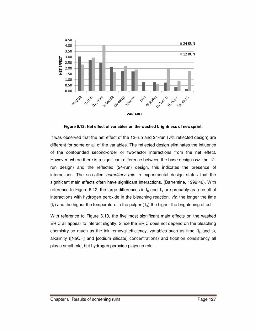
Chapter 6: Results of screening runs Page 127
Figure 6.12: Net effect of variables on the washed brightness of newsprint.
It was observed that the net effect of the 12-run and 24-run (viz. reflected design) are
different for some or all of the variables. The reflected design eliminates the influence
of the confounded second-order or two-factor interactions from the net effect.
However, where there is a significant difference between the base design (viz. the 12-
run design) and the reflected (24-run) design, this indicates the presence of
interactions. The so-called hereditary rule in experimental design states that the
significant main effects often have significant interactions. (Barrentine, 1999:46). With
reference to Figure 6.12, the large differences in tp and Tp are probably as a result of
interactions with hydrogen peroxide in the bleaching reaction, viz. the longer the time
(tp) and the higher the temperature in the pulper (Tp) the higher the brightening effect.
With reference to Figure 6.13, the five most significant main effects on the washed
ERIC all appear to interact slightly. Since the ERIC does not depend on the bleaching
chemistry so much as the ink removal efficiency, variables such as time (tp and tf),
alkalinity ([NaOH] and [sodium silicate] concentrations) and flotation consistency all
play a small role, but hydrogen peroxide plays no role.
0.00
0.50
1.00
1.50
2.00
2.50
3.00
3.50
4.00
4.50
NE
T E
FF
EC
T
VARIABLE
24 RUN
12 RUN

Chapter 6: Results of screening runs Page 128
Figure 6.13: Net effect of variables on washed ERIC of newsprint.
Factors which affect the flotation of fibres rather than ink seem to play a role in
determining the yield. Figure 6.14 indicates that the main variables influencing fibre
yield were flotation conditions (tf and consistency) and to a lesser extent sodium
hydroxide concentration and surfactant concentrations (Surf-f and Surf-p).
Figure 6.14: Net effect of variables on the yield of newsprint.
6.5.2 Magazines
Similarly, the Pareto analysis of the main variables affecting the deinking of magazine
waste are shown in Figures 6.15 to 6.17. In general terms, the variables had similar
effects for both newsprint and magazine waste. The ERIC was not influenced by the
1.00
10.00
100.00
1000.00
NE
T E
FF
EC
T
VARIABLE
24 RUN
12 RUN
0.00
2.00
4.00
6.00
8.00
10.00
12.00
14.00
16.00
18.00
20.00
NE
T E
FF
EC
T
VARIABLE
24 RUN
12 RUN

Chapter 6: Results of screening runs Page 129
concentration of hydrogen peroxide or bleaching chemistry, because ERIC is a direct
measure of ink, irrespective of the underlying brightness of the paper substrate.
Figure 6.15: Net effect of variables on the washed brightness of magazine papers.
Figure 6.16: Net effect of variables on the washed ERIC of magazine papers.
0.00
0.50
1.00
1.50
2.00
2.50
3.00
3.50
NE
T E
FFE
CT
24 RUN
12 RUN
0.00
10.00
20.00
30.00
40.00
50.00
60.00
70.00
NE
T E
FFE
CT
VARIABLE
24 RUN
12 RUN

Chapter 6: Results of screening runs Page 130
Figure 6.17: Net effect of variables on the yield of magazine papers.
6.5.3 Heavy Letter 1 (HL1)
The Pareto analysis for heavy letter 1 is shown in Figures 6.18 to 6.20.
With reference to Figure 6.18, the process residence time (as given by pulping time tp
and flotation time tf) plays a large role in determining the final brightness, as does the
alkalinity (combination of sodium silicate and sodium hydroxide). Hydrogen peroxide
seems to play a lesser role, probable due to the already very high base brightness of
Xerographic papers.
Figure 6.18: Net effect of variables on the washed brightness of HL1.
0.00
2.00
4.00
6.00
8.00
10.00
12.00
14.00
16.00
NE
T E
FF
EC
T
VARIABLE
24 RUN
12 RUN
0.00
0.50
1.00
1.50
2.00
2.50
3.00
3.50
4.00
4.50
5.00
NE
T E
FF
EC
T
VARIABLE
24 RUN
12 RUN

Chapter 6: Results of screening runs Page 131
The influence of pulping temperature (Tp) in deinking of office paper grades agrees
with Berg et al. (1997), who found that higher temperatures close to or above the
softening points of the toner particles facilitated the detachment of toner from fibres.
The prominent role of sodium hydroxide and its effect on ink fragmentation was also
evident.
Figure 6.19: Net effect of variables on the washed ERIC of HL1.
Not surprisingly, the hydrogen peroxide concentration is not a significant factor. In fact
the data suggests that it plays a slightly negative role on the ERIC, which is not easy to
explain.
Figure 6.20: Net effect of variables on the yield of HL1.
0.00
5.00
10.00
15.00
20.00
25.00N
ET
EF
FE
CT
VARIABLE
24 RUN
12 RUN
0.00
1.00
2.00
3.00
4.00
5.00
6.00
7.00
8.00
NE
T E
FFE
CT
VARIABLE
24 RUN
12 RUN

Chapter 6: Results of screening runs Page 132
Factors which affect the flotation of fibres rather than ink seem to play a role in
determining the yield. Figure 6.20 indicates that the main variables influencing fibre
yield were alkalinity (NaOH and sodium silicate) and flotation conditions (tf and
consistency). As expected, hydrogen peroxide played a minimal role.
6.5.4 Heavy Letter 2 (HL2)
The Pareto analyses of the main variables affecting the deinking of HL2 are shown in
Figures 6.21 to 6.23. The effect of pulping temperature (Tp) on brightness was
prominent for this grade, again due to its role in the fragmentation of the electrographic
inks found on this type of paper. A higher pulping temperature also benefited the
bleaching reaction. HL2 has a lower base brightness than HL1, and thus hydrogen
peroxide was seen to have a greater effect on the brightness.
Figure 6.21: Net effect of variables on the washed brightness of HL2.
With respect to the ERIC of HL2 (Figure 6.22), hydrogen peroxide continued to play a
negligible role, with flotation conditions (consistency and time tf) dominating.
0.00
1.00
2.00
3.00
4.00
5.00
6.00
7.00
8.00
NE
T E
FF
EC
T
VARIABLE
24 RUN
12 RUN

Chapter 6: Results of screening runs Page 133
Figure 6.22: Net effect of variables on the washed ERIC of HL2.
A different set of variables affected the yield of HL2 (Figure 6.23). Flotation conditions
(consistency and time) now dominated and alkalinity has become less influential.
Figure 6.23: Net effect of variables on the yield of HL2.
0.00
2.00
4.00
6.00
8.00
10.00
12.00
14.00
16.00
18.00
20.00
NE
T E
FF
EC
T
VARIABLE
24 RUN
12 RUN
0.00
2.00
4.00
6.00
8.00
10.00
12.00
14.00
16.00
18.00
NE
T E
FF
EC
T
VARIABLE
24 RUN
12 RUN

Chapter 6: Results of screening runs Page 134
6.6 Selection of control variables
The objective of this work was not so much to identify and explain all the interactions
that take place in a deinking system, but rather to identify the global variables most
influential in producing the main effects and then model the output. In order to select
the best combination of potential control variables, a factor ranking analysis was
carried out. The variable or factor responsible for the greatest net effect in each case
was assigned the rank of 1, intermediate factors were assigned ranks of 2 to 10 and
the factor with the least effect was assigned a rank of 11. The outputs for which factors
were ranked were washed brightness, washed ERIC and the yield. For each factor the
mean, greatest (1) and least (11) rank across all of the waste paper grades and all
outputs was calculated and arranged in ascending order. The order of priority for the
ranking was taken as greatest rank first followed by mean rank. These calculations are
shown in Appendix 2, and summarized in Figure 6.24.
Figure 6.24: Ranking of control variables – greatest influence-MEAN-least influence.
It can be seen from Figure 6.24 that the flotation pH, surfactant concentration in the
float cell (%Surf-f), the flotation temperature (Tf) and pulping time (tp) are the least
ranked variables on average. Their greatest ranking was only 3-4.
Energy constraints and the requirement for heat transfer equipment make the
temperature an uneconomical control variable. In addition, the effect of temperature in
flotation was small. Thus temperature was eliminated as a practical control variable.
However, in some instances Tp (in the case of HL2 brightness, HL1 ERIC and OMG
ERIC) was a factor which showed significant influence. In these cases the Tp can be
0
2
4
6
8
10
12
FAC
TO
R R
AN
K

Chapter 6: Results of screening runs Page 135
considered an important optimisation variable, whilst not being suitable for process
control purposes.
The pulping time (tp) appeared to have a small influence on the outcome of deinking.
This is in agreement with the discussion in Section 2.2.4.
Flotation pH and surfactant concentrations, particularly in the flotation cell in the float
cell were deemphasized in terms of data collection, especially as no surfactant is
added into the float cells in the three deinking mills under study.
In addition to the grade of recycled paper, the remaining variables viz. flotation
conditions (time and consistency), alkalinity (sodium hydroxide and sodium silicate)
and bleaching are the most practical and influential variables to control the de inking
process.
.

Chapter 7: Generation of Laboratory Data Page 136
CHAPTER 7: GENERATION OF LABORATORY DATA
7.1 Introduction
A combination of a statistically designed screening process, a ranking analysis and
practical considerations resulted in the elimination of pulping temperature, flotation
temperature and surfactant addition in the flotation cell as influential parameters in the
deinking process. This resulted in a shortened list of modelling parameters, listed in
descending order of ranking of effect:
• Flotation time
• Flotation consistency
• NaOH addition level
• H2O2 addition level
• Sodium silicate addition level
• Surfactant addition to the pulper
• Pulping time
• Flotation pH
These parameters were varied, in conjunction with the four grades of recycled paper in
varying proportions to generate data for the training of a neural network model.
Excluding the four grades of waste paper, eight possible control variables remained
under consideration.
7.2 Methodology
The four grades of recycled paper formed a “mixture”, which means that the sum total
of all the components must total 100%. A four-component mixture can be represented
in a tetrahedral mixture space, which will correspond to all possible proportions of
waste that add up to 100%. With reference to Figure 7.1, the single components are
represented by the corners of the tetrahedron. Two-component mixtures are
represented along the edges of the tetrahedron, three-component mixtures fall on the
surfaces and four component mixtures will fall within the body of the tetrahedron.
(Brereton, 2006: 86)

Chapter 7: Generation of Laboratory Data Page 137
Figure 7.1: Mixture space for four recycled paper grades.
Accordingly, the percentage waste mixes depicted in Table 7.1 were run.
For each of these mixtures, about 15 runs were performed in which the eight variables
listed in Section 7.1 were varied randomly (using the random number function RAND()
in Excel), and the remainder were held constant. The ranges of variation were
modified due to practical reasons. The new ranges are summarized in Table 7.2.
In addition to these mixtures, a number of ONP/OMG 25:75, ONP/OMG 75:25,
HL1/HL2 25:75 and HL1/HL2 75:25 blends were run, to provide more data for the
specific industrial processes of newsprint deinking and office waste deinking.
Thereafter, numerous runs (denoted as Test1 to Test60) were carried out in which all
variables (waste grades and process parameters) were varied randomly within the
limits given in Table 7.2. In addition, a Plackett-Burman design on a
ONP/OMG/HL1/HL2 25:25:25:25 waste mix was run, denoted as ALL1 to ALL24.
Finally Mix1 to Mix40 were run at a higher flotation consistency, as the plants were
running higher consistencies than the original consultations had indicated. The
brightness, ERIC and yields were determined as described in Chapter 5.

Chapter 7: Generation of Laboratory Data Page 138
Table 7.1: Waste mixture experimental design.
WASTE GRADE
MIX ONP OMG HL1 HL2
Plackett-Burman ONP
100 0 0 0
Plackett – Burman OMG
0 100 0 0
Plackett – Burman HL1
0 0 100 0
Plackett – Burman
HL2 0 0 0 100
ONP/OMG 50:50 50 50 0 0
ONP/HL1 50:50 50 0 50 0
ONP/HL2 50:50 50 0 0 50
OMG/HL1 50:50 0 50 50 0
OMG/HL2 50:50 0 50 0 50
HL1/HL2 50:50 0 0 50 50
ONP/OMG/HL1 33:33:33
33.3 33.3 33.3 0
ONP/OMG/HL2 33:33:33
33.3 33.3 0 33.3
ONP/HL1/HL2 33:33:33
33.3 0 33.3 33.3
ONP/OMG/HL2 33:33:33
33.3 33.3 0 33.3
OMG/HL1/HL2 33:33:33
0 33.3 33.3 33.3
ONP/OMG/HL1/HL2 25:25:25:25
25 25 25 25

Chapter 7: Generation of Laboratory Data Page 139
Table 7.2: Modified ranges of deinking parameters with reasons for changes.
Variable Plackett-Burman range
Modified range
Reason for change
ONP 100 0; 25; 33; 50; 75; 0-100
Mixing design and randomly varied
OMG 100 0; 25; 33; 50; 75; 0-100
Mixing design and randomly varied
HL1 100 0; 25; 33; 50; 75; 0-100
Mixing design and randomly varied
HL2 100 0; 25; 33; 50; 75; 0-100
Mixing design and randomly varied
%NaOH 0 7 & 0.67 0 – 1.5 Extended to include greater variability
% Sodium silicate 0 & 2 0 - 3 Extended to include greater variability
% H2O2 0 & 1 0 - 2 Extended to include greater variability
%Surfactant in pulper
0.25 & 0.75 0.25 – 1.0 Extended to include greater variability
Pulping time, mins 5 & 15 5 - 15
Pulping temperature,
⁰C 35 & 50 43 Eliminated as control variable,
maintained constant
Flotation
temperature, ⁰C 30 & 45 38 Eliminated as control variable,
maintained constant
Flotation consistency, %
0.8 & 1.3 0.8 – 1.3
Flotation pH 8 & 10 7 -10 Extended to include greater variability
% Surfactant in flotation cell
0 & 0.5 0 – 0.25 De-emphasized as a control variable, only a few variations run
Flotation time, mins 5 & 20 2 - 12 Reduced, very little change in 12-15 min. range.

Chapter 7: Generation of Laboratory Data Page 140
7.3 Results
A total of 490 deinking runs were carried out, as per the methodology described in
Section 7.2. The raw material inputs, process variables and outputs are detailed in
Appendix 3.
Interspersed with the deinking runs were midpoint runs for the four base recycled
paper grades. Figures 7.2 to 7.5 depict the midpoint results for the four base grades
across all the main properties measured. Statistics for the midpoint runs are
summarized in Table 7.3. The statistics are presented for the Plackett-Burman runs in
Chapter 6 and the total data base of Chapter 7.
A logarithmic scale was used for the y-axis, to accommodate the large range in the
data and to enhance visibility.
Figure 7.2: Variability and drift in ONP results (Brightness & Yield in %, Eric in ppm).
10.0
100.0
1000.0
% B
rig
htn
ess
or
ER
IC
Date
PULPER BRT
WASHED BRT
PULPER ERIC
WASHED ERIC
YIELD

Chapter 7: Generation of Laboratory Data Page 141
Figure 7.3: Variability and drift in OMG results (Brightness & Yield in %, Eric in ppm).
Figure 7.4: Variability and drift in HL1results (Brightness & Yield in %, Eric in ppm).
10.0
100.0
1000.0
% B
rig
htn
ess
or
ER
IC
Date
PULPER BRT
WASHED BRT
PULPER ERIC
WASHED ERIC
YIELD
10.0
100.0
% B
rig
htn
ess
or
ER
IC
Date
PULPER BRT
WASHED BRT
PULPER ERIC
WASHED ERIC
YIELD
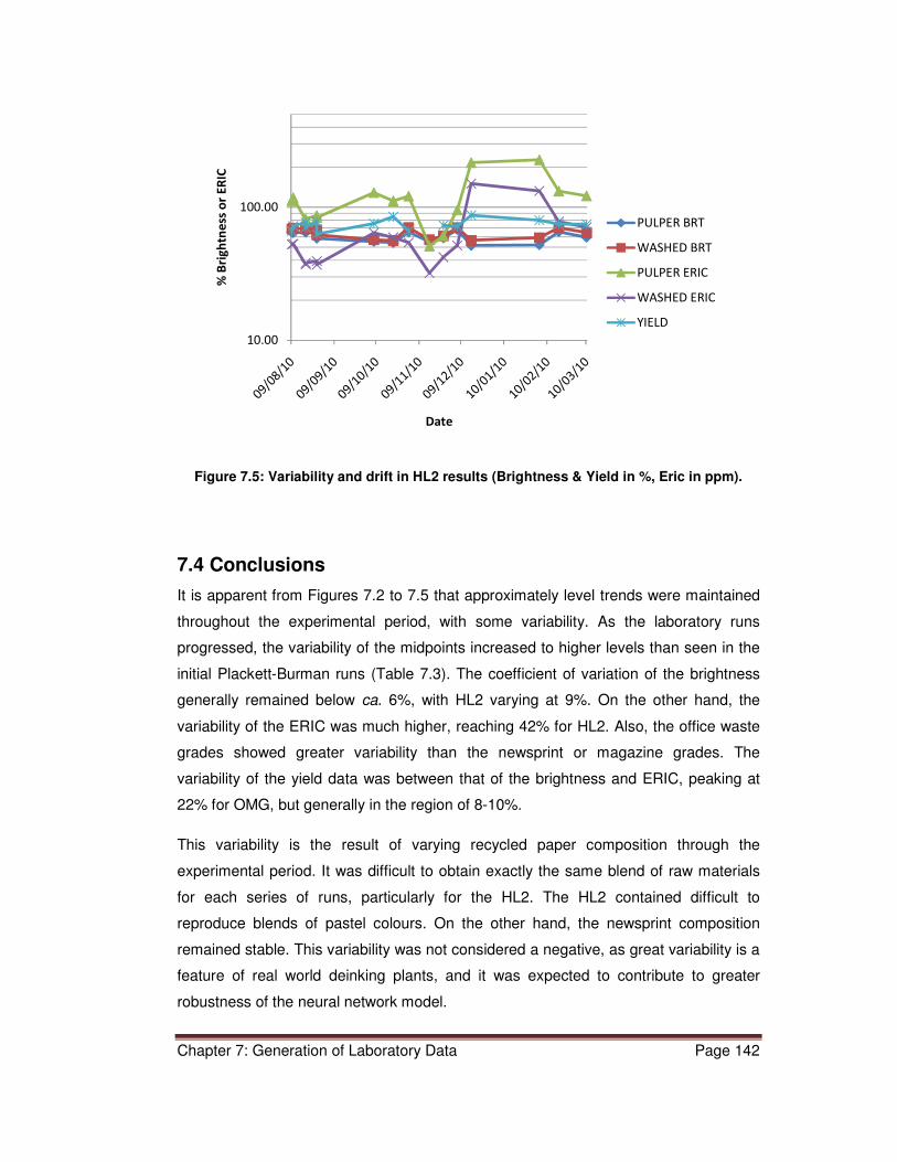
Chapter 7: Generation of Laboratory Data Page 142
Figure 7.5: Variability and drift in HL2 results (Brightness & Yield in %, Eric in ppm).
7.4 Conclusions
It is apparent from Figures 7.2 to 7.5 that approximately level trends were maintained
throughout the experimental period, with some variability. As the laboratory runs
progressed, the variability of the midpoints increased to higher levels than seen in the
initial Plackett-Burman runs (Table 7.3). The coefficient of variation of the brightness
generally remained below ca. 6%, with HL2 varying at 9%. On the other hand, the
variability of the ERIC was much higher, reaching 42% for HL2. Also, the office waste
grades showed greater variability than the newsprint or magazine grades. The
variability of the yield data was between that of the brightness and ERIC, peaking at
22% for OMG, but generally in the region of 8-10%.
This variability is the result of varying recycled paper composition through the
experimental period. It was difficult to obtain exactly the same blend of raw materials
for each series of runs, particularly for the HL2. The HL2 contained difficult to
reproduce blends of pastel colours. On the other hand, the newsprint composition
remained stable. This variability was not considered a negative, as great variability is a
feature of real world deinking plants, and it was expected to contribute to greater
robustness of the neural network model.
10.00
100.00
% B
rig
htn
ess
or
ER
IC
Date
PULPER BRT
WASHED BRT
PULPER ERIC
WASHED ERIC
YIELD

Chapter 7: Generation of Laboratory Data Page 143
These results formed the data base for the training of the neural networks.
Table 7.3: Statistics for the midpoints of the base grades.
Grade Experimental
design Statistics Pulper
bright %
Washed bright.
%
Pulper ERIC, ppm
Washed ERIC, ppm
Yield %
ONP
Plackett-Burman
Mean 38.5 51.5 1098 287 71.5
Standard deviation 0.6 0.6 33 16 5.6
Coefficient of variation % 1.5 1.1 3 5 7.9
Overall
Mean 38.9 51.9 1117 314 71.4
Standard deviation 1.3 0.8 113 84 11.8
Coefficient of variation % 3.4 1.5 10 27 16.5
OMG
Plackett-Burman
Mean 44.1 65.7 643 69 47.5
Standard deviation 1.3 1.0 68 5 5.0 Coefficient of variation % 2.9 1.5 11 7 10.5
Overall
Mean 44.0 64.6 664 83 53.3
Standard deviation 1.9 2.9 107 29 11.8 Coefficient of variation % 4.3 4.5 16 34 22.1
HL1
Plackett-Burman
Mean 88.0 92.6 123 78 86.8
Standard deviation 4.5 2.5 24 10 8.6 Coefficient of variation % 5.1 2.7 20 13 9.9
Overall
Mean 93.9 96.7 106 58 87.0
Standard deviation 5.3 3.8 29 21 5.9 Coefficient of variation % 5.7 3.9 27 37 6.8
HL2
Plackett-Burman
Mean 63.6 67.7 94 43 71.1
Standard deviation 2.6 2.9 17 8 5.9
Coefficient of variation % 4.1 4.3 18 18 8.3
Overall
Mean 60.4 64.2 114 62 74.3
Standard deviation 5.4 5.7 48 34 6.6
Coefficient of variation % 9.0 8.9 42 54 8.9

Chapter 8: Training of Neural Networks Page 144
CHAPTER 8: NEURAL NETWORK MODELLING OF LABORATORY DATA
8.1 Introduction
Neural network projects are akin to information technology projects in terms of their
development. Neural networks are data driven and typically need large quantities of
data to effectively model large complex systems (Tarassenko, 1998). The amount of
data that had been collected (490 inputs) was limited due to time and resource
constraints. The challenge in this particular case was to obtain the best possible
network with the data available.
In terms of Equation 10 in Section 4.4.5, the ideal number of input vectors P, should
lie between W and 10W:
W = (I + 1)J + (J+1)K (10)
Where I = number of inputs, J = number of hidden neurons and K = number of outputs.
In order to make optimum use of the 490 (=P) training vectors available, K was
restricted to 1 output, and I was minimized by training the network with only those
variables which have the most significant effects on the process. Restricting K to 1
meant that the properties of brightness, ERIC and yield were modelled separately
using the same data set. The number of neurons in the NN model (J) was selected so
as to produce the highest performance.
8.2 Software
A commercial software package, MATLAB Version R2009a was used to implement the
neural network model of the laboratory deinking data. Notwithstanding the general
principles of neural networks outlined in Chapter 4, the specific terminology and
methodology as implemented in the MATLAB package was used. This is discussed in
Section 8.3.

Chapter 8: Training of Neural Networks Page 145
8.3 Training using MATLAB
8.3.1 General methodology
The application in question was that of function fitting, and it has been found that a
feed-forward network structure with one hidden layer and an output layer is capable of
approximating any function (Demuth et al., 2009). In particular, the hidden layers
typically contain the tan-sigmoid transfer (or activation) function and the output layer
commonly contains a linear transfer function (Section 4.4.2).
The number of input layers corresponds to the number of variables in the input vector,
and the number of output layers corresponds to the number of outputs. In this work, a
single output layer was chosen as explained in Section 8.1. The number of neurons
required was to be determined by iteration. The greater the number of neurons, the
more complex is the function which can be approximated. On the other hand, more
neurons require more data which can also lead to over-fitting of a function (Demuth et
al., 2009:1-8).
The MATLAB neural network toolbox makes use of the following default settings and
procedures for training networks for function fitting:
• The input vectors are divided randomly upon initialisation into three sets as
follows: 70% of the data for training; 15% of the data for validation and 15% for
independent testing.
• The network is initialized with random values close to zero and the data is
presented as a batch a.k.a. batch training (Figure 8.1 and Section 4.6.3).
• The performance of the network is determined by computing the mean-square-
error (MSE) of all the sets.
• The MSE of the validation and test sets typically decrease to a minimum and
then increase again. However, the MSE of the training set continues to
decrease as training proceeds. The network is approximating the data more
and more closely, and gets to a point where the data is memorized. This is
referred to as over-fitting, illustrated in Figure 4.9. Unfortunately the result of
over-fitting is that the underlying trends are compromised, and the network will
no longer predict well (poor generalisation) with unseen data (Demuth et al.,
2009). Thus, once the validation set has increased for six iterations, the training

Chapter 8: Training of Neural Networks Page 146
is stopped (early stopping) and the network weights at the minimum point are
retained as the final weights for the trained network (Figure 4.8 and Figure 8.2).
• Once the training is complete, the regressions of the training, validation and
test sets are calculated and displayed (Figure 8.3).
Figure 8.1: MATLAB training window, showing training parameters. (Demuth et al.,
2009:1-9)
Neural Network
Alyor iU IIIIS
Tralnln;;J: Levenberg-Mar::Juardt (rralrlrr) PErformance: Mean Squcre:J Error (mse) Dats Divsion: Rsndom ~jivider3rd)
Progress
Fror.h: 0 7~ i~P.r!lHo'"ls ·onr. nme: o:oo:o"' Performance: 3.32e+03 3.84 0.00
Gracient :.00 10.5 :.ooe-10
Mu: 0.00100 O.lO:l :.OOe+lO
"J!'Jirl~mn l.he.rxs: 0 F, 6
Plots
I Perbrman:e (plolp~r'orm)
Trainin;~ State (plottr!lins·!l~P.:
Fit (plotfit)
~.egressicn (plotregressior)
m 1 P.'1Cor.hs Plot lll:ervdl: Y, ...... .......................................... .
.., Validation stop.
eStop T·aning e ::ancel

Chapter 8: Training of Neural Networks Page 147
Figure 8.2: Example of plot of performance of training, validation and test sets,
demonstrating early stopping. (Demuth et al., 2009: 1-10)
The phenomenon of the error associated with the validation set increasing after the
optimum stopping point has been discussed in Section 4.6.4.2.

Chapter 8: Training of Neural Networks Page 148
Figure 8.3: Example of plots of regression of a training session. (Demuth et al., 2009: 1-
10)
At this point the training information and the neural network can be saved and inputted
with other real data to produce a predicted output. If the performance of the network is
not adequate, a number of possibilities exist (Demuth et al., 2009: 1-10):
• The network can be reset or initialized with new initial weights and biases and
retrained,
• The number of neurons can be increased or decreased,
• More data can be added to the training set,
• Change the number of input values,
• The ratio of data in training, validation and test sets can be changed,

Chapter 8: Training of Neural Networks Page 149
• Try alternate learning and training algorithms.
• Pre-processing of inputs and outputs
It is obvious from the above that training of a neural network was a highly iterative
process, with many parameters that could be manipulated to produce the desired
result. There are no hard and fast rules, and experience plays a role. Arriving at the
final “best” network has been likened to cooking (Hajek, 2010), where a good recipe
has to be found by trial and error.
8.3.2 Specific training options used
8.3.2.1 Network initialisation
Each time the network is initialised, different initial parameters are introduced which
might produce a different final solution. Thus with the same network structure and
input data a number of different solutions can be obtained purely by re-initializing and
retraining. It was found that the first training attempt could generally be improved upon,
but after three or four initializations the training performance started to decrease.
8.3.2.2 The number of neurons and layers
An increasing number of neurons will give the network more power to approximate the
function. However, too many neurons will lead to over-fitting and poor generalisation
(Demuth et al., 2009:5-52). In addition, more neurons will require more data as
discussed in Section 8.1, a shortage of which could lead to under-characterization of
the function (Demuth et al., 2009:5-6).
It was found in this work that low numbers of neurons (1 to 3) generally lead to linear
functions, more neurons (3 to 5) produced curve-linear functions and more neurons
(> 5) tended to produce complex, over-fitted functions. However, the use of Bayesian
Regularisation (Section 8.3.2.6) tended to reduce the tendency of networks to over-fit.
In addition to the number of neurons, the number of hidden layers could also be
increased, to allow the network to respond to complex functions. This will of course
require even more data. This was attempted in this work but did not improve
generalisation. As in polynomial fitting, the network should have fewer parameters
(weights and biases) than data points in the training set. Thus the practice is to use the
simplest network that adequately describes the data (Hagan et al., 1996:11-23).

Chapter 8: Training of Neural Networks Page 150
8.3.2.3 Addition of data
As with polynomial fitting, more data will allow more neurons to be used and better
generalisation to be achieved. The data in this work was limited to 490 training vectors,
due to time and resource constraints.
8.3.2.4 The number of input values
The number of input values could not be arbitrarily reduced, but had to be done with
due consideration of the effect of the different parameters on the final outcome. Thus,
the process of selecting the initial number of input values was informed by the results
of the Plackett-Burman designs, where only those process parameters which have a
consistent and significant effect on the final properties were selected. These
experimental designs were useful as a first step, but could not be expected to predict
the behaviour of the system in complex mixtures of four different waste grades. The
process of evaluating the neural networks (see Section 8.6) revealed that certain
parameters were not consistently reliable in influencing the process and were thus
eliminated. This resulted in a further reduced number of input variables.
8.3.2.5 The ratio of data in training, validation and test sets
Initial work was carried out using the default split of training:validation:test::70:15:15.
As more data became available, the split was changed to 80:15:5, and an additional
test set of 40 vectors, drawn from the database of 441 vectors and common to all
training runs was employed. This facilitated a comparison of networks by using the
same test set for all networks.
The training, validation and test data sets were divided randomly in the ratios specified
above, for all training runs.
8.3.2.6 Learning and training algorithms
Data structure
There are two types of input data structure: concurrent input vectors are presented to
the network at the same time in no particular time sequence, and sequential input
vectors, which are presented one at a time, in a particular order.
Static networks (where there are no feedback loops or delays) are commonly trained
with concurrent data, whereas dynamic networks are trained with sequential data,
where the order of data presentation is important. In a processing environment, neural

Chapter 8: Training of Neural Networks Page 151
networks which undergo continual training with live plant data would be dynamic in
nature. For the current work, a static network was used. (Demuth et al., 2009:2-14)
Training styles
In incremental training the weights and biases of a neural network are updated each
time an input vector is presented to the network, whereas in batch training all the input
vectors are presented and the weights and biases are then updated. Incremental
training is commonly used to train dynamic networks, although incremental training
can also be applied to static networks (Demuth et al., 2009:2-20). This can assist to
alleviate the problem of converging to local minima in back propagation training
(Hajek, 2010). In the current work, because a static network was being trained, batch
training was used.
Training algorithms
MATLAB presents many different methods of mathematically implementing back-
propagation by gradient descent. The Levenberg-Marquardt method of back-
propagation by gradient decent has been shown to be fast and accurate for function
approximation type problems for networks with less than one hundred weights, and
has thus been used in this work. A disadvantage of the Levenberg-Marquardt
algorithm is that it requires a large amount of computer memory (Demuth et al.,
2009:5-50, Hagan et al., 1996:12-27), which was however not a constraint in this work.
Prevention of over-training
The early stopping procedure described in Section 8.3.1 was used for all training.
Performance functions
The default performance function is the mean square error (mse), which is defined as
the difference between the network output and the target output, squared and
summed. This function was used in the early training exercises. However, this was
modified in later training runs by invoking regularisation. In regularisation, a
performance term consisting of a combination of the mean squared sum of the network
weights and biases (msw) and the mean square error (mse) is used, as follows:

Chapter 8: Training of Neural Networks Page 152
� ���� = �. � � + (1 – �). � � (1)
where γ is termed the performance ratio.
This function tends to reduce the weights and biases in the network itself, resulting in a
smoother response with less likelihood of over-fitting. There is some guesswork
involved in the selection of the performance ratio. If γ is too close to 1 then the
performance function will essentially be mse, and if it is too low msw will dominate and
generalization will be poor. The MATLAB default of γ = 0.5 was used. An advanced
technique called Bayesian Regularisation has been implemented in MATLAB, which
chooses the optimum value for γ (Demuth et al., 2009:5-56). This technique was used
in the final phases of training.
8.3.2.7 Pre-processing
By default, MATLAB applies the following processing functions to data and outputs:
• Unknown input values are re-encoded into numerical values. This functionality
was not required as all inputs were numerical values, and there were no
blanks.
• Input values that do not change for all the input vectors are automatically
removed.
• Input values were scaled linearly to values between -1 and 1, to allow faster
training and obviate scaling problems with very large or very small numbers.
These processes are reversed for the output values.
8.4 Problems with backpropagation
In the backpropagation algorithm, the mean square error is minimized. The error
surface of a single layer linear network is a quadratic function, which when
differentiated and set to zero has only one minimum. However, the error surface of a
more complex multilayer network will not necessarily have only one minimum. One of
the problems with back propagation is that it can converge to any one of a number of
local minima, instead of the global minimum. Thus networks should be retrained a

Chapter 8: Training of Neural Networks Page 153
number of times, and a number of different network structures should be tried in order
to find the best (global optimum) solution (Hajek, 2010; Demuth et al., 2009:5-71;
Hagan et al., 1996:12-13). It is possible that the network can converge to two different
minima, but with the same value of the squared error, resulting in very different values
for the weights and biases (Hagan et al., 1996:12-17).
8.5 Evaluating neural network performance
To generate a neural network for the flotation deinking system is a simple process of
inputting the data into the MATLAB program and letting the computer generate any
number of networks. The problem arises in deciding which network is a good
representation of the physical system. As a first step this can be done mathematically
by selecting the networks with the lowest mean square errors or the highest
regressions.
8.6 Specific methodology and results
As the above discussion indicates, the procedure of producing a valid neural network
model is highly iterative and not well defined. The following methodology was adopted
after considerable trial and error.
8.6.1 Selection of output variables
To reduce the complexity of the network and the resultant data requirements, it was
decided to produce separate networks for the brightness, ERIC and yield, with a view
to optimising the inputs and networks for each property. The methodology was worked
out using the brightness as a starting point, because the brightness is the most
important and least variable of the outputs. The methodology developed for brightness
was then applied to ERIC and yield.
8.6.2 Final selection of input variables by sensitivity analysis
The first decision to be made was how many variables to include in the model. Whilst
the Plackett-Burman experimental runs gave an indication for single grades of recycled
paper, they were limited in their ability to predict behaviour in mixtures of waste
grades.

Chapter 8: Training of Neural Networks Page 154
The first possibility was to start with the four waste inputs and by adding additional
parameters the network performance could be monitored and the growing of the
network could be stopped once a performance peak was passed (Hajek, 2008). This
approach was tried, but abandoned because of the large number of possible
permutations in selecting the additional parameters.
An alternate approach proved to be more convenient:
• An independent test set of 44 runs was extracted from the data. This set was
selected by taking every 10th run. The training set was formed from the balance
of the data.
• A series of large networks were produced by using all of the input parameters
with an increasing number of neurons (ranging from 1 to 10) and retrained four
times each. The number of neurons was limited to a maximum of 10, for
reasons discussed in Section 8.3.2.
• The networks were ranked according to performance (regression value of the
independent test set). In this way each network was tested with the same
independent data set, which facilitated comparison of the networks.
• The individual variables of each network were assessed (as described later in
this section) for their effect on the model output.
• Those variables which displayed a consistent behaviour (as described later in
this section) were adopted as inputs to the final network.
The results of the neural network training are listed in Appendix 4A to 4C.
Those variables which displayed a consistent behaviour were adopted as inputs to the
final network.
By considering hydrogen peroxide as an example, the Plackett-Burman experiments
suggest, and this agrees with what is well known in the industry, that hydrogen
peroxide has a favourable (mathematically positive) effect on brightness. Thus a
network should predict a positive trend for brightness as a function of increasing
hydrogen peroxide concentration. In some cases a trained network actually predicted a
negative trend, even though the regression and mean square error values for this
network were acceptable. In this case the network had obviously converged to a non-
optimum local minimum, as discussed in Section 8.4. In the light of this behaviour it

Chapter 8: Training of Neural Networks Page 155
was necessary to use an additional means of determining whether a network actually
correlated with what is well known behaviour for the deinking system. This was done
by visually assessing the slope or shape of the response surface of the network output
with respect to changes in input variables. The descriptors used to describe the
response surface are listed in Table 8.1.
Table 8.1: Symbols and descriptors of response surfaces.
SYMBOL DESCRIPTOR OF RESPONSE SURFACE
+ The surface had a general positive slope with respect to the independent variable. There might be maxima or minima, but an overall positive trend was discernible.
- The surface had a negative positive slope with respect to the independent variable. There might be maxima or minima, but an overall negative trend was discernible.
+- The surface had both positive and negative slopes with respect to the independent variable, viz. the surface had a saddle, ridge, maxima or minima or saw tooth shape, with no overall trend.
O The surface had no significant slope with respect to the independent variable, viz.
a flat response, less than 1 brightness point change.
o+, o- The surface had a general flat response with respect to the independent variable,
with a slight positive or negative slope respectively.
With reference to Figure 8.4, and applying the descriptors listed in Table 8.1, an
example of such an assessment is shown in Table 8.2.

Chapter 8: Training of Neural Networks Page 156
Figure 8.4: Response surface of brightness to selected variables.
Table 8.2: Assessment of response surfaces in Figure 8.4.
Variable Characterisation of response surface
tf -
Consistency -
% sodium silicate +
H2O2 +
tp o-
NaOH +-
A response surface characterized as “+” or “–“suggests that the variable has a strong
and consistent influence on the output, and should be included as a potential control
variable in the model. On the other hand, responses characterised by “+-“, “o”, “o+”
0.80.9
11.1
1.21.3
2
4
6
8
10
12
50
52
54
56
%cons
BRIGHTNESS
tf (min) 00.5
11.5
2
0
1
2
340
45
50
55
60
%H2O2
BRIGHTNESS
%Sod Silicate
00.5
11.5
5
10
15
50
52
54
%NaOH
BRIGHTNESS
tp (min) ONP OMG HL1 HL20
20
40
60
80
100
Grade mix
Grade
%

Chapter 8: Training of Neural Networks Page 157
or “o- “ do not have a consistent or strong enough influence to qualify as good
control variables.
The twenty best networks (according to regression of the independent test set, two per
network size) were assessed according to Table 8.1. The results of this assessment
are tabulated in Appendix 5A to 5C. For each variable, the % of each characteristic
response was calculated (Appendix 5A-C), and summarized in Table 8.3.
Table 8.3: Summary of neural network model % responses to process parameters.
%NaOH
%Sod
Silicate %H2O2 %Surf p tp %cons pH %Surf f tf
Brightness
+ [73] 74 [84] 22 47 11 14 50 [82]
- 14 6 4 38 26 [72] 59 [26] 3
other 13 21 13 40 27 17 27 24 15
ERIC
+ 9 21 79 18 53 [85] 53 21 1
- [77] 48 [6] 50 21 4 12 43 [94]
other 14 31 16 32 26 11 35 36 4
Yield
+ 24 [64] 76 22 30 [84] [68] 20 1
- 50 6 [7] [47] 15 1 2 42 [94]
other 26 30 16 31 55 15 30 38 4
The shaded cells in Table 8.3 indicate those parameters for which more than 67% of
the 20 neural network models predicted a definite (“+” or “–“) response. The numbers
in square brackets “[ ]” indicate the most significant responses according to the
Plackett-Burman screening designs. It can be seen from Table 8.3 that in most cases
the results of the Plackett-Burman screening runs agreed with the predictions of a
“committee” of neural networks.
The one noticeable exception is the behaviour of hydrogen peroxide. The neural
networks predicted with a high percentage that hydrogen peroxide has an adverse
effect on ERIC and a positive effect on the yield. In both cases this is counter-intuitive,
and difficult to explain. It would be expected that hydrogen peroxide would improve
brightness and leave yield and ERIC unaffected.

Chapter 8: Training of Neural Networks Page 158
8.7 Discussion
The results of the training are listed in Appendix 4A to 4C. The best results for each
property have been summarized in Table 8.4.
Table 8.4: Summary of best Neural Network performance.
Property Highest
regression (R)
Lowest mean square error
(mse)
Root mean square error as
% of highest and lowest
average
Brightness 0.954 17.6 4.5 to 8.4
ERIC 0.840 3781 19.6 to 106
Yield 0.725 84.3 10.6 to 19.3
It is apparent that the brightness had the highest correlation (0.954) and the lowest
percentage errors (4.5 to 8.4%). The correlation for ERIC was reasonable at 0.84, but
the error was considerable in the case of low ERIC grades such as HL1. The yield had
the lowest regression, although the percentage errors are smaller than those of ERIC.
By considering the parameters listed in Table 8.3, it can be seen that the pulping time
(tp), and surfactant concentrations in pulper and float cell (% Surf p and %Surff) do not
produce consistent trends more than 50% of the time, and can thus be eliminated as
influential modeling parameters. The pH had an influence on the yield. Thus, the final
list of parameters reduced to:
• Flotation time (tf),
• Flotation consistency,
• % Hydrogen peroxide,
• % Sodium hydroxide,
• % Sodium silicate and
• Flotation pH.

Chapter 8: Training of Neural Networks Page 159
8.8 Further work
Subsequent to the sensitivity analysis described above, another 50 deinking runs were
performed, to produce the final training data base of 490 vectors. A new set of neural
networks were trained with the additional data and the consolidated list of process
parameters. The final networks were tested against actual plant data (Chapter 9).

Chapter 9: Plant testing of neural networks Page 160
CHAPTER 9: PLANT TESTING OF NEURAL NETWORK
MODELS
9.1 Introduction
In the process of training the neural networks, the test data was drawn from the
laboratory generated training data set. The final process of testing involved inputting
real data from functioning plants and comparing the plant outputs to the outputs
predicted by the neural networks.
The laboratory simulation data was collected for the processes of (in order):
• pulping (with hydrogen peroxide bleaching),
• flotation (batch process, single stage), and
• washing (single stage)
The mills who participated in the model testing process had in some cases either more
unit operations, or operations in a different order. The exact nature of the processes is
discussed below. It was thus expected that the neural networks based on the
laboratory model would more or less approximate the real plant processes.
9.2 Alignment of plant and laboratory flotation processes
Laboratory cells can and have been used to successfully simulate plant processes
(Beneventi et al., 2007; Dionne, 1994). Laboratory processes do not exactly replicate
mill scale plants (Borchardt, 1993b), but are useful for comparisons and trends.
Laboratory tests do not produce absolute values, as they do not take into account
factors such as recirculation of contaminants in back-water systems (Ferguson, 1993).
Thus, a means of “closing the gap” between laboratory and plant scale processes was
sought.
Figure 9.1 depicts a typical brightness response of a laboratory cell in relation to the
solids losses viz. the yield. Solids loss is often used as a basis for comparing
laboratory flotation results to plant flotation performance (Goettsching & Pakarinen,
2000:167). The ultimate efficiency of a deinking process can be determined by a
process called ''infinite flotation'' (McCool 1993). This is determined by floating a
sample of pulp in a laboratory flotation unit for an extended period of time. This results
in complete removal of the ink, but at the cost of a high yield loss.

Chapter 9: Plant testing of neural networks Page 161
However in this study this basis was not used, as it was not possible to accurately
determine the solids losses across the commercial flotation cells. It was necessary to
roughly estimate the actual flotation yields, as discussed in Sections 9.3.1.7, 9.3.2.7
and 9.3.3.7.
Figure 9.1: Brightness development vs solids losses for a ONP/OMG mix. (Goettsching &
Pakarinen, 2000:167)
A more convenient basis for comparison was the flotation time. The brightness
developed in a laboratory cell depends on flotation time. Figure 9.2 depicts a typical
theoretical brightness response to flotation time. The initial sharp increase is due to the
removal of ink particles. The dip in the plateau on the response graph represents the
removal of bright fillers, which leads to a reduction in brightness. Once the fillers have
been removed, the brightness increases again as lower brightness mechanical pulp
fibres continue to be removed. This behaviour obviously depends on the nature of the
recycled paper being floated (Goettsching & Pakarinen, 2000:167). In practice, a
simpler curve with a maximum is more often encountered.

Chapter 9: Plant testing of neural networks Page 162
Figure 9.2: Brightness development for a ONP/OMG mixture vs time. (Goettsching &
Pakarinen 2000:167)
Figure 9.3: Brightness development vs. number of cells for a ONP/OMG mix. (Goettsching
& Pakarinen 2000:167)
In a flotation plant, the brightness development depends on the relative air volume
(ratio of volume of air to volume of suspension) and the number of cells in series
(Goettsching & Pakarinen 2000:167), as depicted in Figure 9.3. The plant flotation
cells are continuous, and the process variables are consistency and feed flow rate.

Chapter 9: Plant testing of neural networks Page 163
The empirical approaches by Peters et al. (2007) and Carrasco et al. (1999),
discussed in Section 5.4.11, suggested a way of aligning the performance of a
laboratory batch cell to a continuous plant cell through the common parameters of
consistency and flotation residence time. The process of training the neural network
would uncover the value of L equation (3), and the process of flotation cell alignment
would determine the relationship between the constants L in equations (3) and P in
equation (6) respectively.
9.3 Data collection
The collection of mill data was found to be fraught with complexities. Not all input
parameters were monitored or recorded at all times. Typically, considerable variation
around set points existed, and the outputs generally contained a strong scatter of data.
This has also been the experience of other researchers (Moe & RØring, 2001).
Process data was collected initially from the newsprint deinking mill and the double
loop office paper deinking mill. In order to obtain a wider variety of process conditions,
the data collection exercise was extended to a single loop office paper deinking mill.
The processes have been described in Section 5.2, but are repeated below for ease of
reference. The descriptions detailed below provide the basic conditions under which
the plants were operating, and formed the basis of the data collected.
Generally, shift averages (8 hours) or daily averages (24 hours) for the process
conditions and outputs were collected. This depended on the amount of information
normally recorded by the mill in question. Sometimes, a brightness test or other
measurement was only performed once per day or once per shift. The process inputs
were averaged accordingly to produce one process record per brightness test. The
nature of the model being tested allowed this approach. The model was not intended
to be a short term dynamic model, but rather a longer term aggregate model, intended
for management purposes.
In some cases, process conditions were either not recorded or recorded sporadically.
In these cases either average values were inserted for the missing data, or the data
was estimated using correlations or interpolations.
Mill data from the immediate past was recorded, up to about one year old. A number of
50 to 100 data points was considered adequate to represent the plant’s performance.

Chapter 9: Plant testing of neural networks Page 164
In some cases, where grades of paper are not made in huge volumes, much less data
was available and hence collected.
9.3.1 Single-loop newsprint deinking mill
The newsprint deinking facility is a typical single loop, alkaline deinking recycling plant,
with the following main process steps:
Pulping (peroxide bleaching)-cleaning/screening – flotation –cleaning/screening -
washing – dispersing – sodium dithionite bleaching. This plant does not have any
backwater clarification process. A schematic of the process is shown in Figure 9.4:
9.3.1.1 Recycled paper inputs
Recycled paper inputs were constant in the ratio of 3 bales of ONP to 1 bale of OMG.
This equated to a mass ratio of 64% to 36% respectively, due to the different densities
of the baled ONP and OMG. This ratio was increased for a short trial period up to 40%
ONP to 60% OMG.
9.3.1.2 Chemical additions
Additions of chemicals were measured in kilograms per ton of dry fibre. These were
setpoints on the process control system, and were maintained at the specified levels
by online flow measurement and control valves. The unit of Kg/ton was converted to %
for use in the models. The addition of surfactant into the pulper was less in practice
that the range used in the laboratory. Thus, the addition level of surfactant was
assigned the average value of 0.62%.

Chapter 9: Plant testing of neural networks Page 165
9.3.1.3 Pulping conditions
Pulping time varied between 570 and 700 seconds and averaged 650 seconds (10.83
minutes). This average was inserted for missing data.
Fig
ure
9.4
: P
roce
ss f
low
dia
gra
m –
sin
gle
-lo
op
alk
ali
ne n
ew
sp
rin
t d
ein
kin
g p
lan
t. (
Refe
r to
Fig
ure
5.1
)

Chapter 9: Plant testing of neural networks Page 166
The pulper temperature and consistency are measured on a 2-4 hourly basis, and the
pulper pH was measured on an 8 hourly basis. Again, the averages were inserted for
missing data.
9.3.1.4 Flotation conditions
The flotation temperature is known to be the same as the pulping temperature, and
was taken to be constant at 44ºC.
The consistency in the flotation cell was determined on a 2-4 hourly basis. The
average was 1.4%, which was inserted for missing data.
The feed flow rate to the flotation cells had a constant set point, but it did show short-
term fluctuations. The average flow rate for 8 hours was determined from the trends
retained on the process control system.
The flotation cells are eliptical Voith Sulzer EcoCells®, and the flotation sequence
consists of a mixing cell, six primary cells in series, and a secondary cell which
processes the ink sludge (rejects) from the primary cells. The flotation air is aspirated
into the cell through a static air injection device. The percentage of air introduced per
cell is about 30% of the stock flow rate (Finch & Hardie, 1999; Kemper, 1999; Martin &
Britz, 1995). The working volume of one cell was determined to be 8 m3, by
measurement and calculation from the equipment drawings. The total volume for the
six primary cells was thus calculated to be 48 m3. The residence time was thence
calculated from the volume and the flow rate. The average flotation time was 3.1
minutes. This value was inserted for missing data and used in the laboratory/plant
flotation alignment exercise (Figures 9.5 & 9.6).
9.3.1.5 Laboratory-plant flotation alignment
The flotation residence time was not immediately equated to the laboratory flotation
time. In recognition of the fact that the flotation dynamics and efficiency in a large
commercial flotation cell are very different to a laboratory cell, a flotation efficiency
comparison was carried out. This involved taking a pulper sample from the plant,
floating it in the laboratory under average conditions (viz. corresponding to the
midpoint conditions in the Plackett-Burman runs) and comparing the result. This
exercise determined the relationship of the process constants L and P, as discussed in
Sections 9.2 and 5.4.11.This was repeated a number of times, and the results are
listed in Appendix 6A.

Chapter 9: Plant testing of neural networks Page 167
The changes in brightness, ERIC and yield were expressed as ratios relative to the
properties after pulping. The brightness and ERIC after pulping were taken as flotation
time zero. The ratios are shown graphically in Figure 9.5 for brightness, ERIC and
yield respectively.
Thus, with reference to Figure 9.5, for brightness a plant residence time of 3.1 minutes
was equivalent to a laboratory flotation time of ca. 3.7 minutes, viz. a factor of ca. 1.2.
For ERIC, a plant residence time of 3.1 minutes was equivalent to a laboratory flotation
time of ca.6.3 minutes, viz. a factor of ca. 2.0. For the yield, a plant residence time of
3.1 minutes was equivalent to a laboratory flotation time of ca. 3 minutes, hence a
factor of ca. 1.
The plant residence times for the specific outputs were modified by the time factors
determined above.
Figure 9.5: Comparison of brightness, ERIC and yield for laboratory to single-loop
newsprint deinking plant flotation.
9.3.1.6 Deinked fibre properties
The fibre properties of pulper and floated pulp were measured approximately every 2
hours. The mill measured UVexcluded whereas in the laboratory the UVincluded brightness
was used in the training of the neural network. A series of pulp pads were measured in
the mill’s laboratory and in the experimental laboratory, to determine the correlation
0.000
0.200
0.400
0.600
0.800
1.000
1.200
1.400
1.600
0 2 4 6 8 10 12 14
Ra
tio
s
Flotation time (mins)
Lab B/Bo Lab E/Eo Plant B/Bo Plant E/Eo Lab Y/Yo Plant Y/Yo

Chapter 9: Plant testing of neural networks Page 168
between the brightness measurements. This correlation, shown in Figure 9.6, was very
high at R2 = 0.976 and confirmed that the differences incurred in measuring UVincluded
as against UVexcluded are small for the ONP/OMG system.
Figure 9.6: Correlation of laboratory and plant brightness measurements.
A further complication was that the washed brightness was not routinely measured in
the plant, but only the brightness immediately after the flotation cell. However, the
model had been trained on washed brightness, so it was necessary to establish a
correlation between plant flotation brightness (UVexcluded) and the plant washed
brightness, measured as UVincluded in the laboratory. This overall correlation of R2 =
0.806 as shown in Figure 9.7 is still reasonably high. Hence, the plant flotation
brightness values were adjusted according to the following formula (Figure 9.7):
Predicted washed brightness = 1.043 x plant floated brightness - 0.972 (1)
in order to align the laboratory and plant measurements. This relationship suggested
that there was only a ca. 4% improvement in brightness across the washing process.
y = 1.027x - 1.362R² = 0.976
35
40
45
50
55
60
35 40 45 50 55 60
Lab
ora
tory
UV
inclu
ded
Plant UVexcluded

Chapter 9: Plant testing of neural networks Page 169
Figure 9.7: Correlation of laboratory washed and plant floated brightness
measurements.
A similar exercise was carried out with the ERIC values. The overall correlation
between mill measured ERIC values and laboratory measured ERIC values was high
(R2 = 0.989), as shown in Figure 9.8.
Figure 9.8: Linear correlation between laboratory and plant measured ERIC.
y = 1.043x - 0.972
R² = 0.806
45
47
49
51
53
55
57
59
45 47 49 51 53 55 57 59
Pla
nt
wa
she
d U
Vin
me
asu
red
in
la
b.
Plant floated UVexcluded
y = 0.985x - 30.42
R² = 0.989
100
300
500
700
900
1100
1300
100 300 500 700 900 1100 1300
Lab
ora
tory
ER
IC
Plant ERIC

Chapter 9: Plant testing of neural networks Page 170
The predicted values of ERIC after washing, measured in the laboratory as a function
of the mill ERIC after flotation are shown in Figure 9.9. Thus:
Predicted washed ERIC = 0.805 x plant floated ERIC + 22.6 (2)
The washed ERIC is about 80% of the floated ERIC, and represents the effects of
washing on the floated ERIC.
Figure 9.9: Prediction of ERIC after washing from plant ERIC after flotation.
9.3.1.7 Yield
The total yield of the recycling plant is calculated by integrating the final flow to the
storage chest and the final on-line consistency measurement, and dividing by the
amount of waste added to the pulper for a 24 hour period. This total yield includes the
losses due to heavy media separation (staples, metal, grit etc.), rejects from cleaners
and flotation losses (ink sludge). However the yield measured in the laboratory refers
only to the fibres, fines and fillers lost during flotation.
The ink sludge losses by the recycling plant are determined once per day and from
these figures a yield loss due to flotation only was calculated. There was a very weak
correlation between the total yield (YT) and flotation yield (YF) (Figure 9.10), as many
other factors could influence the yield. However, there was a reasonable inverse
correlation (R2 = 0.707) between the total yield (YT) and the difference in yield (∆Y):
the higher the total yield the less the difference between flotation yield and total yield.
y = 0.805x + 22.6
R² = 0.821
150
200
250
300
350
400
450
500
550
150 200 250 300 350 400 450 500 550
Pre
dic
ted
La
b E
RIC
aft
er
wa
sh
ing
Plant ERIC after flotation

Chapter 9: Plant testing of neural networks Page 171
Thus: ∆( = )0.969(* + 87.33 from Figure 9.10
and ∆( = YF – YT = )0.969(* + 87.33
gives YF = 0.031YT + 87.33
Figure 9.10: Yield relationships in newsprint deinking plant.
Thus, from the total yield, the flotation yield was estimated using the relationship
derived above
Estimated flotation yield = 0.031 x Total yield + 87.33 (3)
Equation 3 indicates that the flotation yield actually varied vary little from ca. 87, and
that most of the variation in yield could be ascribed to losses other than flotation. The
processed plant data is displayed in Appendix 7.
9.3.2 Double-loop office paper deinking plant
This plant was the most sophisticated of the plants in this study. The process is a
multi-stage plant designed for the production of high quality deinked pulp (Carre &
Galland 2007). The main steps are:
Pulping – flotation I – washing I – dispersing (FAS bleaching) – flotation II – washing II
– storage.
y = -0.969x + 87.33
R² = 0.707
-5.00
0.00
5.00
10.00
15.00
20.00
25.00
82
84
86
88
90
92
94
96
98
100
60 65 70 75 80 85 90 95
%D
dif
fere
nce
in
yie
ld
Flo
tati
on
yie
ld
Total yield
Flotation yield % Yield difference

Chapter 9: Plant testing of neural networks Page 172
Although not shown in Figure 9.11, this plant has a dissolved air flotation unit to clarify
the process water. A schematic of the process is shown in Figure 9.11.
9.3.2.1 Recycled paper inputs
The mill makes two grades of tissue: A medium grade (MG2) and a high grade (HG2)
product. The “2” denotes the double-loop process. This process uses a mixture of HL1,
HL2, SUPERMIX, ONP and SBM (OMG) in various ratios, depending on the quality of
tissue made. The current waste mixes used as raw materials are given in Table 9.1, in
terms of furnish mix to the tissue machine. Supermix is a 50:50 blend of HL1 and HL2,
thus the breakdown of raw materials fed to the recycling plant in terms of the raw
materials used in the modelling exercise (viz. ONP, OMG, HL1 and HL2) has been
calculated in Table 9.1.

Chapte
r 9: P
lant te
stin
g o
f neura
l netw
ork
s
Page 1
73
Figure 9.11: Process flow diagram – double-loop neutral office waste deinking plant. (Refer to Figure 5.2)
Recycled Fibre (bal es) I ACCEPT MAIN FLOW DIAGRAM I
Hcmtihg Screw (15. SO' C)
t)
Head box ((0.2-0.3)% Consisten~;y)
<::::::3:
Steam
~ Low P ulse Screen ((0.2-0.3)%
L::::>
L::::> Dump Chest (4·6% Consistency)
6 HD Cleaner (4-6% Consistc nc)')
Core Clf'aners I (0.8-1.2'1• Consish·ncy)
Slotscrcns (0.1 ~
~ 1.3% Consis•cncy)
Waler
:Jl ~
2Fiotation Cl·lls (0.8-1.2% Consist ency)
Fan Pump (0. 2-0.3)% Consistency)
,
::c::::::>
<::::::3: L<wel Box (3.5-4.5% Consistency)
2::=> Om ni Scre~n 1 {3,8· 4.5°/o Consisten~;y)
2:=::::> Omni Screen 2 (3.5-4.2% Consistency)
<::::::3:
<=:s:
Ccllcco Cleaners I (0.8-U% Consistency)
:\·lachine Chests (4-6% Cons.istency)
~ Intermed iate Chest (1.89-2%
Wator==>U
<==3::
~
I F lotation Cells (0.~-1.2%
Consistency)
Blending Chest (4-6% Consistency)

Chapter 9: Plant testing of neural networks Page 174
Table 9.1: Raw material breakdown for double-loop office waste deinking plant.
WASTE PAPER GRADE
Medium grade MG2
(tissue machine)
Medium grade MG2
(model raw materials)
High grade HG2
(tissue machine)
High grade HG2
(model raw materials)
SUPERMIX 55 60
HL1 15 47 30 67
HL2 10 42 33
SBM 10 11
Broke 10 10
Total 100 100 100 100
9.3.2.2 Chemical additions
This mill does not use caustic soda, sodium silicate of hydrogen peroxide in the pulper.
Essentially neutral deinking is carried out, which is more typical for deinking for tissue
manufacture. A small amount of deinking surfactant (0.9 kg/t) is added into the pulper.
This level is much lower than the range used in the laboratory deinking trials. Because
neural networks should not work on extrapolated data, this level was set to the
average of 0.62% used in the laboratory.
Additions of chemicals are measured in kilograms per ton of dry fibre. These addition
levels are setpoints on the process control system, and are maintained at the specified
levels by flow measurement and control valves. Kg/ton was converted to % for use in
the models.
9.3.2.3 Pulping conditions
Pulping time was maintained constant. On the 16th July 2010 the pulping time was
reduced from 960s (16 min) down to 840s (14 min). The pulping consistency was
targeted at 16 to 18%, and varied a little around this range. Also on the 16th July, the
pulping consistency target was reduced from 18% to 15%, but this is not reflected in
the data as the pulping consistency was not modelled.
The pulper temperature is monitored and not controlled. It varied between 29 ºC and
37 ºC. On days when it was not recorded, the process average of 33 ºC was inserted.

Chapter 9: Plant testing of neural networks Page 175
9.3.2.4 Flotation conditions
The flotation temperature was known to be the same as the pulping temperature, and
was taken to be constant at 33ºC.
The consistency in the flotation cell is not measured on a regular basis. The
consistency was taken to be that indicated on the process control system, viz. 1.2%.
This consistency is a calculated value based on a pre-dilution consistency (measured
online) and a dilution ratio. However, ad-hoc. measurements taken during the time of
the visit suggested that the consistency varied between 0.8% and 1.75%. Similarly,
the feed flow rate to the flotation cells had a set point, but it also showed quite large
short-term fluctuations, which were not recorded. The average flow rate was taken to
be that of the set point on the process control system.
The flotation cells are Sulzer-Escher Wyss CFS/CF cells, with flotation air introduced
tangentially through a step-diffuser at four points in the cell (Martin & Britz, 1995). The
flotation sequence consists of two first stage cells in series (CFS cells), interspersed
with cleaning and screening, followed by two series second stage cells (CF cells),
whose rejects are processed in a secondary cell. The working volume of one cell was
determined to be 2.1 m3, by measurement of the equipment and calculation. The total
volume was taken to be the sum of the first and second stage cells, as they were all
connected in series. Thus total volume = 4 x 2.1 = 8.4 m3. The residence time was
thence calculated from the volume and the flow rate.
The flotation residence time was not immediately equated to the laboratory flotation
time. As per the procedure discussed in Section 9.3.1.5, a pulper sample from the
plant was floated in the laboratory under average conditions (as used for the midpoints
in the Plackett-Burman runs) and at a consistency of 1.2%. The laboratory results were
compared to the average conditions obtained in the plant. For this exercise, the
residence time and brightness increases across the first flotation stage only were
used. This corresponded to a flotation residence time of 0.9 min (2 cells at 4.2 m3,
equating to 0.9 minutes). The results for the two grades made by this plant are detailed
in Appendix 6B and plotted in Figure 9.12. The brightness ratios showed a small but
steady increase, whereas the ERIC and yield ratios showed a sharp drop followed by a
steadily decreasing linear region.

Chapter 9: Plant testing of neural networks Page 176
Figure 9.12: Comparison of brightness, ERIC and yield for laboratory to double-loop
deinking plant flotation.
Thus, for brightness, a plant residence time of 0.9 minutes was equivalent to a
laboratory flotation time of 3.67 minutes, viz. a factor of ca. 4.08. And for ERIC, a plant
residence time of 0.9 minutes was equivalent to a laboratory flotation time of 1.6
minutes, viz. a factor of ca. 1.78. Finally, for yield, a plant residence time of 0.9
minutes was equivalent to a laboratory flotation time of 2.2 minutes, viz. a factor of ca.
2.44. These factors were used to adjust the flotation times in the model.
9.3.2.5 Pulp bleaching conditions
No bleaching agent in the form of hydrogen peroxide is added into the pulper.
However, since the 17th May 2010, an interstage formamidine sulphinic acid (FAS)
brightening has been carried out. The FAS is added at the heating screw before the
disperger, which is located between the first and second stage flotation cells (Figure
9.11). The bleaching solution is a dilute solution of FAS and caustic soda in a ratio of
0.40000
0.50000
0.60000
0.70000
0.80000
0.90000
1.00000
1.10000
0 2 4 6 8 10 12
Ra
tio
s
Flotation time (mins)
Lab B/Bo Plant B/Bo - MG2 Plant B/Bo - HG2
Plant E/Eo Plant Y/Yo - MG2 Plant Y/Yo- HG2
Lab E/Eo Lab Y/Yo

Chapter 9: Plant testing of neural networks
2:1 by mass of delivered product. The FAS is dosed at 2kg/t dry fibre,
increase of ca.1 % point is achieved.
middle of the process (ie
addition as an equivalent amount of hydrogen peroxide
The relative bleaching performance of FAS systems, sodium hydrosulphite based
systems (including Borol systems
mixed office waste was obtained
The data from the suppliers compared various mill case studies of bleaching
performance. The results of these case studies have been combined and summarized
in Figure 9.13 for the various bleaching systems.
as different mills and waste mixes are
performance is apparent from Figure
Figure 9.13: Comparative case studies of
The brightness increase as a result of the FAS addition has been 1.1% on average
based on the collected data and a FAS addition rate of 0.2% (2 kg/t)
according to the data in Figure
brightness by 3.5 percentage points
hydrogen peroxide addition rate of
addition rates, the FAS is 4.5 times as effective. Hence, in the model
Plant testing of neural networks
delivered product. The FAS is dosed at 2kg/t dry fibre, and a brightness
1 % point is achieved. Because the bleaching agent was added in the
ie not post-bleaching), an attempt was made to model
equivalent amount of hydrogen peroxide added at the pulper.
The relative bleaching performance of FAS systems, sodium hydrosulphite based
systems, refer to Section 9.3.3.5) and hydrogen peroxide for
mixed office waste was obtained from supplier data (Bremner, 2010; Makaza
The data from the suppliers compared various mill case studies of bleaching
performance. The results of these case studies have been combined and summarized
or the various bleaching systems. There is some variation in the data,
as different mills and waste mixes are compared. Nevertheless the comparative
performance is apparent from Figure 9.13.
: Comparative case studies of various office waste bleaching
ncrease as a result of the FAS addition has been 1.1% on average
based on the collected data and a FAS addition rate of 0.2% (2 kg/t)
according to the data in Figure 9.13, a 0.2% addition of FAS should increase the
percentage points. A 3.5% increase in brightness corresponds to a
hydrogen peroxide addition rate of 0.9%. Thus, in terms of chemical addition at low
addition rates, the FAS is 4.5 times as effective. Hence, in the model testing
Page 177
and a brightness
s added in the
made to model this
added at the pulper.
The relative bleaching performance of FAS systems, sodium hydrosulphite based
) and hydrogen peroxide for
Makaza, 2010).
The data from the suppliers compared various mill case studies of bleaching
performance. The results of these case studies have been combined and summarized
There is some variation in the data,
. Nevertheless the comparative
office waste bleaching agents.
ncrease as a result of the FAS addition has been 1.1% on average,
based on the collected data and a FAS addition rate of 0.2% (2 kg/t). However,
, a 0.2% addition of FAS should increase the
3.5% increase in brightness corresponds to a
0.9%. Thus, in terms of chemical addition at low
testing process,

Chapter 9: Plant testing of neural networks Page 178
the 0.2% FAS will be equated to 0.9% hydrogen peroxide. The 0.1% sodium hydroxide
added with the FAS was treated as an addition to the pulper.
9.3.2.6 Deinked fibre properties
The mill measures UVexcluded whereas in the laboratory the UVincluded brightness was
measured. A series of pulp pads were measured in the mill and in the research
laboratory, to determine the correlation between the brightness measurements. This
correlation shown in Figure 9.14 is very high, at R2 = 0.934.
The mill measures pulper brightness, no brightness after flotation, brightness after first
wash (Vario1) and brightness after the second wash and bleach (Vario2). ERIC is not
measured. The plant brightness was adjusted thus:
Predicted washed brightness = 1.214 x plant final brightness – 8.125 (4)
Figure 9.14: Correlation of laboratory and plant brightness measurements.
The process modelled in the laboratory consisted of pulping - flotation - washing,
whereas in this plant the processes were pulping - flotation – washing – dispersion
(FAS bleach) – flotation - washing. The fit of the model to the 2-stage flotation deinking
plant was tested by using the combined flotation time of both stages and equating the
interstage bleaching to an equivalent pulper bleaching with hydrogen peroxide and
caustic soda.
y = 1.214x - 8.125R² = 0.934
60
65
70
75
80
85
90
60 70 80 90Lab
ora
tory
UV
in
clu
ded
bri
gh
tness, %
Plant UV excluded brightness, %

Chapter 9: Plant testing of neural networks Page 179
9.3.2.7 Yield
The total process yield of the recycling plant is calculated by dividing the daily tissue
production off the paper machine by the amount of waste fed to the waste plant. This
total yield includes the losses due to heavy media separation (staples, metal, grit etc.),
rejects from cleaners, flotation losses (ink sludge), tissue machine losses and process
spillages. However the yield measured in the laboratory refers only to the fibres, fines
and fillers lost during flotation.
The ink sludge losses by the recycling plant are determined by weighing the fibrous
sludge as it is sent to the landfill side for disposal. A sample is taken once a day for the
determination of moisture content, from which the daily sludge losses (and hence
flotation yield) on a dry basis are calculated. This exercise had only been done for the
five months prior to the collection of the data, and is summarized in Table 9.2.
Table 9.2: Monthly flotation yield calculation for recycling plant.
Month,
2010
Waste
fibre input
(10%
moisture)
Fibrous
sludge
(dry tons)
Process
yield
Flotation
yield Yield ratio
3 3060 795 62.5 71.1 1.14
4 2787 669 63.7 73.3 1.15
5 2906 726 64.2 72.3 1.13
6 2907 627 62.9 76.0 1.21
7 2591 646 64.7 72.3 1.12
The average ratio of flotation yield to process yield is 1.148. This ratio was applied to
all the process yield data to generate an estimate for the flotation yield.
The final processed data is shown in Appendix 7.
9.3.3 Single-loop office paper deinking plant
The second office paper deinking plant is a single loop flotation and washing plant
designed for tissue production (Carré & Galland, 2007). The main process steps are:
Pulping – flotation – washing – sodium dithionit bleaching process, with dissolved air
flotation cleaning of the process water.
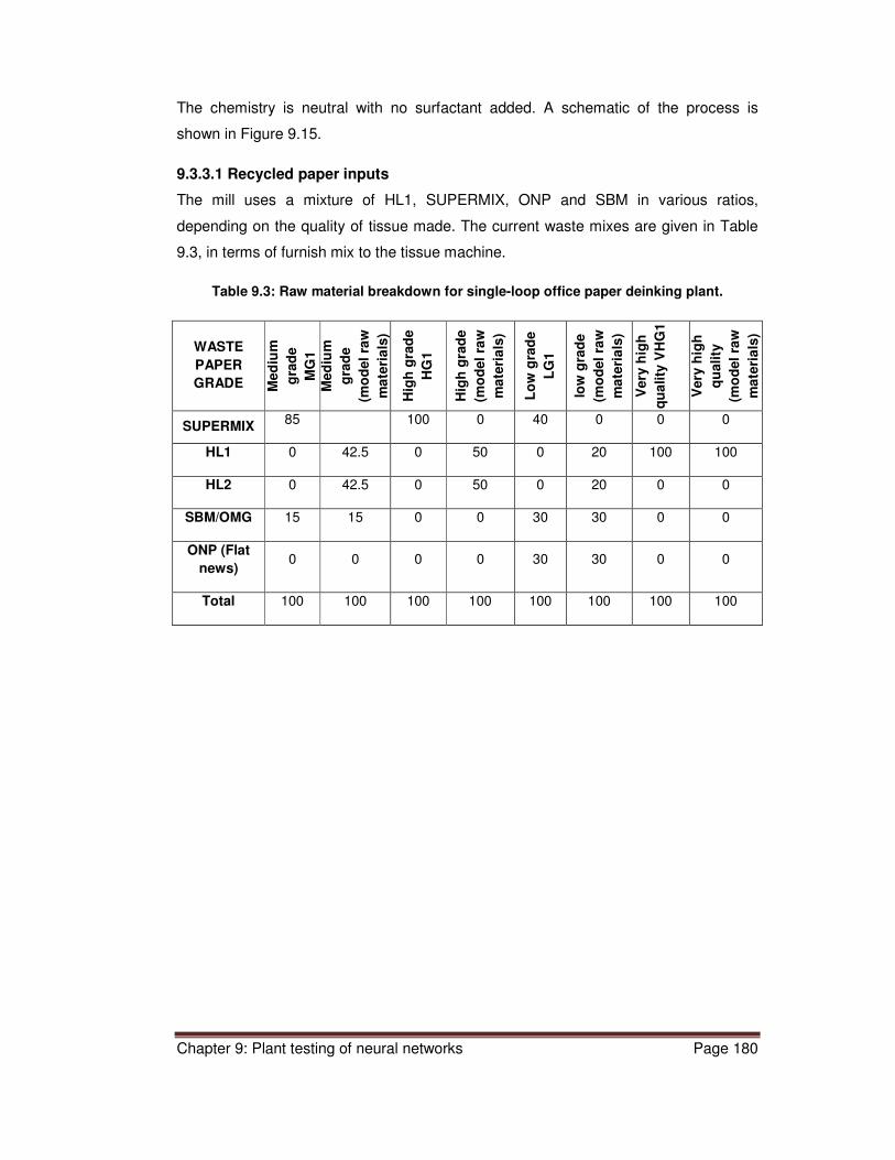
Chapter 9: Plant testing of neural networks Page 180
The chemistry is neutral with no surfactant added. A schematic of the process is
shown in Figure 9.15.
9.3.3.1 Recycled paper inputs
The mill uses a mixture of HL1, SUPERMIX, ONP and SBM in various ratios,
depending on the quality of tissue made. The current waste mixes are given in Table
9.3, in terms of furnish mix to the tissue machine.
Table 9.3: Raw material breakdown for single-loop office paper deinking plant.
WASTE
PAPER
GRADE Med
ium
gra
de
MG
1
Med
ium
gra
de
(mo
del
raw
ma
teri
als
)
Hig
h g
rad
e
HG
1
Hig
h g
rad
e
(mo
del
raw
ma
teri
als
)
Lo
w g
rad
e
LG
1
low
gra
de
(mo
del
raw
ma
teri
als
)
Very
hig
h
qu
ality
VH
G1
Very
hig
h
qu
ality
(mo
del
raw
ma
teri
als
)
SUPERMIX 85 100 0 40 0 0 0
HL1 0 42.5 0 50 0 20 100 100
HL2 0 42.5 0 50 0 20 0 0
SBM/OMG 15 15 0 0 30 30 0 0
ONP (Flat
news) 0 0 0 0 30 30 0 0
Total 100 100 100 100 100 100 100 100

Chapter 9: Plant testing of neural networks Page 181
Fig
ure
9.1
5:
Pro
cess
flo
w d
iag
ram
- s
ing
le-l
oo
p o
ffic
e p
ap
er
dein
kin
g p
lan
t. (
Refe
r to
Fig
ure
5.3
)
Chapter 9: Plant testing of neural networks Page 182
Supermix is a 50:50 blend of HL1 and HL2, thus the breakdown of raw materials fed to
the recycling plant in terms of the raw materials used in the modelling exercise (viz.
ONP, OMG, HL1 and HL2) is shown in Table 9.3. The most popular grades are
medium grade (MG1) and high grade (HG1), where “1” designates the single-loop
process. The other grades (low grade LG1 and very high grade VHG1) are made
infrequently and in small volume.
9.3.3.2 Chemical additions
This mill does not use caustic soda, sodium silicate, hydrogen peroxide or any
surfactant in the pulper. There appears to be sufficient surfactant in circulation in the
process water to ensure wetting of the fibre in slushing and froth formation in the
flotation cell. Office waste papers typically contain a certain amount of surfactants
which are released into the water upon pulping. This has been demonstrated in
practice, particularly for rotogravure printed papers (Vernac, Carré & Beneventi, 2001).
Surfactant is not normally necessary in the flotation of hydrophobic inks such as toner
particles (Zhao, Deng & Zhu, 2004). Essentially neutral deinking is carried out. During
October 2010 a trial surfactant was being added into the pulper. The purpose of this
surfactant was to improve the slushing and increase the size on the plastic waste
removed. It was assumed that this surfactant had no effect on the deinking process.
The minimum addition rate used in the training data (viz 0.25%) was assigned to the
surfactant added to the pulper. Additions of chemicals (if added) are measured in
kilograms per ton of dry fibre. Setpoints on the process control system are maintained
at the specified levels by flow measurement and control valves. Kg/ton was converted
to % for use in the models.
9.3.3.3 Pulping conditions
Pulping time varied between 15 and 20 minutes, but was not recorded. An average of
18 minutes was assigned as the input to the model. The consistency was tested once
per day, and remained fairly constant in the range of 16-18%.The pulper temperature
has a setpoint of 65 ºC on the process control system, maintained by live steam
injection. However, a short term monitoring of the temperature indicated that the
practical range was 56 to 60 ºC region. A value of 60 ºC was assigned. The pulper pH
was monitored on a daily basis, and ranged from 7 to 8.

Chapter 9: Plant testing of neural networks Page 183
9.3.3.4 Flotation conditions
The flotation temperature varied from 46 to 50 ºC, and was taken to be constant at
48ºC. The consistency in the flotation cell had only recently (from September 2010)
been monitored on a regular basis. It varied between 0.9% and 1.4%, and the average
for this period was 1.16%. This average was used for those periods when the flotation
consistency was not measured. The feed flow rate to the flotation cells has a set point
of 7000 l/min, which seemed to be fairly well controlled.
The flotation cells were originally Voith Tubular Multi-Injector cells, which were
upgraded some time ago by dividing the cell into five units and retrofitting with the
EcoCell® aeration element. This element contains a multistage micro-turbulence
generator similar to the Escher Wyss aeration element (Kemper, 1999), as found on
the double-loop deinking flotation cells.
The flotation sequence consists of a mixing cell, five flotation cells in series, and a
secondary cell which refloats the rejects from the first stage cells. The volume of the
main bank of float cells was estimated from drawings and measurements to be ca. 8.5
m3 per cell, or 42.4 m3 in total. At the end of September 2010, the pump which
transfers stock from cell 2 to cell 3 broke down and cell number two had been by-
passed. For this period the flotation volume was reduced by 1/5th to 33.9 m3. The
flotation residence time was accordingly calculated from the flotation volume and the
volumetric throughput.
The relationship between laboratory and plant flotation efficiency was determined as in
the previous section. The results are listed in Appendix 6C and are shown in Figure
9.16. The flotation efficiency probably varied somewhat with the different grades.
However, a global average for all the grades was taken, for reasons of simplicity and
unavailability of good plant date for all grades, especially the small volume grades
made only occasionally. With reference to Figure 9.16, it can be seen that the plant
performance exceeds the laboratory performance. Thus, the flotation time at maximum
laboratory flotation performance was used, viz. 8 minutes by estimation of the
maximum of the curve. The ratio of flotation times was thus ca. 1.3.

Chapter 9: Plant testing of neural networks Page 184
Figure 9.16: Comparison of brightness, ERIC and yield for laboratory to single-loop
office paper deinking plant flotation.
In this case, the removal of ink as measured by the ERIC was much less for the plant
than in the laboratory. Hence the flotation time factor was less than unity, in this case
ca. 0.1.
There appeared to be little difference between the plant and the laboratory results
when it came to the yield (Figure 9.16). Accordingly, a factor of 1 was applied.
The pH in the flotation cell had only recently (from September 2010) been monitored
on a regular basis. It varied between 6.8 and 8.2, and the average for this period was
7.6. This average was used for those periods when the flotation pH was not measured.
9.3.3.5 Pulp bleaching conditions
No hydrogen peroxide is used in the pulper in the single-loop process, but a post
bleaching is carried out after washing, prior to final storage. The bleaching system
consists of a solution of sodium borohydride and sodium hydroxide (Chloraclear®,
12% active NaBH4) which is co-fed at a ratio of 1:13 into the pulp with a sodium
bisulphite solution (38% active). In this process, sodium hydrosulphite (sodium
dithionate) is produced in situ. The process is essentially a sodium hydrosulphite
bleaching process, with some superior efficiency claimed by the supplier (Bremner,
0.400
0.500
0.600
0.700
0.800
0.900
1.000
1.100
1.200
0 2 4 6 8 10 12 14
Ra
tio
s
Flotation time (mins)
Lab B/Bo Lab E/Eo Lab Y/Yo Plant B/Bo Plant Y/Yo Plant E/Eo

Chapter 9: Plant testing of neural networks Page 185
2010). With reference to Figure 9.13, the Chromaclear® system seems to perform
similar to the FAS system in the double-loop process.
However, the addition of bleaching agent is done on an ad hoc basis, when it is
required to boost the brightness into specification. There was no regular addition, and
when added the amount was not recorded. This will thus be regarded as a post-
bleaching and was not included in the model.
9.3.3.6 Deinked fibre properties
This mill also measures UVexcluded brightness. The correlation between mill and
research laboratory brightness is shown in Figure 9.17. Hence:
Predicted brightness = 1.185 x plant brightness – 5.672 (5)
The mill routinely measured brightness on the pulper, before and after flotation, and
after bleaching. Not all of these properties were measured all the time. Brightness after
washing was not always measured. However sufficient measurements were made to
obtain a correlation between floated and washed brightness, shown in Figure 9.18.
Thus, where necessary, the washed brightness was predicted from the flotation
brightness using the correlation in Figure 9.18. Thereafter, all the brightness values
were scaled up using equation (5). As before, averages were inserted for missing data.
Figure 9.17: Correlation of laboratory and plant brightness measurements.
y = 1.185x - 5.672R² = 0.774
65
70
75
80
85
90
95
65 70 75 80 85 90 95
Lab
ora
tory
UV
inclu
ded
bri
gh
tne
ss,
%
Plant brightness

Chapter 9: Plant testing of neural networks Page 186
Figure 9.18: Correlation between washed brightness and floated brightness.
9.3.3.7 Yield
As in the previous cases, the flotation yield had to be deduced from the total process
yield.
The process yield is calculated by the mill on a daily basis by consideration of the total
production input (comprising waste input, addition of virgin fibre and broke) and tissue
output.
With reference to Figure 9.15, it can be seen that the recycling plant losses consisted
of three streams:
waste from the Fiberizer – comprising plastic, staples and some fibre;
waste from the High Density cleaner - comprising grit, staples and other heavy
material;
solid material from the centrifuges - comprising rejects from the deinking cell.
It is this last stream that corresponds most closely to the flotation losses. The relative
magnitude of these three streams was estimated from the average number of waste
bins removed daily, as detailed in Table 9.4.
y = 0.945x + 6.234
R² = 0.901
45.00
50.00
55.00
60.00
65.00
70.00
75.00
80.00
85.00
45.00 50.00 55.00 60.00 65.00 70.00 75.00 80.00 85.00
Bri
gh
tne
ss a
fte
r w
ash
ing
(%
)
Brightness after flotation (%)

Chapter 9: Plant testing of neural networks Page 187
Table 9.4: Estimation of yield losses.
HD cleaner rejects Fiberizer rejects Centrifuge solids
Volume of bin, m3 6.0 12.0 12.0
Estimated Density, t/m3 1.2 2.3 2.5
Average bins/day 0.3 1.0 5.0
Calculated wet mass 2.2 28.0 150.0
Consistency % 40 30 40
Calculated dry mass, t/d 0.9 7.0 60.0
Dry mass fraction 0.01 0.10 ca 0.9
Thus, 90% of the total losses are made up of flotation losses. Using this assumption
and by mass balance, the flotation yield was estimated from the process yield
according to the following formula:
% 234565748 97:3; = 100 <1 ) =>.? @ ABACD DBEEFEGCEAF HIJKA LM (6)
where the total losses were calculated from knowledge of the total inputs and outputs
viz. the process yield. The final process data, after all adjustments as discussed above
have been made, is shown in Appendix 7. This data was used to test the performance
of the neural networks.
9.4 Results of model testing and discussion
9.4.1 Brightness
The training data (as given in Appendix 3) were used to train a final set of neural
networks, according to the methodology detailed in Section 8.3. For each final
property, the full set of input variables (Appendix 3), and a reduced set of input
variables (Section 8.7) were modelled. The number of neurons was varied from one to
twenty, with four attempts for each structure; viz. eighty networks were generated for
each of the final properties of brightness, ERIC and yield.
At the same time, the networks were tested with the modified plant data (Appendix 7)
by determining the correlation and mean square error of actual versus predicted
values. The networks were ranked in order of increasing mean square error. The top

Chapter 9: Plant testing of neural networks Page 188
ten networks were retained as possible final models. The best networks and their
performances are listed in Appendix 8.
For the reduced set of process parameters, the means of the predicted values of the
top (Bright_FinalA_20_2), second (Bright_FinalA_5_1) and tenth (Bright_FinalA_3_3)
ranked networks were plotted against the actual plant values in Figure 9.19.
Figure 9.20 is a similar plot for the networks trained with the full set of process
parameters. In this case the networks are: first - BrightB_16_2, second - BrightB_13_2
and tenth - BrightB_11_3. It appears that the networks trained on the full range of
process parameters gave slightly lower mean square errors and slightly higher
correlations (Appendix 8A) than those trained on the reduced set of variables.
However, the differences are not great, and the added practical complexities of
working with the full set of parameters do not justify the slight improvements in
prediction obtained. Thus, the neural networks based on the reduced set of process
variables were preferred.
The variability of the plant data was quite high, but with the large number of data points
acquired for most of the grades, the resulted standard error (N/√8 ) was low. The
calculated standard errors are shown in Appendix 8. Thus, only the average values
were depicted in the graphs.
Figure 9.19: Brightness prediction performance of top (Bright_FinalA_20_2), second
(Bright_FinalA_5_1) and 10th
(Bright_FinalA_3_3) ranked neural networks with reduced
inputs.
50.0
55.0
60.0
65.0
70.0
75.0
80.0
85.0
90.0
95.0
50.0 60.0 70.0 80.0 90.0
NN
pre
dic
ted
bri
gh
tne
ss (
%)
Actual plant brightness (%)
'Bright_FinalA_20_2'
'Bright_FinalA_5_1'
'Bright_FinalA_3_3'

Chapter 9: Plant testing of neural networks Page 189
Figure 9.20: Brightness prediction performance of top (BrightB_16_2), second
(BrightB_13_2),and 10th
(BrightB_11_3) ranked neural networks with full set of inputs.
It is apparent from Figures 9.19 and 9.20, in terms of the deviations from the Y = X
line, that there are only small differences between the top-ten networks. However the
mean square errors (MSE) and correlations do show differences, listed in Appendix 8.
The predicted brightness of the best network was plotted against the plant actual
brightness, for each grade of paper recycled in the three plants, and shown in Figure
9.21. Points lying on the Y = X line would denote a perfect prediction. It can be seen
from Figure 9.21 that the predicted brightnesses of the newsprint and low-grade tissue
grades were close to the plant actuals. These grades all contained medium to high
levels of newsprint and/or magazine (refer to Tables 9.1 and 9.3) and were processed
on single-loop deinking plants.
50.0
55.0
60.0
65.0
70.0
75.0
80.0
85.0
90.0
95.0
50.0 60.0 70.0 80.0 90.0
NN
pre
dic
ted
bri
gh
tne
ss (
%)
Actual plant brightness (%)
'Bright_FinalB_16_2'
'Bright_FinalB_13_2'
'Bright_FinalB_11_3'

Chapter 9: Plant testing of neural networks Page 190
Figure 9.21: Brightness prediction performance of neural network Bright_FinalA_20_2
for different grades and plants.
On the other hand, grades (single-loop medium grade, single-loop high grade and
double-loop medium grade, Table 9.1 and 9.3) containing high levels of office papers,
in particular HL2, showed negative deviations from the Y = X line. In other words, the
brightness achieved by the plants was higher than that achieved in the laboratory, and
hence predicted by the neural networks. HL2 contains appreciable quantities of
coloured materials, and it could be possible that the plant processes would be more
efficient than the laboratory process in removing coloured materials. In addition, the
plants have extra equipment (screens and cleaners, extra flotation and washing stages
interspersed by dispersion) which could remove some ink and the full scale flotation
cells appeared to be more efficient than the laboratory cell. This was apparent from the
alignment work described in Section 9.3.2.4 and 9.3.3.4.
The one anomaly in Figure 9.21 is the very high grade pulp manufactured on the
single-loop process. This grade has 100% HL1 as its raw material, and the neural
networks accordingly predicted a very high brightness. In practice however the
brightness achieved for this grade on the plant was only slightly higher than that
achieved on the high grade. The reason for this is probably that the very high grade is
manufactured sporadically in small quantities, interspersed between the lower quality
high-volume grades. The process water streams would be carrying higher ink and
contaminant loading from the lower quality grades, which would “contaminate” the very
45.0
50.0
55.0
60.0
65.0
70.0
75.0
80.0
85.0
90.0
95.0
45.0 55.0 65.0 75.0 85.0 95.0
NN
Pre
dic
ted
bri
gh
tne
ss (
%)
Actual plant brightness (%)
Newsprint Trial
Newsprint
Double-loop, medium grade
Double-loop, high grade
Single-loop. Very high grade
Single-loop, medium grade
Single-loop, low grade
Single-loop, high grade

Chapter 9: Plant testing of neural networks Page 191
high quality grade with ink recirculating in the process water. It could be expected that
an extended run of very high grade on the plant would yield higher brightness. This
suggests the usefulness on the models in diagnosing unexpected results in a practical
plant.
The response surfaces of the selected network (Bright_FinalA_20_2) are shown in
Figures 9.22 to 9.24, for three representative standard grade mixes:
ONP:OMG:HL1:HL2::25:25:25:25, ONP:OMG::50:50 and HL1:HL2::50:50.
Figure 9.22: Bright_FinalA_20_2 network brightness response surface for a mixture of all
grades.

Chapter 9: Plant testing of neural networks Page 192
Figure 9.23: Bright_FinalA_20_2 network brightness response surface for a mixture of
ONP and OMG grades.
Figure 9.24: Bright_FinalA_20_2 network brightness response surface for a mixture of
HL1 and HL2 grades.
Chapter 9: Plant testing of neural networks Page 193
The trends indicated in the response surfaces are as expected from what is known
about the behaviour of deinking systems, viz. brightness increases with level of
hydrogen peroxide addition, alkalinity and flotation time. Flotation consistency has a
negative effect and flotation pH a neutral to negative effect. Figure 9.24 suggests that
increasing alkalinity would have a small but positive effect on office paper deinking. In
this case, judging from the shapes of the surfaces, is seems as if the neural network
converged to a near-linear model.
9.4.2 Residual ink concentration (ERIC)
The variability in the ERIC values was greater than the brightness values, as shown
and discussed in Section 7.3. This manifested as much lower correlations and higher
mean squared errors in the neural network training processes (Appendix 8B). An
additional problem was that the tissue mills did not measure ERIC. Practically, it was
possible to obtain only limited plant ERIC data, by getting sample pads from the plants
and testing them in the research laboratory (Appendix 6). Thus extensive plant ERIC
data was only available for the newsprint mill, and it was not possible to obtain
correlations over the whole deinking range, as was the case with brightness. Neural
networks for the full set of input variables, a reduced set and a very reduced set were
trained and tested against the plant data (Appendix 8B).The performance of the best
models for each variable set is shown in Figure 9.25. To accommodate the wide range
of the data, logarithmic axes have been used.
It can be seen from Figure 9.25 and Appendix 8B that again the best performance
(lowest MSE) was obtained by the networks trained on the full set of process variables
(ERIC_FinalB_14_4). As with brightness, the improvement in prediction was
considered insufficient to justify the added complexity introduced by the full set of
inputs. However, in this case a very reduced set of inputs, comprising only flotation
time and flotation consistency proved to be marginally better that the reduced set of
ten variables (Appendix 8B). Thus, network ERIC_FinalC_17_3 was chosen as the
preferred network.
The prediction performance of network ERIC_FinalC_17_3 for the different paper
grades and processing plants is shown in Figure 9.26.

Chapter 9: Plant testing of neural networks Page 194
Figure 9.25: ERIC prediction performance of top ranked neural networks with different
variable data sets. Full set – ERIC_FinalB_14_4, Reduced set - ERIC_FinalA_4_1 and
very reduced set - ERIC_FinalC_17_3.
Figure 9.26: ERIC prediction performance of network ERIC_FinalC_17_3 for different paper grades and processing plants.
The prediction performance for the newsprint grades was again close to the plant
values. However, as was the case for brightness, deviations were observed for the
office waste paper grades. The ink loading of newsprint is much higher than that of
50
500
50 500
NN
pre
dic
ted
Pre
dic
ted
ER
IC
Actual plant ERIC
'ERIC_FinalB_14_4'
'ERIC_FinalA_4_1'
'ERIC_FinalC_17_3'
50
500
50 500
Pre
dic
ted
ER
IC
Actual plant ERIC
Newsprint Trial
Newsprint
Double-loop, medium grade
Double-loop, high grade
Single-loop. Very high grade
Single-loop, medium grade
Single-loop, high grade

Chapter 9: Plant testing of neural networks Page 195
office papers. Thus ink content will have a major effect on the brightness and ERIC of
newsprint, and a relatively minor effect on the brightness and ERIC of the office papers
viz. factors other than deinking were affecting the brightness and ERIC of the office
papers.
In this case the network ERIC predictions were lower (viz. better ink removal) than the
plant actuals. These figures suggested that the laboratory processes removed ink
more effectively than the plant processes. In contrast, the results in Section 9.4.1
showed that the plant processes produced high brightness products. This could be
attributed to the extra processing equipment in the plants which removes dirty
contaminants other than ink which might otherwise negatively influence brightness.
The response surfaces of the network Eric_FinalC_17_3 are shown in Figures 9.27 to
9.29.
Figure 9.27: Eric_FinalC_17_3 network ERIC response surface for a mixture of all
grades.

Chapter 9: Plant testing of neural networks Page 196
Figure 9.28: Eric_FinalC_17_3 network ERIC response surface for a mixture of ONP and
OMG grades.
Figure 9.29: Eric_FinalC_17_3 network ERIC response surface for a mixture of HL1 and
HL2 grades.
Chapter 9: Plant testing of neural networks Page 197
The response surfaces for all three of the representative grade mixes showed an
increasing ink removal with increasing flotation time and decreasing flotation
consistency. This is in agreement with known behaviour.
9.4.3 Yield
Comprehensive data was not available to calculate the estimated flotation yield for the
plants. Consequently, average values had to be inserted for missing data. In addition,
assumptions had to be made to estimate the flotation yields. These assumptions and
estimations are detailed in Section 9.3.1.7, 9.3.2.7 and 9.3.3.7.
As for the brightness, the neural network predicted yields were evaluated against the
estimated plant flotation yield data. This was also carried out for three combinations of
input variables: a complete variable set, a reduced set and a very reduced set
(Appendix 8C). The results for the ten best networks in each case are shown in
Appendix 8C.
The correlations for the best networks are in the region of R = 0.8 based on the
training data. Again the networks trained with the full variable set showed a slightly
better prediction, as measured by the correlations and mean square errors. The
correlations achieved are the lowest of the three properties modelled.
This is due to the fact that many factors other than those modelled can contribute to
yield losses. For example, cleaner rejects, process spillages and washing losses were
not accounted for in the laboratory. The prediction efficiency of the best network for
each variable set is shown in Figure 9.30.

Chapter 9: Plant testing of neural networks Page 198
Figure 9.30: Yield prediction performance of top ranked neural networks for different variable data sets. Full set – Yield_FinalB_4_3, reduced set –
Yield_FinalA_11_1, very reduced set – Yield_FinalC_8_4.
It can be seen in Figure 9.30 that the uncertainty is greatest at lower yields. The lower
the yield the greater the probability that multiple losses have occurred, including
random process spillages.
From the mean square error data (Appendix 8C) and Figure 9.30, it can be seen that
the networks trained on the simplest set of variables (Yield_FinalC_8_4) again
produced the best predications. The prediction performance of network
Yield_FinalC_8_4 for the various grades and plants is shown in Figure 9.31. The low
grade tissue made on the single-loop office waste plant was omitted due to lack of
specific data.
60
65
70
75
80
85
90
95
100
60 70 80 90 100
Pre
dic
ted
yie
ld %
Actual plant yield %
'Yield_FinalA_11_1'
'Yield_FinalB_4_3'
'Yield_FinalC_8_4'

Chapter 9: Plant testing of neural networks Page 199
Figure 9.31: Yield prediction performance of top neural network (Yield_FinalC_8_4) for different paper grades and processing plants.
Inspection of Figure 9.31 shows that the major excursions from the Y = X line all occur
in the single-loop office waste deinking plant: the plant yields are all much lower than
predicted. This indicates either an error in the estimation of the yield for the single-loop
office waste process or an unexplained process leakage at some point. This again
highlights the possibility of the models being used to detect process abnormalities.
The response surfaces of the network Yield_FinalC_8_4 are shown in Figures 9.32 to
9.34.
The neural networks converged to almost linear response surfaces and demonstrated
that yield is negatively affected by long flotation times and lower flotation
consistencies. This conforms to known behaviour, and suggests that the yield was
modelled fairly well by the networks, despite the uncertainties in the plant data.
60
65
70
75
80
85
90
95
100
60 70 80 90 100
Pre
dic
ted
yie
ld %
Actual plant yield %
Newsprint Trial
Newsprint
Double-loop, medium
grade
Double-loop, high grade
Single-loop. Very high
grade
Single-loop, medium grade
Single-loop, high grade
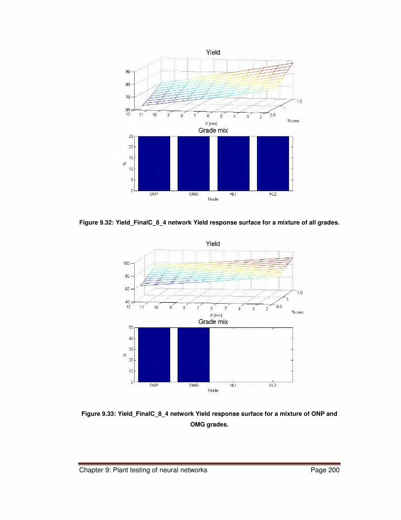
Chapter 9: Plant testing of neural networks Page 200
Figure 9.32: Yield_FinalC_8_4 network Yield response surface for a mixture of all grades.
Figure 9.33: Yield_FinalC_8_4 network Yield response surface for a mixture of ONP and
OMG grades.

Chapter 9: Plant testing of neural networks Page 201
Figure 9.34: Yield_FinalC_8_4 network Yield response surface for a mixture of HL1 and
HL2 grades.
Whilst the neural network predictions could not be used to accurately predict plant
flotation yields, they could still be used to predict changes in yield which might occur if
raw material or process changes were made.
The MATLAB code used to train and test the networks is given in Appendix 9.
The structures and layer weight matrices of the top performing networks are listed in
Appendix 10.
A CD with electronic versions of the data and MATLAB files is included.

Chapter 10: Conclusions and further work Page 202
CHAPTER 10: FINAL CONCLUSIONS AND APPLICATIONS
10.1 Review of work done
A need was identified in the South African paper recycling industry for better control of
deinking processes in the face of ever increasing variability in the recycled paper raw
material stream fed to the recycling plants.
It was proposed to establish a global mathematical model which would enable
recycling plants to predict how the processes would react to changing raw material
streams without having to perform extensive experimental work. Also, there was a
need to have alternative process parameters available for control in the event that the
recycled paper mix could not be varied at will.
As it was not possible to experiment on the production plants, it was necessary to base
the modelling on deinking experiments performed in the research laboratory. The
many possible process parameters and chemical additions were screened using
statistical experimental design techniques. It was possible to identify influential
variables and eliminate those variables that had a limited effect on the process.
Four recycled paper grades as well as the influential process parameters were varied
over a wide range in many random combinations to produce a data base of nearly 500
deinking runs.
This data base was used to train neural networks to predict brightness, residual ink
content and flotation yield. The neural networks were tested and selected against
actual process data collected from three different plants. The process plants
encompassed single-loop and double-loop processes, and eight different grades of
recycled pulp, ranging from low brightness newsprint to high brightness recycled office
papers.

Chapter 10: Conclusions and further work Page 203
10.2 Conclusions
10.2.1 Screening of control variables
A statistically designed screening process, utilising Plackett-Burman experimental
design techniques indicated that process parameters such as surfactant additions,
flotation temperature, flotation pH and pulping time were not particularly influential in
determining the brightness, residual ink concentration (ERIC) or yield of the flotation
deinking process. On the other hand, flotation time and flotation consistency, bleaching
conditions and alkalinity were most influential with respect to brightness, residual ink
concentration and yield. Whilst pulping temperature was influential in determining the
ERIC of magazine papers and HL1 and the washed brightness of HL2, it was rejected
as a practical control variable. A ranking analysis with respect to brightness, residual
ink concentration and yield resulted in the following list of process variables, in order of
descending influence:
• Flotation time
• Flotation consistency
• NaOH addition level
• H2O2 addition level
• Sodium silicate addition level
• Surfactant addition to the pulper
• Pulping time
• Flotation pH
A subsequent sensitivity analysis carried out using neural networks confirmed the
findings of the Plackett-Burman screening runs with respect to which process
parameters were most influential.
However, the grade of recycled paper used as a raw material for deinking had an
overriding influence on the optical properties. The order of influence on optical
properties (brightness and ERIC) was in descending order:
• Heavy Letter 1
• Heavy Letter 2
• Magazines
• Newsprint
This order corresponds with the level of incoming brightness of the recycled paper.
The yield was determined predominantly by the flotation time and consistency, with
alkalinity playing a role in the case of Heavy Letter 1. The largest yield loss was

Chapter 10: Conclusions and further work Page 204
experienced by magazine grades, followed by newsprint and then office papers. The
yield did not seem to be dependent solely on the filler content of the paper, as
newsprint has lower levels of filler than office papers.
10.2.2 Data generation
The generation of nearly 500 deinking runs to form the data base for the training of the
neural networks was performed continuously over a 17 month period. All of the
process variables initially identified were varied over the full range used in the South
African deinking industry. More data was collected for the variables that were most
influential, whilst much less data was gathered for the least influential variables.
By careful selection of recycled paper raw material, the “noise” induced by raw
material quality variations was minimised. This variability was tracked and monitored
by performing midpoint runs at regular intervals. The coefficient of variation of the
brightness generally remained below ca. 6%, with the variability of HL2 brightness
peaking at 8.9%. On the other hand, the coefficient of variation of the ERIC was much
higher, varying from 27% to 54%. The coefficient of variation of the yield data ranged
between 6.8% for HL1 up to 22% for OMG, but generally in the region of 8-10%.
Generally, the office recovered paper grades showed the greatest variability with
respect to ERIC and lowest variability with respect to yield data.
10.2.3 Generation of neural networks
Neural networks were able to effectively model the laboratory processes to high levels
of correlation. With reference to Table 10.1, laboratory brightness results were
modelled with correlations greater than 95%.
Slightly lower correlations (84%<R<91%) were achieved for the ink removal (ERIC) in
the laboratory. The lower correlations were probably due to the inherently higher
variability of the ERIC results.
Although the variability of the laboratory flotation yield data was less than the ERIC
data, weaker correlations (R<80%) were found (Table 10.1). The agitation speed in the
flotation cell was maintained constant throughout the experimental period, but it is
presumed that variations in hydrodynamic factors (bubble size, bubble number) in the
float cell, which were not included in the models, are responsible for the weaker yield
correlations. Flotation time and consistency have the greatest influence on yield,
whereas a greater variety of factors influence the optical properties, thereby diluting
the effect of hydrodynamic factors.

Chapter 10: Conclusions and further work Page 205
Table 10.1: Summary of neural network performance. (Appendix 8)
Property modelled
Number of process
parameters
Neural network correlation
with lab data (R)
Neural network prediction of plant data (R)
Neural network prediction of
plant data (MSE)
Brightness % 10 0.951 0.922 53.5
15 0.954 0.940 26.0
Residual ink
concentration
ERIC, ppm
6 0.841 0.937 1342
10 0.907 0.934 1370
15 0.853 0.934 1021
Flotation yield %
6 0.767 0.534 83.6
10 0.791 0.453 87.5
15 0.790 0.425 101.2
Notes:
1. 15 process parameters: ONP, OMG, HL1, HL2, NaOH, sodium silicate, hydrogen
peroxide, surfactant addition to pulper and flotation cell, pulping time and temperature,
flotation time, flotation temperature, flotation consistency and flotation pH.
2. 10 process parameters: ONP, OMG, HL1, HL2, NaOH, sodium silicate, hydrogen
peroxide, flotation time, flotation consistency and flotation pH.
3. 6 process parameters: ONP, OMG, HL1, HL2, flotation time and flotation consistency.
10.2.4 Prediction of neural networks
The plant brightness was predicted at R > 90% for 10 and 15 process parameters,
only slightly lower than the correlations with the laboratory brightness data (Table
10.1).
On the other hand, the plant ERIC data was predicted with slightly higher correlations
than the laboratory ERIC data (Table 10.1) for 6, 10 and 15 process parameters. The
newsprint deinking plant routinely measured ERIC values. However, the ERIC data
collected for the tissue deinking plants was very limited. A single average value was
inserted for a range of plant conditions, which probably contributed to the slightly
stronger correlations found with the plant data. Nevertheless, the laboratory
correlations for ERIC were good, so it can be expected that good plant correlations
would be achieved if more data were available.
The neural network correlations with the laboratory yield data were the lowest
(R<80%) for 6, 10 and 15 process parameters, although still reasonable. However, the
flotation yield was not directly measured by the plants, and had to be estimated from
the incomplete data available. Some unit operations in a full scale plant can contribute
to yield losses (e.g. hydrocyclone cleaning, screening, process spillages) and others

Chapter 10: Conclusions and further work Page 206
can contribute to fibre savings (e.g. secondary flotation of removed ink, recirculation of
fibrous filtrates). The effect of these operations could not be simulated in the laboratory
process. Hence much weaker predictions (R< 55%) with the plant data were obtained
using 6, 10 and 15 inputs.
Neural networks trained with the complete set of 15 process variables generally
produced better correlations and lower mean square errors (MSE) than models with 10
or 6 process variables (Table 10.1). Yield was the exception to this trend, and was
predicted best with only six variables. However, the networks based on the optimised
set of 10 variables produced predictions which were almost as good as the 15 variable
networks, but with the advantage of the much greater simplicity of fewer variables.
Thus, the best networks were selected on the basis of prediction ability, but a small
amount of prediction ability was sacrificed in favour of a simpler fewer-variable model.
The selected models are indicated in bold type in Table 10.1.
10.3 Applications
The global neural network models effectively approximated the brightness and ERIC
values produced by the plants studied. The yield was less effectively modelled.
The process of visiting the plants to gather data highlighted some possibilities for the
application of the neural networks, elaborated below:
10.3.1 Process applications
The models developed in this research could be used for deinking plant process
optimisation. A recent case study will illustrate this application. The brightness at a
local newsprint deinking plant had been deteriorating in the recent past, and the author
was called in to advise the mill. Based on the results of the research, the mill was
informed that the alkalinity and bleaching conditions have a major influence on the
brightness. After some discussion it emerged that the amount of caustic soda added to
the pulper had been cut back for various reasons. The lower deinking alkalinity had
possibly resulted in lower deinking efficiency and lower brightness. The mill was
advised to increase the pulping alkalinity. At the time of writing the suggested changes
had not yet been implemented at the mill.
These models could be of assistance in troubleshooting exercises. The models
represent “standard” or average conditions, and deviations from predicted values can
be indicative of some malfunctioning equipment or other process deviation. As an

Chapter 10: Conclusions and further work Page 207
example, the very high grade tissue pulp manufactured on the single-loop process
showed an anomalously low plant brightness for the high quality raw material used,
compared to the neural network predicted brightness. It is possible that this could have
been due to the low volumes manufactured and the effect of recirculating back water.
Another example was the yield deviations of the single-loop tissue recycling process.
This process displayed deviations from predicted values for all of its grades. This
indicates that there is perhaps an undetected yield leakage from the system.
The models could also be used to pre-empt the results of trials. An example of this
was the trial carried out in the newsprint mill, where the ratio of magazine to newsprint
was increased to 60:40, from the usual 30:70. The result of this trial was that the
brightness increased only marginally, despite the large change in furnish composition.
This marginal change was also predicted by the neural networks. The use of the
models pre-trial would have avoided the unnecessary costs and disruptions of trials on
production plants.
10.3.2 Raw material changes
Recycling plants are sometime confronted with sudden raw material changes. A
particular grade of recycled paper could suddenly become unavailable, and the plant is
confronted with the need to change the ratio or even the grade mix of recycled paper
raw material. These changes could be fed into the models to predict the outcome. In
addition, the corresponding changes to the alkalinity or bleaching regime required to
maintain the output quality could be determined in a short period of time. This would
enable the plant management to make a rapid decision on the use of the changed raw
materials.
10.4 Future work.
In any research work, time and resource constraints limit the amount that can be done.
The following areas could form the basis of further work.
10.4.1 Unresolved questions
The main unresolved question in this research was the “gap” between the laboratory
based model predictions and the plant brightness values. This was indicated by the
deviations of the neural network predictions from the Y = X lines. An empirical attempt
was made to bridge this gap by relating the laboratory-based data to the plant data
through the flotation performance curve of brightness verses flotation residence time. It

Chapter 10: Conclusions and further work Page 208
was hoped that by adjusting the flotation time in the model a near perfect fit would be
obtained. This was only partially successful.
Most of the “gaps” occurred with the predictions for the office paper deinking plants,
where the plant brightness was higher than the predicted brightness by up to 10
brightness points. It is known that toner inks produce large, difficult to float particles.
The office paper recycling plants had extra equipment (screens, cleaners and
dispersers) to eliminate the large ink particles. This equipment was not simulated in
the laboratory, and hence not modelled. This would account for the consistent under-
estimation of the final brightness by the models. This limitation needs to be taken into
account when applying the models. It would be possible to apply a mathematical
correction or bias to the output of the models to bring the predications in line with the
actual values.
Another unresolved issue was the lack of sufficient plant ERIC data, particularly for the
office paper recycling plants, to obtain a good test of the models against plant data.
This was due to the fact that the ERIC was not measured by these plants, and
practical obstacles prevented a large amount of data being collected.
The last unresolved question was the quality of the yield data from the plants. Although
sufficient data was available, it did not correspond to the actual flotation yield, but to
general and combined yield losses of the plants. Data corresponding to flotation yield
had to be teased out of the data using indirect means and estimates, which negatively
affected the quality of the data. It would be instructive for further work to obtain high
quality data from the plants for ERIC and yield, and to re-test the models, to try to find
a better fitting neural network.
10.4.2 Extensions of the model to other parameters
The experimental research work generated a large number handsheets. These
handsheets could be further tested for filler content and sheet strengths, and models
could be developed for these properties as well. These properties were initially
excluded from the project due to resource constraints.
With the available data, it would be possible to model the pulping stage, flotation stage
and washing stage separately, and combine them into a total model. This approach
was not followed in this work, as the original concept was to produce a global model
responding to raw material changes. However, the advantage of a more unit-
operations based model would be that the units could possibly be built up into multi-

Chapter 10: Conclusions and further work Page 209
stage processes, thereby allowing more possibilities for process design and
modification.
The models developed were trained on laboratory data and tested and selected on the
basis of aggregated plant data. They are thus suitable as static “management” models
for the selection and modification of set points or operating regimes. The models were
not trained on dynamic plant data, and were not intended for the control of short-term
plant variations. However, it would be an interesting exercise to use the models in a
short-term dynamic situation, to see how well they would control a plant.
10.4.3 Practical implementation
It is intended to use the neural networks produced in this study to develop a desk-top
model which would enable plant personnel to proactively anticipate quality and
process adjustments in response to changing recycled paper raw material conditions.
What would follow now is an information technology project process. A prototype has
been developed which needs to be implemented, in the following steps (Tarassenko,
1998: 46-48):
10.4.3.1 Implement the prototype on customer hardware and software
The models currently exist in MATLAB format, requiring specific expertise and
computing skills to input data and produce outputs. A software programming exercise
is required to provide user interfaces to enable plant personnel with more general
computing skills to access and use the models.
10.4.3.2 Acceptance testing
The models must be tested on plant data over a longer period of time and variety of
conditions. This would make it possible to quantify confidence limits for the model. It
would be advisable to repeat the laboratory-plant flotation alignment processes,
specific to the plant, as discussed in Section 9.2 and to correct the data deficiencies
for ERIC (if desired) and yield.
10.4.3.3 Handover and training
The use of these models to troubleshoot or optimise processes must be combined with
extensive knowledge and experience in deinking processes. The models rely heavily
on the underlying data base of laboratory work. An understanding of this data base
and its limitations is essential to make effective use of the neural network models.

Chapter 10: Conclusions and further work Page 210
10.4.3.4 Maintenance
The system would need to be maintained. Bugs could develop and the operating
environment could change, necessitating revisions and enhancements.

References
REFERENCES
Ackerman, C., Putz, H. J. & Goettsching, L. Effect of pulping conditions on deinking of wood-containing recovered paper grades. Pulp & Paper Canada, 100:4 (1999).
Ali, T., Fairbank, M., McArthur, D., Evans, T. & Whiting, P. 1988. The role of silicate in peroxide brightening of mechanical pulp. Part II: The effects of retention time and temperature. Journal of pulp and paper science. Vol. 14, No. 2, March 1988.
Ali, T., McLellan, F., Adiwinata, J., May, M. and Evans, T. 1994. Functional and performance characteristics of soluble silicates in deinking. Part I: Alkaline deinking of newsprint/magazine. Journal of Pulp and Paper Science. Vol. 20 No. 1, Jan. 1994. pp J3-8.
Anderson, J. 1993. High efficiency for clean deinking. Paper Technology. Sept. 1993. pp 12-16.
Andrew, J. E. 2007. Questionnaire to identify the research areas of focus for processing of South African recovered fibres. Forest and Forest Products Research Centre internal report. November 2007.
Aspler, J. 1991. Introduction to printing technology and ink chemistry. In: TECH ’91- Recycling and deinking of newsprint and fine papers course. Toronto, Feb. 17-22. Montreal, Quebec, Canada. CPPA. Pp 1-26.
Azevedo, M. A. D., Drelich, J. and Miller, J. D. 1999. The effect of pH on pulping and flotation of mixed office waste paper. Journal of Pulp and paper Science. 25:9. September 1999.
Barrentine, L. B. 1999. An Introduction to Design of Experiments. American Society for Quality, Milwaukee, Wisconsin. 1999.
Ben, Y and Dorris, G. M. 2000. Irreversable ink redeposition during repulping. Part II: ONP/OMG furnishes. Journal of Pulp and Paper Science: Vol. 26 No. 8. August 2000. pp 289-293.
Beneventi, D., Benesse, M., Carre, B., Julien Saint Amand, F., and Salgueiro, L. 2007. Modelling deinking selectivity in multistage flotation systems. Separation and Purification Technology. 54: 77-87
Beneventi, D. and Carré, B. 2000. The mechanisms of flotation deinking and the role of fillers. Progress in Paper Recycling. February.

References
Beneventi, D., Carbo, A. C., Fabry, B., Pelach, M.A., Pujol, P.M. 2006. Modelling of flotation deinking: contribution of froth-removal height and silicate on ink removal and yield. Journal of Pulp and Paper Science. Vol. 32(2).
Beneventi, D., Carré, B., Hannuksela, T. and Rosencrance, S. 2007. Assessment of deinking chemistry performance: from laboratory flotation tests to the simulation of an industrial pre-flotation line. 8th. TAPPI Research Forum on Recycling. 2007.
Bennington, C. P. J., Sui, O. S. and Smith J. D. 1998. The effect of mechanical action on waste paper defibering and ink removal in repulping operations. Journal of Pulp and paper Science. Vol 24: 11. November 1998.
Bennington, C. P. J. and Wang, M. H. 2001. A kinetic model of ink detachment in the repulper. Journal of Pulp and Paper Science: Vol. 27, No. 10, October 2001.
Bergh, L. G. and Yianatos, J. B. 2002. Flotation column automation: state of the art. Control Engineering Practice. 11, p67-72
Berg, S.R, Johnson, D.A. and Thompson, E.V. 1997. Toner detachment during repulping of laser-printed office copy paper. TAPPI Journa.. Vol. 80(4).
Bloom, F. 2006. A mathematical model of continuous flotation deinking. Mathematical and Computer Modelling of Dynamical Systems. 12: No. 4, August: 277-311
Bloom, F. and Heindel, T. J. 1997. A Theoretical model of flotation deinking efficiency. Journal of Colloid and Interface Science. 190:182-197.
Borchardt, J.K. 2003. [online]. Recent developments in paper deinking technology. Taken from: http://www.pulpandpapercanada.com/news/recent-developments-in-paper-deinking-technology/1000127971/. Accessed 15/06/2011
Borchardt, J. K. 1997. The use of surfactants in deinking paper for paper recycling. Current Opinion in Interface Science, 2(4), 402-408. 1997
Borchardt, J. K. 1995. [Chemistry of unit operations in paper deinking mills.] In: Plastics, rubber and paper recycling. Chapter 27, pp 323-341. American Chemical Society. 1995
Borchardt, J. K. 1993, Possible deinking mechanisms and potential analogies to laundering. Progress in paper recycling, February 1993.
Borchardt, J.K. 1993b. Effect of process variables in laboratory deinking experiments. Tappi Journal. Vol. 76, No. 11.
Borchardt, J. K. and Lott, V.G. 1996. Deinking toner containing furnishes. Part 4: The role of microscopic ink particles in deinking office paper. TAPPI Proceedings of 1996 Recycling Symposium. New Orleans. Pg 107-124
Bremner, M. 2010. Pers. Comm.. to W. J. Pauck. Managing Director PaperChem. Chromaclear Premix Bleaching Technology (Dow Chemicals).

References
Brereton, R.G. 2006. Chemometrics – Data Analysis for the Laboratory and Chemical Plant. John Wiley & Sons, Ltd. University of Bristol, UK.
Brouillette, F., Daneault, C. and Dorris, G. 2001. Effect of initial repulping pH on the deflaking rate of recovered papers. Preprints 6th Research Forum on Recycling. Magog, QC.Oct. 1-4. Pp. 29-36.
Brouillette, F., Paradis, J. and Lafrenière, S. Pilot paper machine production of newsprint using high filler loads and dry strength technologies. Pulp & Paper Canada. September/October 2010.
Bureau of International Recycling. 2009. BIR Annual Report [online]. Accessed at http://www.bir.org. [22 Feb. 2011]
Carrasco, F., Pelach, M. A. and Mutje, P. 1999. Deinking of high quality offset papers: influence of consistency, agitation speed and air flow rate in the flotation stage. Tappi Journal. 82:3
Carré, B. and Galland, G. 2007. Overview of deinking technology. 8th CTP/PTS Deinking Training Course. Grenoble, May 29-31.
Carré, B., Galland, G and Julien Saint Amand, F. 1994. Estimation of ink detachment and removal. Progress in Paper Recycling. November 1994. Vol 4, pg 80-87.
Carré, B., Galland, G., Vernac, Y. and Suty,H. 1996. The effect of hydrogen peroxide bleaching on ink detachment during pulping and kneading. Revue A.T.I.P Vol. 50, No. 3. May/June.
Carré, B. and Magnin, L. 2004. Digital Prints: A survey of the various deinkability behaviours. 7th Research Forum on Recycling PAPTAC – TAPPI. September 27-29. Quebec, Canada.
Carré, B. and Magnin, L., Galland, G. and Vernac, Y. 2000. Deinking difficulties related to ink formulation, printing process and type of paper. TAPPI Journal. Vol. 83(6)
Carré, B. and Magnin, L., Galland, G. 2003. [online] Printing processes and deinkability. Das Papier 2003 – T195. Available at: http://epub.zellcheming.de/index.php?timestamp=1268527903&do=download&document_id=190&sessionid=3ea4e*af4b9c331fafb89. Accessed on 15/06/2011
Crosby, J. 1999. Personal communication to J. Pauck. Deinking plant superintendant. Mondi Merebank. P.O Box 17001, Merebank, Durban, 4001. 1999.
Crosby, J. 2008. Personal communication to J. Pauck. Former deinking plant superintendant. Mondi Merebank. P.O Box 17001, Merebank, Durban, 4001October 2008.

References
Crosfield. 1993. Soluble silicates and their applications. Crosfields Technical Information, Issue No. 1, July 1993. Crosfield Group, Warrington, England, WA5 1AB.
Cubillos, F. A. and Lima, E. L. 1998. Adaptive hybrid neural models for process control. Computers Chem. Engng vol.22, Suppl., pp. S989-S992. Elsevier Science Ltd. Great Britain.
Cubillos, F. A. and Lima, E. L. 1997. Identification and optimising control of a rougher flotation circuit using an adaptable hybrid-neural model. Minerals Engineering. 10, No. 7,pp. 707-721.
Dash, B. and Patel, M. 1997. Recent advances in deinking technology. Indian Pulp and Paper Technical Association. 9(1): 61-70.
Dayhoff, J. E. 1990. Neural Network Architectures – an Introduction. Van Nostrand Reinhold. 1990
Demuth, H., Beale M. and Hagan M. 2009. MATLAB Version 6.0.3 (Release R2009a) - Neural Network Toolbox 6 Users Guide. The MathWorks, Inc., Natwick, MA 01760-2098.
Dionne, Y. 1994. In mill optimisation of deinking chemicals by laboratory experiment. Paper Technology: Jan./Feb. 1994. pp37-42.
Dorris, G. M. 1999. Ink detachment and flotation efficiency in ONP/OMG Blends. Part 1: Effect of specimen preparation procedure on estimates. Journal of Pulp and Paper Science. Vol 25(1), January 1999.
Dobias, B., Klar, W., Schwinger, K., 1992. [Flotation of pigments and inks from waste paper]. Innovations in Flotation Technology, 499-511, 1992.
Edwards, P. J., Murry, A. F., Papadopoulos, G., Wallace, R., Barnard, J. and Smith, G. 1999. The application of neural networks to the papermaking industry. IEEE Transactions on Neural Networks. Vol. 10, No. 6, November 1999.
Eriksson, L., Hagberg, P., Johansson, E., Rannar, S., Whelehan, O., Astrom, A. and Lindgren, T. 2001. Multivariate process monitoring of a newsprint mill. Application to modeling and predicting COD load resulting from deinking of recycled paper. Journal of Chemometrics: 15: 337-352
References
European Declaration on Paper Recycling 2006 – 2010. Monitoring Report 2007. European Recovered Paper Council. Available at: http://www.intergraf.eu/Content/ContentFolders/PressReleases/2008-09_ERPC_AnnualReport_2007.pdf. Retrieved 2009-11-29
Fabry, B. and Carré, B. 2004. A new approach to characterize pulping processes for deinking. 11th PTS/CTP Deinking Symposium. Leipzig. Pp 17.1-23
Fabry, B., Carré, B and Crémon, P. 2001. Pulping optimisation: effect of pulping parameters on defibering, ink detachment and ink removal. Proc. From 6th PAPTAC Research Forum on Recycling. Vol.: none. Pp 37-44.
Fabry, B., Carré, B. and Galland, G. 2005. New pulping strategy for DIP for tissue making. Tissue World. France. Pp 1-6.
Falcone, J S. 1982. The effect of degree of polymerisation of silicates on their interactions with cations in solution. In: Soluble Silicates – ACS Symposium Series 194, ed. J S Falcone Jr. 182nd National Meeting of the ACS, New York, August 1981. American Chemical Society, 1982.
Forouzi, S. and Meech, J. A. 1999. An adaptive artificial neural network to model a Cu/Pb/Zn flotation circuit. Proceedings of the Second International Conference on Intelligent Processing and Manufacturing of Materials. 1999. Vol 2: 967-974.
Ferguson, L. D. 1993. Laboratory deinking practices. Pulp & Paper Canada. 94(4).
Ferguson, L. D. 1992a. Deinking chemistry: part 1. TAPPI J., 75(7):75(1992)
Ferguson, L. D. 1992b. Deinking chemistry: part 2. TAPPI J., 75(8): 75(1992)
Ferguson, L. D. 1991. The role of pulper chemistry in deinking., TAPPI 1991 Pulping Conference Proceedings, TAPPI Press, Atlanta.
Figueiredo, L. S.,Ribeiro, J. C. T., da Costa, E. F. and da Costa, A. O. S. 2008. Predicting the characteristics of white liquor by modeling and simulation of the causticising process using artificial neural networks. Proceedings: ABTCP conference. Sao Paulo, Brazil. October 2008.
Finch, J. A. and Hardie, C. A. 1999. An example of innovation from the waste
management industry: deinking flotation cells. Minerals Engineering. Vol. 12,
no. 5, pp. 467-475.
Froass, W. C., Francis, R. C., Dence, C. W. and Lefevre, G. 1997. The interactions of calcium, magnesium and silicate ions under alkaline conditions. Journal of Pulp and Paper Science: Vol. 23 No. 7. July 1997. pp J318-325.

References
Galland, G., Vernac, Y. and Carré, G. 1997a. The advantages of combining neutral and alkaline deinkinh, Part I: comparison of deinking of offset and flexo printed paper. Pulp and Paper Canada. Vol. 98(6).
Galland, G., Vernac, Y. and Carré, G. 1997b. The advantages of combining neutral and alkaline deinkinh, Part II: comparison of various processes for deinking mixtures containing waterbased printed paper in the CTP pilot plant. Pulp and Paper Canada. Vol. 98(7)
Gehr, V., Reinholdt, T. and Koberi, D. 2000. A new smart brightness control concept for more consistent pulp qualities. Proceedings of the PTS-CTP deinking symposium, Paper 11. Munich, 9-12th May.
Goettsching, L. and Pakarinen, H. 2000. In: L. Goetsching and H. Pakarinen (ed.). Recycled Fibre and Deinking. Papermaking Science and Technology Series. Book 7. Helsinki, Finland. Fapet OY.
Govender, P. 2008. Personal communication to J. Pauck. Production manager, Mondi Merebank. P.O Box 17001, Merebank, Durban, 4001. October 2008.
Grant, J and Blain ,T. 1995. Short sequence recycling: The factors affecting ink agglomeration and stability. Proceedings 3rd Research Forum on recycling, 1995. CPPA., Montreal, Que., Canada. pp 247-255.
Gupta, H., Liu, P., and Svoronos, S. A. 1999. Hybrid first-principles/neural networks model for column flotation. AIChE Journal. 45, No. 3.
Hach, M. and Joachimides, T. 1991. The influence of bleaching on color in deinked pulps. Proceedings TAPPI 1991 Pulping Conference. Pg 801-812.
Hagan, M. T., Demuth, H. B. and Beale, M. 1996. Neural Network Design. PWS Publishing Company, Boston, MA 02116-4324.
Hajek, M. 2008. Neural Networks lecture notes. Department of Computer Science. University of KwaZulu Natal.
Hajek, M. 2010. Personal communication to J Pauck. Department of Computer Science. University of KwaZulu Natal. 3 March 2010.
Hannuksela, T. and Rosencrance, S. No Date. Deinking Chemistry. [online] http://www.cost-e46.eu.org/files/Deinking%20primer/Deinking%20Chemistry-final.pdf. Assessed 17/06/2011
Haykin, S. 1994. Neural Networks - A Comprehensive Foundation. Macmillan College Publishing Company, Inc. 113 Sylvan Avenue, Englewood Cliffs, NJ 07632
Haynes, D. 2008. A decade of deciphering the “Summer Effect”. PaperAge. May/June 2008.

References
Haynes, R. D. 2000. Measuring ink content: from pulper to deinked pulp. TAPPI Recycling Symposium. Washington D.C. Vol. 2, pp. 677-691
Harper, R. 2009. Personal communication to J Pauck. Manager at Mondi Recycling, 231 Maydon Road, Durban. 15 Jan. 2009.
Heindel, T.J.1999. Fundamentals of flotation deinking. TAPPI Journal, Vol. 82: No. 3, p 115-124.
Heindel, T. J. 1997. The fundamentals of flotation deinking. IPST Technical paper series number 656.
Hladnik, A., BolanČa, I. and BolanČa, Z. 2006. Characteristics of recycled firbres from digital prints using solid and liquid toner. [online] http://www2.grafica.ntf.uni-lj.si/fileadmin/uporabniki/ot216/adnik/Isng_06.pdf. accessed: 19/11/2010.
Hodouin, D., Jamsa-Jounela, S. –L., Carvalho, M. T., Bergh, L. 2001. Control Engineering Practice. 9, pp 995-1005.
Huang, S. H. and Zhang, H.-C. 1995. Neural-expert hybrid approach for intelligent manufacturing: A survey. Computers in Industry. 26, pp 107-126.
Hunold, H., Krauthauf, T., Müller, J. and Putz, H.J. 1997. Effect of air volume and air bubble size distribution on flotation in injector-aerated deinking cells. Journal of Pulp and Paper Science. Vol. 23, No. 12. December.pp 3555-3560.
Hunt, J. 2008. Paper Recycling in South Africa. Available from: www.enviropaedia.com/topic/default.php?topic_id=184 [Accessed November 2008]
Johansson, B., Wickman, M. and Ström, G. 1996. The mechanism of offset ink particles agglomeration in a calcium-fatty acid collector system. Journal of Pulp and Paper Science: Vol. 22 No. 10. Oct. 1996. pp J381-385.
Johansson, B. and Ström, G. 1999. Floatability of model offset ink. Appita Journal. Vol. 52 No. 1. Jan. 1999. pp37-40.
Johnson, D.A. and Thompson, E.V. 1995. Fiber and toner detachment during repulping of mixed office waste containing photocopied and laser-printed paper. TAPPI Journal. Vol. 78., No. 2.
Jordan, B.D. and Popson, S.J. 1994. Measuring the concentration of residual ink in recycled newsprint. Journal of Pulp and Paper Science. Vol. 20. No. 6. June.
Julien Saint Amand, F. 1999. Hydrodynamics of deinking flotation. International Journal of Mineral Processing. 56: 277-316.

References
Julien Saint Amand, F., Perrin, B. J. and Sabater, J.A. 1993. Advanced deinking supervision using a new sensor for on-line speck measurements. Tappi Journal. Vol. 76, No. 5.
Kanhekar, S. K., Agnihotri, P. K., Sharma, C. and Bansal, M. C. 2005. Effects of surfactants in flotation deinking of old newsprint. IPPTA Journal. Vol. 17(3):63-67.
Kemper, M. 1999. State-of-the-art and new technologies in flotation deinking. Int. J. Miner. Process. 56(1999): 317-333.
Koh, P. T. L. & Schwartz, M. P. 2003. CFD modelling of bubble–particle collision rates and efficiencies in a flotation cell. Mineral Engineering 16, No. 11, pp:1055-1059.
Krumrine, P H. 1982. Sodium silicate in chemical flooding processes for recovery of crude oils. In: Soluble Silicates – ACS Symposium Series 194, ed. J S Falcone Labidi, J., Pelach, M. A., Turon, X. and Mutje, P. 2007. Predicting flotation efficiency using neural networks. Chemical Engineering and Processing. 46, pp 314-322.
Körkkö, M. and Laitinen, O. 2008. [online]. Deinking Primer Pulping. Fibre and Particle Engineering Laboratory, University of Oulu. Available from http://www.cost-e46.eu.org/files/Deinking%20primer/Deinking%20Primer%20-%20Pulping.pdf. Accessed on 3 Mar. 2011
Labidi, J., Pelach, M. A., Turon, X. and Mutje, P. 2007. Predicting flotation efficiency using neural networks. Chemical Engineering and Processing. 46, p. 314-322.
Lakshmana Reddy, B.H., Nayak, R.G. and Vasanthakumar Pai, K. 2008. Neutral flotation deinking – A new opportunity for Indian paper industries. IPPTA Journal. Vol. 20, No. 1. Jan.-Mar.
Laperrière L. and Wasik L. 2000. Implementation of a Neural Network Modelling Module in a Commercial Software Simulation Package, CD-ROM proceedings of TAPPI Engineering Conference, Atlanta, USA, September 17-21, 2000
Larsson, A. 1987. Surface chemistry in flotation deinking. Paper Technology and Industry. Feb. 1987. pp 383-390.
Larsson, A., Stenius, P., Odberg, L. 1984. Sv. Papperstidning 88(3),R2(1985) and 87(18),R165(1984).
References
Le Nuy, C., Haveri, M and Pakarinen, H. 2001. Impact of RCF raw materials quality on deinking performance. Pilot and mill scale study. Preprints 6th Research Forum on Recycling. Magog, QC. Oct. 1-4. Vol. none. Pg 191-196
Levesque, M., Dessureault, P., Carabin, P. and Barbe, M. C. 1998a. Measurement of deinked pulp quality and deinking efficiency, part 2: Impact of specimen preparation procedures ink content results. Pulp and Paper Canada. 99:5.
Levesque, M., Dessureault, P., Carabin, P. and Barbe, M. C. 1998b. Measurement of deinked pulp quality and deinking efficiency, part 1: Impact of specimen preparation procedures on ISO brightness results. Pulp and Paper Canada. 99:6.
Letcher, M. K. and Sutman, F. J. 1991. The effects of magazine and filler on the flotation deinking of newsprint. Proceedings 1st Research Forum on Recycling, Toronto, Oct. 1991. CPPA, Montreal, 1991.
Licht, H. and Leighton, W.G. 1991. A practical guide to deinking chemistry. 77th Annual Meeting of the Technical Section of the Canadian Pulp and Paper Association. Montreal, Canada. Februaray 1991.
Liphard, M., Hornfeck, K. & Schreck, B. 1991. The surface chemical aspects of filler flotation in waste paper recycling. Proceedings 1st Research Forum on Recycling. Toronto, Oct. 1991 Pp 55-64, Canadian Pulp and Paper Association, Quebec, Canada.
Magnin, L.,Angelier, M.C., and Galland, G. 2000. Comparison of various oxidizing and reducing agents to bleach wood free recycled fibres. Proceedings of the PTS-CTP Deinking Symposium. Paper 12, Munich.
Mahagaonkar M, Banham P & Stack K. 1997. The effects of different furnishes and flotation conditions on the deinking of newsprint. Progress in Paper Recycling. February 1997, pp 50-57.
Mahagaonkar, M., Banham, P. and Stack, K. 1996. The role of different alkalis in the deinking process. Appita Journal: Vol 49 No. 6. Nov. 1996. pp403-410.
Mahagaonkar M, Stack K. and Banham P. 1998. The effects of coated magazines on deinking of newsprint after pulping and flotation. TAPPI Journal. Vol. 81(12).
Mak, N. and Stevens, J., S. 1993. Characteristics of fatty acid as an effective flotation deinking collector. Proceedings 2nd. Research Forum on Recycling. Canadian Pulp and Paper Association, Quebec, Canada. 5-7 October 1993 Montreal. CPPA 1993: 145-152.
Makaza, A. R. 2010. Pers. Comm.. to W. J. Pauck. Technical Sales Representative, SA Paper Chemicals. Degussa-HÜlls Degafas bleaching technology. 2000.

References
Marchildon, L., Daneault, C., Lapointe, M. and Pelletier, C. 1993. Hydrogen peroxide, a plus to obtain an adequately white de-inked pulp at proper tint. Pulp and Paper Canada. Vol. 94(5).
Martin, T. and Britz, H. 1995. The EcoCell, an example of synergy effects in flotation
cell development. Twogether. Voith-Sulzer, Volume 1. November 1995.
Mathur I. 1994. Preferred method of removal of filler from deinked pulp. Proceedings: 1994 Recycling Symposium. Pp 53-57. Tappi Press, Atlanta, Georgia. 1994.
Mathur I. 1991. Chelant optimisation in deinking formulation. First research forum on recycling, Toronto, October 1991. Omni Continental, Vancouver, Canada. Pp 115-123.
McCool, M.A. 1993. Flotation Deinking. In: R. J. Spangenberg (ed.) Secondary Fibre Recycling. Atlanta, GA. U.S.A. Tappi Press. pp. 177-198.
McCormick, D. 1990. Chemistry of flotation and washing for deinking newsprint part I. Proceedings 1990 Tappi Pulping Conference. Tappi press, Atlanta, Georgia. 1990.
McCormick, D. 1991. Chemistry of flotation and washing for deinking newsprint: part II, particle interactions and systems. Tappi 1991 Papermakers Conference, pgs 141-155. Tappi Press, Atlanta, Georgia. 1991
Merza, J. and Haynes, R. D. 2001. Batch pulping versus drum pulping: the impact on deinking performance. Proc. 6th PAPTAC Research Forum on Recycling. 2001. pp. 45-51.
Moe, S. T. and RØring, A. 2001. Theory and practice of flotation deinking. Taken from:
http://www.chemeng.ntnu.no/research/paper/Publications/2001/moe%26roring.
pdf. Accessed 19/11/2010.
Oliveira, A. P. and Thorem, M. L. 1996. The influence of some metallic cations on deinking flotation. Colloids Surfaces A: Physicochemical Engineering Aspects, 110(1996). Pp 75-85.
Olson, C.R. and Letscher, M.K. 1992. Increasing use of secondary fibre: an overview of deinking chemistry and stickies control. APPITA Journal. Vol. 45, No. 2.
Pala, H., Mota, M., Gama, F. M. 2007. Laboratory paper pulp deinking: an evaluation based on Image Analysis, ISO brightness and ERIC. Appita Journal. 60:2. 2007

References
PAMSA. 2007. Paper … The Power to Move You. A Perspective on South Africa. 2007. Paper Manufacturers Association of South Africa brochure. 2007.
Pan, R., Paulsen, F. G.,Johnson, D. A., Bousfield, D. W., and Thompson, E. V. 1996. A global model for predicting flotation efficiency. Part 1: model results and experimental studies. TAPPI JOURNAL. Vol 79 (4).
Pan, R., Paulsen, F. G. Kocer, H., Neraz, R., Johnson, D. A., Bousfield, D. W., and Thompson, E. V. 1994. A global model for predicting flotation efficiency. Part II: particle size and flotation rate predictions, and experimental studies and comparisons. TAPPI Recycling Symposium. 1994, p 291-301.
Pauck, W. J. 2003. The role of sodium silicate in newsprint deinking. Masters dissertation. School of Pure and Applied Chemistry, University of Natal.
Pescantin, M., Gu, Y. and Edwards, L. 1999. Syntesis and design of optimum deinking systems. Paper Technology. Vol 40, no. 2, pp. 35-40.
Peters, H., Remigio, T., Evans, T. and Dagenais, M. 2007. Interaction of flotation cell operating variables. Taken from: http://www.tappi.org/content/events/07recycle/papers/peters.pdf. accessed 23/11/2010.
Pirttinen, E. and Stenius, P. 2000. The effects of chemical conditions on newsprint ink detachment and fragmentation. TAPPI Journal. November 2000.
Pletka, J., Gosiewska, A., Chee, K.Y., McGuire, J.P., Drelich, J. and Groleau, L. 2000. Interfacial effects of a polyalkylene oxide/fatty acid surfactant blend in flotation deinking of mixed office papers. Progress in Paper Recycling. Feb. 2000. Pg 40-48.
PRASA. 2008. Paper Recycling Association of South Africa. 2008. RSA Forecast statistics. Available from: www.prasa.co.za [Accessed November 2008]
PRASA. 2009. Paper Recycling Association of South Africa. South African Paper Recycling Facts for 2008. Available at: www.prasa.co.za [Accessed Nov. 2009]
Putz, H., J., Schaffrath, H., J. and Goettsching, L. 1993. Deinking of oil and water-borne printing inks: A new flotation deinking model. Pulp and Paper Canada 94:7 (1993), pp 16-21
Rao, R., Bourdelin, M. and Stenius, P. 1999. The influence of surfactant structure on ink detachment. Appita Journal: Vol. 52 No. 3. May 1999. pp192-196.
Rao, R., Johansson, B., Pirtinnen, E and Stenius, P. 1998. Understanding of the processes that control the deinkability of news offset inks. COST E1 Final

References
Conference: Improvement of Recyclability and the Recycling Paper Industry of the Future. Madrid. Nov. 24-26. Pg 175-187.
Rao, R., N. and Stenius, P. 1998. Mechanisms of ink release from model surfaces and fibre. Journal of Pulp and Paper Science:Vol. 24 No. 6. June 1998. pp 183-187.
Read B. R. 1986. Deinking Chemical and Their Effects. North Western Branch Papers 1986 No. 2, Institution of chemical Engineers.
Read, B. R. 1991. The Chemistry of Flotation Deinking. Proceedings of 1991 Tappi Pulping Conference, Tappi Press, Atlanta, Georgia, 1991.
“2006 Recovered Paper Annual Statistics" [online]. 2006. Paper Industry Association Council. Available at: http://stats.paperrecycles.org/. Retrieved 29-11-2009.
“2007 Recovered Paper Annual Statistics” [online]. 2007. Available at: http://stats.paperrecycles.org/index.php?graph=corrcont&x=37&y=9. Retrieved 29-11-2009.
Renders, A. 1993. Hydrogen peroxide and related chemical additives in deinking processes. Tappi Journal: Vol. 76 No. 11. Nov. 1993. pp 155-161.
Renders, A., Chauveheid, E. and Dionne, P., Y. 1996. The use of chemical additives in deinking. Paper Technology: March 1996. pp39-47.
RISI. 2008a. World Recovered Paper Statistics by Region 2006-2007. [online]. 2008. Available at: http://www.risiinfo.com. RISI. 2008b. World Pulp production by Grade 2006-2007. [online]. 2008. Available at:
http://www.risiinfo.com. Roberts, J (ed.) 2007. The state of the paper industry - A collaborative report by the
Steering Committee of the Environmental Paper Network. [online]. Accessed at http://www.environmentalpaper.com/documents/StateOfPaperIndsm.pdf. [22 Feb. 2011]
RØring, A. and Haynes, R.D. 1998. What are the benefits and barriers of neutral deinking? Progress in Paper Recycling. Volume 7. May. Pp 73-79
Rudd, J.B. 1991. Using a neural network system for advanced process control. Tappi Journal. Oct. 1991
Rughooputh, H. C. S., and Rughooputh, S. D. D. 2002. Neural network process vision systems for flotation process. Kybernetes. 31 3/4.

References
Santos, A., Carre, B. & Roring, A. 1996. Contribution to a better understanding of the basic mechanisms involved in the pulping and flotation of offset ink particles. Proceedings: 1996 Recycling Symposium. Pp 339-347. Tappi Press, Atlanta, Georgia, 1996.
Scheldorf, J. M. and Strand, B. C. 1996. Simulation of ink removal at a newsprint deinking facility. TAPPI JOURNAL. 79 no. 12.
Schlang, M., Lang, B., Poppe, T., Runkler, T. and Weinzierl, K. 2001. Current and future development in neural computation in steel processing. Control Engineering Practice. 9 p 975-986
Schulze, H.J. 1991. The fundamentals of flotation deinking in comparison to mineral flotation. Proceedings First Research Forum on Recycling. Toronto, 29-31 Oct. Montreal, Quebec, Canada. CPPA. pp. 27-39.
Schriver, E. 1990. Mill chemistry must be considered before making deink line decision. Pulp and Paper, March 1990.
Shen, J., Abubakr, S. and Springer, A. M. 1995. The influence of clay addition on flotation deinking. Proceedings 1995 Tappi Recycling Symposium. pp 257-267. Tappi Press, Atlanta, Georgia. 1995.
Singh, A., Louw, J. J., and Hulbert, D. G. 2003. Flotation stabilisation and optimisation. The Journal of The South African Institute of Mining and Metallurgy. November 2003.
Smith, B. A. and Broeren, L. A. 1996. A tool for process optimization: neural network software. In: Recycling Symposium. New Orleans, 1996, pp 163-187.
South African Paper Recovery Information for 2008. 2009. PRASA information pamphlet.
South African Standard Grade Definitions for Recovered Paper. [online]. http://www.prasa.co.za/sa-standard-grade-definitions. Feb. 2009. Accessed 7 July 2011.
Spence, K., Venditti, R. and Rojas, O.J. 2009. Sugar Surfactants in Paper Recycling. Nordic Pulp and Paper Research Journal, 24(1), 107-111.
Steyn, J. 2008. Personal communication to J. Pauck, Process Development Manager, Nampak Tissue. October 2008.
Steyn, J. 2009. Personal communication to J. Pauck, Process Development Manager, Nampak Tissue. July 2009.
Sundblad, P. and Mattila, P. 2001. Hydrogen peroxide decomposition in deinking mills. Pulp and Paper Canada. Vol. 102, No. 5. 2001. p 46-48.

References
Schwinger, K. and Dobias, B. 1991. The influence of calcium ions on the loss of fibre in the flotation deinking process. Proceedings 1st Research Forum on Recycling. Toronto, Oct. 1991 Pp 73-80, Canadian Pulp and Paper Association, Quebec, Canada.
Tarassenko, L. 1998. A Guide to Neural Computing Applications. Hodder Headline Group, London. 1998.
Theander, K. and Pugh, R.J. 2004. Surface chemical concepts of flotation de-inking. Colloids and Surfaces A: Physiochem. Eng. Aspects 240(2004):111-130.
Turvey, R. W. 1987. Stock loss as a function of water hardness in deinking. Paper Technology and Industry, Feb. 1987. pp 366-368.
Turvey, R. W. 1990. The role of calcium ions in flotation deinking. PITA Annual Conference 1990 – Technology of Secondary Fibre. Mar. 1990, Manchester, UK.
Turvey, R. W. 1991. Why do fibres float?. Proceedings 1st Research Forum on Recycling. Toronto, Oct. 1991 Pp 55-64, Canadian Pulp and Paper Association, Quebec, Canada.
Tayler, C., Allen, J., Hill, G., Lapierre, G., Merza, J and Haynes, R.D. 2006. A 10-day mill trial of near-neutral sulphite deinking, Part I: deinked pulp optical and physical properties. Pulp and Paper Canada. Vol. 107(4).
Vahlroos, S., Körkkö, M., Rosencrance, S. and Niinimäki, J. 2007. Comparison of DIP bleachability between traditional soap and reduced alkaline chemistries. 8th TAPPI Research Forum on Recycling.
Venditti, R. 2010. Personal communication to J Pauck. Department of Forest Biomaterials, North Carolina state University. PO Box 8005, Raleigh NC, 27695-8005, USA.
Verikas, A., Malmqvist, K., Bacauskiene, L. and Bergman, L. 2000. Monitoring the deinking process through neural network based colour image analysis. Neural computing and Applications. 9, pp 142-151.
Vernac, Y., Carré, B., and Beneventi, D. 2001. Reduction of flotation losses, Part 2: detrimental effect of released surfactants on flotation efficiency. Pulp and Paper Canada. Vol. 102(7). Pg 26.

References
Weigl, J., Scheidt, W., Phan-Tri, D. and Grossmann, H. 1987. Water hardness and its effects on deinking. Proceedings of PTS Deinking Symposium: Munich, 1987. pp25-29.
Wold, S., Sjöström, M., and Eriksson, L. 2001. PLS-regression: a basic tool of chemometrics. Chemometrics and Intelligent Laboratory Systems. 58, pp. 109-130.
World trade in waste paper. 2001. Taken from www.paperloop.com/pp_mag/paperhelp/9_2_1.html. 11/01/2001.
Zabala, J. M. and McCool, M. A. 1988. Deinking at Papelera Peninsular and the philosophy of deinking system design. Tappi Journal, August 1988. Page 62-68. Tappi Press, Atlanta, Georgia. 1988.
Zhang, Q. and Stanley, S. J. 1999. Real-time water treatment process control with artificial neural networks. Journal of Environmental Engineering. Feb.
Zhao, Y., Deng, Y. and Zhu, J.Y. 2004. Roles of surfactants in flotation deinking. Progress in Paper Recycling. Vol. 14(1), November 2004.

APPENDIX 1A(i) – PLACKETT-BURMAN DESIGN AND RESULTS FOR NEWSPRINT
PULPING FLOTATION RUN A B C D E F G H I J K Y
NO. %NaOH % Sod
Sil %H2O2 % Surf-
p tp, min Tp, deg
C Tf, deg
C % cons pH % Surf-f tf, min WASHED
BRT WASHED
ERIC %
YIELD
1 0.67 0 1 0.25 5 35 45 1.3 10 0 20 271.20 52.2 271.2 88.0 2 0.67 2 0 0.75 5 35 30 1.3 10 0.5 5 289.60 45.2 289.6 88.9 3 0 2 1 0.25 15 35 30 0.8 10 0.5 20 318.30 47.3 318.3 49.1
4 0.67 0 1 0.75 5 50 30 0.8 8 0.5 20 216.20 52.7 216.2 77.6
5 0.67 2 0 0.75 15 35 45 0.8 8 0 20 184.50 49.1 184.5 72.2
6 0.67 2 1 0.25 15 50 30 1.3 8 0 5 484.70 47.8 484.7 92.4 7 0 2 1 0.75 5 50 45 0.8 10 0 5 265.20 52.4 265.2 90.5 8 0 0 1 0.75 15 35 45 1.3 8 0.5 5 899.70 40.8 899.7 88.8 9 0 0 0 0.75 15 50 30 1.3 10 0 20 675.30 44.2 675.3 84.3
10 0.67 0 0 0.25 15 50 45 0.8 10 0.5 5 491.40 44.9 491.4 82.2 11 0 2 0 0.25 5 50 45 1.3 8 0.5 20 261.00 49.5 261.0 71.9 12 0 0 0 0.25 5 35 30 0.8 8 0 5 467.00 46.3 467.0 82.0
13 0 2 0 0.75 15 50 30 0.8 8 0.5 5 403.70 46.7 403.7 79.4 14 0 0 1 0.25 15 50 45 0.8 8 0 20 461.20 47.7 461.2 48.1 15 0.67 0 0 0.75 5 50 45 1.3 8 0 5 496.10 44.8 496.1 91.5 16 0 2 0 0.25 15 35 45 1.3 10 0 5 631.00 42.5 631.0 95.9 17 0 0 1 0.25 5 50 30 1.3 10 0.5 5 685.60 44.0 685.6 87.5 18 0 0 0 0.75 5 35 45 0.8 10 0.5 20 392.30 47.4 392.3 57.2 19 0.67 0 0 0.25 15 35 30 1.3 8 0.5 20 388.70 46.3 388.7 74.3 20 0.67 2 0 0.25 5 50 30 0.8 10 0 20 211.80 47.7 211.8 52.5 21 0.67 2 1 0.25 5 35 45 0.8 8 0.5 5 343.00 52.1 343.0 84.3 22 0 2 1 0.75 5 35 30 1.3 8 0 20 247.30 53.6 247.3 72.8 23 0.67 0 1 0.75 15 35 30 0.8 10 0 5 373.30 49.0 373.3 89.8 24 0.67 2 1 0.75 15 50 45 1.3 10 0.5 20 334.00 51.5 334.0 93.1
ΣY+ 4084.50 3974.10 4899.70 4777.20 5645.80 4986.20 5030.60 5664.20 4939.00 5023.50 3961.80 ΣY- 5707.60 5818.00 4892.40 5014.90 4146.30 4805.90 4761.50 4127.90 4853.10 4768.60 5830.30
Yavg+ 340.38 331.18 408.31 398.10 470.48 415.52 419.22 472.02 411.58 418.63 330.15 Yavg- 475.63 484.83 407.70 417.91 345.53 400.49 396.79 343.99 404.43 397.38 485.86
EFFECT -135.26 -153.66 0.61 -19.81 124.96 15.03 22.43 128.03 7.16 21.24 -155.71

APPENDIX 1A(ii): NET EFFECTS FOR 12-RUN AND 24-RUN REFLECTED DESIGN - NEWSPRINT
A B C D E F G H I J K
%NaOH % Sod
Silicat
e
%H2O2 % Surfp tp, min Tp, deg
C
Tf,
deg C
% flotation
consistenc
y
pH % Surff tf,
min
24
Run
WASHED BRIGHTNESS
1.73
2.10
3.05
0.77
-2.52
0.18
0.36
-1.74
-0.78
-0.75
2.74
24
Run WASHED ERIC
-135
-154
0.6
-19
-125
15
22
128
7
21
-156
24
Run % YIELD
6.6
-0.7
2.5
6.5
0.4
0.7
2.8
13.7
1.96
-2.1
-17.7
12
Run
WASHED BRIGHTNESS
1.89
1.70
2.34
0.60
-4.07
1.79
0.91
-2.18
-0.03
-1.94
2.96
12 Run
WASHED ERIC -271
-307
1.22
-39.6
-250
30
45
256
14
42
-311
12
Run % YIELD
5.8
6.3
0.83
6.11
5.0
4.9
3.2
10.1
0.34
-8.5
-13.6

APPENDIX 1B(i) – PLACKETT-BURMAN DESIGN AND RESULTS FOR MAGAZINES
PULPING FLOTATION
A B C D E F G H I J K Y RESULTS
NO. %NaOH % Sod
Sil %H2O2 % Surf-
p tp, min Tp, deg C Tf, deg
C % cons pH % Surf-f tf, min WASHED
BRT WASHED
ERIC % YIELD 1 0.67 0 1 0.25 5 35 45 1.3 10 0 20 70.76 70.76 56.53 46.65 2 0.67 2 0 0.75 5 35 30 1.3 10 0.5 5 64.05 64.05 81.80 70.14 3 0 2 1 0.25 15 35 30 0.8 10 0.5 20 63.53 63.53 76.05 63.18
4 0.67
0 1 0.75 5 50 30 0.8 8 0.5 20 69.24 69.24 73.31 29.09
5 0.67
2 0 0.75 15 35 45 0.8 8 0 20 61.77 61.77 89.60 35.00
6 0.67
2 1 0.25 15 50 30 1.3 8 0 5 63.13 63.13 130.77 69.79 7 0 2 1 0.75 5 50 45 0.8 10 0 5 63.77 63.77 100.80 52.54 8 0 0 1 0.75 15 35 45 1.3 8 0.5 5 68.89 68.89 75.34 58.18 9 0 0 0 0.75 15 50 30 1.3 10 0 20 64.77 64.77 74.04 50.10
10 0.67 0 0 0.25 15 50 45 0.8 10 0.5 5 60.18 60.18 115.15 54.42 11 0 2 0 0.25 5 50 45 1.3 8 0.5 20 65.62 65.62 72.73 47.32 12 0 0 0 0.25 5 35 30 0.8 8 0 5 64.10 64.10 102.40 55.11
13 0 2 0 0.75 15 50 30 0.8 8 0.5 5 60.36 60.36 120.15 46.95 14 0 0 1 0.25 15 50 45 0.8 8 0 20 64.00 64.00 83.26 46.12 15 0.67 0 0 0.75 5 50 45 1.3 8 0 5 59.50 59.50 113.33 60.19 16 0 2 0 0.25 15 35 45 1.3 10 0 5 59.21 59.21 116.78 77.10 17 0 0 1 0.25 5 50 30 1.3 10 0.5 5 61.38 61.38 123.65 73.65 18 0 0 0 0.75 5 35 45 0.8 10 0.5 20 64.44 64.44 72.45 28.79 19 0.67 0 0 0.25 15 35 30 1.3 8 0.5 20 61.13 61.13 79.95 50.37 20 0.67 2 0 0.25 5 50 30 0.8 10 0 20 63.98 61.22 72.85 48.50 21 0.67 2 1 0.25 5 35 45 0.8 8 0.5 5 95.6075 64.39 87.08 41.35 22 0 2 1 0.75 5 35 30 1.3 8 0 20 64.8375 66.39 67.46 51.66 23 0.67 0 1 0.75 15 35 30 0.8 10 0 5 117.3225 60.16 102.50 53.43
24 0.67 2 1 0.75 15 50 45 1.3 10 0.5 20 59 67.10 68.80 43.13
ΣY+ 762.61 760.53 782.74 770.43 754.23 760.26 769.62 771.93 760.56 770.30 779.96 ΣY- 766.46 768.55 746.34 758.64 774.85 768.82 759.46 757.15 768.52 758.77 749.11
Yavg+ 63.55 63.38 65.23 64.20 62.85 63.35 64.13 64.33 63.38 64.19 65.00 Yavg- 63.87 64.05 62.20 63.22 64.57 64.07 63.29 63.10 64.04 63.23 62.43
EFFECT -0.32 -0.67 3.03 0.98 -1.72 -0.71 0.85 1.23 -0.66 0.96 2.57

APPENDIX 1B(ii): NET EFFECTS FOR 12-RUN AND 24-RUN REFLECTED DESIGN - MAGAZINES
A B C D E F G H I J K
%NaO
H
% Sod
Silicate
%H2O2 % Surfp tp, min Tp,
deg C
Tf,
deg C
% flotation
consistency
pH % Surff tf,
min
24
Run
WASHED BRIGHTNESS
-0.32
-0.67
3.03
0.98
-1.72
-0.71
0.85
1.23
-0.66
0.96
2.57
24
Run
WASHED ERIC
-1.1 1.1
-5.5
-6.5
9.0
12
-4.4
-2.9
-2.8
-5.3
-32
24
Run
% YIELD
-4.1
3.4
0.4
-7.9
3.6
-0.8
-5.9
11.9
5.9
-3.3
-14.4
12 Run
WASHED BRT 0.26
-2.68
3.14
0.86
-2.54
-1.06
0.36
2.44
-0.95
0.54
1.93
12
Run
WASHED ERIC
-2.2
2.2
-11
-12.9
18
24
-8.9
-5.7
-5.7
-10.6
-64
12
Run
% YIELD -3.6
7.4
1.22
-6.9
4.9
-4.2
-7.2
8.8
7.1
-2.2
-14.8

APPENDIX 1C(i) – PLACKETT-BURMAN DESIGN AND RESULTS FOR HEAVY LETTER 1
PULPING FLOTATION A B C D E F G H I J K Y RESULTS
NO. %NaOH
% Sod Sil
%H2O2 % Surf-p tp, min Tp, deg
C Tf, deg
C % cons pH % Surf-f tf, min
WASHED
BRT WASHED
ERIC %
YIELD 1 0.67 0 1 0.25 5 35 45 1.3 10 0 20 87.65 93.23 69.64 87.65 2 0.67 2 0 0.75 5 35 30 1.3 10 0.5 5 94.68 91.50 60.60 94.68 3 0 2 1 0.25 15 35 30 0.8 10 0.5 20 91.35 92.82 101.71 91.35
4
0.67
0 1 0.75 5 50 30 0.8 8 0.5 20 88.35 91.27 89.92 88.35
5
0.67
2 0 0.75 15 35 45 0.8 8 0 20 83.14 99.92 52.53 83.14
6
0.67
2 1 0.25 15 50 30 1.3 8 0 5 93.26 95.58 75.05 93.26 7 0 2 1 0.75 5 50 45 0.8 10 0 5 92.23 91.58 111.02 92.23 8 0 0 1 0.75 15 35 45 1.3 8 0.5 5 95.97 94.30 84.02 95.97 9 0 0 0 0.75 15 50 30 1.3 10 0 20 91.54 90.29 102.93 91.54
10 0.67 0 0 0.25 15 50 45 0.8 10 0.5 5 88.88 87.56 106.74 88.88 11 0 2 0 0.25 5 50 45 1.3 8 0.5 20 86.48 96.31 63.70 86.48 12 0 0 0 0.25 5 35 30 0.8 8 0 5 92.38 88.51 76.89 92.38
13 0 2 0 0.75 15 50 30 0.8 8 0.5 5 90.97 92.63 102.91 90.97 14 0 0 1 0.25 15 50 45 0.8 8 0 20 83.65 91.25 98.86 83.65 15 0.67 0 0 0.75 5 50 45 1.3 8 0 5 86.65 89.56 90.19 86.65 16 0 2 0 0.25 15 35 45 1.3 10 0 5 92.75 90.41 86.73 92.75 17 0 0 1 0.25 5 50 30 1.3 10 0.5 5 83.43 94.68 81.66 83.43 18 0 0 0 0.75 5 35 45 0.8 10 0.5 20 84.85 95.77 64.96 84.85 19 0.67 0 0 0.25 15 35 30 1.3 8 0.5 20 85.86 95.72 78.41 85.86 20 0.67 2 0 0.25 5 50 30 0.8 10 0 20 85.95 91.77 84.66 85.95 21 0.67 2 1 0.25 5 35 45 0.8 8 0.5 5 82.15 91.80 74.91 82.15 22 0 2 1 0.75 5 35 30 1.3 8 0 20 92.16 90.96 89.48 92.16 23 0.67 0 1 0.75 15 35 30 0.8 10 0 5 71.02 94.44 91.08 71.02 24 0.67 2 1 0.75 15 50 45 1.3 10 0.5 20 85.09 100.00 48.79 85.09
ΣY+ 1032.67 1070.21 1046.31 1056.65 1053.47 1056.49 1049.49 1075.51 1049.41 1058.07 1046.07 ΣY- 1077.77 1040.23 1064.12 1053.79 1056.96 1053.95 1060.95 1034.92 1061.02 1052.37 1064.37
Yavg+ 86.06 89.18 87.19 88.05 87.79 88.04 87.46 89.63 87.45 88.17 87.17 Yavg- 89.81 86.69 88.68 87.82 88.08 87.83 88.41 86.24 88.42 87.70 88.70
EFFECT -3.76 2.50 -1.48 0.24 -0.29 0.21 -0.95 3.38 -0.97 0.47 -1.52

APPENDIX 1C(ii): NET EFFECTS FOR 12-RUN AND 24-RUN REFLECTED DESIGN – HEAVY
LETTER 1
A B C D E F G H I J K
%N
aO
H
% S
od
S
ilic
ate
%
H2O
2
% S
urf
p
t p, m
in
Tp, d
eg
C
Tf, d
eg
C
% f
lota
tio
n
co
nsis
ten
cy
pH
% S
urf
f
t f, m
in
24
Run WASHED
BRIGHTNESS 1.07 1.56 1.00 1.05 1.50 -0.58 0.96 1.10 -0.32 1.41 2.23
24 Run WASHED ERIC -11.86 -6.93 3.74 -0.88 6.01 10.46 -6.94 -10.42 2.81 -5.89 -8.02
24
Run % YIELD -3.76 2.50 -1.48 0.24 -0.29 0.21 -0.95 3.38 -0.97 0.47 -1.52
12 Run
WASHED BRIGHTNESS 2.14 3.12 1.99 2.10 2.99 -1.15 1.92 2.2 -0.63 2.81 4.46
12
Run WASHED ERIC -23.7 -13.9 7.5 -1.76 12.0 20.9 -13.9 -20.8 5.6 -11.8 -16.0
12 Run % YIELD -7.52 5.0 -2.97 0.48 -0.58 0.42 -1.91 6.8 -1.9 0.95 -3.05

APPENDIX 1D(i)– PLACKETT-BURMAN DESIGN AND RESULTS FOR HEAVY LETTER 2
PULPING FLOTATION A B C D E F G H I J K Y
NO. %NaOH % Sod Silicate %H2O2
% Surf-p tp, min
Tp, deg C
Tf, deg C
% cons pH % Surf-f tf, min
WASHED BRT
WASHED ERIC % YIELD
1 0.67 0 1 0.25 5 35 45 1.3 10 0 20 73.58 73.58 53.30 67.84 2 0.67 2 0 0.75 5 35 30 1.3 10 0.5 5 74.98 74.98 69.47 85.73 3 0 2 1 0.25 15 35 30 0.8 10 0.5 20 78.33 78.33 56.85 75.48
4
0.67
0 1 0.75 5 50 30 0.8 8 0.5 20 80.06 80.06 63.24 67.92
5
0.67
2 0 0.75 15 35 45 0.8 8 0 20 68.34 68.34 61.02 66.08
6
0.67
2 1 0.25 15 50 30 1.3 8 0 5 87.99 87.99 75.59 84.90 7 0 2 1 0.75 5 50 45 0.8 10 0 5 73.54 73.54 59.29 85.44 8 0 0 1 0.75 15 35 45 1.3 8 0.5 5 65.19 65.19 83.10 94.41 9 0 0 0 0.75 15 50 30 1.3 10 0 20 68.71 68.71 78.77 90.31
10 0.67 0 0 0.25 15 50 45 0.8 10 0.5 5 70.11 70.11 62.57 83.77 11 0 2 0 0.25 5 50 45 1.3 8 0.5 20 78.91 78.91 38.67 79.48 12 0 0 0 0.25 5 35 30 0.8 8 0 5 69.84 69.84 55.83 87.76
13 0 2 0 0.75 15 50 30 0.8 8 0.5 5 66.61 66.61 45.78 85.18 14 0 0 1 0.25 15 50 45 0.8 8 0 20 70.68 70.68 42.04 77.38 15 0.67 0 0 0.75 5 50 45 1.3 8 0 5 69.47 69.47 65.36 91.59 16 0 2 0 0.25 15 35 45 1.3 10 0 5 68.50 68.50 67.59 95.00 17 0 0 1 0.25 5 50 30 1.3 10 0.5 5 70.73 70.73 74.43 92.93 18 0 0 0 0.75 5 35 45 0.8 10 0.5 20 67.84 67.84 63.24 94.62 19 0.67 0 0 0.25 15 35 30 1.3 8 0.5 20 63.31 63.31 62.86 93.17 20 0.67 2 0 0.25 5 50 30 0.8 10 0 20 66.15 66.15 49.28 86.32 21 0.67 2 1 0.25 5 35 45 0.8 8 0.5 5 64.03 64.03 63.86 94.47 22 0 2 1 0.75 5 35 30 1.3 8 0 20 64.58 64.58 61.44 89.38 23 0.67 0 1 0.75 15 35 30 0.8 10 0 5 67.87 67.87 64.47 102.78 24 0.67 2 1 0.75 15 50 45 1.3 10 0.5 20 65.75 65.75 65.14 95.15
ΣY+ 851.64 857.71 862.32 832.95 841.39 868.71 835.93 851.70 846.09 845.85 846.23 ΣY- 843.45 837.38 832.76 862.14 853.70 826.38 859.16 843.39 848.99 849.23 848.86
Yavg+ 70.97 71.48 71.86 69.41 70.12 72.39 69.66 70.97 70.51 70.49 70.52 Yavg- 70.29 69.78 69.40 71.84 71.14 68.86 71.60 70.28 70.75 70.77 70.74
EFFECT 0.68 1.69 2.46 -2.43 -1.03 3.53 -1.94 0.69 -0.24 -0.28 -0.22

APPENDIX 1D(ii): NET EFFECTS FOR 12-RUN AND 24-RUN REFLECTED DESIGN – HEAVY
LETTER 2
A B C D E F G H I J K
%NaOH % Sod Silicate %H2O2 % Surfp tp, min Tp, deg C
Tf, deg C
% flotation consistency pH % Surff tf, min
24
Run WASHED
BRIGHTNESS 0.68 1.69 2.46 -2.43 -1.03 3.53 -1.94 0.69 -0.24 -0.28 -0.22
24 Run WASHED ERIC 2.43 -4.60 3.53 6.45 4.03 -3.57 -2.74 9.02 3.80 1.27 -7.62
24
Run % YIELD -2.30 -1.82 -0.91 2.51 1.68 -2.20 -1.39 4.39 3.64 1.46 -8.40
12 Run
WASHED BRIGHTNESS 1.36 3.39 4.93 -4.87 -2.05 7.06 -3.87 1.38 -0.48 -0.56 -0.44
12
Run WASHED ERIC 4.9 -9.2 7.1 12.9 8.1 -7.1 -5.5 18.0 7.6 2.5 -15.3
12 Run % YIELD -4.6 -3.6 -1.8 5.0 3.4 -4.3 -2.8 8.8 7.3 2.9 -16.8

APPENDIX 2 – FACTOR RANK ANALYSIS
WASHED BRT WASHED ERIC YIELD
No. Factor ONP OMG HL1 HL2 ONP OMG HL1 HL2 ONP OMG HL1 HL2 Mean Greatest Least
11 tf, min 2 2 1 11 1 1 4 2 1 1 4 1 2.58 1 11
8 % cons 5 4 5 7 4 8 3 1 2 2 2 2 3.75 1 8
1 %NaOH 6 11 6 8 3 10 1 10 3 6 1 5 5.83 1 11
3 %H2O2 1 1 8 2 11 5 9 8 6 11 5 11 6.50 1 11
6 Tp, deg C 11 8 10 1 9 2 2 7 10 10 11 6 7.25 1 11
2 % Sod Sil 4 9 2 5 2 11 6 4 9 8 3 7 5.83 2 11
4 % Surf-p 8 5 7 3 8 4 11 3 4 3 10 4 5.83 3 11
5 tp, min 3 3 3 6 5 3 7 5 11 7 9 8 5.83 3 11
9 pH 7 10 11 10 10 9 10 6 8 5 6 3 7.92 3 11
7 Tf, deg C 10 7 9 4 6 7 5 9 5 4 7 10 6.92 4 10
10 % Surf-f 9 6 4 9 7 6 8 11 7 9 8 9 7.75 4 11
Notes:
1. Highest rank = 1, lowest rank = 11.
2. The means were calculated across all grades for all output properties.
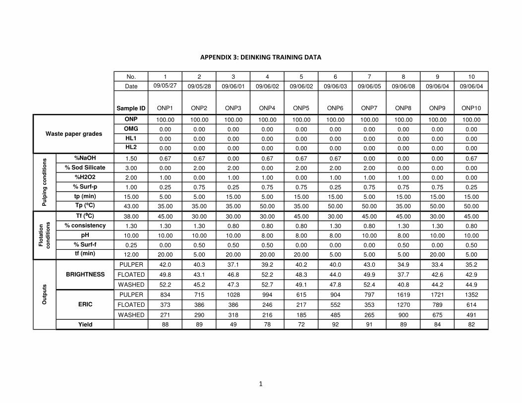
APPENDIX 3: DEINKING TRAINING DATA
No. 1 2 3 4 5 6 7 8 9 10
Date 09/05/27 09/05/28 09/06/01 09/06/02 09/06/02 09/06/03 09/06/05 09/06/08 09/06/04 09/06/04
Sample ID ONP1 ONP2 ONP3 ONP4 ONP5 ONP6 ONP7 ONP8 ONP9 ONP10
ONP 100.00 100.00 100.00 100.00 100.00 100.00 100.00 100.00 100.00 100.00
OMG 0.00 0.00 0.00 0.00 0.00 0.00 0.00 0.00 0.00 0.00
HL1 0.00 0.00 0.00 0.00 0.00 0.00 0.00 0.00 0.00 0.00
HL2 0.00 0.00 0.00 0.00 0.00 0.00 0.00 0.00 0.00 0.00
%NaOH 1.50 0.67 0.67 0.00 0.67 0.67 0.67 0.00 0.00 0.00 0.67
% Sod Silicate 3.00 0.00 2.00 2.00 0.00 2.00 2.00 2.00 0.00 0.00 0.00
%H2O2 2.00 1.00 0.00 1.00 1.00 0.00 1.00 1.00 1.00 0.00 0.00
% Surf-p 1.00 0.25 0.75 0.25 0.75 0.75 0.25 0.75 0.75 0.75 0.25
tp (min) 15.00 5.00 5.00 15.00 5.00 15.00 15.00 5.00 15.00 15.00 15.00
Tp (⁰C) 43.00 35.00 35.00 35.00 50.00 35.00 50.00 50.00 35.00 50.00 50.00
Tf (⁰⁰⁰⁰C) 38.00 45.00 30.00 30.00 30.00 45.00 30.00 45.00 45.00 30.00 45.00
% consistency 1.30 1.30 1.30 0.80 0.80 0.80 1.30 0.80 1.30 1.30 0.80
pH 10.00 10.00 10.00 10.00 8.00 8.00 8.00 10.00 8.00 10.00 10.00
% Surf-f 0.25 0.00 0.50 0.50 0.50 0.00 0.00 0.00 0.50 0.00 0.50
tf (min) 12.00 20.00 5.00 20.00 20.00 20.00 5.00 5.00 5.00 20.00 5.00
PULPER 42.0 40.3 37.1 39.2 40.2 40.0 43.0 34.9 33.4 35.2
FLOATED 49.8 43.1 46.8 52.2 48.3 44.0 49.9 37.7 42.6 42.9
WASHED 52.2 45.2 47.3 52.7 49.1 47.8 52.4 40.8 44.2 44.9
PULPER 834 715 1028 994 615 904 797 1619 1721 1352
FLOATED 373 386 386 246 217 552 353 1270 789 614
WASHED 271 290 318 216 185 485 265 900 675 491
Yield 88 89 49 78 72 92 91 89 84 82
BRIGHTNESS
ERIC
Waste paper grades
Pu
lpin
g c
on
dit
ion
sF
lota
tio
n
co
nd
itio
ns
Ou
tpu
ts
1

APPENDIX 3: DEINKING TRAINING DATA
11 12 13 14 15 16 17 18 19 20 21 22 23
09/06/29 09/06/29 09/06/09 09/06/10 09/06/10 09/06/11 09/06/11 09/06/12 09/06/17 09/06/17 09/06/18 09/06/18 09/06/30
ONP11 ONP12 ONP13 ONP14 ONP15 ONP16 ONP17 ONP18 ONP19 ONP20 ONP21 ONP22 ONP23
100.00 100.00 100.00 100.00 100.00 100.00 100.00 100.00 100.00 100.00 100.00 100.00 100.00
0.00 0.00 0.00 0.00 0.00 0.00 0.00 0.00 0.00 0.00 0.00 0.00 0.00
0.00 0.00 0.00 0.00 0.00 0.00 0.00 0.00 0.00 0.00 0.00 0.00 0.00
0.00 0.00 0.00 0.00 0.00 0.00 0.00 0.00 0.00 0.00 0.00 0.00 0.00
0.00 0.00 0.00 0.00 0.67 0.00 0.00 0.00 0.67 0.67 0.67 0.00 0.67
2.00 0.00 2.00 0.00 0.00 2.00 0.00 0.00 0.00 2.00 2.00 2.00 0.00
0.00 0.00 0.00 1.00 0.00 0.00 1.00 0.00 0.00 0.00 1.00 1.00 1.00
0.25 0.25 0.75 0.25 0.75 0.25 0.25 0.75 0.25 0.25 0.25 0.75 0.75
5.00 5.00 15.00 15.00 5.00 15.00 5.00 5.00 15.00 5.00 5.00 5.00 15.00
50.00 35.00 50.00 50.00 50.00 35.00 50.00 35.00 35.00 50.00 35.00 35.00 35.00
45.00 30.00 30.00 45.00 45.00 45.00 30.00 45.00 30.00 30.00 45.00 30.00 30.00
1.30 0.80 0.80 0.80 1.30 1.30 1.30 0.80 1.30 0.80 0.80 1.30 0.80
8.00 8.00 8.00 8.00 8.00 10.00 10.00 10.00 8.00 10.00 8.00 8.00 10.00
0.50 0.00 0.50 0.00 0.00 0.00 0.50 0.50 0.50 0.00 0.50 0.00 0.00
20.00 5.00 5.00 20.00 5.00 5.00 5.00 20.00 20.00 20.00 5.00 20.00 5.00
39.3 37.1 40.3 33.5 38.9 39.1 37.4 36.0 35.2 38.1 40.6 42.0 37.6
48.7 46.2 45.0 48.0 40.9 39.1 39.0 47.5 44.6 46.6 48.9 52.4 47.4
49.5 46.3 46.7 47.7 44.8 42.5 44.0 47.4 46.3 47.7 52.1 53.6 49.0
908 1184 888 1732 948 1042 1279 1343 1389 944 945 855 1109
302 527 504 489 721 852 996 400 489 245 477 304 439
261 467 404 461 496 631 686 392 389 212 343 247 373
72 82 79 48 92 96 88 57 74 52 84 73 90
2

APPENDIX 3: DEINKING TRAINING DATA
24 25 26 27 28 29 30 31 32 33 34 35 36
09/06/30 09/06/03 09/06/22 09/06/23 09/06/23 09/06/24 09/06/24 09/06/25 09/06/25 09/06/26 09/06/26 09/07/01 09/07/01
ONP24 ONPMID0 ONPMID1 ONPMID2 ONPMID3 ONPMID4 ONPMID5 OMG1 OMG2 OMG3 OMG4 OMG5 OMG6
100.00 100.00 100.00 100.00 100.00 100.00 100.00 0.00 0.00 0.00 0.00 0.00 0.00
0.00 0.00 0.00 0.00 0.00 0.00 0.00 100.00 100.00 100.00 100.00 100.00 100.00
0.00 0.00 0.00 0.00 0.00 0.00 0.00 0.00 0.00 0.00 0.00 0.00 0.00
0.00 0.00 0.00 0.00 0.00 0.00 0.00 0.00 0.00 0.00 0.00 0.00 0.00
0.67 0.34 0.34 0.34 0.34 0.34 0.34 0.67 0.67 0.00 0.67 0.67 0.67
2.00 1.00 1.00 1.00 1.00 1.00 1.00 0.00 2.00 2.00 0.00 2.00 2.00
1.00 0.50 0.50 0.50 0.50 0.50 0.50 1.00 0.00 1.00 1.00 0.00 1.00
0.75 0.50 0.50 0.50 0.50 0.50 0.50 0.25 0.75 0.25 0.75 0.75 0.25
15.00 10.00 10.00 10.00 10.00 10.00 10.00 5.00 5.00 15.00 5.00 15.00 15.00
50.00 43.00 43.00 43.00 43.00 43.00 43.00 35.00 35.00 35.00 50.00 35.00 50.00
45.00 38.00 38.00 38.00 38.00 38.00 38.00 45.00 30.00 30.00 30.00 45.00 30.00
1.30 1.05 1.05 1.05 1.05 1.05 1.05 1.30 1.30 0.80 0.80 0.80 1.30
10.00 9.00 9.00 9.00 9.00 9.00 9.00 10.00 10.00 10.00 8.00 8.00 8.00
0.50 0.25 0.25 0.25 0.25 0.25 0.25 0.00 0.50 0.50 0.50 0.00 0.00
20.00 12.50 12.50 12.50 12.50 12.50 12.50 20.00 5.00 20.00 20.00 20.00 5.00
42.2 38.2 39.0 38.2 37.9 39.4 38.2 46.4 46.9 42.2 44.6 42.0 45.0
49.6 48.6 50.0 49.4 49.5 50.3 49.6 68.8 61.9 63.5 66.8 62.2 61.5
51.5 50.8 51.7 51.5 51.5 52.5 51.0 70.8 64.0 63.5 69.2 61.8 63.1
826 1098 1041 1117 1131 1081 1122 558 557 606 591 636 682
384 357 348 360 361 345 370 84 100 89 87 103 160
334 287 294 282 291 260 307 57 82 76 73 90 131
93 83 70 68 67 70 71 47 70 63 29 35 70
3

APPENDIX 3: DEINKING TRAINING DATA
37 38 39 40 41 42 43 44 45 46 47 48 49
09/07/02 09/07/02 09/07/03 09/07/03 09/07/07 09/07/08 09/07/09 09/07/09 09/07/09 09/07/10 09/07/10 09/07/10 09/07/13
OMG7 OMG8 OMG9 OMG10 OMG11 OMG12 OMG13 OMG14 OMG15 OMG16 OMG17 OMG18 OMG19
0.00 0.00 0.00 0.00 0.00 0.00 0.00 0.00 0.00 0.00 0.00 0.00 0.00
100.00 100.00 100.00 100.00 100.00 100.00 100.00 100.00 100.00 100.00 100.00 100.00 100.00
0.00 0.00 0.00 0.00 0.00 0.00 0.00 0.00 0.00 0.00 0.00 0.00 0.00
0.00 0.00 0.00 0.00 0.00 0.00 0.00 0.00 0.00 0.00 0.00 0.00 0.00
0.00 0.00 0.00 0.67 0.00 0.00 0.00 0.00 0.67 0.00 0.00 0.00 0.67
2.00 0.00 0.00 0.00 2.00 0.00 2.00 0.00 0.00 2.00 0.00 0.00 0.00
1.00 1.00 0.00 0.00 0.00 0.00 0.00 1.00 0.00 0.00 1.00 0.00 0.00
0.75 0.75 0.75 0.25 0.25 0.25 0.75 0.25 0.75 0.25 0.25 0.75 0.25
5.00 15.00 15.00 15.00 5.00 5.00 15.00 15.00 5.00 15.00 5.00 5.00 15.00
50.00 35.00 50.00 50.00 50.00 35.00 50.00 50.00 50.00 35.00 50.00 35.00 35.00
45.00 45.00 30.00 45.00 45.00 30.00 30.00 45.00 45.00 45.00 30.00 45.00 30.00
0.80 1.30 1.30 0.80 1.30 0.80 0.80 0.80 1.30 1.30 1.30 0.80 1.30
10.00 8.00 10.00 10.00 8.00 8.00 8.00 8.00 8.00 10.00 10.00 10.00 8.00
0.00 0.50 0.00 0.50 0.50 0.00 0.50 0.00 0.00 0.00 0.50 0.50 0.50
5.00 5.00 20.00 5.00 20.00 5.00 5.00 20.00 5.00 5.00 5.00 20.00 20.00
44.6 45.7 45.8 43.7 43.3 47.1 43.4 44.3 44.2 42.9 44.9 46.2 42.8
62.8 68.5 65.9 59.6 65.9 63.7 61.3 64.9 58.4 57.9 58.7 65.0 61.4
63.8 68.9 64.8 60.2 65.6 64.1 60.4 64.0 59.5 59.2 61.4 64.4 61.1
647 729 640 673 600 638 669 566 591 671 588 532 704
104 94 69 121 62 110 130 80 132 146 147 86 76
101 75 74 115 73 102 120 83 113 117 124 72 80
53 58 50 54 47 55 47 46 60 77 74 29 50
4

APPENDIX 3: DEINKING TRAINING DATA
50 51 52 53 54 55 56 57 58 59 60 61 62
09/07/13 09/07/14 09/07/14 09/07/15 09/07/15 09/07/03 09/07/07 09/07/08 09/07/16 09/07/16 09/07/16 09/07/20 09/07/20
OMG20 OMG21 OMG22 OMG23 OMG24 OMGMID1 OMGMID2 OMGMID3 OMGMID4 OMGMID5 OMGMID6 HL1-1 HL1-2
0.00 0.00 0.00 0.00 0.00 0.00 0.00 0.00 0.00 0.00 0.00 0.00 0.00
100.00 100.00 100.00 100.00 100.00 100.00 100.00 100.00 100.00 100.00 100.00 0.00 0.00
0.00 0.00 0.00 0.00 0.00 0.00 0.00 0.00 0.00 0.00 0.00 100.00 100.00
0.00 0.00 0.00 0.00 0.00 0.00 0.00 0.00 0.00 0.00 0.00 0.00 0.00
0.67 0.67 0.00 0.67 0.67 0.34 0.34 0.34 0.34 0.34 0.34 0.67 0.67
2.00 2.00 2.00 0.00 2.00 1.00 1.00 1.00 1.00 1.00 1.00 0.00 2.00
0.00 1.00 1.00 1.00 1.00 0.50 0.50 0.50 0.50 0.50 0.50 1.00 0.00
0.25 0.25 0.75 0.75 0.75 0.50 0.50 0.50 0.50 0.50 0.50 0.25 0.75
5.00 5.00 5.00 15.00 15.00 10.00 10.00 10.00 10.00 10.00 10.00 5.00 5.00
50.00 35.00 35.00 35.00 50.00 43.00 43.00 43.00 43.00 43.00 43.00 35.00 35.00
30.00 45.00 30.00 30.00 45.00 38.00 38.00 38.00 38.00 38.00 38.00 45.00 30.00
0.80 0.80 1.30 0.80 1.30 1.05 1.05 1.05 1.05 1.05 1.05 1.30 1.30
10.00 8.00 8.00 10.00 10.00 9.00 9.00 9.00 9.00 9.00 9.00 10.00 10.00
0.00 0.50 0.00 0.00 0.50 0.25 0.25 0.25 0.25 0.25 0.25 0.00 0.50
20.00 5.00 20.00 5.00 20.00 12.50 12.50 12.50 12.50 12.50 12.50 20.00 5.00
51.0 43.3 44.8 43.4 44.4 46.1 42.5 43.6 43.1 44.8 44.3 88.5 87.3
62.1 64.0 66.1 59.5 66.4 68.4 65.3 66.6 64.4 66.7 65.7 91.9 92.4
61.2 64.4 66.4 60.2 67.1 66.7 64.6 66.1 64.8 66.8 65.1 93.2 91.5
564 589 585 612 618 579 707 738 654 591 589 112 90
64 96 65 117 59 62 73 62 68 60 67 73 52
73 87 67 103 69 75 76 63 69 69 65 70 61
49 41 52 53 43 40 53 47 53 46 45 88 95
5

APPENDIX 3: DEINKING TRAINING DATA
63 64 65 66 67 68 69 70 71 72 73 74 75
09/07/21 09/07/22 09/07/22 09/07/23 09/07/23 09/07/24 09/07/24 09/07/27 09/07/27 09/07/27 09/07/29 09/07/29 09/07/30
HL1-3 HL1-4 HL1-5 HL1-6 HL1-7 HL1-8 HL1-9 HL1-10 HL1-11 HL1-12 HL1-13 HL1-14 HL1-15
0.00 0.00 0.00 0.00 0.00 0.00 0.00 0.00 0.00 0.00 0.00 0.00 0.00
0.00 0.00 0.00 0.00 0.00 0.00 0.00 0.00 0.00 0.00 0.00 0.00 0.00
100.00 100.00 100.00 100.00 100.00 100.00 100.00 100.00 100.00 100.00 100.00 100.00 100.00
0.00 0.00 0.00 0.00 0.00 0.00 0.00 0.00 0.00 0.00 0.00 0.00 0.00
0.00 0.67 0.67 0.67 0.00 0.00 0.00 0.67 0.00 0.00 0.00 0.00 0.67
2.00 0.00 2.00 2.00 2.00 0.00 0.00 0.00 2.00 0.00 2.00 0.00 0.00
1.00 1.00 0.00 1.00 1.00 1.00 0.00 0.00 0.00 0.00 0.00 1.00 0.00
0.25 0.75 0.75 0.25 0.75 0.75 0.75 0.25 0.25 0.25 0.75 0.25 0.75
15.00 5.00 15.00 15.00 5.00 15.00 15.00 15.00 5.00 5.00 15.00 15.00 5.00
35.00 50.00 35.00 50.00 50.00 35.00 50.00 50.00 50.00 35.00 50.00 50.00 50.00
30.00 30.00 45.00 30.00 45.00 45.00 30.00 45.00 45.00 30.00 30.00 45.00 45.00
0.80 0.80 0.80 1.30 0.80 1.30 1.30 0.80 1.30 0.80 0.80 0.80 1.30
10.00 8.00 8.00 8.00 10.00 8.00 10.00 10.00 8.00 8.00 8.00 8.00 8.00
0.50 0.50 0.00 0.00 0.00 0.50 0.00 0.50 0.50 0.00 0.50 0.00 0.00
20.00 20.00 20.00 5.00 5.00 5.00 20.00 5.00 20.00 5.00 5.00 20.00 5.00
92.2 88.5 96.6 92.2 85.8 92.3 88.5 88.2 91.6 89.8 88.7 85.3 90.4
95.0 91.9 99.0 92.5 87.9 92.2 88.0 87.9 95.7 93.5 91.5 90.1 93.4
92.8 91.3 99.9 95.6 91.6 94.3 90.3 87.6 96.3 88.5 92.6 91.2 89.6
94 124 85 102 139 101 127 118 101 93 121 145 110
89 107 62 88 135 83 110 112 70 87 117 133 86
102 90 53 75 111 84 103 107 64 77 103 99 90
91 88 83 93 92 96 92 89 86 92 91 84 87
6

APPENDIX 3: DEINKING TRAINING DATA
76 77 78 79 80 81 82 83 84 85 86 87 88
09/07/30 09/07/31 09/07/31 09/07/31 09/08/03 09/08/03 09/08/04 09/08/04 09/08/05 09/07/21 09/07/28 09/07/28 09/07/28
HL1-16 HL1-17 HL1-18 HL1-19 HL1-20 HL1-21 HL1-22 HL1-23 HL1-24 HL1MID1 HL1MID2 HL1MID3 HL1MID4
0.00 0.00 0.00 0.00 0.00 0.00 0.00 0.00 0.00 0.00 0.00 0.00 0.00
0.00 0.00 0.00 0.00 0.00 0.00 0.00 0.00 0.00 0.00 0.00 0.00 0.00
100.00 100.00 100.00 100.00 100.00 100.00 100.00 100.00 100.00 100.00 100.00 100.00 100.00
0.00 0.00 0.00 0.00 0.00 0.00 0.00 0.00 0.00 0.00 0.00 0.00 0.00
0.00 0.00 0.00 0.67 0.67 0.67 0.00 0.67 0.67 0.34 0.34 0.34 0.34
2.00 0.00 0.00 0.00 2.00 2.00 2.00 0.00 2.00 1.00 1.00 1.00 1.00
0.00 1.00 0.00 0.00 0.00 1.00 1.00 1.00 1.00 0.50 0.50 0.50 0.50
0.25 0.25 0.75 0.25 0.25 0.25 0.75 0.75 0.75 0.50 0.50 0.50 0.50
15.00 5.00 5.00 15.00 5.00 5.00 5.00 15.00 15.00 10.00 10.00 10.00 10.00
35.00 50.00 35.00 35.00 50.00 35.00 35.00 35.00 50.00 43.00 43.00 43.00 43.00
45.00 30.00 45.00 30.00 30.00 45.00 30.00 30.00 45.00 38.00 38.00 38.00 38.00
1.30 1.30 0.80 1.30 0.80 0.80 1.30 0.80 1.30 1.05 1.05 1.05 1.05
10.00 10.00 10.00 8.00 10.00 8.00 8.00 10.00 10.00 9.00 9.00 9.00 9.00
0.00 0.50 0.50 0.50 0.00 0.50 0.00 0.00 0.50 0.25 0.25 0.25 0.25
5.00 5.00 20.00 20.00 20.00 5.00 20.00 5.00 20.00 12.50 12.50 12.50 12.50
92.2 90.7 92.7 91.4 91.4 91.5 83.1 90.6 93.5 81.2 89.5 91.0 88.0
90.0 92.9 95.3 93.7 95.4 94.1 89.4 92.9 96.7 90.4 91.8 90.8 94.3
90.4 94.7 95.8 95.7 91.8 91.8 91.0 94.4 100.0 88.3 92.0 92.5 92.8
112 113 89 106 109 102 155 105 89 165 126 93 113
96 88 75 75 89 92 112 103 57 118 87 63 84
87 82 65 78 85 75 89 91 49 96 81 65 74
93 83 85 86 86 82 92 71 85 71 86 90 92
7

APPENDIX 3: DEINKING TRAINING DATA
89 90 91 92 93 94 95 96 97 98 99 100 101
09/08/05 09/08/05 09/08/14 09/08/17 09/08/17 09/08/18 09/08/18 09/08/19 09/08/19 09/08/19 09/08/20
HL1MID5 HL1MID6 HL2-1 HL2-2 HL2-3 HL2-4 HL2-5 HL2-6 HL2-7 HL2-8 HL2-9 HL2-10 HL2-11
0.00 0.00 0.00 0.00 0.00 0.00 0.00 0.00 0.00 0.00 0.00 0.00 0.00
0.00 0.00 0.00 0.00 0.00 0.00 0.00 0.00 0.00 0.00 0.00 0.00 0.00
100.00 100.00 0.00 0.00 0.00 0.00 0.00 0.00 0.00 0.00 0.00 0.00 0.00
0.00 0.00 100.00 100.00 100.00 100.00 100.00 100.00 100.00 100.00 100.00 100.00 100.00
0.34 0.34 0.67 0.67 0.00 0.67 0.67 0.67 0.00 0.00 0.00 0.67 0.00
1.00 1.00 0.00 2.00 2.00 0.00 2.00 2.00 2.00 0.00 0.00 0.00 2.00
0.50 0.50 1.00 0.00 1.00 1.00 0.00 1.00 1.00 1.00 0.00 0.00 0.00
0.50 0.50 0.25 0.75 0.25 0.75 0.75 0.25 0.75 0.75 0.75 0.25 0.25
10.00 10.00 5.00 5.00 15.00 5.00 15.00 15.00 5.00 15.00 15.00 15.00 5.00
43.00 43.00 35.00 35.00 35.00 50.00 35.00 50.00 50.00 35.00 50.00 50.00 50.00
38.00 38.00 45.00 30.00 30.00 30.00 45.00 30.00 45.00 45.00 30.00 45.00 45.00
1.05 1.05 1.30 1.30 0.80 0.80 0.80 1.30 0.80 1.30 1.30 0.80 1.30
9.00 9.00 10.00 10.00 10.00 8.00 8.00 8.00 10.00 8.00 10.00 10.00 8.00
0.25 0.25 0.00 0.50 0.50 0.50 0.00 0.00 0.00 0.50 0.00 0.50 0.50
12.50 12.50 20.00 5.00 20.00 20.00 20.00 5.00 5.00 5.00 20.00 5.00 20.00
93.6 84.7 67.8 73.7 76.3 75.4 63.4 82.3 69.1 60.0 65.7 63.7 74.3
96.6 92.7 72.0 73.3 77.0 80.2 65.9 83.7 69.9 61.6 67.3 67.9 76.2
95.8 94.3 73.6 75.0 78.3 80.1 68.3 88.0 73.5 65.2 68.7 70.1 78.9
111 128 98 94 84 100 121 115 101 113 104 104 77
80 93 51 65 60 68 78 91 62 94 86 55 33
75 78 53 69 57 63 61 76 59 83 79 63 39
95 87 68 86 75 68 66 85 85 94 90 84 79
8

APPENDIX 3: DEINKING TRAINING DATA
102 103 104 105 106 107 108 109 110 111 112 113 114
09/08/20 09/08/21 09/08/21 09/08/24 09/08/25 09/08/25 09/08/26 09/08/26 09/08/26 09/08/27 09/08/27 09/08/27 09/08/28
HL2-12 HL2-13 HL2-14 HL2-15 HL2-16 HL2-17 HL2-18 HL2-19 HL2-20 HL2-21 HL2-22 HL2-23 HL2-24
0.00 0.00 0.00 0.00 0.00 0.00 0.00 0.00 0.00 0.00 0.00 0.00 0.00
0.00 0.00 0.00 0.00 0.00 0.00 0.00 0.00 0.00 0.00 0.00 0.00 0.00
0.00 0.00 0.00 0.00 0.00 0.00 0.00 0.00 0.00 0.00 0.00 0.00 0.00
100.00 100.00 100.00 100.00 100.00 100.00 100.00 100.00 100.00 100.00 100.00 100.00 100.00
0.00 0.00 0.00 0.67 0.00 0.00 0.00 0.67 0.67 0.67 0.00 0.67 0.67
0.00 2.00 0.00 0.00 2.00 0.00 0.00 0.00 2.00 2.00 2.00 0.00 2.00
0.00 0.00 1.00 0.00 0.00 1.00 0.00 0.00 0.00 1.00 1.00 1.00 1.00
0.25 0.75 0.25 0.75 0.25 0.25 0.75 0.25 0.25 0.25 0.75 0.75 0.75
5.00 15.00 15.00 5.00 15.00 5.00 5.00 15.00 5.00 5.00 5.00 15.00 15.00
35.00 50.00 50.00 50.00 35.00 50.00 35.00 35.00 50.00 35.00 35.00 35.00 50.00
30.00 30.00 45.00 45.00 45.00 30.00 45.00 30.00 30.00 45.00 30.00 30.00 45.00
0.80 0.80 0.80 1.30 1.30 1.30 0.80 1.30 0.80 0.80 1.30 0.80 1.30
8.00 8.00 8.00 8.00 10.00 10.00 10.00 8.00 10.00 8.00 8.00 10.00 10.00
0.00 0.50 0.00 0.00 0.00 0.50 0.50 0.50 0.00 0.50 0.00 0.00 0.50
5.00 5.00 20.00 5.00 5.00 5.00 20.00 20.00 20.00 5.00 20.00 5.00 20.00
65.6 62.4 66.4 66.9 66.1 66.5 64.3 60.4 61.7 61.8 64.0 63.5 60.8
67.7 65.2 69.1 65.9 65.3 68.6 64.4 59.9 63.8 62.8 62.7 65.7 62.2
69.8 66.6 70.7 69.5 68.5 70.7 67.8 63.3 66.2 64.0 64.6 67.9 65.8
79 96 90 83 97 89 77 97 82 85 73 94 86
48 39 35 73 85 87 73 91 44 84 80 86 90
56 46 42 65 68 74 63 63 49 64 61 64 65
88 85 77 92 95 93 95 93 86 94 89 103 95
9

APPENDIX 3: DEINKING TRAINING DATA
115 116 117 118 119 120 121 122 123 124 125 126 127
09/08/10 09/08/11 09/08/20 09/08/20 09/08/28 09/08/28 09/09/07 09/09/07 09/09/08 09/09/08 09/09/09 09/09/09 09/09/10
HL2MID1 HL2MID2 HL2MID3 HL2MID4 HL2MID5 HL2MID6
ONPOMG5
050.1
ONPOMG5
050.2
ONPOMG5
050.3
ONPOMG5
050.4
ONPOMG5
050.5
ONPOMG5
050.6
ONPOMG5
050.7
0.00 0.00 0.00 0.00 0.00 0.00 50.00 50.00 50.00 50.00 50.00 50.00 50.00
0.00 0.00 0.00 0.00 0.00 0.00 50.00 50.00 50.00 50.00 50.00 50.00 50.00
0.00 0.00 0.00 0.00 0.00 0.00 0.00 0.00 0.00 0.00 0.00 0.00 0.00
100.00 100.00 100.00 100.00 100.00 100.00 0.00 0.00 0.00 0.00 0.00 0.00 0.00
0.34 0.34 0.34 0.34 0.34 0.34 0.88 1.36 1.29 1.33 1.29 1.24 1.27
1.00 1.00 1.00 1.00 1.00 1.00 0.20 1.60 0.60 0.90 1.90 2.70 0.20
0.50 0.50 0.50 0.50 0.50 0.50 0.30 1.70 1.30 1.50 1.30 1.10 1.20
0.50 0.50 0.50 0.50 0.50 0.50 0.60 0.50 0.70 0.40 0.50 0.80 0.70
10.00 10.00 10.00 10.00 10.00 10.00 14.00 13.00 5.00 13.00 5.00 7.00 14.00
43.00 43.00 43.00 43.00 43.00 43.00 43.00 43.00 43.00 43.00 43.00 43.00 43.00
38.00 38.00 38.00 38.00 38.00 38.00 38.00 38.00 38.00 38.00 38.00 38.00 38.00
1.05 1.05 1.05 1.05 1.05 1.05 0.80 0.90 1.10 0.80 0.90 0.90 1.00
9.00 9.00 9.00 9.00 9.00 9.00 9.00 9.00 9.00 9.00 9.00 9.00 9.00
0.25 0.25 0.25 0.25 0.25 0.25 0.00 0.00 0.00 0.00 0.00 0.00 0.00
12.50 12.50 12.50 12.50 12.50 12.50 12.00 5.00 6.00 5.00 10.00 11.00 6.00
64.9 64.3 64.7 65.3 64.0 58.4 39.5 37.6 42.1 46.6 44.7 44.6 46.3
67.5 66.4 67.5 68.0 65.7 60.0 53.0 47.9 53.6 58.4 58.7 59.4 57.3
68.7 69.5 68.6 69.9 67.6 62.0 54.0 50.6 56.3 59.8 60.3 59.8 59.2
112 118 80 82 87 83 847 935 657 598 672 606 703
61 59 28 30 47 53 169 353 208 117 121 97 163
52 53 37 38 39 37 153 245 151 99 95 87 129
66 72 77 71 78 63 51 76 76 76 69 61 78
10

APPENDIX 3: DEINKING TRAINING DATA
128 129 130 131 132 133 134 135 136 137 138 139 140
09/09/10 09/09/11 09/09/11 09/09/14 09/09/14 09/09/15 09/09/15 09/09/16 09/09/16 09/09/16 09/09/17 09/09/17 09/09/17
ONPOMG5
050.8
ONPOMG5
050.9
ONPOMG5
050.10
ONPOMG5
050.11
ONPOMG5
050.12
ONPOMG7
525.13
ONPOMG7
525.14
ONPOMG7
525.15
ONPOMG7
525.16
ONPOMG7
525.17
ONPOMG7
525.18 ONPMID.7
HL1HL2505
0.1
50.00 50.00 50.00 50.00 50.00 75.00 75.00 75.00 75.00 75.00 75.00 100.00 0.00
50.00 50.00 50.00 50.00 50.00 25.00 25.00 25.00 25.00 25.00 25.00 0.00 0.00
0.00 0.00 0.00 0.00 0.00 0.00 0.00 0.00 0.00 0.00 0.00 0.00 50.00
0.00 0.00 0.00 0.00 0.00 0.00 0.00 0.00 0.00 0.00 0.00 0.00 50.00
0.88 0.96 1.31 1.07 1.31 1.27 0.77 1.24 1.22 1.15 0.77 0.34 1.33
1.60 2.90 1.50 0.90 2.80 2.90 0.80 0.90 1.20 1.10 0.10 1.00 2.10
0.30 0.40 1.40 0.60 1.40 1.20 0.20 1.10 1.00 0.80 0.20 0.50 1.50
0.50 0.70 0.90 0.30 0.80 1.00 0.80 0.70 0.80 0.40 0.70 0.50 0.50
6.00 7.00 14.00 9.00 11.00 6.00 11.00 15.00 10.00 7.00 5.00 10.00 11.00
43.00 43.00 43.00 43.00 43.00 43.00 43.00 43.00 43.00 43.00 43.00 43.00 43.00
38.00 38.00 38.00 38.00 38.00 38.00 38.00 38.00 38.00 38.00 38.00 38.00 38.00
0.80 1.20 1.20 1.00 1.30 0.80 1.00 1.10 1.00 0.90 0.90 1.00 1.10
9.00 9.00 9.00 9.00 9.00 9.00 9.00 9.00 9.00 9.00 9.00 9.00 9.00
0.00 0.00 0.00 0.00 0.00 0.00 0.00 0.00 0.00 0.00 0.00 0.25 0.00
4.00 4.00 3.00 4.00 8.00 6.00 10.00 4.00 10.00 11.00 8.00 12.50 11.00
45.8 45.1 42.0 44.3 44.1 42.4 43.0 43.4 42.1 40.6 40.9 38.5 73.4
56.8 53.4 46.8 55.8 57.8 55.3 52.0 49.1 55.2 54.2 51.8 50.7 75.6
58.0 56.3 49.2 57.5 59.2 57.3 53.8 51.8 56.2 55.9 53.3 51.7 77.4
639 606 645 742 726 788 695 690 959 881 801 1043 106
147 210 314 224 177 208 134 262 211 174 180 285 42
116 150 220 171 154 143 117 188 180 155 161 255 33
82 85 82 77 75 94 67 88 63 59 59 70 80
11

APPENDIX 3: DEINKING TRAINING DATA
141 142 143 144 145 146 147 148 149 150 151 152 153
09/09/18 09/09/18 09/09/21 09/09/21 09/09/21 09/09/22 09/09/22 09/09/23 09/09/23 09/09/28 09/09/28 09/09/28 09/09/29
HL1HL2505
0.2
HL1HL2
5050.3
HL1HL2505
0.4
HL1HL2505
0.5
HL1HL2505
0.6
HL1HL2505
0.7
HL1HL2505
0.8
HL1HL2505
0.9
HL1HL2505
0.10
HL1HL2505
0.11
HL1HL2505
0.12
HL1HL2505
0.13
HL1HL2505
0.14
0.00 0.00 0.00 0.00 0.00 0.00 0.00 0.00 0.00 0.00 0.00 0.00 0.00
0.00 0.00 0.00 0.00 0.00 0.00 0.00 0.00 0.00 0.00 0.00 0.00 0.00
50.00 50.00 50.00 50.00 50.00 50.00 50.00 50.00 50.00 50.00 50.00 67.00 67.00
50.00 50.00 50.00 50.00 50.00 50.00 50.00 50.00 50.00 50.00 50.00 33.00 33.00
0.90 0.10 0.60 0.90 0.50 1.10 0.80 0.10 0.90 1.30 0.60 0.70 1.20
0.50 2.80 2.30 1.00 1.50 1.90 1.80 0.40 0.40 2.70 0.30 1.10 0.80
1.40 1.90 0.20 0.40 1.50 1.70 0.30 0.00 1.20 0.60 1.90 1.50 0.60
0.60 0.70 0.90 0.70 0.50 0.70 0.80 0.30 0.50 1.00 1.00 0.70 0.90
10.00 9.00 10.00 5.00 15.00 10.00 8.00 14.00 5.00 10.00 15.00 7.00 15.00
43.00 43.00 43.00 43.00 43.00 43.00 43.00 43.00 43.00 43.00 43.00 43.00 43.00
38.00 38.00 38.00 38.00 38.00 38.00 38.00 38.00 38.00 38.00 38.00 38.00 38.00
1.20 0.90 0.90 0.80 1.10 0.90 1.00 1.20 1.20 1.10 0.80 1.20 1.10
9.00 9.00 9.00 9.00 9.00 9.00 9.00 9.00 9.00 9.00 9.00 9.00 9.00
0.00 0.00 0.00 0.00 0.00 0.00 0.00 0.00 0.00 0.00 0.00 0.00 0.00
10.00 12.00 8.00 7.00 6.00 11.00 5.00 3.00 6.00 6.00 5.00 10.00 9.00
72.1 69.9 72.4 70.0 68.8 75.1 72.7 66.6 72.1 75.1 73.8 74.5 77.6
72.5 72.1 73.3 72.4 71.4 75.6 74.2 66.5 72.9 75.9 76.7 76.4 75.9
73.8 72.8 74.3 72.7 74.6 77.3 75.3 68.3 73.8 75.2 76.8 73.1 79.8
107 89 127 128 118 94 97 102 90 126 135 115 114
54 43 65 75 75 51 62 65 53 74 81 80 44
41 38 61 65 61 35 42 52 43 57 71 70 31
85 76 84 80 81 77 79 88 79 82 85 85 63
12

APPENDIX 3: DEINKING TRAINING DATA
154 155 156 157 158 159 160 161 162 163 164 165 166
09/09/29 09/09/30 09/09/30 09/09/30 09/10/01 1 0ct 09/09/22 09/09/29 09/10/02 09/10/02 09/10/05 09/10/05 09/10/05
HL1HL2505
0.15
HL1HL2505
0.16
HL1HL2505
0.17
HL1HL2505
0.18
HL1HL2505
0.19
HL1HL2505
0.20 HL1MID HL1MID ONPHL1.1 ONPHL1.2 ONPHL1.3 ONPHL1.4 ONPHL1.5
0.00 0.00 0.00 0.00 0.00 0.00 0.00 0.00 50.00 50.00 50.00 50.00 50.00
0.00 0.00 0.00 0.00 0.00 0.00 0.00 0.00 0.00 0.00 0.00 0.00 0.00
67.00 67.00 67.00 67.00 67.00 67.00 100.00 100.00 50.00 50.00 50.00 50.00 50.00
33.00 33.00 33.00 33.00 33.00 33.00 0.00 0.00 0.00 0.00 0.00 0.00 0.00
0.90 0.30 1.40 0.20 0.40 0.40 0.50 0.50 0.10 1.20 0.90 0.30 1.20
0.20 0.80 0.10 0.00 2.50 1.30 1.00 1.00 2.00 2.80 0.50 2.60 1.50
0.50 1.10 0.70 1.50 1.20 0.80 0.50 0.50 0.50 1.70 1.60 0.99 0.80
1.00 0.40 0.50 0.90 0.50 0.60 0.50 0.50 0.90 0.30 0.80 0.50 0.40
8.00 6.00 9.00 11.00 8.00 6.00 10.00 10.00 11.00 15.00 5.00 5.00 9.00
43.00 43.00 43.00 43.00 43.00 43.00 43.00 43.00 43.00 43.00 43.00 43.00 43.00
38.00 38.00 38.00 38.00 38.00 38.00 38.00 38.00 38.00 38.00 38.00 38.00 38.00
0.90 0.90 1.00 0.90 1.20 1.10 1.05 1.05 1.30 0.93 1.00 1.20 1.30
9.00 9.00 9.00 9.00 9.00 9.00 9.00 9.00 9.00 9.00 9.00 9.00 9.00
0.00 0.00 0.00 0.00 0.00 0.00 0.00 0.00 0.00 0.00 0.00 0.00 0.00
4.00 5.00 10.00 5.00 2.00 3.00 12.50 12.50 6.00 4.00 3.00 6.00 12.00
76.2 76.5 76.7 79.8 81.4 80.2 98.8 99.1 49.2 53.0 53.3 54.0 53.8
79.6 79.4 82.6 81.9 82.5 83.3 102.1 100.8 55.5 60.5 60.6 63.6 64.7
79.9 78.8 83.8 83.7 80.9 84.3 99.3 96.6 59.1 65.5 66.0 65.5 68.6
99 91 99 109 106 108 88 95 646 695 509 480 550
54 45 42 49 64 54 39 46 411 381 336 259 211
43 42 31 46 52 51 40 47 261 215 206 193 141
86 86 77 89 74 83 90 91 88 80 87 78 65
13

APPENDIX 3: DEINKING TRAINING DATA
167 168 169 170 171 172 173 174 175 176 177 178 179
09/10/06 09/10/06 09/10/06 09/10/07 09/10/07 09/10/07 09/10/08 09/10/08 09/10/08 09/10/09 09/10/09 09/10/09 09/10/12
ONPHL1.6 ONPHL1.7 ONPHL1.8 ONPHL1.9
ONPHL1.1
0
ONPHL1.1
1
ONPHL1.1
2 ONPMID HL2MID ONPHL2.1 ONPHL2.2 ONPHL2.3 ONPHL2.4
50.00 50.00 50.00 50.00 50.00 50.00 50.00 100.00 0.00 50.00 50.00 50.00 50.00
0.00 0.00 0.00 0.00 0.00 0.00 0.00 0.00 0.00 0.00 0.00 0.00 0.00
50.00 50.00 50.00 50.00 50.00 50.00 50.00 0.00 0.00 0.00 0.00 0.00 0.00
0.00 0.00 0.00 0.00 0.00 0.00 0.00 0.00 100.00 50.00 50.00 50.00 50.00
1.00 0.40 1.40 0.80 0.60 0.00 0.70 0.34 0.34 1.00 0.80 1.10 1.32
2.00 0.70 0.20 1.00 0.80 0.00 1.10 1.00 1.00 0.60 0.80 2.50 1.70
0.00 0.70 1.80 1.50 0.30 0.00 1.10 0.50 0.50 0.90 0.70 1.70 0.10
0.25 0.40 0.60 1.00 0.90 0.30 0.30 0.50 0.50 0.30 0.50 0.90 0.60
14.00 14.00 10.00 8.00 7.00 9.00 13.00 10.00 10.00 8.00 11.00 15.00 10.00
43.00 43.00 43.00 43.00 43.00 43.00 43.00 43.00 43.00 43.00 43.00 43.00 43.00
38.00 38.00 38.00 38.00 38.00 38.00 38.00 38.00 38.00 38.00 38.00 38.00 38.00
1.20 0.80 1.10 1.20 0.80 1.00 1.20 1.00 1.04 0.90 1.10 1.00 1.20
9.00 9.00 9.00 9.00 9.00 7.80 7.70 8.70 8.90 8.90 8.84 8.85 9.71
0.00 0.00 0.00 0.00 0.00 0.00 0.00 0.25 0.25 0.00 0.00 0.00 0.00
7.00 8.00 7.00 5.00 2.00 11.00 5.00 12.50 12.50 2.00 7.00 8.00 6.00
48.8 53.6 57.8 56.3 52.9 51.6 53.0 40.3 55.2 43.2 44.9 44.0 41.1
53.9 64.9 67.6 66.6 60.3 61.3 61.9 52.8 55.1 44.9 49.9 50.0 41.4
57.8 66.7 70.8 71.4 62.8 63.1 65.7 53.8 56.9 50.1 53.6 54.1 47.8
526 535 453 484 538 556 545 894 129 721 678 687 643
288 197 166 196 312 188 310 232 96 644 365 421 621
177 129 101 130 220 147 194 210 64 394 222 237 310
76 97 76 75 79 58 73 62 75 94 84 77 93
14

APPENDIX 3: DEINKING TRAINING DATA
180 181 182 183 184 185 186 187 188 189 190 191 192
09/10/12 09/10/12 09/10/13 09/10/13 09/10/13 09/10/14 09/10/14 09/10/14 09/10/15 09/10/15 09/10/16 09/10/16 09/10/16
ONPHL2.5 ONPHL2.6 ONPHL2.7 ONPHL2.8 ONPHL2.9 ONPHL2.10 ONPHL2.11 ONPHL2.12 OMGMID HL1MID OMGHL1.1 OMGHL1.2 OMGHL1.3
50.00 50.00 50.00 50.00 50.00 50.00 50.00 50.00 0.00 0.00 0.00 0.00 0.00
0.00 0.00 0.00 0.00 0.00 0.00 0.00 0.00 100.00 0.00 50.00 50.00 50.00
0.00 0.00 0.00 0.00 0.00 0.00 0.00 0.00 0.00 100.00 50.00 50.00 50.00
50.00 50.00 50.00 50.00 50.00 50.00 50.00 50.00 0.00 0.00 0.00 0.00 0.00
0.30 0.90 0.90 1.20 0.20 1.11 1.21 0.51 0.34 0.34 0.50 0.91 1.42
0.10 0.50 0.60 0.20 0.70 2.00 1.10 3.00 1.00 1.00 0.90 1.50 2.80
1.70 1.40 0.70 1.30 1.60 1.10 0.50 2.00 0.50 0.50 0.10 1.20 1.00
0.80 0.80 0.90 0.60 0.80 0.30 0.70 0.40 0.50 0.50 0.50 0.60 0.90
7.00 5.00 13.00 13.00 9.00 13.00 6.00 5.00 10.00 10.00 13.00 7.00 14.00
43.00 43.00 43.00 43.00 43.00 43.00 43.00 43.00 43.00 43.00 43.00 43.00 43.00
38.00 38.00 38.00 38.00 38.00 38.00 38.00 38.00 38.00 38.00 38.00 38.00 38.00
1.08 0.80 1.20 1.08 1.18 0.90 1.10 1.00 1.04 1.04 1.00 1.00 0.89
7.11 8.20 8.30 7.40 9.40 9.70 9.70 9.30 9.10 8.85 8.10 10.00 9.50
0.00 0.00 0.00 0.00 0.00 0.00 0.00 0.00 0.25 0.25 0.00 0.00 0.00
8.00 3.00 3.00 11.00 5.00 8.00 4.00 12.00 12.50 12.50 7.00 2.00 9.00
42.9 45.1 43.8 44.5 44.3 44.3 41.6 45.5 43.5 99.5 67.3 57.9 72.7
49.3 44.8 45.0 49.1 46.1 49.2 43.5 47.3 65.6 104.5 76.9 62.3 85.7
52.7 49.1 50.7 53.3 50.1 52.6 48.1 52.0 66.5 101.5 76.0 65.9 88.1
727 614 619 670 642 648 682 577 655 84 316 329 263
437 616 628 420 524 427 610 544 76 32 108 247 72
297 377 333 252 312 261 355 350 66 40 75 189 51
71 70 91 80 81 83 85 95 53 88 76 77 79
15

APPENDIX 3: DEINKING TRAINING DATA
193 194 195 196 197 198 199 200 201 202 203 204 205
09/10/16 09/10/19 09/10/19 09/10/19 09/10/20 09/10/20 09/10/20 09/10/21 09/10/22 09/10/22 09/10/23 09/10/23 09/10/23
OMGHL1.4 OMGHL1.5 OMGHL1.6 OMGHL1.7 OMGHL1.8 OMGHL1.9 OMGHL1.10OMGHL1.11OMGHL1.12 HL2MID OMGHL2.1 OMGHL2.2 OMGHL2.3
0.00 0.00 0.00 0.00 0.00 0.00 0.00 0.00 0.00 0.00 0.00 0.00 0.00
50.00 50.00 50.00 50.00 50.00 50.00 50.00 50.00 50.00 0.00 50.00 50.00 50.00
50.00 50.00 50.00 50.00 50.00 50.00 50.00 50.00 50.00 0.00 0.00 0.00 0.00
0.00 0.00 0.00 0.00 0.00 0.00 0.00 0.00 0.00 100.00 50.00 50.00 50.00
0.51 0.41 0.71 0.00 0.30 0.71 0.60 1.32 0.41 0.34 0.71 0.41 0.81
0.30 1.90 2.10 1.10 0.20 1.30 0.30 0.40 2.60 1.00 1.50 0.40 0.60
1.90 1.50 0.40 1.30 1.90 1.30 2.00 1.70 2.00 0.50 0.60 1.90 1.20
0.25 0.60 0.70 1.00 0.40 0.50 0.40 0.80 1.00 0.50 0.40 0.50 0.60
8.00 10.00 6.00 8.00 9.00 10.00 11.00 5.00 13.00 10.00 8.00 6.00 5.00
43.00 43.00 43.00 43.00 43.00 43.00 43.00 43.00 43.00 43.00 43.00 43.00 43.00
38.00 38.00 38.00 38.00 38.00 38.00 38.00 38.00 38.00 38.00 38.00 38.00 38.00
1.20 1.10 1.30 0.80 1.10 1.00 0.80 1.20 0.89 1.04 1.20 1.11 0.83
8.50 9.00 7.80 7.20 7.60 9.80 9.00 9.80 9.50 8.85 7.40 8.00 7.50
0.00 0.00 0.00 0.00 0.00 0.00 0.00 0.00 0.00 0.25 0.00 0.00 0.00
11.00 10.00 8.00 12.00 6.00 10.00 5.00 8.00 6.00 12.50 5.00 10.00 12.00
68.4 61.4 58.1 58.9 71.5 70.3 70.6 55.4 57.6 54.1 47.7 47.6 47.9
82.8 69.2 66.1 71.1 83.9 84.2 82.7 64.1 66.0 54.0 49.7 56.0 57.3
82.7 72.2 69.5 71.6 85.0 85.3 83.2 68.2 69.7 56.1 53.7 59.2 60.1
253 284 338 330 238 285 262 288 281 111 346 311 331
63 134 181 109 74 67 78 128 112 100 293 116 117
50 97 133 72 56 54 67 114 90 59 224 100 79
72 91 79 78 70 73 74 71 81 85 84 70 63
16

APPENDIX 3: DEINKING TRAINING DATA
206 207 208 209 210 211 212 213 214 215 216 217 218
09/10/26 09/10/26 09/10/26 09/10/27 09/10/27 09/10/27 09/10/28 09/10/28 09/10/28 09/10/28 09/10/29 09/10/29 09/10/29
OMGHL2.4 OMGHL2.5 OMGHL2.6 OMGHL2.7 OMGHL2.8 OMGHL2.9 OMGHL2.10OMGHL2.11OMGHL2.12OMGHL2.13OMGHL2.14 ONPMID OMGMID
0.00 0.00 0.00 0.00 0.00 0.00 0.00 0.00 0.00 0.00 0.00 100.00 0.00
50.00 50.00 50.00 50.00 50.00 50.00 50.00 50.00 50.00 50.00 50.00 0.00 100.00
0.00 0.00 0.00 0.00 0.00 0.00 0.00 0.00 0.00 0.00 0.00 0.00 0.00
50.00 50.00 50.00 50.00 50.00 50.00 50.00 50.00 50.00 50.00 50.00 0.00 0.00
0.50 0.70 1.42 0.10 1.42 1.11 0.30 1.52 0.51 0.20 0.51 0.34 0.34
0.50 2.70 2.90 1.00 3.00 1.80 0.10 1.20 0.30 0.80 0.70 1.00 1.00
0.70 1.80 1.70 0.70 0.50 1.60 1.50 1.10 2.00 1.20 0.20 0.50 0.50
0.50 0.60 0.50 0.90 0.40 0.90 0.60 0.80 0.70 0.30 0.40 0.50 0.50
13.00 15.00 14.00 10.00 9.00 9.00 8.00 14.00 9.00 12.00 13.00 10.00 10.00
43.00 43.00 43.00 43.00 43.00 43.00 43.00 43.00 43.00 43.00 43.00 43.00 43.00
38.00 38.00 38.00 38.00 38.00 38.00 38.00 38.00 38.00 38.00 38.00 38.00 38.00
0.93 0.92 1.00 1.11 0.92 0.92 1.20 1.11 0.83 1.02 0.93 1.04 1.04
7.00 8.30 8.65 10.00 9.50 9.00 9.50 7.30 8.60 9.25 8.10 8.70 9.10
0.00 0.00 0.00 0.00 0.00 0.00 0.00 0.00 0.00 0.00 0.00 0.25 0.25
3.00 2.00 7.00 6.00 9.00 6.00 11.00 6.00 4.00 10.00 3.00 12.50 12.50
50.4 48.3 48.8 49.4 48.4 49.6 49.0 46.0 47.6 50.7 49.0 39.5 49.3
56.7 51.6 57.7 51.3 57.9 56.1 51.1 52.2 54.7 56.6 53.2 50.9 72.1
59.5 55.3 60.3 54.2 60.4 59.0 55.0 55.1 58.3 60.4 56.3 52.2 71.5
340 409 341 297 332 309 304 309 300 309 312 1039 423
172 286 121 248 109 141 247 158 135 163 181 323 48
118 179 79 180 70 96 181 104 98 109 123 290 41
80 88 65 87 76 81 81 65 68 86 82 76 58
17

APPENDIX 3: DEINKING TRAINING DATA
219 220 221 222 223 224 225 226 227 228 229 230 231
09/10/29 09/11/02 09/10/30 09/10/30 09/10/30 09/11/02 09/11/02 09/11/03 09/11/03 09/11/03 09/11/04 09/11/04 09/11/04
HL1MID HL2MID
ONPOMGH
L2. 1
ONPOMGH
L2.2
ONPOMGH
L2.3
ONPOMGH
L2.4
ONPOMGH
L2.5
ONPOMGH
L2.6
ONPOMGH
L2.7
ONPOMGH
L2.8
ONPOMGH
L2.9
ONPOMGH
L2.10
ONPOMGH
L2.11
0.00 0.00 34.00 34.00 34.00 34.00 34.00 34.00 34.00 34.00 34.00 34.00 34.00
0.00 0.00 33.00 33.00 33.00 33.00 33.00 33.00 33.00 33.00 33.00 33.00 33.00
100.00 0.00 0.00 0.00 0.00 0.00 0.00 0.00 0.00 0.00 0.00 0.00 0.00
0.00 100.00 33.00 33.00 33.00 33.00 33.00 33.00 33.00 33.00 33.00 33.00 33.00
0.34 0.34 1.31 1.01 1.00 0.80 0.40 0.90 0.50 0.60 0.10 1.30 0.40
1.00 1.00 0.90 0.70 2.10 0.80 1.40 0.40 0.10 0.30 2.40 1.50 0.60
0.50 0.50 0.60 0.70 0.90 1.40 1.70 0.30 0.30 1.40 1.80 1.40 0.30
0.50 0.50 0.90 0.30 0.60 0.40 0.40 0.50 0.40 0.80 0.60 0.50 0.30
10.00 10.00 10.00 11.00 13.00 12.00 6.00 9.00 6.00 12.00 5.00 8.00 13.00
43.00 43.00 43.00 43.00 43.00 43.00 43.00 43.00 43.00 43.00 43.00 43.00 43.00
38.00 38.00 38.00 38.00 38.00 38.00 38.00 38.00 38.00 38.00 38.00 38.00 38.00
1.04 1.04 1.20 1.29 1.20 1.10 0.80 1.00 1.10 1.10 1.20 1.20 1.00
8.90 8.90 7.10 7.40 7.90 9.70 7.20 8.80 7.50 9.30 7.60 7.40 9.20
0.25 0.25 0.00 0.00 0.00 0.00 0.00 0.00 0.00 0.00 0.00 0.00 0.00
12.50 12.50 12.00 9.00 5.00 11.00 4.00 4.00 2.00 8.00 8.00 9.00 7.00
95.9 65.1 43.6 44.8 46.4 47.1 45.6 44.1 46.2 47.0 48.9 47.7 48.0
100.2 67.9 53.5 53.8 53.6 59.0 52.5 48.2 50.8 55.4 58.0 56.9 56.6
98.9 70.4 56.3 56.7 57.0 61.6 55.8 51.2 53.2 58.5 59.5 59.4 58.4
65 121 515 493 495 566 742 503 475 554 481 492 514
29 58 172 157 225 191 366 265 306 219 182 153 163
33 54 114 108 143 127 250 179 203 142 138 106 116
88 66 69 69 77 66 92 72 78 70 79 74 58
18
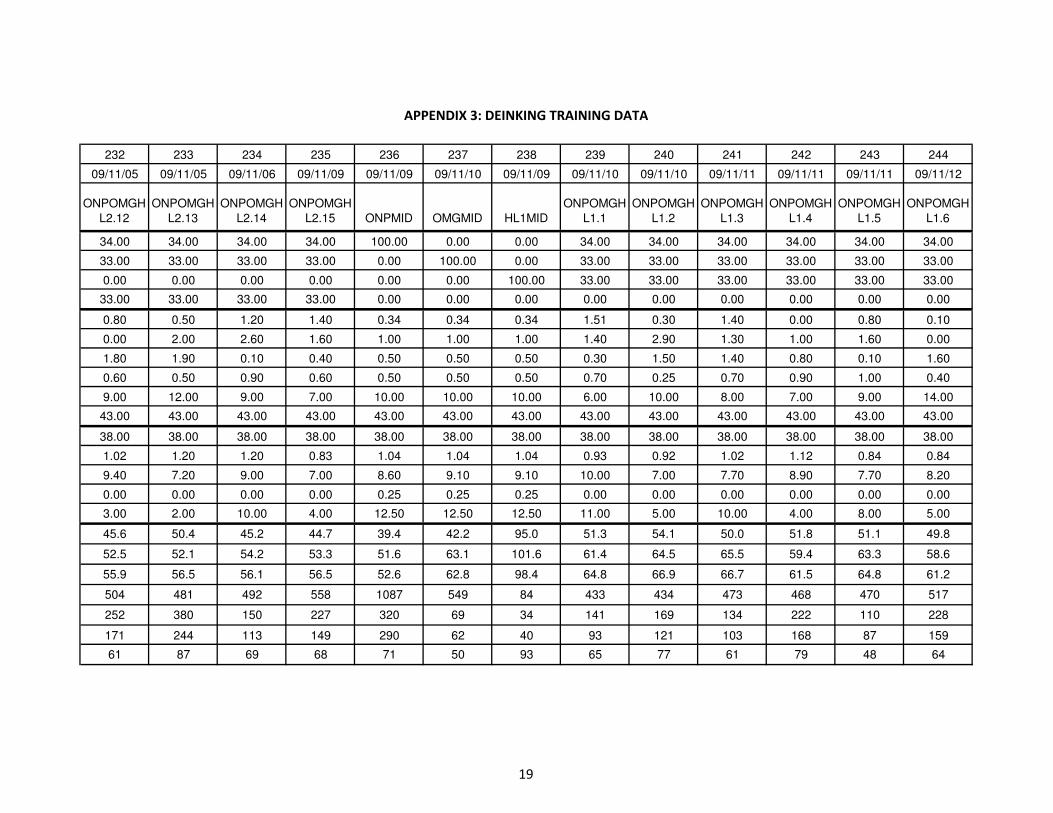
APPENDIX 3: DEINKING TRAINING DATA
232 233 234 235 236 237 238 239 240 241 242 243 244
09/11/05 09/11/05 09/11/06 09/11/09 09/11/09 09/11/10 09/11/09 09/11/10 09/11/10 09/11/11 09/11/11 09/11/11 09/11/12
ONPOMGH
L2.12
ONPOMGH
L2.13
ONPOMGH
L2.14
ONPOMGH
L2.15 ONPMID OMGMID HL1MID
ONPOMGH
L1.1
ONPOMGH
L1.2
ONPOMGH
L1.3
ONPOMGH
L1.4
ONPOMGH
L1.5
ONPOMGH
L1.6
34.00 34.00 34.00 34.00 100.00 0.00 0.00 34.00 34.00 34.00 34.00 34.00 34.00
33.00 33.00 33.00 33.00 0.00 100.00 0.00 33.00 33.00 33.00 33.00 33.00 33.00
0.00 0.00 0.00 0.00 0.00 0.00 100.00 33.00 33.00 33.00 33.00 33.00 33.00
33.00 33.00 33.00 33.00 0.00 0.00 0.00 0.00 0.00 0.00 0.00 0.00 0.00
0.80 0.50 1.20 1.40 0.34 0.34 0.34 1.51 0.30 1.40 0.00 0.80 0.10
0.00 2.00 2.60 1.60 1.00 1.00 1.00 1.40 2.90 1.30 1.00 1.60 0.00
1.80 1.90 0.10 0.40 0.50 0.50 0.50 0.30 1.50 1.40 0.80 0.10 1.60
0.60 0.50 0.90 0.60 0.50 0.50 0.50 0.70 0.25 0.70 0.90 1.00 0.40
9.00 12.00 9.00 7.00 10.00 10.00 10.00 6.00 10.00 8.00 7.00 9.00 14.00
43.00 43.00 43.00 43.00 43.00 43.00 43.00 43.00 43.00 43.00 43.00 43.00 43.00
38.00 38.00 38.00 38.00 38.00 38.00 38.00 38.00 38.00 38.00 38.00 38.00 38.00
1.02 1.20 1.20 0.83 1.04 1.04 1.04 0.93 0.92 1.02 1.12 0.84 0.84
9.40 7.20 9.00 7.00 8.60 9.10 9.10 10.00 7.00 7.70 8.90 7.70 8.20
0.00 0.00 0.00 0.00 0.25 0.25 0.25 0.00 0.00 0.00 0.00 0.00 0.00
3.00 2.00 10.00 4.00 12.50 12.50 12.50 11.00 5.00 10.00 4.00 8.00 5.00
45.6 50.4 45.2 44.7 39.4 42.2 95.0 51.3 54.1 50.0 51.8 51.1 49.8
52.5 52.1 54.2 53.3 51.6 63.1 101.6 61.4 64.5 65.5 59.4 63.3 58.6
55.9 56.5 56.1 56.5 52.6 62.8 98.4 64.8 66.9 66.7 61.5 64.8 61.2
504 481 492 558 1087 549 84 433 434 473 468 470 517
252 380 150 227 320 69 34 141 169 134 222 110 228
171 244 113 149 290 62 40 93 121 103 168 87 159
61 87 69 68 71 50 93 65 77 61 79 48 64
19
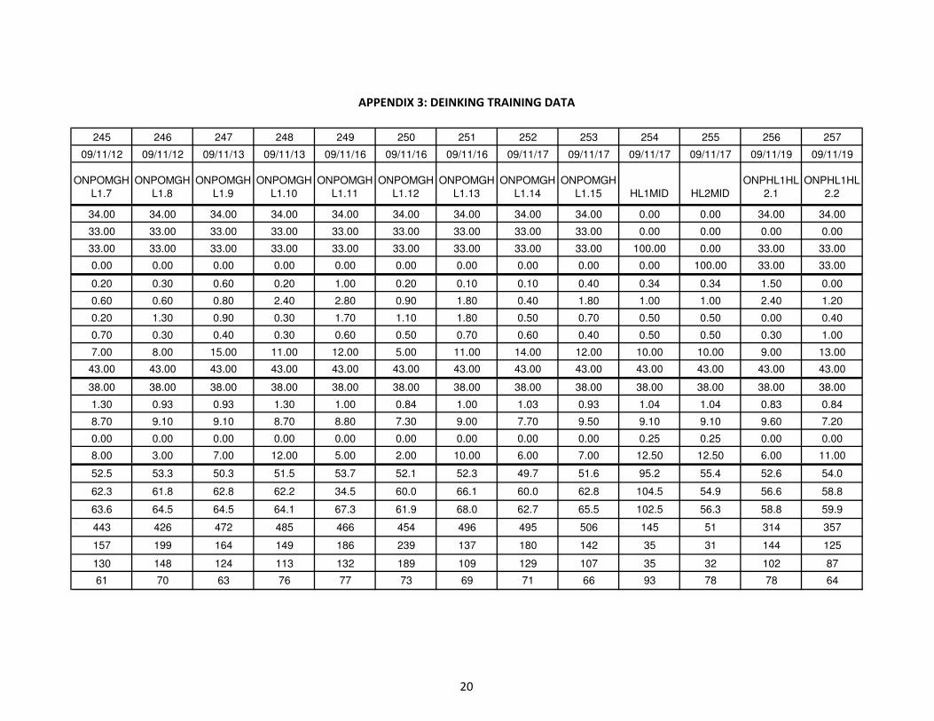
APPENDIX 3: DEINKING TRAINING DATA
245 246 247 248 249 250 251 252 253 254 255 256 257
09/11/12 09/11/12 09/11/13 09/11/13 09/11/16 09/11/16 09/11/16 09/11/17 09/11/17 09/11/17 09/11/17 09/11/19 09/11/19
ONPOMGH
L1.7
ONPOMGH
L1.8
ONPOMGH
L1.9
ONPOMGH
L1.10
ONPOMGH
L1.11
ONPOMGH
L1.12
ONPOMGH
L1.13
ONPOMGH
L1.14
ONPOMGH
L1.15 HL1MID HL2MID
ONPHL1HL
2.1
ONPHL1HL
2.2
34.00 34.00 34.00 34.00 34.00 34.00 34.00 34.00 34.00 0.00 0.00 34.00 34.00
33.00 33.00 33.00 33.00 33.00 33.00 33.00 33.00 33.00 0.00 0.00 0.00 0.00
33.00 33.00 33.00 33.00 33.00 33.00 33.00 33.00 33.00 100.00 0.00 33.00 33.00
0.00 0.00 0.00 0.00 0.00 0.00 0.00 0.00 0.00 0.00 100.00 33.00 33.00
0.20 0.30 0.60 0.20 1.00 0.20 0.10 0.10 0.40 0.34 0.34 1.50 0.00
0.60 0.60 0.80 2.40 2.80 0.90 1.80 0.40 1.80 1.00 1.00 2.40 1.20
0.20 1.30 0.90 0.30 1.70 1.10 1.80 0.50 0.70 0.50 0.50 0.00 0.40
0.70 0.30 0.40 0.30 0.60 0.50 0.70 0.60 0.40 0.50 0.50 0.30 1.00
7.00 8.00 15.00 11.00 12.00 5.00 11.00 14.00 12.00 10.00 10.00 9.00 13.00
43.00 43.00 43.00 43.00 43.00 43.00 43.00 43.00 43.00 43.00 43.00 43.00 43.00
38.00 38.00 38.00 38.00 38.00 38.00 38.00 38.00 38.00 38.00 38.00 38.00 38.00
1.30 0.93 0.93 1.30 1.00 0.84 1.00 1.03 0.93 1.04 1.04 0.83 0.84
8.70 9.10 9.10 8.70 8.80 7.30 9.00 7.70 9.50 9.10 9.10 9.60 7.20
0.00 0.00 0.00 0.00 0.00 0.00 0.00 0.00 0.00 0.25 0.25 0.00 0.00
8.00 3.00 7.00 12.00 5.00 2.00 10.00 6.00 7.00 12.50 12.50 6.00 11.00
52.5 53.3 50.3 51.5 53.7 52.1 52.3 49.7 51.6 95.2 55.4 52.6 54.0
62.3 61.8 62.8 62.2 34.5 60.0 66.1 60.0 62.8 104.5 54.9 56.6 58.8
63.6 64.5 64.5 64.1 67.3 61.9 68.0 62.7 65.5 102.5 56.3 58.8 59.9
443 426 472 485 466 454 496 495 506 145 51 314 357
157 199 164 149 186 239 137 180 142 35 31 144 125
130 148 124 113 132 189 109 129 107 35 32 102 87
61 70 63 76 77 73 69 71 66 93 78 78 64
20

APPENDIX 3: DEINKING TRAINING DATA
258 259 260 261 262 263 264 265 266 267 268 269 270
09/11/19 09/11/19 09/11/20 09/11/20 09/11/20 09/11/23 09/11/23 09/11/23 09/11/25 09/11/24 09/11/24 09/11/24 09/11/24
ONPHL1HL
2.3
ONPHL1HL
2.4
ONPHL1HL
2.5
ONPHL1HL
2.6
ONPHL1HL
2.7
ONPHL1HL
2.8
ONPHL1HL
2.9
ONPHL1HL
2.10
ONPHL1HL
2.11
ONPHL1HL
2.12
ONPHL1HL
2.13
ONPHL1HL
2.14
ONPHL1HL
2.15
34.00 34.00 34.00 34.00 34.00 34.00 34.00 34.00 34.00 34.00 34.00 34.00 34.00
0.00 0.00 0.00 0.00 0.00 0.00 0.00 0.00 0.00 0.00 0.00 0.00 0.00
33.00 33.00 33.00 33.00 33.00 33.00 33.00 33.00 33.00 33.00 33.00 33.00 33.00
33.00 33.00 33.00 33.00 33.00 33.00 33.00 33.00 33.00 33.00 33.00 33.00 33.00
0.90 1.30 0.50 0.70 0.60 1.00 0.30 0.90 0.50 1.00 1.40 1.00 0.40
0.80 0.60 2.40 1.10 2.50 0.20 1.40 0.40 1.40 2.20 0.70 0.10 2.10
0.10 0.70 0.90 1.20 1.30 0.70 0.20 1.20 1.50 1.20 0.60 1.80 0.20
0.60 0.70 0.40 1.00 0.70 0.50 0.60 0.60 1.00 0.60 0.50 0.60 0.90
5.00 6.00 12.00 11.00 11.00 13.00 10.00 12.00 5.00 15.00 10.00 8.00 10.00
43.00 43.00 43.00 43.00 43.00 43.00 43.00 43.00 43.00 43.00 43.00 43.00 43.00
38.00 38.00 38.00 38.00 38.00 38.00 38.00 38.00 38.00 38.00 38.00 38.00 38.00
1.20 1.20 1.20 1.02 1.20 1.02 1.30 1.02 0.83 1.11 0.93 0.83 0.93
9.00 8.10 9.90 9.20 9.70 7.60 7.30 9.40 7.20 8.50 9.30 7.80 7.50
0.00 0.00 0.00 0.00 0.00 0.00 0.00 0.00 0.00 0.00 0.00 0.00 0.00
6.00 12.00 6.00 9.00 5.00 11.00 9.00 3.00 4.00 2.00 10.00 3.00 3.00
53.5 55.9 53.7 54.3 53.4 52.2 53.0 55.1 55.2 57.5 50.7 52.0 53.5
57.9 61.2 56.3 59.5 57.8 60.0 57.9 59.7 62.1 62.0 58.3 53.9 61.1
60.0 64.4 59.3 61.9 60.3 62.5 60.2 62.7 63.4 66.1 61.0 63.2 56.4
332 315 363 370 358 432 380 334 398 445 477 411 439
168 112 299 176 216 156 183 227 223 333 184 298 208
114 82 181 110 141 103 132 117 167 206 140 149 205
77 67 86 80 80 73 73 90 73 88 67 72 91
21

APPENDIX 3: DEINKING TRAINING DATA
271 272 273 274 275 276 277 278 279 280 281 282 283
09/11/25 09/11/27 09/11/26 09/11/26 09/11/26 09/11/27 09/12/01 09/12/01 09/12/01 09/12/02 09/12/02 09/12/02 09/12/03
HL1MID HL2MID
OMGHL1H
L2.1
OMGHL1H
L2.2
OMGHL1H
L2.3
OMGHL1H
L2.4
OMGHL1H
L2.5
OMGHL1H
L2.6
OMGHL1H
L2.7
OMGHL1H
L2.8
OMGHL1H
L2.9
OMGHL1H
L2.10
OMGHL1H
L2.11
0.00 0.00 0.00 0.00 0.00 0.00 0.00 0.00 0.00 0.00 0.00 0.00 0.00
0.00 0.00 33.00 33.00 33.00 33.00 33.00 33.00 33.00 33.00 33.00 33.00 33.00
100.00 0.00 33.00 33.00 33.00 33.00 33.00 33.00 33.00 33.00 33.00 33.00 33.00
0.00 100.00 33.00 33.00 33.00 33.00 33.00 33.00 33.00 33.00 33.00 33.00 33.00
0.34 0.34 0.00 1.00 1.22 0.60 1.10 0.50 0.40 0.10 0.40 0.20 1.32
1.00 1.00 1.50 0.50 1.70 1.20 2.00 0.00 2.80 1.20 0.70 1.40 2.80
0.50 0.50 2.00 0.60 1.90 1.30 0.20 0.50 1.20 0.30 0.50 1.80 0.90
0.50 0.50 0.50 0.50 0.70 0.60 1.00 0.30 0.60 0.90 0.70 0.80 0.25
10.00 10.00 14.00 5.00 10.00 6.00 6.00 8.00 9.00 12.00 12.00 11.00 13.00
43.00 43.00 43.00 43.00 43.00 43.00 43.00 43.00 43.00 43.00 43.00 43.00 43.00
38.00 38.00 38.00 38.00 38.00 38.00 38.00 38.00 38.00 38.00 38.00 38.00 38.00
1.04 1.04 1.02 1.20 0.83 1.10 1.20 1.30 1.20 1.10 1.20 0.93 1.01
9.10 9.10 7.40 9.70 8.30 9.50 8.00 9.20 8.70 8.20 9.50 7.90 7.00
0.25 0.25 0.00 0.00 0.00 0.00 0.00 0.00 0.00 0.00 0.00 0.00 0.00
12.50 12.50 10.00 12.00 9.00 4.00 5.00 6.00 11.00 4.00 8.00 2.00 10.00
96.6 58.7 56.0 54.6 53.9 60.2 60.4 61.7 59.7 58.9 60.2 59.4 61.7
103.0 59.7 62.8 62.8 62.4 64.4 67.1 62.5 66.0 60.2 65.4 66.4 69.3
99.3 61.0 65.0 64.3 64.5 63.8 68.3 67.0 68.0 62.2 67.5 67.3 70.6
115 61 427 430 464 219 296 283 285 300 295 335 291
54 33 168 176 148 126 112 254 151 258 161 171 131
57 42 128 131 120 130 93 195 118 209 130 141 89
88 73 72 70 60 80 79 79 83 90 79 77 78
22

APPENDIX 3: DEINKING TRAINING DATA
284 285 286 287 288 289 290 291 292 293 294 295 296
09/12/03 09/12/04 09/12/04 09/12/04 09/12/09 09/12/07 09/12/07 09/12/07 09/12/09 09/12/09 09/12/10 09/12/10 09/12/11
OMGHL1H
L2.12
OMGHL1H
L2.13
OMGHL1H
L2.14
OMGHL1H
L2.15 ONPMID HL1MID HL2MID OMGMID
ONPOMGH
L1HL2.1
ONPOMGH
L1HL2.2
ONPOMGH
L1HL2.3
ONPOMGH
L1HL2.4
ONPOMGH
L1HL2.5
0.00 0.00 0.00 0.00 100.00 0.00 0.00 0.00 25.00 25.00 25.00 25.00 25.00
33.00 33.00 33.00 33.00 0.00 0.00 0.00 100.00 25.00 25.00 25.00 25.00 25.00
33.00 33.00 33.00 33.00 0.00 100.00 0.00 0.00 25.00 25.00 25.00 25.00 25.00
33.00 33.00 33.00 33.00 0.00 0.00 100.00 0.00 25.00 25.00 25.00 25.00 25.00
0.30 0.80 1.52 0.20 0.34 0.34 0.34 0.34 1.20 1.20 0.40 0.10 1.32
1.40 0.10 2.50 1.50 1.00 1.00 1.00 1.00 2.10 1.90 0.00 1.50 1.40
1.30 0.10 1.60 1.60 0.50 0.50 0.50 0.50 1.20 2.00 0.10 1.10 1.70
0.80 0.80 1.00 0.30 0.50 0.50 0.50 0.50 0.40 0.60 1.00 0.30 0.80
12.00 15.00 12.00 14.00 10.00 10.00 10.00 10.00 10.00 15.00 8.00 13.00 13.00
43.00 43.00 43.00 43.00 43.00 43.00 43.00 43.00 43.00 43.00 43.00 43.00 43.00
38.00 38.00 38.00 38.00 38.00 38.00 38.00 38.00 38.00 38.00 38.00 38.00 38.00
0.93 0.84 1.10 0.93 1.04 1.04 1.04 1.04 1.11 1.00 1.20 0.93 0.83
8.30 9.70 9.30 7.70 8.60 9.10 9.10 9.10 7.50 9.00 9.50 7.00 9.00
0.00 0.00 0.00 0.00 0.25 0.25 0.25 0.25 0.00 0.00 0.00 0.00 0.00
5.00 11.00 4.00 7.00 12.50 12.50 12.50 12.50 5.00 9.00 9.00 3.00 11.00
62.6 60.1 57.3 62.1 40.5 92.1 67.8 42.1 51.9 52.2 49.9 51.7 53.5
69.4 71.3 65.9 70.2 50.1 96.7 68.9 62.5 61.6 66.4 58.5 58.2 60.3
68.9 72.2 68.0 71.0 52.2 94.0 70.1 61.2 63.8 67.8 58.9 61.1 63.6
267 317 301 279 1147 154 95 776 554 550 508 548 554
77 101 126 81 393 96 44 129 260 203 213 275 323
72 90 96 76 327 100 52 136 184 142 184 218 213
74 69 77 69 82 80 72 45 71 69 69 76 85
23

APPENDIX 3: DEINKING TRAINING DATA
297 298 299 300 301 302 303 304 305 306 307 308 309
09/12/11 09/12/11 09/12/14 09/12/14 09/12/14 09/12/15 09/12/15 09/12/15 09/12/15 09/12/17 09/12/18 09/12/17 09/12/18
ONPOMGH
L1HL2.6
ONPOMGH
L1HL2.7
ONPOMGH
L1HL2.8
ONPOMGH
L1HL2.9
ONPOMGH
L1HL2.10
ONPOMGH
L1HL2.11
ONPOMGH
L1HL2.12
ONPOMGH
L1HL2.13
ONPOMGH
L1HL2.14
ONPOMGH
L1HL2.15 HL1MID HL2MID OMGMID
25.00 25.00 25.00 25.00 25.00 25.00 25.00 25.00 25.00 25.00 0.00 0.00 0.00
25.00 25.00 25.00 25.00 25.00 25.00 25.00 25.00 25.00 25.00 0.00 0.00 100.00
25.00 25.00 25.00 25.00 25.00 25.00 25.00 25.00 25.00 25.00 100.00 0.00 0.00
25.00 25.00 25.00 25.00 25.00 25.00 25.00 25.00 25.00 25.00 0.00 100.00 0.00
0.60 0.40 0.20 0.40 0.51 1.00 0.61 0.80 0.30 0.10 0.34 0.34 0.34
1.90 1.60 2.50 0.10 2.90 2.70 1.40 0.00 1.80 1.70 1.00 1.00 1.00
1.70 0.30 1.50 0.40 0.60 1.40 1.10 1.20 1.20 0.70 0.50 0.50 0.50
0.90 0.70 0.60 0.70 0.60 0.40 1.00 0.70 0.50 0.90 0.50 0.50 0.50
12.00 14.00 10.00 9.00 6.00 6.00 13.00 13.00 5.00 13.00 10.00 10.00 10.00
43.00 43.00 43.00 43.00 43.00 43.00 43.00 43.00 43.00 43.00 43.00 43.00 43.00
38.00 38.00 38.00 38.00 38.00 38.00 38.00 38.00 38.00 38.00 38.00 38.00 38.00
0.92 1.11 1.02 1.12 1.20 1.10 1.28 0.83 0.83 0.93 1.04 1.04 1.04
7.50 7.50 9.50 8.00 9.00 9.50 8.50 9.50 8.00 10.00 9.10 9.10 9.10
0.00 0.00 0.00 0.00 0.00 0.00 0.00 0.00 0.00 0.00 0.25 0.25 0.25
5.00 7.00 9.00 7.00 12.00 3.00 6.00 3.00 4.00 10.00 12.50 12.50 12.50
54.4 53.6 54.6 50.8 52.6 53.2 50.9 51.9 55.3 48.7 100.7 51.5 42.5
59.7 60.2 63.4 57.4 62.1 59.1 58.6 58.8 62.9 59.7 104.6 53.0 60.9
62.5 63.2 64.1 59.1 64.0 62.5 62.0 61.8 65.1 62.1 100.2 56.3 61.6
505 517 544 575 544 522 563 514 429 613 62 216 770
328 273 251 353 238 345 284 317 227 211 40 176 126
226 186 198 289 201 258 195 215 172 174 41 151 113
76 77 86 80 80 88 78 84 83 79 89 87 58
24

APPENDIX 3: DEINKING TRAINING DATA
310 311 312 313 314 315 316 317 318 319 320 321 322
10/01/20 10/01/20 10/01/21 10/01/22 10/01/25 10/01/25 10/01/27 10/01/27 10/01/28 10/01/28 10/01/29 10/02/01 10/02/01
ONPMID OMGMID
ONPOMG7
525.19
ONPOMG7
525.20
ONPOMG7
525.21
ONPOMG7
525.22
ONPOMG7
525.23
ONPOMG7
525.24
ONPOMG7
525.25
ONPOMG7
525.26
ONPOMG7
525.27
ONPOMG7
525.28
ONPOMG7
525.29
100.00 0.00 25.00 75.00 25.00 75.00 25.00 75.00 25.00 75.00 25.00 75.00 25.00
0.00 100.00 75.00 25.00 75.00 25.00 75.00 25.00 75.00 25.00 75.00 25.00 75.00
0.00 0.00 0.00 0.00 0.00 0.00 0.00 0.00 0.00 0.00 0.00 0.00 0.00
0.00 0.00 0.00 0.00 0.00 0.00 0.00 0.00 0.00 0.00 0.00 0.00 0.00
0.34 0.34 1.50 1.50 1.30 1.50 1.30 1.10 1.40 1.30 1.40 1.30 1.00
1.00 1.00 2.90 2.60 2.80 2.60 3.00 3.00 2.70 2.70 2.90 2.50 2.60
0.50 0.50 1.80 2.00 1.20 1.80 2.00 1.60 1.80 1.40 2.00 1.50 1.20
0.50 0.50 0.35 0.35 0.35 0.85 0.85 0.85 0.85 0.35 0.35 0.35 0.35
10.00 10.00 7.50 7.50 7.50 7.50 7.50 7.50 7.50 12.50 12.50 12.50 12.50
43.00 43.00 43.00 43.00 43.00 43.00 43.00 43.00 43.00 43.00 43.00 43.00 43.00
38.00 38.00 38.00 38.00 38.00 38.00 38.00 38.00 38.00 38.00 38.00 38.00 38.00
1.04 1.04 0.90 0.90 1.15 0.90 1.15 0.90 1.15 0.90 1.15 0.90 1.15
9.10 9.10 7.30 8.30 8.30 7.30 7.30 8.30 8.30 7.30 7.30 8.30 8.30
0.25 0.25 0.00 0.00 0.00 0.00 0.00 0.00 0.00 0.00 0.00 0.00 0.00
12.50 12.50 6.00 10.00 11.00 9.00 7.00 7.00 9.00 10.00 6.00 7.00 7.00
40.34 43.47 46.56 43.04 45.30 44.39 45.27 45.26 46.89 45.96 47.68 48.47 46.15
43.11 58.85 52.86 55.25 59.81 53.04 56.80 57.04 0.00 0.00 0.00 0.00 0.00
51.51 60.27 57.13 57.69 61.21 57.10 58.70 58.51 64.95 60.71 64.28 59.74 63.72
1156.00 733.50 729.00 943.75 830.25 859.75 707.25 817.50 666.75 839.50 778.00 781.75 762.50
887.50 176.00 525.50 351.75 262.00 458.25 325.75 280.00 0.00 0.00 0.00 0.00 0.00
571.60 136.40 349.90 261.50 199.40 330.20 232.10 216.90 106.39 190.00 180.70 180.40 136.10
94 84 88.59 81.35 71.44 82.04 70.44 79.10 62.01 63.58 66.57 70.75 70.08
25

APPENDIX 3: DEINKING TRAINING DATA
323 324 325 326 327 328 329 330 331 332 333 334 335
10/02/02 10/02/02 10/02/03 10/02/03 10/02/04 10/02/04 10/02/05 10/02/05 10/02/08 10/02/08 10/02/09 10/02/09 10/02/10
ONPOMG7
525.30
ONPOMG7
525.31
ONPOMG7
525.32
ONPOMG7
525.33 HL1MID HL2MID
HL1HL2-
7525.1
HL1HL2-
7525.2
HL1HL2-
7525.3
HL1HL2-
7525.4
HL1HL2-
7525.5
HL1HL2-
7525.6
HL1HL2-
7525.7
75.00 25.00 75.00 25.00 0.00 0.00 0.00 0.00 0.00 0.00 0.00 0.00 0.00
25.00 75.00 25.00 75.00 0.00 0.00 0.00 0.00 0.00 0.00 0.00 0.00 0.00
0.00 0.00 0.00 0.00 100.00 0.00 75.00 25.00 75.00 25.00 75.00 25.00 75.00
0.00 0.00 0.00 0.00 0.00 100.00 25.00 75.00 25.00 75.00 25.00 75.00 25.00
1.30 1.40 1.30 1.30 0.34 0.34 1.50 1.50 1.30 1.52 1.32 1.11 1.40
2.70 2.70 2.80 2.90 1.00 1.00 2.90 2.60 2.80 2.60 3.00 3.00 2.70
1.20 1.40 1.80 1.20 0.50 0.50 1.80 2.00 1.20 1.80 2.00 1.60 1.80
0.85 0.85 0.85 0.85 0.50 0.50 0.35 0.35 0.35 0.85 0.85 0.85 0.85
12.50 12.50 12.50 12.50 10.00 10.00 7.50 7.50 7.50 7.50 7.50 7.50 7.50
43.00 43.00 43.00 43.00 43.00 43.00 43.00 43.00 43.00 43.00 43.00 43.00 43.00
38.00 38.00 38.00 38.00 38.00 38.00 38.00 38.00 38.00 38.00 38.00 38.00 38.00
0.90 1.15 0.90 1.15 1.04 1.04 0.90 0.90 1.15 0.90 1.14 0.92 1.15
7.30 7.30 8.30 8.30 9.10 9.10 7.30 8.30 8.30 7.30 7.30 8.30 8.30
0.00 0.00 0.00 0.00 0.25 0.25 0.00 0.00 0.00 0.00 0.00 0.00 0.00
8.00 7.00 10.00 6.00 12.50 12.50 6.00 10.00 11.00 9.00 7.00 7.00 9.00
48.70 46.65 47.67 44.79 95.98 52.05 85.32 67.85 87.15 67.65 87.60 66.65 86.67
0.00 0.00 0.00 0.00 0.00 0.00 0.00 0.00 0.00 0.00 0.00 0.00 0.00
61.12 63.91 60.60 62.52 98.50 59.05 90.32 76.21 87.84 73.55 88.29 71.80 90.26
714.00 723.50 801.50 723.75 91.50 226.75 107.75 184.93 103.90 167.75 100.75 155.00 107.25
0.00 0.00 0.00 0.00 0.00 0.00 0.00 0.00 0.00 0.00 0.00 0.00 0.00
163.30 136.50 173.90 143.50 43.50 132.50 57.80 86.90 50.00 84.23 51.20 88.90 46.08
68.30 64.63 72.46 69.67 86.16 79.82 84.40 72.20 77.19 88.80 79.94 76.57 74.05
26

APPENDIX 3: DEINKING TRAINING DATA
336 337 338 339 340 341 342 343 344 345 346 347 348
10/02/10 10/02/11 10/02/11 10/02/12 10/02/12 10/02/15 10/02/16 10/02/16 10/02/17 10/02/18 10/02/17 10/02/17 10/02/19
HL1HL2-
7525.8
HL1HL2-
7525.9
HL1HL2-
7525.10
HL1HL2-
7525.11
HL1HL2-
7525.12
HL1HL2-
7525.13
HL1HL2-
7525.14
HL1HL2-
7525.15 HL1MID HL2MID OMGMID ONPMID TEST.1
0.00 0.00 0.00 0.00 0.00 0.00 0.00 0.00 0.00 0.00 0.00 100.00 70.00
0.00 0.00 0.00 0.00 0.00 0.00 0.00 0.00 0.00 0.00 100.00 0.00 5.00
25.00 75.00 25.00 75.00 25.00 75.00 25.00 75.00 100.00 0.00 0.00 0.00 15.00
75.00 25.00 75.00 25.00 75.00 25.00 75.00 25.00 0.00 100.00 0.00 0.00 10.00
1.30 1.40 1.32 1.00 1.30 1.42 1.30 1.30 0.34 0.34 0.34 0.34 0.80
2.70 2.90 2.50 2.60 2.70 2.70 2.80 2.90 1.00 1.00 1.00 1.00 0.70
1.40 2.00 1.50 1.20 1.20 1.40 1.80 1.20 0.50 0.50 0.50 0.50 2.00
0.35 0.35 0.35 0.35 0.85 0.85 0.85 0.85 0.50 0.50 0.50 0.50 0.30
12.50 12.50 12.50 12.50 12.50 12.50 12.50 12.50 10.00 10.00 10.00 10.00 14.00
43.00 43.00 43.00 43.00 43.00 43.00 43.00 43.00 43.00 43.00 43.00 43.00 43.00
38.00 38.00 38.00 38.00 38.00 38.00 38.00 38.00 38.00 38.00 38.00 38.00 38.00
0.90 1.15 0.90 1.15 0.90 1.15 0.90 1.15 1.04 1.04 1.04 1.04 1.00
7.30 7.30 8.30 8.30 7.30 7.30 8.30 8.30 9.10 9.10 9.10 9.10 8.50
0.00 0.00 0.00 0.00 0.00 0.00 0.00 0.00 0.25 0.25 0.25 0.25 0.00
10.00 6.00 7.00 7.00 8.00 7.00 10.00 6.00 12.50 12.50 12.50 12.50 3.00
66.49 89.38 73.20 87.20 71.03 87.15 72.93 83.93 98.88 65.35 44.03 38.60 42.67
0.00 0.00 0.00 0.00 0.00 0.00 0.00 0.00 0.00 0.00 0.00 0.00 44.15
73.44 93.53 79.89 92.73 80.18 91.08 79.42 90.79 100.24 70.03 62.51 51.73 50.66
147.50 86.63 121.75 88.13 122.50 95.75 110.25 150.00 86.25 132.25 718.25 1207.25 993.11
0.00 0.00 0.00 0.00 0.00 0.00 0.00 0.00 0.00 0.00 0.00 0.00 951.71
64.09 37.00 63.80 43.70 48.10 43.90 51.60 46.57 42.90 77.89 95.79 334.60 588.76
96.47 70.16 77.60 78.60 64.80 68.04 76.50 42.50 80.28 74.65 42.37 70.10 95.77
27

APPENDIX 3: DEINKING TRAINING DATA
349 350 351 352 353 354 355 356 357 358 359 360 361
10/02/19 10/02/23 10/02/22 10/02/22 10/02/23 10/02/24 10/02/24 10/02/25 10/02/25 10/02/26 10/02/26 10/03/01 10/03/01
TEST.2 TEST.3 TEST.4 TEST.5 TEST.6 TEST.7 TEST.8 TEST.9 TEST.10 TEST.11 TEST.12 TEST.13 TEST.14
20.00 50.00 15.00 47.00 50.00 70.00 60.00 80.00 20.00 18.00 25.00 27.00 37.00
30.00 5.00 5.00 15.00 0.00 15.00 20.00 10.00 20.00 22.00 8.00 18.00 20.00
23.00 20.00 40.00 28.00 30.00 10.00 10.00 0.00 30.00 52.00 59.00 30.00 25.00
27.00 25.00 40.00 10.00 20.00 5.00 10.00 10.00 30.00 8.00 8.00 25.00 18.00
1.15 0.70 0.90 0.20 0.94 0.10 1.00 0.73 1.56 0.52 0.94 1.25 0.10
0.50 0.50 2.10 1.03 0.40 0.90 2.68 2.58 0.10 2.16 0.40 2.47 0.93
0.80 0.50 0.40 1.44 1.65 1.85 1.23 1.34 1.13 1.03 1.75 1.34 1.13
0.72 0.50 0.40 0.72 0.80 0.82 0.41 0.72 0.31 1.00 0.41 1.00 0.72
10.00 5.00 8.00 6.00 8.00 10.00 5.00 13.00 13.00 7.00 14.00 13.00 9.00
43.00 43.00 43.00 43.00 43.00 43.00 43.00 43.00 43.00 43.00 43.00 43.00 43.00
38.00 38.00 38.00 38.00 38.00 38.00 38.00 38.00 38.00 38.00 38.00 38.00 38.00
1.00 0.81 0.90 1.00 1.16 1.08 0.90 1.16 0.80 0.90 1.00 1.00 1.08
8.50 8.50 8.50 8.50 8.50 8.50 8.50 8.50 8.50 8.50 8.50 8.50 8.50
0.00 0.00 0.00 0.00 0.00 0.00 0.00 0.00 0.00 0.00 0.00 0.00 0.00
2.00 9.00 7.00 2.00 12.00 11.00 5.00 5.00 8.00 6.00 5.00 5.00 10.00
53.57 48.15 59.93 47.46 48.98 42.43 46.64 41.64 53.71 59.02 58.60 53.71 48.98
57.78 57.44 65.02 48.92 54.17 45.99 57.62 47.64 67.01 71.11 70.99 62.23 58.17
60.96 59.45 67.51 55.63 59.15 51.38 60.33 52.56 68.23 71.73 72.67 65.86 61.31
545.30 606.29 313.60 737.66 732.50 1074.55 741.54 1032.69 474.28 432.48 474.67 486.92 624.40
392.42 286.32 215.52 698.22 522.06 761.66 313.36 728.86 153.55 171.65 235.75 267.68 283.94
263.61 212.77 160.52 389.31 294.70 500.29 230.44 461.97 112.47 143.96 163.85 173.33 199.43
83.26 74.64 77.77 87.02 77.36 88.07 70.33 88.99 63.74 73.29 74.46 71.50 74.11
28

APPENDIX 3: DEINKING TRAINING DATA
362 363 364 365 366 367 368 369 370 371 372 373 374
10/03/01 10/03/02 10/03/02 10/03/02 10/03/04 10/03/04 10/03/05 10/03/05 10/03/05 10/03/08 10/03/08 10/03/10 10/03/10
TEST.15 TEST.16 TEST.17 TEST.18 TEST.19 TEST.20 TEST.21 TEST.22 TEST.23 TEST.24 TEST.25 TEST.26 TEST.27
20.00 6.00 20.00 28.00 10.00 20.00 66.00 43.00 63.00 71.00 51.00 47.00 85.00
5.00 12.00 15.00 7.00 5.00 25.00 26.00 9.00 0.00 7.00 8.00 10.00 8.00
70.00 70.00 25.00 38.00 60.00 50.00 8.00 15.00 32.00 22.00 20.00 12.00 0.00
5.00 12.00 40.00 27.00 25.00 5.00 0.00 33.00 5.00 0.00 21.00 31.00 7.00
0.20 0.94 1.36 1.15 1.56 0.63 1.00 0.30 1.36 0.00 1.00 1.25 0.94
1.34 2.26 1.13 0.10 1.85 0.21 2.79 1.00 1.34 1.55 1.55 2.06 2.58
2.10 0.92 1.54 0.60 1.75 0.41 0.82 1.54 0.82 1.75 0.72 0.93 0.20
0.41 0.82 0.30 0.62 0.72 0.93 0.30 0.82 0.93 0.82 0.51 1.00 0.52
10.00 6.00 7.00 8.00 12.00 8.00 13.00 13.00 14.00 11.00 10.00 13.00 8.00
43.00 43.00 43.00 43.00 43.00 43.00 43.00 43.00 43.00 43.00 43.00 43.00 43.00
38.00 38.00 38.00 38.00 38.00 38.00 38.00 38.00 38.00 38.00 38.00 38.00 38.00
0.81 1.17 1.16 0.90 1.16 1.26 1.16 1.00 0.90 0.90 0.90 0.80 1.16
8.50 8.50 8.50 8.50 8.50 8.50 9.40 9.30 8.60 8.80 9.10 8.80 9.00
0.00 0.00 0.00 0.00 0.00 0.00 0.00 0.00 0.00 0.00 0.00 0.00 0.00
7.00 9.00 11.00 4.00 5.00 12.00 5.00 10.00 12.00 8.00 5.00 7.00 2.00
64.35 71.11 53.54 53.15 70.14 54.67 41.72 47.73 42.95 42.45 45.80 43.05 40.26
75.70 79.94 59.23 61.74 76.66 68.54 49.29 58.47 57.04 54.98 57.75 59.24 38.98
77.14 81.48 64.60 65.94 80.40 69.72 53.39 60.20 59.21 55.36 58.92 60.41 46.90
360.73 246.71 446.56 511.82 270.89 512.24 1110.33 701.85 972.38 1033.97 766.56 744.25 976.43
160.94 125.40 323.02 263.67 158.88 187.73 609.85 252.58 372.49 336.25 319.56 231.60 1103.53
125.95 99.26 196.85 177.53 107.75 151.98 393.53 201.05 292.90 294.22 250.17 192.82 554.36
63.73 70.40 79.38 67.03 71.41 63.54 71.86 57.92 57.67 54.77 61.64 32.85 84.18
29

APPENDIX 3: DEINKING TRAINING DATA
375 376 377 378 379 380 381 382 383 384 385 386 387
10/03/11 10/03/11 10/03/11 10/03/12 10/03/12 10/03/12 10/03/15 10/03/15 10/03/15 10/03/16 10/03/16 10/03/16 10/03/17
TEST.28 TEST.29 TEST.30 TEST.31 TEST.32 TEST.33 TEST.34 TEST.35 TEST.36 TEST.37 TEST.38 TEST.39 TEST.40
43.00 34.00 22.00 11.00 8.00 0.00 19.00 26.00 28.00 28.00 10.00 17.00 28.00
17.00 11.00 23.00 4.00 31.00 5.00 22.00 7.00 15.00 15.00 18.00 29.00 15.00
11.00 30.00 22.00 59.00 49.00 69.00 34.00 67.00 43.00 43.00 58.00 22.00 42.00
29.00 25.00 33.00 26.00 12.00 26.00 25.00 0.00 14.00 14.00 14.00 32.00 15.00
1.25 0.10 0.94 0.94 1.25 0.94 1.36 0.83 1.56 0.83 0.31 0.52 0.10
2.10 0.70 2.99 2.16 0.00 1.96 1.54 0.21 1.03 0.62 3.00 1.03 2.99
1.95 0.40 1.85 0.90 1.85 0.62 1.54 0.31 1.64 1.13 0.62 0.21 0.00
0.93 1.00 0.40 0.72 1.00 0.62 0.51 0.31 0.51 0.82 0.31 0.51 0.82
11.00 10.00 10.00 6.00 9.00 9.00 6.00 5.00 7.00 13.00 8.00 7.00 6.00
43.00 43.00 43.00 43.00 43.00 43.00 43.00 43.00 43.00 43.00 43.00 43.00 43.00
38.00 38.00 38.00 38.00 38.00 38.00 38.00 38.00 38.00 38.00 38.00 38.00 38.00
0.80 1.10 1.16 0.80 1.08 0.90 1.08 0.82 1.10 1.17 1.00 1.10 0.90
9.80 9.90 8.60 9.50 10.00 9.40 10.00 9.40 7.00 7.50 7.50 8.00 7.20
0.00 0.00 0.00 0.00 0.00 0.00 0.00 0.00 0.00 0.00 0.00 0.00 0.00
11.00 9.00 9.00 6.00 6.00 4.00 5.00 7.00 11.00 2.00 7.00 11.00 4.00
47.54 50.35 55.03 72.13 61.89 73.08 56.35 60.45 56.19 55.22 65.84 51.69 55.36
61.22 60.60 65.04 77.49 70.03 77.85 65.54 73.15 70.62 61.83 75.31 61.83 59.75
62.91 62.37 68.21 78.86 72.73 79.88 67.65 73.39 72.57 65.85 76.08 63.19 62.03
767.24 646.96 440.76 193.29 348.61 163.61 429.28 391.16 469.68 474.15 287.01 427.99 407.29
206.55 196.20 204.43 123.42 200.36 88.19 229.13 150.18 140.70 309.06 122.80 143.19 232.30
164.29 156.76 140.16 104.86 153.96 77.10 160.52 129.15 108.25 194.92 103.59 119.48 177.23
55.61 61.25 69.97 75.80 75.81 70.53 61.49 54.55 61.97 69.93 70.80 61.90 72.65
30

APPENDIX 3: DEINKING TRAINING DATA
388 389 390 391 392 393 394 395 396 397 398 399 400
10/03/09 10/03/09 10/03/09 10/03/10 10/03/17 10/03/17 10/03/18 10/03/18 10/03/18 10/03/19 10/03/19 10/03/23 10/03/23
ONPMID OMGMID HL1MID HL2MID ALL MIDPT ALL 1 ALL 2 ALL 3 ALL 4 ALL 5 ALL 6 ALL 7 ALL 8
100.00 0.00 0.00 100.00 25.00 25.00 25.00 25.00 25.00 25.00 25.00 25.00 25.00
0.00 100.00 0.00 0.00 25.00 25.00 25.00 25.00 25.00 25.00 25.00 25.00 25.00
0.00 0.00 100.00 0.00 25.00 25.00 25.00 25.00 25.00 25.00 25.00 25.00 25.00
0.00 0.00 0.00 100.00 25.00 25.00 25.00 25.00 25.00 25.00 25.00 25.00 25.00
0.34 0.34 0.34 0.34 0.34 0.67 0.67 0.00 0.67 0.67 0.67 0.00 0.00
1.00 1.00 1.00 1.00 1.00 0.00 2.00 2.00 0.00 2.00 2.00 2.00 0.00
0.50 0.50 0.50 0.50 0.50 1.00 0.00 1.00 1.00 0.00 1.00 1.00 1.00
0.50 0.50 0.50 0.50 0.50 0.25 0.75 0.25 0.75 0.75 0.25 0.75 0.75
10.00 10.00 10.00 10.00 10.00 5.00 5.00 15.00 5.00 15.00 15.00 5.00 15.00
43.00 43.00 43.00 43.00 43.00 35.00 35.00 35.00 50.00 35.00 50.00 50.00 35.00
38.00 38.00 38.00 38.00 38.00 45.00 30.00 30.00 30.00 45.00 30.00 45.00 45.00
1.04 1.04 1.04 1.04 1.04 1.30 1.30 0.80 0.80 0.80 1.30 0.80 1.30
9.10 9.10 9.10 9.10 9.10 10.00 10.00 10.00 8.00 8.00 8.00 10.00 8.00
0.25 0.25 0.25 0.25 0.25 0.00 0.50 0.50 0.50 0.00 0.00 0.00 0.50
12.50 12.50 12.50 12.50 12.50 20.00 5.00 20.00 20.00 20.00 5.00 5.00 5.00
35.56 44.96 93.71 59.42 53.63 53.41 46.57 49.71 49.41 45.13 48.59 48.40 46.72
50.33 65.20 98.02 61.33 62.09 64.92 48.48 57.74 61.34 54.80 55.80 57.28 52.73
51.57 63.63 96.14 64.53 64.02 66.41 51.63 59.27 62.64 55.05 59.78 58.64 56.49
1396.56 809.35 101.02 121.57 492.11 465.98 469.23 481.54 554.43 551.36 521.43 527.53 599.96
371.77 99.98 56.87 93.93 217.11 136.30 311.87 141.03 152.03 148.88 236.86 187.06 307.85
342.36 98.02 57.39 70.67 155.08 114.93 230.19 115.32 128.50 122.35 167.83 157.71 194.86
43.52 70.32 80.44 74.57 59.93 58.22 77.14 60.07 36.74 36.56 65.25 60.74 67.85
31

APPENDIX 3: DEINKING TRAINING DATA
401 402 403 404 405 406 407 408 409 410 411 412 413
10/03/23 10/03/24 10/03/24 10/03/25 10/04/01 10/03/25 10/03/26 10/03/26 10/03/26 10/03/29 10/03/29 10/03/29 10/03/31
ALL 9 ALL 10 ALL 11 ALL 12 ALL 13 ALL 14 ALL 15 ALL 16 ALL 17 ALL 18 ALL 19 ALL 20 ALL 21
25.00 25.00 25.00 25.00 25.00 25.00 25.00 25.00 25.00 25.00 25.00 25.00 25.00
25.00 25.00 25.00 25.00 25.00 25.00 25.00 25.00 25.00 25.00 25.00 25.00 25.00
25.00 25.00 25.00 25.00 25.00 25.00 25.00 25.00 25.00 25.00 25.00 25.00 25.00
25.00 25.00 25.00 25.00 25.00 25.00 25.00 25.00 25.00 25.00 25.00 25.00 25.00
0.00 0.67 0.00 0.00 0.00 0.00 0.67 0.00 0.00 0.00 0.67 0.67 0.67
0.00 0.00 2.00 0.00 2.00 0.00 0.00 2.00 0.00 0.00 0.00 2.00 2.00
0.00 0.00 0.00 0.00 0.00 1.00 0.00 0.00 1.00 0.00 0.00 0.00 1.00
0.75 0.25 0.25 0.25 0.75 0.25 0.75 0.25 0.25 0.75 0.25 0.25 0.25
15.00 15.00 5.00 5.00 15.00 15.00 5.00 15.00 5.00 5.00 15.00 5.00 5.00
50.00 50.00 50.00 35.00 50.00 50.00 50.00 35.00 50.00 35.00 35.00 50.00 35.00
30.00 45.00 45.00 30.00 30.00 45.00 45.00 45.00 30.00 45.00 30.00 30.00 45.00
1.30 0.80 1.30 0.80 0.80 0.80 1.30 1.30 1.30 0.80 1.30 0.80 0.80
10.00 10.00 8.00 8.00 8.00 8.00 8.00 10.00 10.00 10.00 8.00 10.00 8.00
0.00 0.50 0.50 0.00 0.50 0.00 0.00 0.00 0.50 0.50 0.50 0.00 0.50
20.00 5.00 20.00 5.00 5.00 20.00 5.00 5.00 5.00 20.00 20.00 20.00 5.00
46.66 45.24 50.71 50.10 50.75 47.90 47.03 47.48 50.08 49.63 46.03 48.45 51.58
54.98 51.94 58.61 56.14 57.48 59.10 50.13 52.81 53.73 56.82 54.80 55.30 61.72
57.21 54.51 59.92 57.72 58.88 60.57 54.69 53.50 55.84 57.07 56.50 57.64 62.78
665.29 626.06 498.08 501.26 444.25 573.48 570.81 594.58 524.95 487.00 627.50 519.50 487.25
236.98 253.90 137.00 217.10 179.25 163.55 382.32 278.29 301.00 158.75 185.75 179.00 176.50
172.22 177.21 129.28 178.70 135.60 142.14 194.35 260.94 237.22 147.50 147.87 143.90 147.30
59.33 65.85 49.14 59.66 67.52 39.37 75.99 68.07 68.19 35.70 54.87 97.08 57.63
32

APPENDIX 3: DEINKING TRAINING DATA
414 415 416 417 418 419 420 421 422 423 424 425 426
10/03/31 10/04/01 10/04/06 10/04/06 10/04/06 10/04/07 10/04/07 10/04/08 10/04/08 10/04/09 10/04/09 10/04/12 10/04/13
ALL 22 ALL 23 ALL 24 ALL MIDPT ALL MIDPT ALL MIDPT ALL MIDPT TEST.41 TEST.42 TEST.43 TEST.44 TEST.45 TEST.46
25.00 25.00 25.00 25.00 25.00 25.00 25.00 40.00 42.00 57.00 51.00 54.00 53.00
25.00 25.00 25.00 25.00 25.00 25.00 25.00 18.00 20.00 7.00 29.00 15.00 6.00
25.00 25.00 25.00 25.00 25.00 25.00 25.00 22.00 12.00 8.00 12.00 11.00 10.00
25.00 25.00 25.00 25.00 25.00 25.00 25.00 20.00 26.00 28.00 8.00 20.00 31.00
0.00 0.67 0.67 0.34 0.34 0.34 0.34 1.46 0.00 0.20 1.46 0.30 0.40
2.00 0.00 2.00 1.00 1.00 1.00 1.00 1.55 1.55 1.55 1.55 1.50 1.50
1.00 1.00 1.00 0.50 0.50 0.50 0.50 1.13 1.65 0.72 1.65 1.70 1.20
0.75 0.75 0.75 0.50 0.50 0.50 0.50 0.62 0.62 0.62 0.62 0.62 0.62
5.00 15.00 15.00 10.00 10.00 10.00 10.00 8.00 8.00 8.00 8.00 13.00 11.00
35.00 35.00 50.00 43.00 43.00 43.00 43.00 43.00 43.00 43.00 43.00 50.00 50.00
30.00 30.00 45.00 38.00 38.00 38.00 38.00 38.00 38.00 38.00 38.00 45.00 45.00
1.30 0.80 1.30 1.04 1.04 1.04 1.04 1.25 0.81 1.10 1.16 1.30 1.10
8.00 10.00 10.00 9.10 9.10 9.10 9.10 9.90 9.30 8.10 9.40 7.00 7.60
0.00 0.00 0.50 0.25 0.25 0.25 0.25 0.10 0.16 0.12 0.11 0.30 0.30
20.00 5.00 20.00 12.50 12.50 12.50 12.50 10.00 2.00 10.00 11.00 4.00 9.00
50.95 53.20 50.23 46.70 43.48 54.35 53.70 51.60 49.33 46.60 48.93 46.11 48.30
61.60 62.13 61.90 59.38 57.35 63.25 65.15 58.60 53.33 61.05 52.65 48.90 54.65
62.29 64.96 64.27 61.23 59.76 64.70 66.14 61.96 56.23 63.21 55.28 53.74 56.90
529.75 449.25 487.25 502.50 522.00 418.50 418.25 446.75 525.75 576.25 593.75 640.00 556.00
190.75 161.00 114.75 157.25 154.75 128.00 113.00 240.25 340.50 182.25 265.00 503.00 280.00
169.70 116.60 94.77 124.90 116.20 108.60 98.31 164.20 251.50 141.30 209.70 333.00 216.00
56.32 65.58 58.64 66.98 67.93 61.44 63.70 77.08 77.85 76.60 76.28 86.70 76.20
33

APPENDIX 3: DEINKING TRAINING DATA
427 428 429 430 431 432 433 434 435 436 437 438 439
10/04/13 10/04/20 10/04/20 10/04/23 10/04/23 10/04/28 10/04/28 10/04/29 10/04/30 10/04/30 10/05/03 10/05/03 10/05/04
TEST.47 Test 48 Test 49 Test 50 ALLMIDPT ALLMIDPT Test 51 Test 52 Test 53 Test 54 Test 55 Test 56 Test 57
74.00 59.00 87.00 76.00 25.00 25.00 53.00 16.00 53.00 36.00 51.00 53.00 70.00
17.00 16.00 1.00 5.00 25.00 25.00 21.00 25.00 7.00 20.00 16.00 8.00 14.00
7.00 12.00 10.00 15.00 25.00 25.00 17.00 31.00 23.00 24.00 14.00 30.00 3.00
2.00 13.00 2.00 4.00 25.00 25.00 9.00 28.00 17.00 20.00 19.00 9.00 13.00
0.80 1.10 1.40 1.30 0.34 0.34 1.20 0.90 1.40 0.50 1.30 0.10 0.00
1.50 1.50 1.50 1.50 1.00 1.00 1.50 1.50 1.50 1.50 1.50 1.50 1.50
0.80 1.20 0.30 0.70 0.50 0.50 0.00 1.80 1.30 1.70 0.40 1.20 0.10
0.62 0.62 0.62 0.62 0.50 0.50 0.62 0.62 0.62 0.62 0.62 0.62 0.62
7.00 13.00 13.00 8.00 10.00 10.00 8.00 13.00 14.00 8.00 7.00 12.00 5.00
50.00 50.00 50.00 50.00 43.00 43.00 50.00 50.00 50.00 50.00 50.00 50.00 50.00
45.00 45.00 45.00 45.00 38.00 38.00 45.00 45.00 45.00 45.00 45.00 45.00 45.00
0.90 1.10 1.20 1.00 1.04 1.04 0.80 1.20 1.20 0.90 1.30 1.00 1.00
7.50 7.20 8.10 9.60 9.10 9.10 7.20 8.60 9.60 8.70 7.30 7.50 7.10
0.30 0.30 0.30 0.30 0.25 0.25 0.30 0.30 0.30 0.30 0.30 0.30 0.30
8.00 9.00 5.00 10.00 12.50 12.50 10.00 10.00 4.00 8.00 8.00 8.00 10.00
44.50 47.24 43.26 42.42 51.30 51.03 43.67 55.82 50.38 50.60 46.34 52.12 41.82
54.74 58.08 48.66 52.38 62.79 61.80 52.65 60.29 54.68 60.89 50.89 60.68 52.80
57.23 61.03 53.02 56.44 64.65 63.08 53.82 63.88 60.19 63.23 56.48 62.87 53.81
792.00 703.53 816.29 893.26 467.07 526.66 709.15 384.21 582.23 520.96 639.50 508.11 892.08
327.00 248.63 529.00 369.31 129.99 144.72 197.06 252.44 416.57 209.47 392.40 203.88 229.48
243.00 177.96 327.55 254.15 106.46 112.01 169.56 168.42 249.38 154.90 241.10 150.00 196.69
80.60 72.96 88.44 78.36 62.05 63.98 43.78 82.03 88.38 70.95 80.20 74.27 62.85
34

APPENDIX 3: DEINKING TRAINING DATA
440 441 442 443 444 445 446 447 448 449 450 451 452
10/05/04 10/05/06 10/05/06 10/05/07 10/05/07 10/08/30 10/08/30 10/08/31 10/09/01 10/08/31 10/09/01 10/09/02 10/09/02
Test 58 Test 59 Test 60 ALLMIDPT ALLMIDPT All Midpoint 1 MIX1 MIX2 MIX3 MIX4 MIX5 MIX6 MIX7
55.00 17.00 75.00 25.00 25.00 25.00 42.00 39.00 65.00 65.00 42.00 29.00 63.00
9.00 21.00 14.00 25.00 25.00 25.00 17.00 10.00 9.00 20.00 30.00 27.00 15.00
23.00 30.00 6.00 25.00 25.00 25.00 14.00 25.00 13.00 4.00 12.00 19.00 17.00
13.00 32.00 5.00 25.00 25.00 25.00 27.00 26.00 13.00 11.00 16.00 25.00 5.00
0.80 1.00 0.30 0.34 0.34 0.34 0.10 1.15 0.10 0.50 0.00 0.63 0.30
1.50 1.50 1.50 1.00 1.00 1.00 0.10 0.40 2.68 1.34 0.20 1.24 0.20
1.50 0.30 1.10 0.50 0.50 0.50 0.80 1.10 1.75 1.65 1.95 1.95 0.50
0.62 0.62 0.62 0.50 0.50 0.50 1.00 1.00 0.93 0.52 0.62 1.00 0.52
8.00 12.00 6.00 10.00 10.00 10.00 8.00 6.00 7.00 13.00 5.00 10.00 13.00
50.00 50.00 50.00 43.00 43.00 43.00 43.00 43.00 43.00 43.00 43.00 43.00 43.00
45.00 45.00 45.00 38.00 38.00 38.00 38.00 38.00 38.00 38.00 38.00 38.00 38.00
1.10 1.20 0.90 1.04 1.04 1.04 1.50 1.50 1.50 1.50 1.50 1.50 1.50
8.90 8.10 8.80 9.10 9.10 9.00 8.40 9.70 9.40 9.70 9.00 7.50 8.20
0.30 0.30 0.30 0.25 0.25 0.25 0.00 0.00 0.00 0.00 0.00 0.00 0.00
11.00 4.00 3.00 12.50 12.50 12.50 4.00 1.00 5.00 1.00 3.00 1.00 1.00
48.38 56.69 43.53 49.60 48.93 47.11 44.49 46.32 41.43 38.40 42.66 46.24 38.89
59.73 62.04 46.12 60.57 61.86 58.23 44.72 46.64 39.55 37.09 40.03 46.63 38.16
62.02 65.41 51.81 63.96 64.14 59.82 50.44 53.54 46.89 46.11 47.39 51.57 45.77
619.79 388.90 879.13 564.68 579.39 613.92 684.66 671.05 988.94 1219.01 828.91 620.74 1189.70
221.19 231.54 741.23 168.70 169.50 175.84 650.76 664.45 1200.89 1394.83 1026.27 657.79 1225.34
164.39 164.33 460.33 126.45 131.56 144.83 367.43 387.89 679.79 732.66 559.57 422.35 710.92
67.50 78.87 88.96 69.31 69.30 61.06 82.87 96.35 98.82 93.97 87.66 96.51 89.90
35

APPENDIX 3: DEINKING TRAINING DATA
453 454 455 456 457 458 459 460 461 462 463 464 465
10/09/03 10/09/06 10/09/06 10/09/13 10/09/13 10/09/20 10/09/20 10/09/21 10/09/21 10/09/22 10/09/22 10/09/23 10/09/23
All Midpoint 2 Mix 8 Mix 9 Mix 10 Mix 11 Mix 12 Mix 13 Mix 14 All Midpoint 3 Mix 15 Mix 16 Mix 17 Mix 18
25.00 73.00 30.00 35.00 43.00 59.00 44.00 37.00 25.00 36.00 59.00 56.00 47.00
25.00 0.00 24.00 23.00 30.00 23.00 10.00 27.00 25.00 13.00 14.00 0.00 9.00
25.00 19.00 14.00 18.00 14.00 0.00 21.00 24.00 25.00 32.00 27.00 16.00 24.00
25.00 8.00 32.00 24.00 13.00 18.00 25.00 12.00 25.00 19.00 0.00 28.00 20.00
0.34 0.84 0.73 0.63 0.42 1.46 1.15 1.56 0.34 1.15 1.00 0.00 0.20
1.00 1.65 2.27 1.85 0.40 0.93 2.37 0.30 1.00 1.34 1.65 2.47 0.40
0.50 1.96 0.30 1.10 1.75 1.00 0.62 1.65 0.50 0.62 0.30 0.50 1.65
0.50 0.82 0.93 0.41 0.93 0.51 0.72 0.31 0.50 0.41 0.31 0.51 0.62
10.00 12.00 11.00 15.00 8.00 13.00 6.00 9.00 10.00 9.00 10.00 7.00 9.00
43.00 43.00 43.00 43.00 43.00 43.00 43.00 43.00 43.00 43.00 43.00 43.00 43.00
38.00 38.00 38.00 38.00 38.00 38.00 38.00 38.00 38.00 38.00 38.00 38.00 38.00
1.04 1.50 1.50 1.50 1.50 1.50 1.50 1.50 1.04 1.50 1.50 1.50 1.50
9.00 9.20 7.40 8.10 7.20 8.70 8.00 8.40 9.00 9.80 8.60 8.30 9.20
0.25 0.00 0.00 0.00 0.00 0.00 0.00 0.00 0.25 0.00 0.00 0.00 0.00
12.50 3.00 2.00 2.00 5.00 2.00 2.00 3.00 12.50 1.00 3.00 4.00 5.00
48.52 41.09 48.38 46.35 43.36 39.49 45.30 51.32 51.53 48.17 51.08 47.21 46.21
60.06 40.53 50.27 46.42 48.53 41.78 46.04 54.49 62.11 48.75 51.90 47.20 48.42
61.87 47.83 54.70 52.50 54.02 48.03 52.75 60.64 63.52 56.02 57.35 51.67 54.42
596.41 1092.39 559.30 709.66 836.65 989.17 639.67 518.94 464.54 672.16 429.94 576.57 663.19
176.36 1176.49 521.78 748.88 574.93 906.78 661.44 454.79 112.05 717.63 401.43 589.22 515.30
145.51 711.95 325.83 458.05 362.94 580.93 411.77 259.09 96.53 410.84 230.45 366.37 306.64
58.14 94.21 79.10 89.58 77.00 86.61 89.46 86.92 61.15 88.16 92.55 89.79 90.88
36

APPENDIX 3: DEINKING TRAINING DATA
466 467 468 469 470 471 472 473 474 475 476 477 478
10/09/27 10/09/27 10/09/28 10/09/28 10/09/28 10/09/29 10/09/29 10/09/29 10/09/30 10/09/30 10/10/01 10/10/01 10/10/04
Mix 19 Mix 20 MIX21 All Midpoint 3 MIX22 MIX23 MIX24 MIX25 MIX26 MIX27 MIX28 MIX29 All Midpoint 3
50.00 38.00 19.00 25.00 22.00 26.00 21.00 33.00 9.00 31.00 12.00 14.00 25.00
19.00 22.00 14.00 25.00 18.00 14.00 14.00 0.00 9.00 8.00 1.00 15.00 25.00
5.00 22.00 57.00 25.00 31.00 37.00 60.00 35.00 82.00 33.00 55.00 60.00 25.00
26.00 18.00 10.00 25.00 29.00 23.00 5.00 32.00 0.00 28.00 32.00 11.00 25.00
0.94 1.25 0.00 0.34 0.10 0.73 1.36 0.52 0.83 0.94 0.30 0.42 0.34
1.13 3.00 1.34 1.00 0.62 1.34 2.88 0.52 1.54 2.78 0.10 1.54 1.00
0.41 0.72 1.44 0.50 0.82 0.51 1.64 1.95 1.54 1.75 1.34 1.64 0.50
0.62 1.03 0.62 0.50 0.82 1.00 0.62 0.93 0.51 0.30 1.03 0.82 0.50
14.00 5.00 13.00 10.00 5.00 12.00 9.00 8.00 8.00 12.00 12.00 10.00 10.00
43.00 43.00 43.00 43.00 43.00 43.00 43.00 43.00 43.00 43.00 43.00 43.00 43.00
38.00 38.00 38.00 38.00 38.00 38.00 38.00 38.00 38.00 38.00 38.00 38.00 38.00
1.50 1.50 1.50 1.04 1.50 1.50 1.50 1.50 1.50 1.50 1.50 1.50 1.50
10.00 7.50 8.00 9.00 8.70 9.80 9.50 7.90 8.10 7.40 8.10 8.90 9.00
0.00 0.00 0.00 0.25 0.00 0.00 0.00 0.00 0.00 0.00 0.00 0.00 0.25
4.00 1.00 5.00 12.50 1.00 5.00 3.00 5.00 1.00 2.00 4.00 2.00 12.50
44.40 50.18 63.72 49.93 54.46 50.34 61.13 50.81 72.25 51.78 61.86 60.18 48.87
45.14 50.50 66.96 60.87 54.16 53.78 64.19 55.35 74.92 54.00 64.23 61.72 57.45
51.23 57.12 71.23 62.10 57.75 59.03 70.40 60.86 77.78 60.40 67.75 65.98 59.51
669.90 487.39 313.43 402.96 319.68 565.40 386.20 580.49 263.88 515.24 283.24 354.72 502.67
651.79 556.61 210.61 109.62 313.40 459.90 332.55 432.75 244.01 496.00 215.23 340.03 157.73
357.75 336.51 131.86 92.06 188.46 285.32 209.88 259.06 192.95 278.57 149.12 239.09 124.72
96.03 91.82 87.76 57.18 88.99 79.04 87.64 75.94 91.80 88.78 82.72 93.51 56.72
37

APPENDIX 3: DEINKING TRAINING DATA
479 480 481 482 483 484 485 486 487 488 489 490
10/10/04 10/10/04 10/10/05 10/10/05 10/10/05 10/10/06 10/10/06 10/10/07 10/10/07 10/10/08 10/10/11 10/10/11
MIX30 MIX31 MIX32 MIX33 MIX34 All Midpoint 3 MIX35 MIX36 MIX37 MIX38 MIX39 MIX40
21.00 14.00 18.00 10.00 26.00 25.00 11.00 27.00 16.00 14.00 5.00 14.00
13.00 6.00 24.00 1.00 15.00 25.00 28.00 6.00 8.00 15.00 18.00 26.00
45.00 77.00 50.00 81.00 51.00 25.00 45.00 42.00 67.00 50.00 63.00 55.00
21.00 3.00 8.00 8.00 8.00 25.00 16.00 25.00 9.00 21.00 14.00 5.00
1.00 1.56 0.73 0.83 0.94 0.34 1.15 1.25 0.20 0.31 0.30 0.73
1.65 1.24 2.37 3.00 1.96 1.00 2.27 2.78 2.37 2.37 1.34 1.96
1.03 1.00 1.44 0.21 1.13 0.50 1.03 0.92 1.85 1.13 0.62 1.44
0.72 0.62 0.93 0.82 0.82 0.50 0.41 0.72 0.31 0.62 0.62 1.03
11.00 9.00 11.00 14.00 9.00 10.00 10.00 12.00 11.00 8.00 11.00 10.00
43.00 43.00 43.00 43.00 43.00 43.00 43.00 43.00 43.00 43.00 43.00 43.00
38.00 38.00 38.00 38.00 38.00 38.00 38.00 38.00 38.00 38.00 38.00 38.00
1.50 1.50 1.50 1.50 1.50 1.50 1.50 1.50 1.50 1.50 1.50 1.50
7.70 8.90 7.80 8.10 8.80 9.00 7.20 8.50 9.00 7.20 8.60 7.40
0.00 0.00 0.00 0.00 0.00 0.25 0.00 0.00 0.00 0.00 0.00 0.00
4.00 2.00 5.00 4.00 2.00 12.50 1.00 1.00 4.00 2.00 1.00 2.00
55.98 68.76 60.33 71.10 56.52 50.81 59.84 53.98 66.76 65.96 70.45 59.25
58.37 73.42 66.10 69.44 58.30 59.97 60.84 54.71 71.39 68.62 71.03 60.84
62.98 78.78 70.03 76.50 64.25 62.53 67.87 59.82 73.75 71.52 74.48 67.09
390.79 279.02 339.75 272.69 479.33 451.66 359.08 465.51 291.25 296.79 202.26 385.63
349.95 241.67 244.98 303.91 477.91 175.83 348.45 515.56 224.84 269.19 198.63 385.88
201.66 152.03 158.52 176.31 306.05 131.19 225.57 315.88 155.52 186.39 140.79 251.95
82.10 85.06 81.78 88.12 83.52 63.33 88.80 92.15 83.54 84.55 84.57 82.97
38

APPENDIX 4A – TRAINING RESULTS FOR BRIGHTNESS
Performance (mse) Performance - regression Independent test
N.Net name No.
Neurons Training
set Validation
set Test set Training
set Validation
set Test set Total R Regression mse
'Bright_ALL_5_1' 5 40.374 65.271 43.219 0.936 0.886 0.936 0.926 0.954 17.617
'Bright_ALL_8_4' 8 18.321 31.048 27.218 0.965 0.904 0.891 0.955 0.951 21.088
'Bright_ALL_9_4' 9 11.862 19.816 20.030 0.962 0.938 0.892 0.955 0.950 19.278
'Bright_ALL_5_4' 5 49.793 48.891 50.228 0.953 0.963 0.957 0.955 0.950 20.253
'Bright_ALL_10_3' 10 13.943 18.885 20.234 0.964 0.935 0.954 0.960 0.942 22.482
'Bright_ALL_1_4' 1 18.207 14.334 13.068 0.935 0.965 0.945 0.941 0.942 22.725
'Bright_ALL_4_3' 4 21.558 23.941 23.811 0.957 0.967 0.924 0.957 0.942 22.758
'Bright_ALL_1_1' 1 17.742 20.558 13.105 0.939 0.949 0.943 0.941 0.942 23.003
'Bright_ALL_5_2' 5 248.143 250.895 502.695 0.967 0.961 0.578 0.924 0.941 23.224
'Bright_ALL_2_2' 2 25.536 29.500 26.875 0.946 0.932 0.949 0.943 0.941 23.012
'Bright_ALL_2_4' 2 98.687 96.813 95.641 0.957 0.965 0.940 0.958 0.940 22.987
'Bright_ALL_6_1' 6 144.980 143.286 156.134 0.962 0.960 0.913 0.958 0.940 23.732
'Bright_ALL_8_1' 8 23.677 24.654 22.248 0.963 0.960 0.954 0.962 0.936 24.359
'Bright_ALL_4_2' 4 23.645 21.727 21.362 0.962 0.976 0.976 0.965 0.936 24.284
'Bright_ALL_1_2' 1 16.965 17.765 40.464 0.945 0.933 0.848 0.938 0.936 24.628
'Bright_ALL_9_2' 9 14.007 17.482 33.998 0.970 0.945 0.921 0.964 0.935 26.207
'Bright_ALL_8_3' 8 14.722 21.781 10.289 0.959 0.925 0.948 0.953 0.934 27.501
'Bright_ALL_7_1' 7 34.599 41.132 44.508 0.971 0.949 0.918 0.966 0.933 25.237
'Bright_ALL_6_4' 6 19.816 17.945 17.173 0.958 0.964 0.951 0.959 0.932 26.033
'Bright_ALL_2_1' 2 17.254 24.620 423.081 0.966 0.928 0.499 0.895 0.932 26.280
'Bright_ALL_7_3' 7 104.561 108.287 108.129 0.947 0.937 0.935 0.945 0.931 26.635
'Bright_ALL_4_1' 4 27.293 29.097 34.405 0.947 0.966 0.963 0.950 0.931 26.727
'Bright_ALL_10_2' 10 9.662 20.360 16.778 0.973 0.947 0.927 0.966 0.930 27.538
'Bright_ALL_7_4' 7 31.646 40.753 63.822 0.959 0.924 0.898 0.949 0.929 27.849
'Bright_ALL_3_2' 3 28.935 35.778 38.964 0.946 0.940 0.799 0.941 0.928 27.999
'Bright_ALL_6_3' 6 31.039 27.832 45.952 0.935 0.926 0.902 0.932 0.926 28.737
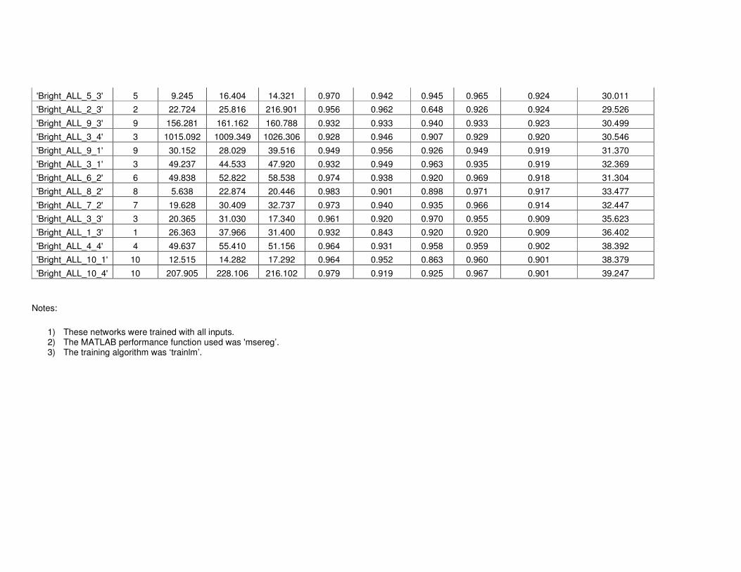
'Bright_ALL_5_3' 5 9.245 16.404 14.321 0.970 0.942 0.945 0.965 0.924 30.011
'Bright_ALL_2_3' 2 22.724 25.816 216.901 0.956 0.962 0.648 0.926 0.924 29.526
'Bright_ALL_9_3' 9 156.281 161.162 160.788 0.932 0.933 0.940 0.933 0.923 30.499
'Bright_ALL_3_4' 3 1015.092 1009.349 1026.306 0.928 0.946 0.907 0.929 0.920 30.546
'Bright_ALL_9_1' 9 30.152 28.029 39.516 0.949 0.956 0.926 0.949 0.919 31.370
'Bright_ALL_3_1' 3 49.237 44.533 47.920 0.932 0.949 0.963 0.935 0.919 32.369
'Bright_ALL_6_2' 6 49.838 52.822 58.538 0.974 0.938 0.920 0.969 0.918 31.304
'Bright_ALL_8_2' 8 5.638 22.874 20.446 0.983 0.901 0.898 0.971 0.917 33.477
'Bright_ALL_7_2' 7 19.628 30.409 32.737 0.973 0.940 0.935 0.966 0.914 32.447
'Bright_ALL_3_3' 3 20.365 31.030 17.340 0.961 0.920 0.970 0.955 0.909 35.623
'Bright_ALL_1_3' 1 26.363 37.966 31.400 0.932 0.843 0.920 0.920 0.909 36.402
'Bright_ALL_4_4' 4 49.637 55.410 51.156 0.964 0.931 0.958 0.959 0.902 38.392
'Bright_ALL_10_1' 10 12.515 14.282 17.292 0.964 0.952 0.863 0.960 0.901 38.379
'Bright_ALL_10_4' 10 207.905 228.106 216.102 0.979 0.919 0.925 0.967 0.901 39.247
Notes:
1) These networks were trained with all inputs. 2) The MATLAB performance function used was 'msereg’. 3) The training algorithm was ‘trainlm’.

APPENDIX 4B – TRAINING RESULTS FOR ERIC
Performance (mse) Performance - regression Independent test
N.Net name No.
Neurons Training
set Validation
set Test set Training
set Validation
set Test set Total R Regression mse
'Eric_ALL_4_4' 4.000 2728 2857 1644 0.873 0.876 0.860 0.874 0.840 3781
'Eric_ALL_3_4' 3.000 3053 5346 4686 0.829 0.811 0.652 0.819 0.815 3965
'Eric_ALL_2_1' 2.000 3378 7279 5121 0.836 0.660 0.403 0.798 0.810 4371
'Eric_ALL_7_4' 7.000 3125 4103 4025 0.838 0.846 0.721 0.829 0.806 4155
'Eric_ALL_1_4' 1.000 5507 2536 2056 0.773 0.821 0.692 0.773 0.804 5235
'Eric_ALL_5_2' 5.000 3530 5096 2441 0.856 0.840 0.832 0.851 0.803 4146
'Eric_ALL_5_1' 5.000 2356 3014 2839 0.898 0.819 0.690 0.882 0.800 4678
'Eric_ALL_1_2' 1.000 2750 3781 3026 0.861 0.791 0.842 0.850 0.798 4289
'Eric_ALL_6_1' 6.000 10155 11424 8771 0.834 0.755 0.893 0.824 0.797 4385
'Eric_ALL_2_4' 2.000 8397 9455 11564 0.887 0.770 0.698 0.864 0.795 4458
'Eric_ALL_2_2' 2.000 3130 2400 9562 0.854 0.731 0.804 0.839 0.781 4736
'Eric_ALL_10_2' 10.000 15526 16503 16242 0.845 0.834 0.800 0.838 0.781 4623
'Eric_ALL_8_4' 8.000 1930 3147 2607 0.900 0.895 0.826 0.894 0.778 4591
'Eric_ALL_5_4' 5.000 5736 5564 4193 0.849 0.700 0.917 0.830 0.777 4643
'Eric_ALL_4_2' 4.000 2739 3665 5151 0.863 0.744 0.901 0.853 0.773 5124
'Eric_ALL_9_4' 9.000 4145 2790 3987 0.835 0.869 0.796 0.837 0.772 4744
'Eric_ALL_1_3' 1.000 3501 2623 6294 0.834 0.832 0.852 0.831 0.770 5034
'Eric_ALL_1_1' 1.000 2707 2805 10174 0.849 0.901 0.785 0.842 0.770 4989
'Eric_ALL_9_3' 9.000 2700 4310 1687 0.883 0.752 0.551 0.861 0.769 4882
'Eric_ALL_2_3' 2.000 3381 8100 1605 0.811 0.789 0.840 0.800 0.769 4787
'Eric_ALL_3_3' 3.000 2875 3588 3196 0.858 0.825 0.831 0.849 0.767 4823
'Eric_ALL_4_3' 4.000 3105 2693 3612 0.854 0.844 0.850 0.851 0.764 4953
'Eric_ALL_6_3' 6.000 3550 2826 2799 0.866 0.871 0.817 0.865 0.760 5085
'Eric_ALL_3_1' 3.000 2495 2600 3021 0.898 0.740 0.931 0.878 0.758 5181
'Eric_ALL_7_3' 7.000 1827 5002 4416 0.919 0.842 0.805 0.896 0.746 5431
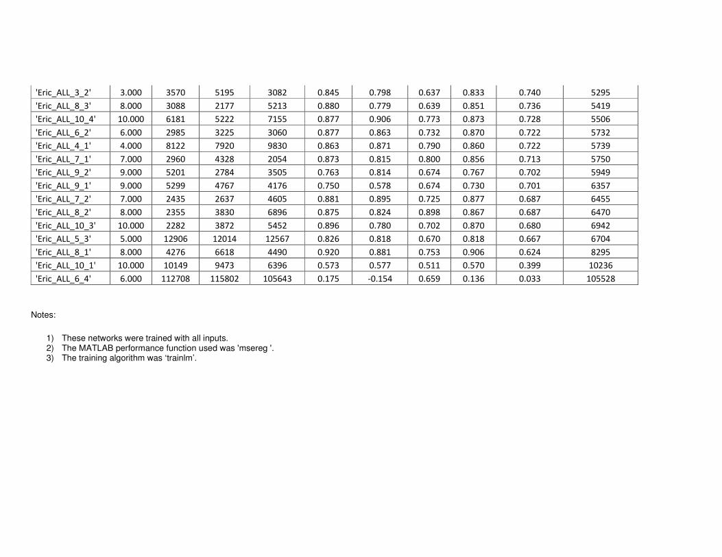
'Eric_ALL_3_2' 3.000 3570 5195 3082 0.845 0.798 0.637 0.833 0.740 5295
'Eric_ALL_8_3' 8.000 3088 2177 5213 0.880 0.779 0.639 0.851 0.736 5419
'Eric_ALL_10_4' 10.000 6181 5222 7155 0.877 0.906 0.773 0.873 0.728 5506
'Eric_ALL_6_2' 6.000 2985 3225 3060 0.877 0.863 0.732 0.870 0.722 5732
'Eric_ALL_4_1' 4.000 8122 7920 9830 0.863 0.871 0.790 0.860 0.722 5739
'Eric_ALL_7_1' 7.000 2960 4328 2054 0.873 0.815 0.800 0.856 0.713 5750
'Eric_ALL_9_2' 9.000 5201 2784 3505 0.763 0.814 0.674 0.767 0.702 5949
'Eric_ALL_9_1' 9.000 5299 4767 4176 0.750 0.578 0.674 0.730 0.701 6357
'Eric_ALL_7_2' 7.000 2435 2637 4605 0.881 0.895 0.725 0.877 0.687 6455
'Eric_ALL_8_2' 8.000 2355 3830 6896 0.875 0.824 0.898 0.867 0.687 6470
'Eric_ALL_10_3' 10.000 2282 3872 5452 0.896 0.780 0.702 0.870 0.680 6942
'Eric_ALL_5_3' 5.000 12906 12014 12567 0.826 0.818 0.670 0.818 0.667 6704
'Eric_ALL_8_1' 8.000 4276 6618 4490 0.920 0.881 0.753 0.906 0.624 8295
'Eric_ALL_10_1' 10.000 10149 9473 6396 0.573 0.577 0.511 0.570 0.399 10236
'Eric_ALL_6_4' 6.000 112708 115802 105643 0.175 -0.154 0.659 0.136 0.033 105528
Notes:
1) These networks were trained with all inputs. 2) The MATLAB performance function used was 'msereg '. 3) The training algorithm was ‘trainlm’.

APPENDIX 4C – TRAINING RESULTS FOR YIELD
Performance (mse) Performance - regression Independent test
N.Net name No.
Neurons Training
set Validation
set Test set Training
set Validation
set Test set Total R Regression mse
'Yield_all_3_3' 3.000 65.143 97.148 86.368 0.790 0.540 0.577 0.753 0.725 84.375
'Yield_all_5_2' 5.000 198.325 201.706 179.268 0.788 0.748 0.634 0.774 0.707 90.618
'Yield_all_10_4' 10.000 66.605 71.079 75.427 0.772 0.795 0.636 0.769 0.670 98.089
'Yield_all_7_3' 7.000 360.112 388.086 361.714 0.716 0.710 0.803 0.721 0.667 108.762
'Yield_all_1_4' 1.000 93.990 80.146 87.105 0.653 0.743 0.637 0.664 0.662 99.678
'Yield_all_5_3' 5.000 273.846 248.223 252.858 0.686 0.724 0.750 0.692 0.653 103.238
'Yield_all_1_2' 1.000 95.078 91.795 42.668 0.653 0.703 0.770 0.663 0.642 104.246
'Yield_all_1_3' 1.000 96.518 77.721 109.817 0.637 0.779 0.564 0.660 0.618 108.433
'Yield_all_8_3' 8.000 688.020 739.643 727.596 0.726 0.569 0.430 0.689 0.612 113.298
'Yield_all_5_1' 5.000 132.293 142.171 139.715 0.730 0.678 0.663 0.717 0.610 123.201
'Yield_all_2_4' 2.000 77.632 99.454 134.668 0.728 0.660 0.455 0.705 0.600 116.364
'Yield_all_6_1' 6.000 121.325 104.607 82.785 0.667 0.633 0.657 0.656 0.592 116.523
'Yield_all_8_2' 8.000 57.083 66.781 76.382 0.821 0.715 0.341 0.797 0.592 117.234
'Yield_all_3_1' 3.000 83.336 97.380 96.367 0.737 0.680 0.391 0.722 0.582 121.401
'Yield_all_9_3' 9.000 904.403 868.882 951.156 0.741 0.784 -0.129 0.724 0.579 133.865
'Yield_all_2_2' 2.000 129.959 134.592 119.168 0.740 0.716 0.633 0.732 0.573 125.972
'Yield_all_9_1' 9.000 243.550 233.445 212.470 0.609 0.624 0.757 0.619 0.560 121.096
'Yield_all_7_1' 7.000 322.241 374.623 322.287 0.703 0.503 0.460 0.663 0.546 125.619
'Yield_all_6_4' 6.000 111.784 113.214 96.978 0.754 0.748 0.801 0.754 0.546 141.490
'Yield_all_5_4' 5.000 100.589 139.504 129.790 0.720 0.513 0.551 0.680 0.534 125.291
'Yield_all_4_1' 4.000 137.695 126.173 165.527 0.696 0.764 0.607 0.702 0.527 151.019
'Yield_all_10_2' 10.000 413.659 425.551 497.974 0.689 0.498 0.201 0.645 0.526 138.974
'Yield_all_3_4' 3.000 68.905 83.157 61.285 0.761 0.749 0.607 0.753 0.526 146.740
'Yield_all_1_1' 1.000 91.793 94.379 136.564 0.681 0.640 0.133 0.658 0.514 149.990
'Yield_all_2_1' 2.000 113.356 121.969 252.268 0.696 0.626 0.125 0.661 0.510 154.254
'Yield_all_3_2' 3.000 235.511 219.907 214.708 0.644 0.590 0.576 0.638 0.508 138.835
'Yield_all_4_3' 4.000 231.049 288.906 265.286 0.713 0.605 0.684 0.692 0.492 159.236

'Yield_all_10_1' 10.000 134.003 188.829 146.976 0.640 0.522 0.482 0.612 0.486 142.589
'Yield_all_4_4' 4.000 290.906 293.864 277.011 0.468 0.419 0.494 0.462 0.482 145.304
'Yield_all_8_4' 8.000 208.256 210.409 275.212 0.609 0.574 0.060 0.581 0.482 137.286
'Yield_all_9_4' 9.000 78.501 121.025 161.478 0.729 0.474 0.605 0.685 0.476 161.971
'Yield_all_8_1' 8.000 255.334 287.573 260.884 0.782 0.572 0.746 0.753 0.460 170.600
'Yield_all_7_2' 7.000 137.943 165.387 178.800 0.660 0.545 0.395 0.629 0.443 142.696
'Yield_all_6_2' 6.000 91.086 135.170 149.873 0.747 0.587 0.418 0.711 0.418 209.665
'Yield_all_9_2' 9.000 232.227 213.111 263.337 0.545 0.614 0.317 0.542 0.400 154.080
'Yield_all_2_3' 2.000 164.892 156.057 240.515 0.420 0.534 0.190 0.427 0.373 194.730
'Yield_all_10_3' 10.000 2210.503 2246.136 2412.175 0.650 0.390 0.043 0.576 0.356 165.918
'Yield_all_4_2' 4.000 82.267 159.433 84.537 0.772 0.506 0.765 0.726 0.290 428.520
'Yield_all_7_4' 7.000 94.822 153.727 164.360 0.772 0.566 0.364 0.723 0.195 551.227
'Yield_all_6_3' 6.000 485.690 428.305 518.434 0.047 -0.002 -0.011 0.036 0.015 288.742
Notes:
1) These networks were trained with all inputs. 2) The MATLAB performance function used was 'msereg '. 3) The training algorithm was ‘trainlm’.

APPENDIX 5A: NEURAL NETWORK SENSITIVITY ANALYSIS - BRIGHTNESS
Neural network NaOH Ssil H2O2 Surf p tp cons pH Surf f tf NaOH Ssil H2O2 Surf p tp cons pH Surf f tf NaOH Ssil H2O2 Surf p tp cons pH Surf f tf NaOH Ssil H2O2 Surf p tp cons pH Surf F tf
'Bright_ALL_5_1' +- O + +- O O +- + + - + - - + - O- - + + + +- +- + - +- + + - + O - + - + - -
'Bright_ALL_8_4' - + + +- - - + - + - + + +- - O - - + + + + + - - - O+ + - + + + - - - - +
'Bright_ALL_9_4' + + + - - +- - +- +- - + + O - - - - + + O+ + - + +- - + O+ - + + + - - - - +
'Bright_ALL_5_4' +- + +- +- - - + + + + + + O - + - - + + + + - - + - + O+ +- O + + - - - - +
'Bright_ALL_10_3' + + + +- + - +- + + + + +- +- + - +- - + + + + - - + +- + + + + +- +- + - - - +
'Bright_ALL_1_4' + + + - + - - + + + + + - O - - + + + + + - O+ - - + + + + + - O+ - - + +
'Bright_ALL_4_3' + O + O O- - - - + + O + O - - - - + + + + - + - - + + + O + O - - - - +
'Bright_ALL_1_1' + + + - + - - + + + + + - + - - + + + + + - + - - + + + + + O- O+ - - + +
'Bright_ALL_2_2' + + + +- +- - - + + + + +- +- +- - - + + + + + +- +- - - + + + + + O + - O- + +
'Bright_ALL_2_4' + + + O + - - + + + + + + - O- - O + + + + O + - - + + + + + + - - - O +
'Bright_ALL_6_1' + + + - - O- - + + + + + O - +- - - + + + + O + - - + + + + + +- - + - - +
'Bright_ALL_8_1' + O+ + + +- - - - + +- +- + +- - - - +- + + + + + +- - +- + + +- +- + + - - - - +
'Bright_ALL_4_2' + + + O +- - +- +- + +- + + + - - +- +- + +- + + - +- - +- + O- +- + + O+ - - +- +- +
'Bright_ALL_9_2' + +- + +- + - - - + + +- + + - - - - + + + + +- + - + - +- +- +- + + - - - - +
Bright_ALL_7_1' + + + + - +- - +- + - + + + +- +- +- +- + + - + O + - +- + + +- + + + - +- - - +
Bright_ALL_6_4' + +- + O + + +- +- + + + + + + - - O- + +- +- + - +- - + + + + + +- +- + - - - +
Bright_ALL_7_3' + + +- +- + +- - + + - + + +- O - - + + + + + - + + + + +- - + + + O - +- +- +
Bright_ALL_10_2' +- - + +- + - - +- + + - + + + - - - + - - + +- + +- +- +- + +- +- + +- + - - - +
Bright_ALL_3_2' + + + - + - - + + O + + - + - - - + + O + - + - + + + - + + - O- - - - +
Bright_ALL_3_4' + + + - + - - +- +- + + + - + - O +- + + + + - + - - + + + + + - O - - + +
% Response
% + 80 70 90 10 50 5 10 50 90 60 80 85 30 35 5 0 20 100 85 75 95 10 60 15 20 85 75 45 75 85 40 25 5 5 20 95
% - 5 5 0 30 25 70 70 20 0 25 5 5 25 45 75 75 50 0 5 10 0 55 15 75 50 5 0 25 0 0 20 50 90 80 65 5
% other 15 25 10 60 25 25 20 30 10 15 15 10 45 20 20 25 30 0 10 15 5 35 25 10 30 10 25 30 25 15 40 25 5 15 15 0
Neural network NaOH Ssil H2O2 Surf p tp cons pH Surf f tf NaOH Ssil H2O2 Surf p tp cons pH Surf f tf NaOH Ssil H2O2 Surf p tp cons pH Surf f tf
'Bright_ALL_5_1' +- + +- + + - + - + + + +- + + +- +- + O + + +- + +- + + + +-
'Bright_ALL_8_4' - + +- - + - + + + + + + + +- - - - + + + + +- + - - + +
'Bright_ALL_9_4' - + + - - - - - + + + + - + +- - + +- + O + - + O +- + +-
'Bright_ALL_5_4' + + + + - + - + + + + +- +- O - + + + - + +- - - + - + +-
'Bright_ALL_10_3' +- + +- +- + - +- - +- + + +- +- + - +- +- +- - - + - + + + + +-
'Bright_ALL_1_4' + + + - O+ - - + + + + + - O+ - - + + + + + - O+ - - + +
'Bright_ALL_4_3' + O - O+ - - - - + + + - - + - - + - + + - - + - - + +-
'Bright_ALL_1_1' + + + - + - - + + + + + - + - - + + + + + - + - - + +
'Bright_ALL_2_2' + + + O+ O+ - O- + + + + + O O- + O + + + + + O O+ - O- + +
'Bright_ALL_2_4' + + + + - - - + + + + + + + - - O + + + + - + - + + O-
'Bright_ALL_6_1' + + + O - - - - + + + + +- + - - + + + + - +- +- - - + +
'Bright_ALL_8_1' +- +- + - - +- - +- + + - + +- + +- +- +- + + O + + + - - +- +
'Bright_ALL_4_2' - + + O +- - +- +- + + + + + O- +- +- +- + + O+ + - + +- +- + -
'Bright_ALL_9_2' + O + +- + + + + + + O + - + + + + + - + +- +- + - +- - -
Bright_ALL_7_1' - + + + +- +- +- +- + + O- + O + - +- +- + + O + - +- - + +- +-
Bright_ALL_6_4' + + + + +- +- - - + + O- + O + +- +- + + + O + O + O + +- +
Bright_ALL_7_3' - + + +- O - - - + + + +- + O - +- +- + + + + - + +- + + +
Bright_ALL_10_2' + - + +- - - +- +- + + + + - + + + + + +- +- + - O+ - +- +- +
Bright_ALL_3_2' + +- + - + - +- + + + + + - + - +- + + + - + + - + + + +-
Bright_ALL_3_4' + + + - + - - +- +- + + + - O - - + + + + + - + - - +- +-
% Response
% + 60 75 80 25 35 10 15 40 90 100 80 75 25 65 15 15 65 80 80 60 75 15 60 20 35 70 45
% - 25 5 5 35 35 75 55 35 0 0 5 5 40 0 60 40 5 5 15 10 10 60 10 60 40 5 10
% other 15 20 15 40 30 15 30 25 10 0 15 20 35 35 25 45 30 15 5 30 15 25 30 20 25 25 45
OMG 100% HL1 100% HL2 100%
All Grades: ONP:OMG:HL1:HL2::25:25:25:25 ONP:OMG::50:50 HL1:HL2::50:50 ONP 100%

APPENDIX 5B: NEURAL NETWORK SENSITIVITY ANALYSIS - ERIC
Neural network NaOH Ssil H2O2 Surf p tp cons pH Surf f tf NaOH Ssil H2O2 Surf p tp cons pH Surf f tf NaOH Ssil H2O2 Surf p tp cons pH Surf f tf NaOH Ssil H2O2 Surf p tp cons pH Surf F tf
'Eric_ALL_4_4' +- - + - - + +- +- - - - + - + + + - - +- - + +- - + +- + - - - + - + + O+ - -
'Eric_ALL_3_4' - - + - O + + - - - + + - O + + - - - + + - O + + - - - O + - O + + - -
'Eric_ALL_2_1' - - + - + + + O - - - + - + + + O - - - + - + + + o+ - - - + - + + + O -
'Eric_ALL_7_4' - + + O+ + + + - - - - + - + + + - - - +- + +- + + + - - - - + - + + + - -
'Eric_ALL_1_4' - - + + + + O - - - - + + + + O - - - - + + + + O - - - - + + + + O - -
'Eric_ALL_5_2' - +- + +- +- + + - - - - + - O + + - - - - +- +- +- + + +- - - - + - + + O - -
'Eric_ALL_5_1' +- +- - + +- + + +- - +- +- + +- + + + + - +- - +- +- + + + +- - - - + - + + + +- -
'Eric_ALL_1_2' - - + - + + O+ - - - - + - + + + - - - - + - + + O+ - - - - + - + + + - -
'Eric_ALL_6_1' - - + - + + + + - - + + - O+ + +- +- - + - +- +- + +- + + - - + + - + + + - -
'Eric_ALL_2_4' - O + - + + + - - - O + - + + + - - - O + - + + + - - - O + - + + O O O
'Eric_ALL_10_2' +- +- + +- +- + O - - - O + - + + + + - O + +- +- +- + O O +- - - + +- +- +- + - -
Eric_ALL_8_4' +- - + + - + + +- - +- - + - - + +- +- - - + +- +- - + +- +- - - - + - + + O - -
'Eric_ALL_4_2' - + +- +- +- +- + O+ +- - + +- - +- +- O+ O+ - - - + + - +- - - + + + + - + + O - -
'Eric_ALL_9_4' - - + + +- + - +- - - - + +- + + - - - - - + + - + - +- - - - + +- - + - +- -
'Eric_ALL_9_3' O + + - + + +- +- - - +- + +- + + +- - - +- +- +- - + + + +- - - - + - + + + - -
'Eric_ALL_2_3' - - + - + + + + - - O + O- + + + + - - O + O- + + + + - - O + O- + + + + -
Eric_ALL_3_3' - - + - + + + - - - - + - + + + - - + - + - + + + - - - O- + - + + + - -
Eric_ALL_6_3' - + +- +- +- + + +- - - +- + - + + + - - - +- + +- +- + + + - - - + - + + + - -
Eric_ALL_7_3' - +- + - +- + +- +- - - +- + +- - + +- +- - - +- + +- - + +- +- - - +- + +- - + +- +- -
Eric_ALL_8_3' +- - + + - + + +- - +- - + - - + - +- - - + +- +- O- + - + - - - + - + + O - -
% Response
% + 0 20 85 25 45 95 65 10 0 0 15 95 5 65 95 60 15 0 10 20 65 15 50 90 55 25 5 5 10 100 5 80 95 55 5 0
% - 70 55 5 50 15 0 5 40 95 85 50 0 70 15 0 10 55 100 70 50 0 30 25 0 15 35 90 95 65 0 75 10 0 5 70 95
% other 30 25 10 25 40 5 30 50 5 15 35 5 25 20 5 30 30 0 20 30 35 55 25 10 30 40 5 0 25 0 20 10 5 40 25 5
Neural network NaOH Ssil H2O2 Surf p tp cons pH Surf f tf NaOH Ssil H2O2 Surf p tp cons pH Surf f tf NaOH Ssil H2O2 Surf p tp cons pH Surf f tf
'Eric_ALL_4_4' + - + +- - + +- + - + +- + +- - + +- + - - - + +- - + +- - -
'Eric_ALL_3_4' - O- + - o + + - - - + + - + + +- - - - o + - o + + - -
'Eric_ALL_2_1' - - + - + + + o - - - + - + + + o - - - + - + + + o+ -
'Eric_ALL_7_4' - + + + + +- + - - - +- + + + + + - +- - - + - + + + - -
'Eric_ALL_1_4' - - + + + + o - - - - + + + + o - - - - + + + + o - -
'Eric_ALL_5_2' - + +- + +- + o + - - + +- + - + + + - - - + +- +- + + - -
'Eric_ALL_5_1' + + - + - +- + + - + + - - + + + + - +- - +- +- +- +- + - -
'Eric_ALL_1_2' - - + - + + o+ - - - - + - + + + - - - - + - + + + - -
'Eric_ALL_6_1' O+ O- +- + + +- +- +- - + - - + + - + + - +- - + - + + +- +- -
'Eric_ALL_2_4' - O + - o+ + o+ o- - - o + - + + o+ - - - o + o- + + o+ - -
'Eric_ALL_10_2' - - +- - o+ +- - o - + + + + - +- - + + - - + +- +- - - - -
Eric_ALL_8_4' - + +- +- - + - + - - + +- +- - + - o +- +- +- + +- + + +- +- -
'Eric_ALL_4_2' - + - - +- +- + + - - + - - +- +- + + - - o+ - - - - + o+ -
'Eric_ALL_9_4' +- + + + +- + + +- - - - + + - o+ - + - - - + + +- + +- +- -
'Eric_ALL_9_3' +- + - o- + +- +- +- - + +- +- - +- +- + + - - + + - + + - +- -
'Eric_ALL_2_3' - O +- + - + + +- - - o + - + + + + - - o + o- o+ + + + -
Eric_ALL_3_3' - - + - + + + - - - - + - + + + - - + o + - - + + + -
Eric_ALL_6_3' - + +- +- - - o- + - + - + +- + - - + - - +- + - +- + +- +- -
Eric_ALL_7_3' - +- + +- - + +- +- - - +- + +- - + +- +- - - +- + +- - + +- +- -
Eric_ALL_8_3' - + +- +- - + - + - - + +- +- o- + - o +- +- +- + +- +- + +- +- -
% Response
% + 10 45 50 35 35 65 40 35 0 30 35 65 30 55 70 50 50 5 5 5 90 10 40 85 45 10 0
% - 75 30 15 35 35 5 15 25 100 70 35 15 45 30 10 25 30 80 75 50 5 45 20 10 10 45 100
% other 15 25 35 30 30 30 45 40 0 0 30 20 25 15 20 25 20 15 20 45 5 45 40 5 45 45 0
OMG 100% HL1 100% HL2 100%
All Grades: ONP:OMG:HL1:HL2::25:25:25:25 ONP:OMG::50:50 HL1:HL2::50:50 ONP 100%

APPENDIX 5C: NEURAL NETWORK SENSITIVITY ANALYSIS - YIELD
Neural network NaOH Ssil H2O2 Surf p tp cons pH Surf F tf NaOH Ssil H2O2 Surf p tp cons pH Surf F tf NaOH Ssil H2O2 Surf p tp cons pH Surf F tf NaOH Ssil H2O2 Surf p tp cons pH Surf F tf
Yield_all_3_3 - + + - o+ + + - - + + + - o + + - - - + o - + + + - - - +- o - o + + - -
Yield_all_5_2 - + + - o+ + + +- - - + + o - + - - - - +- + - +- +- + + - - o + +- +- + + + -
Yield_all_10_4 +- +- + + +- + + - - +- +- + + o + +- +- - + +- + + + + + - - - + + +- o + +_ - -
Yield_all_7_3 + + + +- +- + + - - + + + o o+ + o+ - - - +- +- +- + +- + +- - + - +- o o + + o- -
Yield_all_1_4 O- + + - o+ + + o+ - - + + - o + + o - - + + - o + + o - - + + - o + + o- -
Yield_all_5_3 - + + - - +- +- - - - + + - - +- + - - - o- + +- + + +- +- - - + + - + + + - -
Yield_all_1_2 - + + - o+ + + + - - + + - o + + + - - + + - o + + + - - + + - o + + + -
Yield_all_8_3 +- +- +- +- +- +- +- +- - o- + + - +- +- +- +- - +- +- + o- + + o+ +- - + + + +- - +- +- +- -
Yield_all_2_4 +- + + +- - + + - - +- + + + +- + + +- - + + + - - + + - - o- + + + o+ + + + +-
Yield_all_6_1 +- + + - o+ + + +- - o + + - o + + + - +- + o+ o- o + + - - - + o+ - +- + + - -
Yield_all_8_2 + +- + + +- + + - - + +- + o+ +- + + +- - + + + +- + + + +- - + - + + + + + - -
Yield_all_3_1 +- + + + o+ + + +- - + + + + o + + - - - + + - - +- + + - + + + - o + + - -
Yield_all_9_3 +- + + - +- + + +- - + o + +- - + - - - +- +- - +- - + + + o- + +- - - +- + _ - -
Yield_all_2_2 - + + - - + + - - +- + + - o+ + + - - - + + - - + + - - + +- + +- + + + o- -
Yield_all_9_1 - + + + +- + +- +- - - + o+ + +- + =- +- - - o+ + +- +- + +- +- - - - + + +- +- +- - -
Yield_all_7_1 - + +- - + + + + - - + +- - + + + + - +- + - - + + + + - - + - - + + + o- -
Yield_all_6_4 +- - + + + + + + - + + - + + + + - - +- +- + + + + +- - - +- + + + + + + - -
Yield_all_4_1 +- + + +- + + +- - - + + + + + + + - - - +- o - + + +- +- - +- +- o - +- + + + -
Yield_all_10_2 +- +- + + +- + + - - +- + + + - + +- +- - + +- + + + + + - - - + + +- - +- +- - -
Yield_all_4_3 + + + +- +- + + +- - + + + +- + + + +- - + + + + +- + +- - - - + + +- +- +- +- - -
% Response
% + 15 75 90 30 15 90 80 15 0 40 85 85 35 20 90 65 15 0 25 50 70 20 50 85 70 25 0 30 60 70 20 25 80 70 20 0
% - 35 5 0 45 15 0 0 45 100 30 0 5 40 20 0 10 45 100 50 0 10 45 20 0 0 40 95 55 15 10 45 10 0 0 55 95
% other 50 20 10 25 70 10 20 40 0 30 15 10 25 60 10 25 40 0 25 50 20 35 30 15 30 35 5 15 25 20 35 65 20 30 25 5
Neural network
Yield_all_3_3 NaOH Ssil H2O2 Surf p tp cons pH Surf F tf NaOH Ssil H2O2 Surf p tp cons pH Surf F tf NaOH Ssil H2O2 Surf p tp cons pH Surf F tf
Yield_all_5_2 - + + - o + + - - - o- + - + - + - + - + + - o + + - -
Yield_all_10_4 - + + - 0 + + - - - o- - - + + + + - - + + +- o + + +- -
Yield_all_7_3 - + + - o- o+ + +- - - o- +- + o + +- + - - o+ + +- o- + +- + -
Yield_all_1_4 + + +- +- + +- + - - - +- +- +- + + + +- - - +- +- +- +- + +- +- -
Yield_all_5_3 - + + - o + + o - - + + - o + + o - - + + - o + + o -
Yield_all_1_2 - + + - - + + - - - o- + +- + +- +- +- - - - + +- o+ +- +- +- -
Yield_all_8_3 - + + - o + + + - - + + - o + + + - - + + - o + + + -
Yield_all_2_4 - + + - +- +- + +- - - +- + o +- +- +- +- - - + + - + + +- - -
Yield_all_6_1 + + + +- - + + - - o- + + + + + + + + + + + - - + + - -
Yield_all_8_2 o + + o- o + + + - - +- + +- + +- + - - o + + - o + + +- -
Yield_all_3_1 +- - + o+ o + + +- - + o+ + + + + + - - + +- + + + + + - -
Yield_all_9_3 + + + + o + + - - +- +- + + o + + +- - +- + + - o + +- =- -
Yield_all_2_2 + +- +- +- - + + +- - +- - - - +- +- o - o- +- +- - +- +- + +- o o-
Yield_all_9_1 - + + - - + o+ - - - + + - - + o - - + - + + + + +- o -
Yield_all_7_1 - + o- - o+ + + +- - +- +- + - o o + o+ o- + + +- +- +- + +- - -
Yield_all_6_4 - + + - + + + o - - + +- - + + + + - +- +- +- - + +- +- + -
Yield_all_4_1 +- +- - + + + + +- +- +- +- - - + + +- - - - - + +- +- + +- + -
Yield_all_10_2 + + + + + + + - - - + + - + + +- - - - +- o - +- + +- +- -
Yield_all_4_3 - + + - - + + +- - - o +- + o + +- + - - + + +- - + +- + -
+ + + - + + + +- - + + + +- + + + - - - + + +- +- + - - -
% Response
% +
% - 30 85 80 15 25 85 95 10 0 10 35 65 25 55 70 60 30 10 20 55 75 10 20 90 35 25 0
% other 55 5 5 60 25 0 0 40 95 65 5 15 50 5 5 0 40 80 60 15 5 45 10 0 5 30 95
15 10 15 25 50 15 5 50 5 25 60 20 25 40 25 40 30 10 20 30 20 45 70 10 60 45 5
OMG 100% HL1 100% HL2 100%
All Grades: ONP:OMG:HL1:HL2::25:25:25:25 ONP:OMG::50:50 HL1:HL2::50:50 ONP 100%

APPENDIX 6A: FLOTATION ALIGNMENT NEWSPRINT
Ratios
Flo
tati
on
ti
me
(m
in)
%B
rig
ht
-n
es
s (
B)
ER
IC (
E)
pp
m
%F
lota
tio
n
Yie
ld (
Y)
B/Bo E/Eo Y/Yo
Lab run 1
0 42.5 975 100 1.000 1.000 1.000
2 48.0 655 91 1.129 0.671 0.909
4 48.9 630 91 1.150 0.646 0.912
8 57.7 226 69 1.357 0.232 0.686
12 60.9 126 49 1.432 0.129 0.494
Lab run 2
0 40.1 797 100 1.000 1.000 1.000
2 46.0 678 83 1.148 0.850 0.831
4 50.8 409 79 1.267 0.513 0.786
8 53.6 275 71 1.336 0.345 0.708
12 55.3 210 70 1.380 0.264 0.701
Lab run 3
0 39.4 954 100 1.000 1.000 1.000
2 51.4 486 91 1.304 0.510 0.908
4 50.3 548 87 1.275 0.574 0.867
8 56.9 252 79 1.443 0.264 0.791
12 58.9 181 71 1.493 0.190 0.705
Standard error
Average Ratios B/Bo E/Eo Y/Yo
Lab averages
0 40.7 909 100 1.000 1.000 1.000 0.000 0.000 0.000
2 48.5 606 88 1.194 0.677 0.883 0.055 0.098 0.026
4 50.0 529 85 1.231 0.578 0.855 0.040 0.039 0.037
8 56.1 251 73 1.379 0.280 0.728 0.032 0.033 0.032
12 58.4 173 63 1.435 0.194 0.633 0.033 0.039 0.070
Plant averages
0 42.1 846 100.0 1.000 1.000 1 0 0 0
3.1 52.7 269 89.0 1.2531 0.327
1 0.89
1 0.003
7 0.0092 0.4900
Notes:
1. Calculated as the average of the ratios, not the ratio of averages.

APPENDIX 6B: FLOTATION ALIGNMENT - DOUBLE LOOP TISSUE
Flo
tati
on
ti
me
(m
in)
%B
rig
htn
ess
(B
)
ER
IC (
E)
pp
m
%F
lota
tio
n
Yie
ld (
Y)
B/Bo E/Eo Y/Yo
Lab run 1
0 82.6 105 100 1.000 1.000 1.000
2 85.4 72 79 1.034 0.690 0.789
6 85.6 67 82 1.036 0.639 0.819
12 86.7 61 74 1.050 0.581 0.738
Lab run 2
0 74.6 283 100 1.000 1.000 1.000
4 75.7 237 83 1.015 0.838 0.831
12 77.9 139 75 1.045 0.490 0.751
Lab run 3
0 79.1 126 100 1.000 1.000 1.000
2 82.3 89 91 1.040 0.706 0.908
4 84.2 91 81 1.064 0.725 0.810
8 85.2 79 79 1.076 0.625 0.786
12 86.0 80 82 1.086 0.637 0.821
Lab run 4
0 77.3 154 100 1.000 1.000 1.000
2 77.4 145 85 1.003 0.941 0.848
8 80.2 115 74 1.038 0.746 0.735
12 79.5 127 72 1.029 0.823 0.724
Lab run 5
0 76.6 141 100 1.000 1.000 1.000
2 81.8 94 83 1.067 0.667 0.831
4 85.6 69 77 1.117 0.485 0.772
12 87.4 52 75 1.141 0.370 0.753
Lab run 6
0 82.0 118 100 1.000 1.000 1.000
2 85.0 70 66 1.037 0.597 0.661
4 88.0 70 70 1.073 0.591 0.698
8 88.5 55 66 1.079 0.468 0.656
12 88.6 52 62 1.080 0.440 0.623
Standard error
Average Ratios B/Bo E/Eo Y/Yo
Laboratory averages
0 78.7 155 100 1.00000 1.000 1.000 0.000 0.000 0.000
2 82.4 94 81 1.03603 0.720 0.807 0.010 0.058 0.041
4 83.4 117 78 1.06732 0.660 0.778 0.021 0.077 0.029
6 85.6 67 82 1.03637 0.639 0.819
8 84.6 83 73 1.06464 0.613 0.726 0.013 0.081 0.038
12 84.4 85 74 1.07194 0.557 0.735 0.016 0.066 0.026 Plant averages
Medium grade 2
0 71.8 120 100.0 1.000 1.000 1.000 0 0 0
0.9 79.7 922
80.7 1.0451
0.7672
0.8071
0.0092 0.0614 0.807
High grade 2
0 75.6 100.0 1.000 1.000 0 0
0.9 81.8 77.2 1.0381
0.7721
0.0123 0.772
Notes:
1. Calculated as the average of the ratios, not the ratio of averages.
2. Based on limited data.

APPENDIX 6C: FLOTATION ALIGNMENT SINGLE - LOOP TISSUE
Flo
tati
on
ti
me
(m
in)
%B
rig
htn
es
s (
B)
ER
IC (
E)
pp
m
%F
lota
tio
n
Yie
ld (
Y)
B/Bo E/Eo Y/Yo
Lab run 1
0 80.7 78 100 1.000 1.000 1.000
2 80.5 58 78 0.997 0.743 0.777
4 81.4 52 76 1.008 0.662 0.763
8 81.5 47 72 1.009 0.603 0.716
12 73.2 50 71 0.907 0.642 0.709
Lab run 2
0 83.7 131 100 1.000 1.000 1.000
2 86.8 114 86 1.038 0.875 0.863
4 88.4 83 75 1.057 0.632 0.751
8 89.0 82 72 1.063 0.625 0.722
12 86.4 86 71 1.032 0.660 0.706
Lab run 3
0 81.0 146 100 1.000 1.000 1.000
2 80.0 145 83 0.989 0.996 0.827
4 79.2 143 82 0.978 0.981 0.816
12 80.0 0.988
Lab run 4
0 85.3 123 100 1.000 1.000 1.000
2 85.7 109 85 1.004 0.890 0.848
12 87.1 74 77 1.021 0.601 0.770
Lab run 5
0 69.2 200 100 1.000 1.000 1.000
2 74.0 139 80 1.069 0.697 0.802
4 75.6 101 66 1.092 0.505 0.661
8 75.6 88 65 1.092 0.439 0.653
12 72.7 122 71 1.050 0.608 0.714
Lab run 6
0 77.3 132 100 1.000 1.000 1.000
2 76.3 90 83 0.988 0.683 0.828
4 81.3 83 80 1.053 0.628 0.800
8 82.9 69 76 1.073 0.526 0.764
12 83.8 64 71 1.085 0.488 0.707
Standard error
Average Ratios B/Bo E/Eo Y/Yo
Laboratory averages
0 79.5 135 100 1.000 1.000 1.000 0.000 0.000 0.000
2 80.6 109 82 1.014 0.814 0.824 0.013 0.051 0.013
4 81.2 92 76 1.038 0.681 0.758 0.020 0.080 0.027
8 82.2 72 71 1.059 0.548 0.713 0.018 0.042 0.023
12 80.5 79 72 1.014 0.600 0.722 0.025 0.030 0.012
Plant average
3 0 71.1 151 100 1.000 1.000 1.000 0.000 0.000 0.000
5.8 76.6 1442
71.4 1.0821
0.9542
0.7141
0.004 0.115 0.005
Notes:
1. Calculated as the average of the ratios, not the ratio of averages
2. Based on limited data, used ratio of averages.
3. For all grades

APPENDIX 7: PROCESSED PLANT DATA
Gra
de
ON
P
OM
G
HL1
HL2
NaO
H (
%)
Sodiu
m s
ilicate
(%
)
Hydro
gen p
ero
xid
e (
%)
Surf
acta
nt
in p
ulp
er
(%)
Pulp
ing T
ime(m
ins)
Pulp
ing
T (
oC
)
Estim
ate
d f
lota
tion
Tem
p (
oC
)
Flo
tation c
onsis
tency %
Flo
tation
pH
Surf
acta
nt
in f
lota
tion%
Adju
ste
d f
lota
tion t
ime (
min
s),
Brightn
ess
Adju
ste
d
Flo
tation t
ime (
min
s),
ER
IC
Adju
ste
d f
lota
tion t
ime (
min
s),
Yie
ld
Pulp
er
Flo
ate
d
Washed,
befo
re b
leachin
g
Pulp
er
Flo
ate
d
Washed,
befo
re b
leachin
g
Estim
ate
d F
lota
tion
Yie
ld
news 64.0 36.0 0.0 0.0 0.55 0.36 0.50 0.62 10.8 44 44 1.36 7.8 0.00 3.69 6.14 3.10 42.4 54.5 55.9 885 212 221 89
news 64.0 36.0 0.0 0.0 0.55 0.36 0.50 0.62 10.8 44 44 1.41 7.9 0.00 3.69 6.14 3.10 41.0 52.3 53.5 931 244 247 89
news 64.0 36.0 0.0 0.0 0.55 0.36 0.50 0.62 10.8 44 44 1.31 8.3 0.00 3.69 6.14 3.10 41.5 50.2 51.4 792 235 240 90
news 64.0 36.0 0.0 0.0 0.55 0.36 0.50 0.62 10.8 44 44 1.38 7.9 0.00 3.69 6.14 3.10 38.8 50.6 51.8 1034 242 245 84
news 64.0 36.0 0.0 0.0 0.55 0.36 0.50 0.62 10.8 44 44 1.33 8.2 0.00 3.69 6.14 3.10 37.6 48.0 49.1 1034 314 304 93
news 64.0 36.0 0.0 0.0 0.55 0.37 0.55 0.62 10.8 44 44 0.00 0.0 0.00 3.69 6.14 3.10 41.4 52.6 53.9 920 259 259 90
news 64.0 36.0 0.0 0.0 0.55 0.38 0.55 0.62 10.8 45 44 1.39 7.8 0.00 3.58 5.95 3.01 41.2 51.0 52.3 939 210 219 88
news 64.0 36.0 0.0 0.0 0.55 0.38 0.55 0.62 10.2 45 44 1.34 7.8 0.00 3.59 5.97 3.01 38.0 48.5 49.6 1053 276 273 90
news 64.0 36.0 0.0 0.0 0.54 0.38 0.55 0.62 10.2 45 44 1.42 7.9 0.00 3.75 6.24 3.15 39.9 51.2 52.4 864 215 223 90
news 64.0 36.0 0.0 0.0 0.53 0.38 0.53 0.62 9.8 45 44 1.52 7.9 0.00 3.75 6.25 3.15 38.2 48.8 49.9 1023 270 268 90
news 64.0 36.0 0.0 0.0 0.53 0.38 0.52 0.62 9.3 45 44 1.40 7.8 0.00 3.75 6.23 3.15 41.4 52.6 53.9 920 259 259 90
news 64.0 36.0 0.0 0.0 0.53 0.37 0.52 0.62 10.6 46 44 1.40 7.8 0.00 3.72 6.19 3.13 41.4 52.6 53.9 920 259 259 90
news 64.0 36.0 0.0 0.0 0.53 0.36 0.50 0.62 9.9 44 44 1.67 8.0 0.00 3.66 6.10 3.08 41.2 53.1 54.5 873 250 252 90
news 64.0 36.0 0.0 0.0 0.52 0.36 0.50 0.62 9.6 45 44 1.40 7.6 0.00 3.89 6.47 3.27 40.8 53.1 54.4 897 278 275 90
news 64.0 36.0 0.0 0.0 0.52 0.36 0.50 0.62 9.6 45 44 1.40 7.6 0.00 3.89 6.47 3.27 40.8 53.1 54.4 897 278 275 90
news 64.0 36.0 0.0 0.0 0.51 0.36 0.50 0.62 10.3 43 44 1.60 7.8 0.00 4.12 6.86 3.46 40.0 51.9 53.1 993 245 248 90
news 64.0 36.0 0.0 0.0 0.50 0.36 0.50 0.62 10.8 43 44 1.42 8.1 0.00 3.97 6.60 3.33 40.8 53.2 54.6 926 214 223 90
news 64.0 36.0 0.0 0.0 0.50 0.36 0.50 0.62 11.0 46 44 1.55 7.8 0.00 3.93 6.54 3.30 43.8 55.8 57.2 883 204 214 90
news 64.0 36.0 0.0 0.0 0.50 0.36 0.50 0.62 11.4 45 44 1.49 7.9 0.00 3.85 6.41 3.24 44.0 54.1 55.4 828 243 246 87
news 64.0 36.0 0.0 0.0 0.50 0.36 0.50 0.62 10.7 43 44 1.41 8.3 0.00 3.99 6.65 3.36 40.8 52.7 54.0 990 226 232 90
news 64.0 36.0 0.0 0.0 0.50 0.36 0.50 0.62 9.6 42 44 1.53 8.1 0.00 3.95 6.57 3.32 44.1 54.3 55.6 813 231 236 90
news 64.0 36.0 0.0 0.0 0.50 0.36 0.50 0.62 12.5 41 44 1.52 8.0 0.00 3.94 6.56 3.31 41.7 51.8 53.0 914 285 280 90
news 64.0 36.0 0.0 0.0 0.50 0.37 0.53 0.62 11.0 40 44 1.40 7.8 0.00 3.84 6.39 3.23 41.4 52.6 53.9 920 259 259 90
news 64.0 36.0 0.0 0.0 0.50 0.38 0.54 0.62 10.6 41 44 1.40 7.8 0.00 3.63 6.04 3.05 41.4 52.6 53.9 920 259 259 90
news 64.0 36.0 0.0 0.0 0.50 0.38 0.55 0.62 11.3 39 44 1.30 8.3 0.00 3.63 6.04 3.05 41.1 50.7 51.9 925 471 432 90
news 64.0 36.0 0.0 0.0 0.50 0.38 0.54 0.62 11.1 45 44 1.34 9.1 0.00 3.52 5.85 2.96 42.1 52.9 54.2 886 221 228 89
news 64.0 36.0 0.0 0.0 0.50 0.36 0.50 0.62 10.8 43 44 1.40 8.0 0.00 3.66 6.09 3.08 44.6 55.0 56.4 790 222 229 91
news 64.0 36.0 0.0 0.0 0.51 0.38 0.54 0.62 11.6 43 44 1.38 8.0 0.00 3.74 6.21 3.14 42.3 54.2 55.6 931 225 231 87
news 64.0 36.0 0.0 0.0 0.49 0.37 0.54 0.62 10.6 45 44 1.41 8.0 0.00 3.86 6.43 3.25 41.7 53.5 54.8 919 254 255 89
news 64.0 36.0 0.0 0.0 0.48 0.37 0.53 0.62 9.4 42 44 1.40 7.8 0.00 3.72 6.19 3.13 41.4 52.6 53.9 920 259 259 90
news 64.0 36.0 0.0 0.0 0.47 0.37 0.52 0.62 10.8 44 44 1.40 7.8 0.00 3.72 6.19 3.13 41.4 52.6 53.9 920 259 259 90
BRIGHTNESS
UV-included ERIC
1

news 64.0 36.0 0.0 0.0 0.45 0.37 0.51 0.62 11.2 45 44 1.46 8.0 0.00 3.67 6.10 3.08 42.8 54.2 55.6 865 204 214 93
news 64.0 36.0 0.0 0.0 0.45 0.36 0.50 0.62 10.2 45 44 1.52 7.8 0.00 3.63 6.04 3.05 38.9 51.6 52.9 1043 247 250 89
news 64.0 36.0 0.0 0.0 0.45 0.36 0.50 0.62 7.9 44 44 1.46 8.0 0.00 3.74 6.23 3.14 43.5 53.3 54.6 818 240 244 74
news 64.0 36.0 0.0 0.0 0.45 0.36 0.50 0.62 9.9 42 44 1.45 8.2 0.00 3.74 6.22 3.14 39.4 51.2 52.5 969 291 285 89
news 64.0 36.0 0.0 0.0 0.45 0.36 0.50 0.62 9.9 44 44 1.38 8.2 0.00 3.63 6.04 3.05 43.0 55.1 56.5 866 225 231 88
news 64.0 36.0 0.0 0.0 0.45 0.36 0.50 0.62 9.7 43 44 1.40 7.8 0.00 3.64 6.06 3.06 41.4 52.6 53.9 920 259 259 90
news 64.0 36.0 0.0 0.0 0.45 0.36 0.50 0.62 10.6 44 44 1.40 7.8 0.00 3.65 6.08 3.07 41.4 52.6 53.9 920 259 259 90
news 64.0 36.0 0.0 0.0 0.45 0.36 0.50 0.62 9.6 45 44 1.44 7.8 0.00 3.69 6.15 3.10 42.4 52.4 53.7 882 302 294 87
news 64.0 36.0 0.0 0.0 0.45 0.36 0.50 0.62 8.9 45 44 1.48 8.0 0.00 3.56 5.92 2.99 41.6 53.3 54.6 847 229 235 90
news 64.0 36.0 0.0 0.0 0.45 0.36 0.50 0.62 10.0 45 44 1.44 7.7 0.00 3.46 5.76 2.91 42.0 53.2 54.5 911 254 255 95
news 64.0 36.0 0.0 0.0 0.45 0.36 0.50 0.62 10.2 45 44 1.40 7.6 0.00 3.60 5.99 3.03 41.0 50.1 51.3 1048 324 312 87
news 64.0 36.0 0.0 0.0 0.45 0.36 0.50 0.62 11.3 44 44 1.35 8.1 0.00 3.51 5.84 2.95 42.5 52.0 53.3 874 277 274 90
news 64.0 36.0 0.0 0.0 0.45 0.36 0.50 0.62 11.8 46 44 1.31 7.5 0.00 3.66 6.08 3.07 41.8 54.3 55.7 934 222 229 89
news 64.0 36.0 0.0 0.0 0.45 0.36 0.50 0.62 10.8 45 44 1.44 8.0 0.00 3.56 5.93 2.99 40.9 53.2 54.5 946 228 234 89
news 64.0 36.0 0.0 0.0 0.45 0.36 0.50 0.62 10.0 45 44 1.44 7.7 0.00 3.48 5.79 2.92 43.8 54.5 55.9 837 278 275 91
news 64.0 36.0 0.0 0.0 0.45 0.36 0.50 0.62 9.8 45 44 1.43 8.0 0.00 3.48 5.79 2.92 42.2 54.8 56.2 902 190 203 86
news 64.0 36.0 0.0 0.0 0.45 0.36 0.50 0.62 9.6 45 44 1.40 7.8 0.00 3.57 5.95 3.00 41.0 54.4 55.8 994 202 213 96
news 64.0 36.0 0.0 0.0 0.45 0.36 0.50 0.62 10.4 45 44 1.40 7.8 0.00 3.49 5.80 2.93 41.4 52.6 53.9 920 259 259 90
news 64.0 36.0 0.0 0.0 0.45 0.36 0.50 0.62 10.4 45 44 1.40 7.8 0.00 3.51 5.85 2.95 41.4 52.6 53.9 920 259 259 90
news 64.0 36.0 0.0 0.0 0.45 0.36 0.50 0.62 10.2 45 44 1.39 8.0 0.00 3.51 5.84 2.95 41.6 52.5 53.8 813 222 229 88
news 64.0 36.0 0.0 0.0 0.45 0.36 0.50 0.62 10.8 45 44 1.38 7.9 0.00 3.51 5.84 2.95 41.4 53.6 55.0 867 241 244 87
news 64.0 36.0 0.0 0.0 0.45 0.36 0.50 0.62 10.8 45 44 1.41 7.7 0.00 3.62 6.03 3.04 42.3 52.8 54.1 856 228 234 88
news 64.0 36.0 0.0 0.0 0.45 0.36 0.50 0.60 12.9 45 44 1.47 7.8 0.00 3.68 6.13 3.09 41.0 51.8 53.0 1003 294 288 80
news 64.0 36.0 0.0 0.0 0.45 0.36 0.50 0.59 11.7 45 44 1.53 7.7 0.00 3.90 6.48 3.27 38.8 49.9 51.1 1104 319 308 90
news 64.0 36.0 0.0 0.0 0.45 0.36 0.50 0.59 11.3 46 44 1.40 7.8 0.00 3.77 6.27 3.16 41.4 52.6 53.9 920 259 259 90
news 64.0 36.0 0.0 0.0 0.45 0.36 0.50 0.59 12.2 45 44 1.40 7.8 0.00 3.71 6.17 3.12 41.4 52.6 53.9 920 259 259 90
news 64.0 36.0 0.0 0.0 0.45 0.36 0.50 0.62 9.6 45 44 1.37 7.8 0.00 3.78 6.29 3.18 42.2 52.2 53.5 936 288 282 96
news 64.0 36.0 0.0 0.0 0.45 0.36 0.50 0.62 11.2 41 44 1.45 8.0 0.00 3.73 6.20 3.13 42.1 53.2 54.5 925 261 261 87
news 64.0 36.0 0.0 0.0 0.45 0.36 0.50 0.62 11.6 44 44 1.36 8.2 0.00 3.64 6.06 3.06 40.6 50.4 51.6 916 231 236 96
news 64.0 36.0 0.0 0.0 0.45 0.36 0.50 0.61 11.0 43 44 1.47 7.9 0.00 4.07 6.77 3.42 42.6 55.3 56.7 634 538 487 82
news 64.0 36.0 0.0 0.0 0.45 0.36 0.50 0.61 10.6 41 44 1.40 8.2 0.00 3.74 6.23 3.15 37.3 50.8 52.0 1168 278 275 90
news 64.0 36.0 0.0 0.0 0.45 0.36 0.50 0.61 10.6 45 44 1.40 7.8 0.00 3.62 6.03 3.05 41.4 52.6 53.9 920 259 259 89
news 64.0 36.0 0.0 0.0 0.45 0.36 0.50 0.61 10.2 45 44 1.45 7.9 0.00 3.59 5.98 3.02 43.7 54.2 55.6 920 259 259 93
news 64.0 36.0 0.0 0.0 0.45 0.36 0.50 0.61 11.3 45 44 1.46 7.7 0.00 3.69 6.14 3.10 42.8 54.0 55.4 959 280 276 90
news 64.0 36.0 0.0 0.0 0.45 0.36 0.50 0.61 11.7 45 44 1.53 7.8 0.00 3.65 6.07 3.06 40.1 51.5 52.7 1076 306 298 40
news 64.0 36.0 0.0 0.0 0.45 0.36 0.50 0.61 11.6 42 44 1.37 8.0 0.00 3.46 5.76 2.91 41.1 52.8 54.1 963 264 264 87
news 64.0 36.0 0.0 0.0 0.45 0.36 0.50 0.61 11.3 42 44 1.37 8.0 0.00 3.30 5.48 2.77 43.3 54.2 55.6 770 226 232 90
news 64.0 36.0 0.0 0.0 0.45 0.36 0.50 0.61 9.8 42 44 1.40 7.8 0.00 3.51 5.83 2.95 41.4 52.6 53.9 920 259 259 90
news 64.0 36.0 0.0 0.0 0.45 0.36 0.50 0.61 10.2 42 44 1.40 7.8 0.00 3.61 6.01 3.04 41.4 52.6 53.9 920 259 259 90
news trial 64.0 36.0 0.0 0.0 0.45 0.36 0.50 0.61 10.0 44 44 1.42 7.8 0.00 3.95 6.57 3.32 42.2 53.4 54.8 975 268 267 91
news trial 64.0 36.0 0.0 0.0 0.15 0.37 0.58 0.82 11.7 46 46 1.42 7.6 0.00 3.59 5.98 3.02 40.5 50.9 52.1 856 320 309 90
news trial 64.0 36.0 0.0 0.0 0.15 0.37 0.58 0.82 11.7 46 46 1.42 7.6 0.00 3.59 5.98 3.02 41.7 52.0 53.3 742 280 276 90
news trial 64.0 36.0 0.0 0.0 0.15 0.37 0.58 0.82 11.7 46 46 1.42 7.6 0.00 3.59 5.98 3.02 43.3 52.2 53.5 745 322 311 90
news trial 64.0 36.0 0.0 0.0 0.15 0.37 0.58 0.82 11.7 46 46 1.42 7.6 0.00 3.59 5.98 3.02 45.0 53.0 54.3 687 561 506 90
news trial 64.0 36.0 0.0 0.0 0.15 0.37 0.58 0.82 11.7 46 46 1.42 7.6 0.00 3.59 5.98 3.02 42.5 51.7 52.9 777 276 273 90
news trial 64.0 36.0 0.0 0.0 0.15 0.37 0.58 0.82 11.7 46 46 1.42 7.6 0.00 3.59 5.98 3.02 42.4 53.7 55.0 732 241 244 90
2

news trial 64.0 36.0 0.0 0.0 0.16 0.64 0.54 0.76 11.7 46 46 1.42 7.6 0.00 3.59 5.98 3.02 42.5 52.3 53.6 794 197 209 90
news trial 64.0 36.0 0.0 0.0 0.16 0.64 0.54 0.76 11.7 46 46 1.42 7.6 0.00 3.59 5.98 3.02 42.1 52.8 54.1 757 271 269 90
news trial 64.0 36.0 0.0 0.0 0.16 0.64 0.54 0.76 11.7 46 46 1.42 7.6 0.00 3.59 5.98 3.02 44.6 52.5 53.8 647 250 252 90
news trial 64.0 36.0 0.0 0.0 0.16 0.64 0.54 0.76 11.7 46 46 1.42 7.6 0.00 3.59 5.98 3.02 45.7 53.7 55.0 625 262 262 90
news trial 64.0 36.0 0.0 0.0 0.16 0.64 0.54 0.76 11.7 46 46 1.42 7.6 0.00 3.59 5.98 3.02 41.5 52.3 53.6 827 285 280 90
news trial 64.0 36.0 0.0 0.0 0.16 0.64 0.54 0.76 11.7 46 46 1.42 7.6 0.00 3.59 5.98 3.02 43.4 51.9 53.1 754 307 298 90
news trial 64.0 36.0 0.0 0.0 0.16 0.64 0.54 0.76 11.7 46 46 1.42 7.6 0.00 3.59 5.98 3.02 44.9 51.9 53.2 661 312 302 90
news trial 64.0 36.0 0.0 0.0 0.16 0.64 0.54 0.76 11.7 46 46 1.42 7.6 0.00 3.59 5.98 3.02 43.3 50.2 51.4 734 372 351 90
news trial 64.0 36.0 0.0 0.0 0.16 0.37 0.56 0.74 11.7 46 46 1.42 7.6 0.00 3.59 5.98 3.02 40.6 52.2 53.5 882 286 281 90
news trial 64.0 36.0 0.0 0.0 0.16 0.37 0.56 0.74 11.7 46 46 1.42 7.6 0.00 3.59 5.98 3.02 40.1 52.4 53.7 882 281 277 90
news trial 60.0 40.0 0.0 0.0 0.16 0.37 0.56 0.74 11.7 46 46 1.42 7.6 0.00 3.59 5.98 3.02 44.0 51.2 52.4 709 334 321 90
news trial 60.0 40.0 0.0 0.0 0.16 0.37 0.56 0.74 11.7 46 46 1.42 7.6 0.00 3.59 5.98 3.02 42.0 50.8 52.1 738 313 303 90
news trial 60.0 40.0 0.0 0.0 0.16 0.37 0.56 0.74 11.7 46 46 1.42 7.6 0.00 3.59 5.98 3.02 41.1 50.2 51.4 902 350 334 90
news trial 60.0 40.0 0.0 0.0 0.16 0.37 0.56 0.74 11.7 46 46 1.42 7.6 0.00 3.59 5.98 3.02 44.1 52.2 53.4 646 289 284 90
news trial 60.0 40.0 0.0 0.0 0.16 0.37 0.56 0.74 11.7 46 46 1.42 7.6 0.00 3.59 5.98 3.02 43.9 52.1 53.4 727 242 245 90
news trial 60.0 40.0 0.0 0.0 0.16 0.37 0.56 0.74 11.7 46 46 1.42 7.6 0.00 3.59 5.98 3.02 44.7 53.6 54.9 727 255 256 90
news trial 55.6 44.4 0.0 0.0 0.16 0.37 0.56 0.74 11.7 46 46 1.42 7.6 0.00 3.59 5.98 3.02 44.2 53.3 54.6 592 248 250 90
news trial 55.6 44.4 0.0 0.0 0.15 0.38 0.54 0.72 11.7 46 46 1.42 7.6 0.00 3.59 5.98 3.02 43.7 51.9 53.1 641 309 300 90
news trial 55.6 44.4 0.0 0.0 0.15 0.38 0.54 0.72 11.7 46 46 1.42 7.6 0.00 3.59 5.98 3.02 42.3 53.2 54.5 741 267 266 90
news trial 55.6 44.4 0.0 0.0 0.15 0.38 0.54 0.72 11.7 46 46 1.42 7.6 0.00 3.59 5.98 3.02 44.2 53.7 55.0 690 251 252 90
news trial 55.6 44.4 0.0 0.0 0.15 0.38 0.54 0.72 11.7 46 46 1.42 7.6 0.00 3.59 5.98 3.02 42.6 53.0 54.3 731 255 256 90
news trial 51.0 49.0 0.0 0.0 0.15 0.38 0.54 0.72 11.7 46 46 1.42 7.6 0.00 3.59 5.98 3.02 42.6 54.9 56.3 677 299 292 90
news trial 51.0 49.0 0.0 0.0 0.15 0.38 0.54 0.72 11.7 46 46 1.42 7.6 0.00 3.59 5.98 3.02 41.9 55.0 56.4 807 269 267 90
news trial 51.0 49.0 0.0 0.0 0.15 0.38 0.54 0.72 11.7 46 46 1.42 7.6 0.00 3.59 5.98 3.02 42.7 55.0 56.4 747 279 275 90
news trial 51.0 49.0 0.0 0.0 0.15 0.38 0.54 0.72 11.7 46 46 1.42 7.6 0.00 3.59 5.98 3.02 44.0 55.9 57.4 702 211 220 90
news trial 51.0 49.0 0.0 0.0 0.15 0.38 0.54 0.72 11.7 46 46 1.42 7.6 0.00 3.59 5.98 3.02 45.8 56.5 57.9 681 195 207 90
news trial 51.0 49.0 0.0 0.0 0.15 0.38 0.54 0.72 11.7 46 46 1.42 7.6 0.00 3.59 5.98 3.02 44.8 54.7 56.1 683 234 239 90
news trial 51.0 49.0 0.0 0.0 0.15 0.38 0.54 0.72 11.7 46 46 1.42 7.6 0.00 3.59 5.98 3.02 43.3 51.9 53.2 773 293 287 90
news trial 46.0 54.0 0.0 0.0 0.18 0.59 0.56 0.76 11.7 46 46 1.42 7.6 0.00 3.59 5.98 3.02 44.8 54.3 55.7 696 287 282 90
news trial 46.0 54.0 0.0 0.0 0.18 0.59 0.56 0.76 11.7 46 46 1.42 7.6 0.00 3.59 5.98 3.02 45.7 53.6 55.0 608 280 276 90
news trial 46.0 54.0 0.0 0.0 0.18 0.59 0.56 0.76 11.7 46 46 1.42 7.6 0.00 3.59 5.98 3.02 41.4 53.2 54.5 766 291 285 90
news trial 40.2 59.8 0.0 0.0 0.18 0.59 0.56 0.76 11.7 46 46 1.42 7.6 0.00 3.59 5.98 3.02 42.3 52.0 53.3 769 268 267 90
news trial 40.2 59.8 0.0 0.0 0.18 0.59 0.56 0.76 11.7 46 46 1.42 7.6 0.00 3.59 5.98 3.02 45.4 54.3 55.7 608 261 261 90
news trial 40.2 59.8 0.0 0.0 0.18 0.59 0.56 0.76 11.7 46 46 1.42 7.6 0.00 3.59 5.98 3.02 42.9 54.0 55.3 716 283 278 90
news trial 40.2 59.8 0.0 0.0 0.18 0.59 0.56 0.76 11.7 46 46 1.42 7.6 0.00 3.59 5.98 3.02 44.1 53.3 54.6 710 291 285 90
news trial 40.2 59.8 0.0 0.0 0.18 0.59 0.56 0.76 11.7 46 46 1.42 7.6 0.00 3.59 5.98 3.02 44.3 53.0 54.3 679 254 255 90
news trial 40.2 59.8 0.0 0.0 0.18 0.59 0.56 0.76 11.7 46 46 1.42 7.6 0.00 3.59 5.98 3.02 43.4 52.9 54.2 732 265 264 90
news trial 40.2 59.8 0.0 0.0 0.18 0.59 0.56 0.76 11.7 46 46 1.42 7.6 0.00 3.59 5.98 3.02 42.6 53.2 54.5 703 387 364 90
MG2 0.0 11.0 47.0 42.0 0.00 0.00 0.00 0.62 16.0 33 33 1.20 7.4 0.00 7.25 3.16 4.34 72.9 N/A 80.9 N/A N/A 79 77
MG2 0.0 11.0 47.0 42.0 0.00 0.00 0.00 0.62 16.0 33 33 1.20 7.4 0.00 7.25 3.16 4.34 71.2 N/A 79.7 N/A N/A 79 83
MG2 0.0 11.0 47.0 42.0 0.00 0.00 0.00 0.62 16.0 33 33 1.20 7.4 0.00 7.25 3.16 4.34 73.6 N/A 81.7 N/A N/A 79 76
MG2 0.0 11.0 47.0 42.0 0.00 0.00 0.00 0.62 16.0 33 33 1.20 7.4 0.00 7.25 3.16 4.34 67.2 N/A 76.5 N/A N/A 79 77
MG2 0.0 11.0 47.0 42.0 0.00 0.00 0.00 0.62 16.0 33 33 1.20 7.4 0.00 7.25 3.16 4.34 69.9 N/A 82.1 N/A N/A 79 84
MG2 0.0 11.0 47.0 42.0 0.00 0.00 0.00 0.62 16.0 33 33 1.20 7.4 0.00 7.25 3.16 4.34 71.6 N/A 73.7 N/A N/A 79 72
MG2 0.0 11.0 47.0 42.0 0.00 0.00 0.00 0.62 16.0 33 33 1.20 7.4 0.00 7.25 3.16 4.34 75.6 N/A 79.3 N/A N/A 79 70
MG2 0.0 11.0 47.0 42.0 0.00 0.00 0.00 0.62 16.0 33 33 1.20 7.4 0.00 7.25 3.16 4.34 80.4 N/A 82.7 N/A N/A 79 88
3

MG2 0.0 11.0 47.0 42.0 0.00 0.00 0.00 0.62 16.0 33 33 1.20 7.4 0.00 7.25 3.16 4.34 79.0 N/A 82.9 N/A N/A 79 69
MG2 0.0 11.0 47.0 42.0 0.00 0.00 0.00 0.62 16.0 33 33 1.20 7.4 0.00 7.25 3.16 4.34 80.4 N/A 76.7 N/A N/A 79 60
MG2 0.0 11.0 47.0 42.0 0.00 0.00 0.00 0.62 16.0 33 33 1.20 7.4 0.00 7.25 3.16 4.34 75.3 N/A 78.1 N/A N/A 79 67
MG2 0.0 11.0 47.0 42.0 0.00 0.00 0.00 0.62 16.0 33 33 1.20 7.4 0.00 7.25 3.16 4.34 76.9 N/A 80.2 N/A N/A 79 75
MG2 0.0 11.0 47.0 42.0 0.00 0.00 0.00 0.62 16.0 33 33 1.20 7.4 0.00 7.25 3.16 4.34 72.3 N/A 83.3 N/A N/A 79 80
MG2 0.0 11.0 47.0 42.0 0.00 0.00 0.00 0.62 16.0 33 33 1.20 7.4 0.00 7.25 3.16 4.34 72.2 N/A 74.3 N/A N/A 79 90
MG2 0.0 11.0 47.0 42.0 0.00 0.00 0.00 0.62 16.0 33 33 1.20 7.4 0.00 7.25 3.16 4.34 78.4 N/A 79.9 N/A N/A 79 78
MG2 0.0 11.0 47.0 42.0 0.00 0.00 0.00 0.62 16.0 33 33 1.20 7.4 0.00 7.25 3.16 4.34 61.6 N/A 77.3 N/A N/A 79 72
MG2 0.0 11.0 47.0 42.0 0.00 0.00 0.00 0.62 16.0 33 33 1.20 7.4 0.00 7.25 3.16 4.34 77.7 N/A 70.5 N/A N/A 79 70
MG2 0.0 11.0 47.0 42.0 0.00 0.00 0.00 0.62 16.0 33 33 1.20 7.4 0.00 7.25 3.16 4.34 68.8 N/A 76.4 N/A N/A 79 78
MG2 0.0 11.0 47.0 42.0 0.00 0.00 0.00 0.62 16.0 33 33 1.20 7.4 0.00 7.25 3.16 4.34 70.1 N/A 76.7 N/A N/A 79 73
MG2 0.0 11.0 47.0 42.0 0.00 0.00 0.00 0.62 16.0 33 33 1.20 7.4 0.00 7.25 3.16 4.34 76.9 N/A 71.5 N/A N/A 79 77
MG2 0.0 11.0 47.0 42.0 0.00 0.00 0.00 0.62 16.0 33 33 1.20 7.4 0.00 7.25 3.16 4.34 63.5 N/A 81.7 N/A N/A 79 77
MG2 0.0 11.0 47.0 42.0 0.00 0.00 0.00 0.62 16.0 33 33 1.20 7.4 0.00 7.25 3.16 4.34 61.0 N/A 75.9 N/A N/A 79 63
MG2 0.0 11.0 47.0 42.0 0.00 0.00 0.00 0.62 16.0 33 33 1.20 7.4 0.00 7.25 3.16 4.34 65.6 N/A 79.8 N/A N/A 79 75
MG2 0.0 11.0 47.0 42.0 0.00 0.00 0.00 0.62 16.0 33 33 1.20 7.4 0.00 7.25 3.16 4.34 72.3 N/A 80.6 N/A N/A 79 75
MG2 0.0 11.0 47.0 42.0 0.00 0.00 0.00 0.62 16.0 33 33 1.20 7.4 0.00 7.25 3.16 4.34 73.2 N/A 79.8 N/A N/A 79 61
MG2 0.0 11.0 47.0 42.0 0.00 0.00 0.00 0.62 16.0 33 33 1.20 7.4 0.00 7.25 3.16 4.34 74.5 N/A 80.1 N/A N/A 79 80
MG2 0.0 11.0 47.0 42.0 0.00 0.00 0.00 0.62 16.0 33 33 1.20 7.4 0.00 7.25 3.16 4.34 76.8 N/A 80.5 N/A N/A 79 74
MG2 0.0 11.0 47.0 42.0 0.00 0.00 0.00 0.62 16.0 33 33 1.20 7.4 0.00 7.25 3.16 4.34 74.8 N/A 81.5 N/A N/A 79 91
MG2 0.0 11.0 47.0 42.0 0.00 0.00 0.00 0.62 16.0 33 33 1.20 7.4 0.00 7.25 3.16 4.34 76.0 N/A 79.4 N/A N/A 79 88
MG2 0.0 11.0 47.0 42.0 0.00 0.00 0.00 0.62 16.0 33 33 1.20 7.4 0.00 7.25 3.16 4.34 63.5 N/A 75.2 N/A N/A 79 76
MG2 0.0 11.0 47.0 42.0 0.00 0.00 0.00 0.62 16.0 33 33 1.20 7.4 0.00 7.25 3.16 4.34 67.5 N/A 78.8 N/A N/A 79 75
MG2 0.0 11.0 47.0 42.0 0.00 0.00 0.00 0.62 16.0 33 33 1.20 7.4 0.00 7.25 3.16 4.34 73.0 N/A 75.6 N/A N/A 79 84
MG2 0.0 11.0 47.0 42.0 0.00 0.00 0.00 0.62 16.0 33 33 1.20 7.4 0.00 7.25 3.16 4.34 67.5 N/A 76.1 N/A N/A 79 102
MG2 0.0 11.0 47.0 42.0 0.00 0.00 0.00 0.62 16.0 33 33 1.20 7.4 0.00 7.25 3.16 4.34 61.4 N/A 84.6 N/A N/A 79 75
MG2 0.0 11.0 47.0 42.0 0.00 0.00 0.00 0.62 16.0 33 33 1.20 7.4 0.00 7.25 3.16 4.34 76.1 N/A 84.5 N/A N/A 79 87
MG2 0.0 11.0 47.0 42.0 0.00 0.00 0.00 0.62 16.0 33 33 1.20 7.4 0.00 7.25 3.16 4.34 75.3 N/A 81.3 N/A N/A 79 76
MG2 0.0 11.0 47.0 42.0 0.00 0.00 0.00 0.62 16.0 33 33 1.20 7.4 0.00 7.25 3.16 4.34 71.5 N/A 82.1 N/A N/A 79 71
MG2 0.0 11.0 47.0 42.0 0.00 0.00 0.00 0.62 16.0 33 33 1.20 7.4 0.00 7.25 3.16 4.34 72.0 N/A 79.7 N/A N/A 79 71
MG2 0.0 11.0 47.0 42.0 0.10 0.00 0.90 0.62 16.0 37 37 1.20 8.6 0.00 7.25 3.16 4.34 73.7 N/A 81.8 N/A N/A 79 82
MG2 0.0 11.0 47.0 42.0 0.10 0.00 0.90 0.62 16.0 30 30 1.20 7.0 0.00 7.25 3.16 4.34 73.6 N/A 79.8 N/A N/A 79 69
MG2 0.0 11.0 47.0 42.0 0.10 0.00 0.90 0.62 16.0 30 30 1.20 7.0 0.00 7.25 3.16 4.34 61.4 N/A 78.0 N/A N/A 79 85
MG2 0.0 11.0 47.0 42.0 0.10 0.00 0.90 0.62 16.0 33 33 1.20 7.4 0.00 7.25 3.16 4.34 58.2 N/A 79.5 N/A N/A 79 74
MG2 0.0 11.0 47.0 42.0 0.10 0.00 0.90 0.62 16.0 32 32 1.20 7.0 0.00 7.25 3.16 4.34 72.3 N/A 76.0 N/A N/A 79 74
MG2 0.0 11.0 47.0 42.0 0.10 0.00 0.90 0.62 16.0 33 33 1.20 7.0 0.00 7.25 3.16 4.34 72.3 N/A 74.7 N/A N/A 79 85
MG2 0.0 11.0 47.0 42.0 0.10 0.00 0.90 0.62 16.0 33 33 1.20 7.0 0.00 7.25 3.16 4.34 73.2 N/A 78.1 N/A N/A 79 74
MG2 0.0 11.0 47.0 42.0 0.10 0.00 0.90 0.62 16.0 30 30 1.20 7.0 0.00 7.25 3.16 4.34 75.3 N/A 81.7 N/A N/A 79 71
MG2 0.0 11.0 47.0 42.0 0.10 0.00 0.90 0.62 16.0 32 32 1.20 7.4 0.00 7.25 3.16 4.34 56.2 N/A 76.6 N/A N/A 79 85
MG2 0.0 11.0 47.0 42.0 0.10 0.00 0.90 0.62 16.0 31 31 1.20 7.0 0.00 7.25 3.16 4.34 71.9 N/A 79.8 N/A N/A 79 90
MG2 0.0 11.0 47.0 42.0 0.10 0.00 0.90 0.62 16.0 33 33 1.20 7.4 0.00 7.25 3.16 4.34 72.3 N/A 86.6 N/A N/A 79 91
MG2 0.0 11.0 47.0 42.0 0.10 0.00 0.90 0.62 16.0 33 33 1.20 7.4 0.00 7.25 3.16 4.34 72.3 N/A 72.0 N/A N/A 79 82
MG2 0.0 11.0 47.0 42.0 0.10 0.00 0.90 0.62 16.0 34 34 1.20 7.4 0.00 7.25 3.16 4.34 72.3 N/A 72.0 N/A N/A 79 86
MG2 0.0 11.0 47.0 42.0 0.10 0.00 0.90 0.62 16.0 33 33 1.20 7.4 0.00 7.25 3.16 4.34 69.9 N/A 78.6 N/A N/A 79 91
MG2 0.0 11.0 47.0 42.0 0.10 0.00 0.90 0.62 16.0 32 32 1.20 8.0 0.00 7.25 3.16 4.34 71.5 N/A 81.2 N/A N/A 79 88
MG2 0.0 11.0 47.0 42.0 0.10 0.00 0.90 0.62 16.0 35 35 1.20 7.6 0.00 7.25 3.16 4.34 76.0 N/A 83.0 N/A N/A 79 96
4

MG2 0.0 11.0 47.0 42.0 0.10 0.00 0.90 0.62 16.0 34 34 1.20 7.4 0.00 7.25 3.16 4.34 74.8 N/A 76.1 N/A N/A 79 74
MG2 0.0 11.0 47.0 42.0 0.10 0.00 0.90 0.62 16.0 36 36 1.20 8.4 0.00 7.25 3.16 4.34 72.3 N/A 79.8 N/A N/A 79 103
MG2 0.0 11.0 47.0 42.0 0.10 0.00 0.90 0.62 16.0 33 33 1.20 7.4 0.00 7.25 3.16 4.34 65.1 N/A 81.9 N/A N/A 79 87
MG2 0.0 11.0 47.0 42.0 0.10 0.00 0.90 0.62 16.0 33 33 1.20 7.4 0.00 7.25 3.16 4.34 72.3 N/A 79.8 N/A N/A 79 93
MG2 0.0 11.0 47.0 42.0 0.10 0.00 0.90 0.62 16.0 34 34 1.20 7.0 0.00 7.25 3.16 4.34 60.5 N/A 84.5 N/A N/A 79 106
MG2 0.0 11.0 47.0 42.0 0.10 0.00 0.90 0.62 16.0 30 30 1.20 7.8 0.00 7.25 3.16 4.34 79.8 N/A 79.8 N/A N/A 79 125
MG2 0.0 11.0 47.0 42.0 0.10 0.00 0.90 0.62 16.0 30 30 1.20 7.3 0.00 7.25 3.16 4.34 72.3 N/A 79.8 N/A N/A 79 89
MG2 0.0 11.0 47.0 42.0 0.10 0.00 0.90 0.62 16.0 30 30 1.20 7.9 0.00 7.25 3.16 4.34 71.9 N/A 85.4 N/A N/A 79 90
MG2 0.0 11.0 47.0 42.0 0.10 0.00 0.90 0.62 16.0 34 34 1.20 7.0 0.00 7.25 3.16 4.34 72.3 N/A 81.2 N/A N/A 79 101
MG2 0.0 11.0 47.0 42.0 0.10 0.00 0.90 0.62 16.0 30 30 1.20 7.2 0.00 7.25 3.16 4.34 72.3 N/A 79.8 N/A N/A 79 83
MG2 0.0 11.0 47.0 42.0 0.10 0.00 0.90 0.62 16.0 30 30 1.20 7.4 0.00 7.25 3.16 4.34 71.1 N/A 79.6 N/A N/A 79 83
MG2 0.0 11.0 47.0 42.0 0.10 0.00 0.90 0.62 16.0 30 30 1.20 7.9 0.00 7.25 3.16 4.34 72.3 N/A 83.5 N/A N/A 79 88
MG2 0.0 11.0 47.0 42.0 0.10 0.00 0.90 0.62 16.0 31 31 1.20 7.9 0.00 7.25 3.16 4.34 77.8 N/A 85.8 N/A N/A 79 79
MG2 0.0 11.0 47.0 42.0 0.10 0.00 0.90 0.62 16.0 33 33 1.20 7.4 0.00 7.25 3.16 4.34 74.9 N/A 80.4 N/A N/A 79 77
MG2 0.0 11.0 47.0 42.0 0.10 0.00 0.90 0.62 16.0 34 34 1.20 8.1 0.00 7.25 3.16 4.34 63.6 N/A 80.0 N/A N/A 79 68
MG2 0.0 11.0 47.0 42.0 0.10 0.00 0.90 0.62 16.0 33 33 1.20 7.4 0.00 7.25 3.16 4.34 63.1 N/A 79.1 N/A N/A 79 80
MG2 0.0 11.0 47.0 42.0 0.10 0.00 0.90 0.62 16.0 34 34 1.20 8.0 0.00 7.25 3.16 4.34 76.0 N/A 80.1 N/A N/A 79 71
MG2 0.0 11.0 47.0 42.0 0.10 0.00 0.90 0.62 16.0 34 34 1.20 8.0 0.00 7.25 3.16 4.34 72.6 N/A 82.1 N/A N/A 79 77
MG2 0.0 11.0 47.0 42.0 0.10 0.00 0.90 0.62 14.0 34 34 1.20 7.7 0.00 7.25 3.16 4.34 72.3 N/A 79.2 N/A N/A 79 81
MG2 0.0 11.0 47.0 42.0 0.10 0.00 0.90 0.62 14.0 32 32 1.20 7.8 0.00 7.25 3.16 4.34 69.2 N/A 79.5 N/A N/A 79 81
MG2 0.0 11.0 47.0 42.0 0.10 0.00 0.90 0.62 14.0 30 30 1.20 7.0 0.00 7.25 3.16 4.34 76.7 N/A 77.3 N/A N/A 79 81
MG2 0.0 11.0 47.0 42.0 0.10 0.00 0.90 0.62 14.0 33 33 1.20 7.4 0.00 7.25 3.16 4.34 78.3 N/A 86.7 N/A N/A 79 81
MG2 0.0 11.0 47.0 42.0 0.10 0.00 0.90 0.62 14.0 33 33 1.20 7.4 0.00 7.25 3.16 4.34 70.3 N/A 79.7 N/A N/A 79 81
MG2 0.0 11.0 47.0 42.0 0.10 0.00 0.90 0.62 14.0 33 33 1.20 7.4 0.00 7.25 3.16 4.34 78.2 N/A 82.4 N/A N/A 79 81
MG2 0.0 11.0 47.0 42.0 0.10 0.00 0.90 0.62 14.0 35 35 1.75 7.0 0.00 7.25 3.16 4.34 73.3 N/A 82.1 N/A N/A 79 81
MG2 0.0 11.0 47.0 42.0 0.10 0.00 0.90 0.62 14.0 37 37 1.00 7.0 0.00 5.86 2.56 3.50 76.6 N/A 87.0 N/A N/A 79 81
MG2 0.0 11.0 47.0 42.0 0.10 0.00 0.90 0.62 14.0 33 35 1.28 7.0 0.00 5.75 2.51 3.44 77.9 N/A 84.3 N/A N/A 79 81
HG2 0.0 0.0 67.0 33.0 0.00 0.00 0.00 0.62 16.0 34 34 1.20 7.4 0.00 7.25 3.16 4.34 80.8 N/A 89.6 N/A N/A 79 77
HG2 0.0 0.0 67.0 33.0 0.00 0.00 0.00 0.62 16.0 34 34 1.20 7.4 0.00 7.25 3.16 4.34 80.9 N/A 78.1 N/A N/A 79 79
HG2 0.0 0.0 67.0 33.0 0.00 0.00 0.00 0.62 16.0 34 34 1.20 7.4 0.00 7.25 3.16 4.34 77.2 N/A 80.5 N/A N/A 79 83
HG2 0.0 0.0 67.0 33.0 0.00 0.00 0.00 0.62 16.0 34 34 1.20 7.4 0.00 7.25 3.16 4.34 74.4 N/A 75.2 N/A N/A 79 71
HG2 0.0 0.0 67.0 33.0 0.00 0.00 0.00 0.62 16.0 34 34 1.20 7.4 0.00 7.25 3.16 4.34 73.2 N/A 79.8 N/A N/A 79 75
HG2 0.0 0.0 67.0 33.0 0.00 0.00 0.00 0.62 16.0 34 34 1.20 7.4 0.00 7.25 3.16 4.34 71.2 N/A 76.3 N/A N/A 79 60
HG2 0.0 0.0 67.0 33.0 0.00 0.00 0.00 0.62 16.0 34 34 1.20 7.4 0.00 7.25 3.16 4.34 77.4 N/A 81.8 N/A N/A 79 85
HG2 0.0 0.0 67.0 33.0 0.00 0.00 0.00 0.62 16.0 34 34 1.20 7.4 0.00 7.25 3.16 4.34 82.1 N/A 83.6 N/A N/A 79 77
HG2 0.0 0.0 67.0 33.0 0.00 0.00 0.00 0.62 16.0 34 34 1.20 7.4 0.00 7.25 3.16 4.34 63.4 N/A 86.4 N/A N/A 79 75
HG2 0.0 0.0 67.0 33.0 0.00 0.00 0.00 0.62 16.0 34 34 1.20 7.4 0.00 7.25 3.16 4.34 77.2 N/A 87.0 N/A N/A 79 79
HG2 0.0 0.0 67.0 33.0 0.00 0.00 0.00 0.62 16.0 34 34 1.20 7.4 0.00 7.25 3.16 4.34 80.9 N/A 85.2 N/A N/A 79 85
HG2 0.0 0.0 67.0 33.0 0.00 0.00 0.00 0.62 16.0 34 34 1.20 7.4 0.00 7.25 3.16 4.34 73.6 N/A 84.0 N/A N/A 79 78
HG2 0.0 0.0 67.0 33.0 0.00 0.00 0.00 0.62 16.0 34 34 1.20 7.4 0.00 7.25 3.16 4.34 77.2 N/A 79.8 N/A N/A 79 72
HG2 0.0 0.0 67.0 33.0 0.10 0.00 0.90 0.62 16.0 30 30 1.20 7.0 0.00 7.25 3.16 4.34 72.3 N/A 79.8 N/A N/A 79 76
HG2 0.0 0.0 67.0 33.0 0.10 0.00 0.90 0.62 16.0 34 34 1.20 7.8 0.00 7.25 3.16 4.34 72.6 N/A 80.3 N/A N/A 79 87
VHG1 0.0 0.0 100.0 0.0 0.00 0.00 0.00 0.25 18.0 60 48 1.21 7.6 0.00 8.00 0.61 6.06 75.4 77.7 79.7 N/A N/A 88 70
VHG1 0.0 0.0 100.0 0.0 0.00 0.00 0.00 0.25 18.0 60 48 1.21 7.6 0.00 8.00 0.61 6.06 77.6 82.2 83.1 N/A N/A 88 68
VHG1 0.0 0.0 100.0 0.0 0.00 0.00 0.00 0.25 18.0 60 48 1.21 7.6 0.00 8.00 0.61 6.06 77.5 86.9 89.1 N/A N/A 88 71
VHG1 0.0 0.0 100.0 0.0 0.00 0.00 0.00 0.25 18.0 60 48 1.21 7.6 0.00 8.00 0.61 6.06 79.2 78.7 85.0 N/A N/A 88 77
5

VHG1 0.0 0.0 100.0 0.0 0.00 0.00 0.00 0.25 18.0 60 48 1.21 7.6 0.00 8.00 0.61 6.06 77.5 79.6 80.7 N/A N/A 88 71
VHG1 0.0 0.0 100.0 0.0 0.00 0.00 0.00 0.25 18.0 60 48 1.21 7.6 0.00 8.00 0.61 6.06 77.5 80.1 80.8 N/A N/A 88 63
VHG1 0.0 0.0 100.0 0.0 0.00 0.00 0.00 0.25 18.0 60 48 1.21 7.6 0.00 8.00 0.61 6.06 77.5 79.4 78.3 N/A N/A 88 63
VHG1 0.0 0.0 100.0 0.0 0.00 0.00 0.00 0.25 18.0 60 48 1.21 7.6 0.00 8.00 0.61 6.06 77.8 80.1 80.8 N/A N/A 88 63
VHG1 0.0 0.0 100.0 0.0 0.00 0.00 0.00 0.25 18.0 60 48 1.21 7.6 0.00 8.00 0.61 6.06 77.5 80.7 83.1 N/A N/A 88 74
VHG1 0.0 0.0 100.0 0.0 0.00 0.00 0.00 0.25 18.0 60 48 1.21 7.6 0.00 8.00 0.61 6.06 77.5 79.3 81.4 N/A N/A 88 68
VHG1 0.0 0.0 100.0 0.0 0.00 0.00 0.00 0.25 18.0 60 48 1.21 7.6 0.00 8.00 0.61 6.06 77.5 81.8 82.0 N/A N/A 88 71
VHG1 0.0 0.0 100.0 0.0 0.00 0.00 0.00 0.25 18.0 60 48 1.21 7.6 0.00 8.00 0.61 6.06 77.5 79.6 80.7 N/A N/A 88 84
VHG1 0.0 0.0 100.0 0.0 0.00 0.00 0.00 0.25 18.0 60 48 1.21 7.6 0.00 8.00 0.61 6.06 80.9 81.4 84.1 N/A N/A 88 70
VHG1 0.0 0.0 100.0 0.0 0.00 0.00 0.00 0.25 18.0 60 48 1.19 7.6 0.00 8.00 0.61 6.06 77.5 80.1 82.5 N/A N/A 88 78
VHG1 0.0 0.0 100.0 0.0 0.00 0.00 0.00 0.25 18.0 60 48 1.11 7.8 0.00 8.00 0.61 6.06 74.0 81.0 83.6 N/A N/A 88 66
VHG1 0.0 0.0 100.0 0.0 0.00 0.00 0.00 0.25 18.0 60 48 1.27 8.0 0.00 6.40 0.48 4.85 71.4 80.3 83.0 N/A N/A 88 66
VHG1 0.0 0.0 100.0 0.0 0.00 0.00 0.00 0.25 18.0 60 48 1.22 7.4 0.00 6.40 0.48 4.85 77.7 83.9 86.4 N/A N/A 88 74
MG1 0.0 15.0 42.5 42.5 0.00 0.00 0.00 0.25 18.0 60 48 2.08 8.3 0.00 6.40 0.48 4.85 68.7 75.6 78.5 N/A N/A 88 72
MG1 0.0 15.0 42.5 42.5 0.00 0.00 0.00 0.25 18.0 60 48 1.21 7.6 0.00 8.00 0.61 6.06 67.4 74.0 76.7 N/A N/A 88 73
MG1 0.0 15.0 42.5 42.5 0.00 0.00 0.00 0.25 18.0 60 48 1.21 7.6 0.00 8.00 0.61 6.06 75.8 77.9 81.9 N/A N/A 88 71
MG1 0.0 15.0 42.5 42.5 0.00 0.00 0.00 0.25 18.0 60 48 1.21 7.6 0.00 8.00 0.61 6.06 77.4 78.9 80.2 N/A N/A 88 72
MG1 0.0 15.0 42.5 42.5 0.00 0.00 0.00 0.25 18.0 60 48 1.21 7.6 0.00 8.00 0.61 6.06 71.3 75.4 79.6 N/A N/A 88 70
MG1 0.0 15.0 42.5 42.5 0.00 0.00 0.00 0.25 18.0 60 48 1.21 7.6 0.00 8.00 0.61 6.06 75.9 77.9 81.3 N/A N/A 88 70
MG1 0.0 15.0 42.5 42.5 0.00 0.00 0.00 0.25 18.0 60 48 1.21 7.6 0.00 8.00 0.61 6.06 77.0 80.4 85.5 N/A N/A 88 68
MG1 0.0 15.0 42.5 42.5 0.00 0.00 0.00 0.25 18.0 60 48 1.21 7.6 0.00 8.00 0.61 6.06 72.4 77.3 79.0 N/A N/A 88 63
MG1 0.0 15.0 42.5 42.5 0.00 0.00 0.00 0.25 18.0 60 48 1.21 7.6 0.00 8.00 0.61 6.06 70.0 78.8 81.9 N/A N/A 88 73
MG1 0.0 15.0 42.5 42.5 0.00 0.00 0.00 0.25 18.0 60 48 1.21 7.6 0.00 8.00 0.61 6.06 66.8 74.2 78.9 N/A N/A 88 74
MG1 0.0 15.0 42.5 42.5 0.00 0.00 0.00 0.25 18.0 60 48 1.21 7.6 0.00 8.00 0.61 6.06 75.8 79.0 82.1 N/A N/A 88 74
MG1 0.0 15.0 42.5 42.5 0.00 0.00 0.00 0.25 18.0 60 48 1.21 7.6 0.00 8.00 0.61 6.06 69.1 75.2 78.2 N/A N/A 88 74
MG1 0.0 15.0 42.5 42.5 0.00 0.00 0.00 0.25 18.0 60 48 1.21 7.6 0.00 8.00 0.61 6.06 72.0 75.6 78.6 N/A N/A 88 76
MG1 0.0 15.0 42.5 42.5 0.00 0.00 0.00 0.25 18.0 60 48 1.21 7.6 0.00 8.00 0.61 6.06 75.3 78.1 81.6 N/A N/A 88 76
MG1 0.0 15.0 42.5 42.5 0.00 0.00 0.00 0.25 18.0 60 48 1.21 7.6 0.00 8.00 0.61 6.06 76.4 82.2 82.4 N/A N/A 88 66
MG1 0.0 15.0 42.5 42.5 0.00 0.00 0.00 0.25 18.0 60 48 1.21 7.6 0.00 8.00 0.61 6.06 76.0 77.0 79.2 N/A N/A 88 68
MG1 0.0 15.0 42.5 42.5 0.00 0.00 0.00 0.25 18.0 60 48 1.21 7.6 0.00 8.00 0.61 6.06 76.4 81.5 82.9 N/A N/A 88 70
MG1 0.0 15.0 42.5 42.5 0.00 0.00 0.00 0.25 18.0 60 48 1.21 7.6 0.00 8.00 0.61 6.06 76.6 77.4 77.8 N/A N/A 88 70
MG1 0.0 15.0 42.5 42.5 0.00 0.00 0.00 0.25 18.0 60 48 1.21 7.6 0.00 8.00 0.61 6.06 79.4 80.5 81.2 N/A N/A 88 67
MG1 0.0 15.0 42.5 42.5 0.00 0.00 0.00 0.25 18.0 60 48 1.21 7.6 0.00 8.00 0.61 6.06 77.3 79.9 82.4 N/A N/A 88 67
MG1 0.0 15.0 42.5 42.5 0.00 0.00 0.00 0.25 18.0 60 48 1.21 7.6 0.00 8.00 0.61 6.06 72.5 77.6 79.0 N/A N/A 88 65
MG1 0.0 15.0 42.5 42.5 0.00 0.00 0.00 0.25 18.0 60 48 1.21 7.6 0.00 8.00 0.61 6.06 76.2 73.7 78.0 N/A N/A 88 65
MG1 0.0 15.0 42.5 42.5 0.00 0.00 0.00 0.25 18.0 60 48 1.21 7.6 0.00 8.00 0.61 6.06 71.1 79.3 81.8 N/A N/A 88 75
MG1 0.0 15.0 42.5 42.5 0.00 0.00 0.00 0.25 18.0 60 48 1.21 7.6 0.00 8.00 0.61 6.06 77.2 77.6 84.6 N/A N/A 88 75
MG1 0.0 15.0 42.5 42.5 0.00 0.00 0.00 0.25 18.0 60 48 1.21 7.6 0.00 8.00 0.61 6.06 69.9 78.5 81.8 N/A N/A 88 84
MG1 0.0 15.0 42.5 42.5 0.00 0.00 0.00 0.25 18.0 60 48 1.21 7.6 0.00 8.00 0.61 6.06 72.6 79.0 79.5 N/A N/A 88 84
MG1 0.0 15.0 42.5 42.5 0.00 0.00 0.00 0.25 18.0 60 48 1.21 7.6 0.00 8.00 0.61 6.06 67.6 77.5 81.4 N/A N/A 88 71
MG1 0.0 15.0 42.5 42.5 0.00 0.00 0.00 0.25 18.0 60 48 1.21 7.6 0.00 8.00 0.61 6.06 65.2 66.9 69.2 N/A N/A 88 71
MG1 0.0 15.0 42.5 42.5 0.00 0.00 0.00 0.25 18.0 60 48 1.21 7.6 0.00 8.00 0.61 6.06 76.1 76.8 79.1 N/A N/A 88 71
MG1 0.0 15.0 42.5 42.5 0.00 0.00 0.00 0.25 18.0 60 48 1.21 7.6 0.00 8.00 0.61 6.06 76.3 75.6 77.5 N/A N/A 88 71
MG1 0.0 15.0 42.5 42.5 0.00 0.00 0.00 0.25 18.0 60 48 1.21 7.6 0.00 8.00 0.61 6.06 75.4 78.3 81.0 N/A N/A 88 71
MG1 0.0 15.0 42.5 42.5 0.00 0.00 0.00 0.25 18.0 60 48 1.21 7.6 0.00 8.00 0.61 6.06 75.5 77.1 79.4 N/A N/A 88 71
MG1 0.0 15.0 42.5 42.5 0.00 0.00 0.00 0.25 18.0 60 48 1.21 7.6 0.00 8.00 0.61 6.06 73.2 74.7 78.3 N/A N/A 88 71
6

MG1 0.0 15.0 42.5 42.5 0.00 0.00 0.00 0.25 18.0 60 48 1.21 7.6 0.00 8.00 0.61 6.06 78.5 80.4 81.5 N/A N/A 88 80
MG1 0.0 15.0 42.5 42.5 0.00 0.00 0.00 0.25 18.0 60 48 1.21 7.6 0.00 8.00 0.61 6.06 75.8 77.7 81.1 N/A N/A 88 71
MG1 0.0 15.0 42.5 42.5 0.00 0.00 0.00 0.25 18.0 60 48 1.21 7.6 0.00 8.00 0.61 6.06 74.4 79.2 80.0 N/A N/A 88 69
MG1 0.0 15.0 42.5 42.5 0.00 0.00 0.00 0.25 18.0 60 48 1.21 7.6 0.00 8.00 0.61 6.06 74.3 77.3 81.0 N/A N/A 88 69
MG1 0.0 15.0 42.5 42.5 0.00 0.00 0.00 0.25 18.0 60 48 1.21 7.6 0.00 8.00 0.61 6.06 74.7 77.8 83.1 N/A N/A 88 68
MG1 0.0 15.0 42.5 42.5 0.00 0.00 0.00 0.25 18.0 60 48 1.21 7.6 0.00 8.00 0.61 6.06 77.3 81.3 81.6 N/A N/A 88 78
MG1 0.0 15.0 42.5 42.5 0.00 0.00 0.00 0.25 18.0 60 48 1.21 7.6 0.00 8.00 0.61 6.06 73.9 76.9 79.1 N/A N/A 88 78
MG1 0.0 15.0 42.5 42.5 0.00 0.00 0.00 0.25 18.0 60 48 1.21 7.6 0.00 8.00 0.61 6.06 68.4 76.6 80.6 N/A N/A 88 78
MG1 0.0 15.0 42.5 42.5 0.00 0.00 0.00 0.25 18.0 60 48 1.21 7.6 0.00 8.00 0.61 6.06 68.9 78.1 79.8 N/A N/A 88 77
MG1 0.0 15.0 42.5 42.5 0.00 0.00 0.00 0.25 18.0 60 48 1.21 7.6 0.00 8.00 0.61 6.06 69.8 78.0 79.5 N/A N/A 88 71
MG1 0.0 15.0 42.5 42.5 0.00 0.00 0.00 0.25 18.0 60 48 1.21 7.6 0.00 8.00 0.61 6.06 80.1 80.4 81.6 N/A N/A 88 71
MG1 0.0 15.0 42.5 42.5 0.00 0.00 0.00 0.25 18.0 60 48 1.21 7.6 0.00 8.00 0.61 6.06 80.4 81.0 81.7 N/A N/A 88 71
MG1 0.0 15.0 42.5 42.5 0.00 0.00 0.00 0.25 18.0 60 48 1.21 7.6 0.00 8.00 0.61 6.06 77.3 80.8 82.3 N/A N/A 88 72
MG1 0.0 15.0 42.5 42.5 0.00 0.00 0.00 0.25 18.0 60 48 1.21 7.6 0.00 8.00 0.61 6.06 76.3 82.6 83.1 N/A N/A 88 69
MG1 0.0 15.0 42.5 42.5 0.00 0.00 0.00 0.25 18.0 60 48 1.21 7.6 0.00 8.00 0.61 6.06 74.4 77.8 82.4 N/A N/A 88 64
MG1 0.0 15.0 42.5 42.5 0.00 0.00 0.00 0.25 18.0 60 48 1.21 7.6 0.00 8.00 0.61 6.06 73.6 75.1 77.5 N/A N/A 88 79
MG1 0.0 15.0 42.5 42.5 0.00 0.00 0.00 0.25 18.0 60 48 1.21 7.6 0.00 8.00 0.61 6.06 75.4 77.2 80.4 N/A N/A 88 84
MG1 0.0 15.0 42.5 42.5 0.00 0.00 0.00 0.25 18.0 60 48 1.21 7.6 0.00 8.00 0.61 6.06 73.7 75.5 80.1 N/A N/A 88 71
MG1 0.0 15.0 42.5 42.5 0.00 0.00 0.00 0.25 18.0 60 48 1.21 7.6 0.00 8.00 0.61 6.06 73.7 84.4 87.1 N/A N/A 88 71
MG1 0.0 15.0 42.5 42.5 0.00 0.00 0.00 0.25 18.0 60 48 1.21 7.6 0.00 8.00 0.61 6.06 73.7 78.1 78.6 N/A N/A 88 71
MG1 0.0 15.0 42.5 42.5 0.00 0.00 0.00 0.25 18.0 60 48 1.21 7.6 0.00 8.00 0.61 6.06 73.7 78.9 81.8 N/A N/A 88 72
MG1 0.0 15.0 42.5 42.5 0.00 0.00 0.00 0.25 18.0 60 48 1.21 7.6 0.00 8.00 0.61 6.06 73.7 78.0 83.9 N/A N/A 88 72
MG1 0.0 15.0 42.5 42.5 0.00 0.00 0.00 0.25 18.0 60 48 1.21 7.6 0.00 8.00 0.61 6.06 73.7 84.3 84.4 N/A N/A 88 72
MG1 0.0 15.0 42.5 42.5 0.00 0.00 0.00 0.25 18.0 60 48 1.21 7.6 0.00 8.00 0.61 6.06 73.7 75.3 79.2 N/A N/A 88 76
MG1 0.0 15.0 42.5 42.5 0.00 0.00 0.00 0.25 18.0 60 48 1.21 7.6 0.00 8.00 0.61 6.06 73.7 78.9 85.7 N/A N/A 88 76
MG1 0.0 15.0 42.5 42.5 0.00 0.00 0.00 0.25 18.0 60 48 1.21 7.6 0.00 8.00 0.61 6.06 73.7 84.2 85.0 N/A N/A 88 70
MG1 0.0 15.0 42.5 42.5 0.00 0.00 0.00 0.25 18.0 60 48 1.21 7.6 0.00 8.00 0.61 6.06 73.7 84.2 85.0 N/A N/A 88 70
MG1 0.0 15.0 42.5 42.5 0.00 0.00 0.00 0.25 18.0 60 48 1.21 7.6 0.00 8.00 0.61 6.06 73.7 85.7 86.4 N/A N/A 88 71
MG1 0.0 15.0 42.5 42.5 0.00 0.00 0.00 0.25 18.0 60 48 1.21 7.6 0.00 8.00 0.61 6.06 73.7 81.3 82.1 N/A N/A 88 72
MG1 0.0 15.0 42.5 42.5 0.00 0.00 0.00 0.25 18.0 60 48 1.21 7.6 0.00 8.00 0.61 6.06 73.7 77.0 81.8 N/A N/A 88 74
MG1 0.0 15.0 42.5 42.5 0.00 0.00 0.00 0.25 18.0 60 48 1.21 7.6 0.00 8.00 0.61 6.06 73.7 80.0 80.2 N/A N/A 88 74
MG1 0.0 15.0 42.5 42.5 0.00 0.00 0.00 0.25 18.0 60 48 1.21 7.6 0.00 8.00 0.61 6.06 73.7 77.8 82.8 N/A N/A 88 78
MG1 0.0 15.0 42.5 42.5 0.00 0.00 0.00 0.25 18.0 60 48 1.21 7.6 0.00 8.00 0.61 6.06 73.7 83.6 85.7 N/A N/A 88 78
MG1 0.0 15.0 42.5 42.5 0.00 0.00 0.00 0.25 18.0 60 48 1.21 7.6 0.00 8.00 0.61 6.06 73.7 69.2 75.1 N/A N/A 88 78
MG1 0.0 15.0 42.5 42.5 0.00 0.00 0.00 0.25 18.0 60 48 1.21 7.6 0.00 8.00 0.61 6.06 73.7 79.2 84.4 N/A N/A 88 83
MG1 0.0 15.0 42.5 42.5 0.00 0.00 0.00 0.25 18.0 60 48 1.21 7.6 0.00 8.00 0.61 6.06 73.7 81.5 81.8 N/A N/A 88 83
MG1 0.0 15.0 42.5 42.5 0.00 0.00 0.00 0.25 18.0 60 48 1.21 7.6 0.00 8.00 0.61 6.06 73.7 79.4 82.7 N/A N/A 88 71
MG1 0.0 15.0 42.5 42.5 0.00 0.00 0.00 0.25 18.0 60 48 1.21 7.6 0.00 8.00 0.61 6.06 73.7 77.6 82.3 N/A N/A 88 71
MG1 0.0 15.0 42.5 42.5 0.00 0.00 0.00 0.25 18.0 60 48 1.21 7.6 0.00 8.00 0.61 6.06 73.7 83.0 83.8 N/A N/A 88 71
MG1 0.0 15.0 42.5 42.5 0.00 0.00 0.00 0.25 18.0 60 48 1.21 7.6 0.00 8.00 0.61 6.06 73.7 81.6 84.2 N/A N/A 88 71
MG1 0.0 15.0 42.5 42.5 0.00 0.00 0.00 0.25 18.0 60 48 1.21 7.6 0.00 8.00 0.61 6.06 73.7 76.0 77.8 N/A N/A 88 69
MG1 0.0 15.0 42.5 42.5 0.00 0.00 0.00 0.25 18.0 60 48 1.21 7.6 0.00 8.00 0.61 6.06 73.7 81.2 82.8 N/A N/A 88 69
MG1 0.0 15.0 42.5 42.5 0.00 0.00 0.00 0.25 18.0 60 48 1.21 7.6 0.00 8.00 0.61 6.06 73.7 78.7 85.5 N/A N/A 88 69
MG1 0.0 15.0 42.5 42.5 0.00 0.00 0.00 0.25 18.0 60 48 1.21 7.6 0.00 8.00 0.61 6.06 73.7 79.2 82.5 N/A N/A 88 67
MG1 0.0 15.0 42.5 42.5 0.00 0.00 0.00 0.25 18.0 60 48 1.21 7.6 0.00 8.00 0.61 6.06 73.7 77.8 84.3 N/A N/A 88 67
MG1 0.0 15.0 42.5 42.5 0.00 0.00 0.00 0.25 18.0 60 48 1.21 7.6 0.00 8.00 0.61 6.06 73.7 75.6 79.9 N/A N/A 88 70
7

MG1 0.0 15.0 42.5 42.5 0.00 0.00 0.00 0.25 18.0 60 48 1.21 7.6 0.00 8.00 0.61 6.06 73.7 79.3 81.4 N/A N/A 88 71
MG1 0.0 15.0 42.5 42.5 0.00 0.00 0.00 0.25 18.0 60 48 1.21 7.6 0.00 8.00 0.61 6.06 73.7 77.0 78.0 N/A N/A 88 71
MG1 0.0 15.0 42.5 42.5 0.00 0.00 0.00 0.25 18.0 60 48 1.21 7.6 0.00 8.00 0.61 6.06 79.8 81.4 85.6 N/A N/A 88 68
MG1 0.0 15.0 42.5 42.5 0.00 0.00 0.00 0.25 18.0 60 48 1.21 7.6 0.00 8.00 0.61 6.06 73.7 81.4 85.7 N/A N/A 88 68
MG1 0.0 15.0 42.5 42.5 0.00 0.00 0.00 0.25 18.0 60 48 1.21 7.6 0.00 8.00 0.61 6.06 73.7 80.2 86.3 N/A N/A 88 80
MG1 0.0 15.0 42.5 42.5 0.00 0.00 0.00 0.25 18.0 60 48 1.21 7.6 0.00 8.00 0.61 6.06 73.7 80.4 82.7 N/A N/A 88 80
MG1 0.0 15.0 42.5 42.5 0.00 0.00 0.00 0.25 18.0 60 48 1.21 7.6 0.00 8.00 0.61 6.06 78.3 77.8 82.7 N/A N/A 88 71
MG1 0.0 15.0 42.5 42.5 0.00 0.00 0.00 0.25 18.0 60 48 1.21 7.6 0.00 8.00 0.61 6.06 73.7 79.2 84.3 N/A N/A 88 74
MG1 0.0 15.0 42.5 42.5 0.00 0.00 0.00 0.25 18.0 60 48 1.21 7.6 0.00 8.00 0.61 6.06 73.7 76.8 83.3 N/A N/A 88 72
MG1 0.0 15.0 42.5 42.5 0.00 0.00 0.00 0.25 18.0 60 48 1.21 7.6 0.00 8.00 0.61 6.06 75.3 76.8 83.3 N/A N/A 88 72
MG1 0.0 15.0 42.5 42.5 0.00 0.00 0.00 0.25 18.0 60 48 1.21 7.6 0.00 8.00 0.61 6.06 75.1 77.5 80.3 N/A N/A 88 97
MG1 0.0 15.0 42.5 42.5 0.00 0.00 0.00 0.25 18.0 60 48 1.21 7.6 0.00 8.00 0.61 6.06 80.9 81.4 84.1 N/A N/A 88 72
MG1 0.0 15.0 42.5 42.5 0.00 0.00 0.00 0.25 18.0 60 48 1.21 7.6 0.00 8.00 0.61 6.06 75.0 77.4 80.1 N/A N/A 88 75
MG1 0.0 15.0 42.5 42.5 0.00 0.00 0.00 0.25 18.0 60 48 1.21 7.6 0.00 8.00 0.61 6.06 75.7 79.7 82.4 N/A N/A 88 75
MG1 0.0 15.0 42.5 42.5 0.00 0.00 0.00 0.25 18.0 60 48 1.21 7.6 0.00 8.00 0.61 6.06 68.2 77.6 79.1 N/A N/A 88 75
MG1 0.0 15.0 42.5 42.5 0.00 0.00 0.00 0.25 18.0 60 48 1.21 7.6 0.00 8.00 0.61 6.06 76.9 79.6 79.8 N/A N/A 88 71
MG1 0.0 15.0 42.5 42.5 0.00 0.00 0.00 0.25 18.0 60 48 1.21 7.6 0.00 8.00 0.61 6.06 71.2 74.1 76.3 N/A N/A 88 62
MG1 0.0 15.0 42.5 42.5 0.00 0.00 0.00 0.25 18.0 60 48 1.52 7.9 0.00 8.00 0.61 6.06 71.2 73.6 76.6 N/A N/A 88 64
MG1 0.0 15.0 42.5 42.5 0.00 0.00 0.00 0.25 18.0 60 48 1.28 6.8 0.00 8.00 0.61 6.06 72.1 79.7 82.4 N/A N/A 88 63
MG1 0.0 15.0 42.5 42.5 0.00 0.00 0.00 0.25 18.0 60 48 0.78 7.4 0.00 8.00 0.61 6.06 72.5 80.6 83.2 N/A N/A 88 62
MG1 0.0 15.0 42.5 42.5 0.00 0.00 0.00 0.25 18.0 60 48 1.10 7.8 0.00 8.00 0.61 6.06 76.1 81.7 84.3 N/A N/A 88 60
MG1 0.0 15.0 42.5 42.5 0.00 0.00 0.00 0.25 18.0 60 48 0.99 7.7 0.00 8.00 0.61 6.06 70.9 82.1 84.6 N/A N/A 88 59
MG1 0.0 15.0 42.5 42.5 0.00 0.00 0.00 0.25 18.0 60 48 0.95 7.7 0.00 8.00 0.61 6.06 66.6 81.9 84.4 N/A N/A 88 80
MG1 0.0 15.0 42.5 42.5 0.00 0.00 0.00 0.25 18.0 60 48 1.18 7.6 0.00 8.00 0.61 6.06 74.0 80.4 83.1 N/A N/A 88 67
MG1 0.0 15.0 42.5 42.5 0.00 0.00 0.00 0.25 18.0 60 48 0.90 7.6 0.00 8.00 0.61 6.06 73.0 80.1 82.8 N/A N/A 88 69
MG1 0.0 15.0 42.5 42.5 0.00 0.00 0.00 0.25 18.0 60 48 1.42 7.6 0.00 8.00 0.61 6.06 70.7 79.0 81.7 N/A N/A 88 67
MG1 0.0 15.0 42.5 42.5 0.00 0.00 0.00 0.25 18.0 60 48 1.24 7.4 0.00 8.00 0.61 6.06 78.1 82.2 84.7 N/A N/A 88 69
MG1 0.0 15.0 42.5 42.5 0.00 0.00 0.00 0.25 18.0 60 48 1.61 7.7 0.00 8.00 0.61 6.06 71.5 78.5 81.3 N/A N/A 88 71
MG1 0.0 15.0 42.5 42.5 0.00 0.00 0.00 0.25 18.0 60 48 1.01 7.8 0.00 8.00 0.61 6.06 75.8 81.6 84.2 N/A N/A 88 74
MG1 0.0 15.0 42.5 42.5 0.00 0.00 0.00 0.25 18.0 60 48 0.93 7.8 0.00 8.00 0.61 6.06 74.5 77.3 80.1 N/A N/A 88 66
MG1 0.0 15.0 42.5 42.5 0.00 0.00 0.00 0.25 18.0 60 48 1.28 7.6 0.00 8.00 0.61 6.06 69.1 79.7 82.4 N/A N/A 88 66
MG1 0.0 15.0 42.5 42.5 0.00 0.00 0.00 0.25 18.0 60 48 0.53 7.8 0.00 8.00 0.61 6.06 78.7 84.0 86.5 N/A N/A 88 86
MG1 0.0 15.0 42.5 42.5 0.00 0.00 0.00 0.25 18.0 60 48 0.95 7.7 0.00 8.00 0.61 6.06 65.8 80.9 83.5 N/A N/A 88 50
MG1 0.0 15.0 42.5 42.5 0.00 0.00 0.00 0.25 18.0 60 48 1.21 7.6 0.00 8.00 0.61 6.06 71.4 78.7 81.4 N/A N/A 88 81
MG1 0.0 15.0 42.5 42.5 0.00 0.00 0.00 0.25 18.0 60 48 1.49 7.6 0.00 8.00 0.61 6.06 72.4 79.2 81.9 N/A N/A 88 69
MG1 0.0 15.0 42.5 42.5 0.00 0.00 0.00 0.25 18.0 60 48 0.99 7.7 0.00 8.00 0.61 6.06 72.9 86.9 89.2 N/A N/A 88 73
MG1 0.0 15.0 42.5 42.5 0.00 0.00 0.00 0.25 18.0 60 48 0.96 7.5 0.00 8.00 0.61 6.06 70.1 82.3 84.9 N/A N/A 88 77
MG1 0.0 15.0 42.5 42.5 0.00 0.00 0.00 0.25 18.0 60 48 0.88 7.3 0.00 8.00 0.61 6.06 73.3 81.9 84.5 N/A N/A 88 72
MG1 0.0 15.0 42.5 42.5 0.00 0.00 0.00 0.25 18.0 60 48 1.05 7.5 0.00 8.00 0.61 6.06 71.9 80.5 83.1 N/A N/A 88 67
MG1 0.0 15.0 42.5 42.5 0.00 0.00 0.00 0.25 18.0 60 48 1.17 7.6 0.00 8.00 0.61 6.06 74.0 83.5 86.0 N/A N/A 88 71
MG1 0.0 15.0 42.5 42.5 0.00 0.00 0.00 0.25 18.0 60 48 0.98 7.8 0.00 8.00 0.61 6.06 72.7 78.9 81.6 N/A N/A 88 70
MG1 0.0 15.0 42.5 42.5 0.00 0.00 0.00 0.25 18.0 60 48 0.92 8.2 0.00 8.00 0.61 6.06 74.3 80.1 82.8 N/A N/A 88 70
MG1 0.0 15.0 42.5 42.5 0.00 0.00 0.00 0.25 18.0 60 48 1.56 7.6 0.00 8.00 0.61 6.06 73.1 78.0 80.8 N/A N/A 88 94
MG1 0.0 15.0 42.5 42.5 0.00 0.00 0.00 0.25 18.0 60 48 1.72 7.6 0.00 6.40 0.49 4.85 71.2 79.7 82.4 N/A N/A 88 54
MG1 0.0 15.0 42.5 42.5 0.00 0.00 0.00 0.25 18.0 60 48 1.37 8.0 0.00 6.40 0.49 4.85 73.8 82.7 85.2 N/A N/A 88 72
MG1 0.0 15.0 42.5 42.5 0.00 0.00 0.00 0.25 18.0 60 48 1.30 7.5 0.00 6.40 0.49 4.85 68.1 78.6 81.4 N/A N/A 88 71
8

MG1 0.0 15.0 42.5 42.5 0.00 0.00 0.00 0.25 18.0 60 48 0.97 7.3 0.00 6.40 0.49 4.85 72.3 78.6 81.4 N/A N/A 88 70
MG1 0.0 15.0 42.5 42.5 0.00 0.00 0.00 0.25 18.0 60 48 1.13 7.6 0.00 6.40 0.49 4.85 71.7 78.4 81.1 N/A N/A 88 70
MG1 0.0 15.0 42.5 42.5 0.00 0.00 0.00 0.25 18.0 60 48 1.20 7.6 0.00 6.40 0.49 4.85 73.8 80.2 82.8 N/A N/A 88 66
MG1 0.0 15.0 42.5 42.5 0.00 0.00 0.00 0.25 18.0 60 48 1.08 7.6 0.00 6.40 0.49 4.85 72.4 77.6 80.4 N/A N/A 88 75
MG1 0.0 15.0 42.5 42.5 0.00 0.00 0.00 0.25 18.0 60 48 1.34 7.6 0.00 6.40 0.49 4.85 72.8 82.1 84.6 N/A N/A 88 78
MG1 0.0 15.0 42.5 42.5 0.00 0.00 0.00 0.25 18.0 60 48 1.22 7.8 0.00 6.40 0.49 4.85 72.3 84.2 86.7 N/A N/A 88 72
MG1 0.0 15.0 42.5 42.5 0.00 0.00 0.00 0.25 18.0 60 48 1.29 7.4 0.00 6.40 0.49 4.85 75.4 83.0 85.5 N/A N/A 88 75
MG1 0.0 15.0 42.5 42.5 0.00 0.00 0.00 0.25 18.0 60 48 1.05 7.6 0.00 6.40 0.48 4.85 74.6 81.2 83.8 N/A N/A 88 71
MG1 0.0 15.0 42.5 42.5 0.00 0.00 0.00 0.25 18.0 60 48 1.16 7.6 0.00 6.40 0.48 4.85 73.2 82.8 85.4 N/A N/A 88 71
MG1 0.0 15.0 42.5 42.5 0.00 0.00 0.00 0.25 18.0 60 48 1.06 7.5 0.00 6.40 0.48 4.85 72.2 82.4 85.0 N/A N/A 88 71
MG1 0.0 15.0 42.5 42.5 0.00 0.00 0.00 0.25 18.0 60 48 1.25 7.8 0.00 6.40 0.48 4.85 74.4 82.7 85.3 N/A N/A 88 71
MG1 0.0 15.0 42.5 42.5 0.00 0.00 0.00 0.25 18.0 60 48 1.35 7.6 0.00 6.40 0.48 4.85 75.1 82.1 84.7 N/A N/A 88 71
MG1 0.0 15.0 42.5 42.5 0.00 0.00 0.00 0.25 18.0 60 48 0.98 7.4 0.00 6.40 0.48 4.85 70.0 78.8 81.5 N/A N/A 88 75
MG1 0.0 15.0 42.5 42.5 0.00 0.00 0.00 0.25 18.0 60 48 1.16 7.4 0.00 6.40 0.48 4.85 71.1 79.6 82.3 N/A N/A 88 71
MG1 0.0 15.0 42.5 42.5 0.00 0.00 0.00 0.25 18.0 60 48 1.25 7.5 0.00 6.40 0.48 4.85 67.9 74.4 77.4 N/A N/A 88 71
MG1 0.0 15.0 42.5 42.5 0.00 0.00 0.00 0.25 18.0 60 48 1.04 7.2 0.00 6.40 0.48 4.85 77.5 81.5 84.1 N/A N/A 88 61
MG1 0.0 15.0 42.5 42.5 0.00 0.00 0.00 0.25 18.0 60 48 1.70 7.9 0.00 6.40 0.48 4.85 70.4 73.8 76.9 N/A N/A 88 68
MG1 0.0 15.0 42.5 42.5 0.00 0.00 0.00 0.25 18.0 60 48 1.07 7.6 0.00 6.40 0.48 4.85 74.7 78.6 81.3 N/A N/A 88 67
MG1 0.0 15.0 42.5 42.5 0.00 0.00 0.00 0.25 18.0 60 48 1.87 7.4 0.00 6.40 0.48 4.85 67.1 71.1 74.3 N/A N/A 88 67
MG1 0.0 15.0 42.5 42.5 0.00 0.00 0.00 0.25 18.0 60 48 1.21 7.6 0.00 6.40 0.48 4.85 69.8 79.9 82.6 N/A N/A 88 75
LG1 30.0 30.0 20.0 20.0 0.00 0.00 0.00 0.25 18.0 60 48 1.21 7.6 0.00 8.00 0.61 6.06 52.8 57.7 60.8 N/A N/A 88 76
LG1 30.0 30.0 20.0 20.0 0.00 0.00 0.00 0.25 18.0 60 48 1.21 7.6 0.00 8.00 0.61 6.06 49.2 53.2 58.5 N/A N/A 88 71
LG1 30.0 30.0 20.0 20.0 0.00 0.00 0.00 0.25 18.0 60 48 1.21 7.6 0.00 8.00 0.61 6.06 42.2 42.7 58.8 N/A N/A 88 71
LG1 30.0 30.0 20.0 20.0 0.00 0.00 0.00 0.25 18.0 60 48 1.21 7.6 0.00 8.00 0.61 6.06 51.7 60.3 59.5 N/A N/A 88 70
LG1 30.0 30.0 20.0 20.0 0.00 0.00 0.00 0.25 18.0 60 48 1.21 7.6 0.00 8.00 0.61 6.06 51.4 53.1 53.7 N/A N/A 88 82
LG1 30.0 30.0 20.0 20.0 0.00 0.00 0.00 0.25 18.0 60 48 1.21 7.6 0.00 8.00 0.61 6.06 56.2 63.1 64.8 N/A N/A 88 82
LG1 30.0 30.0 20.0 20.0 0.00 0.00 0.00 0.25 18.0 60 48 1.21 7.6 0.00 8.00 0.61 6.06 60.2 62.2 66.4 N/A N/A 88 82
LG1 30.0 30.0 20.0 20.0 0.00 0.00 0.00 0.25 18.0 60 48 1.21 7.6 0.00 8.00 0.61 6.06 52.8 50.7 52.5 N/A N/A 88 70
LG1 30.0 30.0 20.0 20.0 0.00 0.00 0.00 0.25 18.0 60 48 1.21 7.6 0.00 8.00 0.61 6.06 52.8 63.8 65.6 N/A N/A 88 71
LG1 30.0 30.0 20.0 20.0 0.00 0.00 0.00 0.25 18.0 60 48 1.21 7.6 0.00 8.00 0.61 6.06 48.1 52.6 57.3 N/A N/A 88 83
LG1 30.0 30.0 20.0 20.0 0.00 0.00 0.00 0.25 18.0 60 48 1.21 7.6 0.00 8.00 0.61 6.06 61.9 63.2 70.3 N/A N/A 88 77
LG1 30.0 30.0 20.0 20.0 0.00 0.00 0.00 0.25 18.0 60 48 1.21 7.6 0.00 8.00 0.61 6.06 54.6 55.8 60.7 N/A N/A 88 77
LG1 30.0 30.0 20.0 20.0 0.00 0.00 0.00 0.25 18.0 60 48 0.86 7.7 0.00 8.00 0.61 6.06 50.4 59.5 63.3 N/A N/A 88 80
LG1 30.0 30.0 20.0 20.0 0.00 0.00 0.00 0.25 18.0 60 48 1.30 7.5 0.00 6.40 0.48 4.85 49.1 63.7 67.2 N/A N/A 88 88
LG1 30.0 30.0 20.0 20.0 0.00 0.00 0.00 0.25 18.0 60 48 0.88 8.5 0.00 6.40 0.48 4.85 50.3 54.1 58.2 N/A N/A 88 75
LG1 30.0 30.0 20.0 20.0 0.00 0.00 0.00 0.25 18.0 60 48 0.85 7.8 0.00 6.40 0.48 4.85 53.9 68.9 72.2 N/A N/A 88 73
LG1 30.0 30.0 20.0 20.0 0.00 0.00 0.00 0.25 18.0 60 48 1.65 8.3 0.00 6.40 0.48 4.85 55.0 58.6 62.5 N/A N/A 88 69
LG1 30.0 30.0 20.0 20.0 0.00 0.00 0.00 0.25 18.0 60 48 1.21 7.9 0.00 6.40 0.48 4.85 49.9 54.1 58.2 N/A N/A 88 56
LG1 30.0 30.0 20.0 20.0 0.00 0.00 0.00 0.25 18.0 60 48 1.21 7.0 0.00 6.40 0.48 4.85 49.5 53.6 57.7 N/A N/A 88 57
LG1 30.0 30.0 20.0 20.0 0.00 0.00 0.00 0.25 18.0 60 48 1.21 7.9 0.00 6.40 0.48 4.85 47.1 53.1 57.3 N/A N/A 88 60
LG1 30.0 30.0 20.0 20.0 0.00 0.00 0.00 0.25 18.0 60 48 1.94 7.6 0.00 6.40 0.48 4.85 42.8 47.5 52.0 N/A N/A 88 63
LG1 30.0 30.0 20.0 20.0 0.00 0.00 0.00 0.25 18.0 60 48 1.10 7.7 0.00 6.40 0.48 4.85 50.9 56.4 60.4 N/A N/A 88 62
LG1 30.0 30.0 20.0 20.0 0.00 0.00 0.00 0.25 18.0 60 48 0.88 8.3 0.00 6.40 0.48 4.85 43.3 54.1 58.2 N/A N/A 88 71
LG1 30.0 30.0 20.0 20.0 0.00 0.00 0.00 0.25 18.0 60 48 1.35 7.8 0.00 6.40 0.48 4.85 37.9 46.6 51.1 N/A N/A 88 74
LG1 30.0 30.0 20.0 20.0 0.00 0.00 0.00 0.25 18.0 60 48 1.21 7.5 0.00 6.40 0.48 4.85 35.3 45.2 49.7 N/A N/A 88 41
LG1 30.0 30.0 20.0 20.0 0.00 0.00 0.00 0.25 18.0 60 48 1.21 7.5 0.00 6.40 0.48 4.85 35.3 45.2 49.7 N/A N/A 88 41
9

HG1 0.0 0.0 50.0 50.0 0.00 0.00 0.00 0.25 18.0 60 48 1.21 7.6 0.00 8.00 0.61 6.06 77.2 84.0 87.9 N/A N/A 88 76
HG1 0.0 0.0 50.0 50.0 0.00 0.00 0.00 0.25 18.0 60 48 1.21 7.6 0.00 8.00 0.61 6.06 68.2 76.8 81.9 N/A N/A 88 77
HG1 0.0 0.0 50.0 50.0 0.00 0.00 0.00 0.25 18.0 60 48 1.21 7.6 0.00 8.00 0.61 6.06 73.2 79.6 84.8 N/A N/A 88 77
HG1 0.0 0.0 50.0 50.0 0.00 0.00 0.00 0.25 18.0 60 48 1.21 7.6 0.00 8.00 0.61 6.06 73.4 79.4 81.4 N/A N/A 88 69
HG1 0.0 0.0 50.0 50.0 0.00 0.00 0.00 0.25 18.0 60 48 1.21 7.6 0.00 8.00 0.61 6.06 82.0 86.0 89.8 N/A N/A 88 69
HG1 0.0 0.0 50.0 50.0 0.00 0.00 0.00 0.25 18.0 60 48 1.21 7.6 0.00 8.00 0.61 6.06 76.6 79.7 82.2 N/A N/A 88 71
HG1 0.0 0.0 50.0 50.0 0.00 0.00 0.00 0.25 18.0 60 48 1.21 7.6 0.00 8.00 0.61 6.06 76.3 78.8 88.3 N/A N/A 88 71
HG1 0.0 0.0 50.0 50.0 0.00 0.00 0.00 0.25 18.0 60 48 1.21 7.6 0.00 8.00 0.61 6.06 79.8 85.7 86.1 N/A N/A 88 71
HG1 0.0 0.0 50.0 50.0 0.00 0.00 0.00 0.25 18.0 60 48 1.21 7.6 0.00 8.00 0.61 6.06 76.2 80.2 87.0 N/A N/A 88 71
HG1 0.0 0.0 50.0 50.0 0.00 0.00 0.00 0.25 18.0 60 48 1.21 7.6 0.00 8.00 0.61 6.06 80.3 83.3 84.4 N/A N/A 88 71
HG1 0.0 0.0 50.0 50.0 0.00 0.00 0.00 0.25 18.0 60 48 1.21 7.6 0.00 8.00 0.61 6.06 77.9 86.4 85.4 N/A N/A 88 71
HG1 0.0 0.0 50.0 50.0 0.00 0.00 0.00 0.25 18.0 60 48 1.21 7.6 0.00 8.00 0.61 6.06 69.5 77.4 79.4 N/A N/A 88 71
HG1 0.0 0.0 50.0 50.0 0.00 0.00 0.00 0.25 18.0 60 48 1.21 7.6 0.00 8.00 0.61 6.06 75.8 80.2 84.2 N/A N/A 88 81
HG1 0.0 0.0 50.0 50.0 0.00 0.00 0.00 0.25 18.0 60 48 1.21 7.6 0.00 8.00 0.61 6.06 75.5 76.8 78.2 N/A N/A 88 74
HG1 0.0 0.0 50.0 50.0 0.00 0.00 0.00 0.25 18.0 60 48 1.21 7.6 0.00 8.00 0.61 6.06 75.5 81.8 82.0 N/A N/A 88 68
HG1 0.0 0.0 50.0 50.0 0.00 0.00 0.00 0.25 18.0 60 48 1.21 7.6 0.00 8.00 0.61 6.06 75.5 80.2 88.7 N/A N/A 88 70
HG1 0.0 0.0 50.0 50.0 0.00 0.00 0.00 0.25 18.0 60 48 1.21 7.6 0.00 8.00 0.61 6.06 75.5 77.6 79.8 N/A N/A 88 74
HG1 0.0 0.0 50.0 50.0 0.00 0.00 0.00 0.25 18.0 60 48 1.21 7.6 0.00 8.00 0.61 6.06 75.5 77.6 80.8 N/A N/A 88 74
HG1 0.0 0.0 50.0 50.0 0.00 0.00 0.00 0.25 18.0 60 48 1.21 7.6 0.00 8.00 0.61 6.06 75.5 76.9 80.0 N/A N/A 88 71
HG1 0.0 0.0 50.0 50.0 0.00 0.00 0.00 0.25 18.0 60 48 1.21 7.6 0.00 8.00 0.61 6.06 74.2 77.8 86.7 N/A N/A 88 72
HG1 0.0 0.0 50.0 50.0 0.00 0.00 0.00 0.25 18.0 60 48 1.21 7.6 0.00 8.00 0.61 6.06 76.5 82.2 84.7 N/A N/A 88 76
HG1 0.0 0.0 50.0 50.0 0.00 0.00 0.00 0.25 18.0 60 48 1.21 7.6 0.00 8.00 0.61 6.06 73.8 78.6 80.0 N/A N/A 88 69
HG1 0.0 0.0 50.0 50.0 0.00 0.00 0.00 0.25 18.0 60 48 1.29 7.8 0.00 8.00 0.61 6.06 71.1 80.2 82.9 N/A N/A 88 67
HG1 0.0 0.0 50.0 50.0 0.00 0.00 0.00 0.25 18.0 60 48 1.09 7.8 0.00 8.00 0.61 6.06 65.0 80.2 82.9 N/A N/A 88 66
HG1 0.0 0.0 50.0 50.0 0.00 0.00 0.00 0.25 18.0 60 48 1.12 7.8 0.00 6.40 0.49 4.85 70.9 79.0 81.8 N/A N/A 88 72
HG1 0.0 0.0 50.0 50.0 0.00 0.00 0.00 0.25 18.0 60 48 1.26 7.6 0.00 6.40 0.49 4.85 74.0 79.1 81.8 N/A N/A 88 67
HG1 0.0 0.0 50.0 50.0 0.00 0.00 0.00 0.25 18.0 60 48 1.49 7.6 0.00 6.40 0.49 4.85 78.5 86.0 88.3 N/A N/A 88 75
HG1 0.0 0.0 50.0 50.0 0.00 0.00 0.00 0.25 18.0 60 48 1.16 7.6 0.00 6.40 0.48 4.85 72.5 79.2 81.9 N/A N/A 88 63
HG1 0.0 0.0 50.0 50.0 0.00 0.00 0.00 0.25 18.0 60 48 0.98 7.6 0.00 6.40 0.48 4.85 72.2 82.4 84.9 N/A N/A 88 71
HG1 0.0 0.0 50.0 50.0 0.00 0.00 0.00 0.25 18.0 60 48 1.18 8.1 0.00 6.40 0.48 4.85 73.6 79.1 81.9 N/A N/A 88 71
HG1 0.0 0.0 50.0 50.0 0.00 0.00 0.00 0.25 18.0 60 48 1.54 7.8 0.00 6.40 0.48 4.85 77.8 80.1 82.8 N/A N/A 88 74
HG1 0.0 0.0 50.0 50.0 0.00 0.00 0.00 0.25 18.0 60 48 1.50 7.3 0.00 6.40 0.48 4.85 77.2 80.1 82.7 N/A N/A 88 68
HG1 0.0 0.0 50.0 50.0 0.00 0.00 0.00 0.25 18.0 60 48 0.92 7.3 0.00 6.40 0.48 4.85 76.3 81.0 83.6 N/A N/A 88 69
HG1 0.0 0.0 50.0 50.0 0.00 0.00 0.00 0.25 18.0 60 48 1.88 7.4 0.00 6.40 0.48 4.85 72.1 75.5 78.5 N/A N/A 88 74
HG1 0.0 0.0 50.0 50.0 0.00 0.00 0.00 0.25 18.0 60 48 1.35 7.8 0.00 6.40 0.48 4.85 70.9 79.3 82.1 N/A N/A 88 74
HG1 0.0 0.0 50.0 50.0 0.00 0.00 0.00 0.25 18.0 60 48 1.19 7.7 0.00 6.40 0.48 4.85 67.9 79.3 82.0 N/A N/A 88 71
HG1 0.0 0.0 50.0 50.0 0.00 0.00 0.00 0.25 18.0 60 48 1.20 7.2 0.00 6.40 0.48 4.85 72.9 78.5 81.3 N/A N/A 88 74
HG1 0.0 0.0 50.0 50.0 0.00 0.00 0.00 0.25 18.0 60 48 1.56 7.5 0.00 6.40 0.48 4.85 73.1 80.0 82.7 N/A N/A 88 68
10

APPENDIX 8A(i): PERFORMANCE OF NEURAL NETWORKS FOR THE PREDICTION OF BRIGHTNESS
Name of Neural Net
No.
neurons
Training
performance
Validation
performance
Test
performance Training R Validation R Test R Total R
Correlation
with plant
data
MSE against
plant data
'Bright_FinalA_20_2' 20 5477 1166 1100 0.952 0.954 0.946 0.951 0.922 53.5
'Bright_FinalA_5_1' 5 5292 1031 833 0.954 0.963 0.928 0.954 0.912 57.2
'Bright_FinalA_1_3' 1 6933 1428 977 0.942 0.923 0.942 0.939 0.920 59.4
'Bright_FinalA_1_2' 1 6604 1220 1434 0.946 0.930 0.911 0.939 0.913 64.8
'Bright_FinalA_1_4' 1 6905 1511 883 0.939 0.944 0.939 0.939 0.917 66.9
'Bright_FinalA_1_1' 1 6936 997 1386 0.942 0.951 0.904 0.939 0.914 69.9
'Bright_FinalA_11_3' 11 5191 1044 741 0.956 0.953 0.951 0.955 0.910 72.1
'Bright_FinalA_14_4' 14 4564 1544 1174 0.960 0.934 0.939 0.954 0.902 74.8
Neural network
variables:
reduced set of 10
variables
'Bright_FinalA_14_4' 14 4564 1544 1174 0.960 0.934 0.939 0.954 0.902 74.8
'Bright_FinalA_3_4' 3 5201 740 739 0.952 0.974 0.961 0.957 0.896 76.7
'Bright_FinalA_3_3' 3 5046 1018 677 0.955 0.962 0.956 0.957 0.892 76.8
'Bright_FinalB_16_2' 16 5845 992 601 0.950 0.966 0.957 0.954 0.940 26.0
'Bright_FinalB_13_2' 13 5282 1243 528 0.954 0.944 0.968 0.954 0.933 33.5
'Bright_FinalB_9_2' 9 5553 1088 1028 0.953 0.949 0.949 0.952 0.937 34.8
'Bright_FinalB_3_3' 3 5152 1662 813 0.957 0.930 0.944 0.952 0.933 35.0
'Bright_FinalB_18_2' 18 4815 1060 1201 0.959 0.948 0.930 0.954 0.920 39.8
'Bright_FinalB_20_2' 20 5018 1294 1147 0.961 0.944 0.940 0.956 0.929 40.1
'Bright_FinalB_13_4' 13 6887 2207 859 0.943 0.872 0.953 0.936 0.945 46.1
'Bright_FinalB_14_3' 14 4439 1351 785 0.961 0.950 0.952 0.958 0.909 46.8
'Bright_FinalB_3_2' 3 5565 1103 748 0.952 0.949 0.957 0.952 0.924 47.0
'Bright_FinalB_11_3' 11 4914 1138 693 0.962 0.949 0.896 0.957 0.927 47.5
Notes: 1
Reduced set of 10
variables:
2Full set of 15 variables:
ONP,OMG, HL1, HL2, NaOH, Sodium silicate, hydrogen peroxide, flotation consistency, flotation pH and flotation time
ONP,OMG, HL1, HL2, NaOH, sodium silicate, hydrogen peroxide, surfactant addition to pulper and float cell, pulping time and pulping
temperature, flotation time, flotation consistency, flotation temperature and flotation pH
Neural network
variables: full set
of 15 variables

APPENDIX 8A(ii): MEAN PREDICTED BRIGHTNESS OF NEURAL NETWORKS COMPARED TO PLANT BRIGHTNESS, BY PAPER GRADE
Mean Std error Mean Std error Mean Std error Mean Std error Mean Std error Mean Std error Mean Std error Mean Std error
Plant output 54.6 0.291 53.8 0.164 79.7 0.384 81.8 1.054 82.6 0.631 81.8 0.237 59.9 1.152 82.4 0.978
'Bright_FinalA_20_2' 53.8 0.206 52.5 1.015 74.0 0.043 80.4 0.078 89.2 0.057 72.2 0.044 57.8 0.163 75.4 0.479
'Bright_FinalA_5_1' 53.3 0.203 52.1 0.784 74.1 0.069 81.0 0.121 91.0 0.069 71.7 0.062 56.9 0.170 75.6 0.509
'Bright_FinalA_1_3' 53.0 0.136 52.1 0.241 73.8 0.087 79.1 0.153 88.9 0.075 71.8 0.063 58.9 0.114 73.6 0.411
'Bright_FinalA_1_2' 53.0 0.134 52.2 0.185 73.3 0.086 78.8 0.155 89.3 0.074 71.3 0.058 58.6 0.102 73.1 0.404
'Bright_FinalA_1_4' 52.0 0.130 51.2 0.238 73.1 0.082 78.9 0.136 89.2 0.079 71.2 0.078 58.2 0.147 73.1 0.428
'Bright_FinalA_1_1' 52.6 0.126 51.8 0.154 72.7 0.073 78.4 0.129 88.8 0.071 70.9 0.054 58.4 0.102 72.9 0.401
'Bright_FinalA_11_3' 51.9 0.202 50.8 1.037 72.8 0.066 79.3 0.126 90.5 0.062 70.7 0.043 56.7 0.109 73.8 0.464
'Bright_FinalA_14_4' 53.4 0.203 52.0 0.589 72.4 0.073 79.1 0.111 89.3 0.078 70.1 0.050 57.3 0.182 74.5 0.479
'Bright_FinalA_3_4' 53.1 0.204 51.9 0.929 72.5 0.079 79.6 0.144 90.5 0.062 69.9 0.043 56.4 0.169 74.1 0.474
'Bright_FinalA_3_3' 53.2 0.228 51.9 0.956 72.6 0.074 79.9 0.130 91.1 0.066 69.9 0.054 56.7 0.217 74.2 0.469
Single-loop, medium
grade
Single-loop, low
grade
Single-loop, high
grade
Double-loop, medium
grade
Double-loop, high
grade
Single-loop. Very high
gradeNewsprint Trial Newsprint
Neural network
variables:
reduced set of
10 variables
Plant output 54.6 0.291 53.8 0.164 79.7 0.384 81.8 1.054 82.6 0.631 81.8 0.237 59.9 1.152 82.4 0.978
'Bright_FinalB_16_2' 53.0 0.202 51.8 0.924 75.0 0.086 80.6 0.133 93.9 0.064 77.6 0.058 60.3 0.195 80.8 0.552
'Bright_FinalB_13_2' 52.1 0.204 51.1 1.306 73.4 0.038 80.9 0.053 94.4 0.042 76.8 0.011 58.2 0.127 80.9 0.602
'Bright_FinalB_9_2' 52.0 0.195 51.0 0.954 74.2 0.079 80.3 0.129 92.2 0.054 75.7 0.033 60.2 0.153 78.7 0.494
'Bright_FinalB_3_3' 53.7 0.207 52.4 0.858 75.8 0.071 82.2 0.092 91.3 0.058 74.6 0.093 59.0 0.250 78.2 0.546
'Bright_FinalB_18_2' 53.4 0.210 52.1 0.780 72.3 0.051 80.1 0.037 95.2 0.058 75.7 0.043 58.3 0.178 80.2 0.586
'Bright_FinalB_20_2' 52.7 0.199 51.7 0.889 71.5 0.057 78.7 0.070 92.1 0.044 75.7 0.035 58.9 0.147 79.8 0.556
'Bright_FinalB_13_4' 52.2 0.208 51.0 1.164 72.8 0.057 77.2 0.078 87.4 0.058 74.3 0.096 59.6 0.384 75.2 0.450
'Bright_FinalB_14_3' 53.2 0.197 51.9 0.938 70.1 0.091 77.9 0.127 94.5 0.040 75.6 0.019 59.5 0.117 80.6 0.555
'Bright_FinalB_3_2' 52.6 0.171 51.7 0.983 73.0 0.064 79.5 0.116 92.6 0.067 73.9 0.056 58.8 0.148 76.7 0.488
'Bright_FinalB_11_3' 53.8 0.203 52.5 0.767 71.7 0.092 78.0 0.140 90.8 0.062 74.1 0.060 59.1 0.170 77.3 0.488
Neural network
variables: full set
of 15 variables

APPENDIX 8B(i): PERFORMANCE OF NEURAL NETWORKS FOR THE PREDICTION OF ERIC
Name of Neural Net
No.
neuro
ns
Training
performa
nce
Validation
performanc
e
Test
performa
nce
Training
R
Validation
R Test R Total R
Correlation
with plant
data
MSE
against
plant data
'ERIC_FinalB_14_4' 14 1974668 319646 332271 0.867 0.832 0.806 0.853 0.934 1021
'ERIC_FinalB_19_1' 19 1465832 315638 530372 0.894 0.863 0.674 0.860 0.930 1523
'ERIC_FinalB_6_3' 6 840299 184242 237098 0.922 0.931 0.884 0.918 0.935 1829
'ERIC_FinalB_20_2' 20 2779947 220083 493533 0.800 0.838 0.845 0.810 0.936 1856
'ERIC_FinalB_16_4' 16 1584583 464151 160071 0.887 0.790 0.849 0.869 0.920 2008
'ERIC_FinalB_5_3' 5 821831 266343 351412 0.923 0.893 0.839 0.906 0.936 2125
'ERIC_FinalB_8_4' 8 890688 83841 435705 0.921 0.938 0.836 0.908 0.941 2168
'ERIC_FinalB_19_3' 19 741554 387278 207916 0.936 0.830 0.853 0.913 0.936 2272
'ERIC_FinalB_10_2' 10 705403 331473 469510 0.939 0.881 0.741 0.901 0.904 2694
'ERIC_FinalB_9_1' 9 1039210 582879 157508 0.899 0.838 0.876 0.882 0.919 2822
Neural network
variables: full set
of 15 variables
'ERIC_FinalA_4_1' 4 906314 185784 322531 0.911 0.940 0.844 0.907 0.934 1370
'ERIC_FinalA_11_4' 11 875128 184303 107720 0.934 0.878 0.840 0.924 0.922 1408
'ERIC_FinalA_10_4' 10 1071051 127152 191441 0.923 0.904 0.804 0.911 0.925 1535
'ERIC_FinalA_18_4' 18 674602 386724 279475 0.925 0.924 0.854 0.913 0.917 1549
'ERIC_FinalA_9_2' 9 770143 285339 309375 0.921 0.910 0.874 0.911 0.928 1636
'ERIC_FinalA_12_2' 12 799381 241831 158268 0.933 0.895 0.875 0.922 0.914 1655
'ERIC_FinalA_17_1' 17 900853 194978 200701 0.928 0.884 0.874 0.915 0.926 1658
'ERIC_FinalA_9_4' 9 872563 227309 126958 0.920 0.928 0.907 0.921 0.942 1682
'ERIC_FinalA_17_3' 17 811992 326751 194279 0.918 0.903 0.939 0.915 0.921 1705
'ERIC_FinalA_18_2' 18 824360 231545 135497 0.928 0.930 0.867 0.923 0.932 1715
'ERIC_FinalC_17_3' 17 2800784 335744 235524 0.846 0.828 0.868 0.841 0.937 1341
'ERIC_FinalC_5_2' 5 1104794 318404 276497 0.899 0.796 0.910 0.889 0.918 2336
'ERIC_FinalC_17_2' 17 1182248 321966 502893 0.873 0.894 0.807 0.866 0.907 2454
'ERIC_FinalC_13_1' 13 1310021 105458 83272 0.890 0.942 0.956 0.902 0.884 2531
'ERIC_FinalC_11_1' 11 1135103 291660 174227 0.904 0.862 0.884 0.894 0.872 2681
'ERIC_FinalC_11_3' 11 1248304 239538 148458 0.892 0.838 0.938 0.892 0.883 2761
'ERIC_FinalC_7_1' 7 1326503 190120 115420 0.889 0.880 0.930 0.892 0.902 2779
'ERIC_FinalC_4_4' 4 1132455 133318 371360 0.898 0.945 0.827 0.892 0.884 2808
'ERIC_FinalC_1_2' 1 2335186 445193 155008 0.829 0.779 0.776 0.816 0.923 2829
'ERIC_FinalC_19_4' 19 1300055 206100 136754 0.878 0.928 0.920 0.891 0.907 2894
Notes: 1
Reduced set of 10
variables:
2Full set of 15 variables:
3
Very reduced set of 6
variables: ONP,OMG, HL1, HL2, flotation consistency, flotation time
ONP,OMG, HL1, HL2, NaOH, sodium silicate, hydrogen peroxide, surfactant addition to pulper and float cell,
pulping time and pulping temperature, flotation time, flotation consistency, flotation temperature and flotation
pH
ONP,OMG, HL1, HL2, NaOH, Sodium silicate, hydrogen peroxide, flotation consistency, flotation pH and flotation
time
Neural network
variables: very
reduced set of 6
variables
Neural network
variables:
reduced set of
10 variables
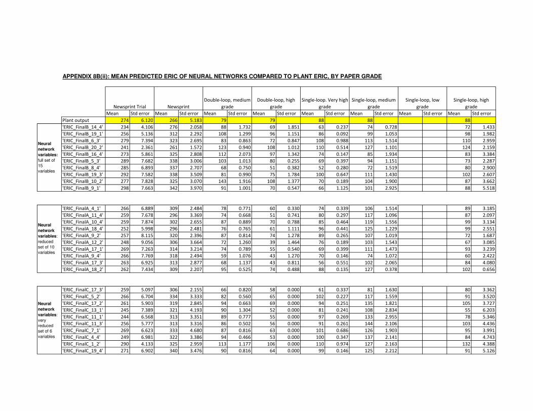
APPENDIX 8B(ii): MEAN PREDICTED ERIC OF NEURAL NETWORKS COMPARED TO PLANT ERIC, BY PAPER GRADE
Mean Std error Mean Std error Mean Std error Mean Std error Mean Std error Mean Std error Mean Std error Mean Std error
Plant output 274 6.120 266 5.183 79 79 88 88 88
'ERIC_FinalB_14_4' 234 4.106 276 2.058 88 1.732 69 1.851 63 0.237 74 0.728 72 1.433
'ERIC_FinalB_19_1' 256 5.136 312 2.292 108 1.299 96 1.151 86 0.092 99 1.053 98 1.982
'ERIC_FinalB_6_3' 279 7.394 323 2.695 83 0.863 72 0.847 108 0.988 113 1.514 110 2.959
'ERIC_FinalB_20_2' 241 2.361 261 1.572 123 0.940 108 1.012 110 0.514 127 1.101 124 2.159
'ERIC_FinalB_16_4' 273 5.861 325 2.808 112 2.073 97 1.342 74 0.147 85 1.934 83 3.384
'ERIC_FinalB_5_3' 289 7.682 338 3.006 103 1.013 80 0.255 69 0.397 94 1.151 73 2.287
'ERIC_FinalB_8_4' 285 6.893 337 2.707 68 0.750 51 0.382 52 0.280 72 1.519 80 2.900
'ERIC_FinalB_19_3' 292 7.582 338 3.509 81 0.990 75 1.784 100 0.647 111 1.430 102 2.607
'ERIC_FinalB_10_2' 277 7.828 325 3.070 143 1.916 108 1.377 70 0.189 104 1.900 87 3.662
'ERIC_FinalB_9_1' 298 7.663 342 3.970 91 1.001 70 0.547 66 1.125 101 2.925 88 5.518
Newsprint
Single-loop. Very high
grade
Single-loop, medium
grade
Single-loop, low
grade
Single-loop, high
grade
Double-loop, medium
grade
Double-loop, high
gradeNewsprint Trial
Neural
network
variables:
full set of
15
variables
'ERIC_FinalA_4_1' 266 6.889 309 2.484 78 0.771 60 0.330 74 0.339 106 1.514 89 3.185
'ERIC_FinalA_11_4' 259 7.678 296 3.369 74 0.668 51 0.741 80 0.297 117 1.096 87 2.097
'ERIC_FinalA_10_4' 259 7.874 302 2.655 87 0.889 70 0.788 85 0.464 119 1.556 99 3.134
'ERIC_FinalA_18_4' 252 5.998 296 2.481 76 0.765 61 1.111 96 0.441 125 1.229 99 2.551
'ERIC_FinalA_9_2' 257 8.115 320 2.396 87 0.814 74 1.278 89 0.265 107 1.019 72 1.687
'ERIC_FinalA_12_2' 248 9.056 306 3.664 72 1.260 39 1.464 76 0.189 103 1.543 67 3.085
'ERIC_FinalA_17_1' 269 7.263 314 3.214 74 0.789 55 0.540 69 0.399 111 1.473 93 3.239
'ERIC_FinalA_9_4' 266 7.769 318 2.494 59 1.076 43 1.270 70 0.146 74 1.072 60 2.422
'ERIC_FinalA_17_3' 263 6.925 313 2.877 68 1.137 43 0.811 56 0.551 102 2.065 84 4.080
'ERIC_FinalA_18_2' 262 7.434 309 2.207 95 0.525 74 0.488 88 0.135 127 0.378 102 0.656
'ERIC_FinalC_17_3' 259 5.097 306 2.155 66 0.820 58 0.000 61 0.337 81 1.630 80 3.362
'ERIC_FinalC_5_2' 266 6.704 334 3.333 82 0.560 65 0.000 102 0.227 117 1.559 91 3.520
'ERIC_FinalC_17_2' 261 5.903 319 2.845 94 0.663 69 0.000 94 0.251 135 1.821 105 3.727
'ERIC_FinalC_13_1' 245 7.389 321 4.193 90 1.304 52 0.000 81 0.241 108 2.834 55 6.203
'ERIC_FinalC_11_1' 244 6.568 313 3.351 89 0.777 55 0.000 97 0.269 133 2.955 78 5.346
'ERIC_FinalC_11_3' 256 5.777 313 3.316 86 0.502 56 0.000 91 0.261 144 2.106 103 4.436
'ERIC_FinalC_7_1' 269 6.623 333 4.680 87 0.816 63 0.000 101 0.686 126 1.903 95 3.991
'ERIC_FinalC_4_4' 249 6.981 322 3.386 94 0.466 53 0.000 100 0.347 137 2.141 84 4.743
'ERIC_FinalC_1_2' 290 4.133 325 2.959 113 1.177 106 0.000 110 0.974 127 2.163 132 4.388
'ERIC_FinalC_19_4' 271 6.902 340 3.476 90 0.816 64 0.000 99 0.146 125 2.212 91 5.126
Neural
network
variables:
reduced
set of 10
variables
Neural
network
variables:
very
reduced
set of 6
variables

APPENDIX 8C(i): PERFORMANCE OF NEURAL NETWORKS FOR THE PREDICTION OF YIELD
Name of Neural Net
No.
neurons
Training
performan
ce
Validation
performanc
e
Test
performa
nce
Training
R
Validation
R Test R Total R
Correlation
with plant
data
MSE
against
plant
data
'Yield_FinalA_11_1' 11 26943 3573 3285 0.783 0.846 0.782 0.791 0.453 87.5
'Yield_FinalA_14_4' 14 24554 6519 4390 0.797 0.771 0.547 0.779 0.444 90.7
'Yield_FinalA_3_4' 3 30480 7184 3653 0.744 0.690 0.772 0.739 0.380 94.0
'Yield_FinalA_9_1' 9 25319 4609 6421 0.792 0.856 0.327 0.774 0.423 94.9
'Yield_FinalA_5_4' 5 24966 5674 5063 0.799 0.736 0.691 0.777 0.371 95.7
'Yield_FinalA_6_2' 6 26203 6088 3670 0.782 0.772 0.749 0.775 0.428 95.9
'Yield_FinalA_3_1' 3 30137 6655 3919 0.734 0.813 0.723 0.743 0.319 96.4
'Yield_FinalA_12_1' 12 27022 5712 6167 0.782 0.743 0.466 0.754 0.329 96.5
'Yield_FinalA_2_2' 2 25293 5975 6053 0.768 0.814 0.704 0.767 0.360 100.6
'Yield_FinalA_6_4' 6 24405 6095 4742 0.810 0.664 0.648 0.780 0.264 104.8
Neural network
variables: reduced
set of 10 variables
'Yield_FinalB_4_3' 4 21063 10013 2786 0.825 0.598 0.816 0.790 0.425 101.2
'Yield_FinalB_13_3' 13 48607 7649 5085 0.702 0.358 0.753 0.678 0.069 110.8
'Yield_FinalB_19_3' 19 22223 6233 6470 0.804 0.785 0.705 0.782 0.176 111.1
'Yield_FinalB_10_3' 10 26201 3706 6708 0.783 0.851 0.545 0.770 0.137 117.8
'Yield_FinalB_9_3' 9 22060 4581 5142 0.813 0.839 0.724 0.806 0.094 118.2
'Yield_FinalB_5_3' 5 21572 4681 7077 0.823 0.814 0.585 0.794 0.171 119.4
'Yield_FinalB_3_4' 3 26578 4435 4418 0.777 0.837 0.697 0.779 -0.018 120.3
'Yield_FinalB_1_3' 1 55637 6198 7558 0.608 0.505 0.695 0.604 -0.109 121.8
'Yield_FinalB_7_4' 7 46277 9557 7444 0.647 0.473 0.776 0.642 -0.020 124.4
'Yield_FinalB_6_3' 6 22726 5532 5133 0.813 0.783 0.692 0.795 0.058 129.6
'Yield_FinalC_8_4' 8 25803 4523 6905 0.789 0.756 0.668 0.767 0.534 83.6
'Yield_FinalC_13_3' 13 27413 5106 5571 0.752 0.799 0.771 0.761 0.502 89.4
'Yield_FinalC_10_1' 10 29143 7695 2148 0.763 0.702 0.819 0.755 0.472 90.1
'Yield_FinalC_3_4' 3 29548 4624 2803 0.756 0.808 0.809 0.768 0.479 90.7
'Yield_FinalC_11_4' 11 28326 6167 2727 0.754 0.756 0.879 0.766 0.525 92.3
'Yield_FinalC_17_4' 17 28553 5014 3890 0.748 0.854 0.753 0.767 0.475 93.1
'Yield_FinalC_13_4' 13 26724 5973 3746 0.772 0.780 0.775 0.772 0.510 93.8
'Yield_FinalC_10_4' 10 27960 4694 3555 0.779 0.728 0.777 0.773 0.544 94.4
'Yield_FinalC_6_3' 6 23878 6189 5439 0.798 0.776 0.621 0.778 0.519 95.0
'Yield_FinalC_10_3' 10 25910 5723 6669 0.774 0.824 0.549 0.758 0.387 96.9
Notes: 1
Reduced set of 10
variables:
2Full set of 15 variables:
3
Very reduced set of 6
variables:
Neural network
variables: full set of
15 variables
Neural network
variables: very
reduced set of 6
variables
ONP,OMG, HL1, HL2, NaOH, Sodium silicate, hydrogen peroxide, flotation consistency, flotation pH and flotation
time
ONP,OMG, HL1, HL2, NaOH, sodium silicate, hydrogen peroxide, surfactant addition to pulper and float cell, pulping
time and pulping temperature, flotation time, flotation consistency, flotation temperature and flotation pH
ONP,OMG, HL1, HL2, flotation consistency, flotation time

APPENDIX 8C(ii): MEAN PREDICTED YIELD OF NEURAL NETWORKS COMPARED TO PLANT YIELD, BY PAPER GRADE
Mean Std error Mean Std error Mean Std error Mean Std error Mean Std error Mean Std error Mean Std error Mean Std error
Plant output 90 89 0.645 81 1.143 77 1.761 70 1.385 72 0.503 71 2.079 71 0.960
'Yield_FinalA_11_1' 83 0.341 85 0.217 80 0.157 82 0.115 85 0.111 76 0.139 65 0.805 81 0.452
'Yield_FinalA_14_4' 81 0.244 82 0.392 75 0.204 77 0.190 86 0.093 72 0.241 73 1.144 75 0.463
'Yield_FinalA_3_4' 78 0.310 81 0.322 76 0.169 78 0.128 82 0.034 74 0.266 72 0.998 77 0.549
'Yield_FinalA_9_1' 83 0.386 86 0.407 81 0.171 84 0.172 87 0.090 77 0.117 70 0.901 82 0.370
'Yield_FinalA_5_4' 81 0.339 84 0.427 80 0.135 83 0.109 86 0.076 77 0.115 69 0.945 82 0.380
'Yield_FinalA_6_2' 79 0.297 82 0.509 74 0.195 78 0.280 88 0.068 71 0.139 70 0.892 74 0.233
'Yield_FinalA_3_1' 79 0.209 81 0.105 79 0.136 81 0.124 84 0.086 76 0.121 68 0.699 80 0.367
'Yield_FinalA_12_1' 80 0.322 82 0.411 78 0.141 81 0.109 87 0.098 75 0.185 71 0.757 79 0.379
'Yield_FinalA_2_2' 77 0.288 80 0.369 75 0.151 79 0.118 87 0.040 72 0.196 70 0.810 75 0.406
'Yield_FinalA_6_4' 79 0.331 82 0.281 80 0.140 83 0.078 87 0.089 78 0.150 68 0.821 82 0.446
Neural network
variables:
reduced set of
10 variables
Single-loop, low
grade
Single-loop, high
grade
Double-loop,
medium gradeNewsprint Trial Newsprint
Single-loop, medium
grade
Double-loop, high
grade
Single-loop. Very
high grade
'Yield_FinalB_4_3' 77 0.410 81 0.417 82 0.141 87 0.135 90 0.133 69 0.184 68 0.938 70 0.340
'Yield_FinalB_13_3' 75 0.110 76 0.190 80 0.072 80 0.046 78 0.077 76 0.122 74 0.414 77 0.245
'Yield_FinalB_19_3' 75 0.287 78 0.478 80 0.107 84 0.056 83 0.102 75 0.194 69 0.870 79 0.471
'Yield_FinalB_10_3' 75 0.407 79 0.393 78 0.178 81 0.161 89 0.153 74 0.302 72 1.032 78 0.619
'Yield_FinalB_9_3' 77 0.319 80 0.459 82 0.077 87 0.071 84 0.077 78 0.138 71 0.834 82 0.401
'Yield_FinalB_5_3' 78 0.356 82 0.384 83 0.107 84 0.049 87 0.097 79 0.176 66 0.846 83 0.542
'Yield_FinalB_3_4' 76 0.254 80 0.365 77 0.181 80 0.179 84 0.079 78 0.271 76 0.812 81 0.553
'Yield_FinalB_1_3' 73 0.128 75 0.076 79 0.040 80 0.029 79 0.063 75 0.105 73 0.313 78 0.210
'Yield_FinalB_7_4' 75 0.247 78 0.331 84 0.101 86 0.111 80 0.115 78 0.141 75 0.457 81 0.294
'Yield_FinalB_6_3' 72 0.210 75 0.394 79 0.101 84 0.059 82 0.062 73 0.127 68 0.903 78 0.360
'Yield_FinalC_8_4' 87 0.246 89 0.369 78 0.048 76 0.000 85 0.016 78 0.098 75 1.045 77 0.131
'Yield_FinalC_13_3' 86 0.283 88 0.351 79 0.066 80 0.000 87 0.030 78 0.130 77 0.877 79 0.229
'Yield_FinalC_10_1' 85 0.246 87 0.345 79 0.069 81 0.000 86 0.028 77 0.145 77 0.916 80 0.239
'Yield_FinalC_3_4' 87 0.217 88 0.372 78 0.065 79 0.000 89 0.043 77 0.129 76 1.058 79 0.201
'Yield_FinalC_11_4' 87 0.310 90 0.439 80 0.043 81 0.000 86 0.012 78 0.096 76 0.974 80 0.139
'Yield_FinalC_17_4' 86 0.286 88 0.342 79 0.091 80 0.000 88 0.070 78 0.170 76 0.974 81 0.339
'Yield_FinalC_13_4' 88 0.257 90 0.373 79 0.017 79 0.000 90 0.055 78 0.043 76 0.812 79 0.134
'Yield_FinalC_10_4' 90 0.298 91 0.449 80 0.039 80 0.000 88 0.028 79 0.083 75 0.938 79 0.133
'Yield_FinalC_6_3' 87 0.276 89 0.294 80 0.053 81 0.000 88 0.082 79 0.125 76 0.922 80 0.209
'Yield_FinalC_10_3' 83 0.289 86 0.338 79 0.111 81 0.000 89 0.037 77 0.218 77 0.820 80 0.444
Neural network
variables: full set
of 15 variables
Neural network
variables: very
reduced set of 6
variables

i
APPENDIX 9: MATLAB CODE
%A GENERAL PROGRAM FOR TRAINING NETWORKS AND SIMULTANEOUS PLANT
VALIDATION load DATA %load training data %create training data files inputs = [DATA(1:4,:); DATA(12,:) ; DATA(15,:)]; %create training target file targets = DATA(21,:);%brightness
%load Plantdata %load plant data files PlantInput = [Plantdata(:,1:4) Plantdata(:,12)
Plantdata(:,16)]';%inputs for brightness PlantOutput = Plantdata(:,23)';% brightness
n = 1 %order number in data base Headings = {'n', 'date', 'filename',
'Neurons','Train_perf','Val_perf','Test_perf','Train R', 'Validation
R', 'Test R', 'Total R','Plant R','Plant mse','Comments'}; %DEFINE THE NETWORK comments = 'input: traininputs:1-4, 12, 15; using DATA 22x490 , BTF =
trainbr, msereg '; for Si = 11:20; %size of ith layer, number of hidden
neurons for m = 1:4; %number of iterations for Si
filename = 'ERIC_FinalC'; %File name to save Filename = [filename '_' int2str(Si) '_' int2str(m)];
TF1 = 'tansig'; %Transfer function of ith layer, default tansig TF2 = 'purelin'; % default purelin %BTF = 'trainlm'; %Training function, default trainlm BTF = 'trainbr'; BLF = 'learngdm'; %Learning function, default learngdm %PF = 'mse'; %Performance function PF = 'trainbr'; %PF = 'msereg'; %net.performParam.ratio = 0.5; IPF = {'fixunknowns', 'removeconstantrows', 'mapminmax'}; %input
processing functions OPF = {'mapminmax'}; %Output processing functions DDF = 'dividerand' ; %Data division function
%NETWORK net = newff(inputs,targets,[Si],{TF1,TF2},BTF, BLF,PF,IPF,OPF, DDF);
%SET TRAINING PARAMETERS net.divideParam.trainRatio = 75/100; % Adjust as desired net.divideParam.valRatio = 15/100; % Adjust as desired net.divideParam.testRatio = 10/100; % Adjust as desired net.trainParam.epochs = 100;

ii
net.trainparam.max_fail = 7 % Train and Apply Network %net = init(net) [net,tr] = train(net, inputs, targets); outputs = sim(net,inputs);
save(Filename,'net','Si','tr');
%Create data base a = 1 + getfield(tr,'best_epoch'); A = getfield(tr, 'perf'); B = getfield(tr, 'vperf'); C = getfield(tr,'tperf'); Train_perf = A(1,a); Val_perf = B(1,a); Test_perf = C(1,a);
ti = getfield(tr,'trainInd'); vi = getfield(tr,'valInd'); testi = getfield(tr,'testInd');
tr_cor = corrcoef(outputs(ti),targets(1,ti)); val_cor = corrcoef(outputs(vi),targets(1,vi)); test_cor = corrcoef(outputs(testi),targets(1,testi)); tot_cor = corrcoef(outputs, targets); TrainR = tr_cor(1,2); ValidationR = val_cor(1,2); TestR = test_cor(1,2); TotalR = tot_cor(1,2);
% Test network against Plant data set val = sim(net, PlantInput); PredictValues(n,:) = val; mse = mean((val-PlantOutput).^2); R = corrcoef(val, PlantOutput); correlation = R(1,2); %ResultsNetwork(n,:) = {Filename}; %ResultNumbers(n,:) = {correlation mse}; plotregression(PlantOutput ,val,'o') xlabel('Plant values') ylabel('Output predictions')
%Save data to data base Training_Data(n,:) = {n, date, Filename,
Si,Train_perf,Val_perf,Test_perf,TrainR, ValidationR, TestR, TotalR,
correlation, mse,comments }; n = n+1 end end save Training_Data save PredictValues

iii
%Function to input and create a 3D plot of Brightness vs. two
variables % load the required network load Yield_FinalB_6_3 upperlimit = [100;100;100;100;1.5;3;2;1.0;15;50;45;1.5;10;0.5;12]; lowerlimit = [0;0;0;0;0;0;0;0.25;5;35;30;0.8;7;0;2]; lables = {'ONP'; 'OMG'; 'HL1' ;'HL2'; '%NaOH'; '%Sod Silicate'
;'%H2O2'; '%Surf-p'; 'tp (min)' ;'Tp (deg C)';' Tf (deg C)'; '%cons';
'pH'; '%Surf-f' ;' tf (min)'}; for n=1:7 Scenario = SCENARIO(:,n);
row_m = 5;%Define 1st parameter to be varied row_n = 7;%Define 2nd parameter to be varied [new, X, Y] = geninput(Scenario, row_m, lowerlimit(row_m),
upperlimit(row_m), row_n, lowerlimit(row_n), upperlimit(row_n)); outputs = sim(net, new); subplot(2,2,1); bivariate_mesh(reshape(outputs(1,:), 10, 10)',X,Y) xlabel(lables(row_m)) ylabel(lables(row_n)) title('Yield','FontSize',16)
row_m = 6;%Define 3rd parameter to be varied row_n = 13;%Define 4th parameter to be varied [new, X, Y] = geninput(Scenario, row_m, lowerlimit(row_m),
upperlimit(row_m), row_n, lowerlimit(row_n), upperlimit(row_n)); outputs = sim(net, new); subplot(2,2,2); bivariate_mesh(reshape(outputs(1,:), 10, 10)',X,Y) xlabel(lables(row_m)) ylabel(lables(row_n)) title('Yield','FontSize',16)
row_m = 12;%Define 5th parameter to be varied row_n = 15;%Define 6th parameter to be varied [new, X, Y] = geninput(Scenario, row_m, lowerlimit(row_m),
upperlimit(row_m), row_n, lowerlimit(row_n), upperlimit(row_n)); outputs = sim(net, new); subplot(2,2,3); bivariate_mesh(reshape(outputs(1,:), 10, 10)',X,Y) xlabel(lables(row_m)) ylabel(lables(row_n)) title('Yield','FontSize',16)
subplot(2,2,4); bar(Scenario(1:4)) title('Grade mix', 'Fontsize', 16) set(gca,'xTickLabel',{'ONP';'OMG';'HL1';'HL2'}) xlabel('Grade') ylabel('%') pause end
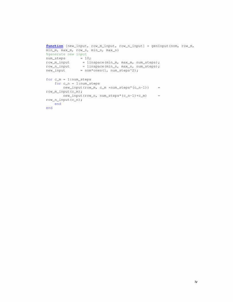
iv
function [new_input, row_m_input, row_n_input] = geninput(nom, row_m,
min_m, max_m, row_n, min_n, max_n) %generate new input num_steps = 10; row_m_input = linspace(min_m, max_m, num_steps); row_n_input = linspace(min_n, max_n, num_steps); new_input = nom*ones(1, num_steps^2);
for c_m = 1:num_steps for c_n = 1:num_steps new_input(row_m, c_m +num_steps*(c_n-1)) =
row_m_input(c_m); new_input(row_n, num_steps*(c_n-1)+c_m) =
row_n_input(c_n); end end

i
APPENDIX 10: NEURAL NETWORK STRUCTURES
'Bright_FinalA_20_2'
Neural Network object:
architecture:
numInputs: 1
numLayers: 2
biasConnect: [1; 1]
inputConnect: [1; 0]
layerConnect: [0 0; 1 0]
outputConnect: [0 1]
numOutputs: 1 (read-only)
numInputDelays: 0 (read-only)
numLayerDelays: 0 (read-only)
subobject structures:
inputs: {1x1 cell} of inputs
layers: {2x1 cell} of layers
outputs: {1x2 cell} containing 1 output
biases: {2x1 cell} containing 2 biases
inputWeights: {2x1 cell} containing 1 input weight
layerWeights: {2x2 cell} containing 1 layer weight
functions:
adaptFcn: 'trains'
divideFcn: 'dividerand'
gradientFcn: 'calcjx'
initFcn: 'initlay'
performFcn: 'sse'
plotFcns: {'plotperform','plottrainstate','plotregression'}
trainFcn: 'trainbr'
parameters:
adaptParam: .passes
divideParam: .trainRatio, .valRatio, .testRatio
gradientParam: (none)
initParam: (none)
performParam: .show, .showWindow, .showCommandLine, .epochs,
.time, .goal, .max_fail, .mem_reduc,
.min_grad, .mu, .mu_dec, .mu_inc,
.mu_max
trainParam: .show, .showWindow, .showCommandLine, .epochs,

ii
.time, .goal, .max_fail, .mem_reduc,
.min_grad, .mu, .mu_dec, .mu_inc,
.mu_max
weight and bias values:
IW: {2x1 cell} containing 1 input weight matrix
Columns 1 through 9
-0.0250 0.0488 -0.0038 -0.0900 -0.0019 0.0224 -0.0053 -0.0494 -0.0075
0.0021 0.1598 0.0613 -0.2002 0.0377 0.0308 0.0802 -0.0404 -0.0442
0.0162 -0.0143 -0.0109 0.0280 -0.0011 -0.0062 0.0009 0.0118 0.0024
-0.0188 0.0183 0.0116 -0.0347 0.0012 0.0078 -0.0010 -0.0149 -0.0030
0.0205 -0.0192 -0.0138 0.0356 -0.0016 -0.0083 0.0007 0.0158 0.0031
-0.0294 0.0890 0.0510 -0.0933 0.0187 0.0216 0.0346 -0.0249 -0.0153
-0.0255 0.0611 -0.0014 -0.1025 0.0006 0.0272 0.0026 -0.0565 -0.0102
-0.0246 0.0520 -0.0101 -0.1006 -0.0042 0.0256 -0.0087 -0.0596 -0.0079
-0.0246 0.0469 -0.0028 -0.0865 -0.0016 0.0212 -0.0053 -0.0463 -0.0072
-0.0108 0.1412 0.0751 -0.1631 0.0346 0.0231 0.0662 -0.0241 -0.0349
-0.0117 -0.0068 0.0214 0.0089 0.0013 -0.0006 0.0018 0.0006 0.0004
0.0186 -0.0193 -0.0106 0.0364 -0.0011 -0.0081 0.0013 0.0155 0.0031
-0.1652 0.0415 0.6690 0.2176 0.0834 -0.0325 0.0769 -0.0230 -0.0466
0.0297 -0.0770 -0.0374 0.0859 -0.0145 -0.0233 -0.0266 0.0307 0.0127
-0.0270 0.1545 0.2070 -0.1600 0.0418 -0.0169 0.0569 0.0121 -0.0299
-0.3455 -0.1715 0.5286 0.7436 -0.0793 0.0713 -0.0940 0.0369 0.0915
-0.0105 0.0015 0.0132 -0.0049 0.0010 0.0017 0.0005 -0.0034 -0.0006
0.0266 -0.0588 -0.0052 0.0935 -0.0026 -0.0248 -0.0049 0.0485 0.0098
-0.0563 0.1875 0.4289 -0.1783 0.0578 -0.0736 0.0494 0.0085 -0.0327
-0.0060 0.0031 0.0057 -0.0068 0.0004 0.0016 -0.0001 -0.0031 -0.0006
Column 10
0.0393
0.0346
-0.0104
0.0129
-0.0141
0.0300
0.0467
0.0472
0.0368
0.0271
0.0037
-0.0132
0.0596
-0.0322
0.0299
0.0247
0.0049
-0.0410

iii
0.0696
0.0031
LW: {2x2 cell} containing 1 layer weight matrix
Columns 1 through 9
0.1066 0.1946 -0.0312 0.0390 -0.0402 0.0988 0.1200 0.1212 0.1022
Columns 10 through 18
0.1582 -0.0101 -0.0410 0.4521 -0.0934 0.1353 0.5689 0.0054 -0.1085
Columns 19 through 20
0.2206 0.0075
b: {2x1 cell} containing 2 bias vectors
0.0379
-0.0060
-0.0104
0.0129
-0.0127
-0.0051
0.0376
0.0450
0.0364
-0.0163
-0.0062
-0.0138
-0.3707
-0.0040
-0.0819
-0.3662
0.0005
-0.0312
-0.1831
0.0023

iv
'Bright_FinalB_16_2'
Neural Network object:
architecture:
numInputs: 1
numLayers: 2
biasConnect: [1; 1]
inputConnect: [1; 0]
layerConnect: [0 0; 1 0]
outputConnect: [0 1]
numOutputs: 1 (read-only)
numInputDelays: 0 (read-only)
numLayerDelays: 0 (read-only)
subobject structures:
inputs: {1x1 cell} of inputs
layers: {2x1 cell} of layers
outputs: {1x2 cell} containing 1 output
biases: {2x1 cell} containing 2 biases
inputWeights: {2x1 cell} containing 1 input weight
layerWeights: {2x2 cell} containing 1 layer weight
functions:
adaptFcn: 'trains'
divideFcn: 'dividerand'
gradientFcn: 'calcjx'
initFcn: 'initlay'
performFcn: 'sse'
plotFcns: {'plotperform','plottrainstate','plotregression'}
trainFcn: 'trainbr'
parameters:
adaptParam: .passes
divideParam: .trainRatio, .valRatio, .testRatio
gradientParam: (none)
initParam: (none)
performParam: .show, .showWindow, .showCommandLine, .epochs,
.time, .goal, .max_fail, .mem_reduc,
.min_grad, .mu, .mu_dec, .mu_inc,
.mu_max
trainParam: .show, .showWindow, .showCommandLine, .epochs,
.time, .goal, .max_fail, .mem_reduc,
.min_grad, .mu, .mu_dec, .mu_inc,
.mu_max

v
weight and bias values:
IW: {2x1 cell} containing 1 input weight matrix
Columns 1 through 9
-0.0058 -0.0311 -0.0079 0.0070 0.0003 -0.0080 -0.0029 -0.0024 0.0083
0.0047 0.0212 0.0047 -0.0046 -0.0002 0.0054 0.0019 0.0018 -0.0056
0.0067 0.0537 0.0185 -0.0145 -0.0003 0.0139 0.0066 0.0033 -0.0162
0.0052 0.0257 0.0061 -0.0057 -0.0002 0.0066 0.0023 0.0021 -0.0068
0.0140 0.0958 0.0132 -0.0560 -0.0111 0.0343 -0.0105 -0.0123 -0.0438
0.2158 0.1677 -0.6162 -0.5592 0.0601 -0.0046 -0.0087 0.0468 -0.0949
-0.0070 -0.0526 -0.0171 0.0142 0.0004 -0.0138 -0.0059 -0.0031 0.0157
0.1778 -0.0206 -0.5384 -0.5647 -0.0106 0.0811 -0.0513 0.0918 -0.0098
0.0430 0.1507 0.0553 -0.1191 -0.0034 0.0454 -0.0085 -0.0038 -0.0615
-0.0761 -0.2005 -0.1958 0.1641 -0.0256 -0.0198 -0.0095 -0.0289 0.0257
-0.0063 -0.0205 -0.0024 0.0046 0.0006 -0.0049 -0.0011 -0.0018 0.0054
-0.1209 -0.3335 -0.4685 0.1696 -0.1364 -0.0079 -0.0981 -0.0378 -0.0200
0.0999 0.2314 0.1596 -0.1940 0.0335 0.0273 0.0283 0.0509 -0.0112
-0.0137 -0.0875 -0.0194 0.0404 0.0058 -0.0263 -0.0001 0.0025 0.0325
0.0073 0.0288 0.0051 -0.0066 -0.0006 0.0071 0.0018 0.0023 -0.0075
0.0505 0.1585 0.0825 -0.1095 0.0078 0.0299 0.0160 0.0196 -0.0336
Columns 10 through 15
-0.0102 0.0009 0.0133 0.0049 0.0107 -0.0049
0.0072 -0.0007 -0.0088 -0.0032 -0.0077 0.0026
0.0161 -0.0019 -0.0220 -0.0088 -0.0144 0.0112
0.0086 -0.0008 -0.0108 -0.0040 -0.0091 0.0036
0.0386 -0.0101 -0.0735 -0.0100 -0.0534 0.0533
0.0115 0.0575 -0.0469 0.0199 -0.0062 0.0247
-0.0160 0.0018 0.0222 0.0086 0.0150 -0.0111
-0.0642 -0.0346 0.0146 0.0257 -0.0428 -0.0597
0.0259 -0.0069 -0.0900 -0.0163 -0.0380 0.0798
0.0170 -0.0480 0.0065 0.0080 -0.0300 -0.0467
-0.0073 0.0007 0.0087 0.0029 0.0089 -0.0016
0.0323 0.0069 0.0138 -0.0516 -0.0242 -0.0276
-0.0426 0.0411 -0.0321 -0.0346 0.0269 0.0465
-0.0283 0.0050 0.0501 0.0119 0.0358 -0.0326
0.0098 -0.0008 -0.0124 -0.0043 -0.0114 0.0036
0.0034 0.0132 -0.0434 -0.0239 -0.0065 0.0378
LW: {2x2 cell} containing 1 layer weight matrix
Columns 1 through 9
-0.0408 0.0278 0.0697 0.0337 0.1551 -0.5549 -0.0687 -0.5343 0.2191
Columns 10 through 16
-0.2291 -0.0273 -0.3250 0.2564 -0.1258 0.0380 0.1930

vi
b: {2x1 cell} containing 2 bias vectors
0.0212
0.0146
0.0347
0.0176
0.0992
0.1171
-0.0347
0.1832
0.1137
-0.0085
-0.0149
0.1599
0.0314
-0.0735
0.0204
0.0711

vii
'ERIC_FinalB_14_4'
Neural Network object:
architecture:
numInputs: 1
numLayers: 2
biasConnect: [1; 1]
inputConnect: [1; 0]
layerConnect: [0 0; 1 0]
outputConnect: [0 1]
numOutputs: 1 (read-only)
numInputDelays: 0 (read-only)
numLayerDelays: 0 (read-only)
subobject structures:
inputs: {1x1 cell} of inputs
layers: {2x1 cell} of layers
outputs: {1x2 cell} containing 1 output
biases: {2x1 cell} containing 2 biases
inputWeights: {2x1 cell} containing 1 input weight
layerWeights: {2x2 cell} containing 1 layer weight
functions:
adaptFcn: 'trains'
divideFcn: 'dividerand'
gradientFcn: 'calcjx'
initFcn: 'initlay'
performFcn: 'sse'
plotFcns: {'plotperform','plottrainstate','plotregression'}
trainFcn: 'trainbr'
parameters:
adaptParam: .passes
divideParam: .trainRatio, .valRatio, .testRatio
gradientParam: (none)
initParam: (none)
performParam: .show, .showWindow, .showCommandLine, .epochs,
.time, .goal, .max_fail, .mem_reduc,
.min_grad, .mu, .mu_dec, .mu_inc,
.mu_max
trainParam: .show, .showWindow, .showCommandLine, .epochs,
.time, .goal, .max_fail, .mem_reduc,
.min_grad, .mu, .mu_dec, .mu_inc,
.mu_max
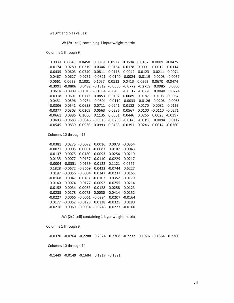
viii
weight and bias values:
IW: {2x1 cell} containing 1 input weight matrix
Columns 1 through 9
0.0039 0.0840 0.0450 0.0819 0.0527 0.0504 0.0187 0.0009 -0.0475
-0.0174 0.0280 0.0319 0.0346 0.0154 0.0128 0.0091 0.0012 -0.0114
-0.0435 0.0603 0.0740 0.0811 0.0118 -0.0042 0.0123 -0.0211 0.0074
0.0467 -0.0627 -0.0751 -0.0821 -0.0140 0.0024 -0.0119 0.0208 -0.0057
0.0661 0.0629 0.1031 0.1037 0.0513 0.0413 0.0362 0.0670 -0.0474
-0.3991 -0.0806 0.0482 -0.1819 -0.0530 -0.0772 -0.2759 0.0985 0.0805
0.0614 -0.0909 -0.1015 -0.1084 -0.0438 -0.0317 -0.0228 0.0040 0.0274
-0.0318 0.0601 0.0772 0.0853 0.0192 0.0089 0.0187 -0.0103 -0.0067
0.0431 -0.0596 -0.0734 -0.0804 -0.0119 0.0033 -0.0126 0.0206 -0.0065
-0.0306 0.0541 0.0658 0.0711 0.0241 0.0182 0.0170 -0.0031 -0.0165
-0.0377 0.0303 0.0209 0.0563 0.0286 0.0567 0.0100 -0.0110 -0.0271
-0.0661 0.0996 0.1066 0.1135 0.0551 0.0446 0.0266 0.0023 -0.0397
0.0403 -0.0683 -0.0846 -0.0918 -0.0250 -0.0143 -0.0196 0.0094 0.0117
-0.0545 0.0839 0.0936 0.0993 0.0463 0.0391 0.0246 0.0014 -0.0360
Columns 10 through 15
-0.0381 0.0275 -0.0072 0.0016 0.0073 -0.0354
-0.0071 0.0005 0.0001 -0.0087 0.0107 -0.0043
-0.0137 0.0075 0.0180 -0.0093 0.0254 -0.0219
0.0135 -0.0077 -0.0157 0.0110 -0.0229 0.0217
-0.0004 -0.0351 0.0139 0.0122 0.1121 0.0567
0.1828 -0.0672 -0.2669 0.0423 -0.0744 0.6227
0.0197 -0.0056 -0.0004 0.0247 -0.0237 0.0165
-0.0168 0.0047 0.0167 -0.0102 0.0352 -0.0179
0.0140 -0.0074 -0.0177 0.0092 -0.0255 0.0214
-0.0152 0.0034 0.0062 -0.0128 0.0258 -0.0123
-0.0235 0.0178 0.0073 0.0030 -0.0414 -0.0152
-0.0227 0.0066 -0.0061 -0.0294 0.0207 -0.0164
0.0177 -0.0052 -0.0128 0.0138 -0.0325 0.0180
-0.0216 0.0069 -0.0034 -0.0248 0.0223 -0.0160
LW: {2x2 cell} containing 1 layer weight matrix
Columns 1 through 9
-0.0370 -0.0764 -0.2288 0.2324 0.2708 -0.7232 0.1976 -0.1864 0.2260
Columns 10 through 14
-0.1449 -0.0149 -0.1684 0.1917 -0.1391

ix
b: {2x1 cell} containing 2 bias vectors
0.1307
0.0047
0.1182
-0.1226
-0.4445
0.7752
-0.0686
0.0513
-0.1153
0.0256
0.1185
0.0582
-0.0579
0.0444
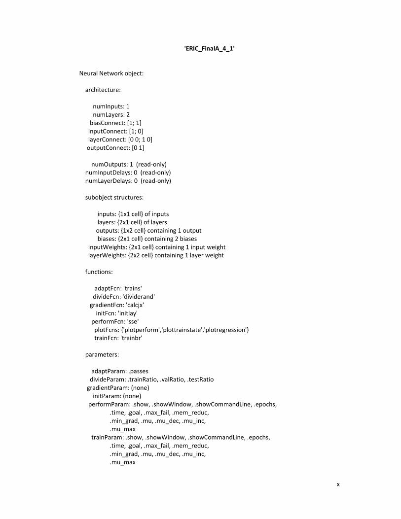
x
'ERIC_FinalA_4_1'
Neural Network object:
architecture:
numInputs: 1
numLayers: 2
biasConnect: [1; 1]
inputConnect: [1; 0]
layerConnect: [0 0; 1 0]
outputConnect: [0 1]
numOutputs: 1 (read-only)
numInputDelays: 0 (read-only)
numLayerDelays: 0 (read-only)
subobject structures:
inputs: {1x1 cell} of inputs
layers: {2x1 cell} of layers
outputs: {1x2 cell} containing 1 output
biases: {2x1 cell} containing 2 biases
inputWeights: {2x1 cell} containing 1 input weight
layerWeights: {2x2 cell} containing 1 layer weight
functions:
adaptFcn: 'trains'
divideFcn: 'dividerand'
gradientFcn: 'calcjx'
initFcn: 'initlay'
performFcn: 'sse'
plotFcns: {'plotperform','plottrainstate','plotregression'}
trainFcn: 'trainbr'
parameters:
adaptParam: .passes
divideParam: .trainRatio, .valRatio, .testRatio
gradientParam: (none)
initParam: (none)
performParam: .show, .showWindow, .showCommandLine, .epochs,
.time, .goal, .max_fail, .mem_reduc,
.min_grad, .mu, .mu_dec, .mu_inc,
.mu_max
trainParam: .show, .showWindow, .showCommandLine, .epochs,
.time, .goal, .max_fail, .mem_reduc,
.min_grad, .mu, .mu_dec, .mu_inc,
.mu_max

xi
weight and bias values:
IW: {2x1 cell} containing 1 input weight matrix
Columns 1 through 9
0.2497 0.2771 0.2173 0.0967 0.0102 -0.1094 -0.0321 -0.0195 0.1303
0.0897 -0.0900 0.4865 0.8039 -0.2196 -0.0958 0.1313 0.0442 0.0226
0.8783 0.0195 -0.0404 0.2472 -0.1842 0.0048 0.2854 0.3217 -0.0486
-0.1342 0.3925 -0.0319 -0.3051 0.2308 0.2135 -0.0692 -0.0104 -0.1973
Column 10
0.1087
0.0228
-1.0689
-0.1635
LW: {2x2 cell} containing 1 layer weight matrix
-0.4833 -0.7142 1.1648 -0.5553
b: {2x1 cell} containing 2 bias vectors
0.1145
-0.1195
-1.6169
0.4884

xii
'ERIC_FinalC_17_3'
Neural Network object:
architecture:
numInputs: 1
numLayers: 2
biasConnect: [1; 1]
inputConnect: [1; 0]
layerConnect: [0 0; 1 0]
outputConnect: [0 1]
numOutputs: 1 (read-only)
numInputDelays: 0 (read-only)
numLayerDelays: 0 (read-only)
subobject structures:
inputs: {1x1 cell} of inputs
layers: {2x1 cell} of layers
outputs: {1x2 cell} containing 1 output
biases: {2x1 cell} containing 2 biases
inputWeights: {2x1 cell} containing 1 input weight
layerWeights: {2x2 cell} containing 1 layer weight
functions:
adaptFcn: 'trains'
divideFcn: 'dividerand'
gradientFcn: 'calcjx'
initFcn: 'initlay'
performFcn: 'sse'
plotFcns: {'plotperform','plottrainstate','plotregression'}
trainFcn: 'trainbr'
parameters:
adaptParam: .passes
divideParam: .trainRatio, .valRatio, .testRatio
gradientParam: (none)
initParam: (none)
performParam: .show, .showWindow, .showCommandLine, .epochs,
.time, .goal, .max_fail, .mem_reduc,
.min_grad, .mu, .mu_dec, .mu_inc,
.mu_max
trainParam: .show, .showWindow, .showCommandLine, .epochs,
.time, .goal, .max_fail, .mem_reduc,
.min_grad, .mu, .mu_dec, .mu_inc,
.mu_max

xiii
weight and bias values:
IW: {2x1 cell} containing 1 input weight matrix
-0.0374 0.0171 0.0448 0.0593 0.0096 0.0065
0.0758 -0.0239 -0.0830 -0.1091 -0.0064 -0.0161
0.0469 -0.0096 -0.0476 -0.0620 0.0023 -0.0113
-0.0631 0.0801 0.0870 0.1093 0.0730 -0.0279
0.0412 -0.0295 -0.0568 -0.0755 -0.0227 -0.0039
0.0173 0.0131 -0.0077 -0.0070 0.0182 -0.0081
-0.0114 -0.0181 -0.0003 -0.0040 -0.0215 0.0076
0.0419 0.0019 -0.0346 -0.0428 0.0166 -0.0130
-0.0264 0.0234 0.0384 0.0520 0.0183 0.0016
0.0149 -0.0397 -0.0370 -0.0518 -0.0338 0.0049
-0.0152 0.0304 0.0318 0.0448 0.0269 -0.0034
-0.0316 0.0020 0.0296 0.0377 -0.0060 0.0087
-0.0245 0.0056 0.0257 0.0334 0.0001 0.0057
-0.0076 0.0127 0.0143 0.0203 0.0109 -0.0009
0.0239 -0.1110 -0.0772 -0.1085 -0.1019 0.0425
-0.5831 -0.0448 0.0843 -0.1174 -0.3470 0.3439
0.0470 -0.0084 -0.0466 -0.0605 0.0044 -0.0119
LW: {2x2 cell} containing 1 layer weight matrix
Columns 1 through 9
-0.0798 0.1396 0.0816 -0.1801 0.1033 0.0100 0.0047 0.0569 -0.0712
Columns 10 through 17
0.0722 -0.0618 -0.0504 -0.0450 -0.0276 0.1856 -0.6564 0.0794
b: {2x1 cell} containing 2 bias vectors
0.0416
-0.0851
-0.0533
0.1731
-0.0451
-0.0233
0.0176
-0.0491
0.0274
-0.0095
0.0124
0.0369
0.0280
0.0065
-0.0974
0.7180
-0.0534

xiv
'Yield_FinalA_11_1'
Neural Network object:
architecture:
numInputs: 1
numLayers: 2
biasConnect: [1; 1]
inputConnect: [1; 0]
layerConnect: [0 0; 1 0]
outputConnect: [0 1]
numOutputs: 1 (read-only)
numInputDelays: 0 (read-only)
numLayerDelays: 0 (read-only)
subobject structures:
inputs: {1x1 cell} of inputs
layers: {2x1 cell} of layers
outputs: {1x2 cell} containing 1 output
biases: {2x1 cell} containing 2 biases
inputWeights: {2x1 cell} containing 1 input weight
layerWeights: {2x2 cell} containing 1 layer weight
functions:
adaptFcn: 'trains'
divideFcn: 'dividerand'
gradientFcn: 'calcjx'
initFcn: 'initlay'
performFcn: 'sse'
plotFcns: {'plotperform','plottrainstate','plotregression'}
trainFcn: 'trainbr'
parameters:
adaptParam: .passes
divideParam: .trainRatio, .valRatio, .testRatio
gradientParam: (none)
initParam: (none)
performParam: .show, .showWindow, .showCommandLine, .epochs,
.time, .goal, .max_fail, .mem_reduc,
.min_grad, .mu, .mu_dec, .mu_inc,
.mu_max
trainParam: .show, .showWindow, .showCommandLine, .epochs,
.time, .goal, .max_fail, .mem_reduc,
.min_grad, .mu, .mu_dec, .mu_inc,
.mu_max

xv
weight and bias values:
IW: {2x1 cell} containing 1 input weight matrix
Columns 1 through 9
-0.0582 -0.0799 -0.0315 0.0267 -0.0241 -0.0012 -0.0153 0.1022 -0.0157
-0.0596 -0.1203 -0.0604 0.0314 -0.0303 -0.0039 0.0128 0.1620 -0.0172
-0.9807 -0.1439 0.3436 -0.0428 -0.0840 0.0278 -0.1158 -0.1761 0.0827
0.0587 0.0824 0.0328 -0.0274 0.0245 0.0009 0.0144 -0.1055 0.0158
-0.2950 0.2282 -0.6254 -0.3317 -0.1442 -0.0050 0.1590 -0.1163 -0.1653
0.3261 -0.5544 -0.1209 0.0542 0.1787 0.0570 -0.0464 0.3635 0.1368
-0.0565 -0.1304 -0.0735 0.0275 -0.0292 -0.0089 0.0339 0.1834 -0.0189
-0.1018 -0.0341 -0.1845 -0.0951 -0.1869 -0.0519 -0.1268 -0.0532 -0.0304
-0.0500 -0.1502 -0.1055 0.0160 -0.0255 -0.0255 0.0950 0.2448 -0.0286
-0.5439 -0.3465 0.3772 0.2257 0.1954 0.2210 0.1178 0.0183 0.2559
0.1156 0.0171 0.2358 0.1203 0.2312 0.0654 0.1505 0.0993 0.0447
Column 10
0.0017
-0.0075
0.3667
-0.0017
-0.2917
0.2852
-0.0178
0.1133
-0.0496
-0.1484
-0.1509
LW: {2x2 cell} containing 1 layer weight matrix
Columns 1 through 9
0.1606 0.2421 -0.9673 -0.1653 -0.5965 -0.4603 0.2691 0.2928 0.3360
Columns 10 through 11
0.8000 -0.3565
b: {2x1 cell} containing 2 bias vectors
0.0721
0.1056
0.4108
-0.0740
0.5121
0.1466
0.1177
0.2090
0.1462
0.1454
-0.2457

xvi
'Yield_FinalB_4_3'
Neural Network object:
architecture:
numInputs: 1
numLayers: 2
biasConnect: [1; 1]
inputConnect: [1; 0]
layerConnect: [0 0; 1 0]
outputConnect: [0 1]
numOutputs: 1 (read-only)
numInputDelays: 0 (read-only)
numLayerDelays: 0 (read-only)
subobject structures:
inputs: {1x1 cell} of inputs
layers: {2x1 cell} of layers
outputs: {1x2 cell} containing 1 output
biases: {2x1 cell} containing 2 biases
inputWeights: {2x1 cell} containing 1 input weight
layerWeights: {2x2 cell} containing 1 layer weight
functions:
adaptFcn: 'trains'
divideFcn: 'dividerand'
gradientFcn: 'calcjx'
initFcn: 'initlay'
performFcn: 'sse'
plotFcns: {'plotperform','plottrainstate','plotregression'}
trainFcn: 'trainbr'
parameters:
adaptParam: .passes
divideParam: .trainRatio, .valRatio, .testRatio
gradientParam: (none)
initParam: (none)
performParam: .show, .showWindow, .showCommandLine, .epochs,
.time, .goal, .max_fail, .mem_reduc,
.min_grad, .mu, .mu_dec, .mu_inc,
.mu_max
trainParam: .show, .showWindow, .showCommandLine, .epochs,
.time, .goal, .max_fail, .mem_reduc,
.min_grad, .mu, .mu_dec, .mu_inc,
.mu_max

xvii
weight and bias values:
IW: {2x1 cell} containing 1 input weight matrix
Columns 1 through 9
0.6509 -0.0755 -0.8161 0.6953 0.2249 -0.0567 -0.0110 0.0374 -0.1010
0.3205 -0.3754 -0.3956 0.3032 0.2333 -0.2098 -0.1001 0.1490 0.0670
0.3801 0.5514 -0.0720 0.0219 0.0732 -0.2240 0.0054 0.1467 0.0323
0.1990 -0.1735 0.1862 -0.0897 0.0736 -0.3204 -0.0323 0.3248 0.2343
Columns 10 through 15
0.0614 0.0198 0.0920 -0.0892 -0.0223 -0.1286
-0.0143 0.3412 0.1748 -0.0020 0.2645 0.2142
-0.0144 -0.0490 -0.2254 -0.1658 -0.0215 0.0857
-0.1208 0.2963 0.2220 0.0882 0.2359 -0.0505
LW: {2x2 cell} containing 1 layer weight matrix
0.7807 -0.8271 -0.7423 0.6609
b: {2x1 cell} containing 2 bias vectors
-0.2604
0.1332
-0.1827
-0.2807

xviii
'Yield_FinalC_8_4'
Neural Network object:
architecture:
numInputs: 1
numLayers: 2
biasConnect: [1; 1]
inputConnect: [1; 0]
layerConnect: [0 0; 1 0]
outputConnect: [0 1]
numOutputs: 1 (read-only)
numInputDelays: 0 (read-only)
numLayerDelays: 0 (read-only)
subobject structures:
inputs: {1x1 cell} of inputs
layers: {2x1 cell} of layers
outputs: {1x2 cell} containing 1 output
biases: {2x1 cell} containing 2 biases
inputWeights: {2x1 cell} containing 1 input weight
layerWeights: {2x2 cell} containing 1 layer weight
functions:
adaptFcn: 'trains'
divideFcn: 'dividerand'
gradientFcn: 'calcjx'
initFcn: 'initlay'
performFcn: 'sse'
plotFcns: {'plotperform','plottrainstate','plotregression'}
trainFcn: 'trainbr'
parameters:
adaptParam: .passes
divideParam: .trainRatio, .valRatio, .testRatio
gradientParam: (none)
initParam: (none)
performParam: .show, .showWindow, .showCommandLine, .epochs,
.time, .goal, .max_fail, .mem_reduc,
.min_grad, .mu, .mu_dec, .mu_inc,
.mu_max
trainParam: .show, .showWindow, .showCommandLine, .epochs,
.time, .goal, .max_fail, .mem_reduc,
.min_grad, .mu, .mu_dec, .mu_inc,
.mu_max

xix
weight and bias values:
IW: {2x1 cell} containing 1 input weight matrix
0.6650 0.5515 -0.5316 -0.4863 -0.0580 0.2901
-0.1443 0.0157 -0.0381 -0.0166 0.0524 0.0716
0.1911 0.0697 0.0305 0.0739 -0.1327 0.0226
0.2285 -0.2666 0.1579 0.0750 0.1740 -0.1777
-0.8297 -0.2673 0.4995 -0.1549 -0.1887 0.4259
0.1518 -0.0380 0.0383 0.0132 -0.0414 -0.0867
-0.1665 0.1463 -0.1224 -0.0616 -0.0931 0.1367
-0.7295 -0.3607 -0.5015 0.7976 -0.0751 0.0045
LW: {2x2 cell} containing 1 layer weight matrix
-0.9141 0.1812 -0.2359 -0.3270 -0.9511 -0.1815 0.2522 -0.5112
b: {2x1 cell} containing 2 bias vectors
-0.0818
0.0838
-0.1740
-0.0886
0.3897
-0.0747
0.0947
0.4049


