Open Econ Rev (2010) 21:109–126DOI 10.1007/s11079-009-9156-2

RESEARCH ARTICLE

Wage and Price Rigidity in a Monetary Union

Bernardino Adao · Isabel Correia · Pedro Teles

Published online: 15 January 2010© Springer Science+Business Media, LLC 2010

Abstract We extend irrelevance results of sticky prices and fixed exchangerates to environments with sticky wages. Provided payroll taxes can be usedwith the same flexibility as monetary policy, then sticky wages are irrelevantfor both optimal allocations and policies in response to shocks. This is the casealso under fixed exchange rates or in a monetary union.

Keywords Monetary union · Fixed exchange rates ·Fiscal and monetary policy · Stabilization policy · Sticky prices · Sticky wages

JEL Classification E31 · E50 · E63 · F20 · F31 · F33 · F41 · F42

1 Introduction

With enough fiscal flexibility, the same equilibrium allocations that can beachieved under flexible prices with flexible exchange rates, can be achievedunder sticky prices with fixed exchange rates. This result, in Adao et al. (2009),

We gratefully acknowledge financial support of FCT.

B. Adao (B) · I. Correia · P. TelesBanco de Portugal, Lisbon, Portugale-mail: badao@bportugal.pt

I. Correia · P. TelesUniversidade Católica Portuguesa, Lisbon, Portugal

I. Correia · P. TelesCEPR, London, UK

110 B. Adao et al.

requires wages to fluctuate. Prices must be stable in order to neutralize thesticky price restrictions and therefore, so that real wages may move in responseto shocks, nominal wages must fluctuate. Is it the case that the irrelevanceresults for sticky prices, and exchange rate regimes, require that wages beflexible? In this paper we show that is not the case. Even if both wages andprices are sticky, as long as payroll taxes can be used in response to shocks,then the irrelevance results are still valid. Sticky prices and sticky wages, andfixed exchange rate regimes, are irrelevant for stabilization policy.

There is a potential trade-off between price and wage stability in the openeconomy, as well as in the closed economy. This is the case in the model withsticky prices and wages of Erceg et al. (2000), but it is also the case in theRamsey closed economy model of Correia et al. (2008). Erceg et al. (2000)show that the optimal monetary policy in an environment with sticky pricesand sticky wages does not fully stabilize prices, as there is a trade off betweenthe distortions associated with price and wage rigidity. In Correia et al. (2008),that consider a Ramsey second best problem with taxes on consumption andlabor income, sticky prices are irrelevant for policy provided wages are flexible.If they were sticky, the irrelevance results would no longer hold.

Flexible payroll taxes can eliminate the trade-off between price and wagestability. Provided payroll taxes can be used with the same flexibility asmonetary policy, sticky wages have no implications for optimal allocations,and in some sense also for optimal policies. This is true in the closed economyenvironments of Erceg et al. (2000) and Correia et al. (2008), or in the mone-tary union model of Adao et al. (2009).

Under sticky prices and sticky wages, optimal policy keeps producer pricesand wages received by households stable over time and across states. Thepolicies that achieve this are the same irrespective of the degree of priceor wage rigidity. In the open economy it is possible to keep exchange ratesconstant as well. Naturally, fiscal policy will have to be flexible and to move inresponse to shocks in order to guarantee that prices, wages and exchange ratesare kept stable in response to shocks.

We consider a standard two country model, but the results can be gener-alized to multiple countries. Each country specializes in the production of acomposite tradable good, which aggregates a continuum of goods producedusing labor only. Labor is not mobile across countries. Money is used fortransactions according to a cash-in-advance constraint on the purchases of thetwo composite goods by the households of each country. The government ofeach country must finance exogenous expenditures on the good produced athome with distortionary taxes and seigniorage. The tax instruments are laborincome taxes, consumption taxes, and payroll taxes, as well as profit taxes. Forsimplicity we assume there is state-contingent debt traded internationally.

We first analyze a simpler economy with flexible prices and wages and com-petitive firms (Section 2). We show that the full set of equilibrium allocationscan be implemented with constant prices and wages and fixed exchange rates.This means that the set of allocations in a flexible world can be implementedunder sticky prices and wages in a monetary union.

Wage and Price Rigidity in a Monetary Union 111

Under sticky prices and wages there are other equilibrium allocations thatcannot be attained under flexible prices and wages. We show that thoseallocations would not be chosen by a Ramsey planner. The intuition is as inDiamond and Mirrlees (1971), that even in a second best environment it is notoptimal to distort production.

There is a vast literature on the topic of optimal exchange rate regimes,after Milton Friedman (1953)’s case for exchange rate flexibility, and Mundell(1961)’s optimal currency areas. Corsetti (2008) is a good summary of the morerecent literature.

2 The economy

The economy has two countries,1 the home country and the foreign country.In each country there is a representative household, a representative firm anda government. In each period, the economy experiences one of finitely manyevents st. The initial realization s0 is given. The set of all possible events inperiod t is denoted by St, the history of these events up to and including periodt, which we call state at t, (s0, s1, ..., st), is denoted by st, and the set of allpossible states in period t is denoted by St. The number of all possible states inperiod t is #St. To simplify the notation we do not index formally the variablesto the state.

There are markets for goods, labor, money, state-contingent debt and state-noncontingent debt. The labor market is segmented across countries. Weassume that firms are competitive. In Section 4 we discuss the case wherefirms and households behave under monopolistic competition setting pricesand wages. To make the points we want to make in this section we do not needmonopolistic competitive firms or households. We also assume for now thatexchange rates are flexible.

2.1 The households

The preferences of the home households are described by the expected utilityfunction

U = E0

∞∑

t=0

β tu(Ch,t, C f,t, Lt

). (1)

Ch,t is the consumption of the home good, C f,t is consumption of the foreigngood, Lt is leisure time. Total time is normalized to one.

The preferences of the foreign households are described by

U∗ = E0

∞∑

t=0

β tu(

C∗h,t, C∗

f,t, L∗t

),

1The assumption of two countries is for simplicity only.

112 B. Adao et al.

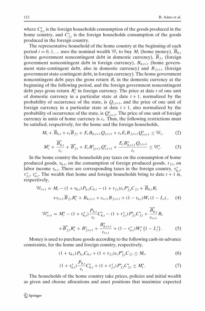
where C∗h,t is the foreign households consumption of the goods produced in the

home country, and C∗f,t is the foreign households consumption of the goods

produced in the foreign country.The representative household of the home country at the beginning of each

period t = 0, 1, ... uses the nominal wealth Wt to buy Mt (home money), Bh,t

(home government noncontingent debt in domestic currency), B f,t (foreigngovernment noncontingent debt in foreign currency), Bh,t+1 (home govern-ment state-contingent debt, also in domestic currency) and B f,t+1 (foreigngovernment state-contingent debt, in foreign currency). The home governmentnoncontingent debt pays the gross return Rt in the domestic currency at thebeginning of the following period, and the foreign government noncontingentdebt pays gross return R∗

t in foreign currency. The price at date t of one unitof domestic currency in a particular state at date t + 1, normalized by theprobability of occurrence of the state, is Qt,t+1, and the price of one unit offoreign currency in a particular state at date t + 1, also normalized by theprobability of occurrence of the state, is Q∗

t,t+1. The price of one unit of foreigncurrency in units of home currency is εt. Thus, the following restrictions mustbe satisfied, respectively, for the home and the foreign households,

Mt + Bh,t + εt B f,t + Et Bh,t+1 Qt,t+1 + εt Et B f,t+1 Q∗t,t+1 ≤ Wt, (2)

M∗t + B

∗h,t

εt+ B

∗f,t + Et B∗

f,t+1 Q∗t,t+1 + Et B∗

h,t+1 Qt,t+1

εt≤ W

∗t . (3)

In the home country the households pay taxes on the consumption of homeproduced goods, τh,t, on the consumption of foreign produced goods, τ f,t, onlabor income τn,t. There are corresponding taxes in the foreign country, τ ∗

h,t,τ ∗

f,t, τ ∗n,t. The wealth that home and foreign households bring to date t + 1 is,

respectively,

Wt+1 = Mt − (1 + τh,t)Ph,tCh,t − (1 + τ f,t)εt P∗f,tC f,t + Bh,t Rt

+εt+1 B f,t R∗t + Bh,t+1 + εt+1 B f,t+1 + (1 − τn,t)Wt (1 − Lt) , (4)

W∗t+1 = M∗

t − (1 + τ ∗h,t)

Ph,t

εtC∗

h,t − (1 + τ ∗f,t)P∗

f,tC∗f,t + B

∗h,t

εt+1Rt

+B∗f,t R

∗t + B∗

f,t+1 + B∗h,t+1

εt+1+ (1 − τ ∗

n,t)W∗t

(1 − L∗

t

). (5)

Money is used to purchase goods according to the following cash-in-advanceconstraints, for the home and foreign country, respectively,

(1 + τh,t)Ph,tCh,t + (1 + τ f,t)εt P∗f,tC f,t ≤ Mt, (6)

(1 + τ ∗h,t)

Ph,t

εtC∗

h,t + (1 + τ ∗f,t)P∗

f,tC∗f,t ≤ M∗

t . (7)

The households of the home country take prices, policies and initial wealthas given and choose allocations and asset positions that maximize expected

Wage and Price Rigidity in a Monetary Union 113

utility (1) subject to the cash-in-advance constraints (6) and the budget con-straints (2) and (4), together with a terminal condition on the accumulation ofassets. The households of the foreign country solve a similar problem.

Among the first order conditions for the home and foreign households arethe intertemporal conditions for the contingent assets,

Qt−1,tuCh (t − 1)

Ph,t−1(1 + τh,t−1)= βuCh (t)

Ph,t(1 + τh,t), (8)

Qt−1,t = Q∗t−1,tεt−1

εt, (9)

Q∗t−1,t

εt−1uC∗h(t − 1)

Ph,t−1(1 + τ ∗h,t−1)

= εtβuC∗h(t)

Ph,t(1 + τ ∗h,t)

. (10)

These imply that

uCh (t − 1)

uCh (t)1 + τh,t

1 + τh,t−1= uC∗

h(t − 1)

uC∗h(t)

1 + τ ∗h,t

1 + τ ∗h,t−1

. (11)

The intertemporal conditions for the noncontingent assets are

uCh (t − 1)

Ph,t−1(1 + τh,t−1)= Rt−1 Et−1

[βuCh (t)

Ph,t(1 + τh,t)

], (12)

εt−1uCh (t − 1)

Ph,t−1(1 + τh,t−1)= R∗

t−1 Et−1

[εtβuCh (t)

Ph,t(1 + τh,t)

], (13)

uC∗h(t − 1)

Ph,t−1(1 + τ ∗h,t−1)

= Rt−1 Et−1

[βuC∗

h(t)

Ph,t(1 + τ ∗h,t)

], (14)

εt−1uC∗h(t − 1)

Ph,t−1(1 + τ ∗h,t−1)

= R∗t−1 Et−1

[εtβuC∗

h(t)

Ph,t(1 + τ ∗h,t)

], (15)

and the intratemporal conditions are

uL (t)uCh (t)

= Wt(1 − τn,t)

Ph,t Rt(1 + τh,t), (16)

uCh (t)uC f (t)

= (1 + τh,t)Ph,t

(1 + τ f,t)εt P∗f,t

, (17)

uL∗t(t)

uC∗f(t)

= W∗t (1 − τ ∗

n,t)

P∗f,t R

∗t (1 + τ ∗

f,t), (18)

114 B. Adao et al.

uC∗h(t)

uC∗f(t)

= (1 + τ ∗h,t)Ph,t

(1 + τ ∗f,t)εt P∗

f,t

. (19)

The budget constraints of the households of each country together with theterminal conditions, can be written as intertemporal budget constraints, thatat the optimum hold with equality. For the home country households, thoseconstraints are the following:∑∞

t=0E0 Qt+1

[(1 + τh,t)Ph,tCh,t + (1 + τ f,t)εt P∗

f,tC f,t − (1 − τn,t)Wt (1 − Lt)]

+∑∞

t=0E0 Qt+1

[Mt

(Qt

Qt+1− 1

)]= W0,

where Qt = Q0,1...Qt−1,t, and Q0 = 1.Using the marginal conditions, as well as the cash-in-advance constraints,

in the intertemporal budget constraints, we can rewrite the household budgetconstraints in the home country and foreign country, respectively, as

∑∞t=0

β t E0[uCh (t) Ch,t + uC f (t) C f,t − uL (t) (1 − Lt)

] = W0uCh (0)

Ph,0(1 + τh,0),

(20)

∑∞t=0

β t E0

[uC∗

h(t) C∗

h,t + uC∗f(t) C∗

f,t − uL∗ (t)(1 − L∗

t

)] = W∗0

uC∗f(0)

P∗f,0(1 + τ ∗

f,0).

(21)

2.2 The government

The government of each country includes both the fiscal authority and themonetary authority. We assume, as is standard in this literature, that aggregatepublic expenditures are exogenous. Each government only consumes goodsproduced by local firms.

The home government issues state-contingent debt, Bh,t+1 + B∗h,t+1, and

noncontingent debt, Bh,t + B∗h,t, and money, Ms

t , and taxes labor income, laborpayments and private consumption.

The home government intertemporal budget constraint can be written as∑∞

t=0E0 Qt+1

[τh,t Ph,tCh,t+τ f,tεt P∗

f,tC f,t+τn,tWt (1 − Lt)+τp,tWt Nt−Ph,tGt

]

+∑∞

t=0E0 Qt+1 Ms

t

(Qt

Qt+1− 1

)=W

g0.

where Nt is labor used by the domestic firms, τp,t is a payroll tax, Gt is publicconsumption and W

g0 are initial nominal liabilities of the government.

There is a similar condition for the government of the foreign country.

Wage and Price Rigidity in a Monetary Union 115

2.3 Firms

We assume that firms are competitive so that there is a representative firm.The technology uses labor only according to

Yh,t = At Nt, (22)

where Yh,t is the production of the home good and At is an aggregatetechnology shock in the home country. The home good can be used for privateand public consumption, Yh,t = Ch,t + C∗

h,t + Gt. The technology in the foreigncountry is

Y f,t = A∗t N∗

t , (23)

where the technology parameter A∗t is the same across firms but can be

different from At. The good produced in the foreign country can be consumedby households or by the foreign government, Y f,t = C f,t + C∗

f,t + G∗t .

Prices are flexible. The firms in the home country take prices as given andmaximize profits �h,t = Ph,tYh,t − (

1 + τp,t)

Wt Nt. Firms in the foreign countrysolve the analogous problem.

In equilibrium it must be that(1 + τp,t

)Wt

Ph,t= At, (24)

and(

1 + τ ∗p,t

)W∗

t

P∗f,t

= A∗t . (25)

2.4 Equilibrium

A flexible price, flexible wage, equilibrium with flexible exchange rates is

defined as allocations{

Ch,t, C f,t, Lt, Nt, C∗h,t, C∗

f,t, L∗t , N∗

t

}, asset positions

{Mt, Bh,t, B f,t, Bh,t+1, B f,t+1, M∗

t , B∗h,t, B

∗f,t, B∗

h,t+1, B∗f,t+1

}, prices and policies

{Ph,t, Wt, Rt, Qt,t+1, τh,t, τ f,t, τn,t, τp,t, MS

t , εt}

and{

P f,t, W∗t , R∗

t , Q∗t,t+1, τ

∗h,t,

τ ∗f,t, τ

∗n,t, τ

∗p,t, M∗S

t

}, such that the households and firms solve their problems;

the governments satisfy their budget constraints; the markets clear, implyingthat for all st, all t,

1 − Lt = Nt, (26)

1 − L∗t = N∗

t , (27)

Ch,t + C∗h,t + Gt = At (1 − Lt) , (28)

116 B. Adao et al.

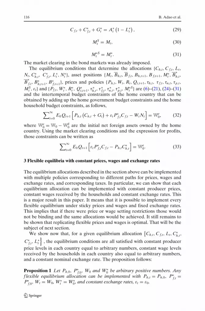
C f,t + C∗f,t + G∗

t = A∗t

(1 − L∗

t

), (29)

MSt = Mt, (30)

M∗St = M∗

t . (31)

The market clearing in the bond markets was already imposed.The equilibrium conditions that determine the allocations {Ch,t, C f,t, Lt,

Nt, C∗h,t, C∗

f,t, L∗t , N∗

t }, asset positions {Mt, Bh,t, B f,t, Bh,t+1, B f,t+1, M∗t , B

∗h,t,

B∗f,t, B∗

h,t+1, B∗f,t+1}, prices and policies {Ph,t, Wt, Rt, Qt,t+1, τh,t, τ f,t, τn,t, τp,t,

MSt , εt} and {Pf,t, W∗

t , R∗t , Q∗

t,t+1, τ∗h,t, τ

∗f,t, τ

∗n,t, τ

∗p,t, M∗S

t } are (6)–(21), (24)–(31)and the intertemporal budget constraints of the home country that can beobtained by adding up the home government budget constraints and the homehousehold budget constraints, as follows,

∑∞t=0

E0 Qt+1

[Ph,t

(Ch,t + Gt

) + εt P∗f,tC f,t − Wt Nt

]= W

e0, (32)

where We0 = W0 − W

g0 are the initial net foreign assets owned by the home

country. Using the market clearing conditions and the expression for profits,those constraints can be written as

∑∞t=0

E0 Qt+1

[εt P∗

f,tC f,t − Ph,tC∗h,t

]= W

e0. (33)

3 Flexible equilibria with constant prices, wages and exchange rates

The equilibrium allocations described in the section above can be implementedwith multiple policies corresponding to different paths for prices, wages andexchange rates, and corresponding taxes. In particular, we can show that eachequilibrium allocation can be implemented with constant producer prices,constant wages received by the households and constant exchange rates. Thisis a major result in this paper. It means that it is possible to implement everyflexible equilibrium under sticky prices and wages and fixed exchange rates.This implies that if there were price or wage setting restrictions those wouldnot be binding and the same allocations would be achieved. It still remains tobe shown that replicating flexible prices and wages is optimal. That will be thesubject of next section.

We show now that, for a given equilibrium allocation{Ch,t, C f,t, Lt, C∗

h,t,

C∗f,t, L∗

t

}, the equilibrium conditions are all satisfied with constant producer

price levels in each country equal to arbitrary numbers, constant wage levelsreceived by the households in each country also equal to arbitrary numbers,and a constant nominal exchange rate. The proposition follows:

Proposition 1 Let Ph,0, P∗f,0, W0 and W∗

0 be arbitrary positive numbers. Anyf lexible equilibrium allocation can be implemented with Ph,t = Ph,0, P∗

f,t =P∗

f,0, Wt = W0, W∗t = W∗

0 , and constant exchange rates, εt = ε0.

Wage and Price Rigidity in a Monetary Union 117

Proof We take as given an arbitrary equilibrium allocation {Ch,t, C f,t, Lt, C∗h,t,

C∗f,t, L∗

t }, in the set defined above. We show that there are constant priceswith Ph,t = Ph,0 and P∗

f,t = P∗f,0, constant wages, Wt = W0 and W∗

t = W∗0 ,

and fixed exchange rates, εt = ε0, which implies that Rt = R∗t , that satisfy

the equilibrium equations for that allocation which are (6)–(21), (24)–(31)and (33).

First, the allocation satisfies trivially the two feasibility constraints, (28) and(29), as it is an equilibrium allocation. For given Ph,0, P∗

f,0, W0, and W∗0 , we use

the remaining equilibrium conditions to determine the values for the policyvariables and remaining prices.

The firms’ conditions(1 + τp,t

)W0

Ph,0= At,

(1 + τ ∗

p,t

)W∗

0

P∗f,0

= A∗t ,

determine τp,t and τ ∗p,t. The intertemporal budget constraints for the two repre-

sentative households are∑∞

t=0β t E0

[(uCh (t) Ch,t + uC f (t) C f,t − uL (t) (1 − Lt)

)] = W0uCh (0)

Ph,0(1 + τh,0),

∑∞t=0

β t E0

[(uC∗

h(t) C∗

h,t + uC∗f(t) C∗

f,t − uL∗ (t)(1 − L∗

t

))]= W

∗0

uC∗h(0)

Ph,0

ε0

(1 + τ ∗

h,0

) ,

which are satisfied by appropriately choosing τh,0 and τ ∗h,0. Given a common

process for the nominal interest rate

Rt−1 = R∗t−1, t ≥ 1

and for given τh,t−1 and τ ∗h,t−1, the intertemporal conditions

uCh (t − 1)

(1 + τh,t−1)= Rt−1 Et−1

βuCh (t)(1 + τh,t)

, t ≥ 1

uC∗h(t − 1)

(1 + τ ∗

h,t−1

) = Rt−1 Et−1βuC∗

h(t)

(1 + τ ∗

h,t

) , t ≥ 1

impose #St−1 restrictions on the taxes τh,t and #St−1 restrictions on the taxesτ ∗

h,t.The marginal conditions for the state-contingent assets,

Qt−1,tuCh (t − 1)

1 + τh,t−1= βuCh (t)

1 + τh,t,

Qt−1,t = Q∗t−1,t,

118 B. Adao et al.

Q∗t−1,t

uC∗h(t − 1)

1 + τ ∗h,t−1

= βuC∗h(t)

1 + τ ∗h,t

.

determine the prices Qt−1,t and Q∗t−1,t and impose #St restrictions on τh,t, and

τ ∗h,t. The total restrictions on the tax rates are then #St + 2#St−1, which is less

than or equal to the number of variables 2#St, since with a discrete distributionof shocks, #St ≥ 2#St−1.

The intratemporal conditions

uL (t)uCh (t)

= W0(1 − τn,t)

Ph,0 Rt(1 + τh,t),

uCh (t)uC f (t)

= (1 + τh,t)Ph,0

(1 + τ f,t)ε0 P∗f,0

,

uL∗t(t)

uC∗f(t)

= W∗0 (1 − τ ∗

n,t)

P∗f,0 Rt

(1 + τ ∗

f,t

) ,

uC∗h(t)

uC∗f(t)

= (1 + τ ∗h,t)Ph,0(

1 + τ ∗f,t

)ε0 P∗

f,0

,

are satisfied by the choice of tax rates, τn,t, τ f,t, τ ∗n,t, τ ∗

f,t. The cash-in-advanceconstraints

(1 + τh,t)Ph,0Ch,t + (1 + τ f,t)ε0 P∗f,0C f,t ≤ Mt,

(1 + τ ∗

h,t

) Ph,0

ε0C∗

h,t + (1 + τ ∗

f,t

)P∗

f,0C∗f,t ≤ M∗

t ,

are satisfied by the choice of Mt and M∗t .

The home country intertemporal budget constraint∑∞

t=0E0 Qt+1

[ε0 P∗

f,tC f,t − Ph,tC∗h,t

]= W

e0.

is satisfied by choice of the initial value of the nominal exchange rate, ε0. ��

We have shown that for any equilibrium allocation,{Ch,t, C f,t, Lt, C∗

h,t,

C∗f,t, L∗

t

}, the equilibrium conditions can be satisfied by asset positions, prices

and policies such that producer prices and wages received by households areconstant and equal to arbitrary constants, Ph,t = Ph,0, P∗

f,t = P∗f,0, Wt = W0,

W∗t = W∗

0 and exchange rates are also constant, εt = ε0.The proposition above is the main result in this paper. It means, first,

that a fixed exchange rate regime does not impose restrictions on the set ofequilibrium allocations under flexible prices and wages. But it has a strongerimplication. If prices or wages were sticky and the policies followed were theones that kept those aggregate prices and wages constant over time, thenthe sticky price and wage restrictions would not be binding. The same set of

Wage and Price Rigidity in a Monetary Union 119

allocations could still be obtained even under a fixed exchange rate regime ora monetary union.

This paper differs from Adao et al. (2009) in that here we show how payrolltaxes have a different role from labor income taxes when wages should be keptconstant. With those taxes, wage rigidity is no longer a restriction on the setof implementable allocations. The simultaneous existence of payroll taxes andlabor income taxes allows wages paid by firms to be constant, with productivityshocks, while households are reacting efficiently to these shocks, through anadequate choice of the other taxes. We also consider that there are marketsfor state contingent debt, but this assumption is only for simplicity.

4 Sticky prices and wages

4.1 Monopolistic price and wage setters

In order to consider the economy with sticky prices and sticky wages we needto make assumptions that allow for price and wage setting. We assume, as isstandard, that the final goods in each country are produced using a contin-uum of differentiated goods that are supplied under monopolist competition.We also assume that households are monopolistic-competitive suppliers ofdifferentiated labor.

The consumption aggregates Ch,t and C f,t are Dixit–Stiglitz compositegoods, aggregating a continuum of differentiated intermediate goods. Theintermediate good firms in the home country are indexed by i in the unitinterval and are aggregated according to

Ch,t =[∫ 1

0Ch,t(i)

θ−1θ di

] θθ−1

, θ > 1, (34)

where Ch,t(i) is the consumption of the good produced by firm i. C f,t is theforeign composite consumption good aggregating the goods produced by theforeign firms, indexed by j in the unit interval,

C f,t =[∫ 1

0C f,t( j)

θ−1θ dj

] θθ−1

. (35)

C∗h,t is the foreign households composite consumption of the goods produced

in the home country and C∗f,t is the foreign households composite consumption

of the goods produced in the foreign country.The households of either country minimize expenditure in the home and

foreign goods to obtain a given aggregate consumption of either good. Thisimplies

Ch,t (i) =(

Ph,t (i)Ph,t

)−θ

Ch,t and C f,t ( j) =(

P∗f,t ( j)

P∗f,t

)−θ

C f,t,

120 B. Adao et al.

where

Ph,t =[∫ 1

0Ph,t(i)1−θdi

] 11−θ

and P∗f,t =

[∫ 1

0P∗

f,t( j)1−θ dj] 1

1−θ

where Ph,t(i) is the price of the good produced by the home firm i in unitsof domestic currency, and P∗

f,t( j) is the price of the good produced by theforeign firm j in units of foreign currency. Expenditure before taxes in eithercomposite good purchased by the home households can then be written as

∫ 1

0Ph,t(i)Ch,t(i)di = Ph,tCh,t and

∫ 1

0P∗

f,t(i)C f,t(i)di = P∗f,tC f,t.

Similar expressions are obtained for the households of the foreign country.Governments choose consumption of each good to minimize expenditure

on the aggregate level of expenditures, Gt for the home country and G∗t , for

the foreign country, respectively,

Gt =[∫ 1

0Gh,t(i)

θ−1θ di

] θθ−1

,

G∗t =

[∫ 1

0G∗

f,t( j)θ−1θ dj

] θθ−1

,

where Gh,t(i) is the home government consumption of the good produced byfirm i and G∗

f,t( j) is the foreign government consumption of the good producedin that country by firm j. It follows that

Gh,t (i) =(

Ph,t (i)Ph,t

)−θ

Gt and G∗f,t ( j) =

(P∗

f,t ( j)

P∗f,t

)−θ

G∗t .

Each intermediate good firm produces the consumption good with a tech-nology that uses labor only. Each home firm i has the production technology

Yh,t (i) = At Nt (i) , (36)

where Yh,t (i) is the production of good i, Nt (i) is the labor used in theproduction of good i. Good i can be used for private and public consumption,Yh,t (i) = Ch,t (i) + C∗

h,t (i) + Gt (i). The technology in the foreign country is

Y f,t ( j) = A∗t N∗

t ( j) . (37)

Each good j produced in the foreign country can be consumed by householdsor by the foreign government, Y f,t ( j) = C f,t ( j) + C∗

f,t ( j) + G∗t ( j).

Flexible price firms in the home country choose prices to maximize profits�h,t (i) = Ph,t (i) Yh,t (i) − (

1 + τp,t)

Wt Nt (i), given the demand functions

Yh,t (i) =(

Ph,t (i)Ph,t

)−θ

Yh,t,

Wage and Price Rigidity in a Monetary Union 121

where Yh,t = Ch,t + C∗h,t + Gt, obtained using the demand functions of the

home good at home and abroad, and given the production functions (22).The home firms set a common price Ph,t (i) = Ph,t such that

(1 + τp,t

)Wt

Ph,t= θ − 1

θAt, (38)

and the foreign firms set P∗f,t( j) = P∗

f,t, where(

1 + τ ∗p,t

)W∗

t

P∗f,t

= θ − 1

θA∗

t . (39)

In each country there is a single household, but a continuum of differ-entiated types of labor indexed by l and n, respectively, in the home and theforeign country, that are supplied monopolistically.

Leisure for the households in each country is now

Lt = 1 −∫ 1

0Nt(l)dl

and

L∗t = 1 −

∫ 1

0N∗

t (n)dn.

The aggregate supplies of labor in each country, Nt and N∗t , are given by

Nt =[∫ 1

0Nt(l)

θw−1θw dl

] θwθw−1

, θw > 1, (40)

and

N∗t =

[∫ 1

0N∗

t (n)θw−1θw dn

] θwθw−1

. (41)

The demand of labor by the firms in each country must be equal to the totalsupply of labor in that country

∫ 1

0Nt(i)di = Nt

and∫ 1

0N∗

t ( j)dj = N∗t .

The minimization of the wage bill for a given aggregate labor, implies

Nt (l) =(

Wt (l)Wt

)−θw

Nt and N∗t (n) =

(W∗

t (n)

W∗t

)−θw

N∗t ,

122 B. Adao et al.

where

Wt =[∫ 1

0Wt(l)1−θw dl

] 11−θw

and W∗t =

[∫ 1

0W∗

t (n)1−θw dn] 1

1−θw

.

The total wage bill in each country is given by∫ 1

0Wt(l)Nt(l)dl = Wt Nt and

∫ 1

0W∗

t (n)N∗t (n)dn = W∗

t N∗t .

Because the firms are monopolistic competitive, there are profits. As thetax on profits is lump-sum, it is optimal that all profits be taxed away, sothat the net profits are zero. The home households choose consumption ofboth composite goods

{Ch,t, C f,t

}and set wages {Wt(l)} to maximize utility (1)

subject to the budget constraint

∑∞t=0

E0 Qt

{(1 + τh,t)Ph,tCh,t + (1 + τ f,t)εt P∗

f,tC f,t

− (1 − τn,t)

Rt

∫ 1

0Wt(l)Nt(l)dl

}= W0,

where

Nt (l) =(

Wt (l)Wt

)−θw

Nt

and

Lt = 1 −∫ 1

0Nt(l)dl.

The marginal conditions include

β tuCh (t)uCh (0)

= Qt(1 + τh,t)Ph,t

(1 + τh,0)Ph,0,

uC f (t)

uCh (t)= (1 + τ f,t)εt P∗

f,t

(1 + τh,t)Ph,t,

anduCh (t − 1)

(1 + τh,t−1)Ph,t−1= Et−1 Rt−1

βuCh (t)(1 + τh,t)Ph,t

,

together with the arbitrage conditions (9) and (13), which are common to thecase where households behaved competitively, and

uCh (t)uL (t)

= θw

θw − 1

(1 + τh,t

)Rt Ph,t(

1 − τn,t)

Wt (l), (42)

where the mark up θw

θw−1 − 1 reflects the monopolistic behavior of households.Proposition 1 holds directly in this set up with monopolistic competitive

firms and households. We restate the proposition here.

Wage and Price Rigidity in a Monetary Union 123

Proposition 2 Consider the model with monopolistic competitive f irms andhouseholds, and let Ph,0, P∗

f,0, W0, and W∗0 be arbitrary positive numbers.

Any f lexible equilibrium allocation can be implemented with Ph,t = Ph,0, P∗f,t =

P∗f,0, Wt = W0, W∗

t = W∗0 , and constant exchange rates, εt = ε0.

Because under flexible prices and wages it is possible to do policy sothat prices and wages are constant, then, if there were sticky price or wagerestrictions, those would not be effective. This means that under sticky pricesand wages it is possible to attain the allocations under full flexibility, even ifexchange rates are fixed. The set of implementable allocations under stickyprices and wages is a larger set, with allocations that may have price or wagedispersion. In the next section we show that those allocations would never bechosen by a benevolent planner, even in a second best framework.

4.2 Sticky prices and sticky wages

In this section we compare the sets of implementable allocations under fullflexibility and under sticky prices and wages and show that the latter set isdominated in welfare terms. Firms set prices as in Calvo (1983) in the domesticcurrency. In each country, starting from an historical common price, at everydate, each firm can optimally set its price with some probability, that can differacross countries. The probability is also the share of firms that optimally revisethe price in each period. For simplicity, we consider the case in which a shareof wages are set one period in advance.

Suppose there were lump-sum transfers between countries which is a usefulabstraction to construct a Pareto frontier. The set of implementable allocations

under flexible prices and wages{

Ch,t, C f,t, Lt, C∗h,t, C∗

f,t, L∗t

}as well as initial

taxes, prices, and exchange rate{τh,0, τ

∗h,0, Ph,0, ε0

}is, then, characterized by

the following conditions:∑∞

t=0β t E0

[(uCh (t) Ch,t + uC f (t) C f,t − θw

θw − 1uL (t) (1 − Lt)

)]

= W0uCh (0)

Ph,0(1 + τh,0)(43)

∑∞t=0

β t E0

[(uC∗

h(t) C∗

h,t + uC∗f(t) C∗

f,t − θw

θw − 1uL∗ (t)

(1 − L∗

t

))]

= W∗0

uC∗h(0)

Ph,0

ε0(1 + τ ∗

h,0)(44)

Ch,t + C∗h,t + Gt = At (1 − Lt) , (45)

C f,t + C∗f,t + G∗

t = A∗t

(1 − L∗

t

). (46)

124 B. Adao et al.

If there is a share αw of wages that are set one period in advance, then thecondition corresponding to (42) is

Wt (l) Et−1

[(1 − τn,t)uCh (t)(1 + τh,t)Ph,t Rt

Nt

(Wt)−θw

]= θw

θw − 1Et−1

[uL (t)

Nt

(Wt)−θw

]. (47)

Let Nst be the supply of labor by the households that set wages one period

in advance and let Wst be the corresponding wage. Since Ns

t =(

Wst

Wt

)−θw

Nt,

condition (47) can be written as

Et−1

[(1 − τn,t)uCh (t)(1 + τh,t)Ph,t Rt

Wst Ns

t

]= θw

θw − 1Et−1

[uL (t) Ns

t

]. (48)

Replacing prices and taxes in the budget constraint of the households,we have

∑∞t=0

E0βt [uCh (t) Ch,t + uC f (t) C f,t

] −∑∞

t=0β tuCh (t)

(1 − τn,t)

(1 + τh,t)Rt Ph,t

×[αwWs

t Nst + (1 − αw) W f

t N ft

]= uCh (0)

(1 + τh,0)Ph,0W0,

which can be written as the implementability condition in the flexible case (43).Similarly for the foreign country, the implementability condition (44) will alsobe common to the flexible and the sticky case.

Under sticky prices or sticky wages the resource constraints include a re-source loss. To see this consider the resource constraint for the home country.Firm i in the home country has to satisfy

Ch,t (i) + C∗h,t (i) + Gt (i) = At Nt (i) (49)

We can use the demand functions for the private and public consumption andintegrate to obtain

(Ch,t + C∗

h,t + Gt) ∫ 1

0

(Ph,t (i)

Ph,t

)−θ

di = At Nt. (50)

Adding and subtracting At∫ 1

0 Nt(l)dl = At(1 − Lt), we obtain

(Ch,t + C∗

h,t + Gt) ∫ 1

0

(Ph,t (i)

Ph,t

)−θ

di = At (1 − Lt)

+At Nt

(1 −

∫ 1

0

(Wt (l)

Wt

)−θw

dl

)(51)

Given that∫ 1

0

(Ph,t(i)

Ph,t

)1−θ

di = 1, it must be the case that∫ 1

0

(Ph,t(i)

Ph,t

)−θ

di ≥ 1,

with∫ 1

0

(Ph,t(i)

Ph,t

)−θ

di > 1 if Ph,t(i)Ph,t

�= 1 for some i. Similarly, with∫ 1

0

(Wt(l)

Wt

)1−θw

Wage and Price Rigidity in a Monetary Union 125

dl = 1, it must be that∫ 1

0

(Wt(l)

Wt

)−θw

dl ≥ 1, with∫ 1

0

(Wt(l)

Wt

)−θw

dl > 1 if Wt(l)Wt

�= 1

for some l.Thus, when there is no price or wage dispersion, as under flexible prices and

wages, the resource constraint

Ch,t + C∗h,t + Gt ≤ At (1 − Lt) . (52)

holds with equality, while with price and wage dispersion, as under sticky pricesand wages, we have that the constraint holds with strict inequality. There is a

loss of resources due to price dispersion, measured by∫ 1

0

(Ph,t(i)

Ph,t

)−θ

di − 1, and

one due to wage dispersion, measured by∫ 1

0

(Wt(l)

Wt

)−θw

dl − 1.

Thus, under sticky prices and sticky wages, the allocations{Ch,t, C f,t, Lt,

C∗h,t, C∗

f,t, L∗t

}are restricted by the same intertemporal implementability con-

ditions as in the flexible case, (43) and (44). Under sticky prices or wages withprice or wage dispersion, the resource constraints will have to be satisfied withstrict inequality. Thus the set of allocations with flexible prices and wagesdominates the set under sticky prices or wages. The restrictions over theallocations under sticky prices and wages are the same only when Ph,t (i) =Ph,0, P f,t ( j) = P f,0, Wt (l) = W0, and W∗

t (n) = W∗0 .

This result, that even in a second best it is optimal to fully eliminate thedistortions associated with price or wage dispersion, is an application of theresult in Diamond and Mirrlees (1971), that it is not optimal to tax intermediategoods when there are consumption taxes on the final goods. The optimalchoice is always in the frontier of production.

5 Concluding remarks

Correia et al. (2008) have shown that sticky prices are irrelevant for stabiliza-tion policy in the closed economy. Adao et al. (2009) show that both stickyprices and fixed exchange rates are irrelevant for policy in the open economy.They conclude that every currency area is an optimal currency area. In bothmodels, wages have to move in response to shocks in order for real wages to beadjusted. Is wage flexibility a necessary condition for those irrelevance results?

In this paper we extend the irrelevance results to environments with stickywages. Provided payroll taxes can be used with the same flexibility as monetarypolicy, then sticky wages do not matter for allocations, and in some sense alsofor policies, both in the closed and open economy. Furthermore, the flexibilityof exchange rates is also not relevant.

These extreme irrelevance results hold only possible because we assumethat tax instruments can be flexible. But isn’t that the common assumption, aswell as the natural one, when the question is a regime question such as the onewe ask in this paper? It is also the standard assumption on monetary policy,which in our models has the same effects as fiscal policy.

126 B. Adao et al.

References

Adao B, Correia I, Teles P (2009) On the relevance of exchange rate regimes for stabilizationpolicy. J Econ Theory 144(4):1468–1488

Calvo G (1983) Staggered prices in a utility-maximizing framework. J Monet Econ 12:383–398Correia I, Nicolini JP, Teles P (2008) Optimal fiscal and monetary policy: equivalence results.

J Polit Econ 168:141–170Corsetti G (2008) New open economy macroeconomics. In: Durlauf SN, Blume LE (eds) The new

Palgrave dictionary. London: MacmillanDiamond PA, Mirrlees JA (1971) Optimal taxation and public production. Am Econ Rev

61(8–27):261–268Erceg C, Henderson D, Levin A (2000) Optimal monetary policy with staggered wage and price

contracts. J Monet Econ 46(2):281–313Friedman M (1953) The case for flexible exchange rates. In: Essays in positive economics. University

of Chicago Press, ChicagoMundell R (1961) A theory of optimum currency areas. Am Econ Rev 51:657–675