Embed Size (px)
Citation preview

What Determines Sectoral Trade in the Enlarged EU?
Helena Marques and Hugh Metcalf*
AbstractIn this paper, we estimate a sectoral gravity model for trade within a heterogeneous trade bloc, the enlargedEU, comprised of a high-income group (wealthiest EU), a middle-income group (Greece, Portugal andSpain), and a low-income group (new Central and Eastern European member countries). The estimationwas conducted on sectors with different degrees of scale economies and skill-intensities in the presence oftransport costs. The results offer support for the call to incorporate trade theories based on both endow-ments and scale economies. In addition, whilst integrating poorer countries is beneficial for all of the participants in the bloc, there is still a role for a redistribution policy, such as the EU’s Regional Policy,which should comprise a mix of policies, focusing on both income and education/skills, together with infra-structure development.
1. Introduction
The globalization phenomenon has been accompanied by a great deal of regionaliz-ation, whereby countries have joined regional trade blocs with varying degrees of heterogeneity. Two of the most important regional trade blocs, the NAFTA in theAmerican continent and the EU in the European continent, integrate countries at dif-ferent levels of development. In the case of the EU, such heterogeneity has just beenaggravated with the May 2004 Eastern enlargement. Ten countries have becomemembers of what was already one of the largest trade blocs in the world, and two more(Bulgaria and Romania) may be admitted by 2007. Except for the Mediterraneanislands of Cyprus and Malta, the new and potential members are Central and EasternEuropean Countries (CEECs),1 which started a process of economic transition morethan a decade ago. During the transition period, East–West trade was progressivelyliberalized under the Europe Agreements signed between the EU and each of theCEECs. However, such liberalization has not produced uniform results either at the country or at the sectoral level. More specifically, not only the CEECs have beentrading far more with the richer (Northern) than with the poorer (Southern) pre-enlargement EU members, but also the Europe Agreements sheltered the so-calledsensitive sectors, such as motor vehicles and textiles and clothing, from liberalization(Baldwin, 1994).
Given the different characteristics of the countries and sectors involved in the liberalization process, we can expect trade in heterogeneous industrial sectors within
Review of Development Economics, 9(2), 197–231, 2005
*Marques: Department of Economics, Sir Richard Morris Building, Loughborough University, Lough-borough LE11 3TU, UK. Tel: + 44 1509 222 704; Fax: + 44 1509 223 910; E-mail: [email protected]: Newcastle-upon-Tyne Business School, Ridley Building, University of Newcastle, Newcastle uponTyne NE1 7RU, UK. Tel: + 44 191 222 8648; Fax: + 44 191 222 6548; E-mail: [email protected]. We gratefully acknowledge the valuable comments of the anonymous referees, as well as those of the partici-pants in a seminar at the University of Newcastle-upon-Tyne, the 2003 EEFS Conference (University ofBologna, Italy), the 2003 ETSG Conference (University Carlos III, Madrid, Spain), and the Inter-AmericanDevelopment Bank’s Euro-Latin Study Network 2003 Conference on Integration and Trade (UniversityPompeu Fabra, Barcelona, Spain). Any remaining errors are our full responsibility.
© Blackwell Publishing Ltd 2005, 9600 Garsington Road, Oxford OX4 2DQ, UK and 350 Main Street, Malden, MA 02148, USA

a heterogeneous EU-25 to be determined differently. Thus it is the aim of this paperto study the relative importance of different determinants of trade, such as locationand endowments, in shaping the trade patterns of a heterogeneous trade bloc, exem-plified by the post-enlargement EU.This is done by estimating a gravity model of tradeflows between country groups with different skilled/unskilled labor ratios and differ-ent spatial and non-spatial trade costs, in sectors with different degrees of economiesof scale and skill-intensity.
We think of the enlarged EU as constituted of three country groups—EU-North2
(N), EU-South3 (S) and EU-East (E)—that differ in the skill endowment as well asboth spatial and non-spatial trade costs. The latter are compressed to zero when E integrates with N and S, but the former persist and give rise to a hub effect.4 In thisset-up, N is a hub and has a higher skill endowment, this is, more skilled workers percapita, than the two peripheries S and E. Following the EU’s Eastern enlargement, thedifferent locational and endowment advantages of the three country groups con-sidered, can be expected to influence the location of sectors with different degrees ofeconomies of scale and skill intensity, this is, different skilled/unskilled labor ratio(Marques and Metcalf, 2003). The location of different sectors will, in turn, determinethe sectoral net exports of each country group. The three country groups can also be characterized in terms of their stages of development, with N being the most developed, followed by S and E the least developed.
The relative role of endowments and location in determining trade patterns has been a subject of debate in the literature (Davis, 2000). It is now consensual that,though endowments are important, geography also plays a role. In particular, byincreasing transport costs, an unfavorable geographical location can significantlyexplain international inequalities, as shown by Limao and Venables (2001), Venables(2001), and Redding and Venables (2004). Earlier cross-section studies focusing onEast–West trade, such as Havrylyshyn and Pritchett (1991), Hamilton and Winters(1992), and Winters and Wang (1992), also concluded that geographical distance wasa main determinant of East–West trade. These studies used a simple aggregate gravitymodel, later improved by using only EU and CEEC data to compute the gravity para-meters (Fidrmuc, 1998; Buch and Piazolo, 2001), by modifying the gravity model toeither incorporate the Krugman (1991) assumption, that proximity increases tradebecause it decreases transport costs (Maurel and Cheikbossian, 1998), or by incorpo-rating both geographical and economic distances (Vittas and Mauro, 1997). In addition, Nilsson (2000) is the only study after Baldwin (1994) that takes into accounteach of the EU-15 countries. All others look exclusively at East–North trade.
We improve on these previous empirical studies in several ways. First, the length ofthe transition period and the enforcement of the Europe Agreements provide datathat is a better indicator of normalized trade patterns than the pre-transition, pre-liberalization data used in most of the earlier studies. Second, we believe our sectoralapproach to be innovative since most previous studies were conducted at an aggregatelevel. In fact, we find that the determinants of trade can differ greatly across sectorswith different characteristics. Third, we use panel data that accounts for sources of heterogeneity and idiosyncrasy, producing unbiased results, as shown by Matyas (1997;1998) and Breuss and Egger (1999). We take this further by using the Prais–Winstenregression with Panel-Corrected Standard Errors (PCSEs). To the best of our knowl-edge, this is the first time PCSEs are used in the study of trade patterns within theenlarged EU. This method incorporates the assumption that the disturbances are heteroskedastic (each country has its own variance) and contemporaneously corre-
198 Helena Marques and Hugh Metcalf
© Blackwell Publishing Ltd 2005

lated across countries (each pair of countries has their own covariance). This assump-tion seems to be especially suited for any study involving transition economies.
2. A Sectoral Gravity Model
In this section, we present the four alternative gravity equations that are the basis ofour empirical study. Our benchmark equation keeps the two main hypotheses behindthe gravity model. The first main hypothesis is that the volume of trade is directlyrelated to the market size of the trading partners, here proxied by their population(POP),5 and inversely related to the physical distance between them (DIST). Thesecond main hypothesis is that the volume of trade is a function of country wealth, asmeasured by GDP per capita (GDPPC). This second element represents more faith-fully the so-called Linder (1961) hypothesis on the importance of demand structureand preferences in a world of differentiated goods. High-income countries consumehigh-quality goods and low-income countries consume low-quality goods. Thus thequality content of exports and imports should increase with GDP per capita.
The two main gravity hypotheses are augmented in two ways. First, the source ofquality is the human capital endowment that differs across countries. Thus, we add thepartner countries’ skilled/unskilled labor ratio (HKPC), proxied by the fraction of the country’s population with tertiary education studies. Countries relatively abundantin human capital are expected to be net exporters of skill-intensive goods, and coun-tries relatively poor in human capital are expected to be net importers of such goods.Second, we distinguish between spatial and non-spatial trade barriers. Spatial tradebarriers are given by physical distance and a common border dummy (BORDER).The non-spatial trade barriers are dealt with by means of time dummies, one forEURO membership and another controlling for progressive trade liberalization with the East since 1991, under the enforcement of the Europe Agreements (EA).Accordingly, our benchmark specification of the gravity model to be estimated forexports and imports of sector k products between countries i and j in year t takes theform:
(1)
We modify equation (1) by interacting the skilled/unskilled labor ratio with both thepartners’ GDPs per capita and the physical distance between partners. The first inter-action crosses demand with supply factors. It can be read as representing differencesin the skill endowment controlling for similar levels of quality consumption or, alter-natively, as representing differences in quality consumption for similar levels of skillendowment. The interaction of the skilled/unskilled labor ratio with distance proxiesfor knowledge spillovers. These decrease with distance between countries and provideanother reason why distance can negatively influence trade. In the light of an information economy, distance might be thought to no longer play a role. However,the literature has not been unanimous in declaring the “death of distance” and thiseffect is sector-dependent, as found by Venables (2001). In addition, our sampleincludes pre-information society industrial sectors, and as such distance may still beexpected to have an impact on the dissemination of information. Industry clustering
TRADE POP POP GDPPC GDPPC
HKPC HKPC DIST BORDER
EA EURO u
ijtk
it jt it jt
it jt ij ij
ijt ijt ijtk
= + + + ++ + + ++ + +
a b b b bb b b b
b b
1 2 3 4
5 6 7 8
9 10 .
SECTORAL TRADE IN ENLARGED EU 199
© Blackwell Publishing Ltd 2005

effects may still be out there, at least for manufacturing industry. There is no a priorireason to believe that skilled workers would not benefit from clustering and, thus, weleave the answer to the data. Hence, the second specification is as follows:
(2)
An alternative to equations (1) and (2) is to replace the GDP per capita and theskilled/unskilled labor ratio of each country, with the absolute value of the differencebetween them.These variables will be called, respectively,economic distance (ECDIST)and human capital distance (HKDIST). The impact of economic distance on trade is atest for intra versus inter-industry trade. Following the Linder (1961) hypothesis, in a world of intra-industry trade we expect countries with similar demand structures to trade more. As a consequence, if economic distance decreases trade we are in the presence of the intra-industry type, whereas, if it increases trade then the inter-industrytype is predominant. The impact of human capital distance on trade may be seen as a test for the HOS hypothesis, according to which trade increases with differences inendowments.6 The modified models are as follows:
(3)
(4)
In specifications (1) and (2), we included the income levels and human capitalendowments of each of the partner countries, either separately or interacted. Thus itmatters how much of income and endowment each country has. In specifications (3)and (4) we consider the differences in income levels and human capital endowments,again separately or interacted. Now it matters how different countries are, irrespectiveof being richer or poorer, more or less endowed.
3. Estimation Results
We use equations (1)–(4) to study the relative importance of different determinantsof trade, such as location and endowments, in shaping the trade patterns of a heterogeneous trade bloc, exemplified by the post-enlargement EU. This bloc containsa high-income group, EU-North (N), a middle-income group, EU-South (S), and a low-income group, EU-East (E).The three groups differ in the skill endowment as wellas both spatial and non-spatial trade costs. In this framework, N is a hub and has ahigher skill endowment, this is, more skilled workers per capita, than the two periph-eries S and E. Sectors also differ in their characteristics, namely economies of scaleand skill-intensity. As N has better access to markets and suppliers, as well as moreskilled workers, it has a double advantage in sectors with high degree of scaleeconomies and high skill-intensity, also producing higher quality products. On the con-trary, the peripheries (S and E) compete in low scale economies, low skill-intensitysectors.
TRADE POP POP ECDIST HKDIST
DIST HKDIST BORDER EA EURO u
ijtk
it jt ijt ijt
ij ijt ij ijt ijt ijtk
= + + + ( )+ ( ) + + + +a b b b
b b b b1 2 3
5 6 7 8
*
* .
TRADE POP POP ECDIST HKDIST
DIST BORDER EA EURO u
ijtk
it jt ijt t
ij ij ijt ijt ijtk
= + + + ++ + + + +a b b b b
b b b b1 2 3 4
5 6 7 8 ,
TRADE POP POP GDPPC HKPC
GDPPC HKPC DIST HKPC
DIST HKPC BORDER EA EURO u
ijtk
it jt it it
jt jt ij it
ij jt ij ijt ijt ijtk
= + + + ( )+ ( ) + ( )+ ( ) + + + +
a b b bb b
b b b b
1 2 3
4 5
6 7 8 9
*
* *
* .
200 Helena Marques and Hugh Metcalf
© Blackwell Publishing Ltd 2005
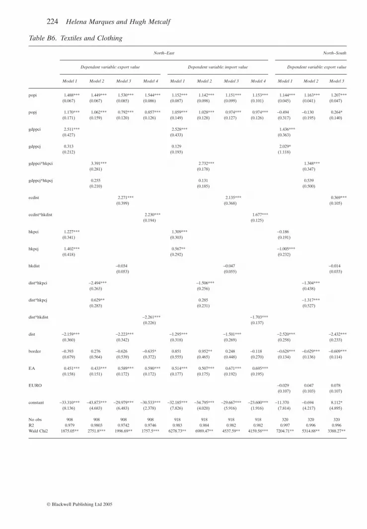
We estimate equations (1)–(4) for bilateral trade flows between the three possiblepairs—North–East (N–E), North–South (N–S) and South–East (S–E)—for fourgroups of sectors distinguished by degree of economies of scale as in Pratten (1988),and skill-intensity as in Baldwin et al. (2000). These four groups are as follows:Chemicals, Machinery, and Transport Equipment, are high scale economies and highskill-intensive; Metals are high scale economies and low skill-intensive; Leather andFootwear; Minerals, and Textiles and Clothing, are low scale economies and low skill-intensive; and Wood Products are low scale economies and high skill-intensive. A fulldescription of the data sources is provided in Appendix A.
Estimation of equations (1)–(4) is carried out through the Prais–Winsten regressionwith correlated Panel Corrected Standard Errors (PCSEs), which assumes that the disturbances are heteroskedastic (each country has its own variance), and contempo-raneously correlated across countries (each pair of countries has their own covariance).On the whole, common coefficients are robust to the different specifications. At thesame time, the estimation of the four models highlights two main differences amongthem. First, absolute income and human capital levels are more important than theirrelative counterparts. Second, the interaction of income and human capital is moreimportant than each of these variables considered individually. We now present thecoefficients and p-values obtained through each model specification, and show the fullestimation results in Appendix B. The regression coefficients and p-values are given inTables 1 to 13 for the different country groups and sectors considered.7
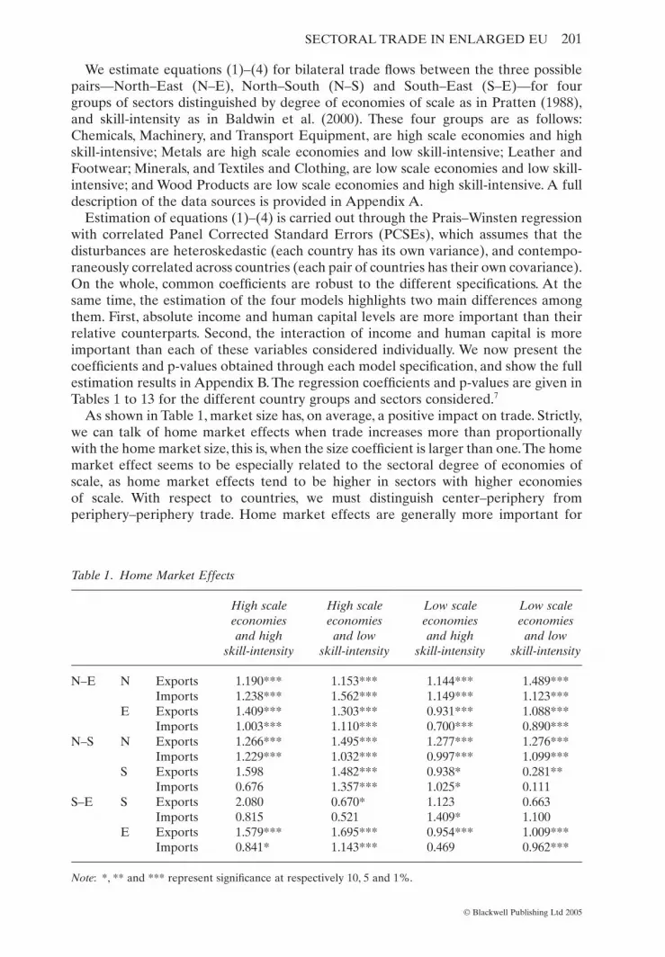
As shown in Table 1, market size has, on average, a positive impact on trade. Strictly,we can talk of home market effects when trade increases more than proportionallywith the home market size, this is, when the size coefficient is larger than one.The homemarket effect seems to be especially related to the sectoral degree of economies ofscale, as home market effects tend to be higher in sectors with higher economies of scale. With respect to countries, we must distinguish center–periphery from periphery–periphery trade. Home market effects are generally more important for
SECTORAL TRADE IN ENLARGED EU 201
© Blackwell Publishing Ltd 2005
Table 1. Home Market Effects
High scale High scale Low scale Low scaleeconomies economies economies economies and high and low and high and low
skill-intensity skill-intensity skill-intensity skill-intensity
N–E N Exports 1.190*** 1.153*** 1.144*** 1.489***Imports 1.238*** 1.562*** 1.149*** 1.123***
E Exports 1.409*** 1.303*** 0.931*** 1.088***Imports 1.003*** 1.110*** 0.700*** 0.890***
N–S N Exports 1.266*** 1.495*** 1.277*** 1.276***Imports 1.229*** 1.032*** 0.997*** 1.099***
S Exports 1.598 1.482*** 0.938* 0.281**Imports 0.676 1.357*** 1.025* 0.111
S–E S Exports 2.080 0.670* 1.123 0.663Imports 0.815 0.521 1.409* 1.100
E Exports 1.579*** 1.695*** 0.954*** 1.009***Imports 0.841* 1.143*** 0.469 0.962***
Note: *, ** and *** represent significance at respectively 10, 5 and 1%.

EU-North than for either the Southern or Eastern peripheries, which would beexpected given EU-North’s position as center. Though the two largest coefficientsoccur in periphery–periphery trade, more specifically in Eastern exports of productsfrom high scale economies sectors to EU-South, size is mostly not significant forperiphery–periphery trade with EU-East, this is, Spain does not significantly trademore with the East than Portugal or Greece. This could be due to Spain’s lower open-ness to trade, in general, that carries over to trade with the East.
Our measure of income (GDP per capita) is positive and significant most of the time(Table 2). Thus, richer countries tend to register a higher value of exports and imports.We can think of income as determining both the supply of and the demand for up-market products, that countries with higher income have the means to produce andfor which they also have a higher preference. As we control for size, which determinesthe volume of international trade, the income effects will determine mostly the unitvalues of the traded goods. As a consequence, we conclude that the unit values of thegoods traded also increase with the income of the trading partners. Interestingly,the most sizeable significant effects occur in EU-South’s trade with both North andEast. Thus, an increase in the income of countries like Greece, Portugal, and Spain,would substantially increase the unit values of the products they trade with the rest ofthe EU. In addition, whereas for the center size is a more important determinant of trade than income, exactly the opposite is true for the two peripheries, supporting theargument on the relevance of catching-up in boosting trade. Furthermore, by increas-ing the South’s income, the rest of the EU would benefit from a pull-through effect intrade.
Income effects are especially noticeable in sectors with high skill-intensity, as wouldbe expected, though two of the highest mean coefficients show in sectors with low skill-intensity, more exactly in Southern exports to the East. The issue here would be oneof product upgrading within the same sectors. As expected, income is generally not
202 Helena Marques and Hugh Metcalf
© Blackwell Publishing Ltd 2005
Table 2. Income Effects
High scale High scale Low scale Low scaleeconomies economies economies economies and high and low and high and low
skill-intensity skill-intensity skill-intensity skill-intensity
N–E N Exports 2.132*** 2.819*** 1.753*** 1.169Imports 1.338 1.681*** 2.867*** 1.236
E Exports 1.728*** 1.264*** 0.890*** 0.687Imports 0.885*** 0.958*** 0.510*** 0.532*
N–S N Exports 0.638* 1.775*** 3.344*** 1.334**Imports 1.203 0.450* 1.162** 1.728
S Exports 8.861*** 0.561*** 7.733*** 4.022*Imports 3.912*** -0.219 2.867* 1.186
S–E S Exports 7.703 11.483*** 7.394 9.298**Imports 4.195 4.652 6.416*** 6.805
E Exports 1.553*** 1.251*** 1.488*** 0.625Imports 1.063*** 0.206 0.964*** 0.711
Note: *, ** and *** represent significance at respectively 10, 5 and 1%.

relevant in low scale economies, low skill-intensity sectors. In addition, income doesnot matter in determining trade in high-scale economies, high skill-intensity in twoinstances. First, the imports of Northern countries from East and South do not dependon their incomes. This can be explained by thinking that the preference for up-marketproducts depends on income. Thus, if imported goods are relatively low-priced, allNorthern countries would be equally driven to demand them, as the bottom quartilesof income are at a similar level, and the top quartiles are the main reason responsiblefor overall income differences. The second case of insignificance relates to Southerntrade with the East. Spain is simultaneously the largest and richest country in theSouthern group. Thus, the income and the size results are similar: Spain’s size andincome have not significantly enhanced its trade with the East during the 1990s, withrespect to Portugal and Greece.
Human capital endowments would be expected to influence trade as follows:countries relatively abundant in human capital are expected to be net exporters ofskill-intensive goods, and countries relatively poor in human capital are expected tobe net importers of such goods. In Table 3, the magnitude and significance of theendowment effects are more related to the countries involved than to the sectoral skill-intensity, though endowments are particularly important for high skill-intensity sectors.On average, human capital endowments increase trade for the North and East, butdecrease trade for the South. This is in line with the empirical observation that EU-East is better endowed with human capital than EU-South and, as a consequence,have the potential to gain competitiveness in high skill-intensive sectors (or more skill-intensive products within low skill-intensive sectors).
In addition, the most sizeable (negative) coefficients occur in Southern exports tothe North. This situation translates a different type of relationship between the centerand each of the peripheries: Eastern human capital endowments increase imports from the North, but Southern human capital endowments actually decrease Southern
SECTORAL TRADE IN ENLARGED EU 203
© Blackwell Publishing Ltd 2005
Table 3. Endowment Effects
High scale High scale Low scale Low scaleeconomies economies economies economies and high and low and high and low
skill-intensity skill-intensity skill-intensity skill-intensity
N–E N Exports 0.458** 0.114 1.170*** 0.180Imports 0.793** 0.793*** 1.191*** 1.264
E Exports 1.120 0.433 0.814** -0.117Imports 1.621*** 1.036*** 1.060*** 1.145
N–S N Exports 0.665 0.367 0.127 -0.028Imports 0.754 0.821*** 0.654*** 0.463
S Exports -2.616*** 0.154 -3.024*** -2.527***Imports -0.671** -0.272 -0.230 -0.623*
S–E S Exports -0.554*** 0.684 0.904 0.669Imports -0.473 -1.130 0.682 -0.971
E Exports 0.592** 1.762* 0.286 -0.431Imports 1.202 -0.228 1.336* 0.850
Note: *, ** and *** represent significance at respectively 10, 5 and 1%.

exports to the North. This happens in sectors that represent over 2/3 of the exports ofGreece, Portugal, and Spain, and it is evidence pointing to a South–North trade basedon the absence of human capital in the South, with the South supplying the North withlow-priced goods. An increase in human capital in the East may increase imports fromthe North, also through both supply and demand links: if the East has more humancapital, both firms and consumers will be more demanding, and it will import morehighly priced inputs and final products from the North.
While endowments per se perform poorly, their interaction with income levels has a significantly positive effect on trade (Table 4). For similar endowments, wealthmakes a difference, or put differently, for similar levels of income endowments areimportant. Thus, income and endowments are relevant when we talk about countriesthat are similar in one of the dimensions. This is an important result, as it shows thatlow-income countries may have difficulty in turning potential comparative advantagesinto effective comparative advantages. The issue is certainly topical in transitioneconomies undergoing rapid structural change. Moreover, in center-periphery tradeincome effects are amplified by endowments, but the endowment weighing actuallyreduces the income effects in periphery–periphery trade. Thus, when compared toTable 2, weighted income effects tend to be higher for the most well endowed partner(North in North–East trade or East in South–East trade). For North–South trade, theendowment weighting actually reduces the income effects, showing that this trade ismore determined by income than by endowments, and reinforcing the conclusions onthe negative effect of human capital endowments on Southern trade. The weightedincome effects are least significant in low scale economies, low skill-intensity sectors,in accordance with the low skill content, and price of these goods. The effects are con-sistently significant across sectors for Northern and Southern exports to the East.Whendifferent human capital endowments are accounted for, an increase in incomeincreases exports to the East by over twice as much in the case of North, and over
204 Helena Marques and Hugh Metcalf
© Blackwell Publishing Ltd 2005
Table 4. Income Effects (Endowment-Weighted)
High scale High scale Low scale Low scaleeconomies economies economies economies and high and low and high and low
skill-intensity skill-intensity skill-intensity skill-intensity
N–E N Exports 2.411*** 2.502*** 2.670*** 2.016***Imports 1.492*** 1.701*** 2.386*** 1.500*
E Exports 1.694*** 1.263*** 0.925*** 0.678Imports 0.889*** 0.953*** 0.501*** 0.509
N–S N Exports 0.504 1.805*** 3.245*** 1.316**Imports 0.682 0.456* 0.620 1.462
S Exports 0.935 1.028*** 1.478* -0.300Imports 1.684** -1.019** -0.983 0.792
S–E S Exports 3.576*** 3.321*** 4.107*** 3.156**Imports 1.368 3.976*** 1.933*** 1.318
E Exports 1.722** 1.147*** 1.643*** 0.885Imports 1.249*** 0.488 1.094*** 0.890**
Note: *, ** and *** represent significance at respectively 10, 5 and 1%.

three times as much in the case of South. These results may be related to the HOScase of differences in demand. According to this interpretation, when differences indemand are accounted for, the role of endowments becomes very significant.
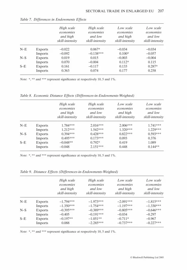
The interaction of human capital with distance, which proxies for knowledgespillovers, has an average negative effect on trade (Table 5). For some countries andsectors, proximity is important for sharing knowledge, and the capacity to do it tendsto decrease with distance. Whilst the East seems to benefit from knowledge spilloversfrom the North, there are no significant spillover effects from trade with the South.Again this is in line with the argument that the East is well endowed in human capitaland, thus, would be able to absorb the technological content of traded goods. Thereseems to be technology embodied in imports from the North, but not in imports fromthe South. This is because the South is poorly endowed with human capital. However,the spillovers are significant in Southern exports to both North and East, in all sectorsexcept low-scale economies, low skill-intensity. This can be better explained as theeffect of distance after controlling for endowments: distance decreases Southernexports in both Northern and Eastern markets, and can be seen as a major disadvan-tage for the South.
The results also provide a test of Linder’s hypothesis, according to which countrieswith similar demand structures trade more when trade is intra-industry, and trade lesswhen trade is inter-industry.The answer is provided by the economic distance variable,defined as the absolute difference in the partners’ GDPs per capita. Hence, this vari-able measures income differences and these proxy for differences in demand structures. In Table 6, we can clearly distinguish the impact of economic distance ontrade between EU-North and both EU-South and EU-East, on one hand, and tradebetween EU-South and EU-East, on the other hand. The impact on center–peripherytrade is positive and mostly significant, except for low scale economies, low skill-intensity sectors, meaning that differences in income actually increase North–South and
SECTORAL TRADE IN ENLARGED EU 205
© Blackwell Publishing Ltd 2005
Table 5. Spillover Effects
High scale High scale Low scale Low scaleeconomies economies economies economies and high and low and high and low
skill-intensity skill-intensity skill-intensity skill-intensity
N–E N Exports -1.502 -1.601* -1.976*** -2.136***Imports -0.631 -2.360 -1.045*** -0.412
E Exports -1.349 -0.049* -0.018 -0.843*Imports -0.268 0.432 -0.056 0.081
N–S N Exports -1.799 -1.743* -2.833*** -1.266Imports -0.980 -3.665 1.054 -0.518*
S Exports -1.164* 0.499* -3.603*** -1.494Imports -0.116 0.786 1.321 -1.324
S–E S Exports -3.195*** -1.519 -2.733*** -1.606Imports -1.638*** -5.153*** -0.859 -1.555
E Exports -0.631** 0.992 -0.626 -0.395Imports 0.912 0.667 0.770 0.882
Note: *, ** and *** represent significance at respectively 10, 5 and 1%.

North–East trade. This is in accordance with a center–periphery pattern as describedin the new economic geography theory. Assuming that wages form the larger part ofincome, lower incomes represent lower wages and thus lower production costs, whichact as an incentive for firms to locate in peripheries. On the contrary, this logic doesnot totally apply to trade between peripheries, as income differences are negativelyrelated to trade, though only significantly for EU-South’s imports from the East.Income differences are not significant for Southern exports to the East. However, com-paring Table 6 with Table 2, we can see that the income of the exporter is important,except in high scale economies, high skill-intensity sectors. Thus, wealthier Southerncountries would export more, though not necessarily to wealthier Eastern countries.As before, low-priced exports will be demanded by the lower income quartiles and,thus, their demand is less affected by increases in overall income.
If we think of the effect of economic distance on trade as a test for inter versus intra-industry trade, then North–East and North–South trade would be mainly inter-industry, whereas South–East trade would follow a more mixed pattern, withintra-industry trade predominating on the import side. Rice et al. (2003) present arecent study of the impact of similarities in production, and demand on intra-industrytrade. They conclude that proximity increases intra-industry trade, because neighbor-ing countries produce and demand a similar mix of products. However, the concept of“proximity” should be seen more in an economic than physical way. Our resultsprovide a good justification.Though North is physically closer to South and East, Southand East are economically closer to each other. As a consequence, intra-industry tradeis stronger between the peripheries than in center–periphery trade.
Not only the human capital endowment of each country group is of interest, but also the endowment differences, proxied by the absolute difference in human capitalendowments of the partner countries (Table 7). The significance of differences inendowments can be seen as a test, even if weak, of the HOS model, especially whenthe information on factor endowments is crossed with information on factor intensity.In our results, endowment differences are, on the whole, not significant, nor do theyshow any consistent pattern. This is probably due to the differentiated nature of thesectors considered.
The differences in endowments per se do not influence trade, but their interactionseither with economic (Table 8) or physical distance (Table 9) do. The weighting intro-duces two major changes in the economic distance effects. First, the negative sign
206 Helena Marques and Hugh Metcalf
© Blackwell Publishing Ltd 2005
Table 6. Economic Distance Effects
High scale High scale Low scale Low scaleeconomies economies economies economies and high and low and high and low
skill-intensity skill-intensity skill-intensity skill-intensity
N–E Exports 1.711** 1.688*** 1.335*** 0.756Imports 0.643 0.890** 1.751*** 0.633
N–S Exports 0.384*** 0.363*** 0.585*** 0.474***Imports 0.488*** 0.183*** 0.098 0.309
S–E Exports -0.831 0.384 -0.261 -0.352Imports -2.021*** -1.249*** -0.804*** -1.120
Note: *, ** and *** represent significance at respectively 10, 5 and 1%.
SECTORAL TRADE IN ENLARGED EU 207
© Blackwell Publishing Ltd 2005
Table 7. Differences in Endowments Effects
High scale High scale Low scale Low scaleeconomies economies economies economies and high and low and high and low
skill-intensity skill-intensity skill-intensity skill-intensity
N–E Exports -0.022 0.067* -0.034 -0.034Imports -0.092 -0.138*** 0.100* -0.057
N–S Exports 0.019 0.015 -0.003 -0.004Imports 0.070 -0.004 0.112* 0.115
S–E Exports 0.161 -0.117 0.133 0.287*Imports 0.363 0.074 0.177 0.258
Note: *, ** and *** represent significance at respectively 10, 5 and 1%.
Table 8. Economic Distance Effects (Differences-in-Endowments-Weighted)
High scale High scale Low scale Low scaleeconomies economies economies economies and high and low and high and low
skill-intensity skill-intensity skill-intensity skill-intensity
N–E Exports 1.784*** 2.016*** 2.006*** 1.741***Imports 1.212*** 1.542*** 1.320*** 1.229***
N–S Exports 0.394*** 0.428*** 0.822*** 0.593***Imports 0.495*** 0.173*** 0.093 0.376
S–E Exports -0.048** 0.792* 0.419 1.089Imports -0.048 2.151*** 0.448 0.144**
Note: *, ** and *** represent significance at respectively 10, 5 and 1%.
Table 9. Distance Effects (Differences-in-Endowments-Weighted)
High scale High scale Low scale Low scaleeconomies economies economies economies and high and low and high and low
skill-intensity skill-intensity skill-intensity skill-intensity
N–E Exports -1.794*** -1.973*** -2.091*** -1.815***Imports -1.350*** -1.754*** -1.197*** -1.330***
N–S Exports -0.395*** -0.389*** -0.805*** -0.646***Imports -0.405 -0.191*** -0.034 -0.297
S–E Exports -0.197** -1.051** -0.711* -0.967Imports 0.088 -2.285*** -0.737*** -0.227***
Note: *, ** and *** represent significance at respectively 10, 5 and 1%.

almost disappears from South–East trade, and the effect becomes significantly positivefor high scale economies, low skill-intensity sectors. Second, the effect becomes signifi-cant for North–East trade in low scale economies, low skill-intensity sectors. This is an important finding, as it helps explaining the apparent contradiction between the celebrated abundance of human capital in the East, and their specialization in low skill-intensity sectors during the 1990s. This specialization was induced by their low income level, not by their endowments and, thus, as incomes start rising, the impor-tance of endowments will increase.
As the differences in endowments are not significant, their interaction with distancefollows essentially the behavior of the latter in terms of significance of the effects. Therole of endowment differences is mostly to correct the magnitude of the distance effect.This correction is generally downwards (cf. Table 10), as differences in endowmentsprovide a motive for trade, in spite of the distance, by compensating higher transportcosts with lower production costs. When we control for endowments, distance becomesless important as the former provide another motive for trade. Thus, if the advantagein endowments is strong enough it may compensate for a disadvantage in marketaccess.
One of the features of our econometric model, is the distinction between spatial andnon-spatial trade barriers. Distance and borders make up spatial barriers, whereas theEurope Agreements and Euro dummies constitute non-spatial trade barriers, or theirdegree of removal through economic integration.The distance variable is, on the whole,significantly negative: trade tends to decrease with distance as distance increases transport costs (Table 10). The distance effect tends to be higher in South–East trade,as these countries are peripheries located far apart and with poor transport infra-structures. An increase in distance decreases trade between the two peripheries by upto 3.5 times as much. Even though the distance effects are very negative for the periph-eries,Table 9 shows that they are substantially reduced when we control for differencesin endowments. If we interpret this as the consequence of poor infrastructures withrespect to the North, there is still a role for policies of infrastructure improvement thatwill decrease the market access gap between the EU’s center and its peripheries. Inaddition, an increase in distance decreases Northern exports of products from low scaleeconomies, low skill-intensity sectors by more than twice as much. Data on sectoraltransport costs would be necessary to evaluate the sectoral impact of distance moreprecisely.
208 Helena Marques and Hugh Metcalf
© Blackwell Publishing Ltd 2005
Table 10. Distance Effects
High scale High scale Low scale Low scaleeconomies economies economies economies and high and low and high and low
skill-intensity skill-intensity skill-intensity skill-intensity
N–E Exports -1.708*** -2.046*** -2.316*** -2.295***Imports -1.594** -2.052*** -0.903** -1.511***
N–S Exports -1.145*** -0.133 -0.305 -2.553***Imports -0.458 -0.665*** -1.615*** -1.339
S–E Exports -2.429*** -1.591** -2.368*** -1.147Imports -2.035 -3.507*** -2.163*** -2.003
Note: *, ** and *** represent significance at respectively 10, 5 and 1%.

The other component of spatial trade barriers is the existence (or not) of a commonborder (Table 11).There is a large literature on border effects, according to which coun-tries that share a common border trade more. In our results, we can identify some sec-toral significance, especially in Southern exports to the North.An interesting argumentis put forward by Davis (2000), according to which product differentiation tends toreduce the magnitude of the border effect, this being strongest within homogeneousgoods categories. As we deal only with manufacturing industry, we can expect prod-ucts to be differentiated and, thus, border effects to be insignificant.
The removal of non-spatial trade barriers under economic integration is proxied bythe Europe Agreements and the adoption of a single currency.The Europe Agreementeffect (Table 12) applies only to the North–East and South–East pairs and the EUROeffect (Table 13) applies only to the North–South pair. On the whole, the EuropeAgreements have increased East–West trade and the effects are generally higher inthe South–East than in the North–East pair. In both cases, it seems that the EuropeAgreements have been especially beneficial for trade in high scale economies sectors,though they have not affected Eastern exports to the South in high scale economiessectors.
SECTORAL TRADE IN ENLARGED EU 209
© Blackwell Publishing Ltd 2005
Table 11. Border Effects
High scale High scale Low scale Low scaleeconomies economies economies economies and high and low and high and low
skill-intensity skill-intensity skill-intensity skill-intensity
N–E Exports 0.040* 0.169 -0.426 -0.041Imports 0.810 0.088 1.524*** 0.703
N–S Exports 0.154 0.048 0.417 -0.437Imports 0.431 0.315* 0.818*** 0.261*
S–E Exports 1.496 1.525 1.935* 2.300Imports 1.157 -0.228 1.769 1.382*
Note: *, ** and *** represent significance at respectively 10, 5 and 1%.
Table 12. EA Effects
High scale High scale Low scale Low scaleeconomies economies economies economies and high and low and high and low
skill-intensity skill-intensity skill-intensity skill-intensity
N–E Exports 0.684*** 0.828*** 0.621*** 0.585***Imports 0.572* 0.298 0.426*** 0.544***
S–E Exports 1.255*** 1.029*** 1.207*** 0.699Imports 0.280 -0.028 0.694*** 0.745**
Note: *, ** and *** represent significance at respectively 10, 5 and 1%.

Finally, being a Eurozone country does not have an effect on trade among the coun-tries analysed, though again the impact on high-skill sectors tends to be higher. Thisresult is in contrast to that of Rose (2000), who found a very large, significant, androbust trade effect of currency unions. However, Persson (2001) argued that Rose’sresult is due to systematic selection into common currencies of country pairs with peculiar characteristics, and suggests an alternative methodology that substantiallyincreases uncertainty around the impact of currency unions on trade. Melitz (2001)adds to the argument, by considering the effects of forming a currency union on thirdcountries. The idea is that the Euro brings a benefit, not just for the Eurozone coun-tries, but for those like the UK, who opted out, as in their trade with the Euro zonecountries they now deal with just one currency. In our case, the magnitude of the standard errors renders the Euro effect on the whole not significant in trade betweenEU-North and EU-South. This should not be made a case against the Euro. It simplymeans that Greece, Portugal, and Spain, have not significantly exported nor importedmore from EU-North countries that have adopted the Euro relatively to those whohave not.The externality argument can help in explaining this: if a country like the UKhas also benefited from the single currency even though it does not participate, thenthere would be no discernible advantage for trade of Euro and non-Euro EU members.This happens not because the Euro is not beneficial, but because it benefits all countries, even those not participating.
4. Conclusions
In this paper, we have estimated a sectoral gravity model of trade within a hetero-geneous regional trade bloc, the enlarged EU, comprised of a high-income group(North), a medium-income group (South), and a low-income group (East). We use theestimated coefficients to draw conclusions on the determinants of trade patterns be-tween these three groups, in sectors with different degrees of scale economies and skill-intensities. The results reveal important differences across sectors and countrygroups, and offer relevant policy recommendations. The results also emphasize that allcountry groups benefit from integration and from an increase in the level of incomeor human capital endowments of their neighbors, as a substantial pull-through effectis found.
Our main findings can be summarized as follows. First, even though Spain is simul-taneously the largest and richest country in the Southern group, its size and income
210 Helena Marques and Hugh Metcalf
© Blackwell Publishing Ltd 2005
Table 13. EURO Effects
High scale High scale Low scale Low scaleeconomies economies economies economies and high and low and high and low
skill-intensity skill-intensity skill-intensity skill-intensity
N–S Exports 0.138 0.166 0.078 0.122Imports 0.267 -0.037 0.184 0.056
Note: *, ** and *** represent significance at respectively 10, 5 and 1%.

have not significantly enhanced its trade with the East during the 1990s, when com-pared to Portugal and Greece. This can be due to Spain’s lower openness to trade,in general, that carries over to trade with the East. However, size would give Spain aprivileged position in high economies of scale sectors, and income would give it anadvantage in high skill-intensity sectors. In an enlarged EU, these two characteristicshave the potential to make Spain a stronger player in the markets for sectors withhigher scale economies and higher skill-intensity, than would be possible for Portugaland Greece.
Second, we also find that for the center (North) size is a more important deter-minant of trade than income, whereas exactly the opposite is true for the Southern and Eastern peripheries, supporting the argument on the relevance of catching-up in boosting trade. We can think of size as determining trade volume and income as deter-mining unit values. Along these lines, our finding means that an increase in the incomeof Southern countries would substantially increase the unit values of the products theytrade with the rest of the EU. Conversely, for the North, the size effect would mostlyincrease the volume of trade, as the North is already producing higher priced goods.Hence the peripheries income catching-up would have an important impact on productladder catching-up.
Third, income catching-up would also impact on the enlarged EU internal trade pat-terns. We find that economic distance increases center–periphery trade, but decreasesperiphery–periphery trade. Thus, more similarity in incomes across members of the EU has an important consequence: it would tend to decrease the pull of the hub bydecreasing center–periphery and increasing periphery–periphery trade. If we think ofthe economic distance effect as a test for inter versus intra-industry trade, incomecatching-up also implies more intra-industry and less inter-industry trade within theEU, which reduces the adjustment costs of enlargement.
Fourth, along with size and income, human capital endowments are an importantdeterminant of trade. They reveal a different type of relationship between the centerand each of the peripheries: human capital endowments increase Eastern trade, butdecrease Southern trade. This finding is in line with the empirical observation that theEast is better endowed with human capital than the South and, as a consequence,has the potential to gain competitiveness in high skill-intensity sectors, or more skill-intensive products within low skill-intensity sectors. Generally, North–South trade ismore determined by incomes than by endowments, and it is likely to remain so.A different picture is detected in North–East trade. The East specialized in low skill-intensity sectors during the 1990s, but we find that such specialization was inducedby their low income level, not by their endowments. Thus, as Eastern incomes start rising, it is likely that the importance of endowments in North–East trade willincrease.
Fifth, the distance effects are very negative for the peripheries. If we interpret thisas the consequence of poor infrastructures with respect to the North, there is still arole for policies of infrastructure improvement that will decrease the market accessgap between the EU’s center and its peripheries. When we control for differences in endowments, distance becomes less important, as the former provide another motive for trade. Thus, if the advantage in endowments is strong enough, it may com-pensate for a disadvantage in market access. A good example would be the South’strade in low scale/low skill goods.
Finally, the effects on specific sectors differ from what might be suggested by aggre-gate trade flows. The home market effect tends to be higher in sectors with higher
SECTORAL TRADE IN ENLARGED EU 211
© Blackwell Publishing Ltd 2005

economies of scale. Income and human capital are especially important in sectors withhigh skill-intensity, though, generally not relevant in low scale economies, low skill-intensity sectors. This result is robust to their interaction with distance. The EuropeAgreements have been especially beneficial for trade in high scale economies sectors,whereas being a Eurozone country tends to have a higher impact on high-skill sectors.The sectoral approach also highlights the importance of history. The South has tradi-tional strengths in the low skill and low economy of scale sectors, and despite risingincomes remains focused on these areas. The East, as the poorest group, can exploitits comparative advantage in human capital endowments with the South, and benefitby focusing on the high skill sectors.
Our results come as a support of recent developments in both trade theory and theEU’s Agenda 2000. From the theory point of view, we provide empirical justificationfor the use of hybrid theories in explaining trade patterns. Our specifications bear such hybrid character between the more traditional trade theory, based on endow-ments and the new economic geography, based on economies of scale and transportcosts. Economies of scale together with transport costs prove to be an important determinant of trade patterns and, even if non-spatial trade barriers fade away withintegration, spatial trade barriers will always have a role to play. In the case of EU-East, it seems that the human capital endowment does not prevail over market access.On the contrary, trade between EU-North and EU-South seems to be equally relatedto endowments and market access.
From the policy standpoint, the paper’s results back the integration of poorer coun-tries into regional trading blocs, accompanied by income redistribution mechanisms,which should be linked to investment in education and infrastructure. The EU’sAgenda 2000 has been a first step in the right direction, by emphasizing different rolesfor the EU’s Regional Policy. The latter should, in fact, be a mix of policies, focusingon both income and education/skills, together with infrastructure development. Thislast aspect has successfully benefited Southern Europe, and the same would beexpected in Eastern Europe. The same recommendation can be carried over to developing countries that suffer from poor market access and low human capitalendowments. When these integrate with more developed countries, it is important toadopt a balanced mix of policies, fostering both income and education/skill levels,together with infrastructure improvement. The excessive focus on one of the policieswithout the right balance may do more harm than good.
Appendix A
Data Sources
Data is taken for the transition period, this is, 1990–99, for the following aggregates ofSITC Rev. 2 sectors: chemicals (5), leather products (61, 85), machinery (71–77), metals(67–69), minerals (66), textiles and clothing (65, 84), transport equipment (78, 79), andwood products (63, 82). Trade data (value of exports and imports) is provided by theOECD International Trade Statistics CD-ROM in thousands USD. Trade liberaliza-tion with the East is accounted for by means of a dummy variable. For each Easterncountry, it is defined as taking a value of one after the year of signature of the EuropeAgreements. The data for all regional trade associations was taken from the WTOwebsite (http://www.wto.org). Data for distances and borders was taken from theCEPII website (http://www.cepii.fr). Distance data is measured in km between
212 Helena Marques and Hugh Metcalf
© Blackwell Publishing Ltd 2005
the partner countries’ economic centers. These correspond to the capital city, exceptfor Germany (Hamburg is the city used). Countries are considered to share a commonborder when they share a land border or a small body of water border. Data for population (given in thousands) and for GDP (given in billions USD at 1995 pricesand exchange rates), was taken from the web version of IMF’s International FinancialStatistics at http://www.imf.org.The schooling variable is given by the number of peoplewith tertiary education studies. This number was obtained from the Barro–Lee datasetfor 1990, and then added of the yearly number of enrolments. The enrolment data was taken from the web versions of OECD Education Statistics and UNESCO Statistics of Educational Attainment and Literacy at http://www.oecd.org andhttp://www.unesco.org.
Appendix B
Regression Results
Note: Standard errors are shown in parenthesis, and the symbols *, ** and *** indi-cate significance at 10, 5 and 1%, respectively.
SECTORAL TRADE IN ENLARGED EU 213
© Blackwell Publishing Ltd 2005

214 Helena Marques and Hugh Metcalf
© Blackwell Publishing Ltd 2005
Table B1. Chemicals
North–East North–South
Dependent variable: export value Dependent variable: import value Dependent variable: export value
Model 1 Model 2 Model 3 Model 4 Model 1 Model 2 Model 3 Model 4 Model 1 Model 2 Model 3
popi 1.088*** 1.094*** 1.105*** 1.082*** 1.290*** 1.246*** 1.249*** 1.301*** 0.998*** 0.984*** 1.178***(0.050) (0.057) (0.055) (0.058) (0.054) (0.070) (0.066) (0.062) (0.061) (0.066) (0.062)
popj 1.276*** 1.304*** 0.987*** 0.985*** 1.397*** 1.276*** 0.949*** 0.893*** 0.033 0.115 0.978***(0.134) (0.151) (0.114) (0.126) (0.103) (0.114) (0.071) (0.069) (0.222) (0.157) (0.093)
gdppci 2.019*** -0.044 0.259(0.368) (0.517) (0.240)
gdppcj 0.982*** 0.954*** 3.054***(0.217) (0.188) (0.887)
gdppci*hkpci 1.821*** 1.125*** 0.031(0.206) (0.379) (0.325)
gdppcj*hkpcj 0.968*** 0.862*** 2.958***(0.207) (0.184) (0.499)
ecdist 1.583*** -0.053 0.518***(0.378) (0.325) (0.124)
ecdist*hkdist 1.296*** 0.786***(0.167) (0.182)
hkpci 0.196 0.648* 1.276*** (0.126) (0.356) (0.203)
hkpcj 1.275*** 1.437*** -0.358*(0.306) (0.438) (0.188)
hkdist -0.007 -0.072 0.026(0.036) (0.054) (0.026)
dist*hkpci -1.537*** -1.093*** 1.234***(0.222) (0.372) (0.438)
dist*hkpcj 0.447* -0.011 -3.281***(0.235) (0.325) (0.575)
dist*hkdist -1.276*** -0.945***(0.182) (0.176)
dist -1.030*** -1.141*** -1.426*** -1.398*** -2.072*** -1.224***(0.326) (0.278) (0.363) (0.315) (0.228) (0.166)
border 0.929* 0.821** 0.872** 0.637*** 0.406 0.641*** 0.018 1.167*** -0.049 -0.146 -0.073(0.493) (0.354) (0.380) (0.230) (0.284) (0.243) (0.464) (0.239) (0.100) (0.136) (0.130)
EA 0.688*** 0.686*** 0.788*** 0.778*** 0.134 0.152 0.261* 0.237*(0.200) (0.200) (0.197) (0.207) (0.164) (0.163) (0.150) (0.145)
EURO -0.025 -0.021 0.107(0.082) (0.079) (0.113)
constant -39.087*** -36.448*** -26.093*** -21.698*** -19.577** -33.669*** -10.697*** -22.605*** -11.710* -9.650*** -12.863***(8.313) (4.718) (6.766) (2.478) (9.149) (4.058) (5.104) (1.096) (6.518) (2.720) (3.674)
No obs 915 915 915 915 902 902 902 902 320 320 320R2 0.9811 0.9811 0.9799 0.9775 0.962 0.963 0.967 0.966 0.998 0.998 0.996Wald Chi2 2740.17*** 2657.21*** 3974.91*** 2401.81*** 3980.39*** 3184.75*** 3105.07*** 2686.67*** 4846.72*** 5112.73*** 1322.02***

SECTORAL TRADE IN ENLARGED EU 215
© Blackwell Publishing Ltd 2005
South–East
Dependent variable: import value Dependent variable: export value Dependent variable: import value
Model 4 Model 1 Model 2 Model 3 Model 4 Model 1 Model 2 Model 3 Model 4 Model 1 Model 2 Model 3 Model 4
1.116*** 1.109*** 1.061*** 0.979*** 0.949*** 2.524*** 1.570*** 2.437*** 1.549*** 1.619** 0.701*** 1.697*** 1.856***(0.045) (0.072) (0.069) (0.050) (0.063) (0.648) (0.251) (0.299) (0.326) (0.790) (0.276) (0.357) (0.241)
1.130*** 0.412 1.053*** 1.896*** 1.766*** 1.077*** 0.992*** 0.326 0.249 1.480*** 1.360*** 1.280*** 1.147***(0.059) (0.341) (0.181) (0.089) (0.164) (0.128) (0.131) (0.245) (0.338) (0.149) (0.128) (0.135) (0.128)
0.362 1.185 -1.264(0.384) (2.228) (3.228)
4.657*** 1.094*** 0.379**(1.288) (0.279) (0.183)
0.133 5.199*** 2.516***(0.387) (0.837) (0.656)
1.336*** 0.980*** 0.329*(0.523) (0.282) (0.188)
0.335*** -0.131 -0.986***(0.092) (0.524) (0.382)
0.451*** 0.311** 2.075*** -0.659(0.098) (0.129) (0.803) (0.591)
1.171*** 3.383*** -0.030(0.307) (0.623) (0.739)
-1.293*** 2.110*** 1.855***(0.247) (0.692) (0.509)
0.093** 0.148 0.361***(0.049) (0.115) (0.122)
1.579*** -2.253** -3.209***(0.593) (1.032) (0.713)
-2.333*** 0.539 0.986**(0.607) (0.674) (0.513)
-0.454*** -0.197 -2.105*** 0.648(0.099) (0.162) (0.712) (0.553)
-0.331 -0.050 -1.574*** -3.587*** -2.070*** -1.455***(0.282) (0.405) (0.467) (0.480) (0.356) (0.156)
0.187* 0.622*** 0.771*** 0.450* 0.560* 0.304 0.413 -0.905 0.997 0.234 0.478 1.849*** 5.373***(0.105) (0.161) (0.161) (0.253) (0.300) (0.694) (0.704) (0.577) (1.084) (0.407) (0.397) (0.274) (1.061)
0.951*** 0.836*** 1.733*** 1.273*** 0.406** 0.317* 0.482** 0.371*(0.210) (0.194) (0.225) (0.242) (0.200) (0.180) (0.212) (0.223)
0.114 -0.103 0.119 0.101 0.103(0.110) (0.129) (0.129) (0.128) (0.133)
-19.556*** -53.693*** -24.331*** -32.731*** -28.659*** -37.671*** -59.290*** -4.375 -20.556*** -6.633*** -27.111*** -13.132** -34.425***(1.382) (7.309) (3.372) (3.736) (3.396) (12.990) (6.114) (3.581) (6.441) (18.444) (5.585) (5.442) (4.328)
320 321 321 321 321 239 239 239 239 226 226 226 2260.998 0.993 0.992 0.991 0.991 0.9373 0.936 0.9292 0.9367 0.958 0.955 0.964 0.973
3234.27*** 8188.41*** 7243.64*** 1681.05*** 1985.75*** 1137.35*** 757.59*** 931.52*** 385.02*** 1322.41*** 3156.34*** 1680.52*** 1159.86***

Table B2. Leather and Footwear
North–East North–South
Dependent variable: export value Dependent variable: import value Dependent variable: export value
Model 1 Model 2 Model 3 Model 4 Model 1 Model 2 Model 3 Model 4 Model 1 Model 2 Model 3
popi 1.556*** 1.568*** 1.582*** 1.532*** 1.309*** 1.292*** 1.307*** 1.349*** 1.213*** 1.231*** 1.106***(0.073) (0.078) (0.070) (0.079) (0.053) (0.070) (0.060) (0.073) (0.070) (0.069) (0.116)
popj 0.776*** 0.686*** 0.679*** 0.595*** 0.932*** 0.991*** 0.980*** 1.050*** -0.944** -1.177*** -0.626***(0.109) (0.095) (0.067) (0.068) (0.199) (0.156) (0.115) (0.113) (0.431) (0.315) (0.240)
gdppci 0.286 0.751 0.594(0.467) (0.739) (0.380)
gdppcj 0.323* 0.807*** 0.772(0.187) (0.200) (1.604)
gdppci*hkpci 1.096*** 0.332 0.539(0.312) (0.283) (0.383)
gdppcj*hkpcj 0.327* 0.785*** 1.811**(0.200) (0.209) (0.786)
ecdist -0.101 -0.681 0.341***(0.375) (0.463) (0.117)
ecdist*hkdist 1.692*** 0.626***(0.203) (0.156)
hkpci -0.613*** 0.152 0.113(0.179) (0.362) (0.420)
hkpcj 0.503 -0.736 -0.428(0.550) (0.572) (0.343)
hkdist -0.025 0.046 -0.048(0.067) (0.072) (0.042)
dist*hkpci -1.894*** 0.023 -0.535(0.324) (0.350) (0.588)
dist*hkpcj -0.410 -1.147*** -2.388***(0.262) (0.378) (0.845)
dist*hkdist -1.802*** -0.708***(0.235) (0.159)
dist -2.515*** -2.570*** -0.984*** -1.442*** -3.045*** -3.211***(0.299) (0.284) (0.171) (0.120) (0.648) (0.559)
border -0.514 -0.219 -0.642* 0.924*** 1.520*** 1.292** 0.690* 2.477*** -0.590** -0.589** -0.665**(0.394) (0.307) (0.384) (0.326) (0.444) (0.568) (0.392) (0.719) (0.280) (0.271) (0.333)
EA 0.595*** 0.586*** 0.607*** 0.553*** 0.509*** 0.495*** 0.583*** 0.540***(0.153) (0.152) (0.144) (0.133) (0.195) (0.194) (0.187) (0.185)
EURO 0.316** 0.265* 0.315**(0.163) (0.161) (0.137)
constant -13.199** -23.828*** -5.044 -26.620*** -31.529*** -25.167*** -6.562*** -27.212*** 19.922 12.552** 28.556***(6.108) (3.688) (4.752) (1.371) (7.646) (3.313) (5.197) (1.362) (12.944) (5.727) (8.631)
No obs 844 844 844 844 865 865 865 865 320 320 320R2 0.9621 0.9599 0.9598 0.954 0.952 0.952 0.952 0.956 0.982 0.982 0.978Wald Chi2 2890.44*** 1946.36*** 1797*** 1221.97*** 4203.49*** 2492.67*** 2020.68*** 1561.35*** 2003.04*** 1928.10*** 856.18***
216 Helena Marques and Hugh Metcalf
© Blackwell Publishing Ltd 2005

SECTORAL TRADE IN ENLARGED EU 217
© Blackwell Publishing Ltd 2005
South–East
Dependent variable: import value Dependent variable: export value Dependent variable: import value
Model 4 Model 1 Model 2 Model 3 Model 4 Model 1 Model 2 Model 3 Model 4 Model 1 Model 2 Model 3 Model 4
1.458*** 1.173*** 1.203*** 1.209*** 1.485*** -0.577 0.637** 1.286*** 0.691** 0.551 1.665*** 1.883*** 1.513***(0.088) (0.081) (0.084) (0.099) (0.169) (0.722) (0.320) (0.314) (0.355) (1.229) (0.681) (0.417) (0.516)
-0.079 -0.539 0.759*** 1.734*** 2.281*** 0.759*** 0.855*** 0.624*** 0.541** 0.836** 1.026*** 1.137*** 0.843***(0.215) (0.606) (0.208) (0.179) (0.284) (0.196) (0.215) (0.215) (0.230) (0.365) (0.310) (0.253) (0.250)
3.115*** 6.667** 2.255(0.586) (3.031) (4.217)
5.372** 1.049*** 0.976(2.296) (0.163) (0.699)
2.623*** 1.418* -1.978(0.630) (0.774) (1.709)
-0.934 1.218*** 1.248**(0.905) (0.171) (0.649)
0.576*** -0.721 -2.024***(0.177) (0.725) (0.514)
0.396** 0.538*** 0.613 -1.404**(0.177) (0.182) (0.448) (0.619)
0.837*** -0.806 -2.117*(0.274) (0.951) (1.112)
-4.177*** 0.622 -0.017(0.614) (0.798) (1.264)
0.198*** 0.273 0.658***(0.075) (0.176) (0.181)
-1.376* -1.411 0.463(0.825) (1.127) (2.372)
-2.048*** 0.315 -0.654(0.801) (0.746) (1.108)
-0.527*** -0.374* -0.370 1.789***(0.180) (0.214) (0.386) (0.555)
-2.800*** -2.984** -1.173** -0.770** -0.325 0.371(0.567) (1.429) (0.555) (0.396) (1.489) (0.498)
0.134 -1.090*** -1.120*** -1.230 -0.472 2.230*** 1.800** 2.562*** 3.070*** 2.472 2.333 2.284*** 4.207***(0.343) (0.360) (0.373) (0.902) (0.510) (0.760) (0.767) (0.426) (0.535) (2.313) (2.431) (0.877) (1.034)
0.296 0.288 0.559** 0.372 1.003*** 1.097*** 0.989*** 0.969***(0.255) (0.246) (0.233) (0.233) (0.276) (0.287) (0.274) (0.265)
0.333** -0.012 0.323 0.014 0.040(0.143) (0.258) (0.259) (0.218) (0.226)
-7.705* -66.085*** -14.108*** -14.883 -48.054*** -53.001*** -22.052*** -5.760 -10.075 -44.085*** -25.263* -19.665** -26.378***(4.141) (14.194) (2.968) (10.528) (7.602) (18.017) (7.933) (9.274) (8.758) (20.446) (14.282) (8.624) (10.352)
320 318 318 318 318 226 226 226 226 219 219 219 2190.972 0.979 0.979 0.979 0.976 0.9363 0.9336 0.9476 0.9347 0.851 0.869 0.884 0.885
449.71*** 1266.09*** 1417.04*** 718.97*** 499.56*** 600.83*** 800*** 784.3*** 544.78*** 52.21*** 64.49*** 57.11*** 44.56***

218 Helena Marques and Hugh Metcalf
© Blackwell Publishing Ltd 2005
Table B3. Machinery
North–East North–South
Dependent variable: export value Dependent variable: import value Dependent variable: export value
Model 1 Model 2 Model 3 Model 4 Model 1 Model 2 Model 3 Model 4 Model 1 Model 2 Model 3
popi 0.946*** 0.927*** 0.938*** 0.931*** 1.140*** 1.119*** 1.149*** 1.010*** 1.047*** 1.042*** 0.995***(0.052) (0.050) (0.059) (0.058) (0.074) (0.069) (0.098) (0.079) (0.044) (0.035) (0.025)
popj 1.318*** 1.260*** 0.790*** 0.833*** 1.921*** 1.921*** 1.391*** 1.434*** -0.164 0.732*** 1.290***(0.111) (0.118) (0.098) (0.121) (0.182) (0.184) (0.108) (0.103) (0.204) (0.114) (0.050)
gdppci 1.471*** 1.701*** 0.894***(0.409) (0.461) (0.264)
gdppcj 0.960*** 2.050*** 5.003***(0.180) (0.232) (0.863)
gdppci*hkpci 1.928*** 1.472*** 0.694***(0.306) (0.245) (0.212)
gdppcj*hkpcj 0.976*** 2.045*** 0.875**(0.174) (0.236) (0.364)
ecdist 0.944* 1.575*** 0.289***(0.494) (0.526) (0.070)
ecdist*hkdist 1.503*** 1.048***(0.181) (0.220)
hkpci 0.361*** 0.489*** 0.409**(0.145) (0.158) (0.178)
hkpcj 1.778*** 1.831*** -1.119***(0.284) (0.369) (0.180)
hkdist -0.060 0.067 -0.041(0.051) (0.067) (0.028)
dist*hkpci -1.850*** -0.891*** 0.126(0.275) (0.315) (0.292)
dist*hkpcj 0.563** -0.026 -1.270***(0.279) (0.297) (0.372)
dist*hkdist -1.560*** -0.975***(0.184) (0.231)
dist -1.418*** -1.754*** -0.840** -0.766* -0.543*** -0.595***(0.220) (0.195) (0.434) (0.412) (0.190) (0.179)
border 0.699*** 0.828*** -0.018 0.485** 2.314*** 2.073*** 3.120*** 2.457*** 0.067 0.002 -0.204**(0.278) (0.233) (0.254) (0.237) (0.673) (0.557) (0.650) (0.353) (0.155) (0.105) (0.088)
EA 0.727*** 0.730*** 0.876*** 0.821*** 0.610*** 0.633*** 0.802*** 0.813***(0.153) (0.149) (0.189) (0.188) (0.145) (0.147) (0.162) (0.169)
EURO -0.035 0.197** 0.270***(0.076) (0.091) (0.096)
constant -26.176*** -32.096*** -8.846 -16.329*** -54.807*** -50.836*** -36.403*** -27.950*** -49.544*** -15.514*** -16.776***(6.890) (4.664) (6.692) (2.602) (9.506) (4.233) (8.850) (2.077) (5.231) (0.964) (1.630)
No obs 920 920 920 920 909 909 909 909 320 320 320R2 0.9858 0.9859 0.9772 0.9766 0.971 0.974 0.964 0.965 0.998 0.998 0.998Wald Chi2 1472.36*** 1227.07*** 3461.76*** 3094.16*** 1281.95*** 1836.61*** 667.5*** 820.64*** 10,159.06*** 20,836.64*** 6042.46***

SECTORAL TRADE IN ENLARGED EU 219
© Blackwell Publishing Ltd 2005
South–East
Dependent variable: import value Dependent variable: export value Dependent variable: import value
Model 4 Model 1 Model 2 Model 3 Model 4 Model 1 Model 2 Model 3 Model 4 Model 1 Model 2 Model 3 Model 4
1.007*** 1.220*** 1.135*** 1.075*** 1.038*** 0.048 1.906*** 2.665*** 2.393*** -1.994*** -0.052 1.825*** 0.201(0.028) (0.071) (0.044) (0.060) (0.057) (0.535) (0.182) (0.204) (0.236) (0.723) (0.256) (0.465) (0.825)
1.318*** 0.072 1.355*** 1.933*** 1.791*** 0.839*** 1.173*** 0.838*** 1.002*** 1.961*** 2.339*** 2.045*** 2.365***(0.047) (0.335) (0.103) (0.087) (0.055) (0.139) (0.132) (0.102) (0.125) (0.186) (0.217) (0.256) (0.435)
0.267 9.708*** 10.595***(0.397) (2.162) (2.880)
6.844*** 0.800*** 1.940***(1.353) (0.231) (0.327)
0.114 2.342*** 2.186***(0.320) (0.576) (0.562)
0.757 1.063*** 2.402***(0.506) (0.219) (0.365)
0.225*** -0.915*** -3.210***(0.066) (0.346) (0.512)
0.280*** 0.227*** -0.952* 0.736(0.072) (0.067) (0.524) (2.111)
0.707*** -1.176*** -3.812***(0.187) (0.411) (1.044)
-2.123*** -0.154 1.814***(0.288) (0.740) (0.495)
0.018 0.165*** 0.724***(0.047) (0.068) (0.132)
1.323*** -2.739*** -4.996***(0.454) (0.791) (0.672)
-2.083*** 0.635 0.870*(0.419) (0.604) (0.466)
-0.330*** -0.195** 0.764* -0.054(0.085) (0.097) (0.445) (2.148)
-0.319 0.236 -2.021*** -1.732*** -4.608*** -2.172***(0.233) (0.213) (0.307) (0.257) (0.736) (0.862)
-0.103 0.470** 0.721*** 0.828*** 0.740*** 1.301** 0.346 1.081*** 4.687*** -2.942*** -2.903*** -0.500 1.954(0.076) (0.245) (0.134) (0.083) (0.089) (0.615) (0.567) (0.430) (0.964) (0.732) (0.478) (1.495) (3.602)
1.156*** 1.231*** 1.527*** 1.359*** 0.141 0.306 0.463** 0.387(0.202) (0.211) (0.191) (0.212) (0.206) (0.227) (0.227) (0.253)
0.274*** -0.027 0.349** 0.273** 0.277**(0.097) (0.109) (0.151) (0.133) (0.135)
-19.383*** -73.127*** -26.250*** -36.033*** -29.752*** -86.894*** -47.528*** -22.006*** -40.119*** -70.290*** -29.543*** 0.028 -30.791**(0.752) (8.921) (1.448) (3.384) (1.415) (12.279) (4.710) (2.688) (4.622) (15.811) (6.481) (9.888) (15.331)
320 321 321 321 321 236 236 236 236 239 239 239 2390.998 0.995 0.994 0.993 0.993 0.9698 0.9668 0.9661 0.9615 0.926 0.950 0.936 0.933
4836.15*** 4853.60*** 11,320.56*** 15,726.97*** 14,249.55*** 5190.27*** 4739.36*** 1124.98*** 427.5*** 670.01*** 431.15*** 573.07*** 282.19***

220 Helena Marques and Hugh Metcalf
© Blackwell Publishing Ltd 2005
Table B4. Metals
North–East North–South
Dependent variable: export value Dependent variable: import value Dependent variable: export value
Model 1 Model 2 Model 3 Model 4 Model 1 Model 2 Model 3 Model 4 Model 1 Model 2 Model 3
popi 1.201*** 1.203*** 1.100*** 1.106*** 1.590*** 1.591*** 1.538*** 1.531*** 1.489*** 1.468*** 1.544***(0.075) (0.075) (0.092) (0.094) (0.084) (0.083) (0.082) (0.075) (0.060) (0.056) (0.095)
popj 1.297*** 1.332*** 0.902*** 0.910*** 1.447*** 1.447*** 1.198*** 1.118*** 1.261*** 1.452*** 1.339***(0.133) (0.140) (0.087) (0.098) (0.099) (0.105) (0.121) (0.114) (0.389) (0.149) (0.071)
gdppci 2.819*** 1.681*** 1.775***(0.394) (0.523) (0.306)
gdppcj 0.958*** 1.264*** -0.219(0.239) (0.194) (1.490)
gdppci*hkpci 2.502*** 1.701*** 1.805***(0.196) (0.345) (0.286)
gdppcj*hkpcj 0.953*** 1.263*** -1.019**(0.236) (0.194) (0.466)
ecdist 1.688*** 0.890** 0.363***(0.345) (0.387) (0.100)
ecdist*hkdist 2.016*** 1.542***(0.128) (0.119)
hkpci 0.114 0.793*** 0.367(0.174) (0.210) (0.246)
hkpcj 1.036*** 0.433 -0.272(0.310) (0.440) (0.375)
hkdist 0.067* -0.138*** 0.015(0.039) (0.054) (0.039)
dist*hkpci -2.282*** -0.920*** -1.396***(0.302) (0.282) (0.329)
dist*hkpcj 0.204 -0.843** 0.862(0.273) (0.376) (0.624)
dist*hkdist -1.973*** -1.754***(0.134) (0.101)
dist -1.957*** -2.136*** -1.776*** -2.328*** -0.435 0.169(0.323) (0.230) (0.236) (0.224) (0.387) (0.452)
border 0.118 -0.087 -0.032 0.341 0.215 0.236 -0.439 0.674*** -0.159 -0.169 0.100(0.479) (0.326) (0.402) (0.238) (0.355) (0.270) (0.306) (0.165) (0.251) (0.224) (0.208)
EA 0.763*** 0.769*** 0.898*** 0.883*** 0.219 0.220 0.400** 0.354**(0.178) (0.180) (0.188) (0.187) (0.169) (0.169) (0.181) (0.176)
EURO 0.131 0.175 0.188(0.172) (0.166) (0.167)
constant -44.557*** -40.391*** -19.447*** -24.225*** -44.782*** -45.163*** -22.367*** -31.902*** -40.109*** -34.482*** -34.502***(7.813) (3.862) (5.369) (1.930) (6.656) (4.104) (4.453) (2.032) (7.847) (3.271) (5.285)
No obs 911 911 911 911 902 902 902 902 320 320 320R2 0.9762 0.9763 0.9746 0.9727 0.969 0.969 0.965 0.964 0.992 0.992 0.994Wald Chi2 7034.91*** 6113.83*** 4822.65** 5012.09*** 970.28*** 958.1*** 720.37*** 1070.55*** 3340.77** 3255.60** 3803.73**

SECTORAL TRADE IN ENLARGED EU 221
© Blackwell Publishing Ltd 2005
South–East
Dependent variable: import value Dependent variable: export value Dependent variable: import value
Model 4 Model 1 Model 2 Model 3 Model 4 Model 1 Model 2 Model 3 Model 4 Model 1 Model 2 Model 3 Model 4
1.479*** 0.989*** 1.002*** 1.052*** 1.087*** -0.960 0.936** 1.459*** 1.246*** -0.036 0.131 1.536*** 0.450(0.060) (0.035) (0.032) (0.026) (0.027) (0.803) (0.485) (0.377) (0.473) (0.854) (0.408) (0.584) (0.427)
1.375*** 1.463*** 1.181*** 1.625*** 1.660*** 1.255*** 1.538*** 0.962*** 0.820*** 1.885*** 1.830*** 1.573*** 1.492***(0.084) (0.354) (0.114) (0.076) (0.073) (0.302) (0.254) (0.207) (0.177) (0.468) (0.390) (0.297) (0.256)
0.450* 11.483*** 4.652(0.242) (2.939) (3.572)
-0.246 0.206 1.169***(1.515) (0.277) (0.420)
0.456* 3.321*** 3.976***(0.241) (0.820) (0.816)
1.028*** 0.488 1.147***(0.414) (0.319) (0.353)
0.183*** 0.384 -1.249***(0.060) (0.460) (0.465)
0.428*** 0.173*** 0.792* 2.151***(0.107) (0.047) (0.473) (0.549)
0.821*** 0.684 -1.130(0.173) (0.841) (1.098)
0.154 -0.228 1.762*(0.212) (1.000) (0.971)
-0.004 -0.117 0.074(0.038) (0.145) (0.170)
0.229 -1.519 -5.153***(0.345) (1.090) (1.277)
-1.020*** 0.667 0.992(0.399) (0.747) (0.660)
-0.389*** -0.191*** -1.051** -2.285***(0.114) (0.062) (0.452) (0.495)
-0.877*** -0.454*** -1.133* -2.050*** -3.913*** -3.101***(0.122) (0.115) (0.640) (0.431) (0.983) (0.385)
-0.182 0.561*** 0.534*** 0.349** 0.420** 2.406*** 1.884** 1.140* 2.681*** -1.515* -1.864** -0.215 0.668(0.169) (0.094) (0.094) (0.149) (0.176) (0.950) (0.903) (0.671) (0.755) (0.907) (0.951) (0.509) (1.001)
0.692** 0.796*** 1.369*** 1.260*** -0.202 -0.208 0.219 0.079(0.291) (0.272) (0.273) (0.288) (0.333) (0.318) (0.294) (0.308)
0.169 -0.039 -0.122 0.007 0.007(0.167) (0.124) (0.118) (0.107) (0.100)
-30.296*** -16.096* -25.195*** -25.377*** -28.501*** -91.008*** -47.042*** -15.467** -21.681*** -36.685*** -29.391*** -1.086 -20.122**(2.054) (9.524) (1.610) (2.391) (1.571) (18.023) (7.763) (6.909) (7.816) (18.991) (9.337) (6.617) (9.289)
320 321 321 321 321 234 234 234 234 230 230 230 2300.994 0.995 0.996 0.995 0.995 0.8931 0.9028 0.9498 0.9461 0.944 0.938 0.946 0.927
2742.38*** 9787.12** 10,702.48*** 7916.79** 5052.91*** 957.29*** 1263.38** 2295.19** 1390.47*** 436.68*** 439.5*** 296.58** 289.06**

222 Helena Marques and Hugh Metcalf
© Blackwell Publishing Ltd 2005
Table B5. Minerals
North–East North–South
Dependent variable: export value Dependent variable: import value Dependent variable: export value
Model 1 Model 2 Model 3 Model 4 Model 1 Model 2 Model 3 Model 4 Model 1 Model 2 Model 3
popi 1.460*** 1.437*** 1.398*** 1.320*** 0.980*** 0.972*** 0.850*** 0.822*** 1.301*** 1.286*** 1.311***(0.087) (0.089) (0.079) (0.097) (0.150) (0.147) (0.134) (0.130) (0.082) (0.102) (0.070)
popj 1.279*** 1.166*** 0.869*** 0.753*** 1.368*** 1.299*** 1.175*** 1.222*** 0.641*** 0.776*** 1.053***(0.136) (0.127) (0.095) (0.102) (0.128) (0.116) (0.113) (0.121) (0.264) (0.255) (0.138)
gdppci 0.708 0.430 1.971***(0.473) (0.690) (0.443)
gdppcj 0.961*** 1.124*** 0.758(0.218) (0.192) (0.974)
gdppci*hkpci 1.560*** 1.436*** 2.061***(0.196) (0.234) (0.489)
gdppcj*hkpcj 0.946*** 1.117*** 0.026(0.203) (0.187) (0.464)
ecdist 0.099 0.443 0.712***(0.240) (0.347) (0.122)
ecdist*hkdist 1.302*** 1.383***(0.142) (0.270)
hkpci -0.073 2.331*** -0.009(0.246) (0.514) (0.209)
hkpcj 1.530*** -0.181 -0.438**(0.498) (0.391) (0.195)
hkdist -0.044 -0.168** 0.048(0.045) (0.073) (0.036)
dist*hkpci -2.021*** 0.247 -1.958***(0.274) (0.356) (0.569)
dist*hkpcj 0.025 -1.667*** -0.265(0.235) (0.328) (0.512)
dist*hkdist -1.382*** -1.578***(0.160) (0.259)
dist -2.201*** -2.103*** -1.742*** -2.100*** -1.972*** -2.138***(0.288) (0.251) (0.328) (0.373) (0.455) (0.378)
border -0.241 0.103 -0.021 1.497*** 0.132 0.703 -0.776 0.471 -0.329 -0.415 -0.515*(0.384) (0.466) (0.300) (0.256) (0.397) (0.461) (0.525) (0.388) (0.267) (0.399) (0.308)
EA 0.607*** 0.609*** 0.745*** 0.661*** 0.418*** 0.433*** 0.589*** 0.571***(0.189) (0.185) (0.180) (0.181) (0.139) (0.138) (0.153) (0.148)
EURO -0.035 -0.011 0.033(0.081) (0.080) (0.094)
constant -26.108*** -36.540*** -9.963*** -24.162*** -18.827* -32.871*** -9.371*** -22.909*** -29.948*** -23.087*** -13.555***(6.599) (3.440) (3.648) (1.291) (10.385) (3.884) (5.874) (3.284) (8.587) (4.796) (4.755)
No obs 886 886 886 886 892 892 892 892 320 320 320R2 0.9633 0.9679 0.9647 0.9612 0.953 0.953 0.949 0.951 0.993 0.991 0.993Wald Chi2 11,232.23** 6363.32** 7086.41*** 6367.47*** 804.890*** 721.61*** 425*** 763.62*** 3531.86*** 2452.70*** 2501.03***

SECTORAL TRADE IN ENLARGED EU 223
© Blackwell Publishing Ltd 2005
South–East
Dependent variable: import value Dependent variable: export value Dependent variable: import value
Model 4 Model 1 Model 2 Model 3 Model 4 Model 1 Model 2 Model 3 Model 4 Model 1 Model 2 Model 3 Model 4
1.482*** 1.254*** 1.191*** 1.087*** 1.214*** 0.420 1.803*** 2.210*** 1.523*** -0.654 0.548 1.844*** 1.116***(0.075) (0.108) (0.084) (0.077) (0.130) (1.136) (0.651) (0.431) (0.497) (0.611) (0.483) (0.247) (0.357)
1.357*** -0.488 0.423*** 1.313*** 1.514*** 1.162*** 1.357*** 0.640*** 0.462* 1.251*** 1.377*** 1.218*** 0.900***(0.119) (0.305) (0.175) (0.124) (0.178) (0.174) (0.216) (0.236) (0.247) (0.249) (0.262) (0.225) (0.294)
0.296 10.306** 9.725***(0.790) (4.623) (2.024)
5.666*** 0.084 0.261(1.340) (0.206) (0.482)
-0.055 4.751*** 4.850***(0.790) (1.296) (1.017)
1.094* 0.338 0.492(0.619) (0.236) (0.446)
-0.118 0.461 -0.264(0.213) (0.293) (0.551)
0.837*** 0.115 2.458*** 1.115**(0.177) (0.347) (0.678) (0.549)
0.429 2.316 -0.307(0.275) (1.528) (1.369)
-2.306*** 0.503 -0.222(0.348) (1.157) (1.507)
0.137* 0.374** 0.029(0.079) (0.194) (0.275)
1.344 -1.524 -4.458**(0.839) (1.837) (2.036)
-2.832*** 0.924 0.145(0.574) (1.004) (1.257)
-0.823*** -0.057 -2.269*** -1.631***(0.187) (0.361) (0.578) (0.629)
-0.471 -0.797* -0.783 -2.627*** -4.609*** -4.235***(0.561) (0.424) (0.899) (0.516) (1.065) (0.630)
-0.224 0.689** 0.601* 0.760** 0.851*** 2.295 2.070 0.471 0.703 -2.027 -2.083 -1.855** 2.065***(0.245) (0.359) (0.339) (0.337) (0.346) (1.506) (1.456) (0.891) (0.998) (1.576) (1.527) (0.852) (0.758)
0.293 0.405 1.336*** 1.198*** 0.262 0.365 0.622*** 0.589***(0.384) (0.394) (0.318) (0.326) (0.272) (0.276) (0.256) (0.199)
0.086 -0.171 0.100 0.035 0.024(0.104) (0.152) (0.155) (0.140) (0.134)
-32.699*** -55.134*** -10.700*** -15.915*** -29.518*** -97.013*** -69.217*** -18.484* -25.971*** -56.747*** -32.287*** -2.745 -20.558***(2.098) (10.559) (4.357) (3.384) (4.436) (30.474) (11.503) (10.659) (8.942) (11.352) (9.865) (7.006) (7.590)
320 321 321 321 321 219 219 219 219 208 208 208 2080.991 0.981 0.983 0.983 0.973 0.917 0.9155 0.9131 0.909 0.919 0.928 0.929 0.927
2745.62*** 1643.24*** 2958.70*** 2307.57*** 1322.56*** 866.91*** 753.65*** 579.67*** 392.18*** 3596.23*** 1820.82*** 1386.570* 653.99***
224 Helena Marques and Hugh Metcalf
© Blackwell Publishing Ltd 2005
Table B6. Textiles and Clothing
North–East North–South
Dependent variable: export value Dependent variable: import value Dependent variable: export value
Model 1 Model 2 Model 3 Model 4 Model 1 Model 2 Model 3 Model 4 Model 1 Model 2 Model 3
popi 1.488*** 1.449*** 1.530*** 1.544*** 1.152*** 1.142*** 1.151*** 1.153*** 1.144*** 1.163*** 1.207***(0.067) (0.067) (0.085) (0.086) (0.087) (0.098) (0.099) (0.101) (0.045) (0.041) (0.047)
popj 1.170*** 1.062*** 0.792*** 0.857*** 1.059*** 1.028*** 0.974*** 0.974*** -0.494 -0.130 0.264*(0.171) (0.159) (0.120) (0.126) (0.149) (0.128) (0.127) (0.126) (0.317) (0.195) (0.140)
gdppci 2.511*** 2.528*** 1.436***(0.427) (0.433) (0.363)
gdppcj 0.313 0.129 2.029*(0.212) (0.193) (1.118)
gdppci*hkpci 3.391*** 2.732*** 1.348***(0.281) (0.178) (0.347)
gdppcj*hkpcj 0.255 0.131 0.539(0.210) (0.185) (0.500)
ecdist 2.271*** 2.135*** 0.369***(0.399) (0.368) (0.105)
ecdist*hkdist 2.230*** 1.677***(0.194) (0.125)
hkpci 1.227*** 1.309*** -0.186(0.341) (0.303) (0.191)
hkpcj 1.402*** 0.567** -1.005***(0.418) (0.292) (0.232)
hkdist -0.034 -0.047 -0.014(0.053) (0.055) (0.033)
dist*hkpci -2.494*** -1.506*** -1.304***(0.263) (0.256) (0.438)
dist*hkpcj 0.629** 0.285 -1.317***(0.283) (0.231) (0.527)
dist*hkdist -2.261*** -1.703***(0.226) (0.137)
dist -2.159*** -2.223*** -1.295*** -1.501*** -2.520*** -2.432***(0.360) (0.342) (0.318) (0.269) (0.258) (0.233)
border -0.393 0.276 -0.626 -0.635* 0.851 0.952** 0.248 -0.118 -0.628*** -0.629*** -0.609***(0.679) (0.564) (0.539) (0.372) (0.555) (0.465) (0.448) (0.270) (0.134) (0.136) (0.114)
EA 0.451*** 0.433*** 0.589*** 0.590*** 0.514*** 0.507*** 0.671*** 0.695***(0.158) (0.151) (0.172) (0.172) (0.177) (0.175) (0.192) (0.195)
EURO -0.029 0.047 0.078(0.107) (0.103) (0.107)
constant -33.310*** -43.873*** -29.979*** -30.533*** -32.185*** -34.795*** -29.667*** -23.600*** -11.370 -0.694 8.112*(8.136) (4.683) (6.483) (2.378) (7.826) (4.020) (5.916) (1.916) (7.814) (4.217) (4.895)
No obs 908 908 908 908 918 918 918 918 320 320 320R2 0.979 0.9803 0.9742 0.9746 0.983 0.984 0.982 0.982 0.997 0.996 0.996Wald Chi2 1875.05** 2751.8*** 1996.69** 1757.5*** 6278.73** 6989.47** 4537.59** 4159.58*** 7204.71** 5314.88** 3388.27**
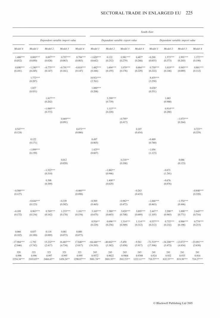
SECTORAL TRADE IN ENLARGED EU 225
© Blackwell Publishing Ltd 2005
South–East
Dependent variable: import value Dependent variable: export value Dependent variable: import value
Model 4 Model 1 Model 2 Model 3 Model 4 Model 1 Model 2 Model 3 Model 4 Model 1 Model 2 Model 3 Model 4
1.406*** 0.889*** 0.887*** 0.797*** 0.794*** -1.620*** 0.122 0.981*** 0.487* -0.200 1.573*** 1.991*** 1.372***(0.052) (0.050) (0.028) (0.083) (0.083) (0.642) (0.252) (0.279) (0.268) (0.855) (0.373) (0.203) (0.198)
0.690*** -1.240*** -0.775*** -0.791*** -0.818*** 1.482*** 1.694*** 1.079*** 0.884*** 0.750*** 1.019*** 0.945*** 0.801***(0.101) (0.245) (0.147) (0.161) (0.147) (0.166) (0.155) (0.176) (0.229) (0.222) (0.148) (0.089) (0.112)
1.772*** 10.921*** 8.435***(0.287) (2.761) (3.258)
1.027 1.000*** 0.636*(0.931) (0.208) (0.351)
1.817*** 3.299*** 1.083(0.202) (0.739) (0.988)
-1.060*** 1.115*** 0.914***(0.373) (0.220) (0.288)
0.469*** -0.795* -1.073***(0.091) (0.417) (0.264)
0.547*** 0.473*** 0.197 0.723**(0.124) (0.086) (0.454) (0.329)
0.122 0.497 -0.489(0.171) (0.803) (0.780)
-1.099*** 1.425** -1.056(0.199) (0.607) (1.123)
0.012 0.216** 0.086(0.028) (0.108) (0.123)
-1.522*** -1.882** -0.671(0.310) (0.946) (1.241)
0.398 1.408** -0.676(0.389) (0.625) (0.876)
-0.588*** -0.460*** -0.263 -0.840***(0.127) (0.098) (0.433) (0.328)
-0.644*** -0.339 -0.569 -0.962** -1.666*** -1.554***(0.123) (0.302) (0.465) (0.472) (0.463) (0.446)
-0.189 0.963*** 0.769*** 1.233*** 1.181*** 3.105*** 2.380*** 3.020*** 3.895*** 2.447** 2.208** 1.890*** 2.645***(0.172) (0.134) (0.162) (0.178) (0.154) (0.675) (0.663) (0.708) (0.689) (1.105) (0.965) (0.771) (0.716)
0.516** 0.696*** 1.314*** 1.114*** 0.557*** 0.732*** 0.986*** 0.774***(0.229) (0.256) (0.309) (0.312) (0.212) (0.232) (0.198) (0.215)
0.066 0.037 0.118 0.081 0.080(0.102) (0.100) (0.089) (0.073) (0.073)
-17.904*** -1.792 15.232*** 16.465*** 17.840*** -84.446*** -40.602*** -5.450 -9.561 -71.519*** -34.200*** -13.073*** -23.091***(2.046) (5.742) (2.417) (4.734) (3.017) (16.203) (3.382) (5.858) (5.917) (17.506) (5.473) (4.834) (3.638)
320 321 321 321 321 243 243 243 243 241 241 241 2410.996 0.996 0.997 0.995 0.995 0.9572 0.9622 0.9404 0.9388 0.924 0.932 0.933 0.914
2354.34*** 2103.65** 2468.43** 1458.24** 1290.87*** 3001.74** 2691.93** 2012.53** 1222.11*** 718.57*** 632.33*** 819.38*** 718.27***

226 Helena Marques and Hugh Metcalf
© Blackwell Publishing Ltd 2005
Table B7. Transport Equipment
North–East North–South
Dependent variable: export value Dependent variable: import value Dependent variable: export value
Model 1 Model 2 Model 3 Model 4 Model 1 Model 2 Model 3 Model 4 Model 1 Model 2 Model 3
popi 1.584*** 1.575*** 1.505*** 1.507*** 1.362*** 1.350*** 1.358*** 1.280*** 1.667*** 1.675*** 1.693***(0.058) (0.062) (0.072) (0.073) (0.099) (0.099) (0.106) (0.117) (0.074) (0.070) (0.056)
popj 1.094*** 1.011*** 0.589*** 0.594*** 1.547*** 1.601*** 1.316*** 1.263*** -0.053 0.508* 1.025***(0.135) (0.137) (0.135) (0.144) (0.120) (0.125) (0.100) (0.122) (0.411) (0.277) (0.197)
gdppci 2.905*** 2.358*** 0.760**(0.429) (0.543) (0.332)
gdppcj 0.712*** 2.179*** 3.680**(0.160) (0.229) (1.557)
gdppci*hkpci 3.485*** 1.880*** 0.788***(0.277) (0.348) (0.325)
gdppcj*hkpcj 0.722*** 2.176*** 1.220*(0.158) (0.239) (0.644)
ecdist 2.605*** 0.407 0.344***(0.454) (0.349) (0.130)
ecdist*hkdist 2.552*** 1.801***(0.152) (0.183)
hkpci 0.816*** 1.240*** 0.310(0.295) (0.294) (0.311)
hkpcj 1.811*** 0.091 -0.536*(0.317) (0.335) (0.297)
hkdist 0.002 -0.272*** 0.074(0.054) (0.077) (0.080)
dist*hkpci -2.864*** -0.402 -0.135(0.279) (0.319) (0.451)
dist*hkpcj 0.689*** -1.825*** -1.436*(0.279) (0.265) (0.753)
dist*hkdist -2.545*** -2.129***(0.133) (0.183)
dist -2.378*** -2.528*** -2.082*** -3.051*** -1.353*** -1.085***(0.215) (0.184) (0.318) (0.282) (0.373) (0.286)
border -1.222*** -0.782** -1.403*** -1.365*** -0.174 -0.191 -1.699*** -0.414 0.539*** 0.491*** 0.531**(0.367) (0.325) (0.270) (0.259) (0.451) (0.361) (0.470) (0.350) (0.195) (0.194) (0.225)
EA 0.451*** 0.459*** 0.598*** 0.601*** 0.736*** 0.730*** 0.911*** 0.851***(0.175) (0.173) (0.194) (0.194) (0.188) (0.192) (0.223) (0.221)
EURO 0.061 0.204* 0.272**(0.114) (0.109) (0.114)
constant -39.178*** -46.755*** -27.498*** -26.937*** -56.138*** -49.532*** -13.979*** -32.582*** -41.802*** -24.704*** -21.888***(6.812) (3.815) (6.319) (2.541) (8.803) (3.423) (5.068) (1.901) (11.347) (5.355) (5.249)
No obs 900 900 900 900 869 869 869 869 320 320 320R2 0.9712 0.9718 0.9679 0.9677 0.939 0.938 0.934 0.926 0.990 0.990 0.988Wald Chi2 4072.88*** 3470.12*** 1674.04*** 1876.18*** 2112.48** 2001.87** 1537.23** 1044.2*** 4930.12*** 5108.39*** 1822.89***
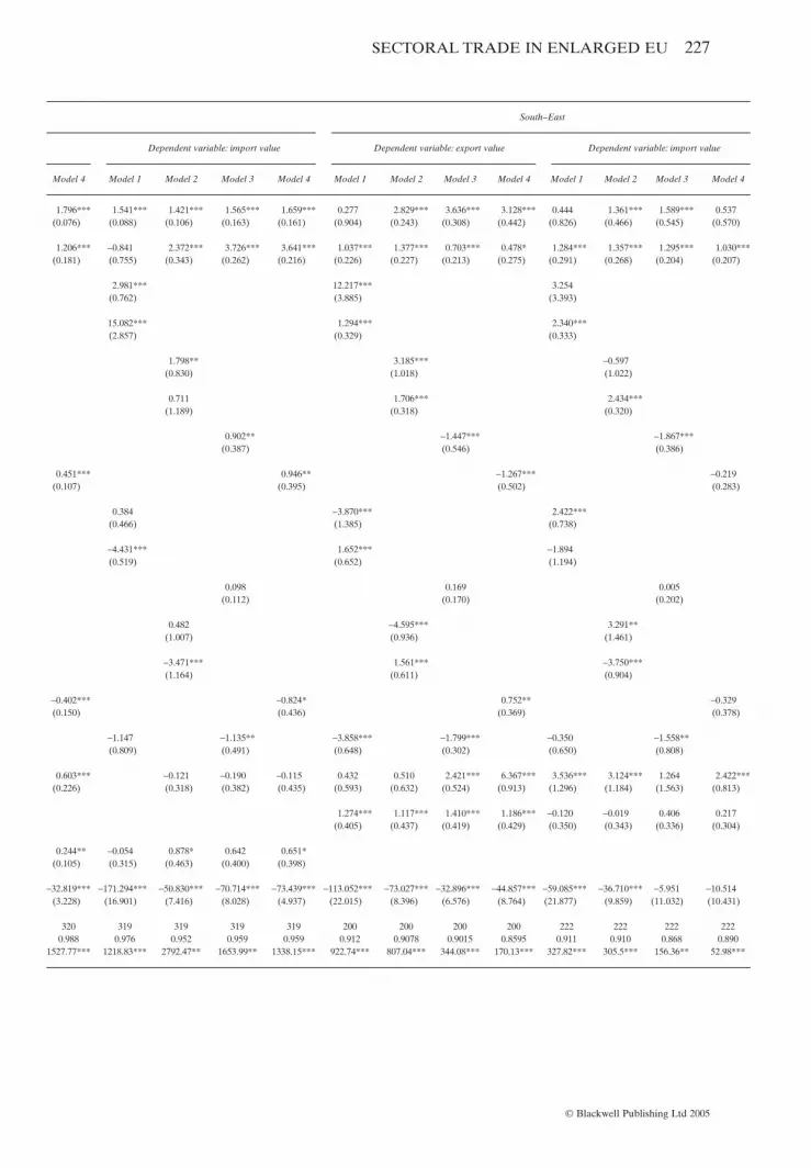
SECTORAL TRADE IN ENLARGED EU 227
© Blackwell Publishing Ltd 2005
South–East
Dependent variable: import value Dependent variable: export value Dependent variable: import value
Model 4 Model 1 Model 2 Model 3 Model 4 Model 1 Model 2 Model 3 Model 4 Model 1 Model 2 Model 3 Model 4
1.796*** 1.541*** 1.421*** 1.565*** 1.659*** 0.277 2.829*** 3.636*** 3.128*** 0.444 1.361*** 1.589*** 0.537(0.076) (0.088) (0.106) (0.163) (0.161) (0.904) (0.243) (0.308) (0.442) (0.826) (0.466) (0.545) (0.570)
1.206*** -0.841 2.372*** 3.726*** 3.641*** 1.037*** 1.377*** 0.703*** 0.478* 1.284*** 1.357*** 1.295*** 1.030***(0.181) (0.755) (0.343) (0.262) (0.216) (0.226) (0.227) (0.213) (0.275) (0.291) (0.268) (0.204) (0.207)
2.981*** 12.217*** 3.254(0.762) (3.885) (3.393)
15.082*** 1.294*** 2.340***(2.857) (0.329) (0.333)
1.798** 3.185*** -0.597(0.830) (1.018) (1.022)
0.711 1.706*** 2.434***(1.189) (0.318) (0.320)
0.902** -1.447*** -1.867***(0.387) (0.546) (0.386)
0.451*** 0.946** -1.267*** -0.219(0.107) (0.395) (0.502) (0.283)
0.384 -3.870*** 2.422***(0.466) (1.385) (0.738)
-4.431*** 1.652*** -1.894(0.519) (0.652) (1.194)
0.098 0.169 0.005(0.112) (0.170) (0.202)
0.482 -4.595*** 3.291**(1.007) (0.936) (1.461)
-3.471*** 1.561*** -3.750***(1.164) (0.611) (0.904)
-0.402*** -0.824* 0.752** -0.329(0.150) (0.436) (0.369) (0.378)
-1.147 -1.135** -3.858*** -1.799*** -0.350 -1.558**(0.809) (0.491) (0.648) (0.302) (0.650) (0.808)
0.603*** -0.121 -0.190 -0.115 0.432 0.510 2.421*** 6.367*** 3.536*** 3.124*** 1.264 2.422***(0.226) (0.318) (0.382) (0.435) (0.593) (0.632) (0.524) (0.913) (1.296) (1.184) (1.563) (0.813)
1.274*** 1.117*** 1.410*** 1.186*** -0.120 -0.019 0.406 0.217(0.405) (0.437) (0.419) (0.429) (0.350) (0.343) (0.336) (0.304)
0.244** -0.054 0.878* 0.642 0.651*(0.105) (0.315) (0.463) (0.400) (0.398)
-32.819*** -171.294*** -50.830*** -70.714*** -73.439*** -113.052*** -73.027*** -32.896*** -44.857*** -59.085*** -36.710*** -5.951 -10.514(3.228) (16.901) (7.416) (8.028) (4.937) (22.015) (8.396) (6.576) (8.764) (21.877) (9.859) (11.032) (10.431)
320 319 319 319 319 200 200 200 200 222 222 222 2220.988 0.976 0.952 0.959 0.959 0.912 0.9078 0.9015 0.8595 0.911 0.910 0.868 0.890
1527.77*** 1218.83*** 2792.47** 1653.99** 1338.15*** 922.74*** 807.04*** 344.08*** 170.13*** 327.82*** 305.5*** 156.36** 52.98***

228 Helena Marques and Hugh Metcalf
© Blackwell Publishing Ltd 2005
Table B8. Wood Products
North–East North–South
Dependent variable: export value Dependent variable: import value Dependent variable: export value
Model 1 Model 2 Model 3 Model 4 Model 1 Model 2 Model 3 Model 4 Model 1 Model 2 Model 3
popi 1.219*** 1.145*** 1.110*** 1.101*** 1.187*** 1.220*** 1.088*** 1.101*** 1.396*** 1.339*** 1.228***(0.071) (0.074) (0.064) (0.073) (0.107) (0.112) (0.110) (0.114) (0.136) (0.121) (0.105)
popj 0.890*** 0.731*** 0.597*** 0.584*** 1.044*** 1.078*** 0.791*** 0.809*** 0.622 1.161** 1.077***(0.135) (0.141) (0.099) (0.106) (0.170) (0.170) (0.138) (0.138) (0.607) (0.555) (0.408)
gdppci 1.753*** 2.867*** 3.344***(0.343) (0.474) (0.564)
gdppcj 0.510*** 0.890*** 2.867*(0.183) (0.218) (1.723)
gdppci*hkpci 2.670*** 2.386*** 3.245***(0.190) (0.269) (0.621)
gdppcj*hkpcj 0.501*** 0.925*** -0.983(0.175) (0.210) (1.174)
ecdist 1.335*** 1.751*** 0.585***(0.276) (0.370) (0.215)
ecdist*hkdist 2.006*** 1.320***(0.143) (0.204)
hkpci 1.170*** 1.191*** 0.127(0.207) (0.240) (0.330)
hkpcj 1.060*** 0.814** -0.230(0.312) (0.395) (0.363)
hkdist -0.034 0.100* -0.003(0.041) (0.053) (0.038)
dist*hkpci -1.976*** -1.045*** -2.833***(0.230) (0.359) (0.798)
dist*hkpcj -0.056 -0.018 1.321(0.214) (0.327) (1.205)
dist*hkdist -2.091*** -1.197***(0.157) (0.230)
dist -2.270*** -2.361*** -0.822** -0.984*** -0.325 -0.285(0.253) (0.235) (0.408) (0.347) (0.589) (0.728)
border -0.657** -0.143 -0.909*** 0.005 1.962*** 1.477*** 1.545*** 1.111*** 0.181 0.143 0.901*(0.293) (0.263) (0.309) (0.187) (0.695) (0.476) (0.598) (0.363) (0.571) (0.493) (0.510)
EA 0.554*** 0.577*** 0.710*** 0.642*** 0.374*** 0.380*** 0.463*** 0.486***(0.179) (0.176) (0.195) (0.199) (0.154) (0.155) (0.152) (0.157)
EURO -0.106 0.088 0.173(0.185) (0.198) (0.220)
constant -20.383*** -30.620*** -11.362*** -19.823*** -46.035*** -40.088*** -26.128*** -20.710*** -76.522*** -35.874*** -25.989**(7.890) (4.225) (4.680) (2.047) (9.423) (4.840) (6.251) (2.423) (14.571) (9.292) (11.996)
No obs 893 893 893 893 915 915 915 915 320 320 320R2 0.9734 0.9739 0.9724 0.969 0.974 0.974 0.966 0.966 0.979 0.978 0.980Wald Chi2 2166.29** 2431.36** 1957.5*** 2598.88*** 2075.33** 2292.92** 1871.08** 1879.7*** 1668.00** 1112.95** 949.85**

SECTORAL TRADE IN ENLARGED EU 229
© Blackwell Publishing Ltd 2005
South–East
Dependent variable: import value Dependent variable: export value Dependent variable: import value
Model 4 Model 1 Model 2 Model 3 Model 4 Model 1 Model 2 Model 3 Model 4 Model 1 Model 2 Model 3 Model 4
1.148*** 0.939*** 1.001*** 0.978*** 1.069*** 0.259 1.078*** 1.728*** 1.429*** 0.498 1.551*** 2.165*** 1.420***(0.082) (0.064) (0.033) (0.070) (0.080) (1.113) (0.399) (0.425) (0.508) (0.518) (0.224) (0.319) (0.397)
1.241*** -0.534 0.762*** 1.634*** 1.888*** 0.768*** 0.879*** 0.276 -0.047 1.211*** 1.329*** 0.715*** 0.559***(0.261) (0.455) (0.219) (0.171) (0.111) (0.210) (0.190) (0.210) (0.253) (0.138) (0.163) (0.207) (0.210)
1.162** 7.394 6.416***(0.563) (4.577) (1.938)
7.733*** 0.964*** 1.488***(1.812) (0.363) (0.162)
0.620 4.107*** 1.933***(0.604) (0.881) (0.636)
1.478* 1.094*** 1.643***(0.872) (0.272) (0.148)
0.098 -0.261 -0.804***(0.141) (0.377) (0.267)
0.822*** 0.093 0.419 0.448(0.194) (0.150) (0.365) (0.356)
0.654*** 0.904 0.682(0.178) (0.802) (0.644)
-3.024*** 1.336* 0.286(0.410) (0.728) (0.680)
0.112* 0.133 0.177(0.067) (0.152) (0.137)
1.054 -2.733*** -0.859(0.712) (0.862) (0.885)
-3.603*** 0.770 -0.626(0.682) (0.512) (0.668)
-0.805*** -0.034 -0.711* -0.737***(0.205) (0.176) (0.397) (0.281)
-2.119*** -1.111*** -2.110*** -2.627*** -1.543*** -2.784***(0.210) (0.393) (0.766) (0.545) (0.388) (0.471)
0.443 0.476** 0.581*** 0.952*** 1.261*** 1.353* 1.264 1.094** 4.028*** 2.02*** 1.779*** 0.198 3.080***(0.351) (0.204) (0.214) (0.245) (0.258) (0.826) (0.893) (0.471) (0.715) (0.649) (0.661) (0.539) (0.573)
0.992*** 1.091*** 1.589*** 1.157*** 0.353** 0.518*** 1.034*** 0.870***(0.260) (0.260) (0.315) (0.288) (0.179) (0.180) (0.209) (0.271)
0.156 -0.037 0.318 0.233 0.221(0.222) (0.176) (0.208) (0.191) (0.192)
-25.462*** -67.929*** -17.010*** -20.243*** -34.343*** -60.786*** -44.406*** -0.196 -12.592 -73.216*** -48.804*** -6.892 -21.021***(4.203) (12.317) (3.129) (6.041) (2.876) (24.598) (8.604) (11.356) (11.461) (10.629) (4.720) (4.943) (6.163)
320 321 321 321 321 212 212 212 212 217 217 217 2170.983 0.981 0.982 0.980 0.974 0.768 0.7848 0.8268 0.8174 0.945 0.951 0.947 0.923
513.82*** 12,770.07** 6329.83** 5064.83** 2138.20*** 283.05*** 280.87*** 136.84*** 96.38*** 840.31*** 692.88*** 387.07** 267.61***

References
Baldwin, Richard, Towards an Integrated Europe, London: CEPR (1994).Baldwin, Richard, Rikard Forslid, Jan Haaland, and Karen-Helene Midelfart-Knarvik, “EU
Integration and Outsiders: A Simulation Study of Industrial Location,” Norwegian School ofEconomics and Business Administration Discussion Paper 02/2000 (2000).
Breuss, Fritz and Peter Egger, “How Reliable Are Estimations of East–West Trade PotentialsBased on Cross-Section Gravity Analyses?,” Empirica 26 (1999):81–94.
Buch, Claudia and Daniel Piazolo, “Capital and Trade Flows in Europe and the Impact ofEnlargement,” Economic Systems 25 (2001):183–214.
Davis, Donald,“Understanding International Trade Patterns:Advances of the 1990s,” Integration& Trade 4 (2000):61–79.
Fidrmuc, Jarko, “Application of Gravity Models to Commodity Groups and Trade Projectionsbetween the EU and the CEECs,” manuscript, Vienna: Institute for Advanced Studies (1998).
Hamilton, Carl and Alan Winters, “Opening Up International Trade with Eastern Europe,” Eco-nomic Policy 14 (1992):77–116.
Havrylyshyn, Oleg and Lance Pritchett, “European Trade Patterns after the Transition,” WorldBank Working Paper 748 (1991).
Krugman, Paul, “Increasing Returns and Economic Geography,” Journal of Political Economy99 (1991):483–99.
———, “The Hub Effect, or Threeness in Interregional Trade,” in Wilfred Ethier, ElhananHelpman, and Peter Neary (eds), Theory, Policy and Dynamics in International Trade,Cambridge: Cambridge University Press (1993), pp. 29–37.
Limao, Nuno and Anthony Venables, “Infrastructure, Geographical Disadvantage, TransportCosts and Trade,” World Bank Economic Review 15 (2001):451–79.
Linder, Staffan, An Essay on Trade and Transformation, New York: Wiley (1961).Marques, Helena and Hugh Metcalf, “The EU’s New Economic Geography after the Eastern
Enlargement,” Journal of Economic Integration 18 (2003):627–41.Matyas, Lazlo, “Proper Econometric Specification of the Gravity Model,” World Economy 20
(1997):363–8.———, “The Gravity Model: Some Econometric Considerations,” World Economy 21
(1998):397–401.Maurel, Mathilde and Guillaume Cheikbossian, “The New Geography of Eastern European
Trade,” Kyklos 51 (1998):45–71.Melitz, Jacques, “Geography, Trade and Currency Union,” CEPR Discussion Paper 2987 (2001).Nilsson, Lars, “Trade Integration and the EU Membership Criteria,” European Journal of Politi-
cal Economy 16 (2000):807–27.Persson, Torsten, “Currency Unions and Trade: How Large Is the Treatment Effect?,” Economic
Policy 16 (2001):433–62.Pratten, Chris, “A Survey of Economies of Scale,” in CEC (ed.), Research on the Cost of Non-
Europe, Luxembourg: CEC (1988).Redding, Stephen and Anthony Venables, “Economic Geography and International Inequality,”
Journal of International Economics 62 (2004):53–82.Rice, Patricia, Martin Stewart and Anthony Venables, “The Geography of Intraindustry Trade:
Empirics,” Topics in Economic Analysis and Policy 3 (2003).Rose, Andrew, “One Money, One Market: The Effect of Common Currencies on Trade,” Eco-
nomic Policy 15 (2000):7–46.Venables, Anthony, “Geography and International Inequalities: The Impact of New Tech-
nologies,” CEP Discussion Paper 507 (2001).Vittas, Hari and Polo Mauro, “Potential Trade with Core and Periphery: Industry Differences in
Trade Patterns,” in Stanley Black (ed.), Europe’s Economy Looks East, Cambridge: Cam-bridge University Press (1997), pp. 67–99.
Winters, Alan and Zhen Wang, “The Trading Potential of Eastern Europe,” Journal of EconomicIntegration 7 (1992):113–36.
230 Helena Marques and Hugh Metcalf
© Blackwell Publishing Ltd 2005

Notes
1. In the paper we refer to CEECs, or alternatively to EU-East, as being the group formed byCzech Republic, Estonia, Hungary, Latvia, Lithuania, Poland, Slovak Republic, Slovenia, and,on the assumption that they will effectively join the EU, Bulgaria, and Romania.2. We define EU-North as the group formed by all EU-15 countries except Greece, Portugal,and Spain.3. We define EU-South as the group formed by Greece, Portugal, and Spain.4. The hub effect was introduced by Krugman (1993) in a three country model: a country is saidto be a hub if the spatial trade costs between itself and each of the two other countries are lowerthan the spatial trade costs between the latter two.5. We have also run alternative regressions with GDP as a measure of size. The coefficientsobtained were exactly the same as when population was used. Population was selected as themeasure of size, as it potentially raises less endogeneity problems than GDP. In addition,the market size measure is intended to proxy for demand in the sense that the whole popula-tion constitutes demand, this is, we are all active in consumption. Even for the exporting country,the size variable represents demand, as with economies of scale the larger countries will be ableto produce at a lower average cost and, thus, will be more competitive as exporters.6. The robustness of the use of this variable as a test for the HOS model must be qualified. TheBarro–Lee dataset used to construct the human capital variable, does not allow disaggregationof those with tertiary education in terms of level and type of skills. As a consequence, we arenot able to tell how homogeneous our skilled workers are or to match skills across countries.Hence, the implications for the HOS model must be interpreted with caution.7. The coefficients and p-values shown, are averages across model specifications in the case ofvariables common to more than one specification. For example, population and border arepresent in all four models and, thus, we take the average of the coefficients obtained in each ofthem.
SECTORAL TRADE IN ENLARGED EU 231
© Blackwell Publishing Ltd 2005


