Embed Size (px)
Citation preview

EXPERIMENTAL ANALYSIS AND VALIDATION OF A NUMERICAL PCM MODEL FOR
BUILDING ENERGY PROGRAMS
by
Wijesuriya Arachchige Sajith Indika Wijesuriya
ii
A thesis submitted to the Faculty and the Board of Trustees of the Colorado School of
Mines in partial fulfillment of the requirements for the degree of Doctor of Philosophy
(Mechanical Engineering).
Golden, Colorado
Date ---------------------------------------------------
Signed: ------------------------------------------------- Wijesuriya Wijesuriya
Signed: ------------------------------------------------- Dr. Paulo Tabares-Velasco
Thesis Advisor
Golden, Colorado
Date ---------------------------------------------------
Signed: ------------------------------------------------- Dr. John Berger
Professor and Department Head Department of Mechanical Engineering
iii
ABSTRACT
The increase in peak electricity demand in recent years has stressed the importance of peak
electricity demand shifting technologies. Phase Change Materials (PCMs) have a potential to
improve the building envelope by increasing the thermal mass as well as contribute to a significant
peak shift in whole building power demand. Therefore, special attention is given to properly
capture the thermal behavior of PCMs in advanced building energy modeling software. Design of
effective PCM thermal storage systems requires accurate energy modeling. There are analytical
and numerical models developed during last few decades for this purpose, many have not been
fully validated. Based on the current status of literature, the study identifies the limitations and
drawbacks of existing methods. A parametric study is conducted to identify the optimum PCM
thermo-physical properties, PCM locations in building envelope, under forced convection and a 5
hour pre-cooling strategy. Furthermore, an improved advanced numerical building envelope model
is created in MATLAB to simulate the PCM performance in building envelope and an
experimental apparatus is constructed to obtain useful experimental data for PCM included wall
assemblies for validation purposes. This thesis also uses two datasets from laboratory studies of
shape-stabilized and field studies Nano-PCMs to validate and compare PCM modelling algorithms
of 6 modules in 5 building energy modelling software. Finally, two macroencapsulated PCMs (Bio
based PCM and hydrate salts) are tested using the experimental apparatus to obtain data for
validation purposes. To approximate the heat transfer through a wall assembly with PCM pouches
several techniques are investigated that can capture 3D heat transfer characteristics. Method with
the highest agreement is used to validate and compare the developed MATLAB algorithm and
different building energy modelling software.
iv
TABLE OF CONTENTS
LIST OF FIGURES ....................................................................................................................... ix
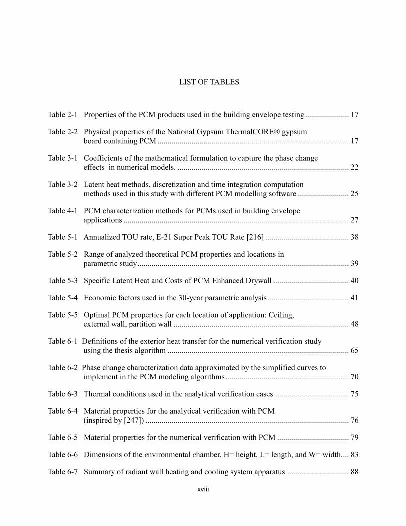
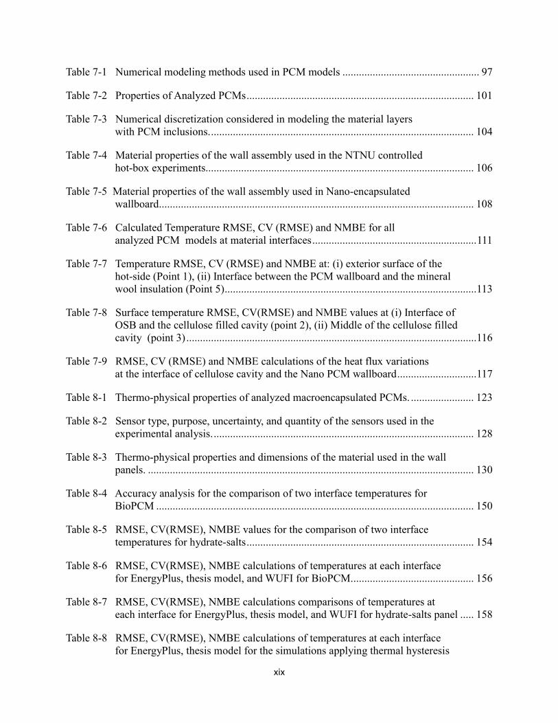
LIST OF TABLES ..................................................................................................................... xviii
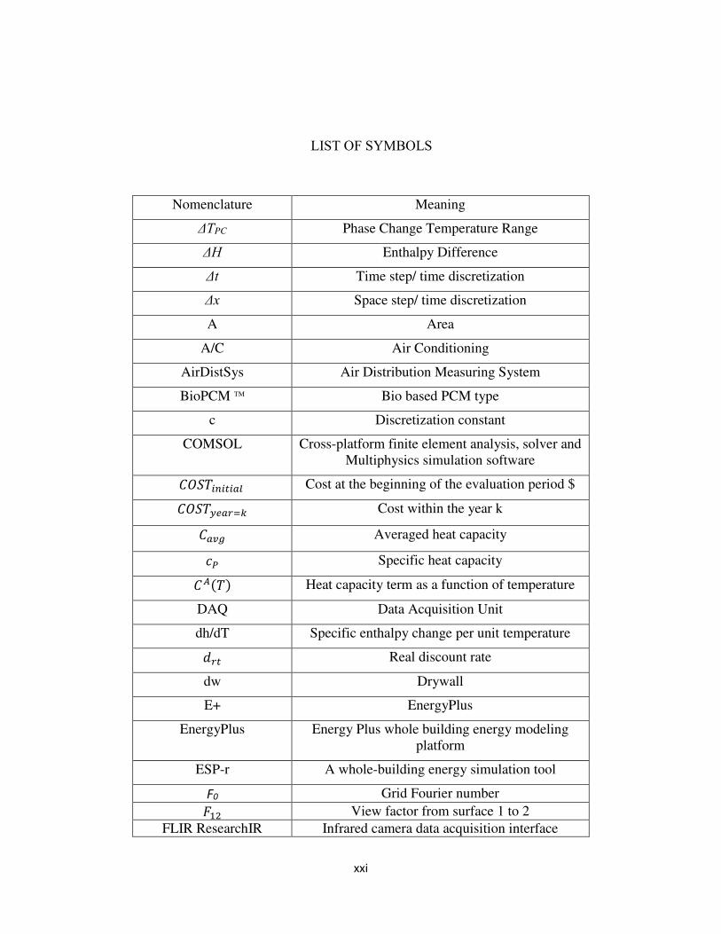
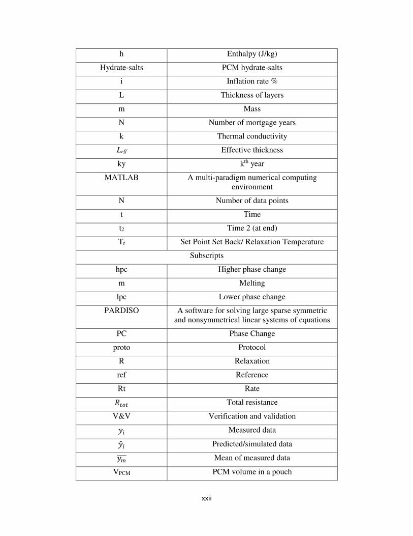
LIST OF SYMBOLS ................................................................................................................... xxi
CHAPTER 1 INTRODUCTION ...................................................................................................1
CHAPTER 2 BACKGROUND AND SIGNIFICANCE ...............................................................5
2.1. Phenomena of Phase Change of PCMs ................................................................................ 6
2.2. PCM encapsulation methods ................................................................................................ 7
2.3. Thermal characteristics and properties of PCMs ............................................................... 10
“Mushy” region of Phase Change ................................................................................ 10
Phase separation of the material .................................................................................. 12
Subcooling/supercooling effect and Hysteresis ........................................................... 12
PCM Thermal conductivity ......................................................................................... 14
PCM phase-change temperature range ........................................................................ 14
2.4. Types of PCMs ................................................................................................................... 15
Analyzed PCMs ........................................................................................................... 16
CHAPTER 3 MODELING PCMS IN BUILDING ENVELOPE ...............................................19
3.1. Analytical Models .............................................................................................................. 20
3.2. Numerical Models .............................................................................................................. 20
Numerical models: Simulation methods ...................................................................... 20
Numerical Models: Grid and boundary considerations. .............................................. 23
Numerical Models: Discrete forms and solution schemes .......................................... 23
Numerical Models: In building energy modeling platforms ....................................... 24
v
CHAPTER 4 EXPERIMENTAL STUDIES ON PCM INCLUSION IN BUILDING ENVELOPE .........................................................................................................26
4.1. Scale of experimental studies ............................................................................................. 26
4.2. PCM characterization methods .......................................................................................... 26
Differential Scanning Calorimetry (DSC) ................................................................... 27
T-history method ......................................................................................................... 28
Thermogravimetric analyses (TG) ............................................................................... 29
Dynamic Hot Box Method ........................................................................................... 29
Heat Flow Meter Apparatus (HFMA) methods ........................................................... 30
Other methods .............................................................................................................. 32
4.3.Experimental studies on macroencapsulated and microencapsulated PCMs ...................... 32
CHAPTER 5 PARAMETRIC ANALYSIS OF A RESIDENTIAL BUILDING WITH PHASE CHANGE MATERIAL (PCM)-ENHANCED DRYWALL, PRE-COOLING, AND VARIABLE ELECTRIC RATES IN A HOT AND DRY CLIMATE .........34
5.1. Approach ............................................................................................................................ 36
Building Description .................................................................................................... 37
Precooling Strategy ...................................................................................................... 42
Convection Heat Transfer ............................................................................................ 43
Mechanical Ventilation and Fan Selection .................................................................. 44
5.2. Results and Discussion ....................................................................................................... 45
Parametric analysis results ........................................................................................... 45
Hourly Results ............................................................................................................. 48
5.3. Conclusions ........................................................................................................................ 60
CHAPTER 6 NUMERICAL HEAT TRANSFER MODEL FOR OPAQUE WALLS AND DESCRIPTION OF LABORATORY FACILITY FOR EXPERIMENTAL ANALYSIS ...........................................................................................................62
6.1. 1D heat transfer algorithm to model building walls with PCM ......................................... 63
6.2. Modeling of PCM inclusions in the thesis model .............................................................. 66
vi
Modeling hysteresis in the thesis model ...................................................................... 67
6.3. PCM modeling objects in building energy modeling software .......................................... 71
EnergyPlus PCM modules ........................................................................................... 71
WUFI PCM module ..................................................................................................... 72
6.4. Numerical PCM building envelope model verification ..................................................... 73
Analytical Verification ................................................................................................ 73
Numerical Verification ................................................................................................ 78
6.5. State-of-the-art Laboratory for full-scale experimental studies of PCMs .......................... 81
Wall Assembly Tests ................................................................................................... 81
Environmental Chamber and the HVAC System ........................................................ 82
HVAC and Chamber Instrumentation System ............................................................ 84
Control and Data Acquisition ...................................................................................... 86
Construction of Building Envelope Assemblies within the Chamber ......................... 91
CHAPTER 7 EMPIRICAL VALIDATION AND COMPARISON OF PCM MODELING ALGORITHEMS COMMONLY USED IN BUILDING ENERGY AND HYGROTHERMAL SOFTWARE ......................................................................93
7.1. Introduction ........................................................................................................................ 93
7.2. Methodology ...................................................................................................................... 95
Validation .................................................................................................................... 99
Enthalpy-temperature curves of PCMs ...................................................................... 102
Numerical modeling considerations .......................................................................... 103
Shape-stabilized PCM wall data ................................................................................ 106
Nano-encapsulated wallboard data ............................................................................ 107
7.3. Results and Discussion ..................................................................................................... 109
NTNU shape-stabilized PCM .................................................................................... 109
Nano-encapsulated PCM wall ................................................................................... 113
vii
7.4. Conclusions ...................................................................................................................... 118
CHAPTER 8 EMPIRICAL VALIDATION AND COMPARISON OF PCM ALGORITHMS MODELING MACRO-ENCAPSULATED PCMS IN THE BUILDING ENVELOPE ....................................................................................................... 119
8.1. Introduction ...................................................................................................................... 119
8.2. Methodology .................................................................................................................... 122
Macroencapsulated Phase Change Materials ............................................................. 122
Full scale testing environment ................................................................................... 127
Envelope assemblies .................................................................................................. 129
Cooling and heating temperature set-points for full-cycle tests ................................ 133
Heat transfer modeling of macroencapsulated PCMs................................................ 134
Using the simplified methods in the 1D thesis model ............................................... 142
PCM models used in Building energy and hygrothermal software ........................... 144
Validation .................................................................................................................. 144
8.3. Results and Discussion ..................................................................................................... 145
Temperature variation on the surfaces of the panels ................................................. 145
Temperature variation of the PCMs behind drywall ................................................. 147
Comparison of heat transfer approaches for PCM macroencapsulation ................... 148
Comparison of EnergyPlus, thesis model, and WUFI software ................................ 155
Validation study with hysteresis characteristic data .................................................. 158
8.4.Conclusions ....................................................................................................................... 162
CHAPTER 9 CONCLUSIONS AND FUTURE WORK ............................................................164
9.1. Summary of significant results ......................................................................................... 164
9.2. Potential for Future Work ................................................................................................. 166
Further development of the building envelope model ............................................... 166
Laboratory experiments of different PCMs ............................................................... 166
viii
REFERENCES CITED ................................................................................................................168
APPENDIX A. DISCRETE FORMS PREVIOUSELY USED IN NUMERICALLY MODELLING PCMS .........................................................................................199
APPENDIX B. SUMMERY OF WHERE WHOLE BUILDING ENERGY MODELING PLATFORMS WITH PCM MODELS ARE USED ..........................................200
APPENDIX C. COST CALCULATION PROCEDURES OF BEOPT ......................................204
APPENDIX D. SENSOR INFORMATION OF THE CHAMBER, HVAC SYSTEM, AND OUTSIDE ...........................................................................................................206
APPENDIX E. SENSOR INFORMATION OF THE CHAMBER, HVAC SYSTEM, AND OUTSIDE ...........................................................................................................209
ix
LIST OF FIGURES
Figure 2-1 Different PCM encapsulation types: (a) microencapsulated PCMs embedded in drywall, (b) Shape-stabilized PCMs: thin PCM layers enclosed between aluminum foil sheets, and (c) Macroencapsulated PCMs: PCMs enclosed in pouches. Figure shows the dimensions of the single PCM included unit and the commercially available dimensions. ..................................................................... 9
Figure 2-2 Enthalpy variation across the mushy region and deviation observed in PCMs used in building applications (Real PCM) in contrast to an ideal PCM. Graph shows the melting temperature range, melting latent heat, and melting sensible heat of the PCM. Graph constructed based on the data provided by [14]. ................ 10
Figure 2-3 Sensible heat and latent heat in the enthalpy change during the melting process. Graph constructed based on the data provided by [14]. .............................................11
Figure 2-4 Enhanced view of different PCM enthalpy curve combinations showing hysteresis (a) Subcooling effect and freezing temperature curve comes back and overlay on the melting curve, (b) subcooling causing separate curves for melting and freezing (c) hysteresis due to slow latent heat release, (d) apparent hysteresis due to non-isothermal conditions in measurements (Enthalpy data available at [53] and the curve concept inspired by [54]). ................ 13
Figure 2-5 Melting enthalpy and melting temperature (𝑇𝑚)– for different PCMs, An important criterion in selecting PCMs for building envelope applications: .. .... 15
Figure 2-6 Visualization of PCM packing in pouches once heated to a temperature of ~90 ˚C. . 18
Figure 3-1 Different scales of building energy modeling considered in the current study are at building scale, envelope scale. The PCM modeling algorithm incorporates PCM characteristics in the envelope modeling algorithm. ........................................ 19
Figure 5-1 View of the simulated house, orientation and, and its neighboring buildings. .......... 37
Figure 5-2 Enthalpy curves showcasing 1) Real PCM data from BioPCMTM Q23º obtained from DSC test and 2) Ideal PCM curves with thermal properties similar to the real PCM. ............................................................................................ 39
Figure 5-3 Multilayer envelope constructions of the evaluated home indicating the location of the PCM-drywall. The interior environment is on the right and the exterior environment is on the left for all cases (the layer thicknesses does not represent the actual scale). ........................................................................................................ 41
x
Figure 5-4 Precooling strategy with 25.6 °C setback temperature. The peach-shaded rectangle indicates peak hours while the blue shaded-region indicates precooling. ................................................................................................................. 42
Figure 5-5 Heat transfer coefficient values used next to the ceiling and exterior wall within the living zone for, (i) forced convection model (FC), (ii) CeilingDiffuser convection model (CeilingDiffuser) and (iii) natural convection model (NC). ........ 44
Figure 5-6 BEopt parametric results, where each point represents a simulated home with a different combination of PCM properties and locations. The point close to the upper right corner and in red color represents the home with no PCM or pre-cooling. Point closest to the lower left corner in black color represents a home with precooling but no PCMs. ...................................................................... 45
Figure 5-7 BEopt parametric results for the cases with lowest energy related costs, where each point represents a simulated home with a different combination of PCM properties and locations. The point close to the upper right corner represents the home with no PCM. ........................................................................... 46
Figure 5-8 Selection of optimum points for each PCM location and envelope condition: PCMs in all three locations (3 Different PCMs optimized), single/same type of PCMs in three locations (A single PCM) and PCMs only in the ceiling (PCMs in ceiling only). Each of these points are the lowest annualized energy related cost (AERC) points for each category above. ........................................................... 47
Figure 5-9 Annual variation of temperatures for the forced convection mode for PCMsoptimized for all locations. 0 indicates the start of the month January and the time is shown for the calendar year of 12 months. .............................................. 48
Figure 5-10 Annual variation of temperatures for the natural convection mode for PCMs optimized for all locations. X-axis represent the months of the year. 0 indicates the start of the month January and the time is shown for the calendar year of 12 months. ...................................................................................................................... 49
Figure 5-11 Average indoor air temperature within the living zone for forced convection model for all envelope types. Hour 0 represents midnight of the first day. .............. 50
Figure 5-12 Average indoor air temperature for the natural convection model for all envelope types. Hour 0 represents midnight of the first day. .................................... 50
Figure 5-13 Average indoor air temperature for homes with pre-cooling only and forced convection mode, and three setback temperatures (Tr): 24.4, 25.5 and 26.7˚C. Hour 0 represents midnight of the first day. .............................................................. 51
Figure 5-14 Averaged indoor air temperature for homes with PCMs optimized in each location, with forced convection mode, three setback temperatures (Tr): 24.4, 25.5 and 26.7˚C. Indoor air temperature for Tr: 25.5 ˚C and 26.7 ˚C perform the same. Hour 0 represents midnight of the first day. ................................ 52
xi
Figure 5-15 Averaged PCM-drywall temperature in external wall for homes with PCMs optimized in each location, with forced convection mode, three setback temperatures (Tr): 24.4, 25.56 and 26.67˚C. Average drywall temperature (at ceiling) for Tr: 25.5 ˚C and 26.7 ˚C. Hour 0 represents midnight of the first day. ..................................................................................................................... 53
Figure 5-16 Averaged PCM-drywall temperature in the external wall for the PCM optimized and installed in all drywall (PCM optimized) case: A comparison between the forced convection model and natural convection models. ........................................ 53
Figure 5-17 Average drywall temperature of the exterior wall under forced convection (FC) and natural convection (NC) model for, PCM optimized and installed in all drywall (PCM optimized case) and regular drywall (No PCM case). Hour 0 represents midnight of the first day. .......................................................................... 54
Figure 5-18 Average drywall temperature of the ceiling under forced convection (FC) and natural convection (NC) models for, PCM optimized and installed in all drywall (PCM optimized case) and regular drywall (No PCM case). Hour 0 represents midnight of the first day. ........................................................................................... 54
Figure 5-19 Heat gain rates per unit area of the ceiling drywall for forced and natural convection models for cases: (i) No-PCM and precooling only (ii) PCMs included in the ceiling only. Hour 0 represents midnight of the first day. ................ 55
Figure 5-20 Cooling electricity power consumption variations for all cases with the forced convection model for July 22. Hour 0 represents midnight of the first day. ............. 56
Figure 5-21 Cooling electricity power consumption for all analyzed cases with the natural convection mode for July 22. .................................................................................... 56
Figure 5-22 Cost variations through the day when TOU rates are applied during the peak time for July 22 for all analyzed cases and with the forced convection. ................... 57
Figure 5-23 Cost variations through the day when TOU rates are applied during the peak time for July 22 for all analyzed cases and with the natural convection. .................. 57
Figure 5-24 Aggregated cooling and ventilation related electricity consumption in the precooling months (May-Oct), assuming the fan power is 25W for each fan. ......... 58
Figure 5-25 Aggregated cooling and ventilation related electricity consumption in the precooling months (May-Oct), assuming the fan power is 2 W for each fan............ 58
Figure 5-26 Seasonal cooling electricity energy cost for May-Oct period for each analyzed case with natural and forced convection assuming the fan power is 25W for each fan. ...................................................................................................... 59
Figure 5-27 Seasonal cooling electricity energy cost for May-Oct period for each analyzed case with natural and forced convection assuming the fan power is 2W for
xii
each fan. ..................................................................................................................... 60
Figure 6-1 Structure of the full validation study includes analytical verification, comparative testing, and empirical validation. .......................................................... 62
Figure 6-2 Structure of interior and interface nodes, space and time discretization of the 1D algorithm. ............................................................................................................. 64
Figure 6-3 Structure of the functions in the numerical envelope model. ..................................... 65
Figure 6-4 Manufacturer provided melting curve data and melting and freezing curves obtained from the Dynamic Heat Flux Meter Apparatus (DHFMA) method for the hydrate-salts PCM of InfiniteRTM (Nominal melting temperature =23 ºC). .. 68
Figure 6-5 Approximated melting curve for the PCM hydrate-salts from DSC data. ................. 69
Figure 6-6 Approximated melting curve for the PCM hydrate-salts from DHFMA data. ........... 69
Figure 6-7 Approximated freezing curve for the PCM hydrate-salts from DHFMA data. .......... 70
Figure 6-8 EnergyPlus original PCM model data input interface. ............................................... 71
Figure 6-9 EnergyPlus Hysteresis PCM model data input interface to define PCM properties for melting and freezing curves separately. .............................................. 72
Figure 6-10 WUFI PCM model data input interface indicating the enthalpy curve input............ 73
Figure 6-11 Cross section temperature variation of the semi-infinite material layer after 24h period for the PCM drywall case. .............................................................................. 77
Figure 6-12 Transient temperature variation at a location 0.021m in the material layer for (i) Analytical solution (ii) thesis model, and (iii) EnergyPlus solutions (𝛥𝑇𝑃𝐶 of 0.2 ºC is implemented in the numerical solutions). .................................. 77
Figure 6-13 Heat flux at the exterior surface of the PCM layer. .................................................. 78
Figure 6-14 West facing wall of the residential building evaluated for numerical verification. .. 80
Figure 6-15 External and internal surface temperatures of the examined exterior wall without PCM inclusions from the thesis model and EnergyPlus. ............................. 80
Figure 6-16 Verification of temperature variations on the internal and external; surfaces of the wall examined. ................................................................................................ 81
Figure 6-17 Overview of the air handling unit and the chamber, Section A: AHU Main Duct, Section B: AHU Return Duct, and Section C: Chamber .............. 82
Figure 6-18 Plan View of the Ceiling Setup of the Chamber including the inlet diffuser, lights, and exhaust diffuser. ....................................................................................... 83
xiii
Figure 6-19 SkylineTM Outdoor AHU by DAIKIN, Group: Applied Air systems, Part Number: IM 770 houses the heating and cooling elements, filters, humidifier to condition the air. .................................................................................. 84
Figure 6-20 Sensor locations in the AHU and other components of the HVAC system describes the sensors in each section, section A: Main AHU enclosure and the connection to the supply air duct and the return air duct, section B: Return air duct. ........................................................................................................................... 85
Figure 6-21 The ABB control unit consists of a (i) C1867 - MODBUS TCP Interface, (ii) PM 851 Processor UNIT, (III) 3 Analog Input Units, (iv) 1 Analog Output Unit, (v) 1 Digital Input Unit, and (vi) 1 Digital Output Unit. ......................................................................................... 86
Figure 6-22 Instrunet data acquisition unit with connections linked to the experimental apparatus sensors and some ABB main system sensors also linked to the Instrunet system to verify readings. .......................................................................... 87
Figure 6-23 Hydraulic radiant wall heating and cooling apparatus. ............................................. 87
Figure 6-24 Radiant wall flow control apparatus includes the primary flow sensor, 3 speed flow pump, temperature sensors to measure inlet and outlet temperatures of the fluid flow to the radiant wall heat exchanger. ........................... 89
Figure 6-25 Flow control valve apparatus indicates the process of flow from the boiler and flow from the chiller is mixed. The flow measurements through the radiant wall heat exchanger are also taken using the unit. ........................................ 89
Figure 6-26 PLC Control flow chart for the radiant wall control PID settings for the mixing valve operation is indicated in the Figure 6-25. ............................................ 90
Figure 6-27 Current PID settings for the mixing valve for the setpoint of 120 ºF. ....................... 90
Figure 6-28 Radiant wall location within the environmental chamber and the locations of wall assembly panels relative to the radiant wall. ................................................. 92
Figure 7-1 (a) Enthalpy-Temperature (h-T) curves for shape-stabilized PCM, (b) and nano-encapsulated PCM. .................................................................................. 102
Figure 7-2 Non-uniform finite volume mesh implemented in COMSOL simulate the Nano-PCM layer in ORNL field test data. Nano-PCM layer comprises of two elements. ...................................................................................................... 103
Figure 7-3 Non-uniform finite volume mesh implemented in WUFI to simulate the Nano-PCM layer in ORNL field test data. Nano-PCM layer comprises of 24 volumes. .................................................................................................................. 103
Figure 7-4 Uniform finite difference mesh implemented in thesis model to simulate the
xiv
Nano-PCM layer in ORNL field test data. Nano-PCM layer comprises of 4 points. ...................................................................................................................... 104
Figure 7-5 Analyzed wall assembly using shape-stabalize PCMs. Red dots represent temperature measurement points, while black hollow circles represent WUFI monitoring locations. PCMs are located in the white layer (between Point 2 and 3). .......................................................................................... 107
Figure 7-6 Analyzed wall assembly using nano-encapsulated PCMs. Red dots represent temperature measurement points, while black hollow circles represent WUFI monitoring locations. PCMs are located in the white layer (between Point 5 and 6). .......................................................................................... 108
Figure 7-7 Temperature at Point (2): between the gypsum and PCM wallboard, and measured temperature at the boundary: Point (1). Simulated data for COMSOL, ESP-r, EnergyPlus (2 modules), Thesis model, and WUFI is shown.......................................................................... 109
Figure 7-8 Temperature at the Point (3): between the PCM wallboard and mineral wool insulation. Simulated data for COMSOL, ESP-r, EnergyPlus (2 modules), Thesis model, and WUFI is shown...........................................................................110
Figure 7-9 Heat flux at the Point (1): Hot-side boundary surface. Simulated data for COMSOL, EnergyPlus (2 modules), Thesis model, and WUFI is shown. ..............112
Figure 7-10 Heat flux at the Point (3): Interface of the PCM wallboard and mineral wool insulation. Simulated data for COMSOL, EnergyPlus (2 modules), Thesis model, and WUFI is shown...........................................................................112
Figure 7-11 Temperature at the Point (2): interface of OSB and cellulose insulation Simulated data for COMSOL, ESP-r, EnergyPlus (2 modules), Thesis model, and WUFI is shown. .................................................................................................114
Figure 7-12 Temperature at the Point (3): middle of cellulose insulation. Simulated data for COMSOL, ESP-r, EnergyPlus (2 modules), Thesis model, and WUFI is shown. ........................................................................................................115
Figure 7-13 Model results at the Point (4), Point (5): interface of the cellulose insulation and the PCM wallboard. Simulated data for ESP-r, EnergyPlus (2 modules), Thesis model, and WUFI is shown...........................................................................115
Figure 7-14 Heat flux at the Point (5): interface of the cellulose cavity and the Nano PCM wallboard. Simulated data for COMSOL, EnergyPlus (2 modules), Thesis model, and WUFI is shown...........................................................................117
Figure 8-1 Dimensions of analyzed PCM pouches: (a) BioPCM, (b) hydrate-salts. ................. 122
Figure 8-2 Enthalpy-temperature melting curves obtained using DSC characterization
xv
method for BioPCM. ............................................................................................... 125
Figure 8-3 Enthalpy-temperature curves obtained using DSC and DHFMA characterization methods for PCM hydrate-salts. ................................................... 126
Figure 8-4 Schematic overview of, Section A: Air handling unit (AHU), Section B: return duct of the air to the AHU, Section C: Environmental chamber. ........................................................................ 127
Figure 8-5 Front view and the key dimensions of how the 4 panels constructed. The exposed radiant wall in the right end is insulated with 5.08 cm (2 in) of R-10 insulation. Panel 3 and 4 are shown here with the front drywall layer removed to showcase the PCM pouch mats arrangement. ...................................... 130
Figure 8-6 Front view of the PCM pouches and the sensor locations of the interface with the drywall layer removed. ............................................................................. 131
Figure 8-7 Top view of the core section with each material layers and the sensor locations (split view) (a) wall panels with just regular drywall (b) wall panels with PCM pouches and regular drywall. ........................................ 132
Figure 8-8 Radiant wall supply fluid temperature setpoint and chamber air temperature......... 133
Figure 8-9 PCM inclusion in pouches (BioPCM case is shown here) (a) front view of the uneven PCM distribution (BioPCM) (b) schematic of the side view when PCM mats are placed between plywood and the drywall. ........................................................................................ 134
Figure 8-10 Considered heat transfer simplification methods: (a) PCM distributed as a thin continuous layer, (b) PCM layer as a parallel path heat transfer, and (c) PCM as a porous material and parallel path ................................................ 135
Figure 8-11 Parallel path heat transfer across the wall assemblies with PCM pouches. This method assumes two paths across the entire assembly and assumes surfaces parallel to the heat transfer process are adiabatic. Here temperature at surface 1 and 5/ 4 and 8 are different. ................................................................. 136
Figure 8-12 Parallel path heat transfer across the wall assemblies with PCM pouches. This method assumes two paths across only the PCM layer and the nodes on the interfaces are isothermal (temperature at surface 1 and 5/ 4 and 8 are same). ...................................................................................................................... 137
Figure 8-13 Geometry based dimension reductions used in the study (a) actual view of the pouch with 3D characteristics, (b) adjusted 3D view based on PCM volume and geometry, (c) reduced 2D view with the parallel path methods, (d) using the thermal resistance values temperature dependent effective conductivity is calculated and applied for 1D thesis model. .................... 143
xvi
Figure 8-14 Boundary and interface temperatures of the wall assembly with BioPCM. Lines, 1. Exterior surface temperature, 2. Plywood-pouches interface temperature, 3. Pouches-drywall interface temperature, 4. Exterior surface temperature. .............................................................................. 146
Figure 8-15 Boundary and interface temperatures of the wall assembly with PCM hydrate salts. Lines, 1. Exterior surface temperature, 2. Plywood-pouches interface temperature, 3. Pouches-drywall interface temperature, 4. Exterior surface temperature. ......................................................... 146
Figure 8-16 Surface temperature recorded and visualized through the Infrared Camera measured every 2 hour intervals after radiant wall setpoint is increase from 40 ºC to 140 ºC. ....................................................................................................... 147
Figure 8-17 Average core surface temperature (panel 3): The temperatures at every 2 hour period is mapped with the figure Figure 8-16. ................................................ 148
Figure 8-18 Temperature at the interface of plywood and PCM of BioPCM wall panel. Lines, 1. Experimental data. 5 simplification methods: 2. Effective thickness 3. Full parallel path, solid PCM, 4. Partial parallel path, solid PCM, 5. Full parallel path, porous PCM, 6. Partial parallel path, porous PCM, and 7. Partial parallel path, without PCM (no-latent heat). ..................................... 149
Figure 8-19 Temperature at the interface of PCM and drywall of BioPCM wall panel. Lines, 1. Experimental data. 5 simplification methods: 2. Effective thickness 3. Full parallel path, solid PCM, 4. Partial parallel path, solid PCM, 5. Full parallel path, porous PCM, 6. Partial parallel path, porous PCM, and 7. Partial parallel path, without PCM (no-latent heat). ..................................... 150
Figure 8-20 Heat-flux calculations of BioPCMs panel, 1. Using heat released or absorbed by the fluid, 2. Heat flux meter measurements, and 3. Using thesis model and partial parallel path, solid PCM method. ...................... 151
Figure 8-21 Cross section temperature plot of the BioPCM panel comparing the experimental data at the beginning of the heating cycle (t=0h) and at the end of the heating cycle (t=16h) for the modeled data with the thesis model for c=1 and c=0.5 discretization constants. .......................... 152
Figure 8-22 Temperature at the interface of plywood and pouches of hydrate-salt wall panel. Lines, 1. Experimental data. 5 simplification methods: 2. Effective thickness 3. Full parallel path, solid PCM, 4. Partial parallel path, solid PCM, 5. Full parallel path, porous PCM, 6. Partial parallel path, porous PCM, and 7. Partial parallel path, without PCM (no-latent heat). ................................................................................. 153
Figure 8-23 Temperature at the interface of pouches and drywall of hydrate-salt wall panel Lines, 1. Experimental data. 5 simplification methods: 2. Effective thickness 3. Full parallel path, solid PCM,
xvii
4. Partial parallel path, solid PCM, 5. Full parallel path, porous PCM, 6. Partial parallel path, porous PCM, and 7. Partial parallel path, without PCM (no-latent heat). ................................................................................. 153
Figure 8-24 Plywood-pouches interface temperature compared with the E+ (two modules), thesis model, and WUFI for BioPCM. ........................................... 155
Figure 8-25 Pouches-drywall interface temperature compared with the E+ (two modules), thesis model, and WUFI for BioPCM. ........................................... 156
Figure 8-26 Plywood-pouches interface temperature compared with the E+ (two modules), thesis model, and WUFI for hydrate-salts. ............................... 157
Figure 8-27 Pouches-drywall interface temperature compared with the E+ (two modules), thesis model, and WUFI for hydrate-salts. ..................................... 157
Figure 8-28 Graphical comparison of interface temperature with and without the consideration of hysteresis for BioPCM simulated in EnergyPlus (a) plywood-pouches interface and (b) pouches-drywall interface. ........................ 159
Figure 8-29 Graphical comparison of interface temperature with and without the consideration of hysteresis for BioPCM simulated in the thesis model (a) plywood-pouches interface and (b) pouches-drywall interface. Hysteresis data show an improved graphical comparison. ...................................... 159
Figure 8-30 Graphical comparison of interface temperature with and without the consideration of hysteresis for PCM hydrate-salts simulated in EnergyPlus (a) plywood-pouches interface and (b) pouches-drywall interface. ........................ 161
Figure 8-31 Graphical comparison of interface temperature with and without the consideration of hysteresis for PCM hydrate-salts simulated in thesis model (a) plywood-pouches interface and (b) pouches-drywall interface. ........................ 161
xviii
LIST OF TABLES
Table 2-1 Properties of the PCM products used in the building envelope testing ...................... 17
Table 2-2 Physical properties of the National Gypsum ThermalCORE® gypsum board containing PCM ................................................................................................ 17
Table 3-1 Coefficients of the mathematical formulation to capture the phase change effects in numerical models. ...................................................................................... 22
Table 3-2 Latent heat methods, discretization and time integration computation methods used in this study with different PCM modelling software .......................... 25
Table 4-1 PCM characterization methods for PCMs used in building envelope applications ................................................................................................................. 27
Table 5-1 Annualized TOU rate, E-21 Super Peak TOU Rate [216] .......................................... 38
Table 5-2 Range of analyzed theoretical PCM properties and locations in parametric study .......................................................................................................... 39
Table 5-3 Specific Latent Heat and Costs of PCM Enhanced Drywall ...................................... 40
Table 5-4 Economic factors used in the 30-year parametric analysis ......................................... 41
Table 5-5 Optimal PCM properties for each location of application: Ceiling, external wall, partition wall ........................................................................................ 48
Table 6-1 Definitions of the exterior heat transfer for the numerical verification study using the thesis algorithm ........................................................................................... 65
Table 6-2 Phase change characterization data approximated by the simplified curves to implement in the PCM modeling algorithms .............................................................. 70
Table 6-3 Thermal conditions used in the analytical verification cases ..................................... 75
Table 6-4 Material properties for the analytical verification with PCM (inspired by [247]) ...................................................................................................... 76
Table 6-5 Material properties for the numerical verification with PCM .................................... 79
Table 6-6 Dimensions of the environmental chamber, H= height, L= length, and W= width. ... 83
Table 6-7 Summary of radiant wall heating and cooling system apparatus ............................... 88
xix
Table 7-1 Numerical modeling methods used in PCM models .................................................. 97
Table 7-2 Properties of Analyzed PCMs ................................................................................... 101
Table 7-3 Numerical discretization considered in modeling the material layers with PCM inclusions. ................................................................................................ 104
Table 7-4 Material properties of the wall assembly used in the NTNU controlled hot-box experiments.................................................................................................. 106
Table 7-5 Material properties of the wall assembly used in Nano-encapsulated wallboard................................................................................................................... 108
Table 7-6 Calculated Temperature RMSE, CV (RMSE) and NMBE for all analyzed PCM models at material interfaces ............................................................ 111
Table 7-7 Temperature RMSE, CV (RMSE) and NMBE at: (i) exterior surface of the hot-side (Point 1), (ii) Interface between the PCM wallboard and the mineral wool insulation (Point 5) ............................................................................................113
Table 7-8 Surface temperature RMSE, CV(RMSE) and NMBE values at (i) Interface of OSB and the cellulose filled cavity (point 2), (ii) Middle of the cellulose filled cavity (point 3) ..........................................................................................................116
Table 7-9 RMSE, CV (RMSE) and NMBE calculations of the heat flux variations at the interface of cellulose cavity and the Nano PCM wallboard .............................117
Table 8-1 Thermo-physical properties of analyzed macroencapsulated PCMs. ....................... 123
Table 8-2 Sensor type, purpose, uncertainty, and quantity of the sensors used in the experimental analysis. ............................................................................................... 128
Table 8-3 Thermo-physical properties and dimensions of the material used in the wall panels. ....................................................................................................................... 130
Table 8-4 Accuracy analysis for the comparison of two interface temperatures for BioPCM .................................................................................................................... 150
Table 8-5 RMSE, CV(RMSE), NMBE values for the comparison of two interface temperatures for hydrate-salts ................................................................................... 154
Table 8-6 RMSE, CV(RMSE), NMBE calculations of temperatures at each interface for EnergyPlus, thesis model, and WUFI for BioPCM............................................. 156
Table 8-7 RMSE, CV(RMSE), NMBE calculations comparisons of temperatures at each interface for EnergyPlus, thesis model, and WUFI for hydrate-salts panel ..... 158
Table 8-8 RMSE, CV(RMSE), NMBE calculations of temperatures at each interface for EnergyPlus, thesis model for the simulations applying thermal hysteresis

xx
characteristics for BioPCM panel. ............................................................................ 160
Table 8-9 Accuracy analysis of comparisons of temperatures at each interface for EnergyPlus, and thesis model for the simulations applying thermal hysteresis characteristics for PCM hydrate-salts ....................................................................... 162
xxi
LIST OF SYMBOLS
Nomenclature Meaning
ΔTPC Phase Change Temperature Range
ΔH Enthalpy Difference
Δt Time step/ time discretization
Δx Space step/ time discretization
A Area
A/C Air Conditioning
AirDistSys Air Distribution Measuring System
BioPCM TM Bio based PCM type
c Discretization constant
COMSOL Cross-platform finite element analysis, solver and Multiphysics simulation software 𝐶𝑂𝑆𝑇𝑖𝑛𝑖𝑡𝑖𝑎𝑙 Cost at the beginning of the evaluation period $ 𝐶𝑂𝑆𝑇𝑦𝑒𝑎𝑟=𝑘 Cost within the year k 𝐶𝑎𝑣𝑔 Averaged heat capacity 𝑐𝑃 Specific heat capacity 𝐶𝐴(𝑇) Heat capacity term as a function of temperature
DAQ Data Acquisition Unit
dh/dT Specific enthalpy change per unit temperature 𝑑𝑟𝑡 Real discount rate
dw Drywall
E+ EnergyPlus
EnergyPlus Energy Plus whole building energy modeling platform
ESP-r A whole-building energy simulation tool
F0 Grid Fourier number 𝐹12 View factor from surface 1 to 2 FLIR ResearchIR Infrared camera data acquisition interface
xxii
h Enthalpy (J/kg)
Hydrate-salts PCM hydrate-salts
i Inflation rate %
L Thickness of layers
m Mass
N Number of mortgage years
k Thermal conductivity
Leff Effective thickness
ky kth year
MATLAB A multi-paradigm numerical computing environment
N Number of data points
t Time
t2 Time 2 (at end)
Tr Set Point Set Back/ Relaxation Temperature
Subscripts
hpc Higher phase change
m Melting
lpc Lower phase change
PARDISO A software for solving large sparse symmetric and nonsymmetrical linear systems of equations
PC Phase Change
proto Protocol
R Relaxation
ref Reference
Rt Rate 𝑅𝑡𝑜𝑡 Total resistance
V&V Verification and validation 𝑦𝑖 Measured data �̂�𝑖 Predicted/simulated data 𝑦𝑚̅̅ ̅̅ Mean of measured data
VPCM PCM volume in a pouch
xxiii
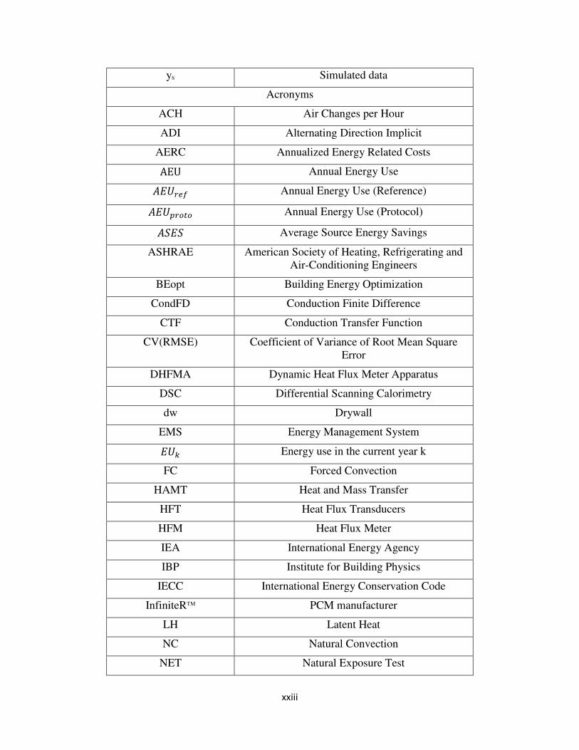
ys Simulated data
Acronyms
ACH Air Changes per Hour
ADI Alternating Direction Implicit
AERC Annualized Energy Related Costs AEU Annual Energy Use 𝐴𝐸𝑈𝑟𝑒𝑓 Annual Energy Use (Reference) 𝐴𝐸𝑈𝑝𝑟𝑜𝑡𝑜 Annual Energy Use (Protocol) 𝐴𝑆𝐸𝑆 Average Source Energy Savings
ASHRAE American Society of Heating, Refrigerating and Air-Conditioning Engineers
BEopt Building Energy Optimization
CondFD Conduction Finite Difference
CTF Conduction Transfer Function
CV(RMSE) Coefficient of Variance of Root Mean Square Error
DHFMA Dynamic Heat Flux Meter Apparatus
DSC Differential Scanning Calorimetry
dw Drywall
EMS Energy Management System 𝐸𝑈𝑘 Energy use in the current year k
FC Forced Convection
HAMT Heat and Mass Transfer
HFT Heat Flux Transducers
HFM Heat Flux Meter
IEA International Energy Agency
IBP Institute for Building Physics
IECC International Energy Conservation Code
InfiniteRTM PCM manufacturer
LH Latent Heat
NC Natural Convection
NET Natural Exposure Test
xxiv
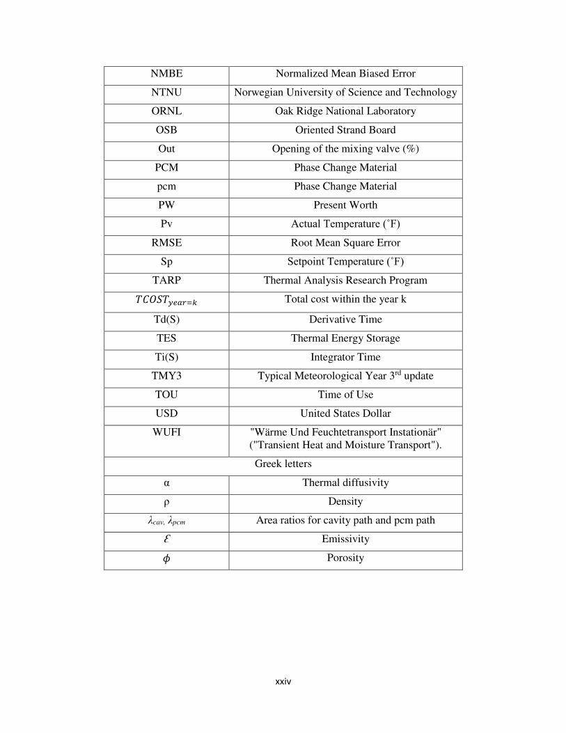
NMBE Normalized Mean Biased Error
NTNU Norwegian University of Science and Technology
ORNL Oak Ridge National Laboratory
OSB Oriented Strand Board
Out Opening of the mixing valve (%)
PCM Phase Change Material
pcm Phase Change Material
PW Present Worth
Pv Actual Temperature (˚F)
RMSE Root Mean Square Error
Sp Setpoint Temperature (˚F)
TARP Thermal Analysis Research Program 𝑇𝐶𝑂𝑆𝑇𝑦𝑒𝑎𝑟=𝑘 Total cost within the year k
Td(S) Derivative Time
TES Thermal Energy Storage
Ti(S) Integrator Time
TMY3 Typical Meteorological Year 3rd update
TOU Time of Use
USD United States Dollar
WUFI "Wärme Und Feuchtetransport Instationär" ("Transient Heat and Moisture Transport").
Greek letters
α Thermal diffusivity
ρ Density
λcav, λpcm Area ratios for cavity path and pcm path
Ԑ Emissivity 𝜙 Porosity
1
CHAPTER 1
INTRODUCTION
Buildings account for about 40% of the global energy consumption and contribute over
30% of the CO2 emissions and a considerable proportion of this energy is used for thermal comfort
in buildings [1]. In the United States, buildings use about 41% of primary energy (manual
electricity from nuclear, hydro, wind and geothermal sources). This energy consumption
contributes to the peak energy demand and increases the need for more fossil fuel based peaking
power plants [2]. Climate change, which in part is the result of increased energy related greenhouse
gas (GHG) emissions, mostly from fossil fuels, has become a major environmental issue
worldwide [3]. United Nations Environmental Program (UNEP) reports on the contribution that
buildings have on energy use and greenhouse gas emissions [4].
Peak electricity energy demand consists of several elements such as energy demand for
industrial operations, energy demand of electric appliances including lighting and energy demand
for space conditioning. In the research discussed here, the main focus is energy demanded for
space conditioning i.e. heating and cooling of living spaces. In USA, around 32 % of the building
energy in the commercial sector is consumed for space conditioning, and 53.1% for space
conditioning in residential sector [5]. Air conditioning is an important component of this
consumption, as more than 95% of the space cooling is generated using site electricity therefore
increasing the electricity demand significantly during the peak. During the summer the building
cooling related non coincident peak demand can be as high as 50%.
There are different strategies to reduce peak building power demand and overall reduction
of building space conditioning energy such as: on site generation [6], smart controls [7] and
distributed energy storage [8]. Many studies have been conducted in incorporating renewable
energy sources through demand response (DR) and smart grid strategies as discussed by Aghaei
and Alizadeh [9]. Sun et al. [10] defines and compares different conclude that PCMs require
sophisticated control strategies to achieve maximum cost saving.
2
Nowadays, there are several advanced TES systems integrated into the building envelope.
These materials need to store and release energy within desired time periods for demand response
purposes. However, this requires adequate design and controls to optimal dispatch. The application
of PCMs in building applications depends on the ability to accurately predict the heat transfer
characteristics of the improved envelope. Therefore, PCM modeling techniques have become a
critical component within the building energy modeling platforms and it is the focus on this Thesis.
Al-Saadi and Zhai [11] in their review of PCM modeling techniques, show many modeling
approaches that attempt to recognize the PCM behavior in building envelope applications.
However, these models fail to capture advanced thermal characteristics of PCMs that contribute
to successful predictions of PCM included building envelope heat transfer. Therefore, the overall
goals of the proposed research is to: (1) identify important variables and find optimal PCM
properties (2) test different PCMs encapsulation types (3) develop, verify, and validate a heat
transfer PCM model that can simulate different PCMs applications in the building envelope. This
is done through investigation and comparison of different whole building energy modeling
software that can model PCMs, experimental investigations using a state-of-the art experimental
chamber, development of a numerical model which includes a numerical solution to represent
advanced thermal behaviors of PCM like hysteresis and sub-cooling observed in PCM
applications.
The overall objectives of this research are to,
i. Identify important variables and find optimal PCM properties for building envelope
applications.
ii. Develop a numerical model which utilizes effective numerical techniques to solve a
building envelope assembly with PCM inclusions.
iii. Design and build experimental apparatus inside controlled environment to test different
PCMs.
iv. Conduct laboratory research to validate the numerical model and identify PCMs
characteristics that could further improve the numerical solution.
v. Verify and validate different PCM models in software like EnergyPlus and WUFI.
The following steps summarize the technical approach of the proposed project:
3
I. Parametric analysis of a residential building with phase change material (PCM)-
enhanced drywall, precooling, and variable electric rates in a hot and dry climate to
investigate potential cost savings and energy savings for the consumer.
II. Verification and validation of different PCM models available in whole building
energy models such as, EnergyPlus, ESP-r, MATLAB (Thesis model), and WUFI.
III. Laboratory experiments to test different PCMs and develop data to validate the
building envelope studies.
This thesis is divided in the following chapters:
Chapter 2 reviews the characteristics and thermo-physical properties of PCMs to
gain knowledge on thermal characteristics and influence of properties associated
with phase change phenomena. This chapter also highlights the significance of the
PCMs and lays a background on why further research is required.
Chapter 3 evaluates the existing analytical solutions and numerical modeling
techniques used to model PCMs in building applications. The analysis of
numerical studies includes, methods used to capture the thermal characteristics,
grid considerations for numerical PCM models, and properties of existing
numerical PCM models. The most suitable numerical techniques for the current
research are established using this evaluation.
Chapter 4 looks into current state of experimental studies which uses the PCM
types used in the experimental and numerical analysis in different scales of
experiments. It also discusses the PCM characterization methods.
Chapter 5 conducts a parametric study using an existing whole building energy
modeling platform to identify the optimum PCM properties to shift and reduce
peak cooling power demand with pre-cooling, ToU electricity rates, and different
convection modes. Mr. Matthew Brandt at Colorado School of Mines has
contributed to the research discussed in this chapter to construct EnergyPlus input
files used in the parametric analysis. This work has been published in the journal
of Applied Energy [12].
4
Chapter 6 describes the multilayer building envelope algorithm and also discusses
the experimental facility located at the Department of Mechanical Engineering of
Colorado School of Mines which facilitates system scale experiments of wall
assemblies.
Chapter 7 conducts validation study using data obtained from laboratory studies
and field experiments. Data for the validation study on shape-stabilized PCMs is
granted from Norwegian University of Science and Technology (NTNU) [13]. The
experimental data for the validation studies on Nano-PCMs comes from the Oak
Ridge National Laboratory [14]. Dr. Kaushik Biswas provided latent heat curve
for the analyzed PCM hydrate salts using Dynamic Heat Flux Meter Apparatus
(DHFMA) method and also developed a 2D model of a wood stud wall with the
Nano-PCMs and the 1D model for shape-stabilized PCM wall in COMSOL used
in chapter 7. ESP-r simulations presented in this thesis were done by Dr. Dariuz
Heim from Lodz University of Technology in Poland.
Chapter 8 conducts a validation study using in-house experiments of two
macroencapsulated PCMs in full-scale. These experimental are conducted at the
environmental chamber discussed in the chapter 8. It also introduces 5 simplified
techniques to calculate heat transfer through pouched PCMs.
Finally, chapter 9 discusses the summary of significant results and the future
research based on this work.
Chapters 5, 7 and 8 include the introduction, methodology, results, and conclusions of each
step.
5
CHAPTER 2
BACKGROUND AND SIGNIFICANCE
PCMs can store energy in two forms, latent heat and sensible heat. The magnitude and the
rate of latent heat absorbed and released depends on material properties [15]. Therefore, the
advantage of using PCMs lies in the amount of latent heat a small amount of PCM can store under
different storage techniques compared to that in a sensible heat storage material of the same
volume. For an instance, a 25 mm thick PCM layer can hold same amount of energy as a 420 mm
concrete wall as long as the PCM layer changes phase [11]. Therefore, PCMs can shift peak time
periods based on the latent heat capacity, and other physical parameters related to the application
of PCMs [10].
PCMs can also reduce or delay external fluctuations in temperatures, solar load, and
heating or cooling needs. There are several modeling methods that are used to simulate the PCM
behavior in building envelope applications [11, 16]. More detailed evaluation of available
numerical models indicates both advantages and disadvantages of these modeling approaches [17].
The main concern highlighted in the above work is that these models fail to capture advanced
thermal characteristics of PCMs which is essential for successful predictions of PCM included
building envelope heat transfer. PCMs used in building applications deviate from the ideal
behavior displaying these advanced thermal characteristics. One way of mitigating these behaviors
is by reducing hysteresis effects, increasing latent capacity by increasing the density of the PCMs
within the PCM product [18], improving conduction properties to increase the rate of heat storage
and release [19, 20], chemical construction by including additives [21], and encapsulation methods
like shape stabilization and microencapsulation [22, 23]. However, it is important to note that
these methods should be employed without increasing the building mass because the current
construction market prefer lightweight structures while improving the energy usage characteristics
within the structure (wallboard types instead of masonry or concrete).
Heat transfer through many PCMs is complex because of the nonlinear behavior of thermal
characteristics. Kosny [15] explains how the solid phase and the liquid phase of a PCM has
6
different thermo-physical characteristics while they co-exist within the enclosure.
Enclosure/encapsulation is how the PCM is packed in the particular application. During the phase
transition of the PCMs, the liquid state and the solid state are separated by a moving interface.
Considering the basic physics, the energy and mass balances should be satisfied in either side of
this moving boundary which makes it difficult to model. Either side of this moving boundary is
also called two phase/ “mushy” region. The enthalpy change which occurs across this region is
quite complex and dependent upon the material properties of the PCMs such as the latent heat,
expansion coefficient, melting range and rate of heat transfer [17].
Latent heat of the PCMs defines the heat storage capability of the PCMs. When compared
with other building envelope materials like stone, wood, brick and gypsum, PCMs present more
attractive thermal storage characteristics. To indicate the importance of the latent heat, Zhang et
al. [24] discuss how in order to keep the indoor air in the comfort range for a longer period without
heating or cooling load, the heat of fusion of a PCM should be high enough to keep the inner
surface of the wall at the melting temperature. This refers to having high latent heat next to the
inner surface of the wall so the PCM are not fully melted nor frozen. Furthermore, the latent heat
capacity of the material determines the weight/volume fraction of the PCMs required for the
optimum performance of the building envelope.
Melting temperature of the PCM is another important property. Melting temperature is
usually selected to fall within the comfort range of the occupants and are researched in the existing
standards [25]. The exact value of the optimum melting temperature required depends on the
building, climate, and the application [24]. Furthermore, a study of a PCM wall in a passive solar
house indicates that heat storage occurs with a melting temperature of 1-3 ˚C above the average
room temperature [26]. This section discusses these attractive characteristics of PCM in detail.
2.1. Phenomena of Phase Change of PCMs
Generally, phase change/ phase transition happens from solid to solid, solid to liquid, from
solid to air, liquid to vapor and even solid to solid (restructuring of bonds at atomic level). In
building applications mostly Solid-Liquid [27, 28], and Solid-Solid phase change [29, 30] is used.
The material can be a pure substance, eutectic mixture, or non-eutectic mixture. Eutectic mixtures
7
change the phase at a constant temperature but, non-eutectic mixtures change the phase during a
temperature interval.
PCMs used in real world applications are not usually pure substances and therefore,
temperature interval in which the phase change becomes an important factor [31]. This temperature
interval is called the melting range. Kuznik et al. [27] review the phase change process in a multi
component mixture of PCMs in great detail. This study indicates that behavior of the system
becomes more complex with the presence of multiple melting points from eutectic to non-eutectic
mixtures.
Using the phase change behavior, PCM-enhanced building envelopes gain the ability to
manipulate the thermal response. They can delay the effects of external thermal excitations
reaching the interior of the building [15]. At a warmer exterior weather the interior is kept cooler
and at cooler exterior weather the interior is kept relatively warmer. A high thermal conductivity
is not required for these applications because the design expectations of the thermal system are
peak load reduction and time shift of thermal response. But, there can be other building
applications where the enhanced envelope is required to absorb and release heat faster. When fast
absorption and release of latent heat is required, PCM properties need to be enhanced. Kosny [15]
highlights that, most of the applications seem to use low conductive organic PCMs. Due to thermal
comfort considerations the operating temperature of these PCMs are low. Kosny [15] further
suggests switching from organic PCMs inorganic PCMs that have 4-5 times higher thermal
conductivities would be advisable. This research therefore investigates hydrate-salt inorganic
PCMs and is discussed in the later sections.
It is evident that the exact thermal performances expected need to be achieved by carefully
managing the contributing characteristics. Parametric and optimization studies help determine
these optimum combination of characteristics and properties.
2.2. PCM encapsulation methods
Encapsulation contains the PCM inside a coating or shell material to hold the PCM and to
keep it separated from the surrounding material. Separation of PCMs helps to monitor the
composition of liquid/solid phases as well as avoids reactions with surroundings. The
encapsulation method,
8
Offer corrosion resistance, thermal stability, strength, and flexibility.
Offer an adequate heat transfer surface.
Ensure structural stability and offer easy handling.
Encapsulation methods may change with the PCM based on the chemical characteristics. PCM
applications in building envelope commonly uses shape stabilization, nano/microencapsulation,
and macroencapsulation [32]:
• Shape stabilization: Shape-stabilized PCMs (also referred to as ss-PCMs), are prepared by
impregnating the PCMs within a supporting material. The PCM takes the form or the shape of
the enclosure. They can be composites and microencapsulated [33]. Shape-stabilized PCMs
are also available in larger areas like thin sheets/plates [34-36].
• Microencapsulation: Microencapsulation is a type of shape-stabilization. It is generally a
polymer/inorganic shell [37], having a diameter in the range of 1μm–1000μm.
Microencapsulation assists adding organic PCMs safely in to the building envelope layers.
Micro-PCMs have a core-shell structure that can prevent the interior PCMs from leaking
during its solid–liquid phase change procedure. Qiu et al. [38] indicates the ability to withstand
volume change during phase transition and significant increase of heat transfer area as featured
advantages of microencapsulated PCMs. Improvements in heat transfer results from the latent
heat absorption by the PCM in the suspended MEPCM (Micro Encapsulated Phase Change
Material) particles during the melting process. Karkri al. [39] highlights the importance of
microencapsulation in widening the scope of PCM applications for instance, by preventing
leakage of molding paraffin during phase transition. Microencapsulated PCMs have been
applied in concrete/mortar [40-42], wall boards, and gypsum plaster or implemented as
sandwich panels or slabs [43]. Konuklu et al. [44] discusses the mechanical and thermal
improvements in the material due to the addition of microencapsulated PCMs. Micro
encapsulation can help increase the latent capacity of gypsum dry wall around 10 times [45].
However, microencapsulation is the more expensive than macroencapsulation and
microencapsulation of salt hydrates is a difficult task due to their hydrophilic nature. Figure
2-1a shows a microencapsulated PCM embedded gypsum wallboard. Figure 2-1(c) shows the
panel is used in the wall construction.
9
• Macroencapsulation: A common way of encapsulating the PCM in a spherical, tubular,
cylindrical or rectangular container having milliliters to several liters of PCM and t serving
directly as heat exchangers (usually 1-10 cm in size). Wei et al. [46] investigates several types
of encapsulation shapes and indicate that, from the heat release point of view, spherical PCM
capsules show the highest thermal performance. The skin of the container acts as a self –
supporting structure isolating PCM from the surrounding environment. For building envelope
applications, plastics (polyethylene [47], formed white poly-film and heavy-duty nylon [48])
films are commonly used as the container materials. Metallic encapsulates can increase the
heat transfer due to the high conductivity. However, metal vessels are not suitable to
encapsulate PCM hydrate-salts due to corrosion and degradation [49]. PCM leakage can be a
challenge in macroencapsulation in pouches and to prevent that techniques like improved
formed poly-film for encapsulation and mixing PCMs with thickening agents are used [50].
Macroencapsulation is the least complex encapsulation method due to simplicity of containers
and the low production costs of the containers.
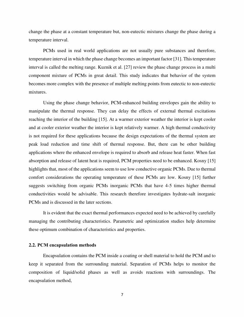
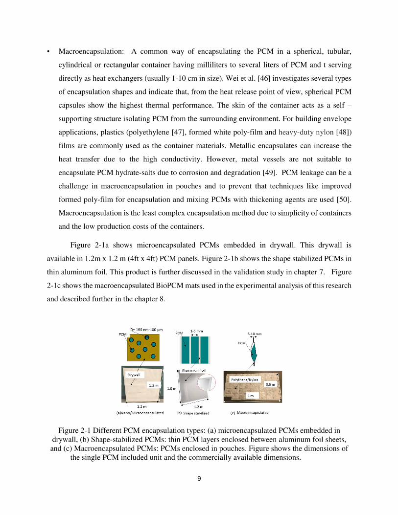
Figure 2-1a shows microencapsulated PCMs embedded in drywall. This drywall is
available in 1.2m x 1.2 m (4ft x 4ft) PCM panels. Figure 2-1b shows the shape stabilized PCMs in
thin aluminum foil. This product is further discussed in the validation study in chapter 7. Figure
2-1c shows the macroencapsulated BioPCM mats used in the experimental analysis of this research
and described further in the chapter 8.
Figure 2-1 Different PCM encapsulation types: (a) microencapsulated PCMs embedded in drywall, (b) Shape-stabilized PCMs: thin PCM layers enclosed between aluminum foil sheets, and (c) Macroencapsulated PCMs: PCMs enclosed in pouches. Figure shows the dimensions of
the single PCM included unit and the commercially available dimensions.
10
2.3. Thermal characteristics and properties of PCMs
Phase change phenomena and heat transfer characteristics discussed in the previous section
is highly influenced by complex behavior observed in PCMs used in building applications. These
characteristics are observed in experimental PCM studies and have presented problems in attempts
to model PCMs. Therefore, this section looks into these complex characteristics.
“Mushy” region of Phase Change
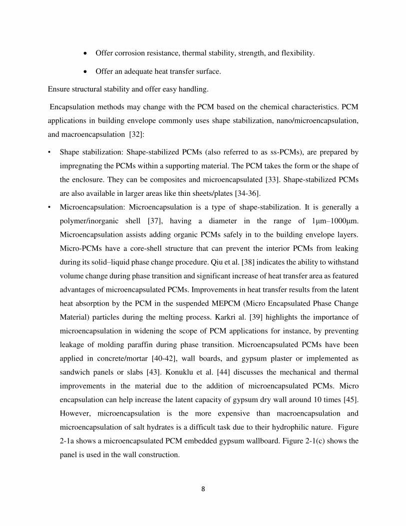
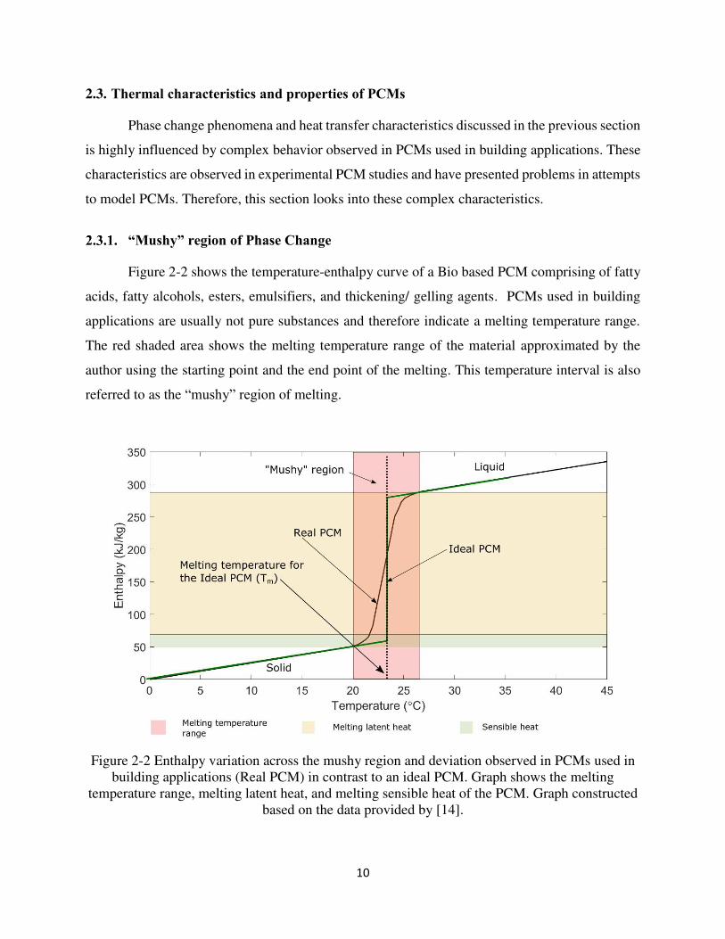
Figure 2-2 shows the temperature-enthalpy curve of a Bio based PCM comprising of fatty
acids, fatty alcohols, esters, emulsifiers, and thickening/ gelling agents. PCMs used in building
applications are usually not pure substances and therefore indicate a melting temperature range.
The red shaded area shows the melting temperature range of the material approximated by the
author using the starting point and the end point of the melting. This temperature interval is also
referred to as the “mushy” region of melting.
Figure 2-2 Enthalpy variation across the mushy region and deviation observed in PCMs used in building applications (Real PCM) in contrast to an ideal PCM. Graph shows the melting
temperature range, melting latent heat, and melting sensible heat of the PCM. Graph constructed based on the data provided by [14].
11
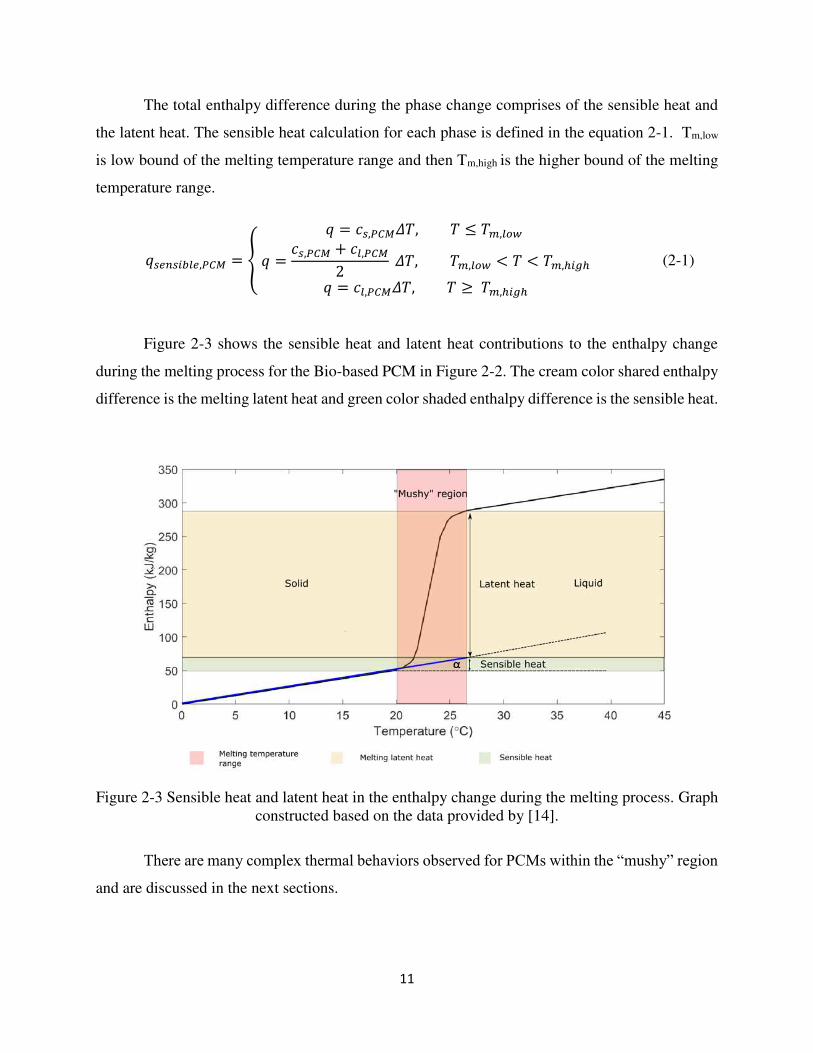
The total enthalpy difference during the phase change comprises of the sensible heat and
the latent heat. The sensible heat calculation for each phase is defined in the equation 2-1. Tm,low
is low bound of the melting temperature range and then Tm,high is the higher bound of the melting
temperature range.
𝑞𝑠𝑒𝑛𝑠𝑖𝑏𝑙𝑒,𝑃𝐶𝑀 = { 𝑞 = 𝑐𝑠,𝑃𝐶𝑀𝛥𝑇, 𝑇 ≤ 𝑇𝑚,𝑙𝑜𝑤 𝑞 = 𝑐𝑠,𝑃𝐶𝑀 + 𝑐𝑙,𝑃𝐶𝑀2 𝛥𝑇, 𝑇𝑚,𝑙𝑜𝑤 < 𝑇 < 𝑇𝑚,ℎ𝑖𝑔ℎ 𝑞 = 𝑐𝑙,𝑃𝐶𝑀𝛥𝑇, 𝑇 ≥ 𝑇𝑚,ℎ𝑖𝑔ℎ (2-1)
Figure 2-3 shows the sensible heat and latent heat contributions to the enthalpy change
during the melting process for the Bio-based PCM in Figure 2-2. The cream color shared enthalpy
difference is the melting latent heat and green color shaded enthalpy difference is the sensible heat.
Figure 2-3 Sensible heat and latent heat in the enthalpy change during the melting process. Graph constructed based on the data provided by [14].
There are many complex thermal behaviors observed for PCMs within the “mushy” region
and are discussed in the next sections.
12
Phase separation of the material
Phase separation of the material takes place within this “mushy” region of phase change.
This phenomenon usually occurs when there is more than one constituent in the substance, which
is common practice in commercial PCMs. Kosny [15] discusses how the melting/solidifying
temperature of each component might also be influenced by the composition of each constituent
of the mixture.
Subcooling/supercooling effect and Hysteresis
Hysteresis PCMs are categorized as real hysteresis and apparent hysteresis. Real hysteresis
occurs due to material properties and apparent hysteresis is independent of the material properties.
The most common form of real hysteresis is Subcooling. Many PCMs do not freeze at the melting
temperature and start crystallization only after a temperature below the nominal melting
temperature [31]. Solidification/ freezing of the PCM happens where the solid phase grows with
the liquid layer at the interface. As the temperature decreases this interface should occur at a certain
point. At the initiation, there is no or only a small solid particle. This solid particle is also called
the nucleus. At the surface of the nucleus there occurs an instance where energy released by
crystallization at the surface is lesser than that of surface energy gained. This energy flow barrier
exists until the nucleus grow satisfactorily. If this nucleation is delayed to occur with the
temperature decreases below the melting point the Subcooling occurs. Due to this the freezing
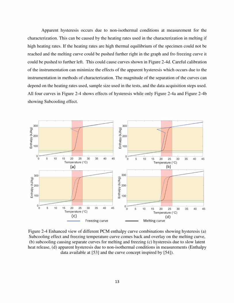
curve indicates a delay in initiation of solidification. This is shown in the figures Figure 2-4a and
Figure 2-4b by the blue line continuing towards the left showing decrease of temperature and again
turning towards increasing temperature in the figures [31]. Subcooling is more visible in hydrate
salts but can be reduced using additives [15]. A recent study by Li et al. [51] discusses the sub-
cooling effects of PCMs and how the effect can vary with different additives.
Real hysteresis can occur as a result of slow latent heat release. Mehling and Cabeza [31]
discusses the reason for the slow heat release being slow formation of the crystal lattice or diffusion
processes are necessary to homogenize the sample. The temperature of the sample then drops
below the cooling heating temperature. This is not observed in the melting process since the
kinetics process occurs much faster [52]. These conditions can separate melting and freezing curve
and is shown in Figure 2-4c.
13
Apparent hysteresis occurs due to non-isothermal conditions at measurement for the
characterization. This can be caused by the heating rates used in the characterization in melting if
high heating rates. If the heating rates are high thermal equilibrium of the specimen could not be
reached and the melting curve could be pushed further right in the graph and fro freezing curve it
could be pushed to further left. This could cause curves shown in Figure 2-4d. Careful calibration
of the instrumentation can minimize the effects of the apparent hysteresis which occurs due to the
instrumentation in methods of characterization. The magnitude of the separation of the curves can
depend on the heating rates used, sample size used in the tests, and the data acquisition steps used.
All four curves in Figure 2-4 shows effects of hysteresis while only Figure 2-4a and Figure 2-4b
showing Subcooling effect.
Figure 2-4 Enhanced view of different PCM enthalpy curve combinations showing hysteresis (a) Subcooling effect and freezing temperature curve comes back and overlay on the melting curve, (b) subcooling causing separate curves for melting and freezing (c) hysteresis due to slow latent
heat release, (d) apparent hysteresis due to non-isothermal conditions in measurements (Enthalpy data available at [53] and the curve concept inspired by [54]).
14
There are several methods used to characterize PCM: Differential Scanning Calorimetry (DSC),
Twin bath method, T-history, Dynamic Hot-Box method, Heat Flow Meter Apparatus (HFMA)
methods are some of these tests. These are discussed in detail in chapter 4.
PCM Thermal conductivity
PCM thermal conductivity can differ between liquid and solid phases [55]. Low
conductivity is typically undesirable and is observed in PCMs like Paraffins [15]. Thus, there are
efforts to increase the thermal conductivity of PCMs using composites, graphite, aluminum
powder, copper, and microencapsulation techniques [56-59] [15].
Thermal conductivity of PCMs also has an impact on the PCM characterization results.
High temperature gradients created within the PCM samples due to low conductivity can cause
inaccuracies in estimations of the heat storage capacity with respect to temperature when using
PCM characterization methods.
PCM phase-change temperature range
Selection of a particular PCM depends on the application (envelope, HVAC), location
inside the building envelope (exterior/interior, wall, ceiling, floor) and the geographical location
(weather data) of the implementation. Because PCMs have a melting/freezing temperature range,
many studies have optimized this temperature range for the particular application.
For: different PCM products [60], for different locations in the residential buildings [61],
related to layer thicknesses [62], and PCM use in different climates/climate zone
classifications [63, 64]. The objective of some of these optimizations are either, cooling/heating
load reduction, energy savings, comfort, cost savings, or a combination of these objectives.
Once a suitable phase-change temperature and the phase-change temperature range is
selected for the application, further selections can be carried out for other important properties
like, conductivity, durability, melting and freezing behaviors, energy density (important factor
when designing lightweight structures).
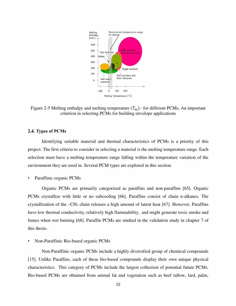
15
Figure 2-5 Melting enthalpy and melting temperature (𝑇𝑚)– for different PCMs, An important criterion in selecting PCMs for building envelope applications
2.4. Types of PCMs
Identifying suitable material and thermal characteristics of PCMs is a priority of this
project. The first criteria to consider in selecting a material is the melting temperature range. Each
selection must have a melting temperature range falling within the temperature variation of the
environment they are used in. Several PCM types are explored in this section.
• Paraffinic organic PCMs
Organic PCMs are primarily categorized as paraffins and non-paraffins [65]. Organic
PCMs crystallize with little or no subcooling [66]. Paraffins consist of chain n-alkanes. The
crystallization of the –CH3 chain releases a high amount of latent heat [67]. However, Paraffins
have low thermal conductivity, relatively high flammability, and might generate toxic smoke and
fumes when wet burning [68]. Paraffin PCMs are studied in the validation study in chapter 7 of
this thesis.
• Non-Paraffinic Bio-based organic PCMs
Non-Paraffinic organic PCMs include a highly diversified group of chemical compounds
[15]. Unlike Paraffins, each of these bio-based compounds display their own unique physical
characteristics. This category of PCMs include the largest collection of potential future PCMs.
Bio-based PCMs are obtained from animal fat and vegetation such as beef tallow, lard, palm,
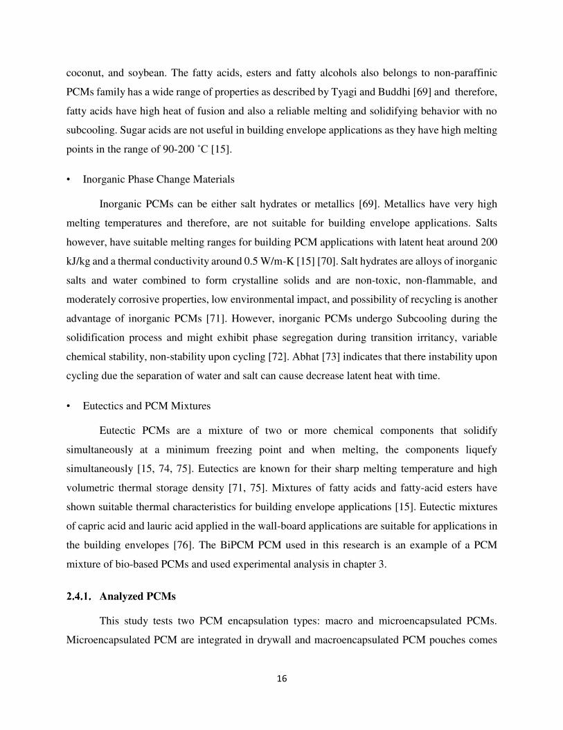
16
coconut, and soybean. The fatty acids, esters and fatty alcohols also belongs to non-paraffinic
PCMs family has a wide range of properties as described by Tyagi and Buddhi [69] and therefore,
fatty acids have high heat of fusion and also a reliable melting and solidifying behavior with no
subcooling. Sugar acids are not useful in building envelope applications as they have high melting
points in the range of 90-200 ˚C [15].
• Inorganic Phase Change Materials
Inorganic PCMs can be either salt hydrates or metallics [69]. Metallics have very high
melting temperatures and therefore, are not suitable for building envelope applications. Salts
however, have suitable melting ranges for building PCM applications with latent heat around 200
kJ/kg and a thermal conductivity around 0.5 W/m-K [15] [70]. Salt hydrates are alloys of inorganic
salts and water combined to form crystalline solids and are non-toxic, non-flammable, and
moderately corrosive properties, low environmental impact, and possibility of recycling is another
advantage of inorganic PCMs [71]. However, inorganic PCMs undergo Subcooling during the
solidification process and might exhibit phase segregation during transition irritancy, variable
chemical stability, non-stability upon cycling [72]. Abhat [73] indicates that there instability upon
cycling due the separation of water and salt can cause decrease latent heat with time.
• Eutectics and PCM Mixtures
Eutectic PCMs are a mixture of two or more chemical components that solidify
simultaneously at a minimum freezing point and when melting, the components liquefy
simultaneously [15, 74, 75]. Eutectics are known for their sharp melting temperature and high
volumetric thermal storage density [71, 75]. Mixtures of fatty acids and fatty-acid esters have
shown suitable thermal characteristics for building envelope applications [15]. Eutectic mixtures
of capric acid and lauric acid applied in the wall-board applications are suitable for applications in
the building envelopes [76]. The BiPCM PCM used in this research is an example of a PCM
mixture of bio-based PCMs and used experimental analysis in chapter 3.
Analyzed PCMs
This study tests two PCM encapsulation types: macro and microencapsulated PCMs.
Microencapsulated PCM are integrated in drywall and macroencapsulated PCM pouches comes
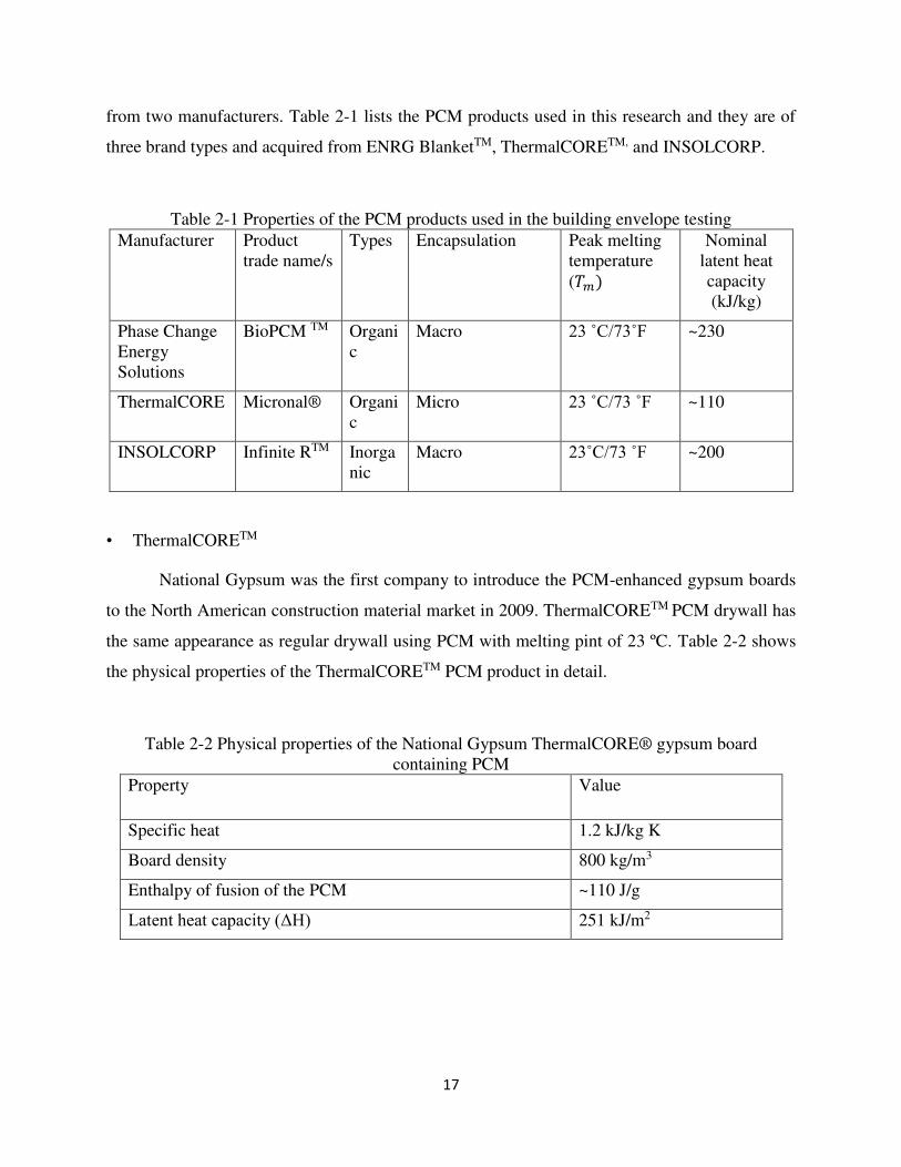
17
from two manufacturers. Table 2-1 lists the PCM products used in this research and they are of
three brand types and acquired from ENRG BlanketTM, ThermalCORETM, and INSOLCORP.
Table 2-1 Properties of the PCM products used in the building envelope testing Manufacturer Product
trade name/s Types Encapsulation Peak melting
temperature (𝑇𝑚) Nominal
latent heat capacity (kJ/kg)
Phase Change Energy Solutions
BioPCM TM Organic
Macro 23 ˚C/73˚F ~230
ThermalCORE Micronal® Organic
Micro 23 ˚C/73 ˚F ~110
INSOLCORP Infinite RTM Inorganic
Macro 23˚C/73 ˚F ~200
• ThermalCORETM
National Gypsum was the first company to introduce the PCM-enhanced gypsum boards
to the North American construction material market in 2009. ThermalCORETM PCM drywall has
the same appearance as regular drywall using PCM with melting pint of 23 ºC. Table 2-2 shows
the physical properties of the ThermalCORETM PCM product in detail.
Table 2-2 Physical properties of the National Gypsum ThermalCORE® gypsum board containing PCM
Property Value
Specific heat 1.2 kJ/kg K
Board density 800 kg/m3
Enthalpy of fusion of the PCM ~110 J/g
Latent heat capacity (ΔH) 251 kJ/m2
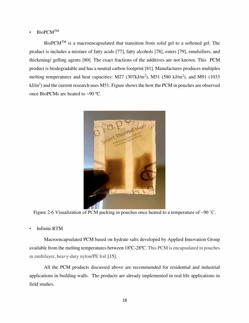
18
• BioPCMTM
BioPCMTM is a macroencapsulated that transition from solid gel to a softened gel. The
product is includes a mixture of fatty acids [77], fatty alcohols [78], esters [79], emulsifiers, and
thickening/ gelling agents [80]. The exact fractions of the additives are not known. This PCM
product is biodegradable and has a neutral carbon footprint [81]. Manufactures produces multiples
melting temperatures and heat capacities: M27 (307kJ/m2), M51 (580 kJ/m2), and M91 (1033
kJ/m2) and the current research uses M51. Figure shows the how the PCM in pouches are observed
once BioPCMs are heated to ~90 ºC.
Figure 2-6 Visualization of PCM packing in pouches once heated to a temperature of ~90 ˚C.
• Infinite RTM
Macroencapsulated PCM based on hydrate salts developed by Applied Innovation Group
available from the melting temperatures between 18ºC-28ºC. This PCM is encapsulated in pouches
in multilayer, heavy-duty nylon/PE foil [15].
All the PCM products discussed above are recommended for residential and industrial
applications in building walls. The products are already implemented in real life applications in
field studies.
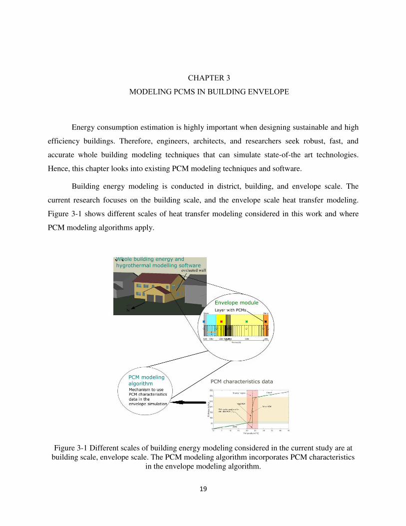
19
CHAPTER 3
MODELING PCMS IN BUILDING ENVELOPE
Energy consumption estimation is highly important when designing sustainable and high
efficiency buildings. Therefore, engineers, architects, and researchers seek robust, fast, and
accurate whole building modeling techniques that can simulate state-of-the art technologies.
Hence, this chapter looks into existing PCM modeling techniques and software.
Building energy modeling is conducted in district, building, and envelope scale. The
current research focuses on the building scale, and the envelope scale heat transfer modeling.
Figure 3-1 shows different scales of heat transfer modeling considered in this work and where
PCM modeling algorithms apply.
Figure 3-1 Different scales of building energy modeling considered in the current study are at building scale, envelope scale. The PCM modeling algorithm incorporates PCM characteristics
in the envelope modeling algorithm.
20
3.1. Analytical Models
Stefan problem defines the temperature distribution u (x, t) that yields an explicit type
solution for freezing/melting of a semi-infinite PCM- layer initially at a constant temperature in a
homogenous phase, with a constant temperature at the surface [82]. The analytical solution for the
case of heat transfer in a PCM in a 1-dimensional semi-infinite layer is used for our baseline
verification purposes and has been used in previous research [83, 84]. Furthermore, recent studies
discuss analytical solutions for solid-liquid phase transition of pure PCMs [85-87]. However, most
PCMs do not demonstrate isothermal phase change process and the complex behavior of PCMs
have led to more advanced analytical methods. Generally, analytical solutions have drawbacks
when capturing dynamic behavior of PCMs with their complex thermal characteristics. For that
reason, whole building energy modeling platforms use comprehensive numerical methods.
3.2. Numerical Models
Approximate numerical models constructed during last several decades use many
mathematical methods to recognize PCM behavior. ANSYS Fluent, BSim, COMSOL, DeST,
EnergyPlus, HEATING, IDA ICE, , PCMexpress, PowerDomus, RADCOOL, SUNREL, and
WUFI are software are capable of modeling PCMs [15]. Among these software, EnergyPlus, ESP-
r, and WUFI are considered in this study based on their popularity, key recent applications in
literature, and the potential for future research. In addition, an additional model is developed in
MATLAB some results are compared to a 2-Dimensional model in COMSOL. This section
discusses how these methods are integrated to modeling PCMs and specifically in building
applications.
Numerical models: Simulation methods
Heat Source Method
Heat source method splits the enthalpy in to sensible heat and latent heat. Latent heat
portion is defined as the heat source [88]. This has been used for different PCM applications
designed to take advantage of the off-peak electrical energy for space heating [89-91].
21
Heat capacity method
The heat capacity method describes the temperature change T(x, t) using the heat capacity
cp(T). Within the temperature range of a phase transition, this method deals with heat capacity as
a function of temperature. Heat capacity method has been used to evaluate phase change in liquid
metals in recent studies [92, 93]. Most of the modelling algorithms using heat capacity method are
built for 1D heat transfer studies [83]. A 3D study by Sa et al. [94] numerically compares two
PCM-enhanced wallboards with heat capacity defined to vary with the temperature and a
Gaussian-type equation and expresses the capacitance-temperature relationship. Heat capacity
method shows low accuracy with high temperature gradients in the mushy region [95]. It is
suggested in literature that application of heat capacity method in numerical solutions for real
PCMs needs further evaluation. TRNSYS software uses heat capacity method to model PCMs in
building applications.
Enthalpy Method
Eyres et al. [96] introduces enthalpy method, and uses this technique to demonstrate the
variations of thermal properties with time (enthalpy change with time). The enthalpy method deals
with a total amount of energy required during the phase-change. This includes both sensible and
latent heat. It is one of the most commonly used fixed-domain methods for solving the moving
boundary problem, Voller and Swaminathan [97] Studies a general implicit source based enthalpy
model. The consistent linearization of the discretized source is a highlighted feature in this study.
In using enthalpy method the conductivity and the density is considered to be temperature
dependent. The key feature of the outcomes of the above studies is eliminating the need of
accurately track the phase change boundary.
The enthalpy method used in this study includes subsets of both apparent heat capacity and
source based methods. TRNSYS Type-241 [98], PCM Express – ESP-r [99], and EnergyPlus [100]
utilizes different versions of the enthalpy method. These applications indicate the applicability of
the enthalpy model to approximate PCM behavior. Günther et al. [101] discusses the ability of
enthalpy method to correctly account for the subcooling effect.
22
Apparent heat capacity and combined methods
Apparent heat capacity method increases the heat capacity at the mushy region directly
proportional to the latent heat and inversely proportional to the temperature difference. This
method is also one of the extensively studied method alongside enthalpy method says Kuznik. et
al. [55], but when the phase change happens without the mushy region, the solutions of this method
may not be accurate as shown by Tenchev, R. and P. Purnell [102] or produces an error with large
time steps [103, 104].
A recent study incorporates a similar enthalpy method implemented by Swaminathan, C.
and V. Voller [105] where the PCM model is represented by a nonlinear source term in the
governing equation [106]. Within the source term the authors take into account the liquid phase
fraction and it is set to vary with the temperature. Therefore, this approach is called a quasi-
enthalpy method. TRNSYS Type-204 and TRANSYS Type-260 uses effective heat capacity
method [55].
Table 3-1 compares the analyzed methods in terms of how they solve transient heat transfer
equation. Each of these methods are solved using different numerical solvers such as G-S (Gauss
Seidel) or TDMA (Tri-Diagonal Matrix Algorithm) [17]. Equation 3-1 shows the generalized form
of the heat equation. In summary, (i) heat source method: latent heat is treated as a source term (ii)
heat capacity method: heat capacity term accounts for both sensible and latent heat (iii) enthalpy
method: enthalpy term accounts for sensible and latent heat.
A∂ϕ∂t = ∂∂x (Γϕ ∂ϕ∂x) + R (3-1)
Table 3-1 Coefficients of the mathematical formulation to capture the phase change effects in numerical models.
Mathematical method
Values of the coefficients in the order as they appear in the formulation
A 𝜙 Γ𝜙 𝑅 Heat source method ρ 𝐶𝑎𝑣𝑔 T k - ρL𝜕𝑓𝑙𝜕𝑡
Heat capacity method
ρ𝐶𝐴(𝑇) T k 0
Enthalpy method Ρ h k/𝐶𝑃 0
23
Here, 𝐶𝑎𝑣𝑔 = averaged heat capacity 𝐶𝑃 = specific heat capacity 𝐶𝐴(𝑇) = heat capacity term as a function of temperature ρ = density
h = enthalpy 𝑘 = thermal conductivity 𝑇 = temperature 𝐿 = latent heat 𝑡 = time 𝜕𝑓𝑙𝜕t = liquid fraction gradient Numerical Models: Grid and boundary considerations.
PCM modeling must solve the moving boundary problem because, in addition to the fixed
boundaries which define the computational domain, there is a boundary across which the phase
change takes place (the “mushy” region). Thermodynamic equilibrium conditions should be
satisfied on this time dependent moving boundary. Literature looks into several grid methods for
numerical solutions. There are three main methods: fixed grid method [105], front tracking method
[107], and hybrid method [108]. Fixed grid method is commonly used in building envelope
problems with PCMs due to the complex nature of implementing a moving grid method. The
complexities of front tracking and moving mesh methods can lead to significantly increased
computational time [11]. All PCM algorithms used in this research use fixed grid methods.
Numerical Models: Discrete forms and solution schemes
Finite element method, finite difference method and finite volume method are frequently used
modeling formulations used in PCM modeling. Discrete forms used in literature when numerically
modeling PCMs are shown in detail in Appendix A.
24
Numerical Models: In building energy modeling platforms
Building energy modeling programs include numerical solutions for building envelope
with PCMs. However, most of these programs consider convenience over accuracy and therefore,
make assumptions to simplify the algorithm when implemented in the models [17]. A PCM study
which uses COMSOL to simulate PCMs and discusses how the 3D/2D models [109]. Several
studies use in-house whole building energy models implementing numerical solutions for PCM
inclusions which are verified with existing numerical solutions or validated with experimental data
[103, 110, 111]. However, the commercial whole building energy modeling platforms are more
comprehensive and are updated frequently with more effective PCM models. Therefore, the PCMs
modeling algorithms require frequent validation.
Commercially available building simulation platforms are useful in evaluating annual
energy simulations for PCM included building models [112]. The following software is among
mostly referenced and have some type of PCM mod
ESP-r: Tool developed by University of Strathclyde and commonly used in Europe that
has couple of PCM models [113-115]. PCMs are introduced as special materials and
defined as active building elements that have the ability to change their thermo-physical
properties. Fallahi et al. [116] Proposes a numerical solution for ESP-r. The solution is
based on a finite difference method. The program simulates and predicts temperature
profiles and heat fluxes for different configurations of PCM inclusion. ESP-r is used by
Kośny et al. [117] due to its built in ability to model PCM sub-cooling effect.
TRNSYS: Tool Developed by University of Wisconsin-Madison. Earlier TRNSYS
models use enthalpy method and solved using explicit schemes [118, 119]. However, later
TRNSYS models do not use enthalpy method and use heat capacity/ heat source methods
[120]. Castellón, et al.[121] compares, but does not offer proper validation results. There
are other TRNSYS PCM models for building wall PCM applications [55, 122].
Implements TRNSYS Type-1270 PCM model which assumes that the PCM undergoes its
phase transition at a constant temperature and the specific heat capacity of the two phases
are constant. TRNSYS Type-285 uses the boundary temperature concept through a
massless dummy layer with a small resistance [16]. Validation is done in small scale tests
[55].
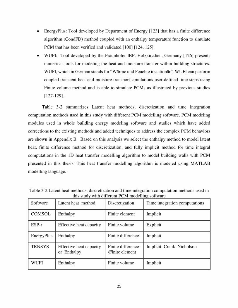
25
EnergyPlus: Tool developed by Department of Energy [123] that has a finite difference
algorithm (CondFD) method coupled with an enthalpy temperature function to simulate
PCM that has been verified and validated [100] [124, 125].
WUFI: Tool developed by the Fraunhofer IBP, Holzkirc.hen, Germany [126] presents
numerical tools for modeling the heat and moisture transfer within building structures.
WUFI, which in German stands for “Wärme und Feuchte instationär”. WUFI can perform
coupled transient heat and moisture transport simulations user-defined time steps using
Finite-volume method and is able to simulate PCMs as illustrated by previous studies
[127-129].
Table 3-2 summarizes Latent heat methods, discretization and time integration
computation methods used in this study with different PCM modelling software. PCM modeling
modules used in whole building energy modeling software and studies which have added
corrections to the existing methods and added techniques to address the complex PCM behaviors
are shown in Appendix B. Based on this analysis we select the enthalpy method to model latent
heat, finite difference method for discretization, and fully implicit method for time integral
computations in the 1D heat transfer modelling algorithm to model building walls with PCM
presented in this thesis. This heat transfer modelling algorithm is modeled using MATLAB
modelling language.
Table 3-2 Latent heat methods, discretization and time integration computation methods used in this study with different PCM modelling software
Software Latent heat method Discretization Time integration computations
COMSOL Enthalpy Finite element Implicit
ESP-r Effective heat capacity Finite volume Explicit
EnergyPlus Enthalpy Finite difference Implicit
TRNSYS Effective heat capacity or Enthalpy
Finite difference /Finite element
Implicit: Crank–Nicholson
WUFI Enthalpy Finite volume Implicit
26
CHAPTER 4
EXPERIMENTAL STUDIES ON PCM INCLUSION IN BUILDING ENVELOPE
Laboratory studies are used to characterize PCMs and to collect data for validating different
numerical PCM models. This chapter discusses the literature of experimental PCM
characterization, PCM inclusion methods, and the experimental methods to improve the numerical
solutions.
4.1. Scale of experimental studies
PCM are characterized by thermal properties (density, thermal conductivity, specific heat)
that might change in liquid phase and solid phase. Additional properties are latent heat and melting
temperature Tm. Latent heat is typically represented by the temperature dependent enthalpy curve
h(T). PCM calorimetric measurement are used to determine h(T) curve for PCMs. Kosny [15]
indicates that theoretical and experimental analyses of building technologies is performed at three
levels.
• Material scale
• System scale
• Whole building scale
Material scale occurs when only the PCMs performance is examined. System scale relates
to are applications in exterior/interior wall, ceiling, and floor envelope assemblies. PCM
characterization studies are conducted in material scale.
4.2. PCM characterization methods
PCM characterization methods quantify the phase melting and freezing enthalpy of PCMs as
well as its melting and crystallization behaviour. The sample sizes used and the final output of the
thermal property after processing the data from some commonly used methods are shown in Table
4-1. These methods are discussed in detail in the following section.
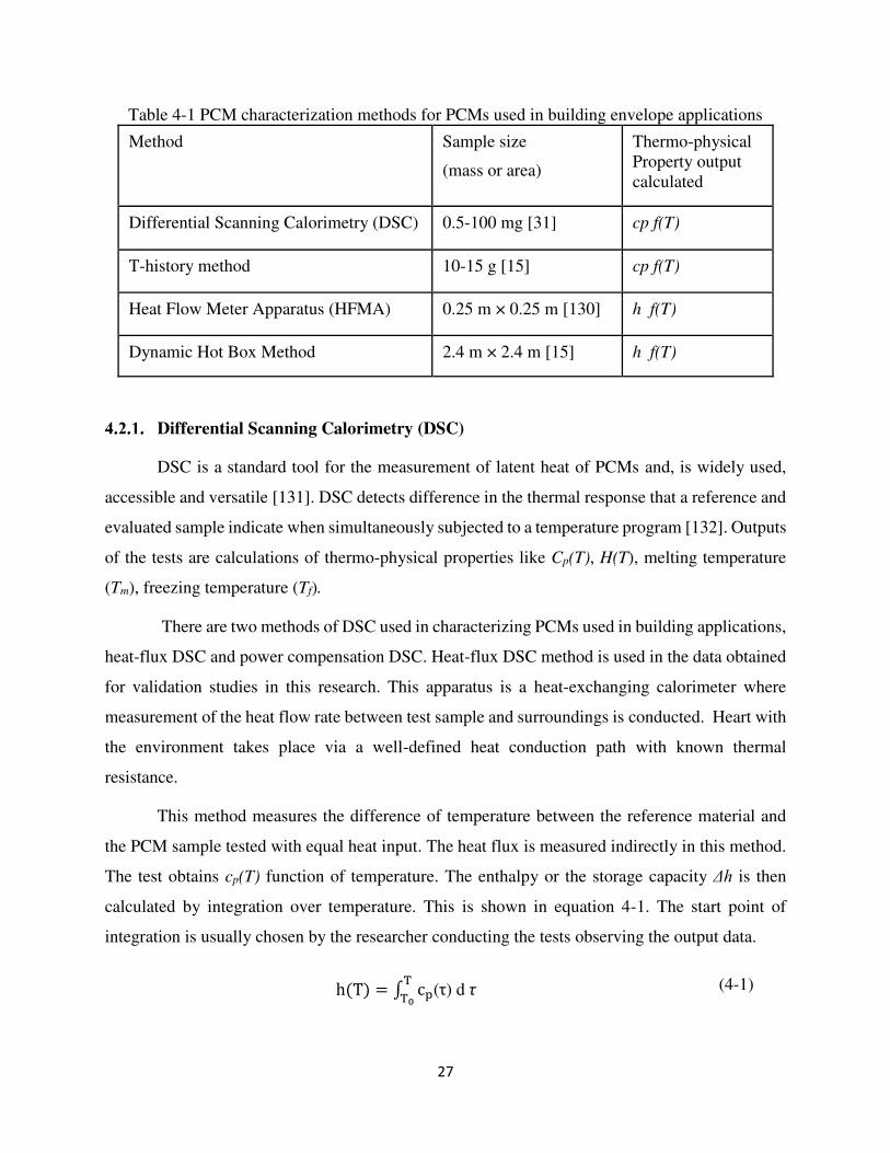
27
Table 4-1 PCM characterization methods for PCMs used in building envelope applications
Method Sample size
(mass or area)
Thermo-physical Property output calculated
Differential Scanning Calorimetry (DSC) 0.5-100 mg [31] cp f(T)
T-history method 10-15 g [15] cp f(T)
Heat Flow Meter Apparatus (HFMA) 0.25 m × 0.25 m [130] h f(T)
Dynamic Hot Box Method 2.4 m × 2.4 m [15] h f(T)
Differential Scanning Calorimetry (DSC)
DSC is a standard tool for the measurement of latent heat of PCMs and, is widely used,
accessible and versatile [131]. DSC detects difference in the thermal response that a reference and
evaluated sample indicate when simultaneously subjected to a temperature program [132]. Outputs
of the tests are calculations of thermo-physical properties like Cp(T), H(T), melting temperature
(Tm), freezing temperature (Tf).
There are two methods of DSC used in characterizing PCMs used in building applications,
heat-flux DSC and power compensation DSC. Heat-flux DSC method is used in the data obtained
for validation studies in this research. This apparatus is a heat-exchanging calorimeter where
measurement of the heat flow rate between test sample and surroundings is conducted. Heart with
the environment takes place via a well-defined heat conduction path with known thermal
resistance.
This method measures the difference of temperature between the reference material and
the PCM sample tested with equal heat input. The heat flux is measured indirectly in this method.
The test obtains cp(T) function of temperature. The enthalpy or the storage capacity Δh is then
calculated by integration over temperature. This is shown in equation 4-1. The start point of
integration is usually chosen by the researcher conducting the tests observing the output data.
h(T) = ∫ cpTT0 (τ) d τ (4-1)
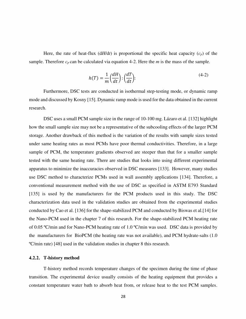
28
Here, the rate of heat-flux (dH/dt) is proportional the specific heat capacity (cp) of the
sample. Therefore cp can be calculated via equation 4-2. Here the m is the mass of the sample.
ℎ(𝑇) = 1𝑚 (𝑑𝐻𝑑𝑡 ) : (𝑑𝑇𝑑𝑡): (4-2)
Furthermore, DSC tests are conducted in isothermal step-testing mode, or dynamic ramp
mode and discussed by Kosny [15]. Dynamic ramp mode is used for the data obtained in the current
research.
DSC uses a small PCM sample size in the range of 10-100 mg. Lázaro et al. [132] highlight
how the small sample size may not be a representative of the subcooling effects of the larger PCM
storage. Another drawback of this method is the variation of the results with sample sizes tested
under same heating rates as most PCMs have poor thermal conductivities. Therefore, in a large
sample of PCM, the temperature gradients observed are steeper than that for a smaller sample
tested with the same heating rate. There are studies that looks into using different experimental
apparatus to minimize the inaccuracies observed in DSC measures [133]. However, many studies
use DSC method to characterize PCMs used in wall assembly applications [134]. Therefore, a
conventional measurement method with the use of DSC as specified in ASTM E793 Standard
[135] is used by the manufacturers for the PCM products used in this study. The DSC
characterization data used in the validation studies are obtained from the experimental studies
conducted by Cao et al. [136] for the shape-stabilized PCM and conducted by Biswas et al.[14] for
the Nano-PCM used in the chapter 7 of this research. For the shape-stabilized PCM heating rate
of 0.05 ºC/min and for Nano-PCM heating rate of 1.0 ºC/min was used. DSC data is provided by
the manufacturers for BioPCM (the heating rate was not available), and PCM hydrate-salts (1.0
ºC/min rate) [48] used in the validation studies in chapter 8 this research.
T-history method
T-history method records temperature changes of the specimen during the time of phase
transition. The experimental device usually consists of the heating equipment that provides a
constant temperature water bath to absorb heat from, or release heat to the test PCM samples.
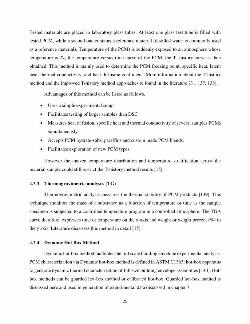
29
Tested materials are placed in laboratory glass tubes. At least one glass test tube is filled with
tested PCM, while a second one contains a reference material (distilled water is commonly used
as a reference material). Temperature of the PCM) is suddenly exposed to an atmosphere whose
temperature is T∞, the temperature versus time curve of the PCM, the T -history curve is then
obtained. This method is mainly used to determine the PCM freezing point, specific heat, latent
heat, thermal conductivity, and heat diffusion coefficient. More information about the T-history
method and the improved T-history method approaches re found in the literature [31, 137, 138].
Advantages of this method can be listed as follows,
Uses a simple experimental setup
Facilitates testing of larger samples than DSC
Measures heat of fusion, specific heat and thermal conductivity of several samples PCMs
simultaneously
Accepts PCM hydrate-salts, paraffins and custom made PCM blends.
Facilitates exploration of new PCM types
However the uneven temperature distribution and temperature stratification across the
material sample could still restrict the T-history method results [15].
Thermogravimetric analyses (TG)
Thermogravimetric analysis measures the thermal stability of PCM products [139]. This
technique monitors the mass of a substance as a function of temperature or time as the sample
specimen is subjected to a controlled temperature program in a controlled atmosphere. The TGA
curve therefore, expresses time or temperature on the x-axis and weight or weight percent (%) in
the y axis. Literature discusses this method in detail [15].
Dynamic Hot Box Method
Dynamic hot-box method facilitates the full scale building envelope experimental analysis.
PCM characterization via Dynamic hot-box method is defined in ASTM C1363: hot-box apparatus
to generate dynamic thermal characterization of full size building envelope assemblies [140]. Hot-
box methods can be guarded hot-box method or calibrated hot-box. Guarded hot-box method is
discussed here and used in generation of experimental data discussed in chapter 7.
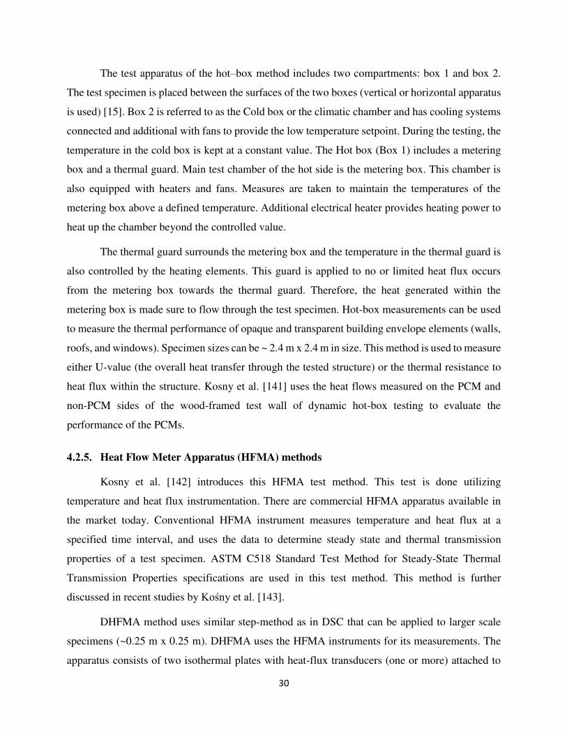
30
The test apparatus of the hot–box method includes two compartments: box 1 and box 2.
The test specimen is placed between the surfaces of the two boxes (vertical or horizontal apparatus
is used) [15]. Box 2 is referred to as the Cold box or the climatic chamber and has cooling systems
connected and additional with fans to provide the low temperature setpoint. During the testing, the
temperature in the cold box is kept at a constant value. The Hot box (Box 1) includes a metering
box and a thermal guard. Main test chamber of the hot side is the metering box. This chamber is
also equipped with heaters and fans. Measures are taken to maintain the temperatures of the
metering box above a defined temperature. Additional electrical heater provides heating power to
heat up the chamber beyond the controlled value.
The thermal guard surrounds the metering box and the temperature in the thermal guard is
also controlled by the heating elements. This guard is applied to no or limited heat flux occurs
from the metering box towards the thermal guard. Therefore, the heat generated within the
metering box is made sure to flow through the test specimen. Hot-box measurements can be used
to measure the thermal performance of opaque and transparent building envelope elements (walls,
roofs, and windows). Specimen sizes can be ~ 2.4 m x 2.4 m in size. This method is used to measure
either U-value (the overall heat transfer through the tested structure) or the thermal resistance to
heat flux within the structure. Kosny et al. [141] uses the heat flows measured on the PCM and
non-PCM sides of the wood-framed test wall of dynamic hot-box testing to evaluate the
performance of the PCMs.
Heat Flow Meter Apparatus (HFMA) methods
Kosny et al. [142] introduces this HFMA test method. This test is done utilizing
temperature and heat flux instrumentation. There are commercial HFMA apparatus available in
the market today. Conventional HFMA instrument measures temperature and heat flux at a
specified time interval, and uses the data to determine steady state and thermal transmission
properties of a test specimen. ASTM C518 Standard Test Method for Steady-State Thermal
Transmission Properties specifications are used in this test method. This method is further
discussed in recent studies by Kośny et al. [143].
DHFMA method uses similar step-method as in DSC that can be applied to larger scale
specimens (~0.25 m x 0.25 m). DHFMA uses the HFMA instruments for its measurements. The
apparatus consists of two isothermal plates with heat-flux transducers (one or more) attached to
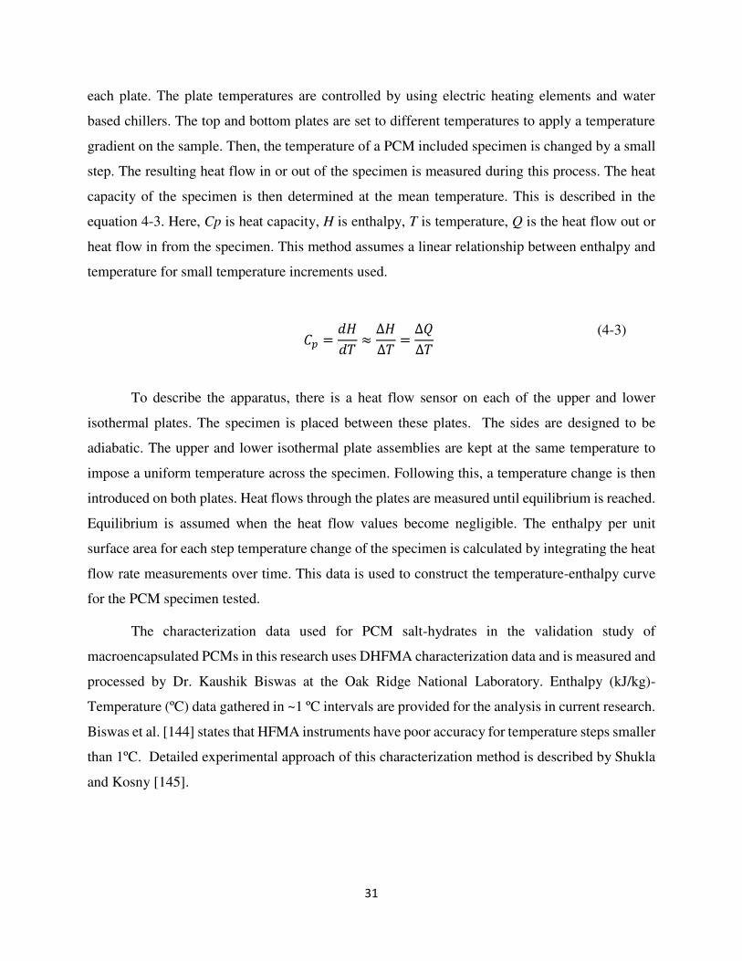
31
each plate. The plate temperatures are controlled by using electric heating elements and water
based chillers. The top and bottom plates are set to different temperatures to apply a temperature
gradient on the sample. Then, the temperature of a PCM included specimen is changed by a small
step. The resulting heat flow in or out of the specimen is measured during this process. The heat
capacity of the specimen is then determined at the mean temperature. This is described in the
equation 4-3. Here, Cp is heat capacity, H is enthalpy, T is temperature, Q is the heat flow out or
heat flow in from the specimen. This method assumes a linear relationship between enthalpy and
temperature for small temperature increments used.
𝐶𝑝 = 𝑑𝐻𝑑𝑇 ≈ ∆𝐻∆𝑇 = ∆𝑄∆𝑇 (4-3)
To describe the apparatus, there is a heat flow sensor on each of the upper and lower
isothermal plates. The specimen is placed between these plates. The sides are designed to be
adiabatic. The upper and lower isothermal plate assemblies are kept at the same temperature to
impose a uniform temperature across the specimen. Following this, a temperature change is then
introduced on both plates. Heat flows through the plates are measured until equilibrium is reached.
Equilibrium is assumed when the heat flow values become negligible. The enthalpy per unit
surface area for each step temperature change of the specimen is calculated by integrating the heat
flow rate measurements over time. This data is used to construct the temperature-enthalpy curve
for the PCM specimen tested.
The characterization data used for PCM salt-hydrates in the validation study of
macroencapsulated PCMs in this research uses DHFMA characterization data and is measured and
processed by Dr. Kaushik Biswas at the Oak Ridge National Laboratory. Enthalpy (kJ/kg)-
Temperature (ºC) data gathered in ~1 ºC intervals are provided for the analysis in current research.
Biswas et al. [144] states that HFMA instruments have poor accuracy for temperature steps smaller
than 1ºC. Detailed experimental approach of this characterization method is described by Shukla
and Kosny [145].
32
Other methods
In addition to above characterization methods, DSC Step-Testing method and DSC
Dynamic Ramp Mode [146], Differential Thermal Analysis (DTA) [147] are some methods that
have been used to characterize PCMs in material scale. These methods are mostly examines to
improve the results of DSC method.
There are some studies which compare different characterization methods. A recent study
compares DSC and improved DHFMA methods and concludes that at very low heating rates for
DSC method both methods showed same sub-cooling effects therefore, indicating that DHFMA
method is effective to test PCM wallboards [148].
4.3. Experimental studies on macroencapsulated and microencapsulated PCMs
This research focuses on the use of PCMs in the whole building scale and system scale
applications. System scale tests are conducted in test huts designed to conduct field studies,
envelope of existing buildings, or specialized chambers constructed for the testing of wall
assemblies.
PCM wall assemblies are tested in dynamic hot-box apparatus to examine shape-stabilized
PCM behind drywall to gather experimental data to investigate the impact of PCMs in reducing
temperature fluctuation [136]. PCM-enhanced foams are tested at the Oak Ridge National
Laboratory using a hot-box apparatus [15]. Same facility is used to test wood-framed wall
containing blown PCM-enhanced fiberglass insulation [149].
Test cubicles are used to examine macro encapsulated PCMs in free-floating conditions in
a recent study with the PCM containers are attached to polyurethane foam wall [150]. System scale
tests are conducted at Oak Ridge National Laboratory to analyze Nano-PCMs and a wall of
existing building was used to construct the experimental apparatus [14]. Wall structures are made
of OSB, cellulose insulation in addition to the Nano-PCM embedded gypsum and the heat transfer
study using this assembly is used to gather data for validation purposes. Kosny et al. [151] tested
a retrofit strategy for masonry walls using inorganic PCM-enhanced foam insulation using the
walls and roof of an existing building. Another study conducted field testing of walls side-by-side
to evaluate Phase Change Frame Wall (PCFW)s and examined lower peak heat transfer rates across
the walls and gathered data for validation purposes [152]. Muruganantham et al. [153] tested
33
macroencapsulated PCM pouches arrays covering the ceiling to investigate cooling load reductions
of the interior environment. Allqallaf et al. [154] tested a concrete slab with vertical cylindrical
holes to examine the effect of the geometry of macroencapsulation for PCM use in roofs.
Whole building scale tests apply PCMs in multiple components like exterior/interior walls,
slabs, ceilings, and floors. An 82-m2 single-family home is used in a study at the university campus
in Nottingham, England to implement PCM wallboards with microencapsulated PCM. A
commercial building at Charles Sturt University (CSU) located in New South Wales, Victoria,
Australia is used to implement microencapsulated PCM in floors and ceilings. This building has
880-m2 floor area and was constructed using lightweight steel framing technology [15]. A two
story PCM house is constructed at Oak Ridge National Laboratory [155]. This construction had a
with total floor area of 253-m2. Then floor of this house is insulated with 10.2-cm-thick layer of
PCM-enhanced cellulose insulation and 9 cm of PCM-enhanced cellulose insulation is installed
on the attic gable walls. Furthermore, A 20 % by weight of microencapsulated bio-based PCM is
also added to blown cellulose fibers in the exterior framed cavity of this house enabling a whole
building PCM application. All the above whole building level studies are used to assess the impact
of PCMs on the interior temperature profiles and heat transfer across the envelope.
To date, there has not been a study that investigates multiple wall panels in parallel in a controlled
environment. The experimental facility discussed in this study facilitates experimental
investigation multiple wall panels with PCMs.
34
CHAPTER 5
PARAMETRIC ANALYSIS OF A RESIDENTIAL BUILDING WITH PHASE CHANGE
MATERIAL (PCM)-ENHANCED DRYWALL, PRE-COOLING, AND VARIABLE
ELECTRIC RATES IN A HOT AND DRY CLIMATE
This section contributes to the fulfillment of the following objectives of this research: (i)
identify important variables and find optimal PCM properties for building envelope applications.
This study was published in the journal of Applied Energy, 15 July 2018: 497-514 [12].
Buildings account for about 75% of U.S. electricity consumption and 40% of total U.S.
energy consumption [156]. Nearly 15% of U.S. electricity use comes from building cooling
systems, and it can be as high as 50% in summer when considering non-coincident peak demand
[157]. Peak loads can cause difficulties for electric companies because the power generation
capacity must be equal to peak demand [158], which may result in electric companies significantly
increasing their production rates during peak hours. Shifting demand away from peak hours (i.e.,
reducing the total peak demand) is therefore a viable solution for utilities as well as building
owners. Therefore, many potential technologies, such as batteries and thermal storage, are being
considered to help reduce peak demand and also improve thermal comfort [159-161].
Building thermal storage has the potential to rely on the innate building mass; however,
U.S. homes typically have low thermal mass [162, 163], thus one option is to use phase change
materials (PCMs) to increase homes’ thermal mass. PCMs may be combined with precooling,
where smart programmable thermostats cool the house during off-peak time and increase the set
point at peak time [164-167]. Although the overall benefits of PCMs and precooling are well
known from several decades of research [69, 168-170], few studies examine the process of
optimizing various PCM properties and concentrations with specific precooling strategies.
Previous PCM studies have analyzed different applications, encapsulation techniques, and
locations within buildings. The location of PCMs in buildings varies widely in the literature,
including micro- and macro-encapsulation in or behind drywall [69, 171-176], concrete [177, 178],
fiber insulation [141, 179], or other systems, such as hot water systems, floor heating systems [25,
35
69, 180] and storage tanks [181, 182]. Wallboard applications have been studied extensively [69,
168-170, 183-185]. Early studies focused primarily on drywall impregnated with PCMs [186, 187]
and later on micro- and macro-encapsulation of PCMs [172, 173, 185]. Studies indicate that PCM-
enhanced drywall can improve thermal comfort by reducing thermal stratification due to natural
convective air mixing [184], and can help mitigate effects of extreme events like heat waves [188].
PCM performance in different applications heavily depends on proper PCM selection
based on their properties: melting temperature, melting temperature range, latent heat, thermal
conductivity, and others. However, few studies have looked into different combinations of PCM
inclusion [189-195]; some optimized the PCM thickness [196] or examined the effects of PCMs
on interior partition walls [183], ceilings, and exterior walls [197]. Others looked at increasing
heat transfer between the indoor environment and the walls [198, 199] or explored the optimum
PCM melting temperature in different cities [200] according to the outdoor boundary conditions,
which showed that the use of passive PCM systems in the building envelope with optimized peak
melting temperature for each climate zone can yield energy savings [201]. However, no study has
analyzed synergies between PCMs with programmable thermostats and variable electric rates
(Time-Of-Use Rates or TOU), as precooling has been used previously to reduce peak demand.
When PCMs are embedded in the drywall or behind the drywall, effective heat transfer
depends on several parameters, one of which is the convection heat transfer between the indoor air
and the interior wall surfaces. Under regular indoor conditions, natural convection is present,
resulting in low heat transfer coefficients between the indoor air and inside wall surfaces of the
building envelope (1-6 W/m2-K). A couple of studies suggest that natural convection cannot
adequately transfer heat towards the envelope to store a high amount of thermal energy in the PCM
wallboard [198, 202]. Thus, this study addresses the current gaps on PCM performance when
combined with precooling in a home subjected to TOU pricing and with a variable set point. It
also addresses the gaps on the role convection has on PCM performance by focusing on optimizing
PCM embedded in drywall using parametric analysis. The contributions of this study are: (1) to
analyze the impact indoor natural and forced convection have on the effectiveness to reduce peak
demand in a home with a precooling schedule with and without PCMs and (2) to inform engineers,
architects, and PCM’s manufacturers about the optimal PCM properties used when PCMs are
embedded in drywall. No previous study has analyzed this important issue in residential buildings.
36
In addition, one interest in this study is to look further than annualized energy related costs and
investigate the cooling related costs.
5.1. Approach
This study uses Building Energy Optimization (BEopt) Version 2.3 and EnergyPlus
Version 8.1 to perform all energy and cost analysis associated in the parametric analysis. BEopt
performs annual building energy simulations using EnergyPlus as the background simulation
engine. BEopt can perform parametric or optimization analyses based on monetary savings, energy
savings, or a combination of both using a sequential search optimization technique to find different
energy packages [203]. BEopt optimization algorithm identifies the least-cost approach to achieve
minimal whole-house energy use involving different combinations of discrete residential system
equipment and material options. BEopt can find intermediate optimal points all along the least-
cost curve minimum-cost building designs at different target energy savings levels [203].
However, BEopt’s sequential optimization algorithm has the objective function to minimize
energy use and the optimization mode only keeps the most cost effective points and few near
optimum points which eliminates the combinations that are required to the next stage of the study.
Therefore, all cases are evaluated using parametric analysis, where every single combination is
analyzed, allowing us to study how all the different PCM combinations (cost, location, and PCM
concentration) perform. After analysis of the entire results, subsequent post-processing finds
optimal solutions, as the study focuses on the cases with lowest energy cost and perform hourly
comparisons.
EnergyPlus is a whole building energy simulation program, which uses an integrated,
simultaneous solution approach to solve for different heat transfers processed in and out of the
built environment. Both BEopt and EnergyPlus have been validated for residential peak reduction
using the building envelope and electric bill calibration [204-206]. The default conduction heat
transfer algorithm in EnergyPlus is Conduction Transfer Function (CTF). This method is efficient
because it calculates the current surface temperature and heat fluxes with a limited number of
previous surface temperatures and fluxes [207]. However, BEopt uses a hybrid approach in PCM
modeling: SurfaceProperty:HeatTransferAlgorithm. Any construction assembly with PCMs is
modeled with the conduction finite difference (CondFD) algorithm while all others surfaces use
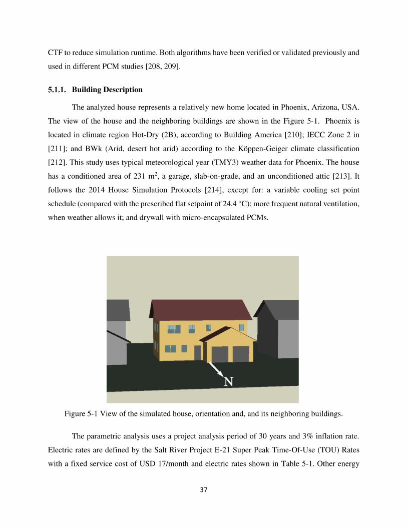
37
CTF to reduce simulation runtime. Both algorithms have been verified or validated previously and
used in different PCM studies [208, 209].
Building Description
The analyzed house represents a relatively new home located in Phoenix, Arizona, USA.
The view of the house and the neighboring buildings are shown in the Figure 5-1. Phoenix is
located in climate region Hot-Dry (2B), according to Building America [210]; IECC Zone 2 in
[211]; and BWk (Arid, desert hot arid) according to the Köppen-Geiger climate classification
[212]. This study uses typical meteorological year (TMY3) weather data for Phoenix. The house
has a conditioned area of 231 m2, a garage, slab-on-grade, and an unconditioned attic [213]. It
follows the 2014 House Simulation Protocols [214], except for: a variable cooling set point
schedule (compared with the prescribed flat setpoint of 24.4 °C); more frequent natural ventilation,
when weather allows it; and drywall with micro-encapsulated PCMs.
Figure 5-1 View of the simulated house, orientation and, and its neighboring buildings.
The parametric analysis uses a project analysis period of 30 years and 3% inflation rate.
Electric rates are defined by the Salt River Project E-21 Super Peak Time-Of-Use (TOU) Rates
with a fixed service cost of USD 17/month and electric rates shown in Table 5-1. Other energy
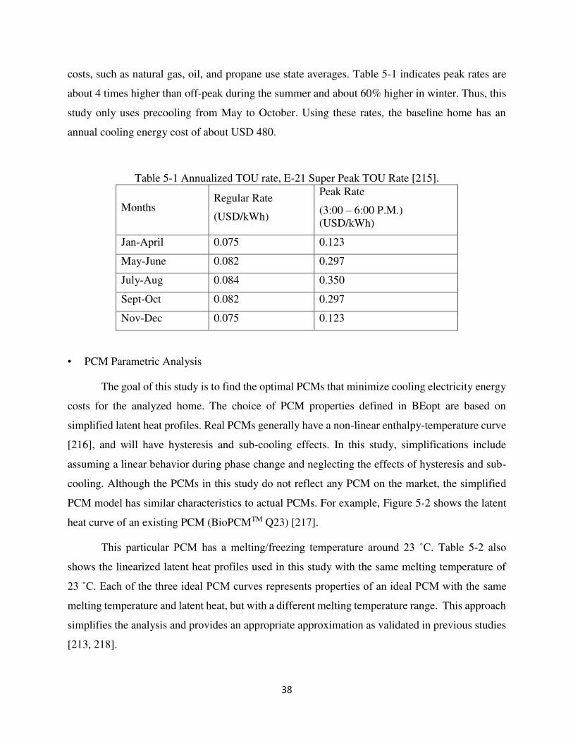
38
costs, such as natural gas, oil, and propane use state averages. Table 5-1 indicates peak rates are
about 4 times higher than off-peak during the summer and about 60% higher in winter. Thus, this
study only uses precooling from May to October. Using these rates, the baseline home has an
annual cooling energy cost of about USD 480.
Table 5-1 Annualized TOU rate, E-21 Super Peak TOU Rate [215].
Months Regular Rate
(USD/kWh)
Peak Rate
(3:00 – 6:00 P.M.) (USD/kWh)
Jan-April 0.075 0.123
May-June 0.082 0.297
July-Aug 0.084 0.350
Sept-Oct 0.082 0.297
Nov-Dec 0.075 0.123
• PCM Parametric Analysis
The goal of this study is to find the optimal PCMs that minimize cooling electricity energy
costs for the analyzed home. The choice of PCM properties defined in BEopt are based on
simplified latent heat profiles. Real PCMs generally have a non-linear enthalpy-temperature curve
[216], and will have hysteresis and sub-cooling effects. In this study, simplifications include
assuming a linear behavior during phase change and neglecting the effects of hysteresis and sub-
cooling. Although the PCMs in this study do not reflect any PCM on the market, the simplified
PCM model has similar characteristics to actual PCMs. For example, Figure 5-2 shows the latent
heat curve of an existing PCM (BioPCMTM Q23) [217].
This particular PCM has a melting/freezing temperature around 23 ˚C. Table 5-2 also
shows the linearized latent heat profiles used in this study with the same melting temperature of
23 ˚C. Each of the three ideal PCM curves represents properties of an ideal PCM with the same
melting temperature and latent heat, but with a different melting temperature range. This approach
simplifies the analysis and provides an appropriate approximation as validated in previous studies
[213, 218].
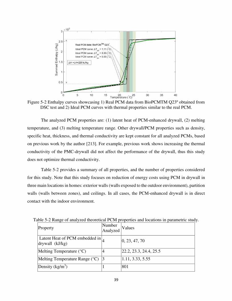
39
Figure 5-2 Enthalpy curves showcasing 1) Real PCM data from BioPCMTM Q23º obtained from
DSC test and 2) Ideal PCM curves with thermal properties similar to the real PCM.
The analyzed PCM properties are: (1) latent heat of PCM-enhanced drywall, (2) melting
temperature, and (3) melting temperature range. Other drywall/PCM properties such as density,
specific heat, thickness, and thermal conductivity are kept constant for all analyzed PCMs, based
on previous work by the author [213]. For example, previous work shows increasing the thermal
conductivity of the PMC-drywall did not affect the performance of the drywall, thus this study
does not optimize thermal conductivity.
Table 5-2 provides a summary of all properties, and the number of properties considered
for this study. Note that this study focuses on reduction of energy costs using PCM in drywall in
three main locations in homes: exterior walls (walls exposed to the outdoor environment), partition
walls (walls between zones), and ceilings. In all cases, the PCM-enhanced drywall is in direct
contact with the indoor environment.
Table 5-2 Range of analyzed theoretical PCM properties and locations in parametric study.
Property Number Analyzed
Values
Latent Heat of PCM embedded in drywall (kJ/kg)
4 0, 23, 47, 70
Melting Temperature (°C) 4 22.2, 23.3, 24.4, 25.5
Melting Temperature Range (°C) 3 1.11, 3.33, 5.55
Density (kg/m3) 1 801
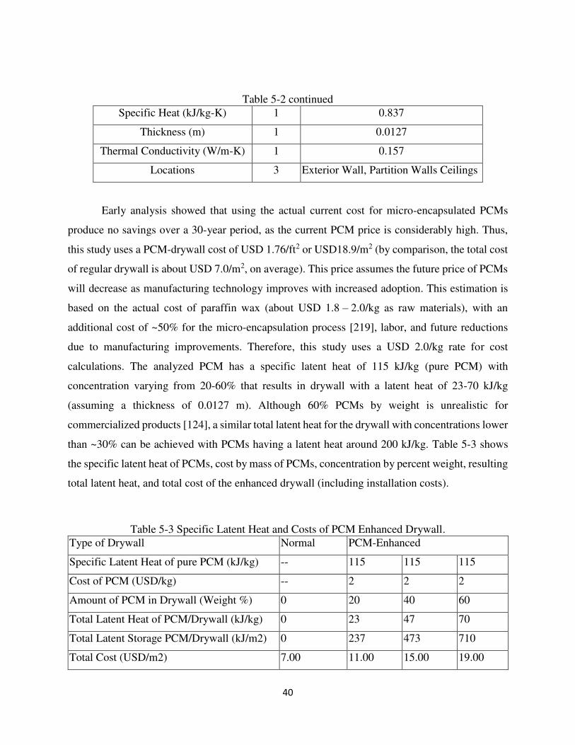
40
Table 5-2 continued Specific Heat (kJ/kg-K) 1 0.837
Thickness (m) 1 0.0127
Thermal Conductivity (W/m-K) 1 0.157
Locations 3 Exterior Wall, Partition Walls Ceilings
Early analysis showed that using the actual current cost for micro-encapsulated PCMs
produce no savings over a 30-year period, as the current PCM price is considerably high. Thus,
this study uses a PCM-drywall cost of USD 1.76/ft2 or USD18.9/m2 (by comparison, the total cost
of regular drywall is about USD 7.0/m2, on average). This price assumes the future price of PCMs
will decrease as manufacturing technology improves with increased adoption. This estimation is
based on the actual cost of paraffin wax (about USD 1.8 – 2.0/kg as raw materials), with an
additional cost of ~50% for the micro-encapsulation process [219], labor, and future reductions
due to manufacturing improvements. Therefore, this study uses a USD 2.0/kg rate for cost
calculations. The analyzed PCM has a specific latent heat of 115 kJ/kg (pure PCM) with
concentration varying from 20-60% that results in drywall with a latent heat of 23-70 kJ/kg
(assuming a thickness of 0.0127 m). Although 60% PCMs by weight is unrealistic for
commercialized products [124], a similar total latent heat for the drywall with concentrations lower
than ~30% can be achieved with PCMs having a latent heat around 200 kJ/kg. Table 5-3 shows
the specific latent heat of PCMs, cost by mass of PCMs, concentration by percent weight, resulting
total latent heat, and total cost of the enhanced drywall (including installation costs).
Table 5-3 Specific Latent Heat and Costs of PCM Enhanced Drywall. Type of Drywall Normal PCM-Enhanced
Specific Latent Heat of pure PCM (kJ/kg) -- 115 115 115
Cost of PCM (USD/kg) -- 2 2 2
Amount of PCM in Drywall (Weight %) 0 20 40 60
Total Latent Heat of PCM/Drywall (kJ/kg) 0 23 47 70
Total Latent Storage PCM/Drywall (kJ/m2) 0 237 473 710
Total Cost (USD/m2) 7.00 11.00 15.00 19.00
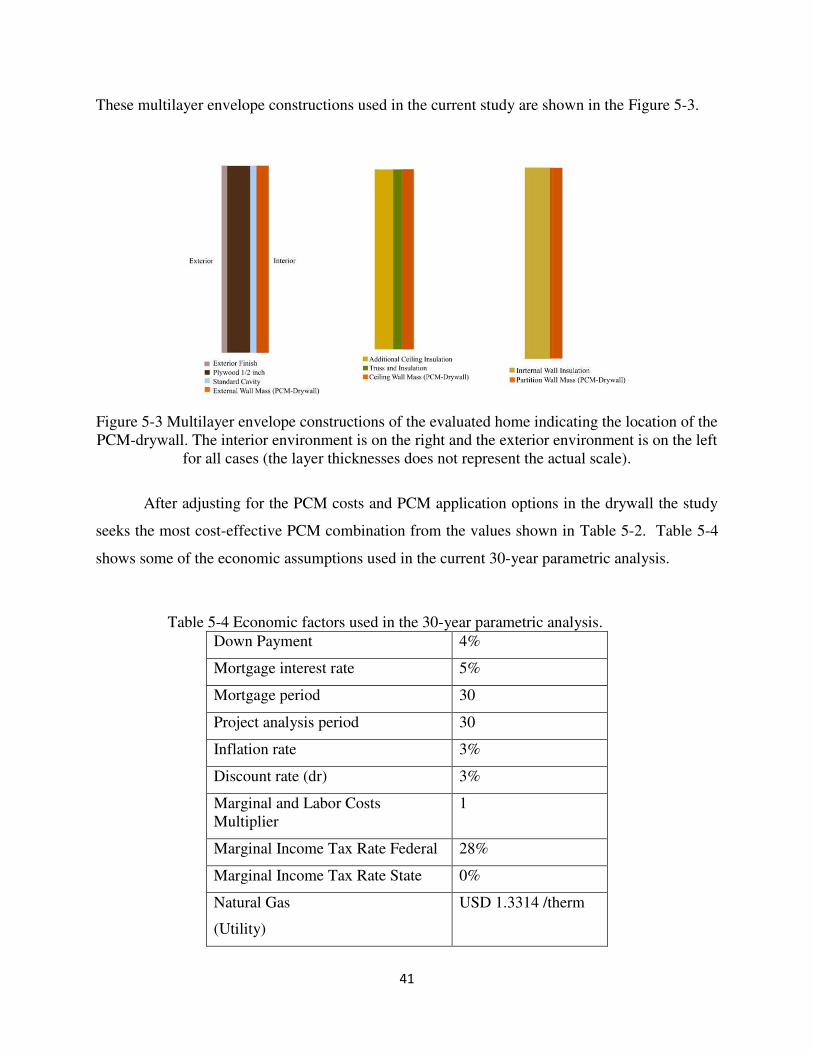
41
These multilayer envelope constructions used in the current study are shown in the Figure 5-3.
Figure 5-3 Multilayer envelope constructions of the evaluated home indicating the location of the PCM-drywall. The interior environment is on the right and the exterior environment is on the left
for all cases (the layer thicknesses does not represent the actual scale).
After adjusting for the PCM costs and PCM application options in the drywall the study
seeks the most cost-effective PCM combination from the values shown in Table 5-2. Table 5-4
shows some of the economic assumptions used in the current 30-year parametric analysis.
Table 5-4 Economic factors used in the 30-year parametric analysis. Down Payment 4%
Mortgage interest rate 5%
Mortgage period 30
Project analysis period 30
Inflation rate 3%
Discount rate (dr) 3%
Marginal and Labor Costs Multiplier
1
Marginal Income Tax Rate Federal 28%
Marginal Income Tax Rate State 0%
Natural Gas
(Utility)
USD 1.3314 /therm
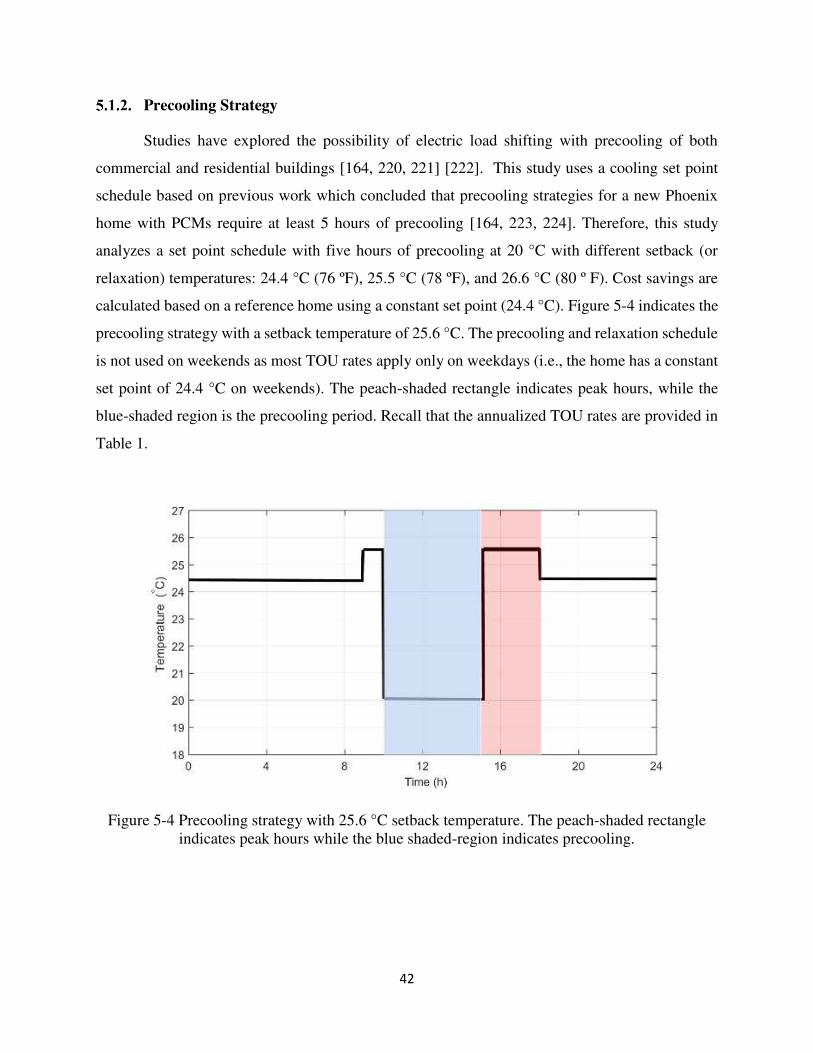
42
Precooling Strategy
Studies have explored the possibility of electric load shifting with precooling of both
commercial and residential buildings [164, 220, 221] [222]. This study uses a cooling set point
schedule based on previous work which concluded that precooling strategies for a new Phoenix
home with PCMs require at least 5 hours of precooling [164, 223, 224]. Therefore, this study
analyzes a set point schedule with five hours of precooling at 20 °C with different setback (or
relaxation) temperatures: 24.4 °C (76 ºF), 25.5 °C (78 ºF), and 26.6 °C (80 º F). Cost savings are
calculated based on a reference home using a constant set point (24.4 °C). Figure 5-4 indicates the
precooling strategy with a setback temperature of 25.6 °C. The precooling and relaxation schedule
is not used on weekends as most TOU rates apply only on weekdays (i.e., the home has a constant
set point of 24.4 °C on weekends). The peach-shaded rectangle indicates peak hours, while the
blue-shaded region is the precooling period. Recall that the annualized TOU rates are provided in
Table 1.
Figure 5-4 Precooling strategy with 25.6 °C setback temperature. The peach-shaded rectangle indicates peak hours while the blue shaded-region indicates precooling.
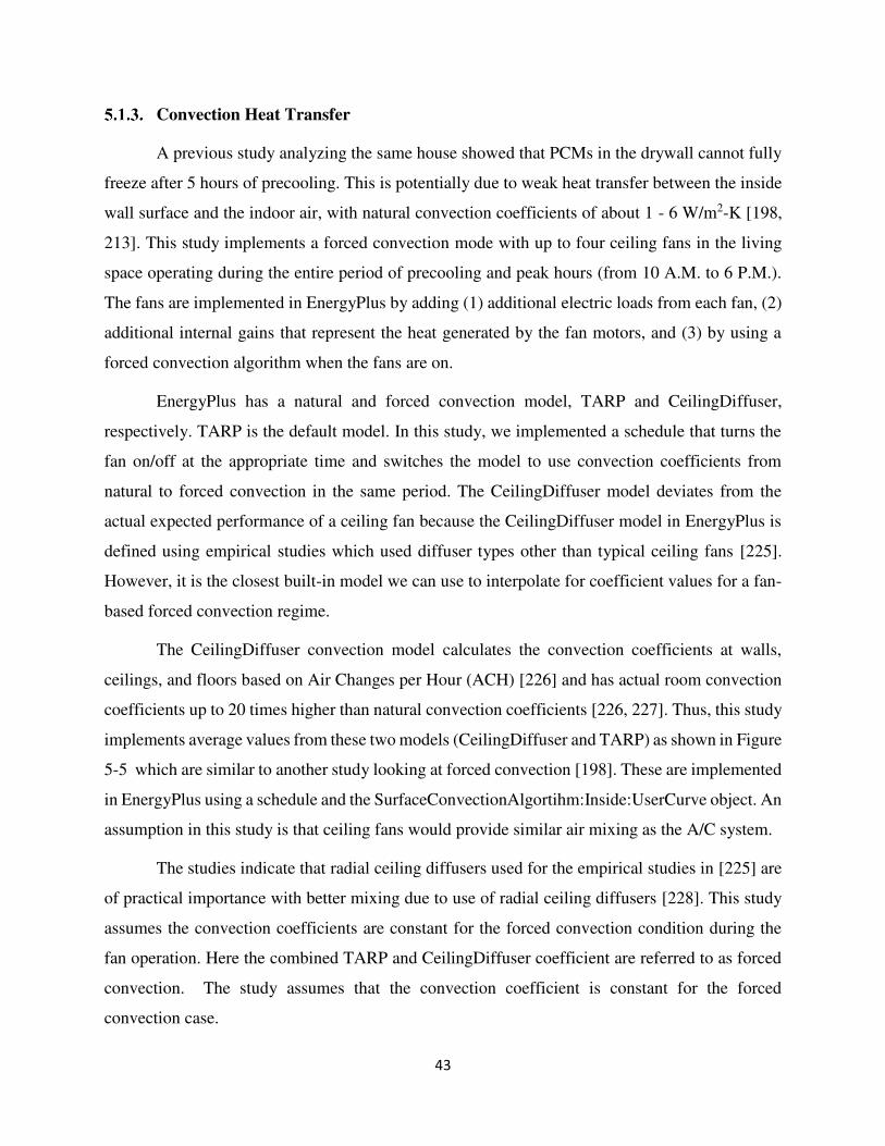
43
Convection Heat Transfer
A previous study analyzing the same house showed that PCMs in the drywall cannot fully
freeze after 5 hours of precooling. This is potentially due to weak heat transfer between the inside
wall surface and the indoor air, with natural convection coefficients of about 1 - 6 W/m2-K [198,
213]. This study implements a forced convection mode with up to four ceiling fans in the living
space operating during the entire period of precooling and peak hours (from 10 A.M. to 6 P.M.).
The fans are implemented in EnergyPlus by adding (1) additional electric loads from each fan, (2)
additional internal gains that represent the heat generated by the fan motors, and (3) by using a
forced convection algorithm when the fans are on.
EnergyPlus has a natural and forced convection model, TARP and CeilingDiffuser,
respectively. TARP is the default model. In this study, we implemented a schedule that turns the
fan on/off at the appropriate time and switches the model to use convection coefficients from
natural to forced convection in the same period. The CeilingDiffuser model deviates from the
actual expected performance of a ceiling fan because the CeilingDiffuser model in EnergyPlus is
defined using empirical studies which used diffuser types other than typical ceiling fans [225].
However, it is the closest built-in model we can use to interpolate for coefficient values for a fan-
based forced convection regime.
The CeilingDiffuser convection model calculates the convection coefficients at walls,
ceilings, and floors based on Air Changes per Hour (ACH) [226] and has actual room convection
coefficients up to 20 times higher than natural convection coefficients [226, 227]. Thus, this study
implements average values from these two models (CeilingDiffuser and TARP) as shown in Figure
5-5 which are similar to another study looking at forced convection [198]. These are implemented
in EnergyPlus using a schedule and the SurfaceConvectionAlgortihm:Inside:UserCurve object. An
assumption in this study is that ceiling fans would provide similar air mixing as the A/C system.
The studies indicate that radial ceiling diffusers used for the empirical studies in [225] are
of practical importance with better mixing due to use of radial ceiling diffusers [228]. This study
assumes the convection coefficients are constant for the forced convection condition during the
fan operation. Here the combined TARP and CeilingDiffuser coefficient are referred to as forced
convection. The study assumes that the convection coefficient is constant for the forced
convection case.
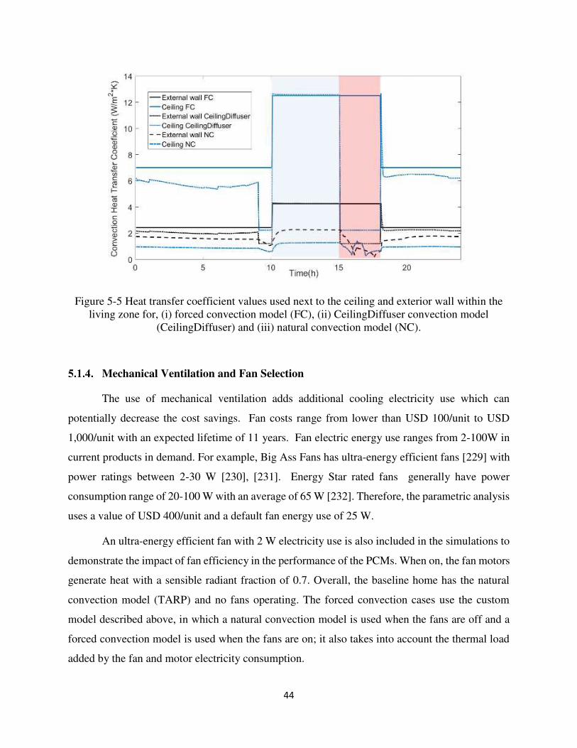
44
Figure 5-5 Heat transfer coefficient values used next to the ceiling and exterior wall within the living zone for, (i) forced convection model (FC), (ii) CeilingDiffuser convection model
(CeilingDiffuser) and (iii) natural convection model (NC).
Mechanical Ventilation and Fan Selection
The use of mechanical ventilation adds additional cooling electricity use which can
potentially decrease the cost savings. Fan costs range from lower than USD 100/unit to USD
1,000/unit with an expected lifetime of 11 years. Fan electric energy use ranges from 2-100W in
current products in demand. For example, Big Ass Fans has ultra-energy efficient fans [229] with
power ratings between 2-30 W [230], [231]. Energy Star rated fans generally have power
consumption range of 20-100 W with an average of 65 W [232]. Therefore, the parametric analysis
uses a value of USD 400/unit and a default fan energy use of 25 W.
An ultra-energy efficient fan with 2 W electricity use is also included in the simulations to
demonstrate the impact of fan efficiency in the performance of the PCMs. When on, the fan motors
generate heat with a sensible radiant fraction of 0.7. Overall, the baseline home has the natural
convection model (TARP) and no fans operating. The forced convection cases use the custom
model described above, in which a natural convection model is used when the fans are off and a
forced convection model is used when the fans are on; it also takes into account the thermal load
added by the fan and motor electricity consumption.
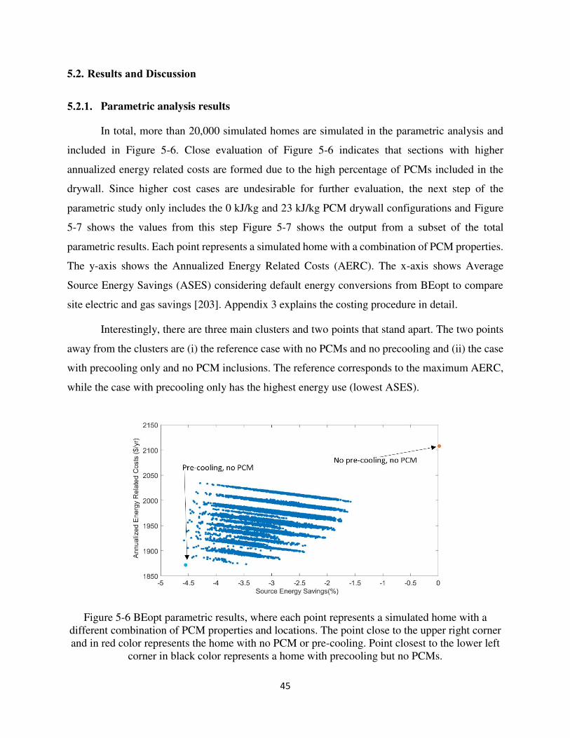
45
5.2. Results and Discussion
Parametric analysis results
In total, more than 20,000 simulated homes are simulated in the parametric analysis and
included in Figure 5-6. Close evaluation of Figure 5-6 indicates that sections with higher
annualized energy related costs are formed due to the high percentage of PCMs included in the
drywall. Since higher cost cases are undesirable for further evaluation, the next step of the
parametric study only includes the 0 kJ/kg and 23 kJ/kg PCM drywall configurations and Figure
5-7 shows the values from this step Figure 5-7 shows the output from a subset of the total
parametric results. Each point represents a simulated home with a combination of PCM properties.
The y-axis shows the Annualized Energy Related Costs (AERC). The x-axis shows Average
Source Energy Savings (ASES) considering default energy conversions from BEopt to compare
site electric and gas savings [203]. Appendix 3 explains the costing procedure in detail.
Interestingly, there are three main clusters and two points that stand apart. The two points
away from the clusters are (i) the reference case with no PCMs and no precooling and (ii) the case
with precooling only and no PCM inclusions. The reference corresponds to the maximum AERC,
while the case with precooling only has the highest energy use (lowest ASES).
Figure 5-6 BEopt parametric results, where each point represents a simulated home with a different combination of PCM properties and locations. The point close to the upper right corner and in red color represents the home with no PCM or pre-cooling. Point closest to the lower left
corner in black color represents a home with precooling but no PCMs.
46
Figure 5-7 BEopt parametric results for the cases with lowest energy related costs, where each point represents a simulated home with a different combination of PCM properties and locations.
The point close to the upper right corner represents the home with no PCM.
In all cases, precooling decreases energy costs, but increases energy use (negative energy
savings) as also shown in the literature [213]. The clustering of other points relates to the location
of PCMs and the latent heat. Cases with 60% and 40% PCM inclusion still show high cost, thus
are not shown in Figure 5-7. The lower cost points indicated above have a 20% PCM inclusion
corresponding to an effective latent heat of 23 kJ/kg. PCMs included in the ceiling-only cases have
a higher energy penalty and lower AERC. PCMs installed in all three locations (ceilings, exterior
walls, interior walls) tend to have lower energy penalties but higher annualized energy related
costs due to the greater quantity of PCMs in use (higher initial costs).
For each of these option classes (PCMs in all three locations, PCMs in two locations, PCMs
in ceilings only), there is a case with the lowest annualized energy cost. For further analysis, these
optimum points are considered in greater detail. Table 5-5 shows the optimal PCM properties for
each case as indicated also in Figure 5-8, where the rest of the simulated homes are removed. One
interest in this study is to look further than annualized energy related costs and investigate the
cooling related costs.
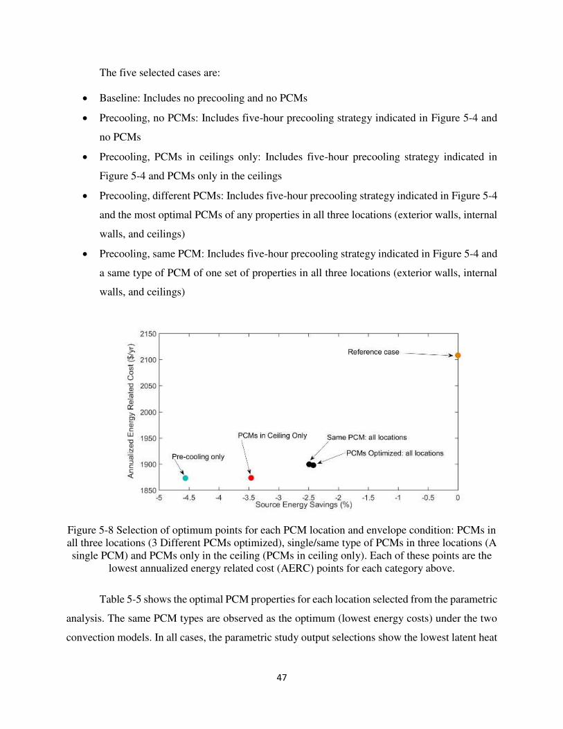
47
The five selected cases are:
Baseline: Includes no precooling and no PCMs
Precooling, no PCMs: Includes five-hour precooling strategy indicated in Figure 5-4 and
no PCMs
Precooling, PCMs in ceilings only: Includes five-hour precooling strategy indicated in
Figure 5-4 and PCMs only in the ceilings
Precooling, different PCMs: Includes five-hour precooling strategy indicated in Figure 5-4
and the most optimal PCMs of any properties in all three locations (exterior walls, internal
walls, and ceilings)
Precooling, same PCM: Includes five-hour precooling strategy indicated in Figure 5-4 and
a same type of PCM of one set of properties in all three locations (exterior walls, internal
walls, and ceilings)
Figure 5-8 Selection of optimum points for each PCM location and envelope condition: PCMs in all three locations (3 Different PCMs optimized), single/same type of PCMs in three locations (A single PCM) and PCMs only in the ceiling (PCMs in ceiling only). Each of these points are the
lowest annualized energy related cost (AERC) points for each category above.
Table 5-5 shows the optimal PCM properties for each location selected from the parametric
analysis. The same PCM types are observed as the optimum (lowest energy costs) under the two
convection models. In all cases, the parametric study output selections show the lowest latent heat
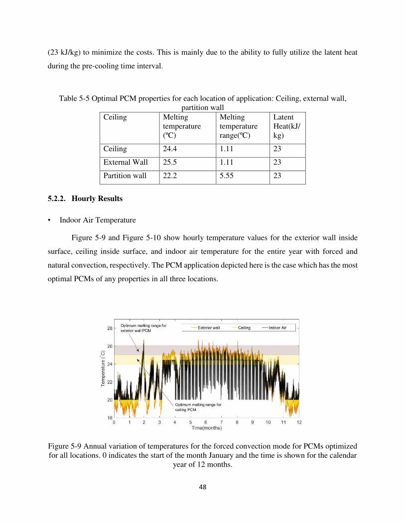
48
(23 kJ/kg) to minimize the costs. This is mainly due to the ability to fully utilize the latent heat
during the pre-cooling time interval.
Table 5-5 Optimal PCM properties for each location of application: Ceiling, external wall, partition wall
Ceiling Melting temperature (ºC)
Melting temperature range(ºC)
Latent Heat(kJ/kg)
Ceiling 24.4 1.11 23
External Wall 25.5 1.11 23
Partition wall 22.2 5.55 23
Hourly Results
• Indoor Air Temperature
Figure 5-9 and Figure 5-10 show hourly temperature values for the exterior wall inside
surface, ceiling inside surface, and indoor air temperature for the entire year with forced and
natural convection, respectively. The PCM application depicted here is the case which has the most
optimal PCMs of any properties in all three locations.
Figure 5-9 Annual variation of temperatures for the forced convection mode for PCMs optimized for all locations. 0 indicates the start of the month January and the time is shown for the calendar
year of 12 months.
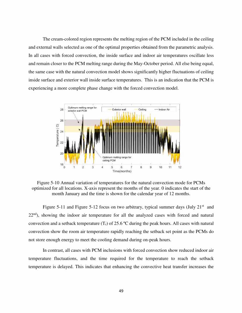
49
The cream-colored region represents the melting region of the PCM included in the ceiling
and external walls selected as one of the optimal properties obtained from the parametric analysis.
In all cases with forced convection, the inside surface and indoor air temperatures oscillate less
and remain closer to the PCM melting range during the May-October period. All else being equal,
the same case with the natural convection model shows significantly higher fluctuations of ceiling
inside surface and exterior wall inside surface temperatures. This is an indication that the PCM is
experiencing a more complete phase change with the forced convection model.
Figure 5-10 Annual variation of temperatures for the natural convection mode for PCMs optimized for all locations. X-axis represent the months of the year. 0 indicates the start of the
month January and the time is shown for the calendar year of 12 months.
Figure 5-11 and Figure 5-12 focus on two arbitrary, typical summer days (July 21st and
22nd), showing the indoor air temperature for all the analyzed cases with forced and natural
convection and a setback temperature (Tr) of 25.6 ºC during the peak hours. All cases with natural
convection show the room air temperature rapidly reaching the setback set point as the PCMs do
not store enough energy to meet the cooling demand during on-peak hours.
In contrast, all cases with PCM inclusions with forced convection show reduced indoor air
temperature fluctuations, and the time required for the temperature to reach the setback
temperature is delayed. This indicates that enhancing the convective heat transfer increases the
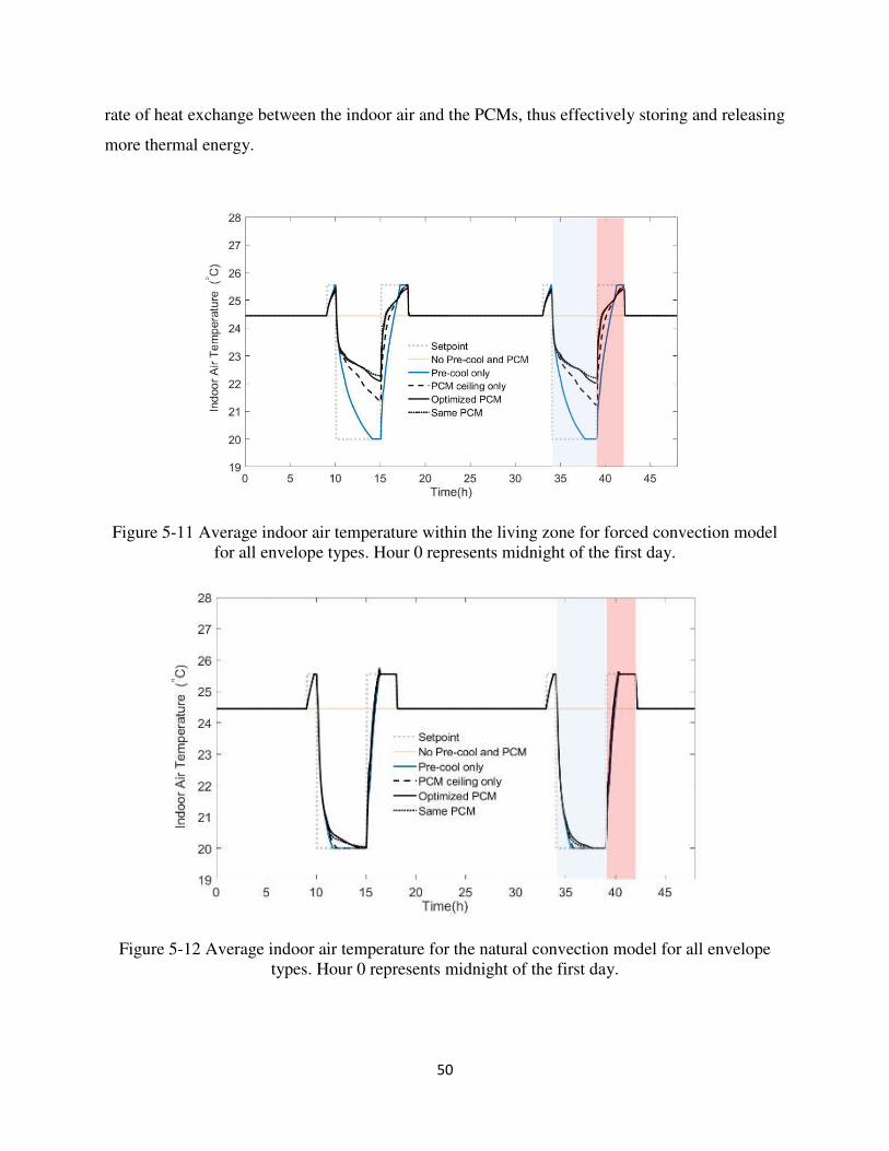
50
rate of heat exchange between the indoor air and the PCMs, thus effectively storing and releasing
more thermal energy.
Figure 5-11 Average indoor air temperature within the living zone for forced convection model for all envelope types. Hour 0 represents midnight of the first day.
Figure 5-12 Average indoor air temperature for the natural convection model for all envelope types. Hour 0 represents midnight of the first day.
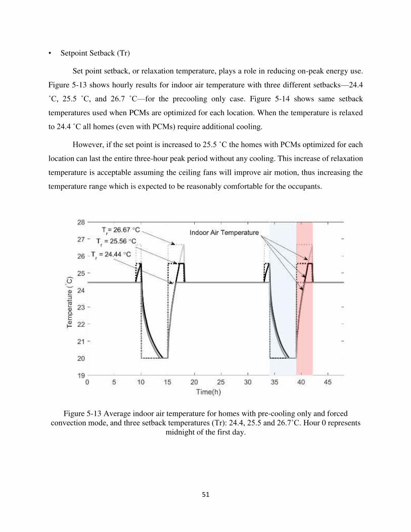
51
• Setpoint Setback (Tr)
Set point setback, or relaxation temperature, plays a role in reducing on-peak energy use.
Figure 5-13 shows hourly results for indoor air temperature with three different setbacks—24.4
˚C, 25.5 ˚C, and 26.7 ˚C—for the precooling only case. Figure 5-14 shows same setback
temperatures used when PCMs are optimized for each location. When the temperature is relaxed
to 24.4 ˚C all homes (even with PCMs) require additional cooling.
However, if the set point is increased to 25.5 ˚C the homes with PCMs optimized for each
location can last the entire three-hour peak period without any cooling. This increase of relaxation
temperature is acceptable assuming the ceiling fans will improve air motion, thus increasing the
temperature range which is expected to be reasonably comfortable for the occupants.
Figure 5-13 Average indoor air temperature for homes with pre-cooling only and forced convection mode, and three setback temperatures (Tr): 24.4, 25.5 and 26.7˚C. Hour 0 represents
midnight of the first day.
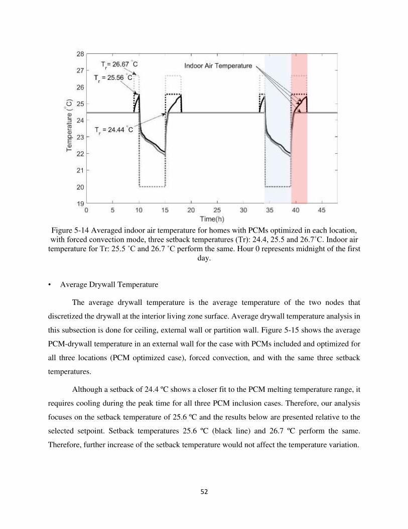
52
Figure 5-14 Averaged indoor air temperature for homes with PCMs optimized in each location, with forced convection mode, three setback temperatures (Tr): 24.4, 25.5 and 26.7˚C. Indoor air
temperature for Tr: 25.5 ˚C and 26.7 ˚C perform the same. Hour 0 represents midnight of the first day.
• Average Drywall Temperature
The average drywall temperature is the average temperature of the two nodes that
discretized the drywall at the interior living zone surface. Average drywall temperature analysis in
this subsection is done for ceiling, external wall or partition wall. Figure 5-15 shows the average
PCM-drywall temperature in an external wall for the case with PCMs included and optimized for
all three locations (PCM optimized case), forced convection, and with the same three setback
temperatures.
Although a setback of 24.4 ºC shows a closer fit to the PCM melting temperature range, it
requires cooling during the peak time for all three PCM inclusion cases. Therefore, our analysis
focuses on the setback temperature of 25.6 ºC and the results below are presented relative to the
selected setpoint. Setback temperatures 25.6 ºC (black line) and 26.7 ºC perform the same.
Therefore, further increase of the setback temperature would not affect the temperature variation.
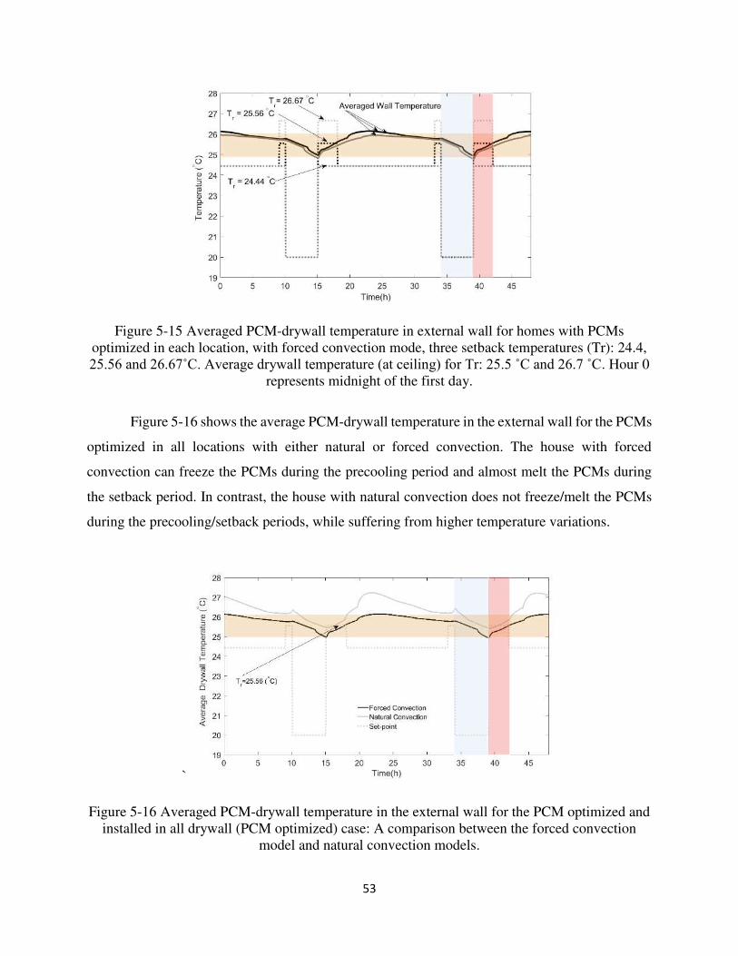
53
Figure 5-15 Averaged PCM-drywall temperature in external wall for homes with PCMs optimized in each location, with forced convection mode, three setback temperatures (Tr): 24.4, 25.56 and 26.67˚C. Average drywall temperature (at ceiling) for Tr: 25.5 ˚C and 26.7 ˚C. Hour 0
represents midnight of the first day.
Figure 5-16 shows the average PCM-drywall temperature in the external wall for the PCMs
optimized in all locations with either natural or forced convection. The house with forced
convection can freeze the PCMs during the precooling period and almost melt the PCMs during
the setback period. In contrast, the house with natural convection does not freeze/melt the PCMs
during the precooling/setback periods, while suffering from higher temperature variations.
`
Figure 5-16 Averaged PCM-drywall temperature in the external wall for the PCM optimized and installed in all drywall (PCM optimized) case: A comparison between the forced convection
model and natural convection models.
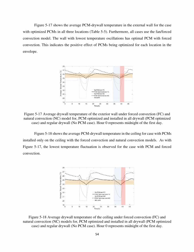
54
Figure 5-17 shows the average PCM-drywall temperature in the external wall for the case
with optimized PCMs in all three locations (Table 5-5). Furthermore, all cases use the fan/forced
convection model. The wall with lowest temperature oscillations has optimal PCM with forced
convection. This indicates the positive effect of PCMs being optimized for each location in the
envelope.
Figure 5-17 Average drywall temperature of the exterior wall under forced convection (FC) and natural convection (NC) model for, PCM optimized and installed in all drywall (PCM optimized
case) and regular drywall (No PCM case). Hour 0 represents midnight of the first day.
Figure 5-18 shows the average PCM-drywall temperature in the ceiling for case with PCMs
installed only on the ceiling with the forced convection and natural convection models. As with
Figure 5-17, the lowest temperature fluctuation is observed for the case with PCM and forced
convection.
Figure 5-18 Average drywall temperature of the ceiling under forced convection (FC) and natural convection (NC) models for, PCM optimized and installed in all drywall (PCM optimized
case) and regular drywall (No PCM case). Hour 0 represents midnight of the first day.
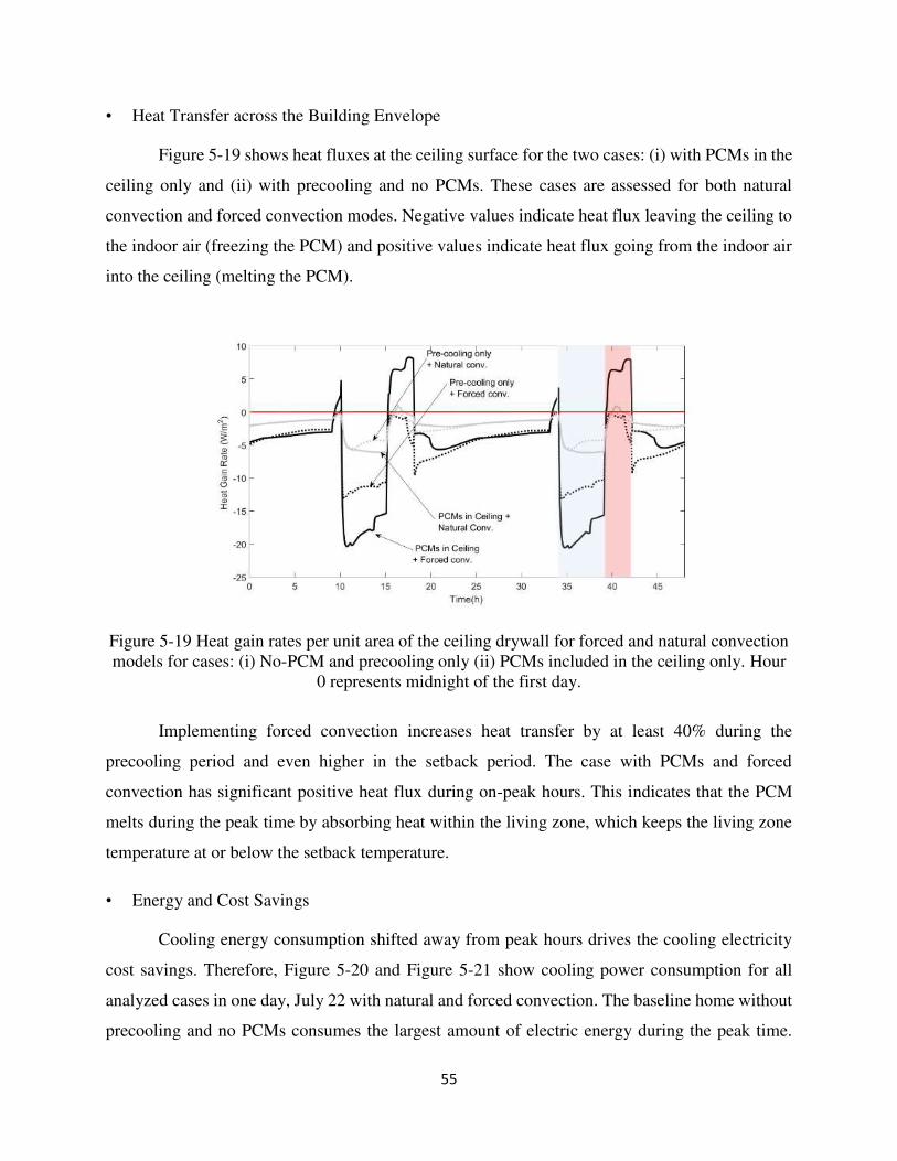
55
• Heat Transfer across the Building Envelope
Figure 5-19 shows heat fluxes at the ceiling surface for the two cases: (i) with PCMs in the
ceiling only and (ii) with precooling and no PCMs. These cases are assessed for both natural
convection and forced convection modes. Negative values indicate heat flux leaving the ceiling to
the indoor air (freezing the PCM) and positive values indicate heat flux going from the indoor air
into the ceiling (melting the PCM).
Figure 5-19 Heat gain rates per unit area of the ceiling drywall for forced and natural convection models for cases: (i) No-PCM and precooling only (ii) PCMs included in the ceiling only. Hour
0 represents midnight of the first day.
Implementing forced convection increases heat transfer by at least 40% during the
precooling period and even higher in the setback period. The case with PCMs and forced
convection has significant positive heat flux during on-peak hours. This indicates that the PCM
melts during the peak time by absorbing heat within the living zone, which keeps the living zone
temperature at or below the setback temperature.
• Energy and Cost Savings
Cooling energy consumption shifted away from peak hours drives the cooling electricity
cost savings. Therefore, Figure 5-20 and Figure 5-21 show cooling power consumption for all
analyzed cases in one day, July 22 with natural and forced convection. The baseline home without
precooling and no PCMs consumes the largest amount of electric energy during the peak time.
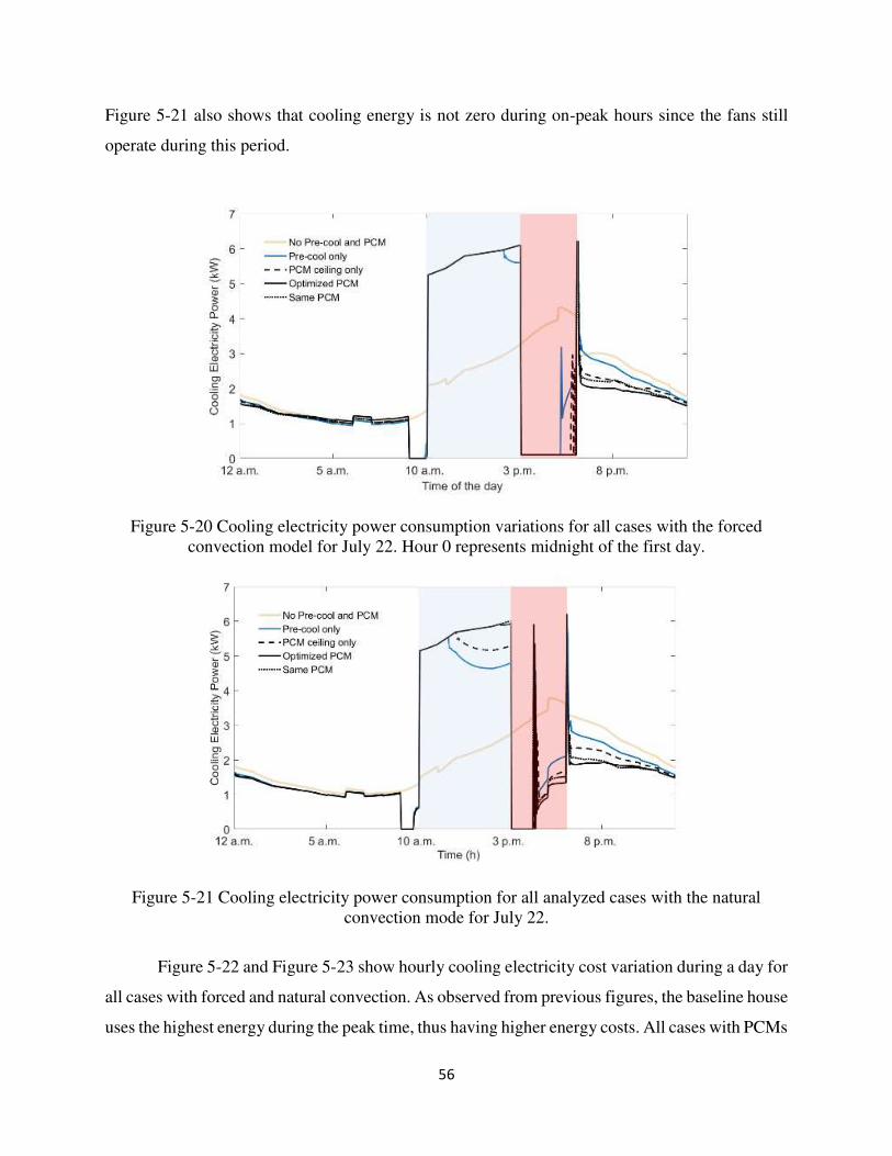
56
Figure 5-21 also shows that cooling energy is not zero during on-peak hours since the fans still
operate during this period.
Figure 5-20 Cooling electricity power consumption variations for all cases with the forced convection model for July 22. Hour 0 represents midnight of the first day.
Figure 5-21 Cooling electricity power consumption for all analyzed cases with the natural convection mode for July 22.
Figure 5-22 and Figure 5-23 show hourly cooling electricity cost variation during a day for
all cases with forced and natural convection. As observed from previous figures, the baseline house
uses the highest energy during the peak time, thus having higher energy costs. All cases with PCMs
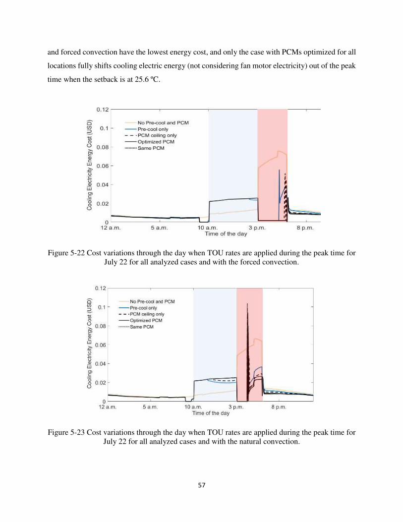
57
and forced convection have the lowest energy cost, and only the case with PCMs optimized for all
locations fully shifts cooling electric energy (not considering fan motor electricity) out of the peak
time when the setback is at 25.6 ºC.
Figure 5-22 Cost variations through the day when TOU rates are applied during the peak time for July 22 for all analyzed cases and with the forced convection.
Figure 5-23 Cost variations through the day when TOU rates are applied during the peak time for July 22 for all analyzed cases and with the natural convection.
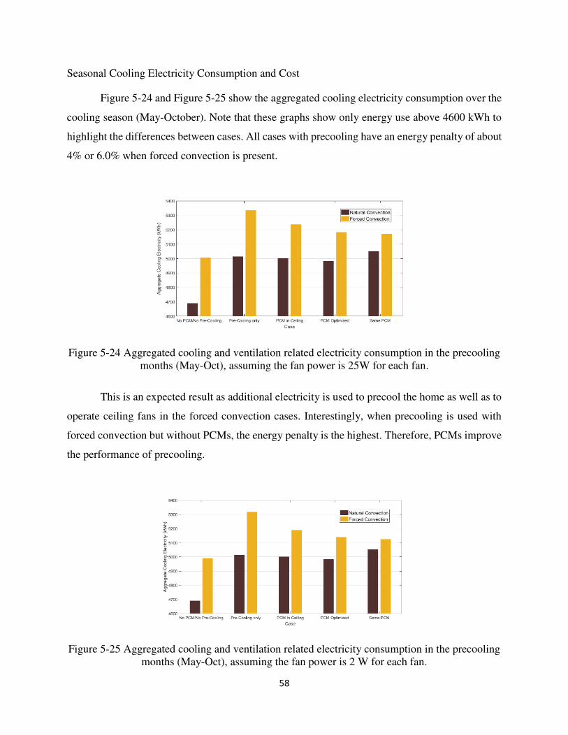
58
Seasonal Cooling Electricity Consumption and Cost
Figure 5-24 and Figure 5-25 show the aggregated cooling electricity consumption over the
cooling season (May-October). Note that these graphs show only energy use above 4600 kWh to
highlight the differences between cases. All cases with precooling have an energy penalty of about
4% or 6.0% when forced convection is present.
Figure 5-24 Aggregated cooling and ventilation related electricity consumption in the precooling months (May-Oct), assuming the fan power is 25W for each fan.
This is an expected result as additional electricity is used to precool the home as well as to
operate ceiling fans in the forced convection cases. Interestingly, when precooling is used with
forced convection but without PCMs, the energy penalty is the highest. Therefore, PCMs improve
the performance of precooling.
Figure 5-25 Aggregated cooling and ventilation related electricity consumption in the precooling months (May-Oct), assuming the fan power is 2 W for each fan.
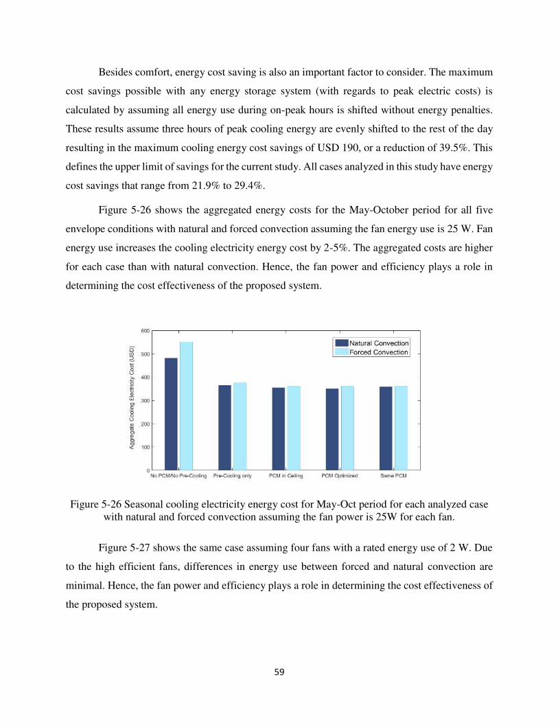
59
Besides comfort, energy cost saving is also an important factor to consider. The maximum
cost savings possible with any energy storage system (with regards to peak electric costs) is
calculated by assuming all energy use during on-peak hours is shifted without energy penalties.
These results assume three hours of peak cooling energy are evenly shifted to the rest of the day
resulting in the maximum cooling energy cost savings of USD 190, or a reduction of 39.5%. This
defines the upper limit of savings for the current study. All cases analyzed in this study have energy
cost savings that range from 21.9% to 29.4%.
Figure 5-26 shows the aggregated energy costs for the May-October period for all five
envelope conditions with natural and forced convection assuming the fan energy use is 25 W. Fan
energy use increases the cooling electricity energy cost by 2-5%. The aggregated costs are higher
for each case than with natural convection. Hence, the fan power and efficiency plays a role in
determining the cost effectiveness of the proposed system.
Figure 5-26 Seasonal cooling electricity energy cost for May-Oct period for each analyzed case with natural and forced convection assuming the fan power is 25W for each fan.
Figure 5-27 shows the same case assuming four fans with a rated energy use of 2 W. Due
to the high efficient fans, differences in energy use between forced and natural convection are
minimal. Hence, the fan power and efficiency plays a role in determining the cost effectiveness of
the proposed system.
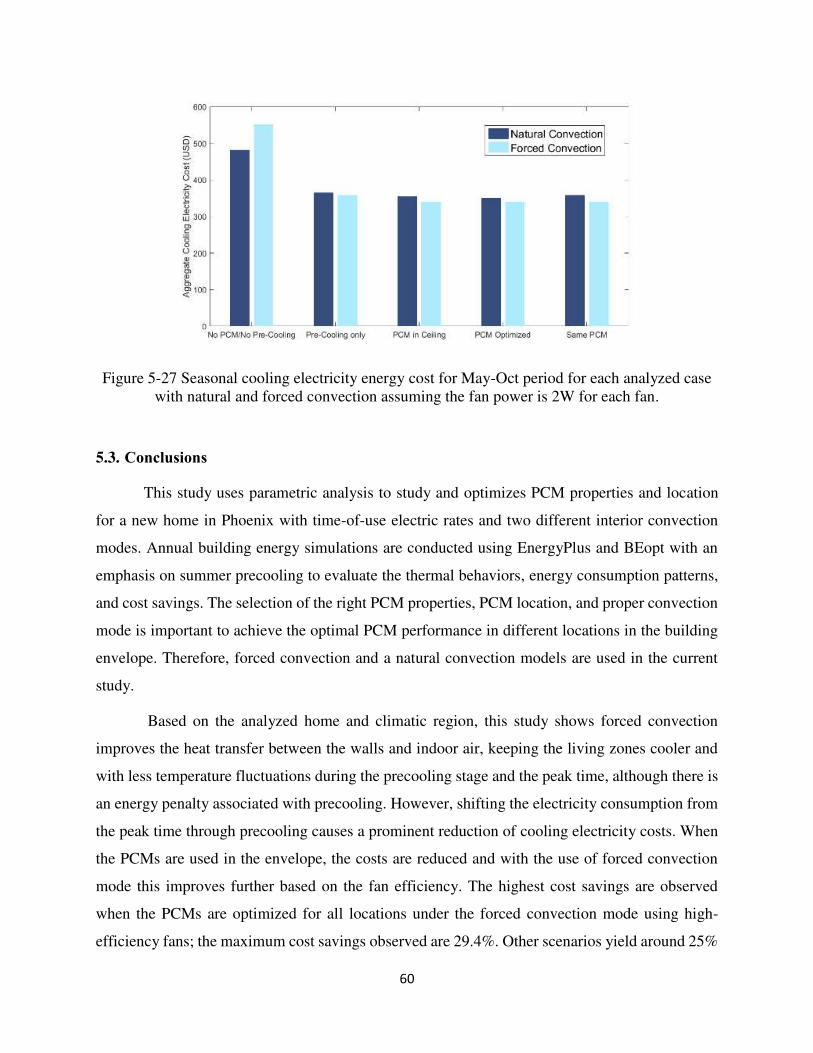
60
Figure 5-27 Seasonal cooling electricity energy cost for May-Oct period for each analyzed case with natural and forced convection assuming the fan power is 2W for each fan.
5.3. Conclusions
This study uses parametric analysis to study and optimizes PCM properties and location
for a new home in Phoenix with time-of-use electric rates and two different interior convection
modes. Annual building energy simulations are conducted using EnergyPlus and BEopt with an
emphasis on summer precooling to evaluate the thermal behaviors, energy consumption patterns,
and cost savings. The selection of the right PCM properties, PCM location, and proper convection
mode is important to achieve the optimal PCM performance in different locations in the building
envelope. Therefore, forced convection and a natural convection models are used in the current
study.
Based on the analyzed home and climatic region, this study shows forced convection
improves the heat transfer between the walls and indoor air, keeping the living zones cooler and
with less temperature fluctuations during the precooling stage and the peak time, although there is
an energy penalty associated with precooling. However, shifting the electricity consumption from
the peak time through precooling causes a prominent reduction of cooling electricity costs. When
the PCMs are used in the envelope, the costs are reduced and with the use of forced convection
mode this improves further based on the fan efficiency. The highest cost savings are observed
when the PCMs are optimized for all locations under the forced convection mode using high-
efficiency fans; the maximum cost savings observed are 29.4%. Other scenarios yield around 25%

61
savings. Under these conditions, cooling-related energy can be shifted up to 99.98% for a design
day. These potential savings, along with the increased thermal comfort while precooling, will be
beneficial to the homeowner and provide relief to the electric grid during peak hours. The results
in this section sets-up important inputs for the work described in the next 2 chapters.
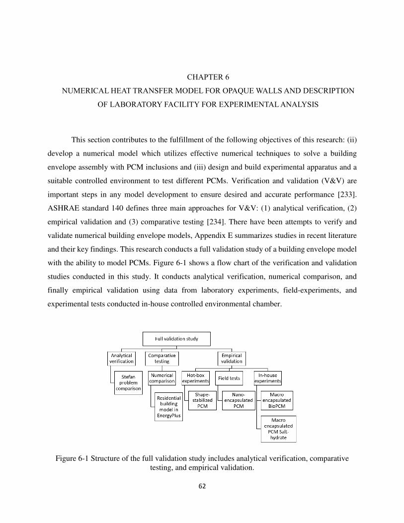
62
CHAPTER 6
NUMERICAL HEAT TRANSFER MODEL FOR OPAQUE WALLS AND DESCRIPTION
OF LABORATORY FACILITY FOR EXPERIMENTAL ANALYSIS
This section contributes to the fulfillment of the following objectives of this research: (ii)
develop a numerical model which utilizes effective numerical techniques to solve a building
envelope assembly with PCM inclusions and (iii) design and build experimental apparatus and a
suitable controlled environment to test different PCMs. Verification and validation (V&V) are
important steps in any model development to ensure desired and accurate performance [233].
ASHRAE standard 140 defines three main approaches for V&V: (1) analytical verification, (2)
empirical validation and (3) comparative testing [234]. There have been attempts to verify and
validate numerical building envelope models, Appendix E summarizes studies in recent literature
and their key findings. This research conducts a full validation study of a building envelope model
with the ability to model PCMs. Figure 6-1 shows a flow chart of the verification and validation
studies conducted in this study. It conducts analytical verification, numerical comparison, and
finally empirical validation using data from laboratory experiments, field-experiments, and
experimental tests conducted in-house controlled environmental chamber.
Figure 6-1 Structure of the full validation study includes analytical verification, comparative testing, and empirical validation.
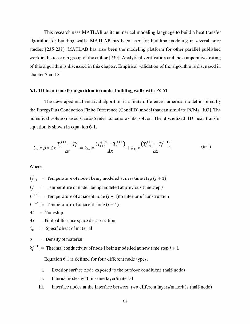
63
This research uses MATLAB as its numerical modeling language to build a heat transfer
algorithm for building walls. MATLAB has been used for building modeling in several prior
studies [235-238]. MATLAB has also been the modeling platform for other parallel published
work in the research group of the author [239]. Analytical verification and the comparative testing
of this algorithm is discussed in this chapter. Empirical validation of the algorithm is discussed in
chapter 7 and 8.
6.1. 1D heat transfer algorithm to model building walls with PCM
The developed mathematical algorithm is a finite difference numerical model inspired by
the EnergyPlus Conduction Finite Difference (CondFD) model that can simulate PCMs [103]. The
numerical solution uses Gauss-Seidel scheme as its solver. The discretized 1D heat transfer
equation is shown in equation 6-1.
𝐶𝑃 ∗ 𝜌 ∗ 𝛥𝑥 𝑇𝑖𝑗+1 − 𝑇𝑖𝑗𝛥𝑡 = 𝑘𝑊 ∗ (𝑇𝑖+1𝑗+1 − 𝑇𝑖𝑗+1)𝛥𝑥 + 𝑘𝐸 ∗ (𝑇𝑖−1𝑗+1 − 𝑇𝑖𝑗+1)𝛥𝑥 (6-1)
Where, 𝑇𝑗+1 𝑖 = Temperature of node i being modeled at new time step (𝑗 + 1) 𝑇𝑗𝑖 = Temperature of node i being modeled at previous time step 𝑗 𝑇𝑖+1 = Temperature of adjacent node (𝑖 + 1)to interior of construction 𝑇 𝑖−1 = Temperature of adjacent node (𝑖 − 1) 𝛥𝑡 = Timestep 𝛥𝑥 = Finite difference space discretization 𝐶𝑝 = Specific heat of material 𝜌 = Density of material 𝑘𝑖𝑗+1 = Thermal conductivity of node I being modelled at new time step 𝑗 + 1
Equation 6.1 is defined for four different node types,
i. Exterior surface node exposed to the outdoor conditions (half-node)
ii. Internal nodes within same layer/material
iii. Interface nodes at the interface between two different layers/materials (half-node)
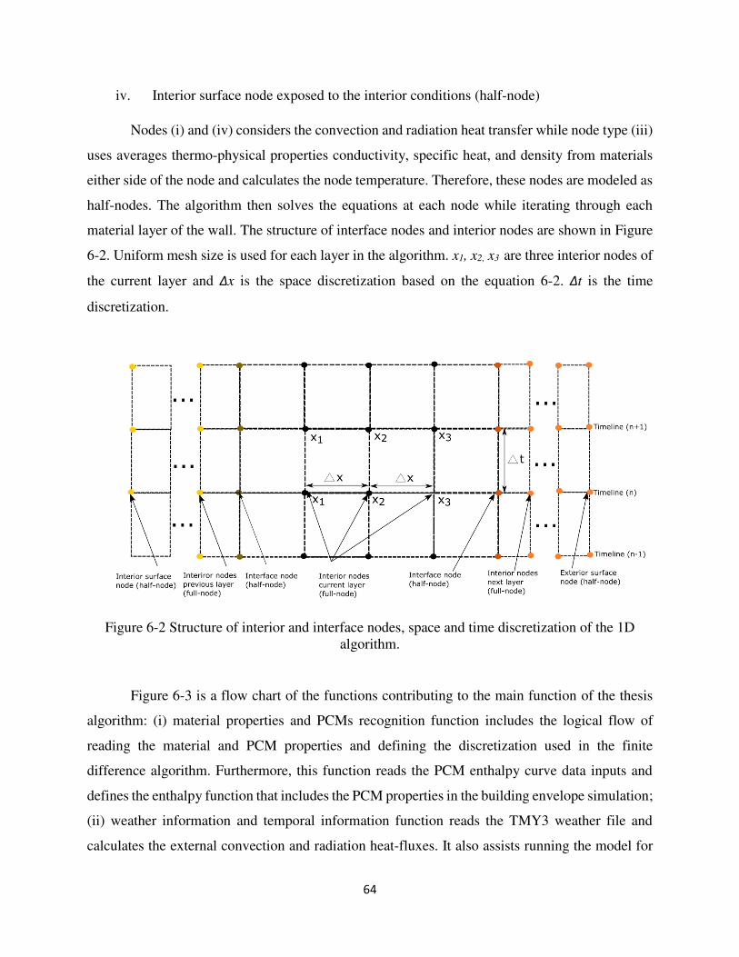
64
iv. Interior surface node exposed to the interior conditions (half-node)
Nodes (i) and (iv) considers the convection and radiation heat transfer while node type (iii)
uses averages thermo-physical properties conductivity, specific heat, and density from materials
either side of the node and calculates the node temperature. Therefore, these nodes are modeled as
half-nodes. The algorithm then solves the equations at each node while iterating through each
material layer of the wall. The structure of interface nodes and interior nodes are shown in Figure
6-2. Uniform mesh size is used for each layer in the algorithm. x1, x2, x3 are three interior nodes of
the current layer and Δx is the space discretization based on the equation 6-2. Δt is the time
discretization.
Figure 6-2 Structure of interior and interface nodes, space and time discretization of the 1D algorithm.
Figure 6-3 is a flow chart of the functions contributing to the main function of the thesis
algorithm: (i) material properties and PCMs recognition function includes the logical flow of
reading the material and PCM properties and defining the discretization used in the finite
difference algorithm. Furthermore, this function reads the PCM enthalpy curve data inputs and
defines the enthalpy function that includes the PCM properties in the building envelope simulation;
(ii) weather information and temporal information function reads the TMY3 weather file and
calculates the external convection and radiation heat-fluxes. It also assists running the model for
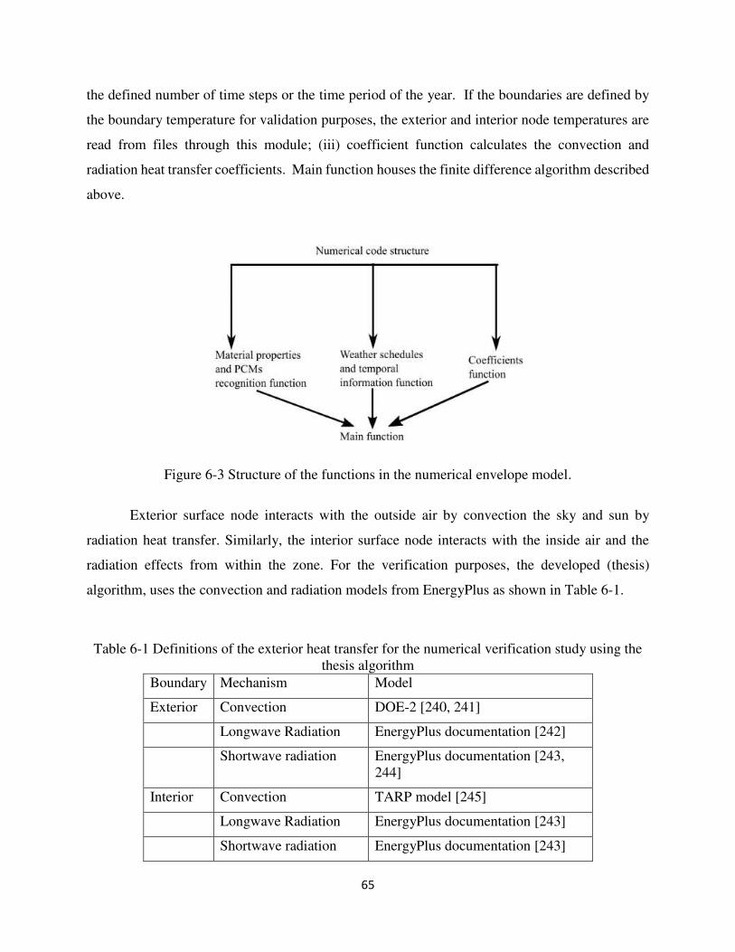
65
the defined number of time steps or the time period of the year. If the boundaries are defined by
the boundary temperature for validation purposes, the exterior and interior node temperatures are
read from files through this module; (iii) coefficient function calculates the convection and
radiation heat transfer coefficients. Main function houses the finite difference algorithm described
above.
Figure 6-3 Structure of the functions in the numerical envelope model.
Exterior surface node interacts with the outside air by convection the sky and sun by
radiation heat transfer. Similarly, the interior surface node interacts with the inside air and the
radiation effects from within the zone. For the verification purposes, the developed (thesis)
algorithm, uses the convection and radiation models from EnergyPlus as shown in Table 6-1.
Table 6-1 Definitions of the exterior heat transfer for the numerical verification study using the thesis algorithm
Boundary Mechanism Model
Exterior Convection DOE-2 [240, 241]
Longwave Radiation EnergyPlus documentation [242]
Shortwave radiation EnergyPlus documentation [243, 244]
Interior Convection TARP model [245]
Longwave Radiation EnergyPlus documentation [243]
Shortwave radiation EnergyPlus documentation [243]
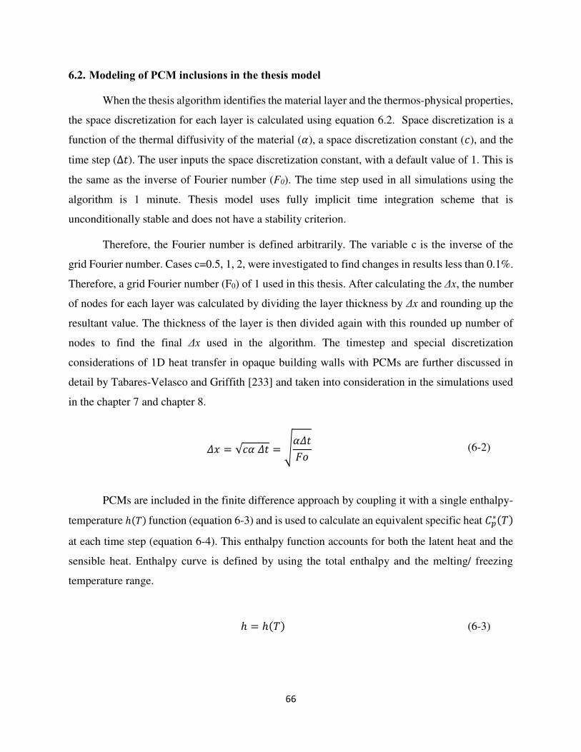
66
6.2. Modeling of PCM inclusions in the thesis model
When the thesis algorithm identifies the material layer and the thermos-physical properties,
the space discretization for each layer is calculated using equation 6.2. Space discretization is a
function of the thermal diffusivity of the material (𝛼), a space discretization constant (𝑐), and the
time step (Δ𝑡). The user inputs the space discretization constant, with a default value of 1. This is
the same as the inverse of Fourier number (F0). The time step used in all simulations using the
algorithm is 1 minute. Thesis model uses fully implicit time integration scheme that is
unconditionally stable and does not have a stability criterion.
Therefore, the Fourier number is defined arbitrarily. The variable c is the inverse of the
grid Fourier number. Cases c=0.5, 1, 2, were investigated to find changes in results less than 0.1%.
Therefore, a grid Fourier number (F0) of 1 used in this thesis. After calculating the Δx, the number
of nodes for each layer was calculated by dividing the layer thickness by Δx and rounding up the
resultant value. The thickness of the layer is then divided again with this rounded up number of
nodes to find the final Δx used in the algorithm. The timestep and special discretization
considerations of 1D heat transfer in opaque building walls with PCMs are further discussed in
detail by Tabares-Velasco and Griffith [233] and taken into consideration in the simulations used
in the chapter 7 and chapter 8.
𝛥𝑥 = √𝑐𝛼 𝛥𝑡 = √𝛼𝛥𝑡𝐹𝑜 (6-2)
PCMs are included in the finite difference approach by coupling it with a single enthalpy-
temperature ℎ(𝑇) function (equation 6-3) and is used to calculate an equivalent specific heat 𝐶𝑝∗(𝑇) at each time step (equation 6-4). This enthalpy function accounts for both the latent heat and the
sensible heat. Enthalpy curve is defined by using the total enthalpy and the melting/ freezing
temperature range.
ℎ = ℎ(𝑇) (6-3)
67
𝐶𝑝∗(𝑇) = ℎ𝑖𝑗 − ℎ𝑖𝑗−1𝑇𝑖𝑗 − 𝑇𝑖𝑗−1 (6-4)
For the simulation of PCMs, this algorithm uses the enthalpy method implemented with a
fixed uniform grid. Furthermore, finite difference discretization technique is implicitly solved
using fully implicit method.
Modeling hysteresis in the thesis model
The thesis model does not simulate the subcooling characteristics discussed in the chapter
2 (section 2.3.3). It simulates the real and apparent hysteresis when two curve data is available.
The simplification methods used in modelling enthalpy curves is discussed in this section. The
thesis algorithm has a built in function to recognize the PCM included layer. Once the PCM layer
is recognized the algorithm needs effective heat capacity and conductivity values to dynamically
implement at each time step through the phase change temperature range.
Figure 6-4 shows all available PCM curves for the InfiniteRTM hydrate-salt PCM with
nominal melting temperature of 23 ºC based on the commercial rating by the manufacturer. The
manufacturer has provided PCM characteristics data and has only the melting curve. This is shown
in black color. The hysteresis curves were provided for this PCM by Dr. Kaushik Biswas from the
Oak Ridge National Laboratory who used DHFMA tests. There are two distinct curves in this data
for melting and freezing and shown in yellow and blue.
The circles in the curves represent discrete data points provided. Note that within the
temperature range the phase change occurs the data is recorded every 1 ºC and outside this range
the points temperature is recorded are more relaxed. The frequency of reporting data is determined
by the researcher who conducts the characterization study. The curves are drawn linking these data
points. The peak melting/ freezing temperature for each curve is suggested by the
manufacturer/researchers who provided the data. Based on this information further approximations
are made to obtain the enthalpy data to include in the algorithms.
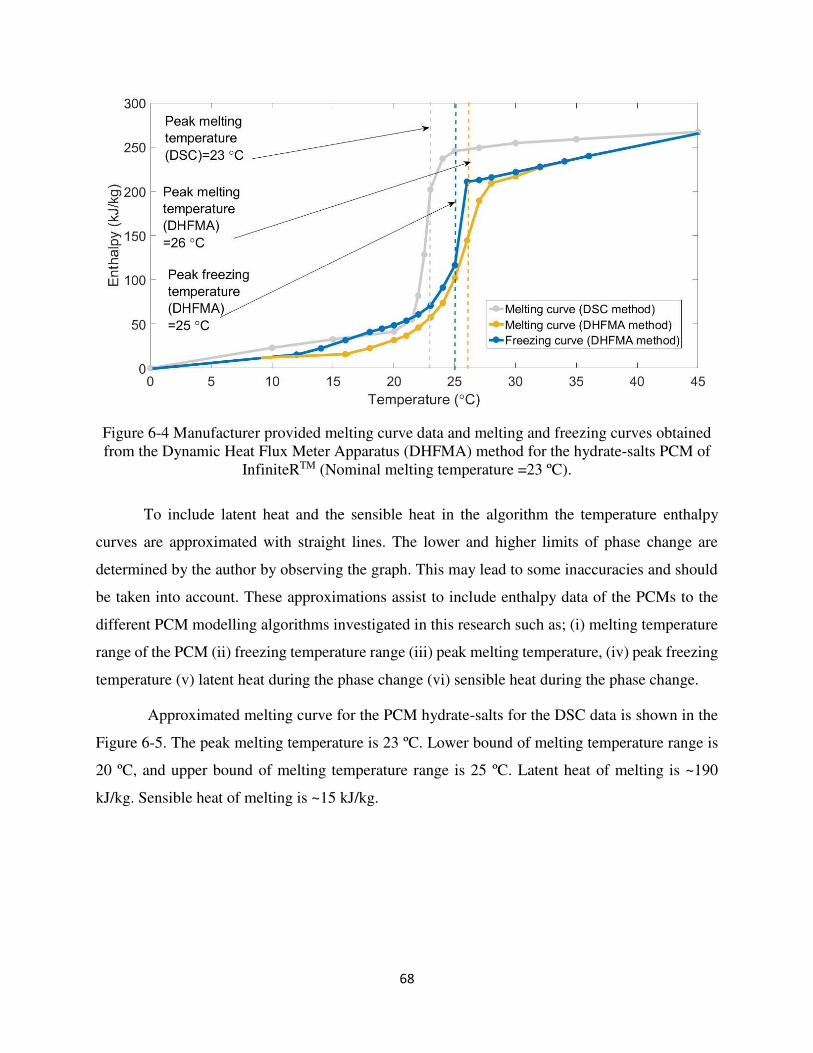
68
Figure 6-4 Manufacturer provided melting curve data and melting and freezing curves obtained from the Dynamic Heat Flux Meter Apparatus (DHFMA) method for the hydrate-salts PCM of
InfiniteRTM (Nominal melting temperature =23 ºC).
To include latent heat and the sensible heat in the algorithm the temperature enthalpy
curves are approximated with straight lines. The lower and higher limits of phase change are
determined by the author by observing the graph. This may lead to some inaccuracies and should
be taken into account. These approximations assist to include enthalpy data of the PCMs to the
different PCM modelling algorithms investigated in this research such as; (i) melting temperature
range of the PCM (ii) freezing temperature range (iii) peak melting temperature, (iv) peak freezing
temperature (v) latent heat during the phase change (vi) sensible heat during the phase change.
Approximated melting curve for the PCM hydrate-salts for the DSC data is shown in the
Figure 6-5. The peak melting temperature is 23 ºC. Lower bound of melting temperature range is
20 ºC, and upper bound of melting temperature range is 25 ºC. Latent heat of melting is ~190
kJ/kg. Sensible heat of melting is ~15 kJ/kg.
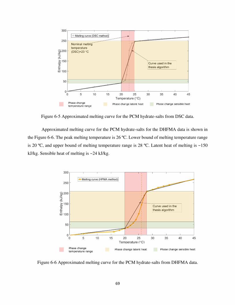
69
Figure 6-5 Approximated melting curve for the PCM hydrate-salts from DSC data.
Approximated melting curve for the PCM hydrate-salts for the DHFMA data is shown in
the Figure 6-6. The peak melting temperature is 26 ºC. Lower bound of melting temperature range
is 20 ºC, and upper bound of melting temperature range is 28 ºC. Latent heat of melting is ~150
kJ/kg. Sensible heat of melting is ~24 kJ/kg.
Figure 6-6 Approximated melting curve for the PCM hydrate-salts from DHFMA data.
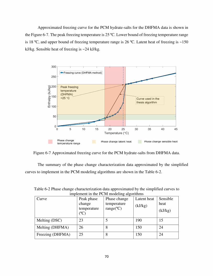
70
Approximated freezing curve for the PCM hydrate-salts for the DHFMA data is shown in
the Figure 6-7. The peak freezing temperature is 25 ºC. Lower bound of freezing temperature range
is 18 ºC, and upper bound of freezing temperature range is 26 ºC. Latent heat of freezing is ~150
kJ/kg. Sensible heat of freezing is ~24 kJ/kg.
Figure 6-7 Approximated freezing curve for the PCM hydrate-salts from DHFMA data.
The summary of the phase change characterization data approximated by the simplified
curves to implement in the PCM modeling algorithms are shown in the Table 6-2.
Table 6-2 Phase change characterization data approximated by the simplified curves to implement in the PCM modeling algorithms
Curve Peak phase change temperature (ºC)
Phase change temperature range(ºC)
Latent heat
(kJ/kg)
Sensible heat
(kJ/kg)
Melting (DSC) 23 5 190 15
Melting (DHFMA) 26 8 150 24
Freezing (DHFMA) 25 8 150 24
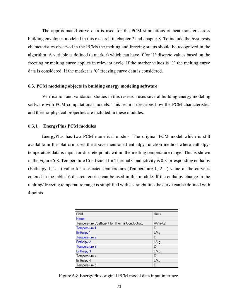
71
The approximated curve data is used for the PCM simulations of heat transfer across
building envelopes modeled in this research in chapter 7 and chapter 8. To include the hysteresis
characteristics observed in the PCMs the melting and freezing status should be recognized in the
algorithm. A variable is defined (a marker) which can have ‘0’or ‘1’ discrete values based on the
freezing or melting curve applies in relevant cycle. If the marker values is ‘1’ the melting curve
data is considered. If the marker is ‘0’ freezing curve data is considered.
6.3. PCM modeling objects in building energy modeling software
Verification and validation studies in this research uses several building energy modeling
software with PCM computational models. This section describes how the PCM characteristics
and thermo-physical properties are included in these modules.
EnergyPlus PCM modules
EnergyPlus has two PCM numerical models. The original PCM model which is still
available in the platform uses the above mentioned enthalpy function method where enthalpy-
temperature data is input for discrete points within the melting temperature range. This is shown
in the Figure 6-8. Temperature Coefficient for Thermal Conductivity is 0. Corresponding enthalpy
(Enthalpy 1, 2…) value for a selected temperature (Temperature 1, 2…) value of the curve is
entered in the table 16 discrete entries can be used in this module. If the enthalpy change in the
melting/ freezing temperature range is simplified with a straight line the curve can be defined with
4 points.
Figure 6-8 EnergyPlus original PCM model data input interface.
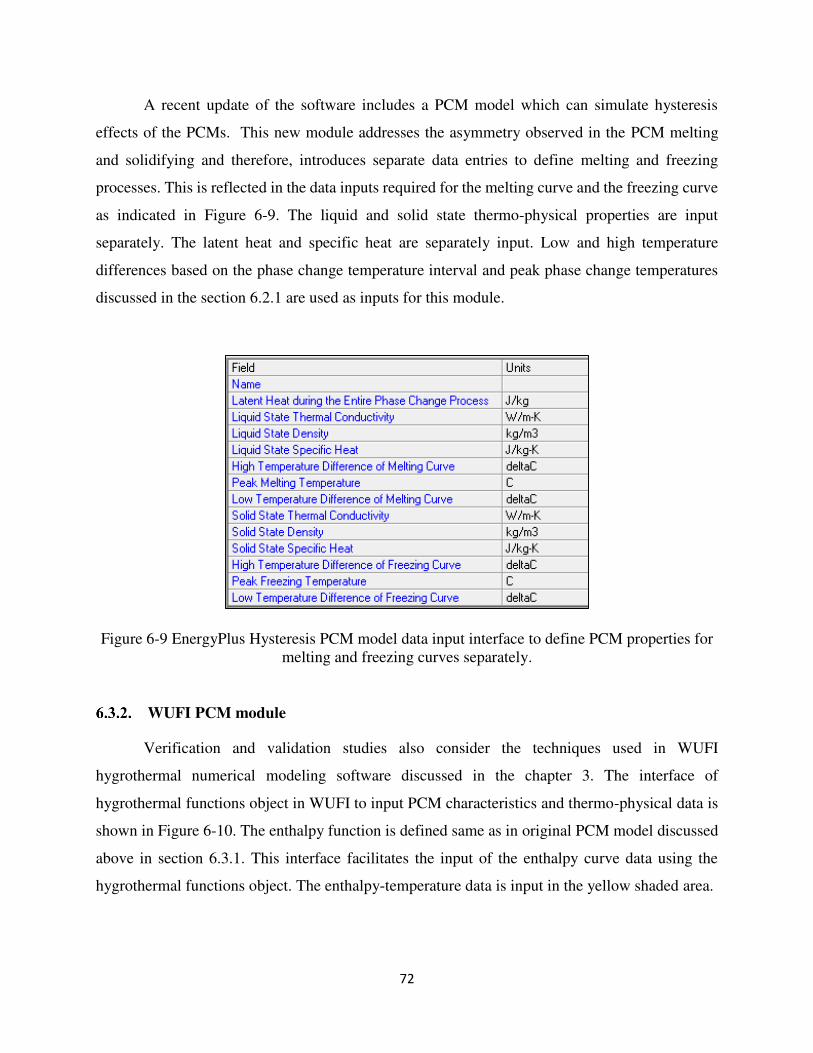
72
A recent update of the software includes a PCM model which can simulate hysteresis
effects of the PCMs. This new module addresses the asymmetry observed in the PCM melting
and solidifying and therefore, introduces separate data entries to define melting and freezing
processes. This is reflected in the data inputs required for the melting curve and the freezing curve
as indicated in Figure 6-9. The liquid and solid state thermo-physical properties are input
separately. The latent heat and specific heat are separately input. Low and high temperature
differences based on the phase change temperature interval and peak phase change temperatures
discussed in the section 6.2.1 are used as inputs for this module.
Figure 6-9 EnergyPlus Hysteresis PCM model data input interface to define PCM properties for melting and freezing curves separately.
WUFI PCM module
Verification and validation studies also consider the techniques used in WUFI
hygrothermal numerical modeling software discussed in the chapter 3. The interface of
hygrothermal functions object in WUFI to input PCM characteristics and thermo-physical data is
shown in Figure 6-10. The enthalpy function is defined same as in original PCM model discussed
above in section 6.3.1. This interface facilitates the input of the enthalpy curve data using the
hygrothermal functions object. The enthalpy-temperature data is input in the yellow shaded area.
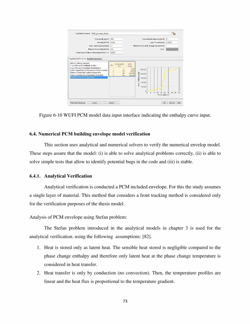
73
Figure 6-10 WUFI PCM model data input interface indicating the enthalpy curve input.
6.4. Numerical PCM building envelope model verification
This section uses analytical and numerical solvers to verify the numerical envelop model.
These steps assure that the model: (i) is able to solve analytical problems correctly, (ii) is able to
solve simple tests that allow to identify potential bugs in the code and (iii) is stable.
Analytical Verification
Analytical verification is conducted a PCM included envelope. For this the study assumes
a single layer of material. This method that considers a front tracking method is considered only
for the verification purposes of the thesis model.
Analysis of PCM envelope using Stefan problem:
The Stefan problem introduced in the analytical models in chapter 3 is used for the
analytical verification. using the following assumptions: [82].
1. Heat is stored only as latent heat. The sensible heat stored is negligible compared to the
phase change enthalpy and therefore only latent heat at the phase change temperature is
considered in heat transfer.
2. Heat transfer is only by conduction (no convection). Then, the temperature profiles are
linear and the heat flux is proportional to the temperature gradient.
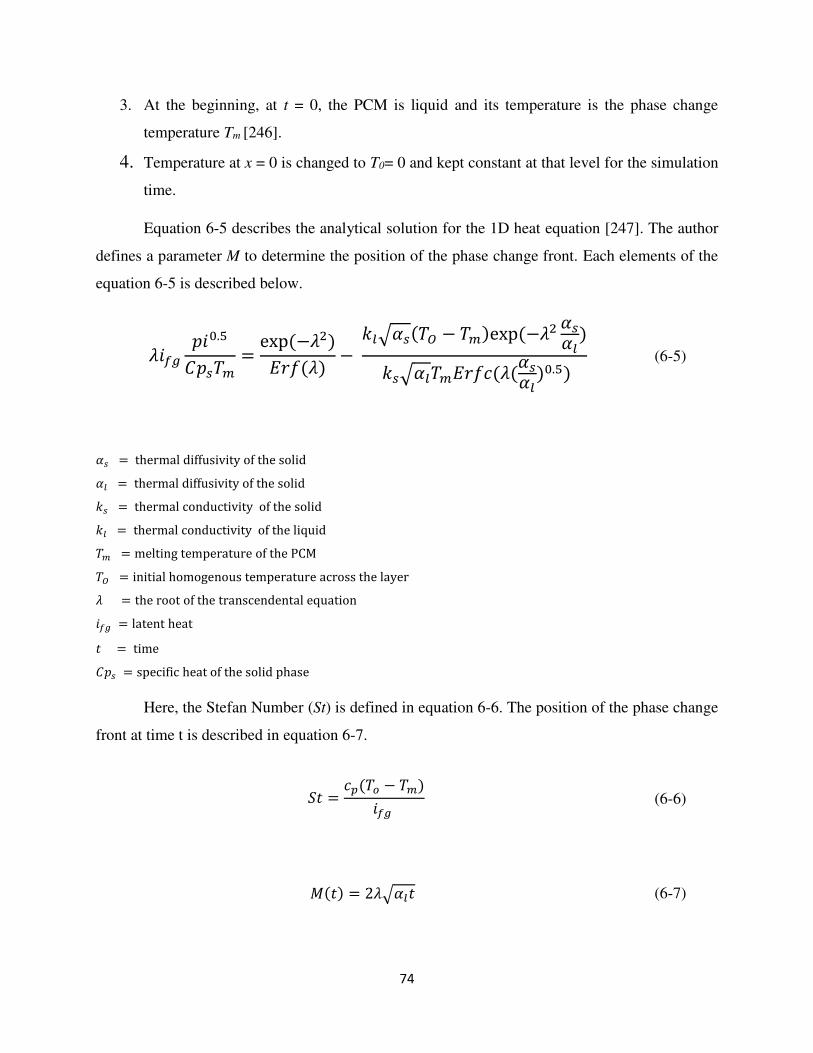
74
3. At the beginning, at t = 0, the PCM is liquid and its temperature is the phase change
temperature Tm [246].
4. Temperature at x = 0 is changed to T0= 0 and kept constant at that level for the simulation
time.
Equation 6-5 describes the analytical solution for the 1D heat equation [247]. The author
defines a parameter M to determine the position of the phase change front. Each elements of the
equation 6-5 is described below.
𝜆𝑖𝑓𝑔 𝑝𝑖0.5𝐶𝑝𝑠𝑇𝑚 = exp (−𝜆2)𝐸𝑟𝑓(𝜆) − 𝑘𝑙√𝛼𝑠(𝑇𝑂 − 𝑇𝑚)exp (−𝜆2 𝛼𝑠𝛼𝑙) 𝑘𝑠√𝛼𝑙𝑇𝑚𝐸𝑟𝑓𝑐 (𝜆(𝛼𝑠𝛼𝑙)0.5) (6-5)
𝛼𝑠 = thermal diffusivity of the solid 𝛼𝑙 = thermal diffusivity of the solid 𝑘𝑠 = thermal conductivity of the solid 𝑘𝑙 = thermal conductivity of the liquid 𝑇𝑚 = melting temperature of the PCM 𝑇𝑂 = initial homogenous temperature across the layer 𝜆 = the root of the transcendental equation 𝑖𝑓𝑔 = latent heat 𝑡 = time 𝐶𝑝𝑠 = specific heat of the solid phase Here, the Stefan Number (St) is defined in equation 6-6. The position of the phase change
front at time t is described in equation 6-7.
𝑆𝑡 = 𝑐𝑝(𝑇𝑜 − 𝑇𝑚)𝑖𝑓𝑔 (6-6)
𝑀(𝑡) = 2𝜆√𝛼𝑙𝑡 (6-7)
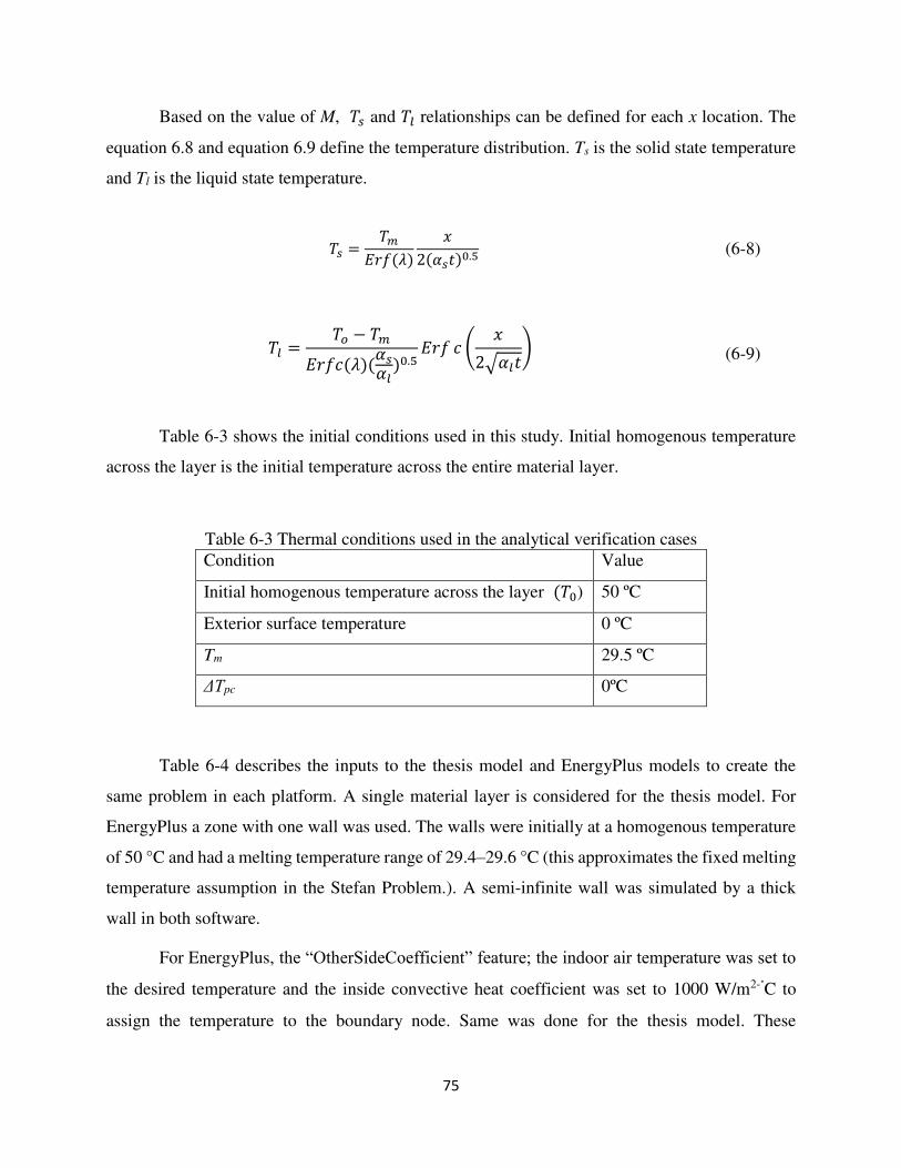
75
Based on the value of M, 𝑇𝑠 and 𝑇𝑙 relationships can be defined for each x location. The
equation 6.8 and equation 6.9 define the temperature distribution. Ts is the solid state temperature
and Tl is the liquid state temperature.
𝑇𝑠 = 𝑇𝑚𝐸𝑟𝑓(𝜆) 𝑥2(𝛼𝑠𝑡)0.5 (6-8)
𝑇𝑙 = 𝑇𝑜 − 𝑇𝑚𝐸𝑟𝑓𝑐 (𝜆)(𝛼𝑠𝛼𝑙)0.5 𝐸𝑟𝑓 𝑐 ( 𝑥2√𝛼𝑙𝑡) (6-9)
Table 6-3 shows the initial conditions used in this study. Initial homogenous temperature
across the layer is the initial temperature across the entire material layer.
Table 6-3 Thermal conditions used in the analytical verification cases Condition Value
Initial homogenous temperature across the layer (𝑇0) 50 ºC
Exterior surface temperature 0 ºC
Tm 29.5 ºC
ΔTpc 0ºC
Table 6-4 describes the inputs to the thesis model and EnergyPlus models to create the
same problem in each platform. A single material layer is considered for the thesis model. For
EnergyPlus a zone with one wall was used. The walls were initially at a homogenous temperature
of 50 °C and had a melting temperature range of 29.4–29.6 °C (this approximates the fixed melting
temperature assumption in the Stefan Problem.). A semi-infinite wall was simulated by a thick
wall in both software.
For EnergyPlus, the “OtherSideCoefficient” feature; the indoor air temperature was set to
the desired temperature and the inside convective heat coefficient was set to 1000 W/m2-˚C to
assign the temperature to the boundary node. Same was done for the thesis model. These
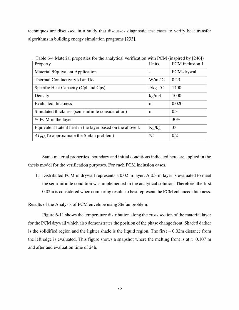
76
techniques are discussed in a study that discusses diagnostic test cases to verify heat transfer
algorithms in building energy simulation programs [233].
Table 6-4 Material properties for the analytical verification with PCM (inspired by [246]) Property Units PCM inclusion 1
Material /Equivalent Application - PCM-drywall
Thermal Conductivity kl and ks W/m-˚C 0.23
Specific Heat Capacity (Cpl and Cps) J/kg- ˚C 1400
Density kg/m3 1000
Evaluated thickness m 0.020
Simulated thickness (semi-infinite consideration) m 0.3
% PCM in the layer - 30%
Equivalent Latent heat in the layer based on the above f. Kg/kg 33 𝛥𝑇𝑃𝐶(To approximate the Stefan problem) ºC 0.2
Same material properties, boundary and initial conditions indicated here are applied in the
thesis model for the verification purposes. For each PCM inclusion cases,
1. Distributed PCM in drywall represents a 0.02 m layer. A 0.3 m layer is evaluated to meet
the semi-infinite condition was implemented in the analytical solution. Therefore, the first
0.02m is considered when comparing results to best represent the PCM enhanced thickness.
Results of the Analysis of PCM envelope using Stefan problem:
Figure 6-11 shows the temperature distribution along the cross section of the material layer
for the PCM drywall which also demonstrates the position of the phase change front. Shaded darker
is the solidified region and the lighter shade is the liquid region. The first ~ 0.02m distance from
the left edge is evaluated. This figure shows a snapshot where the melting front is at x=0.107 m
and after and evaluation time of 24h.
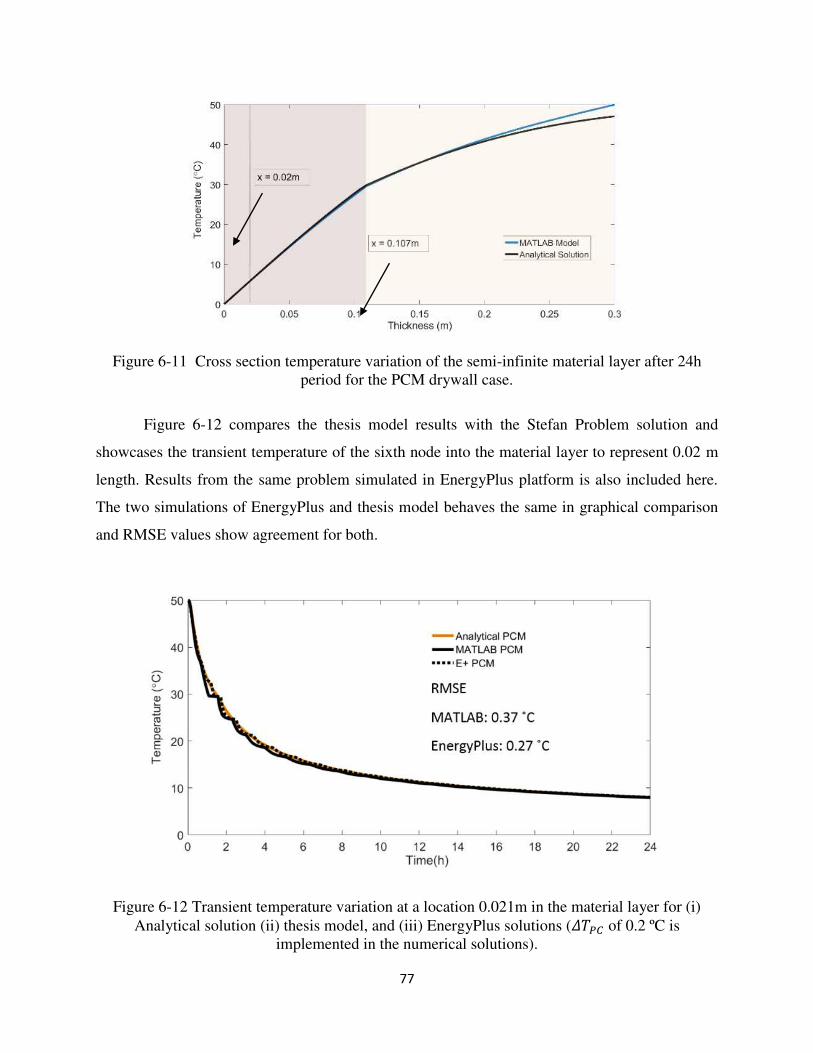
77
Figure 6-11 Cross section temperature variation of the semi-infinite material layer after 24h period for the PCM drywall case.
Figure 6-12 compares the thesis model results with the Stefan Problem solution and
showcases the transient temperature of the sixth node into the material layer to represent 0.02 m
length. Results from the same problem simulated in EnergyPlus platform is also included here.
The two simulations of EnergyPlus and thesis model behaves the same in graphical comparison
and RMSE values show agreement for both.
Figure 6-12 Transient temperature variation at a location 0.021m in the material layer for (i) Analytical solution (ii) thesis model, and (iii) EnergyPlus solutions (𝛥𝑇𝑃𝐶 of 0.2 ºC is
implemented in the numerical solutions).
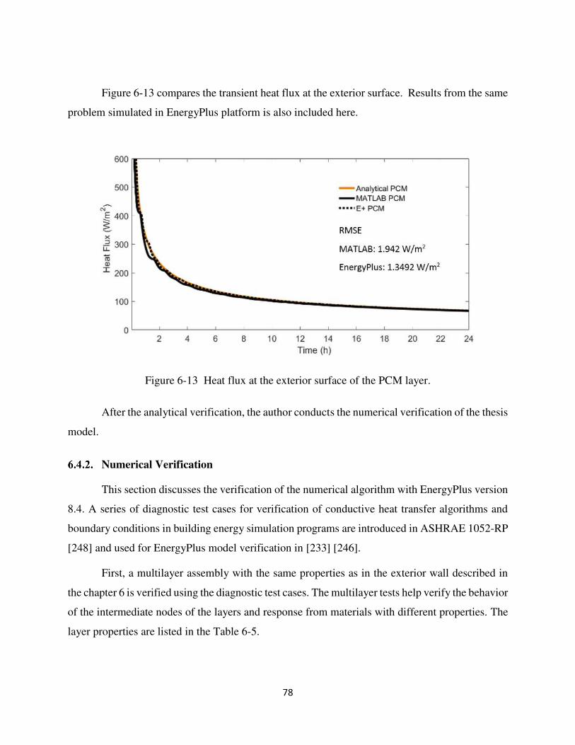
78
Figure 6-13 compares the transient heat flux at the exterior surface. Results from the same
problem simulated in EnergyPlus platform is also included here.
Figure 6-13 Heat flux at the exterior surface of the PCM layer.
After the analytical verification, the author conducts the numerical verification of the thesis
model.
Numerical Verification
This section discusses the verification of the numerical algorithm with EnergyPlus version
8.4. A series of diagnostic test cases for verification of conductive heat transfer algorithms and
boundary conditions in building energy simulation programs are introduced in ASHRAE 1052-RP
[248] and used for EnergyPlus model verification in [233] [246].
First, a multilayer assembly with the same properties as in the exterior wall described in
the chapter 6 is verified using the diagnostic test cases. The multilayer tests help verify the behavior
of the intermediate nodes of the layers and response from materials with different properties. The
layer properties are listed in the Table 6-5.
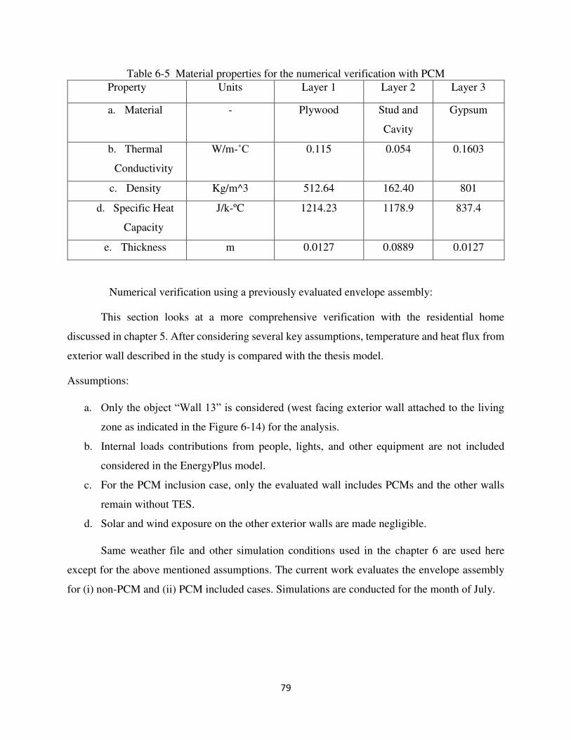
79
Table 6-5 Material properties for the numerical verification with PCM
Property Units Layer 1 Layer 2 Layer 3
a. Material - Plywood Stud and
Cavity
Gypsum
b. Thermal
Conductivity
W/m-˚C 0.115 0.054 0.1603
c. Density Kg/m^3 512.64 162.40 801
d. Specific Heat
Capacity
J/k-ºC 1214.23 1178.9 837.4
e. Thickness m 0.0127 0.0889 0.0127
Numerical verification using a previously evaluated envelope assembly:
This section looks at a more comprehensive verification with the residential home
discussed in chapter 5. After considering several key assumptions, temperature and heat flux from
exterior wall described in the study is compared with the thesis model.
Assumptions:
a. Only the object “Wall 13” is considered (west facing exterior wall attached to the living
zone as indicated in the Figure 6-14) for the analysis.
b. Internal loads contributions from people, lights, and other equipment are not included
considered in the EnergyPlus model.
c. For the PCM inclusion case, only the evaluated wall includes PCMs and the other walls
remain without TES.
d. Solar and wind exposure on the other exterior walls are made negligible.
Same weather file and other simulation conditions used in the chapter 6 are used here
except for the above mentioned assumptions. The current work evaluates the envelope assembly
for (i) non-PCM and (ii) PCM included cases. Simulations are conducted for the month of July.
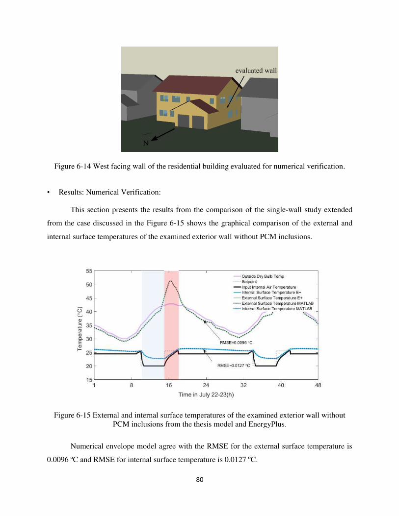
80
Figure 6-14 West facing wall of the residential building evaluated for numerical verification.
• Results: Numerical Verification:
This section presents the results from the comparison of the single-wall study extended
from the case discussed in the Figure 6-15 shows the graphical comparison of the external and
internal surface temperatures of the examined exterior wall without PCM inclusions.
Figure 6-15 External and internal surface temperatures of the examined exterior wall without PCM inclusions from the thesis model and EnergyPlus.
Numerical envelope model agree with the RMSE for the external surface temperature is
0.0096 ºC and RMSE for internal surface temperature is 0.0127 ºC.
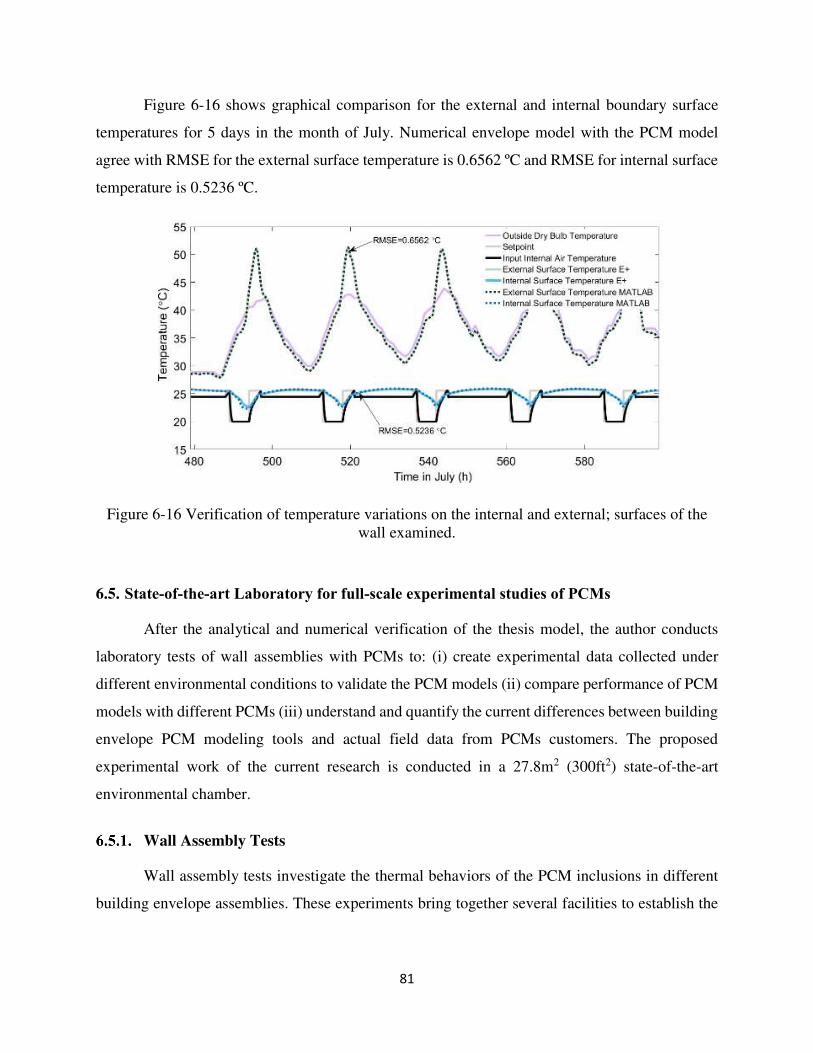
81
Figure 6-16 shows graphical comparison for the external and internal boundary surface
temperatures for 5 days in the month of July. Numerical envelope model with the PCM model
agree with RMSE for the external surface temperature is 0.6562 ºC and RMSE for internal surface
temperature is 0.5236 ºC.
Figure 6-16 Verification of temperature variations on the internal and external; surfaces of the wall examined.
6.5. State-of-the-art Laboratory for full-scale experimental studies of PCMs
After the analytical and numerical verification of the thesis model, the author conducts
laboratory tests of wall assemblies with PCMs to: (i) create experimental data collected under
different environmental conditions to validate the PCM models (ii) compare performance of PCM
models with different PCMs (iii) understand and quantify the current differences between building
envelope PCM modeling tools and actual field data from PCMs customers. The proposed
experimental work of the current research is conducted in a 27.8m2 (300ft2) state-of-the-art
environmental chamber.
Wall Assembly Tests
Wall assembly tests investigate the thermal behaviors of the PCM inclusions in different
building envelope assemblies. These experiments bring together several facilities to establish the
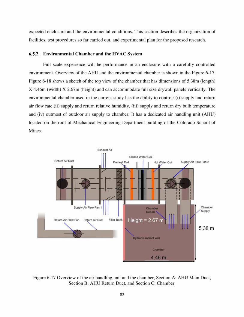
82
expected enclosure and the environmental conditions. This section describes the organization of
facilities, test procedures so far carried out, and experimental plan for the proposed research.
Environmental Chamber and the HVAC System
Full scale experience will be performance in an enclosure with a carefully controlled
environment. Overview of the AHU and the environmental chamber is shown in the Figure 6-17.
Figure 6-18 shows a sketch of the top view of the chamber that has dimensions of 5.38m (length)
X 4.46m (width) X 2.67m (height) and can accommodate full size drywall panels vertically. The
environmental chamber used in the current study has the ability to control: (i) supply and return
air flow rate (ii) supply and return relative humidity, (iii) supply and return dry bulb temperature
and (iv) outmost of outdoor air supply to chamber. It has a dedicated air handling unit (AHU)
located on the roof of Mechanical Engineering Department building of the Colorado School of
Mines.
Figure 6-17 Overview of the air handling unit and the chamber, Section A: AHU Main Duct, Section B: AHU Return Duct, and Section C: Chamber.
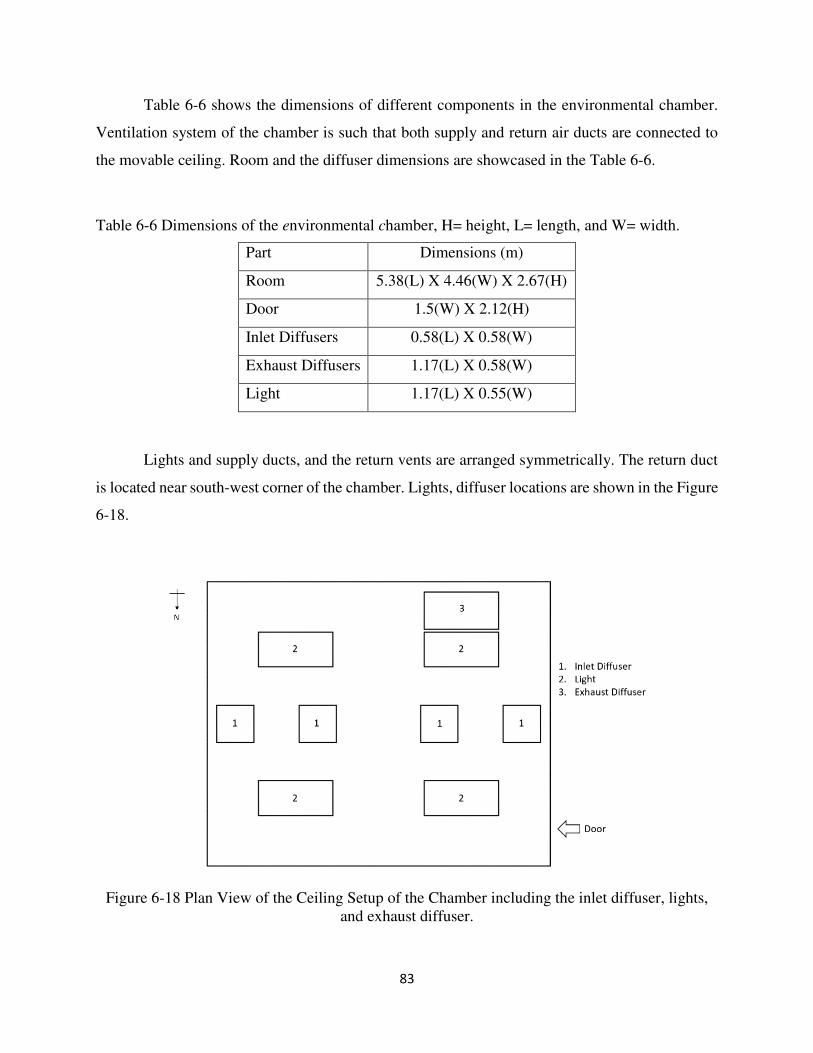
83
Table 6-6 shows the dimensions of different components in the environmental chamber.
Ventilation system of the chamber is such that both supply and return air ducts are connected to
the movable ceiling. Room and the diffuser dimensions are showcased in the Table 6-6.
Table 6-6 Dimensions of the environmental chamber, H= height, L= length, and W= width.
Part Dimensions (m)
Room 5.38(L) X 4.46(W) X 2.67(H)
Door 1.5(W) X 2.12(H)
Inlet Diffusers 0.58(L) X 0.58(W)
Exhaust Diffusers 1.17(L) X 0.58(W)
Light 1.17(L) X 0.55(W)
Lights and supply ducts, and the return vents are arranged symmetrically. The return duct
is located near south-west corner of the chamber. Lights, diffuser locations are shown in the Figure
6-18.
Figure 6-18 Plan View of the Ceiling Setup of the Chamber including the inlet diffuser, lights, and exhaust diffuser.
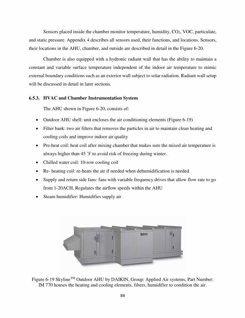
84
Sensors placed inside the chamber monitor temperature, humidity, CO2, VOC, particulate,
and static pressure. Appendix 4 describes all sensors used, their functions, and locations. Sensors,
their locations in the AHU, chamber, and outside are described in detail in the Figure 6-20.
Chamber is also equipped with a hydronic radiant wall that has the ability to maintain a
constant and variable surface temperature independent of the indoor air temperature to mimic
external boundary conditions such as an exterior wall subject to solar radiation. Radiant wall setup
will be discussed in detail in later sections.
HVAC and Chamber Instrumentation System
The AHU shown in Figure 6-20, consists of:
Outdoor AHU shell: unit encloses the air conditioning elements (Figure 6-19)
Filter bank: two air filters that removes the particles in air to maintain clean heating and
cooling coils and improve indoor air quality
Pre-heat coil: heat coil after mixing chamber that makes sure the mixed air temperature is
always higher than 45 ˚F to avoid risk of freezing during winter.
Chilled water coil: 10-row cooling coil
Re- heating coil: re-heats the air if needed when dehumidification is needed
Supply and return side fans: fans with variable frequency drives that allow flow rate to go
from 1-20ACH. Regulates the airflow speeds within the AHU
Steam humidifier: Humidifies supply air
Figure 6-19 SkylineTM Outdoor AHU by DAIKIN, Group: Applied Air systems, Part Number:
IM 770 houses the heating and cooling elements, filters, humidifier to condition the air.
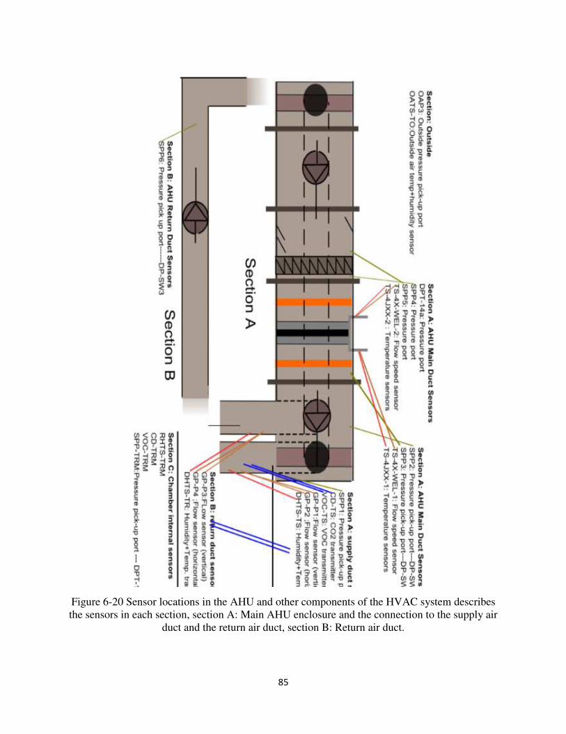
85
Figure 6-20 Sensor locations in the AHU and other components of the HVAC system describes the sensors in each section, section A: Main AHU enclosure and the connection to the supply air
duct and the return air duct, section B: Return air duct.
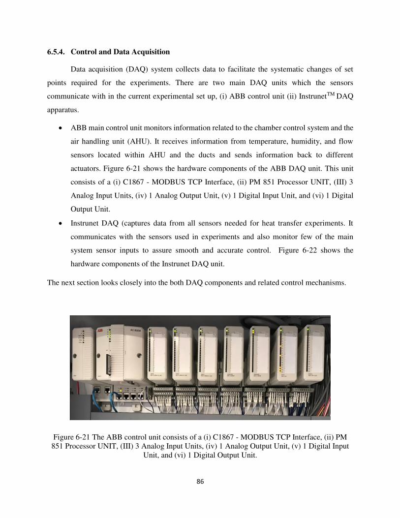
86
Control and Data Acquisition
Data acquisition (DAQ) system collects data to facilitate the systematic changes of set
points required for the experiments. There are two main DAQ units which the sensors
communicate with in the current experimental set up, (i) ABB control unit (ii) InstrunetTM DAQ
apparatus.
ABB main control unit monitors information related to the chamber control system and the
air handling unit (AHU). It receives information from temperature, humidity, and flow
sensors located within AHU and the ducts and sends information back to different
actuators. Figure 6-21 shows the hardware components of the ABB DAQ unit. This unit
consists of a (i) C1867 - MODBUS TCP Interface, (ii) PM 851 Processor UNIT, (III) 3
Analog Input Units, (iv) 1 Analog Output Unit, (v) 1 Digital Input Unit, and (vi) 1 Digital
Output Unit.
Instrunet DAQ (captures data from all sensors needed for heat transfer experiments. It
communicates with the sensors used in experiments and also monitor few of the main
system sensor inputs to assure smooth and accurate control. Figure 6-22 shows the
hardware components of the Instrunet DAQ unit.
The next section looks closely into the both DAQ components and related control mechanisms.
Figure 6-21 The ABB control unit consists of a (i) C1867 - MODBUS TCP Interface, (ii) PM 851 Processor UNIT, (III) 3 Analog Input Units, (iv) 1 Analog Output Unit, (v) 1 Digital Input
Unit, and (vi) 1 Digital Output Unit.
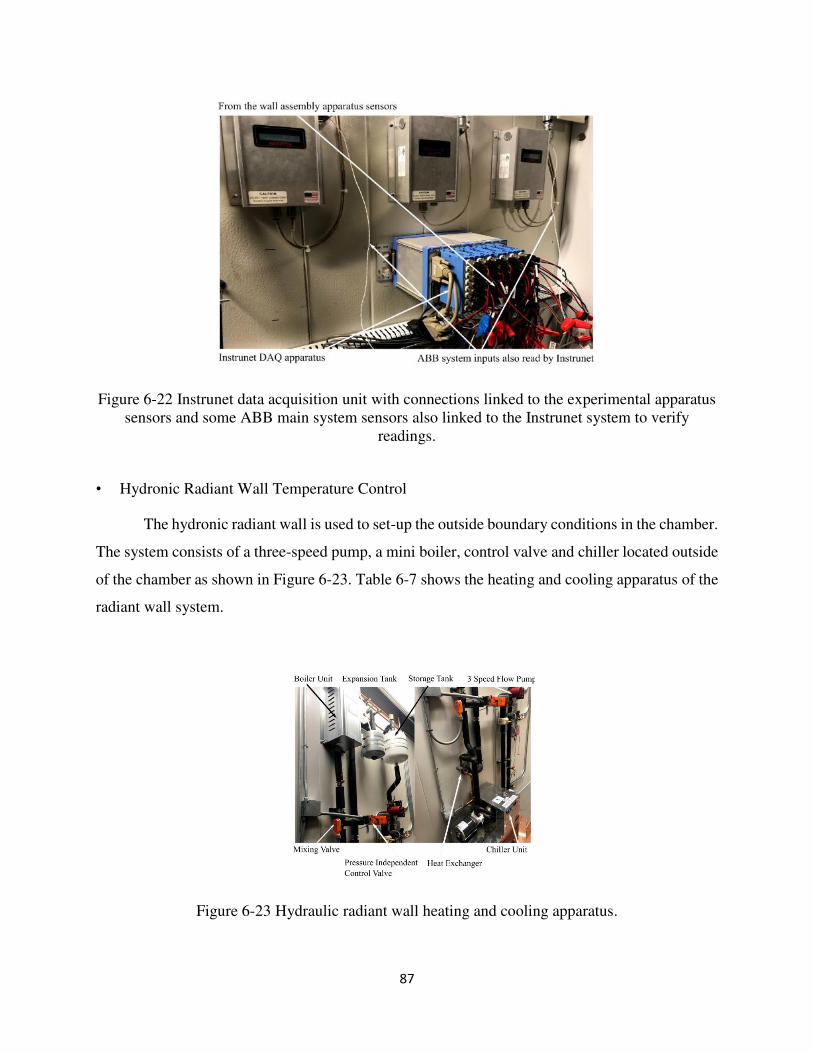
87
Figure 6-22 Instrunet data acquisition unit with connections linked to the experimental apparatus sensors and some ABB main system sensors also linked to the Instrunet system to verify
readings.
• Hydronic Radiant Wall Temperature Control
The hydronic radiant wall is used to set-up the outside boundary conditions in the chamber.
The system consists of a three-speed pump, a mini boiler, control valve and chiller located outside
of the chamber as shown in Figure 6-23. Table 6-7 shows the heating and cooling apparatus of the
radiant wall system.
Figure 6-23 Hydraulic radiant wall heating and cooling apparatus.
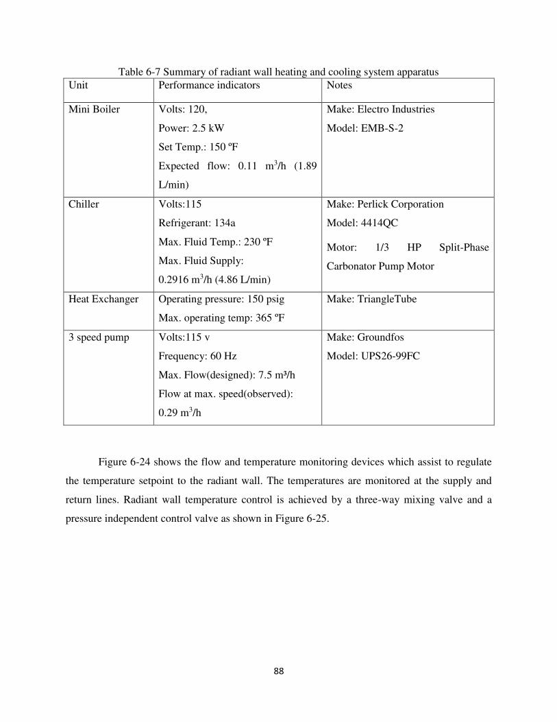
88
Table 6-7 Summary of radiant wall heating and cooling system apparatus Unit Performance indicators Notes
Mini Boiler Volts: 120,
Power: 2.5 kW
Set Temp.: 150 ºF
Expected flow: 0.11 m3/h (1.89
L/min)
Make: Electro Industries
Model: EMB-S-2
Chiller Volts:115
Refrigerant: 134a
Max. Fluid Temp.: 230 ºF
Max. Fluid Supply:
0.2916 m3/h (4.86 L/min)
Make: Perlick Corporation
Model: 4414QC
Motor: 1/3 HP Split-Phase
Carbonator Pump Motor
Heat Exchanger Operating pressure: 150 psig
Max. operating temp: 365 ºF
Make: TriangleTube
3 speed pump Volts:115 v
Frequency: 60 Hz
Max. Flow(designed): 7.5 m³/h
Flow at max. speed(observed):
0.29 m3/h
Make: Groundfos
Model: UPS26-99FC
Figure 6-24 shows the flow and temperature monitoring devices which assist to regulate
the temperature setpoint to the radiant wall. The temperatures are monitored at the supply and
return lines. Radiant wall temperature control is achieved by a three-way mixing valve and a
pressure independent control valve as shown in Figure 6-25.
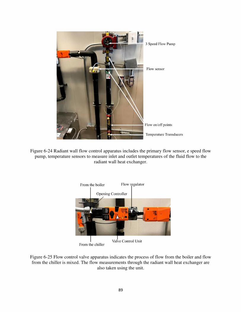
89
Figure 6-24 Radiant wall flow control apparatus includes the primary flow sensor, e speed flow pump, temperature sensors to measure inlet and outlet temperatures of the fluid flow to the
radiant wall heat exchanger.
Figure 6-25 Flow control valve apparatus indicates the process of flow from the boiler and flow from the chiller is mixed. The flow measurements through the radiant wall heat exchanger are
also taken using the unit.
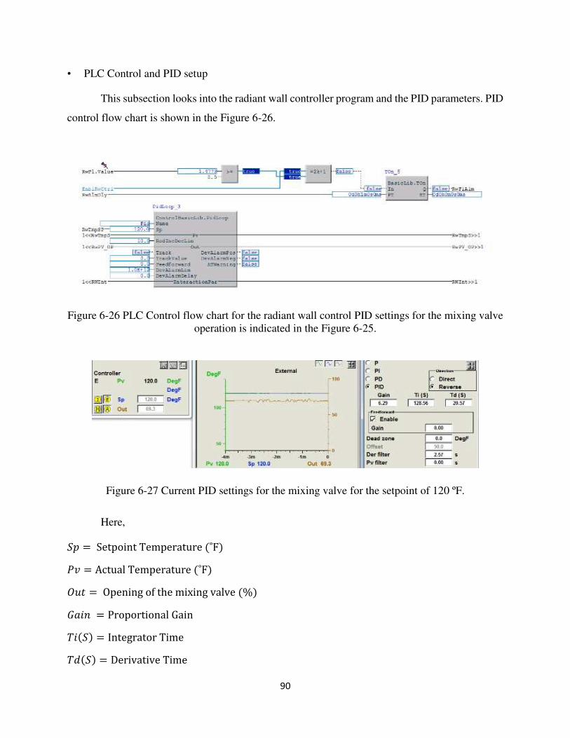
90
• PLC Control and PID setup
This subsection looks into the radiant wall controller program and the PID parameters. PID
control flow chart is shown in the Figure 6-26.
Figure 6-26 PLC Control flow chart for the radiant wall control PID settings for the mixing valve operation is indicated in the Figure 6-25.
Figure 6-27 Current PID settings for the mixing valve for the setpoint of 120 ºF.
Here, 𝑆𝑝 = Setpoint Temperature (˚F) 𝑃𝑣 = Actual Temperature (˚F) 𝑂𝑢𝑡 = Opening of the mixing valve (%) 𝐺𝑎𝑖𝑛 = Proportional Gain 𝑇𝑖(𝑆) = Integrator Time 𝑇𝑑(𝑆) = Derivative Time
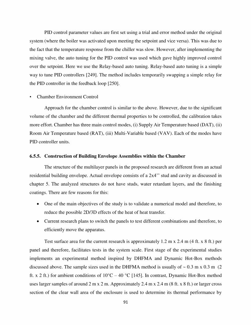
91
PID control parameter values are first set using a trial and error method under the original
system (where the boiler was activated upon meeting the setpoint and vice versa). This was due to
the fact that the temperature response from the chiller was slow. However, after implementing the
mixing valve, the auto tuning for the PID control was used which gave highly improved control
over the setpoint. Here we use the Relay-based auto tuning. Relay-based auto tuning is a simple
way to tune PID controllers [249]. The method includes temporarily swapping a simple relay for
the PID controller in the feedback loop [250].
• Chamber Environment Control
Approach for the chamber control is similar to the above. However, due to the significant
volume of the chamber and the different thermal properties to be controlled, the calibration takes
more effort. Chamber has three main control modes, (i) Supply Air Temperature based (DAT), (ii)
Room Air Temperature based (RAT), (iii) Multi-Variable based (VAV). Each of the modes have
PID controller units.
Construction of Building Envelope Assemblies within the Chamber
The structure of the multilayer panels in the proposed research are different from an actual
residential building envelope. Actual envelope consists of a 2x4’’ stud and cavity as discussed in
chapter 5. The analyzed structures do not have studs, water retardant layers, and the finishing
coatings. There are few reasons for this:
One of the main objectives of the study is to validate a numerical model and therefore, to
reduce the possible 2D/3D effects of the heat of heat transfer.
Current research plans to switch the panels to test different combinations and therefore, to
efficiently move the apparatus.
Test surface area for the current research is approximately 1.2 m x 2.4 m (4 ft. x 8 ft.) per
panel and therefore, facilitates tests in the system scale. First stage of the experimental studies
implements an experimental method inspired by DHFMA and Dynamic Hot-Box methods
discussed above. The sample sizes used in the DHFMA method is usually of ~ 0.3 m x 0.3 m (2
ft. x 2 ft.) for ambient conditions of 10°C – 40 °C [145]. In contrast, Dynamic Hot-Box method
uses larger samples of around 2 m x 2 m. Approximately 2.4 m x 2.4 m (8 ft. x 8 ft.) or larger cross
section of the clear wall area of the enclosure is used to determine its thermal performance by
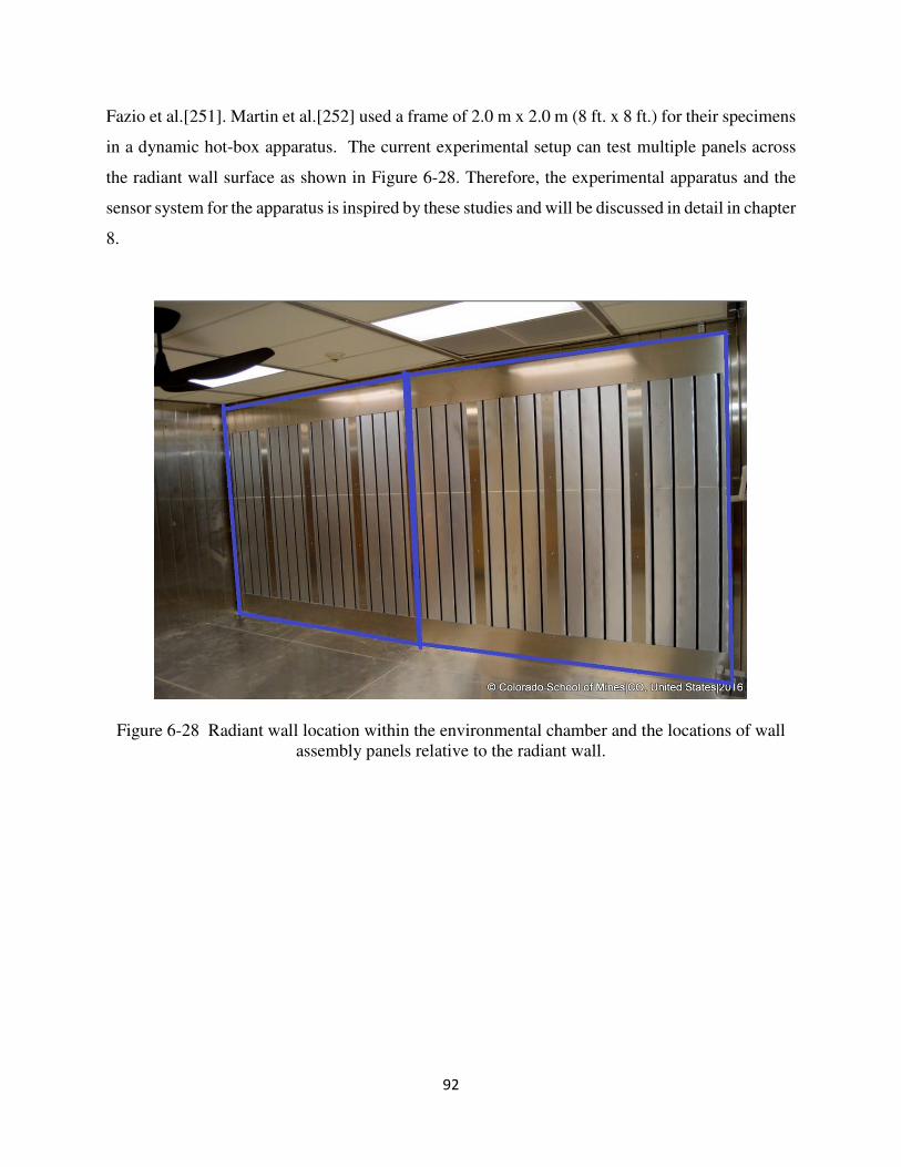
92
Fazio et al.[251]. Martin et al.[252] used a frame of 2.0 m x 2.0 m (8 ft. x 8 ft.) for their specimens
in a dynamic hot-box apparatus. The current experimental setup can test multiple panels across
the radiant wall surface as shown in Figure 6-28. Therefore, the experimental apparatus and the
sensor system for the apparatus is inspired by these studies and will be discussed in detail in chapter
8.
Figure 6-28 Radiant wall location within the environmental chamber and the locations of wall assembly panels relative to the radiant wall.
93
CHAPTER 7
EMPIRICAL VALIDATION AND COMPARISON OF PCM MODELING ALGORITHEMS
COMMONLY USED IN BUILDING ENERGY AND HYGROTHERMAL SOFTWARE
This section contributes to the fulfillment of the following objectives of this research: (v)
Verify (using the numerical model) and validate (using the experimental data from laboratory
experiments and field experiments) different PCM models in software platforms like EnergyPlus
and WUFI. This study is under review in the journal of Building and Environment. Dr. Kaushik
Biswas of Oak Ridge National Laboratory conducted the COMSOL simulations and the PCM
characterization for the Nano-PCMs. Dr. Dariuz Heim at Lodz University of Technology
conducted the ESP-r simulations of this study.
7.1. Introduction
Buildings are responsible for nearly 40% of the total energy consumed in United States
[253]. A large portion of this energy consumption is used for space-conditioning, up to 50% during
peak time [254]. Therefore, there is an interest to increase the energy efficiency in buildings and
energy storage potential to reduce peak demand and potential energy use. Innovative sustainable
design, materials with improved thermal properties, and integration of thermal energy storage are
some of the methods used in the industry today.
Thermal energy storage (TES) is used in buildings due to its capacity to shift loads [255,
256]. TES can make buildings more grid friendly and energy or cost efficient [257, 258]. TES can
be either sensible storage or a combination of latent and sensible storage. Interest and products
using latent heat storage in building envelopes has increased and have regained interest of
researchers during the last decades due its high capacity to store energy per mas [15]. In buildings
TES can be applied in passive systems, which utilizes building envelope components to store and
release energy, or in active systems, which tend to be integrated with building heating, ventilation,
and air conditioning (HVAC) systems [259]. Passive PCM storage has become a popular research
topic due to building envelope large surface area and the ability to add latent heat storage into light
94
mass buildings [260-263] and is also the focus on this study: PCMs uses in the building envelope
[264, 265].
Due to their variable properties, design of PCM inclusions in buildings require careful and
accurate energy analysis as it is important to maximize the number of times PCMs cycle between
solid and liquid phases to utilize its latent heat. For this and other reasons, several PCM heat
transfer models have been implemented in different building energy modeling tools [266-272].
However, an IEA Annex 23 surveyed over 250 research publications concluding that the general
confidence in currently used numerical models is still too low to use them for designing and code
purposes [266, 273]. Another article analyzes several modeling tools capable of simulating PCMs
and supports the need for extensive model validation and comparison of the different numerical
tools available today using a standardized procedure for PCM model validation [274]. These
studies show validation has an important role in model development but previous work has been
limited in range, applications, and conditions. For example: EnergyPlus PCM model was validated
using PCM shape-stabilized experimental data [246, 275], COMSOL 2D PCM model was
validated using PCM enhanced drywall with field data [14], ESP-r PCM model was validated for
microencapsulated PCM [276], and WUFI PCM model was validated with data from Dynamic
Heat Flux Meter Apparatus (DHFMA) [277]. These studies did not consider hysteresis in their
models. Recent studies have implemented different PCM models in EnergyPlus using Energy
Management System (EMS) and also as part of the source code with no clear validation with
hysteresis [277]. The thermal hysteresis in PCMs occur due to PCM characterization test method
and type of equipment used, and impaired PCM nucleation during the freezing process which is
also known as sub-cooling [15]. Thus, there is a need for a careful validation and comparison for
different PCM applications in the building envelope.
Additionally, it is important to consider the computational runtime and the performance
limitations of building energy modeling, PCM models included in whole building energy modeling
platforms tend to simplify the use of temperature dependent PCM properties like specific heat,
thermal conductivity, and melting points [120]. The temperature dependent properties of PCMs
should be obtained from characterization methods [15], but often it is not possible to use properties
obtained from small samples (such from differential scanning calorimetry, DSC). The sample size
of the PCM used in the characterization influences the measured values of the thermal properties
and may not reflect the thermal behavior for different encapsulation methods accurately [278, 279].
95
Finally, materials that exhibit two or three dimensional behavior, hysteresis, and subcooling [277,
280-283], have been difficult to incorporate into the PCM models without compromising the
computational runtime. Therefore, assessment and comparison of the different PCM modeling
software is required.
While there has been studies comparing the thermal load modeling capabilities of different
building energy modeling programs (BEMPs) using ASHRAE Standard 140 tests [284] or doing
broad simulation engine comparison [285], there are no previous efforts comparing specifically
PCMs models using laboratory and field data to understand and quantify the limitations of
modeling techniques used in each numerical tool for an specific application (e.g. PCMs micro/nano
encapsulated in drywall). Given the need for validated models that can accurately model PCMs,
this study compares and validates PCM models that are part of popular building energy and
hygrothermal software commonly used in building industry [286-297]: EnergyPlus, ESP-r, and
WUFI. WUFI is compared here since building designers and modelers commonly use it for energy
and hygrothermal performance assessments. It also compares COMSOL, a specialized numerical
modeling software, using a more detailed two-dimensional heat transfer model and finally an
algorithm developed in MATLAB (Thesis algorithm). PCM applications analyzed are Nano-PCM
in drywall and shape-stabilized PCM layer behind drywall.
7.2. Methodology
Validation data used in this study uses experimental data from two independent PCM
studies and compares PCM models implemented in different energy modeling software. The
analyzed PCM heat and mass transfer models in this study are part of the following software:
(i) ESP-r: Building energy simulation tool commonly used in Europe that has two PCM models
introduced as special material (PCM_Cap, model no. 53) and defined as an active building
elements with variable thermo-physical properties (spmatl subroutine) [113, 298]. The latent heat
is calculated based on effective heat capacity which is a linear function of temperature.
Temperature dependence conductivity (linearly) can be also taken into account during simulation.
ESP-r has developed sub-routines to model hysteresis in PCMs.
(ii) WUFI v6.1: Heat and mass transfer (HAMT) software for building structures [127, 129, 299-
301]. WUFI has the ability to define temperature dependent input functions via ‘Hygrothermal
96
Functions’ object set and ‘Enthalpy, temperature dependent’ object [302]. WUFI also has the
ability to define temperature dependent conductivity via ‘Thermal Conductivity, temperature-
dependent’ object. This study uses these two objects to define the temperature dependent functions
of PCM properties. WUFI uses coupled heat and mass transfer equations to model heat and
moisture transfer. The moisture transfer modeling component of this program is turned off in the
current study to exclusively model just the heat transfer as rest of considered models only capture
heat transfer phenomena.
(iii) COMSOL: The heat transfer module of COMSOL Multiphysics®
(https://www.comsol.com/heat-transfer-module) is used for the simulations presented here.
Temperature-dependent material properties are incorporated in COMSOL using the ‘interpolation’
function. For PCMs, the measured enthalpy as a function of temperature is provided as input and
the specific heat is defined as the slope of the enthalpy vs. temperature curve, the latter is calculated
as part of the solution routine [14] [144]. Biswas et al. [130] developed an algorithm using the
‘previous solution’ operator of COMSOL to capture the hysteresis in PCM and evaluated the
differences in energy saving estimates with and without considering the impacts of hysteresis.
(iv) EnergyPlus v9.0: Building energy simulation software that models PCMs with a finite
difference algorithm (CondFD) coupled with an enthalpy temperature function [100, 123, 246,
289]. EnergyPlus has two PCM models: with and without hysteresis. Hysteresis model uses
polynomial fitting curves to describe the properties of PCM adapted from the Ginzburg-Landau
theory of phase transitions [277]. EnergyPlus’ original PCM model object is
MaterialProperty:PhaseChange. The object requests the inputs, (i) temperature dependent
coefficient for thermal conductivity, and (ii) temperature-enthalpy data points to define the
enthalpy curve. The recently introduced PCM model object named is MaterialProperty:
PhaseChangeHysteresis. For both EnergyPlus PCM models, temperature dependent thermal
conductivity is defined with the MaterialProperty: VariableThermalConductivity object.
(v) MATLAB: A multi-paradigm numerical computing environment and proprietary
programming language [303]. MATLAB is used to model PCM inclusions in the building
envelope in literature [111, 216, 297, 304]. Thesis model (in MATLAB) has been analytically
verified using Stefan problem, and numerically verified with the PCM model in EnergyPlus in the
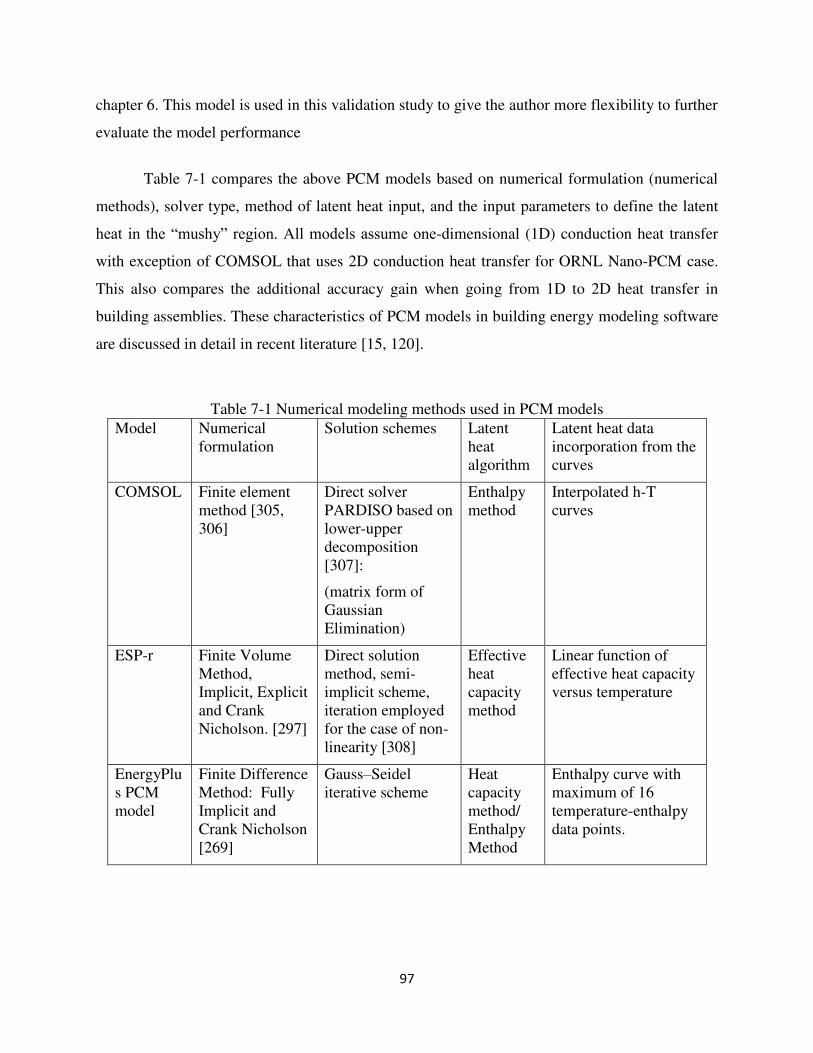
97
chapter 6. This model is used in this validation study to give the author more flexibility to further
evaluate the model performance
Table 7-1 compares the above PCM models based on numerical formulation (numerical
methods), solver type, method of latent heat input, and the input parameters to define the latent
heat in the “mushy” region. All models assume one-dimensional (1D) conduction heat transfer
with exception of COMSOL that uses 2D conduction heat transfer for ORNL Nano-PCM case.
This also compares the additional accuracy gain when going from 1D to 2D heat transfer in
building assemblies. These characteristics of PCM models in building energy modeling software
are discussed in detail in recent literature [15, 120].
Table 7-1 Numerical modeling methods used in PCM models Model Numerical
formulation Solution schemes Latent
heat algorithm
Latent heat data incorporation from the curves
COMSOL Finite element method [305, 306]
Direct solver PARDISO based on lower-upper decomposition [307]:
(matrix form of Gaussian Elimination)
Enthalpy method
Interpolated h-T curves
ESP-r Finite Volume Method, Implicit, Explicit and Crank Nicholson. [297]
Direct solution method, semi-implicit scheme, iteration employed for the case of non-linearity [308]
Effective heat capacity method
Linear function of effective heat capacity versus temperature
EnergyPlus PCM model
Finite Difference Method: Fully Implicit and Crank Nicholson [269]
Gauss–Seidel iterative scheme
Heat capacity method/ Enthalpy Method
Enthalpy curve with maximum of 16 temperature-enthalpy data points.
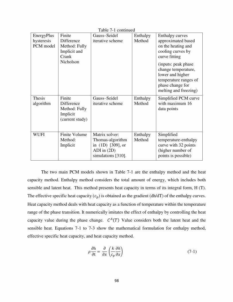
98
Table 7-1 continued EnergyPlus hysteresis PCM model
Finite Difference Method: Fully Implicit and Crank Nicholson
Gauss–Seidel iterative scheme
Enthalpy Method
Enthalpy curves approximated based on the heating and cooling curves by curve fitting
(inputs: peak phase change temperature, lower and higher temperature ranges of phase change for melting and freezing)
Thesis algorithm
Finite Difference Method: Fully Implicit (current study)
Gauss–Seidel iterative scheme
Enthalpy Method
Simplified PCM curve with maximum 16 data points
WUFI Finite Volume Method: Implicit
Matrix solver: Thomas-algorithm in (1D) [309], or ADI in (2D) simulations [310].
Enthalpy Method
Simplified temperature-enthalpy curve with 32 points (higher number of points is possible)
The two main PCM models shown in Table 7-1 are the enthalpy method and the heat
capacity method. Enthalpy method considers the total amount of energy, which includes both
sensible and latent heat. This method presents heat capacity in terms of its integral form, H (T).
The effective specific heat capacity (𝑐𝑝) is obtained as the gradient (dh/dT) of the enthalpy curves.
Heat capacity method deals with heat capacity as a function of temperature within the temperature
range of the phase transition. It numerically imitates the effect of enthalpy by controlling the heat
capacity value during the phase change. 𝐶𝐴(𝑇) Value considers both the latent heat and the
sensible heat. Equations 7-1 to 7-3 show the mathematical formulation for enthalpy method,
effective specific heat capacity, and heat capacity method.
𝜌 ∂h∂t = 𝜕𝜕𝑥 ( 𝑘𝑐𝑝 𝜕ℎ𝜕𝑥) (7-1)
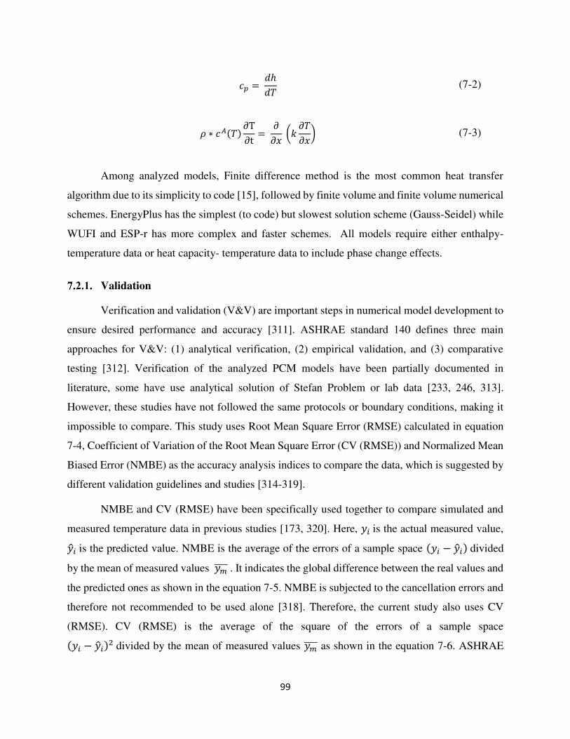
99
𝑐𝑝 = 𝑑ℎ𝑑𝑇 (7-2)
𝜌 ∗ 𝑐𝐴(𝑇) ∂T∂t = 𝜕𝜕𝑥 (𝑘 𝜕𝑇𝜕𝑥) (7-3)
Among analyzed models, Finite difference method is the most common heat transfer
algorithm due to its simplicity to code [15], followed by finite volume and finite volume numerical
schemes. EnergyPlus has the simplest (to code) but slowest solution scheme (Gauss-Seidel) while
WUFI and ESP-r has more complex and faster schemes. All models require either enthalpy-
temperature data or heat capacity- temperature data to include phase change effects.
Validation
Verification and validation (V&V) are important steps in numerical model development to
ensure desired performance and accuracy [311]. ASHRAE standard 140 defines three main
approaches for V&V: (1) analytical verification, (2) empirical validation, and (3) comparative
testing [312]. Verification of the analyzed PCM models have been partially documented in
literature, some have use analytical solution of Stefan Problem or lab data [233, 246, 313].
However, these studies have not followed the same protocols or boundary conditions, making it
impossible to compare. This study uses Root Mean Square Error (RMSE) calculated in equation
7-4, Coefficient of Variation of the Root Mean Square Error (CV (RMSE)) and Normalized Mean
Biased Error (NMBE) as the accuracy analysis indices to compare the data, which is suggested by
different validation guidelines and studies [314-319].
NMBE and CV (RMSE) have been specifically used together to compare simulated and
measured temperature data in previous studies [173, 320]. Here, 𝑦𝑖 is the actual measured value, �̂�𝑖 is the predicted value. NMBE is the average of the errors of a sample space (𝑦𝑖 − �̂�𝑖) divided
by the mean of measured values 𝑦𝑚̅̅ ̅̅ . It indicates the global difference between the real values and
the predicted ones as shown in the equation 7-5. NMBE is subjected to the cancellation errors and
therefore not recommended to be used alone [318]. Therefore, the current study also uses CV
(RMSE). CV (RMSE) is the average of the square of the errors of a sample space (𝑦𝑖 − �̂�𝑖)2 divided by the mean of measured values 𝑦𝑚̅̅ ̅̅ as shown in the equation 7-6. ASHRAE
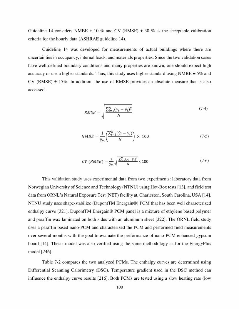
100
Guideline 14 considers NMBE ± 10 % and CV (RMSE) ± 30 % as the acceptable calibration
criteria for the hourly data (ASHRAE guideline 14).
Guideline 14 was developed for measurements of actual buildings where there are
uncertainties in occupancy, internal loads, and materials properties. Since the two validation cases
have well-defined boundary conditions and many properties are known, one should expect high
accuracy or use a higher standards. Thus, this study uses higher standard using NMBE ± 5% and
CV (RMSE) ± 15%. In addition, the use of RMSE provides an absolute measure that is also
accessed.
𝑅𝑀𝑆𝐸 = √ ∑ (𝑦𝑖 − �̂�𝑖)2𝑁𝑖=1 𝑁 (7-4)
𝑁𝑀𝐵𝐸 = 1𝑦𝑚̅̅ ̅̅ (∑ (�̂�𝑖 − 𝑦𝑖)𝑁𝑖=1 𝑁 ) × 100 (7-5)
𝐶𝑉 (𝑅𝑀𝑆𝐸) = 1𝑦𝑚̅̅ ̅̅̅√ ∑ (𝑦𝑖−�̂�𝑖)2𝑁𝑖=1 𝑁 × 100 (7-6)
This validation study uses experimental data from two experiments: laboratory data from
Norwegian University of Science and Technology (NTNU) using Hot-Box tests [13], and field test
data from ORNL’s Natural Exposure Test (NET) facility at, Charleston, South Carolina, USA [14].
NTNU study uses shape-stabilize (DupontTM Energain®) PCM that has been well characterized
enthalpy curve [321]. DupontTM Energain® PCM panel is a mixture of ethylene based polymer
and paraffin wax laminated on both sides with an aluminum sheet [322]. The ORNL field study
uses a paraffin based nano-PCM and characterized the PCM and performed field measurements
over several months with the goal to evaluate the performance of nano-PCM enhanced gypsum
board [14]. Thesis model was also verified using the same methodology as for the EnergyPlus
model [246].
Table 7-2 compares the two analyzed PCMs. The enthalpy curves are determined using
Differential Scanning Calorimetry (DSC). Temperature gradient used in the DSC method can
influence the enthalpy curve results [216]. Both PCMs are tested using a slow heating rate (low
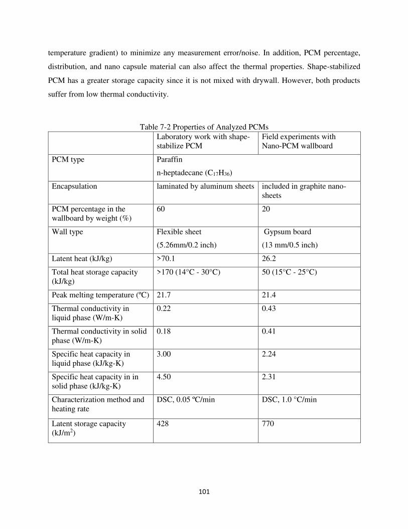
101
temperature gradient) to minimize any measurement error/noise. In addition, PCM percentage,
distribution, and nano capsule material can also affect the thermal properties. Shape-stabilized
PCM has a greater storage capacity since it is not mixed with drywall. However, both products
suffer from low thermal conductivity.
Table 7-2 Properties of Analyzed PCMs Laboratory work with shape-
stabilize PCM Field experiments with Nano-PCM wallboard
PCM type Paraffin
n-heptadecane (C17H36)
Encapsulation laminated by aluminum sheets included in graphite nano-sheets
PCM percentage in the wallboard by weight (%)
60 20
Wall type Flexible sheet
(5.26mm/0.2 inch)
Gypsum board
(13 mm/0.5 inch)
Latent heat (kJ/kg) >70.1 26.2
Total heat storage capacity (kJ/kg)
>170 (14°C - 30°C) 50 (15°C - 25°C)
Peak melting temperature (ºC) 21.7 21.4
Thermal conductivity in liquid phase (W/m-K)
0.22 0.43
Thermal conductivity in solid phase (W/m-K)
0.18 0.41
Specific heat capacity in liquid phase (kJ/kg-K)
3.00 2.24
Specific heat capacity in in solid phase (kJ/kg-K)
4.50 2.31
Characterization method and heating rate
DSC, 0.05 ºC/min DSC, 1.0 °C/min
Latent storage capacity (kJ/m2)
428 770
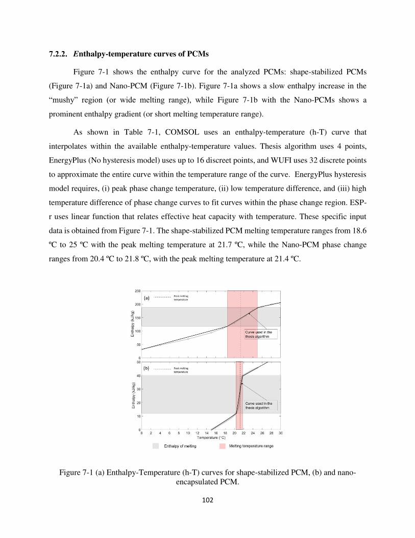
102
Enthalpy-temperature curves of PCMs
Figure 7-1 shows the enthalpy curve for the analyzed PCMs: shape-stabilized PCMs
(Figure 7-1a) and Nano-PCM (Figure 7-1b). Figure 7-1a shows a slow enthalpy increase in the
“mushy” region (or wide melting range), while Figure 7-1b with the Nano-PCMs shows a
prominent enthalpy gradient (or short melting temperature range).
As shown in Table 7-1, COMSOL uses an enthalpy-temperature (h-T) curve that
interpolates within the available enthalpy-temperature values. Thesis algorithm uses 4 points,
EnergyPlus (No hysteresis model) uses up to 16 discreet points, and WUFI uses 32 discrete points
to approximate the entire curve within the temperature range of the curve. EnergyPlus hysteresis
model requires, (i) peak phase change temperature, (ii) low temperature difference, and (iii) high
temperature difference of phase change curves to fit curves within the phase change region. ESP-
r uses linear function that relates effective heat capacity with temperature. These specific input
data is obtained from Figure 7-1. The shape-stabilized PCM melting temperature ranges from 18.6
ºC to 25 ºC with the peak melting temperature at 21.7 ºC, while the Nano-PCM phase change
ranges from 20.4 ºC to 21.8 ºC, with the peak melting temperature at 21.4 ºC.
Figure 7-1 (a) Enthalpy-Temperature (h-T) curves for shape-stabilized PCM, (b) and nano-encapsulated PCM.
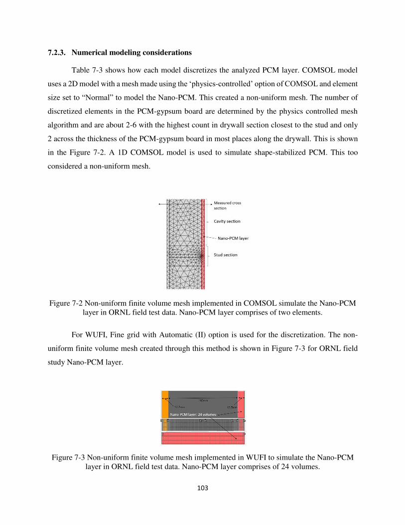
103
Numerical modeling considerations
Table 7-3 shows how each model discretizes the analyzed PCM layer. COMSOL model
uses a 2D model with a mesh made using the ‘physics-controlled’ option of COMSOL and element
size set to “Normal” to model the Nano-PCM. This created a non-uniform mesh. The number of
discretized elements in the PCM-gypsum board are determined by the physics controlled mesh
algorithm and are about 2-6 with the highest count in drywall section closest to the stud and only
2 across the thickness of the PCM-gypsum board in most places along the drywall. This is shown
in the Figure 7-2. A 1D COMSOL model is used to simulate shape-stabilized PCM. This too
considered a non-uniform mesh.
Figure 7-2 Non-uniform finite volume mesh implemented in COMSOL simulate the Nano-PCM layer in ORNL field test data. Nano-PCM layer comprises of two elements.
For WUFI, Fine grid with Automatic (II) option is used for the discretization. The non-
uniform finite volume mesh created through this method is shown in Figure 7-3 for ORNL field
study Nano-PCM layer.
Figure 7-3 Non-uniform finite volume mesh implemented in WUFI to simulate the Nano-PCM layer in ORNL field test data. Nano-PCM layer comprises of 24 volumes.
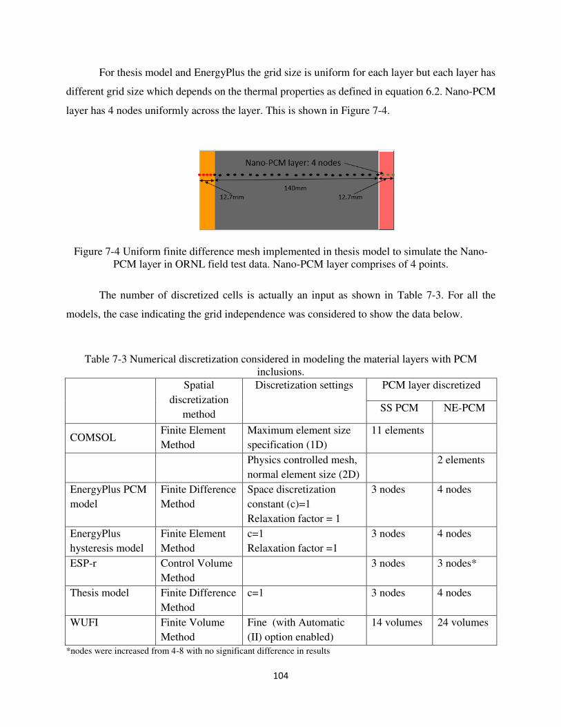
104
For thesis model and EnergyPlus the grid size is uniform for each layer but each layer has
different grid size which depends on the thermal properties as defined in equation 6.2. Nano-PCM
layer has 4 nodes uniformly across the layer. This is shown in Figure 7-4.
Figure 7-4 Uniform finite difference mesh implemented in thesis model to simulate the Nano-PCM layer in ORNL field test data. Nano-PCM layer comprises of 4 points.
The number of discretized cells is actually an input as shown in Table 7-3. For all the
models, the case indicating the grid independence was considered to show the data below.
Table 7-3 Numerical discretization considered in modeling the material layers with PCM inclusions.
Spatial discretization
method
Discretization settings PCM layer discretized
SS PCM NE-PCM
COMSOL Finite Element Method
Maximum element size specification (1D)
11 elements
Physics controlled mesh, normal element size (2D)
2 elements
EnergyPlus PCM model
Finite Difference Method
Space discretization constant (c)=1 Relaxation factor = 1
3 nodes 4 nodes
EnergyPlus hysteresis model
Finite Element Method
c=1 Relaxation factor =1
3 nodes 4 nodes
ESP-r Control Volume Method
3 nodes 3 nodes*
Thesis model Finite Difference Method
c=1 3 nodes 4 nodes
WUFI Finite Volume Method
Fine (with Automatic (II) option enabled)
14 volumes 24 volumes
*nodes were increased from 4-8 with no significant difference in results
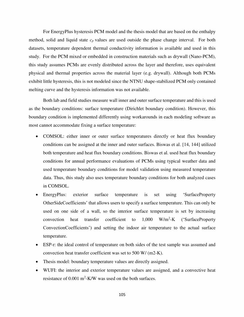
105
For EnergyPlus hysteresis PCM model and the thesis model that are based on the enthalpy
method, solid and liquid state cp values are used outside the phase change interval. For both
datasets, temperature dependent thermal conductivity information is available and used in this
study. For the PCM mixed or embedded in construction materials such as drywall (Nano-PCM),
this study assumes PCMs are evenly distributed across the layer and therefore, uses equivalent
physical and thermal properties across the material layer (e.g. drywall). Although both PCMs
exhibit little hysteresis, this is not modeled since the NTNU shape-stabilized PCM only contained
melting curve and the hysteresis information was not available.
Both lab and field studies measure wall inner and outer surface temperature and this is used
as the boundary conditions: surface temperature (Dirichlet boundary condition). However, this
boundary condition is implemented differently using workarounds in each modeling software as
most cannot accommodate fixing a surface temperature:
COMSOL: either inner or outer surface temperatures directly or heat flux boundary
conditions can be assigned at the inner and outer surfaces. Biswas et al. [14, 144] utilized
both temperature and heat flux boundary conditions. Biswas et al. used heat flux boundary
conditions for annual performance evaluations of PCMs using typical weather data and
used temperature boundary conditions for model validation using measured temperature
data. Thus, this study also uses temperature boundary conditions for both analyzed cases
in COMSOL.
EnergyPlus: exterior surface temperature is set using ‘SurfaceProperty
OtherSideCoefficients’ that allows users to specify a surface temperature. This can only be
used on one side of a wall, so the interior surface temperature is set by increasing
convection heat transfer coefficient to 1,000 W/m2-K (‘SurfaceProperty
ConvectionCoefficients’) and setting the indoor air temperature to the actual surface
temperature.
ESP-r: the ideal control of temperature on both sides of the test sample was assumed and
convection heat transfer coefficient was set to 500 W/ (m2-K).
Thesis model: boundary temperature values are directly assigned.
WUFI: the interior and exterior temperature values are assigned, and a convective heat
resistance of 0.001 m2-K/W was used on the both surfaces.
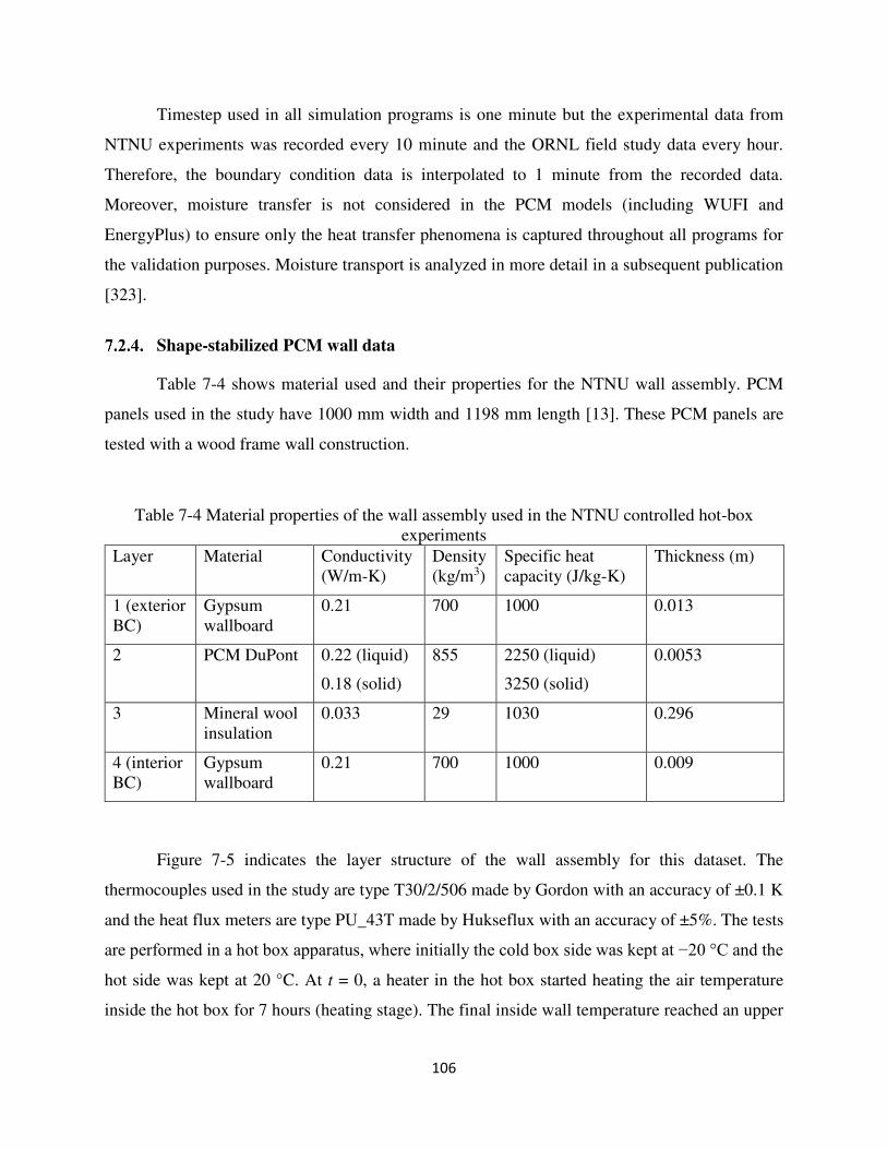
106
Timestep used in all simulation programs is one minute but the experimental data from
NTNU experiments was recorded every 10 minute and the ORNL field study data every hour.
Therefore, the boundary condition data is interpolated to 1 minute from the recorded data.
Moreover, moisture transfer is not considered in the PCM models (including WUFI and
EnergyPlus) to ensure only the heat transfer phenomena is captured throughout all programs for
the validation purposes. Moisture transport is analyzed in more detail in a subsequent publication
[323].
Shape-stabilized PCM wall data
Table 7-4 shows material used and their properties for the NTNU wall assembly. PCM
panels used in the study have 1000 mm width and 1198 mm length [13]. These PCM panels are
tested with a wood frame wall construction.
Table 7-4 Material properties of the wall assembly used in the NTNU controlled hot-box experiments
Layer Material Conductivity (W/m-K)
Density (kg/m3)
Specific heat capacity (J/kg-K)
Thickness (m)
1 (exterior BC)
Gypsum wallboard
0.21 700 1000 0.013
2 PCM DuPont 0.22 (liquid)
0.18 (solid)
855 2250 (liquid)
3250 (solid)
0.0053
3 Mineral wool insulation
0.033 29 1030 0.296
4 (interior BC)
Gypsum wallboard
0.21 700 1000 0.009
Figure 7-5 indicates the layer structure of the wall assembly for this dataset. The
thermocouples used in the study are type T30/2/506 made by Gordon with an accuracy of ±0.1 K
and the heat flux meters are type PU_43T made by Hukseflux with an accuracy of ±5%. The tests
are performed in a hot box apparatus, where initially the cold box side was kept at −20 °C and the
hot side was kept at 20 °C. At t = 0, a heater in the hot box started heating the air temperature
inside the hot box for 7 hours (heating stage). The final inside wall temperature reached an upper
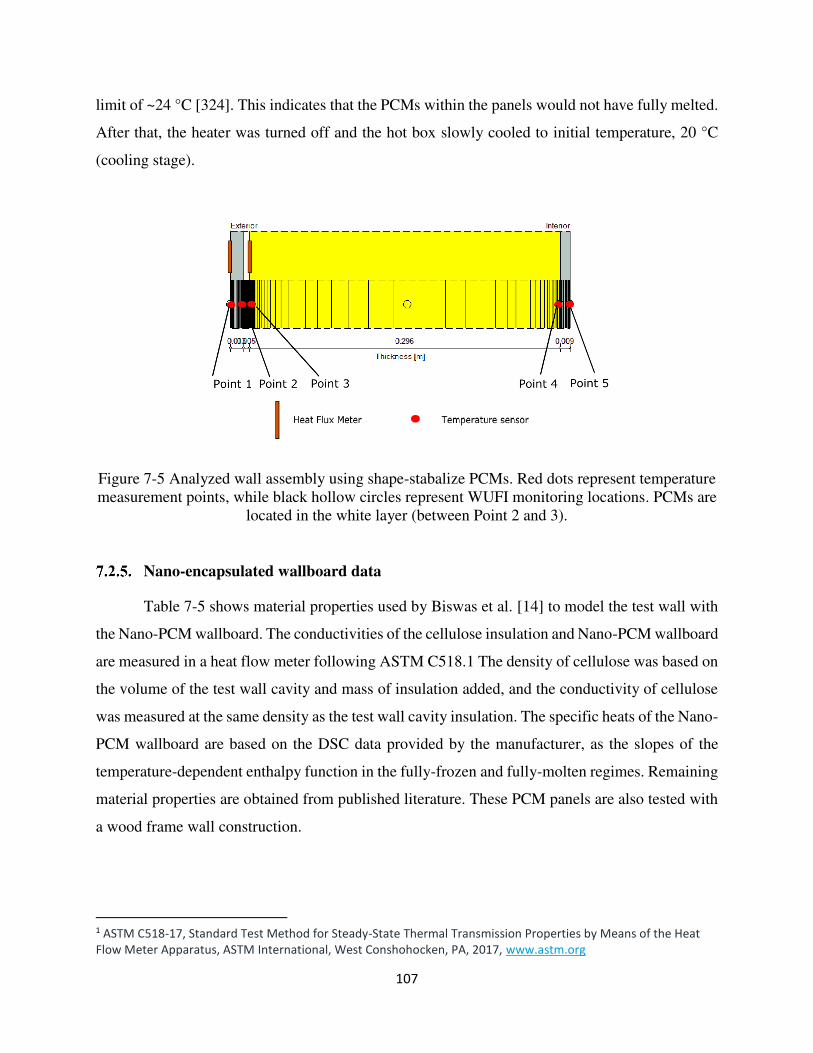
107
limit of ~24 °C [324]. This indicates that the PCMs within the panels would not have fully melted.
After that, the heater was turned off and the hot box slowly cooled to initial temperature, 20 °C
(cooling stage).
Figure 7-5 Analyzed wall assembly using shape-stabalize PCMs. Red dots represent temperature measurement points, while black hollow circles represent WUFI monitoring locations. PCMs are
located in the white layer (between Point 2 and 3).
Nano-encapsulated wallboard data
Table 7-5 shows material properties used by Biswas et al. [14] to model the test wall with
the Nano-PCM wallboard. The conductivities of the cellulose insulation and Nano-PCM wallboard
are measured in a heat flow meter following ASTM C518.1 The density of cellulose was based on
the volume of the test wall cavity and mass of insulation added, and the conductivity of cellulose
was measured at the same density as the test wall cavity insulation. The specific heats of the Nano-
PCM wallboard are based on the DSC data provided by the manufacturer, as the slopes of the
temperature-dependent enthalpy function in the fully-frozen and fully-molten regimes. Remaining
material properties are obtained from published literature. These PCM panels are also tested with
a wood frame wall construction.
1 ASTM C518-17, Standard Test Method for Steady-State Thermal Transmission Properties by Means of the Heat
Flow Meter Apparatus, ASTM International, West Conshohocken, PA, 2017, www.astm.org
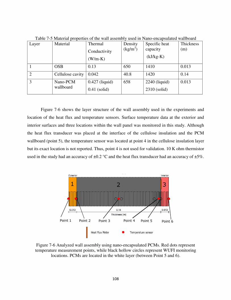
108
Table 7-5 Material properties of the wall assembly used in Nano-encapsulated wallboard Layer Material Thermal
Conductivity
(W/m-K)
Density (kg/m3)
Specific heat capacity
(kJ/kg-K)
Thickness (m)
1 OSB 0.13 650 1410 0.013
2 Cellulose cavity 0.042 40.8 1420 0.14
3 Nano-PCM wallboard
0.427 (liquid)
0.41 (solid)
658 2240 (liquid)
2310 (solid)
0.013
Figure 7-6 shows the layer structure of the wall assembly used in the experiments and
location of the heat flux and temperature sensors. Surface temperature data at the exterior and
interior surfaces and three locations within the wall panel was monitored in this study. Although
the heat flux transducer was placed at the interface of the cellulose insulation and the PCM
wallboard (point 5), the temperature sensor was located at point 4 in the cellulose insulation layer
but its exact location is not reported. Thus, point 4 is not used for validation. 10 K ohm thermistor
used in the study had an accuracy of ±0.2 °C and the heat flux transducer had an accuracy of ±5%.
Figure 7-6 Analyzed wall assembly using nano-encapsulated PCMs. Red dots represent temperature measurement points, while black hollow circles represent WUFI monitoring
locations. PCMs are located in the white layer (between Point 5 and 6).
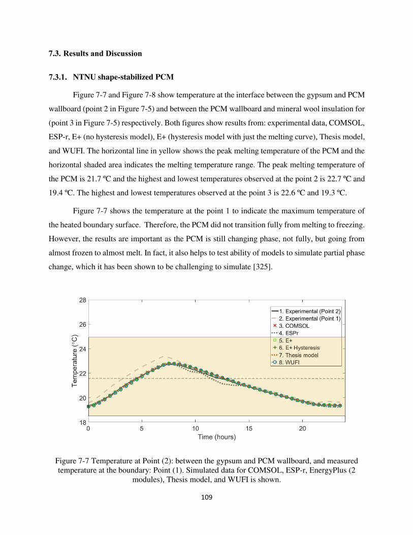
109
7.3. Results and Discussion
NTNU shape-stabilized PCM
Figure 7-7 and Figure 7-8 show temperature at the interface between the gypsum and PCM
wallboard (point 2 in Figure 7-5) and between the PCM wallboard and mineral wool insulation for
(point 3 in Figure 7-5) respectively. Both figures show results from: experimental data, COMSOL,
ESP-r, E+ (no hysteresis model), E+ (hysteresis model with just the melting curve), Thesis model,
and WUFI. The horizontal line in yellow shows the peak melting temperature of the PCM and the
horizontal shaded area indicates the melting temperature range. The peak melting temperature of
the PCM is 21.7 ºC and the highest and lowest temperatures observed at the point 2 is 22.7 ºC and
19.4 ºC. The highest and lowest temperatures observed at the point 3 is 22.6 ºC and 19.3 ºC.
Figure 7-7 shows the temperature at the point 1 to indicate the maximum temperature of
the heated boundary surface. Therefore, the PCM did not transition fully from melting to freezing.
However, the results are important as the PCM is still changing phase, not fully, but going from
almost frozen to almost melt. In fact, it also helps to test ability of models to simulate partial phase
change, which it has been shown to be challenging to simulate [325].
Figure 7-7 Temperature at Point (2): between the gypsum and PCM wallboard, and measured temperature at the boundary: Point (1). Simulated data for COMSOL, ESP-r, EnergyPlus (2
modules), Thesis model, and WUFI is shown.
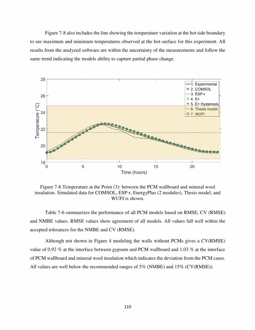
110
Figure 7-8 also includes the line showing the temperature variation at the hot side boundary
to see maximum and minimum temperatures observed at the hot-surface for this experiment. All
results from the analyzed software are within the uncertainty of the measurements and follow the
same trend indicating the models ability to capture partial phase change.
Figure 7-8 Temperature at the Point (3): between the PCM wallboard and mineral wool insulation. Simulated data for COMSOL, ESP-r, EnergyPlus (2 modules), Thesis model, and
WUFI is shown.
Table 7-6 summarizes the performance of all PCM models based on RMSE, CV (RMSE)
and NMBE values. RMSE values show agreement of all models. All values fall well within the
accepted tolerances for the NMBE and CV (RMSE).
Although not shown in Figure 4 modeling the walls without PCMs gives a CV(RMSE)
value of 0.92 % at the interface between gypsum and PCM wallboard and 1.03 % at the interface
of PCM wallboard and mineral wool insulation which indicates the deviation from the PCM cases.
All values are well below the recommended ranges of 5% (NMBE) and 15% (CV(RMSE)).
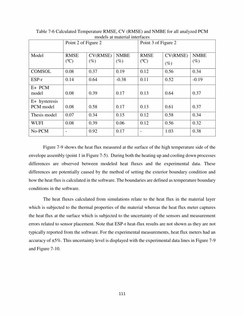
111
Table 7-6 Calculated Temperature RMSE, CV (RMSE) and NMBE for all analyzed PCM models at material interfaces
Point 2 of Figure 2 Point 3 of Figure 2
Model RMSE (ºC)
CV(RMSE) (%)
NMBE (%)
RMSE (ºC)
CV(RMSE)
(%)
NMBE (%)
COMSOL 0.08 0.37 0.19 0.12 0.56 0.34
ESP-r 0.14 0.64 -0.38 0.11 0.52 -0.19
E+ PCM model 0.08 0.39 0.17 0.13 0.64 0.37
E+ hysteresis PCM model 0.08 0.58 0.17 0.13 0.61 0.37
Thesis model 0.07 0.34 0.15 0.12 0.58 0.34
WUFI 0.08 0.39 0.06 0.12 0.56 0.32
No-PCM - 0.92 0.17 - 1.03 0.38
Figure 7-9 shows the heat flux measured at the surface of the high temperature side of the
envelope assembly (point 1 in Figure 7-5). During both the heating up and cooling down processes
differences are observed between modeled heat fluxes and the experimental data. These
differences are potentially caused by the method of setting the exterior boundary condition and
how the heat flux is calculated in the software. The boundaries are defined as temperature boundary
conditions in the software.
The heat fluxes calculated from simulations relate to the heat flux in the material layer
which is subjected to the thermal properties of the material whereas the heat flux meter captures
the heat flux at the surface which is subjected to the uncertainty of the sensors and measurement
errors related to sensor placement. Note that ESP-r heat-flux results are not shown as they are not
typically reported from the software. For the experimental measurements, heat flux meters had an
accuracy of ±5%. This uncertainty level is displayed with the experimental data lines in Figure 7-9
and Figure 7-10.
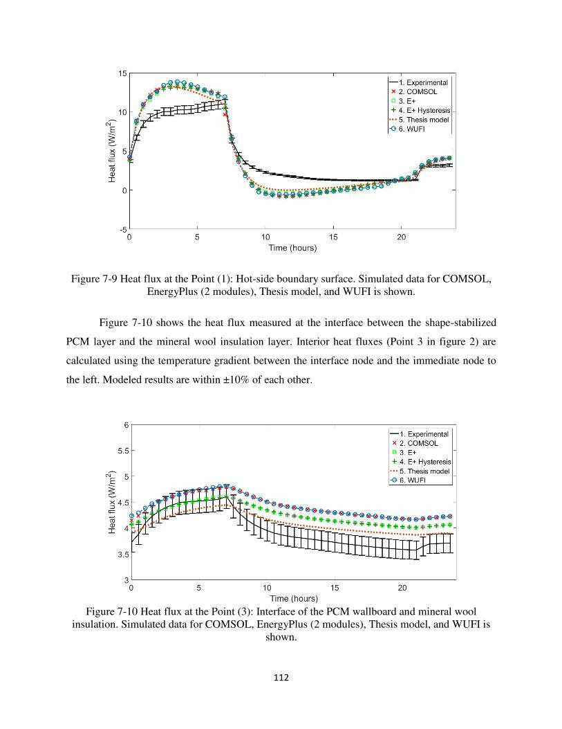
112
Figure 7-9 Heat flux at the Point (1): Hot-side boundary surface. Simulated data for COMSOL, EnergyPlus (2 modules), Thesis model, and WUFI is shown.
Figure 7-10 shows the heat flux measured at the interface between the shape-stabilized
PCM layer and the mineral wool insulation layer. Interior heat fluxes (Point 3 in figure 2) are
calculated using the temperature gradient between the interface node and the immediate node to
the left. Modeled results are within ±10% of each other.
Figure 7-10 Heat flux at the Point (3): Interface of the PCM wallboard and mineral wool
insulation. Simulated data for COMSOL, EnergyPlus (2 modules), Thesis model, and WUFI is shown.
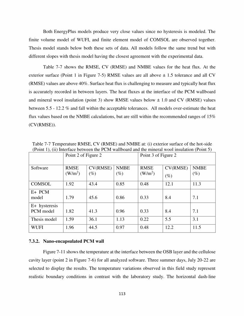
113
Both EnergyPlus models produce very close values since no hysteresis is modeled. The
finite volume model of WUFI, and finite element model of COMSOL are observed together.
Thesis model stands below both these sets of data. All models follow the same trend but with
different slopes with thesis model having the closest agreement with the experimental data.
Table 7-7 shows the RMSE, CV (RMSE) and NMBE values for the heat flux. At the
exterior surface (Point 1 in Figure 7-5) RMSE values are all above ± 1.5 tolerance and all CV
(RMSE) values are above 40%. Surface heat flux is challenging to measure and typically heat flux
is accurately recorded in between layers. The heat fluxes at the interface of the PCM wallboard
and mineral wool insulation (point 3) show RMSE values below ± 1.0 and CV (RMSE) values
between 5.5 - 12.2 % and fall within the acceptable tolerances. All models over-estimate the heat
flux values based on the NMBE calculations, but are still within the recommended ranges of 15%
(CV(RMSE)).
Table 7-7 Temperature RMSE, CV (RMSE) and NMBE at: (i) exterior surface of the hot-side (Point 1), (ii) Interface between the PCM wallboard and the mineral wool insulation (Point 5)
Point 2 of Figure 2 Point 3 of Figure 2
Software RMSE (W/m2)
CV(RMSE) (%)
NMBE (%)
RMSE (W/m2)
CV(RMSE)
(%)
NMBE (%)
COMSOL 1.92 43.4 0.85 0.48 12.1 11.3
E+ PCM model 1.79 45.6 0.86 0.33 8.4 7.1
E+ hysteresis PCM model 1.82 41.3 0.96 0.33 8.4 7.1
Thesis model 1.59 36.1 1.13 0.22 5.5 3.1
WUFI 1.96 44.5 0.97 0.48 12.2 11.5
Nano-encapsulated PCM wall
Figure 7-11 shows the temperature at the interface between the OSB layer and the cellulose
cavity layer (point 2 in Figure 7-6) for all analyzed software. Three summer days, July 20-22 are
selected to display the results. The temperature variations observed in this field study represent
realistic boundary conditions in contrast with the laboratory study. The horizontal dash-line
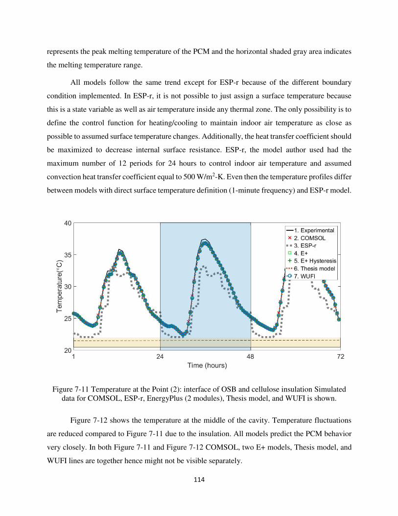
114
represents the peak melting temperature of the PCM and the horizontal shaded gray area indicates
the melting temperature range.
All models follow the same trend except for ESP-r because of the different boundary
condition implemented. In ESP-r, it is not possible to just assign a surface temperature because
this is a state variable as well as air temperature inside any thermal zone. The only possibility is to
define the control function for heating/cooling to maintain indoor air temperature as close as
possible to assumed surface temperature changes. Additionally, the heat transfer coefficient should
be maximized to decrease internal surface resistance. ESP-r, the model author used had the
maximum number of 12 periods for 24 hours to control indoor air temperature and assumed
convection heat transfer coefficient equal to 500 W/m2-K. Even then the temperature profiles differ
between models with direct surface temperature definition (1-minute frequency) and ESP-r model.
Figure 7-11 Temperature at the Point (2): interface of OSB and cellulose insulation Simulated data for COMSOL, ESP-r, EnergyPlus (2 modules), Thesis model, and WUFI is shown.
Figure 7-12 shows the temperature at the middle of the cavity. Temperature fluctuations
are reduced compared to Figure 7-11 due to the insulation. All models predict the PCM behavior
very closely. In both Figure 7-11 and Figure 7-12 COMSOL, two E+ models, Thesis model, and
WUFI lines are together hence might not be visible separately.
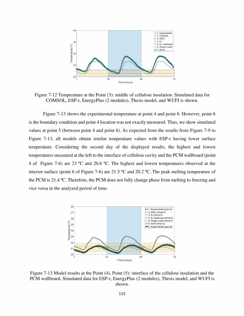
115
Figure 7-12 Temperature at the Point (3): middle of cellulose insulation. Simulated data for COMSOL, ESP-r, EnergyPlus (2 modules), Thesis model, and WUFI is shown.
Figure 7-13 shows the experimental temperature at point 4 and point 6. However, point 6
is the boundary condition and point 4 location was not exactly measured. Thus, we show simulated
values at point 5 (between point 4 and point 6). As expected from the results from Figure 7-9 to
Figure 7-13, all models obtain similar temperature values with ESP-r having lower surface
temperature. Considering the second day of the displayed results, the highest and lowest
temperatures measured at the left to the interface of cellulose cavity and the PCM wallboard (point
4 of Figure 7-6) are 23 ºC and 20.6 ºC. The highest and lowest temperatures observed at the
interior surface (point 6 of Figure 7-6) are 21.5 ºC and 20.2 ºC. The peak melting temperature of
the PCM is 21.4 ºC. Therefore, the PCM does not fully change phase from melting to freezing and
vice versa in the analyzed period of time.
Figure 7-13 Model results at the Point (4), Point (5): interface of the cellulose insulation and the PCM wallboard. Simulated data for ESP-r, EnergyPlus (2 modules), Thesis model, and WUFI is
shown.
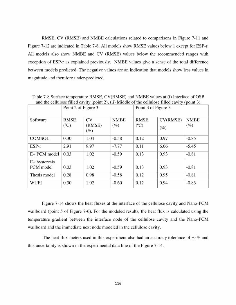
116
RMSE, CV (RMSE) and NMBE calculations related to comparisons in Figure 7-11 and
Figure 7-12 are indicated in Table 7-8. All models show RMSE values below 1 except for ESP-r.
All models also show NMBE and CV (RMSE) values below the recommended ranges with
exception of ESP-r as explained previously. NMBE values give a sense of the total difference
between models predicted. The negative values are an indication that models show less values in
magnitude and therefore under-predicted.
Table 7-8 Surface temperature RMSE, CV(RMSE) and NMBE values at (i) Interface of OSB and the cellulose filled cavity (point 2), (ii) Middle of the cellulose filled cavity (point 3)
Point 2 of Figure 3 Point 3 of Figure 3
Software RMSE (ºC)
CV (RMSE) (%)
NMBE (%)
RMSE (ºC)
CV(RMSE)
(%)
NMBE (%)
COMSOL 0.30 1.04 -0.58 0.12 0.97 -0.85
ESP-r 2.91 9.97 -7.77 0.11 6.06 -5.45
E+ PCM model 0.03 1.02 -0.59 0.13 0.93 -0.81
E+ hysteresis PCM model 0.03 1.02 -0.59 0.13 0.93 -0.81
Thesis model 0.28 0.98 -0.58 0.12 0.95 -0.81
WUFI 0.30 1.02 -0.60 0.12 0.94 -0.83
Figure 7-14 shows the heat fluxes at the interface of the cellulose cavity and Nano-PCM
wallboard (point 5 of Figure 7-6). For the modeled results, the heat flux is calculated using the
temperature gradient between the interface node of the cellulose cavity and the Nano-PCM
wallboard and the immediate next node modeled in the cellulose cavity.
The heat flux meters used in this experiment also had an accuracy tolerance of ±5% and
this uncertainty is shown in the experimental data line of the Figure 7-14.
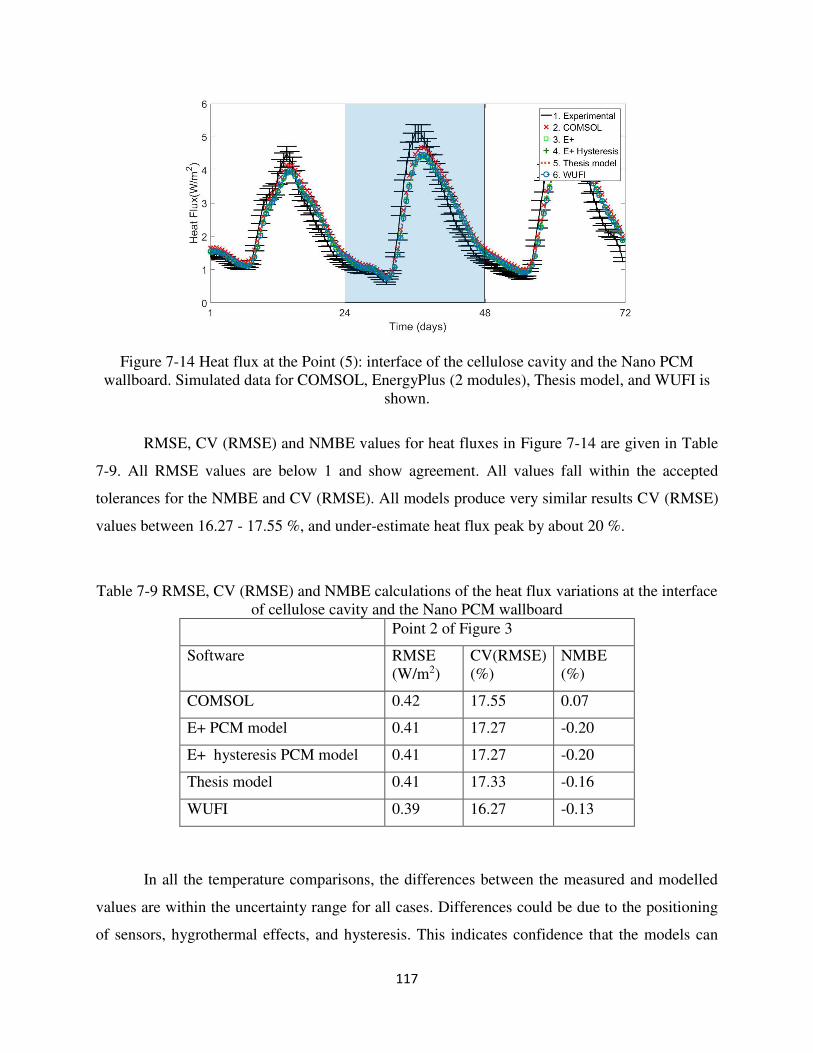
117
Figure 7-14 Heat flux at the Point (5): interface of the cellulose cavity and the Nano PCM wallboard. Simulated data for COMSOL, EnergyPlus (2 modules), Thesis model, and WUFI is
shown.
RMSE, CV (RMSE) and NMBE values for heat fluxes in Figure 7-14 are given in Table
7-9. All RMSE values are below 1 and show agreement. All values fall within the accepted
tolerances for the NMBE and CV (RMSE). All models produce very similar results CV (RMSE)
values between 16.27 - 17.55 %, and under-estimate heat flux peak by about 20 %.
Table 7-9 RMSE, CV (RMSE) and NMBE calculations of the heat flux variations at the interface of cellulose cavity and the Nano PCM wallboard
Point 2 of Figure 3
Software RMSE (W/m2)
CV(RMSE) (%)
NMBE (%)
COMSOL 0.42 17.55 0.07
E+ PCM model 0.41 17.27 -0.20
E+ hysteresis PCM model 0.41 17.27 -0.20
Thesis model 0.41 17.33 -0.16
WUFI 0.39 16.27 -0.13
In all the temperature comparisons, the differences between the measured and modelled
values are within the uncertainty range for all cases. Differences could be due to the positioning
of sensors, hygrothermal effects, and hysteresis. This indicates confidence that the models can
118
predict temperature values along similar walls. In contrast, there is greater disagreement with heat
flux data, as this is typically harder to measure and compute. Interestingly, COMSOL 2D model
show similar results to rest of the PCM models that used 1D heat transfer models. Therefore, for
the measured locations, 2D calculation did not produce more accurate results.
7.4. Conclusions
This study empirically validates and compares 6 PCM models implemented in different
building energy (EnergyPlus, ESP-r), hygrothermal (WUFI) and heat transfer (COMSOL)
software, and mathematical programming language (MATLAB)/ Thesis model using data from
two independent experimental studies with Nano-PCM embedded in drywall and shape-stabilized
PCM behind the drywall construction material. This is a unique study that compares several up to
date PCM numerical modeling software commonly used in the field with two different PCM types
commonly used. The author conducts an extensive accuracy analysis of the compared results using
RMSE, CV (RMSE) and NMBE calculations. Based on the analyzed PCMs, all the evaluated
software tools demonstrate their ability to accurately model shape-stabilized PCM behind drywall.
However, heat flux predictions show greater deviation from than surface measurements. All
models agree also with the Nano-PCM experiments but ESP-r has the lowest convergence due to
less precise definition of boundary conditions. Interestingly, this study shows no additional gains
in accuracy when comparing a 2D heat transfer model with 1D modeling for Nano-PCM and
shape-stabilized PCMs. Study affirms that this numerical modeling software can be used to model
PCMs and extend the studies to evaluate unique behaviors like hygrothermal performance (WUFI,
EnergyPlus). However, more work is needed to evaluate PCM in macroencapsulated applications
when 2D/3D heat transfer hysteresis can have stronger effects.
119
CHAPTER 8
EMPIRICAL VALIDATION AND COMPARISON OF PCM ALGORITHMS MODELING
MACRO-ENCAPSULATED PCMS IN THE BUILDING ENVELOPE
This section contributes to the fulfillment of the following objectives of this research: (iii)
Design and build experimental apparatus and a suitable controlled environment to test different
PCMs, (iv) Conduct laboratory research to validate the numerical model and identify PCMs
characteristics that could further improve the numerical solution, (v) Verify (using the numerical
model) and validate (using data from laboratory experiments, field experiments, and experimental
data from the in-house test apparatus) different PCM models in software platforms like EnergyPlus
and WUFI. The Dynamic Heat Flux Meter Apparatus characterization of PCM hydrate salts in this
study is conducted by Dr. Kaushik Biswas at the Oak Ridge National Laboratory.
8.1. Introduction
Reducing electricity demand during peak period decreases the stress on the electricity grid
[326]. Specifically, electricity used for space cooling has a significant contribution to peak
electricity demand as residential cooling drives electric peak demand in summer [327, 328].
Energy storage is one of the potential solutions to shave and shift building energy demand [329,
330]. Building thermal mass can be used as thermal energy storage (TES) due to the variability
of heating and cooling energy demand of the buildings [15, 331]. However, most residential
buildings in the U.S. tend to have low thermal mass [135], thus PCMs used in building envelope
can increase the thermal mass of the building envelope, shift peak demand of HVAC system, and
improve thermal comfort [332, 333]. In current research projects performed in the United States,
PCMs are often used as an integral part of the building thermal envelope [219].
Due to its variable thermal properties, PCM heat transfer modeling requires algorithms that
allow for variable properties, such as finite different approach. Although there are studies
proposing conduction transfer function (CTF), this approach has some limitations and has not been
adopted in any building energy simulation programs [334]. Most PCMs models used in building
energy simulation tools use either finite different of finite volume method [15]. The design and
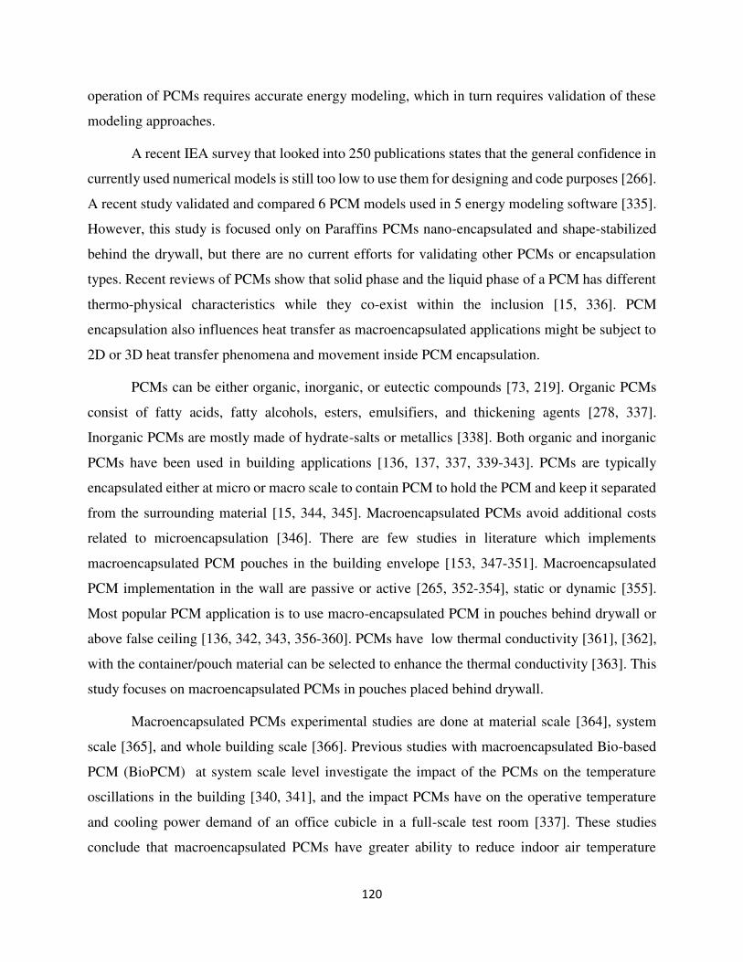
120
operation of PCMs requires accurate energy modeling, which in turn requires validation of these
modeling approaches.
A recent IEA survey that looked into 250 publications states that the general confidence in
currently used numerical models is still too low to use them for designing and code purposes [266].
A recent study validated and compared 6 PCM models used in 5 energy modeling software [335].
However, this study is focused only on Paraffins PCMs nano-encapsulated and shape-stabilized
behind the drywall, but there are no current efforts for validating other PCMs or encapsulation
types. Recent reviews of PCMs show that solid phase and the liquid phase of a PCM has different
thermo-physical characteristics while they co-exist within the inclusion [15, 336]. PCM
encapsulation also influences heat transfer as macroencapsulated applications might be subject to
2D or 3D heat transfer phenomena and movement inside PCM encapsulation.
PCMs can be either organic, inorganic, or eutectic compounds [73, 219]. Organic PCMs
consist of fatty acids, fatty alcohols, esters, emulsifiers, and thickening agents [278, 337].
Inorganic PCMs are mostly made of hydrate-salts or metallics [338]. Both organic and inorganic
PCMs have been used in building applications [136, 137, 337, 339-343]. PCMs are typically
encapsulated either at micro or macro scale to contain PCM to hold the PCM and keep it separated
from the surrounding material [15, 344, 345]. Macroencapsulated PCMs avoid additional costs
related to microencapsulation [346]. There are few studies in literature which implements
macroencapsulated PCM pouches in the building envelope [153, 347-351]. Macroencapsulated
PCM implementation in the wall are passive or active [265, 352-354], static or dynamic [355].
Most popular PCM application is to use macro-encapsulated PCM in pouches behind drywall or
above false ceiling [136, 342, 343, 356-360]. PCMs have low thermal conductivity [361], [362],
with the container/pouch material can be selected to enhance the thermal conductivity [363]. This
study focuses on macroencapsulated PCMs in pouches placed behind drywall.
Macroencapsulated PCMs experimental studies are done at material scale [364], system
scale [365], and whole building scale [366]. Previous studies with macroencapsulated Bio-based
PCM (BioPCM) at system scale level investigate the impact of the PCMs on the temperature
oscillations in the building [340, 341], and the impact PCMs have on the operative temperature
and cooling power demand of an office cubicle in a full-scale test room [337]. These studies
conclude that macroencapsulated PCMs have greater ability to reduce indoor air temperature
121
oscillations compared with a non-PCM envelope. Another study compares field indoor air
temperature against EnergyPlus with macroencapsulated PCMs to find PCM in wall and ceiling is
shown to be the most suitable options in terms of increased thermal comfort and peak daytime
temperature reduction [197] and with no complete validation. Biswas [367] performs a partial
validation of EnergyPlus using data from BioPCM applications in a metal roof but only focusing
on the attic with no clear description on how to simulate plastic pouches in a 1D model. Another
study implements BioPCM behind the drywall in the exterior walls of a test hut to record PCM
performance data to apply in a numerical PCM algorithm and used the inverse method to analyze
PCM performance but did not conduct a validation study [80]. Muruganantham [356] implemented
BioPCMs as a retrofitted mock up building and simulated the PCM as thin layer in EnergPlus to
conduct a whole building energy analysis but did not validate their approach. PCM salts (calcium
chloride hydrate) pouches have been implemented in a metal roof in a study to quantify the
residential attic performance but does not validate the approach [340]. Therefore, these studies do
not conduct validation and comparison of the heat transfer across the building envelope and also
do not consider hysteresis effects.
Literature shows that macroencapsulated PCMs show 2D heat transfer effects due to the
pouches or containing devices [368]. However, since most building energy modeling software
assumes 1D heat transfer, it is important to develop, validate, and document a methodology to
simplify this complex heat transfer and include the challenging thermal behaviors of
macroencapsulated PCMs into these models.
Thus, this study validates and compares PCM algorithms in energy modeling software such
as EnergyPlus, thesis model and WUFI to quantify their accuracy when modeling PCMs in
building envelopes. No previous study has validated this software with different
macroencapsulated PCMs. Thus, the objectives and contributions of this study are: (1) show full-
scale wall experimental data from two walls with macroencapsulated PCMs, (2) validate and
compare different PCM models used in building simulation programs and (3) develop a
methodology to simplify 2D/3D heat transfer from the macroencapsulated system to a 1D heat
transfer.
122
8.2. Methodology
This study validates and compares 4 PCM models using in-house laboratory data from two
macroencapsulated PCMs: a BioPCM in plastic foil/white plastic sheeting pouches and PCM
hydrate–salts (hydrate-salts) encapsulated in thermoplastic foil/ multilayer white polyfilm
pouches. As a reference an additional wall is also tested without PCMs. The analyzed PCMs
models are EnergyPlus hysteresis PCM model [369], EnergyPlus regular (without hysteresis)
PCM model [233], thesis model, and WUFI. These computational approach of these PCM models
are compared and fully described in a previous publication [335](chapter 7 of the thesis). The
experimental work in this study is conducted in a state-of-the-art experimental chamber located at
the Department of Mechanical Engineering at Colorado School of Mines that facilitates testing of
full scale wall panels under controlled conditions. Wall panels are constructed inside the chamber
and placed against a radiant wall to control the exterior boundary conditions and conduct full cycle
melting and freezing tests of the PCM products. Collected data is then used to validate and compare
PCM modeling software.
Macroencapsulated Phase Change Materials
Figure 8-1 shows the analyzed PCMs which are commercially available and contained in
pouches [370]. Figure 8-1a shows BioPCM contained in pouches made of plastic foil /white plastic
sheeting. These sheets are available in 0.42 m wide mats that come in lengths of 1.22 m or 2.44 m.
Figure 8-1b shows hydrate-salts contained in heavy-duty nylon/PE foil sheets. The average
thickness of the pouches is 6.4 mm for the BioPCM and 6.0 mm for the hydrate-salts. The pouch
thickness is not consistent over the surface area as the PCM is loosely packed.
Figure 8-1 Dimensions of analyzed PCM pouches: (a) BioPCM, (b) hydrate-salts.
123
As shown in the figure, these sheets are not uniform since there is 6-21 mm gap between
pouches. Therefore, extra attention is given to evaluate the impact of the presence of air with the
PCM layer
Table 8-1 shows thermo-physical properties of the analyzed PCMs. Typical PCM melting
temperatures used in the envelope applications are 19-27 ºC [353]. All PCMs used in the current
study have a nominal melting point of 23 ºC. Hydrate-salts have higher density and thermal
conductivity than the BioPCM. Therefore, for a given storage capacity, hydrate-salts add more
weight to the building. Hydrate-salts are also about 4 times more conductive than the BioPCM.
Table 8-1 Thermo-physical properties of analyzed macroencapsulated PCMs.
BioPCM Hydrate-salts
Product name M-51 BioPCM TM InfiniteRTM
Peak nominal melting temperature 23˚C/73˚F 23˚C/73˚F
Latent heat capacity (kJ/kg) ~230 ~200
Specific heat capacity (J/kg-K) 1,970 3,140
Thermal conductivity (W/m-K) Liquid: ~ 0.15
Solid: ~ 0.25
Liquid: ~0.54
Solid: ~1.09
Density (kg/m3) 860 3,420
Average thickness of the pouch – L
pouch (m) 0.0064 0.0060
Latent heat (kJ/m2) ~580 ~684
Pouch material Plastic foil / white plastic sheeting.
Thermos-plastic foil/ multilayer white heavy-duty nylon/PE foil bags
Pouch material thickness between the pouches (mm)
0.508 1.118
• Characterization curves of PCMs
Material characterization method is important in determining the thermal characteristics of
the PCMs. There are several methods used in literature and the accuracy of the characteristic data
depends on the method used [15, 278, 371]. Commonly used methods of characterization are:
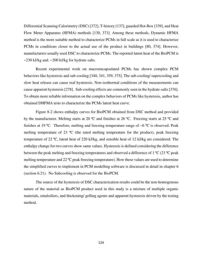
124
Differential Scanning Calorimetry (DSC) [372], T-history [137], guarded Hot-Box [339], and Heat
Flow Meter Apparatus (HFMA) methods [130, 373]. Among these methods, Dynamic HFMA
method is the more suitable method to characterize PCMs in full scale as it is used to characterize
PCMs in conditions closer to the actual use of the product in buildings [80, 374]. However,
manufacturers usually used DSC to characterize PCMs. The reported latent heat of the BioPCM is
~230 kJ/kg and. ~200 kJ/kg for hydrate-salts.
Recent experimental work on macroencapsulated PCMs has shown complex PCM
behaviors like hysteresis and sub-cooling [340, 341, 359, 375]. The sub-cooling/ supercooling and
slow heat release can cause real hysteresis. Non-isothermal conditions of the measurements can
cause apparent hysteresis [278]. Sub-cooling effects are commonly seen in the hydrate-salts [376].
To obtain more reliable information on the complex behaviors of PCMs like hysteresis, author has
obtained DHFMA tests to characterize the PCMs latent heat curve.
Figure 8-2 shows enthalpy curves for BioPCM obtained from DSC method and provided
by the manufacturer. Melting starts at 20 ºC and finishes at 26 ºC. Freezing starts at 25 ºC and
finishes at 19 ºC. Therefore, melting and freezing temperature range of ~6 ºC is observed. Peak
melting temperature of 23 ºC (the rated melting temperature for the product), peak freezing
temperature of 22 ºC, latent heat of 220 kJ/kg, and sensible heat of 12 kJ/kg are considered. The
enthalpy change for two curves show same values. Hysteresis is defined considering the difference
between the peak melting and freezing temperatures and observed a difference of 1 ºC (23 ºC peak
melting temperature and 22 ºC peak freezing temperature). How these values are used to determine
the simplified curves to implement in PCM modelling software is discussed in detail in chapter 6
(section 6.21). No Subcooling is observed for the BioPCM.
The source of the hysteresis of DSC characterization results could be the non-homogenous
nature of the material as BioPCM product used in this study is a mixture of multiple organic
materials, emulsifiers, and thickening/ gelling agents and apparent hysteresis driven by the testing
method.
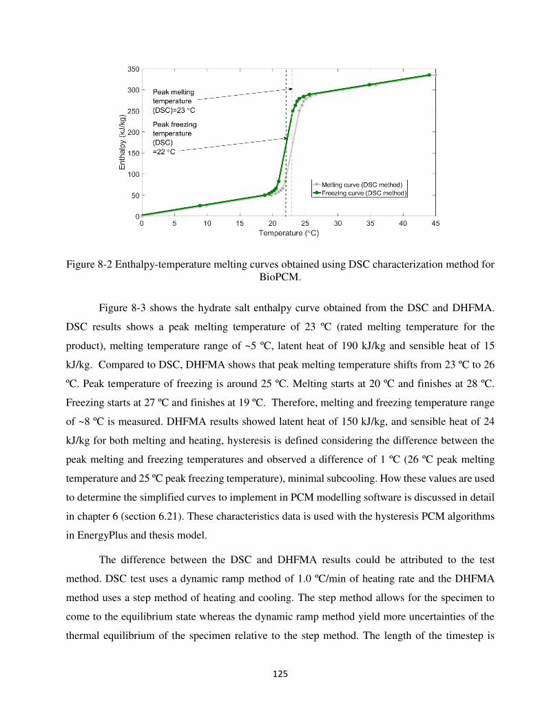
125
Figure 8-2 Enthalpy-temperature melting curves obtained using DSC characterization method for BioPCM.
Figure 8-3 shows the hydrate salt enthalpy curve obtained from the DSC and DHFMA.
DSC results shows a peak melting temperature of 23 ºC (rated melting temperature for the
product), melting temperature range of ~5 ºC, latent heat of 190 kJ/kg and sensible heat of 15
kJ/kg. Compared to DSC, DHFMA shows that peak melting temperature shifts from 23 ºC to 26
ºC. Peak temperature of freezing is around 25 ºC. Melting starts at 20 ºC and finishes at 28 ºC.
Freezing starts at 27 ºC and finishes at 19 ºC. Therefore, melting and freezing temperature range
of ~8 ºC is measured. DHFMA results showed latent heat of 150 kJ/kg, and sensible heat of 24
kJ/kg for both melting and heating, hysteresis is defined considering the difference between the
peak melting and freezing temperatures and observed a difference of 1 ºC (26 ºC peak melting
temperature and 25 ºC peak freezing temperature), minimal subcooling. How these values are used
to determine the simplified curves to implement in PCM modelling software is discussed in detail
in chapter 6 (section 6.21). These characteristics data is used with the hysteresis PCM algorithms
in EnergyPlus and thesis model.
The difference between the DSC and DHFMA results could be attributed to the test
method. DSC test uses a dynamic ramp method of 1.0 ºC/min of heating rate and the DHFMA
method uses a step method of heating and cooling. The step method allows for the specimen to
come to the equilibrium state whereas the dynamic ramp method yield more uncertainties of the
thermal equilibrium of the specimen relative to the step method. The length of the timestep is
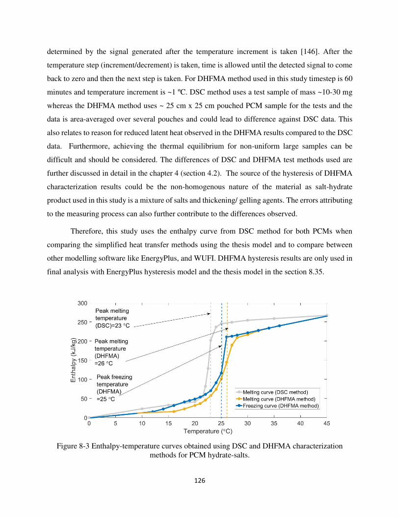
126
determined by the signal generated after the temperature increment is taken [146]. After the
temperature step (increment/decrement) is taken, time is allowed until the detected signal to come
back to zero and then the next step is taken. For DHFMA method used in this study timestep is 60
minutes and temperature increment is ~1 ºC. DSC method uses a test sample of mass ~10-30 mg
whereas the DHFMA method uses ~ 25 cm x 25 cm pouched PCM sample for the tests and the
data is area-averaged over several pouches and could lead to difference against DSC data. This
also relates to reason for reduced latent heat observed in the DHFMA results compared to the DSC
data. Furthermore, achieving the thermal equilibrium for non-uniform large samples can be
difficult and should be considered. The differences of DSC and DHFMA test methods used are
further discussed in detail in the chapter 4 (section 4.2). The source of the hysteresis of DHFMA
characterization results could be the non-homogenous nature of the material as salt-hydrate
product used in this study is a mixture of salts and thickening/ gelling agents. The errors attributing
to the measuring process can also further contribute to the differences observed.
Therefore, this study uses the enthalpy curve from DSC method for both PCMs when
comparing the simplified heat transfer methods using the thesis model and to compare between
other modelling software like EnergyPlus, and WUFI. DHFMA hysteresis results are only used in
final analysis with EnergyPlus hysteresis model and the thesis model in the section 8.35.
Figure 8-3 Enthalpy-temperature curves obtained using DSC and DHFMA characterization methods for PCM hydrate-salts.
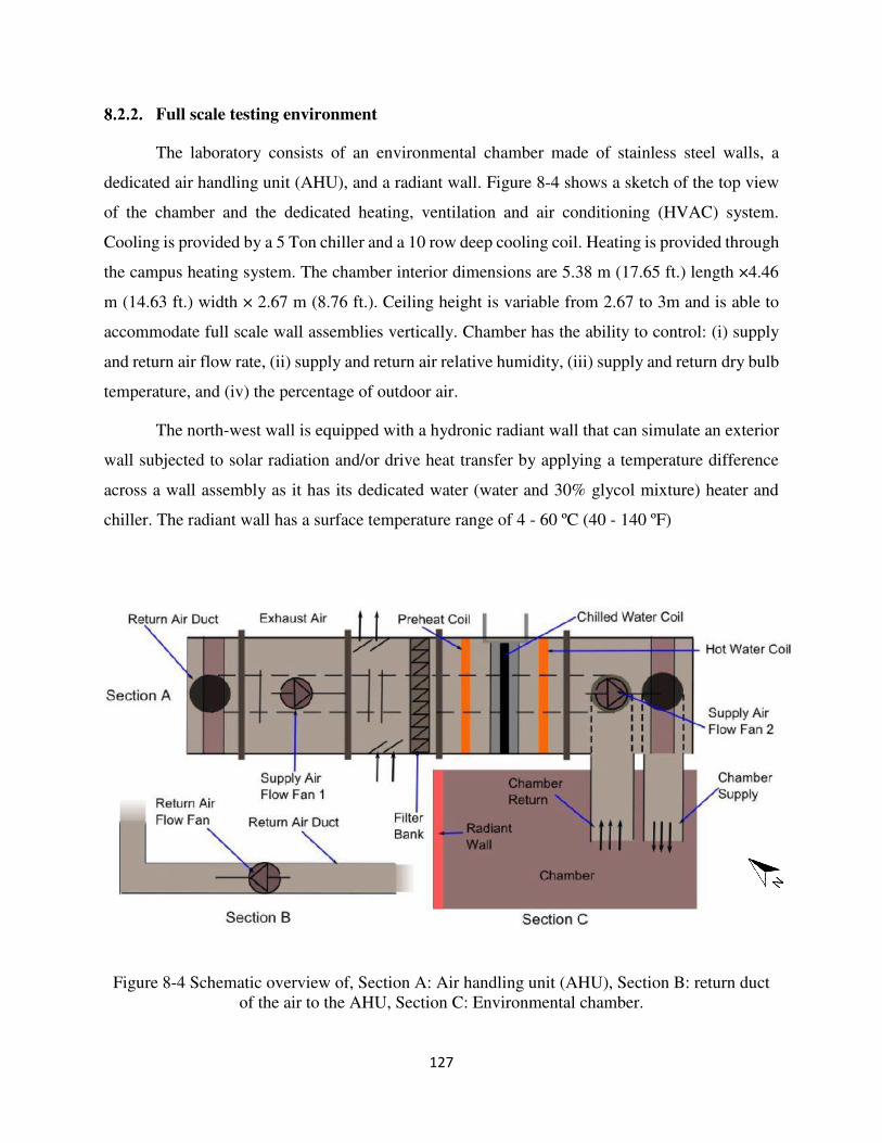
127
Full scale testing environment
The laboratory consists of an environmental chamber made of stainless steel walls, a
dedicated air handling unit (AHU), and a radiant wall. Figure 8-4 shows a sketch of the top view
of the chamber and the dedicated heating, ventilation and air conditioning (HVAC) system.
Cooling is provided by a 5 Ton chiller and a 10 row deep cooling coil. Heating is provided through
the campus heating system. The chamber interior dimensions are 5.38 m (17.65 ft.) length ×4.46
m (14.63 ft.) width × 2.67 m (8.76 ft.). Ceiling height is variable from 2.67 to 3m and is able to
accommodate full scale wall assemblies vertically. Chamber has the ability to control: (i) supply
and return air flow rate, (ii) supply and return air relative humidity, (iii) supply and return dry bulb
temperature, and (iv) the percentage of outdoor air.
The north-west wall is equipped with a hydronic radiant wall that can simulate an exterior
wall subjected to solar radiation and/or drive heat transfer by applying a temperature difference
across a wall assembly as it has its dedicated water (water and 30% glycol mixture) heater and
chiller. The radiant wall has a surface temperature range of 4 - 60 ºC (40 - 140 ºF)
Figure 8-4 Schematic overview of, Section A: Air handling unit (AHU), Section B: return duct of the air to the AHU, Section C: Environmental chamber.
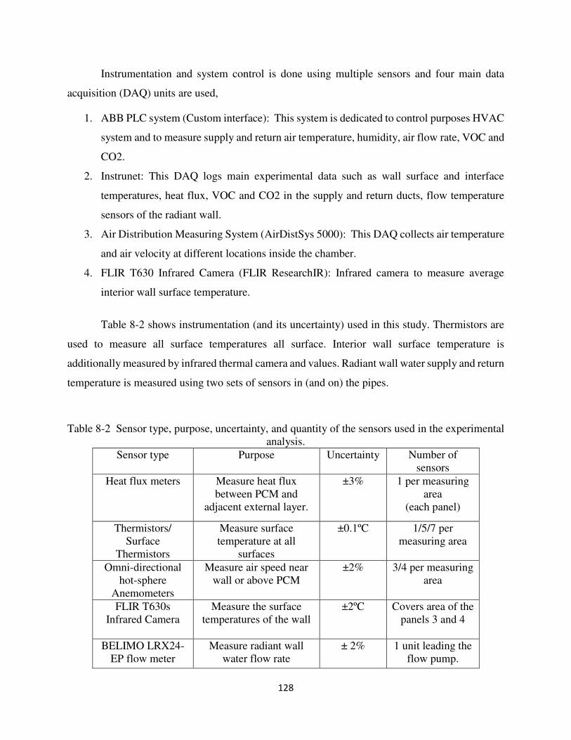
128
Instrumentation and system control is done using multiple sensors and four main data
acquisition (DAQ) units are used,
1. ABB PLC system (Custom interface): This system is dedicated to control purposes HVAC
system and to measure supply and return air temperature, humidity, air flow rate, VOC and
CO2.
2. Instrunet: This DAQ logs main experimental data such as wall surface and interface
temperatures, heat flux, VOC and CO2 in the supply and return ducts, flow temperature
sensors of the radiant wall.
3. Air Distribution Measuring System (AirDistSys 5000): This DAQ collects air temperature
and air velocity at different locations inside the chamber.
4. FLIR T630 Infrared Camera (FLIR ResearchIR): Infrared camera to measure average
interior wall surface temperature.
Table 8-2 shows instrumentation (and its uncertainty) used in this study. Thermistors are
used to measure all surface temperatures all surface. Interior wall surface temperature is
additionally measured by infrared thermal camera and values. Radiant wall water supply and return
temperature is measured using two sets of sensors in (and on) the pipes.
Table 8-2 Sensor type, purpose, uncertainty, and quantity of the sensors used in the experimental analysis.
Sensor type Purpose Uncertainty Number of sensors
Heat flux meters Measure heat flux between PCM and
adjacent external layer.
±3% 1 per measuring area
(each panel)
Thermistors/ Surface
Thermistors
Measure surface temperature at all
surfaces
±0.1ºC 1/5/7 per measuring area
Omni-directional hot-sphere
Anemometers
Measure air speed near wall or above PCM
±2% 3/4 per measuring area
FLIR T630s Infrared Camera
Measure the surface temperatures of the wall
±2ºC Covers area of the panels 3 and 4
BELIMO LRX24-
EP flow meter Measure radiant wall
water flow rate ± 2% 1 unit leading the
flow pump.
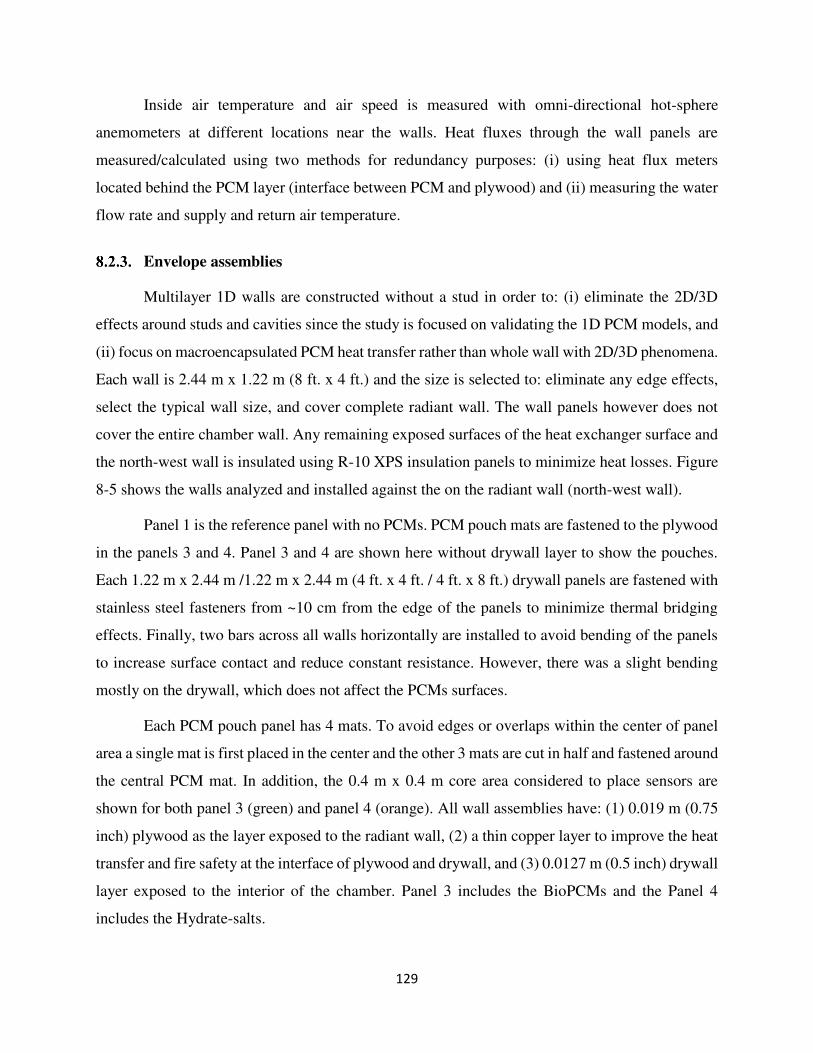
129
Inside air temperature and air speed is measured with omni-directional hot-sphere
anemometers at different locations near the walls. Heat fluxes through the wall panels are
measured/calculated using two methods for redundancy purposes: (i) using heat flux meters
located behind the PCM layer (interface between PCM and plywood) and (ii) measuring the water
flow rate and supply and return air temperature.
Envelope assemblies
Multilayer 1D walls are constructed without a stud in order to: (i) eliminate the 2D/3D
effects around studs and cavities since the study is focused on validating the 1D PCM models, and
(ii) focus on macroencapsulated PCM heat transfer rather than whole wall with 2D/3D phenomena.
Each wall is 2.44 m x 1.22 m (8 ft. x 4 ft.) and the size is selected to: eliminate any edge effects,
select the typical wall size, and cover complete radiant wall. The wall panels however does not
cover the entire chamber wall. Any remaining exposed surfaces of the heat exchanger surface and
the north-west wall is insulated using R-10 XPS insulation panels to minimize heat losses. Figure
8-5 shows the walls analyzed and installed against the on the radiant wall (north-west wall).
Panel 1 is the reference panel with no PCMs. PCM pouch mats are fastened to the plywood
in the panels 3 and 4. Panel 3 and 4 are shown here without drywall layer to show the pouches.
Each 1.22 m x 2.44 m /1.22 m x 2.44 m (4 ft. x 4 ft. / 4 ft. x 8 ft.) drywall panels are fastened with
stainless steel fasteners from ~10 cm from the edge of the panels to minimize thermal bridging
effects. Finally, two bars across all walls horizontally are installed to avoid bending of the panels
to increase surface contact and reduce constant resistance. However, there was a slight bending
mostly on the drywall, which does not affect the PCMs surfaces.
Each PCM pouch panel has 4 mats. To avoid edges or overlaps within the center of panel
area a single mat is first placed in the center and the other 3 mats are cut in half and fastened around
the central PCM mat. In addition, the 0.4 m x 0.4 m core area considered to place sensors are
shown for both panel 3 (green) and panel 4 (orange). All wall assemblies have: (1) 0.019 m (0.75
inch) plywood as the layer exposed to the radiant wall, (2) a thin copper layer to improve the heat
transfer and fire safety at the interface of plywood and drywall, and (3) 0.0127 m (0.5 inch) drywall
layer exposed to the interior of the chamber. Panel 3 includes the BioPCMs and the Panel 4
includes the Hydrate-salts.
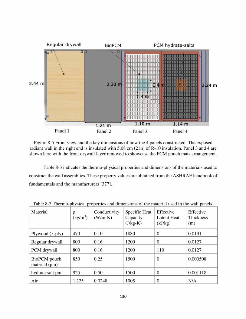
130
Figure 8-5 Front view and the key dimensions of how the 4 panels constructed. The exposed radiant wall in the right end is insulated with 5.08 cm (2 in) of R-10 insulation. Panel 3 and 4 are shown here with the front drywall layer removed to showcase the PCM pouch mats arrangement.
Table 8-3 indicates the thermo-physical properties and dimensions of the materials used to
construct the wall assemblies. These property values are obtained from the ASHRAE handbook of
fundamentals and the manufacturers [377].
Table 8-3 Thermo-physical properties and dimensions of the material used in the wall panels.
Material ρ (kg/m3)
Conductivity (W/m-K)
Specific Heat Capacity (J/kg-K)
Effective Latent Heat (kJ/kg)
Effective Thickness (m)
Plywood (5-ply) 470 0.10 1880 0 0.0191
Regular drywall 800 0.16 1200 0 0.0127
PCM drywall 800 0.16 1200 110 0.0127
BioPCM pouch material (pm)
850 0.25 1500 0 0.000508
hydrate-salt pm 925 0.50 1500 0 0.001118
Air 1.225 0.0248 1005 0 N/A
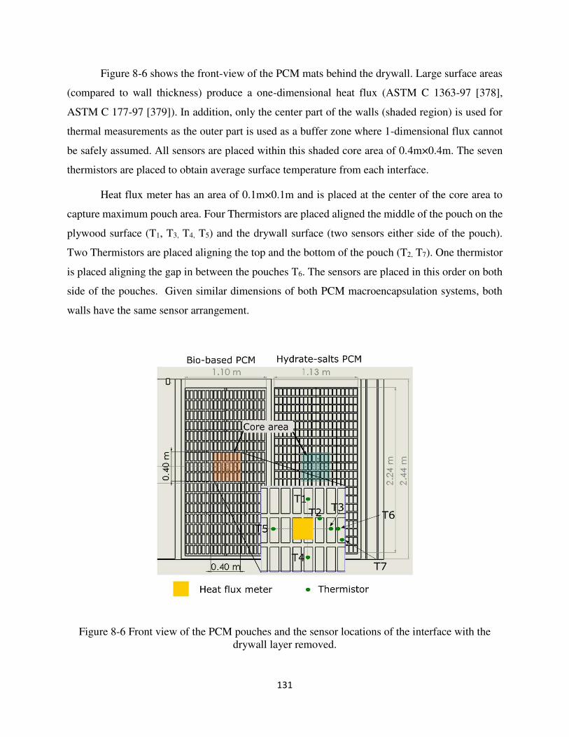
131
Figure 8-6 shows the front-view of the PCM mats behind the drywall. Large surface areas
(compared to wall thickness) produce a one-dimensional heat flux (ASTM C 1363-97 [378],
ASTM C 177-97 [379]). In addition, only the center part of the walls (shaded region) is used for
thermal measurements as the outer part is used as a buffer zone where 1-dimensional flux cannot
be safely assumed. All sensors are placed within this shaded core area of 0.4m×0.4m. The seven
thermistors are placed to obtain average surface temperature from each interface.
Heat flux meter has an area of 0.1m×0.1m and is placed at the center of the core area to
capture maximum pouch area. Four Thermistors are placed aligned the middle of the pouch on the
plywood surface (T1, T3, T4, T5) and the drywall surface (two sensors either side of the pouch).
Two Thermistors are placed aligning the top and the bottom of the pouch (T2, T7). One thermistor
is placed aligning the gap in between the pouches T6. The sensors are placed in this order on both
side of the pouches. Given similar dimensions of both PCM macroencapsulation systems, both
walls have the same sensor arrangement.
Figure 8-6 Front view of the PCM pouches and the sensor locations of the interface with the drywall layer removed.
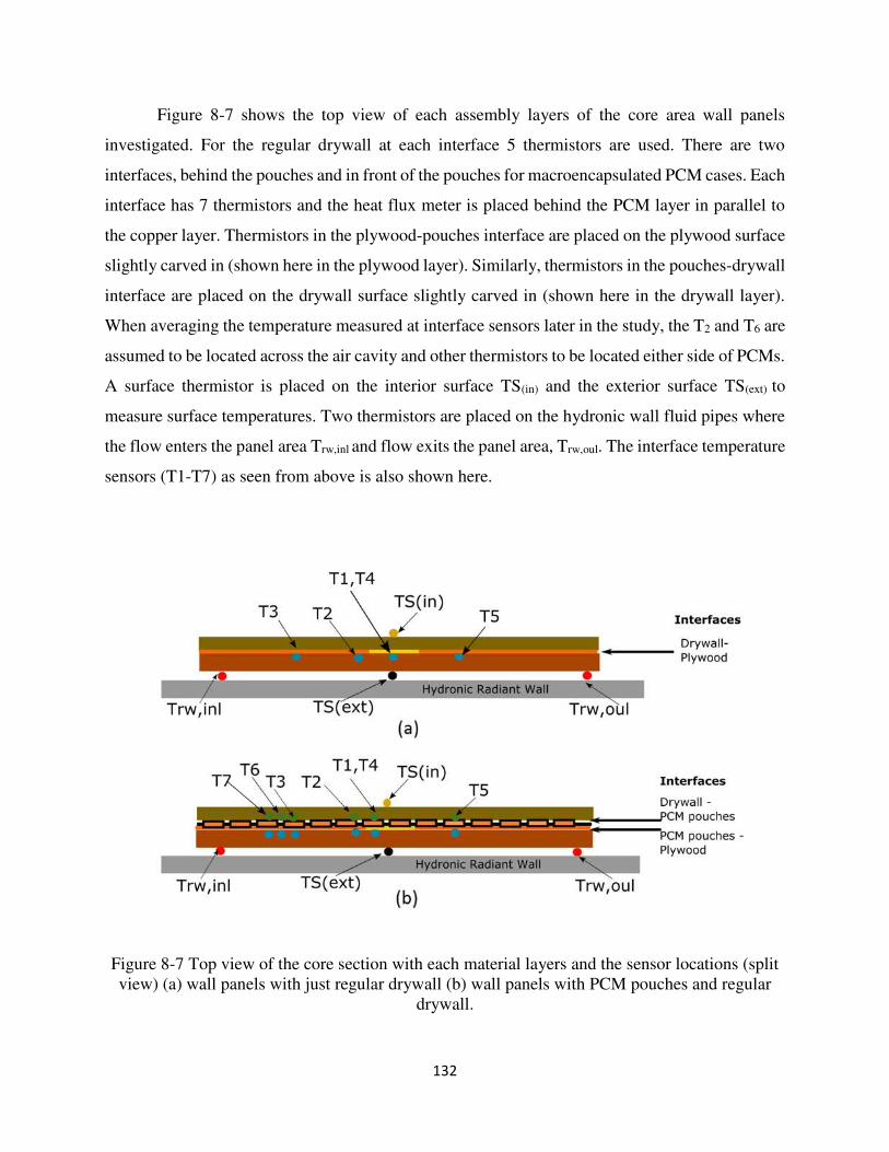
132
Figure 8-7 shows the top view of each assembly layers of the core area wall panels
investigated. For the regular drywall at each interface 5 thermistors are used. There are two
interfaces, behind the pouches and in front of the pouches for macroencapsulated PCM cases. Each
interface has 7 thermistors and the heat flux meter is placed behind the PCM layer in parallel to
the copper layer. Thermistors in the plywood-pouches interface are placed on the plywood surface
slightly carved in (shown here in the plywood layer). Similarly, thermistors in the pouches-drywall
interface are placed on the drywall surface slightly carved in (shown here in the drywall layer).
When averaging the temperature measured at interface sensors later in the study, the T2 and T6 are
assumed to be located across the air cavity and other thermistors to be located either side of PCMs.
A surface thermistor is placed on the interior surface TS(in) and the exterior surface TS(ext) to
measure surface temperatures. Two thermistors are placed on the hydronic wall fluid pipes where
the flow enters the panel area Trw,inl and flow exits the panel area, Trw,oul. The interface temperature
sensors (T1-T7) as seen from above is also shown here.
Figure 8-7 Top view of the core section with each material layers and the sensor locations (split view) (a) wall panels with just regular drywall (b) wall panels with PCM pouches and regular
drywall.
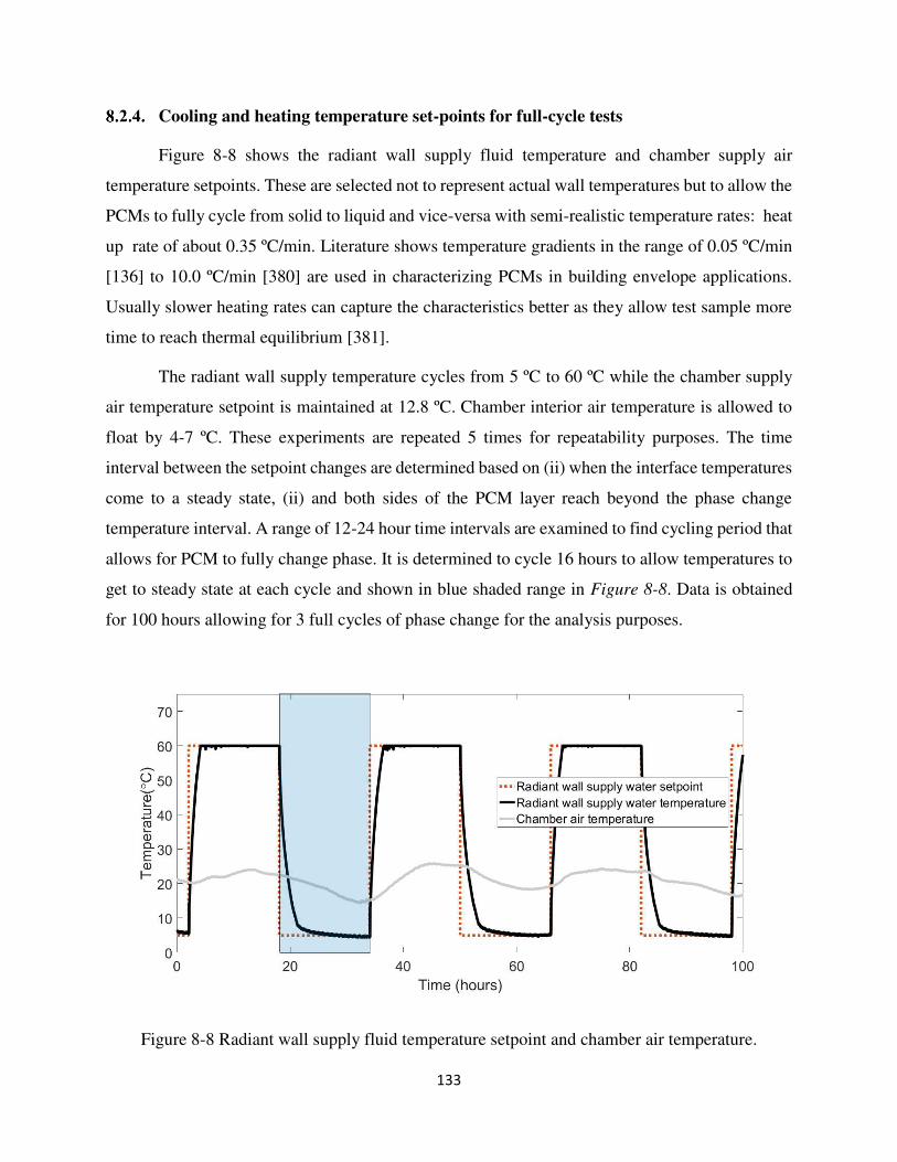
133
Cooling and heating temperature set-points for full-cycle tests
Figure 8-8 shows the radiant wall supply fluid temperature and chamber supply air
temperature setpoints. These are selected not to represent actual wall temperatures but to allow the
PCMs to fully cycle from solid to liquid and vice-versa with semi-realistic temperature rates: heat
up rate of about 0.35 ºC/min. Literature shows temperature gradients in the range of 0.05 ºC/min
[136] to 10.0 ºC/min [380] are used in characterizing PCMs in building envelope applications.
Usually slower heating rates can capture the characteristics better as they allow test sample more
time to reach thermal equilibrium [381].
The radiant wall supply temperature cycles from 5 ºC to 60 ºC while the chamber supply
air temperature setpoint is maintained at 12.8 ºC. Chamber interior air temperature is allowed to
float by 4-7 ºC. These experiments are repeated 5 times for repeatability purposes. The time
interval between the setpoint changes are determined based on (ii) when the interface temperatures
come to a steady state, (ii) and both sides of the PCM layer reach beyond the phase change
temperature interval. A range of 12-24 hour time intervals are examined to find cycling period that
allows for PCM to fully change phase. It is determined to cycle 16 hours to allow temperatures to
get to steady state at each cycle and shown in blue shaded range in Figure 8-8. Data is obtained
for 100 hours allowing for 3 full cycles of phase change for the analysis purposes.
Figure 8-8 Radiant wall supply fluid temperature setpoint and chamber air temperature.
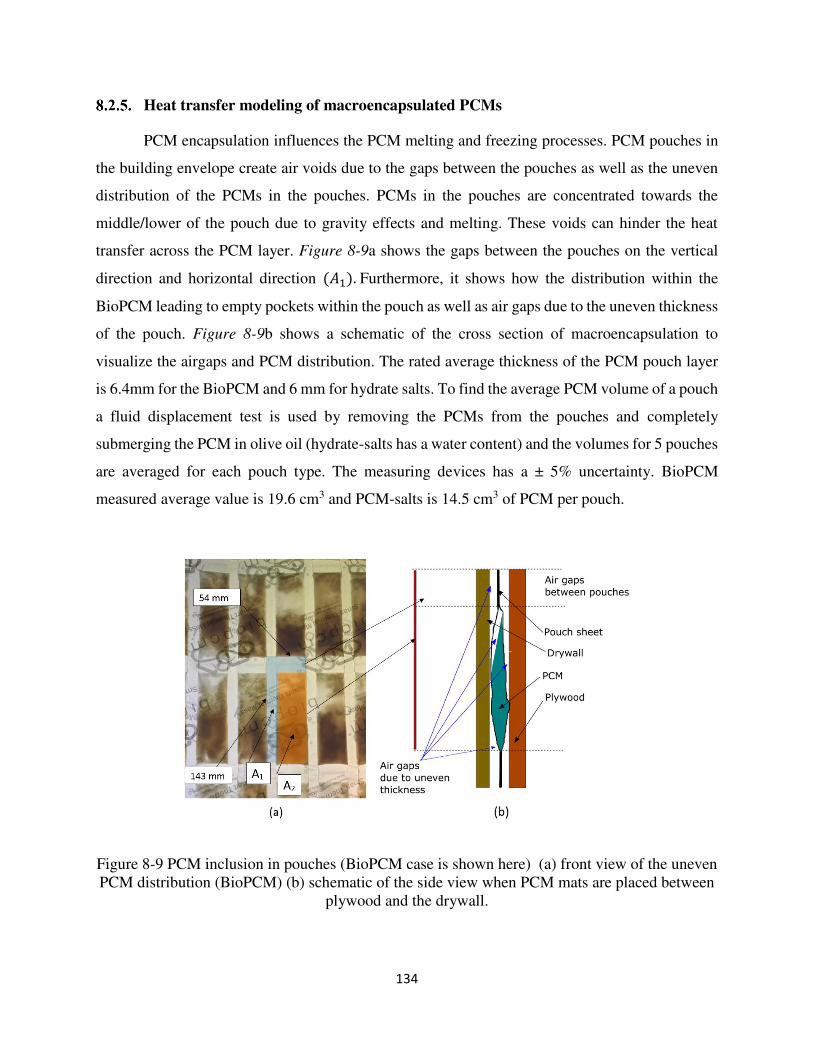
134
Heat transfer modeling of macroencapsulated PCMs
PCM encapsulation influences the PCM melting and freezing processes. PCM pouches in
the building envelope create air voids due to the gaps between the pouches as well as the uneven
distribution of the PCMs in the pouches. PCMs in the pouches are concentrated towards the
middle/lower of the pouch due to gravity effects and melting. These voids can hinder the heat
transfer across the PCM layer. Figure 8-9a shows the gaps between the pouches on the vertical
direction and horizontal direction (𝐴1). Furthermore, it shows how the distribution within the
BioPCM leading to empty pockets within the pouch as well as air gaps due to the uneven thickness
of the pouch. Figure 8-9b shows a schematic of the cross section of macroencapsulation to
visualize the airgaps and PCM distribution. The rated average thickness of the PCM pouch layer
is 6.4mm for the BioPCM and 6 mm for hydrate salts. To find the average PCM volume of a pouch
a fluid displacement test is used by removing the PCMs from the pouches and completely
submerging the PCM in olive oil (hydrate-salts has a water content) and the volumes for 5 pouches
are averaged for each pouch type. The measuring devices has a ± 5% uncertainty. BioPCM
measured average value is 19.6 cm3 and PCM-salts is 14.5 cm3 of PCM per pouch.
Figure 8-9 PCM inclusion in pouches (BioPCM case is shown here) (a) front view of the uneven PCM distribution (BioPCM) (b) schematic of the side view when PCM mats are placed between
plywood and the drywall.
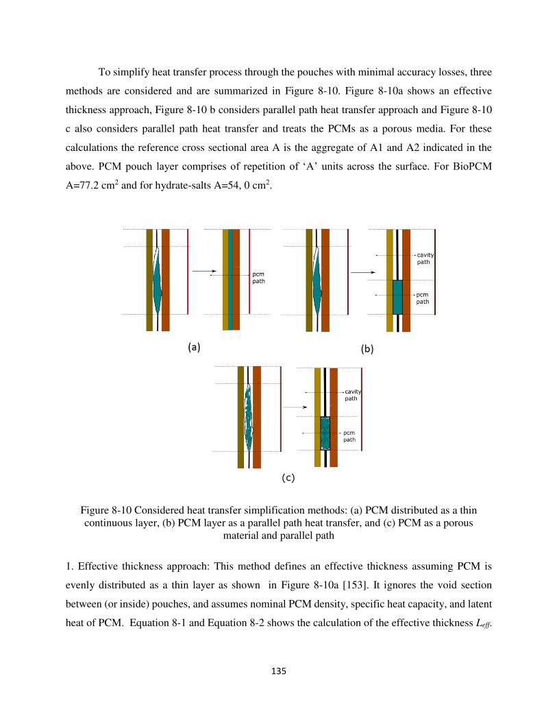
135
To simplify heat transfer process through the pouches with minimal accuracy losses, three
methods are considered and are summarized in Figure 8-10. Figure 8-10a shows an effective
thickness approach, Figure 8-10 b considers parallel path heat transfer approach and Figure 8-10
c also considers parallel path heat transfer and treats the PCMs as a porous media. For these
calculations the reference cross sectional area A is the aggregate of A1 and A2 indicated in the
above. PCM pouch layer comprises of repetition of ‘A’ units across the surface. For BioPCM
A=77.2 cm2 and for hydrate-salts A=54, 0 cm2.
Figure 8-10 Considered heat transfer simplification methods: (a) PCM distributed as a thin continuous layer, (b) PCM layer as a parallel path heat transfer, and (c) PCM as a porous
material and parallel path
1. Effective thickness approach: This method defines an effective thickness assuming PCM is
evenly distributed as a thin layer as shown in Figure 8-10a [153]. It ignores the void section
between (or inside) pouches, and assumes nominal PCM density, specific heat capacity, and latent
heat of PCM. Equation 8-1 and Equation 8-2 shows the calculation of the effective thickness Leff.
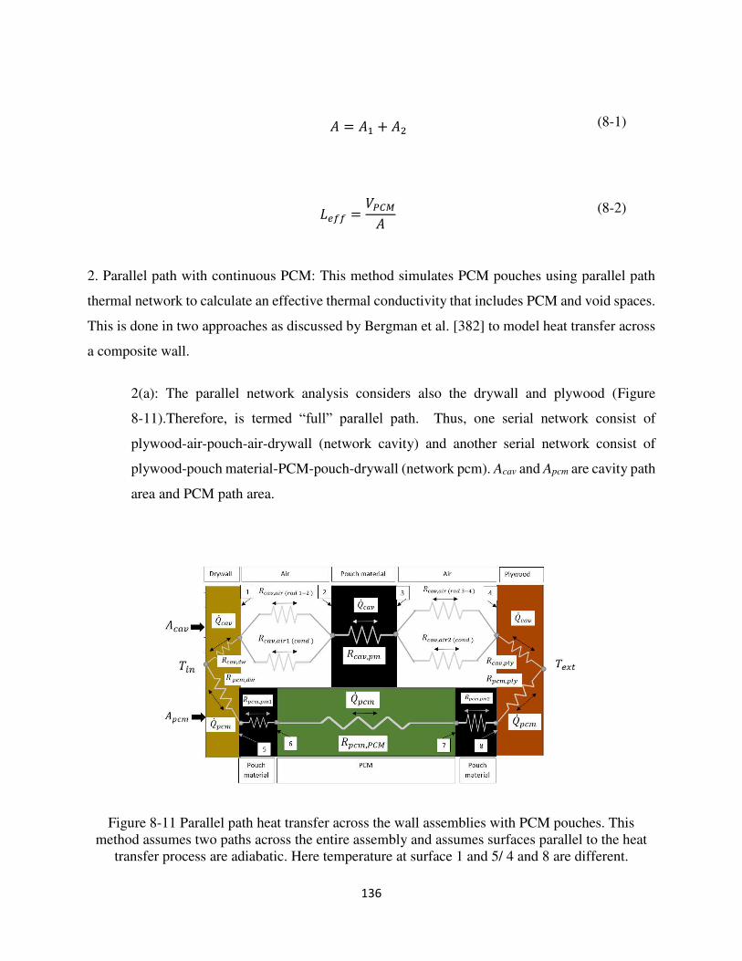
136
𝐴 = 𝐴1 + 𝐴2 (8-1)
𝐿𝑒𝑓𝑓 = 𝑉𝑃𝐶𝑀𝐴 (8-2)
2. Parallel path with continuous PCM: This method simulates PCM pouches using parallel path
thermal network to calculate an effective thermal conductivity that includes PCM and void spaces.
This is done in two approaches as discussed by Bergman et al. [382] to model heat transfer across
a composite wall.
2(a): The parallel network analysis considers also the drywall and plywood (Figure
8-11).Therefore, is termed “full” parallel path. Thus, one serial network consist of
plywood-air-pouch-air-drywall (network cavity) and another serial network consist of
plywood-pouch material-PCM-pouch-drywall (network pcm). Acav and Apcm are cavity path
area and PCM path area.
Figure 8-11 Parallel path heat transfer across the wall assemblies with PCM pouches. This method assumes two paths across the entire assembly and assumes surfaces parallel to the heat
transfer process are adiabatic. Here temperature at surface 1 and 5/ 4 and 8 are different.
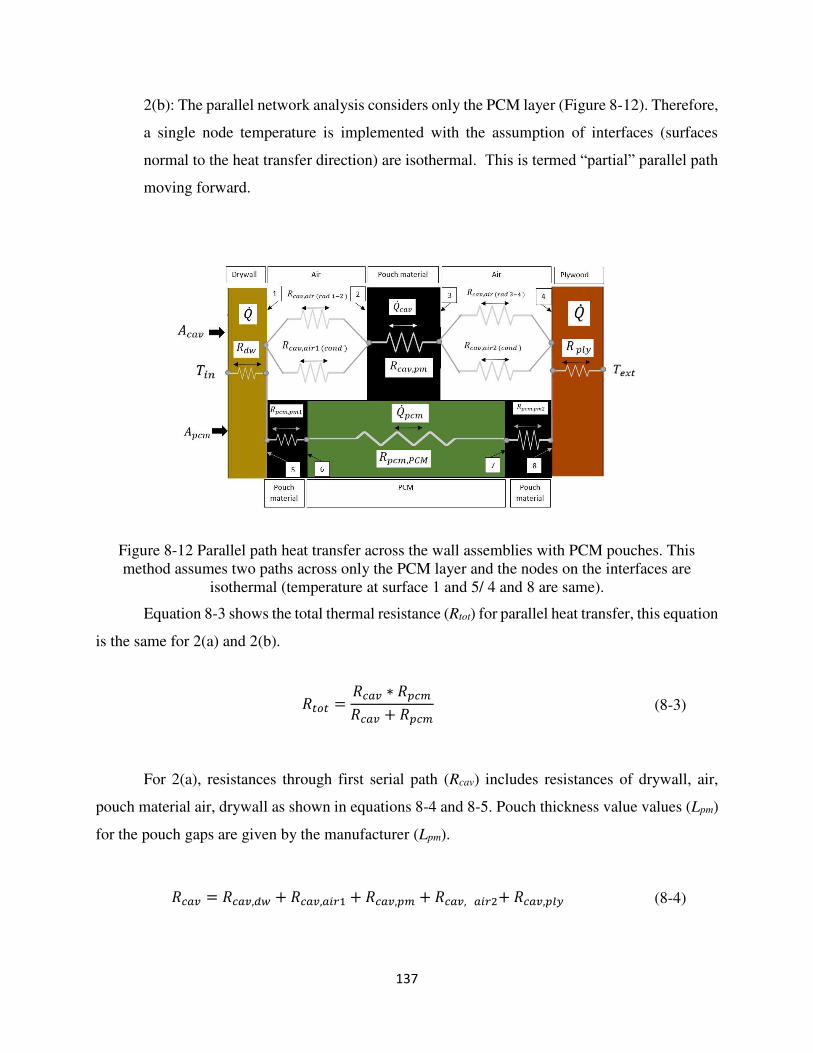
137
2(b): The parallel network analysis considers only the PCM layer (Figure 8-12). Therefore,
a single node temperature is implemented with the assumption of interfaces (surfaces
normal to the heat transfer direction) are isothermal. This is termed “partial” parallel path
moving forward.
Figure 8-12 Parallel path heat transfer across the wall assemblies with PCM pouches. This method assumes two paths across only the PCM layer and the nodes on the interfaces are
isothermal (temperature at surface 1 and 5/ 4 and 8 are same).
Equation 8-3 shows the total thermal resistance (Rtot) for parallel heat transfer, this equation
is the same for 2(a) and 2(b).
𝑅𝑡𝑜𝑡 = 𝑅𝑐𝑎𝑣 ∗ 𝑅𝑝𝑐𝑚𝑅𝑐𝑎𝑣 + 𝑅𝑝𝑐𝑚 (8-3)
For 2(a), resistances through first serial path (Rcav) includes resistances of drywall, air,
pouch material air, drywall as shown in equations 8-4 and 8-5. Pouch thickness value values (Lpm)
for the pouch gaps are given by the manufacturer (Lpm).
𝑅𝑐𝑎𝑣 = 𝑅𝑐𝑎𝑣,𝑑𝑤 + 𝑅𝑐𝑎𝑣,𝑎𝑖𝑟1 + 𝑅𝑐𝑎𝑣,𝑝𝑚 + 𝑅𝑐𝑎𝑣, 𝑎𝑖𝑟2+ 𝑅𝑐𝑎𝑣,𝑝𝑙𝑦 (8-4)
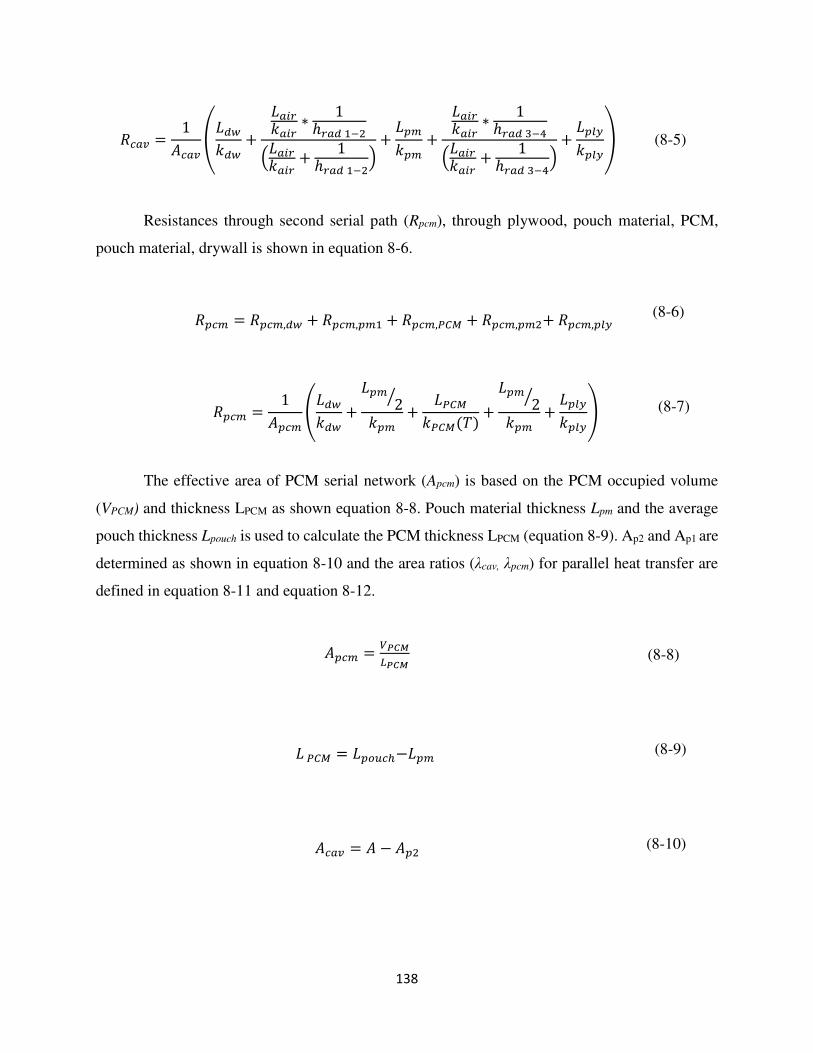
138
𝑅𝑐𝑎𝑣 = 1𝐴𝑐𝑎𝑣 (𝐿𝑑𝑤𝑘𝑑𝑤 + 𝐿𝑎𝑖𝑟𝑘𝑎𝑖𝑟 ∗ 1ℎ𝑟𝑎𝑑 1−2(𝐿𝑎𝑖𝑟𝑘𝑎𝑖𝑟 + 1ℎ𝑟𝑎𝑑 1−2) + 𝐿𝑝𝑚𝑘𝑝𝑚 + 𝐿𝑎𝑖𝑟𝑘𝑎𝑖𝑟 ∗ 1ℎ𝑟𝑎𝑑 3−4(𝐿𝑎𝑖𝑟𝑘𝑎𝑖𝑟 + 1ℎ𝑟𝑎𝑑 3−4) + 𝐿𝑝𝑙𝑦𝑘𝑝𝑙𝑦) (8-5)
Resistances through second serial path (Rpcm), through plywood, pouch material, PCM,
pouch material, drywall is shown in equation 8-6.
𝑅𝑝𝑐𝑚 = 𝑅𝑝𝑐𝑚,𝑑𝑤 + 𝑅𝑝𝑐𝑚,𝑝𝑚1 + 𝑅𝑝𝑐𝑚,𝑃𝐶𝑀 + 𝑅𝑝𝑐𝑚,𝑝𝑚2+ 𝑅𝑝𝑐𝑚,𝑝𝑙𝑦 (8-6)
𝑅𝑝𝑐𝑚 = 1𝐴𝑝𝑐𝑚 (𝐿𝑑𝑤𝑘𝑑𝑤 + 𝐿𝑝𝑚 2⁄𝑘𝑝𝑚 + 𝐿𝑃𝐶𝑀𝑘𝑃𝐶𝑀(𝑇) + 𝐿𝑝𝑚 2⁄𝑘𝑝𝑚 + 𝐿𝑝𝑙𝑦𝑘𝑝𝑙𝑦) (8-7)
The effective area of PCM serial network (Apcm) is based on the PCM occupied volume
(VPCM) and thickness LPCM as shown equation 8-8. Pouch material thickness Lpm and the average
pouch thickness Lpouch is used to calculate the PCM thickness LPCM (equation 8-9). Ap2 and Ap1 are
determined as shown in equation 8-10 and the area ratios (λcav, λpcm) for parallel heat transfer are
defined in equation 8-11 and equation 8-12.
𝐴𝑝𝑐𝑚 = 𝑉𝑃𝐶𝑀𝐿𝑃𝐶𝑀 (8-8)
𝐿 𝑃𝐶𝑀 = 𝐿𝑝𝑜𝑢𝑐ℎ−𝐿𝑝𝑚 (8-9)
𝐴𝑐𝑎𝑣 = 𝐴 − 𝐴𝑝2 (8-10)
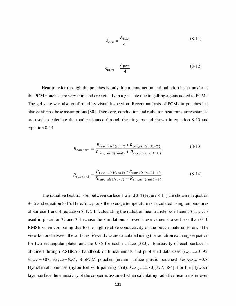
139
𝜆𝑐𝑎𝑣 = 𝐴𝑐𝑎𝑣𝐴 (8-11)
𝜆𝑝𝑐𝑚 = 𝐴𝑝𝑐𝑚𝐴 (8-12)
Heat transfer through the pouches is only due to conduction and radiation heat transfer as
the PCM pouches are very thin, and are actually in a gel state due to gelling agents added to PCMs.
The gel state was also confirmed by visual inspection. Recent analysis of PCMs in pouches has
also confirms these assumptions [80]. Therefore, conduction and radiation heat transfer resistances
are used to calculate the total resistance through the air gaps and shown in equation 8-13 and
equation 8-14.
𝑅𝑐𝑎𝑣,𝑎𝑖𝑟1 = 𝑅𝑐𝑎𝑣, 𝑎𝑖𝑟1(𝑐𝑜𝑛𝑑) ∗ 𝑅𝑐𝑎𝑣,𝑎𝑖𝑟 (𝑟𝑎𝑑1−2 )𝑅𝑐𝑎𝑣, 𝑎𝑖𝑟1(𝑐𝑜𝑛𝑑) + 𝑅𝑐𝑎𝑣,𝑎𝑖𝑟 (𝑟𝑎𝑑1−2 ) (8-13)
𝑅𝑐𝑎𝑣,𝑎𝑖𝑟2 = 𝑅𝑐𝑎𝑣, 𝑎𝑖𝑟1(𝑐𝑜𝑛𝑑) ∗ 𝑅𝑐𝑎𝑣,𝑎𝑖𝑟 (𝑟𝑎𝑑 3−4 )𝑅𝑐𝑎𝑣, 𝑎𝑖𝑟1(𝑐𝑜𝑛𝑑) + 𝑅𝑐𝑎𝑣,𝑎𝑖𝑟 (𝑟𝑎𝑑 3−4 ) (8-14)
The radiative heat transfer between surface 1-2 and 3-4 (Figure 8-11) are shown in equation
8-15 and equation 8-16. Here, Tave (1, 4) is the average temperature is calculated using temperatures
of surface 1 and 4 (equation 8-17). In calculating the radiation heat transfer coefficient Tave (1, 4) is
used in place for T2 and T3 because the simulations showed these values showed less than 0.10
RMSE when comparing due to the high relative conductivity of the pouch material to air. The
view factors between the surfaces, F12 and F34 are calculated using the radiation exchange equation
for two rectangular plates and are 0.85 for each surface [383]. Emissivity of each surface is
obtained through ASHRAE handbook of fundamentals and published databases (Ԑplywood=0.95,
Ԑcopper=0.07, Ԑdrywall=0.85, BioPCM pouches (cream surface plastic pouches) ԐBioPCM,pm =0.8,
Hydrate salt pouches (nylon foil with painting coat): Ԑsalts,pm=0.80)[377, 384]. For the plywood
layer surface the emissivity of the copper is assumed when calculating radiative heat transfer even
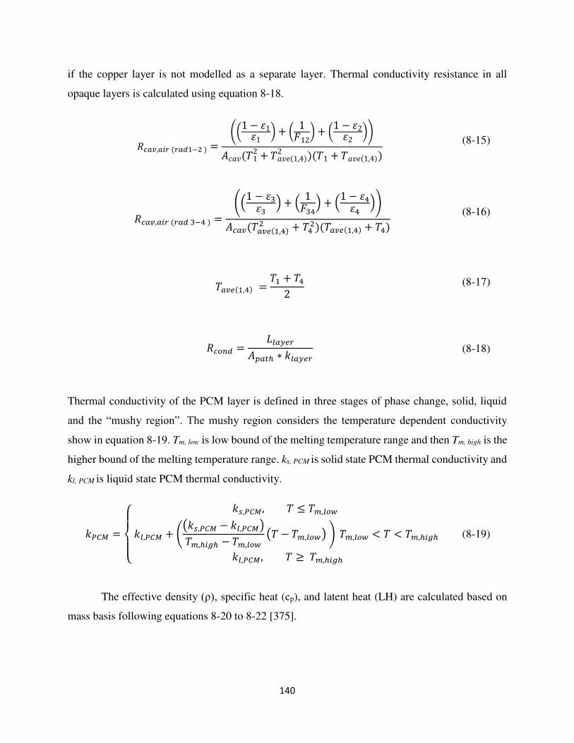
140
if the copper layer is not modelled as a separate layer. Thermal conductivity resistance in all
opaque layers is calculated using equation 8-18.
𝑅𝑐𝑎𝑣,𝑎𝑖𝑟 (𝑟𝑎𝑑1−2 ) = ((1 − 𝜀1𝜀1 )+ ( 1𝐹12)+ (1 − 𝜀2𝜀2 ))𝐴𝑐𝑎𝑣(𝑇12 + 𝑇𝑎𝑣𝑒(1,4)2 )(𝑇1 + 𝑇𝑎𝑣𝑒(1,4)) (8-15)
𝑅𝑐𝑎𝑣,𝑎𝑖𝑟 (𝑟𝑎𝑑 3−4 ) = ((1 − 𝜀3𝜀3 ) + ( 1𝐹34) + (1 − 𝜀4𝜀4 ))𝐴𝑐𝑎𝑣(𝑇𝑎𝑣𝑒(1,4)2 + 𝑇42)(𝑇𝑎𝑣𝑒(1,4) + 𝑇4) (8-16)
𝑇𝑎𝑣𝑒(1,4) = 𝑇1 + 𝑇42 (8-17)
𝑅𝑐𝑜𝑛𝑑 = 𝐿𝑙𝑎𝑦𝑒𝑟𝐴𝑝𝑎𝑡ℎ ∗ 𝑘𝑙𝑎𝑦𝑒𝑟 (8-18)
Thermal conductivity of the PCM layer is defined in three stages of phase change, solid, liquid
and the “mushy region”. The mushy region considers the temperature dependent conductivity
show in equation 8-19. Tm, low is low bound of the melting temperature range and then Tm, high is the
higher bound of the melting temperature range. ks, PCM is solid state PCM thermal conductivity and
kl, PCM is liquid state PCM thermal conductivity.
𝑘𝑃𝐶𝑀 = { 𝑘𝑠,𝑃𝐶𝑀, 𝑇 ≤ 𝑇𝑚,𝑙𝑜𝑤 𝑘𝑙,𝑃𝐶𝑀 + ((𝑘𝑠,𝑃𝐶𝑀 − 𝑘𝑙,𝑃𝐶𝑀)𝑇𝑚,ℎ𝑖𝑔ℎ − 𝑇𝑚,𝑙𝑜𝑤 (𝑇 − 𝑇𝑚,𝑙𝑜𝑤) ) 𝑇𝑚,𝑙𝑜𝑤 < 𝑇 < 𝑇𝑚,ℎ𝑖𝑔ℎ 𝑘𝑙,𝑃𝐶𝑀, 𝑇 ≥ 𝑇𝑚,ℎ𝑖𝑔ℎ (8-19)
The effective density (ρ), specific heat (cp), and latent heat (LH) are calculated based on
mass basis following equations 8-20 to 8-22 [375].
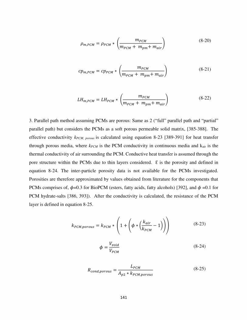
141
𝜌𝑚,𝑃𝐶𝑀 = 𝜌𝑃𝐶𝑀 ∗ ( 𝑚𝑃𝐶𝑀𝑚𝑃𝐶𝑀 + 𝑚𝑝𝑚+ 𝑚𝑎𝑖𝑟) (8-20)
𝑐𝑝𝑚,𝑃𝐶𝑀 = 𝑐𝑝𝑃𝐶𝑀 ∗ ( 𝑚𝑃𝐶𝑀𝑚𝑃𝐶𝑀 + 𝑚𝑝𝑚+ 𝑚𝑎𝑖𝑟) (8-21)
𝐿𝐻𝑚,𝑃𝐶𝑀 = 𝐿𝐻𝑃𝐶𝑀 ∗ ( 𝑚𝑃𝐶𝑀𝑚𝑃𝐶𝑀 + 𝑚𝑝𝑚+ 𝑚𝑎𝑖𝑟) (8-22)
3. Parallel path method assuming PCMs are porous: Same as 2 (“full” parallel path and “partial”
parallel path) but considers the PCMs as a soft porous permeable solid matrix, [385-388]. The
effective conductivity kPCM, porous is calculated using equation 8-23 [389-391] for heat transfer
through porous media, where kPCM is the PCM conductivity in continuous media and kair is the
thermal conductivity of air surrounding the PCM. Conductive heat transfer is assumed through the
pore structure within the PCMs due to thin layers considered. Ԑ is the porosity and defined in
equation 8-24. The inter-particle porosity data is not available for the PCMs investigated.
Porosities are therefore approximated by values obtained from literature for the components that
PCMs comprises of, 𝜙=0.3 for BioPCM (esters, fatty acids, fatty alcohols) [392], and 𝜙 =0.1 for
PCM hydrate-salts [386, 393]). After the conductivity is calculated, the resistance of the PCM
layer is defined in equation 8-25.
𝑘𝑃𝐶𝑀,𝑝𝑜𝑟𝑜𝑢𝑠 = 𝑘𝑃𝐶𝑀 ∗ (1 + (𝜙 ∗ ( 𝑘𝑎𝑖𝑟𝑘𝑃𝐶𝑀 − 1))) (8-23)
𝜙 = 𝑉𝑣𝑜𝑖𝑑𝑉𝑃𝐶𝑀 (8-24)
𝑅𝑐𝑜𝑛𝑑,𝑝𝑜𝑟𝑜𝑢𝑠 = 𝐿𝑃𝐶𝑀𝐴𝑝2 ∗ 𝑘𝑃𝐶𝑀,𝑝𝑜𝑟𝑜𝑢𝑠 (8-25)
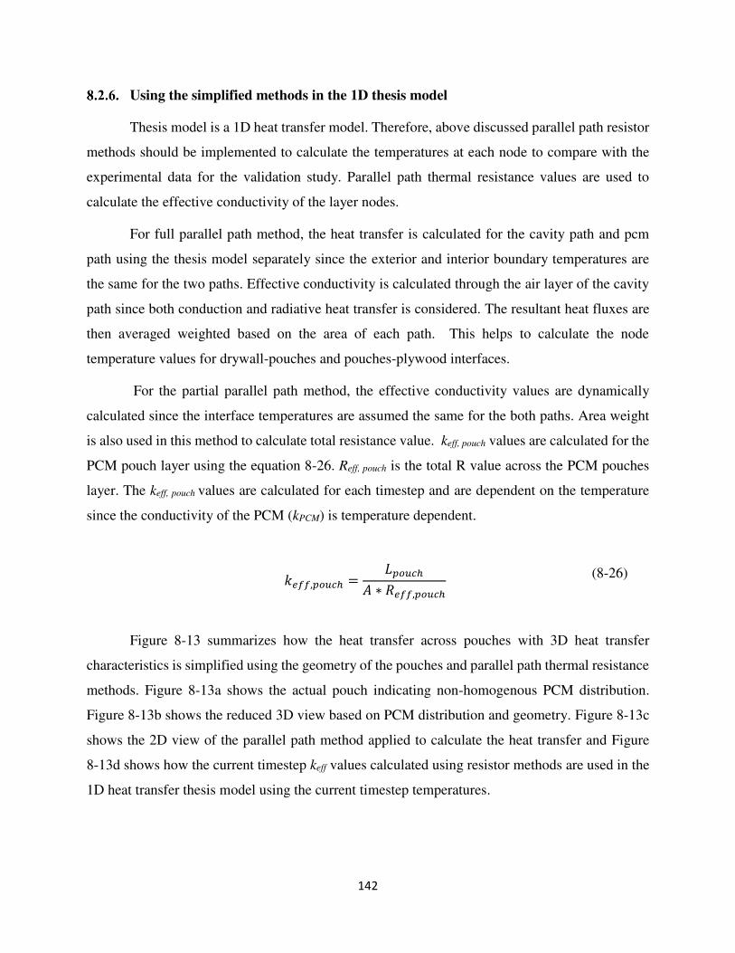
142
Using the simplified methods in the 1D thesis model
Thesis model is a 1D heat transfer model. Therefore, above discussed parallel path resistor
methods should be implemented to calculate the temperatures at each node to compare with the
experimental data for the validation study. Parallel path thermal resistance values are used to
calculate the effective conductivity of the layer nodes.
For full parallel path method, the heat transfer is calculated for the cavity path and pcm
path using the thesis model separately since the exterior and interior boundary temperatures are
the same for the two paths. Effective conductivity is calculated through the air layer of the cavity
path since both conduction and radiative heat transfer is considered. The resultant heat fluxes are
then averaged weighted based on the area of each path. This helps to calculate the node
temperature values for drywall-pouches and pouches-plywood interfaces.
For the partial parallel path method, the effective conductivity values are dynamically
calculated since the interface temperatures are assumed the same for the both paths. Area weight
is also used in this method to calculate total resistance value. keff, pouch values are calculated for the
PCM pouch layer using the equation 8-26. Reff, pouch is the total R value across the PCM pouches
layer. The keff, pouch values are calculated for each timestep and are dependent on the temperature
since the conductivity of the PCM (kPCM) is temperature dependent.
𝑘𝑒𝑓𝑓,𝑝𝑜𝑢𝑐ℎ = 𝐿𝑝𝑜𝑢𝑐ℎ𝐴 ∗ 𝑅𝑒𝑓𝑓,𝑝𝑜𝑢𝑐ℎ (8-26)
Figure 8-13 summarizes how the heat transfer across pouches with 3D heat transfer
characteristics is simplified using the geometry of the pouches and parallel path thermal resistance
methods. Figure 8-13a shows the actual pouch indicating non-homogenous PCM distribution.
Figure 8-13b shows the reduced 3D view based on PCM distribution and geometry. Figure 8-13c
shows the 2D view of the parallel path method applied to calculate the heat transfer and Figure
8-13d shows how the current timestep keff values calculated using resistor methods are used in the
1D heat transfer thesis model using the current timestep temperatures.
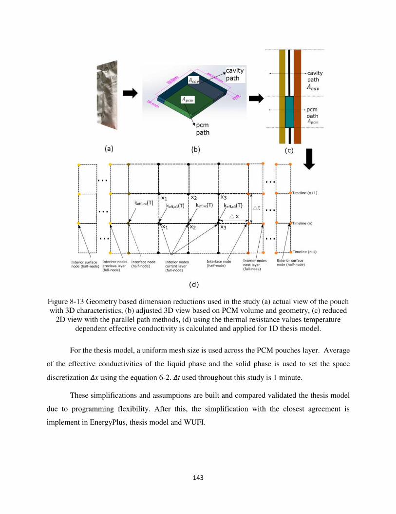
143
Figure 8-13 Geometry based dimension reductions used in the study (a) actual view of the pouch with 3D characteristics, (b) adjusted 3D view based on PCM volume and geometry, (c) reduced
2D view with the parallel path methods, (d) using the thermal resistance values temperature dependent effective conductivity is calculated and applied for 1D thesis model.
For the thesis model, a uniform mesh size is used across the PCM pouches layer. Average
of the effective conductivities of the liquid phase and the solid phase is used to set the space
discretization Δx using the equation 6-2. Δt used throughout this study is 1 minute.
These simplifications and assumptions are built and compared validated the thesis model
due to programming flexibility. After this, the simplification with the closest agreement is
implement in EnergyPlus, thesis model and WUFI.
144
PCM models used in Building energy and hygrothermal software
This study compares PCM models from EnergyPlus (2 modules), and WUFI in addition to
a customized validated PCM model in thesis model previously validated with analytical and
empirical data. A detailed description and comparison between these models is described in a
recent study [335]. The comparison of the different heat transfer methods and validation study of
EnergyPlus, thesis model and WUFI are conducted without hysteresis data. Hysteresis data of
PCMs are used in the final section of the study to compare the simulations of EnergyPlus and
thesis model with and without hysteresis.
Validation
ASHRAE standard 140 defines three main approaches for V&V: (1) analytical verification,
(2) empirical validation, and (3) comparative testing [394]. Verification and validation (V&V) are
important steps in numerical model development to ensure desired performance and accuracy
[233]. Tabares et al. discusses an approach to validate PCM models with experimental data. The
empirical validation of the PCM modeling software has not been done for PCM pouches using the
system scale implementation.
RMSE, NMBE and CV (RMSE) are recommended for error evaluation of energy, heat-
flux and temperature [317]. This study uses graphical comparison, Root Mean Square Error
(RMSE), Coefficient of Variation of the Root Mean Square Error (CV (RMSE)), and Normalized
Mean Biased Error (NMBE) as the indices to validate the models and are used together in several
recent studies [320, 395]. The recommended ranges of (NMBE) and (CV (RMSE)) are ± 10%
and 30% according to the ASHRAE guideline14.
The thesis tolerances considered are NMBE of ± 5% and CV(RMSE) of ± 15%. These
measures are calculated using equations 8-27 to 8-29. Here, 𝑦𝑖 represents measured values and �̂�𝑖 represents simulated values. N is number of data points. 𝑦𝑚̅̅ ̅̅ is the mean of the measured values.
𝑅𝑀𝑆𝐸 = √ ∑ (𝑦𝑖 − �̂�𝑖)2𝑁𝑖=1 𝑁 (8-27)
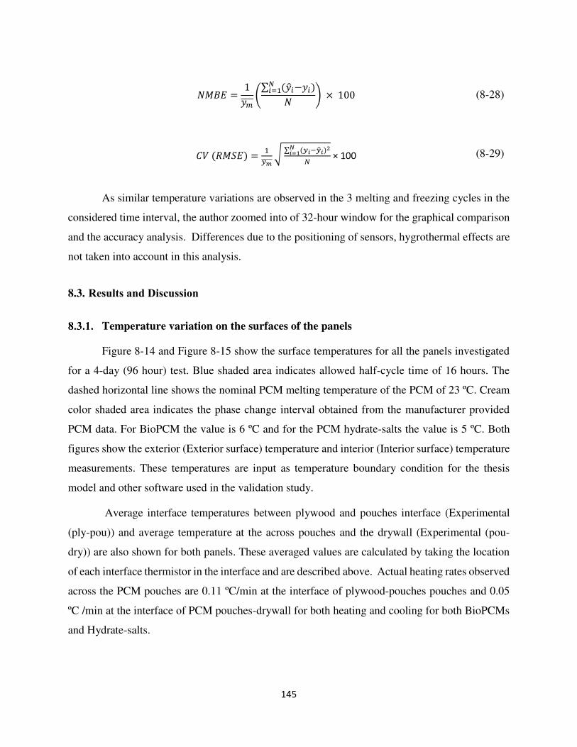
145
𝑁𝑀𝐵𝐸 = 1𝑦𝑚̅̅ ̅̅ (∑ (�̂�𝑖−𝑦𝑖)𝑁𝑖=1 𝑁 ) × 100 (8-28)
𝐶𝑉 (𝑅𝑀𝑆𝐸) = 1𝑦𝑚̅̅ ̅̅̅√ ∑ (𝑦𝑖−�̂�𝑖)2𝑁𝑖=1 𝑁 × 100 (8-29)
As similar temperature variations are observed in the 3 melting and freezing cycles in the
considered time interval, the author zoomed into of 32-hour window for the graphical comparison
and the accuracy analysis. Differences due to the positioning of sensors, hygrothermal effects are
not taken into account in this analysis.
8.3. Results and Discussion
Temperature variation on the surfaces of the panels
Figure 8-14 and Figure 8-15 show the surface temperatures for all the panels investigated
for a 4-day (96 hour) test. Blue shaded area indicates allowed half-cycle time of 16 hours. The
dashed horizontal line shows the nominal PCM melting temperature of the PCM of 23 ºC. Cream
color shaded area indicates the phase change interval obtained from the manufacturer provided
PCM data. For BioPCM the value is 6 ºC and for the PCM hydrate-salts the value is 5 ºC. Both
figures show the exterior (Exterior surface) temperature and interior (Interior surface) temperature
measurements. These temperatures are input as temperature boundary condition for the thesis
model and other software used in the validation study.
Average interface temperatures between plywood and pouches interface (Experimental
(ply-pou)) and average temperature at the across pouches and the drywall (Experimental (pou-
dry)) are also shown for both panels. These averaged values are calculated by taking the location
of each interface thermistor in the interface and are described above. Actual heating rates observed
across the PCM pouches are 0.11 ºC/min at the interface of plywood-pouches pouches and 0.05
ºC /min at the interface of PCM pouches-drywall for both heating and cooling for both BioPCMs
and Hydrate-salts.
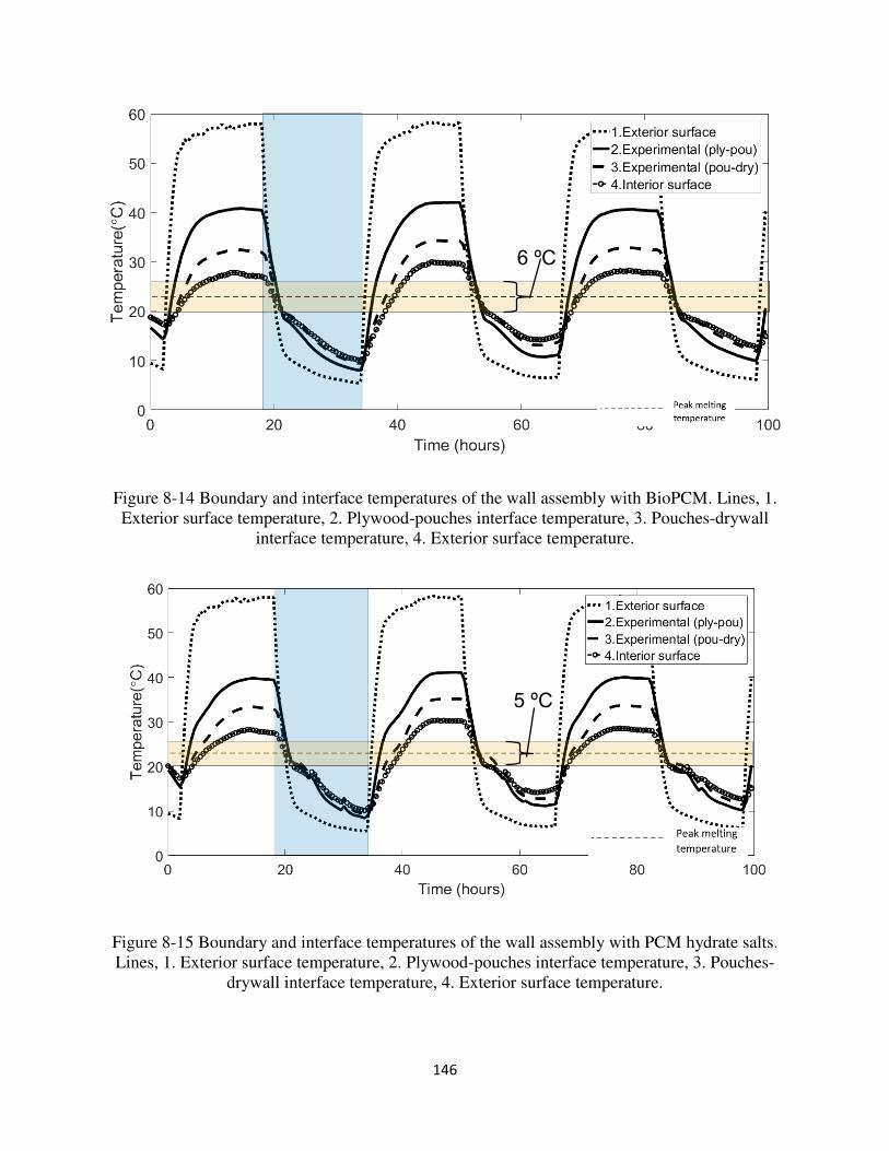
146
Figure 8-14 Boundary and interface temperatures of the wall assembly with BioPCM. Lines, 1. Exterior surface temperature, 2. Plywood-pouches interface temperature, 3. Pouches-drywall
interface temperature, 4. Exterior surface temperature.
Figure 8-15 Boundary and interface temperatures of the wall assembly with PCM hydrate salts. Lines, 1. Exterior surface temperature, 2. Plywood-pouches interface temperature, 3. Pouches-
drywall interface temperature, 4. Exterior surface temperature.
6 ºC
5 ºC
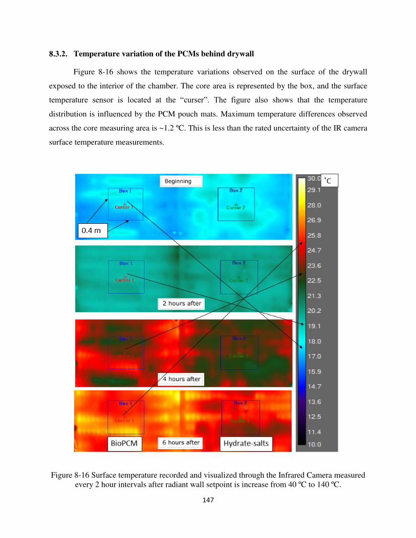
147
Temperature variation of the PCMs behind drywall
Figure 8-16 shows the temperature variations observed on the surface of the drywall
exposed to the interior of the chamber. The core area is represented by the box, and the surface
temperature sensor is located at the “curser”. The figure also shows that the temperature
distribution is influenced by the PCM pouch mats. Maximum temperature differences observed
across the core measuring area is ~1.2 ºC. This is less than the rated uncertainty of the IR camera
surface temperature measurements.
Figure 8-16 Surface temperature recorded and visualized through the Infrared Camera measured every 2 hour intervals after radiant wall setpoint is increase from 40 ºC to 140 ºC.
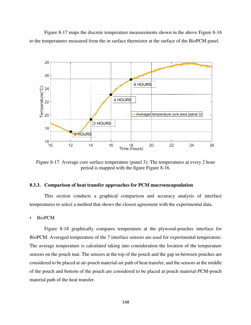
148
Figure 8-17 maps the discrete temperature measurements shown in the above Figure 8-16
to the temperatures measured from the in surface thermistor at the surface of the BioPCM panel.
Figure 8-17 Average core surface temperature (panel 3): The temperatures at every 2 hour period is mapped with the figure Figure 8-16.
Comparison of heat transfer approaches for PCM macroencapsulation
This section conducts a graphical comparison and accuracy analysis of interface
temperatures to select a method that shows the closest agreement with the experimental data.
• BioPCM
Figure 8-18 graphically compares temperature at the plywood-pouches interface for
BioPCM. Averaged temperature of the 7 interface sensors are used for experimental temperature.
The average temperature is calculated taking into consideration the location of the temperature
sensors on the pouch mat. The sensors at the top of the pouch and the gap in-between pouches are
considered to be placed at air-pouch material-air path of heat transfer, and the sensors at the middle
of the pouch and bottom of the pouch are considered to be placed at pouch material-PCM-pouch
material path of the heat transfer.
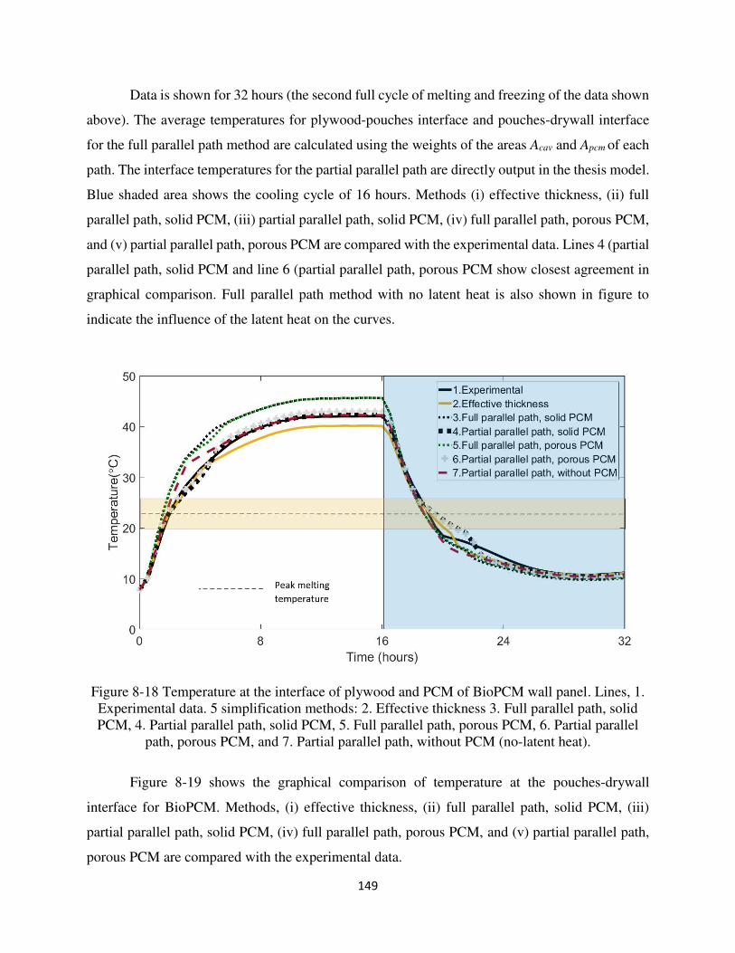
149
Data is shown for 32 hours (the second full cycle of melting and freezing of the data shown
above). The average temperatures for plywood-pouches interface and pouches-drywall interface
for the full parallel path method are calculated using the weights of the areas Acav and Apcm of each
path. The interface temperatures for the partial parallel path are directly output in the thesis model.
Blue shaded area shows the cooling cycle of 16 hours. Methods (i) effective thickness, (ii) full
parallel path, solid PCM, (iii) partial parallel path, solid PCM, (iv) full parallel path, porous PCM,
and (v) partial parallel path, porous PCM are compared with the experimental data. Lines 4 (partial
parallel path, solid PCM and line 6 (partial parallel path, porous PCM show closest agreement in
graphical comparison. Full parallel path method with no latent heat is also shown in figure to
indicate the influence of the latent heat on the curves.
Figure 8-18 Temperature at the interface of plywood and PCM of BioPCM wall panel. Lines, 1. Experimental data. 5 simplification methods: 2. Effective thickness 3. Full parallel path, solid PCM, 4. Partial parallel path, solid PCM, 5. Full parallel path, porous PCM, 6. Partial parallel
path, porous PCM, and 7. Partial parallel path, without PCM (no-latent heat).
Figure 8-19 shows the graphical comparison of temperature at the pouches-drywall
interface for BioPCM. Methods, (i) effective thickness, (ii) full parallel path, solid PCM, (iii)
partial parallel path, solid PCM, (iv) full parallel path, porous PCM, and (v) partial parallel path,
porous PCM are compared with the experimental data.
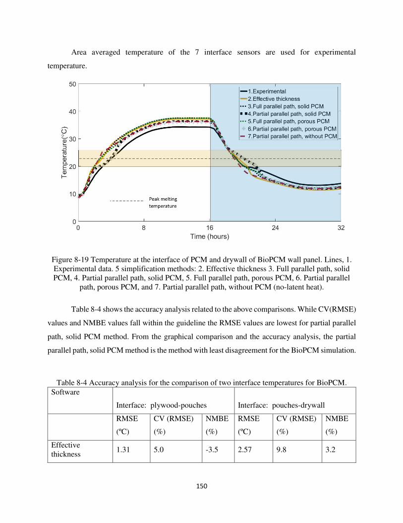
150
Area averaged temperature of the 7 interface sensors are used for experimental
temperature.
Figure 8-19 Temperature at the interface of PCM and drywall of BioPCM wall panel. Lines, 1. Experimental data. 5 simplification methods: 2. Effective thickness 3. Full parallel path, solid PCM, 4. Partial parallel path, solid PCM, 5. Full parallel path, porous PCM, 6. Partial parallel
path, porous PCM, and 7. Partial parallel path, without PCM (no-latent heat).
Table 8-4 shows the accuracy analysis related to the above comparisons. While CV(RMSE)
values and NMBE values fall within the guideline the RMSE values are lowest for partial parallel
path, solid PCM method. From the graphical comparison and the accuracy analysis, the partial
parallel path, solid PCM method is the method with least disagreement for the BioPCM simulation.
Table 8-4 Accuracy analysis for the comparison of two interface temperatures for BioPCM. Software
Interface: plywood-pouches
Interface: pouches-drywall
RMSE
(ºC)
CV (RMSE)
(%)
NMBE
(%)
RMSE
(ºC)
CV (RMSE)
(%)
NMBE
(%)
Effective thickness
1.31 5.0 -3.5 2.57 9.8 3.2
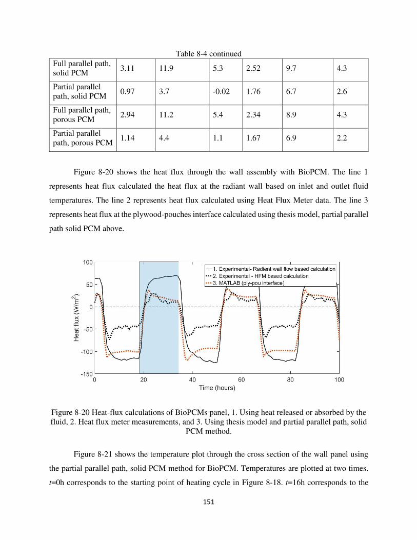
151
Table 8-4 continued Full parallel path, solid PCM
3.11 11.9 5.3 2.52 9.7 4.3
Partial parallel path, solid PCM
0.97 3.7 -0.02 1.76 6.7 2.6
Full parallel path, porous PCM
2.94 11.2 5.4 2.34 8.9 4.3
Partial parallel path, porous PCM
1.14 4.4 1.1 1.67 6.9 2.2
Figure 8-20 shows the heat flux through the wall assembly with BioPCM. The line 1
represents heat flux calculated the heat flux at the radiant wall based on inlet and outlet fluid
temperatures. The line 2 represents heat flux calculated using Heat Flux Meter data. The line 3
represents heat flux at the plywood-pouches interface calculated using thesis model, partial parallel
path solid PCM above.
Figure 8-20 Heat-flux calculations of BioPCMs panel, 1. Using heat released or absorbed by the fluid, 2. Heat flux meter measurements, and 3. Using thesis model and partial parallel path, solid
PCM method.
Figure 8-21 shows the temperature plot through the cross section of the wall panel using
the partial parallel path, solid PCM method for BioPCM. Temperatures are plotted at two times.
t=0h corresponds to the starting point of heating cycle in Figure 8-18. t=16h corresponds to the
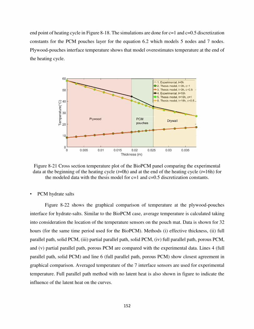
152
end point of heating cycle in Figure 8-18. The simulations are done for c=1 and c=0.5 discretization
constants for the PCM pouches layer for the equation 6.2 which models 5 nodes and 7 nodes.
Plywood-pouches interface temperature shows that model overestimates temperature at the end of
the heating cycle.
Figure 8-21 Cross section temperature plot of the BioPCM panel comparing the experimental data at the beginning of the heating cycle (t=0h) and at the end of the heating cycle (t=16h) for
the modeled data with the thesis model for c=1 and c=0.5 discretization constants.
• PCM hydrate salts
Figure 8-22 shows the graphical comparison of temperature at the plywood-pouches
interface for hydrate-salts. Similar to the BioPCM case, average temperature is calculated taking
into consideration the location of the temperature sensors on the pouch mat. Data is shown for 32
hours (for the same time period used for the BioPCM). Methods (i) effective thickness, (ii) full
parallel path, solid PCM, (iii) partial parallel path, solid PCM, (iv) full parallel path, porous PCM,
and (v) partial parallel path, porous PCM are compared with the experimental data. Lines 4 (full
parallel path, solid PCM) and line 6 (full parallel path, porous PCM) show closest agreement in
graphical comparison. Averaged temperature of the 7 interface sensors are used for experimental
temperature. Full parallel path method with no latent heat is also shown in figure to indicate the
influence of the latent heat on the curves.
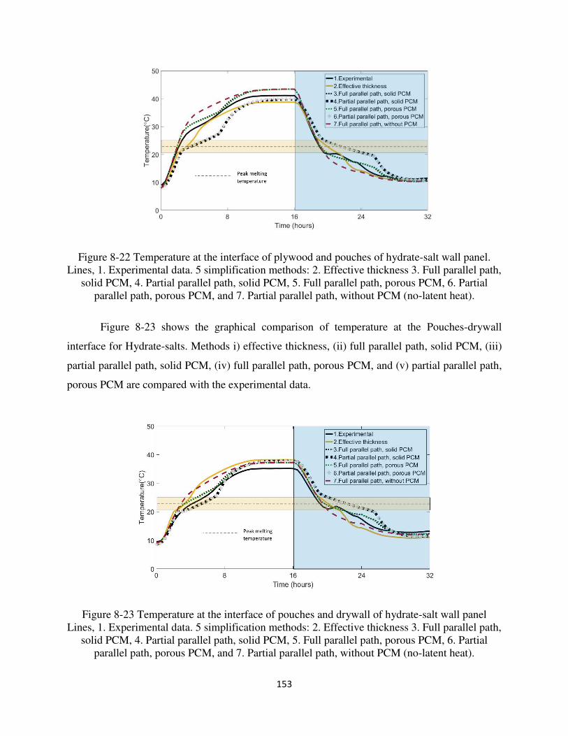
153
Figure 8-22 Temperature at the interface of plywood and pouches of hydrate-salt wall panel. Lines, 1. Experimental data. 5 simplification methods: 2. Effective thickness 3. Full parallel path,
solid PCM, 4. Partial parallel path, solid PCM, 5. Full parallel path, porous PCM, 6. Partial parallel path, porous PCM, and 7. Partial parallel path, without PCM (no-latent heat).
Figure 8-23 shows the graphical comparison of temperature at the Pouches-drywall
interface for Hydrate-salts. Methods i) effective thickness, (ii) full parallel path, solid PCM, (iii)
partial parallel path, solid PCM, (iv) full parallel path, porous PCM, and (v) partial parallel path,
porous PCM are compared with the experimental data.
Figure 8-23 Temperature at the interface of pouches and drywall of hydrate-salt wall panel Lines, 1. Experimental data. 5 simplification methods: 2. Effective thickness 3. Full parallel path,
solid PCM, 4. Partial parallel path, solid PCM, 5. Full parallel path, porous PCM, 6. Partial parallel path, porous PCM, and 7. Partial parallel path, without PCM (no-latent heat).
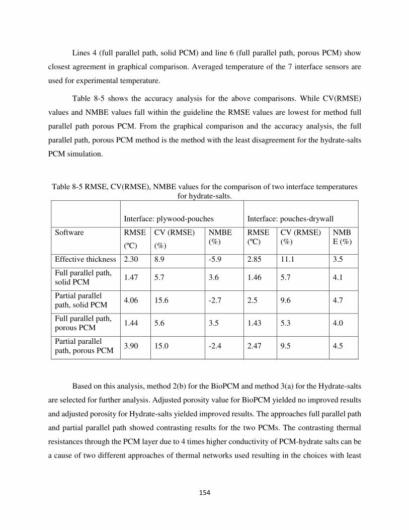
154
Lines 4 (full parallel path, solid PCM) and line 6 (full parallel path, porous PCM) show
closest agreement in graphical comparison. Averaged temperature of the 7 interface sensors are
used for experimental temperature.
Table 8-5 shows the accuracy analysis for the above comparisons. While CV(RMSE)
values and NMBE values fall within the guideline the RMSE values are lowest for method full
parallel path porous PCM. From the graphical comparison and the accuracy analysis, the full
parallel path, porous PCM method is the method with the least disagreement for the hydrate-salts
PCM simulation.
Table 8-5 RMSE, CV(RMSE), NMBE values for the comparison of two interface temperatures for hydrate-salts.
Interface: plywood-pouches
Interface: pouches-drywall
Software RMSE
(ºC)
CV (RMSE)
(%)
NMBE (%)
RMSE (ºC)
CV (RMSE) (%)
NMBE (%)
Effective thickness 2.30 8.9 -5.9 2.85 11.1 3.5
Full parallel path, solid PCM
1.47 5.7 3.6 1.46 5.7 4.1
Partial parallel path, solid PCM
4.06 15.6 -2.7 2.5 9.6 4.7
Full parallel path, porous PCM
1.44 5.6 3.5 1.43 5.3 4.0
Partial parallel path, porous PCM
3.90 15.0 -2.4 2.47 9.5 4.5
Based on this analysis, method 2(b) for the BioPCM and method 3(a) for the Hydrate-salts
are selected for further analysis. Adjusted porosity value for BioPCM yielded no improved results
and adjusted porosity for Hydrate-salts yielded improved results. The approaches full parallel path
and partial parallel path showed contrasting results for the two PCMs. The contrasting thermal
resistances through the PCM layer due to 4 times higher conductivity of PCM-hydrate salts can be
a cause of two different approaches of thermal networks used resulting in the choices with least
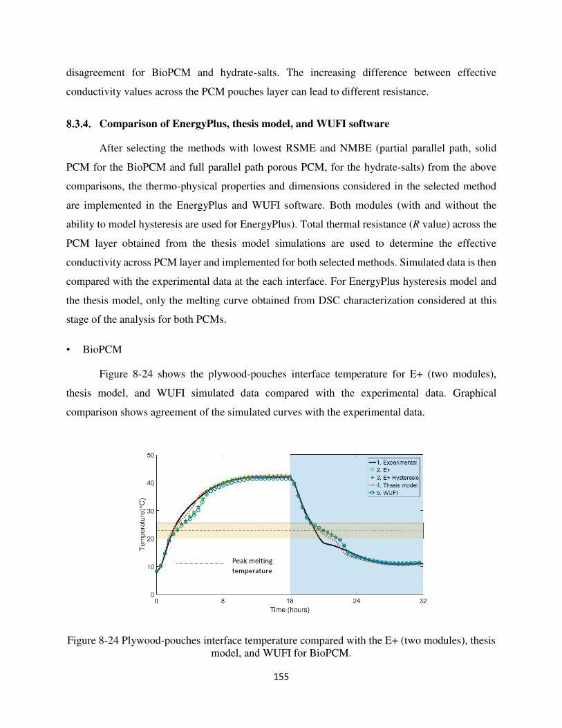
155
disagreement for BioPCM and hydrate-salts. The increasing difference between effective
conductivity values across the PCM pouches layer can lead to different resistance.
Comparison of EnergyPlus, thesis model, and WUFI software
After selecting the methods with lowest RSME and NMBE (partial parallel path, solid
PCM for the BioPCM and full parallel path porous PCM, for the hydrate-salts) from the above
comparisons, the thermo-physical properties and dimensions considered in the selected method
are implemented in the EnergyPlus and WUFI software. Both modules (with and without the
ability to model hysteresis are used for EnergyPlus). Total thermal resistance (R value) across the
PCM layer obtained from the thesis model simulations are used to determine the effective
conductivity across PCM layer and implemented for both selected methods. Simulated data is then
compared with the experimental data at the each interface. For EnergyPlus hysteresis model and
the thesis model, only the melting curve obtained from DSC characterization considered at this
stage of the analysis for both PCMs.
• BioPCM
Figure 8-24 shows the plywood-pouches interface temperature for E+ (two modules),
thesis model, and WUFI simulated data compared with the experimental data. Graphical
comparison shows agreement of the simulated curves with the experimental data.
Figure 8-24 Plywood-pouches interface temperature compared with the E+ (two modules), thesis model, and WUFI for BioPCM.
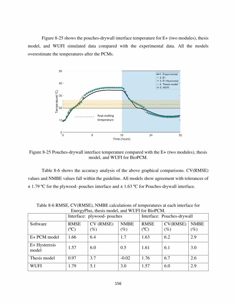
156
Figure 8-25 shows the pouches-drywall interface temperature for E+ (two modules), thesis
model, and WUFI simulated data compared with the experimental data. All the models
overestimate the temperatures after the PCMs.
Figure 8-25 Pouches-drywall interface temperature compared with the E+ (two modules), thesis model, and WUFI for BioPCM.
Table 8-6 shows the accuracy analysis of the above graphical comparisons. CV(RMSE)
values and NMBE values fall within the guideline. All models show agreement with tolerances of
± 1.79 ºC for the plywood- pouches interface and ± 1.63 ºC for Pouches-drywall interface.
Table 8-6 RMSE, CV(RMSE), NMBE calculations of temperatures at each interface for EnergyPlus, thesis model, and WUFI for BioPCM.
Interface: plywood- pouches Interface: Pouches-drywall
Software RMSE (ºC)
CV (RMSE) (%)
NMBE (%)
RMSE (ºC)
CV(RMSE) (%)
NMBE (%)
E+ PCM model 1.66 6.4 1.7 1.63 6.2 2.9
E+ Hysteresis model
1.57 6.0 0.5 1.61 6.1 3.0
Thesis model 0.97 3.7 -0.02 1.76 6.7 2.6
WUFI 1.79 5.1 3.0 1.57 6.0 2.9
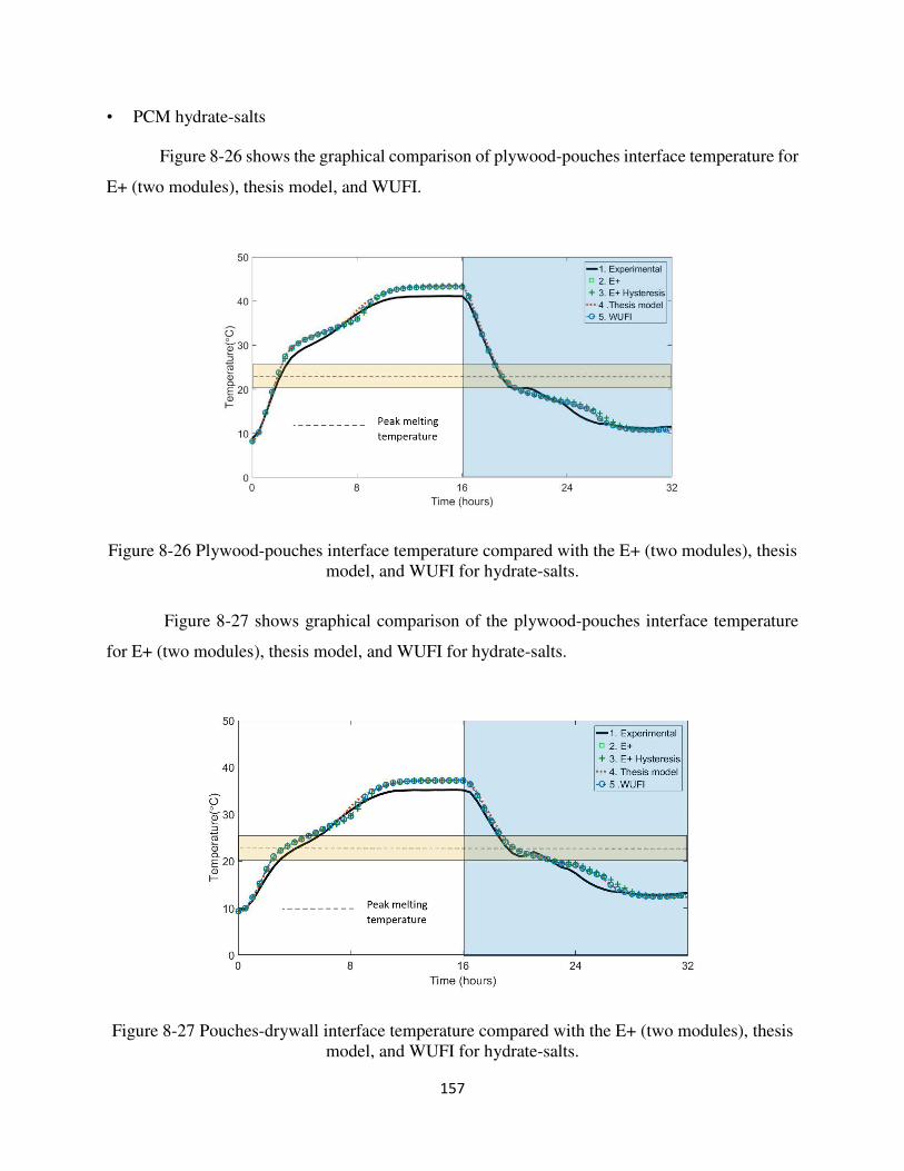
157
• PCM hydrate-salts
Figure 8-26 shows the graphical comparison of plywood-pouches interface temperature for
E+ (two modules), thesis model, and WUFI.
Figure 8-26 Plywood-pouches interface temperature compared with the E+ (two modules), thesis model, and WUFI for hydrate-salts.
Figure 8-27 shows graphical comparison of the plywood-pouches interface temperature
for E+ (two modules), thesis model, and WUFI for hydrate-salts.
Figure 8-27 Pouches-drywall interface temperature compared with the E+ (two modules), thesis model, and WUFI for hydrate-salts.
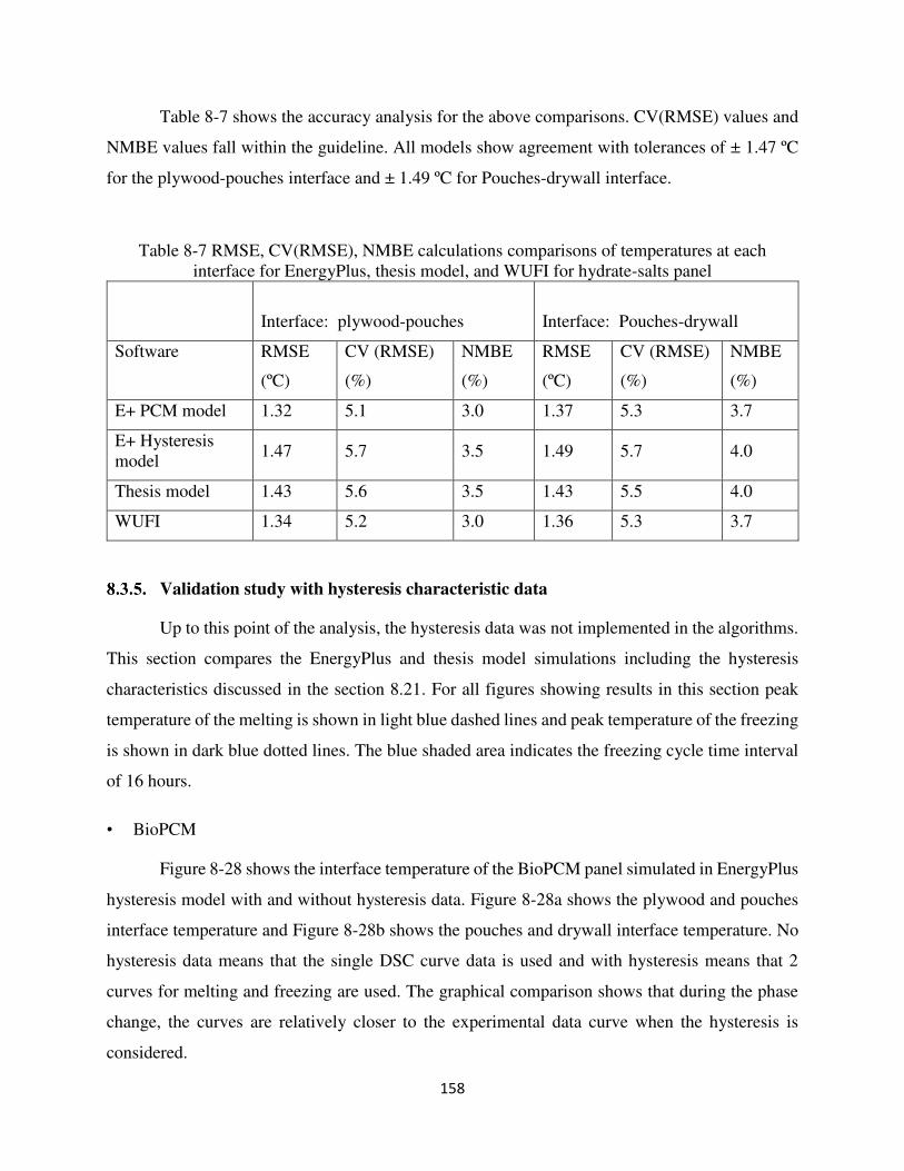
158
Table 8-7 shows the accuracy analysis for the above comparisons. CV(RMSE) values and
NMBE values fall within the guideline. All models show agreement with tolerances of ± 1.47 ºC
for the plywood-pouches interface and ± 1.49 ºC for Pouches-drywall interface.
Table 8-7 RMSE, CV(RMSE), NMBE calculations comparisons of temperatures at each interface for EnergyPlus, thesis model, and WUFI for hydrate-salts panel
Interface: plywood-pouches
Interface: Pouches-drywall
Software RMSE
(ºC)
CV (RMSE)
(%)
NMBE
(%)
RMSE
(ºC)
CV (RMSE)
(%)
NMBE
(%)
E+ PCM model 1.32 5.1 3.0 1.37 5.3 3.7
E+ Hysteresis model
1.47 5.7 3.5 1.49 5.7 4.0
Thesis model 1.43 5.6 3.5 1.43 5.5 4.0
WUFI 1.34 5.2 3.0 1.36 5.3 3.7
Validation study with hysteresis characteristic data
Up to this point of the analysis, the hysteresis data was not implemented in the algorithms.
This section compares the EnergyPlus and thesis model simulations including the hysteresis
characteristics discussed in the section 8.21. For all figures showing results in this section peak
temperature of the melting is shown in light blue dashed lines and peak temperature of the freezing
is shown in dark blue dotted lines. The blue shaded area indicates the freezing cycle time interval
of 16 hours.
• BioPCM
Figure 8-28 shows the interface temperature of the BioPCM panel simulated in EnergyPlus
hysteresis model with and without hysteresis data. Figure 8-28a shows the plywood and pouches
interface temperature and Figure 8-28b shows the pouches and drywall interface temperature. No
hysteresis data means that the single DSC curve data is used and with hysteresis means that 2
curves for melting and freezing are used. The graphical comparison shows that during the phase
change, the curves are relatively closer to the experimental data curve when the hysteresis is
considered.
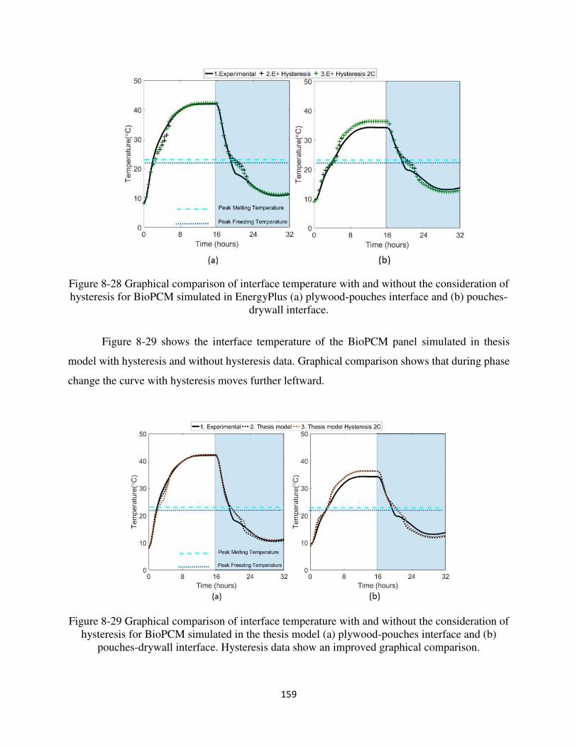
159
Figure 8-28 Graphical comparison of interface temperature with and without the consideration of hysteresis for BioPCM simulated in EnergyPlus (a) plywood-pouches interface and (b) pouches-
drywall interface.
Figure 8-29 shows the interface temperature of the BioPCM panel simulated in thesis
model with hysteresis and without hysteresis data. Graphical comparison shows that during phase
change the curve with hysteresis moves further leftward.
Figure 8-29 Graphical comparison of interface temperature with and without the consideration of hysteresis for BioPCM simulated in the thesis model (a) plywood-pouches interface and (b)
pouches-drywall interface. Hysteresis data show an improved graphical comparison.
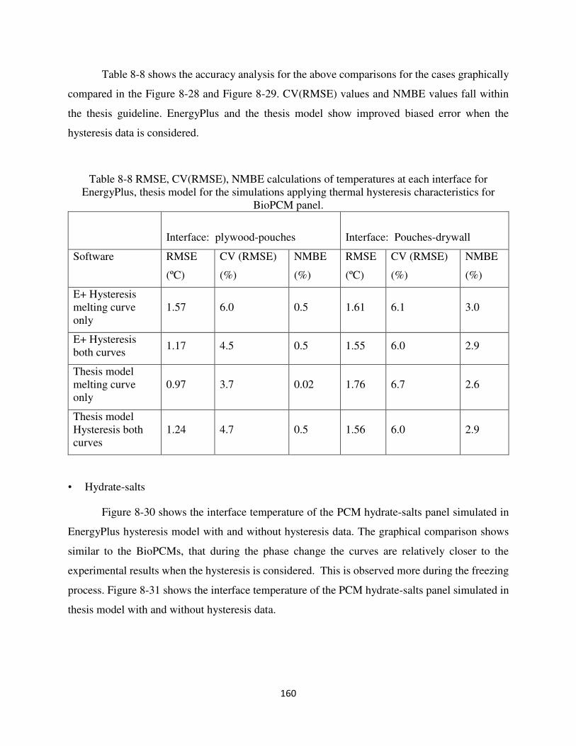
160
Table 8-8 shows the accuracy analysis for the above comparisons for the cases graphically
compared in the Figure 8-28 and Figure 8-29. CV(RMSE) values and NMBE values fall within
the thesis guideline. EnergyPlus and the thesis model show improved biased error when the
hysteresis data is considered.
Table 8-8 RMSE, CV(RMSE), NMBE calculations of temperatures at each interface for EnergyPlus, thesis model for the simulations applying thermal hysteresis characteristics for
BioPCM panel.
Interface: plywood-pouches
Interface: Pouches-drywall
Software RMSE
(ºC)
CV (RMSE)
(%)
NMBE
(%)
RMSE
(ºC)
CV (RMSE)
(%)
NMBE
(%)
E+ Hysteresis melting curve only
1.57 6.0 0.5 1.61 6.1 3.0
E+ Hysteresis both curves
1.17 4.5 0.5 1.55 6.0 2.9
Thesis model melting curve only
0.97 3.7 0.02 1.76 6.7 2.6
Thesis model Hysteresis both curves
1.24 4.7 0.5 1.56 6.0 2.9
• Hydrate-salts
Figure 8-30 shows the interface temperature of the PCM hydrate-salts panel simulated in
EnergyPlus hysteresis model with and without hysteresis data. The graphical comparison shows
similar to the BioPCMs, that during the phase change the curves are relatively closer to the
experimental results when the hysteresis is considered. This is observed more during the freezing
process. Figure 8-31 shows the interface temperature of the PCM hydrate-salts panel simulated in
thesis model with and without hysteresis data.
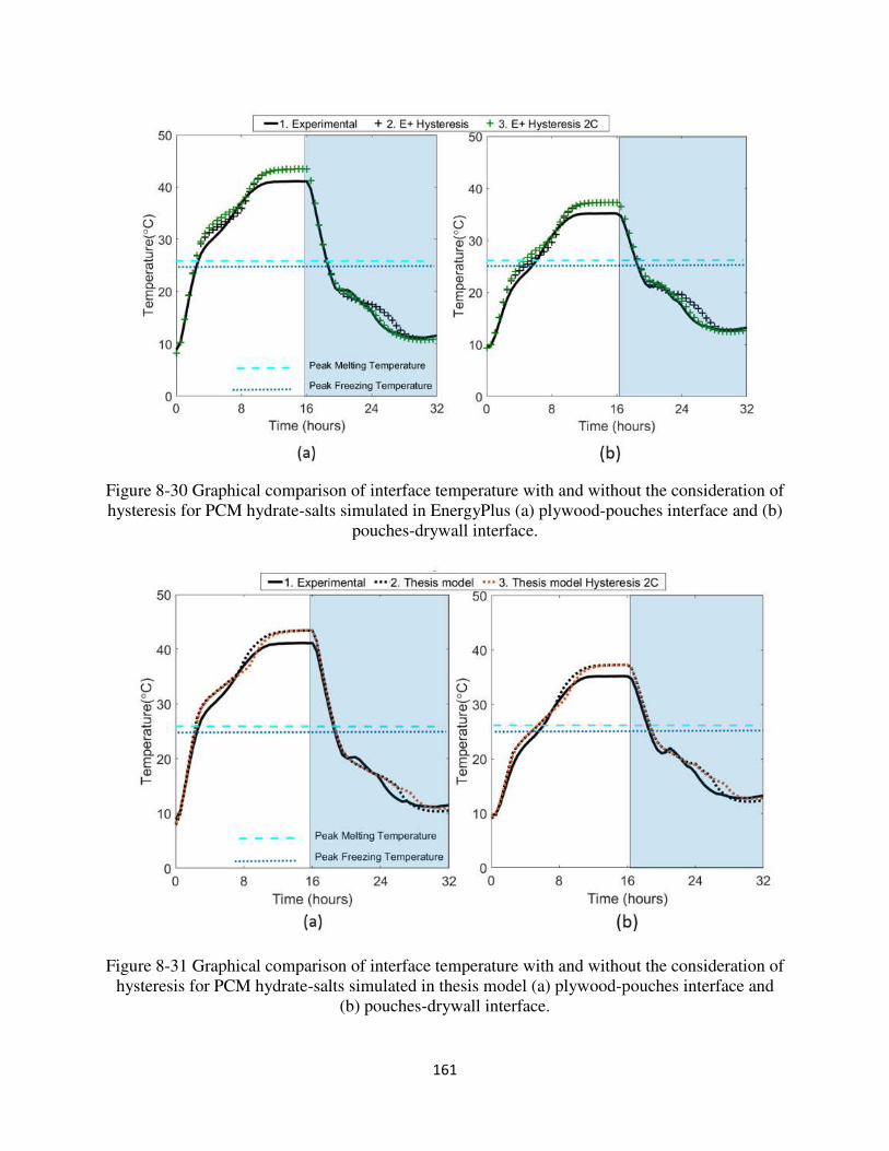
161
Figure 8-30 Graphical comparison of interface temperature with and without the consideration of hysteresis for PCM hydrate-salts simulated in EnergyPlus (a) plywood-pouches interface and (b)
pouches-drywall interface.
Figure 8-31 Graphical comparison of interface temperature with and without the consideration of hysteresis for PCM hydrate-salts simulated in thesis model (a) plywood-pouches interface and
(b) pouches-drywall interface.
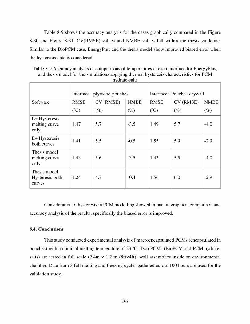
162
Table 8-9 shows the accuracy analysis for the cases graphically compared in the Figure
8-30 and Figure 8-31. CV(RMSE) values and NMBE values fall within the thesis guideline.
Similar to the BioPCM case, EnergyPlus and the thesis model show improved biased error when
the hysteresis data is considered.
Table 8-9 Accuracy analysis of comparisons of temperatures at each interface for EnergyPlus, and thesis model for the simulations applying thermal hysteresis characteristics for PCM
hydrate-salts
Interface: plywood-pouches
Interface: Pouches-drywall
Software RMSE
(ºC)
CV (RMSE)
(%)
NMBE
(%)
RMSE
(ºC)
CV (RMSE)
(%)
NMBE
(%)
E+ Hysteresis melting curve only
1.47 5.7 -3.5 1.49 5.7 -4.0
E+ Hysteresis both curves
1.41 5.5 -0.5 1.55 5.9 -2.9
Thesis model melting curve only
1.43 5.6 -3.5 1.43 5.5 -4.0
Thesis model Hysteresis both curves
1.24 4.7 -0.4 1.56 6.0 -2.9
Consideration of hysteresis in PCM modelling showed impact in graphical comparison and
accuracy analysis of the results, specifically the biased error is improved.
8.4. Conclusions
This study conducted experimental analysis of macroencapsulated PCMs (encapsulated in
pouches) with a nominal melting temperature of 23 ºC. Two PCMs (BioPCM and PCM hydrate-
salts) are tested in full scale (2.4m × 1.2 m (8ft×4ft)) wall assemblies inside an environmental
chamber. Data from 3 full melting and freezing cycles gathered across 100 hours are used for the
validation study.
163
Several heat transfer methods are proposed to simplify 3D heat transfer into a 2D model in
PCM algorithm developed in MATLAB (thesis model) which was previously verified and
validated. These methods capture 2D heat transfer effects due to the presence of different materials,
voids between material interfaces, uneven and lose packaging of the PCMs in pouches. In total, 5
different methods are compared using laboratory data and the methods with lowest disagreement
are implemented in the two wall panels with EnergyPlus (2 PCM modules), and WUFI. The
comparison of the different software shows agreement for temperature comparisons of the both
interfaces for both PCMs with. Temperature tolerances of ± 1.79 ºC for the plywood-pouches
interface and ± 1.63 ºC for Pouches-drywall interface are observed for BioPCM and tolerances of
± 1.47 ºC for the plywood-pouches interface and ± 1.49 ºC for pouches-drywall interface are
observed for the hydrate-salts. Application of hysteresis data showed improvements in the
comparison of EnergyPlus and thesis model simulation results. However, heat flux predictions
showed greater deviation from than surface measurements indicating additional measures must be
taken to implement further instrumentation for reliable heat flux measurements.
In conclusion, EnergyPlus, thesis model, and WUFI software show capability of simulating
the heat transfer across the wall assemblies with macroencapsulated PCMs in pouches with
additional simplifications and assumptions discussed in this research. Engineers and researchers
can adopt the simplification approaches of heat transfer across the PCM pouches (Partial parallel
path, solid PCM for BioPCM pouches and Full parallel path, porous PCM for PCM hydrate-salt
pouches) to improve the heat transfer predictions of building walls of whole building energy
modeling software. These methods can be included in the PCM modeling algorithms with the
modules to enter thermo-physical and dimensions data of the PCM pouches.
164
CHAPTER 9
CONCLUSIONS AND FUTURE WORK
The research conducted in this thesis has been motivated by the need to (i) investigate
optimum PCM properties and application types in building envelopes, (ii) verify and validate PCM
modeling algorithms with experimental data with different PCM encapsulations, (iii) generate
experimental data for validation purposes of different PCM encapsulations, and (iv) develop
accurate numerical algorithms to simulate the heat transfer process associated with phase change
for building envelope applications.
The main tasks of this research has been to (i) conduct a parametric analysis of a residential
building with phase change material (PCM)-enhanced drywall, pre-cooling, and variable electric
rates in a hot and dry climate to investigate potential cost savings and energy savings for the
consumer, (ii) conduct verification and validation of different PCM models available in whole
building energy modeling software like EnergyPlus, ESP-r and WUFI, (iii) design, implement,
and conduct laboratory experiments to test different PCM products and develop data to validate
the PCM modeling algorithms of building energy modeling software.
The research presented in this thesis the author constructed a numerical algorithm in
MATLAB (thesis model) to simulate opaque building envelope with passive PCM applications.
Furthermore, a state of the art environmental chamber is used to construct and implement
experimental apparatus to test the heat transfer across multilayer wall assemblies with
microencapsulated and macroencapsulated PCM.
The following section summarizes the significant results from this research work.
9.1. Summary of significant results
A parametric study of a residential building located in hot-and dry climate was
conducted using a pre-cooling of 5 hours, with different PCM latent heats, melting
temperatures, melting temperature ranges, PCM conductivities, and locations of
application and the author found the optimum PCM applications can shift the
165
cooling electricity demand ~99.9% from the peak time with forced convection
during precooling using high-efficiency fans.
When the Time of Use (ToU) electricity rates are implemented (Arizona Salt River
project), highest cost savings are observed when the PCMs are optimized for all
locations of the envelope (ceiling, exterior opaque walls, and interior partition
walls) under the forced convection mode using high-efficiency fans; the maximum
cost savings observed are 29.4%. Other scenarios yield around 25% savings.
6 PCM modeling algorithms implemented in different building energy and
hygrothermal modeling software (EnergyPlus, ESP-r, and WUFI) and heat transfer
(COMSOL) software, and math thesis model are validated and compared using data
from two independent experimental studies with and shape-stabilized PCM behind
the drywall and Nano-PCM embedded in gypsum wallboards. Based on the
analyzed PCMs, all the evaluated software tools demonstrate their ability to
accurately model shape-stabilized PCM behind drywall. All modeling software
agreed with the Nano-PCM experiments but ESP-r had the lowest convergence due
to less precise definition of boundary conditions. Interestingly, this study showed
no additional gains in accuracy when comparing a 2D heat transfer model with 1D
modeling for Nano-PCM and shape-stabilized PCMs.
An experimental analysis of macroencapsulated PCMs encapsulated in pouches
with a nominal phase change temperature of 23 ºC is conducted. Two PCMs
(BioPCM and PCM hydrate-salts) are tested in full scale: 2.4m × 1.2 m (8ft × 4ft)
wall assemblies in a controlled environment. Five simplification steps are
evaluated using the thesis model to simulate the heat transfer across the PCM
pouches layer. These methods showed improved accuracy.
After the comparison, the methods with closest accuracy agreement are
implemented in E+ (2 PCM modules), thesis model, and WUFI. Temperature
tolerances of ± 1.79 ºC for the plywood-pouches interface and ± 1.63 ºC for
Pouches-drywall interface are observed for BioPCM and tolerances of ± 1.47 ºC
for the plywood-pouches interface and ± 1.49 ºC for pouches-drywall interface are
observed for the hydrate-salts for this validation study.
166
Application of hysteresis data obtained from the manufacturer (for BioPCM) and
Dynamic Heat Flux Meter Apparatus (DHFMA) tests (for hydrate-salts) improved
the bias error of EnergyPlus and thesis model results.
EnergyPlus, thesis model, and WUFI show capability of simulating the heat transfer
across the wall assemblies with pouched macro encapsulated PCMs with additional
simplifications and assumptions discussed in this research.
9.2. Potential for Future Work
Future work of this research falls into two sections: (i) further development of the building
envelope model and (ii) laboratory experiments on different PCMs for validation purposes.
Further development of the building envelope model
Thesis model developed here to evaluate PCMs in building envelope can be
implemented in a whole building energy modeling platform like EnergyPlus to conduct
whole building energy analysis and the simplification methods used can be used in
modelling PCM pouches in future research.
There are several parameters considered in modeling PCM pouches. Dimensions like
thickness of the air layer, PCM volume, thermo-physical properties like variable
conductivity of the PCMs, approximated PCM enthalpy data are a few. Therefore, this
research can be extended to conduct sensitivity analysis of these parameters and how
they influence the accuracy of the model.
This research did not analyze the efficiency of the methods used to evaluate heat
transfer across PCM pouches layer. Therefore, the current model can be made faster
solving and more robust by
Laboratory experiments of different PCMs
Macroencapsulated PCM products vary with the material type, pouch sizes, pouch
material. There are products with increased PCM mass (2x mass BioPCM inside
pouches), increased conductivity (3x conductivity BioPCM). Therefore, the current
167
facility will be used to test these PCMs in parallel and create data for validation
purposes.
Full scale apparatus discussed here can be improved to quick switching of PCM mats.
This would enable the researchers to test multiple PCMs parallel and quickly and create
experimental databases for validation purposes of PCM modelling algorithms.
Hygrothermal effects can also influence the heat transfer across the building envelope
in realistic applications. Using the ability of the chamber to control interior relative
humidity, the experimental hygrothermal analysis of PCM included building envelopes
can be conducted.
168
REFERENCES CITED
1. Yang, L., H. Yan, and J.C. Lam, Thermal comfort and building energy consumption
implications–a review. Applied Energy, 2014. 115: p. 164-173.
2. Hadjipaschalis, I., A. Poullikkas, and V. Efthimiou, Overview of current and future energy
storage technologies for electric power applications. Renewable and sustainable energy reviews, 2009. 13(6-7): p. 1513-1522.
3. Davis, S.J., K. Caldeira, and H.D. Matthews, Future CO2 emissions and climate change
from existing energy infrastructure. Science, 2010. 329(5997): p. 1330-1333.
4. Sbci, U., Buildings and climate change: Summary for decision-makers. United Nations Environmental Programme, Sustainable Buildings and Climate Initiative, Paris, 2009: p. 1-62.
5. Deru, M., et al., US Department of Energy commercial reference building models of the
national building stock. 2011.
6. Bahaj, A. and P. James, Urban energy generation: the added value of photovoltaics in
social housing. Renewable and Sustainable Energy Reviews, 2007. 11(9): p. 2121-2136.
7. Tabares-Velasco, P.C., et al., A modeling framework for optimization-based control of a
residential building thermostat for time-of-use pricing. Applied Energy, 2019. 242: p. 1346-1357.
8. Tabbone, L., et al. Energy in the city: how residential location is linked to energy
consumption. in BEHAVE Energy Conference. 2014.
9. Aghaei, J. and M.-I. Alizadeh, Demand response in smart electricity grids equipped with
renewable energy sources: A review. Renewable and Sustainable Energy Reviews, 2013. 18: p. 64-72.
10. Sun, Y., et al., Peak load shifting control using different cold thermal energy storage
facilities in commercial buildings: a review. Energy conversion and management, 2013. 71: p. 101-114.
11. Al-Saadi, S.N. and Z.Q. Zhai, Modeling phase change materials embedded in building
enclosure: A review. Renewable & Sustainable Energy Reviews, 2013. 21: p. 659-673.
12. Wijesuriya, S., M. Brandt, and P.C. Tabares-Velasco, Parametric analysis of a residential
building with phase change material (PCM)-enhanced drywall, precooling, and variable
electric rates in a hot and dry climate. Applied Energy, 2018. 222: p. 497-514.
169
13. Cao, S., State of the art thermal energy storage solutions for high performance buildings. 2010.
14. Biswas, K., et al., Combined experimental and numerical evaluation of a prototype nano-
PCM enhanced wallboard. Applied energy, 2014. 131: p. 517-529.
15. Kośny, J., Short history of PCM applications in building envelopes, in PCM-Enhanced
Building Components. 2015, Springer. p. 21-59.
16. Al-Saadi, S.N. and Z.Q. Zhai, A new validated TRNSYS module for simulating latent heat
storage walls. Energy and Buildings, 2015. 109: p. 274-290.
17. Al-Saadi, S.N. and Z. Zhai, Systematic evaluation of mathematical methods and numerical
schemes for modeling PCM-enhanced building enclosure. Energy and Buildings, 2015. 92: p. 374-388.
18. Tyagi, V., et al., Thermal performance assessment of encapsulated PCM based thermal
management system to reduce peak energy demand in buildings. Energy and Buildings, 2016. 117: p. 44-52.
19. Jeon, J., et al., High thermal performance composite PCMs loading xGnP for application
to building using radiant floor heating system. Solar Energy Materials and Solar Cells, 2012. 101: p. 51-56.
20. Jeong, S.-G., et al., Improvement of the thermal properties of Bio-based PCM using
exfoliated graphite nanoplatelets. Solar Energy Materials and Solar Cells, 2013. 117: p. 87-92.
21. Akbari, A., et al., Quantum mechanical study on the mechanism and kinetics of the cis-to-
trans isomerization of [Pd (C6Cl2F3) I (PH3) 2]. Inorganica Chimica Acta, 2013. 394: p. 423-429.
22. Borreguero, A.M., et al., Improvement of the thermal behaviour of gypsum blocks by the
incorporation of microcapsules containing PCMS obtained by suspension polymerization
with an optimal core/coating mass ratio. Applied Thermal Engineering, 2010. 30(10): p. 1164-1169.
23. Tyagi, V., et al., Development of phase change materials based microencapsulated
technology for buildings: a review. Renewable and sustainable energy reviews, 2011. 15(2): p. 1373-1391.
24. Zhang, Y.P., et al., Application of latent heat thermal energy storage in buildings: State-
of-the-art and outlook. Building and Environment, 2007. 42(6): p. 2197-2209.
25. Zhang, Y., et al., Preparation, thermal performance and application of shape-stabilized
PCM in energy efficient buildings. Energy and Buildings, 2006. 38(10): p. 1262-1269.
170
26. Peippo, K., P. Kauranen, and P. Lund, A multicomponent PCM wall optimized for passive
solar heating. Energy and buildings, 1991. 17(4): p. 259-270.
27. Kuznik, F., et al., A review on phase change materials integrated in building walls. Renewable and Sustainable Energy Reviews, 2011. 15(1): p. 379-391.
28. Zalba, B., et al., Review on thermal energy storage with phase change: materials, heat
transfer analysis and applications. Applied thermal engineering, 2003. 23(3): p. 251-283.
29. Zhou, D., C.-Y. Zhao, and Y. Tian, Review on thermal energy storage with phase change
materials (PCMs) in building applications. Applied energy, 2012. 92: p. 593-605.
30. Su, J.-C. and P.-S. Liu, A novel solid–solid phase change heat storage material with
polyurethane block copolymer structure. Energy Conversion and Management, 2006. 47(18-19): p. 3185-3191.
31. Mehling, H. and L.F. Cabeza, Heat and cold storage with PCM. 2008: Springer.
32. Salunkhe, P.B. and P.S. Shembekar, A review on effect of phase change material
encapsulation on the thermal performance of a system. Renewable and Sustainable Energy Reviews, 2012. 16(8): p. 5603-5616.
33. Fang, G., F. Tang, and L. Cao, Preparation, thermal properties and applications of shape-
stabilized thermal energy storage materials. Renewable and Sustainable Energy Reviews, 2014. 40: p. 237-259.
34. Zhou, G., et al., Thermal analysis of a direct-gain room with shape-stabilized PCM plates. Renewable Energy, 2008. 33(6): p. 1228-1236.
35. Ye, H., et al., The performance evaluation of shape-stabilized phase change materials in
building applications using energy saving index. Applied energy, 2014. 113: p. 1118-1126.
36. Kuznik, F. and J. Virgone, Experimental investigation of wallboard containing phase
change material: Data for validation of numerical modeling. Energy and Buildings, 2009. 41(5): p. 561-570.
37. Giro-Paloma, J., et al., Types, methods, techniques, and applications for
microencapsulated phase change materials (MPCM): A review. Renewable and Sustainable Energy Reviews, 2016. 53: p. 1059-1075.
38. Qiu, X., et al., Microencapsulated n-octadecane with different methylmethacrylate-based
copolymer shells as phase change materials for thermal energy storage. Energy, 2012. 46(1): p. 188-199.
39. Karkri, M., et al., Thermal properties of phase-change materials based on high-density
polyethylene filled with micro-encapsulated paraffin wax for thermal energy storage. Energy and Buildings, 2015. 88: p. 144-152.
171
40. Kheradmand, M., et al., Assessing the feasibility of impregnating phase change materials
in lightweight aggregate for development of thermal energy storage systems. Construction and Building Materials, 2015. 89: p. 48-59.
41. Ye, R.D., et al., Preparation, Mechanical and Thermal Properties of Cement Board with
Expanded Perlite Based Composite Phase Change Material for Improving Buildings
Thermal Behavior. Materials, 2015. 8(11): p. 7702-7713.
42. Sun, D. and L.J. Wang, Utilization of paraffin/expanded perlite materials to improve
mechanical and thermal properties of cement mortar. Construction and Building Materials, 2015. 101: p. 791-796.
43. Konuklu, Y., et al., Review on using microencapsulated phase change materials (PCM) in
building applications. Energy and Buildings, 2015. 106: p. 134-155.
44. Figueiredo, A., et al., Mechanical and thermal characterization of concrete with
incorporation of microencapsulated PCM for applications in thermally activated slabs. Construction and Building Materials, 2016. 112: p. 639-647.
45. Wiser, R.H. and M. Bolinger, 2017 Wind Technologies Market Report. 2018: United States.
46. Wei, J., et al., Study on a PCM heat storage system for rapid heat supply. Applied thermal engineering, 2005. 25(17-18): p. 2903-2920.
47. Zukowski, M., Experimental study of short term thermal energy storage unit based on
enclosed phase change material in polyethylene film bag. Energy Conversion and Management, 2007. 48(1): p. 166-173.
48. InfiniteR, 23 C⁰ Infinite R Energy Sheet. InfiniteR.
49. Solé, A., et al., Corrosion of metals and salt hydrates used for thermochemical energy
storage. Renewable Energy, 2015. 75: p. 519-523.
50. Formato, R.M., The Advantages & Challenges of Phase Change Materials (PCMs) In
Thermal Packaging, in White papers and presentations on PCMs and thermal energy
storage. 2013, Cold Chain Technology. p. 1-8.
51. Li, X., et al., Advanced nanocomposite phase change material based on calcium chloride
hexahydrate with aluminum oxide nanoparticles for thermal energy storage. Energy & Fuels, 2017. 31(6): p. 6560-6567.
52. Mandilaras, I., D. Kontogeorgos, and M. Founti, A hybrid methodology for the
determination of the effective heat capacity of PCM enhanced building components. Renewable Energy, 2015. 76: p. 790-804.
53. Solutions, P.C. ENRG Blanket Specifications. 2019 [cited 2019; Available from: phasechange.com/products/enrg-blanket/.
172
54. Soares, N.M.L., Thermal energy storage with phase change materials (PCMs) for the
improvement of the energy performance of buildings. 2016.
55. Kuznik, F., J. Virgone, and K. Johannes, Development and validation of a new TRNSYS
type for the simulation of external building walls containing PCM. Energy and Buildings, 2010. 42(7): p. 1004-1009.
56. Knowles, T., Proportioning composites for efficient thermal storage walls. Solar Energy, 1983. 31(3): p. 319-326.
57. Kim, S. and L.T. Drzal, High latent heat storage and high thermal conductive phase
change materials using exfoliated graphite nanoplatelets. Solar Energy Materials and Solar Cells, 2009. 93(1): p. 136-142.
58. Darkwa, J. and T. Zhou, Enhanced laminated composite phase change material for energy
storage. Energy conversion and management, 2011. 52(2): p. 810-815.
59. Koizumi, H., Time and spatial heat transfer performance around an isothermally heated
sphere placed in a uniform, downwardly directed flow (in relation to the enhancement of
latent heat storage rate in a spherical capsule). Applied thermal engineering, 2004. 24(17-18): p. 2583-2600.
60. Ezra, M., et al., Analysis and optimization of melting temperature span for a multiple-PCM
latent heat thermal energy storage unit. Applied Thermal Engineering, 2016. 93: p. 315-329.
61. Ascione, F., et al., Optimization of building envelope design for nZEBs in Mediterranean
climate: Performance analysis of residential case study. Applied energy, 2016. 183: p. 938-957.
62. Baniassadi, A., et al., Economic optimization of PCM and insulation layer thickness in
residential buildings. Sustainable Energy Technologies and Assessments, 2016. 14: p. 92-99.
63. Saffari, M., et al., Simulation-based optimization of PCM melting temperature to improve
the energy performance in buildings. Applied Energy, 2017. 202: p. 420-434.
64. Soares, N., et al., Multi-dimensional optimization of the incorporation of PCM-drywalls in
lightweight steel-framed residential buildings in different climates. Energy and buildings, 2014. 70: p. 411-421.
65. Baetens, R., B.P. Jelle, and A. Gustavsen, Phase change materials for building
applications: a state-of-the-art review. Energy and buildings, 2010. 42(9): p. 1361-1368.
66. Hasnain, S., Review on sustainable thermal energy storage technologies, Part I: heat
storage materials and techniques. Energy conversion and management, 1998. 39(11): p. 1127-1138.
173
67. Lingayat, A.B. and Y.R. Suple, Review on phase change material as thermal energy
storage medium: materials, application. Int J Eng Res Appl, 2013. 3: p. 916-21.
68. Warzoha, R.J., R.M. Weigand, and A.S. Fleischer, Temperature-dependent thermal
properties of a paraffin phase change material embedded with herringbone style graphite
nanofibers. Applied Energy, 2015. 137: p. 716-725.
69. Tyagi, V.V. and D. Buddhi, PCM thermal storage in buildings: a state of art. Renewable and Sustainable Energy Reviews, 2007. 11(6): p. 1146-1166.
70. Jeon, J., et al., Application of PCM thermal energy storage system to reduce building
energy consumption. Journal of thermal analysis and calorimetry, 2013. 111(1): p. 279-288.
71. Memon, S.A., Phase change materials integrated in building walls: A state of the art
review. Renewable and sustainable energy reviews, 2014. 31: p. 870-906.
72. Cantor, S., DSC study of melting and solidification of salt hydrates. Thermochimica Acta, 1979. 33: p. 69-86.
73. Abhat, A., Low temperature latent heat thermal energy storage: heat storage materials. Solar energy, 1983. 30(4): p. 313-332.
74. Feldman, D., D. Banu, and D. Hawes, Development and application of organic phase
change mixtures in thermal storage gypsum wallboard. Solar Energy Materials and Solar Cells, 1995. 36(2): p. 147-157.
75. Karaipekli, A. and A. Sarı, Capric–myristic acid/vermiculite composite as form-stable
phase change material for thermal energy storage. Solar Energy, 2009. 83(3): p. 323-332.
76. Shilei, L., Z. Neng, and F. Guohui, Eutectic mixtures of capric acid and lauric acid applied
in building wallboards for heat energy storage. Energy and Buildings, 2006. 38(6): p. 708-711.
77. Yuan, Y., et al., Fatty acids as phase change materials: a review. Renewable and Sustainable Energy Reviews, 2014. 29: p. 482-498.
78. Ghadim, H.B., et al., Binary mixtures of fatty alcohols and fatty acid esters as novel solid‐liquid phase change materials. International Journal of Energy Research, 2019.
79. Ravotti, R., et al., Analysis of Bio-Based Fatty Esters PCM’s Thermal Properties and Investigation of Trends in Relation to Chemical Structures. Applied Sciences, 2019. 9(2): p. 225.
80. Delcroix, B., Modeling of thermal mass energy storage in buildings with phase change
materials. 2015, École Polytechnique de Montréal.
174
81. Lassandro, P. and T. Cosola. Innovative flat roof solutions for existing buildings: from
energy efficiency to impacts mitigation. in Proceeding of the 41st IAHS World Congress
on Sustainability and Innovation for the Future. Albufeira (Portugal). 2016.
82. Carslaw, H.S. and J.C. Jaeger, Conduction of heat in solids. Oxford: Clarendon Press, 1959, 2nd ed., 1959.
83. Ogoh, W. and D. Groulx. Stefan’s Problem: Validation of a One-Dimensional Solid-Liquid
Phase Change Heat Transfer Process. in Comsol Conference 2010. 2010.
84. Solomon, A., Melt time and heat flux for a simple PCM body. Solar Energy, 1979. 22(3): p. 251-257.
85. EVANS, R.S., et al., Primary thrombocytopenic purpura and acquired hemolytic anemia:
evidence for a common etiology. AMA archives of internal medicine, 1951. 87(1): p. 48-65.
86. Friedman, H.L. Kinetics of thermal degradation of char‐forming plastics from
thermogravimetry. Application to a phenolic plastic. in Journal of Polymer Science:
Polymer Symposia. 1964. Wiley Online Library.
87. Crank, J., Free and moving boundary problems. 1984. Clarendon Press, Oxford.
88. NR Eyres, M., et al., The calculation of variable heat flow in solids. Phil. Trans. R. Soc. Lond. A, 1946. 240(813): p. 1-57.
89. Costa, M., D. Buddhi, and A. Oliva, Numerical simulation of a latent heat thermal energy
storage system with enhanced heat conduction. Energy Conversion and Management, 1998. 39(3-4): p. 319-330.
90. Arnault, A., F. Mathieu-Potvin, and L. Gosselin, Internal surfaces including phase change
materials for passive optimal shift of solar heat gain. International Journal of Thermal Sciences, 2010. 49(11): p. 2148-2156.
91. Joulin, A., et al., A numerical study of the melting of phase change material heated from a
vertical wall of a rectangular enclosure. International Journal of Computational Fluid Dynamics, 2009. 23(7): p. 553-566.
92. Salcudean, M. and Z. Abdullah, On the numerical modelling of heat transfer during
solidification processes. International journal for numerical methods in engineering, 1988. 25(2): p. 445-473.
93. Crivelli, L.A. and S.R. Idelsohn, A temperature‐based finite element solution for phase‐change problems. International journal for numerical methods in engineering, 1986. 23(1): p. 99-119.
94. Sa, A.V., et al., Thermal enhancement of plastering mortars with Phase Change Materials:
Experimental and numerical approach. Energy and Buildings, 2012. 49: p. 16-27.
175
95. Blank, M., P. Nair, and T. Pöschel, Influence of capillary viscous flow on melting dynamics. arXiv preprint arXiv:1804.06307, 2018.
96. Eyres, N., et al., The calculation of variable heat flow in solids. Philosophical Transactions of the Royal Society of London. Series A, Mathematical and Physical Sciences, 1946. 240(813): p. 1-57.
97. Voller, V. and C. Swaminathan, ERAL Source-based method for solidification phase
change. Numerical Heat Transfer, Part B Fundamentals, 1991. 19(2): p. 175-189.
98. Schranzhofer, H., et al. Validation of a trnsys simulation model for pcm energy storages
and pcm wall construction elements,”. in Ecostock conference. 2006.
99. Schossig, P., et al., Micro-encapsulated phase-change materials integrated into
construction materials. Solar Energy Materials and Solar Cells, 2005. 89(2-3): p. 297-306.
100. Pedersen, C.O., Advanced zone simulation in energyplus: Incorporation of variable
properties and phase change material (PCM) capability. Building Simulation 2007, Vols 1-3, Proceedings, 2007: p. 1341-1345.
101. Günther, E., H. Mehling, and S. Hiebler, Modeling of subcooling and solidification of
phase change materials. Modelling and Simulation in Materials Science and Engineering, 2007. 15(8): p. 879.
102. Tenchev, R. and P. Purnell, An application of a damage constitutive model to concrete at
high temperature and prediction of spalling. International Journal of Solids and Structures, 2005. 42(26): p. 6550-6565.
103. Sadasivam, S., et al., An Iterative Enthalpy Method to Overcome the Limitations in ESP-
r's PCM Solution Algorithm. Ashrae Transactions 2011, Vol 117, Pt 2, 2011. 117: p. 100-107.
104. El Mankibi, M., et al., Optimization of an Air-PCM heat exchanger and elaboration of
peak power reduction strategies. Energy and Buildings, 2015. 106: p. 74-86.
105. Swaminathan, C. and V. Voller, On the enthalpy method. International Journal of Numerical Methods for Heat & Fluid Flow, 1993. 3(3): p. 233-244.
106. Zwanzig, S.D., Y. Lian, and E.G. Brehob, Numerical simulation of phase change material
composite wallboard in a multi-layered building envelope. Energy Conversion and Management, 2013. 69: p. 27-40.
107. Alexiades, V., Mathematical modeling of melting and freezing processes. 1992: CRC Press.
108. Voller, V., et al., An enthalpy method for moving boundary problems on the earth's surface. International Journal of Numerical Methods for Heat & Fluid Flow, 2006. 16(5): p. 641-654.
176
109. Lamberg, P., R. Lehtiniemi, and A.M. Henell, Numerical and experimental investigation
of melting and freezing processes in phase change material storage. International Journal of Thermal Sciences, 2004. 43(3): p. 277-287.
110. Mirzaei, P.A. and F. Haghighat, Modeling of phase change materials for applications in
whole building simulation. Renewable & Sustainable Energy Reviews, 2012. 16(7): p. 5355-5362.
111. Bastani, A., F. Haghighat, and J. Kozinski, Designing building envelope with PCM
wallboards: design tool development. Renewable and Sustainable Energy Reviews, 2014. 31: p. 554-562.
112. Eisenhower, B., I. Mezic, and Asme, EXTRACTING DYNAMIC INFORMATION FROM
WHOLE-BUILDING ENERGY MODELS. Proceedings of the Asme International Design Engineering Technical Conferences and Computers and Information in Engineering Conference, Vol 6, 2012: p. 3-10.
113. Manual, E., U02/1. The ESP-r System for Building Energy Simulation, User Guide Version
10 Series, University of Strathclyde. Energy Systems Research Unit, Glasgow, 2002.
114. Heim, D. and J.A. Clarke, Numerical modelling and thermal simulation of PCM-gypsum
composites with ESP-r. Energy and Buildings, 2004. 36(8): p. 795-805.
115. Gelissier, A., SPMCMP56 subroutine in ESP-r Source Standard Code. 2008.
116. Fallahi, A., N. Shukla, and J. Kosny, Numerical thermal performance analysis of PCMs
integrated with residential attics. Proceedings of SimBuild, 2012. 5(1): p. 431-439.
117. Kośny, J., et al., Thermal load mitigation and passive cooling in residential attics
containing PCM-enhanced insulations. Solar Energy, 2014. 108: p. 164-177.
118. Ghoneim, A.A., S.A. Klein, and J.A. Duffie, ANALYSIS OF COLLECTOR-STORAGE
BUILDING WALLS USING PHASE-CHANGE MATERIALS. Solar Energy, 1991. 47(3): p. 237-242.
119. Stritih, U. and P. Novak, Solar heat storage wall for building ventilation. Renewable Energy, 1996. 8(1-4): p. 268-271.
120. Al-Saadi, S.N. and Z.J. Zhai, Modeling phase change materials embedded in building
enclosure: A review. Renewable and Sustainable Energy Reviews, 2013. 21: p. 659-673.
121. Castellón, C., et al., Experimental study of PCM inclusion in different building envelopes. Journal of Solar Energy Engineering, 2009. 131(4): p. 041006.
122. Jayalath, A., et al., Effects of phase change material roof layers on thermal performance
of a residential building in Melbourne and Sydney. Energy and Buildings, 2016. 121: p. 152-158.
177
123. Crawley, D.B., et al., EnergyPlus: Energy simulation program. Ashrae Journal, 2000. 42(4): p. 49-56.
124. Tabares-Velasco, P.C., C. Christensen, and M. Bianchi, Verification and validation of
EnergyPlus phase change material model for opaque wall assemblies. Building and Environment, 2012. 54(0): p. 186-196.
125. Lee, K.O., M.A. Medina, and X.Q. Sun, Development and verification of an EnergyPlus-
based algorithm to predict heat transfer through building walls integrated with phase
change materials. Journal of Building Physics, 2016. 40(1): p. 77-95.
126. Kunzel, R., Pulp fictions and problem girls: Reading and rewriting single pregnancy in
the postwar United States. The American Historical Review, 1995: p. 1465-1487.
127. Spaeh, P., et al., Manufacturing studies of double wall components for the ITER EC H&CD
upper launcher. Fusion Engineering and Design, 2012. 87(7-8): p. 956-960.
128. Korjakins, A., et al. Simulation of PCM behaviour in buildings for latvia climate
conditions. in Proceedings of sustainable energy storage in buildings conference:
sustainable energy storage in buildings, Ireland, Dublin. 2013.
129. Chang, S.J., et al., Hygrothermal performance improvement of the Korean wood frame
walls using macro-packed phase change materials (MPPCM). Applied Thermal Engineering, 2017. 114: p. 457-465.
130. Biswas, K., et al., Thermal characterization of full-scale PCM products and numerical
simulations, including hysteresis, to evaluate energy impacts in an envelope application. Applied Thermal Engineering, 2018. 138: p. 501-512.
131. Barreneche, C., et al., Study on differential scanning calorimetry analysis with two
operation modes and organic and inorganic phase change material (PCM). Thermochimica Acta, 2013. 553: p. 23-26.
132. Lázaro, A., et al., Verification of a T-history installation to measure enthalpy versus
temperature curves of phase change materials. Measurement Science and Technology, 2006. 17(8): p. 2168.
133. Gschwander, S., et al., Development of a Test Standard for PCM and TCM
Characterization Part 1: Characterization of Phase Change Materials. IEA Report A, 2011. 2.
134. Delcroix, B., et al., Experimental assessment of a phase change material in walls for
heating and cooling applications. Proceedings of eSim, International Building Performance Simulation Association,(Ottawa, Canada), 2014.
135. E793, A., Standard Test Method for Enthalpies of Fusion and Crystallization by
Differential Scanning Calorimetry. ASTM International West Conshohocken, PA, USA.
178
136. Cao, S., et al., The effect of wall-integrated phase change material panels on the indoor
air and wall temperature-Hot box experiments. Zero Emission Buildings, 2010: p. 15-26.
137. Solé, A., et al., Review of the T-history method to determine thermophysical properties of
phase change materials (PCM). Renewable and Sustainable Energy Reviews, 2013. 26: p. 425-436.
138. Barreneche, C., et al., Improvement of the thermal inertia of building materials
incorporating PCM. Evaluation in the macroscale. Applied energy, 2013. 109: p. 428-432.
139. Sarı, A., Thermal Energy Storage Properties and Laboratory-Scale Thermoregulation
Performance of Bentonite/Paraffin Composite Phase Change Material for Energy-
Efficient Buildings. Journal of Materials in Civil Engineering, 2017. 29(6): p. 04017001.
140. ASTM, C., 1363, Standard test method for thermal performance of building materials and
envelope assemblies by means of a hot box apparatus. ASTM C, 2005. 1363.
141. Kosny, J., et al., 2006/07 Field Testing of Cellulose Fiber Insulation Enhanced with Phase
Change Material. 2008, Oak Ridge National Laboratory (ORNL); Building Technologies Research and Integration Center.
142. Kosny, J., et al. Thermal performance of PCM-enhanced building envelope systems. in Thermal Performance of the Exterior Envelopes of Whole Buildings X, Proceedings of the
ASHRAE/DOE/BTECC Conference. 2007.
143. Kośny, J., et al., Development and testing of ignition resistant microencapsulated phase
change material. Proceedings of effstock, 2009.
144. Biswas, K. and R. Abhari, Low-cost phase change material as an energy storage medium
in building envelopes: experimental and numerical analyses. Energy Conversion and Management, 2014. 88: p. 1020-1031.
145. Shukla, N. and J. Kosny, DHFMA Method for Dynamic Thermal Property Measurement
of PCM-integrated Building Materials. Current Sustainable/Renewable Energy Reports, 2015. 2(2): p. 41-46.
146. Günther, E., et al., Enthalpy of phase change materials as a function of temperature:
required accuracy and suitable measurement methods. International Journal of Thermophysics, 2009. 30(4): p. 1257-1269.
147. Xie, J., et al., Comments on thermal physical properties testing methods of phase change
materials. Advances in Mechanical Engineering, 2013. 5: p. 695762.
148. Shukla, N., A. Fallahi, and J. Kosny, Performance characterization of PCM impregnated
gypsum board for building applications. Energy Procedia, 2012. 30: p. 370-379.
179
149. DOE, A., Theoretical and experimental thermal performance analysis of building shell
components containing blown fiber glass insulation enhanced with phase change material
(PCM). 2010.
150. Castell, A., et al. Analysis of the simulation models for the use of PCM in buildings. in the
11th Effstock Conference Proceedings, Thermal Energy Storage for Efficiency and
Sustainability. 2009.
151. Kośny, J., W. Miller, and A. Zaltash. Dynamic thermally-disconnected building
envelopes—a new paradigm for walls and roofs in low energy buildings. in Proceedings
of DOE, ASHRAE, ORNL conference—thermal envelopes XI—thermal performance of the
exterior envelopes of buildings, Clearwater, Florida. 2010.
152. Medina, M. and R. Stewart, Phase-change frame walls (PCFWs) for peak demand
reduction, load shifting, energy conservation and comfort. 2008.
153. Muruganantham, K., Application of phase change material in buildings: field data vs.
EnergyPlus simulation. 2010: Arizona State University.
154. Alqallaf, H.J. and E.M. Alawadhi, Concrete roof with cylindrical holes containing PCM
to reduce the heat gain. Energy and Buildings, 2013. 61: p. 73-80.
155. Miller, W., et al. Advanced residential envelopes for two pair of energy-saver homes. in Proceedings of ACEEE summer study on energy efficiency in buildings. 2010.
156. EIA, U., How much energy is consumed in residential and commercial buildings in the
United States. 2014.
157. Denholm, P., S. Ong, and C. Booten, Using utility load data to estimate demand for space
cooling and potential for shiftable loads. 2012, National Renewable Energy Laboratory (NREL), Golden, CO.
158. Doorman, G.L., Capacity subscription: solving the peak demand challenge in electricity
markets. IEEE Transactions on Power Systems, 2005. 20(1): p. 239-245.
159. Jin, X., et al. User-preference-driven model predictive control of residential building loads
and battery storage for demand response. in American Control Conference (ACC), 2017. 2017. IEEE.
160. Karaipekli, A. and A. Sarı, Development and thermal performance of pumice/organic
PCM/gypsum composite plasters for thermal energy storage in buildings. Solar Energy Materials and Solar Cells, 2016. 149: p. 19-28.
161. Alam, M., et al., Evaluating the passive and free cooling application methods of phase
change materials in residential buildings: A comparative study. Energy and Buildings, 2017. 148: p. 238-256.
180
162. Burch, D., et al. A Field study of the effect of wall mass on the Heating and cooling loads
of residential buildings. in Proceedings of the Building Thermal Mass Seminar, Knoxville,
TN. 1982.
163. Dexter, M.E., Energy conservation design guidelines: including mass and insulation in
building walls. ASHRAE Journal, 1980. 22(3): p. 35-38.
164. Turner, W.J.N., I.S. Walker, and J. Roux, Peak load reductions: Electric load shifting with
mechanical pre-cooling of residential buildings with low thermal mass. Energy, 2015. 82: p. 1057-1067.
165. German, A., et al. Maximizing the Benefits of Residential Pre-Cooling. in EEBA Excellence
in Building. 2014. St. Louis, MO: American Council for an Energy-Efficient Economy.
166. German, A., M. Hoeschele, and Alliance for Residential Building Innovation, Residential
Mechanical Precooling. 2014, NREL and U.S. Department of Energy's Building America Program: Davis, CA.
167. Booten, C. and P.C. Tabares-Velasco, Using EnergyPlus to Simulate the Dynamic
Response of a Residential Building to Advanced Cooling Strategies, in Presented at the
2nd International Conference an Building Energy and Environment. 2012: Boulder, CO.
168. Farid, M.M., et al., A review on phase change energy storage: materials and applications. Energy Conversion and Management, 2004. 45(9–10): p. 1597-1615.
169. Zhu, N., Z. Ma, and S. Wang, Dynamic characteristics and energy performance of
buildings using phase change materials: a review. Energy Conversion and Management, 2009. 50(12): p. 3169-3181.
170. Cui, Y., et al., Review of phase change materials integrated in building walls for energy
saving. Procedia Engineering, 2015. 121: p. 763-770.
171. Karkri, M., et al., Thermal properties of smart microencapsulated paraffin/plaster
composites for the thermal regulation of buildings. Energy and Buildings, 2015. 88: p. 183-192.
172. Eddhahak-Ouni, A., J. Colin, and D. Bruneau, On an experimental innovative setup for the
macro scale thermal analysis of materials: Application to the Phase Change Material
(PCM) wallboards. Energy and Buildings, 2013. 64: p. 231-238.
173. Akeiber, H., et al., A review on phase change material (PCM) for sustainable passive
cooling in building envelopes. Renewable and Sustainable Energy Reviews, 2016. 60: p. 1470-1497.
174. Biswas, K., et al., Combined experimental and numerical evaluation of a prototype nano-
PCM enhanced wallboard. Applied Energy, 2014. 131(Supplement C): p. 517-529.
181
175. Biswas, K., P. Childs, and A. J, Testing of Nano-PCM-Enhanced Building Envelope
Components in a Warm-Humid Climate. 2013, Oak Ridge National Laboratory: Oak Ridge
176. Lee, K.O., et al., Assessing the integration of a thin phase change material (PCM) layer in
a residential building wall for heat transfer reduction and management. Applied Energy, 2015. 137(Supplement C): p. 699-706.
177. Cabeza, L.F., et al., Use of microencapsulated PCM in concrete walls for energy savings. Energy and Buildings, 2007. 39(2): p. 113-119.
178. Khudhair, A.M. and M.M. Farid, A review on energy conservation in building applications
with thermal storage by latent heat using phase change materials. Energy conversion and management, 2004. 45(2): p. 263-275.
179. Miller, W.A., et al., Theoretical and Experimental Thermal Performance Analysis of
Building Shell Components Containing Blown Fiber Glass Insulation Enhanced with
Phase Change Material (PCM). 2010, Oak Ridge National Laboratory (ORNL); Building Technologies Research and Integration Center.
180. Sharif, M.A., et al., Review of the application of phase change material for heating and
domestic hot water systems. Renewable and Sustainable Energy Reviews, 2015. 42: p. 557-568.
181. Moreno, P., et al., PCM thermal energy storage tanks in heat pump system for space
cooling. Energy and Buildings, 2014. 82: p. 399-405.
182. Real, A., et al., Improvement of a heat pump based HVAC system with PCM thermal
storage for cold accumulation and heat dissipation. Energy and buildings, 2014. 83: p. 108-116.
183. Kuznik, F., J. Virgone, and J.-J. Roux, Energetic efficiency of room wall containing PCM
wallboard: A full-scale experimental investigation. Energy and buildings, 2008. 40(2): p. 148-156.
184. Kuznik, F. and J. Virgone, Experimental assessment of a phase change material for wall
building use. Applied Energy, 2009. 86(10): p. 2038-2046.
185. Stovall, T. and J. Tomlinson, What are the potential benefits of including latent storage in
common wallboard? Journal of Solar Energy Engineering, 1995. 117(4): p. 318-325.
186. Solomon, A., Design criteria in PCM wall thermal storage. Energy, 1979. 4(4): p. 701-709.
187. Benard, C., Y. Body, and A. Zanoli, Experimental comparison of latent and sensible heat
thermal walls. Solar Energy, 1985. 34(6): p. 475-487.
182
188. Ramakrishnan, S., et al., Thermal performance of buildings integrated with phase change
materials to reduce heat stress risks during extreme heatwave events. Applied Energy, 2017. 194(Supplement C): p. 410-421.
189. Cascone, Y., A. Capozzoli, and M. Perino, Optimisation analysis of PCM-enhanced
opaque building envelope components for the energy retrofitting of office buildings in
Mediterranean climates. Applied Energy, 2018. 211: p. 929-953.
190. Figueiredo, A., et al., Indoor thermal comfort assessment using different constructive
solutions incorporating PCM. Applied Energy, 2017. 208(Supplement C): p. 1208-1221.
191. Jin, X., M.A. Medina, and X. Zhang, On the importance of the location of PCMs in building
walls for enhanced thermal performance. Applied Energy, 2013. 106(Supplement C): p. 72-78.
192. Saffari, M., et al., Simulation-based optimization of PCM melting temperature to improve
the energy performance in buildings. Applied Energy, 2017. 202(Supplement C): p. 420-434.
193. Xiao, W., X. Wang, and Y. Zhang, Analytical optimization of interior PCM for energy
storage in a lightweight passive solar room. Applied Energy, 2009. 86(10): p. 2013-2018.
194. Ascione, F., et al., Optimization of building envelope design for nZEBs in Mediterranean
climate: Performance analysis of residential case study. Applied Energy, 2016. 183(Supplement C): p. 938-957.
195. Shafie-khah, M., et al., Optimal behavior of responsive residential demand considering
hybrid phase change materials. Applied Energy, 2016. 163(Supplement C): p. 81-92.
196. Kuznik, F., J. Virgone, and J. Noel, Optimization of a phase change material wallboard
for building use. Applied Thermal Engineering, 2008. 28(11): p. 1291-1298.
197. Jamil, H., et al., Investigation of PCM as retrofitting option to enhance occupant thermal
comfort in a modern residential building. Energy and Buildings, 2016. 133: p. 217-229.
198. Álvarez, S., et al., Building integration of PCM for natural cooling of buildings. Applied Energy, 2013. 109(Supplement C): p. 514-522.
199. Ramakrishnan, S., et al., Parametric analysis for performance enhancement of phase
change materials in naturally ventilated buildings. Energy and Buildings, 2016. 124: p. 35-45.
200. Alam, M., et al., Energy saving potential of phase change materials in major Australian
cities. Energy and Buildings, 2014. 78: p. 192-201.
201. Saffari, M., et al., Passive cooling of buildings with phase change materials using whole-
building energy simulation tools: A review. Renewable & Sustainable Energy Reviews, 2017. 80: p. 1239-1255.
183
202. Evola, G., L. Marletta, and F. Sicurella, A methodology for investigating the effectiveness
of PCM wallboards for summer thermal comfort in buildings. Building and Environment, 2013. 59: p. 517-527.
203. Christensen, C., et al., BEopt™ Software for Building Energy Optimization: Features and
Capabilities. National Renewable Energy Laboratory (NREL) Technical Report, 2006.
204. Booten, C. and P.C. Tabares-Velasco. Using EnergyPlus to Simulate the Dynamic
Response of a Residential Building to Advanced Cooling Strategies. in The Second
International Conference on Building Energy and Environment,. 2012. Boulder, CO.
205. Robertson, J.J., B.J. Polly, and J.M. Collis, Reduced-order modeling and simulated
annealing optimization for efficient residential building utility bill calibration. Applied Energy, 2015. 148(Supplement C): p. 169-177.
206. Rhodes, J.D., et al., Using BEopt (EnergyPlus) with energy audits and surveys to predict
actual residential energy usage. Energy and Buildings, 2015. 86(Supplement C): p. 808-816.
207. Crawley, D.B., et al., EnergyPlus: energy simulation program. ASHRAE journal, 2000. 42(4): p. 49.
208. Tabares-Velasco, P.C., Energy Impacts of Nonlinear Behavior of Phase Change Materials
When Applied to Opaque Building Envelopes. Journal of Solar Energy Engineering, 2014. 136(1): p. 011013.
209. Christensen, C., Validation methodology to allow simulated peak reduction and energy
performance analysis of residential building envelope with phase change materials. ASHRAE Transactions, 2012. 118: p. 90.
210. Baechler, M., et al., Guide to Determining Climate Regions by County (No. PNNL-17211).
Richland, WA: Pacific Northwest National Laboratory. 2010.
211. Program, B., Residential Prescriptive Requirements IECC, D.o. Energy, Editor. 2009.
212. Kottek, M., et al., World map of the Köppen-Geiger climate classification updated. Meteorologische Zeitschrift, 2006. 15(3): p. 259-263.
213. M. Brandt, S.W., P. C. Tabares-Velasco, . Optimization of PCM-Enhanced Drywall
Installed in Walls and Ceilings for Light-Weight Residential Buildings. in Advanced
Building Skins. 2015. Golden, CO.
214. Wilson, E., et al., 2014 Building America House Simulation Protocols. 2014, National Renewable Energy Laboratory (NREL), Golden, CO.
215. Project, S.R., Standard Electric Price Plans, S.R. Project, Editor. 2015.
184
216. Kośny, J., PCM-enhanced building components: an application of phase change materials
in building envelopes and internal structures. 2015: Springer.
217. PhaseChangeEnergySolutions, BioPCM Q23 Tunable Physical and Chemical Properties. Phase Change Energy Solutions.
218. Mi, X., et al., Energy and economic analysis of building integrated with PCM in different
cities of China. Applied Energy, 2016. 175(Supplement C): p. 324-336.
219. Kosny, J., N. Shukla, and A. Fallahi, Cost analysis of simple phase change material-
enhanced building envelopes in southern US climates. 2013, Fraunhofer CSE, Cambridge, MA (United States).
220. Chandan, V., et al. Short Paper: Data Driven Pre-cooling for Peak Demand Reduction in
Commercial Buildings. in Proceedings of the 2nd ACM International Conference on
Embedded Systems for Energy-Efficient Built Environments. 2015. ACM.
221. Solgi, E., R. Fayaz, and B.M. Kari, Cooling load reduction in office buildings of hot-arid
climate, combining phase change materials and night purge ventilation. Renewable Energy, 2016. 85: p. 725-731.
222. Santamouris, M. and D. Kolokotsa, Passive cooling dissipation techniques for buildings
and other structures: The state of the art. Energy and Buildings, 2013. 57: p. 74-94.
223. Brandt, M., S. Wijesuriya, and P.C. Tabares-Velasco, Optimization of PCM-Enhanced
Drywall Installed in Walls and Ceilings for Light-Weight Residential Buildings. 2015.
224. Arababadi, R. and K. Parrish, Modeling and testing multiple precooling strategies in three
residential building types in the Phoenix climate, in 2016 ASHRAE Annual Conference. 2016, ASHRAE: St. Louis, MO. p. 202-214.
225. Fisher, D.E. and C.O. Pedersen, Heat Transfer Thermal Load. 1997.
226. Fisher, D.E. and C.O. Pedersen, Convective heat transfer in building energy and thermal
load calculations. 1997, American Society of Heating, Refrigerating and Air-Conditioning Engineers, Inc., Atlanta, GA (United States).
227. Walton, I., The onset of cellular convection in a shallow two-dimensional container of fluid
heated non-uniformly from below. Journal of Fluid Mechanics, 1983. 131: p. 455-470.
228. Nielsen, P.V., T. Heby, and B. Moeller-Jensen, Air Distribution in a Room with Ceiling-
Mounted Diffusers--Comparison with Wall-Mounted Diffuser, Vertical Ventilation, and
Displacement Ventilation. ASHRAE transactions, 2006. 112(2).
229. Noble, E.J., Fan. 2010, Google Patents.
230. Gao, Y., et al., Ceiling fan air speeds around desks and office partitions. Building and Environment, 2017. 124: p. 412-440.
185
231. Samuelson, H.W., Comparing Modes of Operation for Residential Ceiling Fans to Achieve
Thermal Destratification. 2016.
232. Sanchez, M.C., et al., Savings estimates for the United States Environmental Protection
Agency's ENERGY STAR voluntary product labeling program. Energy policy, 2008. 36(6): p. 2098-2108.
233. Tabares-Velasco, P.C. and B. Griffith, Diagnostic test cases for verifying surface heat
transfer algorithms and boundary conditions in building energy simulation programs. Journal of Building Performance Simulation, 2012. 5(5): p. 329-346.
234. Standard, A., Standard 140-2001,“. ASHRAE Standard Method of Test for the Evaluation of Building Energy Analysis Computer Programs, 2011.
235. Mendes, N., G.H. Oliveira, and H.X. De Araújo. Building thermal performance analysis
by using matlab/simulink. in Seventh International IBPSA Conference, Rio de Janeiro,
Brazil. 2001.
236. Swaminathan, C.R. and V.R. Voller, ON THE ENTHALPY METHOD. International Journal of Numerical Methods for Heat & Fluid Flow, 1993. 3(1): p. 233-244.
237. Škrjanc, I., et al., Theoretical and experimental fuzzy modelling of building thermal
dynamic response. Building and Environment, 2001. 36(9): p. 1023-1038.
238. Ascione, F., et al., Dynamic insulation of the building envelope: Numerical modeling under
transient conditions and coupling with nocturnal free cooling. Applied Thermal Engineering, 2015. 84: p. 1-14.
239. Harris, M., Robust Rapid Prototyping System for Model Predictive Control of Single Zone
Residential Buildings, in Mechanical Engineering. 2016, Colorado School of Mines, Mechanical Engineering Dept.
240. Arasteh, D., E. Finlayson, and C. Huizenga, Window 4. I: Program Description, Lawrence
Berkeley National Laboratory, report no LBL-35298. Berkeley, California: Lawrence Berkeley Laboratory, 1994.
241. Crawley, D.B., et al., EnergyPlus: creating a new-generation building energy simulation
program. Energy and buildings, 2001. 33(4): p. 319-331.
242. Evins, R., V. Dorer, and J. Carmeliet, Simulating external longwave radiation exchange
for buildings. Energy and Buildings, 2014. 75: p. 472-482.
243. DOE, U., EnergyPlus Documentation. US Department of Energy, 2010.
244. Threlkeld, J. and R. Jordan, Direct radiation available on clear days. ASHRAE Trans.;(United States), 1958. 64.
186
245. Walton, G.N., Thermal analysis research program reference manual. National Bureau of Standards, March, 1983.
246. Tabares-Velasco, P.C., C. Christensen, and M. Bianchi, Verification and validation of
EnergyPlus phase change material model for opaque wall assemblies. Building and Environment, 2012. 54: p. 186-196.
247. Solomon, A., An easily computable solution to a two-phase Stefan problem. Solar Energy, 1979. 23(6): p. 525-528.
248. Rees, S.J., D. Xiao, and J.D. Spitler, An analytical verification test suite for building fabric
models in whole building energy simulation programs. ASHRAE Transactions, 2002. 108: p. 30.
249. Wilson, D.I., Relay-based PID tuning. Automation and Control, 2005. 2005: p. 10-11.
250. Åström, K.J. and T. Hägglund, PID controllers: theory, design, and tuning. Vol. 2. 1995: Instrument society of America Research Triangle Park, NC.
251. Fazio, P., et al., Environmental chamber for investigation of building envelope
performance. Journal of Architectural Engineering, 1997. 3(2): p. 97-102.
252. Martin, K., et al., Analysis of a thermal bridge in a guarded hot box testing facility. Energy and Buildings, 2012. 50: p. 139-149.
253. Kamel, E. and A.M. Memari, Automated Building Energy Modeling and Assessment Tool
(ABEMAT). Energy, 2018. 147: p. 15-24.
254. Sieminski, A., Annual energy outlook 2015. US Energy Information Administration, 2015.
255. de Gracia, A. and L.F. Cabeza, Phase change materials and thermal energy storage for
buildings. Energy and Buildings, 2015. 103: p. 414-419.
256. Heim, D. and M. Pawłowski, The The Methodology of Thermal Energy Management for
Nearly Zero Energy Buildings. Periodica Polytechnica Civil Engineering, 2017.
257. Mehling, H. and L.F. Cabeza, Heat and cold storage with PCM. Vol. 308. 2008: Springer.
258. Heier, J., C. Bales, and V. Martin, Combining thermal energy storage with buildings–a
review. Renewable and Sustainable Energy Reviews, 2015. 42: p. 1305-1325.
259. Lizana, J., et al., Advances in thermal energy storage materials and their applications
towards zero energy buildings: A critical review. Applied Energy, 2017. 203: p. 219-239.
260. Coppola, L., D. Coffetti, and S. Lorenzi, Cement-based renders manufactured with phase-
change materials: applications and feasibility. Advances in Materials Science and Engineering, 2016. 2016.
187
261. Kyriaki, E., et al., Life cycle analysis (LCA) and life cycle cost analysis (LCCA) of phase
change materials (PCM) for thermal applications: A review. International Journal of Energy Research, 2018. 42(9): p. 3068-3077.
262. Wu, Z., M. Qin, and Z. Chen, Phase Change Humidity Control Material and its Application
in Buildings. Procedia Engineering, 2017. 205: p. 1011-1018.
263. Al-Jethelah, M., et al., Nano-PCM filled energy storage system for solar-thermal
applications. Renewable Energy, 2018. 126: p. 137-155.
264. Navarro, L., et al., Thermal energy storage in building integrated thermal systems: A
review. Part 2. Integration as passive system. Renewable Energy, 2016. 85: p. 1334-1356.
265. Saffari, M., et al., Passive cooling of buildings with phase change materials using whole-
building energy simulation tools: A review. Renewable and Sustainable Energy Reviews, 2017. 80: p. 1239-1255.
266. Judkoff, R. and J. Neymark, IEA SHC Task 34/ECBCS Annex 43, Testing and Validation
of Building Energy Simulation Tools. 2004, Annex Document. Paris, France: International Energy Agency: Solar Heating ….
267. Strachan, P., et al., Whole model empirical validation on a full-scale building. Journal of Building Performance Simulation, 2016. 9(4): p. 331-350.
268. Gerlich, V., K. Sulovská, and M. Zálešák, COMSOL Multiphysics validation as simulation
software for heat transfer calculation in buildings: Building simulation software
validation. Measurement, 2013. 46(6): p. 2003-2012.
269. Pedersen, C.O. Advanced zone simulation in EnergyPlus: incorporation of variable
properties and phase change material (PCM) capability. in Building simulation. 2007.
270. Wetter, M. and C. Haugstetter, Modelica versus TRNSYS–A comparison between an
equation-based and a procedural modeling language for building energy simulation. Proceedings of SimBuild, 2006. 2(1).
271. Shaikh, P.H., et al., A review on optimized control systems for building energy and comfort
management of smart sustainable buildings. Renewable and Sustainable Energy Reviews, 2014. 34: p. 409-429.
272. Harish, V. and A. Kumar, A review on modeling and simulation of building energy systems. Renewable and Sustainable Energy Reviews, 2016. 56: p. 1272-1292.
273. Dutil, Y., et al. Modeling phase change materials behaviour in building applications:
selected comments. in World Renewable Energy Congress-Sweden; 8-13 May; 2011;
Linköping; Sweden. 2011. Linköping University Electronic Press.
188
274. Treado, S. and P. Delgoshaei. Agent-Based Approaches for Adaptive Building HVAC
System Control. in International High Performance Buildings. 2010. Purdue: Purdue e-Pubs.
275. Haavi, T., et al. Numerical simulations of a well-insulated wall assembly with integrated
phase change material panels eComparison with hot box experiments. in The international
conference on sustainable systems and the environment. 2011.
276. Heim, D. and A. Wieprzkowicz, Positioning of an isothermal heat storage layer in a
building wall exposed to the external environment. Journal of Building Performance Simulation, 2016. 9(5): p. 542-554.
277. Goia, F., G. Chaudhary, and S. Fantucci, Modeling and experimental validation of an
algorithm for simulation of hysteresis effects in phase change materials for building
components. Energy and Buildings, 2018.
278. Cabeza, L.F., et al., Unconventional experimental technologies available for phase change
materials (PCM) characterization. Part 1. Thermophysical properties. Renewable and Sustainable Energy Reviews, 2015. 43: p. 1399-1414.
279. Matias, T., et al. Thermophysical characterization of commercial paraffin-based PCMs for
low temperature thermal energy storage applications. in Proc. of the Seminar
PCMs4Buildings–PCMs: Thermophysical characterization and buildings' applications. 2018.
280. Young, B.A., et al., Reduced-scale experiments to evaluate performance of composite
building envelopes containing phase change materials. Construction and Building Materials, 2018. 162: p. 584-595.
281. Navarro, L., et al., Thermal behaviour of insulation and phase change materials in
buildings with internal heat loads: experimental study. Energy Efficiency, 2015. 8(5): p. 895-904.
282. Fantucci, S., et al., Sinusoidal response measurement procedure for the thermal
performance assessment of PCM by means of Dynamic Heat Flow Meter Apparatus. Energy and Buildings, 2019. 183: p. 297-310.
283. Bony, J. and S. Citherlet, Numerical model and experimental validation of heat storage
with phase change materials. Energy and Buildings, 2007. 39(10): p. 1065-1072.
284. Zhu, D., et al. A detailed loads comparison of three building energy modeling programs:
EnergyPlus, DeST and DOE-2.1 E. in Building Simulation. 2013. Springer.
285. Crawley, D.B., et al., Contrasting the capabilities of building energy performance
simulation programs. Building and environment, 2008. 43(4): p. 661-673.
189
286. Petrou, G., et al., Can the choice of building performance simulation tool significantly alter
the level of predicted indoor overheating risk in London flats? Building Services Engineering Research and Technology, 2018: p. 0143624418792340.
287. Castell, A., M. Medrano, and S. Vall, 7 Computational performance prediction of phase
change materials in opaque components. Building Performance Simulation and Characterisation of Adaptive Facades–Adaptive Facade Network, 2017: p. 77.
288. Saffari, M., et al. Study on the optimum PCM melting temperature for energy savings in
residential buildings worldwide. in IOP Conference Series: Materials Science and
Engineering. 2017. IOP Publishing.
289. Lee, K.O., M.A. Medina, and X. Sun, Development and verification of an EnergyPlus-
based algorithm to predict heat transfer through building walls integrated with phase
change materials. Journal of Building Physics, 2016. 40(1): p. 77-95.
290. Ratnieks, J., et al., Experimental and numerical analysis of overheating in test houses with
PCM in Latvian climate conditions.
291. Kazjonovs, J., et al., Analysis of simulation models of PCM in buildings under Latvia’s climate conditions. CIVIL ENGINEERING’13, 2013: p. 160.
292. Delcroix, B., M. Kummert, and A. Daoud, Development and numerical validation of a new
model for walls with phase change materials implemented in TRNSYS. Journal of Building Performance Simulation, 2017. 10(4): p. 422-437.
293. Konstantinidou, C.A., W. Lang, and A.M. Papadopoulos, Multiobjective optimization of a
building envelope with the use of phase change materials (PCMs) in Mediterranean
climates. International Journal of Energy Research, 2018.
294. Cetin, K.S., et al., Development and validation of an HVAC on/off controller in EnergyPlus
for energy simulation of residential and small commercial buildings. Energy and Buildings, 2019. 183: p. 467-483.
295. Ye, R., et al., Experimental and numerical investigations on the thermal performance of
building plane containing CaCl2· 6H2O/expanded graphite composite phase change
material. Applied energy, 2017. 193: p. 325-335.
296. Errebai, F.B., S. Chikh, and L. Derradji, Experimental and numerical investigation for
improving the thermal performance of a microencapsulated phase change material
plasterboard. Energy Conversion and Management, 2018. 174: p. 309-321.
297. Sadasivam, S., et al., An iterative enthalpy method to overcome the limitations in ESP-r's
PCM solution algorithm. ASHRAE Transactions, 2011. 117(2): p. 100-108.
298. Heim, D. and J.A. Clarke, Numerical modelling and thermal simulation of PCM–gypsum
composites with ESP-r. Energy and buildings, 2004. 36(8): p. 795-805.
190
299. HM, K. and J. Radoń, Building envelope design by hygrothermal simulations-experience
and guidelines. Fizyka Budowli w Teorii i Praktyce, 2005. 1: p. 230-238.
300. Künzel, H., WUFI® PC-Program for calculating the coupled heat and moisture transfer
in buildings. Fraunhofer Institute for Building Physics. Holzkirchen, Germany, 2002.
301. Korjakins, A., et al. Simulation of PCM behaviour in buildings for latvia climate
conditions. in Proceedings of sustainable energy storage in buildings conference:
sustainable energy storage in buildings, Ireland, Dublin. 2013.
302. Fraunhofer. WUFI Update Archive 2013 [cited 2018.
303. Kuncicky, D.C., Matlab programming. 2004: Pearson Education.
304. Chen, C., et al., A new kind of phase change material (PCM) for energy-storing wallboard. Energy and Buildings, 2008. 40(5): p. 882-890.
305. Lamberg, P., R. Lehtiniemi, and A.-M. Henell, Numerical and experimental investigation
of melting and freezing processes in phase change material storage. International Journal of Thermal Sciences, 2004. 43(3): p. 277-287.
306. Pepper, D.W. and J.C. Heinrich, The Finite Element Method: Basic Concepts and
Applications with MATLAB, MAPLE, and COMSOL. 2017: CRC Press.
307. Vanden, K.J. and D. Whitefield, Direct and iterative algorithms for the three-dimensional
Euler equations. AIAA journal, 1995. 33(5): p. 851-858.
308. Santamouris, M., Advances in building energy research. Vol. 1. 2012: Earthscan.
309. Lee, W., Tridiagonal matrices: Thomas algorithm. MS6021, Scientific Computation, University of Limerick, 2011.
310. Tian, Z. and Y. Ge, A fourth-order compact ADI method for solving two-dimensional
unsteady convection–diffusion problems. Journal of Computational and Applied Mathematics, 2007. 198(1): p. 268-286.
311. 794, A.E., Standard Test Method for Melting and Crystallization Temperatures by Thermal
Analysis. ASTM International West Conshohocken, PA, USA.
312. Judkoff, R. and J. Neymark, Model validation and testing: The methodological foundation
of ASHRAE Standard 140. Transactions-American Society of Heating Refrigerating and Air Conditioning Engineers, 2006. 112(2): p. 367.
313. Sasic Kalagasidis, A., A multi-level modelling and evaluation of thermal performance of
phase-change materials in buildings. Journal of Building Performance Simulation, 2014. 7(4): p. 289-308.
191
314. Vogt, M., et al., Selecting statistical indices for calibrating building energy models. Building and Environment, 2018. 144: p. 94-107.
315. Coakley, D., P. Raftery, and M. Keane, A review of methods to match building energy
simulation models to measured data. Renewable and sustainable energy reviews, 2014. 37: p. 123-141.
316. Scofield, J.H., Do LEED-certified buildings save energy? Not really…. Energy and Buildings, 2009. 41(12): p. 1386-1390.
317. Polly, B., N. Kruis, and D. Roberts, Assessing and improving the accuracy of energy
analysis for residential buildings. 2011, National Renewable Energy Lab.(NREL), Golden, CO (United States).
318. Ruiz, G. and C. Bandera, Validation of calibrated energy models: Common errors. Energies, 2017. 10(10): p. 1587.
319. Paliouras, P., et al., Using measured indoor environment parameters for calibration of
building simulation model-a passive house case study. Energy Procedia, 2015. 78: p. 1227-1232.
320. Amos-Abanyie, S., F. Akuffo, and V. Kutin-Sanwu, Effects of thermal mass, window size,
and night-time ventilation on peak indoor air temperature in the warm-humid climate of
ghana. The Scientific World Journal, 2013. 2013.
321. Sallee, H., Thermal characterization, before and after aging of DupontTM Energain®
Panels. CSTB, Saint Martin d’Hères, N/Réf. CPM/09-035/HS/MLE, 2008.
322. Haavi, T., et al. Zero emission building envelopes—numerical simulations of a Well-
insulated building with phase change material panels Integrated in the floor. in Proceedings of Building Simulation. 2011.
323. Wijesuriya, S. and P.C. Tabares - Velasco, Energy and Hygrothermal analysis of Phase
Change Materials (PCMs) in Exterior Wall Assemblies in ASHRAE Buildings XIV
International Conference 2019: Clearwater, Florida, USA.
324. Sunliang, C., State of the art thermal energy storage solutions for high performance
buildings. Dept. of Physics, Univ. of Jyvaskyla, 2010.
325. Shrestha, S., et al. Modeling PCM-enhanced insulation system and benchmarking
EnergyPlus against controlled field data. in Proceedings of building simulation. 2011.
326. Vazquez, S., et al., Energy storage systems for transport and grid applications. IEEE Transactions on Industrial Electronics, 2010. 57(12): p. 3881-3895.
327. Franco, G. and A.H. Sanstad, Climate change and electricity demand in California. Climatic Change, 2008. 87(1): p. 139-151.
192
328. Perez, K.X., et al., Nonintrusive disaggregation of residential air-conditioning loads from
sub-hourly smart meter data. Energy and Buildings, 2014. 81: p. 316-325.
329. Mohammadi, S. and A. Mohammadi, Stochastic scenario-based model and investigating
size of battery energy storage and thermal energy storage for micro-grid. International Journal of Electrical Power & Energy Systems, 2014. 61: p. 531-546.
330. Wang, R., et al., The present and future of residential refrigeration, power generation and
energy storage. Applied Thermal Engineering, 2013. 53(2): p. 256-270.
331. Eyer, J. and G. Corey, Energy storage for the electricity grid: Benefits and market potential
assessment guide. Sandia National Laboratories, 2010. 20(10): p. 5.
332. Sadasivam, S., D. Zhang, and F. Almeida, An iterative enthalpy method to overcome the
limitations in ESP-r's PCM solution algorithm. ASHRAE Transactions, 2011. 117: p. 100.
333. Mostafaei, A., et al., Mathematical Modelling of Engineering Problems. 2019. 6(1): p. 47-51.
334. Hittle, D. and A. Lee, Tile structures having phase change material (PCM) component for
use in flooring and ceilings. 2004, Google Patents.
335. Wijesuriya, S., et al., Empirical validation and comparison of PCM modeling algorithms
commonly used in building energy and hygrothermal software. Building and Environment, 2020. (Under review).
336. Alexiades, V. and J. Kośny, F 3.4. 3 MELTING AND REEZING. CRC Handbook of Thermal Engineering, 2017: p. 393.
337. Gowreesunker, B., et al., Experimental and numerical investigations of the optical and
thermal aspects of a PCM-glazed unit. Energy and Buildings, 2013. 61: p. 239-249.
338. Sharma, A., et al., Review on thermal energy storage with phase change materials and
applications. Renewable and Sustainable energy reviews, 2009. 13(2): p. 318-345.
339. Gracia Cuesta, A.d., et al., New equipment for testing steady and transient thermal
performance of multilayered building envelopes with PCM. 2011.
340. Kosny, J., W. Miller, and A. Syed, Field testing of second-generation residential attic
using inorganic PCM thermal storage. Oak ridge national laboratory (ORNL), 2007.
341. Miller, W.A., J. Kosny, and A. Zaltash, DYNAMIC THERMALLY-DISCONNECTED
BUILDING ENVELOPES A NEW PARADIGM FOR WALLS AND ROOFS IN LOW
ENERGY BUILDINGS. 2010, Oak Ridge National Lab.(ORNL), Oak Ridge, TN (United States); Building ….
342. Mehling, H. and L.F. Cabeza, Phase change materials and their basic properties, in Thermal energy storage for sustainable energy consumption. 2007, Springer. p. 257-277.
193
343. Pendyala, S., Macroencapsulation of phase change materials for thermal energy storage. 2012.
344. Sun, X., et al., Use of encapsulated phase change materials in lightweight building walls
for annual thermal regulation. Energy, 2019. 180: p. 858-872.
345. Liu, Z., et al., A review on macro-encapsulated phase change material for building
envelope applications. Building and Environment, 2018. 144: p. 281-294.
346. Kosny, J., A. Fallahi, and N. Shukla, Cold climate building enclosure solutions. 2013, National Renewable Energy Lab.(NREL), Golden, CO (United States).
347. Kosny, J., et al., Theoretical and experimental thermal performance analysis of complex
thermal storage membrane containing bio-based phase change material (PCM). 2010, Oak Ridge National Lab.(ORNL), Oak Ridge, TN (United States); Building ….
348. Biswas, K., et al., A Study of the Energy-Saving Potential of Metal Roofs Incorporating
Dynamic Insulation Systems. 2013, Oak Ridge National Lab.(ORNL), Oak Ridge, TN (United States); Building ….
349. Jamil, H., Investigation of Passive Storage of Thermal Energy at Different Temperatures. 2016.
350. Lauck, J.S., Evaluation of phase change materials for cooling in a super-insulated passive
house. 2013.
351. Köse, E. and G. Manioğlu. Evaluation of the Performance of a Building Envelope
Constructed with Phase-Change Materials in Relation to Orientation in Different Climatic
Regions. in E3S Web of Conferences. 2019. EDP Sciences.
352. Kong, X., et al., Experimental study on thermal performance of phase change material
passive and active combined using for building application in winter. Applied energy, 2017. 206: p. 293-302.
353. Wegmueller, R., et al. Controlled active thermal storage in smart PCM walls for energy
independent building applications. in 2018 5th International Conference on Renewable
Energy: Generation and Applications (ICREGA). 2018. IEEE.
354. Claros-Marfil, L., et al. Active and passive PCM walls simulation–a new TRNSYS PCM-
Type. in Proceedings of the 1st international congress on research in construction and
architectural technologies. 2014.
355. de Gracia, A., Dynamic building envelope with PCM for cooling purposes–Proof of
concept. Applied energy, 2019. 235: p. 1245-1253.
356. Muruganantham, K., et al. Experimental investigation of a bio-based phase change
material to improve building energy performance. in ASME 2010 4th international
conference on energy sustainability. 2010. American Society of Mechanical Engineers.
194
357. Lee, K.O., et al., Assessing the integration of a thin phase change material (PCM) layer in
a residential building wall for heat transfer reduction and management. Applied Energy, 2015. 137: p. 699-706.
358. Weinläder, H., W. Körner, and B. Strieder, A ventilated cooling ceiling with integrated
latent heat storage—monitoring results. Energy and Buildings, 2014. 82: p. 65-72.
359. Berardi, U. and S. Soudian, Experimental investigation of latent heat thermal energy
storage using PCMs with different melting temperatures for building retrofit. Energy and Buildings, 2019. 185: p. 180-195.
360. Mathis, D., et al., Thermal characterization of bio-based phase changing materials in
decorative wood-based panels for thermal energy storage. Green Energy & Environment, 2019. 4(1): p. 56-65.
361. Sage-Lauck, J. and D. Sailor, Evaluation of phase change materials for improving thermal
comfort in a super-insulated residential building. Energy and Buildings, 2014. 79: p. 32-40.
362. Chiu, J.N., V. Martin, and F. Setterwall. A review of thermal energy storage systems with
salt hydrate phase change materials for comfort cooling. in EFFSTOCK 2009. 2009.
363. Saeed, R.M., et al., Preparation and enhanced thermal performance of novel (solid to gel)
form-stable eutectic PCM modified by nano-graphene platelets. Journal of Energy Storage, 2018. 15: p. 91-102.
364. Demirbağ, S. and S.A. Aksoy, Encapsulation of phase change materials by complex
coacervation to improve thermal performances and flame retardant properties of the
cotton fabrics. Fibers and Polymers, 2016. 17(3): p. 408-417.
365. Zhang, M., M.A. Medina, and J.B. King, Development of a thermally enhanced frame wall
with phase‐change materials for on‐peak air conditioning demand reduction and energy
savings in residential buildings. International Journal of Energy Research, 2005. 29(9): p. 795-809.
366. Banu, D., D. Feldman, and D. Hawes, Evaluation of thermal storage as latent heat in phase
change material wallboard by differential scanning calorimetry and large scale thermal
testing. Thermochimica acta, 1998. 317(1): p. 39-45.
367. Biswas, K. Field Evaluation of Energy-Saving Technologies for Steep-Slope Roofs. 2017.
368. Duan, J., Y. Xiong, and D. Yang, Melting Behavior of Phase Change Material in
Honeycomb Structures with Different Geometrical Cores. Energies, 2019. 12(15): p. 2920.
369. Lee, E.S., EnergyPlus Hysteresis PCM Model: Cooperative Research and Development
Final Report, CRADA Number CRD-16-639. 2018, National Renewable Energy Lab.(NREL), Golden, CO (United States).
195
370. Vik, T.A., et al., Thermal Performance of an Office Cubicle Integrated with a Bio-based
PCM: Experimental Analyses. Energy Procedia, 2017. 111: p. 609-618.
371. Johansson, P., A.S. Kalagasidis, and H. Jansson, Investigating PCM activation using
transient plane source method. Energy Procedia, 2015. 78: p. 800-805.
372. Gschwander, S., et al. Standardization of PCM characterization via DSC. in Proceedings
of SHC 2015 International Conference on Solar Heating and Cooling for Buildings and
Industry. 2015.
373. Kośny, J., Laboratory Thermal Testing of PCM-Enhanced Building Products and
Envelope Systems, in PCM-Enhanced Building Components. 2015, Springer. p. 107-141.
374. Testing, A.S.f. and Materials, Standard test method for steady-state thermal transmission
properties by means of the heat flow meter apparatus. 2017: ASTM International.
375. Delcroix, B., M. Kummert, and A. Daoud, Thermal Behavior Mapping of a Phase Change
Material Between the Heating and Cooling Enthalpy-temperature Curves. Energy Procedia, 2015. 78: p. 225-230.
376. Lázaro, A., et al., Verification of a T-history installation to measure enthalpy versus
temperature curves of phase change materials. Measurement Science and Technology, 2006. 17(8): p. 2168.
377. Handbook-Fundamentals, A., In Chapter 25-Heat, Air and Moisture Control in Building
Assemblies-Fundamentals. ASHRAE. Atlanta, 2009.
378. ASTM, C., 1363-97. Standard Test Method for Steady-State Thermal Performance of Building Assemblies by Means of Guarded Hot Box, 1997. 4: p. 717-768.
379. Astm, C., 177-97, Standard test method for steady-state heat flux measurements and
thermal transmission properties by means of the guarded hot plate apparatus. Annual Book of ASTM Standards, 1997. 4(06): p. 21-42.
380. Feng, G., et al., DSC test error of phase change material (PCM) and its influence on the
simulation of the PCM floor. Renewable energy, 2016. 87: p. 1148-1153.
381. Shukla, N., et al., Lab-scale dynamic thermal testing of PCM-enhanced building materials. 2014.
382. Bergman, T.L., et al., Fundamentals of heat and mass transfer. 2011: John Wiley & Sons.
383. Hines, A.L. and R.N. Maddox, Mass transfer: fundamentals and applications. 1985: Prentice-Hall Englewood-Cliffs, NJ.
384. Modest, M.F., Radiative heat transfer. 2013: Academic press.
196
385. Misran, H., et al., Nonsurfactant synthesis and characterizations of metal-organic
framework MOF-5 materials using fatty alcohols. Science of Advanced Materials, 2014. 6(7): p. 1638-1644.
386. Balasubramanian, G., et al., Modeling of thermochemical energy storage by salt hydrates. International Journal of Heat and Mass Transfer, 2010. 53(25-26): p. 5700-5706.
387. Kundu, S.K. and A. Bhaumik, Pyrene-based porous organic polymers as efficient catalytic
support for the synthesis of biodiesels at room temperature. ACS Sustainable Chemistry & Engineering, 2015. 3(8): p. 1715-1723.
388. Ullah, R., et al., Investigation of ester-and amide-linker-based porous organic polymers
for carbon dioxide capture and separation at wide temperatures and pressures. ACS applied materials & interfaces, 2016. 8(32): p. 20772-20785.
389. Söylemez, M.S., On the effective thermal conductivity of building bricks. Building and Environment, 1998. 34(1): p. 1-5.
390. Bauer, T., A general analytical approach toward the thermal conductivity of porous media. International journal of heat and mass transfer, 1993. 36(17): p. 4181-4191.
391. Wyrwal, J., A. Marynowicz, and J. Swirska, Effective thermal conductivity of porous
building materials-analysis and verification. Bauphysik, 2008. 30(6): p. 431.
392. Prouzet, E., et al., Assembly of mesoporous silica molecular sieves based on nonionic
ethoxylated sorbitan esters as structure directors. Chemistry of materials, 1999. 11(6): p. 1498-1503.
393. Ristić, A. and N. Zabukovec Logar, New Composite Water Sorbents CaCl2-PHTS for Low-
Temperature Sorption Heat Storage: Determination of Structural Properties. Nanomaterials, 2019. 9(1): p. 27.
394. Judkoff, R.D. and J. Neymark, Standard method of test for the evaluation of building
energy analysis computer programs. American Society of Heating, Refrigerating and Air-Conditioning Engineers, Inc, 2004.
395. Aird, G., D. Coakley, and R. Kerrigan, APPLICATION OF AN OPTIMISATION
APPROACH FOR THE CALIBRATION OF HIGH-FIDELITY BUILDING ENERGY
MODELS TO SUPPORT MODEL-2 PREDICTIVE CONTROL (MPC) OF HVAC
SYSTEMS 3.
396. Alawadhi, E.M., Using phase change materials in window shutter to reduce the solar heat
gain. Energy and Buildings, 2012. 47: p. 421-429.
397. Kalousck, M. and J. Hirs, Simulation of the summer indoor thermal comfort by using
wallboard with phase change material. Eurosun, Bologna, 2002. 19: p. 263-270.
197
398. Feulvarch, E. and J.-M. Bergheau, An implicit fixed-grid method for the finite-element
analysis of heat transfer involving phase changes. Numerical Heat Transfer, Part B: Fundamentals, 2007. 51(6): p. 585-610.
399. Gawlik, E.S. and A.J. Lew, High-order finite element methods for moving boundary
problems with prescribed boundary evolution. Computer Methods in Applied Mechanics and Engineering, 2014. 278: p. 314-346.
400. Mirzaei, P.A. and F. Haghighat, Modeling of phase change materials for applications in
whole building simulation. Renewable and Sustainable Energy Reviews, 2012. 16(7): p. 5355-5362.
401. Hembade, L., N. Neithalath, and S.D. Rajan, Understanding the energy implications of
phase-change materials in concrete walls through finite-element analysis. Journal of Energy Engineering, 2013. 140(1): p. 04013009.
402. Hudobivnik, B., et al., FEM thermal performance analysis of multi-layer external walls
during typical summer conditions considering high intensity passive cooling. Applied Energy, 2016. 178: p. 363-375.
403. Kolokotsa, D., J. Yang, and L. Siew Eang, 5.20 Energy Management in University
Campuses A2 - Dincer, Ibrahim, in Comprehensive Energy Systems. 2018, Elsevier: Oxford. p. 808-826.
404. Younsi, Z., H. Naji, and M. Lachheb, Numerical investigation of transient thermal
behavior of a wall incorporating a phase change material via a hybrid scheme. International Communications in Heat and Mass Transfer, 2016. 78: p. 200-206.
405. Izquierdo-Barrientos, M.A., et al., A numerical study of external building walls containing
phase change materials (PCM). Applied Thermal Engineering, 2012. 47: p. 73-85.
406. Jin, X., M.A. Medina, and X.S. Zhang, Numerical analysis for the optimal location of a
thin PCM layer in frame walls. Applied Thermal Engineering, 2016. 103: p. 1057-1063.
407. Heim, D. Two solution methods of heat transfer with phase change within whole building
dynamic simulation. in 9th International IBPSA Conference, Montréal, Canada. 2005.
408. Heidarinejad, M., et al., Actual building energy use patterns and their implications for
predictive modeling. Energy Conversion and Management, 2017. 144: p. 164-180.
409. Almeida, F., et al. Comparison of corrective phase change material algorithm with ESP-r
simulation. in 12th Conference of IBPSA, Sydney. 2011.
410. Jokisalo, J., P. Lamberg, and K. Siren. Thermal simulation of PCM structures with
TRNSYS. 2000. Terrastock Stuttgart.
198
411. Lamberg, P., J. Jokisalo, and K. Sirén. The effects on indoor comfort when using phase
change materials with building concrete products. in Proceedings of Healthy Buildings. 2000.
412. Ibanez, M., et al., An approach to the simulation of PCMs in building applications using
TRNSYS. Applied Thermal Engineering, 2005. 25(11-12): p. 1796-1807.
413. Kwiatkowski, J., M. Woloszyn, and J.-J. Roux, Influence of sorption isotherm hysteresis
effect on indoor climate and energy demand for heating. Applied Thermal Engineering, 2011. 31(6-7): p. 1050-1057.
414. Delcroix, B., M. Kummert, and A. Daoud, Building-scale experimental validation of a new
model for walls with phase change materials. Science and Technology for the Built Environment, 2017. 23(6): p. 1049-1062.
415. Koehler, S. and F. Borrelli. Building temperature distributed control via explicit MPC and
"Trim and Respond"; methods. in Control Conference (ECC), 2013 European. 2013.
416. Zhuang, C.L., et al., Validation of Veracity on Simulating the Indoor Temperature in PCM
Light Weight Building by EnergyPlus. Life System Modeling and Intelligent Computing, Pt I, 2010. 6328: p. 486-496.
417. Shrestha, S.S., et al., Modeling PCM-enhanced insulation system and benchmarking
EnergyPlus against controlled field data. 2011, Oak Ridge National Laboratory (ORNL); Building Technologies Research and Integration Center.
418. Tardieu, A., et al. Computer simulation and experimental measurements for an
experimental PCM-impregnated office building. in Proceedings of the building simulation
2011: 12th conference of international building performance simulation association. 2011.
419. Kissock, J.K., et al., Testing and simulation of phase change wallboard for thermal storage
in buildings. Solar Engineering, 1998: p. 45-52.
420. De Gracia, A., et al., Life Cycle Assessment of the inclusion of phase change materials
(PCM) in experimental buildings. Energy and Buildings, 2010. 42(9): p. 1517-1523.
421. Childs, K., HEATING 7. 1 user's manual. 1991, Oak Ridge K-25 Site, TN (United States).
422. Lee, K.O. and M.A. Medina, Using phase change materials for residential air conditioning
peak demand reduction and energy conservation in coastal and transitional climates in the
State of California. Energy and Buildings, 2016. 116: p. 69-77.
423. El Mankibi, M., et al., Numerical modeling of thermal behaviors of active multi-layer living
wall. Energy and Buildings, 2015. 106: p. 96-110.
424. Multiphysics, C., Heat transfer module user’s guide. COMSOL version, 2014. 4.
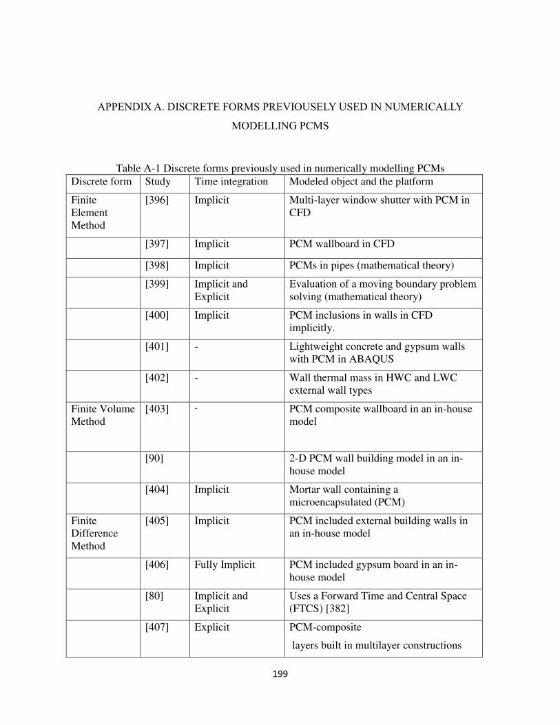
199
APPENDIX A. DISCRETE FORMS PREVIOUSELY USED IN NUMERICALLY
MODELLING PCMS
Table A-1 Discrete forms previously used in numerically modelling PCMs Discrete form Study Time integration Modeled object and the platform
Finite Element Method
[396] Implicit Multi-layer window shutter with PCM in CFD
[397] Implicit PCM wallboard in CFD
[398] Implicit PCMs in pipes (mathematical theory)
[399] Implicit and Explicit
Evaluation of a moving boundary problem solving (mathematical theory)
[400] Implicit PCM inclusions in walls in CFD implicitly.
[401] - Lightweight concrete and gypsum walls with PCM in ABAQUS
[402] - Wall thermal mass in HWC and LWC external wall types
Finite Volume Method
[403] - PCM composite wallboard in an in-house model
[90] 2-D PCM wall building model in an in-house model
[404] Implicit Mortar wall containing a microencapsulated (PCM)
Finite Difference Method
[405] Implicit PCM included external building walls in an in-house model
[406] Fully Implicit PCM included gypsum board in an in-house model
[80] Implicit and Explicit
Uses a Forward Time and Central Space (FTCS) [382]
[407] Explicit PCM-composite
layers built in multilayer constructions
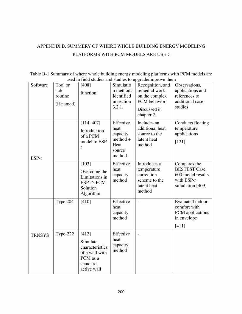
200
APPENDIX B. SUMMERY OF WHERE WHOLE BUILDING ENERGY MODELING
PLATFORMS WITH PCM MODELS ARE USED
Table B-1 Summary of where whole building energy modeling platforms with PCM models are used in field studies and studies to upgrade/improve them
Software Tool or sub routine
(if named)
[408]
function
Simulation methods Identified in section 3.2.1.
Recognition, and remedial work on the complex PCM behavior
Discussed in chapter 2.
Observations, applications and references to additional case studies
ESP-r
[114, 407]
Introduction of a PCM model to ESP-r
Effective heat capacity method + Heat source method
Includes an additional heat source to the latent heat method
Conducts floating temperature applications
[121]
[103]
Overcome the Limitations in ESP-r's PCM Solution Algorithm
Effective heat capacity method
Introduces a temperature correction scheme to the latent heat method
Compares the BESTEST Case 600 model results with ESP-r simulation [409]
TRNSYS
Type 204 [410] Effective heat capacity method
- Evaluated indoor comfort with PCM applications in envelope
[411]
Type-222 [412]
Simulate characteristics of a wall with PCM as a standard active wall
Effective heat capacity method
-
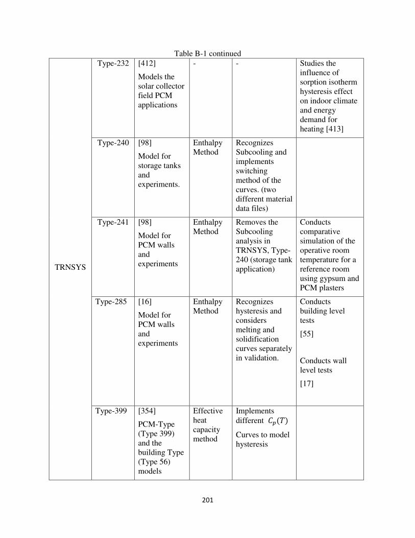
201
Table B-1 continued
TRNSYS
Type-232 [412]
Models the solar collector field PCM applications
- - Studies the influence of sorption isotherm hysteresis effect on indoor climate and energy demand for heating [413]
Type-240 [98]
Model for storage tanks and experiments.
Enthalpy Method
Recognizes Subcooling and implements switching method of the curves. (two different material data files)
Type-241 [98]
Model for PCM walls and experiments
Enthalpy Method
Removes the Subcooling analysis in TRNSYS, Type-240 (storage tank application)
Conducts comparative simulation of the operative room temperature for a reference room using gypsum and PCM plasters
Type-285 [16]
Model for PCM walls and experiments
Enthalpy Method
Recognizes hysteresis and considers melting and solidification curves separately in validation.
Conducts building level tests
[55]
Conducts wall level tests
[17]
Type-399 [354]
PCM-Type (Type 399) and the building Type (Type 56) models
Effective heat capacity method
Implements different 𝐶𝑝(𝑇) Curves to model hysteresis
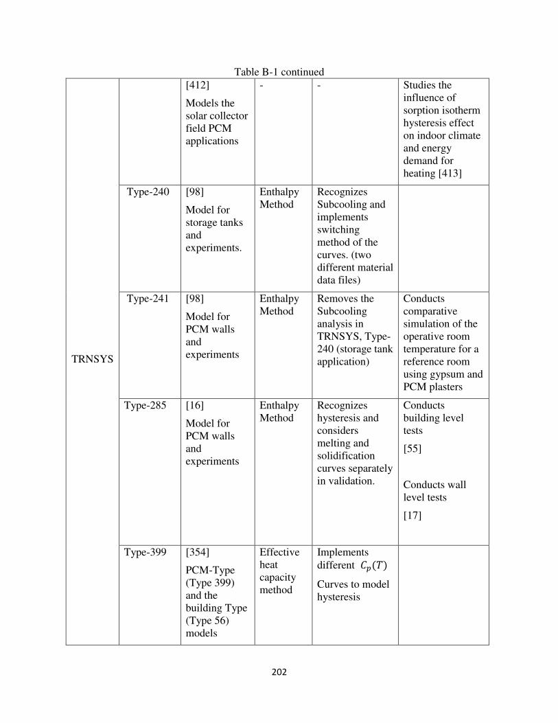
202
Table B-1 continued
TRNSYS
[412]
Models the solar collector field PCM applications
- - Studies the influence of sorption isotherm hysteresis effect on indoor climate and energy demand for heating [413]
Type-240 [98]
Model for storage tanks and experiments.
Enthalpy Method
Recognizes Subcooling and implements switching method of the curves. (two different material data files)
Type-241 [98]
Model for PCM walls and experiments
Enthalpy Method
Removes the Subcooling analysis in TRNSYS, Type-240 (storage tank application)
Conducts comparative simulation of the operative room temperature for a reference room using gypsum and PCM plasters
Type-285 [16]
Model for PCM walls and experiments
Enthalpy Method
Recognizes hysteresis and considers melting and solidification curves separately in validation.
Conducts building level tests
[55]
Conducts wall level tests
[17]
Type-399 [354]
PCM-Type (Type 399) and the building Type (Type 56) models
Effective heat capacity method
Implements different 𝐶𝑝(𝑇) Curves to model hysteresis
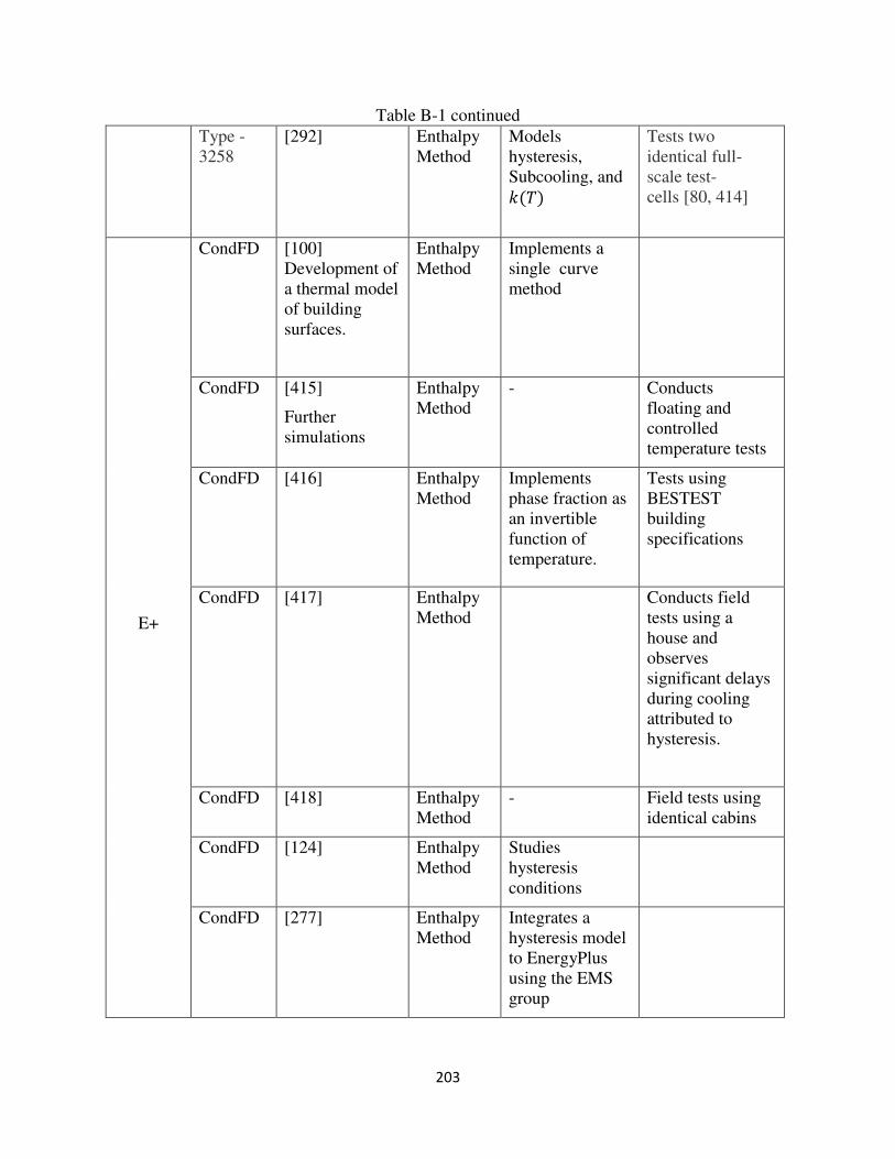
203
Table B-1 continued Type -
3258 [292] Enthalpy
Method Models hysteresis, Subcooling, and 𝑘(𝑇)
Tests two identical full-scale test-cells [80, 414]
E+
CondFD [100] Development of a thermal model of building surfaces.
Enthalpy Method
Implements a single curve method
CondFD [415]
Further simulations
Enthalpy Method
- Conducts floating and controlled temperature tests
CondFD [416] Enthalpy Method
Implements phase fraction as an invertible function of temperature.
Tests using BESTEST building specifications
CondFD [417] Enthalpy Method
Conducts field tests using a house and observes significant delays during cooling attributed to hysteresis.
CondFD [418] Enthalpy Method
- Field tests using identical cabins
CondFD [124] Enthalpy Method
Studies hysteresis conditions
CondFD [277] Enthalpy Method
Integrates a hysteresis model to EnergyPlus using the EMS group
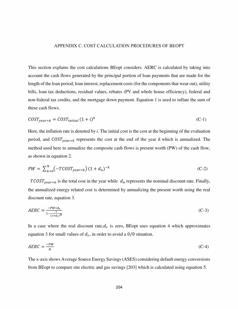
204
APPENDIX C. COST CALCULATION PROCEDURES OF BEOPT
This section explains the cost calculations BEopt considers. AERC is calculated by taking into
account the cash flows generated by the principal portion of loan payments that are made for the
length of the loan period, loan interest, replacement costs (for the components that wear out), utility
bills, loan tax deductions, residual values, rebates (PV and whole house efficiency), federal and
non-federal tax credits, and the mortgage down payment. Equation 1 is used to inflate the sum of
these cash flows. 𝐶𝑂𝑆𝑇𝑦𝑒𝑎𝑟=𝑘 = 𝐶𝑂𝑆𝑇𝑖𝑛𝑖𝑡𝑖𝑎𝑙 (1 + 𝑖)𝑘 (C-1)
Here, the inflation rate is denoted by i. The initial cost is the cost at the beginning of the evaluation
period, and 𝐶𝑂𝑆𝑇𝑦𝑒𝑎𝑟=𝑘 represents the cost at the end of the year 𝑘 which is annualized. The
method used here to annualize the composite cash flows is present worth (PW) of the cash flow,
as shown in equation 2. 𝑃𝑊 =∑ (−𝑇𝐶𝑂𝑆𝑇𝑦𝑒𝑎𝑟=𝑘)𝑁𝑘=0 (1 + 𝑑𝑛)−𝑘 (C-2)
𝑇𝐶𝑂𝑆𝑇𝑦𝑒𝑎𝑟=𝑘 is the total cost in the year while 𝑑𝑛 represents the nominal discount rate. Finally,
the annualized energy related cost is determined by annualizing the present worth using the real
discount rate, equation 3. 𝐴𝐸𝑅𝐶 = −𝑃𝑊∗𝑑𝑟1− 1(1+𝑑𝑟)𝑁 (C-3)
In a case where the real discount rate,𝑑𝑟 is zero, BEopt uses equation 4 which approximates
equation 3 for small values of 𝑑𝑟, in order to avoid a 0/0 situation. 𝐴𝐸𝑅𝐶 = −𝑃𝑊𝑁 (C-4)
The x-axis shows Average Source Energy Savings (ASES) considering default energy conversions
from BEopt to compare site electric and gas savings [203] which is calculated using equation 5.
205
𝐴𝑆𝐸𝑆 = 𝐴𝐸𝑈𝑟𝑒𝑓∗𝐴𝐸𝑈𝑝𝑟𝑜𝑡𝑜∗100%𝐴𝐸𝑈𝑟𝑒𝑓 (C-5)
Here, the average of annual energy use is denoted by AEU. Equation 6 is used to calculate AEU,
where 𝐸𝑈𝑘 the energy is use in year 𝑘 and 𝑁 is the mortgage period.
AEU = ∑ 𝐸𝑈𝑘𝑁𝑘=0𝑁 (C-6)
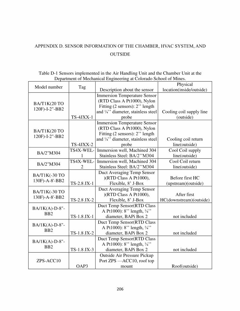
206
APPENDIX D. SENSOR INFORMATION OF THE CHAMBER, HVAC SYSTEM, AND
OUTSIDE
Table D-1 Sensors implemented in the Air Handling Unit and the Chamber Unit at the Department of Mechanical Engineering at Colorado School of Mines.
Model number Tag Description about the sensor
Physical location(inside/outside)
BA/T1K(20 TO 120F)-I-2"-BB2
TS-4JXX-1
Immersion Temperature Sensor (RTD Class A Pt1000), Nylon Fitting (2 sensors): 2’’ length
and ¼’’ diameter, stainless steel probe
Cooling coil supply line (outside)
BA/T1K(20 TO 120F)-I-2"-BB2
TS-4JXX-2
Immersion Temperature Sensor (RTD Class A Pt1000), Nylon Fitting (2 sensors): 2’’ length
and ¼’’ diameter, stainless steel probe
Cooling coil return line(outside)
BA/2"M304 TS4X-WEL-
1 Immersion well, Machined 304 Stainless Steel: BA/2’’M304
Cool Coil supply line(outside)
BA/2"M304 TS4X-WEL-
2 Immersion well, Machined 304 Stainless Steel: BA/2’’M304
Cool Coil return line(outside)
BA/T1K(-30 TO 130F)-A-8'-BB2
TS-2.8 JX-1
Duct Averaging Temp Sensor )(RTD Class A Pt1000),
Flexible, 8’ J-Box Before first HC
(upstream)(outside)
BA/T1K(-30 TO 130F)-A-8'-BB2
TS-2.8 JX-2
Duct Averaging Temp Sensor )(RTD Class A Pt1000),
Flexible, 8’ J-Box After first
HC(downstream)(outside)
BA/1K(A)-D-8"-BB2
TS-1.8 JX-1
Duct Temp Sensor(RTD Class A Pt1000): 8’’ length, ¼’’
diameter, BAPi Box 2 not included
BA/1K(A)-D-8"-BB2
TS-1.8 JX-2
Duct Temp Sensor(RTD Class A Pt1000): 8’’ length, ¼’’
diameter, BAPi Box 2 not included
BA/1K(A)-D-8"-BB2
TS-1.8 JX-3
Duct Temp Sensor(RTD Class A Pt1000): 8’’ length, ¼’’
diameter, BAPi Box 2 not included
ZPS-ACC10 OAP3
Outside Air Pressure Pickup Port ZPS —ACC10, roof top
mount Roof(outside)
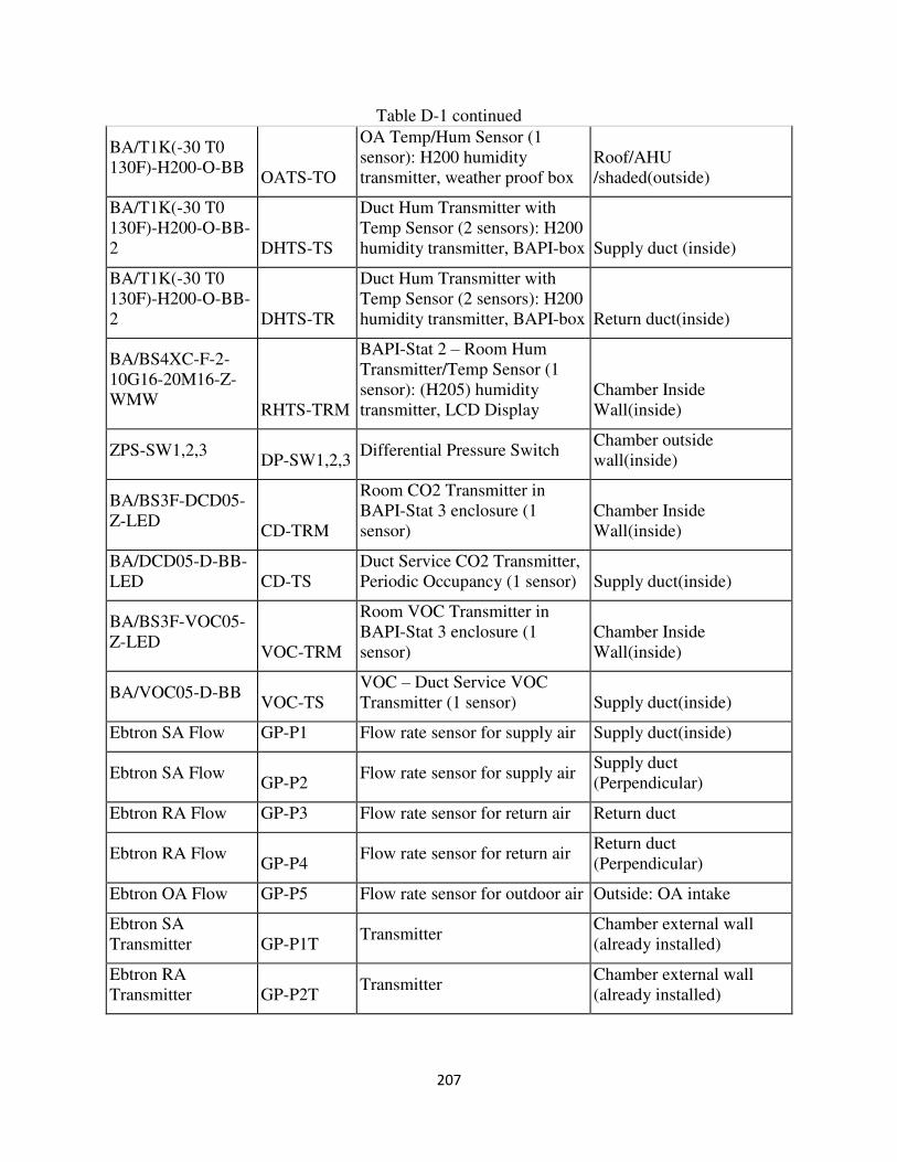
207
Table D-1 continued
BA/T1K(-30 T0 130F)-H200-O-BB
OATS-TO
OA Temp/Hum Sensor (1 sensor): H200 humidity transmitter, weather proof box
Roof/AHU /shaded(outside)
BA/T1K(-30 T0 130F)-H200-O-BB-2 DHTS-TS
Duct Hum Transmitter with Temp Sensor (2 sensors): H200 humidity transmitter, BAPI-box Supply duct (inside)
BA/T1K(-30 T0 130F)-H200-O-BB-2 DHTS-TR
Duct Hum Transmitter with Temp Sensor (2 sensors): H200 humidity transmitter, BAPI-box Return duct(inside)
BA/BS4XC-F-2-10G16-20M16-Z-WMW
RHTS-TRM
BAPI-Stat 2 – Room Hum Transmitter/Temp Sensor (1 sensor): (H205) humidity transmitter, LCD Display
Chamber Inside Wall(inside)
ZPS-SW1,2,3 DP-SW1,2,3
Differential Pressure Switch Chamber outside wall(inside)
BA/BS3F-DCD05-Z-LED
CD-TRM
Room CO2 Transmitter in BAPI-Stat 3 enclosure (1 sensor)
Chamber Inside Wall(inside)
BA/DCD05-D-BB-LED CD-TS
Duct Service CO2 Transmitter, Periodic Occupancy (1 sensor) Supply duct(inside)
BA/BS3F-VOC05-Z-LED
VOC-TRM
Room VOC Transmitter in BAPI-Stat 3 enclosure (1 sensor)
Chamber Inside Wall(inside)
BA/VOC05-D-BB VOC-TS
VOC – Duct Service VOC Transmitter (1 sensor) Supply duct(inside)
Ebtron SA Flow GP-P1 Flow rate sensor for supply air Supply duct(inside)
Ebtron SA Flow GP-P2
Flow rate sensor for supply air Supply duct (Perpendicular)
Ebtron RA Flow GP-P3 Flow rate sensor for return air Return duct
Ebtron RA Flow GP-P4
Flow rate sensor for return air Return duct (Perpendicular)
Ebtron OA Flow GP-P5 Flow rate sensor for outdoor air Outside: OA intake
Ebtron SA Transmitter GP-P1T
Transmitter Chamber external wall (already installed)
Ebtron RA Transmitter GP-P2T
Transmitter Chamber external wall (already installed)
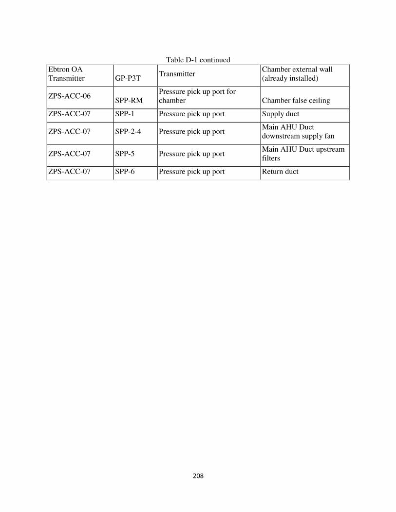
208
Table D-1 continued
Ebtron OA Transmitter GP-P3T
Transmitter Chamber external wall (already installed)
ZPS-ACC-06 SPP-RM
Pressure pick up port for chamber Chamber false ceiling
ZPS-ACC-07 SPP-1 Pressure pick up port Supply duct
ZPS-ACC-07 SPP-2-4 Pressure pick up port Main AHU Duct downstream supply fan
ZPS-ACC-07 SPP-5 Pressure pick up port Main AHU Duct upstream filters
ZPS-ACC-07 SPP-6 Pressure pick up port Return duct
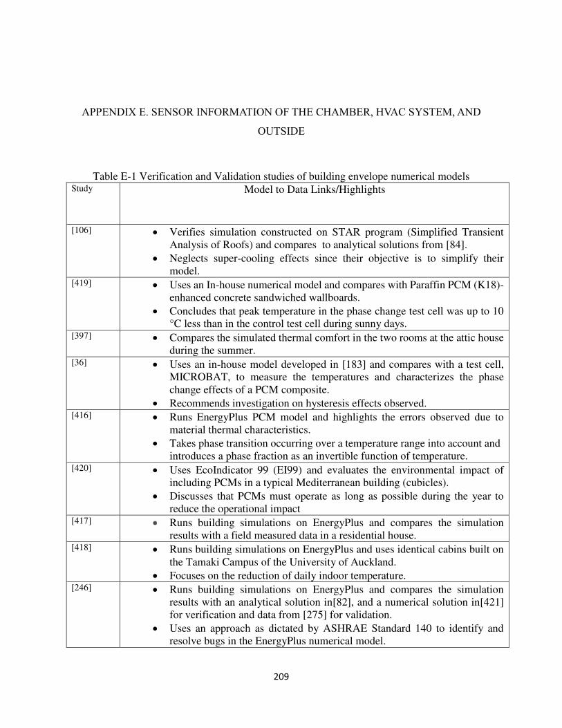
209
APPENDIX E. SENSOR INFORMATION OF THE CHAMBER, HVAC SYSTEM, AND
OUTSIDE
Table E-1 Verification and Validation studies of building envelope numerical models Study Model to Data Links/Highlights
[106] Verifies simulation constructed on STAR program (Simplified Transient Analysis of Roofs) and compares to analytical solutions from [84].
Neglects super-cooling effects since their objective is to simplify their model.
[419] Uses an In-house numerical model and compares with Paraffin PCM (K18)-enhanced concrete sandwiched wallboards.
Concludes that peak temperature in the phase change test cell was up to 10 °C less than in the control test cell during sunny days.
[397] Compares the simulated thermal comfort in the two rooms at the attic house during the summer.
[36] Uses an in-house model developed in [183] and compares with a test cell, MICROBAT, to measure the temperatures and characterizes the phase change effects of a PCM composite.
Recommends investigation on hysteresis effects observed. [416]
Runs EnergyPlus PCM model and highlights the errors observed due to material thermal characteristics.
Takes phase transition occurring over a temperature range into account and introduces a phase fraction as an invertible function of temperature.
[420] Uses EcoIndicator 99 (EI99) and evaluates the environmental impact of including PCMs in a typical Mediterranean building (cubicles).
Discusses that PCMs must operate as long as possible during the year to reduce the operational impact
[417] Runs building simulations on EnergyPlus and compares the simulation results with a field measured data in a residential house.
[418] Runs building simulations on EnergyPlus and uses identical cabins built on the Tamaki Campus of the University of Auckland.
Focuses on the reduction of daily indoor temperature. [246] Runs building simulations on EnergyPlus and compares the simulation
results with an analytical solution in[82], and a numerical solution in[421] for verification and data from [275] for validation.
Uses an approach as dictated by ASHRAE Standard 140 to identify and resolve bugs in the EnergyPlus numerical model.
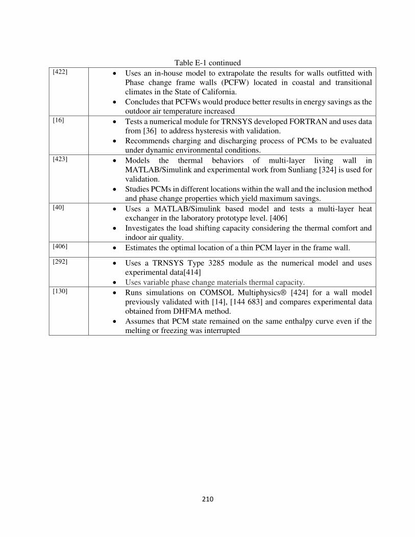
210
Table E-1 continued
[422] Uses an in-house model to extrapolate the results for walls outfitted with Phase change frame walls (PCFW) located in coastal and transitional climates in the State of California.
Concludes that PCFWs would produce better results in energy savings as the outdoor air temperature increased
[16] Tests a numerical module for TRNSYS developed FORTRAN and uses data from [36] to address hysteresis with validation.
Recommends charging and discharging process of PCMs to be evaluated under dynamic environmental conditions.
[423]
Models the thermal behaviors of multi-layer living wall in MATLAB/Simulink and experimental work from Sunliang [324] is used for validation.
Studies PCMs in different locations within the wall and the inclusion method and phase change properties which yield maximum savings.
[40]
Uses a MATLAB/Simulink based model and tests a multi-layer heat exchanger in the laboratory prototype level. [406]
Investigates the load shifting capacity considering the thermal comfort and indoor air quality.
[406] Estimates the optimal location of a thin PCM layer in the frame wall.
[292] Uses a TRNSYS Type 3285 module as the numerical model and uses experimental data[414]
Uses variable phase change materials thermal capacity. [130] Runs simulations on COMSOL Multiphysics® [424] for a wall model
previously validated with [14], [144 683] and compares experimental data obtained from DHFMA method.
Assumes that PCM state remained on the same enthalpy curve even if the melting or freezing was interrupted


![pace sy ntllaetic fae]lts report - Mountain Scholar](https://img.pdfslide.net/doc/110x75/63196a4b1a1adcf65a0ea4b0/pace-sy-ntllaetic-faelts-report-mountain-scholar.jpg)


