World Agriculture and Climate Change: Economic Adaptations

United States An Economic Research Service ReportDepartment ofAgriculture

AgriculturalEconomicReportNumber 703

World Agriculture andClimate ChangeEconomic AdaptationsRoy DarwinMarinos TsigasJan LewandrowskiAnton Raneses

It’s Easy To Order Another Copy!

Just dial 1-800-999-6779. Toll free in the United States and Canada.

Ask for World Agriculture and Climate Change: Economic Adaptations (AER-703).

Cost is $12.00 per copy ($15.00 for non-U.S. addresses). Charge to VISA or Mastercard. Or send acheck or purchase order (payable to ERS-NASS) to:

ERS-NASS341 Victory Drive

Herndon, VA 20170-5217

For additional information about ERS publications, databases, and other prod-ucts, both paper and electronic, visit the ERS Home Page on the Internet athttp://www.econ.ag.gov/

The United States Department of Agriculture (USDA) prohibits discrimination inits programs on the basis of race, color, national origin, sex, religion, age, dis-ability, political beliefs, and marital or familial status. (Not all prohibited basesapply to all programs.) Persons with disabilities who require alternative means

for communication of program information (braille, large print, audiotape, etc.)should contact the USDA Office of Communications at (202) 720-2791.

To file a complaint, write the Secretary of Agriculture, U.S. Department of Agri-

culture, Washington, DC 20250, or call l-800-245-6340 (voice) or (202) 720-1127 (TDD). USDA is an equal employment opportunity employer.

World Agriculture and Climate Change: Economic Adaptations. By RoyDarwin, Marinos Tsigas, Jan Lewandrowski, and Anton Raneses. NaturalResources and Environment Division, Economic Research Service, U.S. Depart-ment of Agriculture. Agricultural Economic Report No. 703.

Abstract

Recent studies suggest that possible global increases in temperature andchanges in precipitation patterns during the next century will affect world agricul-ture. Because of the ability of farmers to adapt , however, these changes arenot likely to imperil world food production. Nevertheless, world production ofall goods and services may decline, if climate change is severe enough or ifcropland expansion is hindered. Impacts are not equally distributed around theworld. Agricultural production may increase in arctic and alpine areas, but de-crease in tropical and some other areas. In the United States, soil moisturelosses may reduce agricultural production in the Corn Belt and Southeast.

Keywords: Climate change, world agriculture

Acknowledgments

The authors gratefully acknowledge the encouragement and input of our ERScolleagues John Miranowski, John Reilly, Betsey Kuhn, and George Frisvold.We also thank Tom Hertel, Hari Eswaran, Everett Van den Berg, RichardAdams, Jae Edmonds, Norman Rosenberg, Nicholas Komninos, and partici-pants in the Natural Resources and Environment Division’s seminar series fortheir numerous contributions to this research.

Note: Roy Darwin and Jan Lewandrowski are with the U.S. Department ofAgriculture’s Economic Research Service, Marinos Tsigas is a visiting scholarat the Natural Resources and Environment Division, and Anton Raneses is withthe University of California at Davis. For more information contact Roy Dar-win, USDA/ERS, Room 408, 1301 New York Avenue, NW, Washington, DC20005-4788. Voice: 202-219-0428. Fax: 202-2 19-0473. E-mail: [email protected].

Washington, DC 20005-4788 June 1995

Contents

Summary . . . . . . . . . . . . . . . . . . . . . . . . . . . . . . .

Introduction . . . . . . . . . . . . . . . . . . . . . . . . . . . . . . . .

Previous Research . . . . . . . . . . . . . . . . . . . . . . . . . .Crop Production Studies . . . . . . . . . . . . . . . . . . . . . . . .Livestock Production Studies . . . . . . . . . . . . . . . . .Regional Economic Studies . . . . . . . . . . . . . . . . . . . .Global Economic Studies . . . . . . . . . . . . . . . . . . . .

Procedures . . . . . . . . . . . . . . . . . . . . . . . . . . . . . .Modeling Framework . . . . . . . . . . . . . . . . . . . .Simulating Climate Change . . . . . . . . . . . . . . . . . . . . . . .Limitations and Strengths . . . . . . . . . . . . . . . . . . . . . . .

Results . . . . . . . . . . . . . . . . . . . . . . . . . . . . . . . . . . .Impacts on Endowments . . . . . . . . . . . . . . . . . . . . . . . .Impacts on Commodity Markets . . . . . . . . . . . . . . . . . . . .Land and Water Use . . . . . . . . . . . . . . . . . . . . . . . .Impacts on Gross Domestic Product . . . . . . . . . . . . . . . . . . . . . . . . . . . . . . . . .

Conclusions . . . . . . . . . . . . . . . . . . . . . . . . . . . . . . . . . . . . . . . . . . . . . . . . . .

References . . . . . . . . . . . . . . . . . . . . . . . . . . . . . . . . . . . . . . . . . . . . .

Appendix A: FARM’s CGE Model . . . . . . . . . . . . . . . . . . . . . . .Model Structure . . . . . . . . . . . . . . . . . . . . . . . . . . . . . . . . . . . . . .Parameter Calibration . . . . . . . . . . . . . . . . . . . . . . . . . . . . . .Data Calibration . . . . . . . . . . . . . . . . . . . . . . . . . . . . . . . . . . . .

Appendix B: Detailed FARM Results . . . . . . . . . . . . . . . . . . . . . . . . . . . . .

. vi

1

. 2

. 2

. 2

. 3

. 3

. 5

. 51618

1919233035

39

41

45455151

62

World Agriculture and Climate Change I AER-703

List of Tables

1. Regions, sectors, and commodities in FARM . . . . . . . . . . . . . . . 7

2. Land class boundaries in FARM . . . . . . . . . . . . . . . . . . 9

3. Current land class endowments, by region . . . . . . . . . . . . . . . . . . 9

4. Water runoff, supply, and supply elasticities, by region . . . . . . . . . . 10

5. Cropland, permanent pasture, forest land, and land in other uses,by region and land class . . . . . . . . . . . . . . . . . . . . . 11

6. Water use, by land class and region . . . . . . . . . . . . . . . . . 12

7. Value of commodity production, by region and land class . . . . . . . I2

8. Major components of agricultural and silvicultural production, by region . 13

9. Production of agricultural and silvicultural commodities,by region and land class . . . . . . . . . . . . . . . . . . . 14

10. Per hectare production of agricultural and silvicultural commodities,by region and land class . . . . . . . . . . . . . . . . . . . . . 15

11. Summary statistics for the general circulation models used asthe basis for climate change scenarios . . . . . . . . . . . . . . . 17

12. Percentage of total land changing land class, by regionand climate change scenario . . . . . . . . . . . . . . . . . . . 20

13. Changes in world land class endowments, by climate change scenario . . 20

14. Changes in agriculturally important land, by area andclimate change scenario . . . . . . . . . . . . . . . . . . . . . 21

15. Global changes in land classes on existing cropland and in thevalue of existing cropland and agricultural land under existing rents . . . 21

16. Changes in water runoff and water supply, by region andclimate change scenario . . . . . . . . . . . . . . . . . . . 22

17. Changes in U.S. land class endowments, by climate change scenario . . 23

18. Changes in land classes on existing U.S. cropland and in the valueof existing cropland and agricultural land under existing rents . . . . . 23

19. Changes in quantities and prices of agricultural, silvicultural, andprocessed food commodities, by region and climate change scenario . . . 24

20. Changes in U.S. production and U.S. shares of world productionof agricultural and silvicultural products, by commodity and climatechangescenario . . . . . . . . . . . . . . . . . . . . . . . 26

21. Changes in world production and prices of goods and services notproduced in the agricultural or silvicultural sectors, by climatechangescenario . . . . . . . . . . . . . . . . . 27

22. Changes in U.S. and world supply and production of cereals undervarious constraints, by climate change scenario . . . . . . . 28

23. Changes in world and U.S. production of selected commodities when landuse changes are and are not restricted, by climate change scenario . . . . 29

24. Net changes in cropland, permanent pasture, forest land, and other-use land,by region and climate change scenario . . . . . . . . . . . 30


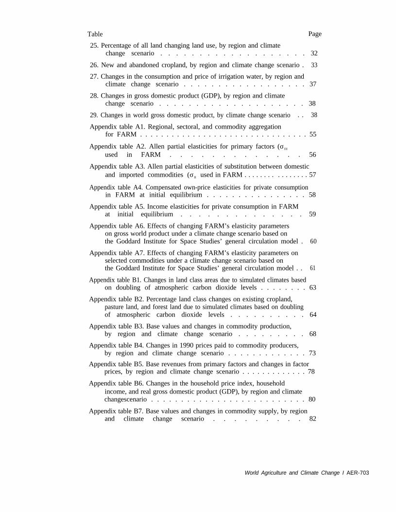
Table Page

25. Percentage of all land changing land use, by region and climatechange scenario . . . . . . . . . . . . . . . . . . . 32

26. New and abandoned cropland, by region and climate change scenario . 33

27. Changes in the consumption and price of irrigation water, by region andclimate change scenario . . . . . . . . . . . . . . . . . . 37

28. Changes in gross domestic product (GDP), by region and climatechange scenario . . . . . . . . . . . . . . . . . . . . 38

29. Changes in world gross domestic product, by climate change scenario . . 38

Appendix table A1. Regional, sectoral, and commodity aggregationfor FARM . . . . . . . . . . . . . . . . . . . . . . . . . . . . . . . . 55

Appendix table A2. Allen partial elasticities for primary factors (σΠΙ)used in FARM . . . . . . . . . . . . . 56

Appendix table A3. Allen partial elasticities of substitution between domesticand imported commodities (σΙΙ) used in FARM . . . . . . . . . . . . . . . . 57

Appendix table A4. Compensated own-price elasticities for private consumptionin FARM at initial equilibrium . . . . . . . . . . . . . . . . 58

Appendix table A5. Income elasticities for private consumption in FARMat initial equilibrium . . . . . . . . . . . . . . 59

Appendix table A6. Effects of changing FARM’s elasticity parameterson gross world product under a climate change scenario based onthe Goddard Institute for Space Studies’ general circulation model . 60

Appendix table A7. Effects of changing FARM’s elasticity parameters onselected commodities under a climate change scenario based onthe Goddard Institute for Space Studies’ general circulation model . . 61

Appendix table B1. Changes in land class areas due to simulated climates basedon doubling of atmospheric carbon dioxide levels . . . . . . . . 63

Appendix table B2. Percentage land class changes on existing cropland,pasture land, and forest land due to simulated climates based on doublingof atmospheric carbon dioxide levels . . . . . . . . . . 64

Appendix table B3. Base values and changes in commodity production,by region and climate change scenario . . . . . . . . . 68

Appendix table B4. Changes in 1990 prices paid to commodity producers,by region and climate change scenario . . . . . . . . . . . . . 73

Appendix table B5. Base revenues from primary factors and changes in factorprices, by region and climate change scenario . . . . . . . . . . . . . 78

Appendix table B6. Changes in the household price index, householdincome, and real gross domestic product (GDP), by region and climatechangescenario . . . . . . . . . . . . . . . . . . . . . . . . . . 80

Appendix table B7. Base values and changes in commodity supply, by regionand climate change scenario . . . . . . . . . 82


List of Figures

1. FARM modeling framework . . . . . . . . . . . . . . . . . . 6

2. Land classes under current climate . . . . . . . . . . . . . . 8

3. Effect of climate change on distribution of land among land classes (LC) . 21

4. Climate-induced land class changes that occur on cropland acreage . . 22

5. Effect of climate change on world crop, livestock, and forest products . 23

6. Net global changes in land use . . . . . . . . . . . 31

7. Climate-induced land use changes that occur on LC 6 in tropical areas . 31

8. Regional land use conversions . . . . . . . . . 32

9. Cropland converted to other uses . . . . . . . . . . 34

10. Increases in new cropland . . . . . . . . . . . . 35

11. Potential new cropland areas in Canada under the GISS 2xCO2

climate change scenario . . . . . . . . .

Appendix figure A1. Supply of services from land in FARM . . .

Appendix figure A2. Regional water markets in FARM . . . .

Appendix figure A3. Crop production in FARM . . . . . .

Appendix figure A4. Production of manufacture and services in FARM

Appendix figure AS. Household behavior and consumption in FARM .

. 36

. 46

. 46

. 47

. 49

. 50

World Agriculture and Climate Change / AER-703 V

Summary

Possible changes in climate may spur geographic shifts in agricultural productionand structure, but should not significantly affect the level of U.S. and world foodproduction. We evaluate the effects of global climate change on world agricul-ture with a model that links climatic conditions to land and water resources andto production, trade, and consumption of 13 commodities throughout the world.The model has three unique capabilities. First, it simulates the potential effectsof global climate change on the availability and productivity of agriculturally suit-able land. Second, it determines the extent to which farmers respond to climatechange, such as by adopting alternative production systems and by expanding(or abandoning) agricultural lands. Third, it provides quantitative estimates ofland and water use changes, because it simulates the competition between agri-culture and the rest of the economy for these resources.

We evaluated four global-climate-change scenarios based on a doubling of at-mospheric concentrations of carbon dioxide. These scenarios were derivedfrom results projected by meteorological models at the Goddard Institute forSpace Studies, the Geophysical Fluid Dynamics Laboratory, the United King-dom Meteorological Office, and Oregon State University and embody a range ofaverage global temperature and precipitation changes (2.8-5.2oC and 7.8-15.0percent, respectively). Our principal results are:

(1) Global changes in temperature and precipitation patterns during thenext century are not likely to imperil food production for the world as awhole. Although world production of nongrain crops is likely to decline (0.2-1.3 percent), production of wheat is likely to increase (0.5-3.3 percent) as wellas livestock (0.7-0.9 percent). Changes in world production of other grainsrange from -0.1 to 0.4 percent, increasing in three scenarios. World productionof processed foods, which is the primary source of food for households, wouldrise (0.2-0.4 percent).

(2) Farmer adaptations are the main mechanisms for keeping up worldfood production under global climate change. By selecting the most profit-able mix of inputs and outputs on existing cropland, for example, farmers maybe able to offset from 79 to 88 percent of the 19- to 30-percent reductions inworld cereals (wheat plus other grains) supply directly attributable to climatechange. Including adjustments in domestic markets and international trade (butstill holding cropland fixed) mitigates more than 97 percent of the original nega-tive impacts. Farmers also are likely to adapt by increasing the amount of landunder cultivation (up 7.1-14.8 percent). This enables world cereals productionto actually increase (0.2-1.2 percent) under climate change.

vi World Agriculture and Climate Change I AER-703

(3) Costs and benefits of global climate change are not equally distributedaround the world. Warming in arctic and mountainous areas will increase thequantity of land suitable for farming and forestry, but warming in tropical andsome other areas will reduce soil moisture, thereby causing decreases in farm andforestry productivity. These changes affect commodity production. In Canada,for example, output of wheat, other grains, nongrains, livestock, and forest prod-ucts increases, while in Southeast Asia, output of these commodities generallydecreases in all scenarios. Impacts on commodity production in mid-latituderegions are mixed. Real gross domestic product (GDP) tends to mirror agricul-tural and silvicultural activity. GDP in high-latitude regions, like Canada,increases under climate change, while GDP in tropical areas, like Southeast Asia,declines. Impacts on GDP in mid-latitudes vary by region, sometimes consis-tently increasing (Japan, other East Asia) or decreasing (European Community)across all climate change scenarios, and sometimes varying by scenario (theUnited States and a combined Australia and New Zealand region).

(4) Climate change is likely to affect the overall structure of agricultureand food processing in the United States. Land suitable for farming and for-estry is likely to increase, but soil moisture losses may reduce agriculturalpossibilities in the Corn Belt and in the Southeast. Farmers are likely to adaptby increasing wheat production and reducing production of other grains, primarilymaize. As a result of less feed available, livestock production also decreases.Output of nongrains and forest products increases or decreases depending on thescenario. Production of processed food commodities generally declines. U.S.shares of world production move in the same direction as changes in production.Across scenarios, effects on GDP range from -0.1 to 0.1 percent annually (in1990 dollars, from -$4.8 billion to $5.8 billion).

(5) World GDP may decline if climate change is severe enough or if crop-land expansion is hindered. Across the four climate change scenarios, netannual impacts on world GDP range from -0.1 to 0.1 percent (in 1990 dollars,from -US$24.5 billion to US$25.2 billion). These results indicate that worldGDP may decline if increases in agricultural and food production are more thanoffset by losses in other sectors. Also, when land use is constrained to 1990activities, world GDP declines by 0.004 to 0.35 percent annually (in 1990 dollars,from US$0.7 billion to US$74.3 billion). World output of processed fooddeclines as well (from 0.002 to 0.58 percent). This implies that the new tem-perature and precipitation patterns under climate change are likely to reduce theaverage productivity of the world’s existing agricultural lands.

(6) Land use changes that accompany climate-induced shifts in croplandand permanent pasture are likely to raise additional social and environ-mental issues. Although there are net increases in cropland for the world as awhole, from 4.2 to 10.5 percent of existing cropland is converted to other usesunder the climate change scenarios. In the United States, from 8.6 to 19.1 per-cent of existing cropland is converted. Farm communities in areas where theonly economically viable adaptation is to abandon crop production could beseverely disrupted. Also, forest land is likely to decrease under global climatechange (3.6-9.1 percent, net). This could cause more conflicts over the environ-mental consequences of agriculture in some areas. In tropical regions, forexample, competition from crop production could aggravate direct climate-induced losses of tropical rain forests.

World Agriculture and Climate Change I AER-703 vii

(7) Although water supplies are likely to increase for the world as a wholeunder climate change, shortages could occur in some regions. Across sce-narios, world water supplies increase by 6.4 to 12.4 percent. In Japan, however,changes in water supplies range from -9.4 to 10.2 percent. In addition, the priceof water in Japan increases by more than 75 percent in all scenarios. Theseresults indicate likely conflicts over water in Japan. In the United States, theprice of water increases in only one climate change scenario when farmers areallowed to fully adapt. If land use in the United States is constrained to 1990activities, however, then water prices increase in all scenarios. This indicatesthat conflicts over water resources might increase in the United States.

A number of caveats and limitations remain. First, we do not consider the well-documented, beneficial effects of higher concentrations of atmospheric carbondioxide on plant growth and water use. There remains considerable debate aboutthe magnitude of this effect. Second, our simulations of water resources do notcapture all potential impacts. The potential effects of too much water, such asflooding or water logging of soils, for example, are not evaluated. Finally,changes in socioeconomic conditions which might take place by the time climatechanges occur were not considered.

viii World Agriculture and Climate Change I AER-703

World Agriculture and Climate ChangeEconomic Adaptations

Roy DarwinMarinos Tsigas

Jan LewandrowskiAnton Raneses

Introduction

Many studies project that Earth’s climate will warm by1.5 to 5.0°C during the next century (Manabe andWetherald, 1987; Wilson and Mitchell, 1987; Hansenand others, 1988; and Schlesinger and Zhao, 1989).A substantial portion of this warming may occur evenif global efforts are undertaken to reduce emissions ofheat-trapping gases. Estimates of the economic andecological effects of this warming and associated shiftsin precipitation patterns are needed by policymakersto determine how much to control emissions and howbest to adapt to unavoidable climate changes.

The agricultural consequences of these climate changesare twofold. First, climate change may affect crop andlivestock productivity.1 Second, ensuing economicresponses may alter the regional distribution and inten-sity of farming. This means that, for some regions,(1) the long-term productivity and competitiveness ofagriculture may be at risk, (2) farm communities couldbe disrupted, and (3) conflicts over environmental im-pacts of agriculture on land and water resources couldbecome increasingly contentious.

A substantial amount of research has been conducted onthe potential effects of climate change on agriculturalproductivity (especially crop yields). A few studieshave used climate-induced changes in crop yields toestimate global economic impacts. These global stud-ies, however, have generally failed to consider thatclimate change would affect the availability of agricul-turally suitable land, that economic factors drive farm-level adaptations, and that farmers must compete withother economic agents for land and water resources.

This research effort is unique in that it directly linksdetailed climate projections with distributions of landand water resources. These distributions are then inte-grated within a global economic model that accountsfor all market-based activity. This approach enablesus to simulate how climate change might affect watersupplies and the availability of agriculturally suitableland, and to analyze how these impacts might affecttotal world production of goods and services.

This effort is also unique in that it simulates the econom-ics of how farmers respond to climate change (such asby adopting alternative production systems or expand-ing/abandoning agricultural land). Such a simulationreflects the fact that farmers are likely to consider theeconomic viability of their responses to climate-inducedchanges in yield, and it avoids the arbitrariness associ-ated with projections of farmer responses that do notexplicitly consider economic variables.

Finally, this effort is unique in that impacts in themajor resource-using sectors (crops, livestock, and for-estry) are estimated simultaneously. Crop, livestock,and forestry sectors often compete for land resources.Separate estimates of the land demanded by these sec-tors may implicitly lead to some land being countedtwice, allowing the effects of climate change in thesesectors to be underestimated. Treating land demandsexplicitly and simultaneously avoids such problems andenables one to provide quantitative estimates of landuse changes. The combination of these unique featuresleads to the most comprehensive and economicallyconsistent projections to date of how climate changemight alter the location and intensity of farming.

1In this report. climate change refers to an overall trend towardglobal warming and increased precipitation amounts.

World Agriculture and Climate Change / AER-703

Previous Research

Since the late 1970’s, the literature addressing agricul-tural impacts of climate change has evolved from“expert opinion” surveys to dynamic multiregion, multi-sector economic models. Among the first major effortsto assess potential impacts of climate change on agri-culture was that undertaken by the National DefenseUniversity (NDU) (1978). This study assembled aninternational group of climate experts and elicitedtheir opinions concernin g the probabilities of variousclimate change events and the resulting impacts onagriculture. NDU’s most consistent finding was thatthe experts disagreed on most matters related to cli-mate change,

Crop Production Studies

In the early and mid-1980’s, research focused on thedirect effects of climate change on crop production.Two complementary approaches were developed. The"analogous region” approach looked at potential shiftsin climatic zones favorable to particular crops. Thesestudies generally concluded that projected climate changewould significantly alter regional patterns of crop pro-duction. Newman (1980), for example, estimated thatthe U.S. Corn Belt would shift 175 km north-northeastfor every 1°C rise in temperature. Blasing and Solomon(1982) concluded that the U.S. Corn Belt would con-tract. particularly in its southwest region, under warmerand drier growing seasons. Rosenzweig (1985) foundthat climate change could greatly expand winter wheatproduction in Canada: while in the United States, themajor effect would be regional shifts in the use ofwheat cultivars.

More recently, Carter. Porter, and Parry (1991) used ageographic information system (GIS) to look at shiftsin production of grain maize, sunflower, and soybeansin Europe. Eswaran and Van den Berg (1992), usinga GIS-derived index of agricultural production basedon length of growing season, analyzed the impacts ofclimate change on grain production and grazing in In-dia, Pakistan. and Afghanistan. Leemans and Solomon(1993) used similar methods to match crop productionwith climate conditions globally. Both Carter, Porter,and Parry (1991) and Leemans and Solomon (1993)concluded that climate change could induce large spa-tial shifts in crop production patterns and that high-latitude regions would likely benefit as large areas be-come suitable to crops.

The second approach to estimating the effect of globalclimate change on agriculture was based on crop-growth

models.2 These mathematical models are intuitivelyappealing for analyzing the effects of change on cropyields because they incorporate daily data on tempera-ture, precipitation, solar radiation, and (often) atmos-pheric carbon dioxide, as well as data on soils andmanagement practices in their simulations of plantdevelopment. Earlier works (Warrick, 1984; and Ter-jung. Liverman, and Hayes, 1984) considered warmertemperatures and/or drier growing seasons and gener-ally concluded that climate change would cause cropyields to decline. Later studies (Robertson and others,1987; Ritchie, Baer, and Chou, 1989; and Peart andothers, 1989) supported this result but found that manydecreases in yield would be largely offset by positiveimpacts on plant growth associated with higher levelsof atmospheric carbon dioxide.3

Livestock Production Studies

A relatively new line of research has started to analyzepotential impacts of climate change on livestock. Vir-tually all examine current production practices givenone or more specific climate change scenarios. A fewstudies also draw on the “analogous regions” frameworkto assess how likely farm-level adaptations might miti-gate any negative impacts.

Results are consistent across studies. Studies tend toagree that, because of decreases in feed conversionefficiency, global climate change would reduce animalweight gains and dairy output during the summermonths in relatively warm areas, such as the SouthernUnited States (Hahn, Klinedinst, and Wilhite, 1990;Klinedinst and others, 1993; Baker and others, 1993).In relatively cool areas, grazed livestock generally dobetter (due to increased forage), but more capital-inten-sive operations, like dairy, are negatively affected(Parry, Carter, and Konijn, 1988; Klinedinst and others,1993; Baker and others, 1993). The studies also specu-late that reduced feed requirements, increased survivalof young, and lower energy costs may benefit livestockin all regions during fall and winter. On the down side,a number of livestock diseases are likely to expandtheir ranges under global warming (Stem, 1988; U.S.Environmental Protection Agency, 1989).

Management techniques for adapting livestock opera-tions to climate change are not formally analyzed but

2Commonly cited crop-growth models are CERES (wheat, maize,

and rice), EPIC (wheat, maize, and sorghum), GAPS (maize and

sorghum). and SOYGRO (soybeans).

3Increases in atmospheric concentrations of carbon dioxide would

probably act like a fertilizer for some plants and improve water-use

efficiency for others (Intergovernmental Panel on Climate Change,

1990).

2 World Agriculture and Climate Change / AER-703

are generally assumed to be significant (Hahn, Kline-dinst, and Wilhite, 1990; Klinedinst and others, 1993;Baker and others, 1993). Several relatively inexpensivetechnologies for cooling animals in hot climates (shad-ing, wetting, increasing air circulation, and air condi-tioning), have contributed to the growth of dairy produc-tion in the Southwestern and Southeastern United States.Herd reduction during dry years is a key managementtechnique in regions subject to frequent droughts, wherelivestock are often more resistant to severe weatherevents than crops and are, therefore, a better hedge forincome protection and food security (Abel and Levin,1981).

Other climate-induced responses include adopting newbreeds or substituting species. Where warming is mod-erate, for example, Brahman cattle and Brahmancrosses, which are more heat- and insect-resistant thanbreeds now dominant in Texas and southern Europe,might be adopted. In cases of extreme warming, sheepmight substitute for cattle (Hahn, Klinedinst, and Wil-hite, 1990; Klinedinst and others, 1993; Baker andothers, 1993; and personal communications with B.Baker and G. Hahn).

Regional Economic Studies

The crop production studies discussed above did notconsider farmers’ responses to changing climate condi-tions. Without these responses, little could be con-cluded about likely effects on commodity markets.Crop-growth models became important in economicmodeling, however, because yield effects were easy toincorporate into available economic models. The firstresearch in this vein looked at farm-sector responsesto specified climate change scenarios. In a series ofcase studies, Parry, Carter, and Konijn (1988) foundthat, for areas in Saskatchewan (Canada), Iceland, Fin-land, the former Soviet Union, and Japan, manynegative impacts of climate change could be reducedby switching crop varieties, applying fertilizer differ-ently, and/or improving soil drainage. They also foundthat projected climate change led to increased com-modity production and farm income in some regions.

Subsequent country/region studies expanded economicanalysis of climate change and agriculture to includemore farm-level adaptations, input and output substitu-tions, effects on commodity prices, and impacts onwelfare (see Adams and others, 1988; Arthur and Abi-zadeh, 1988; Adams and others, 1990; and Mooney andArthur, 1990). Adams and others (1990), for example,focused on U.S. agriculture and climate-induced shiftsin output mixes, input use, and welfare. Their modelincluded 64 producing regions, 10 input (land, labor,and water) supply regions, and 1,683 possible output

mixes for maize, wheat, soybeans, cotton, barley, sor-ghum, rice, alfalfa, and/or livestock. The inclusion ofwater stocks as a climate-dependent input was a majorstrength of the study. Water increases heat tolerancein many crops, so water availability is a key variablein assessing how climate change might affect agriculture.

Bowes and Crosson (1991) looked at the Missouri,Iowa, Nebraska, and Kansas (MINK) region underwarmer and drier growing conditions (the conditionsthat prevailed in the 1930’s) assuming zero, marginal,and significant levels of farm-level adaptation. Moreimportant, they considered how impacts in the agricul-tural, water, and forestry sectors would be transmittedto the MINK area’s general economy. First, actionsembodied in each adaptation scenario were incorporatedinto crop-growth models and simulations were run for48 “typical” farms. Next, farm results were averagedand scaled up to obtain regional yield effects. Impactsfor the total MINK economy were then estimated byconverting regional yields to farm revenues and feedingthese values into an input-output model. Bowes andCrosson (1991) found that a climate like that of the1930’s would likely reduce agricultural production inthe MINK area by 0.3 to 1.4 percent (10 percent undera worst-case scenario). Because the climate-impactedsectors’ share of the regional economy was small, totaleconomic impacts were negligible in all scenarios.

Single country/region studies provided first estimatesof how climate change might affect agricultural marketsand input use. Results generally indicated small tomodest reductions in crop output but net gains in pro-ducer welfare once adaptation, higher crop prices,and/or carbon dioxide effects on crop growth wereaccounted for (Adams and others, 1988; Arthur andAbizadeh, 1988; Adams and others, 1990; and Mooneyand Arthur, 1990). Consumers and society usually faredsomewhat worse under climate change, but not always.In Adams and others (1990), for example, economicimpacts of climate change ranged from losses of $10.33billion to gains of $10.89 billion per year for the UnitedStates, depending on the scenario. They concluded thatclimate change would not jeopardize U.S. agriculture’sability to meet domestic food needs but may shift do-mestic crop production patterns and (perhaps) reducethe role of U.S. producers in some world markets.More concern was expressed for natural ecosystemsbecause of increased demands for irrigation water.

Global Economic Studies

Two important limitations of country/region studiesare that they do not consider (1) effects of climatechange in other regions (they assume climate outsidethe study area is constant) or (2) the role of world

World Agriculture and Climate Change I AER-703 3

trade in dissipating effects across regions. As Reilly(1994) points out, such omissions are valid only whenclimate change occurs entirely within a country/regionor under the assumption of a closed economy.

Recently, several studies have considered global impactsusing agricultural market models (Kane, Reilly, andTobey, 1991) or general equilibrium models (Rosen-zweig and Parry, 1994). Kane, Reilly. and Tobey(1991) modeled world agriculture in a partial equilib-rium framework using 13 regions and 20 commodities.Trade through global commodity markets linked theregions. The study’s key finding was that, while cli-mate change may significantly reduce crop yields insome regions, trade adjusts global patterns of produc-tion and consumption such that national and worldeconomic impacts are small. Reported percentagechanges in world gross domestic product ranged from-0.17 to 0.09 percent. For a “moderate impacts” sce-nario, world gross domestic product would increaseby 0.01 percent.4

Rosenzweig and Parry ( 1994) examined the effects ofclimate change on world cereal production and thedistribution of these impacts among developed and de-veloping countries in the year 2060.5 Their analyticalframework is the Basic Link System (BLS) (Fischerand others, 1988), a set of 34 country/region modelsthat interact through financial flows and trade. Onecommodity, “nonagriculture,” links agriculture to therest of the economy through competition for labor andcapital inputs. Results are reported for climate changescenarios based on (1) temperature and precipitationchanges only, (2) changes in temperature and precipi-tation plus increased crop growth due to greater concen-trations of atmospheric carbon dioxide, (3) the formercombined with farm-level adaptations (level 1 adapta-tions), and (4) the former combined with more extensiveadaptations (level 2 adaptations). Level I adaptationsinclude shifting planting dates by I month or less, usingadditional water on crops already irrigated, andswitching to readily available crop varieties more suit-able to the altered climate. Level 2 adaptations includeshifting planting dates by more than 1 month, applyingmore fertilizer, installing new irrigation systems, andswitching to new crop varieties specifically developed

in response to the altered climate.6 Without farm--leveladaptations (but with carbon dioxide effects), Rosen-zweig and Parry (1994) report decreases in world cerealproduction ranging from 1 to 8 percent. World cerealprices increase by 24 to 145 percent. Including farm-level adaptations helps to mitigate these impacts;changes in world cereal production ranged from -2.5to 1 percent, while changes in the world cereal priceranged from -5 to 3.5 percent. Their results also suggestpotential disparities in climate change impacts amongdeveloped and developing countries. Under the level1 adaptation scenario, cereal production in developedcountries increases 4 to 14 percent while productionin developing areas falls 9 to 12 percent.

In summary, since the late 1970’s, analysis of agricul-ture under climate change has evolved to include (1) aglobal perspective on the agricultural impacts of cli-mate change and (2) adaptive responses at either thelocal or international levels. However, using changesin crop yields to simulate climate change has a numberof limitations. First, because of the focus on crop pro-duction, impacts on other sectors have been partially orcompletely ignored. Global studies that include live-stock, for example, limit their scope to impacts ongrain-fed livestock; impacts on range-fed livestockhave not been considered. Global studies that jointlyconsider crop, livestock, and forest products also havenot been done. Under these circumstances, impacts ofclimate change would be underestimated. Second,only a few crops-wheat, maize, rice, and soybeans—have been modeled extensively. The validity ofextrapolating yield effects from these models to othercrops depends on the extent to which modeled growthprocesses reflect unmodeled crops.

Other limitations pertain to farmer adaptation. First,using yield changes to simulate how farmers aroundthe world are likely to revise their production practicesin response to climate change is a time-consuming,cumbersome, and somewhat arbitrary process. A nearinfinite number of potential adaptive responses (can bepropagated with crop-growth models. The responsesactually selected by farmers, however, will depend onwhether they are economically viable. Second, climate-induced impacts on the availability of water and thedistribution of agriculturally suitable land have been

4This scenario was based on early research undertaken by Work-ing Group 2 of the Intergovernmental Panel on Climate Change (Parry 1990).

5Some rebuilt discussed here are also in Rosenzweig and others(1993). Related work appears in Reilly, Hohmann, and Kane (1993).

6BLS has some dynamic economic adjustments related to agricul-ture, such as changes in agricultural investment (including reclama-tion of additional arable land) and reallocation of agriculturalresources (including crop switching and fertilization) according toeconomic returns. However, BLS’s regional stocks of potential ar-able land were not adjusted by Rosenzweig and others (1993) to re-flect the altered temperature and precipitation patterns implicit intheir climate change scenarios.

4 World Agriculture and Climate Change I AER-703

omitted from previous global studies. Hence, two majoradaptive mechanisms have been neglected-using moreabundant water resources for irrigation or expandinginto new agriculturally suitable areas. Our approachwas developed to address these limitations.

Procedures

The methodology employed in this research assumesthat: (1) changes in climate will directly affect landand water resources and (2) changes in land and waterresources will affect economic activity. The economicinsight embodied in this approach is that climate changewould affect production possibilities associated withland and water resources throughout the world, andthe resultant shifts in regional production possibilitieswould alter current patterns of world agricultural out-put and trade.7 By explicitly incorporating land andwater resources, our framework enables us to simulatehow climate change affects the availability of agricu-turally suitable land and to allow economic factors todetermine the nature and extent of adaptive responsesto climate change by farmers.

Modeling Framework

The framework used in our research is embedded in theFuture Agricultural Resources Model (FARM) (fig. 1).FARM is composed of a geographic information system(GIS) and a computable general equilibrium (CGE)economic model. The GIS links climate with produc-tion possibilities in eight regions (table 1). The CGEmodel determines how changes in production possibili-ties affect production, trade, and consumption of 13commodities.

Environmental Framework

Climate, which is defined in terms of mean monthlytemperature and precipitation, affects production possi-bilities by determining a region’s length of growingseason and its water runoff. Length of growing seasonis defined as the longest continuous period of time ina year that soil temperature and moisture conditionssupport plant growth. Growing season length is theprimary constraint to crop choice and crop productivitywithin a region. Water runoff is that portion of annualprecipitation that is not evapotranspirated back to theatmosphere.8 Runoff limits a region’s water supply.

7The economic principles behind our approach are demonstratedin Darwin and others (1994).

8Evapotranspiration is the removal of water from soil by evapora-tion from the surface and by transpiration from plants growingthereon.

thereby constraining its ability to irrigate crops, gener-ate hydropower, and provide drinking water.

Growing season lengths are provided in FARM’s GIS.The GIS can be thought of as a grid overlaid on a mapof the world. Grid cells have a spatial resolution of0.5° latitude and longitude (360 rows by 720 columns)and contain information from various global data baseson climate and current land use and cover. Two datasets on growing season lengths are derived from currentclimatic conditions.9 One data set is computed fromLeemans and Cramer’s (199 1) monthly temperatureand precipitation data using Newhall’s (1980) method.The other data set is derived from monthly temperaturedata only and is used to determine length of growingseasons on irrigated lands.

For any GIS grid cell, growing season length can rangefrom 0 to 365 days. To obtain a broader picture of thedistribution of growing conditions around the world,we divide the world’s land into six classes (table 2).A region’s distribution of land classes is a major deter-minant of its agricultural and silvicultural possibilities.Current distributions of land classes are presented pic-torially in figure 2 and numerically in table 3.

Land Classes (LC’s) 1 and 2 have growing seasons of100 days or less. LC 1 occurs where cold temperatureslimit growing seasons-mainly arctic and alpine ar-eas. High-latitude regions (such as Canada and theformer Soviet Union) contain 79.3 percent of theworld’s stock of LC 1. LC 2 occurs where growingseasons are limited by low precipitation levels—mostly deserts and semidesert shrublands andgrasslands. Africa, Latin America, and western Asiacontain 56.1 percent of the world’s stock of LC 2.Crop production on LC 1 and rain-fed LC 2 is mar-ginal and restricted to areas where growing seasonsapproach 100 days. LC 1 and 2 (without irrigation)are limited to one crop per year. Only 1 percent of LC1 is cropland. LC 2, however, is an important crop-pro-ducing land class where irrigation extends growingseasons. Almost half of the world’s land is either LC1 or 2. Without irrigation then, 50 percent of theworld’s land is, at best, marginal for crop productiondue to cold temperatures and/or limited precipitation.

LC’s 3, 4, and 5 are important agriculturally, especiallyin high-latitude (LC 3 and LC 4) and mid-latitude (LC 4and LC 5) regions. LC 3 has growing seasons of 101-165 days; principal crops are wheat, other short-seasongrains, and forage. LC 3 is limited to one crop per year.

9Growing season lengths were provided by the World Soil Re-sources Office of USDA’s Natural Resources Conservation Service.

World Agriculture and Climate Change / AER-703 5

Figure 1

FARM modeling framework

CLIMATE

Temperature, precipitationENV FI RR AO MN EM WE ON RT KAL

Length ofgrowing season

Runoff

Distribution of Waterland by classes supply

Labor and PRODUCTIONcapital POSSIBILITIES Technology

E FC RO AN MO EM WI OC R

K

Ownership of primary factorsconverted to household income

Sale of Trade inSupply responses

primary intermediate inputsfactors

Trade in finalACTUAL PRODUCTION

(market prices and quantities) goods and services

Consumer demands

Consumer preferences

World trade

Foreign region 1

Foreign region 7


Table 1—Regions, sectors, and commodities in FARM

Item World product

Percent of total dollar value

Regions1

United StatesAustralia and New ZealandCanadaJapanOther East Asia:

China, Hong Kong, Taiwan, and South KoreaSoutheast Asia:

Thailand, Indonesia, Philippines, and MalaysiaEuropean Community:

Belgium, Denmark, Federal Republic of Germany, France, Greece, Ireland,Italy, Luxembourg, Netherlands, Portugal, Spain, and United Kingdom

Rest of worldSectors/commodities

Crops 3

WheatOther grainsNongrain crops

LivestockForestryCoal, oil, and gasOther mineralsFish, meat, and milkOther processed foodsTextiles, clothing, and footwearOther nonmetallic manufacturesOther manufacturesServices

100.022.2

1.62.7

14.8

4.2

1.4

25.327.788.12

2.50.20.91.41.40.42.01.21.84.12.6

11.813.347.0

1The regions listed are for FARM’s computable general equilibrium model. In FARM’s geographic information system, rest of world is di-vided into the former Soviet Union (plus Mongolia), other Europe, other Asia and Oceania, Latin America, and Africa. 2Saving (equal toinvestment) is 11.9 percent. 3The crops sector produces three crop commodities, (wheat, other grains, and nongrains). Each of the othersectors produces one commodity.

Growing seasons on LC 4 range from 166 to 250days and are long enough to produce maize. Somedouble-cropping occurs on LC 4. LC 5 has growingseasons of 251-300 days; major crops include cottonand rice. Two or more crops per year are common onLC 5.

Year-round growing seasons characterize LC 6, whichis the primary land class for rice, tropical maize, sugarcane, and rubber. Two or more crops per year arecommon on LC 6. LC 6 accounts for 20 percent ofall land. Most (87.2 percent) LC 6 land is located intropical areas of Africa, Asia, and Latin America.

FARM’s benchmark water runoff and water suppliesare derived from country-level data compiled by theWorld Resources Institute (WRI, 1992) (table 4).Changes in a region’s water supply are linked tochanges in runoff by elasticities of water supply (table4). These elasticities indicate percentage changes inregional water supplies that would be generated by l-percent increases in runoff. Runoff elasticities arepositive, implying that water supplies increase whenrunoff increases. Regional differences in elasticitiesare related to differences in hydropower capacity.Production of hydropower depends on dams, whichenable a region to store water temporarily. The ability


World A

griculture and Clim

ate Change /

AE

R-703

Table 2—Land class boundaries in FARM

Length of Time soilLand growing temperatureclass season above 5°C

Principal cropsand cropping patterns Sample regions

------------Days------------

1 0-100 < 125

2 0-100 > 125

3 101-165 "

4 166-250 ”

5 251-300 ”

6 301-365 ”

Sparse forage for rough grazing.

Millets, pulses, sparse forage forrough grazing.

Short-season grains; forage: onecrop per year.

Maize: some double-croppingpossible.

Cotton and rice: double-croppingcommon.

Rubber and sugarcane: double-cropping common.

Table 3—Current land class endowments, by region

United States: northern Alaska.World: Greenland.United States: Mojave Desert.World: Sahara Desert.United States: Palouse River area, western Nebraska.World: southern Manitoba.United States: Corn Belt.World: northern European Community.United States: Tennessee.World: Zambia, nonpeninsular Thailand.United States: Florida, southeast coast.World: Indonesia.

Region

Land Unitedclass States Canada EC Japan OEA1 SEA2 ANZ3 ROW4 Total

Million hectares

1 120.45 504.10 3.10 0.22 225.57 0.00 3.55 1,413.10 2,270.092 300.97 79.11 7.07 0.00 308.40 0.00 506.47 2,985.81 4,187.823 116.21 309.72 33.27 9.62 121.71 1.34 91.13 1,014.91 1,697.914 198.80 29.18 117.63 18.62 87.56 4.36 91.48 785.08 1,332.715 68.96 0.00 45.07 7.64 69.31 39.80 29.04 748.14 1,007.956 111.26 0.00 16.69 1.54 130.07 249.48 69.58 2,003.79 2,582.42

Total 916.66 922.10 222.82 37.65 942.61 294.98 791.24 8,950.83 13,078.89

1Other East Asia (China, Hong Kong, Taiwan, and South Korea). 2Southeast Asia (Thailand, Indonesia, Philippines, and Malaysia).3Australia and New Zealand. 4Rest of world.

to store water allows people within a region to con-sume water during both dry and rainy seasons.

Economic Framework10

Production possibilities interact with consumer prefer-ences to determine a region’s output (fig. 1). A region’sproduction possibilities, that is, what it can supply,depend on its primary factor endowments (land, water,labor, and capital) and existing technology. We con-

sider regional endowments of land, labor, and capitalto be fixed; climate change scenarios, however, mayalter regional water endowments and the distributionof land among the land classes. Although there areupper limits to what can be produced, the number ofdifferent product mixes is infinite. What actually getsproduced depends on how firms and consumers interactin commodity markets. Consumer demands are drivenby preferences and income. Firm supplies, consumerdemands, and their interactions are embedded withinFARM’s CGE component.

10A more complete description of FARM’s economic frameworkis in appendix A.


Table 4—Water runoff, supply, and supply elasticities, by region

Region

ItemUnitedStates Canada EC Japan OEA1 SEA2 ANZ3 ROW4 Total

Runoff5 2,478 2,901 818 547Supply 5 467 42 254 108Elasticity6 0.469 0.448 0.342 0.426

Unit

2,863471

0.412

3,420 740 26,940 40,70788 19 1,791 3,240

0.279 0.341 n/a7 n/a

n/a = Not available.1Other East Asia (China, Hong Kong, Taiwan, and South Korea). 2Southeast Asia (Thailand, Indonesia, Philippines, and Malaysia).

3Australia and New Zealand. 4Rest of world. 5Source: World Resources Institute (WRI), 1990. 6Estimated from regression analysis.7Elasticities of rest of world include those for the former Soviet Union (0.453), Europe outside the European Community (0.299),western and southern Asia (0.324), Latin America (0.318), and Africa (0.223).

The CGE model contains eight regions. Each regionhas 11 sectors that produce 13 commodity aggregates(table 1). All 13 commodities are traded internationallyand are used as both intermediate inputs and as con-sumption goods. This enables FARM to simulate howinternational trade offsets reduced production potentialin some regions by gains in others. Finally, householdsown all primary factors and derive income from theirsale as well as from net tax collections. Consumptionand savings exhaust regional income. The main advan-tage of a general equilibrium approach is that it fullyaccounts for all income and expenditures and, therefore,provides comprehensive measures of economic activity.

To translate factor endowments into production possibili-ties, regional land and water resources are appropriatelydistributed as inputs to the production of goods andservices. Land resources are distributed by land class.The distributions capture three economic realities: (1)land is used by all sectors; (2) water is used in thecrops, livestock, and services sectors; and (3) differentareas within a region are often associated with distinctproduct mixes. Within the CGE model, these assign-ments serve three purposes. First, major differences inthe potential productivity of land are captured. Second,all sectors compete for the services of all land. Third,major water-using sectors compete for the services ofwater. A summary of the distribution of land and waterresources to the economic sectors follows.

Owners of land within a land class provide productiveservices to all 11 sectors. Table 5 shows the distribu-tion of land to cropland, permanent pasture, forest land,and other land by region and land class for 1990. Crop-land, which includes land in permanent crops (orchards,rubber, etc.), is used by the crops sector. Permanent

pasture, which includes range, is used by the livestocksector. Forest land is used by the forestry sector. Otherland, which includes urban land, is used by the manu-facturing and services sectors. Other land also includesdeserts and ice fields. Within a land class, quantitiesof land supplied to the various sectors reflect the landclass’s productive capabilities. For example, LC’s 3,4, and 5 make up only 31 percent of all land but 58percent of all cropland.

Water is used for irrigation by the crops and livestocksectors and is used for other purposes by the servicessector (table 6). Table 6 also shows the distributionof irrigation water across land classes within each re-gion. These distributions are based on the amount ofirrigated land in a given land class and the amount ofirrigation water required per hectare. Crops grown ondesertlike LC 2, for example, use more irrigation waterper hectare than crops grown on midwestern LC 4.Also, agricultural land on LC 2 is more likely to beirrigated than agricultural land on other land classes.Sixty-six percent of the world’s irrigation water is al-located to LC 2 (table 6). Another 21 percent isassigned to LC’s 5 and 6, which are heavily used forproduction of paddy rice and sugar cane.

Almost 40 percent of world production occurs on LC4, which is comprised of the Northeast, Midwest, andpart of the west coast in the United States; Great Brit-ain, France, and the German Republic in the EuropeanCommunity; and much of the main island of Honshuin Japan (table 7). Almost all the rest is distributedon an approximately equal basis to LC’s 2, 3, 5, and6. Per hectare values also indicate the importance ofLC 4 for the world as a whole. The broader range ofper hectare values for LC’s 3, 4, 5, and 6 more clearly


Table 5-Cropland, permanent pasture, forest land, and land in other uses, by region and land class

Land use/ Unitedland class States

Cropland123456

Total

0.06 0.00 0.54 0.00 1.22 0.00 0.00 15.36 17.1837.01 15.64 2.38 0.00 31.11 0.00 3.45 200.08 289.6822.68 20.42 11.72 0.42 14.19 0.40 12.42 178.54 260.7985.93 9.90 41.24 2.74 14.67 1.32 13.41 169.43 338.6423.97 0.00 16.70 1.01 14.61 10.92 3.35 107.09 177.6720.27 0.00 5.25 0.47 22.79 44.03 16.73 248.63 358.17

189.92 45.96 77.84 4.64 98.59 56.68 49.36 919.14 1,442.12

Pasture123456

Total

13.49 10.48 0.00 0.00 66.82 0.00 3.16 210.01 303.96137.11 8.34 2.23 0.00 149.30 0.00 341.24 896.82 1,535.04

18.18 6.64 9.38 0.11 45.81 0.36 29.63 241.59 351.7139.71 2.73 29.86 0.39 31.64 0.91 27.54 264.79 397.5613.71 0.00 10.88 0.13 32.07 2.41 10.53 214.53 284.2619.26 0.00 2.72 0.02 74.45 10.16 19.58 404.35 530.52

241.47 28.20 55.07 0.64 400.08 13.84 431.67 2,232.10 3,403.06

Forest123456

Total

36.07 136.89 0.59 0.00 12.73 0.00 0.08 658.38 844.7548.76 21.77 1.45 0.00 7.71 0.00 33.78 115.90 229.3756.20 184.22 7.40 8.34 38.85 0.17 28.96 436.40 760.5458.48 15.12 29.14 11.44 26.63 0.60 26.97 204.20 372.5726.77 0.00 9.50 4.88 17.24 14.99 9.36 340.89 423.6367.62 0.00 6.33 0.44 29.86 142.22 14.17 1,143.22 1,403.86

293.90 358.00 54.41 25.11 133.01 157.98 113.32 2,898.99 4,034.72

Other123456

Total

70.84 356.73 1.96 0.22 144.81 0.00 0.31 529.34 1,104.2078.08 33.35 1.01 0.00 120.28 0.00 128.00 1,773.01 2,133.7319.15 98.43 4.77 0.75 22.86 0.40 20.12 158.38 324.8714.68 1.43 17.39 4.05 14.62 1.53 23.56 146.66 223.94

4.51 0.00 7.98 1.62 5.39 11.48 5.79 85.62 122.404.12 0.00 2.39 0.62 2.97 53.08 19.11 207.59 289.87

191.38 489.94 35.50 7.27 310.93 66.49 196.90 2,900.61 4,199.00

Region

Canada EC Japan OEA1 SEA2 ANZ3 ROW4 Total

Million hectares



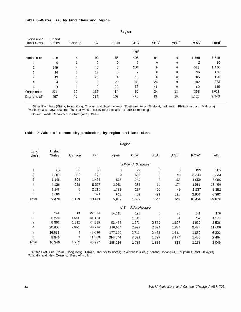
Table 6--Water use, by land class and region

Region

Land use/ Unitedland class States Canada EC Japan OEA1 SEA2 ANZ3 ROW4 Total5

Agriculture 196 4 92 53 408 64 6 1,396 2,2191 0 0 0 0 8 0 0 2 102 149 4 46 0 284 0 6 971 1,460

3 14 0 19 0 7 0 0 96 136

4 19 0 26 4 16 0 0 85 150

5 4 0 0 29 36 23 0 182 273

6 IO 0 0 20 57 41 0 60 189

Other uses 271 39 163 54 62 24 13 395 1,021

Grand total5 467 42 254 108 471 88 19 1,791 3,240

Km3

1Other East Asia (China, Hong Kong, Taiwan, and South Korea). 2Southeast Asia (Thailand, Indonesia, Philippines, and Malaysia).3Australia and New Zealand. 4Rest of world. ‘Totals may not add up due to rounding.

Source: World Resources Institute (WRI), 1990.

Table 7-Value of commodity production, by region and land class

Landclass

UnitedStates

1 652 1,8873 1,1464 4,1365 1,1486 1,095

Total 9,478

1 5412 6,2703 9,8634 20,8055 16,6516 9,845

Total 10,340

Canada EC

21 68360 291505 1,473232 5,377

0 2,2100 694

1,119 10,113

43 22,0864,551 41,1841,632 44,2657,951 45,716

0 49,0300 41,568

1,213 45,387

Region

Japan OEA1 SEA2

Billion U. S. dollars

3 27 00 503 0

505 240 33,361 256 111,355 257 99

612 402 4335,837 1,685 547

U.S. dollars/hectare

14,315 120 00 1,631 0

52,488 1,971 2,589180,524 2,929 2,624

177,290 3,711 2,482396,644 3,088 1,735

155,014 1,788 1,853

ANZ3 ROW4 Total

0 199 38548 2,244 5,333

155 1,959 5,986174 1,911 15,459

46 1,237 6,352221 2,906 6,363643 10,456 39,878

95 141 17094 752 1,273

1,697 1,930 3,5261,897 2,434 11,600

1,581 1,653 6,3023,177 1,450 2,464

813 1,168 3,049

1Other East Asia (China, Hong Kong, Taiwan, and South Korea). 2Southeast Asia (Thailand, Indonesia, Philippines, and Malaysia)3Australia and New Zealand. 4Rest of world.


differentiates the contribution of these land classes toworld production. It is clear from these per hectarevalues, for example, that production is more concen-trated on LC 5 than on LC 6.

Each region in the CGE has three land-intensive sec-tors--crops, livestock, and forestry. Each of thosesectors is divided into, at most, six subsectors, corre-sponding to the six land classes. In addition, cropproducers may, on a given land class, produce up tothree crop aggregates-wheat, other grains, and non-grains. There are substantial regional differences. Inthe United States, for example, maize is a major com-ponent of “other grains”; produce (fruits and vegetables),soybeans, and sugar crops are major components of“nongrains”; and cattle and pigs are major componentsof “livestock” (table 8). Most U.S. forest products aresoftwood products (derived from coniferous trees), andonly 17 percent of the U.S. forestry harvest is used forfuel. In southeast Asia, however, “other grains” is pri-marily rice, “nongrains” is sugar cane and roots andtubers (such as cassava), and “livestock” is pigs, sheep,goats, and cattle. All forest products in southeast Asiaare hardwood products, (derived from deciduous trees),and 69 percent of the harvest is used for fuel. Becauseof such regional differences in the composition of theseand other commodities (including wheat), each region’scommodities are treated as separate goods when traded.

Large portions of agricultural and silvicultural com-modities (approximately 50 percent or more) are

produced in the “rest of world” region (table 9). Otherregions producing more than 10 percent of a given com-modity include the United States (wheat, other grains,and wood), the European Community (wheat), and otherEast Asia (wheat, other grains, nongrains, and live-stock). Crop production on LC I is very small. Worldwheat production is clustered (in descending order) onLC’s 4, 3, 2, and 5. No wheat is produced on LC 6.However, LC 6 does produce 25 percent of the world’sother grains (primarily rice and tropical maize) and 44percent of the world’s nongrains (primarily sugar,tropical roots and tubers, and tropical fruits and vege-tables). Approximately 70 percent of world livestockproduction occurs on LC’s 2, 4, and 6. The prevalenceof both range and irrigated agriculture make LC 2 themost important land class for livestock production.Livestock production on LC’s 4 and 6 is closely asso-ciated with grain production. World production offorest products is most prevalent (46 percent) on LC 6.

Per hectare production of FARM’s agricultural andsilvicultural commodities are presented in table 10.11

For crop outputs, these values reflect productivity dif-ferences across land classes as well as differences in

11Per hectare production values are calculated by dividing a landclass’s output by the total amount of land in that land class used bythe sector. They are not yields. Yields are calculated by dividing aparticular crop’s output by the amount of land planted (or harvested) tothe particular crop.

Table 8-Major components of agricultural and silvicultural production, by region1

Region Other grains

Crops

Nongrains Livestock 2

Forest products

Hardwood Fuelwood

United States Maize Produce, soybeans, and sugar Cattle and pigsCanada Barley and maize Oils, produce, and roots and Cattle and pigs

tubersEC Maize Produce and sugar Cattle, pigs, and sheep and goatsJapan Rice Produce Cattle and pigsOEA3 Rice and maize Produce and roots and tubersSEA4

Pigs and sheep and goatsRice Sugar and roots and tubers Cattle, pigs, and sheep and goats

ANZ5 Barley Sugar Sheep and goatsROW6 Rice, maize, and barley Sugar and produce Cattle and sheep and goats

Percent

34 1710 4

32 1334 152 67

100 6942 969 62

1Commodities that make up more than 20 percent of the total are listed from most to least dominant. 2Does not include poultry.3Other East Asia (China, Hong Kong, Taiwan, and South Korea). 4Southeast Asia (Thailand, Indonesia, Philippines, and Malaysia).5Australia and New Zealand. Rest of world.

Source: United Nations, Food and Agriculture Organization (FAO), 1992.


Table 9--Distribution of agricultural and silvicultural commodities, by region and land class

Commodity/ Unitedland class States

Wheat123456

Total’

0 0 015 12 111 18 1035 2 5313 0 16

0 0 074 32 80

0001001

Other grains123456

Total

0 0 0 023 7 1 0

4 10 1 0156 8 11 9

31 0 9 223 0 3 2

238 25 25 13

Nongrains123456

Total

01910852555

194

All crops123456

Total

0 0 158 21 525 30 44

276 19 24369 0 8278 0 11

506 70 385

Livestock’123456

Total

1 0 038 8 317 8 2879 9 21517 0 3920 0 9

171 24 295

Forest products123456

Total

1731629366

230498

Canada E C Japan OEA1 SEA2 ANZ3 ROW4 Total

Million metric tons

34192420

098

0 0 6 70 1 63 1260 5 72 1340 8 97 2190 2 53 1050 0 0 00 15 291 591

727

4686

103315

0 0 7 80 1 174 2780 4 111 1370 2 150 382

13 0 68 20976 1 134 34389 9 644 1,357

0 0 0 0 72 3 0 51 0 3292 33 2 24 2 1979 179 13 36 3 2540 57 11 87 2 2900 7 6 230 26 873

13 280 32 429 33 1,949

0001

20178200

8404270579492

1,3763,129

0 3 0 190 156 2 5662 50 10 380

23 106 13 50013 194 4 411

8 333 27 1,00746 842 57 2,884

Million head

0001

33255289

24808542

1,181806

1,7195,081

0 77 5 540 164 86 8262 90 44 395

10 102 43 4734 84 22 338

174 64 52017 691 264 2,606

Million m3

0013

135774

1361,125

585935517844

4,142

39 1 0 3 0 2546 2 0 0 3 27

101 19 99 91 16

56 6 30460 7 147

0 30 4 51 4 2510 28 114 12 902

155 171 30 284 32 1,884

0001

23237261

31369

556424428

1,5253,315

Region

1Other East Asia (China, Hong Kong, Taiwan, and South Korea). 2Southeast Asia (Thailand, Indonesia, Philippines, and Malaysia). 3Australiaand New Zealand. 4Rest of world. 5Totals may not add due to rounding. 6The numbers presented here do not include poultry production. Poultryproduction, however, is included in FARM.

Source: United Nations, Food and Agriculture Organization (FAO), 1992.


Table 10-Per hectare production of agricultural and silvicultural commodities, by region and land class

Commodity/ Unitedland class States Canada EC Japan OEA1 SEA2 ANZ3 ROW4 Total

Wheat123456

Total

Other grains123456

Total

Nongrains123456

Total

All crops123456

Total

Livestock123456

Total

Forest products123456

Total

0.44 0.00 0.57 0.00 0.96 0.00 0.00 0.37 0.420.42 0.78 0.33 0.00 1.09 0.00 0.15 0.32 0.440.47 0.87 0.84 0.22 1.32 0.00 0.39 0.40 0.510.41 0.20 1.28 0.22 1.63 0.00 0.57 0.57 0.650.52 0.00 0.97 0.30 1.39 0.00 0.61 0.50 0.590.00 0.00 0.00 0.00 0.00 0.00 0.00 0.00 0.000.39 0.70 1.03 0.22 0.99 0.00 0.30 0.32 0.41

0.13 0.00 0.00 0.00 1.06 0.00 0.00 0.43 0.460.63 0.45 0.33 0.00 2.30 0.00 0.38 0.87 0.960.19 0.48 0.09 0.26 0.52 0.02 0.31 0.62 0.531.82 0.83 0.26 3.36 3.12 0.01 0.18 0.89 1.131.31 0.00 0.53 1.57 5.89 1.16 0.00 0.64 1.171.13 0.00 0.66 4.48 4.52 1.73 0.09 0.54 0.961.25 0.54 0.32 2.80 3.20 1.57 0.18 0.70 0.94

0.15 0.00 0.70 0.00 0.86 0.00 0.00 0.46 0.490.51 0.12 1.41 0.00 1.62 0.00 0.09 1.64 1.390.42 0.12 2.82 4.54 1.70 0.65 0.14 1.10 1.040.98 0.88 4.34 4.77 2.46 0.86 0.23 1.50 1.711.06 0.00 3.41 10.79 5.98 1.86 0.54 2.70 2.772.74 0.00 1.40 13.10 10.09 4.05 1.56 3.51 3.841.02 0.28 3.60 6.90 4.35 3.53 0.67 2.12 2.17

0.71 0.00 1.27 0.00 2.87 0.00 0.00 1.27 1.381.56 1.35 2.07 0.00 5.01 0.00 0.62 2.83 2.791.09 1.47 3.76 5.03 3.54 0.66 0.84 2.13 2.083.21 1.91 5.88 a.35 7.20 0.87 0.97 2.95 3.492.89 0.00 4.91 12.66 13.26 3.03 1.15 3.84 4.533.87 0.00 2.06 17.58 14.61 5.78 1.64 4.05 4.802.66 1.52 4.95 9.92 8.54 5.10 1.15 3.14 3.52

Head

0.04 0.01 0.00 0.00 1.15 0.00 1.44 0.26 0.450.28 0.91 1.46 0.00 1.10 0.00 0.25 0.92 0.730.93 1.15 3.03 16.63 1.96 2.11 1.48 1.64 1.662.00 3.16 7.22 26.31 3.24 3.19 1.56 1.79 2.351.22 0.00 3.57 33.61 2.62 5.59 2.11 1.57 1.821.02 0.00 3.35 43.13 2.33 5.60 3.28 1.29 1.590.71 0.85 5.36 26.48 1.73 5.35 0.61 1.17 1.22

0.47 0.28 1.07 0.00 0.24 0.00 0.35 0.39 0.370.63 0.29 1.62 0.00 0.00 0.00 0.09 0.23 0.301.10 0.55 2.53 1.03 1.45 0.67 0.21 0.70 0.731.59 0.60 3.13 1.43 2.24 1.44 0.26 0.72 1.142.45 0.00 3.14 0.84 2.96 1.51 0.43 0.74 1.013.40 0.00 4.47 2.18 3.82 1.67 0.84 0.79 1.091.69 0.43 3.14 1.19 2.14 1.65 0.28 0.65 0.82

Metric tons



the mix of crops planted and the use of nonland inputs.For livestock and forest products, these values alsoreflect differences in the extent to which grasslandsand forest lands are used for agricultural and silvicul-tural purposes. For example, only a portion of SouthAmerica’s forests and Africa’s savannahs are activelymanaged for timber and livestock.

Because of these distributions, each land class withina region is associated with its own production structure.Of the 301 million hectares of LC 2 in the UnitedStates, for example, 12 percent is cropland, 46 percent ispasture and range, and 16 percent is forest (table 5).LC 2 agricultural land (cropland and pasture) uses149 km3 of irrigation water (11,453 m3 per hectare onaverage) (table 6); produces 15 million metric tons (mt)of wheat, 23 million mt of other grains, and 19 millionmt of nongrains; and supports 38 million head of live-stock. LC 2 forest land in the United States produces31 million m3 of wood (table 9). Output per LC 2 hec-tare is 0.42, 0.63, and 0.51 mt, respectively, for wheat,other grains, and nongrains; 0.28 head for livestock;and 0.63 m3 for wood (table 10). Of the 199 millionhectares of LC 4 in the United States, however, 43percent is cropland, 20 percent is pasture, and 29 per-cent is forest (table 5). LC 4 agricultural land uses 19km’ of irrigation water (221 m3 per hectare on average)(table 6); produces 35 million mt of wheat, 156 millionmt of other grains, and 85 million mt of nongrains; andsupports 79 million head of livestock. LC 4 forest landin the United States produces 93 million m3 of wood(table 9). Output per LC 4 hectare is 0.41, 1.82, and0.98 mt, respectively, for wheat, other grains, and non-grains; 2.00 head for livestock; and 1.59 m3 for wood.These differences indicate that an increase in LC 2coupled with a simultaneous decrease in LC 4 wouldreduce production possibilities overall, while pastureand range would expand at the expense of croplandand forest.

This structure supports the capability of FARM’s CGEmodel to simulate a number of adaptive responses toclimate change by farmers. With respect to outputs,farmers adopt the crop and livestock mix best suitedto their climatic and economic conditions. If changingclimatic conditions alter the growing season enough toshift their land to a new land class, farmers may adopt adifferent crop and livestock mix. (This is like incorpo-rating the “analogous regions” methodology into aformal economic structure.) Farmers also may adjusttheir mix of crops and livestock in response to climate-induced price changes. If the price of wheat were torise, for example, farmers would tend to increase boththeir cropland and the amount of wheat produced perhectare relative to other crops.

Farmers also adopt the mix of primary factor inputs bestsuited to their climatic and economic conditions.12 Ifwater supplies are adversely affected and water pricesincrease, for example, farmers may use less irrigationwater and more land, labor, and/or capital. This mightbe done within a particular land class or, alternatively,by shifting production from land classes that requirerelatively large amounts of irrigation water to landclasses that require less. Similarly, if climate changereduces the amount of land in an agriculturally impor-tant land class, farmers may use less of that land andmore water, labor, and/or capital. They may also usemore land in other land classes. Thus, FARM’s frame-work enables us to analyze how climate change mightalter the distribution and intensity of farming within aregion.13

Simulating Climate Change

In FARM, climate change is simulated by altering watersupplies and the distribution of land across the landclasses within each region. These impacts shift theproduction possibilities associated with regional landand water resources. Given prevailing prices, shifts inproduction possibilities are simultaneously translatedinto changes in commodity supplies and primary fac-tor income. Changes in primary factor income, in turn,generate changes in consumer demands, which are thenreflected in new levels of production, trade, and con-sumption. This section focuses on how FARM’s GIStransforms temperature and precipitation changes gen-erated by general circulation models (GCM’s) intochanges in land and water resources.

General Circulation Models

Climate change scenarios are derived from monthlytemperature and precipitation estimates generated byGCM’s of the Goddard Institute for Space Studies(GISS) (Hansen and others, 1988), Geophysical FluidDynamics Laboratory (GFDL) (Manabe and Wetherald,1987), United Kingdom Meteorological Office (UKMO)(Wilson and Mitchell, 1987), and Oregon State Uni-versity (OSU) (Schlesinger and Zhao, 1989). Thescenarios represent equilibrium climates given a dou-

12Only primary factor inputs are substitutable for one another inproduction. Intermediate inputs (represented by the traded com-modities) are assumed to be used in fixed proportions.

13Most model parameters that govern adaptive responses parameterswere estimated for a limited number of countries but have been appliedbroadly. In other cases, parameters are based on expert opinion.


bling of atmospheric CO2.14 Summary statistics for

the scenarios are presented in table 11. The Intergov-ernmental Panel on Climate Change (IPCC) recentlyconcluded that a doubling of trace gases would lead toan increase in mean global temperature of 1.5-5.0°Cby 2090 (IPCC, 1992). The GCM scenarios consideredhere are at the upper end of the IPCC’s range.

Land Resources

Revised data sets of monthly temperature and precipi-tation are obtained for each GCM by: (1) adding toLeemans and Cramer’s (1991) temperature data, dif-ferences in mean monthly temperatures obtained inGCM runs with current (1xCO2) and double (2xCO2)atmospheric carbon dioxide levels; and (2) multiply-ing Leemans and Cramer’s (1991) precipitation databy the ratio of precipitation in the 2xCO2 GCM run toprecipitation in the 1xCO2 GCM run.15

Using the revised temperature and precipitation data,new sets of growing season lengths (one with and onewithout precipitation constraints) are computed for each

14Equilibrium scenarios presume that atmospheric concentrationsof carbon dioxide, temperature, and precipitation have stabilized.At present, meteorologists arc working to provide “transient” climatechange scenarios that show how temperature and precipitationwould respond to increasing levels of atmospheric carbon dioxidethrough time.

15Results from GCM simulations of current (1xCO2) climatesometimes differ from actual climatic conditions. Comparing2xCO2 GCM runs with 1xCO2 GCM runs minimizes the impacts ofthese errors while maintaining the overall integrity of the simula-tion results.

GIS grid ce11.16 Each GIS grid cell is assigned theappropriate land class. The revised growing seasonlength may alter the land class to which a given cellis assigned. In this way, climate change can alter re-gional endowments of the six land classes.

Two sets of land class changes are computed for eachGCM scenario. One set contains regional net changesin land classes and is used to evaluate all potentialeconomic impacts of global climate change, includingimpacts generated by changes in land use. The secondset contains net changes in land classes on existing landuse and cover patterns in the regions. Using both setsof changes enables us to evaluate economic impactsof climate change while constraining total quantitiesof cropland, permanent pasture, and forest land in eachregion to their 1990 levels. This has two purposes.First, it serves as a check on situations where land usescannot change as easily as indicated in our model.Second, it measures climate change’s potential effectson existing agricultural and silvicultural systems.

Water Resources

Changes in regional water supplies also are estimatedwith the revised temperature and precipitation data.First, estimates of water runoff under current climaticconditions are calculated using Leemans and Cramer’s(1991) mean monthly temperature and precipitationdata. Annual water runoff is the sum of monthly run-offs in an area. Monthly runoff is that portion ofmonthly precipitation that is not evapotranspirated backto the atmosphere. Monthly evapotranspiration esti-

16Revised growing season lengths are provided by the World SoilResources Office of USDA’s Natural Resources Conservation Service.

Table 11-Summary statistics for the general circulation models used as the basisfor climate change scenarios

Change in average global:

Scenario1 Year calculated Resolution Carbon dioxide Temperature Precipitation

Lat. * long. ppm Celsius Percent

GISS 1982 7.83° l 10.0° 630 4.2° 11GFDL 1988 4.44° l 7.5° 600 4.0° 8UKMO 1986 5.00° * 7.5° 640 5.2° 15OSU 1985 4.00° * 5.0° 652 2.8° 8

1Climate change scenarios generated by the general circulation models of the Goddard Institute for Space Studies (GISS), the Geophysi-cal Fluid Dynamics Laboratory (GFDL), the United Kingdom Meteorological Office (UKMO), and Oregon State University (OSU).

Sources: For GISS, GFDL, and UKMO scenarios: Rosenzweig, Parry, Frohberg, and Fischer, 1993. For the OSU scenario: Dixit, 1994.


mates are obtained from monthly temperature data(Thomthwaite, 1948).17

Second, water runoff in each region is derived for thefour GCM scenarios using the appropriate revised tem-perature and precipitation data. Third, regionalpercentage changes in water runoff are calculated bycomparing the GCM-based runoff estimates with run-off estimates derived from the original Leemans andCramer (1991) temperature and precipitation data.18

Fourth, regional percentage changes in water suppliesare computed using the runoff elasticities of watersupply presented in table 4 (% ∆ W = % ∆ RxE, where% ∆ W is the percentage change in a region’s watersupply, % ∆ R is the percentage change in a region’srunoff, and E is the runoff elasticity of water supply).

Limitations and Strengths

The FARM framework contains several strengths thatsignificantly advance our ability to evaluate potentialimpacts of global climate change on regional andworld agriculture. At the same time, a number oflimitations should be made explicit.

Land and Water Resources

One limitation is that land classes are defined by cli-matic variables and do not account for soil character-istics or other factors that affect productivity. Thesenonclimatic factors may not accompany climate-inducedshifts in length of growing season. While we assumethat productivity per unit area follows the migrationof growing seasons, it is more likely to decrease orincrease in a given instance. This means that farmeradaptations simulated by FARM are somewhat uncer-tain and subject to independent verification. Per unitarea productivity of natural ecosystems also is not likelyto follow the migration of growing seasons. Somenatural ecosystems will find it difficult or impossibleto migrate, even with direct human assistance.

Procedures for simulating water resources are limitedin three ways. First, water storage in alpine snowpackis not taken into account. Alpine snowpack is animportant source of irrigation water in the WesternUnited States, northern Africa, the Middle East, Indra,and China. Reductions in snowpack might causeshortages of irrigation water in some of these regionsduring critical times of the year. Second, water istreated as though it could be used anywhere within agiven region; hence, water is considerably more mobilein our model than in reality. Third, water is alwaysbeneficial. In fact, too much water can wash awaycrops, waterlog soils, delay planting, or inhibit har-vesting. These limitations suggest that our estimatesof climate-induced changes in water supplies are prob-ably optimistic and that negative impacts attributableto water supply changes are probably underestimated.We examine the sensitivity of our results to the speci-fication of water shocks by simulating each climatechange scenario with and without climate-induced watersupply shocks.

Economic Impacts

Four limitations of FARM’s economic framework needto be made clear. First, substitution between interme-diate goods or between intermediate and primary factorsis not allowed. This means that increases in fertilizercannot be used to offset climate-induced productivitylosses. Second, FARM considers only the commodityvalue of land. The value of land’s environmentalamenities is not included. This means, for example,that values of sawlogs, pulpwood, and similar forestcommodities are tracked, but values for forest-relatedimprovements in air and water quality are not. Third,the region “rest of world” includes Latin America, Af-rica, west Asia, much of South Asia, the former SovietUnion, and countries in Europe outside the EuropeanCommunity (EC). For a large portion of the world,then, it is difficult to obtain precise information abouthow the economic impacts of climate change wouldbe distributed.

17McKenney and Rosenberg (1993) suggest that Thornthwaite’smethod produces estimates of potential evapotranspiration that areunrealistically high at warmer locations, In Thornthwaite’s method,however, potential evapotranspiration generally (1) is equal to zerowhen temperature is less than or equal to 0°C; (2) increases at an in-creasing rate as temperatures range between 0°C and 26.5°C; (3) in-creases at a decreasing rate as temperatures range from 26.5°C to37.5°C; and (4) is constant when temperature is above 37.5°C.McKenney and Rosenberg derive their results solely from the for-mula used to estimate potential evapotranspiration between 0°C and26.5°C. Their results, therefore, do not accurately portrayThornthwaite’s method at warmer locations.

18GIS estimates of water runoff computed with Leemans and Cra-mer’s (1991) weather data differ from those derived from WRI(1992). Comparing estimates of runoff based on a standard weatherdatabase minimizes the impacts of these differences.

Finally, our benchmark is the world economy as itexisted in 1990. This means that: (1) some potentialadaptations (such as new cultivars or new livestockbreeds) are not considered; (2) direct costs of physicallyconverting land from one use to another (such asbuilding roads, clearing trees, or burning brush) areignored; and (3) current economic distortions in theform of subsidies and tariffs are in place.”

19The model embodies some technological innovation by assumingthat productivity per unit area does not change when following aclimate-induced migration of land classes even when the migrationis to poorer quality soils.


Climate Change Scenarios

Our climate change scenarios are limited to how alter-native global patterns of mean monthly temperatureand precipitation affect land and freshwater resources.We do not simulate all potential impacts associatedwith climate change (such as possible rises in sea levelor increased variability in weather).

Results

We also do not consider physiological effects of greateratmospheric concentrations of carbon dioxide or othertrace gases on plant growth. Based on results of manycontrolled-environment experiments, higher levels ofatmospheric carbon dioxide act as a fertilizer for someplants and improve water-use efficiency for others(Kimball, 1983; Cure and Acock, 1986; IPCC, 1990).A number of studies that assess economic impacts ofclimate change on regional and world food systemspositively adjust crop yields in their climate changesimulations to reflect this “fertilizer effect” (Adamsand others, 1988; Easterling and others, 1992; andRosenzweig and Parry, 1994). The magnitude of any“fertilizer effect,” however, is still very uncertain.Major sources of uncertainty include impacts of in-creased carbon dioxide on weed growth, interactioneffects on crop growth among atmospheric carbondioxide levels and other environmental variables (nota-bly temperature and water availability), and negativeimpacts on crop yields of other gases (particularlyozone, sulfur dioxide, and nitrogen dioxide) releasedby burning fossil fuels (Wolfe and Erickson, 1993).

Strengths

Limitations aside, FARM extends previous research bylinking land and water resources directly to climateconditions and economic activity; hence, our simula-tions of human responses to climate change areeconomically consistent with resource impacts, pro-duction technologies, and consumer preferences.FARM also integrates many advances made in earlierworks. Specifically, FARM (1) uses GIS data similarto Leemans and Solomon (1993), (2) incorporates mul-tisector impacts as in Bowes and Crosson (1991), and(3) simulates global impacts on production and tradeas in Kane, Reilly, and Tobey (1991) and Rosenzweigand Parry (1994). The result is a framework that (1) in-cludes climate effects on crops, livestock, and forestrysimultaneously, (2) simulates endogenous adaptive re-sponses to climate change by farmers, (3) explicitlysimulates land and water resource markets, (4) in-cludes detailed interactions with the rest of theeconomy, and (5) provides global coverage.

We place special emphasis on the role of adaptation inadjusting to new climatic conditions. By necessity,many regional and sectoral effects are not discussed.Appendix B presents detailed results of climate-inducedchanges in land class endowments and economic effectsby region and GCM scenario.

Impacts on Endowments

Changes in the distribution of land across land classesand changes in water supplies are used by the CGEmodel to simulate climate change. These and otherresults are used to evaluate economic responses to theclimate change scenarios with respect to their overallmagnitude, impacts on land and water resources, andimplications for U.S. and global agriculture.

Land Resources

Twenty-nine to forty-six percent of the world’s landendowment (outside Antarctica) faces changes in cli-matic conditions that are large enough to result in newland class assignments.20 The scenario ranking, fromlowest to highest, is OSU, GISS, GFDL, and UKMO(table 12). This ranking is not perfectly correlated witheither GCM temperature or precipitation changes. Weuse this ranking when referring to the strength of cli-matic shocks generated by the four GCM scenarios; thatis, we consider the OSU climatic shock to be “weaker”than the UKMO climatic shock. The shock patterngenerally follows the same order in each region as forthe world as a whole. The major exception is Austra-lia/New Zealand. This indicates that the GCM’s areconsistently different with respect to each other.

Across scenarios, the global endowment of LC 1 (landwith short growing seasons due to cold temperatures)decreases (table 13 and fig. 3).21 In terms of growingseason lengths, climate change is likely to increase theamount of land suitable for agriculture and silviculture,especially in arctic and alpine areas. However, LC 6(land with growing seasons longer than 10 months, pri-marily in the tropics) decreases in each scenario and LC2 (desert/dry grasslands) increases in three scenarios.This indicates that soil moisture losses are likely to re-duce agricultural possibilities in many areas of theworld. These results are consistent with Leemans andSolomon (1993).

20Results are reported in ranges because we examine four climatechange scenarios. Results for specific scenarios are shown in the ta-bles or figures cited.

21Regional changes in the distribution of land across land classesare used by the CGE model to simulate climate change’s impactson land resources. These are presented in appendix B.


Agriculturally important land increases in high-latituderegions, but decreases in tropical regions (table 14).In mid-latitude regions, changes in agriculturally im-portant land may be positive or negative. These resultssuggest that, under global climate change, agriculturalpossibilities are likely to increase in high-latitude re-gions and decrease in tropical areas.

the total value of existing agricultural land declines un-der the land class distributions generated by the fourclimate change scenarios. These results imply thatclimate change will likely impair the existing agricul-tural system.

Water Resources

Globally, 41.2 to 59.7 percent of existing cropland faceschanges in climatic conditions that result in new landclass assignments (table 15 and fig. 4).22 Under eachscenario, more than half of the cropland that does ex-perience a change in land class shifts to a class with ashorter growing season (LCi < LC0). Using current rents,

22The GIS can track, for example, how much LC 4 cropland in agiven region becomes LC 2, LC 3, LC 5, or LC 6 as well as howmuch remains LC 4. This is done by combining the relevant land-use and cover data in Olson (1989-91) with the current and appro-priate scenario-based land-class data sets.

Water runoff for the world as a whole will likely in-crease with climate change (table 16). The scenarioranking, from lowest to highest, is UKMO, OSU, GISS,and GFDL. This ranking is not perfectly correlatedwith either GCM precipitation changes or the strengthof climate change shock indicated by land classchanges. Among the regions, the only scenario rankingthat is the same as the world’s is that for “rest ofworld.” These results reveal the high levels of vari-ability and uncertainty that accompany our knowledgeabout potential climate-induced changes in water re-sources.

Table 12-Percentage of total land changing land class, by region and climate change scenario

Region

Scenario1UnitedStates Canada EC Japan OEA2 SEA3 ANZ4 ROW 5 Total

GISS 40.0 37.7 71.8 65.9GFDL 47.0 48.7 84.0 73.9UKMO 55.3 58.8 85.7 78.8OSU 38.9 35.3 59.3 63.8

Percent

34.934.543.926.1

21.9 18.5 31.2 32.327.1 25.1 38.6 39.434.3 24.6 45.6 46.216.0 26.4 26.8 28.6

1Climate change scenarios generated by the general circulation models of the Goddard Institute for Space Studies (GISS), the Geophysi-cal Fluid Dynamics Laboratory (GFDL), the United Kingdom Meteorological Office (UKMO), and Oregon State University (OSU).2Other East Asia (China, Hong Kong, Taiwan, and South Korea).4Australia and New Zealand.

3Southeast Asia (Thailand, Indonesia, Philippines, and Malaysia).5Rest of world.

Table 13-Changes in world land class endowments, by climate change scenario

Land class

Scenario1 1 2 3 4 5 6

GISS

GFDL

UKMO

OSU

-39.8

-47.7

-62.5

-32.6

-1.4

17.2

16.4

6.9

Percent change

28.7 51.6

28.7 37.0

38.8 78.1

16.7 21.9

4.7 -10.1

18.2 -31.1

4.4 -39.2

17.8 -11.7

‘Climate change scenarios generated by the general circulation models of the Goddard Institute for Space Studies (GISS), the Geophysi-cal Fluid Dynamics Laboratory (GFDL), the United Kingdom Meteorological Office (UKMO), and Oregon State University (OSU).


Figure 3

Effect of climate change on distribution of landamong land classes (LC)

Percent change in acreage

150GISS UKMO

100 GFDL OSU

50

0

-50

-100LC 1 LC 2 LC 3 LC 4 LC 5 LC 6

Table 14-Changes in agriculturally importantland, by area and climate change scenario

Scenario1 High latitudes2 Tropics3 Other areas4

GISS 58.6GFDL 21.2UKMO 49.3OSU 7.8

Percent change

-20.5-39.7-52.0-18.6

-0.51.2

-3.66.8

1Climate change scenarios generated by the general circula-tion models of the Goddard Institute for Space Studies (GISS),the Geophysical Fluid Dynamics Laboratory (GFDL), the UnitedKingdom Meteorological Office (UKMO), and Oregon State Uni-versity (OSU). 2Land with growing season length from 101 to250 days in Canada, non-EC Europe, and the former SovietUnion. 3Land with growing season length greater than 300days in Africa, Latin America, and Asia (except Japan, China,and South Korea). 4Land with growing season length from 101to 300 days.

GISS = Goddard Institute for Space Studies.GFDL = Geophysical Fluid Dynamics LaboratoryUKMO = United Kingdom Meteorological Office.OSU = Oregon State University.

Table 15-Global changes in land classes on existing cropland and in the value of existing croplandand agricultural land under existing rents

Scenario1

GISSGFDLUKMOOSU

Cropland land class changes Value changes

Total To shorter land classes2 Cropland Agricultural land3

Percent change

43.8 21.9 0.7 -0.343.4 37.0 -3.2 -1.859.7 41.3 -5.4 -3.541.2 25.1 -0.5 -0.8

1Climate change scenarios generated by the general circulation models of the Goddard Institute for Space Studies (GISS), the Geo-physical Fluid Dynamics Laboratory (GFDL), the United Kingdom Meteorological Office (UKMO), and Oregon State University (OSU).

2Shifts to land classes with shorter growing seasons. 3Includes cropland and pasture.

All changes in regional water supplies follow the samedirection as changes in runoff. Regional water runoffdecreases in five cases (the United States, GISS; Euro-pean Community, GISS; Japan, GISS and UKMO; andsoutheast Asia, OSU), indicating potential water shortagesin some areas (table 16). Regional runoff also Increasesby more than 20 percent in eight cases (Canada, UKMO;other East Asia, GISS and GFDL; Australia/New Zea-land, GISS, GFDL, and OSU; and “rest of world,”GISS and OSU). These results show that increasedflooding or water logged soils could become moreprevalent in some areas.

Our methodology does not include climate-inducedchanges in snowpack when determining changes inwater supplies. This means that the water supplychanges presented in table 16 are likely to be too highwhen supplies are estimated to increase and not lowenough when supplies are estimated to decrease. Inturn, estimated impacts on production possibilities willbe too positive.

U.S. Resources

Across scenarios, 38.9 to 55.3 percent of U.S. land faceschanges in climatic conditions that result in new land


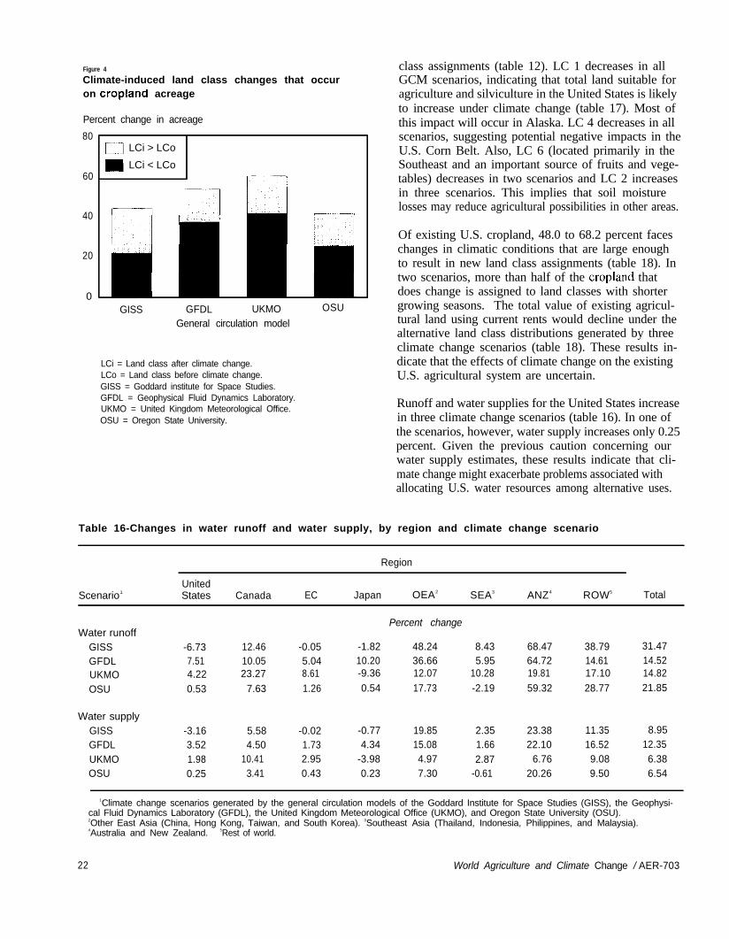
Figure 4

Climate-induced land class changes that occuron cropland acreage


80

60

40

20

0

LCi > LCo

LCi < LCo

GISS GFDL UKMO OSU

General circulation model

LCi = Land class after climate change.LCo = Land class before climate change.GISS = Goddard institute for Space Studies.GFDL = Geophysical Fluid Dynamics Laboratory.UKMO = United Kingdom Meteorological Office.OSU = Oregon State University.

class assignments (table 12). LC 1 decreases in allGCM scenarios, indicating that total land suitable foragriculture and silviculture in the United States is likelyto increase under climate change (table 17). Most ofthis impact will occur in Alaska. LC 4 decreases in allscenarios, suggesting potential negative impacts in theU.S. Corn Belt. Also, LC 6 (located primarily in theSoutheast and an important source of fruits and vege-tables) decreases in two scenarios and LC 2 increasesin three scenarios. This implies that soil moisturelosses may reduce agricultural possibilities in other areas.

Of existing U.S. cropland, 48.0 to 68.2 percent faceschanges in climatic conditions that are large enoughto result in new land class assignments (table 18). Intwo scenarios, more than half of the cropland thatdoes change is assigned to land classes with shortergrowing seasons. The total value of existing agricul-tural land using current rents would decline under thealternative land class distributions generated by threeclimate change scenarios (table 18). These results in-dicate that the effects of climate change on the existingU.S. agricultural system are uncertain.

Runoff and water supplies for the United States increasein three climate change scenarios (table 16). In one ofthe scenarios, however, water supply increases only 0.25percent. Given the previous caution concerning ourwater supply estimates, these results indicate that cli-mate change might exacerbate problems associated withallocating U.S. water resources among alternative uses.

Table 16-Changes in water runoff and water supply, by region and climate change scenario

Region

Scenario1UnitedStates Canada EC Japan OEA2 SEA3 ANZ4 ROW5 Total

Water runoffGISSGFDLUKMOOSU

Water supplyGISSGFDLUKMOOSU

-6.73 12.46 -0.05 -1.82 48.24 8.43 68.47 38.79 31.477.51 10.05 5.04 10.20 36.66 5.95 64.72 14.61 14.524.22 23.27 8.61 -9.36 12.07 10.28 19.81 17.10 14.82

0.53 7.63 1.26 0.54 17.73 -2.19 59.32 28.77 21.85

-3.16 5.58 -0.02 -0.77 19.85 2.35 23.38 11.35 8.953.52 4.50 1.73 4.34 15.08 1.66 22.10 16.52 12.351.98 10.41 2.95 -3.98 4.97 2.87 6.76 9.08 6.380.25 3.41 0.43 0.23 7.30 -0.61 20.26 9.50 6.54

Percent change

1Climate change scenarios generated by the general circulation models of the Goddard Institute for Space Studies (GISS), the Geophysi-cal Fluid Dynamics Laboratory (GFDL), the United Kingdom Meteorological Office (UKMO), and Oregon State University (OSU).2Other East Asia (China, Hong Kong, Taiwan,4Australia and New Zealand.

and South Korea). 3Southeast Asia (Thailand, Indonesia, Philippines, and Malaysia).5Rest of world.


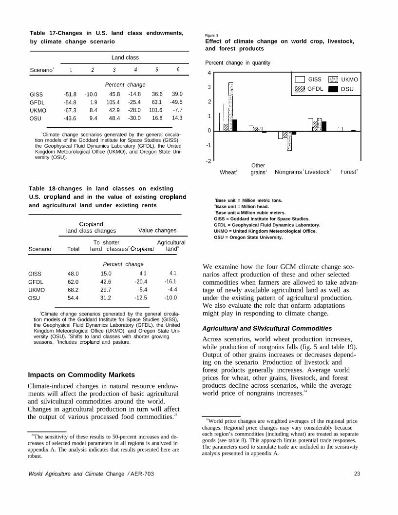
Table 17-Changes in U.S. land class endowments,by climate change scenario

Land class

Scenario1 1 2 3 4 5 6

Percent change

GISS -51.8 -10.0 45.8 -14.8 36.6 39.0

GFDL -54.8 1.9 105.4 -25.4 63.1 -49.5

UKMO -67.3 8.4 42.9 -28.0 101.6 -7.7

OSU -43.6 9.4 48.4 -30.0 16.8 14.3

2

1

0

-1

1Climate change scenarios generated by the general circula-tion models of the Goddard Institute for Space Studies (GISS),the Geophysical Fluid Dynamics Laboratory (GFDL), the UnitedKingdom Meteorological Office (UKMO), and Oregon State Uni-versity (OSU).

Table 18-changes in land classes on existingU.S. cropland and in the value of existing croplandand agricultural land under existing rents

Scenario1

Croplandland class changes Value changes

To shorterland classes2 Cropland

AgriculturalTotal land3

GISS 48.0

GFDL 62.0UKMO 68.2OSU 54.4

Percent change

15.0 4.1

42.6 -20.429.7 -5.431.2 -12.5

4.1-16.1

-4.4-10.0

1Climate change scenarios generated by the general circula-tion models of the Goddard Institute for Space Studies (GISS),the Geophysical Fluid Dynamics Laboratory (GFDL), the UnitedKingdom Meteorological Office (UKMO), and Oregon State Uni-versity (OSU). 2Shifts to land classes with shorter growingseasons. 3Includes cropland and pasture.

Impacts on Commodity Markets

Climate-induced changes in natural resource endow-ments will affect the production of basic agriculturaland silvicultural commodities around the world.Changes in agricultural production in turn will affectthe output of various processed food commodities.23

23The sensitivity of these results to 50-percent increases and de-creases of selected model parameters in all regions is analyzed inappendix A. The analysis indicates that results presented here arerobust.

Figure 5

Effect of climate change on world crop, livestock,and forest products

Percent change in quantity

4GISS UKMO

3 GFDL OSU

-2Other

Wheat1 grains 1 Nongrains 1 Livestock 2 Forest 3

1Base unit = Million metric tons.2Base unit = Million head.3Base unit = Million cubic meters.GISS = Goddard Institute for Space Studies.GFDL = Geophysical Fluid Dynamics Laboratory.UKMO = United Kingdom Meteorological Office.OSU = Oregon State University.

We examine how the four GCM climate change sce-narios affect production of these and other selectedcommodities when farmers are allowed to take advan-tage of newly available agricultural land as well asunder the existing pattern of agricultural production.We also evaluate the role that onfarm adaptationsmight play in responding to climate change.

Agricultural and Silvicultural Commodities

Across scenarios, world wheat production increases,while production of nongrains falls (fig. 5 and table 19).Output of other grains increases or decreases depend-ing on the scenario. Production of livestock andforest products generally increases. Average worldprices for wheat, other grains, livestock, and forestproducts decline across scenarios, while the averageworld price of nongrains increases.24

24World price changes are weighted averages of the regional pricechanges. Regional price changes may vary considerably becauseeach region’s commodities (including wheat) are treated as separategoods (see table 8). This approach limits potential trade responses.The parameters used to simulate trade are included in the sensitivityanalysis presented in appendix A.


Table 19-Changes in quantities and prices of agricultural, silvicultural, and processed food commodities,by region and climate change scenario

Scenario1 Variable CommodityUnitedStates

GISS Quantity Wheat 6.0 2.4 -13.2 -49.8 -0.3 0.0 17.5Other grains -5.9 12.4 29.2 11.3 0.6 -3.7 4.3Nongrains 2.8 35.6 -10.6 13.4 3.8 0.3 -3.8Total crops -0.8 12.1 -8.6 11.5 2.1 -0.9 3.1Livestock -0.7 8.6 -1.7 1.6 0.7 -0.9 -0.9Forest products 0.7 3.5 3.5 6.2 0.6 -4.6 -0.5Fish, meat, and milk -0.2 4.9 -1.3 1.4 0.6 -1.2 -0.2Other proc. foods 0.1 3.1 -1.4 1.4 1.0 -3.4 0.3

Price Wheat 3.0 7.4 30.9 56.1 5.5 0.0 1.6Other grains 1.1 -11.7 -29.7 -13.1 0.0 10.0 -7.2Nongrains -4.3 -19.8 6.6 -18.4 -5.9 -2.8 1.2Total crops -0.5 -4.9 6.9 -15.4 -2.6 1.6 2.0Livestock 0.0 -9.2 1.1 -2.5 -0.8 -1.1 -0.5Forest products -3.0 -6.2 -10.7 -5.3 -0.2 1.6 -0.4Fish, meat, and milk 0.0 -4.7 1.5 -1.0 -0.3 -0.1 -0.2Other proc. foods -0.4 -1.8 0.7 -2.4 -0.5 2.7 -0.2

GFDL Quantity Wheat 12.4 9.5 -12.0 -60.3 -12.1 0.0 3.3Other grains -6.5 16.8 21.9 12.5 0.9 -3.1 1.7Nongrains -3.9 36.1 -6.5 17.2 6.6 1.3 -3.9Total crops -2.7 17.0 -5.8 14.2 2.3 0.0 -1.1Livestock -0.5 8.4 -1.6 1.6 0.7 -0.8 -1.2Forest products -0.8 3.9 3.4 9.1 1.3 -4.4 -0.3Fish, meat, and milk -0.2 4.9 -1.1 1.3 0.6 -1.0 -0.5Other proc. foods -0.4 3.3 -1.2 1.4 0.8 -2.8 0.0

Price Wheat -10.4 -4.1 19.3 0.0 59.1 9.2 -3.7Other grains 2.2 -14.6 -25.1 -14.3 -0.9 7.8 -5.2Nongrains 3.9 -16.9 6.1 -20.1 -6.3 -0.9 3.6Total crops 1.5 -9.5 5.8 -17.3 -2.7 2.0 0.2Livestock -0.6 -9.0 1.4 -2.9 -1.1 -1.0 -0.5Forest products -0.1 -4.4 -8.8 -6.7 -0.1 2.4 -0.2Fish, meat, and milk -0.4 -4.8 1.3 -1.0 -0.4 -0.1 -0.3

Canada EC Japan OEA2 SEA3 ANZ4

Region

Percent change

ROW5 Total

5.61.6

-0.70.51.50.21.11.5

-14.9-6.72.5

-2.0-2.7-0.7-1.2-1.7

1.90.4

-0.50.00.90.30.40.4

-2.5-3.50.5

-1.5-1.9-1.7-0.4-0.8

0.50.3

-0.4-0.10.70.00.30.2

-7.8-4.32.9

-0.9-1.9-0.1-0.5

Continued-

5.11.4

-1.20.01.3

-0.10.80.8

-18.9-8.25.6

-1.0-2.70.9

-1.1

See footnotes at end of table.


Table 19-Changes in quantities and prices of agricultural, silvicultural, and processed food commodities,by region and climate change scenario-continued

Scenario1 Variable CommodityUnitedStates Canada

UKMO Quantity Wheat 9.4 7.4Other grains -7.1 17.8Nongrains 0.6 46.8Total crops -1.7 18.5Livestock -0.6 10.5Forest products -0.5 5.3Fish, meat, and milk -0.1 6.0Other foodsproc. -0.2 4.1

Price Wheat -3.5 1.8Other grains 0.0 -16.9Nongrains -0.6 -21.5Total crops 0.4 -8.9Livestock -0.7 -11.0Forest products -1.7 -8.0Fish, meat, and milk -0.5 -5.8Other foodsproc. -0.1 -2.3

OSU Quantity Wheat 1.5 14.0Other grains -7.3 15.5Nongrains -0.3 23.2Total crops -3.4 16.3Livestock -1.3 7.1Forest products -0.3 2.6Fish, meat, and milk -0.6 4.1Other foodsproc. -0.3 2.7

Price Wheat -2.4 -3.8Other grains 6.2 -11.3Nongrains -1.4 -13.9Total crops 1.8 -8.3Livestock 1.2 -7.3Forest products -1.2 -2.7Fish, meat, and milk 0.7 -3.8Other foodsproc. 0.0 -1.5

EC Japan OEA2 SEA3 ANZ4 ROW5 Total

Percent change

-14.7 -64.5 -0.7 0.0 2.8 a.7 3.329.6 12.4 -0.2 -5.5 -3.3 2.4 0.3-9.3 17.9 3.1 2.3 -2.5 -2.0 -1.3-7.9 14.6 1.4 -0.1 -1.2 0.0 -0.3-1.9 1.4 0.5 -1.6 -3.3 1.9 0.93.9 10.4 0.8 -6.6 -1.7 0.0 0.0

-1.4 1.1 0.5 -1.9 -1.4 1.2 0.2-1.6 1.3 0.8 -5.1 -0.3 1.5 0.2

31.9 79.9 0.9 0.0 2.0 -24.6 -9.7-31.4 -16.1 -0.1 14.4 -3.9 -12.4 -6.4

7.8 -21.8 -3.9 -2.6 1.6 7.9 4.48.1 -19.1 -2.0 2.9 1.4 -1.5 -1.10.9 -3.2 -1.0 -1.3 0.2 -4.0 -2.7

-11.2 -8.8 -0.2 3.1 0.6 0.1 -1.01.5 -1.0 -0.4 0.0 0.0 -1.7 -0.70.9 -2.9 -0.7 4.1 -0.1 -2.4 -1.0

-6.6 -55.7 -5.2 0.0 17.7 2.9 0.817.3 13.2 0.4 -1.0 11.7 0.9 -0.1-5.2 14.9 4.7 -1.2 -2.0 -0.7 -0.2-4.0 13.0 1.9 -1.1 5.3 0.0 0.0-1.0 1.6 0.2 -0.1 3.5 0.9 0.71.8 6.7 0.7 -2.5 2.2 0.1 0.1

-0.6 1.4 0.1 -0.2 2.0 0.6 0.3-0.6 1.3 0.2 -0.9 1.5 0.6 0.3

8.7 55.9 4.1 0.0 -6.0 -11.3 -4.6-19.5 -12.2 2.4 2.8 -6.9 -4.2 -1.0

3.0 -19.1 -6.3 -0.7 0.8 2.0 0.22.2 -15.3 -2.1 0.6 -1.4 -1.1 -1.21.3 -2.2 -0.2 -0.6 -2.2 -1.7 -1.2

-4.9 -5.1 -0.2 0.8 -2.6 0.3 -0.40.8 -0.9 0.0 -0.2 -1.1 -0.7 -0.20.2 -2.2 0.3 0.6 -0.6 -1.0 -0.6

Region


2Other East Asia (China, Hong Kong, Taiwan,4Australia and New Zealand.

and South Korea). 3Southeast Asia (Thailand, Indonesia, Philippines, and Malaysia).5Rest of world.


Global impacts mask more pronounced variations inregional impacts (table 19). In Canada, FARM’s onlyunambiguously high-latitude region, output of wheat.other grains, nongrains, livestock, and forest productsincreases in all scenarios. In southeast Asia, FARM’sonly unambiguously tropical region, production of thesecommodities generally decreases in all scenarios (ex-ceptions are nongrains in the GISS, GFDL, and UKMOscenarios). These changes in regional production ofagricultural and silvicultural commodities reflect longerand warmer growing seasons at high latitudes andshorter and drier growing seasons in the tropics. Im-pacts on mid-latitude regions are mixed.

In the United States, output of wheat increases, whileoutput of other grains (primarily maize) decreasesacross all scenarios (table 20). Production of nongrainsincreases or decreases depending on the scenario.Livestock production decreases in all scenarios, andforestry production decreases in three scenarios. U.S.shares of world production move in the same directionas changes in U.S. production. These results indicatethat climate change is likely to have negative impactson some important U.S. agricultural sectors.

Other Commodities

Although climate-induced changes in production possi-bilities will be most pronounced for agriculture andsilviculture, other sectors will be affected as well. Ingeneral, world production of the goods and services inmany sectors will increase (table 21). Output of fish,meat, milk. and other processed foods, for example,increases in all scenarios. This indicates that climatechange’s overall impact on world food production islikely to be beneficial. Not all sectors will increase

output, however. Production of minerals such as metalores, salt, and phosphate rock, for example, declinesin all scenarios. Also, world production of services,which makes up 47 percent of world output in dollarterms, falls in the two strongest climate change scenar-ios (the GFDL and UKMO scenarios).

Regional production of processed food commoditiestends to follow regional production of agriculturalcommodities. For example, production of processedfood commodities increases in all scenarios for Canadaand decreases in all scenarios for southeast Asia (table19). In the United States, production of processed foodcommodities generally declines. The decreases in pro-duction of fish, meat, and milk are associated withdecreases in output of other grains (primarily maize)and livestock in all four scenarios. U.S. production ofother processed foods decreases in three scenarios.The increase in the GISS scenario is associated with arelatively large increase in nongrain production.

Comparison with Previous Research

Our results are more positive for world food productionthan those reported in earlier research, even in researchthat includes the beneficial effects of atmosphericcarbon dioxide on plant growth. This can be illustratedin more detail by focusing on cereals (wheat and othergrains). After taking carbon dioxide fertilization andvarious adaptations into account, climate-induced im-pacts on world cereal production in Rosenzweig andParry (1994) are approximately 1.0, 0.0, and -2.5 per-cent, respectively, for the GISS, GFDL, and UKMOscenarios. However, our research indicates that, withoutcarbon dioxide fertilization, world cereal productionincreases by 0.9, 0.3, and 1.2 percent, respectively,

Table 20-Changes in U.S. production and U.S. shares of world production of agriculturaland silvicultural products, by commodity and climate change scenario

U.S. production U.S. share of world production

Other Forest OtherScenario1

ForestWheat grains Nongrains Livestock products Wheat grains Nongrains Livestock products

Percent change

GISS 6.0 -5.9 2.8 -0.7 0.7 4.0 -6.2 3.3 -1.5 0.4GFDL 12.4 -6.5 -3.9 -0.5 -0.8 11.9 -6.8 -3.5 -1.2 -0.8UKMO 9.4 -7.1 0.6 -0.6 -0.5 5.9 -7.4 1.9 -1.5 -0.5OSU 1.5 -7.3 -0.3 -1.3 -0.3 0.7 -7.2 -0.2 -2.0 -0.4


2 6 World Agriculture and Climate Change I AER-703

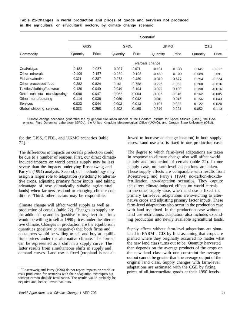
Table 21-Changes in world production and prices of goods and services not producedin the agricultural or silvicultural sectors, by climate change scenario

Scenario1

GISS GFDL UKMO OSU

Commodity Quantity Price Quantity Price Quantity Price Quantity Price

Percent change

Coal/oil/gas 0.182 -0.087 0.097 -0.071 0.101 -0.138 0.145 -0.022Other minerals -0.409 0.157 -0.280 0.108 -0.439 0.109 -0.089 0.091Fish/meat/milk 0.371 -0.387 0.273 -0.489 0.310 -0.677 0.294 -0.224Other processed food 0.382 -0.824 0.161 -0.758 0.225 -1.032 0.260 -0.616Textiles/clothing/footwear 0.120 -0.049 0.049 0.104 -0.022 0.100 0.190 -0.016Other nonmetal manufacturing 0.098 -0.047 0.062 -0.004 -0.006 -0.046 0.162 -0.005Other manufacturing 0.114 0.036 0.060 0.042 0.001 0.046 0.156 0.043Services 0.023 0.044 -0.003 0.013 -0.107 0.022 0.122 0.020Global shipping services -0.033 0.258 -0.202 0.168 -0.319 0.224 -0.052 0.113

1Climate change scenarios generated the by general circulation models of the Goddard Institute for Space Studies (GISS), the Geo-physical Fluid Dynamics Laboratory (GFDL), the United Kingdom Meteorological Office (UKMO), and Oregon State University (OSU).

for the GISS, GFDL, and UKMO scenarios (table22).25

The differences in impacts on cereals production couldbe due to a number of reasons. First, our direct climate-induced impacts on world cereals supply may be lesssevere than the impacts underlying Rosenzweig andParry’s (1994) analysis. Second, our methodology mayassign a larger role to adaptation (switching to alterna-tive crops, adjusting primary factor inputs, and takingadvantage of new climatically suitable agriculturallands) when farmers respond to changing climate con-ditions. Third, other factors may be responsible.

Climate change will affect world supply as well asproduction of cereals (table 22). Changes in supply arethe additional quantities (positive or negative) that firmswould be willing to sell at 1990 prices under the alterna-tive climate. Changes in production are the equilibriumquantities (positive or negative) that both firms andconsumers would be willing to sell and buy at equilib-rium prices under the alternative climate. The formercan be represented as a shift in a supply curve. Thelatter results from simultaneous shifts in supply anddemand curves. Land use is fixed (cropland is not al-

25Rosenzweig and Parry (1994) do not report impacts on world ce-reals production for scenarios with their adaptation techniques butwithout carbon dioxide fertilization. The results would probably benegative and, hence, lower than ours.


lowed to increase or change location) in both supplycases. Land use also is fixed in one production case.

The degree to which farm-level adaptations are takenin response to climate change also will affect worldsupply and production of cereals (table 22). In onesupply case, no farm-level adaptations are taken.These supply effects are comparable with results fromRosenzweig and Parry’s (1994) no-carbon-dioxide-fertilization, no-adaptation scenarios. They capturethe direct climate-induced effects on world cereals.In the other supply case, when land use is fixed, theprimary farm-level adaptations are switching to alter-native crops and adjusting primary factor inputs. Thesefarm-level adaptations also occur in the production casewith land use fixed. In the production case withoutland use restrictions, adaptation also includes expand-ing production into newly available agricultural lands.

Supply effects without farm-level adaptations are simu-lated in FARM’s GIS by first assuming that crops areplanted where they originally occurred no matter whatthe new land class turns out to be. Quantity harvestedthen depends on the average products of the crops onthe new land class with one constraint-the averageoutput cannot be greater than the average output of theoriginal land class. Supply changes with farm-leveladaptations are estimated with the CGE by fixingprices of all intermediate goods at their 1990 levels.

27

Table 22-Changes in U.S. and world supply and production of cereals under various constraints,by climate change scenario1

Supply2 Production

No farm-level Farm-level Land use No land-useRegion/scenario 3 adaptations adaptations 4 fixed restrictions 5

Percent change

WorldGISS -22.9 -2.4 0.2 0.9

GFDL -23.2 -4.4 -0.6 0.3

UKMO -29.6 -6.4 -0.2 1.2

OSU -18.8 -3.9 -0.5 0.2

United StatesGISS -24.4 -8.7 -2.0 -3.0

GFDL -38.0 -22.3 -4.6 -2.0

UKMO -38.4 -19.4 -3.2 -5.0

OSU -33.3 -20.9 -5.6 -5.2

1Changes in supply represent the additional quantities (positive or negative) that firms would be willing to sell at 1990 prices under thealternative climate. Changes in production represent changes in equilibrium quantities (changes in quantities that firms are willing to selland consumers are willing buy at new market prices under the alternative climate). 2Land use is fixed (cropland is not allowed to increase) inboth supply cases. 3Climate change scenarios generated by the general circulation models of the Goddard Institute for Space Studies (GISS),the Geophysical Fluid Dynamics Laboratory (GFDL), the United Kingdom Meteorological Office (UKMO), and Oregon State University (OSU).4Includes switching to alternative crops and adjusting primary factor inputs. 5Expansion in the new agriculturally suitable lands is allowed.

In our no-adaptation case, world cereals supply de-creases 22.9, 23.2, and 29.6 percent, respectively, forthe GISS. GFDL, and UKMO climates (table 22). Forno-carbon-dioxide-fertilization, no-adaptation scenar-ios in Rosenzweig and others (1993). world cerealssupply decreases 19.9, 24.5, and 30.0 percent, respec-tively, for the GISS, GFDL, and UKMO climates.26

A comparison of these results indicates that direct climate-induced effects on world cereals supply are similar inthe two modeling frameworks. With farm-level adap-tations (and cropland fixed), world supplies of cerealsdecrease by 2.4, 4.4. 6.4, and 3.9 percent, respectively,for the GISS, GFDL, UKMO, and OSU scenarios. Com-paring these changes with the no-adaptation farmer sup-ply changes indicates that from 78 to 90 percent of theinitial climate-induced reductions in world cereals sup-ply might be offset by allowing farmers to select the mostprofitable mix of inputs and crops on existing cropland.

After allowing for trade and changes in demand (butstill holding cropland fixed), changes in world cerealsproduction range from -0.6 to (0.2 percent, thereby

26These values arc derived from changes in simulated wheat, rice,and maize yields presented in Rosenzweig and others (1993) com-bined with production data for 1990 in United Nations, Food andAgriculture Organization (1992).

28

mitigating more than 97 percent of the original nega-tive impacts. Finally, after allowing farmers to takeadvantage of new agriculturally suitable lands, changesin world production of cereals range from 0.2 to 1.2percent. These results indicate that farmer adaptationsare likely to offset many of the economic losses thatglobal climate change may otherwise induce.

The relatively small impacts on cereals production arealso due to how FARM’s CGE component simulatesconsumption of final goods and services. Simply put,consumption of nonfood items will vary more than foodconsumption during economic upturns and downturns.For example, after allowing for land use movements,changes in the world supply of cereals are much larger(ranging from 10.9 to 26.5 percent) than changes inworld production of cereals.27 In FARM's simulations,climate-induced impacts will be shared by all sectorsof the economy, not just those related to food produc-tion. This is also illustrated by decreases in the servicessectors in two climate change scenarios.

Adaptation in specific regions may be more difficultfor a number of reasons. First, initial regional impactsmay be more negative. Under our no-adaptation sce-

27See appendix table B7 for changes in world supplies of wheatand nongrains.


narios, initial impacts on U.S. cereals supplies are moresevere than for the world as a whole (table 22). Sec-ond, farm-level adaptations may not be as effective.Selecting the most profitable mix of inputs and cropson existing cropland in the United States mitigatesfrom 37 to 64 percent (rather than 78 to 90 percent)of initial climate-induced shocks to cereals supply.Further allowing for trade and changes in demandmitigates from 83 to 92 percent (instead of more than97 percent) of these shocks. Finally, greater availabilityof potential cropland in foreign regions could have anadverse affect on domestic agricultural production.After all the world’s farmers take advantage of newlyavailable agricultural land, U.S. production of cereals

would be smaller in the GISS and UKMO scenariosthan if agricultural land were fixed (table 22).

Impacts on the Existing System

By restricting land uses and covers to their currentpatterns, we get an idea of how climate change mightaffect existing agricultural systems. World production ofselected commodities is generally lower than when landuse movements are allowed (table 23). This phenome-non is most striking with regard to processed foods.When land use changes are not allowed, world produc-tion in the processed foods sectors decreases in allfour GCM scenarios-the opposite of what we foundwhen farmers were allowed to take advantage of newly

Table 23-Changes in world and U.S. production of selected commodities when land use changes areand are not allowed, by climate change scenario

Location/Land use changes/scenario 1

WorldLand use changes:

AllowedGISSGFDLUKMOOSU

Not allowedGISSGFDLUKMOOSU

United StatesLand use changes:

AllowedGISSGFDLUKMOOSU

Not allowedGISSGFDLUKMOOSU

Commodity

WheatOthergrains

OtherForest Fish, meat, processed

Nongrains Livestock products and milk foods

Percent change

1.9 0.4 -0.5 0.9 0.3 0.4 0.40.5 0.3 -0.4 0.7 0.0 0.3 0.23.3 0.3 -1.3 0.9 0.0 0.2 0.20.8 -0.1 -0.2 0.7 0.1 0.3 0.3

0.6 0.0 -1.3 0.6 0.1 0.0 -0.1-1.0 -0.4 -0.6 0.3 -0.2 -0.2 -0.41.2 -0.8 -2.6 0.4 -0.3 -0.3 -0.6

-0.4 -0.5 0.4 0.8 0.0 0.0 -0.1

6.0 -5.9 2.8 -0.7 0.7 -0.2 0.112.4 -6.5 -3.9 -0.5 -0.8 -0.2 -0.49.4 -7.1 0.6 -0.6 -0.5 -0.1 -0.21.5 -7.3 -0.3 -1.3 -0.3 -0.6 -0.3

8.2 -5.2 7.7 -0.5 0.6 -0.1 0.414.8 -10.6 -3.5 -1.5 -2.0 -0.6 -0.810.5 -9.8 9.5 -1.5 -1.4 -0.7 0.1

6.1 -9.3 1.5 -1.8 -0.3 -1.0 -0.3



available agricultural land.28 This suggests that climatechange is likely to reduce productivity on Earth’s currentagricultural land. This result also points out the im-portance of incorporating impacts on the availabilityof potential agricultural land into climate change analysis.

U.S. production of other grains and livestock, as wellas output of fish, meat, and milk, falls in all scenarios(table 23). Wheat production increases in each scenario.Production of forest products, nongrains, and other

28Results in table 23 indicate that world production of fish, meat,and milk falls even though livestock numbers increase. This anom-aly is due to increases in world output of small livestock (such asgoats and sheep) and simultaneous declines in world production oflarge livestock (such as cattle). In the United States. the livestockand fish, meat, and milk sectors move together.

processed foods varies from one scenario to another.These results are not very different from those thatoccur when farmers can take advantage of newly avail-able agricultural land.

Land and Water Use

The ability of farmers to take advantage of newly avail-able agricultural land will help to offset the negativeeffects of global climate change on the world’s currentagricultural and food processing system. Some of theland use changes that such activity is likely to generatemight alter the distribution and intensity of farming.

Net Land Use Changes

Global climate change causes more land to be used foragricultural purposes (table 24 and fig. 6). AcrossGCM scenarios, world cropland and pasture land in-

Table 24-Net changes in cropland, permanent pasture, forest land, and other-use land, by regionand climate change scenario

Scenario1

CroplandGISSGFDLUKMOOSU

PastureGISSGFDLUKMOOSU

ForestGISSGFDLUKMO

OSU

Other land

GISSGFDLUKMOOSU

UnitedStates Canada EC Japan OEA2 SEA3

Percent change

ANZ4 ROW 5 Total

9.7 63.0 6.8 17.9 10.1 19.4 2.8 10.1 11.7

3.9 78.8 8.7 26.7 7.0 21.9 1.6 6.7 9.2

4.9 112.3 9.3 40.7 12.1 30.8 -5.3 12.7 14.8

1.6 49.1 4.0 17.6 7.5 9.5 22.0 5.3 7.1

-0.1 2.6 -9.0 -9.5 1.5 57.1 -2.3 3.8 2.5

0.7 15.8 -4.0 -13.8 6.5 48.1 -2.0 4.3 3.77.0 35.0 -11.9 -17.7 6.3 66.4 1.7 4.3 4.77.4 4.4 5.8 -12.0 1.6 20.7 -10.6 3.0 1.5

2.9 6.9 8.8 -21.1 5.6 -8.6 5.8 -6.1 -3.62.3 -1.9 -0.6 -26.4 -6.3 -9.5 5.5 -9.6 -7.50.6 -0.1 7.7 -33.8 4.0 16.4 -0.3 -11.8 -9.1

-0.8 2.4 -4.5 -21.2 6.1 -4.5 18.5 -6.8 -4.4

-13.9 -11.1 -14.5 62.3 -7.5 -7.9 1.1 0.0 -2.6-8.4 -6.9 -11.9 75.4 -7.8 -6.1 0.7 4.2 1.1

-14.6 -12.5 -13.9 92.2 -13.7 -1.1 -2.1 4.5 -0.1-9.7 -6.7 -10.9 63.0 -7.1 -1.8 7.1 2.8 0.5

Region

1Climate change scenarios generatea by the general circulation models of the Goddard Institute for Space Studies (GISS), the Geo-physical Fluid Dynamics Laboratory (GFDL), the United Kingdom Meteorological Office (UKMO), and Oregon State University (OSU).2Other East Asia (China, Hong Kong, Taiwan, and South Korea). 3Southeast Asia (Thailand, Indonesia, Philippines, and Malaysia).4Australia and New Zealand. 5Rest of world.


Figure 6 Figure 7

Net global changes in land use Climate-induced land use changes that occuron LC 6 in tropical areas

Percent change in acreage20

15

10

5

0

-5

-10

GISS UKMO

GFDL OSU

Total Cropland

Forest Pasture

Cropland Pasture Forest Other

GISS = Goddard Institute for Space Studies.GFDL = Geophysical Fluid Dynamics Laboratory.UKMO = United Kingdom Meteorological Office.OSU = Oregon State University.

crease by 7.1 to 14.8 percent and by 1.5 to 4.7 percent,respectively. Changes in total crop and livestock pro-duction, however, range from -0.3 to 0.0 percent andfrom 0.7 to 0.9 percent, respectively (table 19). Totalcrop production remains approximately the same in allscenarios (table 19). This implies that crop and livestockyields will decline, on average, under climate change.

Cropland generally increases in all regions and sce-narios. In percentage terms, the largest net increases ofcropland occur in Canada, ranging from 49.1 to 112.3percent (22.6 to 51.7 million hectares) across scenar-ios.29 Other regions with relatively large net increasesin cropland are Japan and southeast Asia. In the UnitedStates. cropland increases by 1.6 to 9.7 percent.

Coinciding with the global expansion of cropland, for-est land decreases by 3.6 to 9.1 percent (table 24).Thus suggests that expansion of cropland into new ar-eas is likely to be at the expense of existing forest.Although this may be true in the aggregate, it might notbe true for all forests. Because of tropical rain forests’biodiversity and large stores of carbon, we conducted

29Most of the cropland increases in the rest of world region alsooccur at high latitudes, such as the former Soviet Union and non-EC Europe, ranging from 7.5 to 33.3 percent. respectively, for theOSU and UKMO scenarios.


0

-20

-40

-60

-80GISS GFDL UKMO

General circulation modelOSU

GISS = Goddard Institute for Space Studies.GFDL = Geophysical Fluid Dynamics Laboratory.UKMO = United Kingdom Meteorological Office.OSU = Oregon State University.

a more detailed analysis of climate-induced impactson those areas.30

Rain forests are located primarily on LC 6 in tropicalareas. The amount of land classified as LC 6 in tropicalareas declines by 18.4 to 51.0 percent (fig. 7). Asestimated by FARM’s CGE, forest land on LC 6 intropical areas declines by 18.7 to 51.6 percent, croplandby 18.3 to 49.3 percent, and pasture land by 20.5 to55.7 percent. Decreases in forest are larger (while de-creases in cropland are smaller) than decreases in totalLC 6 in all scenarios. These results indicate that com-petition from crop production could aggravate climate-induced losses of tropical rain forests.

Land Use Movements

Behind the net land-use changes lie various conversionsof land from one use to another.” Minimum estimates

30Tropical rain forests store large quantities of carbon in treetrunks. If the area covered by rain forests decreases. some of thiscarbon would be released into the atmosphere as carbon dioxide.This could cause the strength of global climate change to increase.

31Estimates of the quantities of land converted are derived by com-paring the CGE model’s land-class pattern of land uses with theland-class pattern of current land uses under alternative climaticconditions. The latter are generated by the GIS. If, for example.the CGE-estimated acreage for a particular land use in a given landclass is less than the GIS-estimated acreage, then one can assumethat the difference was converted to other uses.


of global land movements range from 6.4 to 11.3 per-cent of total acreage (table 25). In most regions, mini-mum estimates of land converted from one use toanother are less than 15 percent (table 25 and fig. 8).In the European Community (EC) and Japan, however,

estimated land use changes range from 10.5 to 20.4percent and from 15.2 to 23.9 percent, respectively.Minimum estimates of land use changes in the UnitedStates range from 8.3 to 15.1 percent of total acreage.

Table 25-Percentage of all land changing land use, by region and climate change scenario

Region

UnitedScenario1 States Canada EC Japan OEA2 SEA3 ANZ4 ROW5 Total

Percent change

GISS 8.3 8.4 16.6 15.8 7.7 7.5 2.4 5.9 6.4GFDL 14.1 13.0 20.4 18.8 6.8 7.5 4.9 9.1 9.5UKMO 15.1 13.9 19.8 23.9 9.7 13.2 7.9 10.8 11.3OSU 11.6 8.1 10.5 15.2 6.7 3.5 8.1 5.4 6.4


2Other East Asia (China, Hong Kong, Taiwan, and South Korea).4Australia and New Zealand.


Figure 8

Regional land use conversions

Percent of acreage

35

30

25

20

15

10

5

0

GISS

GFDL

UKMO

OSU

United States Canada EC

EC = European Community.OEA = Other East Asia.SEA = Southeast Asia.ANZ = Australia and New Zealand.ROW = Rest of world.GISS = Goddard Institute for Space StudiesGFDL = Geophysical Fluid Dynamics LaboratoryUKMO = United Kingdom Meteorological Office.OSU = Oregon State University.

Japan OEA SEA ANZ ROW


In some areas, negative impacts of climate change would Land newly converted to crop production is estimatedcause farmers to abandon existing cropland. For the to range from 14.4 to 25.2 percent (from 207.4 millionworld as a whole, 4.2 to 10.5 percent (60.2 million hectares to 363.8 million hectares) of existing croplandhectares to 150.7 million hectares) of existing cropland (table 26). In percentage terms, the largest increaseswould be converted to other uses (table 26 and fig. 9). are in Canada, ranging from 54.5 to 115.4 percent (fromIn percentage terms, cropland losses are greatest in the 25.1 million hectares to 53.1 million hectares) of exist-EC and the United States-from 7.2 to 15.6 percent ing cropland (fig. 10). Such large increases may not be(from 5.6 million hectares to 12.1 million hectares) and possible in Canada, however, because poor soil qualityfrom 8.6 to 19.1 percent (16.2 million hectares to 36.4 may limit cropland expansion regardless of how favor-million hectares), respectively. These results imply that able temperature and precipitation conditions becomesome U.S. and EC farm communities could be severely (Ward, Hardt, and Kuhule, 1989). One advantage ofdisrupted by climate change. our methodology is its ability to map the possibilities.

Table 26-New and abandoned cropland, by region and climate change scenario

Scenario1UnitedStates

New croplandGISSGFDLUKMOOSU

18.3 63.0 21.223.1 87.1 23.122.3 115.4 24.917.0 54.5 11.2

New croplandGISSGFDLUKMOOSU

34.8 28.9 16.543.8 40.0 18.042.4 53.1 19.432.2 25.1 8.7

Abandoned croplandGISSGFDLUKMOOSU

8.6 0.0 14.419.1 8.3 14.417.5 3.1 15.615.3 5.4 7.2

Abandoned croplandGISSGFDLUKMOOSU

16.2 0.0 11.2 0.336.4 3.8 11.2 0.233.2 1.4 12.1 0.329.1 2.5 5.6 0.2

Canada EC Japan OEA2 SEA3

Region

Percent of current

24.2 10.7 21.331.9 12.2 23.246.4 17.5 33.622.4 14.3 10.8

Million ha

1.1 10.5 12.11.5 12.1 13.22.2 17.2 19.11.0 14.1 6.1

Percent of current

6.3 0.6 1.9 7.8 2.9 4.25.3 5.2 1.3 17.5 1.7 5.75.7 5.3 2.9 16.1 9.7 10.54.7 6.8 1.4 5.6 6.2 7.3

Million ha

0.6 1.1 3.8 27.0 60.25.2 0.8 8.6 15.8 82.05.3 1.6 7.9 88.9 150.76.7 0.8 2.8 57.4 105.0

1Climate cnange scenarios generated by the general circulation models of the Goddard Institute for Space Studies (GISS), the Geo-physical Fluid Dynamics Laboratory (GFDL), the United Kingdom Meteorological Office (UKMO), and Oregon State University (OSU).

2Other East Asia (China, Hong Kong, Taiwan, and South Korea).4Australia and New Zealand.


ANZ4 ROW5 Total

10.5 13.0 15.919.0 8.4 14.910.7 22.3 25.227.6 11.6 14.4

5.2 119.9 229.09.4 77.4 215.45.3 205.2 363.8

13.6 106.4 207.4


Figure 9

Cropland converted to other uses

Million hectares

90

75

60

45

30

15

0

GISS

GFDL

UKMO

OSU

United States Canada 1 EC Japan OEA SEA ANZ ROW

1In Canada, no cropland was convened to other uses under the GISS scenario.EC = European Community.OEA = Other East Asia.SEA = Southeast Asia.ANZ = Australia and New Zealand.ROW = Rest of worldGISS = Goddard Institute for Space Studies.GFDL = Geophysical Fluid Dynamics LaboratoryUKMO = United Kingdom Meteorological Office.OSU = Oregon State University.

Under the GISS scenario, for example, Canadian crop-land is estimated to increase by 28.9 million hectares.Figure 11 maps primary locations of existing croplandas well as areas of potential cropland under the GISSclimate scenario in Canada. Areas shown as high crop-land potential are LC 2, LC 3, and LC 4 lands (notprimarily cropland at present) that shift to or remain LC4-approximately 144.6 million hectares. Areas withmoderate cropland potential, about 36.9 million hec-tares. represent LC 3 land that remains LC 2. Areas oflow cropland potential are LC 3 lands that remain LC3.32 Areas of very low cropland potential arc assumedto exist on land that had originally been LC I. Areasof low and very low cropland potential contain 190.8million hectares and 588.2 million hectares, respectively.

Water Use

For the world as a whole, use of water for irrigationincreases in all four scenarios (table 27). This is not

32Because it is located at lower latitudes, LC 2 that remains LC 2in Canada is likely to have greater cropping potential than LC 3 thatremains LC 3 under this scenario.

surprising, since world supplies of water increase in allscenarios as well. Regions always using more irrigationwater are Japan, other east Asia, and “rest of world.”This is consistent with their greater reliance on irri-gated agriculture. Not all regions use more water forirrigation, however. The EC and Australia/New Zealanduse less water for irrigation despite genera1 increasesin water supplies. Also, Southeast Asia uses less irri-gation water in three scenarios despite supply increases.In the United States, consumption of irrigation waterincreases in the GFDL and OSU scenarios, but decreasesin the GISS and UKMO scenarios.

Each climate change scenario affects water prices bothwhen climate-induced water supply changes are simu-lated and when they are not (table 27). When watersupply changes are simulated, price changes are pre-sented for both the existing (fixed) and expandingcropland cases. The cases where water supply shocksare not simulated are expanding cropland cases. Waterprice increases indicate potential problems for waterresource users.


Figure 10

Increases in new cropland

Million hectares

250

200

150

100

50

0

GISS

GFDL

UKMOOSU

United States Canada EC Japan

EC = European Community.OEA = Other East Asia.SEA = Southeast Asia.ANZ = Australia and New Zealand.ROW = Rest of world.GISS = Goddard Institute for Space Studies.GFDL = Geophysical Fluid Dynamics Laboratory.UKMO = United Kingdom Meteorological Office.OSU = Oregon State University.

When cropland is allowed to expand and water supplyshocks are simulated, world water prices increase, onaverage, for the OSU scenario and decrease for theGISS, GFDL, and UKMO scenarios. When croplandis held fixed, however, world water prices increase, onaverage, for the UKMO scenario and decrease for allother scenarios. These results demonstrate the potentialsensitivity of water resource use to changes in the abil-ity of farmers to take advantage of newly availablecropland under alternative climates. When water supplyshocks are not simulated, world water prices increase,on average, for the OSU and GFDL scenarios and de-crease for the GISS and UKMO scenarios.

Regional water prices generally decline in the expandingcropland cases (table 27). The major exception is Japan,where water prices increase by more than 75 percentan all scenarios. These results indicate that, with awarmer climate, relatively severe conflicts over waterresources are likely to occur in Japan. In the UnitedStates, water prices generally decline when there areno restrictions on cropland expansion (the exception

OEA SEA ANZ ROW

is the OSU scenario). However, U.S. water prices in-crease in all scenarios when farmers are not allowedto adapt to climate change by expanding cropland.

Impacts on Gross Domestic Product

Real gross domestic product (GDP) is used as a meas-ure of aggregate economic activity. Changes in GDPreflect changes in the prices of all goods and servicesconsumed by households as well as changes in primaryfactor income and income from other sources.33

World GDP

Each climate change scenario affects GDP when crop-land expansions are allowed, when land use changes

33FARM uses utility functions to determine household demandsfor goods and services. Changes in real GDP are equivalent tochanges in utility. The sensitivity of these results to 50-percent in-creases and decreases of selected model parameters in all regions isanalyzed in appendix A. The analysis indicates that results presentedhere are not very sensitive to changes in model parameters.


36W

orld Agriculture and C

limate C

hange / A

ER

-703

Table 27-Changes in the consumption and price of irrigation water, by regionand climate change scenario

Region

Simulation/ Unitedscenario 1 States Canada EC Japan OEA2 SEA3 ANZ4 ROW5 Total

Simulation: No land use restrictions, water shocks includedPercent change

Consumption effectsGISS -11.21 -40.06 -58.04 54.15GFDL 5.57 55.68 -42.78 65.71

UKMO -1.64 26.82 -63.37 57.82

OSU 16.18 64.65 -40.59 58.44

Price effects

GISS -1.79 -5.75 -18.49 77.08GFDL -1.52 0.82 -15.80 80.56UKMO -3.22 -5.16 -21.81 111.51

OSU 8.97 2.23 -14.08 83.70

Simulation: No land use movements, water shocks includedPrice effects

GISS 6.41 -3.71 -6.34 70.37GFDL 4.05 -1.50 -5.18 76.57

UKMO 9.29 -5.96 -6.50 109.46

OSU 11.73 -1.57 -10.53 71.85

Simulation: No land use restrictions, no water shocksPrice effects

GISS -4.50 -1.90 -18.50 75.33GFDL 1.64 4.33 -14.63 91.10

UKMO -1.51 2.26 -20.05 100.11

OSU 9.25 4.93 -13.79 84.27

13.81 -11.82 -21.95 2.92 0.1313.26 -1.51 -17.51 13.55 11.085.31 -7.12 -3.40 4.19 1.735.27 0.94 -51.41 6.52 7.23

-28.21 -21.88 -23.91 -21.88 -16.88-15.47 -6.97 -22.50 -15.76 -10.48

-1.74 -17.51 -8.15 -15.54 -8.38-12.32 3.45 -27.23 0.30 1.10

-27.02 -17.95 -11.74 -13.62 -10.10-15.85 1.18 9.01 -8.77 -4.7826.37 0.73 30.67 0.78 8.42

-22.30 7.12 -7.81 -10.53 -6.07

-10.48 -19.77 -10.62 -12.42 -8.600.82 -5.05 -9.61 0.01 2.114.43 -14.72 -3.23 -7.13 -2.15

-4.31 2.66 -16.54 -2.84 0.90


2Other East Asia (China, Hong Kong, Taiwan, and South Korea).4Australia and New Zealand. Rest of world.

3Southeast Asia (Thailand, Indonesia, Philippines, and Malaysia).

are not allowed, and when water supply shocks arenot simulated (table 28).34 When cropland expansionsare allowed, world GDP increases or decreases depend-ing on the scenario. The impacts tend to be relativelysmall, in the range of + 0.1 percent of 1990 world GDP(losses of $24.5 billion to gains of $25.2 billion peryear). World economic welfare appears to increase atrelatively low levels of climate change and decrease athigher levels.

34We include the no-water-shocks cases to show that any bias as-sociated with our water supply procedures does not have a majorimpact on estimates of overall economic activity (there is one smallchange in world product under the GFDL scenario).

These results bound the 0.01-percent increase in worldGDP reported for Kane, Reilly, and Tobey’s (1990)“moderate impacts” scenario, which also did not includecarbon dioxide fertilization. Our impacts on world GDPare less negative than results derived from Reilly,Hohmann, and Kane (1993) (table 29). These impacts,based on yield effects underlying Rosenzweig andothers (1993) and Rosenzweig and Parry (1994), rangefrom -0.6 to -1.3 percent. Reilly, Hohmann, and Kane(1993), however, did not consider Rosenzweig andParry’s (1994) level 2 adaptations. If they had, theirresults would have been less negative.

When land use changes are not allowed, world GDPdeclines by 0.004 to 0.352 percent (from $0.7 billion


Table 28-Changes in gross domestic product (GDP), by region and climate change scenario

Region

Scenario1

Base GDP 5.497 598 5,923

Unrestricted casesGISSGFDLUKMOOSU

Land-use-restricted casesGISSGFDLUKMOOSU

No-water-shocks casesGISSGFDLUKMOOSU

UnitedStates

0.1 1.9 -0.9 0.8 0.4 -0.9 0.1 0.4 0.01-0.1 2.3 -0.7 0.6 0.4 -0.6 -0.2 0.3 -0.010.0 2.8 -1.1 0.3 0.4 -1.3 -0.4 0.3 -0.12

-0.1 1.9 -0.3 0.7 0.2 -0.2 0.8 0.3 0.12

0.1 1.7 -1.1 0.6 0.2 -1.6 0.2 0.2 -0.13-0.2 2.0 -0.9 0.3 0.0 -1.3 -0.1 0.1 -0.250.0 2.4 -1.3 0.0 -0.2 -2.6 -0.2 0.0 -0.35

-0.1 1.6 -0.5 0.5 0.0 -0.6 1.0 0.1 0.00

0.1 1.9 -1.0 0.8 0.4 -0.9 0.1 0.4 0.01-0.1 2.3 -0.7 0.6 0.4 -0.6 -0.2 0.3 -0.02

0.0 2.8 -1.1 0.3 0.4 -1.3 -0.4 0.3 -0.12-0.1 1.9 -0.3 0.7 0.2 -0.2 0.8 0.3 0.12

Canada EC Japan OEA2 SEA3 ANZ4 ROW5 Total

Billion U.S. dollars

3.041 743 292 362 4,603 21,059

Percent change

1Climate change scenarios generated by the general circulation models of the Goddard Institute for Space Studies (GISS), the Geo-physical Fluid Dynamics Laboratory (GFDL), the United Kingdom Meteorological Office (UKMO), and Oregon State University (OSU)

2Other East Asia (China, Hong Kong, Taiwan, and South Korea).4Australia and New Zealand. 5Rest of world.

3Southeast Asia (Thailand, Indonesia, Philippines, and Malaysia).

Table 29-Changes in world gross domesticproduct, by climate change scenario

Scenario1 FARM Alternative 2

Percent change

GISS 0.01 -0.6GFDL -0.01 -0.8UKMO -0.12 -1.3

1Climate change scenarios generated by the general circula-tion models of the Goddard Institute for Space Studies (GISS),Geophysical Fluid Dynamics Laboratory (GFDL), and UnitedKingdom Meteorological Office (UKMO). 2Derived from resultsin Reilly, Hohmann, and Kane, 1993.

to $74.3 billion) per year across the four scenarios. Oneinterpretation of these results is that, under global cli-mate change, productivity losses on existing cropland,pasture, and forest land would generate losses in eco-nomic activity for the world as a whole.

Another interpretation is that these results serve as acorrection for overly optimistic land use changes.Changes in land use implied by these scenarios maybe overly optimistic because agricultural land expansionmay be limited by agronomic, environmental, or otherfactors. Because of poor soil conditions, for example,some land may be unsuitable for some uses regardlessof how favorable temperature and precipitation condi-tions become. Where production possibilities associatedwith land resources are limited by factors we have notconsidered, the cost of shifting land to some uses couldbe very high. Given the limitations of our modelingframework, results of the cases in which land usechanges are not allowed represent lower bounds.


A third interpretation would be to consider the differ-ence between the land-use-fixed and land-use-flexiblescenarios as equivalent to the value of expanding crop-land. Our analysis, however, considers only commercialuse values associated with land and water resources.Not included here is the value of the environmentalbenefits provided by these resources (and their associ-ated ecosystems).

Regional GDP

Changes in regional GDP are related to changes inregional production of primary commodities. Canadagains the most economically from climate change.Relative to 1990, real GDP increases in all scenarios(from 1.9 to 2.8 percent), Real GDP also increases inJapan (from 0.3 to 0.8 percent) and in other east Asia(from 0.2 to 0.4 percent). Real GDP drops by 0.2 to1.3 percent in Southeast Asia and by 0.3 to 1.1 percentin the EC (table 28).

Impacts on U.S. GDP range from -0.1 to 0.1 percent(in 1990 dollars, from -US$4.8 billion to US$5.8 bil-lion) per year. When land use changes are not allowed,changes in real GDP range from -0.2 to 0. I percent (in1990 dollars, from -US$11.1 to US$5.9 billion) peryear. These results indicate the impacts of climatechange on U.S. GDP are characterized by a relativelyhigh level of uncertainty.

Conclusions

As predicted by four major GCM’s, global warming andassociated changes in precipitation patterns during thenext century are not likely to imperil food productionfor the world as a whole. Although world productionof nongrain crops would probably decline, productionof grain and livestock would likely increase. The netresult is that world production of processed foods wouldbe maintained slightly above current levels. These re-sults are more positive than those suggested in previousresearch, even in research that included the beneficialeffects of atmospheric carbon dioxide on plant growth.

The agricultural benefits of climate change are notequally distributed. In Canada, for example, output ofagricultural and processed food commodities increases,while in Southeast Asia, output of these commoditiesgenerally decreases in all scenarios. Impacts on mid-latitude regions are mixed. These production changesare correlated with changes in the world’s endowmentof land resources. Warming in arctic and alpine areasis likely to increase the quantity of land suitable foragricultural production. Warming in some areas, how-ever, particularly the tropics, is likely to reduce soil

moisture, thereby shortening growing seasons and de-creasing agricultural possibilities.

For world food production to maintain its level of out-put under climate change, farmers will have to respondto new climatic conditions. Even in areas where pro-ductivity is considerably reduced for existing agriculture,the initial impacts of climate change could be substan-tially alleviated by adopting appropriate crop andlivestock mixes. Ways to encourage adopting appro-priate crop and livestock mixes include reducingbarriers to trade and implementing commodity supportprograms that allow farmers more flexibility in pro-duction decisions (Lewandrowski and Brazee, 1993).Also, though not explicitly modeled in this research,expanding technical possibilities by strengtheninginstitutions currently involved in the identification,development, and transfer of agricultural technologieswould increase crop and livestock possibilities avail-able to farmers. Such technical advances would helpfarmers adjust to changes in soil or other nonclimaticcharacteristics not considered here.

Another key reason for maintaining world food pro-duction under global climate change will be the abilityof farmers to increase the amount of land under culti-vation. This could be especially important in high-latitude regions, where the amount of agriculturallysuitable land is expected to increase with a warmerclimate. Some farm communities could be disruptedin this process, however, particularly in areas where theonly economically viable adaptation is to abandon agri-culture. Some land use and cover changes we simulate,however, may be hindered by agronomic, political,environmental, or other constraints not accounted forin the FARM framework. Our framework’s ability tolink quantitative estimates of land use changes with spe-cific geographic locations will help to flag and resolvesome of these cases.

Another reason that world food production remainsrelatively stable under all climate change scenarios isthat household consumption of food is likely to varyless than consumption of nonfood items during periodsof economic change. This means that climate-inducedimpacts are likely to spill over into sectors only dis-tantly related to food production. Thus, as indicatedby our results. gross world product is likely to declinewhen climate change becomes relatively more severebecause increases in food production will be morethan offset by losses in other sectors.

In some regions, farmers will have a difficult timeadapting to climate change. This may be because theinitial effects on agricultural productivity are particu-


larly severe, the amount of agriculturally suitable landremains the same or declines, or competition from for-eign producers increases. In most regions, the directionof climate-induced impacts (both positive and negative)is the same for all four scenarios. In some regions,however, climate-induced impacts are characterized byuncertainty-their direction may vary from one scenarioto another.

In the United States, for example, GDP increases in twoscenarios and decreases in the other two. This uncer-tainty arises from differences in effects on land endow-ments. Productivity on existing agricultural land de-clines under three of the four climate change scenarios.In all scenarios, some gains obtained by increases inthe amount of agriculturally suitable land are offset bynegative impacts in the Corn Belt. Farmers adapt byincreasing wheat production and reducing productionof other grains, primarily maize. In two scenarios,negative impacts also occur in the Southeast, an im-portant source of fruits and vegetables. Hence, outputof nongrains also increases or decreases, depending

on the scenario. The end result is that production oflivestock, as well as fish, meat, and milk, decreases inall scenarios, while production of other processed foodsdecreases in three scenarios.

Finally, the potential for decreases in world productionwhen climate change impacts are strong suggests thatsome mitigation of trace gas emissions is likely to bedesirable. How aggressively to pursue mitigation,however, is a question that will be answered differentlyby people who live in regions that incur economiclosses than by those who live in regions that benefitfrom climate change. More precise information aboutthe costs and benefits of climate change can be obtainedin future research by incorporating the effects of atmos-pheric carbon dioxide on plant growth, by improvingthe methods used to simulate water supply and use,and by further disaggregating the regions in the mod-eling framework. Adding these features, however,will probably have little qualitative effect on the re-sponses to changing temperature and precipitationpatterns captured by this research.


References

Abel, M.E., and S.K. Levins. 1981. “Botswana’s Food:A Case of Livestock Versus Climate.” Ch. 5 inClimate's Impact on Food Supplies: Strategies andTechnologies for Climate-Defensive Food Produc-tion. M.E. Abel and S.K. Levin, eds. Boulder:Westview Press.

Adams, R.M., B. McCarl, D. Dudek, and J. Glyer. 1988.“Implications of Global Climate Change for West-ern Agriculture,” Western Journal of AgriculturalEconomics, 13(2): 348-56.

Adams, R.M., C. Rosenzweig, R.M. Peart, J.T. Ritchie,B.A. McCarl, J.D. Glyer, R.B. Curry, J.W. Jones,K.J. Boote, and L.H. Allen. 1990. “Global ClimateChange and U.S. Agriculture,” Nature, 345: 219-23.

Arthur, L.M., and F. Abizadeh. 1988. “Potential Effectsof Climate Change on Agriculture in the PrairieRegion of Canada,” Western Journal of Agricul-tural Economics, 13(2): 2 16-24.

Baker, B.B., J.D. Hanson, R.M. Bourdon, and J.B.Eckert. 1993. “The Potential Effects of ClimateChange on Ecosystem Processes and Cattle Pro-duction on U.S. Rangelands.” Climatic Change,23(Oct.): 97-117.

Blasing, T.J., and A.M Solomon. 1982. Response ofthe North American Corn Belt to Climatic Warming.Publication No. 2134. Oak Ridge National Labora-tory, Environmental Sciences Division, Oak Ridge,Tennessee.

Bowes, M.D., and P.R. Crosson. 1991. Processes forIdentifying Regional Influences of and Responses toIncreasing Atmospheric CO2 and Climate Change—The MINK Project—Report VI—Consequences ofClimate Change for the MINK Economy: Impactsand Responses. U.S. Department of Energy/RL/01830T-H12.

Carter, T.R., J.H. Porter, and M.L. Parry. 1991.“Climatic Warming and Crop Potential in Europe.”Global Environmental Change, Sept.: 29 I-3 12.

Chyc, K. 1993. “CDE Private Household Demands,”Ch. 6 in Notebook for Short Course in Global TradeAnalysis. T.W. Hertel, compiler. Department ofAgricultural Economics, Purdue University, WestLafayette, Indiana.

Codsi, G., and K.R. Pearson. 1988. “GEMPACK:General-Purpose Software for General Equilibriumand Other Economic Modellers,” Computer Sciencein Economics and Management. 1: 189-207.

Cure, J.D. and B. Acock. 1986. “Crop Responses toCarbon Dioxide Doubling: A Literature Survey,”Agricultural and Forest Meteorology. 38: 127-45.

Darwin, R. F., J. Lewandrowski, B. J. McDonald, andM. Tsigas. 1994. “Global Climate Change: Ana-lyzing Environmental Issues and Agricultural Tradewithin a Global Context.” In Environmental Poli-cies: Implications for Agricultural Trade. J. Sulli-van, ed. U.S. Dept. Agr., Econ. Res. Serv.,FAER-252, 122-45.

Dixit, S. Personal communication. 1994.

Dixon, P.B., B.R. Parmenter, J. Sutton, and D.P. Vincent.1982. ORANI: A Multisectoral Model of the Aus-tralian Economy. Amsterdam: North-Holland.

Easterling, W.E., P.R. Crosson, N.J. Rosenberg, M.S.McKenney, and K.D. Frederick. 1992. “Methodol-ogy for Assessing Regional Economic Impacts ofand Responses to Climate Change: The MINKStudy,” Ch. 10 in Economic Issues in Global Cli-mate Change: Agriculture, Forestry, and NaturalResources. J.M. Reilly and M. Anderson, eds.Boulder: Westview Press, pp. 168-99.

Eswaran, H., and E. Van den Berg. 1992. “Impact ofDoubling of Atmospheric CO2 on Length of Grow-ing Season in the Indian Subcontinent,” Pedologie.42(3): 289-96.

Fischer, G., K. Frohberg, M.A. Keyzer, and K.S. Parikh.1988. Linked National Models: A Tool for Interna-tional Food Policy Analysis. Dordtecht, Netherlands:Kluwer.

Hahn, G.L., P.L. Klinedinst, and D.A. Wilhite. 1990.“Climate Change Impacts on Livestock Productionand Management.” Paper presented at the AmericanMeteorological Society Annual Meeting, Anaheim,Feb. 4-9.

Hanoch, G. 1975. “Production and Demand Modelswith Direct or Indirect Implicit Additivity,”Econometrica. 43: 395-4 19.


Hansen, J., I. Fung, A. Lacis, D. Rind, S. Lebedeff, R.Ruedy, and G. Russell. 1988. “Global ClimateChanges as Forecasted by the Goddard Institutefor Space Studies Three-Dimensional Model,”Journal of Geophysical Research, 93(D8): 9341-64.

Hertel, T.W., compiler. 1993. Notebookfor ShortCourse in Global Trade Analysis. Department ofAgricultural Economics, Purdue University, WestLafayette, Indiana.

Hertel, T.W., E.B. Peterson, P.V. Preckel, Y. Surry,and M.E. Tsigas. 199 1. “Implicit Additivity as aStrategy for Restricting the Parameter Space inCGE Models,” Economic and Financial Computing.l(1): 265289.

Hertel, T.W., and M.E. Tsigas. 1993. “GTAP ModelDocumentation,” Ch. 1 in Notebook for ShortCourse in Global Trade Analysis. T.W. Hertel,compiler. Department of Agricultural Economics,Purdue University, West Lafayette, Indiana.

Intergovernmental Panel on Climate Change (IPCC).1990. Climate Change: The IPCC Impact Assess-ment. Canberra, Australia: Australian Govern-ment Publishing Service.

Intergovernmental Panel on Climate Change (IPCC).1992. Climate Change 1992: The SupplementaryReport to the IPCC Scientific Assessment. Cam-bridge, England: Cambridge University Press.

Kane, S., J. Reilly, and J. Tobey. 1991. Climate Change:Economic Implications for World Agriculture.U.S. Dept. Agr., Econ. Res. Serv. AER-647.

Kimball, B.A. 1983. “Carbon Dioxide and AgriculturalYield: An Assemblage and Analysis of 430 PriorObservations,” Agronomic Journal. 75: 779-88.

Klinedinst, P.L., D.A. Wilhite, G.L. Hahn, and K.G.Hubbard. 1993. “The Potential Effects of ClimateChange on Summer Season Dairy Cattle Milk Pro-duction and Reproduction,” Climatic Change. 23(1):21-36.

Leemans, R., and W.P. Cramer. 1991. The IIASA Data-base for Mean Monthly Values of Temperature,Precipitation, and Cloudiness on a Global Terres-trial Grid. Digital Raster Data on a 30-minuteGeographic (lat/long) 360x720 grid. InternationalInstitute for Applied Systems Analysis, Laxenburg,Austria.

Leemans, R., and A.M. Solomon. 1993. “Modeling thePotential Change in Yield and Distribution of theEarth’s Crops Under a Warmed Climate,” ClimateResearch. 3: 79-96

Lemer, J., E. Matthews, and I. Fung. 1989. MethaneEmissions from Animals: A Global High ResolutionDatabase. Digital Raster Data on a l-degree Geo-graphic (lat/long) 180x360 grid. National Centerfor Atmospheric Research, Boulder, Colorado.

Lewandrowski, J.K., and R.J. Brazee. 1993. “FarmPrograms and Climate Change,” Climatic Change.23(1):1-20.

Manabe, S., and R.T. Wetherald. 1987. “Large-ScaleChanges in Soil Wetness Induced by an Increasein CO2,” Journal of Atmospheric Science. 44:1211-35.

Mansur, A., and J. Whalley. 1984. “Numerical Speci-fication of Applied General Equilibrium Models:Estimation, Calibration, and Data,” Applied Gen-eral Equilibrium Analysis. H.E. Scarf and J.B.Shoven, ed. New York: Cambridge UniversityPress.

McKenney, M.S., and N.J. Rosenberg. 1993. “Sensitivityof Some Potential Evapotranspiration EstimationMethods to Climate Change,” Agricultural andForest Meteorology. 64(l): 81-110.

Mooney, S., and L.M. Arthur. 1990. “The Impacts onClimate Change on Agriculture in Manitoba,”Canadian Journal of Agricultural Economics 38(4):68.5-94.

National Defense University. 1978. Climate Changeto the Year 2000. Washington, DC: U.S. Govern-ment Printing Office.

Newhall, F. 1980. “Calculation of Soil Moisture Regimesfrom the Climatic Record.” Mimeograph, rev. 7.U.S. Dept. Agric., Soil Conservation Service (nowpart of Natural Resources Conservation Service).

Newman, J.E. 1980. “Climate Change Impacts on theGrowing Season of the North American Corn Belt,”Biometeorology. 7: 128-42.

Olson, J.S. 1989-91. World Ecosystems (WE1.3).Digital Raster Data on Global Geographic (lat/long)360x720 grid. NOAA National Geophysical DataCenter, Boulder, Colorado.


Paltridge, G., ed. 1989. “Climate Impact ResponseFunctions.” Report of workshop held at Coolfont,West Virginia, Sept. 11-14, 1989, National ClimateProgram Office, Washington, D.C.

Parry, M. 1990. Climate Change and World Agriculture.London: Earthscan Publications Limited.

Parry, M., T. Carter, and N. Konijn, eds. 1988. TheImpacts of Climatic Variations on Agriculture.Vol. I: Assessments in Cool Temperate and ColdRegions. Boston: Kluwer Academic Publishers.

Pearson, K. 1988. “Automating the Computation ofSolutions of Large Economic Models,” EconomicModeling. 5: 385-95.

Pearson, K. 1991. “Solving Nonlinear Economic Mod-els Accurately Via a Linear Representation.” Pre-liminary Working Paper No. IP-55. The ImpactProject, Impact Research Centre, University ofMelbourne.

Peart, B., J.W. Jones, R.B. Curry, K.J. Boote, and L.H.Allen, Jr. 1989. “Appendix C,” The PotentialEffects of Global Climate Change on the U.S. J.B.Smith and D.A. Tirpak, eds. Washington, DC:U.S. Environmental Protection Agency.

Reilly, J. 1994. “Crops and Climate Change,” Na-ture. 367:118-19.

Reilly, J., N. Hohmann, and S. Kane. 1993. ClimateChange and Agriculture: Global and RegionalEffects Using an Economic Model of InternationalTrade. MIT-CEEPR 93-012WP. MassachusettsInstitute of Technology, Center for Energy andEnvironmental Policy Research.

Ritchie, J.T., D.B. Baer, and T.W. Chou. 1989. “Ap-pendix C,” The Potential Effects of Global ClimateChange on the U.S. J.B. Smith and D.A. Tirpak,eds. Washington, DC: U.S. Environmental Protec-tion Agency.

Robertson, T., V.W. Benson, J.R. Williams, CA. Jones,and J.R. Kiniry. 1987. “Impacts of Climate Changein the Southern United States,” Proceedings of theSymposium on Climate Change in the SouthernU.S.: Impacts and Present Policy Issues. M. Meo,ed. Science and Public Policy Program, Univer-sity of Oklahoma, Norman, Oklahoma.

Robinson, S. 1989. “Computable General EquilibriumModels of Developing Countries: Strengthening

the Neoclassical Paradigm.” Working Paper No.5 13. Department of Agricultural and ResourceEconomics, University of California, Berkeley.

Robinson, S. 1990. “Analyzing Agricultural TradeLiberalization with Single-Country ComputableGeneral Equilibrium Models.” Working Paper No.524. Department of Agricultural and Resource Eco-nomics, University of California, Berkeley.

Rosenzweig, C. 1985. “Potential CO2-Induced Effectson North American Wheat Producing Regions,”Climatic Change. 7: 367-89.

Rosenzweig, C., and M. Parry. 1994. “Potential Impactof Climate Change on World Food Supply,” Nature.367: 133-38.

Rosenzweig, C., M. Parry, K. Frohberg, and G. Fisher.1993. Climate Change and World Food Supply.Research Report No. 3. Environmental ChangeUnit, University of Oxford.

Schlesinger, M.E., and A.C. Zhao. 1989. Seasonal Cli-matic Changes Induced by Doubled CO2 as Simu-lated by the OSU Atmospheric GCM/Mixed-LayerOcean Model. Climate Research Institute ReportNo. 70. Oregon State University, Corvallis, Oregon.

Shoven, J., and J. Whalley. 1984. “Applied GeneralEquilibrium Models of Taxation and InternationalTrade: An Introduction and Survey,” Journal ofEconomic Literature. 22: 1007-51.

Stem, E., G.A. Mertz, J.D, Stryker, and M. Huppi. 1988.Changing Animal Disease Patterns Introduced bythe Greenhouse Effect. Report of a PreliminaryStudy to the Environmental Protection Agency,Tufts University School of Veterinary Medicine,North Grafton, Massachusetts.

Terjung, W.H., D.M. Liverman, and J.T. Hayes. 1984.“Climate Change and Water Requirements for GrainCorn in the North American Plains,” ClimaticChange. 6: 193-220.

Thornthwaite, C. W. 1948. “An Approach toward aRational Classification of Climate,” GeographicalReview. 38: 55-94.

United Nations, Food and Agriculture Organization(FAO). 1992. Agrostat. Rome, Italy.

U.S. Department of Agriculture, Foreign AgriculturalService. 1991. Foreign Agriculture 1990-91.


U.S. Department of Agriculture, Soil ConservationService. 1993. Growing Season Lengths. DigitalRaster Data on a 30-minute Geographic (lat/long)180x360 grid. World Soil Resources Office (nowpart of Natural Resources Conservation Service),Washington, DC.

U.S. Department of Commerce, Bureau of the Census.1990. Census of Agriculture (1987)-Volume 3:Related Surveys, Part 1, Farm and Ranch IrrigationSurvey (1988).

U.S. Environmental Protection Agency. 1989. ThePotential Effects of Climate Change on the UnitedStates, Report to Congress. EPA-230-05-89-050.Washington, DC: U.S. Government Printing Office.

Ward, J.R., R.A. Hardt, and T.E. Kuhule. 1989. Farm-ing in the Greenhouse: What Global WarmingMeans for American Agriculture. Washington,DC: National Resources Defense Council.

Warrick, R.A. 1984. “The Possible Impacts on WheatProduction of a Recurrence of the 1930’s Droughtin the Great Plains,” Climatic Change. 6: 5-26.

Washington, W.M., and G.A. Meehl. 1984. “SeasonalCycle Experiment on the Climate Sensitivity Dueto a Doubling of CO2 With an Atmospheric GeneralCirculation Mode1 Coupled to a Mixed-Layer OceanModel,” Journal of Geophysical Research. 89:9475-503.

Wilson, C.A., and J.F.B. Mitchell. 1987. “A DoubledCO2 Climate Sensitivity Experiment with a GlobalClimate Model Including a Simple Ocean,” Journalof Geophysical Research. 92(13): 315-43.

Wilson, M.F., and A. Henderson-Sellers. 1985. AGlobal Archive of Land Cover and Soils Data forUse in General Circulation Climate Models. DigitalRaster Data on a 1-degree Geographic (lat/long)180x360 grid. National Center for AtmosphericResearch, Boulder, Colorado.

Wolfe, D.W., and J.D. Erickson. 1993. “Carbon Diox-ide Effects on Plants: Uncertainties and Implicationsfor Modeling Crop Response to Climate Change,”Ch. 8 in Agricultural Dimensions of Global ClimateChange. H.M. Kaiser and T.E. Drennen, eds. Del-ray Beach: St. Lucie Press.

World Resources Institute (WRI). 1990. “Table 22. 1—Freshwater Resources and Withdrawals,” WorldResources 1990-91: A Guide to the Global Envi-ronment. Oxford: Oxford UP, 330-1.

World Resources Institute (WRI). 1992. World Re-sources 1992-93: A Guide to the Global Environ-ment. Oxford: Oxford University Press.


Appendix A: FARM’s CGE Model

FARM’s economic structure is embodied in a multire-gion, multisector, computable general equilibrium(CGE) model. CGE models explicitly account for alldomestic and international value flows. Because house-holds are assumed to own all primary factors ofproduction, value flows are traced from householdsthrough domestic and international markets to producingsectors and then back to households. CGE models,therefore, provide comprehensive measures of economicactivity. For surveys of computable general equilibriumstudies, see Shoven and Whalley (1984) and Robinson(1989 and 1990).

Model Structure

FARM’s CGE model is an aggregation and extensionof the Global Trade Analysis Project (GTAP) model(Hertel, 1993). Appendix table Al shows the mappingbetween GTAP’s regions, sectors, and commodities andFARM’s regions, sectors, and commodities. FARMdivides the world into 8 geographic regions. Each re-gion has 11 economic sectors. which produce 13tradable commodities. Except for the crops sector, thereis a one-to-one correspondence between sectors andcommodities. The crops sector is multioutput, producingwheat, other grains, and nongrains.

All regions produce, consume, and trade the 13 com-modities. Moving goods across regions requiresexpenditures for international transportation services.All regional income ultimately accrues to householdswhich, in turn, spend it on private consumption, govern-ment goods and services, and savings. Global savingsfinance the building of new capital goods (a 12th eco-nomic sector) in each region. Savings equals investmentfrom a global perspective, but the equality need nothold in any given region.

FARM’s major extensions to GTAP are (1) the inclusionof heterogeneous land endowments, (2) the introductionof water as a primary input in the crops, livestock, andservice sectors, and (3) the modeling of crop productionas a multioutput sector. These extensions allow us toaccount for climate-induced changes in the productivityand availability of land and water resources when ana-lyzing how climate change might impact regional andworld commodity markets (production, consumption,prices, and trade). These extensions also allow us toestimate climate-induced shifts in land use within andamong the crops, livestock, and forestry sectors.

Primary Factor Endowments

There are four types of primary factors-land, water,labor, and capital. Primary factors are owned by

households, which supply the services of these factorsto producing sectors. Economic sectors compete forthe services of each primary factor within each region.Primary factors are region-specific (one region’s primaryfactors can not be used by another region’s sectors).

To capture various productivity differences associatedwith land resources, FARM treats land as a heteroge-neous factor. This is done two ways. First, each regionmay have up to six types of land resources or “landclasses.” Land classes are determined by the lengthof the growing season. Each land class supplies servicesto the 11 commodity producing sectors (app. fig. Al).Second, by basing land supplies on constant elasticityof transformation (CET) functions with Allen partialelasticities ( TL) less than zero, FARM simulates pro-ductivity differences within land classes. CET functionsrestrict land’s mobility among sectors, so for a givenregion and land class, cropland owners may receivehigher rents than pasture land owners. This structureallows land to shift among economic sectors (such asinto new uses) in response to changing conditions with-out losing sight of land’s inherent productivity differences.

Water in FARM is used by the crops, livestock, andservice sectors. Appendix figure A2 depicts a regionalwater market. Within a region, the supply of water isperfectly inelastic. A region’s water demand is down-ward sloping (sensitive to the price of water) and is thesummation of water demands from the crops, livestock,and service sectors. The crops and livestock sectorsuse water for irrigation. The services sector uses waterfor all other uses. Water is a homogeneous input, whichmeans that it is mobile among a region’s crops, livestock,and services sectors and that there is one regionwidewater price.

Regional markets for labor and existing capital aresimilar in structure to regional water markets. Thesupply of both factors are perfectly inelastic. Demandsfor both factors are downward sloping and are thesummation of demands from all producing sectors.Labor and capital are also homogeneous within regions(mobile across all economic sectors and each with oneregional price).

Production

Producer behavior in FARM is driven by profit maxi-mization assuming competitive markets. Technologyin each sector is assumed to be constant returns toscale. Three sectors (crops, livestock, and forestry)are composed of land-class-specific subsectors. Pro-duction in a crops subsector is depicted by the treediagram in appendix figure A3. The branches of the


Appendix figure A1

Supply of services from land in FARM

r=region=1,...,8.

i=land class=1, ..., 6.

Appendix figure A2

Regional water markets in FARM

P

P 0

H 2O0 H 2O

46

DO

Land endowment (r,i)

tree represent activities that connect different levels inthe production process.

On the input side, crop producers start by undertakingtwo independent activities. One activity combines land(from a specific land class), labor, capital, and waterinto a composite primary input. The other activitycombines domestically produced and imported inter-mediate inputs into composite intermediate inputs. Theoccurrence of these activities in different branches im-plies that the activities are separable (the optimal factormix in a particular branch is unaffected by changes inthe relative prices of factors in other branches).

Firms combine the composite primary factor with com-posite intermediate inputs in fixed proportions (using aLeontief technology) to produce a final composite input.In the crops sector, this final input is used to producewheat, other grains, and nongrains. In single-outputsectors, the final composite input is equal to output.


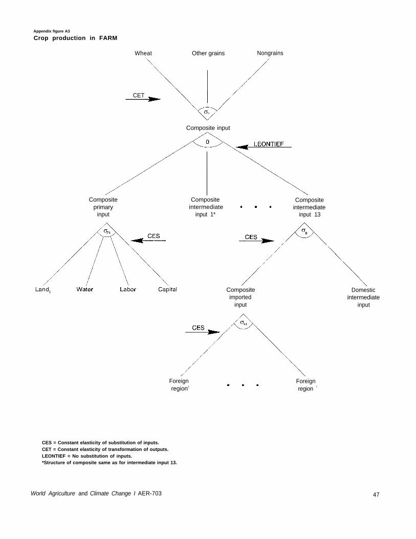
Appendix figure A3

Crop production in FARM

Wheat Other grains Nongrains

CET

Composite input

Compositeprimary

input

Compositeintermediate

input 1*

Compositeintermediate

input 13

Compositeimported

input

Domesticintermediate

input

Foreignregion1

Foreignregion 7

CES = Constant elasticity of substitution of inputs.CET = Constant elasticity of transformation of outputs.LEONTIEF = No substitution of inputs.*Structure of composite same as for intermediate input 13.


Primary inputs. As indicated by appendix figure A3,the composite primary input in the crops subsectors isa Constant Elasticity of Substitution (CES) function ofland, water, labor, and capital. In CES functions, Allenpartial elasticities ( TL) are greater than zero. CESfunctions mimic the difficulty in substituting one pri-mary factor for another. Capital, for example, is notperfectly substitutable for land in agricultural produc-tion. This means that if the price of a particular factorincreases, the sector will demand less of that factor.The relative strength of this effect is an increasingfunction of the Allen partial elasticity of substitutionand a decreasing function of the factor’s cost share.

The composite primary input in the livestock subsectorsalso contains land, water, labor, and capital. The com-posite input in the forestry subsectors only containsland, labor, and capital. Composite primary inputs inthe manufacturing and service sectors are not land-classspecific (there is not a unique production structureassociated with each land class). Instead, each sector’scomposite primary input contains land from all six landclasses together with labor, capital, and, in the servicessector, water (app. fig. A4). The capital goods sectordoes not use primary factors; these have been incorpo-rated in the cost structure of all other industries thatprovide intermediate inputs to the capital goods sector.

Intermediate inputs. As indicated by appendix figuresA3 and A4, composite intermediate inputs are formedin two stages. For a given commodity, producers atone stage choose the optimal mix of imported anddomestic goods. At another stage they source theamount to be imported by region. Both stages aremodeled using CES specifications with Allen partialelasticities of substitution II and FI, respectively,greater than zero.

The II elasticity measures the degree of substitutionbetween domestic and imported commodities. It deter-mines the change in imports demanded when the relativeprice of imported to domestic commodities changes.The FI elasticity measures the degree of substitutionamong commodities from different regions. It determinesthe change in demand for imports from a region whenthe relative price of that region’s goods changes. Pricesof foreign intermediate inputs depend on prices in theregion of origin plus transport costs and other import fees.

This structure means that trade in intermediate inputsfollows an Armington structure. The Armington struc-ture assumes that sectors differentiate among importedcommodities according to the country of origin, andamong domestic and imported varieties. The Armingtonstructure has been criticized as being unnecessarily re-

strictive. It has, however, been popular in world trademodels because it accommodates, in a straightforwardmanner, trade in similar goods (which is observed intrade statistics) and less-than-perfectly-elastic importdemands (which are found in the literature). Also, asHertel (1993) notes, more flexible functional forms oftrade have not yet been operationalized in the contextof disaggregated world trade models.

Composite primary inputs are then combined in fixedproportion with appropriate sets of composite interme-diate inputs to produce composite inputs. This structureimplies no substitution between primary and intermedi-ate inputs or between intermediate inputs within a sector.

Product supply. Each crops subsector within a regionproduces its own mix of wheat, other grains, and non-grains. This mix is determined by CET functions withAllen partial elasticities T less than zero. These elas-ticities determine how supplies of wheat, other grains,and nongrains change in response to changes in therelative prices of these commodities. Regional produc-tion of wheat, other grains, and nongrains is the sumof production across the six land classes. Regionallivestock and forestry outputs are also obtained bysumming production across the land classes in theirrespective sectors. In other sectors, the final compositeinput is equal to output.

Consumption

Household behavior and consumption are depicted bythe tree diagram in appendix figure A5. Consumptionis modeled using the concept of a utility-maximizing“super household.” The super household owns all pri-mary factors of production and, through payments forthe use of these factors, receives all regional income.The household maximizes utility derived from privateconsumption, government purchases, and savings (futureconsumption). Utility at this level is modeled usingCobb-Douglas utility functions (CES specifications withAllen partial elasticities of substitution equal to one).This means that the income shares of private con-sumption, government purchases, and savings within aregion are constant (but not equal) across all incomelevels. Private households and governments consumedomestic and imported commodities.

Private household demands are modeled with ConstantDifference of Elasticities (CDE) specifications (Hanoch,1975; and Hertel and others 1991). The CDE structureis less restrictive than the CES function in that (1)elasticities of substitution between pairs of commoditiescan differ (one elasticity does not capture all substitutionpossibilities between commodities), and (2) incomeelasticities are not restricted to equal one. Total gov-


Appendix figure A4

Production of manufacture and services in FARM

Goodj

Composite input

Compositeprimary

input

L a n d1 • • • L a n d6 Water** Labor Capital

Composite Compositeintermediate intermediate

input 1* input 13

Compositeimported

input

Domesticintermediate

input

Foreignregion 1

Foreignregion 7

CES = Constant elasticity of substitution of inputs.LEONTIEF = No substitution of inputs.*Structure of composite same as for intermediate input 13.**Services sector only.


Appendix figure A5

Household behavior and consumption in FARM

Household

Private consumption

Wheat Othergrains*

Domestic Compositewheat imported wheat

(regional income)

Services*

Savings Governmentpurchases

Wheat Othergrains* Services*

Domesticwheat

Compositeimported wheat

Foreign Foreignregion1 region7

CDE = Constant difference of elasticities for input substitution.CES = Constant elasticity of substitution of inputs.Cobb-Douglas = Elasticity of substitution is equal to one.*Stage 3 and 4 expenditure branches similar to wheat but omitted for clarity.

50

Foreignregion1

Foreignregion7


ernment purchases are allocated across commoditiesusing Cobb-Douglas utility functions (commoditybudget shares are constant but not equal).

Consumption of imported commodities by householdsand governments is subject to the Armington assump-tion in a manner analogous to the derivation of compositeintermediate inputs in production. That is, for eachcommodity in the private consumption and governmentpurchases nests, it is assumed that domestically producedand imported goods are imperfect substitutes. Com-modity expenditures are allocated to domesticallyproduced and imported goods using a CES functionalform at one stage. Expenditures on imported commodi-ties are allocated to foreign regions at another stage.

Regional savings are a constant share of income andsavers across regions see the same price. The price ofsavings is also the numeraire. Savings is used to purchasethe capital goods commodity. The sum of regionalsavings is allocated across regions based on their demandfor new capital goods.

Global Transport Services

Commodities are traded both as intermediate inputs inproduction and as goods and services in private con-sumption and government purchases (app. fig. A3,A4, and A5). Trade across regions requires transporta-tion services. Transportation requirements are routeand commodity specific and are determined in fixedproportions to the quantities of goods shipped. Theworld price of transportation services is market deter-mined and equates the global demand for such serviceswith the global supply; each region supplies a fixedvalue share of global transportation services.

Parameter Calibration

To simulate with FARM, we need to specify values forall its production and consumption parameters. Theseparameters are usually calibrated (values are chosensuch that the initial equilibrium data are reproducedexactly as an equilibrium solution) (Mansur and Whalley,1984). For example, let output, Q, be a CES functionof labor, L, and capital, K:

Q = Φ [δ L (σ−1)/σ + (1−δ) K (σ−1) /σ] σ/(σ−1) (A1)

A standard approach is to obtain an estimate of the Allenpartial elasticity of substitution, σ > 0, from the litera-ture and then choose parameters Φ and δ such that ininitial equilibrium: (1) the first order conditions forcost minimization with respect to capital and labor aresatisfied, and (2) profits are zero.

FARM, however, uses linearized CES (or CET) func-tions.’ With a linearized CES function, we only needto obtain an estimate of σ. Estimates of Φ, and δ arenot required because they are embedded in the initialequilibrium data which are in value terms. Thus, cali-bration is a simple task for FARM, because most ofthe functional forms are of the CES or CET type. Theonly exception is the private household commodity de-mand system which is based on the CDE expenditurefunction. Its calibration is discussed by Chyc (1993).

Most parameters in FARM come from GTAP (Hertel,1993) and are based on a review of the literature. Theseinclude the Allen partial elasticities for primary factors,the Allen partial elasticities of import substitution ofintermediate commodities, and the price and incomeelasticities for private consumption. These elasticitiesare presented in appendix tables A2-A5.

There are few estimates of Allen partial elasticities ofsubstitution for land and crop supplies as modeled inFARM. At present, therefore, the default values forthese elasticities (σ TL and σ T in appendix figures Aland A3, respectively) are set equal to -1.0. This reducesthe CET frontiers to Cobb-Douglas form. This meansthat the revenue shares for crops services and livestockservices, for example, received by land owners andthe revenue shares received for wheat, other grains,and nongrains by crop producers within a region areconstant (but not equal) across all levels of revenue.

Data Calibration

Because FARM calibrates crop, livestock, and forestryproduction by land class and water use by sector, theGTAP data on regional revenues and expenditures (in1990 US dollars) for sectors and consumers needed tobe disaggregated. Several global databases were usedin conjunction with FARM’s geographic informationsystem to accomplish this task.

Resource Supply

All acreage in each region is allocated to one of fourland-use types—cropland, permanent pasture, forest,and other-using 1990 estimates from United Nations,Food and Agriculture Organization (FAO) (1992).Regional land-use acreage is allocated to land classesby combining land use and cover data in Olson (1989-91) with the land class data set pertaining to currentclimatic conditions. These regional land class distribu-tions of cropland, permanent pasture, and forest landare used in allocating the GTAP input and output valuesassociated with the crop, livestock, and forestry sectors.

1Hertel and Tsigas (1993) and Dixon and others (1982) show howthese linearized functions are obtained from their nonlinear forms.


Regional water supply estimates are derived from waterwithdrawal data in World Resources Institute (WRI)(1992). WRI gives water withdrawals for agricultureand nonagriculture by country. In each region, irrigatedacreage (FAO, 1992) is distributed to the land classesbased on irrigated land data in Wilson and Henderson-Sellers (1985), crops and settlements data in Olson(1989-91), and length-of-growing-season data.

Output Values

GTAP’s regional output values for wheat, other grains,nongrains, livestock, and forest products are distributedto the land classes based on various output quantityshares. Producers of a given commodity within a regionare assumed to receive the same price for the commodityno matter what land class they use in production.Table 9 in the main text shows crop, livestock, andforest product quantities by region and land class.

Values of wheat, other grains, and nongrains are dis-tributed to land classes based on 1990 crop productiondata compiled from FAO (1992). To keep the taskmanageable, the FAO data are aggregated into 32 cropgroups. For paddy rice, regional production is allocatedentirely to irrigated acreage. In making the rice allo-cations, differences in length of growing season, whichgoverns plant maturing time and multicropping potential,were taken into account.

For all other crop groups, regression analysis was usedto allocate regional production to the land classes.Specifically, regional output was regressed on croplandacreage in the six land classes with adjustments madeto account for irrigation. Irrigation adjustments werenecessary because irrigation lengthens the growingseason and may move land into a new land class forpurposes of crop production.

We were able to visually compare most of our cropdistributions with crop distribution maps from othersources (U.S. Department of Agriculture, Foreign Agri-cultural Service, 199 I). These comparisons resultedin some adjustments to our distributions. The land classshares of total value of regional wheat, other grain, and

nongrain production are obtained by appropriately aggre-gating the land-class distributions of the 32 crop outputs.

Production of cattle, sheep, pigs, goats, and other live-stock in ! 990 is detailed in FAO (I 992). Regionalproduction of these livestock is distributed among theland classes based on animal densities in Lerner, Mat-thews, and Fung (1989). Land class shares of totalvalue of regional livestock production are obtained byaggregating the land-class distributions of the differentlivestock outputs.

Regional forestry outputs are based on 1990 productiondata for coniferous and nonconiferous industrialroundwood and fuelwood from FAO (1992). Theseare allocated to land classes based on distributions of co-niferous, broadleaf, and mixed forests derived fromOlson (1989-91). Adjustments are made to captureproductivity differences due to length of growing sea-son. Each land class’s share of total value of regionalforestry production is obtained by aggregating itsshares of the various forest products.

Input Values

To maintain the integrity of the database, FARM usesGTAP’s sectoral payments to each intermediate inputas well as GTAP’s sectoral payments to primary factorsin each region. GTAP’s primary factor payments,however, do not include separate values for water or forland in nonagricultural sectors. The first step in allo-cating input values, therefore, is to divide GTAP’sprimary factor payments into land, labor, and capital.From a review of the literature we obtained a morecomplete set of sectoral payments to land, labor, andcapital in each region. For GTAP’s nonagriculturalsectors, the land payments are subtracted from GTAP’spayments to capital; that is, we assume that, in the GTAPdata, payments to capital include payments to land.

Next, we distribute the (revised) agricultural and silvicul-tural sectors’ payments to land, labor, capital, andintermediate inputs to the land classes. These paymentsare distributed to the land classes based on their respec-tive commodity output shares. Input payments for thecrops subsectors are then obtained by summing acrossthe appropriate land-class specific input values attributedto wheat, other grains, and nongrains. This results ina different input structure for each crop subsector.

We then distribute the remaining sectors’ land paymentsto the land classes. Except for the services sector, landpayments are allocated to land classes based on theland class distribution of crops and settlements in Olson(1989-91). For the services sector, 90 percent of theland payment is allocated based on the land class dis-tribution of crops and settlements in Olson (1989-91)

and 10 percent of the land payment is allocated basedon length of growing season (as defined by the landclass distribution of hectare day shares).

Once regional payments to land, labor, capital, andintermediate inputs are distributed to the land classes,three land-class-specific adjustments are made. First,payments to water are subtracted from payments to land.Second, payments to irrigation capital are subtractedfrom land and added to capital. Third, payments tolivestock feed and pasture are adjusted to account for


the relative importance of grazing on dryland pasturein areas where growing seasons are short.

Water. FARM requires values for water used in thecrops, livestock, and services sectors. Global data onwater prices are almost nonexistent so a price of$2.55 million (US) per cubic kilometer is used in allregions. This value is based on U.S. data (U.S. Depart-ment of Commerce, 1990). The same water price isapplied to water used in the agricultural and servicessectors. The latter is composed of both domestic andindustrial water (WRI, 1992). Values of irrigationwater on cropland and permanent pasture are derivedby allocating 90 percent of agriculture’s water paymentsto crops and 10 percent to livestock.

Once total water payments for the three sectors arederived, the amount to charge each land class is deter-mined. This determination is based on estimates ofeach land class’s requirement for irrigation water (eachland class’s share of regional water shortages on irri-gated land). Water shortage is defined as the amount ofwater required to maintain potential evapotranspirationduring the growing season minus precipitation. Eachsector’s land class specific water payments are thensubtracted from the appropriate land payments.

In this approach, variability of water requirements isreflected in the variability of water payments by theland-class-specific crops and livestock subsectors.Variability in water requirements is also reflected in aregion’s service sector by varying payments to land.The service sector’s payment to water, however, occursas one lump sum. It is not differentiated by land class.

Irrigation capital. Regional payments to irrigationcapital are calculated from payments to land using theshares of total hectare-days in a region’s growing sea-son attributed solely to irrigation (total hectare-daysminus rainfed hectare-days divided by total hectare-days).2 This assumes that value of a region’s irrigationcapital is equivalent to the additional length of growingseason that such capital provides. Ninety percent ofthese payments are allocated to crops and 10 percentto pasture. Land-class-specific payments to irrigationcapital are based on the distribution of a region’s require-ments for irrigation water. These payments are thenadded to the appropriate land class’s capital payments.

Livestock feed and pasture. GTAP’s regional valuesfor livestock feed are allocated to the land classes based

2The number of hectare-days in a region’s growing season accountsfor both growing season lengths and the amount of land under culti-vation.

on weighted shares of feed consumed by the livestockassociated with the land classes. The weights are 20, 15,10, 3, and 2 percent, respectively, for dairy cattle, beefcattle and water buffalo, horses and camels, pigs, andsheep and goats. These weights are combined with theanimal densities in Lemer, Matthews, and Fung (1989).

We also adjust for the relative importance of grazing onunirrigated pasture in areas where growing season isless than or equal to 100 days. We assume, for example,that sheep, goats, camels, and horses raised on theselands would receive little, if any, livestock feed otherthan hay. Therefore, payments to dryland pasture inareas where growing seasons are less than or equal to100 days are increased, while the value of livestockfeed allocated to these pastures is decreased. We makethe adjustment using densities of camels, goats, andsheep in Lerner, Matthews, and Fung (1989). Thesechanges are balanced by decreasing values of pastureand increasing values of livestock feed on other landclasses. This approach simulates the substitution ofland for feed in some livestock operations.

Modeling Climate Change

FARM models global climate change as (1) right or leftshifts in regional water supplies and (2) changes in thedistribution of land across land classes (app. fig. A2)These regional changes in land and water endowmentsare computed in FARM’s geographic information sys-tem for each climate change scenario considered. Weassume that climate change does not affect endowmentsof either labor or capital.

FARM is implemented using the GEMPACK suite ofmodel development software (Codsi and Pearson, 1988;and Pearson, 1988). GEMPACK solves a system ofnonlinear equations via a linearized representation andthis has implications for data requirements and interpre-tation of results (Pearson, 1991). First, an initialequilibrium is fully described in terms of revenues andexpenditures only (information on the associated quan-tity and price terms is not necessary). Second, resultsfor variables are given in terms of percentage changes.

Most model results can be interpreted in a straightfor-ward manner; the major exception is land services.The CET functions used to simulate supplies of landservices in FARM are nonlinear. Quantities of landservices, therefore, are not measured in hectares (or anyother measure of area). Rather, they are measured in“productivity” units, which are consistent with a CETfrontier. Because land is generally measured, and moreeasily comprehended, in area units, we convert produc-tivity units to hectares. This conversion, however, issomewhat imprecise because conversion factors (hec-


tares per unit productivity) and complete specificationsof the CET functions are not known (app. equation Al).

We start by assuming that the relationship betweenpercentage changes in land area and percentage changesin productivity quantities (as computed in FARM) isdirect and monotonic. If, for example, a crops subsec-tor uses more land services while the correspondinglivestock subsector uses less, then we assume that thecrops subsector uses more land area, while the corre-sponding livestock sector uses less.

We also impose three constraints. First, the sum of netchanges in land use within each land class of any re-gion must equal the climate-induced shock to that landclass endowment. This ensures that the net change intotal land within each region equals zero. This constraintis imposed by proportionally adjusting land quantitiesderived from the FARM simulations. Proportional ad-justments also maintain our second constraint (all landquantities must be non-negative.

The third constraint is that land-use changes must besign preserving relative to expected changes. Expectedland use changes equal the climate-induced land-classchanges. When this constraint fails, we compute sec-toral differences between reported and expected landuse quantities, group them by sign, and calculate theabsolute value of each group’s total differences. Thefirst constraint is imposed by assigning the smallestabsolute value of differences to each group. This alsoensures that land quantities remain equal to or greaterthan zero. The adjusted differences are then proportion-ally reassigned to the sectors contributing to that group.

Sensitivity Analysis

Most parameters in FARM were obtained from a reviewof the literature. In some cases, however, parametersthat were estimated for a limited number of countrieshave been applied broadly. In addition, empirical esti-mates of some model parameters were unavailable. Wetherefore conducted sensitivity analyses to assess theimportance of model results to parameter specifications.All sensitivity analyses were done using the climatechange scenario generated by the Goddard Institute ofSpace Studies’ general circulation model.

The analysis consisted of simultaneously increasing ordecreasing all substitution elasticities of a given type(such as land supply, crop supply, primary factor demand,and import demand) by 50 percent. This, therefore, isnot an uncertainty analysis (an attempt to predict a range

of results given information about the bounds or confi-dence limits of parameters). This also means that thefocus of the analysis is on global, rather than regional,impacts. Sensitivity analysis results for impacts on grossworld product as well as world production of agricul-tural and silvicultural products are presented in appendixtables A6 and A7.

Results pertaining to gross world product suggest thatmodel results are relatively sensitive to changes in valuesassumed for the primary factor demand elasticities(app. table A6). Reducing these elasticities by 50 per-cent causes gross world product to decrease by $115.9billion, while increasing them by 50 percent causesgross world product to increase by $45.2 billion. Thisis a range of $161.1 billion. Results are much less sensi-tive to changes in values of land supply, crop supply,and imported demand elasticities. The range of grossworld product between high and low values of theseelasticities is always less than $8.8 billion.

A similar pattern occurs with world production of se-lected commodities. In general, commodity productionis more sensitive to changes in primary factor demandelasticities than to changes in land supply, crop supply,or import demand elasticities (app. table A7). The rea-son results are most sensitive to changes in primary factordemand elasticities is that they affect all commoditiesthrough all primary factors. Land supply elasticities, onthe other hand, affect all commodities but only throughone primary factor (land), while crop supply elasticitiesaffect crop commodities only and import elasticitiesaffect only the traded portion of commodities.

This analysis suggests that FARM simulation results aregenerally robust with respect to land supply, crop supply,and import demand elasticities. Adjusting any one setof these elasticities has a relatively small impact on themagnitude of climate change’s impact on gross worldproduct or on world production of agricultural andsilvicultural products relative to the base simulation.Using different values of primary factor demand elastici-ties does affect model results more. FARM’s primaryfactor demand elasticities are based on a review ofthe literature and so reflect empirical evidence to date.Our analysis suggests, however, that this is an areawhere good parameter estimates are important. Moregenerally, this analysis suggests that FARM’s “solutionmethod” is robust (the results are stable within a verylarge neighborhood of solutions generated with the baseparameter set).


Appendix table Al--Regional, sectoral. and commodity aggregation for FARM

A. Regional aggregation D. Commodity aggregation

1. ANZ-Australia and New Zealand 1. WHT-Wheat2. OGR-Other grains

2. CAN-Canada Paddy riceOther grains

3. USA-United States of America 3. NGR-Nongrains4. Livestock

4. JPN-Japan WoolOther livestock products

5. OEA-Other East Asia 5. ForestryRepublic of Korea 6. Coal, oil, and gasPeople's Republic of China 7. Other mineralsHong Kong 8. Fish, meat, and milkTaiwan Fishing

Meat products6. SEA-Southeast Asia Milk products

Indonesia 9. Other processed foodsMalaysia Processed ricePhilippines Other food productsThailand Beverages and tobacco

10. Textiles, clothing, and footwear7. EC-European Commodity Textiles

Wearing apparel8. ROW-Rest of the world Leather, fur, and their products

11. Other nonmetallic manufacturesLumber and wood products

B. Sectoral Aggregation Pulp, paper, and printedproducts

1. CRP-Crops (six sectors) Petroleum and coal products2. LIV-Livestock (six sectors) Chemicals, rubber, and plastic3. FOR-Forestry (six sectors) Nonmetallic mineral products4. COG-Coal, oil, and gas 12. Other manufactures5. MIN-Other minerals Primary iron and steel6. FMM-Fish, meat, and milk Primary nonferrous metals7. OPF-Other processed food Fabricated metal products8. TCF-Textiles, clothing, and Transport industries

footwear Other machinery and equipment9. NMM-Other nonmetallic manufactures Other manufacturing

10. OMN-Other manufactures 13. Services11. SRV-Services Electricity, gas, and water12. FCF-Fixed capital formation Construction

Trade and transportC. Endowments Other services (private)

Other services (government)l-6. Six land classes Other services (dwellings)

7. Water 14. Fixed capital formation8. Labor9. Capital



Appendix table A2--Allen partial elasticitiesfor primary factors ( σ σ PI) used in FARM

1

Sector σ P I

CropsLivestockForestryCoal, oil, and gasOther mineralsFish, meat, and milkOther processed foodAll other manufacturing sectorsServices

1Elasticities are the same in allSource: Hertel, 1993.

0.560.560.561.121.120.851.121.261.39

regions.

Appendix table A3--Allen partial elasticitiesof substitution between domestic and importedcommodities ( σ σ II) used in FARM

1

Commodity σ I I

Wheat 2.20Other grains 2.20Nongrains 2.20Livestock 2.78Forestry 2.80Coal, oil, and gas 2.80Other minerals 2.80Fish, meat, and milk 2.34Other processed food 2.44Textiles, clothing, and footwear 3.17Other nonmetallic manufactures 2.06Other manufactures 3.28Services 1.94

1Elasticities are the same in all regions.Allen partial elasticities of substitutionbetween imported commodities ( σ FI) are twiceas large as the elasticities listed above.Source: Hertel, 1993.


Appendix table A4--Compensated own-price elasticities for private consumption in FARM at initial equilibriumRegion

Australia and United Other Southeast European Rest ofCommodity New Zealand Canada States Japan East Asia Asia Community WorldWheat -0.0705 -0.0638 -0.0657 -0.1380 -0.1505 -0.1063 -0.1490 -0.1201Other grains -0.0706 -0.0636 -0.0657 -0.1380 -0.1498 -0.1226 -0.1489 -0.1801

Nongrains -0.0722 -0.0642 -0.0663 -0.1433 -0.1833 -0.1438 -0.1510 -0.2022Livestock -0.6347 -0.5694 -0.5880 -0.4545 -0.3547 -0.2451 -0.5521 -0.3023Forest products -0.6287 -0.5681 -0.5868 -0.4528 -0.3508 -0.2392 -0.5440 -0.4003

Coal, oil, and gas -0.6298 -0.5703 -0.5867 -0.4528 -0.3496 -0.2346 -0.5456 -0.4007Other minerals -0.6285 -0.5672 -0.5867 -0.4528 -0.3496 -0.2348 -0.5436 -0.4000

Fish, meat, and milk -0.1011 -0.0704 -0.0745 -0.2083 -0.2484 -0.1536 -0.1746 -0.2042Other processed food -0.3044 -0.2202 -0.2384 -0.2539 -0.2223 -0.1547 -0.2967 -0.2474Textiles, clothing,

and footwear -0.3639 -0.3912 -0.4131 -0.3384 -0.2320 -0.1448 -0.2923 -0.1737Other nonmetallic

manufactures -0.6840 -0.6098 -0.6375 -0.4787 -0.3649 -0.2533 -0.5955 -0.4108Other manufactures -0.6318 -0.5712 -0.6057 -0.4477 -0.3153 -0.2119 -0.5333 -0.3636Services -0.2092 -0.1713 -0.1559 -0.1527 -0.4292 -0.3393 -0.2288 -0.2690

Appendix table A5--Income elasticities for private consumption in FARM at initial equilibriumRegion

Australia and United Other Southeast European Rest ofCommodity New Zealand Canada States Japan East Asia Asia Community WorldWheat 0.9996 0.9997 0.9976 0.9997 0.8701 0.9959 0.9710 0.9447Other grains 0.9962 0.9991 0.9941 0.9994 0.6817 0.9206 0.9729 0.8167Nongrains 0.7736 0.7470 0.8511 0.8133 0.6426 0.7227 0.8723 0.6520Livestock 0.8966 0.9520 0.9689 0.9648 0.7957 0.9021 0.8356 0.8795Forest products 1.0002 1.0031 1.0005 1.0000 1.0007 1.0302 1.0016 1.0076Coal, oil, and gas 1.0015 1.0087 1.0002 1.0001 1.0397 1.0049 1.0066 1.0181Other minerals 1.0001 1.0003 1.0003 1.0000 0.9899 1.0046 1.0003 1.0009Fish, meat, and milk 0.4172 0.3477 0.5285 0.7239 0.8859 0.8921 0.4484 0.7889Other processed food 0.4680 0.4478 0.4937 0.5265 0.7346 0.7246 0.5736 0.6417Textiles, clothing,

and footwear 0.9499 0.9431 0.9512 0.9539 0.9586 0.9610 0.9440 0.9489Other nonmetallic

manufactures 1.0828 1.0668 1.0362 1.0613 1.1780 1.1493 1.0812 1.1191Other manufactures 1.0144 1.0045 1.0000 1.0058 1.0498 0.9697 1.0061 0.9385Services 1.0972 1.0868 1.0503 1.0951 1.2342 1.1647 1.0971 1.1272

Appendix table A6--Effects of changing FARM's elasticity parameterson gross world product under a climate change scenario based onthe Goddard Institute for Space Studies' general circulation model

Change from base elasticityElasticity -50 percent None 50 percent

Land supply

Percentage

Value

-0.013

-2,633

Percent0.011

$U.S. million2,230

0.029

6,191

Crop supply

Percentage

Value

0.003

563

Percent0.011

$U.S. million2,230

0.016

3,277

Primary factor demand

Percentage -0.549

Value -115,900

Percent0.011

$U.S. million2,230

0.215

45,153

Import demand

Percentage

Value

0.004

797

Percent0.011

$U.S. million2.230

0.014

3.026


Appendix table AT--Effects of changing FARM's elasticity parameterson selected commodities under a climate change scenario based onthe Goddard Institute for Space Studies' general circulation model

Change from base elasticityElasticity -50 percent None 50 percent

PercentLand supply

WheatOther grainsNongrainsLivestockForest productsFish, meat, and milkOther processed food

1.945 1.920 1.9070.516 0.409 0.340-0.578 -0.505 -0.4660.974 0.858 0.7870.372 0.274 0.2000.338 0.371 0.3920.343 0.382 0.404

Crop supplyWheatOther grainsNongrainsLivestockForest productsFish, meat, and milkOther processed food

2.466 1.920 1.6210.184 0.409 0.569-0.599 -0.505 -0.4400.860 0.858 0.8560.244 0.274 0.2910.354 0.371 0.3810.357 0.382 0.397

Primary factor demandWheatOther grainsNongrainsLivestockForest productsFish, meat, and milkOther processed food

3.098 1.920 1.7171.983 0.409 0.427

-0.398 -0.505 -0.3991.852 0.858 0.808-0.609 0.274 0.4630.206 0.371 0.4390.605 0.382 0.447

Import demandWheatOther grainsNongrainsLivestockForest productsFish, meat, and milk

1.701 1.920 2.0990.785 0.409 0.074-0.196 -0.505 -0.8250.807 0.858 0.8850.330 0.274 0.3990.384 0.371 0.380

Other processed food 0.115 0.382 0.114


62

Appendix B: Detailed FARM Results


Appendix table Bl--Changes in land class areas due to simulated climates based on doubling of atmosphericcarbon dioxide levels

RegionScenario 1/ United European Other Southeast Australia/ Rest ofland class States Canada Community Japan East Asia2 Asia3 New Zealand World Total

Percent change

-51.77 -40.74 -64.14 -95 00 -26 02 0 00 -93.69 -40.39 -39.77-9.97 4.89 -57.80 0 00 -2 45 0 00 -3.90 -0.09 -1.4445.83 26.32 -56.69 -85 93 5 20 476 43 36.20 32.92 28.71-14.84 411.26 -69.36 -0 40 32 45 963 06 -4.18 78.05 51.6436.61 0.00 37.48 -11 38 -42 05 -43 15 11.51 6.54 4.6838.96 0.00 536.96 610 97 46 63 -12 50 -13.52 -21.08 -10.06

-54.84 -45.26 -85.33 -95 00 -30 25 0 00 -93.69 -50.58 -47.721.89 186.91 -70.03 0 00 16 67 0 00 -2.70 17.91 17.22

105.41 -2.01 -3.18 -93 15 -32 79 426 49 43.61 37.06 28.74-25.42 296.50 -62.73 -9 92 -0 69 875 58 -12.19 64.47 36.9863.11 0.00 28.22 -8 59 -35 60 -0 78 29.31 19.30 18.21-49.54 0.00 417.72 757 09 63 05 -17 46 -28.90 -42.25 -31.05

GISS123456

GFDL123456

UKMO123456

OSU123456 14.25 0.00 189.38 643.39 48.25 -9.43 -9.24 -19.57 -11.69

1 Climate change scenarios based on results generated by the general circulation models of the GoddardInstitute for Space Studies (GISS), the Geophysical Fluid Dynamics Laboratory (GFDL), the United KingdomMeterological Office (UKMO), and Oregon State University (OSU).2China (including Taiwan), Hong Kong, and North Korea. 3Indonesia, Malaysia, Philippines, and Thailand.

-67.28 -59.48 -92.85 -95.00 -55.36 0.00 -95.00 -64.08 -62.458.40 135.56 -71.95 0.00 24.58 0.00 3.67 15.56 16.39

42.85 3.71 -56.79 -93.24 5.44 331.43 8.96 59.73 38.81-27.96 620.66 -68.34 -16.37 38.53 1533.83 -15.18 116.16 78.09101.64 0.00 25.18 -28.30 -54.85 -24.09 6.14 1.42 4.37-7.68 0.00 574.49 933.24 35.92 -24.74 -16.19 -54.29 -39.20

-43.57 -33.96 -64.14 -95.00 -20.96 0.00 -93.69 -32.76 -32.579.42 155.41 -32.46 0.00 -4.78 0.00 -18.74 8.32 6.87

48.42 -0.42 -9.26 -72.08 27.28 50.38 80.21 12.93 16.68-29.98 169.77 -54.93 -8.90 -6.71 378.13 18.48 43.34 21.8716.81 0.00 89.57 -14.64 -40.49 15.99 50.56 18.06 17.76

Appendix table B2--Percentage land class changes on existing cropland, pasture land, and forestland due to simulated climates based on doubling of atmospheric carbon dioxide levelsScenariol/ Regionland use/ United European Other Southeast Australia/ Rest ofland class States Canada Community Japan East Asia2 Asia3 New Zealand World

Percent changeGISS

Cropland1 -952 -53 144 -415 796 75

00 0.00 -36.06 0.00 -84 66 0.00 0.00 -68.8973 -10.62 -40.81 0.00 -9 89 0.00 22.68 -4.8819 -36.24 -51.73 -95.00 -18 86 804.50 5.01 -3.3209 91.57 -82.37 -45.26 12 43 998.61 10.75 54.3821 0.00 13.26 -29.62 -42 62 -64.11 19.16 -7.1736 0.00 742.30 415.49 49 07 -21.43 -20.85 -23.40

Pasture1 -61.682 -7.383 60.844 7.225 -31.376 45.78

Forest1 -89.162 -11.643 15.764 6.155 30.26

-19.24 -47.15 0 00 -26.61 0.00 -95.00 -52.37-2.53 -57.33 0 00 -12.79 0.00 -2.59 -2.62

101.74 -76.58 -78 66 59.79 67.41 39.89 43.7164.23 -44.95 -35 74 25.76 134.03 1.82 44.730.00 48.11 -16 01 -43.96 -12.93 7.75 9.250.00 612.26 1531 04 20.74 -11.36 -6.61 -27.29

-81.71 -88.57 0.00 -60.93 0.00 -95.00 -52.399.06 -94.95 0.00 47.43 0.00 -16.28 74.13

17.76 -38.91 -84.39 -38.42 1103.84 33.84 24.87510.33 -76.81 30.67 21.95 3438.73 -10.62 176.290.00 83.32 0.62 -44.22 -45.86 10.59 3.79

6 25.55 0.00 304.09 799.72 69.67 -10.89 -16.58 -19.46Continued--


Appendix table B2--Percentage land class changes on existing cropland, pasture land, and forestland due to simulated climates based on doubling of atmospheric carbon dioxide levels--continuedScenario1/ Regionland use/ United European Other Southeast Australia/ Rest ofland class States Canada Community Japan East Asia2 Asia3 New Zealand World

GFDLGFDLCroplandCropland

112233445566

Percent change

-95 00 0.00 -63.44 0.00 -88 08 0 00 0 00 -79.24-34 95 24.90 -42.91 0.00 -1 12 0 00 106 21 8.58253 95 -20.74 -0.02 -95.00 -44 31 673 90 -16 73 22.68-53 49 3.44 -82.37 -55.59 -26 28 860 02 4 28 27.1034 67 0.00 14.97 -36.84 -54 65 -5 42 68 72 17.85

-34 24 0.00 625.31 491.80 85 75 -30 64 -26 67 -44.45

Pasture12

-66 07 -88.52 -42.91 0 00 -29 78 0 00 -95 00 -53.27-9 85 4.00 -84.69 0 00 12 76 0 00 -2 35 11.96

165 41 112.54 -55.12 -95 00 -18 88 56 33 37 37 48.00-11 42 53.66 -29.71 -48 31 -21 47 90 96 14 67 33.69

9 27 0.00 24.51 -5 11 -46 59 14 74 -17 48 7.94-22 77 0.00 487.69 1861 55 41 96 -13 66 -11 48 -53.826

Forest1 -90 71 -89.86 -95.00 0 00 -58 78 0 00 -95 00 -63.552 54 95 446.79 -81.28 0 00 193 84 0 00 -15 69 285.723 27 44 -16.41 61.20 -92 45 -71 11 1100 37 55 21 23.30

1 00 370.29 -69.85 23 70 15 64 2958 18 -28 32 163.215 119 33 0.00 72.20 6 67 -21 13 2 45 40 69 24.036 -62.15 0.00 169.12 1067.75 65.78 -13.97 -47.83 -37.58

See footnotes at end of table. Continued--

Appendix table B2--Percentage land class changes on existing cropland, pasture land, and forestland due to simulated climates based on doubling of atmospheric carbon dioxide levels--continuedScenario 1/ Regionland use/ United European Other Southeast Australia/ Rest ofland class States Canada Community Japan East Asia2 Asia3 New Zealand World

Percent changeUKMO

Cropland1 -95.002 -2.023 97.134 -76.755 130.246 66.61

Pasture1 -73.032 0.023 80.074 -20.195 10.686 9.49

Forest1 -98.122 52.873 -16.784 20.585 119.06

0.00 -68 03 0.00 -88.08 0.00 0 00 -94.849.40 -40 81 0.00 32.21 0.00 134 68 20.21-8.23 -48 17 -95.00 -32.45 478.50 -19 30 43.462.13 -86 73 -65.83 3.90 1434.48 7 58 36.430.00 2 89 -43.82 -64.70 -7.45 -27 27 -50.070.00 804 92 567.05 19.90 -45.57 -14 02 -44.87

-94.24 -73 58 0.00 -60.87 0.00 -95 00 -73.4516.43 -92 56 0.00 17.92 0.00 -4 47 11.47

127.28 -77 26 -95.00 40.10 39.85 33 13 62.281.84 -33 38 -65.31 25.81 226.51 41 84 75.530.00 23 06 6.41 -51.13 34.00 -15 28 -5.890.00 616 72 2180.82 5.08 -29.82 -7 54 -70.85

-96.13 -95 00 0.00 -87.44 0.00 -95 00 -78.43308.77 -80 31 0.00 110.55 0.00 39 76 213.62-25.78 -57 29 -92.54 -46.14 964.79 2 57 49.28739.84 -80 82 23.77 28.65 5766.71 -45 73 280.19

0.00 90 40 -28.64 -54.65 -56.40 21 65 20.566 -36.77 0.00 330.64 1461.28 74.77 -19.37 -26.74 -51.48


Appendix table B2--Percentage land class changes on existing cropland, pasture land, and forestland due to simulated climates based on doubling of atmospheric carbon dioxide levels--continuedScenario1/ Regionland use/ United European Other Southeast Australia/ Rest ofland class States Canada Community Japan East Asia2 Asia3 New Zealand World

OSUCropland

123

Percent change

-95.00 0 00 -36 06 0.00 -84 66 0.00 0.00 -57.26-4.65 11 85 -57 03 0.00 -28 45 0.00 13.64 26.80

160.10 -22 44 13 43 -95.00 58 92 81.74 -15.65 -3.74-58.09 27 57 -64 49 -45.26 -42 40 573.84 4.74 22.5236.79 0 00 76 41 -40.20 -24 75 15.39 53.39 -14.8232.40 0 00 263 06 438.44 49 82 -21.78 -5.70 -24.31

456

Pasture-51.30 -24 24 -47 15 0 00 -20 30 0.00 -95.00 -42.86

0.01 9 07 -52 05 0 00 -12 74 0.00 -19.05 3.2264.18 26 23 -46 15 -78 66 62 64 5.60 134.13 10.21-8.55 1 50 -42 84 -35 74 -15 46 58.12 96.01 32.57

-47.00 0 00 115 06 -18 13 -52 91 3.81 12.49 19.7726.35 0 00 211 68 1547 63 34 58 -6.32 2.60 -22.80

Forest12345

-75.7251.73

-15.45-1.1430.15

-69377-9

2070

9011632700

-6367

-12-5189

8559670375

0.000.00

159.601036.42

27.66

-95.00-36.4546.02-14.2562.38

-44.84147.2311.8492.8123.58

13 0 00 -5219 0 00 2895 -70 34 -2057 16 57 1194 2 33 -49

6 4.98 0.00 108.05 881.13 60.93 -7.45 -20.64 -17.231Climate change scenarios based on results generated by the general circulation models of theGoddard Institute for Space Studies (GISS), the Geophysical Fluid Dynamics Laboratory (GFDL),the United Kingdom Meterological Office (UKMO), and Oregon State University (OSU).2China (including Taiwan), Hong Kong, and North Korea.3Indonesia, Malaysia, Philippines, and Thailand.

Appendix table B3--Base values and changes in commodity production, by region and climate change scenarioScenario1

Region/ Base (1990) GISS GFDL UKMO OSUcommodity value2 Rest3 Unrest Rest Unrest Rest Unrest Rest Unrest

United StatesWheatOther grainsNongrainsLivestockForest productsCoal/oil/gasOther mineralsFish/meat/milkOther processed foodsText./cloth./footwearOther nonmetal. manuf.Other manufacturesServices

CanadaWheatOther grainsNongrainsLivestockForest productsCoal/oil/gasOther mineralsFish/meat/milkOther processed foodsText./cloth./footwearOther nonmetal. manuf.Other manufactures

Number ---------------------------- Percent change----------------------------

74,475 8.191 5.986 14 761 12 392 10.518 9.374 6.087 1.479238,352 -5.177 -5.854 -10 638 -6 479 -9.804 -7.071 -9.298 -7.349194,389 7.655 2.768 -3 454 -3 947 9.549 0.643 1.550 -0.317170,647 -0.464 -0.691 -1 476 -0 462 -1.512 -0.582 -1.819 -1.274498,000 0.566 0.713 -2 028 -0 818 -1.435 -0.470 -0.296 -0.253215,073 -0.173 -0.010 -0 228 -0 063 -0.343 -0.042 -0.279 -0.16624,786 -0.293 0.047 -0 050 0 136 -0.454 0.094 -0.284 -0.118

121,363 -0.081 -0.155 -0 837 -0 156 -0.736 -0.102 -0.987 -0.588292,850 0.380 0.130 -0 584 -0 372 0.072 -0.165 -0.327 -0.321155,999 0.091 0.091 0 021 -0 046 0.278 0.180 -0.082 -0.126

1,067,890 0.048 0.099 -0 224 -0 027 -0.122 0.052 -0.207 -0.1271,266,520 -0.183 0.156 0 070 0 218 -0.213 0.258 -0.091 0.0766,103,870 0.050 0.077 -0 190 -0 075 -0.087 0.002 -0.156 -0.100

32,098 -2.149 2.402 5. 138 9 548 13.175 7.440 -1.568 14.04524,981 3.456 12.441 5. 084 16 751 3.951 17.828 4.807 15.52913,015 19.253 35.579 6. 815 36 054 4.908 46.809 8.014 23.24723,820 5.455 8.620 3. 866 8 390 4.117 10.530 2.655 7.124

155,475 2.631 3.470 2. 851 3 854 3.467 5.321 1.766 2.61627,388 1.937 1.781 3. 067 2 638 3.535 3.090 2.430 2.01810,210 1.557 1.184 3. 259 2 173 3.533 2.372 2.579 1.69224,438 3.396 4.852 2. 673 4 883 2.984 6.049 1.879 4.08732,418 2.513 3.141 2. 109 3 333 2.582 4.099 1.726 2.65418,635 1.914 1.768 2. 867 2 596 3.419 3.093 2.124 1.910

130,143 2.219 2.548 2. 512 3 059 3.126 3.871 1.979 2.314119,236 1.477 1.003 3. 091 2 001 3.642 2.320 2.418 1.508

Services 719,538 1.800 1,944 2.206 2.453 2.630 2.937 1.797 1.961See footnotes at end of table. Continued--

Appendix table B3--Base values and changes in commodity production, by region and climate change scenario--continued

Region/commodity

Scenario1

Base (1990) GISS GFDL UKMO OSUvalue 2 Rest3 Unrest Rest Unrest Rest Unrest Rest Unrest

European CommunityWheatOther grainsNongrainsLivestockForest productsCoal/oil/gasOther mineralsFish/meat/milkOther processed foodsText./cloth./footwearOther nonmetal. manufOther manufacturesServices

Number -------------------------- --Percent change--------------------------

80,319 -18 590 -13.170 17 111 -11.978 -21.123 -14.713 -8.002 -6.61624,994 28 408 29.207 27 128 21.912 33.109 29.565 16.627 17.270279,884 -17 892 -10.609 13 033 -6.525 -17.407 -9.294 -6.992 -5.176295,049 -2 864 -1.672 -1 982 -1.572 -2.761 -1.888 -1.706 -1.041171,394 0 693 3.546 0 408 3.412 0.942 3.937 0.181 1.77082,886 -1 885 -1.851 -1 310 -1.271 -1.937 -1.860 -0.828 -0.775

270,580 -1 374 -1.477 -1 002 -1.002 -1.410 -1.450 -0.633 -0.602157,710 -2 250 -1.279 -1 664 -1.088 -2.383 -1.439 -1.036 -0.609485,433 -2 265 -1.411 -1 702 -1.167 -2.397 -1.618 -0.891 -0.626284,159 -1 840 -1.725 -1 050 -1.081 -1.596 -1.562 -0.743 -0.742

1,472,520 -1 451 -1.227 -1 057 -0.860 -1.516 -1.263 -0.613 -0.4891,292,320 -1 130 -1.278 -0 832 -0.842 -1.128 -1.214 -0.515 -0.4925,815,930 -1 165 -1.068 -0 864 -0.771 -1.280 -1.154 -0.467 -0.400

JapanWheat 952 -31 428 -49 832 -43 388 -60 279 -47.984 -64.489 38.036 -55.747Other grains 13,499 6 890 11 270 11 859 12 522 10.365 12.445 11.628 13.217Nongrains 32,151 9 369 13 388 13 458 17 175 14.142 17.854 10.263 14.893Livestock 16,665 1 254 1 644 1 076 1 582 0.885 1.424 1.023 1.603Forest products 29,593 5 181 6 224 854 9 136 8.478 10.425 5.667 6.737Coal/oil/gas 8,662 0 844 0 801 0 167 0 057 -0.759 -0.730 0.678 0.590Other minerals 16,568 0 868 0 937 0 450 0 559 0.040 0.160 0.720 0.804Fish/meat/milk 68,056 1 100 1 410 0 776 1 262 0.607 1.066 0.879 1.353Other processed foods 312,381 0 820 1 395 478 1 392 0.384 1.306 0.600 1.313Text./cloth./footwear 121,234 1 014 1 188 0 467 0 811 0.158 0.505 0.778 0.979Other nonmetal. manuf. 719,010 0 928 1 083 0 616 0 835 0.312 0.532 0.820 1.005Other manufactures 1,146,530 0 708 0 649 0 165 0 157 -0.217 -0.254 0.506 0.468Services 3,327,640 0.695 0.794 0.386 0.554 0.086 0.258 0.597 0.724


Appendix table B3--Base values and changes in commodity production, by region and climate change scenario--

continued

Region/commodity

Scenario1

Base (1990) GISS GFDL UKMO OSUvalue 2 Rest3 Unrest Rest Unrest Rest Unrest Rest Unrest

Other East Asia4

WheatOther grainsNongrainsLivestockForest productsCoal/oil/gasOther mineralsFish/meat/milkOther processed foodsText./cloth./footwearOther nonmetal. manuf.Other manufacturesServices

Number ---------------------------- -Percent change--------------------------

98,233 -0.500 -0.260 -14 003 -12.128 0.730 -0.654 -5.477 -5.159314,527 1.184 0.612 2 962 0.905 1.058 -0.158 1.330 0.358428,755 5.113 3.755 11 288 6.563 1.903 3.054 6.676 4.703691,279 0.427 0.663 -0 088 0.729 -0.506 0.479 -0.450 0.157283,530 0.049 0.553 1 332 1.284 -0.040 0.797 0.507 0.68921,468 -0.329 0.004 -0 737 -0.174 -0.461 0.057 -0.453 -0.18915,752 -0.250 0.008 -0 842 -0.282 -0.159 0.091 -0.480 -0.25335,760 0.459 0.601 -0 073 0.565 -0.202 0.514 -0.427 0.064

102,987 0.778 0.982 -0 083 0.812 -0.458 0.750 -0.547 0.197149,392 0.851 1.458 -0 062 1.241 -0.066 1.512 0.323 1.006223,391 0.149 0.376 -0 230 0.226 -0.121 0.390 -0.123 0.131323,723 -0.306 0.019 -0 986 -0.255 -0.085 0.234 -0.514 -0.191650,319 0.054 0.220 -0 223 0.123 -0.102 0.251 -0.125 0.064

Southeast Asia5

WheatOther grains

089,191

Nongrains 200,148Livestock 74,225Forest products 260,901Coal/oil/gas 23,597Other minerals 6,084Fish/meat/milk 20,591Other processed foods 51,512Text./cloth./footwear 30,416Other nonmetal. manuf. 68,154Other manufactures 50,624

0.000 0.000 0.000 0.000 0.000 0.000 0.000 0.000-6.104 -3.744 -5.720 -3.079 -9.823 -5.487 -2.949 -1.008-6.186 0.340 -5.778 1 . 3 1 9 -11.138 2.252 -4.836 -1.158-2.611 -0.900 -2.377 -0.797 -4.380 -1.593 -1.200 -0.135-2.518 -4.633 -1.423 -4.399 -2.746 -6.594 -1.278 -2.4810.379 -0.603 0.624 -0.315 0.925 -1.116 1.084 0.4480.477 -0.476 0.255 -0.526 0.775 -1.264 0.981 0.421-2.249 -1.161 -1.995 -1.031 -3.731 -1.948 -0.851 -0.181-6.000 -3.427 -5.788 -2.838 -9.835 -5.069 -3.021 -0.914-0.173 -0.066 -0.986 -0.480 -0.839 -0.916 0.431 0.666-1.299 -0.985 -1.472 -0.896 -2.318 -1.661 -0.397 -0.0550.463 -0.165 0.113 -0.216 0.821 -0.571 0.747 0.475

Services 247.521 -0.793 -0.621 -0.744 -0.479 -1.373 -1.048 -0.147 0.023See footnotes at end of table. Continued--

Appendix table B3--Base values and changes in commodity production, by region and climate change scenario--continued

Scenario1

Region/ Base (1990) GISS GFDL UKMO OSUcommodity value' Rest3 Unrest Rest Unrest Rest Unrest Rest Unrest

Australia and New ZealandWheatOther grainsNongrainsLivestockForest productsCoal/oil/gasOther mineralsFish/meat/milkOther processed foodsText./cloth./footwearOther nonmetal. manuf.Other manufacturesServices

Rest of worldWheatOther grainsNongrainsLivestockForest productsCoal/oil/gasOther mineralsFish/meat/milk

Number -------------------------- --Percent change--------------------------

15,254 26.170 17.509 12.064 3.278 11.432 2.818 7.646 17.6598,584 4.850 4.301 7.202 1.708 9.292 -3.333 3.614 11.714

33,360 -2.776 -3.849 -0.424 -3.874 1.638 -2.505 0.757 -1.992264,475 1.019 -0.923 0.990 -1.229 2.224 -3.293 10.337 3.53932,132 -1.835 -0.547 -2.409 -0.333 -4.080 -1.671 -0.228 2.19312,659 -1.082 -0.024 -1.371 0.007 -2.381 -0.173 -0.552 0.6248,372 -1.105 0.155 -1.441 0.195 -2.429 0.148 -0.726 0.680

17,714 0.813 -0.176 0.792 -0.494 1.502 -1.375 4.992 2.00520,731 0.413 0.303 0.388 0.028 0.655 -0.346 1.521 1.49118,175 -0.997 -0.141 -1.054 -0.103 -1.126 -0.172 1.592 1.35066.743 -0.094 0.138 -0.408 -0.113 -0.649 -0.302 0.805 1.01762,302 -0.646 0.221 -0.953 0.225 -1.456 0.263 -0.163 0.811

413,544 -0.016 0.086 -0.296 -0.165 -0.495 -0.340 0.746 0.812

291,182644,130

1,948,9092,605,9511,883,532

518,792198,475251,547

40

-0100000000

334 5977 1582 -0102 1077 0276 0517 0882 1962 1131 0385 0517 0

637 3606 1662 -0463 0183 -0535 -0744 0098 0454 0596 -0677 0734 0

869192589817140100090542472370056139

5.1031.448-1.2491.267

-0.0900.2780.4460.7580,8090.1480.4010.486

4.4911.444-1.9111.026

-0.252-0.0810.2350.6910.600-0.5420.0660.320

8.6692.434-2.0401.8530.0190.3900.6391.1521.4680.2050.5800.697

1.8451.207-0.9180.686-0.0150.0830.2280.4960.521-0.1500.1650.260

2.8880.945-0.7020.8870.0520.3010.4130.5950.6330.2670.3770.434

Other processed foods 642,189Text./cloth./footwear 378,729Other nonmetal. manuf. 1,608,410Other manufactures 1,720,940Services 4,277,060 0.353 0.497 0.135 0.315 0.127 0.383 0.203 0.317


Appendix table B3--Base values and changes in commodity production, by region and climate change scenario--

continuedScenario1


Number -------------------------- --Percent change----------------------------------

World

Wheat 592,515 0.625 1.920 -0.971 0.471 1.171 3.293 -0.395 0.781

Other grains 1,358,258 0.006 0.409 -0.434 0.287 -0.811 0.320 -0.532 -0.125

Nongrains 3,130,611 -1.250 -0.505 -0.596 -0.432 -2.633 -1.252 -0.417 -0.170

Livestock 4,142,111 0.589 0.858 0.340 0.744 0.383 0.899 0.786 0.723

Forest products 3,314,557 0.117 0.274 -0.190 0.007 -0.342 -0.014 0.027 0.144

Coal/oil/gas 910,525 0.001 0.182 -0.155 0.097 -0.223 0.101 -0.004 0.145

Other minerals 550,827 -0.467 -0.409 -0.432 -0.280 -0.596 -0.439 -0.186 -0.089

Fish/meat/milk 697,179 -0.013 0.371 -0.207 0.273 -0.349 0.310 -0.002 0.294

Other processed foods 1,940,501 -0.140 0.382 -0.406 0.161 -0.580 0.225 -0.070 0.260

Text./cloth./footwear 1,156,739 -0.171 0.120 -0.332 0.049 -0.509 -0.022 -0.049 0.190

Other nonmetal. manuf. 5,356,261 -0.107 0.098 -0.208 0.062 -0.346 -0.006 -0.002 0.162Other manufactures 5,982,195 0.011 0.114 -0.095 0.060 -0.179 0.001 0.066 0.156

Services 21,555,422 -0.068 0.023 -0.147 -0.003 -0.271 -0.107 0.032 0.1221Climate scenarios based on results generated by the general circulation models of the Goddard Institute forSpaces Studies (GISS), the Geophysical Fluid Dynamics Laboratory (GFDL),Office (UKMO),

the United Kingdom Meterologicaland Oregon State University (OSU).

2For wheat, other grains, and nongrains, values are in 1,000 metric tons. For livestock, values are in1,000 head. For forest products, values are in 1,000 cubic meters. For all other commdities, values are inmillion U.S. dollars.3Rest = cropland, pasture, forest, and land in other uses restricted to 1990 locations and quantities.Unrest = all land can move among cropland, pasture, and other uses.

4China (including Taiwan), Hong Kong, and North Korea.5Indonesia, Malaysia, Philippines, and Thailand.

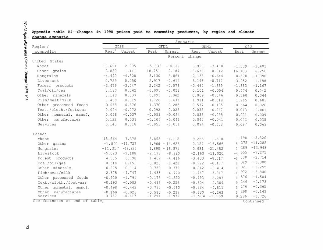
Appendix table B4--Changes in 1990 prices paid to commodity producers, by region and climatechange scenario

Region/ GISScommodity Rest2 Unrest

Scenario1

GFDL UKMO OSURest Unrest Rest Unrest Rest Unrest

United StatesWheatOther grainsNongrainsLivestock

Percent change

10.621 2.995 -5.633 -10.367 3.916 -3.470 -1.639 -2.4013.839 1.111 18.751 2.184 13.673 -0.042 16.703 6.250-4.990 -4.308 8.130 3.861 -2.133 -0.644 -0.378 -1.3900.759 0.050 2.917 -0.614 3.146 -0.717 3.252 1.188-3.479 -3.047 2.242 -0.076 -0.467 -1.659 -1.383 -1.1670.180 0.042 -0.095 -0.058 0.101 -0.054 0.074 0.0420.148 0.037 -0.093 -0.042 0.069 -0.046 0.060 0.0440.488 -0.019 1.726 -0.433 1.911 -0.519 1.965 0.683-0.068 -0.376 1.370 0.285 0.537 -0.135 0.564 0.0260.024 -0.072 0.092 0.028 0.038 -0.067 0.043 -0.0010.058 -0.037 -0.053 -0.054 0.033 -0.095 0.021 0.0090.132 0.038 -0.106 -0.041 0.047 -0.041 0.042 0.0380.143 0.018 -0.053 -0.031 0.094 -0.053 0.097 0.063

Forest productsCoal/oil/gasOther mineralsFish/meat/milkOther processed foodsText./cloth./footwearOther nonmetal. manuf.Other manufacturesServices

CanadaWheatOther grainsNongrainsLivestockForest productsCoal/oil/gasOther mineralsFish/meat/milkOther processed foodsText./cloth./footwearOther nonmetal. manuf.Other manufactures

190 -3.826275 -11.285289 -13.948555 -7.271038 -2.714329 -0.300321 -0.255972 -3.840576 -1.504246 -0.173276 -0.365298 -0.143

Services -0.737 -0.617 -1.291 -0.979 -1.504 -1.169 0.296 -0.726See footnotes at end of table, Continued--

18.664-1.801 -11.357 -5.023-4.585-0.318-0.275-2.675-0.920-0.193-0.498-0.160

7.375-11.727-19.820-9.188-6.198-0.151-0.114-4.747-1.791-0.082-0.443-0.026

3.8651.966 -1.898 --2.193-1.462-0.828-0.759-1.433-0.175-0.496-0.730-0.585

-4.11214.62316.872-8.990-4.416-0.428-0.372-4.770-1.820-0.253-0.560-0.239

9.266 1.8100.127 -16.8660.981 -21.482-2.163 -11.020-3.433 -8.017-0.922 -0.477-0.842 -0.414-1.447 -5.817-0.493 -2.287-0.604 -0.309-0.934 -0.811-0.630 -0.263

151

-4-000

-10

-000

Appendix table B4--Changes in 1990 prices paid to commodity producers, by region and climatechange scenario--continued

Region/ GISS GFDL UKMO OSUcommodity Rest2 Unrest Rest Unrest Rest Unrest Rest Unrest

Percent changeEuropean Community

WheatOther grainsNongrainsLivestockForest productsCoal/oil/gasOther mineralsFish/meat/milkOther processed foodsText./cloth./footwearOther nonmetal. manuf.Other manufacturesServices

JapanWheatOther grainsNongrainsLivestockForest productsCoal/oil/gasOther mineralsFish/meat/milkOther processed foodsText./cloth./footwearOther nonmetal. manuf.Other manufactures

718 55.918063 -12.186827 -19.059103 -2.247897 -5.112083 0.034099 0.013379 -0.872263 -2.183123 -0.137194 -0.109116 -0.014

Services -0.390 -0.298 -0.259 -0.138 -0.136 0.003 -0.264 -0.177See footnotes at end of table. Continued--

40.081 56.056-5.806 -13.08912.534 -18.375-1.552 -2.475-5.479 -5.280-0.174 -0.053-0.196 -0.082-0.584 -0.987-0.808 -2.409-0.258 -0.287-0.319 -0.218-0.215 -0.111

37.154-4.045 -

-13.645 --1.263-5.5730.017-0.010-0.240-0.1080.130-0.131-0.071

59.08814.29520.119-2.938-6.6980.1760.141-0.979-2.688-0.006-0.0420.071

55.055 79-5.302 -16

-15.013 -21-1.429 -3-7.878 -80.144 00.123 0-0.196 -0-0.193 -20.188 0-0.094 00.039 0

917136768224774326295978860051029199

33-4

-12-1-4-0-0-0-0-0-0-0

62.740 30.948 45 237 19 277 73 875 31.930 15.506 8.65926.799 - 29.742 -22 489 -25 135 -27 459 -31.393 -15.009 - 19.47815.757 6.597 15 694 6 051 19 750 7.784 6.564 3.0023.339 1.113 2 119 1 396 2 477 0.943 2.835 1.303-5.586 - 10.726 -2 665 -8 837 -5 826 -11.163 -1.873 -4.9000.337 0.474 0 212 0 314 0 252 0.404 0.196 0.2420.349 0.487 0 214 0 319 0 258 0.414 0.194 0.2443.757 1.497 2 848 1 266 3 978 1.514 1.842 0.7601.811 0.683 1 763 0 672 2 367 0.882 0.836 0.2330.415 0.394 0 375 0 314 0 446 0.391 0.237 0.1940.265 0.331 0 185 0 211 0 195 0.263 0.164 0.1750.282 0.434 0 163 0 284 0 189 0.362 0.168 0.2260.473 0.607 0 301 0 402 0 388 0.535 0.240 0.286


Scenario1


Other East Asia3

WheatOther grainsNongrainsLivestock

Percent change

Forest productsCoal/oil/gasOther mineralsFish/meat/milkOther processed foodsText./cloth./footwearOther nonmetal. manuf.Other manufacturesServices

13.231 5.466 17.300 9.228 5.776 0.861 7.935 4.1040.462 0.011 0.819 -0.919 2.635 -0.115 4.308 2.374-5.398 -5.884 -7.396 -6.301 0.168 -3.884 -6.627 -6.327-0.041 -0.826 0.931 -1.060 0.914 -0.974 0.807 -0.224-0.347 -0.230 0.038 -0.093 -0.552 -0.169 -0.224 -0.1590.129 0.129 0.221 0.189 -0.079 0.035 0.156 0.1760.137 0.127 0.236 0.181 -0.061 0.033 0.173 0.1700.098 -0.298 0.606 -0.364 0.430 -0.432 0.542 0.0230.349 -0.526 1.272 -0.660 1.777 -0.661 1.779 0.338-0.159 -0.364 0.241 -0.179 0.200 -0.271 -0.020 -0.235-0.008 -0.037 0.157 0.059 -0.033 -0.053 0.061 0.0310.086 0.081 0.187 0.143 -0.041 0.034 0.127 0.1270.094 0.065 0.252 0.152 -0.069 -0.016 0.171 0.144

Southeast Asia4

WheatOther grainsNongrainsLivestockForest productsCoal/oil/gasOther mineralsFish/meat/milkOther processed foodsText./cloth./footwearOther nonmetal. manuf.Other manufactures

000 0.000509 2.802062 -0.685963 -0.618790 0.843347 -0.061337 -0.087128 -0.214011 0.606128 -0.210031 0.003190 -0.041

Services -0.209 0.090 -0.122 0.122 -0.430 0.206 -0.246 -0.079See footnotes at end of table. Continued--

0.00016.5214.5341.855-1.334-0.329-0.3040.5735.621

-0.1610.058-0.200

0.00010.046-2.794-1.1111.6450.0880.102-0.0852.651

-0.1830.1960.039

0.00015.4158.3281.939

-0.264-0.390-0.2850.5825.8240.2390.252-0.161

0.0007.771-0.918-1.0122.4250.0310.092-0.1192.2020.0610.2750.063

0.00027.41412.0823.160

-1.619-0.784-0.6780.8339.8960.0330.168-0.393

0.00014.441-2.643-1.3053.0570.0700.166-0.0454.0620.0440.3860.100

0840

-0-0-003

-0-0-0


Scenario1


Australia and New ZealandWheatOther grainsNongrainsLivestockForest productsCoal/oil/gasOther mineralsFish/meat/milkOther processed foodsText./cloth./footwearOther nonmetal. manuf.Other manufacturesServices

Rest of worldWheatOther grains

-7-3

NongrainsLivestockForest productsCoal/oil/gasOther mineralsFish/meat/milkOther processed foodsText./cloth./footwearOther monmetal. manuf.Other manufactures

493 -14 653 -18462 -6 438 -8043 2 307 5

-1 705 -2 -1 277 -2-1 015 -0 0 905 0-0 262 -0 -0 100 -0-0 239 -0 -0 086 -0-0 709 -1 -0 431 -1-0 487 -1 -0 214 -10 055 -0 0 461 0

-0 178 -0 0 078 -0-0 173 -0 -0 049 -0

Services -0.267 -0.292 -0.086 -0.178 -0.278 -0.327 -0.081 -0.116See footnotes at end of table. Continued--

882700505666661243227187669154299165

12-4

936188556711869136134116574151121093

-11.441 -24.641-6.714 -12.36810.309 7.897-2.063 -3.985-0.402 0.144-0.291 -0.263-0.270 -0.257-0.742 -1.655-0.359 -2.3920.503 0.145-0.068 -0.277-0.205 -0.199

-5.556 -11.284-3.286 -4.1754.222 2.026-1.111 -1.695-0.008 0.301-0.071 -0.081-0.069 -0.080-0.394 -0.714-0.273 -0.9840.222 -0.0170.007 -0.102-0.039 -0.050

8 019 1 615 -0 035 -3.698 7.655 1.958 1.190 -5.955-4 508 -7 194 -0 512 -5.151 -3.849 -3.928 5.275 -6.8863 575 1 227 5 646 3.601 4.150 1.608 1.289 0.836

-0 428 -0 464 -0 003 -0.459 -0.846 0.241 -4.555 -2.1730 466 -0 418 2 551 -0.228 3.346 0.595 -0.038 -2.5640 319 -0 003 0 348 -0.075 0.528 -0.160 0.329 -0.0580 321 -0 003 0 350 -0.071 0.533 -0.150 0.321 -0.065

-0 005 -0 234 0 234 -0.250 -0.063 0.042 -1.972 -1.0980 695 -0 181 0 831 -0.109 0.965 -0.070 0.576 -0.5780 353 -0 026 0 537 0.029 0.520 -0.025 -0.246 -0.2930 284 -0 019 0 350 -0.073 0.512 -0.129 0.276 -0.1010 288 -0 000 0 307 -0.065 0.483 -0.124 0.298 -0.0460 345 -0 013 0 390 -0.075 0.604 -0.141 0.296 -0.125

Percent change


Scenario 1


Percent changeWorld

Wheat 7.554 -2.481 0.584 -7.771 3.751 -9.704 0.512 -4,586Other grains -0.593 -3.468 1.528 -4.309 0.480 -6.426 2.399 -1.022Nongrains 2.871 0.540 5.711 2.949 8.565 4.407 2.316 0.217Livestock -0.851 -1.855 -0.369 -1.928 -0.871 -2.735 -0.529 -1.169Forest products -1.794 -1.658 0.594 -0.093 -0.986 -1.022 -0.474 -0.413

Coal/oil/gas -0.090 -0.087 -0.086 -0.071 -0.162 -0.138 -0.026 -0.022Other minerals 0.085 0.157 0.064 0.108 0.018 0.109 0.066 0.091Fish/meat/milk 0.537 -0.387 0.763 -0.489 0.927 -0.677 0.524 -0.224Other processed foods 0.299 -0.824 0.780 -0.758 0.863 -1.032 0.330 -0.616Text./cloth./footwear 0.073 -0.049 0.306 0.104 0.324 0.100 0.107 -0.016Other nonmetal. manuf. -0.021 -0.047 0.042 -0.004 0.011 -0.046 0.018 -0.005Other manufactures -0.000 0.036 -0.015 0.042 -0.014 0.046 0.012 0.043Services 0.035 0.044 -0.022 0.013 0.007 0.022 0.010 0.020

1Climate scenarios based on results generated by the general circulation models of the GoddardInstitute for Space Studies (GISS), the Geophysical Fluid Dynamics Laboratory (GFDL), the UnitedKingdom Meteorological Office (UKMO),2Rest = cropland, pasture, forest,

and Oregon State University (OSU).and land in other uses restricted to 1990 locations and

quantities. Unrest = all land can move among cropland, pasture, and other uses.3China (including Taiwan), Hong Kong, and North Korea.4Indonesia, Malaysia, Philippines, and Thailand.

Appendix table B5--Base revenues from primary factors and changes in factor prices, by region and climate

Region/commodity

Scenario 1

Base (1990) GISS GFDL UKMO OSUvalue2 Rest3 Unrest Rest Unrest Rest Unrest Rest Unrest

United StatesWaterLaborCapitalLand

Mil. $U.S.

1,1913,273,8101,666,670

114,317

CanadaWaterLaborCapitalLand

107 -3.711 -5.751 -1.496 0.819 -5.964 -5.159 -1.571 2.227322,388 0.758 1.034 0.471 1.054 0.608 1.290 0 . 4 5 8 0.887211,063 0.864 1.114 0.651 1.197 0.823 1.455 0.589 0.99822,691 10.640 7.105 16.568 11.075 19.811 12.638 12.548 8.943

European CommunityWater 648Labor 3,601,650Capital 1,836,530Land 186,894

JapanWaterLaborCapitalLand

274 70.368 77.082 76.5751,635,900 0.222 0.409 0.140

989,909 0.233 0.425 0.143175,307 0.801 -0.439 -0.234

------------------------------ - - Percent change - - - - - - - - - - - - - - - - - - - - - - - - - - - - - -

6.407 -1.792 4.052 -1.524 9.288 -3.217 11.731 8.9720.191 0.100 -0.205 -0.075 0.036 -0.022 -0.023 -0.0040.253 0.085 -0.147 -0.109 0.145 -0.053 0.040 -0.0060.753 -0.438 3.535 -1.150 2.558 -0.838 1.133 -1.062

-6.338 18.489 -5.178-0.525 -0.279 -0.428-0.579 -0.313 -0.464-4.304 -8.280 -1.850

-15.797 -6.498 -21.809 10.526 14.081-0.226 -0.678 -0.397 -0.158 -0.053-0.254 -0.734 -0.438 -0.177 -0.071-5.409 -3.727 -8.517 -1.206 -3.234

80.562 109.459 111.505 71.853 83.7040.403 0.042 0.323 0.278 0.4750.417 0.045 0.337 0.282 0.486-1.962 -2.151 -3.929 0.786 -0.679

27.0210.4870.319

28.2060.4400.379

15.8500.6780.312

15.4740.4890.418

22.2990.5000.183

12.3210.4320.335

Other East Asia4

Water 1,200 26.373 -1.735Labor 354,219 0.125 0.300Capital 252,881Land 40,724

0.108 0.318-2.023 -3.123 -1.363 -3.341 0.391 -2.132 -0.348 -2.805

See footnotes at end of table, Continued--

Appendix table B5--Base revenues from primary factors and changes in factor prices, by region and climatechange scenario--continued

Scenario1


Mil. $U.S. --------------------- --Percent change------------------------------

Southeast Asia5

Water 223 -17.946 -21.879 1.178 -6.974 0.726 -17.514 7.122 3.447Labor 93,692 -1.322 -0.601 -0.975 -0.293 -2.248 -0.672 -0.699 -0.290Capital 144,175 -1.246 -0.620 -1.151 -0.459 -2.236 -0.967 -0.567 -0.119

L a n d 25,112 3.713 -0.806 6.132 0.391 8.217 -0.312 3.228 -0.095

Australia andNew ZealandWater 48 -11.744 -23.906 9.010 -22.504 30.671 -8.145 -7.808 -27.225Labor 193,618 0.429 0.049 0.243 -0.252 0.365 -0.461 1.066 0.571Capital 106,900 0.395 0.083 0.199 -0.212 0.265 -0.443 0.992 0.601Land 18,382 1.912 0.428 0.329 -1.170 -0.543 -1.679 3.164 2.783

Rest of worldWater 4,568 -13.622 -21.875 -8.771 -15.759 0.781 -15.536 -10.526 0.302Labor 2,222,300 -0.028 -0.010 -0.005 -0.072 -0.241 -0.207 -0.158 0.040Capital 2,115,540 -0.016 0.072 -0.008 0.045 -0.215 -0.056 -0.177 0.092Land 260.384 0.930 -0.786 1.915 -0.054 1.816 -1.218 0.480 -0.028

1Climate scenarios based on results generated by the general circulation models of the GoddardInstitute for Space Studies (GISS), the Geophysical Fluid Dynamics Laboratory (GFDL), the UnitedKingdom Meteorological Office (UKMO), and Oregon State University (OSU).2Base values reflect total value of regional factor endowments (price times quantity). For (all) land,labor, and capital, regional endowments are constant across the base period and all GCM scenarios.For water, we use a price of $2.55 million per cubic kilometer globally; all percentage changes inwater prices apply to this figure. Since climate change affects regional water endowments, percentagechanges in water prices do not reflect percentage changes in total values of regional waterendowments.3Rest = cropland, pasture, forest, and land in other uses restricted to 1990 locations and quantities.Unrest = all land can move among cropland, pasture, and other uses.4China (including Taiwan), Hong Kong, and North Korea.5Indonesia, Malaysia, Philippines, and Thailand.

Appendix table B6--Changes in the household price index, household income, and real gross domestic product(GDP), by region and climate change scenario

Scenario 1

Item/ GISS GFDL UKMO OSUregion Rest2 Unrest Rest Unrest Rest Unrest Rest Unrest

Percent changeHousehold Price IndexUnited States 0.102 -0.034 0.111 -0.010 0.147 -0.076 0.151 0.056Canada -0.776 -0.881 -0.990 -1.110 -1.202 -1.373 -0.802 -0.857European Community 0.814 0.599 0.635 0.444 0.842 0.574 0.402 0.277Japan -0.536 -0.733 -0.325 -0.646 -0.255 -0.578 -0.363 -0.610Other East Asia3 -0.089 -0.473 0.158 -0.502 0.569 -0.446 0.273 -0.196Southeast Asia4 1.396 0.418 1.732 0.468 2.660 0.805 0.762 0.018Australia/New Zealand 0.365 -0.027 0.453 -0.044 0.601 -0.094 0.197 -0.192Rest of world -0.264 -0.613 0.012 -0.444 -0.111 -0.722 -0.057 -0.314

Household IncomeUnited States 0.201 0.083 -0.132 -0.100 0.094 -0.042 0.001 -0.022Canada 1.172 1.293 1.172 1.501 1.437 1.792 0.991 1.245European Community -0.590 -0.500 -0.460 -0.382 -0.747 -0.639 -0.180 -0.136Japan 0.265 0.325 0.083 0.193 -0.109 0.008 0.286 0.355Other East Asia 0.166 0.144 0.146 0.143 0.129 0.162 0.140 0.118Southeast Asia -0.811 -0.668 -0.403 -0.353 -1.226 -0.865 -0.227 -0.161Australia/New Zealand 0.477 0.076 0.223 -0.283 0.262 -0.519 1.151 0.702Rest of world 0.028 -0.029 0.108 -0.019 -0.103 -0.202 0.099 0.066

Continued--


Appendix table B6--Changes in the household price index, household income, and real gross domestic product(GDP), by region and climate change scenario--continued

Scenario 1

Item/ GISS GFDL UKMO OSUregion Rest2 Unrest Rest Unrest Rest Unrest Rest Unrest

Million $U.S.Real GDP5

United States 5919.8 5784.2 -11142.6 -4818.5 -1246.8 1135.0 -6584.7 -3892.4

Canada 10350.1 11306.3 11638.8 13673.7 14147.5 16491.8 9594.4 11036.8

European Community -67975.3 -56518.6 -52313.7 -42061.5 -77444.1 -63210.0 -27015.3 -20535.2

Japan 18124.0 23066.5 8675.9 17159.0 1341.9 10026.8 15507.1 21559.6Other East Asia 1519.8 3019.6 186.1 3062.3 -1418.8 3103.2 -286.6 1579.1

Southeast Asia -4596.0 -2652.6 -3950.2 -1812.8 -7812.3 -3877.8 -1851.5 -485.3

Australia/New Zealand 733.0 344.7 -403.9 -884.9 -710.6 -1597.7 3543.1 3027.8

Rest of world 9578.3 17879.9 4662.5 13063.8 -1160.3 13446.7 6343.8 12874.1World -26346.4 2230.2 -42647.2 -2618.9 -74303.5 -24481.9 -749.7 25164.31Climate scenarios based on results generated by the general circulation models of the GoddardInstitute for Space Studies (GISS), the Geophysical Fluid Dynamics Laboratory (GFDL), the UnitedKingdom Meteorological Office (UKMO),2Rest = cropland, pasture, forest,

and Oregon State University (OSU).and land in other uses restricted to 1990 locations and

quantities. Unrest = all land can move among cropland, pasture, and other uses.3China (including Taiwan), Hong Kong, and North Korea.4Indonesia, Malaysia, Philippines, and Thailand.5Base (1990) values for GNP (in million $US) are: United States = 5,496,575; Canada = 597,823;European Community = 5,923,307; Japan = 3,041,381; Other East Asia = 743,368; Southeast Asia =292,032; Australia/New Zealand = 361,917; Rest of world = 4,602,790; and world = 21,059,193.

Appendix table B7--Base values and chances in commodity supply, by region and climate change scenario1

Scenario2


United StatesWheatOther grainsNongrainsLivestockForest productsCoal/oil/gasOther mineralsFish/meat/milkOther processed foodsText./cloth./footwearOther nonmetal. manuf.Other manufacturesServices

CanadaWheatOther grainsNongrainsLivestockForest productsCoal/oil/gasOther mineralsFish/meat/milkOther processed foodsText./cloth./footwearOther nonmetal manuf.Other manufactures

32,098 -19.678 66.971 -3.583 164.539 -2.922 163.651 -7 596 126.48024,981 11.458 244.284 -1.694 259.211 -1.961 421.658 2 203 169.41813,015 51.286 473.314 0.186 376.649 -0.934 751.158 14 416 221.04723,820 46.816 230.915 45.644 244.332 34.565 384.238 5 953 162.915

155,475 18.647 50.192 3.657 20.500 11.056 51.191 1 400 10.67627,388 6.146 -18.800 7.875 -18.855 7.499 -35.965 9 572 -9.48710,210 -22.627 -28.256 -27.876 -32.807 -34.001 -43,662 -20 951 -24.59524,438 -38.781 -32.613 -48.250 -41.112 -58.882 -50.176 -36 569 -31.65732,418 -24.942 -29.110 -30.606 -34.020 -37.008 -44.355 -23 392 -25.91218,635 -37.549 -35.071 -44.435 -41.361 -50.247 -47.997 -37 411 -34.714

130,143 -33.044 -33.234 -39.439 -38.880 -44.897 -46.530 -32 770 -31.998119,236 -30.566 -32.259 -36.652 -37.548 -41.873 -45.751 -30 214 -30.540

Services 719,538 12.152 5.763 15.770 8.961 18.571 7.237 12.965 8.393See footnotes at end of table. Continued--

Number - - - - - - - - - - - - - - - - - - - - - - - - - - - - Percent change - - - - - - - - - - - - - - - - - - - - - - - - - - - - - -

74,475 -5.529 7.299 9.988 29.061 -1 020 22.275 0.622 -0.485238,352 -9.633 -1.361 -32.432 -12.039 -25 153 -2.264 -27.609 -18.794194,389 14.005 16.109 -19.252 -10.195 7 196 6.308 -3.730 -3.351170,647 9.622 6.068 7.000 6.174 0 436 6.826 0.698 -2.727498,000 15.015 35.148 -9.009 -0.135 0 374 16.659 4.866 14.562215,073 -4.007 -4.273 4.506 3.819 -0 283 -0.439 3.841 3.79524,786 -3.130 -2.833 1.545 2.230 -0 750 -0.120 2.329 2.546

121,363 -2.860 -2.728 -2.277 -1.669 -2 238 -2.045 -0.240 -0.254292,850 -3.356 -3.205 2.298 2.636 -0 630 -0.202 2.716 2.866155,999 -2.716 -1.932 1.278 2.979 -0 437 0.974 2.530 3.047

1,067,890 -3.082 -2.538 2.501 3.646 -0 243 0.839 3.162 3.5721,266,520 -2.755 -1.997 1.409 3.050 -0 417 0.960 2.597 3.1036,103,870 0.950 0.665 -0.508 -1.082 0 171 -0.348 -0.947 -1.127

Appendix table B7--Base values and changes in commodity supply, by region and climate change scenario1--continued

Scenario 2


Number ----------------------------Percent change------------------------------

European CommunityWheatOther grainsNongrainsLivestockForest productsCoal/oil/gasOther mineralsFish/meat/milkOther processed foodsText./cloth./footwearOther nonmetal. manufOther manufacturesServices

80,319 -58.023 -51.772 -51.542 -42.977 -62 726 -55 597 -25 701 -16.85224,994 70.306 152.121 56.176 109.012 73 737 157 921 34 835 75.581

279,884 -36.127 -17.035 -33.032 -16.739 -38 989 -18 360 -17 404 -5.046295,049 -13.293 -19.009 -7.942 -20.799 -8 226 -18 085 -13 697 -19.382171,394 19.057 159.057 9.233 117.281 20 769 171 292 5 700 49.98882,886 -1.633 -0.467 -1.173 -0.254 -1 613 -0 392 -1 496 -1.268

270,580 -1.711 -0.220 -1.316 -0.203 -1 640 -0 108 -2 217 -1.392157,710 -26.314 -24.746 -19.307 -17.965 -27 103 -25 451 -13 461 -12.453485,433 -1.623 -0.499 -1.155 -0.260 -1 609 -0 428 -1 912 -1.253284,159 14.678 16.035 9.349 10.285 15 538 16 873 3 793 4.519

1,472,520 15.087 14.734 10.054 10.037 15 683 15 372 5 050 5.0941,292,320 14.625 16.206 9.258 10.318 15 518 17 071 3 630 4.4455,815,930 -5.131 -5.931 -3.224 -3.687 -5 500 -6 252 -1 142 -1.567

JapanWheatOther grainsNongrainsLivestockForest productsCoal/oil/gasOther mineralsFish/meat/milkOther processed foodsText./cloth./footwearOther nonmetal. manuf.Other manufacturesServices 3,327,640 2.987 -0.998 3.265 -1.707 2.710 -3.306 2.521 -1.515


952 -45.787 -16.270 -54.007 -23.529 -62.173 -36.919 -48 885 -24 82613,499 28.401 204.352 32.630 250.127 36.563 305.230 30 860 206 72432,151 42.877 233.827 50.949 294.872 58.665 358.822 43 755 241 89016,665 21.875 11.259 28.089 8.955 31.392 -2.612 22 201 4 54429,593 17.300 15.164 20.855 20.413 28.941 28,266 16 565 12 4318,662 -10.195 -10.079 -14.277 -14.020 -15.810 -15.352 -8 756 -8 535

16,568 -10.712 -10.970 -14.900 -15.109 -16.450 -16.572 -9 226 -9 39768,056 -20.399 -19.331 -30.152 -28.783 -33.391 -31.571 -16 148 -14 907

312,381 -11.386 -12.127 -15.713 -16.520 -17.285 -18.149 -9 841 -10 519121,234 -9.497 -12.679 -11.807 -15.772 -12.016 -16.960 -8 607 -11 847719,010 -6.652 -7.879 -8.265 -9.764 -8.287 -10.135 -6 032 -7 236

1,146,530 -7.054 -8.564 -8.767 -10.628 -8.817 -11.121 -6 395 -7 894

. . . .. . . . .

Appendix table B7--Base values and changes in commodity supply, by region and climate change scenariol--continued

Scenario 2

Region/ Base (1990) GISS GFDL UKMO OSUcommodity value Rest4 Unrest Rest Unrest Rest Unrest Rest Unrest

Other East AsiaWheatOther grainsNongrainsLivestockForest productsCoal/oil/gasOther mineralsFish/meat/milkOther processed foodsText./cloth./footwearOther nonmetal. manufOther manufacturesServices

Southeast AsiaWheatOther grainsNongrainsLivestockForest productsCoal/oil/gasOther mineralsFish/meat/milkOther processed foods

Number ----------------------- -Percent change------------------------------

98,233 -12 310 -16 270 -27.013 -10.960 -10.582 6.666 -13.662 -5.194314,527 4 015 204 352 7.811 16.268 -5.929 8.053 -1.242 4.805428,755 16 827 29.500 31.292 -1.564 16.184 18.155 22.269691,279 4 336 11 259 -2.129 7.027 0.562 10.001 2.156 6.479283,530 10 634 15 164 6.050 0.849 10.684 1.683 9.509 10.06821,468 3 841 -10 079 5.797 8.617 -2.038 5.020 3.484 5.63215,752 -2 288 -10 970 -1.325 -1.475 -1.445 -1.869 -1.666 -1.65035,760 -8 052 -19 331 -8.235 -11.342 -0.560 -8.636 -7.089 -8.871

102,987 2 903 -12 127 4.703 7.047 -1.950 3.962 2.699 4.512149,392 -6 037 -12 679 -5.484 -6.998 -1.419 -5.939 -4.580 -5.774223.391 1 440 -7 879 3.192 5.179 -2.161 2.434 1.777 3.125323,723 -3 087 -8 564 -2.074 -2.270 -1.720 -2.646 -2.062 -2.280650,319 -0 998 -2.956 -5.001 2.371 -2.016 -0.975 -2.666

089,191200,14874,225

260,90123,5976,084

20,59151,51230,416

0-25-17-0-0

-12

Text./cloth./footwearOther nonmetal. manuf. 68,154Other manufactures 50,624

-9-16

-22

000 0 000 0.000 0.000 0.000 0.000 0.000 0.000713 -19 349 -25.456 -17.465 -37.880 -28.335 -15.688 -6.708076 -3 255 -20.585 -5.366 -30.304 -5.956 -13.748 -3.351708 91 272 -0.376 81.673 -1.290 144.921 -0.813 28.787691 -10 542 -1.080 -12.581 -0.947 -17.416 -0.350 -6.130601 -4 953 -13.295 -5.326 -19.622 -7.311 -8.388 -2.591070 -2 673 3.061 -0.779 3.290 -2.792 2.901 0.387090 -8 153 -6.443 -5.456 -11.492 -9.878 -2.066 -1.585865 -3 139 -0.490 -1.716 -1.842 -3.724 0.507 -0.222663 0 263 8.171 1.678 11.937 1.175 5.338 1.340302 -1 157 -2.498 -1.139 -3.907 -1.697 -1.706 -0.459127 -0 441 2.749 0.276 3.777 -0.255 1.792 0.447

Services 247,521 5.459 -0.132 6.063 0.437 8.575 -0.572 4.137 0.620See footnotes at end of table. Continued--

Appendix table B7--Base values and changes in commodity supply, by region and climate change scenario1--continued

Scenario2


NumberAustralia and New ZealandWheatOther grainsNongrainsLivestockForest productsCoal/oil/gasOther mineralsFish/meat/milkOther processed foodsText./cloth./footwearOther nonmetal. manuf.Other manufacturesServices

15,254 10.426 18.182 10.120 21 438 -1.286 -4.254 3.815 66.3728,584 5.292 21.123 5.015 21 645 9.776 -1.343 -5.437 59.491

33,360 14.070 12.604 16.405 26 818 -10.942 17.838 -3.888 -0.818264,475 3.348 1.917 2.191 0 696 6.650 -5.654 30.122 19.52732,132 -2.316 3.963 -9.323 0 832 -12.457 -8.385 1.144 32.44412,659 -1.264 -1.237 -1.264 -2 126 -0.418 -0.755 -2.219 -2.2608,372 -1.046 -1.038 -1.001 -1 698 -0.187 -0.409 -2.368 -2.439

17,714 -0.022 -0.048 -2.095 -1 632 -1.203 -0.606 -1.259 -1.29820,731 -0.342 -0.396 -0.154 -0 314 0.556 0.707 -2.843 -3.00818,175 0.305 0.167 1.796 2 004 2.400 2.787 -4.308 -4.62966,743 -0.026 -0.134 1.391 1 338 2.044 2.249 -4.096 -4.37562,302 0.381 0.237 1.891 2 159 2.483 2.912 -4.359 -4.689

413,544 0.251 0.155 -0.261 -0 156 -0.882 -0.302 1.159 0.704

Rest of worldWheat 291,182 13.035 47.596 18.012 50 905 15 783 78.260 8.020 29.559Other grains 644,130 4.021 27.425 4.245 26 795 5 347 43.070 4.095 16.106Nongrains 1,948,909 -6.311 7.204 10.410 0 515 -15 693 3.070 -6.688 2.990Livestock 2,605,951 8.142 21.281 6.163 23 190 10 057 35.053 5.294 14.041Forest products 1,883,532 2.194 -2.948 -3.227 14 163 -0 147 14.417 -0.355 -6.829Coal/oil/gas 518,792 0.573 5.178 -0.729 3 275 -1 300 5.838 -0.296 2.612Other minerals 198,475 -0.867 -0.075 -0.753 0 037 -1 604 -0.105 -0.422 0.091Fish/meat/milk 251,547 -0.006 0.552 -1.838 -1 079 -5 562 -3.530 0.421 0.630Other processed foods 642,189 -1.327 -1.708 -0.761 -0 984 -1 702 -1.945 -0.462 -0.707Text./cloth./footwear 378,729 -2.989 -6.010 -0.463 -3 108 -0 397 -5.065 -1.054 -2.980Other nonmetal. manuf. 1,608,410 -1.571 -1.040 -0.438 0 068 -0 086 0.647 -0.927 -0.507Other manufactures 1,720,940 -2.535 -4.442 -0.455 -2 099 -0 297 -3.268 -1.013 -2.192Services 4,277,060 1.803 -1.285 1.285 -1.513 1.774 -2.952 1.099 -0.739


------------------------------ --Percent change------------------------------

Appendix table B7--Base values and changes in commodity supply, by region and climate change scenariol--continued

Scenario2


Number ---------------------------- --Percent change------------------------------

WorldWheat 592,515 -9.216 14.860 -5.616 21.673 -8.157 29.780 -2.987 16.152Other grains 1,358,258 0.513 19.342 -3.916 17.721 -5.642 25.048 -4.261 8.683Nongrains 3,130,611 -5.814 8.502 -9.023 3.166 -15.456 4.452 -4.428 5.584Livestock 4,142,111 5.647 15.265 3.604 15.835 6.393 23.958 4.458 10.331Forest products 3,314,557 6.151 10.051 -2.143 -4.518 2.359 -0.656 1.776 1.303Coal/oil/gas 910,525 -0.987 1.191 0.349 2.082 -1.519 1.763 0.555 1.950Other minerals 550,827 -2.145 -1.292 -1.898 -1.213 -2.642 -1.659 -1.887 -1.400Fish/meat/milk 697,179 -11.298 -10.399 -11.576 -10.438 -15.581 -13.968 -6.664 -6.051Other processed foods 1,940,501 -3.631 -3.594 -3.288 -3.249 -4.929 -4.809 -2.195 -2.203Text./cloth./footwear 1,156,739 -0.312 -1.662 -0.437 -1.621 1.210 -1.254 -1.271 -2.233Other nonmetal. manuf. 5,356,261 0.958 1.039 0.784 1.025 1.298 1.475 -0.085 0.041Other manufactures 5,982,195 -0.603 -1.095 -0.613 -0.970 0.132 -0.823 -1.080 -1.481Services 21.555.422 0.096 -1.751 0.196 -1.731 0.020 -2.742 0.475 -0.913

1Changes in supply represent the additional quantities (positive or negative) that firms would bewilling to sell at 1990 prices under the alternative climate.2Climate scenarios based on results generated by the general circulation models of the GoddardInstitute for Space Studies (GISS), the Geophysical Fluid Dynamics Laboratory (GFDL), the UnitedKingdom Meteorological Office (UKMO), and Oregon State University (OSU).3For wheat, other grains, and nongrains, values are in 1,000 metric tons. For livestock, values are in1,000 head. For forest products, values are in 1,000 cubic meters. For all other commodities, valuesare in million U.S. dollars.4Rest = cropland, pasture, forest, and land in other uses restricted to 1990 locations andquantities. Unrest = all land can move among cropland, pasture, and other uses.5China (including Taiwan), Hong Kong, and North Korea.6Indonesia, Malaysia, Philippines, and Thailand.

Stay Up to Dateon World Agriculture

International Agriculture and Trade Situation andOutlook Reports. Subscription. 4 issues. Stock #WRS. Call 1-800-999-6779 for price and availability.

Drawing on original foreign source materials, each report in this seriesexplains how basic forces are changing agriculture and agricultural trade.Anticipates short-and long-term production, consumption, and trade of theregion's key commodities. The 4-report series covers China, Europe, formerUSSR, and NAFTA.

World Agriculture: Trends and Indicators. 3.5" disks. Annual data for 160countries, 1961-89 on macroeconomics consumption; factors of production;aggregate production (value and indexes); crop production, area, and yieldand livestock production by commodity; value of total merchandise andagricultural trade (including US. bilateral trade), and trade indicators; andvalue of ag trade by commodity groups. (.WK1), updated 1/94.

Stock # 89024A North America (1 disk) $25.00Stock # 89024B Central America (1 disk) $25.00Stock # 89024C The Caribbean (1 disk) $25.00Stock # 89024D South America (2 disks) $35.00Stock # 89024E Western Europe (2 disks) $35.00Stock # 89024F Eastern Europe & former USSR (1 disk) $25.00Stock # 89024G Sub-Saharan Africa (4 disks) $55.00Stock # 89024H North Africa & Middle East (2 disks) $35.00Stock # 89024I South Asia (1 disk) $25.00Stock # 89024J Southeast Asia & Pacific Islands (2 disks) $35.00Stock # 89024K East Asia & Peoples' Republic of China (1 disk) $25.00Stock # 89024L DISCONTINUEDStock # 89024M EC-12 (2 disks) $35.00Stock # 89024N World & regional data series only (2 disks) $35.00

To order, just dial 1-800-999-6779. Toll free in the United States and Canada. Otherareas, please call 1-703-834-0125. Or fax your order by dialing 1-703-837-0110. Call1-800-999-6779 to charge your purchases to your VISA or MasterCard. Or send acheck or money order (made payable to ERS-NASS) to: ERS-NASS, 341 VictoryDrive, Herndon, VA 22070. Payment must accompany all mail orders. Please add25 percent to all foreign address. Data products are available on DOS-compatible3.5:, 1.44 MB diskettes.

NOTE: Data products are not returnable unless defective.

U.S. Department of AgricultureEconomic Research Service1301 New York Avenue, NW

Washington, DC 20005-4788

Documents

World Agriculture and Climate Change: Economic Adaptations