YIELDING OSCILLATOR UNDER TRIANGULAR GROUND ACCELERATION PULSE

April 26, 2001 15:5 WSPC/124-JEE 00038

Journal of Earthquake Engineering, Vol. 5, No. 2 (2001) 225–251c© Imperial College Press

YIELDING OSCILLATOR UNDER TRIANGULARGROUND ACCELERATION PULSE

GEORGE MYLONAKIS

Department of Civil Engineering, City University of New York (CUNY),New York, NY 10031, USA

ANDREI M. REINHORN

Department of Civil Engineering, State University of New York at Buffalo,Buffalo, NY 14260, USA

Received 22 April 2000Revised 28 October 2000

Accepted 4 November 2000

An analytical solution is presented for the response of a bilinear inelastic simple oscillatorto a symmetric triangular ground acceleration pulse. This type of motion is typical ofnear-fault recordings generated by source-directivity effects that may generate severedamage. Explicit closed-form expressions are derived for: (i) the inelastic response of theoscillator during the rising and decaying phases of the excitation as well as the ensuingfree oscillations; (ii) the time of structural yielding; (iii) the time of peak response;(iv) the associated ductility demand. It is shown that when the duration of the pulseis long relative to the elastic period of the structure and its amplitude is of the sameorder as the yielding seismic coefficient, serious damage may occur if significant ductilitycannot be supplied. The effect of post-yielding structural stiffness on ductility demand isalso examined. Contrary to presently-used numerical algorithms, the proposed analyticalsolution allows many key response parameters to be evaluated in closed-form expressionsand insight to be gained on the response of inelastic structures to such motions. Themodel is evaluated against numerical results from actual near-field recorded motions.Illustrative examples are also presented.

Keywords: ductility, pulse, shock, spectrum, near field, oscillator, inelastic response.

1. Introduction

Significant interest has emerged in recent years in studying the severe destructive-

ness of strong near-source earthquake motions. According to seismologists, these

motions are the result of superimposed shear waves propagating in the same direc-

tion as the fault rupture, generating a long-duration high-amplitude pulse known

as “fling”. The phenomenon had already been described [Boore and Zoback, 1974;

Bertero et al., 1978; Singh, 1985; Somerville and Graves, 1993] when Northridge

and Kobe earthquakes occurred and the interest in the subject skyrocketed. A num-

ber of structural failures has been attributed to near-field pulses including that of

Olive View Hospital in the 1971 San Fernando Earthquake [Bertero et al., 1978]

and Elevated Hanshin Expressway in Kobe [Park, 1996]. Evidence for the role of a

225

April 26, 2001 15:5 WSPC/124-JEE 00038

226 G. Mylonakis & A. M. Reinhorn

fling on the collapse of a large industrial building in Greece during the 1995 Aegion

earthquake, has been presented by Gazetas et al. [1995]. Examples of near-field

recorded motions from four destructive earthquakes are given in Fig. 1.

Despite an ever-increasing database of near-field recorded accelerograms and the

intense research on the subject [Hall et al., 1995; Iwan, 1997; Malhotra, 1999; Baez

and Miranda, 2000], the inelastic response of structures to such motions has not

been sufficiently explored. It is noted that most of the foregoing studies utilise actual

time histories in conjunction with numerical algorithms to analyse the response of

inelastic single- or multi-degree-of-freedom structures to a single or multiple records

[Bertero et al., 1978; Iwan, 1997; Baez and Miranda, 2000]. In contrast, simple

idealized pulses and analytical techniques that can provide useful insight on the

physics of the problem have received less research attention [Bozognia and Mahin,

1998; Cuesta and Aschheim, 2000].

The scope of this paper is to explore the fundamental mechanics of the problem

by studying analytically the response of a bilinear yielding oscillator to an idealised

ground acceleration pulse. The specific objectives are: (1) outline a simple analyti-

cal procedure for determining the response of the oscillator; (2) determine the times

of yielding, peak response, and the associated ductility demand; (3) examine the

sensitivity of the response to the post-yielding stiffness of the structure; (4) derive

a set of analytical closed-form expressions for the response parameters in (2). It

should be noted that while the elastic perfectly-plastic system has been studied as

TIME : s

0 5 10 15 20

Pyrgos (1993)

GR

OU

ND

A

CC

ELE

RA

TIO

N:

g

-0.8

-0.4

0.0

0.4

0.8

PacoimaDam (1971)

TIME : s

0 5 10 15 20

-0.8

-0.4

0.0

0.4

0.8

Erzican (1992)

Rinaldi (1994)

2 3

0.84 g

3.0 3.5

0.46 g

2 3 4

0.52 g

0.53s

0.15s0.53s

3 4

0.66 g

0.46s

Fig. 1. Four selected near-field ground motions containing long-period, high-acceleration pulses:Pacoima-N164W (1971), Rinaldi-N22W (1994), Erzican-NS (1992), and Pyrgos-EW (1993). Thecorresponding peak ground velocities are, respectivitly, 113, 166, 84, and 25 cm/s (Table 1).

April 26, 2001 15:5 WSPC/124-JEE 00038

Yielding Oscillator Under Triangular Pulse 227

early as the 1960’s [Biggs, 1964], the response of oscillators with hardening (non-

zero post-yielding stiffness) has not been explored. In addition, little effort has been

put to derive analytical closed form solutions for the inelastic problem. Such ex-

plicit solutions can provide valuable insight on the mechanics of inelastic response

which is often obscured by the complexity of numerical solutions. The results pre-

sented in this paper complement and extend foregoing studies on inelastic shock

spectra by Jacobsen and Ayre [1958] and Biggs [1964]. Because of their simplicity,

the proposed solutions can advance the development of engineering provisions for

structural design against near-field motions.

2. Problem Definition and Solution

The problem studied in this paper is depicted in Fig. 2: a bilinear SDF oscilla-

tor with mass m, elastic stiffness K (leading to an elastic period T = 2π√m/K),

yielding strength Qy, and post-yielding stiffness Kpy = (αK)(0 ≤ α ≤ 1), is sub-

jected to a symmetric triangular ground acceleration pulse. The pulse is described

by its amplitude Ag and duration td. It is noted that this idealised excitation does

not carry all the characteristics of an actual seismic motion. For instance, ground

velocity at the end of the pulse is not zero, which implies that ground displace-

ment increases linearly with time after the end of the excitation. Nevertheless, the

pulse incorporates the large acceleration and velocity excursions observed in actual

near-field recordings and, thereby, is well suited for exploring the salient features

of structural response to such motions. This is especially true since there is ev-

idence, documented in several analytical studies of actual recordings, that only

a short interval of the ground motion, associated with the pulse, contributes to

most of the inelastic seismic demand [Bertero et al., 1978; Cuesta and Aschheim,

..Ug

Ag

td / 2 td t0

um

K, α, Qy

..Ug

K

uy

α x K

u

F

Qy

Fig. 2. System considered.

April 26, 2001 15:5 WSPC/124-JEE 00038


2000; Bozorgnia and Mahin, 1998]. In addition, it will be shown that a large set

of yielding oscillators attain their maximum response before the end of the exci-

tation and, thereby, the idealised pulse can be used for quantitative predictions of

seismic demand. Given that for impulsive excitations the effect of damping on the

response is minor [Jacobsen and Ayre, 1958; Chopra, 1995], our study concentrates

on undamped oscillators.

2.1. Model development

The variation with time of ground acceleration can be written the form (Fig. 2):

Ug(τ) = 2Ag[b1τ + b2] (1)

in which

τ =t

td(2)

is a dimensionless time variable; b1 and b2 are dimensionless coefficients. In the

rising phase of the pulse (0 ≤ τ ≤ 1/2), b1 = 1, b2 = 0. In the decaying phase

(1/2 < τ1), b1 = −1, b2 = 1. After the end of the excitation (τ > 1), b1 = b2 = 0.

Written in terms of relative displacement, the governing equation of motion of

the system is (Appendix A)

mu(τ) + αKu(τ) = −2mAg(b1τ + b2)−K(1− α)uy (3)

where the term [K(1− α)uy] on the right side applies only for yielding conditions.

Enforcing the initial conditions u(τ0) = u0 and v(τ0) = v0, a general solution to

Eq. (3) is (Appendix A):

D(τ) =

(D0 −

b3

απf

)cos[b4(τ − τ0)]

+1√α

(V0 −

b1

απf

)sin[b4(τ − τ0)] +

2b1α

(τ − τ0) +b3

απf(4)

V (τ) =

(V0 −

b1

απf

)cos[b4(τ − τ0)]

+√α

(D0 −

b3

απf

)sin[b4(τ − τ0)] +

b1

απf(5)

where D(τ) and V (τ) are amplification functions expressing the displacement and

velocity of the oscillator normalised by its elastic response, us, to a static acceler-

ation equal to the peak pulse acceleration Ag [Jacobsen and Ayre, 1958; Chopra,

1995] i.e.,

D(τ) = u(τ)/us (6)

V (τ) = v(τ)/(ωus) (7)

us = mAg/K . (8)

April 26, 2001 15:5 WSPC/124-JEE 00038


In the above equations, ω denotes the elastic cyclic natural frequency of the system

and D0, V0 the dimensionless initial conditions; b3, b4 stand for the dimensionless

quantities

b3 = 2πf(b1τ0 + b2)− (1− α)ηπf (9)

b4 =√α2πf (10)

in which f and η are dimensionless parameters describing, respectively, the duration

of the pulse and the yielding resistance of the oscillator:

f =td

T(11)

η =Qy

mAg. (12)

Equations (4) and (5) can be used to describe the response of the system under

both elastic (α = 1) and yielding (α < 1) conditions, in a piece-wise linear fashion.

It is noted that the second term in the right side of Eq. (9), −(1− α)ηπf , should

only be considered if yielding takes place.

3. Elastic Oscillator

To demonstrate the use of Eqs. (4) and (5), the response of an elastic oscillator is

examined first. Detailed discussions on the topic can be found in Jacobsen and Ayre

[1958], Biggs [1964], and Chopra [1995]. The problem is analysed in three phases:

rising pulse (phase 1), decaying pulse (phase 2), and free-vibrations (phase 3). For

each individual phase, the two equations are used in conjunction with the following

values for τ0, b3, D0, V0:

• phase 1 (0 ≤ τ ≤ 1/2) : τ0 = 0, b3 = 0, D0 = 0, V0 = 0

• phase 2 (1/2 < τ ≤ 1) : τ0 = 1/2, b3 = πf,D0 = D1/2, V0 = V1/2

• phase 3 (τ > 1) : τ0 = 1, b3 = 0, D0 = D1, V0 = V1

in which (D1/2, V1/2) and (D1, V1) denote the response of the system at the peak

(τ = 1/2) and the end (τ = 1) of the pulse, respectively. Substituting the above

values in Eqs. (4) and (5), the following expressions are obtained (see also [Jacobsen

and Ayre, 1958])

D(τ) = 2τ − 1

τfsin(2πfτ) (13a)

D(τ) =1

πf

[sinπf cos 2πf

(τ − 1

2

)

− (2− cosπf) sin 2πf

(τ − 1

2

)]− 2τ + 2 (13b)

D(τ) = D1 cos[2πf(τ − 1)] + V1 sin[2πf(τ − 1)] (13c)

April 26, 2001 15:5 WSPC/124-JEE 00038


which correspond to phases 1, 2 and 3, respectively. It can be easily shown that

Eq. (13a) increases monotonically with time. Accordingly, the response at the peak

of the pulse, D1/2, is the maximum response within the interval 0 < τ < 1/2,

providing a lower bound for the overall peak response.

Differentiating Eqs. (13b) and (13c) one can determine the critical time τm at

which the velocity changes sign and the system reaches its peak response. After

some tedious yet straightforward algebra, the following expressions are obtained:

τm =1

2+

1

2πf

[arctan

(sinπf

2− cosπf

)+ arccos

(1√

5− 4 cosπf

)](14a)

τm =1

2+

1

4f(14b)

which pertain to the decaying acceleration branch and free oscillations, respectively.

Obviously, only dimensionless times smaller than 1 are admissible from Eq. (14a),

and times greater than 1 from Eq. (14b). The maximum response is determined by

substituting the pertinent value of τm into Eq. (13b) or (13c).

In Fig. 3(a), the maximum response of the system, Dm, is plotted as function of

the dimensionless pulse duration f . The response at the peak of the pulse, D1/2, end

of pulse, D1, and free vibrations, Df , are also shown for comparison. The following

are worthy of note: Firstly, the overall peak value, Dm = 1.52, is quite small which

indicates that resonant effects are of minor importance for this type of loading.

Secondly, for small pulse durations (f less than about 0.5) the response at the end

0.0

0.5

1.0

1.5

2.0

PEAK

RESPONSE: Dm

RESPONSE AT

PULSE PEAK: D1/2

AMPLITUDEOF RESIDUAL

RESPONSE: Df

RESPONSE AT

PULSE END: D1

NO

RM

ALI

ZE

D R

ES

PO

NS

E

D =

u /

u s

(a)

Fig. 3. Normalised peak displacement response (a) and corresponding time (b) of an undampedelastic oscillator subjected to a symmetric triangular acceleration pulse. (Graph (b) modified fromBiggs, [1964]).

April 26, 2001 15:5 WSPC/124-JEE 00038


DIMENSIONLESS PULSE DURATION f = td / T0

0 1 2 3 4

TIM

E O

F P

EA

K R

ES

PO

NS

E

τ m

= t m

/ t d

0.0

0.5

1.0

1.5

2.0

0.5

RISING PULSE

DECAYING PULSE

FREE VIBRATIONSEqn (14b)

Eqn (14a)

(b)

Fig. 3. (Continued)

of the pulse is very close to the maximum. In contrast, for long pulse durations

(f greater than 1.3), the maximum response can be approximated reasonably well

by the response at the pulse peak. Thirdly, the response amplitude during free

oscillations is not accurate for predicting peak response for f greater than about

0.5. It will be shown that these trends do not hold for inelastic oscillators.

In Fig. 3(b), the time of peak response is plotted as function of f . It is seen that

the maximum response occurs before the end of the pulse (τ = 1) if and only if f

is larger than 0.5. For shorter pulse durations (f < 0.5), peak response takes place

during free vibrations [see Eq. 14(b)].

4. Yielding Oscillator

Fundamental to the analysis of a yielding oscillator is the determination of the time

of yielding τy. To this end, yielding oscillators can be classified in the following

groups:

• Group A: yielding originates during rising pulse (τy < 1/2)

• Group B: yielding originates during decaying pulse (1/2 < τy < 1)

• Group C: yielding originates during free-vibrations (τy > 1)

• Group D: no yielding develops.

A useful relation to be used to this end is that the normalised yielding strength and

yielding displacement of the system are numerically equal (Eqs. 6, 8 and 12) i.e.,

Dy = η . (15)

April 26, 2001 15:5 WSPC/124-JEE 00038


The above classification can be made based only on the yielding strength of the

system and information from the elastic response. For instance, given that the

response increases monotonically during rising pulse, if η is smaller than D1/2

the system will yield prior to the pulse peak (Group A). In contrast, if η is larger

than Dm the system will remain elastic (Group D). Classifying a system into the

two remaining categories (B and C) involves pulse duration as well. For example,

for long pulse durations (f > 1/2), maximum elastic response occurs before the end

of the pulse (see Fig. 3). Accordingly, if f > 1/2 and D1/2 < η < Dm the system

will yield during decaying pulse (Group B). Classification criteria for all four groups

are summarised in Table 1.

Table 1. Determination of time of yielding for an undamped yielding oscillator.

Group Description System Strength Pulse Duration

Yielding occurs during

A rising pulse η < D1/2 all f ’s

(0 < τy < 1/2)

Yielding occurs during f > 1/2

B decaying pulse D1/2 < η < Dm or

(1/2 < τy < 1) f < 1/2, η < D1

Yielding occurs during

C free oscillations D1 < η < Dm f < 1/2

(1 < τy)

D No yielding develops η > Dm all f ’s

Additional insight on time of yielding is provided in Fig. 4 in which curves from

Fig. 1(a) have been re-plotted. In this figure, vertical axis corresponds to yielding

coefficient η = Qy/(mAg) [instead of displacement D used in Fig. 3]. A yielding

oscillator is represented in the graph by a point with coordinates (f, η). If the

point lies under the curve corresponding to D1/2, the system matches Group A

(i.e. yielding originates during rising pulse). In contrast if (f, η) plots above Dm,

the oscillator will not yield (Group D). Group C exists only for f < 0.5 and is

mapped in the shaded area between Dm and D1. The residual area between Dm

and D1/2 pertains to Group B. The importance of Group A among the various

yielding systems is evident in the graph.

4.1. Determination of time of yielding

To determine the time of yielding τy requires solving the equation

D(τy) = η . (16)

April 26, 2001 15:5 WSPC/124-JEE 00038


DIMENSIONLESS PULSE DURATION f = td / T

0 1 2 3

YIE

LDIN

G C

OE

FF

ICIE

NT

η

0.0

0.5

1.0

1.5

Dm

D1/2

D1

4

A

B

C

D

B

(f, η)

Fig. 4. Graphical respresentation of the time of yielding of an inelastic undamped oscillator.Group A: yielding originates during rising pulse; Group B: yielding originates during decayingpulse; Group C: yielding originates during free oscillations; Case D: no yielding develops.

DIMENSIONLESS YIELDING DISPLACEMENT (f η)

0 1 2 3 4

DIM

EN

SIN

OLE

SS

YIE

LDIN

G T

IME

(

f τ y

)

0.0

0.5

1.0

1.5

2.0

fitted curve: Eqn (18)

first branchg (f η)

mirror part1 − g (2 − f η)

static response:(f τy) = 1/2 (f η)

1 + g (f η − 2)

2 − g (2 − f η + 2)

dynamic response: Eqn (17)

Fig. 5. Determination of time of yielding.

For oscillators in Groups A and B, Eq. (16) transcendental and requires numer-

ical treatment (Eqs. 13a and b). For instance, for an oscillator in Group A

(fτy)− 1

2πsin[2π(fτy)] =

1

2(fη) . (17)

Equation (17) is illustrated in Fig. 5 in which (fη) is plotted as a function of

(fτy). It is seen that dimensionless time (fτy) oscillates about the line 1/2(fη)

April 26, 2001 15:5 WSPC/124-JEE 00038


which corresponds to the static response of the system (obtained by setting the sine

term equal to zero). As evident from the graph, the first branch of the solution,

(fτy) < 1/2, can be well approximated by the function

g = 1/2(fη)0.4 . (18)

Based on the symmetry of the solution, the following explicit expression for τywas developed

fτy = κ+

{g(fη − 2κ) , if (fη)− 2κ < 1

1− g(2− fη + 2κ) , if (fη)− 2κ > 1(19a)

where

κ = Int

(fη

2

)(19b)

is an integer expressing the number of complete oscillation cycles at the time of

yielding. [Int( ) denotes integer part.] The above expression was derived to approx-

imate τy for systems in Group A; yet, it will be shown that it yields acceptable

estimates for systems in the other Groups as well.

From Eq. (19b), it is evident that if (ηf) < 2, κ = 0; the system will yield during

its first oscillation cycle. In such a case, Eq. (19a) simplifies to

τy ∼=1

2η0.4f−0.6 . (20)

Further, in order for the system to yield before the pulse peak (τy < 1/2) requires

η ≤ f3/2 . (21)

4.2. Maximum inelastic response

The response of a yielding oscillator can be analysed in the same way as the elastic

response, i.e. by applying Eqs. (4) and (5) for each response interval in conjunction

with pertinent values for coefficients τ0, D0, V0, and b3. A description of this piece-

wise linear solution is given in Timoshenko et al. [1974]. As an example, for an

oscillator in Group A, the velocity at yielding can be computed from Eq. (5) by

substituting the values τ = τy, D0 = V0 = 0:

Vy =1

πf(1− cos[2πfτy]) . (22)

Equations (4) and (5) can then be used in conjunction with the initial condi-

tions τ0 = τy , D0 = η, V0 = Vy to describe the solution during the remainder

of the increasing branch and obtain the displacement and velocity at the pulse

peak (D1/2, V1/2). The same set of equations with initial conditions τ0 = τy, D0 =

D1/2, V0 = V1/2 is then applied to determine the response during the decaying pulse.

April 26, 2001 15:5 WSPC/124-JEE 00038


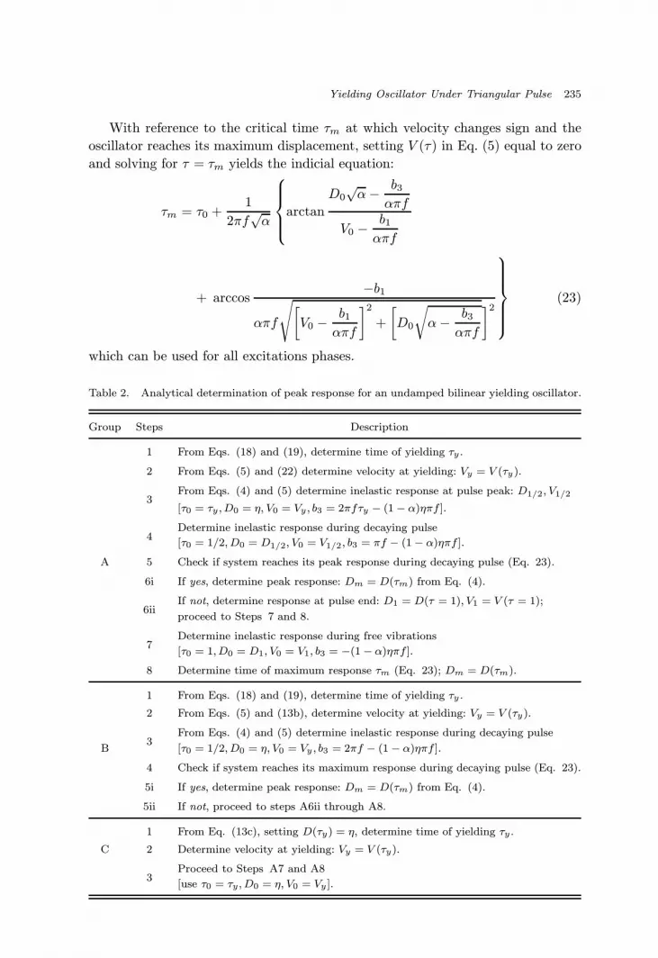
With reference to the critical time τm at which velocity changes sign and the

oscillator reaches its maximum displacement, setting V (τ) in Eq. (5) equal to zero

and solving for τ = τm yields the indicial equation:

τm = τ0 +1

2πf√α

arctan

D0√α− b3

απf

V0 −b1

απf

+ arccos−b1

απf

√[V0 −

b1

απf

]2

+

[D0

√α− b3

απf

]2

(23)

which can be used for all excitations phases.

Table 2. Analytical determination of peak response for an undamped bilinear yielding oscillator.

Group Steps Description

1 From Eqs. (18) and (19), determine time of yielding τy .

2 From Eqs. (5) and (22) determine velocity at yielding: Vy = V (τy).

3From Eqs. (4) and (5) determine inelastic response at pulse peak: D1/2, V1/2

[τ0 = τy ,D0 = η, V0 = Vy , b3 = 2πfτy − (1− α)ηπf ].

4Determine inelastic response during decaying pulse

[τ0 = 1/2, D0 = D1/2, V0 = V1/2, b3 = πf − (1− α)ηπf ].

A 5 Check if system reaches its peak response during decaying pulse (Eq. 23).

6i If yes, determine peak response: Dm = D(τm) from Eq. (4).

6iiIf not, determine response at pulse end: D1 = D(τ = 1), V1 = V (τ = 1);

proceed to Steps 7 and 8.

7Determine inelastic response during free vibrations

[τ0 = 1,D0 = D1, V0 = V1, b3 = −(1− α)ηπf ].

8 Determine time of maximum response τm (Eq. 23); Dm = D(τm).

1 From Eqs. (18) and (19), determine time of yielding τy .

2 From Eqs. (5) and (13b), determine velocity at yielding: Vy = V (τy).

3From Eqs. (4) and (5) determine inelastic response during decaying pulse

B [τ0 = 1/2, D0 = η, V0 = Vy , b3 = 2πf − (1− α)ηπf ].

4 Check if system reaches its maximum response during decaying pulse (Eq. 23).

5i If yes, determine peak response: Dm = D(τm) from Eq. (4).

5ii If not, proceed to steps A6ii through A8.

1 From Eq. (13c), setting D(τy) = η, determine time of yielding τy .

C 2 Determine velocity at yielding: Vy = V (τy).

3Proceed to Steps A7 and A8

[use τ0 = τy, D0 = η, V0 = Vy ].

April 26, 2001 15:5 WSPC/124-JEE 00038


For instance, returning to oscillators in Group A, Eq. (23) should be used in the

decreasing brancha with τ0 = 1/2, D0 = D1/2, V0 = V1/2 which refer to the initial

conditions at the pulse peak. If τm < 1, the peak displacement will be obtained

from Eq. (4) using the same initial conditions and τ = τm. On the other hand, if

τm > 1, τm should be re-determined from Eq. (23) using τ0 = 1, D0 = D1, V0 = V1.

The corresponding peak displacement would then be obtained from Eq. (4) using

the same initial conditions and τ = τm.

The whole procedure is outlined in Table 2 and can be easily implemented in a

computer spreadsheet. It is noted that the method does not require discretization

of the ground motion (as done in existing numerical solvers), or subdivisions of the

time step to better locate the times of yielding and peak response. It is also noted

that the solution is essentially exact (with the exception of determining τy) and,

thereby, provides highly accurate results.

5. Explicit Solution for Elastic-Perfectly Plastic Oscillators

The equation of dynamic equilibrium of a perfectly plastic oscillator (α = 0) is

u = −Ug −Qy

m. (24)

Integrating the above equation twice with respect to time and enforcing the per-

tinent initial conditions at t = ty, the relative velocity and displacement of the

system are determined as

u = uy + [Ug − Ug(ty)]− Qy

m(t− ty) (25)

v = vy + [Ug − Ug(ty)] + [U − U(ty)](t− ty)− Qy

2m(t− ty)2 . (26)

The time of peak response tm is obtained from Eq. (25) by setting the oscillator

velocity equal to zero

tm = ty +Qy

m[vy + Ug(tm)− Ug(ty)] . (27)

With reference to the problem in question, it is reasonable to assume (see Fig. 3)

that peak displacement occurs after (or slightly before) the end of the pulse. Ac-

cordingly, ground velocity at t = tm can be well approximated by the value at the

end of the pulse i.e.

Ug(tm) ∼= Ug(td) . (28)

Under this assumption and for oscillators in Group A, the dimensionless critical

time τm can be easily determined as

τm ∼= τy −1

η

[τ2y −

1

2− 1

2π2f2(1− cos 2πfτy)

]. (29)

aRecall that peak response occurs always after the pulse peak.

April 26, 2001 15:5 WSPC/124-JEE 00038


Substituting Eq. (29) into Eq. (26) and after some lengthy yet straightforward

algebra, an explicit solution is obtained for the imposed ductility demand

µ = 1 +π2f2

η

(2τm − 1− 4

3τ3y

)− 2

η[2π2f2τ2

y + cos 2πfτy − 1](τm − τy)− 2π2f2(τm − τy)2 . (30)

It is noted that the above expression is exact for oscillators attaining their peak

displacement at or after the end of the pulse (τm > 1). However, as will be shown

later on, this equation gives satisfactory predictions for other oscillators attaining

their peak displacement close to the end of the pulse.

6. Results

In Fig. 6, ductility demand µ(= Dm/Dy) is plotted as function of dimensionless

pulse duration f for a set of elastic perfectly-plastic systems (α = 0). Many notewor-

thy features are apparent in the graph: Firstly, µ is in general an increasing function

of f . For instance, with f = 1 (i.e. pulse duration equal to elastic structural period)

and η = 0.5 (i.e. yielding structural acceleration equal to 50% of peak pulse accel-

eration), µ may exceed the astonishing value of 10. The trend is understandably

stronger with low-strength systems. It is noted that the increased response with

increasing f is in contrast to the elastic oscillator in which the maximum response

is obtained near f = 1 (Fig. 3). Secondly, the response is sensitive to the yielding

resistance of the structure. For example, for η = 0.8 and f = 2, a reduction in


0 1 2 3 4

DU

CT

ILIT

Y D

EM

AN

D

µ =

Dm

/ Dy

0.1

1

10

100η = 0.2 0.3

0.5

0.7

0.8

0.9

ELASTIC

Practical capacity limitfor most structures

PROPOSED ANALYTICAL SOLUTIONNUMERICAL SOLUTION (BIGGS 1964)

Fig. 6. Ductility demand for an elastic-perfectly plastic oscillator.

April 26, 2001 15:5 WSPC/124-JEE 00038


strength by just 15% leads to an increase in ductility demand of the order of 150%.

It is noted, however, that absolute displacements may be less sensitive to η and f .

Justification of the herein proposed solution comes from comparison with results

from the numerical study of Biggs [1964].

Figure 7(a) presents results for time of yielding as function of pulse duration. It

is seen that τy is generally a decreasing function of η which implies that the smaller

the yielding strength the sooner the system will yield. The importance of Group A

TIM

E O

F Y

IELD

ING

τ y

= t

y / t

d

0.0

0.5

1.0

1.5

η = 0.9

0.8

0.5

0.2RISING PULSE

DECAYING PULSE

FREE VIBRATIONS

EXACT NUMERICAL SOLUTIONAPPROXIMATE SOLUTION: EQNS (18, 19)

(a)


0 1 2 3 4

TIM

E O

F P

EA

K R

ES

PO

NS

E

τm

= t

m /

t d

0

1

2

3

η = 0.3

0.2

0.5

0.7

0.8

ELASTIC

NUMERICAL SOLUTION (BIGGS 1964)PROPOSED ANALYTICAL SOLUTION: EQN (23)

(b)

Fig. 7. Dimensionless time of yielding (a) and time of peak response (b) for an undamped elastic-perfectly plastic oscillator.

April 26, 2001 15:5 WSPC/124-JEE 00038


among the various systems is evident in the graph. The accuracy of the approximate

solution [Eqs. (18) and (19)] is very good for oscillators in both Groups A and B.

In Fig. 7(b), the critical time τm at which the system reaches its peak response

is presented. For f < 0.5 the peak response occurs after the end of the pulse,

practically regardless of yielding strength. On the other hand, for longer pulse du-

rations two different types of behaviour are observed: relatively “strong” systems

(η > 0.5) attain their maximum response during decaying pulse (τm < 1), while

DU

CT

ILIT

Y D

EM

AN

D

µ =

Dm /

Dy

1

10

10α = 0

0.050.1

0.2

α = 0

0.1

0.2

η = 0.3 0.7

(a)


0 1 2 3 4

TIM

E O

F

PE

AK

RE

SP

ON

SE

τ m

=

t m /

t d

0

1

2

3

α = 0

0.05

0.2

0.2

α = 0

(b)

Fig. 8. Effect of post yielding stiffness on ductility demand (a) and time of peak response (b) foran undamped yielding oscillator.

April 26, 2001 15:5 WSPC/124-JEE 00038


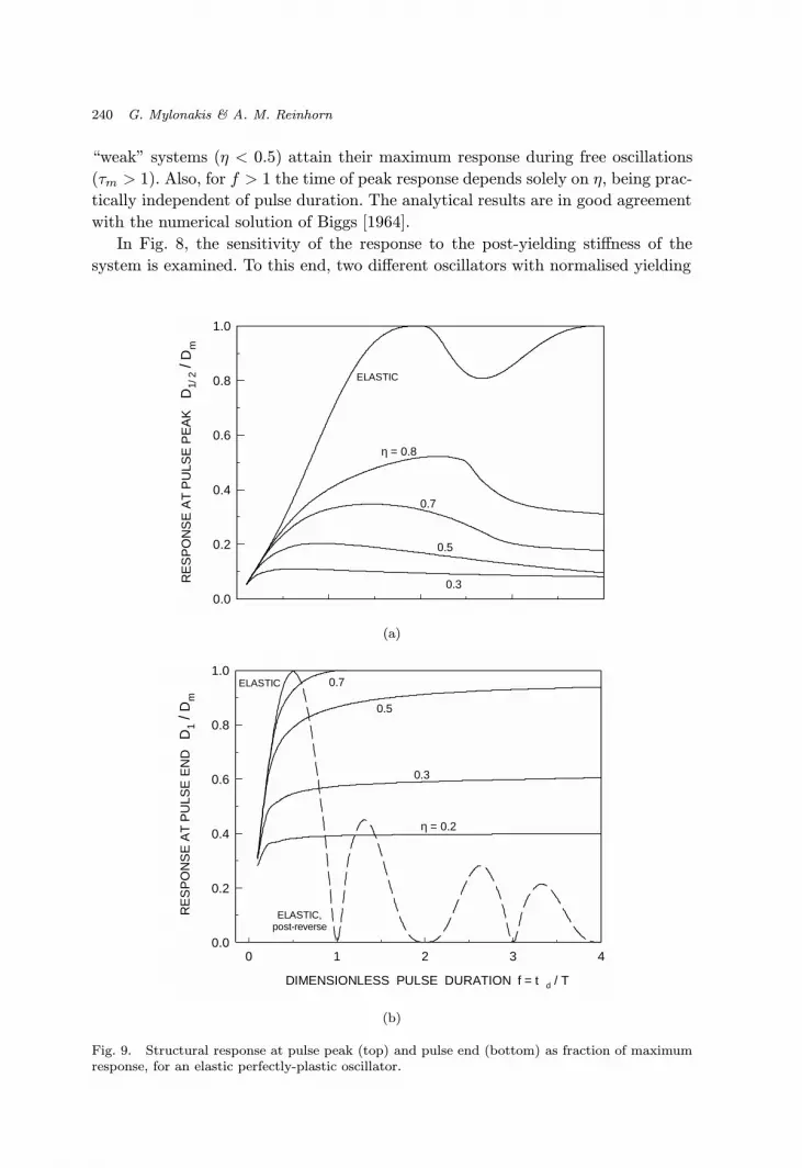
“weak” systems (η < 0.5) attain their maximum response during free oscillations

(τm > 1). Also, for f > 1 the time of peak response depends solely on η, being prac-

tically independent of pulse duration. The analytical results are in good agreement

with the numerical solution of Biggs [1964].

In Fig. 8, the sensitivity of the response to the post-yielding stiffness of the

system is examined. To this end, two different oscillators with normalised yielding

RE

SP

ON

SE

AT

PU

LSE

PE

AK

D

1/ 2 /

Dm

0.0

0.2

0.4

0.6

0.8

1.0

ELASTIC

0.5

0.3

η = 0.8

0.7

(a)

DIMENSIONLESS PULSE DURATION f = t d / T

0 1 2 3 4

RE

SP

ON

SE

AT

PU

LSE

EN

D

D1

/ Dm

0.0

0.2

0.4

0.6

0.8

1.0

η = 0.2

0.7

0.3

0.5

ELASTIC,post-reverse

ELASTIC

(b)

Fig. 9. Structural response at pulse peak (top) and pulse end (bottom) as fraction of maximumresponse, for an elastic perfectly-plastic oscillator.

April 26, 2001 15:5 WSPC/124-JEE 00038


strengths η = 0.3 and 0.7 are studied, with α varying between 0 and 20%. It is seen

that with η = 0.7 the effect of post-yielding stiffness on ductility demand is minor.

This is especially true for small pulse durations (f < 1) for which the decrease in

µ due to an increase in α from 0 to 20% is less than about 20%. The beneficial

role of α becomes apparent with low-strength systems (η = 0.3). For example, with

f = 1.5 an increase in α from 0 to 5% reduces ductility demand by a substantial

150%. Increasing α by an additional 15% leads to a total reduction in µ of about

400%.

Additional evidence on the importance of post-yielding stiffness is given in

Fig. 8(b), which presents the time of peak response τm for the same systems ex-

amined in Fig. 8(a). For η = 0.7, τm is not significantly affected by α, which is

in agreement with what observed in Fig. 8(a). On the other hand, for the weak,

η = 0.3, oscillators, τm is strongly influenced (reduced) by α: even for α as small as

0.05, τm is significantly smaller as compared to the corresponding perfectly plastic

system. For long pulse durations (f > 1), peak response may occur before the end

of the pulse.

Figure 9 depicts the normalised displacements D1/2 and D1 as fractions of the

maximum response Dm, for elastic-perfectly-plastic oscillators. Figure 9(a) reveals

that for an inelastic system the response at the peak of the pulseD1/2 is not reliable

for predicting peak response. This is in contrast to the elastic oscillator [Fig. 3(a)]

for which D1/2 is a reliable predictor of Dm beyond about f = 1.5. Indeed, as

evident in Fig. 9, even for η as high as 0.8, the response at pulse peak does not

exceed 60% of maximum. With smaller yielding strengths, the response may be less

than 20% of Dm.


0 1 2 3 4

TIM

E O

F P

EA

K R

ES

PO

NS

E

τ m =

tm /

t d

0

1

2

3

η = 0.3

0.2

0.5

0.7

0.8

APPROXIMATE SOLUTION: EQN 29EXACT SOLUTION: EQN 23 & TABLES I, 2

Fig. 10. Time of peak response for an elastic-perfectly plastic oscillator. Comparison of the exactsolution in Tables 1 and 2 with the approximate solution in Eq. (29).

April 26, 2001 15:5 WSPC/124-JEE 00038



0 1 2 3 4

DU

CT

ILIT

Y D

EM

AN

D

µ =

Dm

/ Dy

0.1

1

10

100η = 0.2 0.3

0.5

0.7

0.8

EXACT SOLUTION: EQNS 4 & 5 and TABLES I & 2APPROXIMATE SOLUTION: EQN 30

Fig. 11. Ductility demand for an elastic perfectly-plastic oscillator. Comparison of the exactsolution in Table 1 and 2 with the approximate solution in Eq. (30).

In Fig. 9(b), the response at the end of the excitation, D1, is presented as

fraction of Dm. The behaviour is again different from the elastic. For f larger than

about 1, the response at the end of the pulse is practically independent of pulse

duration, depending solely on η. For η equal to 0.5, 0.3, and 0.2, the response is

equal to about 90, 60, and 40% of the peak, respectively.

The predictions of the closed-form solution in Eqs. (29) and (30) are illus-

trated in Figs. 10 and 11, respectively. With reference to the time of peak response

(Fig. 10), it is seen that Eq. (29) is exact for τm higher than 1. On the other

hand, the equation somewhat overestimates the time of peak response for τm less

than 1. Nevertheless, for the range of parameters of the most practical interest (say

η < 0.8, f < 1), the accuracy of the closed-form solution is excellent. Similar trends

are observed for the ductility µ in Fig. 11.

7. Comparison with Actual Near-Field Recordings

To evaluate the applicability of the model to more realistic situations, its predictions

are compared against inelastic spectra from four actual near-field motions. The

accelerograms, which are shown in Fig. 1, were recorded during four destructive

earthquakes around the world. It is noted that the pulses contained in the records

exhibit various degrees of similarity to the symmetric triangular pulse of the model.

For instance, the 0.46g pulse in the Pyrgos [1993] record resembles closely that of

the model. In contrast, the 0.66g pulse in the Pacoima [1971] record does not possess

April

26,

2001

15:5

WSP

C/124-J

EE

00038

Yield

ing

Oscilla

tor

Un

der

Tria

ngu

lar

Pu

lse243

Table 3. Selected near-field motions with long-period, high-acceleration pulses.

Station Name Event/Date Magnitude Distance Direction Peak Pulse PGV Ta Tg t†d

(Ms) from Fault Acceleration (m/s) (s) (s) (s)

(km) (g)

PyrgosPyrgos, Greece

5.2 < 5 EW 0.46 0.25 0.27 0.37 0.193/26/93

ErzicanErzican, Turkey

6.9 2 NS 0.52 0.84 0.30 2.03 1.013/13/92

RinaldiNorthridge

6.7 7.1 N228W 0.84 1.66 0.72 1.06 0.581/17/94

Pacoima DamSan Fernando

6.6 2.8 N164W 0.66 1.13 0.39 1.20 0.602/9/71

†Computed as td = Tg/2 (Eq. 31).

April 26, 2001 15:5 WSPC/124-JEE 00038


such an obvious similarity. The Erzican [1992] and Rinaldi [1994] motions represent

intermediate cases. Key engineering characteristics of the motions are summarised

in Table 3.

To determine the duration of the pulse in an unambiguous manner, the following

definition was adopted

td ≈Tg

2(31)

where Tg is the period at which the 5%-damped velocity spectrum of the motion be-

comes maximum [Miranda and Bertero, 1994; Cuesta and Aschheim, 2000]. Notice

the good agreement between the predictions based on the above equation (Table 3)

and the pulse durations indicated in Fig. 1.

For simplicity, the amplitude of the pulse in the model was considered equal to

the peak pulse acceleration, PPA, (Table 3) i.e.

Ag ≈ PPA . (32)

In Fig. 12, ductility demands from the Pyrgos [1993] record are presented for three

different oscillator strengths. The agreement between the numerical results and the

predictions of the model is excellent (except perhaps for the case of η = 0.9), which

is expected in view of the similarity in shape of the pulses. The good matching

also confirms some earlier observations [Bertero, 1978; Borzognia and Mahin, 1998;

Cuesta and Aschheim, 2000] that most of the inelastic response caused by such

motions is associated with the pulses.

DIMENSIONLESS PULSE DURATION f = Tg / 2 T

0 1 2 3 4

DU

CT

ILIT

Y

DE

MA

ND

µ

0.1

1

10

100

η = 0.5

0.7

0.9

PYRGOS (1993) EWTRIANGULAR PULSE

Fig. 12. Ductility demand for an elastic-perfectly plastic simple oscillator. Comparison of thepredictions of the model with an actual record.

April 26, 2001 15:5 WSPC/124-JEE 00038



0 1 2 3 4

DU

CT

ILIT

Y

DE

MA

ND

µ

0.1

1

10

100

η = 0.5

0.7

0.9

ERZICAN (1992) NSTRIANGULAR PULSE



0 1 2 3 4

DU

CT

ILIT

Y

DE

MA

ND

µ

0.1

1

10

100

η = 0.5

0.7

0.9

PACOIMA (1971) N164WTRIANGULAR PULSE


April 26, 2001 15:5 WSPC/124-JEE 00038


Corresponding results obtained with the Erzican [1992] record are shown in

Fig. 13. The agreement between the model and the earthquake results is again

satisfactory, although not as good as with the previous record. The largest dis-

crepancies are observed with the “weak” η = 0.5 oscillator and can be possibly

attributed to a pre-pulse contained in the record. Nevertheless, studying the details

of the excitation is beyond the scope of this work. Analogous trends (not shown)

are observed with the Rinaldi (1994) record.

The Pacoima (1971) record is examined in Fig. 14. In this case the two solutions

do not compare very well, particularly for dimensionless pulse durations higher

than about 1. This is understood in view of the different shapes of the pulses

in the two motions. Nevertheless, for the frequency range of the most practical

importance (i.e. f < 1), the predictions of the two solutions are quite similar.

Additional discussion is provided in the example below.

8. Case Study: The Collapse of Olive View Hospital in the 1971

San Fernando Earthquake

The Olive View Hospital was a six-storey reinforced concrete building located at

the meizoseismal area of the 1971 San Fernando Earthquake. The structural system

included shear walls that did not extend to the lower two storeys. The discontinuity

in stiffness made the upper four floors act essentially as a rigid box supported on

soft columns. During the earthquake, the columns were displaced horizontally with

respect to their bases by as much as 30 inches [Mahin et al., 1976]. Because of the

extensive damage, the building (which had been completed only few months before

the earthquake) had to be demolished. While no records were obtained at the site,

there are indications that the imposed excitation was similar to that recorded at the

nearby Pacoima Dam [Mahin et al., 1976; Bertero et al., 1978]. The performance of

the building is analysed here using the Pacoima record to demonstrate the destruc-

tiveness of strong pulse-like motions and evaluate the predictions of the model.

Based on earlier investigations [Mahin et al., 1976], the estimated fundamental

natural period and yielding seismic coefficient of the building are, respectively,

T = 0.58s and Cy = 0.35. From Table 3, using the values td = 0.6s, Ag = 0.66g

corresponding to Pacoima record,b the dimensionless pulse duration and oscillator

strength are respectively

f =td

T=

0.60

0.58≈ 1.03 (33)

η =Cy

Ag=

0.35

0.66≈ 0.53 . (34)

Considering the structure as a simple oscillator, it is evident from Fig. 4 that

yielding will occur prior to pulse peak (Group A). The “exact” yielding time is

bNote that the modified Pacoima motion used by Mahin et al. [1976] and Bertero et al. [1978] hasthe same Ag and td.

April 26, 2001 15:5 WSPC/124-JEE 00038


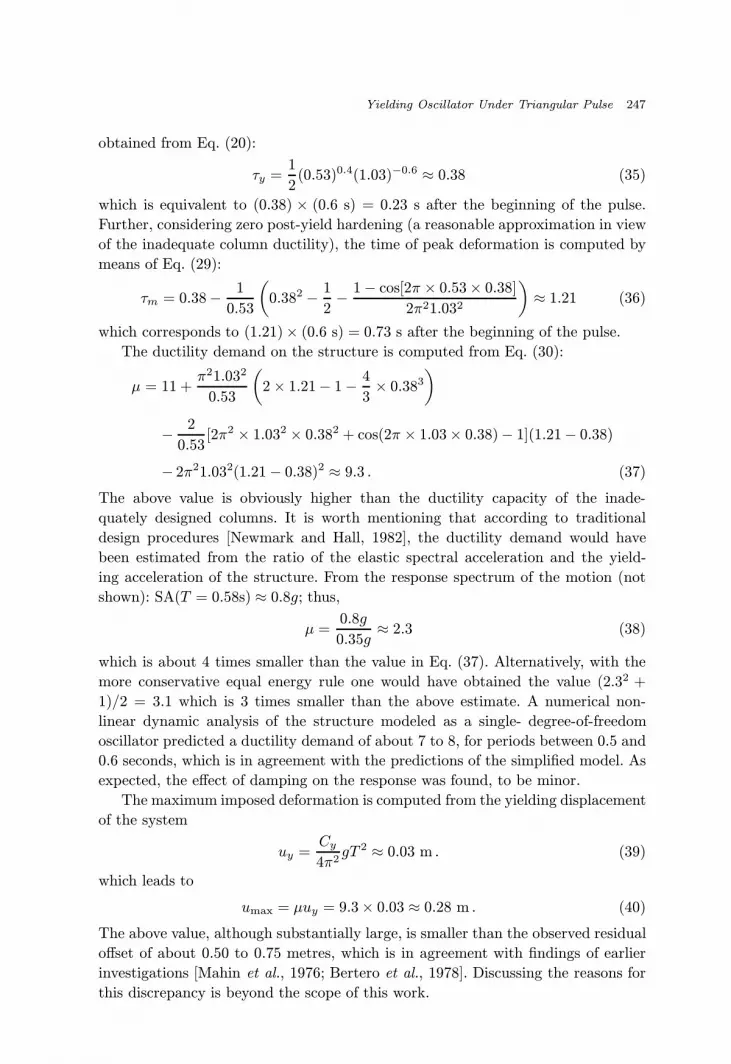
obtained from Eq. (20):

τy =1

2(0.53)0.4(1.03)−0.6 ≈ 0.38 (35)

which is equivalent to (0.38) × (0.6 s) = 0.23 s after the beginning of the pulse.

Further, considering zero post-yield hardening (a reasonable approximation in view

of the inadequate column ductility), the time of peak deformation is computed by

means of Eq. (29):

τm = 0.38− 1

0.53

(0.382 − 1

2− 1− cos[2π × 0.53× 0.38]

2π21.032

)≈ 1.21 (36)

which corresponds to (1.21)× (0.6 s) = 0.73 s after the beginning of the pulse.

The ductility demand on the structure is computed from Eq. (30):

µ = 11 +π21.032

0.53

(2× 1.21− 1− 4

3× 0.383

)− 2

0.53[2π2 × 1.032 × 0.382 + cos(2π × 1.03× 0.38)− 1](1.21− 0.38)

− 2π21.032(1.21− 0.38)2 ≈ 9.3 . (37)

The above value is obviously higher than the ductility capacity of the inade-

quately designed columns. It is worth mentioning that according to traditional

design procedures [Newmark and Hall, 1982], the ductility demand would have

been estimated from the ratio of the elastic spectral acceleration and the yield-

ing acceleration of the structure. From the response spectrum of the motion (not

shown): SA(T = 0.58s) ≈ 0.8g; thus,

µ =0.8g

0.35g≈ 2.3 (38)

which is about 4 times smaller than the value in Eq. (37). Alternatively, with the

more conservative equal energy rule one would have obtained the value (2.32 +

1)/2 = 3.1 which is 3 times smaller than the above estimate. A numerical non-

linear dynamic analysis of the structure modeled as a single- degree-of-freedom

oscillator predicted a ductility demand of about 7 to 8, for periods between 0.5 and

0.6 seconds, which is in agreement with the predictions of the simplified model. As

expected, the effect of damping on the response was found, to be minor.

The maximum imposed deformation is computed from the yielding displacement

of the system

uy =Cy

4π2gT 2 ≈ 0.03 m . (39)

which leads to

umax = µuy = 9.3× 0.03 ≈ 0.28 m . (40)

The above value, although substantially large, is smaller than the observed residual

offset of about 0.50 to 0.75 metres, which is in agreement with findings of earlier

investigations [Mahin et al., 1976; Bertero et al., 1978]. Discussing the reasons for

this discrepancy is beyond the scope of this work.

April 26, 2001 15:5 WSPC/124-JEE 00038


9. Conclusions

A simple analytical procedure was developed for the determining the response of

a yielding simple oscillator to a symmetric triangular ground acceleration pulse.

The method allows many key response parameters to be evaluated in closed form

expressions and valuable insight to be gained on the mechanics of the problem. The

most important findings gleaned from the study are:

(1) Ductility demand on elastic-perfectly-plastic structures with yielding resistance

smaller than the amplitude of the pulse may attain considerably high values

(i.e. larger that 10). Ductility demand is generally an increasing function of

pulse duration. This is in contrast with elastic systems where the maximum

response is obtained near resonance (f = 1).

(2) Time of yielding can be predicted accurately based on the normalised yielding

strength η and pulse duration f [Eqs. (18) and (19)]. For instance, if (ηf) < 2

the system will yield during its first oscillation cycle. In addition, if η < f3/2,

the system will yield before the peak of the pulse. Quick approximate estimates

of time of yielding can be obtained by means of Eq. (20).

(3) Peak response always takes place after the pulse peak for both elastic and

yielding oscillators. Time of peak response can be determined from Eqs. (23)

(general) and (29) (zero post yielding stiffness).

(4) Structural response is sensitive to post-yielding stiffness. Oscillators with post-

yield hardening of approximately 5% may experience 100% less deformation as

compared to corresponding perfectly plastic systems. This emphasises the need

for providing sufficient post-yielding stiffness (“ductility”) to structures located

in the vicinity of active faults.

(5) A study of the failure of Olive View Hospital in the 1971 San Fernando earth-

quake was presented. Using the Pacoima Dam record it was shown that the

structure could not sustain the imposed ductility demand. While the deforma-

tions predicted by the model were found to be in reasonable agreement with

results from inelastic numerical analyses, the estimated peak displacements

were significantly smaller that the observed offset. This is accord with earlier

investigations of the failure.

Appendix A. Derivation of Eqs. (4) and (5)

Considering linear variation with time of ground acceleration, the equation of

motion of a linearly elastic undamped oscillator is

mu(t) +Ku(t) = −m(a1t+ a2) . (A.1)

Equation (1) has the well-known solution [Chopra, 1995]:

April 26, 2001 15:5 WSPC/124-JEE 00038


u(t) =(u0 −

a2

ω2

)cos[ω(t− t0)] +

1

ω

(v0 −

a1

ω2

)sin[ω(t− t0)]

+a1

ω2(t− t0) +

a2

ω2(A.2)

v(t) =(v0 −

a1

ω2

)cos[ω(t− t0)]− ω

(u0 −

a2

ω2

)sin[ω(t− t0)] +

a1

ω2(A.3)

which pertain to the initial conditions u(t0) = u0; v(t0) = v0. In the case of a

bilinear inelastic structure, the restoring force (Ku) on the left side of Eq. (A.1)

should be replaced by:

Ku(t)→ Kuy + αK(u− uy) . (A.4)

Accordingly, during inelastic loading (u > uy; v > 0), the cyclic natural frequency

of the structure is:

ω →√αω . (A.5)

In addition, the constant restoring force [αK(u−uy)] in Eq. (A.4) can be interpreted

as a negative force term:

m(a1t+ a2)→ m(a1t+ a2)− αK(u− uy) . (A.6)

Introducing the substitutions

τ0 =t0

td, b1 =

a1td

2Ag, b2 =

a2

2Ag(A.7,8,9)

and using Eq. (1) and Eqs. (6) to (12), Eqs. (A.2) and (A.3) can be written,

respectively, in the form of Eqs. (4) and (5).

Appendix B. List of Symbols

Ag peak ground acceleration

bi (i = 1, 2, 3, 4) dimensionless response parameter

Cy yielding seismic coefficient

D dimensionless relative displacement

D0 dimensionless “initial” relative displacement (initial condition)

D1/2 dimensionless relative displacement at pulse peak

D1 dimensionless relative displacement at pulse end

Df dimensionless peak relative displacement during free oscillations

Dm dimensionless peak relative displacement envelope

f dimensionless pulse duration (dimensionless oscillator frequency)

g acceleration of gravity

K elastic stiffness

Kpy post-yielding stiffness parameter

κ number of complete oscillation cycles at the time of yielding

m oscillator mass

April 26, 2001 15:5 WSPC/124-JEE 00038


Qy yielding strength

Ug time history of ground displacement

u relative oscillator displacement

u0 “initial” relative displacement

umax maximum relative displacement

us static relative displacement

uy yielding relative displacement

PPA peak pulse acceleration (ground motion)

T elastic period

Tg period where 5%-damped SV spectrum becomes maximum

t time

td pulse duration

v relative oscillator velocity

v0 “initial” relative velocity

V dimensionless relative velocity

V0 dimensionless “initial” relative velocity

V1/2 dimensionless relative velocity at pulse peak

V1 dimensionless relative velocity at pulse end

α post-yielding stiffness parameter

η dimensionless yielding strength

τ dimensionless time

τy dimensionless yielding time

τm dimensionless time of peak relative displacement

τ0 dimensionless “initial” time (initial condition)

ω cyclic natural frequency

References

Baez, J. I. and Miranda, E. [2000] “Amplification factors to estimate inelastic displace-ment demands for the design of structures in the near field,” paper 1561, 12th WorldConference on Earthquake Engineering, New Zealand.

Bertero V. V., Mahin, S. A. and Herrera, R. A. [1978] “A seismic design implications ofnear-fault San Fernando earthquake records,” Earthq. Engrg. Struct. Dyn. 6, 31–42.

Biggs, J. M. [1964] Introduction to Structural Dynamic, McGraw-Hill.Boore, D. M. and Zoback M. D. [1974] “Near-field motions from kinematic models of

propagating faults,” Bull. Seism. Soc. Am. 64, 321–341.Bozorgnia, Y. and Mahin, S. A. [1998] “Ductility and strength demands of near-fault

ground motions of the Northridge earthquake,” Proceedings of the 6th U.S. NationalConference on Earthquake Engineering, EERI, Seattle.

Chopra, A. K. [1995] Dynamics of Structures, Prentice Hall.Cuesta, I. and Aschheim, M. A. [2000] “Waveform independence ofR-factors,” paper 1546,

12th World Conference on Earthquake Engineering, New Zealand.Gazetas, G. Loukakis, K., Kolias, V. and Stavrakakis, G. [1995] “The 1995 Aegion earth-

quake: analysis of the causes of the collapse of soft-first-story buildings,” Bulletin ofthe National Chamber of Greece 1883, 30–41 (in Greek).

April 26, 2001 15:5 WSPC/124-JEE 00038


Hall, J. F., Heaton, T. H., Wald, D. J. and Halling, M. W. [1995] “Near-source groundmotion and its effects on flexible buildings,” Earthq. Spectra 11(4), 569–605.

Iwan, W. D. [1997] “Drift spectrum: measure of demand for earthquake ground motions,”J. Struct. Engrg. ASCE 123(4), 397–404.

Jacobsen, L. and Ayre, S. M. [1958] Engineering Vibrations, McGraw-Hill, Inc.Mahin, S. A., Bertero, V. V., Chopra, A. K. and Collins, R. G. [1976] “Response of the

Olive View Hospital Main Building During the San Fernando Earthquake,” ReportNo. EERC 76-22, Earthquake Engineering Research Center, University of California,Berkeley.

Malhotra, P. K. [1999] “Response of buildings to near-field pulse-like ground motions,”Earthq. Engrg. Struct. Dyn. 28(11), 1309–1326.

Mylonakis, G. and Reinhorn, A. M., [1997] “Inelastic seismic response of structuresnear fault: an analytical solution,” Proc., STESSA-97: 2nd International Conferenceon the Behavior of Steel Structures in Seismic Areas, eds. Mazzolani, F. M. andAkiyama, H., pp. 82–89.

Newmark, N. M. and Hall, W. J. [1982] Earthquake Spectra and Design, EERI(monograph).

Naeim, F. [1995] “Implications of the 1994 Northridge earthquake ground motions for theseismic design of tall buildings,” Struct. Design Tall Buildings 3(4), 247–267.

Park, R. [1996] “An analysis of the failure of the 630 m elevated expressway in GreatHanshin earthquake,” Bull. New Zealand Nat. Soc. Earthq. Engrg. 29, 2.

Singh, J. P. [1985] “Earthquake ground motions: implications for designing structures andreconciling structural damage,” Earthq. Spectra 1(2), 239–270.

Somerville, P. and Graves, R. [1993] “Conditions that give rise to unusually large long-period ground motions,” Struct. Design Tall Buildings 2, 211–232.

Timoshenko, S., Young, D. H. and Weaver, W. [1974] Vibration Problems in Engineering,Fourth Edition, John Wiley.

Documents

YIELDING OSCILLATOR UNDER TRIANGULAR GROUND ACCELERATION PULSE