ethesis.nitrkl.ac.inethesis.nitrkl.ac.in/5013/1/VELOCITY_DISTRIBUTION... · 1.2 Velocity Distribution in Open Channels The knowledge of velocity distribution helps to know the velocity

VELOCITY DISTRIBUTION IN TRAPEZOIDAL MEANDERING CHANNEL

A thesis submitted to

National Institute of Technology, Rourkela

In partial fulfillment for the award of the degree

of

Master of Technology in Civil Engineering

With specialization in

Water Resources Engineering

By

Laxmipriya Mohanty (211CE4252)

Under the supervision of

Professor K.C. Patra

Department of Civil Engineering

National Institute of Technology, Rourkela

Odisha-769008

May 2013

DEPARTMENT OF CIVIL ENGINEERING

NATIONAL INSTITUTE OF TECHNOLOGY, ROURKELA

DECLARATION

I hereby declare that this submission is my own work and that, to the best of my knowledge and

belief, it contains no material previously published or written by another person nor material

which to a substantial extent has been accepted for the award of any other degree or diploma of

the university or other institute of higher learning, except where due acknowledgement has been

made in the text.

LAXMIPRIYA MOHANTY

i

DEPARTMENT OF CIVIL ENGINEERING

NATIONAL INSTITUTE OF TECHNOLOGY, ROURKELA

CERTIFICATE

This is to certify that the thesis entitled “Velocity Distribution in Trapezoidal Meandering Channel”

is a bonafide record of authentic work carried out by Laxmipriya Mohanty under my supervision and

guidance for the partial fulfillment of the requirement for the award of the degree of Master of

Technology in hydraulic and Water Resources Engineering in the department of Civil Engineering at the

National Institute of Technology, Rourkela.

The results embodied in this thesis have not been submitted to any other University or Institute for the

award of any degree or diploma.

Date: Prof. K.C. Patra

Department of Civil Engineering

Place: Rourkela National Institute of Technology, Rourkela

Rourkela-769008

ii

ACKNOWLEDGEMENTS

I am deeply indebted to National Institute of Technology, Rourkela for providing me the

opportunity to pursue my Master’s degree with all necessary facilities.

I take this opportunity to express my sincere and profound gratitude towards my guide Prof. K.C

Patra whose whole hearted support, timely encouragement in every stage of this work has been

the real cause to shape the work in present form. I would also like to thank Prof. KK Khatua to

boost my confidence during my low times and providing me potential helps without whom this

project might not be a successful one.

I would like to extend my thanks to all professors of Water Resources department for their

valuable help they have provided when I was in need. I am also thankful to staff members and

students associated with the Fluid Mechanics and Hydraulics Laboratory of Civil Engineering

Department, especially Mr. P. Rout for his useful assistance and cooperation during the entire

course of the experimentation and helping me in all possible ways.

I wish to thank all of my fellow classmates for their kind help and co-operation extended during

my course of study.

Lastly I thank my parents for their overall support and encouragement.

Date: LAXMIPRIYA MOHANTY

iii

ABSTRACT

Analysis of fluvial flows are strongly influenced by geometry complexity and large overall

uncertainty on every single measurable property, such as velocity distribution on different

sectional parameters like width ratio, aspect ratio and hydraulic parameter such as relative

depth. The geometry selected for this study is that of a smooth sine generated trapezoidal

main channel flanked on both sides by wide flood plains. The parameters which were

changed in this research work include the overbank flow depth, main channel flow depth,

incoming discharge of the main channel and floodplains.

This paper presents a practical method to predict lateral depth-averaged velocity

distribution in trapezoidal meandering channels. Flow structure in meandering channels is

more complex than straight channels due to 3-Dimentional nature of flow. Continuous

variation of channel geometry along the flow path associated with secondary currents makes

the depth averaged velocity computation difficult. Design methods based on straight-wide

channels incorporate large errors while estimating discharge in meandering channel. Hence

based on the present experimental results, a nonlinear form of equation involving 3

parameters for estimating lateral depth-averaged velocity is formulated. The present

experimental meandering channel is wide (aspect ratio = b/h > 5) and with high sinuosity of

2.04. A quasi1D model Conveyance Estimation System (CES) was then applied in turn to the

same compound meandering channel to validate with the experimental depth averaged

velocity. The study serves for a better understanding of the flow and velocity patterns in

trapezoidal meandering channel.

A commercial code, ANSYS-CFX 13.0 is used to simulate a 60 meander channel

using Large Scale Eddy (LES) model. Contours regarding the velocities in three directions

are derived.

Keywords: Aspect Ratio; Compound Channel; CES; Depth averaged velocity; Discharge;

Flow depth; Meandering channels; Secondary currents.

iv

CONTENTS Page No.

Certificate i

Acknowledgements ii

Abstract iii

Contents iv

List of Tables vii

List of Figures and Photographs viii

Notations x

CHAPTER 1

Introduction 1-7

1.1 Overview of Meandering Channels 1

1.2 Velocity Distribution in Open Channels 2

1.2.1 Logarithmic law 3

1.2.2 Power law 4

1.2.3 Chiu's velocity distribution 4

1.3 Depth-Averaged Velocity 5

1.4 Aim of Present Research 5

1.5 Organisation of Thesis 6

CHAPTER 2

Review of Literature 8-19

2.1 Overview 8

2.2 Previous Experimental Research on Velocity Distribution 8

2.2.1 Straight Simple Channel 8

2.2.2 Straight Compound Channels 11

v

2.2.3 Meander Simple Channels 13

2.2.4 Meander Compound Channel 14

2.3 Overview of Numerical Modelling on Open Channel Flow 15

CHAPTER 3

Experimental Details 20-29

3.1 Overview 20

3.2 Apparatus & Equipments Used 20

3.3 Experimental Setup and Procedure 21

3.3.1 Measurement of Bed Slope 25

3.3.2 Calibration of Notch 25

3.3.3 Measurement of Depth of flow and Discharge 26

3.3.4 Measurement of tangential Velocity 27

CHAPTER 4

Experimental Results 30-34

4.1 Overview 30

4.2 Stage-Discharge Relationship in Meandering Channels 30

4.3 Distribution of Longitudinal Velocity 31

4.3.1 Inbank Velocity Contours 32

4.3.2 Overbank Velocity Contours 33

CHAPTER 5

Analysis based on Experimental Results 35-40

5.1 Overview 35

5.2 Lateral Distribution of Depth Averaged Velocity 35

5.2.1 Inbank Flow Studies 35

vi

5.2.2 Overbank Flow Studies 37

CHAPTER 6

Model Development 41-43

CHAPTER 7

Numerical Studies 44-59

7.1 Overview 44

7.2 Geometry and Set-Up 46

7.3 Discretizaton of Domain (Meshing) 47

7.4 Turbulence 48

7.5 Numerical Model 50

7.5.1 Large Eddy Simulation (LES) 50

7.5.2 Mathematical Model 52

7.6 Boundary Conditions 55

7.6.1 Wall 55

7.6.2 Free Surface 55

7.6.3 Inlet and Outlet 55

7.7 Numerical Results 56

CHAPTER 8

Conclusion and Future Work 60-62

8.1 Conclusions 60

8.2 Future Scope 61

REFERENCES 63-66

(Appendix A-I) Published and Accepted Papers from the Work 67

vii

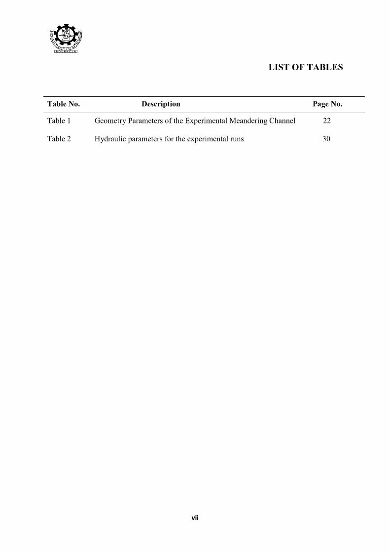
LIST OF TABLES

Table No. Description Page No.

Table 1 Geometry Parameters of the Experimental Meandering Channel 22

Table 2 Hydraulic parameters for the experimental runs 30

viii

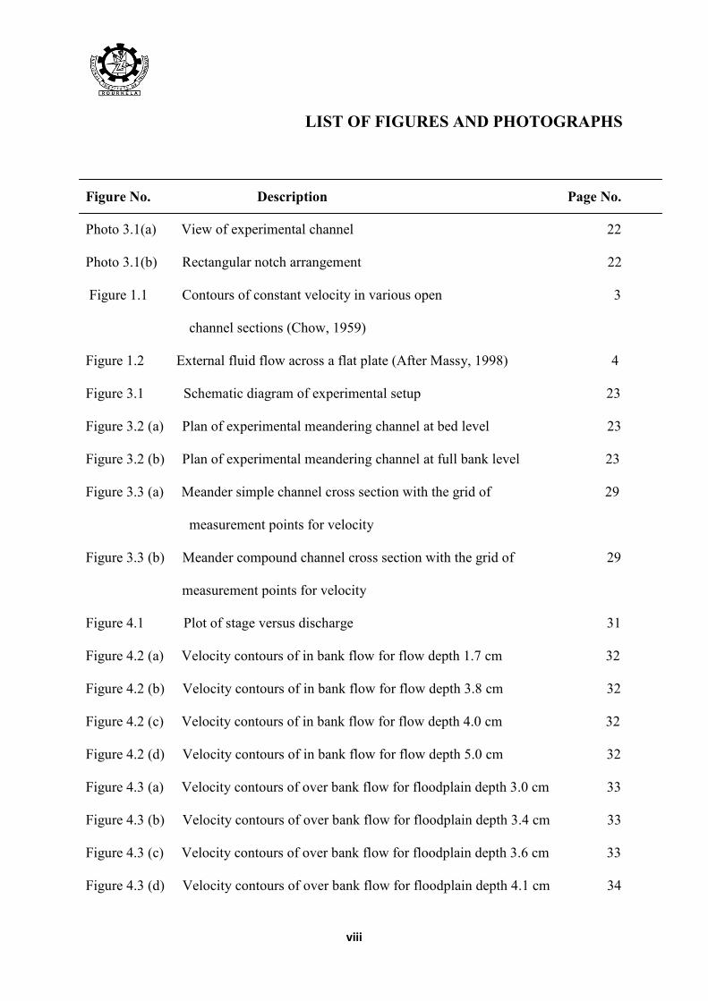
LIST OF FIGURES AND PHOTOGRAPHS

Figure No. Description Page No.

Photo 3.1(a) View of experimental channel 22

Photo 3.1(b) Rectangular notch arrangement 22

Figure 1.1 Contours of constant velocity in various open 3

channel sections (Chow, 1959)

Figure 1.2 External fluid flow across a flat plate (After Massy, 1998) 4

Figure 3.1 Schematic diagram of experimental setup 23

Figure 3.2 (a) Plan of experimental meandering channel at bed level 23

Figure 3.2 (b) Plan of experimental meandering channel at full bank level 23

Figure 3.3 (a) Meander simple channel cross section with the grid of 29

measurement points for velocity

Figure 3.3 (b) Meander compound channel cross section with the grid of 29

measurement points for velocity

Figure 4.1 Plot of stage versus discharge 31

Figure 4.2 (a) Velocity contours of in bank flow for flow depth 1.7 cm 32

Figure 4.2 (b) Velocity contours of in bank flow for flow depth 3.8 cm 32

Figure 4.2 (c) Velocity contours of in bank flow for flow depth 4.0 cm 32

Figure 4.2 (d) Velocity contours of in bank flow for flow depth 5.0 cm 32

Figure 4.3 (a) Velocity contours of over bank flow for floodplain depth 3.0 cm 33

Figure 4.3 (b) Velocity contours of over bank flow for floodplain depth 3.4 cm 33

Figure 4.3 (c) Velocity contours of over bank flow for floodplain depth 3.6 cm 33

Figure 4.3 (d) Velocity contours of over bank flow for floodplain depth 4.1 cm 34

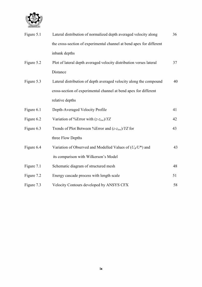
ix

Figure 5.1 Lateral distribution of normalized depth averaged velocity along 36

the cross-section of experimental channel at bend apex for different

inbank depths

Figure 5.2 Plot of lateral depth averaged velocity distribution verses lateral 37

Distance

Figure 5.3 Lateral distribution of depth averaged velocity along the compound 40

cross-section of experimental channel at bend apex for different

relative depths

Figure 6.1 Depth-Averaged Velocity Profile 41

Figure 6.2 Variation of %Error with (z-ztoe)/YZ 42

Figure 6.3 Trends of Plot Between %Error and (z-ztoe)/YZ for 43

three Flow Depths

Figure 6.4 Variation of Observed and Modelled Values of (Ud/U*) and 43

its comparison with Wilkerson’s Model

Figure 7.1 Schematic diagram of structured mesh 48

Figure 7.2 Energy cascade process with length scale 51

Figure 7.3 Velocity Contours developed by ANSYS CFX 58

x

NOTATIONS

Qa Actual discharge;

Cd Coefficient of discharge calculated from notch calibration = 0.74;

Cr Courant number;

Cs Smagorinsky constant;

L Length of the notch;

Hn Height of water above the notch;

g Acceleration due to gravity;

l Length scale of unresolved motion;

b Channel base width;

d Outside diameter of the probe;

G Gaussian filters;

H In bank depth of flow;

H' Over bank depth of flow;

k Turbulent kinetic energy;

P Wetted perimeter;

R Hydraulic radius;

Y,h Main channel bank full depth;

Sr Sinuosity;

s Bed slope of the channel;

Sij Resolved strain rate tensor;

U Longitudinal point velocity;

|z-ztoe| Lateral distance from the toe of slope to the point of interest (positive going

towards edge of water and negative over the channel bed);

xi

y Lateral distance;

Z Cotangent of bank slope;

U(z) , Ud Depth-averaged velocity;

U* Cross-sectional averaged velocity;

Ud /U* Normalised Depth-averaged velocity

x (+| z-ztoe |/YZ);

α Aspect ratio;

Fluid density;

θ Angle between channel bed and horizontal;

ν Kinematic viscosity;

ε Turbulent kinetic energy dissipation rate;

ω Specific dissipation;

σij Normal stress component on plane normal to i along j;

τij Shear stress component on plane normal to i along j;

ūi', ūj' Time averaged instantaneous velocity component along i,j directions

µ Coefficient of dynamic viscosity;

∆h Difference between dynamic and static head;

xii

Subscripts

a actual

b, bed bed

d depth average

r relative

t theoretical

w wall

mod. modelled

i, j, k x, y, z directions respectively

i, inner inner bank or wall of meandering channel

o, outer outer bank or wall of meandering channel

* mean

Introduction

1 | P a g e

INTRODUCTION

1.1 Overview of Meandering Channels

River is the author of its geometry. The river network is an open system always tending

towards equilibrium and the hydraulically interdependent factors such as velocity, depth,

channel width and slope mutually interact and self adjust to accommodate the changes in

river plan form geometry and discharge contributed by drainage basin. Straightness of rivers

is a temporary state, the more usual and stable state whereas a meander is characterized by

lower variances of hydraulic factors. Therefore not a single natural river possesses a straight

geometry. Almost all natural rivers meander. In fact Straight River reaches longer than 10 to

12 times the channel widths are non existence in nature.

A meander, in general, is a bend in a sinuous watercourse or river. A meander is

formed when the moving water in a stream erodes the outer banks and widens its valley. As

the inner part of the river has less energy it deposits what it is carrying. As a result a snaking

pattern is formed, the stream back and forth across its down axis valley. Also second reason

of formation of meander as suggested by Leopold (1996) is the secondary circulation in the

cross sectional plane. As Leliavsky (1955) describes the second phenomenon of river

meandering in his book which quotes “The centrifugal effect, which causes the super

elevation may possibly be visualized as the fundamental principles of the meandering theory,

for it represents the main cause of the helicoidal crosscurrents which removes the soil from

the concave banks, transport the eroded material across the channel, and deposit it on the

convex banks, thus intensifying the tendency towards meandering. It follows therefore that

the slightest accidental irregularity in channel formation, turning as it does, the streamlines

Introduction

2 | P a g e

from their straight course may, under certain circumstances constitute the focal point for the

erosion process which leads ultimately to meander”.

The two critical parameters that govern the flow in open meandering channel are

sinuosity and least centreline radius (rc) to channel width (b) ratio. Sinuosity defines how

much a river course deviates from shortest possible path (how much it meanders). the

sinuosity index is 1 for straight channels whereas for meandering channels it is greater than 1

and can increase to infinity for a closed loop (where the shortest path length is zero) or for an

infinitely-long actual path. Meandering channels are also classified as shallow or deep

depending on the ratio of the average channel width (b) to its depth (h). In shallow channels

(b/h’>5, Rozovskii, 1961) the wall effects are limited to a small zone near the wall which

may be called as "wall zone". The central portion called "core zone" is free from the wall

effects. Whereas in deep channels (b/h’<5) the influence of walls are felt throughout the

channel width. However meandering channels are still a subject of research which involves

numerous flow parameters that are intricately related giving rise to complex three

dimensional motions in the flow. Due to this the 1 D and 2D modeling of open channel flows

fail to estimate the discharge precisely. So a paradigm shift is towards the study of three

dimensional modelling of open channel flows that can capture and take into account the

complicated unseen phenomena called "turbulence".

1.2 Velocity Distribution in Open Channels

The knowledge of velocity distribution helps to know the velocity magnitude at each point

across the flow cross-section. It is also essential in many hydraulic engineering studies

involving bank protection, sediment transport, conveyance, water intakes and

geomorphologic investigation. Despite several researches on various aspects of velocity

distributions in curved meander rivers, no systematic effort has yet been made to establish the

Introduction

3 | P a g e

relationship between the dominant meander wavelength, discharge and the velocity

distributions. In straight channel velocity distribution varies with different width-depth ratio,

whereas in meandering channel velocity distribution varies with aspect ratio, sinuosity,

meandering making the flow more complex to analyze. Compound channels are all the way

different and velocity distribution is a combination of flood plain and main channel (straight

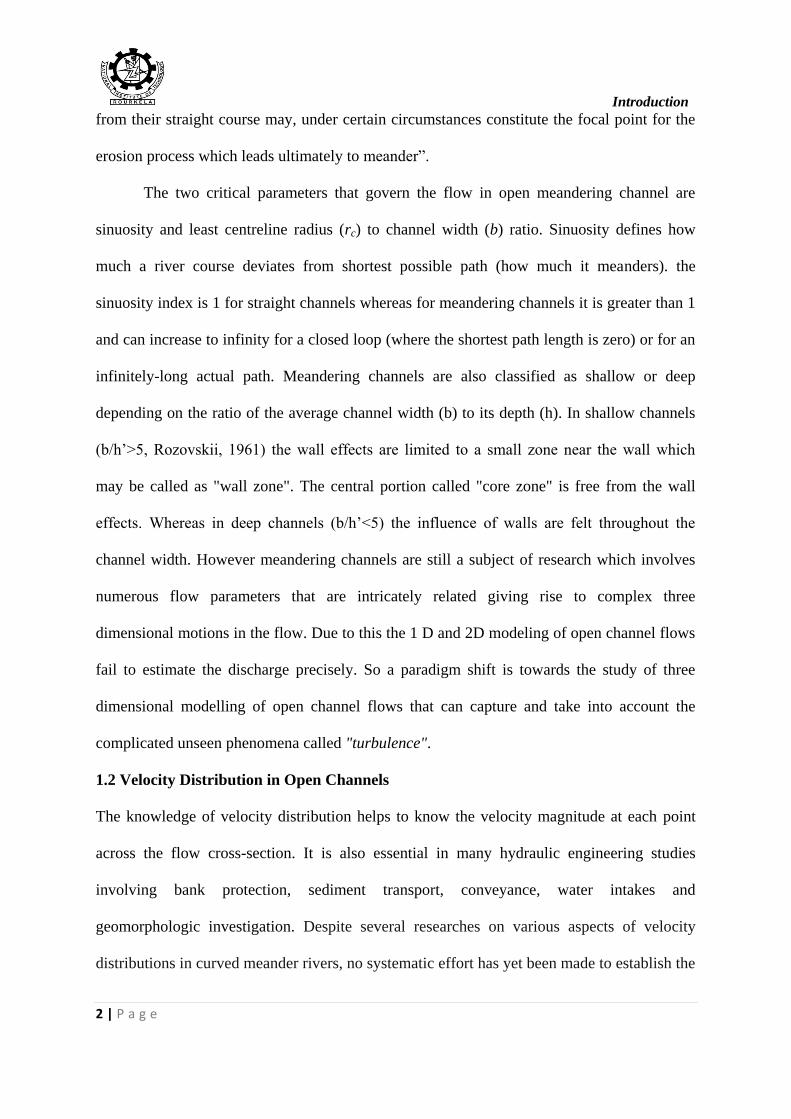
or meandering). In laminar flow max stream wise velocity occurs at water level; for turbulent

flows, it occurs at about 5-25% of water depth below the water surface (Chow, 1959).

Typical stream wise velocity contour lines (isovels) for flow in various cross sections are

shown in Fig. 1.1.

Fig.1.1 Contours of constant velocity in various open channel sections (Chow, 1959)

1.2.1 Logarithmic law

The “logarithmic law” formulation for the velocity profile in turbulent open channel flow is

based on Prandtl’s (1926) theory of the “law of the wall” and the “boundary layer” concept.

The boundary layer is a thin region of fluid near a solid surface (bed or wall) where the

boundary resistance and the viscous interactions affect the fluid motion and subsequently, the

velocity distribution. In the fully developed flow region, this layer includes two main sub-

layers. Near the solid boundary, a viscous sub-layer (laminar layer) forms where the viscous

Introduction

4 | P a g e

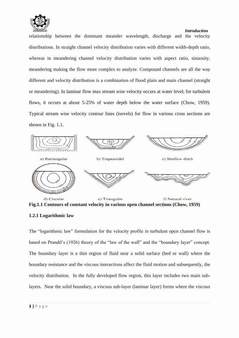
force is predominant. In contrast, further away from the boundary, the turbulent shear

stresses play a major role in the defect layer (turbulent layer).

Fig. 1.2 External fluid flow across a flat plate (after Massy, 1998)

The “law of the wall” states that the in the stream wise direction, the average fluid velocity in

the boundary layer varies logarithmically with distance from the wall surface.

1.2.2 Power law

An alternative function for the velocity distribution is the “power law”. The general form of

this law is proposed as (Barenblatt and Prostokishin, 1993; Schlichting, 1979):

u+ = C4(z+)

m , where C4 and m are the coefficient and exponent of the power law.

1.2.3 Chiu's velocity distribution

An alternative approach from the stated empirical velocity distribution equations is the

method developed by Chiu (1987, 1989). Based on the probability concept and entropy

maximization principle, Chiu derived a new two-dimensional equation for the velocity field.

This equation is capable of describing the variation of velocity in both vertical and transverse

directions with the maximum velocity occurring on or below the water surface. It can also

Introduction

5 | P a g e

accurately describe the velocity distribution in regions near the water surface and channel

bed, where most the existing measuring devices face problems.

1.3 Depth-Averaged Velocity

It is quite difficult to model flows in meandering trapezoidal channel as the inner and outer

banks exert unequal shear drag on the fluid flow that ultimately controls the depth- averaged

velocity. Depth-averaged velocity means the average velocity for a depth ‘h’ is assumed to

occur at a height of 0.4h from the bed level.

1.3.1 AIM OF PRESENT RESEARCH

It is concluded from literature review that very less work has been done regarding lateral

distribution of depth-averaged velocity in meandering trapezoidal channel. However lack of

qualitative and quantitative experimental data on the depth averaged velocity in meandering

channels is still a matter of concern. The present study aims at collecting velocity data from

wide meandering channel trapezoidal at cross section. The objective of the present work is

listed as:

To study the distribution of stream wise depth-averaged velocity at channel bend apex

for single flow depth. Also to study its variation at different flow depths for in bank

and overbank flow conditions.

To propose equations for simple meandering channel trapezoidal at cross section to fit

experimental data.

To validate the depth averaged velocity data with quasi one dimensional model

Conveyance Estimation System (CES) for overbank flow conditions.

To simulate a 60 degree simple meandering channel using Large Eddy Simulation

(LES) model and to derive 3 dimensional velocity contours for the same.

Introduction

6 | P a g e

1.4 ORGANISATION OF THESIS

The thesis consists of seven chapters. General introduction is given in Chapter 1, literature

survey is presented in Chapter 2, experimental work is described in Chapter 3, experimental

results are outlined in Chapter 4 and analysis based on experimental results are done in

Chapter 5, Chapter 6 comprises numerical modelling and finally the conclusions and

references are presented in Chapter 7.

General view on rivers and flooding is provided at a glance in the first chapter. Also

the chapter introduces the concept of velocity distribution in meandering channels. It gives an

overview of numerical modelling in open channel flows.

The detailed literature survey by many eminent researchers that relates to the present

work from the beginning till date is reported in chapter 2. The chapter emphasizes on the

research carried out in straight and meandering channels for both in bank and overbank flow

conditions based on velocity distribution.

Chapter three describes the experimental programme as a whole. This section explains

the experimental arrangements and procedure adopted to obtain observation at different

points in the channel. Also the detailed information about the instrument used for taking

observation is given.

The experimental results regarding stage-discharge relationship, velocity for in bank

and overbank flow conditions and depth average velocity are outlined in chapter four. Also

this chapter discusses the technique adopted for measuring depth average velocity.

Analyses of the experimental results are done in Chapter 5. The analysis of depth average

velocity distribution pattern for in bank and overbank flow conditions is presented in this

chapter.

Introduction

7 | P a g e

Chapter six presents significant contribution to numerical simulation of in bank

channels. The numerical model and the software used within this research are also discussed.

Finally, chapter seven summarizes the conclusion reached by the present research and

recommendation for the further work is listed out.

References that have been made in subsequent chapters are provided at the end of the

thesis.

REVIEW OF LITERATURE

8 | P a g e


2.1 OVERVIEW

Distribution of flow velocity in longitudinal and lateral direction is one of the important

aspects in open channel flows. It directly relates to numerous flow features like water profile

estimation, shear stress distribution, secondary flow, channel conveyance and host to other

flow entities. Various factors that affect the velocity distribution such as channel geometry,

types and patterns of channel, channel roughness and sediment concentration in flow has

been critically studied by many eminent researchers in the past. Prandtl (1932) developed the

general form of velocity distribution, which is generally considered as P-vK law, this law was

derived by assuming the “shear stress is constant”, and can be applied near bed, but has been

applied in outer flow region with modification of von karman constant like Milikan(1939) ,

Vanoni (1941). The P-vK law was derived by taking shear stress as constant whereas the

shear stress is not constant in turbulent layer (outer zone) in open channel flow. Milikan

(1939) suggested that actual velocity distribution consists of logarithmic part and correction

part, where the correction part considers the outer layer into account. So detailed literature

review is done for four different channel types followed by works on numerical modelling for

open channel flows.

2.2 PREVIOUS EXPERIMENTAL RESEARCH ON VELOCITY DISTRIBUTION

2.2.1 STRAIGHT SIMPLE CHANNEL

Coles (1956) proposed a semi-empirical equation of velocity distribution, which can

be applied to outer region and wall region of plate and open channel. He generalized the

logarithmic formula of the wall with tried wake function, w(y/8).This formula is asymptotic

to the logarithmic equation of the wall as the distance y approaches the wall. This is basic

formulation towards outer layer region.


9 | P a g e

Coleman (1981) proposed that the velocity equation for sediment-laden flow consists

of two parts, as originally discussed by Coles for clear-water flow. Also he has revealed that

the von Karman coefficient is independent of sediment concentration. The elevation of the

maximum velocity and the deviation of velocity from the logarithmic formula at the water

surface are functions of the aspect ratio of the channel. The log-law is developed into an

equation applicable to the whole flow including the region near the water surface for various

boundary conditions. The wake law describes the velocity distribution below the maximum

velocity point.

M. Salih Kirkgoz et al. (1997) measured mean velocities using a Laser Doppler

Anemometer (LDA) in developing and fully developed turbulent subcritical smooth open

channel flows. From the experiments it is found that the boundary layer along the centre line

of the channel develops up to the free surface for a flow aspect ratio . In the turbulent

inner regions of developing and fully developed boundary flows, the measured velocity

profiles agree well with the logarithmic "law of the wall" distribution. The "wake" effect

becomes important in the velocity profiles of the fully developed boundary layers.

Sarma et al. (2000) tried to formulate the velocity distribution law in open channel

flows by taking generalized version of binary version of velocity distribution, which

combines the logarithmic law of the inner region and parabolic law of the outer region. The

law developed by taking velocity-dip in to account.

Wilkerson et al. (2005) using data from three previous studies, developed two models

for predicting depth-averaged velocity distributions in straight trapezoidal channels that are

not wide, where the banks exert form drag on the fluid and thereby control the depth-

averaged velocity distribution. The data they used for developing the model are free from the

effect of secondary current. The 1st model required measured velocity data for calibrating the

model coefficients, where as the 2nd

model used prescribed coefficients. The 1st model is


10 | P a g e

recommended when depth-averaged velocity data are available. When the 2nd

model is used,

predicted depth-averaged velocities are expected to be within 20% of actual velocities.

Knight et al. (2007) used Shiono and Knight Method (SKM), which is a new

approach to calculating the lateral distributions of depth-averaged velocity and boundary

shear stress for flows in straight prismatic channels, also accounted secondary flow effect. It

accounts for bed shear, lateral shear, and secondary flow effects via3 coefficients- f, λ, and Γ

—thus incorporating some key 3D flow feature into a lateral distribution model for stream

wise motion. This method used to analyze in straight trapezoidal open channel. The number

of secondary current varies with aspect ratio. It is three for aspect ratio less than equal to 2.2

and four for aspect ratio greater than equal 4.

Afzal et al. (2007) analyzed power law velocity profile in fully developed turbulent

pipe and channel flows in terms of the envelope of the friction factor. This model gives good

approximation for low Reynolds number in designed process of actual system compared to

log law.

Yang (2010) investigate depth-average shear stress and velocity in rough channels.

Equations of the depth-averaged shear stress in typical open channels have been derived

based on a theoretical relation between the depth-averaged shear stress and boundary shear

stress. Equation of depth mean velocity in a rough channel is also obtained and the effects of

water surface (or dip phenomenon) and roughness are included. Experimental data available

in the literature have been used for verification that shows that the model reasonably agrees

with the measured data.

Oscar Castro-Orgaz (2010) reanalysed the available data on turbulent velocity profiles

in steep chute flow, to determine general law by taking into account both the laws of the wall

and wake. Once the velocity profile is defined, an equivalent power-law velocity

approximation is proposed, with generalised coefficients determined by the rational approach.


11 | P a g e

The results obtained for the turbulent velocity profiles were applied to analytically determine

the resistance characteristics for chute flows.

Albayrak et al. (2011) combined the detailed acoustic Doppler velocity profiler

(ADVP ), large-scale particle image velocimetry (LSPIV) and hot film measurements to

analyse secondary current dynamics within the water column and free surface of an open

channel flow over a rough movable (not moving) bed in a wider channel, with a higher bed

roughness and at higher Reynolds number.

Kundu and Ghoshal (2012) re-investigated the velocity distribution in open channel

flows based on flume experimental data. From the analysis, it is proposed that the wake layer

in outer region may be divided into two regions, the relatively weak outer region and the

relatively strong outer region. Combining the log law for inner region and the parabolic law

for relatively strong outer region, an explicit equation for mean velocity distribution of steady

and uniform turbulent flow through straight open channels is proposed and verified with the

experimental data. It is found that the sediment concentration has significant effect on

velocity distribution in the relatively weak outer region.

2.2.2 STRAIGHT COMPOUND CHANNELS

Wormleaton and Hadjipanos (1985) measured the velocity in each subdivision of the

channel, and found that even if the errors in the calculation of the overall discharge were

small, the errors in the calculated discharges in the floodplain and main channel may be very

large when treated separately. They also observed that, typically, underestimating the

discharge on the floodplain was compensated by overestimating it for the main channel. The

failure of most subdivision methods is due to the complicated interaction between the main

channel and floodplain flows.

Myers (1987) presented theoretical considerations of ratios of main channel velocity

and discharge to the floodplain values in compound channel. These ratios followed a straight-


12 | P a g e

line relationship with flow depth and were independent of bed slope but dependent on

channel geometry only. Equations describing these relationships for smooth compound

channel geometry were presented. The findings showed that at low depths, the conventional

methods always overestimated the full cross sectional carrying capacity and underestimated

at large depths, while floodplain flow capacity was always underestimated at all depths. He

underlined the need for methods of compound channel analysis that accurately model

proportions of flow in floodplain and main channel as well as full cross-sectional discharge

capacity.

Tominaga & Nezu (1992) measured velocity with a fibre-optic laser-Doppler

anemometer in steep open-channel flows over smooth and incompletely rough beds. As

velocity profile in steep open channel is necessary for solving the problems of soil erosion

and sediment transport, and he observed the integral constant A in the log law coincided with

the usual value of 5.29 regardless of the Reynolds and Froude number in subcritical flows,

whereas it decreased with an increase of the bed slope in supercritical flows.

Willetts and Hardwick (1993) reported the measurement of stage–discharge

relationship and observation of velocity fields in small laboratory two stage channels. It was

found that the zones of interaction between the channel and floodplain flows occupied the

whole or at least very large portion of the main channel. The water, which approached the

channel by way of floodplain, penetrated to its full depth and there was a vigorous exchange

of water between the inner channel and floodplain in and beyond the downstream half of each

bend. This led to consequent circulation in the channel in the whole section. The energy

dissipation mechanism of the trapezoidal section was found to be quite different from the

rectangular section and they suggested for further study in this respect. They also suggested

for further investigation to quantify the influence of floodplain roughness on flow parameters.


13 | P a g e

Czernuszenko, Kozioł, Rowiński (2007) describes some turbulence measurements

carried out in an experimental compound channel with flood plains. The surface of the main

channel bed was smooth and made of concrete, whereas the flood plains and sloping banks

were covered by cement mortar composed with terrazzo. Instantaneous velocities were

measured be means of a three-component acoustic Doppler velocity meter (ADV)

manufactured by Sontek Inc. This article presents the results of measurements of primary

velocity, the distribution of turbulent intensities, Reynolds stresses, autocorrelation functions,

turbulent scales, as well as the energy spectra.

Xiaonan Tang, Donald W. Knight (2008) reviewed a model, developed by Shiono and

Knight (SKM) to overcome the difficulties in defining the boundary conditions at the internal

wall between the main channel and the flood plain. They proposed a novel approach for

imposing the boundary conditions by taking 3sets of different experimental data.

M. M. Ahmadi et al. (2009) proposed an unsteady 2D depth-averaged flow model

taking into consideration the dispersion stress terms to simulate the bend flow field using an

orthogonal curvilinear co-ordinate system. The dispersion terms which arose from the

integration of the product of the discrepancy between the mean and the actual vertical

velocity distribution were included in the momentum equations in order to take into

account the effect of the secondary current.

2.2.3 MEANDER SIMPLE CHANNELS

Johannesson and Parker (1989) presented an analytical model for calculating the

lateral distribution of the depth-averaged primary flow velocity in meandering rivers. The

well-known "moment method," commonly used to solve the concentration distributions, is

then used to obtain an approximate solution. This makes it possible to take into account the

convective transport of primary flow momentum by the secondary flow. This oft-neglected


14 | P a g e

influence of the secondary flow is shown to be an important cause of the redistribution of the

primary flow velocity.

Maria and Silva (1999) expressed the friction factor of rough turbulent meandering

flows as the function of sinuosity and position (which is determined by, among other factors,

the local channel curvature).They validated the expression by the laboratory data for two

meandering channels of different sinuosity. The expression was found to yield the computed

vertically averaged flows that are in agreement with the flow pictures measured for both large

and small values of sinuosity.

Zarrati, Tamai and Jin (2005) developed a depth averaged model for predicting water

surface profiles for meandering channels. They applied the model to three meandering

channels (two simple and one compound) data. The model was found to predict well the

water surface profile and velocity distribution for simple channels and also for the main

channel of compound meandering channel.

2.2.4 MEANDER COMPOUND CHANNEL

D. Alan Ervine, et al. (2000) presented a practical method to predict depth-averaged

velocity and shear stress for straight and meandering overbank flows. An analytical solution

to depth-integrated turbulent form of the Navier-Stokes equation was presented that included

lateral shear and secondary flows in addition to bed friction. The novelty of that approach

was not only its inclusion of the secondary flows in the formulation but also its applicability

to straight and meandering channels.

Patra and Kar (2004) reported the test results concerning the flow and velocity

distribution in meandering compound river sections. Using power law they presented

equations concerning the three-dimensional variation of longitudinal, transverse, and vertical

velocity in the main channel and floodplain of meandering compound sections in terms of

channel parameters. The results of formulations compared well with their respective


15 | P a g e

experimental channel data obtained from a series of symmetrical and unsymmetrical test

channels with smooth and rough surfaces. They also verified the formulations against the

natural river and other meandering compound channel data.

3.0 OVERVIEW OF NUMERICAL MODELLING ON OPEN CHANNEL FLOW

For the past three decades, flow in simple and compound meandering channels has been

extensively studied both experimentally and numerically. Various numerical models such as

standard k-ε model, non-linear k-ε model, k-ω model, algebraic Reynolds stress model

(ASM), Reynolds stress model (RSM) and large eddy simulation (LES) have been developed

to simulate the complex secondary structure in compound meandering channel. The standard

k- ε model is an isotropic turbulence closure but fails to reproduce the secondary flows.

Although nonlinear k- ε model can simulate secondary currents successfully in a compound

channel, it cannot accurately capture some of the turbulence structures. ASM is economical

because it uses adhoc expressions to solve Reynolds stress transport equations. But the

simulated results by ASM found to be unreliable. Reynolds stress model (RSM) computes

Reynolds stresses by directly solving Reynolds stress transport equation but its application to

open channel is still limited due to the complexity of the model. Large eddy simulation (LES)

solves spatially-averaged Navier-Stokes equation. Large eddies are directly resolves, but the

eddies smaller than mesh are modelled. LES is computationally very expensive to be used for

industrial application.

Giuseppe Pezzinga (1994) examined the problem of prediction of uniform turbulent

flow in a compound channel with the nonlinear k-ε model. This model is capable of

predicting the secondary currents, caused by the anisotropy of normal turbulent stresses that

are important features of the flow in compound channels, as they determine the transverse

momentum transfer. The comparison shows that the model predicts with accuracy the


16 | P a g e

distribution of the primary velocity component, the secondary circulation, and the discharge

distribution. The numerical results are used to search a subdivision surface between main

channel and floodplain on the basis of the flow field and to compare different subdivision

surfaces on the basis of the discharge distribution by a simple uniform flow formula, The

better subdivision surfaces as predicted by the model are the diagonal surface going from the

corner between main channel and floodplain to the free surface on the symmetry plane and

the bisector of the same corner.

Cokljat and Younis and Basara and Cokljat (1995) proposed the RSM for numerical

simulations of free surface flows in a rectangular channel and in a compound channel and

found good agreement between predicted and measured data.

Thomas and Williams (1995) describes a Large Eddy Simulation of steady uniform

flow in a symmetric compound channel of trapezoidal cross-section with flood plains at a

Reynolds number of 430,000. The simulation captures the complex interaction between the

main channel and the flood plains and predicts the bed stress distribution, velocity

distribution, and the secondary circulation across the floodplain. The results are compared

with experimental data from the SERC Flood Channel Facility at Hydraulics Research Ltd,

Wallingford, England.

Salvetti et al. (1997) has conducted LES simulation at a relatively large Reynolds

number for producing results of bed shear, secondary motion and vorticity well

comparable to experimental results.

Rameshwaran P, Naden PS.(2003) analyzed three dimensional nature of flow in

compound channels.

Sugiyama H, Hitomi D, Saito T.(2006) used turbulence model consists of transport

equations for turbulent energy and dissipation, in conjunction with an algebraic stress model


17 | P a g e

based on the Reynolds stress transport equations. They have shown that the fluctuating

vertical velocity approaches zero near the free surface. In addition, the compound meandering

open channel is clarified somewhat based on the calculated results. As a result of the analysis,

the present algebraic Reynolds stress model is shown to be able to reasonably predict the

turbulent flow in a compound meandering open channel.

Kang H, Choi SU. (2006) used a Reynolds stress model for the numerical simulation

of uniform 3D turbulent open-channel flows. The developed model is applied to a flow at a

Reynolds number of 77000 in a rectangular channel with a width to depth ratio of 2. The

simulated mean flow and turbulence structures are compared with measured and computed

data from the literature. It is found that both production terms by anisotropy of Reynolds

normal stress and by Reynolds shear stress contribute to the generation of secondary currents.

Jing, Guo and Zhang (2008) simulated a three-dimensional (3D) Reynolds stress

model (RSM) for compound meandering channel flows. The velocity fields, wall shear

stresses, and Reynolds stresses are calculated for a range of input conditions. Good

agreement between the simulated results and measurements indicates that RSM can

successfully predict the complicated flow phenomenon.

Cater and Williams (2008) reported a detailed Large Eddy Simulation of turbulent

flow in a long compound open channel with one floodplain. The Reynolds number is

approximately 42,000 and the free surface was treated as fully deformable. The results are in

agreement with experimental measurements and support the use of high spatial resolution and

a large box length in contrast with a previous simulation of the same geometry. A secondary

flow is identified at the internal corner that persists and increases the bed stress on the

floodplain.


18 | P a g e

Kim et al. (2008) analyses three-dimensional flow and transport characteristics in

two representative multi-chamber ozone contactor models with different chamber width

using LES.

Wang et.al., (2008) used different turbulence closure schemes i.e., the mixing-length

model and the k-ε model with different pressure solution techniques i.e., hydrostatic

assumptions and dynamic pressure treatments are applied to study the helical secondary flows

in an experiment curved channel. The agreements of vertically-averaged velocities between

the simulated results obtained by using different turbulence models with different pressure

solution techniques and the measured data are satisfactory. Their discrepancies with respect

to surface elevations, super elevations and secondary flow patterns are discussed.

Balen et.al. (2010) performed LES for a curved open-channel flow over topography.

It was found that, notwithstanding the coarse method of representing the dune forms, the

qualitative agreement of the experimental results and the LES results is rather good.

Moreover, it is found that in the bend the structure of the Reynolds stress tensor shows a

tendency toward isotropy which enhances the performance of isotropic eddy viscosity closure

models of turbulence.

Beaman (2010) studied the conveyance estimation using LES method.

Esteve et.al., (2010) simulated the turbulent flow structures in a compound

meandering channel by Large Eddy Simulations (LES) using the experimental configuration

of Muto and Shiono (1998). The Large Eddy Simulation is performed with the in-house code

LESOCC2. The predicted stream wise velocities and secondary current vectors as well as

turbulent intensity are in good agreement with the LDA measurements.

Larocque, Imran, Chaudhry (2013) presented 3D numerical simulation of a dam-break

flow using LES and k- ε turbulence model with tracking of free surface by volume-of-fluid

model. Results are compared with published experimental data on dam-break flow through a


19 | P a g e

partial breach as well as with results obtained by others using a shallow water model. The

results show that both the LES and the k –ε modelling satisfactorily reproduce the temporal

variation of the measured bottom pressure. However, the LES model captures better the free

surface and velocity variation with time.

Experimental Set-Up

20 | P a g e

EXPERIMENTAL WORK AND METHODOLOGY

3.1 OVERVIEW

Evaluation of discharge capacity in a meandering river channels is a complicated process

due to variations in geometry, surface roughness, channel alignments and flow conditions.

The evaluation of discharge capacity is directly dependent on accurate prediction of

knowledge of velocity distribution in channel. Velocity distribution is never uniform across a

compound channel cross-section. It is higher in deeper main channel than the shallower

floodplain, as in compound channels the shallow floodplains offer more resistance to flow

than the deep main channel. Variation of velocity leads to lateral momentum transfer between

the deep main channel and the adjoining shallow floodplains. This further complicates the

flow process, leading to the uneven distribution of shear stress in the main channel and

floodplain peripheral regions. The trends and behaviour pattern observed in the laboratory

flumes can be used in better understanding of the mechanism of flow in a meandering

channel and so for the solution of many practical river problems.

In the present work the velocity distribution has been studied through a series experimental

runs in a meandering channel of higher sinuosity existing in the laboratory. Details of

hydraulics and geometric parameters of meandering channel, apparatus and measuring

equipments used and working procedure adopted has been outlined in this chapter.

3.2 APPARATUS & EQUIPMENTS USED

In this study Measuring devices like a pointer gauge having least count of 0.1 mm,

rec tangular notch , five micro-Pitot tubes each of them having 4.6 mm external diameter

and five manometers were used in the experimentation. These are used to measure velocity

and its direction of flow in the channels. Including these also useful apparatus without which

Experimental Set-Up

21 | P a g e

experiments could not be possible. Those were baffle walls, stilling chamber, baffle, head

gate, travelling bridge, sump, tail gate, volumetric tank, over head tank arrangement, water

supply devices, two parallel pumps etc. The measuring equipments and the devices were

arranged properly to carry out experiments in the channels. Keeping the set up with sufficient

care and management experiments runs were taken for the meandering channel.

3.3 EXPERIMENTAL SETUP AND PROCEDURE

Experiments are conducted utilising the channel facility available at the Hydraulics

Laboratory of the Civil Engineering Department, National Institute of Technology, Rourkela.

The experimental meandering channel is fabricated using 6mm thick Perspex sheet inside a

tilting flume. The tilting flume is 15m long having a rectangular cross-section of 4m wide and

0.5m deep, made up of deep metal frame with glass walls. The flume can be tilted to different

bed slopes by hydraulic jack arrangement. The experimental meandering channel has

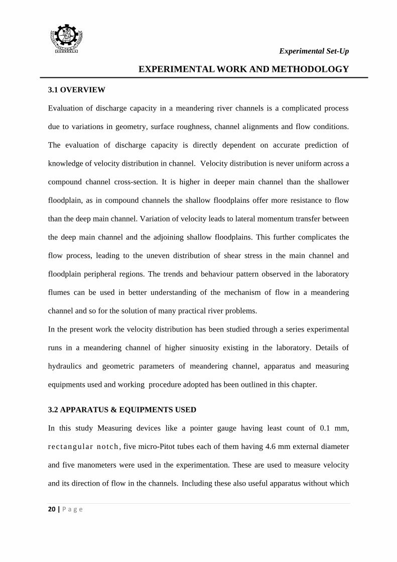
trapezoidal cross-section. All observations are recorded at the central bend apex. Photograph

of the experimental meandering channel with measuring equipments are shown in Photo.3.1

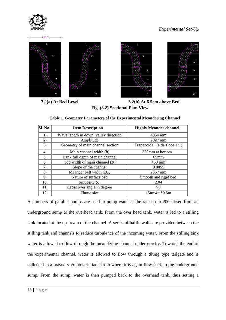
(a, b). Fig.3.2 (a, b) shows the plan view of half meander wavelength with dimensional

details while the plan view of full length experimental channel with other arrangements is

shown in Fig.3.1.

Experimental channel: The meandering channel is trapezoidal in cross section. The channel is

330 mm wide at bottom, 460 mm at top having full depth of 65 mm, and side slopes of 1:1.

The channel has wavelength L = 3972 mm and double amplitude 2A’ = 1365 mm. Sinuosity

for this channel is scaled as 2.04 Photo. 3.1(a, b). For better information, the geometrical

parameters and hydraulic details of the experimental runs of the channel is tabulated below.

Experimental Set-Up

22 | P a g e

Channel Photographs

Photo.3.1 (a) View of Experimental Channel Photo.3.1 (b) Rectangular Notch

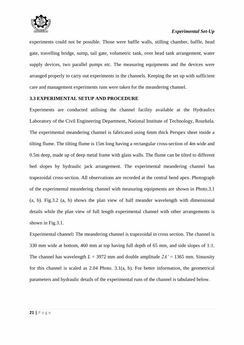
Fig.3.1 *Schematic diagram of Experimental Setup

*After Mohanty et.al (2013)

Experimental Set-Up

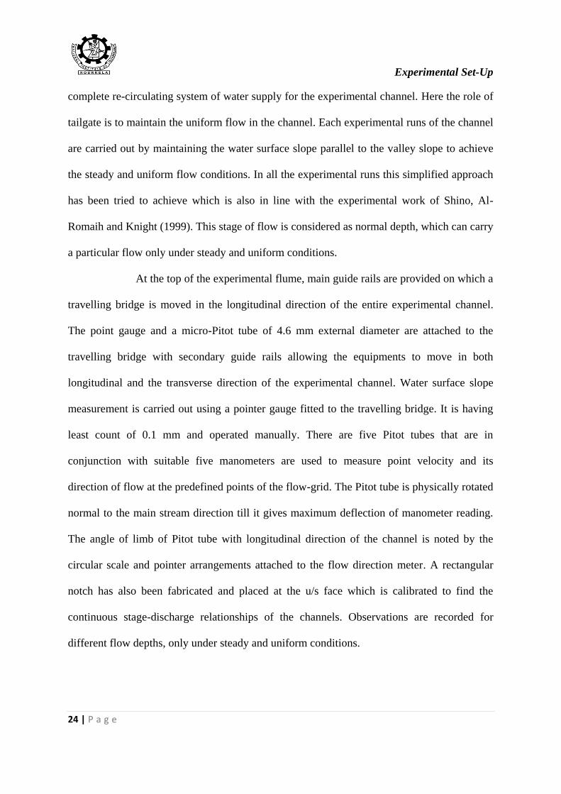
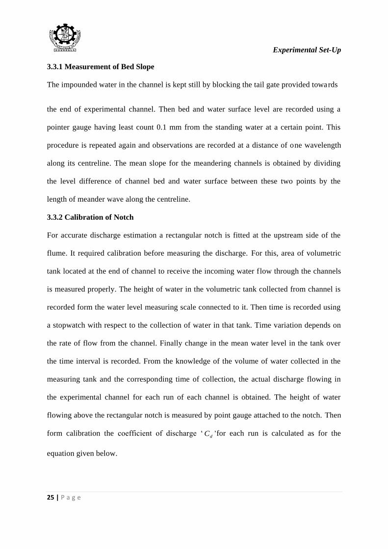
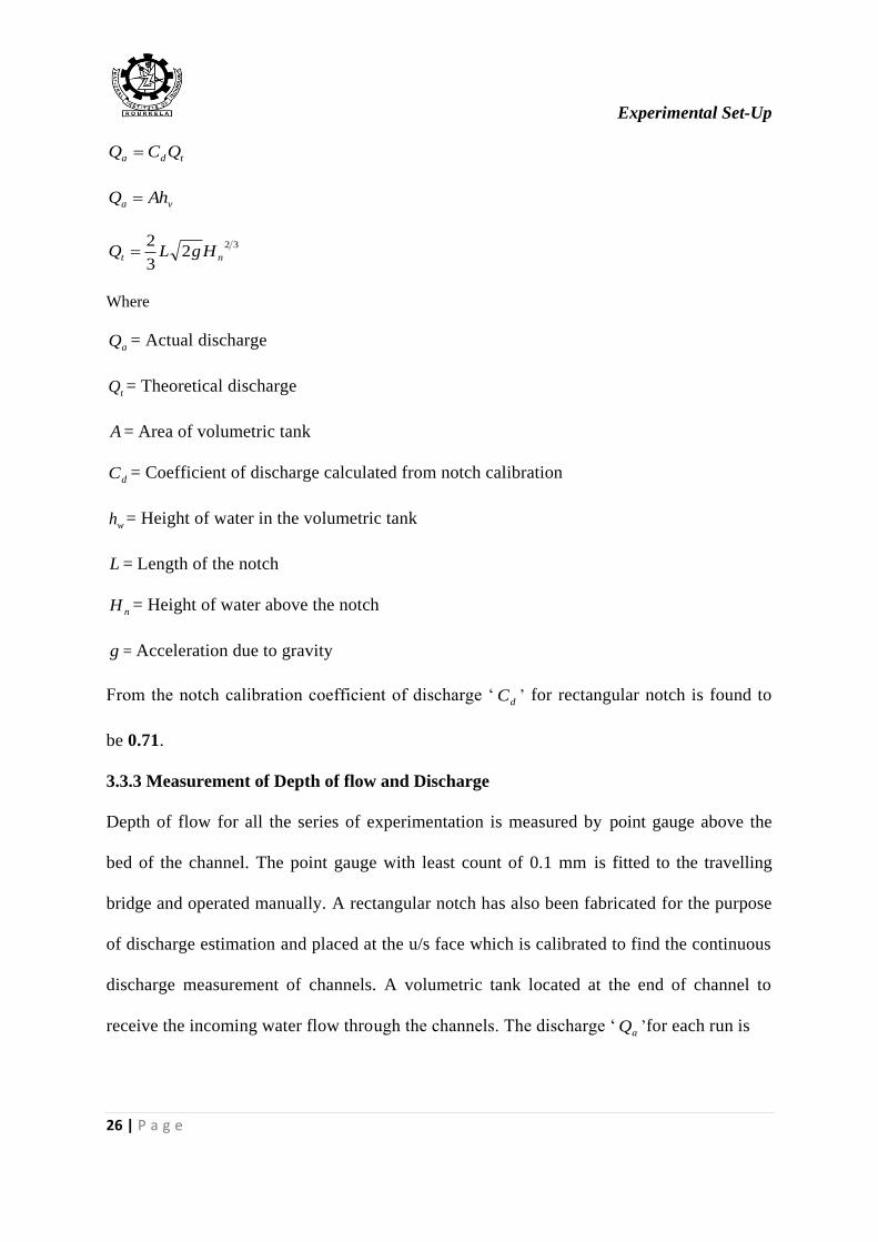
23 | P a g e

3.2(a) At Bed Level 3.2(b) At 6.5cm above Bed

Fig. (3.2) Sectional Plan View

Table 1. Geometry Parameters of the Experimental Meandering Channel

A numbers of parallel pumps are used to pump water at the rate up to 200 lit/sec from an

underground sump to the overhead tank. From the over head tank, water is led to a stilling

tank located at the upstream of the channel. A series of baffle walls are provided between the

stilling tank and channels to reduce turbulence of the incoming water. From the stilling tank

water is allowed to flow through the meandering channel under gravity. Towards the end of

the experimental channel, water is allowed to flow through a tilting type tailgate and is

collected in a masonry volumetric tank from where it is again flow back to the underground

sump. From the sump, water is then pumped back to the overhead tank, thus setting a

Sl. No. Item Description Highly Meander channel

1. Wave length in down valley direction 4054 mm

2. Amplitude 2027 mm

3. Geometry of main channel section Trapezoidal (side slope 1:1)

4. Main channel width (b) 330mm at bottom

5. Bank full depth of main channel 65mm

6. Top width of main channel (B) 460 mm

7. Slope of the channel 0.0055

8. Meander belt width (BW) 2357 mm

9. Nature of surface bed Smooth and rigid bed

10. Sinuosity(Sr) 2.04

11. Cross over angle in degree

12. Flume size 15m*4m*0.5m

Experimental Set-Up

24 | P a g e

complete re-circulating system of water supply for the experimental channel. Here the role of

tailgate is to maintain the uniform flow in the channel. Each experimental runs of the channel

are carried out by maintaining the water surface slope parallel to the valley slope to achieve

the steady and uniform flow conditions. In all the experimental runs this simplified approach

has been tried to achieve which is also in line with the experimental work of Shino, Al-

Romaih and Knight (1999). This stage of flow is considered as normal depth, which can carry

a particular flow only under steady and uniform conditions.

At the top of the experimental flume, main guide rails are provided on which a

travelling bridge is moved in the longitudinal direction of the entire experimental channel.

The point gauge and a micro-Pitot tube of 4.6 mm external diameter are attached to the

travelling bridge with secondary guide rails allowing the equipments to move in both

longitudinal and the transverse direction of the experimental channel. Water surface slope

measurement is carried out using a pointer gauge fitted to the travelling bridge. It is having

least count of 0.1 mm and operated manually. There are five Pitot tubes that are in

conjunction with suitable five manometers are used to measure point velocity and its

direction of flow at the predefined points of the flow-grid. The Pitot tube is physically rotated

normal to the main stream direction till it gives maximum deflection of manometer reading.

The angle of limb of Pitot tube with longitudinal direction of the channel is noted by the

circular scale and pointer arrangements attached to the flow direction meter. A rectangular

notch has also been fabricated and placed at the u/s face which is calibrated to find the

continuous stage-discharge relationships of the channels. Observations are recorded for

different flow depths, only under steady and uniform conditions.

Experimental Set-Up

25 | P a g e

3.3.1 Measurement of Bed Slope

The impounded water in the channel is kept still by blocking the tail gate provided towards

the end of experimental channel. Then bed and water surface level are recorded using a

pointer gauge having least count 0.1 mm from the standing water at a certain point. This

procedure is repeated again and observations are recorded at a distance of one wavelength

along its centreline. The mean slope for the meandering channels is obtained by dividing

the level difference of channel bed and water surface between these two points by the

length of meander wave along the centreline.

3.3.2 Calibration of Notch

For accurate discharge estimation a rectangular notch is fitted at the upstream side of the

flume. It required calibration before measuring the discharge. For this, area of volumetric

tank located at the end of channel to receive the incoming water flow through the channels

is measured properly. The height of water in the volumetric tank collected from channel is

recorded form the water level measuring scale connected to it. Then time is recorded using

a stopwatch with respect to the collection of water in that tank. Time variation depends on

the rate of flow from the channel. Finally change in the mean water level in the tank over

the time interval is recorded. From the knowledge of the volume of water collected in the

measuring tank and the corresponding time of collection, the actual discharge flowing in

the experimental channel for each run of each channel is obtained. The height of water

flowing above the rectangular notch is measured by point gauge attached to the notch. Then

form calibration the coefficient of discharge ‘dC ’for each run is calculated as for the

equation given below.

Experimental Set-Up

26 | P a g e

tda QCQ

va AhQ

322

3

2nt HgLQ

Where

aQ = Actual discharge

tQ = Theoretical discharge

A = Area of volumetric tank

dC = Coefficient of discharge calculated from notch calibration

wh = Height of water in the volumetric tank

L = Length of the notch

nH = Height of water above the notch

g = Acceleration due to gravity

From the notch calibration coefficient of discharge ‘dC ’ for rectangular notch is found to

be 0.71.

3.3.3 Measurement of Depth of flow and Discharge

Depth of flow for all the series of experimentation is measured by point gauge above the

bed of the channel. The point gauge with least count of 0.1 mm is fitted to the travelling

bridge and operated manually. A rectangular notch has also been fabricated for the purpose

of discharge estimation and placed at the u/s face which is calibrated to find the continuous

discharge measurement of channels. A volumetric tank located at the end of channel to

receive the incoming water flow through the channels. The discharge ‘aQ ’for each run is

Experimental Set-Up

27 | P a g e

calculated as for the equation given below.

322

3

2nda HgLCQ

Where

aQ = Actual discharge

dC = Coefficient of discharge calculated from notch calibration

L = Length of the notch

nH = Height of water above the notch

g = Acceleration due to gravity

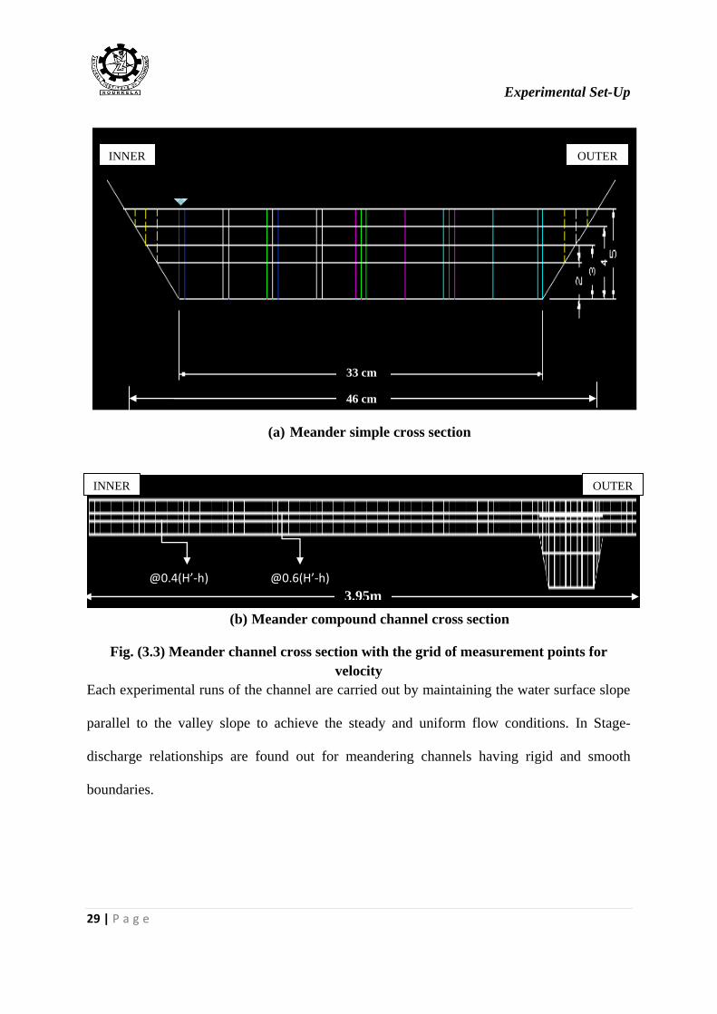
3.3.4 Measurement of tangential Velocity

Velocity measurements are taken at the bend apex in meandering channel due to minimum

curvature effect and to study the flow parameters covering half the meander wave length. In

the present work velocity readings are taken using Pitot tubes. These are placed in the

direction of flow and then allowed to rotate along a plane parallel to the bed and till a

relatively maximum head difference appeared in manometers attached to the respective

Pitot tubes. The deviation angle between the reference axis and the total velocity vector is

assumed to be positive, when the velocity vector is directed away from the outer bank. The

total head h reading by the Pitot tube at the predefined points of the flow-grid in the channel

is used to measure the magnitude of point velocity vector as U = (2gh)1/2

, where g is the

acceleration due to gravity. Resolving U into the tangential and radial directions, the local

velocity components is obtained. Here the tube coefficient is taken as unit and the error due to

turbulence considered negligible while measuring velocity. Point velocities were measured

along verticals spread across the main channel and flood plain so as to cover the width of

Experimental Set-Up

28 | P a g e

entire cross section. Also at a no. of horizontal layers in each vertical, point velocities were

taken. Particularly the point velocities at a depth of 0.4H (where H is the depth of flow at that

lateral section across the channel) from channel bed in main channel region and 0.4(H-h) on

floodplains (h is depth of main channel) were measured throughout the lateral section of the

compound cross section to experimentally determine the depth averaged velocity distribution

under each discharge condition. Measurements were thus taken from left edge point of flood

plain to the right edge of floodplain including the main channel bed and side slope

(Figure.3.3 (a, b) shows the grid diagram used for experiments). Velocity measurements were

taken by five pitot static tube (outside diameter 4.77mm) connected with five piezometers

fitted inside a transparent fiber block fixed to a wooden board and hung vertically at the edge

of flume the ends of which were open to atmosphere at one end and connected to total

pressure hole and static hole of pitot tube by long transparent PVC tubes at other ends. Before

taking the readings the pitot tube along with the long tubes measuring about 5m were to be

properly immersed in water and caution was exercised for complete expulsion of any air

bubble present inside the pitot tube or the PVC tube. Even the presence of a small air bubble

inside the static limb or total pressure limb could give erroneous readings in piezometers used

for recording the pressure.

Experimental Set-Up

29 | P a g e

(a) Meander simple cross section

(b) Meander compound channel cross section

Fig. (3.3) Meander channel cross section with the grid of measurement points for

velocity

Each experimental runs of the channel are carried out by maintaining the water surface slope

parallel to the valley slope to achieve the steady and uniform flow conditions. In Stage-

discharge relationships are found out for meandering channels having rigid and smooth

boundaries.

INNER OUTER

INNER OUTER

3.95m

46 cm

@0.4(H’-h) @0.6(H’-h)

33 cm

Experimental Results

30 | P a g e

EXPERIMENTAL RESULTS

4.1 OVERVIEW

The results of experiments concerning the distribution of velocity, flow in the meandering

channels are presented in this chapter. Analysis is also done for depth averaged velocity in

the meandering channel. The overall summary of experimental runs for the meandering

channel is given in Table-2.

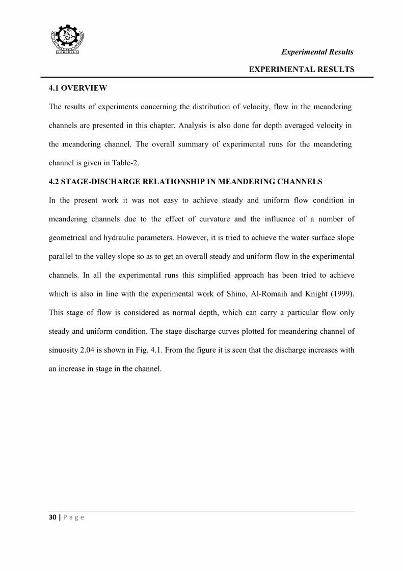
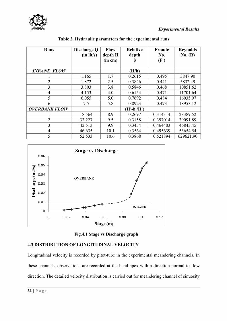
4.2 STAGE-DISCHARGE RELATIONSHIP IN MEANDERING CHANNELS

In the present work it was not easy to achieve steady and uniform flow condition in

meandering channels due to the effect of curvature and the influence of a number of

geometrical and hydraulic parameters. However, it is tried to achieve the water surface slope

parallel to the valley slope so as to get an overall steady and uniform flow in the experimental

channels. In all the experimental runs this simplified approach has been tried to achieve

which is also in line with the experimental work of Shino, Al-Romaih and Knight (1999).

This stage of flow is considered as normal depth, which can carry a particular flow only

steady and uniform condition. The stage discharge curves plotted for meandering channel of

sinuosity 2.04 is shown in Fig. 4.1. From the figure it is seen that the discharge increases with

an increase in stage in the channel.


31 | P a g e

Table 2. Hydraulic parameters for the experimental runs

Runs Discharge Q

(in lit/s)

Flow

depth H

(in cm)

Relative

depth

β

Froude

No.

(Fr)

Reynolds

No. (R)

INBANK FLOW (H/h)

1 1.165 1.7 0.2615 0.495 3847.90

2 1.872 2.5 0.3846 0.441 5832.49

3 3.803 3.8 0.5846 0.468 10851.62

4 4.153 4.0 0.6154 0.471 11701.64

5 6.055 5.0 0.7692 0.484 16035.97

6 7.5 5.8 0.8923 0.473 18953.12

OVERBANK FLOW (H'-h /H')

1 18.564 8.9 0.2697 0.314314 28389.52

2 33.227 9.5 0.3158 0.397014 39091.89

3 42.513 9.9 0.3434 0.464403 46843.45

4 46.635 10.1 0.3564 0.495639 53654.54

5 52.533 10.6 0.3868 0.521894 629621.90

Fig.4.1 Stage vs Discharge graph

4.3 DISTRIBUTION OF LONGITUDINAL VELOCITY

Longitudinal velocity is recorded by pitot-tube in the experimental meandering channels. In

these channels, observations are recorded at the bend apex with a direction normal to flow

direction. The detailed velocity distribution is carried out for meandering channel of sinuosity

OVERBANK

INBANK


32 | P a g e

2.04. The radial distribution of longitudinal velocity in contour form for the runs of the

meandering channel is shown below. It gives the point form velocity measurement at that

depth of flow. The radial distribution of tangential velocity for four flow inbank depths are

shown in Figs.4.2 (a, b, c and d) and for four overbank flow depths in Figs.4.3 (a,b,c,d).

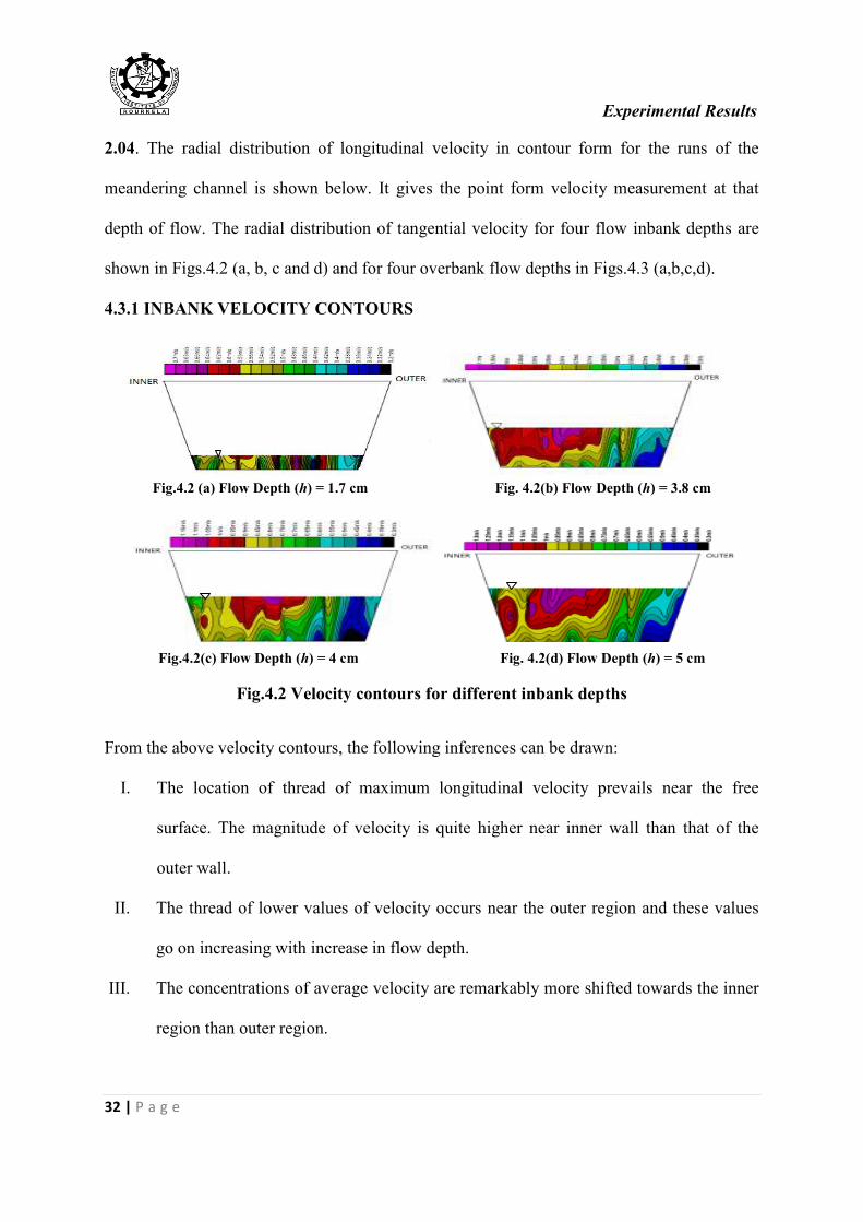
4.3.1 INBANK VELOCITY CONTOURS

Fig.4.2 (a) Flow Depth (h) = 1.7 cm Fig. 4.2(b) Flow Depth (h) = 3.8 cm

Fig.4.2(c) Flow Depth (h) = 4 cm Fig. 4.2(d) Flow Depth (h) = 5 cm

Fig.4.2 Velocity contours for different inbank depths

From the above velocity contours, the following inferences can be drawn:

I. The location of thread of maximum longitudinal velocity prevails near the free

surface. The magnitude of velocity is quite higher near inner wall than that of the

outer wall.

II. The thread of lower values of velocity occurs near the outer region and these values

go on increasing with increase in flow depth.

III. The concentrations of average velocity are remarkably more shifted towards the inner

region than outer region.


33 | P a g e

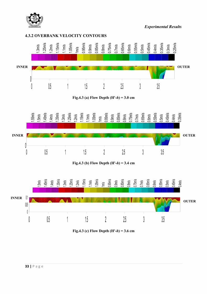
4.3.2 OVERBANK VELOCITY CONTOURS

Fig.4.3 (a) Flow Depth (H'-h) = 3.0 cm

Fig.4.3 (b) Flow Depth (H'-h) = 3.4 cm

Fig.4.3 (c) Flow Depth (H'-h) = 3.6 cm

INNER OUTER

OUTER INNER

INNER OUTER


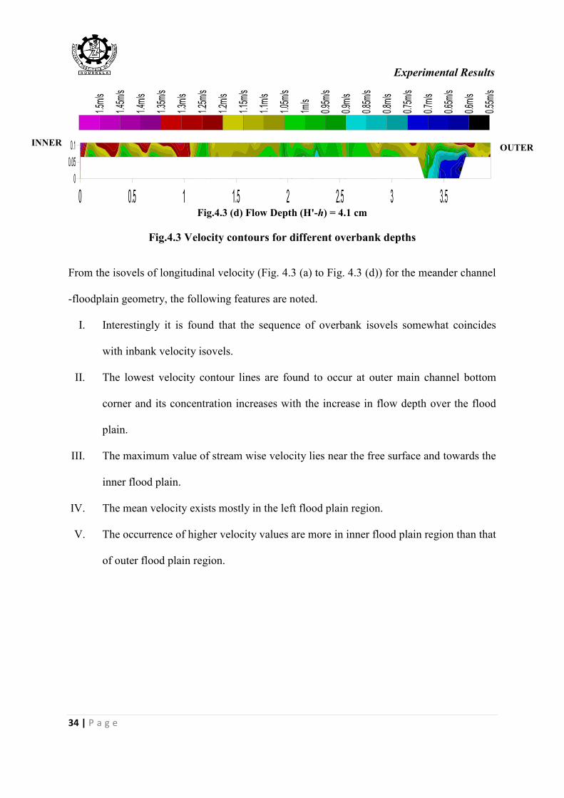
34 | P a g e

Fig.4.3 (d) Flow Depth (H'-h) = 4.1 cm

Fig.4.3 Velocity contours for different overbank depths

From the isovels of longitudinal velocity (Fig. 4.3 (a) to Fig. 4.3 (d)) for the meander channel

-floodplain geometry, the following features are noted.

I. Interestingly it is found that the sequence of overbank isovels somewhat coincides

with inbank velocity isovels.

II. The lowest velocity contour lines are found to occur at outer main channel bottom

corner and its concentration increases with the increase in flow depth over the flood

plain.

III. The maximum value of stream wise velocity lies near the free surface and towards the

inner flood plain.

IV. The mean velocity exists mostly in the left flood plain region.

V. The occurrence of higher velocity values are more in inner flood plain region than that

of outer flood plain region.

INNER OUTER

Experimental Analysis

35 | P a g e

ANALYSIS BASED ON EXPERIMENTAL RESULTS

5.1 OVERVIEW

Once normal depth conditions were established for a given discharge, point velocity

measurements were made across one section of the channel at z = 0.4h from the bed. At each

lateral position, a number of readings were taken at constant intervals and then averaged to

reduce error.

5.2 LATERAL DISTRIBUTION OF DEPTH AVERAGED VELOCITY

5.2.1 Inbank Flow Studies

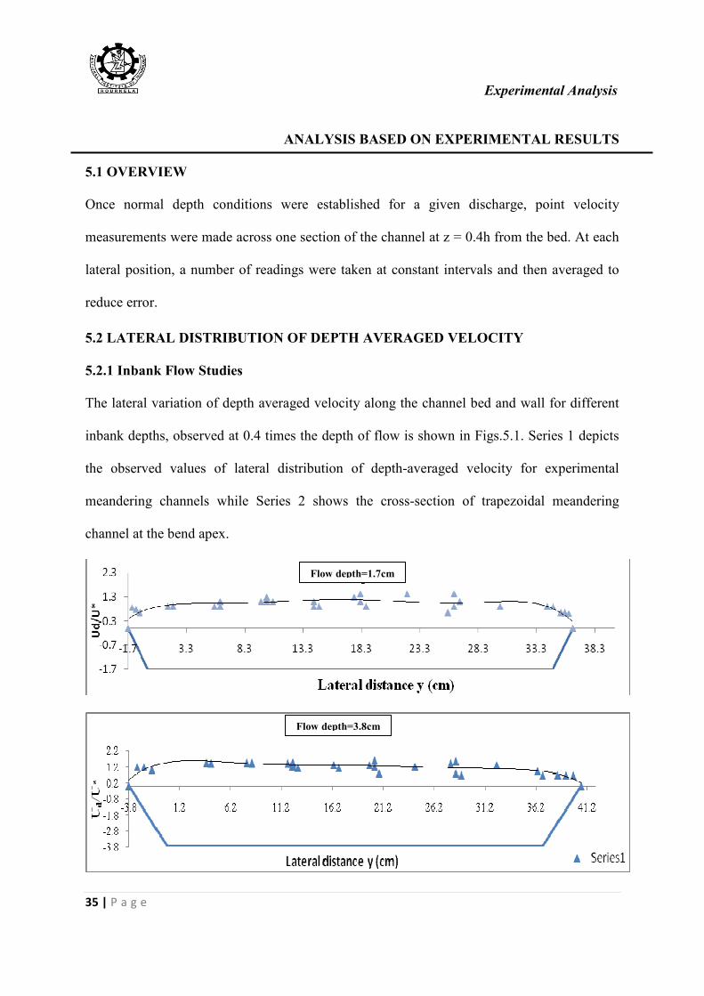
The lateral variation of depth averaged velocity along the channel bed and wall for different

inbank depths, observed at 0.4 times the depth of flow is shown in Figs.5.1. Series 1 depicts

the observed values of lateral distribution of depth-averaged velocity for experimental

meandering channels while Series 2 shows the cross-section of trapezoidal meandering

channel at the bend apex.

Flow depth=3.8cm

Flow depth=1.7cm


36 | P a g e

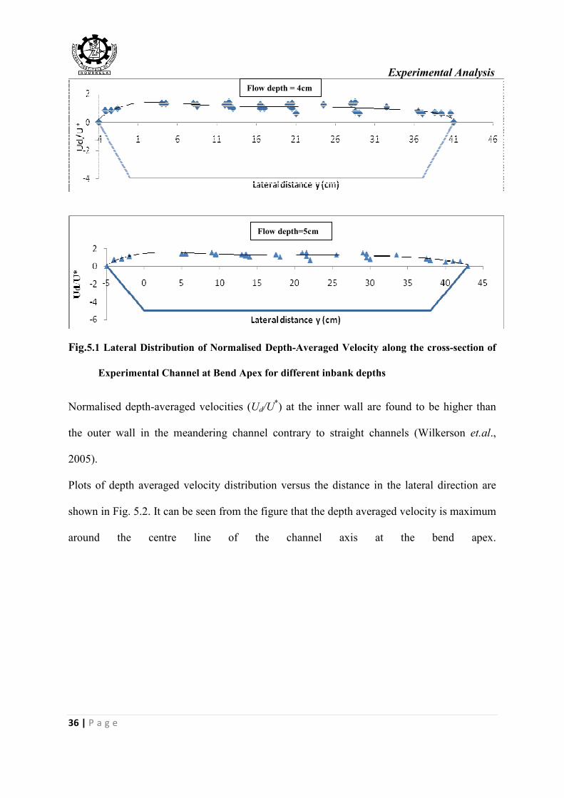
Fig.5.1 Lateral Distribution of Normalised Depth-Averaged Velocity along the cross-section of

Experimental Channel at Bend Apex for different inbank depths

Normalised depth-averaged velocities (Ud/U*) at the inner wall are found to be higher than

the outer wall in the meandering channel contrary to straight channels (Wilkerson et.al.,

2005).

Plots of depth averaged velocity distribution versus the distance in the lateral direction are

shown in Fig. 5.2. It can be seen from the figure that the depth averaged velocity is maximum

around the centre line of the channel axis at the bend apex.

Flow depth=5cm

Flow depth = 4cm


37 | P a g e

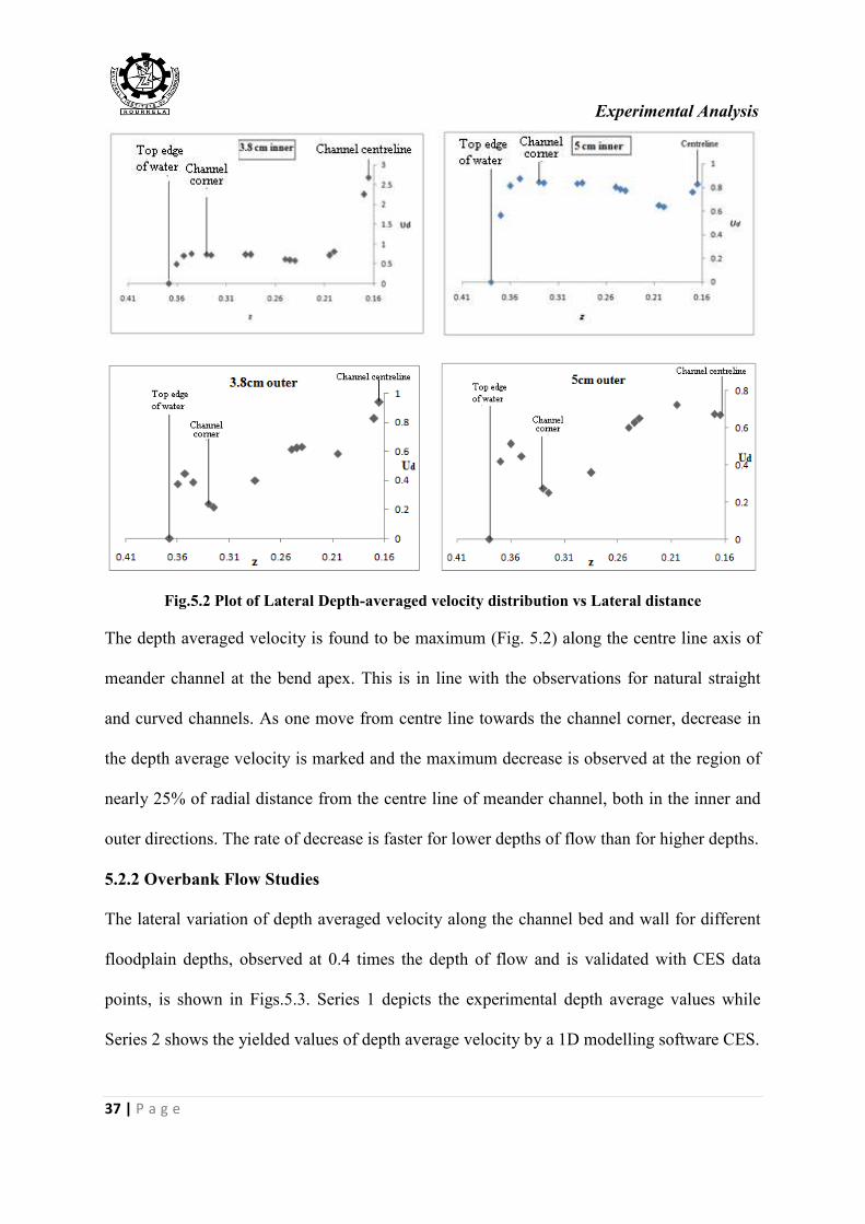
Fig.5.2 Plot of Lateral Depth-averaged velocity distribution vs Lateral distance

The depth averaged velocity is found to be maximum (Fig. 5.2) along the centre line axis of

meander channel at the bend apex. This is in line with the observations for natural straight

and curved channels. As one move from centre line towards the channel corner, decrease in

the depth average velocity is marked and the maximum decrease is observed at the region of

nearly 25% of radial distance from the centre line of meander channel, both in the inner and

outer directions. The rate of decrease is faster for lower depths of flow than for higher depths.

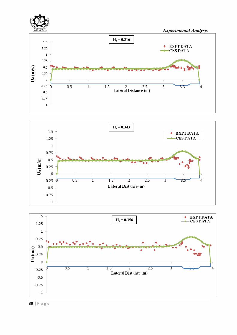
5.2.2 Overbank Flow Studies

The lateral variation of depth averaged velocity along the channel bed and wall for different

floodplain depths, observed at 0.4 times the depth of flow and is validated with CES data

points, is shown in Figs.5.3. Series 1 depicts the experimental depth average values while

Series 2 shows the yielded values of depth average velocity by a 1D modelling software CES.


38 | P a g e

Overbank flow cases are complicated processes to model due to the presence of turbulent

structures ranging from large to small scales which transfers momentum from faster moving

fluids in main channel to relatively slower fluid in flood plain while increasing and

decreasing the conveyance respectively. Therefore a lot of experimental and numerical

approaches has been recently adopted to quantify this lateral momentum transfer at the main

channel and flood plain interface. This accretion in technical knowledge compel operating

authorities should use recent improved knowledge on conveyance to reduce uncertainty in

flood predictions. Taking this into account a team of experts led by HR Wallingford

introduced a new Conveyance Estimation System (CES) which is being adopted in

England, Wales, Scotland and Northern Ireland. CES has been recommended for use in

natural rivers, artificial straight and meandering channels for estimating conveyance,

computing stage discharge relationship and also a number of flow parameters like depth

averaged velocity, boundary shear, shear velocity, energy coefficients etc. The software

includes a roughness advisor, conveyance generator, and an uncertainty estimator. The

conveyance generator is based on 1D Shiono and Knight Conveyance estimation method

(SKM). Previously conveyance estimation methods incorporate only roughness parameter

such as Manning’s n, Chezy’s C and Darcy Weisbach f, but SKM consists three calibration

constants: Weisbach f, dimensionless eddy viscosity λ, transverse gradient of secondary flow

term Г. Therefore it precisely models the flow to reduce uncertainties in the estimation of

river flood levels, discharge and velocities.


39 | P a g e

Hr = 0.316

Hr = 0.356

Hr = 0.343


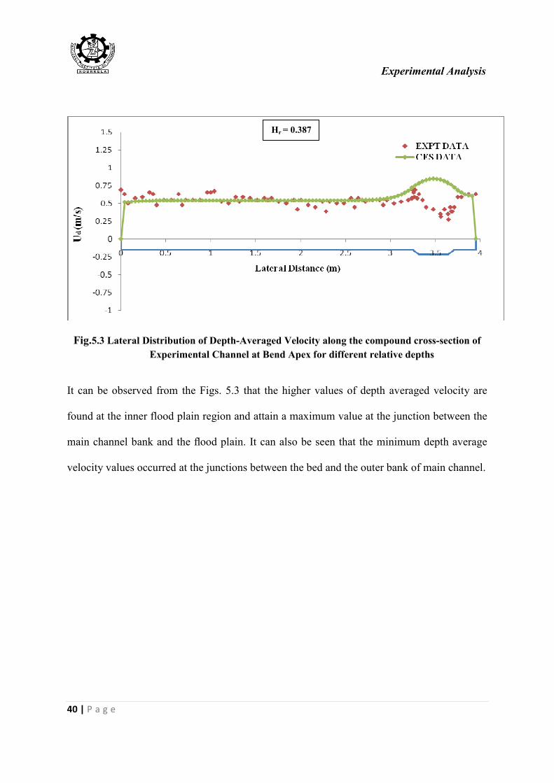
40 | P a g e

Fig.5.3 Lateral Distribution of Depth-Averaged Velocity along the compound cross-section of

Experimental Channel at Bend Apex for different relative depths

It can be observed from the Figs. 5.3 that the higher values of depth averaged velocity are

found at the inner flood plain region and attain a maximum value at the junction between the

main channel bank and the flood plain. It can also be seen that the minimum depth average

velocity values occurred at the junctions between the bed and the outer bank of main channel.

Hr = 0.387

Model Development

41 | P a g e

MODEL DEVELOPMENT

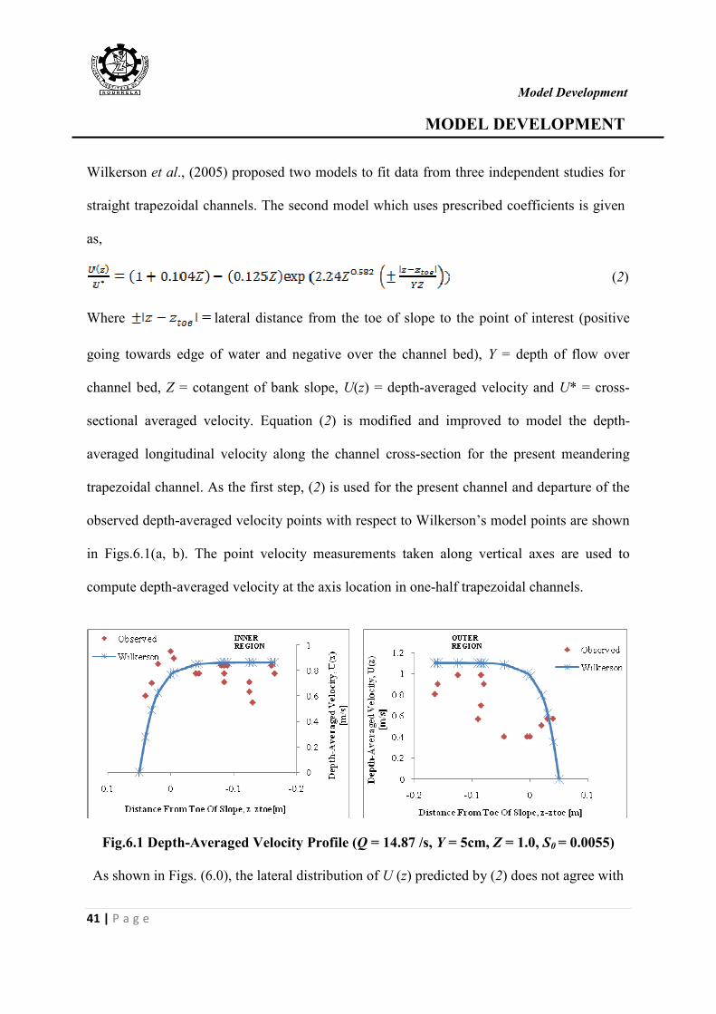
Wilkerson et al., (2005) proposed two models to fit data from three independent studies for

straight trapezoidal channels. The second model which uses prescribed coefficients is given

as,

(2)

Where lateral distance from the toe of slope to the point of interest (positive

going towards edge of water and negative over the channel bed), Y = depth of flow over

channel bed, Z = cotangent of bank slope, U(z) = depth-averaged velocity and U* = cross-

sectional averaged velocity. Equation (2) is modified and improved to model the depth-

averaged longitudinal velocity along the channel cross-section for the present meandering

trapezoidal channel. As the first step, (2) is used for the present channel and departure of the

observed depth-averaged velocity points with respect to Wilkerson’s model points are shown

in Figs.6.1(a, b). The point velocity measurements taken along vertical axes are used to

compute depth-averaged velocity at the axis location in one-half trapezoidal channels.

Fig.6.1 Depth-Averaged Velocity Profile (Q = 14.87 /s, Y = 5cm, Z = 1.0, S0 = 0.0055)

As shown in Figs. (6.0), the lateral distribution of U (z) predicted by (2) does not agree with

Model Development

42 | P a g e

the observed data for this wide channel. This deviation ascertains that Wilkerson formula of

U(z) for straight trapezoidal channel needs to be modified for present channel to involve

meandering effect.

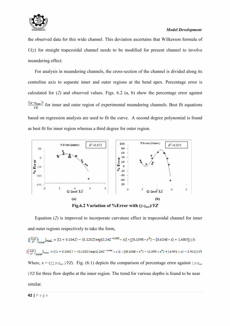
For analysis in meandering channels, the cross-section of the channel is divided along its

centreline axis to separate inner and outer regions at the bend apex. Percentage error is

calculated for (2) and observed values. Figs. 6.2 (a, b) show the percentage error against

for inner and outer region of experimental meandering channels. Best fit equations

based on regression analysis are used to fit the curve. A second degree polynomial is found

as best fit for inner region whereas a third degree for outer region.

(a) (b)

Fig.6.2 Variation of %Error with (z-ztoe)/YZ

Equation (2) is improved to incorporate curvature effect in trapezoidal channel for inner

and outer regions respectively to take the form,

(3)

(4)

Where, x = (+| z-ztoe |/YZ). Fig. (6.1) depicts the comparison of percentage error against | z-ztoe

|/YZ for three flow depths at the inner region. The trend for various depths is found to be near

similar.

R2=0.872 R

2=0.835

Model Development

43 | P a g e

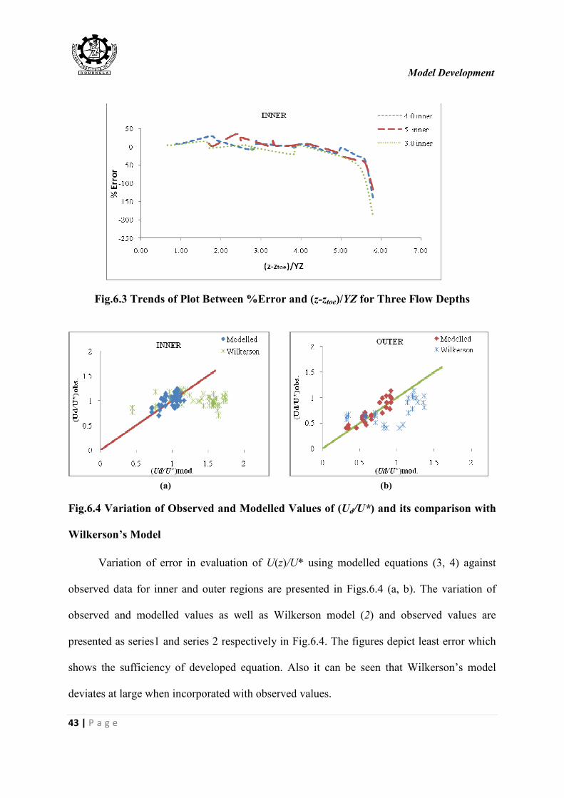
Fig.6.3 Trends of Plot Between %Error and (z-ztoe)/YZ for Three Flow Depths

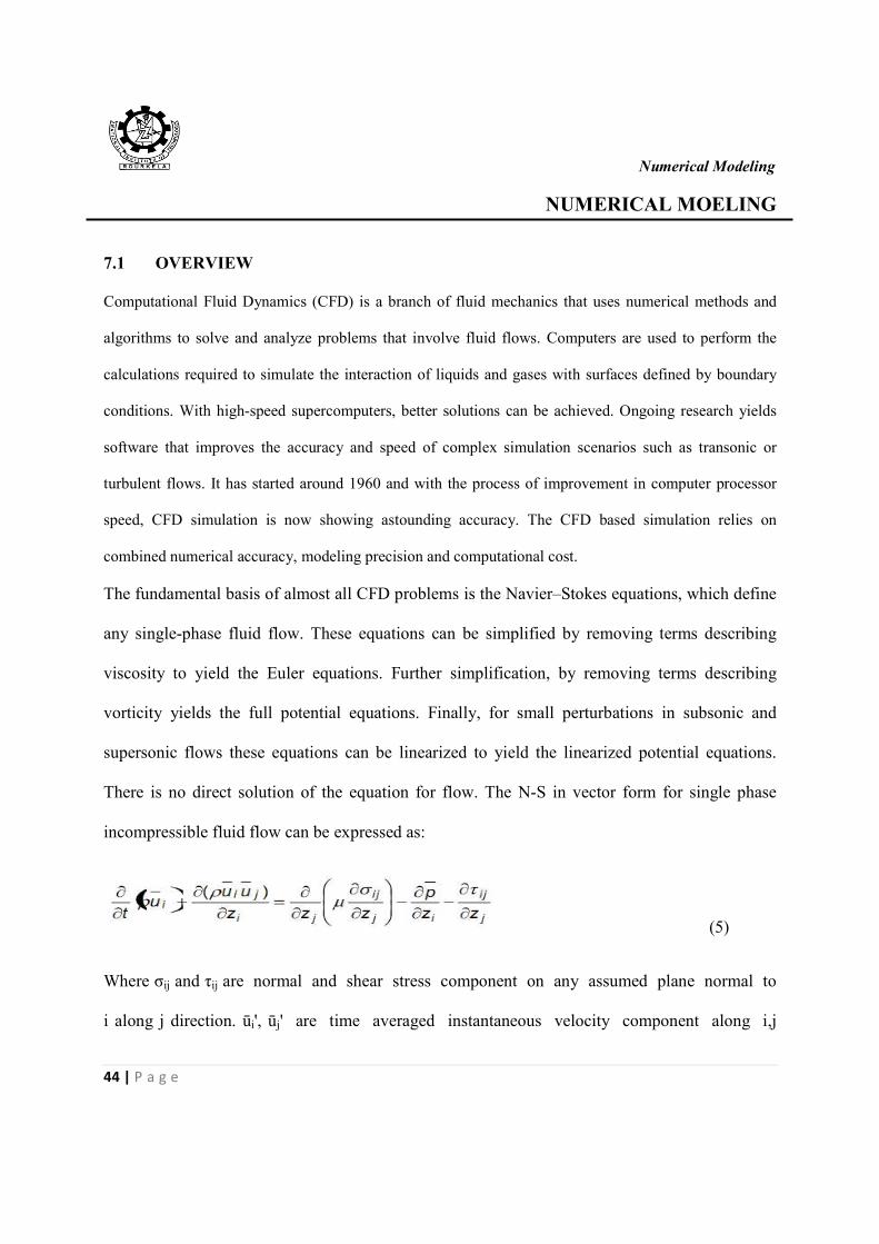
(a) (b)

Fig.6.4 Variation of Observed and Modelled Values of (Ud/U*) and its comparison with

Wilkerson’s Model

Variation of error in evaluation of U(z)/U* using modelled equations (3, 4) against

observed data for inner and outer regions are presented in Figs.6.4 (a, b). The variation of

observed and modelled values as well as Wilkerson model (2) and observed values are

presented as series1 and series 2 respectively in Fig.6.4. The figures depict least error which

shows the sufficiency of developed equation. Also it can be seen that Wilkerson’s model

deviates at large when incorporated with observed values.

Numerical Modeling

44 | P a g e

NUMERICAL MOELING

7.1 OVERVIEW

Computational Fluid Dynamics (CFD) is a branch of fluid mechanics that uses numerical methods and

algorithms to solve and analyze problems that involve fluid flows. Computers are used to perform the

calculations required to simulate the interaction of liquids and gases with surfaces defined by boundary

conditions. With high-speed supercomputers, better solutions can be achieved. Ongoing research yields

software that improves the accuracy and speed of complex simulation scenarios such as transonic or

turbulent flows. It has started around 1960 and with the process of improvement in computer processor

speed, CFD simulation is now showing astounding accuracy. The CFD based simulation relies on

combined numerical accuracy, modeling precision and computational cost.

The fundamental basis of almost all CFD problems is the Navier–Stokes equations, which define

any single-phase fluid flow. These equations can be simplified by removing terms describing

viscosity to yield the Euler equations. Further simplification, by removing terms describing

vorticity yields the full potential equations. Finally, for small perturbations in subsonic and

supersonic flows these equations can be linearized to yield the linearized potential equations.

There is no direct solution of the equation for flow. The N-S in vector form for single phase

incompressible fluid flow can be expressed as:

(5)

Where σij and τij are normal and shear stress component on any assumed plane normal to

i along j direction. ūi', ūj' are time averaged instantaneous velocity component along i,j

Numerical Modeling

45 | P a g e

directions. p = pressure, µ = co-efficient of viscosity, ρ = density. The process of the numerical

simulation of fluid flow using the above equation generally involves four steps and the details

are:

(a)Problem identification

1. Defining the modeling goals

2. Identifying the domain to model

(b) Pre-Processing

1. Creating a solid model to represent the domain (Geometry Setup)

2. Design and create the mesh (grid)

3. Set up the physics

• Defining the condition of flow (e.g turbulent, laminar etc.)

• Specification of appropriate boundary condition and temporal

condition.

(c) Solver

1. Using different numerical schemes to discretize the governing equations.

2. Controlling the convergence by iterating the equation till accuracy is achieved

(d) Post processing

1. Visualising and examining the results

2. Considering revisions to the model

Numerical Modeling

46 | P a g e

7.2 GEOMETRY SETUP

The fluid flow governing equations (momentum equation, continuity equation) are solved based

on the discretization of domain using the Cartesian co-ordinate system. This procedure involves

dividing the continuum into finite number of nodes. The CFD computations need a spatial

discretization scheme and time marching scheme. Mainly the domain discretization is based on

Finite element, Finite Volume and Finite Difference Method. Finite Element method is based on

dividing the domain into elements. The numerical solution can be obtained in this method

by integrating the shape function and weighted factor in an appropriate domain. This method

is suitable with respect to both structured and unstructured mesh. The application of Finite

Volume method needs dividing the domain into finite number of volumes. Here the specified

variables are calculated by solving the discreitized equation in the centre of the cell. This

method is developed by taking conservation law in to account. Finite Volume method is

suitable for applying in unstructured domain. Finite Difference method is based on Taylor's

series approximation. This method is more suitable for regular domain.

The meandering open channel corresponding to one wavelength of five wavelengths is

continuously constructed in the experimental flume. In the experimental flume, five meander

waves are fabricated for the case of Sr = 1.29, where the sinuosity, Sr, is defined as the ratio of

the meandering channel length to the meander wavelength. One meander wavelength has

trapezoidal cross-section with following dimensions: bed width, 330mm; top width, 460mm;

main channel depth, 65mm; meander wavelength, 4054mm and central angle of the bend; 120◦.

Each section has a 60° circular bend with the centreline radius of 1.1 m followed by a 0.68m

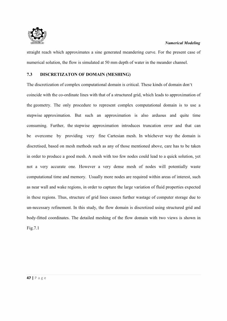
Numerical Modeling

47 | P a g e

straight reach which approximates a sine generated meandering curve. For the present case of

numerical solution, the flow is simulated at 50 mm depth of water in the meander channel.

7.3 DISCRETIZATON OF DOMAIN (MESHING)

The discretization of complex computational domain is critical. These kinds of domain don‘t

coincide with the co-ordinate lines with that of a structured grid, which leads to approximation of

the geometry. The only procedure to represent complex computational domain is to use a

stepwise approximation. But such an approximation is also arduous and quite time

consuming. Further, the stepwise approximation introduces truncation error and that can

be overcome by providing very fine Cartesian mesh. In whichever way the domain is

discretised, based on mesh methods such as any of those mentioned above, care has to be taken

in order to produce a good mesh. A mesh with too few nodes could lead to a quick solution, yet

not a very accurate one. However a very dense mesh of nodes will potentially waste

computational time and memory. Usually more nodes are required within areas of interest, such

as near wall and wake regions, in order to capture the large variation of fluid properties expected

in these regions. Thus, structure of grid lines causes further wastage of computer storage due to

un-necessary refinement. In this study, the flow domain is discretized using structured grid and

body-fitted coordinates. The detailed meshing of the flow domain with two views is shown in

Fig.7.1

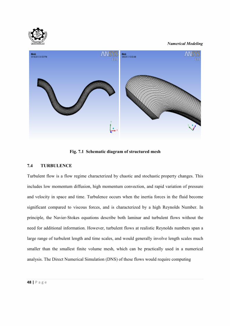
Numerical Modeling

48 | P a g e

Fig. 7.1 Schematic diagram of structured mesh

7.4 TURBULENCE

Turbulent flow is a flow regime characterized by chaotic and stochastic property changes. This

includes low momentum diffusion, high momentum convection, and rapid variation of pressure

and velocity in space and time. Turbulence occurs when the inertia forces in the fluid become

significant compared to viscous forces, and is characterized by a high Reynolds Number. In

principle, the Navier-Stokes equations describe both laminar and turbulent flows without the

need for additional information. However, turbulent flows at realistic Reynolds numbers span a

large range of turbulent length and time scales, and would generally involve length scales much

smaller than the smallest finite volume mesh, which can be practically used in a numerical

analysis. The Direct Numerical Simulation (DNS) of these flows would require computing

Numerical Modeling

49 | P a g e

power which is many orders of magnitude higher than available in the foreseeable future. To

enable the effects of turbulence to be predicted, a large amount of CFD research has concentrated

on methods which make use of turbulence models. Turbulence models have been specifically

developed to account for the effects of turbulence without recourse to a prohibitively fine mesh

and direct numerical simulation. Most turbulence models are statistical turbulence model, as

mentioned below.

Turbulence Models

� Algebraic (zero-equation) model

� k-ε, RNG k-ε

� Shear stress transport

� k-ω

� Reynolds stress transport model (second moment closure)

� k-ω Reynolds stress

� Detached eddy simulation (DES) turbulence model

� SST scale adaptive simulation (SAS) turbulence model

� Smagorinsky large eddy simulation model (LES)

� Scalable wall functions

� Automatic near-wall treatment including integration to the wall

� User-defined turbulent wall functions and heat transfer

The two exceptions to this in ANSYS CFX are:

• Large Eddy Simulation Theory

• Detached Eddy Simulation Theory

Numerical Modeling

50 | P a g e

However open-channel flows are characterized by complicated flow structures, even for simple

geometry, such as that of a rectangular channel. This is largely due to wall and free surface

boundaries. The secondary currents are generated in open channel flow because free surface and

walls reduce the turbulence intensity in the direction normal to the surface or the walls and lead

to anisotropy of turbulence. The three dimensional nature of turbulent flow can be decomposed

into mean part and fluctuation part, which is called Reynolds decomposition. Gravity and

channel geometry are mainly responsible for turbulent flow for this particular condition.

7.5 NUMERICAL MODEL

7.5.1 Large Eddy Simulation (LES)

The three major types of turbulence methodologies are Direct Numerical Simulation (DNS),

Large eddy Simulation (LES) and k-ε modelling. k-ε models the turbulent flows by time or space

averaging. But it is not suitable for transient flows because the averaging process removes most

of the important characteristics of a time-dependent solution. On the other hand, Direct

Numerical Simulation, attempts to solve all time and spatial scales. As a result, the solution is

very accurate. However to resolve almost all ranges of scales, the spatial and temporal grids

would need to be extremely small in the order of Kolmogorov length and time scale, resulting in

a problem which would take an extraordinarily long time to solve, making it computationally

intensive.

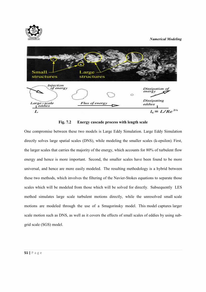
Numerical Modeling

51 | P a g e

Fig. 7.2 Energy cascade process with length scale

One compromise between these two models is Large Eddy Simulation. Large Eddy Simulation

directly solves large spatial scales (DNS), while modeling the smaller scales (k-epsilon). First,

the larger scales that carries the majority of the energy, which accounts for 80% of turbulent flow

energy and hence is more important. Second, the smaller scales have been found to be more

universal, and hence are more easily modeled. The resulting methodology is a hybrid between

these two methods, which involves the filtering of the Navier-Stokes equations to separate those

scales which will be modeled from those which will be solved for directly. Subsequently LES

method simulates large scale turbulent motions directly, while the unresolved small scale

motions are modeled through the use of a Smagorinsky model. This model captures larger

scale motion such as DNS, as well as it covers the effects of small scales of eddies by using sub-

grid scale (SGS) model.

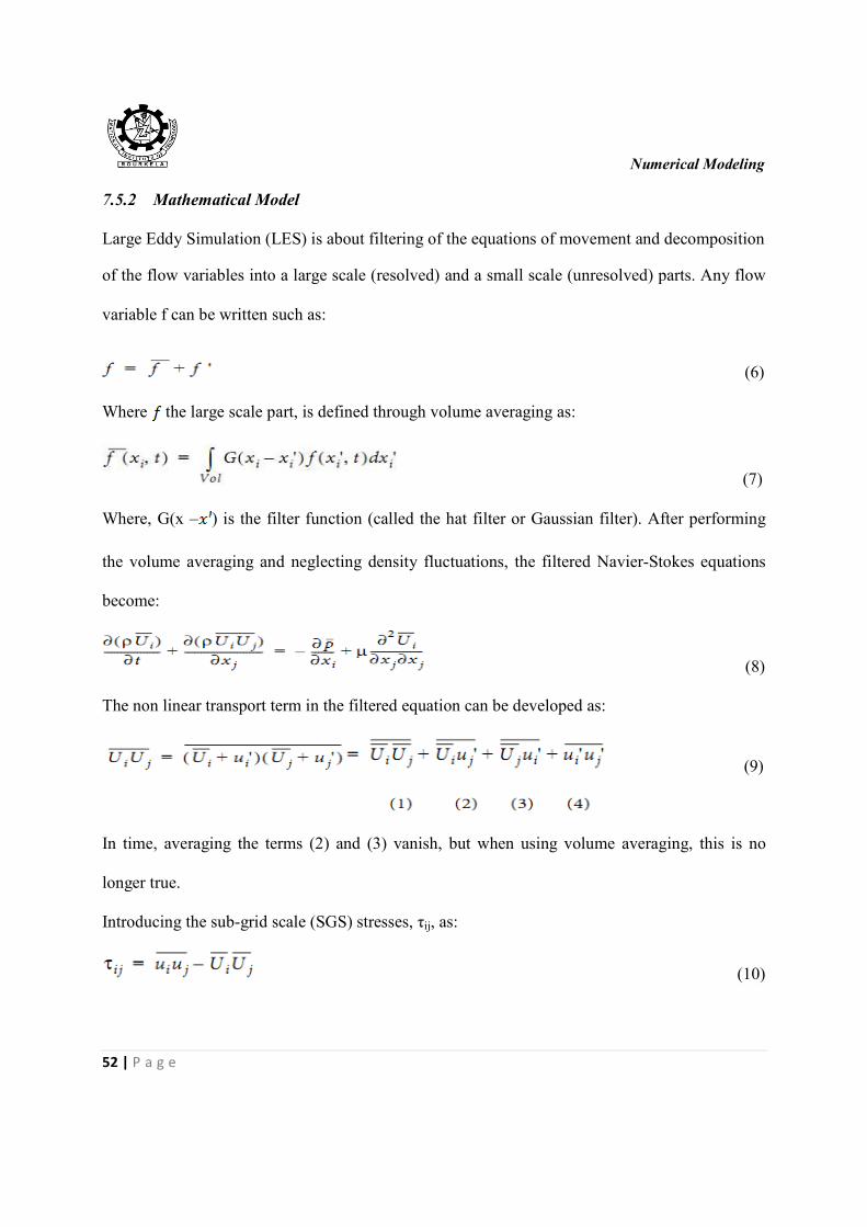
Numerical Modeling

52 | P a g e

7.5.2 Mathematical Model

Large Eddy Simulation (LES) is about filtering of the equations of movement and decomposition

of the flow variables into a large scale (resolved) and a small scale (unresolved) parts. Any flow

variable f can be written such as:

(6)

Where the large scale part, is defined through volume averaging as:

(7)

Where, G(x – ) is the filter function (called the hat filter or Gaussian filter). After performing

the volume averaging and neglecting density fluctuations, the filtered Navier-Stokes equations

become:

(8)

The non linear transport term in the filtered equation can be developed as:

(9)

In time, averaging the terms (2) and (3) vanish, but when using volume averaging, this is no

longer true.

Introducing the sub-grid scale (SGS) stresses, τij, as:

(10)

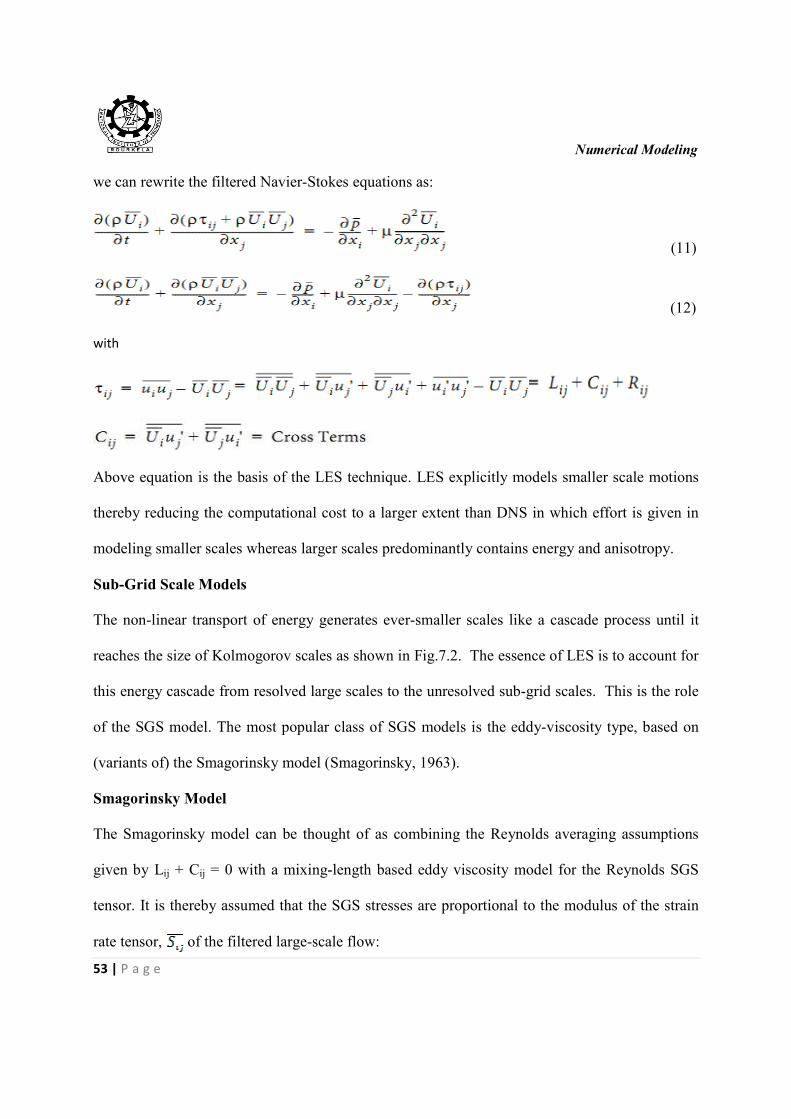
Numerical Modeling

53 | P a g e

we can rewrite the filtered Navier-Stokes equations as:

(11)

(12)

with

Above equation is the basis of the LES technique. LES explicitly models smaller scale motions

thereby reducing the computational cost to a larger extent than DNS in which effort is given in

modeling smaller scales whereas larger scales predominantly contains energy and anisotropy.

Sub-Grid Scale Models

The non-linear transport of energy generates ever-smaller scales like a cascade process until it

reaches the size of Kolmogorov scales as shown in Fig.7.2. The essence of LES is to account for

this energy cascade from resolved large scales to the unresolved sub-grid scales. This is the role

of the SGS model. The most popular class of SGS models is the eddy-viscosity type, based on

(variants of) the Smagorinsky model (Smagorinsky, 1963).

Smagorinsky Model

The Smagorinsky model can be thought of as combining the Reynolds averaging assumptions

given by Lij + Cij = 0 with a mixing-length based eddy viscosity model for the Reynolds SGS

tensor. It is thereby assumed that the SGS stresses are proportional to the modulus of the strain

rate tensor, of the filtered large-scale flow:

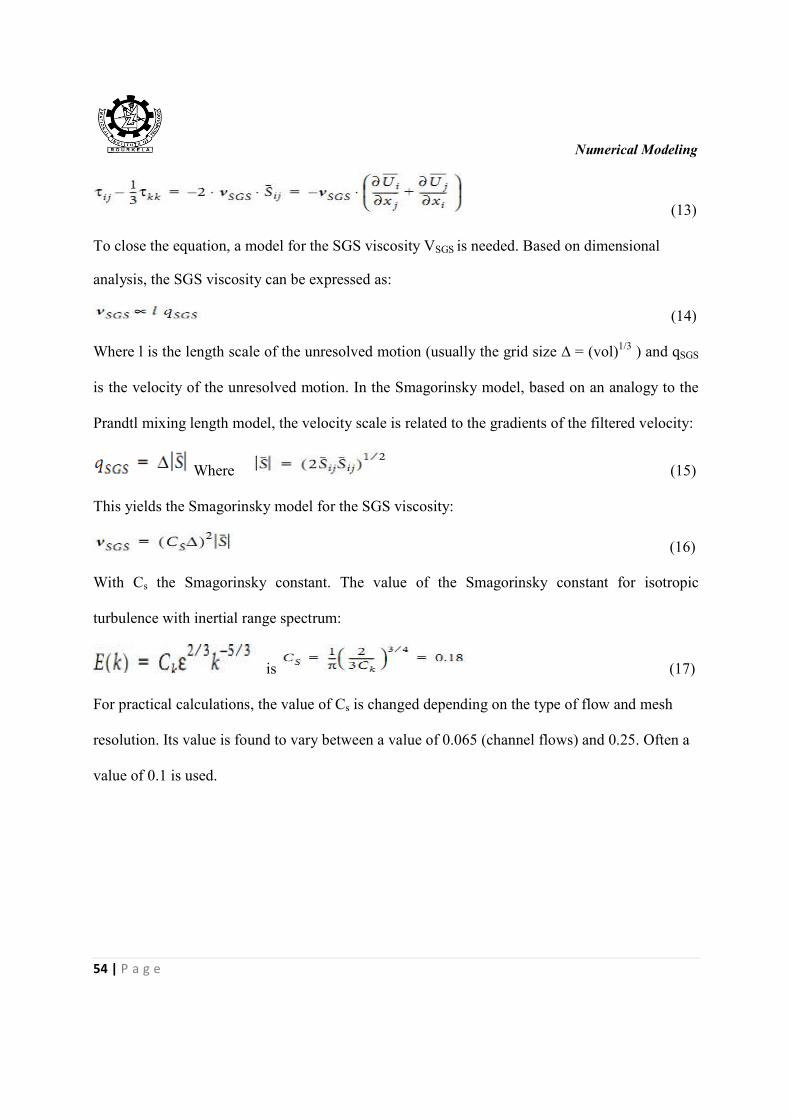
Numerical Modeling

54 | P a g e

(13)

To close the equation, a model for the SGS viscosity VSGS is needed. Based on dimensional

analysis, the SGS viscosity can be expressed as:

(14)

Where l is the length scale of the unresolved motion (usually the grid size ∆ = (vol)1/3

) and qSGS

is the velocity of the unresolved motion. In the Smagorinsky model, based on an analogy to the

Prandtl mixing length model, the velocity scale is related to the gradients of the filtered velocity:

Where (15)

This yields the Smagorinsky model for the SGS viscosity:

(16)

With Cs the Smagorinsky constant. The value of the Smagorinsky constant for isotropic

turbulence with inertial range spectrum:

is (17)

For practical calculations, the value of Cs is changed depending on the type of flow and mesh

resolution. Its value is found to vary between a value of 0.065 (channel flows) and 0.25. Often a

value of 0.1 is used.

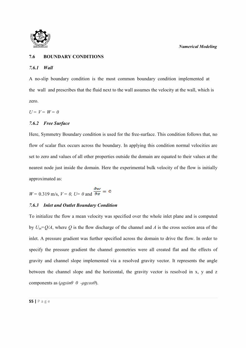
Numerical Modeling

55 | P a g e

7.6 BOUNDARY CONDITIONS

7.6.1 Wall

A no-slip boundary condition is the most common boundary condition implemented at

the wall and prescribes that the fluid next to the wall assumes the velocity at the wall, which is

zero.

U = V = W = 0

7.6.2 Free Surface

Here, Symmetry Boundary condition is used for the free-surface. This condition follows that, no

flow of scalar flux occurs across the boundary. In applying this condition normal velocities are

set to zero and values of all other properties outside the domain are equated to their values at the

nearest node just inside the domain. Here the experimental bulk velocity of the flow is initially

approximated as:

W = 0.319 m/s, V = 0, U= 0 and

7.6.3 Inlet and Outlet Boundary Condition

To initialize the flow a mean velocity was specified over the whole inlet plane and is computed

by Uin=Q/A, where Q is the flow discharge of the channel and A is the cross section area of the

inlet. A pressure gradient was further specified across the domain to drive the flow. In order to

specify the pressure gradient the channel geometries were all created flat and the effects of

gravity and channel slope implemented via a resolved gravity vector. It represents the angle

between the channel slope and the horizontal, the gravity vector is resolved in x, y and z

components as (ρgsinθ 0 -ρgcosθ).

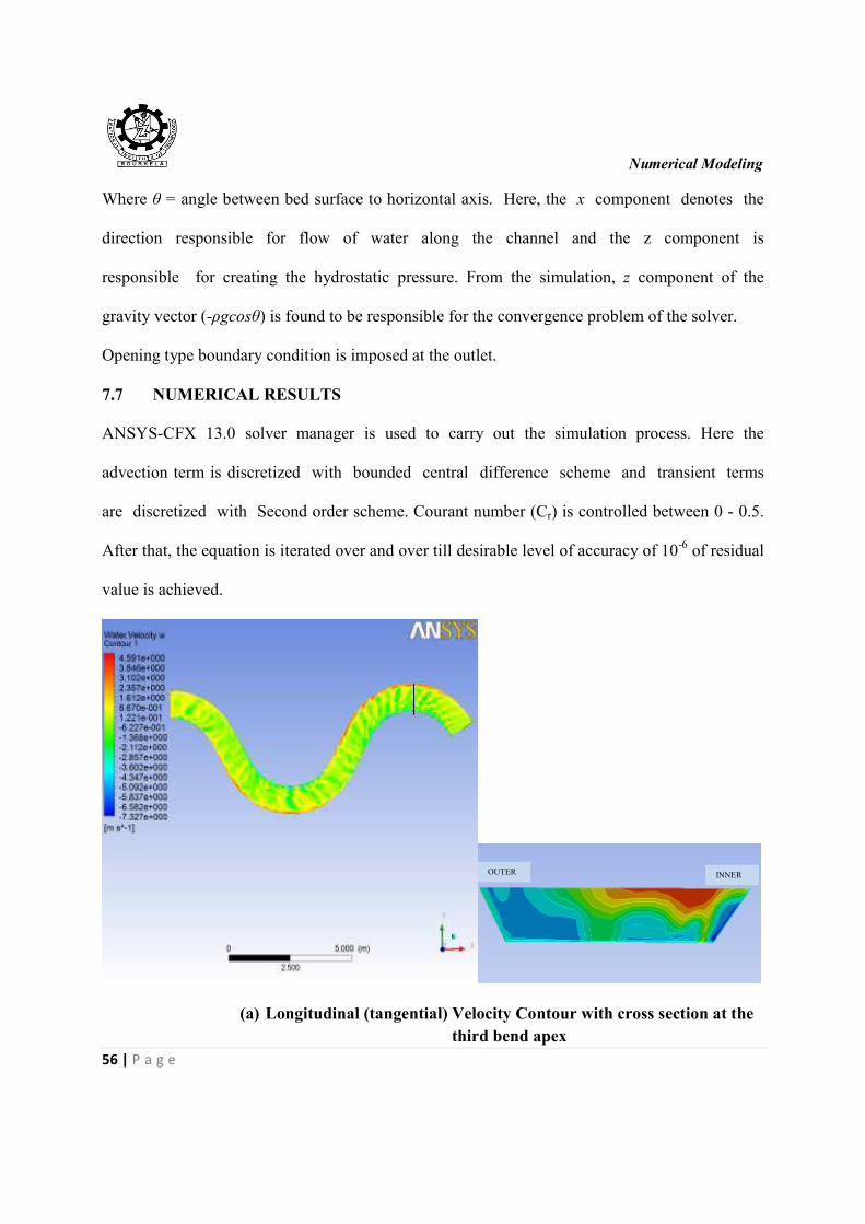
Numerical Modeling

56 | P a g e

Where θ = angle between bed surface to horizontal axis. Here, the x component denotes the

direction responsible for flow of water along the channel and the z component is

responsible for creating the hydrostatic pressure. From the simulation, z component of the

gravity vector (-ρgcosθ) is found to be responsible for the convergence problem of the solver.

Opening type boundary condition is imposed at the outlet.

7.7 NUMERICAL RESULTS

ANSYS-CFX 13.0 solver manager is used to carry out the simulation process. Here the

advection term is discretized with bounded central difference scheme and transient terms

are discretized with Second order scheme. Courant number (Cr) is controlled between 0 - 0.5.

After that, the equation is iterated over and over till desirable level of accuracy of 10-6

of residual

value is achieved.

(a) Longitudinal (tangential) Velocity Contour with cross section at the

third bend apex

INNER OUTER

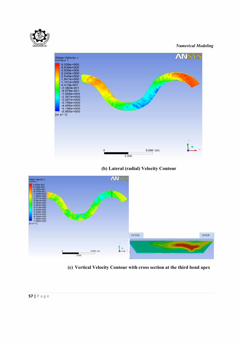
Numerical Modeling

57 | P a g e

(b) Lateral (radial) Velocity Contour

(c) Vertical Velocity Contour with cross section at the third bend apex

INNER OUTER

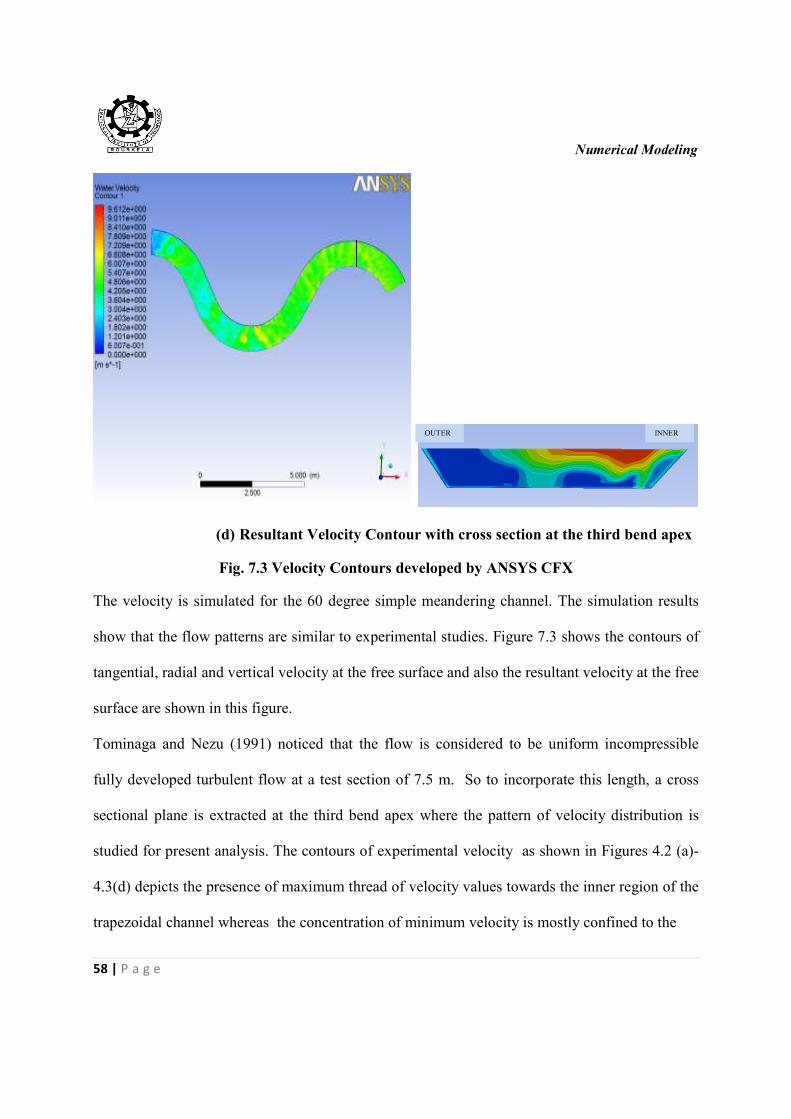
Numerical Modeling

58 | P a g e

(d) Resultant Velocity Contour with cross section at the third bend apex

Fig. 7.3 Velocity Contours developed by ANSYS CFX

The velocity is simulated for the 60 degree simple meandering channel. The simulation results

show that the flow patterns are similar to experimental studies. Figure 7.3 shows the contours of

tangential, radial and vertical velocity at the free surface and also the resultant velocity at the free

surface are shown in this figure.

Tominaga and Nezu (1991) noticed that the flow is considered to be uniform incompressible

fully developed turbulent flow at a test section of 7.5 m. So to incorporate this length, a cross

sectional plane is extracted at the third bend apex where the pattern of velocity distribution is

studied for present analysis. The contours of experimental velocity as shown in Figures 4.2 (a)-

4.3(d) depicts the presence of maximum thread of velocity values towards the inner region of the

trapezoidal channel whereas the concentration of minimum velocity is mostly confined to the

INNER OUTER

Numerical Modeling

59 | P a g e

outer regions, as such the modeled velocity reveals almost the same distribution pattern as given

in Figure 7.3. Another feature which is discernible from the experimental velocity contour is that

the maximum velocity lies towards the inner free surface which is also marked in the velocity

contours of numerically modeled trapezoidal cross section. It is seen that the numerical

simulation is in reasonable agreement with the experimental measurements.

Conclusions

60 | P a g e

CONCLUSIONS AND FURTHER WORK

8.1 CONCLUSIONS

The present theoretical investigation supported by experimental observation is made for

meandering channels with and without floodplains having different flow aspect ratios. On the

basis of the investigations concerning flow, velocity distribution, and depth average velocity

distribution in smooth open compound channels, the following conclusions are drawn.

1. The model for depth-averaged velocity distribution proposed by Wilkerson (2005)

does not fit to meandering channels. The modelled equations (3, 4) which include the

influencing dimensionless channel parameters are found to be adequate for the present

set of simple meander channel data and can be used to compute the depth average

velocity across the channel cross sections.

2. For simple meandering channel, normalised depth-averaged velocities (Ud/U*) at the

inner wall are found to be higher than the outer wall in the meandering channel

contrary to straight channels (Wilkerson et.al., 2005).

3. The depth averaged velocity is found to be maximum (Fig. 5.2) along the centre line

axis of simple meander channel at the bend apex. This is in line with the observations

for natural straight and curved channels. As one move from centre line towards the

channel corner, decrease in the depth average velocity is marked and the maximum

decrease is observed at the region of nearly 25% of radial distance from the centre

line of meander channel, both in the inner and outer directions. The rate of decrease is

faster for lower depths of flow than for higher depths.

4. In compound meander channel, the higher values of depth averaged velocity are

found at the inner flood plain region and attain a maximum value at the junction

between the main channel bank and the flood plain. It can also be seen that the

Conclusions

61 | P a g e

minimum depth average velocity values occurred at the junctions between the bed and

the outer bank of main channel.

5. As shown in the experimental velocity contours, the numerical velocity contours also

give the same result. The presence of maximum thread of velocity values towards the

inner region of the trapezoidal channel whereas the concentration of minimum

velocity is mostly confined to the outer regions. The maximum velocity lies towards

the inner free surface which is also marked in the velocity contours of numerically

modelled trapezoidal cross section. It is seen that the numerical simulation is in

reasonable agreement with the experimental measurements.

8.2 FUTURE SCOPE OF WORK

The present work leaves a wide scope for future investigators to explore many other aspects

of compound channel analysis.

1. The result can be compared with data of straight channel and further the work can be

extended to natural channels and other laboratory channels with different sinuosity,

geometry and surface conditions.

2. Further investigations can be done to study depth-averaged velocity in vertical and

lateral directions and develop models using analytical and numerical approaches

which are more convenient than conventional methods.

3. Velocity profiles can be drawn in transverse direction, the type of wall law that

coexists at inner and outer wall of meandering channels can be defined and velocity

dip phenomenon can be studied.

4. The accretion in 3D flow structure is obvious when water overtops the bank to flow in

flood plains as mostly seen in natural rivers during flood, which is commonly

modelled as compound channel in laboratory. Thus a model can be proposed to

evaluate velocity distribution in compound channel incorporating turbulence effects.

Conclusions

62 | P a g e

5. Proceedings on lateral velocity distribution can be done on mobile bed to represent

real situation prevailing in natural rivers; so that sediment load transport and boundary

shear distribution can be determined to its accuracy.

6. Further investigations can be done to study stream wise depth-averaged velocity and

develop models using analytical and numerical approaches which are more

convenient than conventional methods.

References

63 | P a g e

REFERENCES

1. Afzal, N., Seena A., Bushra A.2007. Power law velocity profile in fully developed

turbulent pipe and channel flows. J. Hydr. Engrg , Vol. 133, No. 9, 1080-1086.

2. Ahmadi, M. M., Ayyoubzadeh, S. A., Montazeri Namin, M., and Samani, J. M. V.,2009.

A 2D Numerical Depth-averaged Model for Unsteady Flow in Open Channel Bends. J.

Agr. Sci. Tech. Vol. 11: 457-468.

3. Albayrak, I., and Lemmin, U. 2011. Secondary Currents and Corresponding Surface

Velocity Patterns in a Turbulent Open-Channel Flow over a Rough Bed. J. Hydr. Engrg.

,Vol. 137, No. 11, 1318 – 1334.

4. Beaman F.(2010). Large Eddy Simulation of open channel flows for conveyance estimation. Ph.D

thesis, University of Nottingham.

5. Boussinesq, J. (1868). Mémoire sur l’influence des frottements dans les mouvements reguliers des

fluids. J. Math. Pures Appl. (2me sér.), 13, 377-424.

6. Cater, J.E., and Williams, J.R. 2008. Large eddy simulation of a long asymmetric

compound open channel. Journal of Hydraulic Research. Vol. 46(4).

7. Celik I, Rodi W. Modeling suspended sediment transport in non-equilibrium situation.

Journal of Hydraulic Engineering (ASCE) 1988; 114:1157 – 1191.

8. Cokljat D, Younis BA. Second-order closure study of open channel flows. Journal of

Hydraulic Engineering (ASCE) 1995; 121:94 – 107.

9. Coleman, N. L. (1981). Velocity profiles with suspended sediment. J. Hydr. Res, 19(3),

211-229.

10. Coles, D. 1956.The law of the wake in the turbulent boundary layer. J. Fluid Mech.,

1,191-226.

References

64 | P a g e

11. Ervine, D.A., et al. 2000. Two-Dimensional solution for straight and meandering

overbank flows. J. Hydr. Engrg , Vol. 126, No. 9, 0653-0669.

12. Jia, Y., Blanckaert, K. & Wang, S.S. 2001. Numerical simulation of secondary currents in

curved channels. Proc. 8th

FMTM-congress, Tokyo.

13. Johannesson, H. and Parker, G. 1989. Velocity Redistribution in Meandering Rivers. J.

Hydr. Engrg , Vol. 115, No. 8, 0008-1019.

14. Jing, H., Guo, Y., Li, C., & Zhang, J. 2009. Three dimensional numerical simulation of

compound meandering open channel flow by the Reynolds stress model. International

Journal for Numerical Methods in Fluids, 59, 927-943.

15. Kang H, Choi SU. (2006) “Reynolds stress modeling of rectangular open-channel flow.”

International Journal for Numerical Methods in Fluids 2006; 51:1319 – 1334.

16. Kirkgoz, M.S. et al. 1997. Velocity Profiles of Developing and Developed Open Channel

Flow. J. Hydr. Engrg , Vol. 123, No. 12, 1099-1105.

17. Knight, D.W., et al. 2007. Modelling Depth-Averaged Velocity and Boundary Shear in

Trapezoidal Channels with Secondary Flows. J. Hydr. Engrg , Vol. 133, No. 1, 1-39– 47.

18. Kundu .S and Ghoshal .K., 2010. Velocity Distribution in Open Channels: Combination

of Log-law and Parabolic-law. World Academy of Science, Engineering and Technology

68 2012.

19. Launder BE, Spalding DB.1974. The numerical computation of turbulent flows.

Computer Methods in Applied Mechanics and Engineering 1974; 3:269 – 289.

20. Orgaz, O.C. 2010. Velocity Profile and Flow Resistance Models for Developing Chute

Flow. J. Hydr. Engrg , Vol. 136, No. 7, 7-447– 452.

21. Maria, A.A, and DaSilvaA. F.1999. Friction Factor of Meandering Flows. Journal of

Hydraulic Engineering, ASCE, Vol.125, No.7, pp. 779-783.

References

65 | P a g e

22. Myers, W.R.C. (1987. Velocity and Discharge in Compound Channels. Journal of

Hydraulic Engineering, ASCE, Vol.113, No.6, pp. 753-766.

23. Patra, K.C. 2004. Flow and Velocity Distribution in Meandering Compound Channels. J.

Hydr. Engrg , Vol. 130, No. 5, 5-398 – 411.

24. Pezzinga, G. 1994. Velocity Distribution in Compound Channel Flows by Numerical

Modeling. . Hydr. Engrg , Vol. 120, No. 10, 0010-1176.

25. Prandtl, L.1932. Recent Results of Turbulent Research, translation by National Advisory

Committee for Aeronautics, TM No. 720 (originally published in German in 1933).

26. Rameshwaran P, Naden PS.2003. Three-dimensional numerical simulation of compound

channel flows.” Journal of Hydraulic Engineering (ASCE) 2003; 129:645 – 652.

27. Salvetti MV, Zang Y, Street RL and Banerjee S. 1997. Large-eddy simulation of free

surface decaying turbulence with dynamic subgrid -scale models. Physics of Fluids. 9, pp.

2405.

28. Sarma, N.V.K., Prasad R.V.B., Sarma K.A. (2000). “Detailed study of binary law for

open channel.” J. Hydr. Engrg., Vol. 126, No. 3,210-214.

29. Sugiyama H, Hitomi D, Saito T. 2006. Numerical analysis of turbulent structure in

compound meandering open channel by algebraic Reynolds stress model. International

Journal for Numerical Methods in Fluids 2006; 51:791 – 818.

30. Tang, X. And Knight, D.W. 2008. A general model of lateral depth-averaged velocity

distributions for open channel flows. J. Hydr. Engrg., Vol. 134, No. 9, 1337-1342.

31. Tominaga, A., Nezu I.1992. Velocity profiles in steep open-channel flows. J. Hydr.

Engrg., Vol. 118, No. 1, 73-90.

32. Thomas TG. and Williams J.1995a. Large eddy simulation of a symmetric trapezoidal

channel at Reynolds number of 430,000. J. Hydraul. Res.. 33(6), pp. 825-842.

References

66 | P a g e

33. Thomas TG. and Williams J.1995b. Large eddy simulation of turbulent flow in an

asymmetric compound open channel. J. Hydraul. Res. 33(1), pp. 27-41.

34. Thomas TG. and Williams J.1999. Large eddy simulation of flow in a rectangular open

channel. J. Hydraul Res. 37(3), pp. 345-361.

35. Willetts, B.B., and Hardwick, R.I. 1993. Stage Dependency for Over Bank Flow in

Meandering Channels. Proceedings of the Institution of Civil Engineers, Water, Maritime

and Energy, March, Vol.101, paper No.10049, 45-54.

36. Wilkerson, V.G., McGahan J.L.2005. Depth averaged velocity distribution in straight

trapezoidal channel. J. Hydr. Engrg, Vol. 131, No. 6, 509-512.

37. Wormleaton, P. R., and Hadjipanos, P. 1985. ‘‘Flow distribution in compound channels.’’

J. Hydr. Div., Vol. 111, No. 2, 357–361.

38. Yang K, Cao S, and Liu X. 2007.Flow resistance and its prediction methods in

compound channels, Acta Mechanic Sinica; 21, pp.353-61Yen BC. (2002). Open

flow resistance. J. Hydr. Eng, 1(20), pp.20-39.

39. Zarrati, A.R., Tamai, N., and Jin, Y.C.2005. Mathematical Modeling of Meandering

Channels with a Generalized Depth Averaged Model. Journal of Hydraulic Engineering,

ASCE, Vol.131, No.6, pp. 467-475.

68| P a g e

Appendix A-I

Publications from the Work

A: Published

1. Mohanty, L., Patra.K.C., Khatua, K.K., Patnaik, M. (2012) “Depth-Averaged Velocity

Distribution in Trapezoidal Meandering Channels” Proceedings of National Conference

on Hydraulic and Water Resources, IIT Bombay, India, HYDRO 2012, 625-634.

2. Patnaik, M., Patra.K.C., Khatua, K.K., Mohanty, L. (2012) “Boundary Shear Distribution

in Highly Sinuous Meandering Channels” Proceedings of National Conference on

Hydraulic and Water Resources, IIT Bombay, India, HYDRO 2012, 1233-1242.

3. Mohanty, L., Patnaik, M., Patra.K.C. (2013) “Lateral Distribution of Depth-Averaged

Velocity in Trapezoidal Meandering Channels” Symposium on Sustainable Infrastructure

Development, IIT, Bhubaneswar, Odisha, India, IWMSID 2013, 383-389.

4. Patnaik, M., Mohanty, L., Patra.K.C. (2013) “Wall and Bed Shear Distribution in

Meandering Channels” Symposium on Sustainable Infrastructure Development, IIT,

Bhubaneswar, Odisha, India, IWMSID 2013, 374-382.

B: Accepted for Publication

1. Mohanty, L., Patra.K.C., Khatua, K.K., Patnaik, M. (2012) “Modeling Depth-Averaged

Velocity in Trapezoidal Meandering Channels” accepted for ISH Journal of Hydraulic

Engineering, Taylor & Francis Group, UK.

2. Patnaik, M., Patra.K.C., Khatua, K.K., Mohanty, L. (2012) “Modeling Boundary Shear

Stress in Highly Sinuous Meandering Channels” accepted for ISH Journal of Hydraulic

Engineering, Taylor & Francis Group, UK.

Documents

ethesis.nitrkl.ac.inethesis.nitrkl.ac.in/5013/1/VELOCITY_DISTRIBUTION... · 1.2 Velocity Distribution in Open Channels The knowledge of velocity distribution helps to know the velocity