- 196 - RaSiM8

8th

Int. Symp. on Rockbursts and Seismicity in Mines, A. Malovichko & D. Malovichko (eds)

© 2013 GS RAS & MI UB RAS, Obninsk-Perm, ISBN 978-5-903258-28-4

NUMERICAL MODELING OF SEISMICITY: THEORY AND APPLICATIONS - 197 -

KEYNOTE LECTURE:

NUMERICAL MODELING OF SEISMICITY: THEORY AND APPLICATIONS

A.M. Linkov Rzeszow University of Technology, Rzeszow, Poland;

Institute for Problems of Mechanical Engineering, Saint Petersburg, Russia

Numerical modelling of seismic events is the basis for quantitative studying and interpretation of seismicity in well-established

terms of solid mechanics. In this way we obtain a better basis for making decisions concerning with mining, rock burst mitigation,

oil and gas exploration and production. The paper summarizes computational, geomechanical and geophysical rationale for

progress in this area. We explain in detail how to employ the theoretical rationale for developing a computer code providing both

mechanical quantities (stresses, strains, displacement, etc.) and seismic data (spatial and temporal distributions of events and

seismic characteristics used in mining seismology). It is shown that a conventional code of the BEM, FEM, DEM or FPC type

may be easily adjusted to simulations of seismic and aseismic events by complimenting it with a number of subroutines, described

in due course. Examples illustrate applications to problems of mining and hydraulic fracturing.

In memory of the founder of synthetic mining

seismicity, Professor Miklos Salamon

INTRODUCTION

A Little of History

Twenty years have passed since 1993, when Professor

Miklos Salamon formulated the first theoretical rationale

and practical application of synthetic mining seismicity. In

fact, his key-note address to the 3rd International

Symposium RaSiM (Salamon1993

) contained all the germs

of generality. He suggested as an urgent task for rock

mechanics “to evolve a tool which provides the opportunity

of relating seismicity to the changing mining layout and to

geological environment”. And what is especially

significant, he suggested “the method … to furnish the basis

of such a tool” (p. 299).

Further development has actually followed the line by

Salamon. The only principal improvements consisted in

including:

Softening of a fractured element which, as shown by

Cook1965a, 1965b

(see also Hudson et al.1972

and Linkov1994

),

provides a measure of brittleness and instability of rock.

Time effects, which opens an opportunity to account

for aseismic events and to model intervals between seismic

events.

A natural way to account for time is to explicitly

include creep into the constitutive equations. Napier and

Malan1997

, Malan and Spottiswoode1997

included the time

explicitly into constitutive equations for contact interaction

when numerically modeling seismicity. The contact was

assumed to be viscoplastic. The authors employed the

simplest viscous element in the programs DIGS, MINSIM,

and MINF, what allowed accounting for aseismic effects.

In addition to the mentioned dependences, the results

included catalogues of synthetic seismicity and chains of

events after a blast.

The advantages of this step included providing (under

certain assumptions) the main seismic characteristics

(location, energy, etc.) and agreement with observations.

Nevertheless, in the cited papers, there were limitations as

concerned with accounting for softening. The latter was

used in a model, which includes a softening element

in parallel with a viscous element. In accordance with

the general theory (Linkov2002

), the latter model exhibits

fracture acceleration, but actually it ceases to generate

instability in the form of a jump. It is because infinite

instant stiffness of a viscous dash-pot prevents instability.

The simplest model capable to simulate both seismic

and aseismic events is the Elasticity-Softening-Creep (ESC)

model (Linkov1997

). In this model, in contrast with that used

previously, the softening element is included in series

(not parallel) with the viscous (creeping) element. Its

analysis shows (see, e.g. Linkov1997, 2002

) that the ESC-

model captures the most important effects: decaying

aseismic deformation; smooth although accelerating

aseismic deformation; and instant instability (seismic

event). It appears that near a point of instant instability,

there occur fracture acceleration and that arbitrary short

time intervals may be observed near the point of dynamic

instability. At the level of the earth crust, such aseismic

accelerating movement appears as a so-called silent

earthquake (see, e.g. Linder et al.1996

, Dragert et al.2001

and

Kawasaki2004

). Revealing the existence of accelerating

events fills the gap between slow creep and instant

instability (seismic event).

Although models used differ in significant details,

their employment has clearly demonstrated that synthetic

seismicity mimics observed seismicity in the most essential

features (Sellers and Napier2001

, Spottiswoode2001

,

Linkov2005, 2006

). As noted by Napier2001

: “… it appears that

- 198 - RaSiM8

the explicit failure mode shows some superficial

correspondence to observed seismic behavior but displays

number of shortcomings”.

Note that sometimes modeling in the line of Salamon

is called “active”, because it models expected events

without employing the data on observed passed events. In

contrast, “passive” modeling is based on employing data on

events observed in a mine (e.g. Wiles et al.2001

).

Passive modelling uses data on the location,

orientation, radius of cracks and displacement

discontinuities (DD), obtained from seismic monitoring.

They serve as input data for numerical modeling of stress

distribution on mining steps. The calculated stresses are

used for conclusions on stability and for calibration of the

model. The main problem of the passive approach is to

transform seismic data into input information on the

orientation of elements and values of the DD.

The applications of the passive approach look quite

promising. As written in the paper by Wiles et al.2001

: “The

authors believe that this technique provides a unique

opportunity for construction of mine-wide stability models

incorporating major structural factors”. The authors

continue: “Some would argue that since part of the

rockmass behavior occurs aseismically, we cannot achieve

this goal. We would argue that it is also true that part of

rockmass behavior occurs seismically…” Still the approach

has obvious shortcomings: impossibility to use it on the

stage of planning, neglecting aseismic events and

difficulties with inversion of seismic data into the DD

on cracks.

So far the active and passive approaches have been

used separately. Meanwhile, nothing prevents to join them.

In fact, this means calibration of the input data, used in

direct modeling, by comparing the simulated events with

the data of observation. Such joined geomechanical and

seismic monitoring, discussed below, presents a challenge

for modern science and practice.

Rock Mechanics and Seismicity:

Advantages of Integration

Why is it important to join rock mechanics and

seismicity? Let us recall merits and flaws of the two. Rock

mechanics operates with concepts and quantities rigorously

established in solid mechanics, such as displacement, strain,

stress, equilibrium, stability, and the like. Consequently,

if provided with reliable input data on rock structure,

properties, contact and boundary conditions, it is possible

to solve a problem by using modern computers and

numerical techniques.

Unfortunately, the needed input information is limited

and uncertain. For years, it has raised a doubt in practical

usefulness of numerical simulations. As wrote Starfield and

Cundall1988

: “…models (mathematical or computational)

were generally thought to be either irrelevant or

inadequate. Modellers spent a large part of their efforts

trying to persuade skeptics that modeling was a useful

engineering exercise”.

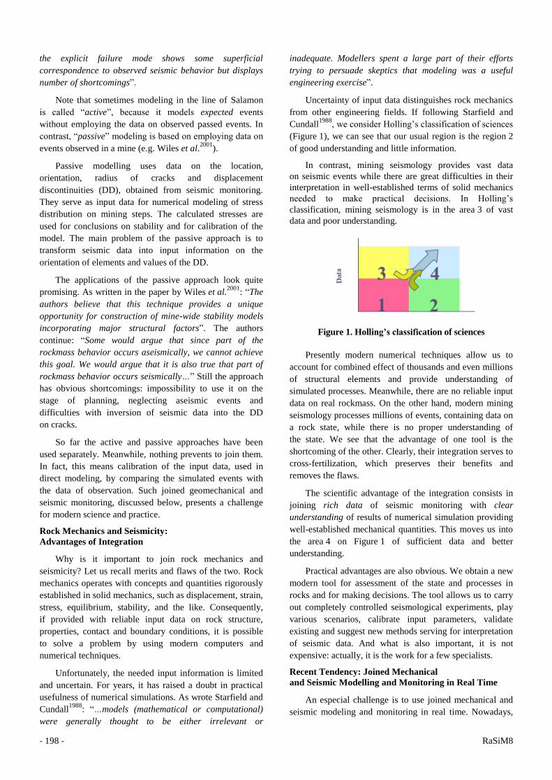
Uncertainty of input data distinguishes rock mechanics

from other engineering fields. If following Starfield and

Cundall1988

, we consider Holling‟s classification of sciences

(Figure 1), we can see that our usual region is the region 2

of good understanding and little information.

In contrast, mining seismology provides vast data

on seismic events while there are great difficulties in their

interpretation in well-established terms of solid mechanics

needed to make practical decisions. In Holling‟s

classification, mining seismology is in the area 3 of vast

data and poor understanding.

Figure 1. Holling’s classification of sciences

Presently modern numerical techniques allow us to

account for combined effect of thousands and even millions

of structural elements and provide understanding of

simulated processes. Meanwhile, there are no reliable input

data on real rockmass. On the other hand, modern mining

seismology processes millions of events, containing data on

a rock state, while there is no proper understanding of

the state. We see that the advantage of one tool is the

shortcoming of the other. Clearly, their integration serves to

cross-fertilization, which preserves their benefits and

removes the flaws.

The scientific advantage of the integration consists in

joining rich data of seismic monitoring with clear

understanding of results of numerical simulation providing

well-established mechanical quantities. This moves us into

the area 4 on Figure 1 of sufficient data and better

understanding.

Practical advantages are also obvious. We obtain a new

modern tool for assessment of the state and processes in

rocks and for making decisions. The tool allows us to carry

out completely controlled seismological experiments, play

various scenarios, calibrate input parameters, validate

existing and suggest new methods serving for interpretation

of seismic data. And what is also important, it is not

expensive: actually, it is the work for a few specialists.

Recent Tendency: Joined Mechanical

and Seismic Modelling and Monitoring in Real Time

An especial challenge is to use joined mechanical and

seismic modeling and monitoring in real time. Nowadays,

NUMERICAL MODELING OF SEISMICITY: THEORY AND APPLICATIONS - 199 -

the possibility to implement it is facilitated by tremendous

progress in computers, numerical techniques, information

technologies and automatic measurements. Actually, the

passive approach contains the germs of the joined

monitoring. It is visibly recognized by the specialists

applying it, who wrote (Wiles et al.2001

): “The integration

of deterministic modeling with seismic monitoring offers

crucial data regarding local variability and sensitive

features… Taken together this clearly enhances our

deterministic prediction accuracy of rockmass response to

mining”.

The feasibility of the purpose is evident from the

papers by Cai et al.2007

and Dobroskok et al.2010

. The

authors of the first of them used the FLAC and PFC for

simulation of seismicity induced by large-scale

underground excavations. The second work employed the

code SEISM-3D, based on using the general theory

(Linkov2005, 2006

) in frames of the hypersingular boundary

element method (H-BEM). The both papers vividly

demonstrate that geomechanical and seismic modeling may

be efficiently joined with daily seismic monitoring in

mines. It provides important data for making reliable

practical decisions.

The trend to meet the challenge is obvious from

merging of ITASCA (geomechanics consulting and

software development company) with ASC (Applied

Seismology Consultants) in 2009. As advertised the site

http://www.seismology.org/itasca_msapps.aspx (September

26, 2012), “ASC and Itasca have developed advanced,

groundbreaking techniques for correlating microseismic

field observations with simulated microseismicity from

Itasca's models”.

The same trend is also seen in transforming the

ISS International by Dr. Mendecki into Institute of Mine

Seismology (IMS) in 2011. The Institute, among other

purposes, aims to compliment daily geomechanical

calculations with numerical modeling of seismicity in real

time and to compare the synthetic seismicity with the data

of seismic monitoring.

The modeling of stressed state and seismicity joined

with direct observations becomes of crucial significance for

hydraulic fracturing. Hydraulic fracturing is widely used

for stimulation of oil, gas and heat reservoirs. Its

importance grows with the tendency to extract gas from

low-permeable shales. The geomechanical data in these

problems are even less than in those concerning with

mining. In fact, seismic observations are the main source of

information on the hydraulic fracture propagation. For this

reason, the newest methods for modeling hydraulic

fractures employ the observed seismicity to calibrate

the input data (see, e.g. Cipolla et al.2011

and

Kresse et al.2011

). Obviously, the reliability of the methods

employed will notably gain when complimenting them with

numerical modeling of seismic events and comparing

synthetic seismicity with observations. The papers by Al-

Busadi et al.2005

, Dobroskok and Linkov2008

show that

simulation of seismicity, accompanying hydraulic fracture

propagation, can be efficiently performed.

Scope and Structure of the Paper

The main objective of the paper is to present the

modern theory of joined modeling of mechanical state and

seismicity in such a form, which provides easy

implementation in a computer code of a conventional

numerical method (BEM, FEM, FDM, DEM and the like).

The paper also aims to:

1) Distinctly outline the fundamental issues, which stay

the same when considering a wide variety of applications.

2) Point out flexible elements, which may vary depending

on a particular problem and/or available computational

facilities.

The exposition takes into account the mentioned

tendency to carry out joined modeling in real time. It is

accompanied with examples.

The structure of the papers is as follows. Firstly, we

consider fundamentals of modeling a single event. This

involves concepts of instability in the form of a jump,

softening behavior, elastic energy release, elastic rigidity

of rock near a flaw, seismic energy, seismic moment and

seismic shear.

Then we consider the time effects of two kinds: those

governed by processes external to the sources of events

(for instance, mining steps) and those, which are defined

by processes in the source of an event. The first group is

the same as in conventional calculations of stresses. The

second is specific and it leads us to the Elasticity-Softening-

Creep (ESC) model as the simplest model capable to serve

for modeling both seismic and aseismic events and intervals

between the events.

Having the background for modeling a single event,

we follow the line by Salamon1993

of random seeding crack-

like flaws in the rock mass and checking their stability

under current stresses. Special attention is paid to proper

prescribing the values and statistical distributions of

geometrical and mechanical properties of seeded flaws.

With these prerequisites, we come to the general

structure of a computer code for simulation of seismic and

aseismic events. It appears that it is sufficient to

compliment a conventional code with a set of quite general

„seismic‟ subroutines, which may be used in diverse

computational environments. The discussion of subroutines,

serving for processing the output data, is accompanied

by examples of various applications. Brief summary

concludes the exposition.

- 200 - RaSiM8

MODELING OF A SINGLE SEISMIC EVENT

Seismicity is a sequence of many individual events.

Therefore, to simulate seismicity we need to clearly

understand and properly model a single event. Having a

tool for such modeling, it becomes possible to randomly

generate parameters, defining an event, and to obtain

statistical collection of events called synthetic seismicity.

Instability in a Form of a Jump

The essence of a seismic event is a jump from one

equilibrium state to another with release of elastic energy.

The excess of the elastic energy released in a jump over the

energy consumption manifests itself through elastic waves,

registered in (micro)seismic observations. Although wave

receivers are located at a distance from the source,

seismograms contain important information on the source

such as its location, magnitude, seismic moment, etc.

(see, e.g. Aki and Richards2002

, Gibowicz and Kijko1994

,

Mendecki1997

and Rice1980

). These seismological data

obtained at a distance from the source may be compared

with that provided by an analysis of the jump in the source

itself. Here we focus on such an analysis.

From the mechanical point of view, a jump is a form of

instability with elastic energy excess transformed into

kinetic energy of waves. Jumps occur in rock at different

scales. In a loaded specimen, they occur on the level of

microcracks and appear as acoustic emission. It may serve

to validate modeling of seismic events under known

conditions of loading. In oil and gas production, jumps

appear as microseismicity around a borehole or propagating

front of a hydraulic fracture. In a mine, we have a larger

scale: there emerge not only microseismic events but also

large dangerous jumps, rockbursts. Their magnitude in the

Righter scale may reach two. Moreover, in the earth crust

the length and magnitude scales are much greater; an event

may appear as an earthquake. The magnitude may reach

eight.

Despite the length scale changes nine orders (from

micro meters to kilometres) the essence of a single event is

the same: it is the dynamic (with the energy excess)

instability. Consequently, proper modeling of a single event

requires the study of instability and it refers to events on a

wide range of scales.

Equilibrium, Stability and Instability

The theoretical canvas of studying instability in

mechanics is common. Firstly, we need to find a current

state. To this end, the equations of continuum mechanics

for a small volume of a medium, associated with

a mathematic point, are used. They include:

Dynamic or static equations of motion (equilibrium),

which are actually the Newton‟s second law, specified for

a point of continuum.

Kinematics equations, defining changes in mutual

positions between closely located points of the medium.

Constitutive equations for a volume element, which

connect dynamic quantities of the first group with

geometric quantities of the second.

This yields a complete system of partial differential

equations (PDE), defined at points of a considered region of

the medium. It is solved under prescribed initial, contact

and boundary conditions to distinguish the particular

solution of the PDE, corresponding to a particular problem,

from the general solution.

In static problems, which are of prime interest to our

theme, there is no need in initial conditions: we use only

contact and boundary conditions. The contact conditions

include constitutive equations for a contact element.

(In the simplest case of a perfect contact, the constitutive

equations express continuity of tractions and displacements

through the contact).

Suppose we have found the solution of a problem and

know the equilibrium state. Now we want to know if the

state is stable or unstable.

A rigorous analysis of stability requires strict

definitions of what is assumed to be a stable or unstable

state. Naturally, the definition differs in different problems.

Still, the general feature is that instability is always

induced by some source(s) of non-linearity. The problem

of stability does not exist for a linear system. Thus we need

to inspect the possible sources of nonlinearity.

For a massive body of hard rock, in contrast with

slender bodies, we may neglect non-linear terms in

equilibrium and kinematics equations. Thus the only

candidates to be the sources of instability remain non-linear

constitutive equations for volume or/and contact elements.

These equations are obtained in physical experiments with

rock volumes and contacts.

Figure 2 presents typical non-linear diagrams for a

volume element obtained by using a rigid testing machine.

Figure 2. Complete diagrams for a volume element

Of importance is that the diagrams have descending

parts, corresponding to so-called softening behaviour.

As known from the pioneering work by Cook1965b

, under

some conditions, softening becomes the source of

NUMERICAL MODELING OF SEISMICITY: THEORY AND APPLICATIONS - 201 -

instability with the energy excess transformed into kinetic

energy of fragments of fractured rock. Note that from the

plasticity theory (e.g. Kachanov2004

), we know that such

kind of instability cannot occur for linear elasticity and

hardening that is for deformation on ascending parts of

diagrams.

Similarly Figure 3 presents typical non-linear shear

traction-shear displacement discontinuity (DD) diagrams

for a contact (surface) element. They also have descending

(softening) parts. Again they may cause dynamic instability

(see, e.g. Linkov1994

).

Figure 3. Complete diagrams for a contact element

Now we need to decide which of the two types of

softening or both of them should be taken into account

when modeling a seismic event? Actually, modern

numerical techniques may account for the both types. Still

the surface type looks dominating as concerns with

seismicity in hard rock, at least. As wrote Napier2001

:

“The fundamental 'building block' of material failure can

then be considered to be a 'crack element' rather than a

'particle'”. Furthermore, even volumetric softening of a

pillar may be modeled by using the dependence between

average displacements of its boundaries and average

tractions on them (see, e.g. Linkov1994

). Thus in the

problem considered, it is reasonable to focus on surface

(contact) softening.

Constitutive Equations for Contact Interaction

Consider an element of rock surfaces in contact.

Denote n the normal to the element, the traction

vector on that side of the contact, with respect to which the

normal is outward, u is the vector of displacement on this

side; and

u the traction and displacement on the

opposite side (Figure 4).

Commonly, in problems involving contact instabilities,

the contact is either not filled or it is filled with a material

softer than embedding rock. Then we may neglect bending

of a contact layer. This yields that (i) the contact interaction

is characterized by the DD:

, uuu (2.1)

rather than by the average displacement )(2/1

uu and

(ii) the traction is continuous through the contact:

. (2.2)

Figure 4. Traction and DD vectors on a contact

Therefore, the contact interaction is characterized by

components of the vectors and u . In the component

form, the vector Equation (2.2) in 3D presents three scalar

equations. Three other needed equations express the

dependence between the traction and DD vectors:

)( uF . For irreversible deformations at a contact,

this dependence should be incremental, connecting

increments of the tractions with increments of the DD in a

way similar to plasticity theory. Quite general equations of

this type may be found elsewhere (e.g. Linkov1994

).

However, having in mind that the properties of a surface

are uncertain and difficult to find, using a general

description looks impractical. It is reasonable to employ

as simple description as possible to shorten the list of

uncertain parameters. For our purpose, we shall use the

following simplifications.

1) A flaw (crack), on which an event may occur, is closed

if the traction does not reach the tensile strength nc0 or the

initial shear strength C . For simplicity, the initial shear

strength is prescribed by the Coulomb‟s law:

tan)(0 nC c , (2.3)

where is the shear component of the traction, 0c is the

initial cohesion,

is the surface friction angle. For

illustrative purposes we assume that the shear traction

vector is directed along a local coordinate axis in the plane

of shear; thus we assume positive. Then the shear DD

is negative, and we shall use u to have a positive value.

A compressive normal traction, like compressive stresses,

is assumed negative.

Thus we have:

Cnn cu and if ,0 0 . (2.4)

2) When the traction reaches a limit value, there DD

occur.

For the tensile mode )( 0nn c , the DD are defined

by the condition that the traction on an open crack becomes

zero:

0 . (2.5)

- 202 - RaSiM8

For the shear mode )( C , the DD are defined

in accordance with the piece-wise linear diagrams with

descending parts shown in Figure 5:

*

*

*0 uu-

uu-

)(

)(

cc

uM

C

cC , (2.6)

where cM is the shear softening modulus,

cMccu /)( *0* is the shear DD, corresponding to

reaching the residual cohesion *c .

Figure 5. Simplest diagrams for a shear

softening contact

The normal DD nu for the shear mode may be

prescribes as

tanuun , (2.7)

where is the dilation angle. The minus sign in front of

nu serves to have a positive value. Recall that we assume

u to be negative and that under the accepted definition

(2.1) of DD, a DD, corresponding to opening, is negative

(see Figure 4). Commonly, we may neglect the dilation;

then nu = 0 for the shear mode.

Equations (2.1) – (2.7) completely define the properties

of a contact element. The dependence (2.6) accounts for

softening what serves for modeling dynamic instability.

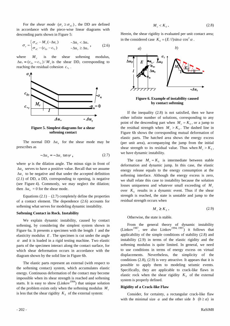
Softening Contact in Rock. Instability

We explain dynamic instability, caused by contact

softening, by considering the simplest system shown in

Figure 6a. It presents a specimen with the length l and the

elasticity modulus E . The specimen is cut under the angle

and it is loaded in a rigid testing machine. Two elastic

parts of the specimen interact along the contact surface, for

which shear deformation occurs in accordance with the

diagram shown by the solid line in Figure 6b.

The elastic parts represent an external (with respect to

the softening contact) system, which accumulates elastic

energy. Continuous deformation of the contact may become

impossible when its shear strength is reached and softening

starts. It is easy to show (Linkov1994

) that unique solution

of the problem exists only when the softening modulus cM

is less that the shear rigidity SK of the external system:

Sc KM . (2.8)

Herein, the shear rigidity is evaluated per unit contact area;

in the considered case 2cossin)/( lEKS .

Figure 6. Example of instability caused

by contact softening

If the inequality (2.8) is not satisfied, then we have

either infinite number of solutions, corresponding to any

point of the descending part when Sc KM , or a jump to

the residual strength when Sc KM . The dashed line in

Figure 6b shows the corresponding mutual deformation of

elastic parts. The hatched area shows the energy excess

(per unit area), accompanying the jump from the initial

shear strength to its residual value. Thus when Sc KM ,

we have dynamic instability.

The case Sc KM is intermediate between stable

deformation and dynamic jump. In this case, the elastic

energy release equals to the energy consumption at the

softening interface. Although the energy excess is zero,

we shall relate this case to instability because the solution

losses uniqueness and whatever small exceeding of cM

over SK results in a dynamic event. Thus if the shear

strength is reached, the state is unstable and jump to the

residual strength occurs when

Sc KM . (2.9)

Otherwise, the state is stable.

From the general theory of dynamic instability

(Linkov1987

, see also Linkov1994, 1997

) it follows that

applicability of the simple conditions of stability (2.8) and

instability (2.9) in terms of the elastic rigidity and the

softening modulus is quite limited. In general, we need

to use conditions in terms of energy excess on virtual

displacements. Nevertheless, the simplicity of the

conditions (2.8), (2.9) is very attractive. It appears that it is

possible to apply them to modeling seismic events.

Specifically, they are applicable to crack-like flaws in

elastic rock when the shear rigidity SK of the external

system is properly defined.

Rigidity of a Crack-like Flaw

Consider, for certainty, a rectangular crack-like flaw

with the minimal size a and the other side b )( ab in

NUMERICAL MODELING OF SEISMICITY: THEORY AND APPLICATIONS - 203 -

elastic rocks with the elasticity modulus E and the

Poisson‟s ratio v (Figure 7). We use the local coordinate

system with the axis 1x normal to the flaw plane, 2x and

3x in the plane. The 2x -axis is directed along the long side

of the rectangle, the 3x -axis is along the short side. The

flaw sizes are small as compared with the sizes of openings,

faults and other structural elements of a considered region.

Then the total influence of these disturbing factors and

stresses at infinity is incorporated in the total traction t ,

induced at the location of the flaw on its surface.

Figure 7. A rectangular flaw in elastic rock

It is easy to solve numerically a 3D problem for a plane

crack of an arbitrary configuration in an infinite elastic

region under prescribed traction at the crack surface

(e.g. Linkov et al.1997

). From the solution we can find the

dependence between the average traction vector and

the average DD vector u :

tuK , (2.10)

where K is a matrix with known coefficients; it has the

meaning of average (per unit area) rigidity matrix. In

particular, for a rectangular crack in isotropic rock, by

symmetry, the rigidity matrix is diagonal. Its diagonal

coefficients 1K , 2K and 3K may be written as:

a

kEK

i

i 21 , (2.11)

where the dimensionless coefficients ik ( i = 1, 2, 3)

depend on the ratio ab / ; besides the coefficients 2k and

3k depend on the Poisson‟s ratio.

Figure 8 presents the graphs of the coefficients ik

as functions of ab / for the Poisson‟s ratio v = 0.25

(Linkov2006

). Note that in the limiting case of a plane-strain

problem )/( ab , the coefficients found analytically

are: /21 k , /22 k , /)1(23 k . From

calculations it follows that to the accuracy of 3% the

plain-strain conditions are acceptable when ab / = 4.

This implies that the coefficients 2k and 3k differ by the

factor 1 at most. Therefore, for simplicity, we may use

their mean value 2/)( 32 kkk S , which becomes the

only characteristic of shear rigidity. (The bold line in

Figure 8 gives the dependence of Sk on the ratio ab / ).

Then (2.11) becomes:

a

kEK

1

211

, a

kEKKK

S

S 2321

. (2.12)

Figure 8. Rigidities as functions of b/a

In view of (2.12), we may write the dependence (2.10)

between the average DD and average tractions in terms of

separated normal n , nu and shear , u components:

nnn tuK 1 , tuK S . (2.13)

Equations (2.13) notably simplify analysis of the

system “flaw – embedding rock”. The unified shear rigidity

SK makes the rectangular flaw isotropic in its response

to shear, like it is for a circular flaw. By employing this

simplification, from now on, we shall assume the local

coordinate 2x directed along the shear traction.

Comment. The actual configuration of flaws in rock

mass is uncertain. Thus there is no sense to distinguish

between the shear rigidities 2K and 3K and to exactly

specify the Poisson‟s ratio. Moreover, as the shear rigidity

SK is compared with the shear softening modulus cM ,

which is even more uncertain, it is enough to use rough

estimations. In particular, since the shear rigidity changes

only 1.6-fold when the rectangle changes from a square

)( ab to an infinite strip ),/( ab it is possible to set

ab . Then for v = 0.25, the rigidities are:

a

EK 0.11 ,

a

EK S 9.0 . (2.14)

Note that the analytical solution for a circle of the

radius 2/aR , yields the normal rigidity aEK /95.01 ;

the difference with the first of (2.14) is only 5%. Thus

the configuration of a flaw does not influence the rigidity

significantly. Roughly, the rigidity is defined by the

minimal size of a flaw. Using a circular flaw simplifies also

input data and estimations of the energy release. For these

reasons, Salamon1993

seeded circular flaws.

- 204 - RaSiM8

Equilibrium and Instability

of a Crack-like Flaw in Rock

We are in a position to obtain an approximate solution

for a softening crack-like flaw by equating the tractions

and DD on its surface to those of elastic rock. Before the

tensile or shear strength is reached nn ct 0( , )Ct ,

Equations (2.4) and (2.10) yield the obvious result:

t .

After the tensile strength is reached )( 0nn ct ,

Equations (2.5) and (2.10) give:

tKu 1. (2.15)

At last, if the shear strength is reached )( Ct ,

joining the first of (2.6) and the second of (2.13) gives the

system, defining the shear DD under softening:

)( uM cC , tuK S .

Its solution is:

cS

C

MK

tu

. (2.16)

Recall that by the accepted agreement on signs, for a

physically significant solution, it should be – u > 0.

Since the numerator in (2.16) is non-negative, this implies

that a continuous solution exists only under the condition

of (2.8) form: Sc KM . If Sc KM , there is no

continuous solution: the system jumps to the state

corresponding to the residual strength. We see that the

condition (2.9) is the condition of dynamic instability for

a flaw in elastic rock.

For the final state after the jump, the second line in

(2.6) and the second Equation in (2.13) yield:

S

C

K

cctu

)( *0

. (2.17)

Note that the r. h. s. in (2.17) is positive.

Comment. Recall that the solutions (2.16), (2.17) are

approximate because we have used tractions and DD

averaged over a flaw. It is of interest to estimate the

accuracy of such an approach. It can be done by using the

results of the exact solution to the plain-strain problem for

a straight shear-softening crack of the length a in elastic

rock (Belov and Linkov1995

). From inspecting dimensions,

it is obvious that the condition of dynamic instability has

the form (2.9). The value of the rigidity, corresponding to

the exact solution, is a

EKS

1

1675.0

2 . Its comparison

with the approximate valuea

EKS

1

1

22

, obtained by

averaging, shows that the error is 9.3%. Such an error looks

acceptable when modeling a seismic event.

Seismic Characteristics of a Single Event

Consider a flaw with the normal n in rock (Figure 7).

Suppose that the tractions n and are such that the

shear strength is reached. Then the flaw may experience

softening in accordance with a diagram in Figure 5,

corresponding to the current normal traction nn t . This

diagram is shown by solid line in Figure 9.

Figure 9. Diagrams of softening element

and external system (embedding rock)

We are interested in characteristics of the jump

occurring when the instability condition,

,Sc KM

is met. Then the deformation of rock surfaces follows the

diagram shown by the dashed line in Figure 9. The area

between the diagrams represents the energy excess per unit

area. Therefore, for the whole flaw area, equal to ab , the

total elastic energy excess is:

abM

K

K

ccW

c

S

S

1

)(

2

12

*0 . (2.18)

Note that the total elastic energy release is

abK

ccW

S

r

2

*0 )(

2

1 , (2.19)

while the total energy consumption on the softening surface

is cC MabccW /)(2/1 2

*0 . Introduce the seismic

efficiency factor, defined in seismology as

rCreff WWWK /)( , so that reffWKW . Then Equation

(2.18) implies that in the considered case the seismic

efficiency is:

c

Seff

M

KK 1 . (2.20)

Depending on the softening modulus it may change

from the unity for ideally brittle rock, considered by

Salamon1993

)( CM , to zero at the threshold of

instability SC KM .

We obtain a rough estimation of the seismic energy by

using the second of Equations (2.14) for a square flaw:

effKaE

ccW 3

2

*0 )(56.0 . (2.21)

NUMERICAL MODELING OF SEISMICITY: THEORY AND APPLICATIONS - 205 -

Equation (2.21) shows that the energy of an event is

proportional to the cubed crack size a . The simple

estimation (2.21) is useful in numerical simulation of

seismicity. It serves for the choice of the average size of

flaws, which define the average level of energy; the latter is

available from seismic observations.

The seismic shear Su , according Figure 9, is:

S

SK

ccu

*0 . (2.22)

The tensor of seismic moment in the local coordinates

of the flaw is:

.

000

001

010

mM seism

Herein, m is the magnitude, defined as usual by the

equation Sum S , where is the shear modulus

)1(2 E , S is the flaw area )( abS . (Recall that

we have assumed the local coordinate 2x directed along the

shear traction, so that the shear DD has the direction

opposite to 2x what explains the minus sign in front of m ).

One nodal plane of an event is normal to the local axis 1x ,

another is normal to 2x .

Usual tensor transformation gives the tensor of seismic

moment in a global system of coordinates. For brevity,

the value m is also called the seismic moment when there

might be no confusion.

Using (2.22) yields:

abK

ccm

S

*0 . (2.23)

From (2.19) and (2.23), it follows that the energy

release is proportional to the moment m :

mcc

Wr

2

*0 .

The energy excess differs only by the seismic

efficiency factor:

effe mKcc

W

2

*0 .

Therefore, in rough estimations, assuming the seismic

efficiency constant, the energy excess is proportional to

the seismic moment.

Summary for Modeling a Single Seismic Event

We have seen that the essence of a seismic event is

instability in the form of a jump. It occurs when the elastic

energy release exceeds the energy consumption for

softening deformation of a flaw. Therefore, when modeling

a single event we need to account for:

1) Elasticity, which provides the source of energy.

2) Softening, which defines the energy consumption.

Thus,

Elasticity + Softening → Single seismic event

This implies that when seeding many flaws, at which

seismic events may occur, the minimal input data for

a flaw are:

1) Its location (three global coordinates of the flaw

center).

2) Orientation of the flaw plane (two coordinates of the

unit normal to the plane; and, for a rectangular flaw,

orientation of one of the sides in the plane).

3) The size(s) of the flaw (two lengths of a rectangle, or

one size for a square or circle).

4) Mechanical properties of the flaw: its tensile nc0 and

initial shear 0c strength, friction angle ρ, residual cohesion

*c , softening modulus cM and dilation angle ; in

simplified models, one may set nc0 = 0, *c = 0, = 0

and/or consider ideally brittle contact )( cM .

5) Elasticity modulus E and Poisson‟s ratio ν of rock

at the location of the flaw.

The elastic properties of rock and minimal size of a

flaw define the shear rigidity SK of rock with respect to

the flaw. It is found from the second of Equations (2.12)

and Figure 8 for a rectangular flaw, or from the second of

Equations (2.14) for a square or circular flaw with the

radius aR .

The behavior of a flaw in rock depends on the tractions

t induced on its surface by external stresses. The stresses

are found by solving a boundary value problem for rock

masses with openings, faults, inclusions, etc. under

prescribed in-situ stresses. A common code of FEM, BEM,

DEM and the like may serve to find the induced stresses.

A flaw is closed and it does not influence the rock state

when neither tensile, nor shear strength is reached.

A flaw opens when the normal traction becomes equal

or exceeds its tensile strength )( 0nn ct ; then the flaw

obtains the DD defined by (2.15).

A flaw experiences shear deformation when its shear

strength is reached )( Ct . In this case, there are two

options:

1) There is no seismic event if the stability condition (2.8)

is met )( Sc KM . Then the shear DD is found from

(2.16); the normal DD is defined by (2.7); when setting the

dilation angle zero, the normal DD is zero.

2) A seismic event (jump) occurs if the instability

condition (2.9) is met )( Sc KM . Then the characteristics

of the event (energy release, energy excess, seismic

- 206 - RaSiM8

efficiency, seismic shear, seismic moment, etc.) are found

by using Equations (2.18) – (2.23).

TIME EFFECTS

Multiple Events: Seismicity

Time effects are obviously present in rock. “The first

law of rock mechanics is that holes tend to close up”

(saying of “wise old engineer” quoted by van der

Merwe1995

). As concerns with seismic events, they are

distributed in time; obviously time effects control intervals

between individual events. They lead also to aseismic

deformations. Thus to consider many seismic events and to

include aseismic events, we need to compliment the two

discussed fundamental factors (elasticity and softening)

with time. A multiplicity of seismic events is called

seismicity. Therefore,

Elasticity + Softening + Time → Seismicity

For events of small magnitude, the term

microseismicity is commonly used; dynamic events in

a loaded specimen are called acoustic emission. We assume

these terms equivalent.

External Time

It looks reasonable to distinguish two types of time

processes:

1) Those which run out of the source of an event and its

close vicinity.

2) Those which occur in the source and its close

neighbourhood.

The first group of processes is external, while the

second is internal with respect to an event.

Figure 10 presents examples of processes controlled

by external time. They include a specimen loaded with

stresses, which change in time in accordance with a

prescribed loading path (Figure 10a); mining with changes

of geometry planned by an engineer (Figure 10b). In these

two cases the time is just a parameter defining changes

in boundary conditions. The other two examples refer to oil

(gas, heat) production (Figure 10c), where changes in the

stressed state are defined by transient processes of fluid

flow, and propagation of a hydraulic fracture (Figure 10d),

which changes the stresses around it.

Various conventional codes of FEM, BEM, DEM, etc.

may serve to numerically trace the change of stresses in the

external time. We assume that a numerical code to simulate

these changes is available. From now on we focus on the

„internal time‟.

Internal Time. Elasticity-Softening-Creep (ESC) Model

There is obvious evidence of internal time present in

seismicity: after a strong excitation of rock, such as an

earthquake, or rockburst, or blast, a cascade of seismic

events occurs during some interval of time. The events

cease in time approximately exponentially, what in

seismology is called the Omori‟s law. The questions are:

how to account for the internal time in the simplest way and

how to model aseismic events?

Figure 10. Examples of processes running

in ‘external’ time

We may follow the common path of solid mechanics to

get an answer. As known, the simplest description,

explicitly accounting for the time, is the Newton‟s viscosity

law, which linearly connects a force (stress) with a

kinematic quantity (velocity, strain rate, DD). In schemes,

presenting model behavior, it is shown by a dash-pot

(Figure 11a).

Figure 11. Using a dash-pot (a) to simulate viscous

deformation of a volume (b) or surface (c) element

In constitutive equations for a volume element

(Figure 11b), the dependence between a time-dependent

part of the stress c

ij and the strain rate c

ij is c

ij

c

ij with the coefficient having the dimension of

dynamic viscosity ][ = stress/strain rate = stress·time.

For a contact element (Figure 11c), time-depending shear

traction c

linearly depends on the velocity cu of shear

DD: cc u with the coefficient having the

dimension ][ = stress/velocity = stress·time/length. The

dot over a symbol denotes the derivative with respect to

time.

There are numerous option for including this model

into constitutive equations for embedding rock (volumes)

or/and interfaces (surfaces). When choosing between them,

it is reasonable to have in mind that a dash-pot responds

absolutely rigidly to instant changes. Actually its instant

NUMERICAL MODELING OF SEISMICITY: THEORY AND APPLICATIONS - 207 -

rigidity is infinite. Specifically, its reaction is absolutely

rigid in a jump, which corresponds to dynamic instability

associated with a seismic event. Consequently, there is no

sense to include a viscous element in parallel with an

elastic element when modeling external system, represented

by external rock (Figure 12a). Such a system will not

provide elastic energy instantly. It is also senseless to

include a viscous element in parallel with a softening

element modeling the behavior of a crack-like flaw

(Figure 12b). Such a system is unable to consume energy in

a jump.

Figure 12. Schemes with parallel inclusion

of a viscous element

We conclude that the reasonable way of accounting for

internal time is to include a viscous element in series with

an elastic element representing an external system

(Figure 13a), or/and with a softening element shown in

Figure 13b.

Figure 13. Schemes with inclusion

of a viscous element in series

In the simplest softening element shown in Figure 5,

we have neglected the elastic DD on the flaw surface.

Consequently, to have a time scale, it is reasonable to use

the viscous element in frames of the Kelvin-Voight model.

Then we obtain the simplest model (Figure 14), which

exhibits instant softening and has a characteristic time rt .

We call this model the Elasticity-Softening-Creep (ESC)

model, because it includes the elastic element with the

rigidity lE , softening element with the softening

modulus cM and viscous (creeping) element with the

viscosity . The characteristic time of the model is the

retardation time:

l

rE

t

. (3.1)

Figure 14. Elasticity-Softening-Creep model

The instant reaction of the model is that of the

softening element with the instant softening modulus cM .

The long term reaction is that of a softening element with

the long-term softening modulus M , defined by equation:

lc EMM

111

. (3.2)

The ESC-model is the simplest extension of the

standard linear body. It reduces to the standard body when

excluding softening of the upper element in Figure 14,

so that it becomes elastic. Below we shall use the opposite

option and neglect elastic deformation of the upper element.

Surely, non-Newtonian viscous element may be used when

appropriate.

ESC-model, being not much more complicated than

models used to the date, it provides significant advantages.

It allows us to account for rock brittleness, to distinguish

between stable and unstable states, to evaluate energy

consumption and to follow damping or accelerating

aseismic deformations.

Constitutive Equations for ESC-Model

We shall use the simplified diagrams of Figure 5 and

their analytical form (2.6). The corresponding ESC-model

is shown in Figure 15.

The properties of the model are as follows. Until the

tensile or shear strength is reached, we assume that a flaw

is closed and DD at its surface are zero. If the tensile

strength is reached, the reaction is instant, thus the flaw

opens and the traction turns to zero (Equation 2.5). If the

shear strength is reached, then the upper element of the

- 208 - RaSiM8

ESC-model behaves in accordance with Equations (2.6).

We rewrite them with the subscript „u‟ at the shear DD

to mark that the DD refer to the upper element in Figure 15:

*

*

*0 uu-

uu-

)(

)(

u

u

C

ucC

cc

uM

. (3.3)

Figure 15. ESC-model (no elastic DD prior softening)

For the lower Kelvin-Voight element, we have:

)()(lll uuE , (3.4)

where the subscript l marks that the DD refers to the lower

element. The traction is the same in the upper and lower

element because they are joined in series. For the same

reason, the total DD is the sum:

)()(lll uuE . (3.5)

The total normal DD may correspond to dilation in

accordance with (2.7).

Joined System of ESC-Surface Element and Rock

We join Equations (2.13) of the external system with

Equations (3.3) – (3.5) for a flaw described by the

ESC-model. If neither tensile nor shear strength is reached,

the flaw is closed; its DD are zero. If the tensile strength

is reached, the DD are defined by Equation (2.15). If the

shear strength is reached )( Ct , the joined system

yields the ordinary differential equation (ODE):

)()()(

C

rr

tt

utdt

ud

, (3.6)

where rt is the retardation time defined by (3.1),

1/

1/

cS

S

MK

MK ,

1/

/1

cS MK

M , (3.7)

M is the long-term softening modulus defined by (3.2);

note that (3.2) implies inequality cMM . When deriving

the ODE (3.6) we neglected the viscous deformation, which

occurred long before the current time, and the time

derivative of the induced traction. The agreements on the

signs of shear DD and shear traction are those accepted

above.

The ODE (3.6) is solved under the initial condition

)( 0tu = 0, where 0t is the moment when the shear

strength is exceeded. We shall not write down the obvious

solution. Rather we discuss the general solution of a

homogeneous ODE, corresponding to (3.6), because it

defines general features of the mechanical system. The

general solution, including an arbitrary constant C , is:

r

gt

tCtu exp)( . (3.8)

From (3.8) it is clear that a solution exponentially

grows (decays) when < 0 ( > 0). The sign of

depends on the signs of numerator and denominator in the

first of (3.7). This implies that there are three types

of shear motion depending on particular values of SK ,

cM and M :

1) Instant instability (jump) occurs when Sc KM .

Then we have a seismic event with characteristics

discussed in the previous subsection.

Otherwise, the state is stable ( Sc KM ). In this case,

the deformation occurs in aseismic (without energy excess)

form. Although it is continuous in time, there appear two

additional options (we do not consider the exclusive case

Sc KM , which is not of practical interest):

2) Decaying aseismic motion occurs if SKM .

3) Accelerating aseismic motion occurs if SKM .

We see that the ESC-model describes both seismic and

aseismic events. For the latter, the motion may be very fast

when the instant softening modulus cM is close to the

rigidity SK : , when Sc KM . This explains

why intervals between observed seismic events are

different; the difference may be of several orders. The fast

aseismic motion explains also so-called silent earthquakes

(see, e.g. Linder et al.1996

, Dragert et al.2001

and

Kawasaki2004

).

From the analysis it appears that, actually, we need

to prescribe only three parameters rt , Sc KM / and

SKM / to model the deformation of a flaw after its

initiation by external shear traction.

Aseismic Behavior

and Characteristics of a Single Aseismic Event

We have seen that aseismic motion at flaw surfaces

occurs when the stability condition Sc KM is met. The

motion runs with acceleration if the long-term modulus

exceeds the rock rigidity )( SKM . Otherwise, it decays

in time. In the both cases, if the residual shear strength is

reached in the course of motion, we have for the final shear

DD:

NUMERICAL MODELING OF SEISMICITY: THEORY AND APPLICATIONS - 209 -

S

C

fK

cctu

*0

. (3.9)

The time ft of reaching the residual shear strength is:

u

u

MM

KMtt

c

Scrf

*1/1

/1ln

, (3.10)

where )/()( MKtu SC , MMuu c /** ,

cMccu /)( *0* . Equations (3.9) and (3.10) refer to

both accelerating and decaying motion.

MODELING OF SEISMICITY. INPUT DATA

General Considerations

With the ESC-model, we can simulate a single seismic

or aseismic event arising at a flaw with prescribed position

of its center and orientation of its plane. It is assumed

that there is a computer code, which provides stresses at

the flaw location as a function of external time. Then if at

some instant the tensile or shear strength is reached, we

have an event (seismic or aseismic) with known time,

location, orientation, seismic and aseismic DD and other

characteristics discussed above.

Obviously, when having many flaws, we simulate

events distributed in space and time. Therefore, to model

seismicity, it is sufficient to seed a set of flaws in an area

of interest and to check the state of each of them on steps of

external time.

There are two comments to this general scheme.

Firstly, imagine that the flaws are seeded in a natural state

of rock, which is not disturbed by mining or oil (gas)

production. We may expect that in situ tractions at some of

the flaws exceed the shear strength. Then, in accordance

with the discussion, there should be DD at such flaws.

However, these DD may be referred to times long before

the current time. Clearly these DD should be excluded from

the totality of seeded events. In a computer code, it has to

be done by a special subroutine checking seeded flaws

under in situ stresses and excluding those initiated by these

stresses. We shall call this subroutine “ExclusInSitu”.

Secondly, an event arising at a flaw on a time step leads

to DD on the flaw. The DD notably change the stresses

around the flaw. The change of stresses may be strong

enough to initiate some of the neighbouring flaws. Each of

the initiated flaws, in its turn, experiences DD, influences

its neighbours and may initiate new flaws. And so on, till

new flaws are initiated. In this way, there may arise chains

of seismic and aseismic events.

Obviously, if the density of flaws is small, they

practically do not interact. Then there are no chains of the

type. On the other hand, if the density is too high, there

arises a chain reaction, involving practically all the flaws.

The case intermediate between the two is of major interest

for simulation of seismicity. In this case, we may expect

that it will be possible to model the dependence of Omori

type. Therefore, it is of value to find the range of flaw

density, in which a chain reaction does not arise while the

interaction of flaws is sufficient to produce successive

cascades of events. Below we shall define the range.

Deterministic Input Data

We have assumed that a computer code is available for

calculating stresses at each point of a region as functions

of the external time. The input data of the code commonly

contain:

1) Initial geometry of a problem; specifically, for a

mining problem, we prescribe the depth, dip angle, strike

angle, contours of pillars and openings.

2) Physical properties of a medium.

3) In situ stresses.

4) Some additional information for a particular problem,

such as pumping rate and fluid viscosity for hydraulic

fracturing, pore pressure and permeability of rock for oil

(gas, heat) production, etc.

All these data are prescribed in the same way as in

cases when a code is used without simulation of seismicity.

Normally these data are deterministic.

The influence of the external time is also deterministic.

Specifically, in mining problems, we plan the change of

mining geometry in time; in hydraulic fracturing, we follow

the fracture propagation and the change of the net-pressure

in time steps of calculations.

Briefly, we assume deterministic all what concerns

with the performance of a conventional code when there is

no simulation of seismicity. The following discussion

entirely refers to parameters specific for modeling seismic

and aseismic events. They include geometric input data on

positions and orientations of randomly seeded flaws, data

on flaw sizes and density, data on mechanical properties of

flaws. In the next subsection we specify prescribing these

data. In a computer code, a special subroutine produces

these data. We call it “FlawInput”.

Input Data on Position and Orientation of Seeded Flaws

We seed flaws in a parallelepiped with the sides

parallel to the global coordinates, with the sizes 1X , 2X

3X and volume 321 XXXV . The sizes notably (three- to

five-fold) exceed those of the region of interest, where we

want to model seismic and aseismic events.

The uniform random distribution is used for:

1) Three coordinates of the flaw center, changing in the

intervals ]2/,2/[ 11 XX , ]2/,2/[ 22 XX

and

]2/,2/[ 33 XX for the global coordinates 1x , 2x and 3x ,

respectively.

2) Dip angle of a flaw changing from 0 to π/2.

- 210 - RaSiM8

3) Strike angle changing from 0 to 2π.

4) Rotation angle in the dip plane, changing from 0 to π

(for a rectangular flaw).

5) Ratio ab / , changing from 1 to 3 (for a rectangular

flaw).

In general the total number of geometric parameters is

seven. For square flaws )( ba , the item )(v is not used;

the number of parameters is six. For circular flaws )( Ra ,

the item )(iv is not used, as well; the number of parameters

is five.

For the size a of a flaw, we use the exponential

distribution of the probability density:

l

a

laP exp

1)( , (4.1)

where l is the average length of the smallest side. The

average length l and the total number N of the flaws are

prescribed as explained below.

Input Data on Mechanical Properties of Seeded Flaws

Shear rigidity SK . Having the input data on the rock

elasticity modulus and the sizes of flaws, we find the shear

rigidity from the second Equation (2.12) or (2.14).

Tensile strength nc0 . Commonly we may assume that

the tensile strength is zero: nc0 = 0.

Shear strength 0c , *c , . The shear strength is

characterized by the initial cohesion 0c , residual cohesion

*c and the contact friction angle . As follows from

Equations (2.18), (2.19), (2.22) and (2.23), actually we need

the difference *0 cc , rather than 0c and *c separately.

Therefore, we may set *c = 0. To reduce the number of

quite uncertain parameters, like 0c and , we may

prescribe the latter two quantities by their average values.

In particular, for hard rocks, according to Salamon1993

,

the initial cohesion changes from 0.02 to 4.3 MPa with the

statistically mean value 0c = 2.5; the friction coefficient

tanρ changes from 0.5 to 1 with the mean friction angle

= 310. When high confining pressure prevents shear, the

number of initiated events may be increased by decreasing

the friction angle to 20° or even to 10°.

Shear softening modulus cM . For the prescribed shear

rigidity SK , prescribing the softening modulus is

equivalent to that of the ratio Sc KM / . The latter defines

the instability condition and seismic efficiency. As both

cM and SK decrease with growing crack size, they are

partly correlated. Still their ratio is a random quantity and

quite uncertain. We may prescribe the ratio Sc KM / as a

sum of the determined (mean) part Ma and the random part

MM fb , uniformly distributed on the interval [ Mb , Mb ]:

MMM

S

cfba

K

M , (4.2)

where MM ba , Mf is a random value uniformly

distributed on the interval [-1, 1]. The values of Ma and

Mb in (4.2) may be prescribed by using the following

considerations.

If MM ba ≥ 1, then Sc KM / ≥ 1; hence in

accordance with the instability condition (2.9), all the

modeled events will be seismic. In modeling, this choice

serves to neglect aseismic events.

If MM ba < 1, then Sc KM / < 1; hence all the

modeled events will be aseismic. In modeling, this choice

serves to model only aseismic events.

If MM ba 1 , the ratio of numbers of modeled

seismic events SN to that of aseismic events AN is:

)1(

)1(

MM

MM

A

S

ab

ab

N

N. (4.3)

Thus, by an appropriate choice of Ma and Mb , one

may adjust the ratio of seismic to aseismic deformation

to data of observations. Note that when Ma = 1,

Equation (4.3) implies that the number of seismic

events equals to the number of aseismic events for any

value of Mb .

The mean seismic efficiency of seismic events is:

1

1

MM

MMeff

ba

baK . (4.4)

Therefore, one may choose the parameters Ma and Mb

to prescribe the mean value of effK .

Internal time scale rt . In the ESC-model, the time

scale is defined by the only combination with the time

dimension, which is the retardation time lr Et / of the

Kelvin-Voight element. Both the viscosity and rigidity

lE of this element are perhaps the most uncertain for rock.

Meanwhile, the internal time is no more than a parameter

ordering events in a sequence. Note also that according

to (3.10), the mean time of aseismic events is characterized

by /rt rather than rt . Still, as in many cases the mean

value of is of order of unity, the retardation time is

typical for the majority of aseismic events.

The contact viscosity being uncertain, the time scale

is conditional. Clearly, it should be less than a typical time

step of the external time. It may be roughly estimated if a

dependence of Omori type is available from observations.

Suppose we have dependence of the number of seismic

events, occurred in equal time intervals after a strong

excitation of rock (Figure 16a). The dependence is

approximated by decaying exponent (Figure 16b) as

)/exp(0 OS ttNN . (4.5)

Then we may associate the retardation time with the

characteristic time Ot of the Omori dependence (4.5).

NUMERICAL MODELING OF SEISMICITY: THEORY AND APPLICATIONS - 211 -

Figure 16. Dependence of Omori type for the number

of seismic events after excitation of rock

Rigidity of Kelvin-Voight element lE . It can be shown

(Linkov2006

) that for the distribution (3.12), the mean

portion of accelerating events in the total number of all

aseismic events is Mlc bEM /)/(2/1 if either (i)

MM ba 1 and 1/ lcM EMa , or (ii) Ma > 1 and

MlcM bEMa /1 . In these cases we may prescribe the

rigidity lE by choosing its value, which provides a needed

portion of accelerating events.

Mean length of flaws l . The mean length l of seeded

flaws may be defined via the expected level of energy lW

of events. Then, by using la in (2.21), we obtain:

3 2

*0

3

/)(

21.1

EccK

Wl

eff

l

. (4.6)

Note that the expression under the cubic root in (4.6)

has the order of elastic energy released from a unit volume

of rock under the stress drop *0 cc .

Flaw density and the number N of seeded flaws.

We have mentioned that the dominant factor causing chains

of events is flaw interaction. The interaction is significant at

distances less or comparable with the flaw minimal size .a

Therefore, in problems concerning with modeling

seismicity it is reasonable to introduce the flaw density as

the ratio of the mean length l of flaws to the mean distance

L between them:

L

l . (4.7)

In a 3D volume V with uniform distribution of N

flaws, the mean distance between their centers is:

3

N

VL . (4.8)

From (4.7) and (4.8) we obtain the total number of

flaws to be seeded in a volume V to have the density :

3

N

VL . (4.9)

When using (4.9) we need to specify the range of the

density, in which interaction of flaws is strong enough to

produce chains of events while it is not too strong to lead

to a chain reaction. For 3D problems, the range was

established by numerical experiments (Linkov2006

). It is:

75.014.0 . (4.10)

When the density is below the lower threshold, there is

actually no flaw interaction. Consequently, there are no

chains of events. When the density is above the upper

threshold, the interaction becomes so strong that there arise

chain reaction involving almost all the seeded flaws into

deformation.

A particular value of the density in the range (4.10)

may be chosen from additional considerations. Consider

rare strong events with the energy strW notably, say

200-fold, exceeding the mean energy lW . The number strN

of such strong events is first units, say strN = 1. Then

assuming the number of seismic events proportional to the

number of flaws capable to produce events of prescribed

energy, we have from (2.21) and (4.1) the expected number

SN of all seismic events:

3exp

l

str

strSW

WNN . (4.11)

Naturally, the total number of seeded flaws should be

at least an order greater than the expected number of

seismic events. Denote Nk the fraction of flaws, which

produce seismic events, so that S

N

Nk

N1

. When using

(4.11), we obtain the estimation:

3exp

1

l

str

str

N W

WN

kN . (4.12)

When having N , Equation (3.19) defines 3 /VNl .

The found should be within the range (4.10).

For a particular problem, the number Nk is not known

in advance. Consequently, there might be need to perform a

series of calibrating runs with a computer code. They start

from a guess regarding Nk . Then for a prescribed ratio

lstr WW / , the value of N becomes available from (4.12)

and (4.9) serves to find the density . (The latter should be

within the range (4.10)). The first run provides the portion

Nk of flaws, which produce seismic events. The found Nk

serves for the next run and so on. If at some step the density

is outside the range (4.10), we need to repeat calibration

by taking another value of strN , say 0.1, or 2, or 5.

Another, although limited option, consists in changing the

volume V of seeded flaws. Finally we obtain the needed

values of N and .

Comment. Calibration is notably simplified when

having the dependence frequency-magnitude of Gutenberg-

Righter type obtained from field observations. We shall

discuss this dependence below in Section “Output Data”.

- 212 - RaSiM8

INITIALIZATION AND TIME STEPS

Initialization

The generated input data on flaws are firstly analysed

on the initialisation step of calculations. As mentioned,

it consists in considering in situ state of rock and exclusion

those of seeded flaws, for which in situ tractions exceed the

tensile or shear strength of a flaw. It is done by a

subroutine, which we have called “ExclusInSitu”. It

presents a cycle over N seeded flaws with checking for

each of them if its strength is exceeded. These flaws are

excluded from further calculation and the number N is

respectively diminished. The remaining flaws are assumed

active in the sense that they are closed and able to

experience seismic or aseismic DD under induced tractions.

Steps in External Time

After the initialisation, the code starts calculations in a

cycle of external time steps. At the beginning of a step,

a conventional (basic) code calculates tractions at the

location of each active flaw. For brevity, we call them

„conventional tractions‟. Besides those, there arise

additional tractions caused by the DD on flaws, which have

been activated on previous steps. We call their sum at each

of the current active flaws „flaw-tractions‟. At the

beginning of the first step, the flaw tractions are zero.

We neglect the back influence of the flaw-stresses on

the conventional stresses. This serves us to use the basic

code unchanged. Normally, it does not lead to notable loss

of accuracy. Still, if there is need, the back influence may

be accounted for by an iteration included into the basis

code.

At each of the time steps, we perform calculations in

a similar way. It is done by a subroutine, which we call

“SeismTimeStep”.

Consider a typical time step. For it, we have

conventional and flaw-tractions at flaws, which are active

to the beginning of the step. Calculations always start from

the zero-stage and may include a number of stages

depending if there arise aseismic events. Specifically, if

there appear aseismic events on the zero stage, it is

followed with the fist stage. If on the first stage there

appear new aseismic events, it is followed with the second

stage, and so on until aseismic events cease to appear.

The calculations are performed as follows.

Zero-stage. At each active flaw, we add the flaw-

tractions to the conventional tractions and check if the

summary tractions exceed the tensile or shear strength.

If the strength is exceeded, we calculate the DD arising

at the flaw by using Equation (2.15) for the tensile mode,

and (2.17) for the shear mode. Besides we check if the

corresponding event is seismic or aseismic.

Then common quadratures of the H-BEM provide

stresses caused by these DD at any point of a medium

(see, e.g., Linkov et al.1997

). The calculation is performed

by a subroutine, which we call “TracFlaw3D”. As a result,

we obtain additional tractions caused by the DD arisen at

an activated flaw at locations of other active flaws. The

additional tractions are summed and stored separately for

seismic and aseismic events, which have appeared on the

zero-stage.

After checking all the active flaws, those of them,

which have produced seismic events, are excluded from

active and declared passive flaws. The sum of their

additional tractions is immediately added to flaw-tractions.

Then we start the next cycle, repeating the same

calculations for the new set of active flaws and with

updated flaw-tractions.

The cycles are repeated until new seismic events cease

to appear. Then we turn to the flaws, which produced

aseismic events. Now we exclude them from active flaws,

declare them passive and add the sum of tractions induced

by them to flaw-tractions. The stage is over.

First and following stages. The new sets of active flaws

and flaw-tractions are used in the same way as that

described for the zero-stage. If there arise new seismic

events, we consider them appeared after those, which have

been simulated on the previous stage. The time lag is

assumed to be equal to the characteristic time of aseismic

events. In this case, the Omori-type dependence may be

modelled.

The stages are repeated until new aseismic events cease

to appear. Then the current time step is over, and we may

start the next step of external time.

Saved Information

In time steps, a computer code saves data on each

event, seismic or aseismic, simulated. The information on

an event includes:

1) Its number in the numeration of events in the sequence

of their arising; the number of the flaw (in initial

numeration of the flaws), on which it appeared; the input

data for the flaw gives location of the event, orientation of

its plane and prescribed mechanical properties.

2) The time step, at which the event is simulated.

3) The type of the event, seismic or aseismic. For a

seismic event, its mode, tensile or shear. For an aseismic

event, its character, accelerating or damping.

4) The stage within the time step, on which the event

occurred.

5) The cycle (for a seismic event) within the stage, on

which the event occurred.

6) Characteristics of a seismic or aseismic event,

described in previous sections.

These data are sorted and analysed by output

subroutines.

NUMERICAL MODELING OF SEISMICITY: THEORY AND APPLICATIONS - 213 -

OUTPUT DATA

General Considerations

Simulation of events notably extends data on a rock

mass state. In addition to common mechanical data on

stresses, strains and displacements, provided by a

conventional code, we obtain data on seismic and aseismic

events caused by changes of stresses. These data are similar

to those observed in mines or around a hydraulic fracture,

or oil (gas, heat) production well. Specifically, we obtain

data on temporal and spatial distributions of events. For

each simulated seismic event, we have its mode (tensile or

shear), coordinates of its source, orientation of the plane,

nodal planes, DD, energy, seismic moment, seismic

efficiency, stress drop and seismic shear. For each aseismic

event, we have its type (accelerating or damping), time and

stage of its occurrence, characteristic duration, stress drop

and final shear DD. What is of special significance, in

contrast with observed seismicity, for any event, we exactly

know the mechanical state, at which the event occurred.

These data on events, placed in output files, undergo

statistical processing. The latter may include building the

tallies of the listed output characteristics; graphical plotting

of Gutenberg-Righter and Omori dependences; delineation

of regions of seismicity concentration such as pillars, edges

of seams, moving front of a propagating hydraulic fracture,

etc. This is done by postprocessor subroutines, which we

assume joined in a single subroutine, called “FlawOutput”.

Consider some of post processing actions applied to mining

and hydraulic fracturing.

Frequency-Magnitude Dependence

The frequency-magnitude dependence presents

logarithm of the number WN of seismic events with the

magnitude exceeding Wm . According to Salamon1993

, the

magnitude of a seismic event in Gutenberg-Righter scale is

connected with the energy W measured in MJ , as:

)2.1(log3/2 WmW . (6.1)

A typical graph of the frequency-magnitude

dependence is shown in Figure 17 by the solid line. It is

obtained when simulating seismicity in a deep gold mine

of South Africa (Linkov2006

). The simulation is performed

for mining conditions similar to those, for which

summarised data of seismic observations are available (data

by Anderson reproduces by Napier2001

). The dashed line in

Figure 17 shows the curve for observed events. The

agreement looks impressive.

Note that in mining practice there are actually no

events with the magnitude exceeding 2. This explains the

drop of the curve near Wm = 1.5. On the other hand, there

are very many events with small magnitude Wm( < 0),

which are not accounted for in earth seismology. This

explains close to horizontal part of the curves at small

magnitudes. The average slope of the curve is close to -0.5.

It is in contrast with the earthquake observations, for which

the Gutenberg-Righter dependence is close to a straight line

with the slope -1.

Figure 17. Dependences of Gutenberg-Righter type

For simulated seismicity, accompanying hydraulic

fractures, the frequency-magnitude dependence is similar

to that shown in Figure 17, but the magnitude of the

strongest events is four orders less (Dobroskok and

Linkov2008

). It is because the net-pressure, which causes the

fracture propagation and defines the change of stresses, is

two-three orders less than the stress change induced by

mining in deep gold mines.

Omori Dependence

Numerical simulation of exponentially decreasing

number of seismic events after a strong excitation,

corresponding to the stope advance in time, has led to an

unexpected result (Linkov2005, 2006

). It appeared that to

simulate the Omori dependence (Figure 16), it is necessary

to seed at least two sets of flaws with different linear scales.

One of them contains flaws having mean length of

order of ten meters; the other is of the mining step (first

meters). The Omori dependence arises as the influence of

rare aseismic events, generated by large flaws of the first

group, on small flaws of the second group, which generate

the majority of seismic events. Figure 18 presents typical

results obtained in this way for long-wall advance in three

time steps. It shows the numbers of events at stages within

each of the time steps.

Joined Geomechanical

and Seismic Modeling and Monitoring

In the Introduction we have mentioned about the need

and easy implementation of joined geomechanical and

seismic modeling and monitoring. Figure 19 shows the

distribution of projections of simulated seismic events to

the horizontal mining plane when the long-wall mining

advances 10 meters downward (along the 3x -direction).

The solid line shows the contour of the mined area at the

end of a mining step. Evidently, the events follow the

change of the geometry.

- 214 - RaSiM8

Figure 18. Numbers of seismic events on stages

within three time steps

Figure 19. Projections of simulated seismic events

to the mining plane

The distribution of the events in the vertical cross-

section orthogonal to the mining line is shown in Figure 20.

We may see that the simulated events group near the

mining front. They are distributed in the roof and floor

mostly beyond the wedge-like zone.

Figure 20. Projections of simulated seismic events

to the vertical plane orthogonal to the mining line

Remarkably, almost no events occur in the seam just

ahead of the mining front. The reason is that the shear

stresses are small along the middle plane of the seam what

prevents shear events. Meantime, calculation of mechanical

quantities shows that the concentration of compressive

normal stresses in this zone is very high. It implies that this

zone is extremely dangerous as concerns with unfavorable

manifestations of rock pressure.

The example clearly demonstrates that there are cases

when seismic monitoring alone is not sufficient for

obtaining reliable practical conclusions. The need to

compare the observed seismicity with simulated events and

to compliment it with geomechanical modeling is obvious.

Validation and Calibration of Input Data

We have already mentioned about extreme value of

direct observations of seismicity for proper prescribing the

input parameters on the seeded flaws. They are also

important for improving a geomechanical model. For

instance, the observed seismicity may serve to disclose

important geological features like faults, dykes, zones of

significant changes of mechanical properties and input data

on in-situ cracks.

An impressive example of the kind is application of the

unconventional fracture model (UFM) to numerical

modeling of hydraulic fractures in low-permeable shales

(Cipolla et al.2007

). The input data of the numerical method,

based on the UFM, include parameters on the supposed in-

situ crack net in the area of simulation. These parameters

are calibrated after obtaining data on spatial distribution of

seismicity observed during hydraulic fracturing. Presently

the method does not employ synthetic seismicity. Surely its

reliability will increase when complimenting calculations of

conventional mechanical quantities with numerical

modeling of seismicity.

Inversion of Simulated Data. PCA and SRS Methods

to Delineate Geometrical Features

For events simulated as described in the previous

section, we know exact geometry, calculated stresses,

strains, DD and displacements on time steps. Thus there is

explicit correspondence between seismicity and mechanical

quantities.

Forget, for a while, the knowledge on the geometry and

mechanical quantities. Now we have only seismic data

similar to that observed in rock. Consequently we may apply

methods, used in mining practice for interpretation of

observed seismicity, to the synthetic data. If the conclusions,

obtained by a method of inversion, agree with the underlying

mechanical state, the method is acceptable. Otherwise, it

needs improvements.

Thus simulation of seismicity opens an opportunity for

validation of existing methods of inversion. It may also serve

for suggestion of new methods, adjusted to peculiarities of

a particular problem (e.g. Dobroskok and

Linkov2008, 2009, 2011

, Dobroskok et al.2010

).

Consider, as an example, tracing of hydraulic fracture

by employing seismic data on location and time of

microseismic events.

0

0.5

1

1.5

2

NUMERICAL MODELING OF SEISMICITY: THEORY AND APPLICATIONS - 215 -

Figure 21 presents projections of simulated events to

the fracture plane. They were obtained in calculations for a

fracture of the height 100 m propagating in 15 time steps,

10 m each. Thus the final fracture is a rectangle with the

height 100 m and the length 150 m: 1500 1 x ,

5050 2 x . We may see that on whole the simulated

events group within and near this rectangle.

Figure 21. Projections of simulated seismic events

to the plane of hydraulic fracture

Now we forget about the actual fracture plane and try

to guess its position from the synthetic seismicity. To this

end, we apply the method of strip ray scanning (SRS),

specially suggested for tracing geometrical changes

(Dobroskok and Linkov2008

). The method employs counting

simulated or observed events within a semi-infinite strip

of a fixed width Sw and arbitrary orientation of the normal

to the strip plane. The normal scans the hemisphere, and the

orientation, corresponding to the maximal number of events

within the strip, is associated with the normal to the plane

containing the source, which induces the events (in the

considered case, the fracture plane). Projections of the

events to this plane are used for further analysis. We find

tallies of events along various azimuths (rays) in the plane.

The tallies contain information on geomechanical features

within the plane. For instance, tallies obtained for a time

step may serve to conclude on the position of the fracture

front at this moment. Specifically, we may associate the

tally having the most distinct peak with the direction of the

front propagation. The most smeared tally, which normally

corresponds to the orthogonal direction, is associated with

the front line.

As an example, Figure 22 shows the tally of the events

occurred at the sixth time step of simulated hydraulic

fracture propagation. The actual position of the front is at

the distance 60 m from the origin.

We may see that the maximal number of events

remarkably agrees with the front location. The number of

events ahead of the front does not differ significantly from

their number behind the front. This means that in practice,

the front line may be associated with the middle of events

occurring per time needed for fracture propagation of about

10 meters. At least half of events are concentrated near the

front line.

The conventional method of analyzing geometrical

features is the principle component analysis, PCA (see, e.g.

Jolliffe1986

), currently employed in the oil (gas) production

industry. It gives the orientation and three principal axes

of an ellipsoid containing the majority of events. It does not

provide tallies. The comparison of the PSA and SRS shows

that when applied to the totality of the events, the both

methods are capable to catch the mining or fracture plane

with reasonable accuracy. However, the totality of events

does not provide unambiguously estimation of the sizes of

active zone (see, for example, Figure 21, where scattering

of the events is notably out of the hydraulic fracture

occupying the area 1500 1 x , 5050 2 x ).

Figure 22. Tally of events simulated at the sixth time step

of hydraulic fracture propagation

Further analysis shows that for tracing changes in

geometry, it is much more informative to use statistically

significant groups of events on time steps. Application of

the PSA and SRS to these groups allows us to delineate the

mining or fracture front and to find the direction of the

propagation in time. The methods give close conclusions,

when applied to the seismicity induced by long-wall

mining. In contrast, the results for hydraulic fracturing

indicate that the SRS is superior over the PCA. On the other

hand, the PCA gives estimation of the strip width Sw ,

prescribed in the SRS. Thus taken together, the methods

complement each other. Using the synthetic seismicity has

allowed us to establish the accuracy, thresholds of

applicability and relation between the methods.

Comment. Presently, in practice, only the totality of the

observed microseismic events is used for making conclusions

on a hydraulic fracture (e.g. Cipolla et al.2011

and Wright2007

).

Meanwhile, the analysis based on numerical simulation of

seismicity clearly shows the advantages of employing groups

of events on time steps providing statistically significant

number of events. It looks reasonable to use this conclusion

in practice.

- 216 - RaSiM8

SUMMARY

We have presented an overview and new results on

numerical modeling of seismic and aseismic events. The

exposition explains how to adjust a conventional code of 3D

BEM, FEM, DEM or other method to the modeling.

It is sufficient to compliment a conventional code with a

number of subroutines. They are conditionally named

“FlawInput” for input data on seeded flaws; “ExclusInSitu”,

“SeismTimeStep” and “TracFlaw” for initialization and

successive time steps; and “FlawOutput” for processing

output data.

The results obtained to the date show the potential of the

developed technique for better understanding processes in

rock and for making practical decisions. The technique (with

possible modifications) is applicable to various problems, in

which events may occur at a wide range of scales: from

microns in a brittle specimen to kilometres in the earth crust.

Its implementation is quite simple and inexpensive. We

suggest its employing to those who deal with brittle fracture

accompanied with (micro)seismic events.

ACKNOWLEDGEMENT

The author appreciates the support of the European

Research Agency (FP7-PEOPLE-2009-IAPP Marie Curie

IAPP transfer of knowledge programme, Project Reference

# 251475).

REFERENCES

AKI, K. and RICHARDS, P.G. Quantitative seismology, 2nd

ed., University Science Books, Sausalito, CA, 2002.

700 p.

AL BUSADI, A., HAZARD, J.F. and YOUNG, R.P. Distinct

element modelling of hydraulically fractured Lac du

Bonnet granite, J. Geophys. Res., vol. 110, 2005.

p. B06302.

BELOV, E.B. and LINKOV, A.M. On instability conditions

for softening on surfaces of a crack, Researches on

Building Mechanics and Constructions (ed.

Harlab, V.D.), St. Petersburg Institute for Architecture

and Building, 1995. pp. 86–92 (in Russian).

CAI, M., KAISER, P.K., MORIOKA, H., MINAMI, M.,

MAEJIMA, T., TASAKA, Y. and KUROSE, H.

FLAC/PFC coupled numerical simulation of AE in

large-scale underground excavations, Int. J. Rock Mech.

Min. Sci. and Geomech. Abs., vol. 44, 2007. pp. 550–

564.

CIPOLLA, C., WENG, X., MACK, M., GANGULY, U.,

GU, H., KRESSE, O. and COHEN, C. Integrating

microseismic mapping and complex fracture modeling to

characterize fracture complexity, in Proc. SPE Hydraulic

Fracturing Tech. Conf. and Exhib., The Woodlands,

Texas, USA, 2011. 22 p.

COOK, N.G.W. The failure of rock, Int. J. Rock Mech. Min.

Sci. and Geomech. Abs., vol. 2, 1965a. pp. 389–403.

COOK, N.G.W. A note on rockbursts considered as a

problem of stability, J. S. Afr. Inst. Min. Metall., vol. 65,

1965b. pp. 437–446.

DETOURNAY, E., PEARSON, J.R.A. and THIERCELIN,

M. Modelling rock mechanical processes in petroleum

exploration and production, ISRM News J., vol. 1, 1992.

pp. 17–20.

DOBROSKOK, A.A. and LINKOV, A.M. Numerical

simulation of seismicity accompanying hydraulic

fracture propagation, in Proc. 42nd US Rock Mech.

Symp., San Francisco, CA, USA, 2008. CD ROM. 6 p.

DOBROSKOK, A.A. and LINKOV, A.M. Joint numerical

simulation of stress changes, acoustic emission and/or

microseismicity, in Proc. of 23rd Int. Conf. Math.

Modelling of Solids and Constructions. Methods of

Boundary and Finite Elements, St. Petersburg, Russia,

2009. pp. 72–74.

DOBROSKOK, A.A. and LINKOV, A.M. Numerical

approach to interpretation of acoustic emission occurring

at different scales, in Proc. of 38th Summer School-

Conf.: Advanced Problems in Mech., Repino, St.

Petersburg, Russia, 2011. pp. 121–126.

DOBROSKOK, A.A., LINKOV, A.M. and ZOUBKOV,

V.V. On joint geomechanical and geophysical

monitoring in mines, J. Min. Sci., vol. 46(1), 2010.

pp. 13–20.

DRAGERT, H., WANG, K. and JAMES, T.S. A silent slip

event on the deeper Cascadia subduction interface,

Science, vol. 292, 2001. pp. 1525–1528.

DU, J., WARPINSKI, N.R., DAWIS, E.J., GRIFFIN, L.G.

and MALONE, S. Joint inversion of downhole tiltmeter

and microseismic data and its application to hydraulic

fracture mapping in tight gas sand formation, in Proc.

42nd US Rock Mech. Symp., San Francisco, CA, USA,

2008. CD-ROM. 11 p.

GIBOWICZ, S.L. and KIJKO, A. An introduction to mining

seismology, Academic Press, San Diego, 1994. 399 p.

GREENGARD, L. and ROKHLIN, V. A fast algorithm for

particle simulations, J. Comp. Phys., vol. 73, 1987.

pp. 325–348.

HUDSON, J.A., CROUCH, S.L. and FAIRHURST, C. Soft,

stiff and servo-controlled testing machines:

A review with reference to rock failure, Eng. Geol.,

vol. 6(2), 1972. pp. 155–189.

FAIRHURST, C. Foreword to special issue: computers, rock

mechanics and rock engineering, Int. J. Rock Mech. Min.

Sci. Geomech. Abs., vol. 25, 1988. pp. v–viii.

JOLLIFFE, I.T. Principal component analysis, Springer-

Verlag, New York – Berlin – Heidelberg – Tokyo, 1986.

262 p.

KACHANOV, L.M. Fundamentals of the theory of

plasticity, Dover Publications Inc., Mineola – New York,

2004. 478 p.

NUMERICAL MODELING OF SEISMICITY: THEORY AND APPLICATIONS - 217 -

KAWASAKI, I. Silent earthquakes occurring in a stable-

unstable transition zone and implications for earthquake

prediction, Earth Planet Space, vol. 42(1), 2004.

pp. 813–821.

KRESSE, O., COHEN, C. and WENG, X. Numerical

modelling of hydraulic fracturing in naturally fractured

formations, in Proc. 45th US Rock Mech. Symp., San

Francisco, CA, USA, 2011. p. 11.

LINDER, A.T., GLADWIN, M.T., JOHNSTON, M.J.S.,

GWYTHER, R.L. and BILHAM, A. Slow earthquake

sequence on the San Andreas fault, Nature, vol. 383,

1996. pp. 65–68.

LINKOV, A.M. Stability of inelastic, geometrically

nonlinear, discrete systems, Soviet Physics Doklady,

vol. 32(5), 1987. pp. 376–378.

LINKOV, A.M. Dynamic phenomena in mines and the

problem of stability, International Society for Rock

Mechanics, Lisboa, Cedex, Portugal, 1994. 133 p.

LINKOV, A.M. Keynote address: New geomechanical

approaches to develop quantitative seismicity, in Proc.

4th Int. Symp. on Rockbursts and Seismicity in Mines

(eds. Gibowicz, S.J. and Lasocki, S.), Balkema,

Rotterdam, 1997. pp. 151–166.

LINKOV, A.M. On modeling of slow and rapid processes in

synthetic seismicity, in Proc. 5th Int. Symp. on

Rockbursts and Seismicity in Mines: Dynamic Rock

Mass Response to Mining (eds. van Aswegen, G.,

Durrheim, R.J. and Ortlepp, W.D.), Southern African

Institute of Mining and Metallurgy, 2001. pp. 433–437.

LINKOV, A.M. Integration of numerical modeling and

seismic monitoring: General theory and first steps,

in Proc. Int. Conf.: New Developments in Rock Mech.

(ed. Yunmei, L.), New York, 2002. pp. 259–264.

LINKOV, A.M. Numerical modelling of seismic and

aseismic events in geomechanics, J. Min. Sci., vol. 41(1),

2005. pp. 14–26.

LINKOV, A.M. Numerical modelling of seismic and

aseismic events in three-dimensional problems of rock

mechanics, J. Min. Sci., vol. 42(1), 2006. pp. 1–14.

LINKOV, A.M., ZUBKOV, V.V. and KHEIB, M.A.

A method of solving three-dimensional problems of

seam working and geological faults, J. Min. Sci.,

vol. 33(4), 1997. pp. 295–315.

LIU, Y.J. and NISHIMURA, N. The fast multipole boundary

element method for potential problems:

A tutorial, Eng. Anal. Bound. Elem., vol. 30, 2006.

pp. 371–381.

MALAN, D.F. and SPOTTISWOODE, S.M. Time-

dependent fracture zone behavior and seismicity

surrounding deep level stoping operations, in Proc. 4th

Int. Symp. on Rockbursts and Seismicity in Mines

(eds. Gibowicz, S.J. and Lasocki, S.), Balkema,

Rotterdam, 1997. pp. 173–177.

MAXELL, S.C. and URBANCIC, T.I. The potential role of

passive seismic monitoring for real-time 4D reservoir

characterization, in Proc. SPE Reservoir Evaluation and

Eng., 2005. pp. 70–76.

MENDECKI, A.J. Seismic monitoring in mines, Chapman

and Hall, London, 1997. 261 p.

NAPIER, J.A.L. Scale effects in the numerical simulation of

time-dependent mine seismic activity, in Proc. Int.

Conf.: Rock Mech. in National Interest (eds. Tinucci, J.

and Heasley, J.), Swets and Zeilinger Lisse, 2001.

pp. 1297–1304.

NAPIER, J.A.L. and MALAN, D.F. A viscoplastic

discontinuum model and time-dependent fracture and

seismicity effects in brittle rock, Int. J. Rock Mech. Min.

Sci. and Geomech. Abs., vol. 34(7), 1997. pp. 1075–

1089.

RICE, J. The mechanics of earthquake rupture, Phys. Earth’s

Interior (eds. Dziewonski, A.M. and Boschi, E.),

Elsevier, New York, 1980. pp. 555–649.

ROKHLIN, V. Rapid solution of integral equations of

classical potential theory, J. Comp. Phys., vol. 60, 1983.

pp. 187–207.

SALAMON, M.D.G. Keynote address: Some applications of

geomechanical modelling in rockburst and related

research, in Proc. 3rd Int. Symp. on Rockbursts and

Seismicity in Mines (ed. Young, P.), Balkema,

Rotterdam, 1993. pp. 297–309.

SELLERS, E.J. and NAPIER, J.A.L. A point kernel

representation of large-scale seismic activity in mining,

in Proc. 5th Int. Symp. on Rockbursts and Seismicity in

Mines: Dynamic Rock Mass Response to Mining

(eds. van Aswegen, G., Durrheim, R.J. and Ortlepp,

W.D.), Southern African Institute of Mining Metallurgy,

2001. pp. 405–411.

SPOTTISWOODE, S. Keynote address: Synthetic seismicity

mimics observed seismicity in deep tabular mines, in

Proc. 5th Int. Symp. on Rockbursts and Seismicity in

Mines: Dynamic Rock Mass Response to Mining (eds.

van Aswegen, G., Durrheim, R.J. and Ortlepp, W.D.),

South African Institute of Mining and Metallurgy, 2001.

pp. 371–377.

STARFIELD, A. and CUNDALL, P.A. Toward a

methodology for rock mechanics modelling, Int. J. Rock

Mech. Min. Sci. and Geomech. Abs., vol. 25, 1988.

pp. 99–106.

VAN DER MERWE, N. Time – the conventionally ignored

dimension, ISRM News J., vol. 2(3, 4), 1995. p. 57.

WILES, T., LACHENICHT, R. and VAN ASWEGEN, G.

Integration of deterministic modeling with seismic

monitoring for assessment of rockmass response to

mining, in Proc. 5th Int. Symp. on Rockbursts and

Seismicity in Mines: Dynamic Rock Mass Response to

Mining (eds. van Aswegen, G., Durrheim, R.J. and

Ortlepp, W.D.), Southern African Institute of Mining

and Metallurgy, 2001. pp. 379–387.

- 218 - RaSiM8

WRIGHT, C. Case study: HDTV versus early television–

you get to choose, Pinnacle Newsletters, 2007(spring).

p. 4.

YING, L., BIROS, J. and ZORIN, D. A kernel independent

fast multipole algorithm, Technical Report TR2003-839,

Courant Institute, New York University, 2003. 31 p.