Embed Size (px)
Citation preview

© 2008 Prentice-Hall, Inc.
Chapter 2
To accompanyQuantitative Analysis for Management, Tenth Edition, by Render, Stair, and Hanna Power Point slides created by Jeff Heyl
Probability Concepts and Applications
© 2009 Prentice-Hall, Inc.
© 2008 Prentice-Hall, Inc. 2 – 2
Learning Objectives
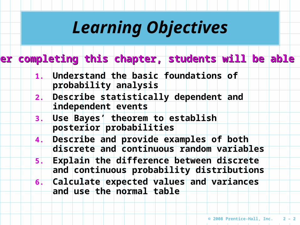
1. Understand the basic foundations of probability analysis
2. Describe statistically dependent and independent events
3. Use Bayes’ theorem to establish posterior probabilities
4. Describe and provide examples of both discrete and continuous random variables
5. Explain the difference between discrete and continuous probability distributions
6. Calculate expected values and variances and use the normal table
After completing this chapter, students will be able to:After completing this chapter, students will be able to:
© 2008 Prentice-Hall, Inc. 2 – 3
Chapter Outline
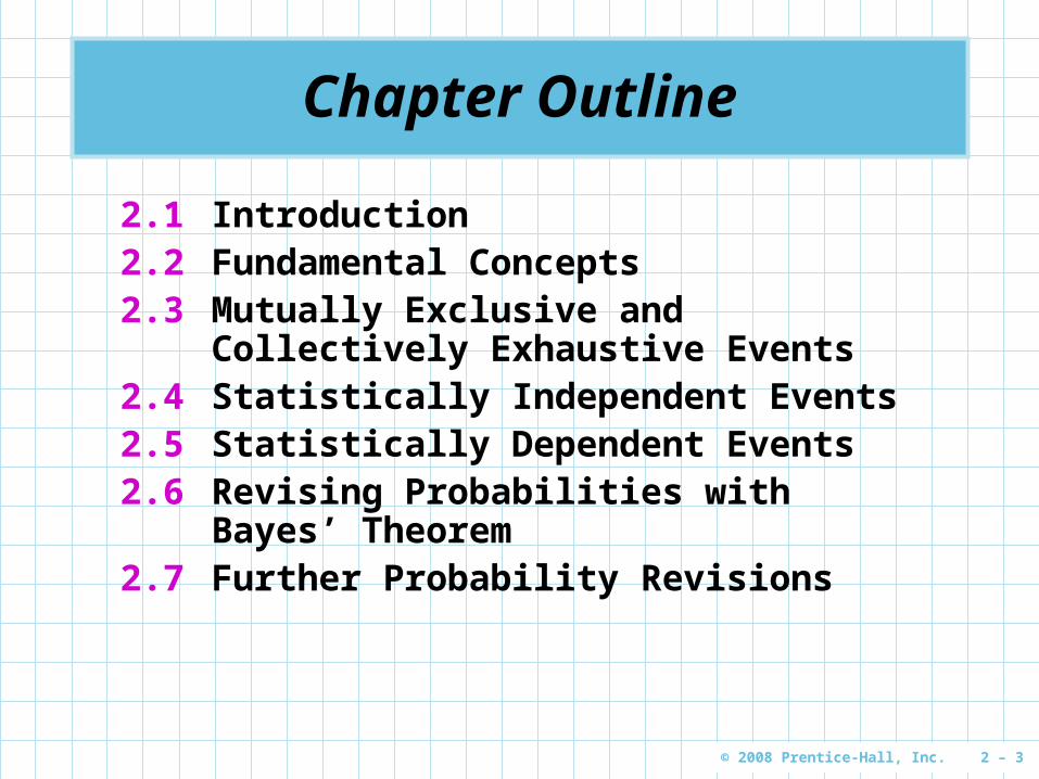
2.1 Introduction2.2 Fundamental Concepts2.3 Mutually Exclusive and Collectively
Exhaustive Events2.4 Statistically Independent Events2.5 Statistically Dependent Events2.6 Revising Probabilities with Bayes’
Theorem2.7 Further Probability Revisions
© 2008 Prentice-Hall, Inc. 2 – 4
Chapter Outline
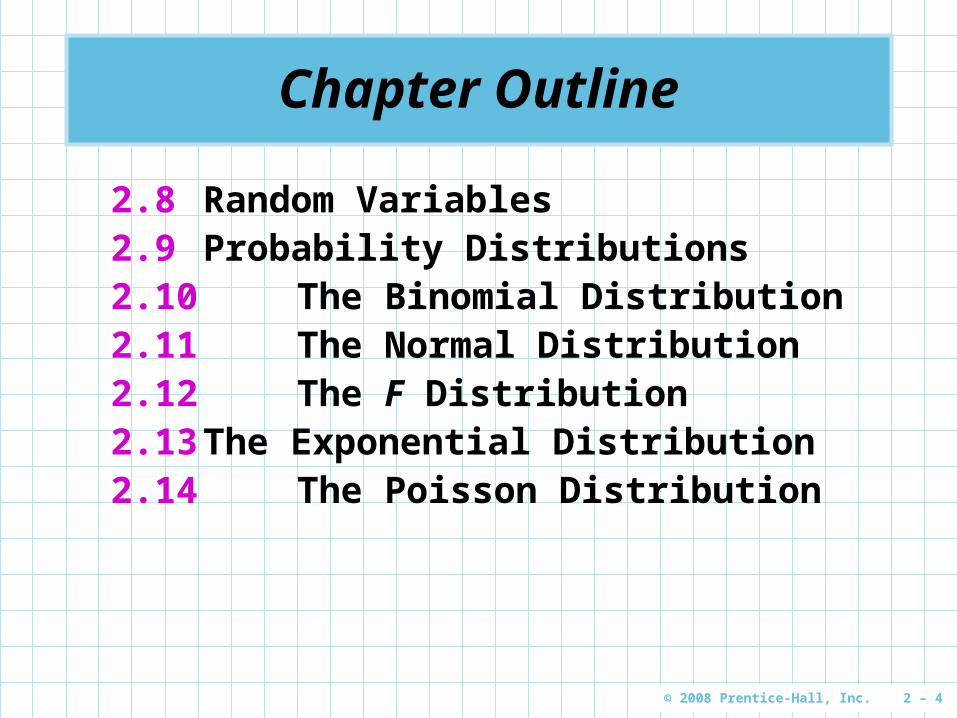
2.8 Random Variables2.9 Probability Distributions2.10 The Binomial Distribution2.11 The Normal Distribution2.12 The F Distribution2.13 The Exponential Distribution2.14 The Poisson Distribution
© 2008 Prentice-Hall, Inc. 2 – 5
Introduction
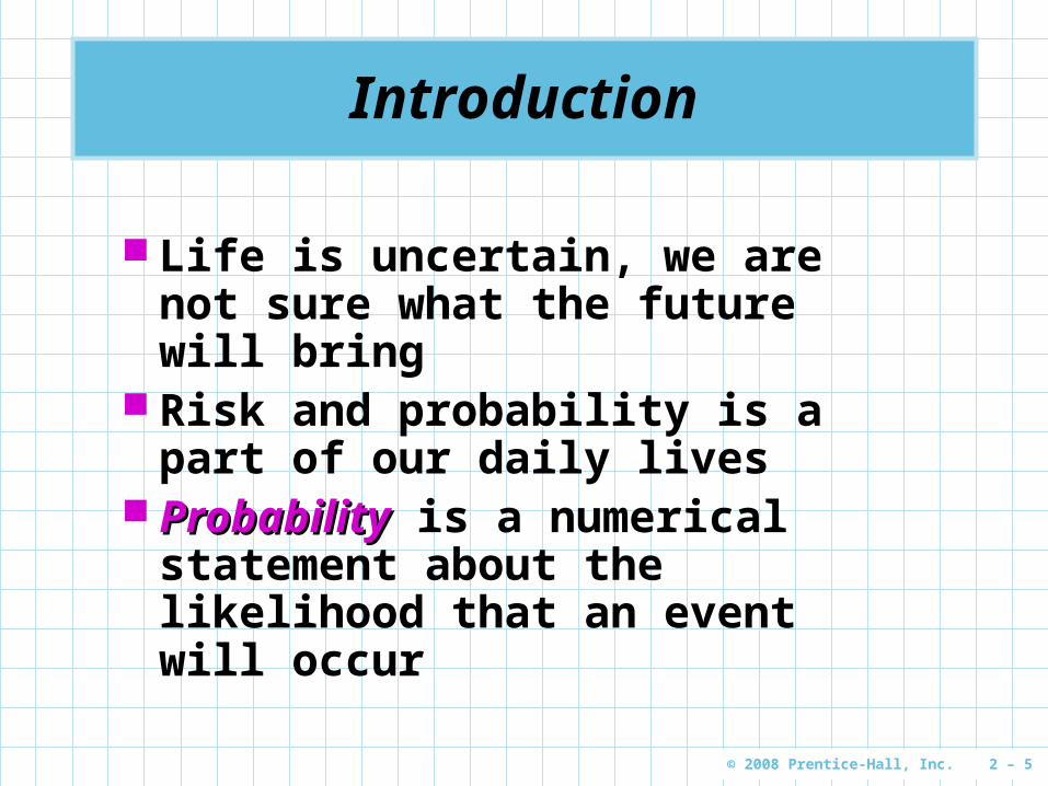
Life is uncertain, we are not sure what the future will bring
Risk and probability is a part of our daily lives
ProbabilityProbability is a numerical statement about the likelihood that an event will occur
© 2008 Prentice-Hall, Inc. 2 – 6
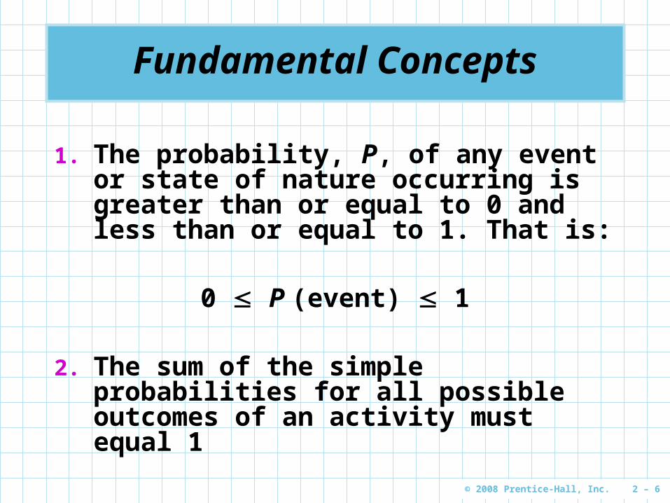
Fundamental Concepts
1. The probability, P, of any event or state of nature occurring is greater than or equal to 0 and less than or equal to 1. That is:
0 P (event) 1
2. The sum of the simple probabilities for all possible outcomes of an activity must equal 1
© 2008 Prentice-Hall, Inc. 2 – 7
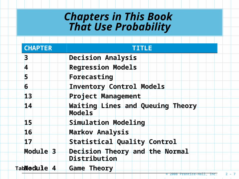
Chapters in This Book That Use Probability
CHAPTER TITLE
3 Decision Analysis
4 Regression Models
5 Forecasting
6 Inventory Control Models
13 Project Management
14 Waiting Lines and Queuing Theory Models
15 Simulation Modeling
16 Markov Analysis
17 Statistical Quality Control
Module 3 Decision Theory and the Normal Distribution
Module 4 Game Theory
Table 2.1
© 2008 Prentice-Hall, Inc. 2 – 8
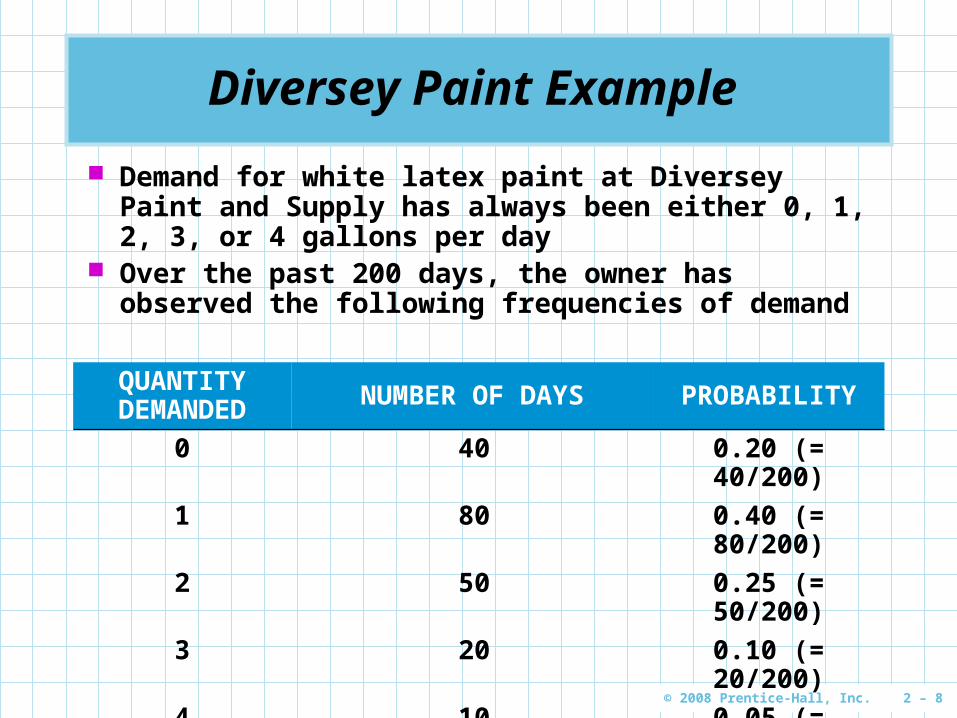
Diversey Paint Example
Demand for white latex paint at Diversey Paint and Supply has always been either 0, 1, 2, 3, or 4 gallons per day
Over the past 200 days, the owner has observed the following frequencies of demand
QUANTITY DEMANDED NUMBER OF DAYS PROBABILITY
0 40 0.20 (= 40/200)
1 80 0.40 (= 80/200)
2 50 0.25 (= 50/200)
3 20 0.10 (= 20/200)
4 10 0.05 (= 10/200)
Total 200
Total 1.00 (= 200/200)
© 2008 Prentice-Hall, Inc. 2 – 9
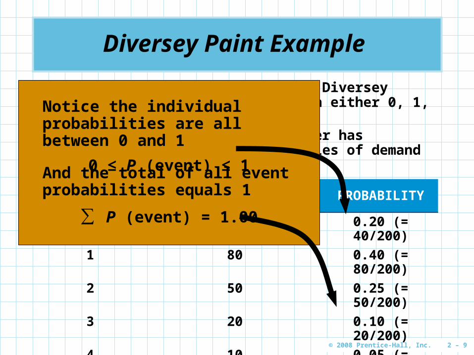
Diversey Paint Example
Demand for white latex paint at Diversey Paint and Supply has always been either 0, 1, 2, 3, or 4 gallons per day
Over the past 200 days, the owner has observed the following frequencies of demand
QUANTITY DEMANDED NUMBER OF DAYS PROBABILITY
0 40 0.20 (= 40/200)
1 80 0.40 (= 80/200)
2 50 0.25 (= 50/200)
3 20 0.10 (= 20/200)
4 10 0.05 (= 10/200)
Total 200
Total 1.00 (= 200/200)
Notice the individual probabilities are all between 0 and 1
0 ≤ P (event) ≤ 1And the total of all event probabilities equals 1
∑ P (event) = 1.00

© 2008 Prentice-Hall, Inc. 2 – 10
Determining objective probabilityobjective probability Relative frequency
Typically based on historical data
Types of Probability
P (event) =Number of occurrences of the event
Total number of trials or outcomes
Classical or logical method Logically determine probabilities without trials
P (head) = 12
Number of ways of getting a head
Number of possible outcomes (head or tail)
© 2008 Prentice-Hall, Inc. 2 – 11
Types of Probability
Subjective probabilitySubjective probability is based on the experience and judgment of the person making the estimate
Opinion polls Judgment of experts Delphi method Other methods
© 2008 Prentice-Hall, Inc. 2 – 12
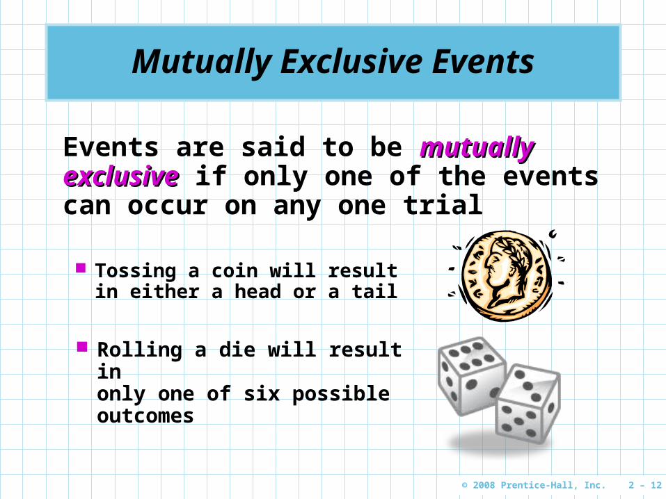
Mutually Exclusive Events
Events are said to be mutually mutually exclusiveexclusive if only one of the events can occur on any one trial
Tossing a coin will result in either a head or a tail
Rolling a die will result in only one of six possible outcomes
© 2008 Prentice-Hall, Inc. 2 – 13
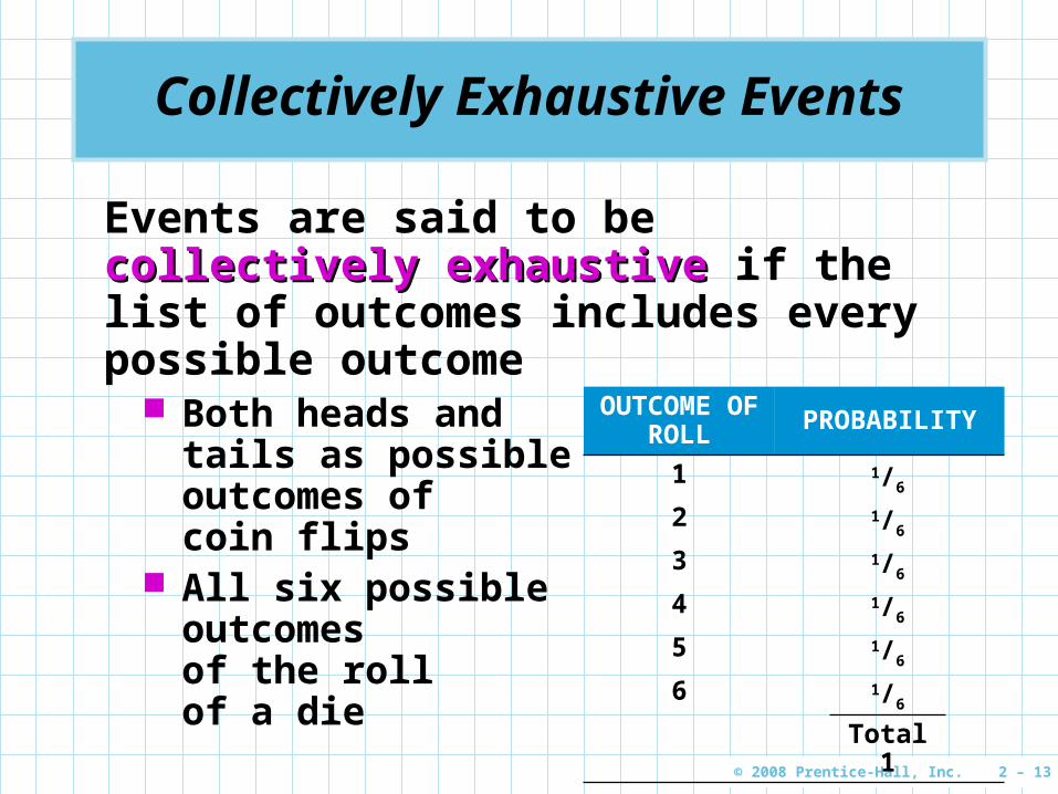
Collectively Exhaustive Events
Events are said to be collectively collectively exhaustiveexhaustive if the list of outcomes includes every possible outcome
Both heads and tails as possible outcomes of coin flips
All six possible outcomes of the roll of a die
OUTCOME OF ROLL PROBABILITY
1 1/6
2 1/6
3 1/6
4 1/6
5 1/6
6 1/6
Total 1

© 2008 Prentice-Hall, Inc. 2 – 14
Drawing a Card
Draw one card from a deck of 52 playing cards
P (drawing a 7) = 4/52 = 1/13
P (drawing a heart) = 13/52 = 1/4
These two events are not mutually exclusive since a 7 of hearts can be drawn
These two events are not collectively exhaustive since there are other cards in the deck besides 7s and hearts
© 2008 Prentice-Hall, Inc. 2 – 15
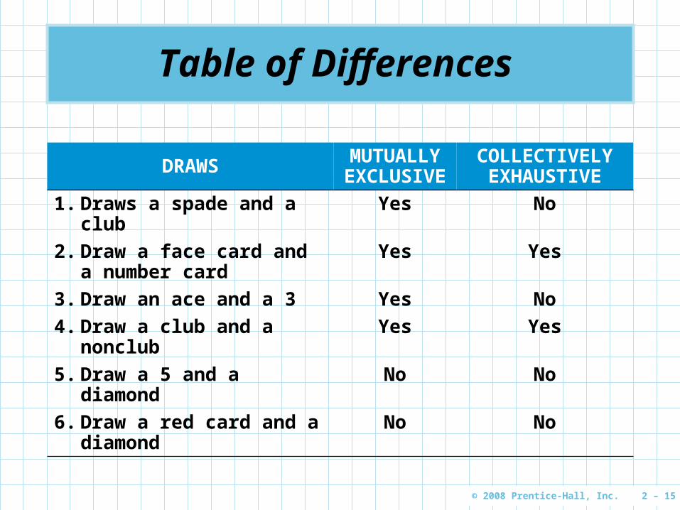
Table of Differences
DRAWS MUTUALLY EXCLUSIVE
COLLECTIVELY EXHAUSTIVE
1. Draws a spade and a club Yes No
2. Draw a face card and a number card
Yes Yes
3. Draw an ace and a 3 Yes No
4. Draw a club and a nonclub Yes Yes
5. Draw a 5 and a diamond No No
6. Draw a red card and a diamond
No No
© 2008 Prentice-Hall, Inc. 2 – 16
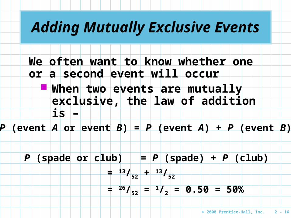
Adding Mutually Exclusive Events
We often want to know whether one or a second event will occur
When two events are mutually exclusive, the law of addition is –
P (event A or event B) = P (event A) + P (event B)
P (spade or club) = P (spade) + P (club)
= 13/52 + 13/52
= 26/52 = 1/2 = 0.50 = 50%

© 2008 Prentice-Hall, Inc. 2 – 17
Adding Not Mutually Exclusive Events
P (event A or event B) = P (event A) + P (event B)– P (event A and event B both occurring)
P (A or B) = P (A) + P (B) – P (A and B)
P(five or diamond) = P(five) + P(diamond) – P(five and diamond)
= 4/52 + 13/52 – 1/52
= 16/52 = 4/13
The equation must be modified to account for double counting
The probability is reduced by subtracting the chance of both events occurring together
© 2008 Prentice-Hall, Inc. 2 – 18
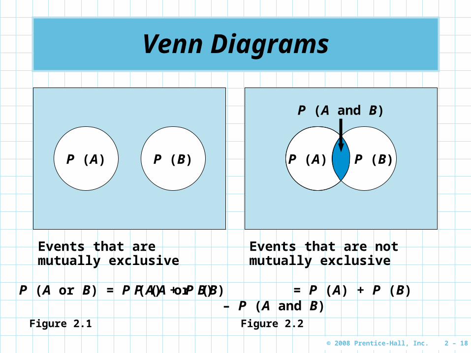
Venn Diagrams
P (A) P (B)
Events that are mutually exclusive
P (A or B) = P (A) + P (B)
Figure 2.1
Events that are not mutually exclusive
P (A or B) = P (A) + P (B) – P (A and B)
Figure 2.2
P (A) P (B)
P (A and B)
© 2008 Prentice-Hall, Inc. 2 – 19
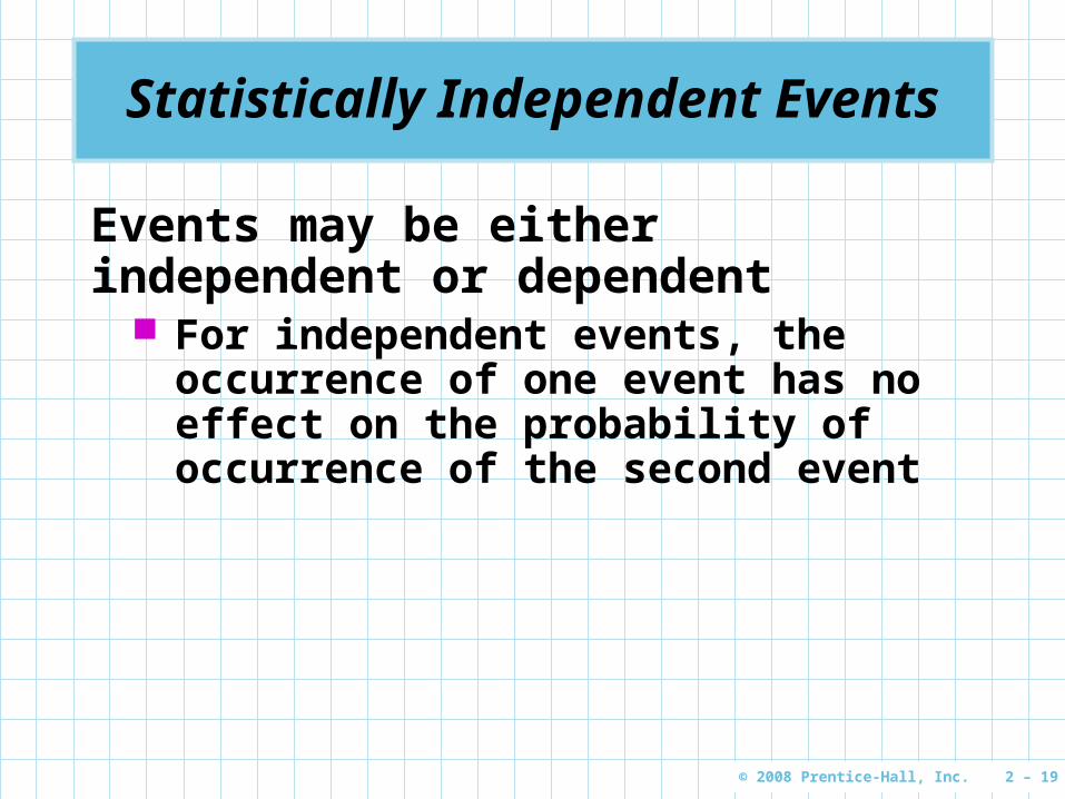
Statistically Independent Events
Events may be either independent or dependent
For independent events, the occurrence of one event has no effect on the probability of occurrence of the second event
© 2008 Prentice-Hall, Inc. 2 – 20
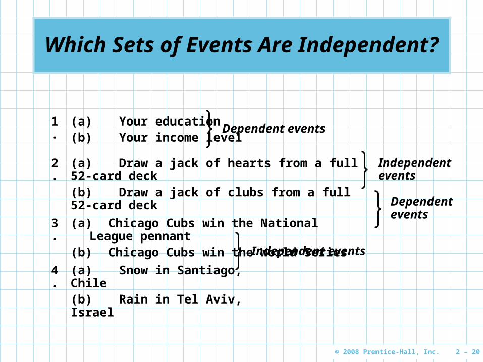
Which Sets of Events Are Independent?
1. (a) Your education(b) Your income level
2. (a) Draw a jack of hearts from a full 52-card deck(b) Draw a jack of clubs from a full 52-card deck
3. (a) Chicago Cubs win the National League pennant(b) Chicago Cubs win the World Series
4. (a) Snow in Santiago, Chile(b) Rain in Tel Aviv, Israel
Dependent events
Dependent events
Independent events
Independent events
© 2008 Prentice-Hall, Inc. 2 – 21
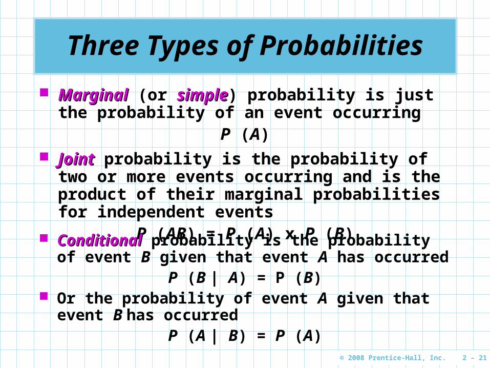
Three Types of Probabilities
MarginalMarginal (or simplesimple) probability is just the probability of an event occurring
P (A) JointJoint probability is the probability of two or more
events occurring and is the product of their marginal probabilities for independent events
P (AB) = P (A) x P (B) ConditionalConditional probability is the probability of event
B given that event A has occurredP (B | A) = P (B)
Or the probability of event A given that event B has occurred
P (A | B) = P (A)
© 2008 Prentice-Hall, Inc. 2 – 22
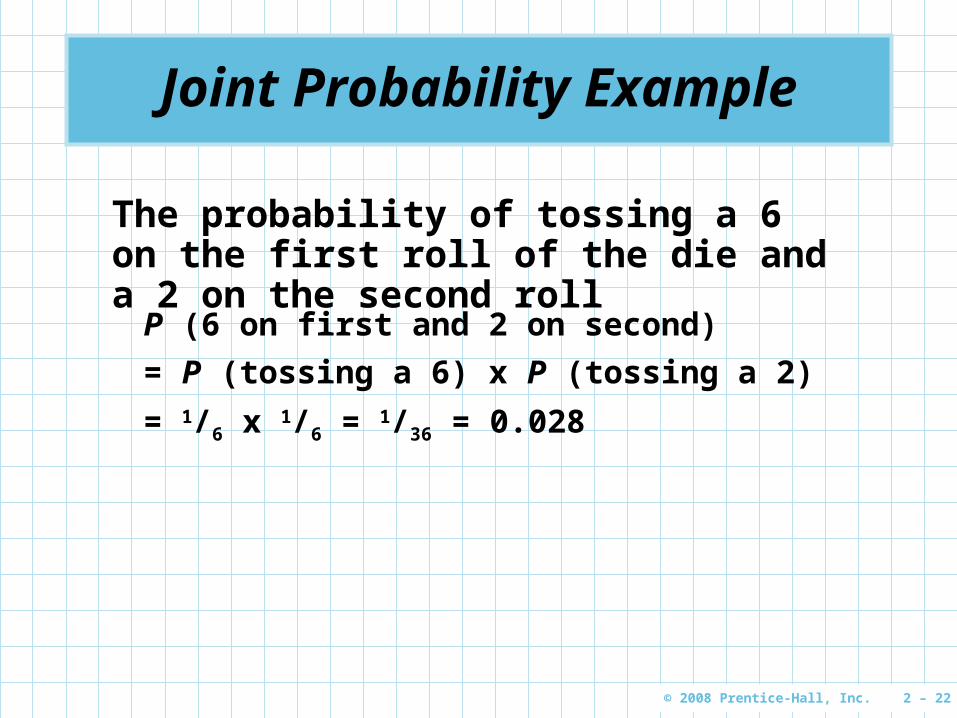
Joint Probability Example
The probability of tossing a 6 on the first roll of the die and a 2 on the second roll
P (6 on first and 2 on second)
= P (tossing a 6) x P (tossing a 2)
= 1/6 x 1/6 = 1/36 = 0.028
© 2008 Prentice-Hall, Inc. 2 – 23
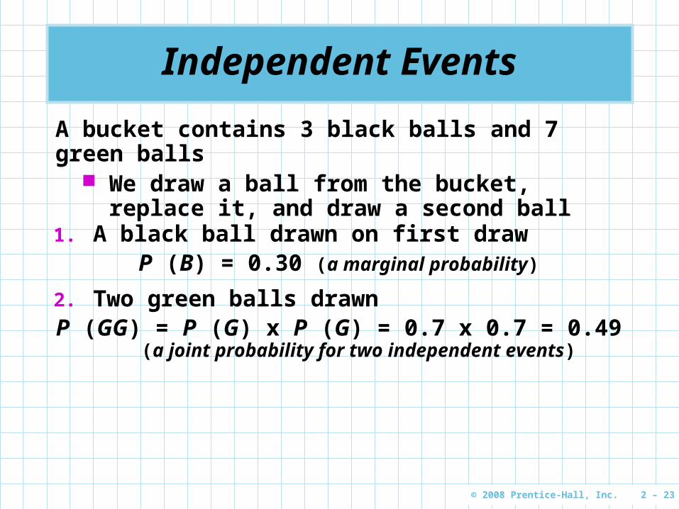
Independent Events
1. A black ball drawn on first drawP (B) = 0.30 (a marginal probability)
2. Two green balls drawnP (GG) = P (G) x P (G) = 0.7 x 0.7 = 0.49
(a joint probability for two independent events)
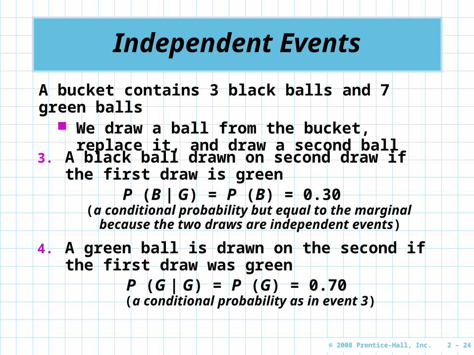
A bucket contains 3 black balls and 7 green balls We draw a ball from the bucket, replace it, and
draw a second ball
© 2008 Prentice-Hall, Inc. 2 – 24
Independent Events
3. A black ball drawn on second draw if the first draw is green
P (B | G) = P (B) = 0.30 (a conditional probability but equal to the marginal
because the two draws are independent events)
4. A green ball is drawn on the second if the first draw was green
P (G | G) = P (G) = 0.70(a conditional probability as in event 3)
A bucket contains 3 black balls and 7 green balls We draw a ball from the bucket, replace it, and
draw a second ball
© 2008 Prentice-Hall, Inc. 2 – 25
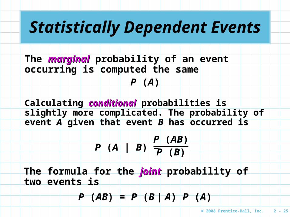
Statistically Dependent Events
The marginalmarginal probability of an event occurring is computed the same
P (A)
The formula for the jointjoint probability of two events is
P (AB) = P (B | A) P (A)
P (A | B) =P (AB)P (B)
Calculating conditionalconditional probabilities is slightly more complicated. The probability of event A given that event B has occurred is
© 2008 Prentice-Hall, Inc. 2 – 26
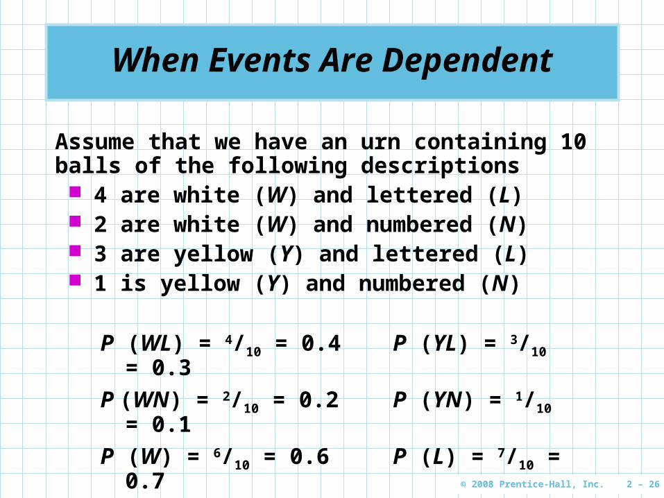
When Events Are Dependent
Assume that we have an urn containing 10 balls of the following descriptions 4 are white (W) and lettered (L) 2 are white (W) and numbered (N) 3 are yellow (Y) and lettered (L) 1 is yellow (Y) and numbered (N)
P (WL) = 4/10 = 0.4 P (YL) = 3/10 = 0.3
P (WN) = 2/10 = 0.2 P (YN) = 1/10 = 0.1
P (W) = 6/10 = 0.6 P (L) = 7/10 = 0.7
P (Y) = 4/10 = 0.4 P (N) = 3/10 = 0.3
© 2008 Prentice-Hall, Inc. 2 – 27
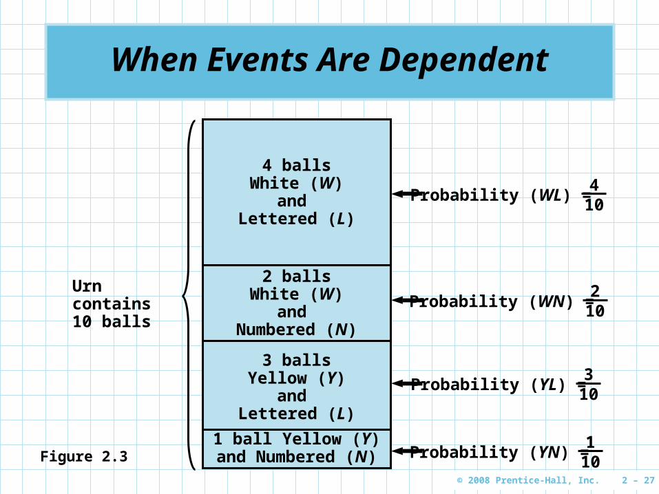
When Events Are Dependent
4 ballsWhite (W)
and Lettered (L)
2 ballsWhite (W)
and Numbered (N)
3 ballsYellow (Y)
and Lettered (L)
1 ball Yellow (Y)and Numbered (N)
Probability (WL) =4
10
Probability (YN) =1
10
Probability (YL) =3
10
Probability (WN) =2
10
Urn contains 10 balls
Figure 2.3
© 2008 Prentice-Hall, Inc. 2 – 28
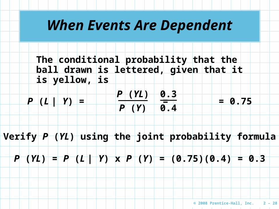
When Events Are Dependent
The conditional probability that the ball drawn is lettered, given that it is yellow, is
P (L | Y) = = = 0.75P (YL)
P (Y)
0.3
0.4
Verify P (YL) using the joint probability formula
P (YL) = P (L | Y) x P (Y) = (0.75)(0.4) = 0.3
© 2008 Prentice-Hall, Inc. 2 – 29
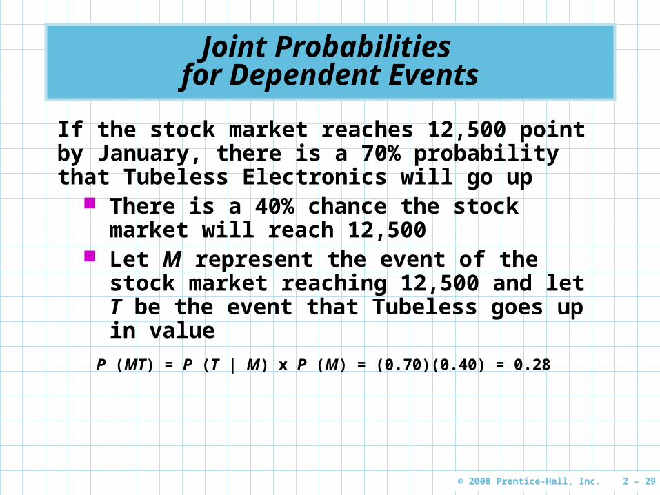
Joint Probabilities for Dependent Events
P (MT) = P (T | M) x P (M) = (0.70)(0.40) = 0.28
If the stock market reaches 12,500 point by January, there is a 70% probability that Tubeless Electronics will go up
There is a 40% chance the stock market will reach 12,500
Let M represent the event of the stock market reaching 12,500 and let T be the event that Tubeless goes up in value
© 2008 Prentice-Hall, Inc. 2 – 30
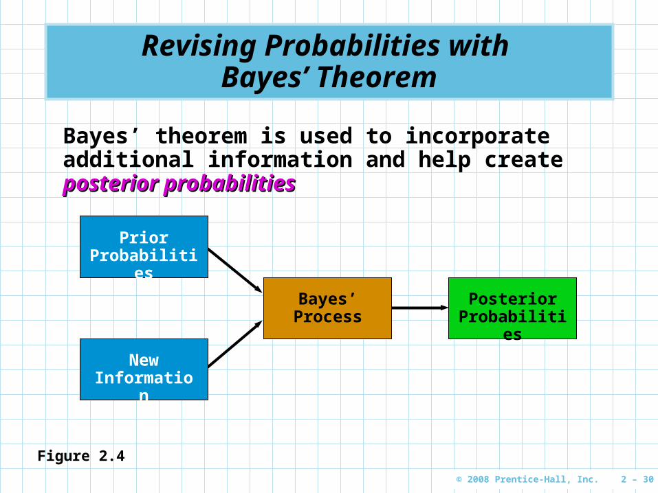
Posterior Probabilities
Bayes’ Process
Revising Probabilities with Bayes’ Theorem
Bayes’ theorem is used to incorporate additional information and help create posterior probabilitiesposterior probabilities
Prior Probabilities
New Information
Figure 2.4

© 2008 Prentice-Hall, Inc. 2 – 31
Posterior Probabilities
A cup contains two dice identical in appearance but one is fair (unbiased), the other is loaded (biased)
The probability of rolling a 3 on the fair die is 1/6 or 0.166 The probability of tossing the same number on the loaded
die is 0.60 We select one by chance,
toss it, and get a result of a 3 What is the probability that
the die rolled was fair? What is the probability that
the loaded die was rolled?
© 2008 Prentice-Hall, Inc. 2 – 32
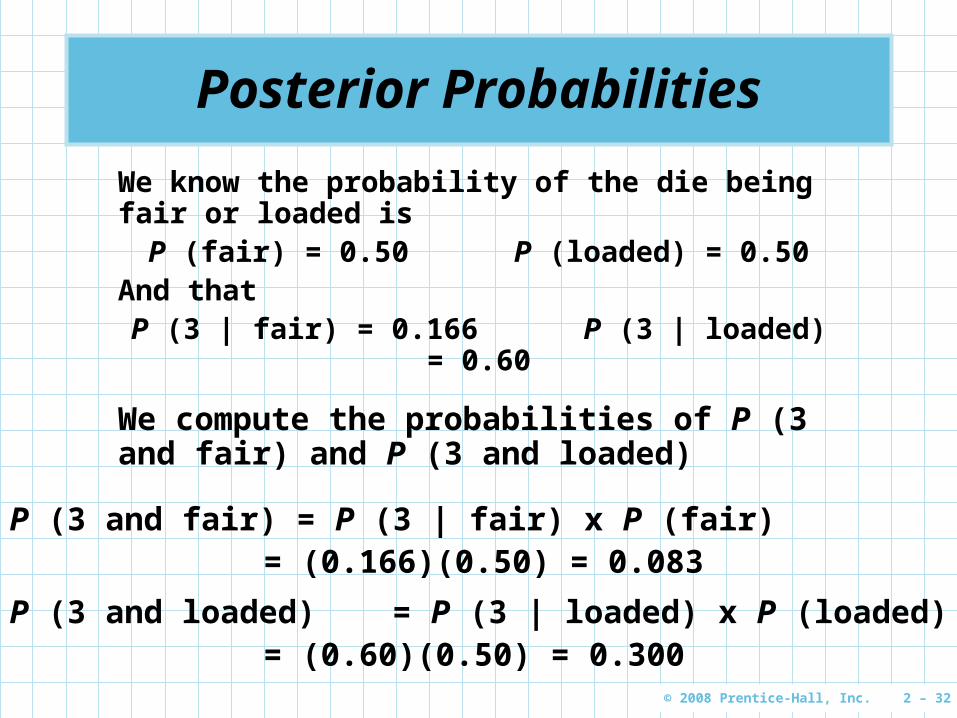
Posterior Probabilities
We know the probability of the die being fair or loaded is
P (fair) = 0.50 P (loaded) = 0.50And that
P (3 | fair) = 0.166 P (3 | loaded) = 0.60
We compute the probabilities of P (3 and fair) and P (3 and loaded)
P (3 and fair) = P (3 | fair) x P (fair)= (0.166)(0.50) = 0.083
P (3 and loaded) = P (3 | loaded) x P (loaded)= (0.60)(0.50) = 0.300
© 2008 Prentice-Hall, Inc. 2 – 33
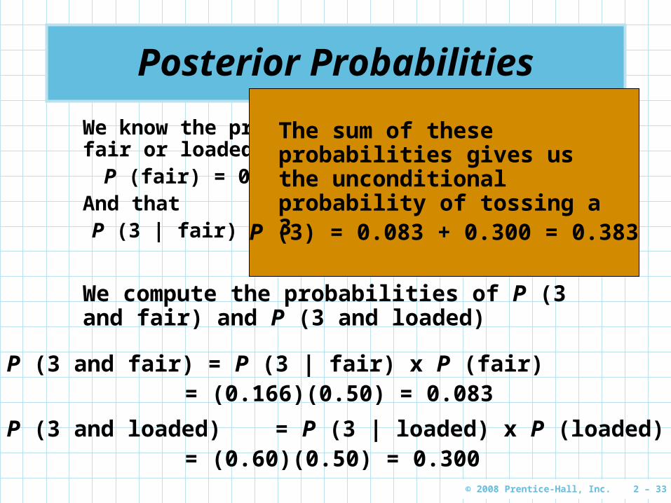
Posterior Probabilities
We know the probability of the die being fair or loaded is
P (fair) = 0.50 P (loaded) = 0.50And that
P (3 | fair) = 0.166 P (3 | loaded) = 0.60
We compute the probabilities of P (3 and fair) and P (3 and loaded)
P (3 and fair) = P (3 | fair) x P (fair)= (0.166)(0.50) = 0.083
P (3 and loaded) = P (3 | loaded) x P (loaded)= (0.60)(0.50) = 0.300
The sum of these probabilities gives us the unconditional probability of tossing a 3
P (3) = 0.083 + 0.300 = 0.383
© 2008 Prentice-Hall, Inc. 2 – 34
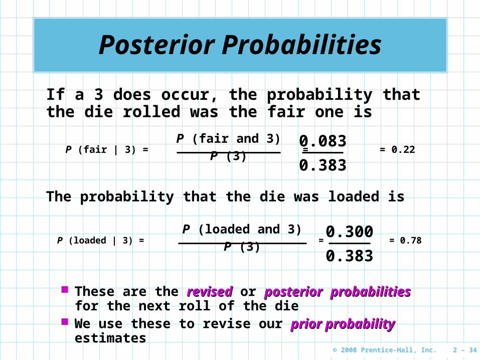
Posterior Probabilities
P (loaded | 3) = = = 0.78P (loaded and 3)
P (3)0.300
0.383
The probability that the die was loaded is
P (fair | 3) = = = 0.22P (fair and 3)
P (3)0.083
0.383
If a 3 does occur, the probability that the die rolled was the fair one is
These are the revisedrevised or posteriorposterior probabilitiesprobabilities for the next roll of the die
We use these to revise our prior probabilityprior probability estimates
© 2008 Prentice-Hall, Inc. 2 – 35
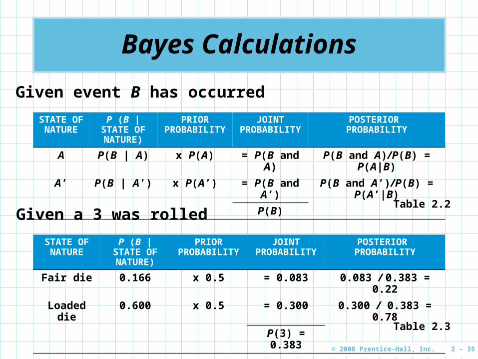
Bayes Calculations
Given event B has occurred
STATE OF NATURE
P (B | STATE OF NATURE)
PRIOR PROBABILITY
JOINT PROBABILITY
POSTERIOR PROBABILITY
A P(B | A) x P(A) = P(B and A) P(B and A)/P(B) = P(A|B)
A’ P(B | A’) x P(A’) = P(B and A’) P(B and A’)/P(B) = P(A’|B)
P(B)
Table 2.2Given a 3 was rolled
STATE OF NATURE
P (B | STATE OF NATURE)
PRIOR PROBABILITY
JOINT PROBABILITY
POSTERIOR PROBABILITY
Fair die 0.166 x 0.5 = 0.083 0.083 / 0.383 = 0.22
Loaded die 0.600 x 0.5 = 0.300 0.300 / 0.383 = 0.78
P(3) = 0.383
Table 2.3
© 2008 Prentice-Hall, Inc. 2 – 36
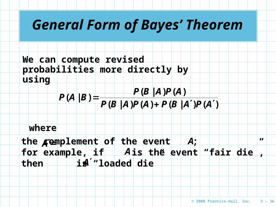
General Form of Bayes’ Theorem
)()|()()|()()|(
)|(APABPAPABP
APABPBAP
We can compute revised probabilities more directly by using
where
the complement of the event ; for example, if is the event “fair die”, then is “loaded die”
AA
A
A
© 2008 Prentice-Hall, Inc. 2 – 37
General Form of Bayes’ Theorem
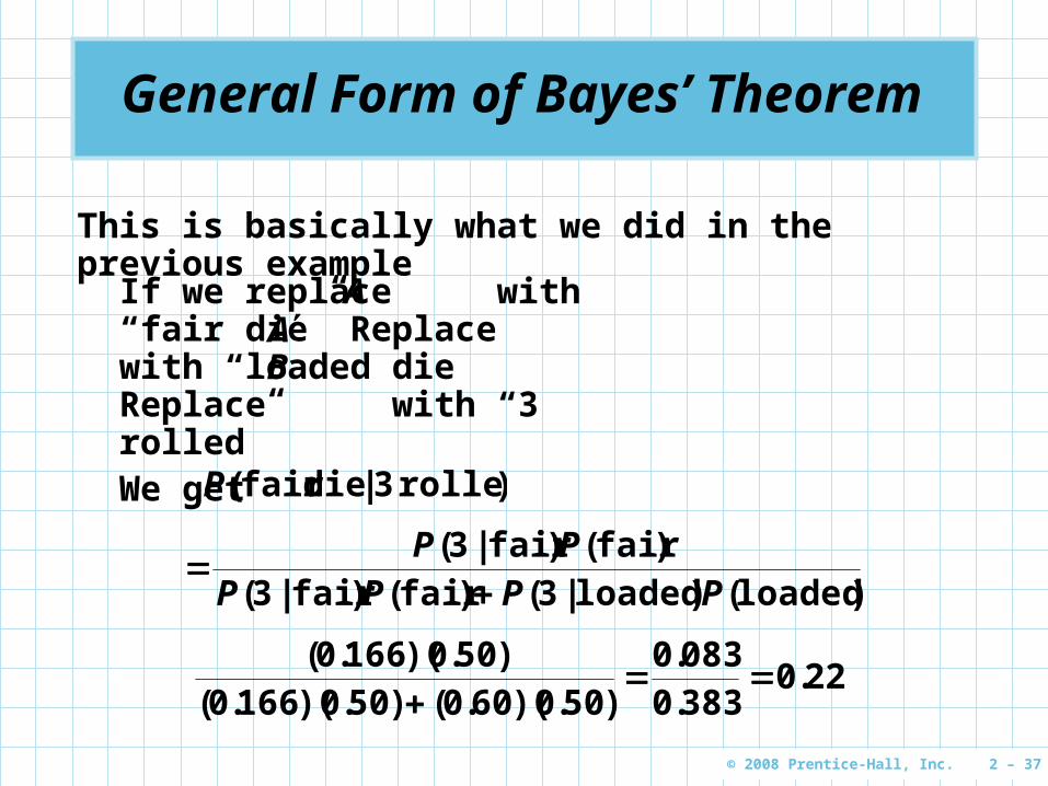
This is basically what we did in the previous example
If we replace with “fair die” Replace with “loaded die Replace with “3 rolled”We get
AAB
)|( rolled 3die fairP
)()|()()|()()|(
loadedloaded3fairfair3fairfair3
PPPPPP
22038300830
50060050016605001660
...
).)(.().)(.().)(.(

© 2008 Prentice-Hall, Inc. 2 – 38
Further Probability Revisions
We can obtain additional information by performing the experiment a second time
If you can afford it, perform experiments several times
We roll the die again and again get a 3
500loaded and 500fair .)(.)( PP
3606060loaded33
027016601660fair33
.).)(.()|,(
.).)(.()|,(
P
P
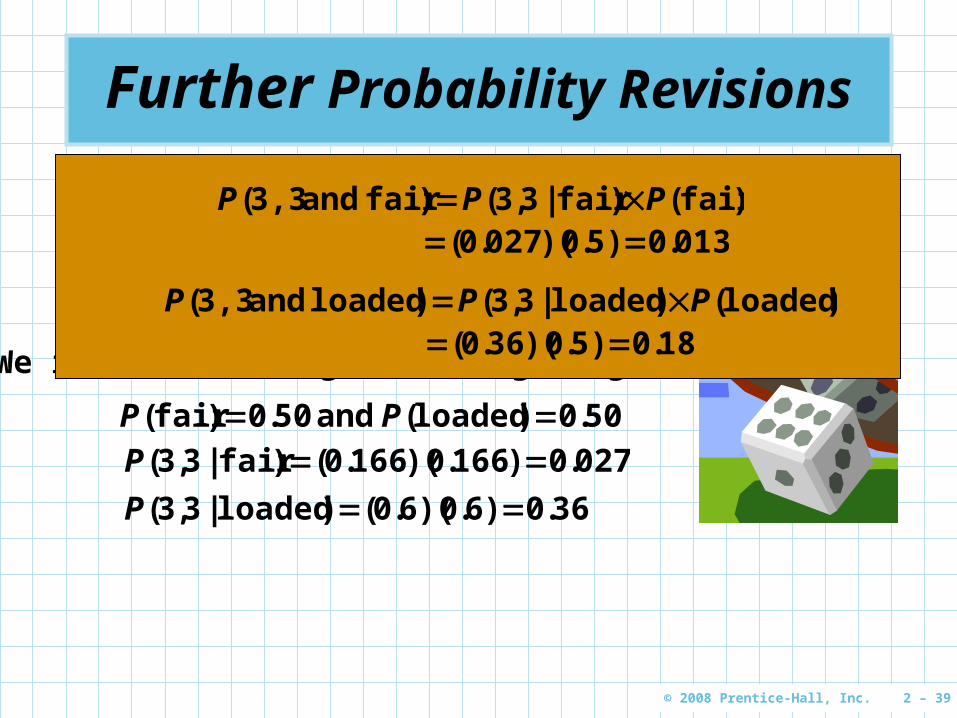
© 2008 Prentice-Hall, Inc. 2 – 39
Further Probability Revisions
We can obtain additional information by performing the experiment a second time
If you can afford it, perform experiments several times
We roll the die again and again get a 3
500loaded and 500fair .)(.)( PP
3606060loaded33
027016601660fair33
.).)(.()|,(
.).)(.()|,(
P
P
)()|,()( fairfair33fair and 3,3 PPP 0130500270 .).)(.(
)()|,()( loadedloaded33loaded and 3,3 PPP 18050360 .).)(.(
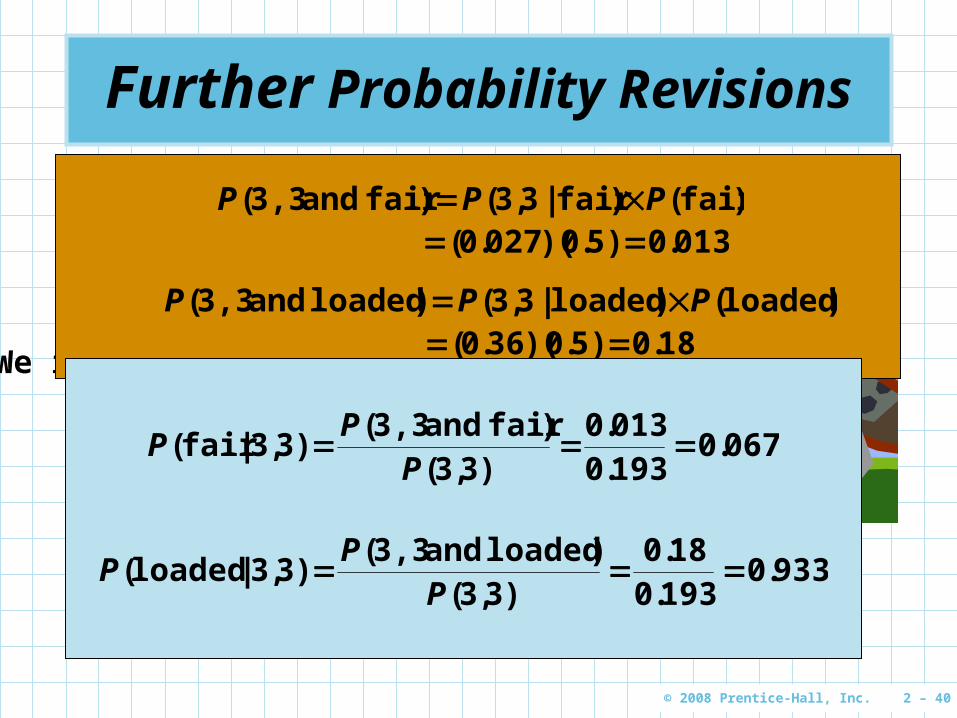
© 2008 Prentice-Hall, Inc. 2 – 40
Further Probability Revisions
We can obtain additional information by performing the experiment a second time
If you can afford it, perform experiments several times
We roll the die again and again get a 3
50.0)loaded( and 50.0)fair( PP
36.0)6.0)(6.0()loaded|3,3(
027.0)166.0)(166.0()fair|3,3(
P
P
)()|,()( fairfair33fair and 3,3 PPP 0130500270 .).)(.(
)()|,()( loadedloaded33loaded and 3,3 PPP 18050360 .).)(.(
067019300130
33fair and 3,3
33fair ...
),()(
),|( P
PP
93301930180
33loaded and 3,3
33loaded ...
),()(
),|( P
PP
© 2008 Prentice-Hall, Inc. 2 – 41
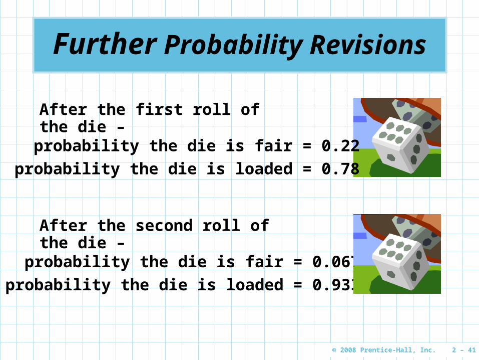
Further Probability Revisions
After the first roll of the die –
probability the die is fair = 0.22
probability the die is loaded = 0.78
After the second roll of the die –
probability the die is fair = 0.067
probability the die is loaded = 0.933
© 2008 Prentice-Hall, Inc. 2 – 42
Random Variables
Discrete random variablesDiscrete random variables can assume only a finite or limited set of values
Continuous random variablesContinuous random variables can assume any one of an infinite set of values
A random variablerandom variable assigns a real number to every possible outcome or event in an experiment
X = number of refrigerators sold during the day
© 2008 Prentice-Hall, Inc. 2 – 43
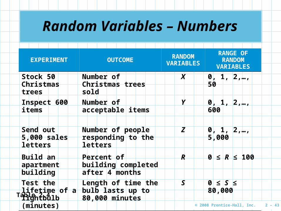
Random Variables – Numbers
EXPERIMENT OUTCOME RANDOM VARIABLES
RANGE OF RANDOM
VARIABLES
Stock 50 Christmas trees
Number of Christmas trees sold
X 0, 1, 2,…, 50
Inspect 600 items
Number of acceptable items
Y 0, 1, 2,…, 600
Send out 5,000 sales letters
Number of people responding to the letters
Z 0, 1, 2,…, 5,000
Build an apartment building
Percent of building completed after 4 months
R 0 ≤ R ≤ 100
Test the lifetime of a lightbulb (minutes)
Length of time the bulb lasts up to 80,000 minutes
S 0 ≤ S ≤ 80,000
Table 2.4
© 2008 Prentice-Hall, Inc. 2 – 44
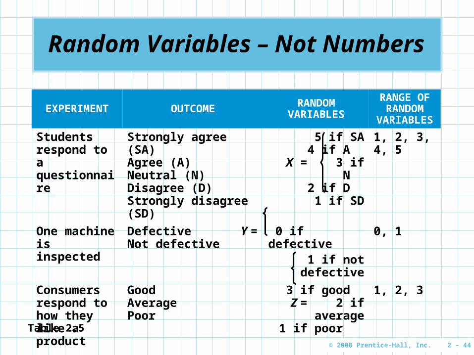
Random Variables – Not Numbers
EXPERIMENT OUTCOME RANDOM VARIABLES
RANGE OF RANDOM
VARIABLES
Students respond to a questionnaire
Strongly agree (SA)Agree (A)Neutral (N)Disagree (D)Strongly disagree (SD)
5 if SA4 if A..
X = 3 if N..2 if D..1 if SD
1, 2, 3, 4, 5
One machine is inspected
Defective Y =Not defective
0 if defective1 if not defective
0, 1
Consumers respond to how they like a product
GoodAveragePoor
3 if good….Z = 2 if average
1 if poor…..
1, 2, 3
Table 2.5

© 2008 Prentice-Hall, Inc. 2 – 45
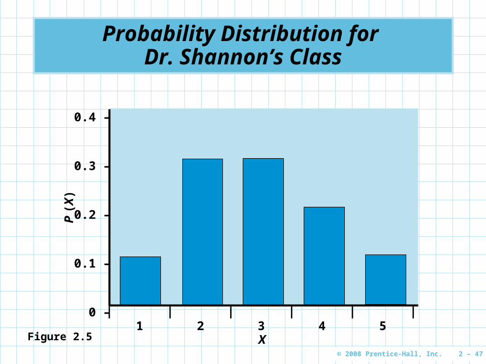
Probability Distribution of a Discrete Random Variable
Dr. Shannon asked students to respond to the statement, “The textbook was well written and helped me acquire the necessary information.”
Selecting the right probability distribution is important
For discrete random variablesdiscrete random variables a probability is assigned to each event
5. Strongly agree4. Agree3. Neutral2. Disagree1. Strongly disagree

© 2008 Prentice-Hall, Inc. 2 – 46
Probability Distribution of a Discrete Random Variable
OUTCOMERANDOM VARIABLE (X)
NUMBER RESPONDING
PROBABILITY P (X)
Strongly agree 5 10 0.1 = 10/100
Agree 4 20 0.2 = 20/100
Neutral 3 30 0.3 = 30/100
Disagree 2 30 0.3 = 30/100
Strongly disagree 1 10 0.1 = 10/100
Total 100 1.0 = 100/100
Distribution follows all three rules1. Events are mutually exclusive and collectively exhaustive2. Individual probability values are between 0 and 13. Total of all probability values equals 1
Table 2.6
© 2008 Prentice-Hall, Inc. 2 – 47
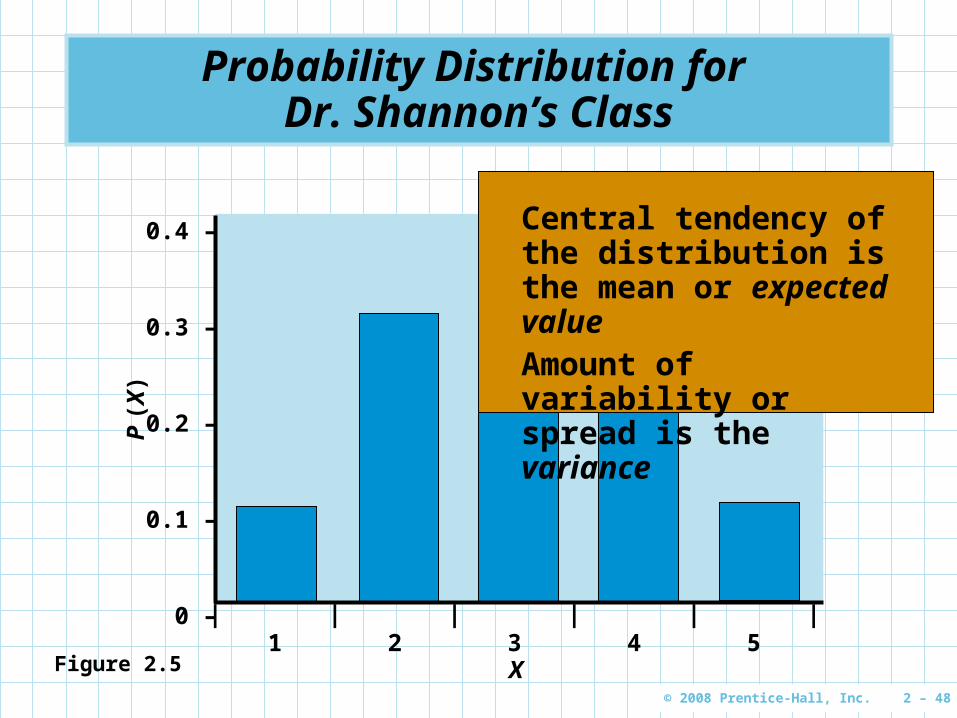
Probability Distribution for Dr. Shannon’s ClassP
(X
)
0.4 –
0.3 –
0.2 –
0.1 –
0 –| | | | | |1 2 3 4 5
XFigure 2.5
© 2008 Prentice-Hall, Inc. 2 – 48
Probability Distribution for Dr. Shannon’s ClassP
(X
)
0.4 –
0.3 –
0.2 –
0.1 –
0 –| | | | | |1 2 3 4 5
XFigure 2.5
Central tendency of the distribution is the mean or expected valueAmount of variability or spread is the variance
© 2008 Prentice-Hall, Inc. 2 – 49
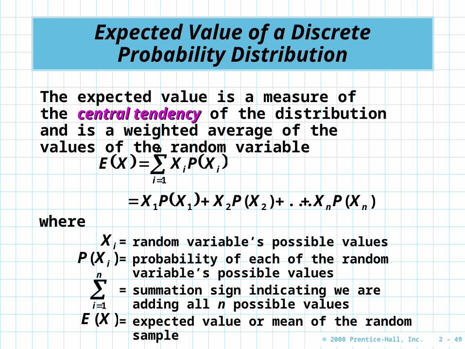
Expected Value of a Discrete Probability Distribution
n
iii XPXXE
1
)(...)( 2211 nn XPXXPXXPX
The expected value is a measure of the central central tendencytendency of the distribution and is a weighted average of the values of the random variable
where
iX)( iXP
n
i 1
)(XE
= random variable’s possible values= probability of each of the random variable’s
possible values= summation sign indicating we are adding all n
possible values= expected value or mean of the random sample
© 2008 Prentice-Hall, Inc. 2 – 50
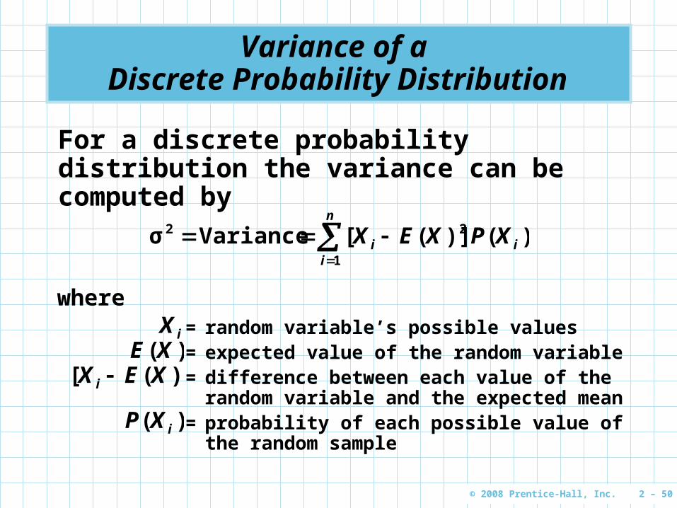
Variance of a Discrete Probability Distribution
For a discrete probability distribution the variance can be computed by
)()]([
n
iii XPXEX
1
22 Varianceσ
where
iX)(XE
)( iXP
= random variable’s possible values= expected value of the random variable= difference between each value of the random
variable and the expected mean= probability of each possible value of the
random sample
)]([ XEX i

© 2008 Prentice-Hall, Inc. 2 – 51
Variance of a Discrete Probability Distribution
For Dr. Shannon’s class
)()]([variance5
1
2
i
ii XPXEX
).().().().(variance 2092410925 22
).().().().( 3092230923 22
).().( 10921 2
291
36102430003024204410
.
.....
© 2008 Prentice-Hall, Inc. 2 – 52
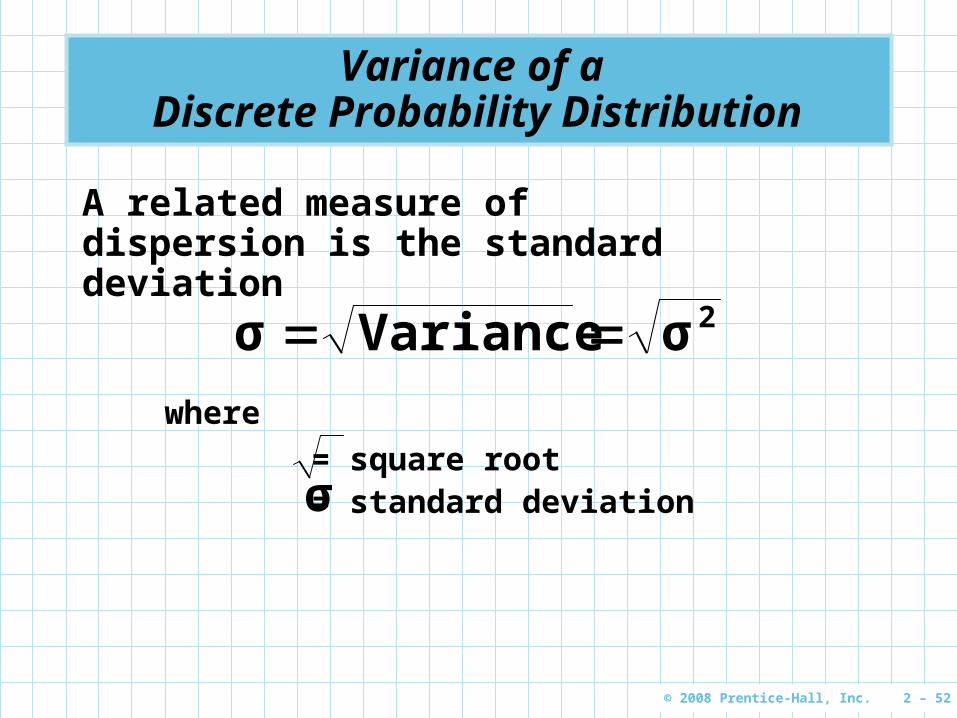
Variance of a Discrete Probability Distribution
A related measure of dispersion is the standard deviation
2σVarianceσ where
σ= square root= standard deviation
© 2008 Prentice-Hall, Inc. 2 – 53
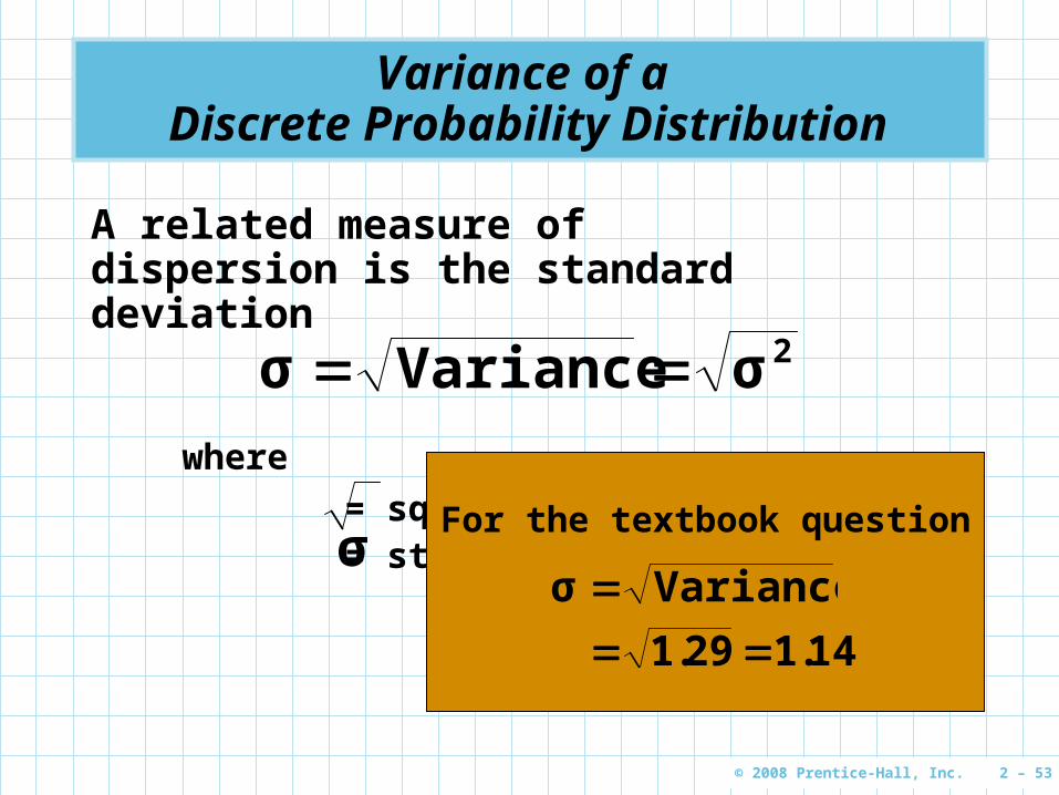
Variance of a Discrete Probability Distribution
A related measure of dispersion is the standard deviation
2σVarianceσ where
σ= square root= standard deviation
For the textbook question
Varianceσ 141291 ..
© 2008 Prentice-Hall, Inc. 2 – 54
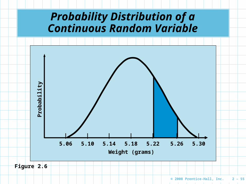
Probability Distribution of a Continuous Random Variable
Since random variables can take on an infinite number of values, the fundamental rules for continuous random variables must be modified
The sum of the probability values must still equal 1
But the probability of each value of the random variable must equal 0 or the sum would be infinitely large
The probability distribution is defined by a continuous mathematical function called the probability density function or just the probability function
Represented by f (X)
© 2008 Prentice-Hall, Inc. 2 – 55
Probability Distribution of a Continuous Random Variable
Pro
bab
ility
| | | | | | |
5.06 5.10 5.14 5.18 5.22 5.26 5.30
Weight (grams)
Figure 2.6
© 2008 Prentice-Hall, Inc. 2 – 56
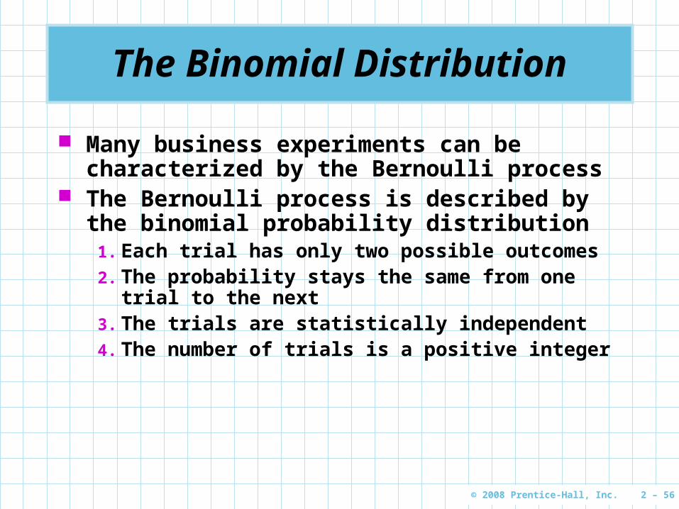
The Binomial Distribution
Many business experiments can be characterized by the Bernoulli process
The Bernoulli process is described by the binomial probability distribution
1. Each trial has only two possible outcomes2. The probability stays the same from one trial
to the next3. The trials are statistically independent4. The number of trials is a positive integer
© 2008 Prentice-Hall, Inc. 2 – 57
The Binomial Distribution
The binomial distribution is used to find the probability of a specific number of successes out of n trials
We need to know
n = number of trialsp = the probability of success on any
single trial
We letr = number of successesq = 1 – p = the probability of a failure
© 2008 Prentice-Hall, Inc. 2 – 58
The Binomial Distribution
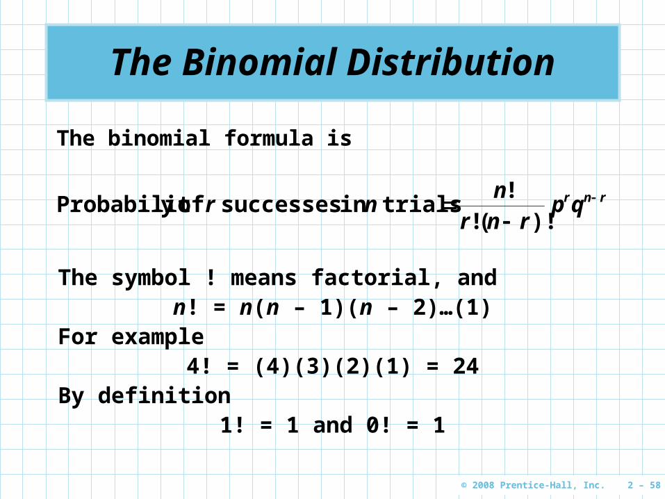
The binomial formula is
rnrqprnr
nnr
)!(!!
trials in successes of yProbabilit
The symbol ! means factorial, and n! = n(n – 1)(n – 2)…(1)
For example4! = (4)(3)(2)(1) = 24
By definition1! = 1 and 0! = 1
© 2008 Prentice-Hall, Inc. 2 – 59
The Binomial Distribution
NUMBER OFHEADS (r) Probability = (0.5)r(0.5)5 – r
5!r!(5 – r)!
0 0.03125 = (0.5)0(0.5)5 – 0
1 0.15625 = (0.5)1(0.5)5 – 1
2 0.31250 = (0.5)2(0.5)5 – 2
3 0.31250 = (0.5)3(0.5)5 – 3
4 0.15625 = (0.5)4(0.5)5 – 4
5 0.03125 = (0.5)5(0.5)5 – 5
5!0!(5 – 0)!
5!1!(5 – 1)!
5!2!(5 – 2)!
5!3!(5 – 3)!
5!4!(5 – 4)!
5!5!(5 – 5)!
Table 2.7

© 2008 Prentice-Hall, Inc. 2 – 60
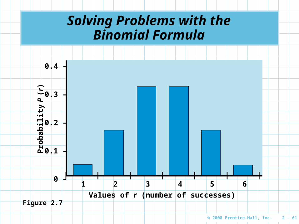
Solving Problems with the Binomial Formula
We want to find the probability of 4 heads in 5 tosses
n = 5, r = 4, p = 0.5, and q = 1 – 0.5 = 0.5
Thus454 5050
4545
trials 5 in successes 4
..
)!(!!
)(P
15625050062501123412345
.).)(.()!)()()(())()()((
Or about 16%
© 2008 Prentice-Hall, Inc. 2 – 61
Solving Problems with the Binomial Formula
Pro
bab
ilit
y P
(r)
| | | | | | |1 2 3 4 5 6
Values of r (number of successes)
0.4 –
0.3 –
0.2 –
0.1 –
0 –
Figure 2.7
© 2008 Prentice-Hall, Inc. 2 – 62
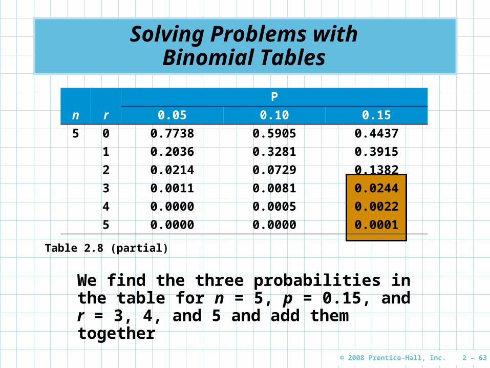
Solving Problems with Binomial Tables
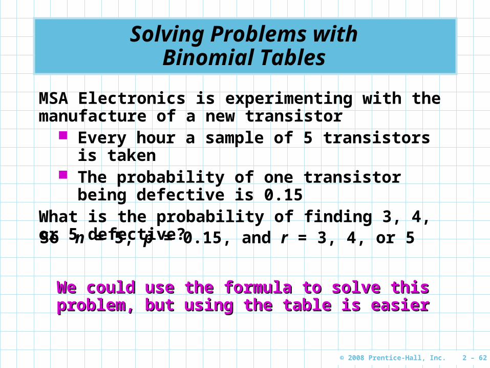
MSA Electronics is experimenting with the manufacture of a new transistor
Every hour a sample of 5 transistors is taken The probability of one transistor being
defective is 0.15What is the probability of finding 3, 4, or 5 defective?
n = 5, p = 0.15, and r = 3, 4, or 5So
We could use the formula to solve this problem, We could use the formula to solve this problem, but using the table is easierbut using the table is easier
© 2008 Prentice-Hall, Inc. 2 – 63
Solving Problems with Binomial Tables
P
n r 0.05 0.10 0.15
5 0 0.7738 0.5905 0.4437
1 0.2036 0.3281 0.3915
2 0.0214 0.0729 0.1382
3 0.0011 0.0081 0.0244
4 0.0000 0.0005 0.0022
5 0.0000 0.0000 0.0001Table 2.8 (partial)
We find the three probabilities in the table for n = 5, p = 0.15, and r = 3, 4, and 5 and add them together

© 2008 Prentice-Hall, Inc. 2 – 64
Table 2.8 (partial)
We find the three probabilities in the table for n = 5, p = 0.15, and r = 3, 4, and 5 and add them together
Solving Problems with Binomial Tables
P
n r 0.05 0.10 0.15
5 0 0.7738 0.5905 0.4437
1 0.2036 0.3281 0.3915
2 0.0214 0.0729 0.1382
3 0.0011 0.0081 0.0244
4 0.0000 0.0005 0.0022
5 0.0000 0.0000 0.0001
)()()()( 543defects more or 3 PPPP
02670000100022002440 ....
© 2008 Prentice-Hall, Inc. 2 – 65
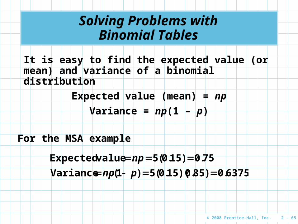
Solving Problems with Binomial Tables
It is easy to find the expected value (or mean) and variance of a binomial distribution
Expected value (mean) = np
Variance = np(1 – p)
For the MSA example
6375085015051Variance
7501505value Expected
.).)(.()(
.).(
pnp
np
© 2008 Prentice-Hall, Inc. 2 – 66
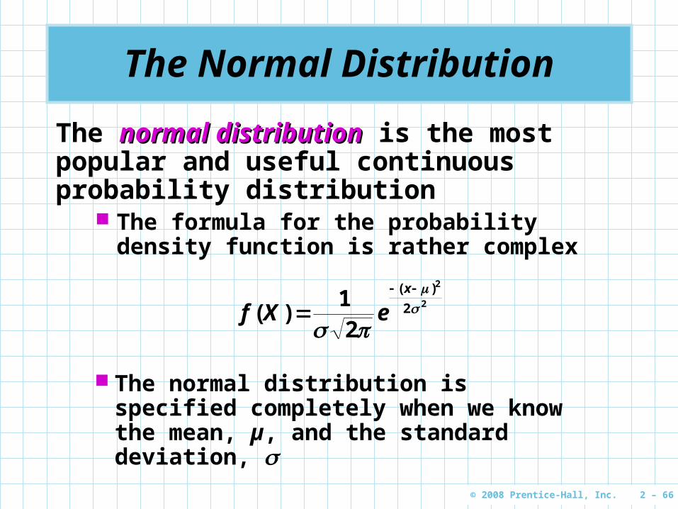
The Normal Distribution
The normal distributionnormal distribution is the most popular and useful continuous probability distribution
The formula for the probability density function is rather complex
2
2
2
21
)(
)(
x
eXf
The normal distribution is specified completely when we know the mean, µ, and the standard deviation,
© 2008 Prentice-Hall, Inc. 2 – 67
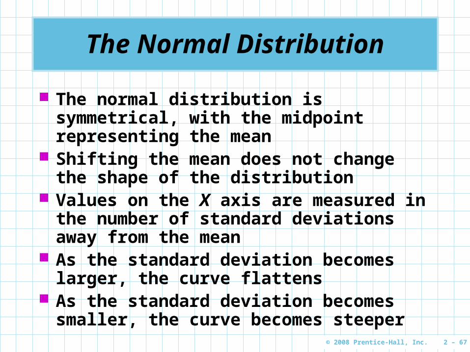
The Normal Distribution
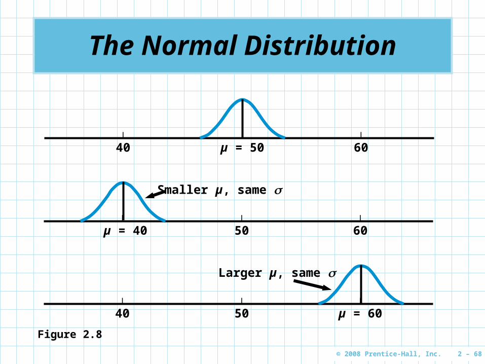
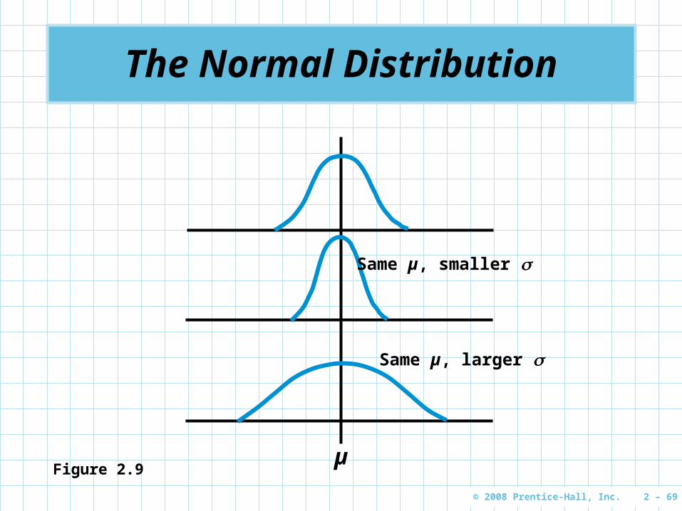
The normal distribution is symmetrical, with the midpoint representing the mean
Shifting the mean does not change the shape of the distribution
Values on the X axis are measured in the number of standard deviations away from the mean
As the standard deviation becomes larger, the curve flattens
As the standard deviation becomes smaller, the curve becomes steeper
© 2008 Prentice-Hall, Inc. 2 – 68
The Normal Distribution
| | |
40 µ = 50 60
| | |
µ = 40 50 60
Smaller µ, same
| | |
40 50 µ = 60
Larger µ, same
Figure 2.8
© 2008 Prentice-Hall, Inc. 2 – 69
µ
The Normal Distribution
Figure 2.9
Same µ, smaller
Same µ, larger
© 2008 Prentice-Hall, Inc. 2 – 70
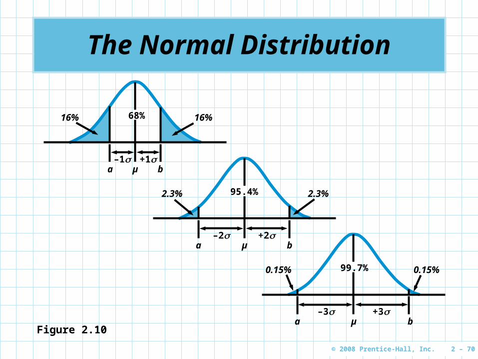
The Normal Distribution
Figure 2.10
68%16% 16%
–1 +1a µ b
95.4%2.3% 2.3%
–2 +2a µ b
99.7%0.15% 0.15%
–3 +3a µ b
© 2008 Prentice-Hall, Inc. 2 – 71
The Normal Distribution
If IQs in the United States were normally distributed with µ = 100 and = 15, then
1. 68% of the population would have IQs between 85 and 115 points (±1)
2. 95.4% of the people have IQs between 70 and 130 (±2)
3. 99.7% of the population have IQs in the range from 55 to 145 points (±3)
4. Only 16% of the people have IQs greater than 115 points (from the first graph, the area to the right of +1)
© 2008 Prentice-Hall, Inc. 2 – 72
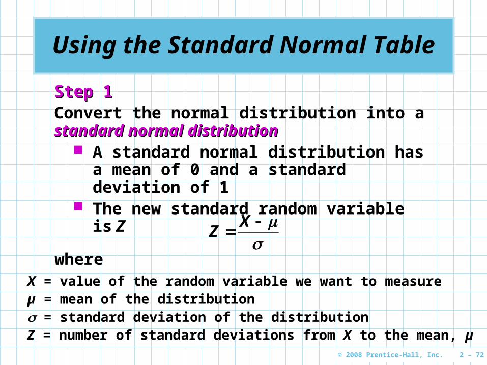
Using the Standard Normal Table
Step 1Step 1Convert the normal distribution into a standard standard normal distributionnormal distribution
A standard normal distribution has a mean of 0 and a standard deviation of 1
The new standard random variable is Z
X
Z
whereX = value of the random variable we want to measureµ = mean of the distribution = standard deviation of the distributionZ = number of standard deviations from X to the mean, µ
© 2008 Prentice-Hall, Inc. 2 – 73
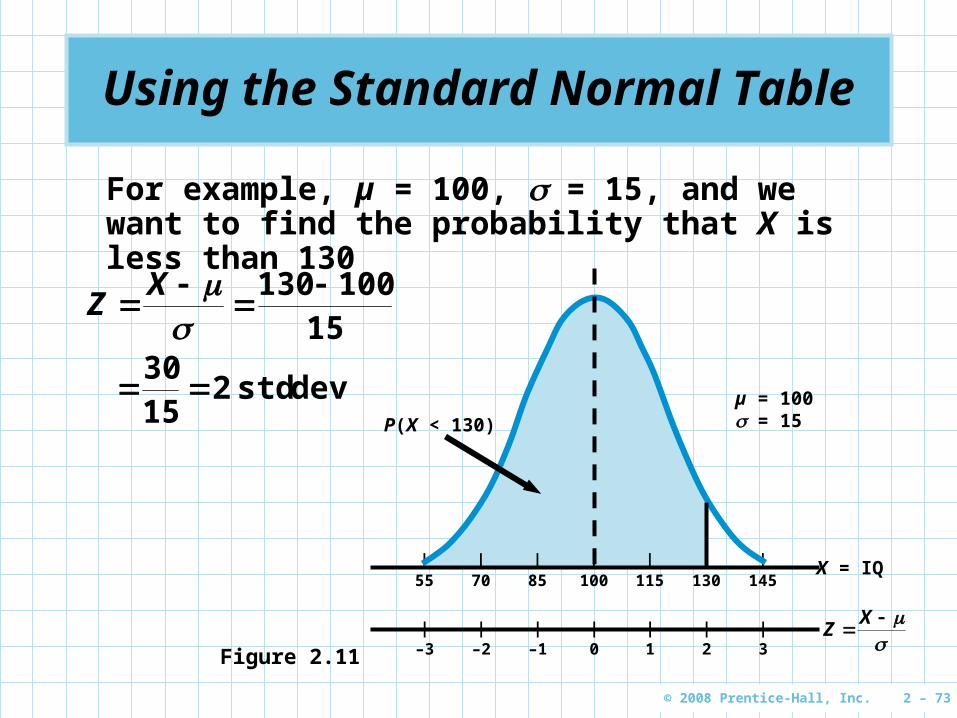
Using the Standard Normal Table
For example, µ = 100, = 15, and we want to find the probability that X is less than 130
15100130
XZ
dev std 21530
| | | | | | |55 70 85 100 115 130 145
| | | | | | |–3 –2 –1 0 1 2 3
X = IQ
X
Z
µ = 100 = 15P(X < 130)
Figure 2.11
© 2008 Prentice-Hall, Inc. 2 – 74
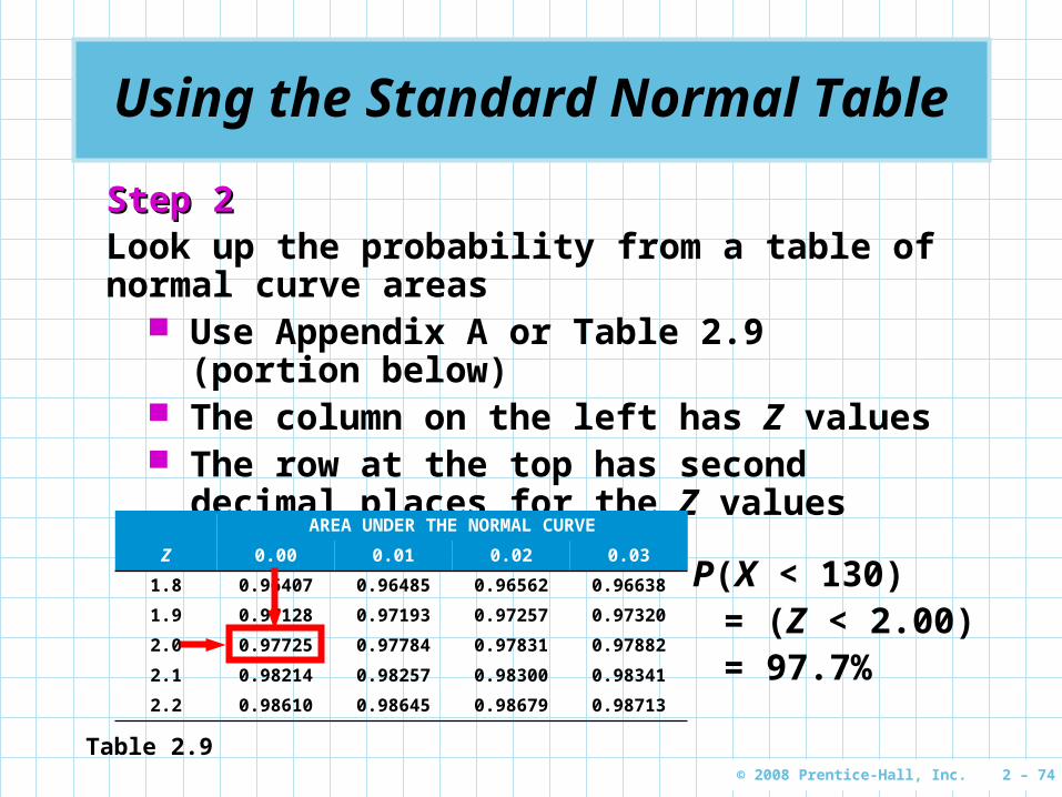
Using the Standard Normal Table
Step 2Step 2Look up the probability from a table of normal curve areas
Use Appendix A or Table 2.9 (portion below) The column on the left has Z values The row at the top has second decimal
places for the Z values
AREA UNDER THE NORMAL CURVE
Z 0.00 0.01 0.02 0.03
1.8 0.96407 0.96485 0.96562 0.96638
1.9 0.97128 0.97193 0.97257 0.97320
2.0 0.97725 0.97784 0.97831 0.97882
2.1 0.98214 0.98257 0.98300 0.98341
2.2 0.98610 0.98645 0.98679 0.98713
Table 2.9
P(X < 130)= (Z < 2.00)= 97.7%
© 2008 Prentice-Hall, Inc. 2 – 75
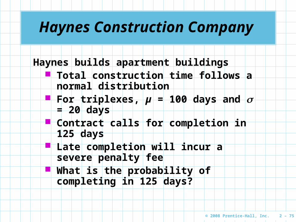
Haynes Construction Company
Haynes builds apartment buildings Total construction time follows a normal
distribution For triplexes, µ = 100 days and = 20 days Contract calls for completion in 125 days Late completion will incur a severe penalty
fee What is the probability of completing in 125
days?
© 2008 Prentice-Hall, Inc. 2 – 76
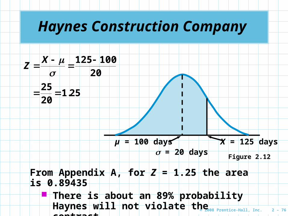
Haynes Construction Company
From Appendix A, for Z = 1.25 the area is 0.89435 There is about an 89% probability Haynes
will not violate the contract
20100125
XZ
2512025
.
µ = 100 days X = 125 days = 20 days
Figure 2.12
© 2008 Prentice-Hall, Inc. 2 – 77
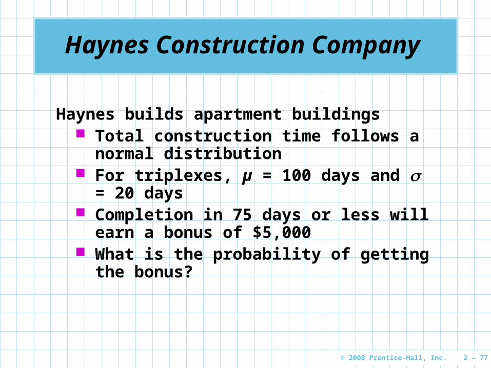
Haynes Construction Company
Haynes builds apartment buildings Total construction time follows a normal
distribution For triplexes, µ = 100 days and = 20 days Completion in 75 days or less will earn a
bonus of $5,000 What is the probability of getting the
bonus?
© 2008 Prentice-Hall, Inc. 2 – 78
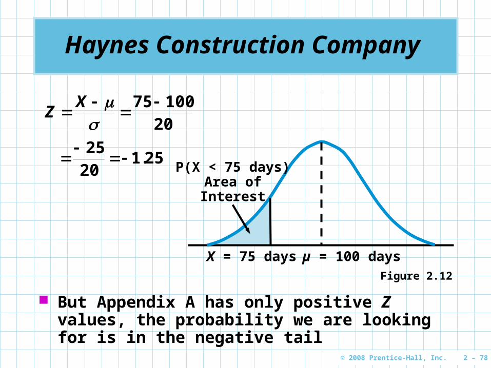
Haynes Construction Company
But Appendix A has only positive Z values, the probability we are looking for is in the negative tail
2010075
XZ
2512025
.
Figure 2.12
µ = 100 daysX = 75 days
P(X < 75 days)Area ofInterest
© 2008 Prentice-Hall, Inc. 2 – 79
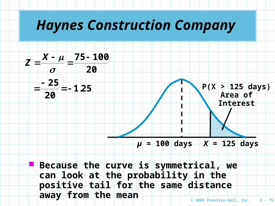
Haynes Construction Company
Because the curve is symmetrical, we can look at the probability in the positive tail for the same distance away from the mean
2010075
XZ
2512025
.
µ = 100 days X = 125 days
P(X > 125 days)Area ofInterest
© 2008 Prentice-Hall, Inc. 2 – 80
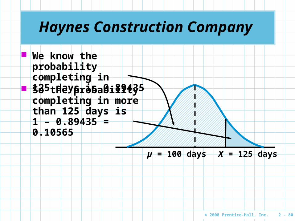
Haynes Construction Company
µ = 100 days X = 125 days
We know the probability completing in 125 days is 0.89435
So the probability completing in more than 125 days is 1 – 0.89435 = 0.10565
© 2008 Prentice-Hall, Inc. 2 – 81
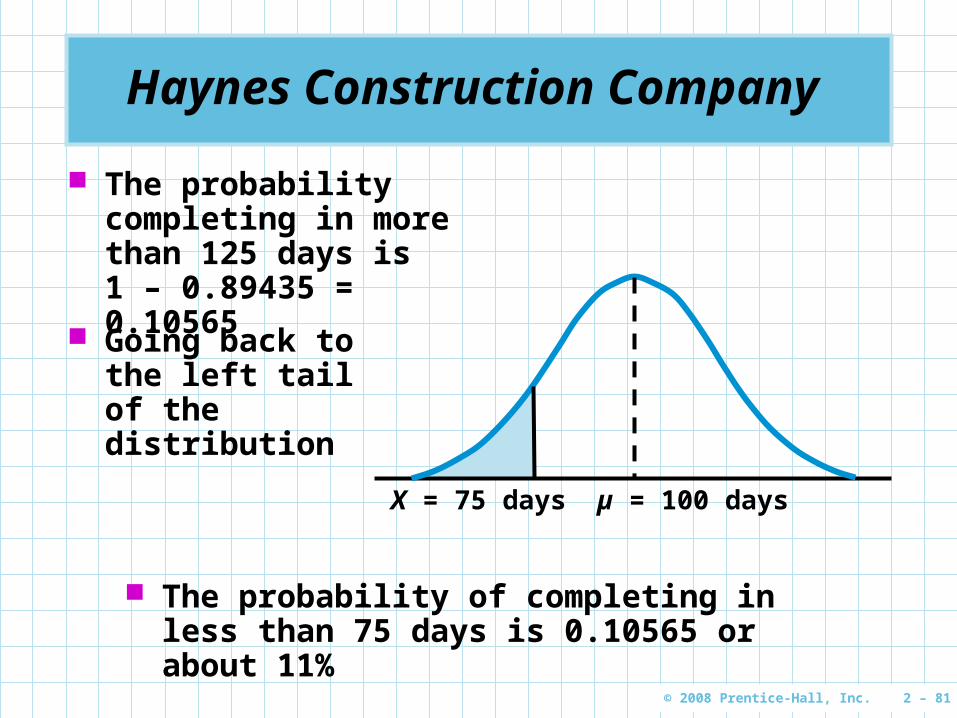
Haynes Construction Company
µ = 100 daysX = 75 days
The probability of completing in less than 75 days is 0.10565 or about 11%
Going back to the left tail of the distribution
The probability completing in more than 125 days is 1 – 0.89435 = 0.10565
© 2008 Prentice-Hall, Inc. 2 – 82
Haynes Construction Company
Haynes builds apartment buildings Total construction time follows a normal
distribution For triplexes, µ = 100 days and = 20 days What is the probability of completing
between 110 and 125 days?
We know the probability of completing in 125 days, P(X < 125) = 0.89435
We have to complete the probability of completing in 110 days and find the area between those two events
© 2008 Prentice-Hall, Inc. 2 – 83
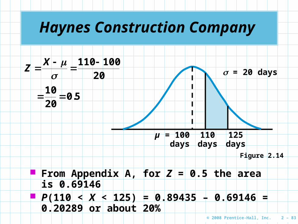
Haynes Construction Company
From Appendix A, for Z = 0.5 the area is 0.69146 P(110 < X < 125) = 0.89435 – 0.69146 = 0.20289
or about 20%
20100110
XZ
502010
.
Figure 2.14
µ = 100 days
125 days
= 20 days
110 days
© 2008 Prentice-Hall, Inc. 2 – 84
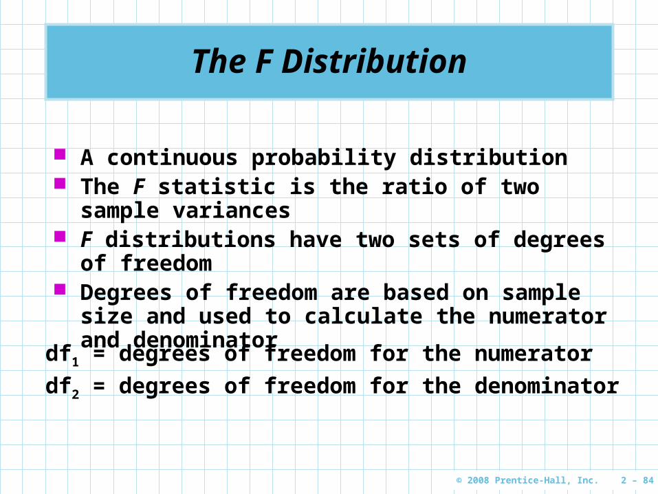
The F Distribution
A continuous probability distribution The F statistic is the ratio of two sample variances F distributions have two sets of degrees of
freedom Degrees of freedom are based on sample size and
used to calculate the numerator and denominator
df1 = degrees of freedom for the numerator
df2 = degrees of freedom for the denominator
© 2008 Prentice-Hall, Inc. 2 – 85
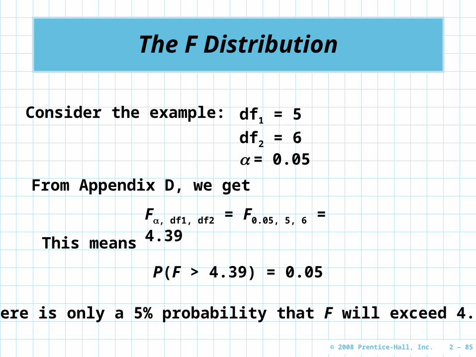
The F Distribution
df1 = 5
df2 = 6 = 0.05
Consider the example:
From Appendix D, we get
F, df1, df2 = F0.05, 5, 6 = 4.39
This means
P(F > 4.39) = 0.05
There is only a 5% probability that F will exceed 4.39
© 2008 Prentice-Hall, Inc. 2 – 86
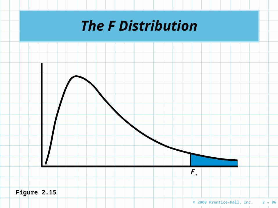
F
The F Distribution
Figure 2.15
© 2008 Prentice-Hall, Inc. 2 – 87
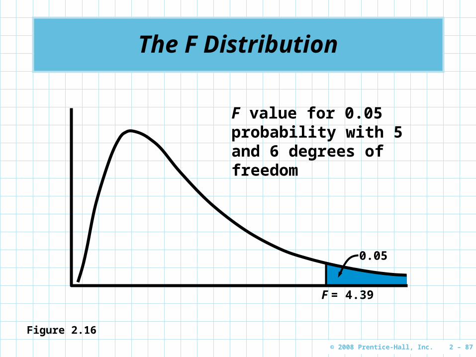
The F Distribution
Figure 2.16
F = 4.39
0.05
F value for 0.05 probability with 5 and 6 degrees of freedom
© 2008 Prentice-Hall, Inc. 2 – 88
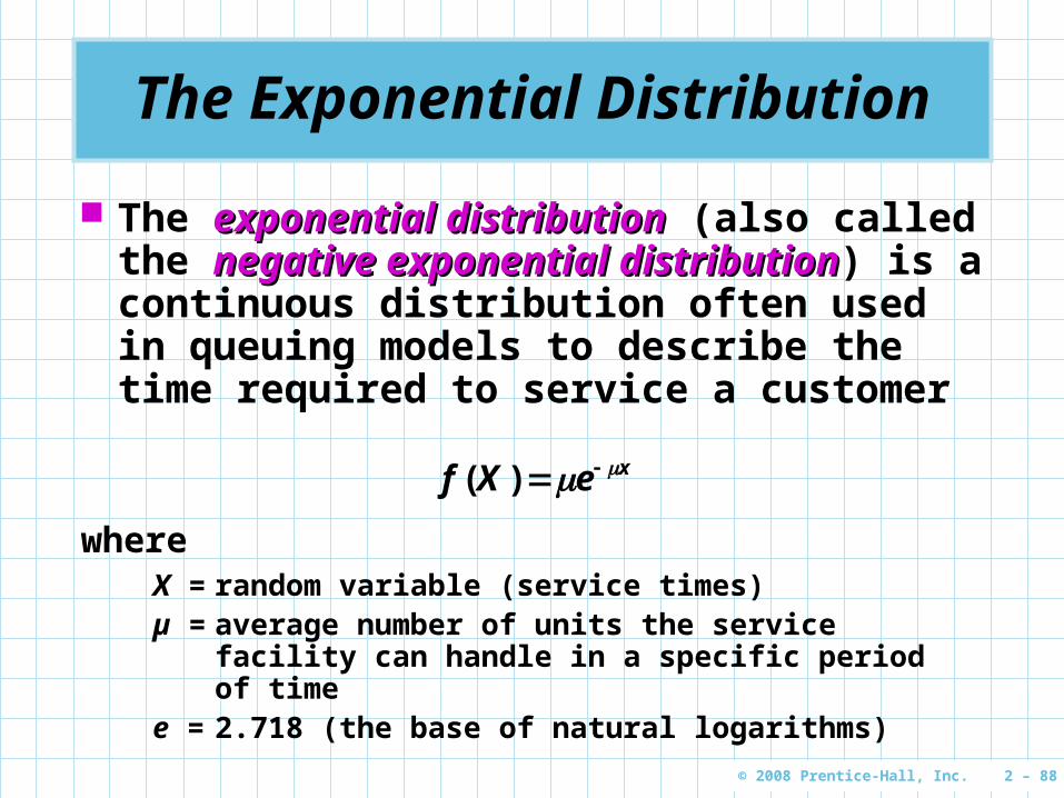
The Exponential Distribution
The exponential distributionexponential distribution (also called the negative exponential distributionnegative exponential distribution) is a continuous distribution often used in queuing models to describe the time required to service a customer
xeXf )(
whereX = random variable (service times)µ = average number of units the service facility can
handle in a specific period of timee = 2.718 (the base of natural logarithms)
© 2008 Prentice-Hall, Inc. 2 – 89
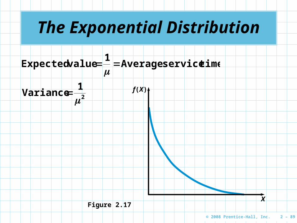
The Exponential Distribution
time service Average1
value Expected
2
1Variance
f(X)
XFigure 2.17
© 2008 Prentice-Hall, Inc. 2 – 90
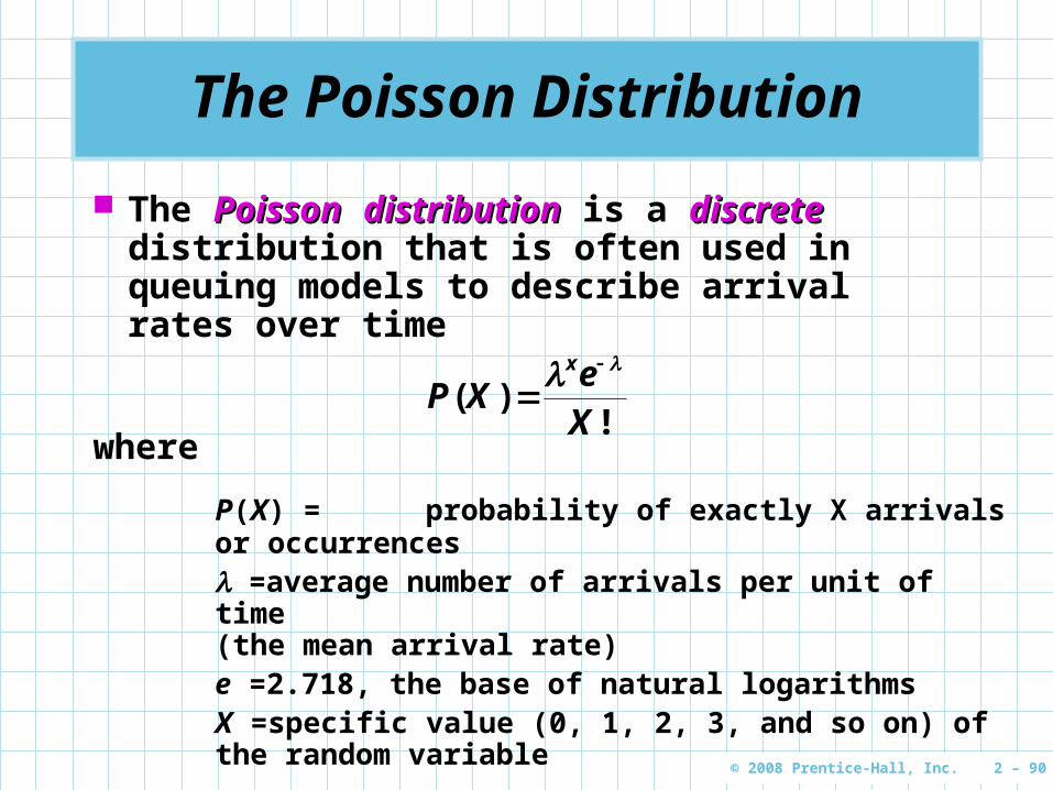
The Poisson Distribution
The PoissonPoisson distributiondistribution is a discretediscrete distribution that is often used in queuing models to describe arrival rates over time
!)(
Xe
XPx
where
P(X) =probability of exactly X arrivals or occurrences =average number of arrivals per unit of time (the mean arrival rate)e =2.718, the base of natural logarithmsX =specific value (0, 1, 2, 3, and so on) of the random variable
© 2008 Prentice-Hall, Inc. 2 – 91
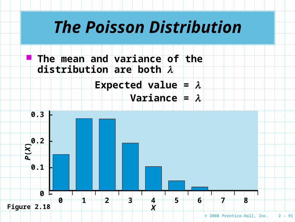
The Poisson Distribution
The mean and variance of the distribution are both
Expected value = Variance =
0.3 –
0.2 –
0.1 –
0 –| | | | | | | | | |
0 1 2 3 4 5 6 7 8
P(X
)
XFigure 2.18


![[PPT]Render/Stair/Hanna Chapter 7 - Inter · Web viewSensitivity Analysis Sensitivity analysis often involves a series of what-if? questions concerning constraints, variable coefficients,](https://img.pdfslide.net/doc/110x75/5ae8171b7f8b9a08778f37fb/pptrenderstairhanna-chapter-7-viewsensitivity-analysis-sensitivity-analysis.jpg)