© 2015 Yang Jiang

FREE FORM FINDING OF GRID SHELL STRUCTURES

BY

YANG JIANG

THESIS

Submitted in partial fulfillment of the requirements

for the degree of Master of Science in Civil Engineering

in the Graduate College of the

University of Illinois at Urbana-Champaign, 2015

Urbana, Illinois

Adviser:

Professor Glaucio H. Paulino

ii

Abstract

The general shape of a shell structure can have a great impact on its structural

performance. This thesis presents a numerical implementation that finds the funicular

form of grid shell structures. Two methods are implemented for the form finding: the

potential energy method (PEM) and the force density method (FDM). The PEM,

inspired by the 3D hanging chain model, find the funicular form by minimization of the

total potential energy. On the other hand, the FDM find the funicular form by solving a

linear system, in which a geometric stiffness matrix is constructed with the force density

and nodal connectivity information. The form finding process is nonlinear, because the

nodal loads are calculated with the rationale of tributary area and evolve with the

structural form. Apart from the form finding, a member sizing procedure is

implemented for a preliminary estimation of the member cross sectional area. In the

member sizing, the stress-ratio method is used to achieve a fully-stressed design. Finally,

three numerical examples are examined to demonstrate the effectiveness of the current

implementation.

iii

To my family and friends

iv

Acknowledgments

First and foremost, I would like to express my deepest gratitude to my advisor,

Professor Glaucio H. Paulino for his constant guidance and support. It is his enthusiasm

that encouraged me to start researching on the current topic. This work is not possible

without his dedication along the way.

My unreserved thanks also goes to my colleagues Tomas Zegard and Lin Yan. We have

been working as a team in the initial stage of the research. They made great contribution

on the development of the design rationale as well as on the detailed implementation.

I would like to acknowledge all my other research colleagues, Sofie Leon, Daniel

Spring, Junho Chun, Maryam Eidini, Peng Wei, Evgueni Filipov, Heng Chi, Xiaojia

Zhang, Tuo Zhao, Ke Liu, Emily Daniels, Oliver Giraldo, Ko-Wei Shih, and Larissa

Novelino. The discussions with them have always been a great source of inspiration.

Especially I wish to thank Heng Chi and Ke Liu, who helped me a lot in the proof-

reading of the thesis.

Also I would like to thank the Department of Civil and Environmental Engineering at

the University of Illinois at Urbana-Champaign, which provided me the chance to know

the lovely and talented people mentioned above and to conduct research with them. I

am grateful to the Georgia Institute of Technology for accepting me as a visiting scholar,

so that I can successfully finalize the research.

Finally, and most importantly, I wish to thank my parents. It is their unconditioned

love that drives me to progress.

v

Table of Contents

NOMENCLATURE ..................................................................................................... vi

CHAPTER 1 INTRODUCTION ............................................................................. 1

1.1 Motivation ............................................................................................................ 1

1.2 Literature Review ................................................................................................. 2

1.3 Design Objective and Methods ............................................................................ 5

1.4 Thesis Organization .............................................................................................. 6

CHAPTER 2 DESIGN METHODOLOGY ............................................................. 7

2.1 Formulation of Potential Energy Method (PEM) ................................................. 7

2.2 Formulation of Force Density Method (FDM)................................................... 10

2.3 Initial Domain Definition ................................................................................... 13

2.4 Nodal Load Calculation...................................................................................... 17

2.5 Snap-through Action Triggering ........................................................................ 19

2.6 Member Sizing ................................................................................................... 21

2.7 Grouped Member Sizing .................................................................................... 23

2.8 Summary for Design Methodology .................................................................... 23

CHAPTER 3 NUMERICAL EXAMPLES ............................................................ 26

3.1 SOM-inspired Grid Shell.................................................................................... 27

3.2 Structured Circular Dome .................................................................................. 40

3.3 Igloo.................................................................................................................... 47

3.4 Remarks on Computational Costs ...................................................................... 55

CHAPTER 4 CONCLUDING REMARKS ........................................................... 57

REFERENCES ............................................................................................................ 59

APPENDIX A: MATLAB CODE FILES

FOR FORM FINDING OF GRID SHELL STRUCTURES ....................................... 62

vi

Nomenclature

𝐴𝑖(𝑘)

Cross sectional area of the i-th grid member in the k-th iteration

𝐴𝑡,𝑖 Triburary area corresponding to the load type i

c(j), d(j) Number of the two end nodes of grid member j in the FDM

formulation

𝐂 Portion of the branch-node matrix belonging to the free nodes

𝐂𝑓 Portion of the branch-node matrix belonging to the fixed nodes

𝐂𝑠 Branch-node matrix

𝐃 The geometric stiffness matrix corresponding to free nodes

𝐃𝑓 The geometric stiffness matrix corresponding to fixed nodes

𝜀 Prescribed tolerance

𝐸𝑖 Young’s modulus of the i-th grid member

(𝐸𝐴)𝑖 The product of the Young’s modulus and the cross sectional area of

the i-th grid member

𝑘𝑖 Stiffness of the i-th grid member

𝐊 Member stiffness matrix. The member stiffness consists of the matrix

diagonal while other entries are zero.

ℓ𝑖 The length of the i-th grid member in the current configuration

ℓ𝑖,0 The length of the i-th grid member in the initial configuration

𝓵 Member length vector

𝐋 Diagonal matrix of 𝓵

𝛥ℓ𝑖 The length change of the i-th grid member

𝚫𝓵 Vector of the member length change

𝑁 Number of free nodes

𝑁𝑏 Number of the grid members (branches)

𝑁𝑑𝑜𝑓 Number of degrees of freedom

𝑁𝑒 Number of shell panels

vii

𝑁𝑓 Number of fixed nodes

𝑁𝑛 Number of nodes

𝐩 Nodal load vector

𝐩𝑥, 𝐩𝑦, 𝐩𝑧 Nodal load vector in x, y and z directions, respectively

𝑃𝐸 Total potential energy of the system

𝑞𝑑𝑖𝑠𝑡,𝑖 The i-th type of distributed load

𝑞𝑗 The force density of the j-th grid member

𝐪 Force density vector

𝐐 Diagonal matrix of 𝐪

s Member internal force vector

𝐒 Diagonal matrix of 𝐬

𝐮 Nodal displacement vector in the potential energy formulation

u, v, w Vectors of the coordinate difference between 2 connected nodes in the

force density formulation

U, V, W Diagonal matrices of the vector u, v and w in the force density

formulation

𝐱 Nodal coordinate vector in the current configuration

𝐱0 Nodal coordinate vector in the initial configuration

𝐱𝑖,𝑎, 𝐱𝑖,𝑏 The nodal coordinate of the two end nodes of the i-th grid member

𝑥𝑐, 𝑦𝑐, 𝑧𝑐 Coordinates of the centroid of nodes around a shell panel

𝐗, 𝐘, 𝐙 Nodal coordinate vectors of free nodes in the force density

formulation

𝐗𝑓 , 𝐘𝑓 , 𝐙𝑓 Nodal coordinate vectors of fixed nodes in the force density

formulation

µ Numerical damping parameter in the stress ratio method

𝜎𝑎𝑑𝑚,𝑖 Admissible stress of the i-th grid member

𝜎𝑖 (𝑘) Stress of the i-th grid member in the k-th iteration

1

CHAPTER 1

Introduction

1.1 Motivation

A thin shell structure is generally defined as a structure in which the thickness is small

compared with the other dimensions. It is a well-recognized form of building structures

as illustrated by Fig. 1.1. Despite the fact that most of the buildings are comprised of

beams and columns, the thin shell structure has been admired for its special flexibility,

aesthetic appearance, light weight and other advantages. The shell structures can be

categorized into two groups: continuous shells and grid shells. As the name implies, the

continuous shell has a continuous shell surface through which loads are transferred. On

the other hand, grid shells are constructed by discrete grid members, usually made of

steel or timber. As the first step of the ongoing research on shell design, we focus on

the grid shell as it is simpler to deal with.

Fig. 1.1 Shell structure examples. (a) L'Oceanogràfic (El Oceanográfico), City of Arts and

Sciences, Valencia, Spain (continuous shell) [31]; (b) Roof for the Multihalle (multi-purpose hall)

in Mannheim, Mannheim, Germany (grid shell) [32].

In a conventional design pattern, the global geometry of a grid shell structure is usually

determined by the client and the architect, with major considerations on functionality

and aesthetics. Moreover, the structural behavior of a shell structure largely relies on

the global geometry. Here, we propose a convenient tool for the form finding of shell

structures, particularly grid shells in the current study, which address the structural

(a) (b)

2

aspects.

1.2 Literature Review

Researchers have worked on the design of grid shell structures in various aspects. For

example, methods to find the grid shell form with minimum self-weight were

investigated [22, 23]. Some proposed how to find the optimal grid patterns for a given

shell surface [9, 29]. In the current study, we are interested in finding a proper form, in

which shell bending can be avoided so that the loads will cause pure axial stresses in

the structural components. Such a form is usually referred to as a “funicular” form.

In the twentieth century, both architects and engineers, such as Gaudí [2, 11], Otto [19],

and Isler [3], applied physical techniques for the form finding. In these techniques, an

efficient 3D structural shape can be found given a certain material, a set of boundary

conditions and gravity loads. Particularly, the 3D hanging chain model pioneered by

Gaudí is a significant inspiration for the current study.

The fundamental rationale of the 3D hanging chain model has long been discussed, as

a quotation from Robert Hooke in 1675 says “As hangs a flexible cable, so but inverted

will stand the rigid arch.” This principle describes the reciprocal relationship of a

tension-only and a compression-only form in 2-dimensional (2D) space under the same

loading case [5, 26]. When extended to design in the 3-dimensional (3D) space, this

rationale supports the use of the 3D hanging chain model for the form finding of a

gravity-loaded structure.

Gaudí constructed 3D hanging chain models for use in his designs such as the Church

of Colònia Güell and the Sagrada Familia [2]. Based on the architectural constraints

and preliminary ideas of the final shape, a scaled hanging system is built with members

of cable and cloth hang on the ceiling. The self-weight of the actual structure is

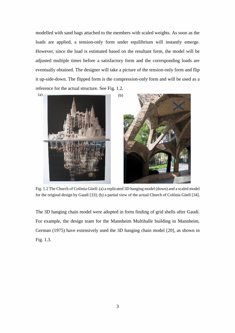
3

modelled with sand bags attached to the members with scaled weights. As soon as the

loads are applied, a tension-only form under equilibrium will instantly emerge.

However, since the load is estimated based on the resultant form, the model will be

adjusted multiple times before a satisfactory form and the corresponding loads are

eventually obtained. The designer will take a picture of the tension-only form and flip

it up-side-down. The flipped form is the compression-only form and will be used as a

reference for the actual structure. See Fig. 1.2.

Fig. 1.2 The Church of Colònia Güell: (a) a replicated 3D hanging model (down) and a scaled model

for the original design by Gaudí [33]; (b) a partial view of the actual Church of Colònia Güell [34].

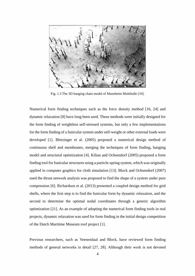
The 3D hanging chain model were adopted in form finding of grid shells after Gaudí.

For example, the design team for the Mannheim Multihalle building in Mannheim,

German (1975) have extensively used the 3D hanging chain model [20], as shown in

Fig. 1.3.

(a) (b)

4

Fig. 1.3 The 3D hanging chain model of Mannheim Multihalle [10].

Numerical form finding techniques such as the force density method [16, 24] and

dynamic relaxation [8] have long been used. These methods were initially designed for

the form finding of weightless self-stressed systems, but only a few implementations

for the form finding of a funicular system under self-weight or other external loads were

developed [1]. Bletzinger et al. (2005) proposed a numerical design method of

continuous shell and membranes, merging the techniques of form finding, hanging

model and structural optimization [4]. Kilian and Ochsendorf (2005) proposed a form

finding tool for funicular structures using a particle-spring system, which was originally

applied in computer graphics for cloth simulation [13]. Block and Ochsendorf (2007)

used the thrust network analysis was proposed to find the shape of a system under pure

compression [6]. Richardson et al. (2013) presented a coupled design method for grid

shells, where the first step is to find the funicular form by dynamic relaxation, and the

second to determine the optimal nodal coordinates through a generic algorithm

optimization [21]. As an example of adopting the numerical form finding tools in real

projects, dynamic relaxation was used for form finding in the initial design competition

of the Dutch Maritime Museum roof project [1].

Previous researchers, such as Veenendaal and Block, have reviewed form finding

methods of general networks in detail [27, 28]. Although their work is not devoted

5

specifically for the form finding of grid shells, it is promising that some of the methods

can be modified to serve our interests.

1.3 Design Objective and Methods

We adopt the definition of “form finding” as “finding an optimal shape of a form-active

structure that is in a state of static equilibrium” from [15]. In the current study, the

optimal shape is defined as a funicular form. Thus, the objective of the form finding is

stated as “finding the form of a grid shell in equilibrium, in which the structural

members suffer no shear or bending moment”.

Here, a grid shell structure is modeled with grid members hinged with each other and

to the boundary, where loads are applied on the hinged nodes. This simplification allows

the use of form finding methods for general network. The design of grid shells follows

an optimization procedure. Among the family of form finding methods, the potential

energy method (PEM) and the force density method (FDM) are explored and

implemented in the current study. The form finding process will provide a funicular

form and the corresponding static loading case derived from the form.

The current implementation includes an optional member sizing given the design

information from the form finding. The member sizing aims to design for the cross

sectional area of each grid member, so that the axial stress of every member equals its

admissible stress. The member sizing is based on the PEM and uses the actual properties

of the construction material.

A flowchart of the general design process is shown in Fig. 1.4. Note that finding, the

designer will choose either the PEM or the FDM for the form finding. Also it is up to

the designer’s choice whether to conduct the member sizing or not.

6

Fig. 1.4 Proposed Design Process. The dashed box enclosed the optional member sizing

procedure.

1.4 Thesis Organization

The remainder of the thesis is organized as follows. The design methodology of the

current implementation is illustrated in Chapter 2, which demonstrates the

fundamentals of the PEM and FDM as well as the important issues in the

implementation. The member sizing with and without “group design” will also be

illustrated in the Chapter 2. In Chapter 3, three numerical examples are provided to

demonstrate the effectiveness of the design tool. Finally, the current work is

summarized together with possible future extension in Chapter 4.

7

CHAPTER 2

Design Methodology

The initial design settings comprise of grid members, hinge nodes and nodal boundary

conditions. Shell panels are considered for nodal load calculation, but not as structural

members in the design. As loads are applied, the grid shell form will change so that an

equilibrium state is achieved. As stated in the introduction, the design goal is to find a

grid form in equilibrium under a certain load case, where the members suffer no

bending moment and no shear force. The state of zero bending moment and shear force

is ensured by the assumptions that:

1. All grid members are hinge-connected;

2. For every grid member, loads are only applied at the end nodes.

Thus the task left is to find the equilibrium form. The current study focuses on two form

finding methods, namely the potential energy method (PEM) and the force density

method (FDM).

In this chapter, the formulations of PEM and FDM will be presented in the first two

sections. Then implementation details will be discussed in aspects of initial domain

definition, nodal load calculation and snap-through action triggering. Besides the

standard form finding, a separate process of member sizing is implemented and

illustrated. This chapter concludes with two flow charts showing procedures of form

finding and member sizing. The current implementation is based on MATLAB 7.14

R2012a [31].

2.1 Formulation of Potential Energy Method (PEM)

The PEM is inspired by Gaudí’s 3D hanging chain model. In this method, grid members

in the design domain are assigned with prescribed member stiffness, with which the

potential energy can be defined. When loaded, the grid members deform according to

8

the constitutive relationship until a new equilibrium is achieved. The PEM finds the

equilibrium form by minimizing the potential energy of the system. In this sense, it

bears some analogy with the elastic formulation for ground structures [30].

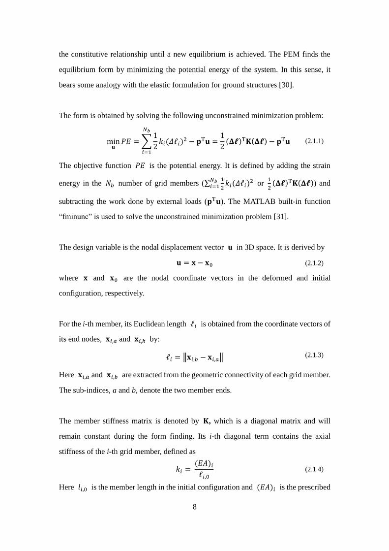
The form is obtained by solving the following unconstrained minimization problem:

min𝐮

𝑃𝐸 = ∑1

2

𝑁𝑏

𝑖=1

𝑘𝑖(𝛥ℓ𝑖)2 − 𝐩T𝐮 =

1

2(𝚫𝓵)T𝐊(𝚫𝓵) − 𝐩T𝐮

The objective function 𝑃𝐸 is the potential energy. It is defined by adding the strain

energy in the 𝑁𝑏 number of grid members (∑1

2

𝑁𝑏𝑖=1 𝑘𝑖(𝛥ℓ𝑖)

2 or 1

2(𝚫𝓵)T𝐊(𝚫𝓵)) and

subtracting the work done by external loads (𝐩T𝐮). The MATLAB built-in function

“fminunc” is used to solve the unconstrained minimization problem [31].

The design variable is the nodal displacement vector 𝐮 in 3D space. It is derived by

𝐮 = 𝐱 − 𝐱0

where 𝐱 and 𝐱0 are the nodal coordinate vectors in the deformed and initial

configuration, respectively.

For the i-th member, its Euclidean length ℓ𝑖 is obtained from the coordinate vectors of

its end nodes, 𝐱𝑖,𝑎 and 𝐱𝑖,𝑏 by:

ℓ𝑖 = ‖𝐱𝑖,𝑏 − 𝐱𝑖,𝑎‖

Here 𝐱𝑖,𝑎 and 𝐱𝑖,𝑏 are extracted from the geometric connectivity of each grid member.

The sub-indices, a and b, denote the two member ends.

The member stiffness matrix is denoted by 𝐊, which is a diagonal matrix and will

remain constant during the form finding. Its i-th diagonal term contains the axial

stiffness of the i-th grid member, defined as

𝑘𝑖 = (𝐸𝐴)𝑖

ℓ𝑖,0

Here 𝑙𝑖,0 is the member length in the initial configuration and (𝐸𝐴)𝑖 is the prescribed

(2.1.1)

(2.1.2)

(2.1.3)

(2.1.4)

9

product of the Young’s modulus and cross sectional area of the i-th grid member. In one

design domain, altering the prescribed value of (𝐸𝐴)𝑖 will result in different forms.

The 3D nodal external load vector is denoted by 𝐩. It is derived by the rationale of

tributary area, which transforms the distributed loads on the assumed shell panels into

concentrated loads at structural nodes. Detailed derivation of 𝐩 will be discussed in

Section 2.4. It should be noted that 𝐩 updates with the evolving form, and thus the

form-finding process is nonlinear.

Due to the nonlinear nature of the problem, it will be solved iteratively. A loop is set up

to account for the changes in nodal loads with respect to form change. Within each

iteration, a nodal load vector is derived with the form from last iteration. Then the

minimization of potential energy is performed to obtain the updated form based on the

current nodal loads. The iteration shall continue until convergence. Here the

convergence criterion is defined as

‖𝐱(𝑘) − 𝐱(𝑘−1)‖

𝑁𝑑𝑜𝑓< 𝜀

where 𝐱(𝑘) and 𝐱(𝑘−1)are the displacement vectors for all degrees of freedom in the

current and previous iteration, 𝑁𝑑𝑜𝑓 is the number of degree of freedom and 𝜀 is a

prescribed tolerance. The norm sign indicates the two-norm. The quantity ‖𝐱(𝑘)−𝐱(𝑘−1)‖

𝑁𝑑𝑜𝑓

is a measure of average movement of nodes from the previous iteration to the current

one.

As the PEM inherits the rationale of the 3D hanging model, the form evolves downward

and is dominated by tension. Fig. 2.1 illustrates the process. Flipping it up-side-down

will result in the grid shell form.

(2.1.5)

10

z=0

z=0

(b)

z=0

z=0

(a)

Fig 2.1 Geometry evolution of a simple grid dome by form finding with PEM. The planar geometry

settles into a reversed dome under nodal loads applied in the downward direction. The left and the

right column show the 3D view (arrows denote nodal loads) and the front view, respectively. (a)

Initial geometry (flat); (b) Final geometry. Note that the magnitude of nodal loads in (b) is greater

than those in (a).

2.2 Formulation of Force Density Method (FDM)

The FDM was initially adopted to perform form finding for general networks of cables

and bars [16, 24]. The name of the method comes after a prescribed design parameter,

force density, defined as the ratio of member force over member length. Given a set of

force density and connectivity information, we can construct a linear system

representing nodal force equilibrium, which links the form with nodal loads. The final

form is obtained by solving the resulting linear system.

Unlike the PEM, the FDM does not recognize member stiffness under the conventional

constitutive relationship. In this sense, it bears some analogy with the plastic

formulation for ground structures [32]. Instead, it correlates member force with member

length by force density. Details in the linear system construction is illustrated below,

with major reference to [24] and [7].

11

(2.2.2)

(2.2.1)

To begin with, we define a grid system with nodes from 1 to 𝑁𝑛 and grid members (or

branches) from 1 to 𝑁𝑏. To simplify the calculation process, we define all the fixed

nodes (𝑁𝑓 nodes, from 𝑁 + 1 to 𝑁 + 𝑁𝑓) after all the free nodes (N nodes from 1 to

N). Thus we have 𝑁𝑛 = 𝑁 + 𝑁𝑓. For any grid member j, there are 2 corresponding

nodes with number c(j) and d(j). With the information above, the branch-node matrix

𝐂𝑠 is defined by

𝐂𝑠(𝑗, 𝑖) = {+1, for 𝑐(𝑗) = 𝑖

−1, for 𝑑(𝑗) = 𝑖0, otherwise

The matrix 𝐂𝑠 has 𝑁𝑏 rows and 𝑁𝑛 columns. Note that the value of c(j) and d(j) for

a grid member may interchange with each other. This interchange will affect 𝐂𝑠, but

will not influence the resultant linear system.

Fig. 2.2 (a) A simple grid system. Nodes are denoted by plain numbers. Branches are denoted by

circled numbers; (b) The connectivity matrix of the grid system.

The branch-node matrix 𝐂𝑠 is separated into 𝐂 and 𝐂𝑓 , with 𝐂 representing the

portion for free nodes and 𝐂𝑓 for the fixed nodes, as illustrated by Fig. 2.2. In a similar

logic, 𝐗, 𝐘, 𝐙 and 𝐗𝑓 , 𝐘𝑓 , 𝐙𝑓 correspond to the nodal coordinate vectors of free and

fixed nodes in the x, y and z directions, respectively.

Vectors holding the coordinate difference between 2 connected nodes are defined as u,

v, and w. They are derived with branch-node matrices and nodal coordinates:

𝐮 = 𝐂𝐗 + 𝐂𝑓𝐗𝑓, 𝐯 = 𝐂𝐘 + 𝐂𝑓𝐘𝑓, 𝐰 = 𝐂𝐙 + 𝐂𝑓𝐙𝑓

Let’s define the member length vector as ℓ and the force density vector as q. The force

𝐂 𝐂𝑓

(a) (b)

12

(2.2.3)

(2.2.4)

(2.2.6)

(2.2.7)

(2.2.8)

(2.2.9)

(2.2.10)

density of the j-th grid members 𝑞𝑗 is defined as its force-length ratios [24]. Then

define U, V, W, L, Q as the diagonal matrices of the vector u, v, w, 𝓵 and q,

respectively. Moreover, define s as the member internal force vector. To maintain force

equilibrium at every node, the sum of internal forces should equal the external forces.

The equilibrium equations are formulated as follows:

𝐂T𝐔𝐋−1𝐬 = 𝐩𝑥, 𝐂T𝐕𝐋−1𝐬 = 𝐩𝑦, 𝐂T𝐖𝐋−1𝐬 = 𝐩𝑧

In the equilibrium equations, representations of Jacobian matrices are utilized:

𝜕𝓵

𝜕𝐗= 𝐂T𝐔𝐋−1,

𝜕𝓵

𝜕𝐘= 𝐂T𝐕𝐋−1,

𝜕𝓵

𝜕𝐙= 𝐂T𝐖𝐋−1

The force density vector 𝐪 is obtained by:

𝐪 = 𝐋−1𝐬

where 𝐋 is the diagonal matrix of the member length vector 𝓵, and 𝐬 is the member

force vector. With (2.2.5), we can then update (2.2.3) into:

𝐂T𝐔𝐪 = 𝐩𝑥, 𝐂T𝐕𝐪 = 𝐩𝑦, 𝐂T𝐖𝐪 = 𝐩𝑧

By means of (2.2.2) and the following identities, we obtain:

𝐔𝐪 = 𝐐𝐮, 𝐕𝐪 = 𝐐𝐯, 𝐖𝐪 = 𝐐𝐰

The nodal force equilibrium equation systems in x, y and z directions are formulated

as follows:

𝐂T𝐐𝐂𝐱 + 𝐂T𝐐𝐂𝑓𝐱𝑓 = 𝐩𝑥

𝐂T𝐐𝐂𝐲 + 𝐂T𝐐𝐂𝑓𝐲𝑓 = 𝐩𝑦

𝐂T𝐐𝐂𝐳 + 𝐂T𝐐𝐂𝑓𝐳𝑓 = 𝐩𝑧

For a simpler representation, we can write 𝐃 = 𝐂T𝐐𝐂 and 𝐃𝑓 = 𝐂T𝐐𝐂𝑓 , so that

(2.2.8) becomes:

𝐃𝐗 + 𝐃𝑓𝐗𝑓 = 𝐩𝑥,𝐃𝐘 + 𝐃𝑓𝐘𝑓 = 𝐩𝑦, 𝐃𝐙 + 𝐃𝑓𝐙𝑓 = 𝐩𝑧

Thus, member forces can be derived by:

𝐬 = 𝐋𝐪

Given the external loads, the branch-node matrix, force densities and fixed degrees of

freedom, we can determine a set of free nodal coordinates by solving the system in

(2.2.5)

13

(2.2.9). Similar to PEM, an iterative solver is introduced due to the nonlinearity in load

calculation. Note that the displacement vector 𝐮1 is not present in the computation of

the FDM, which indicates that the resultant form is not affected by the initial positions

of the free nodes.

2.3 Initial Domain Definition

The geometry of the initial domain is defined by nodes (nodal coordinates) and grid

members (node connectivity). Here, 𝑁𝑛, 𝑁𝑏 and 𝑁𝑒 denotes number of nodes, grid

members and shell panels, respectively. Nodal coordinates are stored in an (𝑁𝑛x 3)

matrix where each row contains the coordinate of one node in x, y and z axis. The nodes

are automatically numbered with its row number in this matrix. Node connectivity is

an (𝑁𝑏x 2) matrix, where each row contains the number of two end nodes. Information

of shell panels is stored in a cell array of 𝑁𝑒 rows, where each row contains the

numbers of surrounding nodes. The designer also needs to prescribe the fixed degrees

of freedom and the values of distributed loads. In FDM implementation, the branch-

node matrix is extracted from the node connectivity. The composition of the initial

domain is illustrated in Fig. 2.3

The current implementation provides three methods to define the initial domain

geometry. These methods are based on finite element shape function interpolation,

spline interpolation and the modified PolyMesher code [25]. Apart from the three

methods, the designer can also select a different scheme for the initial domain geometry

definition.

14

12

3

4

5

6

7

8

9

10

11

12

1 2

3

4

5

6

7

8

9

Fig. 2.3 Decomposition of a simple initial domain. (a) Hinge nodes (blue dot) and fixed nodes (blue

triangle); (b) Grid members (red lines); (c) Panels where loads are applied on (space with green

labels). The dash lines denote grid members that are not active in the design, as they are fixed at

both ends and thus cannot deform; (d) Initial domain without labels.

2.3.1 Finite Element Shape Function Interpolation

The first method uses finite element (FE) shape functions to interpolate for the location

of all other structural nodes from certain predefined nodal coordinates. First, the

designer should choose the type of FE to be used. The current implementation allows

the use of Q8, Q9 and Q12 element. Then the designer prescribes the nodal coordinates

in the physical configuration that are associated with the FE nodes in the intrinsic

configuration. With such information, the designer can choose any other point in the

intrinsic coordinate and obtain its corresponding location in the physical coordinate by

FE shape function interpolation. More details are illustrated in Fig. 2.4. This method is

1

2

3

4

5

6

7

8

(a) (b)

(c) (d)

15

suitable for structured domains, in which the number of grid members in the two

orthogonal directions is known. Also it is favorable that the domain shape can be

reasonably mapped to the shape of the implemented finite element.

Fig. 2.4: Unknown nodal coordinates are interpolated from known nodal coordinates by FE shape

functions. (a). Domain in the physical coordinate. Blue dots denote nodes with known coordinates,

while coordinates of other nodes are to be derived; (b). Domain in the intrinsic coordinate. Known

nodes in (a) correspond to Q12 FE nodes with the same corresponding number; (c) and (d). Q12 FE

shape functions for nodes 1 and 5.

2.3.2 Spline Function Interpolation

The second method uses piece-wise spline functions to interpolate for the location of

all structural nodes from certain predefined nodal coordinates as shown by Fig. 2.5.

Spline functions are widely recognized to interpolate unknown data from a set of known

data in a smooth pattern. In this method, the designer prescribes the coordinates of

certain nodes in the 3D physical coordinate, together with their coordinates in the 2D

intrinsic configuration. The 2D spline functions then allow the designer to obtain the

corresponding physical coordinate for any nodes in the 2D intrinsic domain. The

implementation uses MATLAB-built-in functions to construct the spline functions and

1

2

3

4

5 6

7 8 9

10

11 12

1

2 4

5 6

12 11

10

1 2

3 4

5 6

7

8

9 10

11

12

y

x 11

12

1 2 5 6

7

8

3 4 9 10

(c) (d)

(a) (b)

16

perform the interpolation. Further details of the spline interpolation technique are

illustrated in [12].

Fig. 2.5 Cubic Spline of Monotonic Data in 2D Space. From the limited number of know points

(black dots), the function value of any point can be interpolated by the spline function, as the line

shows. Cited from [12].

2.3.3 Modified PolyMesher

The third method adopts a modified version of a polygonal mesher named PolyMesher

[25]. Given a specified 2D domain with boundary conditions, the code will generate a

centroidal voronoi tessalation (CVT) mesh and apply boundary conditions on

corresponding nodes [25]. The nodes and edges of polygons will be defined as the hinge

nodes and grid members in the initial domain. The definition procedures for a simple

rectangular domain is illustrated in Fig. 2.6. This method is suitable for arbitrary grid

patterns.

Fig. 2.6 Initial domain definition by modified PolyMesher. (a) A rectangular domain with fixed

upper and lower edge; (b) The CVT mesh generated by the modified PolyMesher; (c) The element

nodes and edges are extracted as the nodes and grid members in the initial domain.

(a) (b) (c)

17

2.4 Nodal Load Calculation

For grid shells, major load types include, for example, structural self-weight and wind

load. Loads are mostly applied on the shell surface. In the current implementation, it is

assumed that all loads are primarily distributed onto shell panels and are transmitted to

the structural nodes using the tributary area rationale. We assume that all the loads are

static and in the vertical direction for the current design scope.

Thus, nodal load on any node is derived by:

𝑝𝑧 = ∑ 𝑞𝑑𝑖𝑠𝑡,𝑖 ∗ 𝐴𝑡,𝑖

𝑖

Here 𝑖 is the load case number, 𝑞𝑑𝑖𝑠𝑡,𝑖 is the distributed load and 𝐴𝑡,𝑖 is the tributary

area corresponding to the particular load type.

Before calculating tributary areas, we first need to define the panel geometry. For a

panel with three sides, the shape can be reasonably defined as a planar triangle.

However, for a panel with four or more sides, the nodes are likely not to be in the same

plane, which suggests infinite number of possible panel geometries. Thus an algorithm

is necessary to define a reasonable geometry. At the same time, this geometry should

lead to easy calculation of tributary areas.

For the reasons above, we assume that each shell panel is composed of small triangles

enclosed by surrounding nodes, the centroid of these nodes and the midpoints of

surrounding grid members. Tributary area of a node is then computed from the areas of

these triangles. Fig. 2.7 illustrates the triangulation of quadrilateral panels and the

tributary area calculation in details.

(2.4.1)

18

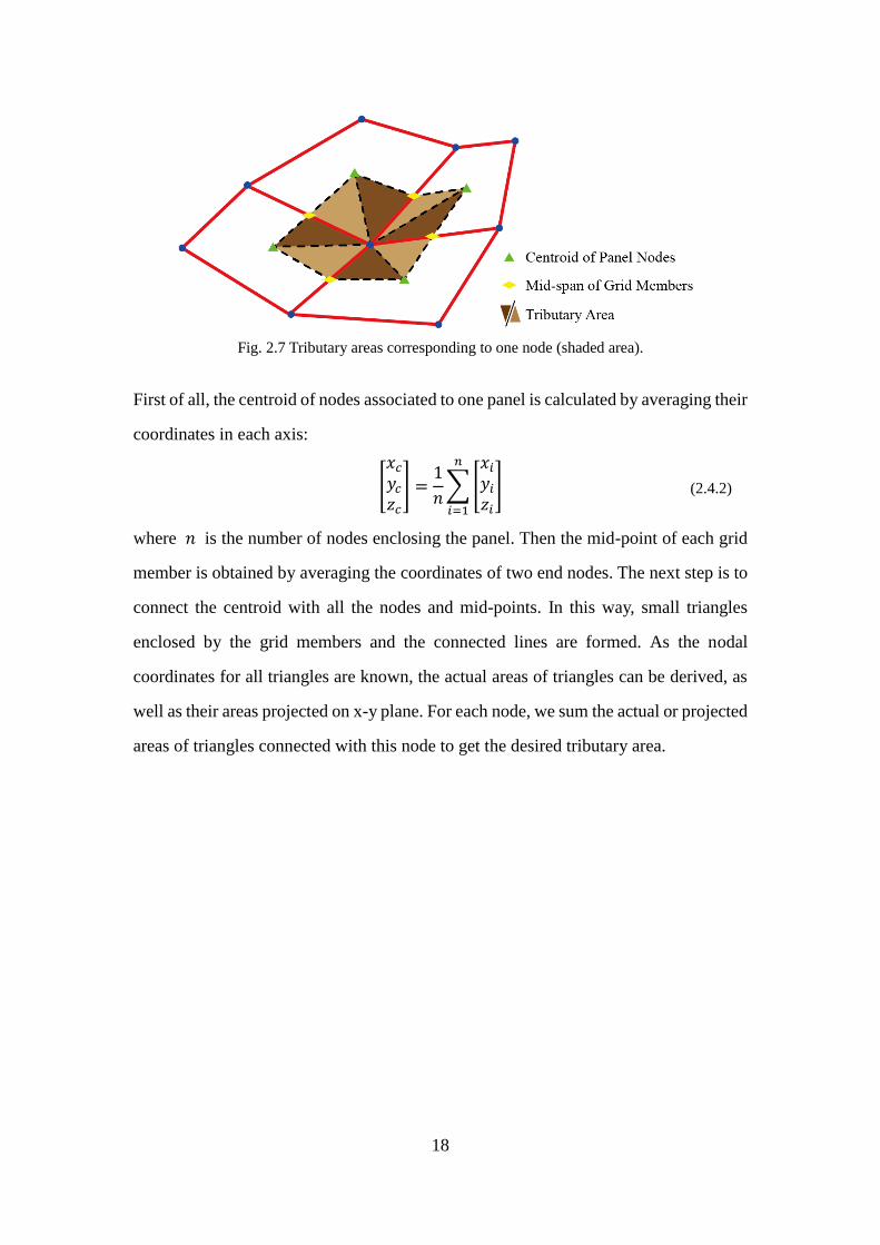
Fig. 2.7 Tributary areas corresponding to one node (shaded area).

First of all, the centroid of nodes associated to one panel is calculated by averaging their

coordinates in each axis:

[

𝑥𝑐

𝑦𝑐

𝑧𝑐

] =1

𝑛∑ [

𝑥𝑖

𝑦𝑖

𝑧𝑖

]

𝑛

𝑖=1

where 𝑛 is the number of nodes enclosing the panel. Then the mid-point of each grid

member is obtained by averaging the coordinates of two end nodes. The next step is to

connect the centroid with all the nodes and mid-points. In this way, small triangles

enclosed by the grid members and the connected lines are formed. As the nodal

coordinates for all triangles are known, the actual areas of triangles can be derived, as

well as their areas projected on x-y plane. For each node, we sum the actual or projected

areas of triangles connected with this node to get the desired tributary area.

(2.4.2)

19

2.5 Snap-through Action Triggering

This implementation is particularly for PEM. During the convergence process of PEM,

kinks towards the positive z direction can occur, especially for an initial domain with

upward regions. Members in these regions can be under compression, rather than

tension, as anticipated. In some cases, this behavior implies that the system potential

energy falls into a local minimum, while a possible better minimum still exists. To cope

with the situation, triggering of snap-through action is implemented.

Fig. 2.8: Two possible equilibrium form for a two-bar system loaded at top and the load-

displacement plot. (a) Case A, bars in compression. Solid lines and dash lines represent unloaded

and loaded configuration, respectively; (b) Case B, bars in Tension; (c) Load-displacement plot

showing critical loads.

A simplified 2D illustration of the problem is shown in Fig. 2.8 (a) and (b), as a 2-bar

system subject to a downward load at the middle hinge node. Relation between the z

direction displacement and load magnitude at the free node is qualitatively

Load

P

Displacement u

Load-Displacement Plot

A B

Critical Load 1

Critical Load 2

Stable Unstable Stable

P

(a) (b)

(c)

Case A Case B

u

P

20

Displacement u

Syste

m p

ote

ntial energ

y

Initial Guess (Zero Disp.)

Case A

Initial Guess (Large Disp.)

Case B

characterized as in Fig 2.8 (c). When the load is beyond the range bounded by two

critical load values, there is only one displacement value corresponding to the load.

However, when the load is within this range, there are three displacement values

corresponding to one load. Theoretically, it is possible to get the result either in Case A

or Case B, as the other mid-point is considered unstable [14]. From the designer’s point

of view, Case B is favored over Case A, since Case B is likely to be have a lower system

potential energy and thus unnecessary compressive members may be avoided in the

flipped configuration.

The energy-displacement plot for the two-bar scenario is shown in Fig. 2.9. Each of

Case A and B represents a local minimum of potential energy, while Case B reaches a

better one. Since the current implementation uses gradient-based method to solve the

minimization problem, the initial guess is a critical factor on which minimum will be

obtained. If the loaded point initially is much lower than the ground level, a better

minimum, where compressive members are likely to be avoided, will be obtained. But

if the initial guess is above the zero-load zero-displacement position, the result will fall

into the local minimum of Case A, which may allow unnecessary compressive members.

Fig. 2.9: Energy-displacement plot of the 2-bar system under a particular load. With an initial guess

of large displacement, we reach the desired minimum of Case B, where bars are in tension instead

of compression.

21

The current implementation improves the initial guess by triggering the snap-through

action. Once compressive members are detected from the last iteration, stiffness of these

particular members will be temporarily reduced (for instance, to 1% of its original

value), and the minimization in the current iteration will be carried out. In this way,

nodes are more likely to snap through with a relatively large displacement. Then this

form given by reduced stiffness will be used as an initial guess for the actual form

finding iteration, where the original values of stiffness are adopted.

2.6 Member Sizing

A preliminary structural member sizing can be performed after the form finding. The

purpose of this procedure is to provide the designer with an idea on member size and

load path, before a detailed structural design is carried out. Based on the form finding

results, the designer finds the cross sectional area of every grid member such that the

axial stresses in all members reaches the admissible stress. The term “fully-stressed” is

conventionally used to describe this condition.

We adopt the PEM, with a similar formulation in form finding:

min𝐮

𝑃𝐸 = ∑1

2

𝑁𝑏

𝑖=1

𝑘𝑖(𝛥ℓ𝑖)2 − 𝐩T𝐮 =

1

2(𝚫𝓵)T𝐊(𝚫𝓵) − 𝐩T𝐮

We expect the form to reach an equilibrium state through a small-strain, small-

displacement deformation. The form from the last stage is treated as the initial domain.

The nodal load vector 𝐩 is obtained from the form finding stage as a constant. The

stiffness of the i-th member 𝑘𝑖 is calculated by:

𝑘𝑖 = 𝐸𝑖𝐴𝑖

ℓ𝑖

where 𝐸𝑖 is the prescribed Young’s modulus of actual construction material (for

instance, G60 steel), ℓ𝑖 is the member length and 𝐴𝑖, the member cross sectional area,

is the design variable. Here an iterative solver is introduced to cope with the

nonlinearity from changing member stiffness. Within each iteration, minimization of

(2.6.1)

(2.6.2)

22

potential energy is performed with constant 𝐊. Then for every design member, 𝐴𝑖 is

updated by the stress ratio method and 𝐊 is recalculated for the next iteration . The

stress ratio method is stated as [18]:

𝐴𝑖(𝑘)

= 𝐴𝑖(𝑘−1)

∗ (|𝜎𝑖

(𝑘−1)

𝜎𝑎𝑑𝑚,𝑖 |)

µ

The super-script denotes the iteration number. The stress ratio |𝜎𝑖

(𝑘−1)

𝜎𝑎𝑑𝑚,𝑖| is defined as

the absolute value of ratio of the member stress in the last iteration 𝜎𝑖(𝑘−1)

over the

member admissible stress 𝜎𝑎𝑑𝑚,𝑖 . The member stress is obtained by constitutive

relation:

𝜎𝑖 (𝑘) =

𝛥ℓ𝑖(𝑘)

ℓ𝑖𝐸𝑖

A numerical damping parameter µ is introduced to improve numerical stability. The

effectiveness of the approach has been demonstrated in practice by many former

researchers. When taking a value between 1/3 and 1/2, the numerical damper tends to

be effective [17]. In the current implementation, 0.3 is adopted as the default value of

the numerical damper for better convergence. The designer can define different

admissible stress under tension and compression for one material. Stress is checked

whether it is positive (tensile) or negative (compressive), and the appropriate admissible

stress will be used to calculate the stress ratio.

When the result converges, the stress ratios of all members will converge to 1,

indicating that the form is close to a fully-stressed state. Thus, the stopping criteria for

the iteration is thus set as

max (||𝜎𝑖

(𝑘−1)

𝜎𝑎𝑑𝑚,𝑖 | − 1|) < 𝜀

where 𝜀 is a prescribed tolerance.

(2.6.4)

(2.6.3)

(2.6.5)

23

2.7 Grouped Member Sizing

For engineering purposes such as constructability, the designer may wish that the

structure be constructed by several groups of members with identical cross sectional

areas. To achieve this goal, a group design is introduced in member sizing. Instead of

having all 𝐴𝑖 as independent variables, the designer can group members and enforce

that members in the same group have one identical cross sectional area. With this

implementation, the stress ratio method is modified as follows:

𝐴𝑖(𝑘) = 𝐴𝑖

(𝑘−1) ∗ (max (|𝜎𝑖

(𝑘−1)

𝜎𝑖,𝑎𝑑𝑚 |))

µ

Members in one group will be assigned with identical initial guess of 𝐴𝑖. Accordingly,

the stress ratio is defined as the maximum stress ratio in a group. Thus, 𝐴𝑖 of one group

will be updated in the same pace along the member sizing process. When the result

converges, it is anticipated that at least one member in each member group will be fully

stressed, while the others will have a stress within the limit of admissible stress. Thus

the stopping criteria for the iteration changes to

max (|max (|𝜎𝑖

(𝑘−1)

𝜎𝑖,𝑎𝑑𝑚 |) − 1|) < 𝜀

which indicates that the stress ratios of all groups have converged to 1.

2.8 Summary for Design Methodology

The whole design process can be separated into two parts: form finding and member

sizing. Given appropriate inputs, the form finding give a funicular form in equilibrium

and the corresponding nodal loads. The member sizing will intake the data from form

finding and conduct a fully-stress design for the cross sectional area of each structural

member.

(2.7.1)

(2.7.2)

24

min𝐮

𝑃𝐸 = ∑1

2

𝑁𝑏

𝑖=1

𝑘𝑖(𝛥ℓ𝑖)2 − 𝐩T𝐮

(2.1.1)

𝐃𝐗 + 𝐃𝑓𝐗𝑓 = 𝐩𝑥,

𝐃𝐘 + 𝐃𝑓𝐘𝑓 = 𝐩𝑦, (2.2.9)

𝐃𝐙 + 𝐃𝑓𝐙𝑓 = 𝐩𝑧

PEM:

FDM:

To summarize the major procedures of the form finding and the member sizing, two

flow charts in Fig. 2.10 and Fig. 2.11 are provided. The governing equations are listed

on the left of the corresponding step if applicable.

Fig 2.10: Flowchart for the proposed form finding procedures.

‖𝐱(𝑘)−𝐱(𝑘−1)‖

𝑁𝑑𝑜𝑓< 𝜀 ? (2.1.5)

𝑝𝑧 = ∑ 𝑞𝑑𝑖𝑠𝑡,𝑖 ∗ 𝐴𝑡,𝑖𝑖 (2.4.1)

25

Fig 2.11 Flowchart for proposed member sizing procedures.

𝑘𝑖 = 𝐸𝑖𝐴𝑖

ℓ𝑖 (2.6.2)

(2.4.1)

min𝐮

𝑃𝐸 = ∑1

2

𝑁𝑏𝑖=1 𝑘𝑖(𝛥ℓ𝑖)

2 − 𝐩T𝐮 (2.6.1) PEM:

𝐴𝑖(𝑘)

= 𝐴𝑖(𝑘−1)

∗ 𝜎𝑖

(𝑘−1)

𝜎𝑎𝑑𝑚,𝑖

µ

(2.6.3)

(2.6.1)

Ungrouped:

𝐴𝑖

(𝑘) = 𝐴𝑖(𝑘−1) ∗ max

𝜎𝑖 (𝑘−1)

𝜎𝑖,𝑎𝑑𝑚

µ

(2.7.1)

Grouped:

𝜎𝑖 (𝑘) =

𝛥ℓ𝑖(𝑘)

ℓ𝑖𝐸𝑖 (2.6.4)

Grouped: max max 𝜎𝑖

(𝑘−1)

𝜎𝑖,𝑎𝑑𝑚 − 1 < 𝜀 ? (2.7.2)

Ungrouped:

max (| 𝜎𝑖

(𝑘−1)

𝜎𝑎𝑑𝑚,𝑖 − 1|) < 𝜀 ? (2.6.5)

26

CHAPTER 3

Numerical Examples

The effectiveness of the proposed design scheme is tested through three numerical

examples. The first one is a grid shell on a structured rectangular domain inspired by

an actual project, originated by Skidmore, Owings & Merrill LLP (SOM). It is followed

by the design of a structured dome over a circular domain. Last, we design an igloo-

shape grid shell with an opening. Inputs and results of each example are illustrated.

Different initial domain definition methods are adopted in these examples. As we have

implemented two methods for the form finding, comparisons of design process and

results between the two methods are presented and discussed. Note that all designs are

conducted in an up-side-down configuration. Basic units for length and force are meter

and kN in all examples.

In this chapter, each example is presented in one section. In each section, the problem

will be defined first and then designed by form finding with the PEM and the FDM in

separate sub-sections. Form finding and member sizing are illustrated in sequence in

each sub-section. For the SOM-inspired shell, we will demonstrate the member sizing

with grouping in additional sub-sections. The final section summarizes the

computational costs of the design examples.

The MATLAB code package consists of three main scripts and two folders containing

other associated functions. To perform form finding using PEM and using FDM, the

user should run the script “FF_PEM_MAIN.m” and “FF_FDM_MAIN.m”,

respectively. The script “MS_MAIN.m” is for member sizing. The two folders, “FF”

and “MS”, contain the MATLAB functions for the form finding and the member sizing.

The implementation should run with MATLAB 2012a or a more updated version. Note

that the numerical examples below are run with an Intel Core i5 processor.

27

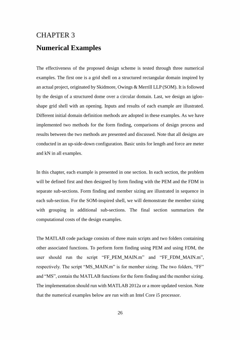
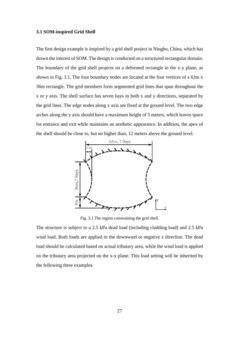
3.1 SOM-inspired Grid Shell

The first design example is inspired by a grid shell project in Ningbo, China, which has

drawn the interest of SOM. The design is conducted on a structured rectangular domain.

The boundary of the grid shell projects on a deformed rectangle in the x-y plane, as

shown in Fig. 3.1. The four boundary nodes are located at the four vertices of a 63m x

36m rectangle. The grid members form segmented grid lines that span throughout the

x or y axis. The shell surface has seven bays in both x and y directions, separated by

the grid lines. The edge nodes along x axis are fixed at the ground level. The two edge

arches along the y axis should have a maximum height of 5 meters, which leaves space

for entrance and exit while maintains an aesthetic appearance. In addition, the apex of

the shell should be close to, but no higher than, 12 meters above the ground level.

Fig. 3.1 The region constraining the grid shell.

The structure is subject to a 2.5 kPa dead load (including cladding load) and 2.5 kPa

wind load. Both loads are applied in the downward or negative z direction. The dead

load should be calculated based on actual tributary area, while the wind load is applied

on the tributary area projected on the x-y plane. This load setting will be inherited by

the following three examples.

28

3.1.1 Form Finding Using PEM

Here we use the Q8 finite element shape functions for initial domain geometry

definition. The physical coordinates of the eight FE nodes are prescribed in vector X,

Y and Z. We define Nx and Ny as the number of grid lines along the x and y direction,

respectively. The problem requires 7 bays in each direction and thus Nx and Ny are

both 8. With the information above, we can obtain the initial nodes, shell panels and

boundary conditions through the function named as “RectangularDomain”. The

corresponding MATLAB code is listed as follows:

method = 'Q8';

X=9*[-3.5 3.5 3.5 -3.5 0 3 0 -3];

Y=9*[-2 -2 2 2 -3 0 3 0];

Z=zeros(1,8);

Nx = 8; Ny = 8;

[NODE_ori,BARS,L0,ELEM,FREE_NODE,FIX_NODE,] =

RectangularDomain(X,Y,Z,Nx,Ny,method);

The resultant initial domain consists of 64 nodes (of which 16 are fixed and 48 are free),

98 grid members and 49 shell panels as shown by Fig. 3.2. All nodes are initially located

in the x-y plane.

Fig. 3.2 The initial domain geometry projected on the x-y plane. The numbering of nodes (black,

over the nodes), grid members (blue, over the midpoints of grid members) and shell panels (magenta,

over the panels) are also included. The blue triangles denote nodes with fixed coordinates in x, y

and z direction.

29

Next, we define the stiffness of all grid members by means of the function

“GetStiffness_Rectangular”, with the prescribed EA value and length of each member.

Define the term “EAunit” as a unit value of EA, which is the product of Young’s

modulus and cross sectional area of the grid member. We divide the members into three

groups, and assign the EA value of each group to be 8, 4 and 2 times of the EAunit,

respectively. The three groups are chosen as the vertical edge members, vertical interior

members and horizontal members, observed from the x-y plane. The stiffness of all grid

members are calculated by Eq. (2.1.4), where the member length is derived from the

initial domain geometry. This process is illustrated by Fig. 3.3. The specific unit EA

value of 2700 kN is chosen after a number of trials and error, in order to satisfy the

geometric constraints. The corresponding MATLAB code is provided below.

EAunit = 2700;

K=GetStiffness_Rectangular(NODE_ori,BARS,Nx,Ny,EAunit);

Fig. 3.3 Distribution of EA values and member stiffness among grid members. (a) Three EA values

are assigned to three groups of members; (b) The stiffness of each grid member.

We denote the uniformly distributed load applied on actual tributary area as q1, and the

uniformly distributed load applied on projected tributary area on x-y plane as q2. Thus

the input for loads is

q1 = 2.5; q2 = 2.5;

30

In Chapter 2, we have defined the convergence criterion as ‖𝐱(𝑘)−𝐱(𝑘−1)‖

𝑁𝑑𝑜𝑓< 𝜀, where

‖𝐱(𝑘)−𝐱(𝑘−1)‖

𝑁𝑑𝑜𝑓 is a measure of average movement of nodes from the previous iteration to

the current one. The tolerance 𝜀 here is set to be 10-3, and a limit of 200 on the iteration

number applies. This setting holds for other form finding cases unless specified.

Now we have the information on the initial domain geometry, the boundary conditions,

the grid member stiffness, the loads and the convergence criteria to perform the form

finding computation. It takes 3 iterations for the form finding to converge. This process

takes 15 seconds of CPU time. The resultant form observed from different views is

shown in Fig. 3.4 and the convergence plot in Fig. 3.5.

Fig. 3.4 The final form obtained from form finding using PEM. (a) 3D View; (b) Top view (in the

x-y plane); (c) Side view (in the y-z plane); (b) Front view (in the x-z plane).

31

Fig. 3.5 Convergence plot of form finding using PEM. Convergence is achieved at the 3rd iteration.

The final step consists of checking if design constraints are satisfied. The apex of the

grid shell has an elevation of 11.8538m at node 28, 29, 36 and 37, which is less than

the constrained height of 12m. The maximum height of the side arch is 5.1689m at node

4, 5, 60 and 61, which is larger than the required height of 5m. Thus both geometric

constraints are satisfied.

Finally, major design input and output are saved in a prescribed file name.

Output_Name_FF='SOMShell_FF_PEM.mat';

save(Output_Name,'NODE','F','BARS','ELEM','FIX','NODE_ori','Nn');

3.1.2 Member Sizing without Grouping Using PEM

With the design output from the form finding, we proceed to the structural member

sizing. Besides the data from the form finding, the Young’s modulus and the admissible

stress of the actual construction material are required. For the current example, we

choose standard G60 steel for the grid members, which has a Young’s modulus of

200,000,000 kPa and an admissible stress of 415000 kPa under both tension and

compression. As no grouping is involved in the current member sizing procedure, the

group flag is set false and the code will treat the cross sectional area of each grid

member as an independent variable. The input is listed below:

32

load SOMShell_FF_PEM

S_adm_T = 415000;

S_adm_C = 415000;

E = 200000000;

group_flag = false;

With the input above, we perform the member sizing. The initial guess of the cross

sectional areas is 0.005 m2 for every grid member. The tolerance for the current member

sizing is set to be 5x10-3. These computational settings apply to other member sizing

examples unless otherwise specified. The result converges at the 23rd iteration with a

computational cost of 86 seconds of CPU time. We define the the ratio of member cross

sectional area over the maximum member cross sectional area as the area ratio. The

member cross sectional area information will be shown in the area ratio plots here and

in the following examples. The member area ratio plots, stress ratio plot and

convergence plot are shown in Fig. 3.6, Fig. 3.7 and Fig. 3.8 respectively.

The maximum cross sectional area of 3684 mm2 occurs on four grid members as circled

in Fig. 3.6. This value is comparable with the gross area of the standard

HSS5.563x0.258 section (AISC, Steel Construction Manual), which is 3690 mm2 or

5.72 in2. The total volume of steel used is 1.3438m3. From Fig. 3.7, we observe that

stress ratios for all grid members have indeed converged to 1 and what we obtain here

is a fully-stressed design.

Fig. 3.6 Area ratio plots with the color scale. The maximum cross sectional area is 3684 mm2. The

color and thickness of each grid member are associated with the area ratio. (a) The 3D view; (b) The

plan view.

33

Fig. 3.7 Stress ratio plot with the color scale. The stress ratios have converged to 1 as expected.

Fig. 3.8 Convergence plot of member sizing without grouping. Convergence is achieved at the 23rd

iteration.

3.1.3 Member Sizing with Grouping Using PEM

In this member sizing trial, we divide the grid members into three groups such that the

member cross sectional areas in each group remain identical. Compared with the

member sizing trial above, the same form finding information and material properties

are provided with the additional grouping information. The groups are defined as the

edge vertical members, inner vertical m embers and horizontal members as shown in

Fig. 3.9. Also, we set the “group_flag” as true such that the implementation of stress

ratio method for group design will be used.

34

Fig. 3.9 Grid member grouping information.

The member sizing with grouping converges at the 19th iteration with a computational

cost of about 76 seconds of CPU time. The maximum cross sectional area is 3687 mm2,

which is applied on all the inner vertical members. The total volume of steel is increased

to 1.6782 m3, as most of the grid members have a cross sectional area larger than the

value associated to fully-stressed design (previous section). As the stress ratio reveals,

not all grid members are fully stressed. Instead, in each of the three grid member groups,

at least one member has a stress ratio of 1 and the others have stress ratios between 0

and 1. The area ratio plots are given in Fig. 3.10 and the stress ratio plot in Fig. 3.11.

The convergence plot is shown below in Fig. 3.12.

Fig. 3.10 Area ratio plots with the color scale. The maximum cross sectional area is 3687 mm2. The

color and thickness of each grid member are associated with the area ratio. (a) The 3D view; (b) The

plan view.

35

Fig. 3.11 Stress ratio plot with color scale. Fully-stressed members in the three groups are labelled

with 1, 2 and 3.

Fig. 3.12 Convergence plot of member sizing with grouping. Convergence is achieved at the 19th

iteration.

3.1.4 Form Finding Using FDM

Form finding using FDM is conducted by the code named “FF_FDM_Main.m”. Here,

the inputs of initial domain geometry, boundary conditions and loads are the same as

those in the form finding using PEM. The difference is that we prescribe force density

instead of member stiffness for every grid member. The following lines of code

prescribe force densities in a grouped manner as shown in Fig. 3.13.

FDunit=75;

FD=GetFD_SOMShell(Nb,Nx,Ny,FDunit);

1

1 1

1

2 2

2 2

3

3

36

Fig. 3.13 Distribution of force densities.

The code takes 5 iterations to converge at a computational cost of about 1 second of

CPU time. The form is shown in Fig. 3.14 and the convergence plot is shown in Fig.

3.15. The apex of the grid shell has an elevation of 11.7420m at node 28, 29, 36 and 37,

which is less than the constrained height of 12m. The maximum height of the side arch

is 5.9544m at node 4, 5, 60 and 61, which is larger than the required height of 5m. Thus

both geometric constraints are satisfied. The node numbers can be referred from Fig.

3.2.

Fig. 3.14 The final form obtained from form finding using FDM. (a) 3D View; (b) Top view (in the

x-y plane); (c) Side view (in the y-z plane); (b) Front view (in the x-z plane).

37

Fig. 3.15 Convergence plot of form finding using FDM.

3.1.5 Member Sizing without Grouping Using FDM

The standard G60 steel is chosen as the material for the grid members in member sizing,

which has a Young’s modulus of 200,000,000 kPa and an admissible stress of 415000

kPa under both tension and compression. Together with the design outputs from the

form finding using FDM, the member sizing without grouping is conducted.

The result converges at the 22nd iteration at a computational cost of about 84 seconds

of CPU time. The member area ratio plots, stress ratio plot and convergence plot are

provided in Fig. 3.16, Fig. 3.17 and Fig. 3.18, respectively. A fully-stressed design is

achieved as stress ratios for all grid members have converged to 1, according to Fig.

3.17. The maximum cross sectional area of 3590 mm2 occurs on four grid members as

circled in Fig. 3.16. The total volume of steel used is 1.4606 m3.

38

Fig. 3.16 Area ratio plots with the color scale. The maximum cross sectional area is 3590 mm2. The

color and thickness of each grid member are associated with the area ratio. (a) The 3D view; (b) The

plan view.

Fig. 3.17 Stress ratio plot with color scale. The stress ratios of all grid members have converged to

1 as expected.

Fig. 3.18 Convergence plot for member sizing without grouping. Convergence is achieved at the

22nd iteration.

39

3.1.6 Member Sizing with Grouping Using FDM

In this member sizing, we input G60 steel material properties and provide the grouping

information as indicated in Fig 3.9. The member sizing with grouping converges at the

19th iteration with a computational cost of about 80 seconds of CPU time. The

maximum cross sectional area is 3632 mm2, which is applied on all the inner vertical

members. The total volume of steel is increased to 1.7325 m3. The area ratio plots, stress

ratio plot and convergence plot are shown in Fig. 3.19, 3.20 and 3.21, respectively.

Fig. 3.19 Area ratio plots with the color scale. The maximum cross sectional area is 3632 mm2. The

color and thickness of each grid member are associated with the area ratio. (a) The 3D view; (b) The

plan view.

Fig. 3.20 Stress ratio plot with color scale. Fully-stressed members in the three groups are labelled

with 1, 2 and 3.

1

1 1

1

2 2

2 2

3

3

40

Fig. 3.21 Convergence plot of member sizing with grouping. Convergence is achieved at the 19th

iteration.

3.2 Structured Circular Dome

This example intends to design a structured grid shell over a circular domain, which

results in a dome shape. The dome is formed by radial ribs and tangential rings

composed of grid members. In the current example, we shall design on a circular

domain with a 5m radius, as shown by Fig. 3.22. The number of radial ribs and

tangential rings are 8 and 4, respectively. Nodes on the perimeter are fixed at the ground

level. The apex of the dome is restricted to be less than 4 m. The 2.5 kPa dead load and

2.5 kPa wind load are applied. For the member sizing, no grouping will be considered.

Fig. 3.22 The region constraining the grid shell.

41

3.2.1 Form Finding Using PEM

Let’s define the radius of domain r = 5, the number of radial ribs Nr = 8 and the number

of tangential rings Nt = 6 (including the merging point in the center and the null

members connecting the fixed nodes). With the information above, the initial domain

is defined as “CircularDomain”. This function is specifically for defining a structured

domain fixed on a circular perimeter, which does not use the three initial domain

definition methods introduced in the Chapter 2. All radial grid members are of equal

length. The input code is as follows:

r = 5; Nr = 8; Nt = 6;

[NODE_ori,ELEM,SUPP,LOAD] = CircularDomain(r,Nr,Nt);

The initial domain consists of 41 nodes (of which 8 are fixed and 33 are free nodes),

72 grid members and 40 shell panels, as shown by Fig. 3.23. All nodes are initially

located in the x-y plane.

Fig. 3.23 (a) The initial domain geometry with labels of nodes (black, over the nodes), grid members

(blue, over the midpoints of grid members) and shell panels (magenta, over the panels). The blue

triangles denote nodes with fixed coordinates in x, y and z direction. (b) Member stiffness

distribution.

The EA property value of all members is identically defined as 80 kN and then the

member stiffness is derived together with the member length. The input code is as

follows:

42

EAedge = 80;

EAinner = 80;

[EDGE,INNER] = GetPolyEdges(ELEM);

[BARS,K] = GetSprings(NODE_ori,EDGE,INNER,EAedge,EAinner);

The definition of loads is the same as in the last example.

With the input, we proceed to the computation of the form finding. The code converges

after 4 iterations at a computational cost of about 6 seconds of CPU time. The resultant

form is shown in Fig. 3.24. The apex of the form occurs at the center with a height

3.8320m, which is less than the 4m height limit. The convergence plot is shown in Fig.

3.25.

Fig. 3.24 The final form obtained from form finding using PEM. (a) 3D View; (b) Top view (in the

x-y plane); (c) Side view (in the y-z plane); (b) Front view (in the x-z plane).

43

Fig. 3.25 Convergence plot of form finding using PEM. Convergence is achieved at the 4th iteration.

3.2.2 Member Sizing Using PEM

The standard G60 steel is chosen as the construction material, which has a Young’s

modulus of 200,000,000 kPa and an admissible stress of 415000 kPa under both tension

and compression. With the form finding results and the material properties, we perform

the member sizing. The result converges at the 35th iteration at a computational cost of

50 seconds of CPU time. Fig 3.26 shows the member area ratio plots and Fig 3.27 shows

both the stress ratio plot and convergence plot for this example.

The maximum cross sectional area is 128 mm2, which occurs at the grid members

attached to the ground. The total volume of steel used is 0.0046249m3. The stress ratios

for all grid members have indeed converged to 1 and the convergence is achieved, as

Fig. 3.27 (a) shows.

44

Fig. 3.26 Area ratio plots with the color scale. The maximum cross sectional area is 128 mm2. The

color and thickness of each grid member are associated with the area ratio. (a) The 3D view; (b) The

plan view.

Fig. 3.27 (a) Stress ratio plot with the color scale. The stress ratios have converged to 1 as expected;

(b) Convergence plot of member sizing. Convergence is achieved at the 35th iteration.

3.2.3 Form Finding Using FDM

With the similar initial domain geometry, boundary condition and load definition as in

the PEM implementation, we define the force density in the pattern shown in Fig. 3.28.

The values are determined such that the final shape is aesthetically appealing and meet

the apex constraint.

(a) (b)

45

Fig. 3.28 Distribution of force densities.

The form finding takes 7 iterations to converge at a computational cost of about 1.1

seconds of CPU time. The form and convergence plot are shown in Fig. 3.29 and Fig.

3.30, respectively. The apex of the grid shell is at a height of 3.7157m.

Fig. 3.29 The final form obtained from form finding using FDM. (a) 3D View; (b) Top view (in the

x-y plane); (c) Side view (in the y-z plane); (b) Front view (in the x-z plane).

46

Fig. 3.30 Convergence plot of form finding using FDM. Convergence is achieved at the 7th

iteration.

3.2.4 Member Sizing Using FDM

The standard G60 steel is chosen as the material for the grid members in member sizing,

which has a Young’s modulus of 200,000,000 kPa and an admissible stress of

415000 kPa under both tension and compression. Together with the design outputs from

the form finding using FDM, the member sizing is conducted. The result converges at

the 63rd iteration at a computational cost of about 57 seconds of CPU time. The

maximum cross sectional area of 155 mm2 occurs on the members attached to ground

as the member area ratio plot in Fig. 3.31 shows. The stress ratio and convergence plot

for this example are provided in Fig. 3.32. The stress ratios of all grid members have

converged to 1, according to Fig. 3.32 (a). The total volume of steel used is 0.005767

m3.

47

Fig. 3.31 Area ratio plots with the color scale. The maximum cross sectional area is 155 mm2. The

color and thickness of each grid member are associated with the area ratio. (a) The 3D view; (b) The

plan view.

Fig. 3.32 (a) Stress ratio plot with color scale. The stress ratios of all grid members have converged

to 1 as expected; (b) Convergence plot for member sizing. Convergence is achieved at the 63rd

iteration.

3.3 Igloo

This example intends to design an igloo-shape grid shell, which can provide the

accommodation for one person. The igloo should stand on the perimeter of a 1m-radius

circle in the x-y plane. As illustrated by Fig. 3.33, the boundary of the igloo is fixed on

the ground except for an opening corresponding to an arc of a 60-degree angle, as shown

in Fig 3.32. The apex of the igloo is limited to be less than 1m.

(a) (b)

48

Fig. 3.33 The region constraining the grid shell.

3.3.1 Form Finding Using PEM

The domain boundary is defined by a 1m-radius circle cut by a secant of a 60-degree

central angle in the x-y plane as shown in Fig. 3.33. The following code generate the

initial domain in the x-y plane with the modified PolyMesher. The initial geometric

boundary is predefined in the file “IglooDomain”, as well as the boundary conditions.

We provide 50 random seeds within the 2D domain and request 1000 iterations for the

PolyMesher to generate the CVT mesh. The input code is provided below:

[NODE_ori,ELEM,SUPP,LOAD] = PolyMesher(@IglooDomain,50,1000);

NODE_ori = [NODE_ori zeros(size(NODE_ori,1),1)];

In this specific design trial, the resultant initial domain consists of 100 nodes (of which

20 are fixed and 80 are free nodes), 130 grid members and 50 shell panels (which is

equal to the prescribed seed number). The grid member 1, 2, 4, 6 and 8 are the edge

members that forms the arch above the entrance. The initial domain geometry is given

by Fig. 3.34.

49

Fig. 3.34 The initial domain geometry observed in the x-y plane with the numbering of nodes (black,

over the nodes), grid members (blue, over the midpoints of grid members) and shell panels (magenta,

over the panels) are included. The blue triangles denote fixed nodes.

The EA value is prescribed as 0.5 kN for the edge members that form the arch and 1.8

for the other members. The EA value and stiffness distribution are shown in Fig. 3.35.

The same load case is considered as in the previous examples.

Fig. 3.35 (a) Distribution of EA values; (b) Distribution of member stiffness.

With the input above, we proceed to the computation of form finding. The form

converges after 3 iterations fat a computational cost of about 16 seconds of CPU time.

The apex of the form occurs at the center with a height 0.9966m, which is less than the

50

1m height limit. Fig. 3.36 shows the resultant form in different views. Fig. 3.37 provides

the convergence plot

Fig. 3.36 The final form obtained from form finding using PEM. (a) 3D View; (b) Top view (in the

x-y plane); (c) Side view (in the y-z plane); (b) Front view (in the x-z plane).

Fig. 3.37 Convergence plot of form finding using PEM. Convergence is achieved at the 3rd iteration.

51

3.3.2 Member Sizing Using PEM

The standard G60 steel is chosen as the construction material, which has a Young’s

modulus of 200,000,000 kPa and an admissible stress of 415000 kPa under both tension

and compression. The default tolerance for the member sizing iteration of 5x10-3is used.

The result converges at the 23rd iteration at a computational cost of 50 second of CPU

time. Fig. 3.38 shows the member area ratio plots. The stress ratio plot and convergence

plot are provided in Fig. 3.39. The maximum cross sectional area is 3 mm2. The total

volume of steel used is 4.2738e-05m3. According to Fig. 3.39 (a), the stress ratios for

all grid members have indeed converged to 1.

Fig. 3.38 Area ratio plots with the color scale. The maximum cross sectional area is 128 mm2. The

color and thickness of each grid member are associated with the area ratio. (a) The 3D view; (b) The

plan view.

52

Fig. 3.39 (a) Stress ratio plot with the color scale. The stress ratios have converged to 1 as expected;

(b) Convergence plot of member sizing. Convergence is achieved at the 23rd iteration.

3.3.3 Form Finding Using FDM

With the similar initial domain geometry, boundary condition and load definition as in

the PEM implementation, we define member force densities in the pattern shown in Fig

3.40. Grid members are divided into two groups: the edge members comprising the

entrance arch have a force density of 1.5 kN/m, and other members have a force density

of 2.9 kN/m.

Fig. 3.40 Distribution of force densities.

The form finding takes 7 iterations to converge at a computational cost of about 1.5

seconds of CPU time. The form and convergence plot are shown below. The apex of

the grid shell is at a height of 0.9665m.

(a) (b)

53

Fig. 3.41 The final form obtained from form finding using FDM. (a) 3D View; (b) Top view (in

the x-y plane); (c) Side view (in the y-z plane); (b) Front view (in the x-z plane).

Fig. 3.42 Convergence plot of form finding using FDM. Convergence is achieved at the 7th

iteration.

54

3.3.4 Member Sizing Using FDM

The standard G60 steel is chosen as the material for the grid members in member sizing,

which has a Young’s modulus of 200,000,000 kPa and an admissible stress of

415000 kPa under both tension and compression. The default tolerance for the member

sizing iteration of 5x10-3is used. Together with the design outputs from the form finding

using FDM, the member sizing is conducted. The result converges at the 23rd iteration

at a computational cost of about 50 seconds of CPU time. The member area ratio plot

is shown by Fig. 3.43. The maximum cross sectional area is 3 mm2.The total volume of

steel used is 4.8434e-05 m3. The stress ratio plot and convergence plot are provided in

Fig. 3.44.

Fig. 3.43 Area ratio plots with the color scale. The maximum cross sectional area is 3 mm2. The

color and thickness of each grid member are associated with the area ratio. (a) The 3D view; (b) The

plan view.

Fig. 3.44 (a) Stress ratio plot with the color scale. The stress ratios have converged to 1 as expected;

(b) Convergence plot of member sizing. Convergence is achieved at the 23rd iteration.

(a) (b)

55

3.4 Remarks on Computational Costs

Both the PEM and the FDM provide satisfactory bending-free forms under equilibrium

in the four numerical examples. Information on the computational costs of the form

finding is tabulated in Table 3.1. From this table, we observe that the computation of

the form finding can be done efficiently (the maximum CPU time cost was 16s).

However, all the examples in the thesis are relatively small.

Another observation is that in general, the PEM takes less iteration to converge than the

FDM, while the PEM requires more computational resources than the FDM. The CPU

time per iteration for form finding using PEM is more than that using FDM. This

happens because within each iteration, the PEM solves a non-linear optimization

problem, while the FDM solves a linear system. Given the same number of design

variables, solution to a linear system is cheaper than to solution of an optimization

problem in general. Thus, the total computational cost of the PEM is more than that of

the FDM, even with a smaller iteration number.

Table 3.1 Computational cost comparison for form finding.

Computational information of the member sizing is tabulated in Table 3.2. Every

example has two separate member sizing results based on the form finding using PEM

and FDM, respectively. The design variable of the member sizing is the cross sectional

areas of every grid member, while the design variables are the degrees of freedom in

the optimization problem at each iteration. For all three examples, the member sizing

requires more computational costs than the form finding.

Iteration

No.

CPU Time

(s)

CPU Time

Per Iter. (s)

Iteration

No.

CPU Time

(s)

CPU Time

Per Iter. (s)

Dome 99 4 6 1.50 7 1.1 0.16

SOM Shell 144 3 15 5.00 5 1 0.20

Igloo 240 3 16 5.33 7 1.5 0.21

Example

No. of Design

Variables

(Dofs)

PEM FDM

56

Table 3.2 Computational cost comparison for the member sizing. In the first column, content in the

bracket indicates the method used to obtain the form.

The computational costs of member sizing with and without group design are compared

for the SOM-inspired shell example. Given the same number of design variables and

the same stopping criteria, the member sizing with group design seems to take less

iteration and total computational cost, but the difference is quite small.

Table 3.3 Computational cost comparison for the member sizing with and without group design.

Descriptions in the first column tell the method for the form finding and whether the member sizing

considers group design.

Dome (PEM) 72 99 35 50

Dome (FDM) 72 99 63 57

SOM Shell

(PEM)98 144 23 86

SOM Shell

(FDM)98 144 22 84

Igloo (PEM) 130 240 23 50

Igloo (FDM) 130 240 23 46

ExampleNo. of Design

Variables (A)No. of Dofs

Iteration

No.

CPU Time

(s)

PEM, No

Group Design23 86

PEM, Group

Design19 76

FDM,No

Group Design22 84

FDM, Group

Design19 80

Example Iteration No.CPU Time

(s)

57

Chapter 4

Concluding Remarks

To find a funicular form is a challenging but important task in the design of grid shell

structures. This thesis presented a numerical implementation that performs the form

finding of grid shell structures. Given the initial domain, boundary conditions and loads,

one can use PEM and/or FDM to find the optimal form of a grid shell, in which the

nodal force equilibrium is maintained and the grid members suffer zero bending

moment and shear. For the convenience of the designer, the current implementation

provides three generic methods for the initial domain definition. Instead of using

predefined constant nodal loads only, the implementation can calculate the form-

dependent nodal loads using a tributary area rationale as the form finding evolves. For

the PEM implementation, the snap-through instability triggering is embedded for a

more optimal design. With the form finding results, the designer can perform a

preliminary member sizing for the grid members either with or without group design.

After the whole design process, the designer obtains an optimal grid shell form, the

nodal loads and a fully-stressed design of the cross sectional areas of the grid members.

The three numerical examples show that the implementation provides the desired

results with a reasonable computational cost.

The current form finding implementation does not directly consider any constraint in

the form finding process. If any specific design constraint is present, such as the shell

apex limit in the example of the SOM-inspired shell, the designer needs to perform a

series of form finding trials to obtain a form in which the design constraint is satisfied.

As a future extension, we can deal with the constraints within the implementation, so

that numerous design trials can be avoided. With this extension, it is expected that each

iterative step of the form finding will change from solving an unconstrained

optimization problem (PEM) or an algebraic equation system (FDM) into solving a

constrained optimization problem.

58

A final remark lies on the issue regarding how much the funicular form suggests a

structurally efficient grid shell. The form finding makes assumptions that may not be

valid in an actual structure. For example, we are assuming that all nodes are hinged and

shell panels do not resist loads. But in reality, the nodes are usually not purely hinged

and the shell panels will transfer loads together with the grid members. Thus a funicular

form on the drawing is likely not to be strictly funicular upon construction. To verify if

the funicular form is a proper form for a real structure, we can use the professional

structural analysis software, such as ABAQUS, to perform a structural analysis with

the form finding results. A further extension along this rationale is to include the

structural analysis in the form finding. In this way, we may introduce more the

computational costs, but obtain grid shell structures that are closer to the optimal in a

practical sense.

59

References

[1] Adriaenssens, S., Ney, L., Bodarwe, E. and Williams, C. (2012). “Finding the form

of an irregular meshed steel and glass shell based on construction constraints.” Journal

of Architectural Engineering, 18:206-213.

[2] Bassegoda, Juan (1989). El gran Gaudí. Barcelona: Sabadell. ISBN 978-84-86329-

44-0.

[3] Billington, D. (2008). The art of structural design: A Swiss legacy, Yale University

Press, New Haven, CT, pp. 128–163.

[4] Bletzinger K., Wüchner, R., Daoud, F. and Camprubí N. (2005). “Computational

methods for form finding and optimization of shells and membranes.” Computational

Methods in Applied Mechanics and Engineering, 194:3438–3452.

[5] Block, P., Dejong, M. and Ochsendorf, J. (2007). “As Hangs the Flexible Line:

Equilibrium of Masonry Arches.” Nexus Network Journal, Vol. 8, No. 2, pp. 9-19.

[6] Block, P., and Ochsendorf, J. (2007). “Thrust network analysis: A new methodology

for three-dimensional equilibrium.” J. Int. Assoc. Shell Spatial Structures, 48(3), pp. 1–

7.

[7] Block, P. (2009). Thrust Network Analysis: Exploring Three-dimensional

Equilibrium, PhD dissertation, Massachusetts Institute of Technology.

[8] Day, A. S. (1965). “An introduction to dynamic relaxation.” The Engineer, 29, pp.

218–221.

[9] Dimčić, M. (2011). Structural Optimization of Grid Shells Based on Genetic

Algorithms, PhD dissertation, Universität Stuttgart.

[10] Happold, E. and Liddell, W. I. (1975). “Timber lattice roof for the Mannheim

Bundesgartenschau.” The Structural Engineer, Volume 53, N03, pp. 99-135.

[11] Huerta, S. (2003). “El calculo de estructuras en la obra de Gaudí.” Ingeniera Civil,

130, pp. 121–133.

[12] Heath, M. T. (2002) Scientific Computing: An Introductory Survey, 2nd ed.,

McGraw-Hill.

[13] Kilian, A. and Ochsendorf, J. (2005). “Particle-spring systems for structural form-

finding.” J. Int. Assoc. Shell Spatial Structures, 46(148), pp. 77–84.

60

[14] Leon, S. E., Paulino, G. H., Pereira, A., Menezes, I. F. M., and Lages, E. N. (2011).

“A unified library of nonlinear solution schemes.” Applied Mechanics Review. 64,

040803.

[15] Lewis, W.J. (2003). Tension structures. Form and Behaviour. Thomas Telford,

London.

[16] Linkwitz, K. and Schek, H. -J. (1971). “Einige Bemerkungen zur Berechung von

vorgespannten Seilnetzkonstruktionen.” Ingenieur-Archiv, (40):145–158.

[17] Mueller, K. M., Liu M. and Burns S. A. (2002). “Fully stressed design of Frame

structures and multiple load paths.” Journal of Structural Engineering, Vol. 128, No. 6,

June 2002, pp. 806-814.

[18] Ohsaki, M. (2010). Optimization of Finite Dimensional Structures. CRC Press.

ISBN 9781439820049.

[19] Otto, F., Rasch, B., Pfafferodt, Schonborn, A.G., and Schanz S. (1995). Finding

form. Deutsche Werkbund Bayern, Edition Axel Menges, Munich, Germany.

[20] Paoli, C. (2007). Past and Future of Grid Shell Structures, ME thesis,

Massachusetts Institute of Technology.

[21] Richardson, J. N., Adriaensses, S., Coelho, R. F. and Bouillard, P. (2013).

“Coupled form-finding and grid optimization approach for single layer grid shells.”

Engineering Structures, 52:230-239.

[22] Rozvany, G. I. N., Prager W. (1979). “A new class of optimization problems:

optimal archgrids.” Comput Methods Appl Mech Eng, 19:127–150

[23] Rozvany G. I. N., Wang C. M., Dow M. (1982). “Archgrids and cable networks of

optimal layout.” Comput Methods Appl Mech Eng, 31:91–113

[24] Schek, H. J. (1974). “The Force Density Method for Form Finding and

Computation of General Networks.” Comput Methods Appl Mech Eng, 3:115–134.

[25] Talischi, C., Paulino, G. H., Pereira, A. and Menezes, I. F. M. (2012). “PolyMesher:

A general-purpose mesh generator for polygonal elements written in Matlab.” Journal

of Structural and Multidisciplinary Optimization, Vol. 45, No. 3, pp. 309-328.

[26] Tomlow, J., Graefe, R., Otto, F. and Szeemann, H, (1989), Das Modell, The Model,

Institut für Leichte Flächentragwerke, Stuttgart, Germany [Edition in German, English

and Spanish.]

61

[27] Veenendaal, D. and Block, P. (2014). “Comparison of form-finding methods.”

Shell Structures for Architecture: Form Finding and Optimization, Adriaenssens, S.,

Block, P., Veenendaal, D. and Williams, C. (editors), Routledge, London.

[28] Veenendaal D. and Block P (2012). “An overview and comparison of structural

form finding methods for general networks.” International Journal of Solids and

Structures, 49(26): 3741-3753.

[29] Winslow P., Pellegrino S. and Sharma S.B. (2010). “Multi-objective optimization

of free-form grid structures.” Structural and multidisciplinary optimization, 4(1-6),

pp.257-269.

[30] Christensen, P. W. and Klarbring A. (2009). An Introduction to Structural

Optimization. Springer Netherlands. ISBN 978-1-4020-8666-3

[31] MATLAB 7.14, R2012a, (2012) The MathWorks Inc., Natick, MA.

[32] Zegard T. and Paulino G. H. (2014). “GRAND — Ground structure based topology

optimization for arbitrary 2D domains using MATLAB." Journal of Structural and

Multidisciplinary Optimization. Vol 50. No. 5. pp. 861-882.

Web References of Figures

[31] “L'Oceanografic, at the City of Arts and Sciences in Valencia (Valencian

Community, Spain).”

https://en.wikipedia.org/wiki/F%C3%A9lix_Candela#/media/File:L%27Oceanografic

_(Valencia,_Spain)_01.jpg

[32] “Roof for the Mannheim Multihalle.”

http://www.pritzkerprize.com/sites/default/files/gallery_images/Frei-Otto-Roof-for-

the-Mannheim-Multihalle-02.jpg

[33] “Colònia Güell.”

https://www.pinterest.com/pin/490892428104983598/

[34] "Cripta de la Colònia Güell 1".

https://commons.wikimedia.org/wiki/File:Cripta_de_la_Col%C3%B2nia_G%C3%BC

ell_1.jpg#/media/File:Cripta_de_la_Col%C3%B2nia_G%C3%BCell_1.jpg

62

Appendix A: MATLAB Code Files for Form Finding

of Grid Shell Structures

MATLAB files for form finding of grid shell structures can be found in the

supplementary file “FormFinding_MATLAB_YJ_Thesis.rar”.