© 2018 Robert Ranieri - ufdcimages.uflib.ufl.edu

AN ANALYSIS OF SELECTED CROP INSURANCE POLICIES AVAILABLE TO FLORIDA BLUEBERRY GROWERS

By

ROBERT RANIERI

A THESIS PRESENTED TO THE GRADUATE SCHOOL OF THE UNIVERSITY OF FLORIDA IN PARTIAL FULFILLMENT

OF THE REQUIREMENTS FOR THE DEGREE OF MASTER OF SCIENCE

UNIVERSITY OF FLORIDA

2018

© 2018 Robert Ranieri

To mom, dad, and Rae

4

ACKNOWLEDGMENTS

First and foremost, I would like to thank my two advisors: Dr. Singerman and Dr.

Kropp. Their expertise and professionalism not only guided me to the ultimate goal of

completing my thesis, but also inspired me to put in the long hours where it seemed the

end was never in sight. I can proudly say that this thesis is my best work, that no short-

cuts were taken and no possible flaw had gone unquestioned. I have my advisors to

thank for that. Without you, this paper would be a shell of what it is now.

A big thanks to my mom, dad, and sister. During my two years at UF, I have

never been farther from home for so long. Without the loving support of my family, I

wouldn’t have been able to graduate middle school, let alone graduate school. You

have always supported me unconditionally, and let me thrive through adversity.

I’d also like to thank Megan. For the countless nights staying up helping me

decide when to include a comma, for listening to me go on tangents about the blueberry

industry, and for all the boring mock-presentations you had to sit through, thank you. I

know it isn’t the easiest to understand or the most interesting, but you listened with open

ears and were there to support me with open arms.

Lastly, I’d like to thank Julio, Rusty, and Scott. We’ve spent far too many long

hours in the Byrne room – studying, teaching each other, and sometimes just cracking

jokes. Academics may have brought us together, but it’s the times outside of class that

kept me sane.

5

TABLE OF CONTENTS page

ACKNOWLEDGMENTS .................................................................................................. 4

LIST OF TABLES ............................................................................................................ 7

LIST OF FIGURES .......................................................................................................... 8

LIST OF CROP INSURANCE TERMINOLOGY ............................................................ 10

ABSTRACT ................................................................................................................... 13

CHAPTER

1 INTRODUCTION .................................................................................................... 15

Background ............................................................................................................. 15

Research Problem .................................................................................................. 17 Objectives ............................................................................................................... 18 Specific Objectives ................................................................................................. 18

2 LITERATURE REVIEW .......................................................................................... 20

A Brief History of Florida Blueberry Production ....................................................... 20

Blueberry Cyclical Price and Seasonality Graphical Analysis ................................. 23

Florida Market Window ........................................................................................... 26

Crop Insurance Policies .......................................................................................... 30 Premium Rate Complications ................................................................................. 38

Distribution of Yields ............................................................................................... 40

3 METHODS .............................................................................................................. 53

Data Collection and Analysis .................................................................................. 53

Crop Insurance Terminology ................................................................................... 55 Premium and Indemnity Calculations ..................................................................... 56 Alachua County Premium Calculations ................................................................... 57

Simulations in R ...................................................................................................... 59

4 RESULTS AND DISCUSSION ............................................................................... 69

Distribution Results ................................................................................................. 69 Simulation Results .................................................................................................. 70

RMA Indemnity Calculation Issues ................................................................... 75 RMA Premium Calculation Issues .................................................................... 78

5 GENERAL CONCLUSIONS ................................................................................... 94

6

Recommendation for Growers ................................................................................ 94

Recommendation for the RMA ................................................................................ 95

APPENDIX: R CODE .................................................................................................... 97

REFERENCES .............................................................................................................. 98

BIOGRAPHICAL SKETCH .......................................................................................... 103

7

LIST OF TABLES

Table page 2-1 Utilized Production of Blueberries by State from 2000 – 2016. .......................... 51

2-2 US Domestic Blueberry Market Share by State from 2000 – 2016. .................... 52

3-1 Summary of the parameters of the six different scenarios analyzed. ................. 68

4-1 Comparison of the APH and WFRP policy under Scenario 1. ............................ 85






4-7 Expected Utility of enrolling in APH or not enrolling for a risk-averse grower under Scenarios 1, 2, 3, 4, 5, & 6. ...................................................................... 91

4-8 Florida Blueberry Growers Participation in APH by Coverage Level .................. 92

4-9 Alachua Blueberry Growers Participation in APH by Coverage Level ................ 93

8

LIST OF FIGURES

Figure page 1-1 US imports, net production, and per capita use of fresh blueberries 1980-

2016. (USDA/ERS, 2017) ................................................................................... 19

2-1 Geographic overlay of average chill hours for a typical Florida winter. Source: Olmstead, Miller, Andersen, & Williamson, 2016 ................................................ 42

2-2 Top Blueberry-Producing Countries in 2014 by volume. Source: Food and Agricultural Organization of the United Nations (FAO, 2017) ............................. 43

2-3 Blueberry volume in the US produced by the United States, Florida, and by Southern Exporters from 2007 – 2017. (USDA/AMS, 2017) ............................... 44

2-4 Weighted Average National US Retail Blueberry Price for 4.4 ounce, 6 ounce, 1 pint, and 18 ounce blueberries (USDA/AMS, 2017) ............................. 45

2-5 United States domestic blueberry production and import timeline. Source: (USDA/AMS, 2017) ............................................................................................ 46

2-6 Side-by-side comparison of Florida blueberry production vs Mexican blueberry imports to the US, 2009 – 2016. (USDA/AMS, 2017) ......................... 49

2-7 The minimum revenue percentage for different numbers of crops to meet the diversification requirements of WFRP (USDA/RMA, 2017a) .............................. 50

3-1 Actual yield, adjusted yields, and the technology trend line of Florida blueberries from 1997-2016. (USDA/ERS, 2017b). ............................................ 64

3-2 Example of APH crop insurance policy payment for non-organic Southern Highbush blueberries with frost protection (USDA/RMA, 2017c) ........................ 65

3-3 Example of Whole-Farm Revenue Protection policy payment for single-commodity blueberries in Alachua county. (USDA/RMA, 2017c) ....................... 66

3-4 Side-by side comparison of the Actual Production History and the Whole Farm Revenue Protection policy. (USDA/RMA, 2017c) ...................................... 67

4-1 Price Histogram of Florida blueberries out of 5,000 iterations. ........................... 80

4-2 Yield Histogram of Florida blueberries out of 5,000 iterations. ........................... 80

4-3 Revenue Histogram of Florida blueberries out of 5,000 iterations. ..................... 81

4-4 Florida Blueberry yield to revenue scatterplot results of estimated yield and price under scenario 1. ....................................................................................... 81

9






10

LIST OF CROP INSURANCE TERMINOLOGY

Applicable to both Actual Production History and Whole-Farm Revenue Protection

Coverage Level

The amount of insurance chosen by the grower (%). The range for APH and WFRP is 50-75%.

Preliminary Premium Amount

The cost of crop insurance before subsidies are accounted for ($/acre).

Subsidy Rate The subsidy percentage that the farmer does not have to pay for (%). The subsidy rate decreases as coverage level increases.

Applicable to Actual Production History

Actual Yield The amount of blueberry pounds produced per acre that the grower produces for the insured season (lbs/acre).

Approved Yield

The amount of blueberry pounds produced per acre (lbs/acre). As long as the farm has been in production for the last four years or more, the Approved Yield is calculated by taking the average of the last 4+ consecutive years of blueberry production up until the last 10 years. If the farm has been in production less than four years, the average is taken from a culmination of transitional yields and any production in the last three years.

Base Rate The starting premium rate established by RMA for the 65% coverage level (%). Factors that influence this rate include state, county, coverage type, etc.

Established Price

Determined by the RMA by the closing date (typically occurring January), it is an estimation of the upcoming price of blueberries per pound during the season ($/lbs). The grower has the option to elect a lower price offered by the RMA and will pay less premium as a result. For the purposes of this analysis, the assumption is that the grower always elects the highest possible price offered by the RMA.

11

Guarantee The number of pounds of blueberries per acre insured, which is determined by multiplying the Approved Yield by the Coverage Level (lbs/acre).

Insured Shared Percent

The percentage of insurance that the grower pays for (%). For all examples, the assumption is that the grower fully owns the farm and is paying the entirety of the insurance directly. The insured shared percent is assumed to be 100%.

Liability Amount

The total value of blueberries insured per acre ($/acre). The Liability Amount for APH is determined by multiplying the Guarantee by the Established Price by the Insured Share Percent.

Applicable to Whole-Farm Revenue Protection

Actual Revenue

The total value of blueberries that the grower sells on a per acre basis for the insured season ($/acre).

Approved Revenue

The amount of acceptable revenue attributable to blueberry production ($/acre). The calculation for the Approved Revenue is the minimum of the Historic Average Revenue and the Expected Revenue.

Diversity Factor

An additional multiplier established by the RMA, which decreases the price of the premium if there is more than one commodity covered (%). For a single commodity, the diversity factor is 1, or 100%.

Expected Revenue

The anticipated amount of revenue for the upcoming insured season ($/acre).

Historic Average Revenue

The average amount of revenue produced per acre over the last 5 years ($/acre). Revenue calculations from year to year are cupped at 80% of the previous year and capped at 120% of the previous year.

Liability Amount

The total value of blueberries insured per acre ($/acre). The Liability Amount for WFRP is determined by multiplying the Approved Revenue by the Coverage Level.

12

Weighted Commodity

Rate

The base rate established by the RMA for a specific commodity, in this case blueberries (%). The weighted commodity rate increases with an increase in coverage level.

13

Abstract of Thesis Presented to the Graduate School of the University of Florida in Partial Fulfillment of the Requirements for the Degree of Master of Science

AN ANALYSIS OF SELECTED CROP INSURANCE

POLICIES AVAILABLE TO FLORIDA BLUEBERRY GROWERS

By

Robert Ranieri

May 2018

Chair: Ariel Singerman Major: Food and Resource Economics

The main purpose of this thesis is to determine which crop insurance policy,

Actual Production History (APH) or Whole-Farm Revenue Protection (WFRP), provides

the most benefit to Florida blueberry growers given certain market conditions. Another

objective of this thesis is to use numerical methods to evaluate the appropriateness of

the premium rates set for these policies. Up until this project, to the best of my

knowledge, no comparison between these two policies for Florida blueberry growers

had been performed. The findings help to explain the enrollment, or lack thereof, by

Florida blueberry growers.

Specialty crops exhibit a high variability in price compared to staple crops (Ligon,

2012). Florida blueberries are especially prone to price volatility, as harvest timing

uniquely influences price. Data on price and yield and their respective volatilities were

assembled as part of the dataset used. Simulations of Florida blueberry yields and

prices were generated to obtain six scenarios to analyze APH and WFRP.

I found that under each scenario, the cost of crop insurance outweighed the

expected gain for both crop insurance policies. The reason that cost is so high for

14

insuring blueberries in Alachua County is due to the lack of data on loss experience by

the Risk Management Agency’s (RMA). Without sufficient data, the RMA has set the

rate too high. These findings help explain the low enrollment rate in APH by blueberry

growers in Alachua county.

15

CHAPTER 1 INTRODUCTION

This introductory chapter begins with a brief background on the rise in demand

and production of blueberries in the United States. With an increase in production,

blueberries have become an increasingly relevant crop in Florida. This chapter

introduces the two chosen crop insurance policies available to Florida blueberry

growers, and provides a short comparison between the two. The main objectives are

defined at the conclusion this chapter.

Background

Blueberries have become one of the most popular fruits in the United States.

According to the US Highbush Blueberry Council (2017a), blueberries contain a high

amount of Vitamin C, which helps the body develop tissues and heal. Blueberries are

rich in manganese, which helps process nutrients and develop bones. In addition, they

contain only 80 calories per cup while providing an excellent source of dietary fiber.

Consumers chose blueberries because of the positive health benefits that they offer,

and consequently marketers have labeled blueberries a “superfood” (Statistics Canada,

2006). Consumers have responded to the positive health information regarding

blueberries by increasing consumption. From 1994 to 2014, US per capita blueberry

consumption increased nearly 600 percent, more than any other fruit or vegetable (US

Highbush Blueberry Council, 2017b). Figure 1-1 shows that per capita fresh blueberry

consumption has risen from roughly 0.3 pounds per person in 2000 to a projected 1.7

pounds per person in 2016 (USDA/ERS, 2017a). Holding all else constant, as demand

increases, the price of blueberries will increase. An increase in the price of blueberries

elicits a response from producers to increase production. As a result, combined US

16

blueberry production and imports have increased more than six-fold, from roughly 80

million pounds in 2000 to over 550 million pounds of production in 2016, as shown in

Figure 1-1.

While producers across the US have increased blueberry production in response

to the growing US demand for blueberries, a unique factor has contributed to the

increase in blueberry production specifically in Florida. Florida is known for producing

citrus, and is second only to California in terms of total utilized citrus production as of

2017 (USDA/NASS, 2017a). Utilized production is the total amount of a crop sold as

well as the amount held in storage (USDA/NASS, 2017b). Yet, citrus production in

Florida has been declining sharply in the last few years due to Huanglongbing (HLB).

HLB is a citrus disease that reduces fruit quality, yield, and size while increasing tree

mortality rate (Lopez & Durborow, 2014). HLB was first discovered in Florida in 2005,

and has had a significant impact on production (Bové, 2006). The Florida citrus industry

has declined to the lowest production level in over 50 years with 94 million boxes

produced in 2016 (USDA/NASS, 2017c). As the citrus industry continues to decline,

farmers and businesses are turning to alternative crops; such as blueberries. Florida’s

blueberry production began at 1 million pounds of annual utilized production in 1993,

and has grown to 14.6 million pounds in 2016 (USDA/ERS, 2017b).

Florida blueberry farm establishment and production costs are high. To

recuperate the initial fixed costs, as well as maintenance costs, farmers are incentivized

to produce the highest possible yields and sell at the highest possible prices (Nicholson

and Snyder, 2011). Farmers only experience profits when revenue is sufficiently high

enough to offset costs. Yields and prices for Florida blueberry operations are volatile

17

(Williamson, Olmstead, & Lyrene, 2015). One way farmers can lower the risks

associated with yield and price variability is by purchasing crop insurance. Crop

insurance compensates producers for eligible losses of either yield or revenue. This

thesis compares and contrasts two available crop insurance policies for Florida

blueberry producers, and seeks to make recommendations for which policy is more

beneficial given certain market conditions.

Research Problem

The two policies currently available to Florida blueberry growers are Actual

Production History (APH) and Whole-Farm Revenue Protection (WFRP). The APH

policy has been available to Florida growers since 2000, whereas the 2014 Farm Bill

established the WFRP policy. The APH policy is available specifically for blueberries

while the WFRP policy can apply to many different crops including blueberries.

At the time of this thesis, to the best of my knowledge, no detailed comparison

between the two policies has been performed. There are two obvious differences

between APH and WFRP: the cost of each policy (i.e.: premium) and their coverage.

WFRP has a higher premium compared to APH. However, under the APH policy, only

physical damages to blueberries (i.e.: yield) trigger an indemnity payment while the

WFRP protects against revenue loss.

The farmer must then choose between the more comprehensive coverage

offered by the WFRP policy or the less expensive APH policy. The most beneficial

policy is not always obvious, as there are many factors to take into consideration when

choosing crop insurance.

18

Objectives

The primary objective of this study is to analyze which insurance policy is

more advantageous for the average Florida blueberry farmer, and under which

market conditions one policy becomes more beneficial than the other. A secondary

objective of this thesis is to evaluate the appropriateness of the premium rate set by

the Risk Management Agency (RMA) using numerical methods. These two primary

objectives will be accomplished through the following specific objectives:

Specific Objectives

Establish a dataset that represents the average Florida blueberry farmer in Alachua county; including the average yield produced and price received, as well as the variation of yield and price.

Run simulations based on the average Florida blueberry yield and price, in order to find the rate at which each policy triggers a payment from the crop insurance company.

Create scenarios of different price to yield correlations to account for market variability and risk.

Analyze each crop insurance policy under different scenarios and determine which are most advantageous by examining the cost, probability of indemnity, and expected indemnity.

Determine the actuarially fair premium rate for each policy and compare that to the current rate established by the RMA.

To meet these objectives, this thesis will first provide relevant information through

the Literature Review, outline the steps taken to measure the objectives in the Methods,

followed by a discussion of the Results, and end with a summary Conclusion. While the

introduction gave a brief overview of the blueberry industry as a whole, the Literature

Review will focus on blueberry production and crop insurance specifically in relation to

Florida.

19

Figure 1-1. US imports, net production, and per capita use of fresh blueberries 1980-2016. Source: United States Department of Agriculture / Economic Research Service, 2017. (USDA/ERS, 2017)

20

CHAPTER 2 LITERATURE REVIEW

This chapter will begin with an overview of the Florida blueberry industry,

including the distinct genetic varieties and climatic factors that make Florida blueberry

production possible. Florida blueberry production is ranked relative to other states, and

a timeline of US blueberry production and imports is established. The two crop

insurance policies are compared in detail to one another, with examples. Complications

in establishing the premium rate are explored. The chapter concludes with a discussion

of the appropriate distribution to use for farm yields.

A Brief History of Florida Blueberry Production

Blueberries are typically grown in climates with mild summers and high-pH soils

(Williamson, Lyrene, & Olmstead, 2015). The amount of time during the dormant winter

months in temperatures below 45° F, referred to as chill-hours, is essential to blueberry

growth (Scherm, Savelle, & Pusey, 2001). Genetic varieties of blueberries have been

cultivated for different climates with different ranges of chill-hours. There are five main

varieties of blueberries grown in the US: Northern Highbush, Southern Highbush,

Rabbiteye, Lowbush, and Half-High (Evans & Ballen, 2014). The Northern and Southern

Highbush varieties are the most commonly grown in the US. The Lowbush variety is

commonly produced in New England and is classified as “wild cultivated”. The main

difference between wild and cultivated blueberries is that wild blueberries are not

planted, yet both are harvested in a similar fashion (Wild Blueberries of North America,

2018). The Northern Highbush varieties require roughly 800 – 1,000 chill hours annually

and are generally produced in the northern half of the US. Southern Highbush varieties

require a lower amount of chill hours (200-300) and are produced in the southern

21

portions of the US, including Florida (Evans & Ballen, 2014). Without the development

of Southern Highbush varieties, Florida would be too warm for any blueberries to grow

(Williamson, Olmstead, England, & Lyrene, 2014). The southern highbush blueberry

variety was first produced commercially in Florida in 1993 (USDA/ERS, 2017b). Figure

2-1 depicts the average chill hours for a typical Florida winter (Olmstead, Anderson, &

Williamson, 2016). Figure 2-1 shows the production area for blueberries in Florida

depicted in blue (540-660) to green (110-210), from the northern border of Florida to De

Soto county. This range of chill hours is ideal for the Southern Highbush variety, which

was developed for warmer climates.

The North American climate is ideal for growing blueberries, and production is

unparalleled anywhere else in the world. The United States and Canada dominate

blueberry production on the global scale. According to the most recent data from Food

and Agriculture Organization of the United Nations, the US and Canada accounted for

38.77% and 26.91% of worldwide blueberry production in 2014, respectively (FAO,

2017). Figure 2-2 depicts the top blueberry-producing nations in 2014. The United

States and Canada lead, followed by Chile, Argentina, Mexico, Poland, Germany, and

France. In 2014, the US produced a total of 578,798,730 pounds of blueberries (FAO,

2017). The US blueberry season is typically from April through October, and the

majority of the harvest occurs from mid-June to mid-August (US Highbush Blueberry

Council, 2017c). Therefore, to meet demand, the US must import blueberries when

domestic blueberries are not in season.

The United States is both the leading producer and importer of blueberries. The

most recent FAO data showed that the US imported 228 million pounds of blueberries in

22

2013 (FAO, 2017). The majority (98.77%) of blueberry imports were from Chile,

Canada, Argentina, and Mexico. Chile accounts for 58.75% of these imports, followed

by Canada at 28.39%, and Argentina and Mexico at 7.10% and 4.52%, respectively.

Despite the Canadian blueberry season being roughly the same time as in the United

States, Canadian blueberry exports to the US run from late summer to early fall, as

domestic blueberry demand peaks in the summer months (Agriculture and Agri-Food

Canada, 2016). The South American blueberry season is from November through

March (Retamales et al., 2014). The Mexican blueberry season typically runs from

November to May (Johnson, 2015).

Northern states dominate US domestic blueberry production. Table 2-1 depicts

the current top ten blueberry-producing states since 2000. As of 2016, the top

blueberry-producing states in order are Washington, Oregon, Michigan, Maine, Georgia,

California, North Carolina, New Jersey, Florida, and Mississippi (USDA/ERS, 2017b).

Nine out of the ten states increased production from 2000 - 2016, attributable to the

rising US demand for blueberries. Washington had the largest percentage increase in

production at 864.14%, followed by California (556.04%), Florida (421.43%), and

Oregon (300.34%).

Table 2-2 depicts the total domestic market share for each of the current top ten

blueberry-producing states from 2000 - 2016. The top four blueberry-producing states

and New Jersey are part of the northern region, and constitute 71% of the entire US

blueberry production as of 2016 (USDA/ERS, 2017b). The southern region of Georgia,

California, North Carolina, Florida, and Mississippi make up the remaining 29%. The

dominance of the northern states in the blueberry market shapes the domestic

23

blueberry season. Northern blueberry varieties require a higher number of chill hours

(800+) compared to southern varieties (200-300). Both northern and southern varieties

may achieve these chill hours by the same date. However, it takes a longer period of

time for northern blueberries to bloom and subsequently ripen. This is due to the lack of

adequate sunlight and lower average temperatures (Evans & Ballen, 2014). Therefore,

the northern blueberries bloom in the summer months and the southern blueberries

bloom in the spring. Florida blueberries are the first to bloom, followed by other southern

states such as Georgia and California. Southern states are out-produced by the

northern states, which dominate the market. Due to increasing economies of scale, the

northern states can sell blueberries at a lower price and drive out competition from

southern states. However, southern states generally end production just before northern

state harvest begins. Due to the southern and northern states producing at different

times, they generally do not compete against each other in the market.

Blueberry Cyclical Price and Seasonality Graphical Analysis

To illustrate how the US blueberry market works, Figure 2-3 shows the

production of domestic blueberries as well as imported blueberries from July 2007 to

July 2017, using data gathered from the Agricultural Marketing Service (AMS) of the

USDA. Figure 2-3 has been broken into three different producers: ‘United States’,

‘Florida’, and ‘Southern’. The ‘United States’ series is the cumulative total of all

blueberry production from Washington, Oregon, Michigan, Maine, Georgia, California,

North Carolina, and New Jersey. Florida was excluded in the ‘United States’ series to

isolate the Florida blueberry season. Mississippi and other states not included in Table

2-1 or Table 2-2 are excluded because they do not produce enough for the AMS to

record weekly blueberry data. The ‘Southern’ series is the aggregate total amount of

24

blueberries imported into the US from Chile, Argentina, and Mexico. These countries

were chosen because they are the top off-season blueberry exporters to the US, and

constitute the clear majority of off-season blueberry imports. Although Canada is a

major exporter of blueberries to the US, Canadian blueberries are imported during US

blueberry production in the late summer and fall. Canadian blueberry exports do not

have an impact on the Florida blueberry season. Thus, Canadian exports are excluded

from Figure 2-3. Figure 2-3 depicts the total amount of blueberries in the US at any

given time from July 2007 – July 2017. Blueberry volume reaches an annual peak

during the summer months, when the northern US states harvest. The ‘Southern’

exporters provide the US with blueberries during the off-season. The ‘Florida’ season

bridges the gap between the ‘Southern’ exports and the beginning of the US domestic

production period.

While Figure 2-3 represents the total volume of blueberry production, Figure 2-4

represents the average national retail price of different blueberry packaging units. Farm-

level prices (prices received by the farmer) are available only on a yearly basis, while

retail price is available on a weekly basis. The high retail price is heavily associated with

the price that farmers will receive, as stores buy wholesale from the farmers then raise

the price to turn a profit. Thus, retail prices are used as a proxy for farm prices. The

prices in Figure 2-4 are not the prices received by farmers, but are the average

weighted national retail price across the entirety of the US. For each package, the blue

line represents the price of the blueberry package. The green line is the average

weighted national retail price for the timeline of each package, which provides a

reference point as to when the price is higher or lower than the average. The pink

25

rectangles symbolize the average Florida blueberry season. The rectangles are only a

guide to show what the price is during the Florida season, which span from mid-March

to mid-May. Any Florida season could be earlier, later, larger, or more compressed than

the rectangles shown, depending on imports and domestic production. Figure 2-4 is

broken down into different packaging units, as well as time ranges. The types of

blueberry packages are 4.4oz cup, 6oz cup, 1 pint, and 18oz cup. Figure 2-4 shows the

national price of 4.4oz cup of blueberries from 2007-2017, the national price of 6oz cup

of blueberries from 2010 – 2017, the national price of 1 pint of blueberries from 2010 –

2017, and the national price of 18oz of blueberries from 2011-2017 (USDA/AMS, 2017).

The packages have different ranges, because the AMS would only record data if there

was a significant amount of observations of that package type.

The heavier the package type, the higher the price of the package. The average

price of blueberries per pound can be found by converting the package types to their

per pound equivalent values. The total weighted average national retail price of

blueberries during the Florida season for 2017 is $6.44 per pound (USDA/AMS, 2017).

The most commonly sold package type is the 6 ounce package. The pink rectangles in

Figure 2-4 represent that average Florida blueberry season. Figures 2-4 shows that the

rectangles depicting the Florida season have a generally higher price in comparison

with the average weighted national retail price. There is typically a drop in price after the

Florida season ends, which is depicted in Figure 2-4, as Georgia and other southern

states begin harvesting.

Figures 2-3 and 2-4 should be compared, as the two are associated with each

other. If there is a year in which the Florida season was isolated, meaning that there

26

were no late imports or early domestic production, prices should reflect that and be

higher. If the Florida production line is overshadowed by imports or domestic production

then prices should not be as high. A trend emerges from Figure 2-4, showing steep

drops in price once the other southern states begin to produce in the United States. The

blueberry price drops abruptly due to the domestic production of blueberries rising

rapidly. If Florida produced at the same time as the other states, Florida blueberry

growers would receive lower prices.

Florida Market Window

Since Florida’s blueberries are the first to ripen and be harvested domestically,

Florida growers can sell blueberries at a higher price. Florida’s blueberries are ready for

harvest as early as late March until mid-May. Meanwhile, the United States average

blueberry harvest time is June through August (US Highbush Blueberry Council, 2017c).

There is a small market window in which prices remain high enough for blueberry

production to be profitable in Florida.

The market window is the same as the prime Florida blueberry season. The

market window for Florida blueberries begins when South American imports decline and

ends when other southern states being to harvest. This window can shift, as well as

become compressed or expand, depending on both international trade and domestic

production. The United States total domestic blueberry production and international

imports timeline is shown in Figure 2-5. The United States imports blueberries from

Chile and Argentina from November through March, shown in green in Figure 2-5.

Blueberry prices are generally higher during these months as South America’s supply of

blueberries does not satisfy domestic blueberry demand in the US. In addition, the

blueberries are higher in price due to cost of transportation. For any internationally

27

traded commodity, import tariffs could raise price. As of March 2018, import tariffs into

the US have the potential to raise the price of blueberries by roughly 1.27 cents per

pound (US International Trade Commission, 2017). However, the United States has

free-trade agreements with Chile, Canada, Argentina, and Mexico on blueberries (US

International Trade Commission, 2017). Thus, there is no import tariff on blueberries

originating from these countries.

Once blueberry imports to the US from South America end in March, the market

window begins for Florida blueberries, depicted in yellow in Figure 2-5. Prices rise

drastically as the United States domestic demand for blueberries remains high, while

little to no blueberries are supplied domestically or imported from other countries. Other

southern states such as Georgia, North Carolina, and California tend to lag behind

Florida a few weeks due to their comparatively colder climates, and generally do not

produce significant quantities of blueberries until early May.

Once these southern states start harvesting the bulk of their blueberries, prices

drop substantially. Prices continue dropping as northern states begin harvesting in

June. Blueberry supply reaches a peak during the summer months, and consequently

prices drop to the lowest yearly value.

Figure 2-6 shows the average grower price received per pound for blueberries by

the top 10 blueberry-producing states in 2016 (USDA/NASS, 2017a). Price is influenced

by two factors: time of production and blueberry type. As mentioned, the earlier that a

state can produce (so long as it does not compete with South American exports), the

higher the price. Blueberry type refers to either fresh blueberries or processed

blueberries. Fresh blueberries are sold as edible fruit, while processed blueberries are

28

used as an ingredient in other foods, such as blueberry yogurt (Li and Gu, 2015).

Mechanical harvesting is typically used for processed blueberries, while fresh

blueberries are handpicked. Mechanical harvesting bruises 78% of blueberries, making

them unmarketable as fresh fruit (Li and Gu, 2015). Fresh blueberries are sold at a

higher price compared to processed blueberries. Figure 2-7 shows the total production

of blueberries by state in 2016, with a breakdown of the percentage of fresh vs

processed blueberries produced (USDA/NASS, 2017a). In Figure 2-7, Florida and

California produce exclusively fresh blueberries. This results in higher prices for

blueberries received by growers, as shown in Figure 2-6. In Figure 2-6, Florida growers

received the highest price among all states, at $3.68 per pound. This is over three times

the national average of $1.22 per pound. These high prices received by Florida growers

are a result of being the first state to produce domestically as well as selling exclusively

in the fresh market. The prices growers receive in Figure 2-6 are correlated with the

type of blueberries produced in Figure 2-7. Northern states which produce later in the

season and produce a high amount of processed blueberries, such as Michigan,

Oregon, Maine and Washington, receive lower prices below the national average.

The domestic blueberry production season, which does not including Florida, is

depicted in blue in Figure 2-5. The US imports blueberries from Canada from the end of

the domestic production season until the beginning of the South American season,

generally from mid-August to mid-October. The Canadian blueberry season is depicted

in pink in Figure 2-5.

Florida exclusively produces blueberries domestically during the market window,

yet faces competition at the international level from Mexico. Mexico is an emerging

29

blueberry producing nation which could have a direct and substantial impact on

Florida’s future blueberry prices. Blueberries die if exposed to too much heat, and will

not bloom if they do not get the required number of chill-hours. Mexico is able to

produce blueberries on centrally-located and highly elevated plateaus, which reduce the

temperature significantly so that the required amount of chill-hours can be achieved

(Johnson, 2015).

The US began to import blueberries from Mexico in 2005, but Mexico could not

produce blueberries at a large enough volume to make an impact on US prices

immediately. Figure 2-8 shows a side-by-side comparison of Florida production and the

number of pounds of blueberries imported from Mexico to the US from years 2011-

2016. The red bar depicts the total blueberry production in Florida. The yellow bar

represents Mexican blueberry imports to the US during the Florida market window. The

green bar represents the rest of the imports of Mexican blueberries to the US outside of

the Florida market window, typically earlier. The sum of the green and yellow bar

represents the total Mexican blueberry imports into the US. Figure 2-8 shows that

Mexican blueberry production has increased substantially since 2009. 2013 was the first

year that total Mexican blueberry production was roughly half of Florida blueberry

production. Only the yellow bar, the Mexican blueberries produced in the months of

March through May, are the ones that can impact the prices received by Florida

growers. The 2016 season marked the first time that Mexico out-produced Florida

during the Florida market window. In Figure 2-8, Mexican blueberries compete with

Florida’s premium blueberry prices during the same market window, as Mexican

blueberries can be harvested anytime from November to May. Mexican producers have

30

an incentive to produce blueberries in April, during the same market window as Florida

to receive higher prices. As Mexico continues to expand their production, prices for

Florida growers are likely to fall. Mexico tends to sell blueberries via truck through

Texas, while Florida mainly sells blueberries to parts of the eastern United States

(Bradley, House, & Wysocki, 2016). Transportation costs could increase the price of

Mexican blueberries in comparison to Florida, but they are assumed to be negligible in

the scope of this thesis. An expanding Mexican blueberry industry could jeopardize the

high prices that Florida growers rely on.

Crop Insurance Policies

Crop insurance is a risk-management tool, which covers farmers against either

production losses or revenue loses, depending on the policy. Growers pay a price for

purchasing crop insurance, which is referred to as a premium. The coverage level

determines the level at which a loss will trigger a payment from the insurance company,

referred to as the indemnity. The loss trigger is the same as the guarantee, which is the

maximum amount under the specified coverage level that the grower is entitled to given

an insurable cause of loss. Any insurable amount below the guarantee will trigger an

indemnity. If there is a loss of the grower’s crop or revenue in an amount that triggers an

indemnity, then the crop insurance company will reimburse the grower a portion of what

was lost based on his/her insurance policy. The premium, as well as the indemnity, both

depend on a multitude of factors including the type of crop, policy, coverage level,

county, etc.

The chosen crop insurance policies available to Florida blueberry growers

analyzed in this thesis are: Actual Production History (APH) and the Whole-Farm

Revenue Protection (WFRP). Actual Production History is available to farmers who

31

specifically grow blueberries. The Whole-Farm Revenue Protection plan can apply to

many different crops, including blueberries.

Actual Production History

APH insures producers against yield loss due to any eligible cause of loss, which

include adverse weather conditions, fire, failure of irrigated water supply, earthquake,

insects and/or plant disease (but not due to misused application of control measures),

insufficient chilling hours, volcanic eruption, or wildlife (unless adequate control

measures are not taken) (USDA/RMA, 2005). At the time of sign up, the producer

chooses an amount of coverage - ranging from 50-75%, as well as the percent price

coverage level, which ranges from 55-100% of the annual RMA established crop price

(USDA/RMA, 2005). APH losses are triggered at the farm level. The Supplemental

Coverage Option (SCO) is available as an additional policy once a grower enrolls in

APH. The coverage selected from the base APH coverage (50-75%) is augmented to

86% coverage with SCO. SCO is only available as additional coverage to APH and not

as a stand-alone coverage policy (USDA/RMA, 2016a). This thesis does not analyze

SCO, as a majority of growers do not enroll in SCO. APH is available for Florida

blueberry growers in the following counties: Alachua, Citrus, De Soto, Hardee,

Hernando, Highlands, Hillsborough, Lake, Marion, Orange, Pasco, Polk, Putnam, and

Sumter (USDA/RMA, 2017a).

Whole-Farm Revenue Protection

As indicated by the name, the WFRP plan protects farmers from revenue losses.

Eligible causes of loss include adverse weather conditions, fire, insects, plant disease,

earthquake, volcanic eruption, failure of irrigated water supply, wildlife, and a decline in

the market price (USDA/FCIC, 2016). The WFRP plan is a holistic policy, insuring the

32

farm’s revenue under one policy. To be eligible for WFRP, the farm must generate no

more than 8.5 million dollars in insured revenue. WFRP is available in most states and

counties, however not all crops are eligible for coverage in all counties. Crop eligibility is

specific to each county. Blueberries are eligible under the WFRP plan in all Florida

counties except for Broward, Martin, Miami-Dade, Okeechobee, Palm Beach, and St.

Lucie (USDA/RMA 2017a).

Coverage levels for the WFRP plan are more complex than APH’s base range of

50-75%. There are bonus maximum coverage levels available depending on the

diversification of the farm’s crops. If revenue is generated from a single crop (the grower

produces one crop exclusively) then the coverage levels available for the WFRP plan

range from 50-75%. The farmer will be given the base subsidy amount for WFRP when

revenue is generated from a single crop. If revenue is generated from two or more crops

in eligible amounts under the WFRP plan, then the grower will receive an additional

premium subsidy (USDA/RMA, 2016b). If revenue is generated from three or more

crops, then the coverage level range increases to 50-85%. For crops to meet the

diversification requirements, the revenue generated by that crop must meet a minimum

percentage of farm revenue, shown in Equation 2-1:

𝑀𝑖𝑛𝑖𝑚𝑢𝑚 𝑅𝑒𝑣𝑒𝑛𝑢𝑒 𝑃𝑒𝑟𝑐𝑒𝑛𝑡𝑎𝑔𝑒 = [100

# 𝑜𝑓 𝑐𝑟𝑜𝑝𝑠] /3 (2-1)

For example, if a farm attains revenue from two crops covered under the WFRP

then the minimum revenue percentage that each crop must make is equal to: [100/2] / 3

= 16.67%. That means that at least 16.67% of total revenue must come from each crop.

The minimum revenue percentage is different than the acreage totals of the crops. One

crop could account for 90 acres while the other crop accounts for 10, but this does not

33

mean that the crops are not eligible. The eligibility is based on the revenue percentage

gained from these crops, not the acreage totals. Figure 2-9 shows what the minimum

diversification requirements are for different numbers of crops, the potential coverage

level, and the additional premium subsidy in the case that at least two crops meet the

diversification requirements. Diversification is another risk management tool capable of

lowering risk regardless of crop insurance. The classical proverb “Don’t put all your

eggs in one basket” applies to farmers looking to mitigate risk. As long as the returns

are not perfectly correlated, farmers can mitigate their unsystematic risk (the risk

associated with the invested crop), by adding additional crops to their farm. On average,

the returns will be less uncertain and thus the risk will decline.

Figure 2-9 shows that there are incentives for farmers who diversify their crops

under the WFRP plan. In Figure 2-9, if a farm produces one crop, the coverage level

ranges from 50-75% and the subsidy percentage ranges from 50-67%. The addition of

one more crop does not change the coverage level choices, but does raise the subsidy

to 80% for all the coverage levels. Three or more crops will allow the farmer to choose

any coverage range from 50-85%, granting the farmer up to 10% more coverage.

Monoculture is risky due to the fact that any disease or weather event, which affects the

crop, could jeopardize the entire production. Monoculture Florida citrus farmers, for

example, had no other crop to turn to for additional sources of revenue in the wake of

HLB. Yet farmers who diversified their crop portfolio with the addition of blueberries or

another alternative crop, mitigated the losses from citrus and relied on the secondary

source of income provided from the alternative crop. This thesis recognizes that crop

diversification under WFRP does have an impact on crop insurance premiums and

34

indemnities, and a simplified example of this impact is provided in the methods section

of this thesis.

While crop diversification under WFRP is available and provides benefits to the

grower, many blueberry growers in Florida do not diversify their crops and produce

exclusively blueberries. Data on multi-crop WFRP enrollment rates that include

blueberries is not available to the public. Additionally, diversification will result in an

exponential amount of possible combinations of crops to consider. Florida growers can

insure over 50 other crops to pair with blueberries, and each crop has an influence on

the premium rate. Furthermore, the revenue percentage of the diversified crops also

influences the premium rate. These factors make scenario analysis and comparison

between APH and WFRP exceedingly complex. Thus, due to lack of data and the

complexity of diversification, this thesis will not consider the WFRP crop diversification

scenario when comparing APH to WFRP in the results section of this thesis. Only the

simplified example in the methods example will consider the impacts of crop

diversification.

While a grower may have to pay a higher premium for a single crop farm under

WFRP compared to APH, the coverage of the WFRP protects against all the production

factors that APH covers in addition to a decline in the market price. The insurable crop

price for the season in the APH policy is established by the RMA (usually occurring in

January) and is fixed. What happens when there is a decline in price? Which coverage

option is more beneficial to the farmer?

APH and WFRP Example

Consider an example where the farmer has a covered revenue of $11,395 per

acre under the WFRP policy. If the blueberry price during a given season is low, for

35

example, only half the price during an average blueberry season, the farmer would

make half the revenue compared to a normal year holding all else constant. Under the

APH policy, no indemnity would be triggered because production never suffered a loss.

This is because it was not the crop that failed or suffered a loss, it was the price that

caused the value of the farm’s production of blueberries to plummet. Under the WFRP

policy, an indemnity would be triggered. If the farmer had a 65% coverage level,

$7,406.75 per acre would be the guarantee or loss trigger. The actual revenue that the

farmer would make from the blueberries would be $5,697.50 per acre. This farmer

would receive an indemnity of $1,709.25 per acre ($7,406.75 – $5,697.50), while a

farmer enrolled in APH would receive no indemnity. The likelihood that prices would

drop substantially to trigger an indemnity under WFRP while the yields remain constant

is low. The most likely case that this would occur is if a grower missed the Florida

market window, producing too late so that prices decline.

Abandoned Acres

When the market window closes in Florida (typically in May) and blueberry prices

drop, harvesting the remaining blueberries may not be the most profitable choice for the

farmer. The cost to harvest blueberries may be higher than the price that the farmer will

receive. In this case, many farmers choose to leave the blueberries in the field. In this

scenario, when farmers try to file a claim for insurance purposes, the blueberries could

become classified as “abandoned”. Blueberries classified as abandoned are not

covered by APH or WFRP, and farmers will not receive compensation. Crop insurance

is particularly important to blueberry growers due to the nature of the Florida blueberry

season. The Florida blueberry season is both more susceptible to freezes than other US

36

blueberry markets due to early blooms, and has a smaller market window in which to

harvest and market the blueberries at premium prices.

Another important difference between both policies is the stance on abandoned

acres. In 2016, there was a decline in Florida blueberry production due to a lack of chill

hours during the winter, as shown by the low production amount compared to 2015 in

Table 2-1. APH does cover insufficient chill hours as a cause of loss if the blueberries

were damaged or bloomed not bloom due to insufficient chill hours. However, the

blueberries finally did fruit later on, and the opportunity to sell blueberries during the

market window at premium prices had passed. The prices had dropped so low that

selling blueberries would not cover the variable cost to harvest. It was in the farmer’s

best interest to leave the blueberries in the field rather than to harvest them. Under

APH, these unharvested fields become classified as “abandoned.” The Common Crop

Insurance Policy Provisions, under which APH is offered, defines “abandon” as:

Failure to continue to care for the crop, providing care so insignificant as to provide no benefit to the crop, or failure to harvest in a timely manner, unless an insured cause of loss prevents you from properly caring for or harvesting the crop or causes damage to it to the extent that most producers of the crop on acreage with similar characteristics in the area would not normally further care for or harvest it. -Common Crop Insurance Policy Basic Provisions (USDA/RMA, 2010)

Once these unharvested fields are classified as abandoned, they count as part of

total production. From the perspective of the crop insurance company, the farmer had a

full production year after adding the unharvested fields to the total production amount.

Thus, the farmers did not receive an indemnity under APH.

The classification of abandoned fields is a major drawback of the APH policy.

However, the Whole Farm Revenue Protection plan is not under the jurisdiction of the

37

Common Crop Insurance Policy Provisions. The WFRP plan defines “abandon”

differently:

Failure to continue activities necessary to produce an amount of allowable revenue equal to or greater than the expected value of a commodity, performing activities so insignificant as to provide no benefit to a commodity, or failure to harvest or market a commodity in a timely manner. -Whole Farm Revenue Protection Pilot Program (USDA/FCIC, 2016)

WFRP focuses on revenue, and the definition of an abandoned acre is more

open to interpretation than the APH definition. However, there is a clause in the WFRP

policy that clarifies the policy’s stance on abandoned fields:

Provided you have met the requirements of section 22(c), a commodity that you have ceased to care for will not be considered abandoned if: You decide not to harvest a commodity due to low market prices, in accordance with section 22(c).

-Whole Farm Revenue Protection Pilot Program (USDA/FCIC, 2016)

Section 22(c) of the WFRP plan specifies that the farmer must notify and obtain

consent from the crop insurance company before they abandon the field(s). Once

section 22(c) has been met, the farmer’s unharvested fields will be covered and counted

as an insurable cause of loss to revenue, as they will no longer be considered

“abandoned”. The farmer will receive an indemnity for the unharvested fields in an

amount up to the revenue guarantee. Under this scenario, the WFRP plan covers

losses of revenue due to declines in price, and also insures unharvested fields due to

low market prices. In order for the WFRP policy to be the most advantageous choice

compared to APH, the indemnity amount must offset the premium cost such that the

WFRP policy is more profitable than APH. This depends on the expected indemnity

under WFRP or APH, as well as the premium.

38

Premium Ratemaking

It is extremely difficult for the RMA to set premiums at an actuarially fair rate (a

rate such that the premium amount is equal to the indemnity in the long run). The APH

policy premium rate is based on historical loss data (Coble et al., 2010). The WFRP rate

is based on that of APH, so a potential misrating in APH would be carried over to

WFRP. Ideally, the RMA would have access to 20-30 years of reliable loss data in to

look back upon and establish an actuarially fair rate. Theoretically, the more data

available to the RMA, the higher the accuracy of setting an actuarially fair premium rate.

Even when there is a vast amount of data available, it is still difficult to set an

actuarially fair rate. Having a data base that spans a long time faces the challenges of

differing participation levels, a shift to revenue-based crop insurance, shifts to other

coverage levels, and rating adjustments (Coble et al., 2010). Cotton and corn, two of the

most commonly-produced crops with enormous amounts of available data, have had

rates that are not actuarially fair.

Cotton producers participating in the Federal Crop Insurance Program pay significantly higher premiums and receive a lower indemnity per dollar of coverage when compared to other major commodities. In addition, cotton insurance premiums vary greatly among otherwise similar counties with little explanation. -Senate Report 105-212 – Agriculture, Rural Development, Food and Drug Administration, and Related Agencies Appropriation Bill, 1999

Illinois corn had estimated premium rates that were 75% - 180% higher than the

actuarially fair rate (Woodard, Sherrick, & Schnitkey, 2011). In 2013, the RMA revised

their rates for wheat, cotton, rice, corn, sorghum, and soybeans; which comprise some

of the most widely produced crops in the US (USDA/RMA, 2012).

Given that it is hard enough to set the premium at an actuarially fair rate when

there is sufficient data available, the task becomes increasingly more difficult when

39

there is a limited amount of data available concerning loss experience. Specialty crops

(such as blueberries) have much less data available concerning loss experience

compared to row crops (e.g.: corn, soybeans, cotton, etc.). Specialty crops have higher

price variation compared to staple crops (Ligon, 2011). Since many specialty crops are

located within a concentrated area, any shocks (significant yield losses) result in a

significant increase in price (Ligon, 2011). The grower may not be harmed by the yield

loss (since a price increase compensates for the yield loss), and a further indemnity

payment from APH for example may be paid to the grower at the expense of the

taxpayer.

The RMA sets crop insurance premiums at the county level, and has an

established method for defining how to set up the rate based on classification of the

county, which in turn depends on the loss experience data available. The base premium

rate set by the RMA is a function of yield, a fixed load, and a reference rate

(USDA/RMA, 2008). The reference rate is measured from the loss experience of the

county. The loss experience of the county is given a credibility rating by the RMA.

Alachua county produces the most blueberries in Florida, and accounts for the

highest blueberry acreage. Thus, Alachua is the most representative county with the

most data available for blueberry production in the state. Yet the RMA classifies

Alachua as a “subjective” county, which is the lowest possible credibility rating a county

can have for crop insurance purposes. Such a rating was given due to a lack of

sufficient data, indicating that Alachua’s base premium rate is determined by making

use of whatever county data is available but also taking into account other factors such

40

as adjacent counties loss experience, and input from the appropriate RMA regional

office (USDA/RMA, 2008).

Distribution of Yields

An important consideration in the analysis of premium rates is that yields and

prices are correlated with. The interaction between supply and demand determines the

price of a commodity (Nicholson and Snyder, 2011). The demand curve for a good is

downward sloping (consumers demand more of a good when it is cheaper). The supply

curve for a good is upward sloping. Where the demand and supply curve meet is the

equilibrium price – the quantity of goods produced is equal to the demand.

Given that blueberries are a perennial crop, once acreage is established, yield is

the main factor affecting supply. Assuming demand is downward sloping, any increase

in yield will result in a decrease in price. Conversely, any decrease in yield will result in

an increase in price.

The distributions of yield and prices are related to production and market risk,

respectively. Risk is a measure of variability. If yields and prices exhibit no variability, it

would mean that they are constant, and no risk is present. Thus, risk can be measured

by analyzing the distribution of a variable.

There are no studies that determine yield distribution specifically for blueberries.

There is also no definitive consensus in the literature on how farm yields in general are

distributed. Arguments have been made for the yield distribution being Beta, skewed

normal, and normal. Under uncertainty, and in the context of analyzing crop insurance

policies, the normal distribution is appropriate (Just and Weninger, 1999). Thus, the

normal distribution is used in this thesis.

41

The next chapter will outline the process used to establish which policy is more

beneficial to Florida blueberry growers in Alachua county. In much the same way that

the RMA gathers data to set the premium rate, data was collected to estimate the yield

and price received for an average Florida blueberry farm. The methods will outline the

computations and parameter values used in simulation, which are key in establishing

the probability than an indemnity will occur. The premium and indemnity equations were

used to calculate which policy is more advantageous.

42

Figure 2-1. Geographic overlay of average chill hours for a typical Florida winter. Source: Olmstead, Miller, Andersen, & Williamson, 2016

43

Figure 2-2. Top Blueberry-Producing Countries in 2014 by volume. Source: Food and Agricultural Organization of the

United Nations (FAO, 2017)

0

100

200

300

400

500

600

700

US Canada Chile Argentina Mexico Poland Germany France

Blu

eber

ry P

rodu

ctio

n(1

mill

ion

poun

ds)

Countries

44

Figure 2-3. Blueberry volume in the US produced by the United States, Florida, and by Southern Exporters from 2007 – 2017. Source: United States Department of Agriculture, Agricultural Marketing Service (USDA/AMS, 2017)

0

500

1000

1500

2000

2500

21-J

ul-0

7

21-O

ct-0

7

21-J

an-0

8

21-A

pr-0

8

21-J

ul-0

8

21-O

ct-0

8

21-J

an-0

9

21-A

pr-0

9

21-J

ul-0

9

21-O

ct-0

9

21-J

an-1

0

21-A

pr-1

0

21-J

ul-1

0

21-O

ct-1

0

21-J

an-1

1

21-A

pr-1

1

21-J

ul-1

1

21-O

ct-1

1

21-J

an-1

2

21-A

pr-1

2

21-J

ul-1

2

21-O

ct-1

2

21-J

an-1

3

21-A

pr-1

3

21-J

ul-1

3

21-O

ct-1

3

21-J

an-1

4

21-A

pr-1

4

21-J

ul-1

4

21-O

ct-1

4

21-J

an-1

5

21-A

pr-1

5

21-J

ul-1

5

21-O

ct-1

5

21-J

an-1

6

21-A

pr-1

6

21-J

ul-1

6

21-O

ct-1

6

21-J

an-1

7

21-A

pr-1

7

Blu

eber

ries

(10,

000l

bs)

Date

UNITED STATESFLORIDASOUTHERN

45

Figure 2-4. Weighted Average National US Retail Blueberry Price for 4.4 ounce, 6 ounce, 1 pint, and 18 ounce blueberries for various years. Source: United States Department of Agriculture, Agricultural Marketing Service (USDA/AMS, 2017)

46

Figure 2-5. United States domestic blueberry production and import timeline. Source: United States Department of

Agriculture, Agricultural Marketing Service (USDA/AMS, 2017)

47

Figure 2-6. United States blueberry grower price received by state, 2016. Source: United States Department of

Agriculture, National Agricultural Statistics Service (USDA/NASS, 2017a)

0 0.5 1 1.5 2 2.5 3 3.5 4

Washington

Maine

Oregon

Michigan

US Total

Georgia

New Jersey

North Carolina

Mississippi

California

Florida

Average Price Received by Grower Per Pound ($) in 2016

$3.68

$1.22

48

Figure 2-7. United States blueberry production by state and type, 2016. Source: United States Department of Agriculture,

National Agricultural Statistics Service (USDA/NASS, 2017a)

100%

69%100%

69%

76% 85%

50%44% 24%

0%

0

20

40

60

80

100

120

140

Flor

ida

Geo

rgia

Cal

iforn

ia

Mis

siss

ippi

Nor

th C

arol

ina

New

Jer

sey

Mic

higa

n

Ore

gon

Was

hing

ton

Mai

ne

Southern States Northern States

Blu

eber

ry P

rodu

ctio

n

Milli

ons

Fresh Processed % Fresh Produced

49

Figure 2-8. Side-by-side comparison of Florida blueberry production vs Mexican blueberry imports to the US, 2009 – 2016. Source: United States Department of Agriculture, Agricultural Marketing Service (USDA/AMS, 2017)

0

5

10

15

20

25

30

Florida Mexico Florida Mexico Florida Mexico Florida Mexico Florida Mexico Florida Mexico Florida Mexico Florida Mexico

2008/09 2009/10 2010/11 2011/12 2012/13 2013/14 2014/15 2015/16

Blue

berr

y Pr

oduc

tion

(pou

nds)

Milli

ons

Season

Florida Production Mexican Production Outside March-May Mexican Production March-May

50

Number of Crops Minimum Required

Revenue Percentage for Each Crop (%)

Coverage Level Range (%)

Premium Subsidy Percentage (%)

5 6.67

85 56 80 71 75

80

70 65 60 55 50

4 8.33

85 56 80 71 75

80

70 65 60 55 50

3 11.11

85 56 80 71 75

80

70 65 60 55 50

2 16.67

75

80

70 65 60 55 50

1 33.33

75 55 70 59 65 59 60 64 55 64 50 67

Figure 2-9. The minimum revenue percentage requirements for different numbers of crops to meet the diversification requirements of the WFRP plan, the potential coverage level, and the additional premium subsidy in the case that at least two crops meet the diversification requirements. Source: United States Department of Agriculture, Risk Management Agency (USDA/RMA) 2017 Actuarial Information Browser (USDA/RMA, 2017a)

51

Table 2-1. Utilized Production of Blueberries by State from 2000 – 2016. Utilized Production1 in terms of 1,000 pounds

Year Washington Oregon Michigan Maine2 Georgia California3 North Carolina New Jersey Florida Mississippi3

2000 12,410 29,000 62,000 110,990 19,000 0 17,500 34,000 2,800 0 2001 15,000 28,500 70,000 75,200 17,000 0 13,500 37,000 3,100 0 2002 13,650 26,500 64,000 62,400 17,000 0 15,500 42,000 2,900 0 2003 13,200 23,900 62,000 80,400 17,000 0 22,500 40,000 3,500 0 2004 18,000 34,000 80,000 46,000 21,000 0 22,900 39,000 5,600 0 2005 19,600 34,500 66,000 60,150 26,000 9,100 26,000 45,000 5,200 0 2006 19,000 35,600 90,000 74,600 31,500 10,000 26,600 52,000 7,000 4,600 2007 29,600 45,000 93,000 77,250 11,000 16,500 16,200 54,000 7,800 9,500 2008 32,000 43,100 110,000 89,950 41,000 14,000 28,500 59,000 9,800 4,000 2009 39,000 48,000 99,000 88,100 43,000 24,200 32,700 53,000 13,500 5,900 2010 42,000 54,600 109,000 83,000 58,000 28,000 39,050 49,000 16,400 8,000 2011 61,000 65,500 72,000 79,900 62,000 42,100 36,200 62,000 21,400 10,500 2012 70,000 72,000 87,000 91,100 64,000 40,900 40,000 51,500 17,100 9,000 2013 81,600 89,500 117,000 87,130 65,550 51,400 40,000 47,940 19,500 6,300 2014 95,800 88,400 99,000 104,400 92,000 55,200 48,800 55,610 19,000 7,300 2015 103,950 96,900 73,100 101,000 84,000 62,150 49,500 48,600 24,800 5,800 2016 119,650 116,100 110,000 101,260 70,000 59,700 46,000 43,990 14,600 7,400 Percentage Change 2000-2016

864.14% 300.34% 77.42% -8.77% 268.42% 556.04% 162.86% 29.38% 421.43% 60.87%

1- Utilized production is the cumulative total of fresh and processed blueberries. 2- Maine produces exclusively wild blueberries. 3- California and Mississippi did not harvest blueberries until 2005 and 2006, respectively. There percentage changes are from the first year of

production to 2016. Source: United States Department of Agriculture, Economic Research Service (USDA/ERS, 2016) & United States Department of Agriculture, Agricultural Marketing Service (USDA/AMS, 2017)

52

Table 2-2. US Domestic Blueberry Market Share by State from 2000 – 2016. Year Washington Oregon Michigan Maine1 Georgia California2 North

Carolina New

Jersey Florida Mississippi2

2000 4.19% 9.78% 20.92% 37.45% 6.41% 0.00% 5.90% 11.47% 0.94% 0.00% 2001 5.60% 10.63% 26.12% 28.06% 6.34% 0.00% 5.04% 13.81% 1.16% 0.00% 2002 5.37% 10.42% 25.16% 24.53% 6.68% 0.00% 6.09% 16.51% 1.14% 0.00% 2003 4.89% 8.85% 22.96% 29.78% 6.30% 0.00% 8.33% 14.81% 1.30% 0.00% 2004 6.55% 12.37% 29.11% 16.74% 7.64% 0.00% 8.33% 14.19% 2.04% 0.00% 2005 6.56% 11.55% 22.09% 20.13% 8.70% 3.05% 8.70% 15.06% 1.74% 0.00% 2006 5.30% 9.93% 25.10% 20.80% 8.78% 2.79% 7.42% 14.50% 1.95% 1.28% 2007 8.12% 12.35% 25.52% 21.20% 3.02% 4.53% 4.45% 14.82% 2.14% 2.61% 2008 7.30% 9.83% 25.08% 20.51% 9.35% 3.19% 6.50% 13.45% 2.23% 0.91% 2009 8.61% 10.60% 21.85% 19.45% 9.49% 5.34% 7.22% 11.70% 2.98% 1.30% 2010 8.50% 11.06% 22.07% 16.81% 11.74% 5.67% 7.91% 9.92% 3.32% 1.62% 2011 11.80% 12.67% 13.93% 15.46% 11.99% 8.14% 7.00% 11.99% 4.14% 2.03% 2012 12.80% 13.17% 15.91% 16.66% 11.70% 7.48% 7.31% 9.42% 3.13% 1.65% 2013 13.36% 14.65% 19.15% 14.26% 10.73% 8.41% 6.55% 7.85% 3.19% 1.03% 2014 14.30% 13.19% 14.77% 15.58% 13.73% 8.24% 7.28% 8.30% 2.84% 1.09% 2015 15.73% 14.67% 11.06% 15.29% 12.71% 9.41% 7.49% 7.36% 3.75% 0.88% 2016 17.34% 16.82% 15.94% 14.67% 10.14% 8.65% 6.67% 6.37% 2.12% 1.07%

% Change

since 2000

314.14% 71.96% -23.79% -60.81% 58.25% 184.08% 12.91% -44.43% 123.97% -16.40%

1- Maine produces exclusively wild blueberries. 2- California and Mississippi did not harvest blueberries until 2005 and 2006, respectively. There percentage changes are from the first

year of production to 2016. Source: United States Department of Agriculture, Economic Research Service (USDA/ERS, 2016) & United States Department of Agriculture, Agricultural Marketing Service (USDA/AMS, 2017)

53

CHAPTER 3 METHODS

This chapter begins with the data collection process, noting the limitations of data

availability. Crop insurance terminology is reviewed so that each variable in the

premium and indemnity equations is understood. A brief example of a comparable loss

under APH and WFRP is provided to better comprehend how each variable influences

the premium and indemnity. Finally, this chapter outlines the parameters used for

simulations, which are essential in determining the probability that an indemnity will

occur.

Data Collection and Analysis

This thesis analyzes two main variables: the price received per pound by the

grower and the yield in pounds produced on a per acre basis. Grower prices and yields

are multiplied to generate data on revenue that growers receive on a per acre basis.

The variability of both prices and yields are also of critical importance, as they are used

to determine the likelihood of an indemnity trigger under the APH and WFRP policies.

Premium rates are established by the RMA at the county level. Data on yields

and prices for enrolled farms are not publicly released by the RMA. County level data

for all farms is only available for years when the census of agriculture takes place. The

last census of agriculture took place in 2012, and the next census results will not be

released until February 2019 (USDA/NASS, 2017d). Since data at the county level was

not available, data on grower prices and yields were assembled at the state level from

the 2017 Fruit and Tree Nut Yearbook, a document from USDA’s Economic Research

Service. The ERS records the annual average yield per acre produced and the fresh

price per pound that blueberry growers received for each state, found on page 96, Table

54

D-2 (USDA/ERS, 2017b). The overwhelming majority of Florida’s blueberries are sold

as fresh fruit. Thus, this thesis only takes into consideration the price of fresh

blueberries sold in the market.

The 2017 Fruit and Tree Nut Yearbook contains yield and fresh grower price data

from 1993-2016. However, years 1993-1996 are omitted, since the RMA only uses the

past 20 years of yield data when determining loss experience. Thus, the year range

from 1997-2016 was included in the dataset of yields and fresh grower price. The

nominal prices from 1995-2016 were adjusted for inflation using the producer price

index of fresh fruit, compiled from the ERS so that all prices are in terms of 2017-dollars

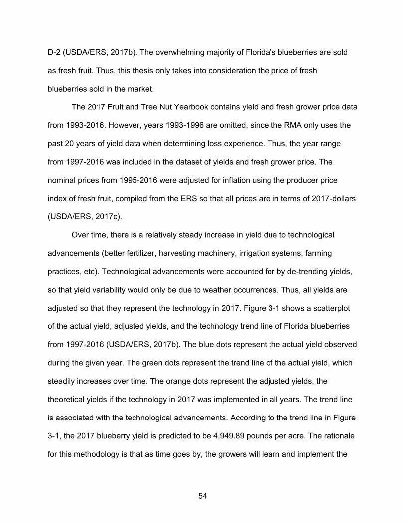
(USDA/ERS, 2017c).

Over time, there is a relatively steady increase in yield due to technological

advancements (better fertilizer, harvesting machinery, irrigation systems, farming

practices, etc). Technological advancements were accounted for by de-trending yields,

so that yield variability would only be due to weather occurrences. Thus, all yields are

adjusted so that they represent the technology in 2017. Figure 3-1 shows a scatterplot

of the actual yield, adjusted yields, and the technology trend line of Florida blueberries

from 1997-2016 (USDA/ERS, 2017b). The blue dots represent the actual yield observed

during the given year. The green dots represent the trend line of the actual yield, which

steadily increases over time. The orange dots represent the adjusted yields, the

theoretical yields if the technology in 2017 was implemented in all years. The trend line

is associated with the technological advancements. According to the trend line in Figure

3-1, the 2017 blueberry yield is predicted to be 4,949.89 pounds per acre. The rationale

for this methodology is that as time goes by, the growers will learn and implement the

55

best strategies to grow blueberries and increase production, through the use of some

type of technology. Technology is a broad term, but is attributable to an improvement in

one or more of the inputs used in production (Debertin, 2012). This improvement in

input, for example: the use of better fertilizer applications, increases yield. Technological

improvements also apply to a reduction in the per unit cost of an input of production. For

example, a new foliar spray which is just as effective as the old but costs less

consequently can increase production, as the grower has more money to spend on

other inputs to increase yield (Debertin, 2012). Technology can refer to physical

technological advancements such as the use of machine harvesting, but it can also

refer to any improvement in farming practice, such as finding the optimal distance to

plan blueberries bushes from one another.

Aside from prices and yields, this paper also analyzes the overall enrollment rate

of growers who partake in APH crop insurance in an attempt to evaluate whether the

premium rate set by the RMA is actuarially fair. The WFRP plan is too new for any data

on enrollment rate to be analyzed, but conclusions about the premium rate for WFRP

can be made since the premium of the WFRP is based on APH. The RMA provides

summary of business reports of data on the APH policy concerning insured acres, policy

count, premiums, and indemnities (USDA/RMA, 2018). These reports are used to

generate enrollment data on Florida as whole and Alachua, which are analyzed in the

results chapter of this thesis.

Crop Insurance Terminology

The results of the yields, prices, and enrollment rates are reflected by premium

and indemnity amounts. Premiums and indemnities are the some of the most important

quantifiable factors that growers look at when choosing to enroll in crop insurance.

56

Premium and indemnity equations for APH and WFRP are set by the RMA, which has a

unique jargon for crop insurance. The “List of Crop Insurance Terminology” on page 9

describes the terminology used by the RMA when calculating crop insurance premium

rates and indemnity payments. Crop insurance terminologies for APH and WFRP are

from the RMA’s Basic Policy Provisions (USDA/RMA, 2017b) and cost estimator

(USDA/RMA, 2017c). Below are the simplified equations used for calculating the

indemnities and premiums under APH and WFRP. Many additional factors could

influence these calculations, including if the grower qualifies for a “Beginning Farmer

Rancher Subsidy”, a “Native Sod Subsidy”, or a “Conservation Compliance Subsidy”, or

if this is the first year that the grower enrolls in insurance (USDA/RMA, 2017c). These

additional factors were all held constant in our calculations and simulations. The

assumption for an average Florida blueberry grower is that the grower does not qualify

for any of the aforementioned subsidies and that they are not enrolling in crop insurance

for the first time.

Premium and Indemnity Calculations

APH Premium Calculation: Equation 3-1

Approved Yield × Coverage Level = Guarantee Guarantee X Established Price × Insured Shared Percent = Liability Amount Liability Amount X Base Rate × Rate differential factor × Unit residual factor =Preliminary Premium Amount Preliminary Premium Amount × (1 − Subsidy Percent) = Premium Per Acre

(3-1)

APH Indemnity Calculation: Equation 3-2

Max((Guarantee) − Actual Yield, 0) × Established Price = Indemnit Per Acre (3-2)

WFRP Premium Calculation: Equation 3-3

57

Min(Historic Average Revenue, Expected Revenue) = Approved Revenue Approved Revenue × Coverage Level = Liability Amount Liability Amount × Diversity Factor X Weighted Commodity Rate =Preliminary Premium Amount Preliminary Premium Amount × (1 − Subsidy Percent) = Premium Per Acre

(3-3)

WFRP Indemnity Calculation: Equation 3-4

Max((Liabilty Amount − Actual Revenue), 0) = Indemnity Per Acre (3-4)

Alachua County Premium and Indemnity Calculation Example

Alachua County is the largest blueberry-producing county in the state of Florida.

Alachua represents over 27% of the blueberry acres in Florida, as of the most recent

county data in 2012 (USDA/NASS, 2012). Alachua is chosen as the county for which all

examples and simulations are run in this thesis. Figure 3-2 depicts the calculations

under the APH policy for Alachua county, irrigated non-organic Southern Highbush

blueberry with frost protection, with an approved yield of 4,558 pounds per acre, and a

100% price election of $2.50 per pound as established by the RMA. The actual yield is

1,500 pounds per acre, a percent acreage loss of roughly 67% (USDA/RMA, 2017c).

Figure 3-2 uses Equations 3-1 and 3-2 to compute the premium and indemnity for APH.

In Figure 3-2, if the farmer chose the 65% coverage level, the farmer would have to pay

the premium of $170.06 per acre (column 14) to purchase the Actual Production History

insurance plan, and would receive an indemnity of $3,656.80 per acre (column 16).

Figure 3-3 depicts an example of the calculations under the WFRP policy for a

similar loss in Figure 3-2. In Figure 3-3, the grower choses to enroll in the WFRP plan

for blueberries in Alachua county in 2017. The grower’s annual average revenue over

the last 5 years is $11,395 per acre. The grower produces only blueberries, which

account for 100% of the farm revenue. Suppose the actual revenue is $3,760, a percent

revenue loss of roughly 67%. Figure 3-3 depicts the calculations of this example, using

58

Equation 3-3 and Equation 3-4 to compute the premium and indemnity for WFRP

(USDA/RMA, 2017c).

In Figure 3-3, if the farmer chose the 65% coverage level, the farmer would have

to pay the premium of $338.30 per acre (column 14) for the cost of the Whole Farm

Revenue Protection insurance plan. The farmer would receive an indemnity of

$3,646.40 per acre (column 18).

The APH and WFRP scenarios were made to be as similar as possible to

analyze which crop insurance policy is more advantageous. In the real world setting,

both crop insurance policies charge a premium as a lump sum and payout an indemnity

as a lump sum. For comparative purposes, in both the APH and WFRP examples, the

farmer pays a premium and receives an indemnity on a per acre basis. Figure 3-4

depicts the side-by-side premiums and indemnities per acre of the APH and WFRP

blueberry scenarios (USDA/RMA, 2017c). The “Actual Production History” and the

Whole-Farm Revenue Protection – One Commodity” column summarize the premium

and indemnity amounts from Figure 3-2, and Figure 3-3, respectively.

In Figure 3-4, the indemnity difference between APH and WFRP is marginal, due

to rounding the loss percentage of roughly 67% under both policies. With a

comparatively lower premium and effectively equal indemnities, APH provides the same

coverage levels as the WFRP policy at a lower cost. The reason that the premium is

lower for APH is that the premium rates for APH are lower compared to the WFRP plan.

However, the APH premium rate cannot be decreased with diversification. The WFRP

plan premium rate could be lower if the grower diversified and added a qualifying

secondary or tertiary crop. This thesis does not consider analyzing and performing

59

simulations on the scenario between a diversified WFRP plan and APH. As previously

mentioned, there is not enough data available on diversified WFRP plans that include

blueberries in Florida, and the possible combinations of crops add complexity beyond

the scope of this thesis. A brief example is provided below only to show the influence of

diversification on the WFRP premium rate compared to APH. After this example, only

single crop blueberry farms are compared between APH and WFRP, and the WFRP is

assumed to insure only blueberries.

Adding another crop that meets the diversification requirements could reduce the

premium significantly. For example, the addition of blackberries as another crop, with

revenue from each crop split as 50% of revenue, has an impact on the premium. The

addition of this crop reduces the 65% coverage level from $338.30 to $156.97, a

reduction of price by 53.60%, as shown in the columns for WFRP- two commodities.

The addition of another crop reduces the premium significantly, such that APH is no

longer the most profitable choice. According to Figure 3-4, the two-commodity WFRP

plan provides an equal indemnity amount compared to APH while costing less than

APH. This thesis focuses only on the comparison between a farm producing blueberries

under the WFRP plan and a farm producing blueberries under the APH policy. The APH

policy will be compared to the single crop WFRP policy.

Simulations

The probability that an indemnity will occur under the APH policy is directly linked

to the variation in yield. The higher the variability – or standard deviation – of yields, the

higher the chance that an indemnity will occur. From the yield data collected from the

ERS, the standard deviation can be calculated. The RMA uses the past twenty years of

yield data in Florida to compute the premium rate (RMA Personal Communication,

60

2018). Thus, the standard deviation of yields over the last 20 years is used for the

simulations. The mean of the yield distribution is based on the 2017 trend yield over the

same time span. Thus, mean yield is established at 4,949.49 pounds per acre with a

standard deviation of 1,017.25 pounds per acre. This thesis uses the normal distribution

for yields, since it is regarded as the base study in the literature.

The probability that an indemnity will occur under the WFRP is similarly linked to

the variability in revenue. Revenue is a function of price multiplied by the yield, on a per

acre basis. There is an inverse relationship between price and yields. The coefficient of

correlation specifies the strength and direction of a linear relationship between two

variables. Using the Excel Add-On “Simetar”, the coefficient of correlation between the

prices and yields was estimated to be -0.60. This indicates that there is a moderate

inverse relationship between yields and prices. Any unit increase in yields will result in a

0.6 unit decrease in price. This natural hedge between prices and yields lowers the

variability of revenue. When yields decrease, prices increase and vice versa such that

their product remains relatively unchanged. The Iman and Conover methodology was

used to impose the target level of correlation between prices and yields (Iman and

Conocer, 1982). The methodology’s only manipulation to the original draws is to resort

them.

To find the probability that revenue falls sufficiently to trigger an indemnity, price

and yield data need to be assembled. As previously mentioned, yields have a mean of

4,949.89 pounds per acre and a standard deviation of 1,017.25 pounds per acre. When

establishing the mean and volatility of prices, we used the same number of years as the

RMA, from 2008 to 2016 (RMA Personal Communication, 2018). The average price is

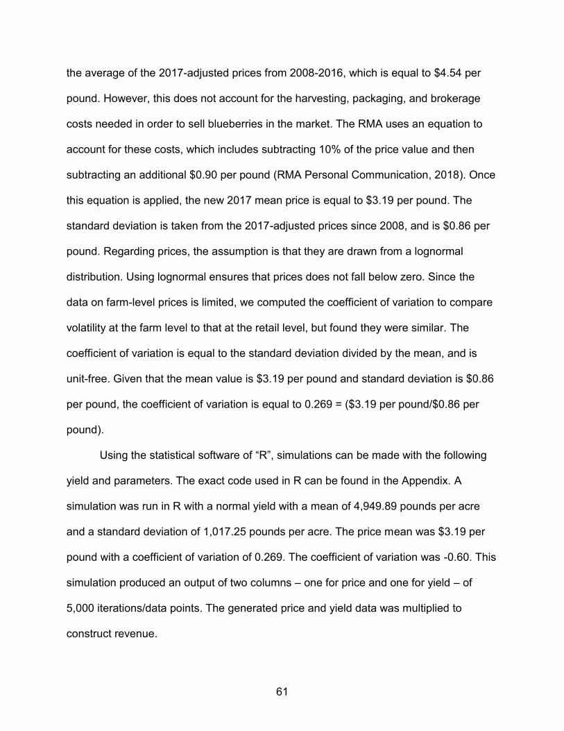
61

the average of the 2017-adjusted prices from 2008-2016, which is equal to $4.54 per

pound. However, this does not account for the harvesting, packaging, and brokerage

costs needed in order to sell blueberries in the market. The RMA uses an equation to

account for these costs, which includes subtracting 10% of the price value and then

subtracting an additional $0.90 per pound (RMA Personal Communication, 2018). Once

this equation is applied, the new 2017 mean price is equal to $3.19 per pound. The

standard deviation is taken from the 2017-adjusted prices since 2008, and is $0.86 per

pound. Regarding prices, the assumption is that they are drawn from a lognormal

distribution. Using lognormal ensures that prices does not fall below zero. Since the

data on farm-level prices is limited, we computed the coefficient of variation to compare

volatility at the farm level to that at the retail level, but found they were similar. The

coefficient of variation is equal to the standard deviation divided by the mean, and is

unit-free. Given that the mean value is $3.19 per pound and standard deviation is $0.86

per pound, the coefficient of variation is equal to 0.269 = ($3.19 per pound/$0.86 per

pound).

Using the statistical software of “R”, simulations can be made with the following

yield and parameters. The exact code used in R can be found in the Appendix. A

simulation was run in R with a normal yield with a mean of 4,949.89 pounds per acre

and a standard deviation of 1,017.25 pounds per acre. The price mean was $3.19 per

pound with a coefficient of variation of 0.269. The coefficient of variation was -0.60. This

simulation produced an output of two columns – one for price and one for yield – of

5,000 iterations/data points. The generated price and yield data was multiplied to

construct revenue.

62

The simulation was repeated two additional times with coefficient of correlations

between price and yield of -0.50 and -0.30.

This provides a sensitivity analysis on the coefficient of correlation, a key

parameter. One of the reasons for which the coefficient of correlation could change in

future years is because of the increased competition for production during the Florida

market window. Mexico is increasing blueberry production consistently each year, and

this country’s production season competes directly with Florida. It is conceivable that

the greater the blueberry imports from Mexico, the weaker the relationship between

prices and yields will be in the market. The increased competition in the market will not

only conceivably change the correlation, but could also affect the mean price and price

distribution as well. However, it would be difficult to isolate the effect on price mean and

distribution from competition from Mexico alone. In addition, Mexico has only recently

(since 2013) produced quantities of blueberries that could potentially influence the mean

price received by Florida growers, and sufficient data would be hard to find

(USDA/AMS, 2017). Thus, this thesis only considers a change in the coefficient of

correlation on price and yields when analyzing future competition.

Three further simulations were run with a mean yield value of 4,118 pounds per

acre, the same as the Approved Yield under RMA for the last 10 years. These three

simulations also considered coefficient of correlations of -0.60, -0.50, and -0.30, for a

total of six different scenarios. The parameters of these scenarios are summarized in

Table 3-1. Table 3-1 indicates shows that under scenarios 1, 2, and 3, the yield mean is

4,949.89 pounds per acre and the coefficient of correlation values are -0.60, -0.50, and -

63

0.30, respectively. Under scenarios 4, 5, and 6, the yield mean is 4,118 pounds per acre

and the coefficient of correlation values are -0.60, -0.50, and -0.30, respectively.

This thesis assumes that growers are risk-averse. Risk-averse individuals refuse

fair bets and exhibit diminishing marginal utility of wealth, meaning that each additional

unit increase in wealth provides a smaller increase in utility (Nicholson and Snyder,

2011). Risk-averse growers are willing to spend some money (i.e.: premium) to avoid a

risky outcome. By purchasing crop insurance, a grower mitigates risk by reducing the

variability of revenue or yield (depending on the policy). The logarithmic function is an

accepted utility function used in the literature to model the expected utility of a risk-

averse grower (Sheng, C. L., 1998; Sheng, Q. 1998). The logarithmic function exhibits

constant relative risk aversion, meaning that the individual’s willingness to take gambles

does not change with the level of wealth. In the context of crop insurance, a grower

characterized by a constant relative risk aversion utility function will be concerned about

proportional gains or losses to their wealth. The logarithmic expected utility function is

applied to each scenario in this thesis, and the total expected utility under APH and

WFRP are compared.

The next chapter examines whether the distribution results are consistent with

the simulation parameters set in this chapter. Scenarios 1 through 6 are examined in

detail, comparing the APH policy to the WFRP policy. In addition, the expected utility of

a risk-averse grower enrolling in crop insurance is compared to that of a grower who

does not enroll in crop insurance. The analysis will ultimately lead to the conclusion of

whether it is beneficial for the average grower to enroll in crop insurance under each

scenario, and if so, which policy to choose.

64

Figure 3-1. Actual yield, adjusted yields, and the technology trend line of Florida

blueberries from 1997-2016. Actual yields were adjusted by removing the technology factor. Source: United States Department of Agriculture, Economic Research Service (USDA/ERS, 2017b).

0

1000

2000

3000

4000

5000

6000

7000

8000

1995 2000 2005 2010 2015 2020

Yiel

d (lb

s/ac

re)

Year

Actual Yield Detrended Yields Trend

65

[1] [2]

[3]

=[1]*[2]

[4]

[5]

=[3]*[4]

[6] [7]

= ([1]-[6])/[1]

[8]

Approved Yield

(lbs/Acre)

Coverage Level (%)

Guarantee – Loss Trigger (lbs/Acres)

Established Price per

pound ($/lbs)

Premium liability amount ($/acre)

Actual Yield

(lbs/Acres)

Percent acreage loss (%)

Base Rate (%)

4,558.00

75.00 3,419.00

2.50

8,546.00

1,500.00 67.09 5.60

70.00 3,191.00 7,977.00 65.00 2,963.00 7,407.00 60.00 2,735.00 6,837.00 55.00 2,507.00 6,267.00 50.00 2,279.00 5,698.00

CAT 2,279.00 1.38 3,145.00

[9] [10] [11]

=[8]*[9]*[10]

[12]

=[5]*[11]

[13]

[14] =

[12]*(1-[13])

[15]

=[3]-[6]

[16] =[4]*[15]

Rate differential factor (%)

Unit Residual Factor

(%)

Base Premium Rate (%)

Total Premium amount ($/acre)

Subsidy Rate (%)

Total Premium ($/acre)

Covered Acres

(lbs/Ares)

Indemnity ($/acre)

145.10 111.00 9.02 770.82 55.00 346.87 1,918.50 4,796.30

120.60 105.50 7.13 568.33 59.00 233.02 1,690.60 4,226.50

100.00

100.0

5.60 414.78 59.00 170.06 1,462.70 3,656.80

83.40 4.67 319.32 64.00 114.95 1,234.80 3,087.00

70.70 3.96 248.13 64.00 89.33 1,006.90 2,517.30

61.90 3.47 197.50 67.00 65.17 779.00 1,947.50

- - - 100.00 0.00 779.00 1,075.02

Figure 3-2. Example of APH crop insurance policy payment for non-organic Southern Highbush blueberries with frost protection, an approved yield of 4,558 lbs/acre in Alachua County and a percentage loss of 67.09%. Source: United States Department of Agriculture, Risk Management Agency (USDA/RMA) 2016 Cost Estimator (USDA/RMA, 2017c). A) Columns 1-8 of APH crop insurance example. B) Columns 9-16 of APH crop insurance example.

A

B

66

1 [2] =

(100,000/[1]) /3

3 4

=IF[3]>[2] then YES

5 6 7

=[5]*[6] 8 9

Total Commodity

Count

Minimum Qualifying

Amount per acre ($)

Expected Revenue

from Commodity per acre ($)

Eligibility? Coverage

Level Percent (%)

Total Allowable Revenue

Amount per acre ($)

Premium Liability

Amount per acre ($)

Blueberry Commodity

Rate (%)

Diversity Factor

1.00 3,798.33 11,395.00 YES

75.00

11,395.00

8,546.25 16.04

1

70.00 7,976.50 13.34 65.00 7,406.75 11.14 60.00 6,837 9.96 55.00 6,267.25 9.11 50.00 5,697.50 8.60

Figure 3-3. Example of Whole-Farm Revenue Protection policy payment for single-commodity blueberries in Alachua county. The farmer in this example has a five-year average revenue of $11,395 per acre, 100% of the revenue comes from blueberries. Source: United States Department of Agriculture, Risk Management Agency. 2017. (USDA/RMA, 2017c). A) Columns 1-9 of WFRP crop insurance example. B) columns 10-18 of WFRP crop insurance example.

10

=[8]*[9]

11

=[7]*[10] 12

13 =[11]*[12]

14 =[11]-[13]

15 16

=[6]*[15]

17 =[6]-[16]

18 =[7]-[17]

Premium Rate (%)

Preliminary Total

Premium Amount per

acre ($)

Subsidy Rate (%)

Subsidy Amount per

acre ($)

Total Premium

($)

Loss Percentage

(%)

Loss Amount per acre ($)

Remaining Revenue

per acre ($)

Indemnity per

acre($)

16.04 1370.82 55.00 753.95 616.87

67.10 7,645.00 3,750.00

4,796.25

13.34 1,064.07 59.00 627.80 436.27 4,226.60

11.14 825.11 59.00 486.82 338.30 3,656.75

9.96 680.97 64.00 435.82 245.15 3,087.00

9.11 570.95 64.00 365.41 205.54 2,517.25

8.60 489.99 67.00 328.29 161.70 1,947.50

A

B

67

Blueberries Actual Production

History

Whole Farm Revenue Protection – One

Commodity

Whole Farm Revenue Protection – Two Commodities

Coverage Level Percent

(%)

Total Premium per acre

($)

Indemnity per acre

($)

Total Premium per acre

($)

Indemnity per acre ($)

Total Premium

per acre ($)

Indemnity per acre

($)

75.00 346.87 4,796.30 616.87 4,796.25 230.74 4,796.25

70.00 233.02 4,226.50 436.27 4,226.60 191.42 4,226.60

65.00 170.06 3,656.80 338.30 3,656.75 156.97 3,656.75

60.00 114.95 3,087.00 245.15 3,087.00 132.61 3,087.00

55.00 89.33 2,517.30 205.54 2,517.25 112.81 2,517.25

50.00 65.17 1,947.50 161.70 1,947.50 95.71 1,947.50

Figure 3-4. Side-by side comparison of the Actual Production History and the Whole Farm Revenue Protection policy. The coverage levels are between 50-75% and the premiums and indemnities of the overall policies are shown to compare the two policies economically given a 67.10% loss in both yield and revenue. Source: United States Department of Agriculture, Risk Management Agency. 2017. (USDA/RMA, 2017c)

68

Table 3-1. Summary of the parameters of the six different scenarios analyzed.

Conditions Scenarios

Parameters Scenario 1 Scenario 2 Scenario 3

Yield Mean (lbs/acre) 4,949.89 4,949.89 4,949.89

Coefficient of Correlation -0.60 -0.50 -0.30

Parameters Scenario 4 Scenario 5 Scenario 6

Yield Mean (lbs/acre) 4,118.00 4,118.00 4,118.00

Coefficient of Correlation -0.60 -0.50 -0.30

Constant variables: Price mean ($3.19/lb) and coefficient of variation (0.269) Yield standard deviation (1,017.25lbs/acre)

69

CHAPTER 4 RESULTS AND DISCUSSION

This chapter discusses the distribution results briefly, confirming that they follow

the proper distributions. This chapter emphasizes the simulation results, which

determine the probability than an indemnity will occur. A discussion of indemnity and

premium calculations justify the scenarios run. By the conclusion of this chapter, the six

scenarios unanimously support an enrollment decision.

Distribution Results

The plots of the distributions under scenario 1 of prices, yields, and revenue are

shown in the histogram Figures 4-1, 4-2, and 4-3, respectively. In Figure 4-1, prices

have a lognormal distribution with a mean of $3.19 per pound, a minimum of $0.90 per

pound, and a maximum of $7.66 per pound. The blue bars of the histogram all have an

equal width, referred to as a bin. Each bin of the price histogram represents a $0.20 per

pound range. In Figure 4-2, yields have a normal distribution with a mean of 4,949.89

pounds per acre, a minimum of 1,179.94 pounds per acre, and a maximum of 8,738.19

pounds per acre. Each bin of the yield histogram represents a width of 200 pounds per

acre. Revenue is a function of yields multiplied by prices, and mimics a normal

distribution. In Figure 4-3, revenue has a mean of $15,285.93 per acre, a minimum of

$5,451.04 per acre, and a maximum of $34,853.80 per acre. Each bin of the revenue

histogram represents a width of $1,000 per acre. The distribution results for other

scenarios have the same distribution types (lognormal for prices, normal for yield and

revenue), yet vary based on mean, minimum, and maximum.

70

Simulation Results

While Figure 4-1, 4-2 and 4-3 provide a snapshot of the distribution results,

Figure 4-4 plots the simulation results of the yield on the X axis and revenue on the Y

axis under scenario 1. This figure provides visual insight as to which policy is more

advantageous. Recall the indemnity equations used for APH and WFRP. Equation 3-1

and 3-3 are the equations for APH and WFRP, respectively. For the APH indemnity

calculation, the Guarantee is the Approved Yield multiplied by the Coverage Level. The

Approved Yield is the average of the last 10 years of yields in Florida, which is 4,118

pounds per acre. The Coverage Level in this example is 65%, as 65% is the base level

set by the RMA. Under these conditions, the guarantee is equal to 2,677 (=4,118*65%)

pounds per acre. Any yields which fall below this value will trigger an indemnity

payment. The vertical red line denotes this guarantee value of 2,677 pounds per acre.

Any data points to the left of this line will trigger an indemnity payment, while any data

points to the right of this line will not.

For the WFRP indemnity calculation, the Liability Amount is equal to the

Approved Revenue multiplied by the Coverage Level. The Approved Revenue is the

minimum of the Expected Revenue for 2017 and the Historic Average Revenue over the

last 5 years. The Expected Revenue is the average of the product between prices and

yields for the 5000 iterations, which is equal to $15,285.93 per acre. The Historic

Average Revenue is equal to $9,958 per acre. Between the Historic Average Revenue

and the Expected Revenue, the Historic Average Revenue is the lower value between

the two. Thus, the Approved Revenue is equal to $9,958 per acre. The Coverage Level

for this example is 65%, so the Liability Amount is equal to $6,472 (=$9,958*65%) per

acre. The horizontal red line denotes this Liability Amount of $6,472 per acre. Any

71

values below this line will trigger an indemnity payment, while any values above this line

will not.

Visually, one can see that there are far more data points that lie to the left of the

vertical line than the number of data points that lie below the horizontal line in Figure 4-

4. This indicates that there is a higher probability of an indemnity trigger under the APH

policy, compared to the WFRP policy for the 65% coverage level. Table 4-1 summarizes

the data shown in Figure 4-4. Table 4-1 shows the number of times an indemnity was

triggered under the APH policy and the WFRP policy out of the 5,000 iterations, the

corresponding percentage chance of a data point triggering an indemnity (the likelihood

of an indemnity), the expected indemnity received for each of the 5,000 iterations, the

grower premium paid on a per acre basis, and the expected indemnity divided by the

guarantee for APH or the liability amount for WFRP. The RMA sets the premium rate

making use of the loss experience data available and computing the loss cost ratio (i.e.:

indemnities/liabilities). Thus, I computed the expected indemnity divided by the

guarantee as a proxy for it. This value is what the premium rate should be set at.

In Table 4-1, for each coverage level, APH has the higher probability of an

indemnity occurring out of the 5,000 iterations (Column 4) when compared to the WFRP

policy. The APH policy also has a higher expected indemnity, a higher expected

indemnity divided by guarantee percentage, and a lower premium cost compared to the

WFRP for every coverage level. Thus, under scenario 1, the APH coverage level is the

unanimous choice for the grower as the most advantageous policy when comparing

between APH and the WFRP.

72

However, the expected indemnity for every coverage level under APH is always

less than the premium the grower has to pay on a per acre basis. The APH policy, and

by extension, the WFRP policy, is costing growers more per acre then what they are

expected to receive in indemnity payments. In this case, it is not clear whether a risk-

averse grower would then chose to either enroll in APH or to refrain from enrolling in

crop insurance. A risk-averse grower is willing to give up some wealth (premium) to

secure a certain outcome. By paying the premium, a risk-averse grower could increase

their expected utility, since the grower values the reduction in risk. The expected utility

determines whether the grower will enroll in crop insurance or not. As mentioned in the

methods, the logarithmic function is used in this thesis as an acceptable expected utility

function for risk-averse individuals (Nicholson and Snyder, 2011).

Assuming that risk-averse growers have a utility function that is logarithmic, the

equation for the expected utility under the APH crop insurance policy is shown in

Equation 4-1:

𝐸𝑥𝑝𝑒𝑐𝑡𝑒𝑑 𝑈𝑡𝑖𝑙𝑖𝑡𝑦 𝑈𝑛𝑑𝑒𝑟 𝐴𝑃𝐻 = ∑ ln (𝑅𝑒𝑣𝑒𝑛𝑢𝑒𝑖 + 𝐼𝑛𝑑𝑒𝑚𝑛𝑖𝑡𝑦𝑖 − 𝑃𝑟𝑒𝑚𝑖𝑢𝑚𝑖

5000𝑖

) (4-1)

In Equation 4-1, the expected utility when enrolling in APH is equal to the

summation of the natural log of the revenue plus the indemnity minus the premium for

each iteration (i), times the probability of that iteration occurring, which is 1 in 5,000 total

iterations. Since the WFRP has a higher premium and lower expected indemnity than

APH, we can conclude that the expected utility of the WFRP is less than that of APH.

Thus, it is only necessary to compare the expected utility under APH with the expected

utility when not enrolling in crop insurance. The equation for the expected utility of a

risk-averse grower when not enrolling in crop insurance is shown in Equation 4-2:

73

𝐸𝑥𝑝𝑒𝑐𝑡𝑒𝑑 𝑈𝑡𝑖𝑙𝑖𝑡𝑦 𝑊𝑖𝑡ℎ𝑜𝑢𝑡 𝐸𝑛𝑟𝑜𝑙𝑙𝑚𝑒𝑛𝑡 = ∑ ln (𝑅𝑒𝑣𝑒𝑛𝑢𝑒𝑖

5000)

𝑖

(4-2)

In Equation 4-2, the expected utility is the summation of the natural log of the

revenue for each iteration (i), times the probability of that iteration occurring. As

depicted in Table 4-1, under scenario 1, the APH policy is the more advantageous

choice compared to the WFRP policy. However, the expected utility under APH (and

WFRP) is lower than the expected utility from not enrolling in crop insurance. The

expected utilities are summarized at the end of this chapter in a table, once all

scenarios have been analyzed. Thus, the most advantageous choice under scenario 1

is for the grower to refrain from enrolling in crop insurance.

Figures 4-5 and 4-6 show revenue plotted vertically and the yield plotted

horizontally, similar to Figure 4-4. Figures 4-5 and 4-6 show the exact same parameters

(price has a mean of $3.19 with a coefficient of variation of 0.269, and yield has a mean

of 4,949.89 lbs/acre with a standard deviation of 1,017.25 lbs/acre) as Figure 4-4,

except that the coefficient of correlation between price and yield is changed. Figures 4-5

and 4-6 correspond to the scenarios 2 and 3, under which the coefficient of correlations

are -0.50 and -0.30, respectively. The values of -0.50 and -0.30 are chosen to provide a

sensitivity analysis, in the event that Mexico continues to increase production in future

years.

In Figure 4-5, the red lines mark the 65% coverage level for APH vertically and

WFRP horizontally. The notable difference between Figure 4-4 and Figure 4-5 is that

there are more data points that fall below the 65% coverage level for the WFRP policy.

This is due to the fact that the coefficient of correlation is higher, at a value of -0.50. The

prices do not respond as drastically to a drop in yield, as shown in Figure 4-4. In Figure

74

4-5, prices will not increase as much due to a proportional decrease in yield when

compared to Figure 4-4. Due to this, revenue values are lower. Yield values remain the

same, as the only thing that is changed is the responsiveness of price to a change in

yield.

In Figure 4-6, the coefficient of correlation is -0.30, a higher coefficient value than

in Figures 4-4 or 4-5, the value of the coefficient is closer to 0, meaning that the

negative association between price and yield is weaker. The notable difference when

comparing Figure 4-6 to Figures 4-4 or 4-5 is that there are more data points that fall

below the 65% coverage level for the WFRP policy. The reasoning why there are more

data points that fall below this line is the same for Figure 4-6 as it was for Figure 4-5;

the coefficient of correlation is higher, the inverse relationship between price and yield is

weaker.

Table 4-2 shows the data in Figure 4-5 under scenario 2. There are no changes

for any of the variables under the APH policy, since yield values do not change when

altering the coefficient of correlation between price and yield. Price data does change,

which affects revenue amounts and in return affects the variables of the WFRP policy.

The WFRP policy’s indemnity triggers, percent trigger occurrence, expected indemnity,

and the expected indemnity divided by the liability amount all increase relative to the

original simulation presented in Table 4-1. While the previously mentioned variables of

the WFRP policy all increased, these variables were all lower than the variables under

the APH policy (indemnity triggers, percent trigger occurrence, expected indemnity, and

expected indemnity divided by the liability amount under WFRP were all lower than the

75

APH values for each coverage level). Thus, Table 4-2 makes the same conclusions as

Table 4-1: growers are expected to lose money if they enroll in crop insurance.

Table 4-3 shows the data in Figure 4-6 under scenario 3. The only difference for

these results is that the coefficient of variation in scenario 3 is -0.30. All the variables

under the WFRP policy rise except for the grower premium per acre relative to scenario

2, while the APH values do not change. Even though the variables rise, the WFRP

policy variables are all still lower than the APH values. Thus, Table 4-3 leads to the

same conclusion that it is in the best interest of a risk-averse grower to refrain from

enrolling in crop insurance.

RMA Indemnity Calculation Issues

So far, we used the 2017 trend yield of 4,949.89 pounds per acre as the basis for

the mean of the yield distribution. However, the last time RMA computed the APH rate

for blueberries in Florida was in 2015. Thus, a potential reason for finding the expected

indemnity from APH and WFRP to be lower than the premium amount per acre is that

the Approved Yield under APH is lower than the expected yield. To account for this

possibility, the Approved Yield is calculated instead by taking the average of the last 10

years of production, which is equal to 4,118 pounds per acre. This value is lower than

the expected amount by roughly 800 pounds per acre. The Approved Yield is multiplied

by the Coverage Level to get the Guarantee amount – which is the vertical red line in

the scatterplot figures. The Guarantee is equal to 2,677 pounds per acre considering an

Approved Yield of 4,118 pounds per acre and the 65% Coverage Level. If the Expected

Yield of 4,949.89 pounds per acre was covered as the Approved Yield, the Guarantee

would rise to 3,217 pounds per acre under the 65% Coverage Level. Looking at any

scatterplot of revenue and yield, moving the red vertical line to the right from 2,677

76

pounds per acre to 3,217 pounds per acre would clearly increase the probability that an

indemnity would trigger. Instead of creating a scenario in which the RMA considers

changing the way Approved Yield is calculated, the mean value in our simulation can be

changed.

Changing the expected yield from 4,949.89 pounds per acre to 4,118 pounds per

acre will provide a scenario that considers the expected yield equal to the Approved

Yield. Ideally, this is what the RMA is trying to accomplish by taking the average of the

last 10 years of production. The yield standard deviation will remain the same at

1,017.25 pounds per acre, since that is the RMA calculated 20-year variation. The same

logic applies to the WFRP policy. One reason why so few indemnity triggers occur is

that the Approved Revenue is too low compared to the Expected Revenue, and

consequently the Liability Amount (the red horizontal line in scatterplots) is lower.

Changing the yield from 4,949.89 to 4,118 pounds per acre will decrease the expected

revenue, and make the Expected Revenue amount closer to the Approved Revenue

average over the last 5 years.

Figure 4-7 depicts the scatterplot of revenue vertically and yield horizontally.

Figure 4-7 depicts the results of simulating 5,000 iterations of yield and price, with a

yield mean of 4,118 pounds per acre, yield standard deviation is 1,017.25 pounds per

acre, price mean is $3.19 per pound, the coefficient of variation of price is 0.269, and

the coefficient of correlation between prices and yields is -0.60. In Figure 4-7, there are

noticeably more data points that fall to the left of the red 65% coverage level APH

vertical line and below the red 65% coverage level WFRP horizontal line compared to

Figure 4-4. Lowering the mean value of yield increased the number of indemnity triggers

77

under both the APH and the WFRP policy. The results of Figure 4-7 are depicted in

Table 4-4. In Table 4-4, the output variables of the number of times indemnity is

triggered, the percentage occurrence of a trigger, the expected indemnity, and the

expected indemnity/liability amount all increased compared to Table 4-1, the scenario

under which the yield mean was 4,949.89 pounds per acre. These output variables for

the WFRP policy remain lower than those of APH. APH and the WFRP plan both have

expected indemnities lower than the premium amounts per acre. The decision choice

for a risk-averse farmer would be to once again refrain from enrolling in crop insurance,

since the expected utility is higher when the grower does not enroll compared to

enrolling in APH or WFRP.

Figure 4-8 depicts the same scenario as Figure 4-7, yet the coefficient of

correlation between prices and yields is lowered to -0.50. Lowering the coefficient of

correlation has no effect on the number of data points triggered under the APH policy,

since the APH policy is only triggered by losses of yields. The amount of data points

under the red horizontal 65% coverage level line for WFRP increased when compared

to Figure 4-5, the scenario with the same parameters except that the yield mean is

4,949.89 pounds per acre. The results of Figure 4-8 are depicted in Table 4-5 under

scenario 5. In Table 4-5, the WFRP indicators increased, but remained less than those

of the APH policy. Thus, the choice would be to once again to refrain from enrolling in

crop insurance.

Figure 4-9 depicts the same scenario as Figure 4-8, except that the coefficient of

correlation is -0.30. Table 4-6 summarizes the results of Figure 4-9 under scenario 6.

The indicators of the WFRP increased, yet remained less than those of the APH policy.

78

Table 4-7 summarizes the expected utility for a risk-averse grower under each

scenario and coverage level. In each scenario, the expected utility of enrolling in crop

insurance is less than the expected utility from not enrolling in crop insurance. Thus, the

optimal decision for a risk-averse grower would be not to enroll in crop insurance.

RMA Premium Calculation Issues

Even after accounting for the difference between the expected and approved

yield, the expected indemnity amount remains lower than the premium amount per acre

under the APH and the WFRP policy. The other possible reason why this occurs is that

the premium rate is set too high by the RMA. The stated goal of the RMA is to give out

just a much in indemnity payments to growers as they receive in premium amounts in

the long run. The RMA calculates the premium rates on a per-county basis by looking at

the past 10 years of data on indemnity amounts, then sets the premium rate accordingly

such that the preliminary premium amount (premium amount before subsidies are

considered) is equal to the indemnity amount. Premium rates for Florida blueberries

under the APH policy are updated every three years.

The RMA has not accomplished the stated goal of setting the premium rate such

that the RMA receives in premium what it gives out in indemnity. The RMA set the

premiums for both policies too high, so the premium amount is always higher than the

expected indemnity. The reason for the misrating is due to a lack of data on blueberry

production loss experience. APH rates are also the basis for WFRP rates, so the APH

misrating is carried over to WFRP. Moreover, for the WFRP policy, there is even less

data available. The WFRP policy was only established in 2014. In 2017, there were only

7 total farms across the state of Florida that enrolled in WFRP (USDA/RMA, 2018).

79

Table 4-8 summarizes the participation of blueberry growers in the APH policy

across Florida since it was first available in 2000. The percentage of acres covered

depicts how many acres of blueberries are coverred under the APH policy compared to

the entirety of commerical blueberry acres across Florida. The enrollment rate has

never risen above 57% and has only once been above 50%. In addition, the policy

count total – the number of farms enrolled in crop insurance – is extremely low. From

2000-2005, the maximum policy count was 6 farms. The highest number of farms to

enroll in crop insurance was in 2017, in which 92 farms enrolled.

The RMA calculates premium rates on a per-county basis, not at the state-level.

The most representative blueberry-producing county in Florida is Alachua. Table 4-9

depcits the participation of growers under the APH policy in Alachua county. A total of

19 farms enrolled in the APH policy in 2017, with a total of 1,086 covered acres. The

majority of the acres in 2017 (84%) are insured under Catastrphic Risk Protection

(CAT). Since 2000, Alachua county policy counts and insured acres have steadily risen

as Florida’s blueberry industry expanded. There is very little data on blueberry

production losses, making it difficult for the RMA to set an actuarily fair premium rate.

The results of this chapter are summarized in the final chapter. The limitations of

this thesis are outlined, and future areas of research are expanded upon. The

concluding chapter makes recommendations to growers and policymakers, taking into

consideration the two main findings of this chapter: firstly, it is in the best interest of a

risk-averse grower to refrain from enrolling in crop insurance, secondly, a lack of data

results in a premium misrating by the RMA.

80

Figure 4-1. Price Histogram of Florida blueberries out of 5,000 iterations.

Figure 4-2. Yield Histogram of Florida blueberries out of 5,000 iterations.

81

Figure 4-3. Revenue Histogram of Florida blueberries out of 5,000 iterations.

Figure 4-4. Florida Blueberry yield to revenue scatterplot results of estimated yield and

price under scenario 1.

82





83

Figure 4-7. Florida Blueberry yield to revenue scatterplot results of estimated yield and price under scenario 4.



84



85

Table 4-1. Comparison of the APH and WFRP policy under Scenario 1.

Policy Coverage Level

# of times Indemnity is Triggered

Percent Occurrence of

Trigger

Expected Indemnity per

acre

Grower Premium per

acre

Expected Indemnity/ Liability

Amount

APH

50% 10 0.20% $1.71 $58.88 0.03% 55% 21 0.42% $3.29 $80.70 0.05% 60% 33 0.66% $5.93 $103.86 0.08% 65% 67 1.34% $10.80 $153.64 0.13% 70% 115 2.30% $20.18 $210.52 0.23% 75% 178 3.56% $35.04 $313.39 0.38%

WFRP

50% 0 0.00% $0.00 $141.30 0.00% 55% 1 0.02% $0.01 $179.62 0.00% 60% 1 0.02% $0.10 $214.23 0.00% 65% 4 0.08% $0.37 $295.63 0.01% 70% 6 0.12% $0.88 $381.25 0.01% 75% 11 0.22% $1.56 $539.08 0.02%

86





Trigger


acre

Grower Premium per

acre


Amount

APH

50% 10 0.20% $1.71 $58.88 0.03% 55% 21 0.42% $3.29 $80.70 0.05% 60% 33 0.66% $5.93 $103.86 0.08% 65% 67 1.34% $10.80 $153.64 0.13% 70% 115 2.30% $20.18 $210.52 0.23% 75% 178 3.56% $35.04 $313.39 0.38%

WFRP

50% 1 0.02% $0.11 $141.30 0.00% 55% 1 0.02% $0.21 $179.62 0.00% 60% 3 0.06% $0.38 $214.23 0.01% 65% 6 0.12% $0.87 $295.63 0.01% 70% 12 0.24% $1.71 $381.25 0.03% 75% 23 0.46% $3.40 $539.08 0.05%

87





Trigger


acre

Grower Premium per

acre


Amount

APH

50% 10 0.20% $1.71 $58.88 0.03% 55% 21 0.42% $3.29 $80.70 0.05% 60% 33 0.66% $5.93 $103.86 0.08% 65% 67 1.34% $10.80 $153.64 0.13% 70% 115 2.30% $20.18 $210.52 0.23% 75% 178 3.56% $35.04 $313.39 0.38%

WFRP

50% 3 0.06% $0.43 $141.30 0.01% 55% 3 0.06% $0.73 $179.62 0.01% 60% 10 0.20% $1.33 $214.23 0.02% 65% 22 0.44% $2.82 $295.63 0.04% 70% 36 0.72% $5.65 $381.25 0.08% 75% 69 1.38% $10.94 $539.08 0.15%

88





Trigger


acre

Grower Premium per

acre


Amount

APH

50% 119 2.23% $20.67 $58.88 0.40% 55% 178 3.56% $35.78 $80.70 0.63% 60% 275 5.50% $59.19 $103.86 0.96% 65% 408 8.16% $93.48 $153.64 1.40% 70% 547 10.94% $142.08 $210.52 1.97% 75% 746 14.92% $208.06 $313.39 2.69%

WFRP

50% 8 0.16% $2.56 $141.30 0.05% 55% 13 0.26% $3.65 $179.62 0.07% 60% 25 0.50% $5.35 $214.23 0.09% 65% 48 0.96% $8.73 $295.63 0.14% 70% 82 1.64% $15.08 $381.25 0.22% 75% 132 2.64% $25.86 $539.08 0.35%

89





Trigger


acre

Grower Premium per

acre


Amount

APH

50% 119 2.23% $20.67 $58.88 0.40% 55% 178 3.56% $35.78 $80.70 0.63% 60% 275 5.50% $59.19 $103.86 0.96% 65% 408 8.16% $93.48 $153.64 1.40% 70% 547 10.94% $142.08 $210.52 1.97% 75% 746 14.92% $208.06 $313.39 2.69%

WFRP

50% 13 0.26% $3.05 $141.30 0.06% 55% 23 0.46% $4.81 $179.62 0.09% 60% 43 0.86% $8.14 $214.23 0.14% 65% 81 1.62% $14.03 $295.63 0.22% 70% 131 2.62% $24.35 $381.25 0.34% 75% 193 3.86% $40.11 $539.08 0.54%

90





Trigger


acre

Grower Premium per

acre


Amount

APH

50% 119 2.23% $20.67 $58.88 0.40% 55% 178 3.56% $35.78 $80.70 0.63% 60% 275 5.50% $59.19 $103.86 0.96% 65% 408 8.16% $93.48 $153.64 1.40% 70% 547 10.94% $142.08 $210.52 1.97% 75% 746 14.92% $208.06 $313.39 2.69%

WFRP

50% 38 0.76% $6.16 $141.30 0.12% 55% 63 1.26% $10.96 $179.62 0.20% 60% 98 1.96% $18.87 $214.23 0.32% 65% 149 2.98% $30.50 $295.63 0.47% 70% 227 4.54% $48.57 $381.25 0.70% 75% 324 6.48% $75.70 $539.08 1.01%

91

Table 4-7. Expected Utility of enrolling in APH or not enrolling for a risk-averse grower under Scenarios 1, 2, 3, 4, 5, & 6. Risk Averse APH Expected Utility – Scenarios 1, 2, and 3

Coverage Level

Do Not Buy

Buy

50.00% 9.609440 9.605601 55.00% 9.609440 9.604261 60.00% 9.609440 9.602912 65.00% 9.609440 9.599888 70.00% 9.609440 9.596725 75.00% 9.609440 9.590764

Risk Averse APH Expected Utility – Scenarios 4, 5, and 6

Coverage Level

Do Not Buy

Buy

50.00% 9.4139768 9.4120839 55.00% 9.4139768 9.4119982 60.00% 9.4139768 9.4126044 65.00% 9.4139768 9.4119442 70.00% 9.4139768 9.4119139 75.00% 9.4139768 9.4094657

92

Table 4-8. Florida Blueberry Growers Participation in APH by Coverage Level

Catastrophic Risk Protection

50% Buy -Up

55% Buy-Up

60% Buy-Up

65% Buy-Up

70% Buy-Up

75% Buy-Up

Total Buy-Up Total Florida

Harvested Acreage

Percentage of Acres

Covered Buy-Up

Percentage of Total Acres

Covered Year Policy Count

Insured Acres

Policy Count

Insured Acres

Policy Count

Insured Acres

Policy Count

Insured Acres

Policy Count

Insured Acres

Policy Count

Insured Acres

Policy Count

Insured Acres

Policy Count

Insured Acres

Policy Count

Insured Acres

2000 1 2 1 24 0 0 0 0 3 214 0 0 0 0 4 238 5 240 1400 17.00% 17.14% 2001 1 1 1 33 0 0 0 0 2 80 0 0 0 0 3 113 4 114 1500 7.53% 7.60% 2002 2 73 2 33 0 0 0 0 1 10 0 0 0 0 3 43 5 116 1600 2.69% 7.25% 2003 3 111 2 39 0 0 0 0 1 10 0 0 0 0 3 49 6 160 1900 2.58% 8.42% 2004 1 249 3 48 0 0 0 0 1 10 0 0 0 0 4 58 5 307 2300 2.52% 13.35% 2005 2 340 2 43 0 0 0 0 1 10 0 0 0 0 3 53 5 393 2500 2.12% 15.72% 2006 4 371 5 116 0 0 1 1 3 18 0 0 1 2 10 137 14 508 2600 5.27% 19.54% 2007 7 425 2 53 0 0 3 36 3 25 0 0 1 25 9 139 16 564 2600 5.35% 21.69% 2008 6 475 7 106 0 0 3 79 1 10 0 0 0 0 11 195 17 670 3000 6.50% 22.33% 2009 10 543 5 83 0 0 3 71 1 5 0 0 0 0 9 159 19 702 3200 4.97% 21.94% 2010 11 629 5 88 1 15 2 55 1 5 0 0 0 0 9 163 20 792 3500 4.66% 22.63% 2011 18 966 14 382 2 16 4 30 3 10 3 6 0 0 26 444 44 1410 3800 11.68% 37.11% 2012 21 1027 9 436 2 19 6 110 5 66 2 0 0 0 24 631 45 1658 4500 14.02% 36.84% 2013 19 1182 14 373 2 24 6 117 8 85 2 0 1 39 33 638 52 1820 4300 14.84% 42.33% 2014 21 1453 15 205 2 66 8 203 6 27 2 0 1 39 34 540 55 1993 4300 12.56% 46.35% 2015 17 1197 19 395 4 163 9 205 3 12 3 33 3 70 41 878 58 2075 5500 15.96% 37.73% 2016 21 1281 27 869 4 137 5 112 3 91 8 100 4 44 51 1358 72 2634 4700 28.79% 56.04% 2017 22 1374 28 752 2 109 8 302 6 208 17 185 11 199 72 1755 94 3129

Source: United States Department of Agriculture, Risk Management Agency. 2018 (USDA/RMA, 2018)

93

Table 4-9. Alachua Blueberry Growers Participation in APH by Coverage Level Catastrophic Risk

Protection 50% Buy -Up 55% Buy-Up 60% Buy-Up 65% Buy-Up 70% Buy-Up 75% Buy-Up Total Buy- Up Total

Year Policy Count

Insured Acres

Policy Count

Insured Acres

Policy Count

Insured Acres

Policy Count

Insured Acres

Policy Count

Insured Acres

Policy Count

Insured Acres

Policy Count

Insured Acres

Policy Count

Insured Acres

Policy Count

Insured Acres

2000 1 2 1 24 0 0 0 0 3 214 0 0 0 0 4 238 5 240 2001 1 1 1 33 0 0 0 0 2 80 0 0 0 0 3 113 4 114 2002 2 73 2 33 0 0 0 0 1 10 0 0 0 0 3 43 5 116 2003 3 111 2 39 0 0 0 0 1 10 0 0 0 0 3 49 6 160 2004 1 249 3 48 0 0 0 0 1 10 0 0 0 0 4 58 5 307 2005 2 340 2 43 0 0 0 0 1 10 0 0 0 0 3 53 5 393 2006 3 352 0 0 0 0 0 0 2 15 0 0 0 0 2 15 5 367 2007 6 405 1 48 0 0 0 0 2 22 0 0 0 0 3 70 9 475 2008 5 462 1 48 0 0 0 15 1 10 0 0 0 0 3 73 8 535 2009 6 493 2 53 0 0 1 15 1 5 0 0 0 0 4 73 10 566 2010 6 572 2 56 1 15 0 0 1 5 0 0 0 0 4 76 10 648 2011 6 643 3 71 0 0 0 0 1 5 3 6 0 0 7 82 13 725 2012 6 638 2 65 0 0 1 98 2 58 2 0 0 0 7 221 13 859 2013 6 507 4 252 0 0 2 106 3 66 2 0 0 0 11 424 17 931 2014 7 692 3 74 0 0 3 173 2 14 2 0 0 0 10 261 17 953 2015 7 712 3 135 0 0 3 134 1 6 1 8 1 8 9 291 16 1003 2016 9 857 5 169 0 0 1 68 0 0 0 0 3 41 9 278 18 1135 2017 10 913 4 54 0 0 1 68 0 0 0 0 4 51 9 173 19 1086

Source: United States Department of Agriculture, Risk Management Agency. 2018 (USDA/RMA, 2018)

94

CHAPTER 5 GENERAL CONCLUSIONS

This chapter summarizes the main findings of this thesis, and the process used

to obtain them. A recommendation for growers as well as policymakers is determined.

The limitations of this thesis are address, and potential future research is suggested.

Summary Conclusions

The main goal of this thesis was to determine which crop insurance policy, Actual

Production History or Whole-Farm Revenue Protection, is more advantageous for

Florida blueberry growers. Data on Florida blueberry yields and prices was gathered to

generate a dataset to run simulations, which allowed the computations of the expected

indemnities under each policy. Comparisons were made between the APH and WFRP

policies by examining the probability of an indemnity trigger, the expected indemnity,

and the premium cost per acre. Scenario analysis revealed that the APH provided a

higher benefit to growers compared to the WFRP, yet the best choice for the grower

was to refrain from enrolling in crop insurance. A secondary goal of this paper was to

address why enrolling in APH or WFRP is not in the best interest of the grower.

Findings showed that the premium rates are set too high by the RMA, due to a lack of

data available.

Recommendation for Growers

It is in the best interest of a representative Florida blueberry grower operating in

Alachua county to refrain from enrolling in crop insurance. Risk-averse growers have a

lower expected utility when enrolling in crop insurance relative to not enrolling. In other

words, growers pay more for crop insurance compared to their long-run expected

indemnities.

95

Recommendation for the RMA

The findings suggest that the premium rates for Alachua count are set too high.

Thus, the RMA should lower the premium rates, which is likely to increase the growers’

enrollment in crop insurance. An increase in enrollment would provide more data so that

the RMA can accurately set premium rates for future years.

Limitations

This thesis utilized the most updated, the state-level prices and yields for Florida

blueberries. However, county-level data would provide a more accurate estimate of

prices and yields. Price and yield distributions were modeled using the lognormal

distribution for price and the normal distribution for yield. There is no consensus in the

literature on how farm yields are distributed, so the normal distribution was used.

Running additional simulations with alternative distribution functions of yield could have

an impact on results. The coefficient of correlation was an independent variable in our

scenarios, which shows the potential impact of an increase in blueberry production from

Mexico. Mexican competition could also influence the mean price that Florida growers

receive, as well as the price distribution. However, this thesis only shows the impact of

Mexican blueberry competition on the coefficient of correlation. Isolating and computing

the influence that Mexican competition has on price mean and distribution is difficult,

and it would make the results exceedingly complex. Lastly, this thesis assumes that

risk-averse growers have a logarithmic utility function. Utility functions are unique to

each individual grower, which is determined by their individual risk preferences. The

logarithmic function was used as the widely accepted utility function for risk-averse

individuals, but other utility functions could be applied in order to capture different risk

preferences.

96

Suggestions for Future Research

Every four to five years, Congress passes a new Farm Bill. Other crop insurance

policies could become available for Florida blueberry growers, and specialty crops in

general. The methodology from this thesis could be used to assess any such policies,

and their benefits to growers. Limitations of this thesis can be addressed in future

research, for example changing the yield distribution function. There is a major debate

in the literature about the way the RMA sets the premium rate for crop insurance

policies, and future policy recommendations can be made through empirical studies.

97

APPENDIX

R CODE

Results <- simulateMvMatrix(5000, distributions = c(Price = "lnormAlt", Yield = "norm"), param.list = list(Price = list(mean = 3.19, cv = 0.269), Yield = list( mean = 4949.89, sd = 1,017.25)),cor.mat = matrix(c(1,-0.60,-0.60,1),2,2), seed = 47)

Results: The name of the dataset created.

SimulateMvMatrix: A simulation of a multivariate matrix (the two variables are yield and price).

5000: The number of iterations or data points for each variable of yield and price. Distributions: The parameter list of how the variables will be distributed. Price = “lnormAlt”: Price follows a lognormal distribution. Yield = “norm”: Yield follows a normal distribution.

Price = list(mean = 3.19, cv = 0.269): Price has a mean of 3.19 and a coefficient of variation of 0.269. Yield = list( mean = 4989.49, sd = 1,017.25): Yield has a mean of 4,949.89 and a standard deviation of 1,017.25. Cor.mat = matrix(c(1,-0.60,-0.60,1),2,2): This specifies the two-by-two (yield by price) matrix with a coefficient of correlation between price and yield of -0.60.

Seed = 47: The random number seed generator.

98

REFERENCES

Agriculture and Agri-Food Canada. 2016. Canadian Blueberries. Agriculture and Agri-Food Canada. http://www.agr.gc.ca/eng/industry-markets-and-trade/buying-canadian-food-products/canadian-blueberries/?id=1426167712421

Bové, J. M. (2006). Huanglongbing: a destructive, newly-emerging, century-old disease of citrus. Journal of plant pathology, 7-37. http://www.crec.ifas.ufl.edu/extension/greening/PDF/HLBADestructiveNewlyEmergingCenturyOldDiseaseofCitrus.pdf

Bradley, T., House, L., Wysocki, A. 2017. Strategic Marketing Plans for Florida Specialty Crops: A Case Study Approach. University of Florida. http://ufdc.ufl.edu/UFE0051101/00001?search=tori+=bradley

Coble, K. H., Knight, T. O., Goodwin, B. K., Miller, M. F., & Rejesus, R. M., & Duffield, G. 2010. A Comprehensive Review of the RMA APH and COMBO Rating Methodology – Final Report. Prepared by Sumaria Systems for the Risk Management Agency https://www.rma.usda.gov/pubs/2009/comprehensivereview.pdf

Debertin, D. L., 2012. Agricultural Production Economics. University of Kentucky. http://www.uky.edu/~deberti/agprod5.pdf

Evans, E. A., & Ballen, F. H. 2014. An Overview of US Blueberry Production, Trade, and Consumption, with Special Reference to Florida. Institute of Food and Agricultural Sciences (IFAS). http://edis.ifas.ufl.edu/fe952

FAO. 2017. Crops – Blueberries – Production Quantity. Various Years. Food and Agricultural Organization of the United Nations. http://www.fao.org/faostat/en/#data/QC

Iman, R. L. and W. J. Conover. 1982. “A Distribution-Free Approach to Inducing Rank Correlation Among Input Variables.” Communication in Statistics: Simulation and Computation 11(3):311-334.

Johnson, T. 2015. Mexico – Best Kown for Tequila, Cactus – Is Now a Berry Powerhouse. McClatchy – DC Bureau. http://www.mcclatchydc.com/news/nation-world/world/article24781093.html

Just, R. E., & Weninger, Q. (1999). Are crop yields normally distributed?. American Journal of Agricultural Economics, 81(2), 287-304. https://www.jstor.org/stable/pdf/1244582.pdf?refreqid=excelsior%3A5cff44e934fdf3b6cda629b64c15879a

Ligon, E. 2011 "Supply and effects of specialty crop insurance." The Intended and Unintended Effects of US Agricultural and Biotechnology Policies. University of Chicago Press 113-142.

http://www.agr.gc.ca/eng/industry-markets-and-trade/buying-canadian-food-products/canadian-blueberries/?id=1426167712421

http://www.agr.gc.ca/eng/industry-markets-and-trade/buying-canadian-food-products/canadian-blueberries/?id=1426167712421

http://www.crec.ifas.ufl.edu/extension/greening/PDF/HLBADestructiveNewlyEmergingCenturyOldDiseaseofCitrus.pdf

http://www.crec.ifas.ufl.edu/extension/greening/PDF/HLBADestructiveNewlyEmergingCenturyOldDiseaseofCitrus.pdf

http://ufdc.ufl.edu/UFE0051101/00001?search=tori+=bradley

https://www.rma.usda.gov/pubs/2009/comprehensivereview.pdf

http://www.uky.edu/~deberti/agprod5.pdf

http://edis.ifas.ufl.edu/fe952

http://www.fao.org/faostat/en/#data/QC

http://www.mcclatchydc.com/news/nation-world/world/article24781093.html

http://www.mcclatchydc.com/news/nation-world/world/article24781093.html

https://www.jstor.org/stable/pdf/1244582.pdf?refreqid=excelsior%3A5cff44e934fdf3b6cda629b64c15879a

https://www.jstor.org/stable/pdf/1244582.pdf?refreqid=excelsior%3A5cff44e934fdf3b6cda629b64c15879a

99

Lopez, J. A., & Durborow, S. L. (2015). Huanglongbing and the California Citrus Industry: A Cost Comparison of Do Nothing vs. Do Something Management Practices. Texas Journal of Agriculture and Natural Resources, 27, 51-68. http://txjanr.agintexas.org/index.php/txjanr/article/viewFile/21/14

Nicholson, W., & Snyder, C. 2011. Microeconomic Theory: Basic Principles and Extensions. Vol 10. Nelson Education. https://pdfs.semanticscholar.org/b02f/0ddd43701368ff3c947553860f59ebb1cf80.pdf

Olmstead, M., Miller, E. P., Andersen, P. C., & Williamson, J. G. 2016. Growing Plums in Florida. Institute of Food and Agricultural Sciences (IFAS). http://edis.ifas.ufl.edu/hs250

Retamales, J. B., Palma, M. J., Morales, Y. A., Lobos, G. A., Moggia, C. E., & Mena, C. A. 2014. Blueberry production in Chile: current status and future developments. Brazilian Journal of Fruticulture, 36(1), 58067 http://www.scielo.br/scielo.php?script=sci_arttext&pid=S0100-29452014000100008

RMA Personal Communication. 2018. United States Department of Agriculture, Risk Management Agency (USDA/RMA)

Scherm, H., Savelle, A. T., & Pusey, P. L. 2001. Interactions between chill-hours and degree-days affect carpogenic germination in Monilinia vaccinii-corymbosi. Phytopathology, 91(1), 77-83. http://apsjournals.apsnet.org/doi/abs/10.1094/PHYTO.2001.91.1.77

Senate Report 105-212. 1999. Agriculture, Rural Development, Food and Drug Administration, and Related Agencies Appropriation Bill. Senate Bill 105-212. https://www.congress.gov/105/crpt/srpt212/CRPT-105srpt212.pdf

Sheng, C. L., & Sheng, Q. 1998. A Utilitarian General Theory of Value (Vol. 61). Rodopi. 59-65 http://museum.lib.nctu.edu.tw/share/cls01/data/cls04-09.pdf

Statistics Canada. 2006. Vista on the Agri-Food Industry and the Farm Community. Statistics Canada. http://www.publications.gc.ca/Collection/Statcan/21-004-X/21-004-XIE2006001.pdf

US International Trade Commission. 2017. Chapter 8 of the Harmonized Tariff Schedule of the United States – Edible fruits and nuts, peel of citrus fruit or melons. United States International Trade Commission. https://hts.usitc.gov/current

USDA/AMS. 2017. Specialty Crops – Blueberries. Various Years. Movement and Retail. United States Department of Agriculture, Agricultural Marketing Service (USDA/AMS). https://www.marketnews.usda.gov/mnp/fv-nav-byCom?navClass=FRUITS&navType=byComm

http://txjanr.agintexas.org/index.php/txjanr/article/viewFile/21/14

https://pdfs.semanticscholar.org/b02f/0ddd43701368ff3c947553860f59ebb1cf80.pdf

https://pdfs.semanticscholar.org/b02f/0ddd43701368ff3c947553860f59ebb1cf80.pdf

http://edis.ifas.ufl.edu/hs250

http://www.scielo.br/scielo.php?script=sci_arttext&pid=S0100-29452014000100008

http://www.scielo.br/scielo.php?script=sci_arttext&pid=S0100-29452014000100008

http://apsjournals.apsnet.org/doi/abs/10.1094/PHYTO.2001.91.1.77

https://www.congress.gov/105/crpt/srpt212/CRPT-105srpt212.pdf

http://museum.lib.nctu.edu.tw/share/cls01/data/cls04-09.pdf

http://www.publications.gc.ca/Collection/Statcan/21-004-X/21-004-XIE2006001.pdf

http://www.publications.gc.ca/Collection/Statcan/21-004-X/21-004-XIE2006001.pdf

https://hts.usitc.gov/current

https://www.marketnews.usda.gov/mnp/fv-nav-byCom?navClass=FRUITS&navType=byComm

https://www.marketnews.usda.gov/mnp/fv-nav-byCom?navClass=FRUITS&navType=byComm

100

USDA/ERS. 2017a. US Fresh Blueberry Demand Continues to Rise. United States Department of Agriculture, Economic Research Service (USDA/ERS). https://www.ers.usda.gov/data-products/chart-gallery/gallery/chart-detail/?chartId=83227

USDA/ERS. 2017b. 2017 Fruit and Free Nut Yearbook. United States Department of Agriculture, Economic Research Service (USDA/ERS). http://usda.mannlib.cornell.edu/usda/ers/89022/2017/FruitandTreeNutYearbook2017.pdf

USDA/ERS. 2017c. Producer Price Indexes. United States Department of Agriculture, Economic Research Service (USDA/ERS). https://data.ers.usda.gov/reports.aspx?stat_year=2007&domain=Fruit&hardCopy=True&summary=False&groupName=Fresh%20fruit&ID=17848#Pf4bb09ee573846698fc2a74fedaa0161_2_72iT0R0R0x1

USDA/FCIC. 2016. Whole-Farm Revenue Protection Pilot Policy. United States Department of Agriculture, Federal Crop Insurance Corportation (USDA/FCIC). https://www.rma.usda.gov/policies/wfrp/2017/17-0076.pdf

USDA/NASS. 2012. Census of Agriculture – Florida – Berries – Table 33. United States Department of Agriculture, National Agricultural Statistics Service (USDA/NASS). https://www.agcensus.usda.gov/Publications/2012/Full_Report/Volume_1,_Chapter_2_County_Level/Florida/st12_2_033_033.pdf

USDA/NASS. 2017a. Quick Stats. Various States and Years. United States Department of Agriculture, National Agricultural Statistics Service (USDA/NASS). https://quickstats.nass.usda.gov/

USDA/NASS. 2017b. Noncitrus Fruits and Nuts 2016 Summary. United States Department of Agriculture, National Agricultural Statistics Service (USDA/NASS). 115. http://usda.mannlib.cornell.edu/usda/current/NoncFruiNu/NoncFruiNu-06-27-2017.pdf

USDA/NASS. 2017c. Florida Citrus Statistics 2015 – 2016. United States Department of Agriculture, National Agricultural Statistics Service (USDA/NASS). https://www.nass.usda.gov/Statistics_by_State/Florida/Publications/Citrus/Citrus_Statistics/2015-16/fcs1516.pdf

USDA/NASS. 2017d. Census of Agriculture. 2017. About the 2017 Census of Agriculture. United States Department of Agriculture, Risk Management Agency (USDA/RMA). https://www.agcensus.usda.gov/Help/FAQs/2017/

USDA/RMA. 2005. Blueberry Crop Provisions. United States Department of Agriculture, Risk Management Agency (USDA/RMA) http://www.rma.usda.gov/policies/2005/crops/pdf/05-012.pdf

https://www.ers.usda.gov/data-products/chart-gallery/gallery/chart-detail/?chartId=83227

https://www.ers.usda.gov/data-products/chart-gallery/gallery/chart-detail/?chartId=83227

http://usda.mannlib.cornell.edu/usda/ers/89022/2017/FruitandTreeNutYearbook2017.pdf

http://usda.mannlib.cornell.edu/usda/ers/89022/2017/FruitandTreeNutYearbook2017.pdf

https://data.ers.usda.gov/reports.aspx?stat_year=2007&domain=Fruit&hardCopy=True&summary=False&groupName=Fresh%20fruit&ID=17848#Pf4bb09ee573846698fc2a74fedaa0161_2_72iT0R0R0x1



https://www.rma.usda.gov/policies/wfrp/2017/17-0076.pdf

https://www.agcensus.usda.gov/Publications/2012/Full_Report/Volume_1,_Chapter_2_County_Level/Florida/st12_2_033_033.pdf

https://www.agcensus.usda.gov/Publications/2012/Full_Report/Volume_1,_Chapter_2_County_Level/Florida/st12_2_033_033.pdf

https://quickstats.nass.usda.gov/

http://usda.mannlib.cornell.edu/usda/current/NoncFruiNu/NoncFruiNu-06-27-2017.pdf

http://usda.mannlib.cornell.edu/usda/current/NoncFruiNu/NoncFruiNu-06-27-2017.pdf

https://www.nass.usda.gov/Statistics_by_State/Florida/Publications/Citrus/Citrus_Statistics/2015-16/fcs1516.pdf

https://www.nass.usda.gov/Statistics_by_State/Florida/Publications/Citrus/Citrus_Statistics/2015-16/fcs1516.pdf

https://www.agcensus.usda.gov/Help/FAQs/2017/

http://www.rma.usda.gov/policies/2005/crops/pdf/05-012.pdf

101

USDA/RMA. 2008. Rate Methodology Handbook Actual Production History (APH). United States Department of Agriculture, Risk Management Agency (USDA/RMA) https://www.rma.usda.gov/pubs/2008/ratemethodology.pdf

USDA/RMA. 2010. Summary of Changes for the Common Crop Insurance Policy Basic Provisions – Reinsured Version. United States Department of Agriculture, Risk Management Agency (USDA/RMA). https://www.rma.usda.gov/policies/2011/11-br.pdf

USDA/RMA. 2012. Premium Rate Adjustment. United States Department of Agriculture, Risk Management Agency (USDA/RMA). https://www.rma.usda.gov/news/2012/11/2013premiumrateadjustment.pdf

USDA/RMA. 2016a. Supplemental Coverage Option for Federal Crop Insurance. United States Department of Agriculture, Risk Management Agency (USDA/RMA). http://www.rma.usda.gov/pubs/rme/2017sco.pdf

USDA/RMA. 2016b. Whole - Farm Revenue Protection. United States Department of Agriculture, Risk Management Agency (USDA/RMA) http://www.rma.usda.gov/pubs/rme/wfrpfactsheet.pdf

USDA/RMA. 2017a. Actuarial Information Browser 2017. United States Department of Agriculture, Risk Management Agency (USDA/RMA). https://webapp.rma.usda.gov/apps/ActuarialInformationBrowser2017/CropCriteria.aspx

USDA/RMA. 2017b. Summary of Changes for the Common Crop Insurance Policy Basic Provisions – Reinsured Version. United States Department of Agriculture, Risk Management Agency (USDA/RMA). https://www.rma.usda.gov/policies/2017/17-br.pdf

USDA/RMA. 2017c. Cost Estimator. United States Department of Agriculture, Risk Management Agency (USDA/RMA) https://ewebapp.rma.usda.gov/apps/costestimator/Estimates/QuickEstimate.aspx

USDA/RMA. 2018. Summary of Business Reports and Data. United States Department of Agriculture, Risk Management Agency (USDA/RMA). https://www.rma.usda.gov/data/sob/scc/index.html

US Highbush Blueberry Council, 2017a. Health Benefits of Blueberries. US Highbush Blueberry Council. https://www.blueberrycouncil.org/blueberry-nutrition/health-benefits-blueberries/

US Highbush Blueberry Council, 2017b. Blueberry Consumption Set to Continue Climbing. US Highbush Blueberry Council. https://www.blueberrycouncil.org/blueberry-consumption-set-continue-climbing/

https://www.rma.usda.gov/pubs/2008/ratemethodology.pdf

https://www.rma.usda.gov/policies/2011/11-br.pdf


http://www.rma.usda.gov/pubs/rme/2017sco.pdf

http://www.rma.usda.gov/pubs/rme/wfrpfactsheet.pdf

https://webapp.rma.usda.gov/apps/ActuarialInformationBrowser2017/CropCriteria.aspx

https://webapp.rma.usda.gov/apps/ActuarialInformationBrowser2017/CropCriteria.aspx


https://ewebapp.rma.usda.gov/apps/costestimator/Estimates/QuickEstimate.aspx

https://www.rma.usda.gov/data/sob/scc/index.html

https://www.blueberrycouncil.org/blueberry-nutrition/health-benefits-blueberries/

https://www.blueberrycouncil.org/blueberry-nutrition/health-benefits-blueberries/

https://www.blueberrycouncil.org/blueberry-consumption-set-continue-climbing/

102

US Highbush Blueberry Council, 2017c. Where Blueberries Grow. US Highbush Blueberry Council. http://www.blueberrycouncil.org/growing-blueberries/where-blueberries-grow/

Wild Blueberries of North America. 2018. Facts and Questions. Wild Blueberries of North America. https://www.wildblueberries.com/the-better-blueberry/faq/

Williamson, J. G., Lyrene, P. M., & Olmstead, J. W., 2015. Blueberry Gardener’s Guide. Institute of Food and Agricultural Sciences (IFAS). http://edis.ifas.ufl.edu/mg359

Williamson, J. G., Olmstead, J. W., England, G. K., & Lyrene, P. M. 2014. Southern Highbush Blueberry Cultivars from the University of Florida. Institute of Food and Agricultural Sciences (IFAS). http://edis.ifas.ufl.edu/hs1245

Williamson, J. G., Olmstead, J. W., & Lyrene, P. M. 2015. Florida’s Commercial Blueberry Industry. Institute of Food and Agricultural Sciences (IFAS). http://edis.ifas.ufl.edu/ac031

Woodard, J. D., Sherrick, B. J., Schnitkey, G. D. 2011. Actuarial impacts of loss cost ratio ratemaking in US crop insurance programs. Journal of Agricultural and Resource Economics, 211-228. https://ageconsearch.umn.edu/record/105550/files/JARE_Apr2011__13_pp211-228_Woodard.pdf?version=1

http://www.blueberrycouncil.org/growing-blueberries/where-blueberries-grow/

http://www.blueberrycouncil.org/growing-blueberries/where-blueberries-grow/

https://www.wildblueberries.com/the-better-blueberry/faq/

http://edis.ifas.ufl.edu/mg359

http://edis.ifas.ufl.edu/hs1245

http://edis.ifas.ufl.edu/ac031

https://ageconsearch.umn.edu/record/105550/files/JARE_Apr2011__13_pp211-228_Woodard.pdf?version=1

https://ageconsearch.umn.edu/record/105550/files/JARE_Apr2011__13_pp211-228_Woodard.pdf?version=1

103

BIOGRAPHICAL SKETCH

Robert Ranieri completed his Bachelor of Science degree at the University of

Connecticut as a double-major in May of 2016. His first major was Environmental

Sciences and his second was in the field of Resource Economics. At the University of

Florida, Robert received an assistantship to work for the Citrus Education and Resource

Center, where he studied alternative crops to Florida’s citrus industry. After completing

coursework at the Food and Resource Economics Department at UF, he received his

Masters of Science degree in the spring of 2018.

Documents

© 2018 Robert Ranieri - ufdcimages.uflib.ufl.edu