Embed Size (px)
Citation preview
Title stata.com
ucm — Unobserved-components model
Description Quick start Menu SyntaxOptions Remarks and examples Stored results Methods and formulasReferences Also see
Description
Unobserved-components models (UCMs) decompose a time series into trend, seasonal, cyclical,and idiosyncratic components and allow for exogenous variables. ucm estimates the parameters ofUCMs by maximum likelihood.
All the components are optional. The trend component may be first-order deterministic or it maybe first-order or second-order stochastic. The seasonal component is stochastic; the seasonal effectsat each time period sum to a zero-mean finite-variance random variable. The cyclical component ismodeled by the stochastic-cycle model derived by Harvey (1989).
Quick startRandom-walk model for y using tsset data
ucm y
Add a cyclical component of order 2ucm y, cycle(2)
Add a seasonal component arising every 3 periodsucm y, cycle(2) seasonal(3)
Random-walk model for y with a drift component and a cyclical component of order 1ucm y, model(rwdrift) cycle(1)
Smooth-trend model for y with cyclical and seasonal components of order 2ucm y, model(strend) cycle(2) seasonal(2)
MenuStatistics > Time series > Unobserved-components model
1
2 ucm — Unobserved-components model
Syntaxucm depvar
[indepvars
] [if] [
in] [
, options]
options Description
Model
model(model) specify trend and idiosyncratic componentsseasonal(#) include a seasonal component with a period of # time unitscycle(#
[, frequency(#f)
]) include a cycle component of order # and optionally set initial
frequency to #f , 0 < #f < π; cycle() may be specified up tothree times
constraints(constraints) apply specified linear constraintscollinear keep collinear variables
SE/Robust
vce(vcetype) vcetype may be oim or robust
Reporting
level(#) set confidence level; default is level(95)
nocnsreport do not display constraintsdisplay options control columns and column formats, row spacing, display of
omitted variables and base and empty cells, andfactor-variable labeling
Maximization
maximize options control the maximization process
coeflegend display legend instead of statistics
model Description
rwalk random-walk model; the defaultnone no trend or idiosyncratic componentntrend no trend component but include idiosyncratic componentdconstant deterministic constant with idiosyncratic componentllevel local-level modeldtrend deterministic-trend model with idiosyncratic componentlldtrend local-level model with deterministic trendrwdrift random-walk-with-drift modellltrend local-linear-trend modelstrend smooth-trend modelrtrend random-trend model
You must tsset your data before using ucm; see [TS] tsset.indepvars may contain factor variables; see [U] 11.4.3 Factor variables.indepvars and depvar may contain time-series operators; see [U] 11.4.4 Time-series varlists.by, fp, rolling, and statsby are allowed; see [U] 11.1.10 Prefix commands.coeflegend does not appear in the dialog box.See [U] 20 Estimation and postestimation commands for more capabilities of estimation commands.
ucm — Unobserved-components model 3
Options
� � �Model �
model(model) specifies the trend and idiosyncratic components. The default is model(rwalk). Theavailable models are listed in Syntax and discussed in detail in Models for the trend and idiosyncraticcomponents under Remarks and examples below.
seasonal(#) adds a stochastic-seasonal component to the model. # is the period of the season, thatis, the number of time-series observations required for the period to complete.
cycle(#) adds a stochastic-cycle component of order # to the model. The order # must be 1, 2, or3. Multiple cycles are added by repeating the cycle(#) option with up to three cycles allowed.
cycle(#, frequency(#f)) specifies #f as the initial value for the central-frequency parameterin the stochastic-cycle component of order #. #f must be in the interval (0, π).
constraints(constraints), collinear; see [R] estimation options.
� � �SE/Robust �
vce(vcetype) specifies the estimator for the variance–covariance matrix of the estimator.
vce(oim), the default, causes ucm to use the observed information matrix estimator.
vce(robust) causes ucm to use the Huber/White/sandwich estimator.
� � �Reporting �
level(#), nocnsreport; see [R] estimation options.
display options: noci, nopvalues, noomitted, vsquish, noemptycells, baselevels,allbaselevels, nofvlabel, fvwrap(#), fvwrapon(style), cformat(% fmt), pformat(% fmt),and sformat(% fmt); see [R] estimation options.
� � �Maximization �
maximize options: difficult, technique(algorithm spec), iterate(#),[no]log, trace,
gradient, showstep, hessian, showtolerance, tolerance(#), ltolerance(#),nrtolerance(#), and from(matname); see [R] maximize for all options except from(), andsee below for information on from().
from(matname) specifies initial values for the maximization process. from(b0) causes ucm tobegin the maximization algorithm with the values in b0. b0 must be a row vector; the numberof columns must equal the number of parameters in the model; and the values in b0 must bein the same order as the parameters in e(b).
If you model fails to converge, try using the difficult option. Also see the technical note belowexample 5.
The following option is available with ucm but is not shown in the dialog box:
coeflegend; see [R] estimation options.

4 ucm — Unobserved-components model
Remarks and examples stata.com
Remarks are presented under the following headings:
An introduction to UCMsA random-walk model exampleFrequency-domain concepts used in the stochastic-cycle modelAnother random-walk model exampleComparing UCM and ARIMAA local-level model exampleComparing UCM and ARIMA, revisitedModels for the trend and idiosyncratic componentsSeasonal component
An introduction to UCMs
UCMs decompose a time series into trend, seasonal, cyclical, and idiosyncratic components andallow for exogenous variables. Formally, UCMs can be written as
yt = τt + γt + ψt + βxt + εt (1)
where yt is the dependent variable, τt is the trend component, γt is the seasonal component, ψt isthe cyclical component, β is a vector of fixed parameters, xt is a vector of exogenous variables, andεt is the idiosyncratic component.
By placing restrictions on τt and εt, Harvey (1989) derived a series of models for the trend and theidiosyncratic components. These models are briefly described in Syntax and are further discussed inModels for the trend and idiosyncratic components. To these models, Harvey (1989) added models forthe seasonal and cyclical components, and he also allowed for the presence of exogenous variables.
It is rare that a UCM contains all the allowed components. For instance, the seasonal componentis rarely needed when modeling deseasonalized data.
Harvey (1989) and Durbin and Koopman (2012) show that UCMs can be written as state-spacemodels that allow the parameters of a UCM to be estimated by maximum likelihood. In fact, ucmuses sspace (see [TS] sspace) to perform the estimation calculations; see Methods and formulas fordetails.
After estimating the parameters, predict can produce in-sample predictions or out-of-sampleforecasts; see [TS] ucm postestimation. After estimating the parameters of a UCM that containsa cyclical component, estat period converts the estimated central frequency to an estimatedcentral period and psdensity estimates the spectral density implied by the model; see [TS] ucmpostestimation and the examples below.
We illustrate the basic approach of analyzing data with UCMs, and then we discuss the details ofthe different trend models in Models for the trend and idiosyncratic components.
Although the methods implemented in ucm have been widely applied by economists, they are generaltime-series techniques and may be of interest to researchers from other disciplines. In example 8, weanalyze monthly data on the reported cases of mumps in New York City.
ucm — Unobserved-components model 5
A random-walk model example
Example 1
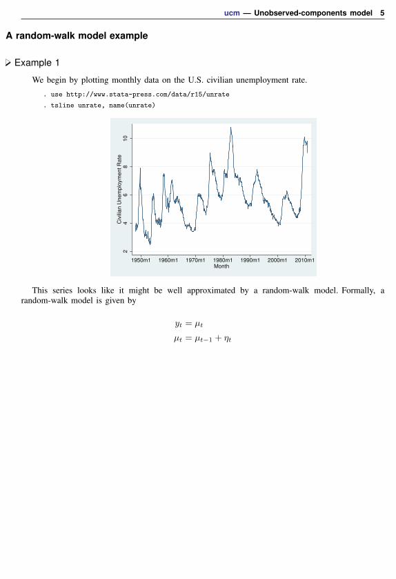
We begin by plotting monthly data on the U.S. civilian unemployment rate.
. use http://www.stata-press.com/data/r15/unrate
. tsline unrate, name(unrate)
24
68
10
Civ
ilia
n U
ne
mp
loym
en
t R
ate
1950m1 1960m1 1970m1 1980m1 1990m1 2000m1 2010m1Month
This series looks like it might be well approximated by a random-walk model. Formally, arandom-walk model is given by
yt = µt
µt = µt−1 + ηt
6 ucm — Unobserved-components model
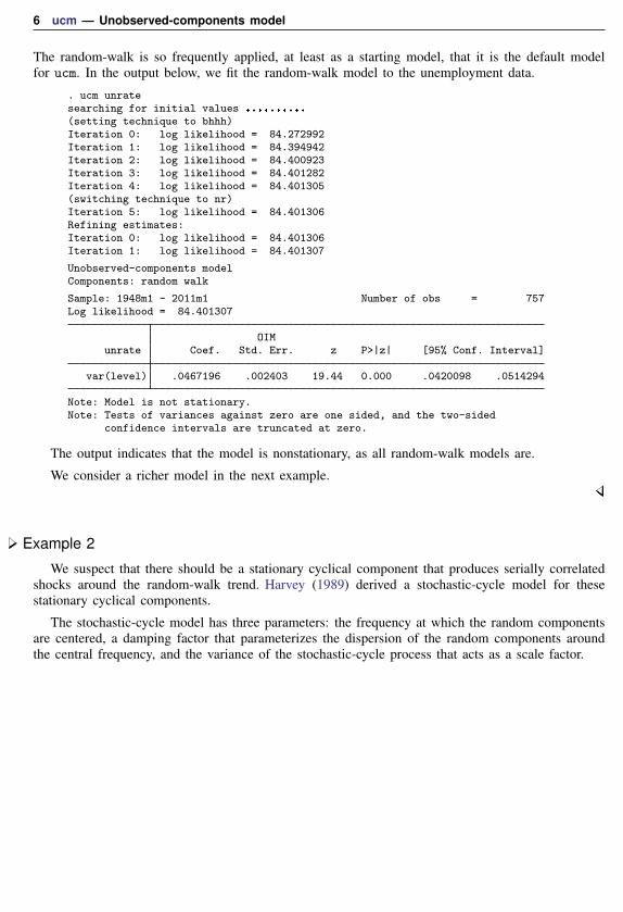
The random-walk is so frequently applied, at least as a starting model, that it is the default modelfor ucm. In the output below, we fit the random-walk model to the unemployment data.
. ucm unratesearching for initial values ..........
(setting technique to bhhh)Iteration 0: log likelihood = 84.272992Iteration 1: log likelihood = 84.394942Iteration 2: log likelihood = 84.400923Iteration 3: log likelihood = 84.401282Iteration 4: log likelihood = 84.401305(switching technique to nr)Iteration 5: log likelihood = 84.401306Refining estimates:Iteration 0: log likelihood = 84.401306Iteration 1: log likelihood = 84.401307
Unobserved-components modelComponents: random walk
Sample: 1948m1 - 2011m1 Number of obs = 757Log likelihood = 84.401307
OIMunrate Coef. Std. Err. z P>|z| [95% Conf. Interval]
var(level) .0467196 .002403 19.44 0.000 .0420098 .0514294
Note: Model is not stationary.Note: Tests of variances against zero are one sided, and the two-sided
confidence intervals are truncated at zero.
The output indicates that the model is nonstationary, as all random-walk models are.
We consider a richer model in the next example.
Example 2
We suspect that there should be a stationary cyclical component that produces serially correlatedshocks around the random-walk trend. Harvey (1989) derived a stochastic-cycle model for thesestationary cyclical components.
The stochastic-cycle model has three parameters: the frequency at which the random componentsare centered, a damping factor that parameterizes the dispersion of the random components aroundthe central frequency, and the variance of the stochastic-cycle process that acts as a scale factor.
ucm — Unobserved-components model 7
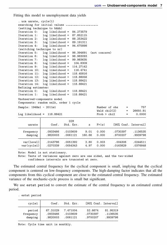
Fitting this model to unemployment data yields
. ucm unrate, cycle(1)searching for initial values ....................
(setting technique to bhhh)Iteration 0: log likelihood = 84.273579Iteration 1: log likelihood = 87.852115Iteration 2: log likelihood = 88.253422Iteration 3: log likelihood = 89.191311Iteration 4: log likelihood = 94.675898(switching technique to nr)Iteration 5: log likelihood = 98.394691 (not concave)Iteration 6: log likelihood = 98.983093Iteration 7: log likelihood = 99.983635Iteration 8: log likelihood = 104.8309Iteration 9: log likelihood = 114.27142Iteration 10: log likelihood = 116.4741Iteration 11: log likelihood = 118.45816Iteration 12: log likelihood = 118.88056Iteration 13: log likelihood = 118.88421Iteration 14: log likelihood = 118.88421Refining estimates:Iteration 0: log likelihood = 118.88421Iteration 1: log likelihood = 118.88421
Unobserved-components modelComponents: random walk, order 1 cycle
Sample: 1948m1 - 2011m1 Number of obs = 757Wald chi2(2) = 26650.81
Log likelihood = 118.88421 Prob > chi2 = 0.0000
OIMunrate Coef. Std. Err. z P>|z| [95% Conf. Interval]
frequency .0933466 .0103609 9.01 0.000 .0730397 .1136535damping .9820003 .0061121 160.66 0.000 .9700207 .9939798
var(level) .0143786 .0051392 2.80 0.003 .004306 .0244511var(cycle1) .0270339 .0054343 4.97 0.000 .0163829 .0376848
Note: Model is not stationary.Note: Tests of variances against zero are one sided, and the two-sided
confidence intervals are truncated at zero.
The estimated central frequency for the cyclical component is small, implying that the cyclicalcomponent is centered on low-frequency components. The high-damping factor indicates that all thecomponents from this cyclical component are close to the estimated central frequency. The estimatedvariance of the stochastic-cycle process is small but significant.
We use estat period to convert the estimate of the central frequency to an estimated centralperiod.
. estat period
cycle1 Coef. Std. Err. [95% Conf. Interval]
period 67.31029 7.471004 52.6674 81.95319frequency .0933466 .0103609 .0730397 .1136535
damping .9820003 .0061121 .9700207 .9939798
Note: Cycle time unit is monthly.
8 ucm — Unobserved-components model
Because we have monthly data, the estimated central period of 67.31 implies that the cyclicalcomponent is composed of random components that occur around a central periodicity of about 5.61years. This estimate falls within the conventional Burns and Mitchell (1946) definition of business-cycleshocks occurring between 1.5 and 8 years.
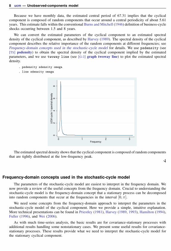
We can convert the estimated parameters of the cyclical component to an estimated spectraldensity of the cyclical component, as described by Harvey (1989). The spectral density of the cyclicalcomponent describes the relative importance of the random components at different frequencies; seeFrequency-domain concepts used in the stochastic-cycle model for details. We use psdensity (see[TS] psdensity) to obtain the spectral density of the cyclical component implied by the estimatedparameters, and we use twoway line (see [G-2] graph twoway line) to plot the estimated spectraldensity.
. psdensity sdensity omega
. line sdensity omega
02
46
8U
CM
cycle
1 s
pe
ctr
al d
en
sity
0 1 2 3Frequency
The estimated spectral density shows that the cyclical component is composed of random componentsthat are tightly distributed at the low-frequency peak.
Frequency-domain concepts used in the stochastic-cycle model
The parameters of the stochastic-cycle model are easiest to interpret in the frequency domain. Wenow provide a review of the useful concepts from the frequency domain. Crucial to understanding thestochastic-cycle model is the frequency-domain concept that a stationary process can be decomposedinto random components that occur at the frequencies in the interval [0, π].
We need some concepts from the frequency-domain approach to interpret the parameters in thestochastic-cycle model of the cyclical component. Here we provide a simple, intuitive explanation.More technical presentations can be found in Priestley (1981), Harvey (1989, 1993), Hamilton (1994),Fuller (1996), and Wei (2006).
As with much time-series analysis, the basic results are for covariance-stationary processes withadditional results handling some nonstationary cases. We present some useful results for covariance-stationary processes. These results provide what we need to interpret the stochastic-cycle model forthe stationary cyclical component.
ucm — Unobserved-components model 9
The autocovariances γj , j ∈ {0, 1, . . . ,∞}, of a covariance-stationary process yt specify itsvariance and dependence structure. In the frequency-domain approach to time-series analysis, thespectral density describes the importance of the random components that occur at frequency ω relativeto the components that occur at other frequencies.
The frequency-domain approach focuses on the relative contributions of random components thatoccur at the frequencies [0, π].
The spectral density can be written as a weighted average of the autocorrelations of yt. Likeautocorrelations, the spectral density is normalized by γ0, the variance of yt. Multiplying the spectraldensity by γ0 yields the power-spectrum of yt.
In an independent and identically distributed (i.i.d.) process, the components at all frequencies areequally important, so the spectral density is a flat line.
In common parlance, we speak of high-frequency noise making a series look more jagged and oflow-frequency components causing smoother plots. More formally, we say that a process composedprimarily of high-frequency components will have fewer runs above or below the mean than an i.i.d.process and that a process composed primarily of low-frequency components will have more runsabove or below the mean than an i.i.d. process.
To further formalize these ideas, consider the first-order autoregressive (AR(1)) process given by
yt = φyt−1 + εt
where εt is a zero-mean, covariance-stationary process with finite variance σ2, and |φ| < 1 so thatyt is covariance stationary. The first-order autocorrelation of this AR(1) process is φ.
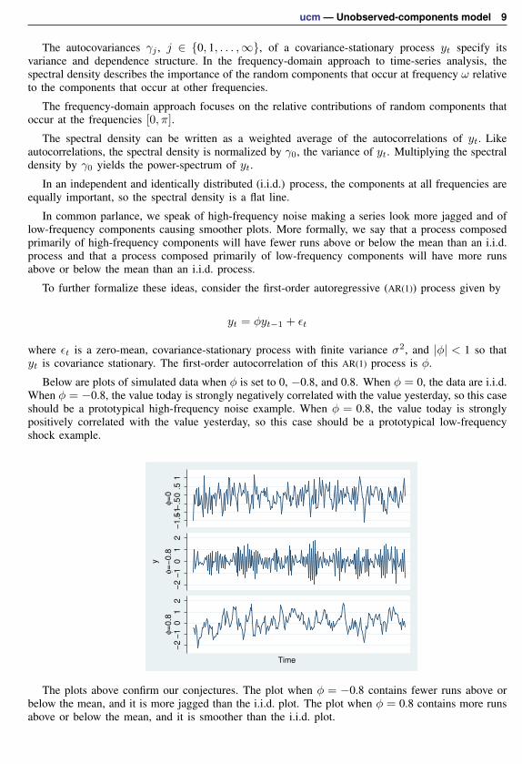
Below are plots of simulated data when φ is set to 0, −0.8, and 0.8. When φ = 0, the data are i.i.d.When φ = −0.8, the value today is strongly negatively correlated with the value yesterday, so this caseshould be a prototypical high-frequency noise example. When φ = 0.8, the value today is stronglypositively correlated with the value yesterday, so this case should be a prototypical low-frequencyshock example.
−1
.5−1−
.50
.51
φ=
0−
2−
10
12
φ=
−0
.8−
2−
10
12
φ=
0.8
y
Time
The plots above confirm our conjectures. The plot when φ = −0.8 contains fewer runs above orbelow the mean, and it is more jagged than the i.i.d. plot. The plot when φ = 0.8 contains more runsabove or below the mean, and it is smoother than the i.i.d. plot.
10 ucm — Unobserved-components model
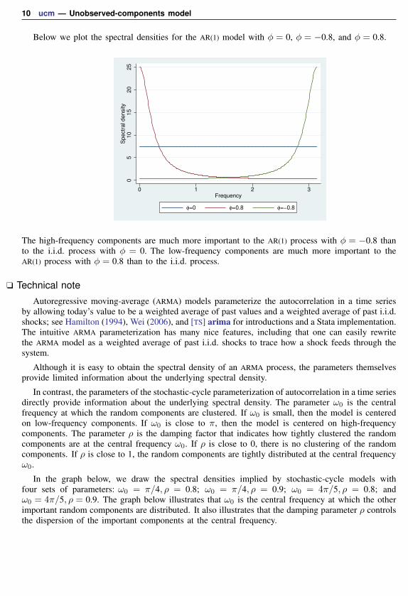
Below we plot the spectral densities for the AR(1) model with φ = 0, φ = −0.8, and φ = 0.8.
05
10
15
20
25
Sp
ectr
al d
en
sity
0 1 2 3Frequency
φ=0 φ=0.8 φ=−0.8
The high-frequency components are much more important to the AR(1) process with φ = −0.8 thanto the i.i.d. process with φ = 0. The low-frequency components are much more important to theAR(1) process with φ = 0.8 than to the i.i.d. process.
Technical note
Autoregressive moving-average (ARMA) models parameterize the autocorrelation in a time seriesby allowing today’s value to be a weighted average of past values and a weighted average of past i.i.d.shocks; see Hamilton (1994), Wei (2006), and [TS] arima for introductions and a Stata implementation.The intuitive ARMA parameterization has many nice features, including that one can easily rewritethe ARMA model as a weighted average of past i.i.d. shocks to trace how a shock feeds through thesystem.
Although it is easy to obtain the spectral density of an ARMA process, the parameters themselvesprovide limited information about the underlying spectral density.
In contrast, the parameters of the stochastic-cycle parameterization of autocorrelation in a time seriesdirectly provide information about the underlying spectral density. The parameter ω0 is the centralfrequency at which the random components are clustered. If ω0 is small, then the model is centeredon low-frequency components. If ω0 is close to π, then the model is centered on high-frequencycomponents. The parameter ρ is the damping factor that indicates how tightly clustered the randomcomponents are at the central frequency ω0. If ρ is close to 0, there is no clustering of the randomcomponents. If ρ is close to 1, the random components are tightly distributed at the central frequencyω0.
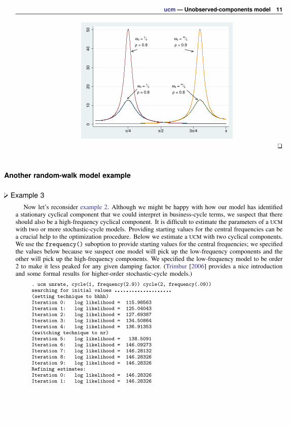
In the graph below, we draw the spectral densities implied by stochastic-cycle models withfour sets of parameters: ω0 = π/4, ρ = 0.8; ω0 = π/4, ρ = 0.9; ω0 = 4π/5, ρ = 0.8; andω0 = 4π/5, ρ = 0.9. The graph below illustrates that ω0 is the central frequency at which the otherimportant random components are distributed. It also illustrates that the damping parameter ρ controlsthe dispersion of the important components at the central frequency.
ucm — Unobserved-components model 11
ω0 = π⁄4
ρ = 0.9
ω0 = 4π
⁄5
ρ = 0.9
ω0 = π⁄4
ρ = 0.8
ω0 = 4π
⁄5
ρ = 0.8
01
02
03
04
05
0
π/4 π/2 3π/4 π
Another random-walk model example
Example 3
Now let’s reconsider example 2. Although we might be happy with how our model has identifieda stationary cyclical component that we could interpret in business-cycle terms, we suspect that thereshould also be a high-frequency cyclical component. It is difficult to estimate the parameters of a UCMwith two or more stochastic-cycle models. Providing starting values for the central frequencies can bea crucial help to the optimization procedure. Below we estimate a UCM with two cyclical components.We use the frequency() suboption to provide starting values for the central frequencies; we specifiedthe values below because we suspect one model will pick up the low-frequency components and theother will pick up the high-frequency components. We specified the low-frequency model to be order2 to make it less peaked for any given damping factor. (Trimbur [2006] provides a nice introductionand some formal results for higher-order stochastic-cycle models.)
. ucm unrate, cycle(1, frequency(2.9)) cycle(2, frequency(.09))searching for initial values ....................
(setting technique to bhhh)Iteration 0: log likelihood = 115.98563Iteration 1: log likelihood = 125.04043Iteration 2: log likelihood = 127.69387Iteration 3: log likelihood = 134.50864Iteration 4: log likelihood = 136.91353(switching technique to nr)Iteration 5: log likelihood = 138.5091Iteration 6: log likelihood = 146.09273Iteration 7: log likelihood = 146.28132Iteration 8: log likelihood = 146.28326Iteration 9: log likelihood = 146.28326Refining estimates:Iteration 0: log likelihood = 146.28326Iteration 1: log likelihood = 146.28326

12 ucm — Unobserved-components model
Unobserved-components modelComponents: random walk, 2 cycles of order 1 2
Sample: 1948m1 - 2011m1 Number of obs = 757Wald chi2(4) = 7681.33
Log likelihood = 146.28326 Prob > chi2 = 0.0000
OIMunrate Coef. Std. Err. z P>|z| [95% Conf. Interval]
cycle1frequency 2.882382 .0668017 43.15 0.000 2.751453 3.013311
damping .7004295 .1251571 5.60 0.000 .4551261 .9457329
cycle2frequency .0667929 .0206849 3.23 0.001 .0262513 .1073346
damping .9074708 .0142273 63.78 0.000 .8795858 .9353559
var(level) .0207704 .0039669 5.24 0.000 .0129953 .0285454var(cycle1) .0027886 .0014363 1.94 0.026 0 .0056037var(cycle2) .002714 .0010281 2.64 0.004 .0006991 .004729
Note: Model is not stationary.Note: Tests of variances against zero are one sided, and the two-sided
confidence intervals are truncated at zero.
The output provides some support for the existence of a second, high-frequency cycle. The high-frequency components are centered at 2.88, whereas the low-frequency components are centered at0.067. That the estimated damping factor is 0.70 for the high-frequency cycle whereas the estimateddamping factor for the low-frequency cycle is 0.91 indicates that the high-frequency components aremore diffusely distributed at 2.88 than the low-frequency components are at 0.067.
We obtain and plot the estimated spectral densities to get another look at these results.
. psdensity sdensity2a omega2a
. psdensity sdensity2b omega2b, cycle(2)
. line sdensity2a sdensity2b omega2a, legend(col(1))
01
23
4
0 1 2 3Frequency
UCM cycle 1 spectral density
UCM cycle 2 spectral density
The estimated spectral densities indicate that we have found two distinct cyclical components.

ucm — Unobserved-components model 13
It does not matter whether we specify omega2a or omega2b to be the x-axis variable, becausethey are equal to each other.
Technical noteThat the estimated spectral densities in the previous example do not overlap is important for
parameter identification. Although the parameters are identified in large-sample theory, we have foundit difficult to estimate the parameters of two cyclical components when the spectral densities overlap.When the spectral densities of two cyclical components overlap, the parameters may not be wellidentified and the optimization procedure may not converge.
Comparing UCM and ARIMA
Example 4
This example provides some insight for readers familiar with autoregressive integrated moving-average (ARIMA) models but not with UCMs. If you are not familiar with ARIMA models, you maywish to skip this example. See [TS] arima for an introduction to ARIMA models in Stata.
UCMs provide an alternative to ARIMA models implemented in [TS] arima. Neither set of modelsis nested within the other, but there are some cases in which instructive comparisons can be made.
The random-walk model corresponds to an ARIMA model that is first-order integrated and hasan i.i.d. error term. In other words, the random-walk UCM and the ARIMA(0,1,0) are asymptoticallyequivalent. Thus
ucm unrate
and
arima unrate, arima(0,1,0) noconstant
produce asymptotically equivalent results.
The stochastic-cycle model for the stationary cyclical component is an alternative functional formfor stationary processes to stationary autoregressive moving-average (ARMA) models. Which modelis preferred depends on the application and which parameters a researchers wants to interpret. Boththe functional forms and the parameter interpretations differ between the stochastic-cycle model andthe ARMA model. See Trimbur (2006, eq. 25) for some formal comparisons of the two models.
That both models can be used to estimate the stationary cyclical components for the random-walkmodel implies that we can compare the results in this case by comparing their estimated spectraldensities. Below we estimate the parameters of an ARIMA(2,1,1) model and plot the estimated spectraldensity of the stationary component.
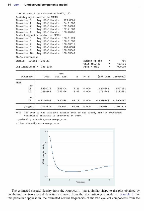
14 ucm — Unobserved-components model
. arima unrate, noconstant arima(2,1,1)
(setting optimization to BHHH)Iteration 0: log likelihood = 129.8801Iteration 1: log likelihood = 134.61953Iteration 2: log likelihood = 137.04909Iteration 3: log likelihood = 137.71386Iteration 4: log likelihood = 138.25255(switching optimization to BFGS)Iteration 5: log likelihood = 138.51924Iteration 6: log likelihood = 138.81638Iteration 7: log likelihood = 138.83615Iteration 8: log likelihood = 138.8364Iteration 9: log likelihood = 138.83642Iteration 10: log likelihood = 138.83642
ARIMA regression
Sample: 1948m2 - 2011m1 Number of obs = 756Wald chi2(3) = 683.34
Log likelihood = 138.8364 Prob > chi2 = 0.0000
OPGD.unrate Coef. Std. Err. z P>|z| [95% Conf. Interval]
ARMAar
L1. .5398016 .0586304 9.21 0.000 .4248882 .6547151L2. .2468148 .0359396 6.87 0.000 .1763744 .3172551
maL1. -.5146506 .0632838 -8.13 0.000 -.6386845 -.3906167
/sigma .2013332 .0032644 61.68 0.000 .1949351 .2077313
Note: The test of the variance against zero is one sided, and the two-sidedconfidence interval is truncated at zero.
. psdensity sdensity_arma omega_arma
. line sdensity_arma omega_arma
0.2
.4.6
.8A
RM
A
sp
ectr
al d
en
sity
0 1 2 3Frequency
The estimated spectral density from the ARIMA(2,1,1) has a similar shape to the plot obtained bycombining the two spectral densities estimated from the stochastic-cycle model in example 3. Forthis particular application, the estimated central frequencies of the two cyclical components from the
ucm — Unobserved-components model 15
stochastic-cycle model provide information about the business-cycle component and the high-frequencycomponent that is not easily obtained from the ARIMA(2,1,1) model. On the other hand, it is easierto work out the impulse–response function for the ARMA model than for the stochastic-cycle model,implying that the ARMA model is easier to use when tracing the effect of a shock feeding throughthe system.
A local-level model example
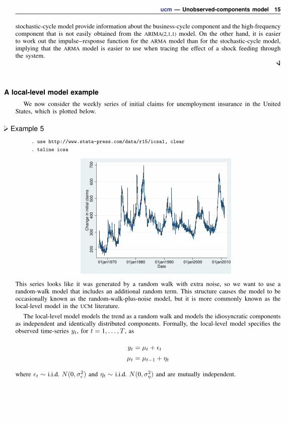
We now consider the weekly series of initial claims for unemployment insurance in the UnitedStates, which is plotted below.
Example 5
. use http://www.stata-press.com/data/r15/icsa1, clear
. tsline icsa
20
03
00
40
05
00
60
07
00
Ch
an
ge
in
in
itia
l cla
ims
01jan1970 01jan1980 01jan1990 01jan2000 01jan2010Date
This series looks like it was generated by a random walk with extra noise, so we want to use arandom-walk model that includes an additional random term. This structure causes the model to beoccasionally known as the random-walk-plus-noise model, but it is more commonly known as thelocal-level model in the UCM literature.
The local-level model models the trend as a random walk and models the idiosyncratic componentsas independent and identically distributed components. Formally, the local-level model specifies theobserved time-series yt, for t = 1, . . . , T , as
yt = µt + εt
µt = µt−1 + ηt
where εt ∼ i.i.d. N(0, σ2ε ) and ηt ∼ i.i.d. N(0, σ2
η) and are mutually independent.

16 ucm — Unobserved-components model
We fit the local-level model in the output below:
. ucm icsa, model(llevel)searching for initial values ..........
(setting technique to bhhh)Iteration 0: log likelihood = -9954.8223Iteration 1: log likelihood = -9917.406Iteration 2: log likelihood = -9905.6679Iteration 3: log likelihood = -9897.7588Iteration 4: log likelihood = -9894.2015(switching technique to nr)Iteration 5: log likelihood = -9893.4337Iteration 6: log likelihood = -9893.2469Iteration 7: log likelihood = -9893.2469Refining estimates:Iteration 0: log likelihood = -9893.2469Iteration 1: log likelihood = -9893.2469
Unobserved-components modelComponents: local level
Sample: 07jan1967 - 19feb2011 Number of obs = 2,303Log likelihood = -9893.2469
OIMicsa Coef. Std. Err. z P>|z| [95% Conf. Interval]
var(level) 116.558 8.806587 13.24 0.000 99.29745 133.8186var(icsa) 124.2715 7.615506 16.32 0.000 109.3454 139.1976
Note: Model is not stationary.Note: Tests of variances against zero are one sided, and the two-sided
confidence intervals are truncated at zero.Note: Time units are in 7 days.
The output indicates that both components are statistically significant.
Technical noteThe estimation procedure will not always converge when estimating the parameters of the local-level
model. If the series does not vary enough in the random level, modeled by the random walk, and inthe stationary shocks around the random level, the estimation procedure will not converge because itwill be unable to set the variance of one of the two components to 0.
Take another look at the graphs of unrate and icsa. The extra noise around the random levelthat can be seen in the graph of icsa allows us to estimate both variances.
A closely related point is that it is difficult to estimate the parameters of a local-level model witha stochastic-cycle component because the series must have enough variation to identify the varianceof the random-walk component, the variance of the idiosyncratic term, and the parameters of thestochastic-cycle component. In some cases, series that look like candidates for the local-level modelare best modeled as random-walk models with stochastic-cycle components.
In fact, convergence can be a problem for most of the models in ucm. Convergence problemsoccur most often when there is insufficient variation to estimate the variances of the components inthe model. When there is insufficient variation to estimate the variances of the components in themodel, the optimization routine will fail to converge as it attempts to set the variance equal to 0.This usually shows up in the iteration log when the log likelihood gets stuck at a particular value andthe message (not concave) or (backed up) is displayed repeatedly. When this happens, use the
ucm — Unobserved-components model 17
iterate() option to limit the number of iterations, look to see which of the variances is being drivento 0, and drop that component from the model. (This technique is a method to obtain convergenceto interpretable estimates, not a model-selection method.)
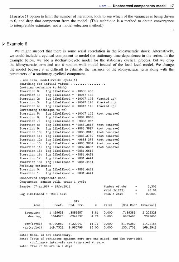
Example 6
We might suspect that there is some serial correlation in the idiosyncratic shock. Alternatively,we could include a cyclical component to model the stationary time-dependence in the series. In theexample below, we add a stochastic-cycle model for the stationary cyclical process, but we dropthe idiosyncratic term and use a random-walk model instead of the local-level model. We changethe model because it is difficult to estimate the variance of the idiosyncratic term along with theparameters of a stationary cyclical component.
. ucm icsa, model(rwalk) cycle(1)searching for initial values ....................
(setting technique to bhhh)Iteration 0: log likelihood = -10055.453Iteration 1: log likelihood = -10047.163Iteration 2: log likelihood = -10047.146 (backed up)Iteration 3: log likelihood = -10047.146 (backed up)Iteration 4: log likelihood = -10047.145 (backed up)(switching technique to nr)Iteration 5: log likelihood = -10047.142 (not concave)Iteration 6: log likelihood = -9889.8038Iteration 7: log likelihood = -9883.967Iteration 8: log likelihood = -9883.3818 (not concave)Iteration 9: log likelihood = -9883.3817 (not concave)Iteration 10: log likelihood = -9883.3815 (not concave)Iteration 11: log likelihood = -9883.3789 (not concave)Iteration 12: log likelihood = -9883.376 (not concave)Iteration 13: log likelihood = -9883.3684 (not concave)Iteration 14: log likelihood = -9882.0687 (not concave)Iteration 15: log likelihood = -9881.6615Iteration 16: log likelihood = -9881.4451Iteration 17: log likelihood = -9881.4441Iteration 18: log likelihood = -9881.4441Refining estimates:Iteration 0: log likelihood = -9881.4441Iteration 1: log likelihood = -9881.4441
Unobserved-components modelComponents: random walk, order 1 cycle
Sample: 07jan1967 - 19feb2011 Number of obs = 2,303Wald chi2(2) = 23.04
Log likelihood = -9881.4441 Prob > chi2 = 0.0000
OIMicsa Coef. Std. Err. z P>|z| [95% Conf. Interval]
frequency 1.469633 .3855657 3.81 0.000 .7139385 2.225328damping .1644576 .0349537 4.71 0.000 .0959495 .2329656
var(level) 97.90982 8.320047 11.77 0.000 81.60282 114.2168var(cycle1) 149.7323 9.980798 15.00 0.000 130.1703 169.2943
Note: Model is not stationary.Note: Tests of variances against zero are one sided, and the two-sided
confidence intervals are truncated at zero.Note: Time units are in 7 days.

18 ucm — Unobserved-components model
Although the output indicates that the model fits well, the small estimate of the damping parameterindicates that the random components will be widely distributed at the central frequency. To get abetter idea of the dispersion of the components, we look at the estimated spectral density of thestationary cyclical component.
. psdensity sdensity3 omega3
. line sdensity3 omega3
.14
5.1
5.1
55
.16
.16
5.1
7U
CM
cycle
1 s
pe
ctr
al d
en
sity
0 1 2 3Frequency
The graph shows that the random components that make up the cyclical component are diffuselydistributed at a central frequency.
Comparing UCM and ARIMA, revisited
Example 7
Including lags of the dependent variable is an alternative method for modeling serially correlatederrors. The estimated coefficients on the lags of the dependent variable estimate the coefficients in anautoregressive model for the stationary cyclical component; see Harvey (1989, 47–48) for a discussion.Including lags of the dependent variable should be viewed as an alternative to the stochastic-cyclemodel for the stationary cyclical component. In this example, we use the large-sample equivalence ofthe random-walk model with pth order autoregressive errors and an ARIMA(p, 1, 0) to illustrate thispoint.
ucm — Unobserved-components model 19
In the output below, we include 2 lags of the dependent variable in the random-walk UCM.
. ucm icsa L(1/2).icsa, model(rwalk)searching for initial values ..........
(setting technique to bhhh)Iteration 0: log likelihood = -10026.649Iteration 1: log likelihood = -9947.9671Iteration 2: log likelihood = -9896.4778Iteration 3: log likelihood = -9890.8199Iteration 4: log likelihood = -9890.3202(switching technique to nr)Iteration 5: log likelihood = -9890.1546Iteration 6: log likelihood = -9889.561Iteration 7: log likelihood = -9889.5608Refining estimates:Iteration 0: log likelihood = -9889.5608Iteration 1: log likelihood = -9889.5608
Unobserved-components modelComponents: random walk
Sample: 21jan1967 - 19feb2011 Number of obs = 2,301Wald chi2(2) = 271.88
Log likelihood = -9889.5608 Prob > chi2 = 0.0000
OIMicsa Coef. Std. Err. z P>|z| [95% Conf. Interval]
icsaL1. -.3250633 .0205148 -15.85 0.000 -.3652715 -.2848551L2. -.1794686 .0205246 -8.74 0.000 -.2196961 -.1392411
var(level) 317.6474 9.36691 33.91 0.000 299.2886 336.0062
Note: Model is not stationary.Note: Tests of variances against zero are one sided, and the two-sided
confidence intervals are truncated at zero.Note: Time units are in 7 days.
Now we use arima to estimate the parameters of an asymptotically equivalent ARIMA(2,1,0) model.(We specify the technique(nr) option so that arima will compute the observed information matrixstandard errors that ucm computes.) We use nlcom to compute a point estimate and a standard errorfor the variance, which is directly comparable to the one produced by ucm.
20 ucm — Unobserved-components model
. arima icsa, noconstant arima(2,1,0) technique(nr)
Iteration 0: log likelihood = -9896.4584Iteration 1: log likelihood = -9896.458
ARIMA regression
Sample: 14jan1967 - 19feb2011 Number of obs = 2302Wald chi2(2) = 271.95
Log likelihood = -9896.458 Prob > chi2 = 0.0000
OIMD.icsa Coef. Std. Err. z P>|z| [95% Conf. Interval]
ARMAar
L1. -.3249383 .0205036 -15.85 0.000 -.3651246 -.284752L2. -.1793353 .0205088 -8.74 0.000 -.2195317 -.1391388
/sigma 17.81606 .2625695 67.85 0.000 17.30143 18.33068
Note: The test of the variance against zero is one sided, and the two-sidedconfidence interval is truncated at zero.
. nlcom _b[sigma:_cons]^2
_nl_1: _b[sigma:_cons]^2
D.icsa Coef. Std. Err. z P>|z| [95% Conf. Interval]
_nl_1 317.4119 9.355904 33.93 0.000 299.0746 335.7491
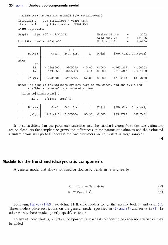
It is no accident that the parameter estimates and the standard errors from the two estimatorsare so close. As the sample size grows the differences in the parameter estimates and the estimatedstandard errors will go to 0, because the two estimators are equivalent in large samples.
Models for the trend and idiosyncratic components
A general model that allows for fixed or stochastic trends in τt is given by
τt = τt−1 + βt−1 + ηt (2)
βt = βt−1 + ξt (3)
Following Harvey (1989), we define 11 flexible models for yt that specify both τt and εt in (1).These models place restrictions on the general model specified in (2) and (3) and on εt in (1). Inother words, these models jointly specify τt and εt.
To any of these models, a cyclical component, a seasonal component, or exogenous variables maybe added.

ucm — Unobserved-components model 21
Table 1. Models for the trend and idiosyncratic components
Model name Syntax option Model
No trend or idiosyncratic component model(none)
No trend model(ntrend) yt=εt
Deterministic constant model(dconstant) yt=µ+ εtµ=µ
Local level model(llevel) yt=µt + εtµt=µt−1 + ηt
Random walk model(rwalk) yt=µtµt=µt−1 + ηt
Deterministic trend model(dtrend) yt=µt + εtµt=µt−1 + ββ=β
Local level with model(lldtrend) yt=µt + εtdeterministic trend µt=µt−1 + β + ηt
β=β
Random walk with drift model(rwdrift) yt=µtµt=µt−1 + β + ηtβ=β
Local linear trend model(lltrend) yt=µt + εtµt=µt−1 + βt−1 + ηtβt=βt−1 + ξt
Smooth trend model(strend) yt=µt + εtµt=µt−1 + βt−1
βt=βt−1 + ξt
Random trend model(rtrend) yt=µtµt=µt−1 + βt−1
βt=βt−1 + ξt
The majority of the models available in ucm are designed for nonstationary time series. Thedeterministic-trend model incorporates a first-order deterministic time-trend in the model. The local-level, random-walk, local-level-with-deterministic-trend, and random-walk-with-drift models are formodeling series with first-order stochastic trends. A series with a dth-order stochastic trend must bedifferenced d times to be stationary. The local-linear-trend, smooth-trend, and random-trend modelsare for modeling series with second-order stochastic trends.
The no-trend-or-idiosyncratic-component model is useful for using ucm to model stationary serieswith cyclical components or seasonal components and perhaps exogenous variables. The no-trend andthe deterministic-constant models are useful for using ucm to model stationary series with seasonalcomponents or exogenous variables.
22 ucm — Unobserved-components model
Seasonal component
A seasonal component models cyclical behavior in a time series that occurs at known seasonalperiodicities. A seasonal component is modeled in the time domain; the period of the cycle is specifiedas the number of time periods required for the cycle to complete.
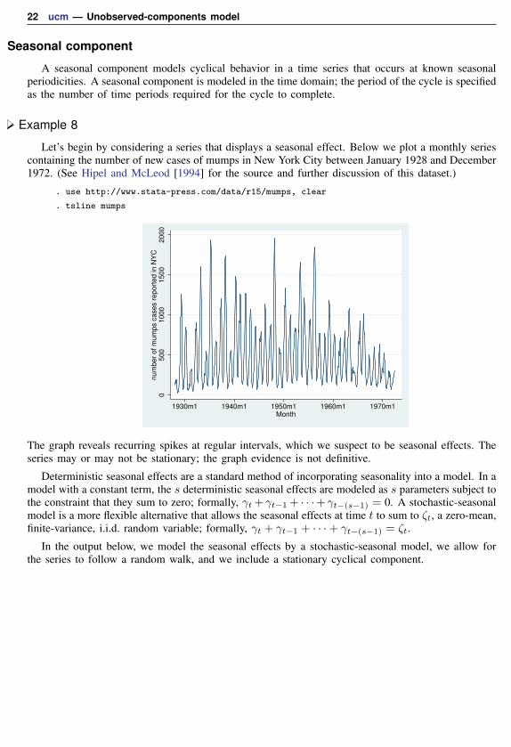
Example 8
Let’s begin by considering a series that displays a seasonal effect. Below we plot a monthly seriescontaining the number of new cases of mumps in New York City between January 1928 and December1972. (See Hipel and McLeod [1994] for the source and further discussion of this dataset.)
. use http://www.stata-press.com/data/r15/mumps, clear
. tsline mumps
05
00
10
00
15
00
20
00
nu
mb
er
of
mu
mp
s c
ase
s r
ep
ort
ed
in
NY
C
1930m1 1940m1 1950m1 1960m1 1970m1Month
The graph reveals recurring spikes at regular intervals, which we suspect to be seasonal effects. Theseries may or may not be stationary; the graph evidence is not definitive.
Deterministic seasonal effects are a standard method of incorporating seasonality into a model. In amodel with a constant term, the s deterministic seasonal effects are modeled as s parameters subject tothe constraint that they sum to zero; formally, γt+ γt−1+ · · ·+ γt−(s−1) = 0. A stochastic-seasonalmodel is a more flexible alternative that allows the seasonal effects at time t to sum to ζt, a zero-mean,finite-variance, i.i.d. random variable; formally, γt + γt−1 + · · ·+ γt−(s−1) = ζt.
In the output below, we model the seasonal effects by a stochastic-seasonal model, we allow forthe series to follow a random walk, and we include a stationary cyclical component.
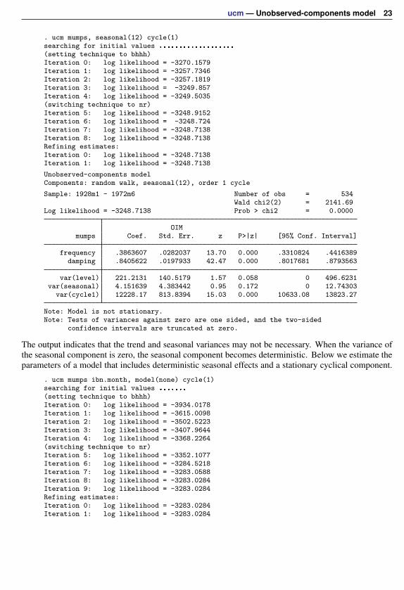
ucm — Unobserved-components model 23
. ucm mumps, seasonal(12) cycle(1)searching for initial values ...................
(setting technique to bhhh)Iteration 0: log likelihood = -3270.1579Iteration 1: log likelihood = -3257.7346Iteration 2: log likelihood = -3257.1819Iteration 3: log likelihood = -3249.857Iteration 4: log likelihood = -3249.5035(switching technique to nr)Iteration 5: log likelihood = -3248.9152Iteration 6: log likelihood = -3248.724Iteration 7: log likelihood = -3248.7138Iteration 8: log likelihood = -3248.7138Refining estimates:Iteration 0: log likelihood = -3248.7138Iteration 1: log likelihood = -3248.7138
Unobserved-components modelComponents: random walk, seasonal(12), order 1 cycle
Sample: 1928m1 - 1972m6 Number of obs = 534Wald chi2(2) = 2141.69
Log likelihood = -3248.7138 Prob > chi2 = 0.0000
OIMmumps Coef. Std. Err. z P>|z| [95% Conf. Interval]
frequency .3863607 .0282037 13.70 0.000 .3310824 .4416389damping .8405622 .0197933 42.47 0.000 .8017681 .8793563
var(level) 221.2131 140.5179 1.57 0.058 0 496.6231var(seasonal) 4.151639 4.383442 0.95 0.172 0 12.74303
var(cycle1) 12228.17 813.8394 15.03 0.000 10633.08 13823.27
Note: Model is not stationary.Note: Tests of variances against zero are one sided, and the two-sided
confidence intervals are truncated at zero.
The output indicates that the trend and seasonal variances may not be necessary. When the variance ofthe seasonal component is zero, the seasonal component becomes deterministic. Below we estimate theparameters of a model that includes deterministic seasonal effects and a stationary cyclical component.
. ucm mumps ibn.month, model(none) cycle(1)searching for initial values .......
(setting technique to bhhh)Iteration 0: log likelihood = -3934.0178Iteration 1: log likelihood = -3615.0098Iteration 2: log likelihood = -3502.5223Iteration 3: log likelihood = -3407.9644Iteration 4: log likelihood = -3368.2264(switching technique to nr)Iteration 5: log likelihood = -3352.1077Iteration 6: log likelihood = -3284.5218Iteration 7: log likelihood = -3283.0588Iteration 8: log likelihood = -3283.0284Iteration 9: log likelihood = -3283.0284Refining estimates:Iteration 0: log likelihood = -3283.0284Iteration 1: log likelihood = -3283.0284

24 ucm — Unobserved-components model
Unobserved-components modelComponents: order 1 cycle
Sample: 1928m1 - 1972m6 Number of obs = 534Wald chi2(14) = 3404.29
Log likelihood = -3283.0284 Prob > chi2 = 0.0000
OIMmumps Coef. Std. Err. z P>|z| [95% Conf. Interval]
cycle1frequency .3272753 .0262922 12.45 0.000 .2757436 .3788071
damping .844874 .0184994 45.67 0.000 .8086157 .8811322
mumpsmonth
1 480.5095 32.67128 14.71 0.000 416.475 544.5442 561.9174 32.66999 17.20 0.000 497.8854 625.94943 832.8666 32.67696 25.49 0.000 768.8209 896.91224 894.0747 32.64568 27.39 0.000 830.0904 958.05915 869.6568 32.56282 26.71 0.000 805.8348 933.47876 770.1562 32.48587 23.71 0.000 706.4851 833.82747 433.839 32.50165 13.35 0.000 370.1369 497.5418 218.2394 32.56712 6.70 0.000 154.409 282.06989 140.686 32.64138 4.31 0.000 76.7101 204.662
10 148.5876 32.69067 4.55 0.000 84.51508 212.660211 215.0958 32.70311 6.58 0.000 150.9989 279.192712 330.2232 32.68906 10.10 0.000 266.1538 394.2926
var(cycle1) 13031.53 798.2719 16.32 0.000 11466.95 14596.11
Note: Tests of variances against zero are one sided, and the two-sidedconfidence intervals are truncated at zero.
The output indicates that each of these components is statistically significant.
Technical noteIn a stochastic model for the seasonal component, the seasonal effects sum to the random variable
ζt ∼ i.i.d. N(0, σ2ζ ):
γt = −s−1∑j=1
γt−j + ζt
Stored resultsBecause ucm is estimated using sspace, most of the sspace stored results appear after ucm. Not
all of these results are relevant for ucm; programmers wishing to treat ucm results as sspace resultsshould see Stored results of [TS] sspace. See Methods and formulas for the state-space representationof UCMs, and see [TS] sspace for more documentation that relates to all the stored results.
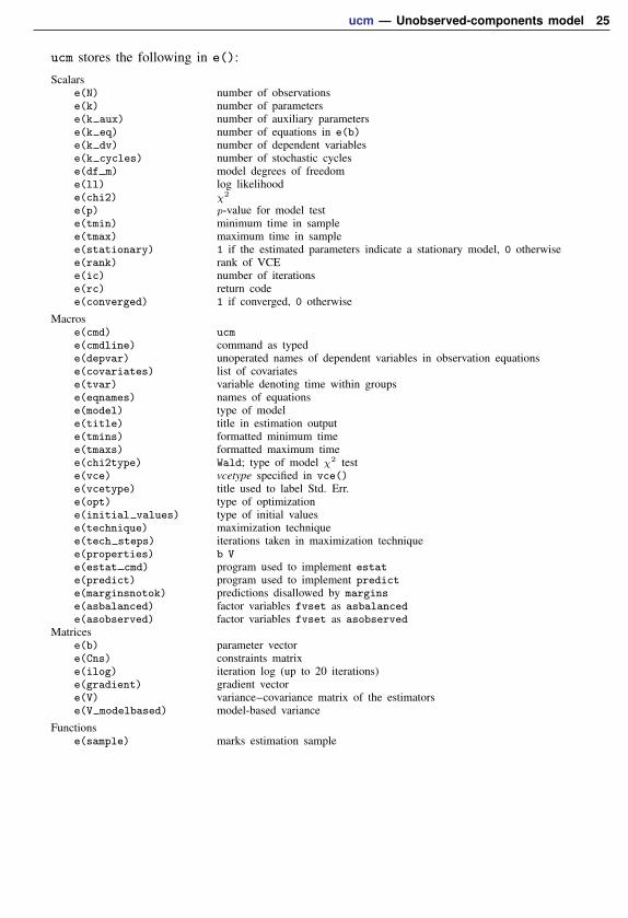
ucm — Unobserved-components model 25
ucm stores the following in e():
Scalarse(N) number of observationse(k) number of parameterse(k aux) number of auxiliary parameterse(k eq) number of equations in e(b)e(k dv) number of dependent variablese(k cycles) number of stochastic cyclese(df m) model degrees of freedome(ll) log likelihoode(chi2) χ2
e(p) p-value for model teste(tmin) minimum time in samplee(tmax) maximum time in samplee(stationary) 1 if the estimated parameters indicate a stationary model, 0 otherwisee(rank) rank of VCEe(ic) number of iterationse(rc) return codee(converged) 1 if converged, 0 otherwise
Macrose(cmd) ucme(cmdline) command as typede(depvar) unoperated names of dependent variables in observation equationse(covariates) list of covariatese(tvar) variable denoting time within groupse(eqnames) names of equationse(model) type of modele(title) title in estimation outpute(tmins) formatted minimum timee(tmaxs) formatted maximum timee(chi2type) Wald; type of model χ2 teste(vce) vcetype specified in vce()e(vcetype) title used to label Std. Err.e(opt) type of optimizatione(initial values) type of initial valuese(technique) maximization techniquee(tech steps) iterations taken in maximization techniquee(properties) b Ve(estat cmd) program used to implement estate(predict) program used to implement predicte(marginsnotok) predictions disallowed by marginse(asbalanced) factor variables fvset as asbalancede(asobserved) factor variables fvset as asobserved
Matricese(b) parameter vectore(Cns) constraints matrixe(ilog) iteration log (up to 20 iterations)e(gradient) gradient vectore(V) variance–covariance matrix of the estimatorse(V modelbased) model-based variance
Functionse(sample) marks estimation sample
26 ucm — Unobserved-components model
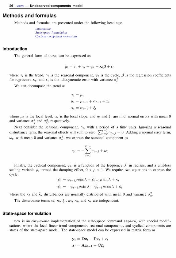
Methods and formulasMethods and formulas are presented under the following headings:
IntroductionState-space formulationCyclical component extensions
Introduction
The general form of UCMs can be expressed as
yt = τt + γt + ψt + xtβ+ εt
where τt is the trend, γt is the seasonal component, ψt is the cycle, β is the regression coefficientsfor regressors xt, and εt is the idiosyncratic error with variance σ2
ε .
We can decompose the trend as
τt = µt
µt = µt−1 + αt−1 + ηt
αt = αt−1 + ξt
where µt is the local level, αt is the local slope, and ηt and ξt are i.i.d. normal errors with mean 0and variance σ2
η and σ2ξ , respectively.
Next consider the seasonal component, γt, with a period of s time units. Ignoring a seasonaldisturbance term, the seasonal effects will sum to zero,
∑s−1j=0 γt−j = 0. Adding a normal error term,
ωt, with mean 0 and variance σ2ω , we express the seasonal component as
γt = −s−1∑j=1
γt−j + ωt
Finally, the cyclical component, ψt, is a function of the frequency λ, in radians, and a unit-lessscaling variable ρ, termed the damping effect, 0 < ρ < 1. We require two equations to express thecycle:
ψt = ψt−1ρ cosλ+ ψ̃t−1ρ sinλ+ κt
ψ̃t = −ψt−1ρ sinλ+ ψ̃t−1ρ cosλ+ κ̃t
where the κt and κ̃t disturbances are normally distributed with mean 0 and variance σ2κ.
The disturbance terms εt, ηt, ξt, ωt, κt, and κ̃t are independent.
State-space formulation
ucm is an easy-to-use implementation of the state-space command sspace, with special modifi-cations, where the local linear trend components, seasonal components, and cyclical components arestates of the state-space model. The state-space model can be expressed in matrix form as
yt = Dzt + Fxt + εt
zt = Azt−1 +Cζt
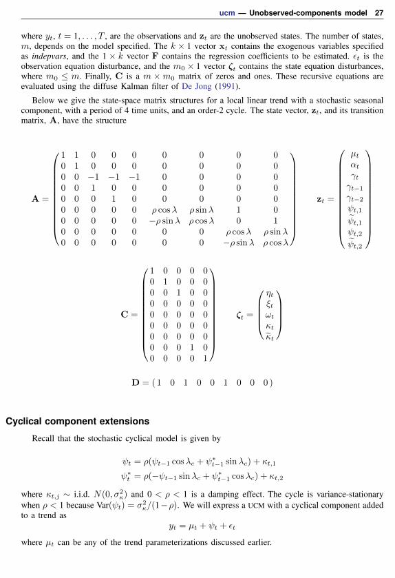
ucm — Unobserved-components model 27
where yt, t = 1, . . . , T , are the observations and zt are the unobserved states. The number of states,m, depends on the model specified. The k × 1 vector xt contains the exogenous variables specifiedas indepvars, and the 1 × k vector F contains the regression coefficients to be estimated. εt is theobservation equation disturbance, and the m0 × 1 vector ζt contains the state equation disturbances,where m0 ≤ m. Finally, C is a m ×m0 matrix of zeros and ones. These recursive equations areevaluated using the diffuse Kalman filter of De Jong (1991).
Below we give the state-space matrix structures for a local linear trend with a stochastic seasonalcomponent, with a period of 4 time units, and an order-2 cycle. The state vector, zt, and its transitionmatrix, A, have the structure
A =
1 1 0 0 0 0 0 0 00 1 0 0 0 0 0 0 00 0 −1 −1 −1 0 0 0 00 0 1 0 0 0 0 0 00 0 0 1 0 0 0 0 00 0 0 0 0 ρ cosλ ρ sinλ 1 00 0 0 0 0 −ρ sinλ ρ cosλ 0 10 0 0 0 0 0 0 ρ cosλ ρ sinλ0 0 0 0 0 0 0 −ρ sinλ ρ cosλ
zt =
µtαtγtγt−1
γt−2
ψt,1ψ̃t,1ψt,2ψ̃t,2
C =
1 0 0 0 00 1 0 0 00 0 1 0 00 0 0 0 00 0 0 0 00 0 0 0 00 0 0 0 00 0 0 1 00 0 0 0 1
ζt =
ηtξtωtκtκ̃t
D = ( 1 0 1 0 0 1 0 0 0 )
Cyclical component extensions
Recall that the stochastic cyclical model is given by
ψt = ρ(ψt−1 cosλc + ψ∗t−1 sinλc) + κt,1
ψ∗t = ρ(−ψt−1 sinλc + ψ∗
t−1 cosλc) + κt,2
where κt,j ∼ i.i.d. N(0, σ2κ) and 0 < ρ < 1 is a damping effect. The cycle is variance-stationary
when ρ < 1 because Var(ψt) = σ2κ/(1−ρ). We will express a UCM with a cyclical component added
to a trend asyt = µt + ψt + εt
where µt can be any of the trend parameterizations discussed earlier.
28 ucm — Unobserved-components model
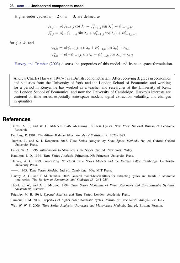
Higher-order cycles, k = 2 or k = 3, are defined as
ψt,j = ρ(ψt−1,j cosλc + ψ∗t−1,j sinλc) + ψt−1,j+1
ψ∗t,j = ρ(−ψt−1,j sinλc + ψ∗
t−1,j cosλc) + ψ∗t−1,j+1
for j < k, andψt,k = ρ(ψt−1,k cosλc + ψ∗
t−1,k sinλc) + κt,1
ψ∗t,k = ρ(−ψt−1,k sinλc + ψ∗
t−1,k cosλc) + κt,2
Harvey and Trimbur (2003) discuss the properties of this model and its state-space formulation.
� �Andrew Charles Harvey (1947– ) is a British econometrician. After receiving degrees in economicsand statistics from the University of York and the London School of Economics and workingfor a period in Kenya, he has worked as a teacher and researcher at the University of Kent,the London School of Economics, and now the University of Cambridge. Harvey’s interests arecentered on time series, especially state-space models, signal extraction, volatility, and changesin quantiles.� �
ReferencesBurns, A. F., and W. C. Mitchell. 1946. Measuring Business Cycles. New York: National Bureau of Economic
Research.
De Jong, P. 1991. The diffuse Kalman filter. Annals of Statistics 19: 1073–1083.
Durbin, J., and S. J. Koopman. 2012. Time Series Analysis by State Space Methods. 2nd ed. Oxford: OxfordUniversity Press.
Fuller, W. A. 1996. Introduction to Statistical Time Series. 2nd ed. New York: Wiley.
Hamilton, J. D. 1994. Time Series Analysis. Princeton, NJ: Princeton University Press.
Harvey, A. C. 1989. Forecasting, Structural Time Series Models and the Kalman Filter. Cambridge: CambridgeUniversity Press.
. 1993. Time Series Models. 2nd ed. Cambridge, MA: MIT Press.
Harvey, A. C., and T. M. Trimbur. 2003. General model-based filters for extracting cycles and trends in economictime series. The Review of Economics and Statistics 85: 244–255.
Hipel, K. W., and A. I. McLeod. 1994. Time Series Modelling of Water Resources and Environmental Systems.Amsterdam: Elsevier.
Priestley, M. B. 1981. Spectral Analysis and Time Series. London: Academic Press.
Trimbur, T. M. 2006. Properties of higher order stochastic cycles. Journal of Time Series Analysis 27: 1–17.
Wei, W. W. S. 2006. Time Series Analysis: Univariate and Multivariate Methods. 2nd ed. Boston: Pearson.

ucm — Unobserved-components model 29
Also see[TS] ucm postestimation — Postestimation tools for ucm
[TS] arima — ARIMA, ARMAX, and other dynamic regression models
[TS] sspace — State-space models
[TS] tsfilter — Filter a time-series, keeping only selected periodicities
[TS] tsset — Declare data to be time-series data
[TS] tssmooth — Smooth and forecast univariate time-series data
[TS] var — Vector autoregressive models
[U] 20 Estimation and postestimation commands


![[PPT]MODEL-MODEL PEMBELAJARANtaqien.blog.uns.ac.id/.../04/model-model-pembelajaran1.ppt · Web viewMODEL-MODEL PEMBELAJARAN MODEL PEMBELAJARAN KONTEKSTUAL MODEL PEMBELAJARAN KOOPERATIF](https://img.pdfslide.net/doc/110x75/5ae268aa7f8b9ad47c8d11a9/pptmodel-model-viewmodel-model-pembelajaran-model-pembelajaran-kontekstual-model.jpg)