ON $\mathrm{P}\mathrm{S}\mathrm{E}\mathrm{U}\mathrm{D}\mathrm{o}_{-}\mathrm{p}\mathrm{o}\mathrm{U}\mathrm{R}\mathrm{I}\mathrm{E}\mathrm{R}$ -MEHLER TRANSFORMSAND INFINITESIMAL GENERATORS

IN WHITE NOISE CALCULUS*)

ISAMU $\mathrm{D}\hat{\mathrm{O}}$ KU (道工勇)

Department of MathematicsSaitama UniversityUrawa 338 Japan

$\mathrm{e}$-mail: doku@sacs.sv.saitama-u.ac.jp

\S 1. IntroductionThe study of the Fourier transform $\mathcal{F}$ in white noise calculus was initiated andhas been developed to a mature level by H.-H. Kuo $[16,17]$ (also $[19]\rangle$ . While, theFourier-Mehler transform $\mathcal{F}_{\theta}$ is a kind of generalization of $\mathcal{F}[18]$ (also [11]), whichfurnishes the theory of infinite dimensional Fourier transforms in white noise spacewith adequately fruitful and profitable ingradients.

In this article we introduce $\mathrm{P}\mathrm{s}\mathrm{e}\mathrm{u}\mathrm{d}_{0}-\mathrm{F}\mathrm{o}\mathrm{u}\mathrm{r}\mathrm{i}\mathrm{e}\mathrm{r}$-Mehler (PFM for short) transformhaving quite similar nice properties as the Fourier-Mehler transform possesses. Itwas originally defined in [5] and used for application to abstract equations in infinitedimensional spaces. In connection with other Fourier type transforms in white noiseanalysis, we can compute the infinitesimal generator of the PFM transform directlyand show that our $\mathrm{p}\mathrm{s}\mathrm{e}\mathrm{u}\mathrm{d}\mathrm{o}- \mathrm{F}_{\mathrm{o}\mathrm{u}\mathrm{r}\mathrm{i}}\mathrm{e}\mathrm{r}$-Mehler transform enjoys intertwining properties.We shall state the characterization theorem for PFM transforms, which is one ofour main results in this article. The Fock expansion of PFM transform can bederived as well. Lastly we shall introduce a generalization idea of PFM transformand investigate some properties that the generalized transform should satisfy.

The $\mathrm{p}_{\mathrm{S}}\mathrm{e}\mathrm{u}\mathrm{d}\mathrm{o}-\mathrm{F}_{\mathrm{o}\mathrm{u}\mathrm{r}\mathrm{i}}\mathrm{e}\mathrm{r}$-Mehler transform is a very important and interesting oper-ator in the standpoint of how to express the solutions for the Fourier-transformedabstract Cauchy problems ([5,6]; see also [4,8]).

In [1] they have studied the two dimensional complex Lie group $\mathcal{G}$ explicitly andsucceeded in describing every one parameter subgroup with infinitesimal generator$( \frac{2a+b}{2})\Delta_{G}+bN$ , where $N$ is the number operator and $\Delta_{G}$ is the Gross Laplacian.Furthermore, one can find in [24] another related work, especially on a systematicstudy of Lie algebras containing infinite dimensional Laplacians.

We are able to state our results in the general setting (e.g., [23]; see also [7])of white noise analysis. As a matter of fact, almost all statements in our theory

$*)$ Research is supported in part by JMESC Grant-in-Aid SR(C) 07640280 and also by JMESCGrant-in-Aid CR(A) 05302012.

数理解析研究所講究録923巻 1995年 33-51 33

remains valid under non-minor change of the basic setting. However, just for sim-plicity we adopt in this article the so-called original standard setting [11] in whitenoise analysis or Hida calculus to state our results related to the PFM transform.

\S 2. Notation and PreliminariesLet $S\overline{=}S(\mathbb{R})$ be the Schwartz class space on $\mathbb{R}$ and $S^{*}\equiv S’(\mathbb{R})$ its dual space.Then $S(\mathbb{R})\subset L^{2}(\mathbb{R})\subset S’(\mathbb{R})$ is a Gelfand triple. We define the family of normsgiven by $|\xi|_{p}=|A^{p}\xi|,$ $p>0,$ $\xi\in S(\mathbb{R})$ , where the operator $A=-d^{2}/dt^{2}+t^{2}+1$

and $|\cdot|$ is the $L^{2}(\mathbb{R})$ -norm. Let $S_{p}\equiv S_{\mathrm{p}}(\mathbb{R})$ be the completion of $S(\mathbb{R})$ with respectto the norm $|\cdot|_{p},p>0$ . We denote its dual space by $S_{p}^{*}\equiv S_{p}’(\mathbb{R})$ , and we have$S_{p}(\mathbb{R})\subset L^{2}(\mathbb{R})\subset S_{p}’(\mathbb{R})$ . Let $\mu$ be the standard Gaussian measure on $S’(\mathbb{R})$ suchthat

$\int_{s*}\exp(\sqrt{-1}\langle X, \xi\rangle)\mu(dx)=\exp(-\frac{1}{2}|\xi|^{2)}$ ,

for any $\xi\in S(\mathbb{R})$ . $(L^{2})$ denotes the Hilbert space of complex-valued $\mu$-squareintegrable functionals with norm $||\cdot||$ . The Wiener-It\^o decomposition theoremgives the unique representation of $\varphi$ in $(L^{2})$ , i.e.,

(1) $\varphi=\sum_{n=0}^{\infty}I(f_{n}n)$ , $f_{n}\in\hat{L}_{\mathbb{C}}^{2}(\mathbb{R}^{n})$ ,

where $I_{n}$ denotes the multiple Wiener integral of order $n$ and $\hat{L}_{\mathbb{C}}^{2}(\mathbb{R}^{n})$ the space ofsymmetric complex valued $L^{2}$ -functions on $\mathbb{R}^{n}$ . The second quantization operator$\Gamma(A)$ is densely defined on $(L^{2})$ as follows: for $\varphi=\sum_{n=0}^{\infty}In(fn)\in \mathrm{D}\mathrm{o}\mathrm{m}(\Gamma(A))$,

(2) $\Gamma(A)\varphi=\sum_{n=0}^{\infty}I(n)A^{\otimes n}f_{n}$ .

For $p\in \mathbb{N}$ , define $||\varphi||_{p}=||\Gamma(A)p\varphi||$ and let $(S)_{p}\equiv\{\varphi\in(L^{2});||\varphi||_{p}<\infty\}$ andthe dual space of $(S)_{p}$ is denoted by $(S)_{p}^{*}$ . Let $(S)$ be the projective limit of$\{(S)_{p};p\in \mathbb{N}\}$ . It is called a space of test white noise functionals. The elements inthe dual space $(S)^{*}$ of $(S)$ are called generalized white noise functionals or Hidadistributions. In fact, $(S)\subset(L^{2})\subset$ (S)*is a Gelfand triple [11]. For convention alldual pairings $\langle\cdot, \cdot\rangle$ , resp. $\langle\langle\cdot, \cdot\rangle\rangle$ mean the canonical bilinear for.ms on $S^{*}\cross S$ (resp.$(S)^{*}\mathrm{x}(S))$ unless otherwise stated.

The $\mathrm{S}$-transform of $\Phi\in(S)^{*}$ is a function on $S$ defined by

(3) $(S\Phi)(\xi):=\langle\langle\Phi, : \exp\langle\cdot, \xi\rangle:\rangle\rangle$ , $\xi\in S(\mathbb{R})$ ,

where : $\exp\langle\cdot, \xi\rangle:\equiv\exp\langle\cdot, \xi\rangle\cdot\exp(-\frac{1}{2}|\xi|^{2}\mathrm{I}\cdot$ Then note that a mapping : $\mathbb{C}\ni z-\neq$

$(S\Phi)(Z\xi+\eta)$ is entire holomorphic for any $\xi,$ $\eta\in S$ . A complex valued function $F$

on $S$ is called a $U$-functional if and only if it is ray entire on $S$ and if there existconstants $C_{1},$ $C_{2}>0$ , and $p\in \mathbb{N}\cup\{0\}$ so that the estimate

$|F(z\xi)|\leq C_{1}\exp(c2|z|^{2}|\xi|_{p)}2$

may hold for all $z\in \mathbb{C},$ $\xi\in S$ . We have the following Characterization Theorem[25]:

34

Theorem 1. If $\Phi\in(S)^{*}$ , then $S\Phi$ is a $U$-functional. Conversely, if $F$ is a U-functional, then there exists a unique element $\Phi$ in $(S)^{*}$ such that $S\Phi=F$ holds.

Based upon the above characterization we are able to give rigorous definitionsto Fourier type transforms of infinite dimensions. The Kuo type Fourier transform$\mathcal{F}$ $[16,17]$ of a generalized white noise functional $\Phi$ in $(S)^{*}$ is the generalized whitenoise functional, $\mathrm{S}$-transformation of which is given by

(4) $S(\mathcal{F}\Phi)(\xi)=\langle\langle\Phi, \exp(-i\langle\cdot, \xi\rangle)\rangle\rangle$ , $\xi\in S$ .

Likewise, the Fourier-Mehler transform $\mathcal{F}_{\theta}(\theta\in \mathbb{R})[18]$ of a generalized white noisefunctional $\Phi$ in $(S)^{*}$ is the generalized white noise functional, $\mathrm{S}$-transformation ofwhich is given by

(5) $S( \mathcal{F}_{\theta}\Phi)(\xi)=\langle\langle\Phi, \exp\{^{i}\mathrm{e}\theta\langle\cdot, \xi\rangle-\frac{1}{2}\mathrm{e}^{i\theta}\cos\theta|\xi|^{2}\}\rangle\rangle$ , $\xi\in S$ .

The Fourier-Mehler transform $\mathcal{F}_{\theta},$ $\theta\in \mathbb{R}$ is a generalization of the Kuo type Fouriertransform $\mathcal{F}$ . Actually, $\mathcal{F}_{0}=Id$ , and $\mathcal{F}_{-\pi/2}$ is coincident with the Fourier transform$\mathcal{F}$ . It is easy to see that $\mathcal{F}_{\pi/2}$ is the inverse Fourier transform $\mathcal{F}^{-1}$ . Hence we have

$S( \mathcal{F}^{-}1\Phi)(\xi)=(S\Phi)(i\xi)\exp(-\frac{1}{2}|\xi|^{2)},$ $\xi\in S$ .

\S 3. $\mathrm{P}\mathrm{s}\mathrm{e}\mathrm{u}\mathrm{d}\mathrm{o}-\mathrm{F}\mathrm{o}\mathrm{u}\mathrm{r}\mathrm{i}\mathrm{e}\mathrm{r}$-Mehler Transform

We begin with introducing the $\mathrm{p}\mathrm{s}\mathrm{e}\mathrm{u}\mathrm{d}_{0^{- \mathrm{F}\mathrm{i}\mathrm{e}}}\mathrm{o}\mathrm{u}\mathrm{r}\mathrm{r}$ -Mehler transform in white noiseanalysis.

Definition 1. $\{\Psi_{\theta}, \theta\in \mathbb{R}\}$ is said to be the $Pseudo-F_{ouri}er-Mehler(PFM)$ trans-form $[\mathit{5},\mathit{6}]$ if $\Psi_{\theta}$ is a mapping from $(.S)^{*}$ into itself for $\theta\in \mathbb{R}$ , whose $U$-functional isgiven by

(6) $S(\Psi_{\theta}\Phi)(\xi)=F(e^{i\theta}\xi)\cdot\exp(ie\sin\theta|\xi|^{2})i\theta$ , $\xi\in S$ ,

or equivalently

(7) $S( \Psi_{\theta}\Phi)(\xi)=\langle\langle\Phi, \exp(^{i\theta}e\langle\cdot, \xi\rangle-\frac{1}{2}|\xi|^{2})\rangle\rangle$ , $\xi\in S$ ,

for $\Phi\in(S)^{*}$ , where $S$ is the $S$-transform in white noise analysis and $F$ denotes the$U$-functional of $\Phi$ .

By virtue of Theorem 1, the right hand sides in $\mathrm{E}\mathrm{q}.(6)$ and $\mathrm{E}\mathrm{q}.(7)$ are U-functionals, and $\Psi_{\theta}\Phi$ exists for each $\Phi$ in $(S)^{*}$ . Therefore the above-mentioned$\mathrm{p}_{\mathrm{S}\mathrm{e}\mathrm{u}}\mathrm{d}_{0^{- \mathrm{F}_{0}}}\mathrm{u}\mathrm{r}\mathrm{i}\mathrm{e}\mathrm{r}$-Mehler transform is well-defined. Hence we have

35

Proposition 2. The following properties hold:(i) $\Psi_{0}=Id;$ ( $Id$ denotes the identity operator.)(ii) $\Psi_{\theta}\neq \mathcal{F}$ for any $\theta\in \mathbb{R}\backslash \{0\}$ ;(iii) $\Psi_{\theta}\neq \mathcal{F}_{\theta}$ for any $\theta\in \mathbb{R}\backslash \{0\}$ .

Proof. As to (i), it is easy to see that $S(\Psi_{0}\Phi)(\xi)=S\Phi(\xi)=F(\xi)$ . The char-acterization theorem allows the equality $\Psi_{0}=Id$ . (iii) is obvious from definitions.Since $\mathcal{F}_{0}=Id$ and $\mathcal{F}_{-\pi/2}=\mathcal{F}$ , it follows clearly from (iii) that $\mathcal{F}$ never coincideswith $\Psi_{\theta}$ for any $\theta\in \mathbb{R}$ except $\theta=0$ . $\square$

Proposition 3. The invese operator of the $P_{S}eudo-Fourier$-Mehler $tran\mathit{8}form\Psi_{\theta}$

is given by $(\Psi_{\theta})^{-1}=\Psi_{-\theta}$ for $\theta\in \mathbb{R}$ .

Proof. It is sufficient to show that $\Psi_{-\theta}\Psi_{\theta}=\Psi_{\theta}\Psi_{-\theta}=Id$. As a matter of fact,for $\Phi\in(S)^{*}$ we get from the definition (6)

(8) $S(\Psi_{-\theta}(\Psi_{\theta}\Phi))(\xi)=S(\Psi_{\theta}\Phi)(\mathrm{e}-i\theta\xi)\cdot\exp(-i\mathrm{e}-i\theta\sin\theta|\xi|2)$

$=(S\Phi)(\mathrm{e}^{i\theta}(\mathrm{e}-i\theta\xi))\cdot\exp(i\mathrm{e}^{i\theta i}\sin\theta|\mathrm{e}-\theta\xi|2)\cdot\exp(_{-i\mathrm{s}}\mathrm{e}^{-i}\mathrm{i}\mathrm{n}\theta|\xi|\theta 2)$

$=(S\Phi)(\xi)$ . exp(O) $=S(.Id\cdot\Phi)(\xi)$ , $\xi\in S$ ,

because we used the relation

$S(\Psi_{-}\theta\Phi)(\xi)=S\Phi(\mathrm{e}^{-i}\xi\theta)\cdot\exp(-i\mathrm{e}^{-i}\mathrm{s}\mathrm{i}\theta \mathrm{n}\theta|\xi|^{2})$

so as to obtain the second line of $\mathrm{E}\mathrm{q}.(8)$ . An application of the characterizationtheorem to $\mathrm{E}\mathrm{q}.(8)$ gives $\Psi_{-\theta}\Psi_{\theta}=Id$. As for the other part of the desired equalities,it goes almost similarly. $\square$

Next let us consider what the image of the space $(S)$ under $\Psi_{\theta}$ is like (see Corol-lary 6 below). The $\mathrm{p}_{\mathrm{S}}\mathrm{e}\mathrm{u}\mathrm{d}\mathrm{o}-\mathrm{F}_{\mathrm{o}\mathrm{u}\mathrm{r}\mathrm{i}}\mathrm{e}\mathrm{r}$-Mehler transform $\Psi_{\theta}$ also enjoys some interestingproperties on the product of Gaussian white noise functionals (see Theorem 4 andTheorem 5).

Theorem 4. Let $g_{c}$ be a Gaussian white noise functional, $i.e,.g_{\mathrm{c}}(\cdot):=N\exp(-|\cdot$

$|^{2}/2c)$ with renormalization $N$ and $c\in \mathbb{C},$ $c\neq 0,$ $-1$ . For $\theta\in \mathbb{R}$ the following$equalitie\mathit{8}$ hold:

$(i)\Psi\theta\Phi$ : $g_{C(\theta)}=\Gamma(e^{i\theta}Id)\Phi$ , $\forall\Phi\in(S)^{*}f$.

(ii) for any $p\in \mathbb{R}$ , $||\Psi_{\theta}\Phi$ : $g_{\mathrm{C}(}\theta$) $||_{p}=||\Phi||_{p}$ , $\forall\Phi\in(S)_{p_{f}}$.

where : denotes the Wick product ($e.g$ . $[\mathit{1}\mathit{1}$ ,p.101]) and the parameter $c(\theta)$ is givenby $c(\theta)=-(2^{-1}ie^{-i\theta}\csc\theta+1)$ .

Proof. Noting that the $\mathrm{U}$-functional of $g_{c}$ is given by $\exp(-2^{-1}(1+c)^{-1}|\xi|^{2})$ ,we readily obtain

(9) $S(\Psi_{\theta}\Phi : g_{c}(\theta))(\xi)=S(\Psi\theta\Phi)(\xi)\cdot(Sg_{C}(\theta))(\xi)$

$=S\Phi(\mathrm{e}^{i\theta-}\xi)\cdot--(\theta, \xi)$ , $\xi\in S$ ,

36

because we employed $\mathrm{E}\mathrm{q}.(6)$ and put

$—( \theta, \xi):=\exp(i\mathrm{e}^{i\theta}\sin\theta|\xi|^{2}-\frac{1}{2(1+c(\theta))}|\xi|^{2})$ .

Then we cannot find any $\theta\in \mathbb{R}$ such that

(9) $=S \Phi(\xi)=\exp(-\frac{1}{2}|\xi|^{2)}\cdot\langle\langle\Phi, \mathrm{e}^{\{\cdot,\xi\rangle}\rangle\rangle$

may hold, which implies that $\Psi_{\theta}\Phi$ : $g_{C(\theta)}\neq\Phi$ for any $\Phi\in(S)^{*}$ . However, when$\Phi(x)=\sum_{n=0}^{\infty}$ $\langle$ : $x^{\otimes n}$ :, $f_{n}\rangle,f_{n}\in\hat{S}_{-p}(\mathbb{R}^{n})$ (the symmetric space $S_{-p}(\mathbb{R}^{n})$ ), thenits $\mathrm{U}$-functional $S\Phi(\xi)$ is given by $\sum_{n=0}^{\infty}\langle\xi^{\otimes n}, f_{n}\rangle$ , so that, we easily get fromdefinition of the second quantization operator $\Gamma$

r.h.s. of (9) $= \sum_{n=0}^{\infty}\langle(\mathrm{e}^{i})^{n}\theta\xi\otimes n, f_{n}\rangle\cdot---(\theta, \xi)=s(\Gamma(\mathrm{e}Id)i\theta\Phi)(\xi)\cdot---(\theta, \xi)$.

Hence, if $2i(1+c(\theta))\mathrm{e}^{i\theta}\sin\theta=1$ holds, then $\mathrm{c}\mathrm{l}\mathrm{e}\mathrm{a}\mathrm{r}\mathrm{l}\mathrm{y}^{-}--(\theta, \xi)$ proves to be 1, suggestingwith the characterization theorem that

$\Psi_{\theta}\Phi$ : $g_{C}(\theta)=\Gamma(\mathrm{e}^{i\theta}Id)\Phi$ .

Moreover, it is easy to see that

$||\Psi_{\theta}\Phi$ : $g_{c}(\theta)||_{p}=||\Gamma(\mathrm{e}^{i\theta}Id)\Phi||p=||\Phi||_{p}$

holds for any $p\in \mathbb{R}$ . $\square$

If we take the assertion obtained in Theorem 4 into account, then the followingquestions will arise naturally: whether the PFM transformed $\Phi$ (i.e. $\Psi_{\theta}\Phi$ ) can berepresented by the Wick product of something like a transformed $\Phi$ and a Gaussianwhite noise functional $g_{c}$ ; furthermore, if so, what is the parameter $c=c(\theta)$ then?First of all, on the assumption that $\Phi(x)=\sum_{n=0}^{\infty}$ $\langle$ : $x^{\otimes n}$ :, $f_{n}\rangle\in(S)^{*}$ , a simplecomputation gives, for $\xi\in S$

(10) $S(\Psi_{\theta}\Phi)(\xi)=S\Phi(\mathrm{e}^{i\theta}\xi)\cdot\exp(i\mathrm{e}^{i\theta}\sin\theta|\xi|^{2})$

$=S(\Gamma(\mathrm{e}^{i\theta}Id)\Phi)(\xi)\cdot\exp(i\mathrm{e}^{i}\sin\theta|\xi|^{2)}\theta$ .

We know from $\mathrm{E}\mathrm{q}.(10)$ that there is no possibility that $\Psi_{\theta}\Phi$ may coincide with$\Phi$ : $g_{K(\theta)}$ even for any $K(\theta),\theta\in \mathbb{R}$ , because

(11) $s(\Phi : g_{K(\theta}))(\xi)=s\Phi(\xi)\cdot(sgK(\theta))(\xi)=S\Phi(\xi)\cdot\Lambda(K(\theta), \xi)$

with$\Lambda(r, \xi):=\exp\{-\frac{1}{2(1+r)}|\xi|^{2}\}$ .

37

On the other hand, since the $\mathrm{S}$-transform of $\Gamma(\mathrm{e}^{i\theta})\Phi$ : $g_{K(\theta)}$ is given by$S(\Gamma(\mathrm{e}^{i\theta}Id)\Phi)(\xi)\cdot\Lambda(K(\theta), \xi)$ ,

it is true from (10) that$\Psi_{\theta}\Phi=\Gamma(\mathrm{e}i\theta Id)\Phi$ : $g_{K}(\theta)$

may possibly hold for $\Phi\in(S)^{*},$ $\theta\in \mathbb{R}$ as far as$2\dot{\iota}(1+K(\theta))\mathrm{e}^{i\theta}\sin\theta+1=0$

is satisfied. Let us next consider the evaluation of the term $\Psi_{\theta}\Phi(\Phi\in(S)_{p})$ relativeto the $(S)_{p}$-norm $(p\in \mathbb{R})$ . We need to determine the parameter $A(\theta)$ , which comesfrom the relation between $\Gamma(\mathrm{e}^{i\theta})\Phi$ : $g_{K(\theta)}$ and $\Gamma(\mathrm{e}^{i\theta})(\Phi : g_{A(\theta)})$ . By a similarcalculation in (10) we readily obtain

(12) $S(\Gamma(\mathrm{e}^{i}I\theta d)(\Phi : g_{A(\theta)}))(\xi)=S(\Phi : g_{A(\theta)})(\mathrm{e}^{i\theta}\xi)$

$=(s\Phi)(\mathrm{e}^{i}\xi\theta)\cdot\Lambda(A(\theta), \mathrm{e}i\theta)$

$=(S \Phi)(\mathrm{e}^{i}\xi\theta)\cdot\exp\{-\frac{\mathrm{e}^{2i\theta}}{2(1+A(\theta))}|\xi|^{2}\}$,

by making use of Eq.(ll). A comparison of (12) with $S(\Gamma(\mathrm{e})i\theta\Phi)(\xi).\Lambda(K(\theta), \xi)$

provides with$\Gamma(\mathrm{e}^{i\theta}Id)\Phi$ : $g_{K(\theta)}=\Gamma(\mathrm{e}^{i\theta}Id)(\Phi : g_{A(\theta)})$

as far as $A(\theta)=2^{-1}i\mathrm{e}^{-i\theta}\csc\theta-1$ . It therefore follows that$||\Psi_{\theta}\Phi||_{p}=||\Gamma(\mathrm{e}^{i\theta}Id)\Phi$ : $gK(\theta)||_{p}$

$=||\Gamma(\mathrm{e}^{i\theta}Id)(\Phi : gA(\theta))||p=||\Phi$ : $gA(\theta)||_{p}$

for all $\Phi\in(S)_{p},p\in \mathbb{R}$ , and any $\theta\in \mathbb{R}$ . Summing up, we thus obtain

Theorem 5. The following equalities hold for any $\theta\in \mathbb{R}$ :(i) if $K(\theta)=2^{-1}ie^{-i\theta}\csc\theta-1$ , then

$\Psi_{\theta}\Phi=\Gamma(e^{i\theta}Id)\Phi$ : $g_{K}(\theta)$ , $\Phi\in(S)^{*};$

(ii) if $A(\theta)=2^{-1}ie^{-i\theta}\csc\theta-1$ , then$||\Psi_{\theta}\Phi||_{\mathrm{P}}=||\Phi$ : $gA(\theta)||_{p}$ , $\Phi\in(S)_{p}$

for all $p\in \mathbb{R}$ .Let us think of the image of $\varphi\in(S)$ under the $\mathrm{p}\mathrm{s}\mathrm{e}\mathrm{u}\mathrm{d}\mathrm{o}- \mathrm{F}_{\mathrm{o}\mathrm{u}\mathrm{r}\mathrm{i}}\mathrm{e}\mathrm{r}$-Mehler transform.

It is easily checked that $g_{c}$ : $g_{d}=1$ holds with $c+d=-2$ . So we have

(13) $g_{C(}\theta):g_{K(\theta)}=1$ .

From (ii) of Theorem 4, immediately, $\varphi\in(S)$ if and only if$\Psi_{\theta}\varphi$ : $g_{c}(\theta)\in(S)$ ,

so that, it is equivalent to

$\Psi_{\theta\varphi:g_{C}(\theta}):g_{K(\theta)}\in(S):g_{K}(\theta)$ ,

where $(S)$ : $g_{K(\theta)}$ denotes the whole space of elements $\varphi$ : $g_{K(\theta)}$ for $\varphi\in(S)$ .Consequently, it is obvious that $\Psi_{\theta}\varphi\in(S)$ : $g_{K(\theta)},$

.by virtue of $\mathrm{E}\mathrm{q}.(13)$ . Therefore

we obtain

38

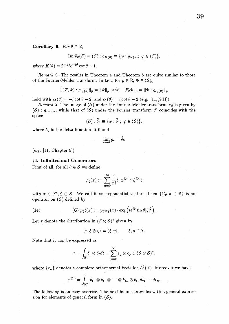
Corollary 6. For $\theta\in \mathbb{R}$,

${\rm Im}\Psi_{\theta}(S)=(S):gK(\theta)\equiv\{\varphi : gK(\theta);\varphi\in(S)\}$ ,

where $K(\theta)=2^{-1}ie^{-i\theta}\csc\theta-1$ .

Remark 2. The results in Theorem 4 and Theorem 5 are quite similar to thoseof the Fourier-Mehler transform. In fact, for $p\in \mathbb{R},$ $\Phi\in(S)_{p}$ ,

$||(\mathcal{F}_{\theta}\Phi)$ : $g_{c_{1}(\theta)}||_{p}=||\Phi||_{p}$ and $||\mathcal{F}_{\theta}\Phi||_{p}=||\Phi$ : $g_{c_{2}(\theta)}||_{p}$

hold with $c_{1}(\theta)=-i\cot\theta-2$ , and $c_{2}(\theta)=i\cot\theta-2$ (e.g. [11,\S 9.H]).Remark 3. The image of $(S)$ under the Fourier-Mehler transform $\mathcal{F}_{\theta}$ is given by

$(S)$ : $g_{i\cot\theta}$ , while that of $(S)$ under the Fourier transform $\mathcal{F}$ coincides with thespace

$(S)$ : $\tilde{\delta}_{0}\equiv\{\varphi : \tilde{\delta}_{0;}\varphi\in(S)\}$,

where $\tilde{\delta}_{0}$ is the delta function at $0$ and

$\lim_{carrow 0}g_{C}=\overline{\delta}0$

(e.g. [11, Chapter 9]).

\S 4. Infinitesimal GeneratorsFirst of all, for all $\theta\in S$ we define

$\varphi_{\xi}(_{X)}$ $:= \sum_{n=0}^{\infty}\frac{1}{n!}\langle:x^{\otimes n}:, \xi^{\otimes n}\rangle$

with $x\in S^{*},$ $\xi\in S$ . We call it an exponential vector. Then $\{G_{\theta}, \theta\in \mathbb{R}\}$ is anoperator on $(S)$ defined by

(14) $(G_{\theta}\varphi\xi)(x):=\varphi \mathrm{e}^{i\theta}\xi(X)\cdot\exp(i\mathrm{e}i\theta 2\sin\theta|\xi|)$ .

Let $\tau$ denote the distribution in $(S\otimes S)^{*}$ given by

$\langle\tau, \xi\otimes\eta\rangle=\langle\xi, \eta\rangle$ , $\xi,$ $\eta\in S$ .

Note that it can be expressed as

$\tau=\int_{\mathbb{R}}\delta_{t}\otimes\delta_{t}dt=\sum_{j=0}ej\otimes e_{j}\infty\in(S\otimes S)*$,

where $\{e_{n}\}$ denotes a complete orthonormal basis for $L^{2}(\mathbb{R})$ . Moreover we have

$\tau^{\otimes n}=\int_{\mathbb{R}^{n}}\delta_{t_{1}}\otimes\delta_{t_{1}}\otimes\cdots\otimes\delta_{t_{n}}\otimes\delta_{t_{n}}dt_{1}\cdots dtn$ .

The following is an easy exercise. The next lemma provides with a general expres-sion for elements of general form in $(S)$ .

39

Lemma 7. When $\varphi(x)=\sum_{n=0}^{\infty}\langle:X^{\otimes n} :, f_{n}\rangle\in(S)$ with $f_{n}\in\hat{S}(\mathbb{R}^{n})$ ,(the symmetric$S(\mathbb{R}^{n}))$, then $G_{\theta}\varphi i_{\mathit{8}}$ given by

$(c_{\theta\varphi})(X)= \sum_{n=0}\langle:x\infty\otimes n:, g_{n}\rangle$,

and

$g_{n} \equiv g_{n}(\varphi)=\sum^{\infty}\frac{(n+2m)!}{n!m!}m=0(i\sin\theta)^{m}ei(n+m)\theta\otimes m_{*f_{2}}\tau m+n$’

where for the element $f_{2m+n}$ in $\hat{s}(\mathbb{R}^{2m+n})$ the term $\tau^{\otimes m}*f_{2m+n}$ actually has thefollowing integral expression

$(\tau^{\otimes m_{*fn}}2m+)(t_{1}, \cdots, t_{n})$

$= \int_{\mathbb{R}^{m}}f_{2n}m+(S_{1}, s_{1}, \cdots, s_{m}, s_{m}, t_{1}, \cdots, t_{n})dS_{1}\cdots dS_{m}$ .

On this account, we obtain immediately

Proposition 8. The $Pseud_{\mathit{0}-}Fourier$-Mehler transform $\{\Psi_{\theta;}\theta\in \mathbb{R}\}$ is given by theadjoint operator of $\{G_{\theta;}\theta\in \mathbb{R}\},$ $i.e.$ ,

$\Psi_{\theta}=G_{\theta}^{*}$

holds in operator equality sense for all $\theta\in \mathbb{R}$ .

The next proposition gives an explicit action of the PFM transform $\Psi_{\theta}$ for thegeneralized white noise functionals of general form. It is due to a direct computa-tion.

Proposition 9. For $\Phi\in(S)^{*}$ given as $\Phi(x)=\sum_{n=0}^{\infty}$ $\langle: x^{\otimes n}:,F_{n}\rangle$ , it holds that

$\Psi_{\theta}\Phi(x)=n\sum^{\infty}\langle:X^{\otimes n}:,\sum_{+l2m=n}a(l=0’\otimes m, \theta)\cdot F_{l^{\wedge}}\tau\otimes m\rangle$ ,

where the constant $a(l, m, \theta)$ is given by

$a(l, m, \theta)=\frac{1}{m!}e^{i(lm)}+\theta(i\sin\theta)^{m}$ .

Remark 4. Similar results for Fourier-Mehler transform as the above can befound in [23]. For the proof of Proposition 9, it is almost the same as those givenin [23].

It follows from Proposition 3 that the $\mathrm{p}_{\mathrm{S}\mathrm{e}}\mathrm{u}\mathrm{d}_{0}-\mathrm{F}_{0}\mathrm{u}\mathrm{r}\mathrm{i}\mathrm{e}\mathrm{r}$-Mehler transform $\Psi_{\theta}$ isinjective and surjective. Moreover, it is easy to check that $\Psi_{\theta}$ is a strongly contin-uous operator from $(S)^{*}$ into itself, when we take Lemma 7 and Proposition 8 intoconsideration. Thus we have the following theorem.

40

Theorem 10 [5]. The $P_{Seu}d_{\mathit{0}-}Fourier$-Mehler transform $\Psi_{\theta}$ : $(S)^{*}arrow(S)^{*}$ is abijective and $\mathit{8}trongly$ continuous linear operator.

Theorem 11 [5]. The set $\{\Psi_{\theta;}\theta\in \mathbb{R}\}$ forms $a$ one parameter group of stronglycontinuous linear operator acting on the space $(S)^{*}$ of Hida distributions.

Proof. For $\Phi\in(S)^{*},$ $\xi\in S$ , and any $\theta,$ $\eta\in \mathbb{R}$ , from (7) of Definition 1 we have

(15) $S( \Psi_{\theta+\eta}\Phi)(\xi)=\langle\langle\Phi, \exp\{\mathrm{e}^{i(\theta}+\eta)\langle\cdot, \xi\rangle-\frac{1}{2}|\xi|^{2}\}\rangle\rangle$ .

While, from (6)

(16)$S(\Psi_{\theta}(\Psi_{\eta}))(\xi)=S(\Psi_{\eta}\Phi)(\mathrm{e}^{i\theta}\xi)\cdot\exp(i\mathrm{e}\sin\theta|\xi|i\theta 2)$

$=F(\mathrm{e}^{i\eta}(\mathrm{e}^{i}\theta\xi)),$ $\exp(i\mathrm{e}\sin\eta|\mathrm{e}^{i}\xi\theta|2i\eta)\cdot\exp(i\mathrm{e}^{i\theta}\sin\theta|\xi|^{2})$

$=\mathrm{e}^{-\frac{1}{2}}|\mathrm{e}^{i(e+}\eta)\xi|^{2}\langle\langle\Phi, \mathrm{e}^{\langle\cdot,\mathrm{e}^{(\theta+}\xi\rangle}i\eta)\rangle\rangle\cdot\exp\{i\mathrm{e}^{i\theta}(\mathrm{e}^{i(\theta+\eta}\mathrm{s}\mathrm{i})\mathrm{n}\eta+\sin\theta)|\xi|^{2}\}$

$= \langle\langle\Phi, \exp\{\mathrm{e}^{i}\langle(\theta+\eta)., \xi\rangle-\frac{1}{2}|\xi|^{2}\}\rangle\rangle$ ,

with the $\mathrm{U}$-functional $F$ of $\Phi$ . By comparing (15) with (16), we get

$S(\Psi_{\theta}+\eta\Phi)(\xi)=S(\Psi\theta\Psi\eta\Phi)(\xi)$ .

Consequently, the characterization theorem leads to

$\Psi_{\theta+\eta\eta}\Phi=\Psi_{\theta}\cdot\Psi\Phi$, $\Phi\in(S)^{*}$ ,

which completes the proof. $\square$

We are now in a position to state one of the principal results in this paper. Thisis a very important property of the Pseudo-Fourier-Mehler transform, especially onan applicational basis.

Theorem 12 [5]. The infinitesimal generator of $\{\Psi_{\theta;}\theta\in \mathbb{R}\}$ is given by $i(N+\Delta_{G}^{*})$ ,where $N$ is the number operator and $\Delta_{G}^{*}$ is the adjoint of the $Gro\mathit{8}S$ Laplacian $\Delta_{G}$ .

Remark 5. It is well known that the infinitesimal generator of the Fourier-Mehlertransforms $\{\mathcal{F}_{\theta;}\theta\in \mathbb{R}\}$ is $iN+ \frac{i}{2}\Delta_{G}^{*}$ , while the adjoint operator of $\{\mathcal{F}_{\theta;}\theta\in \mathbb{R}\}$ has$iN+ \frac{i}{2}\Delta_{G}$ as its infinitesimal generator (e.g. see [11]). The proof of Theorem 12 isalmost similsr to the above ones.

Proof of Theorem 12. First of all we set

$F_{\theta}(\xi):=S(\Psi_{\theta}\Phi)(\xi)$ and $F_{0}(\xi):=s(\Phi)(\xi)$

for $\Phi\in(S)^{*},$ $\xi\in S$ , paying attention to (i) of Proposition 2. From (6) we have$F_{\theta}(\xi)=F_{0}(\mathrm{e}^{i\theta})\cdot\exp[i\mathrm{e}^{i\theta}\sin\theta|\xi|^{2}]$. Since $F_{0}$ is Fr\’echet differentiable, the functional

41

$F_{\theta}(\xi)$ is differentiable in $\theta$ as well, and it is easy to check that

(17) $\lim_{\thetaarrow 0}\frac{1}{\theta}\{F\theta(\xi)-F0(\xi)\}$

$=\langle F_{0}’(\mathrm{e}^{i}\xi\theta), i\mathrm{e}i\theta\rangle\cdot\exp(i\mathrm{e}\theta i\mathrm{i}\mathrm{s}\mathrm{n}\theta|\xi|2)|_{\theta=0}$

$+F_{0}( \mathrm{e}^{i\theta}\xi)\cdot\frac{d}{dt}\exp(i\mathrm{e}^{i\theta}\sin\theta|\xi|2)|_{\theta=0}$

$=i\langle F’(\xi), \xi\rangle+i|\xi|^{2}\cdot F(\xi)$ .

While, we can easily check that the $\mathrm{U}$-functional $\theta^{-1}\cdot\{F_{\theta}(\xi)-F_{0}(\xi)\},$ $\theta\in \mathbb{R}$

satisfies the uniform bounded criterion: $\exists C_{0}>0$ so that

$\sup_{z\in \mathbb{C}}|\frac{1}{\theta}\{\tilde{F}_{\theta}(Z\xi)-\tilde{F}_{0}(_{Z}\xi)\}|\leq C_{0}\exp(c_{1}R^{C}2|\xi|_{p}^{2})$

$|z|=R$

holds for all $R>0$ , all $\xi\in S$ with $c_{1}>0,$ $c_{2}>0$ , where $\tilde{F}_{*}$ denotes an entireanalytic extension of $F$ . Hence, the strong convergence criterion theorem [25] (seealso [11, Chapter 4] $)$ allows convergence of

$S^{-1}( \frac{1}{\theta}\{F_{\theta}(\cdot)-F_{0}(\cdot)\})(X)=\frac{1}{\theta}\{\Psi_{\theta}\Phi(_{X})-\Phi(x)\}$

in $(S)^{*}$ as $\theta$ tends to zero. We need the following two lemmas.

Lemma 13. (cf. [11, Theorem 6.11,p.196]) Let $F(\xi)=s\Phi(\xi),\xi\in S$ for $\Phi\in(S)^{*}$ .Then(i) $F$ is Fr\’echet differentiable;(ii) the $S$-transform of $N\Phi(x)$ is given by $\langle F’(\xi), \xi\rangle,$ $\xi\in S$ ;where $N$ is the number operator.

Lemma 14. (cf. [11, Theorem 6.20,p.206]) For any $\Phi$ in $(S)^{*}$ , the $S$-transform of$\Delta_{G}^{*}\Phi(x)$ is given by $|\xi|^{2}S\Phi(\xi),$ $\xi\in S$ .

We may deduce at once that

(18) $S(N\Phi+\Delta^{*}G)\Phi(\xi)=\langle F’(\xi), \xi\rangle+|\xi|^{2}F(\xi)$ , $\xi\in S$ ,

with simple applications of Lemma 13 and Lemma 14. Moreover, it is easily verifiedfrom (17) and (18) together with the above-mentioned convergence result that

$\lim_{\thetaarrow 0}\frac{1}{\theta}(\Psi_{\theta}-Id)\Phi(x)=\theta\lim s^{-1}arrow 0(\frac{1}{\theta}\{F_{\theta}(\cdot)-F_{0}(\cdot)\})(X)$

$=S^{-1}(i\langle F’(\xi), \xi\rangle+i|\xi|2. F(\xi))$

$=i(N+\Delta^{*}G)\Phi(x)$ , in $(S)^{*}$ ,

which completes the proof. $\square$

42

\S 5. Application of PFM Transform

The purpose of this section is to show a typical example of application of thePseudo-Fourier-Mehler transform $\Psi_{\theta}$ to the Cauchy problem.

Example 6. (A simple application of the PFM transform) Let us consider thefollowing abstract Cauchy problem on the white noise space:

(19) $\frac{\partial u(t,X)}{\partial t}=iNu(t, X)+\varphi(x)$ ,

$u(0, \cdot)=f(\cdot)\in(S)$ ,

with $t>0$ , where $N$ denotes the number operator. One of the most remarkablebenefits of white noise analysis consists in its application to differential equationtheory and how to solve the problem (cf. [1], [2,3], [4,8]). Especially in $[4,8]$ , byresorting to the analogy in the finite dimensional cases we have applied the infinitedimensional Kuo type Fourier transform to the Cauchy problem for heat equationtype with Gross Laplacian, and have succeeded in derivation of the general solutionand also in direct verification for existence and uniqueness of the solution. On thisaccount, we think of using the Fourier transform to the aforementioned problem.Recall the formula:

(20) $\mathcal{F}(N\Phi)=N(\mathcal{F}\Phi)+\Delta_{G}^{*}(\mathcal{F}\Phi)$, for all $\Phi\in(S)^{*}$ .

We set $v(t, y)\equiv(\mathcal{F}u(t, \cdot))(y)$ for each $t\in \mathbb{R}_{+}$ . We may employ the Fourier trans-form $\mathcal{F}$ for (19) so as to obtain

(21) $\frac{\partial v(t,y)}{\partial t}=iNv(t, y)+i\Delta_{G}^{*}v(t, y)+\hat{\varphi}(y)$,

with $v(\mathrm{O}, y)=\hat{f}(y)$ ,

because we made use of the formula (20) and set $\hat{F}=\mathcal{F}F$ . The operator part of theFourier transformed problem (21) is exactly equivalent to the infinitesimal generatorof PFM transform with parameter $t$ (see Theorem 12). Hence, the semigroup theoryin functional equation theory allows immediately the following explicit exression ofthe solution in question:

(22) $v(t, y)= \Psi t\hat{f}(y)+\int_{0}^{t}\Psi_{t-S}\hat{\varphi}(y)dS$ .

We can show the existence and uniqueness of the solution by applying Theorem 4and Theorem 5 to (22) under a certain condition on the initial data $\varphi,$ $f$ . In thatcase the integral term appearing in (22) should be interpreted as Bochner type one.So much for the Cauchy problem, because this is not our main topic in this article.We shall go back to the PFM transform and proceed further in the next section.

43

\S 6. Intertwining Properties

In this section we shall investigate some intertwining properties between the Pseudo-Fourier-Mehler transform $\Psi_{\theta}$ and other typical operators in white noise analysis,such as G\^ateaux differential, the adjoint of G\^ateaux differential, Hida differentialoperator, and Kubo operator (the adjoint of Hida differential), etc. Furthermore,we shall introduce the characterization theorem for PFM transforms, which is oneof our main results in this paper.

We begin with definition of the G\^ateaux differential $D_{y}$ in the direction $y\in S^{*}$ .For $y\in S^{*}$ fixed, for the element $\varphi$ in $(S)$ given by $\varphi(x)=\sum_{n=0}^{\infty}$ $\langle$ : $x^{\otimes n}$ :, $f_{n}\rangle$ , weput

(23) $D_{y} \varphi(x)=\lim_{\thetaarrow 0}\frac{\varphi(x+\theta y)-\varphi(X)}{\theta}$ , $x\in S^{*}$ .

The limit existence in the right hand side of (23) is always guaranteed, and $D_{y}\varphi(x)$

is actually given by

(24) $D_{y} \varphi(x)=\sum_{n=0}^{\infty}n\langle:X\otimes(n-1):, y\otimes_{1}f_{n}\wedge\rangle$ , $x\in S^{*}$ .

In fact, $D_{y}$ becomes a continuous linear operator from $(S)$ into itself. Since theDirac delta function $\delta_{t}$ lies in $S^{*}$ , adoption of $\delta_{t}$ instead of $y$ does make sense inthe above (23) and (24). On the other hand, the Hida differential operator $\partial_{t}(=$

$\partial/\partial x(t))$ is originally proposed by T. Hida [9] and defined by

$\partial_{t}:=s^{-1}s\underline{\delta}$ , $\xi\in S$

$\delta\xi(t)$

(cf. [15]; see also [7]). It is well known that the action of $\partial_{t}$ is equivalent to that of$D_{\delta_{t}}$ on the dense domain [11] (or $[7],[14]$ ). So we can define

$\partial_{t}=D_{\delta_{t}}$ , $t\in \mathbb{R}$ .

The Kubo operator $\partial_{t}^{*}[15]$ is the adjoint of Hida differential $\partial_{t}$ , defined by

$\langle\langle\partial_{t}^{*}\Phi, \varphi\rangle\rangle=\langle\langle\Phi, \partial_{t\varphi\rangle}\rangle$,

for $\Phi\in(S)^{*},$ $\varphi\in(S)$ . As a matter of fact, $\partial_{t}$ (resp. $\partial_{t}^{*}$ ) can be considered as acontinuous linear operator from $(S)$ (resp. $(S)^{*}$ ) into itself with respect to the weakor strong topology. More precisely, the Hida differential proves to be a continuousmapping from $(s)_{P+q}$ into $(S)_{q}$ for $q> \frac{1}{4},$ $p\geq 0$ , while the Kubo operator turnsout to be the one from $(S)_{-p}$ into $(S)_{-(p+q})$ for the same pair $p,$ $q$ as given above.For $\xi\in S,$ $\varphi\in(S)$ , the derivative $(D_{\xi\varphi})(X)$ is defined in the usual manner, andthere exists its extension $\tilde{D}_{\xi}$ : $(S)^{*}arrow(S)^{*}$ . Even for that, we shall henceforth usethe same notation $D_{\xi}$ for brevity, as far as there is no confusion in the context. Weset $q_{\xi}:=i(D_{\xi}+D_{\xi}^{*})$ , where $D_{\xi}^{*}$ is the adjoint of $D_{\xi}$ .

44

Lemma 15. For each $\theta\in \mathbb{R},$ $t\in \mathbb{R}$ ,

$\Psi_{\theta}(\partial_{t}^{*}\Phi)=e^{i\theta*}\partial_{t}(\Psi\theta\Phi)$

holds for all $\Phi\in(S)^{*}$ .Proof. First of all, note that $S(\partial_{t}*\Phi)(\xi)=\xi(t).S(\Phi)(\xi)$ . So, for the generalized

white noise functional $\Phi\in(S)^{*}$ given in the form $\Phi(x)=\sum_{n=0}^{\infty}$ $\langle$ : $x^{\otimes n}$ :, $f_{n}\rangle,$ $x\in$

$S^{*}$ we readily get

(25) $S( \Psi_{\theta}(\partial_{t}^{*}\Phi))(\xi)=\mathrm{e}^{i\theta}\xi(t)\cdot\sum_{=n0}^{\infty}\langle f_{n}, \mathrm{e}^{i\theta n}n\xi^{\otimes}\rangle\cdot\exp(i\mathrm{e}^{i\theta}\sin\theta|\xi|^{2})$ .

While we establish

(26) $S(\Psi_{\theta}(\partial_{t}^{*}\Phi))(\xi)=\mathrm{e}si\theta(\partial_{t}^{*}(\Psi\theta\Phi))(\xi)$

by applying (25), because we made use of the relation

$S(\partial_{t}^{*}(\Psi_{\theta}\Phi))(\xi)=\xi(t)\cdot(S\Phi)(\mathrm{e}^{i\theta}\xi)\cdot\exp(i\mathrm{e}\sin i\theta\theta|\xi|^{2})$ .

An application of the Potthoff-Streit characterization theorem (Theorem 1) to (26)leads to the required equality in Hida distribution sense. $\square$

Proposition 16. For each $\theta\in \mathbb{R},$ $t\in \mathbb{R}$

(i) $\Psi_{\theta}(\partial_{t}\Phi)=e^{-i\theta}\partial_{t}(\Psi_{\theta}\Phi)-2i\sin\theta\partial*(t\Phi\Psi_{\theta})$;(ii) $\Psi_{\theta}(x(t)\Phi)=e^{-i\theta}X(t)(\Psi_{\theta}\Phi)_{f}$ .

hold for all $\Phi\in(S)^{*}$ .

Remark 7. The assertion (i) of Proposition 16 follows from a direct $\mathrm{c}$.omputation.We have only to employ the following two rules:

$S \partial_{t}(\cdot)=\frac{\delta}{\delta\xi(t)}S(\cdot)$ , $\partial_{t}^{*}(\cdot)=s^{-}1\xi(t)S(\cdot)$ .

The second assertion (ii) is also due to a simple computation together with thefirst assertion (i) and Lemma 15. Moreover, we need to apply the multiplicationoperator: $x(t)(\cdot)=(\partial_{t}+\partial_{t}^{*})(\cdot)$ (e.g. [19]). Those proofs go almost similarly as inthe proof of Lemma 15 and are very easy, hence omitted.

The next proposition indicates some intertwining property between the PFMtransform and G\^ateaux differential operator.

Proposition 17. For each parameter $\theta\in \mathbb{R},t\in \mathbb{R}$

(i) $e^{-i\theta}\tilde{D}_{\xi(\Phi)}\Psi_{\theta}=\Psi_{\theta}(\tilde{D}_{\xi}\Phi)+2i\sin\theta\cdot D^{*}(\xi\Psi\theta\Phi)$;

(ii) $\tilde{D}_{\xi}(\Psi_{\theta}\Phi)+D_{\xi}^{*}(\Psi\theta\Phi)=e^{i\theta}\Psi_{\theta}(\overline{\langle\cdot,\xi}\rangle\Phi)_{i}$

hold for all generalized white noise functionals in $(S)^{*}$ .

Proof. It is interesting to note that G\^ateaux differential $D_{\xi}$ and its adjoint $D_{\xi}^{*}$

enjoy the integral kernel operator theoretical expressions in white noise analysis(see the next section; or [11,12], [23]). Namely,

(27) $\tilde{D}_{\xi}:=(\int_{\mathbb{R}}\xi(t)\partial tdt)^{\sim}$ , and $D_{\xi}^{*}:= \int_{\mathbb{R}}\xi(t)\partial_{t}*dt$ , $\forall\xi\in S$ .

45

Let $\Delta=\{t_{k}\}$ be a proper finite partition of the $t$ parameter space, and $|\Delta|$ denotesthe maximum of increment $\triangle t_{k}$ over $1\leq k\leq m$ . The assertion (i) yields from (i)of Proposition 16. In fact, by linearity of the PFM transform we get

(28) $\sum_{k=1}^{m}\triangle t_{k}\xi(t_{k})\cdot\Psi_{\theta(\partial_{t_{k}}}\Phi)=\Psi_{\theta}(_{k}\sum_{=1}^{m}\xi(tk)\partial_{t_{k}}\triangle t_{k}\cdot\Phi)$ ,

for $\forall\xi\in S$ . Consider the same type finite summation for the other terms in (i) ofProposition 16. By taking the limit $marrow\infty$ and by continuity of $\Psi_{\theta}$ (Theorem 10),we can obtain the desired result with consideration of $\mathrm{E}\mathrm{q}.(27)$ .As to (ii), note first that we can have the expression

(29) $\tilde{q}_{\xi}=i\overline{\langle x,\xi\rangle}=(i\int_{\mathbb{R}}x(t)\xi(t)dt)^{\sim}$ ,

by virtue of the multiplication operator $x(t)(\cdot)$ (cf. Remark 7). With (ii) of Propo-sition 16, we may take advantage of continuity of $\Psi_{\theta}$ and (29) to deduce that

$\mathrm{e}^{-i\theta}(D_{\xi}+D_{\xi}^{*})(\Psi_{\theta}\Phi)=\mathrm{e}^{-i\theta}(\int_{\mathbb{R}}x(t)\xi(t)dt)(\Psi_{\theta}\Phi)$

$= \lim_{marrow\infty}\Psi_{\theta}(_{k=0}\sum^{m}\triangle tk\xi(t_{k})x(t_{k})\cdot\Phi)$

$=\Psi_{\theta}(\langle_{X}, \xi\rangle\cdot\Phi)$

by passage to the limit $|\triangle|arrow 0$ . $\square$

The following theorem gives the characterization for $\mathrm{p}\mathrm{s}\mathrm{e}\mathrm{u}\mathrm{d}\mathrm{o}- \mathrm{F}_{\mathrm{o}\mathrm{u}\mathrm{r}\mathrm{i}}\mathrm{e}\mathrm{r}$-Mehlertransforms $\{\Psi_{\theta;}\theta\in \mathbb{R}\}$ , which is one of our main results in this paper.

Theorem 18 [6]. The $Pseudo-F_{ouri}er$-Mehler transform $\{\Psi_{\theta;}\theta\in \mathbb{R}\}$ satisfies thefollowing conditions:$(Pl)\Psi_{\theta}$ : $(S)^{*}arrow(S)^{*}$ is a continuous linear operator for $f_{ora}ll\theta\in \mathbb{R}_{f}$

.$(P\mathit{2})\Psi_{\theta}(\tilde{D}_{\xi}\Phi)=e^{i\theta}\overline{D}_{\xi(\Phi}\Psi_{\theta})-2\sin\theta\cdot\tilde{q}\xi(\Psi\theta\Phi)_{j}$

$(P\mathit{3})\Psi_{\theta}(\tilde{q}\epsilon\Phi)=e^{-}\tilde{q}_{\xi}(i\theta\Psi_{\theta}\Phi)f$ .

where $\Phi\in(S)^{*},$ $\xi\in S.$ Conversely, if a continuous linear operator $A_{\theta}$ : $(S)^{*}arrow$

$(S)^{*}$ satisfies the above conditions: $(P\mathit{1})\sim.(P\mathit{3})_{f}$ then $A_{\theta}$ is a constant multiple of$\Psi_{\theta}$ .

Proof. (P1) is obvious (Theorem 10). $(\mathrm{P}2)$ ( $\mathrm{r}\mathrm{e}\mathrm{s}_{\mathrm{P}}$ . (P3)) yields from $(\mathrm{i})(\mathrm{r}\mathrm{e}\mathrm{s}_{\mathrm{P}}. (\mathrm{i}\mathrm{i}))$

of Proposition 17. It is due to a simple computation. Conversely, suppose that theoperator $A_{\theta}$ be compatible with $(\mathrm{P}1),(\mathrm{P}2)$ and (P3). We need the following results.

Lemma 19. We assume that $A_{\theta}$ be a continuous linear operator from $(S)^{*}$ intoitself, satisfying the three conditions $(P\mathit{1})\sim(P\mathit{3})$ . Then the following relations(i) $(\Psi_{\theta}-1---\theta)D\xi=D\xi(\Psi_{\theta}-1_{-}-_{\theta})-$ ;(ii) $(\Psi_{\theta}^{-1_{-}-}--_{\theta})q\epsilon=q\xi(\Psi 1_{-}-)_{\rangle}\theta-\theta$ .(iii) $(\Psi_{\theta}^{-1_{-}}--\theta)D_{\xi}*=D_{\xi}^{*}(\Psi_{\theta}-1--_{\theta}-)$ ;hold for all $\xi\in S,$ $\theta\in \mathbb{R}$ .

The proof will be given below. The next theorem is well known (e.g. [12,Theorem 3.6, p.267] or [23, Prop.5.7.6, p.148] $)$ .

46

Theorem 20. Let A be a continuous linear operator on $(S)^{*}$ , satisfying(i) $\Lambda\tilde{q}_{\xi}=\tilde{q}_{\xi}\Lambda$ , for any $\xi\in S$ ;(ii) $\Lambda D_{\xi}^{*}=D_{\xi}^{*}\Lambda$ , for any $\xi\in S$ .Then the operator A is a scalar operator.

Thus, by taking $(\mathrm{i}\mathrm{i}),(\mathrm{i}\mathrm{i}\mathrm{i})$ of Lemma 19 into account, we may apply Theorem 20for $A_{\theta}$ to obtain the assertion: $\Psi_{\theta}^{-1}A_{\theta}$ is a scalar operator. $\square$

Proof of Lemma 19. Basically it is due to a direct computation. Each proof goessimilarly, so we shall show only (iii) below. For the other two we will give justrough instructions. First of all, note that we have only to consider $\Psi_{-\theta}$ instead of$\Psi_{\theta}^{-1}$ by virtue of Proposition 3. As to (i), it is sufficient to calculate it with (P2)for both and (P3) for the PFM transform. As for $(,\mathrm{i}\mathrm{i})$ , simply (P3) for both $A_{\theta}$ and$\Psi_{\theta}$ . As to (iii), for $\forall\Phi\in(S)^{*},$ $\forall\xi\in S$

(30) $(\Psi_{\theta}^{-}1A_{\theta})D^{*}\Phi\xi=-i\Psi_{\theta}-1(A_{\theta q}\xi)\Phi-\Psi_{\theta}-1(A\theta D_{\xi})\Phi$,$=-\mathrm{e}^{i\theta}(\Psi_{\theta}^{-1}q_{\xi})A_{\theta}\Phi-\mathrm{e}(i\theta\Psi D\xi)\theta^{-1}A\theta\Phi$

because we used a relation

(31) $D_{\xi}^{*}=-i\tilde{q}_{\xi}-\tilde{D}_{\xi}$

in the first equality and also employed $(\mathrm{P}2),(\mathrm{P}3)$ in the second one. An applicationof $(\mathrm{P}2),(\mathrm{P}3)$ to the last expression in (30), together with (31) again, gives

(30) $=-iq\xi(\Psi_{\theta}^{-1}A\theta)\Phi-D_{\xi(}\Psi_{\theta}^{-}1A_{\theta})\Phi$

$=(-iq\xi-D_{\xi})(\Psi_{\theta}^{-1}A\theta)\Phi=D\xi*(\Psi^{-}1A\theta)\theta\Phi$ ,

which completes the proof. $\square$

47

\S 7. Fock ExpansionLet $\mathcal{L}((S), (S)^{*})$ denote the space of continuous linear operators from $(S)$ into $(S)^{*}$ .The space $\hat{S}_{l,m}’(\mathbb{R}l+m)$ is a symmtrized space of $S’(\mathbb{R}^{lm}+)$ with respect to the first $l$ ,and the second $m$ variables independently. By virtue of the symbol characterizationtheorem for operators on white noise functionals [21](see also [23]), for the operatorII lying in $\mathcal{L}((S), (S)^{*})$ there exists uniquely a kernel distribution $\kappa_{l,m}$ in $\hat{S}_{l,m}’(\mathbb{R}^{l+}m)$

such that the operator $\Pi$ may have the Fock expansion:

$\square =\sum_{l,m=0}^{\infty}\Gamma \mathrm{I}_{l},(ml,m)\kappa$ .

Moreover, the series $\Pi\varphi,$ $\varphi\in(S)$ converges in $(S)^{*}[21]$ . Generally, each componentII$l,m$ of the Fock expansion has a formal integral expression:

$\Pi_{l,m}(\kappa)=\int_{\mathbb{R}^{l+m}}\kappa(S_{1}, \cdots, s_{l}, t_{1}, \cdots, t_{m})$ .

. $\partial_{s_{1}s_{\iota}t_{1}}^{*}..,$$\partial^{*}\partial\cdots\partial_{t_{m}}dS_{1}\cdots dSldt1\ldots dt_{m}$ .

Remark 8. We call it an integral kernel operator with kernel distribution $\kappa$ . Thetheory of integral kernel operators and the general expansion theory in white noiseanalysis were proposed and have been developed enthusiastically by N. Obata [21-23] (see also [11]). Those topics are closely related to quantum stochastic calculus,which has been greatly investigated in chief by Hudson, Meyer, and Parthasarathy.More details on this topic will be found in, for instance, (i) $\mathrm{K}.\mathrm{R}$ .Parthasarathy:An Introduction to Quantum Stochastic Calculus, Birkh\"auser, Basel, 1992; (ii)$\mathrm{P}.\mathrm{A}$ .Meyer: Quantum Probability for Probabilists, Lecture Notes in MathematicsVol.1538, Springer-Verlag, Heidelberg, 1993.

We shall give below two typical examples of the integral kernel operators in whitenoise analysis.

Example 9. (The number operator $N$ ) Let $\tau\in(S\otimes S)^{*}$ be the trace operatordefined by

$\langle\tau, \xi\otimes\eta\rangle=\langle\xi, \eta\rangle$ , $\xi,$ $\eta\in S$ .

The number operator $N$ is usually expressed as

$\int_{\mathbb{R}}\partial_{t}*\partial_{t}dt$

by Kuo’s notation in white noise analysis. By the Obata theory, $N$ has the followingrepresentation as a continuous linear operator from $(S)$ into itself, namely,

$N= \Pi_{1,1}(\tau)=\int_{\mathbb{R}^{2}}\tau(S, t)\partial^{*}\partial tdsdtS^{\cdot}$

Example 10. (The Gross Laplacian $\Delta_{G}$ ) By the usual notation in white noiseanalysis we have the expression

$\Delta_{G}=\int_{\mathbb{R}}\partial_{t}^{2}dt$ .

48

Then the Gross Laplacian $\Delta_{G}$ can be also expressed by

$\Delta_{G}=\Pi_{0,2}(_{\mathcal{T}})=\int_{\mathbb{R}^{2}}\tau(s_{1}, S2)\partial_{s}\partial_{s_{2}}dS1dS_{2}1$

as a continuous linear operator from $(S)$ into $(S)$ .Let us consider the general expansion of our Pseudo-Fourier-Mehler transform.

We may take advantage of Obata’s integral kernel operator theory in order to obtainFock expansion representations of $\Psi_{\theta}$ and its adjoint $G_{\theta}$ . That is to say,

Theorem 21. For $\theta\in \mathbb{R}$ , the $PFM$ transform $\Psi_{\theta}$ and the adjoint operator $G_{\theta}$ havethe following Fock $expansi_{\mathit{0}}n\mathit{8}$ :

(i) $\Psi_{\theta}=\sum_{=l,,m0}^{\infty}\frac{1}{l!m!}(ie\sin\theta)i\theta l(e-i\theta 1)^{m}\cdot\Pi 2l+m,m(\tau^{\otimes l}\otimes\lambda_{m})$ ;

(ii) $G_{\theta}= \sum_{=l,,m0}^{\infty}\frac{1}{l!m!}(ie\sin\theta i\theta)m(e-i\theta 1)^{l}\cdot \mathrm{I}\mathrm{I}_{l,l}+2m(\lambda l^{\otimes}\mathcal{T}\otimes m)$ ;

where the kernel $\lambda_{m}\in(S^{\otimes 2m})^{*}i_{\mathit{8}}$ given by

$\lambda_{m}.\cdot:=,.\sum_{m}^{\infty}e_{i_{1}}i_{1}.i_{2},\cdots,i=0\otimes\cdots\otimes e_{i_{m}}\otimes e_{i_{1}}\otimes\cdots\otimes e_{i_{m}}$.

\S 8. GeneralizationLet $GL((S))$ be the group of all linear homeomorphisms from $(S)$ into $(S)$ . Thenwe have

Proposition 22. $\{G_{\theta;}\theta\in \mathbb{R}\}$ is a regular one para.meter sub.group of $GL((S))$ with$infinite\mathit{8}imal$ generator $i(N+\Delta_{G})$ .

Let us consider some generalization. Suggested by [1], for example we proposeto define the generalized PFM transform $X_{\theta},$ $\theta\in \mathbb{R}$ as operator on $(S)^{*}$ whose$\mathrm{U}$-functional is given by

(32) $S(X_{\theta} \Phi)(\xi)=\langle\langle\Phi, \exp(\mathrm{e}\langle\alpha\theta., \xi\rangle-\frac{1}{2}J(\alpha, \beta;\theta)|\xi|2)\rangle\rangle$,

(cf. Eq. (7) in Definition 1 of PFM transform), for $\xi\in S,$ $\Phi\in(S)^{*}$ . We set

$J(\alpha, \beta;\theta)=\mathrm{e}^{2}-\alpha\theta 2H(\alpha, \beta;\theta)$ ,

with $H(\alpha, \beta;\theta)=h(\alpha, \beta)\cdot(\mathrm{e}^{2\alpha\theta}-1)$ ,

where $h(\alpha, \beta)=\beta/2\alpha$ , for $\alpha,$ $\beta\in \mathbb{C},$ $\alpha\neq 0$ . Then we denote the adjoint operatorof $X_{\theta}$ by $Z_{\theta}$ .

Claim 23. The set $\{Z_{\theta;}\theta\in \mathbb{R}\}$ is a regular one parameter subgroup of $GL((S))$ .

49

Claim 24. The infinitesimal generator of $\{z_{\theta;}\theta\in \mathbb{R}\}$ is given by the operator $\alpha N$

$+\beta\Delta_{G}$ .Claim 25. The generalized $PFM$ transform $\{X_{\theta;}\theta\in \mathbb{R}\}$ is $a$ one parameter sub-group of $GL((S)^{*})$ .

Claim 26. The infinitesimal generator of $\{X_{\theta;}\theta\in \mathbb{R}\}$ is given by the operator $\alpha N$

$+\beta\Delta_{G}^{*}$ .

Remark 11. The above definition (32) of generalized PFM transform $X_{\theta}$ can bealternatively replaced by the following expression:

$S(X_{\theta}\Phi)(\xi)=F(\mathrm{e}\xi\alpha\theta)\cdot\exp(H(\alpha, \beta;\theta)\cdot|\xi|^{2})$ ,

where $F$ denotes the $\mathrm{U}$-functional of $\Phi$ in $(S)^{*}$ , i.e., $S\Phi=F$ .

Remark 12. Especially when $\alpha=\beta=i(\in \mathbb{C})$ , then the above-defined generalizedPFM transforms $X_{\theta}$ are, of course, attributed to the simple PFM transforms $\Psi_{\theta}$

given by (6), (7) in the section 3.

Acknowledgements. The author wishes to express his sincere gratitude to Pro-fessor I. Kubo, Professor N. Obata and Professor $\mathrm{D}.\mathrm{M}$ . Chung for their kind sug-gestions and many useful comments and discussions. The author is also gratefulfor the hospitality of RIMS, Kyoto University during March 29-31, 1995, Inter-national Institute for Advanced Studies (IIAS, Kyoto) during May 27-30, 1995,National University of Singapore ( $23\mathrm{r}\mathrm{d}$ SPA Conference) during June 19-23, 1995,and Training Institute of Meiji MLIC (Japan-Russia Symposium) during July 26-30, 1995. The results on PFM transform and its generalization under fully generalsetting of white noise analysis will appear in our next paper.

REFERENCES

1. D.M.Chung and U.C.Ji, Groups of operator8 on white noise functionals and applications toCauchy problems in white noise analysis I,II, preprint, 1995.

2. I.D\^oku, Hida calculus and its application to a random equation, Proc. PIC on GaussianRandom Fields (Nagoya Univ.) P2 (1991), 1-19.

3. I.D\^oku, Hida calculus and a generalized stochastic differential equation on the white noisespace, J.Saitama Univ.Math.Nat.Sci. 43-2 (1994), 15-30.

4. I.D\^oku, Fourier transform in white noise calculu8 and its application to heat equation, Proc.Workshops on $\mathrm{S}\mathrm{P}\mathrm{D}\mathrm{E}/\mathrm{S}\mathrm{D}\mathrm{E}$ (3rd World Congress) (1994) (to appear).

5. I.D\^oku, Pseudo-Fourier-Mehler transform in white noise analysis and application of liftedconvergence to a certain approximate Cauchy problem, J.Saitama Univ.Math.Nat.Sci. 44-1(1995), 55-79.

6. I.D\^oku, On some properties of Pseudo-Fourier-Mehler transforms in white noise calculus,Collection of Contributed Lectures for the 23rd SPA Conference at National Singapore Univ.(June 19 -23) (1995), Singapore.

7. I.D\^oku, On the Laplacian on a space of white noise functional8, Tsukuba J.Math. 19 (1995),93-119.

8. I.D\^oku, H.-H. Kuo and Y.-J. Lee, Fourier transform and heat equation in white noise analysis,Pitman Research Notes in Math. 310 (1994), 60-74.

9. T.Hida, Analysis of Brownian functionals, Carleton Math.Lecture Notes 13 (1975), 1-83.10. T.Hida, Brownian Motion, Springer-Verlag, New York, 1980.

50

11. T.Hida, H.-H. Kuo, J.Potthoff and L.Streit, White Noise: An Infinite Dimensional Calculus,Kluwer, Dordrecht, 1993.

12. T.Hida, H.-H. Kuo and N.Obata, Transformations for white noise functionals, J.Funct.Anal.111 (1993), 259-277.

13. T.Hida, N.Obata and K.Sait\^o, Infinite dimensional rotation8 and Laplacians in terms of whitenoise calculus, Nagoya Math.J. 128 (1992), 65-93.

14. K.It\^o and T.Hida(eds.), GauS8ian Random Fields, World Scientific, Singapore, 1991.15. I.Kubo and S.Takenaka, Calculus on Gau8sian white noise I,II,III e;IV, Proc. Japan Acad.

$56\mathrm{A}(1980)$ , 376-380; 411-416; $57\mathrm{A}(1981)$ , 433-436; 58A (1982), 186-189.16. H.-H. Kuo, On Fourier transform of generalized Brownian functionals, J. Multivar. Anal. 12

(1982), 415-431.17. H.-H. Kuo, The Fourier transform in white $noi_{\mathit{8}}e$ calculus, J.Multivar.Anal. 31 (1989), 311-

327.18. H.-H. Kuo, Fourier-Mehler transform in white noise analysis, Gaussian Random Fields (Eds.

K.It\^o and T.Hida) (1990), World Scientific, 257-271.19. H.-H. Kuo, Lectures on white noise analysis, Soochow J.Math. 18 (1992), 229-300.20. N.Obata, Rotation invariant operators on white noise functionals, Math.Z. 210 (1992), 69-89.21. N.Obata, An analytic characterization of symbols of operators on white noise functionals,

J.Math.Soc. Japan 45 (1993), 421-445.22. N.Obata, Operator calculus on vector-valued white $noi_{\mathit{8}}e$ functionals, J. Funct. Anal. 121

(1994), 185-232.23. N.Obata, White Noise Calculus and Fock Space, LNM Vol.1577, Springer-Verlag, Berlin,

1994.24. N.Obata, Lie algebras containing infinite dimensional Laplacians, Oberwolfach Conference

on Probability Measures on Groups (1995) (to appear).25. J.Potthoff and L.Streit, A characterization of Hida distributions, J.Funct.Anal. 101 (1991),

212-229.

51