Electronic copy of this paper is available at: http://ssrn.com/abstract=891442

Incentives and Mutual Fund Performance:

Higher Performance or Just Higher Risk Taking?

Massimo Massa* Rajdeep Patgiri**

Abstract We study the impact of contractual incentives on the risk-taking behavior and the performance of US mutual funds. We measure incentives using the shape, i.e. concavity, of the fee structure in the advisory contract. Compared to the standard linear fee structure, a concave structure should create a disincentive to take more risk. Our results show that a high incentive contract induces managers to take more risk and reduces the funds’ probability of survival. On the other hand, high-incentive funds deliver higher return. The net of these two effects is that incentives increase the risk-adjusted performance of the fund. In particular, the top incentive quintile of funds outperforms the bottom incentive quintile by about 2.7 percent per year. Moreover, the performance of the high-incentive funds is highly persistent. High-incentive winner funds from one year have a positive alpha of 41 basis points per month in the following year. By focusing on the funds' holdings, we show that active portfolio rebalancing is the main channel through which incentives increase performance.

JEL Classification: G23, G30, G32

Keywords: mutual fund, incentive, risk taking, performance, persistence.

* Massimo Massa, Finance Department, INSEAD, Boulevard de Constance, 77300 Fontainebleau France, Tel: +33160724481, Fax: +33160724045 Email: massimo.massa@insead.edu. ** Rajdeep Patgiri, Finance Department, INSEAD, Boulevard de Constance, 77300 Fontainebleau France, Tel: +33160729229, Fax: +33160724045 Email: rajdeep.patgiri@insead.edu

Electronic copy of this paper is available at: http://ssrn.com/abstract=891442

1

“Perverse incentives for investment managers may help explain price of risky assets... Most investment managers are rewarded for generating “alpha”. But found it very difficult to do so... In practice most asset managers generated “poor man’s alpha” by taking on liquidity risk – holding illiquid assets to maturity.”

(R Rajan, Financial Times, 9 June 2006)

Agency theory claims that investors can alleviate some agency problems through high-incentive

contracts for managers. Such contracts would mean that managers’ pay-offs were more closely related

to their performance, which could increase managers’ efforts and thus lead to better performance. At

the same time, high-incentive contracts would also induce managers to take more risks. The net effect

is less clear. Indeed, if extra performance compensates only for the additional risk taken, high

incentives are not beneficial for the principal. In fact, it has been argued that higher incentives lead

managers to take excessive risks per unit of performance delivered.

This paper aims to contribute to the understanding of the role of incentives in managerial

performance. We focus on the mutual fund industry and test how incentives, as defined in the

advisory contract, affect performance. The mutual fund industry provides an ideal test setting, because

it allows regular observation of managers’ ex-ante incentive structures and actions, as well as many of

the other factors that may affect managerial choice.

We focus on US mutual funds, for which incentives in contracts are a function of fee rates,

which are based on the total assets managed by the funds. Two-thirds of funds have a fixed fee

structure, while the remaining funds have a concave fee structure, in which the percentage advisory

fee decreases as the total assets increase. In this paper, we postulate that incentives for fund managers

are related to the shape – that is, concavity – of the fee structure. Mutual funds with a concave fee

structure have a lower incentive to increase the assets under management than funds with a linear fee

structure. Hence, compared to the literature on incentive fees of mutual funds (Elton, Gruber and

Blake, 2003), concavity actually quantifies the disincentive to generate superior performance.

Agency theory posits that incentives increase risk taking. We therefore expect a positive

relation between incentives contained in contracts and fund risk taking. Moreover, incentives, by

2

increasing risk, also increase the possibility of large negative return shocks that may induce

liquidation of the fund, which reduces the probability that the fund will survive.

In terms of the net effect, if higher incentives only increase risk taking and reduce the

probability of survival, there should be no relation between performance and incentives after

controlling for risk. Superior performance would be explained entirely by higher risk taking and

would not persist. If, however, incentives improve managerial effort – for example, by increasing

collection of information, encouraging better techniques for constructing portfolios, or improving

technological infrastructure – there should be a positive relation between performance and incentives,

even after controlling for risk and survival. Moreover, according to conditioning on incentives,

performance should persist.

We find that incentives increase risk taking, which supports the theoretical predictions. An

increase of 1% in the incentives investors are willing to pay leads to an increase of nearly 1% in the

annual volatility of monthly fund returns. Moreover, incentives also impact the probability that funds

will survive. After controlling for prior-year risk and risk-adjusted return, higher incentive funds have

higher hazard rates and lower probabilities of survival. In economic terms, an increase in incentives of

1% increases the hazard rate by 8.46%. Equivalently, a 1% increase in incentives leads to a reduction

in survival probability of 2%.

What are the implications for investors in mutual funds? If incentives increase fund managers’

efforts, this should translate into higher risk-adjusted performance. We show that high-incentive funds

outperform low-incentive funds and that the superior performance cannot be explained only by higher

risk taking. Instead, superior performance relates to increases in managers’ efforts, and this makes

superior performance persistent.

The economic significance of the result is quite striking. Over our sample period, the portfolio

of funds with the highest incentive quintile outperforms the portfolio of funds with the lowest

incentive quintile by 23 basis points per month in terms of raw return and 22 basis points per month in

terms of risk-adjusted return. In a standard persistence test setting similar to that described by Carhart

(1997), we provide evidence that the performance of winner funds persists among the funds with the

highest incentives. The best performing funds of the prior year have a positive alpha of 41 basis points

3

per month in the following year. No analogous result exists for funds with the lowest incentives. In

fact, the difference in performance among the best performing funds of the prior year, separated into

high and low incentives, is a significant 71 basis points per month in the following year. The

difference in risk-adjusted performance remains robust even after controlling for survival probabilities

of the funds.

To investigate the channel through which incentives affect performance, we study a measure of

the “unobserved actions” of fund managers. On the basis of the funds’ holdings, this measure captures

the difference between the gross return of the fund and the return of a buy-and-hold strategy based on

the observable portfolio of the fund – the “return gap” (Kacperczyk et al., 2006). Higher incentives

improve performance by increasing the return gap. In particular, the risk-adjusted return gap of the

portfolio of high incentive funds is 13 basis points per month higher than the portfolio of low

incentive funds. However, there is no significant difference in the returns from a buy-and-hold

strategy based on the disclosed portfolio of the funds. This suggests that investors cannot earn

superior returns by mimicking the disclosed portfolios of high-incentive funds, which is public

information. Most superior performances are related to dynamic portfolio rebalancing by the

managers of funds with high-incentive contracts.

These findings make several contributions to the existing literature. First, they provide direct

evidence for the theory on executive compensation and particularly the relation between incentives

and risk taking. Jensen and Meckling (1976) and the corporate finance literature that followed show

that value-maximizing levered-equity holders prefer more asset volatility, even at the expense of firm

value. Grinblatt and Titman (1989) show that fund managers who hedge their incentive fees try to

maximize the value of the fees by increasing fund leverage as much as possible. In the case of risk-

averse managers, Guay (1999) shows that the convexity of the pay-off structure may be offset by the

concavity of the utility function. Ross (2004) shows that no type of incentive scheme can make all

expected utility maximizers willing to take on more risk. We contribute to this literature by providing

empirical evidence that high-incentive contracts do indeed increase performance and risk taking.

Second, our results quantify the role the type of compensation plays in the mutual fund

industry. This contributes to the strand of literature that studies the characteristics of advisory

4

contracts in the mutual fund industry. Deli (2002) used NSAR filings to look at differences in

advisory contracts offered to mutual funds and found that two types of contracts were prevalent in the

mutual fund industry – linear contracts and concave contracts. Kuhnen (2004) and Warner and Wu

(2004) use NSAR filings to analyze the determinants of changes in mutual fund contracts. Although

the absolute number of contract changes is very small, such changes benefit the investors. Almazan et

al. (2004) look at the constraints imposed on mutual fund managers in terms of trading restrictions.

We focus on the trade-off between performance and survival and show that the direct effect of

incentives on risk-adjusted performance has important policy implications. Indeed, the most recent

debate on mutual funds has concentrated on the cost of high compensation and greater incentives for

investors; however, few have been able to quantify directly the benefits of higher incentive

compensation.

Third, our results are relevant to literature that studies mutual fund performance and its

persistence. Hendricks et al. (1993), Goetzmann and Ibbotson (1994), Brown and Goetzmann (1995),

Carhart (1997), and Bollen and Busse (2005) show evidence of short-term persistence in the

performance of mutual funds.1 Traditionally, this performance was attributed to managerial skill.

However, Carhart (1997) shows that the momentum effect can explain all the observed persistence in

performance of the best funds, while Wermers (2000) explains the persistence through funds’

expenses but not through managerial ability. Only the set of worst-performing funds, even after

controlling for the Fama-French factors and momentum, still seems to have persistently bad

performance for up to three years after a year of bad performance.

More recently, the literature has shown new evidence of forecastability of mutual fund

performance. Mamaysky et al. (2005) show that the combined use of an ordinary least square (OLS)

and Kalman filter model increases the number of funds with predictable out-of-sample alphas by

about 60%, which provides evidence of persistence among fund performance. Kacperczyk et al.

(2006) use a new measure of performance based on unobserved actions of mutual funds – the return

gap – and show that it can predict future fund performance. Kosowski et al. (2006) find a sizable 1 Other papers in this literature include Grinblatt et al. (1995); Elton et al. (1996), Gruber (1996); Daniel et al. (1997); Nofsinger and Sias (1999); Wermers (1999); Grinblatt and Keloharju (2000) among others.

5

minority of fund managers have stock picking ability that offset their expenses and the performance of

these funds display persistence over time. Avramov and Wermers (2006) form an investment strategy

in mutual funds that incorporate predictability in manager skills, fund risk loadings and benchmark

returns. Our paper contributes to this literature by presenting novel evidence for the persistence of

mutual fund performance by conditioning on incentives.

The paper is structured as follows. Section I describes the data and construction of the variables.

Section II reports the main results. A brief conclusion follows in Section III.

I. Data and Main Variables

We use data collected from three sources: the US Securities and Exchange Commission (SEC)

electronic data gathering, analysis, and retrieval (EDGAR) database, the Center for Research in

Security Prices (CRSP) mutual fund monthly database, and the CDA/Spectrum mutual fund holdings

database. We focus on the information contained in the NSAR-B filings2 from 1996 to 2003. Apart

from the compensation contracts, we also collect information about the number of shareholder

accounts in the fund, the minimum investment required, and other relevant variables from the NSAR

filings. The NSAR dataset is then matched by fund name with the CRSP mutual fund monthly

database. As CRSP separately reports data for each class within a single fund, we first combine the

information from different classes of the same fund weighted by the total net assets (TNA) of the

class. We take observations only if the fund existed in the CRSP database in the same calendar year as

the NSAR-B filing. Mutual fund advisory contracts are changed rarely (Kuhnen, 2004; Warner and

Wu, 2004), so we interpolate the structure of the advisory contract for the years when we cannot

match the NSAR data to the CRSP database. For example, if matches for a fund are found in 1998 and

2000 but not 1999, we assume the contract to be the same in 1999 as in 1998.

Finally, this dataset is matched with the CDA/Spectrum mutual fund holdings database

(Wermers, 2000). This database merges information about individual funds and the quarterly stock

holdings of each fund. As we measure fund performance with respect to the four common equity risk

factors and have information only about the funds’ equity holdings, we restrict our analysis to mutual 2 Deli (2002) describes NSAR filings in more detail.

6

funds that belong to one of three classifications of the Investment Company Data Inc. (ICDI) –

aggressive growth (AG), long-term growth (LG), and growth and income (GI) – as long as 80% of

their assets are invested in equities. We also remove index funds from our sample. The variables are

defined in the Appendix, and their summary statistics are presented in Table 1.

A. Incentive Variables

We look at two aspects of the compensation contract between managers and investors: the shape and

the slope. We use information on the fund advisory contract, and we build on the literature that has

studied advisory compensation and used it as a proxy for actual incentives received by fund managers

(Coles et al., 2000; Deli, 2002; Deli and Varma, 2002; Kuhnen, 2004; Warner and Wu, 2004).

For the shape of the contract (the aspect of the contract that better defines the contractual

incentives and forms the main focus of our subsequent analyses), we follow the above literature by

calculating incentives on the basis of the concavity of the contract. This measure is defined as the

difference between the last and first marginal compensation rates divided by the effective marginal

compensation rate (henceforth, Coles’ Incentive Rate, or CIR). Thus, the shape of the contract takes

the value zero for linear contracts and negative values for concave contracts, with the incentive

increasing as this variable increases.

This measure of incentive, however, takes into account only the first and last fee rates rather

than the entire shape of the contract. We therefore use alternative measures of incentives. The first

alternative measure, the Weighted Incentive Rate (WIR), is the ratio of the weighted average of the

marginal compensation rates (that is, the linearized compensation rate) to the first applicable marginal

compensation rate. This measure of concavity is equal to 1 for a linear contract and less than 1 for a

concave contract. The second measure of incentives is constructed to account for the fact that

managers mostly are affected by fees defined in dollar terms. This measure – called the “Dollar

Incentive Rate (DIR)” – is defined as the difference between the last and the first fee rates multiplied

by the TNA of the fund times the flow-performance sensitivity of the category that the fund belongs

to in a given year. The DIR measure proxies for the dollar value that accrues to the manager from the

expected inflows due to a unit increase in performance. The third measure captures the potential

7

losses and gains due to changes in TNA around the current TNA of the fund. This measure – the

“Incentive Ratio (IR)” – is defined as the ratio of fee rate that would apply because of a 10% increase

in TNA compared with the fee rate that would apply because of a 10% decrease in TNA. We also use

a dummy variable, which takes a value of 1 for funds with linear contracts and zero for funds with

concave contracts, to test for robustness of our results. All the results in the paper are robust to the

chosen measure of contractual incentives. In order to be consistent with the existing literature (Deli,

2002), however, we focus mainly on the results based on the CIR. The results with other measures are

available on request.

For the slope of the compensation contract, we use the effective fee rate (EFR), which is

defined as the compensation rate paid to the manager on the basis of the current net assets of the fund

reported in the NSAR filing. An increase in any of the four measures (CIR, WIR, DIR, or IR) reflects

an increase in the incentives.

The use of linear contracts in our sample is approximately stable over time. It increased in the

late 1990s and reached a peak in 2000, when 67% of funds had linear contracts. In subsequent years,

however, concave contracts became relatively more frequent, with 36.5% of funds having a concave

contract in 2003. The CIR on average increases, while the effective fee rate slightly decreases. Figure

1 describes the trend for the industry. We report the trends over our sample period for the percentage

of funds with linear fee structure, the average CIR and the average EFR.

B. Endogeneity Issues

The potential endogeneity of the choice of contract and choice of investment strategy is an issue. The

contract may be considered as the outcome of a bargaining process between the fund’s advisors and

its investors. Indeed, the contract type might be set to take into account the fund’s performance and its

other characteristics. To address this issue, we rely on methods used in labor economics to control for

the “matching problem” – that is, the fact that a particular incentive contract is enforced on funds with

certain characteristics. We directly model the choice of contractual incentives and then use this

specification as the first stage of a two-stage least-square estimation procedure.

8

We use one characteristic of the investors in the fund as our main identifying restriction – the

amount invested with the fund (average account size).3 Theory posits that principals who are better

able to monitor agents give higher incentive compensation in order to elicit the desired behavior. This

suggests a direct relation between the size of investors’ accounts and the incentive contained in the

contract. We expect that the bigger the amount invested, the greater an investor’s incentive to monitor

and the more able the investor will be to impose a contract more suited to their own interests. The

resultant contract is likely to be structured in a way that produces the highest incentives per dollar of

compensation. Also, we expect that the level of the overall expense for the investors (expense ratio4)

should be related to the incentive part of the contract. Indeed, investors may find it optimal to

structure the contract so that the incentive is negatively related to the overall expense. In this case, we

expect a negative correlation between incentives and expense ratio.

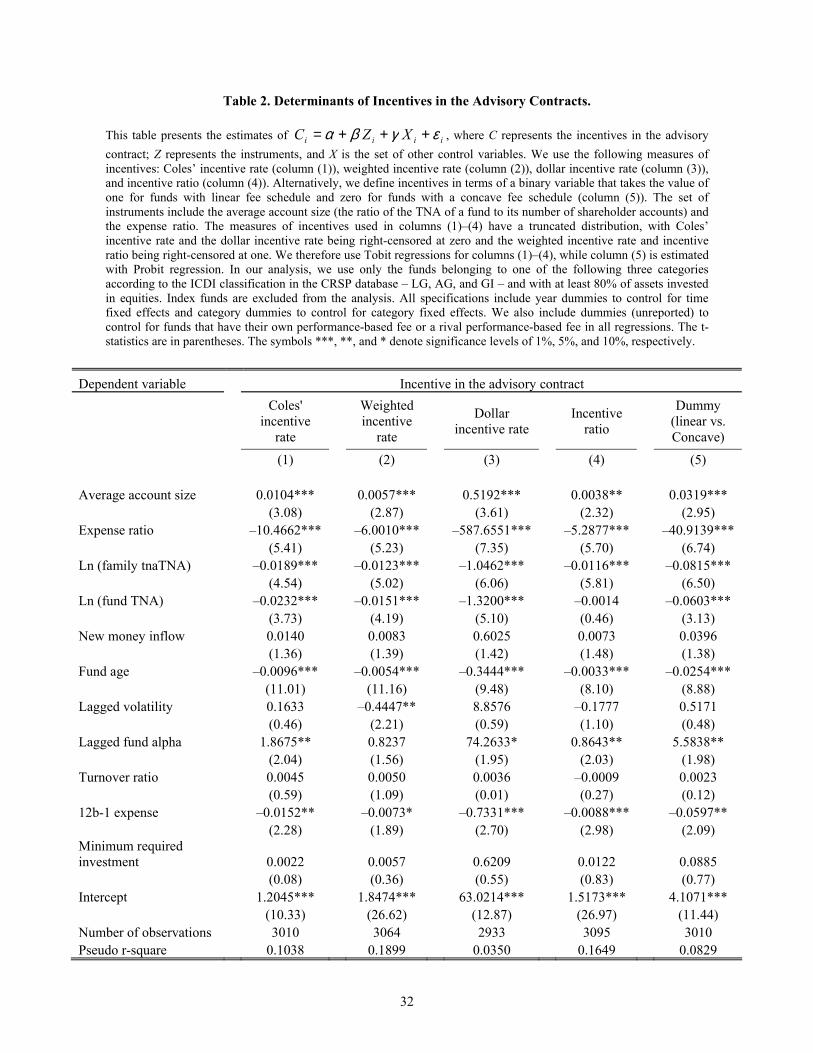
Table 2 provides the results of the determinants of contractual incentives. We consider five

alternative proxies of contractual incentives: CIR, WIR, DIR, and IR, as well as a dummy that takes

the value 1 if the contract is linear and zero if it is concave. The results show a strong and statistically

significant positive relation between incentives and average account size and a negative relation

between incentives and expense ratio. We also check for the robustness of our results by using the

average account size as the only instrument. The results are consistent with those reported.5

Based on the first-stage regression, we derive the implied (estimated) incentive as the expected

value of CIR (or WIR, DIR or IR) projected on the set of instruments and other explanatory variables

that determine the choice of the contract. As the original CIR variable is right-censored at zero, we

use a Tobit regression to derive the estimated value of CIR. We use this estimated incentive in our

subsequent analysis.

3 From NSAR, we know the number of portfolio accounts of a mutual fund – that is, the number of investors in the fund. The TNA divided by the number of investors gives the size of an average shareholder account. 4 This variable accounts for other expenses of the fund (postage, transaction, etc.) as well as the remuneration for the manager. The overall level of expense is what matters. Similar results are obtained by using the expense net of the remuneration. These results are available on request. 5 It is worth noting that if we include the instrument among the explanatory variables in our main set of tests, it is not significant. This (unreported) result is in line with the fact that a good instrument should correlate with the endogenous explanatory variable and should not be related to the dependent variable other than through its effect on the explanatory variable.

9

C. Other Variables

We include a number of additional control variables to control for fund-specific characteristics. We

measure the size of the family as the logarithm of the TNA managed by all the funds belonging to the

family (ln(family TNA)). Similarly, fund size is defined as the logarithm of the TNA managed by the

fund (ln(fund TNA)). Our measure of net inflow (New money inflow) is the net dollar inflow as a

fraction of TNA of the fund. The fund’s age (Age) is the number of years the fund has traded. If

different classes of funds have different ages, we take the oldest age. We use the prior year volatility

of the fund (Lagged fund return volatility) as one of our control variables. This is the standard

deviation of monthly fund returns for the 12 months in a calendar year. The turnover (Turnover ratio)

is defined as the minimum of sales or purchases divided by the TNA of the fund. The 12b-1 expense

(12b-1 expense) and the minimum initial investment required are used as additional control variables

in the subsequent analysis. We also employ a set of dummies for whether the fund charges

performance fees (Performance-based fee) and whether a component of the fees is determined as a

function of the performance of the rival funds (Fee on rival performance). In about 0.42% of funds,

performance-based compensation is tied to the performance of their own fund, while in about 0.85%

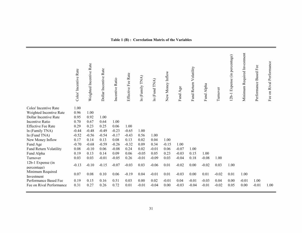
of funds, part of the compensation is linked to the rivals’ performance. Table 1 (Panel B) provides a

correlation matrix for the main variables.

II. Main Findings

A. Incentives and Survival

We start by estimating the impact of incentives on the survival probability of the mutual funds. If

higher incentives indeed lead to increased risk taking, they may also increase the probability of large

negative return shocks, which may force the fund to liquidate – that is, incentives may reduce the

probability that the fund survives. We perform a survival analysis by using data on fund delisting

from CRSP. We use the Cox semi-parametric hazard rate model and a parametric proportional hazard

model, in which the baseline hazard has exponential functional form, on fund closure data.

10

The Cox regression model estimates the hazard rate for fund i as )iZexp()t(0h)iZt(h β= ,

where )( iZth is the hazard rate for fund i at time t, and Z is the vector of explanatory variables that

includes incentive (C) and size of the fund-family (F), as well as the other explanatory variables (X),

as defined in the previous section. The vector β stacks the maximum likelihood estimates of the

coefficients. The Cox model does not impose any parameterization on the baseline hazard rate h0(t)

and does not make any assumption about the shape of the hazard over time. The only assumption is

that the shape of the hazard is the same for all funds. In the parametric proportional hazard model, the

baseline hazard rate (that is, h0(t)) is specified to have the following functional form: )exp()(0 ψ=th ,

where ψ is an additional parameter to be estimated in the model.

We report the results in Table 3. The first two columns report the results for the Cox

proportional hazard model; the other two columns report the results for the exponential hazard model.

We also include EFR, the level of advisory fee, in our regressions. Columns (1) and (3) present the

results of estimating the regression equation in a panel framework in which the standard errors are

adjusted for clustering at the fund level. In columns (2) and (4), we adjust the standard errors of the

estimates to allow for clustering at the fund-family level. All the specifications include year dummies

to control for time fixed effects and category dummies to control for category fixed effects.

The results show that contractual incentives reduce the probability of survival (that is, increase

the hazard rate). This finding is robust across alternative specifications. The results are also

economically significant. An increase of 1% in incentives leads to an increase in hazard rate of 7.54%

in the Cox proportional model and 8.46% in the exponential hazard model. This is equivalent to a

reduction in the probability of survival of about 2%. Results are similar when alternative measures of

contractual incentives (WIR, DIR, and IR) are used.

Interestingly, family affiliation also reduces the probability of survival, with funds that belong

to bigger families less likely to survive. The effect is similar in magnitude to the effect of the

incentive variables and is robust when alternative definitions of the contractual incentives are used. A

1% increase in the log size of the family reduces the probability of survival by about 4%. This is

11

consistent with findings in the literature, which suggest that families tend to proliferate funds and take

on more risk to generate “stars” (Nanda et al., 2004).

Among the control variables, two of the most important factors in terms of increasing the

probability of a fund’s survival are the alpha of the fund in the prior year and the fund’s size. In

economic terms, an increase of 1% in the prior year alpha increases the survival probability by 1.65%,

while a 1% increase in the log of fund size leads to an increase of 1% in survival probability. This

may be because of a “too big to fail” rationale: large established funds are likely to be flagship funds

for families and, therefore, are less likely to be allowed to fail. Overall, these findings suggest that

contractual incentives have a first-order effect in reducing the probability of a fund’s survival.

B. Incentives and Risk Taking

We next analyze the impact of incentives on the risk-taking behavior of mutual funds. We test this by

regressing the calendar year volatility of monthly fund returns (the commonly used measure of fund

risk) on incentives while controlling for other factors that might influence risk-taking. We estimate:

it,it,RXitFitCit σνσφσγσβσασ ++++= (1)

where, for the ith fund at time t, σit is the annual volatility of monthly returns, Cit is the contractual

incentives, Fit is the size of the family to which the fund belongs, and Xit is a vector of control

variables including size, inflow, age, prior year volatility, turnover, 12b-1 expense, minimum required

investment, and estimated probability of a fund’s survival.

The results of the test are reported in Table 4. We start with a specification based on a fixed-

effect at fund level in column (1) to control for unobserved fund heterogeneity that might determine

the level of fund risk. In columns (2)–(5), we cluster the standard errors of the estimated parameters at

the fund level to account for the residual cross-correlation. We also include year dummies to control

for time-series dependence6 and category dummies to control for category fixed effects.

Column (3) presents the results for the sub-sample of funds that have a concave contract.

Column (4) uses an endogenous dummy variable that takes the value of 1 for linear contracts and zero

6 Petersen (2005) includes a detailed discussion of the appropriate methods under different assumptions about the correlation of the residuals.

12

for concave contracts and includes average account size and expense ratio as instruments. The

specification in column (5) includes CIR and the dummy variable. We expect βσ>0, and our findings

support our hypothesis. Indeed, contractual incentives increase risk taking, as βσ is consistently

positive and significant across the different specifications. The results are also economically

significant. An increase of 1% in incentives increases the fund’s return volatility, on average, by about

1.06% in the case of CIR7 and by 0.54% in the case of a linear rather than concave contract. The

impact of the level of fees is also statistically and economically significant. A 1% increase in the level

of fees increases the fund’s return volatility by about 0.82%. Results are similar if the alternative

measures of contractual incentives (WIR, DIR, and IR) are used.

Also, family affiliation increases risk taking: funds that belong to bigger families take more risk

(that is, γσ>0). An increase of 1% in the logarithm of the size of the family increases the fund’s return

volatility by about 0.04%. Furthermore, the probability of a fund’s survival relates positively to the

volatility of fund return. It is worth noting that the relation between incentives and fund risk remains

robust even after controlling for the fund’s fixed effect. The specification controls for any unobserved

heterogeneity in fund characteristics that may lead to spurious correlation between incentives and the

fund’s return volatility. These findings lend strong support to our working hypothesis that contractual

incentives increase the risk-taking behavior for mutual funds.

C. Incentives and Performance

We now consider performance. We start by relating incentives to the annual risk-adjusted return of

the funds. We regress fund return on our incentive variables and a set of control variables using:

it,Rit,RXRitFRitCRRitR νφγβα ++++= (2)

where, for the ith fund at time t, Rit is the fund’s risk-adjusted return with respect to the four-factor

model over the calendar year. The other variables are as defined for equation (1).

The results are reported in Table 5. We start with a specification based on a fixed effect at fund

level in column (1) to control for unobserved fund heterogeneity that might determine the level of

7 The value is calculated as follows: the mean fund return volatility is 0.0580 in the sample, while the coefficient of CIR in column (2) is 0.0613. Hence, the economic impact is (0.0613*0.01)/0.0580 = 1.06%.

13

fund risk. In columns (2)–(5), we cluster the standard errors of the estimated parameters at the fund

level to account for the residual cross-correlation. We also include year dummies to control for time-

series dependence8 and category dummies to control for category fixed effects. Column (3) presents

the results for the sub-sample of funds that have a concave contract. Column (4) uses an endogenous

dummy variable that takes the value of 1 for linear contracts and zero for concave contracts and

includes average account size and expense ratio as instruments. The specification in column (5)

includes CIR and the dummy variable.

The findings show that contractual incentives increase fund returns: βR consistently is positive

and significant across the different specifications. Moreover, the results also are significant

economically: an increase in incentives of 1% increases risk-adjusted fund returns by more than 16

basis points, while funds with linear contracts have a risk-adjusted return 35 basis points higher than

those with concave contracts. In addition, funds that belong to larger families have higher returns.

Consistent with the theory of Berk and Green (2004), we find that inflows have a negative impact on

risk-adjusted returns. Funds that experience significant inflows have a lower alpha. It is interesting to

note that performance relates positively to the probability of the fund’s survival. Indeed, given the

negative relation between survival and incentives and the positive relation between incentives and

performance, we expect that the very funds that are less likely to survive are also the funds with

higher performance ex-ante. Therefore, an estimation that does not account for survival probability

will lead to a downwardly biased estimate of the impact of incentives on performance. Furthermore,

as in the previous specifications, the relation between incentives and performance holds after

controlling for fund fixed effects. The specification takes into account any unobserved heterogeneity

that leads to a spurious correlation between incentives and performance.

Next, we employ a portfolio-based estimation to study the performance of portfolios of funds

grouped on the basis of incentives. This method allows us to control for potential errors induced by

separately estimating the risk-adjusted return for funds, as in the previous multivariate analysis. At the

beginning of each year, we rank funds into quintile portfolios based on incentives. These portfolios

8 Petersen (2005) includes a detailed discussion of the appropriate methods under different assumptions about the correlation of the residuals.

14

are rebalanced every year. The portfolio returns are computed by equally weighting the returns of the

funds in the portfolio. We also form a spread portfolio between the highest and lowest incentive

quintiles. The result is a time-series of the returns of portfolios for 96 months in our sample period.

We then regress the portfolio returns on the three Fama-French risk factors and the momentum factor

using the following equation:

iUMD4HML3SMB2)frMKT(1friR εββββα ++++−+=− (3)

where Ri is the fund return net of expenses for fund i, rf is the risk-free rate, and the four risk factors

are denoted by MKT (market portfolio), SMB (size portfolio), HML (book-to-market portfolio), and

UMD (momentum portfolio). The risk-adjusted return, α, is the intercept of this regression. This

model has been used to analyze mutual fund performance from Carhart (1997) onwards and has been

shown to have good explanatory power for the observed cross-section of fund returns.

We also account for the probability of survival by using incentives to produce a relative ranking

within groups sorted on survival probability (Figure 2). First, funds are sorted into five groups on the

basis of their survival probability. The funds within each group then are sorted further into quintile

portfolios on the basis of their incentives. The top incentive quintiles from each of the five groups

then are combined to form the portfolio of the highest incentive funds. The other incentive quintiles

are aggregated in a similar manner. The five resultant portfolios of mutual funds sorted on incentives

have similar within group variations in survival probabilities. Then, we estimate performance as the

intercept from a regression of excess portfolio returns on the four risk factors.

The results are reported in Table 6. Panel A reports the results before accounting for survival

probability and Panel B reports the results after accounting for survival probability. The average

monthly excess return for the top quintile is significantly higher than for the bottom quintile – before

and after controlling for survival probability. The return of the portfolio of the top incentive quintile

of funds is 60 basis points per month higher than the risk-free rate (63 basis points after controlling

for survival probability), while the return of the portfolio of the bottom incentive quintile of funds is

only 38 basis points per month higher than the risk-free rate (37 basis points after controlling for

survival probability). Indeed, the spread portfolio has a risk-adjusted return of 22 basis points per

15

month (24 basis points after controlling for survival probability) above the four risk factors of market,

SMB, HML and UMD. The other interesting result is the loading on book-to-market and momentum

factors. The high-incentive funds load significantly higher on the SMB and HML factors and

significantly lower on the UMD factor than the low-incentive funds. Results are similar when the

alternative measures of contractual incentives (WIR, DIR, and IR) are used.9

One potential issue is that the existence of a direct relation between fund-specific characteristics

(for example, size, age, or portfolio liquidity) and performance may induce a spurious correlation

between incentives and performance.10 To account for any non-linear relation between fund

characteristics and performance,11 we analyze the relation between incentives and performance within

different characteristics-based groups. We consider three main fund characteristics: size, age, and

portfolio liquidity of the funds. Apart from the well-documented relation between size and

performance, performance might also be related to the age of funds. Indeed, the families of young

funds may help them generate higher performance, as younger funds have shorter track records that

are easier to manipulate. Portfolio liquidity of mutual funds would indicate whether some funds

generate superior performance by holding more illiquid stocks and thereby earning a liquidity

premium.

We construct the average performance for quintile portfolios of mutual funds sorted

according to incentives within tercile groups that are formed on the basis of three fund characteristics

(size, age, and portfolio illiquidity). Mutual funds first are sorted into three groups on the basis of

their characteristics; they are sorted further within each group into quintiles on the basis of CIR.

Portfolios are weighted equally every month, so the weights are readjusted whenever a fund

disappears. Performance is measured as the intercept of a regression of excess portfolio returns on the

four risk factors commonly used: market, SMB, HML, and UMD.

9 It is worth mentioning that estimates of the intercept term of equation (3) remain unchanged when we include Pastor and Stambaugh (2003)’s liquidity factor as an additional risk factor. However, we report only the estimates of the four-factor model to make our results comparable with the literature. 10 Deli (2002) shows a significant relationship between size and incentives. Chen et al. (2004) show that increases in funds’ sizes lead to declines in fund performance. 11 It is worth noting that we have controlled for fund characteristics in our multivariate analyses using a linear specification. Moreover, the use of fixed-effect regression methods helps us to control for any unobserved heterogeneity that remains constant over time.

16

The measure of illiquidity of the portfolio is based on the square-root version of the Amihud

(2002) illiquidity ratio: ∑=j

jtjtit IIlliq 2θ , where itjtjtjt TNAPn=θ is the portfolio weight in stock

j at time t in the portfolio of fund i, and I2 is defined as the average of the square root of the ratio

between absolute return and volume for a given stock: that is, jtjtjt VolrI /2 = . The portfolio

illiquidity of a mutual fund is then calculated as the value-weighted average of the individual stock’s

illiquidity in the fund’s portfolio.

Table 7 reports the alphas of different portfolios formed on the basis of the above procedure.

The difference in alphas between the high- and low-incentive funds is significantly positive, both

before and after controlling for survival probability. This, in general, holds regardless of the

breakdown in different sizes and illiquidity classes. In the case of age, higher incentives lead to higher

performance, mostly in young funds. In addition, the results are similar when the alternative measures

of contractual incentives (WIR, DIR, and IR) are used.

Overall, the findings reported in Tables 5–7 provide strong evidence for a positive impact of

incentives on the risk-adjusted performance of mutual funds.

D. Incentives and Performance Persistence

An important dimension in our analysis is persistence in fund performance. If incentives increase

managerial efforts, this should translate to higher and more stable risk-adjusted performance. To study

persistence in performance of mutual funds, we employ the standard test defined by Carhart (1997).

D.1 Incentives and Performance Persistence: main results

We start by confirming Carhart’s results for our sample. On 31 December every year, funds are sorted

into decile portfolios on the basis of their risk-adjusted return for the calendar year, which is

determined from a factor model using the three Fama-French factors and the momentum factor. For

the following years, the returns on these alpha-sorted portfolios are calculated by equally weighting

the returns of the funds in each of the portfolios. In addition, a spread portfolio is constructed as the

difference between the top and bottom deciles. The time-series of portfolio returns then are regressed

17

on the risk factors, and a significant intercept in this regression provides evidence of persistence in

performance. The (unreported) results show no evidence of significant persistence among the top

decile of funds (the best funds from the previous year), while the intercept of the bottom decile

continues to be negative and significant, which indicates that the worst funds have persistently poor

performance, in line with the existing literature. The spread portfolio has a positive and significant

intercept, which implies a significant performance differential between the best and worst funds from

one year to the next. The results are robust when sorting is based on quintiles rather than deciles of the

prior year’s alpha. The results are qualitatively and quantitatively similar to those obtained by Carhart

(1997) and others in the literature.

We next investigate whether incentives have an effect on performance persistence by

modifying the standard test. As in the previous test, we first form quintile portfolios of funds on the

basis of the prior year’s risk-adjusted return. Within each performance quintile, we then separate the

funds into five equal groups on the basis of their incentives. We define the funds with the highest

incentives within each performance quintile as the high-incentive group and those with the lowest

incentives as the low-incentive group. The procedure creates five alpha-sorted portfolios of high-

incentive funds and another five alpha-sorted portfolios of low-incentive funds. For the next year, the

portfolio returns are calculated by equally weighting the returns of the funds in the portfolios. We also

form spread portfolios between the best- and worst-performing funds for both the high- and low-

incentive groups.

To capture the difference in performance between funds with similar prior returns but

different incentives, we also form two long-short portfolios. The first portfolio is long in funds that

belong to the top alpha quintile of the high-incentive group and short in funds that belong to the top

alpha quintile of the low-incentive group. The second portfolio is long in funds that belong to the

bottom alpha quintile of the high-incentive group and short in funds that belong to the bottom alpha

quintile of the low-incentive group. We then regress the portfolio returns on the four risk factors

(Market, SMB, HML and UMD).

In the next specification, we control for survival probability of the fund by modifying the

sorting procedure. We first sort the funds each year into five groups on the basis of the survival

18

probabilities estimated from our hazard rate model. Within each group, the funds then are sorted into

quintiles on the basis of their prior-year risk-adjusted return. In the next step, the top performance

quintiles from each of the five survival groups are aggregated to form the quintile portfolio of funds

with the highest prior-year performance. The other quintiles of funds are obtained through similar

aggregation. The resulting five quintiles of funds sorted on prior-year performance have similar

within group variations in survival probabilities. The final step is to split the funds within each

quintile into five groups on the basis of their incentives. We then proceed as before to form

performance-sorted portfolios for both the high- and low-incentive groups.

The results are reported in Table 8. In Panel B but not Panel A, we control for the survival

probability of the funds. The results show evidence of performance persistence among the funds with

high-incentive contracts: the top performance quintile portfolio among the high-incentive funds has an

alpha of 41 basis points per month in Panel A and 37 basis points per month in Panel B. On the other

hand, the bottom performance quintile portfolio has a negative alpha of 77 basis points per month in

Panel A and a negative alpha of 67 basis points in Panel B. The spread portfolio between the top and

bottom quintiles has an alpha of 118 basis points per month in panel A and 104 basis points in panel

B. We thus find strong evidence that performance persists not only for the worst-performing funds but

also for the best-performing funds that have high incentives. No analogue for persistence is present

for funds with low-incentive contracts.12

These results are quite striking. The failure of the previous literature to document

performance persistence can be addressed by performing analyses that include conditioning based on

funds’ incentives. Indeed, the alleged lack of persistence previously reported may be simply due to the

fact that funds with high and low incentives were grouped together. Our study provides one simple

conditioning variable (incentive in the advisory contract) that fund investors can use to predict funds

that are likely to generate superior performance.

12 In fact, by being long in prior-year best-performing funds with high incentives and short in prior-year best-performing funds with low incentives, an investor can earn an alpha of 71 basis points per month in Panel A (74 basis points in Panel B).

19

D.2 Incentives and Performance Persistence: robustness checks and more detailed analysis

As an additional check for robustness, we use an alternative method of sorting funds –sorting first on

the basis of incentives and then on the basis of performance – rather than the usual method of sorting

first on performance and then on incentives. We also control for survival probability. Similar to the

method described above, we first sort funds into five groups on the basis of their survival

probabilities. Within each group, we then sort funds into five groups on the basis of their incentives.

Incentive groups then are aggregated from different survival groups, as described previously. The

resulting groups of funds sorted on incentives have similar within group variation in survival

probabilities. Finally, the funds within each of the highest- and lowest-incentive groups are further

sorted into quintile portfolios on the basis of the prior year’s risk-adjusted return. The (unreported)

results are similar in economic and statistical magnitude to those described above.

Our results remain qualitatively and quantitatively robust when the Pastor and Stambaugh

(2003) liquidity factor is included in the factor model. We report only the results of estimates based

on the four-factor model for the sake of comparability with existing literature. In addition, the results

are similar when alternative measures of contractual incentives (WIR, DIR, and IR) are used.

As an additional check for robustness, we also perform a multivariate analysis of performance

persistence. We employ a probit model in which the dependent variable takes a value of one if the

fund was a winner (a fund with a risk-adjusted return greater than the median fund for a given year) in

the current and previous years and a value of zero otherwise. The independent variables in the probit

model include measures of incentives and other control variables as defined in previous sections. The

(unreported) results show that the effect of the incentives is positive and significant. A 1% increase in

incentive leads to an increased probability of winners’ persistence of 4.33%. These findings confirm

that incentives are related positively to higher performance and that this performance is stable.

Finally, we analyze the role of survivorship bias for the performance results in greater detail.

Instead of aggregating across the survival probability quintiles, we provide a three by three table of

the double sort. Mutual funds are sorted first into three groups each year on the basis of the tercile

values of survival probability. Then, on 31 December each year, mutual funds within each (survival

probability-based) tercile group are further sorted into tercile portfolios based on their calendar year

20

alphas from a four-factor model. Within each tercile portfolio based on the prior year’s performance,

funds are sorted further into five groups on the basis of the quintile values of the contractual incentive.

For each alpha-based tercile portfolio, we classify the top incentive quintile as the high-incentive

group and the bottom incentive quintile as the low-incentive group.

The portfolios are equally weighted monthly, so the weights are readjusted whenever a fund

disappears. The portfolios of funds are rebalanced every year. To capture the difference in

performance between the prior year’s top and bottom performers, we also form a spread portfolio for

each of the two incentive groups. The alphas of the different portfolios are reported in Table 9 (Panel

A). Among the group of high-incentive funds, the top performers from one year continue to have

superior risk-adjusted returns among the medium- and low-survival probability groups. Indeed, the

performance differential between the best and worst funds is significant across all survival groups.

There is, however, no evidence of persistence among funds with low-incentive contracts. This holds

true regardless of the degree of survival probability.

To test for the difference in performance between high- and low-incentive funds with similar

survival probability and prior-year performance, we form long-short portfolios. We go long in the

funds belonging to a given survival tercile and prior-year performance tercile in the high-incentive

group of funds and short in the funds that belong to the corresponding survival and prior-year

performance terciles in the low-incentive group of funds. The results are reported in Table 9 (Panel

B). Regardless of the degree of survival probability, high-incentive winner funds in a given year

significantly outperform low-incentive winner funds in the following year. This indicates that any

observed outperformance by a high-incentive fund in a given year is more likely to be due to skill

than luck. These results are similar when alternative measures of contractual incentives (WIR, DIR,

and IR) are used.

D.3 Incentives and Performance Differential among Mutual Funds Managed by the Same

Manager or Belonging to the Same Fund Family

One interesting question is: “As the same advisor may manage multiple funds for the same fund

family, are there interactions between funds from the same family or under the same advisor?” To

21

address this issue, we estimate the performance differential between funds managed by the same

manager or by the same fund family. We form pairs of funds managed by the same fund manager (or,

alternatively, part of the same family) and go long in the fund with a linear contract and short in the

fund with a concave contract.

The results are reported in Table 10. Columns (1)–(3) report the results where pairs are

formed on the basis of funds managed by the same fund manager; Columns (4)–(6) report the results

with pairs formed on the basis of funds that are part of the same family (belonging to the same ICDI

objective category). In columns (1) and (4), the pairs are aggregated to form a long-short portfolio and

then we regress the portfolio returns on the four risk factors of market, SMB, HML, and UMD. In

columns (2) and (5), each individual pair’s return is regressed on the four risk factors. In columns (3)

and (6), we also include the differences in fund characteristics as explanatory variables. The results

show that the performance differential between the high- and low-incentive funds is significantly

positive and robust when controlling for unobserved managerial ability as well as family affiliation.

Given the small sample size, however, the results are only indicative.

E. Incentives and Managers’ Unobserved Actions

We now examine in greater detail the channel through which incentives affect performance. We focus

on the fund return, which is obtained by following a buy-and-hold strategy on the fund’s disclosed

portfolio, and the return gap, which is the difference between gross fund return and buy-and-hold fund

return. The return gap captures the activism of mutual funds (Kacperczyk et al., 2006), and is defined

as the difference between the investor return and the buy-and-hold return from their disclosed

portfolio.13 A higher buy-and-hold return signals better portfolio allocation decisions by the fund

manager, while a higher return gap indicates a higher positive contribution to fund performance by the

trading and dynamic rebalancing of the funds’ portfolio. It has been shown that “unobserved actions

of some funds persistently create value, while the actions of others destroy value” (Kacperczyk et al.,

2006). The return gap measure has been created as a proxy for the unobserved actions of managers in

the absence of direct information on their short-term trading strategies. Indeed, despite extensive

13 Kacperczyk et al. (2006) provide a detailed description of the construction of the return gap.

22

disclosure requirements, it is not possible to observe all of the actions of fund managers. The exact

timing of the trades, transaction costs, and dynamic trading strategies all are unknown.

Similar to our analysis on risk-adjusted fund returns, we form quintile portfolios sorted

according to incentives. We calculate the portfolio buy-and-hold return as the equally-weighted buy-

and-hold return of the funds in the portfolio. The portfolio return gap is the equally-weighted return

gap of the funds in the portfolio. We regress the portfolio buy-and-hold returns and portfolio return

gaps on the risk factors.

Table 11 reports the results for the return gap (Panel A) and the buy-and-hold returns (Panel

B). The results indicate that there is no significant performance differential among the incentive-

sorted portfolios in terms of buy-and-hold return: the spread portfolio has alphas that are statistically

insignificantly different from zero. When we consider the return gap, however, there is a sizable and

statistically significant difference among the incentive-sorted portfolios: before risk adjustment, the

high-incentive portfolio has a positive return gap of 6 basis points per month, while the low-incentive

portfolio has a negative return gap of 4 basis points per month. The spread portfolio between the high-

and low-incentive funds has a positive and statistically significant alpha of 13 basis points per month.

Results are similar when alternative measures of contractual incentives (WIR, DIR, and IR) are used.

As an additional check for robustness, we also perform a multivariate analysis on the return

gap. We regress the annual risk-adjusted return gap on incentives as well as the set of control

variables defined previously. The (unreported) results show that the coefficients on incentive are

positive and significant regardless of the proxy used to define the incentives.

These findings suggest that managers with higher incentives take actions that are beneficial to

the funds’ investors. The value created by their dynamic trading strategies more than offsets the cost.

In addition, taken together with the lack of significance for the case of the buy-and-hold strategies,

these findings suggest that the main channel through which incentives affect fund performance

involves trading strategies and portfolio rebalancing. An investor who simply mimics the observed

holdings of the high-incentive funds and rebalances every quarter would not be able to generate a

significantly positive alpha.

23

F. Discussion

Overall, these findings show that contractual incentives play an important role in increasing risk

taking by mutual funds. However, this does not translate into “poor man’s alpha”. Quite the opposite

occurs, in fact: higher incentives are related to higher performance. The higher performance is due not

only to the higher risk of the fund strategies but to a genuine improvement in fund management.

One possible explanation lies in the relation between the fund manager and the fund family.

Indeed, the advisory contract links the fund to the family and directly quantifies the benefits that

accrue to the family from increased risk taking and higher performance. The fact that higher

incentives provide a persistently higher performance may suggest that better information or support is

provided to high-incentive funds. Fund families may provide managers with ways to perform better

through cross-fund support and/or by smoothing the adverse effects of worse performance (for

example, by reducing the employment risk through job rotation within the family).

In addition, these findings suggest that advisory contracts contain information useful for

selecting funds. This however asks the question of how it could be possible in equilibrium. Indeed, if

any observable fund-specific characteristic were useful to forecast fund performance, rational

investors would be investing massively in funds with those characteristics and driving the other funds

away from the market (Berk and Green, 2004). It can be argued that this does not happen because

higher incentives, by increasing risk, also affect the fund’s probability of survival. Given that funds

with high incentive contracts tend to be riskier, they are also more likely to disappear. So, attrition

would actually eliminate the very funds for which higher incentives imply higher performance. In

other word, incentives, by affecting risk and survival, would make it less likely for fund performance

to persist. However, our analysis of survival, risk, and performance suggests that this is not the case.

We therefore leave this is as a puzzle that provides additional evidence in favor of predictability of

fund performance (Gruber, 1996).

III Conclusion

We test how incentives affect performance and risk taking in the US mutual fund industry. We

hypothesize that incentives increase risk taking as well as performance and provide evidence to

24

support our hypothesis. Incentives directly affect the unobserved actions of the fund managers, with

higher incentives improving performance by increasing the return gap. By affecting performance and

risk taking, incentives also affect the survival probability of the fund. When past performance is

controlled for, an increase in incentives reduces the survival probability of the funds. We also show

evidence of performance persistence among high-incentive funds, even after controlling for the

survival probabilities of the funds.

These findings not only provide direct support for predictions of the theory on compensation

but also quantify the role played by the type of compensation in the mutual fund industry. They also

have implications in terms of the recent debate on mutual fund fees and managers’ compensation in

the US. Indeed, if higher incentives increase both performance and risk in such a way that higher

performance does not persist, the effect of higher incentives is likely to be neutral for investors and

can be justified most likely in terms of producer surplus for the mutual fund management families. If,

instead, they increase the risk-adjusted performance – as seems to be the case – incentives turn out to

be a useful tool to motivate fund managers and increase welfare.

25

References

Aggarwal, R. K., and A. A. Samwick, 1999, “Executive Compensation, Strategic Competition, and Relative Performance Evaluation: Theory and Evidence,” Journal of Finance, 54 (6), 1999-2043.

Almazan, A., K. C. Brown, M. Carlson, and D. A. Chapman, 2004, “Why Constrain Your Mutual Fund Manager?” Journal of Financial Economics, 73, 289-321.

Amihud, Y., 2002, “Illiquidity and Stock Returns: Cross-sectional and Time-series Effects,” Journal of Financial Markets, 5 (1), 31-56.

Avramov, D., and R. Wermers, 2006, “Investing in Mutual Funds When Returns are Predictable,” Journal of Financial Economics, 81, 339-377.

Berk, J. B., and R. C. Green, 2004, “Mutual Fund Flows and Performance in Rational Markets,” Journal of Political Economy, 112 (6), 1269-1295.

Bollen, N. P., and J. A. Busse, 2005, “Short-Term Persistence in Mutual Fund Performance,” Review of Financial Studies, 18, 569-597.

Brown, S. J., and W. N. Goetzmann, 1995, “Performance Persistence,” Journal of Finance, 50 (2), 679-698.

Carhart, M. M., 1997, “On Persistence in Mutual Fund Performance,” Journal of Finance, 52 (1), 57-82.

Carpenter, J. N., 2000, “Does Option Compensation Increase Managerial Risk Appetite?” Journal of Finance, 55 (5), 2311-2331.

Chen, J., H. Hong, M. Huang, and J. Kubik, 2004, “Does Fund Size Erode Mutual Fund Performance? The Role of Liquidity and Organization,” American Economic Review, 94 (5), 1276-1302.

Chevalier, J., and G. Ellison, 1997, “Risk Taking by Mutual Funds as a Response to Incentives,” Journal of Political Economy, 105 (6), 1167-1200.

Coles, J. L., J. Suay, and D. Woodbury, 2000, “Fund Advisor Compensation in Closed-End Funds,” Journal of Finance, 55 (3), 1385-1414.

Daniel, K., M. Grinblatt, S. Titman, and R. Wermers, 1997, “Measuring Mutual Fund Performance with Characteristic-Based Benchmarks,” Journal of Finance, 52 (3), 1035-1058.

Deli, D. N., 2002, “Mutual Fund Advisory Contracts: An Empirical Investigation,” Journal of Finance, 57 (1), 109-133.

Deli, D. N., and R. Varma, 2002, “Contracting in the Investment Management Industry: Evidence from Mutual Funds,” Journal of Financial Economics, 63, 79-98.

Elton, E. J., M. J. Gruber, and C. R. Blake, 1996, “The Persistence of Risk-Adjusted Mutual Fund Performance,” Journal of Business, 69 (2), 133-157.

Elton, E. J., M. J. Gruber, and C. R. Blake, 2003, “Incentive Fees and Mutual Funds,” Journal of Finance, 58 (2), 779-804.

Gaspar, J. M., M. Massa, and P. Matos, 2006, “Favoritism in Mutual Fund Families? Evidence on Strategic Cross-Fund Subsidization,” Journal of Finance, 61 (1) 73-104.

26

Goetzmann, W. N., and R. G. Ibbotson, 1994, “Do Winners Repeat?” Journal of Portfolio Management, 20 (2), 9-18.

Grinblatt, M., and S. Titman, 1989, “Adverse Risk Incentives and the Design of Performance-Based Contracts,” Management Science, 35 (7), 807-822.

Grinblatt, M., and S. Titman, 1992, “The Persistence of Mutual Fund Performance,” Journal of Finance, 47 (5), 1977-1984.

Grinblatt, M., S. Titman, and R. Wermers, 1995, “Momentum Investment Strategies, Portfolio Performance, and Herding: A Study of Mutual Fund Behavior,” American Economic Review, 85 (5), 1088-1105.

Grinblatt, M., and M. Keloharju, 2000, “The Investment Behavior and Performance of Various Investor Types: A Study of Finland's Unique Data Set,” Journal of Financial Economics, 55, 43-67.

Gruber, M. J., 1996, “Another Puzzle: The Growth in Actively Managed Mutual Funds,” Journal of Finance, 51 (3), 783-810.

Guay, W. R., 1999, “The Sensitivity of CEO Wealth to Equity Risk: An Analysis of the Magnitude and Determinants,” Journal of Financial Economics, 53, 43-78.

Guedj, I., and J. Papastaikoudi, 2004, “Can Mutual Fund Families Affect the Performance of Their Funds?” Working Paper, University of Texas, Austin.

Hendricks, D., J. Patel, and R. Zeckhauser, 1993, “Hot Hands in Mutual Funds: Short-Run Persistence of Relative Performance, 1974-1988,” Journal of Finance, 48 (1), 93-130.

Mamaysky, H., M. Spiegel, and H. Zhang, 2004, “Estimating the Dynamics of Mutual Fund Alphas and Betas,” Working paper, Yale University.

Mamaysky, H., M. Spiegel, and H. Zhang, 2005, “Improved Forecasting of Mutual Fund Alphas and Betas,” Working paper, Yale University.

Jensen, M. C., and W. H. Meckling, 1976, “Theory of the Firm: Managerial Behavior, Agency Costs and Ownership Structure,” Journal of Financial Economics, 3, 305-360.

Jensen, M. C., and K. J. Murphy, 1990, “Performance Pay and Top-Management Incentives,” Journal of Political Economy, 98 (2), 225-264.

Ju, N., H. E. Leland, and L. W. Senbet, 2003, “Options, Option Repricing and Severance Packages in Managerial Compensation: Their Effects on Corporate Investment Risk,” Working Paper, University of Maryland.

Kacperczyk, M., C. Sialm, and L. Zheng, 2006, “Unobserved Actions of Mutual Funds,” Review of Financial Studies, forthcoming.

Kosowski, R., A. Timmermann, R. Wermers, and H. White, 2006, “Can Mutual Fund “Stars” Really Pick Stocks? New Evidence from a Bootstrap Analysis,” Journal of Finance, 61 (6) 2551-2595.

Kuhnen, C. M., 2004, “Dynamic Contracting in the Mutual Fund Industry,” Working paper, Stanford University. Lehman, B. N., and D. M. Modest, 1987, “Mutual Fund Performance Evaluation: A Comparison of Benchmarks and Benchmark Comparisons,” Journal of Finance, 42 (2), 233-265.

27

Nanda, V., J. Z. Wang, and L. Zheng, 2004, “Family Values and the Star Phenomenon: Strategies of Mutual Fund Families,” Review of Financial Studies, 17 (3), 667-698.

Nofsinger, J. R., and R. W. Sias, 1999, “Herding and Feedback Trading by Institutional and Individual Investors,” Journal of Finance, 54 (6), 2263-2295.

Pástor, L., and R. F. Stambaugh, 2003, “Liquidity Risk and Expected Stock Returns,” Journal of Political Economy, 111 (3), 642-685.

Petersen, M. A., 2005, “Estimating Standard Errors in Finance Panel Data Sets: Comparing Approaches,” Working Paper, Northwestern University.

Ross, S. A., 2004, “Compensation, Incentives, and the Duality of Risk Aversion and Riskiness,” Journal of Finance, 59 (1), 207-225.

Warner, J. B., and J. S. Wu, 2004, “Changes in Mutual Fund Advisory Contracts,” Working Paper, University of Rochester.

Wermers, R., 1999, “Mutual Fund Herding and the Impact on Stock Prices,” Journal of Finance, 54 (2), 581-622.

Wermers, R., 2000, “Mutual Fund Performance: An Empirical Decomposition into Stock-Picking Talent, Style, Transaction Costs, and Expenses,” Journal of Finance, 55 (4), 1655-1695.

Wermers, R., 2004, “Is Money Really “Smart”? New Evidence on the Relation between Mutual Fund Flows, Manager Behavior, and Performance Persistence,” Working Paper, University of Maryland.

Zitzewitz, E., 2006, “How Widespread is Late Trading in Mutual Funds?” American Economic Review (Papers and Proceedings), 284-289.

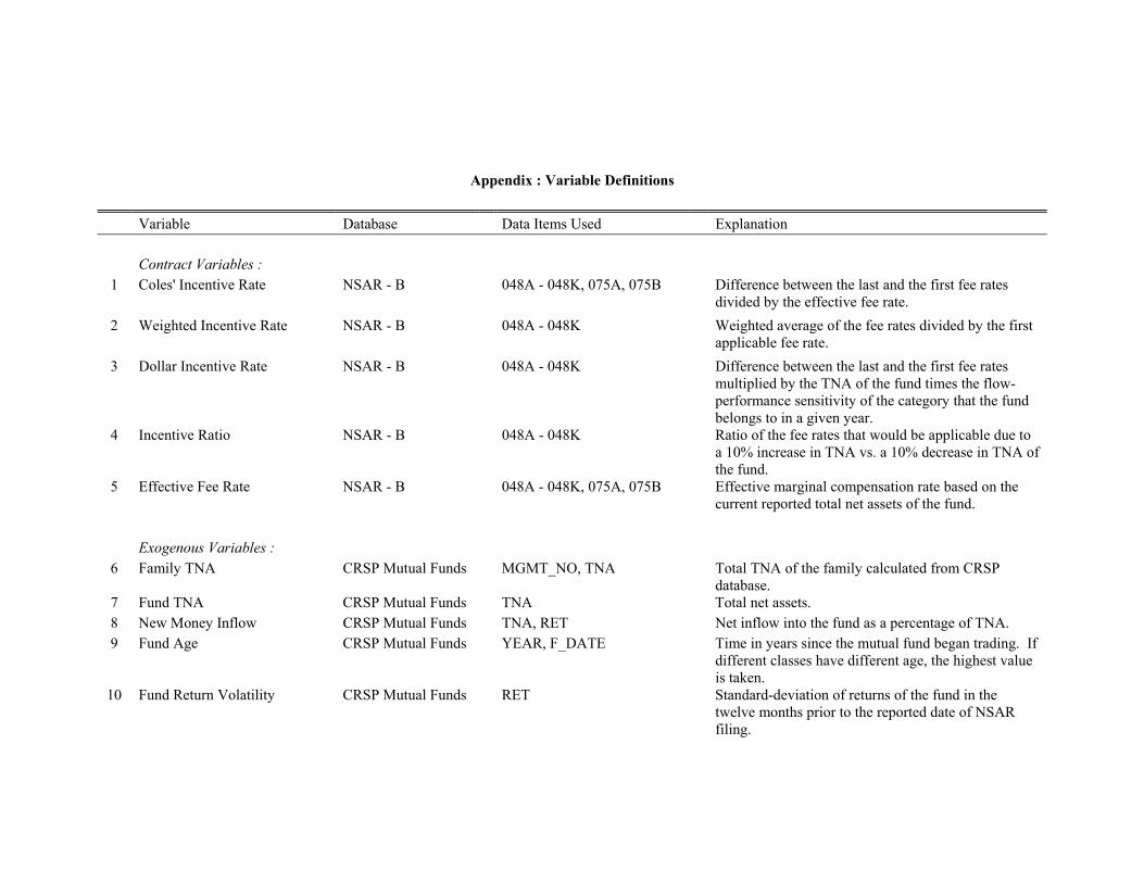
Appendix : Variable Definitions Variable Database Data Items Used Explanation Contract Variables : 1 Coles' Incentive Rate NSAR - B 048A - 048K, 075A, 075B Difference between the last and the first fee rates

divided by the effective fee rate. 2 Weighted Incentive Rate NSAR - B 048A - 048K Weighted average of the fee rates divided by the first

applicable fee rate. 3 Dollar Incentive Rate NSAR - B 048A - 048K Difference between the last and the first fee rates

multiplied by the TNA of the fund times the flow-performance sensitivity of the category that the fund belongs to in a given year.

4 Incentive Ratio NSAR - B 048A - 048K Ratio of the fee rates that would be applicable due to a 10% increase in TNA vs. a 10% decrease in TNA of the fund.

5 Effective Fee Rate NSAR - B 048A - 048K, 075A, 075B Effective marginal compensation rate based on the current reported total net assets of the fund.

Exogenous Variables : 6 Family TNA CRSP Mutual Funds MGMT_NO, TNA Total TNA of the family calculated from CRSP

database. 7 Fund TNA CRSP Mutual Funds TNA Total net assets. 8 New Money Inflow CRSP Mutual Funds TNA, RET Net inflow into the fund as a percentage of TNA. 9 Fund Age CRSP Mutual Funds YEAR, F_DATE Time in years since the mutual fund began trading. If

different classes have different age, the highest value is taken.

10 Fund Return Volatility CRSP Mutual Funds RET Standard-deviation of returns of the fund in the twelve months prior to the reported date of NSAR filing.

29

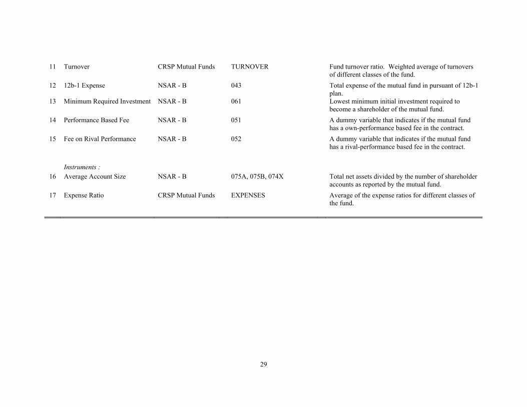
11 Turnover CRSP Mutual Funds TURNOVER Fund turnover ratio. Weighted average of turnovers of different classes of the fund.

12 12b-1 Expense NSAR - B 043 Total expense of the mutual fund in pursuant of 12b-1 plan.

13 Minimum Required Investment NSAR - B 061 Lowest minimum initial investment required to become a shareholder of the mutual fund.

14 Performance Based Fee NSAR - B 051 A dummy variable that indicates if the mutual fund has a own-performance based fee in the contract.

15 Fee on Rival Performance NSAR - B 052 A dummy variable that indicates if the mutual fund has a rival-performance based fee in the contract.

Instruments :

16 Average Account Size NSAR - B 075A, 075B, 074X Total net assets divided by the number of shareholder accounts as reported by the mutual fund.

17 Expense Ratio CRSP Mutual Funds EXPENSES Average of the expense ratios for different classes of the fund.

30

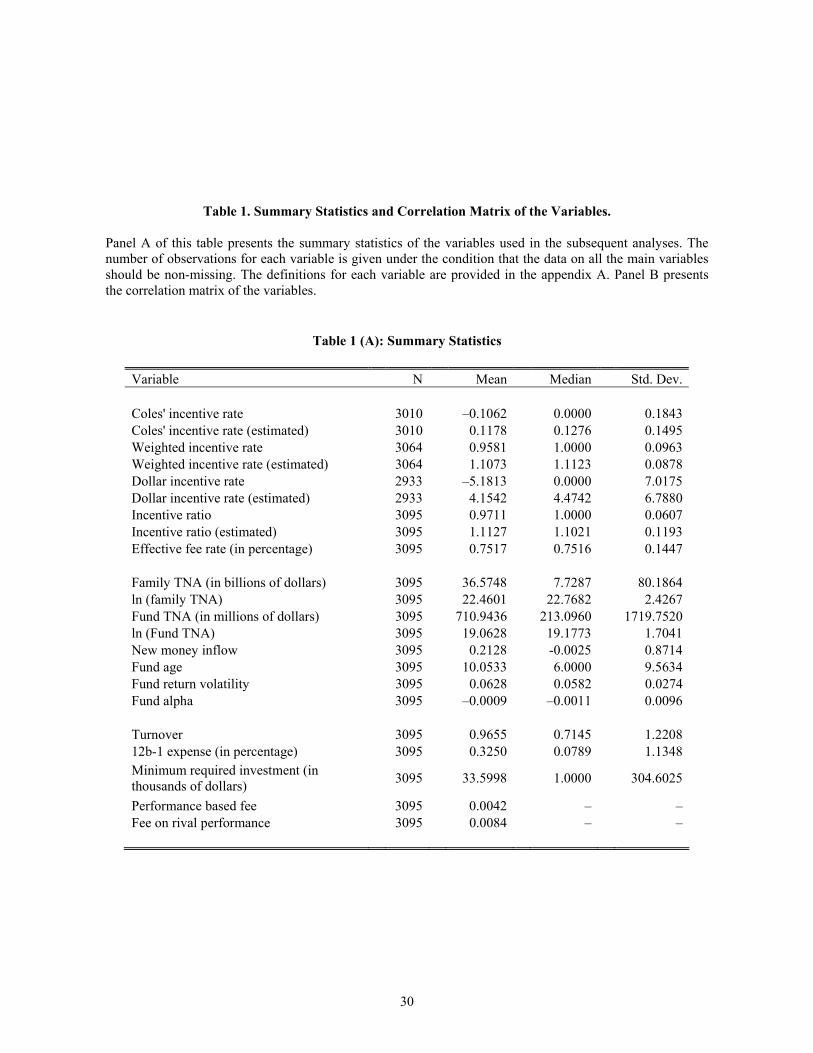
Table 1. Summary Statistics and Correlation Matrix of the Variables.

Panel A of this table presents the summary statistics of the variables used in the subsequent analyses. The number of observations for each variable is given under the condition that the data on all the main variables should be non-missing. The definitions for each variable are provided in the appendix A. Panel B presents the correlation matrix of the variables.

Table 1 (A): Summary Statistics

Variable N Mean Median Std. Dev. Coles' incentive rate 3010 –0.1062 0.0000 0.1843Coles' incentive rate (estimated) 3010 0.1178 0.1276 0.1495Weighted incentive rate 3064 0.9581 1.0000 0.0963Weighted incentive rate (estimated) 3064 1.1073 1.1123 0.0878Dollar incentive rate 2933 –5.1813 0.0000 7.0175Dollar incentive rate (estimated) 2933 4.1542 4.4742 6.7880Incentive ratio 3095 0.9711 1.0000 0.0607Incentive ratio (estimated) 3095 1.1127 1.1021 0.1193Effective fee rate (in percentage) 3095 0.7517 0.7516 0.1447 Family TNA (in billions of dollars) 3095 36.5748 7.7287 80.1864ln (family TNA) 3095 22.4601 22.7682 2.4267Fund TNA (in millions of dollars) 3095 710.9436 213.0960 1719.7520ln (Fund TNA) 3095 19.0628 19.1773 1.7041New money inflow 3095 0.2128 -0.0025 0.8714Fund age 3095 10.0533 6.0000 9.5634Fund return volatility 3095 0.0628 0.0582 0.0274Fund alpha 3095 –0.0009 –0.0011 0.0096 Turnover 3095 0.9655 0.7145 1.220812b-1 expense (in percentage) 3095 0.3250 0.0789 1.1348Minimum required investment (in thousands of dollars) 3095 33.5998 1.0000 304.6025

Performance based fee 3095 0.0042 – –Fee on rival performance 3095 0.0084 – –

31

Col

es' I

ncen

tive

Rat

e

Wei

ghte

d In

cent

ive

Rat

e

Dol

lar I

ncen

tive

Rat

e

Ince

ntiv

e R

atio

Effe

ctiv

e Fe

e R

ate

ln (F

amily

TN

A)

ln (F

und

TNA

)

New

Mon

ey In

flow

Fund

Age

Fund

Ret

urn

Vol

atili

ty

Fund

Alp

ha

Turn

over

12b-

1 Ex

pens

e (in

per

cent

age)

Min

imum

Req

uire

d In

vest

men

t

Perf

orm

ance

Bas

ed F

ee

Fee

on R

ival

Per

form

ance

Coles' Incentive Rate 1.00Weighted Incentive Rate 0.96 1.00Dollar Incentive Rate 0.95 0.92 1.00Incentive Ratio 0.70 0.67 0.64 1.00Effective Fee Rate 0.29 0.23 0.25 0.06 1.00ln (Family TNA) -0.44 -0.48 -0.49 -0.23 -0.65 1.00ln (Fund TNA) -0.52 -0.56 -0.54 -0.17 -0.43 0.56 1.00New Money Inflow 0.17 0.14 0.13 0.08 0.13 0.02 0.04 1.00Fund Age -0.70 -0.68 -0.59 -0.26 -0.32 0.09 0.34 -0.15 1.00Fund Return Volatility 0.08 -0.10 0.06 -0.08 0.24 0.02 -0.01 0.06 -0.07 1.00Fund Alpha 0.19 0.13 0.14 0.09 0.06 -0.05 0.05 0.23 -0.03 0.15 1.00Turnover 0.03 0.03 -0.01 -0.05 0.26 -0.01 -0.09 0.03 -0.04 0.18 -0.08 1.0012b-1 Expense (in percentage) -0.13 -0.10 -0.15 -0.07 -0.03 0.03 -0.06 0.01 -0.02 0.00 -0.02 0.03 1.00

Minimum Required Investment 0.07 0.08 0.10 0.06 -0.19 0.04 -0.01 0.01 -0.03 0.00 0.01 -0.02 0.01 1.00

Performance Based Fee 0.19 0.15 0.16 0.51 0.03 0.00 0.02 -0.01 0.04 -0.01 -0.03 0.04 0.00 -0.01 1.00Fee on Rival Performance 0.31 0.27 0.26 0.72 0.01 -0.01 -0.04 0.00 -0.03 -0.04 -0.01 -0.02 0.05 0.00 -0.01 1.00

Table 1 (B) : Correlation Matrix of the Variables

32

Table 2. Determinants of Incentives in the Advisory Contracts. This table presents the estimates of iiii XZC εγβα +++= , where C represents the incentives in the advisory contract; Z represents the instruments, and X is the set of other control variables. We use the following measures of incentives: Coles’ incentive rate (column (1)), weighted incentive rate (column (2)), dollar incentive rate (column (3)), and incentive ratio (column (4)). Alternatively, we define incentives in terms of a binary variable that takes the value of one for funds with linear fee schedule and zero for funds with a concave fee schedule (column (5)). The set of instruments include the average account size (the ratio of the TNA of a fund to its number of shareholder accounts) and the expense ratio. The measures of incentives used in columns (1)–(4) have a truncated distribution, with Coles’ incentive rate and the dollar incentive rate being right-censored at zero and the weighted incentive rate and incentive ratio being right-censored at one. We therefore use Tobit regressions for columns (1)–(4), while column (5) is estimated with Probit regression. In our analysis, we use only the funds belonging to one of the following three categories according to the ICDI classification in the CRSP database – LG, AG, and GI – and with at least 80% of assets invested in equities. Index funds are excluded from the analysis. All specifications include year dummies to control for time fixed effects and category dummies to control for category fixed effects. We also include dummies (unreported) to control for funds that have their own performance-based fee or a rival performance-based fee in all regressions. The t-statistics are in parentheses. The symbols ***, **, and * denote significance levels of 1%, 5%, and 10%, respectively.

Dependent variable Incentive in the advisory contract

Coles'

incentive rate

Weighted incentive

rate Dollar

incentive rate Incentive ratio

Dummy (linear vs. Concave)

(1) (2) (3) (4) (5) Average account size 0.0104*** 0.0057*** 0.5192*** 0.0038** 0.0319*** (3.08) (2.87) (3.61) (2.32) (2.95) Expense ratio –10.4662*** –6.0010*** –587.6551*** –5.2877*** –40.9139*** (5.41) (5.23) (7.35) (5.70) (6.74) Ln (family tnaTNA) –0.0189*** –0.0123*** –1.0462*** –0.0116*** –0.0815*** (4.54) (5.02) (6.06) (5.81) (6.50) Ln (fund TNA) –0.0232*** –0.0151*** –1.3200*** –0.0014 –0.0603*** (3.73) (4.19) (5.10) (0.46) (3.13) New money inflow 0.0140 0.0083 0.6025 0.0073 0.0396 (1.36) (1.39) (1.42) (1.48) (1.38) Fund age –0.0096*** –0.0054*** –0.3444*** –0.0033*** –0.0254*** (11.01) (11.16) (9.48) (8.10) (8.88) Lagged volatility 0.1633 –0.4447** 8.8576 –0.1777 0.5171 (0.46) (2.21) (0.59) (1.10) (0.48) Lagged fund alpha 1.8675** 0.8237 74.2633* 0.8643** 5.5838** (2.04) (1.56) (1.95) (2.03) (1.98) Turnover ratio 0.0045 0.0050 0.0036 –0.0009 0.0023 (0.59) (1.09) (0.01) (0.27) (0.12) 12b-1 expense –0.0152** –0.0073* –0.7331*** –0.0088*** –0.0597** (2.28) (1.89) (2.70) (2.98) (2.09) Minimum required investment 0.0022 0.0057 0.6209 0.0122 0.0885 (0.08) (0.36) (0.55) (0.83) (0.77) Intercept 1.2045*** 1.8474*** 63.0214*** 1.5173*** 4.1071*** (10.33) (26.62) (12.87) (26.97) (11.44) Number of observations 3010 3064 2933 3095 3010 Pseudo r-square 0.1038 0.1899 0.0350 0.1649 0.0829

33

Table 3. Fund Survival and Incentives.

This table presents the results from survival analyses of mutual funds in which the Cox semi-parametric hazard rate model and the parametric proportional hazard model are applied to fund closure data. The Cox regression model estimates the hazard rate for fund i as )exp()()( 0 βii ZthZth = , where )( iZth is the

hazard rate for fund i at time t, Z is the vector of explanatory variables and β are the maximum likelihood estimates of the coefficients. The Cox model does not impose any parameterization on the baseline hazard rate, )(0 th , and leaves it unestimated. In the parametric proportional hazard model that we estimate,

)(0 th is specified to have the following functional form: )exp()(0 γ=th , where γ is a parameter to be estimated. In our analysis, we use only the funds belonging to one of the following three categories according to the ICDI classification in the CRSP database – LG, AG, and GI – and with at least 80% of assets invested in equities. Index funds are excluded from the analysis. Columns (1) and (3) present the results of estimating the regression equation with standard errors adjusted for clustering at the fund level; in columns (2) and (4), the standard errors are adjusted to allow for clustering at the fund-family level. All specifications include year dummies to control for time fixed effects and category dummies to control for category fixed effects. We also include dummies (unreported) to control for funds that have their own performance-based fee or rival performance-based fee in all regressions. The t-statistics are reported in parentheses. The symbols ***, **, and * denote significance levels of 1%, 5%, and 10%, respectively, for the two-tailed hypothesis test that the coefficient equals zero.

Dependent variable Cox proportional hazard model Parametric (exponential)

hazard model (1) (2) (3) (4) Coles' incentive rate (CIR) 1.0754*** 1.0754*** 1.0846*** 1.0846*** (3.75) (3.53) (3.77) (3.44) Effective Fee Rate (EFR) 1.0484*** 1.0484** 1.0526*** 1.0526** (2.68) (2.26) (2.85) (2.37) ln (Family TNA) 1.7277*** 1.7277*** 1.7500*** 1.7500*** (4.97) (4.43) (4.83) (4.23) ln (Fund TNA) 0.6479*** 0.6479*** 0.6837*** 0.6837*** (–7.45) (–6.70) (–6.14) (–5.57) New money inflow 0.7399 0.7399 0.6907 0.6907 (–1.22) (–1.22) (–1.24) (–1.23) Fund age 1.0807*** 1.0807*** 1.0935*** 1.0935*** (3.16) (3.03) (3.44) (3.23) Lagged volatility 1.0370 1.0370 1.0457 1.0457 (0.93) (0.85) (1.16) (1.10) Lagged fund alpha 0.5544*** 0.5544*** 0.5941*** 0.5941*** (–5.55) (–5.27) (–4.25) (–3.77) Turnover ratio 0.8807* 0.8807 0.8313** 0.8313** (–1.93) (–1.53) (–2.49) (–1.99) 12b-1 expense 1.2037** 1.2037** 1.2307*** 1.2307*** (2.43) (2.50) (2.71) (2.70) Minimum required investment 1.0004*** 1.0004*** 1.0004** 1.0004** (2.83) (3.04) (2.27) (2.40) Clustering Fund level Family level Fund level Family level Number of observations 3010 3010 3010 3010

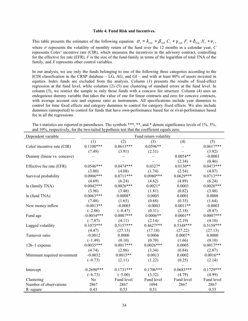
34

Table 4. Fund Risk and Incentives. This table presents the estimates of the following equation: iiriskiriskiriskriski XFC νδγβλσ ++++= , where s represents the volatility of monthly return of the fund over the 12 months in a calendar year, C represents Coles’ incentive rate (CIR), which measures the incentives in the advisory contract, controlling for the effective fee rate (EFR), F is the size of the fund-family in terms of the logarithm of total TNA of the family, and X represents other control variables. In our analysis, we use only the funds belonging to one of the following three categories according to the ICDI classification in the CRSP database – LG, AG, and GI – and with at least 80% of assets invested in equities. Index funds are excluded from the analysis. Column (1) presents the results of fixed-effect regression at the fund level, while columns (2)–(5) use clustering of standard errors at the fund level. In column (3), we restrict the sample to only those funds with a concave fee structure. Column (4) uses an endogenous dummy variable that takes the value of one for linear contracts and zero for concave contracts, with average account size and expense ratio as instruments. All specifications include year dummies to control for time fixed effects and category dummies to control for category fixed effects. We also include dummies (unreported) to control for funds that have own-performance based fee or rival-performance based fee in all the regressions. The t-statistics are reported in parentheses. The symbols ***, **, and * denote significance levels of 1%, 5%, and 10%, respectively, for the two-tailed hypothesis test that the coefficient equals zero.

Dependent variable Fund return volatility (1) (2) (3) (4) (5) Coles' incentive rate (CIR) 0.1100*** 0.0613*** 0.0596** – 0.0617*** (7.49) (3.91) (2.31) – (3.92) Dummy (linear vs. concave) – – – 0.0054** –0.0003 – – – (2.34) (0.46) Effective fee rate (EFR) 0.0546*** 0.0474*** 0.0327* 0.0130** 0.0473*** (3.00) (4.08) (1.74) (2.54) (4.07) Survival probability 0.0906*** 0.0711*** 0.0980*** 0.0629*** 0.0713*** (4.69) (6.24) (4.62) (4.89) (6.24) ln (family TNA) 0.0042*** 0.0026*** 0.0021* 0.0003 0.0026*** (3.96) (3.48) (1.81) (0.82) (3.48) ln (fund TNA) 0.0063*** 0.0008* 0.0005 0.0001 0.0008 (7.48) (1.65) (0.68) (0.35) (1.64) New money inflow –0.0013** –0.0003 –0.0003 0.0011** –0.0003 (–2.06) (–0.47) (0.31) (2.18) (0.47) Fund age –0.0034*** 0.0007*** 0.0006** 0.0001** 0.0007*** (–7.87) (4.11) (2.14) (2.19) (4.10) Lagged volatility 0.1075*** 0.5157*** 0.4627*** 0.5348*** 0.5158*** (4.47) (27.15) (17.18) (27.22) (27.13) Turnover ratio –0.0012 0.0000 0.0006 0.0007* 0.0000 (–1.49) (0.10) (0.70) (1.66) (0.10) 12b–1 expense 0.0035*** 0.0017*** 0.0026*** 0.0005 0.0017*** (4.74) (2.86) (3.34) (0.84) (2.87) Minimum required investment –0.0032 0.0015** 0.0013 0.0002 0.0016** (–0.73) (2.11) (1.22) (0.25) (2.14)

Intercept –0.2690*** –

0.1731*** –

0.1706*** –

0.0683*** –

0.1729*** (–6.73) (–5.00) (3.32) (4.79) (4.99) Clustering No Fund level Fund level Fund level Fund level Number of observations 2867 2867 1094 2867 2867 R–square 0.43 0.53 0.51 – 0.53

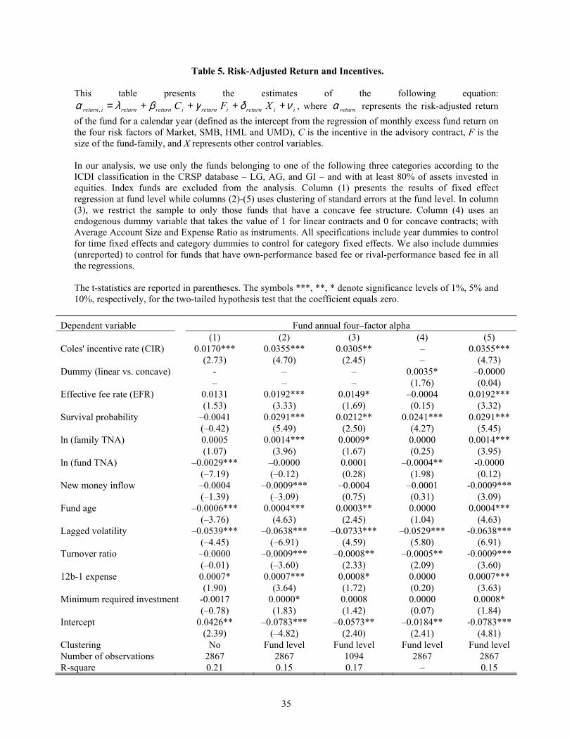
35

Table 5. Risk-Adjusted Return and Incentives. This table presents the estimates of the following equation:

iireturnireturnireturnreturnireturn XFC νδγβλα ++++=, , where returnα represents the risk-adjusted return of the fund for a calendar year (defined as the intercept from the regression of monthly excess fund return on the four risk factors of Market, SMB, HML and UMD), C is the incentive in the advisory contract, F is the size of the fund-family, and X represents other control variables. In our analysis, we use only the funds belonging to one of the following three categories according to the ICDI classification in the CRSP database – LG, AG, and GI – and with at least 80% of assets invested in equities. Index funds are excluded from the analysis. Column (1) presents the results of fixed effect regression at fund level while columns (2)-(5) uses clustering of standard errors at the fund level. In column (3), we restrict the sample to only those funds that have a concave fee structure. Column (4) uses an endogenous dummy variable that takes the value of 1 for linear contracts and 0 for concave contracts; with Average Account Size and Expense Ratio as instruments. All specifications include year dummies to control for time fixed effects and category dummies to control for category fixed effects. We also include dummies (unreported) to control for funds that have own-performance based fee or rival-performance based fee in all the regressions. The t-statistics are reported in parentheses. The symbols ***, **, * denote significance levels of 1%, 5% and 10%, respectively, for the two-tailed hypothesis test that the coefficient equals zero.

Dependent variable Fund annual four–factor alpha (1) (2) (3) (4) (5) Coles' incentive rate (CIR) 0.0170*** 0.0355*** 0.0305** – 0.0355*** (2.73) (4.70) (2.45) – (4.73) Dummy (linear vs. concave) - – – 0.0035* –0.0000 – – – (1.76) (0.04) Effective fee rate (EFR) 0.0131 0.0192*** 0.0149* –0.0004 0.0192*** (1.53) (3.33) (1.69) (0.15) (3.32) Survival probability –0.0041 0.0291*** 0.0212** 0.0241*** 0.0291*** (–0.42) (5.49) (2.50) (4.27) (5.45) ln (family TNA) 0.0005 0.0014*** 0.0009* 0.0000 0.0014*** (1.07) (3.96) (1.67) (0.25) (3.95) ln (fund TNA) –0.0029*** –0.0000 0.0001 –0.0004** -0.0000 (–7.19) (–0.12) (0.28) (1.98) (0.12) New money inflow –0.0004 –0.0009*** –0.0004 –0.0001 -0.0009*** (–1.39) (–3.09) (0.75) (0.31) (3.09) Fund age –0.0006*** 0.0004*** 0.0003** 0.0000 0.0004*** (–3.76) (4.63) (2.45) (1.04) (4.63) Lagged volatility –0.0539*** –0.0638*** –0.0733*** –0.0529*** -0.0638*** (–4.45) (–6.91) (4.59) (5.80) (6.91) Turnover ratio –0.0000 –0.0009*** –0.0008** –0.0005** -0.0009*** (–0.01) (–3.60) (2.33) (2.09) (3.60) 12b-1 expense 0.0007* 0.0007*** 0.0008* 0.0000 0.0007*** (1.90) (3.64) (1.72) (0.20) (3.63) Minimum required investment -0.0017 0.0000* 0.0008 0.0000 0.0008* (–0.78) (1.83) (1.42) (0.07) (1.84) Intercept 0.0426** –0.0783*** –0.0573** –0.0184** -0.0783*** (2.39) (–4.82) (2.40) (2.41) (4.81) Clustering No Fund level Fund level Fund level Fund level Number of observations 2867 2867 1094 2867 2867 R-square 0.21 0.15 0.17 – 0.15

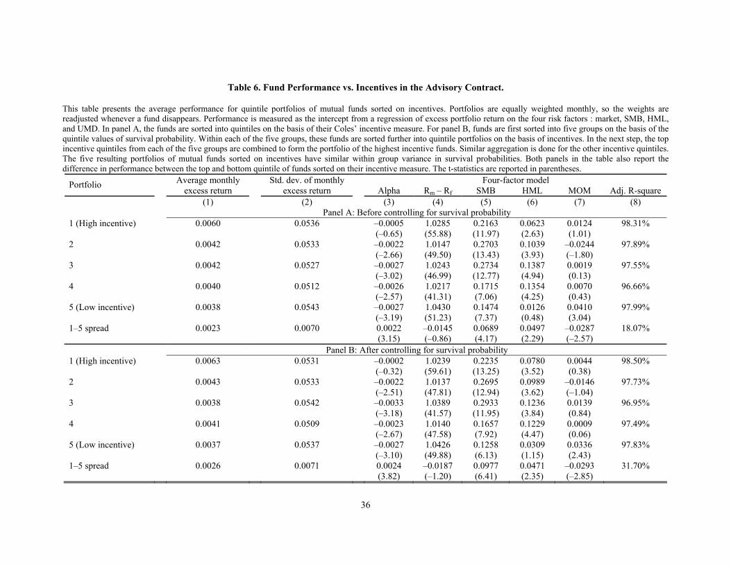
36

Table 6. Fund Performance vs. Incentives in the Advisory Contract. This table presents the average performance for quintile portfolios of mutual funds sorted on incentives. Portfolios are equally weighted monthly, so the weights are readjusted whenever a fund disappears. Performance is measured as the intercept from a regression of excess portfolio return on the four risk factors : market, SMB, HML, and UMD. In panel A, the funds are sorted into quintiles on the basis of their Coles’ incentive measure. For panel B, funds are first sorted into five groups on the basis of the quintile values of survival probability. Within each of the five groups, these funds are sorted further into quintile portfolios on the basis of incentives. In the next step, the top incentive quintiles from each of the five groups are combined to form the portfolio of the highest incentive funds. Similar aggregation is done for the other incentive quintiles. The five resulting portfolios of mutual funds sorted on incentives have similar within group variance in survival probabilities. Both panels in the table also report the difference in performance between the top and bottom quintile of funds sorted on their incentive measure. The t-statistics are reported in parentheses.

Four-factor model Portfolio Average monthly

excess return Std. dev. of monthly

excess return Alpha Rm – Rf SMB HML MOM Adj. R-square (1) (2) (3) (4) (5) (6) (7) (8) Panel A: Before controlling for survival probability 1 (High incentive) 0.0060 0.0536 –0.0005 1.0285 0.2163 0.0623 0.0124 98.31% (–0.65) (55.88) (11.97) (2.63) (1.01) 2 0.0042 0.0533 –0.0022 1.0147 0.2703 0.1039 –0.0244 97.89% (–2.66) (49.50) (13.43) (3.93) (–1.80) 3 0.0042 0.0527 –0.0027 1.0243 0.2734 0.1387 0.0019 97.55% (–3.02) (46.99) (12.77) (4.94) (0.13) 4 0.0040 0.0512 –0.0026 1.0217 0.1715 0.1354 0.0070 96.66% (–2.57) (41.31) (7.06) (4.25) (0.43) 5 (Low incentive) 0.0038 0.0543 –0.0027 1.0430 0.1474 0.0126 0.0410 97.99% (–3.19) (51.23) (7.37) (0.48) (3.04) 1–5 spread 0.0023 0.0070 0.0022 –0.0145 0.0689 0.0497 –0.0287 18.07% (3.15) (–0.86) (4.17) (2.29) (–2.57) Panel B: After controlling for survival probability 1 (High incentive) 0.0063 0.0531 –0.0002 1.0239 0.2235 0.0780 0.0044 98.50% (–0.32) (59.61) (13.25) (3.52) (0.38) 2 0.0043 0.0533 –0.0022 1.0137 0.2695 0.0989 –0.0146 97.73% (–2.51) (47.81) (12.94) (3.62) (–1.04) 3 0.0038 0.0542 –0.0033 1.0389 0.2933 0.1236 0.0139 96.95% (–3.18) (41.57) (11.95) (3.84) (0.84) 4 0.0041 0.0509 –0.0023 1.0140 0.1657 0.1229 0.0009 97.49% (–2.67) (47.58) (7.92) (4.47) (0.06) 5 (Low incentive) 0.0037 0.0537 –0.0027 1.0426 0.1258 0.0309 0.0336 97.83% (–3.10) (49.88) (6.13) (1.15) (2.43) 1–5 spread 0.0026 0.0071 0.0024 –0.0187 0.0977 0.0471 –0.0293 31.70% (3.82) (–1.20) (6.41) (2.35) (–2.85)

37

Table 7. Fund Performance and Incentives within Groups Sorted on Fund Characteristics.

This table presents the average performance for quintile portfolios of mutual funds sorted on incentives within tercile groups formed on the basis of one of the three following fund characteristics: size, age, and portfolio illiquidity. We use the square-root version of the Amihud illiquidity ratio as the measure of stock illiquidity. The portfolio illiquidity of a mutual fund is then calculated as the value-weighted average of the individual stock’s illiquidity in the portfolio of the

fund. Specifically, ∑=j

jtjtit IIlliq 2θ , where it

jtjtjt TNA

Pn=θ is the portfolio weight in stock j at time t in the portfolio of the fund i and I2 is defined as the

average of the square-root of the ratio between absolute return and volume for a given stock, i.e. jtjtjt VolrI /2 = .

Mutual funds are sorted first into three groups on the basis of their characteristics, and within each group they are sorted further into quintiles on the basis of Coles’ incentive rate. Portfolios are equally weighted monthly, so the weights are readjusted whenever a fund disappears. Performance is measured as the intercept from a regression of excess portfolio return on the four risk factors commonly used in the literature: market, SMB, HML, and UMD.

iffi UMDHMLSMBrMKTrR εββββα ++++−+=− 4321 )( The table also reports the difference in performance between the top and bottom quintiles of funds sorted on their incentive measure. The table reports only the estimates of the intercept and their t-statistic.

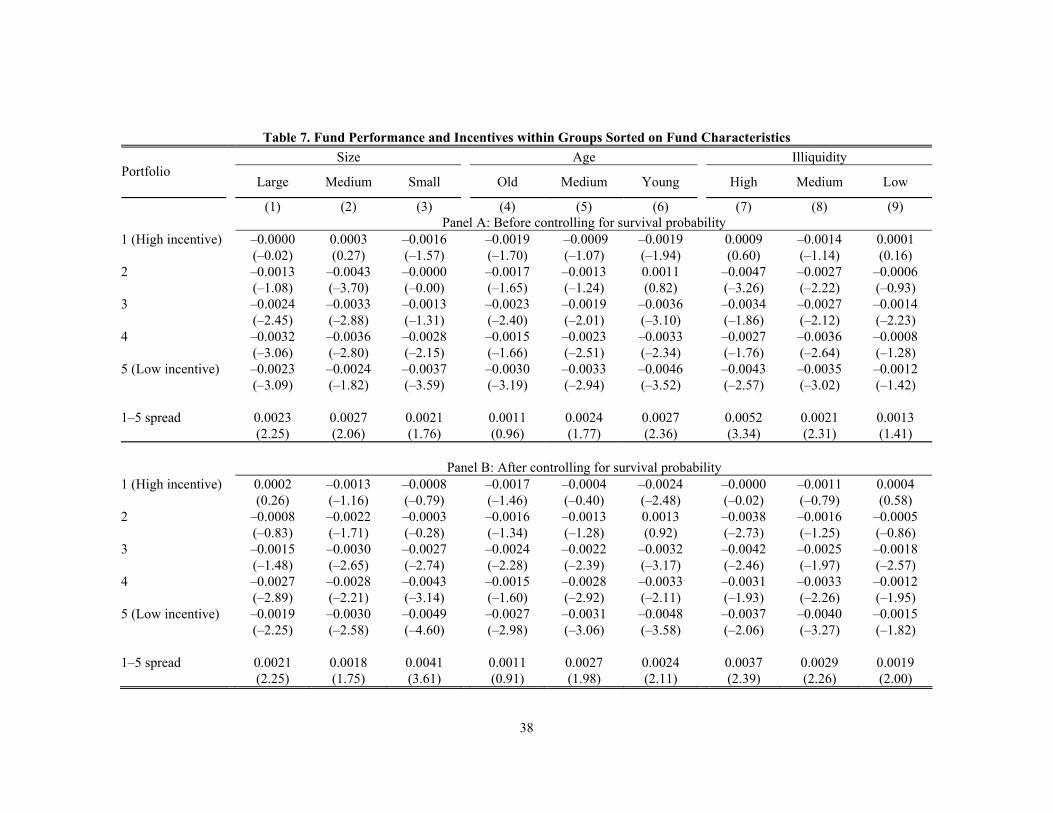
38

Table 7. Fund Performance and Incentives within Groups Sorted on Fund Characteristics

Size Age Illiquidity Portfolio

Large Medium Small Old Medium Young High Medium Low

(1) (2) (3) (4) (5) (6) (7) (8) (9) Panel A: Before controlling for survival probability 1 (High incentive) –0.0000 0.0003 –0.0016 –0.0019 –0.0009 –0.0019 0.0009 –0.0014 0.0001 (–0.02) (0.27) (–1.57) (–1.70) (–1.07) (–1.94) (0.60) (–1.14) (0.16) 2 –0.0013 –0.0043 –0.0000 –0.0017 –0.0013 0.0011 –0.0047 –0.0027 –0.0006 (–1.08) (–3.70) (–0.00) (–1.65) (–1.24) (0.82) (–3.26) (–2.22) (–0.93) 3 –0.0024 –0.0033 –0.0013 –0.0023 –0.0019 –0.0036 –0.0034 –0.0027 –0.0014 (–2.45) (–2.88) (–1.31) (–2.40) (–2.01) (–3.10) (–1.86) (–2.12) (–2.23) 4 –0.0032 –0.0036 –0.0028 –0.0015 –0.0023 –0.0033 –0.0027 –0.0036 –0.0008 (–3.06) (–2.80) (–2.15) (–1.66) (–2.51) (–2.34) (–1.76) (–2.64) (–1.28) 5 (Low incentive) –0.0023 –0.0024 –0.0037 –0.0030 –0.0033 –0.0046 –0.0043 –0.0035 –0.0012 (–3.09) (–1.82) (–3.59) (–3.19) (–2.94) (–3.52) (–2.57) (–3.02) (–1.42) 1–5 spread 0.0023 0.0027 0.0021 0.0011 0.0024 0.0027 0.0052 0.0021 0.0013 (2.25) (2.06) (1.76) (0.96) (1.77) (2.36) (3.34) (2.31) (1.41) Panel B: After controlling for survival probability 1 (High incentive) 0.0002 –0.0013 –0.0008 –0.0017 –0.0004 –0.0024 –0.0000 –0.0011 0.0004 (0.26) (–1.16) (–0.79) (–1.46) (–0.40) (–2.48) (–0.02) (–0.79) (0.58) 2 –0.0008 –0.0022 –0.0003 –0.0016 –0.0013 0.0013 –0.0038 –0.0016 –0.0005 (–0.83) (–1.71) (–0.28) (–1.34) (–1.28) (0.92) (–2.73) (–1.25) (–0.86) 3 –0.0015 –0.0030 –0.0027 –0.0024 –0.0022 –0.0032 –0.0042 –0.0025 –0.0018 (–1.48) (–2.65) (–2.74) (–2.28) (–2.39) (–3.17) (–2.46) (–1.97) (–2.57) 4 –0.0027 –0.0028 –0.0043 –0.0015 –0.0028 –0.0033 –0.0031 –0.0033 –0.0012 (–2.89) (–2.21) (–3.14) (–1.60) (–2.92) (–2.11) (–1.93) (–2.26) (–1.95) 5 (Low incentive) –0.0019 –0.0030 –0.0049 –0.0027 –0.0031 –0.0048 –0.0037 –0.0040 –0.0015 (–2.25) (–2.58) (–4.60) (–2.98) (–3.06) (–3.58) (–2.06) (–3.27) (–1.82) 1–5 spread 0.0021 0.0018 0.0041 0.0011 0.0027 0.0024 0.0037 0.0029 0.0019 (2.25) (1.75) (3.61) (0.91) (1.98) (2.11) (2.39) (2.26) (2.00)

39

Table 8. Performance Persistence and Incentives.

On 31 December of each year for the period 1996–2003, mutual funds are sorted first into quintile portfolios on the basis of their calendar year alphas from a four-factor model in panel A. Within each quintile portfolio, funds then are sorted further into five groups on the basis of the quintile values of Coles’ incentive rate. For each alpha-based quintile portfolio, we classify the top incentive quintile as the high-incentive group and the bottom incentive quintile as the low-incentive group. For the following year (t+1), funds with the highest alphas in year t comprise quintile 1 and funds with the lowest alphas comprise quintile 5. In panel B, mutual funds are sorted first into five groups each year on the basis of the quintile values of survival probability. On 31 December of each year, mutual funds within each quintile group based on survival probability then are sorted further into quintile portfolios on the basis of their calendar year alphas from a four-factor model. In the next step, the top alpha quintiles from each of the five survival groups are combined to form the portfolio of the highest alpha funds. Similar aggregation is done for the other alpha-based quintile portfolios. The five resulting portfolios of mutual funds sorted on alphas have similar within group variance in survival probabilities. Then within each quintile portfolio, funds are further sorted into five groups based on the quintile values of Coles’ incentive rate. For each alpha-based quintile portfolio, we classify the top incentive quintile as the high incentive group and the bottom incentive quintile as the low incentive group. For the following year (t+1), funds with the highest alphas in year t comprise quintile 1 and funds with the lowest alphas comprise quintile 5. The portfolios are equally weighted monthly, so that the weights are readjusted whenever a fund disappears. The portfolios of funds are rebalanced every year. To capture the difference in performance, we also form a spread portfolio between quintile 1 and quintile 5 for each of the two incentive groups. We also form two long-short portfolios. The first portfolio is long in funds that belong to the top alpha quintile in the high-incentive group and short in funds that belong to the top alpha quintile in the low-incentive group. The second portfolio is long in the funds that belong to the bottom alpha quintile in the high-incentive group and short in the funds that belong to the bottom alpha quintile in the low-incentive group. The above procedure results in a total of 14 time-series of returns. The excess returns of the quintile portfolios and the returns on the spread and long-short portfolios are then regressed on the four risk factors of market, SMB, HML, and UMD. The reported alphas in the table are the intercept of this model. We also report the average and standard deviation of raw excess returns for the portfolios. The t-statistics are reported in parentheses.

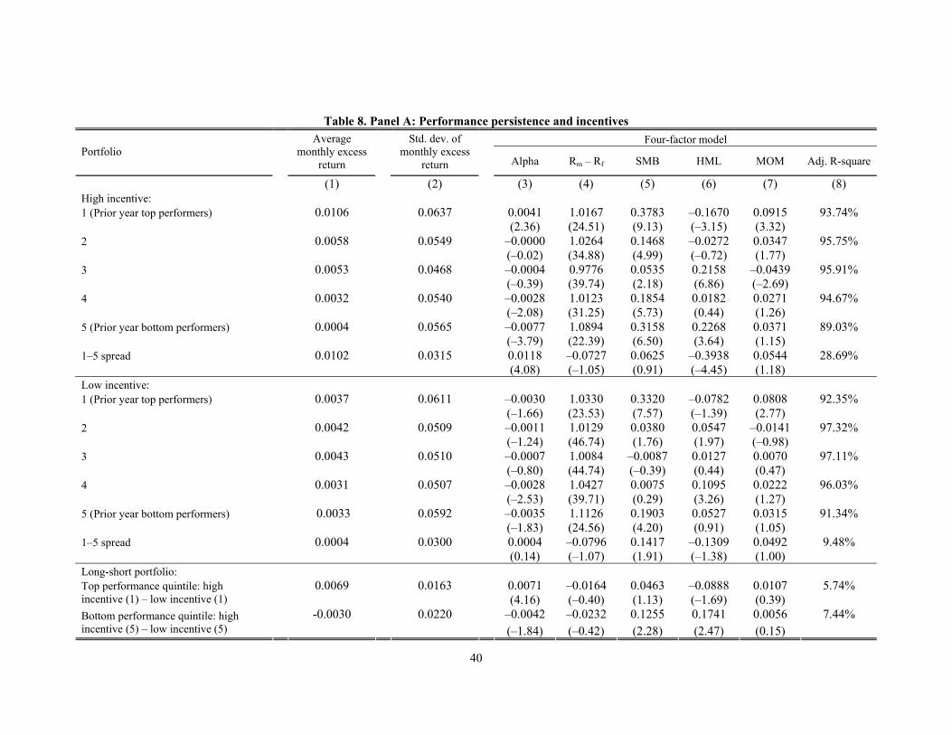
40

Table 8. Panel A: Performance persistence and incentives

Four-factor model Portfolio

Average monthly excess

return

Std. dev. of monthly excess

return Alpha Rm – Rf SMB HML MOM Adj. R-square

(1) (2) (3) (4) (5) (6) (7) (8) High incentive: 1 (Prior year top performers) 0.0106 0.0637 0.0041 1.0167 0.3783 –0.1670 0.0915 93.74% (2.36) (24.51) (9.13) (–3.15) (3.32) 2 0.0058 0.0549 –0.0000 1.0264 0.1468 –0.0272 0.0347 95.75% (–0.02) (34.88) (4.99) (–0.72) (1.77) 3 0.0053 0.0468 –0.0004 0.9776 0.0535 0.2158 –0.0439 95.91% (–0.39) (39.74) (2.18) (6.86) (–2.69) 4 0.0032 0.0540 –0.0028 1.0123 0.1854 0.0182 0.0271 94.67% (–2.08) (31.25) (5.73) (0.44) (1.26) 5 (Prior year bottom performers) 0.0004 0.0565 –0.0077 1.0894 0.3158 0.2268 0.0371 89.03% (–3.79) (22.39) (6.50) (3.64) (1.15) 1–5 spread 0.0102 0.0315 0.0118 –0.0727 0.0625 –0.3938 0.0544 28.69% (4.08) (–1.05) (0.91) (–4.45) (1.18) Low incentive: 1 (Prior year top performers) 0.0037 0.0611 –0.0030 1.0330 0.3320 –0.0782 0.0808 92.35% (–1.66) (23.53) (7.57) (–1.39) (2.77) 2 0.0042 0.0509 –0.0011 1.0129 0.0380 0.0547 –0.0141 97.32% (–1.24) (46.74) (1.76) (1.97) (–0.98) 3 0.0043 0.0510 –0.0007 1.0084 –0.0087 0.0127 0.0070 97.11% (–0.80) (44.74) (–0.39) (0.44) (0.47) 4 0.0031 0.0507 –0.0028 1.0427 0.0075 0.1095 0.0222 96.03% (–2.53) (39.71) (0.29) (3.26) (1.27) 5 (Prior year bottom performers) 0.0033 0.0592 –0.0035 1.1126 0.1903 0.0527 0.0315 91.34% (–1.83) (24.56) (4.20) (0.91) (1.05) 1–5 spread 0.0004 0.0300 0.0004 –0.0796 0.1417 –0.1309 0.0492 9.48% (0.14) (–1.07) (1.91) (–1.38) (1.00) Long-short portfolio:

0.0069 0.0163 0.0071 –0.0164 0.0463 –0.0888 0.0107 5.74% Top performance quintile: high incentive (1) – low incentive (1) (4.16) (–0.40) (1.13) (–1.69) (0.39)

-0.0030 0.0220 –0.0042 –0.0232 0.1255 0.1741 0.0056 7.44% Bottom performance quintile: high incentive (5) – low incentive (5) (–1.84) (–0.42) (2.28) (2.47) (0.15)

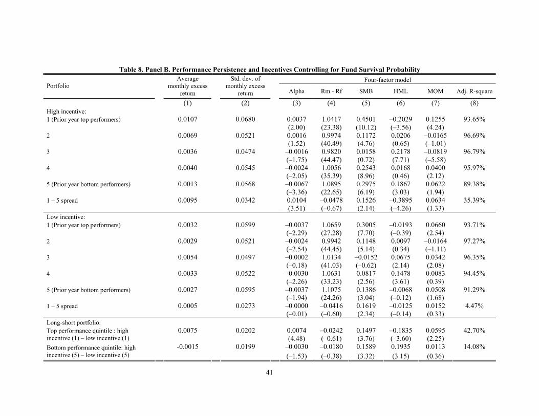
41

Table 8. Panel B. Performance Persistence and Incentives Controlling for Fund Survival Probability

Four-factor model Portfolio

Average monthly excess

return

Std. dev. of monthly excess

return Alpha Rm - Rf SMB HML MOM Adj. R-square

(1) (2) (3) (4) (5) (6) (7) (8) High incentive: 1 (Prior year top performers) 0.0107 0.0680 0.0037 1.0417 0.4501 –0.2029 0.1255 93.65% (2.00) (23.38) (10.12) (–3.56) (4.24) 2 0.0069 0.0521 0.0016 0.9974 0.1172 0.0206 –0.0165 96.69% (1.52) (40.49) (4.76) (0.65) (–1.01) 3 0.0036 0.0474 –0.0016 0.9820 0.0158 0.2178 –0.0819 96.79% (–1.75) (44.47) (0.72) (7.71) (–5.58) 4 0.0040 0.0545 –0.0024 1.0056 0.2543 0.0168 0.0400 95.97% (–2.05) (35.39) (8.96) (0.46) (2.12) 5 (Prior year bottom performers) 0.0013 0.0568 –0.0067 1.0895 0.2975 0.1867 0.0622 89.38% (–3.36) (22.65) (6.19) (3.03) (1.94) 1 – 5 spread 0.0095 0.0342 0.0104 –0.0478 0.1526 –0.3895 0.0634 35.39% (3.51) (–0.67) (2.14) (–4.26) (1.33) Low incentive: 1 (Prior year top performers) 0.0032 0.0599 –0.0037 1.0659 0.3005 –0.0193 0.0660 93.71% (–2.29) (27.28) (7.70) (–0.39) (2.54) 2 0.0029 0.0521 –0.0024 0.9942 0.1148 0.0097 –0.0164 97.27% (–2.54) (44.45) (5.14) (0.34) (–1.11) 3 0.0054 0.0497 –0.0002 1.0134 –0.0152 0.0675 0.0342 96.35% (–0.18) (41.03) (–0.62) (2.14) (2.08) 4 0.0033 0.0522 –0.0030 1.0631 0.0817 0.1478 0.0083 94.45% (–2.26) (33.23) (2.56) (3.61) (0.39) 5 (Prior year bottom performers) 0.0027 0.0595 –0.0037 1.1075 0.1386 –0.0068 0.0508 91.29% (–1.94) (24.26) (3.04) (–0.12) (1.68) 1 – 5 spread 0.0005 0.0273 –0.0000 –0.0416 0.1619 –0.0125 0.0152 4.47% (–0.01) (–0.60) (2.34) (–0.14) (0.33) Long-short portfolio:

0.0075 0.0202 0.0074 –0.0242 0.1497 –0.1835 0.0595 42.70% Top performance quintile : high incentive (1) – low incentive (1) (4.48) (–0.61) (3.76) (–3.60) (2.25)

-0.0015 0.0199 –0.0030 –0.0180 0.1589 0.1935 0.0113 14.08% Bottom performance quintile: high incentive (5) – low incentive (5) (–1.53) (–0.38) (3.32) (3.15) (0.36)

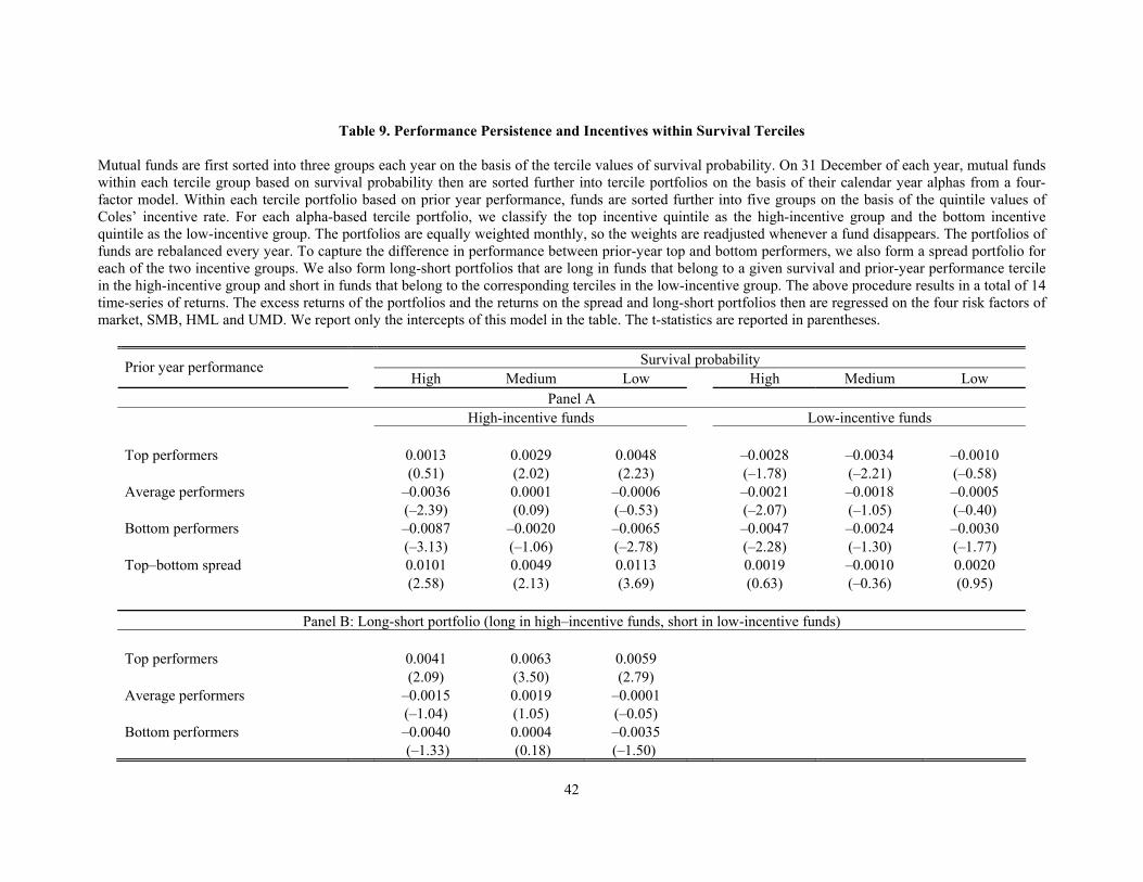
42

Table 9. Performance Persistence and Incentives within Survival Terciles Mutual funds are first sorted into three groups each year on the basis of the tercile values of survival probability. On 31 December of each year, mutual funds within each tercile group based on survival probability then are sorted further into tercile portfolios on the basis of their calendar year alphas from a four-factor model. Within each tercile portfolio based on prior year performance, funds are sorted further into five groups on the basis of the quintile values of Coles’ incentive rate. For each alpha-based tercile portfolio, we classify the top incentive quintile as the high-incentive group and the bottom incentive quintile as the low-incentive group. The portfolios are equally weighted monthly, so the weights are readjusted whenever a fund disappears. The portfolios of funds are rebalanced every year. To capture the difference in performance between prior-year top and bottom performers, we also form a spread portfolio for each of the two incentive groups. We also form long-short portfolios that are long in funds that belong to a given survival and prior-year performance tercile in the high-incentive group and short in funds that belong to the corresponding terciles in the low-incentive group. The above procedure results in a total of 14 time-series of returns. The excess returns of the portfolios and the returns on the spread and long-short portfolios then are regressed on the four risk factors of market, SMB, HML and UMD. We report only the intercepts of this model in the table. The t-statistics are reported in parentheses.

Survival probability Prior year performance High Medium Low High Medium Low

Panel A High-incentive funds Low-incentive funds Top performers 0.0013 0.0029 0.0048 –0.0028 –0.0034 –0.0010 (0.51) (2.02) (2.23) (–1.78) (–2.21) (–0.58) Average performers –0.0036 0.0001 –0.0006 –0.0021 –0.0018 –0.0005 (–2.39) (0.09) (–0.53) (–2.07) (–1.05) (–0.40) Bottom performers –0.0087 –0.0020 –0.0065 –0.0047 –0.0024 –0.0030 (–3.13) (–1.06) (–2.78) (–2.28) (–1.30) (–1.77) Top–bottom spread 0.0101 0.0049 0.0113 0.0019 –0.0010 0.0020 (2.58) (2.13) (3.69) (0.63) (–0.36) (0.95)

Panel B: Long-short portfolio (long in high–incentive funds, short in low-incentive funds) Top performers 0.0041 0.0063 0.0059 (2.09) (3.50) (2.79) Average performers –0.0015 0.0019 –0.0001 (–1.04) (1.05) (–0.05) Bottom performers –0.0040 0.0004 –0.0035 (–1.33) (0.18) (–1.50)

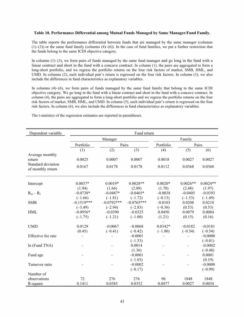
43

Table 10. Performance Differential among Mutual Funds Managed by Same Manager/Fund Family. The table reports the performance differential between funds that are managed by the same manager (columns (1)–(3)) or the same fund family (columns (4)–(6)). In the case of fund families, we put a further restriction that the funds belong to the same ICDI objective category. In columns (1)–(3), we form pairs of funds managed by the same fund manager and go long in the fund with a linear contract and short in the fund with a concave contract. In column (1), the pairs are aggregated to form a long-short portfolio, and we regress the portfolio returns on the four risk factors of market, SMB, HML, and UMD. In columns (2), each individual pair’s return is regressed on the four risk factors. In column (3), we also include the differences in fund characteristics as explanatory variables. In columns (4)–(6), we form pairs of funds managed by the same fund family that belong to the same ICDI objective category. We go long in the fund with a linear contract and short in the fund with a concave contract. In column (4), the pairs are aggregated to form a long-short portfolio and we regress the portfolio returns on the four risk factors of market, SMB, HML, and UMD. In column (5), each individual pair’s return is regressed on the four risk factors. In column (6), we also include the differences in fund characteristics as explanatory variables. The t-statistics of the regression estimates are reported in parentheses.

Dependent variable Fund return Manager Family Portfolio Pairs Portfolio Pairs

(1) (2) (3) (4) (5) (6) Average monthly return 0.0025 0.0007 0.0007 0.0018 0.0027 0.0027 Standard deviation of monthly return 0.0167 0.0178 0.0178 0.0112 0.0368 0.0368

Intercept 0.0037* 0.0019* 0.0028** 0.0020* 0.0026** 0.0024** (1.94) (1.66) (2.09) (1.70) (2.48) (1.97) Rm – Rf –0.0738* –0.0487* –0.0465* –0.0038 –0.0405 –0.0393 (–1.66) (–1.81) (–1.72) (–0.13) (–1.53) (–1.49) SMB –0.1519*** –0.0792*** –0.0765*** –0.0103 0.0208 0.0210 (–3.49) (–2.94) (–2.83) (–0.36) (0.53) (0.53) HML –0.0956* –0.0390 –0.0325 0.0450 0.0079 0.0084 (–1.75) (–1.21) (–1.00) (1.21) (0.15) (0.16)

UMD 0.0129 –0.0067 –0.0068 –

0.0342* –0.0182 –0.0181 (0.45) (–0.41) (–0.42) (–1.80) (–0.54) (–0.54) Effective fee rate – – –0.0001 – – –0.0000 (–1.53) (–0.01) ln (Fund TNA) – – 0.0014 – – –0.0002 (1.36) (–0.48) Fund age – – –0.0001 – – 0.0001 (–1.03) (0.19) Turnover ratio – – –0.0002 – – –0.0008 (–0.17) (–0.99) Number of observations 72 276 276 96 1848 1848 R-square 0.1411 0.0385 0.0352 0.0477 0.0027 0.0034

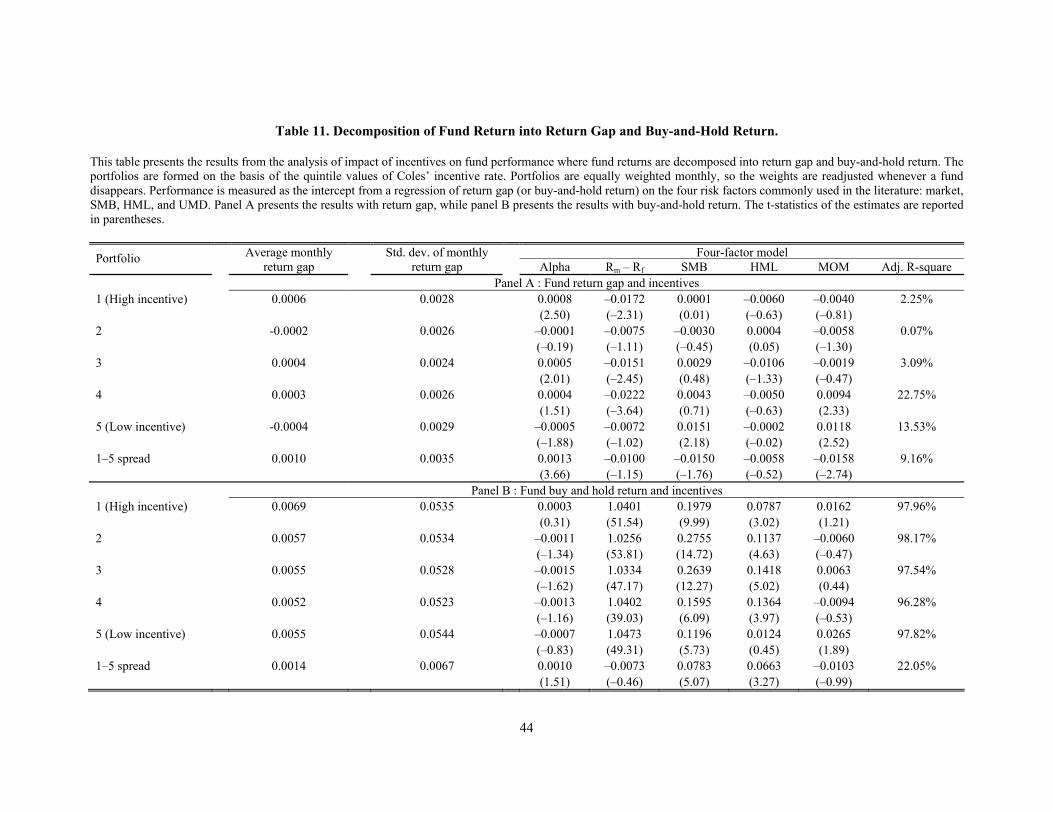
44

Table 11. Decomposition of Fund Return into Return Gap and Buy-and-Hold Return. This table presents the results from the analysis of impact of incentives on fund performance where fund returns are decomposed into return gap and buy-and-hold return. The portfolios are formed on the basis of the quintile values of Coles’ incentive rate. Portfolios are equally weighted monthly, so the weights are readjusted whenever a fund disappears. Performance is measured as the intercept from a regression of return gap (or buy-and-hold return) on the four risk factors commonly used in the literature: market, SMB, HML, and UMD. Panel A presents the results with return gap, while panel B presents the results with buy-and-hold return. The t-statistics of the estimates are reported in parentheses.

Four-factor modelPortfolio

Average monthly return gap

Std. dev. of monthly return gap Alpha Rm – Rf SMB HML MOM Adj. R-square

Panel A : Fund return gap and incentives 1 (High incentive) 0.0006 0.0028 0.0008 –0.0172 0.0001 –0.0060 –0.0040 2.25% (2.50) (–2.31) (0.01) (–0.63) (–0.81) 2 -0.0002 0.0026 –0.0001 –0.0075 –0.0030 0.0004 –0.0058 0.07% (–0.19) (–1.11) (–0.45) (0.05) (–1.30) 3 0.0004 0.0024 0.0005 –0.0151 0.0029 –0.0106 –0.0019 3.09% (2.01) (–2.45) (0.48) (–1.33) (–0.47) 4 0.0003 0.0026 0.0004 –0.0222 0.0043 –0.0050 0.0094 22.75% (1.51) (–3.64) (0.71) (–0.63) (2.33) 5 (Low incentive) -0.0004 0.0029 –0.0005 –0.0072 0.0151 –0.0002 0.0118 13.53% (–1.88) (–1.02) (2.18) (–0.02) (2.52) 1–5 spread 0.0010 0.0035 0.0013 –0.0100 –0.0150 –0.0058 –0.0158 9.16% (3.66) (–1.15) (–1.76) (–0.52) (–2.74) Panel B : Fund buy and hold return and incentives 1 (High incentive) 0.0069 0.0535 0.0003 1.0401 0.1979 0.0787 0.0162 97.96% (0.31) (51.54) (9.99) (3.02) (1.21) 2 0.0057 0.0534 –0.0011 1.0256 0.2755 0.1137 –0.0060 98.17% (–1.34) (53.81) (14.72) (4.63) (–0.47) 3 0.0055 0.0528 –0.0015 1.0334 0.2639 0.1418 0.0063 97.54% (–1.62) (47.17) (12.27) (5.02) (0.44) 4 0.0052 0.0523 –0.0013 1.0402 0.1595 0.1364 –0.0094 96.28% (–1.16) (39.03) (6.09) (3.97) (–0.53) 5 (Low incentive) 0.0055 0.0544 –0.0007 1.0473 0.1196 0.0124 0.0265 97.82% (–0.83) (49.31) (5.73) (0.45) (1.89) 1–5 spread 0.0014 0.0067 0.0010 –0.0073 0.0783 0.0663 –0.0103 22.05% (1.51) (–0.46) (5.07) (3.27) (–0.99)

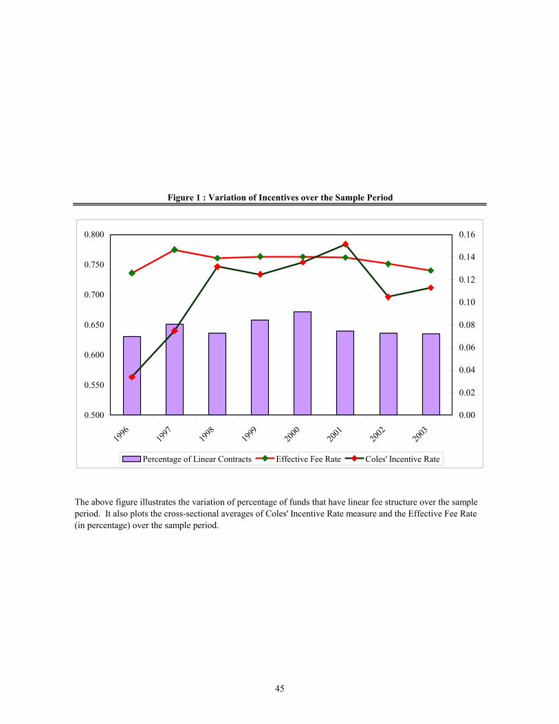
45

Figure 1 : Variation of Incentives over the Sample Period

The above figure illustrates the variation of percentage of funds that have linear fee structure over the sample period. It also plots the cross-sectional averages of Coles' Incentive Rate measure and the Effective Fee Rate (in percentage) over the sample period.

0.500

0.550

0.600

0.650

0.700

0.750

0.800

1996

1997

1998

1999

2000

2001

2002

2003

0.00

0.02

0.04

0.06

0.08

0.10

0.12

0.14

0.16

Percentage of Linear Contracts Effective Fee Rate Coles' Incentive Rate

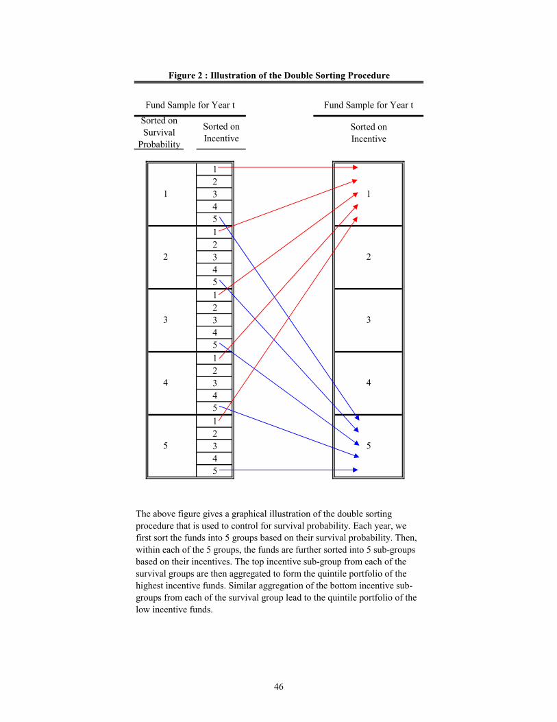
46

Sorted on Incentive

1234512345123451234512345

Fund Sample for Year tSorted on Survival

Probability

4

1

2

3

The above figure gives a graphical illustration of the double sorting procedure that is used to control for survival probability. Each year, we first sort the funds into 5 groups based on their survival probability. Then, within each of the 5 groups, the funds are further sorted into 5 sub-groups based on their incentives. The top incentive sub-group from each of the survival groups are then aggregated to form the quintile portfolio of the highest incentive funds. Similar aggregation of the bottom incentive sub-groups from each of the survival group lead to the quintile portfolio of the low incentive funds.

Fund Sample for Year t

Figure 2 : Illustration of the Double Sorting Procedure

5

Sorted on Incentive

1

2

3

4

5