Embed Size (px)
Citation preview

Prepared in cooperation with National Park Service and U.S. Fish and Wildlife Service
A Decision Framework to Analyze Tide-Gate Options for Restoration of the Herring River Estuary, Massachusetts
Open-File Report 2019–1115U.S. Department of the InteriorU.S. Geological Survey

Cover. (Front) Diagram showing fundamental objectives for the restoration of the Herring River estuary: restoration of the hydrography, restoration of the ecological function and integrity, minimization of adverse effects, maximization of ecosystem services, and minimization of management costs. (Back, top) Aerial view of the Chequessett Neck Road Dike. Image from Google Earth. (Back, bottom) Concept drawing of replacement dike with tide gates fully opened. Artwork by Nils Wiberg, Fuss & O’Neill, Inc. Background photo shows the Chequessett Neck Road Dike looking upstream. Photograph by Timothy P. Smith, National Park Service.

A Decision Framework to Analyze Tide-Gate Options for Restoration of the Herring River Estuary, Massachusetts
By David R. Smith, Mitchell J. Eaton, Jill J. Gannon, Timothy P. Smith, Eric L. Derleth, Jonathan Katz, Kirk F. Bosma, and Elise Leduc
Prepared in cooperation with National Park Service and U.S. Fish and Wildlife Service
Open-File Report 2019–1115
U.S. Department of the InteriorU.S. Geological Survey

U.S. Department of the InteriorDAVID BERNHARDT, Secretary
U.S. Geological SurveyJames F. Reilly II, Director
U.S. Geological Survey, Reston, Virginia: 2020
For more information on the USGS—the Federal source for science about the Earth, its natural and living resources, natural hazards, and the environment—visit https://www.usgs.gov or call 1–888–ASK–USGS.
For an overview of USGS information products, including maps, imagery, and publications, visit https://store.usgs.gov.
Any use of trade, firm, or product names is for descriptive purposes only and does not imply endorsement by the U.S. Government.
Although this information product, for the most part, is in the public domain, it also may contain copyrighted materials as noted in the text. Permission to reproduce copyrighted items must be secured from the copyright owner.
Suggested citation:Smith, D.R., Eaton, M.J., Gannon, J.J., Smith, T.P., Derleth, E.L., Katz, J., Bosma, K.F., and Leduc, E., 2020, A decision framework to analyze tide-gate options for restoration of the Herring River Estuary, Massachusetts: U.S. Geological Survey Open-File Report 2019–1115, 42 p., https://doi.org/10.3133/ofr20191115.
ISSN 2331-1258 (online)

iii
Acknowledgments
The authors thank the Herring River Restoration Committee and Cape Cod National Seashore for support and active participation. The findings and conclusions in this article are those of the author(s) and do not necessarily represent the views of the U.S. Fish and Wildlife Service. Any use of trade, firm, or product names is for descriptive purposes only and does not imply endorsement by any of the authors’ institutions or affiliations.
iv
ContentsAcknowledgments ........................................................................................................................................iiiAbstract ...........................................................................................................................................................1Introduction.....................................................................................................................................................1Study Area.......................................................................................................................................................2Structuring the Decision Analysis ..............................................................................................................2
A Statement of the Problem ................................................................................................................2Definitions of the Objectives ...............................................................................................................4
Management Options ...............................................................................................................12Prediction of Option Consequences ...............................................................................................12
Evaluation of Tradeoffs .............................................................................................................15Implementation of an Option Through Time ...................................................................................15
Prototype Decision Analysis and Results ................................................................................................18Next Steps .....................................................................................................................................................24Summary........................................................................................................................................................24References Cited..........................................................................................................................................25Appendix 1. Conceptual Models ...............................................................................................................27Appendix 2. Summary of Meeting with Herring River Restoration Committee to Elicit Utility
Curves...............................................................................................................................................32

v
Figures
1. Maps showing Herring River estuary and subbasins within Cape Cod National Seashore and towns of Wellfleet and Truro, Massachusetts ...............................................3
2. Objectives hierarchy showing the fundamental objectives and subobjectives for restoration of the hydrography, restoration of the ecological function and integrity, minimization of adverse effects, maximization of ecosystem services, and minimization of management costs .................................................................................10
3. Graphs showing effects of alternative gate operations on mean high water for the Herring River estuary, Massachusetts....................................................................................13
4. Example utility curves for selected objectives relating the level of a performance metric for hypothetical objectives to a standardized score between 0 and 1 based on preferences and risk attitude ..............................................................................................18
5. Graph showing the four weighting schemes applied to the fundamental objectives to evaluate outcomes .................................................................................................................20
6. Graph showing cumulative utility averaged across a range in prediction uncertainty and the four value-weighting schemes in figure 5 to compare seven tide-gate options in figure 3 ......................................................................................................21
7. Diagram showing frequencies of ranks based on cumulative utility after 25 years for seven options across a range in prediction uncertainty and the four value-weighting schemes in figure 5 ......................................................................................21
8. Double-column chart used to evaluate how effectively the tide-gate options address all objectives ................................................................................................................22
9. Graphs showing cumulative utility as a function of uncertainty formulated as the percentile for which confidence limits were computed for value weights: A, balanced, B, ecological, C, equal, and D, socioeconomic ..............................................23
Tables
1. Objectives of the Herring River estuary restoration decision support framework ...........5 2. The unweighted consequence table for the pilot tradeoff analysis ..................................16 3. Overall utility from the pilot tradeoff analysis ........................................................................19

vi
Conversion Factors
U.S. customary units to International System of Units
Multiply By To obtain
Length
inch (in.) 2.54 centimeter (cm)inch (in.) 25.4 millimeter (mm)
Area
acre 0.004047 square kilometer (km2)square mile (mi2) 2.590 square kilometer (km2)
Temperature in degrees Celsius (°C) may be converted to degrees Fahrenheit (°F) as follows:
°F = (1.8 × °C) + 32.
Temperature in degrees Fahrenheit (°F) may be converted to degrees Celsius (°C) as follows:
°C = (°F – 32) / 1.8.
DatumVertical coordinate information is referenced to the North American Vertical Datum of 1988 (NAVD 88).
Horizontal coordinate information is referenced to the North American Datum of 1983 (NAD 83).
Elevation, as used in this report, refers to distance above the vertical datum.
NOTE TO USGS USERS: Use of hectare (ha) as an alternative name for square hectometer (hm2) is restricted to the measurement of small land or water areas. Use of liter (L) as a special name for cubic decimeter (dm3) is restricted to the measurement of liquids and gases. No prefix other than milli should be used with liter. Metric ton (t) as a name for megagram (Mg) should be restricted to commercial usage, and no prefixes should be used with it.

vii
AbbreviationsCACO Cape Code National Seashore
CNR Chequesett Neck Road
CYCC Chequesett Yacht and Country Club
DOI U.S. Department of the Interior
EFDC Environmental Flow Dynamics Code
GHG Greenhouse gas
HREC Herring River Executive Council
HRRC Herring River Restoration Committee
MEM Marsh Equilibrium Model
MHW Mean high water
NPS National Park Service
SLAMM Sea Level Affecting Marsh Migration
USFWS U.S. Fish and Wildlife Service
USGS U.S. Geological Survey
T&E Threatened and endangered
WBNERR Waquoit Bay National Estuarine Research Reserve

viii

A Decision Framework to Analyze Tide-Gate Options for Restoration of the Herring River Estuary, Massachusetts
David R. Smith1, Mitchell J. Eaton2, Jill J. Gannon3, Timothy P. Smith4, Eric L. Derleth3, Jonathan Katz5, Kirk F. Bosma6, and Elise Leduc6
AbstractThe collective set of decisions involved with the res-
toration of degraded wetlands is often more complex than considering only ecological responses and outcomes. Restora-tion is commonly driven by a complex interaction of social, economic, and ecological factors representing the mandate of resource stewards and the values of stakeholders. The authors worked with the Herring River Restoration Committee (HRRC) to develop a decision framework to understand the implications of complex tradeoffs and to guide decision mak-ing for the restoration of the 1,100-acre Herring River estuary within Cape Cod National Seashore, which has been restricted from tidal influence for more than 100 years. The HRRC represents decision maker and stakeholder interests in the restoration process. For a 25-year planning horizon, decisions involve the rate at which newly constructed water-control structures allow tidal exchange, and the timing and location of implementing numerous secondary management options. Decisions affect multiple stakeholders, including residents of two adjacent towns who value the watershed for numer-ous benefits and whose economy relies on seasonal activities and aquaculture. System response to management decisions is characterized by a high degree of uncertainty and risk with positive and negative outcomes possible. Decision policies will affect biophysical (for example, sediment transport, dis-charge of fecal coliform bacteria) and ecological (for example, vegetation response, fish passage, effects on shellfish) pro-cesses, as well as socioeconomic interests (for example, effects on property, viewscapes, recreation). The framework provides a structured approach for evaluating tradeoffs among multiple objectives (ecological and social) while appropriately charac-terizing relevant uncertainties and accounting for levels of risk
tolerances and the values of decision makers and stakeholders. Consequences of tide-gate management options are predicted using a range of methods from quantitative physical process models to elicited expert judgement. The decision framework is presented, and the software developed to implement the tradeoff analysis is introduced. The results from an initial prototype analysis using a software application developed for analyses of tradeoffs and of sensitivity of the decision to risk and uncertainty are presented. The next step is to use the decision-support application to analyze options using improved predictions.
IntroductionEcological restoration is challenging, in part, because it is
not only about ecological endpoints, but also about socioeco-nomic concerns. The motivations driving our will to restore affected systems are based on values, which are complex and vary widely among stakeholders. Therefore, the goal of restor-ing the ecological function of a salt marsh stands alongside the need to avoid or at least minimize the adverse effects to stake-holder interests. Stakeholders, who might be affected by the restoration or who might affect how the restoration proceeds, can have vastly different, and at times conflicting, interests. In addition, uncertainty in restoration outcomes and variation in attitudes about risk contribute to the challenge of restora-tion decision making. Thus, restoration success or failure can be determined by whether tradeoffs among multiple interests and risks associated with uncertain outcomes are suitably evaluated.
Decision analysis (Raiffa and others, 2002; Goodwin and Wright, 2014) is designed to evaluate tradeoffs and risks. Decision analysis examines the available strategies by first considering multiple interests in the outcome, based on the best available information for predicting the consequences of implementing one or more strategies. A large body of literature from management science, operations research, and engineer-ing provides the foundation for decision analysis, which rep-resents the “best management practices” for decision making, especially for complex problems and group decisions (Raiffa and others, 2002). Decision analysis takes a deliberative
1U.S. Geological Survey.2Department of Interior, Southeast Climate Adaptation Science Center.3U.S. Fish and Wildlife Service.4National Park Service.5University of Vermont.6Woods Hole Group.

2 A Decision Framework to Analyze Tide-Gate Options for Restoration of the Herring River Estuary, Massachusetts
approach by providing options rather than advocating for a favored option. The process is transparent and explicit, can be documented, and is replicable, all of which can contribute to stakeholder acceptance of a decision. The decision analysis process guides decision makers towards a “good” decision that has the best chance of achieving the desired outcomes, while at the same time minimizing undesirable effects.
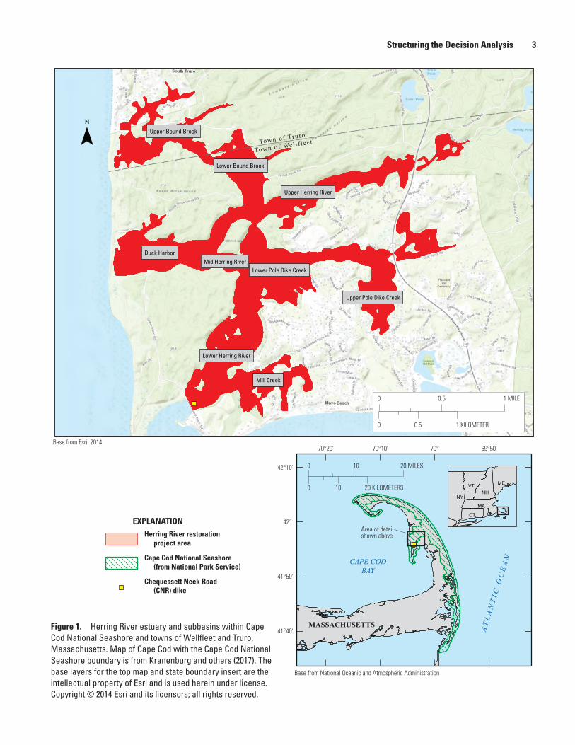
The tide gates at the Chequessett Neck Road (CNR) dike at the mouth of the Herring River (fig. 1) severely restrict tidal exchange and are the cause of severe ecological degradation to the estuary, which has been documented by on-site monitoring (Woods Hole Group, 2012; Cape Cod National Seashore and Herring River Restoration Committee, 2012). The degrada-tion has motivated resource managers to pursue restoration of the Herring River estuary. Decision analysis is appropri-ate for exploring alternatives for the restoration of Herring River because (1) public resources are being used to support public decision making, (2) there is a variety of public and private interests at stake, (3) there is uncertainty about how the system will respond to restoration actions, and (4) resto-ration will take time thus providing the opportunity to adapt through a repeated cycle of prediction, decision making, and targeted monitoring.
To develop a decision analysis framework for evaluating tide-gate options for the restoration of Herring River estuary, the authors worked with the Herring River Restoration Com-mittee (HRRC) to develop the decision framework through a series of meetings involving the committee and a workgroup formed for framework development. The HRRC represents decision maker and stakeholder interests in the restoration process. Workshops with stakeholders, science experts, and regulators helped those involved to better understand underly-ing issues, incorporate concerns and interests into the frame-work, and resolve technical questions. This report includes descriptions of the study area and the framework organized around the major decision components, followed by a discus-sion based on results from a prototype application of the deci-sion framework.
Study AreaThe 1,100-acre Herring River estuary lies within the
towns of Wellfleet and Truro and partly within National Park Service (NPS) Cape Cod National Seashore (CACO) (fig. 1). The full Herring River restoration project area encompasses approximately 890 acres that would be affected by monthly spring high tide; 80 percent of this area falls under Federal stewardship within the CACO boundary, whereas 20 percent is outside the boundary in one of these two municipalities. The Herring River is the largest river system within the CACO and one of the largest tidally restricted estuaries on Cape Cod. The estuary has experienced more than 100 years of ecologi-cal degradation resulting from construction of the CNR dike and up-estuary drainage that began in 1909 and has resulted
in the almost complete exclusion of tidal exchange to most of the estuary. The CNR dike is outside the CACO boundary and is managed by the town of Wellfleet. The restoration area includes several tributary streams separated into nine sub-basins: Herring River (lower, mid, and upper), Mill Creek, Pole Dike Creek (lower and upper), Duck Harbor, and Bound Brook (lower and upper). The restoration project covers a large area encompassing public and private lands and struc-tures, including a nine-hole golf course and an economically valuable oyster industry in Wellfleet Harbor.
Structuring the Decision AnalysisRaiffa and others (2002) and Hammond and others (2015)
recognized the major components of decisions and developed a structured approach for implementation of decision analy-sis that involves defining the problem, specifying measur-able objectives or interests, creating options or alternatives, predicting the consequences of these options relative to the objectives, and evaluating tradeoffs. The decision analysis for the Herring River restoration was structured according to six major components: 1. a clear statement of the problem,
2. comprehensive and measurable objectives,
3. a set of discrete tide-gate options,
4. a means to predict outcomes,
5. a process to evaluate the implications of these outcomes, and
6. a plan for implementation of a tide-gate option over time.
Monitoring will provide feedback to formally incorporate learning, reevaluate options, and possibly adapt management as restoration is implemented over time.
A Statement of the Problem
Representatives of Cape Cod National Seashore and the town of Wellfleet compose the Herring River Executive Council (HREC) and are responsible for restoring the Herring River estuary and minimizing adverse effects over some finite length of time (likely less than 25 years). The HREC will have ultimate responsibility for managing the new tide control gates at CNR, Mill Creek, and Pole Dike Creek and for implement-ing secondary management actions to achieve overall restora-tion goals. The HREC will receive decision recommendations from the HRRC, whose members are scientific and technical experts. The HREC will manage, directly or through contract, the project and implement gate operations and secondary management actions.
Structuring the Decision Analysis 3
Duck Harbor
Lower Herring River
Upper Bound Brook
Mill Creek
Upper Herring River
Lower Pole Dike Creek
Upper Pole Dike Creek
Lower Bound Brook
Mid Herring River
0 0.5 1 KILOMETER
0 0.5 1 MILE
CAPE CODBAY
MASSACHUSETTS AT
LA
NT
I C O
CE
AN
69°50'70°70°10'70°20'
42°10'
42°
41°50'
41°40'
CT
MA
NY
VTNH
ME0 10 20 KILOMETERS
0 10 20 MILES
Herring River restorationproject area
Cape Cod National Seashore(from National Park Service)
Chequessett Neck Road(CNR) dike
EXPLANATION
Base from Esri, 2014
Base from National Oceanic and Atmospheric Administration
Area of detailshown above
Town of Truro
Town of Wellf leet
Figure 1. Herring River estuary and subbasins within Cape Cod National Seashore and towns of Wellfleet and Truro, Massachusetts. Map of Cape Cod with the Cape Cod National Seashore boundary is from Kranenburg and others (2017). The base layers for the top map and state boundary insert are the intellectual property of Esri and is used herein under license. Copyright © 2014 Esri and its licensors; all rights reserved.

4 A Decision Framework to Analyze Tide-Gate Options for Restoration of the Herring River Estuary, Massachusetts
Broadly, project goals are to restore the natural hydrogra-phy (that is, tidal range and marsh surface elevation) and eco-logical integrity of the Herring River estuary, while minimizing adverse economic and social effects, maximizing the estuary’s production of ecosystem services, and minimizing management costs. The primary management actions adjust the volume of tidal flow through of a series of to-be-constructed tide gates at CNR, Mill Creek, and Pole Dike Creek; these actions require decisions on the number, location, magnitude of opening, and flow direction of the individual tide-gate openings at any given time. Timing and frequency of gate operations can be peri-odic or episodic; for example, gate opening can coincide with extreme high tides and storm events to facilitate movement of sediment farther upstream into the estuary. At each decision point, for example annually, gates can be configured to allow a greater, lesser, or the same volume of tidal flux into the estuary. In addition, project options include secondary management actions intended to accelerate the recovery of the estuarine hab-itat, enhance the benefits of tidal restoration achieved through tide-gate management alone, and reduce potential adverse ecological and socioeconomic effects of restoring tidal flow. Examples of secondary actions include management of flood-plain vegetation (for example, vegetation removal or planting), modification of marsh surface elevations through management of sediment supply and distribution, and restoration of con-nectivity and natural sinuosity of tidal creeks to enhance the circulation of saltwater through the system. Decisions regard-ing secondary actions involve where and when to implement management measures, what techniques to use, and how to coordinate the actions with the tide-gate management.
The operational phase of tide-gate management encom-passes the period of time when tidal flow increases until the gates are fully open and the maximum tidal range has been reached. Tide-gate management will cease after the gates are fully open, which is expected to take 25 years or less. The rate at which gates are opened varies among alternatives. In general, tide-gate management during the operational phase could occur 2–3 times a year and could be affected by season or tidal cycle. Secondary actions may be implemented before, during, and after the period of tide-gate management. Deci-sions involving management of the tide gates can be spatially and temporally divided by the subbasins within the project area. Tide-gate management decisions will begin as soon as construction of the tide-control structures is complete. Deci-sions regarding secondary actions may range from simple and independent of other decisions to complex and linked to other management actions requiring coordination with the tide-gate management. For example, removal of vegetation may be beneficial to occur prior to restoration of tidal exchange for logistical purposes or to minimize effects on the flood plain.
Tide-gate management decisions and secondary action decisions will be made (1) based on predicted outcomes of available actions with respect to the multiple project objectives and (2) given the uncertainty in system response to the actions taken. In general, varying degrees of uncertainty revolve around changes in tidal regime and salinity under different
tide-gate configurations and changes to vegetation, water qual-ity, sediment distribution, and other processes resulting from modifications to the hydrodynamics.
Decisions about tide-gate adjustments are subject to regu-latory oversight under the U.S. Clean Water Act [33 U.S.C. §1251 et seq. (1971)], the Massachusetts Wetlands Protection Act (General Laws of Massachusetts Chapter 131, §40) and Waterways Regulations (310 CMR 9.00), the Town of Well-fleet wetland by-laws, and the Massachusetts Endangered Spe-cies Act (321 CMR 10.00). Tide-gate decisions will be con-strained by the management actions required to protect public and private structures and property within the project area.
Definitions of the ObjectivesDefining the objectives starts with the issues deci-
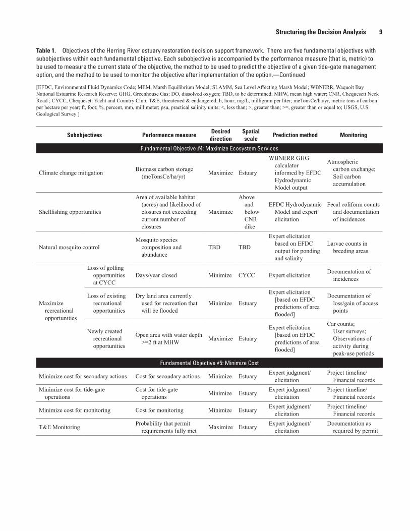
sion makers and stakeholders care about, what they want to achieve, and what they want to avoid (Gregory and Keeney, 2002; McGowan and others, 2015). For Herring River estuary restoration, the focus is on achieving ecological and socio-economic objectives. When the objectives are expressed as measurable attributes, the relative achievements of manage-ment alternatives can be compared to identify the option that best meets the objectives (Keeney and Gregory, 2005). Because achieving value for some objectives may come at the cost of other objectives, a formalized approach for evaluating tradeoffs among these objectives is often required. The manner in which the objectives are weighted in that comparison is part of the tradeoff analysis discussed below. The fundamental and highest-level objectives for Herring River restoration are to restore the hydrography, ecological function, and integrity of the estuary; minimize adverse effects on the local ecosys-tem, adjacent landowners, and other stakeholders; maximize production of ecosystem services; and minimize management costs (table 1, fig. 2). The fundamental objectives are further defined by subobjectives. Each subobjective has a perfor-mance measure, which serves two purposes. They provide a quantitative metric by which (1) predictions are made to evaluate how well an alternative is expected to meet each of the objectives and (2) observations will be made through monitoring to determine the progress towards achieving the objectives once an action has been implemented.
In addition, a set of objectives has been specified that has to do with strategic goals or the underlying process of how decisions are made, implemented, and communicated. Examples include maximize long-term collaboration of the partnership, maximize access to funding opportunities, maximize responsiveness to community concerns, maximize public awareness and support for the project, and maximize learning about ecological restoration. While these objectives are important, they would not be useful in a tradeoff analysis to distinguish among different options for gate operation or secondary management actions. In other words, process and strategic objectives are intended to be met equally, regardless of management options, and therefore are not included when a tide-gate option is analytically selected.

Structuring the Decision Analysis 5
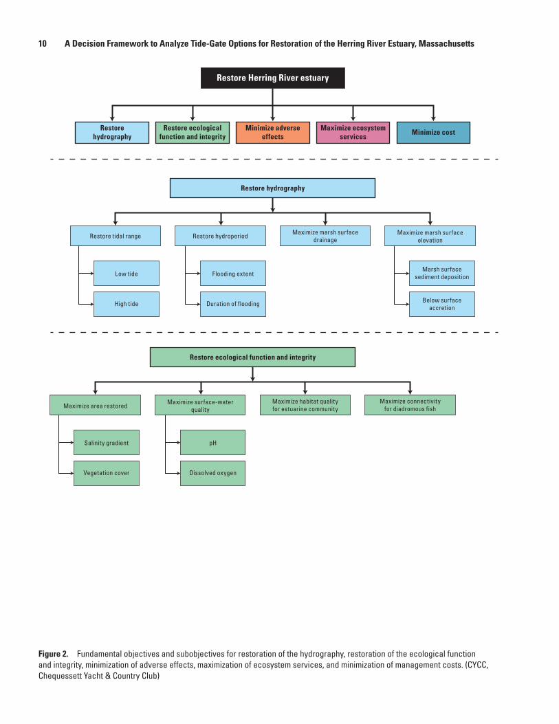
Table 1. Objectives of the Herring River estuary restoration decision support framework. There are five fundamental objectives with subobjectives within each fundamental objective. Each subobjective is accompanied by the performance measure (that is, metric) to be used to measure the current state of the objective, the method to be used to predict the objective of a given tide-gate management option, and the method to be used to monitor the objective after implementation of the option.
[EFDC, Environmental Fluid Dynamics Code; MEM, Marsh Equilibrium Model; SLAMM, Sea Level Affecting Marsh Model; WBNERR, Waquoit Bay National Estuarine Research Reserve; GHG, Greenhouse Gas; DO, dissolved oxygen; TBD, to be determined; MHW, mean high water; CNR, Chequesett Neck Road ; CYCC, Chequesett Yacht and Country Club; T&E, threatened & endangered; h, hour; mg/L, milligram per liter; meTonsCe/ha/yr, metric tons of carbon per hectare per year; ft, foot; %, percent, mm, millimeter; psu, practical salinity units; <, less than; >, greater than; >=, greater than or equal to; USGS, U.S. Geological Survey ]
Subobjectives Performance measureDesired
directionSpatial scale
Prediction method Monitoring
Fundamental Objective #1: Restore Hydrography
Restore tidal range
Low tide
Minimum water surface elevations (ft) averaged for subbasins and at key locations
Minimize Subbasin EFDC Hydrodynamic Model
Electronic water-level data loggers for subbasins and at key locations
High tide
Maximum water surface elevations (ft) averaged for subbasins and at key locations
Maximize Subbasin EFDC Hydrodynamic Model
Electronic water-level data loggers for subbasins and at key locations
Restore hydroperiod
Flooding extent Marsh area inundated by tides (%) Maximize Subbasin EFDC Hydrodynamic
Model
Electronic water-level data loggers for subbasins and at key locations
Duration of flooding
Duration (h) of inundation of marsh surface at key locations
Maximize Subbasin EFDC Hydrodynamic Model
Electronic water-level data loggers for subbasins and at key locations
Maximize marsh surface drainage Extent of ponded water at low tide (%) Minimize Subbasin EFDC Hydrodynamic
Model
Electronic water-level data loggers in areas of predicted ponding
Maximize marsh surface elevation
Marsh surface sediment deposition
Accumulation of sediment at key marsh surface locations (mm)
Maximize Subbasin
EFDC Hydrodynamic Model with Sediment Module, linked with MEM
Deposition/Elevation at surface elevation tables and markers
Below surface accretion (shallow subsidence)
Surface elevation (mm) MaximizeLower
Herring Basin
Baseline data; Published values; Input from SLAMM Model; Expert judgment/elicitation
Soil sampling associated with marsh surface elevation monitoring sites

6 A Decision Framework to Analyze Tide-Gate Options for Restoration of the Herring River Estuary, Massachusetts
Table 1. Objectives of the Herring River estuary restoration decision support framework. There are five fundamental objectives with subobjectives within each fundamental objective. Each subobjective is accompanied by the performance measure (that is, metric) to be used to measure the current state of the objective, the method to be used to predict the objective of a given tide-gate management option, and the method to be used to monitor the objective after implementation of the option.—Continued
[EFDC, Environmental Fluid Dynamics Code; MEM, Marsh Equilibrium Model; SLAMM, Sea Level Affecting Marsh Model; WBNERR, Waquoit Bay National Estuarine Research Reserve; GHG, Greenhouse Gas; DO, dissolved oxygen; TBD, to be determined; MHW, mean high water; CNR, Chequesett Neck Road ; CYCC, Chequesett Yacht and Country Club; T&E, threatened & endangered; h, hour; mg/L, milligram per liter; meTonsCe/ha/yr, metric tons of carbon per hectare per year; ft, foot; %, percent, mm, millimeter; psu, practical salinity units; <, less than; >, greater than; >=, greater than or equal to; USGS, U.S. Geological Survey ]
Subobjectives Performance measureDesired
directionSpatial scale
Prediction method Monitoring
Fundamental Objective #2: Restore Ecological Function/Integrity
Maximize area restored
Appropriate salinity gradient
Area with practical salinity unit (psu)
• <5
• 5 to 18
• >18
Optimize Estuary EFDC Hydrodynamic Model
Conductivity data loggers for subbasins and at key locations
Coverage of emergent vegetation
Area of emergent vegetation with psu
• <5
• 5 to 18
• >18
Maximize Estuary
EFDC (salinity model results) coupled with SLAMM wetland-type results
Transect/Plot cover estimates; Habitat mapping
Surface-water quality
pH % of samples with pH < 5 MinimizeLower
Herring Basin
Expert elicitation informed by EFDC Hydrodynamic Model and USGS model
Continuous surface-water-quality monitoring at key locations
DO % of samples with DO < 5 MinimizeLower
Herring Basin
Expert elicitation informed by EFDC Hydrodynamic Model and USGS model
Continuous surface-water-quality monitoring at key locations
Habitat quality for estuarine community
Species composition of benthic invertebrate community (similarity index 0-1)
Maximize Estuary
Published values; expert elicitation informed by EFDC Hydrodynamic Model
Benthic sampling at key locations
Maximize connectivity for Diadromous fish
Fish passage indicated by fish counts Maximize Estuary
Expert elicitation informed by EFDC predictions of flow velocity at culverts/crossings and current and historical fish counts
Fish counts at crossings

Structuring the Decision Analysis 7
Table 1. Objectives of the Herring River estuary restoration decision support framework. There are five fundamental objectives with subobjectives within each fundamental objective. Each subobjective is accompanied by the performance measure (that is, metric) to be used to measure the current state of the objective, the method to be used to predict the objective of a given tide-gate management option, and the method to be used to monitor the objective after implementation of the option.—Continued
[EFDC, Environmental Fluid Dynamics Code; MEM, Marsh Equilibrium Model; SLAMM, Sea Level Affecting Marsh Model; WBNERR, Waquoit Bay National Estuarine Research Reserve; GHG, Greenhouse Gas; DO, dissolved oxygen; TBD, to be determined; MHW, mean high water; CNR, Chequesett Neck Road ; CYCC, Chequesett Yacht and Country Club; T&E, threatened & endangered; h, hour; mg/L, milligram per liter; meTonsCe/ha/yr, metric tons of carbon per hectare per year; ft, foot; %, percent, mm, millimeter; psu, practical salinity units; <, less than; >, greater than; >=, greater than or equal to; USGS, U.S. Geological Survey ]
Subobjectives Performance measureDesired
directionSpatial scale
Prediction method Monitoring
Fundamental Objective #3: Minimize Adverse Effects
Prevent effects on wells, property, structures, and roads
Number of wells, structures, or roads affected
Minimize Estuary
Water-surface elevation output from EFDC Hydrodynamic Model
Electronic water-level data loggers for subbasins and at key locations
Minimize risk to public safety
Risk to public at water control structures
Number of gates at specified heights Minimize Estuary
Calculated from gate configuration (number of gates at specified heights)
Observations of activity during peak-use periods
Risk to public elsewhere
Number of subbasins with average water depth at MHW of > 1 ft
Minimize Estuary
Calculated from gate configuration and average depth per subbasin at MHW
Observations of activity during peak-use periods
Prevent adverse effects on shellfish beds in harbor
Ammonium export
Concentration in mg/L of export from above CNR dike to harbor (Probability of measurable negative effect to aquaculture)
Minimize Wellfleet Harbor
Expert elicitation based on EFDC predictions of residence time, hydroperiod, and water surface elevation above saturated peat
Surface-water-quality monitoring near aquaculture areas
Fecal coliform levels
Fecal coliform counts near aquaculture areas Minimize Wellfleet
Harbor
Expert elicitation based on EFDC predictions of Residence Time
Surface-water-quality monitoring near aquaculture areas
Sediment deposition onto shellfish beds
Change in sediment dynamics (categorical) Minimize Wellfleet
HarborExpert elicitation
informed by EFDC
Total suspended solids downstream from dike; particle size & deposition near aquaculture areas

8 A Decision Framework to Analyze Tide-Gate Options for Restoration of the Herring River Estuary, Massachusetts
Table 1. Objectives of the Herring River estuary restoration decision support framework. There are five fundamental objectives with subobjectives within each fundamental objective. Each subobjective is accompanied by the performance measure (that is, metric) to be used to measure the current state of the objective, the method to be used to predict the objective of a given tide-gate management option, and the method to be used to monitor the objective after implementation of the option.—Continued
[EFDC, Environmental Fluid Dynamics Code; MEM, Marsh Equilibrium Model; SLAMM, Sea Level Affecting Marsh Model; WBNERR, Waquoit Bay National Estuarine Research Reserve; GHG, Greenhouse Gas; DO, dissolved oxygen; TBD, to be determined; MHW, mean high water; CNR, Chequesett Neck Road ; CYCC, Chequesett Yacht and Country Club; T&E, threatened & endangered; h, hour; mg/L, milligram per liter; meTonsCe/ha/yr, metric tons of carbon per hectare per year; ft, foot; %, percent, mm, millimeter; psu, practical salinity units; <, less than; >, greater than; >=, greater than or equal to; USGS, U.S. Geological Survey ]
Subobjectives Performance measureDesired
directionSpatial scale
Prediction method Monitoring
Fundamental Objective #3: Minimize Adverse Effects—Continued
Public satisfaction
Loss of privacy for abutters Number of complaints Minimize Estuary
Expert elicitation based on EFDC predictions of water surface elevation and salinity, and on predictions of vegetation change
Documentation of incidents
Public viewscapes
% of visual field that looks bad from key locations and visible presence of machinery during tourist season
Minimize Estuary
SLAMM coupled with ArcMap viewshed analysis and expert elicitation
Time series photo stations and documentation of incidents
Appearance of dead woody vegetation
% of visual field that looks bad from private property
Minimize EstuarySLAMM coupled
with ArcMap viewshed analysis
Time series photo stations
Smell Number of complaints Minimize Estuary Expert judgment/elicitation
Documentation of complaints
Community conflict Likelihood of litigation (%) Minimize Estuary Expert judgment/
elicitation
Documentation of conflicts and resolutions
Structuring the Decision Analysis 9
Table 1. Objectives of the Herring River estuary restoration decision support framework. There are five fundamental objectives with subobjectives within each fundamental objective. Each subobjective is accompanied by the performance measure (that is, metric) to be used to measure the current state of the objective, the method to be used to predict the objective of a given tide-gate management option, and the method to be used to monitor the objective after implementation of the option.—Continued
[EFDC, Environmental Fluid Dynamics Code; MEM, Marsh Equilibrium Model; SLAMM, Sea Level Affecting Marsh Model; WBNERR, Waquoit Bay National Estuarine Research Reserve; GHG, Greenhouse Gas; DO, dissolved oxygen; TBD, to be determined; MHW, mean high water; CNR, Chequesett Neck Road ; CYCC, Chequesett Yacht and Country Club; T&E, threatened & endangered; h, hour; mg/L, milligram per liter; meTonsCe/ha/yr, metric tons of carbon per hectare per year; ft, foot; %, percent, mm, millimeter; psu, practical salinity units; <, less than; >, greater than; >=, greater than or equal to; USGS, U.S. Geological Survey ]
Subobjectives Performance measureDesired
directionSpatial scale
Prediction method Monitoring
Fundamental Objective #4: Maximize Ecosystem Services
Climate change mitigation Biomass carbon storage (meTonsCe/ha/yr) Maximize Estuary
WBNERR GHG calculator informed by EFDC Hydrodynamic Model output
Atmospheric carbon exchange; Soil carbon accumulation
Shellfishing opportunities
Area of available habitat (acres) and likelihood of closures not exceeding current number of closures
Maximize
Above and below CNR dike
EFDC Hydrodynamic Model and expert elicitation
Fecal coliform counts and documentation of incidences
Natural mosquito controlMosquito species
composition and abundance
TBD TBD
Expert elicitation based on EFDC output for ponding and salinity
Larvae counts in breeding areas
Maximize recreational opportunities
Loss of golfing opportunities at CYCC
Days/year closed Minimize CYCC Expert elicitation Documentation of incidences
Loss of existing recreational opportunities
Dry land area currently used for recreation that will be flooded
Minimize Estuary
Expert elicitation [based on EFDC predictions of area flooded]
Documentation of loss/gain of access points
Newly created recreational opportunities
Open area with water depth >=2 ft at MHW Maximize Estuary
Expert elicitation [based on EFDC predictions of area flooded]
Car counts; User surveys; Observations of activity during peak-use periods
Fundamental Objective #5: Minimize Cost
Minimize cost for secondary actions Cost for secondary actions Minimize Estuary Expert judgment/elicitation
Project timeline/Financial records
Minimize cost for tide-gate operations
Cost for tide-gate operations Minimize Estuary Expert judgment/
elicitationProject timeline/
Financial records
Minimize cost for monitoring Cost for monitoring Minimize Estuary Expert judgment/elicitation
Project timeline/Financial records
T&E Monitoring Probability that permit requirements fully met Maximize Estuary Expert judgment/
elicitationDocumentation as
required by permit
10 A Decision Framework to Analyze Tide-Gate Options for Restoration of the Herring River Estuary, Massachusetts
Restorehydrography
Restore ecologicalfunction and integrity
Minimize adverseeffects
Maximize ecosystemservices Minimize cost
Restore Herring River estuary
Maximize area restored Maximize surface-waterquality
Maximize habitat qualityfor estuarine community
Maximize connectivityfor diadromous fish
Restore ecological function and integrity
pH
Dissolved oxygen
Salinity gradient
Vegetation cover
Restore tidal range Restore hydroperiod Maximize marsh surfacedrainage
Maximize marsh surfaceelevation
Marsh surfacesediment deposition
Below surfaceaccretion
Restore hydrography
Flooding extent
Duration of flooding
Low tide
High tide
Figure 2. Fundamental objectives and subobjectives for restoration of the hydrography, restoration of the ecological function and integrity, minimization of adverse effects, maximization of ecosystem services, and minimization of management costs. (CYCC, Chequessett Yacht & Country Club)

Structuring the Decision Analysis 11
Maximize climate changemitigation
Maximize natural mosquitocontrol
Maximize shellfishopportunities
Maximize recreationalopportunities
Minimize loss ofgolfing opportunities
at CYCC
Minimize loss ofother recreational
opportunities
Maximize newlycreated recreational
opportunities
Maximize ecosystem services
Tide-gate operations Secondary actions Monitoring
Minimize management cost
Prevent effects to structureand roads Minimize risk to public safety Prevent adverse effects
to harbor shellfish bedsMaximize public satisfaction
Minimize lossof privacy for
abutters
Improve publicviewscapes
Minimize appearanceof dead woody
vegetation
Minimize adversesmell
Minimize communityconflict
Minimize adverse effects
Prevent ammoniumexport
Prevent fecal coliform
Prevent sedimentdeposition onshellfish beds
At water controlstructure
Public risk elsewhere
Figure 2. Fundamental objectives and subobjectives for restoration of the hydrography, restoration of the ecological function and integrity, minimization of adverse effects, maximization of ecosystem services, and minimization of management costs. (CYCC, Chequessett Yacht & Country Club) —Continued

12 A Decision Framework to Analyze Tide-Gate Options for Restoration of the Herring River Estuary, Massachusetts
Management Options
For restoration of the Herring River estuary, there are two broad categories of actions: tide-gate management and secondary management actions designed to affect the estuary by a means other than tidal exchange, such as, mechanical removal of woody vegetation within a subbasin. Thus, the term “option” denotes a set of actions, including tide-gate management or secondary actions, implemented over time. The terms “alternatives” and “options” are used synonymously in this report.
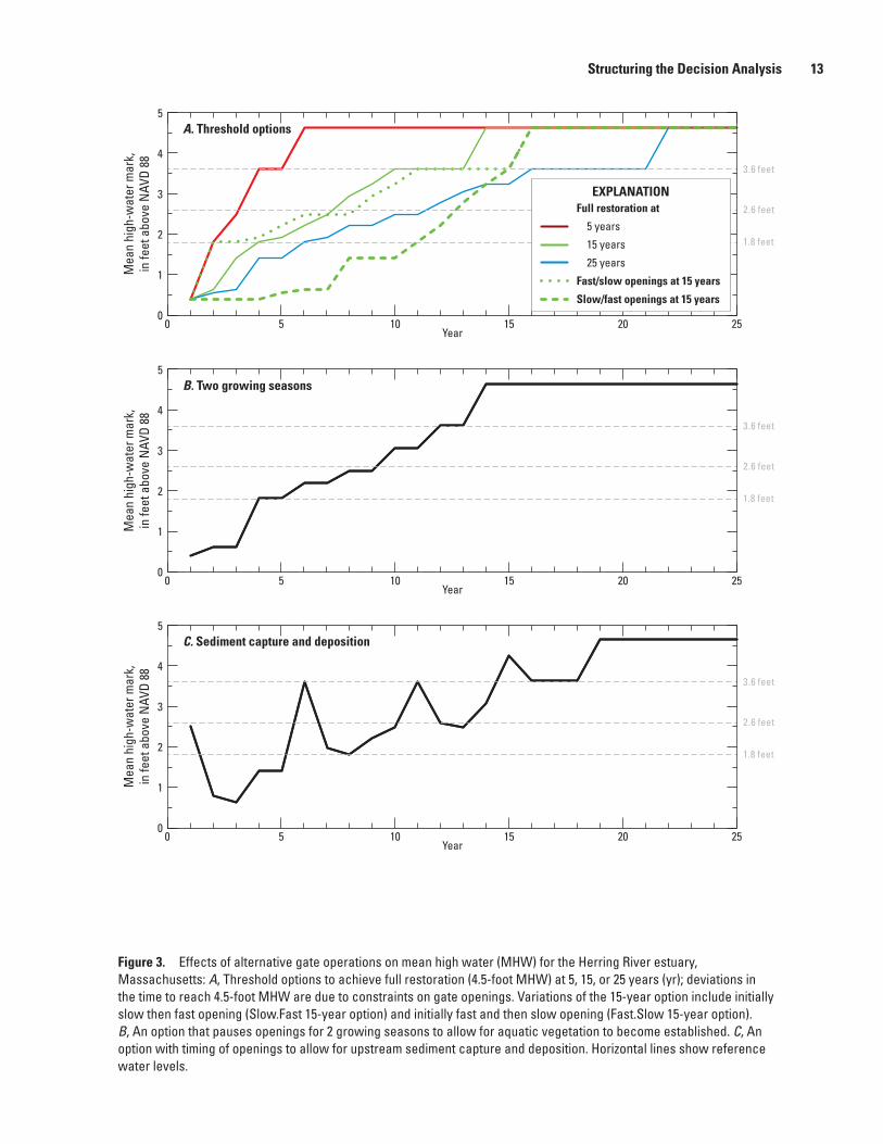
Options for tide-gate management at the CNR dike are defined by the pace of restoring tidal range (fig. 3). Mean high water (MHW) in the Lower Herring River subbasin, expressed as feet above the North American Vertical Datum of 1988, is used to indicate progress towards restoration, and maxi-mum MHW = 4.3 feet (ft) is expected to be reached within a 25-year period (Woods Hole Group, 2012). In contrast, Woods Hole Group (2012) found that MHW in the Lower Herring River subbasin is 0.37 ft. Options for tide-gate manipulations vary by the pace of reaching a benchmark tidal elevation (for example, slow then fast versus fast then slow) or are designed for special purposes, such as facilitating sediment deposition upstream or enhancing recovery of estuarine vegetation com-munities. Each tide-gate option identifies a complete sequence of manipulations that would occur over time frames of up to 25 years.
These policies were developed to achieve full tidal flow by a certain time or to address specific hypotheses, objec-tives, or solutions. The 5-year, 15-year, and 25-year threshold options would open the tide gates at a constant rate so gates will be fully open by 5, 15, or 25 years, respectively (fig. 3A). Variations on these strictly time-based options are designed to be precautionary (that is, the 15-year Slow.Fast and the 15-year Fast.Slow options; fig. 3A), manage vegetation by means of tidal flow (that is, the Growing Season option; fig. 3B), or enhance upstream sediment transport and deposi-tion (that is, the Sediment option; fig. 3C). The 15-year Slow.Fast option opens the gates slowly at first and then accelerates gate opening to fully open the gates by 15 years. In contrast, the 15-year Fast.Slow option initially opens the gates rapidly and then opens gates slowly thereafter to fully open the gates at 15 years. The Growing Season option opens gates in steps to kill invasive reeds (Phragmites) in the lower basin and pauses for a growing season to allow emergent native vegeta-tion growth to capture sediment. The Sediment option opens gates periodically, closes gates on outgoing tides to allow sediment to settle, and then episodically opens the gates dur-ing incoming spring or storm tides to allow greater upstream sediment deposition.
For the purposes of planning, a management year of November–October was assumed, with the indicated gate changes occurring at the beginning of the specified year. The tide gates, and thus MHW, remain static for the full manage-ment year until the next time that a change is scheduled. The Sediment option, which periodically opens and closes gates
to promote sediment deposition (fig. 3C), anticipates a single peak occurring in November; however, there may be one or more peaks in the specified years that will occur with the high-est predicted tide(s) of the year and (or) with an unpredict-able storm event, which introduces some uncertainty into the within year timing of gate operation. Each peak will last four consecutive tidal cycles, centered around the high tide.
Tide-gate options are referred to as “platform” options because they provide the baseline conditions or platform upon which secondary actions will be added. Types of secondary management actions include vegetation management, sedi-ment management, and channel and marsh surface manage-ment. Secondary actions are “added on top of”’ tide-gate man-agement to meet particular objectives. The selection process is to identify the best performing tide-gate platform option, propose alternative secondary actions, and then select the best overall option (tide-gate management plus secondary actions).
The location and timing where secondary actions are needed cannot be anticipated in all cases. Thus, inclusion of secondary actions is one way of adapting management as res-toration progresses. For example, a given tide-gate option may perform well on most objectives but fall short in marsh surface drainage. This would indicate very specific secondary actions to bolster marsh surface drainage in areas where it is needed and would be most effective.
Secondary actions may range from simple independent decisions to complex decisions that are conditionally linked to other management actions. The timing of some secondary actions may have a temporal relation with the tide-gate opera-tions, thus requiring coordination with the tide-gate manage-ment process. For example, removal of vegetation may be ben-eficial to occur prior to restoration of extensive tidal exchange to facilitate work in more conducive, drier conditions.
Prediction of Option Consequences
Decision making is future oriented; good decisions are made after full consideration of What is likely to happen if this or that is done? Therefore, predicting the consequences of management actions is an important step in decision analy-sis. Expected performance, in the terms of each objective, is predicted under each option. A comparison of the relative pre-dicted performance among alternatives provides the basis for selecting an option or, in the case of a multiple-objective prob-lem, the information needed for conducting a tradeoff analysis. For Herring River restoration, the conceptual linkages between tide-gate and secondary management actions and restoration objectives are diagrammed in appendix 1.
Methods for prediction are based on either quantitative models or expert judgement. The methods for prediction are being developed in a tiered approach and are identified in table 1. The first tier (Tier 1) predictions are best professional judgments developed by the HRRC. The second tier (Tier 2) predictions are those provided through formal elicitation methods by subject matter experts and, where appropriate, community stakeholders. The third tier (Tier 3) predictions
Structuring the Decision Analysis 13
3.6 feet
2.6 feet
1.8 feet
0
1
2
3
4
5
0 5 10 15 20 25Year
Mea
n hi
gh-w
ater
mar
k,in
feet
abo
ve N
AVD
88A. Threshold options
3.6 feet
2.6 feet
1.8 feet
0
1
2
3
4
5
0 5 10 15 20 25Year
Mea
n hi
gh-w
ater
mar
k,in
feet
abo
ve N
AVD
88
B. Two growing seasons
3.6 feet
2.6 feet
1.8 feet
0
1
2
3
4
5
0 5 10 15 20 25Year
Mea
n hi
gh-w
ater
mar
k,in
feet
abo
ve N
AVD
88
C. Sediment capture and deposition
EXPLANATIONFull restoration at
5 years
15 years
25 years
Fast/slow openings at 15 years
Slow/fast openings at 15 years
Figure 3. Effects of alternative gate operations on mean high water (MHW) for the Herring River estuary, Massachusetts: A, Threshold options to achieve full restoration (4.5-foot MHW) at 5, 15, or 25 years (yr); deviations in the time to reach 4.5-foot MHW are due to constraints on gate openings. Variations of the 15-year option include initially slow then fast opening (Slow.Fast 15-year option) and initially fast and then slow opening (Fast.Slow 15-year option). B, An option that pauses openings for 2 growing seasons to allow for aquatic vegetation to become established. C, An option with timing of openings to allow for upstream sediment capture and deposition. Horizontal lines show reference water levels.

14 A Decision Framework to Analyze Tide-Gate Options for Restoration of the Herring River Estuary, Massachusetts
are generated by quantitative models. Typically, accuracy and cost increase from Tier 1 to Tier 3; however, the value of the information to the selection of the tide-gate option does not necessarily indicate that Tier 3 predictions are warranted for all objectives. For predicting the percent coverage of non-invasive emergent vegetation, expert elicitation using available expertise from the HRRC is the Tier 1 method, and expert elicitation using a panel of experts is the Tier 2 method. In contrast, the model-based Environmental Fluid Dynamics Code (EFDC; https://www.epa.gov/ceam/environmental-fluid-dynamics-code-efdc; Hamrick, 1996), which predicts hydrol-ogy and water-quality dynamics for surface water, coupled with the Sea Level Affecting Marshes Model (SLAMM; http://warrenpinnacle.com/prof/SLAMM/index.html; Warren Pinacle Consulting, Inc., 2012), is considered the Tier 3 method for predicting the percent coverage of non-invasive emergent vegetation. Tier 1 predictions have been compiled but are be-ing used only to assess and develop the decision framework. Tier 2 and 3 predictions will be used for the decision analysis. Tier 3 predictions can be applied only when a cost-effective quantitative model exists for a given objective. Where no quantitative model is available, Tier 2 predictions will be elicited from technical subject-matter experts and community stakeholders through formal elicitation processes.
Planning for expert elicitation is currently underway (2019) to develop predictions for objectives where use of a quantitative model is not possible or otherwise suitable. Elici-tation is a formal process where technical subject-matter ex-perts or stakeholders are asked to provide their own informed judgments about how a specific management action, integrated within a platform option, may affect a specific objective (Mc-Bride and Burgman, 2012; O’Hagan, 2019). There are various methods for conducting formal elicitations, but the basis of the process is to develop data that allow for quantification of un-certainty and express the range of predictions among multiple experts or responders. For the Herring River, two separate elicitation processes are currently (2019) being planned: one for scientific experts to provide predictions for several measur-able attributes for ecological objectives and another for local stakeholders to develop information about socioeconomic outcomes that are not addressed by existing ecological models. We predominately used the four-step question format com-bined with a modified Delphi format to capture uncertainty (Speirs-Bridge and others, 2010).
The foundational quantitative model for the Herring River project is a two-dimensional hydrodynamic model developed by the Woods Hole Group (2012) using the EFDC software package (Hamrick, 1996). The EFDC model spatially represents the entirety of the historical Herring River flood plain and has been calibrated and validated to a set of tidal observations collected over full lunar cycles in 2007 and 2010. The model has been used to identify the optimal size of the tide gates at the new CNR bridge, the location of the proposed Mill Creek dike, and the road culverts to be replaced as part of the restoration project. It has also been used to simulate the extent of tidal exchange under a range of full and partial resto-
ration scenarios. Outputs from the EFDC model include tidal metrics under normal and storm-driven tidal forcing, including water-surface elevations, tidal range, water-column salinity, flow direction and velocity, and hydroperiod (for example, residence time, flood frequency, flood duration). Data outputs are available for virtually any Herring River location within the model domain and for any time step within the lunar tidal cycle.
The EFDC model has been run to simulate 17 differ-ent tide-gate configurations at the CNR bridge to understand the hydrodynamic effects of incremental tide-gate manage-ment. Output from these simulations provides predictions of low- and high-tide water-surface elevations and other hydro-dynamic metrics, averaged by subbasin and for individual and grouped model nodes. In addition to tabular data output, spatial data have also been compiled to graphically depict the extent of tidal exchange under each of the 17 tide-gate configurations.
In addition to the EFDC hydrodynamic model, other computer-based models have been applied to the Herring Riv-er project. The Sea Level Affecting Marshes Model (SLAMM) is open-source software that was originally developed with U.S. Environmental Protection Agency funding in the 1980s (Warren Pinnacle Consulting, Inc., 2016). It incorporates several input parameters, including Light Detection and Rang-ing (lidar) survey elevations, existing wetland classifications, sea-level-rise rates, tidal range, and accretion and erosion rates for various wetland habitat types to simulate the dominant processes involved with wetland conversions resulting from sea-level rise (Woods Hole Group, 2018).
Although typically utilized to project wetland changes owing to sea-level rise, SLAMM was applied in a unique approach to advance the understanding of how the chang-ing tidal regimes associated with various tide-gate scenarios could potentially affect ecological resources and wetland types throughout the Herring River system. Used in combina-tion, land elevation and tidal range are the main drivers of the simulated vegetation predictions. Rather than using SLAMM to predict water-level increases that are projected to occur because of sea-level rise, this application of SLAMM used different tidal ranges resulting from various tide-gate configu-rations at the CNR Dike to project how the vegetation would likely respond to changes in tidal conditions.
Other quantitative models either have been developed or are being considered for use for predicting outcomes. The U.S. Geological Survey developed a reactive-solute transport model of sediment release of nutrients in response to tidal flooding based on the Nutrient Flux Model (PHAST; Parkhurst and others, 2010). A fully functional version of this water-quality model is not currently available, but in the future, such a model could be used to simulate water chemistry change as salt marshes are restored. The Marsh Equilibrium Model (Morris and others, 2002) is being evaluated for its potential use in simulating sediment and marsh accretion processes and its ability to be integrated with output from the EFDC hydro-dynamic model. Other analytical models are being investigat-

Structuring the Decision Analysis 15
ed to generate quantitative predictions for other water-quality variables, sediment deposition, habitat suitability, and vegeta-tion composition.
Evaluation of TradeoffsPredicting consequences provides information on the
expected performance of individual objectives in response to available management actions. An analysis of tradeoffs among objectives then provides insight into the decision problem and helps decision makers and stakeholders deliberate about the alternative strategies by considering all objectives and their possible interactions. A consequence table is a useful tool for integrating the components of a decision analysis (that is, objectives, alternatives, and consequences) when conducting a tradeoff analysis (table 2). The predicted performance for each objective under each option is presented concisely in the unweighted consequence table. Relative weights are assigned to each objective on the basis of their importance, which can vary among stakeholders. Comparison of options is based on the overall value-weighted performance considering all objectives (Goodwin and Wright, 2014). Software applications have been developed within the R programming environment (R Core Team, 2018) for use by the HRRC to conduct tradeoff analyses for the Herring River restoration.
There are seven steps in the tradeoff analysis. 1. Populate the consequence table with predicted outcomes
for each objective under each alternative action or option.
2. Develop utility curves (described below) for each objec-tive reflecting how the range of possible outcomes are valued by stakeholders. Values may not be linear relative to outcomes, and utility curves can capture risk attitudes.
3. Use the utility curve to determine the utility value asso-ciated with each predicted outcome.
4. Replace the predicted outcomes with the associated utili-ties in the consequence table.
5. Assign an importance weight to each objective.
6. Calculate a weighted average of the utility values across the objectives for each alternative action.
7. Evaluate the sensitivity of the tradeoff analysis to uncer-tainty and identify options that are robust to uncertainty.
Utility functions transform performance metrics into a standardized scale (between 0 and 1) to represent prefer-ence for levels of performance and tolerance for levels of risk (fig. 4). Utility curves take a variety of shapes depending on risk attitude ranging from risk aversion to risk seeking. Risk attitude relates to one’s tolerance for accepting the chance of a bad outcome for the possibility of better performance. A risk-seeking attitude arises when someone is unsatisfied with the prospect of low performance for an objective and is willing
to take chances to achieve a better outcome. A risk-adverse attitude applies to someone who is unwilling to trade existing performance for the unlikely event of better performance when there is also some risk of doing worse than expected. It is common that choices involving gains (for example, improved ecological function) are risk averse; whereas, choices involv-ing losses (for example, avoid adverse effects) are risk seeking (Tversky and Kahneman, 1986). To understand the possible range of stakeholder risk attitudes related to the restoration of the Herring River estuary, utility curves were elicited from the members of the HRRC for a subset of objectives expected to cover this range (appendix 2). Default utility curves were created for each objective based on the elicitation, but the utility curves can be adjusted within the R application prior to conducting a tradeoff analysis.
Implementation of an Option Through Time
Opening of the tide gates at the CNR dike will occur over a definite period of less than 25 years. Gate operation from closed to fully opened has been envisioned as alternative ac-tions composed of incremental tide-gate openings. The HREC will select the tide-gate option with secondary actions based on recommendations from the HRRC informed by the tradeoff and risk analyses. The selected tide-gate option will be imple-mented followed by monitoring of outcomes. The selected tide-gate option will stipulate a schedule for gate operation over a 25-year period or until the gates are fully open, which-ever occurs first. However, there are two ways the selected option can be adapted over time. First, the selected option can be reviewed periodically by repeating tradeoff analyses using updated or new information. The new information based on monitoring data would be used to update predictions based on revised estimates of model parameters in EFDC or SLAMM. Monitoring locations (table 1) are based on protocols devel-oped under the Cape Cod Ecosystem Monitoring program, such as the hydrology protocol developed by McCobb and Weiskel (2003), and rely on general guidance provided by Buchsbaum and Wigand (2012) (see also https://www.nps.gov/caco/learn/nature/cape-cod-monitoring-program.htm). The tradeoff analysis would be conducted with new baseline determined by the current gate openings and hydrology. If in-dicated, a new option could be selected if the updated tradeoff analysis indicates that another option is likely to outperform the current option. For the initial 3–5 years, reviews would be conducted annually to evaluate short-term responses triggered by increases in water-surface elevation; the period between reviews can then increase as needed until full restoration is achieved. Second, monitoring can indicate the need to change secondary management actions. The thresholds that indicate secondary management action have not been stipulated. How-ever, deriving thresholds need not be complex because the need for action could be evident. For example, monitoring can locate where drainage is insufficient to prevent ponded water at low tide, and in response, channel modifications can be used to increase local drainage.

16
A Decision Framew
ork to Analyze Tide-Gate Options for Restoration of the Herring River Estuary, Massachusetts
Table 2. The unweighted consequence table for the pilot tradeoff analysis. The predictions are the modeled and most likely (expected) elicited values. The predicted values were transformed onto a utility scale accumulated over a 25-year period of restoration. The maximum performance on any given objective is indicated by a score of 25 because year-specific scores are summed over the 25-year period and maximum performance in any given year is 1.
[Subobjectives marked with a single asterisk (*) report the average cumulative utility for the nine subbasins. Subobjectives marked with a double asterisk (**) report the average cumulative utility for the vari-able areas in each measurement target range. All other subobjectives report the basin-wide cumulative utility. T, threshold option for for 5 (_5), 15 (_15), or 25 (_25) years; FS, fast.slow 15-year option; SF, slow.fast 15-year option; MHW, mean high water; MLW, mean low water; DO, dissolved oxygen; WQ, water quality; Veg, vegetation; rec, recreation; TE, threatened & endangered species; Sed, sediment; GS, growing season]
Objective hierarchy Tide-gate option (figure 3)
Fundamental objective Objective Subobjective T_5 T_15 FS_15 T_25 SF_15 GS Sed
Hydrography Marsh surface elevation Accretion 8.25 7.25 6.50 6.29 5.34 6.58 8.31Deposition* 3.22 2.76 2.66 2.31 1.91 2.72 3.28
Hydroperiod Flooding duration* 6.43 11.08 16.59 16.91 18.31 10.58 18.02Flooding extent* 23.34 22.78 22.54 20.88 20.12 22.42 21.08
Tidal range MHW* 23.70 21.70 22.23 19.83 17.44 21.03 19.85MLW* 4.97 8.58 9.88 12.22 8.15 8.60 10.88
Marsh surface drainage Ponding* 4.73 12.46 14.27 20.17 14.82 12.65 17.34Ecological function/integrity Surface WQ DO 23.50 23.50 21.50 21.50 18.00 21.50 21.50
Connectivity diadromous fish Fish 11.93 10.12 11.58 9.48 9.45 10.15 10.15Habitat quality native estuarine animals Invertebrate 18.93 17.91 17.93 15.56 14.74 18.29 16.86Surface WQ pH 25.00 25.00 25.00 25.00 25.00 25.00 25.00Area restored Salinity** 23.60 21.54 22.12 19.60 17.56 21.07 19.67
Vegetation** 21.86 21.82 22.36 21.91 20.35 21.78 21.69Adverse effects Harbor shellfish beds Ammonium 24.98 24.97 24.97 24.97 24.98 24.96 24.97
Harbor shellfish beds Sediment 25.00 25.00 25.00 25.00 25.00 25.00 25.00Fecal 23.03 23.94 24.34 23.93 24.44 23.02 23.93
Public satisfaction Conflict 24.96 24.95 24.96 24.96 24.95 24.95 24.95Machine time 25.00 25.00 25.00 25.00 25.00 25.00 25.00Privacy 17.86 19.23 20.49 20.05 20.27 19.47 20.23Smell 7.20 12.50 14.05 12.83 13.01 12.03 12.50Visual field 2.00 5.57 7.19 8.28 11.84 6.45 7.87Woody veg 1.85 5.11 6.21 7.72 11.56 5.95 7.42
Public safety Risk at gate 23.04 17.90 11.89 15.11 15.70 12.57 15.80Risk elsewhere 4.25 3.75 9.68 10.86 9.68 12.00 10.86
Damage Private property 2.92 2.92 2.92 2.92 2.92 2.92 2.92Private wells 1.86 2.26 2.44 2.83 2.49 2.43 2.39Public roads 2.92 2.92 2.92 2.92 2.92 2.92 2.92

Structuring the Decision Analysis
17Table 2. The unweighted consequence table for the pilot tradeoff analysis. The predictions are the modeled and most likely (expected) elicited values. The predicted values were transformed onto a utility scale accumulated over a 25-year period of restoration. The maximum performance on any given objective is indicated by a score of 25 because year-specific scores are summed over the 25-year period and maximum performance in any given year is 1.—Continued
[Subobjectives marked with a single asterisk (*) report the average cumulative utility for the nine subbasins. Subobjectives marked with a double asterisk (**) report the average cumulative utility for the vari-able areas in each measurement target range. All other subobjectives report the basin-wide cumulative utility. T, threshold option for for 5 (_5), 15 (_15), or 25 (_25) years; FS, fast.slow 15-year option; SF, slow.fast 15-year option; MHW, mean high water; MLW, mean low water; DO, dissolved oxygen; WQ, water quality; Veg, vegetation; rec, recreation; TE, threatened & endangered species; Sed, sediment; GS, growing season]
Objective hierarchy Tide-gate option (figure 3)
Fundamental objective Objective Subobjective T_5 T_15 FS_15 T_25 SF_15 GS Sed
Ecosystem services Climate change mitigation Climate 23.17 22.04 23.00 20.73 18.44 20.88 20.73Recreation Existing rec 2.81 2.81 2.81 2.81 2.81 2.81 2.56
Golf 20.76 20.76 20.76 20.76 20.76 20.76 20.76New rec 21.94 13.93 16.00 11.31 13.73 14.87 14.87
Shell fishing opportunities Shellfish acres 18.72 18.69 18.83 18.19 18.17 18.87 18.19Shellfish closure 21.44 21.42 18.92 21.41 21.40 21.41 21.41
Natural mosquito control MosquitosCost Cost of tide-gate operations Gate hours 17.57 18.18 18.80 18.18 18.18 15.97 11.92
Cost of monitoring Monitoring hours 13.81 12.12 14.10 11.27 12.12 12.12 12.12Cost of secondary actions Secondary cost 23.93 23.93 23.93 23.93 23.93 23.93 23.93
Threatened and endangered species Monitoring T&E 19.91 19.91 20.60 19.91 19.91 16.09 14.63

18 A Decision Framework to Analyze Tide-Gate Options for Restoration of the Herring River Estuary, Massachusetts
Objective A Objective B Objective C
Objective D Objective E Objective F
Objective G
Utili
ty
Measured value
Utili
ty
Measured value
Utili
ty
Measured value
Utili
ty
Measured valueUt
ility
Measured value
Utili
tyMeasured value
Utili
ty
Measured value
-3.0 -2.8 -2.6 -2.4 -2.2 -2.0 -1.80
0.2
0.4
0.6
0.8
1.0
0 2 4 6 8 100
0.2
0.4
0.6
0.8
1.0
0 5 10 15 20 250
0.2
0.4
0.6
0.8
1.0
0 50,000 100,000 150,0000
0.2
0.4
0.6
0.8
1.0
0 40 8020 60 1000
0.2
0.4
0.6
0.8
1.0
-1 0 1 2 3 4 50
0.2
0.4
0.6
0.8
1.0
0 5 10 15 20 250
0.2
0.4
0.6
0.8
1.0
Figure 4. Example utility curves for selected objectives relating the level of a performance metric for hypothetical objectives (x-axes) to a standardized score between 0 and 1 (y-axes) based on preferences and risk attitude. The utility curves are for minimized objectives (A–D), maximized objectives (E–G), risk-adverse attitudes (A and E), risk-seeking attitudes (C, D, and G), and risk-neutral attitudes (B and F).
Prototype Decision Analysis and Results
A decision analysis was conducted using preliminary predictions to serve as a starting point, evaluate the decision structure, and identify areas needing improvement. The seven steps outlined in the “Evaluation of Tradeoffs” section were conducted using predictions from the EFDC model for hydro-logical objectives, the SLAMM model for certain ecological objectives, and preliminary expert-elicited predictions for the remaining objectives. Members of the HRRC participated in the prototype analysis by providing expert judgment on many of the performance measures. To limit the potential for elicita-tion fatigue, the initial prototype focused on the lower Her-ring River subbasin for hydrologic and ecological objectives and basinwide for socioeconomic objectives. It was assumed that the Mill Creek and Upper Pole Dike Creek water-control structures were in place to limit the scope of the elicitation. The uncertainty comes from the elicited attributes. The nu-merical models do not yet produce confidence intervals, which will be included in future prototypes.
The tradeoff analysis was conducted using a custom software application developed in the R programming envi-ronment (R Core Team, 2018). The application allowed for se-lection or specification of utility curves, prediction percentile, and importance weighting of the objectives. The prediction percentile, which ranged from 0.55 to 0.8, was used to com-pute confidence limits. For each percentile, the corresponding confidence limits represented worst case (pessimistic) and best case (optimistic) contingent on whether the objective was to be minimized or maximized. Utility curves ranged from risk averse to risk seeking options on a continuous scale and were used to transform the performance measures to utility values between 0 and 1. Some utilities were time specific. For example, the utility curve could be differentiated for different phases of restoration (for example, specifying risk aversion during early restoration and risk neutral or risk seeking late in the restoration planning cycle). A discount rate can be set to place higher value on performance during the first few years relative to performance near full-gate opening.
The scores in the consequence table, which are cumula-tive utilities over the 25-year restoration period, range from 0 to 25 corresponding to performance from poor to excellent
Prototype Decision Analysis and Results 19
for a given objective and tide-gate option (table 2). Thus, the consequence table can be scanned quickly to see how well the objectives are being met by comparing the scores to the maxi-mum value of 25 and to the minimum value of 0.
The overall score for an option is a weighted average of the cumulative utilities across all objectives (table 3). The objective weights in table 3 were allocated as follows: the hydrologic objectives received 30 percent, ecological func-tion objectives received 20 percent, adverse effect objectives received 30 percent, ecosystem service objectives received 10 percent, cost objectives received 5 percent, and threatened and endangered species received 5 percent, which is the balanced-weighting scenario presented in figure 5. The overall score is also scaled from 0 to 25, indicating poor to excellent perfor-mance of a given option. The overall scores, along with the more detailed objective-specific comparisons, provide a tool for comparing options and exploring the predicted outcomes of different options to gain a better understanding of the prob-lem and potential management consequences.
Option scores and rankings change depending on choice of utility and importance weighting, as well as the level of confidence in the prediction. Thus, to complete the tradeoff analysis, it is important to determine whether the best-per-forming option is sensitive to variation in stakeholder values or prediction uncertainty as represented by different levels of pessimistic and optimistic scenarios; we refer to this as a sen-sitivity analysis. The goal is to identify options that are robust to variation in stakeholder values and prediction uncertainty. In other words, the goal is to find an option that is predicted to perform well across a wide range of underlying assumptions.
A sensitivity analysis was conducted in which the tradeoff analysis was repeated assuming different levels of prediction uncertainty and value-weighting schemes. To test the effect of uncertainty, the tradeoff analysis was conducted using the most likely prediction and again using the limits from the confidence interval with a range of percentiles (0.55–0.80). The confidence limit to be used depends on whether a best case or worst-case scenario is being evaluated and the objec-tive’s direction. If an objective is to be maximized, then the upper confidence limit is considered the best-case outcome. In contrast, if an objective is to be minimized, then the lower
confidence limit is the best case. Four weighting schemes were included in the sensitivity analysis, and these included either (1) a preference for ecological objectives, (2) a preference for socioeconomic objectives, (3) a balance between ecological and socioeconomic objectives, or (4) an equal weighting of each fundamental objective (fig. 5). In an ecological weight-ing scheme, hydrography and ecological objectives are highly valued. In a socioeconomic weighting scheme, the social and economic objectives are highly valued. In a balanced weight-ing scheme, some ecological (hydrography) and some social (adverse effects) objectives are highly valued. In the equal weighting scheme, all fundamental objectives are equally valued. Aspects of the analysis that can be investigated in-clude average performance (fig. 6) and frequency of ranking (fig. 7). For example, based on the preliminary predictions, the “15-year Fast.Slow” option (fig. 3A) was ranked first more fre-quently than other options (fig. 7). The predicted performance of this option was quite robust to underlying assumptions about uncertainty and value weighting because it was ranked first more frequently than other options and was never ranked below second (fig. 7). The only other option that ranked first was the 25-year option (fig. 3A), which was rarely ranked below 3rd and never below 4th (figs. 6 and 7).
Although it is important to identify which option has the best and most robust overall performance, it is also important to evaluate how well individual objectives and subobjectives are being met. A double-column chart shows option perfor-mance at the objective level (fig. 8). There are two questions that a double-column chart is designed to answer. First, does performance among option alternatives vary, or do all options perform similarly? Second, is there unmet potential for better performance, or does the best performing option achieve full or nearly full performance? For example, for the Ponding objective there is a wide range in performance among option alternatives, but there is only modest room for improvement because the option that performs best for this objective nearly achieves maximum performance (fig. 8). In contrast, for the Deposition objective there is a narrow range in performance with all options performing about the same, and there is ample room for improvement (fig. 8). Maximizing sediment depo-sition and accretion, minimizing damage to structures, and
Table 3. Overall utility from the pilot tradeoff analysis. The cumulative utilities for each objective, which are presented in table 2, are value weighted and averaged for an overall performance score for each option. The objective weights in table 3 were allocated as follows: the hydrologic objectives received 30 percent, ecological function objectives received 20 percent, adverse effect objectives received 30 percent, ecosystem service objectives received 10 percent, cost objectives received 5 percent, and threatened and endangered species received 5 percent, which is the balanced-weighting scenario presented in figure 5.
Option scoreOptions (figure 3)
Threshold 5 year
Threshold 15 year
Threshold 25 year
Fast.Slow 15 year
Slow.Fast 15 year
Growing season
Sediment
Weighted sum 14.99 15.19 15.67 15.79 14.92 14.92 15.42Rank 5 4 2 1 6 7 3

20 A Decision Framework to Analyze Tide-Gate Options for Restoration of the Herring River Estuary, Massachusetts
maximizing existing recreation are objectives with potential for additional performance. Performance at the individual objective level or overall option level is affected by the assumed utility curves. For example, the utility for incurred damage (fig. 4D) drops off precipitously for incidences greater than 0; thus, there is very little tolerance for any occurrence of damages. There is high confidence that damage incidences will be low (less than or equal to 2 for the life of the project); how-ever, the extreme utility (fig. 4D) penalizes performance even for a few such incidences. The 15-year Fast.Slow (P_15_FS) option earns the highest cumulative utility after 25 years in all
four value weight scenarios and at all levels of uncertainty, but the rank of the other options, and the difference between the P_15_FS option and the other options, vary across weighting scenarios (fig. 9). For each level of uncertainty in fig. 9, the corresponding confidence limits represented worst-case and best-case values contingent on whether the objective was to be minimized or maximized. Varying the levels of uncertainty and the interval between worst- and best-case outcomes had small effect on the range of 25-year cumulative utilities com-pared to different value weighting scenarios.
Wei
ght
0.00
0.05
0.10
0.15
0.20
0.25
0.30
0.35
HydrographyEcological function/integrity
Adverse effectsEcosystem
services
CostThreatened and endangered species
HydrographyEcological function/integrity
Adverse effectsEcosystem
services
CostThreatened and endangered species
HydrographyEcological function/integrity
Adverse effectsEcosystem
services
CostThreatened and endangered species
HydrographyEcological function/integrity
Adverse effectsEcosystem
services
CostThreatened and endangered species
Balanced Equal Socioeconomic Ecological
Figure 5. The four weighting schemes applied to the fundamental objectives to evaluate outcomes. In a balanced scheme some ecological (hydrography) and some social (adverse effects) objectives are highly valued. In the equal scheme, all fundamental objectives are equally valued. In a socioeconomic scheme, the social and economic objectives are highly valued. In an ecological scheme, hydrography and ecological objectives are highly valued.

Prototype Decision Analysis and Results 21
3 4 2 1 5 7 6Cu
mul
ativ
e ut
ility
T_5 T_15 T_25 FS_15 SF_15 GS Sed16.0
16.5
17.0
17.5
Tide-gate policy option
Figure 6. Cumulative utility averaged across a range in prediction uncertainty and the four value-weighting schemes in figure 5 to compare seven tide-gate options in figure 3. The numbers inside each bar indicate the rank of each option. The average cumulative utility for all seven options after 25 years were within 1.5 utility points of one another. (T, threshold option for 5 (_5), 15 (_15), or 25 (_25) years; FS, fast.slow 15-year option; SF, slow.fast 15-year option; GS, growing season; Sed, sediment)
Rank
(Low
er is
bet
ter)
T_5 T_15 T_25 FS_15 SF_15 GS Sed
Policy option
7
6
5
4
3
2
1
0.06
0
0.19
0.23
0.19
0.33
0
0
0
0.02
0.67
0.31
0
0
0
0
0
0.08
0.25
0.56
0.12
0
0
0
0
0
0.12
0.88
0.31
0.19
0.48
0.02
0
0
0
0.13
0.81
0.06
0
0
0
0
0.5
0
0.25
0
0.25
0
0
Figure 7. Frequencies of ranks based on cumulative utility after 25 years for seven options (figure 3) across a range in prediction uncertainty and the four value-weighting schemes in figure 5. Frequencies greater than 0 up to the maximum are increasingly darker blue. (T, threshold option for 5 (_5), 15 (_15), or 25 (_25) years; FS, Fast.Slow 15-year option; SF, Slow.Fast 15-year option; GS, growing season; Sed, sediment)

22 A Decision Framework to Analyze Tide-Gate Options for Restoration of the Herring River Estuary, Massachusetts
Poin
ts s
hort
of m
axim
um |
Scor
e ra
nge
Range across options
MLW
MHW
Flooding extent
Flooding duration
PondingDepositionAccretionSalinityVegetationpH DO InvertebrateFishDam
ageGate riskRisk elsew
hereAm
monium
FecalSedim
entPrivacyVisual fieldM
achine time
Woody veg
Smell
ConflictClim
ateShellfish acShellfish closed
GolfExisting recNew
recGate hoursSecondary cost
Monitoring hours
TE30
20
10
0
10
20
30
Unmet potential, best option
Hydr
ogra
phy
Ecol
ogic
al fu
nctio
n/in
tegr
ity
Adve
rse
effe
cts
Ecos
yste
m s
ervi
ces
Cost
T&E
spp
Figure 8. Double-column chart used to evaluate how effectively the tide-gate options address all objectives. The upper (dark) columns report the spread in cumulative utility after 25 years between the highest and lowest ranking option for each objective. A taller column indicates a greater range among options, whereas a shorter column indicates all options were more similar. The lower (light) columns report how much utility was unrecovered by the best option. A shorter column indicates the objective was well addressed by the best option, and a taller column indicates even the best option did not completely address the objective. (MLW, mean low water; MHW, mean high water; DO, dissolved oxygen; Veg, vegetation; ac, acres; TE, T&E Spp, threatened and endangered species; rec, recreation)

Prototype Decision Analysis and Results 23
17
16
15
14
17.5
16.5
15.5
14.5
0.55 0.60 0.65 0.70 0.75 0.80
Uncertainty
Cum
ulat
ive
utili
ty
A. Balanced
17
16
15
14
17.5
16.5
15.5
14.5
0.55 0.60 0.65 0.70 0.75 0.80
Uncertainty
Cum
ulat
ive
utili
ty
B. Ecological
17
16
15
14
17.5
16.5
15.5
14.5
0.55 0.60 0.65 0.70 0.75 0.80
Uncertainty
Cum
ulat
ive
utili
ty
C. Equal
17
16
15
14
17.5
16.5
15.5
14.5
0.55 0.60 0.65 0.70 0.75 0.80
Uncertainty
Cum
ulat
ive
utili
ty
D. Socioeconomic
T_5T_15FS_15T_25
SF_15GSSed
EXPLANATION
Figure 9. Cumulative utility as a function of uncertainty formulated as the percentile for which confidence limits were computed for value weights: A, balanced, B, ecological, C, equal, and D, socioeconomic. For each level of uncertainty, the corresponding confidence limits represented worst-case and best-case values contingent on whether the objective was to be minimized or maximized. Varying the levels of uncertainty and the interval between worst- and best-case outcomes (x-axes) had a small effect on the range of 25-year cumulative utilities compared to different value weighting scenarios (panels). (T, threshold option for 5 (_5), 15 (_15), or 25 (_25) years; FS_15, fast.slow 15-year option; SF_15, slow.fast 15-year option; GS, growing season; Sed, sediment)

24 A Decision Framework to Analyze Tide-Gate Options for Restoration of the Herring River Estuary, Massachusetts
Next StepsThe decision structure developed for the Herring River
restoration is complex due to the multiple-stakeholder concerns and the importance of the estuary from hydrological, ecologi-cal, and socioeconomic perspectives. The tide-gate options are structured around restoring the tidal range, which is the eco-logical basis for restoration. Predicting outcomes is a continu-ing challenge because of the many and varied objectives. The decision structure represents a good-faith effort to include all stakeholder concerns and provide decision makers with a trans-parent approach to incorporate those concerns in comparisons of tide-gate options using the best-available science.
Eventually, the decision structure can be simplified by removing objectives that are insensitive to decision choice or eliminating dominated alternatives from further consideration. However, at this point we do not want to simplify the problem for a couple reasons. First, there is a communication value in demonstrating that a comprehensive set of objectives is being considered, even though some objectives do not affect the decision choice. Second, the prediction methods are still being developed and improved; thus, the consequences are not final-ized. It would be premature to simplify the problem, although eventually that is the aim.
Based on the prototype analyses, the 15-year Fast.Slow option (fig. 3) performed best among the policies analyzed. Secondary management actions could focus on addressing objectives not fully met, which can be identified using the double-column chart (fig. 8). Opportunities for improvement through secondary actions are related to sediment transport, damage, and existing recreation. The expected performance of the tide-gate option would need to account for updated infor-mation because the need for some secondary actions might not be foreseen.
The management process will be implemented over the project’s finite time line (that is, less than 25 years before full gate opening). As restoration progresses, monitoring will be useful to identify additional areas where secondary actions are warranted. Also, periodic updating of predictive models and tradeoff analysis based on monitoring data can be used to determine whether adjustments in the selected option for tide-gate management are warranted as managers increase their understanding of system dynamics and the response to tide-gate manipulations.
Collaborative processes require, at a minimum, a clear problem statement, institutional support, an issue that warrants significant investment of organizational resources, interdepen-dence among parties to achieve good outcomes, and a zone of possible agreement. For a collaborative process to achieve suc-cess, the parties need a shared vision and trust in the process. It is important that stakeholders and decision makers be explicit and transparent about what they care about, engage in creative development of tide-gate options, and use best-available sci-ence to forecast outcomes.
The next steps are to progress beyond the preliminary predictions and to move predictions from first cut (Tier 1) to
ideal method (Tier 3) wherever possible. Then the applica-tions developed in R programming environment can be used to conduct the tradeoff and sensitivity analyses described and illustrated in this report to inform discussions within the tech-nical and stakeholder committees and formulation of recom-mendations to the decision makers.
SummaryEcological restoration typically involves a complex
interaction of social, economic, and ecological considerations representing the mandate of resource stewards and the values of stakeholders. The success of ecological restoration can be determined by assessing whether tradeoffs among the multiple considerations and risks associated with uncertain outcomes are suitably evaluated and incorporated into decision making. Decision analysis was devised for evaluating tradeoffs and risks to inform management choices. In this report, the authors describe a decision analysis framework to evaluate the com-plex tradeoffs and risks associated with the restoration of the 1,100-acre Herring River estuary within Cape Cod National Seashore in Massachusetts. The tide gates at the Chequessett Neck Road (CNR) dike at the mouth of the Herring River have severely restricted tidal exchange for more than 100 years and caused ecological degradation to the estuary. The degradation of the basin and the structural integrity of the dike have moti-vated resource managers to pursue restoration of the Herring River estuary.
To develop the decision analysis framework, the au-thors worked with the Herring River Restoration Committee (HRRC) through a series of meetings with the full commit-tee and a subgroup tasked with framework development. The HRRC represents the decision makers and stakeholders in the restoration process. Additional workshops with stakeholders, science experts, and regulators helped to elucidate underly-ing issues, incorporate concerns and interests into the frame-work, and resolve technical questions. The decision analysis for the Herring River restoration was structured according to six major components: (1) a clear statement of the problem, (2) comprehensive and measurable objectives, (3) a set of discrete tide-gate options, (4) a means to predict outcomes, (5) a process to evaluate the implications of these outcomes, and (6) a plan for implementation of the selected tide-gate option over time, including monitoring to provide feedback and to formally incorporate learning, reevaluate options, and possibly adapt management as restoration is implemented over time.
The decision framework is based on the understanding that representatives of Cape Cod National Seashore and the town of Wellfleet will be responsible for managing the new tide control gates at CNR, Mill Creek, and Pole Dike Creek and for implementing secondary management actions to achieve restoration goals. The goals are to restore the natural hydrography (that is, tidal range and marsh surface elevation) and ecological integrity of the Herring River estuary while minimizing adverse economic and social effects, maximizing

References Cited 25
the estuary’s production of ecosystem services, and minimiz-ing management costs. Objectives that fit under the project goals define comprehensive performance measures useful for predicting and monitoring the consequences of manage-ment actions.
The primary management actions are to adjust the vol-ume of tidal flow through a series of to-be-constructed tide gates at CNR, Mill Creek, and Pole Dike Creek; the tide-gate adjustments can vary by the number, location, magnitude of opening, and flow direction of the individual tide-gate open-ings at any given time. The sequence of tide-gate adjustments over the years of restoration form the basis for the manage-ment options. In addition, tide-gate options include secondary management actions, such as management of flood-plain vege-tation or restoration of connectivity, intended to accelerate the recovery of the estuarine habitat, enhance the benefits of tidal restoration achieved through tide-gate management alone, and reduce the potential adverse ecological and socioeconomic ef-fects of restoring tidal flow. Over a planning horizon, decisions involve the rate at which newly constructed water-control structures allow tidal exchange, and the timing and location of implementing numerous secondary management actions.
Performance, in the terms of each objective, is predicted for each tide-gate option using a range of methods from quan-titative physical process models to elicited expert judgment. A comparison of the relative predicted performance among options provides the basis for deciding how to manage the tide gates. Decisions will affect biophysical (for example, sediment transport, discharge of fecal coliform bacteria) and ecologi-cal (for example, vegetation response, fish passage, effects on shellfish) processes, as well as socioeconomic interests (for example, effects on property, viewscapes, recreation). The framework provides a structured approach for evaluating trade-offs among multiple objectives (ecological and social) while appropriately characterizing relevant uncertainties and accounting for levels of risk tolerances and the values of deci-sion makers and stakeholders.
In this project, an initial prototype decision analysis was conducted using a software application developed for evaluating tradeoffs and sensitivity of the decision to risk and uncertainty. The next near-term steps are to progress beyond the preliminary predictions, repeat the tradeoff and sensitiv-ity analyses, and inform discussions within the technical and stakeholder committees who will formulate recommendations for the decision makers.
The management process is intended to be implemented over a finite time line (anticipated to be less than 25 years be-fore full gate opening). As the restoration progresses, monitor-ing of outcomes can be used to identify additional areas where secondary actions are needed. Also, monitoring data can be used to update predictions and periodically repeat the tradeoff analysis to determine whether adjustments in the selected tide-gate management option are warranted as managers increase their understanding of system dynamics and the estuary’s response to tide-gate manipulations.
References Cited
Buchsbaum, R.N., and Wigand, C., 2012, Adaptive manage-ment and monitoring as fundamental tools to effective salt marsh restoration, in Roman, C.T., and Burdick, D.M., eds., Tidal marsh restoration—a synthesis of science and man-agement: Washington, D.C., Island Press, p. 213–231.
Cape Cod National Seashore and Herring River Restoration Committee, 2012, Herring River Restoration Project Draft Environmental Impact Statement/Environmental Impact Report: Wellfleet, Mass., 344 p.
Gregory, R.S., and Keeney, R.L., 2002, Making smarter environmental management decisions: Journal of American Water Resources Association, v. 38, p. 1601–1612.
Goodwin, P., and Wright, G., 2014, Decision analysis for management judgment (5th ed.): New York, John Wiley and Sons, 496 p.
Hammond, J.S., Keeney, R.L., and Raiffa, H., 2015, Smart choices—A practical guide to making better decisions: Brighton, Mass., Harvard Business Review Press, 256 p.
Hamrick, J.M., 1996, User’s manual for the environmental fluid dynamic computer code: The College of William and Mary, Virginia Institute of Marine Science, Special Report 328, 224 p.
Keeney. R.L., and Gregory, R.S., 2005, Selecting attributes to measure the achievement of objectives: Operations Research, v. 53, p. 1–11.
Kranenburg, C.J., Hardy, M.W., and Nagle, D.B., 2017, EAARL Coastal Topography–Cape Cod National Seashore, Massachusetts, 2002: U.S. Geological Survey data release, https://doi.org/10.5066/F7VX0DQ2.
McBride, M.F., and Burgman, M.A., 2012, What is expert knowledge, how is such knowledge gathered, and how do we use it to address questions in landscape ecology?, in Perera, A.H., Drew, C.A., and Johnson, C.J., eds., Expert knowledge and its application in landscape ecology: New York, Springer, p. 11–38.
McCobb, T.D., and Weiskel, P.K., 2003, Long-term hydrologic monitoring protocol for coastal ecosystems: U.S. Geologi-cal Survey Open-File Report 02–497, 109 p.
McGowan, C.P., Lyons, J.E., and Smith, D.R., 2015, Develop-ing objectives with multiple stakeholders—adaptive man-agement of horseshoe crabs and red knots in the Delaware Bay: Environmental Management, v. 55, p. 972–982.
Morris, J.T., Sundareshwar, P.V., Nietch, C.T., Kjerfve, B., and Cahoon, D.R., 2002, Responses of coastal wetlands to rising sea level: Ecology, v. 83, p. 2869–2877.
26 A Decision Framework to Analyze Tide-Gate Options for Restoration of the Herring River Estuary, Massachusetts
O’Hagan, A., 2019, Expert knowledge elicitation—subjec-tive but scientific: The American Statistician, v. 73, sup. 1, p. 69–81.
Parkhurst, D.L., Kipp, K.L., and Charlton, S.R., 2010, PHAST Version 2—A program for simulating groundwater flow, solute transport, and multicomponent geochemical reac-tions: U.S. Geological Survey Techniques and Methods 6–A35, 235 p.
Raiffa, H., Richardson, J., and Metcalfe, D., 2002, Negotia-tion analysis—The science and art of collaborative deci-sion making: Cambridge, Mass., Harvard University Press, 576 p.
R Core Team, 2018, R—A language and environment for statistical computing: Vienna, Austria, R Foundation for Statistical Computing, accessed August 14, 2019, at https://www.R-project.org/.
Speirs-Bridge, A., Fidler, F., McBride, M., Flander, L., Cum-ming, G., and Burgman, M., 2010, Reducing overconfi-dence in the interval judgments of experts: Risk Analysis, v. 30, p. 512–523.
Tversky, A., and Kahneman, D., 1986, Rational choice and the framing of decisions: The Journal of Business, v. 59, p. S251–S278.
Warren Pinacle Consulting, Inc., 2012., SLAMM 6.2 Technical Documentation: Waitsfield, Vt., Warren Pinnacle Consulting, Inc., accessed May 3, 2019, at http://warrenpinnacle.com/prof/SLAMM/index.html.
Woods Hole Group, 2012, Herring River hydrodynamic mod-eling final comprehensive report to HRRC and NPS, Cape Cod National Seashore: Woods Hole Group, Bourne, MA, 208 p.
Woods Hole Group, 2018, Herring River ecological modeling: using the Sea Level Affecting Marshes Model (SLAMM) to project habitat change: Woods Hole Group, Bourne, MA, 148 p., accessed October 22, 2019 at https://www.mass.gov/files/documents/2018/12/07/czm-slamm-report-nov2016.pdf.

Appendix 1 27
Appendix 1. Conceptual ModelsThe description and purpose of the conceptual models
are presented in this appendix. Five figures (figs 1.1 to 1.5) are included, one for each of the fundamental objectives: hydrography, ecosystem function, ecosystem services, adverse effects, and cost. In each figure, the fundamental objective is on the right-hand side of the diagram in a green hexagon. Subobjectives that are nested under each fundamental objec-tive are shown to the left of the hexagon in green rectangles, with arrows pointing from the nested subobjectives to the fundamental objective. There may be multiple layers of nested subobjectives, depending on the objective. These, too, will be in green rectangles and have arrows from them pointing into the upper-level objective. Moving to the left on the diagram, things that affect or have influence on the lowest level objec-tives are shown in purple rectangles. There are arrows from the purple rectangles to the lowest-level objective. Continuing to move from right to left, things that affect or have influence on purple rectangles are also shown in purple rectangles, with arrows pointing to the purple rectangle it influences. There
may be several influences depicted from right to left. Sto-chastic events or states are shown in red circles, again with an arrow pointing directly to the rectangle it affects. Decisions that are part of the decision-making process of the restora-tion are depicted in gray rectangles (that is, gate manipula-tions and secondary management actions). On the Minimize Adverse Effects diagram (fig. 1.3), black rectangles are shown. These are actions that can be taken but that are not part of the management aspect of the restoration. For example, the Struc-tural Design of the dike will affect the safety of pedestrians, fishermen, and boaters; however, it is not part of the decision-making process of the restoration. Existing models that make predictions regarding the outcome of a given decision (gray rectangle) and a resulting state (purple or green rectangles) are shown in yellow diamonds. The yellow diamonds are placed on the arrow between two shapes: the shape to the left is the input to the model, whereas the shape the right is the output of the model. Yellow diamonds (that is, predictive models) may also be placed between two state rectangles; that is, the input to the model does not have to start with a decision node. The influence diagrams serve many purposes. They
Restore Hydrography
Marsh surface sediment
deposition
Tidal range
Hydroperiod
Sedimentnet upstream flux
Flooding extent
Duration offlooding
Tide gate number, size,
frequency, timing
Marsh surface drainage
Low tide
High tide
Plant cover
Secondary mgmt
Weather(normal v
storm)
Below surface accretion
Marsh surface elevation
Channels
Storms
SLAMM
Sheet flow
EFDC
EFDC
MEM
MEM
Figure 1.1. Conceptual model for the hydrography objective. (EFDC, Environmental Flow Dynamics Code; MEM, Marsh Equilibrium Model; SLAMM, Sea Level Affecting Marsh Migration; mgmt, management)

28 A Decision Framework to Analyze Tide-Gate Options for Restoration of the Herring River Estuary, Massachusetts
serve as depictions of conceptual models of how the system works regarding the objectives; the decisions we make and actions we take; and the effects that those actions have on the system, and ultimately, the objectives. The diagrams help to communicate our conceptual models. They help elucidate the areas where existing models predict outcomes of actions (for example, the Environmental Flow Dynamics Code [EFDC]) and where predictive models are absent and thus predictions
are based on expert elicitation. The diagrams will also help to identify alternative courses of action, or strategies, whose predicted outcomes can be compared with respect to the objec-tives. The influence diagrams include only as much detail as is necessary and useful for understanding the system and making predictions of outcome with respect to the objectives (that is, the green rectangles and green hexagon).
Area restored
Temp
EFDC
MEM
Temp
Channels
pH
DO
NH4
Flushing
Recreation
Appropriate salinity gradient
Cover emergent vegetation
Plant composition
Primary productivity
Benthic community
Nekton community
Substrate conditions
Velocity at structures &
culverts
Surface-water quality
Habitat quality estuarine community
Maximize ecosystem
function/integrity
Connectivitydiadromous fish
Salination of acid sulfate soil
Sediment disturbance
Plant growth
rate
Marsh surface drainage
Porewater Sslinity
Soil chemistry
Water columnsalinity
Flooding frequency &
duration
Marsh surface elevation
Sediment deposition
Below ground matter
Fresh water inputs
Distance from
harbor
Tide gates number, size,
frequency
Secondary mgmt
Figure 1.2. Conceptual model for the Ecosystem-Function objective. (EFDC, Environmental Flow Dynamics Code; MEM, Marsh Equilibrium Model; DO, dissolved oxygen; NH4, ammonium; mgmt, management; Temp, temperature)

Appendix 1 29
Tide Gatesnumber, size,
frequency
Secondarymgmt
Seasonalheavy
rainfall
EFDC
Channels
Tidalexchange/
flushing
Fish habitat(extent/quality)
Marsh surfacedrainage
Spring watertable Ponding depth,
residence time,salinity, acidity
Natural mosquitocontrol
Mosquitonuisance
Education/communication
Education/communication
Minimizeadverseeffects
Communityconflict
Public viewscapes
Appearance deadwoody vegetation
Smell
Privacy forabutting
properties
Publicsatisfaction
Secondarymgmt
(timing & type)
Secondarymgmt
Tide gatetiming & volume
of release
Tide gatetiming & volume
of release
Tide gatetiming & volume
of release
Tide gatetiming & volume
of release
Preemptivemeasures
Structuraldesign
Planning
Surface drainage
Salination of acidsulfate soils
Flushing frequency
Recreation
Privateproperty
Debris blockagesat structures
DeadFallen
Standing
Decomposingplant material
Temp
Hypoxia (lowpeat oxygen)
Politicalincompatibility
Vegetation mgmt
Competing uses
Maxunyn watersurface elevation
Open/closedareas
Weather
Hydrogensulfide
Abundance ofreactive iron
minerals
Vegetationbuffer
Recreation
Surface waterlevel
Elevation
Pedestrians,fishers, boaters
Accidents
Road closures
Construction
Naturallyoccurring
tides
Congestion anddetours
Emergency access
Control structures
Elsewhere Public safety
Effects on wells,property, and
structures
Salination of acidsulfate soils
Ammonium
Temp
Sediment exportfrom estuary
Grain particle size
Flow velocity
Flow direction
Algal bloom
Sedimentdeposition onshellfish beds
Flushing,residence time
Animalfecal inputs
Low DO
Smothering
Fecal coliform
Shellfishmortality
Shellfish beds(harbor)
EFDCEFDCEFDC
EFDC
Figure 1.3. Conceptual model for the Minimize Adverse Effects objective. (EFDC, Environmental Flow Dynamics Code; Temp, temperature; DO, dissolved oxygen; mgmt, management; veg, vegetation)

30 A Decision Framework to Analyze Tide-Gate Options for Restoration of the Herring River Estuary, Massachusetts
Seasonalheavy
rainfall
Tide gates—number, size,
frequency
Secondarymanagement
Plantgrowth
Temp
Temp
Naturalmosquitocontrol
Climatechange
mitigation
Pollutioncontrol
Shellfishingopportunities
Shellfishing(above and
below)
Fish andcrustaceans
New
Existing
Recreationalopportunities
EFDC
Fish habitat(extent and quality)
Springwater table
Channels
Tidal exchange/flushing
Marsh surfacedrainage
Marsh surfaceelevation
Plantcover
Below-groundorganic matter
Storage(carbon)
Floodingfrequency and
duration
High meantide
Marsh surfacedrainage Oxygen
Nitrogen
Salinity
Decomposition
Rewettingof chronicallydrained peat
Denitrification
Tidal flow
Salination ofacid sulfate
soils
Fecalcoliform
Watercolumnsalinity
Water quality
NH4 Algalbloom
Sedimentdeposition
Low DO
Smothering
Mortality
Harvest
Habitat qualityestuarine
communityAbundance
Access
Bed closures
Abundance
Maximizeecosystem
services
Ponding depth,residence time,salinity, acidity
Figure 1.4. Conceptual model for Ecosystem-Services objective. (DO, dissolved oxygen; EFDC, Environmental Flow Dynamics Code; mgmt, management; NH4, ammonium; Temp, temperature)

Appendix 1 31
Tide gates—number, size,
frequency
Secondarymanagement
Minimize cost
Cost of tide-gateoperations
Time to reachmaximumtide range
Cost of monitoring
Cost of secondarymanagement
Permits
Siteconditions
Communityconflict
Rare speciesmonitoring
requirements
Environmentalconditions
Figure 1.5. Conceptual model for Cost objective.

32 A Decision Framework to Analyze Tide-Gate Options for Restoration of the Herring River Estuary, Massachusetts
Appendix 2. Summary of Meeting with Herring River Restoration Committee to Elicit Utility Curves
In this appendix we, the facilitators, summarize results of an elicitation exercise conducted with the Herring River Res-toration Committee (HRRC). The purpose of the exercise was to explore stakeholders’ values and risk attitudes for a couple key objectives of the restoration project. Elicitation of values and risk attitudes is commonly used in decision science to help decision makers better understand the nature of tradeoffs and make a fully informed decision. This was chiefly a training ex-ercise to verse the HRRC in this form of elicitation; the results we show below are not final.
The elicitation was conducted November 4–5, 2015, at the National Park Service headquarters during an HRRC monthly meeting. The methods are described, and the results are summarized chronologically.
Facilitators: Dave Smith, Jill Gannon, Mitch Eaton (U.S. Geological Survey)
Wednesday, November 4, 2015: Elicitation with the HRRC
Introduction and Practice We introduced three different methods of elicitation: (1)
setting up a gambling scenario (figs. 2.1 and 2.2), (2) bisection method, and (3) direct elicitation. All three methods, when followed, can result in a non-linear relation (that is, a curve), the shape of which describes the value a stakeholder assigns to each level of potential outcome, thus portraying how the person feels about risk (that is, risk averse, risk neutral, or risk seeking; fig. 2.3). We refer to this curve as a utility curve, where “utility” is the value or level of satisfaction a stakehold-er feels regarding any potential outcome. All three methods have merit, and while theoretically each should produce the same relations, because of inherent idiosyncrasies of each method, they can result in different curves. We are seeking a method the committee understands and feels comfortable with. After reviewing the three different methods, the committee unanimously agreed that they preferred the first method—the gambling scenario. Given this agreement, we approached the elicitation exercise the following morning using only the first method.
In figure 2.1, you have a choice of either (1) being given $100 without risk (“sure thing”) or (2) entering a gamble where you might win $200 but risk getting nothing ($0). The odds, or probability (p), of this gamble are unspecified. The question that needs answering is: What probability of win-ning the gamble and receiving $200 (that is, the value of x) is needed for you to feel indifferent about the choice before you?
$100
$0
$200
ChanceWIN
LOSE
p = x
p = 1– x
SURE THING
GAMBLE
Choose anoption
e-Value = [$200 × (x)] + [$0 × (1 – x)]
e-Value = $200
Figure 2.1. An introductory example of a gambling scenario.
For example, a value of x = 0.5 means that there is a 50-per-cent chance you will get $200 and a 50-percent chance you will get $0. Thus, the expected value (e-value) of that gamble, if repeated many times, would be $100, which is equivalent to the expected pay off of choosing the “sure thing” as opposed to the gamble. A person who feels indifferent about the choice with a probability of 0.5 of winning the gamble would be considered risk neutral (fig. 2.3). Of course, this choice is not a repeated choice; it is a one-time offer where, if you choose the gamble, you will either receive $200 or $0. A risk-adverse in-dividual would require the probability of winning the gamble to be higher than 0.5 before that individual would be willing to choose the gamble over the sure thing (fig. 2.3). Alterna-tively, a risk-seeking individual would enter the gamble for the chance of winning $200 over taking the sure thing when the probability of winning the gamble is less than 0.5 (fig. 2.3).
In figure 2.3, the x-axis is the dollar amount received. The y-axis is the utility, or level of satisfaction, received from a specified dollar amount in the given scenario. A minimum of three points is needed to plot the utility curve. We automati-cally set the worst-case scenario (that is, entering the gamble and losing) to a utility of 0 and the best-case scenario (that is, entering the gamble and winning) to a utility of 1. The elicited preference probability is the utility for the third scenario (that is, choosing the sure thing). A risk-neutral person would require the probability of the winning the gamble to be 0.5 be-fore that person felt indifferent between the choice of entering the gamble or taking the sure thing (because in this example the amount of the sure thing is the same as the expected value of the gamble). The risk-adverse curve shows a person that re-quired the probability of winning the gamble to be greater than 0.5 (0.875 in this example) before being willing to choose the

Appendix 2 33
Figure 2.2. The gambling scenario set up for the practice elicitation. This was set up in a spreadsheet so that changing the preference probability in the yellow highlighted cell changed the graphs to visually see the effect on the utility curve.
0
0.25
0.50
0.75
1.00
0 50 100 150 200
Value, in dollars
Utili
ty Risk
aver
se
Risk neutral
Risk se
eking
Figure 2.3. Example utility curves resulting from three different responses to the gambling question in figure 2.1.
gamble over the sure thing. The risk-seeking curve shows a person that would need the probability of winning the gamble to be less than 0.5 (0.125 in this example) before being will-ing to choose the gamble over the sure thing. Another way of looking at these curves is by focusing on the utility. The linear curve of the risk-neutral person reveals that this person gains equal satisfaction from each dollar won, no matter if that is an increase from $10 to $15 or an increase from $75 to $80. In comparison, the risk-adverse person is unhappy with the idea of receiving less than the amount from the sure thing and thus their satisfaction falls steeply below this value. The person is more concerned with the possibility of loss than with the po-tential for gains above this amount, reflected in the relatively flat curve between $100 and $200. The risk-seeking person is more willing to risk losing (for example, ending up with $0) for the chance to win an amount larger than the sure thing; this person’s needs are not met by the amount offered by the sure thing, and therefore, the person assigns low value to each dol-lar gained when the dollar amount is below this point (see the relatively flat curve between $0 and $100) and higher value to each dollar gained when the dollar amount is above this point (steep curve between $100 and $200).

34 A Decision Framework to Analyze Tide-Gate Options for Restoration of the Herring River Estuary, Massachusetts
Thursday, November 5, 2015: Elicitation with the HRRC
As stated earlier, this was chiefly a training exercise to verse the HRRC in this form of elicitation; the results shown below are not final.
The ElicitationFollowing the same format as the practice example, we
posed questions to the group regarding time to reach different levels of restoration. First, we discussed the problem to make sure everyone had a common understanding and the same assumptions. We defined the level restored by the percent area inundated by spring tides. We focused on the five subbasins affected by the Chequessett Neck Road structure: lower Her-ring River, mid-Herring River, lower Pole Dike Creek, Bound Brook, and upper Herring River. Given this spatial area of focus, the maximum acreage that could possibly be restored is 800 acres. Quality of restoration was assumed to reach a minimal standard; that is, an area was simply considered restored (that is, inundated by spring tides) or not restored (not inundated by spring tides). Cost of management actions was removed from consideration by assuming $30–$60 million had been spent.
We posed a gambling scenario for three different levels of restoration (25, 50, 75 percent) at three different time horizons (5 years, 15 years, 25 years) for a total of nine questions. We started by setting the time horizon to 5 years and setting the gambling scenario for 25 percent restored (fig. 2.4A). This is the same set up we practiced on Wednesday (fig. 1), but instead of money, we focused on percent restoration. The sce-nario is as follows: You have a choice of either (1) achieving
25-percent restoration (that is, 200 acres) or (2) entering a gamble where you might achieve 100-percent restoration (that is, all 800 acres) or you might achieve 0-percent restoration (that is, 0 acres). The question posed is, What probability of winning the gamble do you require in order to choose the gam-ble over the sure thing? We asked the same question, again given the same 5-year time horizon, but this time setting the “sure thing” to 50 percent (400 acres) restored (fig. 2.4B). We asked the question a third time, for the same 5-year time hori-zon, but for the “sure thing” of 75-percent (600 acres) restored (fig. 2.4C). We worked to ensure that everyone understood the question, posed the three questions to the full group of partici-pants, and allowed the group about 5 minutes to jot down their individual answers on a piece of paper. We then went around the room, to each participant one by one, and asked them to provide their three preference probabilities. We typed the three probabilities into a spreadsheet (fig. 2.5), which was projected for the group to see; the spreadsheet was set up to show the shape of the curve that resulted from a single respondent’s three probabilities. As a group, we discussed each response. The respondent provided his/her rationale and thought process behind his/her choices, and the group provided feedback. We continued the process until we recorded the three probabili-ties from each of the 11 respondents. As a result of the group discussion, some respondents modified their answers. Chang-ing of a response occurred for various reasons, some of which included (1) gaining a clearer understanding of probability, (2) gaining a better understanding of how the shape of the curve captures their risk tolerance, and (3) perceiving the situation differently after hearing and agreeing or disagreeing with another respondent’s rationale. We then repeated the process, asking for three probabilities for the three different levels of restoration but given the time horizon of 15 years. Lastly,
25%(200 acres)
0%(0 acres)
100%(800 acres)
ChanceWIN
LOSE
p = x
p = 1– x
SURE THING
GAMBLE
50%(400 acres)
0%(0 acres)
100%(800 acres)
ChanceWIN
LOSE
p = x
p = 1– x
SURE THING
GAMBLE
75%(600 acres)
0%(0 acres)
100%(800 acres)
ChanceWIN
LOSE
p = x
p = 1– x
SURE THING
GAMBLE
Choose anoption
Choose anoption
Choose anoption
A B C
Figure 2.4. The three restoration gambling scenarios. A, You have a choice of either (1) achieving 25-percent (200 acres) restoration or (2) entering a gamble where you might achieve 100-percent (800 acres) restoration or you might achieve 0-percent (0 acre) restoration. The respondent sets the preference probability as in the practice example. B, Same question but the sure thing is 50-percent (400 acres) restoration. C, Same question but the sure thing is 75-percent (600 acres) restoration. (ac, acres; %, percent; p, probability)

Appendix 2 35
Figure 2.5. The restoration gambling scenarios shown to the respondents during the elicitation exercise. (ac, acres; %, percent)
we repeated the process under the scenario of a 25-year time horizon. After going through the process three different times, some respondents went back and modified earlier responses they had provided for different time horizons. These changes typically had to do with assessing their risk tolerance and how they perceived it changing, given their greater understanding of the different time horizons and how they felt about the level of restoration achieved at each of these time horizons. We did not capture the range of changes that a respondent provided; we captured only the final response per respondent.
In figure 2.5, the screen capture shows the response of a single respondent for the 5-year time horizon and the three dif-ferent levels of restoration: 25, 50, and 75 percent. The worst case scenario (that is, entering the gamble and losing) is auto-matically set to a utility of 0, whereas the best case scenario (that is, entering the gamble and winning) is automatically set to a utility of 1. The elicited preference probabilities (shown in the highlighted cells) are the utility values for each level of restoration, which are also plotted in the utility curve. This is an example of a risk-adverse utility curve.

36 A Decision Framework to Analyze Tide-Gate Options for Restoration of the Herring River Estuary, Massachusetts
Results of the ElicitationResponses of participants are shown in table 2.1 and
figures 2.6–2.9. In figure 2.6, all respondents show risk aversion at this
time horizon; that is, the preference probability has to be quite high (greater than 75% percent) for a 25-percent level of restoration. Stated another way, at 5 years into the restoration effort, people would be 75 percent satisfied with having had achieved a 25-percent level of restoration.
In figure 2.7, at a 15-year time horizon, respondents feel differently about risk (that is, differently than each other and differently than they, themselves, felt at the earlier time hori-zon); three respondents remain risk adverse, whereas the other respondents are more risk neutral, and a couple are tending toward risk seeking.
In figure 2.8, at a 25-year time horizon, a couple of respondents are risk adverse, but most respondents have shifted to a risk neutral or more risk-seeking behavior. The curves of the risk-seeking respondents reveal dissatisfaction
Table 2.1. Responses provided for the nine elicitation questions.
[%, percent]
Respondent
Time horizon
5 Years 15 Years 25 Years
Percent restored
25% 50% 75% 25% 50% 75% 25% 50% 75%
A 0.75 0.85 0.95 0.1 0.7 0.9 0.05 0.5 0.95B 0.9 1 1 0.25 0.4 0.8 0.05 0.5 0.95C 0.8 0.95 0.99 0.25 0.4 0.8 0.1 0.3 0.6D 0.85 0.95 0.99 0.15 0.6 0.9 0.2 0.95 1E 0.75 0.85 0.95 0.15 0.6 0.9 0.2 0.6 0.9F 0.95 1 1 0.8 0.9 0.95 0.2 0.5 0.9G 0.85 0.85 0.95 0.1 0.5 0.8 0.1 0.4 0.8H 0.95 1 1 0.7 0.9 1 0.6 0.8 1I 0.75 0.9 0.98 0.2 0.5 0.95 0.15 0.65 1J 0.75 0.85 0.95 0.75 0.85 0.95 0.8 0.8 1K 0.75 0.8 0.95 0.25 0.75 0.8 0.1 0.65 0.95
1
0.75
0.50
0.25
00 25 50 75 100
Percent restored
Utili
ty
BCD
FGH
IJK
EARespondent identifier
EXPLANATION
Figure 2.6. Responses of all 11 respondents for the first three questions regarding level of restoration achieved (25, 50, and 75 percent) given a 5-year time horizon.

Appendix 2 37
1
0.75
0.50
0.25
00 25 50 75 100
Percent restored
Utili
ty
BCD
FGH
IJK
EARespondent identifier
EXPLANATION
Figure 2.7. Responses of all 11 respondents for the second trio of questions regarding level of restoration achieved (25, 50, and 75 percent) given a 15-year time horizon.
1
0.75
0.50
0.25
00 25 50 75 100
Percent restored
Utili
ty
BCD
FGH
IJK
EARespondent identifier
EXPLANATION
Figure 2.8. Responses of all 11 respondents for the third trio of questions regarding level of restoration achieved (25, 50, and 75 percent) given a 25-year time horizon.

38 A Decision Framework to Analyze Tide-Gate Options for Restoration of the Herring River Estuary, Massachusetts
with having achieved only 25-percent restoration at 25 years into the restoration effort. These respondents are so unhappy with this level of restoration, that they would be willing to gamble at a chance to achieve increased success at very low odds (ranging from 5:1 to 20:1 against). Stated another way, at 25 years into the restoration effort, most respondents are only marginally happier with 200 acres restored than they are with 0 acres restored.
In figure 2.9, all but two of the respondents shift from a risk-adverse behavior toward a risk-neutral or more risk-seeking behavior from the 5-year to the 25-year time-horizon. Two of the respondents remain risk adverse at all three time
horizons. For the two individuals who are risk adverse at all three time horizons, they would rather have something than risk having nothing, even after 25 years of working towards achieving restoration. The remaining respondents show that as the time horizon extends, their expectations of restoration levels achieved rise, such that they are dissatisfied with a low level of restoration. For most of these respondents, however, even at a 25-year time horizon, the risk-seeking behavior is confined to the lower levels of restoration (25 percent) and switches from risk neutral to risk adverse at higher levels of restoration.
Time horizon
5 year
15 year
25 year
EXPLANATION
1
0.75
0.50
0.25
00 25 50 75 100
Percent restored
Utili
ty
Response A1
0.75
0.50
0.25
00 25 50 75 100
Percent restored
Utili
ty
Response B1
0.75
0.50
0.25
00 25 50 75 100
Percent restored
Utili
ty
Response C
1
0.75
0.50
0.25
00 25 50 75 100
Percent restored
Utili
ty
Response D1
0.75
0.50
0.25
00 25 50 75 100
Percent restored
Utili
ty
Response E1
0.75
0.50
0.25
00 25 50 75 100
Percent restored
Utili
ty
Response F
1
0.75
0.50
0.25
00 25 50 75 100
Percent restored
Utili
ty
Response G1
0.75
0.50
0.25
00 25 50 75 100
Percent restored
Utili
ty
Response H1
0.75
0.50
0.25
00 25 50 75 100
Percent restored
Utili
ty
Response I
1
0.75
0.50
0.25
00 25 50 75 100
Percent restored
Utili
ty
Response J1
0.75
0.50
0.25
00 25 50 75 100
Percent restored
Utili
ty
Response K
Figure 2.9. Responses to each of the three trios of questions per respondent.

Appendix 2 39
How this Type of Information Will be Used?The process would be to elicit this type of information for
the restoration objectives that would be traded off each other. To follow through with this process, we would need to know the performance measure, unit, and the full potential range of each objective from its lowest to highest performance value. We would elicit utility from the decision makers. Depending on the objective, it may be appropriate to elicit this informa-tion from a stakeholder group. Elicited curves from each individual will be kept separate and, if desired, anonymous; we will use the range of the elicited values to explore the sensitivity of the decision to the differences expressed by each individual. A decision is said to be “sensitive” to the differenc-es if one alternative option would be recommended as “best” if one utility curve was used, but a different alternative option would be “best” if another curve was used. If the decision is not sensitive to the differences (that is, the same alternative option would be recommended regardless of the different curves), then we can decide whether and how to combine the responses across individuals for a single objective. If the deci-sion is sensitive to the differences, then some form of negotia-tion would have to take place to select among the identified alternative policies that are in contention.
Values from these curves, which we refer to as “utility,” will be used in the consequence table in place of the actual predicted outcomes (that is, they represent the “true value” of any particular outcome). Imagine a two-step process. In the first step, we populate a consequence table with the raw predicted values of the outcomes of each objective, in terms of its performance measure, for each alternative action/deci-sion that is under consideration. In the second step, we convert the raw predicted values into their respective utility, based on the curves we elicited. In doing so, the consequence table will be capturing two aspects: (1) the prediction, which is based on the best available science and (2) values, which are based on how decision makers/stakeholders feel about the predict-ed outcomes.
Why do we want to use “utility” as opposed to the raw predictions in the consequence table?
Often, our feelings about outcomes are not linear; that is, we do not feel the same about an x unit increase in an objec-tive across the full range of the potential outcomes of that objective. For example, if the objective is to minimize cost, the decision makers may not care that much about a differ-ence in cost of $10 million among alternative actions if one decision costs $5 million and the other costs $15 million; however, decision makers might feel quite differently about the same $10 million difference between alternative actions if the costs of the two options were $60 million and $70 million
(fig. 2.10). When assessing performance of alternative actions across an objective, what matters is how the decision maker feels about the predicted outcome, not the predicted outcome itself. This is part of value-focused decision making; we focus on what we care about (objectives), and we focus on the level of satisfaction with the predicted outcomes (utility) for these objectives.
How does all the information come together to help us identify the decision that performs best across the project objectives?
Imagine a consequence table that is populated with the predicted outcomes for all objectives across each of the deci-sion alternatives under consideration. Also, imagine we have the utility curves for each of the objectives. We then determine the utility of the predicted outcomes of each objective across each decision alternative. We then sum the utility values across all objectives for each decision alternative. Another step, the process of which is not described here, is weighting of the dif-ferent objectives (stated simply, not all objectives are valued equally). The weights for the different objectives will result in a weighted sum of the utilities for each decision alternative. We compare the weighted sum of utilities for each decision alternative; the alternative with the highest weighted sum is the alternative that performs best across the objectives. Below is a contrived example of the generic description above; to keep it simple, the example considers three objectives and two decision alternatives.
1
0.75
0.50
0.25
00 20 4010 30 50 60 70 80 90 100
Millions of dollars
Utili
ty
Cost
Figure 2.10. Example non-linear utility curve for cost. In this scenario, the decision maker has high satisfaction with spending $0–30 million; however, the level of satisfaction decreases quickly with spending beyond $30 million, declining to 0 at the point of $80 million.

40 A Decision Framework to Analyze Tide-Gate Options for Restoration of the Herring River Estuary, Massachusetts
Step 1. Elicit utility curves for the three objectives.
1
0.75
0.50
0.25
00 100 200 300 400 500 600 700 800
Acres restored
Utili
ty
Restoration1
0.75
0.50
0.25
0100 80 6090 70 50 40 30 20 10 0
Percent decrease in volume harvested
Utili
ty
Shellfish
1
0.75
0.50
0.25
00 20 4010 30 50 60 70 80 90 100
Millions of dollars
Utili
ty
Cost
Step 2. Populate the consequence table with the raw predicted outcomes.
Objectives Unit Direction Decision 1 Decision 2
Restoration Acres restored Maximize 600 500
Shellfish Percent decrease in volume harvested Minimize 40 10
Cost Millions of dollars Minimize 50 65

Appendix 2 41
Step 3. Determine the utility associated with each predicted outcome.
1
0.75
0.50
0.25
00 100 200 300 400 500 600 700 800
Acres restored
Utili
ty
Restoration1
0.75
0.50
0.25
0100 80 6090 70 50 40 30 20 10 0
Percent decrease in volume harvested
Utili
ty
Shellfish
1
0.75
0.50
0.25
00 20 4010 30 50 60 70 80 90 100
Millions of dollars
Utili
ty
Cost
Predicted outcome and utility
Decision 1
Decision 2
EXPLANATION
Step 4. Populate the consequence table with the utilities from the elicited curves. Because we are now using utilities as opposed to the raw predictions, we want to maximize utility in all cases. Specifically,
though we wish to minimize the percent decrease in the volume of shellfish harvested and minimize the cost, we wish to maxi-mize the utility for these objectives.
Objectives Unit Direction Decision 1 Decision 2
Restoration Acres restored Maximize 0.8 0.6
Shellfish Percent decrease in volume harvested Minimize (unit)Maximize (utility) .025 0.5
Cost Millions of dollars Minimize (unit)Maximize (utility) 0.6 0.25
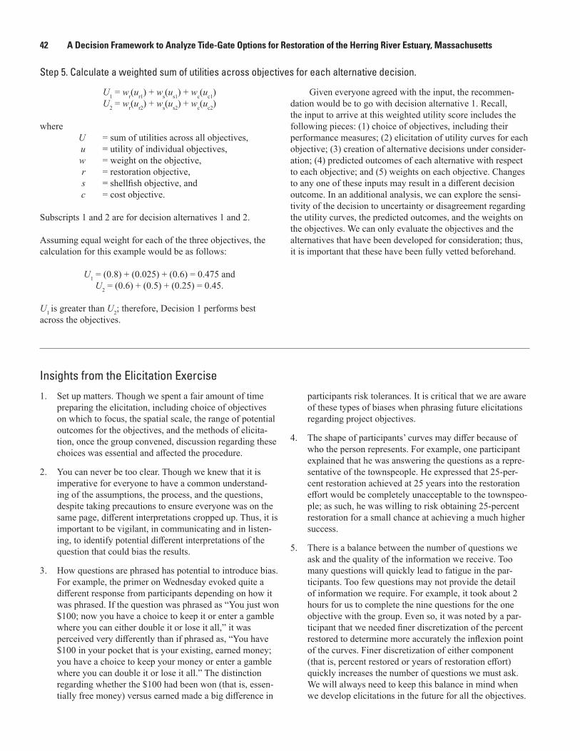
42 A Decision Framework to Analyze Tide-Gate Options for Restoration of the Herring River Estuary, Massachusetts
Step 5. Calculate a weighted sum of utilities across objectives for each alternative decision.
U1 = wr(ur1) + ws(us1) + wc(uc1) U2 = wr(ur2) + ws(us2) + wc(uc2)
where U = sum of utilities across all objectives, u = utility of individual objectives, w = weight on the objective, r = restoration objective, s = shellfish objective, and c = cost objective.
Subscripts 1 and 2 are for decision alternatives 1 and 2.
Assuming equal weight for each of the three objectives, the calculation for this example would be as follows:
U1 = (0.8) + (0.025) + (0.6) = 0.475 and U2 = (0.6) + (0.5) + (0.25) = 0.45.
U1 is greater than U2; therefore, Decision 1 performs best across the objectives.
Given everyone agreed with the input, the recommen-dation would be to go with decision alternative 1. Recall, the input to arrive at this weighted utility score includes the following pieces: (1) choice of objectives, including their performance measures; (2) elicitation of utility curves for each objective; (3) creation of alternative decisions under consider-ation; (4) predicted outcomes of each alternative with respect to each objective; and (5) weights on each objective. Changes to any one of these inputs may result in a different decision outcome. In an additional analysis, we can explore the sensi-tivity of the decision to uncertainty or disagreement regarding the utility curves, the predicted outcomes, and the weights on the objectives. We can only evaluate the objectives and the alternatives that have been developed for consideration; thus, it is important that these have been fully vetted beforehand.
Insights from the Elicitation Exercise
1. Set up matters. Though we spent a fair amount of time preparing the elicitation, including choice of objectives on which to focus, the spatial scale, the range of potential outcomes for the objectives, and the methods of elicita-tion, once the group convened, discussion regarding these choices was essential and affected the procedure.
2. You can never be too clear. Though we knew that it is imperative for everyone to have a common understand-ing of the assumptions, the process, and the questions, despite taking precautions to ensure everyone was on the same page, different interpretations cropped up. Thus, it is important to be vigilant, in communicating and in listen-ing, to identify potential different interpretations of the question that could bias the results.
3. How questions are phrased has potential to introduce bias. For example, the primer on Wednesday evoked quite a different response from participants depending on how it was phrased. If the question was phrased as “You just won $100; now you have a choice to keep it or enter a gamble where you can either double it or lose it all,” it was perceived very differently than if phrased as, “You have $100 in your pocket that is your existing, earned money; you have a choice to keep your money or enter a gamble where you can double it or lose it all.” The distinction regarding whether the $100 had been won (that is, essen-tially free money) versus earned made a big difference in
participants risk tolerances. It is critical that we are aware of these types of biases when phrasing future elicitations regarding project objectives.
4. The shape of participants’ curves may differ because of who the person represents. For example, one participant explained that he was answering the questions as a repre-sentative of the townspeople. He expressed that 25-per-cent restoration achieved at 25 years into the restoration effort would be completely unacceptable to the townspeo-ple; as such, he was willing to risk obtaining 25-percent restoration for a small chance at achieving a much higher success.
5. There is a balance between the number of questions we ask and the quality of the information we receive. Too many questions will quickly lead to fatigue in the par-ticipants. Too few questions may not provide the detail of information we require. For example, it took about 2 hours for us to complete the nine questions for the one objective with the group. Even so, it was noted by a par-ticipant that we needed finer discretization of the percent restored to determine more accurately the inflexion point of the curves. Finer discretization of either component (that is, percent restored or years of restoration effort) quickly increases the number of questions we must ask. We will always need to keep this balance in mind when we develop elicitations in the future for all the objectives.

For additional information, contact: Director, Leetown Science Center U.S. Geological Survey 11649 Leetown Road Kearneysville, WV 25430
or visit our website at: https://www.usgs.gov/centers/lsc
Publishing support provided by the West Trenton Publishing Service Center

Smith and others—
A D
ecision Framew
ork to Analyze Tide-G
ate Options for Restoration of the H
erring River Estuary, Massachusetts—
Open-File Report 2019–1115
ISSN 2331-1258 (online)https://doi.org/10.3133/ofr20191115