Embed Size (px)
Citation preview

-A122 197 1MPROVED SECOND ORDER METHODS FOR-PARABOLIC PARTIAL 1/2DIFFERENTIAL EGURTION..(U) LEHIGH UNIV BETHLEHEM PADEPT OF MECHANICAL ENGINEERING AND M. N C LEE ET AL.
UNCLASSIFIED APR 82 TR-FM-82-2 AFOSR-TR-B2-i934 F/G 12/1i M

MICROOP RESOLUTION TEST CHARTNATIONAL BUREAU OF STANDARDS-196-A
...
m --

- IFOSR-TR- 82-1034
L
ApprfOre tPublic release
41 t"UtIOU Unlimited.
L4J
92 12 09o36

IMPROVED SECOND ORDER METHODS FOR
PARABOLIC PARTIAL DIFFERENTIAL EQUATIONS
by
W.-C. Lee and J.D.A. Walker
Department of Mechanical Engineering and 'MkchanicsLehigh University, Bethlehem, PA
Technical Report FM-82-2
April 1982
Approved for public release; distribution unlimited.
Qualified requestors may obtain additional copies from theDefense Technical Information Service
Reprductontranslation, publication, use andQdisosa inwhoe o inpart by or for the UnitedStats Gvermentis ermtted.
AIR FORcK 017pTCE OF SCIENTIFIC~ ISL'I L,
approveid : ~ h15 bc-Sn and iSF
Dlstributl.., a4Lltd s- A s a,2
Chief, Technical information Divisionl

UNCLASSIFIEDSECURITY CLASSIFICATION OF THIS PAGE (Whlen Data Entered)
REPOT DCUMNTATON AGEREAD INSTRUCTIONSREPOT DCUMNTATON AGEBEFORE COMPLETING FORM
2GOVT ACCESSION NO 3. RECIPIENT'S CATALOG NUMBER
4. TITLE (and Subtitle) 45. TYPE OF REPORT & PERIOD COVERED
IMPROVED SECOND ORDER METHODS FOR INTERIMPARABOLIC PARTIAL DIFFERENTIAL EQUATIONS ______________
S. PERFORMING ORG. REPORT NUMBER
7. AUTHOR(s) 8. CONTRACT OR GRANT MUmER(s)
W.C. LEE F92-8CO7* -J.D.A. WALKER F92-8C07
9. PERFORMING ORGANIZATION NAME AND ADDRESS 10. PROGRAM ELEMENT. PROJECT. TASKAREA A WORK UNIT NUMBERS
*LEHIGH UNIVERSITY 612DEPT. OF MECHANICAL ENGINEERING & MECHANICS 230/2BETHLEHEM. PA 18015 20/A
ICONTROLLING OFFICE NAME AND ADDRESS 12. REPORT DATE
AIR FORCE OFFICE OF SCIENTIFIC RESEARCH/NA APRIL '82BOLLING AIR FORCE BASE, DC 20332 1.NNEO AE
1.MONITORING AGENCY NAME & ADDRESS(il different fromt Controlling Office) 1S. SECURITY CLASS. (.t this report)
UNCLASSIFIEDl11. DESCL ASSI F1CATION/ODOWN GRADING
SCHEDULE
IS. DISTRIBUTION STATEMENT (of this Report)
APPROVED FOR PUBLIC RELEASE; DISTRIBUTION UNLIMITED
17. DISTRIBUTION STATEMENT (of the abstract entered In Block 20, it different from Roert)
* 1S. SUPPLE149NTARY NOTES
19. KEY WORDS (Continue on reverse, olde It noeesavy endl Identify by block number)
NUMERICAL METHODSFINITE DIFFERENCESPARABOLIC EQUATIONS
20. ABSTRACT (Contita en revesei side It necessay and Identify by block monmber)
-)Two new finlte-differenceIIetheds are develepeJ or the calculationof parabolic partial differential equations. The leading truncation errorterms are derived and detailed comparisons are made with the errors associatedwith existing methods, namely the Crank-Nicolson method and Keller Box scheme.A number of examples of both linear and non-linear parabolic problems arecomputed with both the new and also the existing methods. The accuracy ofall four methods are compared; based an the conmuttIional .vprimants
DD 1 1473 EDITION OF 1 Nov 4a is ossoLETe UNGLAMJIILUS/H 0102-014* 66011
SECURITY CLASSIFICATION OF THIS PAGE ("M. Does entered)

~~UUCLASRED .- 2
.6L...ITY CLASSIFICATION OF THIS PAGE(whmn Data Ento,.d)
-.- and a comparison of the magnitudes of the leading truncation errors, it isconcluded Jhat the improved methods are to be preferred over the existingmethods.
UNCLASSIFEDSECURITY CLASSIFICATION OPP TIS PAOI[US.. 0a0a EMiME

ACKNOWLEDGEMENTS.
The authors wish to thank the Air Force Office of Scientific
Research for providi g financial support for this study under
contract no. F4962d;A'C-0071. The present investigation is a
small portion of a larger overall program "Theoretical and
* Experimental Investigation of Coherent Structure in the Turbu-
lent Boundary Layer". The investigation described here is a
preliminary study directed toward the development of improved
numerical techniques for the prediction of turbulent boundary
layers. One of us (W.-C. Lee) wishes to thank the Departmnent
of Mechanical Engineering, Lehigh University, for financial
support as a teaching assistant during this investigation.
A&O1I~n YA~1 or
Ths .C.. '~iLODTIC
~p~r~v 2 *0
w Chlt, Tchziiai~normatonei
- ~ ~ ~ ~ ~ ~ ~ ~ ~ ~ ~ ~ ~ Aii ,. .,.,c.......,. ....- - -- - - -

Abstract
Two new finite-difference methods are developed for the
calculation of parabolic partial differential equations. The
leading truncation error terms are derived and detailed com-
U parisons are made with the errors associated with existing
methods, namely the Crank-Nicolson method and Keller Box scheme.
A number of examles for both linear and non-linear parabolic
• -problems are computed with both the new and also the existing
methods. The accuracy of all four methods are compared; based
- 'on the computational experiments and a comparison of the mag-
nitudes of the leading truncation errors, it is concluded that
* . the improved methods are to be preferred over the existing
methods.a
..
t 1
V. EJ
. ... *
. -. -* . . . .

TABLE OF CONTENTS
Page
ACKNOWLEDGEMENTS I
* ABSTRACT 11
I TABLE OF CONTENTS 11-
LIST OF TABLES v
LIST OF FIGURES vi
1. INTRODUCTION 1
- 2. EXISTING MEIHODS 6
, 2.1 The Crank-Nicolson Method 6
2.2 The Keller Box Scheme 11
3. TWO IMPROVED METHODS FOR PARABOLIC EQUATIONS 20
3.1 Method I 20
3.2 Method 11 26
4. LINEAR EXAMPLE PROBLEMS 36
4.1 Linear Examples 36
4.2 Calculated Results 36
5. NON-LINEAR PROBLEMS 43
5.1 Introduction 43
5.2 The Howarth Boundary Layer Problem 44
5.3 Calculated Results for the Howarth Flow 595.4 An MHD Problem 65
5.5 Calculated Results for the MHD Problem 75
6. SUMMARY AND CONCLUSIONS 78
REFERENCES 79
!-I

(Table of Contents -cont.)
APPENDIX I Solution of the Difference Equations 81
APPENDIX 11 Simpsons Rule for Integration ofIndefinite Integrals 84
APPENDIX iiI The Ackerberg and Philips EliminationMethod 85
APPENDIX IV Newton Iteration 87
-JI-

r,%
LIST OF TABLES
Page
Table 2.1 Comparison of the leading error terms 16, -: arising from the approximations in the
marching direction for the classicalmethod and Keller Box method
Table 2.2 Comparison of the leading error terms 16arising from the approximations in thespatial direction for the classicalmethod and Keller Box method
Table 3.1 Comparison of the leading error terms 32arising from the approximations in themarching direction for Method Iand Method II
- Table 3.2 Comparison of the leading error terms 32arising from the approximations in thespatial direction for the Method I andMethod II
Table 4.1 Differential equations, exact solutions 37and mesh sizes for the linear example
U problemsTable 5.1 Mesh sizes and related number of grid points 60
Table 5.2 Velocity gradient at wall and number of 69iterations at selected C locations
1 (grid sizes are h=.2, ko=.l)
Table 5.3 Velocity gradient at wall and number 70of iterations at selected E locations(grid sizes are h=.l, ko=.05)
Table 5.4 Velocity gradient at wall and number 71of iterations at selected & location(grid sizes are h=0.5, ko=.025)
::v-

LIST OF FIGURES
Page
Figure 2.1 Grid configuration for the Crank- 8Nicolson method
Figure 2.2 Grid configuration for the Keller 8Box method
Figure 3.1 Grid configuration for the Slant 28scheme (Method II)
Figure 4.1 Comparison of RMS error for linear 40test problem 1
Figure 4.2 Comparison of RMS error for linear 41test problem 2
Figure 4.3 Comparison of R14S error for linear 42test problem 3
Figure 5.la Comparison of RMS error for the Howarth 61flow problem for mesh sizes listed inTable 5.1
Figure 5.1b Comparison of RMS error for the Howarth 62flow problem for mesh sizes listed inTable 5.1
Figure 5.1c Comparison of R1S error for the Howarth 63flow problem for mesh sizes listed inTable 5.1
Figure 5.2 Comparison of the RMS error for the 66Howarth flow problem starting with an'exact' initial profile at C-0; meshsizes are the same as for Figure 5.1a
Figure S.3a Mgnitude of the error for Howarth 67flow problem at C-.3
Figure 5.3b Magnitude of the error for Howarth 68flow problem at c-.6
Figure 5.4 Comparison of the root-mean-square 77error
-vi -.
I. INTRODUCTION
Parabolic partial differential equations arise frequently in
engineering applications particularly in problems involving
boundary-layer flows, heat conduction and mass diffusion. Finite-
difference methods are frequently used to solve such equations
numerically, especially in situations where an analytical solu-
tion is not readily available. Finite-difference techniques for
parabolic equations may be divided into two categories, namely
explicit and implicit methods. Both types of techniques are
discussed by Smith (1978) in the context of the unsteady one-
dimensional heat conduction equation and in this case the follow-
ing results apply:
(1) Explicit methods lead to relatively simple computational
algorithms but in order to obtain an accurate and
stable numerical scheme, severe restrictions on the
mesh sizes are usually necessary.
K (2) These restrictions can often require very small mesh
sizes and this can lead to excessively long computation
times.
(3) Implicit methods normally do not suffer from stability
problems and mesh size restrictions are not necessary
to achieve numerical stability.

(4) Of the implicit schemes considered by Smith (1978),
the Crank-Nicolson method, which is based upon approx-
imating the heat conduction equation at the midpoint
* of two successive time planes, is preferred since it
is second order accurate in both time and space.
* Although these results apply strictly only to the one-dimensional
unsteady heat conduction equation, experience suggests that they
are representative of parabolic problems in general and in par-
ticular carry over to the non-linear case. For example, Raetz
(1953), and Wu (1962) have considered the application of explicit
methods for the laminar boundary layer equations and find that
mesh size restrictions are necessary for the numerical scheme
to be stable. Implicit methods have performed very well in the
non-linear case and many modern laminar boundary-layer prediction
methods, for example, use difference equations based on the Crank-
Nicolson approach.
Another finite-difference technique has recently been sug-
gested by Keller (1970) for parabolic differential equations.
In general, for parabolic equations, there is a spatial direction
in which the boundary conditions are assigned and a marching
direction in which the solution is constructed in a step-by-step
manner. In the so-called 'Keller Box' method, the governing
-2-

- . . . . - - s -• -v -, . . . .. - -- " ... - ." - -.
., w . . - . ;• . :... -..-
equations are written as a system of first order eications and
central difference approximations are made at points midway
between the spatial mesh points. One major advantage of this
technique is that unlike the Crank-Nicolson method non-uniform
mesh sizes in the spatial direction may be used. This method
and the Crank-Nicolson method will be described in detail in
Chapter 2.
The Crank-Nicolson scheme and Keller Box scheme may easily
be used with non-linear parabolic partial differential equations.
The main difference in the non-linear case is that once the dif-
ference approximations are made ,the difference equations are non-
linear and cannot, in general, be solved immediately by direct
elimination methods. In order to overcome this difficulty the
difference equations must be linearized in some manner at each
stage in a general iterative procedure and at each station in the march-
ing direction; there are at least two ways in which this can be
carried out. In Picard iteration, the non-linear terms are
linearized by guessing selected terms from either the solution
at the previous station or from the solution at the last itera-
tion. This method is relatively easy to implement and if the
terms being linearized are chosen carefully, then convergence
will normally result. However, the rate of convergence may be
slow and can often be accelerated by an alternative linearization
-3-

technique known as Newton linearization; in this procedure, the
solution at any step is rewritten as a combination of the unknown
exact solution plus a perturbation quantity. Upon substitution
into the non-linear difference equations and neglect of the terms
which are quadratic in the perturbation, a set of linear differ-
ence equations is obtained; these equations may then be solved
by a direct method such as Thomas Algorithm. In practice, an
estimate of the exact solution is obtained by using the solution
at the previous step or from last iteration. This method is
more difficult to implement than Picard iteration but has the
ultimate advantage that the convergence rate at each station -
is quadratic.
The principle difference between the Crank-Nicolson method,
the Keller Box method and the two other approaches developed
here is associated with the method of spatial differencing. In
the Crank-Nicolson method,the spatial difference approximations
are based on the classical central difference approximations
for ordinary differential equations of boundary value type (see
for example Fox, 1957); on the other hand, the Keller Box
method is based on an alternative differencing scheme given by
Keller (1969) for ordinary differential equations of theboundary
value type. In a recent paper Walker and Weigand (1979) have
described a simple finite-difference technique for ordinary
I

differential equations which is shown to produce more accurate
results than either the classical method or the Keller (1969)
method. The objective of the present investigation is to adapt
the spatial differencing scheme of Walker and Weigand (1979) to
solve parabolic partial difference equations. The plan of this
report is as follows. In Chapter 2, the Crank-Nicolson method
and Keller Box method are discussed in connection with linear
- parabolic partial differential equations; modifications of these
schemes for the non-linear case are also discussed in Chapter 5.
Two new methods are developed in Chapter 3 for linear problems
and the modifications for non-linear equations are discussed
in Chapter 5. In Chapters 4 and 5 the various methods forthe linear
and non-linear cases respectively, are compared by using various
mesh lengths for a number of example problems. Based on the
truncation error terms given in Chapter 2, 3 and the computational
experiments of Chapters 4 and 5,lt is concluded that the present
3 methods are to be preferred over the existing methods.
-5-

• . .... - . w b . -. i - , -.- , , . -' - . i.- - , -' " [ • .- - . . - . . - - -" .
2. EXISTING METHODS
2.1 The Crank-Nicolson Method
Parabolic second order partial differential equations
are usually of the form,
Q 2U 2U + Uax 3U ay+ Ru + F, (2.1)
where x and y are two independent variables. The equation is
linear when the coefficients QP,R, and F are constant or
functions of x and y only. If the coefficients are functionsu au
- of xy, u, au y, the equation is non-linear but is usually
described as being quasi-linear since the non-linearity is not
associated with the most highly differentiated terms.
There are two popular methods currently available to solve
equation (2.1). The first of these is the Crank-Nicolson
-.. method and the application of this technique for linear equations
Kwill be discussed here; note that this method may only be used
with a uniform mesh in the y-direction. The conditions usually
associated with equation (2.1) are: (1) an initial condition
specified at sane initial station, say x - 0, according to
u(O,y) = f(y) and (2) boundary conditions at two y locations,
say y = a and b. Here a and b may be finite or infinite and
-. normally either u, 2 or a linear combination of both are given
.ay
S- . ..- 6-j

as specified functions of x. Here the simplest case where
u(x,a) z gl(x) ,u(x,b) =g()(2.2)
is assumed. Derivative boundary conditions may be treated through
obvious modifications of the present development (see Appendix
r.I).
The interval (a,b) in the y direction is split into N equal
parts of mesh length h as indicated as in figure (2.1); the
subscript j denotes a typical point in the mesh. Assuming that
the solution is known at x z xi 1 the object is to construct
the solution at x - x1 = xi- + k; here k is the step length
in the x-direction which may be varied as the integration pro-
ceeds. For simplicity and to avoid double scripting, define
kx xi1 l and x -1 + 7; the convention is then adopted
that all quantities evaluated at x* x and x are denoted by
a single asterick, a double asterisk and no asterisk, respectively.
Quantities at the station are known and the object is
to evaluate the unknown quantities at x.
In the Crank-Nicolson method, the partial differential
equation (2.1) is approximated at the point labelled C in
figure (2.1) which is located mid-way between the (i) and (i-1)
mesh lines and on the jth mesh line. Simple averages in the x
direction and central difference approximations for the deriva-
tives are used; both approximations are second order accurate
-7-
-------------------- --- olson -ehd th-ata ifeeta

yub-
y *-
-J 1
1- 1-1/2 1x
Figure 2.1. Grid configuration for the Crank-Nicolson method
yab
J +1
'A
ya
Figure 2.2. Grid configuration for the Keller Box method

* - - I_. -- r . - - . - . . - - .
and the following difference equations result at the typical
jth mesh line:
* * ***-uj) =l(Uj~ 2u + uj. uj+ 2uj + uj. 1 )
Q**(iJ ____ u4+i2u 4+u 1 u4+l 2U+ li k h+ V
D * ,*
++ j+ 1.- + -+I °_) + R * °3 uj)+ 3*
+ O(h2) + O(k2) . (2.3)
Here J = 1,2,3.. .N-1 where N is the total number of mesh points
in the y direction. Equation (2.3) may be rewritten in the tri-
diagonal form
Bjuj+1 + Au+Cu = D + h2 E (2.4)
where,
A " + "h2R - 2h2 (2.a)
1 e + hP , (2.5b)
C - 1- (2.5c)h h:.:. "-2"h2;" uj+l (l+ I"T ) P ' uj (I' P
Di * * g* +P2 ) j- (-2 + h2R + Q (2.5d)
It is possible to write the leading order terms in the trunca-
tion error Ej in two different but equivalent ways. In the
-9-
U7
Ui

first method, the error is expressed in terms of the partial
derivatives of the dependent variable u; here and in the subse-
quent methods discussed in this study, the point at which these
derivatives are evaluated will be standardized at the point on
3the Jth mesh line (y - yj), midway between the current and
previous solution plane. It may be shown through the use of
Taylor series expansions at the point (x**, yj) that
k2,,3 k2 ;2 32U742. + 2x
+ h2 34U + h2 * 33U + (.+ " T " " "' (2.6)
A second for of the truncation error is in terms of central
Sdifference operators according to,
El ; - 1x6 3Uj + .{(6Q2 x + 2(ux xQ *)(6 u1
+ 6u7 + .p y63uJ + ... (2.7)
Here 6 and P are the usual central difference operators and the
subscript indicates that the differences are to be taken in
that particular direction. Upon neglecting the leading trunca-
tion term, the matrix associated with the system of equations
(2.4) .is tridlagonal and a number of direct methods of solution
-10-
S . ,
, . .

are available; a particularly efficient method is often referred
to as the Thomas Algorithm (Appendix I). For linear problems,
equations(2.4) can then be solved directly to give the solution
at x = xt; the algorithm may then be applied again to obtain
the solution at xi+, and the computation proceeds in the x-
direction in a step-by-step manner.
2.2 The Keller Box Scheme
The basis of this method is to introduce an auxiliary
variable v and to rewrite equatioz (2.1) as the following
set of first order equations:
v u (2.8)ay ,
Qua + Pv + Ru + F (2.9)ax ay
Equations (2.8) and (2.9) are then approximated at point A ofI
Figure (2.2), which is the center of the box formed by points
(j-,i), (,I,i), (J,i-1) and (j-l,i-l); simple central differences
are used for the derivatives and simple averages for v and u.
4 Using the notation of the previous section, quantities evaluated
at x1, xi and xi are denoted by a single asterisk, a double
asterisk and no asterisk, respectively. The results for
equations (2.8) and (2.9) are
-11-
"
|0

~*U. U j.. . U (Vj + -
+Uj--2 = (vj + v i + vi_ 1 + Vi-l) + 2 '2
(2.10)
".Q.
!! (j j. - u J - I1 =W-]i (vi + vi -I .1 - 1)
P *(2.11)+ i ( +vj+vj .1+v l ) 4 ulju 1+uj_1 ) + 'j -"
A similar procedure is used to approximate (2.8) and (2.9) at
the center of the upper box labelled B in Figure (2.2) and the
results are,
+ +2 'T(= + + v j+l + vi + vi) 2
(2.12)
24~i (Uj+ + uj u~ 1 -i)*~ (V~ + + - -v)
II (2.13)
It is worhwiljl+e. not thtti+praha eraiy7+ * *J
adopted for equations for which the use of a non-uniform mesh
in the y direction is desirable; however, In what follows, only
the uniform mesh case will be considered since this is the case
of Interest in this Investigation. Keller (1970) prefers to
-12-
0

solve the linear set of difference equations in the form of equa-
tions (2.10) and (2.11). However, following a procedure simi-
lar to the technique suggested by the work of Ackerberg and
Phillips (1972),the set of difference equations may be written
as a single tridiagonal matrix problem which may then be solved
by a direct method. This procedure is more efficient than the
procedure used by Keller (1970) and moreover for comparative
purposes its convenient to perform the reduction to the tridiag-
onal form here. This reduction is carried out as follows.
Equation (2.10) is used to eliminate the auxiliary variable
v_ 1 in equation (2.11); the resulting equation contains vj, uj U
and uj. 1 and will be denoted as equation (A). A similar pro-
cedure is used to eliminate Vj+ 1 in equation (2.13) using equa-
tion (2.12); the resulting equation is termed equation (B)
and contains vj, uj and uj+i. Equations (A) and (B) are then
combined to completely eliminate the auxiliary variable v.-
from the system; the result is:
Bu + A u + Cu D + h2E, (2.14)SJ+l i Ji Jj-1 Di+ 2E
where E iis the truncation error. The coefficients in equation1 (2.14) are
h *-2-* h2 h2P**
(2.15a)
-13-il-
6 . •. "

B i h , h2 e h2Q**B" yj P - i + F R j - Qj +1 (2.15b)
7-Cji~ P..~ 1 - h2* (2. 15cO
J-** 4* * - k ** 4
4.h2 (F +{ - u{-,- ( , - P)
h I2 * * hT (Rj*i + R*) + (J + J4
+h h2, h2 **- +, (1 +Q ,j.,., + j (2.15d)
(1 h *+ h2 h2+ Ul_ I 1 T Pi-i. T Rl-,I + N Qji, .
It may be shown that the leading term in the truncation error
in equation (2.14),related to the partial derivatives of u
evaluated at the point (x**.yi). is
a"ax T ax a y =axa3y -,
-3U k+ V (2 au + o9j h2 a4Uwx T a x 2x T aI. j
(,p**% a3u h2 (2.16)..T j I = T Ay j
An alternative form for Ej in term of finite-difference opera-
tors is,to leading order,
-14-6'
, t .- . + -
, ' .- ,. ". . . . . -_ . " , . . , , • . - ., , ... -., ,, , ,, ..,, J

= - -I'S(62U) ( 62 Q )Mp6 u)
+ h. (Uy'yu7)(62U*) + 1 (uy6yQ7)(Iy6y(UX6xU*)u))
+ -+ yy ) {(62Q)(U6u + 2( 6XQj ))(62U.-
1 64 (I ** ** (U R.)6 2
(2.17)
Here 6 and u are the usual central difference operators and
the subscript indicates that the differences are to be taken
in that particular direction. Upon neglecting the leading
truncation terms, the tridiagonal problem in (2.14) may be
readily solved directly using, for example, the Thmas Algorithm.
The truncation errors associated with the classical Crank-
Nicolson scheme and the Keller (1970) box scheme are compared
in table (2.1) and (2.2). Referring to the x and y directions
as the marching and spatial directions respectively, it is
convenient to isolate the errors associated with the approxi-
mations in each direction. In table (2.1) the truncation
errors which originate from the approximations in the marching
direction are compared; such errors are defined to be those
-15-
,6

5-+ 0.
>1 4- 0aa )e
4) cx *or
>))4oftI4 4'' 0
o co x
EU - 5
060
--- -- -- ----- -
4))
cnx enx4 .0 4-0com ea a 4J0 >1
(=i x 'x4-3
+ +)5
0*4 CH ' Wa
£ o3* ico v U)D
4
'oreo mCT -x 5 -5
CLa)a-
EU +
9- U
- - 00'4'4- C 0 c
WU 4CJi mC'~ 0-a)0.41

containing partial derivatives with respect to x. It may be
observed that the first group of error terms are identical to
leading order but that the Keller (1970) method contains an
additional group of error terms O(h2). For this reason, the
Crank-Nicholson method apparently has an advantage over the
Keller scheme in regard to the accuracy of the approximation in
the marching direction; this point will be rec.onsidered subse-
quently.
Consider now the leading order error terms arising from the
approximations in the spatial direction which are compared in
table (2.2); these same error terms arise in the approximation
of the two-point boundary value problem,
d2u ddy + P(y) - + R(y)u + F = 0 u(a)=A, u(b)=B , (2.18)
by either the classical method or the Keller method. This prob-
lem has been considered by Walker and Weigand (1979) who also
derive an improved technique. Note that in table (2.2) the
first and second error terms are smaller by a factor of one-
half and one quarter, respectively, as compared to the corre-
sponding terms for the Crank-Nicolson method; however, the Keller
scheme contains an additional third error term O(h2 ). A general
conclusion that may be inferred is that neither the Crank-Nicolson
or the Keller method may be considered superior to the other
-17-

insofar as the approximations in the spatial direction are con-
cerned; this conclusion has been extensively verified for two
point boundary value problems by Walker and Weigand (1979).
It is worthwhile to remark that the errors in table (2.1)
and (2.2) are not independent. For example, for the ordinary
diffusion equation,
-u a2ua- a2U
(2.19)
the additional error term in the Keller (1970) method in table
(2.1) may be combined with the first term in table (2.2) and
the total truncation error is
k2 a3u h2a~u + ... (2.20)-
The corresponding error for the Crank-Nicolson method is
k2 a3U h
and it may be observed that the spatial error is smaller than
for the Keller method but of opposite sign. The total error will
in general depend on the particular problem under consideration
and in particular on the sign of each of the error terms and
how they combine.
-18-
• : .. ...I

At this stage, it appears that the total error term asso-
ciated with the Crank-Nicolson scheme can be expected to be
slightly smaller than for the Keller (1970) scheme because of
the additional error terms associated with the latter scheme.
However, a number of example problems will be considered in
Chapter 4 and 5 to investigate this point since it appears at
this stage that a general preference for the Crank-Nicolson
method would be marginal at best.
-19-

3. TWO IMPROVED METHODS FOR PARABOLIC EQUATIONS
3.1 Method I
Consider the grid configuration of figure (2.2); at any
fixed valpe of x (the marching direction) and at y,= Yj + Bh,
the following expressions may be written for u, au/ay and
92u/ay2 (Walker & Weigand, 1979):
u(x,y 8) - + + 2 6 + oe- - 6. + (3... 1u(x~yj),
(3.1) :
au - , ,+,y 1 + +2 63 ...}u(x,y.),
(3.2)
a2U (62 + op 63 + 64 .. j(Xy1
(3.3)
Here 6y and v are the usual central difference operators and
the subscript y denotes an operator in the y direction.
The general linear parabolic equation (2.1) may be rewritten
according tow
.u L(u) , (3.4)
where the operator L(u). is defined by,
-20-a
S:

L(u) ax+ P r + Ru + F (3.5)
Using the notation of the previous section, quantities evaluated
at xt, xi and xi are denoted by a single asterisk, a double
asterisk and no asterisk, respectively; equation (3.4) is then
approximated at point B of figure (2.2) according to,
Q+ *u J* L(u) + L(u) (3.6)Qj 1 -Xlj j l + i
Note that the error term has been omitted for the moment in
equation (3.6); however, this term is associated only with the
simple average on the right side and is O(k2). The principle
difference between the two methods developed in this section
lies in the approximation to the marching derivative au/ax.
In method I, a central difference approximation is used
along the line y = yj+, and this gives,
au I:. **= (3.7) .
Equation (3.1) may now be used to relate uj+ and uj+ to
values of u at points in the mesh. Using the first three
terms in equation (3.1) leads to, for example,
-21-
..

Lq
U =3u 1 +6u - uJ_ 1 (3.8) -
where the omitted error terms is O(u 63). Combining thesey y
approximations results in,
** [3j + 6u -uj I 3u +6uJ 8ki* * -k
= "fuj+l "2uj + uj. 1 + - 2n + .1)hP + h u
loe o tpitAo ue(.)t obtainL
+ J
+ (3u + 6u j (-.1 )
R..
+ -ft13u + + 6 " uj -1) + Fj+1" (3.9)
A similar procedure is applied to equation (3.4) in the.
lower box at point A of figure (2.2) to obtain
qJ1'l* I.1 .1"l +LuIJ(.0
Using a procedure analogous to that leading to the approximation
(3.9), it may be shown that,
-22-

Ui~l 6uj+ 3u~l +- + 6uj + 3u* 1
(u4 2u l +J1 2uj + u>] (.1
R R*+.k.(-uj+1+6uj+3uj_,) + .4i (-U ++6u3u 1)+F7
Equations (3.9) and (3.11) may be combined to form a set of
algebraic equations of the form,
Buj+ +Au +CIUj- 2 (3.12)
where,
Aju -2 -(jj-jj + --. ( ++Rj~j) - (Q + Q~
(3. 13a)
B. + h*h + r~ h2 (3Q* h2**
(3. 13b)
h2*=1 h h2* 16(* 3
(3. 13c)
Dj z-h 2(Fj+ + Fj -'2- hP -* p
* 3h2 3h2 *
+ (Rj + Rj~) + -W(Q~ + Qjj)
* -23-

S-uj +i(I + 2- P J+j + Tr (3 + -1 + 3jg -
. *h h2 ,. h2 •-u 1 0 h-T - Tr (Rj~j - 3Rj~j) - U2 (Q**j - 3Q))
(3.13d)
In equation (3.12),Ej is the total error term associated with
• the difference approximations. After some algebra it may be
-. shown using Taylor series expansions that the leading truncation
error terms in equation (3.12),related to partial derivatives
of the dependent variable at the point (x**,yj), are
E a3u t + h2 ( 2J u +q 32U aq 32 u5ax- . y T a + +
+ k2 ( + 2 -gax ax ax a2U Ij
h2 a4U h2 a3u + h3 ** a3uI-Ij 2 y a-YI (yJ )Yi
(3.14)
A second form of the truncation error is in terms of central
- difference operators according to,
** *
E + ( Q*)pu) + hk (Vyji 62j ~ x xj U 6yJ xxj yy x j
+ ( 6yQj )(uy6y(x6xuj ) )
+ 1 ((x2Q**)( 6 u') + 2(p 6Q*)(6 2 u))
-24-

64 1* 63U
(3.15) -
Upon neglecting the leading truncation terms,the tridiagonal
problem in equation (3.12) may be readily solved directly.
In situations where P,R,F and Q are not analytic but
numerical functions, the required values at the midway points
must be obtained with Interpolation formulae. For the present
method this situation may be treated by replacing values of P,
R, F and Q at Yj+ andy when they appear in the development
leading to equations (3.13), by the first three terms of equa-
tion (3.1); this procedure leads to an alternative form of
equations (3.13) which is
h 3h2**+**A -- j+1 + j-l + -l, 3-16a)
3h2 * ** **(Q+ I + 6Qj - Qj.) , (3-16a)
h p~+ * h2 -3
Bj =1 +K-(Pj+l + 6Pj - Pj+l + 6R
- .(5Q~ Q 3Q**1 ) ,(3-16b)
C-l h -6 3 h(2 R 5)Cj I+ Tr(Pj+1 -6j 3j_ - U j+l - 6j Sj-l)
+ M (3Q 1 - 6Qj -5Qj 1). (3-16c)
-25-

D h2 + 6Fj + j" *-
u I i 'j+ Fji I u;[. . -
+ h2 (Rj~l - 6Rj +R11_) + TW~ (Qj+l + 6Qj + Q_)
[r h **r h2
u1+ I + R3Pj1 + 6Pj1 +P + SRj + 6Rj.*~ ~ h h_* *
+ -2 (Qj+ 1 + 6Qr - 3Qr.) - u- 1 -(Pj+l - 6Pj -3Pj 1 )
h2** * h2 3lf fl- (3Rj+I-6R -R_)- (3Q2k (3.16d)
Note that the functions in equations (3.16) evaluated at x
may be evaluated at the points in the current and previous
time plane through use of the simple average. For example,
P (P + P (3.17)
3.2 Method II (Slant Scheme)
An alternative approach to method I may be considered where
the approximation of the derivative in marching direction is
modified. The basis of the method II is to approximate the
differential equation at the point x = x and y * yj which is
the same location as for the Crank-Nicolson method. A central
difference approximation along the line y =yj is used for the
1
S!-26- -1

h, .
x derivative as in the Crank-Nicolson method; the new feature
is that the operator L(u) is averaged along a diagonal line
intersecting the midpoints of the mesh at x* and x as illustrated
in figure (3.1). This procedure results in the two approxima-
tions,
Q= 1/2 L(u) + L(u)J . (3.18a)
andt*
Q F = 1/2 [L(u) + L(u) (3.18b)
where the omitted error terms are O(h2,k2 ). Equations (3.18a)
and (3.18b) are now combined into a single equation
* II
2Qj = L(u) + L(u) I + L(u)I.I
(3.19)
Finite difference approximations in the spatial direction are
used which are identical to method I of the previous section.
The approximation in the marching direction is simpler and
potentially more accurate since no errors in the spatial direc-
tion are incurred.
Writing equation (3.19) in finite difference form, the
following tridiagonal problem is obtained,
Ajuj + Bjuj+ I + Cjuj.- D + h2E (3.20)jj~~~~ j + ~ hE
-27-
I-

-
y=b
h I
I .- j+l/I
SJ 1
k
.- I -
:* . I
,, Ij-/
y-a 1_____
n O*
i1 -1/2 i xFigure 3.1. Grid configuration f or the Slant Scheme(method II).
-28-
: od

where,
h** -* 3h2 * * 2h1 *A = -2 Pj+ - P ) -+ 8(R + Rj _) Q Q -
(3.21a)
.h h* ** **
Bj = + y P + Tr (3Rj+j- Rj. ) (3.21b)
1 - _j - T6- (R~ - 3R7~j) ,(3.21c)
Dj =h2 (F* +F '-)
h p32 + 2h2 -
-uj+ 1 1 Pj+ +"- ( P _ -- Rj. Rjj +
• + h** h2 )
-- -11 h h2 (112 - 3Rj-* . (3-1d
It may be shown through the use of Taylor series expansions,
that the leading truncation error terms in equation (3.20)
related to derivatives of u at the point (x**,yj) is,
E.=h2Q~ 3 ~Qa ~ ~ k2Q. *aJ U k2 22 xU a2U 1 3
+h 2 au + Q a2u . _2u)*+B y x ya 2 ay 3yax T -aY
h2 , ;33ul** h3 3 **+ (- hj " (3.22)
-29-

A second form of the truncation error is in terms of central
difference operators according to,
S2**" 1 62 h )(6 2U**i1 _k IIX6X(6uJ ) + NY(V 6 u
IT + (P (i Q 6 * Q)(P 6 (P~ a u**))yy y y x x
Ej
+& Uxjx. j + l (xQ6 )(pxi6 u ) + 2 (u xx6 Q)(62x u)}
4 u... * T4 h j y ,uj + 32 u ) .
(3.23)
Upon neglecting the leading truncation terms the tridiagonal
problem in equation (3.20) may be readily solved directly.
1K In situations where PR,F and Q are not analytic but
numerical functions, the required values at the midway points
must be obtained with interpolation formulae. For the present
method this situation may be treated by replacing values of
P,R,F and Q at yj+ and yj. when they appear in the develop-
ment leading to equations (3.21), by the first three terms of
equation (3.1); this procedure leads to an alternative form
of equations (3.21) which is,
h ** . *3h2 * ) 2h2
i -- (,1 j+, j j- ,
(3.24a)
-30-

+ h * * * * * h 2 * * * *R * *Bj~~~~~ 5 R + J63jI6j-j)* ~ ,+6R -3Rjl (3.24b)j l6 3 j+l+6 j 3 64 j+1 j ji) 32bh * ** ** h2 -** * *= + Pj+-6Pj -3Pj_) - 6-- (3Rj+l'6Rj-5 R-) (3.24c)
h26. 64Fj~l
Dj " T (F;Il + 6**+lj,
h+3h 2 2h2 ~ 1 +jQ
-uj+ l 1 + -e3Pj+I+6Pj PjI ) + -a _5j16j- ,+1 h3*+6 ~ h2 **6R *
• -PPj+.-6Pj -3Pj - (R+-6R -R. )J- l .- J-
(3.24d)
Again equation (3.17) may be used to relate values of P, Q,
R, F at x to values at x and x
The truncation errors associated with both improved methods
are compared in table (3.1) and (3.2). In table (3.1) the
truncation errors which originate from approximations in the
marching direction are compared; such errors are considered
to be those containing partial derivatives with respect to x.
* It may be observed that for method I the first groupof error
terms is identical to the corresponding term of the method II.
The second group oferror terms for method I appear to be smaller
* than for method II because method II contains an additional term
of 0(h2).
* -31-
40

VI1 04x(_ Y
a+ C >'0 '0 +
C IX~ 00 >1 4
+ +3 C"IC% C- JIJco O+ + CL*~C. 4 y~ .;O a
C~tq ==
+ 41~ *
I+ +
+ IA - to E
.r- 0--- -- -- --- L. =
E___: 50
.)c
o -NI~ X .4Im N r S. k
M e. 0*
et - 0 c.0
aj 00 cu=Eu
Eu z zCA -32 4- w
I ~ + -4)S
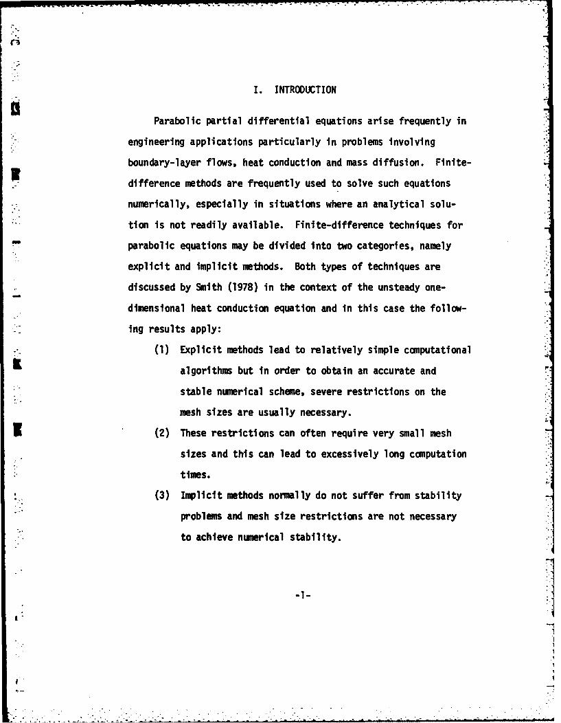
The leading order terms arising from the approximation in
the spatial direction are listed in table (3.2); these same
error terms arise in the approximation of the two-point boundary
value problem
d2u du.+ P(y) T + R(y)u + F(y) = 0,
u(a) - A, u(b) = B . (3.25)
This problem has been considered by Walker and Weigand (1979).
Since both method I and method II use the same scheme in the
spatial direction approximations, the spatial error terms are
identical.
It is also of interest to compare the error of the present
methods to that associated with the Crank-Nicolson and Keller
methods. First consider the error associated with approxima-
tions in the marching direction. Referring to table (2.1) and
(3.1), the first group of error terms for all four methods may
be observed to be identical. The improved methods and the
Keller Box Scheme have an additional second group of error terms
not present in the Crank-Nicolson method. For this reason, the
0 Crank-Nicolson method appears to have some advantage over the
improved methods in regard to the accuracy of the approximation
in the marching direction. Note also for improved Method I
that if Q term is a constant the second group error terms
-33-

associated with method I will vanish; however, method II and
the Keller's method will still contain a term 0(02); note that
the sign of this remaining term is of opposite sign in method
II and the Keller method.
In regard to the approximation in the spatial direction
Walker and Weigand (1979) have shown that the improved tech-
nique is more accurate than the existing methods. Note that
- in table (2.2) and (3.2) the first and second terms of the
improved methods are one-half and a quarter, respectively, of
the corresponding terms for the classical method. In comparison
to the Keller Box method, the first two terms are identical;
however, the third term in Keller's method is an order of mag-
nitude larger than for the improved methods. For this reason,
it is expected that the improved methods will,ln general,pro-
duce more accurate results than either the Keller or classical
method insofar as the approximation associated with spatial
direction is concerned.
On the basis of the error terms listed in tables (2.1),
(2.2), (3.1), and (3.2) as well as the results given by Walker
* and Weigand (1979) for two point boundary value problems, the
improved methods appear to offer improved accuracy over the
Keller (1970) method and possibly over the Crank-Nicolson method.
However, the situation is complicated in the general case by
-34-

the fact that, although a given method may have smaller indi-
vidual error terms, it may not produce more accurate results
on a specific problem. This is because in a particular problem,
the error terms may combine through differences in sign between
individual errors in each error term to produce a smaller over-
all error. For this reason it is important to consider a num-
ber of test cases and this is carried out in the next section.
-35-

4. LINEAR EXAMPLE PROBLEMS
[1 4.1 Linear Examples
Three linear example problems are considered here to cam-
pare the accuracy of the four methods discussed in the previous
Ii two chapters; the three example problems are listed in table
(4.1). For all four methods, the truncation terms were neglec-
ted and solutions were calculated with a uniform spatial mesh size,
* h, and uniform marching mesh size, k (the particular mesh values
are listed in table 4.1). The exact solution for example 1 is
not known, and to produce an 'exact' solution as a basis of
comnparison, example 1 was solved by the Crank-Nicolson method
with a set of extremely small mesh sizes. The accuracy com-
parison for both examples 2 and 3 are based on the quoted exact
* solution in table (4.1).
4.2 Calculated Results
In figure (4.1), the root-mean square errors (defined as
the square root of the sum of the squares of the error at each
mesh point divided by the total nuber of mesh points at a
u given time station) for example 1, are plotted; method I and
method II give better results than both existing methods as
time increases. However, method I I (the Slant Scheme) performed
slightly better than method I. According to the error terms
-36-j

7 S.
N~ 4Jgii
Lt r-I
+4+.0 41
4)4.)
4-
C%' U'o,
J= 4- VIJ=
0 U)
0~C CCis
4t S 43-) U
M, I II (
x 4
41 E
ca 0a ea eaI= 4a 41 41
S.. 0o 4V1
- a a37-
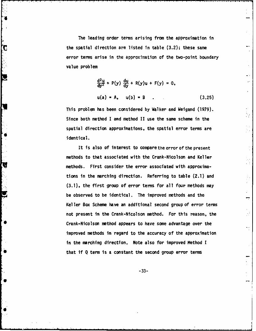
given in chapter 3, method II appears to have an extra leading
error term when compared to method I. In general, method II
might be expected to under-perform method I; however, the situ-
ation is somewhat more complicated than this. It appears that
the reason method II gave a more accurate solution in example 1
is that the error terms combine through differences in sign withhQ. a3u
the extra error term, namely, !f- Ty'axij to produce a
1 smaller overall error.
In example 2 (refering tofigure (4.2)) method II produces a
better solution than the other methods; method I and Crank-
Nicolson method are about even but both under-perform method
II; again; the Keller Box scheme produces the least accurate
results. Example 3 is a simple unsteady heat conduction equa-
* tion; for this equation method II reduces to the Crank-Nicolson
method. The root-mean-square error is computed and plotted on
figure (4.3); the results for this problem shows that Crank-
Nicdlson method performs slightly better than both method I
and',Keller Box scheme.
For the three linear examples considered, both improved
e methods are always clearly superior to the Keller Box scheme.
These results are generally representative of a number of other
linear problems with various values of the mesh lengths which
were considered but not reported here. Method II appears to
-38-

give superior results but it appears that a general prefer-
ence for Method II over either Method I or the Crank-Nicolson
methodis still not conclusively clear. In the next section, the
various methods will be compared for some nonlinear problems.
-
6i
I-39
0o

3 44.
x8
z ) 0 4U 4rq4m 44 1
0 06
EU ' J 4J . 44
01a 010
46 44
TI
-40.

0 0S
E 06
4,1
.13. S-
U 0-
* 5- 0
0
.. B4 a A
swu,

0u C 0
CC
4-
-42

~0
4
0
6
6
V

5. NON-LINEAR PROBLEMS
C 5.1 Introduction
In this chapter the most common type of non-linear para-
bolic problem will be considered; this is the quasi-linear para-
bolic equation which is of the form of equation (2.1) but for
which the coefficients QPR and F also depend on u and au/ay.
For all of the four methods considered thus far, the method of
* approximating the non-linear differential equation is similar
to the linear problem; the distinguishing feature from the linear
case is that the finite difference equations are now non-linear.
For this reason,the solution must be obtained iteratively at
any x station; this is carried out by first estimating values
of u at the current station to linearize the finite difference
* equations and thereby produce new estimates for u; these values
are used to re-estimate the non-linear terms in the finite
difference equations. This iterative process continues until
convergence is obtained. Another common procedure for handling
the non-linear difference equations is to use Newton lineariza-
tion; this approach generally accelerates convergence of the
* iterative scheme at any x-station at the expense of increased -
algebraic complexity in deriving the difference equations.
The application of the new methods developed in this study
to the non-linear type of problem is best illustrated by
-43-

example. In the next two sections two non-linear example
problems are considered and the performance of the methods com-
pared.
5.2 The He:ayth Boundary Layer Problem
The steady incompressible boundary layer equations for
two-dimensional steady flow are (see for example, Schlichting,
1968, p. 121),
au au.. = dgp a2uPu +pVy - dxLu + a' (5.1)
au+2V 0 (5.2)4ax ay
It is convenient to introduce the Levy-Lees variables &,n (see
for example, Blottner, 1975) given by
de = upUdx , (5.3)
dn = pU(2 )- dy , (5.4)
and a stream function
S= V f(,n) (5.5)
Here U is the mainstream velocity outside the boundary layer
and p,p are the fluid density and absolute viscosity. Upon
substitution of these transformations equations (5.1) become,
a3f f +a2f +l af)2 2t raf a2f a2f a9f'an (3n I an an 'an -3 •
(5.6)
-44-
I,
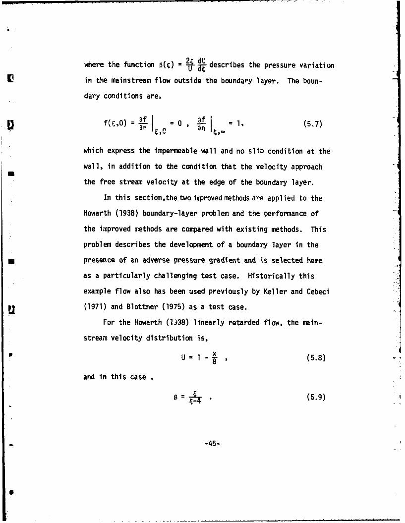
where the function O(c) describes the pressure variation
in the mainstream flow outside the boundary layer. The boun-
dary conditions are,
0 aff. 1 (5.7)]f( ,)-. =0,o ,,I CO anI
which express the impermeable wall and no slip condition at the
wall, in addition to the condition that the velocity approachn
the free stream velocity at the edge of the boundary layer.
In this section,the two inproved methods are applied to the
Howarth (1938) boundary-layer problem and the performance of
the improved methods are compared with existing methods. This
problem describes the development of a boundary layer in the
1 presence of an adverse pressure gradient and is selected here
as a particularly challenging test case. Historically this
example flow also has been used previously by Keller and Cebeci
u(1971) and Blottner (1975) as a test case.For the Howarth (1)38) linearly retarded flow, the main-
stream velocity distribution is,
U 1(5.8)
and in this case
= . . . (5.9)
-45-

It is convenient to rewrite equation (5.6) as a second order
system of equations according to
2u u 2 u a~f a)u- = + (f + 2c 2) 2- u 2 + 0,(5.10)
af5n= U,
with the boundary conditions,
f(C,0) = u(UO) = 0 , u(C,=) 1 . (5.11)
In equation (5.10),e is the marching direction and n is the
spatial direction. At ).0 equations (5.10) reduce to the
ordinary differential equations,
d2U du df (5.12)Tnr+ f 3_n= 0 , n- u. 5.2
which is the Blasius equation describing the boundary layer
flow on a semi-infinite flat plate; the numerical solution of
this equation provides the initial condition for the equations
(5.10).
For all four methods to be described here, a uniform mesh
in the n direction was used with h being the mesh size. Let
N-i be the total number of internal mesh points in the boundary
layer; the value of n, where the mainstream boundary conditions
in equation (5.7) were applied as an approximation is denoted
byL = Nh. In practice a value of t = 8 was found to be large
-46-

enough to ensure no change in the solution. The systems of
equations (5.10) and (5.12) are non-linear; at any stage in an
iterative procedure at each E station, once an estimate of u
is available, the second of equations (5.10) or (5.12) was
rintegrated using a trapezoidal calculation according to
f fj-1 + 'T (u, + uj- 1) (5.13)
for j = 1,2,3,...,N. The differences in the four methods
described here are associated with the approximations to the
first of equations (5.10) and (5.12) and these will now be
described.
Crank-Nicol son Method
In this method, to calculate the initial profile, central
difference approximations at each internal mesh point nj = jh
are made; this classical technique (Walker and Weigand, 1979)
leads to the tridlagonal matrix problem,
B uj+1 + Aj uj + C uj. 1 = Dj , (5.14)
where
A. = -2, B. = I +hfi, C = I - hfi, D 0 (5.15)
In equations (5.15), the fj are evaluated either from an initial
-47-

guess or from a previous iterate. At any stage the tridiagonal
problem for u in equation (5.14) is solved by the Thomas algor-
ithm and the f. are then obtained from equation (5.13). The
iteration was continued until two successive iterates agreed
to within five significant figures at each internal mesh point.
After a converged solution is obtained at 0 = , the marching
procedure may be initiated to advance the solution to { = k
and thence to c ik, 1 2,3,4...; here k denotes the march-
ing step.
The first of equations (5.10) is approximated at
+ k/2 and at n = nj; using the approximations described in
section (2.1), the first of equations (5.10) may be written in
finite difference form as a tridiagonal problem of the form
(5.14) where now,
B= 1 T (fi f j + T* * ff (5.16a)
1- I (f+f h (f(f-~ h (5.16b)
Jii
h2 h* 2 *
A -2 - B (u.+u*) ui (5.16c)
0j. -u., [+ (fj+f) *(f .f)
[2f h2 ** U* +2h12**1
* [I h ( * -h 4**(fj-*)l -2h2o**.~ ~;""* ..1I1 -"*r~i~J
(5.16d)
-48-

Here the u and f (on the right sides of equations (5.16)) are
evaluated initially from the solution at the previous step or
from the last iterate, as the iteration procedes at each C
station.
The iteration method just described is relatively slow
and the rate of convergence can be enhanced by using a standard
procedure of Newton linearization which is desnribed in Appen-
dix IV. This is merely an alternate form of the difference equa-
tions associated with the Crank-Nicolson method which may be
written (after some algebra) in the form,
Aju u +Bu C u + G + jf -+ jM. = D.
(5.17)
where,
B I.. h h * h** h(51a
A ILh 2 a "* * -58 **
Ih f h* h
h * h h * h *+ ITu j+ jl 9uj-I-u
H = 0 , (5.18e)j
-49-
I
, 0 (5.18f)
j u+1 T~ h 7 h2
2,h 2 h2 * h2 h2 .-uj * + T -* ) uJ ( ' - ui + 7 C UP
* 1 h h * 1 h* h
- h2 (5.18g)
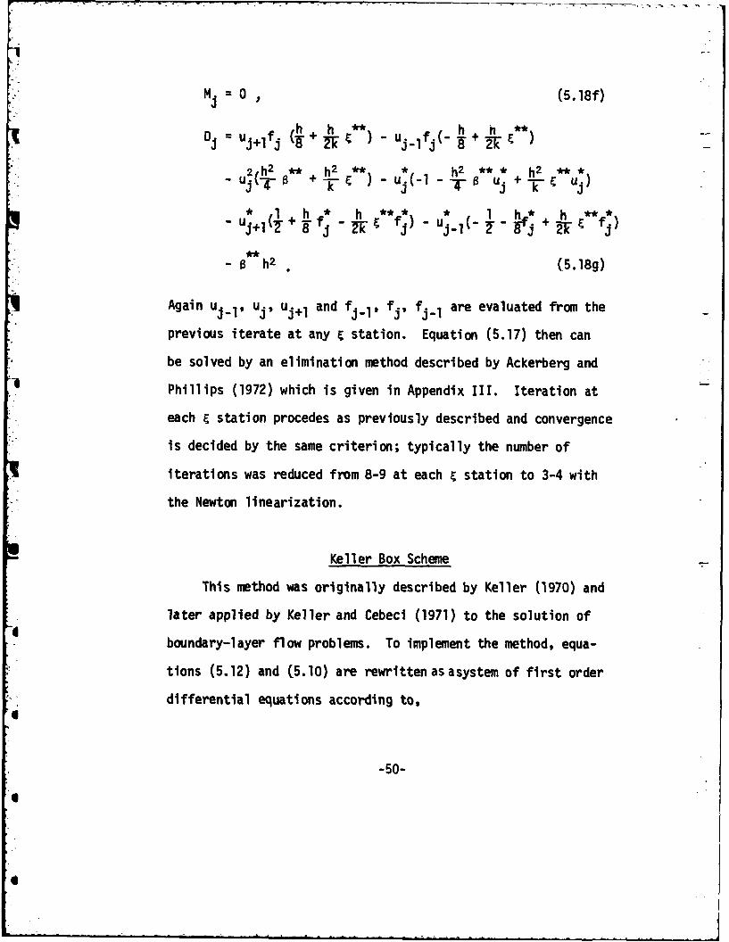
Again uj. I , uj, uj+l and f j 1, f . fj-I are evaluated from the
previous iterate at any c station. Equation (5.17) then can
be solved by an elimination method described by Ackerberg and
Phillips (1972) which is given in Appendix III. Iteration at
each c station procedes as previously described and convergence
is decided by the same criterion; typically the number of
iterations was reduced from 8-9 at each & station to 3-4 with
the Newton linearization.
Keller Box Scheme
This method was originally described by Keller (1970) and
later applied by Keller and Cebeci (1971) to the solution ofboundary-layer flow problems. To implement the method, equa-
tions (5.12) and (5.10) are rewritten as asystem of first order
differential equations according to,
-50-
a"

df du dfd=u , v dL -fv , (5.19)
and
af uu = v (5.20)izf'
a..V = ( + 2 f v + 2Eu u- - Bu2 + aS (f + 2c V~- v+ aE 8 2 B
To compute the initial profile, equations (5.19) are approxi-
mated at points nj+ and nj_ on either side of the typical
mesh point nj as described by Walker and Weigand (1979); the
two sets of approximations are then combined to form algebraic
equations of the form of equation (5.14), where now,
A i = -2 -4h- (fj+l - f-1) ' (5.21a)
B = 1 + h (f j+l + f.) (5.21b)
, = 1 - h (fj + f.-l), (5.21c)
D = 0 . (5.21d)
In equations (5.21), the f are evaluated either from an initial
guess or from a previous iterate. At any stage the tridiagonal
problem for u in equation (5.14) is solved by Thomas algorithm
and the f are then obtained from equation (5.13). The iteration
-51-

K
wascontinued until tosuccessive iterates agreed to within five
significant figures at each internal mesh point. After a con-
verged solution is obtained at E = 0, the marching procedure
may be initiated to advance the solution to { = k and from
there to E = ik, i = 1,2,3,4,...; here k denotes the marching
step.
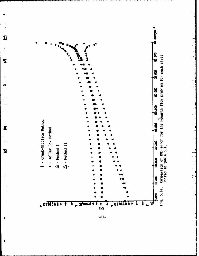
For equation (5.20), the approximations are made at
both n = nj+ and n = nj. using the technique described in
section (2.2). Using Newton linearization, it may be shown
(after a considerable amount of algebra)that the last two of
A equations (5.20) may be written in the form of equation
(5.17), where now,
h2 ** h2 h2A - +0 k + 2uj + uj-l ) +- (uj+ l + 2u
+ u 1) + khh* )(ff J + h1 h-1
(5.22a)
h2 + h2 ** h2 (u * +B= (-4- B + (*)(uj+uj+1 ) + T C**u. + u. l )i (T 7 Tj j+l)
(- + V . f**)(f+f) - hT - -F**(f f 1 1).2, (5.22b)h2 h2 **
Cj = ~~( + - -**)(uj+uJ l ) + E2 *(u*- + u*)
T 8 (u41 1
~*)(fj+fi1 ) + (T V E f** ( _*)-2, (5.22c)
-52-

H h + ' )(ui+ 1 - u + Uj+ 1 - uj) , (5.22d)
Gj -(h + **)(u+l _ uj-1 + uj+ . uj.1 ) , (5.22e)
- (uj -uj. 1 + (5.22f)
Dj = 2(u*+I - 2u + u*.I) + 4h2o **
+ h + ** [(f;+f; l)(Uju-1) + (fi++fi)(ui+-iu'))
+ (h2 S** + h2 **) (u +U j_1) + (uj+ I + Uj)2
(h2 h2 ) (u + u .1)2 + (u'. + u. 1 )2] (5.22g)
:2 i j
Equation (5.17) is readily solved by the Ackerberg and Phillips
(1972) technique coupled with trapezoidal rule of integration
given by equation (5.13). At each time step iteration is required
and the calculation proceeds in the & direction in a manner
similar to the Crank-Nicolson method.
Improved Method I
To conpute the initial profile, equation (5.12) is approx-
imated at points nj+, and nj. on either side of the typical
mesh point nj as described by Walker and Weigand (1979); the
-53-
0

two sets of approximation are then combined to form algebraic
equations in the form of equation (5.14), where now,
A = -2 - h (fj+1 - f-l1) (5.23a)
B Bj Z I + 0 (3fj+l + 6f - f J-1 (5.23b)
j 1 +. j(fi+ l - 6fj - 3 fj-l) (5.2c)
D j M 0 .(5.23d)
In equations (5.23), the fV are evaluated either from an initial
guess or from a previous iterate. At any stage, the tridiagonal4
problem for u in equation (5.14) is solved by theThanas Algorithm
and the f. are then obtained from equation (5.13). The itera-
tion continued until two successive iterates agreed to within
five significant figures at each internal mesh point. The
calculation may then be advanced in the +E direction as pre-
viously indicated for the other methods.
For equation (5.10), the approximationsare made at both
n = nj+ and n = ni_ using the technique described in section
(3.1). Using Newton linearization, it may be shown (after a
considerable amount of algebra) that the approximations to
equation (5.10) can be written in the form of (5.17), where
now,
-54-
I!
II

4 tt~-~ )(f +1-fj- 1) + t)fl
U 3 2 ** + * + (3h2 + R2+18(uj+1 u-1 +6u) j I-Th TO )(Uj+1 +u~. 1
- h2 +* 9h2 (5.4a
B. hh* 3* 3 f~
h28 (5u*1 + 6u~ 3u*_1 )
-5h2 h2 + h2 + 3h2 h2* - *)8F ~ )u~+ (32~ Tk j-
3h2 **+- 3h )u (5.24b)
Uh h 3* 13
+ h2 ** * + h h t **)(lf 3f 3f)32 j+-6 jW-E* 5uW j+1 Yj -4 j-1
+3h 2 **h
2 * - 3h2 R32 *
5h h28*~ (5.24c)
G. = 3h +3h E**) *u * (5.24d)
-55-

3) (u++u 1 -(u+u +il+)-*4j- (h i ..Uj+l+Uj+l)_(ju) 14(ilU~
(5.24e) - I
=Mh U)(uj+u*) + 3(jJl+U;1 )-
(5.24f)D 4u* -2u 2u ** + (4u
j -2u - 1 - 4h2B + jkl*1-uj(fj+l
- fj_l)+uj+1(3fj++6fj-fj_l) + Uj_l(fj+l-6fj-3fj_l)
L 4u* (fJ*l'-fj')U* (f+l6f.l
0 + - h**) +
- Uj_(f +1'6fj-3fj~) + 16 [3(u(uj+l+U_ 1 )
-u.(uj+l+Uj-l)) + 3 (u - *
jT j+1 j-ll 7 (ul u-1*~ (u~iu *I - - + 9(U*.- )
h r [), * * *)2 1 S2,4 u ** Uj+l+Uj+j l UjlijU~
E h 1(u ++6u +u. 1)2 + (u +6u .+u. )2 (52g
Equation (5.17) is readily solved by the Ackerberg and Phillips
(1972) technique oxupled with thetrapezoidal rule of integration
given by equation (5.13). At each time step, iteration is
required and the calculation proceeds in the E direction in
a manner similar to the Crank-Nicolson method.
-56-

Improved Method II (Slant Scheme)
This is a similar but alternative approach to method I,
with the basic difference being in the approximation made in the
marching direction (as discussed in Chapter 3). For this
method, the initial profile is computed with the identical
finite difference approximation and computational procedure
as method I. For equation (5.10), the approximations are made
- at both n = nj+ and n = nj. using the technique described
in section (3.2). Using Newton linearization, it may be
shown that approximations to equation (5.10) are of the form
of equation (5.17), where now,
=h h* * h h*f+ f H + -F Xf +I- r3h2 ** * 3h2 **W (uj+ l + uj 1 + 6uj) - -1-C a (uj3+h+uj)
- ah + 8h (5.25a)
B. 2+ h _ h X* 3 f* + 3 f* 12 __ uS T f+ 1 I+ j -T fj-l ) " (5uj+ l
5h2 * 3h2 3h2 **'632 l ui+1 (+ uj +"( 8 ufj+ (5.25b)
-57-
S
I nm mm m mmm m

4 k 4 fj+ r fj V
+ h2 ** (3u* +6u +5 ~ 1 h h ** 4 1 3
3 +3L 2 a** 3h2 ** 5h2 *
(5.25c)
G 3h +3h **j~ * &u (5.25d)
M - 2k + hj~ ** *
Mi 4 k T ~(uj+i+uj+.O-(ujjuj) +(5.25f)
D 4* -2*+ 2* +* h *
* .=u.-2 -2u -4h2o* + (-- + w i4u.f
f- f )+uj+ 1(3fj+ 1+6fj-f~ 1)+U. (j 1-f~3~-)
-L~..j~f+1 6fffj.. 1 ] _1 i3(u;(+l6fj3fl
3 j-1 2j-j+l j+lj-1) +4~j+lj+1
+ u. u2u-u. l)+q(u~u.-u.2 -1- 2 E*(u+U*U.)3-I j-i1 j- JJj 3 33
* (5. 25g)
The computational and marching procedure is carried out in the
same manner as method I.
-58-

5.3 Calculated Results for the Howarth Flow
The results of the calculations of the incompressible boun-
dary layer equation for the Howarth flow are described in this
section for all four schemes. There is no known analytical solu-
Ution to the problem and in order to produce an 'exact' solution,
as a basis of comparison, equations (5.12) and (5.10) were
solved by using very fine mesh sizes in the n direction and a
decreasing non-uniform mesh in & direction until five significant
figures of accuracy were obtained. The mesh size, h, in then direc-
tion is uniform throughout; however, a non-uniform mesh size, k,
is used in direction; in particular, k is uniform and equal to
ko, say,from e = 0 to e = .8; from g = .8 to E = .85, k is reduced
by a quarter; between E = .85 and = .9, k is reduced by half.
E The root mean square error (defined as the square root of
the sum of the squares of the error at each mesh point divided
by total number of mesh points for a given E station) for the
U four methods were computed for various mesh sizes, this RMS
error is summarized in table (5.1), and the results are plotted
on figures (5.1). According to the results for this test prob-
lem, the improved schemes produced more accurate results than
either the Keller Box Scheme or the Crank-Nicolson method; note
that the Keller Box Scheme performs better than the Crank-
Nicolson method for this problem. Referring to figures (5.1),
-59-

-nV) CD
9=LL. S
4-)S.
CDSo
LL. C ~,-) '4-C) ai r_
I- .C
VU)
4)
LL. 9=J (U 0
C..p-
LcU)
Va)u1-C) 04 U
- 60
+].Z$!h+I( | ( l0 4 Sl
+ 464 44 "
+ 00•
+ 4+ 4.64
+ 4a 4+ 6 4
+ U' 4
+ 64. 4
+ 64. 4v
o a+o +c
4--1 +
U0 + * *
L. +. Lu
w- 44 Gi+ .4to) 4- 4-
I- + 40 6 4 r- .
+ 0 to.4
44-
+. 44
+ lu WCLU4
+ 645
+
swml

4K4J
IA U4 4:
00 @
4) 0 0
S- -
C;
SW..
-.6-

pr
* 4a-
Ecc-
cu 04
0~ c
E ,E3
LL.04
~-63

the root mean square plots indicate Method I has the lowest
overall error of all, while the level accuracy of Method II
lies between the Keller Box Scheme and Method 1. Note that the
root mean square error increases substantially for all methods
as & -)...9; this is because a point of zero skin friction occurs
at o = .9008694 which suggests a flow separation occurs there.
In fact, with the mainstream velocity constrained to be of the
form equation (5.8), equation (5.6) contains an irregular
behavior of the form (&-co)f which is usually referred to as
the Goldsten singularity (1948). For this reason the trunca-
tion error will became large as E * CO for all methods.
It is known that the improved method of Walker and Weigand
(1979) produces more accurate results than either of the exist-
ing methods for solution of the initial equation (5.12) and the
question naturally arises as to whether the apparent better
performance of the two improved parabolic methods is simply a
result of the more accurate initial condition. To investigate
this point, all four methods were re-run but this time using
'exact' solution at the initial station (based on the solution
of equation (5.10) with a very small n~ mesh size); in this way
the error associated with the initial condition is eliminated,
and the accuracy of each parabolic schemne can be isolated,
The root mean square errors (RMS) for one set of computations
-64-

are plotted in figure (5.2); note that the mesh sizes are the
same as was used to figure 5.1a (see table 5.1). It may be
observed that similar conclusions as discussed in connection
with figures (5.1) can be drawn from these computations.
u The velocity gradient at wall (u') and number of iterations
for selected C stations for all four methods and for the three
sets of mesh sizes considered are presented in tables (5.2)
through (5.4) respectively; in addition, a comparison is made
with the 'exact' result. The absolute magnitude of the error
for the test problem at two different C stations for grid sizes
h = .1 and k = .05 are plotted on figures (5.3). It may be
observed that the improved methods have smaller errors than
either the Crank-Nicolson or the Keller Box method; further-
3 more, method I gives slightly better results than method II.
For this example, both improved methods give an accurate
solution for the boundary-layer equations. In the next sec-
U tion, another non-linear problem will be examined.
5.4 An MHD Problem
* The second non-linear example considered here is associated
with the problem of boundary layer for flow past a cylinder with
an applied radial magnetic field (see, for example, Crisalli
and Walker, 1976). The equations governing the flow in the
-65-

1L
4+ L 0
4.4J+ 4A~
8L W* 964
4.IL
4*4 06 4
+46
*oS- M4 -
+ 0
4J ~ 41 4
E* Q 446-.
-L 4u
4 14
SWH
-66-

a'3
±-Crank-Nicolson Method
u Q- Keller Box Method
++~ Metliod I
1.44
h .
k00AL
K IJ A
Yj
0-O j=
Fi. .a.Mgntdeo teero frHoathfowpobe
at C .3
I-67

+ - Crank-Nicolson Method
(D - KellIer Box Method
L- Method I
M ethod II
£ h =.1
k .05
0a4m4
4,6
4.A4
C A
-O ~w - W-ow so amo'Fig. 5.3b. Magnitude of the error for HIowarth flow problem
at =.6.
-68-

PU - qw to (r)LU
di
I-- I-ct
P C'~) CA
r-4-)
Cu) 4J1 -I-- m-
c'a
C) oilg
- -0 ~ %. 0 N. I '
lw CP) CMJ r-
LUJ
43 W)
4J CV) r- a
-jCD r 4-) 0
-- om o(
e-
i~ w-* . . . I U
-69-

O~r- M~ r %4-) qT 0~ r.%~u- m~ LO 0D )to r - q t o enx - Cf) cAi
LLU
4-)LiF- U-
03
4J%D LO co '~
- n ko CD CJ41T k* o 4w.
4.)
Lii 4.)
4-U
c00
en .0030d
.d. (Y') C4~
en cn .n I
- O 00 4
4 en 01 _ -03 O~ t O'I a-If
C') to
00
L n WI- C k)c' CD) ON ~
0 m %0 c
030

4) cVr) In) CD mU r - ko mn C
to) C1 u
4)4-)u
LL) CV) cyl mV ~ a
6-
U 4)
CV) mV **L C) In 0M LO0-- "C %0 CY).d: c! C'%! -
4.)
S- 0S
CV~) to) C) (7
r- q* %0 In L
-~ ~ CV I 0 a
P- V CV) C'J 4)
4-)o
X:L) C C 4J 9-r
-. I**)CV V *- 9aa-A r- r
m CV le 4w 4) U4.)4a)~~~ to9 I
-- In4J V In 4
7 - 'c %n CV) aCY) CJ 9
LAC)
UP cm 4.) co 0'U
-71-

vicinity of the rear stagnation point of the cylinder are
(Leibovich, 1967; Buckmaster, 1969, 19/l; Walker and Stewartson,
1972)2u F !!+(u-m) u+m-l au
ay2
(5.26)
ay
with boundary conditions
2u= F = 0 at y = O, u- l as y- . (5.27)ay
Here m is a parameter which is proportional to the magnetic field
strength. In addition, y measures distance normal to the wall,
u is the velocity tangential to the wall in the boundary layer,
F is a stream function and t is the time.
The time dependent problem considered here corresponds to
that for which the cylinder is impulsively started from rest and
from this initial condition, the solution of equations (5.26)
describes the time-dependent development of the boundary layer
near the rear stagnation point of the cylinder. For small times
it is convenient to introduce Rayleigh variables f, n given by,
n y/2t , f = F/2 . (5.28)
Upon substitution of these transformationsequations (5.26)
-72-4
4

become,
+ (2n-4tf) - + 4t(u-m)u + 4t(m-l) = 4t auan a
af = u (5.29)
The initial condition for equation (5.29) is obtained by takiag
the limit as t + 0 and the solution satisfying the boundary con-
ditions in equation (5.27) is
u = erfn (5.30)
In this section, the improved methods are applied to equa-
tions (5.29) and (5.26) and the performance of the improved
methods are compared with the Crank-Nicolson method. A value
of m = 3 is selected for this test case. As time increases and
te Loundary layer develops, 1:, variables given in equation
(5.28), which were introduced in connection with the impulsive
start, are no longer apprcoriate and it is convenient to switch
back to the original (y,t) variables; this was carried out at
t - .5 in all cases. A brief description of each method follows.
Method I
According to the new method described in section (3.1),
the first of equations (5.29) is reduced to a set of non-linear
algebraic equations of the form of equation (3.12) with
-73-
.. . . .S mL h m d M
m a m ' - u'" "'' " . . . .

associated equations (3.13); for this test example,
Q* 4t (5.31a)
P. = 2nj - 2t (fj + f.) , (5.31b)
R. = 2t. (uj + u) - 4t*m, (5.31c)
F. = 4t (m-i) (5.31d)
Equation (3.12) may then be solved by the Thomas Algorithm in a
general iterative procedure at each time step; in this procedure,
values of uj in equations (5.31) are replaced by the values at
previous iteration and values f. may be determined by the Simpson
rule of integration (see Appendix II). Iteration continues until
a converged solution is obtained to five significant figures;
the solution is then advanced to the next time step.
For larger values of time (t > 0.5) a switch back to prin-
ciple plane (y,t) is made and in this case the first of equations
(5.26) must be solved; it is reduced to the same form as equa-
tions (3.12) and (3.13), where now,
Q. = 1 , (5.32a)
P. = (F. + F.)/2 , (5.32b)
R = (uj + u )/2 m, (5.32c)
-74-
S

Fj =-l- (5.32d)
K Following the same type of procedure as described for the small
time solution, the integration may be advanced to successively
larger times.
Method II (slant scheme)
Referring to the method described in section (3.2), the
first equation of both (5.29) and (5.26) may be reduced to the
form of equation (3.20) with associated equations (3.21); here
the coefficients Q,P,R and F are identical to equations (5.31)
and (5.32) for the small time and large time solutions, respec-
tively. The computational procedure is analogous to that pre-
viously described for Method I.
Crank-Nicol son Method
According to the method described in section (2.1), the
first equations of both (5.29) and (5.26) may be reduced to the
form of equation (2.4) with associated equations (2.5). Again
the coefficients Q,P,R, and F are identical to the two previous
cases and the computational procedure is similar.
5.5 Calculated Results for the MHD Problem
There is no known analytical solution to the example prob-
lem and in order to produce an 'exact' solution, as a basis of
0 -75-

comparison, equations (5.29) and (5.26) were solved by using a
very fine mesh sizes in the and n directions until five sig-
nificant figures of accuracy were obtained. The root mean
square error (RMS) for the three methods were computed for a
mesh size of h = 0.05 and a time step of k = 0.1; the results
are plotted in figures (5.4). According to the results from
this test problem, the improved methods performed better than
the Crank-Nicolson method; however, Method I solution is some-
what more accurate than Method II. This conclusion is similar
to that reached for the Howarth flow problem.
4 -76-
d , . . . =l w t= == = , = , m w MI --: ~ i-..m.,,., o , ' --- ' . .

CL
S-
00
0r_.
4.) 0
0 * *4
-~ 0.+ 0~ .= #A
_77-

6. SUMMARY AND CONCLUSIONS
In this study, second order finite difference methods
for parabolic partial differential equation have been studied.
Two improved methods have been introduced. The leading trun-
cation error terms are discussed and the new methods have been
compared to two existing methods, namely, the Crank-Nicolson
method and Keller Box scheme. Examples of both linear and
non-linear problems for all four methods have been considered.
In general, the new methods give more accurate solutions than
the existing methods. However, in some special cases, Crank-
Nicolson may perform somewhat better than the improved methods.
This is due to the fact that for some problems the error terms
may happen to combine through differences in sign between
individual errors in each error term to produce a small overall
error. In addition, computational results consistantly showed
that improved methods were superior to the Keller Box scheme
and often by a substantial margin. Based on the leading order
truncation term comparisons in chapter 2 and 3, and the com-
putational results, it is concluded that the improved methods
* and particularly method I are preferred for the calculation
of parabolic equations.
-78-
--
I
I

REFERENCES
1. Ackerberg, R.C. & Phillips, J.H. 1972 "The Unsteady LaminarBoundary Layer on a Semi-Infinite Flat Plate due to SmallFluctuations in the Magnitude of the Free Stream Velocity",J. Fluid Mech. 51, 137-157.
2. Blottner, F.G. 1975 "Investigation of Some Finite-DifferenceTechniques for Solving the Boundary Layer Equations", Com-puter Methods in Applied Mechanics and Engineering, 6, 1-30.
3. Buckmaster, J. 1969 "Separation and Magnetohydrodynamics",J. Fluid Mech. 38, 481.
4. Buckmaster, J. 1971 "Boundary Layer Structure at a Mag-netohydrodynamics Near Stagnation Point", Q.J. Mech. Appl.Math. 24, 373.
5. Fox, L. 1957 The Numerical Solution of Two-Point Boundary- Value Problems. Oxford Press.
6. Goldstein, S. 1948 "On Laminar Boundary Layer Flow Neara Position of Separation", Quarterly J. Mech. and App.Math. 1, 43-69.
£ 7. Howarth, L. 1938 "On the Solution of the Laminar BoundaryLayer Equations", Proc. Roy. Soc., London, A164, 547-579.
8. Keller, H.B. 1969 "Accurate Difference Methods for LinearOrdinary Differential Systems Subject to Linear Constraints",SIAM J. Numer. Anal. 6, 8-30.
9. Keller, H.B. 1970 "A New Difference Scheme for ParabolicProblems", in J. Bramble (ed.), Numerical solution of par-tial differential equation 2. Academic Press.
10. Keller, H.B. & T. Cebeci 1971 "Accurate Numerical Methodsfor Boundary Layer Flows Part 1. Two Dimensional LaminarFlows", Proceedings of Second International Conference onNumerical Methods in Fluid Dynamics. Springer-Verlag.
11. Leibovich, S. 1967 "Magnetohydrodynamic Flow at a RearStagnation Point", J. Fluid Mech. 29 401,
-79-
p

12. Raetz, G.S. 1953 "A Method of Calculating the IncompressibleLaminar Boundary Layer on Infinitely-Long Swept Suction Wings,Adaptable to Small-Capacity Automatic Computer", NorthropAircraft Co. Rept. BLC-ll.
13. Smith, G.D. 1978 Numerical Solution of Partial DifferentialEquation. Oxford Press.
14. Walker, J.D.A. and Stewartson 1972 "The Flow Past a Cir-cular Cylinder in a Rotating Frame", Z. Angew. Math. Phys.23, 745.
15. Walker, J.D.A. & Weigand G.G. 1979 "An Accurate Methodfor Two-Point Boundary Value Problems", International Jour-nal for Numerical Methods in Engineering, 14, 1335-1346.
16. Crisalli, A.J. and Ialker, J.D.A. 1976 "Nonlinear Effectsfor the Taylor Column for a Hemisphere", the Physics ofFluids, 19, 1661-1668.
17. Wu, J.C. 1962 "The Solution of the Laminar Boundary LayerEquation by the Finite Difference Method", Proceeding of the1961 Heat Transfer and Fluid Mechanics Institute. StanfordUniversity Press.
-80-
IJ

APPENDIX I
SOLUTION OF THE DIFFERENCE EQUATIONS
1. The Thomas Algorithm
In chapters 2 and 3, the finite difference approximations
for the existing methods and the new methods, lead to a tri-
diagonal matrix problem of the form,
Bjuj+1 + Aju. + Cjuj+ = D . (A.1.1)
Here j = l,2,3,...,n-l and equation (A.l.l) holds at each inter-
nal mesh point. In the simplest case where the boundary con-
ditions are given by equation (2.2), the values of u are given
at the boundary according to
u0 gl(x) , n = g2(x) (A.1.2)
For all methods A., B., C. and D are known.
uThe solution of equations (A.1.2) may be obtained directly
through u. .of a solver generally referred to as the Thomas
algorithm. The procedure is as follows. Define two arrays,6
and F according toB-
F= 0 , Fn+l A n+l F (A.1.3)n+l n+l n
-81-
I
ij

4
[I
6 n+l -C n+l n
S60 = A n+l Cl Fn (A. 1.4)
The solution to equation (A.1.1) is then obtained by back sub-
stitution in
uj = Fjuj+ l + , F (A.l.5)
with j = n-1, n-2, ..., 1 since un is known.
2. Derivative Boundary Conditions
When one of the boundary conditions involves a derivative
condition, the above procedure must be modified. Suppose that
D_ g3(x) at y = b , (A.l.6)
instead of the second of equation (A.l.2). There are a number
of methods available for the approximation of equation (A.1.6);
-the method which is believed to be the most satisfactory and
which preserves the overall second order accuracy in h, is to
approximate the derivative in equation (A.1.6) with a sloping
difference according to,
au =llun-l8 unl+9un.2-2un-3 3)+ O(h ) . (A.1.7)
3y 6h
-82-
SD

Substitution in (A.1.6) leads to
IllUn-1 8u nl+9un-2- 2un-3 =6hg3(x) (A.1.8)
This relation rray be combined with equations (A.1.3) to (A.1.5)
U to compute the value of u at y4- according to
un=( ) (6 -(l 18n +9F - -F n-2F F +6n 3 -F -) 2 n 3u n 1 -18F -1+9Fn-iF n-2 2 n-iF n-2 Fn-3
(A.1.9)
This value may then be used to initiate the back substitution in
equation (A.1.5).
I -83-

a
APPENDIX II
SIMPSONS RULE FOR INTEGRATION OF INDEFINITE INTEGRALS
In the solution of the boundary-layer problems considered
in chapter 5, it is necessary to evaluate an indefinite integral
of the form,
f(yi) = u(y)dy (A.2.1)
This can be accomplished with good accuracy 0(h5) through the
use of Simpson's rule. To calcula e an integral over the first
step, the starting formula is,
f l u dy = h-{9u + 19uI - 5u2 + u3 } , (A.2.2)
and successive values of f are calculated according to
fi+l fi-I + {Ui 1 + 4ui + ui-l} (A.2.3)
for i = 1,2,3....
-84-
S
• S

A
APPENDIX III
THE ACKERBERG AND PHILLIPS (1972) ELIMINATION METHOU
Consider a system equations of the form,
Ll Aji uj+ 1 + Bju. + C uj_ 1 + Gjfj+ 1 + Hjfj + Mjf : j,
(A.3.1)
with the additional relation,
j+ =j + h (uj+uj+l) ' (A.3.2)
where j = 1,2,3,...,n-l. This system may be solved directly
by the following algorithm described by Ackerberg and Phillips
(1972). Assume the following relation,
Uj+l = aj+l + aj+lUi + Yj+fj ' (A.3.3)
and substitute equations (A.3.3) and (A.3.2) into (A.3.1); this
procedure results in an equation of the form,
uj = aj + 8juj_1 + YjfJ- 1 (A.3.4)
where the following recurrence relations are obtained:
hh haj = D j-jaj+- 2"Gjcj+)/(Ajaj+1 +B.+ hG.+ H.+ ejA~
+ GjG+a + h2G j+ (A.3.5)
-85-
! a II~ II ~ I II Idl

AD-A122 197 IMPROVED SECOND ORDER METHODS FOR-PARABOLIC PARTIAL 212DIFFERENTIAL EQURTION.. (U) LEHIGH UNIV BETHLEHEM PADEPT OF MECHANICAL ENGINEERING AND M. . W C LEE ET AL.
UNCLASSIFIED APR 82 TR-FM-82-2 AFOSR-TR-82-i834 F/G 12/1 NL

11.Ig
I
1 111 1.05 1.W
=IRCP RELTIO TES CH22NAIOA BREUOFSTN ARD n96-

- ( h h h h2 hC~ G. I1+~TGj~yj+l)/(Ajoj++Bjh%+ IT Hj
i° .. Pj j jjl
+ Ajyj+l + -Gj+l y+ 1) , (A.3.6)
=j -(GH+N+Ajyj+1+ Pjj,/Ajj I+hG+ hj j~~h h2
+ h 1jq*+ - Gjyj+1 ) (A.3.7)
The values of Aj., Bj, C., and 0. are known. In addition, the
values of u at the boundaries are known, and the boundary condi-
tions given by equation (2.1) my be expressed as,
uo gl(x) and un = g2 (x) . (A.3.8)
At y y Yn a comparison of equation (A.3.3) and the last of
equations (A.3.8) gives,
n 9=g2(x) On 0 and Yn 0 . (A.3.9)
These relations may be used to initiate the calculation of
On and yn' through the use of the recurrence relations (A.3.5)
to (A.3.7). The solution of equations (A.3.1) and (A.3.2)
is then obtained by substitution in equation (A.3.4) with
-86-

APPENDIX IV
NEWTON ITERATION
When the difference equations are non-linear, they cannot
be solved directly at each time step and iteration is required.
," Convergence may be accelerated through use of Newton iteration
which is Implemented as follows. Suppose the unknown variables
are f and u which can be expressed as,
f, fn + 6f (A.4.1)
-um + dum . (A.4.2)
The superbars denote the results of a previous Iteration or the
solution of the previous marching step in the case of the first
iteration. Suppose that a non-linear term of the form,U...
fmum + f + u) , (A.4.3)f~Mm -m
arises in the difference equations. Carrying out the multi-
plication gives
fmUm m(UM) + .fm)
+ 0(82)• (A.4.4)
The terms 0(62) are neglected and substitution for 8u and
B1mf from equations (A.4.1) and (A.4.2) yields,
-87-
. ao-..

Wet U w umem) A45
or
sfu+uf-fu(A.4.6)fmu, u +~ umm fmm.
This is the basis of Newton process for linearization of the-
difference equations.
IS-,
-88-