strathprints.strath.ac.ukstrathprints.strath.ac.uk/6501/1/strathprints006501.pdf · Abstract The behaviour of gas ﬂows in microscale systems cannot be adequately repre-sented by

O'Hare, Lynne (2008) Continuum Simulation of Fluid Flow and Heat Transfer in Gas Microsystems. PhD thesis, University of Strathclyde. http://eprints.cdlr.strath.ac.uk/6501/ This is an author-produced version of an unpublished thesis. Strathprints is designed to allow users to access the research output of the University of Strathclyde. Copyright © and Moral Rights for the papers on this site are retained by the individual authors and/or other copyright owners. You may not engage in further distribution of the material for any profitmaking activities or any commercial gain. You may freely distribute both the url (http://eprints.cdlr.strath.ac.uk) and the content of this paper for research or study, educational, or not-for-profit purposes without prior permission or charge. You may freely distribute the url (http://eprints.cdlr.strath.ac.uk) of the Strathprints website. Any correspondence concerning this service should be sent to The Strathprints Administrator: [email protected]

http://eprints.cdlr.strath.ac.uk/6501/

https://nemo.strath.ac.uk/exchweb/bin/redir.asp?URL=http://eprints.cdlr.strath.ac.uk

University of Strathclyde

Department of Mechanical Engineering

Continuum simulation of fluid flow andheat transfer in gas microsystems

Lynne O’Hare M.Eng.

2008

A thesis presented in fulfilmentof the requirements of the degree of

Doctor of Philosophy

Declaration of Author’s Rights

The copyright of this thesis belongs to the author under the terms of the United

Kingdom Copyright Acts as qualified by University of Strathclyde Regulation

3.49. Due acknowledgement must always be made of the use of any material

contained in, or derived from, this thesis.

Declaration of Author’s Rights i

Abstract

The behaviour of gas flows in microscale systems cannot be adequately repre-

sented by the Navier-Stokes-Fourier (N-S-F) equations of macroscale fluid dy-

namics. The key flow features that cannot typically be replicated by continuum-

based methods are discontinuities of energy and momentum at system boundaries,

known as velocity slip and temperature jump, and the Knudsen layer, a region

of flow close to boundary interfaces where the gas and the surface are not in

local thermodynamic equilibrium. In this thesis, fluid flow and heat transfer in

gas microsystems are simulated numerically using an extended form of the N-S-F

relations, which incorporates these non-equilibrium effects.

Constitutive scaling is a phenomenological approach that alters the linear

constitutive relationships of the N-S-F shear stress and heat flux closures to in-

corporate Knudsen layer effects in microflow simulations. This method has been

implemented here in a 3D finite-volume numerics package. The aim of the present

work is to make use of the constitutive scaling method to produce a computa-

tional tool suitable for analysing microscale flows. Both incompressible and com-

pressible numerical solvers featuring constitutive scaling models and a range of

appropriate boundary conditions have been developed to this end. Verification

and validation processes have been undertaken, comparing the performance of

the numerical models to analytical solutions, discrete molecular simulations and

experimental results for key engineering case studies.

A detailed assessment of the implications of extending the constitutive scaling

method to fully compressible flows has also been carried out. As a result of this

study, a new methodology for defining constitutive scaling functions empirically

has been produced. The methodology has shown, for a simple test case, that

Knudsen layer features can be incorporated in continuum simulations using scal-

ing functions based on the local features of a flow configuration, rather than a

global scaling function curve-fit to theoretical data for a single type of case.

Abstract ii

Acknowledgements

The author would like to thank supervisors J.M. Reese and T.J. Scanlon for guid-

ance and support throughout this project. Work carried out by D.A. Lockerby,

Y. Zheng and C.J. Greenshields that has facilitated this research is also gratefully

acknowledged. The work was funded by the Engineering and Physical Sciences

Research Council under Grant No. GR/S77196/01.

Acknowledgements iii

Contents

Abstract ii

Contents iv

List of Figures viii

List of Tables xiv

Nomenclature xv

1 Introduction 1

1.1 Motivation . . . . . . . . . . . . . . . . . . . . . . . . . . . . . . . 1

1.2 Rarefied flows . . . . . . . . . . . . . . . . . . . . . . . . . . . . . 2

1.2.1 Continuum-equilibrium . . . . . . . . . . . . . . . . . . . . 3

1.3 Scope of this research . . . . . . . . . . . . . . . . . . . . . . . . . 5

1.3.1 Availability of data . . . . . . . . . . . . . . . . . . . . . . 7

1.4 Outline of thesis . . . . . . . . . . . . . . . . . . . . . . . . . . . . 9

2 Modelling rarefied gases 12

2.1 Characterising gas rarefaction . . . . . . . . . . . . . . . . . . . . 12

2.2 Approaches to modelling rarefied flows . . . . . . . . . . . . . . . 16

2.2.1 Kinetic theory of gases . . . . . . . . . . . . . . . . . . . . 16

2.2.2 Discrete molecular models — DSMC . . . . . . . . . . . . 18

2.2.3 The Chapman-Enskog expansion . . . . . . . . . . . . . . 20

2.2.4 Moment models . . . . . . . . . . . . . . . . . . . . . . . . 21

Table of Contents iv

2.2.5 Extending the Navier-Stokes-Fourier equations . . . . . . . 22

2.2.6 Summary . . . . . . . . . . . . . . . . . . . . . . . . . . . 24

3 Physics of rarefied flows 26

3.1 Interfacial phenomena . . . . . . . . . . . . . . . . . . . . . . . . 26

3.1.1 Maxwell’s phenomenological model . . . . . . . . . . . . . 28

3.1.2 Phenomenological model vs. physical behaviour . . . . . . 33

3.1.3 Boundary effects on temperature . . . . . . . . . . . . . . 35

3.1.4 Alternative slip and jump models . . . . . . . . . . . . . . 38

3.2 The Knudsen layer . . . . . . . . . . . . . . . . . . . . . . . . . . 40

4 Constitutive scaling 44

4.1 Introduction . . . . . . . . . . . . . . . . . . . . . . . . . . . . . . 44

4.1.1 State of the art . . . . . . . . . . . . . . . . . . . . . . . . 47

4.2 OpenFOAM: a CFD framework . . . . . . . . . . . . . . . . . . . 52

4.3 Incompressible solver: icoFoam . . . . . . . . . . . . . . . . . . . 52

4.3.1 Boundary conditions . . . . . . . . . . . . . . . . . . . . . 54

4.4 OpenFOAM for non-equilibrium flows . . . . . . . . . . . . . . . . 54

4.4.1 Implementing effective viscosity . . . . . . . . . . . . . . . 56

4.4.2 Maxwell’s slip and constitutive scaling . . . . . . . . . . . 57

4.5 Progress summary . . . . . . . . . . . . . . . . . . . . . . . . . . 58

5 Incompressible flows 60

5.1 Introduction . . . . . . . . . . . . . . . . . . . . . . . . . . . . . . 60

5.2 Poiseuille flow . . . . . . . . . . . . . . . . . . . . . . . . . . . . . 61

5.2.1 Verifying numerical results . . . . . . . . . . . . . . . . . . 64

5.3 Couette flow . . . . . . . . . . . . . . . . . . . . . . . . . . . . . . 71

5.3.1 Verifying numerical results . . . . . . . . . . . . . . . . . . 74

5.3.2 Validating numerical results . . . . . . . . . . . . . . . . . 77

5.4 Constricted channels . . . . . . . . . . . . . . . . . . . . . . . . . 79

5.4.1 Validating numerical results . . . . . . . . . . . . . . . . . 82

Table of Contents v

5.4.2 Extending the analysis . . . . . . . . . . . . . . . . . . . . 88

5.5 Cylindrical Couette flow . . . . . . . . . . . . . . . . . . . . . . . 91

5.6 Summary . . . . . . . . . . . . . . . . . . . . . . . . . . . . . . . 94

6 Compressible flows 96

6.1 Introduction . . . . . . . . . . . . . . . . . . . . . . . . . . . . . . 96

6.2 Compressible solvers in OpenFOAM . . . . . . . . . . . . . . . . 97

6.2.1 Compressible solver: rhopSonicFoam . . . . . . . . . . . . 98

6.2.2 Modified solver: rhopEsonicFoam . . . . . . . . . . . . . . 100

6.2.3 Compressible microflows solver . . . . . . . . . . . . . . . 105

6.3 Constitutive scaling models . . . . . . . . . . . . . . . . . . . . . 106

6.3.1 Model A . . . . . . . . . . . . . . . . . . . . . . . . . . . . 106

6.3.2 Model B . . . . . . . . . . . . . . . . . . . . . . . . . . . . 107

6.4 Half-space problems . . . . . . . . . . . . . . . . . . . . . . . . . . 110

6.4.1 Kramers’ problem . . . . . . . . . . . . . . . . . . . . . . . 110

6.4.2 The temperature jump problem . . . . . . . . . . . . . . . 112

6.4.3 Summary . . . . . . . . . . . . . . . . . . . . . . . . . . . 114

6.5 Compressible micro-Couette flow . . . . . . . . . . . . . . . . . . 115

6.5.1 Discussion . . . . . . . . . . . . . . . . . . . . . . . . . . . 121

6.5.2 Summary . . . . . . . . . . . . . . . . . . . . . . . . . . . 126

7 A new approach to constitutive-scaling 128

7.1 Identifying a scaling function . . . . . . . . . . . . . . . . . . . . . 129

7.2 Extracting effective viscosity . . . . . . . . . . . . . . . . . . . . . 135

7.3 Incorporating Kn . . . . . . . . . . . . . . . . . . . . . . . . . . . 138

7.4 Discussion . . . . . . . . . . . . . . . . . . . . . . . . . . . . . . . 142

7.4.1 Scope for future work . . . . . . . . . . . . . . . . . . . . . 144

7.4.2 Summary . . . . . . . . . . . . . . . . . . . . . . . . . . . 146

8 Conclusions 148

8.1 Research contributions . . . . . . . . . . . . . . . . . . . . . . . . 153

Table of Contents vi

8.2 Scope for future work . . . . . . . . . . . . . . . . . . . . . . . . . 155

Appendices 157

A Analytical solutions: Poiseuille flow 157

A.1 Poiseuille flow . . . . . . . . . . . . . . . . . . . . . . . . . . . . . 157

B Slip-flow in Fluent 162

B.1 Mean free path calculation . . . . . . . . . . . . . . . . . . . . . . 162

B.2 Boundary condition accuracy . . . . . . . . . . . . . . . . . . . . 163

B.3 Maxwell’s slip condition . . . . . . . . . . . . . . . . . . . . . . . 165

C Analytical solutions: Couette flow 168

D Microflows in Matlab 173

D.1 Couette flow . . . . . . . . . . . . . . . . . . . . . . . . . . . . . . 174

D.2 Poiseuille flow . . . . . . . . . . . . . . . . . . . . . . . . . . . . . 176

References 177

Table of Contents vii

List of Figures

2.1 Example of a Maxwellian distribution of molecular velocities in

a 1D case. The most probable molecular velocity is the average

value, with probability decreasing towards the maximum and min-

imum velocities. . . . . . . . . . . . . . . . . . . . . . . . . . . . . 13

2.2 Gas flow regimes classified by Knudsen number; A represents fully

continuous flow, B slip/jump flow, C transitional behaviour and D

free molecular flow. . . . . . . . . . . . . . . . . . . . . . . . . . . 14

3.1 Molecular interaction across a plane S, which gives rise to shear

stress in the gas; and similar molecular interaction in the near-wall

Knudsen layer region, where both incident and reflected “streams”

of molecules interact. . . . . . . . . . . . . . . . . . . . . . . . . . 26

3.2 Schematic of the velocity structure of the Knudsen layer near a

wall in a pressure-driven flow, comparing different types of slip

boundary condition. . . . . . . . . . . . . . . . . . . . . . . . . . 41

4.1 Sketch of Kramers’ problem flow configuration showing applied

constant shear stress, τ ; traditional, no-slip N-S solution (uwall:

dotted line), N-S solution with second order macroslip boundary

condition (u∗∗slip: dashed line) and true velocity profile (uslip: solid

line). The Knudsen layer extends approximately 2λ from the wall

surface. . . . . . . . . . . . . . . . . . . . . . . . . . . . . . . . . 45

5.1 Schematic of Poiseuille flow configuration with velocity profile. . . 61

List of Figures viii

5.2 Analytical and numerical (microIcoFoam) Navier-Stokes solutions

for no-slip Poiseuille flow at any Kn (standard no-slip Navier-

Stokes solutions do not change with increasing Kn.) . . . . . . . . 65

5.3 OpenFOAM results including Maxwell slip compared to analytical

results from Eq. (5.3) for Poiseuille flow at Kn = 0.0035. Inset: a

close-up of the near-wall region highlighting the agreement between

the two profiles for slip at the channel wall. . . . . . . . . . . . . . 66

5.4 Verification of agreement between OpenFOAM simulations with

Maxwell’s slip boundary condition and Eq. (5.3) at various Kn

values. . . . . . . . . . . . . . . . . . . . . . . . . . . . . . . . . . 67

5.5 OpenFOAM results including constitutive scaling compared to an-

alytical results from Eq. (5.4) for Poiseuille flow at Kn = 0.035.

Inset: a close-up of the near-wall region highlighting the agreement

between the two profiles at the channel wall. . . . . . . . . . . . . 69


constitutive scaling and Eq. (5.4) at various Kn values. . . . . . . 70

5.7 Poiseuille flow results: comparison of OpenFOAM using Maxwell’s

slip boundary condition with OpenFOAM using constitutive scaling. 70

5.8 Schematic of Couette flow configuration with velocity profile. . . . 71


Maxwell’s slip boundary condition and Eq. (5.9) at various Kn

values. . . . . . . . . . . . . . . . . . . . . . . . . . . . . . . . . . 75


constitutive scaling and Eq. (5.11) at various Kn values. . . . . . 76

5.11 Comparison of OpenFOAM results for Couette flow with Maxwell’s

slip boundary condition with OpenFOAM results for constitutive

scaling. The top figure shows the velocity across the whole channel,

and the bottom figure the velocity in the upper half of the channel

only. . . . . . . . . . . . . . . . . . . . . . . . . . . . . . . . . . . 78

List of Figures ix

5.12 Constitutive scaling results from microIcoFoam compared to Navier-

Stokes solutions with Maxwell’s slip condition and to DSMC results. 80

5.13 Microchannel orifice constriction geometry. . . . . . . . . . . . . . 81

5.14 Microchannel venturi constriction geometry. . . . . . . . . . . . . 81

5.15 Centreline pressures in a channel with an orifice-plate constriction

compared to experimental data. . . . . . . . . . . . . . . . . . . . 83

5.16 Centreline pressures in a channel with a venturi constriction com-

pared to experimental data. . . . . . . . . . . . . . . . . . . . . . 84

5.17 Centreline pressures in the near-constriction region through venturi

constrictions in rectangular channels as throat height ht decreases,

compared to experimental data. . . . . . . . . . . . . . . . . . . . 84

5.18 Mass flowrates through constricted microchannels: OpenFOAM

results for constitutive scaling and Navier-Stokes equations com-

pared to experimental results. . . . . . . . . . . . . . . . . . . . . 85

5.19 Schematic of low-speed viscous flow through venturi-type and ori-

fice constrictions. . . . . . . . . . . . . . . . . . . . . . . . . . . . 87

5.20 Velocity profiles close to the throat wall for an orifice-plate con-

striction. Standard no-slip Navier-Stokes results are compared to

results with Maxwell’s slip boundary condition applied and to con-

stitutive scaling with microslip. . . . . . . . . . . . . . . . . . . . 87

5.21 Centreline pressures in the near-constriction region through venturi

constrictions in rectangular channels as throat height ht decreases:

constitutive scaling results only. . . . . . . . . . . . . . . . . . . . 89

5.22 Maximum velocity magnitude for orifice-plate constrictions as throat

height ht varies. . . . . . . . . . . . . . . . . . . . . . . . . . . . . 90

5.23 Schematic of Couette flow between concentric cylinders. . . . . . . 93

List of Figures x

5.24 Velocity profiles in cylindrical Couette flow non-dimensionalised

by the tangential velocity of the inner cylinder. Comparison of no

slip (· · ·), conventional slip (- -), Maxwell’s original slip (- · -),

constitutive-scaling in CFD (—) and DSMC data (). . . . . . . . 94

6.1 Effective viscosities provided by the scaling models, compared to

(constant) nominal viscosity. . . . . . . . . . . . . . . . . . . . . . 109

6.2 Effective thermal conductivities provided by the scaling models,

compared to (constant) nominal thermal conductivity. . . . . . . . 110

6.3 Ratio of effective viscosity to effective thermal conductivity (ratio

of momentum to energy diffusivity) provided by the scaling models. 111

6.4 Knudsen layer shape defect predicted for Kramers’ problem: ki-

netic theory data (points connected by solid line) compared to

model A (dashed line) and model B (dotted line). . . . . . . . . . 113

6.5 Schematic of the temperature jump problem showing constant ap-

plied heat flux, q; traditional, no-jump N-S-F solution (Twall: dot-

ted line), N-S-F solution with second order macro-jump boundary

condition (T ∗∗jump: dashed line) and true temperature profile (Tjump:

solid line). . . . . . . . . . . . . . . . . . . . . . . . . . . . . . . . 114

6.6 Knudsen layer shape defect predicted for the temperature jump

problem: kinetic theory data (points connected by solid line) com-

pared to model A (dashed line) and Model B (dotted line). . . . . 115

6.7 Couette flow configuration and nomenclature for the compressible

CFD analysis; UMa=1 is the velocity applied to move the lower

wall at the local speed of sound. . . . . . . . . . . . . . . . . . . . 117

6.8 Micro-Couette velocity profiles predicted by model A, Model B

and DSMC for Kn = 0.1. . . . . . . . . . . . . . . . . . . . . . . 119

6.9 Micro-Couette temperature profiles predicted by model A, Model

B and DSMC for Kn = 0.1. . . . . . . . . . . . . . . . . . . . . . 120

List of Figures xi

6.10 Compressible micro-Couette flow velocity profiles; comparison of

model A results (lines) to DSMC data (points). . . . . . . . . . . 121

6.11 Compressible micro-Couette flow temperature profiles predicted by

model A. . . . . . . . . . . . . . . . . . . . . . . . . . . . . . . . . 122

6.12 Temperature profiles predicted by model A, with high-Kn results. 124

6.13 Temperature profiles predicted by model A; results asKn increases

while σU = σT = 0.8. . . . . . . . . . . . . . . . . . . . . . . . . . 125

6.14 Predicted temperature (in K) at the centre of the channel in com-

pressible micro-Couette flow (i.e. the maximum temperature), plot-

ted against Knudsen number. . . . . . . . . . . . . . . . . . . . . 127

7.1 Schematic of an ellipse showing its centre (x0, y0), major axis a

and minor axis b. . . . . . . . . . . . . . . . . . . . . . . . . . . . 131

7.2 Velocity profiles from three newly proposed elliptical constitutive-

scaling models for Poiseuille flow in a microchannel where Kn =

0.1. Position y across the channel is non-dimensionalised by the

half-channel height. . . . . . . . . . . . . . . . . . . . . . . . . . . 134

7.3 Elliptical model 1 compared to a Navier-Stokes solution with slip

boundary conditions and the constitutively scaled Navier-Stokes

profile given by Eq. (5.4), for Poiseuille flow in a microchannel

whereKn = 0.1. Position y across the channel is non-dimensionalised

by the half-channel height. . . . . . . . . . . . . . . . . . . . . . . 135






List of Figures xii






7.6 Effective viscosity for the three elliptical scaling models compared

to the effective viscosity of the original constitutive scaling model.

Position y across the channel is non-dimensionalised by the half-

channel height. . . . . . . . . . . . . . . . . . . . . . . . . . . . . 138

7.7 Errors between velocity profiles of elliptical scaling models and

Eq. (5.4) for Kn = 0.1, shown at non-dimensional positions across

half a microchannel whose wall is positioned at y = 0. . . . . . . . 140

7.8 Errors between velocity profiles of elliptical scaling models and

Eq. (5.4) for Kn = 0.075, shown at non-dimensional positions

across half a microchannel whose wall is positioned at y = 0. . . . 141

7.9 Average percentage error between velocity profiles from three ellip-

tical scaling models and Eq. (5.4), shown versus Knudsen number,

Kn. . . . . . . . . . . . . . . . . . . . . . . . . . . . . . . . . . . 142

B.1 Schematic of typical near-wall cell in 2D CFD. . . . . . . . . . . . 164

B.2 Top: sketch of a typical near-wall velocity profile returned by Flu-

ent. In the nearest cell to the wall, the velocity gradient is always

manipulated in order to return the velocity of the fluid at the wall,

ugas, to the wall velocity, uwall. This is incorrect — the gas at

the wall should be assigned the calculated slip velocity uslip. Bot-

tom: arrangement of near-wall cells corresponding to the sketched

velocity profile, with cell-centre positions marked. . . . . . . . . . 166

List of Figures xiii

List of Tables

5.1 Variation of channel height, length and applied pressure gradient

for Poiseuille flow verification cases. Channel dimensions are given

in m, and the pressure gradient is specified in N/m3. . . . . . . . 65

5.2 Variation of channel height, length and wall velocities for Couette

flow verification cases. Channel dimensions are given in m and

wall velocities are given in m/s. . . . . . . . . . . . . . . . . . . . 74

5.3 Variation of Knudsen number with throat height for a pressure

drop of 99.63kPa across the channel. . . . . . . . . . . . . . . . . 89

6.1 Coefficients used in Eqs. (6.18) and (6.19) to define the scaling

functions of model B. . . . . . . . . . . . . . . . . . . . . . . . . . 108

6.2 Table of channel heights used to vary Kn in Couette flow simula-

tions, with corresponding Reynolds numbers for each case. . . . . 117

List of Tables xiv

Nomenclature

Latin symbols

A1 First-order velocity slip coefficient

A2 Second-order velocity slip coefficient

Ajump Temperature jump coefficient

AKP,TJ Scaling coefficient

Aslip Velocity slip coefficient

[A] Matrix of coefficients

C (f) Collision integral

C1,2 Constants of integration

D Diffusive coefficient

De Heat adsorption

DKP,TJ Scaling coefficient

E Energy

EKP,TJ Scaling coefficient

F Body force

H Channel height

I (n/λ) Velocity correction function

Kn Knudsen number

Kno Outlet Knudsen number

L Characteristic length scale of a system

Ma Mach number

Pi Inlet pressure

Nomenclature xv

Po Outlet pressure

Pr Prandtl number

Q Heat flux vector at the wall

R Specific gas constant

Re Reynolds number

S Co-ordinate plane

Sf Surface area of cell face

Sh Energy sources

SM Momentum sources

S(n/λ) Shape defect

T Temperature

T1,2 Wall temperatures

Tjump Temperature jump

T Dimensionless temperature

T ∗jump Temperature jump

T ∗∗jump Temperature jump with fictitious jump coefficient

Tr Reference temperature

Tw Wall temperature

Twall Wall temperature

U Velocity

UT Transpose of velocity

UMa=1 Velocity at local speed of sound

a Constant — sec. 4.1.1

Major axis of an ellipse — sec. 7.1

a1,2,n Chapman-Enskog coefficients

b Constant — sec. 4.1.1

Minor axis of an ellipse — sec. 7.1

[b] Matrix of boundary values

c Constant

Nomenclature xvi

c1 Local speed of sound

cp Specific heat at constant pressure

cv Specific heat at constant volume

dc Constriction depth

e Internal energy

f Distribution function

fM Maxwellian distribution function

f (uel) Functional proportion of an ellipse

f(n/λ) Scaling function for viscosity

f(n/λoriginal) Scaling function for mean free path

h Half-height of rectangular channel — ch. 5

Full channel height of constricted channel — sec. 5.4

Separation between rotating cylinders — sec. 5.5

h0 Total enthalpy

hc Constriction height

ht Throat height

in Unit vector normal to and away from a wall

k Thermal conductivity

kB Boltzmann constant

l Longitudinal channel length

m Mass of gas molecule

m Mass flowrate

n Normal distance from nearest surface

p Pressure

p Dimensionless pressure

pd Dynamic pressure

p〈ij〉 Stress

q Heat flux

qi Heat flux

Nomenclature xvii

r Spatial position

ri Inner radius

ro Outer radius

t Time

u Velocity

uslip Gas velocity at wall surface

uwall Velocity of wall surface

u Velocity component in x-direction

u1,2 Wall velocities — ch. 6

u1,2,3 Velocity produced by model 1, 2, 3 — sec. 7.1

uel “Velocity” corresponding to major axis of an ellipse

uc Cell-centre gas velocity — app. B

ug Local reference gas velocity

Gas velocity at first cell boundary — app. B

ui Velocity at ith node — app. B

un Gas velocity normal to the wall

uN-S Navier-Stokes velocity result, no-slip

uslip Slip velocity

utotal Composite velocity profile

uw Gas velocity at wall surface

ux Component of slip velocity in x-direction

u Dimensionless velocity

u∗slip First-order velocity slip

u∗∗slip Second-order velocity slip

[u] Matrix of velocities

v Velocity

v Velocity component in y-direction

v Mean molecular speed

w Velocity component in z-direction

Nomenclature xviii

x Co-ordinate direction

Channel length in x-direction — ch. 5

x0 Origin co-ordinate in x

y Co-ordinate direction

y0 Origin co-ordinate in y

y Dimensionless position in y-direction

z Co-ordinate direction

Channel depth — sec. 5.4

1 Identity tensor

Greek symbols

Γn Number of molecules per unit time

Π Stress tensor at wall surface

Φ Dissipation function

Ω1,2,3 Scaling coefficient for model 1, 2, 3

α Constant

β Kinetic-theory function

γ Specific heat ratio

δ Half-cell width

ε Energy

ζjump Temperature jump coefficient

ζslip Velocity slip coefficient

η Number density of molecules

θ Macroscopic variable in local Kn definition

κ Thermal conductivity

κeff Effective thermal conductivity

κeffAEffective thermal conductivity, Model A

Nomenclature xix

κeffBEffective thermal conductivity, Model B

λ Equilibrium mean free path of a gas

λF Lennard-Jones mean free path of a gas

λeff Effective mean free path

λoriginal Original mean free path

µ Dynamic viscosity

µ1 Dynamic viscosity at wall surface

µeff Effective viscosity

µeffAEffective viscosity, Model A

µeffBEffective viscosity, Model B

µ Dimensionless dynamic viscosity

ν Kinematic viscosity

Exponent of inverse power law — sec. refsoa

ξ Constant

ρ Density

σ Retained proportion of tangential momentum

Lennard-Jones characteristic length scale — app. B

σT Thermal accommodation coefficient

σU Tangential momentum accommodation coefficient

τ Tangential shear stress

τmc Shear stress with multiple components of velocity

τ Shear stress

τw Wall shear stress

φ Diameter of hard-sphere molecule

Mass flux in OpenFOAM

φ1,2,3 Viscosity-scaling function for model 1, 2, 3

ω0 (ν) Tabulated value from kinetic theory

Nomenclature xx

Chapter 1

Introduction

Gas flows in microscale systems display behaviour that cannot be replicated with

the governing equations of classical fluid dynamics, the Navier-Stokes-Fourier

equations (N-S-F). This thesis details how the N-S-F equation set can be mod-

ified to model microscale gas flows successfully, and demonstrates, for the first

time, that such an approach can be fully integrated into mainstream computa-

tional fluid dynamics (CFD). It also describes a new type of modification for the

governing equations that is a generalised and extended alternative to previously

available models.

1.1 Motivation

Gas microflows can now be found in a wide variety of applications, from small-

sample testing equipment for biomedical research through to microscale sensors

and actuators for the aerospace industry. Microscale shear flows occur in os-

cillatory systems such as comb drives, and even in optical applications where

microscale mirrors are moved to redirect signals. In these applications, the drag

forces experienced by systems can be very poorly predicted by classical fluid dy-

namics, leading to the malfunction and eventual failure of moving parts. Pressure-

driven microflows are also common, with banks of micro-thrusters employed in

low-mass satellite propulsion systems, and microscale flow-measurement devices

being produced that would benefit from better design-phase calibration. The

Chapter 1. Introduction 1

inability of the N-S-F equations to accurately predict mass flowrate in these de-

vices requires large margins of error to be employed in the engineering design of

gas microsystems, limiting efficiency. There is also interest in replacing chemical

batteries in portable electronic equipment with microscale power plants, a par-

ticularly interesting application that serves as an illustration of how macroscale

physics cannot always be translated directly to smaller-scale systems [1].

Generally, microdevices are manufactured using mature technology originally

developed for the electronics industry, and it is possible for intricate 3D geometries

and complex multiphysics systems to be produced quickly and effectively. The

design of small-scale systems is uniquely challenging, however, as many of the

assumptions underpinning classical macroscale physics do not hold for microflows.

To illustrate, a truly general model for gas microflows would need to repre-

sent many unusual flow features, including local departures from the macroscopic

second law of thermodynamics, dominant surface effects, and, under certain cir-

cumstances, velocity and temperature profiles completely inverse to those pre-

dicted by macroscopic methods. Although a large body of academic research has

already been conducted dedicated to understanding the physics of microsystems,

very few robust engineering models exist, and trial-and-error approaches are still

used to design commercial products in many cases. Inefficient, and often inef-

fectual, devices are a common result. In order to improve industrial design in

the short-to-medium term future, this thesis integrates new and innovative con-

tinuum models into the CFD package OpenFOAM, to produce an engineering

analysis tool for gas microsystems with capabilities comparable to those available

for macroscale design work.

1.2 Rarefied flows

The primary cause of the unusual, and at times counter-intuitive, behaviour ob-

served in microscale flows is gas rarefaction. This occurs as the molecular mean

free path of a gas in a system, the average distance a particle travels between


collisions with other particles, approaches the order of the physical dimensions

of that system. As the flow becomes rarefied the gas ceases to act as a single

continuous fluid, and begins to behave as a collection of discrete particles. There

are two common causes of rarefaction: either it occurs in the case of decreasing

density of the gas, or, as in microsystems, when the physical device dimensions

are sufficiently small. In microscale devices, the density of the gas can remain

unchanged, but only a relatively small number of molecules is found inside these

low-volume systems. Also, the mean free path begins to approach the order of the

physical dimensions of microsystems. For example, a microscale pipe system car-

rying air at atmospheric conditions would have a mean free path of approximately

0.06µm. This represents a difference of only two orders of magnitude between

the mean free path of the gas and the system’s characterising dimension, the pipe

diameter. The ratio of these two quantities is known as the Knudsen number.

This is the parameter most commonly used to classify the degree of rarefaction

in a gas:

Kn =λ

L, (1.1)

where λ is the mean free molecular path of the gas and L is some characteristic

dimension of the system. Traditionally, flows where the Knudsen number rises

above Kn = 0.001 are considered to be rarefied [2].

1.2.1 Continuum-equilibrium

Local thermodynamic equilibrium is defined as the state of minimum thermody-

namic potential, in which a fluid may be considered to be continuous. This is

true if the fluid is infinitely divisible in both space and time. A fluid may be

described as being in equilibrium if there exist no spatial or temporal gradients

within it.

The loss of local thermodynamic equilibrium in a gas implies that the mi-

croscale behaviour of the gas leads to gradients of macroscopic quantities in the


flow. Macroscopic variables (velocity, temperature, pressure etc.) describe molec-

ular behaviour averaged over an element of gas. This element must be sufficiently

large as to accurately describe the microscopic behaviour of the fluid without

large statistical fluctuations, but sufficiently small as to allow the macroscopic

variables to be represented by differential calculus. This is the continuum as-

sumption, which implies that there is scale separation between the microscopic

and macroscopic behaviour of a gas flow [2].

Complete equilibrium is a clearly defined state where no gradients of macro-

scopic quantities exist in a flow. Generally, when discussing equilibrium in a

practical system, what is meant is that the flow is quasi-equilibrium in nature.

The “equilibrium” assumption, in this context, is that the departures from local

thermodynamic equilibrium in the system are small. Quasi-equilibrium flows can

be successfully modelled using the traditional governing equations.

As rarefaction increases in a dilute gas, first the assumption of a quasi-

equilibrium state becomes invalid, followed by the continuum assumption (the

opposite is true of a dense gas.) If the continuum assumption is invalidated,

the differential equations traditionally used in the analysis of fluid flow and heat

transfer also become invalid.

Larger departures from the equilibrium state lead to discontinuities of mo-

mentum and energy at gas-solid interfaces, phenomena known as velocity slip

and temperature jump, respectively. In addition, the nonlinear behaviour of the

Knudsen layer can have a significant impact on the flow. The Knudsen layer is

a near-wall region of fluid where intermolecular collisions do not fully exchange

energy and momentum between the gas and the bounding surface. It typically ex-

tends one to two mean free paths from solid surfaces in gas flows at any scale, and

cannot be modelled using traditional continuum methods. In a rarefied gas the

increased relative size of the mean free path can mean that large proportions of

the flow are within the Knudsen layer, and exhibit nonlinear behaviour. As such,

near-wall and Knudsen layer physics can greatly influence fluid flow and heat


transfer, particularly in microsystems, where the surface area-to-volume ratio is

often large.

1.3 Scope of this research

In summary, this research comprises

• The implementation of N-S-F continuum models modified to include rar-

efaction effects in OpenFOAM CFD,

• Simulation of key engineering case studies for which analytical, statistical

or experimental data are available, and

• The development of a new approach to modifying the N-S-F equations for

the analysis of microscale flows that is more general and flexible than pre-

viously available alternatives.

The primary contribution of this research is the production of a design-

oriented analytical tool for fluid flow and heat transfer in gas microflows. The

work makes use of specialised boundary conditions alongside modifications to the

N-S-F equations that can replicate Knudsen layer behaviour. It provides engi-

neers with the capability to rationally design gas microsystems using the same

type of numerical studies that are common in macroscale fluid dynamics. With

microscale engineering often at the forefront of developing technology, this is a

valuable new capability for the field. The OpenFOAM model created is the first

modified N-S-F model that is fully integrated into a mainstream CFD package,

and that can successfully simulate compressible, non-isothermal flows.

In order to produce the final OpenFOAM model, the scope of this research

includes extensive review of available technology for the numerical simulation of

gas microflows, a study of the physics of rarefied flows, and a definition of the

state of the art in modified continuum fluid dynamics models. Detailed studies of


the OpenFOAM source code and available modifying functions lead to the imple-

mentation of simple models for incompressible, isothermal microflows. Validation

and verification exercises are carried out using simple flow configurations. The

modified continuum models are then extended for application to compressible

flows. Several engineering case studies are analysed in detail, and the efficacy of

the model as a design tool assessed.

This research has also produced an alternative means of using continuum

methodology to analyse rarefied gas flows. The new approach is based on the

modification of the governing equations according to the geometric and rarefac-

tion parameters of the local system, rather than with a single, specific function,

as is the case in other models studied. Although this new method is empirical

in nature, it offers the possibility of extending the N-S-F equations in a more

general way than was previously possible, based on a parametric classification of

the likely impact of rarefaction on the system. Knudsen layer shape and depth,

for example, can be estimated based on the system geometry, Knudsen number

and local gradients of macroscopic quantities.

The development of this new model was inspired by some of the challenges

encountered when extending existing continuum models to non-isothermal, com-

pressible flows. Work on this subject includes detailed analysis of the relative

merits of available modifications for the governing equations, and in-depth inves-

tigation of the interaction between those models and the most commonly used

boundary conditions for rarefied flows. The new method is devised as a means of

circumventing many of the difficulties associated with the use of previous scaling

models for simulating “real-world” flows. Preliminary testing of this method has

been conducted, and the results are assessed alongside those of the more estab-

lished models. A discussion of the potential future for the technique is presented.


1.3.1 Availability of data

The larger part of this research comprises the implementation of mathematical

models for gas rarefaction behaviour in a numerical framework. Although nu-

merical simulations and CFD can offer excellent performance and flexibility in

the analysis of complex flows, the accuracy of the results is limited primarily by

two factors: the correct application of the technology to the problem, and the

limitations of the numerical approach employed. As rarefied-gas dynamics is a

relatively specialist subject, responsibility for the former remains with the end

user of the OpenFOAM models created in this research. The latter, however, re-

quires the validation and verification of the code to be conducted in a responsible

manner during the development of the simulations.

Unfortunately, the implications of operating experimental gas-flow appara-

tus at micrometre scales mean that reliable experimental data for the type of

microflows in which we are interested are often difficult to find. The specialist

laboratory equipment required to manufacture and conduct experiments on gas

microdevices is prohibitively expensive for most academic institutions. As such,

only data published in academic literature by experimental facilities are available

for validation, which may not be in the area of interest. Much of the available

literature focuses on experimental analysis of two phase flows, on liquid flows, or

on comparatively large physical scales, as these are more practical to investigate

experimentally than dilute gas flows. As such, other sources of data must be

employed along with traditional experimental work to have full confidence in the

results of the numerical studies. To ensure that accuracy is not unreasonably

sacrificed in the pursuit of performance, the numerical models presented here are

evaluated using several different types of available data, as outlined very briefly

below.

Analytical solutions For incompressible, isothermal cases in simple channel

geometries, analytical solutions to the N-S-F equations may be found, both in-


cluding and excluding the impact of the modifying functions used to represent

gas rarefaction. These are exact solutions and, as such, are the preferred method

of verifying that the numerical implementation operates correctly. Analytical

solutions were employed in early development stages of the models.

Other numerical results In some instances, numerical simulations have been

produced by other research groups that provide interesting comparison to the

modified continuum models implemented here. Unless otherwise stated, these

models are compared to those presented in this thesis, but are not used to validate

or verify the results of simulations, as there may be a large degree of uncertainty

involved in the external works.

Kinetic theory of gases The kinetic theory of gases is a term used to describe

equations that determine the macroscopic properties of gas flows from knowledge

of their behaviour at a molecular level. The Boltzmann equation describes, for

example, the statistical position, velocity and state of any given molecule in a gas

at any given time. The complex nature and number of real molecular interactions,

however, make it impossible to solve the Boltzmann equation for any practical

cases [3]. This has led to the development of many simplified kinetic models, but

even these are computationally intractable for all but the simplest of flows. In

cases where kinetic theory solutions are possible, however, the results are often

very accurate, and are good sources of data for comparison, see e.g. [3–9].

Discrete molecular methods Increases in available computing power have

facilitated the use of large-scale statistical simulations as a source of reliable so-

lutions for fluid flow and heat transfer in rarefied gases. These simulations model

the gas flow discretely, and produce results for macroscopic quantities through a

process of ensemble averaging. Typically the application of statistical methods is

limited by prohibitively expensive computational cost and susceptibility to scat-

ter in the data that increases solution times greatly when discrete approaches are


used for low-speed flows. However, statistical results can be very accurate, and are

well-established as an alternative source of data in cases for which experimental

results are not available.

Experimental work Experimental results are obviously the preferred means

of validation for numerical simulations, especially for more complex flows and

system geometry. The most accurate known data is produced by good qual-

ity experimental work, and, where reliable sources are available, they are used

extensively.

1.4 Outline of thesis

Chapter 2 Characterising parameters for microscale flows are introduced. Crit-

ical evaluation of the most commonly applied techniques for modelling rarefied

flows is provided for approaches ranging from discrete molecular simulations

through to classical macroscale fluid dynamics.

Chapter 3 The physical effects of rarefaction in gas flows are described in de-

tail, including the impact of loss of local thermodynamic equilibrium, boundary

discontinuities and the Knudsen layer. Conventionally applied boundary condi-

tions such as Maxwell’s velocity slip and Smoluchowski’s temperature jump are

introduced [10, 11].

Chapter 4 A review of the performance of available continuum models for mi-

croscale gas flows is carried out. Constitutive-relation scaling, a phenomenologi-

cal method whereby the linear constitutive relations of the Navier-Stokes-Fourier

equations are replaced by modified functions is outlined. The technique was pro-

posed only relatively recently by Lockerby et al. [12], and the current state of the

art is presented. The finite-volume numerics package OpenFOAM is introduced,

and the modifications made to the package in order to successfully incorporate

constitutive scaling are detailed [13].


Chapter 5 The new OpenFOAM model is applied to several incompressible,

isothermal flows. Results are reported for a range of cases, presented alongside a

discussion of the efficacy of the approach in each case. Shear-driven Couette flow

and pressure-driven Poiseuille flow results are compared to analytical solutions.

Flows through microchannels with plate and venturi type constrictions are verified

using available experimental data [14]. Cylindrical Couette flow in the special

low accommodation coefficient case is studied, with results compared to available

direct simulation Monte-Carlo (DSMC) results and other numerical solutions [15,

16].

Chapter 6 An OpenFOAM solver for compressible gas microflows is intro-

duced. Two published constitutive relation models implemented within it are

applied to non-isothermal and fully compressible case studies [12, 17]. Initially,

half-space problems are used to contrast the different available constitutive scaling

models, before a compressible Couette flow case is examined, with results com-

pared to available kinetic theory and DSMC data [4, 6, 18]. A detailed critical

evaluation of the method is carried out, focusing in particular on the relation-

ship between momentum and energy transfer and on the selection of appropriate

boundary conditions for complex, non-isothermal flows.

Chapter 7 A new methodology for defining constitutive scaling functions to

model Knudsen layer behaviour is described, in which constitutive scaling is ex-

pressed in terms of local parameters of the system. The approach is demonstrated

using a simple test case. First, the model determines the depth and shape of

the Knudsen layer based on the geometry and rarefaction of the system, then

reverse-engineers an appropriate effective viscosity function for use in the consti-

tutive scaling process. The proposed methodology, and its potential for future

development, are discussed in detail.


Chapter 8 Conclusions are drawn about the effectiveness of the different scal-

ing models applied, including the newly proposed “local-parameters” model, and

about the potential of the constitutive scaling method as an engineering design

tool. Related work ongoing in the MultiScale Flows Research Group is briefly

discussed, and suggestions are made for further research.


Chapter 2

Modelling rarefied gases

2.1 Characterising gas rarefaction

The Knudsen number has been introduced in Chapter 1 as the characterising

parameter of gas rarefaction, and defined as the ratio of the molecular mean free

path of the gas to a characteristic system dimension, Kn = λ/L. The mean

free path of the gas is the average distance that a molecule will travel before

a collision with another molecule. It is typically defined for a gas in equilib-

rium, and depends on the velocity distribution of the molecules in the gas. For

the equilibrium state, molecular velocities conform to the Maxwellian statistical

distribution function, commonly referred to as the equilibrium distribution [19].

An example of a typical Maxwellian distribution (in one spatial dimension) is

shown in Fig. 2.1. The premise of the equilibrium distribution is that the most

probable velocity of a molecule will be the average velocity, and that it is statis-

tically unlikely that a large number of molecules will have either a much greater

or much lower velocity than the average value. The shape of a gas’ equilibrium

distribution will be influenced by its molecular mass, its temperature, and its

velocity in three-dimensional space. In turn, the expression that describes the

mean free path of gas in a system will be determined by both its equilibrium

distribution function and the choice of force-interaction model used to represent

the gas molecules.

The simplest molecular interaction law is the hard-sphere model, which treats

Chapter 2. Modelling rarefied gases 12

Pro

babi

lity

of g

iven

vel

ocity

Increasing velocity

Distribution of molecular velocitiesAverage molecular velocity

Figure 2.1: Example of a Maxwellian distribution of molecular velocities in a 1Dcase. The most probable molecular velocity is the average value, with probabilitydecreasing towards the maximum and minimum velocities.

each molecule as an elastic sphere whose diameter is finite, but small in compar-

ison to the mean molecular separation. Beyond the sphere diameter, there is no

interaction potential between molecules, but when the spheres collide the repul-

sion is taken to be infinite [7]. The hard-sphere model is used throughout this

thesis, as it can offer a reasonable approximation to the behaviour of monoatomic

gases. For the hard-sphere model in a single-species gas, the mean free path is

defined as

λ =1√

2πηφ2, (2.1)

where η is the molecular density per unit volume (the number density), and φ is

the diameter of the elastic spheres [8]. A more common expression of this form,

given in terms of macroscopic quantities, is


λ = ν

√π

2RT, (2.2)

where ν is the kinematic viscosity of the gas, R the specific gas constant and T

the temperature [3]. Eq. (2.2) is the expression used to calculate mean free path

throughout this thesis.

The Knudsen number is also dependent on L, a characteristic system dimen-

sion. This will depend on the system geometry, but in simple configurations it

is most common to use the smallest dimension of the system, normally channel

height or pipe diameter. In other cases the choice is less obvious, for example, in

flow over an unconfined microsphere the sphere radius is used to define the Knud-

sen number [20]. In each case study examined in this thesis, the characteristic

dimension used to define Knudsen number will be stated.

As outlined in Chapter 1, the Knudsen number characterises the degree of

rarefaction of gas flows. The behaviour of rarefied gases is classified into four

main categories, as shown in Fig. 2.2, which are described below [21].

Kn

0.010.0010 0.1 1 10

A C DB

Figure 2.2: Gas flow regimes classified by Knudsen number; A represents fullycontinuous flow, B slip/jump flow, C transitional behaviour and D free molecularflow.

In the limit of Kn → 0, regime A, the gas behaves as an entirely continuous

fluid at, or very near to, the equilibrium state. In this flow regime, which extends

to Kn ≈ 0.001, the N-S-F equations remain valid [2]. The Knudsen layer, a region

of non-equilibrium flow found within one to two mean free paths of a surface, has

no appreciable impact on the flow. The gas is equilibrated with its bounding


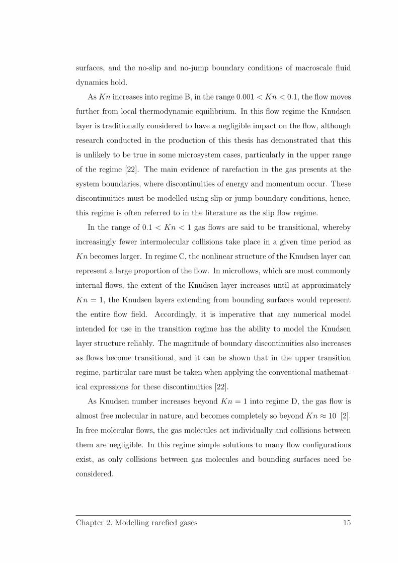
surfaces, and the no-slip and no-jump boundary conditions of macroscale fluid

dynamics hold.

As Kn increases into regime B, in the range 0.001 < Kn < 0.1, the flow moves

further from local thermodynamic equilibrium. In this flow regime the Knudsen

layer is traditionally considered to have a negligible impact on the flow, although

research conducted in the production of this thesis has demonstrated that this

is unlikely to be true in some microsystem cases, particularly in the upper range

of the regime [22]. The main evidence of rarefaction in the gas presents at the

system boundaries, where discontinuities of energy and momentum occur. These

discontinuities must be modelled using slip or jump boundary conditions, hence,

this regime is often referred to in the literature as the slip flow regime.

In the range of 0.1 < Kn < 1 gas flows are said to be transitional, whereby

increasingly fewer intermolecular collisions take place in a given time period as

Kn becomes larger. In regime C, the nonlinear structure of the Knudsen layer can

represent a large proportion of the flow. In microflows, which are most commonly

internal flows, the extent of the Knudsen layer increases until at approximately

Kn = 1, the Knudsen layers extending from bounding surfaces would represent

the entire flow field. Accordingly, it is imperative that any numerical model

intended for use in the transition regime has the ability to model the Knudsen

layer structure reliably. The magnitude of boundary discontinuities also increases

as flows become transitional, and it can be shown that in the upper transition

regime, particular care must be taken when applying the conventional mathemat-

ical expressions for these discontinuities [22].

As Knudsen number increases beyond Kn = 1 into regime D, the gas flow is

almost free molecular in nature, and becomes completely so beyond Kn ≈ 10 [2].

In free molecular flows, the gas molecules act individually and collisions between

them are negligible. In this regime simple solutions to many flow configurations

exist, as only collisions between gas molecules and bounding surfaces need be

considered.


In this thesis the flows analysed are typically in regions B and C, where gas

rarefaction has a significant impact on the behaviour of the flow, but where it

still behaves recognisably as a fluid. In these regimes, the increased importance

of individual molecular interactions at system boundaries and the structure of

the non-equilibrium Knudsen layer are the dominant effects of rarefaction. They

are the most important flow features to capture in numerical analyses [21].

2.2 Approaches to modelling rarefied flows

The loss of local thermodynamic equilibrium and the breach of the continuum

assumption in rarefied gas flows lead to the breakdown of the classical governing

equations of fluid dynamics. As Kn increases beyond 0.001 the N-S-F equations

are no longer able to accurately predict the behaviour of gas flows. In order to

simulate the macroscopic behaviour of rarefied gases properly it is necessary to

consider the influence of their molecular nature. A large number of approaches

to the numerical simulation of rarefied gases exist, ranging from discrete models

of molecular motion, averaged for macroscopic quantities, through to extensions

of the traditional hydrodynamic equations. The following brief review considers

the most commonly applied techniques, assessing their suitability for integration

into mainstream engineering design tools.

2.2.1 Kinetic theory of gases

The Boltzmann equation is the governing equation of the kinetic theory of gases,

and uses classical mechanics to describe the velocity, position, and state of a

gas molecule in a flow at any given time. It is based on several simplifications

of the molecular behaviour of gases; it is assumed that the molecular diameters

remain small in comparison to the molecular separation, that the molecules are

in constant random motion, and that they undergo frequent collisions. It is also

assumed that molecular chaos prevails, and that bulk motion may be superim-

posed on the random molecular motion. Further simplifications, assuming that


the gas flow is dilute and composed of a single, monoatomic species, lead to the

Boltzmann equation:

∂f

∂t+ v · ∂f

∂r+ F · ∂f

∂v= C (f) , (2.3)

where f(r,v, t) describes the number of gas molecules in a volume of gas that

possess velocity v at the time t. The spatial position of a molecule is given by r,

and the flow is acted upon by a body force, F. The first term on the left hand

side of the equation describes the transient changes of the molecular distribution,

f , while the second term on the left hand side is the convective change in the

distribution. The Boltzmann equation describes how the bulk motion of the gas,

on the left hand side, relates to the molecular collisions taking place in the gas,

given by the collision integral C(f) on the right hand side. The collision integral

is highly complex, involving velocity-space coordinates as independent variables,

with the result that it is computationally intractable to solve the equation for

most flows [23].

In order to apply the Boltzmann equation practically, the collision integral can

be replaced by a simplified kinetic model of the collision processes in the flow. The

kinetic models linearize the Boltzmann equation, replacing the complex function

C(f) with expressions that can be solved to determine the distribution function

f of macroscopic quantities. One of the most widely used kinetic models is the

Bhatnagar-Gross-Krook (BGK) model [24]. In this model, the collision integral

is replaced with the product of the collision frequency between molecules and the

difference between a Maxwellian distribution function and the actual distribution

function sought [25]. For analysis of near-wall regions, the collision integral may

be replaced with specialised synthetic scattering kernels, such as the Cercignani-

Lampis model, which include the effects of interactions between the gas and the

wall [5].

Linearizing the Boltzmann equation using kinetic models, it is possible to

produce very accurate solutions for some fundamental cases. Unfortunately, sim-


plified kinetic models are rarely appropriate for complex geometry, and the as-

sumptions implicit in the linearisation process greatly limit applicability of the

results for practical rarefied flows [26].

2.2.2 Discrete molecular models — DSMC

The direct simulation Monte-Carlo (DSMC) method was originally proposed

by Bird, and is a particle-based approach to simulating the Boltzmann equa-

tion, rather than solving it directly [27]. DSMC does not operate on individual

molecules, but on a large number of computational particles, each of which is

assumed to be representative of a much larger number of individual molecules.

At each time step the particles are moved around the system, and can undergo

binary collisions that will alter their velocity and internal energy, but not their

physical position. In consequent time steps, particles have their physical posi-

tions adjusted around the system in a deterministic manner, i.e. according to their

previous collision and the laws of classical mechanics. The simulation continues

until ensemble averages of the individual observed states give a statistical simula-

tion of the physical behaviour of the gas flow to sufficient accuracy. Macroscopic

properties of the gas are inferred from the averages of the particle behaviour.

Although it can be shown that DSMC provides results that are directly equiv-

alent to solving the Boltzmann equation, its computational intensity restricts its

applicability for use as an engineering design tool [23, 28]. There are two key fac-

tors that make DSMC a particularly computationally expensive process. Firstly,

DSMC particles are tracked within a computational mesh, which is used to iden-

tify upcoming collisions at each time step and to produce the information used in

the statistical averaging processes. In order to ensure that only physical results

(i.e. system states) are produced, both the time step and the mesh-cell size must

remain smaller than the mean collision time and mean free path, respectively [27].

Thus, the memory requirements of DSMC processes can be extremely demanding,

given the large number of time steps required for accurate ensemble-averaging of


non-equilibrium systems.

The second factor that limits the use of DSMC as a design tool, particularly

for gas-based microsystems, is susceptibility to statistical noise. In the low-speed

cases commonly found in microscale flows, a much larger number of sample sys-

tem states is required to produce accurate averages of the macroscopic quantities.

The computational time necessary to obtain low-scatter results for low speed rar-

efied gas flows then becomes prohibitive even on massively parallel computing

facilities [23]. In recent work, Baker and Hadjiconstantinou have proposed a

means of significantly reducing the computational effort involved in DSMC for

microsystems by considering the relatively small departures from equilibrium ob-

served in some low-speed flows [29]. Although this modified method may yet

become the de facto standard for low-speed DSMC, it does not currently offer

sufficient improvements in computational requirements for complex cases to pro-

vide the particle-based approach with an advantage over continuum models for

microsystem design applications. It is also limited, in studying small departures

from equilibrium, to relatively low-Kn applications.

Currently, DSMC is predominantly used in academic research for the study of

aerodynamics and hypersonics, but it is now also accepted as an analytical tool

for other non-equilibrium flows. The method produces reliable data in many cases

where equivalent experimental results are not available, and can also be applied

to complex flows in realistic configurations, given sufficient time and comput-

ing resources are available [30, 31]. These features of DSMC are particularly

attractive for analysis of gas microflows, where complex geometry is common,

and where practical constraints often preclude detailed experimental work. In

practice, however, the computational effort involved in most DSMC makes it

prohibitively expensive, in terms of both time and required computational facili-

ties, for consideration as an industrially applicable design tool.


2.2.3 The Chapman-Enskog expansion

As an alternative to directly solving the Boltzmann equation, it is possible to

determine some non-equilibrium distribution functions, represented by f , as a

perturbation of the local Maxwellian distribution, fM , using a series expansion.

The traditional Chapman-Enskog (C-E) series is written in terms of Kn:

f = fM

(1 + a1(Kn) + a2(Kn)2 + · · ·) , (2.4)

where the coefficients an are functions of density, velocity and temperature. The

C-E expansion produces a series of continuum equations that are assumed to

converge to the Boltzmann equation with increasing order [9]. Practically, this

assumption of convergence implies a limit to the degree of departure from the

equilibrium state that may be successfully predicted using the C-E expansion.

To zeroth-order in Kn, the C-E series produces the Euler equations, which are

inviscid constitutive relations, and valid for gas flows far from bounding surfaces

when Kn is below approximately 10−2. To first-order in Kn, the series results in

the viscous N-S-F equations. The higher the order of the terms in the series, in

theory, the greater the departure from the equilibrium distribution that may be

modelled. At the second-order in Kn, the Burnett equations are produced, which

are similar to the N-S-F equations, but which include more complex constitutive

expressions for stress and heat flux [32].

Since Burnett’s original work, many others have derived alternate second-

order equations, using either different physical interpretations of the C-E series,

or working with the assumption that it should converge to kinetic approximations

to the Boltzmann equation, see e.g. [33–35]. Although all of the published models

agree on the form of the first-order N-S-F equations, there is no general agreement

as to the correct form of the second-order equations and, as yet, no single model

is demonstrably superior [36, 37].

The most attractive feature of the higher-order equation sets that arise from

the C-E expansion is that they can, in theory, predict the behaviour of gas flows


further from equilibrium than the N-S-F equations, but reduce to the lower-order

equations in regions of flow where Kn is low. In many flows this would greatly

reduce the computational cost of non-equilibrium numerical simulations, which

would otherwise require stochastic treatments such as DSMC. Also, as the Bur-

nett equations are continuum-based, it would theoretically be possible to integrate

them into CFD simply by altering the constitutive relationships that link the en-

ergy and momentum equations. Unfortunately, the higher-order equation sets

also have drawbacks that limit their applicability for use in engineering design.

Whilst it is true that the Burnett-order equations can capture more of the

non-equilibrium physics of microsystems than the N-S-F equations, such as wall-

normal shear stress and heat flux, they are not generally well-posed. For example,

many of the second-order equations are numerically unstable, and can require

complex solution methods to be employed in order to ensure that they produce

unique solutions. Also, the higher order terms require higher-order boundary con-

ditions, which are not necessarily known a priori. This is particularly problematic

at solid boundaries, where the physical interactions between gas molecules and

wall molecules are not well understood. In addition, not all forms of the Burnett-

order equations are able to model the non-equilibrium Knudsen layer observed

in very near-wall regions, which is an important physical feature of many mi-

croflows [37].

2.2.4 Moment models

As an alternative to the C-E expansion, Grad proposed that the non-equilibrium

distribution function could be approximated using a series of first-order partial

differential moment equations, obtained using the Hilbert expansion [9]. Hermite

tensor polynomials are used to close the equations, taken around the Maxwellian

state, with coefficients related to the moments [38]. Grad’s expansion using five

moments (density ρ, three components of velocity ui and temperature T ) is equiv-

alent to the Euler equations from the C-E expansion. Thirteen moments (density


ρ, momentum density ρui, energy density ρε, stress p〈ij〉 and heat flux qi) equate

to the Burnett-order, then twenty-six moments for Super-Burnett order, and so

on [39]. Grad’s moment equations retain many of the drawbacks of the higher-

order C-E terms, in that they are numerically unstable, and require complex,

and unknown, boundary conditions. Although some recent work such as [40] has

attempted to resolve the problem of boundary conditions for Grad’s equations,

they also require a large number of variables to describe certain flows, and can

be shown to produce non-physical results in some cases.

Recently, Struchtrup combined Grad’s 13-moment expressions with the C-E

expansion to produce the regularized 13-moment equations, the R13, with the

aim of avoiding some of the problems of the traditional methods [41]. Further

work is ongoing to determine appropriate boundary conditions in order to apply

the R13 equations to gas microflows [42–44].

2.2.5 Extending the Navier-Stokes-Fourier equations

The N-S-F equation set in 3D comprises five conservation equations; one equation

for mass, three for momentum and one for energy. The equations are linked by

linear constitutive relationships for shear stress and heat flux. Using a Cartesian

coordinate system where spatial coordinates x, y, z have velocity components u,

v, w, respectively, and u is a velocity vector, the N-S-F equations are given in

unsteady 3D form as follows:

∂ρ

∂t+∇ · (ρu) = 0, (2.5)

∂ (ρu)

∂t+∇ · u (ρu) = −∇p+∇ · τ + SM , (2.6)

where τ is the stress tensor and SM represents momentum sources. The energy

equation is

∂(ρh0)

∂t+∇ · (ρh0u) = ∇ · (κ∇T ) +

∂p

∂t+ Φ + Sh, (2.7)


where h0 is enthalpy, Sh represents source/sink terms, κ is the thermal conduc-

tivity and Φ is the dissipation function given by

Φ = 2µ

[(du

dx

)2

+

(dv

dy

)2

+

(dw

dz

)2]

+ µ

(du

dy+dv

dx

)2

+µ

(du

dz+dw

dx

)2

+ µ

(dv

dz+dw

dy

)2

− 2

3µ (∇u)2 . (2.8)

These equations are widely used at the macroscale for computation of a range

of fluid flow and heat transfer problems. At the microscale, where Kn increases

and the molecular nature of gas flows becomes important, the N-S-F equations

alone do not predict the effects of gas rarefaction [2].

In the slip- and transitional-Kn regimes, the most apparent effects of gas

rarefaction are velocity slip/temperature jump and the Knudsen layer. Using slip

and jump boundary conditions, it is possible to extend the applicability of the

N-S-F equations into the slip flow regime: 0.001 < Kn < 0.1 [10, 11]. This is the

most commonly applied numerical technique for weakly rarefied flows.

Recently, new approaches designed to extend the applicability of the N-S-F

into the transition regime have also been developed, see e.g. [12, 17, 45]. By

modifying the constitutive relationships used to derive the N-S-F equations, for

example, they can be made to incorporate the effects of the Knudsen layer [12].

This process, known as constitutive-relation scaling, uses available data describing

the shape of the Knudsen layer to modify the linear shear stress/strain rate and

heat flux/temperature gradient relationships that define the N-S-F equations.

The primary advantage of the constitutive scaling approach is that it is an efficient

method of simulating rarefaction effects within a continuum framework, which is

much less computationally expensive than direct simulation techniques.

Generally, these modifications do not provide the N-S-F equations with the

means to actually model the physics of rarefied flows, however, they can allow

them to simulate the observed behaviour at higher Kn more accurately. This


type of approach is common in other areas of fluid dynamics, where empirical

models are often used. For example, many different empirical models have been

developed to simulate turbulence in high Reynolds number flows [46].

Given the difficulties inherent in physically modelling non-equilibrium gas

flows, the primary advantage of an extended N-S-F model would be that it would

remain relatively computationally unintensive compared to alternatives such as

kinetic theory and DSMC. Also, modifying the N-S-F equations, which are al-

ready in widespread use, is likely to make for a more practical analysis tool than

emerging alternatives such as the R13 equations [41]. If we consider solving the

Boltzmann equation directly as a bottom-up approach to the problem, in that it

directly incorporates all aspects of the physical behaviour of the gas, then using

extended N-S-F equations constitutes a top-down approach. In such a strategy,

the key features of rarefied flows observed in experimental work or kinetic so-

lutions to the Boltzmann equation are selectively “retro-fit” to a much simpler

continuum model [12]. Although this necessarily implies some loss of generality,

from an engineering perspective it has the potential to generate a very effective

design tool for some non-equilibrium flows. This thesis exploits the potential

of extending the N-S-F equations, by integrating available models into a main-

stream CFD framework, producing an efficient and flexible means of analysing

non-equilibrium flows.

2.2.6 Summary

In summary, it is clear that modelling non-equilibrium flows is both particularly

challenging and traditionally computationally intensive. In order to effectively

design microsystems in the short-to-medium term, one promising approach is

to identify the key features of gas rarefaction, and incorporate them into simpler

numerical models. In order to do so, it is necessary to understand the physics that

characterise the effects of rarefaction in the transition regime, primarily interface

discontinuities and the Knudsen layer, and to discuss how such flow features are


traditionally accommodated in analytical and numerical models.


Chapter 3

Physics of rarefied flows

3.1 Interfacial phenomena

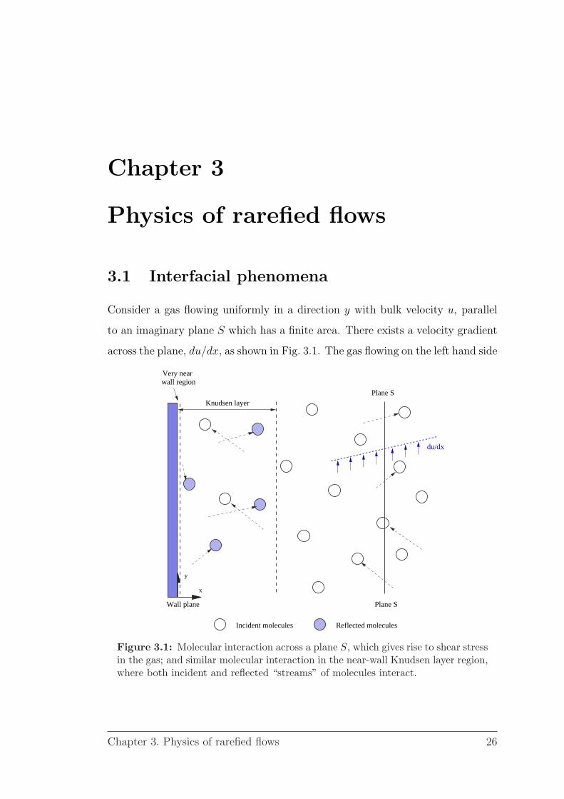
Consider a gas flowing uniformly in a direction y with bulk velocity u, parallel

to an imaginary plane S which has a finite area. There exists a velocity gradient

across the plane, du/dx, as shown in Fig. 3.1. The gas flowing on the left hand side

y

x

wall regionVery near

Plane SWall plane

Plane S

Incident molecules Reflected molecules

Knudsen layer

du/dx

Figure 3.1: Molecular interaction across a plane S, which gives rise to shear stressin the gas; and similar molecular interaction in the near-wall Knudsen layer region,where both incident and reflected “streams” of molecules interact.

Chapter 3. Physics of rarefied flows 26

of the plane S (within a suitably small distance) is moving at a given velocity, and

the gas on the right hand side of the plane is moving at another given velocity

which is higher. As a molecule crosses from the right to the left hand side of

the plane (negative x-direction), it will lose tangential momentum in collisions

until it adopts the same velocity as the gas on the left hand side of the plane.

The inverse will be true of a molecule crossing from left to right — it will gain

tangential momentum from collisions until it assumes the velocity of the stream

on the right hand side. Thus, there exists a force on the surface area of the

plane which acts in both positive and negative y-directions, brought on by the

tangential components of momentum that any crossing molecules have or have

lost. This force acting over the surface area is the shear stress, τ , in the fluid. For

suitably small tangential components of momentum the coefficient of viscosity,

µ, linearly relates shear stress to the velocity gradient, du/dx:

τ = µdu

dx. (3.1)

If we now consider the stationary wall in Fig. 3.1, rather than the plane S,

there will be a stream of gas molecules incident to the wall, and a post-collision

stream receding from it. The viscous force on the wall surface is due to the

difference in tangential momentum between the incident and receding streams,

rather than between molecules crossing an imaginary plane. From a macroscale

perspective (a quasi-equilibrium system) the action of this viscous force is what

reduces the tangential velocity of the gas to zero at the surface — leading to the

no-slip boundary condition.

From a microscale perspective, momentum and energy are being exchanged

between gas molecules and wall molecules in collisions both at and very close

to the gas-surface interface. A non-rarefied gas, by definition, has a molecular

mean free path that is negligible compared to the system dimensions. Molecules

very near the surface will undergo a large number of collisions both with the

wall and with other gas molecules in a very short timescale, reaching an almost


instantaneous equilibrium state. In non-rarefied gases, it is not possible to observe

any discontinuity between the velocity of the gas at the wall and the velocity of

the wall, but thin non-equilibrium regions where these average velocities are not

the same do physically exist. In fact, the macroscopic approach produces the

“correct” approximation of the flow losing tangential momentum at the wall only

because the length scale of the near-wall non-equilibrium region (the Knudsen

layer) is negligibly small.

When gas flows become rarefied, the length-scale of the Knudsen layer be-

comes large in comparison to the system dimensions, and the discontinuity of

momentum at the surface interface becomes significant1. That is to say, the ve-

locity of gas flow at the wall can no longer safely be assumed to be the velocity

of the wall. This was originally observed in experimental work carried out in the

19th century, investigating the effects of gas-damping on a vibrating disc [47]. The

viscous damping was found to be reduced at low pressures as the gas “slipped”

over the solid surface of the disc. This slip is in fact the non-equilibrium discon-

tinuity between the gas velocity and the surface velocity that becomes larger as

the gas becomes rarefied. Specifically, when the mean free path becomes suitably

long, the gas flow at the wall cannot be considered to lose all of its (relative)

tangential momentum to the wall.

3.1.1 Maxwell’s phenomenological model

In order to represent velocity slip at system boundaries, in 1879 Maxwell produced

a phenomenological model, based on his earlier work on the theory of viscosity in

gases [10, 19]. Phenomenological models are mathematical descriptions derived

from the observed behaviour of physical systems, rather than from theoretical

knowledge, and which may be used successfully to predict the behaviour of other,

similar systems. Maxwell’s phenomenological slip model has a lengthy derivation,

1A similar discontinuity of energy also exists at surface interfaces, which is referred to astemperature jump, but for now let us consider the velocity discontinuity as representative ofthe boundary phenomena in rarefied flows.


but can be described more simply as an analogue to the macroscopic model [8, 10].

It is designed to work as a boundary condition with the continuum equations of

fluid dynamics. Consider once more a gas flowing parallel to the planar wall shown

in Fig. 3.1. In the macroscopic approach, shear stress arises at the surface due

to the exchange of tangential momentum between gas molecules approaching the

wall and gas molecules receding from it. The approaching gas and the receding

gas are assumed to have equal influence on the total shear stress at the surface:

⌊1

2µdu

dx

⌋

Approaching

+

⌊1

2µdu

dx

⌋

Receding

=

⌊µdu

dx

⌋

Total.

(3.2)

In Maxwell’s model, each macroscopic term in Eq. (3.2) can be replaced by a

microscopic “equivalent”. The equivalent terms are approximations of molecular

behaviour that Maxwell produced based on his observations of rarefied gas flows.

The fluid approaching the wall from the bulk flow is assumed to be composed

of molecules with an equilibrium velocity distribution. The contribution of this

flow to the shear stress at the wall remains the same as in the macroscopic de-

scription: 12µdu

dx. The stream of molecules receding from the wall is assumed at

the microscopic level to be equivalent to a simple effusive flow. A typical effusive

velocity distribution would be that of a flow of individual molecules through a

small hole (with diameter of the order of the mean free path) in a planar surface.

The total number of molecules that would issue effusively from such a system per

second, Γn, may be described simply in terms of the mean molecular speed, v,

and the number density of molecules in the flow, η: Γn = 14ηv [8]. This number of

molecules leaving the surface is then multiplied by the velocity of the gas at the

wall, the unknown slip velocity, uslip, to produce the receding stream’s contribu-

tion to the shear stress at the wall. However, the observation of a slip velocity in

itself implies that some tangential momentum is retained by the gas at the wall.

To determine the slip velocity whilst conserving momentum, Maxwell represented

the fraction of tangential momentum that the molecules on average lose to the

wall as the proportion σ of their original tangential momentum. This is effectively


a “relaxation” of the macroscopic assumptions, and represents the mathematical

difference between the macroscopic description and the microscopic description,

where, for non-equilibrium flows

⌊1

2µdu

dx

⌋

Receding

6= 1

4ηvuslip.

Effectively, Maxwell’s argument is that if the macroscale shear-stress analogy

were to imagined to hold true, then it would be possible to account for defi-

ciencies in that assumption numerically by specifying the fraction of tangential

momentum lost to the wall. Introducing this relaxation factor, or tangential mo-

mentum accommodation coefficient, as it is more commonly known, a microscopic

description of the shear stress at the wall is obtained,

σ

(1

2µdu

dx+

1

4ηvuslip

)= µ

du

dx. (3.3)

Incorporating ρ = ηm, which relates number density and the mass of the gas

molecules, m, to the macroscopic density, ρ, Eq. (3.3) can be rearranged to give

the velocity slip:

uslip = 2

(2− σ

σ

)µ

ρv

du

dx. (3.4)

Substituting in the expression for mean molecular velocity in a Maxwellian distri-

bution, v = 2√

(2RT/π), the definition of mean free path given in Eq. (2.2), and

the linear constitutive relationship between shear stress and strain-rate given in

Eq. (3.1), we can obtain the most common form of Maxwell’s equation for velocity

slip in rarefied flows over planar surfaces [8]:

uslip =

(2− σ

σ

)λτ

µ. (3.5)

Thus, we can determine the slip velocity of a rarefied hard-sphere gas at an

interface using the mean free path of the gas, λ, the shear stress at the wall,

τ , the dynamic viscosity, µ, which is a temperature dependent property of the


gas, and the degree of tangential momentum accommodation, σ, which may be

thought of as a property of a particular gas-surface interaction. The tangential

momentum accommodation coefficient determines the proportion of molecules

reflected from the wall specularly (equal to σ − 1) or diffusely (simply σ), where

0 < σ ≤ 1. Specular reflection implies that the molecular tangential momentum

of the impinging molecules is perfectly reflected, and that the gas therefore exerts

no tangential stress on the wall. It is also assumed that no energy exchange takes

place between the wall and the gas molecule. In the case of diffuse reflection,

molecules are ascribed random velocities with the average loss of all of their

tangential momentum, and recede at the temperature of the wall.

Eq. (3.5) is the most widely used form of Maxwell’s equation, see e.g. [20].

In following the macroscale approach to derive the equation, however, many of

the subtleties of the original work are easily lost [10]. Eq. (3.5) assumes, for

example, that there is no stream-wise variation in wall-normal velocity (i.e. that

the bounding surfaces of the flow are non-rotating and planar). Also, this formu-

lation neglects the influence of thermal creep, a process whereby a temperature

gradient tangential to the surface generates additional slip flow along the surface

in the direction of increasing temperature [48].

The microscopic explanation of thermal creep is relatively simple. If tangen-

tial momentum is not fully accommodated between the gas and the wall due

to rarefaction, then some proportion of the molecules will be reflected from the

wall diffusely (with Maxwell’s proposed effusive velocity distribution). In re-

gions of higher temperature, the gas molecules have a higher average velocity. If

the molecules were specularly reflected, then their original tangential momentum

would simply be reversed, and the flow would move from hot to cold as expected.

In the hot flow, the higher average velocity implies that the diffusely reflected

gas molecules will rebound more strongly from the wall in randomly ascribed

directions than in the cold flow. Thus, the gas will gain tangential momentum

towards the regions of increased temperature, producing a net flow from cold to


hot [8].

Maxwell’s original expression for velocity slip over planar surfaces included a

second term, incorporating the thermal creep effect. Considering a planar surface

where n is the co-ordinate normal to the wall and x is the co-ordinate tangential

to it, the conventional expression of the full Maxwell slip equation is

uslip =

(2− σ

σ

)λdux

dn+

3

4

µ

ρT

dT

dx, (3.6)

where ux is the x-component of the slip velocity, T is the gas temperature, and

dT/dx is the temperature gradient tangential to the surface interface [10]. Whilst

this form of Maxwell’s equation is commonly implemented in analytical and nu-

merical simulations of the N-S-F equations, it is important to note that it is not

applicable to surfaces with curvature. For example, for a two dimensional surface

curvature, Lockerby et al. showed the correct form of Eq. (3.6) to be

uslip =

(2− σ

σ

)λ

(dux

dn+dun

dx

)+

3

4

µ

ρT

dT

dx, (3.7)

where un is the gas velocity normal to the wall [16]. The additional term featuring

in Eq. (3.6) but not in Eq. (3.5) can have a significant influence on the velocity

slip in flows over surfaces with curvature. For example, it can be demonstrated

that accurate predictions of velocity profile inversions in cylindrical micro-Couette

flow are only achieved when Eq. (3.6) is used [16, 36]. In order to fully generalise

Maxwell’s equation for use in three-dimensional geometries, it should be written

in vector form as follows;

uslip − uwall = A1

(2− σU

σU

)λ

µτ +

3

4

Pr (γ − 1)

γpq, (3.8)

where the tangential shear stress is τ = (in · Π) · (1− inin) and heat flux is

q = Q · (1− inin), with bold type-face denoting a vector quantity. The Prandtl

number Pr relates energy and momentum diffusivity, γ is the specific heat ratio,

and p is the gas pressure at the wall. A unit vector normal to, and away from, the

wall is in, with Π the stress tensor at the wall, 1 the identity tensor, and Q the heat


flux vector at the wall. The slip coefficient A1, is equal to 1 in Maxwell’s original

derivation. The accommodation coefficient symbol σ has also been replaced with

σU , in order to distinguish between the tangential momentum accommodation

coefficient, which affects velocity, and the equivalent thermal value that will be

discussed in section 3.1.3.

Although it is phenomenological in nature, Maxwell’s slip model can be seen

to be very effective across a wide range of cases, and is the most commonly-

applied velocity boundary condition for rarefied gas flows [20]. Unfortunately,

Maxwell’s model does not capture the underlying physics of the microsystem

flows that it is used to represent. Consequently, as Knudsen number approaches

the transition regime, the accuracy of Maxwell’s model can be seen to be greatly

reduced — even when used in conjunction with appropriate models for Knudsen

layer effects [22].

3.1.2 Phenomenological model vs. physical behaviour

Maxwell’s model assumes that in a rarefied gas flow parallel to a wall, molecules

approaching the wall will do so with an equilibrium velocity distribution, such

as would be found elsewhere in the bulk flow. On colliding with the wall, gas

molecules are said to be reflected either specularly or diffusely, with the propor-

tion of each determined by the tangential momentum accommodation coefficient.

Both specularly and diffusively reflected molecules are initially incident to the

wall with the same equilibrium velocity distribution. However, following colli-

sions at the interface, the diffusely reflected molecules will have exerted a tangen-

tial stress on the wall, and the specularly reflected molecules will not. Thus, the

post wall-collision velocity distributions of the specularly and diffusely reflected

molecules cannot be the same, implying that the composite stream of all the

receding molecules has a non-equilibrium velocity distribution.

When the gas flow is rarefied, the number of intermolecular collisions near the

wall surface is insufficient for an equilibrium state to be quickly established be-


tween the approaching and receding streams of molecules. So, it is most unlikely

that Maxwell’s assumption of molecules incident to the wall approaching it with

an equilibrium velocity distribution holds true. As a phenomenological model,

Maxwell’s description of slip velocity can be seen to work well, however, it is not

a physical description of molecular behaviour at interfaces in rarefied gas flows.

This was openly acknowledged by Maxwell in his original paper [10].

Physically, slip is a difference between the average molecular velocity of a gas

and the average molecular velocity of a surface that the gas flows past, which we

know as relative tangential momentum. In a non-rarefied gas, we do not observe

this difference in the average molecular velocities, it is “instantly” dispersed by in-

termolecular collisions. This is not true of a rarefied gas flow, where the difference

in average molecular velocities is seen to persist as a discontinuity of macroscopic

velocity at the boundary.

Fundamentally, rarefied and non-rarefied gases behave similarly, in that energy

and momentum are transported through the fluid by intermolecular collisions. For

example, if we consider a rarefied but quiescent gas in a solid, stationary container,

we know that the fluid will reach a state of equilibrium with its surroundings given

sufficient relaxation time2. This relaxation time will be significantly longer than

the equivalent for a non-rarefied gas. The increase in timescale is due to the larger

mean free path of the rarefied gas; the frequency of collisions is lower, slowing

the rate of diffusive transport. In the quiescent system, the average molecular

velocity of the gas will be zero, as would be true of the oscillating molecules of the

stationary container, so there will be no discontinuity of velocity at the gas-surface

interface. Thus, slip should be considered as a phenomenon that is highlighted by

rarefaction, but is ultimately driven by differences in average molecular velocity

that arise when the rarefied gas is in motion relative to a surface.

If we have an established flow of a transitional rarefied gas in a channel, say,

2It should be noted that energy and momentum diffuse at different rates, and technically havedifferent relaxation times [3]. Momentum is exchanged faster than energy, but here relaxationtime is taken to mean the total relaxation time for the system, which is the longer, energytransport value.


then the gas flow far from the system boundaries will relax to an equilibrium

velocity distribution. The number of molecules is reduced, but the bulk flow

will behave, essentially, in the same manner as a non-rarefied equivalent. Away

from the channel walls, the gas will have a convection transport timescale that

is unaffected by the degree of rarefaction (within the transition regime). The

timescale of diffusive transport of momentum and energy in the regions of gas

near to the channel walls, however, will be altered by rarefaction. The decreased

collision frequency and longer mean free path substantially increase the diffusive

relaxation time, as we observed in discussion of the quiescent flow. Thus, the

diffusive exchange of momentum between the gas and the system boundaries will

take place on a much longer timescale than the convection processes of the bulk

flow. Molecules could, then, on average, be transported through the system by

the bulk flow before they are able to equilibrate fully with the system boundaries,

i.e. before the difference in the average molecular velocity between the gas and

the wall is reduced to zero. This would result in a persistent velocity slip at the

boundary, and a steady-state but non-equilibrium system.

In practice, the most important difference between rarefied and non-rarefied

gas flows is that it is not possible for some rarefied flows to reach an equilibrium

state, even if given infinite time to relax. In rarefied gases that are not at rest,

there will always exist some degree of velocity slip at surface interfaces, brought

on by the loss of local thermodynamic equilibrium. Maxwell’s phenomenological

model gives a reasonable approximation of the degree of velocity slip in transi-

tional flows, but, as it is not a physical model, there are some serious limitations

to its applicability [21].

3.1.3 Boundary effects on temperature

Just as Maxwell’s model describes discontinuities of momentum between a mov-

ing rarefied gas and its bounding surfaces, so Smoluchowski’s phenomenologi-

cal model describes the equivalent discontinuity of energy between an unequally


heated rarefied gas and surrounding surfaces [11]. Temperature jump is driven by

heat flux normal to the wall, rather than a velocity gradient, but can be derived

along similar lines to Maxwell’s model [8]. Rather than determining the con-

tribution to shear stress of the approaching molecules’ transferred momentum,

Smoluchowski’s model examines the differential energy that the molecules have.

That is to say, their energy above or below the average energy of a molecule in

an equivalent equilibrium distribution. The thermal accommodation coefficient

σT is then used to ascribe the temperatures of the receding molecules. Specularly

reflected molecules recede from the wall with their original incident energy, and

diffusely reflected molecules have their temperatures adjusted to those that would

arise in a mass of gas in equilibrium at the temperature of the wall.

For temperature jump at solid boundaries:

Tjump − Twall = Ajump

(2− σT

σT

) (2γ

γ + 1

)λ

Pr

∂T

∂n. (3.9)

The jump coefficient, Ajump, has a value of 1 in the original derivation. The

specific heat ratio of the gas is represented by γ, and the Prandtl number Pr is

used to represent the ratio of momentum diffusivity to energy diffusivity. The

gas temperature is T , and n is the direction normal to the wall’s surface.

It is worth noting that in the derivation of Eq. (3.9), it is assumed that inter-

nal molecular energy and translatory energy are assumed to be described by the

same accommodation coefficient, i.e. that they are transferred at the same rate

in intermolecular collisions. This is not in accordance with the theory of equipar-

tition of energy, and is likely to be a source of error in the equation, but given

the phenomenological nature of the model, its impact is largely negligible [8].

Of greater concern is the relationship between momentum and energy transfer

that is implied when describing the specular and diffuse reflections of Maxwell

and Smoluchowski’s models [49]. In practice, the velocity slip coefficient may

be shown to be dependent on the level of energy accommodation at the surface,

and vice versa, but not in the manner implied by Maxwell and Smoluchowski’s


equations [50]. In Maxwell’s Eq. (3.8), for example, diffuse reflection means that

molecules leave the wall with an equilibrium distribution of velocity, and are

assigned the temperature of the wall. In Smoluchowski’s expression, Eq. (3.9),

diffuse reflection implies an equilibrium distribution of temperatures is assigned,

as if the gas were in equilibrium, with the average temperature being that of the

wall [8].

So, the average temperature of the molecules receding from the wall that the

models predict is equivalent, but the assumed temperature distribution is not.

As outlined in section 3.1.2 above, for the exchange of momentum at bounding

surfaces, when the diffusely reflected stream is combined with the specularly

reflected stream of molecules, it is unlikely to have an equilibrium distribution of

molecular velocities. The same also holds true for temperature distributions.

Consider diffusely reflected molecules that are all assigned the wall tempera-

ture value, as in Maxwell’s model. The new temperature distribution of the full

receding stream will be composed of part of the incident equilibrium temperature

distribution, from the specularly reflected molecules, and all of the diffusely re-

flected molecules will have the same temperature, the wall value. If the diffusely

reflected molecules are assigned an equilibrium distribution with the wall tem-

perature as the average value, as in Smoluchowski’s model, then, when combined

with the specularly reflected molecules, the temperature distribution produced

will be different to that obtained using the Maxwellian treatment. The difference

in these temperature distributions will have an effect on the degree of departure

from equilibrium of the receding stream of molecules and, consequently, an im-

pact on the interaction between approaching and receding streams of molecules

that underpins the physical processes of velocity slip and temperature jump. In

practical rarefied flows, then, where both energy and momentum are being ex-

changed in near wall collisions, the validity of using Maxwell and Smoluchowski’s

expressions in conjunction may be questioned [49].


3.1.4 Alternative slip and jump models

In order to counteract some of the shortcomings of the widely used models for

velocity slip and temperature jump, several alternatives have been proposed;

although none is widely accepted as a complete replacement for Maxwell and

Smoluchowski’s conveniently simple expressions.

As an alternative to Maxwell’s model, it has been suggested that Langmuir’s

theory of the adsorption of gases could be used [51]. Adsorption is a process

where gas molecules become temporarily attached to a solid bounding surface

upon collision with it, and are released again into the bulk flow after some finite

time lag. The Langmuir model is based on surface chemistry, but may be shown

to make equivalent predictions of slip to Maxwell’s model in some key cases [52].

The Langmuir model for velocity slip is given by

uslip =

(βp

1 + βp

)uw +

(1

1 + βp

)ug, (3.10)

where p is the gas pressure, uw is the velocity of the gas interacting with the

surface, ug is a local reference velocity elsewhere in the gas and β is the function

β =

(4 Kn Pr ω0 (ν)

(Tw

Tr

)1+ 2ν−1

exp

( −De

kBTw

))−1

. (3.11)

Here, ω0 (ν) is a tabulated value taken from the kinetic theory of gases, Tw is the

wall temperature, Tr a reference temperature, ν is the exponent of the inverse

power law for viscosity, De is the value of the heat of adsorption, kB is the

Boltzmann constant and Pr the Prandtl number, which describes the relationship

between momentum and energy diffusivities.

Although the Langmuir model is obviously more complex than Maxwell’s

model, its key advantage is that it is possible to determine the slip velocity from

knowledge of the chemical interactions between particular gases and surfaces.

The properties of surface interactions are both more physical and less open to

interpretation than the accommodation coefficient used in Maxwell’s model.


Another alternative to Maxwell’s slip model is Sharipov’s model, in which

the Cercignani-Lampis scattering kernel is used to describe molecular interac-

tions at the wall, rather than Maxwell’s specular/diffuse scattering model [5, 50].

The Cercignani-Lampis model for the behaviour of molecules receding from the

wall is chosen as it contains not one but two accommodation coefficients in the

slip velocity: a tangential momentum accommodation coefficient, and a thermal

accommodation coefficient. There is also a separate energy accommodation co-

efficient used in the expression for temperature jump. This type of model gives

a more accurate representation of both the physical interactions near the wall,

and the interdependence between velocity slip and thermal transpiration effects

(creep). Sharipov uses a more realistic description of the collision physics in the

near wall region to inform general slip/jump equations and then, using kinetic

theory to determine unknown constants, develops accurate expressions for ve-

locity slip and temperature jump. This type of model is an improvement on

Maxwell’s phenomenological model in that it provides very accurate solutions for

particular gas-surface interactions in planar half-spaces. The gas-wall collisions

are also handled using more sophisticated and realistic models than Maxwell pro-

posed. Unfortunately, from a practical point of view, this new type of model does

not address the real, restrictive limitations of Maxwell and Smoluchowski’s mod-

els, namely, that they are inaccurate for transitional Knudsen numbers, and that

they are not applicable to complex 3D geometries without the risk of substantial

error.

Ultimately, while both Langmuir and Sharipov’s models (and several other

alternatives, see [3, 53, 54]) are more accurate than Maxwell and Smoluchowski’s

expressions, in application they must be considered less robust. Generally, alter-

native models are relatively complex and require available kinetic theory data,

which, for practical flows and most engineering design applications renders them

largely unsuitable. Also, it is difficult to justify the complexity of implementing

models that are dependent on individual gas-surface interaction properties, but


derived only for simple flow configurations (typically planar surfaces, and often

isothermal cases). Large accuracy losses can occur when converting kinetic-theory

dependent models to 3D, non-isothermal, compressible and transitional-Kn flows,

which can negate the benefits of using kinetic-theory based slip models altogether

in practical flows. As yet, no alternative to Maxwell or Smoluchowski’s models

has been widely accepted as suitable, particularly for application to complex

flows.

3.2 The Knudsen layer

The Knudsen layer is a near-wall region approximately one to two mean free paths

in thickness where local thermodynamic equilibrium is not maintained. Micro-

scopic interactions in the Knudsen layer do not generate equilibrium distributions

of the macroscopic variables. In rarefied flows, velocity slip and temperature jump

arise within the Knudsen layer as the difference in the average molecular proper-

ties of the wall and those of the gas at the wall. The Knudsen layer thickness is

the average distance over which these discontinuities would be equilibrated in a

quiescent gas.

Macroscopically, the Knudsen layer is observed as a region of flow exhibiting

strong departures from the linear constitutive behaviour of the N-S-F equations:

the relationships between stress/strain-rate and heat flux/temperature-gradient

are nonlinear. As gas flows reach transitional-Kn values, moving from regime

B to C as outlined in section 2.1, the structure of the Knudsen layer becomes

important. For example, in cases of pressure-driven gas flow in a microchannel

with the relatively modest rarefaction of Kn = 0.05, velocity slip may be shown

to increase the observed mass flowrate by 15%. The nonlinear structure of the

Knudsen layer accounts for 30% of this difference between the “true” microscopic

velocity profile and that predicted by the N-S-F equations [37].

To illustrate, a schematic of the Knudsen layer structure is given in Fig. 3.2.

The figure shows Knudsen layer velocity profiles for an isothermal, pressure-driven


gas flow, moving parallel to a planar wall. The velocity of the wall is denoted by

uwall, and the actual speed of the gas at the wall by uslip. The solid line indicates

the true velocity of the gas, which is commonly referred to as the microslip,

as would be found in experimental results or predicted in accurate molecular

dynamics simulations [3, 6, 8].

Solid Wall

Knudsen Layer

Gas

O(λ)

uwall

uslip

u∗slip

u∗∗slip: N-S-F with 2nd order slip

u∗slip: N-S-F with Maxwell slip

uwall: Velocity of the surface

u∗∗slip

uslip: Gas velocity at the surface

Figure 3.2: Schematic of the velocity structure of the Knudsen layer near a wallin a pressure-driven flow, comparing different types of slip boundary condition.

The dash-dot line represents the velocity profile obtained using the N-S-F

equations with Maxwell’s velocity slip condition, Eq. (3.8), giving the slip value

u∗slip at the wall. Although this model over-predicts slip at the boundary, outside

of the Knudsen layer it under-predicts the velocity slightly, and gives a reason-

able approximation of the velocity gradient. Far from the wall in transitional-Kn

flows, where the assumed equilibrium velocity/temperature distributions hold,

the N-S-F equations are appropriate. Therefore, beyond the Knudsen layer, they

may be used in conjunction with Maxwell’s equation for boundary slip to pre-

dict the mass flowrate in moderately high-Kn systems with acceptable accuracy.

As Kn increases, however, Maxwell’s model increasingly under-predicts the gas


velocity outside of the Knudsen layer, until eventually the level of error in the

results becomes unacceptable [21, 49].

In order to improve the mass flowrate prediction of the N-S-F equations with

slip, particularly at high-Kn, it is common to use higher-order slip/jump bound-

ary conditions, which are often referred to as macroslip conditions [3, 6, 21]. These

macroscopic boundary conditions deliberately over-predict the velocity slip at the

surface interface, in order to more accurately capture the velocity profile outwith

the Knudsen layer, as shown in Fig. 3.2 by the dashed line, u∗∗slip.

Higher-order slip models are typically derived using series expansions of the

simplest form of Maxwell’s equation: that for isothermal flows in planar geome-

tries, Eq. (3.5). For example, Cercignani proposed a second order model for slip

at the wall of the form

u∗∗slip = A1λdu

dy− A2λ

2d2u

dy2, (3.12)

where A1 and A2 are the first and second order slip coefficients, du/dy the velocity

gradient and λ the mean free path [55]. Like Maxwell’s model, this expression for

slip is dependent on the mean free path definition and, hence, molecular force-

interaction law applied. For the hard-sphere molecular model, the slip coefficients

would be A1 = 1.1466 and A2 = 0.647 [56].

Other higher-order models, however, use different slip coefficients. For exam-

ple, Deissler [57] suggests values of 1.0 and 1.125 for A1 and A2, respectively, while

Karniadakis and Beskok [21] propose 1.0 and −0.5. Whilst some authors agree

with Cercignani’s coefficients, these models and several others do not match even

the first-order slip coefficient, and there is no universal agreement as to the most

accurate general model [3, 21, 57, 58]. So, despite the useful potential to extend

the applicability of the N-S-F models by introducing macroscopic slip effects to

match observed mass flowrates, the lack of agreement on correct slip coefficients

greatly detracts from the generality of higher-order slip models.

Several other factors also limit the appeal of second-order slip for engineering


applications. Typically, macroslip models are derived from the simplified form

of Maxwell’s equation, Eq. (3.5), which is not suitable for curved surfaces, and

neglects thermal creep. Thus, in non-isothermal and compressible flows, it is likely

that the error introduced by neglecting surface geometry and thermal creep would

negate the benefits of having a second-order-accurate model.

Returning to Fig. 3.2, we see that there are two main differences between the

N-S-F models with slip boundary conditions and the true velocity of the gas.

Firstly, the velocity gradient is much steeper in the Knudsen layer region of the

real gas — the Maxwellian equilibrium-velocity profile coming from the bulk of

the flow does not really extend all the way to the wall. Secondly, this increase

in the velocity gradient means that the true slip of the gas at the wall is lower

than the value Maxwell’s model predicts. There is some debate about the exact

magnitude of the microslip coefficient (for first order slip), but it can be shown

from kinetic theory solutions for the near-wall region to be ≈ 0.8 for both velocity

slip and temperature jump [16, 17]. So, we know that Maxwell’s model and other

macroslip models can be used in some circumstances to improve predictions of

bulk quantities, such as mass flowrate or drag force on a surface, but, also that

ultimately, they do not capture the true physics of the Knudsen layer.


Chapter 4

Constitutive scaling

4.1 Introduction

At transitional-Kn and in the upper slip flow regime, the effects of the non-

equilibrium Knudsen layer must be incorporated into numerical simulations to

obtain accurate results for the macroscopic properties of the flow. Constitutive

scaling, where the relationship between viscous stress and strain-rate (and/or heat

flux and temperature gradient) in the near wall region is modified to represent

Knudsen layer behaviour, is one numerically economical approach to incorporat-

ing the Knudsen layer in continuum analyses. This technique uses linearised ki-

netic theory results to determine a phenomenological function f(n/λ) with which

to scale the N-S-F constitutive relations. The method was originally proposed

by Lockerby et al. [12] for application to isothermal cases. In Lockerby et al’s

paper, Knudsen layer behaviour is incorporated into N-S-F simulations by scal-

ing the relationship between shear stress and strain-rate in planar flows, i.e. the

relationship given in Eq. (3.1):

τ = µdu

dn=⇒ τ =

1

f(n/λ)µdu

dn. (4.1)

The scaling is a function of the normal distance to the nearest surface n, and

the local mean free path λ, and therefore directly relates to changes in Kn. The

scaling function is chosen such that f (n/λ) → 1 with decreasingKn, restoring the

linear relationship between stress and strain-rate assumed in the N-S-F equations.

Chapter 4. Constitutive scaling 44

Hence, the constitutive scaling approach also remains valid as Kn→ 0.

To determine an appropriate scaling function, Lockerby et al. [12] used lin-

earised kinetic theory results for Kramers’ problem, a half-space shear flow over

a planar surface [3]. A schematic of Kramer’s problem is shown in Fig. 4.1.

uslip: True velocity profile

u∗∗slip: Macroslip N-S-F profile

≈ 2λ

u∗∗slip uwalluslip

τ

uwall: No-slip N-S-F profile

Figure 4.1: Sketch of Kramers’ problem flow configuration showing applied con-stant shear stress, τ ; traditional, no-slip N-S solution (uwall: dotted line), N-Ssolution with second order macroslip boundary condition (u∗∗slip: dashed line) andtrue velocity profile (uslip: solid line). The Knudsen layer extends approximately2λ from the wall surface.

Kinetic theory indicates that the Knudsen layer velocity profile in a monoatomic

gas that is subject to a uniform shear stress and flows over a planar surface is

given by

u = −τµ

(n+ ξ − λI (n/λ)) , (4.2)

where τ is the uniform shear stress, µ is the gas viscosity, and ξ is a constant [3].

The velocity correction function I (n/λ) introduces the deviation from a linear

strain-rate profile, i.e. the change in shape from the dotted uwall or dashed u∗∗slip

profiles to the solid uslip profile as shown in Fig. 4.1. The function can be curve-fit


from kinetic theory data given in [3] to be:

I (n/λ) ≈ 7

20

(1 +

n

λ

)−2

. (4.3)

Although kinetic theory is used to define the scaling function used in [12], it is

worth noting that it would be equally possible to use direct-simulation Monte

Carlo (DSMC), molecular dynamics (MD) or experimental data to determine

case-specific scaling functions for I (n/λ). In practice, this could allow the con-

stitutive scaling method to be extended to flows of polyatomic gases.

Differentiating Eq. (4.2) produces an expression for strain-rate, which is ap-

propriate throughout the near-wall Knudsen layer region of the flow:

du

dn= −τ

µf (n/λ) . (4.4)

This expression is then recast into the form of the expressions in Eq. (4.1), and

used in place of the linear N-S-F relation, Eq. (3.1). Mathematically the result is

equivalent to using an “effective” viscosity model,

τ = µeffdu

dn, (4.5)

where the effective viscosity is given by µeff = µ/f (n/λ). Although Eq. (3.1)

describes the relationship between shear stress and velocity gradient in one spatial

dimension only, the variation of the effective viscosity in Eq. (4.5) is with normal

distance the the nearest surface, n, rather than a single plane. This allows the

scaling effect to be realised in 3D when the full Navier-Stokes stress tensor is used

to determine τ . The final shape of the viscosity scaling function f (n/λ) is given

in [12] as

f (n/λ) = 1− λd

dn[I (n/λ)] ≈ 1 +

7

10

(1 +

n

λ

)−3

. (4.6)

Using this function f (n/λ) → 1.7 as n→ 0. WhenKn is in the continuum regime

the extent of the Knudsen layer (≈ 2λ) is small in comparison to the system


dimensions, so constitutive scaling effects imposed by this function automatically

become negligible when it is applied to continuum flows (i.e. as Kn→ 0).

Derived from a kinetic solution for a relatively low speed, planar flow of

monoatomic gas subject to uniform shear stress, this scaling model should be

limited strictly in applicability to cases of that type. The basic assumptions un-

derpinning the kinetic theory solution include a restriction to low Mach number

flow, relatively low Kn values, and planar surfaces with diffuse molecular reflec-

tion. It has been shown, however, that this particular scaling model can improve,

both qualitatively and quantitatively, numerical results for flows that are beyond

these limitations. For example, the model has been successfully applied to flows

over non-planar surfaces [12, 14, 36].

4.1.1 State of the art

Constitutive scaling as a technique was proposed by Lockerby et al. only rel-

atively recently, in 2005 [12]. The primary advantage of the method is that

Knudsen layer structures can quickly and easily be incorporated into standard N-

S-F simulations. This extends the applicability of these relatively fast continuum

analyses for microsystem design applications, where flexibility and low compu-

tational cost are essential. The original model, given in Eq. (4.6), was intended

as a simple means of capturing the Knudsen layer in isothermal flows, and was

intended for primarily planar cases. Using previous work on Maxwell’s bound-

ary conditions carried out in [16], Lockerby et al. then extended the method to

include curved surface geometries, analysing viscous drag over an unconfined mi-

crosphere. The method has also been applied to a quiescent thermal flow in planar

half-space geometry, giving a successful prediction of the temperature profile nor-

mal to the wall [36]. Limitations of the constitutive scaling method as originally

proposed were that it had not been applied to complex geometries, compressible

non-isothermal flows, or to cases where both energy and momentum exchanges are

considered, e.g. non-quiescent thermally-driven flows, or shear/pressure-driven


flows with heat transfer effects.

In an attempt to improve the accuracy and generality of the constitutive

scaling method, Reese et al. [17] and Zheng et al. [45] proposed new scaling

functions for Knudsen layers of both momentum and energy. Kinetic theory data

from a wide literature survey were used to determine separate scaling functions

for effective dynamic viscosity, µ, and effective thermal conductivity, κ. Thermal

conductivity is the material property that is used in the N-S-F equations to

linearly relate heat flux and temperature gradient;

Q = κ∂T

∂n. (4.7)

In the same way that dynamic viscosity is replaced with an effective quantity in

Eq. (4.5), the thermal conductivity may be scaled by a phenomenological function

to produce a Knudsen layer structure. Constitutive scaling for thermal Knudsen

layers replaces the constant thermal conductivity found in Eq. (4.7) with an

effective quantity;

Q = κeff∂T

∂n. (4.8)

Crucially, the use of different scaling for viscosity and thermal conductivity in

these models implies a non-constant effective Prandtl number (which relates en-

ergy and momentum diffusivities) when they are used together [49]. It is possible

that this therefore highlights some physical inconsistency in the models, which

needs further investigation if they are to be considered as a means of extending

the applicability of constitutive scaling to more complex flows.

More recently, Lockerby and Reese [59] have proposed a scaling function de-

rived from the Bhatnagar-Gross-Krook (BGK) kinetic model. It is designed for

use in constitutive scaling in conjunction with a second order velocity slip condi-

tion. Although it is seen to improve the performance of the model as a whole, the

use of a second order slip boundary condition remains inherently unphysical as it

does not represent a Knudsen layer. Whilst constitutive scaling is not in itself a


means of producing a physical model, the intent is to replicate observed Knudsen

layer behaviour. Second order slip conditions do not model the true physics of

gas-surface interactions, but are used solely to improve the performance of simu-

lations beyond the extent of the Knudsen layer. However, this most recent paper

very accurately replicates BGK results for shear-driven and pressure-driven mi-

crochannel flows and, notably, demonstrates that using a BGK based function, it

is theoretically possible to predict the “Knudsen minimum1” using constitutive

scaling. This most recent work has not yet been extended by Lockerby et al. to

include thermal effects, nor has the BGK-based model been applied to non-planar

geometries.

Several other research groups have also now taken an interest in approaches

similar to the constitutive-scaling process, and some even propose alternate scal-

ing functions for various gas microflow configurations. Fichman and Hetsroni [62],

for example, consider a reduction of dynamic viscosity in near-wall regions of rar-

efied flows. Their analysis uses arguments similar to those of Maxwell [10] insofar

as their scaling of the dynamic viscosity as a function of mean free path and

distance from the surface interface is dependent on the proportion of molecules

reflected specularly/diffusely. They find the actual gas viscosity at the surface

interface to reduce to one half of its original free-stream value. This is compa-

rable to the original work of Lockerby et al. [12], which scales dynamic viscosity

with normal distance to the nearest wall, reducing to a value of 0.59 times the

free-stream viscosity at the surface [49].

Lilley and Sader [63] have also proposed modelling rarefied flows as non-

Newtonian fluids, which is mathematically equivalent to scaling the constitutive

relations of the N-S-F equations. They put forward a scaling function that is

curve-fit to linearised solutions to the Boltzmann equation for Kramers’ prob-

lem, as published by various authors [64–67]. The premise of their paper is that

1In experimental work confirmed by Gaede [60], Knudsen [61] showed experimentally thatthe volume flowrate of rarefied gas through a channel reaches a minimum value at Kn ≈ 1,and increases with increasing Kn beyond that condition. This is commonly referred to as theKnudsen minimum [8].


both the linearised Boltzmann equation and DSMC give very similar results for

Kramers’ problem, and the velocity profiles from those solutions may be rep-

resented using a power-law function, which can be translated to a variation of

effective viscosity. Notably, Lilley and Sader’s use of a power law curve fit for

the velocity profile, implies that the velocity gradient need not be finite at the

surface. For example, using

u (y) = a+ byc (4.9)

as a curve fit for the velocity, where y is the distance from a planar wall and a, b

and c are constants, the velocity gradient at the surface would be

du

dy=cbyc

y. (4.10)

So, as y → 0 approaching the surface, the velocity gradient would indeed become

infinite. The authors use this fact to suggest that since the velocity gradient at

the wall is infinite, and the effective viscosity a function of the velocity gradient,

then the effective viscosity at the wall would become zero. This is specifically a

consequence of the power-law curve fit, however, and not necessarily a physical

property of the flow. Had the velocity profile been approximated using another

type of curve fit, then no such singularity would appear. Also, the authors state

that they consider fully diffuse molecular reflection at the surface interface. As

described in section 3.1.2 of the previous chapter, diffuse reflection implies that

the tangential momentum of gas molecules is altered in collisions with the wall

from the incident velocity distribution to a new, effusive velocity distribution.

If the effects of this exchange of momentum extend into the flow as the non-

linear Knudsen layer, then physically some finite viscosity is implied. This is not

consistent with the authors’ findings of zero effective viscosity at the surface.

Cercignani et al. [68] have also recently proposed viscosity scaling as a tool

for analysing microsystems in engineering applications. In their 2007 paper [68],

fluid moving in and around a comb drive is modelled, where the flow is taken


to be a combination of Couette and Poiseuille flows (i.e. a combination of shear-

driven and pressure driven flow). The authors of the paper propose two different

effective viscosities, one for the Couette flow in the device and another for the

Poiseuille type flow. These two effective viscosities are then combined into a

model for the total force on the device structure that is exerted by the fluid, with

coefficients balancing the influence of the effective viscosity for the Couette and

Poiseuille proportions of the flow. The coefficients are determined numerically,

and optimised to produce results that are accurate in comparison to experimental

data available for the particular device analysed [68]. In this paper, the authors

are able to use experimental data to carefully fine-tune their continuum solutions

for fluid flow. This is a very useful validation of the scaling approach, which

highlights the need for constitutive-relation scaling to be informed by reliable

data sources. Where experimental data are available for comparison, it is possible

to produce very useful models, which can be tailored effectively for device design.

In summary, the constitutive-relation scaling approach is a simple but effec-

tive method for incorporating Knudsen layer simulation into N-S-F models. The

approach was proposed originally by Lockerby et al. [12], who have worked with

their group and collaborators to further it [17, 36, 45, 59]. Other research groups

have also attempted to move the approach forward and have proposed similar

strategies [62, 63, 68]. To date, however, none of these models are implemented

in mainstream CFD codes and most are for incompressible and/or isothermal

flows in planar geometry. This thesis exploits the potential of the constitutive

scaling method by developing it for application to compressible flows within a

flexible CFD framework, to produce a design-focused tool for analysing fluid flow

and heat transfer in gas microsystems. Momentum Knudsen layers, which are

fundamental to almost all physical cases, are the primary focus of this research,

although thermal Knudsen layers are included in later models where gas com-

pressibility is considered.


4.2 OpenFOAM: a CFD framework

To meet the eventual aim of creating a flexible tool for fully compressible gas mi-

crosystem design, the open-source CFD package OpenFOAM has been selected as

a suitable numerical framework for constitutive scaling [13]. OpenFOAM (Open-

source Field Operation and Manipulation) is a finite-volume numerics package

designed to solve systems of differential equations in arbitrary 3D geometries,

using a series of discrete C++ modules. These modules are modifiable by the

end user which, in this instance, allows the incorporation of slip/jump boundary

conditions and the integration of the constitutive scaling method with reliable

pre-existing N-S-F solvers.

The modules supplied in the OpenFOAM release include a range of solvers,

utilities and libraries that are used both to pre- and post-process and to simulate

cases. The structure of OpenFOAM is hierarchical, allowing the user to fully

extend the capabilities of, say, a solver application, whilst retaining the benefits

of a general notation and stable numerical framework. The case structure of

OpenFOAM is also open, in that each case comprises accessible and human-

readable files detailing the mesh, boundary conditions and system conditions

under which it is to run. Flexibility and modularity are the key features that

make OpenFOAM attractive as the numerical framework in which to extend the

N-S-F equations for CFD simulations of rarefied gas flows.

4.3 Incompressible solver: icoFoam

The OpenFOAM application icoFoam solves the Navier-Stokes equations for in-

compressible, isothermal flows of Newtonian fluids. The equations are imple-

mented in tensor form, as shown below.


fvVectorMatrix UEqn(

fvm::ddt(U)

+ fvm::div(phi, U)

- fvm::laplacian(nu, U)

);

solve(UEqn == -fvc::grad(p));

icoFoam Eqns.

∂U/∂t

+∇ · (φU)

−∇ · ν∇U

=

−∇pd

The equations use the kinematic viscosity ν, and the pressure pd is equal to the

static pressure p divided by the density ρ, that is to say, density is assumed to be

constant and uniform. The mass flux φ is given by φ = ρU from continuity. The

equations are posed in general transport form, comprising (from top to bottom)

a transient term, convective term, diffusive term and a source term, which in this

case is the pressure gradient. If this value is unspecified in the OpenFOAM case,

the equation is solved for ∇pd = 0.

Each of the terms in the governing equations is discretised using one of a

range of numerical schemes that are individually specified in each solver. A

typical incompressible case would use an implicit Eulerian discretisation for the

transient term, a Gaussian discretisation with linear interpolation between cell-

centre values and face-centre values for the convective terms and source terms,

and a slightly different Gaussian scheme for the diffusive term. The diffusive

discretisation scheme would typically use a linear interpolation for the diffusion

coefficient, ν in the example above, and a corrected (explicit, non-orthogonal)

numerical discretisation for the surface-normal gradient, ∇U, which is generally

a conservative scheme for incompressible cases. Full details of the discretisation

procedure and the numerical schemes are given in the OpenFOAM Programmer’s

Guide and User Guide [69, 70].


4.3.1 Boundary conditions

OpenFOAM is supplied with a range of physical boundary conditions, such as

solid surfaces and symmetry planes, in addition to boundary conditions for the

simulated fluid. The fluid boundary conditions are derived from a small range

of primitive types. The most common types are fixed boundary value (Dirich-

let) or fixed boundary gradient (Neumann). Composite derivatives of these

boundary conditions are also implemented, including a “mixed” condition, which

is a weighted blend of the Dirichlet and Neumann types. This mixed fixed-

value/fixed-gradient boundary condition is the basis for incorporating Maxwell’s

velocity slip model, Eq. (3.8), in OpenFOAM.

Maxwell’s slip model is not included as part of the OpenFOAM general re-

lease, but has been implemented in the package as outlined in [71] as part of

ongoing research at the University of Strathclyde. The slip boundary condition

was originally implemented without the slip coefficient A1, therefore only repre-

senting Maxwell’s original equation with a slip coefficient A1 = 1 . So the slip

coefficient has been added to the code as part of this thesis to allow the true

microslip coefficient to be used when Knudsen layer models are employed, and to

allow a wider range of first and second order slip models to be tested in Open-

FOAM. Thermal creep effects are also not included in incompressible, isothermal

applications in OpenFOAM.

4.4 OpenFOAM for non-equilibrium flows

The Knudsen layer is incorporated into OpenFOAM using the constitutive scaling

technique. The scaling of constitutive relationships is achieved in OpenFOAM

with the introduction of effective viscosity models, known in the code as “trans-

port models”. These may be introduced in a similar fashion to any other non-

Newtonian transport model such as, for example, Sutherland’s viscosity law.

In order to incorporate non-Newtonian fluid dynamics, the icoFoam solver ap-


plication must be modified. Firstly, if the viscosity is no longer constant, then the

momentum equations must be altered to include viscosity as a variable quantity

to be updated at each time step. This is carried out in accordance with the pro-

cedures followed in a variant OpenFOAM solver, nonNewtonianIcoFoam. In the

icoFOAM momentum equations, given above, references to kinematic viscosity

nu are replaced with fluid.nu(), and the function fluid.correct() is called

to update the viscosity appropriately in the solver’s main iterative loop.

Secondly, the constitutive scaling method as implemented by Lockerby et

al. [12], the first constitutive model to be tested in this thesis, employs effective

viscosity as a function of distance to the nearest solid surface. Written fully, the

Navier-Stokes stress tensor is

τ = µ∇U + µ∇UT − 2

3µtr (∇U) I, (4.11)

where the superscript T denotes the transpose (U = Uij, UT = Uji), and I the

identity tensor. The trace of the strain-rate tensor is tr (∇U), which is the sum

of its diagonal components, in this case referring to the deviatoric stresses.

In the Navier-Stokes momentum equations, shown in Eq. (2.6), the divergence

of the stress tensor, ∇ · τ , is the diffusive transport term. Combining this term

from Eq. (2.6) and Eq. (4.11) above, we find

∇ · τ = ∇ · (µ∇U) +∇µ(∇UT − 2

3tr

(UT

)I

). (4.12)

When viscosity is constant and uniform, as it should be in an incompressible,

isothermal Navier-Stokes solution, the second term in Eq. (4.12) is premultiplied

by ∇µ = 0, and is hence omitted from the standard icoFoam code for efficiency.

Thus, for constant viscosity,

∇ · τ = ∇ · (µ∇U) = µ∇2U (4.13)

represents the diffusive transport term in the icoFoam momentum equations.


When introducing a spatially-varying viscosity as part of the constitutive scal-

ing procedure, however, it is necessary to include the complete Navier-Stokes

stress tensor. It is no longer valid to neglect the second term on the right hand

side of Eq. (4.12), which couples the new effective viscosity and the velocity gradi-

ent. The inclusion of this term, in kinematic-viscosity form, is the final modifica-

tion to the momentum equations necessary to implement the constitutive-scaling

technique in icoFoam. These changes form the basis of a new OpenFOAM solver,

which is known as microIcoFoam.

fvVectorMatrix UEqn(

fvm::ddt(U)

+ fvm::div(phi, U)

- fvm::laplacian(nu, U)

- fvc::grad(fluid.nu()& dev2(fvc::grad(U)().T()))

);

solve(UEqn == -fvc::grad(p));

microIcoFoam Eqns.

∂U/∂t

+∇ · (φU)

−∇ · ν∇U

−∇ν · (∇UT − 23tr

(UT

)I)

=

∇pd

4.4.1 Implementing effective viscosity

In practice, the most convenient method of implementing constitutive scaling

in OpenFOAM is to make use of existing structures for non-Newtonian fluid

dynamics, and create a specific “effective viscosity fluid”. Before implementation,

the constitutive expression for effective viscosity µeff is re-cast into an expression

for effective mean free path λeff based on normal distance to the nearest wall n:

λeff =λoriginal

f (n/λoriginal), (4.14)

where λoriginal is the equilibrium mean free path based on the un-scaled constitu-

tive coefficients (e.g. dynamic viscosity), given by Eq. (2.2) for the hard-sphere


gas model. For the original scaling function Eq. (4.6) proposed by Lockerby et

al. [12], Eq. (4.14) then becomes

λeff =λoriginal

1 + 710

(1 + n

λ

)−3 . (4.15)

The definition of molecular mean free path given in Eq. (2.2) is then used to

define an effective dynamic viscosity as a function of the effective mean free path:

µeff =ρλeff√

π2RT

. (4.16)

One motivation to do this is that in real systems it is postulated that some

shortening of the mean free path of the gas would occur in the Knudsen layer re-

gion. Detailed molecular dynamics simulations of gas/wall interaction are needed

to confirm this hypothesis, however it makes some physical sense. Shortening of

the mean free path could occur near surfaces due both to gas-solid collisions,

and to the interaction between gas molecules incident to the surface and those

reflected from it. Molecules reflected from a solid surface have their velocity

distribution ascribed by the slip equation, Eq. (3.8). They are assumed to be

reflected diffusely when their incident tangential momentum and energy is com-

pletely equilibrated with the solid surface. There is no restriction, however, on

the number of collisions an individual molecule may have within the confines of

a rough surface for this condition to be met (i.e. adsorption can take place). If

intermolecular collisions between gas molecules and wall molecules are included

in the definition of local mean free path of the gas, then it also stands to reason

that the mean free path could be shorter in the near-wall region.

4.4.2 Maxwell’s slip and constitutive scaling

The primary motivation for the use of an effective mean free path in constitutive

scaling models is that the strain-rate in Maxwell’s slip model, Eq. (3.8), which is

equal to τ/µ, increases when the original viscosity is replaced with an effective

viscosity. This occurs as the effective viscosity is lower than the original viscosity


in the near-wall region, allowing any given shear stress to generate a higher strain-

rate representing the Knudsen layer.

By including the effective viscosity as a function of mean free path, which is,

in turn, a function of wall-normal distance, it is possible to use the true strain-rate

at the wall to determine the slip velocity. In constant shear-stress problems, such

as Couette flow, the correct shear-stress profile is therefore maintained despite the

variation in strain-rate observed through the Knudsen layer. This cannot be said

of other constitutive-scaling implementations, which rely on separate calculation

of the viscous stress arising from an equivalent equilibrium strain-rate profile [72].

4.5 Progress summary

In summary, at this point, the key physical effects of gas rarefaction at transitional-

Kn that impact microsystem design have been identified. For incompressible and

isothermal flows these are velocity slip, and the presence of a Knudsen layer in

the velocity field, which is caused by the incomplete exchange of momentum be-

tween gas molecules and wall molecules. For non-isothermal flows, temperature

jump at system boundaries and temperature-profile Knudsen layers, caused by

incomplete exchange of thermal energy, are also relevant. Suitable mathematical

models for key non-equilibrium effects have been reviewed and the most practi-

cal chosen for implementation into a CFD-based design tool. For velocity slip

and temperature jump, Maxwell [10] and Smoluchowski’s [11] phenomenological

models will be used, and for the Knudsen layer, a constitutive scaling approach

will be taken, see e.g. [12].

OpenFOAM has been identified as the most suitable mainstream CFD package

for the development of a design tool for gas microsystems, as it is both flexible

and highly extensible [13]. Modifications to the OpenFOAM source code have

been made to produce a new incompressible, isothermal solver that incorporates

the effects of velocity slip and the momentum Knudsen layer. The most notable

feature of the new solver is that it brings together gas rarefaction effects and


practical applicability, in that it is implemented in full 3D form. This is the first

time that the constitutive scaling method has been applied in a full finite-volume

CFD framework, and represents substantial development of the method in itself.

These modifications are, of course, only the first stage in the evolution of a

microsystem CFD tool that is applicable to fully compressible and non-isothermal

flows. The next stage in the development process is the verification of the im-

plemented models, which will be described in the next chapter. Only following

successful verification of the incompressible solver will the model be extended to

compressible flows.


Chapter 5

Incompressible flows

5.1 Introduction

In this chapter the OpenFOAM implementations of Maxwell slip and constitutive

scaling are both verified and validated. Verification is defined in [73] as

The process of determining that a model implementation accurately

represents the developer’s conceptual description of the model and

the solution to the model.

In the context of this thesis, verification implies ensuring that the implemented

descriptions in the OpenFOAM numerical framework accurately correspond to

the original mathematical models for slip [10] and isothermal constitutive scal-

ing [12]. Analytical solutions to the Navier-Stokes equations for flow in planar

channels are used for verification. Two key case types are examined: pressure-

driven Poiseuille flow, and shear-driven Couette flow. In section 5.2, Poiseuille

flow velocity profiles from OpenFOAM are compared to analytical solutions to

examine both Maxwell’s slip boundary condition and the constitutive-relation

scaling model. Worked analytical solutions are given in appendix A, and details

of other relevant numerical analysis are given in appendix B.

In section 5.3 Couette flow results from OpenFOAM are compared to analyt-

ical solutions and alternative numerical methods for verification, and to DSMC

results for validation, where validation is defined as [73]

Chapter 5. Incompressible flows 60

The process of determining the degree to which a model is an accurate

representation of the real world from the perspective of the intended

uses of the model.

Details of the analytical solutions to Couette flow are given in appendix C, and

alternative numerical solutions are described in appendix D.

Following successful verification and validation, in sections 5.4 and 5.5 the

microIcoFoam solver is used to analyse rarefied gas flows in more complex cases,

including channels with orifice plate and venturi constrictions, and flow between

rotating concentric cylinders.

5.2 Poiseuille flow

Poiseuille flow is the name traditionally given to flow of viscous fluid in a channel

or pipe driven by a constant pressure gradient (or acceleration), where pressure

decreases in the direction of the flow. Figure 5.1 shows a schematic of planar

Poiseuille flow in a 2D channel with parallel walls.

dp/dx

2h

Twall = T2

Twall = T1

hy

x

Figure 5.1: Schematic of Poiseuille flow configuration with velocity profile.


The channel height is 2h, and the longitudinal pressure gradient driving the

flow is −dp/dx. A sketch of the velocity profile for fully developed Poiseuille flow

is shown in the figure. The flow is assumed to be fully developed and in a steady

state. In this chapter the case is treated as isothermal, with the upper and lower

wall temperatures T2 and T1 taken to be equal for the purposes of determining

the properties of the gas in the channel.

When non-rarefied Poiseuille flow is fully developed its cross-channel velocity

profile is parabolic. Rarefaction alters the shape of this velocity profile, but at

any Kn the profile remains constant along the length of the channel. As such,

this type of flow may be considered as a special 1D case. For a Newtonian fluid,

the governing equation for the Poiseuille flow case shown in Fig. 5.1 is obtained

by reducing Eqs. (2.5) and (2.6) to obtain a general solution:

dp

dx=

d

dy

(µdu

dy

). (5.1)

An exact analytical expression for the velocity profile across the channel, u (y),

can then be obtained from the general expression given in Eq. (5.1) when two

independent boundary conditions are known. At the channel centre y = h, the

derivative of the velocity profile is zero as the profile is parabolic: du/dy = 0. In

low-Kn flows, the no-slip boundary condition applies at channel walls: u(y) = 0

at y = 0. When these boundary conditions are applied to Eq. (5.1), an expression

for Poiseuille flow in the continuum flow regime is established1:

u (y) =1

µ

dp

dx

(y2

2− hy

). (5.2)

As Kn increases beyond ≈ 0.001 flows enter the slip regime, where boundary

conditions such as Maxwell’s slip boundary condition, Eq. (3.8), are used. The

isothermal analytical solution for the cross-channel velocity profile obtained when

using Maxwell’s expression is

1Full details of the solution procedures for analytical solutions are given in appendix A.


u (y) =1

µ

dp

dx

(y2

2− hy

)− A1

(2− σU

σU

)λ

µτw. (5.3)

where τw represents the shear stress evaluated at the channel wall.

In the upper slip flow and early transition regimes of Kn, Knudsen layer ef-

fects begin to alter the velocity profile of Poiseuille flow [12, 74]. To represent

rarefaction effects, constitutive scaling has been implemented in OpenFOAM.

It is also possible to determine analytical expressions for the Navier-Stokes so-

lution including the effect of constitutive scaling, although these solutions are

considerably more complex than standard results such as Eqs. (5.2) and (5.3)2.

Constitutive scaling is only applied in conjunction with appropriate microslip

boundary conditions. In the case of Maxwell’s slip model, the slip coefficient A1

is reduced to ≈ 0.8 to give the true slip at the wall [12].

When Eq. (4.6), as proposed in [12], describes the shape of the constitutive

scaling function, the analytical expression for the velocity profile becomes

u (y) =1

µ

dp

dx

[y2

2− hy − 7λ2

20

[(1 + 2y

h− h

λ(1 + y

λ

)2

)− 1 +

h

λ

]]− A1

(2− σU

σU

)λ

µτw.

(5.4)

The mass flowrate, m, for incompressible Poiseuille flow at any Kn-value is

given by the expression

m = 2ρ

∫ h

0

u (y) dy, (5.5)

where ρ is the gas density and is assumed to be constant and uniform. This

expression remains valid for incompressible Poiseuille flows at any Kn as rarefac-

tion effects are included directly in the velocity profile. In numerical simulations

2Strictly, when constitutive relations are scaled, the term “Navier-Stokes solution” becomesinvalid, as the N-S-F equations refer only to the continuity, momentum and energy equationslinked by linear constitutive relationships. As the intention of constitutive scaling is not toalter a fluid’s properties, but merely to represent its behaviour when rarefied, the term Navier-Stokes will continue to be used in this thesis for clarity’s sake when discussing constitutivescaling implemented in an N-S-F type framework.


where mass is conserved, any error in mass flowrate will be proportional to the

error between the analytical and numerical velocity profiles.

5.2.1 Verifying numerical results

To test the implementations of Maxwell’s slip condition and constitutive scaling

in OpenFOAM, results from numerical simulations are compared to the analyt-

ical expressions derived above. Poiseuille flow of the type shown in Fig. 5.1 is

considered. Argon is taken to be the working fluid, at a constant temperature

of 300K, and gas properties are determined using [75]. The mean free path of

the gas, λ, is calculated using Eq. (2.2), and the Knudsen number is determined

using the channel height as the characteristic length scale:

Kn =λ

2h. (5.6)

The channel height, length and the applied pressure gradient dp/dx along the

channel are varied to alter the Kn of the system. Cases at four Kn values are

considered. The system configurations for each of these variations are shown in

Table 5.1. These cases are used to analyse the performance of the modifications

to OpenFOAM as Kn moves from the continuum (Kn < 0.001), to the slip flow

(0.001 < Kn < 0.1), to the transition regime (0.1 < Kn < 1). Pressure gradients

for these verification cases have been chosen arbitrarily to minimise numerical

solution time, as density is assumed to be constant throughout in both analytical

and numerical simulations. It is worth noting, however, that for atmospheric

outlet conditions these pressure gradients would induce large density changes, and

that for purposes other than verification of the numerical solvers, a compressible

simulation should be used.

First, it is important to verify that the performance of the original Open-

FOAM Navier-Stokes solver has not been compromised by any of the modifica-

tions described in Chapter 4. To achieve this, a continuum-Kn Poiseuille flow at

Kn = 0.00035 is assessed, whose details are given in the first column of Table 5.1.


Kn 0.00035 0.0035 0.035 0.35

−dp/dx 1× 105 1× 107 1× 109 1× 1011

h 1× 10−4 1× 10−5 1× 10−6 1× 10−7

x 1× 10−2 1× 10−3 1× 10−4 1× 10−5

Table 5.1: Variation of channel height, length and applied pressure gradient forPoiseuille flow verification cases. Channel dimensions are given in m, and thepressure gradient is specified in N/m3.

Constitutive scaling is not applied, and the no-slip boundary condition is used.

Figure 5.2 shows half-channel results from the OpenFOAM solver microIcoFoam

compared to the analytical expression for the velocity profile given by Eq. (5.2).

0

0.2

0.4

0.6

0.8

1

0 0.2 0.4 0.6 0.8 1

Pos

ition

y

Velocity u(y)

microIcoFoamAnalytical solution

Figure 5.2: Analytical and numerical (microIcoFoam) Navier-Stokes solutions forno-slip Poiseuille flow at any Kn (standard no-slip Navier-Stokes solutions do notchange with increasing Kn.)

The velocity profiles are non-dimensionalised by the channel-centre velocity,

and the y-position across the channel is non-dimensionalised by the half-channel

height, h. In all cases 2D structured-hexahedral meshes are used (100× 40 cells),

which have been refined until grid-independence is ensured, and simulations have


minimum convergence criteria of 1×10−6. The maximum recorded error between

the analytical solution and the microIcoFoam results for this case is 0.031%. The

peak velocity corresponds to a Mach number of Ma = 0.067 in the channel,

which is well within the incompressible limit of Ma ≤ 0.3. The agreement of

the analytical and numerical results in Fig. 5.2 verifies that the standard Navier-

Stokes components of microIcoFoam operate as per their original implementation

in OpenFOAM.

Figure 5.3 compares results from microIcoFoam with slip boundaries to those

obtained from Eq. (5.3) for a Poiseuille flow where Kn = 0.0035, which represents

the lower slip-flow regime. Here, the ability of the OpenFOAM implementation

of Maxwell’s slip condition to determine the gas velocity at the channel walls is

tested.

0

0.2

0.4

0.6

0.8

1

0 0.1 0.2 0.3 0.4 0.5 0.6 0.7 0.8 0.9 1

Pos

ition

y

Velocity u(y)


0

0.01

0.02

0.03

0.04

0.05

0 0.02 0.04 0.06 0.08 0.1

microIcoFoamAnalytical soln.

Figure 5.3: OpenFOAM results including Maxwell slip compared to analyticalresults from Eq. (5.3) for Poiseuille flow at Kn = 0.0035. Inset: a close-up of thenear-wall region highlighting the agreement between the two profiles for slip at thechannel wall.

As the inset to Fig. 5.3 shows, the microIcoFoam and analytical results agree


very closely. Interestingly, whilst the OpenFOAM implementation of Maxwell’s

slip condition replicates the analytical solution almost exactly, such accuracy is

not possible with the implementation of Maxwell’s slip equation found in Fluent

6.3, the latest release of the most widely used commercial CFD software [76]. A

full explanation of the issues with Fluent, which were submitted to the company

as a bug report, is given in appendix B.

Figure 5.4 expands on Fig. 5.3, verifying that the agreement between ana-

lytical and numerical results for Poiseuille flow is maintained across a range of

different Knudsen numbers in the slip and transition regimes. The errors between

Eq. (5.3) and the OpenFOAM simulation are again approximately 0.031% across

the channel. This value is acceptably small and remains almost perfectly constant

for both no-slip and Maxwell slip cases as Kn increases. The most likely source

of this small error is truncation in the calculation of the analytical results.

0

0.2

0.4

0.6

0.8

1

0 0.1 0.2 0.3 0.4 0.5 0.6 0.7 0.8 0.9 1

Pos

ition

y

Velocity u(y)

microIcoFoam Kn = 0.0035Analytical Kn = 0.0035



Figure 5.4: Verification of agreement between OpenFOAM simulations withMaxwell’s slip boundary condition and Eq. (5.3) at various Kn values.

As Kn increases beyond the midpoint of the slip flow regime it becomes


necessary to represent the impact of rarefaction on the velocity profile of gas

flows [49, 77]. Figure 5.5 compares results from microIcoFoam to those obtained

from the analytical solution for constitutive scaling, Eq. (5.4), for a Poiseuille

flow case where Kn = 0.035. As the figure shows, numerically implemented

constitutive scaling does not agree quite as closely with its analytical solution as

the Maxwell slip or no-slip results. As Fig. 5.6 shows, when Kn increases the

error diminishes, and it is within 0.1% by the onset of the transition regime, but

this is larger than in the unscaled models. The numerical discrepancy is greater

here as the scaling function used is both relatively steep and dependent on the

normal distance to the nearest wall [12]. The velocity gradient in each cell is

scaled as a funtion of this wall-distance, and hence the smaller the cells in the

near wall region, the more accurate the scaling will be compared to the “ideal”

analytical profile for the function. To ensure acceptable limits of error without

increasing simulation time, the computational mesh can be graded towards the

channel walls rather than refined as a whole. Even with this type of constraint

on the simulation, however, OpenFOAM simulations with slip and constitutive

scaling tend to converge faster than no-slip Navier-Stokes equivalents (and at

approximately the same speed as slip solutions), as the maximum and minimum

velocities in the simulation are generally closer together.

To illustrate the impact of constitutive scaling compared to Navier-Stokes

solutions with Maxwell’s slip boundary condition, Fig. 5.7 shows microIcoFoam

results from both models side by side. The difference in predicted slip at the chan-

nel wall is clearly apparent in the profiles shown for Kn = 0.035, and the changes

to the shape of the velocity profile are pronounced in the transition-Kn results

at Kn = 0.35. This transitional-Kn value reaches, or possibly even exceeds,

the original proposed limits of applicability of the constitutive scaling method,

but illustrates neatly how scaled Navier-Stokes solutions differ from standard

slip-boundary solutions.

In this section, microIcoFoam has been successfully verified in that its imple-


0

0.2

0.4

0.6

0.8

1

0 0.1 0.2 0.3 0.4 0.5 0.6 0.7 0.8 0.9 1

Pos

ition

y

Velocity u(y)


0

0.001

0.002

0.003

0.004

0.005

0.095 0.1 0.105 0.11

microIcoFoamAnalytical soln.

Figure 5.5: OpenFOAM results including constitutive scaling compared to ana-lytical results from Eq. (5.4) for Poiseuille flow at Kn = 0.035. Inset: a close-upof the near-wall region highlighting the agreement between the two profiles at thechannel wall.


0

0.2

0.4

0.6

0.8

1

0 0.1 0.2 0.3 0.4 0.5 0.6 0.7 0.8 0.9 1

Pos

ition

y

Velocity u(y)




Figure 5.6: Verification of agreement between OpenFOAM simulations with con-stitutive scaling and Eq. (5.4) at various Kn values.

0

0.2

0.4

0.6

0.8

1

0 0.1 0.2 0.3 0.4 0.5 0.6 0.7 0.8 0.9 1

Pos

ition

y

Velocity u(y)

Maxwell Slip Kn = 0.0035Constitutive Scaling Kn = 0.0035



Figure 5.7: Poiseuille flow results: comparison of OpenFOAM using Maxwell’sslip boundary condition with OpenFOAM using constitutive scaling.


mentations of the original mathematical models for slip and constitutive scaling

have been shown to be suitably accurate for Poiseuille-type flows. The next stages

in the development process are the verification of the solver for other flow types

and the validation of the solver — testing the accuracy of the results against

reliable external data that represent the true behaviour of microflows.

5.3 Couette flow

Couette flow is driven by shear-forces arising in viscous fluids, for example, the

relative motion of two parallel plates produces a velocity profile in a fluid between

them. Shear-driven flows in other configurations, such as between concentric ro-

tating cylinders, are also commonly referred to as Couette flows. Planar Couette

flow, like Poiseuille flow, can be considered in simple 1D form, making the case

ideal for verification analyses. A schematic of a planar Couette flow is given in

Fig.5.8.

2h

Twall = T2

Twall = T1

hy

x

uwall = u1

uwall = u2

Figure 5.8: Schematic of Couette flow configuration with velocity profile.

The channel height is equal to 2h, and this value can be varied to change the

Knudsen number of the flow. Energy-transfer considerations are not included at


this stage, but the plate wall-temperatures T1 and T2 are considered to be equal

and constant to allow the properties of the gas flow to be determined. Two forms

of planar Couette flow are common. In the first type, one bounding plate remains

stationary and the other moves. In the second type, the upper and lower plates

move in opposite directions, most commonly with equal velocities, although any

relative motion could be considered. In Fig. 5.8 and in the cases used here for

verification, the second Couette-flow type is considered, where the plate walls

move in opposite directions aligned with the x-axis at equal velocities.

In non-rarefied flows, the velocity profile produced by a constant applied shear

stress is constant in the direction of motion of the plates, and varies linearly across

the channel in the y-direction, as shown in Fig 5.8, allowing Couette flow to be

considered alongside Poiseuille flow as a special 1D case. The Navier-Stokes

expression for Couette flow is obtained by reducing Eqs. (2.5) and (2.6) to

µd2u

dy2= 0. (5.7)

When the no-slip condition is imposed at the lower wall, the gas velocity at the

wall u(y) = u1 at y = 0. In planar Couette flows where the condition u1 = −u2 is

imposed, i.e. the wall velocities are equal and opposite, the gas velocity must be

zero in the centre of the channel, giving the second boundary condition: u(y) = 0

at y = h. These boundary conditions can be applied to Eq. (5.7) to find a velocity

profile for non-rarefied planar Couette flow3:

u (y) = u1

(yh− 1

). (5.8)

As Kn increases and slip boundary conditions are applied, the magnitude

of the slip at the channel walls will influence the velocity gradient. Maxwell’s

expression for velocity slip (Eq. (3.8)), however, is dependent on the velocity

gradient at the wall. This circular reference is not hugely problematic, as the slip

velocity magnitude can be obtained either using iterative methods, such as those

3Full details of all analytical solutions for Couette flow are given in appendix C


described in appendix D, or using the value of the shear stress at the wall, if it is

known directly. For convenience, analytical solutions for Couette flow with slip

will be presented in this thesis in terms of the slip velocity at the channel walls,

uslip, on the assumption that its value may be determined by independent means.

When slip is included at the channel walls, the boundary condition u(y) =

u1 + uslip = −u2 + uslip is applied at y = 0. The velocity still changes sign at

the channel centre, so the condition u(y) = 0 at y = h remains valid. The slip

solution for planar Couette flow is given by

u (y) = u2

(yh− 1

)− uslip

(yh− 1

). (5.9)

When constitutive scaling is applied, Couette flow can no-longer be analysed

using the conventional Navier-Stokes expression for a Newtonian fluid, but must

be assessed using the more general expression

d

dy

(µ (y)

du

dy

)= 0, (5.10)

where the viscosity µ(y) is treated as a function of normal distance away from

the nearest wall, y. Note that care must be taken to ensure that y is measured

from the nearest wall, i.e. that in the upper half of the channel the reference

wall-distance is switched appropriately. For the constitutive scaling model pro-

posed in [12], given by Eq. (4.6), the velocity profile for Couette flow with scaled

constitutive relations is given by

u (y) =(u2 − uslip)

(−20y7λ

+ (1 + y/λ)−2 − 1)

−20h7λ

+ (1 + h/λ)−2 − 1− u2 + uslip (5.11)

This expression is obviously cumbersome in comparison with the standard

Navier-Stokes result, however, constitutive scaling is primarily intended as an

aid to numerical analysis of rarefied gas flows, rather than for use in deriving

analytical solutions. As described in Chapter 4, the introduction of constitutive

scaling in OpenFOAM’s numerical framework does not significantly complicate

simulations, and in some cases is even observed to decrease average solution time.


5.3.1 Verifying numerical results

To verify the performance of the OpenFOAM implementations of Maxwell slip

and constitutive scaling for Couette-type flows, results from CFD simulations are

compared to Eqs. (5.9) and (5.11). Four 2D channel configurations, described in

table 5.2, are used. The Knudsen number is defined using the full channel height:

Kn = λ (2h)−1.

Kn 0.00035 0.0035 0.035 0.35

u1 −2.5 −2.5 −2.5 −2.5

u2 2.5 2.5 2.5 2.5

h 1× 10−4 1× 10−5 1× 10−6 1× 10−7

x 1× 10−2 1× 10−3 1× 10−4 1× 10−5

Table 5.2: Variation of channel height, length and wall velocities for Couette flowverification cases. Channel dimensions are given in m and wall velocities are givenin m/s.

The working fluid is argon at 300K, with properties determined from data

available in [75]. The flows are driven by a difference in velocity between the

channel walls of 5m/s, which corresponds to an incompressible Mach number

of Ma = 0.008. The cases are analysed using grids of 100 × 40 cells. When

constitutive scaling is applied the cell density is increased towards the walls at

a ratio of 4:1, which ensures that the near-wall velocity gradients imposed by

constitutive scaling are captured accurately. Grid independence is achieved in

all test cases, and the minimum convergence limit for the simulations is specified

as 1 × 10−6. In all of the figures shown, the y-position across the channel is

non-dimensionalised by the channel height 2h, and the velocity u (y) by the wall

velocities, which are ±2.5m/s.

Figure 5.9 shows velocity profiles obtained using the microIcoFoam solver in

OpenFOAM compared to results from Eq. (5.9). The results shown are for the

upper half of the 2D channel, and are Navier-Stokes solutions with Maxwell’s slip


condition applied. As the figure shows, perfect agreement in the cross-channel

velocity profiles is obtained between the analytical and numerical solutions.

0.5

0.6

0.7

0.8

0.9

1

0 0.2 0.4 0.6 0.8 1

Pos

ition

y

Velocity u(y)




Figure 5.9: Verification of agreement between OpenFOAM simulations withMaxwell’s slip boundary condition and Eq. (5.9) at various Kn values.

The magnitude of the velocity slip at the wall in the analytical solutions was

determined in two ways. At first, for simplicity, the velocity reported by the slip

condition in OpenFOAM was used to represent uslip in the analytical solutions,

and perfect agreement between the two groups of solutions was obtained for each

Kn-value. Then, to check the accuracy of the solutions in a fully independent

fashion, the gas-slip values were obtained using iterative numerical solutions as

described in appendix D. Again, absolute agreement (error ∼ 1× 10−16) between

the combined analytical/numerical and fully numerical results from OpenFOAM

was found.

Figure 5.10 shows the verification of the OpenFOAM implementation of con-

stitutive scaling with the analytical expression Eq. (5.11) at varying Kn values.

The agreement between the two groups of profiles is generally excellent, although


at the lowest Knudsen numbers the CFD results show very slightly exaggerated

constitutive scaling. This error is extremely small, however, and is only appar-

ent in the lowest Kn case, which falls into the lower slip-flow regime where the

Navier-Stokes equations with slip boundary conditions remain valid.

0.5

0.6

0.7

0.8

0.9

1

0 0.2 0.4 0.6 0.8 1

Pos

ition

y

Velocity u(y)




Figure 5.10: Verification of agreement between OpenFOAM simulations withconstitutive scaling and Eq. (5.11) at various Kn values.

In Fig. 5.11, OpenFOAM results for both the Navier-Stokes equations with

Maxwell’s slip boundary condition, and the scaled Navier-Stokes equations are

shown. The upper figure shows results across the full height of the channel,

with the top of the graph corresponding to y = 2h and the bottom of the graph

corresponding to the lower wall at y = 0. The lower figure shows a close-up of the

velocity profile in the upper half of the channel only (h < y < 2h) to highlight

the impact of constitutive scaling in the near-wall region. As the figures show,

the microslip associated with constitutive scaling is lower than that predicted by

Maxwell’s original slip condition, and the velocity gradient of the scaled results

approaching the channel wall is steeper than that predicted by the Navier-Stokes


equations.

The results presented so far in this chapter verify that the slip and consti-

tutive scaling models implemented in OpenFOAM are functioning as intended,

however, they do not speak for the efficacy of the constitutive scaling model as

a representation of rarefaction effects in gas microflows. To test the extent of

the improved functionality that microIcoFoam offers over standard Navier-Stokes

solvers for rarefied flows, validation exercises must also be carried out.

5.3.2 Validating numerical results

As an initial validation exercise, constitutive scaling results from OpenFOAM

are compared to published DSMC data for low-speed Couette flows [77]. Planar

Couette flows in channels are analysed in the paper, with the DSMC results being

obtained using a modified form of a 1D code originally published in [27]. The

maximum scatter in the available DSMC data for velocity profiles is reported as

1% [77].

The flow configuration analysed is slightly different from that used in the

verification cases above, in that the Couette flows in [77] have one stationary wall

and one moving wall. It is the upper wall of the channel that is in motion, moving

at 20m/s in the positive x-direction. The working fluid is argon, and fully diffuse

accommodation is assumed at the channel walls, i.e. σU = 1 in Maxwell’s slip

model. The channel walls are held at 273K, which corresponds to a maximum

Mach number of 0.065 for the gas flow, and which is within the incompressible

limit.

Couette flows are analysed at a range of Kn values, from 0.01 to 10 in the

original paper. In this thesis, a maximum Kn value of 1 will be considered, as

beyond this point it is invalid to apply continuum analysis of any kind. In [77],

Kn values are altered by varying the density of the working fluid. In OpenFOAM,

Kn can be varied most conveniently and consistently in the incompressible solver

by altering the height of the channel whilst maintaining a constant density. Flow


0

0.2

0.4

0.6

0.8

1

-1 -0.8 -0.6 -0.4 -0.2 0 0.2 0.4 0.6 0.8 1

Pos

ition

y

Velocity u(y)




0.5

0.6

0.7

0.8

0.9

1

0 0.2 0.4 0.6 0.8 1

Pos

ition

y

Velocity u(y)




Figure 5.11: Comparison of OpenFOAM results for Couette flow with Maxwell’sslip boundary condition with OpenFOAM results for constitutive scaling. Thetop figure shows the velocity across the whole channel, and the bottom figure thevelocity in the upper half of the channel only.


properties for the CFD analysis are determined using [75].

In Fig. 5.12, results from the microIcoFoam solver are compared to the DSMC

data presented in [77] for Kn = 0.01, 0.1 and 1. Constitutive scaling results are

seen to compare very favourably with the DSMC data. As Kn increases, both the

magnitude of the velocity slip at the channel walls and the curvature of the veloc-

ity profile increase considerably. Results from the Navier-Stokes equations with

constitutive scaling capture both of these trends well and, as Kn increases, offer

significantly better performance than the Navier-Stokes equations with Maxwell’s

slip model alone. The largest errors between constitutive scaling and the DSMC

results occur for Kn = 1, at a y-position of approximately 0.15. This discrepancy

seems to be due to a single anomalous data point in the DSMC, rather than any

failing of the OpenFOAM model. This conclusion is supported by the fact that

this data point does not appear to continue the DSMC profile smoothly, when

compared to its neighbours, and also that in the upper half of the channel, agree-

ment between constitutive scaling and the DSMC data is excellent. Overall, these

DSMC results provide very good validation of the constitutive scaling approach

in its current form, as integrated into CFD.

5.4 Constricted channels

The next stage in the validation process for constitutive scaling in OpenFOAM is

to test the solver using rarefied flows in more complex, 3D geometries. Here, two

different types of constrictions in silicon micro-channels are investigated. The first

case is an orifice constriction plate placed in a rectangular channel. Orifice plates

are small constrictions used in channels or pipes to create a pressure drop, allowing

the mass flowrate of the fluid across the device to be measured. The second case

is a venturi constriction of the same minimum area as the orifice plate, again

in a channel of rectangular cross-section. Venturi constrictions are convergent-

divergent sections that are also commonly used to measure mass flowrate. These

flow configurations are chosen to allow results from OpenFOAM to be compared


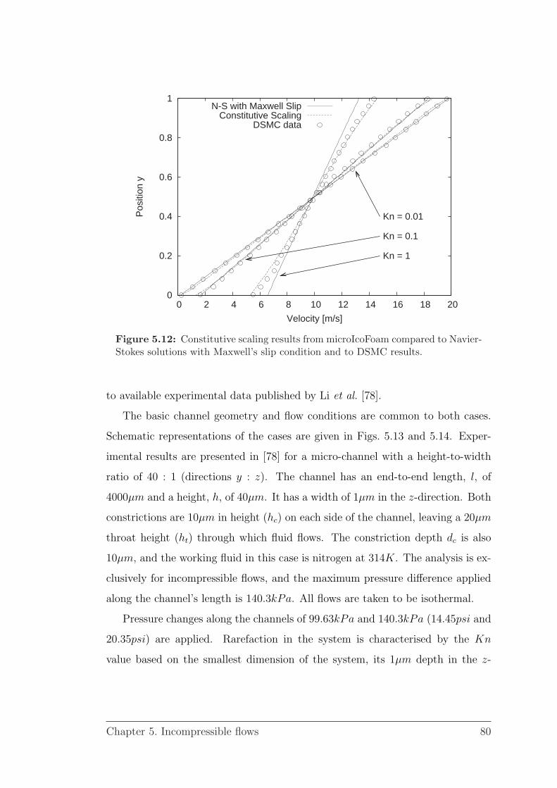
0

0.2

0.4

0.6

0.8

1

0 2 4 6 8 10 12 14 16 18 20

Pos

ition

y

Velocity [m/s]

Kn = 0.01

Kn = 0.1

Kn = 1

N-S with Maxwell SlipConstitutive Scaling

DSMC data

Figure 5.12: Constitutive scaling results from microIcoFoam compared to Navier-Stokes solutions with Maxwell’s slip condition and to DSMC results.

to available experimental data published by Li et al. [78].

The basic channel geometry and flow conditions are common to both cases.

Schematic representations of the cases are given in Figs. 5.13 and 5.14. Exper-

imental results are presented in [78] for a micro-channel with a height-to-width

ratio of 40 : 1 (directions y : z). The channel has an end-to-end length, l, of

4000µm and a height, h, of 40µm. It has a width of 1µm in the z-direction. Both

constrictions are 10µm in height (hc) on each side of the channel, leaving a 20µm

throat height (ht) through which fluid flows. The constriction depth dc is also

10µm, and the working fluid in this case is nitrogen at 314K. The analysis is ex-

clusively for incompressible flows, and the maximum pressure difference applied

along the channel’s length is 140.3kPa. All flows are taken to be isothermal.

Pressure changes along the channels of 99.63kPa and 140.3kPa (14.45psi and

20.35psi) are applied. Rarefaction in the system is characterised by the Kn

value based on the smallest dimension of the system, its 1µm depth in the z-


l

y

x

Inlet

Orifice Plate

Outlet

dcht hhc

Figure 5.13: Microchannel orifice constriction geometry.

l

y

45

Inlet

Venturi

Outlet

dc

hchht

x

Figure 5.14: Microchannel venturi constriction geometry.


axis: Kn = 0.06. The tangential momentum accommodation coefficient in the

velocity slip equation is taken to be σU = 0.8 throughout, which has been shown

experimentally to be representative of gas-surface interactions between nitrogen

and silicon [79].

For each applied pressure drop, three types of OpenFOAM simulation are

carried out:

• No-slip analysis,

• Maxwell slip analysis,

• Constitutive-scaling analysis.

In the first instance, the no-slip boundary conditions applied in macroscale

CFD are applied to the system walls. In the Maxwell slip case, Eq. (3.8) is applied

as a velocity boundary condition with the first order slip coefficient A1 = 1.

The thermal creep is neglected as the cases are taken to be isothermal. When

constitutive scaling is applied, the effective viscosity model proposed in [12], and

given in Eq. (4.6), is used in conjunction with Maxwell’s slip boundary condition,

with microslip coefficient A1 = 0.8.

5.4.1 Validating numerical results

Initially, OpenFOAM results for centreline pressure in the constricted channels

are validated against the experimental data presented in [78]. Figure 5.15 shows

results from microIcoFoam with constitutive scaling compared to experimental

data for the orifice-plate constriction. The figure illustrates longitudinal pres-

sure profiles for both applied pressure changes (99.63kPa and 140.3kPa). The

experimental data, which are restricted to areas of the channel away from the

constriction, have been extracted as lines from plots in [78]. Individual points are

shown on the experimental data in this figure (and in other subsequent figures)

to represent the ends of the available experimental data series, rather discrete


point values. In Figure 5.15, numerical results from OpenFOAM agree very well

with the available data.

0

20

40

60

80

100

120

140

0 0.0005 0.001 0.0015 0.002 0.0025 0.003 0.0035 0.004

Pre

ssur

e (k

Pa)

Channel length (m)

microIcoFoam 140.3kPaExperimental data 140.3kPa


Figure 5.15: Centreline pressures in a channel with an orifice-plate constrictioncompared to experimental data.

For the venturi constriction case, Fig. 5.16 shows the centreline pressure pro-

files. In this case, the agreement between the numerical and experimental data is

poor. The original paper, however, reveals that the experiments found venturi-

type constrictions to produce a higher pressure drop in the flow than orifice plates

of the same minimum area. The paper’s authors acknowledge that this data is

likely to be erroneous, and comment on the role of one particular pressure trans-

ducer in producing these results [78]. Figure 5.17 shows centreline pressures in the

region close to the venturi constriction for the 99.63kPa case. The experimental

results given by Li et al. for the venturi constriction would seem to be consistent

with a much smaller constriction throat height, and are almost certainly incorrect

for the 20µm throat case.

In Fig. 5.18, numerical results for mass flowrate in both orifice- and venturi-

constricted channels are compared to those given by Li et al. The experimental

data, which are for test cases where maximum applied pressure changes peak


0

20

40

60

80

100

120

140

0 0.0005 0.001 0.0015 0.002 0.0025 0.003 0.0035 0.004

Pre

ssur

e (k

Pa)

Channel length (m)



Figure 5.16: Centreline pressures in a channel with a venturi constriction com-pared to experimental data.

25

30

35

40

45

50

55

0.0016 0.0018 0.002 0.0022 0.0024

Pre

ssur

e (k

Pa)

Channel length (m)

ht = 20µmht = 10µm

ht = 5µmht = 2.5µm

Experimental data ht = 20µm

Figure 5.17: Centreline pressures in the near-constriction region through venturiconstrictions in rectangular channels as throat height ht decreases, compared toexperimental data.


at 140.3kPa, are also compared to theoretical predictions of mass flowrate for

an equivalent straight-channel. The theoretical value was calculated using the

following expression [78, 80]:

Qm =z3hP 2

o

24RTlµ

(((Pi

Po

)2

− 1

)+ 12Kno

(Pi

Po

− 1

)), (5.12)

as outlined in the original authors’ paper, using a “best-fit” channel depth of

1.1µm, and Kno = 0.06 [78].

0.2

0.4

0.6

0.8

1

1.2

1.4

95 100 105 110 115 120 125 130 135 140 145

Mas

s flo

wra

te (

µg/m

in)

Inlet pressure (kPa)

Experimental data: orificeExperimental data: venturi

Navier-Stokes: orificeNavier-Stokes: venturi

Theoretical straight channelConstitutive scaling: orifice

Constitutive scaling: venturi

Figure 5.18: Mass flowrates through constricted microchannels: OpenFOAM re-sults for constitutive scaling and Navier-Stokes equations compared to experimentalresults.

Numerical results from microIcoFoam for a 20µm orifice constriction are

shown to agree almost exactly with the experimental data for orifice-plate mass-

flow at both applied pressures. This agreement is possibly better than should

be expected, as the applied pressure gradients along the experimental channels

would typically produce large density changes. Density variations are not mod-

elled using this incompressible solver, which is a potential source of inconsistency

that has not yet been resolved.

The OpenFOAM results for mass flowrate through the venturi constrictions


do not agree with the experimental results from [78]. While the experimental

results return higher flowrates through the venturi constriction, the numerical

simulations return very similar mass flowrates for both the orifice and the ven-

turi; between the two case types the agreement is to within 0.2%. Although

the standard Navier-Stokes simulations under-predict the magnitude of the mass

flowrate, they too predict very similar values between the orifice and venturi case

types. These OpenFOAM results are reasonable, however, as the cases studied

have very low Reynolds numbers: Re ≈ 0.7 for the 99.63kPa pressure difference

and Re ≈ 1 for 140.3kPa pressure difference. In these fully developed laminar

flows, no flow separation occurs at the trailing edge of the orifice plate. In fact,

viscous work causes the orifice constriction to develop a velocity profile similar

to that observed in the venturi constrictions. As Fig. 5.19 illustrates, regions of

very low-speed or stationary flow can develop on the upstream and downstream

edges of the orifice, effectively channelling the flow through a venturi shape. For

a given throat geometry in slow gas-flows such as these, it is reasonable to assume

that the mass flowrate through the two devices would be comparable, and that

there is some error in the venturi constriction results presented in [78].

Figure 5.20 shows numerical results for x-direction throat-exit velocity at the

throat wall for an orifice-plate constriction, contrasting results from the three

types of numerical model tested for verification purposes. Whilst the no-slip case

adopts the velocity of the stationary wall, the Maxwell slip and constitutive scal-

ing cases capture a finite degree of slip at the boundary. The constitutive-scaling

model with microslip profile predicts a slip velocity 20% lower than the Maxwell

slip prediction, and displays a velocity gradient at the wall 1.7 times steeper than

that of the Maxwellian profile, representing the impact of the Knudsen layer. The

increase in the gradient matches the applied scaling function, implying reason-

able grid independence has been achieved, and is consistent with the increase in

strain-rate observed in other analyses of Knudsen layers [3, 8].

Each numerical case is simulated in 3D on a standard desktop PC, with no


y

x

Inlet Outlet

OutletInlet

Figure 5.19: Schematic of low-speed viscous flow through venturi-type and orificeconstrictions.

0

0.05

0.1

0.15

0.2

0 0.5 1 1.5 2 2.5

Dis

tanc

e fr

om th

roat

wal

l (µm

)

Velocity (m/s)

Constitutive scalingMaxwell slip

No slip

Figure 5.20: Velocity profiles close to the throat wall for an orifice-plate constric-tion. Standard no-slip Navier-Stokes results are compared to results with Maxwell’sslip boundary condition applied and to constitutive scaling with microslip.


appreciable time difference introduced by the inclusion of constitutive scaling in

the analysis. Structured, hexahedral meshes are used in all cases which were re-

fined toward the channel walls in ratios of 4 : 1 (minimum of 160×100×50 cells).

Typical solution times for each case are of the order of 30–40 minutes. The effi-

ciency of the OpenFOAM solver for these cases highlights the practicality of the

constitutive scaling method in CFD. At such low Mach numbers (≈ 1.4×10−3) it

would be incredibly computationally expensive to apply DSMC and satisfactorily

reduce scatter in the results. Also, the difficulties encountered by Li et al. in

ensuring the accuracy of experiments conducted at these physical scales reinforce

the need for more reliable means of simulating gas mircoflows.

5.4.2 Extending the analysis

As the OpenFOAM simulation has been shown to replicate some features of Li et

al.’s experimental results, a series of new test geometries are investigated to

examine the behaviour of fluid flow through constrictions with reduced throat

heights. As Knudsen number is directly related to the system geometry, a Kn

value based on throat height would vary directly with changes to the constriction.

By varying the width-based reference value of Kn = 0.06, which is otherwise

independent of changes to geometry in the y-direction, by the factor of change

in geometry, it is possible to include the effects of varying constriction height on

rarefaction. Table 5.3 shows the variation of Kn with throat height, ht.

Throat heights in the channel for both orifice and venturi constrictions are

decreased for the lowest pressure drop, 99.63kPa, to a minimum throat height

of 2.5µm. In the orifice plates, the 10µm constriction depth, shown as dc in

Fig. 5.13, is maintained while the throat height, ht, is decreased. In the venturi

constrictions both constriction depth, dc, and the 45 angle are maintained as the

throat height, ht, is decreased.

Figure 5.21 illustrates the centreline pressure through a channel with a venturi

constriction which has a 5µm throat height. As the constriction height increases


Kn 0.06 0.12 0.24 0.48

ht 20µm 10µm 5µm 2.5µm

Table 5.3: Variation of Knudsen number with throat height for a pressure dropof 99.63kPa across the channel.

35

40

45

50

55

60

65

0.0016 0.0018 0.002 0.0022 0.0024

Pre

ssur

e (k

Pa)

Channel length (m)

ht = 20µmht = 10µm

ht = 5µmht = 2.5µm

Figure 5.21: Centreline pressures in the near-constriction region through venturiconstrictions in rectangular channels as throat height ht decreases: constitutivescaling results only.


(and throat height decreases) the pressure drop across the venturi becomes in-

creasingly sharp, when compared to Fig. 5.16 for example, as would be expected.

The effects of increasing gas rarefaction are also highlighted when throat

heights in the channels are reduced. Fig. 5.22 shows the maximum velocity mag-

nitude for a range of orifice-plate constrictions. Each constriction is analysed

using both the no slip boundary condition and the constitutive scaling model

with microslip boundaries. The figure shows the variation in maximum velocity

predicted by each model as the throat height ht is varied from 20µm to 10µm, 5µm

and 2.5µm. The impact of the Knudsen layer is larger for smaller throat heights,

as shown by the greater separation between the standard Navier-Stokes profile

and the constitutive scaling profile.

0

0.5

1

1.5

2

2.5

3

3.5

4

4.5

4 6 8 10 12 14 16 18 20

Max

imum

vel

ocity

mag

nitu

de (

m/s

)

Throat height ht (µm)

Constitutive Scaling with microslipNavier-Stokes without slip

Figure 5.22: Maximum velocity magnitude for orifice-plate constrictions as throatheight ht varies.

With smaller throat heights, the Knudsen number is higher, and hence the

Knudsen layer and velocity slip have a greater effect on the simulation. To

illustrate, when the constriction height ht is 20µm and Kn = 0.06, the no-

slip model predicts zero-velocity at the wall, and a maximum velocity magni-

tude of 0.389m/s. The constitutive scaling simulations return a slip velocity of


0.00761m/s at the channel walls, and a maximum velocity magnitude of 0.539m/s

at the constriction centre. The difference between the predicted maximum ve-

locities is 39%. When ht is reduced to 2.5µm, and Kn increases to 0.48, the

no-slip model gives a maximum velocity of 3.12m/s, compared to the constitu-

tive scaling model’s slip at the channel walls of 0.67m/s, and constriction-centre

velocity of 4.5m/s. The difference between the maximum centreline velocities for

the higher-Kn case is 44%, which represents a change in the discrepancy between

no-slip and scaled simulations of 5% with a single order of magnitude change in

Kn.

Using the experimental data published in [78], microIcoFoam has been shown

to produce reasonable predictions of the behaviour of low-speed gas flow through

constricted microchannels. As the available experimental data are somewhat

limited, validation using alternate data sources would be desirable to ensure that

the numerical solver provides an accurate representation of the fluid flow through

microscale constrictions. In OpenFOAM, several higher-Kn cases beyond the

scope of the original experimental data have also been studied. The application

of constitutive scaling to these cases has shown that as gas rarefaction increases,

the macroscopic behaviour of gas flow through constricted microchannels is likely

to be significantly altered. This highlights that successful design of microscale

mass flowrate measurement devices will be heavily dependent on the ability of

engineering tools to capture the behaviour of rarefied gases.

5.5 Cylindrical Couette flow

Couette flow between rotating concentric cylinders, as shown in Fig. 5.23, is a

shear-driven problem that behaves in a similar manner to planar Couette flow.

This is an excellent case with which to test the microIcoFoam solver, as it assesses

both the solver’s ability to adequately capture slip and Knudsen layer effects in

curved geometries, and its ability to capture some of the counter-intuitive fea-

tures found in rarefied flows. This flow configuration is of particular engineer-


ing relevance as it corresponds directly to gas behaviour in microscale air bear-

ings, which appear in many applications such as microscale power generation and

micro-turbines, see e.g. [1].

Typically, in cylindrical Couette flow, the inner cylinder rotates at a constant

velocity, whilst the outer cylinder remains stationary. The shear-force arising in

a viscous fluid between the cylinders generates a velocity profile between them

in a radial direction. Rotating Couette flow is quite an unusual case in that, for

rarefied flows over surfaces where the gas-surface interaction is largely specular,

a complete inversion of the velocity profile, compared to the standard Navier-

Stokes results is possible [15]. That is to say, the degree of slip present can allow

the flow to move more quickly over the stationary outer cylinder than over the

rotating inner cylinder, which is entirely counter-intuitive. Rarefaction effects

are the cause of this unusual phenomenon. The low momentum accommodation

coefficient of specular flows implies that the momentum of molecules impinging

the cylinders is largely reversed. Those molecules that have collided with the

rotating cylinder will therefore retain most of their momentum. When the gap

between the cylinders is sufficiently small, molecules reflected form the rotating

inner cylinder will, on average, have their next intermolecular collisions close to

the outer wall, causing the flow nearer the outer cylinder to be faster than the

flow near the stationary wall.

Isothermal Couette flow between rotating cylinders is a case in which no rea-

sonable solution may be obtained using the constitutive scaling technique unless

the coupled velocity-viscosity terms described in Eq. (4.12) are retained in the

momentum equations. In the case of a rotating inner cylinder and a stationary

outer cylinder, direct simulation Monte Carlo (DSMC) molecular dynamics sim-

ulations predict an inverted tangential velocity profile for some rarefied flows, i.e.

the gas velocity increases with radial distance from the moving cylinder [15]. This

case has been investigated previously in order to compare results obtained using

Eq. (3.7) in place of Eq. (3.6), however the constitutive-scaling approach has not


ro = 5λ

ri = 3λ

h

uwall = 0

uwall = u

Figure 5.23: Schematic of Couette flow between concentric cylinders.

previously been applied to this problem [16, 20].

Figure 5.24 illustrates results for tangential velocity in the rotating Couette

flow problem. The inner and outer cylinders are concentric, with respective radii

of 3λ and 5λ, where λ is the mean free path of the gas flowing between the

cylinders, which is argon at standard temperature and pressure [75]. The tangen-

tial momentum accommodation coefficient, σU = 0.1. The figure compares the

velocity profile predictions of several numerical models with DSMC data. Both

no-slip and conventional slip (Eq. (3.6)) simulations fail to predict inversion of

the velocity profile. Maxwell’s original slip equation, in this case Eq. (3.7), is

seen to predict an inverted velocity profile, although it cannot capture the form

of the DSMC results. When the constitutive-scaling method (shown as the solid

line) is applied, not only is good general agreement with Maxwell’s original slip

condition observed, but the shape of the velocity profile is seen to approach that

of the DSMC data. The slight dip in the profile near the inner wall and the re-

duction in gradient towards the outer cylinder can clearly be seen. Quantitative


agreement with the DSMC remains poor, but it should be noted that such high

Knudsen number cases (Kn = 0.5), represent the very edge of applicability for

even scaled continuum models, and close numerical agreement is not expected.

0.15

0.2

0.25

0.3

0 0.5 1 1.5 2

nond

imen

sion

al ta

ngen

tial v

eloc

ity

radial distance from inner cylinder, r / λ

No slip Conventional slip Maxwell’s original slip Wall function DSMC

Figure 5.24: Velocity profiles in cylindrical Couette flow non-dimensionalisedby the tangential velocity of the inner cylinder. Comparison of no slip (· · ·),conventional slip (- -), Maxwell’s original slip (- · -), constitutive-scaling in CFD(—) and DSMC data ().

5.6 Summary

In this chapter, verification analyses have been carried out comparing Open-

FOAM results for Maxwell’s slip boundary condition and constitutive scaling to

analytical solutions for planar Poiseuille and Couette flows. The numerical re-

sults were observed to match the analytical solutions closely, ensuring that the

functions implemented in the code operate correctly. Validation analyses have

also been conducted, comparing results from OpenFOAM to DSMC data and

experimental data for flow in several different configurations. Overall, the results

indicate that the constitutive scaling method is able to satisfactorily capture the

key effects of gas rarefaction, slip and the Knudsen layer, for incompressible and


isothermal cases. The next stage in the development process of constitutive scal-

ing in CFD is the extension of the method to fully compressible flows, and the

inclusion of heat transfer effects.


Chapter 6

Compressible flows

6.1 Introduction

Gas microflows are often compressible, both in the traditional sense that it is

possible for the local Mach number to be large, i.e. the flow is compressible, and

also in the sense that large pressure and density gradients are commonly found

in rarefied flows, i.e. the fluid is compressible. Both “types” of compressibility

lead to coupling of the momentum and energy equations, as the ratio of a fluid’s

kinetic energy to its internal energy becomes large. This ratio is represented by

the Mach number, Ma, and when dealing with rarefaction in compressible flows,

it is common to redefine Knudsen number as a function of the Mach number [81]:

Kn =

√γπ

2

Ma

Re. (6.1)

This compressible definition of Kn is also a function of the specific heat ratio,

γ, and the Reynolds number, Re, which is commonly low in microflows where

viscous dissipation effects are enhanced by large surface-area to volume ratios.

This increased degree of viscous dissipation can substantially alter the impact of

compressibility on a fluid flow. For example, in some microsystems where flow

approaches the local speed of sound, smooth regions of sonic flow develop, rather

than discontinuous shock waves [82, 83]. Rarefaction effects can also be seen

to counteract compressibility effects; the introduction of slip boundary condi-

tions, for instance, reduces shear stress and hence viscous work at system bound-

Chapter 6. Compressible flows 96

aries [74].

In order to accurately model compressible rarefied flows, a CFD simulation

must therefore solve both the energy and momentum equations in a coupled fash-

ion and also incorporate rarefaction effects. For continuum models, both velocity

slip and temperature jump boundary conditions must be included, in addition

to models for Knudsen layers observed in both velocity and temperature fields.

Constitutive scaling of the thermal Knudsen layer has been proposed previously,

however, it has not to date been applied either to cases where both momentum

and energy exchanges are present, nor has it been applied in a generalised CFD

framework [36, 45].

In this chapter, an OpenFOAM solver suitable for compressible rarefied flows

is described and the performance of two published constitutive scaling models

implemented within it is analysed [12, 17]. Half-space problems are used to assess

the implementation of the scaling models, which are compared to kinetic theory

data for validation and then contrasted to each other [4, 6]. The scaling approach

is then applied to an industrially relevant application, compressible micro-Couette

flow, and OpenFOAM results are compared to available DSMC data [18]. This

case study includes a detailed critical analysis of the constitutive scaling method,

which focuses in particular on the relationship between momentum and energy

transfer in constitutive scaling, and on the selection of appropriate boundary

conditions for high-Kn compressible flows.

6.2 Compressible solvers in OpenFOAM

Several compressible flow solvers are available in the OpenFOAM software distri-

bution, each tailored to a specific type of compressible flow [70]. The rhopSonic-

Foam solver has been selected as the most appropriate application to use as the

basis for a compressible microflows solver, as it has been partially redeveloped

for analysing rarefied flows in hypersonic-aerodynamics applications [13, 71, 84].

The rhopSonicFoam solver is a pressure-density-based application for lami-


nar compressible flows, and solves governing equations of continuity, momentum

(posed in terms of mass-flux) and total energy. These equations are solved in a

segregated manner, followed by a PISO-style pressure correction loop. For gas

microflows, however, the solver requires substantial modification — primarily as

the release version is inviscid. The governing equations implemented therefore

do not contain diffusive terms, or sources of mechanical power and heat flux.

The inviscid-flow assumption is valid for some high-speed compressible flows,

but it is not appropriate for microscale flows, which are almost exclusively in-

ternal flows dominated by the effects of bounding surfaces. A viscous version of

rhopSonicFoam, which also includes diffusive terms in the governing equations

and is known as rhopEsonicFoam, has been produced as part of another non-

equilibrium flow project undertaken at the University of Strathclyde [71, 84].

The rhopEsonicFoam solver also features boundary conditions more appropriate

to non-equilibrium flows, including Maxwell’s velocity slip condition [10].

In the following sections, a summary of the differences between rhopSonic-

Foam and rhopEsonicFoam is given, alongside a general description of how the

solvers operate. Then, further changes made as part of the work of this thesis

to rhopEsonicFoam are described, before details of how the new code is used to

implement constitutive scaling for compressible gas microflows are given.

6.2.1 Compressible solver: rhopSonicFoam

The compressible solver rhopSonicFoam released with OpenFOAM (in this case

version 1.3) initially solves for density, ρ, using the continuity equation:

∂ρ

∂t+∇ · U (ρ) = 0. (6.2)

The inviscid momentum and energy equations in the solver are formulated im-

plicitly and solved for mass flux ρU and total energy ρE;

∂ (ρU)

∂t+∇ · U (ρU) = −∇p, (6.3)


∂ (ρE)

∂t+∇ · U (ρE) = −∇ · Up. (6.4)

The temperature field is then extracted from the solution to this form of the

energy equation using the definition of total energy [85]:

ρE = ρcvT +(|ρU|)2

2ρ, (6.5)

∴ T =ρE − 1

2ρ(|ρU|)2

ρcv. (6.6)

The perfect gas law is given by

p = ρRT, (6.7)

where R is the gas constant, and this expression is used to determine a pres-

sure field from the continuity equation prediction for density. The perfect gas

law is a statistical description of microscopic behaviour which represents the

macroscopic behaviour of gases. Although a statistical average taken only in the

non-equilibrium Knudsen layer could theoretically differ from the ideal gas ap-

proximation, where flow properties in slip- and transitional-Kn flows are averaged

over full systems, the perfect gas law should remain valid.

Next, momentum fluxes on cell-face areas are calculated, and a pressure equa-

tion combining the continuity equation and the perfect gas law is formulated in

terms of pressure and the momentum fluxes. The solution to this pressure equa-

tion is used as a corrector for the continuity equation. The momentum equation

is also corrected, based on the momentum fluxes used in the pressure equation.

When reasonable convergence for pressure and momentum flux is obtained iter-

atively, the velocity field is determined by dividing the momentum-equation so-

lution for mass flux ρU by the continuity equation solution for density ρ. Thus,

by solving implicitly for p, ρU and ρE, solutions for ρ, U and T are obtained.

Boundary conditions are applied to individual analyses following OpenFOAM’s

standard case structure, and specified in terms of p, U and T . These conditions


are then interpreted by the code as boundary conditions for the equations posed

in terms of ρ, ρU and ρE. Velocity slip and temperature jump conditions are not

implemented in the rhopSonicFoam release.

6.2.2 Modified solver: rhopEsonicFoam

Redevelopment of the rhopSonicFoam solver by C.J. Greenshields undertaken

as a part of [71] has transformed the publicly released code into a new solver,

rhopEsonicFoam. The primary difference between rhopSonicFoam and rhopEson-

icFoam lies in the formulation of the governing equations, where rhopEsonicFoam

includes viscous terms. The new solver also includes more refined mapping of

boundary conditions between standard macroscopic quantities and the solution

variables, and a wider range of boundary conditions, including Maxwell’s velocity

slip condition, has been implemented [10, 11]. A choice of three viscosity models

is also available in rhopEsonicFoam: Sutherland’s law, the power law and the

standard Newtonian fluid model [70].

The basic solution procedure used in rhopEsonicFoam follows that outlined

above for rhopSonicFoam, and the solvers use identical continuity equations. The

momentum and energy equations, however, are implemented in viscous form. The

momentum equation in rhopEsonicFoam is

∂ (ρU)

∂t+∇ · U (ρU)−∇ · τ = −∇p, (6.8)

where the divergence of the shear stress, ∇ · τ , is a diffusive term. Typically,

the Newtonian shear-stress tensor, given by Eq. (4.11), is formulated explicitly

in terms of velocity.

In order to introduce the normally explicit shear stress term into the implicit

form of the momentum equation, an equivalent expression in terms of mass flux

ρU is defined [71]. To recap briefly, the N-S-F stress tensor is

τ = µ∇U + µ∇UT − 2

3µtr (∇U) I,


where terms with multiple components of U are fully explicit, and may be grouped

together in a new term, τmc, giving

τ = µ∇U + τmc. (6.9)

Substituting kinematic viscosity, ν, for dynamic viscosity, µ, and using the

expression µ = νρ, the first term of the shear stress tensor can be expanded into

implicit and explicit components as follows:

τ = νρ∇U + τmc

= ν∇ (ρU)− ν (∇ρ)U + τmc

= ν∇ (ρU)− ν∇ (ρU) + µ∇U + τmc. (6.10)

The divergence of the stress tensor in this form is then substituted back into

the momentum equation. The identical terms in the last line of Eq. (6.10) are

not cancelled in the final implementation, as one term is implicit and the other

explicit — the original µ∇U term has simply been expanded into implicit and

explicit component parts [71]. OpenFOAM automatically places implicit terms

into a matrix of coefficients for the equation to be solved, and explicit terms are

collated in a source-term matrix. The presence of the implicit part of the shear

stress term in the solution matrix improves convergence as it boosts the matrix’s

diagonal component.

In the rhopEsonicFoam code, the momentum equation given by Eq. (6.8) is

implemented in the following form.


fvVectorMatrix rhoUEqn(

fvm::ddt(rhoU)

+ fv::gaussConvectionScheme<vector>(mesh, phiv, rhoUScheme)

.fvmDiv(phiv, rhoU)

- fvm::laplacian(DrhoU, rhoU)

+ fvc::laplacian(DrhoU, rhoU)

- fvc::laplacian(mu, U)

- fvc::div(tauMC)

);

solve(rhoUEqn == -fvc::grad(p));

Momentum equation

∂(ρU)/∂t

+∇ · U (ρU)

−∇ · ν∇ (ρU)

+∇ · ν∇ (ρU)

−∇ · µ∇U

−∇ · τmc

=

−∇p

Terms labelled fvm:: are fully implicit terms, while those beginning fvc:: are

explicit. All source terms are included in the main body of the equation, with

the exception of the pressure-gradient source term −∇p, which is included in the

solve command.

The energy equation in rhopEsonicFoam is also modified from the inviscid

rhopSonicFoam version given by Eq. (6.4). The energy equation in rhopEsonic-

Foam, in terms of total energy ρE, is given by

∂ (ρE)

∂t+∇ · U (ρE) = −∇ · Up+∇ · κ∇T +∇ · (τ · U) , (6.11)

where κ∇T represents heat flux and (τ · U) is mechanical power flux, and both

terms are explicit. As outlined for the momentum equation above it is helpful to

be able to express some part of these source terms in implicit form. Following

procedures laid down in [71], this is accomplished by using the definitions of

Prandtl number,

Pr =µcpκ, (6.12)


and specific heat ratio, cP = γcv, to express the divergence of the heat flux in

terms of internal energy e:

∇ · κ∇T = ∇ ·(γν

Pr

)∇ρe. (6.13)

The divergence of the translational part of the mechanical power flux (τ · U)trans

is then re-written in terms of kinetic energy:

∇ · (τ · U)trans = ∇ · 2ν∇( |ρU|2

2ρ

). (6.14)

The diffusive coefficients of these two equations are γν/Pr and 2ν, and are ap-

proximately equal when γ/Pr ≈ 2. As this condition is appropriate for many

gas flows, the diffusive coefficients of heat and translational power flux can be

replaced with a single coefficient term, D, multiplied by kinetic viscosity, ν. The

definition of total energy given in Eq. (6.5) is then used to combine the heat flux

and translational power flux into a single, implicit, total energy term:

∇ ·Dν∇ (ρE) = ∇ ·(γν

Pr

)∇ρe+∇ · 2ν∇

( |ρU|22ρ

). (6.15)

Then, in the same way that the shear tress tensor was separated into equal implicit

and explicit component parts above and introduced into the momentum equation

(see Eq. (6.10)), this implicit total energy term may be introduced to the energy

equation by subtracting an equivalent explicit term and the original term. The

energy equation is then implemented in rhopEsonicFoam as follows.


fvScalarMatrix rhoEEqn(

fvm::ddt(rhoE)

+ mvConvection.fvmDiv(phiv, rhoE)

==

- mvConvection.fvcDiv(phiv, p)

+ fvm::laplacian(DrhoE, rhoE)

- fvc::laplacian(DrhoE, rhoE)

+ fvc::laplacian(k, T, "laplacian(k,T)")

+ fvc::div(

fvc::interpolate(mu)*mesh.magSf()*(fvc::snGrad(U) & fvc::interpolate(U))

)

+ fvc::div(

((mesh.Sf() & fvc::interpolate(tauMC))

& fvc::interpolate(U))

)

);

solve(rhoEEqn);

Energy equation

∂(ρE)/∂t

+∇ · U (ρE)

=

−∇ · Up

+∇ ·Dν∇ (ρE)

−∇ ·Dν∇ (ρE)

+∇ · κ∇T

+∇ · µ∇U · U

+∇ · (τmc · U)

Again, fvm:: terms are implicit terms and fvc:: terms are explicit. The pressure

correction loop that follows the energy equation in the solution procedure is

identical to that used in the publicly released version of rhopSonicFoam.

The range of boundary conditions implemented in rhopEsonicFoam includes

Maxwell’s velocity slip condition, incorporating the effects of thermal creep, as

described by Eq. (3.8), and Smoluchowski’s temperature jump condition as given

in Eq. (3.9). As rhopEsonicFoam is designed to solve the momentum and energy

equations with viscosity as a temperature dependent property only, i.e. the N-S-F


equations without constitutive scaling, dynamic viscosity and thermal conductiv-

ity are always assigned a spatially-constant value. The slip and jump boundary

conditions are therefore implemented in terms of constant viscosity and Prandtl

number, Pr, rather than the mean free path. As discussed in section 4.4.1, this

relies on the velocity profile conforming to a Maxwellian equilibrium distribution,

which limits the solver’s applicability to cases where Kn . 0.1 and Knudsen layer

structure represents an insignificant proportion of the flow.

6.2.3 Compressible microflows solver

To implement constitutive scaling in rhopEsonicFoam and extend its applicabil-

ity to transitional-Kn flows, further modifications must be made to the solver.

Firstly, the effective viscosity models that are used to introduce the scaling must

be implemented in the code. This is carried out in a similar manner to that

described in section 4.4, and a range of effective viscosity models are available.

For non-isothermal compressible cases, the thermal conductivity, which linearly

relates heat flux and temperature gradient in the N-S-F equations must also be

scaled, see Eq. (4.8). For this to be possible, thermal conductivity must be intro-

duced to the solver as a variable field, with switches determining its value depend-

ing on whether or not constitutive scaling is used, and also on the constitutive-

scaling model chosen. Appropriate effective thermal conductivity models have

therefore been introduced in the solver, and the value of thermal conductivity is

now calculated and updated alongside the viscosity models as part of the code’s

main iterative loop.

Thermal conductivity and dynamic viscosity are related to each other by the

Prandtl number Pr, which is given by Eq. (6.12). Consequently, the manner

in which µ and κ are scaled relative to each other can be as influential on the

simulation as the shape of the scaling functions used for individual fields. Two

of the foremost constitutive-scaling schemes published, which each treat Prandtl

number differently, are currently implemented in the modified rhopEsonicFoam


solver, although the framework of the solver is such that in future other models

can easily be incorporated as they become available.

6.3 Constitutive scaling models

The currently implemented models are those proposed by Lockerby et al. [12]

and Reese et al. [17], which will be referred to here as model A and model B,

respectively. The main difference between the models is the relationship between

their constitutive scaling functions for shear stress and for heat flux, that is to

say, how combined viscosity and conductivity scaling affect Pr.

6.3.1 Model A

In model A, the scaling function given in Eq. (4.6) is taken alongside the dynamic

viscosity to form an effective viscosity term that varies with normal distance to

the nearest solid surface, i.e.

µeffA=

µ

f (n/λ), (6.16)

where the subscript A refers to a quantity used in model A. This is the constitutive

scaling model that has been applied in earlier chapters of this thesis, and which

has been tested in its isothermal form on several standard benchmark micro-

flows [12, 14, 36].

Model A uses the definition of Prandtl number, which describes the rela-

tionship between momentum diffusivity and energy diffusivity, and is given in

Eq. (6.12), to define its expression for scaling the thermal conductivity, κ. Given

the hard-sphere, monoatomic gas model condition of a constant Pr = 2/3, then

κeffA=µeffA

cpPr

=3

2µeffA

cp. (6.17)

So, in model A the relative magnitudes of the momentum and energy diffusivi-

ties are preserved from the original molecular model. In the modified rhopEsonic-


Foam solver, a fixed Pr value is established when model A is used, and the thermal

conductivity field is calculated from this value in accordance with Eq. (6.17).

6.3.2 Model B

Constitutive scaling functions for Knudsen layers of both momentum and energy

were recently proposed in [17, 45], using kinetic theory data from a wide literature

survey to determine effective values of both dynamic viscosity and thermal con-

ductivity. The effective quantities are presented in similar general form, with the

original constitutive constants scaled by normal distance to the nearest wall and

the appropriate accommodation coefficient for tangential momentum or energy,

corresponding to that used in the velocity slip/temperature jump equations.

From [45], the replacement constitutive relationship for momentum (i.e. effec-

tive viscosity) is:

µeffB(n) =

µ

1− AKP (DKP · σU + EKP )(1 +

√π

2nλ

)AKP−1, (6.18)

and the scaling function for energy (i.e. effective thermal conductivity) is:

κeffB(n) =

κ

1− ATJ (DTJ · σT + ETJ)(1 +

√π

2nλ

)ATJ−1. (6.19)

The subscripts KP and TJ refer to Kramers’ problem and the temperature jump

problem, which were the kinetic-theoretical case studies used in the curve-fitting

to derive the scaling functions; A,D and E are constants generated in the curve-

fitting process, listed in Table 6.1 for the hard-sphere molecular model. Note that

in this model the diffusivities of momentum and energy are not both scaled in

the same way. As a result, any effective Prandtl number that were defined using

those quantities would be non-constant. When model B is used in the modified

rhopEsonicFoam solver, thermal conductivity is defined using Eq. (6.19) and an

effective Prandtl number is then calculated from the scaled viscosity and thermal

conductivity using Eq. (6.12). This is in contrast to using a constant Pr value


to define the thermal conductivity scaling from the viscosity scaling, and is the

fundamental difference between models A and B.

µ-scaling AKP DKP EKP σU

Coeff. value -2.719 -0.293 0.531 1.0

κ-scaling ATJ DTJ ETJ σT

Coeff. value -2.142 -0.745 1.295 1.0

Table 6.1: Coefficients used in Eqs. (6.18) and (6.19) to define the scaling functionsof model B.

It should be noted that the scaled diffusive quantities in both model A and

model B are purely effective values, and were not intended by the original propo-

nents of constitutive scaling to be used to define physical values of, for example,

mean free path or Prandtl number. Rather, the original viscosity and thermal con-

ductivity should be used to define physical quantities. Within a CFD framework,

however, it is important that physical quantities are retrievable from the scaled

model. For example, in the hard-sphere model approximation of monoatomic

gases, flows incorporating both momentum and energy fluxes may be shown to

have a constant Prandtl number, Pr = 2/3 [86]. If this value is not recovered us-

ing the “true” velocity or temperature profiles produced by the scaling approach,

it is possible that this is due to a physical inconsistency in the scaling model.

Comparing Models A and B: Figures 6.1 and 6.2 illustrate the variation of

effective dynamic viscosity µeff and effective thermal conductivity κeff with normal

distance from a planar wall. The scaled quantities are compared to nominal

constant values of µ and κ respectively. Model A scales consistently for both

dynamic viscosity and thermal conductivity, producing effective quantities 0.59

times their original value at the wall, and reaching the full value of the original

quantity outside the Knudsen layer region. Model B is seen to apply different


scaling to each quantity, resulting in wall values of µeff = 0.62µ and κeff = 0.47κ,

and again reaching the full original value outwith the near-wall region of the flow.

0.5

0.6

0.7

0.8

0.9

1

0 0.5 1 1.5 2 2.5

Non

dim

ensi

onal

dyn

amic

vis

cosi

ty, µ

eff/µ

Nondimensional normal distance from wall, n/λ

Model AModel B

Original viscosity

Figure 6.1: Effective viscosities provided by the scaling models, compared to(constant) nominal viscosity.

Figure 6.3 shows the ratio of effective viscosity to effective thermal conductiv-

ity predicted by each scaling model, which is directly comparable to the effective

Prandtl number (i.e. Pr from Eq. (6.12), but using effective quantities and with-

out the specific heat at constant pressure cp as a coefficient). In the hard-sphere

molecular model, only translatory exchanges of energy are present, leading to a

fixed ratio of momentum to thermal energy exchange for a fixed collision time,

which in turn leads to the constant Prandtl number condition. What the figure

illustrates is that using model B effectively induces a difference between the mag-

nitude of momentum exchange and energy exchange in any given collision. This

violates the constant Prandtl number condition of the hard-sphere gas model —

which was the model from which the function in Eq. (6.19) was derived. As such,

model B may be inappropriate for use in cases where both momentum and energy

exchange are considered. In isothermal or isoflux cases, however, model B could

still represent a legitimate form of constitutive scaling.


0.4

0.5

0.6

0.7

0.8

0.9

1

0 0.5 1 1.5 2 2.5

Non

dim

ensi

onal

ther

mal

con

duct

ivity

, κef

f/κ


Model AModel B

Original conductivity

Figure 6.2: Effective thermal conductivities provided by the scaling models, com-pared to (constant) nominal thermal conductivity.

6.4 Half-space problems

In rarefied flows, velocity slip and temperature jump arise within the Knudsen

layer as the difference in the average molecular properties of the wall and those

of the gas at the wall. The Knudsen layer thickness is the average distance over

which these discontinuities would be equilibrated in a quiescent gas (or in an

unheated gas for the thermal case). The Knudsen layer regions are illustrated

schematically in Figs. 4.1 (shown in section 4.1) and 6.5 as extending ≈ 2λ from

the planar surface.

6.4.1 Kramers’ problem

Kramers’ problem was introduced briefly in Chapter 4, and is defined as the in-

compressible, isothermal flow of a gas in a half-space under a constant shear stress

that is applied tangentially to a stationary planar wall. The shear stress gener-

ates a linear velocity profile normal to the wall, except in the near-wall Knudsen

layer region where an increase in strain-rate is observed. This momentum Knud-


1.2

1.25

1.3

1.35

1.4

1.45

1.5

1.55

1.6

1.65

0 0.5 1 1.5 2 2.5

Effe

ctiv

e vi

scos

ity /

effe

ctiv

e co

nduc

tivity

, µef

f/κef

f


Model AModel B

Figure 6.3: Ratio of effective viscosity to effective thermal conductivity (ratio ofmomentum to energy diffusivity) provided by the scaling models.

sen layer arises due to incomplete accommodation of momentum between the gas

and the surface.

Kramers’ problem is a very simple model of flow in, for example, microscale

comb-drives, where oscillating parts induce shear stresses in gas surrounding the

device. The drag force between surfaces depends directly on the surface-normal

velocity gradient, which can be substantially altered by rarefaction.

Although relatively few experimental results are available for constant-shear

problems, there are many reliable kinetic theory solutions in the published liter-

ature. Typically, these solutions report a velocity defect, rather than a velocity

profile, varying with normal distance to the stationary wall. Velocity defect is

taken to be the difference between a standard N-S-F solution to the problem, with

a “fictitious” macroslip coefficient applied to Maxwell’s slip boundary condition,

typically ζslip = 1.146, and the true velocity profile in the Knudsen layer [6].

In the derivation of model B, the concept of velocity defect was used to define

a dimensionless function S(n/λ) describing the spatial structure of the Knud-

sen layer [45]. This is effectively a shape defect term, describing Knudsen layer


changes in the near-wall profiles of given macroscopic quantities of interest, such

as velocity or temperature. The profile defects are curve-fit from a wide range of

data to establish the coefficients given in Table 6.1. By re-casting Eq. (4.6) in

the form of Eqs. (6.18) and (6.19), it is possible to express model A in the form

of model B, using coefficient values of A = −2, D = 0 (i.e. the model A function

is not accommodation-coefficient dependent) and E = 0.35. Combining Eqs. (9)

and (11) given in [17], a general equation for the shape defect is established as

S(n/λ) = (Dσ + E)

(1 +

√π

2

n

λ

)A

, (6.20)

where σ is the surface accommodation coefficient of either tangential momentum

or energy, and the√π/2 term is introduced to convert between those authors’

definition of mean free path and the definition used here, Eq. (2.2). Using the

dimensionless shape defect, S(n/λ), it is possible to compare both constitutive

scaling models directly to the kinetic theory data presented in [6], as shown in

Fig. 6.4.

It is obvious from Fig. 6.4 that the Knudsen layer predicted by model B is

much closer to the kinetic theory data than the structure predicted by model A.

This would imply that, at least in this particular case, model B would be expected

to give more accurate results when applied as a scaling relationship to the N-S-F

equations. It is noteworthy, however, that very close to the wall even the curve-

fit of model B fails to capture accurately the gradient of the shape defect, which

determines, in practice, the shape of the Knudsen layer.

6.4.2 The temperature jump problem

The temperature jump problem (Fig. 6.5) is a constant heat flux in a half-space,

applied normally to a planar wall in a quiescent gas. In the thermal Knudsen layer

near the solid surface the temperature gradient increases, reflecting the incom-

plete exchange of thermal energy between the gas and the wall. Although limited

to diffusive effects, this type of problem is representative of some specialist cool-


0

0.05

0.1

0.15

0.2

0.25

0.3

0.35

0 0.2 0.4 0.6 0.8 1 1.2

Non

dim

ensi

onal

sha

pe d

efec

t, S

(n/λ

)


Kinetic theory dataModel AModel B

Figure 6.4: Knudsen layer shape defect predicted for Kramers’ problem: kinetictheory data (points connected by solid line) compared to model A (dashed line)and model B (dotted line).

ing applications, and of recently published experiments which attempt to quantify

gas-surface interactions by measuring thermal accommodation coefficients [87].

The thermal Knudsen layer structures predicted by the constitutive scaling

models for the temperature jump problem are shown in Fig. 6.6, in comparison

to kinetic theory data from [4]1. Again, the shape defect predicted by model

B would seem to provide a much better representation of the thermal Knudsen

layer, as observed through the temperature profile. Model A provides a realistic

estimate of the shape defect gradient, i.e. the form of the thermal Knudsen layer,

but under-predicts the extent of the Knudsen layer (the magnitude of the shape

defect).

Considered together, Figs. 6.4 and 6.6 illustrate that kinetic models, which

only consider transfer of momentum or energy, not both, appear to predict dif-

ferent Knudsen layer structures [4, 6]. This difference is the source of the vari-

1Very few data points are given in Loyalka’s paper. However, it remains one of the mostreliable available sources of data for the temperature jump problem.


≈ 2λ

TwallTjump

T ∗∗jump: Macro-jump N-S-F profile

Tjump: True temperature profile

q

T ∗∗jump

Twall: No-jump N-S-F profile

Figure 6.5: Schematic of the temperature jump problem showing constant appliedheat flux, q; traditional, no-jump N-S-F solution (Twall: dotted line), N-S-F solutionwith second order macro-jump boundary condition (T ∗∗jump: dashed line) and truetemperature profile (Tjump: solid line).

ation in Prandtl number that occurs in model B. To maintain the monoatomic,

hard-sphere constant Prandtl number of 2/3, a single Knudsen layer structure,

applicable to both momentum and energy transfer, is required — such as that

shown by model A. The model A trace in Figs. 6.4 and 6.6 is roughly equidistant

between the Kramers’ problem and temperature jump problem profiles, with a

gradient that reasonably represents both kinetic theory solutions. It is perhaps

for this reason that model A appears to produce reasonable results across a range

of flow configurations [12, 14, 36], although its original derivation was from an

isothermal Kramers’ problem case [3].

6.4.3 Summary

In analysing Kramers’ problem and the temperature jump problem, the functions

implemented in OpenFOAM to apply constitutive scaling have been assessed.

The impact of each model on the relationship between energy and momentum


0

0.1

0.2

0.3

0.4

0.5

0.6

0 0.2 0.4 0.6 0.8 1 1.2

Non

dim

ensi

onal

sha

pe d

efec

t, S

(n/λ

)


Kinetic theory dataModel AModel B

Figure 6.6: Knudsen layer shape defect predicted for the temperature jump prob-lem: kinetic theory data (points connected by solid line) compared to model A(dashed line) and Model B (dotted line).

diffusivity has also been discussed. In order to validate the rhopEsonicFoam

solver and investigate the potential impact of introducing a non-constant effec-

tive Prandtl number with model B, the implemented constitutive scaling func-

tions must be applied to a more complex case where energy and momentum are

exchanged simultaneously.

6.5 Compressible micro-Couette flow

As a validation exercise, the modified rhopEsonicFoam solver is used to simulate

high-speed Couette flow of argon gas in 2D microchannels. The Couette flow

problem is essentially a 1D flow, but is solved in CFD as a 2D planar flow in

a channel. All of the constitutive-scaling models and solvers are implemented

fully in 3D in OpenFOAM, however, to enable other more general problems to

be investigated in the future.

This Couette flow would be typical of those found in computer hard-disks,

where it is important to be able to quantify the position of the disk-reading head


over the data-storing platter. The drag force experienced by the reader-head

and other macroscopic fields such as velocity can be substantially altered by gas

rarefaction.

The 2D channel configuration for Couette flow is shown in Fig. 6.7. The upper

wall remains stationary and the lower wall moves in the positive x-direction at

Mach 1 (with the local speed of sound calculated using the wall temperature),

generating a constant tangential shear stress. The pressure in planar Couette

flow also remains constant, hence, compressibility effects in this configuration

arise from changes in density that occur due to viscous heating increasing the

temperature of the flow. The simulated channel length is a minimum of 60µm,

and flow is fully developed in the centre of the system. The channel height in

the y-direction is varied in order to determine the Knudsen number of the case.

For validation purposes, results from OpenFOAM are compared to DSMC data

up to a Kn-value of 0.5, which is relatively high for any type of continuum solu-

tion [18]. Then, in order to investigate the behaviour of the constitutive scaling

models beyond the limits of their applicability, a further, high-Kn case is of 0.8

is also analysed. The different channel heights used are given in Table 6.2, with

corresponding Kn values and Reynolds numbers. The Kn values are determined

using Eq. (6.1), with Mach number defined as Ma = U/√γRT and Reynolds

number defined as

Re =UMa=1H

ν, (6.21)

where ν is the kinematic viscosity, H is the height of the channel, and UMa=1 is

the velocity of the moving wall at Ma = 1, i.e. maximum velocity in the system.

Argon gas at a temperature of 300K is used as the working fluid, with both

wall temperatures fixed at 300K. Gas properties are determined using [75]. The

use of argon makes [18] a particularly appropriate source of validation data: it is a

monoatomic gas, which is in keeping with the assumptions of molecular behaviour

inherent in the velocity slip and temperature jump conditions [8], and in the


Kn 0.01 0.1 0.2 0.5 0.8

H (×10−6m) 7.09 0.709 0.3545 0.1418 0.0886

Re 162.71 16.27 8.14 3.25 2.03

Table 6.2: Table of channel heights used to vary Kn in Couette flow simulations,with corresponding Reynolds numbers for each case.

H

y

x

Bottom wall: U = UMa=1, T = 300K

p p

Top wall: U = 0, T = 300K

Figure 6.7: Couette flow configuration and nomenclature for the compressibleCFD analysis; UMa=1 is the velocity applied to move the lower wall at the localspeed of sound.

derivation of the constitutive scaling relationships from hard-sphere molecular

force interaction models [12, 17].

At the channel ends, a fixed-value boundary condition on pressure is used,

p = 101.325kPa, and the temperature and velocity gradients normal to the (par-

allel) inlet and outlet faces are set to zero. Velocity slip and temperature jump

boundary conditions (Eqs. 3.8 and 3.9) are used at the channel walls; tangential

accommodation coefficients of momentum and energy are fixed at σU = σT = 1,

with the slip/jump coefficients ζslip = ζjump = 0.8. Structured hexahedral meshes,

tested to ensure grid-independent results, are used in all cases. The cell den-


sity increases towards the channel walls, in order to capture the Knudsen layer

structure accurately.

In combining the transport of both energy and momentum, this shear-driven

case exposes several limitations of model B.

• The relative diffusivities of energy and momentum for the monoatomic hard-

sphere model must be fixed by the condition Pr = 2/3 — Model B violates

this condition and is therefore, strictly, inappropriate for application to this

case.

• Model B is not only more computationally intensive than model A, as two

effective quantities are calculated, but it is also less numerically stable. This

is due to the relative magnitudes of the diffusive terms in the momentum

and energy equations being altered by scaling viscosity and thermal conduc-

tivity with different functions. This makes achieving converged solutions

more difficult in a segregated analysis, limiting in practice the maximum

Courant number that can be used, and greatly increasing overall computa-

tional effort.

• For this case, the velocity profiles produced by model B are near-identical to

those of model A, as illustrated in Fig. 6.8. Temperature results from model

B are somewhat less accurate than those from model A (in comparison to

DSMC), however, as is illustrated in Fig. 6.9. In compressible Couette flow,

a temperature increase is observed in the channel due to viscous heating.

Whilst it is important to note that both models capture the same type of

temperature profile as that predicted by DSMC, with a similar magnitude

of the peak (channel-centre) temperature, there are differences between the

model results and the DSMC data. These may be attributed to a) the fact

that both models are derived from linear problems, so may not be applicable

to Couette flow where the temperature profile is parabolic, and b) that

DSMC is able to capture other rarefaction effects, such as tangential heat


fluxes, which the present models cannot. (The latter fact may be expected

to result in more pronounced divergences between these models and DSMC

in simulations of more complicated flow systems.)

0

0.2

0.4

0.6

0.8

1

0 0.2 0.4 0.6 0.8 1

Hei

ght y

/Cha

nnel

hei

ght

Velocity U/Wall velocity

Model A - Kn = 0.1Model B - Kn = 0.1

DSMC - Kn = 0.1

Figure 6.8: Micro-Couette velocity profiles predicted by model A, Model B andDSMC for Kn = 0.1.

Considering these factors, and the limited applicability of model B in terms

of recovering a constant Prandtl number physically, validation results reported

below are taken from model A simulations only.

Figure 6.10 shows the cross-channel velocity profiles predicted using the Open-

FOAM implementation of model A for a range of Kn values (shown as lines),

compared to the corresponding DSMC data (shown as points) from [18]. Velocity

is non-dimensionalised by the velocity of the moving lower wall; the spatial posi-

tion in the y-direction is non-dimensionalised by the appropriate channel height.

As the figure illustrates, the Knudsen layer structure is represented relatively well

by the CFD, although as Kn increases the deviation from the DSMC data does

become more appreciable.

Figure 6.11 shows temperature profiles in the lower half of the channel for the


0

0.2

0.4

0.6

0.8

1

1.02 1.03 1.04 1.05 1.06 1.07 1.08 1.09 1.1

Hei

ght y

/Cha

nnel

hei

ght

Temperature T/Wall temperature

Model A - Kn = 0.1Model B - Kn = 0.1

DSMC - Kn = 0.1

Figure 6.9: Micro-Couette temperature profiles predicted by model A, Model Band DSMC for Kn = 0.1.

compressible Couette flow case. Results obtained using model A are compared

to results from the standard form of the N-S-F equations. First, the no-slip,

no-jump boundary conditions common to macroscale CFD are used; then, these

are replaced with slip and jump boundary conditions from Eqs. (3.8) and (3.9).

Temperature is non-dimensionalised by the fixed wall temperature. Results are

shown for two key Kn values, 0.01 and 0.1, which are close to the centre and the

upper limit of the slip-flow regime, respectively [2]. The no-slip/no-jump model

is shown as a single solid line, which is the same for both of these Kn values,

given that the N-S-F equations fail to predict altered flow profiles with increasing

Kn.

The introduction of slip and jump boundary conditions improves the perfor-

mance of the N-S-F model, but nonlinear Knudsen layer effects remain beyond its

scope. As shown in Fig. 6.11, at the lower limit of the slip regime, the difference

between the N-S-F with slip/jump boundary conditions and the constitutive-

scaling model is small, and only practically observed as a very slightly increased

temperature gradient close to the wall. At this Kn, the scaled equations and


the N-S-F equations return near-identical temperature jump values at the wall.

As Kn increases to 0.1, the difference between the standard N-S-F model and

model A becomes marked, with model A predicting lower temperatures across

much of the flow, and a noticeably smaller temperature jump at the wall. The

temperature gradient is also seen to increase near the wall, reflecting the presence

of a thermal Knudsen layer — an effect not captured by the unscaled N-S-F equa-

tions, regardless of the boundary conditions applied. This illustrates that even for

flows with Kn values traditionally considered to be part of the slip regime, the

structure of the Knudsen layer can significantly impact macroscopic quantities

of interest. When Kn approaches the upper limit of the slip regime and tends

towards the lower limit of the transition regime, it is important that numerical

models should capture Knudsen layer behaviour.

0

0.2

0.4

0.6

0.8

1

0 0.2 0.4 0.6 0.8 1

Hei

ght y

/Cha

nnel

hei

ght

Velocity U/Wall velocity

Kn = 0.01Kn = 0.1Kn = 0.2Kn = 0.5

DSMC Kn = 0.01DSMC Kn = 0.1DSMC Kn =0.2DSMC Kn = 0.5

Figure 6.10: Compressible micro-Couette flow velocity profiles; comparison ofmodel A results (lines) to DSMC data (points).

6.5.1 Discussion

One of the primary advantages of constitutive-relation scaling is that it is rel-

atively straightforward to implement but is able to capture some of the trends


0

0.1

0.2

0.3

0.4

0.5

1 1.01 1.02 1.03 1.04 1.05

Hei

ght y

/Cha

nnel

hei

ght


No slip/jumpModel A Kn = 0.01

Slip/jump Kn = 0.01Model A Kn = 0.1

Slip/jump Kn = 0.1

Figure 6.11: Compressible micro-Couette flow temperature profiles predicted bymodel A.

associated with the complex non-equilibrium physics of the Knudsen layer. As

shown above, when applied to lower Kn transitional flows, constitutive scaling

can offer greatly improved accuracy over simple N-S-F solutions, and capture the

behaviour of Knudsen layers to some extent [18]. This performance improvement

does not provide accuracy of the order of discrete or kinetic methods, however it

can substantially improve continuum-simulation predictions of macroscopic quan-

tities of interest, such as mass flowrate [37].

In this chapter a fully compressible implementation of the constitutive scaling

approach in conventional CFD has been validated with a reasonable degree of suc-

cess. The method could, however, be advanced with the derivation of new scaling

models, in place of the models A and B investigated here. Both of these mod-

els are phenomenological in nature, as they are curve-fit from pre-existing (and

case-specific) Knudsen layer solutions using other independent methods. They

are also derived from kinetic solutions that use only the hard-sphere molecular

model. A physical analysis of near-wall intermolecular interactions, and deriv-

ing scaling functions from more complex force-interaction laws (e.g. soft-spheres),


would provide a more general model.

Certain physical flow features, such as wall-normal shear stresses or tangential

heat fluxes, and the Knudsen minimum, also seem to be beyond the scope of ex-

isting constitutive scaling within an N-S-F framework. While replacing the scaled

N-S-F equations with a higher-order continuum model is a potential alternative

to this technique, no single higher-order equation set has, as yet, demonstrated

universal superiority [37]. Higher-order models also require additional boundary

conditions, which can be difficult to obtain or prescribe.

While isothermal flow over spheres, Couette flow between rotating cylinders

and flow through channels with venturi-type constrictions have all been success-

fully analysed previously using model A [12, 14, 36], it is important to explore the

applicability of the model. For example, Fig. 6.12 shows the temperature profile

predicted by model A for the micro-Couette flow case, with results for the high

Kn-value of 0.8 included. The CFD initially shows higher maximum tempera-

tures and a more linear profile as Kn increases, comparable to the data available

in [18, 88]. But lower maximum temperatures start to appear as Kn → 0.5,

as the Knudsen layers from opposite sides of the channel begin to interact with

each other, and boundary slip/jump effects increase. The scaling method ef-

fectively prescribes a velocity/temperature gradient dependent only on normal

distance from a surface, and may not properly account for this physical coupling

between Knudsen layers. It also makes use of Maxwell’s and Smoluchowski’s

phenomenologically-derived boundary conditions for gas-solid interactions and,

as Kn increases, slip/jump effects become dominant, magnifying errors arising

at the system boundaries [3].

The temperature profiles produced are, of course, accommodation-coefficient

dependent. In order to isolate the slip/jump effects, the compressible micro-

Couette flow case detailed above has been reassessed using both model A (the

N-S-F equations scaled using Eqs. 6.16 and 6.17) and the standard unscaled N-S-F

equations, with different combinations of tangential accommodation coefficients


0

0.2

0.4

0.6

0.8

1

1 1.01 1.02 1.03 1.04 1.05

Hei

ght y

/Cha

nnel

hei

ght


Kn = 0.01Kn = 0.1Kn = 0.2Kn = 0.5Kn = 0.8

Figure 6.12: Temperature profiles predicted by model A, with high-Kn results.

for energy and momentum. Two different values of accommodation coefficient

are used, first σ = 1 for comparison to Xue’s DSMC [18], then σ = 0.8, a value

typical of argon flows in silicon channels [79]. For both simulation types, four

combinations of σU and σT are used:

σU = 1 σT = 1,

σU = 0.8 σT = 1,

σU = 1 σT = 0.8,

σU = 0.8 σT = 0.8.

In the model A cases, microslip coefficients of ζslip = ζjump = 0.8 are used, and in

the N-S-F analyses, the standard values of ζslip = ζjump = 1 are applied.

Figure 6.13 shows results from model A at Kn values of 0.2, 0.5 and 0.8 when

σU = σT = 0.8, comparable to the high-Kn results shown in Fig. 6.12 where

σU = σT = 1. The decrease in the accommodation coefficients is seen to increase


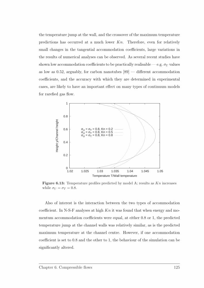
the temperature jump at the wall, and the crossover of the maximum temperature

predictions has occurred at a much lower Kn. Therefore, even for relatively

small changes in the tangential accommodation coefficients, large variations in

the results of numerical analyses can be observed. As several recent studies have

shown low accommodation coefficients to be practically realisable — e.g. σU values

as low as 0.52, arguably, for carbon nanotubes [89] — different accommodation

coefficients, and the accuracy with which they are determined in experimental

cases, are likely to have an important effect on many types of continuum models

for rarefied gas flow.

0

0.2

0.4

0.6

0.8

1

1.02 1.025 1.03 1.035 1.04 1.045 1.05

Hei

ght y

/Cha

nnel

hei

ght


σU = σT = 0.8, Kn = 0.2σU = σT = 0.8, Kn = 0.5σU = σT = 0.8, Kn = 0.8

Figure 6.13: Temperature profiles predicted by model A; results as Kn increaseswhile σU = σT = 0.8.

Also of interest is the interaction between the two types of accommodation

coefficient. In N-S-F analyses at high Kn it was found that when energy and mo-

mentum accommodation coefficients were equal, at either 0.8 or 1, the predicted

temperature jump at the channel walls was relatively similar, as is the predicted

maximum temperature at the channel centre. However, if one accommodation

coefficient is set to 0.8 and the other to 1, the behaviour of the simulation can be

significantly altered.


To illustrate, Fig. 6.14 shows how the maximum predicted temperature (the

temperature at the channel centre) varies with Kn. Each accommodation coeffi-

cient combination displays a definite peak in the predicted temperature, occurring

in the range of Kn values between about 0.15 and 0.45. The largest maximum

temperatures are predicted when the energy accommodation coefficient is at its

lowest value of σT = 0.8, with momentum accommodation coefficient σU = 1.

Conversely, when the momentum accommodation coefficient is σU = 0.8, and the

energy accommodation remains at σT = 1, the maximum predicted temperature

is at its lowest.

As shown in Fig. 6.14, these highest and lowest maximum temperature pro-

files are equidistant from the “reference” state where σU = σT = 1. This im-

plies that energy and momentum are assumed to be exchanged at the same rate

when Maxwell’s and Smoluchowski’s boundary conditions are used simultane-

ously, which is unlikely to be true of any physical system. For example, returning

to the earlier discussion of Prandtl number, we know the momentum diffusivity

to be only a proportion of the energy diffusivity, and momentum is exchanged at

a faster rate than energy [3]. Accommodation coefficients are not physical prop-

erties of a surface, but rather they arise from the interaction between gas and

wall molecules, and little is really known about the complex physics of gas flow in

near-surface regions. It is therefore likely that more physically-based boundary

conditions, such as Langmuir’s slip model, based on surface chemistry, would be

better suited to many practical micro-engineering flow simulations [52].

6.5.2 Summary

By simulating compressible micro-Couette flow with constitutive scaling in Open-

FOAM, it has been shown that the approach has some merit for practical appli-

cations. It is simple to apply, is implemented in an extensible framework and

validation of the results produced with available DSMC data, shown in Figs. 6.8–

6.10, inspires confidence in its ability to incorporate key rarefaction effects, to


306

308

310

312

314

316

318

320

322

0.1 0.2 0.3 0.4 0.5 0.6 0.7 0.8

Tem

pera

ture

T a

t cha

nnel

cen

tre,

y =

H/2

Knudsen number, Kn

σU = σT = 0.8σU = 0.8 σT = 1σU = 1 σT = 0.8

σU = σT = 1

Figure 6.14: Predicted temperature (in K) at the centre of the channel incompressible micro-Couette flow (i.e. the maximum temperature), plotted againstKnudsen number.

some extent, in continuum simulations. That said, there are some limitations to

the method, particularly for application to compressible flows. As demonstrated,

considerable care must be taken in choosing the correct models for the effective

quantities, scaling coefficients and boundary conditions. The computationally-

inexpensive nature of constitutive scaling in CFD when compared to discrete

methods, and its ability to reproduce key rarefaction effects, suggest that the

approach has the potential to become a useful tool for design applications. This

will be particularly true for more complex 3D microflow configurations, to which

very few discrete or kinetic models may be practically applied [26].


Chapter 7

A new approach toconstitutive-scaling

In this thesis, constitutive scaling has been shown to be an efficient and effective

method of including gas rarefaction effects in continuum fluid dynamics simula-

tions. However, in its present form, constitutive scaling is dependent on detailed

kinetic theory solutions providing appropriate functions with which to create an

effective viscosity (or thermal conductivity) [12, 17]. Although it has been shown

that it is possible to apply current constitutive models successfully to some cases

beyond the limits of their original derivations, it would be beneficial if scaling

functions could be derived in more general form.

Rarefaction is most commonly classified using a standard definition of Kn,

given by Eq. (1.1) for incompressible flows and by Eq. (6.1) for compressible flows.

In some systems, it is possible to have a low global value of Kn, but for areas of

the flow to be locally rarefied [27]. This occurs particularly in compressible flows,

where large density gradients can cause local rarefaction. Local rarefaction can

be characterised using a local Knudsen number:

Knlocal =λ

θ

∂θ

∂x, (7.1)

where θ is a macroscopic variable and ∂θ/∂x is its gradient in an arbitrary di-

rection [27]. Current constitutive scaling functions presented in [12, 17] are de-

pendent only on variation of effective viscosity and effective thermal conductivity

Chapter 7. A new approach to constitutive-scaling 128

with the equilibrium mean free path of gas, λ, and normal distance to the nearest

bounding surface. In cases where the global Kn-value is low but Knlocal is large,

these scaling functions will predict only a thin Knudsen layer at system bound-

aries, which does not capture the true extent of rarefaction in the system. This

limitation of the current form of constitutive scaling could perhaps be alleviated

by using a more general model for rarefaction-based scaling in gas flows.

In this chapter, a new methodology for determining constitutive scaling func-

tions empirically is proposed and an initial test-case is presented. The case is

used to demonstrate how effective quantities may be related to local parameters

of a system, and the potential for development of this new approach is discussed.

7.1 Identifying a scaling function

In applying an effective viscosity to alter the relationship between shear stress and

strain-rate, constitutive scaling is effectively “distorting” an N-S-F velocity profile

to incorporate a Knudsen layer. By considering the features that characterise

Knudsen layers in a given flow configuration, such as increased strain-rate or

temperature gradient near system boundaries, then it is possible to determine

functions that describe mathematically how an N-S-F velocity or temperature

profile should be altered to include key Knudsen layer effects. For example,

pressure-driven flow in channels has a parabolic velocity profile whilst shear-

driven flow is largely linear. The mathematical functions describing the difference

between these solutions and their rarefied counterpart flows (found using DSMC

or similar) are therefore very different. Scaling the N-S-F equations based on case-

specific differences in shape between rarefied and non-rarefied profiles, rather than

a single fixed function of distance to the nearest wall, is constitutive scaling from

a different perspective. In theory, this approach could be used to derive more

general constitutive scaling functions, expressed in terms of system parameters

such as geometry, flow conditions and Knudsen number, Kn.

To test this hypothesis, a simple Poiseuille flow case is considered. The case


comprises isothermal, pressure-driven flow through a 2D rectangular channel,

where the Kn-value of the system may be varied by altering the channel height,

2h. The analytical solution to the Navier-Stokes equations for this flow, with or

without slip at the system boundaries, gives a parabolic velocity profile. For no

slip at the system boundaries

uN-S (y) =1

µ

dp

dx

(y2

2− hy

), (7.2)

where µ is a constant dynamic viscosity, dp/dx a longitudinal pressure gradient,

h the half-channel height and y the cross-channel position. For Poiseuille flow

in channels, velocity profiles incorporating the Knudsen layer are not perfectly

parabolic; the gradient of the velocity is steeper within one to two mean free

paths of the channel walls than that predicted by the Navier-Stokes equations.

To replicate this Knudsen layer shape it is proposed that an elliptical function be

added to Eq. (7.2). The general expression describing an ellipse is

(x− x0)2

a2+

(y − y0)2

b2= 1, (7.3)

where (x0, y0) is the origin of the ellipse and a and b are its major and minor axes

respectively, as shown in Fig. 7.1. Positioning the ellipse such that its origin is

at (0, h) in the centre of the Poiseuille flow channel, the shape of the ellipse as a

function of its height y is given by

x (y) =

√a2 − a2 (y − h)2

h2. (7.4)

To relate the dimensions of the ellipse to those of the parabolic velocity profile,

its half-height b is equated with the half-channel height h, and its major axis a is

equated to the peak velocity given by the parabolic profile, uN-S (h). A velocity-

type profile that would be described by the ellipse can therefore be expressed

as


b

a(x0, y0)

y

x

Figure 7.1: Schematic of an ellipse showing its centre (x0, y0), major axis a andminor axis b.

uel (y) =

√uN-S (h)2 − uN-S (h)2 (y − h)2

h2. (7.5)

Although this elliptical profile could perhaps represent a Knudsen layer shape,

in that it is steeper than the parabolic function at the walls, the profile is a fixed

shape constrained on the channel dimensions and a single peak velocity. Rather

than replacing one profile with the other, then, it is proposed that the elliptic and

parabolic profiles are combined, i.e. the parabolic Navier-Stokes velocity profile

can be modified by distorting it using only some portion of the elliptical shape.

A composite velocity profile with Knudsen layer features can then be produced

using the original Navier-Stokes velocity profile, some proportion of the elliptical

profile, and an appropriate slip velocity, which in this case will be determined by

Maxwell’s slip model [10]. Such a function can expressed generally as

utotal (y) = uN-S (y) + f (uel (y)) + uslip (0) , (7.6)

where f (uel (y)) is a function that expresses the proportion of the elliptical profile

included in the final velocity profile, and the slip velocity uslip is a constant

evaluated at the channel wall.

As the “correct” function f (uel (y)) to use to replicate a true Knudsen layer


shape is not known a priori, a scaling factor Ω is introduced to the elliptical

profile. Where the profile is scaled by a coefficient Ω1,

u1 (y) = Ω1 ·√uN-S (h)2 − uN-S (h)2 (y − h)2

h2. (7.7)

This direct relationship incorporates some proportion of a scaled elliptical shape

in the final velocity profile. By scaling the elliptical profile using several differ-

ent coefficients, Ω1, Ω2 and Ω3, the likelihood of finding a satisfactory elliptical

shape to add to the Navier-Stokes velocity profiles is increased. The ellipses

are extended/compressed along their major axes, allowing greater flexibility in

matching their shapes to a Knudsen layer velocity profile. The total proposed

velocity profile for each scaled ellipse can be expressed in the general form of

Eq. (7.6):

utotal (y)1 = uN-S (y) + u1 (y) + uslip (0) , (7.8)

utotal (y)2 = uN-S (y) + u2 (y) + uslip (0) , (7.9)

utotal (y)3 = uN-S (y) + u3 (y) + uslip (0) . (7.10)

The proposed velocity profiles are then compared to that obtained using the

original constitutive scaling function proposed by Lockerby et al. and given by

Eq. (4.6) [12]. Coefficients Ω1−3 are found that best fit velocity profiles utotal (y)1−3

to the original scaling function. These values are determined, simply by eye, to

be Ω1 = 0.12, Ω2 = 0.1225 and Ω3 = 0.1. In a final implementation, the values

would be chosen using an iterative goal-seeking method to produce minimum

error when compared to the macroscopic quantity of interest.

Eq. (4.6) is taken to represent a true Knudsen layer shape in this initial

test case. In practice, any reliable source of information about the shape of the

Knudsen layer could be used for this curve-fitting process, such as DSMC data,


kinetic theory solutions or experimental results, and ideally the correct profile

would be determined using data from a variety of independent sources. As the

original scaling model has been validated for incompressible Poiseuille flow in

channels at a variety of Kn-values, however, it is reasonable to use that function

here as a first approximation to the desired Knudsen layer velocity profile [12].

Figure 7.2 shows the elliptically-scaled velocity profiles from Eqs. (7.8)– (7.10)

for a Poiseuille flow where Kn = 0.1. The working fluid is argon gas at 300K,

whose properties are determined using [75]. The flow is driven by a pressure

gradient dp/dx = −57.1536× 106N/m3. In all cases Maxwell’s Eq. (3.5) using a

microslip coefficient of A1 = 0.8 is used to determine uslip (0). For convenience, the

slip velocity has been calculated here using the velocity gradient of the unscaled

Navier-Stokes solution at the wall, although it is anticipated that in practice the

elliptical scaling method would make use of the mean-free-path-based slip imple-

mentation described in section 4.4.1. The tangential momentum accommodation

coefficient, σU , for the velocity slip is taken to be 1.

All of the elliptically-scaled velocity profiles shown in Fig. 7.2 return the mi-

croslip velocity at the channel wall as expected, although they predict slightly

different maximum velocities at the channel centre. Model 2 shows the highest

peak velocity, closely followed by model 1. Mass flowrates for these velocity pro-

files can be calculated using Eq. (5.5). The mass flowrate obtained by integrating

the analytical expression for Poiseuille flow scaled using Lockerby et al.’s function,

Eq. (5.4), is m = 1.948 × 10−7kg/s. Model 3 produces a mass flowrate for this

case of 1.917×10−7kg/s, which is the least accurate of the three models compared

to the original constitutive scaling function. Model 2 is the most accurate in this

case, with m = 1.949× 10−7kg/s, and model 1 gives m = 1.946× 10−7kg/s.

Figures 7.3–7.5 compare the elliptical velocity profiles individually to the

Navier-Stokes solution for Poiseuille flow with Maxwell’s velocity slip condition,

and to the constitutive scaling function proposed in [12]. In Figs. 7.3 and 7.4,

elliptical models 1 and 2 match the original scaling model’s velocity gradient well


0

0.2

0.4

0.6

0.8

1

0.04 0.06 0.08 0.1 0.12 0.14 0.16 0.18 0.2 0.22 0.24

Pos

ition

y/h

Velocity u(y) (m/s)

Ellipse Model 1Ellipse Model 2Ellipse Model 3

Figure 7.2: Velocity profiles from three newly proposed elliptical constitutive-scaling models for Poiseuille flow in a microchannel where Kn = 0.1. Position yacross the channel is non-dimensionalised by the half-channel height.

in the near-wall region, up to approximately y = 0.05, which is roughly half of the

thickness of the Knudsen layer. Further from the wall, just beyond the Knudsen

layer, the elliptical models more closely resemble the Navier-Stokes slip-velocity

profile, then towards the channel’s centre they return to following the original

scaling function. In Fig. 7.3, model 1 is closer to the N-S-F slip-velocity profile

when 0.15 < y < 0.4, whilst for model 2 in Fig. 7.4 this behaviour occurs slightly

closer to the wall, where 0.1 < y < 0.3.

Model 3, shown in Fig. 7.5, predicts a maximum velocity that lies between

the slip-velocity profile and that of the original constitutive scaling function. For

this Kn = 0.1 case, the average errors in the velocity profiles (when compared to

the solution given by Eq. (5.4)) are −1.198%, −1.023% and −2.615% for models

1− 3 repectively, which implies that all of the elliptical models underpredict the

mass flowrate in the channel by a small amount.


0

0.2

0.4

0.6

0.8

1

0.04 0.06 0.08 0.1 0.12 0.14 0.16 0.18 0.2 0.22 0.24

Pos

ition

y/h

Velocity u(y) (m/s)

Ellipse Model 1Maxwell Slip

Original Scaling Function

Figure 7.3: Elliptical model 1 compared to a Navier-Stokes solution with slipboundary conditions and the constitutively scaled Navier-Stokes profile given byEq. (5.4), for Poiseuille flow in a microchannel where Kn = 0.1. Position y acrossthe channel is non-dimensionalised by the half-channel height.

7.2 Extracting effective viscosity

Whilst it is true that the elliptical distortions described above can simply be added

to the Navier-Stokes solution in the method outlined, if the new models are to be

used in a constitutive scaling framework, it would be preferable to express them

in terms of the effective viscosities with which they relate shear stress and strain-

rate. Not only is this more representative of how the distorted shapes would

be physically imposed on a flow, but it will also eventually enable the elliptical

functions to integrate with the existing implementation of constitutive scaling in

OpenFOAM.

To determine functions for effective viscosity that correspond to the elliptical

models for this test case, the momentum equation is used. For 1D Poiseuille flow

this is given by


0

0.2

0.4

0.6

0.8

1

0.04 0.06 0.08 0.1 0.12 0.14 0.16 0.18 0.2 0.22 0.24

Pos

ition

y/h

Velocity u(y) (m/s)




d

dy

(µ (y)

du

dy

)=dp

dx, (7.11)

which can be solved and rearranged to find the effective viscosity as a function

of the velocity gradient:

µ (y) =dp/dx (y − h)

du/dy. (7.12)

The velocity gradient is then obtained by differentiating the analytical expressions

for the elliptical velocity profiles:

du

dy 1−3

=d

dy(uN-S (y)) +

d

dy(u1−3 (y)) +

d

dy(uslip (0)) . (7.13)

As was the case in the original implementation of constitutive scaling, the

effective viscosity is related to the actual viscosity, µ, by:


0

0.2

0.4

0.6

0.8

1

0.04 0.06 0.08 0.1 0.12 0.14 0.16 0.18 0.2 0.22 0.24

Pos

ition

y/h

Velocity u(y) (m/s)




µ (y) =µ

φ. (7.14)

Substituting in the analytical solution to Eq. (7.13) and simplifying, the scaling

function φ can be shown to be

φ = 1 +h · Ω

2√− (y2 − 2hy)

. (7.15)

Figure 7.6 compares the effective viscosity of elliptical models 1−3, normalised

by the actual viscosity, to that of the original constitutive scaling model. What

is immediately noticeable about the effective viscosity profiles is that the ellip-

tical models and the original effective viscosity function produce quite different

results. The elliptical models all have similar effective viscosities, which have

much steeper gradients than the original profile, and which eventually plateau at

a lower viscosity than Lockerby et al.’s model.


Failure to recover the original viscosity beyond the Knudsen layer region rep-

resents a weakness in the elliptical scaling models, although, the impact of the

discrepancy would seem to be limited as the elliptical models produce a velocity

profile that replicates the original model to within 1 − 2% average error. It is

also likely that this error could be mostly eradicated using a different system of

coefficients Ω1−3. The reasonable mass flowrate and velocity profiles obtained

from the current models suggest that the approach remains viable in spite of the

differences observed in Fig. 7.6.

0

0.2

0.4

0.6

0.8

1

0.45 0.5 0.55 0.6 0.65 0.7 0.75 0.8 0.85 0.9 0.95 1

Pos

ition

y/h

Effective viscosity µ(y)


Original Scaling Model

Figure 7.6: Effective viscosity for the three elliptical scaling models compared tothe effective viscosity of the original constitutive scaling model. Position y acrossthe channel is non-dimensionalised by the half-channel height.

7.3 Incorporating Kn

It has been demonstrated above that combining the equation of an ellipse with the

Navier-Stokes solution for simple 1D Poiseuille flow can replicate with reasonable

accuracy Knudsen layers produced by applying constitutive scaling. Effective


viscosity functions can then be extracted from these elliptically scaled models for

implementation in a standard constitutive scaling process. At present, however,

the new functions are independent of Kn, which limits their applicability. In

order to develop these new scaling models further, it would be desirable to relate

them to the degree of rarefaction in the system.

One simple method of incorporating Knudsen number is to replace the scaling

coefficients Ω1−3 with functions of Kn. Returning to the Poiseuille flow test

case above, where Kn = 0.1 and the Ω-coefficients were defined such that the

elliptically scaled models replicated a known Knudsen layer shape for that case,

it is possible to define new scaling parameters:

Ω1 (Kn) = Ω1 ·Kn = 1.2Kn, (7.16)

Ω2 (Kn) = Ω2 ·Kn = 1.225Kn, (7.17)

Ω3 (Kn) = Ω3 ·Kn = Kn. (7.18)

Introducing Ω (Kn) is an important step in the development of the elliptical

effective viscosity models. With elliptical models based on system geometry, the

original Navier-Stokes solution and Kn, it should be possible to capture changes

in the rarefaction of the system brought on by both geometry changes and changes

in the flow conditions, which is a desirable feature of a constitutive scaling scheme.

Figure 7.7 shows the absolute percentage error between the velocity profiles

produced by the elliptical scaling models when Kn = 0.1 and the solution to

Eq. (5.4) for Poiseuille flow. Based on average error, the most accurate model for

this case is model 2, which has a peak error approximately one mean free path

from the channel wall of 3.5%. In the centre of the channel the average error

reduces to less than 0.5%. Although it is not desirable that the maximum error

occurs in the Knudsen layer region, it is worth noting that the magnitude of the

error is relatively small. For example, the error between the Navier-Stokes velocity


profile with slip boundaries is 25% when compared to the original constitutive

scaling model in the same near-wall region.

-6

-5

-4

-3

-2

-1

0

1

0 0.2 0.4 0.6 0.8 1

Per

cent

age

velo

city

err

or

Position y across channel


Figure 7.7: Errors between velocity profiles of elliptical scaling models andEq. (5.4) for Kn = 0.1, shown at non-dimensional positions across half a mi-crochannel whose wall is positioned at y = 0.

To develop an elliptical-scaling function for the Navier-Stokes equations that

is valid for a range of Kn-values, the cross-channel errors between the three

elliptical models and the velocity profile given by Eq. (5.4) are considered for

Poiseuille flows with varying degrees of rarefaction. The elliptical models contain

scaling coefficients Ω (Kn)1−3, and the range of Knudsen numbers analysed is

0.025 < Kn < 0.5: the upper slip flow and lower transition flow regimes. Fig-

ure 7.8 illustrates the cross-channel error profiles when Kn = 0.075. Model 2

continues to produce the lowest average error in the velocity, −0.41%, however

the performance of model 1 is noticeably worse than it had been for Kn = 0.1.

In fact, as Kn changes, the velocity-profile errors produced by the three different

elliptical models vary greatly.

Figure 7.9 shows the average error between the elliptical velocity profiles and


-7

-6

-5

-4

-3

-2

-1

0

1

2

0 0.2 0.4 0.6 0.8 1

Per

cent

age

velo

city

err

or

Position y across channel


Figure 7.8: Errors between velocity profiles of elliptical scaling models andEq. (5.4) for Kn = 0.075, shown at non-dimensional positions across half a mi-crochannel whose wall is positioned at y = 0.

the original constitutive scaling model as Kn varies. From the figure it is clear

that no single model is always the most accurate; distinct transitions occur at

Kn = 0.1, 0.2 and 0.35. Below Kn = 0.1, elliptical model 2 produces the most

accurate velocity profile and, hence, mass flowrate. In the region 0.1 < Kn <

0.2, model 1 produces a lower average error than the other profiles, but when

0.2 < Kn < 0.35 model 3, which was the least accurate model for Kn = 0.1,

produces the lowest average error. Finally, beyond Kn = 0.35, the error produced

by models 1 and 3 rises whereas the error produced by model 2 reaches a steady

plateau at a value of approximately −2.25%.

Although model 2 is not the most accurate model across the entire range of

Kn-values studied, it produces a consistently low level of error throughout. The

magnitude of the average error is also steady in the lower transitional-Kn regime,

where the behaviour of the Knudsen layer has the greatest impact on the flow.

The final effective viscosity expression for model 2 is given by


-4

-2

0

2

4

6

8

0 0.1 0.2 0.3 0.4 0.5

Ave

rage

vel

ocity

err

or (

%)

Knudsen number


Figure 7.9: Average percentage error between velocity profiles from three ellipticalscaling models and Eq. (5.4), shown versus Knudsen number, Kn.

µ (y) = µ ·(

1 +h · 1.225Kn

2√− (y2 − 2hy)

)−1

. (7.19)

7.4 Discussion

Obviously this has been a preliminary case study, and in using the scaling model

proposed in [12] as the target Knudsen layer shape, it has succeeded in producing

only a replica of another numerical model, rather than a true Knudsen layer

profile. What the exercise demonstrates, however, is that simple approximations

of a Knudsen layer’s shape for a given velocity profile may be used to determine

reasonably accurate Knudsen layer models, which can be shown to be valid across

a range of Kn values. The process produces empirical expressions, which can be

based on a small amount of information on the behaviour of the rarefied flow.

The proposed methodology for determining scaling functions in this manner is

therefore the most promising outcome of the study.


Summary of methodology

• A simple function representative of a macroscopic field is chosen.

For cases where an N-S-F solution exists, knowledge of basic Knudsen-layer

behaviour and rarefaction in the flow can be used to determine an analytical

function describing how its presence would be likely to alter that field. In this

case, velocity has been used as an example.

• The analytical function is related to features of the system.

In this brief study, the channel height, peak predicted velocity of the Navier-

Stokes flow and Kn are used, all of which are known local parameters. The degree

of rarefaction has been defined using a global Kn value in this case, but a local

definition could be applied in cases where steep gradients dominate the flow [27].

In theory any quantities representative of the system could be used.

• This analytical profile is “tuned” to reflect available data.

Crucially, this stage in the process can be carried out with very little data

about the rarefied flow that is to be simulated. For example, in cases where

no information is known about the velocity profile, a scaled model tuned to

provide a Knudsen layer could be developed to minimise errors in mass flowrate

data. The resulting shape of the Knudsen layer would become less exact, but

prediction of the macroscopic quantities would still likely be improved over using

a straightforward slip boundary condition, and would potentially be applicable to

a greater range ofKn. Admittedly this is a phenomenological means of replicating

rarefaction behaviour, but such approaches are already widely used in other areas

of fluid dynamics to model flow features such as turbulence and combustion [46].

In cases where more detailed data are available, the accuracy of the method

can obviously be greatly improved. In this preliminary assessment the coefficients

in the elliptical equations were chosen manually to represent a known velocity


profile. For a final model, these would more likely be determined using numerical

methods, with emphasis on minimising the error in the macroscopic quantity of

interest.

• An effective viscosity is extracted from the chosen function.

Here this has been carried out analytically, although for more complex cases

the expression for the Knudsen layer shape could be differentiated numerically and

the effective viscosity field would become a solved-for variable. This process would

be relatively straightforward as the total function for the quantity of interest in

the rarefied flow comprises only the known analytical expression for the scaling

part of the function, the classical N-S-F solution to the flow and the appropriate

boundary conditions.

• The effective viscosity is applied using the standard constitutive scaling

approach.

As has been outlined in other areas of this thesis, constitutive scaling is now

implemented in a standardised numerical framework in the OpenFOAM CFD

package. New models for effective quantities can therefore be integrated using

existing templates, and with minimal difficulty.

7.4.1 Scope for future work

At this early stage, the local-parameters approach to constitutive scaling has been

tested only on a single example case. The methodology developed, however, has

the potential to be extended to more complex flows. This should be examined

thoroughly with a more detailed study.

It is important that the proposed methodology be applied to various flow

configurations at a range of Kn values, in order that its practicality be assessed.

In the case study above, one effective viscosity model was found to consistently

produce lower average errors than the others in the lower transition regime. In


other cases, perhaps no single model would be identifiable as superior across the

Kn range. This problem could be overcome using a system of charts similar to,

say, a Moody diagram, which relates relative surface roughness, friction coefficient

and Reynolds number in pipe flows [90]. The equivalent for a complex constitutive

scaling case approached with the methodology above could be to chart a range of

geometric functions, i.e. the scaled ellipses above, as they vary with both Kn and

a range of appropriate scaling coefficients, Ω (Kn) in the examples above. Having

chosen a function representative of the Knudsen layer in their system, the end user

would then be able to find appropriate coefficients for that function based upon

the Kn-range they wish to analyse. Such an outcome would require substantial

literature survey and involve considerable effort if many different flow conditions

were to be considered. That said, it could provide a practical means of assessing

a range of standardised microflow systems, particularly if it were implemented in

a computational database structure, which could self-select the most appropriate

scaling functions to use based on system geometry and operating conditions.

It would also be imperative to test the applicability of this new methodology

to cases of non-isothermal, compressible flow. As discussed in Chapter 6, the

definition of the effective viscosity and thermal conductivity in a scaling approach

can substantially affect physical quantities such as Prandtl number. Currently,

maintaining Prandtl number results in a sacrifice of accuracy in curve-fitting a

scaling function, see Figs. 6.4 and 6.6. More accurate scaling profiles derived

from isothermal or isoflux cases, however, cannot recreate physical behaviour

in systems where both energy and momentum are exchanged, as explained in

sections 6.4 and 6.5. The key potential benefit of the proposed methodology

over traditional constitutive scaling methods in this instance would be that the

scaling functions could be defined simultaneously for cases where both energy

and momentum are exchanged. For example, an experimental investigation may

measure temperature profiles in a flow, but not the velocity profiles. Were simple

mass flowrate data also available for the experiments, then this basic information


could be used in tandem with the temperature data to provide constitutive scaling

functions for both conductivity and viscosity. This would allow an appropriate

balance of energy and momentum diffusivities to be maintained, whilst improving

the accuracy of the Knudsen layer shapes predicted by the scaling.

7.4.2 Summary

At this stage in its development, constitutive scaling based on the local parame-

ters of a microsystem is not superior to existing scaling models, it merely repli-

cates their performance for a simple test case. Potentially, however, using the

local parameters of a system to inform scaling of the constitutive relations could

provide a more general approach to extending the N-S-F equations for rarefied

flows. The methodology proposed has the scope to include local rarefaction, which

could greatly improve results for cases where the global Kn-value is secondary

to local gradients in causing rarefaction. This type of flow is common in small-

scale, high-speed devices such as micronozzles, which are used in many practical

applications, including propulsion and control of low-mass satellites [21, 82, 83].

Another potential advantage of this new scaling approach over traditional

methods is that “composite” models could be developed for complex flow systems.

For example, in a compressible-flow system where narrow pipework leads to a

rapidly expanding section, models that scale viscosity or thermal conductivity

based only on normal distance to the nearest wall, and equilibrium mean free

path, would predict that rarefaction had a decreasing impact as flow reached

the expansion. In reality, steep density gradients in the rapid expansion could

produce a large increase in local Knudsen number. By using a blend of scaling

models, individually tuned to each geometric section of the system, the local-

parameters model would be better able to emulate the behaviour of the fluid

flow.

Ultimately, the limitations of this proposed methodology lie in its empirical

nature. As it is not possible to define a single, straightforward expression describ-


ing the shape of a Knudsen layer for any flow configuration, initial implementation

of a model based on case-by-case scaling functions would be a complicated pro-

cess. This type of scaling is also dependent on the quality of information input to

the system; if detailed data on Knudsen layer structure are available, then very

accurate results should be possible. Where information on the rarefied flow is

unavailable or unreliable, this type of approach cannot be applied with any real

confidence. Bearing in mind these limitations, the fact remains that a system

of deriving constitutive-scaling relationships from basic knowledge of system ge-

ometry and Knudsen layer structure, the Navier-Stokes solution to the flow and

minimal data about the rarefied flow, has been successfully demonstrated here. If

the success of the method could be extended beyond this initial test case, the po-

tential exists to produce continuum models for rarefied flows applicable to many

microscale configurations.


Chapter 8

Conclusions

In microsystems, the characteristic dimensions of a device can approach the mean

free path of a gas flowing within it, causing the flow to become rarefied. As the

flow becomes rarefied, the continuum and equilibrium assumptions of macroscale

fluid dynamics begin to break down. The loss of local thermodynamic equilib-

rium implies that the microscopic behaviour of the gas can affect the distribution

of macroscopic quantities such as velocity, temperature and pressure, resulting

in large gradients in these fields. A fluid containing large gradients cannot be

considered to be continuous, which violates the underlying assumptions of dif-

ferential calculus and the governing equations of fluid dynamics derived from it.

As such, the N-S-F equations, the traditional method of analysing fluid flow and

heat transfer at the macroscale, are not suitable for gas microflows.

The Boltzmann equation and the kinetic theory of gases may be used to

accurately determine the behaviour of rarefied gas flows, but are applicable in

practice only to 1- and 2-dimensional problems [26]. An equivalent to solving

the Boltzmann equation is to use the numerical DSMC method, which averages

macroscopic field variables from deterministic simulations of molecular interac-

tions [27]. Given sufficient computational resources, the DSMC method may be

used successfully to model flows in complex, practical geometry. The limiting

factor on the application of DSMC is the requirement to reduce statistical scat-

ter to produce accurate averaged quantities. For the low-speed flows common to

Chapter 8. Conclusions 148

microdevices, the low signal-to-noise ratio can make DSMC prohibitively compu-

tationally expensive.

As many microscale devices are currently designed by trial and error, an effi-

cient analytical tool for engineering design applications is required. One method

of achieving this aim is to extend the N-S-F equations beyond the strict lim-

its of their applicability into the slip- and transitional-Kn flow regimes. Two

key aspects of gas rarefaction that cannot be captured using continuum N-S-F

simulations are boundary discontinuities and the Knudsen layer. These surface

phenomena are dominant in gas microflows, where the surface area-to-volume

ratio is high.

Boundary discontinuities arise when the energy and momentum of a gas flow

in contact with a surface are not fully transferred to the surface. When full ac-

commodation takes place, it leads to the no-slip condition of macroscale flow,

where the velocity and temperature of the gas at a solid boundary are equivalent

to the velocity and temperature of the boundary. In rarefied flows, a smaller

number of intermolecular collisions take place within a given timescale. If the

timescale of convective transport in the system is much shorter than the diffu-

sive relaxation time, in which gas molecules would reach an equilibrium with the

wall, then on average molecules will flow through the system without their en-

ergy and momentum ever relaxing to that of the system boundaries. A number of

boundary conditions describing velocity-slip and temperature-jump phenomena

are available for continuum analyses of rarefied flow. The robust phenomeno-

logical model proposed by Maxwell for velocity slip, and its equivalent proposed

by Smoluchowski for temperature, are the most widely used of these boundary

conditions [10, 11]. These boundary conditions are accurate in many applica-

tions if they are applied within the limits of their original derivations. For curved

surfaces an extra term must be added to the slip boundary condition to describe

wall-normal variation of velocity [16, 20]. When both slip and jump conditions are

applied together, the assumptions implicit in the slip equation about the relative


rate of exchange of energy and momentum must be taken into account [10].

The Knudsen layer is the near-wall region one to two mean free paths thick

where local thermodynamic equilibrium is not maintained between a gas and its

bounding surface. This region exists in gas flows at all scales, but is significant

to the macroscopic behaviour of the flow only when the length scale of the mean

free path approaches the length scale of the system. The Knudsen layer is char-

acterised by strong departures from the linear constitutive relationships of the

N-S-F equations for shear stress/strain-rate and heat flux/temperature-gradient.

In rarefied flows the structure of the Knudsen layer can represent a significant

proportion of a flow, and consequently affect its macroscopic behaviour [37].

Constitutive scaling, which replaces viscosity and thermal conductivity with

effective values, is an efficient method of incorporating non-linear Knudsen layer

effects in continuum fluid dynamics simulations. Several constitutive scaling mod-

els have been proposed in the academic literature, the foremost of which are

functions presented in [12] and [17].

The constitutive scaling process and both of these published models have been

implemented in the open-source computational fluid dynamics package Open-

FOAM [13]. This is the first time that the constitutive scaling process has been

implemented in a finite-volume CFD code. OpenFOAM was identified as a suit-

able framework for constitutive scaling as it is both flexible and highly extensible.

The hierarchical structure of the code allows for extensive modification of the gov-

erning equations within it, whilst the benefits of a general notation and a stable

numerical platform are retained.

Verification exercises comparing constitutive scaling in OpenFOAM to ana-

lytical solutions for incompressible flows have been carried out. For Poiseuille

flow in micro channels no-slip, slip and constitutive scaling results were com-

pared to analytical solutions. The largest discrepancy between the analytical

and numerical results was found to be 0.031%. In contrast, the commercial CFD

code Fluent was found to be entirely unable to resolve slip at system boundaries


when its interpretation of Maxwell’s velocity boundary condition was applied. For

shear-driven Couette flows, constitutive scaling in OpenFOAM was also verified

using analytical solutions, with near-perfect agreement. From these verification

exercises it is possible to conclude that the constitutive scaling method has been

correctly implemented in OpenFOAM for incompressible flows.

Validation case studies were also undertaken using the incompressible Open-

FOAM solver. For shear-driven flows constitutive scaling was shown to capture

DSMC results for both velocity slip and Knudsen layer behaviour accurately at

Kn-values in the lower transition regime, and is therefore proposed for use as a

design tool within conservative approximate limits of 0.01 < Kn < 0.25. For

both planar and rotating shear flows, beyond the midpoint of the transition-Kn

regime at Kn > 0.5, the OpenFOAM model was found to improve on standard N-

S-F results, but could not quantitatively model the behaviour of the flow. When

applied to pressure-driven flows in microchannels with orifice plate constrictions

for validation, good agreement between OpenFOAM and experimental data for

centreline pressure profiles and mass flowrates was obtained. Numerical results

from the solver did not match experimental data available for venturi-type con-

strictions in microchannels, although it was postulated that this may be due to

some discrepancy in the experimental findings.

It has been shown in this thesis that the constitutive scaling method may be

applied to non-isothermal, compressible flows if the relationship between effective

viscosity and effective thermal conductivity is defined. Two approaches have been

proposed: to use a constant Prandtl number to define scaling for conductivity

based on the value of Pr and the viscosity scaling, and to use separate curve-fit

relationships from kinetic theory to scale viscosity and conductivity, with the

consequence that the effective Pr value will be non-constant [12, 17]. For isother-

mal or isoflux cases, the latter approach produces more accurate results. When

both energy and momentum are simultaneously exchanged by a fluid, as they

are in compressible flows, the former approach, using a constant Prandtl number


condition, was found to be more effective. Both models have been implemented

in a specially-modified compressible solver in OpenFOAM, which represents the

first application of constitutive scaling to compressible cases.

Constitutive scaling using a constant Prandtl number condition to determine

effective viscosity was used to analyse high-speed Couette flow between paral-

lel plates. Results were compared to DSMC data, and it was shown that for

Kn-values in the lower transition regime (0.1 < Kn < 0.25) the OpenFOAM

simulations could accurately represent available data for velocity and tempera-

ture. In this regime it is proposed that scaling model A may be used in design

applications for shear-driven compressible flows with reasonable confidence, and

that model B could be used similarly where flows are quiescent and thermally-

driven or isothermal in nature.

When Maxwell’s velocity-slip boundary condition is applied in conjunction

with Smoluchowski’s temperature jump condition in compressible analyses, the

relative magnitude of the tangential momentum accommodation coefficient, σU ,

and the energy accommodation coefficient, σT , was found to be significant. When

momentum accommodation was set lower than energy accommodation by 20%, an

increase in the temperature of the flow was observed, as compared to a reference

state where σU = σT . When momentum accommodation was higher than energy

accommodation, the maximum temperature predicted by the energy equation

was reduced. As very low accommodation coefficients have been found experi-

mentally to apply to some materials used in microsystems (∼ 50% departure from

reference value of unity), this result highlights the need for caution in selection

of accommodation coefficients for gas-surface interaction.

As an alternative to existing constitutive models, which are based on the equi-

librium mean free path of a gas and distance to the nearest bounding surface, a

new method of defining constitutive scaling functions based on local rarefaction

parameters has been proposed. A test-case of Poiseuille flow in a rectangular

channel was used to demonstrate that it is possible to determine new consti-


tutive scaling functions based on Kn, the system geometry and the unscaled

Navier-Stokes solution to the flow. Currently, this method only replicates the

performance of existing constitutive scaling models for isothermal flow, and has

not been extensively tested. The methodology proposed for defining new scaling

models, however, shows promise as a means of avoiding some of the weaknesses

of traditional constitutive scaling methods, such as an inability to deal with rar-

efaction caused by local gradients of the flow.

8.1 Research contributions

A CFD tool for incompressible gas microflows The incompressible Open-

FOAM solver microIcoFoam has been developed and tested using data from a

range of available sources including analytical solutions, DSMC and experimen-

tal results. The solver fully includes the effects of non-constant viscosity in the

momentum equation and shear stress tensor, and links the velocity profile ob-

tained by constitutive scaling correctly to Maxwell’s velocity slip condition using

an effective mean free path approach. Verification work has demonstrated that

this model is an accurate implementation of the constitutive scaling model pro-

posed in [12]. Validation work carried out using the verified solver has contributed

to the existing body of research in providing evidence that constitutive scaling

is an effective method of analysing shear- and pressure-driven flows in several

microflow configurations. The implementation of constitutive scaling in Open-

FOAM has allowed the approach to be applied for the first time within a general,

3D numerical framework, extending its practical applicability for use as a design

tool.

A CFD tool for compressible gas microflows Two constitutive scaling

models [12, 17] have been implemented and tested in a modified version of the

compressible OpenFOAM solver rhopEsonicFoam. It was found that the con-

stitutive scaling model presented in [12] was more appropriate for compressible


flows, as this model preserves the ratio of momentum and energy diffusivities

characterised by the Prandtl number. The OpenFOAM model was validated us-

ing DSMC data for high-speed, shear-driven flow, and was shown to be effective

in the slip and lower transitional-Kn flow regimes. Although further validation

would be desirable, this type of configuration is common in practical applications

such as hard-disk reader heads and comb drives, and hence represents a useful

assessment of the capabilities of constitutive scaling in compressible CFD.

A detailed study of the constitutive scaling method for compressible

flows In developing the compressible OpenFOAM solver, a detailed study of

the implications of extending constitutive scaling to compressible flows was con-

ducted. The limitations of both available constitutive scaling functions and the

velocity-slip and temperature-jump boundary conditions were explored. It was

found that maintaining a constant effective Prandtl number, which implies scal-

ing effective viscosity and thermal conductivity using the same model, produces

more accurate results for temperature profiles than using a separate conductivity

model accurately curve-fitted to temperature data from an isoflux case. It was

also highlighted that the choice of accommodation coefficient for the slip and

jump boundary conditions can influence the macroscopic properties of a flow if

the values chosen are inconsistent with the assumptions of energy-exchange rate

that are implicit in Maxwell’s slip model. This is significant for analysis of com-

pressible microflows as accommodation coefficients are not physical properties,

but representations of particular gas-surface interactions, and are notoriously dif-

ficult to define accurately.

A new methodology for determining constitutive scaling models In

order to derive new constitutive scaling models, a methodology for developing

scaling functions dependent on local system parameters has been defined. A test

case was used to demonstrate the basic principles of the methodology: that simple

analytical functions may be superimposed on Navier-Stokes solutions to represent


rarefaction effects if the impact of rarefaction on the macroscopic fields is known.

Using this methodology, it is proposed that the constitutive scaling approach

could be extended to include rarefaction effects that are currently beyond its

scope, such as local rarefaction caused by the steep density gradients, for example,

which can occur in highly compressible rarefied flows.

8.2 Scope for future work

There are three key areas of future work that would be recommended: further

development and testing of the incompressible solver, more detailed validation of

the compressible solver, and further investigation of the proposed methodology

for defining new constitutive scaling functions for different flow configurations.

The scope for future development of the new scaling methodology has already

been discussed in detail in section 7.4.1. To summarise briefly, the methodol-

ogy should be applied to a range of simple flow configurations for which good

quality experimental, DSMC or kinetic-theory data are available, in order to test

its generality. A system of linking scaling profiles derived for similar systems

to rarefaction parameters and the necessary scaling coefficients should be devel-

oped, either in chart or database form, so that as much information as possible

is retained from the testing of each flow configuration for potential future appli-

cations of the method. Following verification of its efficacy, the method should

be extended to non-isothermal, compressible flows.

Future work on the compressible solver for microflows should first include more

detailed validation studies using the scaling model proposed in [12], particularly

for pressure-driven flows. It would also be advantageous to make use of the general

framework for viscosity and conductivity scaling that has been implemented in the

solver to test new constitutive models as they become available. An interesting

extension of the compressible solver would be to incorporate more complex, local

rarefaction effects in the scaling model, in addition to the boundary rarefaction

effects of the non-equilibrium Knudsen layer.


A final suggestion for future work is that the incompressible OpenFOAM

solver be extended. Specifically, it would be advantageous to be able to solve

the energy equation for incompressible flows. When the solver was originally

developed, specific constitutive scaling relations for thermal conductivity were

unavailable, and the technique was restricted to isothermal cases. As several

models have been published in recent literature, including those applied in the

compressible solver, it would be possible to use the implementation methods

developed in this thesis to include them in the incompressible application. This

would be beneficial as it would allow detailed evaluation of constitutive scaling

for thermal analysis in gas microflows to be carried out.


Appendix A

Analytical solutions: Poiseuilleflow

The Navier-Stokes-Fourier equations for incompressible 2D flows of Newtonian

fluids are given below. They are expressed in Cartesian form with co-ordinates

(x, y, z) having velocity components (u, v, w). Time is denoted t, density ρ, pres-

sure p and dynamic viscosity µ.

Conservation of mass:

∂ (ρu)

∂x+∂ (ρv)

∂y= 0. (A.1)

Momentum in x-direction:

ρ

(∂u

∂t+ u

∂u

∂x+ v

∂u

∂y

)= −∂p

∂x+

∂

∂y

(µ

(∂u

∂x+∂u

∂y

)). (A.2)

Momentum in y-direction:

ρ

(∂v

∂t+ u

∂v

∂x+ v

∂v

∂y

)= −∂p

∂y+

∂

∂y

(µ

(∂v

∂x+∂v

∂y

)). (A.3)

A.1 Poiseuille flow

Isothermal Poiseuille flow in a channel, as described in section 5.2, is a one-

dimensional case, as the velocity profile across the channel is constant along its

length. The only term acting along the length of the channel is the pressure

Appendix A. Analytical solutions: Poiseuille flow 157

gradient, dp/dx, and for incompressible Navier-Stokes solutions viscosity µ is

assumed to be constant. There is no velocity in the v-direction, and no variation

of the velocity in the x-direction, so, to generate an analytical solution for the

velocity profile, we reduce Eqs. (A.1) and (A.2) above to

¢¢¢∂u

∂t+ u

¢¢¢∂u

∂x+½v

∂u

∂y= −∂p

∂x+

∂

∂y

(µ

(

¢¢¢∂u

∂x+∂u

∂y

)),

∴ ∂p

∂x=

∂

∂y

(µ∂u

∂y

). (A.4)

If the viscosity is assumed, for now, to be constant and uniform then

dp

dx= µ

d2u

dy2,

which gives

d2u

dy2=

1

µ

dp

dx.

This expression is integrated to find the velocity gradient,

du

dy=

∫1

µ

dp

dxdy =

1

µ

dp

dxy + C1,

then integrated again to determine the general expression for the velocity profile:

u(y) =

∫ (1

µ

dp

dxy + C1

)dy =

1

µ

dp

dx

y2

2+ C1y + C2. (A.5)

To obtain specific velocity profiles from this general solution, boundary conditions

are applied to determine the unknown constants of integration C1 and C2.

No Slip For macroscale or non-rarefied flows, the no-slip condition is applied

to bounding surfaces.

At y = 0, u (y) = 0:

u (0) =1

2µ

dp

dx· 02 + C1 · 0 + C2 = 0,


∴ C2 = 0.

At y = h, du/dy = 0:

du

dy=

1

µ

dp

dxh+ C1 = 0,

∴ C1 =−hµ

dp

dx.

So, using C1 and C2 we find from A.5:

u (y) =1

µ

dp

dx

(y2

2− hy

). (A.6)

Maxwell Slip Maxwell’s expression for isothermal velocity slip is

uslip = −Aslip

(2− σU

σU

)λ

µτ, (A.7)

where τ is the shear stress at the surface and λ is the mean free path of the gas.

This boundary condition is applied to Eq. (A.5).

At y = 0, u (y) = uslip:

u (0) =1

2µ

dp

dx· 02 + C1 · 0 + C2 = uslip,

∴ C2 = uslip = −Aslip

(2− σU

σU

)λ

µτ.

The constant C1 is determined as above using the condition that du/dy = 0 at

y = h, the channel centre, so it remains

C1 =−hµ

dp

dx.

These results are then substituted into Eq. (A.5) to give the Poiseuille flow ve-

locity profile incorporating Maxwell’s slip boundary condition:


u (y) =1

µ

dp

dx

(y2

2− hy

)− Aslip

(2− σU

σU

)λ

µτ. (A.8)

Constitutive Scaling As the constitutive scaling process introduces an effec-

tive viscosity that is a function of y rather than a constant, the Poiseuille-flow

velocity profile incorporating scaling must be derived assuming non-constant vis-

cosity, i.e. from Eq. (A.4) rather than Eq. (A.5). For an effective viscosity µ (y)

that varies with normal distance y away from the wall,

∂

∂y

(µ (y)

∂u

∂y

)=∂p

∂x. (A.9)

This expression is then integrated twice to find the velocity gradient du/dy and

the velocity profile u (y):

µ (y)du

dy=

∫dp

dxdy =

dp

dxy + C1,

du

dy=

y

µ (y)

dp

dx+

C1

µ (y),

u (y) =

∫ (y

µ (y)

dp

dx+

C1

µ (y)

)dy. (A.10)

To obtain the velocity profile from this point, an analytical expression for the

effective viscosity must be known. For the model proposed in [12], the effective

viscosity is given by

µ (y) = µ

(1 +

7

10(1 + y

λ

)3

)−1

.

Substituting this expression into Eq. (A.10) and integrating, the general velocity

profile for constitutive scaling is produced:

u (y) =1

µ

dp

dx

(y2

2+

7λ4

20 (λ+ y)2 −7λ3

10 (λ+ y)

)+C1

µ

(y − 7λ

20(1 + y

λ

)2

)+ C2

(A.11)


The velocity gradient in the channel centre is used to determine the coefficient of

integration C1 as, at y = h, du/dy = 0:

du

dy=

h

µ (y)

dp

dx+

C1

µ (y),

∴ C1 = −hdpdx. (A.12)

As constitutive scaling is always applied in conjunction with slip boundary condi-

tions, Maxwell’s slip function, given by Eq. (A.7), is applied at the channel walls.

At y = 0, u (y) = uslip:

u (0) =1

µ

dp

dx

(02

2+

7λ4

20 (λ+ 0)2 −7λ3

10 (λ+ 0)

)+C1

µ

(0− 7λ

20(1 + 0

λ

)2

)+C2 = uslip,

1

µ

dp

dx

(7λ4

20λ2− 7λ3

10λ

)+C1

µ

(7λ

20

)+ C2 = uslip,

∴ C2 = − 1

µ

dp

dx

(7λ4

20λ2− 7λ3

10λ

)− C1

µ

(7λ

20

)+ uslip.

C2 is found by substituting the expression in Eq. (A.12) for C1

C2 =1

µ

dp

dx

(7λ2

20− 7λh

20

)+ uslip.

The coefficients of integration C1 and C2 are then substituted into Eq. (A.11) to

find the velocity profile for Poiseuille flow with constitutive scaling and Maxwell’s

slip boundary condition:

u (y) =1

µ

dp

dx

(y2

2− hy − 7λ2

20

((1 + 2y

h− h

λ(1 + y

λ

)2

)− 1 +

h

λ

))−Aslip

(2− σU

σU

)λ

µτ.

(A.13)


Appendix B

Slip-flow in Fluent

Although its makers claim that the popular CFD package Fluent has boundary

conditions implemented that are suitable for assessing slip/jumpKn-regime cases,

in application to microflows, the package has several key weaknesses. From the

perspective of gas microflow analysis, these are

• Fluent’s use of a Lennard-Jones characteristic length scale to determine the

mean free path of a gas flow,

• The calculation of slip as a fixed-value quantity at the system boundary

— this is less accurate than the mixed fixed-value/fixed-gradient approach

used in OpenFOAM, and

• Fluent’s numerical implementation of Maxwell slip is incorrect, leaving the

package incapable of correctly predicting boundary-slip/jump.

B.1 Mean free path calculation

Maxwell’s expression for velocity slip is dependent on the equilibrium mean free

path of the gas [10]. In Fluent, the equilibrium mean free path λF is defined for

the Lennard-Jones (L-J) potential model as

λF =kBT√2πσ2p

, (B.1)

Appendix B. Slip-flow in Fluent 162

where kB is Boltzmann’s constant, T is the gas temperature, σ is the Lennard-

Jones characteristic length and p is the gas pressure [76]. The Lennard-Jones

potential model is a simple description of molecular interaction with both attrac-

tive (long-range) and repulsive (short-range) parts. Whilst the Lennard-Jones

potential is a reasonably accurate description of the collision behaviour of noble

gases, the characteristic length scale used to define its shape must be determined

by curve-fit to experimental data. This length scale corresponds to the finite

distance at which the inter-particle potential reduces to zero, i.e. the end of the

attractive force, a quantity for which sources of accurate experimental data are

not readily available. Thus, it is likely that many users will accept the default

value of L-J characteristic length scale found in Fluent. Testing carried out in

[91], however, illustrates that this default value is often inappropriate and can

lead to large errors in final results. For example, an 8% error in the L-J length

scale translates to velocity profile errors of almost twice that magnitude. Ei-

ther the implementation of another force-interaction model, or the correlation of

default L-J length scales to more commonly available material properties would

solve this problem effectively.

B.2 Boundary condition accuracy

In finite-volume CFD, fluid properties are calculated at grid cell-centres and these

values are then extrapolated to the external faces of the cells. At system bound-

aries, both the method of extrapolation of data from cell centre to cell face, and

the type of boundary condition applied can impact results. Common boundary

condition types for face values are fixed-value, fixed-gradient and weighted fixed-

value/fixed-gradient blends. The choice of boundary condition type can directly

affect the performance of velocity slip/temperature jump models.

In OpenFOAM, a fixed velocity gradient ∇wu on a boundary face is evaluated

using the expression


δ δ

c gw

Figure B.1: Schematic of typical near-wall cell in 2D CFD.

∇wu =uw − uc

δ|Sf|, (B.2)

where the subscripts w, c and g represent wall, cell-centre and gas values respec-

tively, as illustrated in Fig. B.1, and Sf is the face area around the cell [69]. This

expression is then is rearranged to determine the gas velocity at the wall:

uw =δ

|Sf|∇wu + uc, (B.3)

which is dependent on a fixed gradient specified by user input. In Maxwell slip,

which is a mixed fixed value/fixed gradient condition, the fixed gradient value

is calculated using the wall shear stress which, in turn, is calculated using the

gradient of velocity field u at the wall, ∇wu. The shear stress is included in the

main body of the solver, and is updated at each iteration of the solver. So, at

each iteration a weighted blend of the fixed value and fixed gradient condition is

updated, generating an accurate slip value at the wall face.

In Fluent, Maxwell’s slip condition is incorporated as the Low Pressure Slip

Boundary condition, and is given as [76]:

uw − ug =2− σ

σλug − uc

δ, (B.4)

which implies that the boundary-slip value is being determined by a first order


approximation to the gradient over half of the wall-boundary cell. The boundary

condition in this form is imposed by working out a gradient at each time step and

extrapolating that gradient to give a fixed value (rather than a fixed gradient) at

the boundary face. As the cell centre value changes, the calculated boundary-slip

value will “lag” one iteration behind the cell centre and gas values. This method

of implementation is considerably less accurate than the form of implementation

used in OpenFOAM.

In addition, the gradient that fixes the wall-slip value in Fluent is approx-

imated only to first order accuracy, and will hence vary directly with the cell

half-width δ. Accordingly, the Fluent implementation of Maxwell slip will be

very sensitive to near-wall cell size.

B.3 Maxwell’s slip condition

Further to the potential limitations in accuracy introduced by Fluent’s interpre-

tation of Maxwell’s slip boundary condition, in practice, it can be shown that

Fluent’s Low Pressure Boundary Slip condition entirely fails to represent velocity

slip at system boundaries.

Although Eq. (B.4) itself is technically correct, the actual numerical imple-

mentation of the expression does not return any slip at bounding surfaces [91].

Instead, the gas velocity at the wall remains fixed at the wall speed. As illus-

trated in the sketched velocity profile shown in Fig. B.2, the velocity gradient

between the first cell centre and the wall face is always returned by Fluent as

(uc1 − uwall)/δ rather than (uc1 − uslip)/δ. Crucially, the wall velocity uwall is not

equal to uslip, which is the velocity of the gas at the wall. Wall velocity is a fixed

constant value (most commonly zero), which is defined by the user in Fluent as

part of the case setup.

As the figure illustrates, this forced reduction of the gas velocity at the wall

to the fixed wall velocity that is observed in Fluent has two key effects on results

[91]. Firstly, in its current form, the Low Pressure Boundary Slip condition fails


δ δ

ugas = uwall

ugas = uslip

w1 c1 g1 w2 c2 g2 w3 c3 g3

c1

c2

c3

Figure B.2: Top: sketch of a typical near-wall velocity profile returned by Fluent.In the nearest cell to the wall, the velocity gradient is always manipulated in orderto return the velocity of the fluid at the wall, ugas, to the wall velocity, uwall. Thisis incorrect — the gas at the wall should be assigned the calculated slip velocityuslip. Bottom: arrangement of near-wall cells corresponding to the sketched velocityprofile, with cell-centre positions marked.


to capture the gas slip velocity at the wall, as the gas at the wall is mistakenly as-

signed the velocity of the wall. This is obviously unacceptable. Secondly, in order

to reduce the error in velocity profiles and mass flowrates calculated when this

boundary condition is used, the size of the cell nearest the wall must be reduced

until its influence on macroscopic quantities is negligible. This can significantly,

and unnecessarily, increase computational expense. Ultimately, refining the com-

putational grid near bounding surfaces reduces the impact of the error that no

slip is calculated in Fluent, but it does not eradicate the primary problem that

no slip velocity is recovered by Fluent at the wall.

At the most basic level velocity slip is defined as a difference in the velocity

of a gas at a surface and the velocity of the surface itself, however, when this

issue was raised with Fluent’s support, the following response was given — “as

the wall is not moving Fluent shows zero velocity for wall” [92]. This is a serious

misconception of the physics of slip flow, which leads to incorrect results being re-

turned by Fluent when this boundary condition is used. It is intended to continue

to press Fluent to resolve this issue, with the aim of having the implementation

fixed in future releases of the software.

Interestingly, it is possible to work around this issue in Fluent by making use

of the fixed, user-specified wall velocity. If the value of slip at the wall is calculated

independently, which may or not be possible depending on flow configuration and

geometry, it can be used as the fixed wall velocity. Because Fluent unfailingly

reports no slip at the wall, the velocity of the gas at the wall will then be reported

as the “correct” slip velocity. Obviously this is not an ideal solution, and it is

not possible to implement it in all but the simplest of cases, however, it does

allow Fluent to be used to analyse simple cases in the lower slip flow regime more

reliably.


Appendix C

Analytical solutions: Couetteflow

Couette flow in a channel, as described in section 5.3, is a one-dimensional case,

as the velocity profile across the channel is constant along its length. There is no

velocity in the v-direction, and no variation of the velocity in the x-direction, so,

to generate an analytical solution for the velocity profile, we reduce Eqs. (A.1)

and (A.2) from appendix A to

¢¢¢∂u

∂t+ u

¢¢¢∂u

∂x+½v

∂u

∂y=

¡¡

¡−∂p∂x

+∂

∂y

(µ

(

¢¢¢∂u

∂x+∂u

∂y

)),

∴ ∂

∂y

(µ∂u

∂y

)= 0. (C.1)

If the viscosity is assumed, for now, to be constant and uniform then

µd2u

dy2= 0.

This expression is integrated to find the velocity gradient,

µ

∫d2u

dy2dy = µ

du

dy+ C1 = 0,

then integrated again and rearranged to determine the general expression for the

velocity profile:

Appendix C. Analytical solutions: Couette flow 168

µ

∫du

dydy +

∫C1dy = µu (y) + C1 y + C2 = 0,

u (y) = −C1 y

µ− C2

µ. (C.2)

To obtain specific velocity profiles from this general solution, boundary conditions

are applied to determine the unknown constants of integration C1 and C2.

No Slip For macroscale or non-rarefied flows, the no-slip condition is applied

to bounding surfaces, and the velocity of the gas at a wall’s surface is taken to

be the velocity of the wall. In the verification cases the lower wall velocity is u1

and the upper wall velocity is u2, and the condition u1 = −u2 is imposed.

At y = 0, u (y) = u1:

u (0) = −C1

µ· 0− C2

µ= u1,

∴ C2 = −µu1.

At y = h, u (y) = 0:

u (h) = −C1

µ· h+ u1 = 0,

∴ C1 =µu1

h.

So, using C1 and C2 we find from Eq. (C.2):

u (y) = u1

(yh− 1

). (C.3)


Maxwell Slip Maxwell’s expression for isothermal slip velocity, uslip, is given

by Eq. (A.7) from appendix A. In Couette-type flows, the introduction of a slip

condition dependent on the velocity gradient can become problematic, as the

velocity gradient changes with the amount of slip at the wall, creating a circular

dependency. As such, it is most convenient to use iterative methods to determine

the correct slip at system boundaries1, but an analytical solution given in terms

of that slip velocity may still be derived.

At y = 0, u (y) = u1 + uslip, where u1 = −u2:

u (0) = −C1

µ· 0− C2

µ= −u2 + uslip,

∴ C2 = µ (u2 − uslip) .

At y = h, u (y) = 0:

u (h) = −C1

µ· h− (u2 − uslip) = 0,

∴ C1 =µ

h(uslip − u2) .

So, using C1 and C2 we find from Eq. (C.2):

u (y) = −yh

(uslip − u2)− (u2 − uslip) ,

u (y) = u2

(yh− 1

)− uslip

(yh− 1

). (C.4)

Constitutive Scaling When constitutive scaling is applied viscosity is no

longer constant and particular solutions must be derived from Eq. (C.1) with

the viscosity given as a function of distance from the nearest wall, y:

1Details of the type of numerical procedure used are given in appendix D.


∂

∂y

(µ (y)

∂u

∂y

)= 0. (C.5)

Integrating and rearranging to find an expression for the velocity gradient

∫d

dy

(µ (y)

du

dy

)dy = µ (y)

du

dy+ C1 = 0,

∴ du

dy= − C1

µ (y).

This expression is then integrated to give a general expression for the velocity

profile u (y):

u (y) =

∫du

dydy = −C1

∫1

µ (y)dy. (C.6)

To obtain the exact velocity profile, an analytical expression for the effective

viscosity must be known. For the model proposed in [12], the effective viscosity

is given by

µ (y) =µ

f (y/λ)= µ

(1 +

7

10(1 + y

λ

)3

)−1

.

Substituting this expression into Eq. (C.6) and integrating, the general Couette

flow velocity profile for constitutive scaling is produced:

u (y) = −C1y

µ+

7λC1

20µ(1 + y

λ

)2 + C2. (C.7)

Applying a slip boundary condition at the lower channel wall, we know that at

y = 0, u (y) = −u2 + uslip (for u1 = −u2):

u (0) = −C1

µ· 0 +

7λC1

20µ+ C2 = −us + uslip,

∴ C2 = −u2 + uslip − 7λC1

20µ. (C.8)


As the condition u1 = −u2 is imposed on the flow, the velocity profile must

change sign at the channel centre, giving the boundary condition u (y) = 0 at

y = h. Substituting Eq. (C.8) for C2 into the general solution Eq. (C.7) gives

u (h) = −C1

µ· h+

7λC1

20µ(1 + h

λ

)2 − u2 + uslip − 7λC1

20µ= 0,

∴ C1 =u2 − uslip(

−hµ

+ 7λ

20µ(1+ hλ)

2 − 7λ20µ

) .

This result is then used in Eq. (C.8) to find C2:

C2 = −u2 + uslip − 7λ (u2 − uslip)(−20h+ 7λ

(1+ hλ)

2 − 7λ

) .

These expressions for C1 and C2 are then substituted into the general expression

Eq. (C.7) to find the exact solution for the velocity profile. The simplified final

expression is

u (y) =(u2 − uslip)

(−20y7λ

+ (1 + y/λ)−2 − 1)

−20h7λ

+ (1 + h/λ)−2 − 1− u2 + uslip. (C.9)

For ease of implementation in computational programmes such as Microsoft Excel

(in which the analytical solutions in chapter 5 are calculated) this expression is

further “simplified” to

u (y) =y (u2 − uslip) (34λ2 + 47λy + 20y2) (λ+ h)2

h (λ+ y) (34λ2 + 47λh+ 20h)− u2 + uslip. (C.10)


Appendix D

Microflows in Matlab

Using the Matlab programming language and numerical finite-difference schemes

for differentiation, the momentum equations can be solved for simple, isothermal

1D flows including constitutive scaling [93, 94]. The major steps in this numer-

ical process are outlined below. Outline solution procedures are given for both

Couette flow and Poiseuille flow, where a common non-dimensionalisation scheme

proposed in [95] is used throughout.

Non-dimensionalisation scheme

T =Tcpc12

c12 = γRT y =

p1y

µ1c1(D.1)

µ =µ

µ1

p = pp1

u =u1

c1

µ1 = αT1s cp = 5

2R γ =

5

3

Quantities with “peaks” are non-dimensional, and the subscript 1 refers to a

quantity at the channel wall. The velocity is directly proportional to temperature,

i.e. s = 1 with α some constant value. The specific heat at constant pressure is

cp, R is the gas constant, c1 is the local speed of sound at the wall and γ is the

ratio of specific heats.

Appendix D. Microflows in Matlab 173

D.1 Couette flow

The momentum equation for planar Couette flow is expanded using the chain

rule:

d

dy

(µdu

dy

)=dµ

dy

du

dy+ µ

d2u

dy2= 0. (D.2)

Using the scheme above, this expression may be non-dimensionalised to

dT

dy

du

dy+ T

d2u

dy2= 0. (D.3)

First-order finite difference schemes are then used to represent du/dy and d2u/dy2:

du

dy=ui+1 − ui−1

2dy,

d2u

dy2=ui+1 − 2ui + ui−1

dy2,

where ui represents the velocity at the ith node on a regular grid, and dy the

height of the channel. These expressions are substituted into Eq. (D.3), which is

then rearranged in terms of the velocities at each node:

ui−1

(−dTdy

1

2dy+

T

dy2

)+ ui

(−2T

dy2

)+ ui−1

(dT

dy

1

2dy+T

dy

)= 0. (D.4)

The coefficients of the velocities contain terms in T and dT /dy. Using the non-

dimensionalisation scheme above, the dimensionless temperature at the channel

walls is found to be a constant, T = 3/2 for monoatomic gases. The temperature

gradient is determined using a first-order finite difference scheme similar to that

used for to describe the velocity gradient. The node velocities are then determined

by multiplying a matrix of boundary conditions [b], which is zero at all nodes

except the wall nodes, by the inverse of the matrix of coefficients, [A]:


[u] = [A]−1 [b] . (D.5)

The boundary condition matrix is zero for all non-wall nodes, and for no-slip

Couette flow, includes only b = V at the moving wall and b = 0 at the stationary

wall as boundary values. For example, for a Couette flow case across a single

node i bounded by i− 1 and i+ 1, we would see

ui−1

ui

ui+1

[Ai−1 Ai Ai+1

]

bi−1 = 0

bi

bi+1 = V.

To modify the solution to include slip, only the boundary conditions are changed,

i.e. bi−1 = uslip and bi+1 = V − uslip.

It is also possible to include the effects of constitutive scaling in these Matlab

solutions, by replacing the implicitly linear expression for shear stress with a

scaled function. In Couette flow, the velocity gradient at any point in the flow

may be expressed in terms of shear stress,

du

dy=−τµ

=−µV2h

, (D.6)

where h is the channel height. Constitutive scaling operates on the relationship

between shear stress and strain rate, hence, Eq. (D.6) may be scaled using

du

dy=−τψµ

=−τµ

(1 +

7

10(1 + y

λ

)3

), (D.7)

where ψ represents the scaling function proposed in [12]. This expression for the

velocity gradient is then substituted into Eq. (D.3), giving

dT

dy

(−τψµ

)+ T

(d

dy

(−τψµ

))= 0. (D.8)


The Couette flow shear stress, τ , and the constitutive scaling function are then

substituted into Eq. (D.8), and the equation is rearranged to give an expression

for dT /dy:

dT

dy=

21V T

10h(1 + y

λ

)4λ

(V2h

+ 7V

20h(1+ yλ)

3

) (D.9)

When this expression is used in place of a finite-difference scheme for dT /dy in

the matrix of coefficients [A], by substitution into Eq. (D.4), constitutive scaling

is successfully integrated into the velocity profile.

D.2 Poiseuille flow

Following a process similar to that outlined above, constitutively-scaled Poiseuille

flow can also be analysed in Matlab. The dimensionless momentum equation for

this case is

µd2u

dy2+dµ

dy

du

dy=dp

dx, (D.10)

where x is the dimensionless length of the channel. Replacing T = 3/2 and

µ = 23T , and using a first order finite difference scheme for the velocity gradient

we have

T

(ui+1 − 2ui + ui−1

dy2

)+dT

dy

(ui+1 − ui−1

2dy

)=

3

2

dp

dx. (D.11)

This expression is then rearranged to find the velocity coefficients:

ui−1

(T

dy2− dT

dy

1

2dy

)+ ui

(−2T

dy2

)+ ui−1

(T

dy2+dT

dy

1

2dy

)=

3

2

dp

dx. (D.12)

The constitutively-scaled velocity gradient for 1D Poiseuille flow is given by

du

dy=−τψµ

=1

µ

dp

dx(y − h)

(1 +

7

10(1 + y

λ

)3

), (D.13)


where ψ again represents the scaling function proposed in [12]. This expression is

substituted into Eq. (D.10), which can then be rearranged to give an expression for

dT /dy. This is then substituted in turn into Eq. (D.12) to integrate constitutive

scaling into the final velocity profile.

The primary advantages of using Matlab to integrate constitutive scaling in

numerical models are that it is relatively straightforward to accomplish for cases

whose analytical solutions are known, and allows flow conditions/geometry to be

varied quickly and simply to analyse different “analytical” cases for verification.

The method can also be applied to the energy equation for these simple 1D flows,

allowing thermal analyses to be conducted. The obvious disadvantage of this

approach is that analytical solutions to the problem must be used to generate

the results, ruling out its use in all but the simplest of cases. Also, for the

end user, the procedures followed to integrate constitutive scaling in Matlab are

vastly more complex that simply choosing to apply constitutive scaling in a CFD

package, which further limits the applicability of these finite-difference models for

engineering applications.


References

[1] A.H. Epstein, S.D.Senturia, O. Al-Midani, G. Anathasuresh, A. Ayon,

K. Breuer, K.S. Chen, F.F. Ehrich, E. Esteve, and L. Frechette. Micro-heat

engines, gas turbines and rocket engines — the MIT microengine project.

Proceedings of AIAA Fluid Dynamics Conference, CO, USA, AIAA–1997–

1773, 1997.

[2] M. Gad el Hak. The fluid mechanics of microdevices — The Freeman Scholar

lecture. Journal of Fluids Engineering, 121:5–33, 1999.

[3] C. Cercignani. Mathematical Methods in Kinetic Theory. Plenum Press, 2nd

edition, 1990.

[4] S.K. Loyalka. Temperature jump: rigid-sphere gas with arbitrary gas/surface

interaction. Nuclear Science and Engineering, 108:69–73, 1991.

[5] C. Cercignani and M. Lampis. Kinetic model for gas-surface interaction.

Transport Theory and Statistical Physics, 1:101–114, 1971.

[6] C. Cercignani. Knudsen Layers: Theory and Experiment, in Recent De-

velopments in Theoretical and Experimental Fluid Dynamics, U. Muller,

K.G. Rosner and B. Schmidt eds. Springer-Verlag, 1979.

[7] M.N. Kogan. Rarefied Gas Dynamics. Plenum Press, 1969.

[8] E.H. Kennard. Kinetic Theory of Gases. McGraw-Hill Book Company Inc.,

1938.

REFERENCES 178

[9] S. Chapman and T.G. Cowling. The Mathematical Theory of Non-Uniform

Gases. Cambridge University Press, 1970.

[10] J.C. Maxwell. On stresses in rarified gases arising from inequalities of tem-

perature. Philosophical Transactions of the Royal Society of London, Part

1, 170:231–256, 1879.

[11] M. von Smoluchowski. Uber warmeleitung in verdunnten gasen. Annalen

der Physik und Chemie, 64:101–130, 1898.

[12] D.A. Lockerby, J.M. Reese, and M.A. Gallis. Capturing the Knudsen layer

in continuum-fluid models of nonequilibrium gas flows. AIAA Journal, 43

(6):1391–1393, 2005.

[13] OpenFOAM. http://www.openfoam.org.

[14] L. O’Hare, T.J. Scanlon, and J.M. Reese. Gas flow through microscale orifice

plates. Proceedings of ASME ICNMM2006, Limerick, Ireland, ICNMM2006–

96193, 2006.

[15] K.W. Tibbs, F. Baras, and A.L. Garcia. Isothermal slip flow over curved

surfaces. Physical Review E, 56:2282–2283, 1997.

[16] D.A. Lockerby, J.M. Reese, D.R. Emerson, and R.W. Barber. Velocity

boundary condition at solid walls in rarefied gas calculations. Physical Re-

view E, 70:017303, 2004.

[17] J.M. Reese, Y. Zheng, and D.A. Lockerby. Computing the near-wall region

in gas micro- and nanofluidics: critical Knudsen layer phenomena. Journal

of Computational and Theoretical Nanoscience, 4(4):807–813, 2007.

[18] H. Xue, H. Ji, and C. Shu. Prediction of flow and heat transfer characteris-

tics in micro-Couette flow. Microscale Thermophysical Engineering, 7:51–68,

2003.

REFERENCES 179

http://www.openfoam.org

[19] J.C. Maxwell. On the dynamical theory of gases. Philosophical Transactions

of the Royal Society of London, 157:49–88, 1867.

[20] R.W. Barber, Y. Sun, X.J. Gu, and D.R. Emerson. Isothermal slip flow over

curved surfaces. Vacuum, 76:73–81, 2004.

[21] G.E. Karniadakis and A. Beskok. Micro Flows: Fundamentals and Simula-

tion. Springer, 2002.

[22] L. O’Hare and J.M. Reese. Numerical models of gas flow and heat transfer

in microscale channels: capturing rarefaction behaviour using a constitu-

tive scaling approach. Proceedings of ASME ICNMM2007, Puebla, Mexico,

ICNMM2007–30097, 2007.

[23] J.M. Reese, M.A. Gallis, and D.A. Lockerby. New directions in fluid dy-

namics: non-equilibrium aerodynamic and microsystem flows. Philosophical

Transactions of the Royal Society of London A, 361:2967–2988, 2003.

[24] P.L. Bhatnagar, E.P. Gross, and M. Krook. A model for collision processes

in gases i. small amplitude processes in charged and neutral one-component

systems. Physical Review, 94(3):511–525, 1954.

[25] A. Frangi, A. Frezzotti, and S. Lorenzani. On the application of the BGK

kinetic model to the analysis of gas-structure interactions in MEMS. Com-

puters and Structures, 85:810–817, 2007.

[26] C. Cercignani. Rarefied Gas Dynamics: From Basic Concepts to Actual

Calculations. Cambridge University Press, 2001.

[27] G.A. Bird. Molecular Gas Dynamics and the Direct Simulation of Gas Flows.

Clarendon Press, 1994.

[28] W. Wagner. A convergence proof for Bird’s direct simulation Monte Carlo

method for the Boltzmann equation. Journal of Statistical Physics, 66:1011–

1044, 1992.

REFERENCES 180

[29] L.L. Baker and N.G. Hadjiconstantinou. Variance reduction for Monte Carlo

solutions of the Boltzmann equation. Physics of Fluids, 17:051703, 2005.

[30] J.N. Moss, R.N. Gupta, and J.M. Price. DSMC simulations of OREX entry

conditions. NASA Technical Note 111621, NASA, 1995.

[31] J.N. Moss, R.N. Gupta, and J.M. Price. DSMC simulations of Apollo capsule

aerodynamics for hypersonic rarefied conditions. Proceedings of 9th AIAA

ASME Joint Thermophysics and Heat Transfer Conference, San Francisco,

CA, USA, AIAA Paper 2006-3577, 2006.

[32] D. Burnett. The distribution of molecular velocities and the mean motion

in a non-uniform gas. Proceedings of the London Mathematical Society, 40:

382–435, 1935.

[33] R. Balakrishnan. An approach to entropy consistency in second order hy-

drodynamic equations. Journal of Fluid Mechanics, 503:201–245, 2004.

[34] X. Zhong, R.W. MacCormack, and D.R. Chapman. Stabilization of the

Burnett equations and application to hypersonic flows. AIAA Journal, 31:

1036–1043, 1993.

[35] S. Jin and M. Slemrod. Regularization of the Burnett equations via relax-

ation. Journal of Statistical Physics, 103:1009–1033, 2001.

[36] L. O’Hare, D.A. Lockerby, J.M. Reese, and D.R. Emerson. Near-wall ef-

fects in rarefied gas micro-flows: some modern hydrodynamic approaches.

International Journal of Heat and Fluid Flow, 28:37–43, 2007.

[37] D.A. Lockerby, J.M. Reese, and M.A. Gallis. The usefulness of higher-order

constitutive relations for describing the Knudsen layer. Physics of Fluids,

17:100609, 2005.

[38] H. Grad. On the kinetic theory of rarefied gases. Communications on Pure

and Applied Mathematics, 2:331–407, 1949.

REFERENCES 181

[39] H. Struchtrup. Some remarks on the equations of Burnett and Grad. Trans-

port in Transition Regimes, IMA Volume 135, Springer, 2003.

[40] S. Mizzi, R.W. Barber, D.R. Emerson, J.M. Reese, and S.K. Stefanov.

A phenomenological and extended continuum approach for modelling non-

equilibrium flows. Continuum Mechanics and Thermodynamics, 19(5):273–

283, 2007.

[41] H. Struchtrup and M.Torrilhon. Regularization of Grad’s 13 moment equa-

tions: derivation and linear analysis. Physics of Fluids, 15(9):2668–2680,

2003.

[42] T. Thatcher, Y. Zheng, and H. Struchtrup. Boundary conditions for Grad’s

13 moment equations. Accepted for publication in Progress in Computational

Fluid Dynamics, 2007.

[43] M.Torrilhon and H. Struchtrup. Boundary conditions for regularized

13-moment equations for micro-channel-flows. Journal of Computational

Physics, (227):1982–2011, 2008.

[44] M.Torrilhon and H. Struchtrup. Gas micro-flow modeling based on reg-

ularized 13 moment equations. Proceedings of MNHT 2008, ASME Mi-

cro/Nanoscale Heat Transfer International Conference, Tainan, Taiwan,

(MNHT2008-52274), 2008.

[45] Y. Zheng, J.M. Reese, T.J. Scanlon, and D.A. Lockerby. Scaled Navier-

Stokes-Fourier equations for rarefied gas flow and heat transfer phenomena

in micro- and nanosystems. Proceedings of ASME ICNMM2006, Limerick,

Ireland, ICNMM2006–96066, 2006.

[46] H.K. Versteeg and W. Malalasekera. An Introduction to Computational Fluid

Dynamics: The Finite Volume Method. Pearson Prentice Hall, 2nd edition,

2007.

REFERENCES 182

[47] Kundt and Warburg. Ueber reibung und warmeleitung verdunnter gase.

Annalen der Physik und Chemie, 155:337–366, 1875.

[48] R.M. Inman. Heat transfer for laminar slip flow of a rarefied gas between

parallel plates with unsymmetrical wall heat flux. NASA Technical Note

D-2421, NASA, 1964.

[49] L. O’Hare, J.M. Reese, and T.J. Scanlon. Evaluating constitutive scaling

models for application to compressible microflows. International Journal of

Heat and Mass Transfer, (51):1281–1292, 2008.

[50] F. Sharipov. Application of the Cercignani-Lampis scattering kernel to calcu-

lations of rarefied gas flows. II. Slip and jump coefficients. European Journal

of Mechanics B/Fluids, 22:133–143, 2003.

[51] I. Langmuir. Surface chemistry. Chemical Review, 13(2):147–191, 1933.

[52] R.S. Myong, J.M. Reese, R.W. Barber, and D.R. Emerson. Velocity slip in

microscale cylindrical Couette flow: the Langmuir model. Physics of Fluids,

17:087105, 2005.

[53] S. Yuhong, W.K. Chan, and L. Ningyu. A slip model with molecular dy-

namics. Journal of Micromechanics and Microengineering, 12(3):316–322,

2002.

[54] S.A. Schaaf and P.L. Chambre. Flow of Rarefied Gases. Princeton University

Press, 1961.

[55] C. Cercignani. Higher order slip according to the linearized Boltzmann equa-

tion. Institute of Engineering Research Report AS-64-19, UCLA, Berkeley,

1964.

[56] N.G. Hadjiconstantinou. Comment on Cercignani’s second-order slip coeffi-

cient. Physics of Fluids, 15(8):2352–2354, 2003.

REFERENCES 183

[57] R.G. Deissler. An analysis of second-order slip flow and temperature jump

boundary conditions for rarefied gases. International Journal of Heat and

Mass Transfer, 7:681–694, 1964.

[58] C. Aubert and S. Colin. High-order boundary conditions for gaseous flows

in rectangular microducts. Microscale Thermophysical Engineering, 5(1):

41–54, 2001.

[59] D.A. Lockerby and J.M. Reese. Near-wall scaling of the Navier-Stokes con-

stitutive relations for accurate micro gas flow simulations. Proceedings of

ASME ICNMM2007, Puebla, Mexico, ICNMM2007–30061, 2007.

[60] W. Gaede. The external friction of gases. Annalen der Physik, 41(7):289–336,

1913.

[61] M. Knudsen. Molecular current of hydrogen through channels and the heat

conductor manometer. Annalen der Physik, 35(7):389–396, 1911.

[62] M. Fichman and G. Hetsroni. Viscosity and slip in gas flow in microchannels.

Physics of Fluids, 17:123102, 2005.

[63] C.R. Lilley and J.E. Sader. Velocity gradient singularity and structure of the

velocity profile in the Knudsen layer according to the Boltzmann equation.

Physical Review E, 76:026315, 2007.

[64] T. Ohwada, Y. Sone, and K. Aoki. Numerical analysis of the shear and

thermal creep flows of a rarefied gas over a plane wall on the basis of the

linearized Boltzmann equation for hard-sphere molecules. Physics of Fluids

A: Fluid Dynamics, 1(9):1588–1599, 1989.

[65] S.K. Loyalka and K.A. Hickey. Velocity slip and defect: hard sphere gas.

Physics of Fluids A: Fluid Dynamics, 1(3):612–614, 1989.

REFERENCES 184

[66] S.K. Loyalka and K.A. Hickey. The Kramers problem: velocity slip and

defect for a hard sphere gas with arbitrary accommodation. Zeitschrift fur

Angewandte Mathematik und Physik (ZAMP), 41(2):245–253, 1990.

[67] S.K. Loyalka and K.A. Hickey. Unified solutions to classical flow problems

based on the BGK model. Zeitschrift fur Angewandte Mathematik und Physik

(ZAMP), 54(3):517–534, 2001.

[68] C. Cercignani, A. Frangi, S. Lorenzani, and B. Vigna. BEM approaches and

simplified kinetic models for the analysis of damping in deformable MEMS.

Engineering Analysis with Boundary Elements, 31:451–457, 2007.

[69] OpenFOAM 1.4.1 Programmer’s Guide. http://www.openfoam.org, 2007.

[70] OpenFOAM 1.4.1 User Guide. http://www.openfoam.org, 2007.

[71] C.J. Greenshields. Notes on the nonequilibrium hypersonic flow project.

Technical report, University of Strathclyde, 2006.

[72] D.A. Lockerby. Matlab files for calculating Couette and Poiseuille flows with

modified constitutive-relations. Personal communication, 2004–2005.

[73] Guide for the validation and verification of computational fluid dynamics

simulations. AIAA guide, 1998.

[74] A. Beskok, G.E. Karniadakis, and W. Trimmer. Rarefaction and compress-

ibility effects in gas microflows. Journals of Fluids Engineering, 118:448–456,

1996.

[75] G.F.C. Rogers and Y.R. Mayhew. Thermodynamic and Transport Properties

of Fluids. Blackwell, 5th edition, 1995.

[76] Fluent. Fluent 6.3 User’s Guide — 14.2.2 Theory. Fluent Inc.

REFERENCES 185



[77] M.J. McNenly, M.A. Gallis, and I.D. Boyd. Empirical slip and viscosity

model performance for microscale gas flow. International Journal for Nu-

merical Methods in Fluids, 49:1169–1191, 2005.

[78] X. Li, W.Y. Lee, M. Wong, and Y. Zohar. Gas flow in constriction microde-

vices. Sensors and Actuators, 83:277–283, 2000.

[79] E.B. Arkilic. Measurement of the mass flow and tangential momentum ac-

commodation coefficient in silicon micromachined channels. PhD thesis,

M.I.T., 1997.

[80] E.B. Arkilic, M.A. Schmidt, and K.S. Breuer. Gaseous slip flow in long

microchannels. Microelectromechanical Systems, (6):167–178, 1997.

[81] S. Colin. Rarefaction and compressibility effects on steady and transient gas

flows in microchannels. Microfluid Nanofluid, 1:268–279, 2005.

[82] P.F. Hao, Y.T. Ding, Z.H. Yao, F. He, and K.Q. Zhu. Size effect on gas

flow in micro nozzles. Journal of Micromechanics and Microengineering, 15:

2069–2073, 2005.

[83] M. Buoni, D. Dietz, K. Aslam, and V.V. Subramaniam. Simulation of com-

pressible gas flow in a micronozzle: Effects of walls on shock structure. 35th

AIAA Thermophysics Conference, Anaheim, CA, USA, AIAA – 2001 – 3073,

2001.

[84] C.J. Greenshields and J.M. Reese. Some consequences of non-local-

equilibrium in hypersonic aerodynamic flows. Proceedings of European Con-

ference for Aerospace Sciences (EUCASS), Moscow, Russia, Symposium 2:

2.10.03, 2005.

[85] F.M. White. Fluid Mechanics. McGraw-Hill Professional, 2003.

REFERENCES 186

[86] L. Mieussens and H. Struchtrup. Numerical comparison of Bhatnagar-Gross-

Krook models with proper Prandtl number. Physics of Fluids, 16(8):2797–

2813, 2004.

[87] D.J. Rader, J.N. Castaneda, J.R. Torczynski, T.W. Grasser, and W.M.

Trott. Measurements of thermal accommodation coefficients. Technical re-

port, Sandia National Laboratories, 2005.

[88] K. Nanbu. Analysis of the Couette flow by means of the new direct-

simulation method. Journal of the Physical Society of Japan, 52:1602–1608,

1983.

[89] S.M. Cooper, B.A. Cruden, M. Meyyappan, R. Raju, and S. Roy. Gas

transport characteristics through a carbon nanotubule. Nano Letters, 4(2):

377–381, 2004.

[90] B.R. Munson, D.F. Young, and T.H. Okiishi. Fundamentals of Fluid Me-

chanics. John Wiley, third edition, 1998.

[91] W. Nicholls and L. O’Hare. Fluent slip model performance for micro-scale

Poiseuille and Couette flow. Technical report, University of Strathclyde,

2007.

[92] Fluent Inc. Re: Low pressure slip. E-mail communication with Fluent

technical support, August 2007.

[93] Matlab. http://www.mathworks.com.

[94] S.C. Chapra and R. Canale. Numerical Methods for Engineers: With Soft-

ware and Programming Applications. McGraw-Hill Higher Education, 4th

edition, 2001.

[95] D.A. Lockerby and J.M. Reese. High-resolution Burnett simulations of micro

Couette flow and heat transfer. Journal of Computational Physics, 188(2):

333–347, 2003.

REFERENCES 187

http://www.mathworks.com

Documents

strathprints.strath.ac.ukstrathprints.strath.ac.uk/6501/1/strathprints006501.pdf · Abstract The behaviour of gas ﬂows in microscale systems cannot be adequately repre-sented by