Appendix 3: Exercises - World Banksiteresources.worldbank.org/PGLP/Resources/exercises...Assume that children (aged

Poverty Manual, All, JH Revision of August 8, 2005 Page 190 of 218

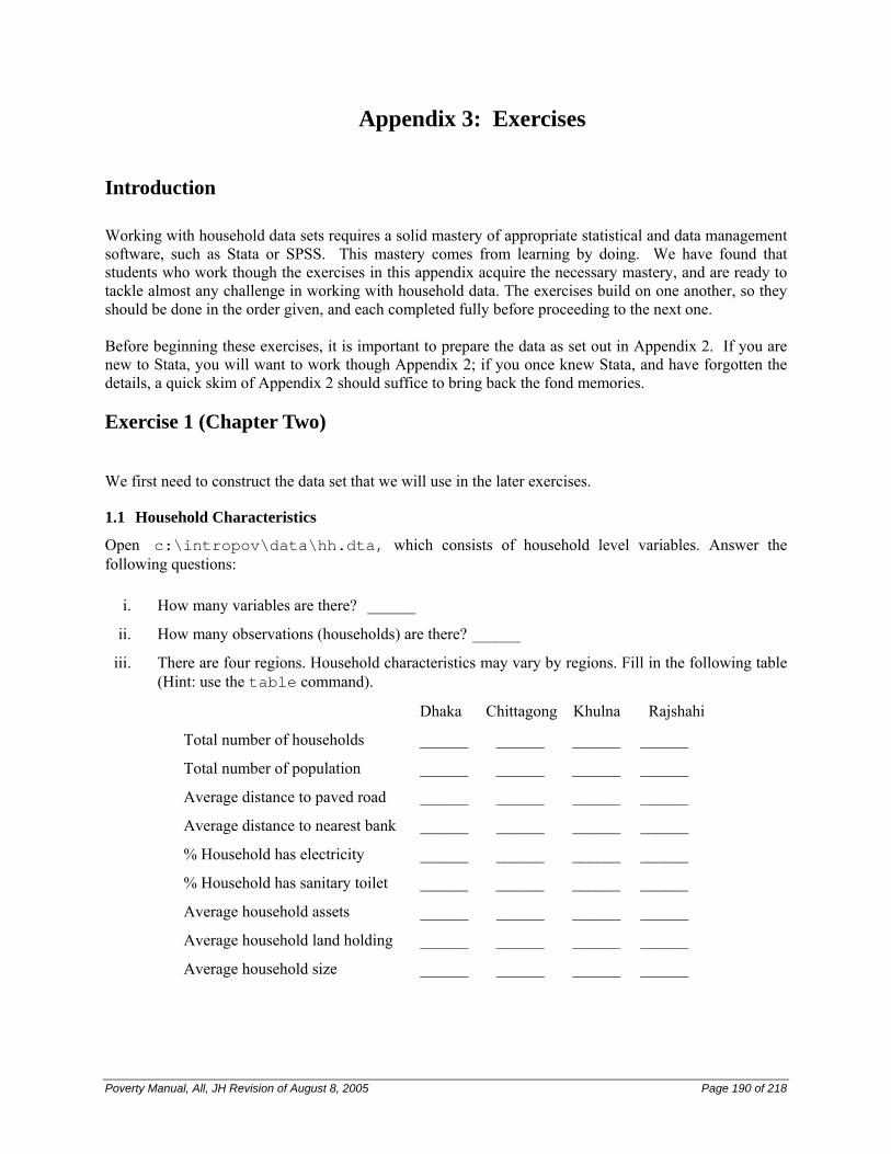
Appendix 3: Exercises

Introduction

Working with household data sets requires a solid mastery of appropriate statistical and data management software, such as Stata or SPSS. This mastery comes from learning by doing. We have found that students who work though the exercises in this appendix acquire the necessary mastery, and are ready to tackle almost any challenge in working with household data. The exercises build on one another, so they should be done in the order given, and each completed fully before proceeding to the next one. Before beginning these exercises, it is important to prepare the data as set out in Appendix 2. If you are new to Stata, you will want to work though Appendix 2; if you once knew Stata, and have forgotten the details, a quick skim of Appendix 2 should suffice to bring back the fond memories.

Exercise 1 (Chapter Two)

We first need to construct the data set that we will use in the later exercises.

1.1 Household Characteristics

Open c:\intropov\data\hh.dta, which consists of household level variables. Answer the following questions:

i. How many variables are there? ______

ii. How many observations (households) are there? ______

iii. There are four regions. Household characteristics may vary by regions. Fill in the following table (Hint: use the table command).

Dhaka Chittagong Khulna Rajshahi

Total number of households ______ ______ ______ ______

Total number of population ______ ______ ______ ______

Average distance to paved road ______ ______ ______ ______

Average distance to nearest bank ______ ______ ______ ______

% Household has electricity ______ ______ ______ ______

% Household has sanitary toilet ______ ______ ______ ______

Average household assets ______ ______ ______ ______

Average household land holding ______ ______ ______ ______

Average household size ______ ______ ______ ______


iv. Are the sampled households very different across regions?

v. The gender of the head of household may also be associated with different household characteristics:

Male-headed Female-headed households households

Average household size _________ ________

Average years of schooling of head _________ ________

Average age (years) of head _________ ________

Average household assets (taka) _________ ________

Average household land holding (acres) _________ ________ [Careful!]

[For consideration: How many decimal places should one report? As a general rule, do not provide spurious precision. Reporting the average household size as 5.35368 gives a false impression of accuracy; but reporting the size as 5 is too blunt. In such cases, 5.4 or 5.35 would be more appropriate, and is accurate enough for almost all uses.]

vi. Are the sampled households headed by males very different from those headed by females?

1.2 Individual Characteristics

Now open c:\intropov\data\ind.dta. This file consists of information on household members. Merge this data with the household level data (hh.dta) – see Appendix 2 if you need a refresher on merging – and answer the following questions for individuals who are 15 years old or older:

i. Regional variation Dhaka Chittagong Khulna Rajshahi

Average years of schooling ______ ______ ______ ______

Gender ratio (% of household that is female) ______ ______ ______ ______ % Working population (with positive working hours) ______ ______ ______ ______ % Working population working on a farm ______ ______ ______ ______


ii. Are the sampled individuals very different across regions?

iii. We now examine some gender differences:

For males For females

Average schooling years(age>=5) _________ ________

Average schooling years(age<15) _________ ________

Average age _________ ________

% Working population (with

positive working hours) _________ ________

% Working population working

on a farm _________ ________

Average working hours per month _________ ________

Average working hours on farm, per month _________ ________

Average working hours off farm, per month _________ ________

iv. Are the characteristics of the sampled women very different from those of the sampled men?

1.3 Expenditure

Open c:\intropov\data\consume.dta. It has household level consumption expenditure information. Merge it with hh.dta.

i. Create three variables: per capita food expenditure (let’s call it pcfood), per capita nonfood expenditure (call it pcnfood) and per capita total expenditure (call it pcexp). Now let’s look at the consumption patterns.


Average per capita expenditure:

pcfood pcexp

by region:

Whole ________ ________

Dhaka region ________ ________

Chittagong region ________ ________

Khulna region ________ ________

Rajshahi region ________ ________

by gender of head:

male-headed households ________ ________

female-headed households ________ ________

by education level of head:

head has some education ________ ________

head has no education ________ ________

by household size:

Large household (>5) ________ ________

Small household (<=5) ________ ________

by land ownership:

Large land ownership (>0.5/person) ________ ________

Small land ownership or landless ________ ________

Summarize your findings on per capita expenditure comparison

ii. Now add another measure of household size, which takes into account the fact that children

consume less than adults. Assume that children (aged <15) will be weighted as 0.75 of an adult. For instance, a household consisting of a couple with one child aged at 7 is worth 2.75 on this adult-equivalence scale, instead of 3. Go back to the ind.dta and create this variable (let’s call it famsize2), then merge the revised file with the household data and the consumption data files. Create per adult equivalent expenditure variables (let’s call them pafood and paexp) and repeat the above exercise.

Average per capita expenditure:

pcfood pcexp


by region:

Whole ________ ________

Dhaka region ________ ________

Chittagong region ________ ________

Khulna region ________ ________

Rajshahi region ________ ________

by gender of head:

male-headed households ________ ________

female-headed households ________ ________

by education level of head:

head has some education ________ ________

head has no education ________ ________

by household size:

Large household (>5) ________ ________

Small household (<=5) ________ ________

by land ownership:

Large land ownership (>0.5/person) ________ ________

Small land ownership or landless ________ ________

Compare your new results with those of per capita expenditure. In analyzing poverty, is it better to use adult-equivalents?

iii. Besides looking at the mean or the median value of consumption, we can also easily look at

the whole distribution of consumption using scatter. The following plots the cumulative distribution function curve of per capita total expenditure.

. cumul pcexp, gen(pcexpcdf)

. twoway scatter pcexpcdf pcexp if pcexp<20000, ytitle(“Cumulative Distribution of pcexp”) xtitle(“Per Capita total expenditure”) title(“CDF of Per Capita Total Expenditure”) subtitle(“Exercise 1.3”) saving(cdf1, replace)

The cumul command creates a variable called pcexpcdf that is defined as the empirical cumulative distribution function (cdf) of pcexp; in effect it sorts the data by pcexp, and


creates a new variable that cumulates and normalizes pcexp, so that its maximum value is 1. To explore the variable, try list pcexp pcexpcdf in 1/10 sort pcexp list pcexp pcexpcdf in 1/10 list pcexp pcexpcdf in –10/-1

Then use the code shown here to graph the cdf. Feel free to experiment with the scatter command. The graph is also saved in a file called cdf1.gph. When you want to look the graph later, you just need to type “graph use cdf1”.

The cumulative distribution function curve of a welfare indicator can reveal quite a lot of information about the poverty and inequality. For example, if we know the value of a poverty line, we can easily find the corresponding percentage value of people below the line. Suppose the poverty line is 5,000. Then the command

sum pcexpcdf if pcexp<5000 will give the poverty rate (under the “max” heading). [For consideration: Why is the mean not the appropriate measure of poverty here?]

iv. Keep pcfood pcexp pafood paexp famsize2 hhcode, merge with hh.dta,

sort by hhcode, and save as pce.dta in the c:\intropov\data directory.

1.4 Household Weights

In most household surveys, observations are selected through a random process, but different observations may have different probabilities of selection. Therefore, we need use weights that are equal to the inverse of the probability of being sampled. A weight of wj for the jth observation means, roughly speaking, that the jth observation represents wj elements in the population from which the sample was drawn. Omitting sampling weights in the analysis usually gives biased estimates, which may be far from the true values (see chapter 2). Various post-sampling adjustments to the weights are sometimes necessary. A household sampling weight is provided in the hh.dta. This is the right weight to use when summarizing data that relates to households. However, often we are interested in the individual, rather than the household, as the unit of analysis. Consider a village with 60 households; thirty households have five individuals each (with income per capita of 2,100), while the other thirty households have 10 individuals each (with income per capita of 1,200). The total population of the village is 450. Now suppose we take a 10% random sample of households, picking three five-person households and three 10-person households. We would estimate the mean income per capita to be 1,650. While this properly reflects the nature of households in the village, it does not give information that is representative of individuals: the village has 150 people in 5-person households and 300 people in 10-person households. Weighted by individuals, per capita income in this village is in fact 1,500 [Try the calculation!]. Such computations can be done easily in STATA. In estimating individual-level parameters such as per capita expenditure, we need to transform the household sample weights into individual sample weights, using the following STATA commands:

. gen weighti = weight*famsize


. table region [pweight=weighti], c(mean pcexp)

STATA has four types of weights: fweight, pweight, aweight, and iweight. Of these, the most important are:

• Frequency weights (fweight), which indicate how many observations in the population are represented by each observation in the sample, must take integer values.

• Analytic weights (aweight) are especially useful when working with data that contain averages (e.g. average income per capita in a household). The weighting variable is proportional to the number of persons over which the average was computed (e.g. number of members of a household). Technically, analytic weights are in inverse proportion to the variance of an observation (i.e. a higher weight means that the observation was based on more information and so is more reliable in the sense of having less variance).

Further information on weights may be obtained by typing help weight. Now let’s repeat some previous estimation with the newly-created weights:



Average per capita food expenditure: ______ ______ ______ ______

Average per capita total expenditure: ______ ______ ______ ______ Are the weighted averages very different from unweighted ones?

1.5 The effects of clustering and stratification

If the survey under consideration has a complex sampling design, then the standard errors of estimates (and sometimes even the means) will be biased if one ignores clustering and stratification.

Consider the following typical case of a multistage stratified random sample with clustering.

i. First one divides the country into regions (the strata), and picks a sample size for each region. Note that it is perfectly legitimate to sample some regions more heavily than others; indeed one would typically want to sample a sparsely populated heterogeneous region more heavily (e.g. one person per 300) than a densely populated, homogeneous region (e.g. one person per 1,000).

ii. Within each region one randomly picks communes, where the probability that a commune is picked depends on the population of the commune; in this case the commune is the primary sampling unit (the psu). Within the commune one may survey households in a cluster – for instance picking 20 households in a single village. Cluster sampling is widespread, because it is much cheaper than taking a simple random sample of the population. Let us assume that someone has also computed a weight variable (wt) that represents the number of households that each representative household “represents;” thus the weight will be small for over-sampled areas, and larger for under-sampled areas.


STATA has a very useful set of commands designed to deal with data that have been collected from multistage and cluster samples surveys. First one needs to provide information on the structure of the survey using the svyset commands. Using our example we would have

svyset [pweight=weighti], strata(region) psu(thana) clear(all)

where region is a variable that indicates the regions.12 Having set out the structure of the survey, one may now use svymean to give estimates of population means and their correct standard errors; and svyreg to perform linear regression, taking into account of survey design. Other commands include svytest (to test whether a set of coefficients are statistically significantly different from zero) and svylc (to test linear combinations, such as the differences between the means of two variables). Repeat the above exercise (1.4) and compare the results.



Average per capita food expenditure: ______ ______ ______ ______

Average per capita total expenditure: ______ ______ ______ ______ Are the new weighted averages, adjusted for clustering and stratification, very different from the unweighted ones?

12 These commands were substantially revised in STATA version 8, and the syntax differs significantly from earlier

versions of STATA.


Exercise 2 (Chapter Three)

In order to compare poverty measures over time, it is important that the poverty line itself represent similar levels of well-being over time and across groups. Three methods have been used to derive poverty lines for Bangladesh: direct caloric intake, food energy intake and cost of basic needs.

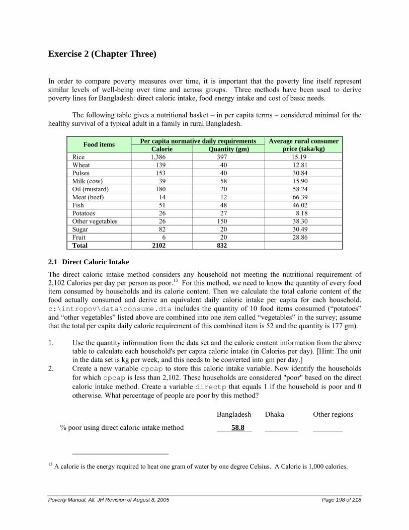
The following table gives a nutritional basket – in per capita terms – considered minimal for the

healthy survival of a typical adult in a family in rural Bangladesh.

Per capita normative daily requirements Food items Calorie Quantity (gm)

Average rural consumer price (taka/kg)

Rice 1,386 397 15.19 Wheat 139 40 12.81 Pulses 153 40 30.84 Milk (cow) 39 58 15.90 Oil (mustard) 180 20 58.24 Meat (beef) 14 12 66.39 Fish 51 48 46.02 Potatoes 26 27 8.18 Other vegetables 26 150 38.30 Sugar 82 20 30.49 Fruit 6 20 28.86 Total 2102 832

2.1 Direct Caloric Intake

The direct caloric intake method considers any household not meeting the nutritional requirement of 2,102 Calories per day per person as poor.13 For this method, we need to know the quantity of every food item consumed by households and its calorie content. Then we calculate the total calorie content of the food actually consumed and derive an equivalent daily caloric intake per capita for each household. c:\intropov\data\consume.dta includes the quantity of 10 food items consumed (“potatoes” and “other vegetables” listed above are combined into one item called “vegetables” in the survey; assume that the total per capita daily calorie requirement of this combined item is 52 and the quantity is 177 gm). 1. Use the quantity information from the data set and the calorie content information from the above

table to calculate each household's per capita caloric intake (in Calories per day). [Hint: The unit in the data set is kg per week, and this needs to be converted into gm per day.]

2. Create a new variable cpcap to store this caloric intake variable. Now identify the households for which cpcap is less than 2,102. These households are considered "poor" based on the direct caloric intake method. Create a variable directp that equals 1 if the household is poor and 0 otherwise. What percentage of people are poor by this method?

Bangladesh Dhaka Other regions

% poor using direct caloric intake method ____58.8__ _________ ________

13 A calorie is the energy required to heat one gram of water by one degree Celsius. A Calorie is 1,000 calories.


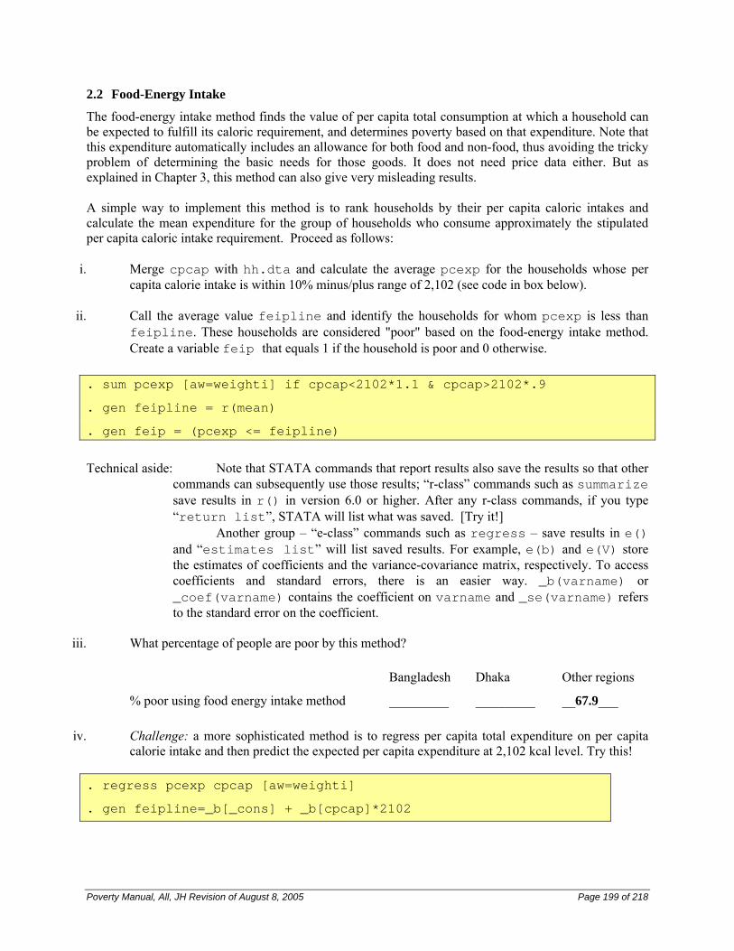
2.2 Food-Energy Intake

The food-energy intake method finds the value of per capita total consumption at which a household can be expected to fulfill its caloric requirement, and determines poverty based on that expenditure. Note that this expenditure automatically includes an allowance for both food and non-food, thus avoiding the tricky problem of determining the basic needs for those goods. It does not need price data either. But as explained in Chapter 3, this method can also give very misleading results. A simple way to implement this method is to rank households by their per capita caloric intakes and calculate the mean expenditure for the group of households who consume approximately the stipulated per capita caloric intake requirement. Proceed as follows:

i. Merge cpcap with hh.dta and calculate the average pcexp for the households whose per capita calorie intake is within 10% minus/plus range of 2,102 (see code in box below).

ii. Call the average value feipline and identify the households for whom pcexp is less than

feipline. These households are considered "poor" based on the food-energy intake method. Create a variable feip that equals 1 if the household is poor and 0 otherwise.

. sum pcexp [aw=weighti] if cpcap<2102*1.1 & cpcap>2102*.9

. gen feipline = r(mean)

. gen feip = (pcexp <= feipline)

Technical aside: Note that STATA commands that report results also save the results so that other

commands can subsequently use those results; “r-class” commands such as summarize save results in r() in version 6.0 or higher. After any r-class commands, if you type “return list”, STATA will list what was saved. [Try it!]

Another group – “e-class” commands such as regress – save results in e() and “estimates list” will list saved results. For example, e(b) and e(V) store the estimates of coefficients and the variance-covariance matrix, respectively. To access coefficients and standard errors, there is an easier way. _b(varname) or _coef(varname) contains the coefficient on varname and _se(varname) refers to the standard error on the coefficient.

iii. What percentage of people are poor by this method?


% poor using food energy intake method _________ _________ __67.9___

iv. Challenge: a more sophisticated method is to regress per capita total expenditure on per capita calorie intake and then predict the expected per capita expenditure at 2,102 kcal level. Try this!

. regress pcexp cpcap [aw=weighti]

. gen feipline=_b[_cons] + _b[cpcap]*2102


v. Should there be separate regression for each region?

2.3 Cost of Basic Needs

The idea behind the cost of basic needs method is to find the value of consumption necessary to meet minimum subsistence needs. Usually it involves a basket of food items based on nutritional requirements and consumption patterns, and a reasonable allowance for non-food consumption.

i. According to the above basket and the average rural consumer prices, how much money does a household of four need each day to meet its caloric requirements?

ii. One way to derive the non-food allowance is simply to assume a certain percentage of the value of

minimum food consumption. How much annual total expenditure does a family of four need if it is to avoid being poor, assuming that non-food expenses amount to 30 percent of food expenses?

iii. vprice.dta gives village-level price information on all 11 food items. Therefore, we can actually

calculate a food poverty line (call it foodline) and a total poverty line (call it cbnpline) for each village using the cost of basic needs method and merge this variable with pce.dta. [Hint: Here we need to sort both data sets and merge by thana vill]. Do this, and create a variable cbnp that equals 1 for the poor and 0 for the non-poor.

iv. What percentage of people are poor by this method?


% poor by cost of basic needs method _________ _________ ________

v. The percentage of people in poverty varies according to the three methods. Which method do you consider to be most suitable here? Why?

vi. Keep all imputed poverty lines and poverty indicators, merge with pce.dta, and save the file as final.dta.


Exercise 3 (Chapter Four):

3.1 A Simple Example

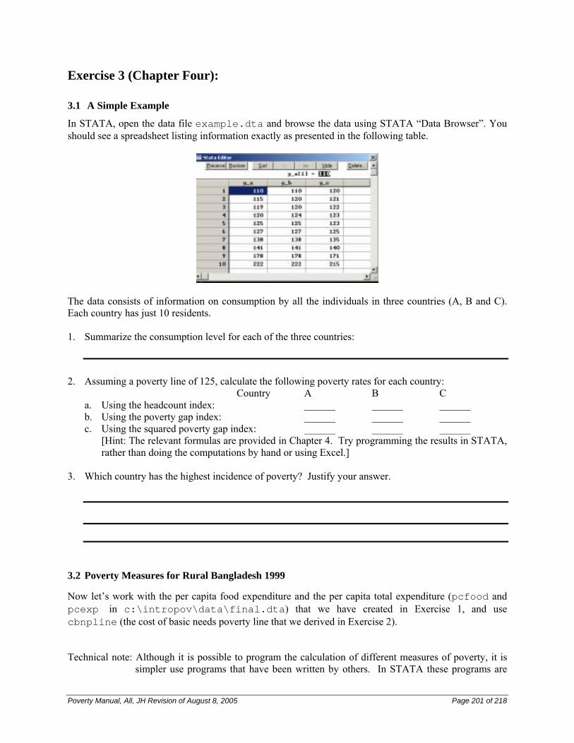
In STATA, open the data file example.dta and browse the data using STATA “Data Browser”. You should see a spreadsheet listing information exactly as presented in the following table.

The data consists of information on consumption by all the individuals in three countries (A, B and C). Each country has just 10 residents.

1. Summarize the consumption level for each of the three countries:

2. Assuming a poverty line of 125, calculate the following poverty rates for each country:

Country A B C a. Using the headcount index: ______ ______ ______ b. Using the poverty gap index: ______ ______ ______ c. Using the squared poverty gap index: ______ ______ ______

[Hint: The relevant formulas are provided in Chapter 4. Try programming the results in STATA, rather than doing the computations by hand or using Excel.]

3. Which country has the highest incidence of poverty? Justify your answer.

3.2 Poverty Measures for Rural Bangladesh 1999

Now let’s work with the per capita food expenditure and the per capita total expenditure (pcfood and pcexp in c:\intropov\data\final.dta) that we have created in Exercise 1, and use cbnpline (the cost of basic needs poverty line that we derived in Exercise 2).

Technical note: Although it is possible to program the calculation of different measures of poverty, it is simpler use programs that have been written by others. In STATA these programs are


known as.ado programs. The basic version of STATA comes with a large library of such programs, but for specialized work (such as computing poverty rates) it is usually necessary to install .ado programs that have been provided on a diskette or obtained on the Web.

For computing poverty rates, and their accompanying standard errors, we have provided FGT.ado , which is based on poverty.ado written by Philippe Van Kerm; the standard error calculation follows Deaton (1997). The FGT.ado file should be put in your working directory; or into a directory given by c:\ado\plus\f (which you may need to create for this purpose). We have also provided two other useful .ado programs, SST.ado (for computing the Sen-Shorrocks-Thon measure poverty) and Sen.ado (for computing the Sen index of poverty). Other .ado programs are available on the Internet; for an example, and how to access them, see section 3.3 below.

FGT.ado can calculate the head count index (or FGT(0)), the poverty gap index (or FGT(1)), and the squared poverty gap index (or FGT(2)). For example, . FGT y, line(1000) fgt0 fgt1 fgt2

will calculate the headcount ratio, the poverty gap ratio, and squared poverty gap index using a poverty line of 1000 and welfare indicator y. Be careful: the command is case sensitive, and in this case FGT must be written in capital letters. After line, the brackets must contain a number. Instead of typing all three measures one could specify all option, or just some of the measures. If one also types sd, then the command will also give standard errors for the estimates, which is very useful in determining the size of sampling error.

The above command works when there is a single poverty line. However, some researchers prefer to compute different poverty lines for each household (as a function of the household size, local price level, etc.). Assume that these tailor-made poverty lines are in a variable called povlines. Now the appropriate command becomes

. FGT y, vline(povlines) fgt0 fgt1 fgt2 sd

You can specify conditions, range and weights with these commands. For example, the following command calculates the headcount ratio for Dhaka region based on a poverty line of 3000.

. FGT pcexp [aw=weighti] if region==1, line(3000) fgt0

Sen.ado and SST.ado calculate the Sen index and SST index respectively. The syntax follows the same format, but does not compute standard errors. So, for example, one could use: . Sen y, line(1000) . SST y, line(1000) Now we are ready to turn to the measurement of poverty using the data from the BHES 1991/2.


1. Compute the five main measures of poverty (headcount, poverty gap, squared poverty gap, Sen index and Sen-Shorrocks-Thon index) for per capita expenditure, using both the food poverty line and the total poverty line derived by the cost of basic needs method in the previous exercise.

Food poverty line Total poverty line i. Headcount index: ________ ________

ii. Poverty gap index: ________ ________ iii. Squared poverty gap index: ________ ________ iv. Sen index: ________ ________ v. Sen-Shorrocks-Thon index ________ ________

2. Compute the headcount and poverty gap indexes for specific subgroups using the food poverty line.

Headcount index Poverty gap index i. Dhaka region: ________ ________

ii. Other three regions: ________ ________ iii. Households headed by men: ________ ________ iv. Households headed by women: ________ ________ v. Large households (>5): ________ ________

vi. Small households (<=5): ________ ________

3. Repeat the above exercise using the total poverty line.

Headcount index Poverty gap index i. Dhaka region: ________ ________

ii. Other three regions: ________ ________ iii. Households headed by men: ________ ________ iv. Households headed by women: ________ ________ v. Large households (>5): ________ ________

vi. Small households (<=5): ________ ________

3.3 Finding and Using .ado files

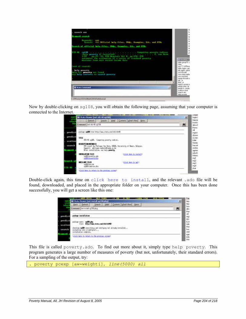
There is a wealth of .ado files on the Web, and some of them are fairly easy to locate. For example, suppose one wants to compute the Sen index of poverty. From within STATA, type search Sen, which will yield the following.


Now by double-clicking on sg108, you will obtain the following page, assuming that your computer is connected to the Internet.

Double-click again, this time on click here to install, and the relevant .ado file will be found, downloaded, and placed in the appropriate folder on your computer. Once this has been done successfully, you will get a screen like this one:

This file is called poverty.ado. To find out more about it, simply type help poverty. This program generates a large number of measures of poverty (but not, unfortunately, their standard errors). For a sampling of the output, try: . poverty pcexp [aw=weighti], line(5000) all


Exercise 4 (Chapter Five): The robustness of poverty measures is very important because if poverty measures are not as

accurate as we would want, then many conclusions that we draw from poverty comparisons between groups and over time may not be warranted.

4.1 Sampling Error

For example, the fact that poverty calculations are based on a sample of households rather than the population implies that calculated measures carry a margin of error. When the standard errors of poverty measures are large, small changes in poverty may well be statistically insignificant and should not be interpreted for policy purpose.

As noted above, FGT also compute the standard errors of its poverty measures if option sd is specified:

. FGT y, Line(1000) fgt0 fgt1 sd

1. Now let’s re-compute the headcount index and poverty gap index for Dhaka, and for the rest of

the country, using the total poverty line, and compute the standard errors of the two measures as well.

Headcount index Poverty gap index a) Dhaka region: Poverty rate ________ ________

Standard error of poverty rate ________ ________ b) Other three regions: Poverty rate ________ ________

Standard error of poverty rate ________ ________

2. Does the factor of standard errors change any conclusion of poverty comparison between Dhaka region and other regions?

4.2 Measurement Error

Another reason that we need to be very careful in poverty comparisons is because the data collected are measured incorrectly. This could be due to recall error on the part of respondents while answering survey questions, or because of enumerator error when the data were entered into specific formats. Let us simulate measurement error in per capita expenditure, and then investigate what effect this error has on basic poverty measures. Try the following: . sum pcexp [aw=weighti]

. gen mu = r(sd)*invnorm(uniform())/10

. gen pcexp_n1 = pcexp + mu

Here we assume that the measurement error is a random normal variable with a standard error as big as a tenth of the standard error of observed per capita expenditure. Let us assume that the measurement error ,


mu, is additive to observed per capita expenditure. Note that, by design, this error is independent of observed per capita expenditure and of any other household or community characteristics. 1. Now re-compute the headcount ratio and poverty gap ratio using this new per capita expenditure.

pcexp pcexp_n1

i. Headcount index: ________ ________ ii. Poverty gap index: ________ ________

2. Are these measures different for the headcount index? For the poverty gap index?

3. Now consider the following situation. If the measurement error is correlated with a household

characteristic – for example, if subsistence farmers usually underreport their consumption of own production – then will the measurement error problem be more or less severe?

4.3 Sensitivity Analysis

Apart from taking standard errors into account, it is also important to test the sensitivity of poverty measures to alternative definitions of consumption aggregates and alternative ways of setting the poverty line. For example, some non-food items are excluded from the expenditure aggregate on the basis that those items are irregular and do not reflect a household’s command over resources on average. Also a 30% allowance for non-food expenditure is quite ad hoc. (i) Create a new measure of total expenditure that includes the previously excluded irregular non-

food expenditure (expnfd2), compute the three FGT poverty measures of per capita expenditure (pcexp_n2), and compare the results with those based on the original definition of expenditure (pcexp).

pcexp pcexp_n2

a. the headcount index: ________ _______ b. the poverty gap index: ________ _______

The non-food allowance can be estimated from data. Two methods have been considered (see chapter 4). • The first finds the average non-food expenditure for households whose total expenditure is equal (or

close) to the food poverty line. The non-food expenditure for this group of households must be necessities since the households are giving up part of minimum food consumption in order to buy non-food items.

• The second finds the non-food expenditure for households whose food expenditure is equal (or close) to the food poverty line. Since the second is more generous than the first, the two are usually referred


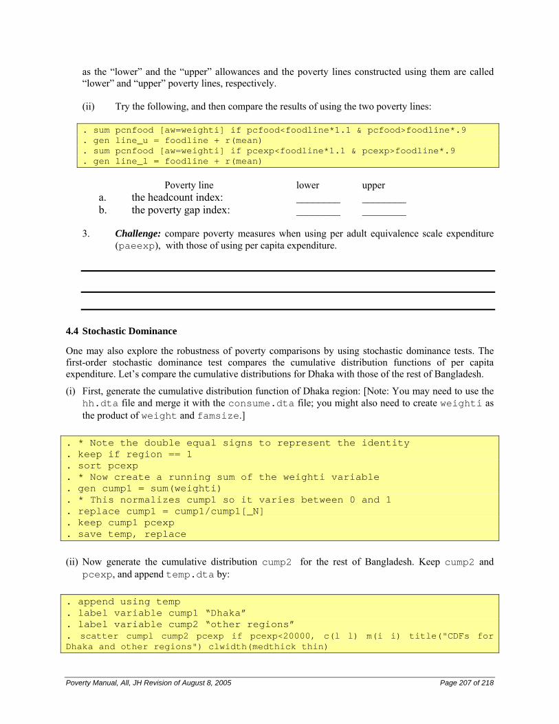
as the “lower” and the “upper” allowances and the poverty lines constructed using them are called “lower” and “upper” poverty lines, respectively. (ii) Try the following, and then compare the results of using the two poverty lines: . sum pcnfood [aw=weighti] if pcfood<foodline*1.1 & pcfood>foodline*.9 . gen line_u = foodline + r(mean) . sum pcnfood [aw=weighti] if pcexp<foodline*1.1 & pcexp>foodline*.9 . gen line_l = foodline + r(mean)

Poverty line lower upper a. the headcount index: ________ ________ b. the poverty gap index: ________ ________

3. Challenge: compare poverty measures when using per adult equivalence scale expenditure (paeexp), with those of using per capita expenditure.

4.4 Stochastic Dominance

One may also explore the robustness of poverty comparisons by using stochastic dominance tests. The first-order stochastic dominance test compares the cumulative distribution functions of per capita expenditure. Let’s compare the cumulative distributions for Dhaka with those of the rest of Bangladesh.

(i) First, generate the cumulative distribution function of Dhaka region: [Note: You may need to use the hh.dta file and merge it with the consume.dta file; you might also need to create weighti as the product of weight and famsize.]

. * Note the double equal signs to represent the identity . keep if region == 1 . sort pcexp . * Now create a running sum of the weighti variable . gen cump1 = sum(weighti) . * This normalizes cump1 so it varies between 0 and 1 . replace cump1 = cump1/cump1[_N] . keep cump1 pcexp . save temp, replace

(ii) Now generate the cumulative distribution cump2 for the rest of Bangladesh. Keep cump2 and

pcexp, and append temp.dta by: . append using temp . label variable cump1 “Dhaka” . label variable cump2 “other regions” . scatter cumpl cump2 pcexp if pcexp<20000, c(l l) m(i i) title("CDFs for Dhaka and other regions") clwidth(medthick thin)


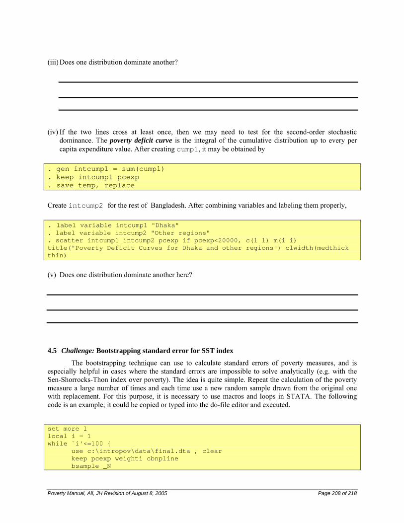
(iii) Does one distribution dominate another?

(iv) If the two lines cross at least once, then we may need to test for the second-order stochastic dominance. The poverty deficit curve is the integral of the cumulative distribution up to every per capita expenditure value. After creating cump1, it may be obtained by

. gen intcump1 = sum(cump1) . keep intcump1 pcexp . save temp, replace

Create intcump2 for the rest of Bangladesh. After combining variables and labeling them properly,

. label variable intcump1 "Dhaka" . label variable intcump2 "Other regions" . scatter intcump1 intcump2 pcexp if pcexp<20000, c(l l) m(i i) title("Poverty Deficit Curves for Dhaka and other regions") clwidth(medthick thin)

(v) Does one distribution dominate another here?

4.5 Challenge: Bootstrapping standard error for SST index

The bootstrapping technique can use to calculate standard errors of poverty measures, and is especially helpful in cases where the standard errors are impossible to solve analytically (e.g. with the Sen-Shorrocks-Thon index over poverty). The idea is quite simple. Repeat the calculation of the poverty measure a large number of times and each time use a new random sample drawn from the original one with replacement. For this purpose, it is necessary to use macros and loops in STATA. The following code is an example; it could be copied or typed into the do-file editor and executed.

set more 1 local i = 1 while ì'<=100 { use c:\intropov\data\final.dta , clear keep pcexp weighti cbnpline bsample _N


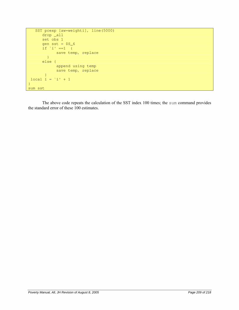
SST pcexp [aw=weighti], line(5000) drop _all set obs 1 gen sst = $S_6 if ì' ==1 { save temp, replace } else { append using temp save temp, replace } local i = ì' + 1 } sum sst

The above code repeats the calculation of the SST index 100 times; the sum command provides

the standard error of these 100 estimates.


Exercise 5 (Chapter Six):

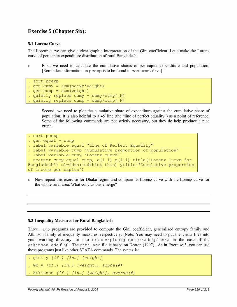
5.1 Lorenz Curve

The Lorenz curve can give a clear graphic interpretation of the Gini coefficient. Let’s make the Lorenz curve of per capita expenditure distribution of rural Bangladesh. o First, we need to calculate the cumulative shares of per capita expenditure and population:

[Reminder: information on pcexp is to be found in consume.dta.]

. sort pcexp

. gen cumy = sum(pcexp*weight)

. gen cump = sum(weight)

. quietly replace cumy = cumy/cumy[_N]

. quietly replace cump = cump/cump[_N] Second, we need to plot the cumulative share of expenditure against the cumulative share of population. It is also helpful to a 45° line (the “line of perfect equality”) as a point of reference. Some of the following commands are not strictly necessary, but they do help produce a nice graph.

. sort pcexp

. gen equal = cump

. label variable equal “Line of Perfect Equality”

. label variable cump “Cumulative proportion of population”

. label variable cumy “Lorenz curve”

. scatter cumy equal cump, c(l l) m(i i) title("Lorenz Curve for Bangladesh") clwidth(medthick thin) ytitle("Cumulative proportion of income per capita")

o Now repeat this exercise for Dhaka region and compare its Lorenz curve with the Lorenz curve for

the whole rural area. What conclusions emerge?

5.2 Inequality Measures for Rural Bangladesh

Three .ado programs are provided to compute the Gini coefficient, generalized entropy family and Atkinson family of inequality measures, respectively. [Note: You may need to put the .ado files into your working directory; or into c:\ado\plus\g (or c:\ado\plus\a in the case of the Atkinson.ado file)]. The gini.ado file is based on Deaton (1997). As in Exercise 3, you can use these programs just like other STATA commands. The syntax is:

. gini y [if…] [in…] [weight]

. GE y [if…] [in…] [weight], alpha(#)

. Atkinson [if…] [in…] [weight], averse(#)


Notes: Alpha(#)sets the parameter value for the generalized entropy measure that determines

the sensitivity of the inequality measure to changes in the distribution. The measure is sensitive to changes at the lower end of the distribution with a parameter value close to zero, equally sensitive to changes across the distribution for the parameter equal to one (which is the Theil index), and sensitive to changes at the higher end of the distribution for higher values. Averse(#)sets the parameter value for the Atkinson measure that measures aversion to inequality.

Let’s continue using the per capita total expenditure to calculate inequality measures:

i. Compute the Gini coefficient, the Theil index and the Atkinson index with inequality aversion parameter equal to 1 for the four regions.

Gini Theil Atkinson All regions ________ ________ ________ Dhaka region: ________ ________ ________ Other three regions: ________ ________ ________

ii. Now repeat the above exercise using two decile dispersion ratios and the share of consumption of poorest 25%. STATA command xtile is good for dividing the sample by ranking. For example, to calculate the consumption expenditure ratio between richest 20% and poorest 20%, you need to identify those two groups.

. xtile group = y, nq(5)

xtile will generate a new variable group that splits the sample into 5 groups according to the ranking of y (from smallest to largest, i.e., the poorest 20% will have group==1, while the richest 20% will have group==5). Similarly, to identify the poorest 25%, you need to split the sample into 4 groups. top 20% ÷ bottom 20% top 10% ÷ bottom 10% Percentage of consumption

of poorest 25%

All Bangladesh __________ __________ __________

Dhaka region __________ __________ __________

Other regions of Bangladesh __________ __________ __________

iii. Challenge: many inequality indexes can be decomposed by subgroups. Decompose the Theil

index by region and comment on the results.


Exercise 6 (Chapter Seven): In the previous exercises we computed poverty measures for various subgroups, such as regions, gender of head of household, household size, etc. Another way to present a poverty profile is by comparing the characteristics of the “poor” with those of the “non-poor”.

6.1 Characteristics of the poor

Complete the following table, where “poor” and “non-poor” are defined by cbnp in Exercise 2. poor non-poor

% of all households ______ ______

% of total population ______ ______

Average distance to paved road ______ ______

Average distance to nearest bank ______ ______

% of households with electricity ______ ______

% of households with a sanitary toilet ______ ______

Average household assets (taka) ______ ______

Average household land holding (decimals) ______ ______

Average household size ______ ______

% of households headed by men ______ ______

Average schooling of head of household (years) ______ ______

Average age of head (years) ______ ______

Average hh working hours on non-farm activities (p.a.) ______ ______

6.2 More Poverty Comparison across subgroups

Calculate the headcount and poverty gap measures of poverty for the following subgroups, using cbnpline to define poverty. Headcount index Poverty gap index a. Household head has no education b. Household head has a primary education only c. Head had secondary or higher education d. Large land ownership (>0.5 ha./person) e. Small land ownership or landless f. Large asset ownership (>50000 taka) g. Small asset ownership (<=50000 taka) h. Combined with the poverty measures computed in Exercise Three, describe the most significant

poverty patterns in Bangladesh?


Exercise 7 (Chapter Eight): Develop and estimate a model that explains log(pcexp/cbnpline) using available data. The regressors may include demographic characteristics such as gender of head and family structure; access to public services such as distance to a paved road; household members’ employment such as working hours on farm and off farm; human capital such as average education of working members; asset positions such as land holding; etc. You need to identify potentially relevant variables and the direction of their effect. Then put all those variables together, and run the regression. Report the result and discuss whether it matches your hypothesis. If not, give possible reasons.

. gen y = log(pcexp/cbnpline)

. reg y age age2 workhour x1-x3 [aw=weighti]

where x1-x3 are other explanatory variables that you want to include; don’t feel confined to just three variables! Note that if you want to include categorical variables, you need to convert them into dummy (“binary”) variables if the ranking of categorical values do not have any meaning. For example,

. tab region, gen(reg)

will generate four variables, labeled reg1, reg2, reg3 and reg4. The variable reg1 takes on a value of 1 for Dhaka and zero otherwise, and so on. When using a set of such dummy variables in a regression, one needs to leave one of them out, to serve as a reference area. So, for instance,

. reg y age age2 workhour x1-x3 reg2-reg4 [aw=weighti]

would include dummy variables for the regions, with Dhaka serving as the point of reference. After the regression, it is usually a good idea to plot the residuals against the fitted values to ensure that the pattern appears sufficiently random. This could be done by adding, right after the regression command,

. predict yhat, xb . predict e, residuals . scatter e yhat

Documents

Appendix 3: Exercises - World Banksiteresources.worldbank.org/PGLP/Resources/exercises...Assume that children (aged