Embed Size (px)
Citation preview

MONARC
SIMULATION OF DISTRIBUTED SYSTEMS. TECHNIQUES OF PERFORMANCE IMPROVEMENT.
TEST CASES.
Author: Dragos Andrei, 354 C4 Scientific Adviser: Prof. Valentin Cristea, Ph.D.
Prof. Iosif Legrand, Ph.D. as. ing. Corina Stratan
ing. Ciprian Dobre
2
Contents
1. Introduction................................................................................................................................ 4 1.1. Generalities ......................................................................................................................... 4 1.2. Theoretical aspects of the simulation .................................................................................. 4
1.2.1. Introduction .................................................................................................................. 4 1.2.2. The Utility and the implementation of the computer simulation................................. 4 1.2.3. Simulation Types ......................................................................................................... 5 1.2.4. A few other examples of simulators ............................................................................ 6
1.3. Distributed Systems. Generalities. ...................................................................................... 8 1.3.1. History.......................................................................................................................... 8 1.3.2. Definition and Characteristics of a Distributed System............................................... 8 1.3.3. Several examples of distributed systems ..................................................................... 9 1.3.4. The Goals of Distributed Systems ............................................................................... 9
1.3.4.1. Connecting users to resources............................................................................... 9 1.3.4.2. Transparency.......................................................................................................10 1.3.4.3. Openness .............................................................................................................10 1.3.4.4. Scalability............................................................................................................10
1.3.5. Hardware concepts .....................................................................................................11 1.4.1. Introduction. Advantages of Java language. ..............................................................12 1.4.2. Java and concurrent programming .............................................................................12 1.4.3. The creation of Threads in Java .................................................................................13
1.4.3.1. The creation of a thread through the derivation of the Thread class ..................13 1.4.3.2. The creation of a thread through the implementation of the Runnable interface13 1.4.3.3. The Thread control..............................................................................................14 1.4.3.4. The Thread Synchronization...............................................................................15 1.4.3.5. The Scheduling and the Priority Mechanism......................................................16
2. General Functioning of the MONARC. Implementation details. ............................................17 2.1. Generalities .......................................................................................................................17 2.2. The Architecture ...............................................................................................................17 2.3. The Components of the System ........................................................................................18 2.4. Component Model - Multitasking Data Processing Model ..............................................19 2.5. Task functioning and their states ......................................................................................20 2.6. The scheduling algorithm (from the engine package) ......................................................21 2.7. The Network Package .......................................................................................................22 2.8. Job Scheduling and Execution..........................................................................................25
3. The simulation of the Proof Cluster .........................................................................................27 3.1. Introduction.......................................................................................................................27 3.2. The Proof parallel model based on ROOT. The CERN perspective ................................27 3.3. The Proof System (made at CERN) Architecture .............................................................28 3.4. The Architecture and premises of Proof simulation .........................................................28
3.4.1. The Architecture ........................................................................................................28 3.4.2. The example description ............................................................................................30 3.4.3. The actual implementation .........................................................................................30 3.4.4. The Two different Scheduling Variants.....................................................................31 3.4.5. The results..................................................................................................................31
3.4.5.1. The Influence of the LAN Bandwidth ................................................................31 3.4.5.2. The Influence of the Data Server Processing Time ............................................34
3
3.4.5.3. The effect of introducing additional data servers................................................35 3.4.5.4. The Optimum Number of Slave Processes .........................................................35 3.4.5.5. The Simulation of Longer Periods of Activity ...................................................36
4. The Optimization of the networking part of the MONARC....................................................38 4.1. Objective ...........................................................................................................................38 4.2. Implementation details......................................................................................................38
4.2.1. The explanation of the problem.................................................................................38 4.2.2. The functioning of the optimised variant...................................................................39 4.2.3. The performance testing of the optimised version. Simulations................................41
4.2.3.1. Simulations .........................................................................................................41 4.2.3.2. Results .................................................................................................................42
5. The Optimization of the Job Processing of the MONARC.....................................................46 5.1. Objective ...........................................................................................................................46 5.2. Implementation details......................................................................................................46
5.2.1. The explanation of the problem.................................................................................46 5.2.2. The functioning of the optimised variant...................................................................47
5.3. The performance testing of the optimized version. Simulations and results. ...................48 5.3.1. Simulations ................................................................................................................48 5.3.2. Results ........................................................................................................................48
6. The Simulation T0/T1 Data Production and Replication (CernTier Simulation) ....................52 6.1. Introduction.......................................................................................................................52 6.2. Problem explanation .........................................................................................................52 6.3. Simulation Results ............................................................................................................54
6.3.1. Generalities and Explanations....................................................................................54 6.3.2. Results ........................................................................................................................56
6.3.2.1. Comparison for Production and DST distribution done with and without the Data Transfer Agent.........................................................................................................56 6.3.2.2. RAW Data Replication .......................................................................................59 6.3.2.3. Production and DST Distribution .......................................................................60 6.3.2.4. Re-production and new DST Distribution ..........................................................61 6.3.2.5. RAW Data Replication activity followed by Production and DST distribution .63 6.3.2.6. RAW Data Replication activity followed by Production and DST distribution followed by Re-production and new DST distribution ....................................................66 6.3.2.7. Detector Analysis activity...................................................................................69 6.3.2.8. RAW Data Replication activity followed by Production and DST distribution followed by Re-production and new DST distribution with Detector Analysis activity .71
7. Conclusions..............................................................................................................................76 8. Bibliography.............................................................................................................................76 9. Appendix..................................................................................................................................77
4
1. Introduction
1.1. Generalities
Distributed system s have become very useful especially in the case of scientific applications, where there is necessary the processing of a very large data volume, in a very short amount of time, as well as the storage of these data.
Taking into account the tremendous popularity of complex distributed systems, favoured by the rapid development of the computing systems, of the high speed networks, and of the Internet, it is clear that it is imperative, in order to achieve performances as high as possible, in the utilization of these systems, to pick an optimal structure and architecture, but also scheduling algorithms, and data replications ones in that distributed system. This thing is particularly difficult, but even impossible, to be done by somebody without the help of a specialized program, because the prediction of the functioning of a distributed system without the aid of the mentioned program is only approximate and there may appear functioning errors in that distributed system.
Therefore, simulators for distributed systems are particularly useful, because they are very flexible and easy to use in the testing of certain architectures, scheduling algorithms, the same result being much more difficult to achieve by testing real systems.
The project MONARC 2 is such a simulator for large scale distributed systems, having as a purpose the modelling and simulation of distributed systems, with the goal of predicting general performances of the applications running on these systems.
1.2. Theoretical aspects of the simulation
1.2.1. Introduction
Computerized simulation consists in the designing of a system model, in the execution of this model on a digital computer, and in the analysis of the results.
For the simulation of a physical system, the first step which must be done is the creation of a mathematical model to represent it. The model will be executed through the mediation of a program which will simulate the passing of the time, modifying the values of the state variables which are of interest in the simulation.
1.2.2. The Utility and the implementation of the computer simulation This modality of simulation has become the most used in the last decades. Although there are a multitude of methods of modelling systems, this kind of simulation proves extremely useful in the case in which we have to deal with a very large scale system, in which the variables computed at every discrete moment are very many, the components are very numerous. There is also useful in the case in which it is wanted as the results of the simulation to be obtained in a visual form, as well as in the case in which inside the model we have
5
variables which vary randomly, or even after certain distributions or mathematical computations that can be very laboriously computed without the aid of the computer. Another simulation advantage is that it can be used exactly the same execution technique for a large number of systems, an especially difficult thing to do through the classical solving of the simulations, in the second case being necessary to solve the problem again. To conclude, the classical systems may be applie d for a relatively limited number of situations, to contrast with the large applicability of the computerized simulations. The designers of the distributed systems want to achieve the best performances with the lowest price. The computer simulation may be even more precise than the real one. The simulation of certain types of architectures is particularly useful before taking the decision of the designing of a real system. The simulation may be used not only to optimize performances, but also to verify the correctness of the real results. For example, there are simulations made to verify the behaviour of a type of cars in extreme conditions, taking into account as accurately as possible all the parameters. The errors must be identified and corrected as rapidly as possible, as in final phases, the errors are much more difficult and more costly to correct. There are cases in which uncorrected mistakes can produce catastrophical results. There exists a multitude of fields in which the computer simulations are largely used: in the scientific field, phenomena which can take whole eras: as the genesis of the universe, or in general the ones related with the astronomy, or oppositely, the ones which take nano-seconds, as the knockings between electrons, can be studied and reproduced with the aid of the computer. The simulations may used to create virtual environments, for example the training of the fighting planes pilots, who can learn on a simulator manoeuvres that, in the case they do not posses, in reality, would make them lose their lives, as well as destroying very valuable equipments.
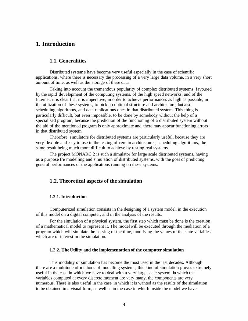
1.2.3. Simulation Types If we classify the computer simulations after the mode in which there appear changes of states in the system they model, we will distinguish two categories:
- continuous time simulation: the state changes appear continuously in time, and the system can be described with the aid of differential equations systems; this model is suitable for simulating the weather's evolution or the fluid dynamic;
- discrete time simulation: the events appear instantaneously, only at certain moments in time; this model can be used for simulating air traffic, communication networks or computing systems.
The simulation models in continuous time are more general and can be converted to discrete time simulations, considering that unitary events are instantaneous. The discrete simulation can be of two types:
- discrete simulation oriented on time - simulation oriented on discrete events
6
1. time-oriented discrete simulation: the time advances in constant -size steps, so system is evaluated once in a certain time interval. When choosing the length of the time interval we have to make a compromise between the accuracy of the simulation and the time needed for execution; usually the time intervals short enough to guarantee the precision we need lead to a longer execution time. If the events appear irregularly in time, this model is inefficient.
2. event-oriented discrete simulation (Discrete Event Simulation - DES): the system is only observed in the moments of time when events appear. The simulator maintains an internal clock, which measures the virtual time (the time of the simulated sys tem). Each event has a timestamp, which indicates the moment when it appears, and the events that must be processed are organized in a priority queue in which a smaller value for the timestamp means a greater priority. In a simulation step, the events with the minimum timestamp are extracted from the queue and the virtual time advances, becoming equal with the timestamp of the events extracted. The processing of an event can have as an effect the change of some state variables and/or the insertion of some new events into the queue.
In MONARC it is used the second approach – DES, because this variant corresponds better with our purpose, which is the simulation of the distributed systems.
1.2.4. A few other examples of simulators There are a lot of computing systems simulators, some of them general, and the other
specific. Below, we have examples of this kind of applications (especially distributed systems oriented):
1. SEDS is a simulator developed at Osaka University They have developed a Simulator for Evaluation of the Distributed Systems (SEDS) for
evaluating not only distributed system (DS) architectures but also distributed algorithms. In their simulator SEDS, through using simple format "forms" defined in SEDS, they can describe both the hardware conf iguration of a DS and the distributed algorithm implemented on it.
7
Through the simulation of the problem by SEDS, they show the availability and applicability of the SEDS to the wide range of the problem around the DS.
2. Bricks is a program developed at the Tokyo Institute of Technology, which has the role of evaluating the high performance computing systems, and of scheduling algorithms. It is written in Java and it simulates the behaviour of different network architectures inside some global systems. The users can specify the parameters of the system that will be modelled through the scripts. The components of the application may be replace with user defined ones, so it can be tested different scheduling algorithms from the ones already implemented.
3. Proteus is a high-performance simulator for MIMD multiprocessors. It is faster than comparable simulators, as they say, and it can reproduce result s from real multiprocessors, it is easily configured to simulate a wide range of architectures. Proteus provides a modular structure that simplifies customization and independent replacement of parts of architecture. There are typically multiple implementations of each module that provide different combinations of accuracy and performance. Finally, PROTEUS provides repeatability, nonintrusive monitoring and debugging, and integrated graphical output, which result in a development environment superior to those available on real multiprocessors.
4. GridSim is a simulator projected for the modelling of Grid systems, and of the peer-to-peer networks. There are supported many types of resources, mono and multi processors, for different types of systems.
5. Peersim has been developed with extreme scalability and support for dynamicity in mind. Peer-to-peer systems can reach huge dimensions such as millions of nodes, which typically join and leave continuously. Evaluating a new protocol in a real environment, especially in its early stages of development, is not feasible. There are distributed planetary-scale open platforms to develop and deploy network services, but these solutions don't include more than 400 nodes.
Peersim is composed of many simple extendable and pluggable components, with a flexible configuration mechanism. To allow for scalability and focus on self-organization properties of large scale systems, some simplifying assumptions have been made, such as ignoring the details of the transport communication protocol stack. Peersim is developed within the Bison project and it is distributed under an open source license. Peersim is written in the Java language.
6. Ptolemy is s system made at Berkeley, with a very large area of utilization, it may handle lots of calculus model, with discrete and continuous time. It is written in Java, and has a modular structure, containing both generic packages, and specialised packages for every model. There are implemented libraries for mathematical functions, graph algorithms, a language interpreted for expressions and many others.
8
1.3. Distributed Systems. Generalities.
1.3.1. History From the beginning, in 1945, until about 1985, computers were large and expensive. As
a result, most organisations had only a handful of computers, and for lack of the way to interconnect them, they operated independent from one another.
Starting from the mid 1980’s, however, two advances began to change the situation. The first was the development of powerful microprocessors. Initially, they were 8-bit machines, but soon 16, 32 and 64 bit CPUs became common. The second development was the invention of high-speed computer networks. Local-area networks allow hundreds of machines within a building to be connected in such a way that small amounts of information can be transferred between machines in a few microseconds. Larger amounts of data can be moved between machines at rates of 10 to 1000 million bits/sec. Wide-area networks allow millions of machines all over the earth to be connected at speeds varying from 64 Kbps to gigabits per second. The results of these technologies is that it is now easy to put together computing systems composed of large numbers of computers, connected by a high-speed network. They are usually called computers networks, or distributed systems , in contrast with the previous centralized systems (or single processor systems) consisting of a single computer, its peripherals, and perhaps some remote terminals.
1.3.2. Definition and Characteristics of a Distributed System
A distributed system is a collection of independent computers that appear to its users as a single coherent system. The two aspects of this definition are: -One that deals with the hardware; the machines are autonomous. - The second deals with the software: the users think that they are dealing with a single system. Characteristics of a distributed system: - The differences between the various computers and the ways in which they communicate are hidden from users. - The internal organisation of a distributed system is hidden to the users. - The users and the applications can interact with the distributed system in a consistent and uniform way, regardless of where and when interaction takes place. -Distributed systems should also be relatively easy to expand or scale. This characteristic is a direct consequence of having independent computers, but at the same time, hiding how these computers actually take part in the system as a whole. A distributed system will normally be continuously available, although perhaps certain parts may be temporarily out of order.
9
In order to support heterogeneous computers and networks while offering a single -system view, distributed systems are often organized by means of a layer of software that is logically placed between a higher-level layer consisting of users and applications, and a layer underneath consisting of operating systems. Such a distributed system is sometimes called middleware .
1.3.3. Several examples of distributed systems A first example could be a network of workstations in a university or company department. In addition to each user’s workstation, there might be a pool of processors in the machine room that are not assigned to specific users, but are allocated dynamically as needed. Such a system might have a single file system, with all files accessible from all machines in the same way as using the same path name. When a user types a command, the system could look for the best place to execute the command, possibly on the user’s own workstation, possible on an idle workstation belonging to someone else, and possibly on one of the unassigned processors in the machine room. If the system as a whole looks and acts as a classical single -processor time sharing system (multi-user), it qualifies as a distributed system. As a second example let us consider a workflow information system that supports the automatic processing of orders. Such a system is used by people from several departments, possibly at different locations. For example people from the sales department may be spread across a large region or an entire country. Orders are placed by the means of laptop computers that are connected to the system through the telephone network. Incoming orders are automatically forwarded to the planning department, resulting in new internal shipping orders sent to the stock department. The system will automatically forward the orders to an available person. Users are unaware of how orders physically flow through the system: to them it appears as if they are all operating on a centralised database. As a final example, let us consider the World Wide Web. The Web offers a simple, consistent and uniform model of distributed documents. To see a document, a user need merely activate a reference, and the document appears on the screen. In theory, there is no need to know from which server the document has been fetched, neither where the server is located. Publishing a document is very simple: you only have to give it a unique name in the form of a Uniform Resource Locator (URL), that refers to a local file containing the document’s content. If the World Wide Web would appear to its users as a gigantic centralized document system, it too would qualify as a distributed system.
1.3.4. The Goals of Distributed Systems
1.3.4.1. Connecting users to resources The man goal of a distributed system is to make it easy for the users to access remote
resources, and to share them with other users in a controlled way. Resources can be virtually anything, but typical examples include printers, computers, storage facilities, data and files.
There are many reasons for wanting to share resources. The main obvious reason is that of economics. It is cheaper to let a printer be shared by several users, than having to buy and maintain a printer for each. Connecting users and resources also make it easier to collaborate
10
and exchange information, as it is best illustrated by the Internet. However, as connectivity and sharing increase, security is becoming more and more important.
1.3.4.2. Transparency An important goal of a distributed system is to hide the fact that its processes and
resources are physically distributed across multiple computers. A distributed system that is able to present itself to users and application as if it were only a single computer system is said to be transparent.
The concept of transparency can be applied to several aspects of a distributed system, as we can see below.
We have transparency for: -Access –there are hidden the differences in data representation and how a resource is accessed. -Location - it is hidden where the resource is located -Migration – it is hidden that a resource may move to another location. -Relocation – hide that a resource may be moved to another location while in use. -Replication – hide that a resource is replicated. -Concurrency – hide that a resource may be shared by several competitive users. -Failure – hide the failure and recovery of a resource. -Persistence – hide whether a software resource is in memory or on disk.
1.3.4.3. Openness
An open distributed system is a system that offers services according to standard rules that describe the syntax and semantics of those services. For example, in computer networks, standard rules govern the format, contents, and meaning of the messages sent and received. Such rules are formalized in protocols. In distributed systems, services are generally specified through interfaces, which are often described in an Interface Definition Language (IDL).
1.3.4.4. Scalability Worldwide connectivity through the Internet is rapidly becoming very common.
Scalability of a system can be measured along at least three different dimensions (Neuman, 1994). First, a system can be scalable with respect to its size, meaning that we can easily add more users and resources to the system. Second, a geographically scalable system is one in which the users and resources may lie far apart. Third, a system can be administratively scalable, meaning that it can still be easy to manage even if it spans many independent administrative organisations. Unfortunately, a system that is scalable in one or more of these dimensions often exhibits some loss of performance as the system scales up.
11
1.3.5. Hardware concepts
Even though all distributed systems consists of multiple CPUs there are several different ways the hardware can be organized, especially in terms of how they are interconnected and how they communicate.
Various classification schemes for multiple CPU computer systems have been proposed over the years. We divide all computers into two groups: those that have shared memory, usually called multiprocessors, and those that do not, called multicomputers. The essential difference is this: in a multiprocessor, there is a single physical address space that is shared by all CPUs. All the machines share the same memory. In contrast, in a multicomputer, every machine has its own private memory.
We can make another further distinction between distributed computer systems: those that are homogenous, and those that are heterogeneous. In a homogenous multicomputer, there is essentially only a single interconnection network that uses the same technology everywhere. Likewise, all processors are the same and generally have access to the same amount of private memory.
Multiprocessors Multiprocessors systems all share a single key property: all the CPUs have direct access
to the shared memory. Bus-based microprocessors consist of some number of CPUs, all connected to a common bus, along with a memory module.
Homogenous Multicomputer Systems In multiprocessors, every CPU has a direct connection to its local memory. The only
problem left is how the CPUs communicate with each other. Clearly, some interconnection scheme is needed here, too, but since it is only for CPU-to-CPU communication, the volume of traffic will be several orders of magnitude lower than when the interconnection network is used for CPU-to-memory traffic. The homogenous multicomputers are also referred as SANs (System Area Networks). In these systems, the nodes are mounted in a big rack and are connected through a single, high-performance interconnection network.
Heterogeneous Multicomputer Systems Most distributed systems as they are used today are built on the top of a heterogeneous
multicomputer. This means that the computers that form part of the system may vary widely with respect to, for example, processor type, memory sizes, and I/O bandwidth. In fact, some of the computers may actually be high performance parallel systems, such as multiprocessors or homogeneous multicomputers. Also, the interconnection network may be highly heterogeneous as well.
12
1.4. The Technology used: Java Concurrent Programming
1.4.1. Introduction. Advantages of Java language.
The Java language offers a series of advantages that made it be preferred by many of the creators of the simulation programs. The main advantages of the Java language are:
- Portability: the MONARC simulation can be used not only on PCs with Linux or Windows as operating system, but also on other, more powerful machines, possibly multi-processor, that use different Linux variants. That is why the fact that a Java program can be used unmodified practically on any platform has a very important role in convincing us to use the Java language.
- Java is an object oriented programming language, that helps us obtain a modular structure of the program, a structure resembling with the real one, and a very easy to change code. - The support for multi-threading programming . Inside a distributed system there appear different entities with autonomous behaviour, for example the local networks, or database servers, or the tasks executed by the system. For their simulation, we need concurrent programming, and Java is one of the few languages that offer a library for the work with threads. The main disadvantage of Java language is the relatively low performance, taking into account the fact that Java is an interpreted language. However, in the last years, significant progress have been made, with the advent of technologies like JIT (Just-In-Time Compiling), and of the last versions of virtual machines from Sun and IBM.
1.4.2. Java and concurrent programming
The term of “concurrency” refers basically to the possibility of executing more actions simultaneously; the concurrent programs are used in numerous situations, like: intense computational applications in the scientific field, the web services, simulations, I/O processing, graphical interface applications. There are more ways to achieve concurrency, each of them being appropriate for different kinds of applications. Among them are the following:
1. Processes: a process represents a program in execution, in fact, the process notion is an abstract one and depending on the operating system (this is the one that handles the process administration). The operating system generates the autonomy, security and interferences between processes.
2. Threads: their usage represents an alternative for the multi-process programming, the advantage being the lower overhead at creation, finishing or commutation between them. The threads associated with a process share its memory zone, the opened files, and other resources associated with the respective process. The not shared things are the general registers, the stack and the program counter. In the Java language, the scheduling policy for the threads is not specified. It can be a nywhere between the most costly solution (between the threads of a process is not done any scheduling – they are let to “cooperate”), and the most complex –the attaining of a preemptive scheduling.
13
3. The utilisation of more systems : -it maps every logical unit of the application on a different system; the advantage is that the systems are autonomous and can be separately administered, but on the other hand the message transfer between the machines can be very costly – in addition it may appear security or other kind of problems.
The concurrent and object oriented programming have been associated from the
beginning of their existence: the first object oriented language, SIMULA , created around 1966. Other languages, created ulterior, offered, in a certain measure, support for object oriented programming and concurrency. This association between concurrent and object oriented programming appears very strongly in Java, which offers two classes (Thread, and ThreadGroup), and an interface (Runnable), in the java.lang package. The Thread class and the Runnable interface offers support for the work with threads as separate entities, and the ThreadGroup class permits the creation of thread gr oups, with the purpose of treating them unitary.
The thread class implements the Runnable interface, and the ThreadGroup objects contains many Thread objects.
1.4.3. The creation of Threads in Java
To create a thread, the programmer has two possibilities: to create a derived class from the Thread class or to create a class that implements the Runnable interface.
1.4.3.1. The creation of a thread through the derivation of the Thread class
The s teps that must be followed in this case are: 1. The creation of a class derived from the Thread class. 2. The superscription of the method public void run() from the Thread class; this
method must implement what the respective Thread will do. 3. The instantiation of an object from the created class 4. The starting of the execution thread, through the calling of the start() method,
inherited from the Thread class. This call makes that the Java virtual machine to create the necessary context for a thread and to call the run() method.
1.4.3.2. The creation of a thread through the implementation of the Runnable interface The programmer may want that a t hread have, through the inheritance, functionalities of another Java class. Because in this language the multiple inheritance is not permitted, it is not possible that the execution thread to derive both from Thread, and from the class whose functionality is necessary. The solution is that, instead of inheriting the Thread class, to implement the Runnable interface. The necessary operations to create a thread in this way are:
1. the creation of a class that implements the Runnable interface. 2. the superscription of the method public void run() from this interface. 3. the instantiation of an object from the created class (let us call it runnable_object). 4. the creation of a Thread type object, starting off the Runnable object (this operation
is necessary to call for the new Thread the methods from the thread class). Thread thread = new Thread(runnable_object);
14
5. the starting of the thread, through the start() method.
1.4.3.3. The Thread control
A Thread may be in one of the following states:
1. created: the Thread object was instanced (through the new() call), but it is not still an execution thread. In this moment, for it can be called only the start() method.
2. ready – ready to run –the start() method was called and the thread was created, and can be executed when the processor is available.
3. suspended: in this state are the threads that called one of the methods sleep() or wait(). The control is given away and they will come back to the ready state, when an extern event will appear (time expiring, if it was ca lled the sleep() method, or the notify()/ notifyAll() call, if the wait() method was called).
4. finished : a thread can be in this state if the run() method execution finished, or if the stop() method was called. (this method generates an exception of ThreadDeath type, that can be “caught” if some processing are wanted before the thread to be finished).
Another special category of Threads are the daemon type ones, that offer services for other execution Threads or objects (an example would be the demon that handles the garbage collector daemon)
Usually, the run() method for the daemon threads contains an infinite cycle. Their finishing takes place in the moment when all the threads from this application, that are not daemons, finished their execution. To declare a thread as a daemon, it can be called the method setDaemon(true), before the call of the start() method.
The main methods in the Thread class, with which we control the Threads are:
• public native synchronized void start() - used to start the execution of a thread; after this call the Java Virtual Machine handles the creation of the context for the new thread and the execution of its run() method.
• public final void stop() – it is forced the stopping of a Thread, in any stage it would be.
• public final void suspend() – stops temporary the execution of the thread, until the call of the resume() method.
• public static native void sleep(long milliseconds) – temporary stops the thread execution, on a time period specified in the argument (in milliseconds ). Because the method is static, it is of the Thread class and not the instanced object’s; the thread from which the sleep() call takes place will be blocked, regardless of the object through which the call is made.
• public final void join() – the thread from where the join() method of another thread will wait thaqt the latter finish the running (there are variants that specify a maximum waiting period).
15
• public static native void yield() – makes that the thread from which it is called be sent in the waiting queue, yielding its place to other concurrent thread (with the same priority).
• public void run() – the method that must be overwritten by the programmer to specify the tasks that the thread will accomplish.
• public void interrupt() – it send an interruption request to the thread (it is useful for the case when the thread blocks – it will be reactivated and will throw an exception).
• public void destroy()- it destroys the thread immediately.
1.4.3.4. The Thread Synchronization
The threads of a process share the same memory zone for data, so they can access, for example, the same variable in the same time. In the same case there may be problems if a thread tries to read a value that other thread modifies in that moment (the first can receive a wrong result), or if two threads write simultaneously in the same memory location (case in which the final result depends of the relative speed of execution of the two threads).
Other situations in which the threads interact is that in which one waits for results from other, or that in which more threads cannot start a new series of processing until the previous series was not finished by the other execution threads. The cases described below can be situated in two categories from the point of view of the relations between threads: these relations can be of concurrency and of cooperation.
In the case of concurrency, the threads try to use the same resources, and this thing must
be done in a consistent manner (usually, at a given moment, a thread can access common resources). In this case, the synchronization role is that of assuring the exclusive access to common resources. In this way it appears the notion of critical region, which is a part of code that only a thread can execute at a given moment.
The cooperation of the threads refers at the information exchange between them; this exchange must be done only when they are at a certain stage of the execution, or else the sent information may be incorrect. So, the synchronisation means that in this case the threads must wait one another until they are ready for the information transfer.
To solve this kind of problems, Java adopted the monitor solution, the concept of monitor being used by C. Hoare, and implies the existence of a special object (the monitor), that permits only one thread to call one of his method at a given time. The other threads that want to call a method of the monitor are suspended until the thread that entered the monitor finishes the execution of the certain method. Java implements this concept with slight differences: every Java object is an object of type monitor, but this thing is valid only for certain methods or code sequences specified by the programmer. This specification is made with the help of the synchronized key-word. An object can have more methods or synchronized blocks, and, at a given moment only a thread can access them (if a thread calls a synchronized method of an object, another thread can not call this method or other synchronized method of the object, until the first one is not finished).
16
We can say that a monitor is in a critical zone in which it can enter only one thread at a
given moment. Once entered, the thread can call any synchronized method existent in that area. For a thread to have access to a method of the zone (this means of the monitor), the first must exit from the monitor.
In the normal mode, the synchronization mechanism is bound to an object, but it is possible as a static method to be declared synchronized; in this way the monitor is the class, and not one of its objects. Only a thread can execute at a given moment of time a method static synchronized of a certain class.
Through the use of synchronized there may be solved the majority of the simultaneous resource access problems, but for the threads that are in cooperation relationship, this solution is not sufficient.
In this case there can be used the methods: wait(), notify() and notifyAll() of the Object class. The method wait() goes to the blocking of the thread, from where it was called, it remaining blocked until other thread will call one of the methods notify() and notifyAll() for the same object for which it was called wait(). For a thread to call one of these methods, it must be entered in the monitor of the object (with other words, their call can be done only for a synchronized sequence of code).
Through the wait() call it is exited from the monitor, to allow other threads to enter and call notify() (or else the thread that called wait() could not be unblocked). There also are variants of the wait() method through which there can be specified a maximum amount of time for the waiting. Through the notify() call it is unblocked only one thread (if there are more that wait for the same monitor, it can not be known which of them can be unblocked). Through notifyAll() there are unblocked all the threads that wait at a monitor.
1.4.3.5. The Scheduling and the Priority Mechanism Even if apparently the threads are executed in parallel, in reality this thing cannot be
happened on a one processor machine. To give the impression that the work threads work in parallel, they get the periodical access to resources, on the basis of a scheduling system.
The Java virtual machine contains a scheduler that handles the thread access to resources, but the specifications of the JVM do not establish the rules of its functioning.
The scheduling algorithm depends on the implementation of the Java machine on a certain platform, so the application must not be based on a certain algorithm, or another.
For example, in the systems of time division, an execution thread runs for a period of time, after which it is forced by the planner to yield his place to other thread, which will run for a period of time, and so on. This way, even the threads with smaller priorities will gain access to resources, avoiding their blocking. In systems without time-division, a thread that received the execution right occupies the resources until the moment it passes in the blocked state, finishes, yields explicitly the controls (through the yield() method), or another thread with a greater priority appears. This way, it may happen that a thread with a greater priority to get the resources, and the ones with smaller priorities not to get executed.
At the start, a thread has an associated priority, which is implicitly equal with that of the tread that was executed. The priority level can take values between Thread.MIN_PRIORITY and Thread.MAX_PRIORITY, constants defined in the Thread class. In the system it is always executed the thread with the greatest priority; if a thread with a greater priority than that of the one executing enters the system, it will be given the control.
17
2. General Functioning of the MONARC. Implementation details.
2.1. Generalities
MONARC 2 is a simulation framework whose purpose is to offer a design and optimization instrument for the large scale distributed systems, to serve, in a first phase to the LHC experiments that take place at CERN. The purpose is to offer a realistic simulation of the distributed computing systems, in particularly for the physical data processing, and to offer a flexible and dynamic medium to evaluate the performances of a category of processing architectures.
2.2. The Architecture
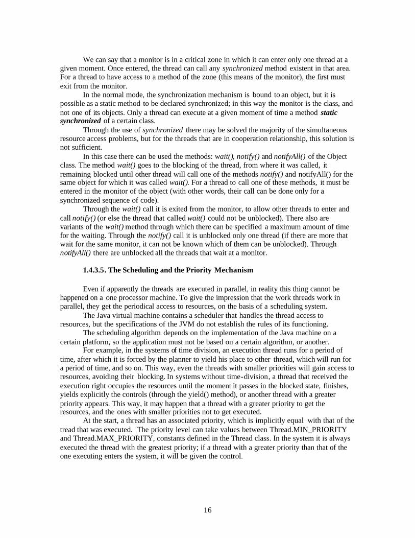
One of the strengths of MONARC is that it can be easily extended, even by users, and this is made possible by its layered structure. The first two layers contain the core of the simulator (which we call "simulation engine") and models for the basic components of a distributed system (CPU units, jobs, databases, networks, job schedulers); these are the fixed parts on top of which some particular components (specific for the simulated systems) can be built. The particular components can be different types of jobs, job schedulers with specific scheduling algorithms or database servers that support data replication.
The following diagram represents the MONARC layers and the way they could interact with a monitoring system:
Fig. 1. MONARC 2 layers
18
MONARC 2 consists of three main packages: engine , network and monarc; the first two of them only contain basic components, while the last one also includes specific components and can be extended with classes added by users.
The engine package contains the core of the simulator, mana ging the tasks and the events and providing the mechanism through which the tasks interact. The network package simulates the data traffic on LANs and WANs, according to different protocols; the ones implemented so far are TCP and UDP. The monarc package is more complex than the other two and contains sub packages needed to implement models for the entities in the regional centres (CPUs, jobs, job schedulers etc.) and other useful features: the graphical interface, the output clients, the parsing of the configuration files, the generation of random numbers wit h specific distributions.
2.3. The Components of the System
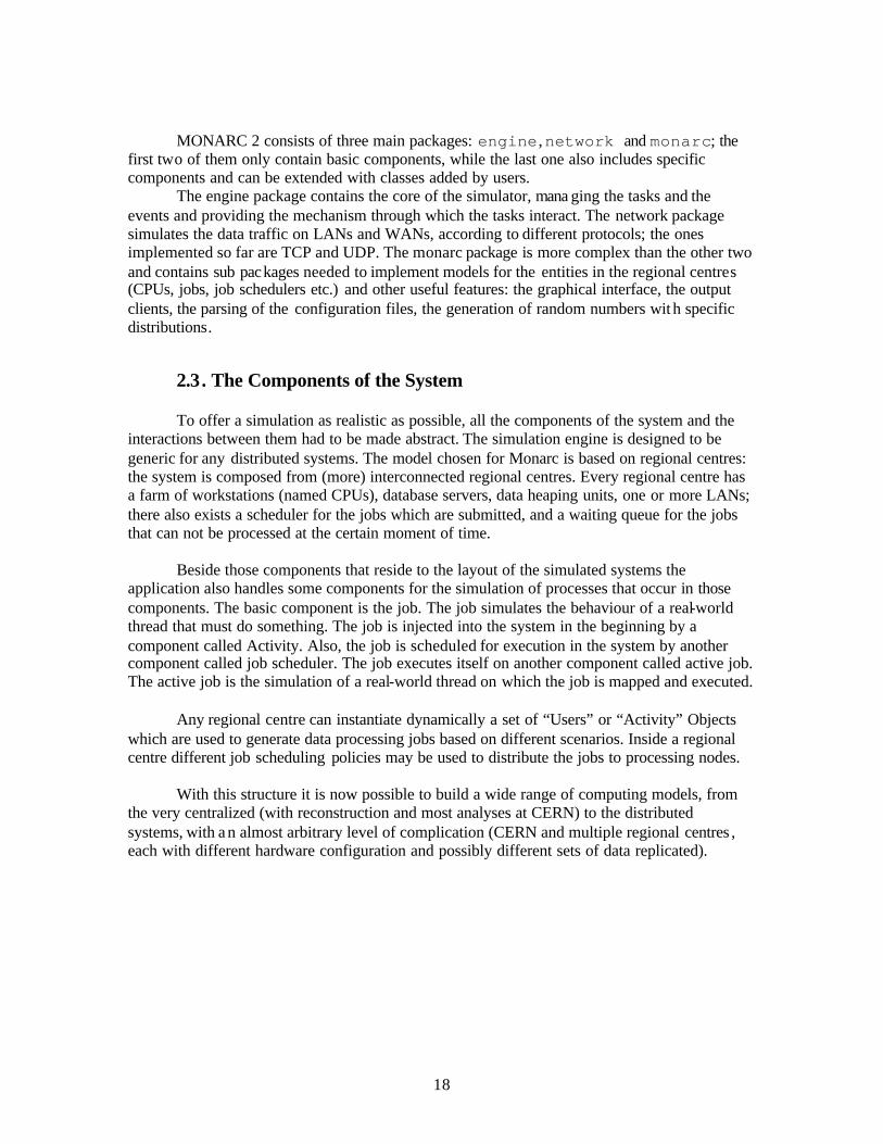
To offer a simulation as realistic as possible, all the components of the system and the interactions between them had to be made abstract. The simulation engine is designed to be generic for any distributed systems. The model chosen for Monarc is based on regional centres: the system is composed from (more) interconnected regional centres. Every regional centre has a farm of workstations (named CPUs), database servers, data heaping units, one or more LANs; there also exists a scheduler for the jobs which are submitted, and a waiting queue for the jobs that can not be processed at the certain moment of time. Beside those components that reside to the layout of the simulated systems the application also handles some components for the simulation of processes that occur in those components. The basic component is the job. The job simulates the behaviour of a real-world thread that must do something. The job is injected into the system in the beginning by a component called Activity. Also, the job is scheduled for execution in the system by another component called job scheduler. The job executes itself on another component called active job. The active job is the simulation of a real-world thread on which the job is mapped and executed. Any regional centre can instantiate dynamically a set of “Users” or “Activity” Objects which are used to generate data processing jobs based on different scenarios. Inside a regional centre different job scheduling policies may be used to distribute the jobs to processing nodes. With this structure it is now possible to build a wide range of computing models, from the very centralized (with reconstruction and most analyses at CERN) to the distributed systems, with a n almost arbitrary level of complication (CERN and multiple regional centres , each with different hardware configuration and possibly different sets of data replicated).
19
These components are represented in the image below:
Fig. 2 . The System A rchitecture
2.4. Component Model - Multitasking Data Processing Model
Multitasking operating systems share resources such as CPU, memory and I/O between concurrently running tasks by scheduling their use for very short time intervals. However, simulating the detail of how tasks are scheduled in the real system would be too complex and time consuming, and thus it is not suitable for our purpose. Therefore we need to model the multitasking data processing.
Our model for multitasking processing is based on an "interrupt" driven mechanism implemented in the simulation engine. An "interrupt()" method, implemented in the "active object" which is the base class for the running jobs, is a key part of our multitasking model.
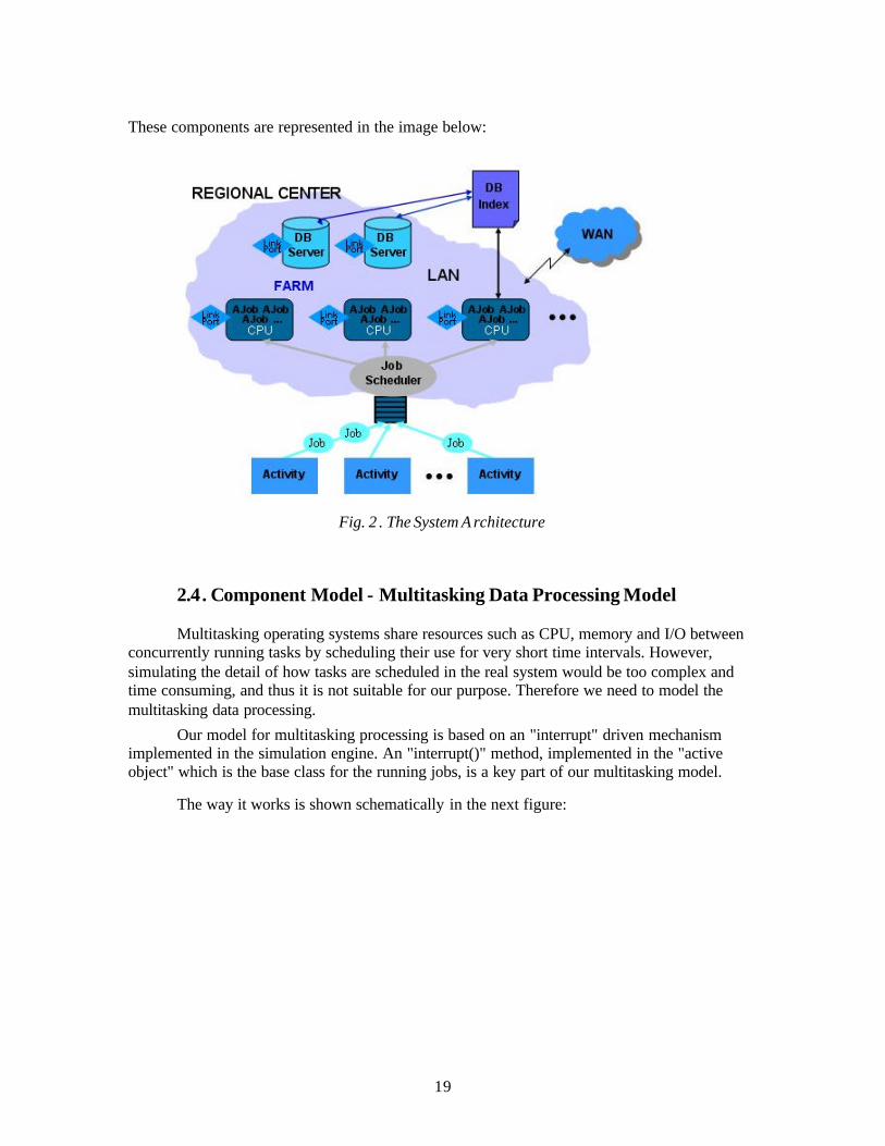
The way it works is shown schematically in the next figure:
20
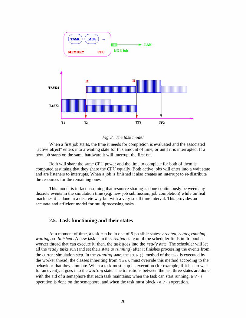
Fig. 3 . The task model
When a first job starts, the time it needs for completion is evaluated and the associated "active object" enters into a waiting state for this amount of time, or until it is interrupted. If a new job starts on the same hardware it will interrupt the first one.
Both will share the same CPU power and the time to complete for both of them is computed assuming that they share the CPU equally. Both active jobs will enter into a wait state and are listeners to interrupts. When a job is finished it also creates an interrupt to re-distribute the resources for the remaining ones.
This model is in fact assuming that resource sharing is done continuously between any discrete events in the simulation time (e.g. new job submission, job completion) while on real machines it is done in a discrete way but with a very small time interval. This provides an accurate and efficient model for multiprocessing tasks.
2.5. Task functioning and their states
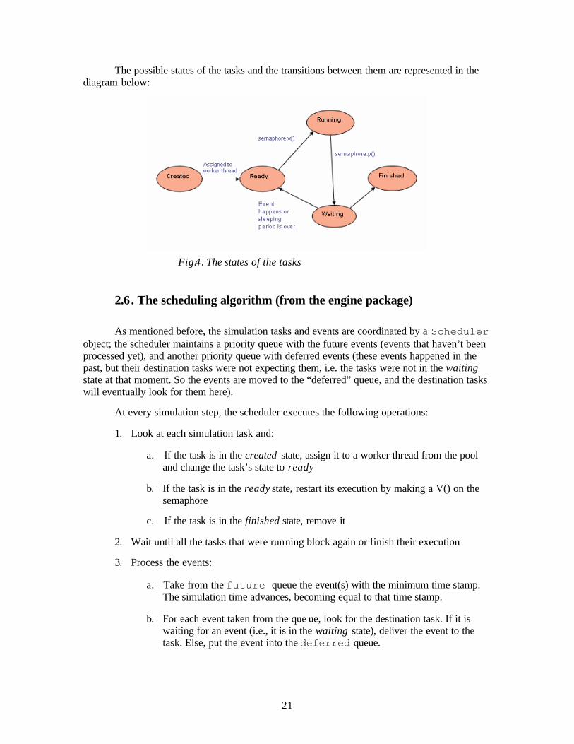
At a moment of time, a task can be in one of 5 possible states: created, ready, running, waiting and finished . A new task is in the created state until the scheduler finds in the pool a worker thread that can execute it; then, the task goes into the ready state. The scheduler will let all the ready tasks run (and set their state to running) after it finishes processing the events from the current simulation step. In the running state, the RUN() method of the task is executed by the worker thread; the classes inheriting from Task must override this method according to the behaviour that they simulate. When a task must stop its execution (for example, if it has to wait for an event), it goes into the waiting state. The transitions between the last three states are done with the aid of a semaphore that each task maintains: when the task can start running, a V() operation is done on the semaphore, and when the task must block - a P()operation.
21
The possible states of the tasks and the transitions between them are represented in the diagram below:
Fig.4. The states of the tasks
2.6. The scheduling algorithm (from the engine package)
As mentioned before, the simulation tasks and events are coordinated by a Scheduler object; the scheduler maintains a priority queue with the future events (events that haven’t been processed yet), and another priority queue with deferred events (these events happened in the past, but their destination tasks were not expecting them, i.e. the tasks were not in the waiting state at that moment. So the events are moved to the “deferred” queue, and the destination tasks will eventually look for them here).
At every simulation step, the scheduler executes the following operations:
1. Look at each simulation task and:
a. If the task is in the created state, assign it to a worker thread from the pool and change the task’s state to ready
b. If the task is in the ready state, restart its execution by making a V() on the semaphore
c. If the task is in the finished state, remove it
2. Wait until all the tasks that were running block again or finish their execution
3. Process the events:
a. Take from the future queue the event(s) with the minimum time stamp. The simulation time advances, becoming equal to that time stamp.
b. For each event taken from the que ue, look for the destination task. If it is waiting for an event (i.e., it is in the waiting state), deliver the event to the task. Else, put the event into the deferred queue.
22
These steps are executed until there are no more alive tasks and no more eve nts in the queues. The next diagram illustrates some of the steps of this algorithm.
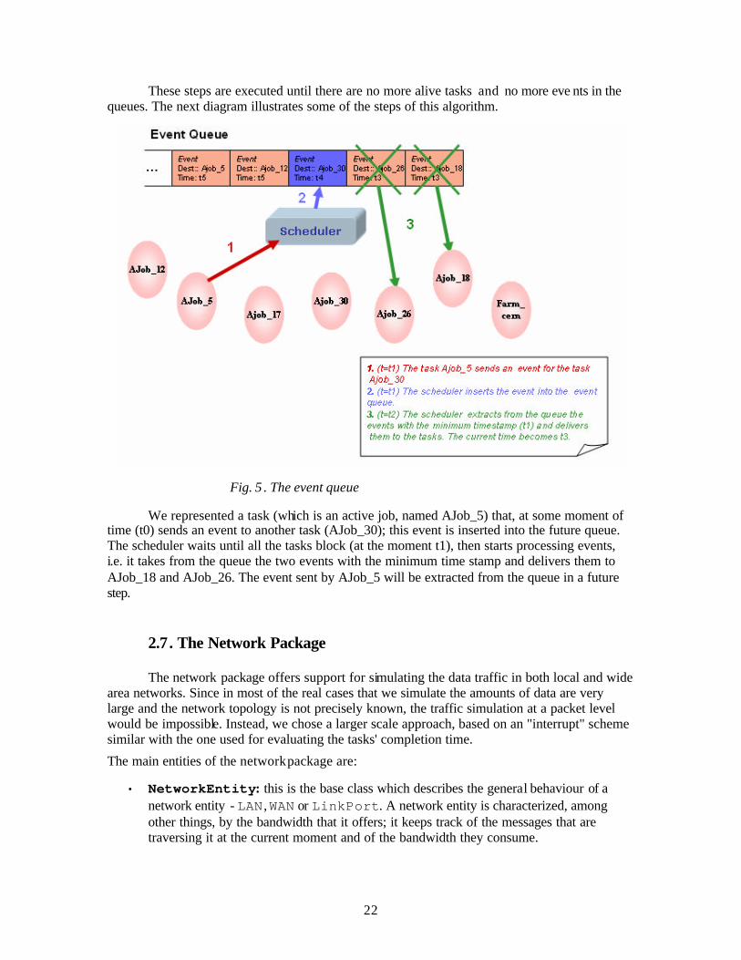
Fig. 5 . The event queue
We represented a task (which is an active job, named AJob_5) that, at some moment of time (t0) sends an event to another task (AJob_30); this event is inserted into the future queue. The scheduler waits until all the tasks block (at the moment t1), then starts processing events, i.e. it takes from the queue the two events with the minimum time stamp and delivers them to AJob_18 and AJob_26. The event sent by AJob_5 will be extracted from the queue in a future step.
2.7. The Network Package
The network package offers support for simulating the data traffic in both local and wide area networks. Since in most of the real cases that we simulate the amounts of data are very large and the network topology is not precisely known, the traffic simulation at a packet level would be impossible. Instead, we chose a larger scale approach, based on an "interrupt" scheme similar with the one used for evaluating the tasks' completion time.
The main entities of the network package are:
• NetworkEntity: this is the base class which describes the general behaviour of a network entity - LAN , WAN or LinkPort. A network entity is characterized, among other things, by the bandwidth that it offers; it keeps track of the messages that are traversing it at the current moment and of the bandwidth they consume.
23
• LinkPort: describes the physical device that connects a computer to the network; it is associated with a network address which, in our model, has an IP-like format. The network messages are always exchanged between two link ports. The link ports also determine, when a message must be sent, its route and initial speed.
• LAN: simulates a local area network. A LAN object has references to the LinkPorts corresponding to the computers from the network; it can be attached to a wide area network.
• WAN: simulates a wide area network. A WAN can have several LANs attached to it and can communicate with one or more routers.
• Router: a router connects two or more wide area networks (in our model, a route between two wide area networks goes through a router). Depending on its configuration, the router can introduce a delay in the data transfer.
• Message : this is the base class used to represent network messages. Every message is characterized by a number of parameters such as the source and destination addresses, the data length, the current speed etc. The classes derived from Message describe protocol-specific messages (TCPMessage , UDPMessage).
• Protocol: each message has a Protocol object which calculates its initial speed, informs the network entities when the message enters or leaves them etc. Protocol is a base class, extended by other classes which model specific protocols (TCP, UDP).
The approach used to simulate the data traffic is again based on an “interrupt” scheme described below:
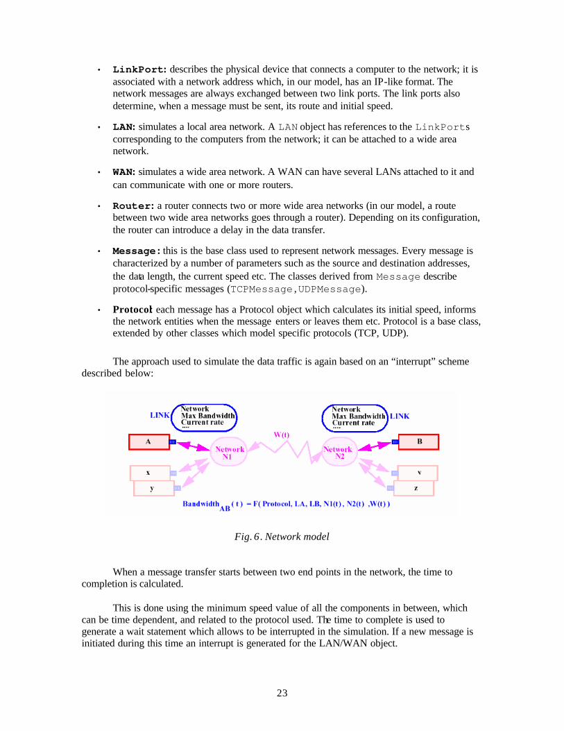
Fig. 6 . Network model
When a message transfer starts between two end points in the network, the time to completion is calculated. This is done using the minimum speed value of all the components in between, which can be time dependent, and related to the protocol used. The time to complete is used to generate a wait statement which allows to be interrupted in the simulation. If a new message is initiated during this time an interrupt is generated for the LAN/WAN object.
24
The speed for each transfer affected by the new one is re-computed, assuming that they are running in parallel and share the bandwidth with weights depending on the protocol. With this new speed the time to complete for all the messages affected is re-evaluated and inserted into the priority queue for futur e events. This approach requires an estimate of the data transfer speed for each component. For a long distance connection an “effective speed” between two points has to be used. This value can be fully time dependent.
This approach for data transfer can provide an effective and accurate way to describe many large and small data transfers occurring in parallel on the same network. This model cannot describe speed variation in the traffic during one transfer if no other transfer starts or finishes. This is a consequence of the fact that we have only discrete events in time. However, by using smaller packages for data transfer, or artificially generating additional interrupts for LAN/WAN objects, the time interval for which the network speed is considered constant can be reduced. As before, this model assumes that the data transfer between time events is done in a continuous way utilizing a certain part of the available bandwidth.
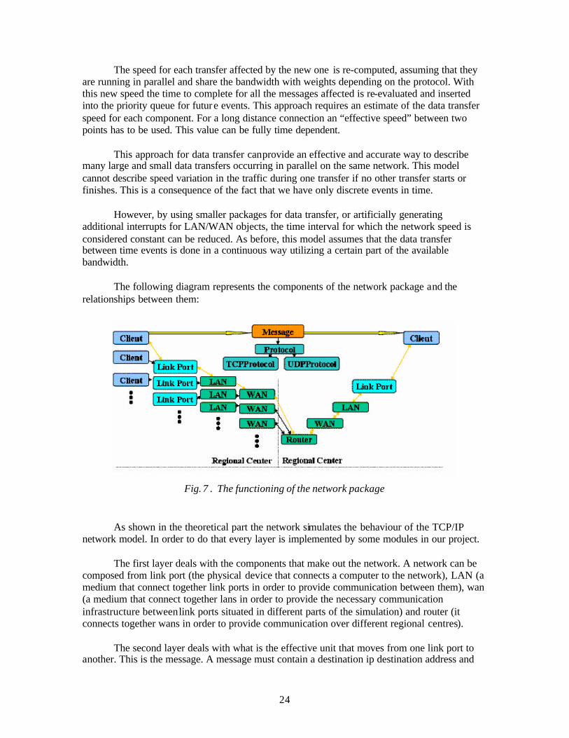
The following diagram represents the components of the network package and the relationships between them:
Fig. 7 . The functioning of the network package
As shown in the theoretical part the network simulates the behaviour of the TCP/IP network model. In order to do that every layer is implemented by some modules in our project.
The first layer deals with the components that make out the network. A network can be composed from link port (the physical device that connects a computer to the network), LAN (a medium that connect together link ports in order to provide communication between them), wan (a medium that connect together lans in order to provide the necessary communication infrastructure between link ports situated in different parts of the simulation) and router (it connects together wans in order to provide communication over different regional centres).
The second layer deals with what is the effective unit that moves from one link port to another. This is the message. A message must contain a destination ip destination address and
25
has a source ip destination address). The message if effectively moved by the means of events. The event is moved between tasks, which in term contains inside a network message. The network message also contain inside data that are carried. Some other parameters such as message length are used in order to provide a mean by which the message time to arrival will be computed. Also the message can take out parameters (such as the time it took in order to arrive at the destination or the bandwidth that occupies) for the output clients.
The third layer deals with the way the message moves through the network. This is
implemented by the Protocol. In the project there were implemented two kinds of transport protocols. Those are TCPProtocol and UDPProtocol. The protocol moves the message from one task from its route to the next until the destination is reached. The way in which the message is moved is the actual way in which the given protocol functions in the real world. That is, for the tcp protocol for instance, the message is first fragmented, then each part is given to the next task after a delay that is computed based on the size of fragment and the bandwidth available. Then, after a number of fragments the protocol sends back an acknowledgement in order to simulate the windowing problem described in the theoretical chapter. The fourth layer is represented by the applications that use the network communication that is the jobs that implements the sending and receiving of messages.
In the following we will describe in more detail the basic units presented above.
The link port is the entity that received and sends messages. Every message is exchange only between the link ports. Also every entity involved in the simulation has a network link port (interface) attached to it in order to practically participate in the network simulation.
Every link port is unique through the ip address of it. So, if a job says he wants to send a message to a given address, there is only one link port that will receive the message. But in the simulation a special kind of addressing was provided. A link port can also be described by the unit to which he is attached. Also, in order to provide more dynamism the addresses of the link ports are allowed not to be unique, in which case the message will be sent to the closer to the sender found link port.
2.8. Job Scheduling and Execution
The jobs are submitted to the regional centres by the Activity classes, which instantiate
Job objects and send them to the centre via the addJob() method. At the moment of (simulated) time when an activity calls addJob(), the regional centre’s farm receives an event associated with the new job, and sends the job to the job scheduler.
The job scheduler first tries to find an available CPU unit to execute the job. The job might need to be executed on a specific CPU unit, and in this case the scheduler doesn’t search anymore – it knows exactly where to send it. Otherwise, the scheduler takes a decision according to the strategy it implements. The basic scheduler sends the job on the CPU unit with the minimum load (by load we understand the total amount of memory used by the jobs that are already running on the CPU). A job can be executed on a CPU unit if the memory needed by the job, added with the current load of the CPU, doesn’t exceed the amount of memory that the CPU has. If a CPU was found, the scheduler also looks for an active job (AJob object) to assign
26
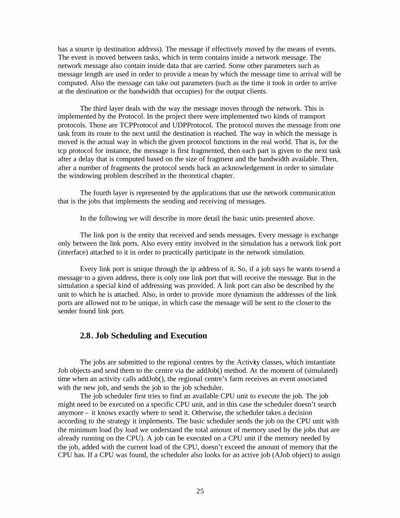
the job to it, the active jobs objects being held in a pool. If there is no CPU or no AJob available, the job is added to a waiting queue, ordered by the jobs' priorities.
When a new job is scheduled on a CPU, the other jobs that are executing on the same CPU are interrupted because the unit's power is reallocated. The jobs (including the new one) estimate the time needed for completion, according to the new amount of power offered by the CPU; then, they wait until a new change of state (beginning/ending of a job) appears, or until the time needed for completion expires (this mechanism is explained in more detail in the next section).
The following diagram represents the process described above, in three steps (job submission, job scheduling and the re-evaluation of the time needed to complete).
Fig. 8. The job Scheduling and execution model
27
3. The simulation of the Proof Cluster
3.1. Introduction
Proof is a facility for distributed data under a Root structure, developed at CERN.
3.2. The Proof parallel model based on ROOT. The CERN perspective
The LHC experiments begun at CERN were challenges for the old systems used until then, because in these experiments, the data quantities that followed to be simulated and analysed are with a few magnitudes grater than what was seen before.
The ROOT project was developed in the NA49 experiment context at CERN. It generated impressive data quantitie s, of approximately 10 TB of raw data on a run. So, the NA 49 experiment is the ideal development and testing medium of the new generation of tools of study of these data quantities.
The ROOT system offers a set of object oriented medium, with all the necessary functionality to handle the analysing of large quantities of data in a very efficient way. Having the data organised as a set of objects, there are used specialized methods of stocking, to have a direct access to separate attributes of the selected objects, without any need to analyse the pure data. There are included histogram methods in 1, 2, or 3 dimensions, function evaluations, minimisations, graphics and visualisation classes, which to offer a system analysis to process the data. From the CERN point of view, the development of the ROOT Parallel Facility, Proof, permits a physician to analyse much larger sets on a much smaller scale time. Root uses the event parallelism and implements an architecture that optimises the I/O and the CPU utilisation in heterogenic clusters with distributed stocking mechanisms. The system offers transparent and interactive access at Giga-bytes level. Proof is an extension of the ROOT system, which makes possible the analysis of a vast set of ROOT files, in parallel on remote computer clusters (which lie at large geographical distances from one another). The main purposes for the Proof systems are:
- transparency - scalability - adaptability
Through transparency it can be understood that it must be a as small as possible difference between a local ROOT session and a parallel remote PROOF session, both of them to be interactive, and to give the same results.
Through scalability it is understood that the base architecture should not require any implied limitation on the number of computers that may be used in parallel.
Through adaptability it can be understood that the system must be capable to adapt to the variations of the remote environment (the networks interrupts, the switching of the load in the cluster nodes).

28
Being an extension of the ROOT system, PROOF is designated to work on ROOT type objects. Being a logical extension of the ROOT system, PROOF is designated to work on ROOT type objects. Through the logical grouping of many ROOT type files in only one very big object, there may be created data sets. In a local cluster environment, these data can be distributed on the disks of the cluster nodes, or made available through a NAS or SAN type solution.
In the close future, through the usage of Grid technologies, it is scheduled the Proof extension from unique clusters to virtual global clusters. In such an environment, the processing can take more, un-interactive, but the user will be presented only one result, as if the processing be made locally.
3.3. The Proof System (made at CERN) Architecture
The Proof consists in a 3 level architecture: - The ROOT client session - The Master Proof server - The Slave Proof servers The user connects from his ROOT session to a Master slave, on a remote distributed
cluster, and the master server, in his turn, creates slave servers on all the cluster nodes. The inquiries are processed in parallel by all the slave servers.
Using a certain protocol, the slave servers ask the master for packages with what they have to do, and this permits the master to distribute the packages to every slave server. The slower slaves take smaller work packages, while the fast ones process more packages.
In this scheme, the parallel processing performance is a function of the duration of each job, packet, and depends also by the available bandwidth and network latency. Because the bandwidth and the latency of a cluster are fixed, the main parameter that may be adjusted in this scheme is the dimension of the package. If the dimension of the package is chos en too small, the parallelism will suffer, as too many packages are sent over the network, between the master and slave servers. If the dimension of the package is too big, then the effect of the difference in performance of each node is not balanced enough.
This allows to the Proof system to adapt itself at the performance and load on each individual cluster node, and to optimize the job execution time.
3.4. The Architecture and premises of Proof simulation
3.4.1. The Architecture
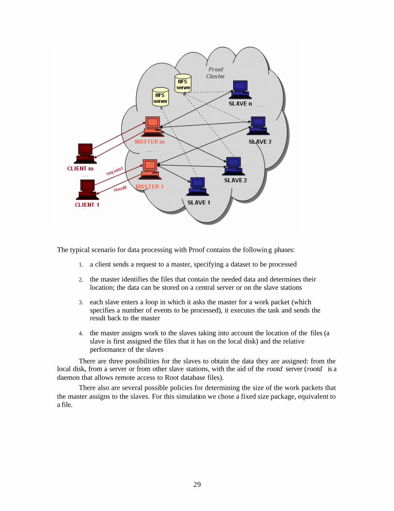
A Proof configuration consists of several clusters; the computers from a cluster run master and slave processes, as the following diagram shows in detail, which presents a possible Proof architecture:
29
The typical scenario for data processing with Proof contains the followin g phases:
1. a client sends a request to a master, specifying a dataset to be processed
2. the master identifies the files that contain the needed data and determines their location; the data can be stored on a central server or on the slave stations
3. each slave enters a loop in which it asks the master for a work packet (which specifies a number of events to be processed), it executes the task and sends the result back to the master
4. the master assigns work to the slaves taking into account the location of the files (a slave is first assigned the files that it has on the local disk) and the relative performance of the slaves
There are three possibilities for the slaves to obtain the data they are assigned: from the local disk, from a server or from other slave stations, with the aid of the rootd server (rootd is a daemon that allows remote access to Root database files).
There also are several possible policies for determining the size of the work packets that the master assigns to the slaves. For this simulation we chose a fixed size package, equivalent to a file.
30
3.4.2. The example description
The simulated scenario is based on the one described above:
• the working cluster contains n master stations, m slave stations and s data servers (we tested with n=20 and m=500, and with different values for s)
• each master receives a data processing request from a client; we assumed that the client needs to process a set of files with the same length, containing analysis data for a certain number of events. We also tested some cases in which the clients repeatedly send requests to the masters, with pause intervals between requests.
• when asking the master for work, a slave is assigned one file which is assumed to be available on the slave's local disk with a certain probability; if not available, the file is taken from a data server
• it was assumed that the master takes some time to handle a work request from a slave and to process the partial results returned by a slave; if there are several slaves that send work requests or partial results at the same time, their messages will be processed by the master sequentially
The behaviour of the system was studied by varying several parameters such as:
• the number of slave processes created by each master (on a slave station there can be more than one slave process; in our test cases, the minimum number of processes on a slave station was 1, corresponding to 25 slave processes created by each master - as we have 20 masters and 500 slave nodes)
• the probability of having the data on the local disk at the slave nodes
• the LAN bandwidth
• the number of data servers available in the cluster
3.4.3. The actual implementation
The implementation of the simulation is achieved in the following classes: -ActivityCaltech , where for each Caltech Client it is requested the respective master to take the work and assign them to the slaves. In is then waited the answer form the JobMasterCollector with the results. -ActivityCern , where the masters create MasterJob objects that send the data to the slaves, and JobMasterCollect objects, that receive the processed data back from the slaves. -The JobMasterCollect receive the processed data back from the slaves, and then send it to the Caltech Clients. -The JobMaster, that creates the JobServer for the servers to function, creates the JobMasterCollect objects, and sends them their addresses, and sends the data to the JobSlaves. -The JobServer, which waits the requests for files from the clients, and then sends them the requested files.
31
-The JobS lave objects, that receives the data from the masters, if they need data from the file servers, then they request it, wait the answer from the Servers , process the data, and then send the results to the JobMasterCollector entities.
3.4.4. The Two different Scheduling Variants
We have implemented two different scheduling variants of the way the master chooses the files to give to the servers that requests work from them. Let us take the two cases. We have clients in the Caltech regional centre that give work to the masters in the CERN regional Centre. Each master has his own slaves to give them work. The slaves, when they are free (do not have anything to do) request work from the masters. The works consists in the processing of some files. The files are processed in some way by the servers (it does not matter what processing is done). The files, numbered from 1 to numberOfFiles can be found on the local disk of the slave that has to do the processing, or it is not found, and then, the slave has to take it through the network from a database server that has all the files. The two scheduling variants differ exactly in the manner the master gives work to the slaves, depending on what they have or not on the local disk. 1. The random variant of scheduling – The files numbers do not count. The masters have events to give to the slave to deal with (events are parts of the files, that are given to the slaves for processing). The master pure and simply randomly generate a number between 0 and 1 and if the number is smaller than a parameter read from the configuration file: localDataProbability, then it will consider that the data file will be found on the slave disk. Else the file is taken from the local file server. This a good policy for the simulation, but a rather simple scheduling policy 2. The variant corresponding to the reality scheduling variant – There are numberOfFiles files that can be given to the slaves. Initially, on the master, for every slave it is retained the list of files existent on the local disk, in a Hashtable. Then, when a slave requests from the master to work, it is first searched in his list of files from the local disk, and if there is any file not processed and available on its local disk, the file is given to the slave for work. Else there will be generated a request for the data file server from the slaves. This is a more realistic scheduling policy.
3.4.5. The results
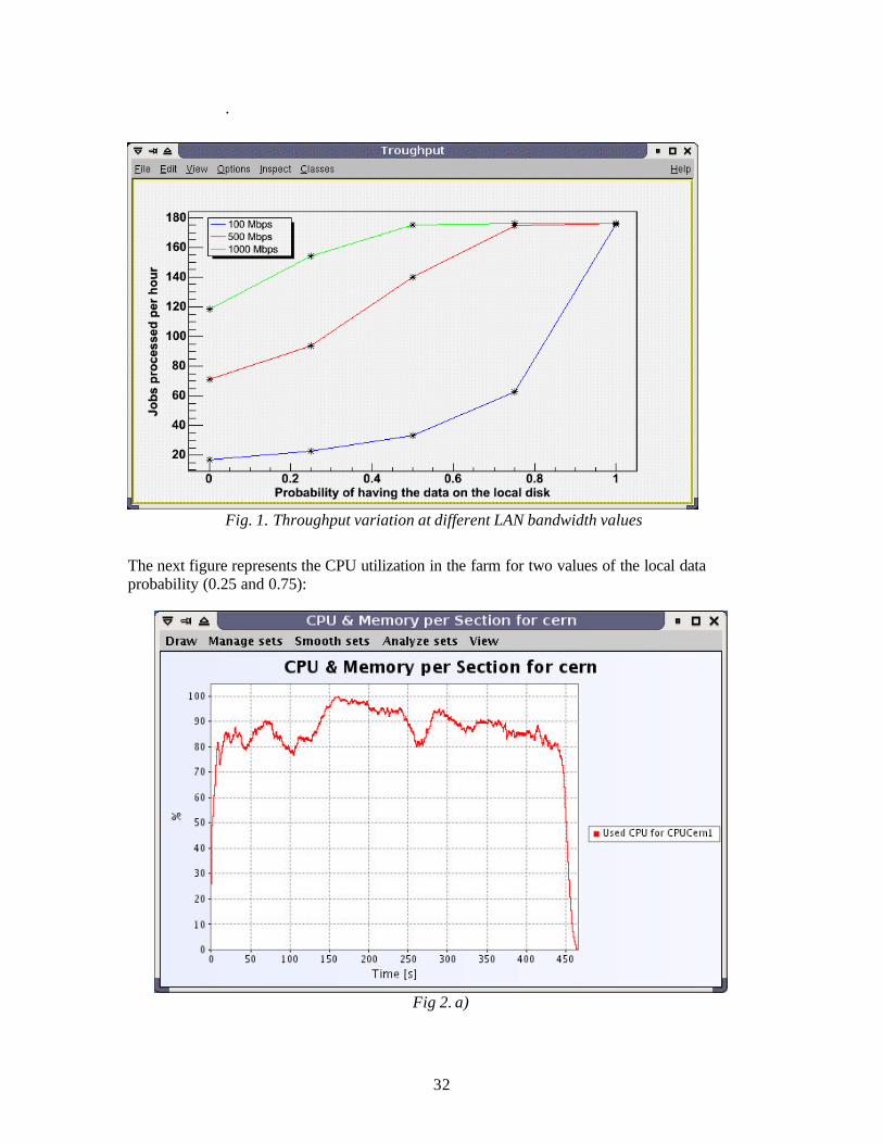
3.4.5.1. The Influence of the LAN Bandwidth The improvement of the LAN bandwidth has the effect of increasing the throughput (computed as number of jobs processed per hour). For this series of simulations, we assumed that the cluster has 2 data servers and each master creates 50 slave processes.
The LAN bandwidth was given the values of 100Mbps, 500Mbps and 1Gbps. As shown in Fig. 2, with a 100Mbps network we don't obtain an acceptable throughput when more than a half of the data files are taken from the network.
32
.
Fig. 1. Throughput variation at different LAN bandwidth values The next figure represents the CPU utilization in the farm for two values of the local data probability (0.25 and 0.75):
Fig 2. a)
33
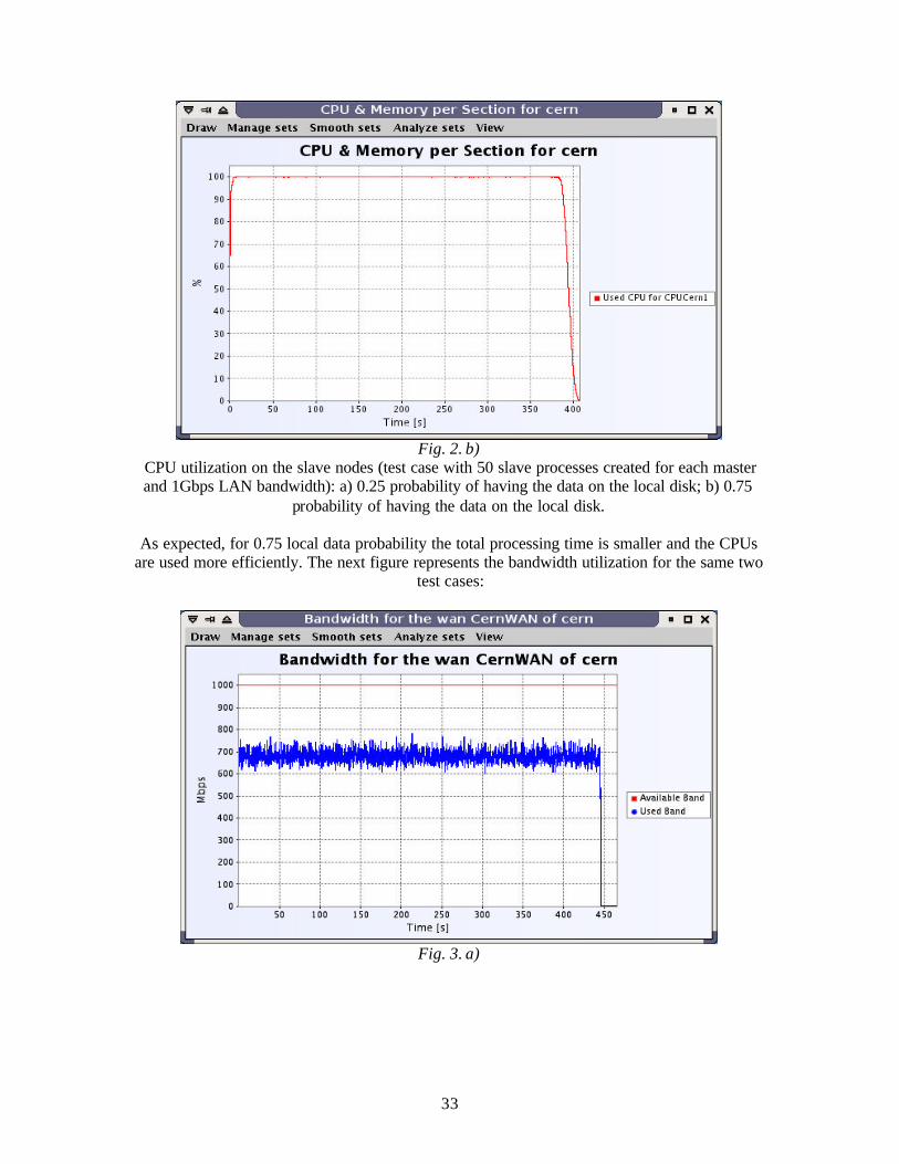
Fig. 2. b)
CPU utilization on the slave nodes (test case with 50 slave processes created for each master and 1Gbps LAN bandwidth): a) 0.25 probability of having the data on the local disk; b) 0.75
probability of having the data on the local disk.
As expected, for 0.75 local data probability the total processing time is smaller and the CPUs are used more efficiently. The next figure represents the bandwidth utilization for the same two
test cases:
Fig. 3. a)
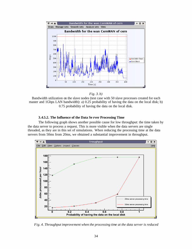
34
Fig. 3. b) Bandwidth utilization on the slave nodes (test case with 50 slave processes created for each
master and 1Gbps LAN bandwidth): a) 0.25 probability of having the data on the local disk; b) 0.75 probability of having the data on the local disk.
3.4.5.2. The Influence of the Data Se rver Processing Time The following graph shows another possible cause for low throughput: the time taken by
the data server to process a request. This is more visible when the data servers are single threaded, as they are in this set of simulations. When reducing the processing time at the data servers from 50ms from 20ms, we obtained a substantial improvement in throughput.
Fig. 4. Throughput improvement when the processing time at the data server is reduced
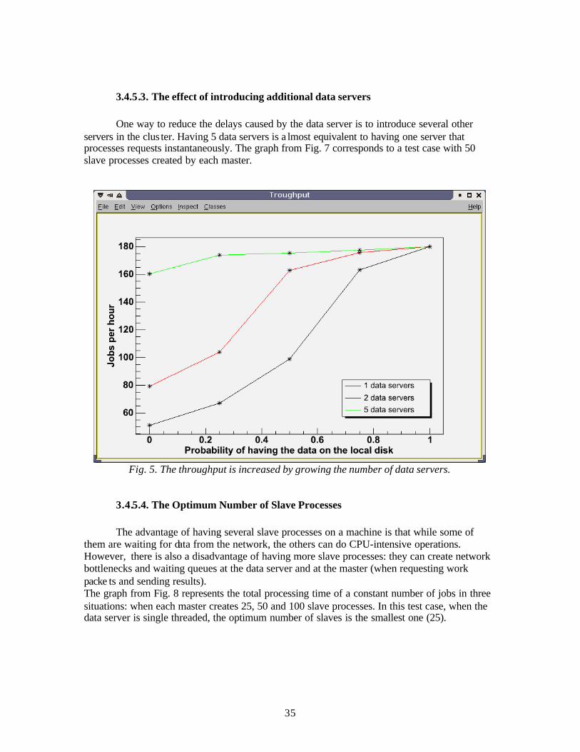
35
3.4.5.3. The effect of introducing additional data servers
One way to reduce the delays caused by the data server is to introduce several other servers in the clus ter. Having 5 data servers is a lmost equivalent to having one server that processes requests instantaneously. The graph from Fig. 7 corresponds to a test case with 50 slave processes created by each master.
Fig. 5. The throughput is increased by growing the number of data servers.
3.4.5.4. The Optimum Number of Slave Processes
The advantage of having several slave processes on a machine is that while some of them are waiting for data from the network, the others can do CPU-intensive operations. However, there is also a disadvantage of having more slave processes: they can create network bottlenecks and waiting queues at the data server and at the master (when requesting work packe ts and sending results). The graph from Fig. 8 represents the total processing time of a constant number of jobs in three situations: when each master creates 25, 50 and 100 slave processes. In this test case, when the data server is single threaded, the optimum number of slaves is the smallest one (25).
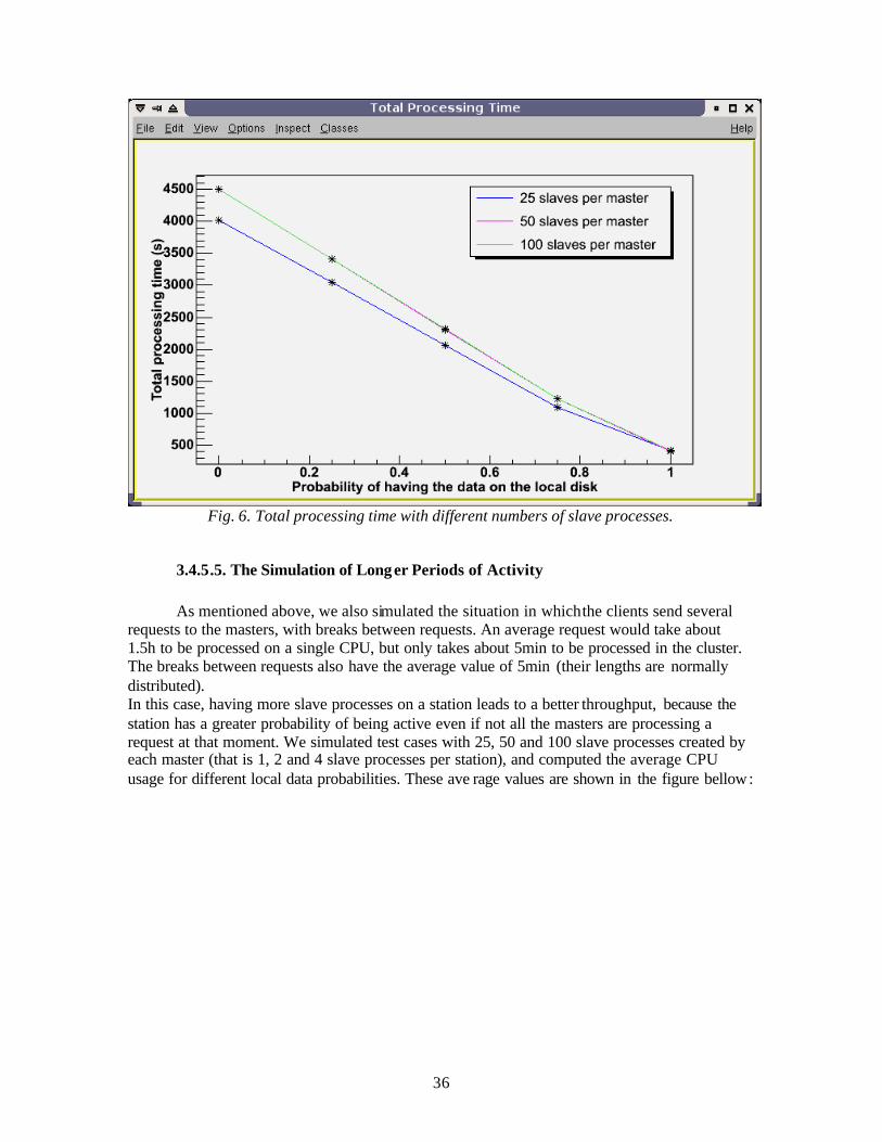
36
Fig. 6. Total processing time with different numbers of slave processes.
3.4.5.5. The Simulation of Longer Periods of Activity
As mentioned above, we also simulated the situation in which the clients send several requests to the masters, with breaks between requests. An average request would take about 1.5h to be processed on a single CPU, but only takes about 5min to be processed in the cluster. The breaks between requests also have the average value of 5min (their lengths are normally distributed). In this case, having more slave processes on a station leads to a better throughput, because the station has a greater probability of being active even if not all the masters are processing a request at that moment. We simulated test cases with 25, 50 and 100 slave processes created by each master (that is 1, 2 and 4 slave processes per station), and computed the average CPU usage for different local data probabilities. These ave rage values are shown in the figure bellow:
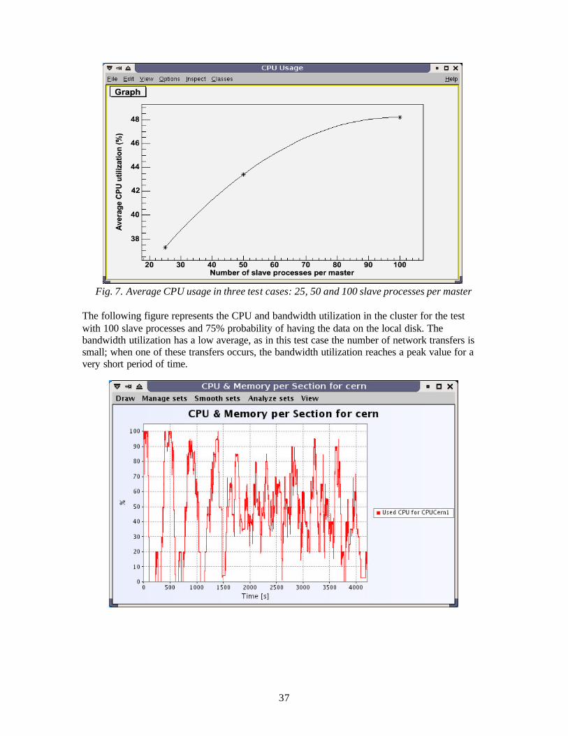
37
Fig. 7. Average CPU usage in three test cases: 25, 50 and 100 slave processes per master
The following figure represents the CPU and bandwidth utilization in the cluster for the test with 100 slave processes and 75% probability of having the data on the local disk. The bandwidth utilization has a low average, as in this test case the number of network transfers is small; when one of these transfers occurs, the bandwidth utilization reaches a peak value for a very short period of time.
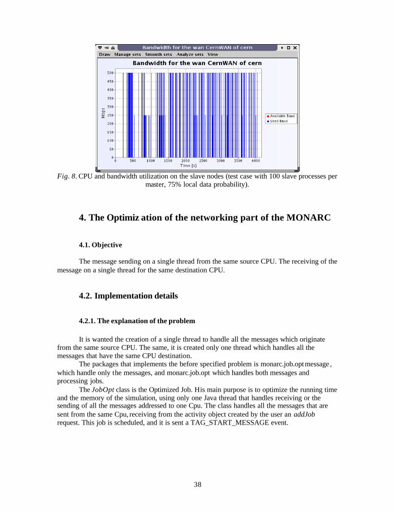
38
Fig. 8. CPU and bandwidth utilization on the slave nodes (test case with 100 slave processes per
master, 75% local data probability).
4. The Optimiz ation of the networking part of the MONARC
4.1. Objective
The message sending on a single thread from the same source CPU. The receiving of the message on a single thread for the same destination CPU.
4.2. Implementation details
4.2.1. The explanation of the problem It is wanted the creation of a single thread to handle all the messages which originate from the same source CPU. The same, it is created only one thread which handles all the messages that have the same CPU destination. The packages that implements the before specified problem is monarc.job.opt message , which handle only the messages, and monarc.job.opt which handles both messages and processing jobs. The JobOpt class is the Optimized Job. His main purpose is to optimize the running time and the memory of the simulation, using only one Java thread that handles receiving or the sending of all the messages addressed to one Cpu. The class handles all the messages that are sent from the same Cpu, receiving from the activity object created by the user an addJob request. This job is scheduled, and it is sent a TAG_START_MESSAGE event.
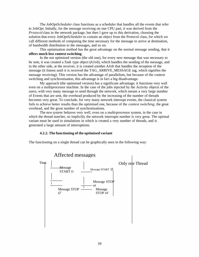
39
The JobOptScheduler class functions as a scheduler that handles all the events that refer to JobOpt. Initially, for the message receiving on one CPU part, it was derived from the Protocol class in the network package, but then I gave up to this derivation, choosing the solution that every JobOptScheduler to contain an object from the Protocol class, for which we call different methods of computing the time necessary for the message to arrive at destination, of bandwidth distribution to the messages, and so on. This optimisation method has the great advantage on the normal message sending, that it offers much less context switching .
In the not optimized version (the old one), for every new message that was necessary to be sent, it was created a Task type object (AJob), which handles the sending of the message, and in the other side, at the receiver, it is created another AJob that handles the reception of the message (it listens until it is received the TAG_ARRIVE_MESSAGE tag, which signifies the message receiving). This version has the advantage of parallelism, but because of the context switching and synchronisation, this advantage is in fact a big disadvantage. My approach (the optimised version) has a significant advantage; it functions very well even on a multiprocessor machine. In the case of the jobs injected by the Activity objects of the users, with very many message to send through the network, which means a very large number of Events that are sent, the overhead produced by the increasing of the number of threads becomes very great. To conclude, for very many network interrupt events, the classical system fails to achieve better results than the optimised one, because of the context switching, the great overhead, and the great number of synchronisations. The new system behaves very well, even on a multi-processor system, in the case in which the thread number, so implicitly the network interrupts number is very great. The optimal variant must be used in simulations in which is created a very number of threads, and is generated a large amount of interruptions.
4.2.2. The functioning of the optimised variant The functioning on a single thread can be graphically seen in the following way:
Message START t1
Time
Affected messages
Message STOP t2’
Message START t3
Message STOP t4
Message STOP t4’
Only one Thread
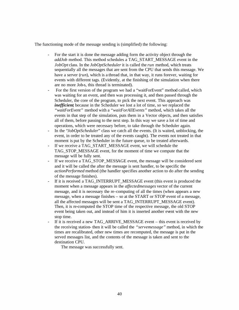
40
The functioning mode of the message sending is (simplified) the following:
- For the start it is done the message adding form the activity object through the addJob method. This method schedules a TAG_START_MESSAGE event in the JobOpt class. In the JobOptScheduler it is called the run method, which treats sequentially all the messages that are sent from the CPU that sends this message. We have a server (run), which is a thread that, in that way, it runs forever, waiting for events with different tags. (Evidently, at the finishing of the simulation when there are no more Job-s, this thread is terminated).
- For the first version of the program we had a “waitForEvent” method called, which was waiting for an event, and then was processing it, and then passed through the Scheduler, the core of the program, to pick the next event. This approach was inefficient, because in the Scheduler we lost a lot of time, so we replaced the “waitForEvent” method with a “waitForAllEvents” method, which takes all the events in that step of the simulation, puts them in a Vector objects, and then satisfies all of them, before passing to the next step. In this way we save a lot of time and operations, which were necessary before, to take through the Scheduler again.
- In the “JobOptScheduler” class we catch all the events. (It is waited, unblocking, the event, in order to be treated any of the events caught). The events not treated in that moment is put by the Scheduler in the future queue, to be treated afterwards.
- If we receive a TAG_START_MESSAGE event, we will schedule the TAG_STOP_MESSAGE event, for the moment of time we compute that the message will be fully sent.
- If we receive a TAG_STOP_MESSAGE event, the message will be considered sent and it will be called the after the message is sent handler, to be specific the actionPerformed method (the handler specifies another action to do after the sending of the message finishes).
- If it is received a TAG_INTERRUPT_MESSAGE event (this event is produced the moment when a message appears in the affectedmessages vector of the current message, and it is necessary the re-computing of all the times (when appears a new message, when a message finishes – so at the START or STOP event of a message, all the affected messages will be sent a TAG_INTERRUPT_MESSAGE event). Then, it is re-computed the STOP time of the respective message, the old STOP event being taken out, and instead of him it is inserted another event with the new stop time.
- If it is received a new TAG_ARRIVE_MESSAGE event – this event is received by the receiving station- then it will be called the “servemessage” method, in which the times are recalibrated, other new times are recomputed, the message is put in the served messages list, and the contents of the message is taken and sent to the destination CPU.
The message was successfully sent.
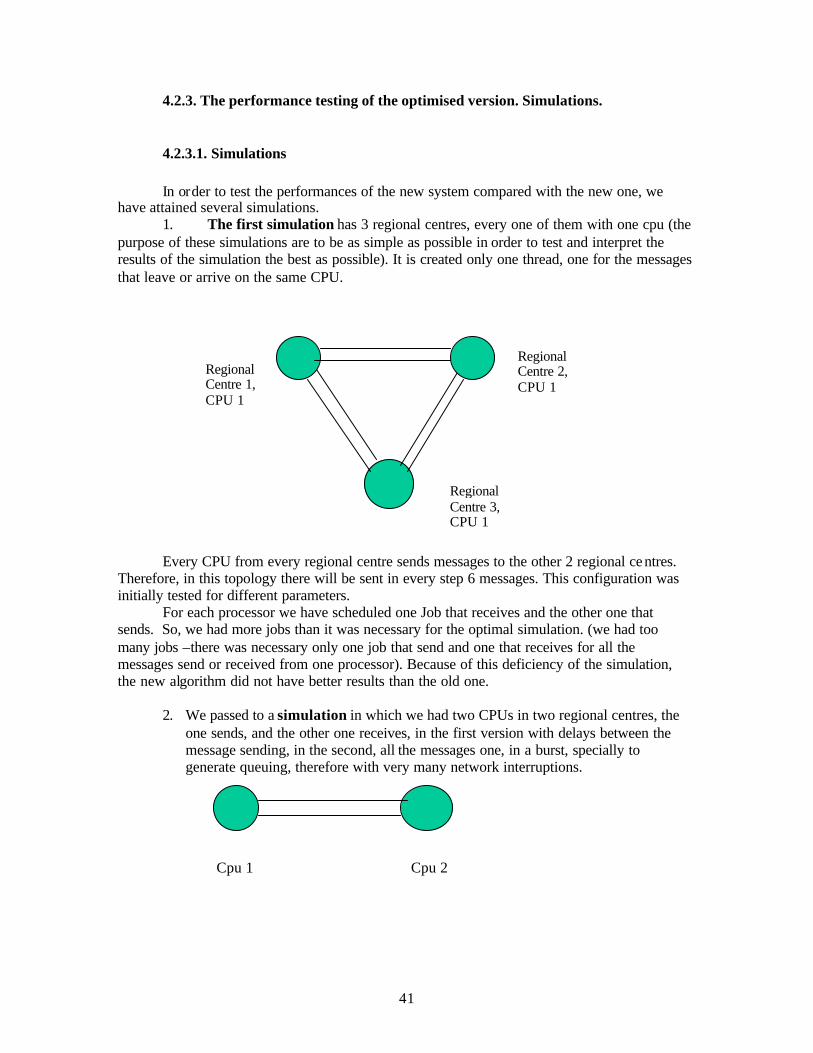
41
4.2.3. The performance testing of the optimised version. Simulations.
4.2.3.1. Simulations
In order to test the performances of the new system compared with the new one, we have attained several simulations.
1. The first simulation has 3 regional centres, every one of them with one cpu (the purpose of these simulations are to be as simple as possible in order to test and interpret the results of the simulation the best as possible). It is created only one thread, one for the messages that leave or arrive on the same CPU.
Every CPU from every regional centre sends messages to the other 2 regional ce ntres. Therefore, in this topology there will be sent in every step 6 messages. This configuration was initially tested for different parameters. For each processor we have scheduled one Job that receives and the other one that sends. So, we had more jobs than it was necessary for the optimal simulation. (we had too many jobs –there was necessary only one job that send and one that receives for all the messages send or received from one processor). Because of this deficiency of the simulation, the new algorithm did not have better results than the old one.
2. We passed to a simulation in which we had two CPUs in two regional centres, the one sends, and the other one receives, in the first version with delays between the message sending, in the second, all the messages one, in a burst, specially to generate queuing, therefore with very many network interruptions.
Cpu 1 Cpu 2
Regional Centre 1, CPU 1
Regional Centre 2, CPU 1
Regional Centre 3, CPU 1
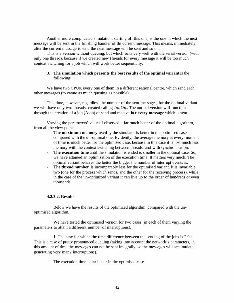
42
Another more complicated simulation, starting off this one, is the one in which the next message will be sent in the finishing handler of the current message. This means, immediately after the current message is sent, the next message will be sent and so on. This is a version without queuing, but which suits very well with the serial version (with only one thread), because if we created new threads for every message it will be too much context switching for a job which will work better sequentially.
3. The simulation which presents the best results of the optimal variant is the following:
We have two CPUs, every one of them in a different regional centre, which send each
other messages (to create as much queuing as possible).
This time, however, regardless the number of the sent messages, for the optimal variant we will have only two threads, created calling JobOpt. The normal version will function through the creation of a job (Ajob) of send and receive fo r every message which is sent. Varying the parameters’ values I observed a far much better of the optimal algorithm, from all the view points.
- The maximum memory used by the simulator is better in the optimised case compared with the un-optimal one. Evidently, the average memory at every moment of time is much better for the optimised case, because in this case it is lost much less memory with the context switching between threads, and with synchronisation.
- The execution time until the simulation is ended is smaller in the optimal case. So, we have attained an optimisation of the execution time. It matters very much. The optimal variant behaves the better the bigger the number of interrupt events is.
- The thread number is incomparably less for the optimised variant. It is invariable two (one for the process which sends, and the other for the receiving process), while in the case of the un-optimized variant it can live up to the order of hundreds or even thousands.
4.2.3.2. Results Below we have the results of the optimized algorithm, compared with the un-
optimised algorithm. We have tested the optimised version for two cases (in each of them varying the
parameters to attain a different number of interruptions). 1. The case for which the time difference between the sending of the jobs is 2.0 s.
This is a case of pretty pronounced queuing (taking into account the network’s parameters, in this amount of time the messages can not be sent integrally, so the messages will accumulate, generating very many interruptions).
The execution time is far better in the optimised case.
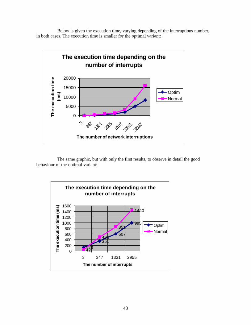
43
The execution time depending on the number of interrupts
129351
607
995
42
496
851
1440
0200400600800
1000120014001600
3 347 1331 2955
The number of interrupts
Th
e ex
ecu
tion
tim
e (m
s)
OptimNormal
The execution time depending on the number of interrupts
0
5000
10000
15000
20000
334
713
3129
5581
0720
611
3214
7
The number of network interruptions
Th
e ex
ecu
tion
tim
e (m
s) OptimNormal
Below is given the execution time, varying depending of the interruptions number, in both cases. The execution time is smaller for the optimal variant:
The same graphic, but with only the first results, to observe in detail the good behaviour of the optimal variant:
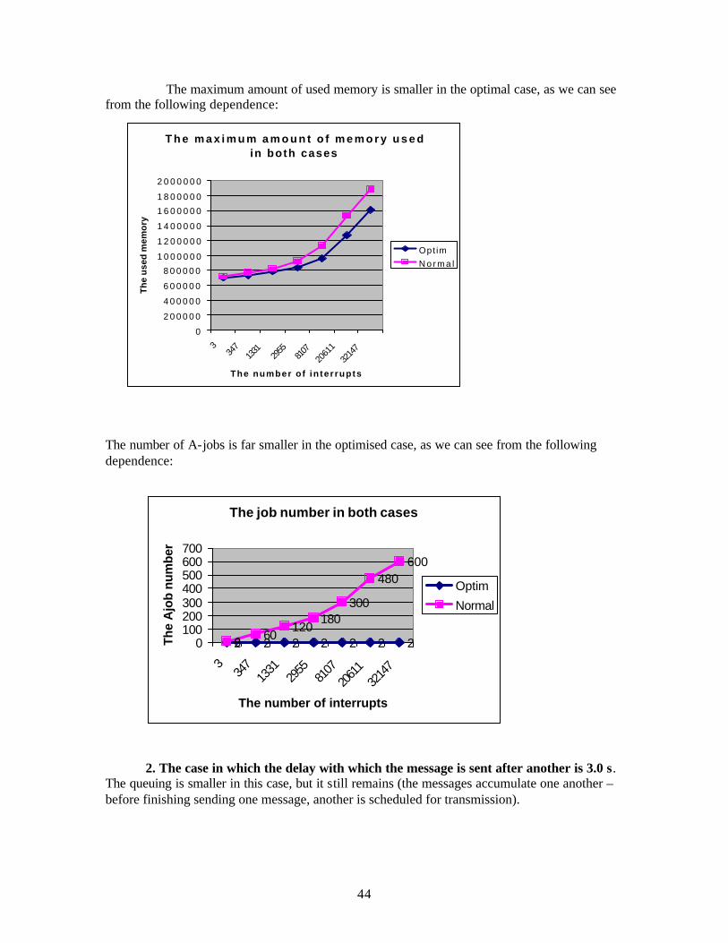
44
The maximum amount of used memory is smaller in the optimal case, as we can see from the following dependence:
The number of A-jobs is far smaller in the optimised case, as we can see from the following dependence:
2. The case in which the delay with which the message is sent after another is 3.0 s. The queuing is smaller in this case, but it still remains (the messages accumulate one another – before finishing sending one message, another is scheduled for transmission).
T h e m a x i m u m a m o u n t o f m e m o r y u s e d in both cases
0
2 0 0 0 0 0
4 0 0 0 0 0
6 0 0 0 0 0
8 0 0 0 0 0
1 0 0 0 0 0 0
1 2 0 0 0 0 0
1 4 0 0 0 0 0
1 6 0 0 0 0 0
1 8 0 0 0 0 0
2 0 0 0 0 0 0
334
713
3129
5581
0720
611
3214
7
The number o f in ter rupts
Th
e u
sed
mem
ory
Opt imN o r m a l
The job number in both cases
2 2 2 2 2 2 26 60120
180300
480600
0100200300400500600700
334
713
3129
5581
0720
611
3214
7
The number of interrupts
The
Ajo
b nu
mbe
r
Optim
Normal
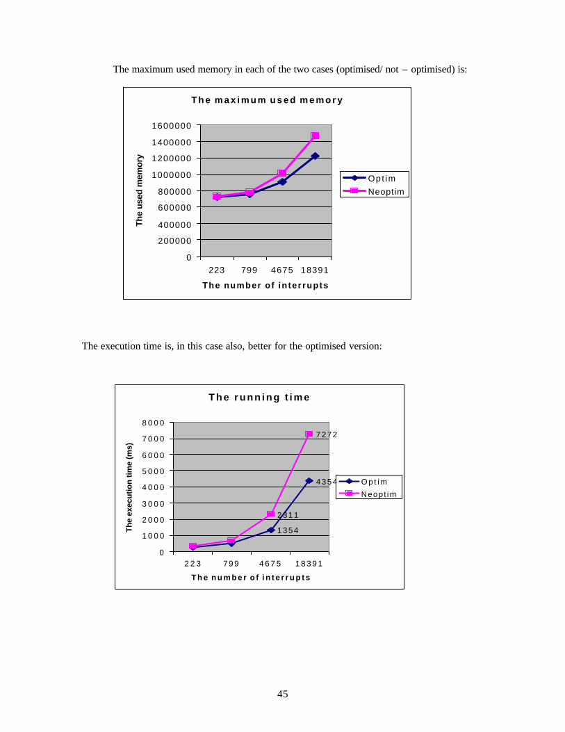
45
T h e m a x i m u m u s e d m e m o r y
0
200000
400000
600000
800000
1000000
1200000
1400000
1600000
223 799 4675 18391
The number of in terrupts
The
used
mem
ory
Opt im
Neoptim
The maximum used memory in each of the two cases (optimised/ not – optimised) is:
The execution time is, in this case also, better for the optimised version:
T h e r u n n i n g t i m e
1 3 5 4
4 3 5 4
2 3 1 1
7 2 7 2
0
1 0 0 0
2 0 0 0
3 0 0 0
4 0 0 0
5 0 0 0
6 0 0 0
7 0 0 0
8 0 0 0
2 2 3 7 9 9 4 6 7 5 1 8 3 9 1
T h e n u m b e r o f i n t e r r u p t s
The
exec
utio
n tim
e (m
s)
O p t i m
Neopt im
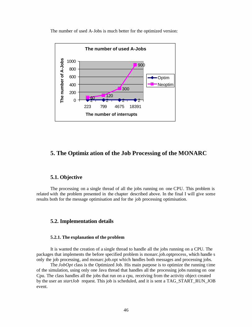
46
The number of used A-Jobs is much better for the optimized version:
5. The Optimiz ation of the Job Processing of the MONARC
5.1. Objective
The processing on a single thread of all the jobs running on one CPU. This problem is related with the problem presented in the chapter described above. In the final I will give some results both for the message optimisation and for the job processing optimisation.
5.2. Implementation details
5.2.1. The explanation of the problem It is wanted the creation of a single thread to handle all the jobs running on a CPU. The packages that implements the before specified problem is monarc.job.optprocess, which handle s only the job processing, and monarc.job.opt which handles both messages and processing jobs. The JobOpt class is the Optimized Job. His main purpose is to optimize the running t ime of the simulation, using only one Java thread that handles all the processing jobs running on one Cpu. The class handles all the jobs that run on a cpu, receiving from the activity object created by the user an startJob request. This job is scheduled, and it is sent a TAG_START_RUN_JOB event.
The number of used A-Jobs
2 2 2 260 120
300
900
0
200
400
600
800
1000
223 799 4675 18391
The number of interrupts
The
num
ber
of A
-Job
s
Optim
Neoptim
47
The JobOptScheduler class functions as a scheduler that handles all the events that refer to JobOpt. This optimisation method has the great advantage on the normal message sending, that it offers much less context switching . In the not optimized version (the old one), for every new job, it was created a Task type object (AJob), which handles the processing. This version has the advantage of parallelism, but because of the context switching and synchronisation, this advantage is in fact a big disadvantage. My approach (the optimised version) has a significant advantage; it functions ve ry well even on a multiprocessor machine. In the case of the jobs injected by the Activity objects of the users, with very many jobs to process for one Cpu, which means a very large number of Events that are sent, the overhead produced by the increasing of the number of threads becomes very great. To conclude, for very many network interrupt events, the classical system fails to achieve better results than the optimised one, because of the context switching, the great overhead, and the great number of synchronisations.
5.2.2. The functioning of the optimised variant The functioning mode of the job processing is (simplified) the following:
- For the start it is done the job adding from the activity object through the startJob method. This method schedules a TAG_START_RUN_JOB event in the JobOpt class. In the “JobOptScheduler” it is called the run method, which treats sequentially all the jobs that will run on the same CPU. We have a server (run), which is a thread that, in that way, it runs forever, waiting for events with different tags. (Evidently, at the finishing of the simulation when there are no more Job-s, this thread is terminated).
- In the “JobOptScheduler” we have a “waitForAllEvents” method, which takes all the events in that step of the simulation, puts them in a Vector objects, and then satisfies all of them, before passing to the next step. In this way we save a lot of time and operations, which were necessary before, to take through the Scheduler again.
- In the “JobOptScheduler” class we catch all the events. (It is waited, unblocking, the event, in order to be treated any of the events caught). The events not treated in that moment is put by the Scheduler in the future queue, to be treated afterwards.
- If we receive a TAG_START_RUN_JOB event, we will schedule the TAG_STOP_RUN_JOB event, for the moment of time we compute that the job will be finished.
- If we receive a TAG_STOP_RUN_JOB event, the job will be considered finished and it will be called the after the job is done handler, and the stopJobProcessng method.
- If it is received a new TAG_CPU_CHANGED event, all the times for the other jobs will be recomputed (estimate dTimeForJob), the old TAG_STOP_RUN_JOB event will be removed from the queue, and the new one will be sent.
The processing job was successfully run on the Cpu.
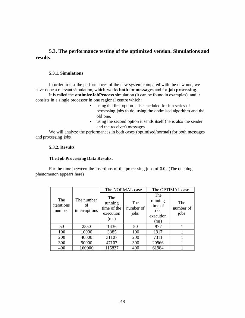
48
5.3. The performance testing of the optimized version. Simulations and results.
5.3.1. Simulations In order to test the performances of the new system compared with the new one, we
have done a relevant simulation, which works both for messages and for job processing. It is called the optimizeJobProcess simulation (it can be found in examples), and it
consists in a single processor in one regional centre which: • using the first option it is scheduled for it a series of
proc essing jobs to do, using the optimised algorithm and the old one.
• using the second option it sends itself (he is also the sender and the receiver) messages.
We will analyze the performances in both cases (optimised/normal) for both messages and processing jobs.
5.3.2. Results
The Job Processing Data Results :
For the time between the insertions of the processing jobs of 0.0 s (The queuing phenomenon appears here)
The NORMAL case The OPTIMAL case
The iterations number
The number of
interruptions
The running
time of the execution
(ms)
The number of
jobs
The running time of
the execution
(ms)
The number of
jobs
50 2550 1436 50 977 1 100 10000 3385 100 1917 1 200 40000 31107 200 7311 1 300 90000 47107 300 20966 1 400 160000 115837 400 61984 1
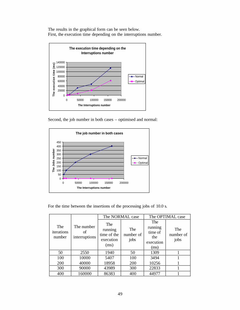
49
The results in the graphical form can be seen below. First, the execution time depending on the interruptions number.
The execution time depending on the Interruptions number
0
2000040000
60000
80000
100000
120000
140000
0 50000 100000 150000 200000
The Interruptions number
The
exec
utio
n ti
me
(ms)
Normal
Optimal
Second, the job number in both cases – optimised and normal:
The job number in both cases
050
100150200250300350400450
0 50000 100000 150000 200000
The Interruptions number
The
Jobs
num
ber
Normal
Optimal
For the time between the insertions of the processing jobs of 10.0 s.
The NORMAL case The OPTIMAL case
The iterations number
The number of
interruptions
The running
time of the execution
(ms)
The number of
jobs
The running time of
the execution
(ms)
The number of
jobs
50 2550 1940 50 1309 1 100 10000 5407 100 3494 1 200 40000 18958 200 10256 1 300 90000 43989 300 22833 1 400 160000 86383 400 44977 1
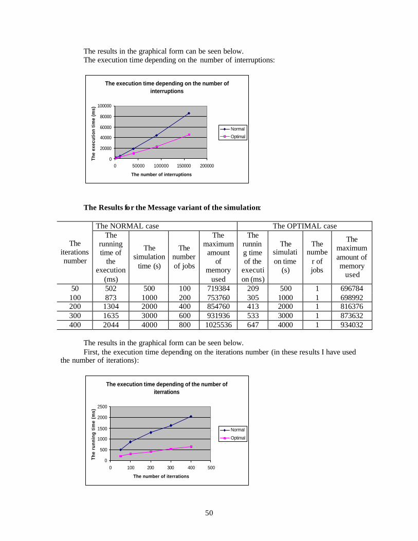
50
The results in the graphical form can be seen below. The execution time depending on the number of interruptions:
The execution time depending on the number of interruptions
0
20000
40000
60000
80000
100000
0 50000 100000 150000 200000
The number of interruptions
The
exec
utio
n ti
me
(ms)
Normal
Optimal
The Results for the Message variant of the simulation:
The NORMAL case The OPTIMAL case
The iterations number
The running time of
the execution
(ms)
The simulation
time (s)
The number of jobs
The maximum
amount of
memory used
The running time of the
execution (ms)
The simulation time
(s)
The numbe
r of jobs
The maximum amount of memory
used
50 502 500 100 719384 209 500 1 696784 100 873 1000 200 753760 305 1000 1 698992 200 1304 2000 400 854760 413 2000 1 816376 300 1635 3000 600 931936 533 3000 1 873632 400 2044 4000 800 1025536 647 4000 1 934032
The results in the graphical form can be seen below.
First, the execution time depending on the iterations number (in these results I have used the number of iterations):
The execution time depending of the number of iterrations
0
500
1000
1500
2000
2500
0 100 200 300 400 500
The number of iterrations
The
runn
ing
tim
e (m
s)
Normal
Optimal
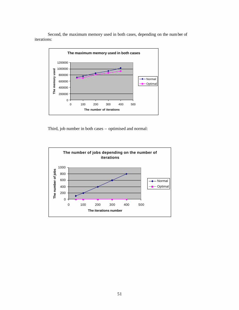
51
Second, the maximum memory used in both cases, depending on the num ber of
iterations:
The maximum memory used in both cases
0
200000
400000
600000
800000
1000000
1200000
0 100 200 300 400 500
The number of iterations
Th
e m
emo
ry u
sed
Normal
Optimal
Third, job number in both cases – optimised and normal:
The number of jobs depending on the number of iterations
0
200
400
600
800
1000
0 100 200 300 400 500
The iterations number
The
num
ber
of jo
bs
Normal
Optimal
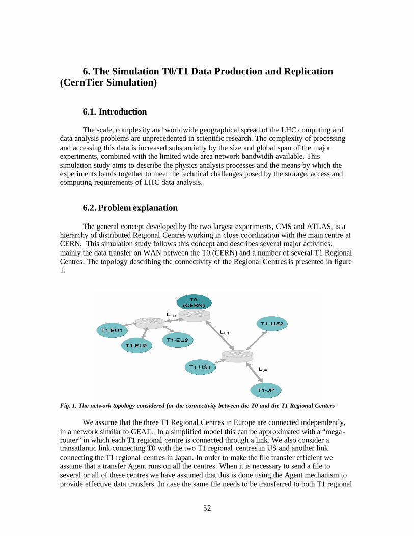
52
6. The Simulation T0/T1 Data Production and Replication (CernTier Simulation)
6.1. Introduction
The scale, complexity and worldwide geographical spread of the LHC computing and data analysis problems are unprecedented in scientific research. The complexity of processing and accessing this data is increased substantially by the size and global span of the major experiments, combined with the limited wide area network bandwidth available. This simulation study aims to describe the physics analysis processes and the means by which the experiments bands together to meet the technical challenges posed by the storage, access and computing requirements of LHC data analysis.
6.2. Problem explanation
The general concept developed by the two largest experiments, CMS and ATLAS, is a hierarchy of distributed Regional Centres working in close coordination with the main centre at CERN. This simulation study follows this concept and describes several major activities; mainly the data transfer on WAN between the T0 (CERN) and a number of several T1 Regional Centres. The topology describing the connectivity of the Regional Centres is presented in figure 1.
Fig. 1. The network topology considered for the connectivity between the T0 and the T1 Regional Centers We assume that the three T1 Regional Centres in Europe are connected independently, in a network similar to GEAT. In a simplified model this can be approximated with a “mega -router” in which each T1 regional centre is connected through a link. We also consider a transatlantic link connecting T0 with the two T1 regional centres in US and another link connecting the T1 regional centres in Japan. In order to make the file transfer efficient we assume that a transfer Agent runs on all the centres. When it is necessary to send a file to several or all of these centres we have assumed that this is done using the Agent mechanism to provide effective data transfers. In case the same file needs to be transferred to both T1 regional
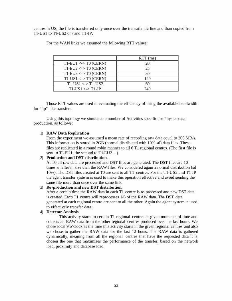
53
centres in US, the file is transferred only once over the transatlantic line and than copied from T1-US1 to T1-US2 or / and T1-JP. For the WAN links we assumed the following RTT values:
RTT (ms) T1-EU1 <-> T0 (CERN) 20 T1-EU2 <-> T0 (CERN) 25 T1-EU3 <-> T0 (CERN) 30 T1-US1 <-> T0 (CERN) 120
T1-US1 <-> T1-US2 60 T1-US1 <-> T1-JP 240
Those RTT values are used in evaluating the efficiency of using the available bandwidth for “ftp” like transfers.
Using this topology we simulated a number of Activities specific for Physics data production, as follows:
1) RAW Data Replication. From the experiment we assumed a mean rate of recording raw data equal to 200 MB/s. This information is stored in 2GB (normal distributed with 10% sd) data files. These files are replicated in a round robin manner to all 6 T1 regional centres. (The first file is sent to T1-EU1, the second to T1-EU2…)
2) Production and DST distribution. At T0 all raw data are processed and DST files are generated. The DST files are 10 times smaller in size than the RAW files. We considered again a normal distribution (sd 10%). The DST files created at T0 are sent to all T1 centres. For the T1-US2 and T1-JP the agent transfer syste m is used to make this operation effective and avoid sending the same file more than once over the same link.
3) Re -production and new DST distribution. After a certain time the RAW data in each T1 centre is re-processed and new DST data is created. Each T1 centre will reprocesses 1/6 of the RAW data. The DST data generated at each regional centre are sent to all the other. Again the agent system is used to effectively transfer data.
4) Detector Analysis. This activity starts in certain T1 regional centres at given moments of time and
collects all RAW data from the other regional centres produced over the last hours. We chose local 9 o’clock as the time this activity starts in the given regional centres and also we chose to gather the RAW data for the last 12 hours. The RAW data is gathered dynamically, meaning from all the regional centres that have the requested data it is chosen the one that maximizes the performance of the transfer, based on the network load, proximity and database load.
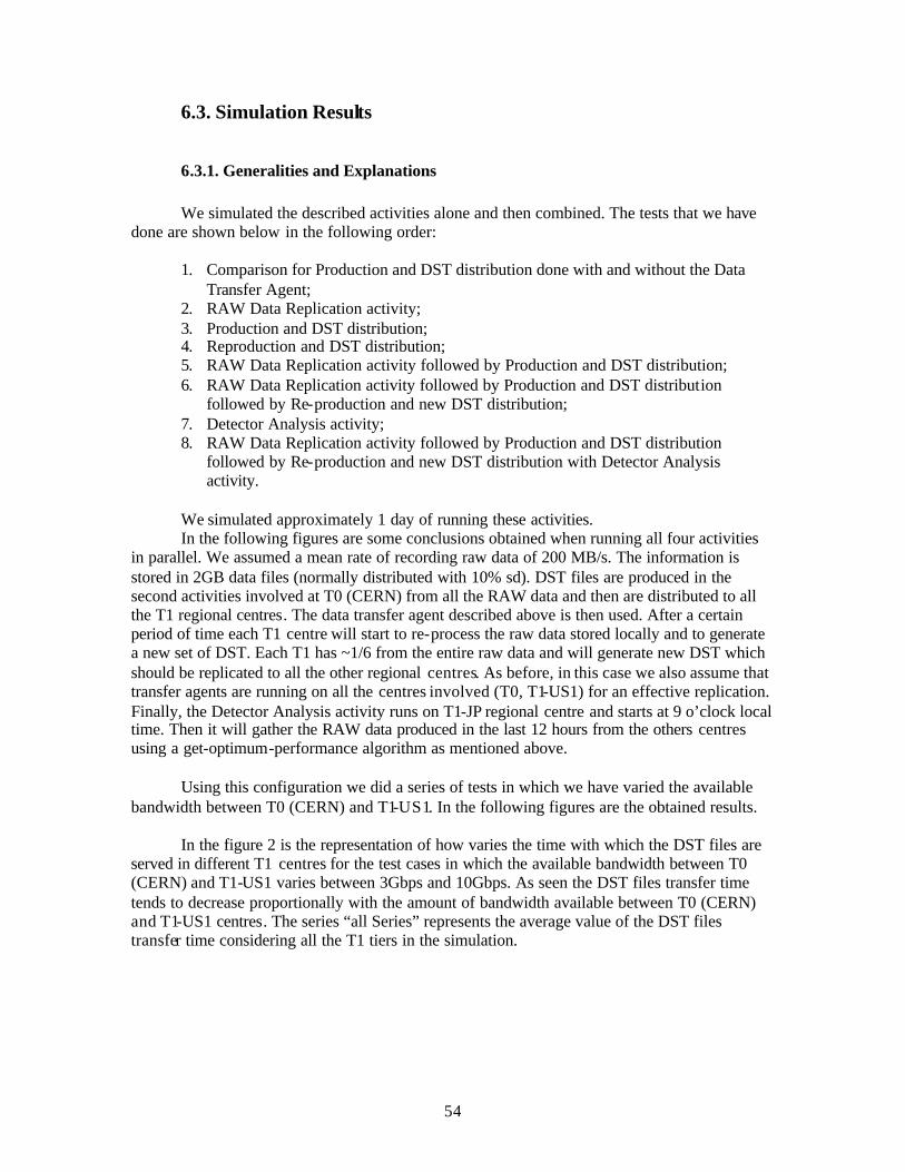
54
6.3. Simulation Results
6.3.1. Generalities and Explanations
We simulated the described activities alone and then combined. The tests that we have done are shown below in the following order:
1. Comparison for Production and DST distribution done with and without the Data Transfer Agent;
2. RAW Data Replication activity; 3. Production and DST distribution; 4. Reproduction and DST distribution; 5. RAW Data Replication activity followed by Production and DST distribution; 6. RAW Data Replication activity followed by Production and DST distribution
followed by Re-production and new DST distribution; 7. Detector Analysis activity; 8. RAW Data Replication activity followed by Production and DST distribution
followed by Re-production and new DST distribution with Detector Analysis activity.
We simulated approximately 1 day of running these activities. In the following figures are some conclusions obtained when running all four activities
in parallel. We assumed a mean rate of recording raw data of 200 MB/s. The information is stored in 2GB data files (normally distributed with 10% sd). DST files are produced in the second activities involved at T0 (CERN) from all the RAW data and then are distributed to all the T1 regional centres. The data transfer agent described above is then used. After a certain period of time each T1 centre will start to re-process the raw data stored locally and to generate a new set of DST. Each T1 has ~1/6 from the entire raw data and will generate new DST which should be replicated to all the other regional centres. As before, in this case we also assume that transfer agents are running on all the centres involved (T0, T1-US1) for an effective replication. Finally, the Detector Analysis activity runs on T1-JP regional centre and starts at 9 o’clock local time. Then it will gather the RAW data produced in the last 12 hours from the others centres using a get-optimum-performance algorithm as mentioned above.
Using this configuration we did a series of tests in which we have varied the available
bandwidth between T0 (CERN) and T1-US1. In the following figures are the obtained results. In the figure 2 is the representation of how varies the time with which the DST files are
served in different T1 centres for the test cases in which the available bandwidth between T0 (CERN) and T1-US1 varies between 3Gbps and 10Gbps. As seen the DST files transfer time tends to decrease proportionally with the amount of bandwidth available between T0 (CERN) and T1-US1 centres. The series “all Series” represents the average value of the DST files transfer time considering all the T1 tiers in the simulation.
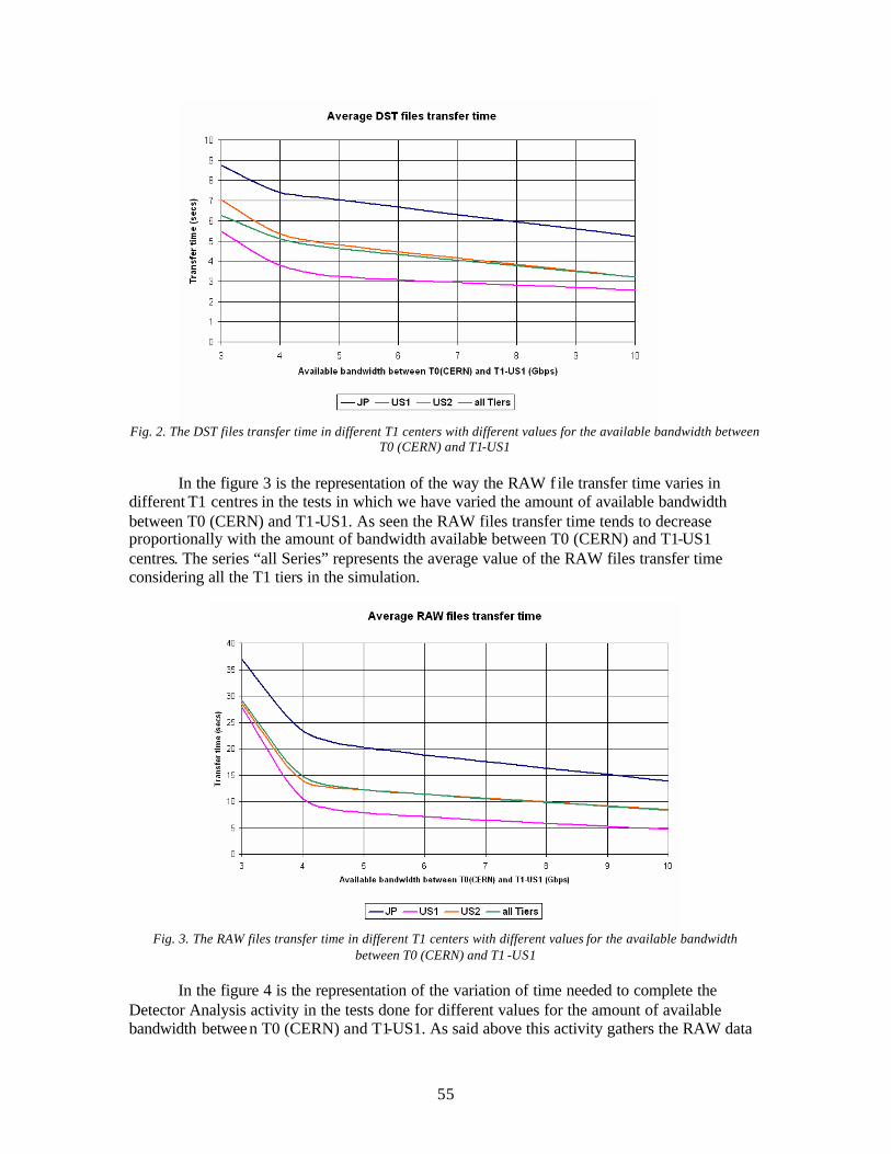
55
Fig. 2. The DST files transfer time in different T1 centers with different values for the available bandwidth between
T0 (CERN) and T1-US1
In the figure 3 is the representation of the way the RAW f ile transfer time varies in different T1 centres in the tests in which we have varied the amount of available bandwidth between T0 (CERN) and T1-US1. As seen the RAW files transfer time tends to decrease proportionally with the amount of bandwidth available between T0 (CERN) and T1-US1 centres. The series “all Series” represents the average value of the RAW files transfer time considering all the T1 tiers in the simulation.
Fig. 3. The RAW files transfer time in different T1 centers with different values for the available bandwidth
between T0 (CERN) and T1 -US1 In the figure 4 is the representation of the variation of time needed to complete the Detector Analysis activity in the tests done for different values for the amount of available bandwidth between T0 (CERN) and T1-US1. As said above this activity gathers the RAW data
56
from the last 12 hours, but as seen here when using a 3Gbps link it takes almost 24 hours to finish, while when using a 10Gbps link between T0 (CERN) and T1-US1 it takes around 15 hours to finish.
Fig. 4. Time needed for the Detector Analysis activity to finish for the tests done centers with different values for
the available bandwidth between T0 (CERN) and T1 -US1
6.3.2. Results
6.3.2.1. Comparison for Production and DST distribution done with and without the Data Transfer Agent
In the first series of tests we tried to see the role of the Data Transfer Agent in the simulated activities. For that we have simulated the Production and DST distribution activity test first using the Data Transfer Agent and then without using it and compare the obtained results. In the Production and DST distribution activity test at T0 (CERN) regional centre are produced DST files from the recorded RAW data, which are then distributed to all the T1 regional centres. The Data Transfer Agent is used on the T1-US1 regional centre and will forward the DST data received in that centre from T0 (CERN) further to T1-US2 and T1-JP regional centres (see figure 1). This means that at T0 (CERN) when using t he Data Transfer Data the DST files will be sent only to T1-EU regional centres and to T1-US1, while the agent will handle the further transfer of those files from T1-US1 to the rest of the regional centres. For the average used bandwidth on the major links the obtained results are shown in figures 5 and 6. As seen the average bandwidth used on the CERN link is greater when we do not use the Data Transfer Agent since more data get transferred from that regional centre.
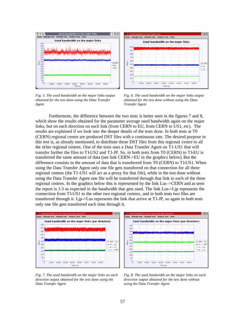
57
Fig. 5. The used bandwidth on the major links output obtained for the test done using the Data Transfer Agent
Fig. 6. The used bandwidth on the major links output obtained for the test done without using the Data Transfer Agent
Furthermore, the difference between the two tests is better seen in the figures 7 and 8, which show the results obtained for the parameter average used bandwidth again on the major links, but on each direction on each link (from CERN to EU, from CERN to US1, etc). The results are explained if we look into the deeper details of the tests done. In both tests at T0 (CERN) regional centre are produced DST files with a continuous rate. The desired purpose in this test is, as already mentioned, to distribute those DST files from this regional centre to all the other regional centres. One of the tests uses a Data Transfer Agent on T1-US1 that will transfer further the files to T1-US2 and T1-JP. So, in both tests from T0 (CERN) to T1-EU is transferred the same amount of data (see link CERN->EU in the graphics below). But the difference consists in the amount of data that is transferred from T0 (CERN) to T1-US1. When using the Data Transfer Agent only one file gets transferred on that connection for all three regional centres (the T1-US1 will act as a proxy for that file), while in the test done without using the Data Transfer Agent one file will be transferred through that link to each of the three regional centres. In the graphics below this is represented by the link Lus ->CERN and as seen the report is 1:3 as expected in the bandwidth that gets used. The link Lus->Ljp represents the connection from T1-US1 to the other two regional centres, and in both tests two files are transferred through it. Ljp->Lus represents the link that arrive at T1-JP, so again in both tests only one file gets transferred each time through it.
Fig. 7. The used bandwidth on the major links on each direction output obtained for the test done using the Data Transfer Agent
Fig. 8. The used bandwidth on the major links on each direction output obtained for the test done without using the Data Transfer Agent
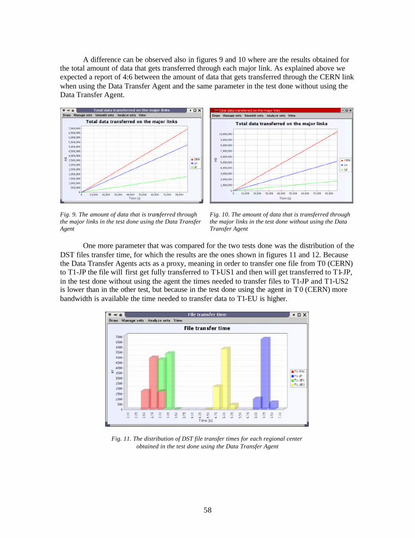
58
A difference can be observed also in figures 9 and 10 where are the results obtained for the total amount of data that gets transferred through each major link. As explained above we expected a report of 4:6 between the amount of data that gets transferred through the CERN link when using the Data Transfer Agent and the same parameter in the test done without using the Data Transfer Agent.
Fig. 9. The amount of data that is transferred through the major links in the test done using the Data Transfer Agent
Fig. 10. The amount of data that is transferred through the major links in the test done without using the Data Transfer Agent
One more parameter that was compared for the two tests done was the distribution of the DST files transfer time, for which the results are the ones shown in figures 11 and 12. Because the Data Transfer Agents acts as a proxy, meaning in order to transfer one file from T0 (CERN) to T1-JP the file will first get fully transferred to T1-US1 and then will get transferred to T1-JP, in the test done without using the agent the times needed to transfer files to T1-JP and T1-US2 is lower than in the other test, but because in the test done using the agent in T0 (CERN) more bandwidth is available the time needed to transfer data to T1-EU is higher.
Fig. 11. The distribution of DST file transfer times for each regional center obtained in the test done using the Data Transfer Agent
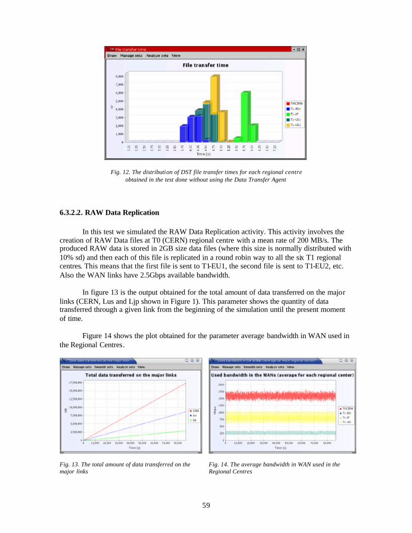
59
Fig. 12. The distribution of DST file transfer times for each regional centre obtained in the test done without using the Data Transfer Agent
6.3.2.2. RAW Data Replication In this test we simulated the RAW Data Replication activity. This activity involves the creation of RAW Data files at T0 (CERN) regional centre with a mean rate of 200 MB/s. The produced RAW data is stored in 2GB size data files (where this size is normally distributed with 10% sd) and then each of this file is replicated in a round robin way to all the six T1 regional centres. This means that the first file is sent to T1-EU1, the second file is sent to T1-EU2, etc. Also the WAN links have 2.5Gbps available bandwidth. In figure 13 is the output obtained for the total amount of data transferred on the major links (CERN, Lus and Ljp shown in Figure 1). This parameter shows the quantity of data transferred through a given link from the beginning of the simulation until the present moment of time. Figure 14 shows the plot obtained for the parameter average bandwidth in WAN used in the Regional Centres.
Fig. 13. The total amount of data transferred on the major links
Fig. 14. The average bandwidth in WAN used in the Regional Centres
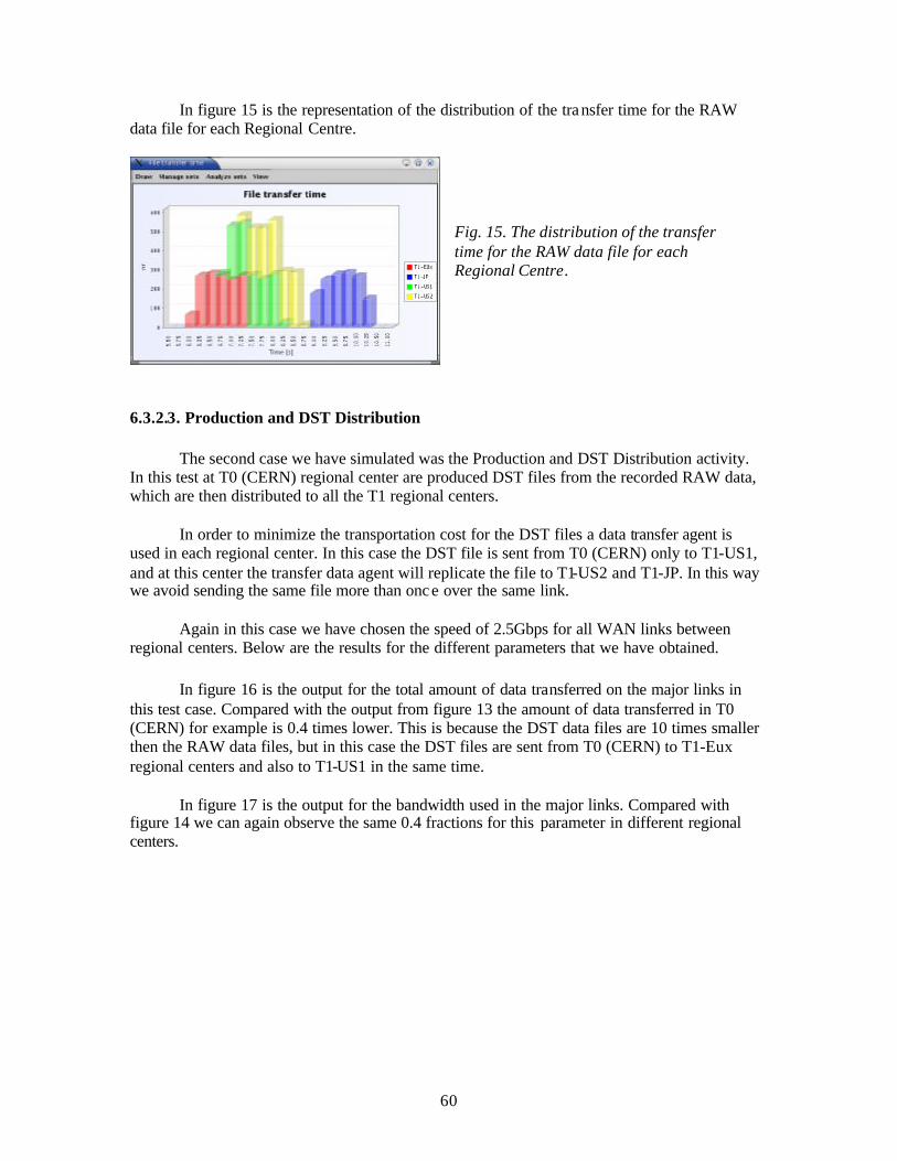
60
In figure 15 is the representation of the distribution of the transfer time for the RAW data file for each Regional Centre.
Fig. 15. The distribution of the transfer time for the RAW data file for each Regional Centre.
6.3.2.3. Production and DST Distribution The second case we have simulated was the Production and DST Distribution activity. In this test at T0 (CERN) regional center are produced DST files from the recorded RAW data, which are then distributed to all the T1 regional centers.
In order to minimize the transportation cost for the DST files a data transfer agent is
used in each regional center. In this case the DST file is sent from T0 (CERN) only to T1-US1, and at this center the transfer data agent will replicate the file to T1-US2 and T1-JP. In this way we avoid sending the same file more than once over the same link.
Again in this case we have chosen the speed of 2.5Gbps for all WAN links between
regional centers. Below are the results for the different parameters that we have obtained. In figure 16 is the output for the total amount of data transferred on the major links in
this test case. Compared with the output from figure 13 the amount of data transferred in T0 (CERN) for example is 0.4 times lower. This is because the DST data files are 10 times smaller then the RAW data files, but in this case the DST files are sent from T0 (CERN) to T1-Eux regional centers and also to T1-US1 in the same time.
In figure 17 is the output for the bandwidth used in the major links. Compared with figure 14 we can again observe the same 0.4 fractions for this parameter in different regional centers.
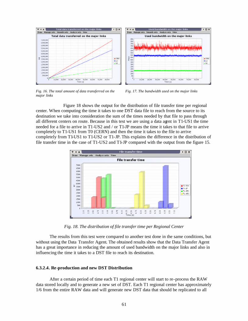
61
Fig. 16. The total amount of data transferred on the major links
Fig. 17. The bandwidth used on the major links
Figure 18 shows the output for the distribution of file transfer time per regional
center. When computing the time it takes to one DST data file to reach from the source to its destination we take into consideration the sum of the times needed by that file to pass through all different centers on route. Because in this test we are using a data agent in T1-US1 the time needed for a file to arrive in T1-US2 and / or T1-JP means the time it takes to that file to arrive completely to T1-US1 from T0 (CERN) and then the time it takes to the file to arrive completely from T1-US1 to T1-US2 or T1-JP. This explains the difference in the distribution of file transfer time in the case of T1-US2 and T1-JP compared with the output from the figure 15.
Fig. 18. The distribution of file transfer time per Regional Center The results from this test were compared to another test done in the same conditions, but without using the Data Transfer Agent. The obtained results show that the Data Transfer Agent has a great importance in reducing the amount of used bandwidth on the major links and also in influencing the time it takes to a DST file to reach its destination.
6.3.2.4. Re-production and new DST Distribution After a certain period of time each T1 regional center will start to re-process the RAW data stored locally and to generate a new set of DST. Each T1 regional center has approximately 1/6 from the entire RAW data and will generate new DST data that should be replicated to all
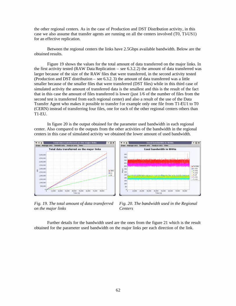
62
the other regional centers. As in the case of Production and DST Distribution activity, in this case we also assume that transfer agents are running on all the centers involved (T0, T1-US1) for an effective replication. Between the regional centers the links have 2.5Gbps available bandwidth. Below are the obtained results. Figure 19 shows the values for the total amount of data transferred on the major links. In the first activity tested (RAW Data Replication – see 6.3.2.2) the amount of data transferred was larger because of the size of the RAW files that were transferred, in the second activity tested (Production and DST distribution – see 6.3.2. 3) the amount of data transferred was a little smaller because of the smaller files that were transferred (DST files) while in this third case of simulated activity the amount of transferred data is the smallest and this is the result of the fact that in this case the amount of files transferred is lower (just 1/6 of the number of files from the second test is transferred from each regional center) and also a result of the use of the Data Transfer Agent who makes it possible to transfer f or example only one file from T1-EU1 to T0 (CERN) instead of transferring four files, one for each of the other regional centers others than T1-EU. In figure 20 is the output obtained for the parameter used bandwidth in each regional center. Also compared to the outputs from the other activities of the bandwidth in the regional centers in this case of simulated activity we obtained the lower amount of used bandwidth.
Fig. 19. The total amount of data transferred on the major links
Fig. 20. The bandwidth used in the Regional Centers
Further details for the bandwidth used are the ones from the figure 21 which is the result obtained for the parameter used bandwidth on the major links per each direction of the link.
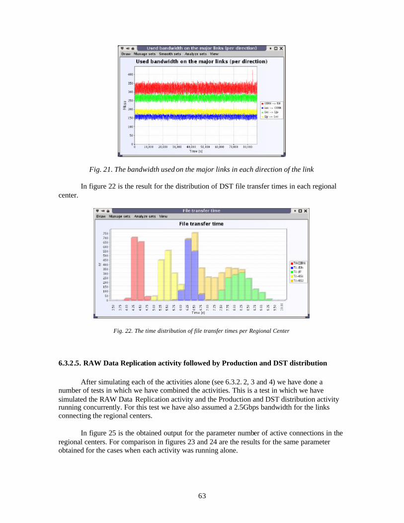
63
Fig. 21. The bandwidth used on the major links in each direction of the link In figure 22 is the result for the distribution of DST file transfer times in each regional center.
Fig. 22. The time distribution of file transfer times per Regional Center
6.3.2.5. RAW Data Replication activity followed by Production and DST distribution After simulating each of the activities alone (see 6.3.2. 2, 3 and 4) we have done a number of tests in which we have combined the activities. This is a test in which we have simulated the RAW Data Replication activity and the Production and DST distribution activity running concurrently. For this test we have also assumed a 2.5Gbps bandwidth for the links connecting the regional centers. In figure 25 is the obtained output for the parameter number of active connections in the regional centers. For comparison in figures 23 and 24 are the results for the same parameter obtained for the cases when each activity was running alone.
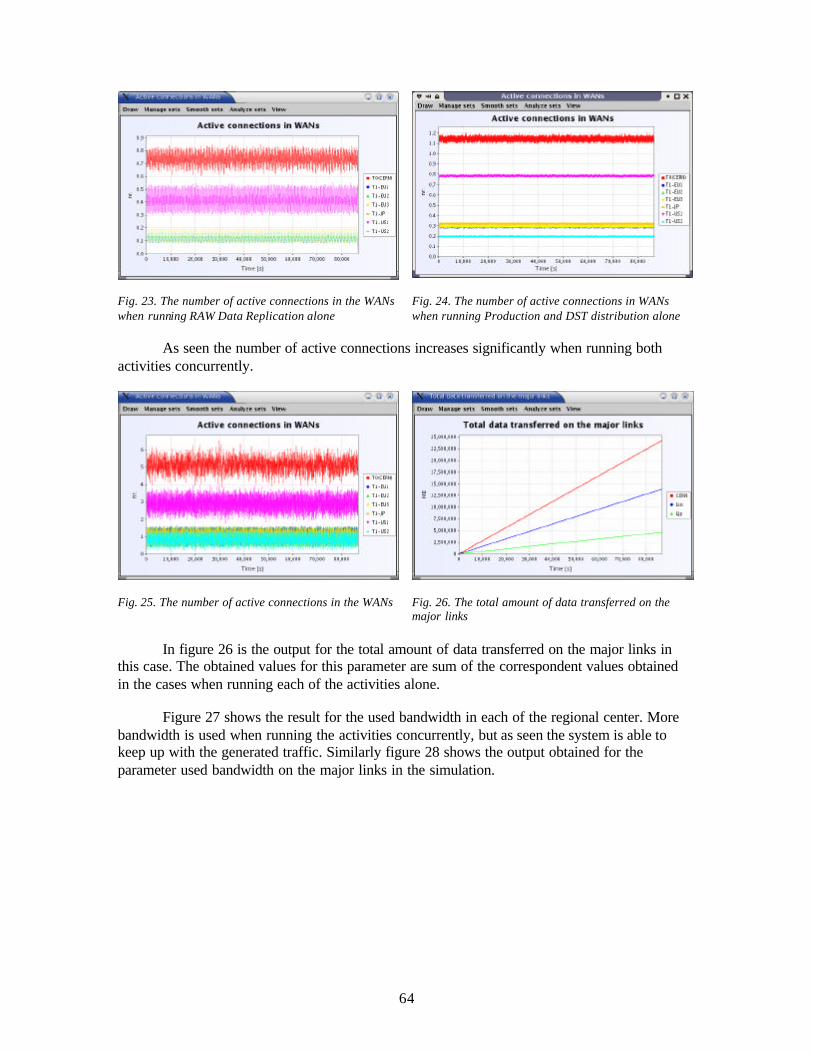
64
Fig. 23. The number of active connections in the WANs when running RAW Data Replication alone
Fig. 24. The number of active connections in WANs when running Production and DST distribution alone
As seen the number of active connections increases significantly when running both activities concurrently.
Fig. 25. The number of active connections in the WANs
Fig. 26. The total amount of data transferred on the major links
In figure 26 is the output for the total amount of data transferred on the major links in this case. The obtained values for this parameter are sum of the correspondent values obtained in the cases when running each of the activities alone. Figure 27 shows the result for the used bandwidth in each of the regional center. More bandwidth is used when running the activities concurrently, but as seen the system is able to keep up with the generated traffic. Similarly figure 28 shows the output obtained for the parameter used bandwidth on the major links in the simulation.
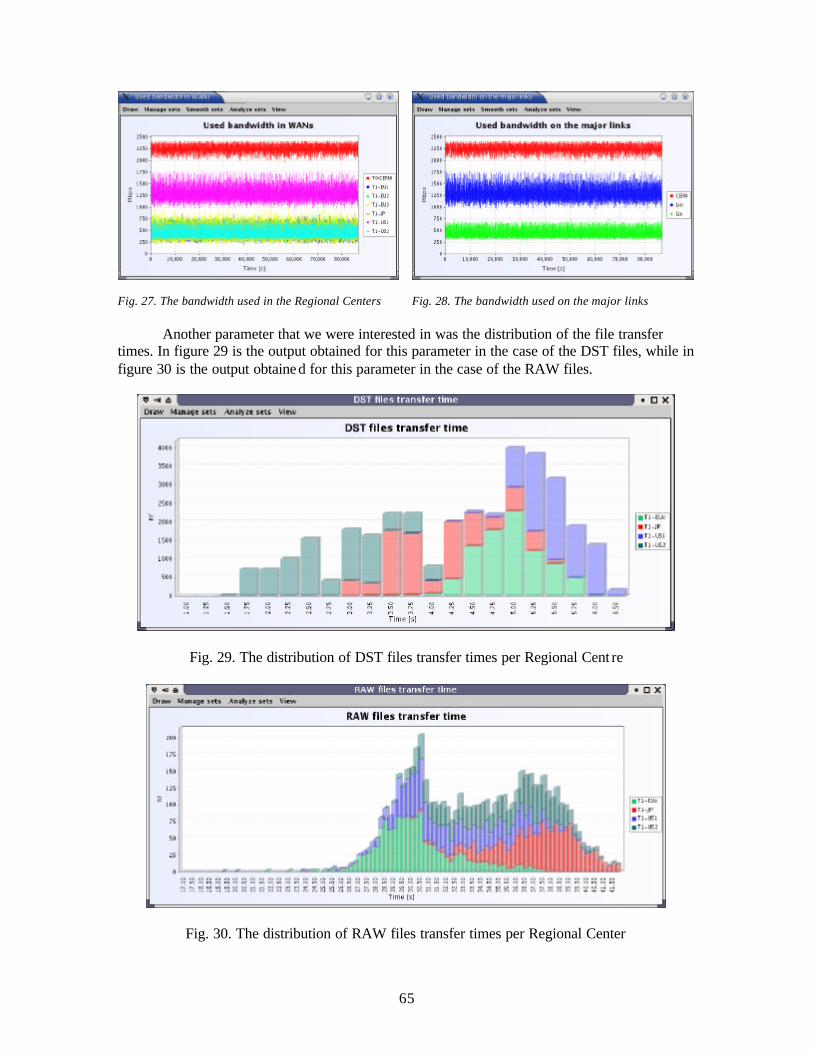
65
Fig. 27. The bandwidth used in the Regional Centers
Fig. 28. The bandwidth used on the major links
Another parameter that we were interested in was the distribution of the file transfer times. In figure 29 is the output obtained for this parameter in the case of the DST files, while in figure 30 is the output obtained for this parameter in the case of the RAW files.
Fig. 29. The distribution of DST files transfer times per Regional Cent re
Fig. 30. The distribution of RAW files transfer times per Regional Center
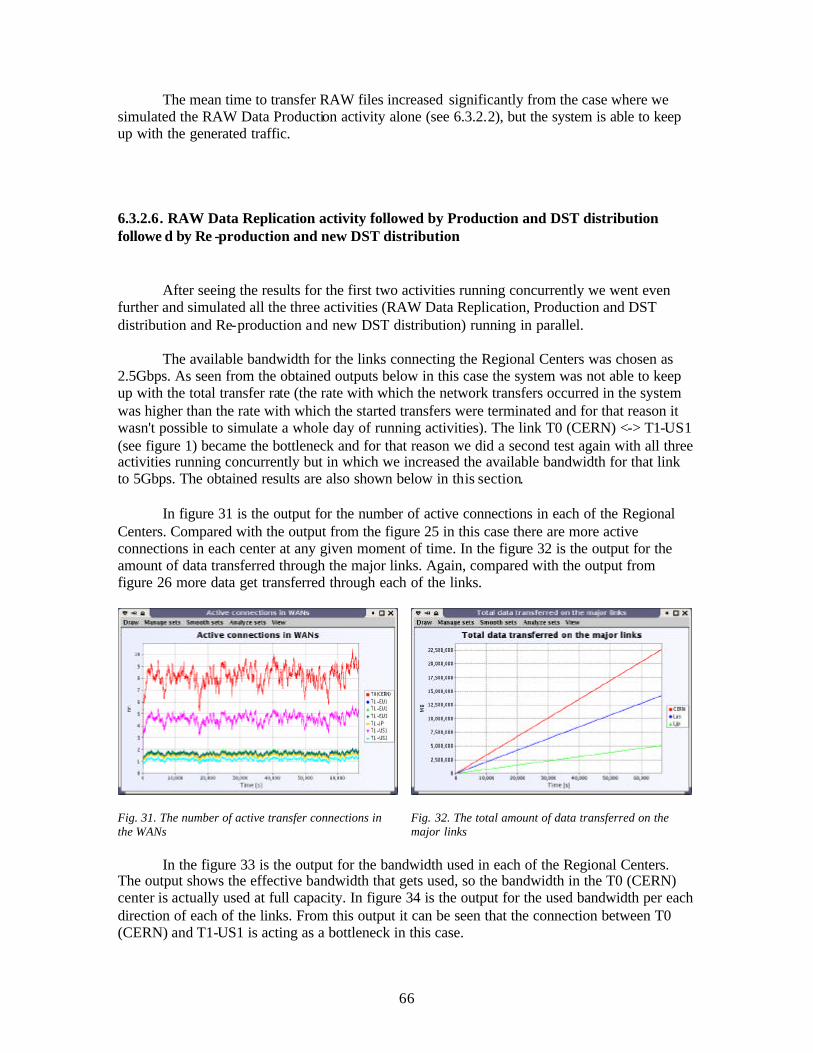
66
The mean time to transfer RAW files increased significantly from the case where we simulated the RAW Data Production activity alone (see 6.3.2.2), but the system is able to keep up with the generated traffic.
6.3.2.6. RAW Data Replication activity followed by Production and DST distribution followe d by Re -production and new DST distribution After seeing the results for the first two activities running concurrently we went even further and simulated all the three activities (RAW Data Replication, Production and DST distribution and Re-production and new DST distribution) running in parallel. The available bandwidth for the links connecting the Regional Centers was chosen as 2.5Gbps. As seen from the obtained outputs below in this case the system was not able to keep up with the total transfer rate (the rate with which the network transfers occurred in the system was higher than the rate with which the started transfers were terminated and for that reason it wasn't possible to simulate a whole day of running activities). The link T0 (CERN) <-> T1-US1 (see figure 1) became the bottleneck and for that reason we did a second test again with all three activities running concurrently but in which we increased the available bandwidth for that link to 5Gbps. The obtained results are also shown below in this section.
In figure 31 is the output for the number of active connections in each of the Regional Centers. Compared with the output from the figure 25 in this case there are more active connections in each center at any given moment of time. In the figure 32 is the output for the amount of data transferred through the major links. Again, compared with the output from figure 26 more data get transferred through each of the links.
Fig. 31. The number of active transfer connections in the WANs
Fig. 32. The total amount of data transferred on the major links
In the figure 33 is the output for the bandwidth used in each of the Regional Centers. The output shows the effective bandwidth that gets used, so the bandwidth in the T0 (CERN) center is actually used at full capacity. In figure 34 is the output for the used bandwidth per each direction of each of the links. From this output it can be seen that the connection between T0 (CERN) and T1-US1 is acting as a bottleneck in this case.
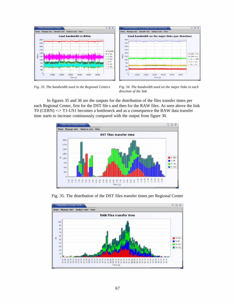
67
Fig. 33. The bandwidth used in the Regional Centers
Fig. 34. The bandwidth used on the major links in each direction of the link
In figures 35 and 36 are the outputs for the distribution of the files transfer times per each Regional Center, first for the DST file s and then for the RAW files. As seen above the link T0 (CERN) <-> T1-US1 becomes a bottleneck and as a consequence the RAW data transfer time starts to increase continuously compared with the output from figure 30.
Fig. 35. The distribution of the DST files transfer times per Regional Center
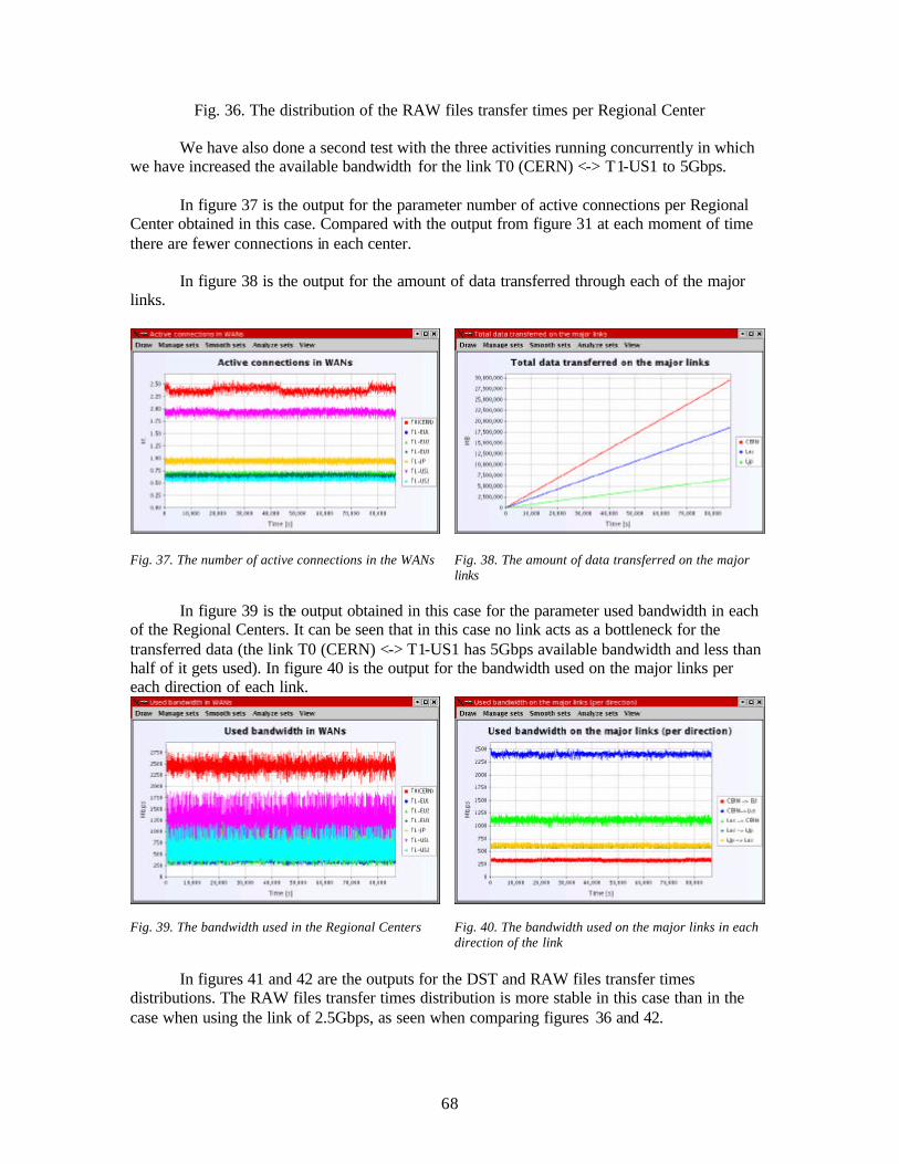
68
Fig. 36. The distribution of the RAW files transfer times per Regional Center We have also done a second test with the three activities running concurrently in which we have increased the available bandwidth for the link T0 (CERN) <-> T1-US1 to 5Gbps. In figure 37 is the output for the parameter number of active connections per Regional Center obtained in this case. Compared with the output from figure 31 at each moment of time there are fewer connections in each center. In figure 38 is the output for the amount of data transferred through each of the major links.
Fig. 37. The number of active connections in the WANs
Fig. 38. The amount of data transferred on the major links
In figure 39 is the output obtained in this case for the parameter used bandwidth in each of the Regional Centers. It can be seen that in this case no link acts as a bottleneck for the transferred data (the link T0 (CERN) <-> T1-US1 has 5Gbps available bandwidth and less than half of it gets used). In figure 40 is the output for the bandwidth used on the major links per each direction of each link.
Fig. 39. The bandwidth used in the Regional Centers
Fig. 40. The bandwidth used on the major links in each direction of the link
In figures 41 and 42 are the outputs for the DST and RAW files transfer times distributions. The RAW files transfer times distribution is more stable in this case than in the case when using the link of 2.5Gbps, as seen when comparing figures 36 and 42.
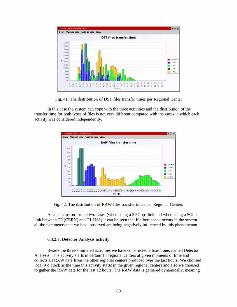
69
Fig. 41. The distribution of DST files transfer times per Regional Center In this case the system can cope with the three activities and the distribution of the transfer time for both types of files is not very different compared with the cases in which each activity was considered independently.
Fig. 42. The distribution of RAW files transfer times per Regional Centers As a conclusion for the two cases (when using a 2.5Gbps link and when using a 5Gbps link between T0 (CERN) and T1-US1) it can be seen that if a bottleneck occurs in the system all the parameters that we have observed are being negatively influenced by this phenomenon.
6.3.2.7. Detector Analysis activity Beside the three simulated activities we have constructed a fourth one, named Detector Analysis. This activity starts in certain T1 regional centers at given moments of time and collects all RAW data from the other regional centers produced over the last hours. We choused local 9 o’clock as the time this activity starts in the given regional centers and also we choused to gather the RAW data for the last 12 hours. The RAW data is gathered dynamically, meaning
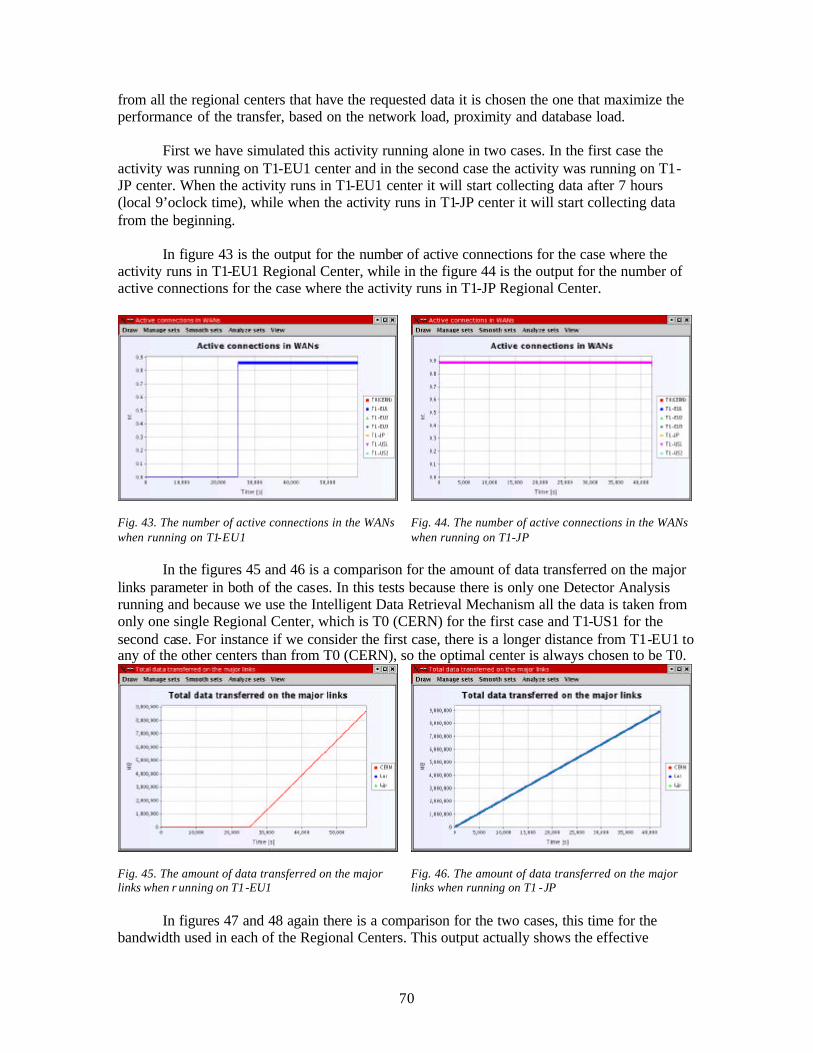
70
from all the regional centers that have the requested data it is chosen the one that maximize the performance of the transfer, based on the network load, proximity and database load. First we have simulated this activity running alone in two cases. In the first case the activity was running on T1-EU1 center and in the second case the activity was running on T1-JP center. When the activity runs in T1-EU1 center it will start collecting data after 7 hours (local 9’oclock time), while when the activity runs in T1-JP center it will start collecting data from the beginning. In figure 43 is the output for the number of active connections for the case where the activity runs in T1-EU1 Regional Center, while in the figure 44 is the output for the number of active connections for the case where the activity runs in T1-JP Regional Center.
Fig. 43. The number of active connections in the WANs when running on T1-EU1
Fig. 44. The number of active connections in the WANs when running on T1-JP
In the figures 45 and 46 is a comparison for the amount of data transferred on the major links parameter in both of the cases. In this tests because there is only one Detector Analysis running and because we use the Intelligent Data Retrieval Mechanism all the data is taken from only one single Regional Center, which is T0 (CERN) for the first case and T1-US1 for the second case. For instance if we consider the first case, there is a longer distance from T1-EU1 to any of the other centers than from T0 (CERN), so the optimal center is always chosen to be T0.
Fig. 45. The amount of data transferred on the major links when r unning on T1-EU1
Fig. 46. The amount of data transferred on the major links when running on T1 -JP
In figures 47 and 48 again there is a comparison for the two cases, this time for the bandwidth used in each of the Regional Centers. This output actually shows the effective
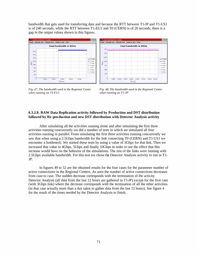
71
bandwidth that gets used for transferring data and because the RTT between T1-JP and T1-US1 is of 240 seconds, while the RTT between T1-EU1 and T0 (CERN) is of 20 seconds, there is a gap in the output values shown in this figures.
Fig. 47. The bandwidth used in the Regional Center when running on T1-EU1
Fig. 48. The bandwidth used in the Regional Center when running on T1-JP
6.3.2.8. RAW Data Replication activity followed by Production and DST distribution followed by Re -pro duction and new DST distribution with Detector Analysis activity After simulating all the activities running alone and after simulating the first three activities running concurrently we did a number of tests in which we simulated all four activities running in parallel. From simulating the first three activities running concurrently we saw that when using a 2.5Gbps bandwidth for the link connecting T0 (CERN) and T1-US1 we encounter a bottleneck. We started those tests by using a value of 3Gbps for that link. Then we increased that value to 4Gbps, 5Gbps and finally 10Gbps in order to see the effect that this increase would have on the behavior of the simulations. The rest of the links were running with 2.5Gbps available bandwidth. For this test we chose the Detector Analysis activity to run in T1-JP.
In figures 49 to 52 are the obtained results for the four cases for the parameter number of active connections in the Regional Centers. As seen the number of active connections decreases from case to case. The sudden decrease corresponds with the termination of the activity Detector Analysis (all data from the last 12 hours are gathered in T1-JP) except for the first case (with 3Gbps link) where the decrease corresponds with the termination of all the other activities (in that case actually more than a day takes to gather data from the last 12 hours). See figure 4 for the result of the times needed by the Detector Analysis to finish.
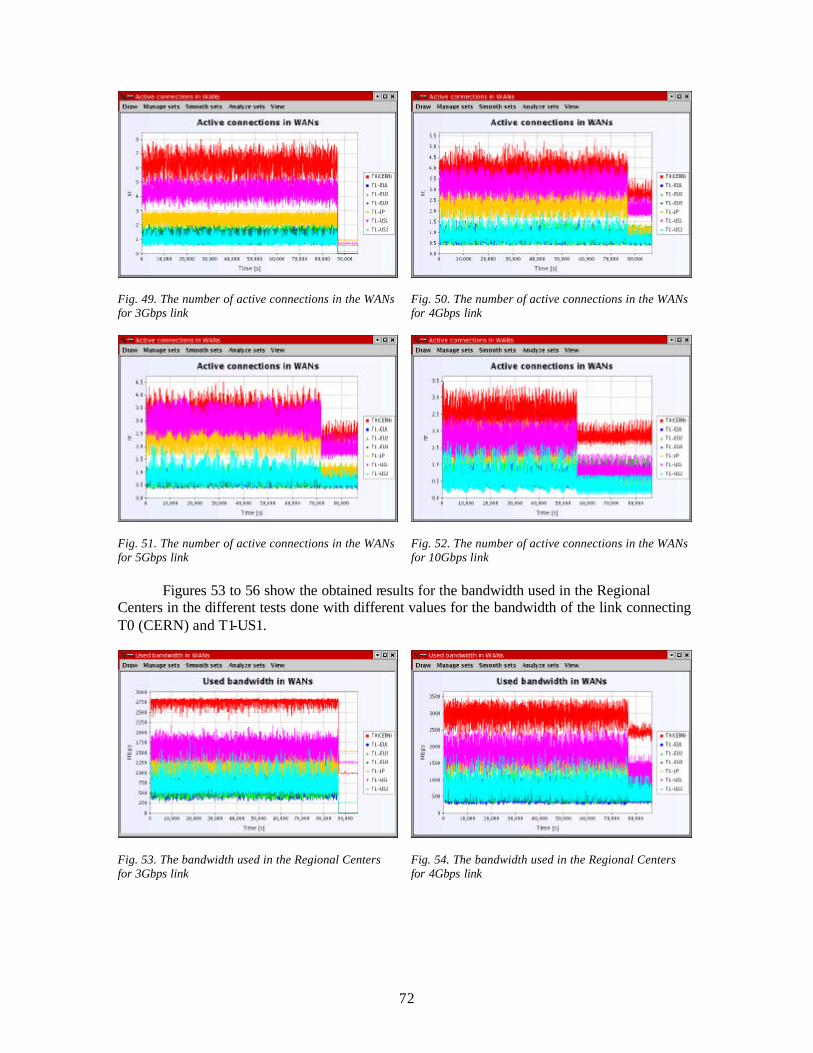
72
Fig. 49. The number of active connections in the WANs for 3Gbps link
Fig. 50. The number of active connections in the WANs for 4Gbps link
Fig. 51. The number of active connections in the WANs for 5Gbps link
Fig. 52. The number of active connections in the WANs for 10Gbps link
Figures 53 to 56 show the obtained results for the bandwidth used in the Regional Centers in the different tests done with different values for the bandwidth of the link connecting T0 (CERN) and T1-US1.
Fig. 53. The bandwidth used in the Regional Centers for 3Gbps link
Fig. 54. The bandwidth used in the Regional Centers for 4Gbps link
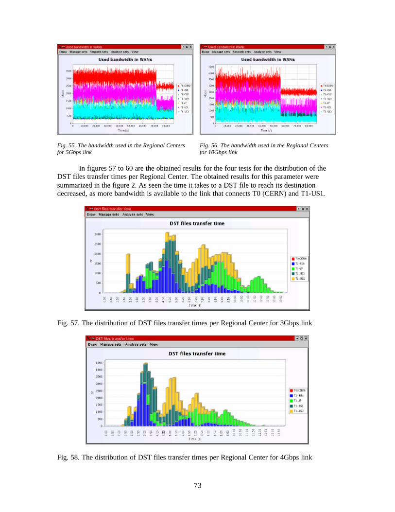
73
Fig. 55. The bandwidth used in the Regional Centers for 5Gbps link
Fig. 56. The bandwidth used in the Regional Centers for 10Gbps link
In figures 57 to 60 are the obtained results for the four tests for the distribution of the DST files transfer times per Regional Center. The obtained results for this parameter were summarized in the figure 2. As seen the time it takes to a DST file to reach its destination decreased, as more bandwidth is available to the link that connects T0 (CERN) and T1-US1.
Fig. 57. The distribution of DST files transfer times per Regional Center for 3Gbps link
Fig. 58. The distribution of DST files transfer times per Regional Center for 4Gbps link
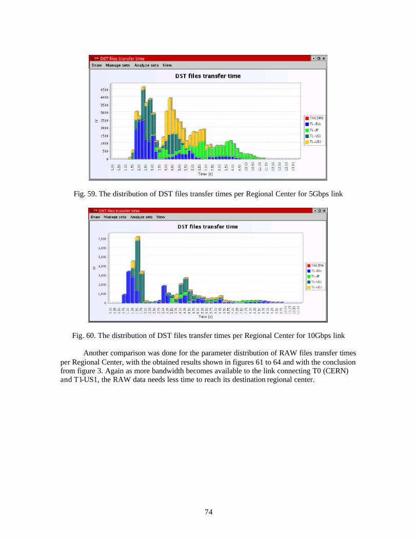
74
Fig. 59. The distribution of DST files transfer times per Regional Center for 5Gbps link
Fig. 60. The distribution of DST files transfer times per Regional Center for 10Gbps link
Another comparison was done for the parameter distribution of RAW files transfer times per Regional Center, with the obtained results shown in figures 61 to 64 and with the conclusion from figure 3. Again as more bandwidth becomes available to the link connecting T0 (CERN) and T1-US1, the RAW data needs less time to reach its destination regional center.
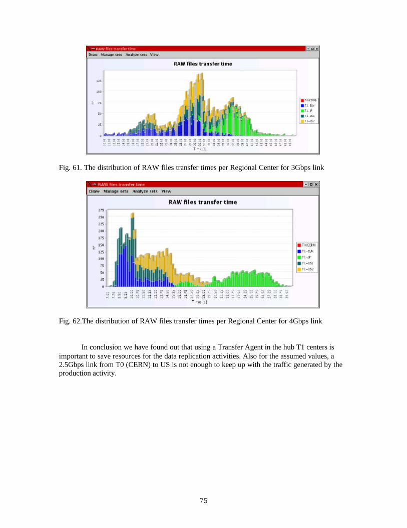
75
Fig. 61. The distribution of RAW files transfer times per Regional Center for 3Gbps link
Fig. 62.The distribution of RAW files transfer times per Regional Center for 4Gbps link
In conclusion we have found out that using a Transfer Agent in the hub T1 centers is important to save resources for the data replication activities. Also for the assumed values, a 2.5Gbps link from T0 (CERN) to US is not enough to keep up with the traffic generated by the production activity.
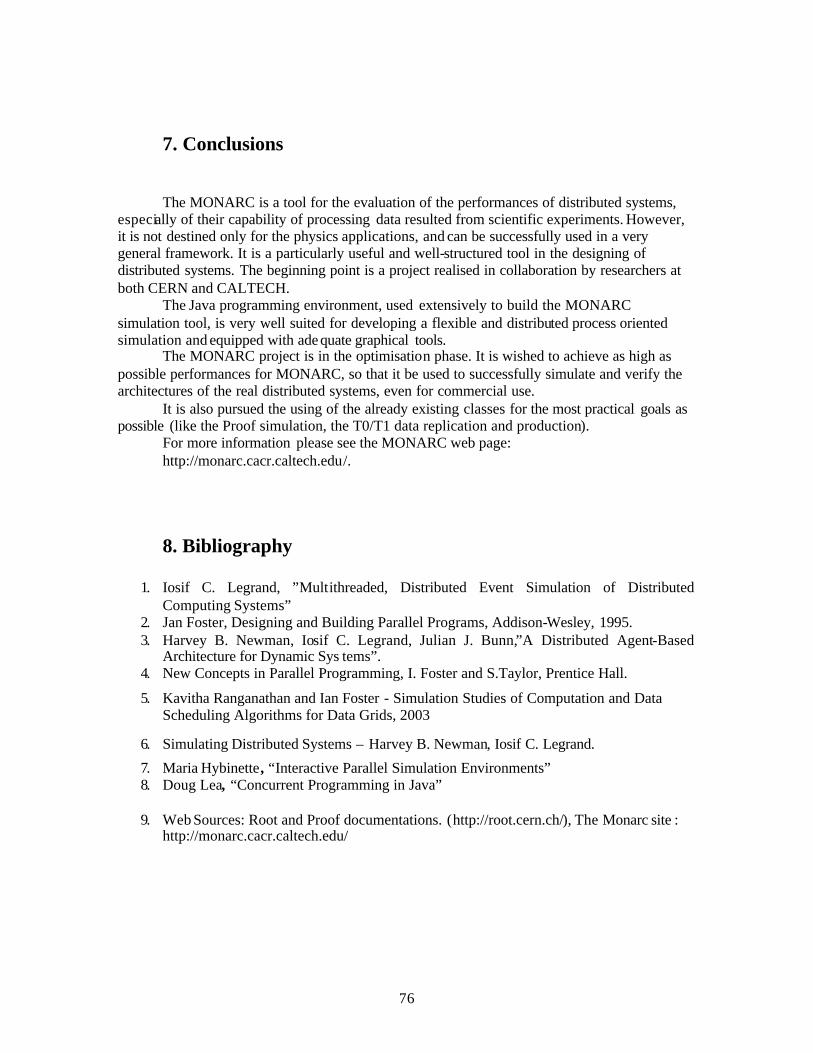
76
7. Conclusions
The MONARC is a tool for the evaluation of the performances of distributed systems, especially of their capability of processing data resulted from scientific experiments. However, it is not destined only for the physics applications, and can be successfully used in a very general framework. It is a particularly useful and well-structured tool in the designing of distributed systems. The beginning point is a project realised in collaboration by researchers at both CERN and CALTECH.
The Java programming environment, used extensively to build the MONARC simulation tool, is very well suited for developing a flexible and distributed process oriented simulation and equipped with ade quate graphical tools.
The MONARC project is in the optimisation phase. It is wished to achieve as high as possible performances for MONARC, so that it be used to successfully simulate and verify the architectures of the real distributed systems, even for commercial use.
It is also pursued the using of the already existing classes for the most practical goals as possible (like the Proof simulation, the T0/T1 data replication and production).
For more information please see the MONARC web page: http://monarc.cacr.caltech.edu/.
8. Bibliography
1. Iosif C. Legrand, ”Multithreaded, Distributed Event Simulation of Distributed Computing Systems”
2. Jan Foster, Designing and Building Parallel Programs, Addison-Wesley, 1995. 3. Harvey B. Newman, Iosif C. Legrand, Julian J. Bunn,”A Distributed Agent-Based
Architecture for Dynamic Sys tems”. 4. New Concepts in Parallel Programming, I. Foster and S.Taylor, Prentice Hall.
5. Kavitha Ranganathan and Ian Foster - Simulation Studies of Computation and Data Scheduling Algorithms for Data Grids, 2003
6. Simulating Distributed Systems – Harvey B. Newman, Iosif C. Legrand.
7. Maria Hybinette, “Interactive Parallel Simulation Environments” 8. Doug Lea, “Concurrent Programming in Java”
9. Web Sources: Root and Proof documentations. (http://root.cern.ch/), The Monarc site :
http://monarc.cacr.caltech.edu/

77
9. Appendix Below I have listed the source code for a few of the classes of the application (the most relevant for my project) :