© aSup -2007 Statistics II – SPECIAL CORRELATION 1 SPECIAL CORRELATION

© aSup -2007

Statistics II – SPECIAL CORRELATION

1

SPECIAL CORRELATION

© aSup -2007


2

The SPEARMAN Correlation The Pearson correlation specially

measures the degree of linear relationship between two variables

Other correlation measures have been developed for nonlinear relationship and of other types of data

One of these useful measures is called the Spearman correlation

© aSup -2007


3

The SPEARMAN Correlation Measure the relationship between

variables measured on an ordinal scale of measurement

The reason that the Spearman correlation measures consistency, rather than form, comes from a simple observation: when two variables are consistently related, their ranks will be linearly related

© aSup -2007


4

INTRODUCTION

Pearson product-moment coefficient is the standard index of the amount of correlation between two variables, and we prefer it whenever its use is possible and convenient.

But there are data to which this kind of correlation method cannot be applied, and there are instances in which can be applied but in which, for practical purpose, other procedures are more expedient

© aSup -2007


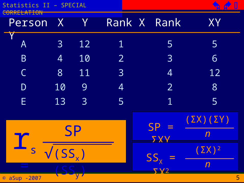
5

Person X Y Rank X Rank Y

A

B

C

D

E

3

4

8

10

13

12

10

11

9

3

1

2

3

4

5

5

3

4

2

1

rs =SP

√(SSx) (SSy)

SP = ΣXY(ΣX)(ΣY)

n

SSX = ΣX2(ΣX)2

n

XY

5

6

12

8

5

© aSup -2007


6

The COMPUTATION

1. Rank the individual in the (two) variables

2. For every pair of rank (for each individual), determine the difference (d) in the two ranks

3. Square each d to find d2

© aSup -2007


7

Person X Y Rank X Rank Y

A

B

C

D

E

3

4

8

10

13

12

10

11

9

3

1

2

3

4

5

5

3

4

2

1

rs = 1 -6 Σ D2

n(n2 – 1)

D2

16

1

1

4

16

© aSup -2007


8

Spearman’s Rank-Difference Correlation Method

Especially, when samples are small It can be applied as a quick substitute

when the number of pairs, or N, is less than 30

It should be applied when the data are already in terms of rank orders rather than interval measurement

© aSup -2007


9

INTERPRETATION OF A RANK DIFFERENCE COEFFICIENT

The rho coefficient is closely to the Pearson r that would be computed from the original measurement.

The rρ values are systematically a bit lower than the corresponding Pearson-r values, but the maximum difference, which occurs when both coefficient are near .50

© aSup -2007


10

To measure the relationship between anxiety level and test performance, a psychologist obtains a sample of n = 6 college students from introductory statistics course. The students are asked to come to the laboratory 15 minutes before the final exam. In the lab, the psychologist records psychological measure of anxiety (heart rate, skin resistance, blood pressure, etc) for each student. In addition, the psychologist obtains the exam score for each student.

LEARNING CHECK

© aSup -2007


11

Student

Anxiety

Rating

Exam Scores

A 5 80

B 2 88

C 7 80

D 7 79

E 4 86

F 5 85

Compute the Pearson and Spearman correlation for the following data.

Test the correlation with α = .05

© aSup -2007


12

The BISERIAL Coefficient of Correlation

The biserial r is especially designed for the situation in which both of the variables correlated are continuously measurable, BUT one of the two is for some reason reduced to two categories

This reduction to two categories may be a consequence of the only way in which the data can be obtained, as, for example, when one variable is whether or not a student passes or fails a certain standard

© aSup -2007


13

The COMPUTATION The principle upon which the formula

for biserial r is based is that with zero correlation

There would no difference means for the continuous variable, and the larger the difference between means, the larger the correlation

© aSup -2007


14

AN EVALUATION OF THE BISERIAL r Before computing rb, of course we need to

dichotomize each Y distribution. In adopting a division point, it is well to

come as near the median as possible, why? In all these special instances, however, we

are not relieve of the responsibility of defending the assumption of the normal population distribution of Y

It may seem contradictory to suggest that when the obtained Y distribution is skewed, we resort the biserial r, but note that is the sample distribution that is skewed and the population distribution that must be assumed to be normal

© aSup -2007


15

THE BISERIAL r IS LESS RELIABLE THAN THE PEARSON r

Whenever there is a real choices between computing a pearson r or a Biserial r, however, one should favor the former, unless the sample is very large and computation time is an important consideration

The standard error for a biserial r is considerably larger than that for a Pearson r derived from the same sample

© aSup -2007


16

The POINT BISERIAL Coefficient of Correlation

When one of the two variables in a correlation problem is genuine dichotomy, the appropriate type of coefficient to use is point biserial r

Examples of genuine dichotomies are male vs female, being a farmer vs not being a farmer

Bimodal or other peculiar distributions, although not representating entirely discrete categories, are sufficiently discontinuous to call for the point biserial rather than biserial r

© aSup -2007


17

The COMPUTATION A product-moment r could be

computed with Pearson’s basic formula If rpbi were computed from data that

actually justified the use of rb, the coefficient computed would be markly smaller than rb obtained from the same data

rb is √pq/y times as large as rpbi

© aSup -2007


18

POINT-BISERIAL vs BISERIAL When the dichotomous variable is

normally distributed without reasonable doubt, it is recommended that rb be computed and interpreted

If there is little doubt that the distribution is a genuine dichotomy, rpbi should be computed and interpreted

When in doubt, the rpbi is probably the safer choice

© aSup -2007


19

TETRACHORIC CORRELATION

A tetrachoric r is computed from data in which both X and Y have been reduced artificially to two categories

Under the appropriate condition it gives a coefficient that is numerically equivalent to a Pearson r and may be regard as an approximation to it

© aSup -2007


20

TETRACHORIC CORRELATION The tetrachoric r requires that both X and Y

represent continuous, normally distributed, and linearly related variables

The tetrachoric r is less reliable than the Pearson r.

It is more reliable whena. N is large, as is true of all statisticb. rt is large, as is true of other r’sc. the division in the two categories are near the medians

© aSup -2007


21

THE Phi COEFFICIENT rФ related to the chi square from 2 x 2 table

When two distributions correlated are genuinely dichotomous– when the two classes are separated by real gap between them, and previously discussed correlational method do not apply– we may resort to the phi coefficient

This coefficient was designed for so-called point distributions, which implies that the two classes have two point values and merely represent some qualitative attribute

© aSup -2007


22

DEFINITION

A partial correlation between two variables is one that nullifies the effects of a third variable (or a number of other variables) upon both the variables being correlated

© aSup -2007


23

EXAMPLE

The correlation between height and weight of boys in a group where age is permitted to vary would be higher than the correlation between height and weight in a group at constant age

The reason is obvious. Because certain boys are older, they are both heavier and taller. Age is a factor that enhances the strength of correspondence between height and weight

© aSup -2007


24

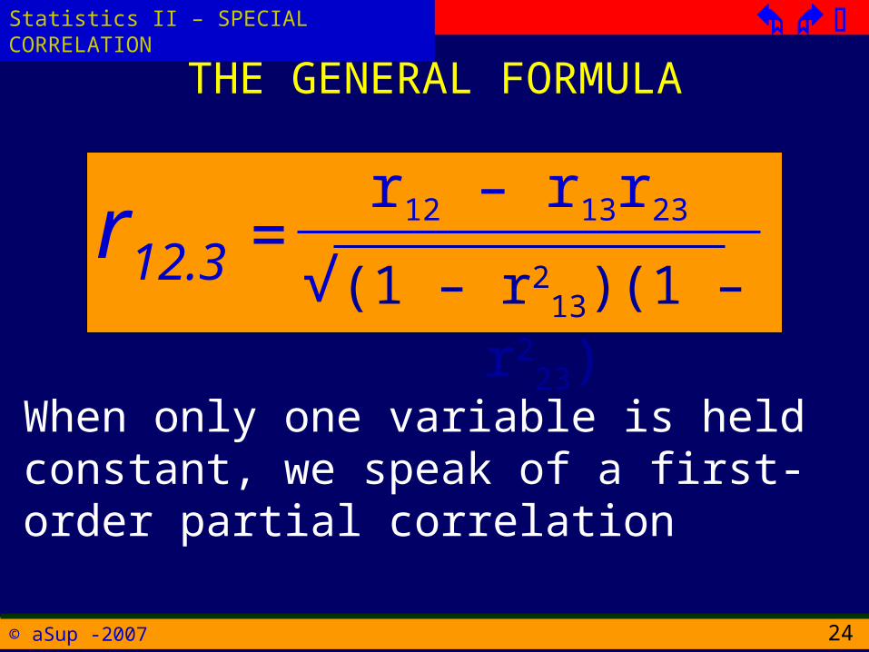
THE GENERAL FORMULA

r12.3 =r12 – r13r23

√ (1 – r213)(1 – r2

23)

When only one variable is held constant, we speak of a first-order partial correlation

© aSup -2007


25

SECOND ORDER PARTIAL r

r12.34 =R12.3 – r14.3r24.3

√ (1 – r214.3)(1 – r2

24.3)


© aSup -2007


26

THE BISERIAL CORRELATION

WhereMp = mean of X values for the higher group in the

dichotomized variable, the one having ability on which sample is divided into two subgroups

Mq = mean of X values for the lower groupp = proportion of cases in the higher groupq = proportion of cases in the higher groupY = ordinate of the unit normal-distribution curve at

the point of division between segments containing p and q proportion of the cases

St = standard deviation of the total sample in the continously measured variable X

rb =Mp – Mq

St

Xpqy

© aSup -2007


27

THE POINT BISERIAL CORRELATION

WhereMp = mean of X values for the higher group in the

dichotomized variable, the one having ability on which sample is divided into two subgroups

Mq = mean of X values for the lower groupp = proportion of cases in the higher groupq = proportion of cases in the higher groupSt = standard deviation of the total sample in the

continously measured variable X

rpbi =Mp – Mq

St

pq

© aSup -2007


28

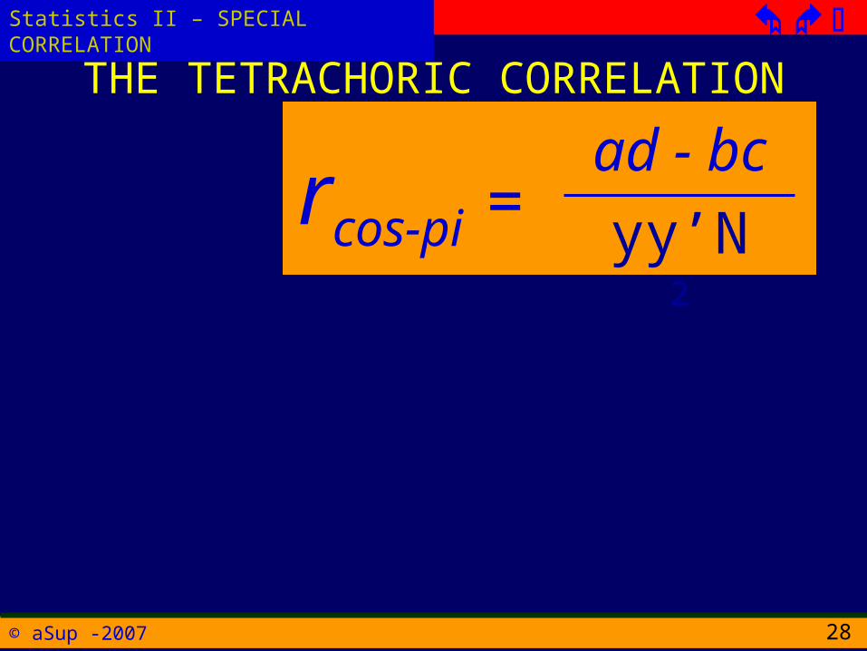
THE TETRACHORIC CORRELATION

rcos-pi =ad - bc

yy’N2

© aSup -2007


29

THE GENERAL FORMULA

r12.3 =r12 – r13r23

√ (1 – r213)(1 – r2

23)


© aSup -2007


30

THE GENERAL FORMULA

r12.3 =r12 – r13r23

√ (1 – r213)(1 – r2

23)

When two variables is held constant, we speak of a second-order partial correlation

Documents

© aSup -2007 Statistics II – SPECIAL CORRELATION 1 SPECIAL CORRELATION