第四章

Brown运动和 Ito公式

Chapter 4

Brownian Motion & Itô Formula

Chapter 4

Brownian Motion

& Itô Formula

Stochastic Process The price movement of an underlying asset is a stochastic

process. The French mathematician Louis Bachelier was the first

one to describe the stock share price movement as a Brownian motion in his 1900 doctoral thesis. introduction to the Brownian motion derive the continuous model of option pricing giving the definition and relevant properties Brownian motion derive stochastic calculus based on the Brownian motion including

the Ito integral & Ito formula. All of the description and discussion emphasize clarity

rather than mathematical rigor.

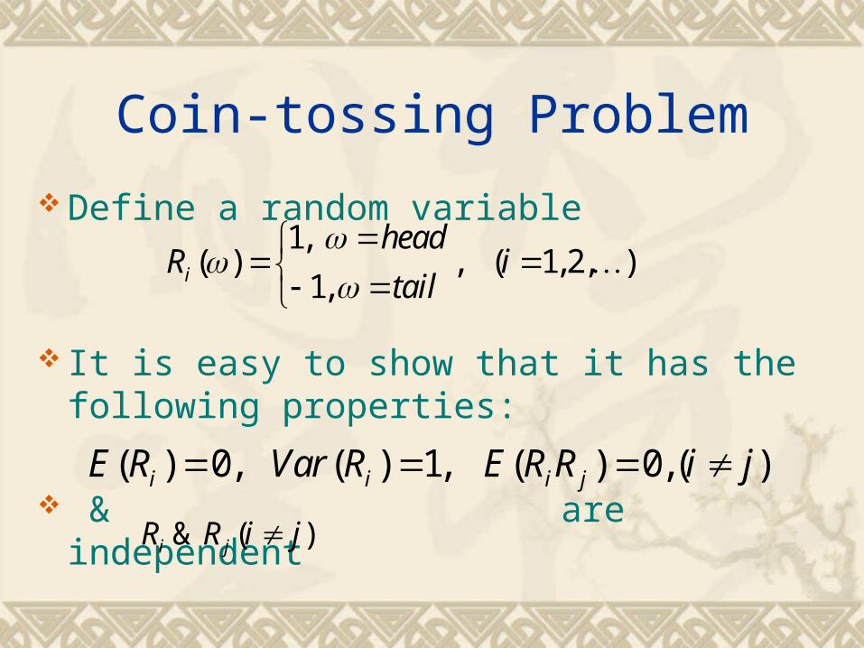
Coin-tossing Problem

Define a random variable

It is easy to show that it has the following properties:

& are independent

1,( ) , ( 1,2, )

1,i

headR i

tail

( ) 0, ( ) 1, ( ) 0, ( )i i i jE R Var R E R R i j

& ( )i jR R i j

Random Variable

With the random variable, define a random variable and a random sequence

i iR R

, ( 0,1, ) :kS k

0

1 1

0,

, 1,2,k k

k i ii i

S

S R R k

Random Walk Consider a time period [0,T], which can

be divided into N equal intervals. Let Δ=T\ N, t_n=nΔ ,(n=0,1,\cdots,N), then

A random walk is defined in [0,T]:

is called the path of the random walk.

0 10 .Nt t t T ( )S t

( )S t

11 1

( ), ,( )

, .

k k

k kk k k k

S t t tS t t t t t

S S t t t

Distribution of the Path

Let T=1,N=4,Δ=1/4,

0

1 1

2 1 2

3 1 2 3

4 1 2 3 4

0,

1/ 4 1/ 2,1/ 2 ,

1/ 4( ) 1,0,1 ,

1/ 4( ) 3 / 2, 1/ 2,0,1/ 2,3 / 2 ,

1/ 4( ) 2, 1,0,1,2 ,

S

S R

S R R

S R R R

S R R R R

Form of Path

the path formed by linear interpolation between the above random points. For

Δ=1/4 case, there are 2^4=16 paths.

t

S

1

Properties of the Path^ ^2 1

^ ^ ^ ^2 1 2 1

^ ^ ^ ^2 1 2 1

^ ^2 1

1. ( ( ) ( )) 0,

2. ( ( ) ( )) | | ( ),

3. ( ( ) ( )) min( , ) ( ),

4. ( ) ( ) & ( ) are independent

where ,1 1; 0;0 , .

k k k

k

E S t S t

Var S t S t t t O

E S t S t t t O

S t S t S t

t k k N t t T

Central Limit Theorem For any random sequence

where the random variable X~ N(0,1), i.e. the random variable X obeys the standard normal distribution:

E(X)=0,Var(X)=1.

defined above, when iR k

1

1,

k

ii

R Xk

Application of Central Limit Them.

Consider limit as Δ→ 0.( ) /S t t

11

11

1 1

11

1 1

( ) 1

1

( 1)

k kk k

k kk k

i ii i

k kk k k k

i i ti i

t t t tS tS S

t t

t t t tR R

t

t t t t t tR R X

tk t k

Definition of Winner Process(Brownian Motion)

1) Continuity of path: W(0)=0,W(t) is a continuous function of t.

2) Normal increments: For any t>0,W(t)~ N(0,t), and for 0 < s < t, W(t)-W(s) is normally distributed with mean 0 and variance t-s, i.e.,

3) Independence of increments: for any choice

of in [0,T] with the increments

are independent.

( ) ( ) ~ (0, )W t W s N t s

it 1 20 ,nt t t

1 1 2 2 1( ) ( ), ( ) ( ), ( ) ( ),n n n nW t W t W t W t W t W t

Continuous Models of Asset Price Movement

Introduce the discounted value

of an underlying asset as follows:

in time interval [t,t+Δt], the BTM can be written as

*tS

* * */ , 0, 1t t tS S B r

*tS

* /tS u * /tS d

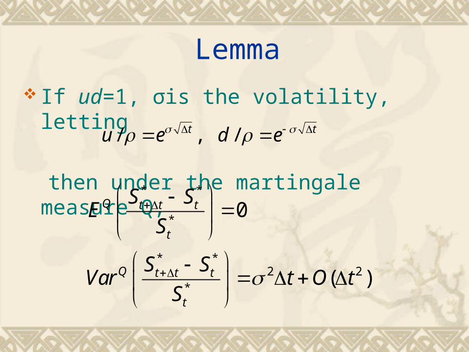
Lemma

If ud=1, σis the volatility, letting

then under the martingale measure Q,/ , /t tu e d e

* *

*

* *2 2

*

0

( )

Q t t t

t

Q t t t

t

S SE

S

S SVar t O t

S

Proof of the Lemma

According to the definition of martingale measure Q, on [t,t+Δt],

thus by straightforward computation,

1Q t t t t t t

t t

S S B BE

S B

* *

*

/1 1 0Q Qt t t t t t t t t

t t

S S S B B SE E

S S

Proof of the Lemma

Moreover, since2* * * *

* *

2 2

2 2

( / 1) (1 / )

( 1) (1 )

Q Qt t t t t t

t t

u d

t tu d

S S S SVar E

S S

q u q d

q e q e

Proof of the Lemma cont.

by the assumption of the lemma,

input these values to the ori. equation. This completes the proof of the lemma.

1 ( )

1 ( )

, 1/ 2 ( )

1, ( )

t

t

u d

u d u d

e t o t

e t o t

q q O t

q q q q O t

Geometric Brownian Motion

By Taylor expansion

neglecting the higher order terms of Δt, we have

* *

*: ( )t t t

t

S StR

S

22 *1ln(1 )

2O S

*2

*

1ln ( )

2t t

t

StR t

S

Geometric Brownian Motion cont.

By definition

therefore after partitioning [0,T], at each instant ,

i.e.

*0 01, 1S B

** 2

*1 1

1ln ln

2

k kt t

k i ki it

SS R t

S

* 2

1

1ln ln ln

2

k

k k k k i ki

S S B rt R t

kt t

Geometric Brownian Motion cont.-

2

2

/ 2 ( )

0

0

ln ( ) ( / 2) ( )

. .

( )r t W t

Let t

S t r t W t

i e

S t S e

Geometric Brownian Motion cont.--

This means the underlying asset price movement as a continuous stochastic process, its logarithmic function is described by the Brownian motion. The underlying asset price S(t) is said to fit geometric Brownian motion.

This means: Corresponding to the discrete BTM of the underlying asset price in a risk-neutral world (i.e. under the martingale measure), its continuous model obeys the geometric Brownian motion .

Definition of Quadratic Variation

Let function f(t) be given in [0,T], and Π be a partition of the interval [0,T]:

the quadratic variation of f(t) is defined by

0 10 Nt t t T

1

2

10

N

k kk

Q f t f t

Quadratic Variation for classical function

1

0If ( ) [0, ], then lim 0f t C T Q

0

If ( ) [0, ], &

it has bounded variation on [0, ]

then lim 0

f t C T

T

Q

Theorem 4.1

Let Π be any partition of the interval [0,T], then the quadratic variation of a Brownian motion has a limit as follows:

0limQ T

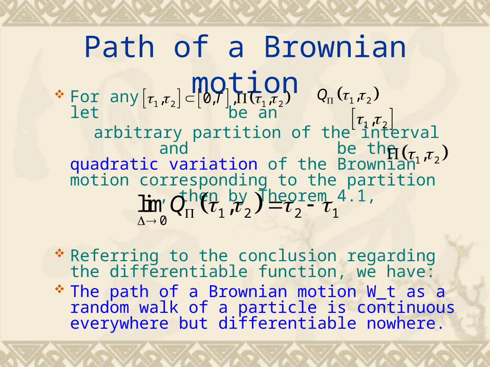
Path of a Brownian motion For any let be an arbitrary partition of the interval and

be the quadratic variation of the Brownian motion corresponding to the partition , then by Theorem 4.1,

Referring to the conclusion regarding the differentiable function, we have:

The path of a Brownian motion W_t as a random walk of a particle is continuous everywhere but differentiable nowhere.

1 2 1 2, 0, , ,T 1 2,Q

1 2,

1 2,

1 2 2 10

lim ,Q

Remark If dt 0 (i.e. Δ 0), let denote the limit of then by Theorem 4.1,

Hence neglecting the higher order terms of dt,

i.e. neglecting higher order terms, the square

of the random variable is a definitive infinitesimal of the order of dt.

2

22 4 2 2

,

2

t

t t t

E dW dt

Var dW E dW E dW dt

2tdW dt

1k kk t tD W W

tdW

tdW

An Example A company invests in a risky asset,

whose price movement is given by

Let f(t) be the investment strategy, with f(t)>0(<0) denoting the number of shares bought (sold) at time t. For a chosen investment strategy, what is the total profit at t=T?

0 ,tW t T

An Example cont. Partition [0,T] by: If the transactions are executed at time

only, then the investment strategy can only be adjusted on trading days, and the gain (loss) at the time interval is

Therefore the total profit in [0,T] is

0 10 Nt t t T

kt t

1 1

( )k kk t tf t W W

1 1

1

0

( ) ( )k k

N

k t tk

I f f t W W

Definition of Itô Integral

If f(t) is a non-anticipating stochastic process, such that the limit

exists, and is independent of the partition, then the limit is called the Itô Integral of f(t), denoted as

1 1

1

10 0

0

lim ( ) lim ( ) , ( max( ))k k

N

k t t k kk

I f f t W W t t

1 1

1

0 00

( ) lim ( ) .k k

NT

t k t tk

f t dW f t W W

Remark of Itô Integral Def. of the Ito Integral ≠ one of the Riemann integral. - the Riemann sum under a particular partition. However, f(t) - non-anticipating, Hence in the value of f must be taken at the left

endpoint of the interval, not at an arbitrary point inΔ. Based on the quadratic variance Them. 4.1 that the value

of the limit of the Riemann sum of a Wiener process depends on the choice of the interpoints.

So, for a Wiener process, if the Riemann sum is calculated over arbitrarily point in Δ, the Riemann sum has no limit.

( )I f

( )I f

Remark of Itô Integral 2

In the above proof process : since the

quadratic variation of a Brownian motion is nonzero, the result of an Ito integral is not the same as the result of an ormal integral.

Ito Differential Formula

This indicates a corresponding change in the differentiation rule for the composite function.

2

2

1 1

2 2

2

t t t

t t t

WdW dW dt

dW W dW dt

Itô Formula

Let , where is a stochastic process. We want to know

This is the Ito formula to be discussed in this section. The Ito formula is the Chain Rule in stochastic calculus.

( , )t tY f X tt tX W

( , ) ?t tdY df X t

Composite Function of a Stochastic Process

The differential of a function is the linear principal part of its increment. Due to the quadratic variation theorem of the Brownian motion, a composite function of a stochastic process will have new components in its linear principal part. Let us begin with a few examples.

Expansion

By the Taylor expansion ,

Then neglecting the higher order terms,

22

2

2

2

1

2

1

2

t t t t

t

f f fdY dt dX dX O dX dt

t x x

f f fdt dW o dt

t x x

2

2

1

2t t

f f fdY dt dW

t x x

2

2

1

2t t

f f fdY dt dW

t x x

( )t tX W

Example

1 2

2

2

,

2 , 0, 2,

2

t t t t

t t t

Y X X W

f f fx

x t xdY dt W dW

Differential of Risky Asset

In a risk-neutral world, the price movement of a risky asset can be expressed by,

We want to find dS(t)=?

2( - / 2)0

tr t WtS S e 2( - / 2)

0tr t W

tS S e

Differential of Risky Asset cont.

2

2

2

( / 2)0

( /2)2 20

( /2)0

( ) ( , ), ,

( , )

( ) ( /2 /2)

( ) ( )

t

t

t

t t t

r t W

r t W

r t Wt

t

S t f X t X W

f x t S e

dS t S r e dt

S e dW

rS t dt S t dW

Stochastic Differential Equation In a risk-neutral world, the underlying asset

satisfies the stochastic differential equation

where is the return of over a time interval dt, rdt is the expected growth of the return of , and is the stochastic component of the return, with variance . σ is called volatility.

tS

/t t tdS S rdt dW /t t tdS S rdt dW

/t tdS StS

tS2dttdW

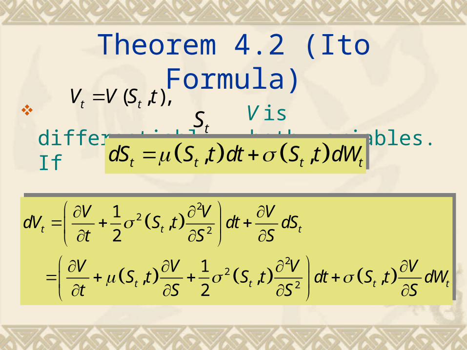
Theorem 4.2 (Ito Formula)

V is differentiable ~ both variables. If satisfies SDE

then

( , ),t tV V S ttS

, ,t t t tdS S t dt S t dW , ,t t t tdS S t dt S t dW

22

2

22

2

1,

2

1, , ,

2

t t t

t t t t

V V VdV S t dt dS

t S S

V V V VS t S t dt S t dW

t S S S

22

2

22

2

1,

2

1, , ,

2

t t t

t t t t

V V VdV S t dt dS

t S S

V V V VS t S t dt S t dW

t S S S

Proof of Theorem 4.2

By the Taylor expansion

But

2

2

2

1

2t t t t

V V VdV dt dS dS O dtdS

t S S

22

22 2 2

2

, ,

, 2

, ( )

t t t t

t t t

t

dS S t dt S t dW

S t dW dtdW dt

S t dt o dt

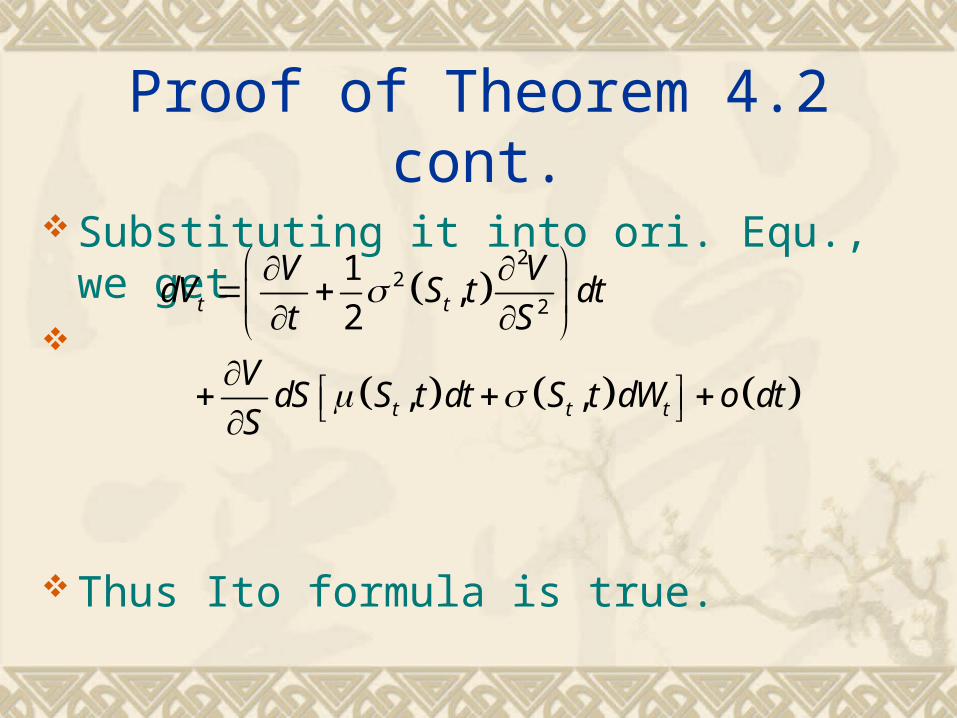
Proof of Theorem 4.2 cont.

Substituting it into ori. Equ., we get

Thus Ito formula is true.

22

2

1,

2

, ,

t t

t t t

V VdV S t dt

t S

VdS S t dt S t dW o dt

S

Theorem 4.3

If are stochastic processes satisfying respectively the following SDE

then

,t tX Y

1 1

2 2

,t t

t t

dX dt dW

dY dt dW

1 2t t t t t td X Y X dY Y dX dt 1 2t t t t t td X Y X dY Y dX dt

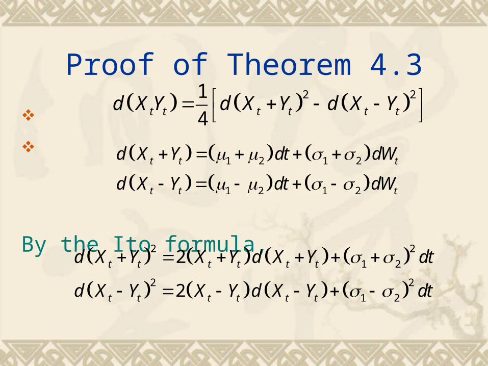
Proof of Theorem 4.3

By the Ito formula,

2 21

4t t t t t td X Y d X Y d X Y

1 2 1 2

1 2 1 2

t t t

t t t

d X Y dt dW

d X Y dt dW

2 2

1 2

2 2

1 2

2

2

t t t t t t

t t t t t t

d X Y X Y d X Y dt

d X Y X Y d X Y dt

Proof of Theorem 4.3 cont.

Substituting them into above formula

Thus the Theorem 4.3 is proved.

2 2

1 2 1 2

1 2

12 2

21

4

t t t t t t t t t t

t t t t

d X Y X Y d X Y X Y d X Y

dt

X dY Y dX dt

Theorem 4.4

If are stochastic processes satisfying the above SDE, then

,t tX Y

2 22 1

2 3t t t t t t t

t t t

X Y dX X dY X Yd

Y Y Y

2 22 1

2 3t t t t t t t

t t t

X Y dX X dY X Yd

Y Y Y

Proof of Theorem 4.4

By Ito formula

222 3

22 2 22

1 1 1

1 1

tt t t

tt t

d dY dtY Y Y

dt dWY Y

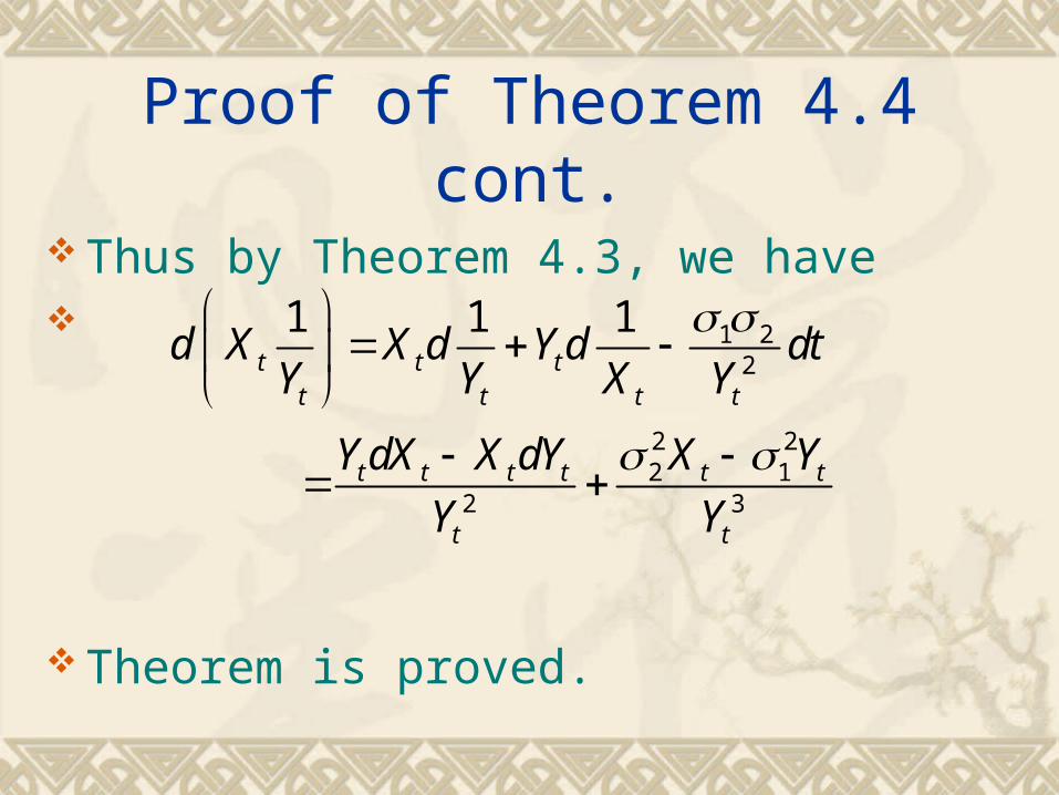
Proof of Theorem 4.4 cont.

Thus by Theorem 4.3, we have

Theorem is proved.

1 22

2 22 1

2 3

1 1 1t t t

t t t t

t t t t t t

t t

d X X d Y d dtY Y X Y

Y dX X dY X Y

Y Y

Remark

Theorems 4.3--4.4 tell us: Due to the change in the Chain Rule for

differentiating composite function of the Wiener process, the product rule and quotient rule for differentiating functions of the Wiener process are also changed.

All these results remind us that stochastic calculus operations are different from the normal calculus operations!

Multidimensional Itô formula Let be independent

standard Brownian motions,

where Cov denotes the covariance:

( ), ( 1, , )jW t j m

0, , ( 1, )

0, ( )

j j

i j

E dW Var dW dt j m

Cov dWdW i j

( , ) ( ) ( )Cov X Y E X E X Y E Y

Multidimensional Equations

Let be stochastic processes satisfying the following SDEs

where are known functions.

( ) ( 1, )iX t i n

11 11 1 1

1

( ), , ( )( ) ( ) ( )

( ) ( ) ( ), , ( ) ( )

m

n n n nm n

t tX t b t X t

d dt d

X t b t t t X t

( ), ( )i ijb t t

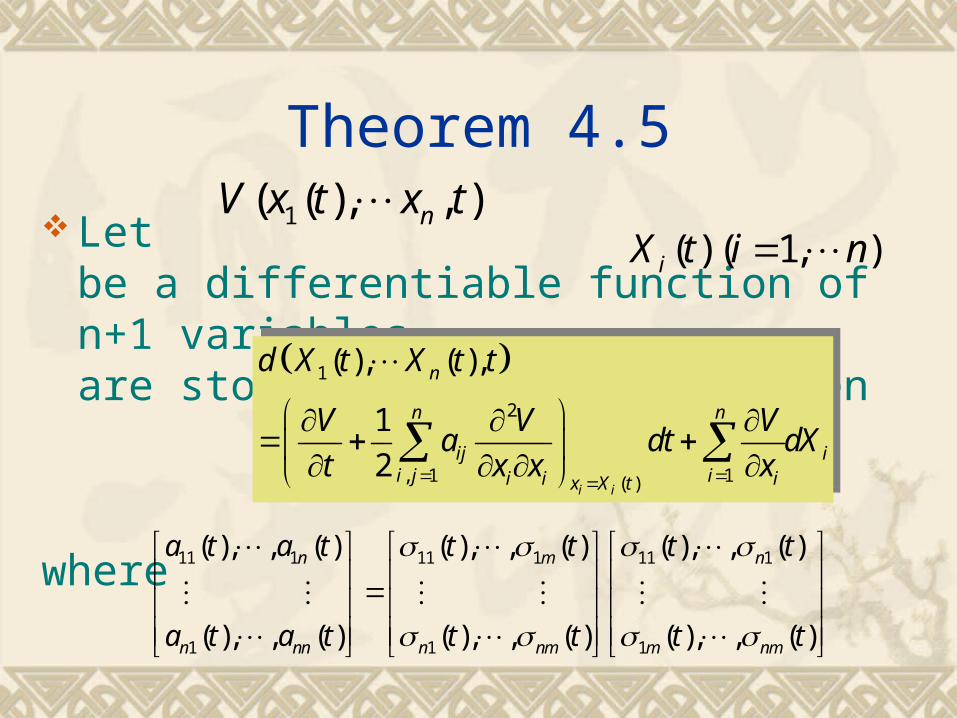
Theorem 4.5

Let be a differentiable function of n+1 variables, are stochastic processes , then

where

1( ( ), , )nV x t x t( ) ( 1, )iX t i n

1

2

, 1 1( )

( ), ( ),

1

2i i

n

n n

ij ii j ii i ix X t

d X t X t t

V V Va dt dX

t x x x

1

2

, 1 1( )

( ), ( ),

1

2i i

n

n n

ij ii j ii i ix X t

d X t X t t

V V Va dt dX

t x x x

11 1 11 1 11 1

1 1 1

( ), , ( ) ( ), , ( ) ( ), , ( )

( ), , ( ) ( ), , ( ) ( ), , ( )

n m n

n nn n nm m nm

a t a t t t t t

a t a t t t t t

Summary 1

The definition of the Brownian motion is the central concept of this chapter. Based on the quadratic variation theorem of the Brownian motion, we have established the basic rules of stochastic differential calculus operations, in particular the Chain Rule for differentiating composite function------the Ito formula, which is the basis for modeling and pricing various types of options.

Summary 2

By the picture of the Brownian motion, we have established the relation between the discrete model (BTM) and the continuous model (stochastic differential equation) of the risky asset

price movement. This sets the ground for further study of the BTM for option pricing (such as convergence proof).

作业： P73 、 1 ， 2