Embed Size (px)
Citation preview

Brian McDaniel Candidate Electrical and Computer Engineering (ECE) Department This thesis is approved, and it is acceptable in quality and form for publication on microfilm: Approved by the Thesis Committee: , Chairperson Accepted: Dean, Graduate School Date

Tasking Delay Constrained Wireless Sensor Networks:
A Performance Analysis
BY
Brian McDaniel
BS., Electronics Engineering Technology, DeVry Institute of Technology, 2002
THESIS
Submitted in Partial Fulfillment of the Requirements for the Degree of
Master of Science
Electrical Engineering
The University of New Mexico Albuquerque, New Mexico
December, 2005

iii
©2005, Brian McDaniel

iv
Dedication
To all my family, friends, and especially my wife and son.

v
Acknowledgments
First I would like to thank the ECE department at UNM and in particular
Professor Chaouki Abdallah and Balu Santhanaham for their dedication and support in
ensuring that my education was “good” one. This thesis and my overall experience at
UNM has been a positive one because of theirs and other ECE staff member’s efforts.
Thanks.
I would also like to thank my co-workers and management at Sandia National
Laboratories for supporting this effort. In particular I want to thank my manager Bob
Longoria for fully supporting me while I was continuing my education, Matt Oswald for
all of his advice and for always taking the time to explain things to me and to Pete
Sholander for his steady guidance and patience. Thanks.
I would also like to say a special thanks to my wife Autumn for always
encouraging and supporting me and to my son Jake who always inspired me to work
harder. Finally, I would like to thank my Lord and Savior Jesus Christ who deserves all
glory and praise.

Tasking Delay Constrained Wireless Sensor Networks:
A Performance Analysis
BY
Brian McDaniel
ABSTRACT OF THESIS
Submitted in Partial Fulfillment of the Requirements for the Degree of
Master of Science
Electrical Engineering
The University of New Mexico Albuquerque, New Mexico
December, 2005

vii
Tasking Delay Constrained Wireless Sensor Networks: A Performance Analysis
by
Brian McDaniel
BS., Electronics Engineering Technology, DeVry Institute of Technology, 2002
MS., Electrical Engineering, University of New Mexico, 2005
Abstract
For some particular Wireless Sensor Network applications partitioning the field of
wireless nodes into clusters of smaller ad hoc multi-hop networks (tasking) offers distinct
advantages over using a large ad hoc multi-hop network. The delay-constrained
application is one such example. A delay-constrained network is a network for which the
time required to communicate “sensed” data to an outside network is strictly constrained.
As such, smaller clusters of networks that can simultaneously communicate “sensed”
data, via clusterheads, to the outside network are necessary. In the literature many
clustering algorithms exist that consider clustering fields of wireless nodes. However, the
performance analysis of such clustering algorithms is typically limited to networks that
are predominately Size, Weight, and Power constrained (SWAP). For such networks
energy is considered the primary performance metric of concern.
This thesis instead examines the design considerations and tradeoffs that exist for
clustering networks that are delay-constrained. As such this thesis includes a first-order

viii
performance analysis based on simulating various clustering algorithms that might be
used to cluster delay-constrained networks. Next the performance analysis is extended to
include the design considerations and tradeoffs that exist for clustering a delay-
constrained network using a distributed clustering algorithm. The simulations of the
distributed clustering algorithm include node and wireless channel models that more
accurately describe sensor network behavior. As such an analysis based on these
simulation results provides even further insight into the cost and overhead associated with
tasking delay-constrained networks.

ix
Contents
List of Figures xi
List of Tables xiv
1 Introduction 1
1.1 Node Architecture ............................................................................................... 3
1.1.1 Application Layer .......................................................................................... 4
1.1.2 Transport Layer ............................................................................................. 5
1.1.3 Network Layer ............................................................................................... 5
1.1.4 Data Link Layer (DLL) ................................................................................. 6
1.1.5 Physical Layer (PHY).................................................................................... 6
1.2 Performance Metrics of Wireless Sensor Networks ........................................... 7
1.3 Organization of Thesis ........................................................................................ 8
2 Sensor Network Clustering Algorithms 10
2.1 DCA and DMAC............................................................................................... 12
2.2 Weighted Clustering Algorithm (WCA)........................................................... 16
2.3 LEACH and LEACH-C .................................................................................... 20

x
2.4 Summary ........................................................................................................... 24
3 Tasking a Delay Constrained Network 26
3.1 The Delay Constrained Application.................................................................. 27
3.2 The Design Considerations ............................................................................... 28
3.3 Network Connectivity and Frequency Re-Use ................................................. 31
3.4 A First-Order Performance Analysis ................................................................ 35
3.4.1 A-Priori ........................................................................................................ 37
3.4.2 LEACH ........................................................................................................ 37
3.4.3 WCA ............................................................................................................ 38
3.4.4 Maxi-Min..................................................................................................... 39
3.5 Summary ........................................................................................................... 45
4 Extending the Performance Analysis 47
4.1 Simulation Setup ............................................................................................... 48
4.2 Simulation Results ............................................................................................ 58
4.3 Consider the “Cost”........................................................................................... 69
4.4 Summary ........................................................................................................... 71
5 Conclusions and Future Work 73
References 76

xi
List of Figures
Figure 1.1 Examples of a Multi-hop Network and Clusters of Multi-hop Network
topologies. ................................................................................................................... 2
Figure 1.2 Block Diagram of 5-layer OSI Model. ............................................................. 4
Figure 3.1 Probability that the network is connected for a 100 uniformly distributed nodes
in a 1 kilometer square region. .................................................................................. 29
Figure 3.2 Probability of a valid network when 50 nodes are uniformally distributed in a
1 kilometer square when the distance-based model and α = 1.5 are used in the
simulations. ............................................................................................................... 34
Figure 3.3 Maxi-Min example when 2 clusterheads need to be chosen in a field of 6
nodes. ........................................................................................................................ 39
Figure 3.4 Probability Density Function (PDF) of WCA upload time. ........................... 41
Figure 3.5 Probability of a valid network when WCA was used to cluster the field of
nodes. ........................................................................................................................ 43

xii
Figure 3.6 Probability of a valid network when WCA was used to cluster the field of
nodes. ........................................................................................................................ 44
Figure 4.1 OPNET Model heirarchy. ............................................................................... 48
Figure 4.2 The Network Model which containes the “Sensor Network”. ........................ 49
Figure 4.3 Scenario Model for a wireless sensor network. .............................................. 50
Figure 4.4 Node Model for each node in the sensor network. ......................................... 55
Figure 4.5 The clustering algorithm Process Model that was used in both scenarios. .... 57
Figure 4.6 Average Cluster-size as a function of transmit power.................................... 60
Figure 4.7 The average convergence time and average node energy consumed as
funcions of transmit power........................................................................................ 61
Figure 4.8 Confidence interval (90 %) for the average number of non-convergent nodes
when BER is included in the simulation. .................................................................. 63
Figure 4.9 The average number of non-convergent nodes as a function of SNR threshold
and PTX when BER was included in the simulations. ............................................... 64
Figure 4.10 Average cluster-size as a function of SNR threshold and PTX...................... 65
Figure 4.11 Average convergence time as a function of SNR threshold and PTX............ 66
Figure 4.12 Average node energy as a function of SNR threshold and PTX. ................... 67
Figure 4.13 Number of non-convergent nodes as function of SNR threshold and PTX in
the presence of log-normal fading and BER’s. ......................................................... 68

xiii
Figure 4.14 Weighted cost as a function of SNR threshold and PTX when BER was
included in the simulations........................................................................................ 70

xiv
List of Tables
Table 3.1 Normalized average and maximum upload times for A-Priori, WCA, Maxi-
Min, and LEACH clustering algorithms. .................................................................. 40

1
Chapter 1
Introduction
Minimally a wireless sensor network is comprised of nodes that are tasked to sense some
physical phenomenon(s) and then process and send the necessary data using wireless
communications to a sink node(s). The sink node then forwards the appropriate data,
using wireless or wired links, to an existing data infrastructure such as a LAN or a
personal computer. Because of the diversity in sensor technology and recent
improvements in communications technology, many different applications for wireless
sensor networks have emerged. For example, sensor networks can be used to conduct
surveillance, bomb damage assessment, forest fire and flood detection, and to remotely
monitor medical patients [1]. Currently many possible applications for wireless sensor
networks exist and as wireless sensor networks become better understood, many more
promise to emerge and change how and where remote sensing is done.
Depending upon the application of a particular wireless sensor network, the
physical placement of the nodes may or may not be well controlled. Nodes may be

Chapter 1. Introduction
2
“hand-emplaced” or they may be distributed randomly through some method of
deployment, such as airdropping the nodes from an airplane. For both physical
placement realizations, it will be necessary that the nodes create and maintain some
network configuration so that data may traverse between the nodes. In general, most
sensor networks are either configured as one ad hoc multi-hop network or as smaller
clusters of ad hoc multi-hop networks. Examples of an ad hoc multi-hop and clusters of
ad hoc multi-hop network topologies are shown in Figure 1.1.
Figure 1.1 Examples of a multi-hop network and clusters of multi-hop network topologies.
Each sink and source node must therefore have a processor that processes sensed

Chapter 1. Introduction
3
data and a radio that establishes and maintains network communications. Sensor nodes
must also have the ability to sense the physical phenomenon of interest, i.e. some sensor
package. Data flows within each node as a result of sensing, processing, and
communicating and can be described by the 5-layer Open System Interconnection (OSI)
model [2, 3, 4]. The following section briefly describes the 5-layer OSI model and the
task, which are typically performed at each of the layers. (Note: “cross-layer design that
blurs the boundaries in the 5-layer OSI model is an active research area. This thesis uses
the traditional OSI model for illustrative purposes.)
1.1 Node Architecture
The 5-layer OSI model consists of the Application, Transport, Network, Data Link or
Medium Access Layer (MAC), and Physical layers. Data flows through the layers up or
down sequentially as shown in Figure 1.2.

Chapter 1. Introduction
4
Figure 1.2 Block Diagram of 5-layer OSI Model.
1.1.1 Application Layer
The application layer is a program or group of programs that is designed for the end user
[2]. There are both global and local services provided by the application layer. Global
services are those services that make direct contributions to the mission objective. For
example a node’s decision to track a vehicle would be a global service. Other examples
of global services would include doing things such as bomb damage assessment. Local
services are those services the node provides to itself. For example, determining the
Quality of Service (QOS), doing authentication, determining communication partners are
all examples of local services. In general, for wireless sensor networks, the application
layer determines the system level behavior of a node.

Chapter 1. Introduction
5
1.1.2 Transport Layer
The transport layer is responsible for passing data to the application layer in such a
manner as to relieve the application layer from concerning itself with cost-effective
transmission and connection reliability [3]. The transport layer manages connections,
provides congestion and flow control, and maintains connection reliability. Examples of
reliable transport protocols used for wireless communications include the Transmission
Control Protocol Westwood (TCPW), and TCP Reno [5, 6]. It should be noted that in
some wireless sensor networks a formal transport layer may not exist.
1.1.3 Network Layer
The network layer establishes, maintains, and terminates the network connections [4].
The protocol in the network layer is tasked to route, address, and possibly assign the node
roles if nodes can assume multiple roles, i.e. sensors or sinks. Examples of routing
protocols for ad hoc multi-hop wireless sensor networks include Dynamic Source
Routing (DSR), Ad Hoc on Demand Distance Vector Routing Protocol (AODV), and
Temporally-Ordered Routing Algorithm (TORA) [7, 8, 9]. Whereas clustering
algorithms such as Weighted Clustering Algorithm (WCA), Low-energy Adaptive

Chapter 1. Introduction
6
Clustering Hierarchy Protocol (LEACH), and Distributed Clustering Algorithm (DCA)
are used to form clusters of ad hoc multi-hop networks [10, 11, 12].
1.1.4 Data Link Layer (DLL)
The data link layer is divided into two sub-layers – namely the Logical Link Control
Layer (LLC) and the Media Access Control Layer (MAC). The LLC layer is tasked to
provide a reliable, error-free link between the MAC and the Network layer. The MAC
layer is primarily tasked to minimize collisions in the medium [4]. The MAC layer
minimizes packet collisions using techniques such as Carrier Sensing Multiple Access
(CSMA), and by multiplexing wireless data from different sensor nodes using Time-
Division Multiple Access (TDMA), Frequency Division Multiple Access (FDMA), or
Code Division Multiple Access (CDMA) [1]. In addition to minimizing collisions the
MAC layer may also provide some link reliability services such as Cyclical Redundancy
Checking (CRC), and unique addressing [3].
1.1.5 Physical Layer (PHY)
The physical layer is responsible for the transmission and reception of the data across
wireless and possibly wired channels [3]. For sensor nodes the physical layer is
Chapter 1. Introduction
7
essentially the RF section of the node. However, a sink node might have more than one
medium that it is connected too. For example the sink node may be connected to the
Internet, as well as wirelessly to sensor nodes. In this instance the sink’s physical layer
would need to include an RF section as well as a wired modem section.
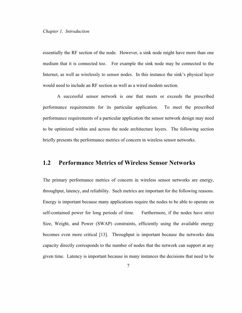
A successful sensor network is one that meets or exceeds the prescribed
performance requirements for its particular application. To meet the prescribed
performance requirements of a particular application the sensor network design may need
to be optimized within and across the node architecture layers. The following section
briefly presents the performance metrics of concern in wireless sensor networks.
1.2 Performance Metrics of Wireless Sensor Networks
The primary performance metrics of concern in wireless sensor networks are energy,
throughput, latency, and reliability. Such metrics are important for the following reasons.
Energy is important because many applications require the nodes to be able to operate on
self-contained power for long periods of time. Furthermore, if the nodes have strict
Size, Weight, and Power (SWAP) constraints, efficiently using the available energy
becomes even more critical [13]. Throughput is important because the networks data
capacity directly corresponds to the number of nodes that the network can support at any
given time. Latency is important because in many instances the decisions that need to be

Chapter 1. Introduction
8
made either within the network or outside of the network are time critical and require
“recent” data [14]. Finally, reliability is important because some QOS must be
guaranteed so that the necessary data reaches its destination(s).
1.3 Organization of Thesis
Many applications, each with their own performance requirements, exist for wireless
sensor networks. The primary application of interest in this thesis is the class of
Unattended Ground Sensor (UGS) applications that warrant the need for clusters of ad
hoc networks – namely the delay-constrained application. In the literature there exists a
number of clustering algorithms that form and manage clusters of ad hoc multi-hop
networks. Typically included in the papers is a performance analysis of the algorithms,
but such analysis is typically limited to sensor networks where energy and
reliability/robustness are considered the primary performance metrics of interest.
Unfortunately, the papers do not adequately address the applications where the primary
performance metrics of concern may not be energy or reliability/robustness. For
example, the delay-constrained network is not as concerned with energy or reliability as it
is concerned with overall throughput and delay. As such, the aim of this thesis is to
understand the design considerations, tradeoffs, and overhead associated with clustering
algorithms for delay-constrained applications.

Chapter 1. Introduction
9
The remainder of the thesis is organized as follows: Chapter 2 contains a brief
summary of some popular clustering algorithms found in the literature. In Chapter 3, the
delay-constrained application is introduced along with its associated design constraints.
One key tradeoff is the pervasive network connectivity vs. frequency re-use. Chapter 3
also includes a performance analysis based on MATLAB simulation results, of using A
Priori, WCA, LEACH, and Maxi-Min clustering algorithms to cluster the nodes in a
delay-constrained application[15]. Chapter 4 extends that performance analysis by
presenting an analysis based on results gathered from simulating a distributed clustering
algorithm using OPNET [16]. For some applications, a distributed clustering algorithm
more closely resembles what might be implemented using real hardware. As such,
Chapter 4 provides further insight into the design considerations, tradeoffs, and overhead
associated with clustering the nodes of a delay-constrained application. Chapter 5
concludes this thesis and provides suggestions for future work.

10
Chapter 2
Sensor Network Clustering Algorithms
Resources such as the available energy and channel bandwidth are limited in wireless
sensor networks. Clustering algorithms are of interest because partitioning the nodes into
clusters provides means whereby these valuable resources may be better managed
throughout the network. Much like a base-station in a wireless cellular system, a cluster
of nodes includes a clusterhead (sink) that controls access to the channel. For wireless
communications controlling the channel access is the means through which available
bandwidth can be managed across some spatial region. However, unlike the base station
of the cellular system, the clusterhead is SWAP-constrained and hence has a limited
amount of energy. Furthermore, the clusterhead may consume considerable energy
controlling channel access and performing the sink responsibilities of communicating
data to the outside network. It quickly becomes evident that the measure of a clustering
algorithms’ effectiveness depends on how well it is able to balance the resource
constraints of the application, while still meeting the performance metrics of concern -
namely energy, throughput, reliability, and latency. For example, if a network is strictly

Chapter 2. Clustering Ad hoc Networks
11
energy constrained the clustering algorithm might distribute costly communications,
(such as communicating to the outside network), evenly among the nodes. However,
such clustering may lead to instances of poorly spatially distributed clusterheads; this
translates to less overall throughput and longer end-to-end delays [11]. In contrast to the
strictly energy constrained applications, are those applications where reliability is the
primary metric of concern, such as when nodes are mobile. If the nodes are mobile the
clustering algorithm needs to be robust and able to effectively manage an ever-changing
network topology [10], requiring more wireless communications and hence more energy.
From a design perspective the question then becomes, “What clustering algorithm(s)
optimize across the resource constraints and ensure that the other required performance
metrics of this application are met?”
Clustering algorithms can be distributed or centralized. A distributed clustering
algorithm executes at each node in the network, acting on at most information from its k-
hop neighbors. The centralized clustering algorithm acts on global information and is
usually executed by a computing resource that is outside of the network, such as a
Mission Operations Center (MOC). A centralized algorithm may be able to optimize the
network topology better than its distributed counterpart, since it has global information to
compute with. However, it may be expensive in terms of energy and latency to
communicate the necessary global information to a centralized algorithm. Therefore, a
centralized algorithm might be ineffective mobile or strictly energy-constrained sensor

Chapter 2. Clustering Ad hoc Networks
12
networks. The following sections summarize and review the performance of a few
popular clustering algorithms. All of the clustering algorithms presented assume that all
nodes within a sensor network are equipped such that they may perform both sensor and
clusterhead roles.
2.1 DCA and DMAC
The Distributed Clustering Algorithm (DCA) and the Distributed Mobility-Adaptive
Clustering Algorithm (DMAC) are the first clustering algorithms that will be presented.
As will be seen, DCA and DMAC demonstrate the complexity required to cluster ad hoc
and mobile ad hoc networks. Although there is no formal performance analysis of DCA
or DMAC, the algorithms are included because in Chapter 4 the distributed clustering
algorithm that was adopted uses DCA packet types and processes. In [12] two distributed
clustering algorithms are proposed – namely DCA and DMAC. DCA is a “leader-
election” clustering algorithm that uses a weighted heuristic approach. Each node has a
weight that is real and unique compared to its neighbors. DCA is simple and requires
only two types of messages: a clusterhead message CH(v) and a join message Join(v,u).
The CH(v) message declares that node v is a clusterhead, and the Join(v,u) message
declares that node v is joining the cluster with clusterhead u. For DCA to execute
correctly it is assumed that at algorithm execution time, T0, every node knows all of its

Chapter 2. Clustering Ad hoc Networks
13
neighbors unique identifier (ID) and weight. It is also assumed that the network topology
will be static during algorithm execution and that a node’s messages are correctly
received by all of its neighbors within a finite time. The DCA algorithm executes as
follows.
• Initially nodes with the highest weight among their neighbors transmit a CH(v)
message.
• When a node has the highest weight among its undecided neighbors (neighbors
that have not sent a CH(v) or Join(v,u) message) it joins the clusterhead with the
largest weight if multiple neighbors are clusterheads, and sends a Join(v,u)
message. If none of its neighbors have become clusterheads the node becomes
a clusterhead and sends a CH(v) message.
DMAC is an extension of DCA that is designed for clustering mobile nodes. The
DMAC algorithm has the added ability to not just react to messages received from
neighboring nodes, but also to handle link failures and link additions due to nodes
moving. DMAC requires the same two messages as DCA – namely Join(v,u) and CH(v).
The following assumptions are required for DMAC to execute correctly.
• A node is always aware of its neighbors IDs and weights.
• Nodes must be aware of new and failed links so it is assumed that a lower level
service will provide reliable link information to the DMAC.
• DMAC procedures are not interruptible.

Chapter 2. Clustering Ad hoc Networks
14
• When a node is added to a network or during clustering setup the node assumes
that it is not a clusterhead and that it does not belong to any cluster.
DMAC executes these five procedures: Init, Link_failure, New_link,
On_receiving_CH(v), and On_receiving_Join(v,u), as follows.
1) The Init procedure is executed at clustering setup or when a node is added to
the network. If one of its neighbors is a clusterhead with a larger weight than
itself than it joins this clusterhead and sends the Join(v,u) message. If none
of its neighbors are clusterheads it becomes a clusterhead and sends the
CH(v) message.
2) Link_failure is executed when node v becomes aware of a link failure with
node u. If node v is a clusterhead it removes node u from its list of nodes.
If node u was the clusterhead of the cluster that v belongs to then node v
needs to decide what its new role is going to be. Node v joins a cluster if one
of its neighbors is a clusterhead with a weight larger than itself and sends a
Join(v,u~) message. Otherwise if node v has the largest weight of its
neighbors then it become a clusterhead and sends the CH(v) message.
3) The New_link procedure is executed when node v becomes aware that node
u is new to its neighborhood. If node u is a clusterhead with a weight larger
than its current clusterhead (including itself if it is a clusterhead) then it
accepts node u as its new clusterhead and sends the Join (v,u) message.

Chapter 2. Clustering Ad hoc Networks
15
4) The On_receiving_CH(v) procedure is executed when node u receives a
CH(v) message. If node v is a clusterhead with a weight larger than its
current clusterhead (including itself if it’s a clusterhead) then it accepts node
v as its new clusterhead and sends the Join (u,v) message.
5) The On_receiving_Join(v,u) procedure is executed when node z receives a
join message from node v announcing that it is joining node u. If node z is a
clusterhead and v = z then node u is added to its cluster list, if v ≠ z then
node z removes u from its list. Finally, if node u was the clusterhead of the
cluster that node z belongs then node z needs to decide its role. Node z joins
a cluster if one of its neighbors is a clusterhead with a weight larger than
itself and sends a Join(z,u~) message. Otherwise if node z has the largest
weight of its neighbors then it becomes a clusterhead and sends the CH(v)
message.
It can be seen from the DCA and DMAC processes that greater algorithm complexity is
required to handle mobile nodes. DCA and DMAC also demonstrate that in the case of
mobile nodes more energy is required to maintain the network, since more
communications are required to perform DMAC than DCA. DCA and DMAC
algorithms can easily be implemented, since the author explicitly defines the processes
and required packet types. Unfortunately, the author does not formally discuss the

Chapter 2. Clustering Ad hoc Networks
16
assignment of the weight parameter or present a performance analysis of DCA and
DMAC for any specific sensor applications.
2.2 Weighted Clustering Algorithm (WCA)
The work discussed in [10] builds upon the clustering approaches presented in DCA,
DMAC and other clustering algorithms. First, the authors summarize three current
heuristic approaches for choosing clusterheads in ad hoc networks, in particular the
highest-Degree heuristic [17, 18, 19, 20], the Lowest-ID heuristic [21, 22, 23], and the
Node-Weight heuristic (DCA and DMAC). The interested reader is encouraged to read
the Highest-Degree, and Lowest-ID heuristic approaches as they will not be presented in
any detail in this paper. The authors contend that the performance of distributed
clustering algorithms can be better optimized across various performance requirements
by refining the weight heuristic approach. As such, a clustering algorithm with a
combined weight metric - namely the Weighted Clustering Algorithm (WCA) is
proposed.
WCA utilizes a combined weight which better accounts for the node’s capabilities
and the performance metrics that the designer needs to optimize across. Each node’s
weight is calculated as a weighted sum of degree difference, sum of neighbor distances,
measure of mobility, and time as a clusterhead, as shown in Equation (2.2.1).

Chapter 2. Clustering Ad hoc Networks
17
(2.2.1)
Where , is the degree difference of the node and equals the |Number of Neighbors – γ|,
with γ being some desired number of neighbors, is the sum of the distances to the
nodes’ neighbors, is the measure of the nodes’ mobility and is computed as the
average velocity over some time interval T, is the cumulative time the node has been a
clusterhead, and w1, w2, w3, w4 are the weighting parameters. The parameters w1, w2, w3,
w4 allow the designer to weight the parameters so that the available network resources
may be better balanced. For example if energy consumption is the most constrained
performance metric then might be chosen so that has the largest impact on ,
assuming that the energy consumed being a clusterhead is much greater than the energy
consumed being a sensor node. However, if some nodes are highly mobile then
should be chosen such that M contributes the most to , since in the mobile case it is
desirable for the least mobile nodes to be clusterheads, so that less time is spent executing
the clustering algorithm. The election of clusterheads consists of the eight steps outlined
below. (Note: these steps imply some built-in capabilities for the sensor nodes. For
example, Step 3 assumes that every node has either on-board GPS, the ability to

Chapter 2. Clustering Ad hoc Networks
18
triangulate position from known landmarks, or pre-placed knowledge of its fixed
location. )
1) The node finds its neighbors with a neighbor discovery process.
2) The node computes its degree difference.
3) The node computes the sum of the distances to its neighbors.
4) The node computes its mobility.
5) The node computes the time it has spent as a clusterhead.
6) The node calculates its combined weight.
7) The node in the network with the smallest weight is selected as the
clusterhead and all of its neighbors are assigned to it.
8) Steps 2 – 7 are repeated for the nodes whose roles have not yet been determined.
It appears as though step 7 requires global information. However, the authors of [10]
state that a distributed solution would be to flood the network with broadcast messages
that contain the nodes’ IDs and weights until every node has global information.
Unfortunately the authors do not adequately account for the overhead and possible
shortcoming associated with flooding. Therefore, it could be argued that WCA does not
actually distribute well, and may actually need to be a centralized algorithm.
Nevertheless, this thesis assumes that WCA does in fact distribute.

Chapter 2. Clustering Ad hoc Networks
19
Compared to DCA, DMAC and the other clustering approaches, WCA allows the
designer to better balance the performance metrics of concern because WCA provides a
means whereby the clustering algorithms’ decisions can be coupled to the performance
metrics (i.e. energy, throughput, latency, and reliability) of interest. To this end the
authors simulate WCA in a mobile network and compare it to the Lowest-ID, Highest-
degree, and Node-Weight heuristic approaches. In particular, the number of re-
affiliations per unit of time vs. the transmission range for the four algorithms are
compared. The number of re-affiliations associated with each approach is important
because it is one way to measure the stability of an algorithm, since a re-affiliation is
defined to occur when a sensor node changes its cluster membership. The authors show
that with respect to re-affiliation, WCA performed much better than the Lowest-ID and
Highest-degree algorithms. While WCA performed only slightly better than the Node-
Weight approach, the authors contend that WCA is still a better solution than the Node-
Weight approach since WCA considers more realistic system parameters and has greater
flexibility because of the weighting method it utilizes – namely a combined weight
metric.

Chapter 2. Clustering Ad hoc Networks
20
2.3 LEACH and LEACH-C
To reduce energy consumption in wireless sensor networks LEACH - a low-energy
adaptive clustering hierarchy protocol is proposed in [11]. Put succinctly, LEACH
randomly rotates the clusterhead assignments among the nodes. Therefore, if being a
clusterhead consumes considerably more energy than being a sensor node (EC >> ES) then
LEACH may increase a system’s lifetime by evenly distributing the clusterhead
assignments and hence energy usage.
LEACH is a distributed algorithm that selects an average number of k
clusterheads each time it is executed (each round). LEACH requires that each node is
aware of k and N (the total number of nodes) before the nodes are deployed. The
optimal ratio of k to N depends on many factors such as node density, sensor abilities,
and the desired energy, throughput, latency performances. Clearly, time should be spent
understanding the application to determine the optimal k to N ratio before the nodes are
deployed. Using a pre-determined k and N, each node autonomously decides its role
(clusterhead or sensor) by using the probabilities defined below. In the beginning of each
round, a node u selects itself to be a clusterhead with probability Pu(t) such that the
E[Pu(t)] = k, so that for N nodes in the network
. (2.3.1)

Chapter 2. Clustering Ad hoc Networks
21
If all nodes start with the same energy the probability that a node chooses to become a
clusterhead should be uniform and equal to k/N. As an example if k = 20, and N = 120
Pu(t) = = so that (2.3.2)
. (2.3.3)
If it is assumed that all nodes should be clusterheads an equal number of times during the
network lifetime then on average each node should be a clusterhead once every N/k
rounds. Therefore, for the rth round when 1 < r < N/k the probability that node u chooses
to become a clusterhead is
. (2.3.4)
Where Cu(t) is the indicator function that node u has been a clusterhead in the current N/k
rounds. Cu(t) = 1 indicates that node u has not been a clusterhead and Cu(t) = 0 indicates
that node u has already been a clusterhead during this N/k rounds. As an example if k =
20, N = 120, r = 2, and node u did not choose to become a clusterhead in round 1. Then
the probability that node u chooses to become a clusterhead this round (r = 2) is
. (2.3.5)

Chapter 2. Clustering Ad hoc Networks
22
After each round of clusterhead assignments the clusters are formed and the sensed data
is sent to clusterheads. The clusterheads then send the received “sensed” data (and
possibly aggregate the data to save energy) to the outside network. The clusters are
formed after each round of clusterhead selection as follows. The elected clusterheads
first announce themselves to be clusterheads. The sensor nodes then determine which
clusterhead they would like to join based on some distance-based metric, such as the
Received Signal Strength (RSS). Sensor nodes then transmit a join-request message
(Join_REQ) to the clusterhead they have chosen. Once the clusters have been formed,
the clusterhead can then act as a local control center and manage the wireless channel by
scheduling data transmissions and controlling the frequency spectrum used by those
transmissions..
For networks that are strictly energy constrained, LEACH promises to better
balance energy so that the system’s lifetime may be increased. However, because
LEACH randomly chooses clusterheads, LEACH may sometimes produce a poor spatial
distribution of clusterheads. To combat these effects LEACH-centralized (LEACH-C)
was proposed in [11]. In contrast to the distributed LEACH algorithm, LEACH-C is a
centralized algorithm that acts on global information. Each node transmits its available
energy and physical location, possibly determined with an onboard GPS receiver, to a
central location such as a MOC.

Chapter 2. Clustering Ad hoc Networks
23
LEACH-C then executes the following processes. First the nodes whose available energy
falls below the energy required to be a clusterhead are removed from the clusterhead
selection process. Next the optimal k clusterheads are chosen using a simulated
annealing algorithm [24]. The simulated annealing algorithm minimizes the amount of
energy sensor nodes spends communicating “sensed” data, by minimizing the sum of the
distances between the sensor nodes and the k clusterheads. Information defining the
sensors and their corresponding clusterheads as determined by LEACH-C at the Mission
Operation Center, is then disseminated through the network.
To demonstrate the performance enhancements gained by using LEACH and
LEACH-C, LEACH and LEACH-C were simulated in [11] and compared to a minimum-
total energy (MTE) routing protocol. MTE routing minimizes the total energy required
for a packet to reach its destination by routing the packet through the minimum energy
path [25]. It was shown that LEACH and LEACH-C were more energy-efficient than
MTE since LEACH and LEACH-C delivered more effective data (effective data is the
data that is the result of aggregating the sensor data from multiple sensor nodes), per unit
of energy consumed, to the outside network. However, LEACH and LEACH-C are only
more efficient than MTE when clusterheads are assumed to be able to aggregate the data
received from the sensor nodes. Given that communications to the outside network is
considerably more expensive than local communications within the network, aggregating
the data at the clusterheads often minimizes the total amount of packets that needs to be

Chapter 2. Clustering Ad hoc Networks
24
communicated to the outside network and hence greatly improves energy efficiency.
However, if clusterheads cannot aggregate sensed data, the effective data equals the total
“sensed” data and MTE will be more energy efficient than LEACH and LEACH-C [11].
2.4 Summary
Depending upon the application, it may be desirable to cluster a wireless sensor network.
As such, some clustering algorithms where presented in this chapter – namely DCA,
DMAC, WCA, LEACH, and LEACH-C. DCA, and DMAC demonstrated the level of
complexity required to cluster static and mobile sensor networks using a weighted
heuristic approach. WCA extended the weighted heuristic approach by defining a
combined weight metric. Simulations of WCA demonstrated that clustering using a
combined weight is an improvement over previous clustering algorithms. This is due to
the fact that WCA is able to optimize the network topology over various potential
applications because the combined weight metric couples desired network performance
with individual node attributes. Finally, LEACH and LEACH-C algorithms were
presented. LEACH is simple and robust since the decision to become a clusterhead is
autonomous and is based only on predefined probabilities. Furthermore, LEACH is
energy efficient if the clusterhead tasks are more energy intense than sensor node tasks
because LEACH rotates the clusterhead assignments evenly through the nodes in the

Chapter 2. Clustering Ad hoc Networks
25
network. LEACH-C was presented to address some negative effects of LEACH
“clusters”, in particular the potential for networks with poorly distributed clusterheads or
too many/few clusterheads. LEACH-C is a centralized algorithm that optimizes the total
number and location of the clusterheads in the network by executing a simulated
annealing algorithm. Previous research has shown that if the clusterheads can aggregate
data, LEACH and LEACH-C will be more energy efficient than MTE. The
aforementioned clustering algorithms are effective and promise to offer added benefits
when partitioning the network into small clusters of multi-hop networks. Unfortunately,
the performance analysis of each algorithm was limited to the specific applications for
which the clustering algorithms were designed for, none of which were delay-
constrained. Those analyses also did not include realistic models for the RF channel, and
its effects on the convergence of the distributed clustering algorithms. In subsequent
chapters, the performance analysis of WCA, LEACH, DCA, and other clustering
algorithms will be presented for the delay constrained application. This thesis’ analysis
included the effects of bit errors and fading within the RF channel. Thos models also
include the effects of message loss on the convergence of the distributed clustering
algorithms.

26
Chapter 3
Tasking a Delay Constrained Network
The primary focus of this chapter is to understand the design consideration/tradeoffs and
overhead associated with tasking (assigning each node’s role) in a delay-constrained
network. As such this chapter is mostly composed of a summary of the previous research
presented in [15], which considered tasking the delay-constrained network. This research
is of interest because it provides some design considerations and tradeoffs associated with
tasking the delay-constrained network. Furthermore, the work presented in Chapter 4 of
this thesis, which contains OPNET simulation results that provide further insight into the
delay-constrained network, is an extension of the work done in [15].
This chapter is organized as follows. First the delay-constrained application is
defined. Next, two opposing monotone properties inherent in the delay constrained
network are examined – namely network connectivity [26] and conflict free scheduling
(time, code, or frequency re-use schemes) [27]. Finally a summary of the performance
analysis done in [15], which uses WCA, LEACH, Maxi-Min, and A-Priori algorithms to
cluster the delay-constrained network, is presented.

Chapter 3. Tasking a Delay Constrained Application
27
3.1 The Delay Constrained Application
A delay-constrained network is considered to be a network with constraints such that
overall latency (the time to communicate to an outside network) becomes the
predominant metric of concern. As an example let us consider a wireless sensor network
in which the “event(s)”, that are sensed by a field of nodes, is such that all the sensor
nodes in the field detect each event. Therefore, “shortly” after the occurrence of an
event all of the sensor nodes will have produced some amount of “sensed” data. Now let
us assume that the overall available throughput within the sensor network is constrained,
such that the time required to communicate all of this “sensed” data back to one sink
node is much greater than the time between events. Furthermore, let us assume that it is
critically important for the information to be communicated to the outside network before
subsequent events occur. Clearly in the case where all of the “sensed” data must reach
the outside network, clusters of nodes which do not interfere are required, so that the
“sensed” data can be communicated to the outside network within the time constraint.
This type of network is delay-constrained and it has been shown in [15] that in a delay-
constrained network, two opposing monotone properties may emerge, in particular
network connectivity and conflict-free channel scheduling.

Chapter 3. Tasking a Delay Constrained Application
28
3.2 The Design Considerations
In graph theory a property is considered monotone if the property remains the same when
edges/vertices are removed or added [28]. A characteristic of some monotone properties,
such as the ones that will be discussed in this thesis, is that they exhibit step phase
changes about some critical region. That is, the property is different but monotone on
both sides of the critical region.
For sensor networks the most pervasive monotone property is the probability that
a network is connected, which is a function of transmission range. A network is
considered connected if a communication path between any two node pairs exists. It has
been shown that if all the nodes have the same transmit power, then there exist some
critical transmission range for a given spatial node density, where the probability that the
network is connected goes steeply from zero to one [15, 26]. An example of this
monotone behavior is shown in Figure 3.1, when 100 nodes, each with the same
transmission power, are uniformly distributed in a 1 square kilometer region [15].

Chapter 3. Tasking a Delay Constrained Application
29
Figure 3.1 Probability that the network is connected for a 100 uniformly distributed nodes in a 1 kilometer square region.
As Figure 3.1 demonstrates, the probability that this network is connected exhibits a steep
phase change around some critical transmission range (Normalized Range ≈0.1 - 0.25).
Network connectivity is therefore a monotone property, since for small transmission
powers the probability that the network is connected is 0, whereas for large transmit
powers the probability that the network is connected is 1.

Chapter 3. Tasking a Delay Constrained Application
30
Another pervasive monotone property found in wireless sensor networks is
conflict-free channel scheduling. Conflict-free channel scheduling is defined as devising
a frequency re-use scheme that guarantees efficient use of the available channels by
minimizing the interference between nodes which occupy the same channels [27]. For a
“clustered” network this can be extended to mean devising a frequency re-use scheme
that efficiently uses the available channels by attempting to assign different frequency
bands to adjacent clusters [15]. It has been shown that partitioning the available
frequency spectrum is a monotone property and is also related to the transmission range.
However, unlike network connectivity, a realizable frequency re-use scheme (reasonable
number of frequency channels) is inversely related to the transmission range [27]. That
is, as the transmission range becomes smaller, it becomes easier (less frequency channels
– reduced complexity) to assign the spectrum such that co-channel interference is
minimized. This relation between frequency allocation and transmission range is
somewhat intuitive since as the transmission range is decreased the average number of
neighbors for each node decreases proportionally. Therefore, because there are fewer
adjacent nodes, fewer available frequency channels are required to minimize co-channel
interference.
Previous research has clearly demonstrated that the process of allocating spectrum
and connecting the network are opposing design constraints [15, 26, 27]. It will be
shown in the remainder of this chapter that this relationship is of interest, because from a

Chapter 3. Tasking a Delay Constrained Application
31
design perspective, it places limits on the possible design space. Both of these monotone
properties (network connectivity and frequency re-use) exhibit steep (and opposite) phase
changes about some critical transmission ranges. Therefore for some transmission
ranges, a reasonable frequency allocation scheme and a connected network may or may
not exist. This means for some transmission ranges the network will be expected to
work, that is be both connected and contain a valid frequency re-use scheme, while for
other transmission ranges the network will not work. The relationship between network
connectivity and frequency re-use is critical and as such the following section examines
the tradeoffs between network connectivity and frequency re-use as functions of node
density, available frequencies, and transmit power.
3.3 Network Connectivity and Frequency Re-Use
This section discusses previous research, which used graph theory techniques to study the
problem of maintaining network connectivity while still being able to create a frequency
re-use scheme [15]. That research used graph theory to consider network connectivity vs.
frequency re-use in a clustered sensor network as follows.
1.) N nodes were randomly distributed in a 1 square kilometer region.
2.) Network connectivity, for a specified range R, was checked by creating a
spanning tree of the graph.

Chapter 3. Tasking a Delay Constrained Application
32
3.) If the network was connected, a Synchronous Backtracking Algorithm, based on
[29], was used to check whether or not a valid frequency re-use pattern existed.
4.) Steps 1 – 3 were then repeated, for a large number of lay-downs, at each transmit
range and allowed number of non-overlapping frequency channels.
When simulating the above described networks with graph theory techniques, two
simple circular pattern based RF Propagation models between Nodes k and l were used.
A Distance-Based model where the Packet Reception Rate (PRR) between Nodes l and k
was set equal to 1 if |dl-dk| < R, R is an assigned range, and 0 otherwise. A Received
Signal Strength Indication (RSSI) model where Nodes l and k were assumed to be able to
communicate if RSSI [l,k] > RSSI_min, where RSSI_min was assigned such that PRR
was close to 1 (i.e. 0.9). Additionally, the interface models between Nodes l and k for the
distance-based and RSSI models assumed a CSMA-based system and were as follows.
Nodes l and k were allowed to occupy the same channel if |dl-dk| > αR or if RSSI [l,k] <
RSSI_min – β for the Distance-Based and RSSI models respectively. To model inter-
cluster interface, α should be set between 1.5 and 2, while for inter-node interference β
should be set between 3 and 6 dB. The RSSI model also assumed a log-normal channel
model of the following form [30, 31]:
(3.3.1)

Chapter 3. Tasking a Delay Constrained Application
33
Where d is the distance between nodes, d0 is a reference distance, n is the path loss
exponent, and is zero-mean Gaussian random variable, with standard deviation σ (in
dB). The parameters of Equation (3.3.1) were set to the following values - =
90dB, = 50m, n = 4, and σ = 1.0 dB. Further notable assumptions used were:
• FSK Modulation.
• Manchester encoding.
• A frame length of 512 bits with 16 bits of preamble and trailer.
• A bit rate of 9600 bps.
• A noise floor of -110.0 dBm (This is in good agreement with the COTS
radios such as the MaxStream 9Xtend radio operating at 9600 baud).
Figure 3.2 shows the results of using the aforementioned graph theory techniques to
determine the probability that the network is valid.

Chapter 3. Tasking a Delay Constrained Application
34
Figure 3.2 Probability of a valid network when 50 nodes are uniformally distributed in a 1 kilometer square when the distance-based model and α = 1.5 are used in the
simulations.
A network is “valid” when the network is both connected on a common network-
wide control channel and a valid frequency re-use scheme exists such that adjacent
clusters have an acceptable level on inter-cluster interference. The designer can quickly
note the regions (number of frequency channels and range) for which the network will
simply not work and the regions where the designer should consider using more detailed
models to verify the expected network performance (i.e. energy consumption, delay,

Chapter 3. Tasking a Delay Constrained Application
35
etc.). The relationship between network connectivity and frequency re-use and the ability
to quickly check this relationship using the graph theory techniques presented in this
chapter will prove to be very useful. It will be used in the next section to quantify the
tradeoffs associated with clustering a delay-constrained network. The next section
summarizes the performance analysis conducted in [15], which considered various
algorithms to cluster a delay-constrained network.
3.4 A First-Order Performance Analysis
This section continues to summarize the first order performance analysis conducted in
[15], which considered using A Priori, WCA, Maxi-Min, and LEACH clustering
techniques to cluster a delay constrained network. As such, the first-order statistics
resulting from clustering a delay-constrained network using various clustering techniques
is presented. The statistics include the normalized average and maximum upload times of
A Priori, WCA, Maxi-Min, and LEACH clustering algorithms. Additional first order
performance analysis includes the probability of a valid network for WCA, and Maxi-
Min clustering algorithms as functions of transmission range, and the number of available
frequency channels.
In [15] the following delay-constrained application and associated assumptions

Chapter 3. Tasking a Delay Constrained Application
36
were used. The network must ex-filtrate data from an UGS network using parallel
Satellite Communication (SATCOM) channels. Because the network is delay-
constrained, multiple non-interfering clusters are required. For each experiment 120
nodes are distributed uniformly in a 1 kilometer square. The communications between
nodes assumes the RSSI propagation model presented in the previous section.
Furthermore, it is assumed that during the clustering process all of the nodes
communicate on a shared communication channel, in addition to the available number of
frequency channels. Furthermore, all the nodes within a cluster transmit “sensed” data
using the same frequency channel, which is also assumed to be non-overlapping with to
the frequency channels of its neighboring clusters. In the A-Priori algorithm,
clutserheads and sensor nodes are assigned before the nodes are deployed such that there
are 20 clusterheads and 100 sensor nodes uniformly distributed on the 1 kilometer square.
The 20 Clusterheads are chosen to maximize overall throughput, because it is assumed
that there are 20 available SATCOM channels. For the other clustering algorithms, it is
assumed that each node is able to assume either the clusterhead or sensor node role post
deployment. Finally, it is also assumed that each sensor node must have a one-hop
connection to its clusterhead. A-Priori, WCA, Maxi-Min, and LEACH are considered for
clustering the ex-filtration application and are summarized briefly below.

Chapter 3. Tasking a Delay Constrained Application
37
3.4.1 A-Priori
The A-Priori clustering algorithm clusters the network when the nodes role is determined
before deployment. For the A-Priori case, all that is required is for each clusterhead to
first announce itself. Then each sensor node picks the clusterhead with whom it has the
best RSSI metric. The A-Priori case is of interest because it could be a viable option if
the cost difference between node roles is considered substantial, for example when the
cost to communicate using SATCOM channels is expensive. This would require a
substantially larger SWAP constraint for clusterheads compared to the SWAP constraint
of being a sensor node. In that case, a fixed function node (clusterhead or sensor) might
be required – as opposed to a multi-function node that could be either a clusterhead or a
sensor.
3.4.2 LEACH
LEACH was implemented as described in Chapter 2 of this thesis by assigning the
probability of becoming a clusterhead during the first round as follows:
k = 20, and N = 120 Pu(t) = = so that (3.2)
. (3.3)

Chapter 3. Tasking a Delay Constrained Application
38
Where k is the desired number of clusterheads, and N is the total number of nodes in the
network. The probability that a node picks itself to be a clusterhead is 1/6 so that on
average 20 nodes will become uplinks. After all the clusterheads have announced
themselves, the remaining nodes pick the clusterhead with which they have the best RSSI
metric.
3.4.3 WCA
WCA was implemented as described in Chapter 2 of this thesis. However, the weighted
metric was only the sum only of the node degree, and the distance metric, where the
distance metric was defined in terms of RSSI. Energy and mobility were not considered
because nodes were assumed to be stationary. In addition every node was considered to
have the same available starting energy. Furthermore, since 20 clusterheads were
desired, a maximum cluster size constraint was added to WCA. After the clusterheads
were chosen, the remaining nodes pick the clusterhead with which they had the best RSSI
metric.

Chapter 3. Tasking a Delay Constrained Application
39
3.4.4 Maxi-Min
The Maxi-Min algorithm attempts to spatially distribute the clusterheads as best as
possible when the nodes are uniformly distributed. A uniform distribution of the
clusterheads, based on RSSI, can be accomplished by maximizing the minimum distance
between clusterheads. This is done using the following procedures. First a clusterhead is
chosen at random. Each subsequent clusterhead is then chosen such that the minimum
distance (measured in received signal strength) between clusterheads is maximized.
After the desired number of clusterheads has been chosen the remaining nodes pick the
clusterhead with which they have the best RSSI metric. Figure 3.3 shows a simple Maxi-
Min example when 2 clusterheads are chosen in a field of 6 nodes.
Figure 3.3 Maxi-Min example when 2 clusterheads need to be chosen in a field of 6 nodes.

Chapter 3. Tasking a Delay Constrained Application
40
Since the data ex-filtration application is delay-constrained, the primary metric of
concern is latency. A measure of overall latency is the time required for the network to
ex-filtrate the “sensed” data to the outside network after each event (upload time). For
this research the events were assumed to be global and such that each sensor node
generated an equal amount of information. As such, “sensed” data is normalized and the
average and maximum upload times then become the expected cluster-size and the
expected maximum cluster-size respectively. Table 3.1 shows the “normalized” average
and maximum upload times for A-Priori, WCA, Maxi-Min, and LEACH.
A-Priori WCA Maxi-Min LEACH Average 5.03 5.75 5.02 5.43 Maximum 13.47 6.03 11.28 13.84
Table 3.1 Normalized average and maximum upload times for A-Priori, WCA, Maxi-
Min, and LEACH clustering algorithms.
The A-Priori average upload time is near optimal because the number of
clusterheads is determined pre-deployment to be 20. However, A-Priori’s relatively large
Maximum Upload time may not be desirable in delay-constrained applications, because
the upper bound for latency is the maximum upload time. LEACH performed relatively
poorly in terms of upload times. This is because LEACH does not pick a deterministic
number of clusterheads. So in many instances the available number of SATCOM

Chapter 3. Tasking a Delay Constrained Application
41
channels will be either under- or over-utilized. It is important to note, however, that
LEACH is designed to conserve energy and hence if the system is also energy
constrained LEACH might be a good alternative because it should increase the system
lifetime. As seen in Table 3.1 and Figure 3.4 there is little variance between average and
maximum upload times for WCA. It can be expected that the upload time is close to 6,
therefore on average WCA under utilizes the number of available SATCOM channels,
which occurs when the average cluster size is 5.
Figure 3.4 Probability Density Function (PDF) of WCA upload time.

Chapter 3. Tasking a Delay Constrained Application
42
The Maxi-Min algorithm has the best average upload time, because the number of
clusterhead is fixed at 20. The Maxi-Min also produces clusterheads that spatially cover
the field “well”, which means it will be easier to assign the frequency scheme such that
neighboring clusters will not interfere with each other. However, if the spatial
distribution of the clusterheads is not of interest, WCA might be best suited for this
delay-constrained application, because its upload time is bounded better.
When the number of available frequency channels is constrained, the ability to
assign a frequency re-use scheme for the clusters formed is determined by using the
following interference test during Step 3 of the aforementioned graphing techniques.
First it is assumed that the interference between clusters is noise. The Packet Reception
Rate (PRR) is therefore just a function of S/(N + I), where S is signal strength of the worst
inter-cluster link, N is the noise floor, and I is the worst case cross-cluster interference.
So to test if a frequency may be re-used, the following steps were taken.
1) A cluster was picked.
2) S/(N + I) was determined (worst inter-cluster case).
3) PRR for the worst inter-cluster case was calculated.
4) PRR<min_PRR was checked.
5) Steps 1-4 where repeated for all clusters or until one failed (PRR<min_PRR).
As was expected the probability of the network being connected was monotone with
the transmission range. Network connectivity and frequency re-use can be coupled using

Chapter 3. Tasking a Delay Constrained Application
43
the probability of a valid network metric discussed in the fist part of this chapter. By
using this metric, it can be seen in Figure 3.5 and 3.6 that creating a frequency scheme for
the Maxi-Min clusters will require fewer frequency channels than WCA. This is because
Maxi-Min clusters are denser than WCA clusters and as a result interfere less with each
other.
Figure 3.5 Probability of a valid network when WCA was used to cluster the field of nodes.

Chapter 3. Tasking a Delay Constrained Application
44
Figure 3.6 Probability of a valid network when WCA was used to cluster the field of nodes.
Therefore, if the number of frequency channels is tightly constrained, i.e. <10, then Maxi-
Min is a better solution than WCA for this application. Conversely, if the number of
available frequency channels is not tightly constrained, i.e. > 10, then WCA is a better
solution than Maxi-Mim for a delay-constrained application.
Chapter 3. Tasking a Delay Constrained Application
45
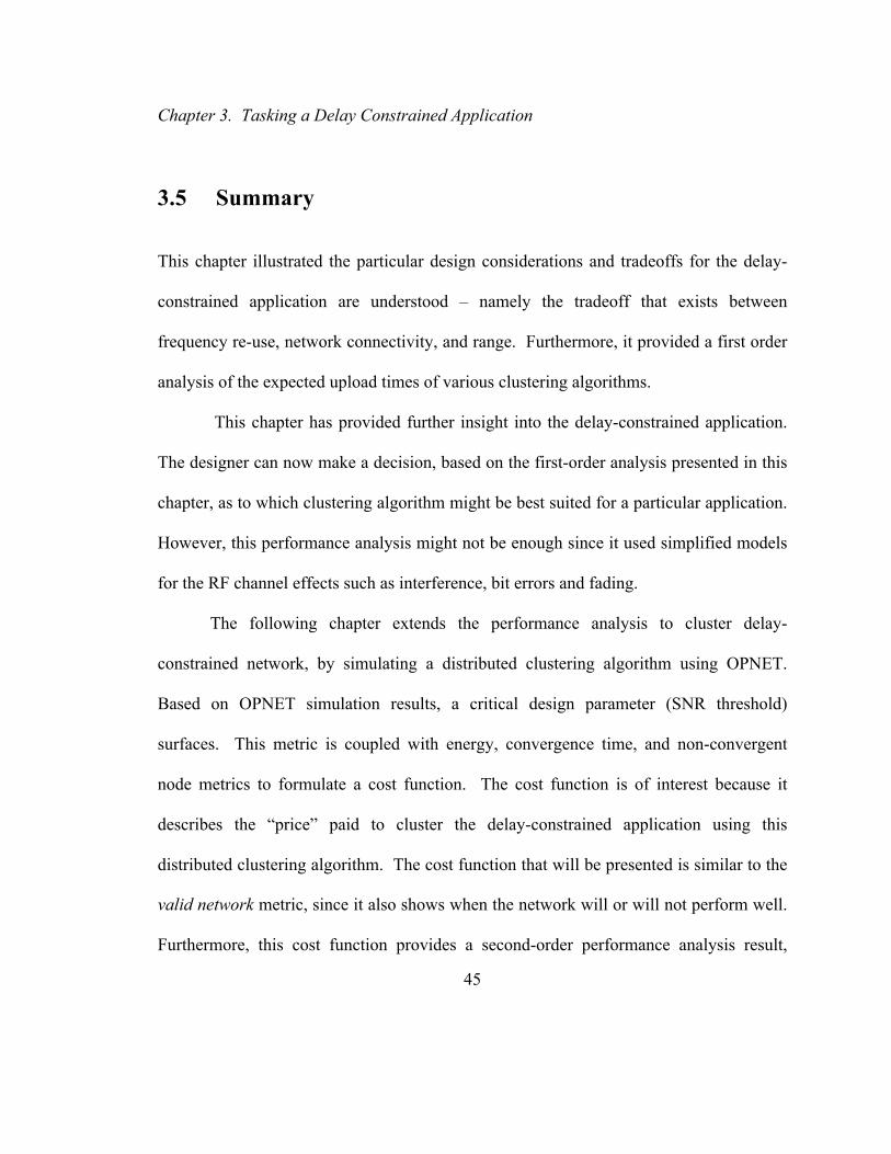
3.5 Summary
This chapter illustrated the particular design considerations and tradeoffs for the delay-
constrained application are understood – namely the tradeoff that exists between
frequency re-use, network connectivity, and range. Furthermore, it provided a first order
analysis of the expected upload times of various clustering algorithms.
This chapter has provided further insight into the delay-constrained application.
The designer can now make a decision, based on the first-order analysis presented in this
chapter, as to which clustering algorithm might be best suited for a particular application.
However, this performance analysis might not be enough since it used simplified models
for the RF channel effects such as interference, bit errors and fading.
The following chapter extends the performance analysis to cluster delay-
constrained network, by simulating a distributed clustering algorithm using OPNET.
Based on OPNET simulation results, a critical design parameter (SNR threshold)
surfaces. This metric is coupled with energy, convergence time, and non-convergent
node metrics to formulate a cost function. The cost function is of interest because it
describes the “price” paid to cluster the delay-constrained application using this
distributed clustering algorithm. The cost function that will be presented is similar to the
valid network metric, since it also shows when the network will or will not perform well.
Furthermore, this cost function provides a second-order performance analysis result,

Chapter 3. Tasking a Delay Constrained Application
46
since the simulation results generated using OPNET, better represent what can be done in
real systems. In particular, the OPNET models included more realistic models for RF
channel effects such as bit errors and channel fading. Those models also included the
effects of message loss on the convergence of the distributed clustering algorithms.

47
Chapter 4
Extending the Performance Analysis
This chapter extends the performance analysis of Chapter 3 by presenting a performance
analysis based on OPNET simulation results. The OPNET simulations consisted of
modeling a distributed algorithm that clusters a delay-constrained application. First the
OPNET simulation setup of the two basic scenarios that were considered – namely the
ideal, and the non-ideal scenarios, are presented. It will be shown that the simulation
results of the ideal scenario demonstrate the clustering algorithms performance when an
ideal wireless channel is assumed. The results from the non-ideal scenario extend the
clustering algorithms performance analysis for clustering algorithms given in Chapter 3.
In particular the non-ideal scenario includes non-deterministic elements inherent in
wireless communications such as Bit-Error Rate (BER) and channel fading. Next, the
simulation results of the two scenarios and the resulting tradeoffs and design
considerations are presented. Finally a cost-function that couples the design
considerations and the simulation results is presented to show the clustering algorithm’s
performance. Based on this cost function, a Signal-to-Noise Ratio (SNR) threshold for

Chapter 4. Extending the Performance Analysis
48
the wireless links is shown to improve the performance of a distributed clustering
algorithm. This threshold prevents the distributed clustering algorithm from using
“marginal links” during cluster formation, which improves the convergence properties of
the distributed clustering algorithm.
4.1 Simulation Setup
OPNET is a network simulator that models the interactions between various elements in a
network. The models (elements) in OPNET are layered and arranged in a hierarchal
fashion, where each model may contain a number of “finer” models within it. Figure 4.1
shows the OPNET Model hierarchy.
Figure 4.1 OPNET Model heirarchy.

Chapter 4. Extending the Performance Analysis
49
The models and the variations between the models used for the ideal and non-ideal
scenarios will now be presented. Figure 4.2 shows the Network Model that was used to
describe the physical sensor network location.
Figure 4.2 The Network Model which containes the “Sensor Network”.
However, for this particular sensor network, the physical location of the network is not
considered important. Figure 4.2 shows the Scenario Model used. The Scenario Model
shows the physical arrangement of the Node Models and the medium that connects them.

Chapter 4. Extending the Performance Analysis
50
Figure 4.3 Scenario Model for a wireless sensor network.
For the networks considered, the Node Models (i.e. node_104, node_60, etc.) were able to
assume the clusterhead or sensor node role, the transmission medium was wireless and so
it is not shown, and the nodes were uniformly distributed in a 1 kilometer square.
The interaction between the field of nodes is described in OPNET using 13 “pipeline
stages”. The “pipeline stages” are invoked for each packet transmission/reception. The
packet traverses each stage sequentially and the important parameters that describe the

Chapter 4. Extending the Performance Analysis
51
wireless channel behavior are assigned. The 13 pipeline stages for the networks
considered were largely functions of the MAC layer chosen for both scenarios, which
was based on the 802.11b protocol [32]. The 13 stages for the two scenarios were as
follows.
1) Transmission Delay
For both scenarios the Transmission Delay was calculated as:
(4.1)
2) Link Closure
For both scenarios the transmission path was never occluded (obstructed).
Every Transmit/Receive (Tx/Rx) pair was in line-of-sight.
3) Channel Match
For both scenarios Tx/Rx pairs were classified as Valid, Ignore, or Noise using
the following criteria:
a) Valid - Tx/Rx pairs with matching bandwidths and Transmit/Receive
Frequencies.
b) Ignore – Tx/Rx pairs with non-overlapping bandwidths.
c) Noise (In band)– Tx/Rx pairs with overlapping bandwidths whose Tx/Rx
attributes didn’t match.

Chapter 4. Extending the Performance Analysis
52
4) Transmit Antenna Gain
0db in all directions (isotropic) for all nodes.
5) Propagation Delay
For both scenarios the Delay between Tx/Rx pairs was calculated as:
Where d is the distance between a Tx/Rx pair in meters and C is the speed of
light.
6) Receive Antenna Gain
0db in all directions (isotropic) for all nodes.
7) Received Power ( )
For the ideal scenario, the received power was deterministic assuming the
following distance-based path loss model:
(4.2)
Where d is the distance between nodes, and is the wavelength of transmit
frequency.

Chapter 4. Extending the Performance Analysis
53
For some instances of the Non-Ideal scenario, the received power was based on
the log-normal shadow model (3.1.3) which has the following form:
(4.3)
Where d is the distance between nodes, d0 is a reference distance, n is the path
loss exponent, and is zero-mean Gaussian RV, with standard deviation
σ (in dB). When the log-normal shadow model was used the parameters of
Equation (4.2) were set to the following values - = 102 dB, = 50m,
n = 3, and σ = 1.0 dB.
8) Background noise (NBK)
For both scenarios the background noise was calculated as follows:
(4.4)
Where B is in-band bandwidth, k is Boltzmann’s constant, FN is the noise
figure of the receiver, T is the temperature of the receiver, and AbmNoise is the
ambient noise of the receiver.

Chapter 4. Extending the Performance Analysis
54
9) Interference Noise (NInterference)
For both scenarios the Interference Noise was calculated by using the in-band
received power that was calculated in stage 7 for signals that the receiver was
not locked onto.
10) Signal–to-Noise Ratio
For both scenarios the SNR between Tx/Rx pairs was calculated as follows:
(4.6)
Where PR was calculated at stage 7, NBK was calculated at stage 8, and
NInterference was calculated at stage 9.
11) Bit Error Rate (BER)
For both scenarios the BER was calculated for a 1Mbps data rate and the
Probability of a bit-error Pb for DPSK which is [33]:
(4.5)
Recall that SNR was calculated at stage 10. However, for the Ideal Scenario
the effects of BER were negated by correcting every bit error at stage 13.
12) Error Allocation
For both scenarios the Error Allocation stage used the BER of stage 11 to
determine the number of errors in a packet.

Chapter 4. Extending the Performance Analysis
55
13) Error Correction
For both scenarios the Error Correction stage determined whether a packet
would be accepted based on the Error-Correction-Code (ECC) parameter and
the number of errors determined at the Error Allocation stage. For the Ideal
scenario the ECC parameter was set to 1, which meant that all errors were
corrected. For the Non-Ideal scenario the ECC parameter was set to zero so
that packets which had bit errors would be dropped.
Figure 4.4 shows the Node Model that was used for both scenarios. As can be
seen in Figure 4.4, the node model describes the flow of packets between process models.
Figure 4.4 Node Model for each node in the sensor network.

Chapter 4. Extending the Performance Analysis
56
The node model consists of a transceiver shown as “wlan_port_rx0” and “wlan_port_tx0”
process models of Figure 4.4. The transceiver is where the physical layer of the node is
described, including the transmit frequency and modulation scheme. These attributes
were set to be consistent with the physical layer portion of the 802.11b protocol. The
Data-Link (MAC) layer of the node is described by the “wireless_lan_mac”, and
“wlan_mac_intf” process models of Figure 4.4. The “wireless_lan_mac”, and
“wlan_mac_intf” process models were based on the data-link portion of the 802.11b
protocol. Though it was not used for these scenarios, had there been a source process
model it would have generated data that modeled actual “sensed” data. The “sink”
model is used to dump the data (clear memory) that is received by a node. The
“clustering_algorithm” process model is used to cluster the nodes in the network. Figure
4.5 shows the Process Model for the clustering algorithm that was used in both scenarios.
The clustering algorithm is based on the DCA algorithm presented in Chapter 2.

Chapter 4. Extending the Performance Analysis
57
Figure 4.5 The clustering algorithm Process Model that was used in both scenarios.
Instead of using a generic weight assignment, the algorithm used the distance based
metric as defined in the WCA algorithm, where the weight of a node was equal to the
sum of the Euclidean distances to the node’s neighbors.
(4.6)
Discovery Stage
Role Selection Stage

Chapter 4. Extending the Performance Analysis
58
The process model can be broken down into two stages: a discovery and a role selection
stage. In the discovery stage, the nodes first broadcast their locations, nodes then
calculate their weights and broadcast another message containing their weight values.
After all nodes had broadcasted their weights, the selection stage of the clustering
algorithm began. First the nodes that had the smallest weight compared to their
neighbors broadcast a “clusterhead” messages, declaring themselves to be clusterheads.
Whenever a node has the lowest weight among its undecided neighbors, it either joins the
closest clusterhead and broadcast a “join” message, or it becomes a clusterhead and
broadcast a “clusterhead” message.
4.2 Simulation Results
This section presents simulation results for the ideal and non-ideal scenarios. For
each simulation,120 nodes were uniformly distributed in a 1 kilometer square region and
each node was assigned the same transmit power level. The following performance
metrics were collected for each simulation - the number of non-convergent nodes, the
energy consumed by each node, the cluster sizes, and the time it took for each node to
complete the clustering algorithm (convergence-time). To gather average statistics, 25
simulations were run for each transmit power (PTX) and SNR threshold value. The
starting random seed value was different for each of the 25 simulations. This section then
presents the results in terms of the following performance metrics – average number of
Chapter 4. Extending the Performance Analysis
59
non-convergent nodes, average algorithm convergence-time, average energy consumed at
a node, and the average cluster-size. A “non-convergent” node is a node that does not
decide to become either a clusterhead or a sensor node. This occurs when the clustering
algorithm is unable to make a decision because it has not received message(s) from its
neighbors who have lower weights. For each simulation the energy consumed by each
node was the sum of the energy consumed in three states – transmit, idle, and receive. It
was assumed that the power required to receive or be idle is equal to 1/2 and 1/10 of the
transmit power respectively. The algorithm convergence time was set equal to the total
time it took for the last role to be assigned and the average cluster size was calculated as
the number of clusterheads divided by the number of nodes. Finally because all
messages are broadcasted a TDMA scheme was assigned so that each node was assigned
1 of 120 time slots.
For the ideal scenario, only deterministic elements were included in the
simulations. As such, the results for the ideal scenario provided the baseline
performance analysis of the clustering algorithm. For the ideal scenario there were no
non-convergent nodes. This is because for the ideal scenario there was no channel fading
and the effects of BERs were negated, since all the bit-errors were corrected. These two
conditions ensured that the probability that two nodes could communicate was either 1 or
0. As can be seen in Figure 4.6 the average cluster-size was directly proportional to PTX.

Chapter 4. Extending the Performance Analysis
60
As PTX was increased, each node had more neighbors and hence fewer nodes were
elected to become clusterheads.
Figure 4.6 Average Cluster-size as a function of transmit power.
As Figure 4.7 shows, the average node energy consumed and the average convergence
time were highly correlated. Both energy and convergence time increased in proportion
to transmit power. Neither result was unexpected. If nodes had more neighbors then it
took longer for each node to decide its role because it had to wait on more neighbors to

Chapter 4. Extending the Performance Analysis
61
make their decisions first. Furthermore, the amount of energy that a node consumed was
proportional to the number of messages it received and its transmit power level (recall
that the receive state requires 1/2 transmit power). So a node will consumed more
energy when it had more neighbors, because it received more “clusterhead” and “join”
messages and its transmit power level was higher.
Figure 4.7 The average convergence time and average node energy consumed as funcions of transmit power.

Chapter 4. Extending the Performance Analysis
62
The simulation results from the ideal scenario thus provide some basic design
considerations - namely that cluster-size is directly proportional to transmit power and
that larger clusters-sizes will require more energy and take longer to create. However,
the effects of the wireless channel on the clustering algorithm have not been properly
being considered. Therefore the non-ideal scenario will now be considered. First the
BER for DPSK and a 1Mbps data rate are included into the simulations to determine the
impact of bit-errors on the clustering algorithms performance. To include the effects of
bit-errors, the ECC parameter used at stage 13 of the “pipeline stages” is set to zero. This
meant that every packet with a bit-error is dropped. Though setting the ECC parameter to
0 might be too stringent, doing so demonstrates the clustering algorithms dependence
upon reliable communications. As can be seen in Figure 4.8, including BER into the
simulations causes a significant degradation of the clustering algorithm’s ability to
converge.

Chapter 4. Extending the Performance Analysis
63
Figure 4.8 Confidence interval (90 %) for the average number of non-convergent nodes when BER is included in the simulation.
As Figure 4.8 shows, there are instances where a large number of nodes fail to decide
their roles. This is because nodes cannot decide their roles if they have not received
“clusterhead” or “join” messages from nodes with lower weights than themselves.
Notice that a high transmit power (PTX >> 10W) negates the effects of bit-errors.
However, in that case, the network will contains only 1 clusterhead which is incompatible
with a delay-constrained network. To increase communication reliability a SNR
threshold parameter can be added to the discovery stage of the clustering algorithm.

Chapter 4. Extending the Performance Analysis
64
During the discovery stage of the clustering algorithm, a node chooses his neighbors to
be only those with whom it has an SNR above a set SNR threshold value. Since the
probability of bit-error is a function of SNR (see Equation 4.5), the effects of bit-errors
can be mitigated by setting the SNR threshold parameter to a large enough value (SNR
Threshold (dB) ≈> 5dB). This can be seen in Figure 4.9 which shows that the average
number of non-convergent nodes tends to 0 as the value of the SNR threshold parameter
is increased.
Figure 4.9 The average number of non-convergent nodes as a function of SNR threshold and PTX when BER was included in the simulations.

Chapter 4. Extending the Performance Analysis
65
However, setting the SNR threshold parameter to larger values means that nodes have
fewer neighbors and therefore the average cluster-size, convergence time, and the
average node energy is also dependent upon the value of the SNR threshold parameter.
The average cluster-size, average convergence time, and average node energy as
functions of the SNR threshold parameter and PTX are shown in Figures 4.10 - 4.12
respectively.
Figure 4.10 Average cluster-size as a function of SNR threshold and PTX.

Chapter 4. Extending the Performance Analysis
66
As was expected when PTX was increased or the value of the SNR threshold parameter
was decreased, the average cluster-size increased because on the average, nodes had more
neighbors.
Figure 4.11 Average convergence time as a function of SNR threshold and PTX.
As can be seen in Figure 4.11 as PTX was increased or as the SNR threshold parameter
was decreased, it took longer for the algorithm to converge, because in such instances a
node typically had more neighbors, and therefore on the average it had to receive more
messages before it could decide its own role.

Chapter 4. Extending the Performance Analysis
67
Figure 4.12 Average node energy as a function of SNR threshold and PTX.
It can be seen in Figure 4.11 and 4.12 that the average node energy and the average
convergence time were highly correlated. This was expected since both were similarly
related to the average number of neighbors. Results for the average number of non-
convergent nodes, average cluster-size, and average energy will prove useful as they will
be used in a cost function that will be presented in the next section.
Next, to further extend the clustering algorithms performance analysis, a
shadowing term was added to the path-loss model (stage 7 of the “pipeline stages”). As

Chapter 4. Extending the Performance Analysis
68
shown in Figure 4.13 the presence of small fading (σ = 1 dB) had a significant impact on
the performance of the clustering algorithm.
Figure 4.13 Number of non-convergent nodes as function of SNR threshold and PTX in the presence of log-normal fading and BER’s.
Furthermore, it takes fairly good links (SNR ≈> 8dB) to negate the effects of fading.
Unfortunately such a stringent requirement for SNR reduces the possible design space of
the clustering algorithm. For example, by referring to Figure 4.10 it can be seen that in
the presence of fading, the algorithm would is unable to effectively (few number of non-
convergent nodes) create cluster-sizes > 20. As such, future work should consider what

Chapter 4. Extending the Performance Analysis
69
other possible design parameters should be added to improve performance over fading
channels. One possible option might be to include a distance threshold parameter, which
relates inter-node distances to a desired PRR in the discovery phase of the clustering
algorithm. Another simple option might be to retransmit the “clusterhead” and “join”
messages multiple times. This would increase energy usage but would also probably
improve the convergence properties.
4.3 Consider the “Cost”
Assuming that nodes are capable of accurately performing SNR measurements, possibly
by determining BER by transmitting known packets and using RSSI, it is important to
consider which design parameters will create clusters that match the desired performance
metrics for a delay-constrained network. As such, an example of a weighted cost
function which weighs the design parameters (SNR threshold and PTX) against the desired
cluster-size, node energy, and non-convergent node metrics associated with a delay-
constrained application is shown below:
(4.7)
CW is the weighted cost, CSAVG is the average cluster-size, EAVG is the average node
energy, and NCAVG is average number of non-convergent nodes (node who decides its

Chapter 4. Extending the Performance Analysis
70
role). Equation (4.7) shows that the minimal cost region occurs when CSAVG is around
10 and EAVG and NCAVG are both minimal. Figure 4.14 shows the result of using the cost
function presented in Equation (4.7) for the simulation results collected in the previous
section when the BER for DPSK and a 1 Mbps data rate were included in the simulations.
Figure 4.14 Weighted cost as a function of SNR threshold and PTX when BER was included in the simulations.
It can be seen in Figure 4.14 that the acceptable design space for this delay-constrained
network is approximately when:
• SNR Threshold (dB) > -2 dB

Chapter 4. Extending the Performance Analysis
71
• SNR Threshold (dB) – 8 < PTX < SNR Threshold (dB) -4
(Note: The previous cost function could be modified so that the weights assigned to each
performance metric represented the desired performance of the clustering algorithm of
particular applications. As such the designer could quickly find the regions (SNR
threshold and transmit power) that should be used that will ensure that desired
performance metrics are met. )
4.4 Summary
This chapter extended the performance analysis presented in Chapter 3 by simulating a
distributed clustering algorithm using OPNET. First, baseline results were presented for
the distributed clustering algorithm when the communications channel was assumed to be
ideal. Next it was shown that the clustering algorithms performance becomes
substantially degraded when more realistic wireless communication behavior are
introduced –namely bit-errors. However, an SNR threshold parameter was introduced
into the discovery stage of the clustering algorithm which could be used to make the
wireless channel arbitrarily reliable. Next it was shown that using the SNR threshold
parameter would also help alleviate the effects of fading in the channel. However, the
SNR threshold parameter values that overcome the impact of channel fading strictly
constrained the other performance metrics, particularly average cluster-size, average
convergence time, and average node energy. Finally a weighted cost function was

Chapter 4. Extending the Performance Analysis
72
presented which showed the portion of the design space (SNR threshold and transmit
power) that had a high probability of meeting the prescribed performance requirements of
a particular instance of a delay-constrained network.

73
Chapter 5
Conclusions and Future Work
This thesis first described the potential applications and architecture of wireless sensor
networks. Next a brief description of the performance metrics associated with wireless
sensor networks was presented – namely energy, throughput, latency, and reliability. In
Chapter 2 a survey of DCA/DMAC, WCA, and LEACH/LEACH-C clustering algorithms
was presented. The algorithms were considered as potential candidates for clustering a
delay constrained network. Chapter 3 presented a performance analysis of using WCA,
LEACH, Maxi-Min, and A-Priori algorithms to cluster a delay-constrained network.
The performance analysis showed that for the delay-constrained network, the probability
of a valid network, which is one in which the network is fully connected and neighboring
clusters have an acceptable level of inter-cluster interference, is highly dependent on the
transmit power and the available number of frequency channels. Therefore, care must be
taken in choosing the communications hardware because of the steep phase changes that
exist between the regions where the network is valid and where the network is not valid.
Furthermore, the desired cluster characteristics, such as average upload time or maximum

Chapter 5. Conclusions and Future Work
74
upload time, of a particular delay-constrained network will determine which clustering
algorithm should be considered for clustering the network. Chapter 4 then extended the
performance analysis presented in Chapter 3 by simulating a distributed clustering
algorithm using OPNET. The simulation results showed that a new design parameter was
needed to ensure algorithm success, which was defined as every node becoming either a
clusterhead or a cluster member – namely an SNR threshold parameter. The SNR
threshold parameter could make the wireless communications channel arbitrarily reliable
even if the channel experienced fading. However, for fading channels the results showed
that the clustering algorithm might need further design changes to ensure that the
prescribed performance metrics will be met. The reason was that the combination of the
Weighted Clustering Algorithm and the SNR threshold parameter constrained the design
space to a narrow range of parameters. As such future work should consider design
changes that ensure that the clustering algorithm converges for lower values of SNR
threshold when the wireless channel experiences fading.
Future work should also consider the cost (energy and latency) of creating a valid
frequency re-use scheme using a distributed algorithm. Therefore, future OPNET
simulations should be conducted using a backtracking algorithm to create a valid
frequency re-use scheme over a field of clustered nodes.

Chapter 5. Conclusions and Future Work
75
Finally, since the distributed clustering algorithm simulated in this paper was
strictly dependent upon reliable communications, future work should also consider using
a clustering algorithm where each node makes autonomous decisions.

76
References
[1] I. Akyildiz, W. Su, Y. Sankarasubramaniam, and E. Cayirci, “Wireless sensor networks, a survey”, Computer Networks 38, Dec. 2002, pp. 393-422. [2] http://webopedia.internet.com/quick_ref/OSI_Layers.asp [3] http://en.wikipedia.org/wiki/Seven-layer_OSI_model [4] N. Briscoe, “Understanding the OSI 7-Layer Model”, PC Network Advisor, July 2000, pp 13-16. [5] C. Casetti, M.Gerla, S. Mascolo, M.Y. Sanadidi and R. Wang, “TCP Westwood: End-to-End Bandwidth Estimation for Enhanced Transport over Wireless Links”, Journal of Wireless Networks, Vol.8, 2002, pp. 467-479. [6] H. Balakrishna, V. Padmanabhan, S. Seshan, and R. Katz, “A Comparison of Mechanisms for Improving TCP Performance over Wireless Links”, IEEE/ACM Transactions on Networking, Vol. 5 1997, pp. 756-769. [7] D. Johnson, D. Maltz, and Y-C Hu, “The Dynamic Source Routing Protocol for Mobile Ad Hoc Networks (DSR)”, draft-ietf-manet-dsr-09.txt, April 2003. [8] C.E. Perkins, et al., “Performance comparison of two on-demand routing protocols for ad hoc networks”, IEEE Personal Communications Volume, 8, Issue, 1, February 2001, pp. 16–28. [9] V. Park, S. Corson, “Temporally-Ordered Routing Algorithm (TORA) Version 1 Functional Specification”, draft-ietf-manet-tora-spec-01.txt, August 1998. [10] M.Chatterjee, S.K. Das and D. Turgut, “WCA: A Weighted Clustering Algorithm for Mobile Ad Hoc Networks”, Cluster Computing 5, 2002, pp. 193–204.

References
77
[11] W. Rabiner, A. Chandrakasan and H. Balakrishnan, “An Application-Specific Protocol Architecture for Wireless Microsensor Networks”, IEEE Transactions on Wireless Communications, Vol. 1, No. 4, October 2002, pp. 660-670. [12] S. Basagni, “Distributed Clustering for Ad Hoc Networks”, International Symposium on Parallel Architectures, Algorithms, and Networks, June 1999, pp. 310-315. [13] P. Sholander, G. Frank, and A. Yankopolus, “Energy-Efficient Networking Techniques for Wireless Sensor Networks”, Military Communications Conference, Oct. 2003, pp. 573-578. [14] M.T. Oswald, J.A. Rohwer, and M.A. Forman, “Analysis of Power Management and System Latency in Wireless Sensor Networks”, Digital Wireless Communications VI, Proceedings of SPIE Vol. 5440, pp. 134-144. [15] M. Oswald, P. Sholander, B. McDaniel, J. Rohwer, D. Kilman, “Data Exfiltration From Sensor Networks Subject to Delay, Connectivity and Frequency Re-Use Constraints”, Military Communications Conference Proceedings. IEEE Meeting, October 19, 2005, preprinted. [16] http://www.opnet.com [17] M. Gerla and J.T.C. Tsai, “Multicluster, mobile, multimedia radio network”, Wireless Networks 1(3), 1995, pp. 255–265. [18] C.-H.R. Lin and M. Gerla, “A distributed control scheme in multi-hop packet radio networks for voice/data traffic support”, Proceedings of IEEE GLOBECOM (1995) pp. 1238–1242. [19] C.-H.R. Lin and M. Gerla, A distributed architecture for multimedia in dynamic wireless networks,”, Proceedings of IEEE GLOBECOM 1995, pp. 1468–1472. [20] A.K. Parekh, “Selecting routers in ad hoc wireless networks”, Proceedings of the SBT/IEEE International Telecommunications Symposium, August 1994, pp. 420-424. [21] D.J. Baker and A. Ephremides, “A distributed algorithm for organizing mobile radio telecommunication networks”, Proceedings of the 2nd International Conference on Distributed Computer Systems, April 1981, pp. 476–483.

References
78
[22] D.J. Baker and A. Ephremides, “The architectural organization of a mobile radio network via a distributed algorithm”, IEEE Transactions on Communications COM-29 11, November 1981, pp. 1694–1701. [23] A. Ephremides, J.E. Wieselthier and D.J. Baker, “A design concept for reliable mobile radio networks with frequency hopping signaling”, Proceedings of IEEE, Vol. 75(1) (1987) pp. 56–73. [24] T. Murata and H. Ishibuchi, “Performance evaluation of genetic algorithms for flowshop scheduling problems,” Proceedings of 1st IEEE Conf. Evolutionary Computation, vol. 2, June 1994, pp. 812–817. [25] J.-H. Chang, and L. Tassiulas, “Maximum Lifetime Routing in Wireless Sensor Networks”, IEEE/ACM Transaction on Networking, Vol. 12, No. 4, August 2004, pp. 609-619. [26] B. Krishnamachari, et al, “Critical Density Thresholds in Distributed Wireless Networks”, Communications, Information and Network Security, Eds. H. Bhargava, et al, Springer Publishing Company 11 West 42nd Street,15th Floor New York, NY 10036, December 2002, 1 Edition. [27] B. Krishnamachari, et al, “On the Complexity of Distributed Self-Configuration in Wireless Networks”, Telecommunication Systems 22:1–4, 33–59, 2003. [28] N. Alon, A. Shapira, “Every Monotone Graph Property is Testable”, Proceedings of the thirty-seventh annual ACM symposium on Theory of computing, May 2005, pp. 128-137. [29] M. Yokoo, E.H. Durfee, T. Ishida, and K. Kuwabara, “The Distributed Constraint Satisfaction Problem: Formalization and Algorithms”, IEEE Transaction on Knowledge and Data Engineering, Sept./Oct. 1998, pp. 673-685. [30] T.S. Rappaport, “Wireless Communications: Principles and Practice”, Prentice Hall One Lake Street, Upper Saddle River, NJ 07458, December 2001, 2nd Edition. [31] M. Zuniga and B. Krishnamachari, “Analyzing the Transitional Region in Low Power Wireless Links”, IEEE SECON Conference, Oct. 2004, pp. 517-526. [32] http://grouper.ieee.org/groups/802/11/

References
79
[33] J.G. Proakis, “Digital Communications”, McGraw-Hill 1221 Avenue of the Americas New York, NY 10020, August 2000, 4th Edition.


![Information Surfing for Radiation Map Buildingece-research.unm.edu/chaouki/PAPERS/Journals/TCST_radiation.pdf · eddies. Singh et al. [15], use active learning techniques to map](https://img.pdfslide.net/doc/110x75/5ed225bb5e0ec842bd789c30/information-suring-for-radiation-map-buildingece-eddies-singh-et-al-15-use.jpg)