Embed Size (px)
Citation preview
© Crown copyright Met Office
Modelling of forecast errors in Data Assimilation for NWP
"Uncertainty Analysis in Geophysical Inverse Problems" Lorentz Centre Workshops in Sciences series, Leiden, Netherlands. Nov 2011. Andrew Lorenc
© Crown copyright Met Office Andrew Lorenc 2
Content
0. Audience-specific orientation!
1. Historical context – what is best for NWP?
2. Bayesian methods and error modelling
3. Adding non-Gaussianity
© Crown copyright Met Office Andrew Lorenc 2
© Crown copyright Met Office Andrew Lorenc ECMWF Seminar 2011 3
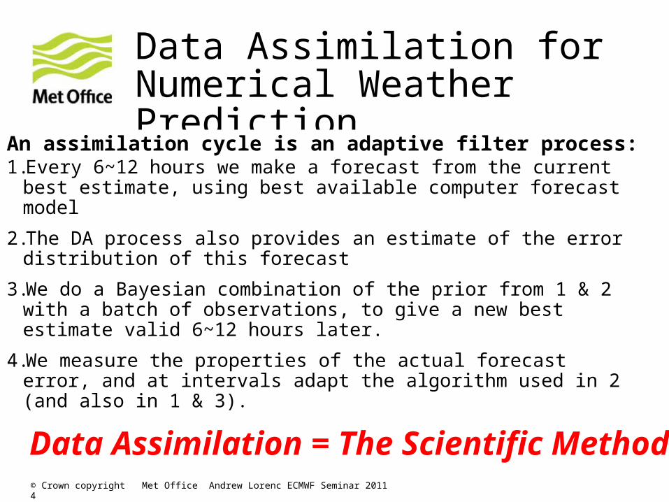
Data Assimilation for Numerical Weather Prediction
An assimilation cycle is an adaptive filter process:1.Every 6~12 hours we make a forecast from the current best
estimate, using best available computer forecast model
2.The DA process also provides an estimate of the error distribution of this forecast
3.We do a Bayesian combination of the prior from 1 & 2 with a batch of observations, to give a new best estimate valid 6~12 hours later.
4.We measure the properties of the actual forecast error, and at intervals adapt the algorithm used in 2 (and also in 1 & 3).
© Crown copyright Met Office Andrew Lorenc ECMWF Seminar 2011 4
Data Assimilation = The Scientific Method
© Crown copyright Met Office Andrew Lorenc 5
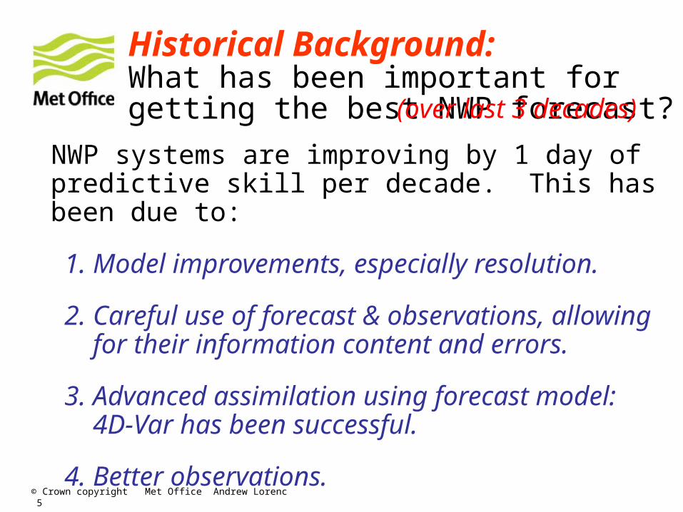
Historical Background: What has been important for getting the best NWP forecast?
NWP systems are improving by 1 day of predictive skill per decade. This has been due to:
1. Model improvements, especially resolution.
2. Careful use of forecast & observations, allowing for their information content and errors.
3. Advanced assimilation using forecast model: 4D-Var has been successful.
4. Better observations.
(over last 3 decades)
© Crown copyright Met Office Andrew Lorenc 5
© Crown copyright Met Office Andrew Lorenc 6
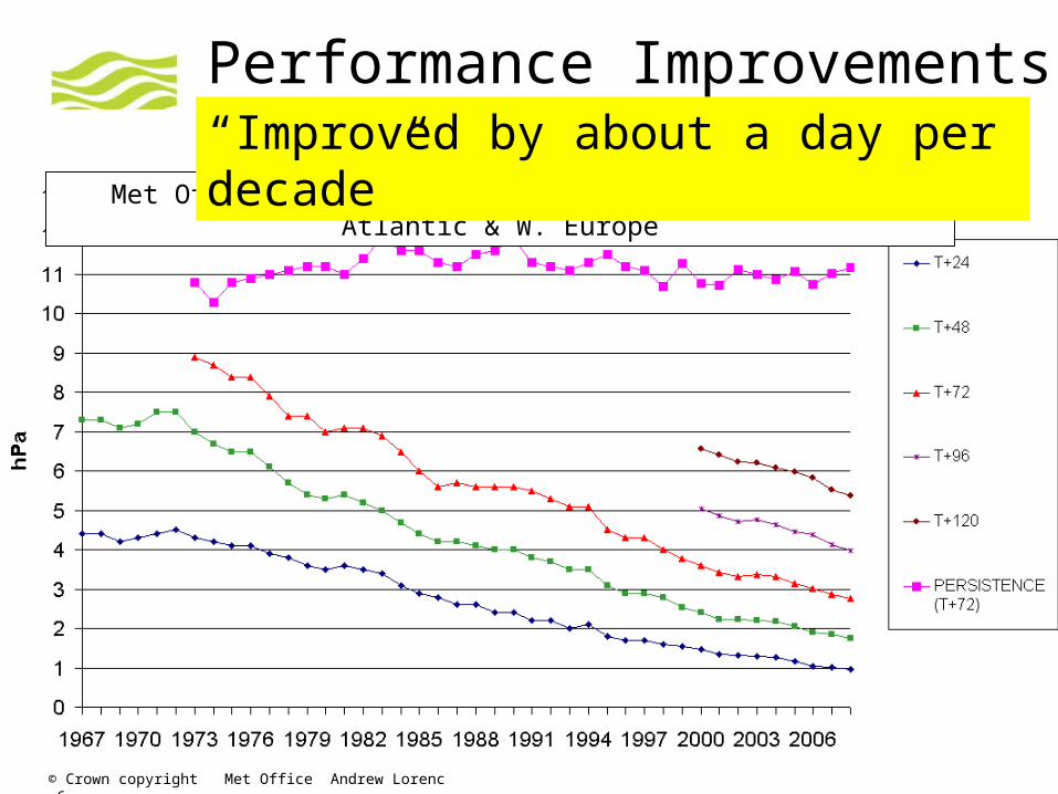
Performance Improvements
Met Office RMS surface pressure error over the N. Atlantic & W. Europe
“Improved by about a day per decade”
© Crown copyright Met Office Andrew Lorenc 7
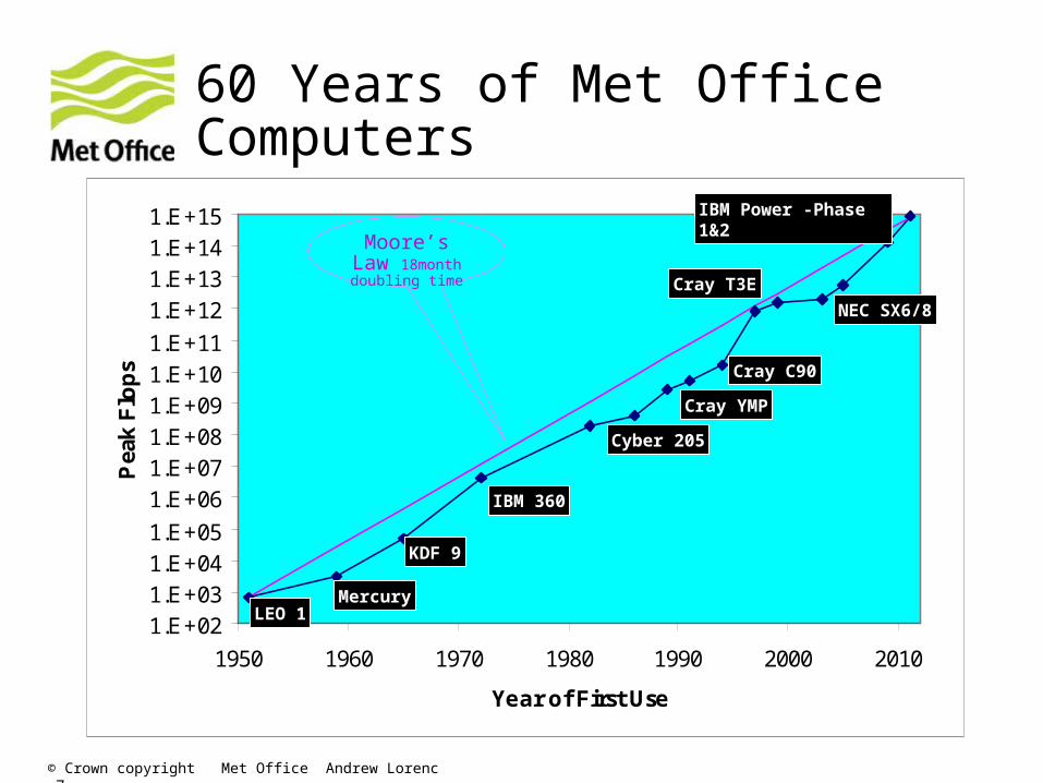
60 Years of Met Office Computers
1.E+021.E+031.E+041.E+05
1.E+061.E+071.E+081.E+091.E+101.E+11
1.E+121.E+131.E+141.E+15
1950 1960 1970 1980 1990 2000 2010
Year of First Use
Pea
k F
lop
s
LEOMercury
LEO 1
KDF 9
IBM 360
Cyber 205
Cray YMP
Cray C90
Cray T3E
NEC SX6/8
IBM Power -Phase 1&2
Moore’s Law 18month doubling
time
Historical Background: Continuing Improvement of a Complex System
• NWP improvements are due to a synergistic combination of improvements of forecast model, DA and observations.
• Each helps the other.
• Total NWP system is very large, complex and expensive.
• We cannot expect to understand it completely as a single entity.
• We cannot afford thorough testing of each improvement.
• Best to base each improvement on scientific insight and analysis of one component.
• With belief (checked by testing) that theoretically better parts will eventually give a better system.
© Crown copyright Met Office Andrew Lorenc 8
Implications for R&D strategy of causes of improvements to NWP
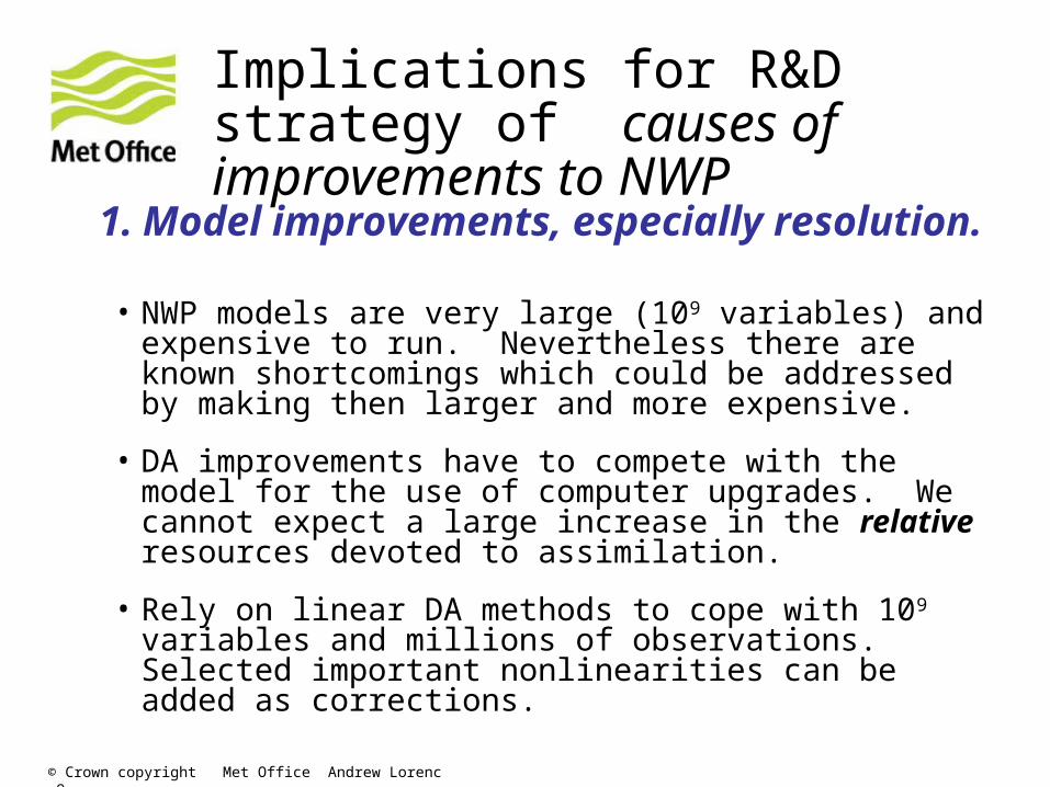
1. Model improvements, especially resolution.
• NWP models are very large (109 variables) and expensive to run. Nevertheless there are known shortcomings which could be addressed by making then larger and more expensive.
• DA improvements have to compete with the model for the use of computer upgrades. We cannot expect a large increase in the relative resources devoted to assimilation.
• Rely on linear DA methods to cope with 109 variables and millions of observations. Selected important nonlinearities can be added as corrections.
© Crown copyright Met Office Andrew Lorenc 9
© Crown copyright Met Office Andrew Lorenc 10
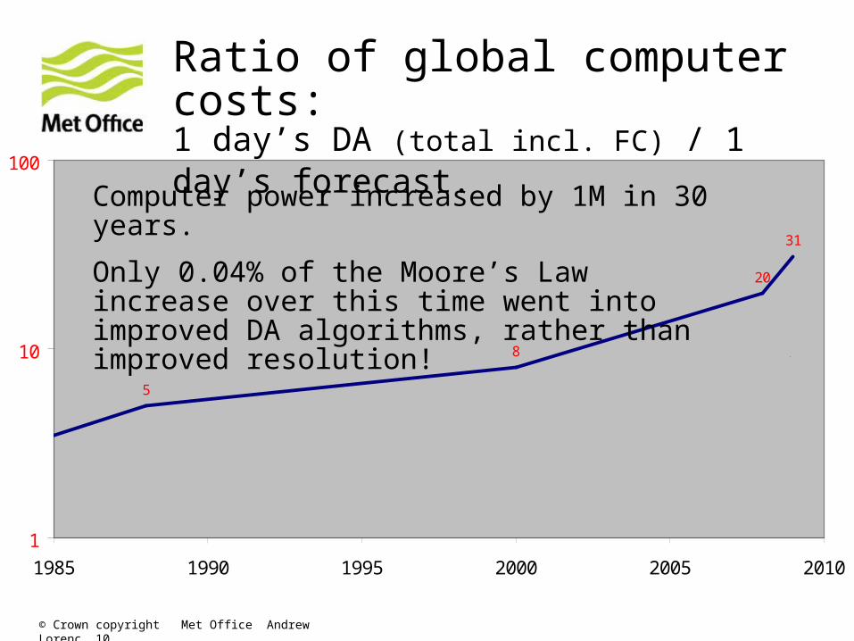
ratio of supercomputer costs: 1 day's assimilation / 1 day forecast
5
8
20
31
1
10
100
1985 1990 1995 2000 2005 2010
AC scheme
3D-Var on T3E
simple 4D-Var on SX8
4D-Var with
outer_loop
Ratio of global computer costs: 1 day’s DA (total incl. FC) / 1 day’s forecast.
Computer power increased by 1M in 30 years.
Only 0.04% of the Moore’s Law increase over this time went into improved DA algorithms, rather than improved resolution!
© Crown Copyright 2011. Source: Met Office
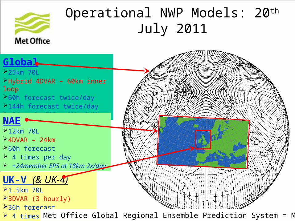
Operational NWP Models: 20th July 2011
Global25km 70LHybrid 4DVAR – 60km inner loop60h forecast twice/day144h forecast twice/day+24member EPS at 60km 2x/day
NAE12km 70L4DVAR – 24km60h forecast 4 times per day +24member EPS at 18km 2x/day
UK-V (& UK-4)1.5km 70L 3DVAR (3 hourly)36h forecast 4 times per day Met Office Global Regional Ensemble Prediction System = MOGREPS
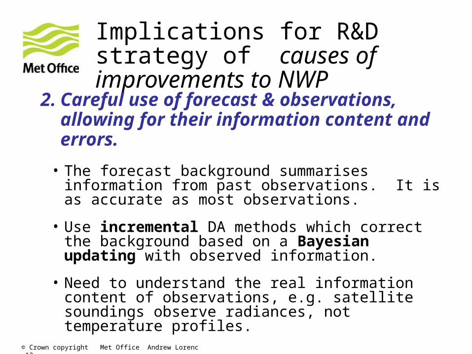
Implications for R&D strategy of causes of improvements to NWP
2. Careful use of forecast & observations, allowing for their information content and errors.
• The forecast background summarises information from past observations. It is as accurate as most observations.
• Use incremental DA methods which correct the background based on a Bayesian updating with observed information.
• Need to understand the real information content of observations, e.g. satellite soundings observe radiances, not temperature profiles.
© Crown copyright Met Office Andrew Lorenc 12
Simplest possible Bayesian NWP analysis
© Crown copyright Met Office Andrew Lorenc 13
© Crown copyright Met Office Andrew Lorenc 14
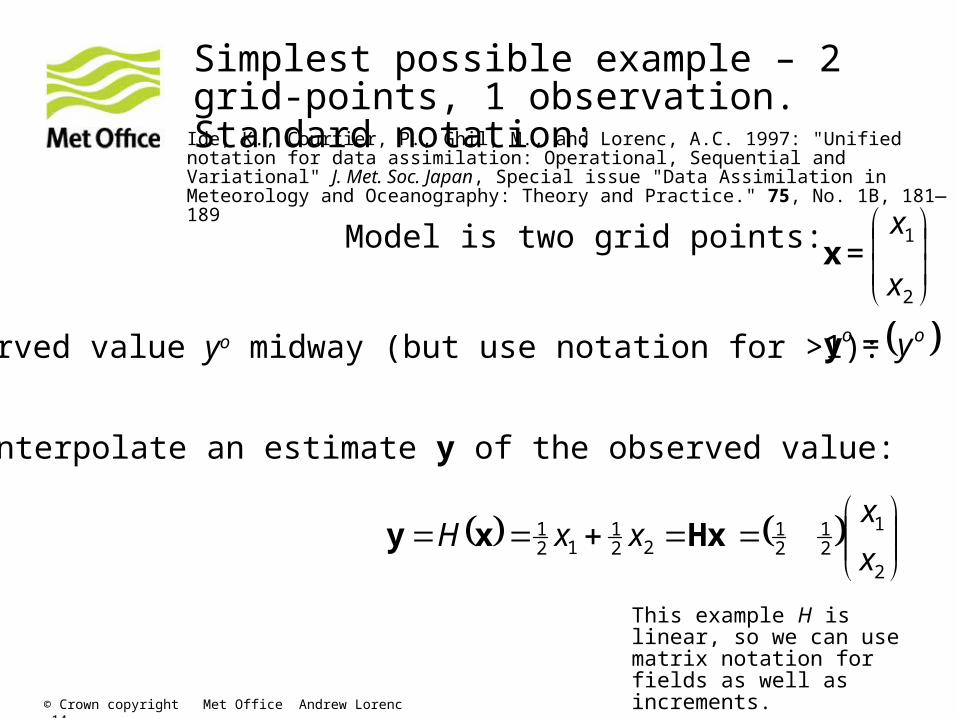
Simplest possible example – 2 grid-points, 1 observation. Standard notation:
2
1 =
x
xx
oo y = y
2
121
21
221
121
x
xxxH Hxxy
Model is two grid points:
1 observed value yo midway (but use notation for >1):
Can interpolate an estimate y of the observed value:
This example H is linear, so we can use matrix notation for fields as well as increments.
Ide, K., Courtier, P., Ghil, M., and Lorenc, A.C. 1997: "Unified notation for data assimilation: Operational, Sequential and Variational" J. Met. Soc. Japan, Special issue "Data Assimilation in Meteorology and Oceanography: Theory and Practice." 75, No. 1B, 181—189
© Crown copyright Met Office Andrew Lorenc 15
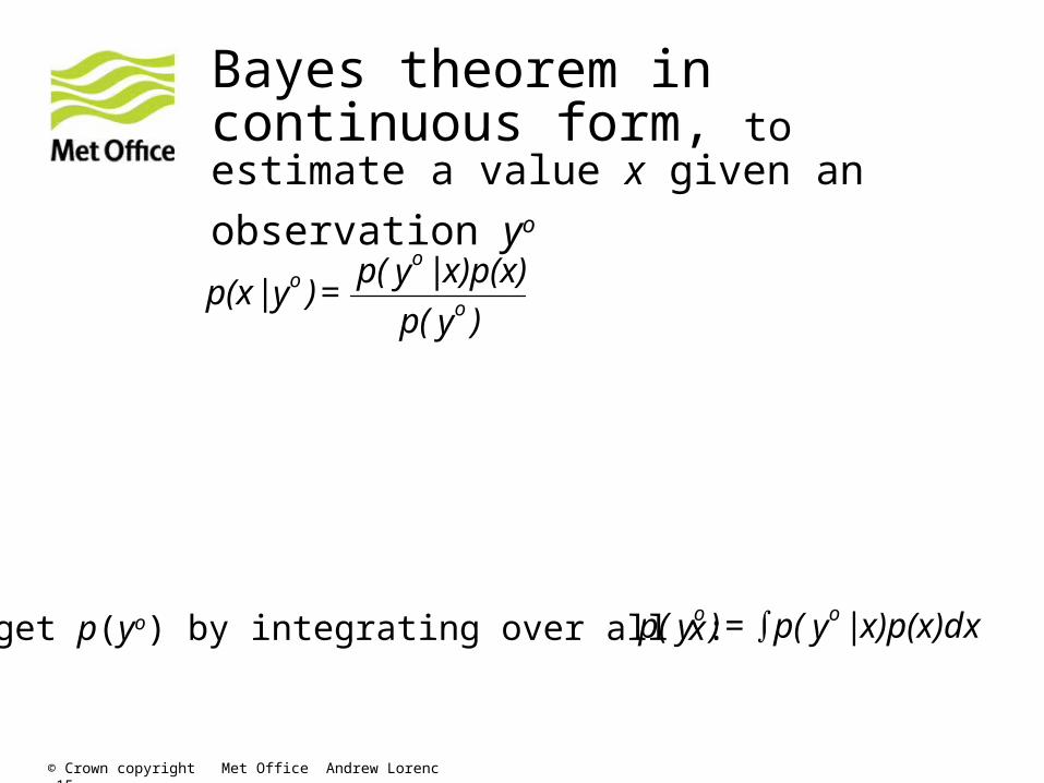
Bayes theorem in continuous form, to estimate a value x given an
observation yo
)yp(
x)p(x)|yp( = )y|p(x o
oo
p(xyo)
is the posterior distribution,p(x)
is the prior distribution,p(yox)
is the likelihood function for x Can get p(yo) by integrating over all x: x)p(x)dx|yp( = )yp( oo
© Crown copyright Met Office Andrew Lorenc 16
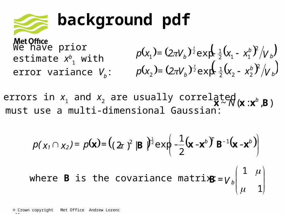
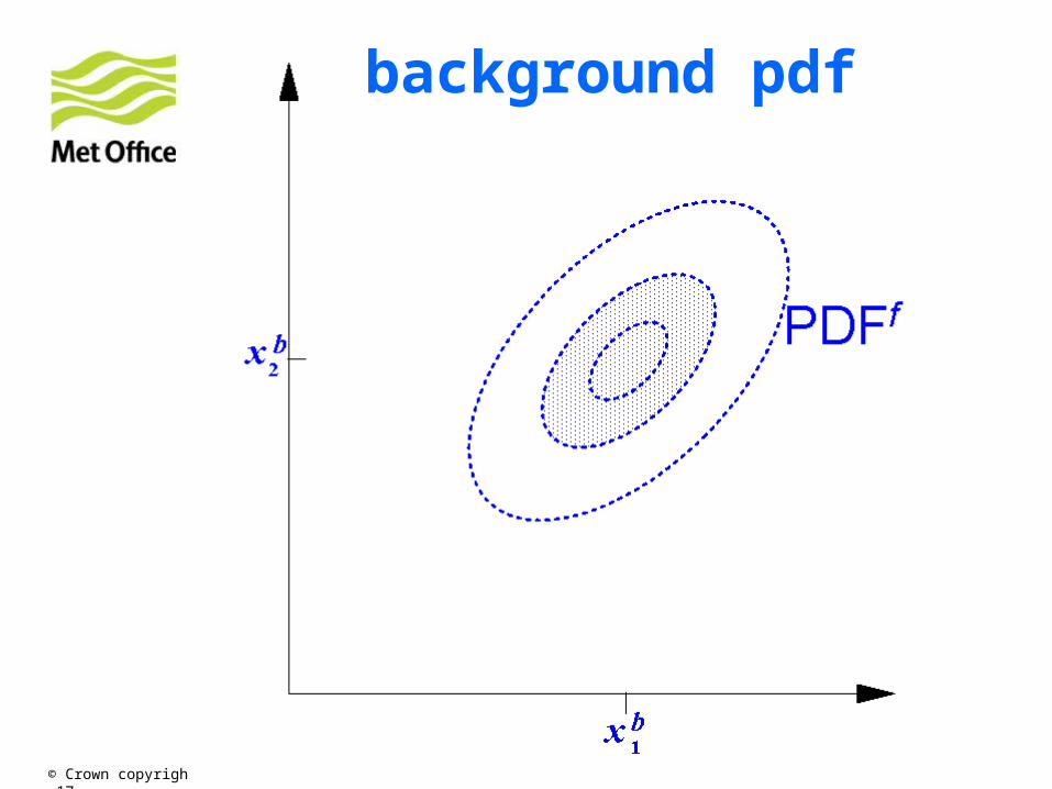
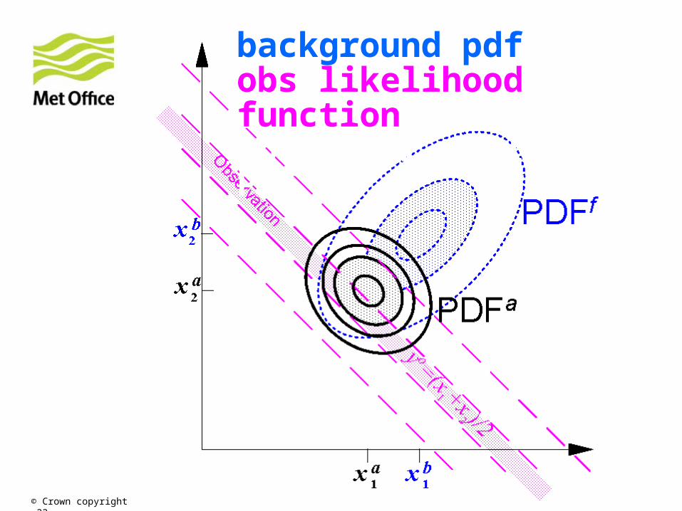
background pdf
Vxx-V2 = xp
Vxx-V2 =xp
bb
b-
bb
b-
21
21
2
2221
2
2
1121
1
exp
exp
),:( ~ Bxxx bN
bTb
21 p = )xxp( xxBxxBx --2
1-exp||)(2 = 12 - 2
1
1
1=
V bB
We have prior estimate xb
1 with error variance Vb:
But errors in x1 and x2 are usually correlated
must use a multi-dimensional Gaussian:
where B is the covariance matrix:
© Crown copyright Met Office Andrew Lorenc 17
background pdf
© Crown copyright Met Office Andrew Lorenc 18
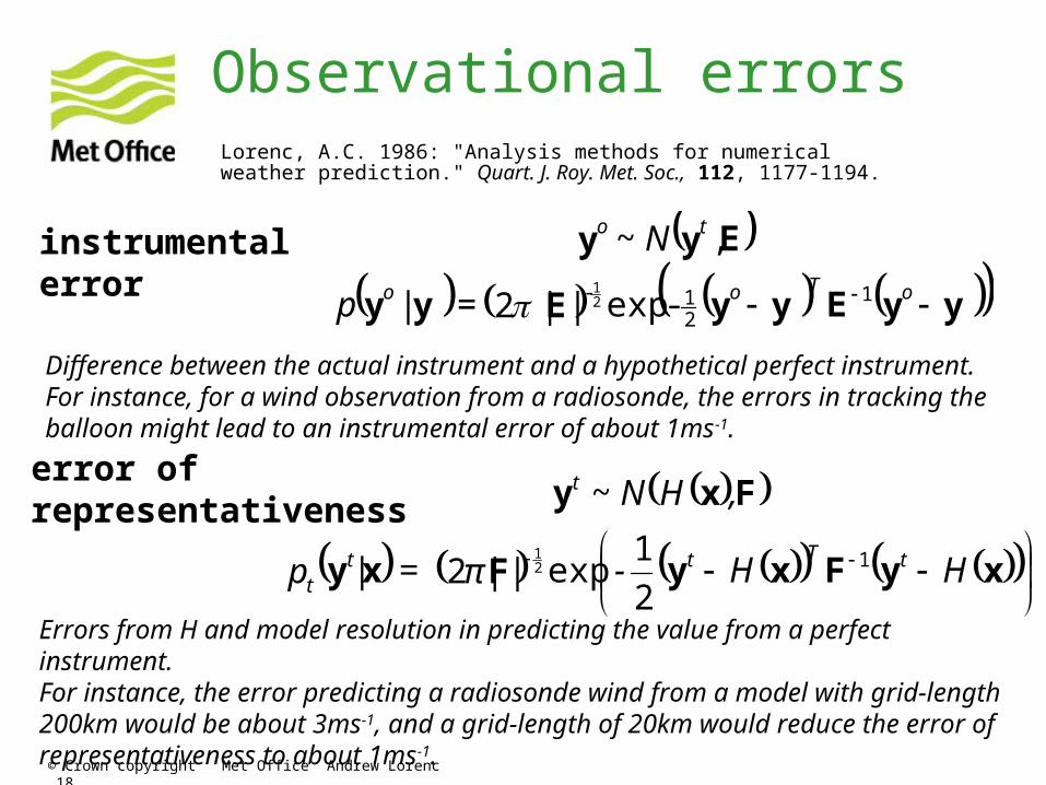
Observational errors
yyEyyEyy
Eyy
oToo
to
|p
N
121- -exp||2 =
,~
21
xyFxyFxy
Fxy
HH-|π| = |p
,HN
tTt-tt
t
1
2
1exp2
~
21
instrumental error
error of representativeness
Lorenc, A.C. 1986: "Analysis methods for numerical weather prediction." Quart. J. Roy. Met. Soc., 112, 1177-1194.
Difference between the actual instrument and a hypothetical perfect instrument.For instance, for a wind observation from a radiosonde, the errors in tracking the balloon might lead to an instrumental error of about 1ms-1.
Errors from H and model resolution in predicting the value from a perfect instrument.For instance, the error predicting a radiosonde wind from a model with grid-length 200km would be about 3ms-1, and a grid-length of 20km would reduce the error of representativeness to about 1ms-1.
© Crown copyright Met Office Andrew Lorenc 19
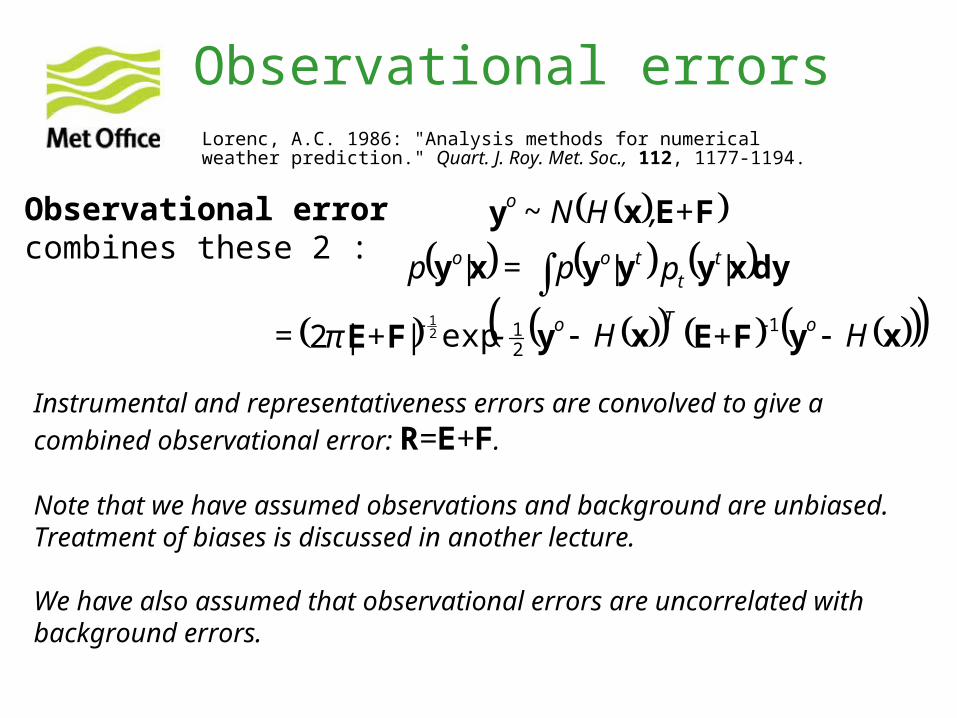
Observational errors
xyFExyFE
dyxyyyxy
FExy
H+H-|+π|=
|p|p = |p
+,HN
o-To-
tt
too
o
1
21exp2
~
21
Observational error combines these 2 :
Lorenc, A.C. 1986: "Analysis methods for numerical weather prediction." Quart. J. Roy. Met. Soc., 112, 1177-1194.
Instrumental and representativeness errors are convolved to give a
combined observational error: R=E+F.
Note that we have assumed observations and background are unbiased. Treatment of biases is discussed in another lecture.
We have also assumed that observational errors are uncorrelated with background errors.
© Crown copyright Met Office Andrew Lorenc 20
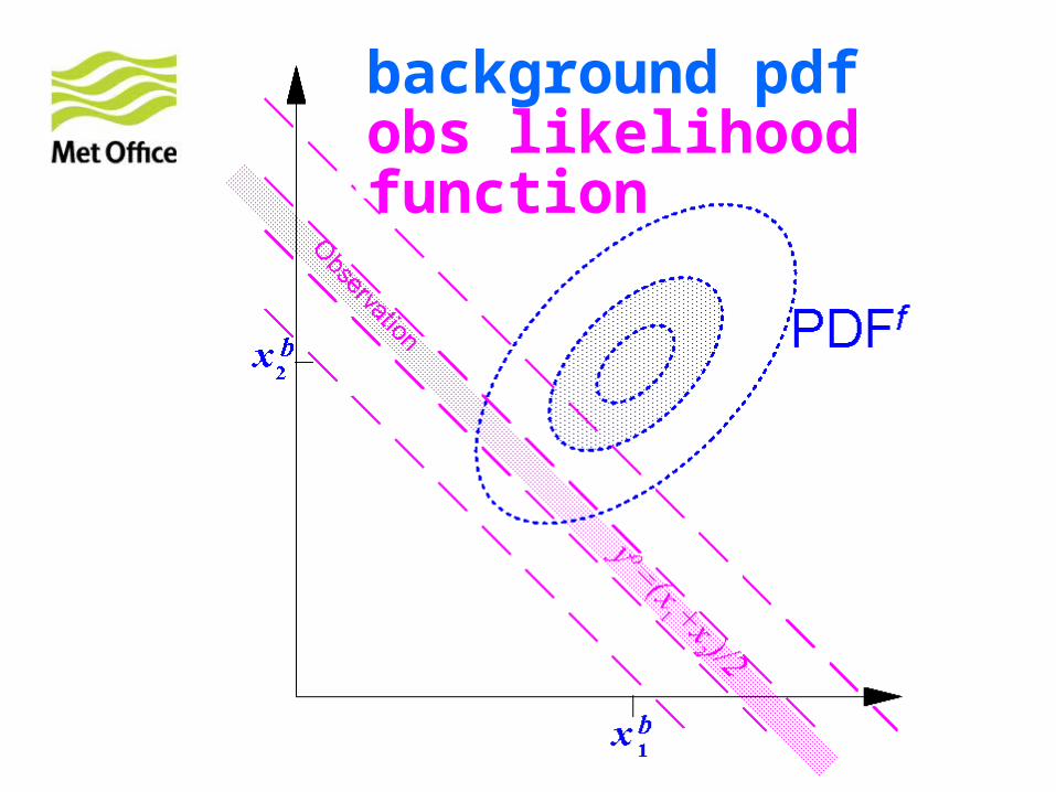
background pdfobs likelihood function
© Crown copyright Met Office Andrew Lorenc 21
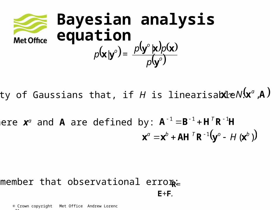
Bayesian analysis equation
y
xxyyx
o
oo
p
p|p = |p
Axx ,~ aN
)( 1
111
boTba
T
H xyRAHxx
HRHBA
Property of Gaussians that, if H is linearisable :
where xa and A are defined by:
R=E+F.
Remember that observational error:
© Crown copyright Met Office Andrew Lorenc 22
background pdfobs likelihood functionposterior analysis PDF
© Crown copyright Met Office Andrew Lorenc 23
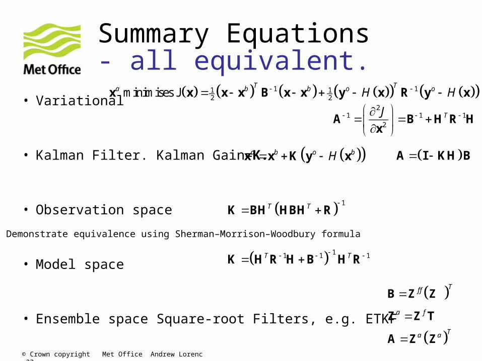
Summary Equations - all equivalent.
• Variational
• Kalman Filter. Kalman Gain=K.
• Observation space
• Model space
• Ensemble space Square-root Filters, e.g. ETKF
1 11 12 2minimises J
T Ta b b o oH H x x x x B x x y x R y x 2
1 1 12
TJ
A B H R Hx
a b o bH x x K y x A I KH B
1T T K BH HBH R
11 1 1T T K H R H B H R
Tf f
a f
Ta a
B Z Z
Z Z T
A Z Z
Demonstrate equivalence using Sherman–Morrison–Woodbury formula
© Crown copyright Met Office Andrew Lorenc 24
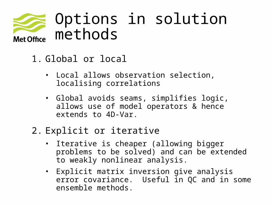
Options in solution methods
1. Global or local
• Local allows observation selection, localising correlations
• Global avoids seams, simplifies logic, allows use of model operators & hence extends to 4D-Var.
2. Explicit or iterative• Iterative is cheaper (allowing bigger problems to be solved)
and can be extended to weakly nonlinear analysis.
• Explicit matrix inversion give analysis error covariance. Useful in QC and in some ensemble methods.
© Crown copyright Met Office Andrew Lorenc 25
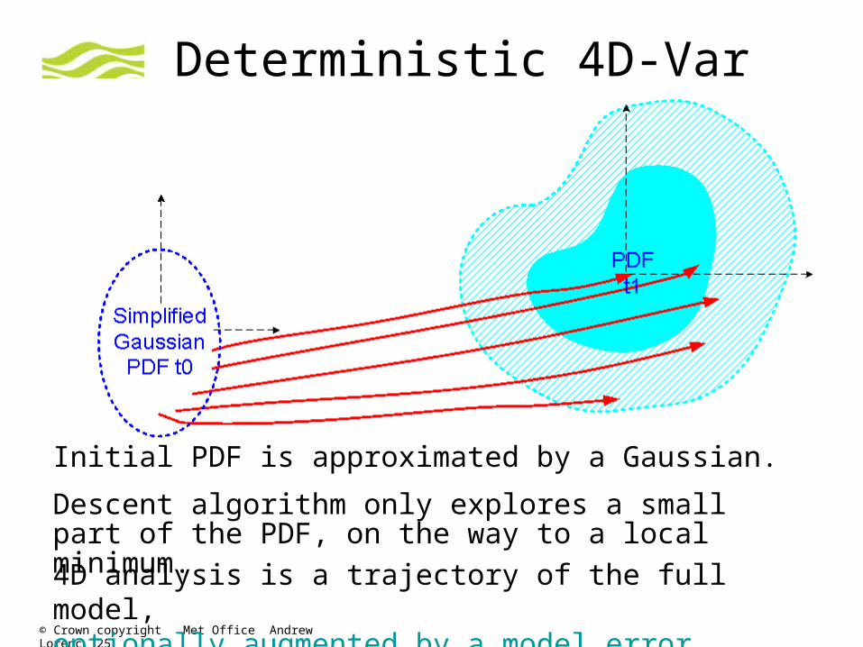
Deterministic 4D-Var
Initial PDF is approximated by a Gaussian.
Descent algorithm only explores a small part of the PDF, on the way to a local minimum.
4D analysis is a trajectory of the full model,optionally augmented by a model error correction term.
© Crown copyright Met Office Andrew Lorenc 26
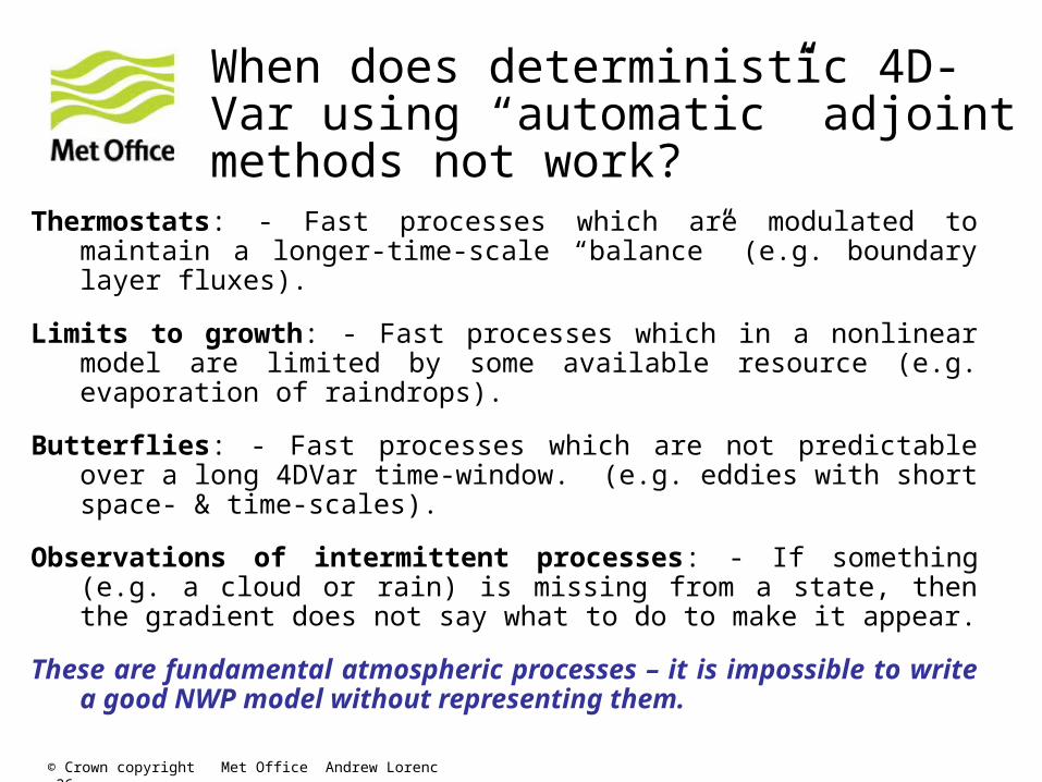
When does deterministic 4D-Var using “automatic” adjoint methods not work?
Thermostats: - Fast processes which are modulated to maintain a longer-time-scale “balance” (e.g. boundary layer fluxes).
Limits to growth: - Fast processes which in a nonlinear model are limited by some available resource (e.g. evaporation of raindrops).
Butterflies: - Fast processes which are not predictable over a long 4D Var time-window. (e.g. eddies with short space- & time-scales).
Observations of intermittent processes: - If something (e.g. a cloud or rain) is missing from a state, then the gradient does not say what to do to make it appear.
These are fundamental atmospheric processes – it is impossible to write a good NWP model without representing them.
© Crown copyright Met Office Andrew Lorenc 27
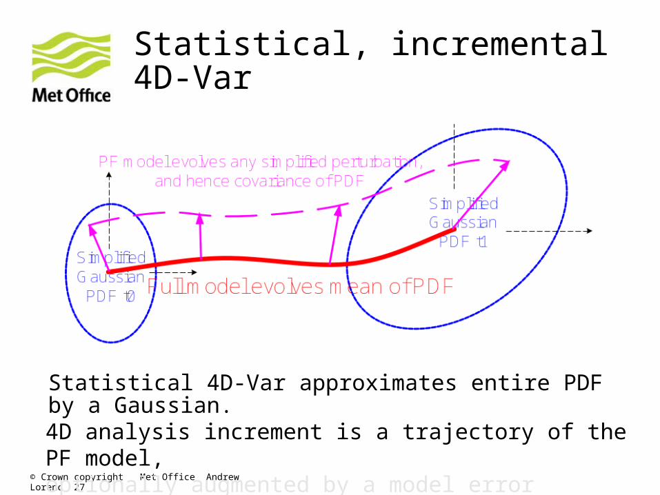
Statistical, incremental 4D-Var
Statistical 4D-Var approximates entire PDF by a Gaussian.
4D analysis increment is a trajectory of the PF model,optionally augmented by a model error correction term.
© Crown copyright Met Office Andrew Lorenc 28
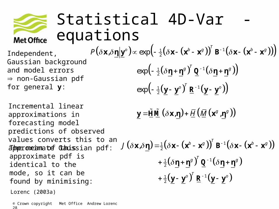
Statistical 4D-Var - equations
112
112
112
, exp
exp
exp
To b g b g
Tg g
To o
P
x η y x x x B x x x
η η Q η η
y y R y y
, ,g gH M y HM x η x η
112
112
112
,T
b g b g
Tg g
To o
J
x η x x x B x x x
η η Q η η
y y R y y
Independent, Gaussian background and model errors non-Gaussian pdf for general y:
Incremental linear approximations in forecasting model predictions of observed values converts this to an approximate Gaussian pdf:
The mean of this approximate pdf is identical to the mode, so it can be found by minimising:
Lorenc (2003a)
© Crown copyright Met Office Andrew Lorenc 29
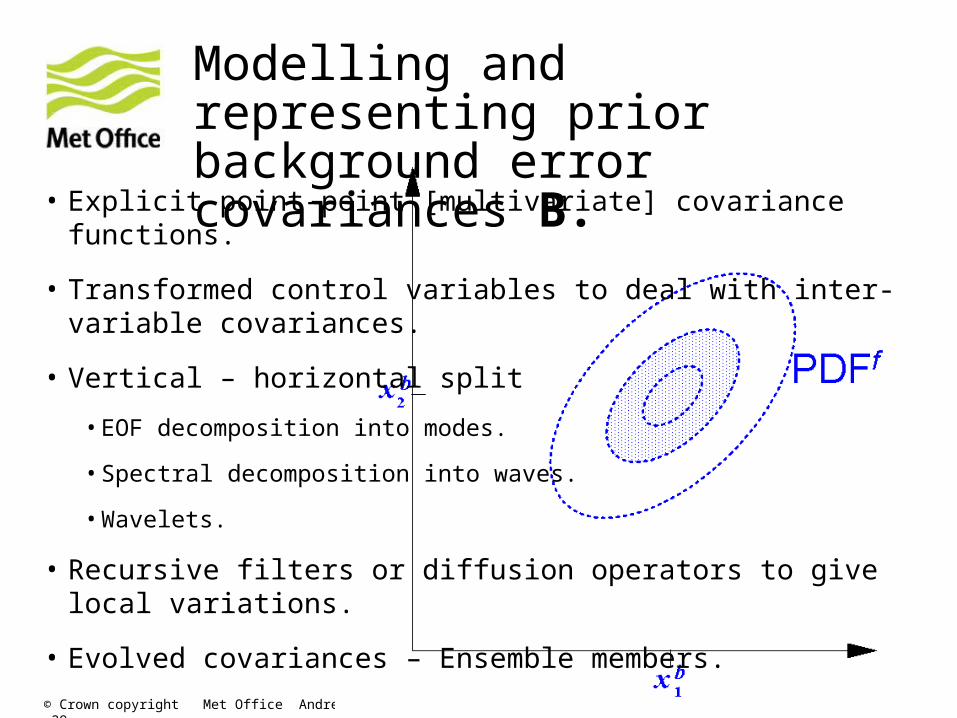
Modelling and representing prior background error covariances B.
• Explicit point-point [multivariate] covariance functions.
• Transformed control variables to deal with inter-variable covariances.
• Vertical – horizontal split
• EOF decomposition into modes.
• Spectral decomposition into waves.
• Wavelets.
• Recursive filters or diffusion operators to give local variations.
• Evolved covariances – Ensemble members.
© Crown copyright Met Office Andrew Lorenc 30
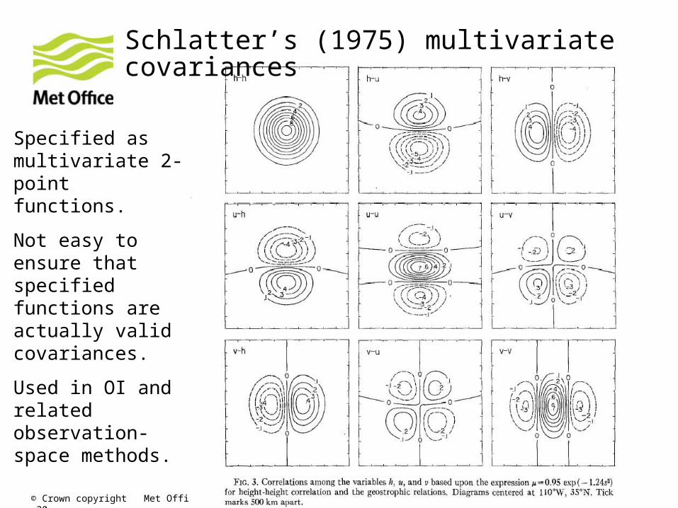
Schlatter’s (1975) multivariate covariances
Specified as multivariate 2-point functions.
Not easy to ensure that specified functions are actually valid covariances.
Used in OI and related observation-space methods.
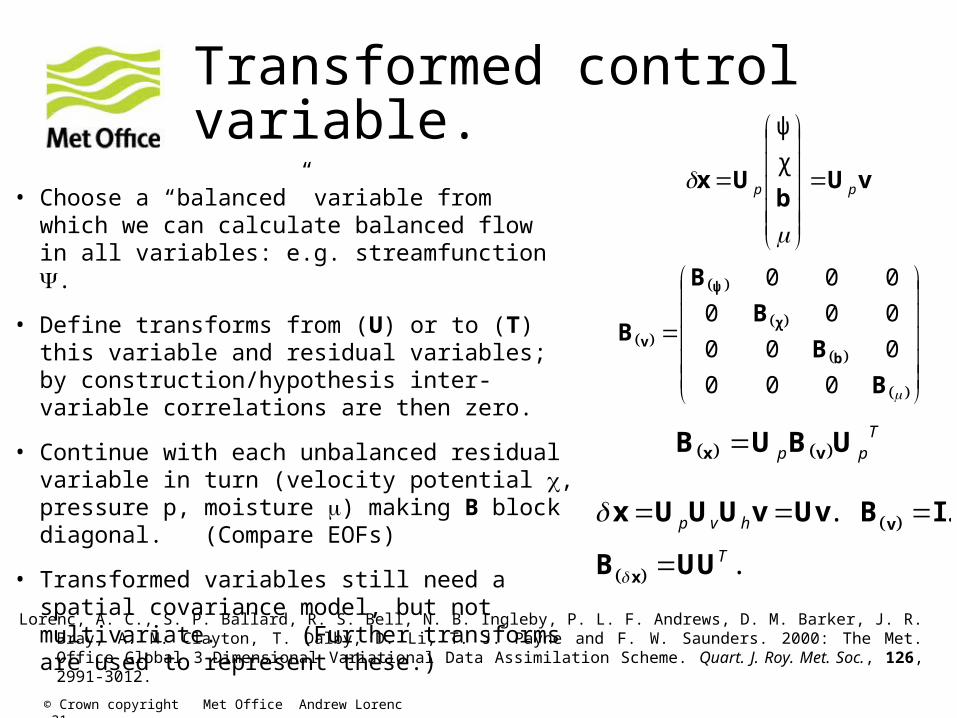
Transformed control variable.
• Choose a “balanced” variable from which we can calculate balanced flow in all variables: e.g. streamfunction .
• Define transforms from (U) or to (T) this variable and residual variables; by construction/hypothesis inter-variable correlations are then zero.
• Continue with each unbalanced residual variable in turn (velocity potential , pressure p, moisture ) making B block diagonal. (Compare EOFs)
• Transformed variables still need a spatial covariance model, but not multivariate. (Further transforms are used to represent these.)
© Crown copyright Met Office Andrew Lorenc 31
vUb
Ux pp
χ
ψ
B
B
B
B
Bb
χ
ψ
v
000
000
000
000
T
pp UBUB vx
Lorenc, A. C., S. P. Ballard, R. S. Bell, N. B. Ingleby, P. L. F. Andrews, D. M. Barker, J. R. Bray, A. M. Clayton, T. Dalby, D. Li, T. J. Payne and F. W. Saunders. 2000: The Met. Office Global 3-Dimensional Variational Data Assimilation Scheme. Quart. J. Roy. Met. Soc., 126, 2991‑3012.
. .
.
p v h
T
v
x
x U U U v Uv B I
B UU
Estimating PDFs or covariances
• Even if we knew the “truth”, we could never run enough experiments in the lifetime of an NWP system to estimate its error PDF, or even its error covariance B.
• Simplifying assumptions are essential (e.g. Gaussian, ...)
• Even a simplified error model has so many parameters that we cannot determine them by NWP trials to determine which give the best forecasts.
• In practice we can only measure innovations – cannot get separate estimates of B & R without assumptions (Talagrand).
• Need to understand physics!
© Crown copyright Met Office Andrew Lorenc 32

Effect of the null space of B
• B should be positive semi-definite. If it has any (near) zero eigenvalues, then no analysis increments are permitted in the direction of the corresponding eigenmodes.
• Causes of a null space:
• Strong constraints used in the definition of B. E.g.
• Hydrostatic & geostrophic relationships
• Model equation in 4D-Var
• Too small a sample when estimating B
• Effects of a null space:
Synergistic use of complementary observations
Spurious long-range correlations and over confidence in accuracy of analysis.
© Crown copyright Met Office Andrew Lorenc 33
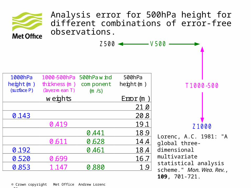
Analysis error for 500hPa height for different combinations of error-free observations.
Z1000
T1000-500
V500Z500
1000hPaheight (m)(surface P)
1000-500hPathickness (m)(layer-mean T)
500hPa windcomponent
(m/s)
500hPaheight (m)
weights Error (m)21.0
0.143 20.80.419 19.1
0.441 18.90.611 0.628 14.4
0.192 0.461 18.40.520 0.699 16.70.853 1.147 0.880 1.9
Lorenc, A.C. 1981: "A global three-dimensional multivariate statistical analysis scheme." Mon. Wea. Rev., 109, 701-721.
© Crown copyright Met Office Andrew Lorenc 34
© Crown copyright Met Office Andrew Lorenc 36
Background error (prior) covariance B modelling assumptions
The first operational 3D multivariate statistical analysis method (Lorenc 1981) made the following assumptions about the B which characterizes background errors, all of which are wrong!
• Stationary – time & flow invariant
• Balanced – predefined multivariate relationships exist
• Homogeneous – same everywhere
• Isotropic – same in all directions
• 3D separable – horizontal correlation independent of vertical levels or structure & vice versa.
Since then many valiant attempts have been made to address them individually, but with limited success because of the errors remaining in the others. The most attractive ways of addressing them all are long-window 4D-Var or hybrid ensemble-VAR.
© Crown copyright Met Office Andrew Lorenc 36
Implications for R&D strategy of causes of improvements to NWP
3. Advanced assimilation using forecast model.
• 4D-Var is used by 5 of the top 7 global NWP centres. Ensemble Kalman filter methods popular in other applications.Hybrid and Ensemble-Var methods are exciting much interest in operational NWP R&D.
• Multiple forecasts allow the evolution of error covariances and hence the definition of a 4D covariance.
• The NWP model is the best tool for defining the “attractor” of plausible “balanced” states.Incremental methods designed such that background
is only altered based on observed evidence.
© Crown copyright Met Office Andrew Lorenc 37
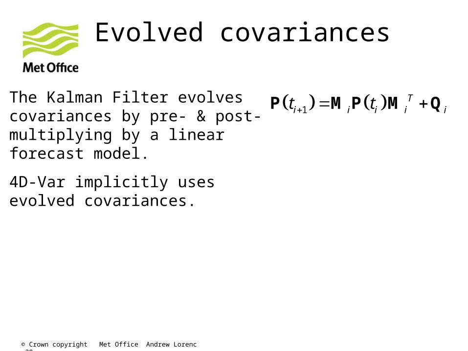
Evolved covariances
1T
i i i i it t P M P M QThe Kalman Filter evolves covariances by pre- & post-multiplying by a linear forecast model.
4D-Var implicitly uses evolved covariances.
© Crown copyright Met Office Andrew Lorenc 38
© Crown copyright Met Office Andrew Lorenc 39
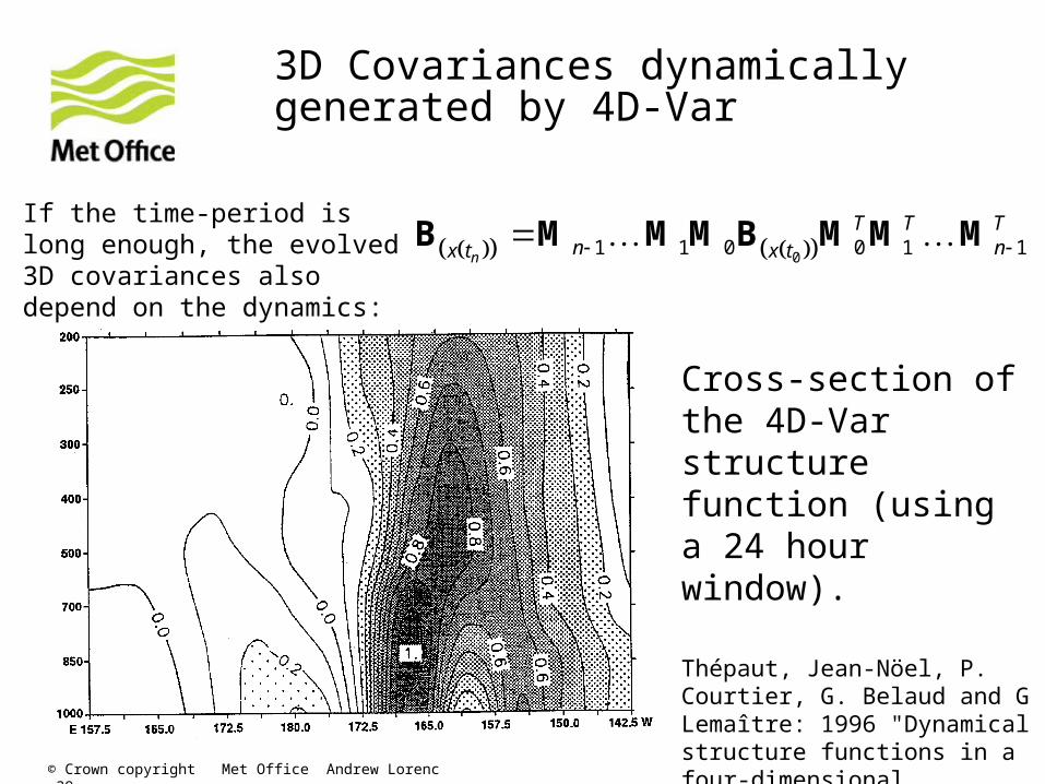
3D Covariances dynamically generated by 4D-Var
If the time-period is long enough, the evolved 3D covariances also depend on the dynamics:
01 1 0 0 1 1 n
T T Tn nx t x t
B M M M B M M M
Cross-section of the 4D‑Var structure function (using a 24 hour window).
Thépaut, Jean-Nöel, P. Courtier, G. Belaud and G Lemaître: 1996 "Dynamical structure functions in a four-dimensional variational assimilation: A case study" Quart. J. Roy. Met. Soc., 122, 535-561
© Crown Copyright 2011. Source: Met Office
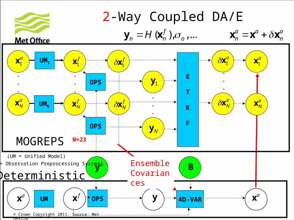
fx 4D-VAR xa
x1f
xNf
x1a
xNf
x1f
y1
yo
yn H (xnf ), o,...
E
T
K
F
x1a
xNa
.
.
.
.
.
.
.
.
.
x1a
xNa
.
.
.
xNa
xna xa xn
a
xaOPS
OPS
OPS
yN
y
Deterministic
UM1
UMN
UM
B
MOGREPS(UM = Unified Model)
(OPS = Observation Preprocessing System)
N=23
Ensemble Covariances
2-Way Coupled DA/E
© Crown copyright Met Office
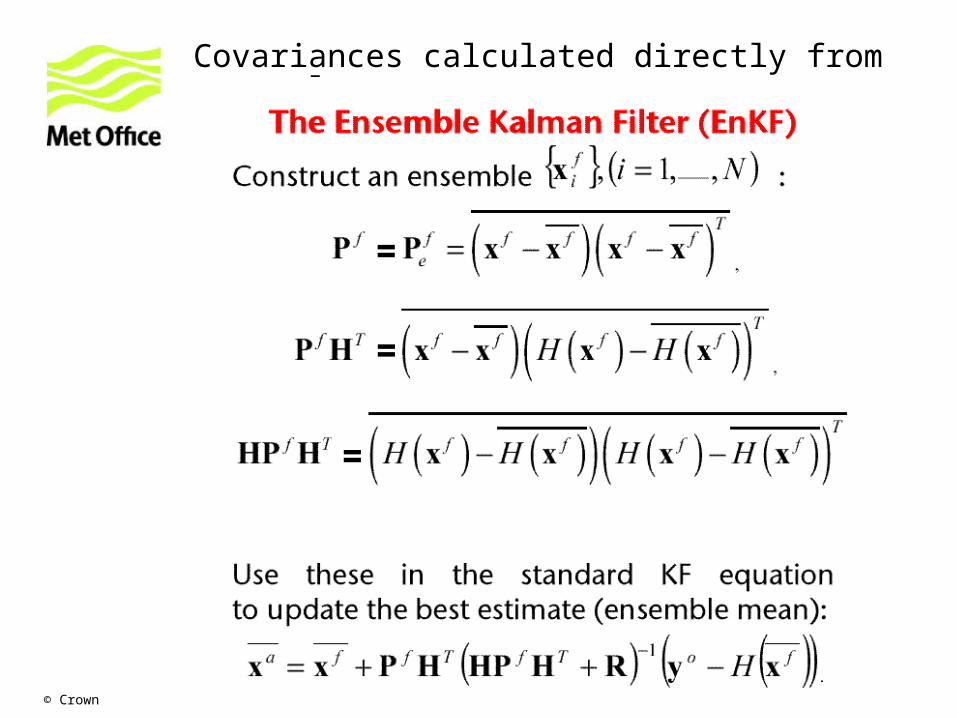
Covariances calculated directly from a sample:
=
=
=
© Crown copyright Met Office
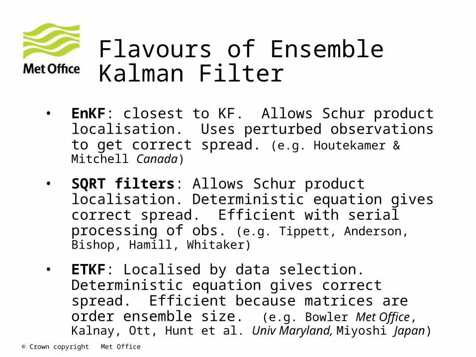
Flavours of Ensemble Kalman Filter
• EnKF: closest to KF. Allows Schur product localisation. Uses perturbed observations to get correct spread. (e.g. Houtekamer & Mitchell Canada)
• SQRT filters: Allows Schur product localisation. Deterministic equation gives correct spread. Efficient with serial processing of obs. (e.g. Tippett, Anderson, Bishop, Hamill, Whitaker)
• ETKF: Localised by data selection. Deterministic equation gives correct spread. Efficient because matrices are order ensemble size. (e.g. Bowler Met Office, Kalnay, Ott, Hunt et al. Univ Maryland, Miyoshi Japan)
© Crown copyright Met Office Andrew Lorenc 44
vvw hvp UUUU c
TUUC loc i
K
iie -
Kα
1
)(1
1xxw
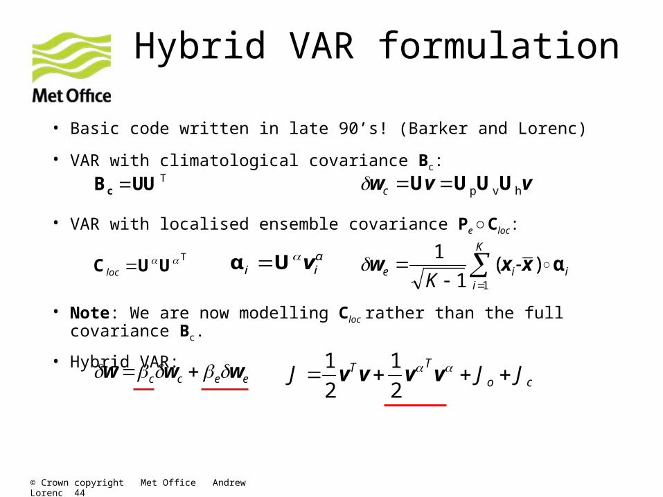
• Basic code written in late 90’s! (Barker and Lorenc)
• VAR with climatological covariance Bc:
αii vUα
TUUBc
• VAR with localised ensemble covariance Pe ○ Cloc:
• Note: We are now modelling Cloc rather than the full covariance Bc.
• Hybrid VAR:
eecc www co
TT JJJ vvvv2
1
2
1
Hybrid VAR formulation
© Crown copyright Met Office Andrew Lorenc 45
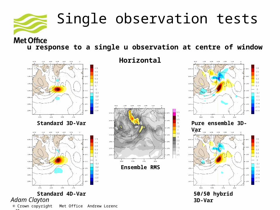
Single observation tests
Standard 3D-Var
Standard 4D-Var 50/50 hybrid 3D-Var
Pure ensemble 3D-Var
Ensemble RMS
u response to a single u observation at centre of window
Horizontal
Adam Clayton
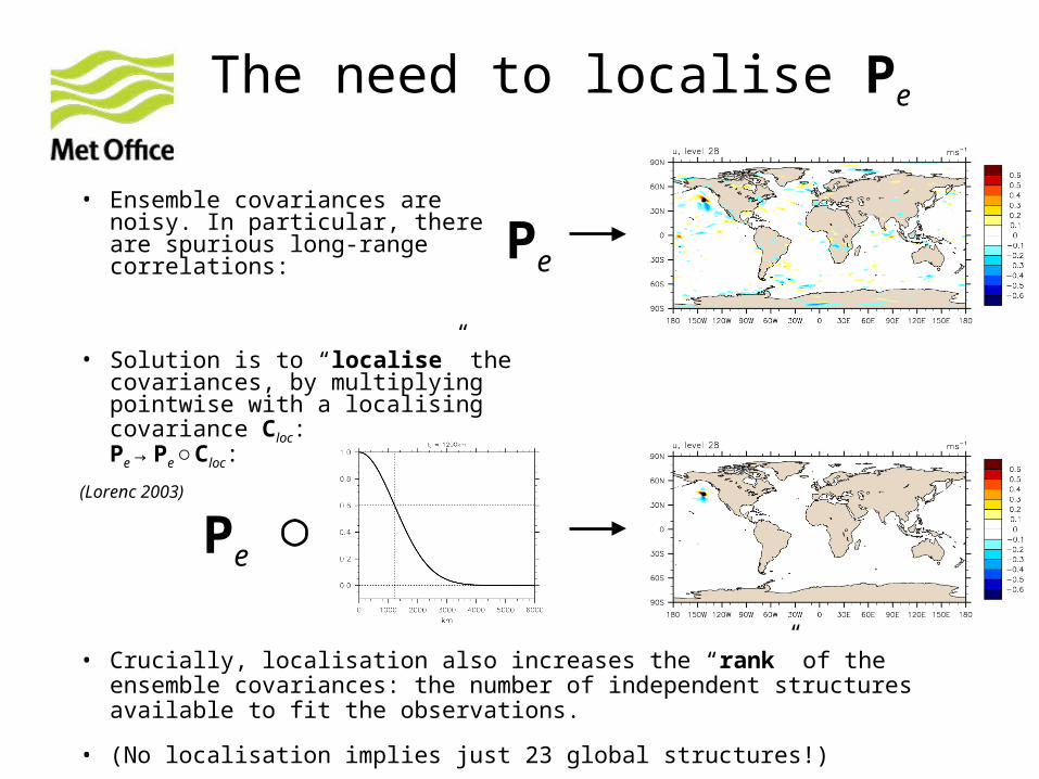
The need to localise Pe
• Ensemble covariances are noisy. In particular, there are spurious long-range correlations:
• Solution is to “localise” the covariances, by multiplying pointwise with a localising covariance Cloc: .
Pe → Pe ○ Cloc:
(Lorenc 2003)
Pe
• Crucially, localisation also increases the “rank” of the ensemble covariances: the number of independent structures available to fit the observations.
• (No localisation implies just 23 global structures!)
Pe
Page 47
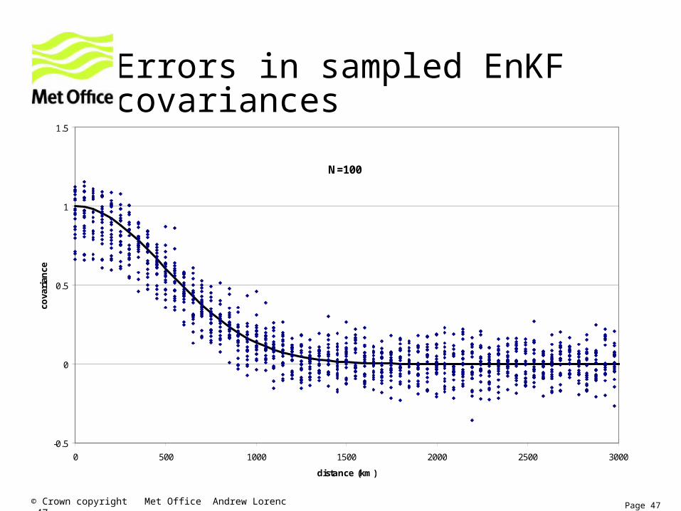
N=100
-0.5
0
0.5
1
1.5
0 500 1000 1500 2000 2500 3000
distance (km)
cova
rian
ce
Errors in sampled EnKF covariances
© Crown copyright Met Office Andrew Lorenc 47
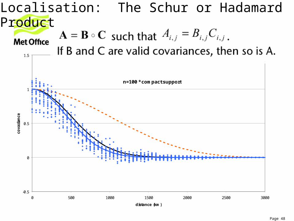
Page 48
n=100 * compact support
-0.5
0
0.5
1
1.5
0 500 1000 1500 2000 2500 3000
distance (km)
cova
rian
ce
Localisation: The Schur or Hadamard Product
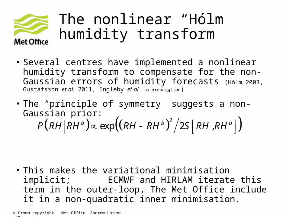
The nonlinear “Hólm” humidity transform
• Several centres have implemented a nonlinear humidity transform to compensate for the non-Gaussian errors of humidity forecasts (Hólm 2003, Gustafsson et al. 2011, Ingleby et al. in preparation)
• The “principle of symmetry” suggests a non-Gaussian prior:
• This makes the variational minimisation implicit; ECMWF and HIRLAM iterate this term in the outer-loop, The Met Office include it in a non-quadratic inner minimisation.
2exp 2 ,b b bP RH RH RH RH S RH RH
© Crown copyright Met Office Andrew Lorenc 49
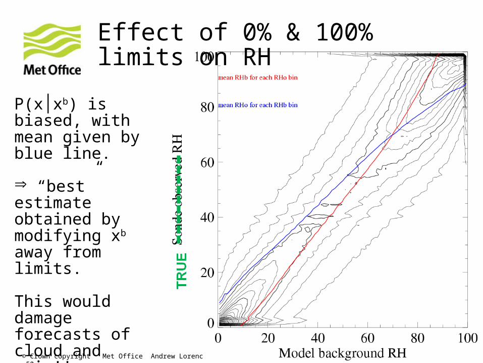
Effect of 0% & 100% limits on RH
P(x│xb) is biased, with mean given by blue line.
“best” estimate obtained by modifying xb away from limits.
This would damage forecasts of cloud and rain!!
Diagram from Lorenc (2007)
© Crown copyright Met Office Andrew Lorenc 50
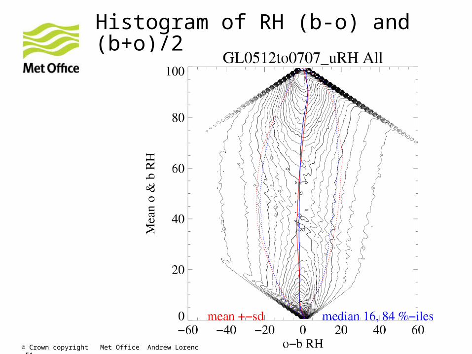
Histogram of RH (b-o) and (b+o)/2
© Crown copyright Met Office Andrew Lorenc 51
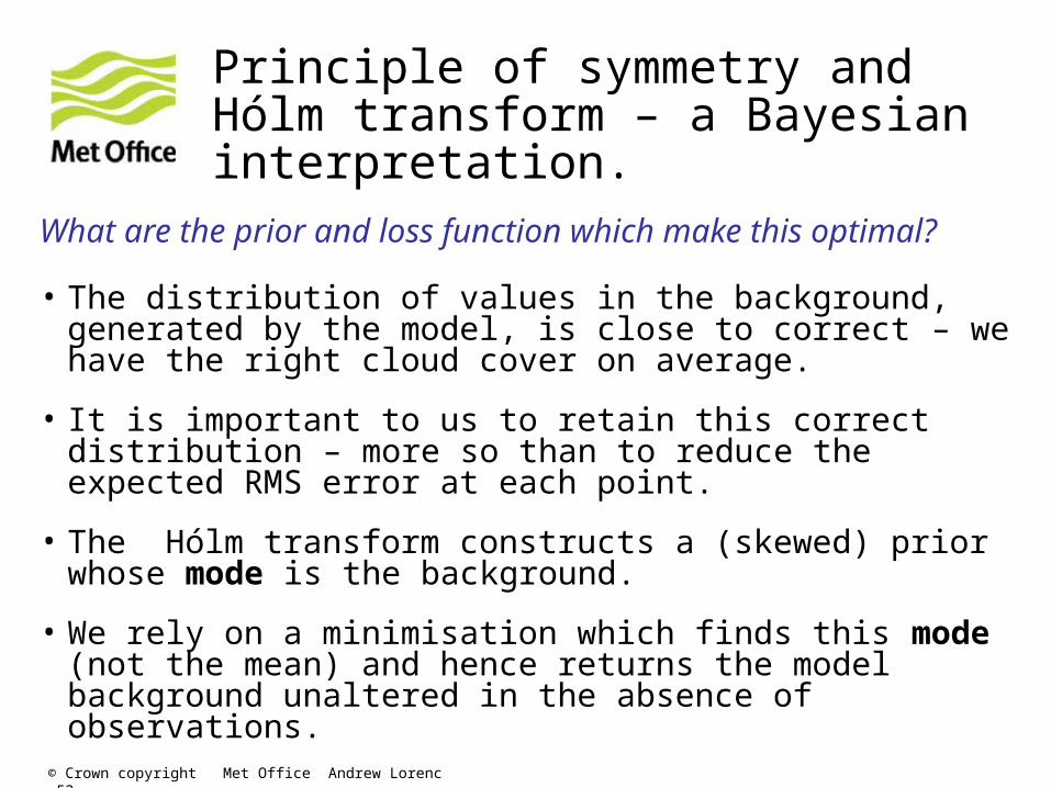
Principle of symmetry and Hólm transform – a Bayesian interpretation.
What are the prior and loss function which make this optimal?
• The distribution of values in the background, generated by the model, is close to correct – we have the right cloud cover on average.
• It is important to us to retain this correct distribution – more so than to reduce the expected RMS error at each point.
• The Hólm transform constructs a (skewed) prior whose mode is the background.
• We rely on a minimisation which finds this mode (not the mean) and hence returns the model background unaltered in the absence of observations.
© Crown copyright Met Office Andrew Lorenc 52
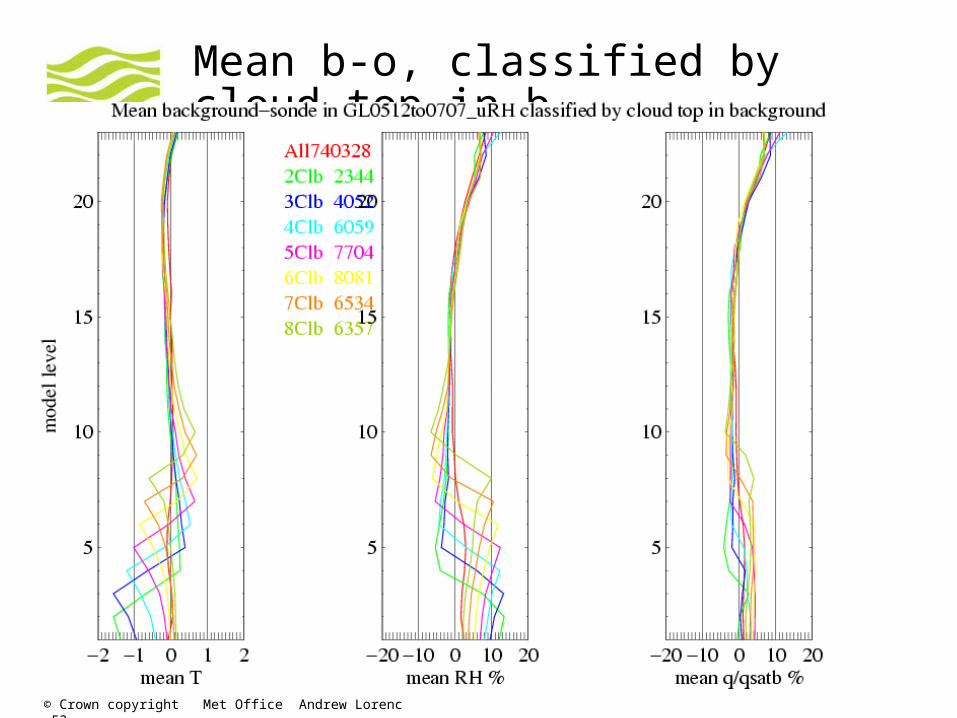
Mean b-o, classified by cloud top in b
© Crown copyright Met Office Andrew Lorenc 53
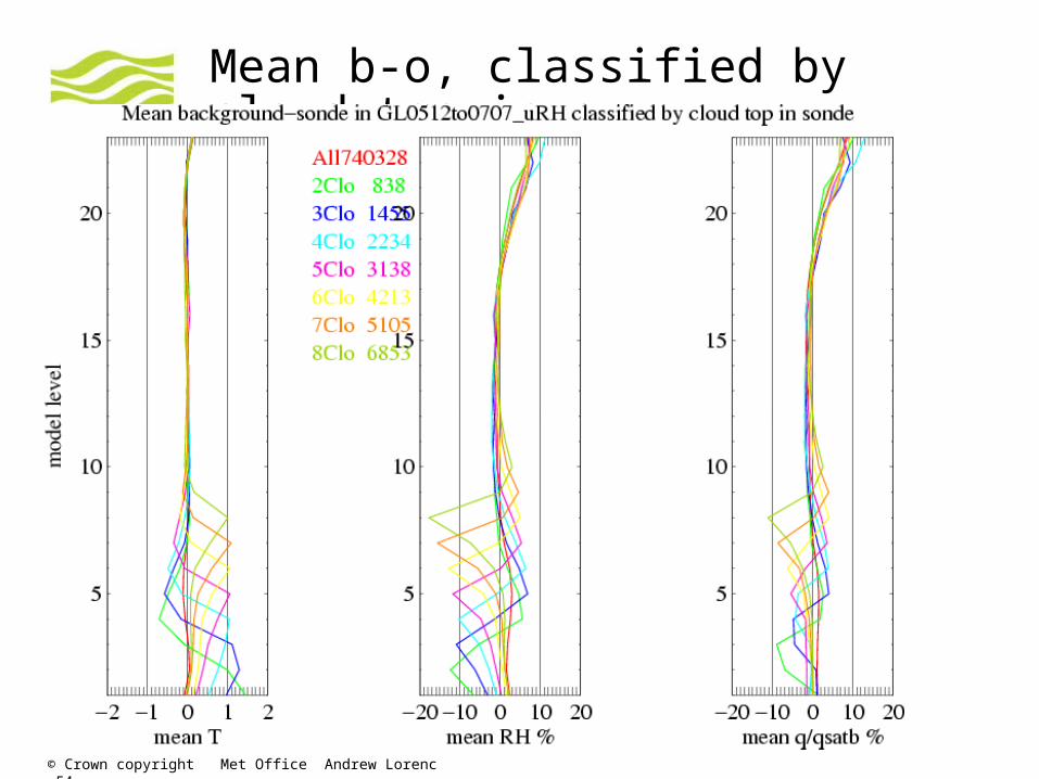
Mean b-o, classified by cloud top in o
© Crown copyright Met Office Andrew Lorenc 54
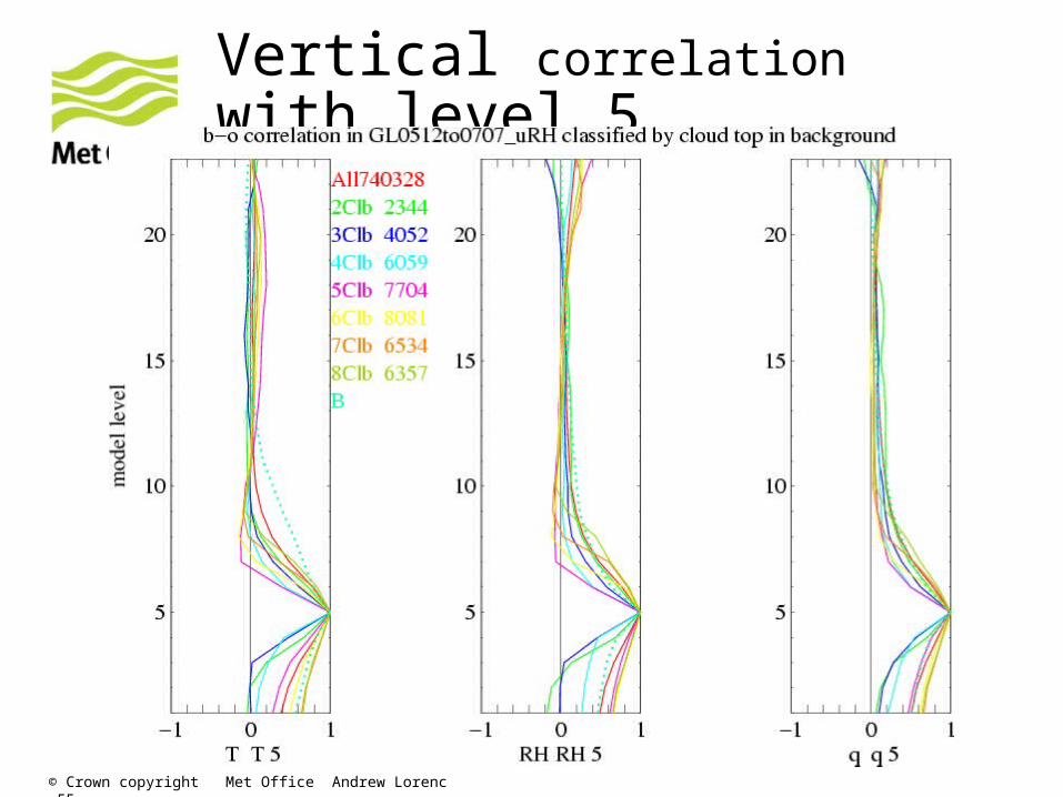
Vertical correlation with level 5
© Crown copyright Met Office Andrew Lorenc 55
© Crown copyright Met Office Andrew Lorenc 56
Nonlinearity – benefitting from the attractor
• The atmospheric state is fundamentally governed by nonlinear effects, e.g. convective-radiative equilibrium, condensation, cloud & precipitation. Nonlinear chaotic systems have a fuzzy attractor manifold of states that occur in reality – far fewer than all possible states. This gives us recognisable weather systems and practical weather prediction!
• Usual minimum variance “best” estimate is not on the attractor.
• The best practical way of defining the attractor in by using the full model, as we have for years in methods for spin-up and diabatic initialisation.
• Methods based on Gaussian PDFs can only approximate near-linear aspects of this balance. We need to add an additional prior that we want the analysis to be a state which the model might generate.
• It is very hard to formulate a practical Bayesian algorithm to do this. We might try engineering solutions:
Incremental methods with an outer-loop. Multiple DA “particles” sampling plausible solutions.
© Crown copyright Met Office Andrew Lorenc 56

© Crown copyright Met Office
Questions and answers


![Data Assimilation for Numerical Weather Prediction - [NWP ......Data Assimilation for Numerical Weather Prediction [NWP] Project Ahmed Attia Statistical and Applied Mathematical Science](https://img.pdfslide.net/doc/110x75/6039cba9995b992a170c4a78/data-assimilation-for-numerical-weather-prediction-nwp-data-assimilation.jpg)