- Department of Mathematics, Purdue University

Journal of Scientific Computing, Vol. 15, No. 2, 2000

A Rational Approximation and Its Applications toDifferential Equations on the Half Line

Ben-Yu Guo,1 Jie Shen,2 and Zhong-Qing Wang3

Received September 25, 2000; accepted October 31, 2000

An orthogonal system of rational functions is introduced. Some results onrational approximations based on various orthogonal projections and interpola-tions are established. These results form the mathematical foundation of therelated spectral method and pseudospectral method for solving differential equa-tions on the half line. The error estimates of the rational spectral method andrational pseudospectral method for two model problems are established. Thenumerical results agree well with the theoretical estimates and demonstrate theeffectiveness of this approach.

KEY WORDS: Legendre rational polynomials; rational approximation;spectral method; pseudospectral method.

1. INTRODUCTION

Many science and engineering problems of current interest are set inunbounded domains. In the context of spectral methods, a number ofapproaches for treating unbounded domains have been proposed andinvestigated. A direct approach is to use spectral method associated withsome orthogonal systems in unbounded domains, such as the Hermitespectral method and the Laguerre method, see, e.g., Maday et al. [12],Guo [8], and Guo and Shen [11]. It is also possible to reformulateoriginal problems in unbounded domains to certain singular�degenerateproblems in bounded domains by variable transformations, and then use

117

0885-7474�00�0600-0117�18.00�0 � 2000 Plenum Publishing Corporation

1 School of Mathematical Sciences, Shangai Normal University, Shanghai 200234, People'sRepublic of China. E-mail: byguo�guomai.sh.cn

2 Department of Mathematics, Penn State University, University Park, Pennsylvania 16802.E-mail: shen�math.psu.edu

3 Department of Mathematics, Shangai University, Shangai 200436, People's Republic ofChina. E-mail: zhqwang�kali.com.cn

the Jacobi polynomials to approximate the resulting singular problems, see,e.g., Guo [6, 10]. Another effective method for solving such problems isbased on rational approximations. For instance, Christov [5] and Boyd[3, 4] developed some spectral methods on infinite intervals by usingmutually orthogonal systems of rational functions. But the convergencesand error estimates for those rational spectral methods are still notavailable.

In this paper, we investigate the spectral method and pseudospectralmethod on the half line by using a new mutually orthogonal system ofrational functions, with the weight function (x+1)&2. We also give aframework for theoretical analysis of rational approximation in weightedSobolev space. Although we may make variable transformations to changedifferential equations on the half line into certain singular�degenerateproblems on a finite interval, it is preferable to approximate the differentialequations on the half line directly using rational approximations in certaincases, such as in exterior problems where the obstacles may become toocomplicated after variable transformations. Indeed, for this type of exteriorproblems, we can choose a circle�sphere which encloses the obstacle, andthen use a combined finite-element, Fourier-rational approximation inwhich the geometric complexity is handled by a finite-element method andthe domain outside the circle�sphere is handled by a rational approximationin the radial direction and Fourier approximation in other direction(s).The details of this approach is beyond the scope of this paper and will beconsidered in a future work.

This paper is organized as follows. In the next section, we introducethe system of rational functions induced by the Legendre polynomials andits basic properties. In Sec. 3, we study various orthogonal projections andestablish some results on the rational approximation. In Sec. 4, we considertwo kinds of rational interpolations. The results in these two sections formthe mathematical foundation for the related spectral method andpseudospectral method. In Sec. 5, we analyze rational spectral methodand rational pseudospectral method for two model problems. In Sec. 6, wediscuss numerical implementations and present some numerical resultswhich agree well with the theoretical analysis and which demonstrate theeffectiveness of this new approach.

2. LEGENDRE RATIONAL FUNCTIONS

We first introduce some notations. Let 4=[x | 0<x<�] and /(x)be a positive weight function. For 1�p��, let

L p/(4)=[v | v is measurable and &v&Lp

/<�]

118 Guo, Shen, and Wang

where

&v&Lp/={\|4

|v(x)| p /(x) dx+1�p

ess supx # 4

|v(x)|

1�p<�

p=�(2.1)

We denote by (u, v)/ and &v&/ respectively the inner product and thenorm of the space L2

/(4), i.e.,

(u, v)/=|4

u(x) v(x) /(x) dx, &v&/=(v, v)1�2/

For any non-negative integer m, we set

H m/ (4)={v } �k

x v=d kvdxk # L2

/(4), 0�k�m=equipped with the inner product, the semi-norm and the norm as follows,

(u, v)m, /= :m

k=0

(�kxu, �k

xv)/ , |v|m, /=&�mx v&/ , &v&m, /=(v, v)1�2

m, /

For any real number r>0, we define the space H r/(4) with the norm &v&r, /

by space interpolation as in Adams [1]. As usual / will be omitted fromthe notations if /(x)#1.

Let Ll (x) be the Legendre polynomial of degree l. We recall that Ll (x)is the eigenfunction of the singular Sturm�Liouville problem

�x((1&x2) �x Ll (x))+l(l+1) Ll (x)=0, l=0, 1, 2,... (2.2)

We define the Legendre rational function of degree l by

Rl (x)=- 2 Ll \x&1x+1+

Thus, Rl (x) is the l th eigenfunction of the singular Sturm�Liouvilleproblem

(x+1)2 �x(x �xv)+*v=0, x # 4 (2.3)

with the corresponding eigenvalue *=l(l+1).

119A Rational Approximation and Its Applications

Clearly, we have

limx � �

Rl (x)=- 2, limx � �

x �xRl (x)= limx � �

2 - 2 x(x+1)2 L$l \x&1

x+1+=0

We also recall that the recurrence formulas and the orthogonality of theLegendre polynomials lead to

Rl+1(x)=2l+1l+1

}x&1x+1

Rl (x)&l

l+1R l&1(x), l�1

2(2l+1) Rl (x)=(x+1)2 (�xRl+1(x)&�xR l&1(x)), l�1

and

|4

R l (x) Rm(x) |(x) dx=(l+ 12)&1 $l, m (2.4)

where |(x)=(x+1)&2 and $l, m is the Kronecker function. Thus, theLegendre rational expansion of a function v # L2

|(4) is

v(x)= :�

l=0

vl Rl (x), with vl=(l+ 12) |

4v(x) Rl (x) |(x) dx

Next, let |1(x)=x. By virtue of (2.3), (2.4) and the asymptoticbehaviors of Rl (x) and x �xRl (x) at infinity, we find that [�xRl (x)] aremutually orthogonal in L2

|1(4), namely,

|4

�xRl (x) �xRm(x) |1(x) dx=l(l+1)(l+ 12)&1 $l, m (2.5)

We shall now derive some inverse inequalities and embeddinginequalities. Let N be any positive integer, and

RN=span[R0 , R1 ,..., RN]

Hereafter, we denote by c a generic positive constant independent ofany function and N.

Theorem 2.1. For any , # RN and 1�p�q��,

&,&Lq|�(2( p+1) N 2)1�p&1�q &,&Lp

|

Proof. Let y # 4� =(&1, 1), x=(1+ y)�(1& y). For any , # RN , weset �( y)=,((1+ y)�(1& y)). By the definition of RN , we have �( y) # PN ,


which is the set of polynomials of degree at most N. By an inverseinequality in PN (see, e.g., Theorem 2.7 of Guo [7]),

\|4�|�( y)|q dy+

1�q

�(( p+1) N 2)1�p&1�q \|4�|�( y)| p dy+

1�p

Therefore,

&,&Lq|=2&1�q \|4�

|�( y)|q dy+1�q

�2&1�q(( p+1) N2)1�p&1�q \|4�|�( y)| p dy+

1�p

=(2( p+1) N 2)1�p&1�q &,&Lp|

Theorem 2.2. Let m be any non-negative integer and 2�p<�.Then, for any , # RN ,

&�mx ,&Lp

|�cN 2m &,&Lp

|

Also for any r�0,

&,&r, |�cN 2r &,&|

Proof. Let y # 4� , PN and �( y) be the same as in the proof of the lasttheorem. Then (see, e.g., Theorem 2.8 of Guo [7]),

&�my �&Lp(4� )�cN 2m &�&Lp(4� )

Thus

&�x,&Lp|=\ 1

2 p+1 |4�

|�y�( y)| p( y&1)2p dy+1�p

�2 \|4�|�y �( y)| p dy+

1�p

�cN 2 \|4�|�( y)| p dy+

1�p

=cN2 &,&Lp|

By repeating the above procedure, we deduce that for any non-negativeinteger m,

&�mx ,&Lp

|�cN 2m &,&Lp

|

The second result follows from the above inequality with p=2 and spaceinterpolation. g


Remark 2.1. In particular, for any � # PN ,

&�y�&L2(4� )�32N2 &�&L2(4� )

which leads to that

&�x,&|�3N2 &,&|

Theorem 2.3. If v # L2|2(4), �xv # L2

|(4) and v(0)=0, then

&v&|2� 23 |v|1, |

If v # L2|(4), �xv # L2(4) and v(0)=0, then

&v&|�2 - 2 |v|1

Proof. Let u( y)=v((1+ y)�(1& y)). Then, in order to prove the firstresult, it suffices to prove that

|4�

u2( y)(1& y)2 dy� 49 |

4�(�yu( y))2 (1& y)4 dy

Since u(&1)=0, we have that for any y # 4� ,

u2( y)(1& y)3=|y

&1�z(u2(z)(1&z)3) dz

Hence,

u2( y)(1& y)3+3 |y

&1u2(z)(1&z)2 dz

=2 |y

&1u(z) �z u(z)(1&z)3 dz

�2 \|4�u2(z)(1&z)2 dz+

1�2

\|4�(�zu(z))2 (1&z)4 dz+

1�2

Letting y � 1, we obtain that

|4�

u2( y)(1& y)2 dy� 49 |

4�(�yu)2 (1& y)4 dy

This proves the first result. The second result follows from the first resultapplied to (x+1) v(x). g


3. LEGENDRE RATIONAL POLYNOMIAL APPROXIMATIONS

In this section, we investigate various orthogonal projections.We define the L2

|(4)-orthogonal projection PN : L2|(4) � RN by

(Pnv&v, ,)|=0, \, # RN

In order to estimate &PNv&v&| , we need to introduce the space

H r|, A(4)=[v | v is a measurable and &v&r, |, A<�]

where for non-negative integer r,

&v&r, |, A=\ :r

k=0

&(x+1) (r�2)+k �kxv&2

|+1�2

For any real r>0, the space H r|, A(4) is defined by space interpolation.

Let A be the Sturm�Liouville operator in (2.3), namely,

Av(x)=&|&1(x) �x(x �xv(x))

By induction,

Amv(x)= :2m

k=1

(x+1)m+k pk(x) �kxv(x) (3.1)

where pk(x) are some rational functions which are bounded uniformly on thewhole interval 4. So Am is a continuous mapping from H 2m

|, A(4) to L2|(4).

Theorem 3.1. For any v # H r|, A(4) and r�0,

&PNv&v&|�cN &r &v&r, |, A

Proof. We first assume that r=2m. By virtue of (2.3), (2.4) andintegration by parts,

v=12

(2l+1) |4

v(x) Rl (x) |(x) dx=2l+1

2l(l+1) |4v(x) AR l (x) |(x) dx

= &2l+1

2l(l+1) |4v(x) �x(x �xRl (x)) dx=

2l+12l(l+1) |4

x �xv(x) �xRl (x) dx

= &2l+1

2l(l+1) |4�x(x �xv(x)) Rl (x) dx=

2l+12l(l+1) |4

Av(x) Rl (x) |(x) dx

= } } } =2l+1

2l m(l+1)m |4

Amv(x) Rl (x) |(x) dx (3.2)


Therefore, we derive from (3.1), (3.2) and the definition of H r|, A(4) that

&PNv&v&2|= :

�

l=N+1

v2l &Rl &2

|

�cN&4m :�

l=N+1\�4 Amv(x) Rl (x) |(x) dx

&Rl &2| +

2

&Rl&2|

�cN&4m &Amv&2|�cN&4m &v&2

r, |, A

Next, let r=2m+1. By (2.3) and integration by parts,

vl =2l+1

2l m(l+1)m |4

Amv(x) R l (x) |(x) dx

=&2l+1

2l m+1(l+1)m+1 |4

Amv(x) �x(x �xRl (x)) dx

=&2l+1

2l m+1(l+1)m+1 |4

�x(Amv(x)) �x Rl (x) |1(x) dx

Thanks to (2.5) and (3.1),

&PNv&v&2|= :

�

l=N+1

v2l &Rl&2

|

= :�

l=N+1

2l+12(l(l+1))2m+2 \|4

�x(Amv) �xRl (x) |1(x) dx+2

= :�

l=N+1

(2l+1) &�xR l&2|1

2(l(l+1))2m+2

_\�4 �x(Amv) �xRl (x) |1(x) dx&�xRl&2

|1+

2

&�xRl&2|1

�cN &2(2m+1) :�

l=N+1 \�4 �x(Amv) �xR l (x) |1(x) dx

&�xRl &2|1

+2

&�xRl&2|1

�cN &2(2m+1) &�x(Amv)&2|1

�cN &2(2m+1) &�x(Amv)(x+1)3�2&2|

�cN &2(2m+1) &v&2r, |, A

The general result follows from the previous results and space interpola-tion. g


The H 1|(4)-orthogonal projection P1

N : H 1|(4) � RN is a mapping

such that for any v # H 1|(4),

(P1Nv&v, ,)1, |=0, \, # RN

In order to estimate &P1Nv&v&1, | , we recall some approximation

results on Jacobi polynomials established in [9]. Let us define

L2:, ;(4� )={u } &u&L2

:, ;=\|4�

u2( y)(1& y): (1+ y); dy+1�2

<+�= (3.3)

and

a:, ;, #, $(u, w)=|4�

�y u �y w(1& y): (1+ y); dy

+|4�

u( y) w( y)(1& y)# (1+ y)$ dy (3.4)

We also denote H 0:, ;, #, $(4� )=L2

#, $(4� ) and

H 1:, ;, #, $(4� )=[u | u is measurable on 4� and &u&1, :, ;, #, $<+�] (3.5)

where &u&1, :, ;, #, $=a1�2:, ;, #, $(u, u). For 0<+<1, H +

:, ;, #, $(4� ) and its norm&u&+, :, ;, #, $ are defined by space interpolation. We also define

H r:, ;, V (4� )=[u | u is measurable on 4� and &u&r, :, ;, V <+�] (3.6)

where for non-negative integer r,

&u&2r, :, ;, V =A (1)

r, :, ;(u)+A (2)r, :, ;(u) (3.7)

with

A (1)r, :, ;(u)= :

r

k=r&[r�2]+1|

4�(�k

y u( y))2 (1& y2)&r+2k&1 (1& y): (1+ y); dy

(3.8)

A (2)r, :, ;(u)= :

[(r+1)�2]

k=1|

4�(�k

y u( y))2 (1& y): (1+ y); dy

The space H r:, ;, V (4� ) and its norm &u&r, :, ;, V for real positive r are defined

by space interpolation.


Let P� 1N, :, ;, #, $ : H 1

:, ;, #, $(4� ) � PN be orthogonal projection operatordefined by

a:, ;, #, $(P� 1N, :, ;, #, $ u&u, �)=0, \� # PN (3.9)

By using the notations on pp. 380�381 and Theorem 2.5 in [9], we knowthat for :�#+2, ;�$+2, and for any u # H r

:, ;, #, $(4� ) with r�1, we have

&P� 1N, :, ;, #, $u&u&2

1, :, ;, #, $�cN 2&2r &u&2r, :, ;, V (3.10)

If in addition, :�#+1, ;�$+1 and 0�+�1, then

&P� 1N, :, ;, #, $u&u&2

+, :, ;, #, $�cN 2+&2r &u&2r, :, ;, V (3.11)

In order to estimate &P1Nv&v&1, | we need to introduce another space.

For any non-negative integer r,

H r|, B(4)=[v | v is measurable on 4 and &v&r, |, B<+�] (3.12)

where

&v&r, |, B=\ :r

k=1

&(x+1)r�2+k&1�2 �kxv&2

|+1�2

(3.13)

As usual, for any r>0, the space H r|, B(4) and its norm are defined by

space interpolation.

Theorem 3.2. For any v # H r|, B(4) with r�1,

&P1Nv&v&1, |�cN1&r &v&r, |, B

Proof. By definition, &P1Nv&v&1, |�&,&v&1, | for any , # RN . Let

y=(x&1)�(x+1), u( y)=v((1+ y)�(1& y)). By taking ,=P� 1N, 2, 0, 0, 0

u( y)|y=(x&1)�(x+1) , a direct computation together with (3.10) (:=2,;=#=$=0) leads to

&,&v&21, |= 1

8 |4�

(�yP� 1N, 2, 0, 0, 0u( y)&�yu( y))2 ( y&1)4 dy

+ 12 |

4�(P� 1

N, 2, 0, 0, 0u( y)&u( y))2 dy

�c &P� 1N, 2, 0, 0, 0u&u&2

1, 2, 0, 0, 0�cN 2&2r &u&2r, 2, 0, V


Note that 1& y=2�(x+1), 1& y2=4x�(x+1)2 and one can show easilyby induction that

�ky u( y)= :

k

j=1

qj (x)(x+1)k+ j � jxv(x) (3.14)

where qj (x) are some rational polynomials which are uniformly boundedon 4. Thus, for any non-negative integer r,

A (1)r, 2, 0(u)�c :

r

k=r&[r�2]+1

:k

j=1

&(x+1)(r�2)+ j&(1�2) � jxv&2

|�c &v&2r, |, B

Similarly, we have

A (2)r, 2, 0(u)�c :

[(r+1)�2]

k=1

:k

j=1

&(x+1)k+ j&1 � jxv&2

|�c &v&2r, |, B

This fact together with space interpolation complete the proof. g

When we apply the Legendre rational spectral method to partial dif-ferential equations with Dirichlet boundary conditions at x=0, we needanother orthogonal projection. Let us denote

H 10, |(4)=[v | v # H 1

|(4), v(0)=0 and v(x)(x+1)&3�2 � 0, as x � �]

R0N=[, # RN | ,(0)=0] (3.15)

a&|(u, v)=(�xu, �x(v|))+&(u, v)|

We define the H 10, |(4)-orthogonal projection P1, 0

N : H 10, |(4) � R0

N by

a&|(P1, 0

N v&v, ,)=0, \, # R0N

Lemma 3.1. For any u, v # H 10, |(4) and &> 3

4 ,

a&|(v, v)�c &v&2

1, |

|a&|(u, v)|�c &u&1, | &v&1, |

Proof. Let &= 34+= and =>0. By integrating by parts and using

Theorem 2.3, we find that


a&|(v, v)=(�x v, �x(v|))+&(v, v)|

=|v| 21, |+& &v&2

|+(�xv, v�x|)

=|v| 21, |+& &v&2

|+12 |

4�x(v2(x)) �x|(x) dx

=|v| 21, |+& &v&2

|&3 |4

v2(x)(x+1)&4 dx

=|v| 21, |+& &v&2

|&3 &v&2|2

=|v| 21, |&\9

4&

=2+ &v&2

|2+\34

+=+ &v&2|&\3

4+

=2+ &v&2

|2

�29

= |v| 21, |+

=2

&v&2| (3.16)

This leads to the first result. Next, by the Cauchy�Schwartz inequality andTheorem 2.3,

|(�xu, v �x |)|= } |4�xu(x) v(x) �x|(x) dx }

�2 &�xu&| &v&|2�c |u| 1, | |v|1, |

which implies the second result. g

In order to estimate &P1, 0N v&v&1, | , we need another result in [9]. Let

us define

H 1, L:, ;, #, $(4� )=[u # H 1

:, ;, #, $(4� ) | u(&1)=0], PLN=[u # PN | u(&1)=0]

and the orthogonal projection P� 1, LN, :, ;, #, $ : H 1, L

:, ;, #, $(4� ) � PLN by

a:, ;, #, $(P� 1, LN, :, ;, #, $u&u, �)=0, \, # PL

N

Thanks to Theorem 2.6 in [9], we know that if :�#+2, ;�0 and $�0,then for any u # H r

:, ;, #, $(4� ) & H 1, L:, ;, #, $(4� ), we have

&P� 1, LN, :, ;, #, $u&u&2

1, :, ;, #, $�cN 2&2r &u&2r, :, ;, V (3.17)

and if in addition, :�#+1, ;�$+1 and 0�+�1, then

&P� 1, LN, :, ;, #, $u&u&2

+, :, ;, #, $�cN 2+&2r &u&2r, :, ;, V (3.18)


Theorem 3.3. For any v # H r|, B(4) & H 1

0, |(4), &> 34 and r�1,

&P1, 0N v&v&1, |�cN1&r &v&r, |, B

Proof. By Lemma 3.1, for any , # R0N ,

&P1, 0N v&v&2

1, |�ca&|(P1, 0

N v&v, P1, 0N v&v)

=ca&|(P1, 0

N v&v, ,&v)

�c &P1, 0N v&v&1, | &,&v&1, |

Therefore

&P1, 0N v&v&1, |�c inf

, # R0N

&,&v&1, | (3.19)

Next, let x=(1+ y)�(1& y), u( y)=v((1+ y)�(1& y)) and take ,=P� 1, L

N, 2, 0, 0, 0u( y)|y=(x&1)�(x+1) in (3.19). Then, the desired result follows from(3.17) and a similar argument as in the proof of Theorem 3.2. g

We now consider yet another orthogonal projection which will beused in the Legendre rational interpolation approximations and in theLegendre rational pseudospectral method. Let

a|(u, v)= 12 |

4�x u(x) �xv(x)(x+1) dx+|

4u(x) v(x) |(x) dx (3.20)

The orthogonal projection P� 1N : H 1

|, A(4) � RN is a mapping such that forany v # H 1

|, A(4),

a|(P� 1N v&v, ,)=0, \, # RN (3.21)

Theorem 3.4. For any v # H r|, A(4) and r�1,

&P� 1Nv&v&|�cN&r &v&r, |, A

and

&(x+1)3�2 �x(P� 1Nv&v)&|�cN1&r &v&r, |, A

Proof. Let us denote

u( y)=v \1+ y1& y+ , u*N( y)=P� 1

N v(x)|x=(1+ y)�(1& y)


By definition, we have

|4�

�y(u*N( y)&u( y)) �y�( y)(1& y) dy

+|4�

(u*N( y)&u( y)) �( y) dy=0, \� # PN (3.22)

Thus, u*N( y)=P� 1N, 1, 0, 0, 0 u( y). Under the transform x=(1+ y)�(1& y), we

have

|4

(P� 1N v&v)2 |(x) dx= 1

2 |4�

(u*N&u)2 dy

|4

(x+1)3 (�x(P� 1Nv&v))2 |(x) dx=|

4�(�y(u*N&u))2 (1& y) dy

Therefore, we derive from (3.11) with :=1, ;=#=$=0 that

&P� 1Nv&v&|�&u*N&u&2

0, 1, 0, 0, 0�cN&2r &u&2r, 1, 0, V (3.23)

and

&(x+1)3�2 �x(P� 1Nv&v)&|�c &u*N&u&2

1, 1, 0, 0, 0�cN2&2r &u&2r, 1, 0, V (3.24)

A direction computation leads to

A (1)r, 1, 0(u)�c :

r

k=r&[r�2]+1

:k

j=1

&(x+1) (r�2)+ j � jxv&2

|�c &v&2r, |, A

Similarly,

A (2)r, 1, 0(u)�c :

[(r+1)�2]

k=0

:k

j=1

&(x+1)k+ j&(1�2) � jxv&2

|�c &v&2r, |, A g

We now give an estimate for the L�-norm of the projection operatorP� 1

N which will be useful for analyzing nonlinear problems. Similar estimatesfor other projection operators can also be established. To do this, we intro-duce the following Hilbert space. For any non-negative integer r,

H r|, C (4)=[v | v is measurable and &v&r, |, C<�]

with the norm

&v&r, |, C=\ :r

k=0

&(x+1)r+k �kxv&2

|+1�2


For any real r>0, the space H r|, C (4) and its norm are defined by space

interpolation.

Theorem 3.5. For any v # H r|, C (4) with r>1, we have

&P� 1Nv&L�(4)�c &v&r, w, C

Proof. Let u( y), u*N and P� 1N, 1, 0, 0, 0u( y) be the same as defined above.

Then

&P� 1Nv&L�(4)=&u*N&L�(4� )=&P� 1

N, 1, 0, 0, 0u( y)&L�(4� )

Thanks to Theorem 2.11 in [9], we have for r>1,

&P� 1N, 1, 0, 0, 0u( y)&L�(4� )�c(&u&r, 1, 0, V +&u&H r(4� ))

Moreover, by (3.14),

&u&2Hr(4� )= :

r

k=0

:k

j=1|

4(x+1)2k+2j (� j

x v(x))2 |(x) dx

�c :r

j=0|

4(x+1)2r+2j (� j

xv(x))2 |(x) dx�c &v&2r, |, C

Then the desired result follows. g

4. LEGENDRE RATIONAL INTERPOLATION APPROXIMATION

In actual computations, it is convenient to use interpolations. We firstconsider the Legendre�Gauss rational interpolation. We denote by `N, j theN+1 distinct real zeros of RN+1(x), 0� j�N. Indeed,

`N, j=(1+_N, j )(1&_N, j )&1 (4.1)

where _N, j are the zeros of LN+1(x). Let |N, j be the correspondingChristoffel numbers, 0� j�N, such that

|4

,(x) |(x) dx= :N

j=0

,(`N, j ) |N, j , \, # R2N+1 (4.2)

As we know, the weights of the Legendre�Gauss quadrature are

\N, j=2

(1&_2N, j)(�xLN+1(_N, j ))2 , 0� j�N


Thus

|N, j=2

`N, j (`N, j+1)2 (�xRN+1(`N, j ))2 (4.3)

Moreover, by virtue of (15.3.10) in Szego� [15],

|N, jt2?`1�2

N, j

(N+1)(`N, j+1)(4.4)

We next introduce the discrete inner product and the discrete normassociated with the Legendre�Gauss rational interpolation points,

(u, v)|, N= :N

j=0

u(`N, j ) v(`N, j ) |N, j , &v&|, N=(v, v)1�2|, N

Thanks to (4.2), we have

(,, �)|, N=(,, �)| , \,� # R2N+1 (4.5)

For any v # C(4), the Legendre�Gauss rational interpolant INv # RN suchthat

INv(`N, j )=v(`N, j ), 0� j�N

or equivalently,

(INv&v, ,)|, N=0, \, # RN

The following theorem is related to the stability of the Legendre�Gauss rational interpolation.

Theorem 4.1. For any v # H 1|, A(4),

&INv&|�c(&v&|+N&1 &x1�2 �xv&)

Proof. By (4.4) and (4.5),

&INv&2|=&INv&2

|, N= :N

j=0

v2(`N, j ) |N, j

�cN &1 :N

j=0

v2(`N, j ) `1�2N, j (`N, j+1)&1


Let x=(1+cos %)�(1&cos %) and v(%)=v((1+cos %)�1&cos %)). Then

&INv&2|�cN &1 :

N

j=0

v2(%N, j ) \1+cos %N, j

1&cos %N, j+1�2

(1&cos %N, j )

According to (4.1) and Theorem 8.9.1 in Szego� , (15)

%N, j=1

N+1( j?+O(1)), 0� j�N (4.6)

where O(1) is bounded uniformly for all 0� j�N. Now, let a0=O(1)�(N+1) and a1=(N?+O(1))�(N+1). Then %N, j # Kj/[a0 , a1], Kj beingof size c�(N+1). Consequently,

&INv&2|�cN &1 :

N

j=0

sup% # Kj

|v2(%) sin %|

By using an inequality of space interpolation (see (13.7) in Bernardi andMaday [2]), we know that for any f # H1(a, b),

maxa�x�b

| f (x)|�c \ 1

- b&a& f &L2(a, b)+- b&a &�x f &L2(a, b) + (4.7)

Hence

&INv&2|�c :

N

j=0

(&v(%) sin1�2 %&2L2(Kj)

+N&2 &�% (v(%) sin1�2 %)&2L2(Kj)

)

�c(&v(%) sin1�2 %&2L2(0, ?)+N&2 &�% (v(%) sin1�2 %)&2

L2(a0 , a1))

�c(&v(%) sin1�2 %&2L2(0, ?)+N&2 &�% v(%) sin1�2 %)&2

L2(0, ?)

+\ supa0�%�a1

cos2 %N2 sin %+ &v(%) sin1�2 %&2

L2(0, ?))

�c(&v(%) sin1�2 %&2L2(0, ?)+N&2 &�% v(%) sin1�2 %&2

L2(0, ?))

�c(&v(x)&2L2

|(4)+N &2 &x1�2 �xv&2)

This completes the proof. g

Theorem 4.2. For any v # H r|, 4(4) and 0�+�1�r,

&INv&v&+, |�cN2+&r &v&r, |, A


Proof. Since IN(P� 1N v) coincides with P� 1

Nv, we derive from Theorems3.4 and 4.1 that

&INv&P� 1Nv&|�(&P� 1

Nv&v&|+N &1&x1�2 �x(P� 1Nv&v)&)

�cN&r &v&r, |, A (4.8)

Using Theorem 3.4 again,

&INv&v&|�&P� 1Nv&v&|+&INv&P� 1

Nv&|�cN &r &v&r, |, A (4.9)

Furthermore, by (4.8) and Theorems 2.2 and 3.4,

|INv&v| 1, |�|P� 1Nv&v|1, |+|INv&P� 1

Nv|1, |

�&P� 1Nv&v&1, |+cN 2 &INv&P� 1

Nv&|

�c &P� 1Nv&v&1, |+cN2&r &v&r, |, A

�cN2&r &v&r, |, A (4.10)

Finally, we get the desired result by (4.9), (4.10) and space interpolation.g

We now deal with the Legendre�Gauss�Radau rational interpolation.We denote by � N, j the N+1 distinct zeros of RN(x)+RN+1(x), 0� j�N.Indeed,

� N, j=(1+_N, j )(1&_N, j )&1 (4.11)

where _N, j are the zeros of LN(x)+LN+1(x). In particular, � N, N=0. Let|N, j be the corresponding Christoffel numbers, 0� j�N, such that

|4

,(x) |(x) dx= :N

j=0

,( � N, j ) |N, j , \, # R2N (4.12)

As we know, the weights of the Legendre�Gauss�Radau quadrature are

\N, j =1

(N+1)2

1&_N, j

(LN(_N, j ))2 , 0� j�N&1

\N, N=2

(N+1)2


Thus

|N, j=2

(N+1)2

1

( � N, j+1)(RN( � N, j ))2, 0� j�N&1

(4.13)

|N, N=1

(N+1)2

Moreover, by virtue of (15.3.10) in Szego� [15],

|N, jt4?N

� 1�2N, j

( � N, j+1), 0� j�N&1 (4.14)

The discrete inner product and the discrete norm associated with theLegendre�Gauss�Radau rational interpolation points are,

(u, v)|, N, t= :N

j=0

u( � N, j ) v( � N, j ) |N, j , &v&|, N, t=(v, v)1�2|, N, t

Thanks to (4.12),

(,, �)|, N, t=(,, �)| , \,� # R2N (4.15)

For any v # C(4� ), the Legendre�Gauss�Radau rational interpolantI� Nv(x) # RN , satisfying

I� Nv( � N, j )=v( � N, j ), 0� j�N

or equivalently,

(I� Nv&v, ,)|, N, t=0, \, # RN

The following theorem is related to the stability of the Legendre�Gauss�Radau rational interpolation.

Theorem 4.3. For any v # H 1|, A(4),

&I� Nv&|�c(&v&|+N&1 &(x+1)1�2 �x v&)

Proof. By (4.13), (4.14) and (4.15),

&I� Nv&2|=&I� Nv&2

|, N, t= :

N

j=0

v2( � N, j ) |N, j

�cN&1 :N&1

j=0

v2( � N, j ) � 1�2N, j (1+ � N, j )

&1+(N+1)&2 v2(0)


By the trace theorem,

|v(0)|2�c &v&2H 1�2(0, 1)�c " 1

x+1v"

2

H 1�2(0, 1)

�c &v&21�2, |�c &v&2

1, |

Let x=(1+cos %)�(1&cos %) and v(%)=v((1+cos %)�(1&cos %)). Then

&I� Nv&2|�cN&1 :

N&1

j=0

v2(%� N, j ) \1+cos %� N, j

1&cos %� N, j+1�2

(1&cos %� N, j )+cN&2 &v&21, |

According to (4.11), Theorem 8.9.1 of Szego� [15], and the relationbetween _N, j and _N, j , we assert that

%� N, j=1N

( j?+O(1)), 0� j�N&1

Then, the conclusion follows from an similar argument as in the proof ofTheorem 4.1. g

Theorem 4.4. For any v # H r|, A(4) and 0�+�1�r,

&I� Nv&v&+, |�cN2+&r &v&r, |, A

Proof. Since I� N(P� 1Nv) coincides with P� 1

Nv, we have from Theorems3.4 and 4.3 that

&I� Nv&P� 1N v&|�c(&P� 1

Nv&v&|+N&1 &(x+1)1�2 �x(P� 1Nv&v)&)

�cN&r &v&r, |, A (4.16)

Using Theorem 3.4 again,

&I� Nv&v&|�&P� 1Nv&v&|+&I� Nv&P� 1

Nv&|�cN &r &v&r, |, A (4.17)

Furthermore, by (4.16), and Theorems 2.2 and 3.4,

|I� Nv&v|1, |�|P� 1Nv&v| 1, |+|I� Nv&P� 1

Nv| 1, |

�&P� 1N v&v&1, |+cN 2 &I� N v&P� 1

Nv&|

�c &P� 1Nv&v&1, |+cN 2&r &v&r, |, A

�cN2&r &v&r, |, A (4.18)

Finally, we get the desired result by (4.16), (4.18) and space interpolation.g


5. APPLICATIONS

We consider first the following model problem

&�2xU(x)+&U(x)= f (x), 0<x<�

{U(0)=0 (5.1)

(x+1)&3�2 U(x) � 0, as x � �

where &>0 and f (x) is a given function. For simplicity, we assume &> 34 .

Otherwise, we can use the variable transformation x=:y, :> 12 - 3�&.

A weak formulation of (5.1) with &> 34 is to find U # H 1

0, |(4) such that

:&|(U, v)=( f, v)| , \v # H 1

0, |(4) (5.2)

If f # (H 10, |(4))$, then by Lemma 3.1 and the Lax�Milgram Lemma, (5.2)

with &> 34 has a unique solution.

The Legendre rational spectral scheme for (5.1) is to find uN # R0N ,

such that

a&|(uN , ,)=( f, ,)| , \, # R0

N (5.3)

Theorem 5.1. If U # H r|, B(4) & H 1

0, |(4), &> 34 and r�1, then

&uN&U&1, |�cN 1&r &U&r, |, B

Proof. Let UN=P1, 0N U. By (5.2),

a&|(UN , ,)=( f, ,)| , \, # R0

N (5.4)

Let U� N=uN&UN . Then, by (5.3) and (5.4),

a&|(U� N , ,)=0, \, # R0

N (5.5)

Thus, uN=UN and the desired result follows from Theorem 3.3. g

We now consider the Legendre�Gauss�Radau rational pseudospectralscheme for (5.1). Let

a&|, N(u, v)=(�x u, �xv&2v(1+x)&1)|, N, t+&(u, v)|, N, t

Since

�x Rl (x)=2 - 2

(x+1)2 L$l \x&1x+1+=

- 22

(1& y)2 L$l ( y) }y=(x&1)�(x+1)

# Rl+1


and

Rl (x)(1+x)&1=- 2

2(1& y) Ll ( y) }y=(x&1)�(x+1)

# Rl+1

we know from (4.15) that for any ,, � # RN&1 ,

a&|, N(,, �)=a&

|(,, �) (5.6)

A legendre rational pseudospectral method for (5.1) is to finduN # R0

N&1 such that

a&|, N(uN , ,)=( f, ,)|, N, t , \, # R0

N&1 (5.7)

Theorem 5.2. If U # H r|, B(4) & H 1

0, |(4), f # H r&1|, A(4), &> 3

4 andr�1, then

&uN&U&1, |�cN 1&r(&U&r, |, B+& f &r&1, |, A) (5.8)

Proof. By (4.15) and Theorem 2.3, we have for any , # RN&1 ,

|( f, ,)|, N, t |= } \I� N((x+1) f ),,

x+1+|, N, t}= } (I� N(x+1) f ),

,x+1+| }

�&I� N((x+1) f )&| &,&| 2

�&I� N((x+1) f )&| &,&1, | (5.9)

Hence, by the Lax�Milgram Lemma, (5.7) has a unique solution such that

&uN&1, |�c &I� N((x+1) f )&|

Let UN=P1, 0N&1U. Then by (5.6) and (5.7), we have for any , # R0

N&1 ,

a&|(UN , ,)=( f, ,)|

(5.10)a&

|(uN , ,)=(IN f, ,)|

Therefore,

a&|(UN&uN , ,)=( f&IN f, ,)| , , # R0

N&1


Let ==&& 34>0. Taking ,=UN&uN and using (3.16), we obtain

=2

&uN&UN&2|+

2=9

|uN&UN | 21, |

�a&|, N(uN&UN , uN&UN)

=( f&IN f, UN&uN)|�& f&IN f &| &UN&uN&|

�= & f&IN f &2|+

=4

&UN&uN &2| (5.11)

Therefore, by Theorems 3.3 and 4.4,

&uN&U&1, |�&UN&U&1, |+&uN&UN &1, |

�cN 1&r(&U&r, |, B+& f &r&1, |, A) g

Next, we consider a time-dependent model problem

{�t U(x, t)&�2

xU(x, t)= f (x, t)�x U(0, t)=0(x+1)&3�2 U(x, t) � 0U(x, 0)=U0(x)

0<x<�, 0<t�T0�t�Tas x � �, 0�t�T0<x<�

(5.12)

A weak formulation of (5.12) is to find U # L2(0, T; H 1|(4)) & L�(0, T;

L2|(4)) such that

(�t U(t), v)|+(�xU(t), �xv)|+(�xU(t), v �x|)=( f, v)| , \v # H 1|(4)

(5.13)

If U0 # L2|(4) and f # L2(0, T; L2

|(4)), then (5.12) has a unique solution.The Legendre rational spectral scheme for (5.12) is to find uN(t) # RN forall 0�t�T such that

{(�tuN(t), ,)|+(�xuN(t), �x,)|+(�xuN(t), , �x|)=( f, ,)| , \, # RN

uN(0)=PNU0(5.14)

Theorem 5.3. If U # H1(0, T; H r|, B(4)) and U0 # H r&1

|, A(4) & H r|, B(4)

with r�1, then for all 0�t�T,

&uN(t)&U(t)&2|+|

t

0&uN(s)&U(s)&2

1, | ds�c*ectN 2&2r

where c* is a positive constant depending only on the norms of U and U0

in the mentioned spaces.


Proof. Let UN=P1N U. By (5.13),

(�tUN(t), ,)|+(UN(t), ,)1, |+(�x UN(t), , �x|)&(UN(t), ,)|

{ =( f, ,)|+ :3

i=1

Gi (t, ,), \, # RN (5.15)

UN(0)=P1NU0

where

G1(t, ,)=(�tUn(t)&�tU(t), ,)|

G2(t, ,)=(�xUN(t)&�xU(t), , �x|)

G3(t, ,)=(U(t)&UN(t), ,)|

Now, let U� N=uN&UN . Then by (5.14) and (5.15),

(�tU� N(t), ,)|+(U� N(t), ,)1, |+(�x U� N(t), , �x|)&(U� N(t), ,)|

{ =& :3

i=1

G i (t, ,) (5.16)

U� N(0)=PN U0&P1NU0

Taking ,=U� N in (5.16), we find

ddt

&U� N(t)&2|+2&U� N(t)&2

1, |+2(�xU� N(t) �x|)&2 &U� N(t)&2|

�2 :3

i=1

|Gi (t, U� N(t))| (5.17)

It is easy to see that

2 |(�x U� N(t), U� N(t) �x|)|+2 &U� N(t)&2|�|U� N(t)| 2

1, |+6 &U� N(t)&2|

By virtue of Theorems 3.1 and 3.2,

2 |G1(t, U� N(t))|�&U� N(t)&2|+cN 2&2r &�t U(t)&2

r, |, B

2 |G2(t, U� N(t))|�&U� N(t)&2|+cN 2&2r &U(t)&2

r, |, B

2 |G3(t, U� N(t))|�&U� N(t)&2|+cN 2&2r &U(t)&2

r, |, B

&U� N(0)&2|�cN 2&2r(&U0&2

r&1, |, A+&U0&2r, |, B)

�cN 2&2r &U0&2r, |, B


Thus,

ddt

&U� N(t)&2|+&U� N(t)&2

1, |

�8 &U� N(t)&2|+cN2&2r(&�tU(t)&2

r, |, B+&U(t)&2r, |, B) (5.18)

Let us denote

E(v, t)=&v(t)&2|+|

t

0&v(s)&2

1, | ds

\(t)=cN2&2r \&U0&2r&1, |, A+&U0&2

r, |, B+|t

0(&�sU(s)&2

r, |, B) ds+Integrating (5.18) with respect to t, we obtain that

E(U� N , t)�c |t

0E(U� N , s) ds+\(t)

Finally, we use the above estimate and Theorem 3.2 to get the followingresult. g

We now consider the Legendre�Gauss rational pseudospectral schemefor (5.13): Find uN(t) # RN&1 for all 0�t�T such that

(�t uN(t), ,)|, N+(�xuN(t), �x ,&2,(x+1)&1)|, N

{ =( f (t), ,)|, N , \, # RN&1 (5.19)

uN(0)=IN&1U0

Theorem 5.4. If U # H1(0, T; H r|, B(4)), U0 # H r&1

|, A(4) & H r|, B(4)

and f # H r&1|, A(4) with r�1, then for all 0�t�T,

&uN(t)&U(t)&2|+|

t

0&uN(s)&U(s)&2

1, | ds�c*ectN 2&2r

where c* is a positive constant depending only on the norms of U, U0 andf in the mentioned spaces.

Proof. Let UN=P1N&1U. We get from (5.13) that

(�t UN(t), ,)|, N+(�xUN(t), �x,&2,(x+1)&1)|, N

=( f (t), ,)|+ :6

i=4

Gi (t, ,), \, # RN&1 , t # (0, T] (5.20)


where

G4=(�tUN(t), ,)|, N&(�tU(t), ,)|

G5=(�xUN(t), �x,)|, N&(�xU(t), �x,)|

G6=2(�xU(t), ,(x+1)&1)|&2(�xUN(t), ,(x+1)&1)|, N

Further, let U� N=uN&UN . then by subtracting (5.20) from (5.19), weobtain that for any , # RN&1 and t # (0, T],

(�t U� N(t), ,)|, N+(�xU� N(t), �x,&2,(x+1)&1)|, N

=( f (t), ,)|, N&( f (t), ,)|& :6

i=4

Gi (t, ,) (5.21)

U� N(0)=IN&1 U0&P1N&1 U0

Taking ,=U� N(t) in (5.21), we get from (4.5) that

ddt

&U� N(t)&2|+2 |U� N(t)| 2

1, |

�2 :6

i=4

|Gi (t, U� N(t))|+4 |(�xU� N(t), U� N(t)(x+1)&1)| |

+2 |( f (t), U� N(t))|, N&( f (t), U� N(t))| | (5.22)

Next, we estimate the terms at the right side of (5.22). By virtue of (4.5)and Theorem 3.2,

2 |G4(t, U� N(t))|�&U� N(t)&2|+cN 2&2r &�t U(t)&2

r, |, B

2 |G5(t, U� N(t))|� 12 |U� N(t)| 2

1, |+cN 2&2r &U(t)&2r, |, B

2 |G6(t, U� N(t))|�&U� N(t)&2|+cN 2&2r &U(t)&2

r, |, B

Clearly,

4 |(�x U� N(t), U� N(t)(x+1)&1)| |� 12 |U� N(t)| 2

1, |+8 &U� N(t)&2|

Thanks to Theorem 4.2,

2 |( f (t), U� N(t))|, N&( f (t), U� N(t))| |=2 |(IN f (t)& f (t), U� N(t))| |

�&U� N(t)&2|+cN 2&2r & f (t)&2

r&1, |, A

(5.23)


Moreover, Theorems 3.2 and 4.2 imply that

&U� N(0)&2|�cN2&2r(&U0&2

r&1, |, A+&U0&2r, |, B)

Thus,

ddt

&U� N(t)&2|+&U� N(t)&2

1, |�12 &U� N(t)&2|+cN 2&2r(&�tU(t)&2

r, |, B

+&U(t)&2r, |, B+& f (t)&2

r&1, |, A) (5.24)

Let

\1(t)=cN 2&2r \&U0&2r&1, |, A+&U0&2

r, |, B

+|t

0(&�sU(s)&2

r, |, B+&U(s)&2r, |, B+& f (s)&2

r&1, |, A) ds+Integrating (5.24) with respect to t, we obtain that

E(U� N , t)�c |t

0E(U� N , s) ds+\1(t)

which implies the desired result. g

6. NUMERICAL IMPLEMENTATIONS

We now present an efficient algorithm for solving (5.1) by using therational pseudospectral scheme (5.7). As is shown in [14] (see also [13]),one need to use compact combinations of rational Legendre polynomials asbasis functions. Indeed, setting �j (x)=1�- 2(Rj (x)+Rj+1(x)), we have�(0)=0 and

R0N&1=span[�j : j=0, 1,..., N&2] (6.1)

Hence, setting

bkj=(�j , �k)|, N, t=(�j , �k)| , akj=a&|, N(�j , �k)=&(�j" , �k)|

uN= :N&2

j=0

x j�j (x), x� =(x0 , x1 ,..., xN&2)t (6.2)

f� =( f0 , f1 ,..., fN&2)t with fk=( f, �j )|


the Rational Legendre Galerkin approximation (5.7) is reduced to:

(&B+A) x� = f� (6.3)

One verify easily by the transform x=(1+ y)�(1& y) that

bkj =|1

&1(Lj ( y)+Lj+1( y))(Lk( y)+Lk+1( y)) dy

akj =& 14 |

1

&1(1& y)2 [(1& y)2(L$j ( y)+L$j+1( y))]$ (Lk( y)+Lk+1( y)) dy

=& 14 |

1

&1[(1& y)2 [(1& y)2(Lk( y)+Lk+1( y))]$]$ (Lj ( y)+Lj+1( y)) dy

(6.4)

By using the orthogonality of Legendre polynomials, one find immediatelythat B=(bkj ) is a symmetric tridiagonal matrix whose nonzero entries are

bkk=2

2k+1+

22k+3

, bk, k+1=bk+1, k=2

2k+3

Similarly, one find that A=(akj ) is a non-symmetric seven diagonal matrixwhose nonzero entries can be directly computed, although a little tedious,using the properties of Legendre polynomials. Hence, (6.3) can be efficientlysolved.

We now present some numerical experiments using the above schemeto solve (5.1) with &=2. Three illustrative examples are considered.

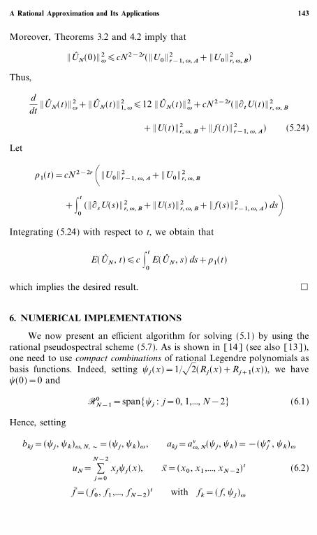
Example 1. U(x)=sin kxe&x.Here, the function decays exponentially at infinity, so Theorem 5.2

predicts that errors of rational pseudospectral approximation will decreasefaster than any algebraic rate. In Fig. 1, we plot the log10 of H 1

|-errors vs.- N. The two near straight lines corresponding to k=1, 2 and 4 indicatethat the errors decay like e&c - N.

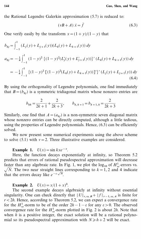
Example 2. U(x)=x�(1+x)h.The second example decays algebraicly at infinity without essential

singularity. One can check directly that &U&r, |, B+& f &r&1, |, A is finite forr<2h. Hence, according to Theorem 5.2, we can expect a convergence ratefor the H 1

| -norm to be of the order 2h&1&= for any =>0. The observedconvergence rate for the H 1

| -norm plotted in Fig. 2 is about 2h. Note thatwhen h is a positive integer, the exact solution will be a rational polyno-mial so its pseudospectral approximation with N�h+2 will be exact.


File: 854J 404829 . By:SD . Date:26:12:00 . Time:15:17 LOP8M. V8.B. Page 01:01Codes: 1046 Signs: 519 . Length: 44 pic 2 pts, 186 mm

Fig. 1. Convergence rates of the rational pseudospectral approximation: Example 1.

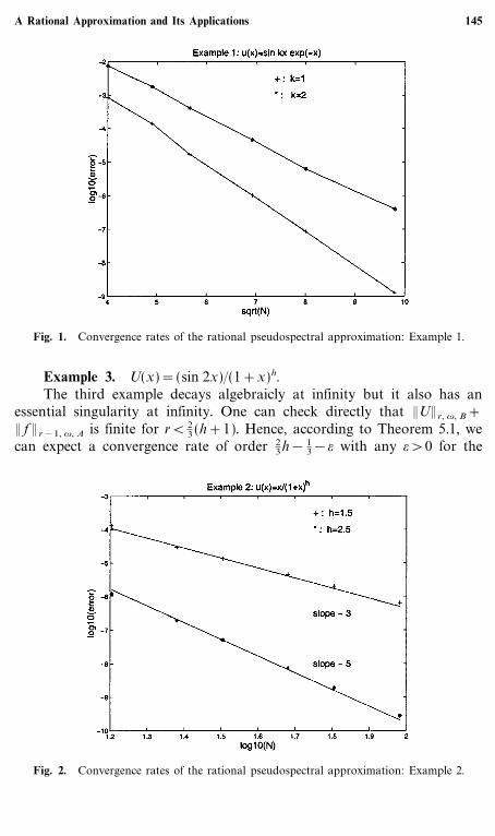
Example 3. U(x)=(sin 2x)�(1+x)h.The third example decays algebraicly at infinity but it also has an

essential singularity at infinity. One can check directly that &U&r, |, B+& f &r&1, |, A is finite for r< 2

3 (h+1). Hence, according to Theorem 5.1, wecan expect a convergence rate of order 2

3h& 13&= with any =>0 for the

Fig. 2. Convergence rates of the rational pseudospectral approximation: Example 2.


File: 854J 404830 . By:XX . Date:12:02:01 . Time:14:59 LOP8M. V8.B. Page 01:01Codes: 2041 Signs: 1353 . Length: 44 pic 2 pts, 186 mm

Fig. 3. Convergence rates of the Legendre rational approximation: Example 3.

H 1| -error. The observed convergence rate plotted in Fig. 3 agrees well with

the theoretical result.

ACKNOWLEDGMENTS

B.-Y.G. is supported by the Chinese Key Project of Basic ResearchG1999032804. J.S. is supported in part by NSF Grants DMS-9706951 andDMS-0074283.

REFERENCES

1. Adams, R. A. (1975). Soblov Spaces, Academic Press, New York.2. Bernardi, C., and Maday, Y. (1997). In Spectral Method, Ciarlet, P. G., and Lions, L. L.

(eds.), Handbook of Numerical Analysis, Vol. 5 (Part 2), North-Holland.3. Boyd, J. P. (1987). Orthogonal rational functions on a semi-infinite interval, J. Comput.

Phys. 70, 63�88.4. Boyd, J. P. (1987). Spectral methods using rational basis functions on an infinite interval,

J. Comput. Phys. 69, 112�142.5. Christov, C. I. (1982). A complete orthogonal system of functions in l 2(&�, �) space,

SIAM J. Appl. Math. 42, 1337�1344.6. Guo, Benuy (1998). Gegenbauer approximation and its applications to differential equa-

tions on the whole line, J. Math. Anal. Appl. 226, 180�206.7. Guo, Benyu (1998). Spectral Methods and Their Applications, World Scientific Publishing

Co. Inc., River Edge, New Jersey.8. Guo, Benyu (1999). Error estimation of Hermite spectral method for nonlinear partial

differential equations, Math. Comp. 68(227), 1067�1078.


9. Guo, Benyu (2000). Jacobi approximations in certain Hilbert spaces and their applica-tions to singular differential equations, J. Math. Anal. Appl. 243, 373�408.

10. Guo, Benyu (2000). Jacobi spectral approximation and its applications to differentialequations on the half line, J. Comput. Math. 18, 95�112.

11. Guo, Benyu and Shen, Jie (2000), Laguerre�Galerkin method for nonlinear partial dif-ferential equations on a semiinfinite interval, Numer. Math. 86, 635�654.

12. Maday, Y., Pernaud-Thomas, B., and Vandeven, H. (1985). Reappraisal of Laguerre typespectral methods, La Recherche Aerospatiale 6, 13�35.

13. Shen, Jie (1994). Efficient spectral-Galerkin method I. direct solvers for second- andfourth-order equations by using Legendre polynomials, SIAM J. Sci. Comput. 15,1489�1505.

14. Shen, Jie (1996). In Efficient Chebyshev�Legendre Galerkin Methods for Elliptic Problems,Ilin, A. V., and Scott, R. (eds.), Proceedings of ICOSAHOM'95, Houston J. Math.,pp. 233�240.

15. Szego� , G. (1975). Orthogonal Polynomials, 4th ed., Vol. 23, AMS Coll. Publ.


Documents

- Department of Mathematics, Purdue University