Embed Size (px)
Citation preview
Economic Equilibrium Modeling with GAMS
An Introduction to GAMS/MCP and GAMS/MPSGE
Thomas F. RutherfordUniversity of Colorado
Preface, June 1998
For the past six years I have been meaning to put together a proper user's guide forthe GAMS/MPSGE economic modeling language. This is proven to be a di�cult task,primarily because I have been too occupied with economics and software to ever thinkabout documentation.1 The present document is a �rst attempt to rectify this problem.It consists of �ve chapters at present, with one more to be added before the end of thesummer. The �ve chapters included here still need work { I want to double or triple thenumber of exercises here, as I have always found that to be an essential learning device.
It is my intention that this manual will in its �nal form be able to introduce a second yeargraduate student working on a correspondence basis to economic equilibrium modelingwith GAMS and MPSGE. It seems that there are many such students at universitieseverywhere, and I always regret that I am unable to provide much guidance for themwhen I receive the occasional Email or phone call. I hope that this text answer some oftheir questions.
The book is currently organized as follows. Chapter 1 provides an review of intermediatemicroeconomics, speci�cally demand theory and general equilibrium; and it then showshow these ideas can be illustrated using small MPSGE models. Chapter 2 is a somewhatmore advanced introduction to general equilibrium analysis with a focus on taxation andpublic �nance. This chapter contains an appendix which describes the MPSGE languagein a complete yet compact manner. Chapter 3 concerns cost and expenditure functions,particularly the constant-elasticity of substitution family. The chapter presents two sampleprograms illustrating how the nested-CES functional form can be calibrated to arbitrarycross-elasticities of substitution in the case of three or four inputs. The �nal section inthis paper collects some de�nitions and a description of some of the other functional formswhich have been widely used in economic equilibrium analysis.
Chapter 4 introduces the mixed complementarity problem in a general format with arange of applications in economics. (This chapter still needs considerable work to producea set of parallell computational exercise.)
Chapter 5 relates the equilibrium and optimization perspectives on general equilibriumallocations, showing how GAMS can be used to compute the same equilibria in either anoptimization or complementarity format. This chapter needs some editing, so that it isclearer how these ideas relate to MPSGE. I will add a few sample programs which comparethe various algebraic formulations of the standard model with the corresponding MPSGEmodels. Of course, this chapter also needs a number of exercises.
1 I will never forget the article in 1982 with those wonderful quotes, \Real programmers write programs,
not documentation." and \Real programmers can write Fortran in any language."

ii
The �nal chapter I wish to add describes how GAMS can be used to compute forward-looking, dynamic general equilibrium models. It builds upon ideas from Chapter 5, com-paring the familiar Ramsey model with the complementarity setup.
I will announce the release of the �nal version on the GAMS list, and I will make noteon the GAMS web site. I hope this will happen before the end of summer, 1998.

Demand Theory and General Equilibrium
An Intermediate Level Introduction to MPSGE
2
1. An Overview
This document describes a mathematical programming system for general equilibriumanalysis named MPSGE which operates as a subsystem to the mathematical programminglanguage GAMS. MPSGE is a library of function and Jacobian evaluation routines whichfacilitates the formulation and analysis of AGE models. MPSGE simpli�es the modellingprocess and makes AGE modelling accessible to any economist who is interested in theapplication of these models. In addition to solving speci�c modelling problems, the systemserves a didactic role as a structured framework in which to think about general equilibriumsystems.
MPSGE separates the tasks of model formulation and model solution, thereby freeingmodel builders from the tedious task of writing model-speci�c function evaluation subrou-tines. All features of a particular model are communicated to GAMS/MPSGE through atabular input format. To use MPSGE, a user must learn the syntax and conventions ofthis model de�nition language.
The present paper is intended for students who have completed two semesters of study inmicroeconomics. The purpose of this presentation is to give students a practical perspectiveon microeconomic theory. The diligent student who works through all of the examplesprovided here should be capable of building small models \from scratch" to illustratebasic theory. This is a �rst step to acquiring a set of useable tools for applied work.
The remainder of this paper is organized as follows. Section 2 provides practical tips onhow to get started with GAMS/MPSGE. Section 3 reviews basic ideas from the theory ofthe consumer. Section 4 introduces the modelling framework with three models illustratingthe representation of consumer demand within the MPSGE language. Section 5 reviewsthe pure exchange model, and Section 5 presents two MPSGE models of exchange. Eachof the model-oriented sections present exercises based on the models which give studentsa chance to work through the material on their own. Section 6 provides solutions toexercises from this paper. Additional introductory examples for self-study can be found inJim Markusen's library of MPSGE examples, as well as in the GAMS model library (lookfor models with names ending in \MGE").
The level of presentation and diagrammatic exposition adopted here is based on HalVarian's undergraduate microeconomics textbook ( Intermediate Microeconomics: A Mod-ern Approach, Third Edition, W. W. Norton & Company, Inc., 1993).
The ultimate objective of this piece is to remind students of some theory which theyhave already seen and illustrate how these ideas can be used to build numerical modelsusing GAMS with MPSGE. It is not my intention to provide a graduate level presentationof this material. So far as possible, I have avoided calculus and even algebra. The objectivehere is to demonstrate that what matters are economic ideas. With the proper tools, it ispossible to do concrete economic modeling without a lot of mathematical formalism.
2. Getting Started
(i) In order to use GAMS/MPSGE, you need to know how to create and edit text �les.There are several methods for doing this. One approach is to use NOTEPAD, the standardtext editor under Windows 95. It is also possible to use a text processor such as MicrosoftWord as a text editor. If you take this approach, you will need to remember to always savethe edited �le in a text format. A �nal approach, one which I suggest to graduate students
Demand Theory and MPSGE 3
who are interested in using numerical modelling in their research, is that you take thetime to develop some facility with a \real" programmer's editor like Emacs, Epsilon orBrief. These editors are far more powerful than Notepad, and they are far better suitedto computational work than is Microsoft Word.
(ii) You need to have a copy of GAMS with MPSGE to run on your computer. There areversions of this program for PCs as well as for Unix workstations. Copies of the program canbe obtained directly from GAMS ([email protected]), or you may get a copy from someonewho already has the program. (Copyright restrictions apply only to GAMS license �les.)When you copy the GAMS systems �les without the license �le and the program will onlyoperate in student/demonstration mode. The student version is perfectly adequate forlearning about modelling {in fact, it may be better because it's dimensionality restrictionsprevent the novice model builder from adding unnecessary details.
(iii) You need to install GAMS with MPSGE on your computer. To do this, follow thestandard installation procedures.
(iv) You should verify that the system is operational. Connect to a working directory(never run models from the GAMS system directory! ). Then, extract and run one of thelibrary models, e.g.
C:\>MKDIR WORK
C:\>CD WORK
C:\WORK>GAMSLIB SCARFMGE
C:\WORK>GAMS SCARFMGE
If the GAMS system is properly installed, these commands will cause GAMS to solve asequence of models from the SCARFMGE sample problem. The output from this process iswritten to �le SCARFMGE.LST . If you search for the word \STATUS". you can verify thatall the cases are processed.
There are a number of MPSGE models included in the GAMS library. If you are usinga student version of GAMS, you will be able to process some but not all of the librarymodels. The student version of the program limits the number of variables in the modelto 100. (I believe that GAMS imposes other limits on use of the student version, but thevariable limitation is the most severe constraint.)
Assuming that you have successfully installed the software, let us now proceed to someexamples which illustrate both the computing syntax and the underlying economics.
3. The Theory of Consumer Demand
A central idea underlying most microeconomic theory is that agents optimize subject toconstraints. The optimizing principle applied to consumer choice begins from the notionthat agents have preferences over consumption bundles and will always choose the mostpreferred bundle subject to applicable constraints. To operationalize this theory, threeissues which must be addressed: (i) How can we represent preferences? (ii) What is thenature of constraints on consumer choice? and (iii) How can the choice be modelled?
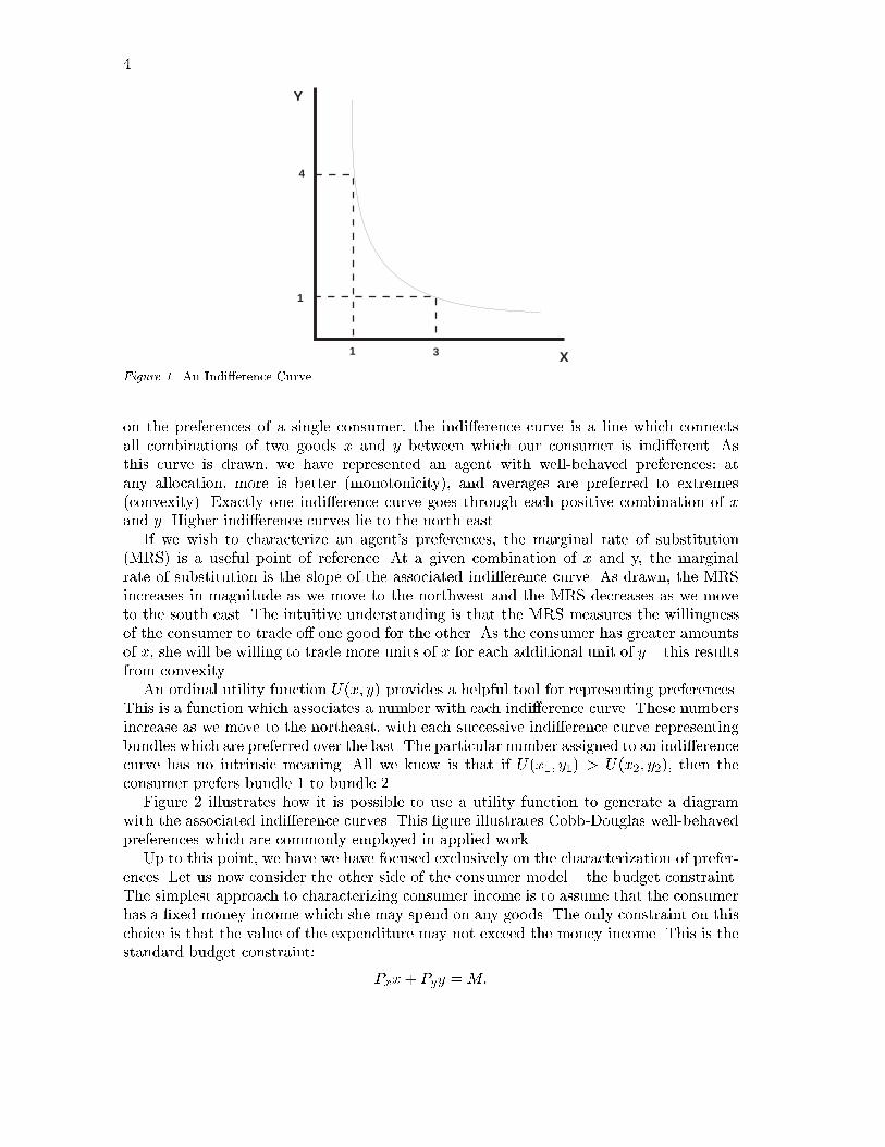
Preferences are relationships between alternative consumption \bundles". These can berepresented graphically using indi�erence curves, as illustrated in Figure 1. Focusing now
4
X
Y
1 3
1
4
Figure 1. An Indi�erence Curve
on the preferences of a single consumer, the indi�erence curve is a line which connectsall combinations of two goods x and y between which our consumer is indi�erent. Asthis curve is drawn, we have represented an agent with well-behaved preferences: atany allocation, more is better (monotonicity), and averages are preferred to extremes(convexity). Exactly one indi�erence curve goes through each positive combination of xand y. Higher indi�erence curves lie to the north-east.
If we wish to characterize an agent's preferences, the marginal rate of substitution(MRS) is a useful point of reference. At a given combination of x and y, the marginalrate of substitution is the slope of the associated indi�erence curve. As drawn, the MRSincreases in magnitude as we move to the northwest and the MRS decreases as we moveto the south east. The intuitive understanding is that the MRS measures the willingnessof the consumer to trade o� one good for the other. As the consumer has greater amountsof x, she will be willing to trade more units of x for each additional unit of y { this resultsfrom convexity.
An ordinal utility function U(x; y) provides a helpful tool for representing preferences.This is a function which associates a number with each indi�erence curve. These numbersincrease as we move to the northeast, with each successive indi�erence curve representingbundles which are preferred over the last. The particular number assigned to an indi�erencecurve has no intrinsic meaning. All we know is that if U(x1; y1) > U(x2; y2), then theconsumer prefers bundle 1 to bundle 2.
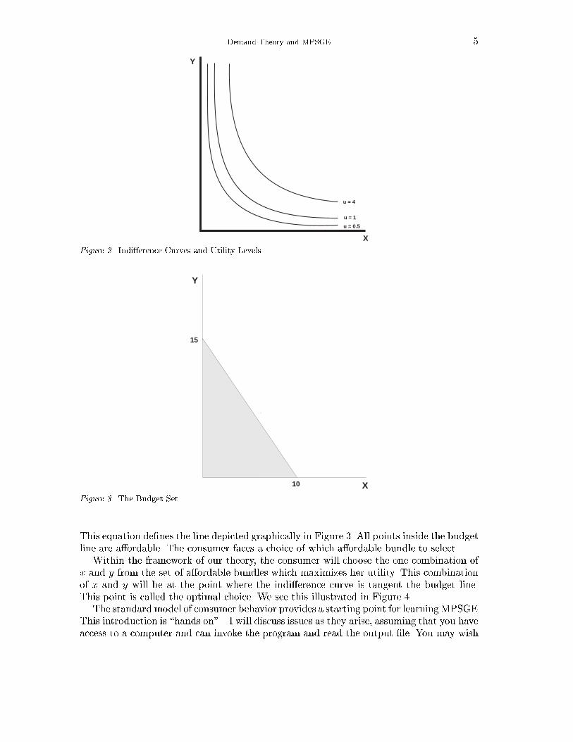
Figure 2 illustrates how it is possible to use a utility function to generate a diagramwith the associated indi�erence curves. This �gure illustrates Cobb-Douglas well-behavedpreferences which are commonly employed in applied work.
Up to this point, we have we have focused exclusively on the characterization of prefer-ences. Let us now consider the other side of the consumer model { the budget constraint.The simplest approach to characterizing consumer income is to assume that the consumerhas a �xed money income which she may spend on any goods. The only constraint on thischoice is that the value of the expenditure may not exceed the money income. This is thestandard budget constraint:
Pxx+ Pyy =M:
Demand Theory and MPSGE 5
u = 0.5
u = 1
u = 4
X
Y
Figure 2. Indi�erence Curves and Utility Levels
10
15
Y
XFigure 3. The Budget Set
This equation de�nes the line depicted graphically in Figure 3. All points inside the budgetline are a�ordable. The consumer faces a choice of which a�ordable bundle to select.
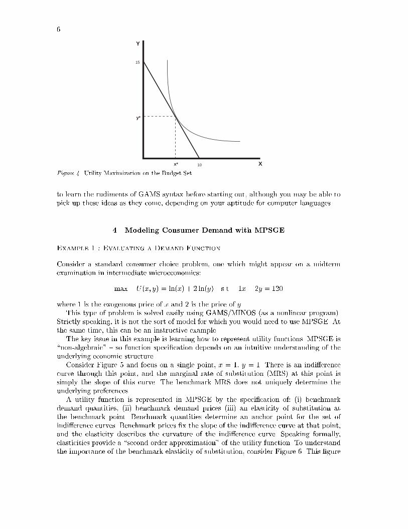
Within the framework of our theory, the consumer will choose the one combination ofx and y from the set of a�ordable bundles which maximizes her utility. This combinationof x and y will be at the point where the indi�erence curve is tangent the budget line.This point is called the optimal choice. We see this illustrated in Figure 4.
The standard model of consumer behavior provides a starting point for learningMPSGE.This introduction is \hands on" { I will discuss issues as they arise, assuming that you haveaccess to a computer and can invoke the program and read the output �le. You may wish
6
X
Y
10
15
x*
y*
Figure 4. Utility Maximization on the Budget Set
to learn the rudiments of GAMS syntax before starting out, although you may be able topick up these ideas as they come, depending on your aptitude for computer languages.
4. Modeling Consumer Demand with MPSGE
Example 1 : Evaluating a Demand Function
Consider a standard consumer choice problem, one which might appear on a midtermexamination in intermediate microeconomics:
max U(x; y) = ln(x) + 2 ln(y) s.t. 1x+ 2y = 120
where 1 is the exogenous price of x and 2 is the price of y.This type of problem is solved easily using GAMS/MINOS (as a nonlinear program).
Strictly speaking, it is not the sort of model for which you would need to use MPSGE. Atthe same time, this can be an instructive example.
The key issue in this example is learning how to represent utility functions. MPSGE is\non-algebraic" { so function speci�cation depends on an intuitive understanding of theunderlying economic structure.
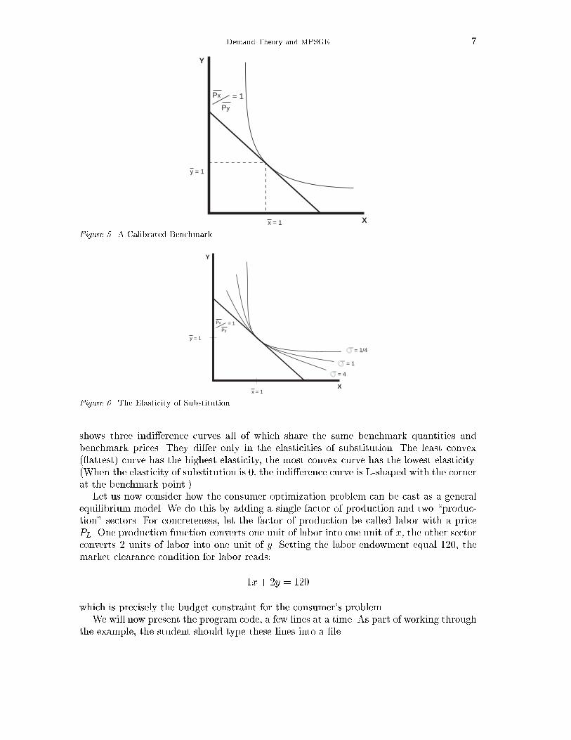
Consider Figure 5 and focus on a single point, x = 1, y = 1. There is an indi�erencecurve through this point, and the marginal rate of substitution (MRS) at this point issimply the slope of this curve. The benchmark MRS does not uniquely determine theunderlying preferences.
A utility function is represented in MPSGE by the speci�cation of: (i) benchmarkdemand quantities, (ii) benchmark demand prices (iii) an elasticity of substitution atthe benchmark point. Benchmark quantities determine an anchor point for the set ofindi�erence curves. Benchmark prices �x the slope of the indi�erence curve at that point,and the elasticity describes the curvature of the indi�erence curve. Speaking formally,elasticities provide a \second order approximation" of the utility function. To understandthe importance of the benchmark elasticity of substitution, consider Figure 6. This �gure
Demand Theory and MPSGE 7
X
Y
Px
Py
= 1
y = 1
x = 1
Figure 5. A Calibrated Benchmark
X
Y
Px
Py
= 1
y = 1
x = 1
= 1/4
= 1
= 4
Figure 6. The Elasticity of Substitution
shows three indi�erence curves all of which share the same benchmark quantities andbenchmark prices. They di�er only in the elasticities of substitution. The least convex( attest) curve has the highest elasticity, the most convex curve has the lowest elasticity.(When the elasticity of substitution is 0, the indi�erence curve is L-shaped with the cornerat the benchmark point.)
Let us now consider how the consumer optimization problem can be cast as a generalequilibrium model. We do this by adding a single factor of production and two \produc-tion" sectors. For concreteness, let the factor of production be called labor with a pricePL. One production function converts one unit of labor into one unit of x, the other sectorconverts 2 units of labor into one unit of y. Setting the labor endowment equal 120, themarket clearance condition for labor reads:
1x+ 2y = 120
which is precisely the budget constraint for the consumer's problem.We will now present the program code, a few lines at a time. As part of working through
the example, the student should type these lines into a �le.
8
A MPSGE model speci�cation is always listed between $ONTEXT and $OFFTEXT state-ments. The �rst statement within an MPSGE model-description assigns a name to themodel. The model name must begin with a letter and must have 10 or fewer characters.
$ONTEXT
$MODEL:DEMAND
The model speci�cation begins by declaring variables for the model. In a standardmodel, there are three types of variables: commodity prices, sectoral activity levels, andconsumer incomes. The end of each line may conclude with a \!", followed by a variabledescription.N.B. The variables associated with commodities are prices, not quantities. (In this and
subsequent models, I use P as the �rst letter for each of the commodity variables to remindus that these variables are prices.)N.B. The variable associated with a consumer is an income level, not a welfare index.
$SECTORS:
X ! ACTIVITY LEVEL FOR X = DEMAND FOR GOOD X
Y ! ACTIVITY LEVEL FOR Y = DEMAND FOR GOOD Y
$COMMODITIES:
PX ! PRICE OF X WHICH WILL EQUAL PL
PY ! PRICE OF Y WHICH WILL EQUAL 2 PL
PL ! PRICE OF THE ARTIFICIAL FACTOR L
$CONSUMERS:
RA ! REPRESENTATIVE AGENT INCOME
Function speci�cations follow the variable declarations. In this model, our �rst decla-rations correspond to the two production sectors. In this model, the production structuresare particularly simple. Each of the sectors has one input and one output. In the MPSGEsyntax, I: denotes an input and O: denotes an output. The output quantity coe�cientsfor both sectors are unity (Q:1). This means that the level values for x and y equal thequantities produced.
The �nal function speci�ed in the model represents the utility function and endowmentsfor the single consumer. In this function, the E: entries correspond to endowments and theD: entries are demands. Reference demands, reference prices and the substitution elasticity(s:1) characterize preferences.
The demand entries shown here are consistent with a Cobb-Douglas utility function inwhich the budget share for y is twice the budget share for x (i.e. the MRS at (1,1) equals1/2):
$PROD:X

Demand Theory and MPSGE 9
O:PX Q:1
I:PL Q:1
$PROD:Y
O:PY Q:1
I:PL Q:2
$DEMAND:RA s:1
E:PL Q:120
D:PX Q:1 P:(1/2)
D:PY Q:1 P:1
$OFFTEXT
The �nal three statements in this �le invoke the MPSGE preprocessor, \generate" andsolve the model:
$SYSINCLUDE mpsgeset DEMAND
$INCLUDE DEMAND.GEN
SOLVE DEMAND USING MCP;
The preprocessor invocation (\$SYSINCLUDE mpsgeset") should be placed immediatelyfollowing the $OFFTEXT block containing the model description. The model generator code,DEMAND.GEN, is produced by the previous statement and must be included immediatelybefore the SOLVE statement.
At this point, the reader should take the time to type the example into a �le and executethe program with GAMS/MPSGE.
This is possibly the �rst GAMS model which some readers have solved, so it is worthlooking through the listing �le in some detail. After running the solver, we examine thelisting �le. I typically begin my assessment of a model's solution by searching for \STATUS".For this model, we have the following:
S O L V E S U M M A R Y
MODEL DEMAND
TYPE MCP
SOLVER PATH FROM LINE 263
**** SOLVER STATUS 1 NORMAL COMPLETION
**** MODEL STATUS 1 OPTIMAL
RESOURCE USAGE, LIMIT 1.432 1000.000
ITERATION COUNT, LIMIT 5 1000
EVALUATION ERRORS 0 0
10
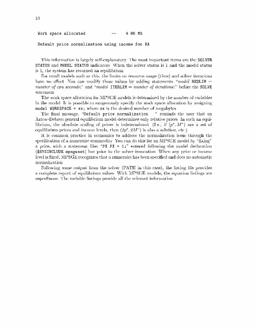
Work space allocated -- 4.86 Mb
Default price normalization using income for RA
This information is largely self-explanatory. The most important items are the SOLVERSTATUS and MODEL STATUS indicators. When the solver status is 1 and the model statusis 1, the system has returned an equilibrium.
For small models such as this, the limits on resource usage (time) and solver iterationshave no e�ect. You can modify these values by adding statements \model.RESLIM =number of cpu seconds;" and \model.ITERLIM = number of iterations;" before the SOLVEstatement.
The work space allocation for MPSGE models is determined by the number of variablesin the model. It is possible to exogenously specify the work space allocation by assigningmodel.WORKSPACE = xx; where xx is the desired number of megabytes.
The �nal message, \Default price normalization..." reminds the user that anArrow-Debreu general equilibrium model determines only relative prices. In such an equi-librium, the absolute scaling of prices is indeterminant. (I.e., if (p�;M�) are a set ofequilibrium prices and income levels, then (2p�; 2M�) is also a solution, etc.)
It is common practice in economics to address the normalization issue through thespeci�cation of a numeraire commodity. You can do this for an MPSGE model by \�xing"a price, with a statement like: \PX.FX = 1;" entered following the model declaration($SYSINCLUDE mpsgeset) but prior to the solver invocation. When any price or incomelevel is �xed, MPSGE recognizes that a numeraire has been speci�ed and does no automaticnormalization.
Following some output from the solver (PATH in this case), the listing �le providesa complete report of equilibrium values. With MPSGE models, the equation listings aresuper uous. The variable listings provide all the relevant information.
Demand Theory and MPSGE 11
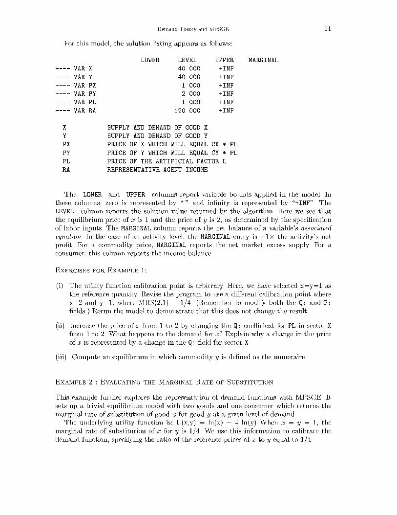
For this model, the solution listing appears as follows:
LOWER LEVEL UPPER MARGINAL
---- VAR X . 40.000 +INF .
---- VAR Y . 40.000 +INF .
---- VAR PX . 1.000 +INF .
---- VAR PY . 2.000 +INF .
---- VAR PL . 1.000 +INF .
---- VAR RA . 120.000 +INF .
X SUPPLY AND DEMAND OF GOOD X
Y SUPPLY AND DEMAND OF GOOD Y
PX PRICE OF X WHICH WILL EQUAL CX * PL
PY PRICE OF Y WHICH WILL EQUAL CY * PL
PL PRICE OF THE ARTIFICIAL FACTOR L
RA REPRESENTATIVE AGENT INCOME
The LOWER and UPPER columns report variable bounds applied in the model. Inthese columns, zero is represented by \." and in�nity is represented by \+INF". TheLEVEL column reports the solution value returned by the algorithm. Here we see thatthe equilibrium price of x is 1 and the price of y is 2, as determined by the speci�cationof labor inputs. The MARGINAL column reports the net balance of a variable's associatedequation. In the case of an activity level, the MARGINAL entry is �1� the activity's netpro�t. For a commodity price, MARGINAL reports the net market excess supply. For aconsumer, this column reports the income balance.
Exercises for Example 1:
(i) The utility function calibration point is arbitrary. Here, we have selected x=y=1 asthe reference quantity. Revise the program to use a di�erent calibration point wherex=2 and y=1, where MRS(2,1) = 1/4. (Remember to modify both the Q: and P:
�elds.) Rerun the model to demonstrate that this does not change the result.
(ii) Increase the price of x from 1 to 2 by changing the Q: coe�cient for PL in sector Xfrom 1 to 2. What happens to the demand for x? Explain why a change in the priceof x is represented by a change in the Q: �eld for sector X.
(iii) Compute an equilibrium in which commodity y is de�ned as the numeraire.
Example 2 : Evaluating the Marginal Rate of Substitution
This example further explores the representation of demand functions with MPSGE. Itsets up a trivial equilibrium model with two goods and one consumer which returns themarginal rate of substitution of good x for good y at a given level of demand.
The underlying utility function is: U(x,y) = ln(x) + 4 ln(y) When x = y = 1, themarginal rate of substitution of x for y is 1=4. We use this information to calibrate thedemand function, specifying the ratio of the reference prices of x to y equal to 1=4.
12
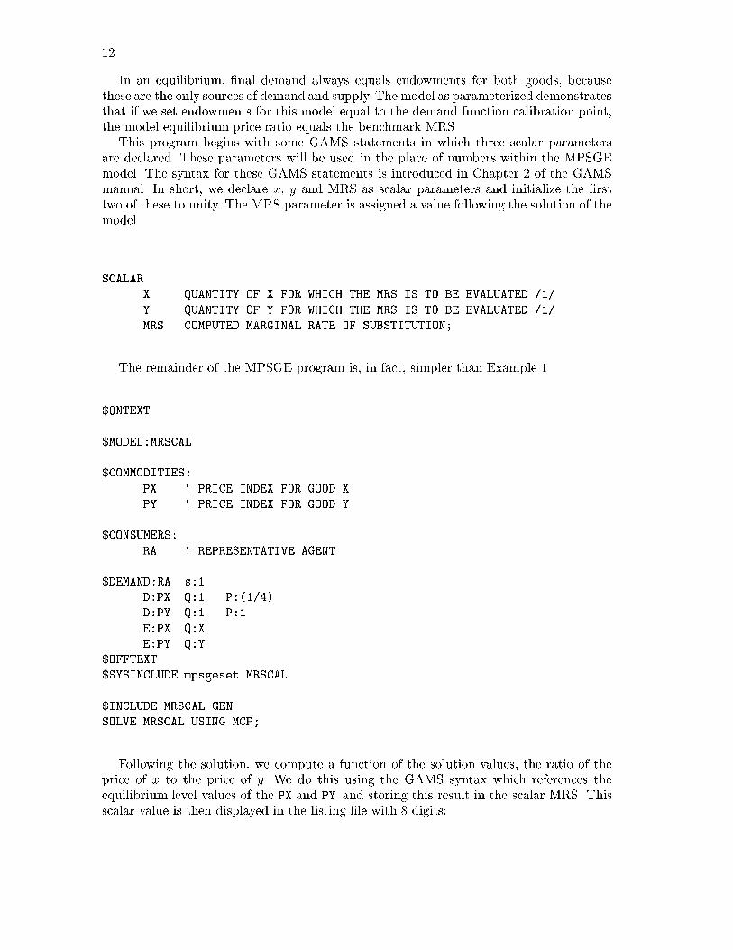
In an equilibrium, �nal demand always equals endowments for both goods, becausethese are the only sources of demand and supply. The model as parameterized demonstratesthat if we set endowments for this model equal to the demand function calibration point,the model equilibrium price ratio equals the benchmark MRS.
This program begins with some GAMS statements in which three scalar parametersare declared. These parameters will be used in the place of numbers within the MPSGEmodel. The syntax for these GAMS statements is introduced in Chapter 2 of the GAMSmanual. In short, we declare x, y and MRS as scalar parameters and initialize the �rsttwo of these to unity. The MRS parameter is assigned a value following the solution of themodel.
SCALAR
X QUANTITY OF X FOR WHICH THE MRS IS TO BE EVALUATED /1/
Y QUANTITY OF Y FOR WHICH THE MRS IS TO BE EVALUATED /1/
MRS COMPUTED MARGINAL RATE OF SUBSTITUTION;
The remainder of the MPSGE program is, in fact, simpler than Example 1.
$ONTEXT
$MODEL:MRSCAL
$COMMODITIES:
PX ! PRICE INDEX FOR GOOD X
PY ! PRICE INDEX FOR GOOD Y
$CONSUMERS:
RA ! REPRESENTATIVE AGENT
$DEMAND:RA s:1
D:PX Q:1 P:(1/4)
D:PY Q:1 P:1
E:PX Q:X
E:PY Q:Y
$OFFTEXT
$SYSINCLUDE mpsgeset MRSCAL
$INCLUDE MRSCAL.GEN
SOLVE MRSCAL USING MCP;
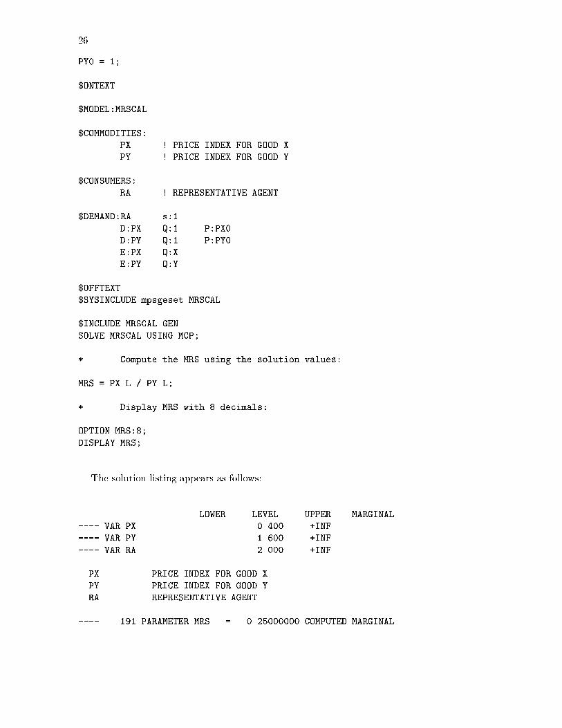
Following the solution, we compute a function of the solution values, the ratio of theprice of x to the price of y. We do this using the GAMS syntax which references theequilibrium level values of the PX and PY and storing this result in the scalar MRS. Thisscalar value is then displayed in the listing �le with 8 digits:
Demand Theory and MPSGE 13
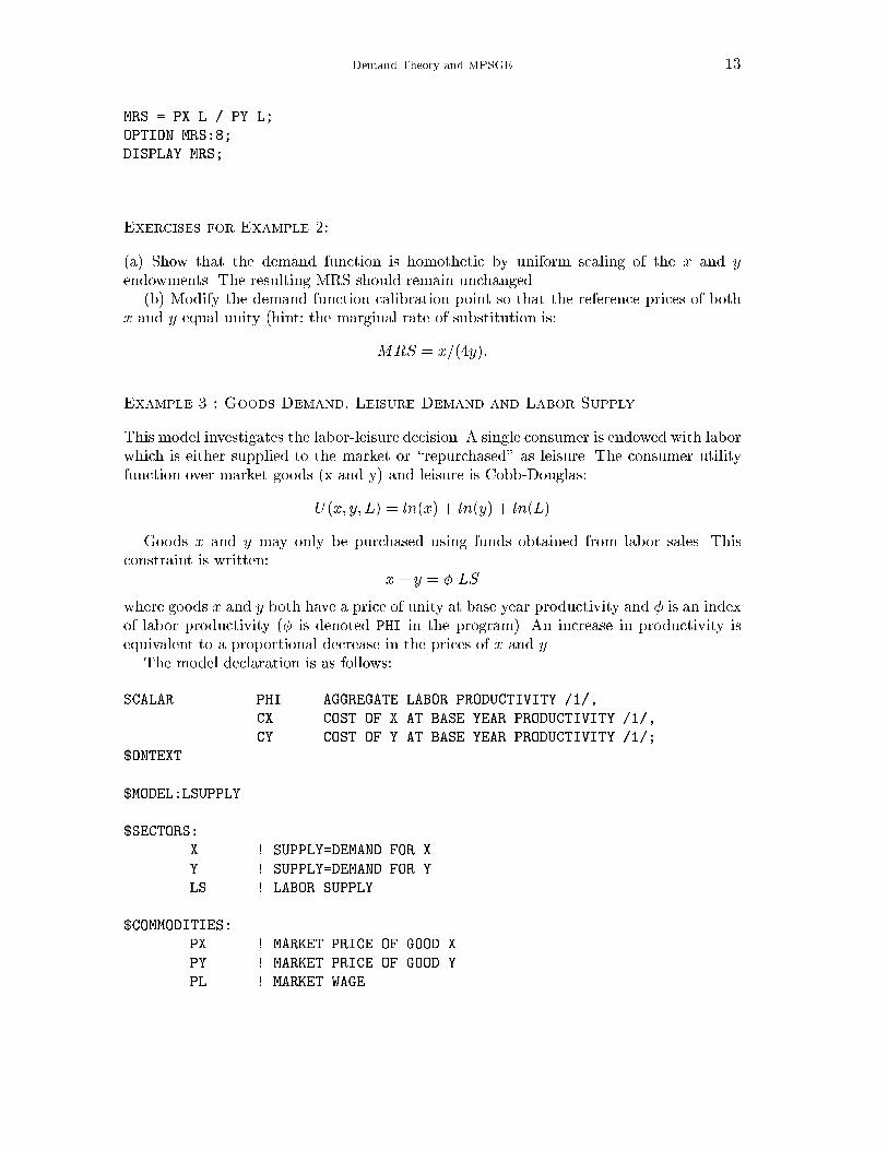
MRS = PX.L / PY.L;
OPTION MRS:8;
DISPLAY MRS;
Exercises for Example 2:
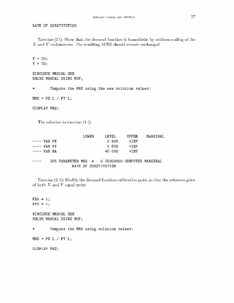
(a) Show that the demand function is homothetic by uniform scaling of the x and yendowments. The resulting MRS should remain unchanged.
(b) Modify the demand function calibration point so that the reference prices of bothx and y equal unity (hint: the marginal rate of substitution is:
MRS = x=(4y):
Example 3 : Goods Demand, Leisure Demand and Labor Supply
This model investigates the labor-leisure decision. A single consumer is endowed with laborwhich is either supplied to the market or \repurchased" as leisure. The consumer utilityfunction over market goods (x and y) and leisure is Cobb-Douglas:
U(x; y; L) = ln(x) + ln(y) + ln(L)
Goods x and y may only be purchased using funds obtained from labor sales. Thisconstraint is written:
x+ y = � LS
where goods x and y both have a price of unity at base year productivity and � is an indexof labor productivity (� is denoted PHI in the program). An increase in productivity isequivalent to a proportional decrease in the prices of x and y.
The model declaration is as follows:
SCALAR PHI AGGREGATE LABOR PRODUCTIVITY /1/,
CX COST OF X AT BASE YEAR PRODUCTIVITY /1/,
CY COST OF Y AT BASE YEAR PRODUCTIVITY /1/;
$ONTEXT
$MODEL:LSUPPLY
$SECTORS:
X ! SUPPLY=DEMAND FOR X
Y ! SUPPLY=DEMAND FOR Y
LS ! LABOR SUPPLY
$COMMODITIES:
PX ! MARKET PRICE OF GOOD X
PY ! MARKET PRICE OF GOOD Y
PL ! MARKET WAGE
14
PLS ! CONSUMER VALUE OF LEISURE
$CONSUMERS:
RA ! REPRESENTATIVE AGENT
$PROD:LS
O:PL Q:PHI
I:PLS Q:1
$PROD:X
O:PX Q:1
I:PL Q:CX
$PROD:Y
O:PY Q:1
I:PL Q:CY
$DEMAND:RA s:1
E:PLS Q:120
D:PLS Q:1 P:1
D:PX Q:1 P:1
D:PY Q:1 P:1
$OFFTEXT
$SYSINCLUDE mpsgeset LSUPPLY
$INCLUDE LSUPPLY.GEN
SOLVE LSUPPLY USING MCP;
We can use this model to evaluate the wage elasticity of labor supply. In the initialequilibrium (computed in the last statement) the demands for x, y and L all equal 40.A subsequent assignment to PHI (below) increases labor productivity. After computing anew equilibrium, we can use the change in labor supply to determine the wage elasticityof labor supply, an important parameter in labor market studies.
It should be emphasized that the elasticity of labor supply should be an input ratherthan an output of a general equilibrium model { this is a parameter for which econometricestimates can be obtained.
Here is how the programming works. First, we declare some scalar parameters whichwe will use for reporting, then save the \benchmark" labor supply in LS0:
SCALAR
LS0 REFERENCE LEVEL OF LABOR SUPPLY
ELS ELASTICITY OF LABOR SUPPLY WRT REAL WAGE;
LS0 = LS.L;
Demand Theory and MPSGE 15
Next, we modify the value of scalar PHI, increasing labor productivity by 1%. Becausethis is a neoclassical model, this change is equivalent to increasing the real wage by 1%.We need to recompute equilibrium prices after having changed the PHI value:
PHI = 1.01;
$INCLUDE LSUPPLY.GEN
SOLVE LSUPPLY USING MCP;
We use this solution to compute and report the elasticity of labor supply as thepercentage change in the LS activity:
ELS = 100 * (LS.L - LS0) / LS0;
DISPLAY ELS;
As the model is currently constructed, the wage elasticity of labor supply equals zero.This is because the utility function is Cobb-Douglas over goods and leisure, and theconsumer's only source of income is labor. As the real wage rises, this increases boththe demand for goods (labor supply) and the demand for leisure. These e�ect exactlybalance out and the supply of labor is unchanged.
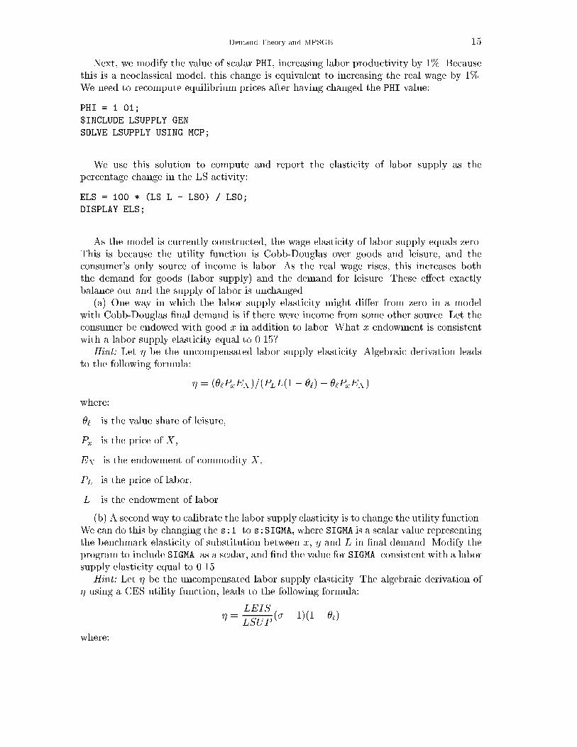
(a) One way in which the labor supply elasticity might di�er from zero in a modelwith Cobb-Douglas �nal demand is if there were income from some other source. Let theconsumer be endowed with good x in addition to labor. What x endowment is consistentwith a labor supply elasticity equal to 0.15?
Hint: Let � be the uncompensated labor supply elasticity. Algebraic derivation leadsto the following formula:
� = (�`PxEX)=(PLL(1� �`)� �`PxEX)
where:
�` is the value share of leisure,
Px is the price of X,
EX is the endowment of commodity X,
PL is the price of labor,
L is the endowment of labor.
(b) A second way to calibrate the labor supply elasticity is to change the utility function.We can do this by changing the s:1 to s:SIGMA, where SIGMA is a scalar value representingthe benchmark elasticity of substitution between x, y and L in �nal demand. Modify theprogram to include SIGMA as a scalar, and �nd the value for SIGMA consistent with a laborsupply elasticity equal to 0.15.
Hint: Let � be the uncompensated labor supply elasticity. The algebraic derivation of� using a CES utility function, leads to the following formula:
� =LEIS
LSUP(� � 1)(1 � �`)
where:
16
Endowment
*
AgentA
AgentB
GoodX
GoodY
E
Ax’
Ay’ By’
Bx’
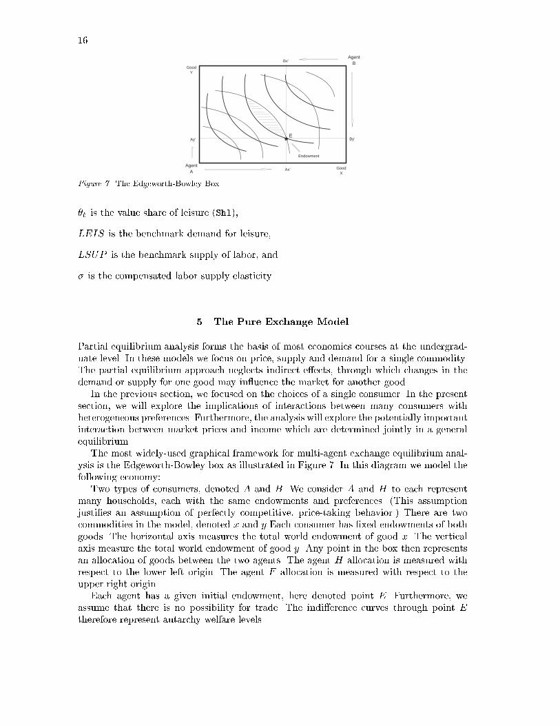
Figure 7. The Edgeworth-Bowley Box
�` is the value share of leisure (Shl),
LEIS is the benchmark demand for leisure,
LSUP is the benchmark supply of labor, and
� is the compensated labor supply elasticity.
5. The Pure Exchange Model
Partial equilibrium analysis forms the basis of most economics courses at the undergrad-uate level. In these models we focus on price, supply and demand for a single commodity.The partial equilibrium approach neglects indirect e�ects, through which changes in thedemand or supply for one good may in uence the market for another good.
In the previous section, we focused on the choices of a single consumer. In the presentsection, we will explore the implications of interactions between many consumers withheterogeneous preferences. Furthermore, the analysis will explore the potentially importantinteraction between market prices and income which are determined jointly in a generalequilibrium.
The most widely-used graphical framework for multi-agent exchange equilibrium anal-ysis is the Edgeworth-Bowley box as illustrated in Figure 7. In this diagram we model thefollowing economy:
Two types of consumers, denoted A and B. We consider A and H to each representmany households, each with the same endowments and preferences. (This assumptionjusti�es an assumption of perfectly competitive, price-taking behavior.) There are twocommodities in the model, denoted x and y Each consumer has �xed endowments of bothgoods. The horizontal axis measures the total world endowment of good x. The verticalaxis measure the total world endowment of good y. Any point in the box then representsan allocation of goods between the two agents. The agent H allocation is measured withrespect to the lower left origin. The agent F allocation is measured with respect to theupper right origin.
Each agent has a given initial endowment, here denoted point E. Furthermore, weassume that there is no possibility for trade. The indi�erence curves through point Etherefore represent autarchy welfare levels.
Demand Theory and MPSGE 17
The key idea in this model is that trade can improve both agents' welfare. One agentgives some amount good x to the other in return for an amount of good y. The termsof trade, the rate of exchange between x and y, is determined by the model. The modelillustrates a number of important properties of market economies:
(i) Trade is mutually bene�cial. So long as the transactions are voluntary, neither H norF will be hurt by engaging in trade.
(ii) Market prices can be used to guide the economy to a Pareto-e�cient allocation, astate of a�airs in which further mutually-bene�cial trades are not possible.
(iii) There is no guarantee that the gains from trade will be \fairly distributed" acrossconsumers. A competitive equilibrium may produce a signi�cant welfare increase forone consumer while have negligible impact on the other.
(iv) There are multiple Pareto-e�cient allocations, typically only one of which is a com-petitive equilibrium.We can use this model to demonstrate that the issues of e�ciencyand equity can be separated when there is the possibility of lump-sum income transfersbetween agents.
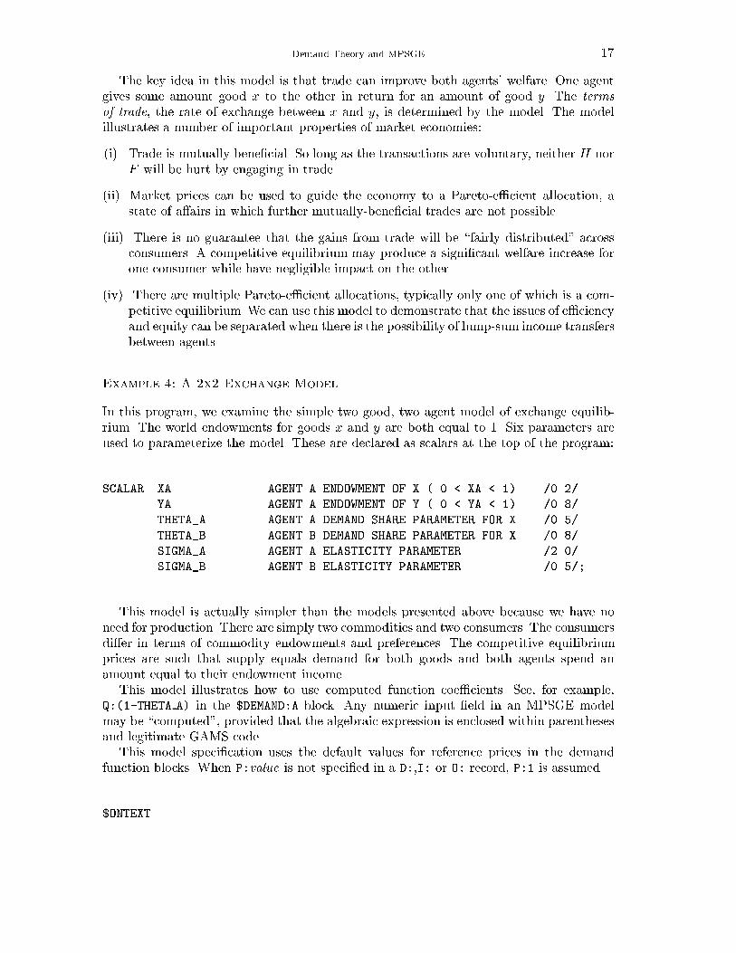
Example 4: A 2x2 Exchange Model
In this program, we examine the simple two good, two agent model of exchange equilib-rium. The world endowments for goods x and y are both equal to 1. Six parameters areused to parameterize the model. These are declared as scalars at the top of the program:
SCALAR XA AGENT A ENDOWMENT OF X ( 0 < XA < 1) /0.2/
YA AGENT A ENDOWMENT OF Y ( 0 < YA < 1) /0.8/
THETA_A AGENT A DEMAND SHARE PARAMETER FOR X /0.5/
THETA_B AGENT B DEMAND SHARE PARAMETER FOR X /0.8/
SIGMA_A AGENT A ELASTICITY PARAMETER /2.0/
SIGMA_B AGENT B ELASTICITY PARAMETER /0.5/;
This model is actually simpler than the models presented above because we have noneed for production. There are simply two commodities and two consumers. The consumersdi�er in terms of commodity endowments and preferences. The competitive equilibriumprices are such that supply equals demand for both goods and both agents spend anamount equal to their endowment income.
This model illustrates how to use computed function coe�cients. See, for example,Q:(1-THETA A) in the $DEMAND:A block. Any numeric input �eld in an MPSGE modelmay be \computed", provided that the algebraic expression is enclosed within parenthesesand legitimate GAMS code.
This model speci�cation uses the default values for reference prices in the demandfunction blocks. When P:value is not speci�ed in a D:,I: or O: record, P:1 is assumed.
$ONTEXT
18
$MODEL:EXCHANGE
$COMMODITIES:
PX ! EXCHANGE PRICE OF GOOD X
PY ! EXCHANGE PRICE OF GOOD Y
$CONSUMERS:
A ! CONSUMER A
B ! CONSUMER B
$DEMAND:A s:SIGMA_A
E:PX Q:XA
E:PY Q:YA
D:PX Q:THETA_A
D:PY Q:(1-THETA_A)
$DEMAND:B s:SIGMA_B
E:PX Q:(1-XA)
E:PY Q:(1-YA)
D:PX Q:THETA_B
D:PY Q:(1-THETA_B)
$OFFTEXT
$SYSINCLUDE mpsgeset EXCHANGE
$INCLUDE EXCHANGE.GEN
SOLVE EXCHANGE USING MCP;
SCALAR
PRATIO EQUILIBRIUM PRICE OF X IN TERMS OF Y,
IRATIO EQUILIBRIUM RATIO OF CONSUMER INCOMES;
PRATIO = PX.L / PY.L;
IRATIO = A.L / B.L;
DISPLAY IRATIO, PRATIO;
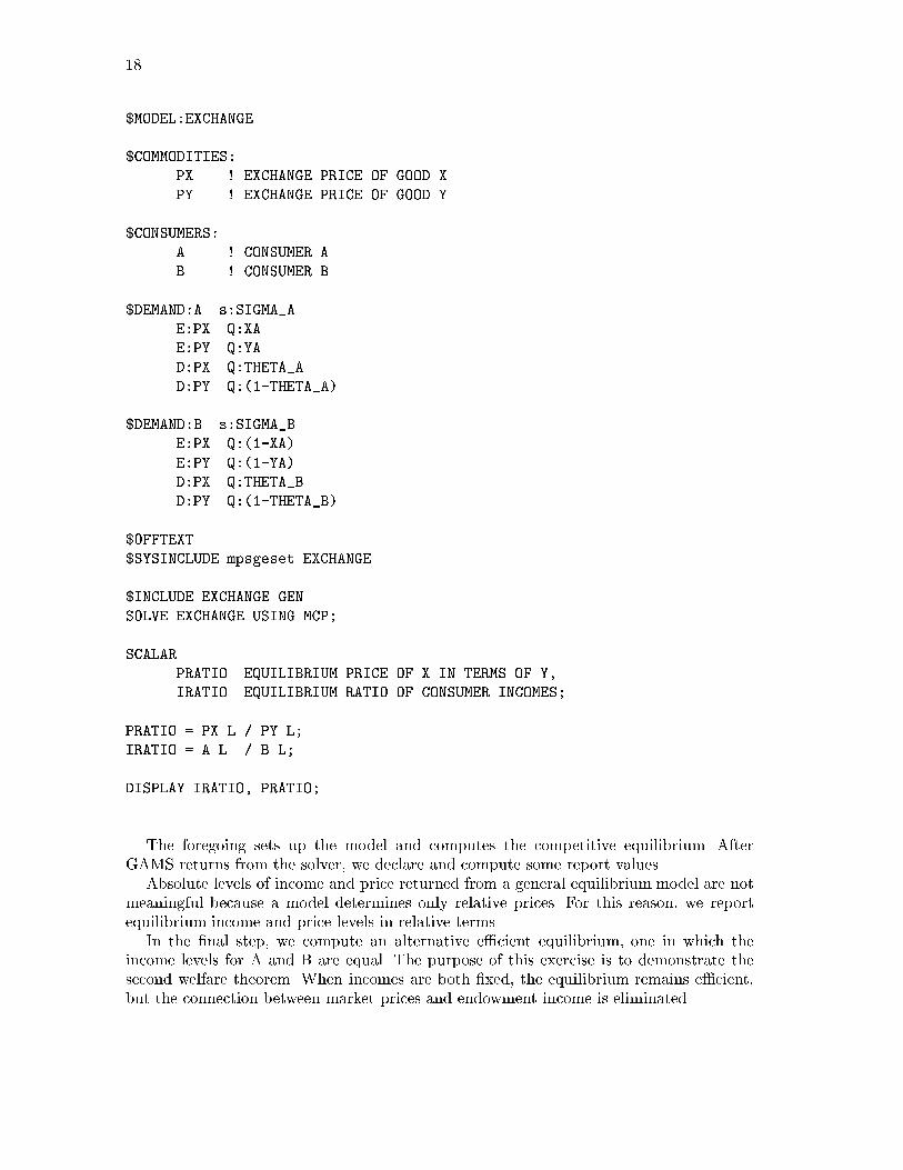
The foregoing sets up the model and computes the competitive equilibrium. AfterGAMS returns from the solver, we declare and compute some report values.
Absolute levels of income and price returned from a general equilibrium model are notmeaningful because a model determines only relative prices. For this reason, we reportequilibrium income and price levels in relative terms.
In the �nal step, we compute an alternative e�cient equilibrium, one in which theincome levels for A and B are equal. The purpose of this exercise is to demonstrate thesecond welfare theorem. When incomes are both �xed, the equilibrium remains e�cient,but the connection between market prices and endowment income is eliminated.
Demand Theory and MPSGE 19
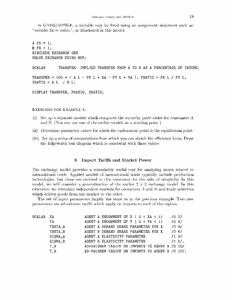
In GAMS/MPSGE, a variable may be �xed using an assignment statement such as:\variable.fx = value;", as illustrated in this model:
A.FX = 1;
B.FX = 1;
$INCLUDE EXCHANGE.GEN
SOLVE EXCHANGE USING MCP;
SCALAR TRANSFER IMPLIED TRANSFER FROM A TO B AS A PERCENTAGE OF INCOME;
TRANSFER = 100 * ( A.L - PX.L * XA - PY.L * YA ); PRATIO = PX.L / PY.L;
IRATIO = A.L / B.L;
DISPLAY TRANSFER, PRATIO, IRATIO;
Exercises for Example 4:
(i) Set up a separate models which computes the autarchy price ratios for consumers Aand B. (You can use one of the earlier models as a starting point.)
(ii) Determine parameter values for which the endowment point is the equilibrium point.
(iii) Set up a series of computations from which you can sketch the e�ciency locus. Drawthe Edgeworth box diagram which is consistent with these values.
6. Import Tari�s and Market Power
The exchange model provides a remarkably useful tool for analyzing issues related tointernational trade. Applied models of international trade typically include productiontechnologies, but these are omitted in this treatment for the sake of simplicity. In thismodel, we will consider a generalization of the earlier 2 � 2 exchange model. In thisextension, we introduce independent markets for consumers A and B and trade activitieswhich deliver goods from one market to the other.
The set of input parameters largely the same as in the previous example. Two newparameters are ad-valorem tari�s which apply on imports to each of the regions.
SCALAR XA AGENT A ENDOWMENT OF X ( 0 < XA < 1) /0.2/
YA AGENT A ENDOWMENT OF Y ( 0 < YA < 1) /0.8/
THETA_A AGENT A DEMAND SHARE PARAMETER FOR X /0.4/
THETA_B AGENT B DEMAND SHARE PARAMETER FOR X /0.6/
SIGMA_A AGENT A ELASTICITY PARAMETER /1.0/
SIGMA_B AGENT B ELASTICITY PARAMETER /1.0/,
T_A AD-VALOREM TARIFF ON IMPORTS TO AGENT A /0.10/
T_B AD-VALOREM TARIFF ON IMPORTS TO AGENT B /0.10/;
20
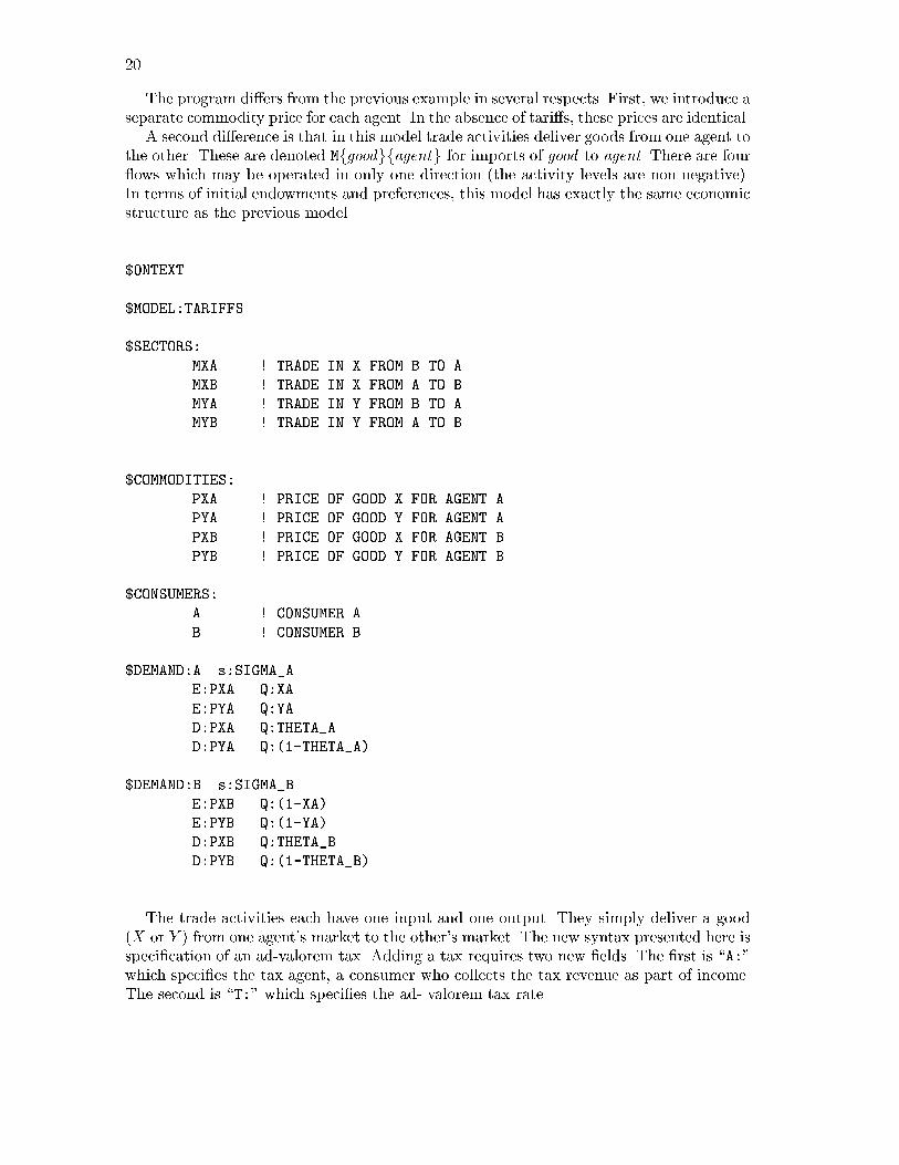
The program di�ers from the previous example in several respects. First, we introduce aseparate commodity price for each agent. In the absence of tari�s, these prices are identical.
A second di�erence is that in this model trade activities deliver goods from one agent tothe other. These are denoted Mfgoodgfagentg for imports of good to agent. There are four ows which may be operated in only one direction (the activity levels are non-negative).In terms of initial endowments and preferences, this model has exactly the same economicstructure as the previous model.
$ONTEXT
$MODEL:TARIFFS
$SECTORS:
MXA ! TRADE IN X FROM B TO A
MXB ! TRADE IN X FROM A TO B
MYA ! TRADE IN Y FROM B TO A
MYB ! TRADE IN Y FROM A TO B
$COMMODITIES:
PXA ! PRICE OF GOOD X FOR AGENT A
PYA ! PRICE OF GOOD Y FOR AGENT A
PXB ! PRICE OF GOOD X FOR AGENT B
PYB ! PRICE OF GOOD Y FOR AGENT B
$CONSUMERS:
A ! CONSUMER A
B ! CONSUMER B
$DEMAND:A s:SIGMA_A
E:PXA Q:XA
E:PYA Q:YA
D:PXA Q:THETA_A
D:PYA Q:(1-THETA_A)
$DEMAND:B s:SIGMA_B
E:PXB Q:(1-XA)
E:PYB Q:(1-YA)
D:PXB Q:THETA_B
D:PYB Q:(1-THETA_B)
The trade activities each have one input and one output. They simply deliver a good(X or Y ) from one agent's market to the other's market. The new syntax presented here isspeci�cation of an ad-valorem tax. Adding a tax requires two new �elds. The �rst is \A:"which speci�es the tax agent, a consumer who collects the tax revenue as part of income.The second is \T:" which speci�es the ad- valorem tax rate.
Demand Theory and MPSGE 21
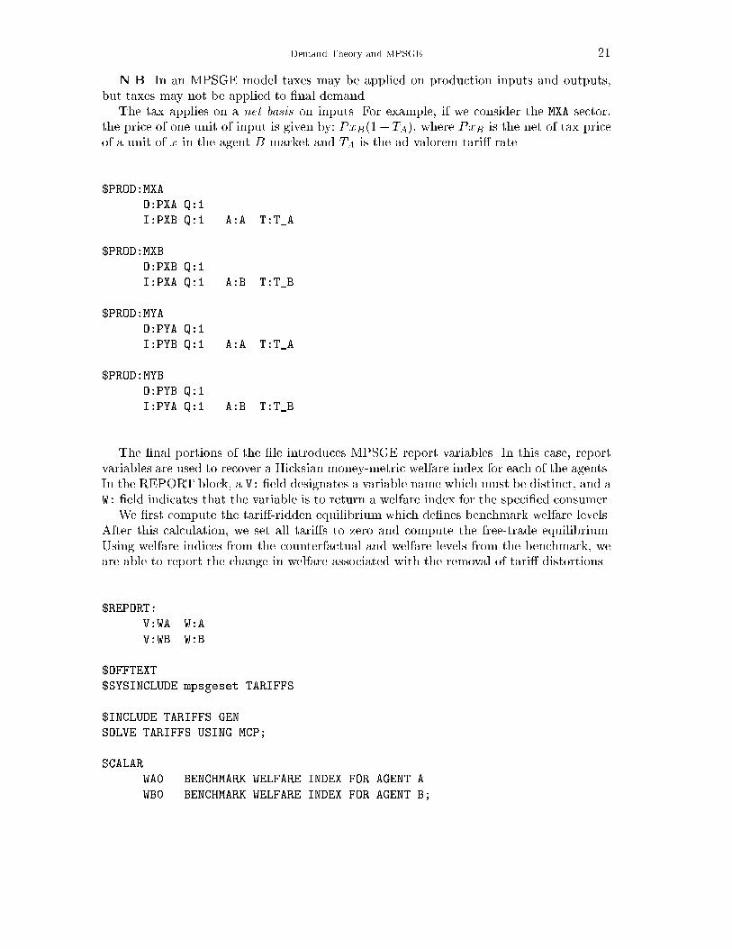
N.B. In an MPSGE model taxes may be applied on production inputs and outputs,but taxes may not be applied to �nal demand.
The tax applies on a net basis on inputs. For example, if we consider the MXA sector,the price of one unit of input is given by: PxB(1 + TA), where PxB is the net of tax priceof a unit of x in the agent B market and TA is the ad-valorem tari� rate.
$PROD:MXA
O:PXA Q:1
I:PXB Q:1 A:A T:T_A
$PROD:MXB
O:PXB Q:1
I:PXA Q:1 A:B T:T_B
$PROD:MYA
O:PYA Q:1
I:PYB Q:1 A:A T:T_A
$PROD:MYB
O:PYB Q:1
I:PYA Q:1 A:B T:T_B
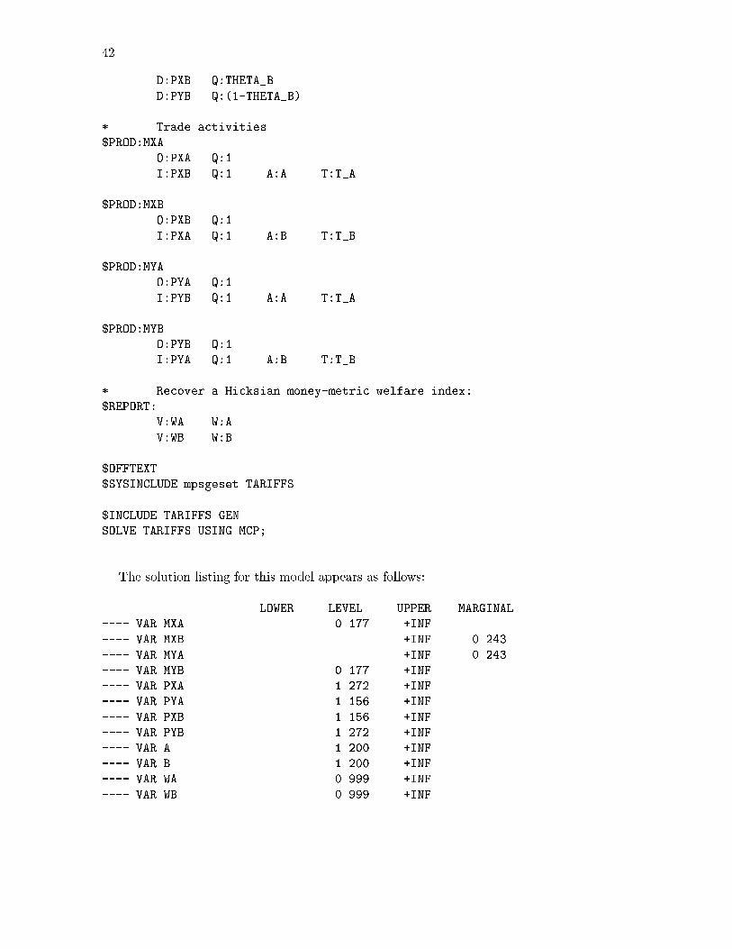
The �nal portions of the �le introduces MPSGE report variables. In this case, reportvariables are used to recover a Hicksian money-metric welfare index for each of the agents.In the REPORT block, a V: �eld designates a variable name which must be distinct, and aW: �eld indicates that the variable is to return a welfare index for the speci�ed consumer.
We �rst compute the tari�-ridden equilibrium which de�nes benchmark welfare levels.After this calculation, we set all tari�s to zero and compute the free-trade equilibrium.Using welfare indices from the counterfactual and welfare levels from the benchmark, weare able to report the change in welfare associated with the removal of tari� distortions.
$REPORT:
V:WA W:A
V:WB W:B
$OFFTEXT
$SYSINCLUDE mpsgeset TARIFFS
$INCLUDE TARIFFS.GEN
SOLVE TARIFFS USING MCP;
SCALAR
WA0 BENCHMARK WELFARE INDEX FOR AGENT A
WB0 BENCHMARK WELFARE INDEX FOR AGENT B;
22
WA0 = WA.L;
WB0 = WB.L;
T_A = 0;
T_B = 0;
$INCLUDE TARIFFS.GEN
SOLVE TARIFFS USING MCP;
SCALAR
EVA HICKSIAN EQUIVALENT VARIATION FOR AGENT A
EVB HICKSIAN EQUIVALENT VARIATION FOR AGENT B;
EVA = 100 * (WA.L-WA0)/WA0;
EVB = 100 * (WB.L-WB0)/WB0;
DISPLAY EVA, EVB;
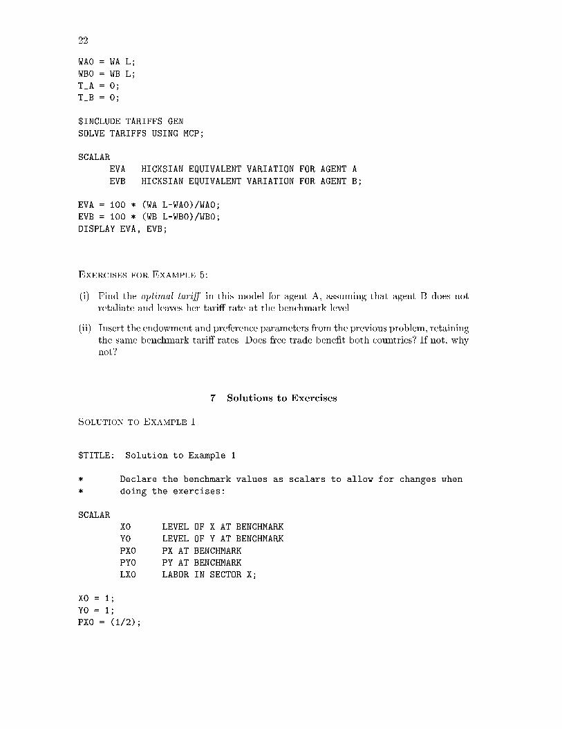
Exercises for Example 5:
(i) Find the optimal tari� in this model for agent A, assuming that agent B does notretaliate and leaves her tari� rate at the benchmark level.
(ii) Insert the endowment and preference parameters from the previous problem, retainingthe same benchmark tari� rates. Does free trade bene�t both countries? If not, whynot?
7. Solutions to Exercises
Solution to Example 1
$TITLE: Solution to Example 1
* Declare the benchmark values as scalars to allow for changes when
* doing the exercises:
SCALAR
X0 LEVEL OF X AT BENCHMARK
Y0 LEVEL OF Y AT BENCHMARK
PX0 PX AT BENCHMARK
PY0 PY AT BENCHMARK
LX0 LABOR IN SECTOR X;
X0 = 1;
Y0 = 1;
PX0 = (1/2);
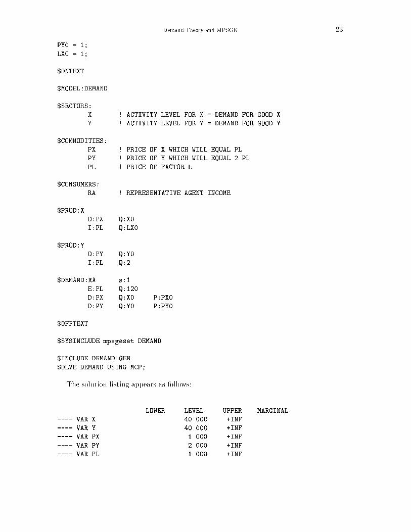
Demand Theory and MPSGE 23
PY0 = 1;
LX0 = 1;
$ONTEXT
$MODEL:DEMAND
$SECTORS:
X ! ACTIVITY LEVEL FOR X = DEMAND FOR GOOD X
Y ! ACTIVITY LEVEL FOR Y = DEMAND FOR GOOD Y
$COMMODITIES:
PX ! PRICE OF X WHICH WILL EQUAL PL
PY ! PRICE OF Y WHICH WILL EQUAL 2 PL
PL ! PRICE OF FACTOR L
$CONSUMERS:
RA ! REPRESENTATIVE AGENT INCOME
$PROD:X
O:PX Q:X0
I:PL Q:LX0
$PROD:Y
O:PY Q:Y0
I:PL Q:2
$DEMAND:RA s:1
E:PL Q:120
D:PX Q:X0 P:PX0
D:PY Q:Y0 P:PY0
$OFFTEXT
$SYSINCLUDE mpsgeset DEMAND
$INCLUDE DEMAND.GEN
SOLVE DEMAND USING MCP;
The solution listing appears as follows:
LOWER LEVEL UPPER MARGINAL
---- VAR X . 40.000 +INF .
---- VAR Y . 40.000 +INF .
---- VAR PX . 1.000 +INF .
---- VAR PY . 2.000 +INF .
---- VAR PL . 1.000 +INF .
24
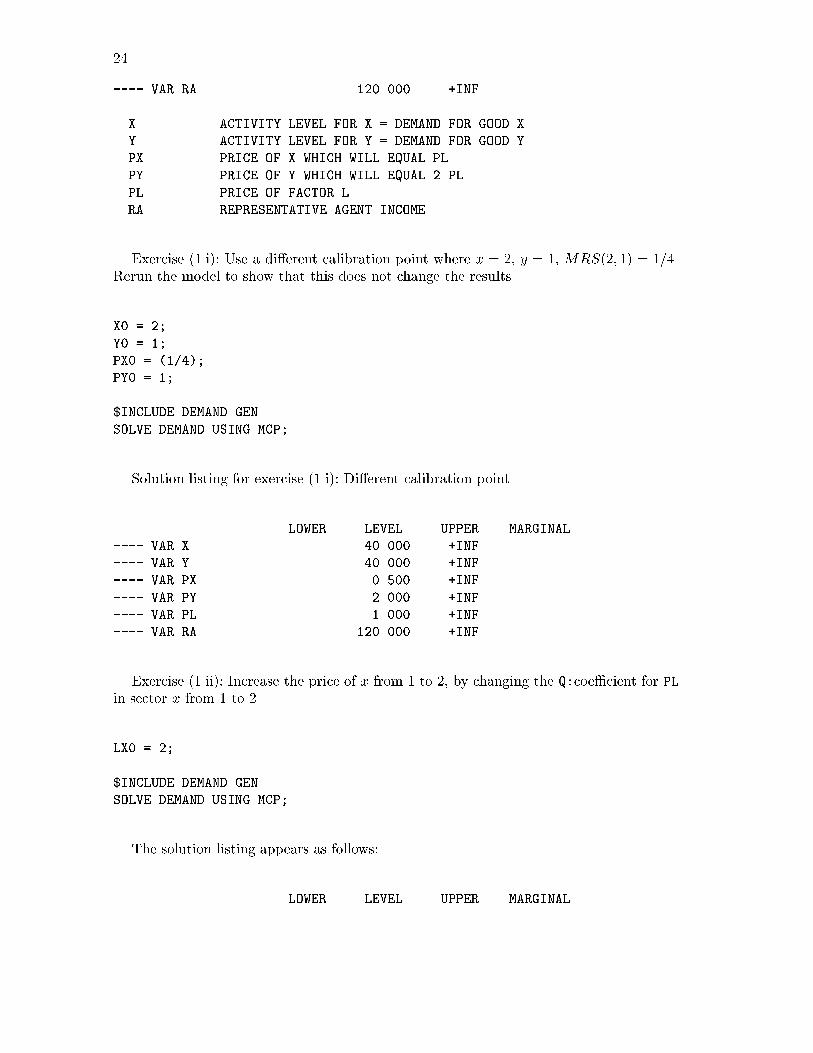
---- VAR RA . 120.000 +INF .
X ACTIVITY LEVEL FOR X = DEMAND FOR GOOD X
Y ACTIVITY LEVEL FOR Y = DEMAND FOR GOOD Y
PX PRICE OF X WHICH WILL EQUAL PL
PY PRICE OF Y WHICH WILL EQUAL 2 PL
PL PRICE OF FACTOR L
RA REPRESENTATIVE AGENT INCOME
Exercise (1.i): Use a di�erent calibration point where x = 2, y = 1, MRS(2; 1) = 1=4.Rerun the model to show that this does not change the results.
X0 = 2;
Y0 = 1;
PX0 = (1/4);
PY0 = 1;
$INCLUDE DEMAND.GEN
SOLVE DEMAND USING MCP;
Solution listing for exercise (1.i): Di�erent calibration point.
LOWER LEVEL UPPER MARGINAL
---- VAR X . 40.000 +INF .
---- VAR Y . 40.000 +INF .
---- VAR PX . 0.500 +INF .
---- VAR PY . 2.000 +INF .
---- VAR PL . 1.000 +INF .
---- VAR RA . 120.000 +INF .
Exercise (1.ii): Increase the price of x from 1 to 2, by changing the Q:coe�cient for PLin sector x from 1 to 2.
LX0 = 2;
$INCLUDE DEMAND.GEN
SOLVE DEMAND USING MCP;
The solution listing appears as follows:
LOWER LEVEL UPPER MARGINAL
Demand Theory and MPSGE 25
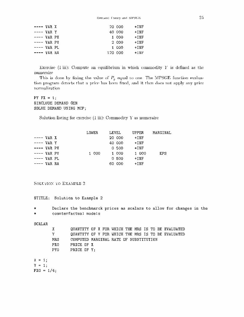
---- VAR X . 20.000 +INF .
---- VAR Y . 40.000 +INF .
---- VAR PX . 1.000 +INF .
---- VAR PY . 2.000 +INF .
---- VAR PL . 1.000 +INF .
---- VAR RA . 120.000 +INF .
Exercise (1.iii): Compute an equilibrium in which commodity Y is de�ned as thenumeraire.
This is done by �xing the value of Py equal to one. The MPSGE function evalua-tion program detects that a price has been �xed, and it then does not apply any pricenormalization.
PY.FX = 1;
$INCLUDE DEMAND.GEN
SOLVE DEMAND USING MCP;
Solution listing for exercise (1.iii): Commodity Y as numeraire.
LOWER LEVEL UPPER MARGINAL
---- VAR X . 20.000 +INF .
---- VAR Y . 40.000 +INF .
---- VAR PX . 0.500 +INF .
---- VAR PY 1.000 1.000 1.000 EPS
---- VAR PL . 0.500 +INF .
---- VAR RA . 60.000 +INF .
Solution to Example 2
$TITLE: Solution to Example 2
* Declare the benchmarck prices as scalars to allow for changes in the
* counterfactual models.
SCALAR
X QUANTITY OF X FOR WHICH THE MRS IS TO BE EVALUATED
Y QUANTITY OF Y FOR WHICH THE MRS IS TO BE EVALUATED
MRS COMPUTED MARGINAL RATE OF SUBSTITUTION
PX0 PRICE OF X
PY0 PRICE OF Y;
X = 1;
Y = 1;
PX0 = 1/4;
26
PY0 = 1;
$ONTEXT
$MODEL:MRSCAL
$COMMODITIES:
PX ! PRICE INDEX FOR GOOD X
PY ! PRICE INDEX FOR GOOD Y
$CONSUMERS:
RA ! REPRESENTATIVE AGENT
$DEMAND:RA s:1
D:PX Q:1 P:PX0
D:PY Q:1 P:PY0
E:PX Q:X
E:PY Q:Y
$OFFTEXT
$SYSINCLUDE mpsgeset MRSCAL
$INCLUDE MRSCAL.GEN
SOLVE MRSCAL USING MCP;
* Compute the MRS using the solution values:
MRS = PX.L / PY.L;
* Display MRS with 8 decimals:
OPTION MRS:8;
DISPLAY MRS;
The solution listing appears as follows:
LOWER LEVEL UPPER MARGINAL
---- VAR PX . 0.400 +INF .
---- VAR PY . 1.600 +INF .
---- VAR RA . 2.000 +INF .
PX PRICE INDEX FOR GOOD X
PY PRICE INDEX FOR GOOD Y
RA REPRESENTATIVE AGENT
---- 191 PARAMETER MRS = 0.25000000 COMPUTED MARGINAL
Demand Theory and MPSGE 27
RATE OF SUBSTITUTION
Exercise (2.i): Show that the demand function is homothetic by uniform scaling of theX and Y endowments. The resulting MRS should remain unchanged.
X = 20;
Y = 20;
$INCLUDE MRSCAL.GEN
SOLVE MRSCAL USING MCP;
* Compute the MRS using the new solution values:
MRS = PX.L / PY.L;
DISPLAY MRS;
The solution to exercise (1.i):
LOWER LEVEL UPPER MARGINAL
---- VAR PX . 0.400 +INF .
---- VAR PY . 1.600 +INF .
---- VAR RA . 40.000 +INF .
---- 255 PARAMETER MRS = 0.25000000 COMPUTED MARGINAL
RATE OF SUBSTITUTION
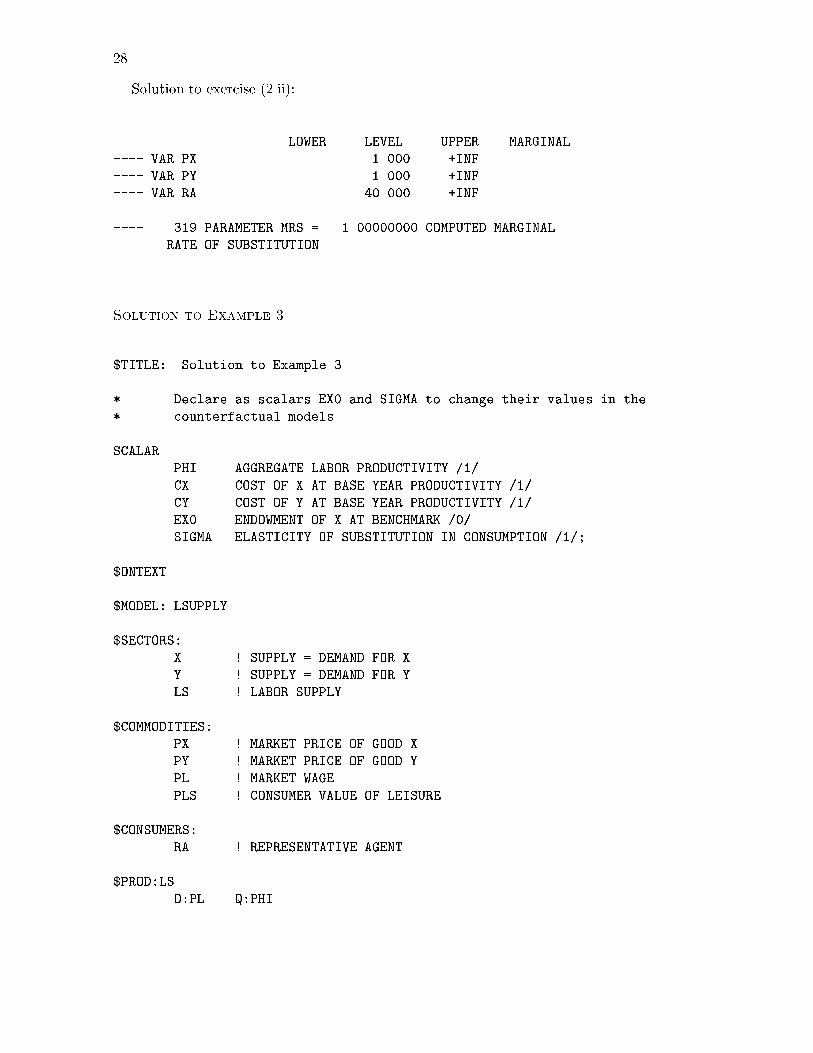
Exercise (2.ii): Modify the demand function calibration point so that the reference priceof both X and Y equal unity.
PX0 = 1;
PY0 = 1;
$INCLUDE MRSCAL.GEN
SOLVE MRSCAL USING MCP;
* Compute the MRS using solution values:
MRS = PX.L / PY.L;
DISPLAY MRS;
28
Solution to exercise (2.ii):
LOWER LEVEL UPPER MARGINAL
---- VAR PX . 1.000 +INF .
---- VAR PY . 1.000 +INF .
---- VAR RA . 40.000 +INF .
---- 319 PARAMETER MRS = 1.00000000 COMPUTED MARGINAL
RATE OF SUBSTITUTION
Solution to Example 3
$TITLE: Solution to Example 3
* Declare as scalars EX0 and SIGMA to change their values in the
* counterfactual models
SCALAR
PHI AGGREGATE LABOR PRODUCTIVITY /1/
CX COST OF X AT BASE YEAR PRODUCTIVITY /1/
CY COST OF Y AT BASE YEAR PRODUCTIVITY /1/
EX0 ENDOWMENT OF X AT BENCHMARK /0/
SIGMA ELASTICITY OF SUBSTITUTION IN CONSUMPTION /1/;
$ONTEXT
$MODEL: LSUPPLY
$SECTORS:
X ! SUPPLY = DEMAND FOR X
Y ! SUPPLY = DEMAND FOR Y
LS ! LABOR SUPPLY
$COMMODITIES:
PX ! MARKET PRICE OF GOOD X
PY ! MARKET PRICE OF GOOD Y
PL ! MARKET WAGE
PLS ! CONSUMER VALUE OF LEISURE
$CONSUMERS:
RA ! REPRESENTATIVE AGENT
$PROD:LS
O:PL Q:PHI
Demand Theory and MPSGE 29
I:PLS Q:1
$PROD:X
O:PX Q:1
I:PL Q:CX
$PROD:Y
O:PY Q:1
I:PL Q:CY
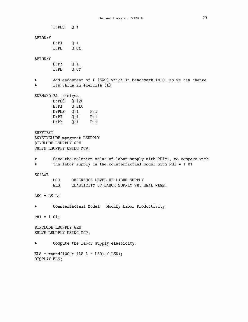
* Add endowment of X (EX0) which in benchmark is 0, so we can change
* its value in exercise (a).
$DEMAND:RA s:sigma
E:PLS Q:120
E:PX Q:EX0
D:PLS Q:1 P:1
D:PX Q:1 P:1
D:PY Q:1 P:1
$OFFTEXT
$SYSINCLUDE mpsgeset LSUPPLY
$INCLUDE LSUPPLY.GEN
SOLVE LSUPPLY USING MCP;
* Save the solution value of labor supply with PHI=1, to compare with
* the labor supply in the counterfactual model with PHI = 1.01.
SCALAR
LS0 REFERENCE LEVEL OF LABOR SUPPLY
ELS ELASTICITY OF LABOR SUPPLY WRT REAL WAGE;
LS0 = LS.L;
* Counterfactual Model: Modify Labor Productivity.
PHI = 1.01;
$INCLUDE LSUPPLY.GEN
SOLVE LSUPPLY USING MCP;
* Compute the labor supply elasticity:
ELS = round(100 * (LS.L - LS0) / LS0);
DISPLAY ELS;
30
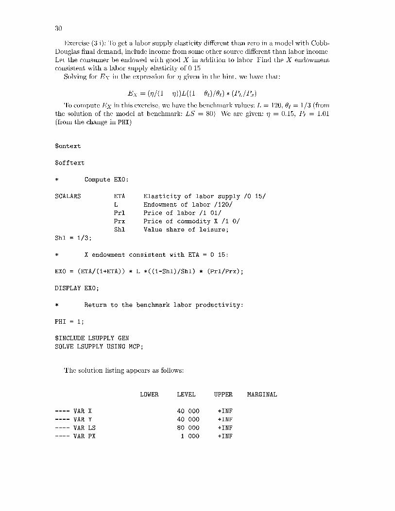
Exercise (3.i): To get a labor supply elasticity di�erent than zero in a model with Cobb-Douglas �nal demand, include income from some other source di�erent than labor income.Let the consumer be endowed with good X in addition to labor. Find the X endowmentconsistent with a labor supply elasticity of 0.15.
Solving for EX in the expression for � given in the hint, we have that:
EX = (�=(1 + �))L((1 � �`)=�`) � (PL=Px)To compute EX in this exercise, we have the benchmark values: L = 120, �` = 1=3 (from
the solution of the model at benchmark: LS = 80). We are given: � = 0:15, P` = 1:01(from the change in PHI).
$ontext
$offtext
* Compute EX0:
SCALARS ETA Elasticity of labor supply /0.15/
L Endowment of labor /120/
Prl Price of labor /1.01/
Prx Price of commodity X /1.0/
Shl Value share of leisure;
Shl = 1/3;
* X endowment consistent with ETA = 0.15:
EX0 = (ETA/(1+ETA)) * L *((1-Shl)/Shl) * (Prl/Prx);
DISPLAY EX0;
* Return to the benchmark labor productivity:
PHI = 1;
$INCLUDE LSUPPLY.GEN
SOLVE LSUPPLY USING MCP;
The solution listing appears as follows:
LOWER LEVEL UPPER MARGINAL
---- VAR X . 40.000 +INF .
---- VAR Y . 40.000 +INF .
---- VAR LS . 80.000 +INF .
---- VAR PX . 1.000 +INF .
Demand Theory and MPSGE 31
---- VAR PY . 1.000 +INF .
---- VAR PL . 1.000 +INF .
---- VAR PLS . 1.000 +INF .
---- VAR RA . 120.000 +INF .
X SUPPLY = DEMAND FOR X
Y SUPPLY = DEMAND FOR Y
LS LABOR SUPPLY
PX MARKET PRICE OF GOOD X
PY MARKET PRICE OF GOOD Y
PL MARKET WAGE
PLS CONSUMER VALUE OF LEISURE
RA REPRESENTATIVE AGENT
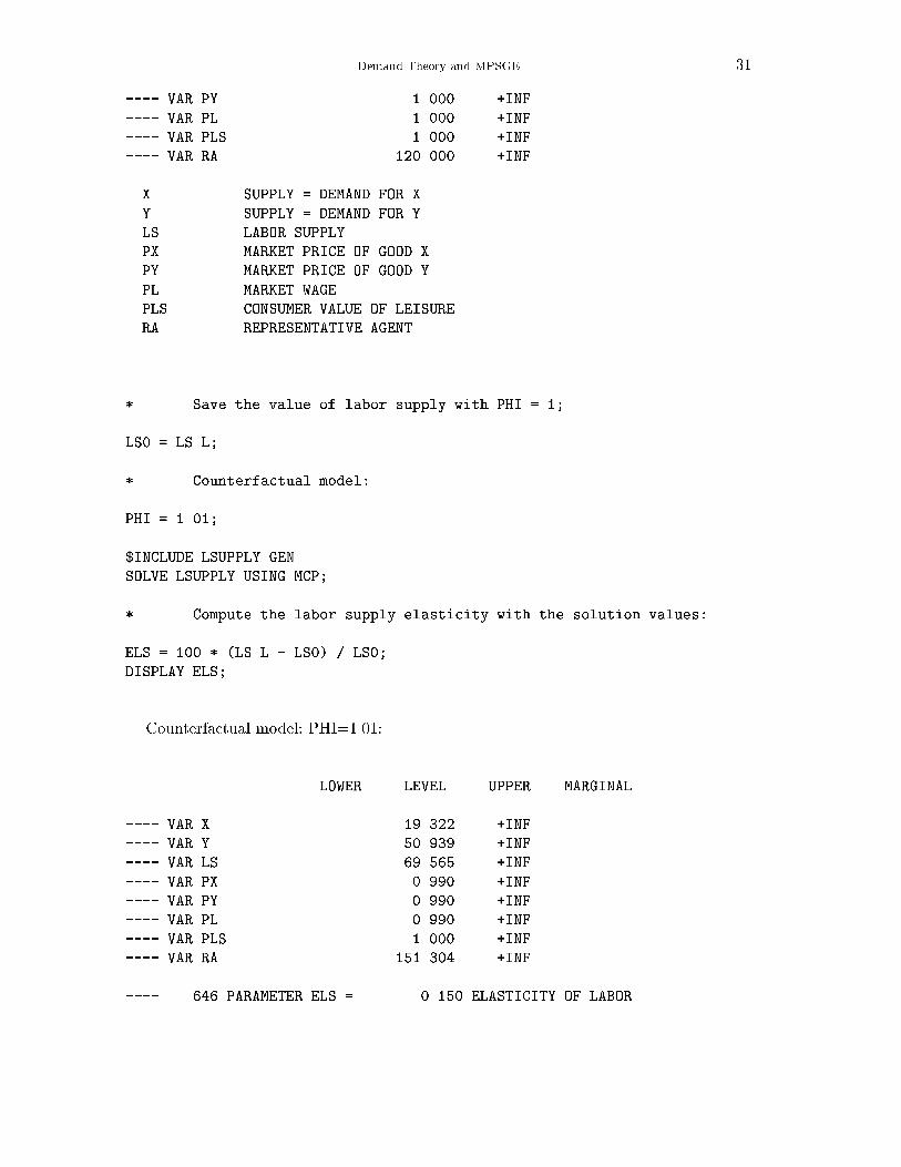
* Save the value of labor supply with PHI = 1;
LS0 = LS.L;
* Counterfactual model:
PHI = 1.01;
$INCLUDE LSUPPLY.GEN
SOLVE LSUPPLY USING MCP;
* Compute the labor supply elasticity with the solution values:
ELS = 100 * (LS.L - LS0) / LS0;
DISPLAY ELS;
Counterfactual model: PHI=1.01:
LOWER LEVEL UPPER MARGINAL
---- VAR X . 19.322 +INF .
---- VAR Y . 50.939 +INF .
---- VAR LS . 69.565 +INF .
---- VAR PX . 0.990 +INF .
---- VAR PY . 0.990 +INF .
---- VAR PL . 0.990 +INF .
---- VAR PLS . 1.000 +INF .
---- VAR RA . 151.304 +INF .
---- 646 PARAMETER ELS = 0.150 ELASTICITY OF LABOR
32
SUPPLY WRT REAL WAGE
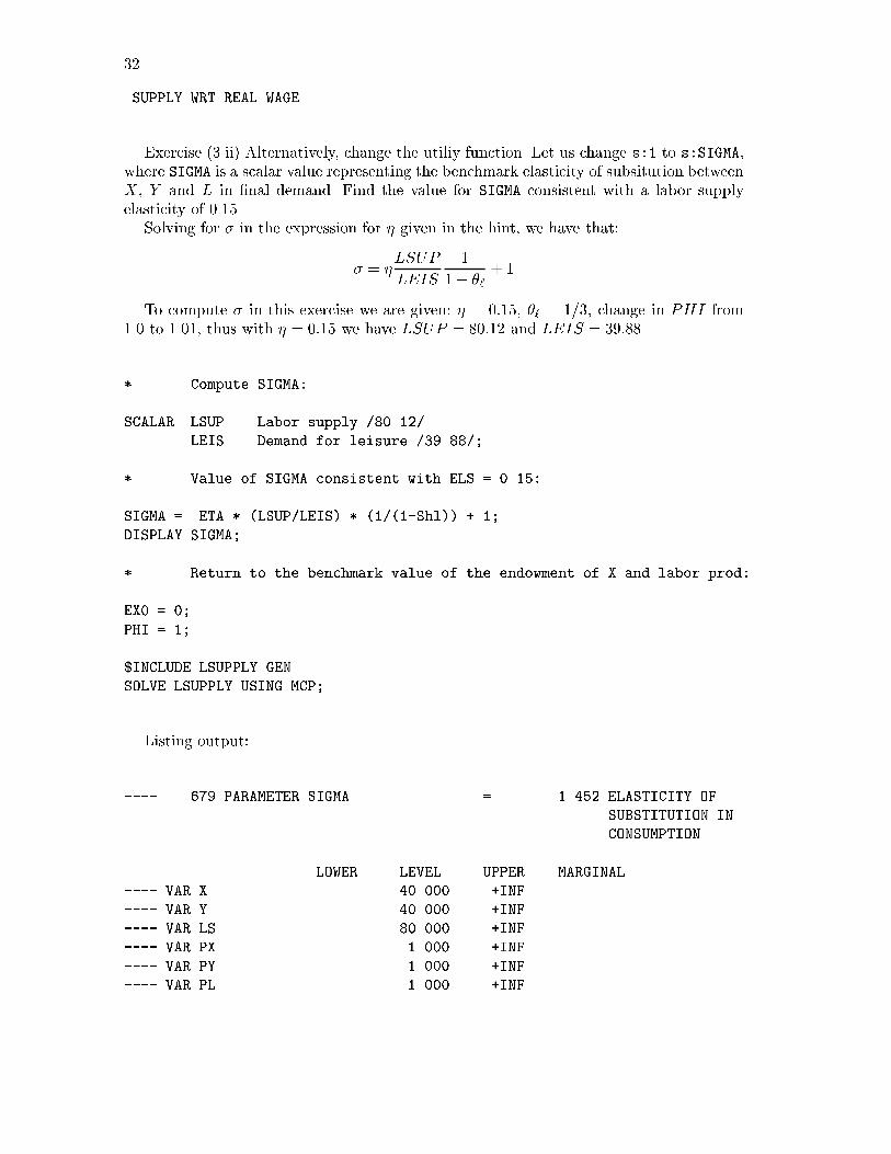
Exercise (3.ii) Alternatively, change the utiliy function. Let us change s:1 to s:SIGMA,where SIGMA is a scalar value representing the benchmark elasticity of subsitution betweenX, Y and L in �nal demand. Find the value for SIGMA consistent with a labor supplyelasticity of 0.15
Solving for � in the expression for � given in the hint, we have that:
� = �LSUP
LEIS
1
1� �` + 1
To compute � in this exercise we are given: � = 0:15, �` = 1=3, change in PHI from1.0 to 1.01, thus with � = 0:15 we have LSUP = 80:12 and LEIS = 39:88.
* Compute SIGMA:
SCALAR LSUP Labor supply /80.12/
LEIS Demand for leisure /39.88/;
* Value of SIGMA consistent with ELS = 0.15:
SIGMA = ETA * (LSUP/LEIS) * (1/(1-Shl)) + 1;
DISPLAY SIGMA;
* Return to the benchmark value of the endowment of X and labor prod:
EX0 = 0;
PHI = 1;
$INCLUDE LSUPPLY.GEN
SOLVE LSUPPLY USING MCP;
Listing output:
---- 679 PARAMETER SIGMA = 1.452 ELASTICITY OF
SUBSTITUTION IN
CONSUMPTION
LOWER LEVEL UPPER MARGINAL
---- VAR X . 40.000 +INF .
---- VAR Y . 40.000 +INF .
---- VAR LS . 80.000 +INF .
---- VAR PX . 1.000 +INF .
---- VAR PY . 1.000 +INF .
---- VAR PL . 1.000 +INF .
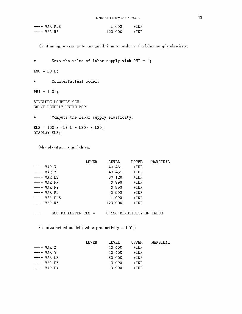
Demand Theory and MPSGE 33
---- VAR PLS . 1.000 +INF .
---- VAR RA . 120.000 +INF .
Continuing, we compute an equilibrium to evaluate the labor supply elasticity:
* Save the value of labor supply with PHI = 1;
LS0 = LS.L;
* Counterfactual model:
PHI = 1.01;
$INCLUDE LSUPPLY.GEN
SOLVE LSUPPLY USING MCP;
* Compute the labor supply elasticity:
ELS = 100 * (LS.L - LS0) / LS0;
DISPLAY ELS;
Model output is as follows:
LOWER LEVEL UPPER MARGINAL
---- VAR X . 40.461 +INF .
---- VAR Y . 40.461 +INF .
---- VAR LS . 80.120 +INF .
---- VAR PX . 0.990 +INF .
---- VAR PY . 0.990 +INF .
---- VAR PL . 0.990 +INF .
---- VAR PLS . 1.000 +INF .
---- VAR RA . 120.000 +INF .
---- 888 PARAMETER ELS = 0.150 ELASTICITY OF LABOR
Counterfactual model (Labor productivity = 1.01):
LOWER LEVEL UPPER MARGINAL
---- VAR X . 40.400 +INF .
---- VAR Y . 40.400 +INF .
---- VAR LS . 80.000 +INF .
---- VAR PX . 0.990 +INF .
---- VAR PY . 0.990 +INF .
34
---- VAR PL . 0.990 +INF .
---- VAR PLS . 1.000 +INF .
---- VAR RA . 120.000 +INF .
---- 402 PARAMETER ELS = 0.000 ELASTICITY OF LABOR
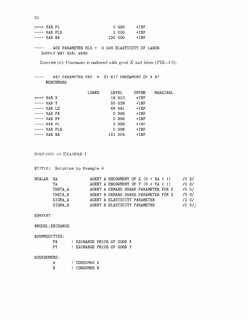
SUPPLY WRT REAL WAGE
Exercise (a): Consumer is endowed with good X and labor (PHI=1.0):
---- 442 PARAMETER EX0 = 31.617 ENDOWMENT OF X AT
BENCHMARK
LOWER LEVEL UPPER MARGINAL
---- VAR X . 18.922 +INF .
---- VAR Y . 50.539 +INF .
---- VAR LS . 69.461 +INF .
---- VAR PX . 0.998 +INF .
---- VAR PY . 0.998 +INF .
---- VAR PL . 0.998 +INF .
---- VAR PLS . 0.998 +INF .
---- VAR RA . 151.304 +INF .
Solution to Example 4
$TITLE: Solution to Example 4
SCALAR XA AGENT A ENDOWMENT OF X (0 < XA < 1) /0.2/
YA AGENT A ENDOWMENT OF Y (0 < YA < 1) /0.8/
THETA_A AGENT A DEMAND SHARE PARAMETER FOR X /0.5/
THETA_B AGENT B DEMAND SHARE PARAMETER FOR X /0.8/
SIGMA_A AGENT A ELASTICITY PARAMETER /2.0/
SIGMA_B AGENT B ELASTICITY PARAMETER /0.5/;
$ONTEXT
$MODEL:EXCHANGE
$COMMODITIES:
PX ! EXCHANGE PRICE OF GOOD X
PY ! EXCHANGE PRICE OF GOOD Y
$CONSUMERS:
A ! CONSUMER A
B ! CONSUMER B
Demand Theory and MPSGE 35
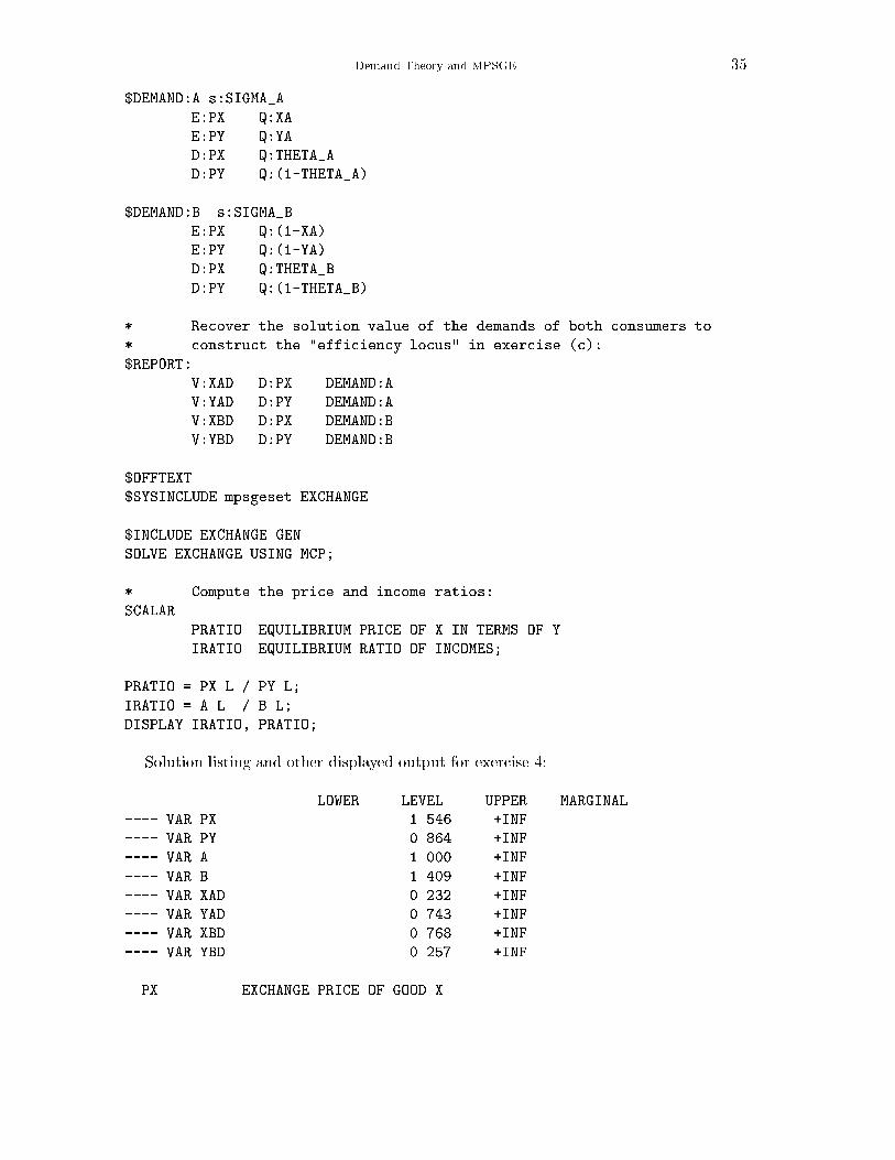
$DEMAND:A s:SIGMA_A
E:PX Q:XA
E:PY Q:YA
D:PX Q:THETA_A
D:PY Q:(1-THETA_A)
$DEMAND:B s:SIGMA_B
E:PX Q:(1-XA)
E:PY Q:(1-YA)
D:PX Q:THETA_B
D:PY Q:(1-THETA_B)
* Recover the solution value of the demands of both consumers to
* construct the "efficiency locus" in exercise (c):
$REPORT:
V:XAD D:PX DEMAND:A
V:YAD D:PY DEMAND:A
V:XBD D:PX DEMAND:B
V:YBD D:PY DEMAND:B
$OFFTEXT
$SYSINCLUDE mpsgeset EXCHANGE
$INCLUDE EXCHANGE.GEN
SOLVE EXCHANGE USING MCP;
* Compute the price and income ratios:
SCALAR
PRATIO EQUILIBRIUM PRICE OF X IN TERMS OF Y
IRATIO EQUILIBRIUM RATIO OF INCOMES;
PRATIO = PX.L / PY.L;
IRATIO = A.L / B.L;
DISPLAY IRATIO, PRATIO;
Solution listing and other displayed output for exercise 4:
LOWER LEVEL UPPER MARGINAL
---- VAR PX . 1.546 +INF .
---- VAR PY . 0.864 +INF .
---- VAR A . 1.000 +INF .
---- VAR B . 1.409 +INF .
---- VAR XAD . 0.232 +INF .
---- VAR YAD . 0.743 +INF .
---- VAR XBD . 0.768 +INF .
---- VAR YBD . 0.257 +INF .
PX EXCHANGE PRICE OF GOOD X
36
PY EXCHANGE PRICE OF GOOD Y
A CONSUMER A
B CONSUMER B
XAD
YAD
XBD
YBD
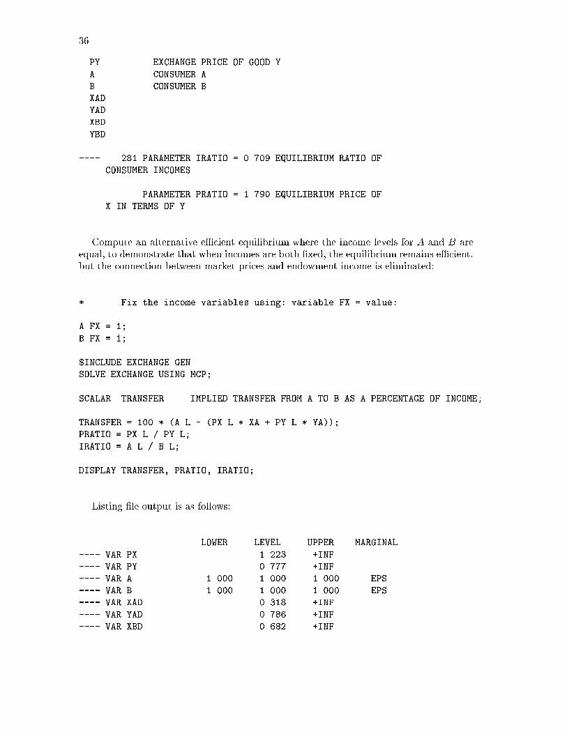
---- 281 PARAMETER IRATIO = 0.709 EQUILIBRIUM RATIO OF
CONSUMER INCOMES
PARAMETER PRATIO = 1.790 EQUILIBRIUM PRICE OF
X IN TERMS OF Y
Compute an alternative e�cient equilibrium where the income levels for A and B areequal, to demonstrate that when incomes are both �xed, the equilibrium remains e�cient,but the connection between market prices and endowment income is eliminated:
* Fix the income variables using: variable.FX = value:
A.FX = 1;
B.FX = 1;
$INCLUDE EXCHANGE.GEN
SOLVE EXCHANGE USING MCP;
SCALAR TRANSFER IMPLIED TRANSFER FROM A TO B AS A PERCENTAGE OF INCOME;
TRANSFER = 100 * (A.L - (PX.L * XA + PY.L * YA));
PRATIO = PX.L / PY.L;
IRATIO = A.L / B.L;
DISPLAY TRANSFER, PRATIO, IRATIO;
Listing �le output is as follows:
LOWER LEVEL UPPER MARGINAL
---- VAR PX . 1.223 +INF .
---- VAR PY . 0.777 +INF .
---- VAR A 1.000 1.000 1.000 EPS
---- VAR B 1.000 1.000 1.000 EPS
---- VAR XAD . 0.318 +INF .
---- VAR YAD . 0.786 +INF .
---- VAR XBD . 0.682 +INF .
Demand Theory and MPSGE 37
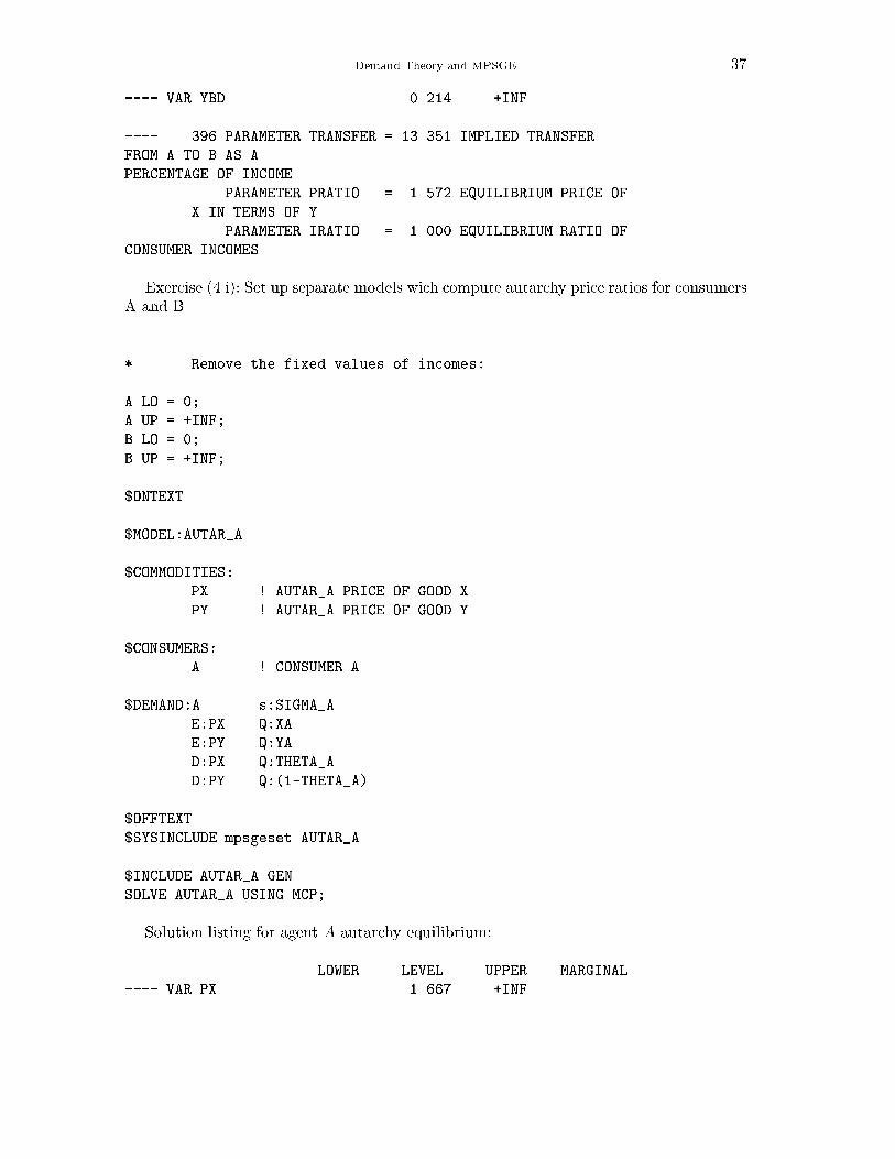
---- VAR YBD . 0.214 +INF .
---- 396 PARAMETER TRANSFER = 13.351 IMPLIED TRANSFER
FROM A TO B AS A
PERCENTAGE OF INCOME
PARAMETER PRATIO = 1.572 EQUILIBRIUM PRICE OF
X IN TERMS OF Y
PARAMETER IRATIO = 1.000 EQUILIBRIUM RATIO OF
CONSUMER INCOMES
Exercise (4.i): Set up separate models wich compute autarchy price ratios for consumersA and B.
* Remove the fixed values of incomes:
A.LO = 0;
A.UP = +INF;
B.LO = 0;
B.UP = +INF;
$ONTEXT
$MODEL:AUTAR_A
$COMMODITIES:
PX ! AUTAR_A PRICE OF GOOD X
PY ! AUTAR_A PRICE OF GOOD Y
$CONSUMERS:
A ! CONSUMER A
$DEMAND:A s:SIGMA_A
E:PX Q:XA
E:PY Q:YA
D:PX Q:THETA_A
D:PY Q:(1-THETA_A)
$OFFTEXT
$SYSINCLUDE mpsgeset AUTAR_A
$INCLUDE AUTAR_A.GEN
SOLVE AUTAR_A USING MCP;
Solution listing for agent A autarchy equilibrium:
LOWER LEVEL UPPER MARGINAL
---- VAR PX . 1.667 +INF .
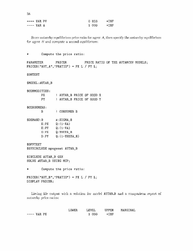
38
---- VAR PY . 0.833 +INF .
---- VAR A . 1.000 +INF .
Store autarchy equilibriumprice ratio for agent A, then specify the autarchy equilibriumfor agent B and compute a second equilibrium:
* Compute the price ratio:
PARAMETER PRICER PRICE RATIO OF THE AUTARCHY MODELS;
PRICER("AUT_A","PRATIO") = PX.L / PY.L;
$ONTEXT
$MODEL:AUTAR_B
$COMMODITIES:
PX ! AUTAR_B PRICE OF GOOD X
PY ! AUTAR_B PRICE OF GOOD Y
$CONSUMERS:
B ! CONSUMER B
$DEMAND:B s:SIGMA_B
E:PX Q:(1-XA)
E:PY Q:(1-YA)
D:PX Q:THETA_B
D:PY Q:(1-THETA_B)
$OFFTEXT
$SYSINCLUDE mpsgeset AUTAR_B
$INCLUDE AUTAR_B.GEN
SOLVE AUTAR_B USING MCP;
* Compute the price ratio:
PRICER("AUT_B","PRATIO") = PX.L / PY.L;
DISPLAY PRICER;
Listing �le output with a solution for model AUTAR B and a comparison report ofautarchy price ratios:
LOWER LEVEL UPPER MARGINAL
---- VAR PX . 1.000 +INF .
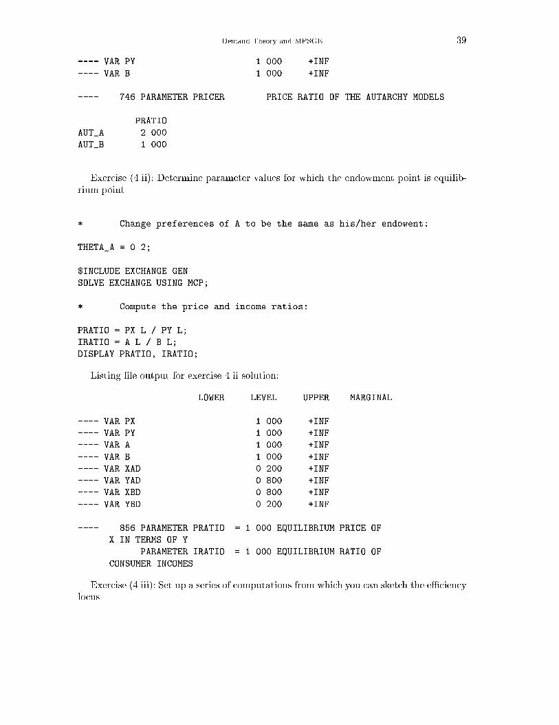
Demand Theory and MPSGE 39
---- VAR PY . 1.000 +INF .
---- VAR B . 1.000 +INF .
---- 746 PARAMETER PRICER PRICE RATIO OF THE AUTARCHY MODELS
PRATIO
AUT_A 2.000
AUT_B 1.000
Exercise (4.ii): Determine parameter values for which the endowment point is equilib-rium point.
* Change preferences of A to be the same as his/her endowent:
THETA_A = 0.2;
$INCLUDE EXCHANGE.GEN
SOLVE EXCHANGE USING MCP;
* Compute the price and income ratios:
PRATIO = PX.L / PY.L;
IRATIO = A.L / B.L;
DISPLAY PRATIO, IRATIO;
Listing �le output for exercise 4.ii solution:
LOWER LEVEL UPPER MARGINAL
---- VAR PX . 1.000 +INF .
---- VAR PY . 1.000 +INF .
---- VAR A . 1.000 +INF .
---- VAR B . 1.000 +INF .
---- VAR XAD . 0.200 +INF .
---- VAR YAD . 0.800 +INF .
---- VAR XBD . 0.800 +INF .
---- VAR YBD . 0.200 +INF .
---- 856 PARAMETER PRATIO = 1.000 EQUILIBRIUM PRICE OF
X IN TERMS OF Y
PARAMETER IRATIO = 1.000 EQUILIBRIUM RATIO OF
CONSUMER INCOMES
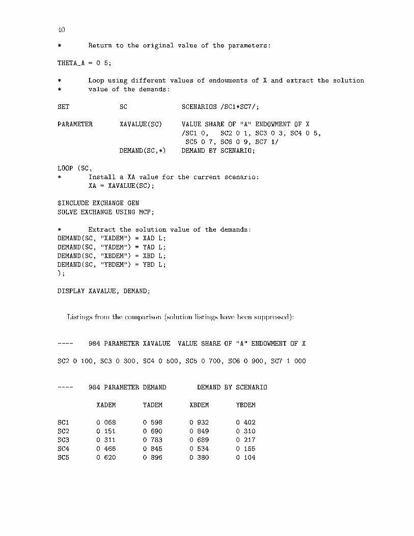
Exercise (4.iii): Set up a series of computations from which you can sketch the e�ciencylocus.
40
* Return to the original value of the parameters:
THETA_A = 0.5;
* Loop using different values of endowments of X and extract the solution
* value of the demands:
SET SC SCENARIOS /SC1*SC7/;
PARAMETER XAVALUE(SC) VALUE SHARE OF "A" ENDOWMENT OF X
/SC1 0, SC2 0.1, SC3 0.3, SC4 0.5,
SC5 0.7, SC6 0.9, SC7 1/
DEMAND(SC,*) DEMAND BY SCENARIO;
LOOP (SC,
* Install a XA value for the current scenario:
XA = XAVALUE(SC);
$INCLUDE EXCHANGE.GEN
SOLVE EXCHANGE USING MCP;
* Extract the solution value of the demands:
DEMAND(SC, "XADEM") = XAD.L;
DEMAND(SC, "YADEM") = YAD.L;
DEMAND(SC, "XBDEM") = XBD.L;
DEMAND(SC, "YBDEM") = YBD.L;
);
DISPLAY XAVALUE, DEMAND;
Listings from the comparison (solution listings have been suppressed):
---- 984 PARAMETER XAVALUE VALUE SHARE OF "A" ENDOWMENT OF X
SC2 0.100, SC3 0.300, SC4 0.500, SC5 0.700, SC6 0.900, SC7 1.000
---- 984 PARAMETER DEMAND DEMAND BY SCENARIO
XADEM YADEM XBDEM YBDEM
SC1 0.068 0.598 0.932 0.402
SC2 0.151 0.690 0.849 0.310
SC3 0.311 0.783 0.689 0.217
SC4 0.466 0.845 0.534 0.155
SC5 0.620 0.896 0.380 0.104
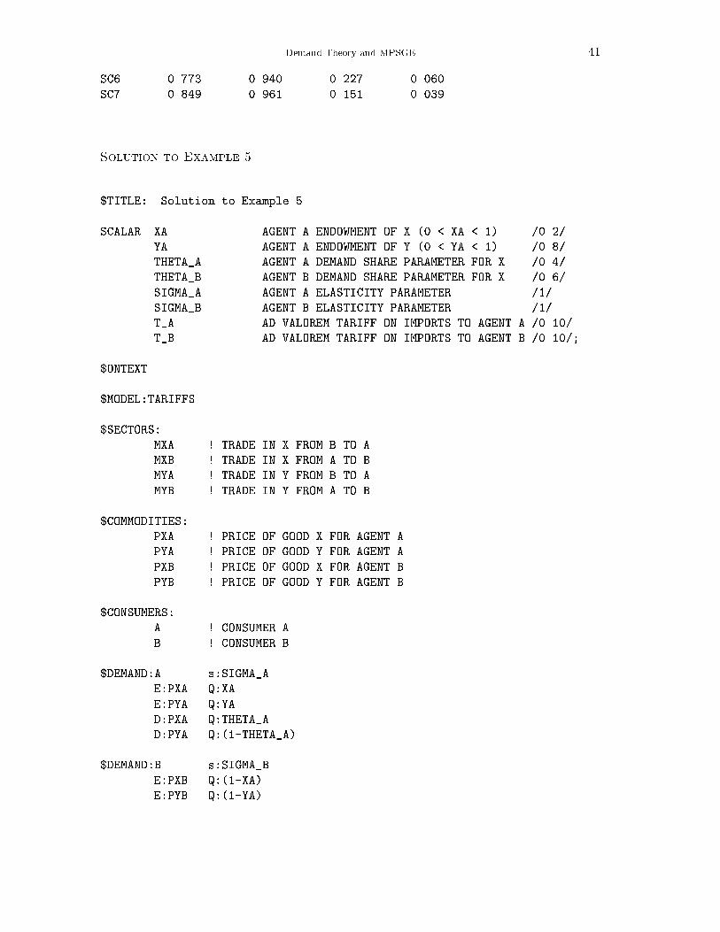
Demand Theory and MPSGE 41
SC6 0.773 0.940 0.227 0.060
SC7 0.849 0.961 0.151 0.039
Solution to Example 5
$TITLE: Solution to Example 5
SCALAR XA AGENT A ENDOWMENT OF X (0 < XA < 1) /0.2/
YA AGENT A ENDOWMENT OF Y (0 < YA < 1) /0.8/
THETA_A AGENT A DEMAND SHARE PARAMETER FOR X /0.4/
THETA_B AGENT B DEMAND SHARE PARAMETER FOR X /0.6/
SIGMA_A AGENT A ELASTICITY PARAMETER /1/
SIGMA_B AGENT B ELASTICITY PARAMETER /1/
T_A AD VALOREM TARIFF ON IMPORTS TO AGENT A /0.10/
T_B AD VALOREM TARIFF ON IMPORTS TO AGENT B /0.10/;
$ONTEXT
$MODEL:TARIFFS
$SECTORS:
MXA ! TRADE IN X FROM B TO A
MXB ! TRADE IN X FROM A TO B
MYA ! TRADE IN Y FROM B TO A
MYB ! TRADE IN Y FROM A TO B
$COMMODITIES:
PXA ! PRICE OF GOOD X FOR AGENT A
PYA ! PRICE OF GOOD Y FOR AGENT A
PXB ! PRICE OF GOOD X FOR AGENT B
PYB ! PRICE OF GOOD Y FOR AGENT B
$CONSUMERS:
A ! CONSUMER A
B ! CONSUMER B
$DEMAND:A s:SIGMA_A
E:PXA Q:XA
E:PYA Q:YA
D:PXA Q:THETA_A
D:PYA Q:(1-THETA_A)
$DEMAND:B s:SIGMA_B
E:PXB Q:(1-XA)
E:PYB Q:(1-YA)
42
D:PXB Q:THETA_B
D:PYB Q:(1-THETA_B)
* Trade activities
$PROD:MXA
O:PXA Q:1
I:PXB Q:1 A:A T:T_A
$PROD:MXB
O:PXB Q:1
I:PXA Q:1 A:B T:T_B
$PROD:MYA
O:PYA Q:1
I:PYB Q:1 A:A T:T_A
$PROD:MYB
O:PYB Q:1
I:PYA Q:1 A:B T:T_B
* Recover a Hicksian money-metric welfare index:
$REPORT:
V:WA W:A
V:WB W:B
$OFFTEXT
$SYSINCLUDE mpsgeset TARIFFS
$INCLUDE TARIFFS.GEN
SOLVE TARIFFS USING MCP;
The solution listing for this model appears as follows:
LOWER LEVEL UPPER MARGINAL
---- VAR MXA . 0.177 +INF .
---- VAR MXB . . +INF 0.243
---- VAR MYA . . +INF 0.243
---- VAR MYB . 0.177 +INF .
---- VAR PXA . 1.272 +INF .
---- VAR PYA . 1.156 +INF .
---- VAR PXB . 1.156 +INF .
---- VAR PYB . 1.272 +INF .
---- VAR A . 1.200 +INF .
---- VAR B . 1.200 +INF .
---- VAR WA . 0.999 +INF .
---- VAR WB . 0.999 +INF .
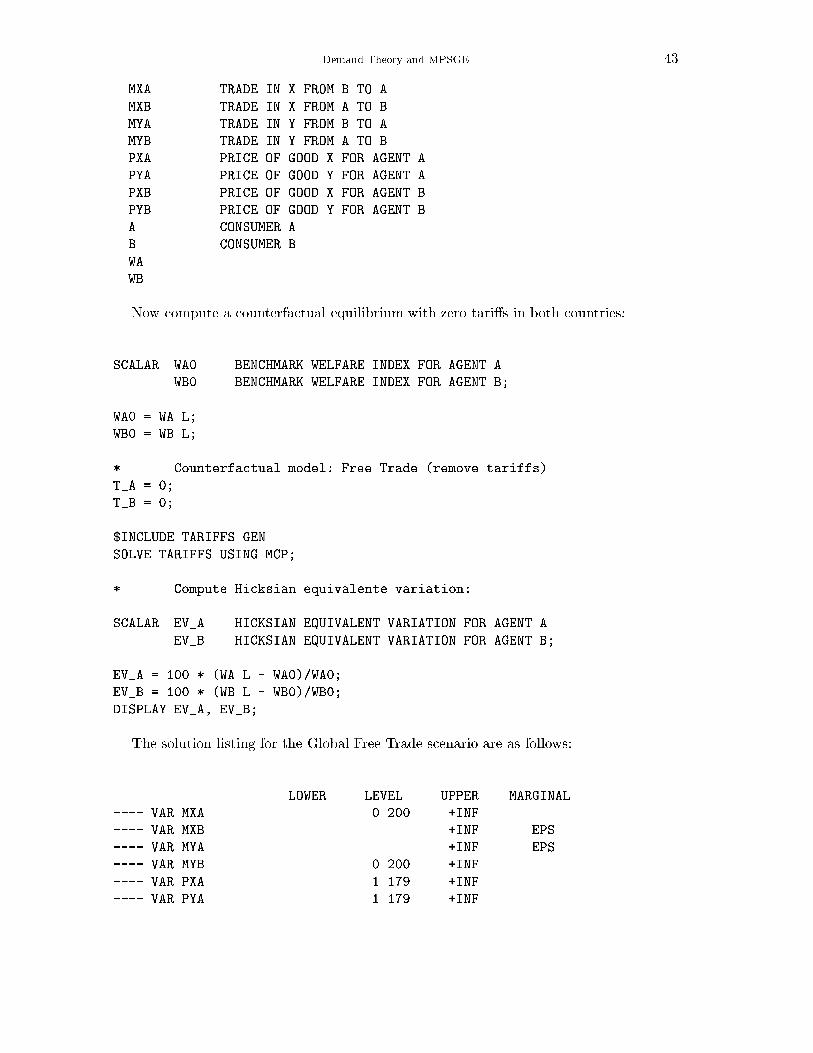
Demand Theory and MPSGE 43
MXA TRADE IN X FROM B TO A
MXB TRADE IN X FROM A TO B
MYA TRADE IN Y FROM B TO A
MYB TRADE IN Y FROM A TO B
PXA PRICE OF GOOD X FOR AGENT A
PYA PRICE OF GOOD Y FOR AGENT A
PXB PRICE OF GOOD X FOR AGENT B
PYB PRICE OF GOOD Y FOR AGENT B
A CONSUMER A
B CONSUMER B
WA
WB
Now compute a counterfactual equilibrium with zero tari�s in both countries:
SCALAR WA0 BENCHMARK WELFARE INDEX FOR AGENT A
WB0 BENCHMARK WELFARE INDEX FOR AGENT B;
WA0 = WA.L;
WB0 = WB.L;
* Counterfactual model: Free Trade (remove tariffs)
T_A = 0;
T_B = 0;
$INCLUDE TARIFFS.GEN
SOLVE TARIFFS USING MCP;
* Compute Hicksian equivalente variation:
SCALAR EV_A HICKSIAN EQUIVALENT VARIATION FOR AGENT A
EV_B HICKSIAN EQUIVALENT VARIATION FOR AGENT B;
EV_A = 100 * (WA.L - WA0)/WA0;
EV_B = 100 * (WB.L - WB0)/WB0;
DISPLAY EV_A, EV_B;
The solution listing for the Global Free Trade scenario are as follows:
LOWER LEVEL UPPER MARGINAL
---- VAR MXA . 0.200 +INF .
---- VAR MXB . . +INF EPS
---- VAR MYA . . +INF EPS
---- VAR MYB . 0.200 +INF .
---- VAR PXA . 1.179 +INF .
---- VAR PYA . 1.179 +INF .

44
---- VAR PXB . 1.179 +INF .
---- VAR PYB . 1.179 +INF .
---- VAR A . 1.179 +INF .
---- VAR B . 1.179 +INF .
---- VAR WA . 1.000 +INF .
---- VAR WB . 1.000 +INF .
---- 543 PARAMETER EV_A = 0.108 HICKSIAN EQUIVALENT
VARIATION FOR AGENT A
PARAMETER EV_B = 0.108 HICKSIAN EQUIVALENT
VARIATION FOR AGENT B
Exercise (5.i): Find an "optimal tari�" in this model for agent A, assuming that AgentB does not retaliate and leaves her tari� rate at the benchmark level.
* Return to original tariffs
T_A = 0.1;
T_B = 0.1;
* Loop using different tariff rates and extract welfare index to
* compute the Hicksian equivalent variation:
SET SC Scenarios /SC1*SC7/;
PARAMETER TVALUE(SC) TARIFF VALUE FOR SC
/SC1 0, SC2 0.2, SC3 0.4, SC4 0.6,
SC5 0.8, SC6 1.0, SC7 1.2/
SUMMARY(SC,*) HICKSIAN EQUIVALENT VARIATION BY SCENARIO;
LOOP(SC,
* Install a tariff rate impossed by Agent A in the current scenario:
* (T_B remains at the benchmark level).
T_A = TVALUE(SC);
$INCLUDE TARIFFS.GEN
SOLVE TARIFFS USING MCP;
* Extract welfare index and compute Hicksian EV:
SUMMARY(SC,"EV_A") = 100 * (WA.L - WA0)/WA0;
SUMMARY(SC,"EV_B") = 100 * (WB.L - WB0)/WB0;
);
OPTION TVALUE:2;
DISPLAY TVALUE, SUMMARY;
Demand Theory and MPSGE 45
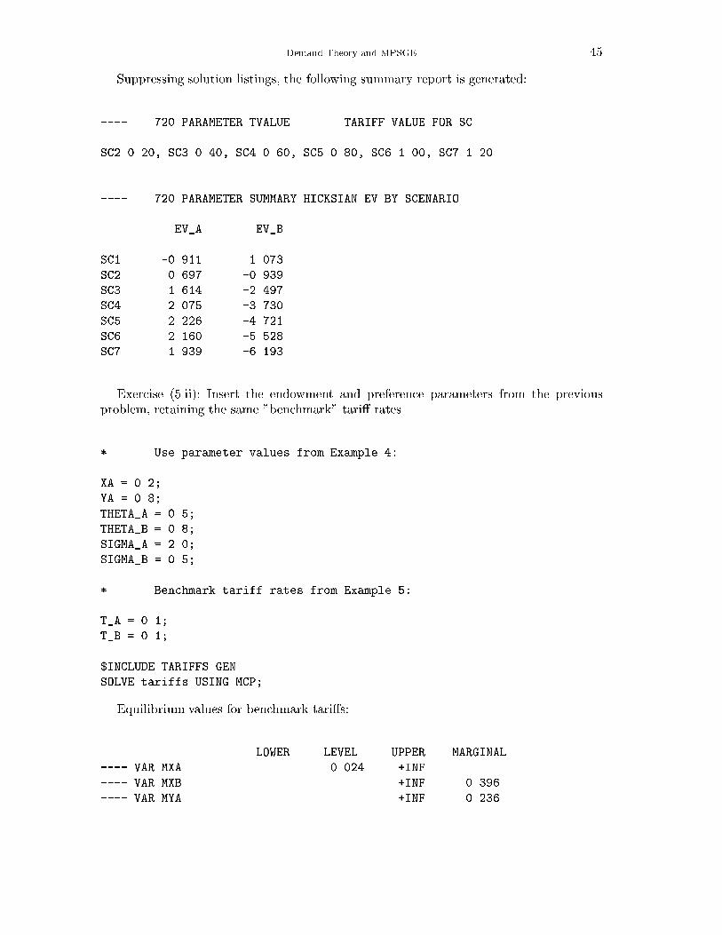
Suppressing solution listings, the following summary report is generated:
---- 720 PARAMETER TVALUE TARIFF VALUE FOR SC
SC2 0.20, SC3 0.40, SC4 0.60, SC5 0.80, SC6 1.00, SC7 1.20
---- 720 PARAMETER SUMMARY HICKSIAN EV BY SCENARIO
EV_A EV_B
SC1 -0.911 1.073
SC2 0.697 -0.939
SC3 1.614 -2.497
SC4 2.075 -3.730
SC5 2.226 -4.721
SC6 2.160 -5.528
SC7 1.939 -6.193
Exercise (5.ii): Insert the endowment and preference parameters from the previousproblem, retaining the same "benchmark" tari� rates.
* Use parameter values from Example 4:
XA = 0.2;
YA = 0.8;
THETA_A = 0.5;
THETA_B = 0.8;
SIGMA_A = 2.0;
SIGMA_B = 0.5;
* Benchmark tariff rates from Example 5:
T_A = 0.1;
T_B = 0.1;
$INCLUDE TARIFFS.GEN
SOLVE tariffs USING MCP;
Equilibrium values for benchmark tari�s:
LOWER LEVEL UPPER MARGINAL
---- VAR MXA . 0.024 +INF .
---- VAR MXB . . +INF 0.396
---- VAR MYA . . +INF 0.236
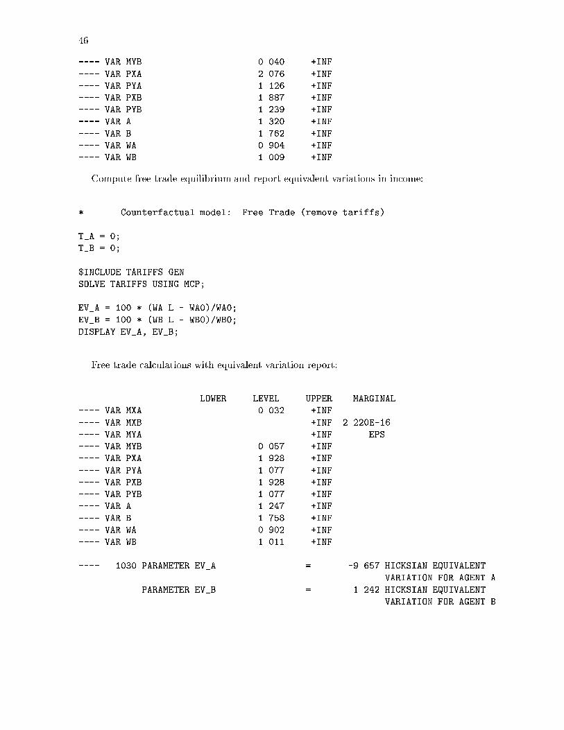
46
---- VAR MYB . 0.040 +INF .
---- VAR PXA . 2.076 +INF .
---- VAR PYA . 1.126 +INF .
---- VAR PXB . 1.887 +INF .
---- VAR PYB . 1.239 +INF .
---- VAR A . 1.320 +INF .
---- VAR B . 1.762 +INF .
---- VAR WA . 0.904 +INF .
---- VAR WB . 1.009 +INF .
Compute free trade equilibrium and report equivalent variations in income:
* Counterfactual model: Free Trade (remove tariffs)
T_A = 0;
T_B = 0;
$INCLUDE TARIFFS.GEN
SOLVE TARIFFS USING MCP;
EV_A = 100 * (WA.L - WA0)/WA0;
EV_B = 100 * (WB.L - WB0)/WB0;
DISPLAY EV_A, EV_B;
Free trade calculations with equivalent variation report:
LOWER LEVEL UPPER MARGINAL
---- VAR MXA . 0.032 +INF .
---- VAR MXB . . +INF 2.220E-16
---- VAR MYA . . +INF EPS
---- VAR MYB . 0.057 +INF .
---- VAR PXA . 1.928 +INF .
---- VAR PYA . 1.077 +INF .
---- VAR PXB . 1.928 +INF .
---- VAR PYB . 1.077 +INF .
---- VAR A . 1.247 +INF .
---- VAR B . 1.758 +INF .
---- VAR WA . 0.902 +INF .
---- VAR WB . 1.011 +INF .
---- 1030 PARAMETER EV_A = -9.657 HICKSIAN EQUIVALENT
VARIATION FOR AGENT A
PARAMETER EV_B = 1.242 HICKSIAN EQUIVALENT
VARIATION FOR AGENT B
Applied General Equilibrium Modeling with
MPSGE as a GAMS Subsystem
An Overview of the Modeling Framework and Syntax
Abstract. This paper describes a programming environment for economic equilibrium analysis. Thesystem introduces the Mathematical Programming System for General Equilibrium analysis (MPSGE,Rutherford 1987) within the Generalized Algebraic Modelling System (GAMS, Brooke, Kendrick andMeeraus (1988)). This arrangement exploits GAMS' set-oriented algebraic syntax for data manipulationand report writing. The system based on the tabular MPSGE input format provides a compact, non-algebraic representation of a model's nonlinear equations. This paper provides an overview of the modellingenvironment and three worked examples in tax policy analysis.
Keywords: Applied General Equilibrium
JEL codes: C68
48
1. INTRODUCTION
This paper introduces a programming language for economic equilibrium modelling.The paper presents the motivation for the system, the programming syntax, and threesmall scale examples. A library of larger models are provided with the program. Thepurpose of the paper is to provide a concise introduction to the modelling environment.
MPSGE is a language for concise representation of Arrow-Debreu economic equilibriummodels (Rutherford, 1987). The name stands for \mathematical programming system forgeneral equilibrium". MPSGE provides a short-hand representation for the complicatedsystems of nonlinear inequalities which underly general equilibrium models. The MPSGEframework is based on nested constant elasticity of substitution utility functions andproduction functions. The data requirements for a model include share and elasticityparameters, endowments, and tax rates for all the consumers and production sectorsincluded in the model. These may or may not be calibrated from a consistent benchmarkequilibrium dataset.
GAMS, the \Generalized Algebraic Modelling System", is a modeling language whichwas originally developed for linear, nonlinear and integer programming. This languagewas developed over 20 years ago by Alex Meeraus when he was working at the WorldBank. (See Brooke, Kendrick and Meeraus 1988.) Since that time, GAMS has been widelyapplied for large-scale economic and operations research modeling projects.
Prior to their marriage, MPSGE and GAMS embodied di�erent design philosophies.MPSGE was (and is) appropriate for a speci�c class of nonlinear equations, while GAMSis capable of representing any system of algebraic equations. While GAMS is applicablein several disciplines, MPSGE is only applicable in the analysis of economic equilibriummodels. The expert knowledge embodied in MPSGE is of particular use to economists whoare interested in the insights provided by formal models but who are unable to devote manyhours to programming. MPSGE provides a structured framework for novice modellers.When used by experts, MPSGE reduces the setup cost of producing an operational modeland the cost of testing alternative speci�cations.
In contrast, the GAMS modelling language is designed for managing large datasets. Theuse of sets and detached-coe�cient matrix notation makes the GAMS environment verynice for both developing balanced benchmark datasets and for writing solution reports.GAMS' main disadvantage for economic applications concerns the speci�cation of themodel structure. Economic equilibrium models, particularly those based on complicatedfunctions such as nested constant-elasticity-of-substitution (CES), are easier to understandat an abstract level than they are to specify in detail, and the translation of a model frominput data into algebraic relations can be a tedious and error- prone undertaking.
The interface between GAMS and MPSGE combines the strengths of both programs.The system uses GAMS as the \front end" and \back end" to MPSGE, facilitating datahandling and report writing. The language employs an extended MPSGE syntax basedon GAMS sets, so that model speci�cation is concise. In addition, the system includestwo large-scale solvers, MILES (Rutherford, 1993) and PATH (Ferris and Dirkse, 1993),which may be used interchangeably. The availability of two algorithms greatly enhancesrobustness and reliability.
The GAMS/MPSGE interface has been commercially available since 1993 and thereare a number of published applications based on the software. Appendix A provides a
MPSGE Syntax 49
selected set of papers based on models programmed with GAMS/MPSGE. The range ofissues which have been addressed testi�es to the exibility of the modeling environment.
Of course, GAMS/MPSGE is not the only software available for formulating and solv-ing CGE models. GEMPACK (General Equilibrium Modelling PACKage, Harrison andPearson (1996), Harrison, Pearson, Powell and Small (1994)) is a suite of general- purposeeconomic modelling software for equilibrium models represented as a mixture of linearizedand level equations.
The remainder of this paper is organized as follows. Section 2 introduces MPSGEinput syntax and the GAMS interface using a small two-sector model of taxation. Section3 extends the 2x2 model to illustrate how the software is used to perform equal-yield(di�erential) tax policy analysis and to analyze tax reform in a model with endogenoustaxation. Section 4 provides a brief summary and conclusion. The paper introduces lan-guage features largely through example. Details on language syntax and program structureare provided in two appendices. Appendix B provides a complete statement of MPSGEsyntax. Appendix C provides an overview of the modeling environment and the structure ofGAMS input �les which employ MPSGE. Appendix D provides an algebraic speci�cationof the three models considered in the paper.
If readers unfamiliar with GAMS wish to go through the examples, it would be helpfulto install a demonstration system (see http://www.gams.com for details), then retrieve andprocess the library �le THREEMGE which contains three MPSGE models (HARBERGER,SHOVEN and SAMUELSON). Once the GAMS system has been installed, two commands toretrieve and run the models used in this paper:
gamslib threemge
gams threemge
After having processed this �le, print the listing �le (THREEMGE.LST) for reference.
2. THE MATHEMATICAL FORMULATION
Mathiesen (1985) demonstrated that an Arrow-Debreu general economic equilibriummodelcould be formulated and e�ciently solved as a complementarity problem. Mathiesen'sformulation may be posed in terms of three sets of \central variables":
p = a non-negative n-vector of commodity prices including all �nal goods, intermediategoods and primary factors of production;
y = a non-negative m-vector of activity levels for constant returns to scale productionsectors in the economy; and
M = an h-vector of income levels, one for each \household" in the model, including anygovernment entities.
An equilibrium in these variables satis�es a system of three classes of nonlinear inequal-ities.
50
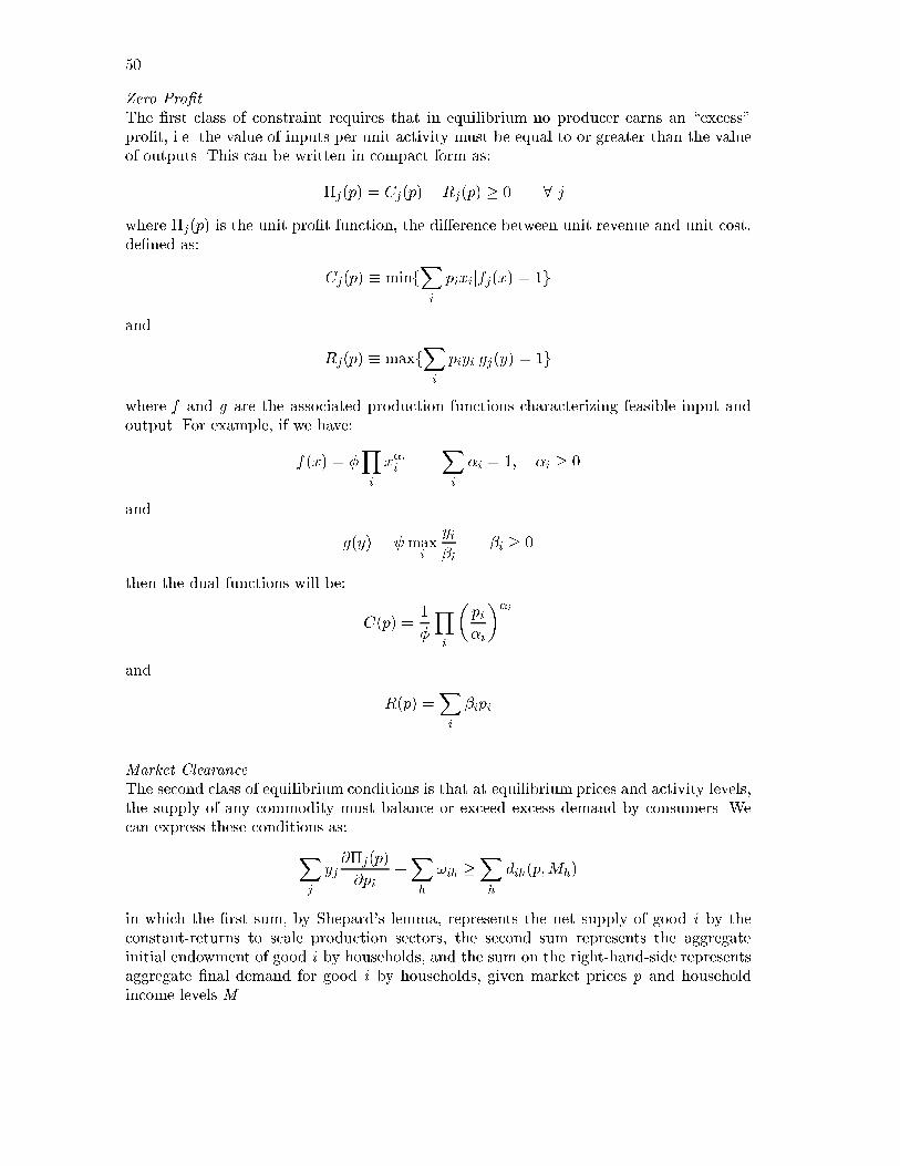
Zero Pro�tThe �rst class of constraint requires that in equilibrium no producer earns an \excess"pro�t, i.e. the value of inputs per unit activity must be equal to or greater than the valueof outputs. This can be written in compact form as:
��j(p) = Cj(p)�Rj(p) � 0 8 jwhere �j(p) is the unit pro�t function, the di�erence between unit revenue and unit cost,de�ned as:
Cj(p) � minfXi
pixijfj(x) = 1g
and
Rj(p) � maxfXi
piyijgj(y) = 1g
where f and g are the associated production functions characterizing feasible input andoutput. For example, if we have:
f(x) = �Yi
x�iiXi
�i = 1; �i � 0
and
g(y) = maxi
yi�i
�i � 0
then the dual functions will be:
C(p) =1
�
Yi
�pi�i
��i
and
R(p) =Xi
�ipi
Market ClearanceThe second class of equilibrium conditions is that at equilibrium prices and activity levels,the supply of any commodity must balance or exceed excess demand by consumers. Wecan express these conditions as:
Xj
yj@�j(p)
@pi+Xh
!ih �Xh
dih(p;Mh)
in which the �rst sum, by Shepard's lemma, represents the net supply of good i by theconstant-returns to scale production sectors, the second sum represents the aggregateinitial endowment of good i by households, and the sum on the right-hand-side representsaggregate �nal demand for good i by households, given market prices p and householdincome levels M.
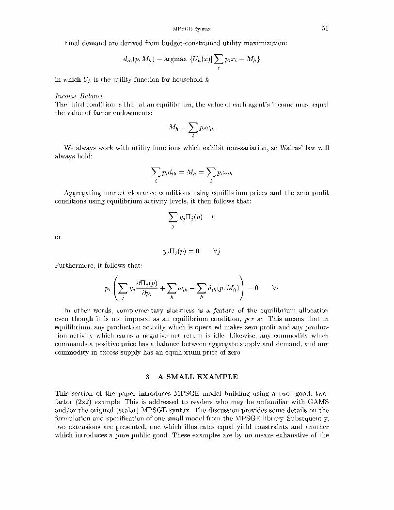
MPSGE Syntax 51
Final demand are derived from budget-constrained utility maximization:
dih(p;Mh) = argmax fUh(x)jXi
pixi =Mhg
in which Uh is the utility function for household h.
Income BalanceThe third condition is that at an equilibrium, the value of each agent's income must equalthe value of factor endowments:
Mh =Xi
pi!ih
We always work with utility functions which exhibit non-satiation, so Walras' law willalways hold: X
i
pidih =Mh =Xi
pi!ih
Aggregating market clearance conditions using equilibrium prices and the zero pro�tconditions using equilibrium activity levels, it then follows that:X
j
yj�j(p) = 0
or
yj�j(p) = 0 8jFurthermore, it follows that:
pi
0@X
j
yj@�j(p)
@pi+Xh
!ih �Xh
dih(p;Mh)
1A = 0 8i
In other words, complementary slackness is a feature of the equilibrium allocationeven though it is not imposed as an equilibrium condition, per se. This means that inequilibrium, any production activity which is operated makes zero pro�t and any produc-tion activity which earns a negative net return is idle. Likewise, any commodity whichcommands a positive price has a balance between aggregate supply and demand, and anycommodity in excess supply has an equilibrium price of zero.
3. A SMALL EXAMPLE
This section of the paper introduces MPSGE model building using a two- good, two-factor (2x2) example. This is addressed to readers who may be unfamiliar with GAMSand/or the original (scalar) MPSGE syntax. The discussion provides some details on theformulation and speci�cation of one small model from the MPSGE library. Subsequently,two extensions are presented, one which illustrates equal yield constraints and anotherwhich introduces a pure public good. These examples are by no means exhaustive of the
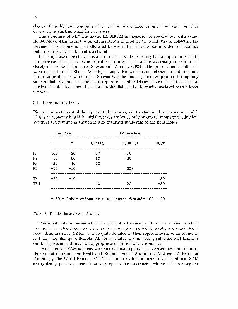
52
classes of equilibrium structures which can be investigated using the software, but theydo provide a starting point for new users.
The structure of MPSGE model HARBERGER is \generic" Arrow-Debreu with taxes.Households obtain income by supplying factors of production to industry or collecting taxrevenue. This income is then allocated between alternative goods in order to maximizewelfare subject to the budget constraint.
Firms operate subject to constant returns to scale, selecting factor inputs in order tominimize cost subject to technological constraints. For an algebraic description of a modelclosely related to this one, see Shoven and Whalley (1984). The present model di�ers intwo respects from the Shoven-Whalley example. First, in this model there are intermediateinputs to production while in the Shoven-Whalley model goods are produced using onlyvalue-added. Second, this model incorporates a labor-leisure choice so that the excessburden of factor taxes here incorporates the disincentive to work associated with a lowernet wage.
3.1. Benchmark Data
Figure 1 presents most of the input data for a two good, two factor, closed economy model.This is an economy in which, initially, taxes are levied only on capital inputs to production.We treat tax revenue as though it were returned lump-sum to the households.
Sectors Consumers
----------------------------------------------------
X Y OWNERS WORKERS GOVT
----------------------------------------------------
PX 100 -20 -30 -50
PY -10 80 -40 -30
PK -20 -40 60
PL -50 -10 60*
----------------------------------------------------
TK -20 -10 30
TRN 10 20 -30
----------------------------------------------------
* 60 = labor endowment net leisure demand= 100 - 40
Figure 1. The Benchmark Social Accounts
The input data is presented in the form of a balanced matrix, the entries in whichrepresent the value of economic transactions in a given period (typically one year). Socialaccounting matrices (SAMs) can be quite detailed in their representation of an economy,and they are also quite exible. All sorts of inter-account taxes, subsidies and transferscan be represented through an appropriate de�nition of the accounts.
Traditionally, a SAM is square with an exact correspondence between rows and columns.(For an introduction, see Pyatt and Round, \Social Accounting Matrices: A Basis forPlanning", The World Bank, 1985.) The numbers which appear in a conventional SAMare typically positive, apart from very special circumstances, whereas the rectangular
MPSGE Syntax 53
SAM displayed in Figure 1 follows a sign convention wherein supplies or receipts arerepresented by positive numbers and demands or payments are represented by negativenumbers. Internal consistency of a rectangular SAM implies that row sums and columnsums are zero. This means that supply equals demand for all goods and factors, taxpayments equal tax receipts, there are no excess pro�ts in production, the value of eachhousehold expenditure equals the value of factor income plus transfers, and the value ofgovernment tax revenue equals the value of transfers to households.
With simple MPSGE models, it is convenient to use a rectangular SAM format. Thisformat emphasizes how the MPSGE program structure is connected to the benchmarkdata. In the rectangular SAM, we have one row for every market (traded commodity),one column for every production sector, and one column for every consumer. Benchmarkequilibrium is re ected in the row and column sums. Columns corresponding to sectorssum to zero re ecting zero excess pro�t (the value of output equals the cost of inputs).Columns corresponding to consumers sum to zero indicating income balance. Rows sumto zero indicating market clearance.
In the present model, there are four markets, for goods X and Y and factors L andK; two production sectors (X and Y) and three consumers (OWNERS, WORKERS andGOVT).
3.2. Data Entry in GAMS
Consider a generalized version of the model in which the set of production sectors bedenoted S (here, S = fX,Yg ). Let the set of goods be G. Production sectors are mappedone-to-one with the goods, so we see that sets S and G are in fact the same set. Let F
denote the set of primary factors (here, F=fL,Kg), and let H denote the set of households(here H=fOWNER,WORKERg).
Now that we have identi�ed the underlying sets, we may interpret the input matrixas a set of parameters with which we can easily specify the benchmark equilibrium. (SeeFigure 2.) It is quite common to begin a general equilibrium modelling project with alarge input-output Figure or social accounting matrix which may then be mapped ontoa number of submatrices, each of which is dimensioned according to the underlying setsused in the model.
It should be emphasized at this point that there is an enormous di�erence betweenFigures 1 and 2. While Figure 1 concisely represents an equilibrium for a single two-sectormodel, Figure 2 represents an arbitrary set of commodities, factors, production sectorsand households. Scalability is an enormous advantage of the GAMS/MPSGE modelingenvironment. Model implementation and debugging can be conducted on a tiny prototype,and then the same computer code can be employed with a large-scale dataset.
The GAMS speci�cation of benchmark data is presented in Figure 3 which begins witha statement of the underlying sets (G, F, H). The statement \ALIAS (S,G);" simplysays that S and G both reference fX,Yg. Thereafter follows the social accounting datatable and declarations for the various submatrices. The parameters ELAS() and ESUB()
are elasticities (\free parameters") which can be chosen independently from the benchmarkaccounts. The parameters TF and PF are calibrated tax and reference price arrays whichare computed given benchmark factor and tax payments. (In this model, average andmarginal tax rates are not distinguished, so the benchmark marginal tax rate is simplythe tax payment divided by the net factor income.)
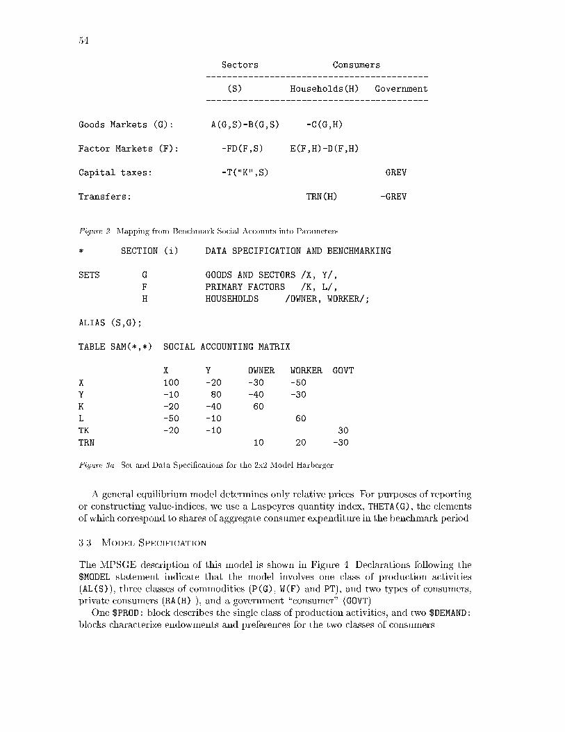
54
Sectors Consumers
------------------------------------------
(S) Households(H) Government
------------------------------------------
Goods Markets (G): A(G,S)-B(G,S) -C(G,H)
Factor Markets (F): -FD(F,S) E(F,H)-D(F,H)
Capital taxes: -T("K",S) GREV
Transfers: TRN(H) -GREV
Figure 2. Mapping from Benchmark Social Accounts into Parameters
* SECTION (i) DATA SPECIFICATION AND BENCHMARKING
SETS G GOODS AND SECTORS /X, Y/,
F PRIMARY FACTORS /K, L/,
H HOUSEHOLDS /OWNER, WORKER/;
ALIAS (S,G);
TABLE SAM(*,*) SOCIAL ACCOUNTING MATRIX
X Y OWNER WORKER GOVT
X 100 -20 -30 -50
Y -10 80 -40 -30
K -20 -40 60
L -50 -10 60
TK -20 -10 30
TRN 10 20 -30
Figure 3a. Set and Data Speci�cations for the 2x2 Model Harberger
A general equilibrium model determines only relative prices. For purposes of reportingor constructing value-indices, we use a Laspeyres quantity index, THETA(G), the elementsof which correspond to shares of aggregate consumer expenditure in the benchmark period.
3.3. Model Specification
The MPSGE description of this model is shown in Figure 4. Declarations following the$MODEL statement indicate that the model involves one class of production activities(AL(S)), three classes of commodities (P(G), W(F) and PT), and two types of consumers,private consumers (RA(H) ), and a government \consumer" (GOVT).
One $PROD: block describes the single class of production activities, and two $DEMAND:
blocks characterize endowments and preferences for the two classes of consumers.

MPSGE Syntax 55
PARAMETER
A(S) BENCHMARK OUTPUT
B(G,S) USE MATRIX (GOODS INPUTS BY SECTOR)
C(G,H) HOUSEHOLD DEMAND
FD(F,S) FACTOR DEMAND BY SECTOR
E(F,H) FACTOR ENDOWMENTS
D(F,H) FACTOR DEMAND BY HOUSEHOLDS
T(F,S) TAX PAYMENT BY FACTOR BY SECTOR
TRN(H) TRANSFER REVENUE
ELAS(S) ELASTICITY OF SUBSTITUTION IN PRODUCTION
ESUB(H) ELASTICITY OF SUBSTITUTION IN DEMAND
GREV BENCHMARK GOVERNMENT REVENUE
TF(F,S) FACTOR TAX RATE
PF(F,S) BENCHMARK FACTOR PRICES GROSS OF TAX
THETA(G) WEIGHTS IN NUMERAIRE PRICE INDEX
WBAR(H) BENCHMARK WELFARE INDEX;
Figure 3b. Parameter Declarations for the 2x2 Model Harberger
* EXTRACT DATA FROM THE SOCIAL ACCOUNTING MATRIX:
A(S) = SAM(S,S); B(G,S) = MAX(0, -SAM(G,S));
C(G,H) = -SAM(G,H); FD(F,S) = -SAM(F,S);
E(F,H) = SAM(F,H); D(F,H) = 0;
T("K",S) = -SAM("TK",S); TRN(H) = SAM("TRN",H);
* INSTALL "FREE" ELASTICITY PARAMETERS:
E("L","WORKER") = 100; D("L","WORKER") = 40;
ELAS(S) = 1; ESUB(H) = 0.5;
* INSTALL FUNCTIONS OF BENCHMARK VALUES:
GREV = SUM(H, TRN(H));
TF(F,S) = T(F,S) / FD(F,S);
PF(F,S) = 1 + TF(F,S);
THETA(G) = SUM(H, C(G,H));
THETA(G) = THETA(G) / SUM(S, THETA(S));
WBAR(H) = SUM(G, C(G,H)) + SUM(F, D(F,H));
Figure 3c. Parameter Assignments for the 2x2 Model Harberger
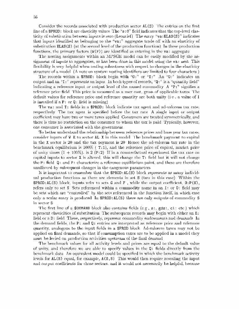
56
Consider the records associated with production sector AL(S). The entries on the �rstline of a $PROD: block are elasticity values. The \s:0" �eld indicates that the top-level elas-ticity of substitution between inputs is zero (Leontief). The entry \va:ELAS(S)" indicatesthat inputs identi�ed as belonging to the \va:" aggregate trade o� with an elasticity ofsubstitution ELAS(S) (at the second level of the production function). In these productionfunctions, the primary factors (W(F)) are identi�ed as entering in the va: aggregate.
The nesting assignments within an MPSGE model can be easily modi�ed by the as-signment of inputs to aggregates, as has been done in this model using the va: nest. This exibility is very helpful when testing robustness with respect to changes in the elasticitystructure of a model. (A note on syntax: nesting identi�ers are limited to four characters.)
The records within a $PROD: block begin with \O:" or \I:". An \O:" indicates anoutput and an \I:" represents an input. In both types of records, \Q:" is a \quantity �eld"indicating a reference input or output level of the named commodity. A \P:" signi�es areference price �eld. This price is measured as a user cost, gross of applicable taxes. Thedefault values for reference price and reference quantity are both unity (i.e., a value of 1is installed if a P: or Q: �eld is missing).
The va: and T: �elds in a $PROD: block indicate tax agent and ad-valorem tax rate,respectively. The tax agent is speci�ed before the tax rate. A single input or outputcoe�cient may have two or more taxes applied. Consumers are treated symmetrically, andthere is thus no restriction on the consumer to whom the tax is paid. Typically, however,one consumer is associated with the government.
To better understand the relationship between reference prices and base year tax rates,consider inputs of W.K to sector AL.X in this model. The benchmark payment to capitalin the X sector is 20 and the tax payment is 20. Hence the ad-valorem tax rate in thebenchmark equilibrium is 100% ( T:1), and the reference price of capital, market priceof unity times (1 + 100%), is 2 (P:2). If in a counterfactual experiment the tax rate oncapital inputs to sector X is altered, this will change the T: �eld but it will not changethe P: �eld. Q: and P: characterize a reference equilibrium point, and these are thereforeuna�ected by subsequent changes in the exogenous parameters.
It is important to remember that the $PROD:AL(S) block represents as many individ-ual production functions as there are elements in set S (two in this case). Within the$PROD:AL(S) block, inputs refer to sets G and F , while the output coe�cient, O:P(S),refers only to set S. Sets referenced within a commodity name in an I: or O: �eld maybe sets which are \controlled" by the sets referenced in the function itself, in which caseonly a scalar entry is produced. In $PROD:AL(S) there are only outputs of commodity S
in sector S.The �rst line of a $DEMAND block also contains �elds (e.g., s:, gds:, cl: etc.) which
represent elasticities of substitution. The subsequent records may begin with either an E:
�eld or a D: �eld. These, respectively, represent commodity endowments and demands. Inthe demand �elds, the P: and Q: entries are interpreted as reference price and referencequantity, analogous to the input �elds in a $PROD block. Ad-valorem taxes may not beapplied on �nal demands, so that if consumption taxes are to be applied in a model theymust be levied on production activities upstream of the �nal demand.
The benchmark values for all activity levels and prices are equal to the default valueof unity, and therefore we are able to specify values in the Q: �elds directly from thebenchmark data. An equivalent model could be speci�ed in which the benchmark activitylevels for AL(S) equal, for example, A(S,S). This would then require rescaling the inputand output coe�cients for those sectors, and it would not necessarily be helpful, because
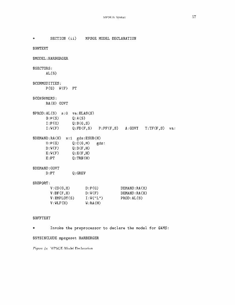
MPSGE Syntax 57
* SECTION (ii) MPSGE MODEL DECLARATION
$ONTEXT
$MODEL:HARBERGER
$SECTORS:
AL(S)
$COMMODITIES:
P(G) W(F) PT
$CONSUMERS:
RA(H) GOVT
$PROD:AL(S) s:0 va:ELAS(S)
O:P(S) Q:A(S)
I:P(G) Q:B(G,S)
I:W(F) Q:FD(F,S) P:PF(F,S) A:GOVT T:TF(F,S) va:
$DEMAND:RA(H) s:1 gds:ESUB(H)
D:P(G) Q:C(G,H) gds:
D:W(F) Q:D(F,H)
E:W(F) Q:E(F,H)
E:PT Q:TRN(H)
$DEMAND:GOVT
D:PT Q:GREV
$REPORT:
V:CD(G,H) D:P(G) DEMAND:RA(H)
V:DF(F,H) D:W(F) DEMAND:RA(H)
V:EMPLOY(S) I:W("L") PROD:AL(S)
V:WLF(H) W:RA(H)
$OFFTEXT
* Invoke the preprocessor to declare the model for GAMS:
$SYSINCLUDE mpsgeset HARBERGER
Figure 4a. MPSGE Model Declaration

58
* ------------------------------------------------------------------
* SECTION (iii) BENCHMARK REPLICATION
HARBERGER.ITERLIM = 0;
$INCLUDE HARBERGER.GEN
SOLVE HARBERGER USING MCP;
ABORT$(ABS(HARBERGER.OBJVAL) GT 1.E-4)
"*** HARBERGER benchmark does not calibrate.";
HARBERGER.ITERLIM = 1000;
Figure 4b. MPSGE Model Speci�cation and Benchmark Replication
in a scaled model it is more di�cult to verify consistency of the benchmark accounts andMPSGE input �le. Furthermore, for numerical reasons it is advisable to scale equilibriumvalues for the central variables to be close to unity.
Government transfers to households are accomplished through the use of an \arti�cialcommodity" (PT). The government is identi�ed as the agent who receives all tax revenue(see the A:GOVT entry in both of the $PROD: blocks). Commodity PT is the only commodityon which GOVT spends this income, hence government tax revenue is divided between thetwo households in proportion to their endowments of the arti�cial good. In order to scaleunits so that the benchmark price of PT is unity, the $30 of government tax revenue chases10 units of PT assigned to OWNER and 20 units assigned to WORKER. (See values for TRN(H)in Figure 3.)
The $REPORT section of the input �le requests the solution system to return valuesfor inputs, outputs, �nal demands or welfare indices at the equilibrium. Only those itemswhich are requested will be written to the solution �le. Each record in the report blockbegins with a V: (variable name) �eld. These names must be distinct from all other namesin the model. The second �eld of the report record must have one of the labels I:, O:or D: followed by a commodity name, or the label W: followed by a consumer name. Thethird �eld's label must be \PROD:" in an I: or O: record, and it must be \DEMAND:" if itis a D: record.
An algebraic formulation of the Harberger model is provided in Appendix D for theinterested reader.
3.4. MPSGE Formulation: Key Ideas
There are two points regarding the MPSGE function format which are important yet easilymisunderstood by new users:
(i) The elasticities together with the reference quantities and reference prices of inputsand outputs completely characterize the underlying nested CES functions. No other data�elds in the $PROD: block alters the technology. If, for example, a tax rate changes as partof a counter-factual experiment, this has no e�ect on the reference price. The value in theP: �eld depends on the benchmark value of the T: �eld if the model has been calibrated,but subsequent changes in T: do not change the underlying technology.
(ii) Tax rates are interpreted di�erently for inputs and outputs. The tax rate on inputsis speci�ed on a net basis, while the tax rate on outputs is speci�ed on a gross basis. That
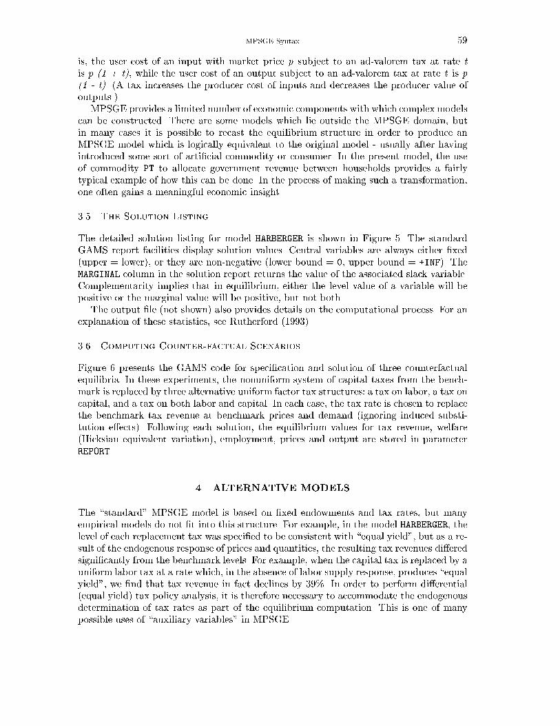
MPSGE Syntax 59
is, the user cost of an input with market price p subject to an ad-valorem tax at rate tis p (1 + t), while the user cost of an output subject to an ad-valorem tax at rate t is p(1 - t). (A tax increases the producer cost of inputs and decreases the producer value ofoutputs.)
MPSGE provides a limited number of economic components with which complex modelscan be constructed. There are some models which lie outside the MPSGE domain, butin many cases it is possible to recast the equilibrium structure in order to produce anMPSGE model which is logically equivalent to the original model - usually after havingintroduced some sort of arti�cial commodity or consumer. In the present model, the useof commodity PT to allocate government revenue between households provides a fairlytypical example of how this can be done. In the process of making such a transformation,one often gains a meaningful economic insight.
3.5. The Solution Listing
The detailed solution listing for model HARBERGER is shown in Figure 5. The standardGAMS report facilities display solution values. Central variables are always either �xed(upper = lower), or they are non-negative (lower bound = 0, upper bound = +INF). TheMARGINAL column in the solution report returns the value of the associated slack variable.Complementarity implies that in equilibrium, either the level value of a variable will bepositive or the marginal value will be positive, but not both.
The output �le (not shown) also provides details on the computational process. For anexplanation of these statistics, see Rutherford (1993).
3.6. Computing Counter-factual Scenarios
Figure 6 presents the GAMS code for speci�cation and solution of three counterfactualequilibria. In these experiments, the nonuniform system of capital taxes from the bench-mark is replaced by three alternative uniform factor tax structures: a tax on labor, a tax oncapital, and a tax on both labor and capital. In each case, the tax rate is chosen to replacethe benchmark tax revenue at benchmark prices and demand (ignoring induced substi-tution e�ects). Following each solution, the equilibrium values for tax revenue, welfare(Hicksian equivalent variation), employment, prices and output are stored in parameterREPORT.
4. ALTERNATIVE MODELS
The \standard" MPSGE model is based on �xed endowments and tax rates, but manyempirical models do not �t into this structure. For example, in the model HARBERGER, thelevel of each replacement tax was speci�ed to be consistent with \equal yield", but as a re-sult of the endogenous response of prices and quantities, the resulting tax revenues di�eredsigni�cantly from the benchmark levels. For example, when the capital tax is replaced by auniform labor tax at a rate which, in the absence of labor supply response, produces \equalyield", we �nd that tax revenue in fact declines by 39%. In order to perform di�erential(equal yield) tax policy analysis, it is therefore necessary to accommodate the endogenousdetermination of tax rates as part of the equilibrium computation. This is one of manypossible uses of \auxiliary variables" in MPSGE.
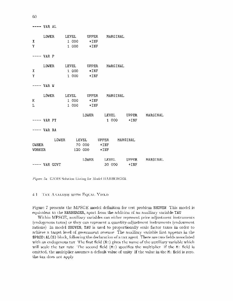
60
---- VAR AL
LOWER LEVEL UPPER MARGINAL
X . 1.000 +INF .
Y . 1.000 +INF .
---- VAR P
LOWER LEVEL UPPER MARGINAL
X . 1.000 +INF .
Y . 1.000 +INF .
---- VAR W
LOWER LEVEL UPPER MARGINAL
K . 1.000 +INF .
L . 1.000 +INF .
LOWER LEVEL UPPER MARGINAL
---- VAR PT . 1.000 +INF .
---- VAR RA
LOWER LEVEL UPPER MARGINAL
OWNER . 70.000 +INF .
WORKER . 120.000 +INF .
LOWER LEVEL UPPER MARGINAL
---- VAR GOVT . 30.000 +INF .
Figure 5a. GAMS Solution Listing for Model HARBERGER
4.1. Tax Analysis with Equal Yield
Figure 7 presents the MPSGE model de�nition for test problem SHOVEN. This model isequivalent to the HARBERGER, apart from the addition of an auxiliary variable TAU.
Within MPSGE, auxiliary variables can either represent price-adjustment instruments(endogenous taxes) or they can represent a quantity-adjustment instruments (endowmentrations). In model SHOVEN, TAU is used to proportionally scale factor taxes in order toachieve a target level of government revenue. The auxiliary variable �rst appears in the$PROD:AL(S) block, following the declaration of a tax agent. There are two �elds associatedwith an endogenous tax. The �rst �eld (N:) gives the name of the auxiliary variable whichwill scale the tax rate. The second �eld (M:) speci�es the multiplier. If the M: �eld isomitted, the multiplier assumes a default value of unity. If the value in the M: �eld is zero,the tax does not apply.
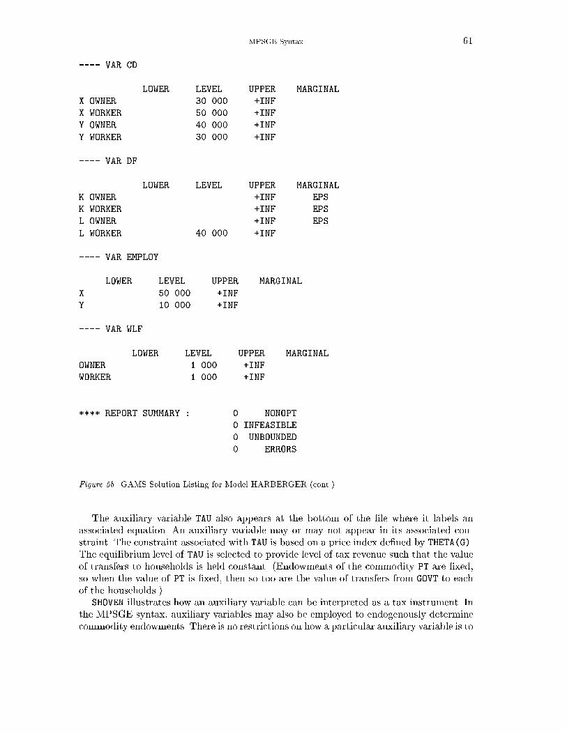
MPSGE Syntax 61
---- VAR CD
LOWER LEVEL UPPER MARGINAL
X.OWNER . 30.000 +INF .
X.WORKER . 50.000 +INF .
Y.OWNER . 40.000 +INF .
Y.WORKER . 30.000 +INF .
---- VAR DF
LOWER LEVEL UPPER MARGINAL
K.OWNER . . +INF EPS
K.WORKER . . +INF EPS
L.OWNER . . +INF EPS
L.WORKER . 40.000 +INF .
---- VAR EMPLOY
LOWER LEVEL UPPER MARGINAL
X . 50.000 +INF .
Y . 10.000 +INF .
---- VAR WLF
LOWER LEVEL UPPER MARGINAL
OWNER . 1.000 +INF .
WORKER . 1.000 +INF .
**** REPORT SUMMARY : 0 NONOPT
0 INFEASIBLE
0 UNBOUNDED
0 ERRORS
Figure 5b. GAMS Solution Listing for Model HARBERGER (cont.)
The auxiliary variable TAU also appears at the bottom of the �le where it labels anassociated equation. An auxiliary variable may or may not appear in its associated con-straint. The constraint associated with TAU is based on a price index de�ned by THETA(G).The equilibrium level of TAU is selected to provide level of tax revenue such that the valueof transfers to households is held constant. (Endowments of the commodity PT are �xed,so when the value of PT is �xed, then so too are the value of transfers from GOVT to eachof the households.)
SHOVEN illustrates how an auxiliary variable can be interpreted as a tax instrument. Inthe MPSGE syntax, auxiliary variables may also be employed to endogenously determinecommodity endowments. There is no restrictions on how a particular auxiliary variable is to
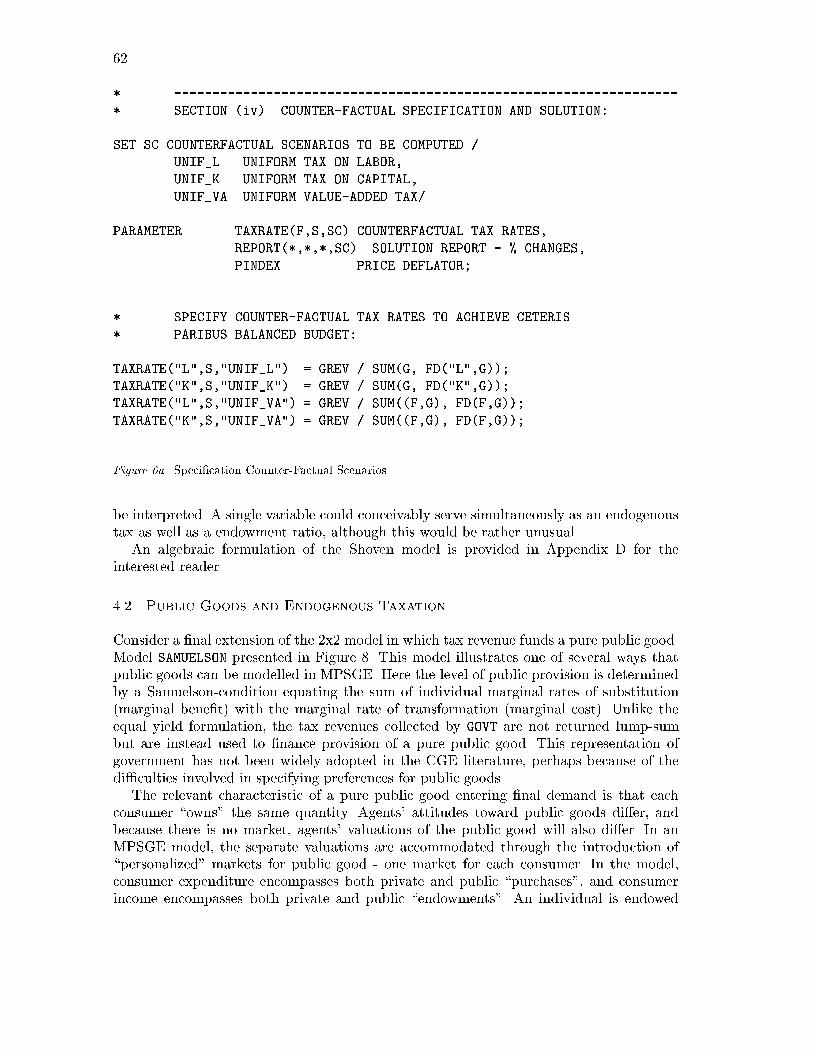
62
* ------------------------------------------------------------------
* SECTION (iv) COUNTER-FACTUAL SPECIFICATION AND SOLUTION:
SET SC COUNTERFACTUAL SCENARIOS TO BE COMPUTED /
UNIF_L UNIFORM TAX ON LABOR,
UNIF_K UNIFORM TAX ON CAPITAL,
UNIF_VA UNIFORM VALUE-ADDED TAX/
PARAMETER TAXRATE(F,S,SC) COUNTERFACTUAL TAX RATES,
REPORT(*,*,*,SC) SOLUTION REPORT - % CHANGES,
PINDEX PRICE DEFLATOR;
* SPECIFY COUNTER-FACTUAL TAX RATES TO ACHIEVE CETERIS
* PARIBUS BALANCED BUDGET:
TAXRATE("L",S,"UNIF_L") = GREV / SUM(G, FD("L",G));
TAXRATE("K",S,"UNIF_K") = GREV / SUM(G, FD("K",G));
TAXRATE("L",S,"UNIF_VA") = GREV / SUM((F,G), FD(F,G));
TAXRATE("K",S,"UNIF_VA") = GREV / SUM((F,G), FD(F,G));
Figure 6a. Speci�cation Counter-Factual Scenarios
be interpreted. A single variable could conceivably serve simultaneously as an endogenoustax as well as a endowment ratio, although this would be rather unusual.
An algebraic formulation of the Shoven model is provided in Appendix D for theinterested reader.
4.2. Public Goods and Endogenous Taxation
Consider a �nal extension of the 2x2 model in which tax revenue funds a pure public good.Model SAMUELSON presented in Figure 8. This model illustrates one of several ways thatpublic goods can be modelled in MPSGE. Here the level of public provision is determinedby a Samuelson-condition equating the sum of individual marginal rates of substitution(marginal bene�t) with the marginal rate of transformation (marginal cost). Unlike theequal yield formulation, the tax revenues collected by GOVT are not returned lump-sumbut are instead used to �nance provision of a pure public good. This representation ofgovernment has not been widely adopted in the CGE literature, perhaps because of thedi�culties involved in specifying preferences for public goods.
The relevant characteristic of a pure public good entering �nal demand is that eachconsumer \owns" the same quantity. Agents' attitudes toward public goods di�er, andbecause there is no market, agents' valuations of the public good will also di�er. In anMPSGE model, the separate valuations are accommodated through the introduction of\personalized" markets for public good - one market for each consumer. In the model,consumer expenditure encompasses both private and public \purchases", and consumerincome encompasses both private and public \endowments". An individual is endowed
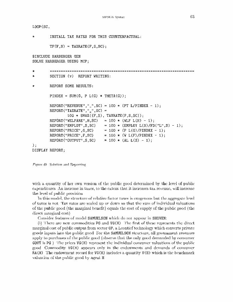
MPSGE Syntax 63
LOOP(SC,
* INSTALL TAX RATES FOR THIS COUNTERFACTUAL:
TF(F,S) = TAXRATE(F,S,SC);
$INCLUDE HARBERGER.GEN
SOLVE HARBERGER USING MCP;
* ------------------------------------------------------------------
* SECTION (v) REPORT WRITING:
* REPORT SOME RESULTS:
PINDEX = SUM(G, P.L(G) * THETA(G));
REPORT("REVENUE","_",SC) = 100 * (PT.L/PINDEX - 1);
REPORT("TAXRATE","_",SC) =
100 * SMAX((F,S), TAXRATE(F,S,SC));
REPORT("WELFARE",H,SC) = 100 * (WLF.L(H) - 1);
REPORT("EMPLOY",S,SC) = 100 * (EMPLOY.L(S)/FD("L",S) - 1);
REPORT("PRICE",G,SC) = 100 * (P.L(G)/PINDEX - 1);
REPORT("PRICE",F,SC) = 100 * (W.L(F)/PINDEX - 1);
REPORT("OUTPUT",S,SC) = 100 * (AL.L(S) - 1);
);
DISPLAY REPORT;
Figure 6b. Solution and Reporting
with a quantity of her own version of the public good determined by the level of publicexpenditures. An increase in taxes, to the extent that it increases tax revenue, will increasethe level of public provision.
In this model, the structure of relative factor taxes is exogenous but the aggregate levelof taxes is not. Tax rates are scaled up or down so that the sum of individual valuationsof the public good (the marginal bene�t) equals the cost of supply of the public good (thedirect marginal cost).
Consider features of model SAMUELSON which do not appear in SHOVEN:(i) There are new commodities PG and VG(H). The �rst of these represents the direct
marginal cost of public output from sector GP, a Leontief technology which converts privategoods inputs into the public good. For the SAMUELSON structure, all government revenuesapply to purchases of the public good (observe that the only good demanded by consumerGOVT is PG ). The prices VG(H) represent the individual consumer valuations of the publicgood. Commodity VG(H) appears only in the endowments and demands of consumerRA(H). The endowment record for VG(H) includes a quantity V(H) which is the benchmarkvaluation of the public good by agent H.

64
$ONTEXT
$MODEL: SHOVEN
$SECTORS:
AL(S)
$COMMODITIES:
P(G) W(F) PT
$CONSUMERS:
RA(H) GOVT
$AUXILIARY:
TAU
$REPORT:
V:CD(G,H) D:P(G) DEMAND:RA(H)
V:DF(F,H) D:W(F) DEMAND:RA(H)
V:EMPLOY(S) I:W("L") PROD:AL(S)
V:WLF(H) W:RA(H)
$PROD:AL(S) s:0 va:ELAS(S)
O:P(G) Q:A(G,S)
I:P(G) Q:B(G,S)
I:W(F) Q:FD(F,S) P:PF(F,S)
+ A:GOVT N:TAU$TF(F,S) M:TF(F,S)$TF(F,S) va:
$DEMAND:RA(H) s:1 gds:ESUB(H)
D:P(G) Q:C(G,H) gds:
D:W(F) Q:D(F,H)
E:W(F) Q:E(F,H)
E:PT Q:TRN(H)
$DEMAND:GOVT
D:PT Q:GREV
$CONSTRAINT:TAU
PT =E= SUM(G, THETA(G) * P(G));
$OFFTEXT
Figure 7. Di�erential Tax Policy Analysis
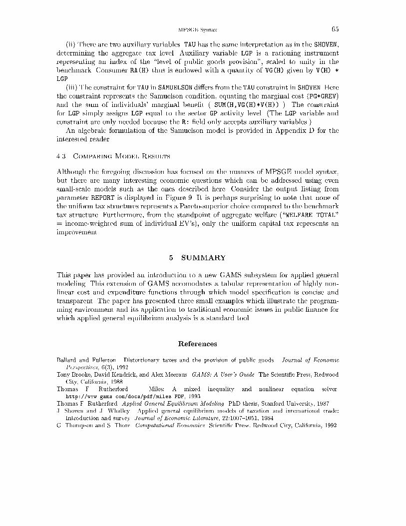
MPSGE Syntax 65
(ii) There are two auxiliary variables. TAU has the same interpretation as in the SHOVEN,determining the aggregate tax level. Auxiliary variable LGP is a rationing instrumentrepresenting an index of the \level of public goods provision", scaled to unity in thebenchmark. Consumer RA(H) thus is endowed with a quantity of VG(H) given by V(H) *
LGP .(iii) The constraint for TAU in SAMUELSON di�ers from the TAU constraint in SHOVEN. Here
the constraint represents the Samuelson condition, equating the marginal cost (PG*GREV)and the sum of individuals' marginal bene�t ( SUM(H,VG(H)*V(H)) ). The constraintfor LGP simply assigns LGP equal to the sector GP activity level. (The LGP variable andconstraint are only needed because the R: �eld only accepts auxiliary variables.)
An algebraic formulation of the Samuelson model is provided in Appendix D for theinterested reader.
4.3. Comparing Model Results
Although the foregoing discussion has focused on the nuances of MPSGE model syntax,but there are many interesting economic questions which can be addressed using evensmall-scale models such as the ones described here. Consider the output listing fromparameter REPORT is displayed in Figure 9. It is perhaps surprising to note that none ofthe uniform tax structures represents a Pareto-superior choice compared to the benchmarktax structure. Furthermore, from the standpoint of aggregate welfare (\WELFARE.TOTAL"= income-weighted sum of individual EV's), only the uniform capital tax represents animprovement.
5. SUMMARY
This paper has provided an introduction to a new GAMS subsystem for applied generalmodeling. This extension of GAMS accomodates a tabular representation of highly non-linear cost and expenditure functions through which model speci�cation is concise andtransparent. The paper has presented three small examples which illustrate the program-ming environment and its application to traditional economic issues in public �nance forwhich applied general equilibrium analysis is a standard tool.
References
Ballard and Fullerton. Distortionary taxes and the provision of public goods. Journal of Economic
Perspectives, 6(3), 1992.Tony Brooke, David Kendrick, and Alex Meeraus. GAMS: A User's Guide. The Scienti�c Press, Redwood
City, California, 1988.Thomas F. Rutherford. Miles: A mixed inequality and nonlinear equation solver.
http://www.gams.com/docs/pdf/miles.PDF, 1993.Thomas F. Rutherford. Applied General Equilibrium Modeling. PhD thesis, Stanford University, 1987.J. Shoven and J. Whalley. Applied general equilibrium models of taxation and international trade:
Introduction and survey. Journal of Economic Literature, 22:1007{1051, 1984.G. Thompson and S. Thore. Computational Economics. Scienti�c Press, Redwood City, California, 1992.
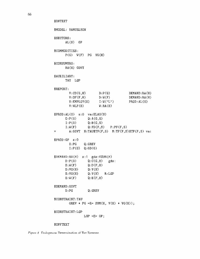
66
$ONTEXT
$MODEL: SAMUELSON
$SECTORS:
AL(S) GP
$COMMODITIES:
P(G) W(F) PG VG(H)
$CONSUMERS:
RA(H) GOVT
$AUXILIARY:
TAU LGP
$REPORT:
V:CD(G,H) D:P(G) DEMAND:RA(H)
V:DF(F,H) D:W(F) DEMAND:RA(H)
V:EMPLOY(S) I:W("L") PROD:AL(S)
V:WLF(H) W:RA(H)
$PROD:AL(S) s:0 va:ELAS(S)
O:P(G) Q:A(G,S)
I:P(G) Q:B(G,S)
I:W(F) Q:FD(F,S) P:PF(F,S)
+ A:GOVT N:TAU$TF(F,S) M:TF(F,S)$TF(F,S) va:
$PROD:GP s:0
O:PG Q:GREV
I:P(G) Q:GD(G)
$DEMAND:RA(H) s:1 gds:ESUB(H)
D:P(G) Q:C(G,H) gds:
D:W(F) Q:D(F,H)
D:VG(H) Q:V(H)
E:VG(H) Q:V(H) R:LGP
E:W(F) Q:E(F,H)
$DEMAND:GOVT
D:PG Q:GREV
$CONSTRAINT:TAU
GREV * PG =E= SUM(H, V(H) * VG(H));
$CONSTRAINT:LGP
LGP =E= GP;
$OFFTEXT
Figure 8. Endogenous Determination of Tax Revenue
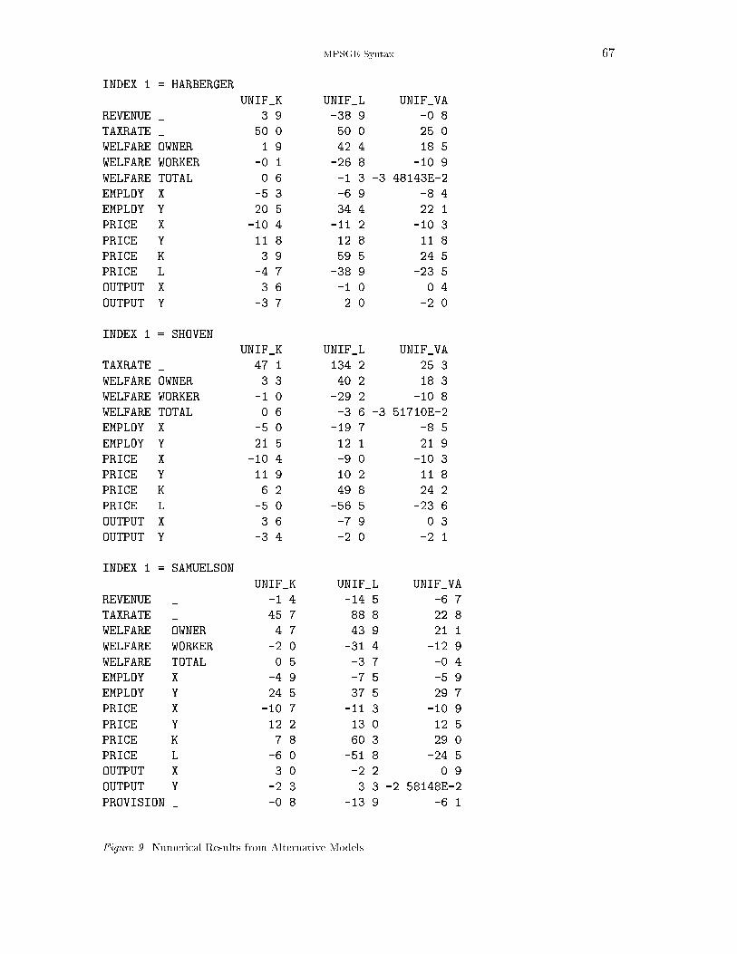
MPSGE Syntax 67
INDEX 1 = HARBERGER
UNIF_K UNIF_L UNIF_VA
REVENUE._ 3.9 -38.9 -0.8
TAXRATE._ 50.0 50.0 25.0
WELFARE.OWNER 1.9 42.4 18.5
WELFARE.WORKER -0.1 -26.8 -10.9
WELFARE.TOTAL 0.6 -1.3 -3.48143E-2
EMPLOY .X -5.3 -6.9 -8.4
EMPLOY .Y 20.5 34.4 22.1
PRICE .X -10.4 -11.2 -10.3
PRICE .Y 11.8 12.8 11.8
PRICE .K 3.9 59.5 24.5
PRICE .L -4.7 -38.9 -23.5
OUTPUT .X 3.6 -1.0 0.4
OUTPUT .Y -3.7 2.0 -2.0
INDEX 1 = SHOVEN
UNIF_K UNIF_L UNIF_VA
TAXRATE._ 47.1 134.2 25.3
WELFARE.OWNER 3.3 40.2 18.3
WELFARE.WORKER -1.0 -29.2 -10.8
WELFARE.TOTAL 0.6 -3.6 -3.51710E-2
EMPLOY .X -5.0 -19.7 -8.5
EMPLOY .Y 21.5 12.1 21.9
PRICE .X -10.4 -9.0 -10.3
PRICE .Y 11.9 10.2 11.8
PRICE .K 6.2 49.8 24.2
PRICE .L -5.0 -56.5 -23.6
OUTPUT .X 3.6 -7.9 0.3
OUTPUT .Y -3.4 -2.0 -2.1
INDEX 1 = SAMUELSON
UNIF_K UNIF_L UNIF_VA
REVENUE ._ -1.4 -14.5 -6.7
TAXRATE ._ 45.7 88.8 22.8
WELFARE .OWNER 4.7 43.9 21.1
WELFARE .WORKER -2.0 -31.4 -12.9
WELFARE .TOTAL 0.5 -3.7 -0.4
EMPLOY .X -4.9 -7.5 -5.9
EMPLOY .Y 24.5 37.5 29.7
PRICE .X -10.7 -11.3 -10.9
PRICE .Y 12.2 13.0 12.5
PRICE .K 7.8 60.3 29.0
PRICE .L -6.0 -51.8 -24.5
OUTPUT .X 3.0 -2.2 0.9
OUTPUT .Y -2.3 3.3 -2.58148E-2
PROVISION._ -0.8 -13.9 -6.1
Figure 9. Numerical Results from Alternative Models
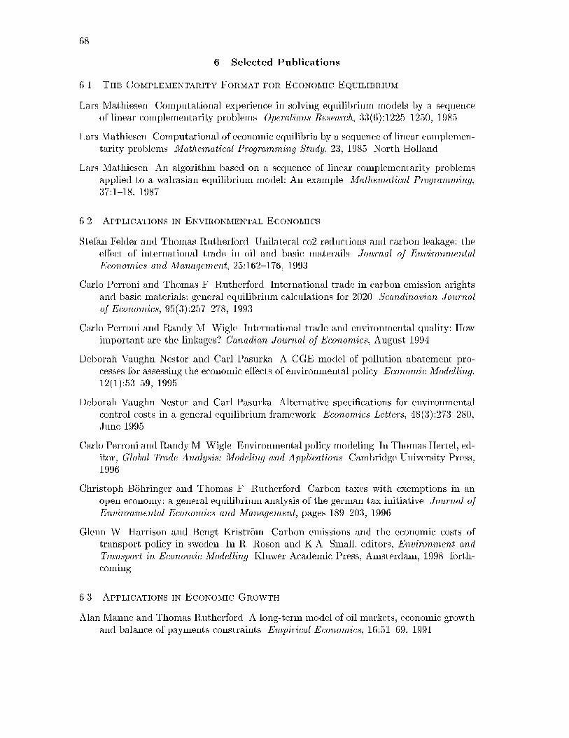
68
6. Selected Publications
6.1. The Complementarity Format for Economic Equilibrium
Lars Mathiesen. Computational experience in solving equilibrium models by a sequenceof linear complementarity problems. Operations Research, 33(6):1225{1250, 1985.
Lars Mathiesen. Computational of economic equilibria by a sequence of linear complemen-tarity problems. Mathematical Programming Study, 23, 1985. North Holland.
Lars Mathiesen. An algorithm based on a sequence of linear complementarity problemsapplied to a walrasian equilibrium model: An example. Mathematical Programming,37:1{18, 1987.
6.2. Applications in Environmental Economics
Stefan Felder and Thomas Rutherford. Unilateral co2 reductions and carbon leakage: thee�ect of international trade in oil and basic materails. Journal of EnvironmentalEconomics and Management, 25:162{176, 1993.
Carlo Perroni and Thomas F. Rutherford. International trade in carbon emission arightsand basic materials: general equilibrium calculations for 2020. Scandinavian Journalof Economics, 95(3):257{278, 1993.
Carlo Perroni and Randy M. Wigle. International trade and environmental quality: Howimportant are the linkages? Canadian Journal of Economics, August 1994.
Deborah Vaughn Nestor and Carl Pasurka. A CGE model of pollution abatement pro-cesses for assessing the economic e�ects of environmental policy. Economic Modelling,12(1):53{59, 1995.
Deborah Vaughn Nestor and Carl Pasurka. Alternative speci�cations for environmentalcontrol costs in a general equilibrium framework. Economics Letters, 48(3):273{280,June 1995.
Carlo Perroni and Randy M. Wigle. Environmental policy modeling. In Thomas Hertel, ed-itor, Global Trade Analysis: Modeling and Applications. Cambridge University Press,1996.
Christoph B�ohringer and Thomas F. Rutherford. Carbon taxes with exemptions in anopen economy: a general equilibrium analysis of the german tax initiative. Journal ofEnvironmental Economics and Management, pages 189{203, 1996.
Glenn W. Harrison and Bengt Kristr�om. Carbon emissions and the economic costs oftransport policy in sweden. In R. Roson and K.A. Small, editors, Environment andTransport in Economic Modelling. Kluwer Academic Press, Amsterdam, 1998. forth-coming.
6.3. Applications in Economic Growth
Alan Manne and Thomas Rutherford. A long-term model of oil markets, economic growthand balance of payments constraints. Empirical Economics, 16:51{69, 1991.
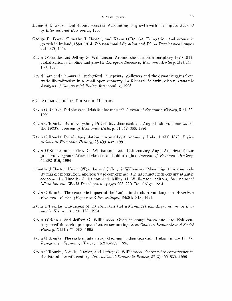
MPSGE Syntax 69
James R. Markusen and Robert Feenstra. Accounting for growth with new inputs. Journalof International Economics, 1993.
George R. Boyer, Timothy J. Hatton, and Kevin O'Rourke. Emigration and economicgrowth in Ireland, 1850{1914. International Migration and World Development, pages221{239, 1994.
Kevin O'Rourke and Je�rey G. Williamson. Around the european periphery 1870-1913:globalization, schooling and growth. European Review of Economic History, 1(2):153{190, 1995.
David Tarr and Thomas F. Rutherford. Blueprints, spillovers and the dynamic gains fromtrade liberalization in a small open economy. In Richard Baldwin, editor, DynamicAnalysis of Commercial Policy. forthcoming, 1998.
6.4. Applications in Economic History
Kevin O'Rourke. Did the great irish famine matter? Journal of Economic History, 51:1{22,1991.
Kevin O'Rourke. Burn everything British but their coal: the Anglo-Irish economic war ofthe 1930's. Journal of Economic History, 51:357{366, 1991.
Kevin O'Rourke. Rural depopulation in a small open economy: Ireland 1856{1876. Explo-rations in Economic History, 28:409{432, 1991.
Kevin O'Rourke and Je�rey G. Williamson. Late 19th century Anglo-American factorprice convergence: Were heckscher and ohlin right? Journal of Economic History,54:892{916, 1994.
Timothy J. Hatton, Kevin O'Rourke, and Je�rey G. Williamson. Mass migration, commod-ity market integration, and real wage convergence: the late nineteenth century atlanticeconomy. In Timothy J. Hatton and Je�rey G. Williamson, editors, InternationalMigration and World Development, pages 203{220. Routledge, 1994.
Kevin O'Rourke. The economic impact of the famine in the short and long run. AmericanEconomic Review (Papers and Proceedings), 84:309{313, 1994.
Kevin O'Rourke. The repeal of the corn laws and irish emigration. Explorations in Eco-nomic History, 31:120{138, 1994.
Kevin O'Rourke and Je�rey G. Williamson. Open economy forces and late 19th cen-tury swedish catch-up: a quantitative accounting. Scandinavian Economic and SocialHistory, XLIII:171{203, 1995.
Kevin O'Rourke. The costs of international economic disintegration: Ireland in the 1930's.Research in Economic History, 15:215{259, 1995.
Kevin O'Rourke, Alan M. Taylor, and Je�rey G. Williamson. Factor price convergence inthe late nineteenth century. International Economic Review, 37(3):499{530, 1996.
70
Kevin O'Rourke. The european grain invasion, 1870-1913. Journal of Economic History,forthcoming, 1998.
6.5. Applications in International Trade
Jan Haaland, Victor Norman, Thomas F. Rutherford, and Tor Wergeland. Vemod: Amodel of world trade. Scandinavian Journal of Economics, 89(3):705{721, 1987.
Glenn W. Harrison, Thomas F. Rutherford, and Ian Wooton. The economic impact of theeuropean community. American Economic Review (Papers and Proceedings), 79:288-294, 1989.
Trien Nguyen, Carlo Perroni, and Randy M. Wigle. An evaluation of the draft �nal act ofthe uruguay round. Economic Journal, November 1993.
Glenn W. Harrison, Thomas F. Rutherford, and David Tarr. Trade reform in the partiallyliberalized economy of Turkey. The World Bank Economic Review, 7(2):191{217,1993.
Florencio Lopez de Silanes, James R. Markusen, and Thomas F. Rutherford. Comple-mentarity and increasing returns in intermediate inputs. Journal of DevelopmentEconomics, 45:133{151, 1994.
Linda Hunter, James R. Markusen, and Thomas F. Rutherford. North American freetrade and the production of �nished automobiles. In Timothy Kehoe and Patrick Ke-hoe, editors,Modeling North American Economic Integration, pages 117{130. Kluwer,1995.
Joseph F. Francois, B. McDonald, and H. Nordstrom. The uruguay round: A numericallybased qualitative assessment. In W. Martin and L.A. Winters, editors, The UruguayRound and the Developing Countries. Cambridge University Press, New York, 1996.
Florencio Lopez de Silanes, James R. Markusen, and Thomas F. Rutherford. Trade policysubtleties with multinational �rms. European Economic Review, pages 1605{1627,1996.
James R. Markusen. The boundaries of multinational enterprises and the theory of inter-national trade. Journal of Economic Perspectives, 9:169{189, 1995.
Glenn W. Harrison, Thomas F. Rutherford, and David Tarr. Quantifying the Uruguayround. Economic Journal, 107:1405-1430, 1997.
Kevin O'Rourke. Measuring protection: a cautionary tale. Journal of Development Eco-nomics, 53(1):169{183, 1997.
Thomas F. Rutherford, David Tarr, and Elisabet Rutstrm. Morocco's free trade agreementwith the EU: A quantitative assessment. Economic Modelling, 14(2):237{269, April1997.
GlennW. Harrison, Thomas F. Rutherford, and David Tarr. Opciones de poltica comercialpara Chile: una evaluacin cuantitiva. Cuadernos de Economa 34:101-137, 1997.
MPSGE Syntax 71
James R. Markusen and Anthony J. Venables. The role of multinational �rms in the wagegap debate. Review of International Economics, 5:435{451, 1997.
James R. Markusen and Anthony J. Venables. Multinational �rms and the new tradetheory. Journal of International Economics, forthcoming,1998. NBER working paper5036.
6.6. Other Applications
Thomas F. Rutherford, John Whalley, and Randy Wigle. Capitalization, conditionalityand dilution: Land prices and the U.S. wheat program. Journal of Policy Modelling,12(3):605{622, 1990.
Kevin O'Rourke. Industrial policy, employment policy and the non-traded sector. Jour-nal of the Statistical and Social Inquiry Society of Ireland, XXVII, Part II:61{80,1994/1995.
Keith Maskus, Thomas F. Rutherford, and Steven Selby. Economic implications of changesin labor standards: A computational analysis for Mexico. North American Journal ofEconomics and Finance, 6(1):171{188, 1996.
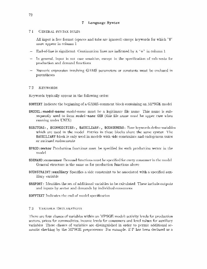
72
7. Language Syntax
7.1. General syntax rules
� All input is free format (spaces and tabs are ignored) except keywords for which "$"must appear in column 1.
� End-of-line is signi�cant. Continuation lines are indicated by a \+" in column 1.
� In general, input is not case sensitive, except in the speci�cation of sub-nests forproduction and demand functions.
� Numeric expression involving GAMS parameters or constants must be enclosed inparentheses.
7.2. Keywords
Keywords typically appear in the following order:
$ONTEXT Indicate the beginning of a GAMS comment block containing an MPSGE model.
$MODEL:model-name model-name must be a legitimate �le name. This name is sub-sequently used to form model-name.GEN (this �le name must be upper case whenrunning under UNIX).
$SECTORS:, $COMMODITIES:, $AUXILIARY:, $CONSUMERS: Four keywords de�ne variableswhich are used in the model. Entries in these blocks share the same syntax. The$AUXILIARY block is only used in models with side constraints and endogenous taxesor rationed endowments.
$PROD:sector Production functions must be speci�ed for each production sector in themodel.
$DEMAND:consumer Demand functions must be speci�ed for every consumer in the model.General structure is the same as for production functions above.
$CONSTRAINT:auxiliary Speci�es a side constraint to be associated with a speci�ed aux-iliary variable.
$REPORT: Identi�es the set of additional variables to be calculated. These include outputsand inputs by sector and demands by individual consumers.
$OFFTEXT Indicates the end of model speci�cation.
7.3. Variable Declarations
There are four classes of variables within an MPSGE model: activity levels for productionsectors, prices for commodities, income levels for consumers and level values for auxiliaryvariables. These classes of variables are distinguished in order to permit additional se-mantic checking by the MPSGE preprocessor. For example, if P has been declared as a
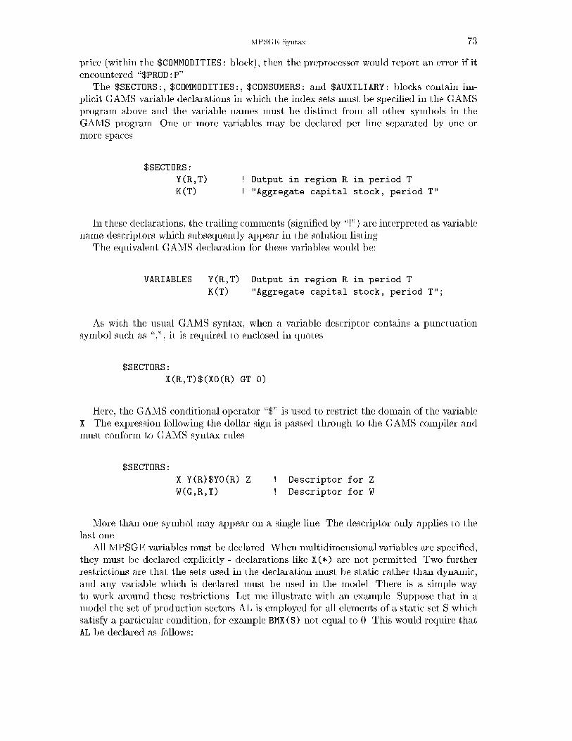
MPSGE Syntax 73
price (within the $COMMODITIES: block), then the preprocessor would report an error if itencountered \$PROD:P".
The $SECTORS:, $COMMODITIES:, $CONSUMERS: and $AUXILIARY: blocks contain im-plicit GAMS variable declarations in which the index sets must be speci�ed in the GAMSprogram above and the variable names must be distinct from all other symbols in theGAMS program. One or more variables may be declared per line separated by one ormore spaces.
$SECTORS:
Y(R,T) ! Output in region R in period T
K(T) ! "Aggregate capital stock, period T"
In these declarations, the trailing comments (signi�ed by \!") are interpreted as variablename descriptors which subsequently appear in the solution listing.
The equivalent GAMS declaration for these variables would be:
VARIABLES Y(R,T) Output in region R in period T
K(T) "Aggregate capital stock, period T";
As with the usual GAMS syntax, when a variable descriptor contains a punctuationsymbol such as \,", it is required to enclosed in quotes.
$SECTORS:
X(R,T)$(X0(R) GT 0)
Here, the GAMS conditional operator \$" is used to restrict the domain of the variableX. The expression following the dollar sign is passed through to the GAMS compiler andmust conform to GAMS syntax rules.
$SECTORS:
X Y(R)$Y0(R) Z ! Descriptor for Z
W(G,R,T) ! Descriptor for W
More than one symbol may appear on a single line. The descriptor only applies to thelast one.
All MPSGE variables must be declared. When multidimensional variables are speci�ed,they must be declared explicitly - declarations like X(*) are not permitted. Two furtherrestrictions are that the sets used in the declaration must be static rather than dynamic,and any variable which is declared must be used in the model. There is a simple wayto work around these restrictions. Let me illustrate with an example. Suppose that in amodel the set of production sectors AL is employed for all elements of a static set S whichsatisfy a particular condition, for example BMX(S) not equal to 0. This would require thatAL be declared as follows:
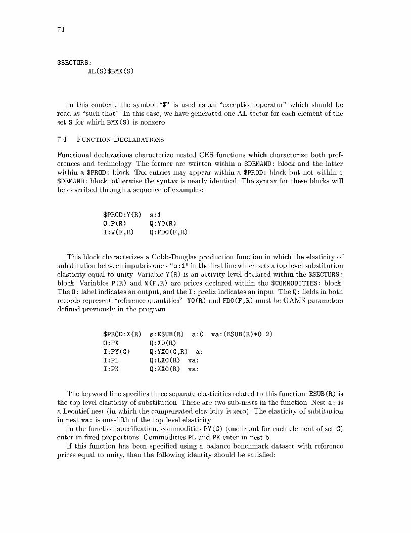
74
$SECTORS:
AL(S)$BMX(S)
In this context, the symbol \$" is used as an \exception operator" which should beread as \such that". In this case, we have generated one AL sector for each element of theset S for which BMX(S) is nonzero.
7.4. Function Declarations
Functional declarations characterize nested CES functions which characterize both pref-erences and technology. The former are written within a $DEMAND: block and the latterwithin a $PROD: block. Tax entries may appear within a $PROD: block but not within a$DEMAND: block, otherwise the syntax is nearly identical. The syntax for these blocks willbe described through a sequence of examples:
$PROD:Y(R) s:1
O:P(R) Q:Y0(R)
I:W(F,R) Q:FD0(F,R)
This block characterizes a Cobb-Douglas production function in which the elasticity ofsubstitution between inputs is one - "s:1" in the �rst line which sets a top level substitutionelasticity equal to unity. Variable Y(R) is an activity level declared within the $SECTORS:block. Variables P(R) and W(F,R) are prices declared within the $COMMODITIES: block.The O: label indicates an output, and the I: pre�x indicates an input. The Q: �elds in bothrecords represent \reference quantities". Y0(R) and FD0(F,R) must be GAMS parametersde�ned previously in the program.
$PROD:X(R) s:ESUB(R) a:0 va:(ESUB(R)*0.2)
O:PX Q:X0(R)
I:PY(G) Q:YX0(G,R) a:
I:PL Q:LX0(R) va:
I:PK Q:KX0(R) va:
The keyword line speci�es three separate elasticities related to this function. ESUB(R) isthe top level elasticity of substitution. There are two sub-nests in the function. Nest a: isa Leontief nest (in which the compensated elasticity is zero). The elasticity of subtitutionin nest va: is one-�fth of the top level elasticity.
In the function speci�cation, commodities PY(G) (one input for each element of set G)enter in �xed proportions. Commodities PL and PK enter in nest b.
If this function has been speci�ed using a balance benchmark dataset with referenceprices equal to unity, then the following identity should be satis�ed:
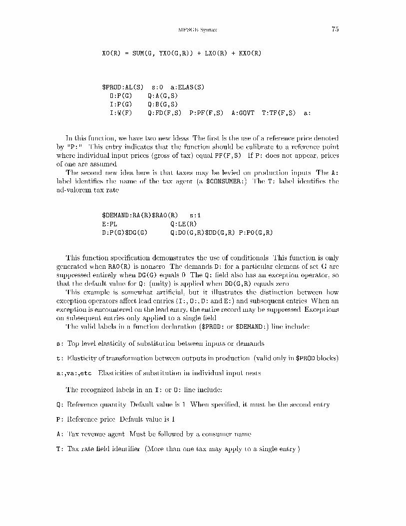
MPSGE Syntax 75
X0(R) = SUM(G, YX0(G,R)) + LX0(R) + KX0(R)
$PROD:AL(S) s:0 a:ELAS(S)
O:P(G) Q:A(G,S)
I:P(G) Q:B(G,S)
I:W(F) Q:FD(F,S) P:PF(F,S) A:GOVT T:TF(F,S) a:
In this function, we have two new ideas. The �rst is the use of a reference price denotedby "P:". This entry indicates that the function should be calibrate to a reference pointwhere individual input prices (gross of tax) equal PF(F,S). If P: does not appear, pricesof one are assumed.
The second new idea here is that taxes may be levied on production inputs. The A:
label identi�es the name of the tax agent (a $CONSUMER:). The T: label identi�es thead-valorem tax rate.
$DEMAND:RA(R)$RA0(R) s:1
E:PL Q:LE(R)
D:P(G)$DG(G) Q:D0(G,R)$DD(G,R) P:P0(G,R)
This function speci�cation demonstrates the use of conditionals. This function is onlygenerated when RA0(R) is nonzero. The demands D: for a particular element of set G aresuppressed entirely when DG(G) equals 0. The Q: �eld also has an exception operator, sothat the default value for Q: (unity) is applied when DD(G,R) equals zero.
This example is somewhat arti�cial, but it illustrates the distinction between howexception operators a�ect lead entries (I:, O:, D: and E:) and subsequent entries. When anexception is encountered on the lead entry, the entire record may be suppressed. Exceptionson subsequent entries only applied to a single �eld.
The valid labels in a function declaration ($PROD: or $DEMAND:) line include:
s: Top level elasticity of substitution between inputs or demands.
t: Elasticity of transformation between outputs in production. (valid only in $PROD blocks)
a:,va:,etc. Elasticities of substitution in individual input nests.
The recognized labels in an I: or O: line include:
Q: Reference quantity. Default value is 1. When speci�ed, it must be the second entry.
P: Reference price. Default value is 1.
A: Tax revenue agent. Must be followed by a consumer name.
T: Tax rate �eld identi�er. (More than one tax may apply to a single entry.)
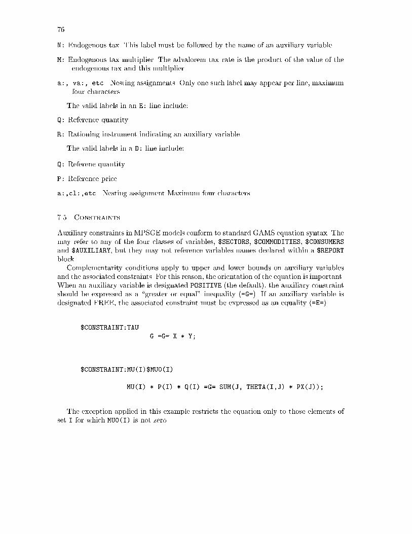
76
N: Endogenous tax. This label must be followed by the name of an auxiliary variable.
M: Endogenous tax multiplier. The advalorem tax rate is the product of the value of theendogenous tax and this multiplier.
a:, va:, etc. Nesting assignments. Only one such label may appear per line, maximumfour characters.
The valid labels in an E: line include:
Q: Reference quantity.
R: Rationing instrument indicating an auxiliary variable.
The valid labels in a D: line include:
Q: Referene quantity.
P: Reference price.
a:,cl:,etc. Nesting assignment Maximum four characters.
7.5. Constraints
Auxiliary constraints in MPSGE models conform to standard GAMS equation syntax. Themay refer to any of the four classes of variables, $SECTORS, $COMMODITIES, $CONSUMERSand $AUXILIARY, but they may not reference variables names declared within a $REPORT
block.Complementarity conditions apply to upper and lower bounds on auxiliary variables
and the associated constraints. For this reason, the orientation of the equation is important.When an auxiliary variable is designated POSITIVE (the default), the auxiliary constraintshould be expressed as a \greater or equal" inequality (=G=). If an auxiliary variable isdesignated FREE, the associated constraint must be expressed as an equality (=E=).
$CONSTRAINT:TAU
G =G= X * Y;
$CONSTRAINT:MU(I)$MU0(I)
MU(I) * P(I) * Q(I) =G= SUM(J, THETA(I,J) * PX(J));
The exception applied in this example restricts the equation only to those elements ofset I for which MU0(I) is not zero.
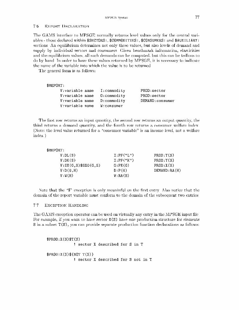
MPSGE Syntax 77
7.6. Report Declaration
The GAMS interface to MPSGE normally returns level values only for the central vari-ables - those declared within $SECTORS:, $COMMODITIES:, $CONSUMERS: and $AUXILIARY:
sections. An equilibrium determines not only these values, but also levels of demand andsupply by individual sectors and consumers. Given benchmark information, elasticitiesand the equilibrium values, all such demands can be computed, but this can be tedious todo by hand. In order to have these values returned by MPSGE, it is necessary to indicatethe name of the variable into which the value is to be returned.
The general form is as follows:
$REPORT:
V:variable name I:commodity PROD:sector
V:variable name O:commodity PROD:sector
V:variable name D:commodity DEMAND:consumer
V:variable name W:consumer
The �rst row returns an input quantity, the second row returns an output quantity, thethird returns a demand quantity, and the fourth row returns a consumer welfare index.(Note: the level value returned for a \consumer variable" is an income level, not a welfareindex.)
$REPORT:
V:DL(S) I:PF("L") PROD:Y(S)
V:DK(S) I:PF("K") PROD:Y(S)
V:SX(G,S)$SX0(G,S) O:PX(G) PROD:X(S)
V:D(G,H) D:P(G) DEMAND:RA(H)
V:W(H) W:RA(H)
Note that the \$" exception is only meaninful on the �rst entry. Also notice that thedomain of the report variable must conform to the domain of the subsequent two entries.
7.7. Exception Handling
The GAMS exception operator can be used on virtually any entry in the MPSGE input �le.For example, if you want to have sector X(S) have one production structure for elementsS in a subset T(S), you can provide separate production function declarations as follows:
$PROD:X(S)$T(S)
... ! sector X described for S in T
$PROD:X(S)$(NOT T(S))
... ! sector X described for S not in T.
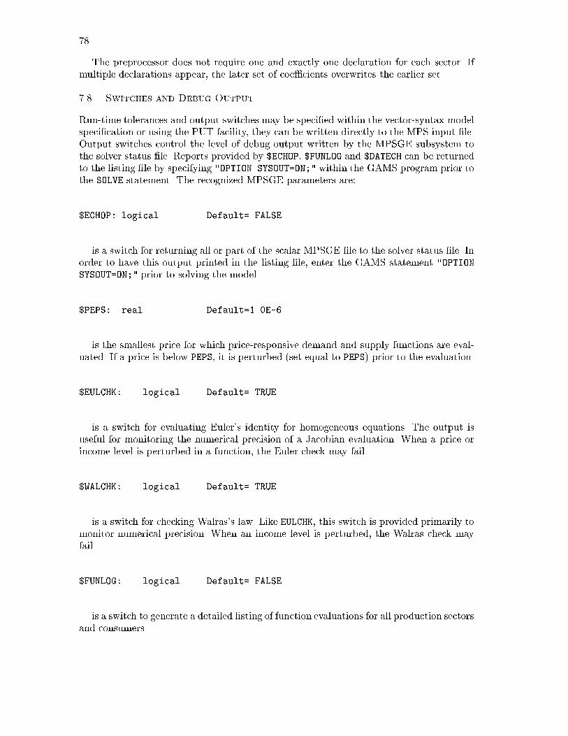
78
The preprocessor does not require one and exactly one declaration for each sector. Ifmultiple declarations appear, the later set of coe�cients overwrites the earlier set.
7.8. Switches and Debug Output
Run-time tolerances and output switches may be speci�ed within the vector-syntax modelspeci�cation or using the PUT facility, they can be written directly to the MPS input �le.Output switches control the level of debug output written by the MPSGE subsystem tothe solver status �le. Reports provided by $ECHOP, $FUNLOG and $DATECH can be returnedto the listing �le by specifying "OPTION SYSOUT=ON;" within the GAMS program prior tothe SOLVE statement. The recognized MPSGE parameters are:
$ECHOP: logical Default=.FALSE.
is a switch for returning all or part of the scalar MPSGE �le to the solver status �le. Inorder to have this output printed in the listing �le, enter the GAMS statement "OPTIONSYSOUT=ON;" prior to solving the model.
$PEPS: real Default=1.0E-6
is the smallest price for which price-responsive demand and supply functions are eval-uated. If a price is below PEPS, it is perturbed (set equal to PEPS) prior to the evaluation.
$EULCHK: logical Default=.TRUE.
is a switch for evaluating Euler's identity for homogeneous equations. The output isuseful for monitoring the numerical precision of a Jacobian evaluation. When a price orincome level is perturbed in a function, the Euler check may fail.
$WALCHK: logical Default=.TRUE.
is a switch for checking Walras's law. Like EULCHK, this switch is provided primarily tomonitor numerical precision. When an income level is perturbed, the Walras check mayfail.
$FUNLOG: logical Default=.FALSE.
is a switch to generate a detailed listing of function evaluations for all production sectorsand consumers.

MPSGE Syntax 79
FUNLOG triggers a function evaluation report which provides detailed output describingthe evaluation of supply and demand coe�cients. The information provide is su�cient thatan industrious graduate student should be able to reproduce the results (given a pencil,paper and slide rule).
The evaluation report has the following headings:
T Coe�cient "type" with the following interpretation:
IA Input aggregate
OA Output aggregate
I Input
O Output
D Demand
E Endowment
N Name (either nest identi�er or commodity name)
PBAR Benchmark price (the P: �eld value)
P Current price (gross of tax)
QBAR Benchmark quantitity (the Q: �eld value)
Q Current quantity
KP Identi�er for parent entry in nesting structure.
ELAS Associated elasticity (input or output aggregates only)
When $FUNLOG:.TRUE is speci�ed, a complete report of demand and supply coe�cientsfor every production and demand function in every iteration. Be warned that with largemodels this can produce an enrmous amount of output!
The following two function evaluation reports are generated in the �rst iteration insolving case "L" for model HARBERGER:
$DATECH: logical Default=.FALSE.
is a switch to generate a annotated listing of the function and Jacobian evaluationincluding a complete listing of all the nonzero coe�cients.
MPSGE generates an analytic full �rst-order Taylor series expansion of the nonlinearequations in every iteration. Nonzero elements of the Jacobian matrix are passed to thesystem solver (MILES or PATH) which uses this information in the direction-�nding stepof the Newton algorithm. Coe�cients are produced with codes which help interpret wherethey came from. The following codes are used:
W0 indicates an element from the orthogonal part of F().
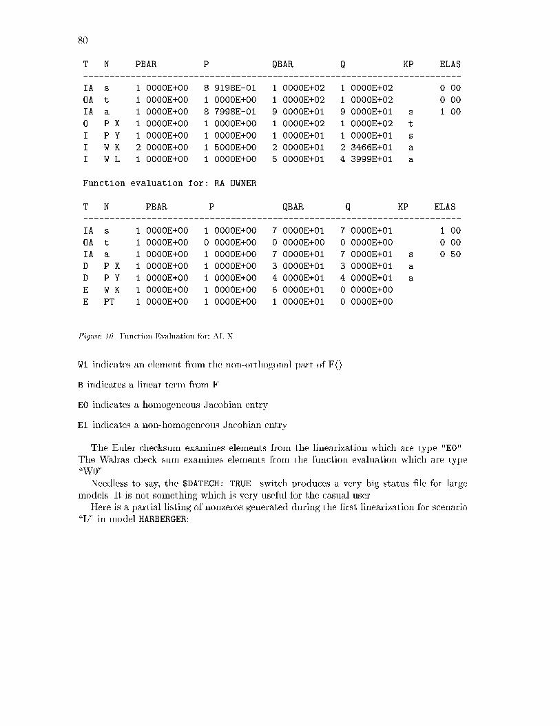
80
T N PBAR P QBAR Q KP ELAS
------------------------------------------------------------------------
IA s 1.0000E+00 8.9198E-01 1.0000E+02 1.0000E+02 0.00
OA t 1.0000E+00 1.0000E+00 1.0000E+02 1.0000E+02 0.00
IA a 1.0000E+00 8.7998E-01 9.0000E+01 9.0000E+01 s 1.00
O P.X 1.0000E+00 1.0000E+00 1.0000E+02 1.0000E+02 t
I P.Y 1.0000E+00 1.0000E+00 1.0000E+01 1.0000E+01 s
I W.K 2.0000E+00 1.5000E+00 2.0000E+01 2.3466E+01 a
I W.L 1.0000E+00 1.0000E+00 5.0000E+01 4.3999E+01 a
Function evaluation for: RA.OWNER
T N PBAR P QBAR Q KP ELAS
------------------------------------------------------------------------
IA s 1.0000E+00 1.0000E+00 7.0000E+01 7.0000E+01 1.00
OA t 1.0000E+00 0.0000E+00 0.0000E+00 0.0000E+00 0.00
IA a 1.0000E+00 1.0000E+00 7.0000E+01 7.0000E+01 s 0.50
D P.X 1.0000E+00 1.0000E+00 3.0000E+01 3.0000E+01 a
D P.Y 1.0000E+00 1.0000E+00 4.0000E+01 4.0000E+01 a
E W.K 1.0000E+00 1.0000E+00 6.0000E+01 0.0000E+00
E PT 1.0000E+00 1.0000E+00 1.0000E+01 0.0000E+00
Figure 10. Function Evaluation for: AL.X
W1 indicates an element from the non-orthogonal part of F().
B indicates a linear term from F.
E0 indicates a homogeneous Jacobian entry.
E1 indicates a non-homogeneous Jacobian entry.
The Euler checksum examines elements from the linearization which are type "E0".
The Walras check sum examines elements from the function evaluation which are type\W0".
Needless to say, the $DATECH:.TRUE. switch produces a very big status �le for largemodels. It is not something which is very useful for the casual user.
Here is a partial listing of nonzeros generated during the �rst linearization for scenario\L" in model HARBERGER:
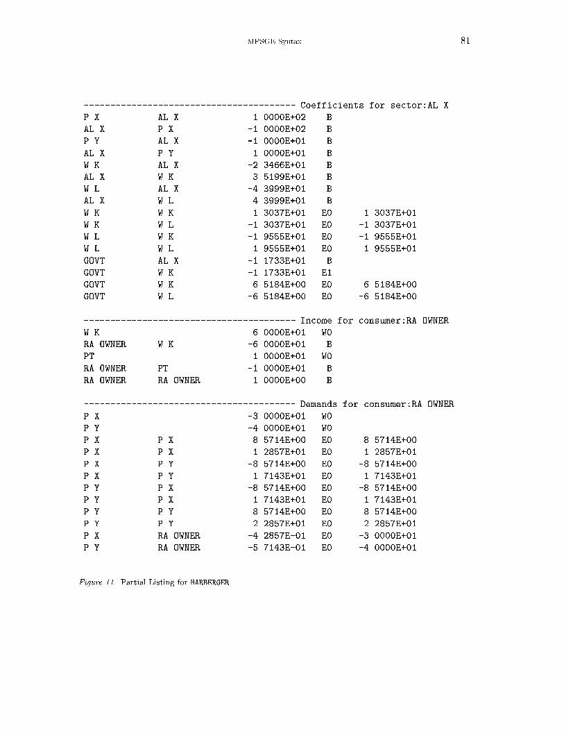
MPSGE Syntax 81
---------------------------------------- Coefficients for sector:AL.X
P.X AL.X 1.0000E+02 B
AL.X P.X -1.0000E+02 B
P.Y AL.X -1.0000E+01 B
AL.X P.Y 1.0000E+01 B
W.K AL.X -2.3466E+01 B
AL.X W.K 3.5199E+01 B
W.L AL.X -4.3999E+01 B
AL.X W.L 4.3999E+01 B
W.K W.K 1.3037E+01 E0 1.3037E+01
W.K W.L -1.3037E+01 E0 -1.3037E+01
W.L W.K -1.9555E+01 E0 -1.9555E+01
W.L W.L 1.9555E+01 E0 1.9555E+01
GOVT AL.X -1.1733E+01 B
GOVT W.K -1.1733E+01 E1
GOVT W.K 6.5184E+00 E0 6.5184E+00
GOVT W.L -6.5184E+00 E0 -6.5184E+00
---------------------------------------- Income for consumer:RA.OWNER
W.K 6.0000E+01 W0
RA.OWNER W.K -6.0000E+01 B
PT 1.0000E+01 W0
RA.OWNER PT -1.0000E+01 B
RA.OWNER RA.OWNER 1.0000E+00 B
---------------------------------------- Demands for consumer:RA.OWNER
P.X -3.0000E+01 W0
P.Y -4.0000E+01 W0
P.X P.X 8.5714E+00 E0 8.5714E+00
P.X P.X 1.2857E+01 E0 1.2857E+01
P.X P.Y -8.5714E+00 E0 -8.5714E+00
P.X P.Y 1.7143E+01 E0 1.7143E+01
P.Y P.X -8.5714E+00 E0 -8.5714E+00
P.Y P.X 1.7143E+01 E0 1.7143E+01
P.Y P.Y 8.5714E+00 E0 8.5714E+00
P.Y P.Y 2.2857E+01 E0 2.2857E+01
P.X RA.OWNER -4.2857E-01 E0 -3.0000E+01
P.Y RA.OWNER -5.7143E-01 E0 -4.0000E+01
Figure 11. Partial Listing for HARBERGER
82
8. File Structure
This appendix provides an overview of the structure of GAMS input �les which includeMPSGE models. The text of the paper presents many of these ideas by way of example,but it may also be helpful for some users to have a \template" for constructing MPSGEmodels. The discussion in this section focuses on a \generic" input �le, the schematic formof which is presented in Figure 10. This section �rst presents a \top down" view of programorganization, and then it discusses aspects of the new syntax for model speci�cation.8.1. Flow of Control
When a model is developed using GAMS as a front-end to MPSGE, the input �le generallyhas �ve sections as identi�ed in Figure 10. Section (i), the benchmarking section, containsstandard GAMS statements. This includes GAMS SET declarations, input data (SCALARS,PARAMETERS and TABLES ), and PARAMETER declarations for intermediate arrays used inbenchmarking or model speci�cation. In complex models, this section of the �le willtypically contain some algebraic derivations, the result of which is a calibrated benchmarkequilibrium dataset.
Users who are unfamiliar with GAMS can consult the manual. Beginning GAMS pro-grammers should remember that the MPSGE interface to GAMS is unlike other solutionsubsystems. \Level values" are passed between the GAMS program and MPSGE in theusual fashion, but MPSGE models do not require the explicit use of the VARIABLE orEQUATION statements.)
The second section of the �le consists of a GAMS comment range, beginning withan $ONTEXT record and ending with an $OFFTEXT record, followed by an invocation ofthe preprocessor. The preprocessor writes operates on statements in the MPSGE modeldeclaration which are \invisible" to the GAMS compiler. This program reads the MPSGEmodel statements and generates GAMS-readable code, including a model-name.gen �le.Additional GAMS code produced by the preprocessor includes declarations for each of thecentral variables and report variables in the MPSGE model.
The third section of the generic input �le performs a \benchmark replication" andmay not be present in all applications. There are four statements required for benchmarkvalidation. The �rst statement sets the iteration limit to be zero; the second statementcauses the MPSGE model to be \generated", and the third statement causes the MPSGEsolver to read the model and return the pdeviations. In this call, the level values passedto the solver are unaltered because the iteration limit is zero. Market excess supplies andzero pro�t checks are returned in the \marginals" of the associated commodity prices andactivity levels, respectively. The �nal statement in this section resets the iteration limit to1000 (the default value) for subsequent counter-factual computations.
Section (iv) de�nes and then computes a counter-factual equilibrium. A counter-factualequilibrium is de�ned by parameter values such as tax rates or endowments which takeon values di�erent from those in the benchmark equilibrium. Within the GAMS interfaceto MPSGE, it is also possible to �x one or more central variables. When any variable is�xed, the associated equation is omitted from the equilibrium system during the solutionprocess but the resulting imbalance is then reported in the solution returned through themarginal.
The �nal section of the �le represents the GAMS algebra required for comparingcounter-factual equilibria. It would be possible, for example, to construct welfare measures

MPSGE Syntax 83
or to report percentage changes in certain values. All of these calculations are quite easybecause the equilibrium values are returned as level values in the associated variables.
For large models, the advantage of the vector format is that by using appropriatelyde�ned GAMS sets, the number of individual functions which need to be de�ned is reducedonly to the number of \classes" of functions. This makes it possible to represent largedimensional models using only a few lines of code.
To summarize, here are the basic features of a program which uses GAMS as a front-endto MPSGE:
(i) An MPSGE model is de�ned within a GAMS comment range followed by
$sysinclude mpsgeset model-name
(ii) Every SOLVE statement for a particular model is preceded by $INCLUDE MODEL.GEN.The GEN �le is written by the preprocessor based on the model structure.
(iii) Solution values for the cental variables in the MPSGE model and any declared\report variables" are returned in GAMS variable level values. Level values for slacks arereturned as \marginals" for the associated variables.
(iv) The model description follows a format which is a direct extension of the scalardata format. Certain aspects of the new language, such as case folding, are incompatiblewith the original MPSGE syntax.
8.2. GAMS Code Generated by the Preprocessor: the GEN File
Most novice users will �nd it easiest to treat the preprocessor output �les as \black boxes".These �les contain GAMS source code required for declaring and generating the MPSGEinput �le. Figure 11 contains portions of the GEN �le for the same model. Figure 12 showsthe preprocessor-generated listing and symbol table which are always appended to thebottom of the GEN �le. If a preprocessor error occurs, it can be helpful to consult thesymbol table to track down the bug. Finally, Figure 13 shows the �rst page of scalarformat MPSGE input �le produced by HARBERGER.GEN. Normally, this �le is written andthen erased in the course of a GAMS run, although all or part of the �le may be retainedusing the $ECHOP: switch.

84
9. Algebraic Representations of Models in this Paper
9.1. The Harberger Model
Zero Net Pro�tThe unit cost of production in sector Ahs is given by a nested Leontief-CES functionde�ned over the cost of intermediate inputs and primary factors with ad-valorem taxeson factor demands. In equilibrium, the unit cost must be no less than the market price ofoutput:
��s =Xg
pgBbs + �s
0@X
f
�fs(wf (1 + tfs))1��s
1A
11��s
� ps � 0 8sj�s 6= 1
and
��s =Xg
pgBbs + �s
0@Y
f
(wf (1 + tfs))�fs
1A� ps � 0 8sj�s = 1
Income Balance for GovernmentGovernment tax income (PT ) is determined by the value of tax revenue, calculated usingactivity levels, compensated demands, market prices and ad-valorem tax rates:
PT =Xs
@�s
@(wf (1 + tfs))ALswf tfs
Income Balance for HouseholdsHousehold income is determined by the net of tax return to primary factors plus thehousehold share of government revenue:
Mh =Xf
wfEfh + shPT
Market Clearance for GoodsProducer output is equal to the sum of intermediate plus �nal demand:
ALg �Xs
ALsBgs +Xh
hMh
eh(p)
�eh(p)
pg
��h
where h is the household budget share devoted to the consumption of goods, and ehhis the \unit expenditure function" which may be written:
eh(p) � X
i
�ihp1��hi
! 11��h
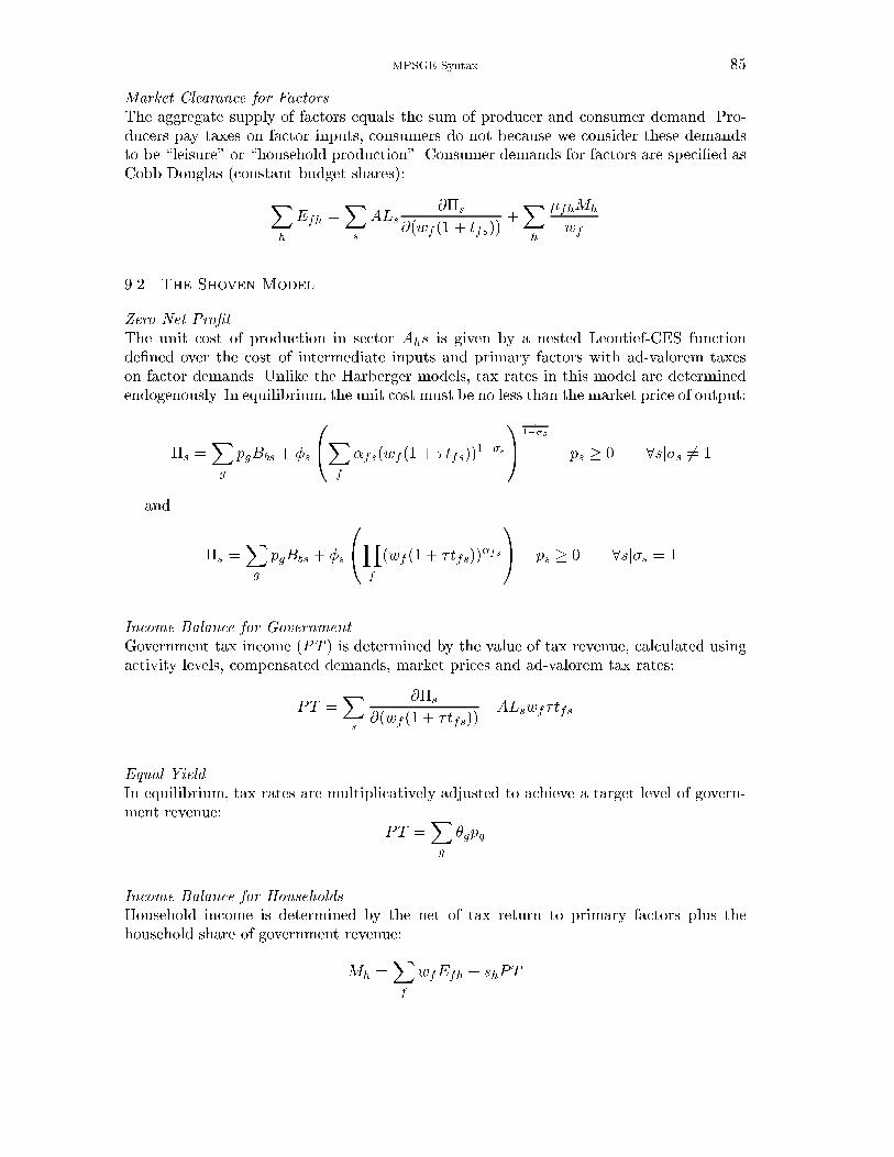
MPSGE Syntax 85
Market Clearance for FactorsThe aggregate supply of factors equals the sum of producer and consumer demand. Pro-ducers pay taxes on factor inputs, consumers do not because we consider these demandsto be \leisure" or \household production". Consumer demands for factors are speci�ed asCobb-Douglas (constant budget shares):
Xh
Efh =Xs
ALs@�s
@(wf (1 + tfs))+Xh
�fhMh
wf
9.2. The Shoven Model
Zero Net Pro�tThe unit cost of production in sector Ahs is given by a nested Leontief-CES functionde�ned over the cost of intermediate inputs and primary factors with ad-valorem taxeson factor demands. Unlike the Harberger models, tax rates in this model are determinedendogenously. In equilibrium, the unit cost must be no less than the market price of output:
��s =Xg
pgBbs + �s
0@X
f
�fs(wf (1 + �tfs))1��s
1A
11��s
� ps � 0 8sj�s 6= 1
and
��s =Xg
pgBbs + �s
0@Y
f
(wf (1 + �tfs))�fs
1A� ps � 0 8sj�s = 1
Income Balance for GovernmentGovernment tax income (PT ) is determined by the value of tax revenue, calculated usingactivity levels, compensated demands, market prices and ad-valorem tax rates:
PT =Xs
@�s
@(wf (1 + �tfs))ALswf�tfs
Equal YieldIn equilibrium, tax rates are multiplicatively adjusted to achieve a target level of govern-ment revenue:
PT =Xg
�gpg
Income Balance for HouseholdsHousehold income is determined by the net of tax return to primary factors plus thehousehold share of government revenue:
Mh =Xf
wfEfh + shPT
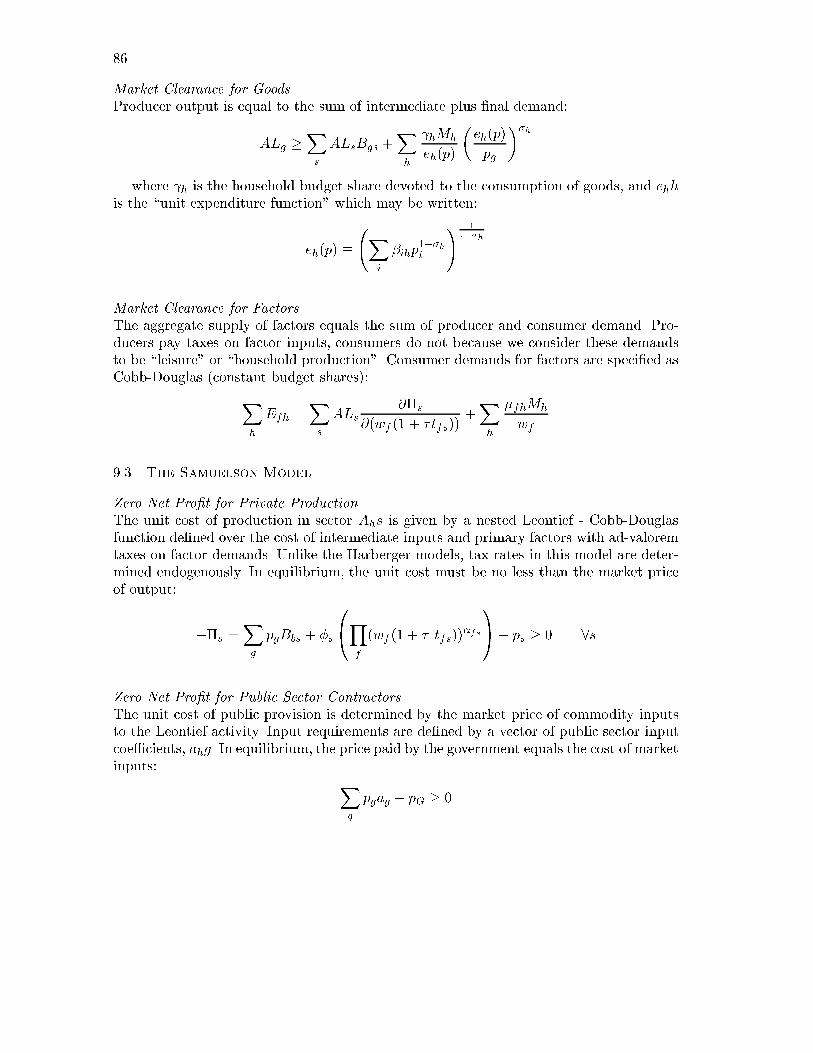
86
Market Clearance for GoodsProducer output is equal to the sum of intermediate plus �nal demand:
ALg �Xs
ALsBgs +Xh
hMh
eh(p)
�eh(p)
pg
��h
where h is the household budget share devoted to the consumption of goods, and ehhis the \unit expenditure function" which may be written:
eh(p) � X
i
�ihp1��hi
! 11��h
Market Clearance for FactorsThe aggregate supply of factors equals the sum of producer and consumer demand. Pro-ducers pay taxes on factor inputs, consumers do not because we consider these demandsto be \leisure" or \household production". Consumer demands for factors are speci�ed asCobb-Douglas (constant budget shares):
Xh
Efh =Xs
ALs@�s
@(wf (1 + �tfs))+Xh
�fhMh
wf
9.3. The Samuelson Model
Zero Net Pro�t for Private ProductionThe unit cost of production in sector Ahs is given by a nested Leontief - Cobb-Douglasfunction de�ned over the cost of intermediate inputs and primary factors with ad-valoremtaxes on factor demands. Unlike the Harberger models, tax rates in this model are deter-mined endogenously. In equilibrium, the unit cost must be no less than the market priceof output:
��s =Xg
pgBbs + �s
0@Y
f
(wf (1 + � tfs))�fs
1A� ps � 0 8s
Zero Net Pro�t for Public Sector ContractorsThe unit cost of public provision is determined by the market price of commodity inputsto the Leontief activity. Input requirements are de�ned by a vector of public sector inputcoe�cients, ahg. In equilibrium, the price paid by the government equals the cost of marketinputs: X
g
pgag � pG � 0
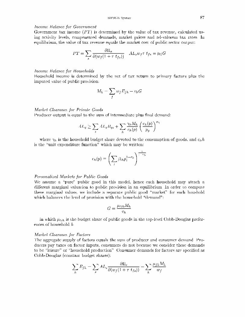
MPSGE Syntax 87
Income Balance for GovernmentGovernment tax income (PT ) is determined by the value of tax revenue, calculated us-ing activity levels, compensated demands, market prices and ad-valorem tax rates. Inequilibrium, the value of tax revenue equals the market cost of public sector output:
PT =Xs
@�s
@(wf (1 + � tfs))ALswf� tfs = pGG
Income Balance for HouseholdsHousehold income is determined by the net of tax return to primary factors plus theimputed value of public provision:
Mh =Xf
wfEfh + vhG
Market Clearance for Private GoodsProducer output is equal to the sum of intermediate plus �nal demand:
ALg �Xs
ALsBgs +Xh
hMh
eh(p)
�eh(p)
pg
��h
where h is the household budget share devoted to the consumption of goods, and ehhis the \unit expenditure function" which may be written:
eh(p) � X
i
�ihp1��hi
! 11��h
Personalized Markets for Public GoodsWe assume a \pure" public good in this model, hence each household may attach adi�erent marginal valuation to public provision in an equilibrium. In order to computethese marginal values, we include a separate public good \market" for each housholdwhich balances the level of provision with the household \demand":
G =�GhMh
vh
in which �Gh is the budget share of public goods in the top-level Cobb-Douglas prefer-ences of household h.
Market Clearance for FactorsThe aggregate supply of factors equals the sum of producer and consumer demand. Pro-ducers pay taxes on factor inputs, consumers do not because we consider these demandsto be \leisure" or \household production". Consumer demands for factors are speci�ed asCobb-Douglas (constant budget shares):
Xh
Efh =Xs
ALs@�s
@(wf (1 + � tfs))+Xh
�fhMh
wf

88
Samuelson Rule for \Optimal" Provision of Public GoodsThe tax rate multiplier is adjusted to balance the marginal cost of public provision withthe summation across households of marginal willingness to pay. Due to the existence ofhousehold factor demand, factor taxes are necessarily distortionary and there will be anexcess social cost of public funds. For this reason, the Samuelson rule is neither neces-sary nor su�cient for optimal provision. We apply the rule here merely to illustrate theprogramming methodology, even though the resulting equilibrium may be \suboptimal":
pG =Xh
vh

CES Preferences and Technology
A Practical Introduction
Abstract. This chapter describes practical approaches to the representation of constant elasticity de-mand functions in computable equilibrium models. A number of examples are presented which relate themathematical derivation of these functional forms to their representation in MPSGE models.
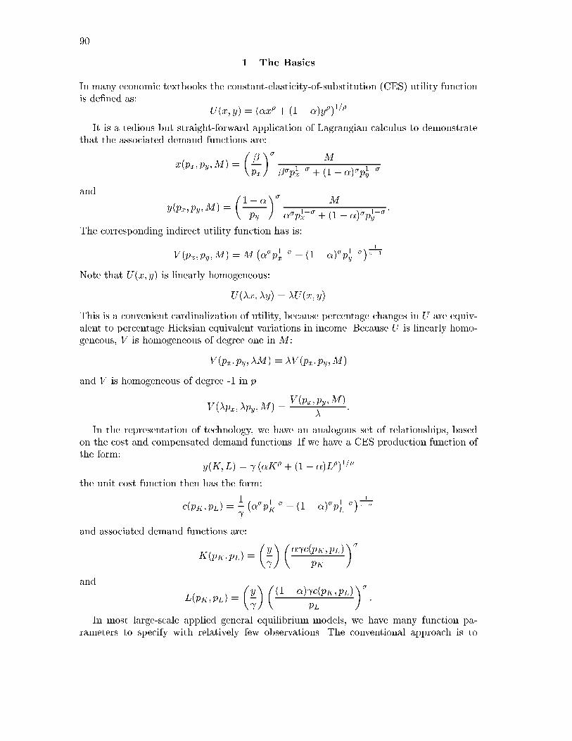
90
1. The Basics
In many economic textbooks the constant-elasticity-of-substitution (CES) utility functionis de�ned as:
U(x; y) = (�x� + (1� �)y�)1=�
It is a tedious but straight-forward application of Lagrangian calculus to demonstratethat the associated demand functions are:
x(px; py;M) =
��
px
�� M
��p1��x + (1� �)�p1��y
and
y(px; py;M) =
�1� �py
�� M
��p1��x + (1� �)�p1��y:
The corresponding indirect utility function has is:
V (px; py;M) =M���p1��x + (1� �)�p1��y
� 1��1
Note that U(x; y) is linearly homogeneous:
U(�x; �y) = �U(x; y)
This is a convenient cardinalization of utility, because percentage changes in U are equiv-alent to percentage Hicksian equivalent variations in income. Because U is linearly homo-geneous, V is homogeneous of degree one in M :
V (px; py; �M) = �V (px; py;M)
and V is homogeneous of degree -1 in p.
V (�px; �py;M) =V (px; py;M)
�:
In the representation of technology, we have an analogous set of relationships, basedon the cost and compensated demand functions. If we have a CES production function ofthe form:
y(K;L) = (�K� + (1� �)L�)1=�
the unit cost function then has the form:
c(pK ; pL) =1
���p1��K + (1� �)�p1��L
� 11��
and associated demand functions are:
K(pK ; pL) =
�y
��� c(pK ; pL)
pK
��and
L(pK ; pL) =
�y
��(1� �) c(pK ; pL)
pL
��:
In most large-scale applied general equilibrium models, we have many function pa-rameters to specify with relatively few observations. The conventional approach is to
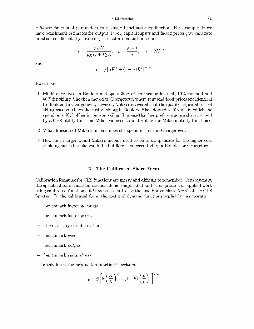
CES Functions 91
calibrate functional parameters to a single benchmark equilibrium. For example, if wehave benchmark estimates for output, labor, capital inputs and factor prices , we calibratefunction coe�cients by inverting the factor demand functions:
� =�pK �K
�pK �K + �PL �L; � =
� � 1
�; � = � �K��
and
= �y�� �K� + (1� �)�L���1=�
Exercises
1. Mikki once lived in Boulder and spent 30% of her income for rent, 10% for food and60% for skiing. She then moved to Georgetown where rent and food prices are identicalto Boulder. In Georgetown, however, Mikki discovered that the quality-adjusted cost ofskiing was ten-times the cost of skiing in Boulder. She adopted a lifestyle in which shespend only 30% of her income on skiing. Suppose that her preferences are characterizedby a CES utility function. What values of � and � describe Mikki's utility function?
2. What fraction of Mikki's income does she spend on rent in Georgetown?
3. How much larger would Mikki's income need to be to compensate for the higher costof skiing such that she would be indi�erent between living in Boulder or Georgetown.
2. The Calibrated Share Form
Calibration formulae for CES functions are messy and di�cult to remember. Consequently,the speci�cation of function coe�cients is complicated and error-prone. For applied workusing calibrated functions, it is much easier to use the "calibrated share form" of the CESfunction. In the calibrated form, the cost and demand functions explicitly incorporate
� benchmark factor demands
� benchmark factor prices
� the elasticity of substitution
� benchmark cost
� benchmark output
� benchmark value shares
In this form, the production function is written:
y = �y
��
�K�K
��+ (1� �)
�L�L
���1=�
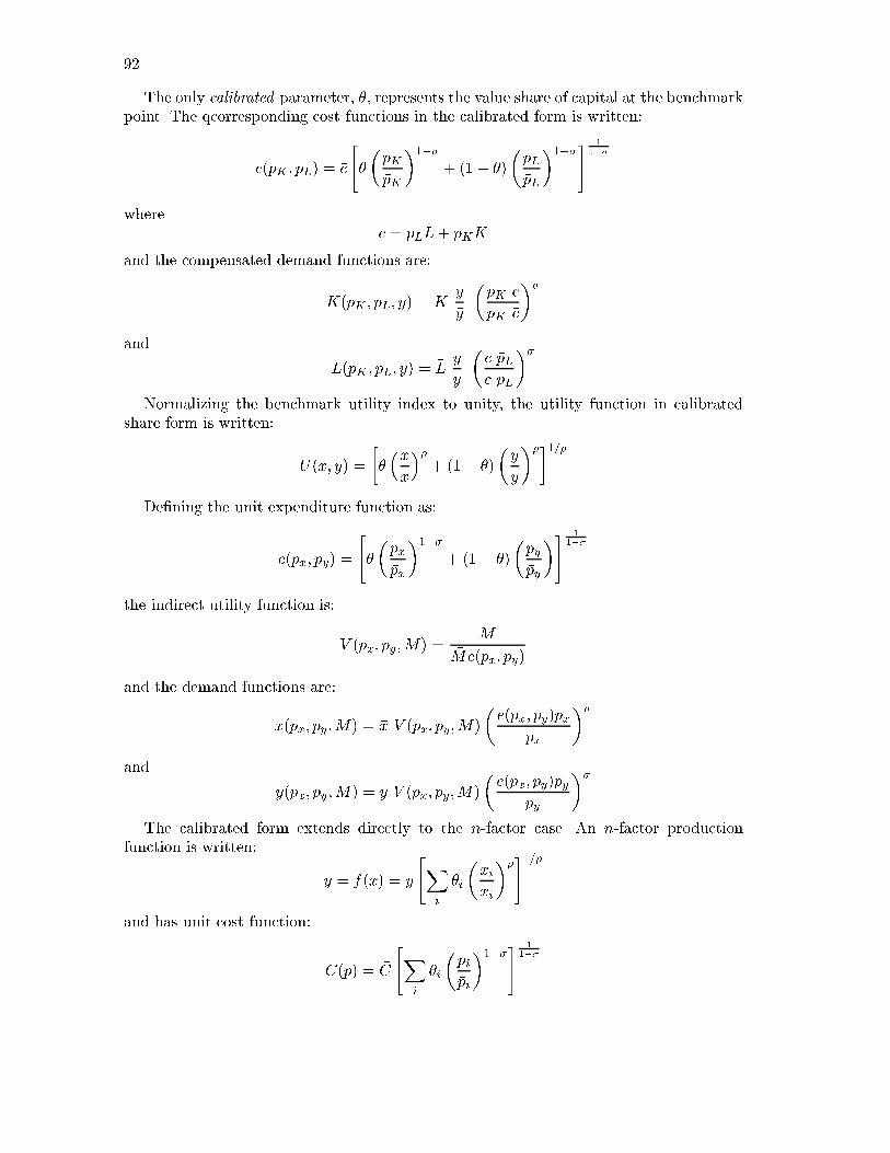
92
The only calibrated parameter, �, represents the value share of capital at the benchmarkpoint. The qcorresponding cost functions in the calibrated form is written:
c(pK ; pL) = �c
"�
�pK�pK
�1��
+ (1� �)�pL�pL
�1��# 1
1��
where�c = �pL �L+ �pK �K
and the compensated demand functions are:
K(pK ; pL; y) = �Ky
�y
��pK c
pK �c
��
and
L(pK ; pL; y) = �Ly
�y
�c �pL�c pL
��Normalizing the benchmark utility index to unity, the utility function in calibrated
share form is written:
U(x; y) =
���x�x
��+ (1� �)
�y
�y
���1=�
De�ning the unit expenditure function as:
e(px; py) =
"�
�px�px
�1��
+ (1� �)�py�py
�# 11��
the indirect utility function is:
V (px; py;M) =M
�Me(px; py)
and the demand functions are:
x(px; py;M) = �x V (px; py;M)
�e(px; py)�px
px
��
and
y(px; py;M) = �y V (px; py;M)
�e(px; py)�py
py
��The calibrated form extends directly to the n-factor case. An n-factor production
function is written:
y = f(x) = �y
"Xi
�i
�xi�xi
��#1=�
and has unit cost function:
C(p) = �C
"Xi
�i
�pi�pi
�1��# 1
1��
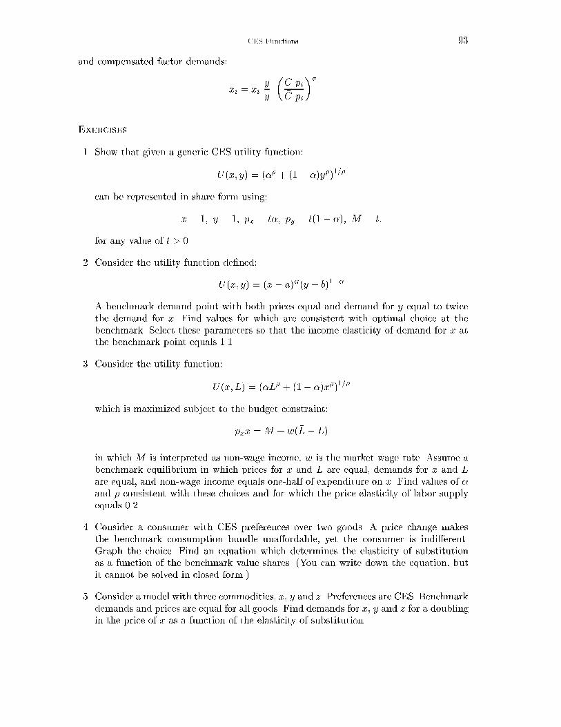
CES Functions 93
and compensated factor demands:
xi = �xiy
�y
�C �pi�C pi
��
Exercises
1. Show that given a generic CES utility function:
U(x; y) = (�� + (1� �)y�)1=�
can be represented in share form using:
�x = 1; �y = 1; �px = t�; �py = t(1� �); �M = t:
for any value of t > 0.
2. Consider the utility function de�ned:
U(x; y) = (x� a)�(y � b)1��
A benchmark demand point with both prices equal and demand for y equal to twicethe demand for x. Find values for which are consistent with optimal choice at thebenchmark. Select these parameters so that the income elasticity of demand for x atthe benchmark point equals 1.1.
3. Consider the utility function:
U(x;L) = (�L� + (1� �)x�)1=�
which is maximized subject to the budget constraint:
pxx =M + w(�L� L)
in which M is interpreted as non-wage income, w is the market wage rate. Assume abenchmark equilibrium in which prices for x and L are equal, demands for x and Lare equal, and non-wage income equals one-half of expenditure on x. Find values of �and � consistent with these choices and for which the price elasticity of labor supplyequals 0.2.
4. Consider a consumer with CES preferences over two goods. A price change makesthe benchmark consumption bundle una�ordable, yet the consumer is indi�erent.Graph the choice. Find an equation which determines the elasticity of substitutionas a function of the benchmark value shares. (You can write down the equation, butit cannot be solved in closed form.)
5. Consider a model with three commodities, x, y and z. Preferences are CES. Benchmarkdemands and prices are equal for all goods. Find demands for x, y and z for a doublingin the price of x as a function of the elasticity of substitution.
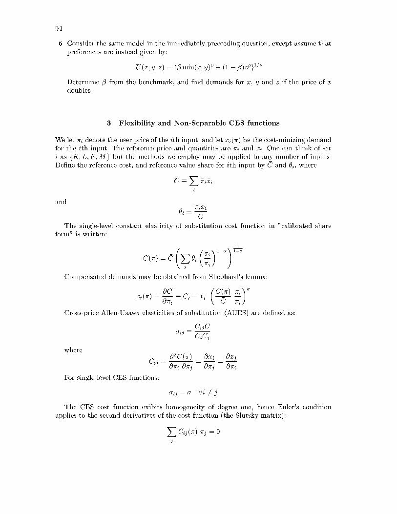
94
6. Consider the same model in the immediately preceeding question, except assume thatpreferences are instead given by:
U(x; y; z) = (�min(x; y)� + (1� �)z�)1=�
Determine � from the benchmark, and �nd demands for x, y and z if the price of xdoubles.
3. Flexibility and Non-Separable CES functions
We let �i denote the user price of the ith input, and let xi(�) be the cost-minizing demandfor the ith input. The reference price and quantities are ��i and �xi. One can think of seti as fK;L;E;Mg but the methods we employ may be applied to any number of inputs.De�ne the reference cost, and reference value share for ith input by �C and �i, where
�C �Xi
��i�xi
and
�i � �i�xi�C
The single-level constant elasticity of substitution cost function in "calibrated shareform" is written:
C(�) = �C
Xi
�i
��i��i
�1��! 11��
Compensated demands may be obtained from Shephard's lemma:
xi(�) =@C
@�i� Ci = �xi
�C(�)�C
��i�i
��Cross-price Allen-Uzawa elasticities of substitution (AUES) are de�ned as:
�ij � CijC
CiCj
where
Cij � @2C(�)
@�i @�j=@xi@�j
=@xj@�i
For single-level CES functions:
�ij = � 8i 6= j
The CES cost function exibits homogeneity of degree one, hence Euler's conditionapplies to the second derivatives of the cost function (the Slutsky matrix):X
j
Cij(�) �j = 0
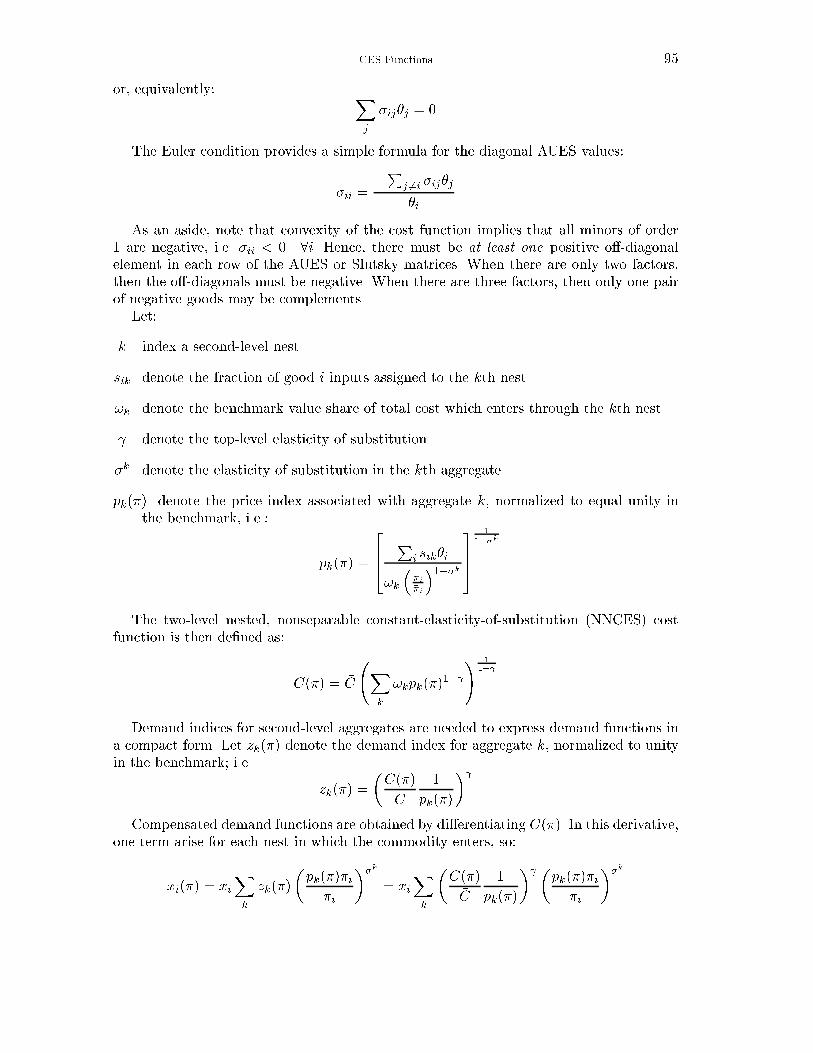
CES Functions 95
or, equivalently: Xj
�ij�j = 0
The Euler condition provides a simple formula for the diagonal AUES values:
�ii =�Pj 6=i �ij�j
�i
As an aside, note that convexity of the cost function implies that all minors of order1 are negative, i.e. �ii < 0 8i. Hence, there must be at least one positive o�-diagonalelement in each row of the AUES or Slutsky matrices. When there are only two factors,then the o�-diagonals must be negative. When there are three factors, then only one pairof negative goods may be complements.
Let:
k index a second-level nest
sik denote the fraction of good i inputs assigned to the kth nest
!k denote the benchmark value share of total cost which enters through the kth nest
denote the top-level elasticity of substitution
�k denote the elasticity of substitution in the kth aggregate
pk(�) denote the price index associated with aggregate k, normalized to equal unity inthe benchmark, i.e.:
pk(�) =
264
Pi sik�i
!k
��i��i
�1��k375
1
1��k
The two-level nested, nonseparable constant-elasticity-of-substitution (NNCES) costfunction is then de�ned as:
C(�) = �C
Xk
!kpk(�)1�
! 11�
Demand indices for second-level aggregates are needed to express demand functions ina compact form. Let zk(�) denote the demand index for aggregate k, normalized to unityin the benchmark; i.e.
zk(�) =
�C(�)�C
1
pk(�)
� Compensated demand functions are obtained by di�erentiating C(�). In this derivative,
one term arise for each nest in which the commodity enters, so:
xi(�) = �xiXk
zk(�)
�pk(�)��i�i
��k= �xi
Xk
�C(�)�C
1
pk(�)
� �pk(�)��i�i
��k
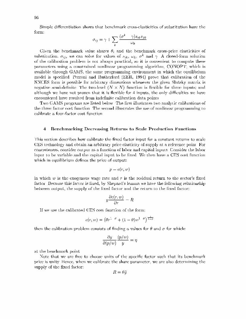
96
Simple di�erentiation shows that benchmark cross-elasticities of substitution have theform:
�ij = +Xk
(�k � )siksjk!k
Given the benchmark value shares �i and the benchmark cross-price elasticities ofsubstitution, �ij, we can solve for values of sik, !k, �
k and . A closed-form solutionof the calibration problem is not always practical, so it is convenient to compute theseparameters using a constrained nonlinear programming algorithm, CONOPT, which isavailable through GAMS, the same programming environment in which the equilibriummodel is speci�ed. Perroni and Rutherford (EER, 1994) prove that calibration of theNNCES form is possible for arbitrary dimensions whenever the given Slutsky matrix isnegative semi-de�nite. The two-level (N � N) function is exible for three inputs; andalthough we have not proven that it is exible for 4 inputs, the only di�culties we haveencountered have resulted from inde�nite calibration data points.
Two GAMS programs are listed below. The �rst illustrates two analytic calibrations ofthe three-factor cost function. The second illustrates the use of nonlinear programming tocalibrate a four-factor cost function.
4. Benchmarking Decreasing Returns to Scale Production Functions
This section describes how calibrate the �xed factor input for a constant returns to scaleCES technology and obtain an arbitrary price elasticity of supply at a reference point. Forconcreteness, consider output as a function of labor and capital inputs. Consider the laborinput to be variable and the capital input to be �xed. We then have a CES cost functionwhich in equilibrium de�nes the price of output:
p = c(r; w)
in which w is the exogenous wage rate and r is the residual return to the sector's �xedfactor. Because this factor is �xed, by Shepard's lemma we have the following relationshipbetween output, the supply of the �xed factor and the return to the �xed factor:
y@c(r; w)
@r= �R
If we use the calibrated CES cost function of the form:
c(r; w) =��r1�� + (1� �)w1��
� 11��
then the calibration problem consists of �nding a values for � and � for which:
@y
@(p=w)
(p=w)
y= �
at the benchmark point.Note that we are free to choose units of the speci�c factor such that its benchmark
price is unity. Hence, when we calibrate the share parameter, we are also determining thesupply of the �xed factor:
�R = ��y
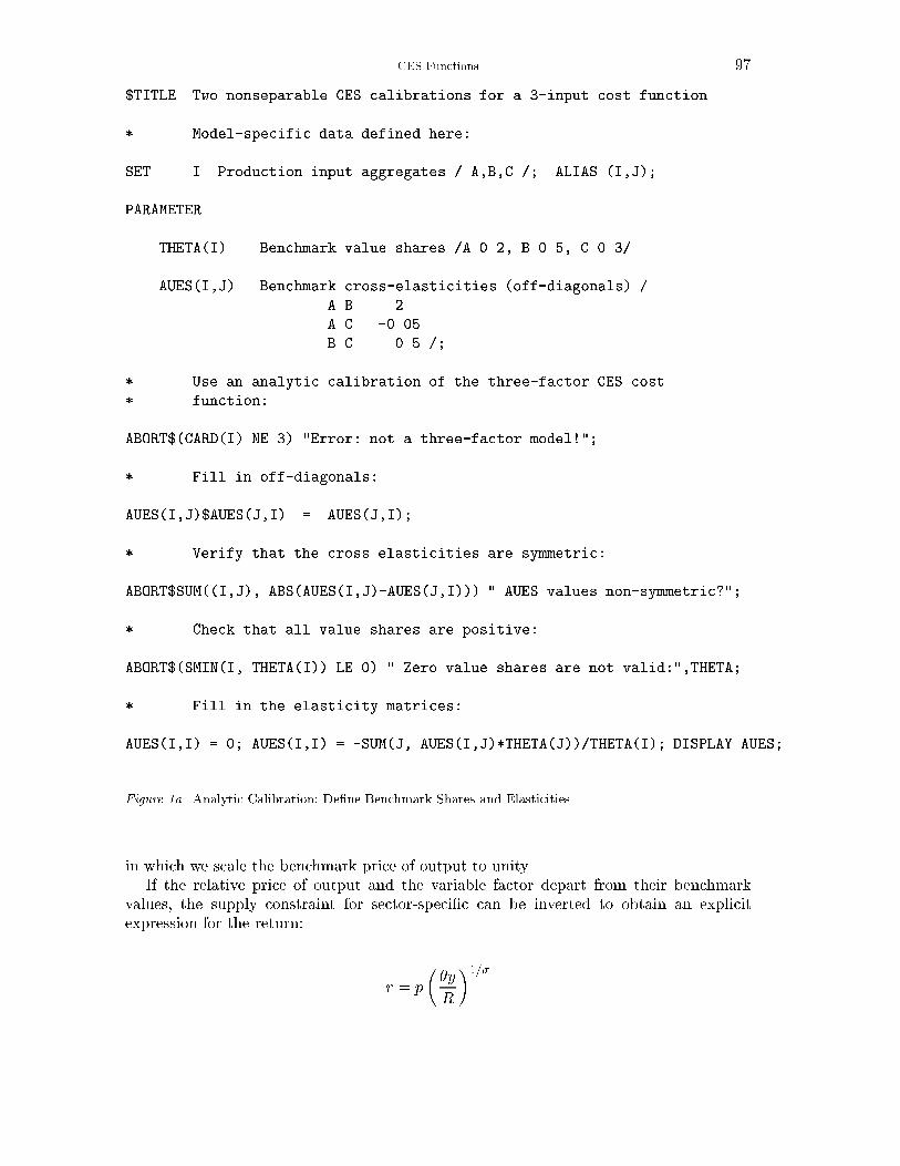
CES Functions 97
$TITLE Two nonseparable CES calibrations for a 3-input cost function.
* Model-specific data defined here:
SET I Production input aggregates / A,B,C /; ALIAS (I,J);
PARAMETER
THETA(I) Benchmark value shares /A 0.2, B 0.5, C 0.3/
AUES(I,J) Benchmark cross-elasticities (off-diagonals) /
A.B 2
A.C -0.05
B.C 0.5 /;
* Use an analytic calibration of the three-factor CES cost
* function:
ABORT$(CARD(I) NE 3) "Error: not a three-factor model!";
* Fill in off-diagonals:
AUES(I,J)$AUES(J,I) = AUES(J,I);
* Verify that the cross elasticities are symmetric:
ABORT$SUM((I,J), ABS(AUES(I,J)-AUES(J,I))) " AUES values non-symmetric?";
* Check that all value shares are positive:
ABORT$(SMIN(I, THETA(I)) LE 0) " Zero value shares are not valid:",THETA;
* Fill in the elasticity matrices:
AUES(I,I) = 0; AUES(I,I) = -SUM(J, AUES(I,J)*THETA(J))/THETA(I); DISPLAY AUES;
Figure 1a. Analytic Calibration: De�ne Benchmark Shares and Elasticities
in which we scale the benchmark price of output to unity.If the relative price of output and the variable factor depart from their benchmark
values, the supply constraint for sector-speci�c can be inverted to obtain an explicitexpression for the return:
r = p
��y�R
�1=�
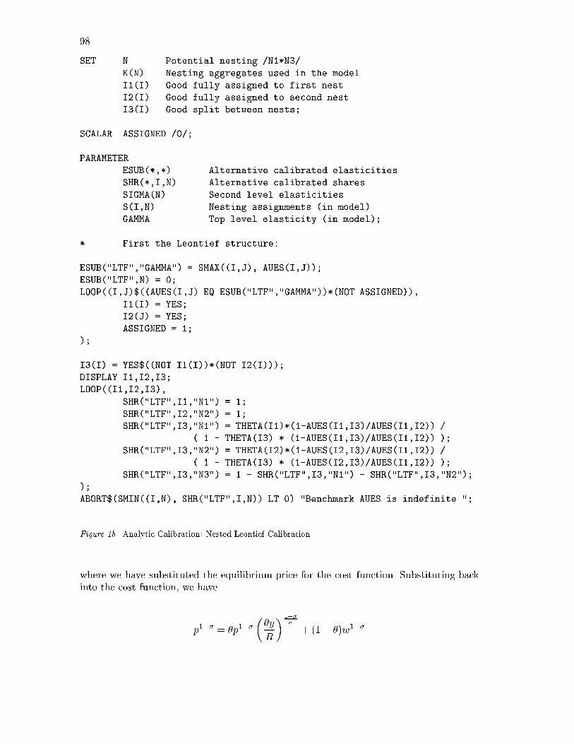
98
SET N Potential nesting /N1*N3/
K(N) Nesting aggregates used in the model
I1(I) Good fully assigned to first nest
I2(I) Good fully assigned to second nest
I3(I) Good split between nests;
SCALAR ASSIGNED /0/;
PARAMETER
ESUB(*,*) Alternative calibrated elasticities
SHR(*,I,N) Alternative calibrated shares
SIGMA(N) Second level elasticities
S(I,N) Nesting assignments (in model)
GAMMA Top level elasticity (in model);
* First the Leontief structure:
ESUB("LTF","GAMMA") = SMAX((I,J), AUES(I,J));
ESUB("LTF",N) = 0;
LOOP((I,J)$((AUES(I,J) EQ ESUB("LTF","GAMMA"))*(NOT ASSIGNED)),
I1(I) = YES;
I2(J) = YES;
ASSIGNED = 1;
);
I3(I) = YES$((NOT I1(I))*(NOT I2(I)));
DISPLAY I1,I2,I3;
LOOP((I1,I2,I3),
SHR("LTF",I1,"N1") = 1;
SHR("LTF",I2,"N2") = 1;
SHR("LTF",I3,"N1") = THETA(I1)*(1-AUES(I1,I3)/AUES(I1,I2)) /
( 1 - THETA(I3) * (1-AUES(I1,I3)/AUES(I1,I2)) );
SHR("LTF",I3,"N2") = THETA(I2)*(1-AUES(I2,I3)/AUES(I1,I2)) /
( 1 - THETA(I3) * (1-AUES(I2,I3)/AUES(I1,I2)) );
SHR("LTF",I3,"N3") = 1 - SHR("LTF",I3,"N1") - SHR("LTF",I3,"N2");
);
ABORT$(SMIN((I,N), SHR("LTF",I,N)) LT 0) "Benchmark AUES is indefinite.";
Figure 1b. Analytic Calibration: Nested Leontief Calibration
where we have substituted the equilibrium price for the cost function. Substituting backinto the cost function, we have
p1�� = �p1����y�R
� 1���
+ (1� �)w1��
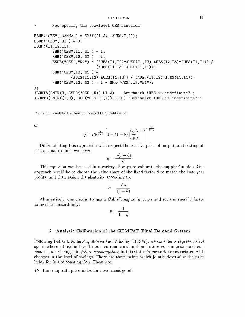
CES Functions 99
* Now specify the two-level CES function:
ESUB("CES","GAMMA") = SMAX((I,J), AUES(I,J));
ESUB("CES","N1") = 0;
LOOP((I1,I2,I3),
SHR("CES",I1,"N1") = 1;
SHR("CES",I2,"N2") = 1;
ESUB("CES","N2") = (AUES(I1,I2)*AUES(I1,I3)-AUES(I2,I3)*AUES(I1,I1)) /
(AUES(I1,I3)-AUES(I1,I1));
SHR("CES",I3,"N1") =
(AUES(I1,I2)-AUES(I1,I3)) / (AUES(I1,I2)-AUES(I1,I1));
SHR("CES",I3,"N2") = 1 - SHR("CES",I3,"N1");
);
ABORT$(SMIN(N, ESUB("CES",N)) LT 0) "Benchmark AUES is indefinite?";
ABORT$(SMIN((I,N), SHR("CES",I,N)) LT 0) "Benchmark AUES is indefinite?";
Figure 1c. Analytic Calibration: Nested CES Calibration
or
y = �R�1
��1
"1� (1� �)
�w
p
�1��# �
1��
Di�erentiating this expression with respect the relative price of output, and setting allprices equal to unit, we have:
� =�(1� �)
�
This equation can be used in a variety of ways to calibrate the supply function. Oneapproach would be to choose the value share of the �xed factor � to match the base yearpro�ts, and then assign the elasticity according to:
� =��
(1� �)Alternatively, one choose to use a Cobb-Douglas function and set the speci�c factor
value share accordingly:
� =1
1 + �
5. Analytic Calibration of the GEMTAP Final Demand System
Following Ballard, Fullerton, Shoven and Whalley (BFSW), we consider a representativeagent whose utility is based upon current consumption, future consumption and cur-rent leisure. Changes in future consumption; in this static framework are associated withchanges in the level of savings. There are three prices which jointly determine the priceindex for future consumption. These are:
PI the composite price index for investment goods
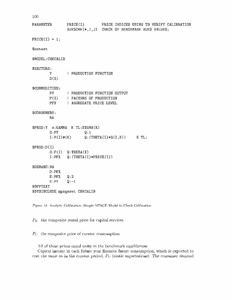
100
PARAMETER PRICE(I) PRICE INDICES USING TO VERIFY CALIBRATION
AUESCHK(*,I,J) CHECK OF BENCHMARK AUES VALUES;
PRICE(I) = 1;
$ontext
$MODEL:CHKCALIB
$SECTORS:
Y ! PRODUCTION FUNCTION
D(I)
$COMMODITIES:
PY ! PRODUCTION FUNCTION OUTPUT
P(I) ! FACTORS OF PRODUCTION
PFX ! AGGREGATE PRICE LEVEL
$CONSUMERS:
RA
$PROD:Y s:GAMMA K.TL:SIGMA(K)
O:PY Q:1
I:P(I)#(K) Q:(THETA(I)*S(I,K)) K.TL:
$PROD:D(I)
O:P(I) Q:THETA(I)
I:PFX Q:(THETA(I)*PRICE(I))
$DEMAND:RA
D:PFX
E:PFX Q:2
E:PY Q:-1
$OFFTEXT
$SYSINCLUDE mpsgeset CHKCALIB
Figure 1d. Analytic Calibration: Simple MPSGE Model to Check Calibration
PK the composite rental price for capital services
PC the composite price of current consumption.
All of these prices equal unity in the benchmark equilibrium.Capital income in each future year �nances future consumption, which is expected to
cost the same as in the current period, PC (static expectations). The consumer demand
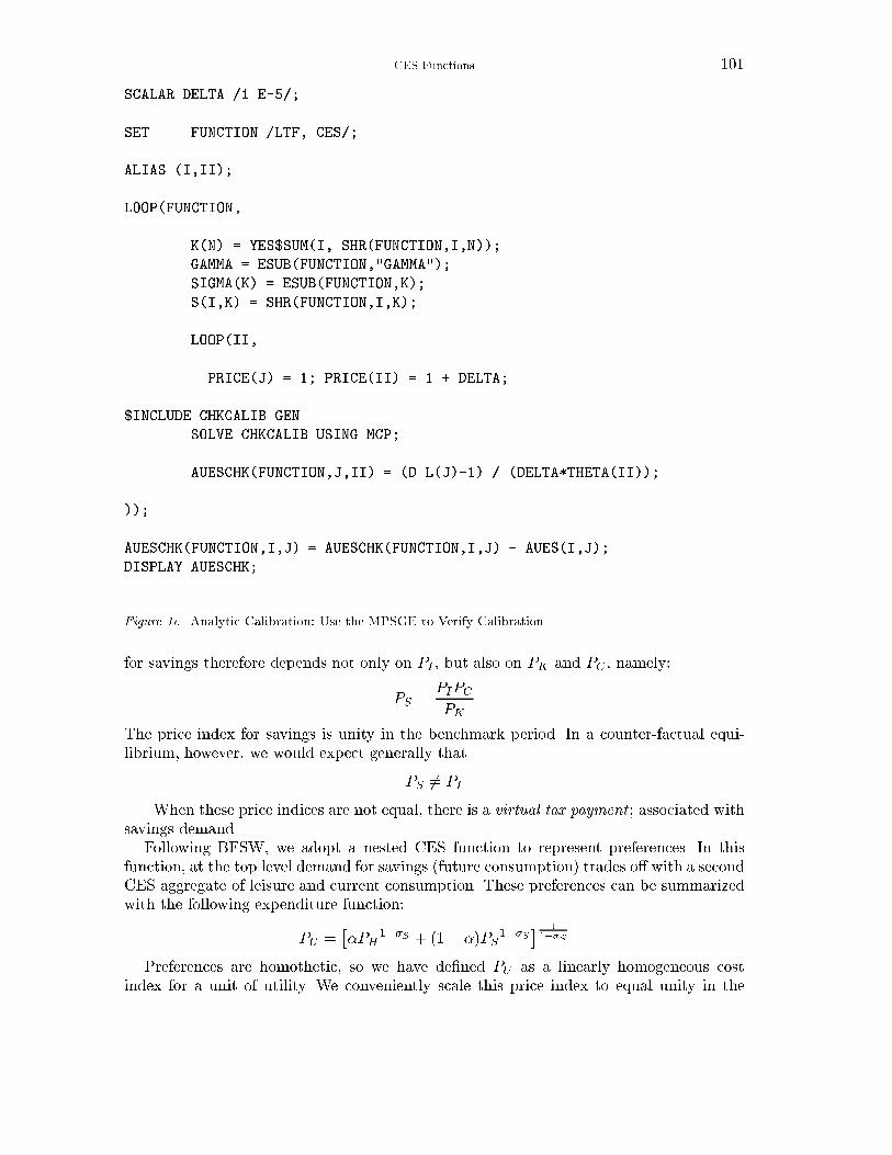
CES Functions 101
SCALAR DELTA /1.E-5/;
SET FUNCTION /LTF, CES/;
ALIAS (I,II);
LOOP(FUNCTION,
K(N) = YES$SUM(I, SHR(FUNCTION,I,N));
GAMMA = ESUB(FUNCTION,"GAMMA");
SIGMA(K) = ESUB(FUNCTION,K);
S(I,K) = SHR(FUNCTION,I,K);
LOOP(II,
PRICE(J) = 1; PRICE(II) = 1 + DELTA;
$INCLUDE CHKCALIB.GEN
SOLVE CHKCALIB USING MCP;
AUESCHK(FUNCTION,J,II) = (D.L(J)-1) / (DELTA*THETA(II));
));
AUESCHK(FUNCTION,I,J) = AUESCHK(FUNCTION,I,J) - AUES(I,J);
DISPLAY AUESCHK;
Figure 1e. Analytic Calibration: Use the MPSGE to Verify Calibration
for savings therefore depends not only on PI , but also on PK and PC , namely:
PS =PIPCPK
The price index for savings is unity in the benchmark period. In a counter-factual equi-librium, however, we would expect generally that
PS 6= PI
. When these price indices are not equal, there is a virtual tax payment ; associated withsavings demand.
Following BFSW, we adopt a nested CES function to represent preferences. In thisfunction, at the top level demand for savings (future consumption) trades o� with a secondCES aggregate of leisure and current consumption. These preferences can be summarizedwith the following expenditure function:
PU =��PH
1��S + (1� �)PS1��S� 11��S
Preferences are homothetic, so we have de�ned PU as a linearly homogeneous costindex for a unit of utility. We conveniently scale this price index to equal unity in the
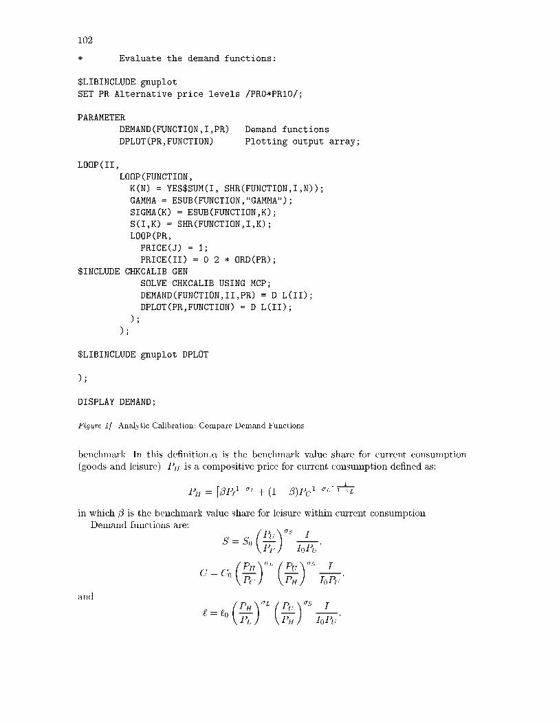
102
* Evaluate the demand functions:
$LIBINCLUDE gnuplot
SET PR Alternative price levels /PR0*PR10/;
PARAMETER
DEMAND(FUNCTION,I,PR) Demand functions
DPLOT(PR,FUNCTION) Plotting output array;
LOOP(II,
LOOP(FUNCTION,
K(N) = YES$SUM(I, SHR(FUNCTION,I,N));
GAMMA = ESUB(FUNCTION,"GAMMA");
SIGMA(K) = ESUB(FUNCTION,K);
S(I,K) = SHR(FUNCTION,I,K);
LOOP(PR,
PRICE(J) = 1;
PRICE(II) = 0.2 * ORD(PR);
$INCLUDE CHKCALIB.GEN
SOLVE CHKCALIB USING MCP;
DEMAND(FUNCTION,II,PR) = D.L(II);
DPLOT(PR,FUNCTION) = D.L(II);
);
);
$LIBINCLUDE gnuplot DPLOT
);
DISPLAY DEMAND;
Figure 1f. Analytic Calibration: Compare Demand Functions
benchmark. In this de�nition,� is the benchmark value share for current consumption(goods and leisure). PH is a compositive price for current consumption de�ned as:
PH =��P`
1��L + (1� �)PC1��L� 11��L
in which � is the benchmark value share for leisure within current consumption.Demand functions are:
S = S0
�PUPF
��S I
I0PU;
C = C0
�PHPC
��L �PUPH
��S I
I0PU;
and
` = `0
�PHPL
��L �PUPH
��S I
I0PU:
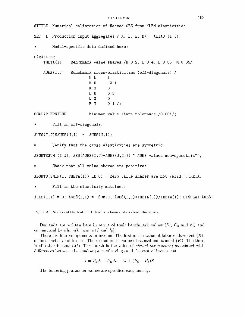
CES Functions 103
$TITLE Numerical calibration of Nested CES from KLEM elasticities
SET I Production input aggregates / K, L, E, M/; ALIAS (I,J);
* Model-specific data defined here:
PARAMETER
THETA(I) Benchmark value shares /K 0.2, L 0.4, E 0.05, M 0.35/
AUES(I,J) Benchmark cross-elasticities (off-diagonals) /
K.L 1
K.E -0.1
K.M 0
L.E 0.3
L.M 0
E.M 0.1 /;
SCALAR EPSILON Minimum value share tolerance /0.001/;
* Fill in off-diagonals:
AUES(I,J)$AUES(J,I) = AUES(J,I);
* Verify that the cross elasticities are symmetric:
ABORT$SUM((I,J), ABS(AUES(I,J)-AUES(J,I))) " AUES values non-symmetric?";
* Check that all value shares are positive:
ABORT$(SMIN(I, THETA(I)) LE 0) " Zero value shares are not valid:",THETA;
* Fill in the elasticity matrices:
AUES(I,I) = 0; AUES(I,I) = -SUM(J, AUES(I,J)*THETA(J))/THETA(I); DISPLAY AUES;
Figure 2a. Numerical Calibration: De�ne Benchmark Shares and Elasticities
Demands are written here in terms of their benchmark values (S0, C0 and `0) andcurrent and benchmark income (I and I0).
There are four components in income. The �rst is the value of labor endowment (E),de�ned inclusive of leisure. The second is the value of capital endowment (K). The thirdis all other income (M). The fourth is the value of virtual tax revenue; associated withdi�erences between the shadow price of savings and the cost of investment.
I = PLE + PKK +M + (PS � PI)S
The following parameter values are speci�ed exogenously:

104
* Define variables and equations for NNCES calibration:
SET N Nests within the two-level NNCES function /N1*N4/,
K(N) Nests which are in use;
VARIABLES
S(I,N) Fraction of good I which enters through nest N,
SHARE(N) Value share of nest N,
SIGMA(N) Elasticity of substitution within nest N,
GAMMA Elasticity of substitution at the top level,
OBJ Objective function;
POSITIVE VARIABLES S, SHARE, SIGMA, GAMMA;
EQUATIONS
SDEF(I) Nest shares must sum to one,
TDEF(N) Nest share in total cost,
ELAST(I,J) Consistency with given AUES values,
OBJDEF Maximize concentration;
ELAST(I,J)$(ORD(I) GT ORD(J))..
AUES(I,J) =E= GAMMA +
SUM(K, (SIGMA(K)-GAMMA)*S(I,K)*S(J,K)/SHARE(K));
TDEF(K).. SHARE(K) =E= SUM(I, THETA(I) * S(I,K));
SDEF(I).. SUM(N, S(I,N)) =E= 1;
* Maximize concentration at the same time keeping the elasticities
* to be reasonable:
OBJDEF.. OBJ =E= SUM((I,K),S(I,K)*S(I,K))
- SQR(GAMMA) - SUM(K, SQR(SIGMA(K)));
MODEL CESCALIB /ELAST, TDEF, SDEF, OBJDEF/;
* Apply some bounds to avoid divide by zero:
SHARE.LO(N) = EPSILON;
Figure 2b. Numerical Calibration: De�ne a Nonlinear Program for Calibration

CES Functions 105
SCALAR SOLVED Flag for having solved the calibration problem /0/
MINSHR Minimum share in candidate calibration;
SET TRIES Counter on the number of attempted calibrations /T1*T10/;
OPTION SEED=0;
LOOP(TRIES$(NOT SOLVED),
* Initialize the set of active nests and the bounds:
K(N) = YES;
S.LO(I,N) = 0; S.UP(I,N) = 1;
SHARE.LO(N) = EPSILON; SHARE.UP(N) = 1;
SIGMA.LO(N) = 0; SIGMA.UP(N) = +INF;
* Install a starting point:
SHARE.L(K) = MAX(UNIFORM(0,1), EPSILON);
S.L(I,K) = UNIFORM(0,1);
GAMMA.L = UNIFORM(0,1);
SIGMA.L(K) = UNIFORM(0,1);
SDEF.M(I) = 0; TDEF.M(K) = 0; ELAST.M(I,J) = 0;
SOLVE CESCALIB USING NLP MAXIMIZING OBJ;
SOLVED = 1$(CESCALIB.MODELSTAT LE 2);
IF (SOLVED,
MINSHR = SMIN(K, SHARE.L(K)) - EPSILON;
IF (MINSHR EQ 0,
K(N)$(SHARE.L(N) EQ EPSILON) = NO;
S.FX(I,N)$(NOT K(N)) = 0;
SHARE.FX(N)$(NOT K(N)) = 0;
SIGMA.FX(N)$(NOT K(N)) = 0;
DISPLAY "Recalibrating with the following nests:",K;
SOLVE CESCALIB USING NLP MAXIMIZING OBJ;
IF (CESCALIB.MODELSTAT GT 2, SOLVED = 0;);
MINSHR = SMIN(K, SHARE.L(K)) - EPSILON;
IF (MINSHR EQ 0, SOLVED = 0;);
);
);
);
IF (SOLVED, DISPLAY "Function calibrated:",GAMMA.L,SIGMA.L,SHARE.L,S.L;
ELSE DISPLAY "Function calibration fails!";
);
Figure 2c. Numerical Calibration: Perform the Calibration
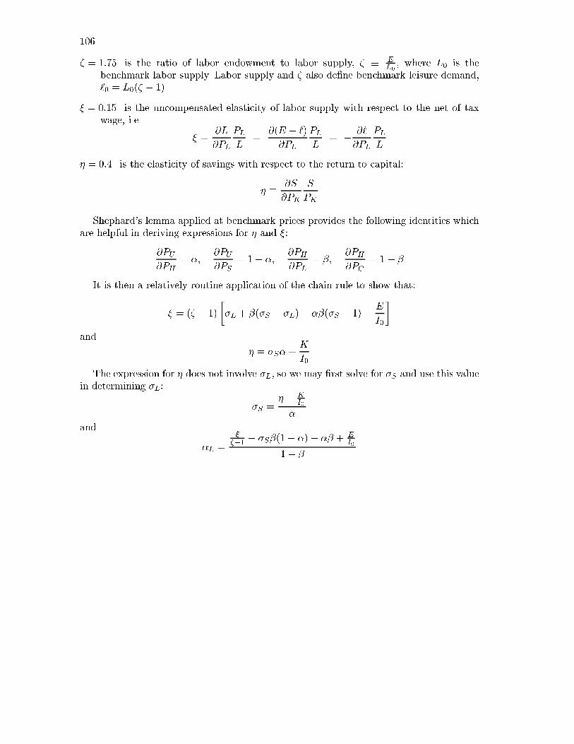
106
� = 1:75 is the ratio of labor endowment to labor supply, � � EL0, where L0 is the
benchmark labor supply. Labor supply and � also de�ne benchmark leisure demand,`0 = L0(� � 1).
� = 0:15 is the uncompensated elasticity of labor supply with respect to the net of taxwage, i.e.
� =@L
@PL
PLL
=@(E � `)@PL
PLL
= � @`
@PL
PLL
� = 0:4 is the elasticity of savings with respect to the return to capital:
� � @S
@PK
S
PK
Shephard's lemma applied at benchmark prices provides the following identities whichare helpful in deriving expressions for � and �:
@PU@PH
= �;@PU@PS
= 1� �; @PH@PL
= �;@PH@PC
= 1� �
It is then a relatively routine application of the chain rule to show that:
� = (� � 1)
��L + �(�S � �L)� ��(�S � 1)� E
I0
�and
� = �S�+K
I0
The expression for � does not involve �L, so we may �rst solve for �S and use this valuein determining �L:
�S =� � K
I0
�
and
�L =
���1 � �S�(1� �)� �� + E
I0
1� �
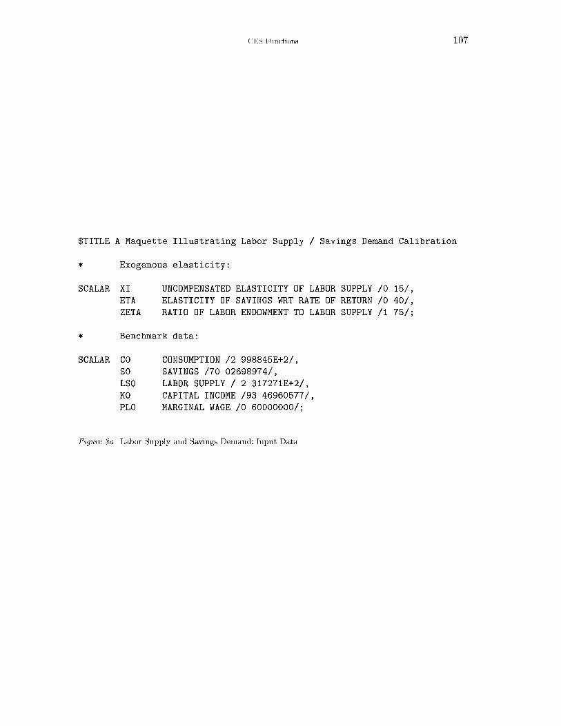
CES Functions 107
$TITLE A Maquette Illustrating Labor Supply / Savings Demand Calibration
* Exogenous elasticity:
SCALAR XI UNCOMPENSATED ELASTICITY OF LABOR SUPPLY /0.15/,
ETA ELASTICITY OF SAVINGS WRT RATE OF RETURN /0.40/,
ZETA RATIO OF LABOR ENDOWMENT TO LABOR SUPPLY /1.75/;
* Benchmark data:
SCALAR C0 CONSUMPTION /2.998845E+2/,
S0 SAVINGS /70.02698974/,
LS0 LABOR SUPPLY / 2.317271E+2/,
K0 CAPITAL INCOME /93.46960577/,
PL0 MARGINAL WAGE /0.60000000/;
Figure 3a. Labor Supply and Savings Demand: Input Data
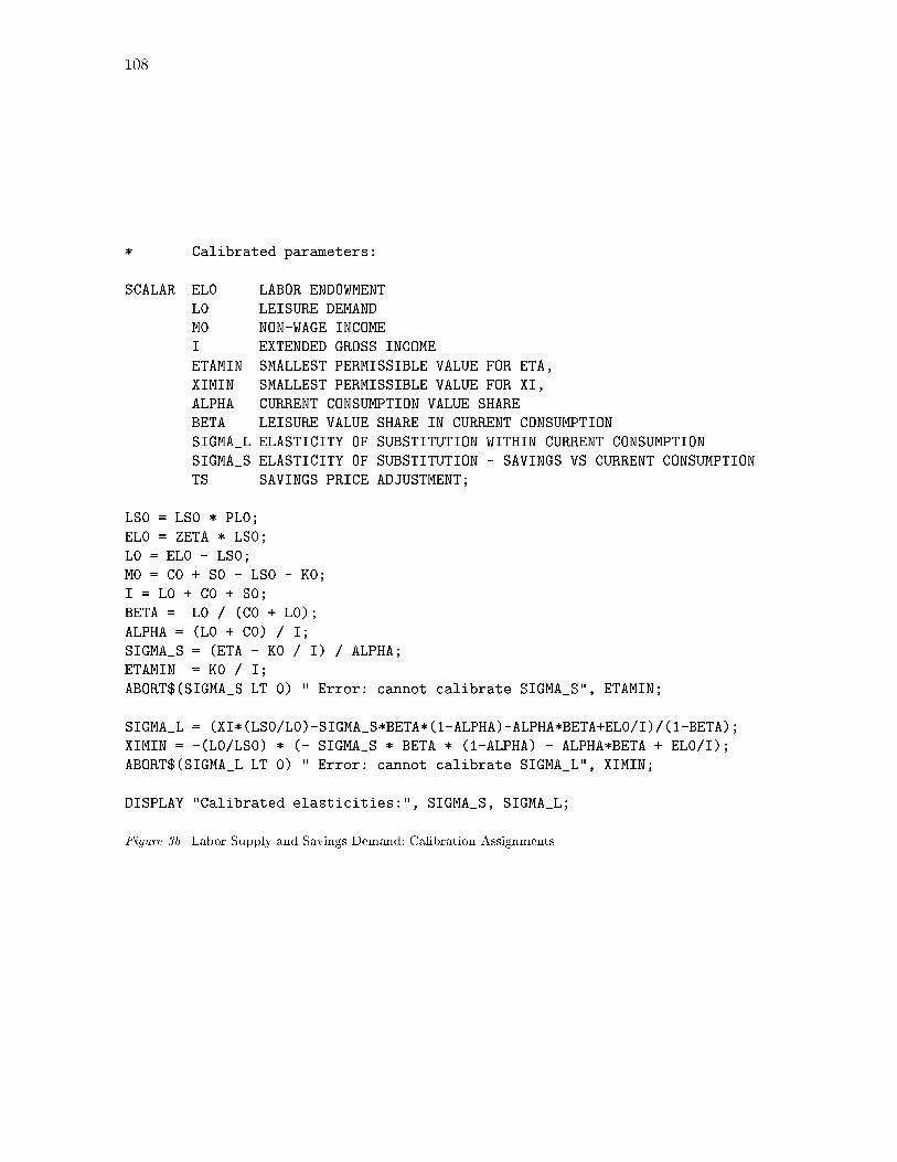
108
* Calibrated parameters:
SCALAR EL0 LABOR ENDOWMENT
L0 LEISURE DEMAND
M0 NON-WAGE INCOME
I EXTENDED GROSS INCOME
ETAMIN SMALLEST PERMISSIBLE VALUE FOR ETA,
XIMIN SMALLEST PERMISSIBLE VALUE FOR XI,
ALPHA CURRENT CONSUMPTION VALUE SHARE
BETA LEISURE VALUE SHARE IN CURRENT CONSUMPTION
SIGMA_L ELASTICITY OF SUBSTITUTION WITHIN CURRENT CONSUMPTION
SIGMA_S ELASTICITY OF SUBSTITUTION - SAVINGS VS CURRENT CONSUMPTION
TS SAVINGS PRICE ADJUSTMENT;
LS0 = LS0 * PL0;
EL0 = ZETA * LS0;
L0 = EL0 - LS0;
M0 = C0 + S0 - LS0 - K0;
I = L0 + C0 + S0;
BETA = L0 / (C0 + L0);
ALPHA = (L0 + C0) / I;
SIGMA_S = (ETA - K0 / I) / ALPHA;
ETAMIN = K0 / I;
ABORT$(SIGMA_S LT 0) " Error: cannot calibrate SIGMA_S", ETAMIN;
SIGMA_L = (XI*(LS0/L0)-SIGMA_S*BETA*(1-ALPHA)-ALPHA*BETA+EL0/I)/(1-BETA);
XIMIN = -(L0/LS0) * (- SIGMA_S * BETA * (1-ALPHA) - ALPHA*BETA + EL0/I);
ABORT$(SIGMA_L LT 0) " Error: cannot calibrate SIGMA_L", XIMIN;
DISPLAY "Calibrated elasticities:", SIGMA_S, SIGMA_L;
Figure 3b. Labor Supply and Savings Demand: Calibration Assignments

CES Functions 109
$ONTEXT
$MODEL:CHKCAL
$COMMODITIES:
PL
PK
PC
PS
$SECTORS:
Y
S
$CONSUMERS:
RA
$PROD:Y
O:PC Q:(K0+LS0-S0)
I:PL Q:(LS0-S0)
I:PK Q:K0
$PROD:S
O:PS A:RA T:TS
I:PL
$DEMAND:RA s:SIGMA_S a:SIGMA_L
E:PC Q:M0
E:PL Q:EL0
E:PK Q:K0
D:PS Q:S0
D:PC Q:C0 a:
D:PL Q:L0 a:
$OFFTEXT
$SYSINCLUDE mpsgeset CHKCAL
S.L = S0;
TS = 0;
* VERIFY THE BENCHMARK:
CHKCAL.ITERLIM = 0;
$INCLUDE CHKCAL.GEN
SOLVE CHKCAL USING MCP;
Figure 3c. Labor Supply and Savings Demand: Maquette Incorporating the Data

110
PL.L = 1.001;
CHKCAL.ITERLIM = 0;
$INCLUDE CHKCAL.GEN
SOLVE CHKCAL USING MCP;
* Compute induced changes in labor supply using the labor market
* "marginal", PL.M. This marginal returns the net excess supply of
* labor at the given prices. We started from a balanced benchmark,
* with no change in labor demand (the iteration limit was zero).
* Hence, PL.M returns the magnitude of the change in labor supply.
* We multiply by the benchmark wage (1) and divide by the benchmark
* labor supply (LS0) to produce a finite difference approximation
* of the elasticity:
DISPLAY "CALIBRATION CHECK -- THE FOLLOWING VALUES SHOULD BE IDENTICAL:", XI;
XI = (PL.M / 0.001) * (1 / LS0);
DISPLAY XI;
Figure 3d. Labor Supply and Savings Demand: Check the Labor Supply Elasticity
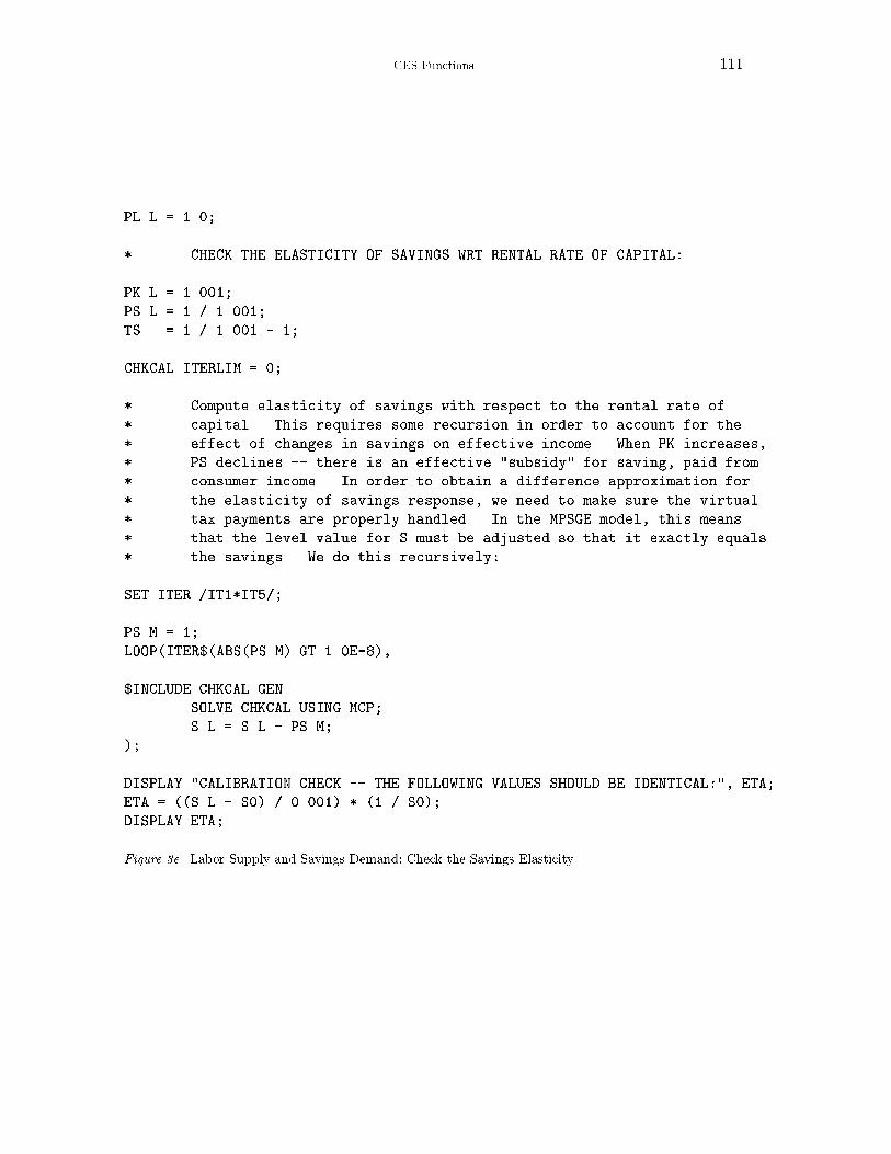
CES Functions 111
PL.L = 1.0;
* CHECK THE ELASTICITY OF SAVINGS WRT RENTAL RATE OF CAPITAL:
PK.L = 1.001;
PS.L = 1 / 1.001;
TS = 1 / 1.001 - 1;
CHKCAL.ITERLIM = 0;
* Compute elasticity of savings with respect to the rental rate of
* capital. This requires some recursion in order to account for the
* effect of changes in savings on effective income. When PK increases,
* PS declines -- there is an effective "subsidy" for saving, paid from
* consumer income. In order to obtain a difference approximation for
* the elasticity of savings response, we need to make sure the virtual
* tax payments are properly handled. In the MPSGE model, this means
* that the level value for S must be adjusted so that it exactly equals
* the savings. We do this recursively:
SET ITER /IT1*IT5/;
PS.M = 1;
LOOP(ITER$(ABS(PS.M) GT 1.0E-8),
$INCLUDE CHKCAL.GEN
SOLVE CHKCAL USING MCP;
S.L = S.L - PS.M;
);
DISPLAY "CALIBRATION CHECK -- THE FOLLOWING VALUES SHOULD BE IDENTICAL:", ETA;
ETA = ((S.L - S0) / 0.001) * (1 / S0);
DISPLAY ETA;
Figure 3e. Labor Supply and Savings Demand: Check the Savings Elasticity
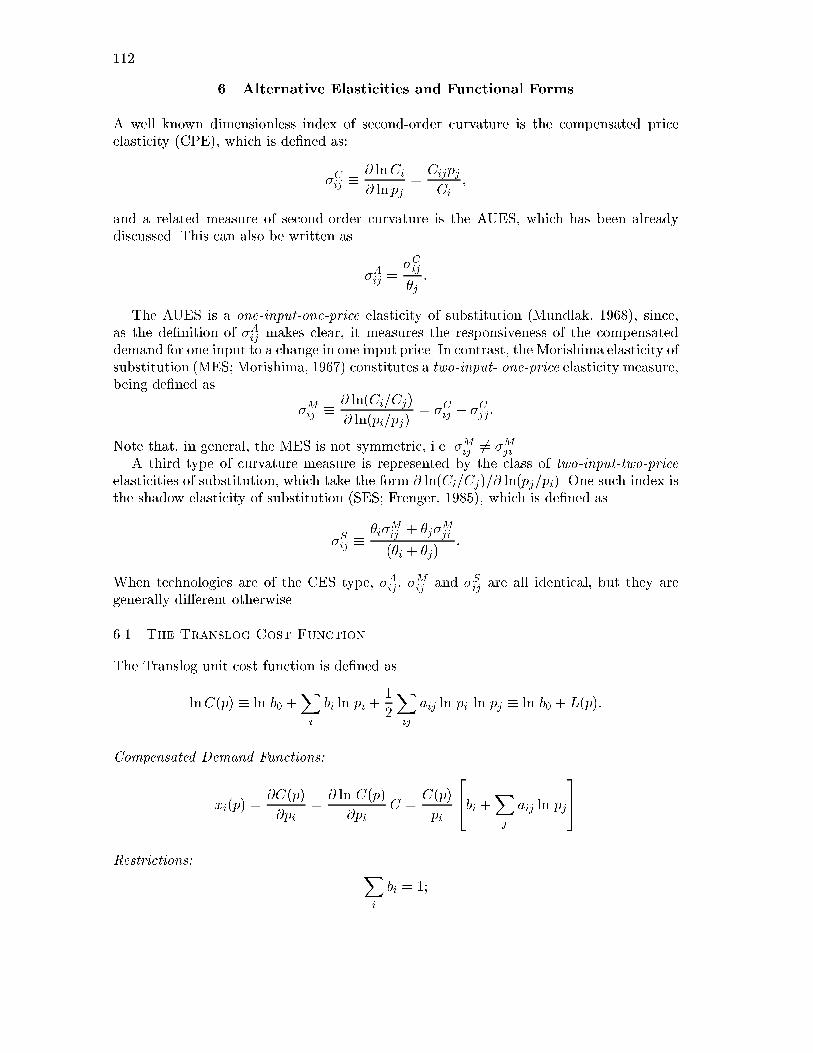
112
6. Alternative Elasticities and Functional Forms
A well known dimensionless index of second-order curvature is the compensated priceelasticity (CPE), which is de�ned as:
�Cij �@ lnCi@ ln pj
=CijpjCi
;
and a related measure of second-order curvature is the AUES, which has been alreadydiscussed. This can also be written as
�Aij =�Cij�j:
The AUES is a one-input-one-price elasticity of substitution (Mundlak, 1968), since,as the de�nition of �Aij makes clear, it measures the responsiveness of the compensateddemand for one input to a change in one input price. In contrast, the Morishima elasticity ofsubstitution (MES; Morishima, 1967) constitutes a two-input- one-price elasticity measure,being de�ned as
�Mij �@ ln(Ci=Cj)
@ ln(pi=pj)= �Cij � �Cjj:
Note that, in general, the MES is not symmetric, i.e. �Mij 6= �Mji .A third type of curvature measure is represented by the class of two-input-two-price
elasticities of substitution, which take the form @ ln(Ci=Cj)=@ ln(pj=pi). One such index isthe shadow elasticity of substitution (SES; Frenger, 1985), which is de�ned as
�Sij ��i�
Mij + �j�
Mji
(�i + �j):
When technologies are of the CES type, �Aij , �Mij and �Sij are all identical, but they are
generally di�erent otherwise.
6.1. The Translog Cost Function
The Translog unit cost function is de�ned as
lnC(p) � ln b0 +Xi
bi ln pi +1
2
Xij
aij ln pi ln pj � ln b0 + L(p):
Compensated Demand Functions:
xi(p) =@C(p)
@pi=@ ln C(p)
@piC =
C(p)
pi
24bi +X
j
aij ln pj
35
Restrictions: Xi
bi = 1;
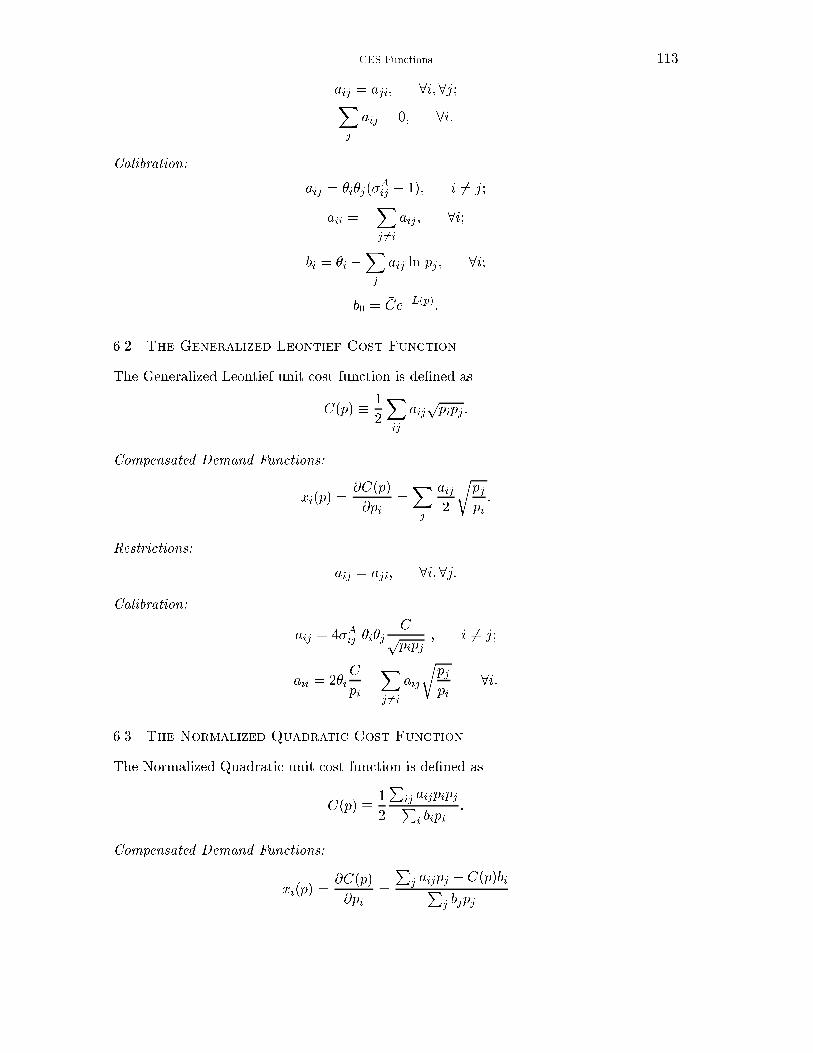
CES Functions 113
aij = aji; 8i;8j;Xj
aij = 0; 8i:
Calibration:
aij = �i�j(�Aij � 1); i 6= j;
aii = �Xj 6=i
aij ; 8i;
bi = �i �Xj
aij ln pj; 8i;
b0 = �Ce�L(p):
6.2. The Generalized Leontief Cost Function
The Generalized Leontief unit cost function is de�ned as
C(p) � 1
2
Xij
aijppipj:
Compensated Demand Functions:
xi(p) =@C(p)
@pi=Xj
aij2
rpjpi:
Restrictions:
aij = aji; 8i;8j:
Calibration:
aij = 4�Aij �i�j�Cppipj
; i 6= j;
aii = 2�i�C
pi�Xj 6=i
aij
rpjpi
8i:
6.3. The Normalized Quadratic Cost Function
The Normalized Quadratic unit cost function is de�ned as
C(p) � 1
2
Pij aijpipjPi bipi
:
Compensated Demand Functions:
xi(p) =@C(p)
@pi=
Pj aijpj � C(p)biP
j bjpj
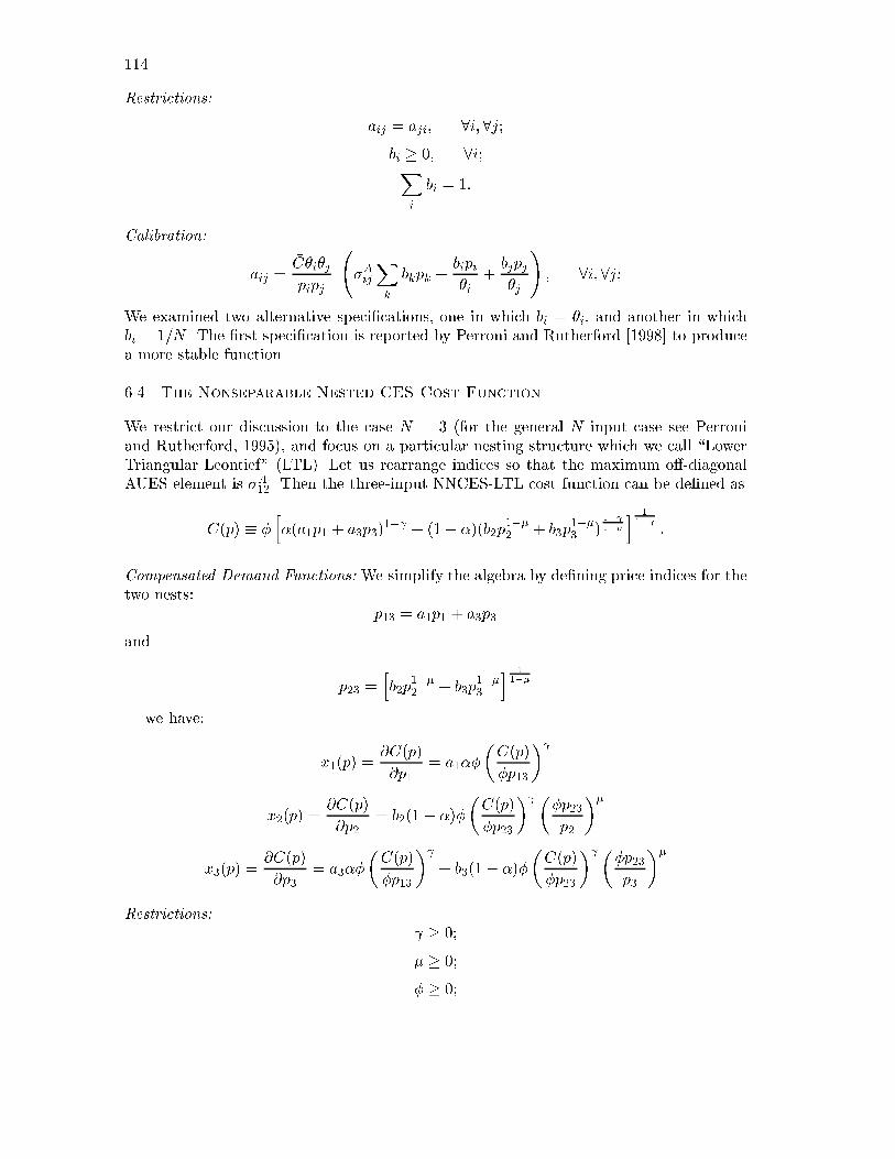
114
Restrictions:
aij = aji; 8i;8j;bi � 0; 8i;X
i
bi = 1:
Calibration:
aij =�C�i�jpipj
�AijXk
bkpk +bipi�i
+bjpj�j
!; 8i;8j;
We examined two alternative speci�cations, one in which bi = �i, and another in whichbi = 1=N . The �rst speci�cation is reported by Perroni and Rutherford [1998] to producea more stable function.
6.4. The Nonseparable Nested CES Cost Function
We restrict our discussion to the case N = 3 (for the general N -input case see Perroniand Rutherford, 1995), and focus on a particular nesting structure which we call \LowerTriangular Leontief" (LTL). Let us rearrange indices so that the maximum o�-diagonalAUES element is �A12. Then the three-input NNCES-LTL cost function can be de�ned as
C(p) � �h�(a1p1 + a3p3)
1� + (1� �)(b2p1��2 + b3p1��3 )
1� 1��
i 11�
:
Compensated Demand Functions: We simplify the algebra by de�ning price indices for thetwo nests:
p13 = a1p1 + a3p3
and
p23 =hb2p
1��2 + b3p
1��3
i 11��
we have:
x1(p) =@C(p)
@p1= a1��
�C(p)
�p13
�
x2(p) =@C(p)
@p2= b2(1� �)�
�C(p)
�p23
� ��p23p2
��
x3(p) =@C(p)
@p3= a3��
�C(p)
�p13
� + b3(1� �)�
�C(p)
�p23
� ��p23p3
��
Restrictions: � 0;
� � 0;
� � 0;
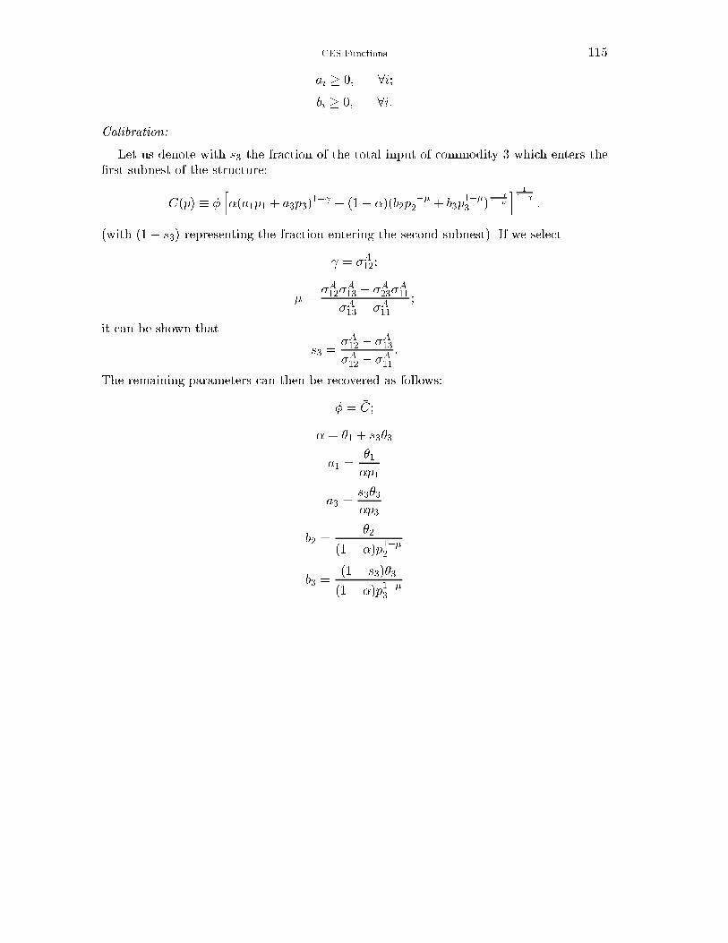
CES Functions 115
ai � 0; 8i;bi � 0; 8i:
Calibration:
Let us denote with s3 the fraction of the total input of commodity 3 which enters the�rst subnest of the structure:
C(p) � �h�(a1p1 + a3p3)
1� + (1� �)(b2p1��2 + b3p1��3 )
1� 1��
i 11�
:
(with (1� s3) representing the fraction entering the second subnest). If we select
= �A12;
� =�A12�
A13 � �A23�A11�A13 � �A11
;
it can be shown that
s3 =�A12 � �A13�A12 � �A11
:
The remaining parameters can then be recovered as follows:
� = �C;
� = �1 + s3�3
a1 =�1�p1
a3 =s3�3�p3
b2 =�2
(1� �)p1��2
b3 =(1� s3)�3(1� �)p1��3


Extensions of GAMS for Complementarity Problems in Economics
Abstract. This paper introduces new features of the GAMS modeling language which have been de-veloped for solving nonlinear complementarity problems. The paper de�nes the "mixed complementarityproblem" (MCP) and its various manifestations. Complementarity formulations for three economic modelsare developed, and computational benchmarks are presented for two large-scale MCP solvers. Finally,procedures for local sensitivity analysis are described.
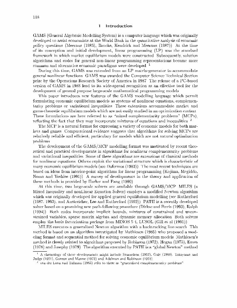
118
1. Introduction
GAMS (General Algebraic Modelling System) is a computer language which was originallydeveloped to assist economists at the World Bank in the quantitative analysis of economicpolicy questions (Meeraus (1983), Brooke, Kendrick and Meeraus (1987)). At the timeof its conception and initial development, linear programming (LP) was the standardframework in which market equilibrium models were constructed. Subsequently, solutionalgorithms and codes for general non-linear programming representations became morecommon and alternative economic paradigms were developed. 1
During this time, GAMS was extended from an LP matrix-generator to accommodategeneral nonlinear functions. GAMS was awarded the Computer Science Technical Sectionprize by the Operations Research Society of America in 1987. The release of a PC-basedversion of GAMS in 1988 lead to its wide-spread recognition as an e�ective tool for thedevelopment of general purpose large-scale mathematical programming models.
This paper introduces new features of the GAMS modelling language which permitformulating economic equilibrium models as systems of nonlinear equations, complemen-tarity problems or variational inequalities. These extensions accommodate market andgame-theoretic equilibriummodels which are not easily studied in an optimization context.These formulations are here referred to as \mixed complementarity problems" (MCPs),re ecting the fact that they may incorporate mixtures of equations and inequalities. 2
The MCP is a natural format for expressing a variety of economic models for both mar-kets and games. Computational evidence suggests that algorithms for solving MCPs arerelatively reliable and e�cient, particulary for models which are not natural optimizationproblems.
The development of the GAMS/MCP modelling format was motivated by recent theo-retical and practical developments in algorithms for nonlinear complementarity problemsand variational inequalities. Some of these algorithms are extensions of classical methodsfor nonlinear equations. Others exploit the variational structure which is characteristic ofmany economic equilibriummodels (see Dafermos (1983)). The most recent techniques arebased on ideas from interior-point algorithms for linear programming (Kojima, Megiddo,Noma and Yoshise (1991)). A survey of developments in the theory and application ofthese methods is provided by Harker and Pang (1990).
At this time, two large-scale solvers are available through GAMS/MCP. MILES (aMixed Inequality and nonLinear Equation Solver) employs a modi�ed Newton algorithmwhich was originally developed for applied general equilibrium modelling (see Rutherford(1987, 1993), and Anstreicher, Lee and Rutherford (1992)). PATH is a recently developedsolver based on a promising new path-following procedure (Dirkse and Ferris (1993), Ralph(1994)). Both codes incorporate implicit bounds, mixtures of constrained and uncon-strained variables, sparse matrix algebra and dynamic memory allocation. Both solversemploy the basis factorization package from MINOS 5.4, LUSOL (Gill et al.(1991)).
MILES executes a generalized Newton algorithm with a backtracking line search. Thismethod is based on an algorithm investigated by Mathiesen (1985) who proposed a mod-eling format and sequential method for solving economic equilibrium models. Mathiesen'smethod is closely related to algorithms proposed by Robinson (1972), Hogan (1975), Eaves(1978) and Josephy (1979). The algorithm executed by PATH is a \global Newton" method
1 A chronology of these developments might include Samuelson (1952), Gale (1960), Takayama andJudge (1971), Goreux and Manne (1973) and Adelman and Robinson (1978).
2 van der Laan and Tallman (1985) refer to these as \generalized complementarity problems".
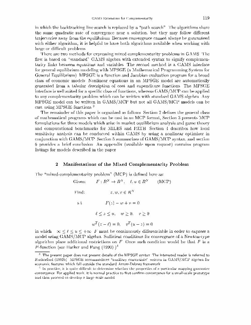
GAMS Extensions for Complementarity 119
in which the backtracking line search is replaced by a \path search". The algorithms sharethe same quadratic rate of convergence near a solution, but they may follow di�erenttrajectories away from the equilibrium. Because convergence cannot always be guaranteedwith either algorithm, it is helpful to have both algorithms available when working withlarge or di�cult problems.
There are two methods for expressing mixed complementarity problems in GAMS. The�rst is based on \standard" GAMS algebra with extended syntax to signify complemen-tarity links between equations and variables. The second method is a GAMS interfacefor general equilibrium modeling with MPSGE (a Mathematical Programming System forGeneral Equilibrium). MPSGE is a function and Jacobian evaluation program for a broadclass of economic models. Nonlinear equations in an MPSGE model are automaticallygenerated from a tabular description of cost and expenditure functions. The MPSGEinterface is well suited for a speci�c class of functions, whereas GAMS/MCP can be appliedto any complementarity problem which can be written with standard GAMS algebra. AnyMPSGE model can be written in GAMS/MCP but not all GAMS/MCP models can becast using MPSGE functions.3
The remainder of this paper is organized as follows. Section 2 de�nes the general classof mathematical programs which can be cast in an MCP format, Section 3 presents MCPformulations for three models which arise in market equilibrium analysis and game theoryand computational benchmarks for MILES and PATH. Section 4 describes how localsensitivity analysis can be conducted within GAMS by using a nonlinear optimizer inconjunction with GAMS/MCP. Section 5 summarizes of GAMS/MCP syntax, and section6 provides a brief conclusion. An appendix (available upon request) contains programlistings for models described in the paper.
2. Manifestations of the Mixed Complementarity Problem
The \mixed-complementarity problem" (MCP) is de�ned here as:
Given: F : RN ! RN ; `; u 2 RN (MCP)
Find: z; w; v 2 RN
s.t. F (z)� w + v = 0
` � z � u; w � 0; v � 0
wT (z � `) = 0; vT (u� z) = 0
in which �1 � ` � u � +1. F must be continuously di�erentiable in order to express amodel using GAMS/MCP algebra. Su�cient conditions for convergence of a Newton-typealgorithm place additional restrictions on F . Once such condition would be that F is aP -function (see Harker and Pang (1990).)4
3 The present paper does not present details of the MPSGE syntax. The interested reader is referred toRutherford (1992b). MPSGE accommodates \auxiliary constraints" written in GAMS/MCP algebra foreconomic features which fall outside the standard Arrow-Debreu framework.
4 In practice, it is quite di�cult to determine whether the properties of a particular mapping guaranteeconvergence. For applied work, it is normal practice to �rst con�rm convergence for a small-scale prototypeand then proceed to develop a large scale model.
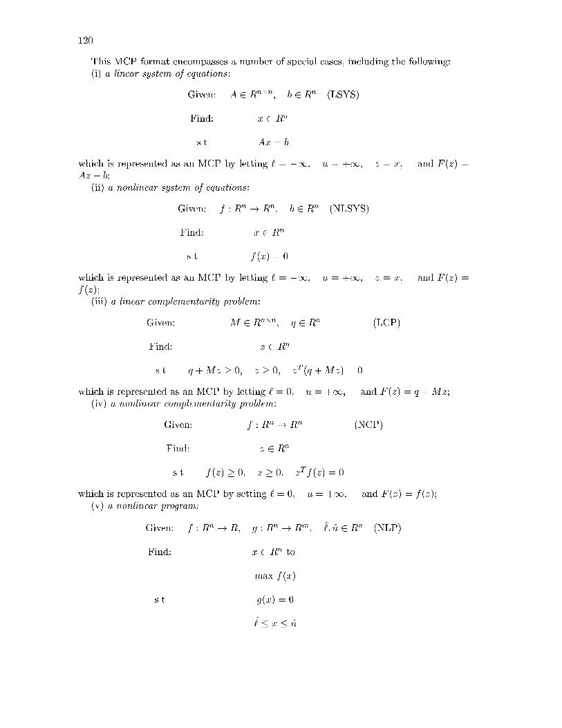
120
This MCP format encompasses a number of special cases, including the following:(i) a linear system of equations:
Given: A 2 Rn�n; b 2 Rn (LSYS)
Find: x 2 Rn
s.t. Ax = b
which is represented as an MCP by letting ` = �1; u = +1; z = x; and F (z) =Az � b;
(ii) a nonlinear system of equations:
Given: f : Rn ! Rn; b 2 Rn (NLSYS)
Find: x 2 Rn
s.t. f(x) = 0
which is represented as an MCP by letting ` = �1; u = +1; z = x; and F (z) =f(z);
(iii) a linear complementarity problem:
Given: M 2 Rn�n; q 2 Rn (LCP)
Find: z 2 Rn
s.t. q +Mz � 0; z � 0; zT (q +Mz) = 0
which is represented as an MCP by letting ` = 0; u = +1; and F (z) = q +Mz;(iv) a nonlinear complementarity problem:
Given: f : Rn ! Rn (NCP)
Find: z 2 Rn
s.t. f(z) � 0; z � 0; zT f(z) = 0
which is represented as an MCP by setting ` = 0; u = +1; and F (z) = f(z);(v) a nonlinear program:
Given: f : Rn ! R; g : Rn ! Rm; ^; u 2 Rn (NLP)
Find: x 2 Rn to
max f(x)
s.t. g(x) = 0
^� x � u
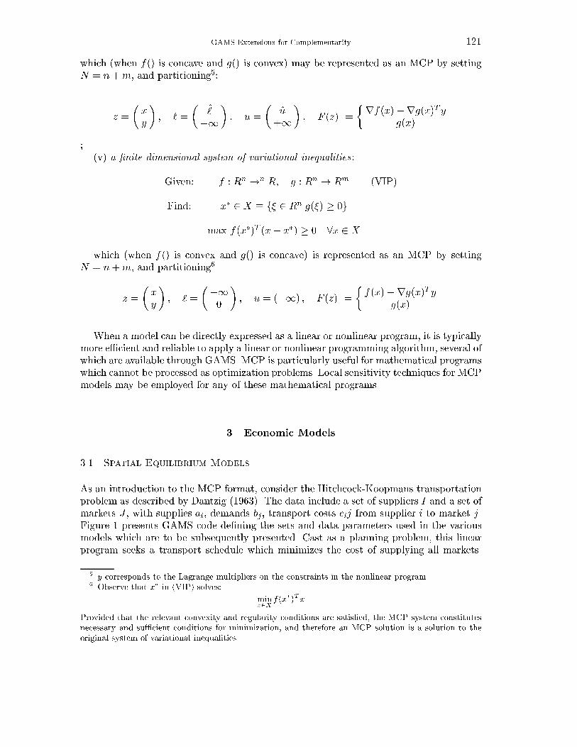
GAMS Extensions for Complementarity 121
which (when f() is concave and g() is convex) may be represented as an MCP by settingN = n+m, and partitioning5:
z =
�xy
�; ` =
�^
�1�; u =
�u
+1�; F (z) =
�rf(x)�rg(x)T yg(x)
;(v) a �nite-dimensional system of variational inequalities:
Given: f : Rn !n R; g : Rn ! Rm (VIP)
Find: x� 2 X � f� 2 Rnjg(�) � 0g
max f(x�)T (x� x�) � 0 8x 2 X
which (when f() is convex and g() is concave) is represented as an MCP by settingN = n+m, and partitioning6
z =
�xy
�; ` =
��10
�; u = (+1) ; F (z) =
�f(x)�rg(x)T y
g(x)
.When a model can be directly expressed as a linear or nonlinear program, it is typically
more e�cient and reliable to apply a linear or nonlinear programming algorithm, several ofwhich are available through GAMS. MCP is particularly useful for mathematical programswhich cannot be processed as optimization problems. Local sensitivity techniques for MCPmodels may be employed for any of these mathematical programs.
3. Economic Models
3.1. Spatial Equilibrium Models
As an introduction to the MCP format, consider the Hitchcock-Koopmans transportationproblem as described by Dantzig (1963). The data include a set of suppliers I and a set ofmarkets J , with supplies ai, demands bj, transport costs cij from supplier i to market j.Figure 1 presents GAMS code de�ning the sets and data parameters used in the variousmodels which are to be subsequently presented. Cast as a planning problem, this linearprogram seeks a transport schedule which minimizes the cost of supplying all markets.
5 y corresponds to the Lagrange multipliers on the constraints in the nonlinear program.6 Observe that x� in (VIP) solves:
minx2X
f(x�)Tx
Provided that the relevant convexity and regularity conditions are satis�ed, the MCP system constitutesnecessary and su�cient conditions for minimization, and therefore an MCP solution is a solution to theoriginal system of variational inequalities.
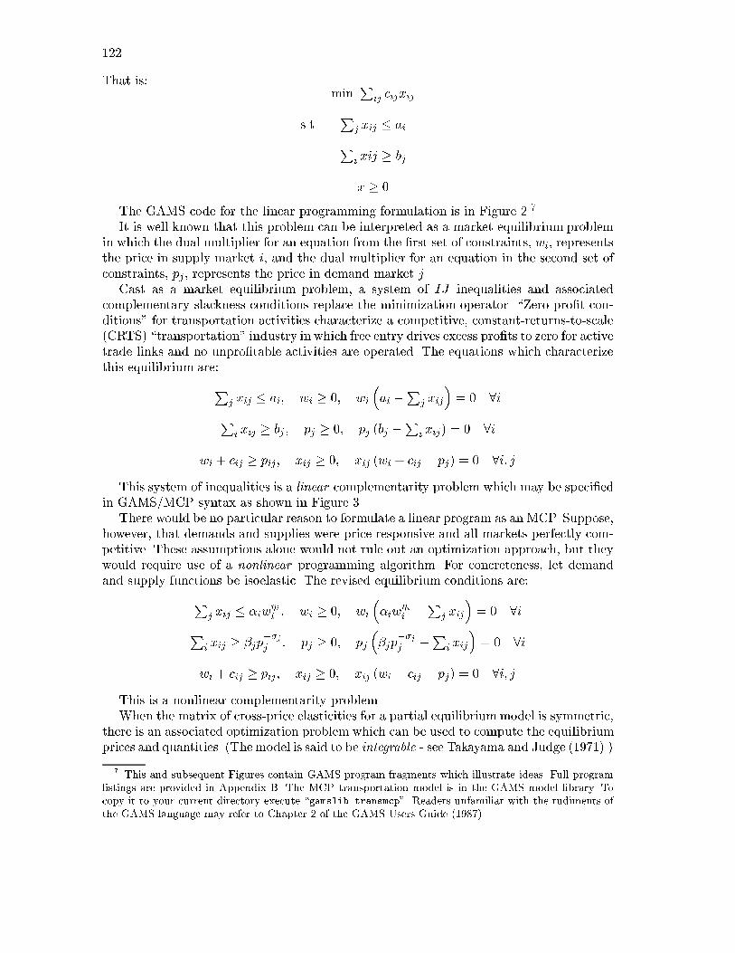
122
That is:min
Pij cijxij
s.t.P
j xij � aiPi xij � bj
x � 0
The GAMS code for the linear programming formulation is in Figure 2.7
It is well known that this problem can be interpreted as a market equilibrium problemin which the dual multiplier for an equation from the �rst set of constraints, wi, representsthe price in supply market i, and the dual multiplier for an equation in the second set ofconstraints, pj , represents the price in demand market j.
Cast as a market equilibrium problem, a system of IJ inequalities and associatedcomplementary slackness conditions replace the minimization operator. \Zero pro�t con-ditions" for transportation activities characterize a competitive, constant-returns-to-scale(CRTS) \transportation" industry in which free entry drives excess pro�ts to zero for activetrade links and no unpro�table activities are operated. The equations which characterizethis equilibrium are:
Pj xij � ai; wi � 0; wi
�ai �
Pj xij
�= 0 8i
Pi xij � bj ; pj � 0; pj (bj �
Pi xij) = 0 8i
wi + cij � pij; xij � 0; xij (wi + cij � pj) = 0 8i; jThis system of inequalities is a linear complementarity problem which may be speci�ed
in GAMS/MCP syntax as shown in Figure 3.There would be no particular reason to formulate a linear program as an MCP. Suppose,
however, that demands and supplies were price responsive and all markets perfectly com-petitive. These assumptions alone would not rule out an optimization approach, but theywould require use of a nonlinear programming algorithm. For concreteness, let demandand supply functions be isoelastic. The revised equilibrium conditions are:
Pj xij � �iw�i
i ; wi � 0; wi
��iw
�ii �
Pj xij
�= 0 8i
Pi xij � �jp
��jj ; pj � 0; pj
��jp
��jj �Pi xij
�= 0 8i
wi + cij � pij; xij � 0; xij (wi + cij � pj) = 0 8i; jThis is a nonlinear complementarity problem.When the matrix of cross-price elasticities for a partial equilibriummodel is symmetric,
there is an associated optimization problem which can be used to compute the equilibriumprices and quantities. (The model is said to be integrable - see Takayama and Judge (1971).)
7 This and subsequent Figures contain GAMS program fragments which illustrate ideas. Full programlistings are provided in Appendix B. The MCP transportation model is in the GAMS model library. Tocopy it to your current directory execute \gamslib transmcp". Readers unfamiliar with the rudiments ofthe GAMS language may refer to Chapter 2 of the GAMS Users Guide (1987).
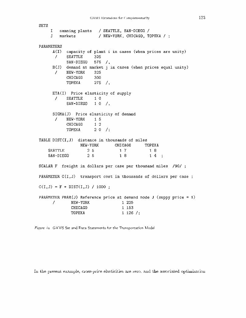
GAMS Extensions for Complementarity 123
SETS
I canning plants / SEATTLE, SAN-DIEGO /
J markets / NEW-YORK, CHICAGO, TOPEKA / ;
PARAMETERS
A(I) capacity of plant i in cases (when prices are unity)
/ SEATTLE 325
SAN-DIEGO 575 /,
B(J) demand at market j in cases (when prices equal unity)
/ NEW-YORK 325
CHICAGO 300
TOPEKA 275 /,
ETA(I) Price elasticity of supply
/ SEATTLE 1.0
SAN-DIEGO 1.0 /,
SIGMA(J) Price elasticity of demand
/ NEW-YORK 1.5
CHICAGO 1.2
TOPEKA 2.0 /;
TABLE DIST(I,J) distance in thousands of miles
NEW-YORK CHICAGO TOPEKA
SEATTLE 2.5 1.7 1.8
SAN-DIEGO 2.5 1.8 1.4 ;
SCALAR F freight in dollars per case per thousand miles /90/ ;
PARAMETER C(I,J) transport cost in thousands of dollars per case ;
C(I,J) = F * DIST(I,J) / 1000 ;
PARAMETER PBAR(J) Reference price at demand node J (suppy price = 1)
/ NEW-YORK 1.225
CHICAGO 1.153
TOPEKA 1.126 /;
Figure 1a. GAMS Set and Data Statements for the Transportation Model
In the present example, cross-price elasticities are zero, and the associated optimization
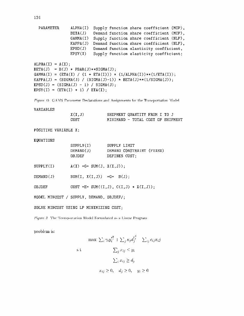
124
PARAMETER ALPHA(I) Supply function share coefficient (MCP),
BETA(J) Demand function share coefficient (MCP),
GAMMA(I) Supply function share coefficient (NLP),
KAPPA(J) Demand function share coefficient (NLP),
EPSD(J) Demand function elasticity coefficient,
EPSY(I) Supply function elasticity coefficient;
ALPHA(I) = A(I);
BETA(J) = B(J) * PBAR(J)**SIGMA(J);
GAMMA(I) = (ETA(I) / (1 + ETA(I))) * (1/ALPHA(I))**(1/ETA(I));
KAPPA(J) = (SIGMA(J) / (SIGMA(J)-1)) * BETA(J)**(1/SIGMA(J));
EPSD(J) = (SIGMA(J) - 1) / SIGMA(J);
EPSY(I) = (ETA(I) + 1) / ETA(I);
Figure 1b. GAMS Parameter Declarations and Assignments for the Transportation Model
VARIABLES
X(I,J) SHIPMENT QUANTITY FROM I TO J
COST MINIMAND - TOTAL COST OF SHIPMENT
POSITIVE VARIABLE X;
EQUATIONS
SUPPLY(I) SUPPLY LIMIT
DEMAND(J) DEMAND CONSTRAINT (FIXED)
OBJDEF DEFINES COST;
SUPPLY(I).. A(I) =G= SUM(J, X(I,J));
DEMAND(J).. SUM(I, X(I,J)) =G= B(J);
OBJDEF.. COST =E= SUM((I,J), C(I,J) * X(I,J));
MODEL MINCOST / SUPPLY, DEMAND, OBJDEF/;
SOLVE MINCOST USING LP MINIMIZING COST;
Figure 2. The Transportation Model Formulated as a Linear Program
problem is:
maxP
i iy�yii +
Pj �jd
�djj �
Pij cijxij
s.t.P
j xij � yiPi xij � dj
xij � 0; dj � 0; yi � 0
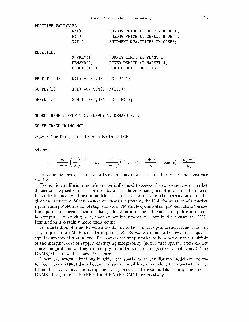
GAMS Extensions for Complementarity 125
POSITIVE VARIABLES
W(I) SHADOW PRICE AT SUPPLY NODE I,
P(J) SHADOW PRICE AT DEMAND NODE J,
X(I,J) SHIPMENT QUANTITIES IN CASES;
EQUATIONS
SUPPLY(I) SUPPLY LIMIT AT PLANT I,
DEMAND(J) FIXED DEMAND AT MARKET J,
PROFIT(I,J) ZERO PROFIT CONDITIONS;
PROFIT(I,J).. W(I) + C(I,J) =G= P(J);
SUPPLY(I).. A(I) =G= SUM(J, X(I,J));
DEMAND(J).. SUM(I, X(I,J)) =G= B(J);
MODEL TRNSP / PROFIT.X, SUPPLY.W, DEMAND.P/ ;
SOLVE TRNSP USING MCP;
Figure 3. The Transportation LP Formulated as an LCP
where:
i =�i
1 + �i
�1
�i
�1=�i
; �j =�j
1 + �j�1=�jj ; �yi =
1 + �i�i
; and �dj =�j � 1
�j
In economic terms, the market allocation \maximizes the sum of producer and consumersurplus".
Economic equilibrium models are typically used to assess the consequences of marketdistortions, typically in the form of taxes, tari�s or other types of government policies.In public �nance, equilibrium models are often used to measure the \excess burden" of agiven tax structure. When ad-valorem taxes are present, the NLP formulation of a marketequilibrium problem is not straight-forward. No single optimization problem characterizesthe equilibrium because the resulting allocation is ine�cient. Such an equilibrium couldbe computed by solving a sequence of nonlinear programs, but in these cases the MCPformulation is certainly more transparent.
As illustration of a model which is di�cult to treat in an optimization framework buteasy to pose as an MCP, consider applying ad-valorem taxes on trade ows in the spatialequilibrium model from above. This causes the supply price to be a non-unitary multipleof the marginal cost of supply, destroying integrability (notice that speci�c taxes do notcause this problem, as they can simply be added to the transport cost coe�cients). TheGAMS/MCP model is shown in Figure 4.
There are several directions in which the spatial price equilibrium model can be ex-tended. Harker (1986) describes several spatial equilibrium models with imperfect compe-tition. The variational and complementarity versions of these models are implemented inGAMS library models HARKER and HARKERMCP, respectively.
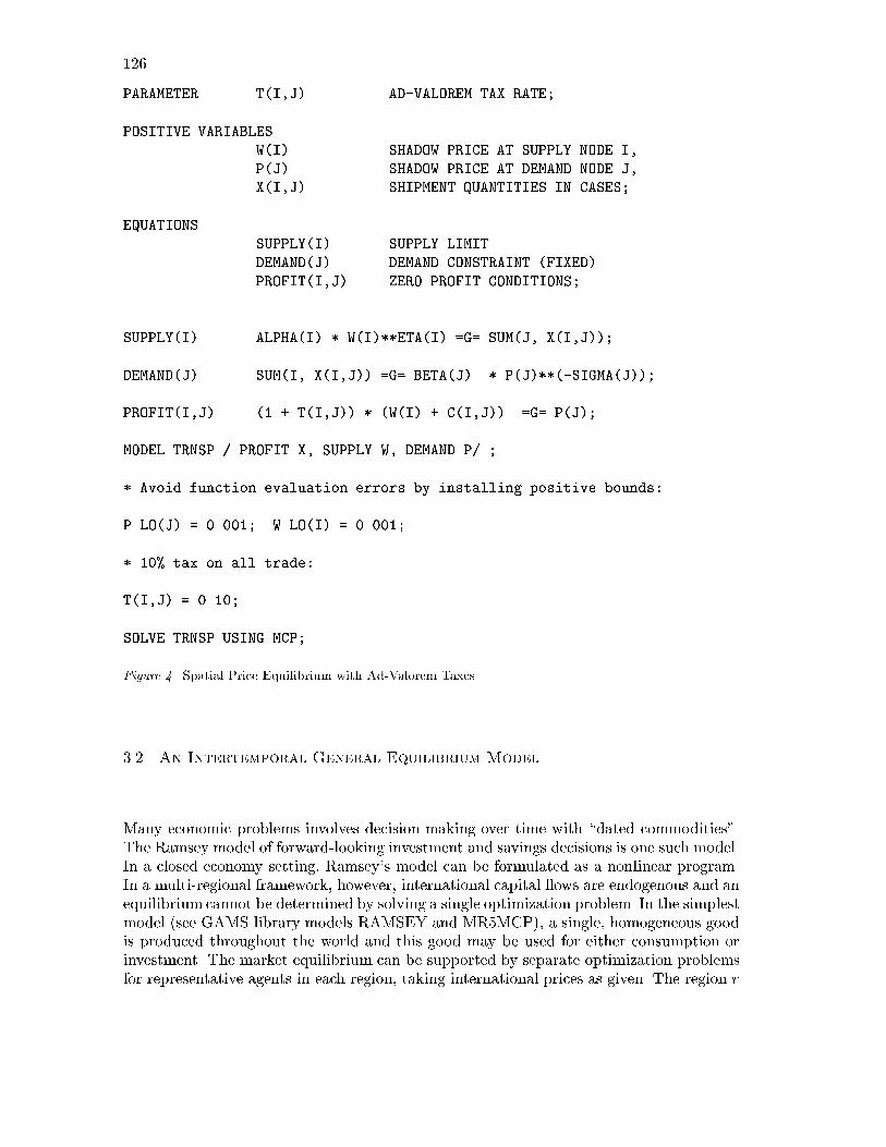
126
PARAMETER T(I,J) AD-VALOREM TAX RATE;
POSITIVE VARIABLES
W(I) SHADOW PRICE AT SUPPLY NODE I,
P(J) SHADOW PRICE AT DEMAND NODE J,
X(I,J) SHIPMENT QUANTITIES IN CASES;
EQUATIONS
SUPPLY(I) SUPPLY LIMIT
DEMAND(J) DEMAND CONSTRAINT (FIXED)
PROFIT(I,J) ZERO PROFIT CONDITIONS;
SUPPLY(I).. ALPHA(I) * W(I)**ETA(I) =G= SUM(J, X(I,J));
DEMAND(J).. SUM(I, X(I,J)) =G= BETA(J) * P(J)**(-SIGMA(J));
PROFIT(I,J).. (1 + T(I,J)) * (W(I) + C(I,J)) =G= P(J);
MODEL TRNSP / PROFIT.X, SUPPLY.W, DEMAND.P/ ;
* Avoid function evaluation errors by installing positive bounds:
P.LO(J) = 0.001; W.LO(I) = 0.001;
* 10% tax on all trade:
T(I,J) = 0.10;
SOLVE TRNSP USING MCP;
Figure 4. Spatial Price Equilibrium with Ad-Valorem Taxes
3.2. An Intertemporal General Equilibrium Model
Many economic problems involves decision-making over time with \dated commodities".The Ramsey model of forward-looking investment and savings decisions is one such model.In a closed economy setting, Ramsey's model can be formulated as a nonlinear program.In a multi-regional framework, however, international capital ows are endogenous and anequilibrium cannot be determined by solving a single optimization problem. In the simplestmodel (see GAMS library models RAMSEY and MR5MCP), a single, homogeneous goodis produced throughout the world and this good may be used for either consumption orinvestment. The market equilibrium can be supported by separate optimization problemsfor representative agents in each region, taking international prices as given. The region r
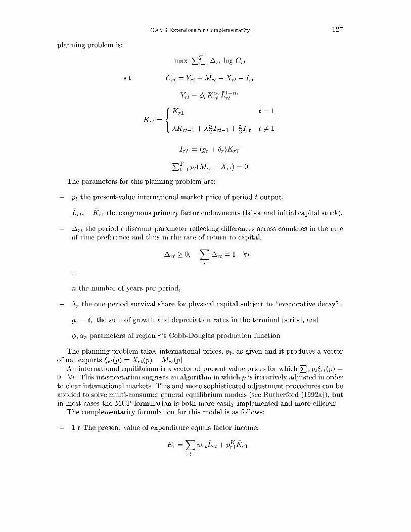
GAMS Extensions for Complementarity 127
planning problem is:
maxPT
t=1�rt log Crt
s.t. Crt = Yrt +Mrt �Xrt � Irt
Yrt = �rK�rrt�L1��rrt
Krt =
8<:
�Kr1 t = 1
�Krt�1 + �n2 Irt�1 +n2 Irt t 6= 1
IrT = (gr + �r)KrTPTt=1 �pt(Mrt �Xrt) = 0
The parameters for this planning problem are:
� pt the present-value international market price of period t output,
� �Lrt; �Kr1 the exogenous primary factor endowments (labor and initial capital stock),
� �rt the period t discount parameter re ecting di�erences across countries in the rateof time preference and thus in the rate of return to capital,
�rt � 0;Xt
�rt = 1 8r
,
� n the number of years per period,
� �r the one-period survival share for physical capital subject to \evaporative decay",
� gr + �r the sum of growth and depreciation rates in the terminal period, and
� �; �r parameters of region r's Cobb-Douglas production function.
The planning problem takes international prices, pt, as given and it produces a vectorof net exports �rt(p) = Xrt(p)�Mrt(p).
An international equilibrium is a vector of present value prices for whichP
r pt�rt(p) =0 8r. This interpretation suggests an algorithm in which p is iteratively adjusted in orderto clear international markets. This and more sophisticated adjustment procedures can beapplied to solve multi-consumer general equilibrium models (see Rutherford (1992a)), butin most cases the MCP formulation is both more easily implemented and more e�cient.
The complementarity formulation for this model is as follows:
� 1.r The present value of expenditure equals factor income:
Er =Xt
wrt �Lrt + pKr1�Kr1
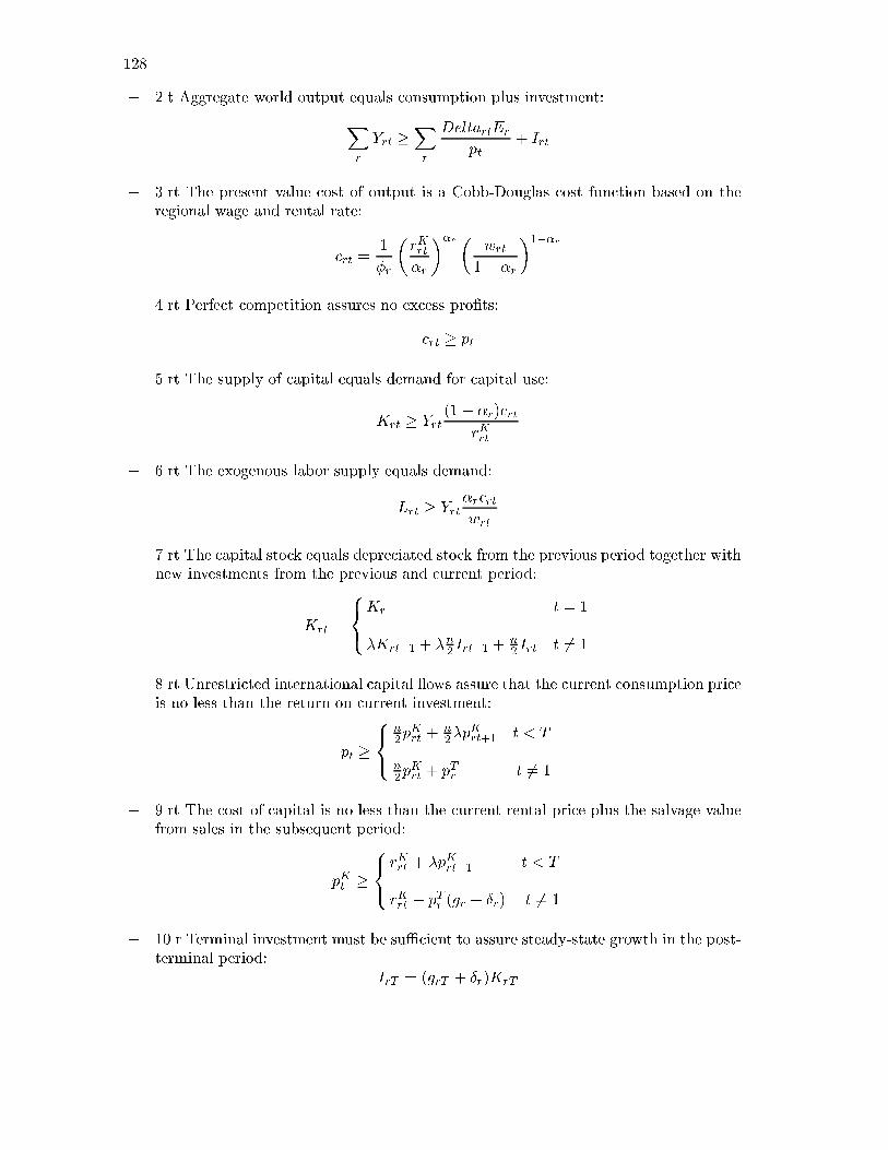
128
� 2.t Aggregate world output equals consumption plus investment:
Xr
Yrt �Xr
DeltartEr
pt+ Irt
� 3.rt The present value cost of output is a Cobb-Douglas cost function based on theregional wage and rental rate:
crt =1
�r
�rKrt�r
��r � wrt1� �r
�1��r
� 4.rt Perfect competition assures no excess pro�ts:
crt � pt
� 5.rt The supply of capital equals demand for capital use:
Krt � Yrt (1� �r)crtrKrt
� 6.rt The exogenous labor supply equals demand:
�Lrt � Yrt�rcrtwrt
� 7.rt The capital stock equals depreciated stock from the previous period together withnew investments from the previous and current period:
Krt =
8<:
�Kr1 t = 1
�Krt�1 + �n2 Irt�1 +n2 Irt t 6= 1
� 8.rt Unrestricted international capital ows assure that the current consumption priceis no less than the return on current investment:
pt �8<:
n2 p
Krt +
n2�p
Krt+1 t < T
n2 p
Krt + pTr t 6= 1
� 9.rt The cost of capital is no less than the current rental price plus the salvage valuefrom sales in the subsequent period:
pKt �8<:rKrt + �pKrt+1 t < T
rKrt � pTr (gr + �r) t 6= 1
� 10.r Terminal investment must be su�cient to assure steady-state growth in the post-terminal period:
IrT = (grT + �r)KrT

GAMS Extensions for Complementarity 129
$TITLE MULTI-REGION RAMSEY MODEL
SET R REGIONS /USA, OOECD, USSR, CHINA, ROW/,
T TIME PERIODS /T1*T11/,
TINIT(T) INITIAL PERIOD /T1/
TTERM(T) TERMINAL PERIOD /T11/;
SCALAR N NUMBER OF YEARS PER PERIOD /10/
PARAMETERS
L(T,R) LABOR STOCK IN EFFICIENCY UNITS
BETA(T,R) INTERTEMPORAL UTILITY PARAMETER
KINIT(R) INITIAL PERIOD CAPITAL STOCK
PHI(R) PRODUCTION FUNCTION SCALE PARAMETER
ALPHA(R) CAPITAL VALUE SHARE
DELTA(R) ANNUAL CAPITAL DEPRECIATION RATE
GAMMA(R) TERMINAL PERIOD GROWTH RATE
LAMBDA(R) ONE PERIOD CAPITAL SURVIVAL SHARE;
Figure 5. Set and Parameter Declarations for the Multi-Region Ramsey Model
Figure 5 displays set and parameter de�nitions for this model (input data tables aresuppressed). The GAMS/MCP equations and solution statements are presented in Figure6. These equations correspond more or less exactly to the formulation given above.
There are two successive solution statements shown in this Figure, illustrating an solu-tion scheme which is advisable for any general equilibriummodel in which a good estimateof equilibrium values is not easily deduced. The �rst MCP solves the \partial equilibriumrelaxation" of the model by �xing relative income levels. (See Rutherford (1992a).) Afterhaving obtained this approximate equilibrium, the model with uncompensated demandfunctions is solved - using the partial equilibrium values as a starting point and holdingthe income for one agent �xed to normalize prices.
3.3. An MCP Formulation for N-Player Non-cooperative Games
The Lemke-Howson (1964) algorithm �nds equilibria for two-player non-cooperative gameswith �nite action spaces in pure or mixed strategies. An N-player extension of bimatrixgames is conveniently expressed with the following notation:
� j denotes players j 2 f1 : : : Ng� i denotes pure strategies i 2 f1 : : : Mg (the same number of strategies are assumed
available to all players to simplify notation)
� s denotes a \pure strategy pro�le" in which one pure strategy is assigned to eachplayer, s 2 f1 : : : MNg
� i(s; j) denotes the pure strategy assigned to player j in strategy pro�le s.
� ajs denotes the payo� to player j which arises from strategy pro�le s.
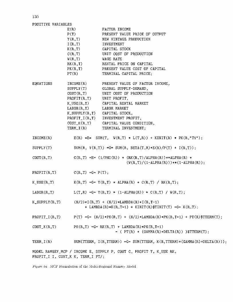
130
POSITIVE VARIABLES
E(R) FACTOR INCOME
P(T) PRESENT VALUE PRICE OF OUTPUT
Y(R,T) NEW VINTAGE PRODUCTION
I(R,T) INVESTMENT
K(R,T) CAPITAL STOCK
C(R,T) UNIT COST OF PRODUCTION
W(R,T) WAGE RATE
RK(R,T) RENTAL PRICE ON CAPITAL
PK(R,T) PRESENT VALUE COST OF CAPITAL
PT(R) TERMINAL CAPITAL PRICE;
EQUATIONS INCOME(R) PRESENT VALUE OF FACTOR INCOME,
SUPPLY(T) GLOBAL SUPPLY-DEMAND,
COST(R,T) UNIT COST OF PRODUCTION
PROFIT(R,T) UNIT PROFIT,
K_USE(R,T) CAPITAL RENTAL MARKET
LABOR(R,T) LABOR MARKET
K_SUPPLY(R,T) CAPITAL STOCK,
PROFIT_I(R,T) INVESTMENT PROFIT,
COST_K(R,T) CAPITAL VALUE CONDITION,
TERM_I(R) TERMINAL INVESTMENT;
INCOME(R).. E(R) =E= SUM(T, W(R,T) * L(T,R)) + KINIT(R) * PK(R,"T1");
SUPPLY(T).. SUM(R, Y(R,T)) =G= SUM(R, BETA(T,R)*E(R)/P(T) + I(R,T));
COST(R,T).. C(R,T) =E= (1/PHI(R)) * (RK(R,T)/ALPHA(R))**ALPHA(R) *
(W(R,T)/(1-ALPHA(R)))**(1-ALPHA(R));
PROFIT(R,T).. C(R,T) =G= P(T);
K_USE(R,T).. K(R,T) =G= Y(R,T) * ALPHA(R) * C(R,T) / RK(R,T);
LABOR(R,T).. L(T,R) =G= Y(R,T) * (1-ALPHA(R)) * C(R,T) / W(R,T);
K_SUPPLY(R,T).. (N/2)*I(R,T) + (N/2)*LAMBDA(R)*I(R,T-1)
+ LAMBDA(R)*K(R,T-1) + KINIT(R)$TINIT(T) =G= K(R,T);
PROFIT_I(R,T).. P(T) =G= (N/2)*PK(R,T) + (N/2)*LAMBDA(R)*PK(R,T+1) + PT(R)$TTERM(T);
COST_K(R,T).. PK(R,T) =G= RK(R,T) + LAMBDA(R)*PK(R,T+1)
- ( PT(R) * (GAMMA(R)+DELTA(R)) )$TTERM(T);
TERM_I(R).. SUM(TTERM, I(R,TTERM)) =G= SUM(TTERM, K(R,TTERM)*(GAMMA(R)+DELTA(R)));
MODEL RAMSEY_MCP / INCOME.E, SUPPLY.P, COST.C, PROFIT.Y, K_USE.RK,
PROFIT_I.I, COST_K.K, TERM_I.PT/;
Figure 6a. MCP Formulation of the Multi-Regional Ramsey Model
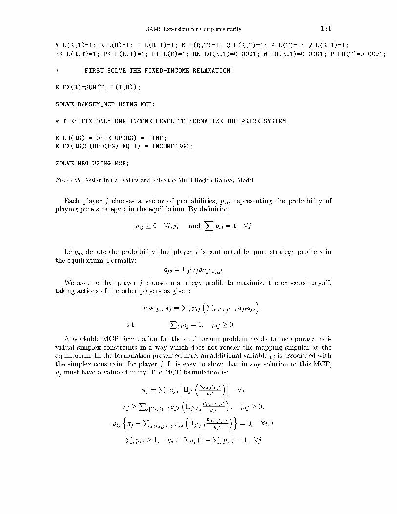
GAMS Extensions for Complementarity 131
Y.L(R,T)=1; E.L(R)=1; I.L(R,T)=1; K.L(R,T)=1; C.L(R,T)=1; P.L(T)=1; W.L(R,T)=1;
RK.L(R,T)=1; PK.L(R,T)=1; PT.L(R)=1; RK.LO(R,T)=0.0001; W.LO(R,T)=0.0001; P.LO(T)=0.0001;
* FIRST SOLVE THE FIXED-INCOME RELAXATION:
E.FX(R)=SUM(T, L(T,R));
SOLVE RAMSEY_MCP USING MCP;
* THEN FIX ONLY ONE INCOME LEVEL TO NORMALIZE THE PRICE SYSTEM:
E.LO(RG) = 0; E.UP(RG) = +INF;
E.FX(RG)$(ORD(RG) EQ 1) = INCOME(RG);
SOLVE MRG USING MCP;
Figure 6b. Assign Initial Values and Solve the Multi-Region Ramsey Model
Each player j chooses a vector of probabilities, pij, representing the probability ofplaying pure strategy i in the equilibrium. By de�nition:
pij � 0 8i; j; andXi
pij = 1 8j
.Letqjs denote the probability that player j is confronted by pure strategy pro�le s in
the equilibrium. Formally:
qjs = �j0 6=jpi(j0;s);j0
We assume that player j chooses a strategy pro�le to maximize the expected payo�,taking actions of the other players as given:
maxpij �j =P
i pij
�Psji(s;j)=i ajsqjs
�s.t.
Pi pij = 1; pij � 0
A workable MCP formulation for the equilibrium problem needs to incorporate indi-vidual simplex constraints in a way which does not render the mapping singular at theequilibrium. In the formulation presented here, an additional variable yj is associated withthe simplex constraint for player j. It is easy to show that in any solution to this MCP,yj must have a value of unity. The MCP formulation is:
�j =P
s ajs
h�j0
�pi(s;j0);j0
yj0
�i8j
�j �P
sji(s;j)=i ajs
��j0 6=j
pi(s;j0);j0
yj0
�; pij � 0;
pij
n�j �
Psji(s;j)=i ajs
��j0 6=j
pi(s;j0);j0
yj0
�o= 0; 8i; j
Pi pij � 1; yj � 0; yj (1�
Pi pij) = 1 8j

132
SET J PLAYERS /J1*J3/,
I ACTIONS /I1*I2/,
SS STRATEGY PROFILES /S1*S1000/,
S(SS) ACTIVE STRATEGY PROFILES,
LINK(SS,I,J) CONNECTION BETWEEN ACTIONS AND PROFILES;
ABORT$(CARD(SS) LT CARD(I1)**3) " SET SS IS NOT LARGE ENOUGH.";
PARAMETER
PAYOFF(SS,J) PAYOFF DATA IN STRATEGY-PROFILE FORMAT;
* READ THE DATA:
TABLE LOSS(J,I,I,I) PAYOFF DATA IN DENSE FORM
I1.I1 I1.I2 I2.I1 I2.I2
J1.I1 1 2 8 5
J1.I2 8 8 2 2
J2.I1 4 2 2 1
J2.I2 2 6 1 1
J3.I1 4 1 4 2
J3.I2 8 8 2 1;
* LET I1, I2 AND I3 ALL STAND FOR SET I:
ALIAS (I,I1),(I,I2),(I,I3);
* ASSIGN PLAYER ACTIONS TO STRATEGY PROFILES USING
* DYNAMIC SET S().
* INITIALIZE SET S WITH A SINGLE ENTRY, THE FIRST ELEMENT OF SS:
S("S1") = YES;
* ONE ELEMENT OF SET S IS GENERATED FOR EACH COMBINATION OF PURE STRATEGIES:
LOOP((I1,I2,I3),
* SET S CONTAINS A SINGLE ELEMENT FOR THE FOLLOWING STATEMENT:
LINK(S,I1,"J1") = YES;
LINK(S,I2,"J2") = YES;
LINK(S,I3,"J3") = YES;
PAYOFF(S,J) = -LOSS(J,I1,I2,I3);
* THE NEXT STATEMENTS MOVE S THE SUBSEQUENT ELEMENT OF SS:
S(SS)$S(SS-1) = YES;
S(SS)$S(SS+1) = NO;
);
* THE NEXT STATEMENTS DEFINE THE SET OF ACTION PROFILES AS
* THOSE ELEMENTS OF SS FOR WHICH PAYOFFS HAVE BEEN ASSIGNED:
S(SS) = NO; S(SS) = YES$SUM(J, ABS(PAYOFF(SS,J)));
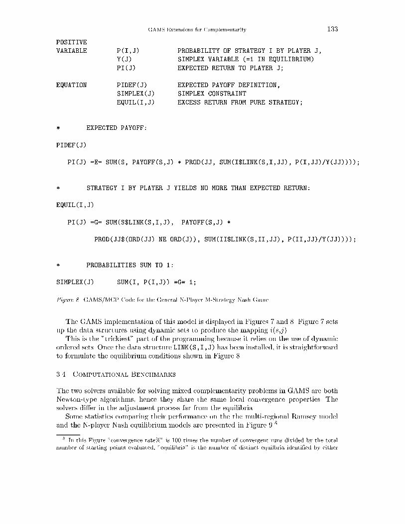
GAMS Extensions for Complementarity 133
POSITIVE
VARIABLE P(I,J) PROBABILITY OF STRATEGY I BY PLAYER J,
Y(J) SIMPLEX VARIABLE (=1 IN EQUILIBRIUM)
PI(J) EXPECTED RETURN TO PLAYER J;
EQUATION PIDEF(J) EXPECTED PAYOFF DEFINITION,
SIMPLEX(J) SIMPLEX CONSTRAINT
EQUIL(I,J) EXCESS RETURN FROM PURE STRATEGY;
* EXPECTED PAYOFF:
PIDEF(J)..
PI(J) =E= SUM(S, PAYOFF(S,J) * PROD(JJ, SUM(I$LINK(S,I,JJ), P(I,JJ)/Y(JJ))));
* STRATEGY I BY PLAYER J YIELDS NO MORE THAN EXPECTED RETURN:
EQUIL(I,J)..
PI(J) =G= SUM(S$LINK(S,I,J), PAYOFF(S,J) *
PROD(JJ$(ORD(JJ) NE ORD(J)), SUM(II$LINK(S,II,JJ), P(II,JJ)/Y(JJ))));
* PROBABILITIES SUM TO 1:
SIMPLEX(J).. SUM(I, P(I,J)) =G= 1;
Figure 8. GAMS/MCP Code for the General N-Player M-Strategy Nash Game
The GAMS implementation of this model is displayed in Figures 7 and 8. Figure 7 setsup the data structures using dynamic sets to produce the mapping i(s,j).
This is the "trickiest" part of the programming because it relies on the use of dynamicordered sets. Once the data structure LINK(S,I,J) has been installed, it is straightforwardto formulate the equilibrium conditions shown in Figure 8.
3.4. Computational Benchmarks
The two solvers available for solving mixed complementarity problems in GAMS are bothNewton-type algorithms, hence they share the same local convergence properties. Thesolvers di�er in the adjustment process far from the equilibria.
Some statistics comparing their performance on the the multi-regional Ramsey modeland the N-player Nash equilibrium models are presented in Figure 9.8
8 In this Figure "convergence rate%" is 100 times the number of convergent runs divided by the totalnumber of starting points evaluated, "equilibria" is the number of distinct equilbria identi�ed by either
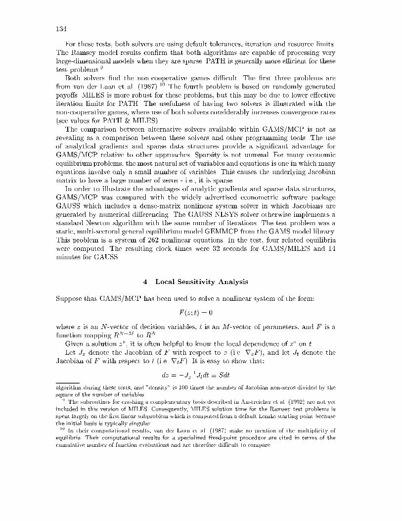
134
For these tests, both solvers are using default tolerances, iteration and resource limits.The Ramsey model results con�rm that both algorithms are capable of processing verylarge-dimensional models when they are sparse. PATH is generally more e�cient for thesetest problems.9
Both solvers �nd the non-cooperative games di�cult. The �rst three problems arefrom van der Laan et al. (1987).10 The fourth problem is based on randomly generatedpayo�s. MILES is more robust for these problems, but this may be due to lower e�ectiveiteration limits for PATH. The usefulness of having two solvers is illustrated with thenon-cooperative games, where use of both solvers considerably increases convergence rates(see values for PATH & MILES).
The comparison between alternative solvers available within GAMS/MCP is not asrevealing as a comparison between these solvers and other programming tools. The useof analytical gradients and sparse data structures provide a signi�cant advantage forGAMS/MCP relative to other approaches. Sparsity is not unusual. For many economicequilibrium problems, the most natural set of variables and equations is one in which manyequations involve only a small number of variables. This causes the underlying Jacobianmatrix to have a large number of zeros - i.e., it is sparse.
In order to illustrate the advantages of analytic gradients and sparse data structures,GAMS/MCP was compared with the widely advertised econometric software packageGAUSS which includes a dense-matrix nonlinear system solver in which Jacobians aregenerated by numerical di�erencing. The GAUSS NLSYS solver otherwise implements astandard Newton algorithm with the same number of iterations. The test problem was astatic, multi-sectoral general equilibriummodel GEMMCP from the GAMS model library.This problem is a system of 262 nonlinear equations. In the test, four related equilibriawere computed. The resulting clock times were 32 seconds for GAMS/MILES and 14minutes for GAUSS.
4. Local Sensitivity Analysis
Suppose that GAMS/MCP has been used to solve a nonlinear system of the form:
F (z; t) = 0
where z is an N -vector of decision variables, t is an M -vector of parameters, and F is afunction mapping RN+M to RN .
Given a solution z�, it is often helpful to know the local dependence of z� on t.Let Jz denote the Jacobian of F with respect to z (i.e. rzF ), and let Jt denote the
Jacobian of F with respect to t (i.e. rtF ). It is easy to show that:
dz = �J�1z Jtdt � Sdtalgorithm during these tests, and "density" is 100 times the number of Jacobian non-zeros divided by thesquare of the number of variables.
9 The subroutines for crashing a complementary basis described in Anstreicher et al. (1992) are not yetincluded in this version of MILES. Consequently, MILES solution time for the Ramsey test problems isspent largely on the �rst linear subproblem which is computed from a default Lemke starting point becausethe initial basis is typically singular.10 In their computational results, van der Laan et al. (1987) make no mention of the multiplicity of
equilibria. Their computational results for a specialized �xed-point procedure are cited in terms of thecumulative number of function evaluations and are therefore di�cult to compare.
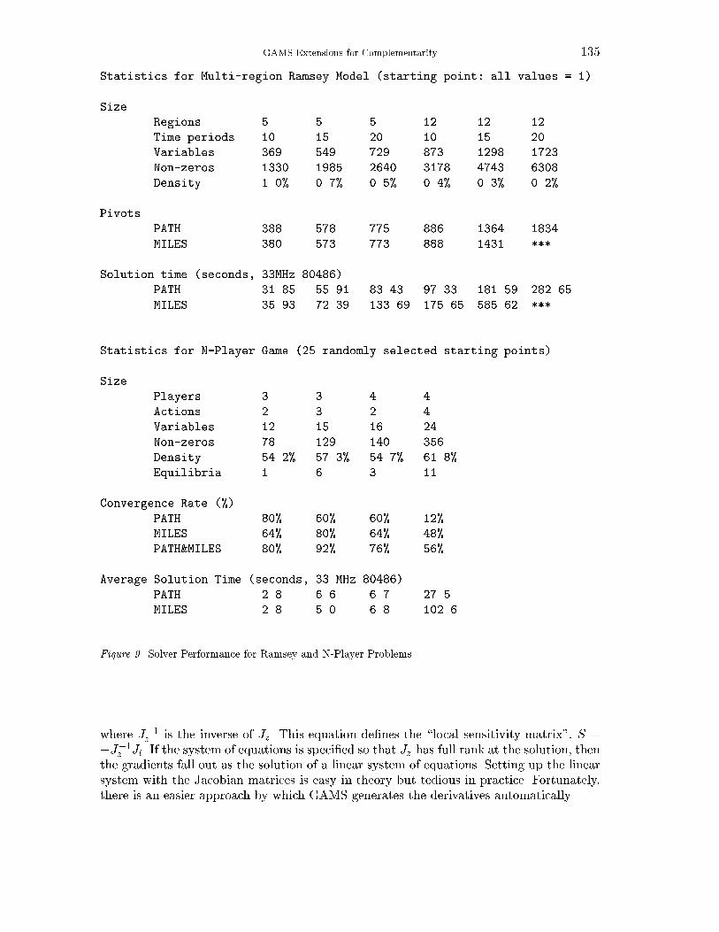
GAMS Extensions for Complementarity 135
Statistics for Multi-region Ramsey Model (starting point: all values = 1)
Size
Regions 5 5 5 12 12 12
Time periods 10 15 20 10 15 20
Variables 369 549 729 873 1298 1723
Non-zeros 1330 1985 2640 3178 4743 6308
Density 1.0% 0.7% 0.5% 0.4% 0.3% 0.2%
Pivots
PATH 388 578 775 886 1364 1834
MILES 380 573 773 888 1431 ***
Solution time (seconds, 33MHz 80486)
PATH 31.85 55.91 83.43 97.33 181.59 282.65
MILES 35.93 72.39 133.69 175.65 585.62 ***
Statistics for N-Player Game (25 randomly selected starting points)
Size
Players 3 3 4 4
Actions 2 3 2 4
Variables 12 15 16 24
Non-zeros 78 129 140 356
Density 54.2% 57.3% 54.7% 61.8%
Equilibria 1 6 3 11
Convergence Rate (%)
PATH 80% 60% 60% 12%
MILES 64% 80% 64% 48%
PATH&MILES 80% 92% 76% 56%
Average Solution Time (seconds, 33 MHz 80486)
PATH 2.8 6.6 6.7 27.5
MILES 2.8 5.0 6.8 102.6
Figure 9. Solver Performance for Ramsey and N-Player Problems
where J�1z is the inverse of Jz . This equation de�nes the \local sensitivity matrix", S =�J�1z Jt. If the system of equations is speci�ed so that Jz has full rank at the solution, thenthe gradients fall out as the solution of a linear system of equations. Setting up the linearsystem with the Jacobian matrices is easy in theory but tedious in practice. Fortunately,there is an easier approach by which GAMS generates the derivatives automatically.
136
Consider the following nonlinear program:
maxz;t zi
s.t. F (z; t) = 0
t = �t
The implicit function theorem (see Varian (1992)) implies that the ith row of S cor-responds to the dual multipliers associated with the bounds on t. To compute the entiresensitivity matrix therefore requires the solution of N separate sets of nonlinear programs,all of which may be initiated at the equilibrium point.
A minor variation on this technique applies to complementarity problems involvingmixtures of equations and inequalities. In the MCP case, the nonlinear system passedto the nonlinear program only include those equations which are binding at the solution(i.e., any equations which are slack in the MCP solution must be omitted from the NLPusing GAMS exception (\$") operators). An illustration of this technique is provided inthe Appendix.
5. GAMS/MCP Syntax
In a GAMS/MCP program, the central unknowns, z, are declared as VARIABLES, thevectors u and are speci�ed as upper and lower bounds. The function F () is written usingGAMS matrix algebra in equation statements. All aspects of the GAMS/MCP languageare identical to GAMS/NLP except that in an MCP problem no objective function isspeci�ed, and bounded variables must be mapped to complementary inequalities.
In the canonical MCP structure, the equations wT (z � `) = 0 and vT (u� z) = 0 implya particular association of variables with equations. Quite naturally, zi is complementarywith Fi(z). In an empirical model, there are typically several classes of variables andequations, and the declaration sequence is arbitrary, so the rule ziFi = 0 is impossible tointerpret.11
To �x the complementarity structure, a GAMS/MCP program explicitly associatesvariables with equations in the MODEL statement. Unlike an NLP in which only equationnames appear on the model statement, in an MCP program both equation and variablenames may be listed. The syntax is:
MODEL NAME /EQU1.VAR1, EQU2.VAR2, .../;
In this list, EQU i and VAR i must be de�ned over the same domains.Complementarity associations are only required for variables which are subject to upper
or lower bounds. Otherwise, GAMS/MCP only requires that the number of unrestricted
11 One way to make this association would have been to use the same name for both equations andvariables. This syntax was rejected because it would not be \upward compatible" with NLP models. Thepresent structure permits \sharing" a system of equations in both complementarity and optimizationmodels within the same program. Furthermore, the present structure makes it quite simple to convertexisting GAMS/NLP models into the complementarity structure.
GAMS Extensions for Complementarity 137
variables equal the number of unassociated equations in the model. It is a simple matter to\mix" equations with inequalities in this format. The speci�cation of linear and nonlinearsystems of equations with no bounds and complementarity conditions requires no variablenames on the MODEL list.
Joint consistency of inequalities and complements assignments is important when �nitebounds are imposed on z. In the MCP structure, slack variables w and v are implicitlyrepresented in a GAMS/MCP model through the equation statement. The fact that thelower bound slack variable (w) appears with a coe�cient of �1 and the upper boundslack variable (v) appears with a coe�cient of +1 means that the \orientation" of theinequality is signi�cant. In GAMS/MCP, the equations \F (z) � 0" and \�F (z) � 0"are not equivalent. In the �rst case, the inequality is assumed to be complementary withthe lower bound slack of the associated variable while in the second case the inequality istaken to be complementary with the upper bound slack.
Compiler error conditions can result from improperly speci�ed bounds and associatedequation types. If an equation is written using =G= then the associated lower bound mustbe �nite. Likewise, if a constraint is written as =L= the associated upper bound must be�nite. Table A.1 outlines the rules which apply when variables are associated with di�erenttypes of equations.
6. References
ADELMAN, I. and S. ROBINSON (1978) Income Distribution Policy in Developing Coun-tries: A Case Study of Korea, Oxford Univeristy Press, London.
ANSTREICHER, K, J. LEE and T.F. RUTHERFORD (1992) \Crashing a MaximumWeight Complementary Basis", Mathematical Programming 54(3), 281-290.
BROOKE, T., D. KENDRICK and A. MEERAUS (1987) GAMS: A User's Guide,Scienti�c Press, South San Francisco.
DAFERMOS, S. (1983) \An Iterative Scheme for Variational Inequalities", Mathemat-ical Programming 26, 40-47.
DANTZIG, G. (1963) Linear Programming and Extensions Princeton University Press.DIRKSE, S. and M. FERRIS (1993) \The PATH Solver: A Non-Monotone Stabi-
lization Scheme for Mixed Complementarity Problems", Tech Report 1179, CS Dept,UW-Madison, September.
DUFFIE, D. and W. SHAFER (1985) \Equilibrium in Incomplete Markets: I. A BasicModel of Generic Existence", Journal of Mathematical Economics 14, 285-300.
EAVES, B.C. (1978) \A locally quadratically convergent algorithm for computing sta-tionary points," Tech. Rep., Department of Operations Research, Stanford University,Stanford, CA.
GALE, D. (1960) The Theory of Linear Economic Models, University of Chicago Press.GILL, P., W. MURRAY, M.A. SAUNDERS and M.H. WRIGHT (1991) \Maintaining
LU factors of a general sparse matrix, Linear Algebra and its Applications 88/89, 239-270.GOREUX, L.M. and A.S. MANNE (1973) Multi-level Planning: Case Studies in Mex-
ico. Amsterdam: North-Holland.HARKER, P. (1986) \Alternative Models of Spatial Competition", Operations Re-
search, 34(3), 410-425.
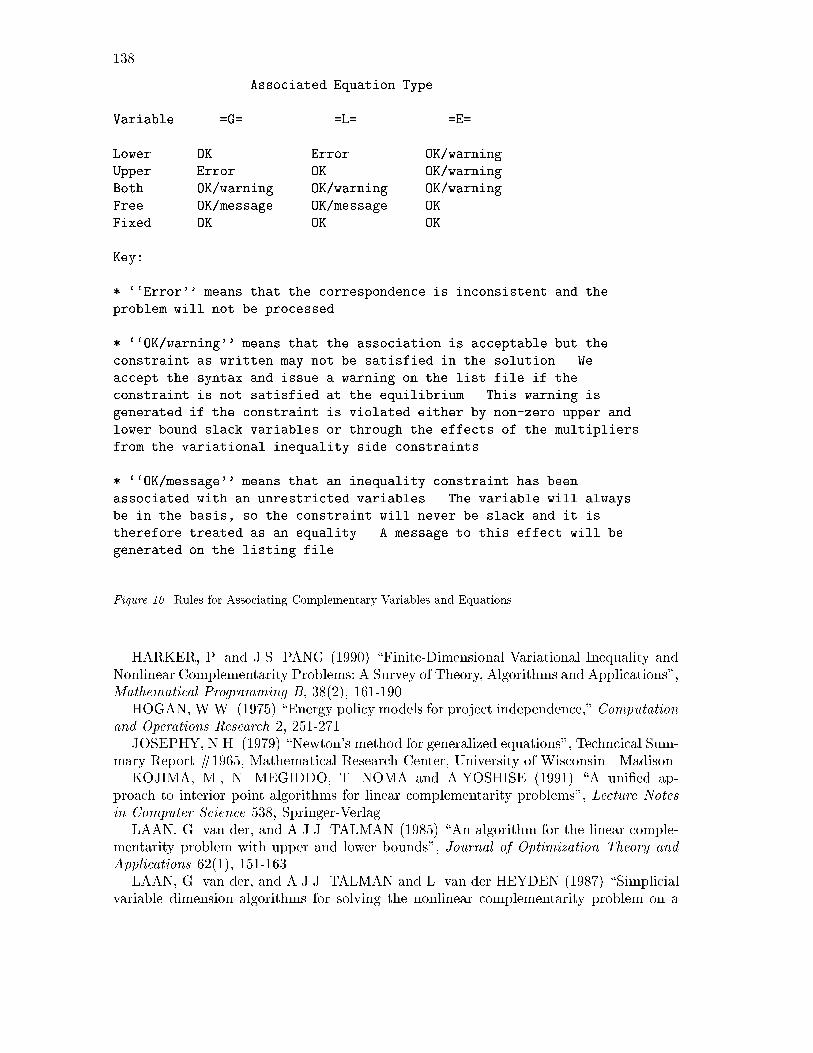
138
Associated Equation Type
Variable =G= =L= =E=
Lower OK Error OK/warning
Upper Error OK OK/warning
Both OK/warning OK/warning OK/warning
Free OK/message OK/message OK
Fixed OK OK OK
Key:
* ``Error'' means that the correspondence is inconsistent and the
problem will not be processed.
* ``OK/warning'' means that the association is acceptable but the
constraint as written may not be satisfied in the solution. We
accept the syntax and issue a warning on the list file if the
constraint is not satisfied at the equilibrium. This warning is
generated if the constraint is violated either by non-zero upper and
lower bound slack variables or through the effects of the multipliers
from the variational inequality side constraints.
* ``OK/message'' means that an inequality constraint has been
associated with an unrestricted variables. The variable will always
be in the basis, so the constraint will never be slack and it is
therefore treated as an equality. A message to this effect will be
generated on the listing file.
Figure 10. Rules for Associating Complementary Variables and Equations
HARKER, P. and J.S. PANG (1990) \Finite-Dimensional Variational Inequality andNonlinear Complementarity Problems: A Survey of Theory, Algorithms and Applications",Mathematical Programming B, 38(2), 161-190.
HOGAN, W.W. (1975) \Energy policy models for project independence," Computationand Operations Research 2, 251-271.
JOSEPHY, N.H. (1979) \Newton's method for generalized equations", Techncical Sum-mary Report #1965, Mathematical Research Center, University of Wisconsin - Madison.
KOJIMA, M., N. MEGIDDO, T. NOMA and A.YOSHISE (1991) \A uni�ed ap-proach to interior point algorithms for linear complementarity problems", Lecture Notesin Computer Science 538, Springer-Verlag.
LAAN, G. van der, and A.J.J. TALMAN (1985) \An algorithm for the linear comple-mentarity problem with upper and lower bounds", Journal of Optimization Theory andApplications 62(1), 151-163.
LAAN, G. van der, and A.J.J. TALMAN and L. van der HEYDEN (1987) \Simplicialvariable dimension algorithms for solving the nonlinear complementarity problem on a
GAMS Extensions for Complementarity 139
product of unit simplices using a general labelling", Mathematics of Operations Research12(3), 337-397.
LEMKE, C.E. and J.T. HOWSON (1964) \Equilibrium points of bimatrix games,"SIAM Review 12, 413-23.
MATHIESEN, L. (1985) \Computation of Economic Equilibrium by a Sequence ofLinear Complementarity Problems",Mathematical Programming Study 23, North-Holland.
MEERAUS, A. (1983) \An algebraic approach to modeling," Journal of EconomicDynamics and Control, 5(1), February.
RALPH, D. (1994) \Global Convergence of Damped Newton's Method for NonsmoothEquations, via the Path Search", Mathematics of Operations Research, 19(2), 352-371.
ROBINSON, S. (1972) \A quadratically-convergent algorithm for general nonlinearprogramming problems," Mathematical Programming Study 3, 145-156.
RUTHERFORD, T. (1987) \Applied general equilibrium modeling", Ph.D. Disserta-tion, Department of Operations Research, Stanford University.
RUTHERFORD, T. (1992a) \Sequential joint maximization", Working Paper 92-8,Department of Economics, University of Colorado.
RUTHERFORD, T. (1992b) \Applied general equilibrium modeling using MPS/GEas a GAMS subsystem", Working Paper 92-15, Department of Economics, University ofColorado.
RUTHERFORD, T. (1993) \MILES: a Mixed Inequality and nonLinear EquationSolver", Working Paper, Department of Economics, University of Colorado.
SAMUELSON, P. (1952) \Spatial price equilibrium and linear programming," TheAmerican Economic Review, 42, 283-303.
TAKAYAMA, T. and G.G. JUDGE (1971) Spatial and Temporal Price and AllocationModels, North Holland, Amsterdam.
VARIAN, H. (1992) Microeconomic Analysis (3rd edition), Norton, New York.

Sequential Joint Maximization
Relating Optimization and General Equilibrium
Abstract. This paper describes a new method by which a competitive market economymay be representedas the optimal solution to a planning problem.The resulting sequential joint maximization (SJM) algorithmsolves a sequence of \partial equilibrium relaxations" of the underlying general equilibrium model. Thepartial equilibrium submodels can be solved as nonlinear complementarity problems or as constrainednonlinear optimization problems in either a primal or dual form. This paper introduces the three SJMalgorithms, evaluates performance and examines convergence theory. Computational tests demonstratethat SJM is not always as e�cient as complementarity methods. A counterexample is presented whichdemonstrates that local convergence of SJM cannot be guaranteed. Although SJM may have neither thetheoretical pedigree of a �xed-point algorithm nor the local convergence rate of a Newton algorithm, theusefulness of the SJM algorithm is demonstrated by the range of real models for which the procedure hasbeen sucessfully applied. SJM bene�ts from the availability of robust, large-scale nonlinear programmingcodes. Consequently, for large scale equilibrium models with inequalities SJM may not be the \best"algorithm in theory, but it works extremely well in practice.
142
1. Introduction
There is a close connection between the allocation of a competitive market economy andthe optimal solution to a representative agent's planning problem.1 This paper describesa new method by which this relationship can be exploited in computing equilibrium pricesand quantities. This optimization{based algorithm can be applied to �nd equilibria formodels in which consumers have heterogeneous preferences and where production sets mayinvolve point-to-set mappings. Large-scale models may be solved through this technique.Extensions of the algorithm may be applied to models with tax distortions, price rigidities,monopolistic competition and arbitrary preferences. The present paper, however, only con-siders applications in which producers are perfectly competitive and consumer preferencesare homothetic.
The algorithm is a Negishi or \joint maximization" procedure based on a sequenceof convex nonlinear programming problems. Typically this sequence will converge to theequilibrium prices and quantities of a competitive market economy. This paper introducesand interprets the algorithm, provides some computational evidence and developes localconvergence theory for a simple example.
The idea behind the SJM algorithm is found in the literature concerning conditionsunder which the demand function describing a set of heterogeneous consumers can bereplaced by the demand function for a single agent. In many settings, this is known as theproblem of exact aggregation. In neoclassical trade theory this relates to the \existenceof community indi�erence curves". This literature investigates the conditions under whicha country's o�er curve may be represented as though it arose from a single optimizingagent. In trade theory, at least two such conditions have been identi�ed. The �rst, due toSamuelson (1956), is that all consumers have identical, homothetic preferences. A second,less widely cited result is due to Eisenberg (1961) and Chipman (1974). This conditionplaces restrictions on endowment vectors in addition to preferences. Eisenberg's result, assummarized by Chipman (1974), is:
\if each of m individuals has a �xed money income, and if they all have ho-mogeneous utility functions (not necessarily identical, it must be emphasized),then their aggregate demand function is integrable, that is, it may be thought ofas resulting from the maximization of some �ctitious aggregate utility function,subject to total expenditure being equal to total income."In the algorithm described in this paper, Eisenberg's aggregate demand function is
embedded in an iterative procedure which accounts for changes in the relative incomes ofagents in the equilibrium system.
The aggregation approach developed by Eisenberg and subsequently interpreted in aneconomic context by Chipman is presented in a \primal" form. This approach begins withan explicit representation of consumer preferences in which the utility of an individual isspeci�ed in terms of quantities consumed of di�erent goods. An analogous result is obtainedusing preferences characterized in a \dual" form (using the indirect utility function which
1 The use of an optimization problem to characterize equilibrium allocations in a general equilibriumframework is due to Negishi (1960). His original paper was primarily concerned with optimization as ameans of proving existence. Dixon (1975) developed the theory and computational e�ectiveness of \jointmaximization algorithms" for multi-country trade models. A survey of early applications of Negishi's theoryis provided by Carey (1977). See also Dantzig, Eaves and Gale (1979). Extensions of joint maximizationmethods to account for tari�s and labor market imperfections are provided by Ginsburgh and Van derHeyden (1988) and Kehoe, Levine and Romer (1992).
Joint Maximization 143
maps prices and income into utility) which provides an interesting connection betweenthe duality theory of linear programming and the duality of demand function theory.This formulation also renders the computational procedure applicable to models based oneconometrically- estimated functions for which primal forms may not exist.
There is an interesting correspondence between the sequential joint maximization (SJM)algorithm and both Mathiesen's (1985) sequential linear complementarity (SLCP) algo-rithm and Goldsman and Harker's (1990) variational inequality (VI) algorithm for generalequilibrium models. SJM can be regarded as a robust form of SLCP; one in which incomeand price adjustments are e�ectively decoupled. The SJM algorithm computes a sequenceof \partial equilibrium relaxations" of the underlying general equilibrium model. UnlikeSLCP (see Mathiesen, 1987), in SJM the choice of numeraire does not a�ect convergence.
In SJM, subproblems may, in some cases, be guaranteed solvable; however, the outersequence generated by the algorithm may not converge in all cases. A small example fromManne, Chow and Wilson (1983) demonstrates that when income e�ects are exceptionallylarge, a backtracking line search is needed for convergence. A second small example fromScarf (1960) demonstrates that local convergence cannot be guaranteed, even in rela-tively simple models. In spite of these contrived examples, the experience with large-scaleempirical models has been excellent.
Two large scale applications which rely on SJM can be cited.2 Manne and Richels(1992,1995) use the primal form SJM algorithm to solve ATL, a 13 period, 5 regionstochastic decision analysis model of energy-economy interactions, carbon emissions andclimate change. The nonlinear programming subproblems for ATL involve 6,800 rows,8,500 columns and 27,000 nonzeros. The SJM iterations typically converge in 5 majoriterations (without a line search) to a satisfactory tolerance. Harrison, Tarr and Rutherford(1992) used the dual SJM algorithm for solving MRT, a 23 commodity, 12 region staticinternational trade model with scale economies and imperfect competition. Monopolymarkups and scale economies are handled through Jacobi iterations. Again, convergenceinvolves at most 5 iterations.
Both ATL and MRT are of such size that the complementarity and variational ap-proaches seem infeasible.3 The fact of the matter is that nonlinear programming solverslike MINOS (Murtaugh and Saunders 1982), CONOPT (Drud 1985, 1994) and CNLP(Kallio and Rosa 1994) are e�cient and robust, and SJM makes it possible to use themfor equilibrium computations.
The remainder of this paper is organized as follows. Section 2 reviews the formulation ofgeneral equilibrium models in a complementarity format, indicating how the equilibriummodel reduces to an optimization problem when there is a single household. Section 3introduces Eisenberg's result in the present context, showing how the multi-agent modelwith heterogenous, homethetic preferences can be reduced to a single agent model when-ever consumers' endowment vectors are strictly proportional. This section also describesthe iterative algorithm based on this formulation. Section 4 introduces the dual form ofthe SJM algorithm. Section 5 relates the SJM algorithm to the complementarity and vari-ational inequality formulations. Section 6 developes necessary conditions for convergence
2 These following claims amount to \proof by testimonial", a technique commonly employed in medicalresearch.
3 A recently developed complementarity solver, PATH (Ferris and Dirkse 1993) is promising, but itremains to be seen whether it can outperform the optimization-based SJM algorithm, particularly onsparse, large-scale scale models with activity analysis process modules.
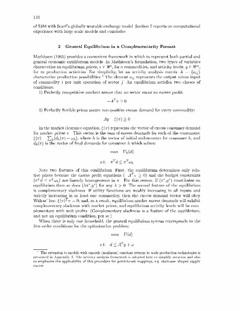
144
of SJM with Scarf's globally unstable exchange model. Section 7 reports on computationalexperience with large scale models and concludes.
2. General Equilibrium in a Complementarity Format
Mathiesen (1985) provides a convenient framework in which to represent both partial andgeneral economic equilibrium models. In Mathiesen's formulation, two types of variablescharacterize an equilibrium: prices, � 2 <n, for n commodities, and activity levels, y 2 <m,for m production activities. For simplicity, let an activity analysis matrix A = faijgcharacterize production possibilities.4 The element aij represents the output minus inputof commodity i per unit operation of sector j. An equilibrium satis�es two classes ofconditions:
1) Perfectly competitive markets assure that no sector earns an excess pro�t:
�AT� � 0
2) Perfectly exible prices assure non-positive excess demand for every commodity:
Ay � �(�) � 0
In the market clearance equation, �(�) represents the vector of excess consumer demandfor market prices � . This vector is the sum of excess demands for each of the consumers:�(�) =
Ph(dh(�)� !h), where h is the vector of initial endowments for consumer h, and
dh(�) is the vector of �nal demands for consumer h which solves:
max Uh(d)
s:t: �Td � �T!hNote two features of this equilibrium. First, the equilibrium determines only rela-
tive prices because the excess pro�t equations (�AT� � 0) and the budget constraints(�Td � �T!h) are linearly homogeneous in � . For this reason, if (��,y�) constitutes anequilibrium then so does (���,y�) for any � > 0. The second feature of the equilibriumis complementary slackness. If utility functions are weakly increasing in all inputs andstrictly increasing in at least one commodity, then the excess demand vector will obeyWalras' law: �(�)T� = 0; and, as a result, equilibrium market excess demands will exhibitcomplementary slackness with market prices, and equilibrium activity levels will be com-plementary with unit pro�ts. (Complementary slackness is a feature of the equilibrium,and not an equilibrium condition, per se.)
When there is only one household, the general equilibrium system corresponds to the�rst-order conditions for the optimization problem:
max U(d)
s:t: d � AT y + !
4 The extension to models with smooth (nonlinear) constant returns to scale production technologies ispresented in Appendix A. The activity analysis framework is adopted here to simplify notation and alsoto emphasize the applicability of this procedure for point-to-set mappings, e.g. staircase- shaped supplycurves.
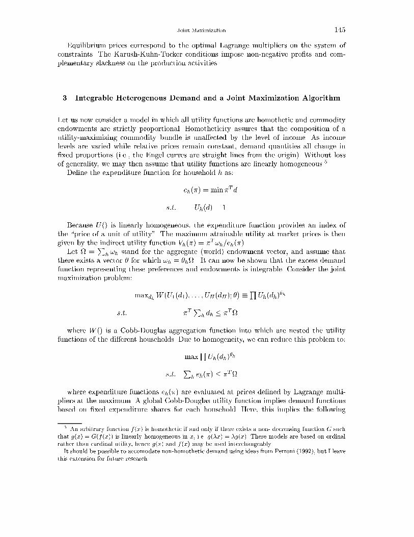
Joint Maximization 145
Equilibrium prices correspond to the optimal Lagrange multipliers on the system ofconstraints. The Karush-Kuhn-Tucker conditions impose non-negative pro�ts and com-plementary slackness on the production activities.
3. Integrable Heterogenous Demand and a Joint Maximization Algorithm
Let us now consider a model in which all utility functions are homothetic and commodityendowments are strictly proportional. Homotheticity assures that the composition of autility-maximizing commodity bundle is una�ected by the level of income. As incomelevels are varied while relative prices remain constant, demand quantities all change in�xed proportions (i.e., the Engel curves are straight lines from the origin). Without lossof generality, we may then assume that utility functions are linearly homogeneous.5
De�ne the expenditure function for household h as:
eh(�) = min�T d
s:t: Uh(d) = 1
Because U() is linearly homogeneous, the expenditure function provides an index ofthe \price of a unit of utility". The maximum attainable utility at market prices is thengiven by the indirect utility function Vh(�) = �T!h=eh(�).
Let =P
h !h stand for the aggregate (world) endowment vector, and assume thatthere exists a vector � for which !h = �h . It can now be shown that the excess demandfunction representing these preferences and endowments is integrable. Consider the jointmaximization problem:
maxdhW (U1(d1); : : : ; UH(dH); �) �QUh(dh)
�h
s:t: �TP
h dh � �T
where W () is a Cobb-Douglas aggregation function into which are nested the utilityfunctions of the di�erent households. Due to homogeneity, we can reduce this problem to:
maxQUh(dh)
�h
s:t:P
h eh(�) � �T
where expenditure functions eh(�) are evaluated at prices de�ned by Lagrange multi-pliers at the maximum. A global Cobb-Douglas utility function implies demand functionsbased on �xed expenditure shares for each household. Here, this implies the following
5 An arbitrary function f(x) is homothetic if and only if there exists a non- decreasing function G suchthat g(x) = G(f(x)) is linearly homogeneous in x, i.e. g(�x) = �g(x). These models are based on ordinalrather than cardinal utility, hence g(x) and f(x) may be used interchangeably.It should be possible to accomodate non-homothetic demand using ideas from Perroni (1992), but I leave
this extension for future research.
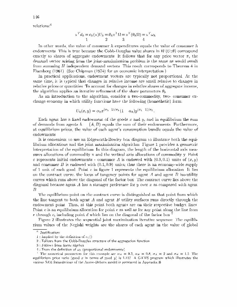
146
relations:6
�Tdh=1eh(�)Uh=
2�h�
T=3�T (�h)=
4�T!h
In other words, the value of consumer h expenditures equals the value of consumer hendowments. This is true because the Cobb-Douglas value shares in W (U ; �) correspondexactly to shares of aggregate endowments. It follows that for any price vector �, thedemand vector arising from the joint-maximization problem is the same as would resultfrom summing H independent demand vectors. This result corresponds to Theorem 4 inEisenberg (1961). (See Chipman (1974) for an economic interpretation.)
In practical applications, endowment vectors are typically not proportional. At thesame time, it is typical that changes in relative income are small relative to changes inrelative prices or quantities. To account for changes in relative shares of aggregate income,the algorithm applies an iterative re�nement of the share parameters �h.
As an introduction to the algorithm, consider a two-commodity, two- consumer ex-change economy in which utility functions have the following (homothetic) form:
Uh(x; y) = �hx(�h�1)=�h(1� �h)y(�h�1)=�h :
Each agent has a �xed endowment of the goods x and y, and in equilibrium the sumof demands from agents h = (A;B) equals the sum of their endowments. Furthermore,at equilibrium prices, the value of each agent's consumption bundle equals the value ofendowments.
It is convenient to use an Edgeworth-Bowley box diagram to illustrate both the equi-librium allocations and the joint maximization algorithm. Figure 1 provides a geometricinterpretation of the equilibrium. In this diagram, the length of the horizontal axis mea-sures allocations of commodity x and the vertical axis allocations of commodity y. Pointe represents initial endowments - consumer A is endowed with (0:9; 0:1) units of (x; y)and consumer B is endowed with (0:1; 0:9) units; thus there is an economy-wide supplyof 1 unit of each good. Point c in �gure 1 represents the equilibrium allocation. It lieson the contract curve, the locus of tangency points for agent A and agent B iso-utilitycurves which runs above the diagonal of the factor box. The contract curve lies above thediagonal because agent A has a stronger preference for y over x as compared with agentB.
The equilibrium point on the contract curve is distinguished as that point from whichthe line tangent to both agent A and agent B utility surfaces runs directly through theendowment point. Thus, at this point both agents are on their respective budget lines.Point c is an equilibrium allocation for point e as well as for any point along the line frome through c, including point d which lies on the diagonal of the factor box.7
Figure 2 illustrates the sequential joint maximization iterative sequence. The equilib-rium values of the Negishi weights are the shares of each agent in the value of global
6 Justi�cation:1 : Implied by the de�nition of eh()2 : Follows from the Cobb-Douglas structure of the aggregation function.3 : Follows from linear algebra.4 : From the de�nition of !h (proportional endowments).7 The numerical parameters for this example are �A = 0:3, �B = 0:8, �A = 2 and �B = 1:5. The
equilibrium price ratio (good x in terms of good y) is 1:127. A GAMS program which illustrates thevarious SJM formulations of the Arrow-Debreu model is presented in Appendix B.
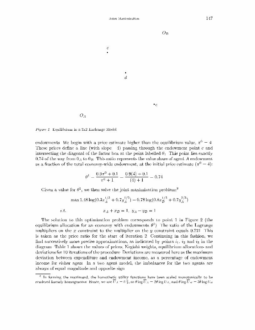
Joint Maximization 147
..
..
..
..
..
..
..
..
..
..
..
..
..
..
..
..
..
..
..
..
..
..
..
..
..
..
..
..
..
..
..
..
..
..
..
..
..
..
..
..
..
..
..
..
..
..
..
..
..
..
..
..
..
..
..
..
..
..
..
..
..
..
..
..
..
..
..
..
..
..
..
..
..
..
..
..
..
..
..
..
..
..
..
..
..
..
..
..
..
..
..
..
..
..
..
..
..
..
..
..
..
..
..
..
..
..
..
..
..
..
..
..
..
..
..
..
..
..
..
..
..
..
..
..
..
..
..
..
..
..
..
..
..
..
..
..
..
..
..
..
..
..
..
..
..
..
..
..
..
..
..
..
..
..
..
..
..
..
..
..
..
..
..
..
..
..
..
..
..
..
..
..
..
..
..
..
..
..
..
..
..
..
..
..
..
..
..
..
..
..
..
..
..
..
..
..
..
..
..
..
..
..
..
..
..
..
..
..
..
..
..
..
..
..
..
..
..
..
..
..
..
..
..
..
..
.............................................................................................................................................................................................................................................................................................................................................................................................................................................................................................................................................................................................................................................................................................................................................................................................................................................................................................................................................................................................................................................................................................................................................................................................................................................................................................................................................................................................................................................................................................................................................................................................................................................................................................................................................................................................................................................................................................................................................................................................................................................................................
..
..
...........................................................................................................................................................................................................................................................................................................................................................................................................................................................................................................................................................................................................................
..
..
..
..
..
..
..
..
..
..
..
..
..
..
..
..
..
..
..
..
..
..
..
..
..
..
..
..
..
..
..
..
..
...
..
..
..
..
..
..
..
..
..
..
..
..
..
..
..
..
..
..
..
..
..
..
..
..
..
..
...
..
..
..
..
..
..
..
..
..
..
..
..
..
..
..
..
..
..
..
..
..
..
..
...
..
..
..
..
..
..
..
..
..
..
..
..
..
..
..
..
..
..
..
..
...
..
..
..
..
..
..
..
..
..
..
..
..
..
..
..
..
..
...
..
..
..
..
..
..
..
..
..
..
..
..
..
..
..
...
..
..
..
..
..
..
..
..
..
..
..
..
..
...
..
..
..
..
..
..
..
..
..
..
..
..
..
...
..
..
..
..
..
......................................................................................................................................................................................................................................................................................................................................................................................................
.........................................................................................................................................................................................................................................................................................................................................................
.........................................................................................................................................................................................................................................................................................................................................................
�
�
�
OA
OB
c
d
e
Figure 1. Equilibrium in a 2x2 Exchange Model
endowments. We begin with a price estimate higher than the equilibrium value, �0 = 4.These prices de�ne a line (with slope �4) passing through the endowment point e andintersecting the diagonal of the factor box at the point labelled �1. This point lies exactly0:74 of the way from 0A to 0B . This ratio represents the value share of agent A endowmentas a fraction of the total economy-wide endowment, at the initial price estimate (�0 = 4):
�1 =0:9�0 + 0:1
�0 + 1=
0:9(4) + 0:1
(4) + 1= 0:74
Given a value for �1, we then solve the joint maximization problem:8
max 1:48 log(0:3x1=2A + 0:7y
1=2A ) + 0:78 log(0:8x
1=3B + 0:7y
2=3A )
s:t: xA + xB = 1; yA + yB = 1
The solution to this optimization problem corresponds to point 1 in Figure 2 (theequilibrium allocation for an economy with endowments �1). The ratio of the Lagrangemultipliers on the x constraint to the multiplier on the y constraint equals 0:721. Thisis taken as the price ratio for the start of iteration 2. Continuing in this fashion, we�nd successively more precise approximations, as indicated by points i1, i2 and i3 in thediagram. Table 1 shows the values of prices, Negishi weights, equilibrium allocations anddeviations for 10 iterations of the procedure. Deviations are measured here as the maximumdeviation between expenditure and endowment income, as a percentage of endowmentincome for either agent. In a two agent model, the imbalances for the two agents arealways of equal magnitude and opposite sign.
8 In forming the maximand, the homothetic utility functions have been scaled monotonically to berendered linearly homogeneous. Hence, we use UA = U2
A, so � logUA = 2� logUA, and � logUB = 3� logUB
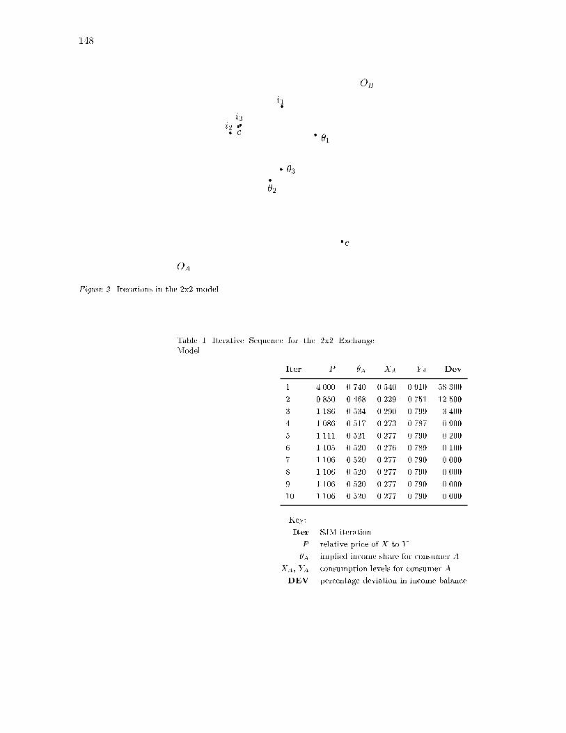
148
..
..
..
..
..
..
..
..
..
..
..
..
..
..
..
..
..
..
..
..
..
..
..
..
..
..
..
..
..
..
..
..
..
..
..
..
..
..
..
..
..
..
..
..
..
..
..
..
..
..
..
..
..
..
..
..
..
..
..
..
..
..
..
..
..
..
..
..
..
..
..
..
..
..
..
..
..
..
..
..
..
..
..
..
..
..
..
..
..
..
..
..
..
..
..
..
..
..
..
..
..
..
..
..
..
..
..
..
..
..
..
..
..
..
..
..
..
..
..
..
..
..
..
..
..
..
..
..
..
..
..
..
..
..
..
..
..
..
..
..
..
..
..
..
..
..
..
..
..
..
..
..
..
..
..
..
..
..
..
..
..
..
..
..
..
..
..
..
..
..
..
..
..
..
..
..
..
..
..
..
..
..
..
..
..
..
..
..
..
..
..
..
..
..
..
..
..
..
..
..
..
..
..
..
..
..
..
..
..
..
..
..
..
..
..
..
..
..
..
..
..
..
..
..
..
.............................................................................................................................................................................................................................................................................................................................................................................................................................................................................................................................................................................................................................................................................................................................................................................................................................................................................................................................................................................................................................................................................................................................................................................................................................................................................................................................................................................................................................................................................................................................................................................................................................................................................................................................................................................................................................................................................................................................................................................................................................................................................
..
..
..
..
..
..
..
..
..
..
..
..
..
..
..
..
..
..
..
..
..
..
..
..
..
..
..
..
..
..
..
..
..
...
..
..
..
..
..
..
..
..
..
..
..
..
..
..
..
..
..
..
..
..
..
..
..
..
..
..
...
..
..
..
..
..
..
..
..
..
..
..
..
..
..
..
..
..
..
..
..
..
..
..
...
..
..
..
..
..
..
..
..
..
..
..
..
..
..
..
..
..
..
..
..
...
..
..
..
..
..
..
..
..
..
..
..
..
..
..
..
..
..
...
..
..
..
..
..
..
..
..
..
..
..
..
..
..
..
...
..
..
..
..
..
..
..
..
..
..
..
..
..
...
..
..
..
..
..
..
..
..
..
..
..
..
..
...
..
..
..
..
..
..
..
..
................................................................................................................................................................................................................................................................................................................................................................................................
..
..
..
..
..
..
..
..
..
..
..
..
..
..
..
..
..
..
..
..
..
..
..
..
..
..
..
..
..
..
..
..
..
..
..
..
..
..
..
..
..
..
..
..
..
..
..
..
..
..
..
..
..
..
..
..
..
..
..
..
..
..
..
..
..
..
..
..
..
..
..
..
..
..
..
..
..
..
..
..
..
..
..
..
..
..
..
..
..
..
..
..
..
..
..
..
..
..
..
..
..
..
..
..
..
..
..
..
..
..
..
..
..
..
..
..
..
..
..
..
..
..
..
..
..
..
..
..
..
..
..
..
..
..
..
..
..
..
..
..
..
..
..
..
..
..
..
..
...
......................................................................................................................
� �1
�
i1
.........................................................................................................................................................................................................................................................................................................................................................................................................................................
�
�2
�
i2
..
..
..
..
..
..
..
..
..
..
..
..
..
..
..
..
..
..
..
..
..
..
..
..
..
..
..
..
..
..
..
..
..
..
..
..
..
..
..
..
..
..
..
..
..
..
..
..
..
..
..
..
..
..
..
..
..
..
..
..
..
..
..
..
..
..
..
..
..
..
..
..
..
..
..
..
..
..
..
..
..
..
..
..
..
..
..
..
..
..
..
..
..
..
..
..
..
..
..
..
..
..
..
..
..
..
..
..
..
..
..
..
..
..
..
..
..
..
..
..
..
..
..
..
..
..
..
..
...
..
..
..
..
.........................................................................................................................................................
� �3
�
i3�
c
e�
OA
OB
Figure 2. Iterations in the 2x2 model
Table I. Iterative Sequence for the 2x2 ExchangeModel.
Iter P �A XA YA Dev
1 4.000 0.740 0.540 0.910 58.300
2 0.850 0.468 0.229 0.751 12.500
3 1.186 0.534 0.290 0.799 3.400
4 1.086 0.517 0.273 0.787 0.900
5 1.111 0.521 0.277 0.790 0.200
6 1.105 0.520 0.276 0.789 0.100
7 1.106 0.520 0.277 0.790 0.000
8 1.106 0.520 0.277 0.790 0.000
9 1.106 0.520 0.277 0.790 0.000
10 1.106 0.520 0.277 0.790 0.000
Key:
Iter SJM iteration
P relative price of X to Y
�A implied income share for consumer A
XA, YA consumption levels for consumer A
DEV percentage deviation in income balance
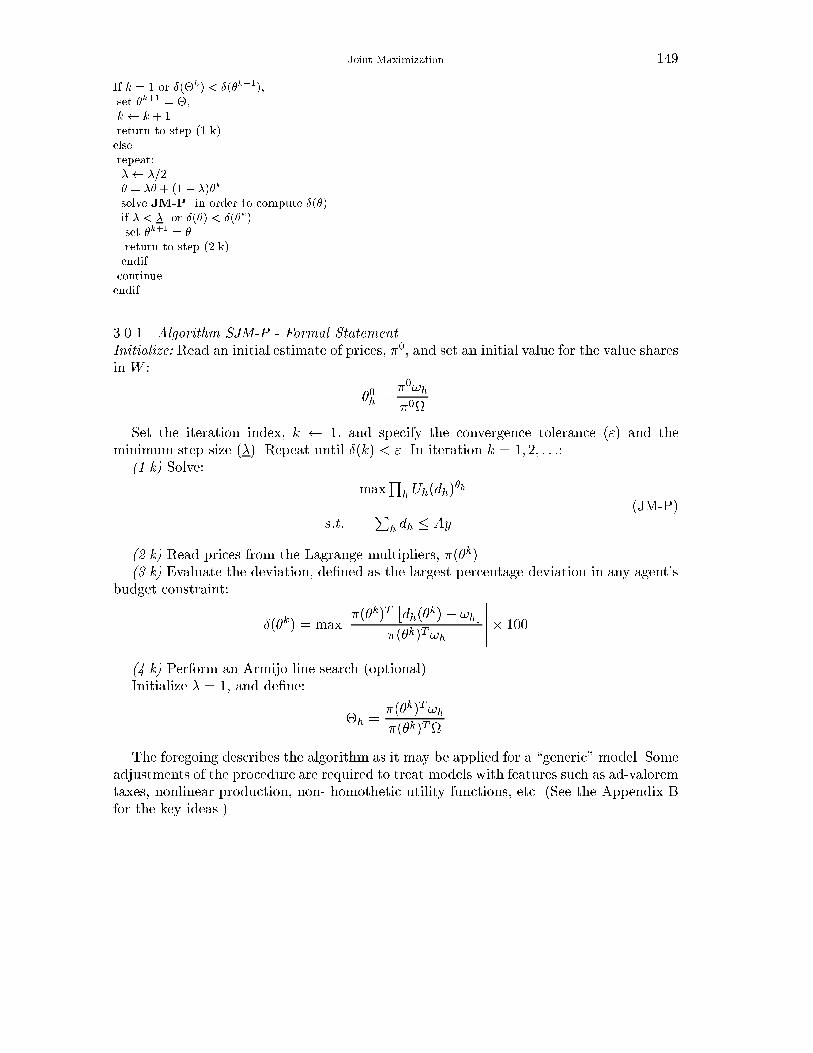
Joint Maximization 149
If k = 1 or �(�k) < �(�k�1),set �k+1 = �,k k + 1return to step (1.k)elserepeat:� �=2� = �� + (1� �)�k
solve JM-P in order to compute �(�)if � < � or �(�) < �(�k)set �k+1 = �return to step (2.k)endifcontinueendif
3.0.1. Algorithm SJM-P - Formal StatementInitialize: Read an initial estimate of prices, �0, and set an initial value for the value sharesin W :
�0h =�0!h�0
Set the iteration index, k 1, and specify the convergence tolerance (") and theminimum step size (�). Repeat until �(k) < ". In iteration k = 1; 2; : : ::
(1.k) Solve:
maxQ
h Uh(dh)�h
s:t:P
h dh � Ay(JM-P)
(2.k) Read prices from the Lagrange multipliers, �(�k).(3.k) Evaluate the deviation, de�ned as the largest percentage deviation in any agent's
budget constraint:
�(�k) = max
������(�k)T
�dh(�
k)� !h�
�(�k)T!h
������ 100
(4.k) Perform an Armijo line search (optional)Initialize � = 1, and de�ne:
�h =�(�k)T!h�(�k)T
The foregoing describes the algorithm as it may be applied for a \generic" model. Someadjustments of the procedure are required to treat models with features such as ad-valoremtaxes, nonlinear production, non- homothetic utility functions, etc. (See the Appendix Bfor the key ideas.)
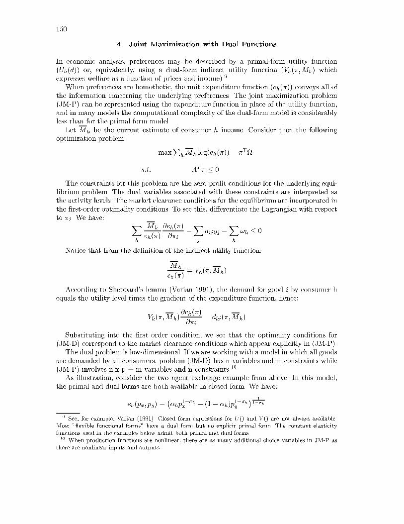
150
4. Joint Maximization with Dual Functions
In economic analysis, preferences may be described by a primal-form utility function(Uh(d)) or, equivalently, using a dual-form indirect utility function (Vh(�;Mh) whichexpresses welfare as a function of prices and income).9
When preferences are homothetic, the unit expenditure function (eh(�)) conveys all ofthe information concerning the underlying preferences. The joint maximization problem(JM-P) can be represented using the expenditure function in place of the utility function,and in many models the computational complexity of the dual-form model is considerablyless than for the primal form model.
Let Mh be the current estimate of consumer h income. Consider then the followingoptimization problem:
maxP
hMh log(eh(�))� �T
s:t: AT� � 0
The constraints for this problem are the zero pro�t conditions for the underlying equi-librium problem. The dual variables associated with these constraints are interpreted asthe activity levels. The market clearance conditions for the equilibrium are incorporated inthe �rst-order optimality conditions. To see this, di�erentiate the Lagrangian with respectto �i. We have: X
h
Mh
eh(�)
@eh(�)
@�i�Xj
aijyj �Xh
!h � 0
Notice that from the de�nition of the indirect utility function:
Mh
eh(�)= Vh(�;Mh)
According to Sheppard's lemma (Varian 1991), the demand for good i by consumer hequals the utility level times the gradient of the expenditure function, hence:
Vh(�;Mh)@eh(�)
@�i= dhi(�;Mh)
Substituting into the �rst order condition, we see that the optimality conditions for(JM-D) correspond to the market clearance conditions which appear explicitly in (JM-P).
The dual problem is low-dimensional. If we are working with a model in which all goodsare demanded by all consumers, problem (JM-D) has n variables and m constraints while(JM-P) involves n x p + m variables and n constraints.10
As illustration, consider the two agent exchange example from above. In this model,the primal and dual forms are both available in closed form. We have:
eh(px; py) =��hp
1��hx + (1� �h)p1��hy
� 11��h
9 See, for example, Varian (1991). Closed form expressions for U() and V () are not always available.Most " exible functional forms" have a dual form but no explicit primal form. The constant elasticityfunctions used in the examples below admit both primal and dual forms.10 When production functions are nonlinear, there are as many additional choice variables in JM-P as
there are nonlinear inputs and outputs.
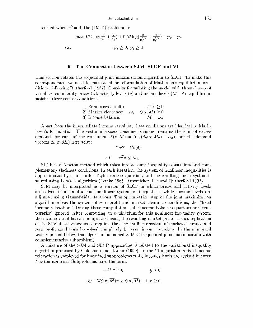
Joint Maximization 151
so that when �0 = 4, the (JM-D) problem is:
max 0:74 log( 3px
+ 7py) + 0:52 log( 8
p1=2x
+ 2
p1=2y
)� px � py
s:t: px � 0; py � 0
5. The Connection between SJM, SLCP and VI
This section relates the sequential joint maximization algorithm to SLCP. To make thiscorrespondence, we need to make a minor reformulation of Mathiesen's equilibrium con-ditions, following Rutherford (1987). Consider formulating the model with three classes ofvariables: commodity prices (�), activity levels (y) and income levels (M). An equilibriumsatis�es three sets of conditions:
1) Zero excess pro�t: �AT� � 02) Market clearance: Ay � �(�;M) � 03) Income balance: M = !�
Apart from the intermediate income variables, these conditions are identical to Math-iesen's formulation. The vector of excess consumer demand remains the sum of excessdemands for each of the consumers: �(�;M) =
Ph(dh(�;Mh) � !h), but the demand
vectors dh(�;Mh) here solve:max Uh(d)
s:t: �Td �Mh
SLCP is a Newton method which takes into account inequality constraints and com-plementary slackness conditions. In each iteration, the system of nonlinear inequalities isapproximated by a �rst-order Taylor series expansion, and the resulting linear system issolved using Lemke's algorithm (Lemke 1965, Anstreicher, Lee and Rutherford 1992).
SJM may be interpreted as a version of SLCP in which prices and activity levelsare solved in a simultaneous nonlinear system of inequalities while income levels areadjusted using Gauss-Seidel iterations. The optimization step of the joint maximizationalgorithm solves the system of zero pro�t and market clearance conditions, the \�xedincome relaxation." During these computations, the income balance equations are (tem-porarily) ignored. After computing an equilibrium for this nonlinear inequality system,the income variables can be updated using the resulting market prices. Exact replicationof the SJM iterative sequence requires that the nonlinear system of market clearance andzero pro�t conditions be solved completely between income revisions. In the numericaltests reported below, this algorithm is named SJM-C (sequential joint maximization withcomplementarity subproblem).
A mixture of the SJM and SLCP approaches is related to the variational inequalityalgorithm proposed by Goldsman and Harker (1990). In the VI algorithm, a �xed-incomerelaxation is employed for linearized subproblems while incomes levels are revised in everyNewton iteration. Subproblems have the form:
�AT� � 0 ? y � 0
Ay �r�(�;M )� � �(�;M) ? � � 0
152
This linear complementarity problem corresponds to the �rst-order conditions for thefollowing quadratic program:
max bT� + 12�
TQ�
s:t: AT� � 0
where b = �(�;M ) and Q = r�(�;M ).The iterative sequence produced by this sequential quadratic programming algorithm
will di�er from the VI algorithm because income levels are treated as exogenous in eachsubproblem. By decoupling income and price adjustments, the required number of Newtoniterations may increase relative to SLCP. At the same time, this approach may help toavoid defective subproblems which can plague SLCP. (See Mathiesen 1987.)
6. Convergence
Computational experiments demonstrate that a line search is sometimes necessary forconvergence. This is the case for a modi�ed version of the Jack{Sprat problem presentedin Manne, Chao andWilson (1980). When Jack{Sprat is initiated from a particular startingpoint, the SJM procedure with � = 1 (i.e. without a line search) after four iterations beginsto cycle between two sets of Negishi weights. When the Armijo line search is applied, theouter iterations converge in �ve steps. (See model Jack-Sprat in Appendix B.)
The second small model presents more serious theoretical problems for the algorithm.Scarf (1960) provides a model which demonstrates that the SJM di�erential process (for� ! 0) may be non-convergent. Furthermore, it can be shown that the conditions forconvergence of the Negishi process locally reduce to exactly the same conditions forconvergence of a simple Tatonnement adjustment process.
Scarf's model involves an equal number of n consumers and goods. Consumer h isendowed with 1 unit of good h and demands only goods h and h + 1. Let dih representdemand for good i by consumer h. Preferences are represented by constant elasticity ofsubstitution utility functions with the following structure:
Uh(d) =
��1=�d
��1�
hh
� ���1
There are two utility function parameters.11. � can be interpreted as the benchmarkvalue share of good i in consumer i demand , and 1� � is then the benchmark value shareof good i+ 1. (Consumer n demands goods n and 1.)
The joint maximization algorithm works with consumer income levels, denoted Mh forhousehold h. These may be normalized so that
PhMh = n. Market clearing commodity
prices are determined given the income levels. Let �i(M) denote the price of good i
consistent with income levelsM =
0BB@M1
M2...
MH
1CCA. Provided that � > 0, utility functions exhibit
non-satiation, soP
i �i =P
hMh.
11 The parameters of this function correspond to Scarf's parameters a and b (Scarf (1960, page 168)) as:� = 1
1+aand � = b
1+b
Joint Maximization 153
Let �(p;M) denote the market excess demand function for �xed income. Given thespecial structure of preferences and endowments, this function has the form:
�i(p;M) = dii + di;i�1 � 1
Given our de�nition of p(M), we have xi(p(M);M) = 0 8i.Let Hh(M) denote the di�erence between the value of agent h allocated income and
the market value of the agent h endowment for prices p(M). That is:
Hh(M) = ph(M)�Mh
The structure of demand and endowments assure an equilibrium in which all incomelevels and prices equal unity. When M�
i = 1 then �i(M�) = 1 8i, and
Hh(M�) = 0 8h
The SJM algorithm, as the step length goes to zero, represents an income adjustmentprocess:
Mh = ph(M)�Mh
Let the initial estimate M0 be selected on the n-simplex (i.e.,P
hM0h = n). The
adjustment process then remains on the n-simplex:
d
dt
Xh
Mh =Xh
Mh =Xh
(ph �Mh) =Xi
pi(M)�Xh
Mh = 0
Local convergence concerns properties of the Jacobian matrix evaluated at the equilib-rium point, rH(M�) = [Hij]. This Jacobian has entries which are de�ned as follows:
Hij � @Hi
@Mj=
(@pi@Mi� 1 i = j
@pi@Mj
i 6= j
If all prinicpal minors ofrH(M�) are negative, the income adjustment process is locally
convergent. If, however, @pi@Mh
> 1, the process is "locally unstable" { a small increase fromthe equilibrium income level for consumer h causes consumer h endowment revenue toincrease more than proportionally. When an equilibrium is unique and the process isuninterrupted, then local instability implies global instability.
For this model, the Tatonnement price adjustment process is unstable (in the case n=3)when �
1�� >1
1�2� (Scarf, 1960). It is shown in the following that the same condition im-plies instability for the income adjustment process, even though these algorithms producedi�erent search directions away from a neighborhood of the equilibrium.
The function p(M) is de�ned implicitly by the equation:
�(p;M) = 0
In order to evaluate rp at M�, we make a �rst-order Taylor series expansion:
rp�(p;M)dp+rM�(p;M)dM = 0;
So
rp =�@pi@Mh
�= �r�1
p rM�

154
Given the special structure of �i(p;M), we have:
@�i@pi
=@dii@pi
+@di;i�1@pi
;@�i@pi�1
=@di;i�1@pi�1
; and@�i@pi+1
=@dii@pi+1
:
If we de�ne the "unit-utility" expenditure function for consumer i as:
ei(p) =��p1��i + (1� �)p1��i+1
� 11��
demand functions are:
dii =�Mi
e1��i p�i; and di+1;i =
(1� �)Mi
e1��i p�i+1
Evaluating gradients at p� = 1, it is apparent that the "�xed income Slutsky matrix"has a tri-diagonal structure:
rp� =
266666664
� � 0 : : : 0 �
� � � 0... 0
0 � � �...
...0 0 � � � � � �� 0 � � � 0 � �
377777775
where � = �� � (1� �) ��2 + (1� �)2� and � = �(1� �)�(1� �). The inverse matrix,rp�
�1, is:
r�1p � =
2666664
� � � � � �� � � � � �
� � � � � ......
. . .
� � � � �
3777775
where = �(�+�)(2�+�)(���) and � = �
(2�+�)(���) .
The gradients of excess demands with respect to income at the equilibrium are:
rM� =
2666664
� 0 0 � � � 1� �1� � � 0 � � � 0
0 1� � � � � � ......
. . .
0 0 0 1� � �
3777775
Hence:@pi(M)
@Mi= �� + (1� �)�
Local instability for n � 3 therefore implies:
��2 � �2 � ��3(��2 � �2 � ��) + 3� � 1
� 1
Joint Maximization 155
which reduces to the same condition as Scarf demonstrated for the Tatonnement processwhen n = 3.
Given the equivalent local behavior, one might be lead to believe that the income andprice-adjustment processes are identical. This is not true. Only local to the equilibrium,where price e�ects dominate income e�ects, do these processes follow the same path. Thisis apparent in Figure 3 where the two vector �elds are superimposed. In this diagram, thetatonnement �eld becomes more divergent than the SJM �eld as one moves further fromthe equilibrium point at the center of the simplex. At the equilibrium point the two �eldscoincide exactly, as demonstrated above.
7. Conclusion
This paper has described a new income adjustment procedure which makes it easy to applythe joint maximization algorithm proposed originally by Negishi and Dixon. The paperpresented three alternative implementations of the solution procedure, based on primaloptimization, dual optimization and complementarity subproblems.
Scarf's model demonstrates that convergence of SJM cannot be guaranteed. At thesame time, the SJM approach seems to be the only reliable method for solving largescale models with activity analysis, such as Manne and Richels (1995). Even though SJMhas neither the theoretical pedigree of a �xed-point algorithm nor the local convergenceproperties of a Newton algorithm, the usefulness of the SJM algorithm is demonstratedby the range of real models for which the procedure has been sucessfully applied.
References
Anstreicher, Kurt M., Jon Lee and Thomas F. Rutherford \Crashing a Maximum-Weight ComplementaryBasis," Mathematical Programming, 54(3), 1992, pp. 281-294.
Carey, Malachy \Integrability and Mathematical Programming Models: A Survey and a ParametricApproach", Econometrica, 45(8), 1977, pp. 1957-1976.
Chipman, John S. \Homothetic Preferences and Aggregation". Journal of Economic Theory, 8, 1974, pp.26-38.
Dantzig, G.B., B.C. Eaves, and D. Gale \An Algorithm for the Piecewise Linear Model of Trade andProduction with Negative Prices and Bankruptcy", Mathematical Programming, 16(2), 1979, pp. 190-209.
Dirkse, Steven and Michael C. Ferris, \The PATH Solver: A Non-Monotone Stabilization Scheme for MixedComplementarity Problems", Optimization Methods and Software, 5, 1995, pp. 123-156.
Dixon, Peter J. The Theory of Joint Maximization, North-Holland, 1975.Drud, Arne Stolbjerg \CONOPT: A GRG Code for Large Sparse Dynamic Nonlinear Optimization
Problems", Mathematical Programming 31(2), 1985, pp. 153-191.Drud, Arne Stolbjerg \CONOPT: A Large Scale GRG Code", ORSA Journal on Computing, 6(2), 1994,
pp. 207-216.Eisenberg, E. \Aggregation of Utility Functions", Management Science 7(4), 1961, pp. 337-350.Ginsburgh, Victor .A. and Ludo Van der Heyden, \On Extending the Negishi Appproach to Computing
Equilibria: The Case of Government Price Support Poicies", Journal of Economic Theory, 44, 1988, pp.168-178.
Goldsman, Lynn and Patrick Harker \A Note on Solving General Equilibrium Problems with VariationalInequality Techniques", OR Letters (9), 1990, pp. 335-339.
Harrison, Glenn, Thomas F. Rutherford, and David Tarr \Increased Competition and Completion of theMarket in the European Union: Static and Steady-State E�ects", Journal of Economic Integration11(3), forthcoming 1996.

156
Figure 3. Tatonnement and SJM Vector Fields Compared
Harrison, Glenn, Thomas F. Rutherford, and David Tarr \Quantifying the Uruguay Round", The EconomicJournal, forthcoming 1997.
Kallio, M. and C.H. Rosa \Large-Scale Convex Optimization with Saddle Point Computation", IIASAWorking Paper WP-94-107, October, 1994.
Kehoe, Timothy J., David K. Levine and Paul M. Romer \On Characterizing Equilibria of Models withExternalities and Taxes as Solutions to Optimization Problems", Economic Theory 2(1), 1992, pp.43-68.
Lemke, C.E. \Bimatrix Equilibrium Points and Mathematical Programming", Management Science 11(7),1965, pp. 681-689.
Manne, Alan .S., Hung-Po Chao, and Robert Wilson, \Computation of Competitive Equilibria by aSequence of Linear Programs", Econometrica 48(7), 1980, pp. 1595-1615.
Manne, Alan S. and Richard B. Richels, Buying Greenhouse Insurance, MIT Press, 1992.Manne, Alan S. and Richard Richels \The Greenhouse Debate { Economic E�ciency, Burden Sharing and
Hedging Strategies", Energy Journal 16(4), 1995, pp. 1-37.Manne, Alan and Thomas F. Rutherford (1992) \International Trade, Capital Flows and Sectoral Analysis:
Formulation and Solution of Intertemporal Equilibrium Models", New Directions in ComputationalEconomics, W.W. Cooper and A.B. Whinston (editors), 1994, pp. 191-205.
Mathiesen, Lars \Computation of Economic Equilibrium by a Sequence of Linear ComplementarityProblems", Mathematical Programming Study 23, North-Holland, 1985, pp. 144-162.
Mathiesen, Lars \An Algorithm Based on a Sequence of Linear Complementarity Problems Applied to aWalrasian Equilibrium Model: An Example", Mathematical Programming 37(1), 1987, pp. 1-18.
Joint Maximization 157
Murtaugh, Bruce A. and Michael A. Saunders \A Projected Lagrangian Algorithm and its Implementationfor Sparse Nonlinear Constraints", Mathematical Programming Study 16: Algorithms for ConstrainedMinimization of Smooth Nonlinear Functions, North-Holland, 1982, pp. 84-117, .
Negishi, T. \Welfare Economics and the Existence of an Equilibrium for a Competitive Economy",Metroeconomica 12, 1960, pp. 92-97.
Perroni, Carlo \Homothetic Representation of Regular Non-Homothetic Preferences" Economics Letters40(1), 1992, pp. 19-22.
Rutherford, Thomas F. \A Modeling System for Applied General Equilibrium Analysis", Yale CowlesFoundation Discussion Paper 836, 1987.
Samuelson, Paul A. \Social Indi�erence Curves", Quarterly Journal of Economics 70(1), 1956.Scarf, Herbert \Some Examples of Global Instability of the Competitive Equilibrium", International
Economic Review 1 (3), 1960, pp. 157-172.Scarf, Herbert (with Terje Hansen) The Computation of Economic Equilibria, Yale University Press, 1973.Varian, Hal Microeconomic Analysis, Norton, 1991.
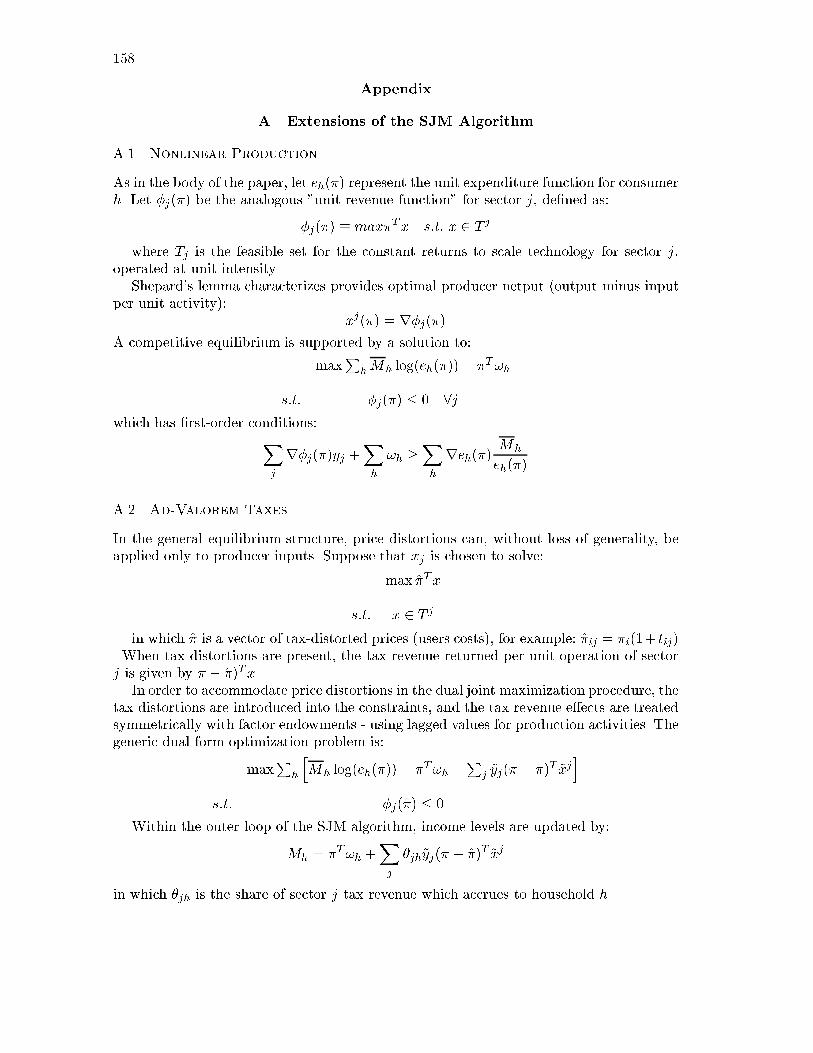
158
Appendix
A. Extensions of the SJM Algorithm
A.1. Nonlinear Production
As in the body of the paper, let eh(�) represent the unit expenditure function for consumerh. Let �j(�) be the analogous "unit revenue function" for sector j, de�ned as:
�j(�) � max�Tx s:t: x 2 T j
where Tj is the feasible set for the constant returns to scale technology for sector j,operated at unit intensity.
Shepard's lemma characterizes provides optimal producer netput (output minus inputper unit activity):
xj(�) = r�j(�)A competitive equilibrium is supported by a solution to:
maxP
hMh log(eh(�))� �T!h
s:t: �j(�) � 0 8jwhich has �rst-order conditions:X
j
r�j(�)yj +Xh
!h �Xh
reh(�) Mh
eh(�)
A.2. Ad-Valorem Taxes
In the general equilibrium structure, price distortions can, without loss of generality, beapplied only to producer inputs. Suppose that xj is chosen to solve:
max �Tx
s:t: x 2 T j
in which � is a vector of tax-distorted prices (users costs), for example: �ij = �i(1+ tij). When tax distortions are present, the tax revenue returned per unit operation of sectorj is given by � � �)Tx.
In order to accommodate price distortions in the dual joint maximization procedure, thetax distortions are introduced into the constraints, and the tax revenue e�ects are treatedsymmetrically with factor endowments - using lagged values for production activities. Thegeneric dual-form optimization problem is:
maxP
h
hMh log(eh(�)) � �T!h �
Pj ~yj(� � �)T ~xj
is:t: �j(�) � 0
Within the outer loop of the SJM algorithm, income levels are updated by:
Mh = �T!h +Xj
�jh~yj(� � �)T ~xj
in which �jh is the share of sector j tax revenue which accrues to household h.

Joint Maximization 159
Appendix
A. GAMS Code
A.1. Two-by-Two Exchange
$TITLE: A pure exchange model solved with joint maximization
SET H HOUSEHOLDS / A, B/
ALIAS (H,HH);
PARAMETER
EX(H) ENDOWMENTS OF X /A 0.9, B 0.1/
EY(H) ENDOWMENTS OF Y /A 0.1, B 0.9/
ALPHA(H) PREFERENCE FOR X /A 0.3, B 0.8/
SIGMA(H) ELASTICITY OF SUBSTITUTION /A 2.0, B 1.5/
RHO(H) ELASTICITY PARAMETER (PRIMAL FORM)
THETA(H) NEGISHI WEIGHTS;
RHO(H) = (SIGMA(H)-1)/SIGMA(H) ;
VARIABLES U(H) UTILITY LEVELS
X(H) FINAL DEMAND FOR X
Y(H) FINAL DEMAND FOR Y
NEGISHI NEGISHI ITERATION MAXIMAND
EQUATIONS OBJDEF DEFINES THE SJM MAXIMAND
UDEF(H) DEFINES UTILITY INDICES
EQUILX MARKET CLEARANCE FOR GOOD X
EQUILY MARKET CLEARANCE FOR GOOD Y;
OBJDEF..
NEGISHI =E= SUM(H, THETA(H) * LOG(U(H)));
UDEF(H)..
U(H) =E= ( ALPHA(H)**(1/SIGMA(H)) * X(H)**RHO(H) +
(1-ALPHA(H))**(1/SIGMA(H)) * Y(H)**RHO(H) )**(1/RHO(H));
EQUILX..
1 =E= SUM(H, X(H));
EQUILY..
1 =E= SUM(H, Y(H));
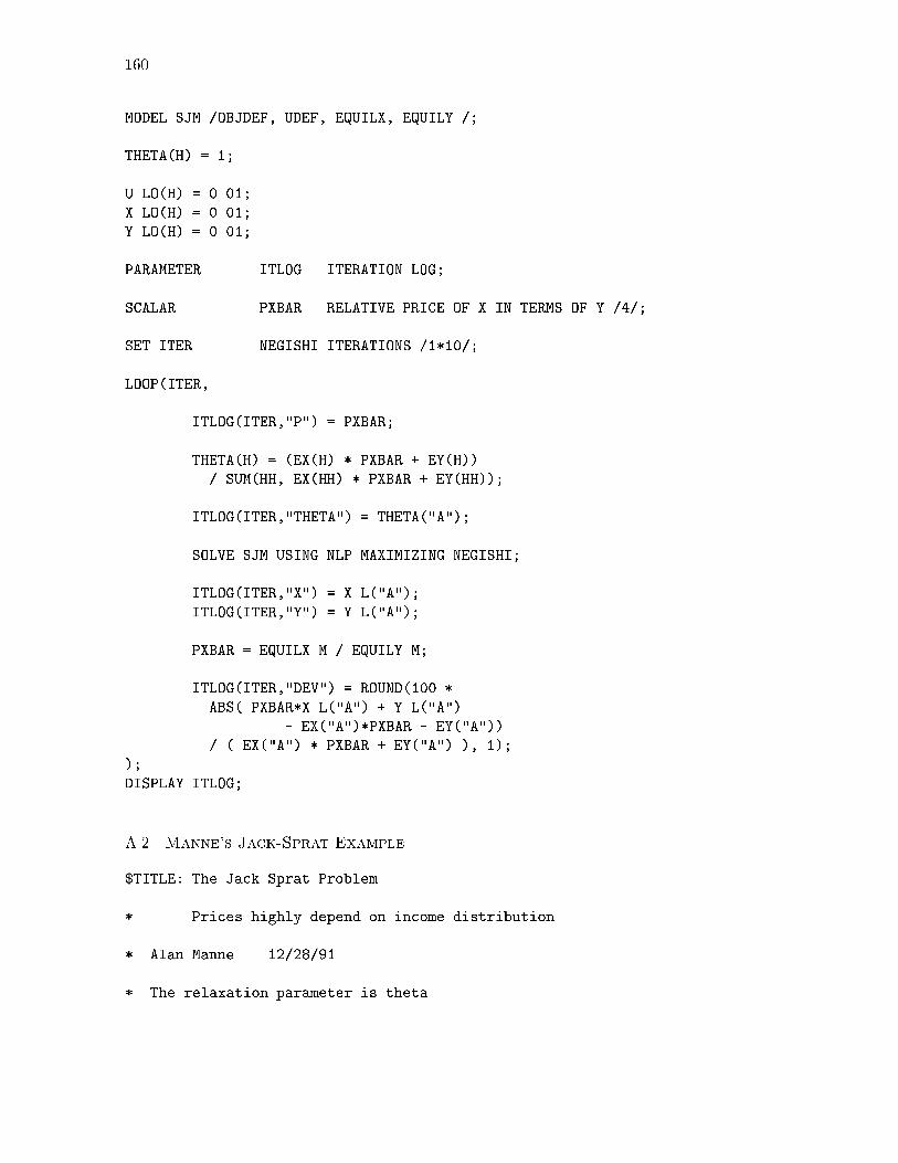
160
MODEL SJM /OBJDEF, UDEF, EQUILX, EQUILY /;
THETA(H) = 1;
U.LO(H) = 0.01;
X.LO(H) = 0.01;
Y.LO(H) = 0.01;
PARAMETER ITLOG ITERATION LOG;
SCALAR PXBAR RELATIVE PRICE OF X IN TERMS OF Y /4/;
SET ITER NEGISHI ITERATIONS /1*10/;
LOOP(ITER,
ITLOG(ITER,"P") = PXBAR;
THETA(H) = (EX(H) * PXBAR + EY(H))
/ SUM(HH, EX(HH) * PXBAR + EY(HH));
ITLOG(ITER,"THETA") = THETA("A");
SOLVE SJM USING NLP MAXIMIZING NEGISHI;
ITLOG(ITER,"X") = X.L("A");
ITLOG(ITER,"Y") = Y.L("A");
PXBAR = EQUILX.M / EQUILY.M;
ITLOG(ITER,"DEV") = ROUND(100 *
ABS( PXBAR*X.L("A") + Y.L("A")
- EX("A")*PXBAR - EY("A"))
/ ( EX("A") * PXBAR + EY("A") ), 1);
);
DISPLAY ITLOG;
A.2. Manne's Jack-Sprat Example
$TITLE: The Jack Sprat Problem
* Prices highly depend on income distribution
* Alan Manne 12/28/91
* The relaxation parameter is theta.
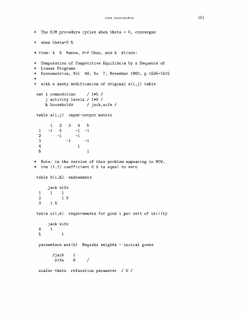
Joint Maximization 161
* The SJM procedure cycles when theta = 0, converges
* when theta=0.5.
* From: A. S. Manne, H-P Chao, and R. Wilson:
* Computation of Competitive Equilibria by a Sequence of
* Linear Programs
* Econometrica, Vol. 48, No. 7, November 1980, p 1595-1615.
*
* with a nasty modification of original a(i,j) table.
set i commodities / 1*5 /
j activity levels / 1*5 /
h households / jack,wife /
table a(i,j) input-output matrix
1 2 3 4 5
1 -1 .5 -1 -1
2 -1 -1
3 -1 -1
4 1
5 1
* Note: in the version of this problem appearing in MCW,
* the (1,2) coefficient 0.5 is equal to zero.
table b(i,h) endowments
jack wife
1 1. 1.
2 1.5
3 1.5
table u(i,h) requirements for good i per unit of utility
jack wife
4 1
5 1
parameters nwt(h) Negishi weights - initial guess
/jack .1
wife .9 /
scalar theta relaxation parameter / 0 /
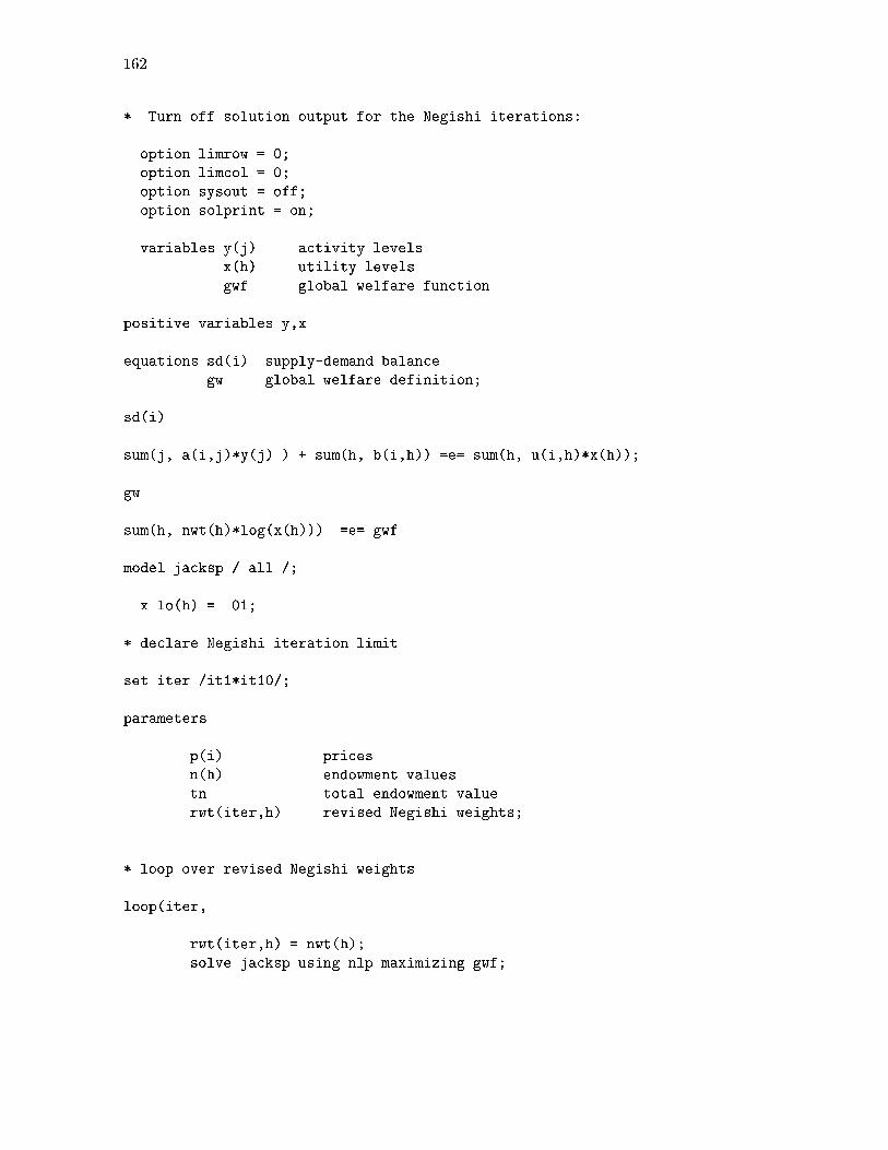
162
* Turn off solution output for the Negishi iterations:
option limrow = 0;
option limcol = 0;
option sysout = off;
option solprint = on;
variables y(j) activity levels
x(h) utility levels
gwf global welfare function
positive variables y,x
equations sd(i) supply-demand balance
gw global welfare definition;
sd(i)..
sum(j, a(i,j)*y(j) ) + sum(h, b(i,h)) =e= sum(h, u(i,h)*x(h));
gw..
sum(h, nwt(h)*log(x(h))) =e= gwf
model jacksp / all /;
x.lo(h) = .01;
* declare Negishi iteration limit
set iter /it1*it10/;
parameters
p(i) prices
n(h) endowment values
tn total endowment value
rwt(iter,h) revised Negishi weights;
* loop over revised Negishi weights
loop(iter,
rwt(iter,h) = nwt(h);
solve jacksp using nlp maximizing gwf;
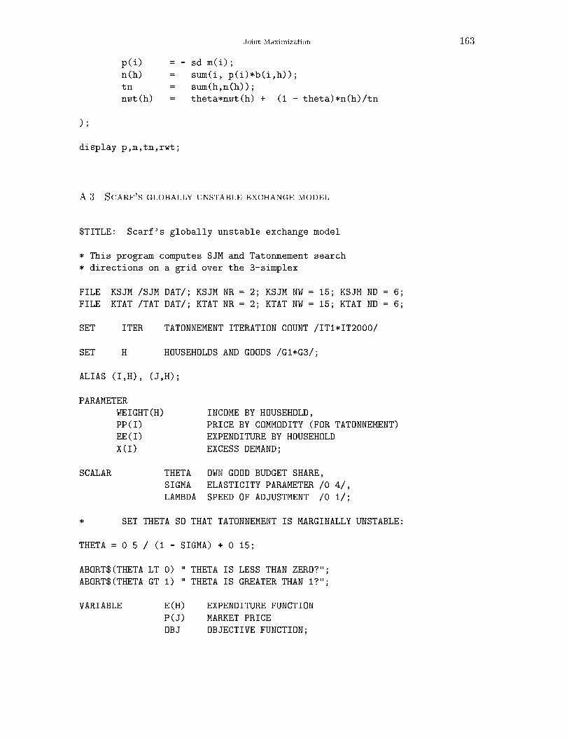
Joint Maximization 163
p(i) = - sd.m(i);
n(h) = sum(i, p(i)*b(i,h));
tn = sum(h,n(h));
nwt(h) = theta*nwt(h) + (1 - theta)*n(h)/tn
);
display p,n,tn,rwt;
A.3. Scarf's globally unstable exchange model
$TITLE: Scarf's globally unstable exchange model
* This program computes SJM and Tatonnement search
* directions on a grid over the 3-simplex.
FILE KSJM /SJM.DAT/; KSJM.NR = 2; KSJM.NW = 15; KSJM.ND = 6;
FILE KTAT /TAT.DAT/; KTAT.NR = 2; KTAT.NW = 15; KTAT.ND = 6;
SET ITER TATONNEMENT ITERATION COUNT /IT1*IT2000/
SET H HOUSEHOLDS AND GOODS /G1*G3/;
ALIAS (I,H), (J,H);
PARAMETER
WEIGHT(H) INCOME BY HOUSEHOLD,
PP(I) PRICE BY COMMODITY (FOR TATONNEMENT)
EE(I) EXPENDITURE BY HOUSEHOLD
X(I) EXCESS DEMAND;
SCALAR THETA OWN GOOD BUDGET SHARE,
SIGMA ELASTICITY PARAMETER /0.4/,
LAMBDA SPEED OF ADJUSTMENT /0.1/;
* SET THETA SO THAT TATONNEMENT IS MARGINALLY UNSTABLE:
THETA = 0.5 / (1 - SIGMA) + 0.15;
ABORT$(THETA LT 0) " THETA IS LESS THAN ZERO?";
ABORT$(THETA GT 1) " THETA IS GREATER THAN 1?";
VARIABLE E(H) EXPENDITURE FUNCTION
P(J) MARKET PRICE
OBJ OBJECTIVE FUNCTION;
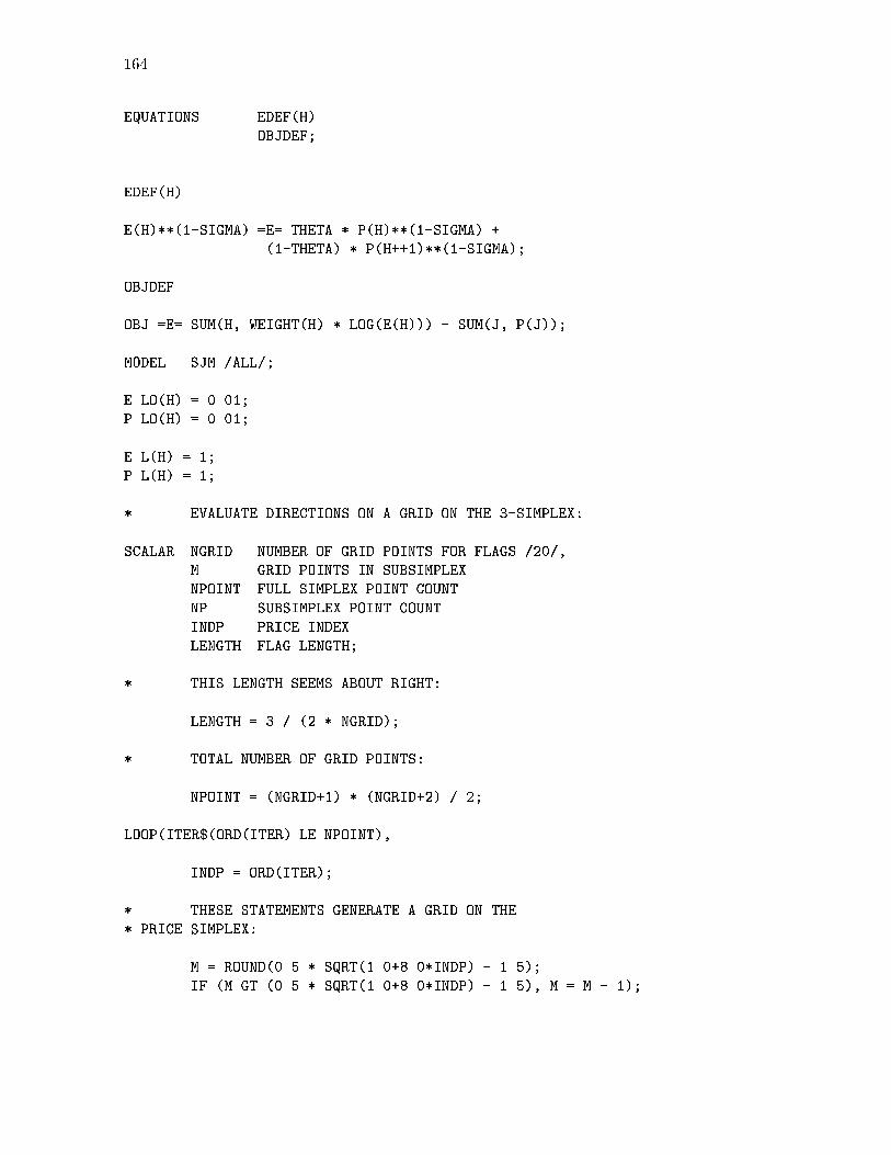
164
EQUATIONS EDEF(H)
OBJDEF;
EDEF(H)..
E(H)**(1-SIGMA) =E= THETA * P(H)**(1-SIGMA) +
(1-THETA) * P(H++1)**(1-SIGMA);
OBJDEF..
OBJ =E= SUM(H, WEIGHT(H) * LOG(E(H))) - SUM(J, P(J));
MODEL SJM /ALL/;
E.LO(H) = 0.01;
P.LO(H) = 0.01;
E.L(H) = 1;
P.L(H) = 1;
* EVALUATE DIRECTIONS ON A GRID ON THE 3-SIMPLEX:
SCALAR NGRID NUMBER OF GRID POINTS FOR FLAGS /20/,
M GRID POINTS IN SUBSIMPLEX
NPOINT FULL SIMPLEX POINT COUNT
NP SUBSIMPLEX POINT COUNT
INDP PRICE INDEX
LENGTH FLAG LENGTH;
* THIS LENGTH SEEMS ABOUT RIGHT:
LENGTH = 3 / (2 * NGRID);
* TOTAL NUMBER OF GRID POINTS:
NPOINT = (NGRID+1) * (NGRID+2) / 2;
LOOP(ITER$(ORD(ITER) LE NPOINT),
INDP = ORD(ITER);
* THESE STATEMENTS GENERATE A GRID ON THE
* PRICE SIMPLEX:
M = ROUND(0.5 * SQRT(1.0+8.0*INDP) - 1.5);
IF (M GT (0.5 * SQRT(1.0+8.0*INDP) - 1.5), M = M - 1);
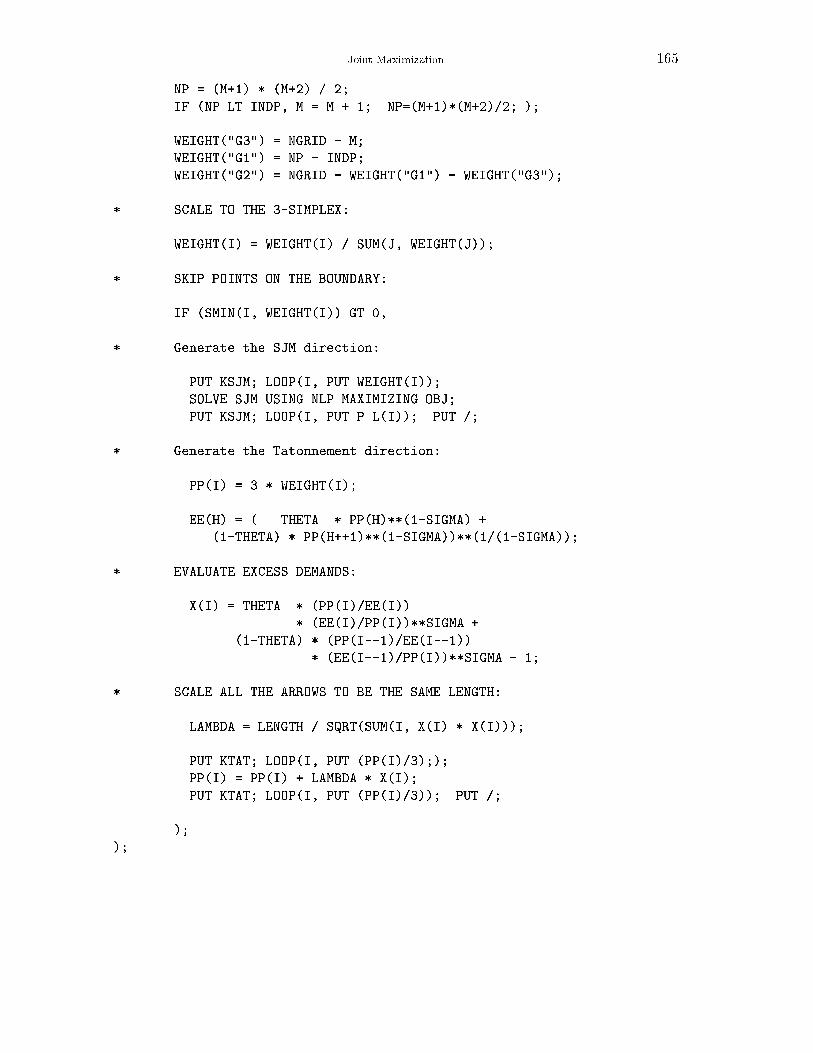
Joint Maximization 165
NP = (M+1) * (M+2) / 2;
IF (NP LT INDP, M = M + 1; NP=(M+1)*(M+2)/2; );
WEIGHT("G3") = NGRID - M;
WEIGHT("G1") = NP - INDP;
WEIGHT("G2") = NGRID - WEIGHT("G1") - WEIGHT("G3");
* SCALE TO THE 3-SIMPLEX:
WEIGHT(I) = WEIGHT(I) / SUM(J, WEIGHT(J));
* SKIP POINTS ON THE BOUNDARY:
IF (SMIN(I, WEIGHT(I)) GT 0,
* Generate the SJM direction:
PUT KSJM; LOOP(I, PUT WEIGHT(I));
SOLVE SJM USING NLP MAXIMIZING OBJ;
PUT KSJM; LOOP(I, PUT P.L(I)); PUT /;
* Generate the Tatonnement direction:
PP(I) = 3 * WEIGHT(I);
EE(H) = ( THETA * PP(H)**(1-SIGMA) +
(1-THETA) * PP(H++1)**(1-SIGMA))**(1/(1-SIGMA));
* EVALUATE EXCESS DEMANDS:
X(I) = THETA * (PP(I)/EE(I))
* (EE(I)/PP(I))**SIGMA +
(1-THETA) * (PP(I--1)/EE(I--1))
* (EE(I--1)/PP(I))**SIGMA - 1;
* SCALE ALL THE ARROWS TO BE THE SAME LENGTH:
LAMBDA = LENGTH / SQRT(SUM(I, X(I) * X(I)));
PUT KTAT; LOOP(I, PUT (PP(I)/3););
PP(I) = PP(I) + LAMBDA * X(I);
PUT KTAT; LOOP(I, PUT (PP(I)/3)); PUT /;
);
);
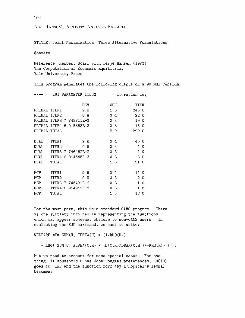
166
A.4. Hansen's Activity Analysis Example
$TITLE: Joint Maximization: Three Alternative Formulations
$ontext
Reference: Herbert Scarf with Terje Hansen (1973)
The Computation of Economic Equilibria,
Yale University Press.
This program generates the following output on a 90 MHz Pentium:
---- 291 PARAMETER ITLOG Iteration log
DEV CPU ITER
PRIMAL.ITER1 9.8 1.0 243.0
PRIMAL.ITER2 0.9 0.4 22.0
PRIMAL.ITER3 7.748711E-2 0.3 19.0
PRIMAL.ITER4 6.915353E-3 0.3 15.0
PRIMAL.TOTAL 2.0 299.0
DUAL .ITER1 9.8 0.4 40.0
DUAL .ITER2 0.9 0.3 4.0
DUAL .ITER3 7.746462E-2 0.3 4.0
DUAL .ITER4 6.914645E-3 0.3 3.0
DUAL .TOTAL 1.3 51.0
MCP .ITER1 9.8 0.4 14.0
MCP .ITER2 0.9 0.3 2.0
MCP .ITER3 7.746431E-2 0.3 1.0
MCP .ITER4 6.914911E-3 0.3 1.0
MCP .TOTAL 1.3 18.0
For the most part, this is a standard GAMS program. There
is one subtlety involved in representing the functions
which may appear somewhat obscure to non-GAMS users. In
evaluating the SJM maximand, we want to write:
WELFARE =E= SUM(H, THETA(H) * (1/RHO(H))
* LOG( SUM(C, ALPHA(C,H) * (D(C,H)/DBAR(C,H))**RHO(H)) ) );
but we need to account for some special cases. For one
thing, if household H has Cobb-Douglas preferences, RHO(H)
goes to -INF and the function form (by L'Hopital's lemma)
becomes:

Joint Maximization 167
SUM(C, ALPHA(C,H) * LOG(D(C,H)/DBAR(C,H)))
To incorporate both functional forms in a single statement,
I have used the GAMS dollar operator, writing:
WELFARE =E= SUM(H, THETA(H) *
( ( (1/RHO(H)) *
LOG( SUM(C, ALPHA(C,H) * (D(C,H)/DBAR(C,H))**RHO(H)))
)$(ESUB(H) NE 1) +
(
SUM(C, ALPHA(C,H) * LOG(D(C,H)/DBAR(C,H)))
)$(ESUB(H) EQ 1)
) );
This simply says, use the CES form if ESUB(H) is not unity,
and use Cobb-Douglas if ESUB(H) is unity.
One additional adjustment of the equation is required
because some of the share parameters, ALPHA(C,H), may be
zero. To avoid evaluating 0/0, I have put another dollar
exception operator on the loops over C.
It is an unfortunate fact of life that computers require a
precise statement of things, and they get cranky if you ask
them to evaluate functions involving 0 times infinity.
$offtext
SETS C COMMODITIES
/ AGRIC, FOOD, TEXTILES, HSERV, ENTERT, HOUSEOP, CAPEOP,
STEEL, COAL, LUMBER, HOUSBOP, CAPBOP, LABOR, EXCHANGE/
N(C) NUMERAIRE /LABOR/
H CONSUMERS
/ AGENT1, AGENT2, AGENT3, AGENT4 /
S SECTORS
/ DOM1, DOM2, DOM3, DOM4, DOM5, DOM6, DOM7,
DOM8, DOM9, DOM10, DOM11, DOM12,
IMP1, IMP2, IMP3, IMP4, IMP5, IMP6, IMP7,
EXP1, EXP2, EXP3, EXP4, EXP5, EXP6, EXP7 /
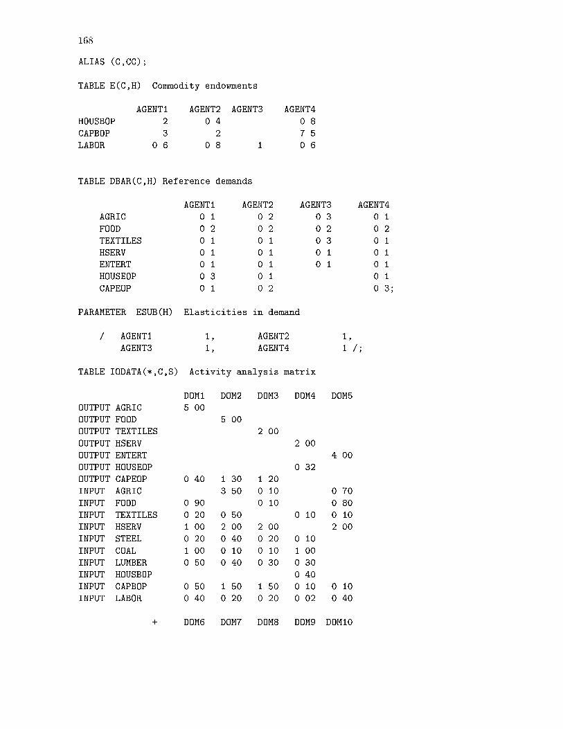
168
ALIAS (C,CC);
TABLE E(C,H) Commodity endowments
AGENT1 AGENT2 AGENT3 AGENT4
HOUSBOP 2 0.4 0.8
CAPBOP 3 2 7.5
LABOR 0.6 0.8 1 0.6
TABLE DBAR(C,H) Reference demands
AGENT1 AGENT2 AGENT3 AGENT4
AGRIC 0.1 0.2 0.3 0.1
FOOD 0.2 0.2 0.2 0.2
TEXTILES 0.1 0.1 0.3 0.1
HSERV 0.1 0.1 0.1 0.1
ENTERT 0.1 0.1 0.1 0.1
HOUSEOP 0.3 0.1 0.1
CAPEOP 0.1 0.2 0.3;
PARAMETER ESUB(H) Elasticities in demand
/ AGENT1 1, AGENT2 1,
AGENT3 1, AGENT4 1 /;
TABLE IODATA(*,C,S) Activity analysis matrix
DOM1 DOM2 DOM3 DOM4 DOM5
OUTPUT.AGRIC 5.00
OUTPUT.FOOD 5.00
OUTPUT.TEXTILES 2.00
OUTPUT.HSERV 2.00
OUTPUT.ENTERT 4.00
OUTPUT.HOUSEOP 0.32
OUTPUT.CAPEOP 0.40 1.30 1.20
INPUT .AGRIC 3.50 0.10 0.70
INPUT .FOOD 0.90 0.10 0.80
INPUT .TEXTILES 0.20 0.50 0.10 0.10
INPUT .HSERV 1.00 2.00 2.00 2.00
INPUT .STEEL 0.20 0.40 0.20 0.10
INPUT .COAL 1.00 0.10 0.10 1.00
INPUT .LUMBER 0.50 0.40 0.30 0.30
INPUT .HOUSBOP 0.40
INPUT .CAPBOP 0.50 1.50 1.50 0.10 0.10
INPUT .LABOR 0.40 0.20 0.20 0.02 0.40
+ DOM6 DOM7 DOM8 DOM9 DOM10
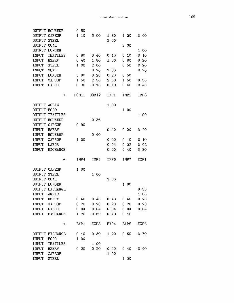
Joint Maximization 169
OUTPUT.HOUSEOP 0.80
OUTPUT.CAPEOP 1.10 6.00 1.80 1.20 0.40
OUTPUT.STEEL 2.00
OUTPUT.COAL 2.00
OUTPUT.LUMBER 1.00
INPUT .TEXTILES 0.80 0.40 0.10 0.10 0.10
INPUT .HSERV 0.40 1.80 1.60 0.80 0.20
INPUT .STEEL 1.00 2.00 0.50 0.20
INPUT .COAL 0.20 1.00 0.20
INPUT .LUMBER 3.00 0.20 0.20 0.50
INPUT .CAPBOP 1.50 2.50 2.50 1.50 0.50
INPUT .LABOR 0.30 0.10 0.10 0.40 0.40
+ DOM11 DOM12 IMP1 IMP2 IMP3
OUTPUT.AGRIC 1.00
OUTPUT.FOOD 1.00
OUTPUT.TEXTILES 1.00
OUTPUT.HOUSEOP 0.36
OUTPUT.CAPEOP 0.90
INPUT .HSERV 0.40 0.20 0.20
INPUT .HOUSBOP 0.40
INPUT .CAPBOP 1.00 0.20 0.10 0.10
INPUT .LABOR 0.04 0.02 0.02
INPUT .EXCHANGE 0.50 0.40 0.80
+ IMP4 IMP5 IMP6 IMP7 EXP1
OUTPUT.CAPEOP 1.00
OUTPUT.STEEL 1.00
OUTPUT.COAL 1.00
OUTPUT.LUMBER 1.00
OUTPUT.EXCHANGE 0.50
INPUT .AGRIC 1.00
INPUT .HSERV 0.40 0.40 0.40 0.40 0.20
INPUT .CAPBOP 0.20 0.20 0.20 0.20 0.20
INPUT .LABOR 0.04 0.04 0.04 0.04 0.04
INPUT .EXCHANGE 1.20 0.60 0.70 0.40
+ EXP2 EXP3 EXP4 EXP5 EXP6
OUTPUT.EXCHANGE 0.40 0.80 1.20 0.60 0.70
INPUT .FOOD 1.00
INPUT .TEXTILES 1.00
INPUT .HSERV 0.20 0.20 0.40 0.40 0.40
INPUT .CAPEOP 1.00
INPUT .STEEL 1.00

170
INPUT .COAL 1.00
INPUT .CAPBOP 0.10 0.10 0.20 0.20 0.20
INPUT .LABOR 0.02 0.02 0.04 0.04 0.04
+ EXP7
OUTPUT.EXCHANGE 0.40
INPUT .HSERV 0.40
INPUT .LUMBER 1.00
INPUT .CAPBOP 0.20
INPUT .LABOR 0.04 ;
* DECLARE SETS, PARAMETERS AND EQUATIONS FOR THE SJM ALGORITHM:
SETS ITER SJM ITERATION INDEX /ITER1*ITER10/
STATS STATISTICS /DEV, CPU, ITER/
PARAMETER
THETA(H) Budget shares for Negishi model
P(C) Market prices
P0(C) Initial prices (random starting point)
INCOME(H) Endowment income
EXPEND(H) Value of allocated demand
ITLOG Iteration log;
SCALAR
DEV Current deviation
CONTOL Convergence tolerance (\%) / 0.01/,
LAMDA Damping factor /1/;
ALIAS (C,CC), (H,HH);
PARAMETER
ALPHA(C,H) Demand function share parameter,
IBAR(H) Reference income associated with DBAR,
RHO(H) Primal form elasticity exponent,
A(C,S) Activity analysis matrix;
ALPHA(C,H) = DBAR(C,H) / SUM(CC, DBAR(CC,H));
IBAR(H) = SUM(C, DBAR(C,H));
RHO(H) = (ESUB(H) - 1)/ESUB(H);
A(C,S) = IODATA("OUTPUT",C,S) - IODATA("INPUT",C,S);
*===========================================================
* PRIMAL MODEL:

Joint Maximization 171
VARIABLES Y(S) ACTIVITY LEVELS
D(C,H) CONSUMPTION LEVELS
WELFARE SOCIAL WELFARE INDEX;
POSITIVE VARIABLE Y;
EQUATIONS MARKET(C) MARKET CLEARANCE FOR PRIMAL MODEL
NEGISHI MAXIMAND FOR PRIMAL PROBLEM;
MARKET(C)..
SUM(H,D(C,H)) =L= SUM(S,A(C,S) * Y(S)) + SUM(H,E(C,H));
NEGISHI..
WELFARE =E= SUM(H, THETA(H) * (
( (1/RHO(H)) *
LOG( SUM(C$ALPHA(C,H), ALPHA(C,H) * (D(C,H)/DBAR(C,H))**RHO(H)))
)$(ESUB(H) NE 1) +
( SUM(C$ALPHA(C,H), ALPHA(C,H) * LOG(D(C,H)/DBAR(C,H)))
)$(ESUB(H) EQ 1)
) );
MODEL PRIMAL / MARKET, NEGISHI/;
*===========================================================
* DUAL MODEL:
VARIABLES PI(C) MARKET PRICE
WELFARE SOCIAL WELFARE INDEX;
POSITIVE VARIABLE PI;
EQUATIONS PROFIT(S) PROFIT CONDITION
DAFERMOS MAXIMAND FOR DUAL PROBLEM;
PROFIT(S)..
0 =G= SUM(C, A(C,S) * PI(C));
DAFERMOS..
WELFARE =E= SUM(H, THETA(H) *
( ( (1/(1-ESUB(H))) *
LOG( SUM(C$ALPHA(C,H), ALPHA(C,H) * PI(C)**(1-ESUB(H))))
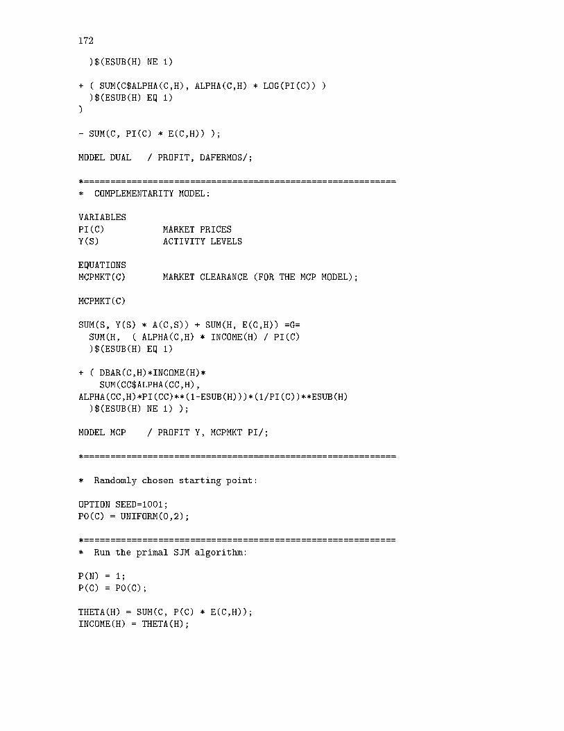
172
)$(ESUB(H) NE 1)
+ ( SUM(C$ALPHA(C,H), ALPHA(C,H) * LOG(PI(C)) )
)$(ESUB(H) EQ 1)
)
- SUM(C, PI(C) * E(C,H)) );
MODEL DUAL / PROFIT, DAFERMOS/;
*===========================================================
* COMPLEMENTARITY MODEL:
VARIABLES
PI(C) MARKET PRICES
Y(S) ACTIVITY LEVELS
EQUATIONS
MCPMKT(C) MARKET CLEARANCE (FOR THE MCP MODEL);
MCPMKT(C)..
SUM(S, Y(S) * A(C,S)) + SUM(H, E(C,H)) =G=
SUM(H, ( ALPHA(C,H) * INCOME(H) / PI(C)
)$(ESUB(H) EQ 1)
+ ( DBAR(C,H)*INCOME(H)*
SUM(CC$ALPHA(CC,H),
ALPHA(CC,H)*PI(CC)**(1-ESUB(H)))*(1/PI(C))**ESUB(H)
)$(ESUB(H) NE 1) );
MODEL MCP / PROFIT.Y, MCPMKT.PI/;
*===========================================================
* Randomly chosen starting point:
OPTION SEED=1001;
P0(C) = UNIFORM(0,2);
*===========================================================
* Run the primal SJM algorithm:
P(N) = 1;
P(C) = P0(C);
THETA(H) = SUM(C, P(C) * E(C,H));
INCOME(H) = THETA(H);
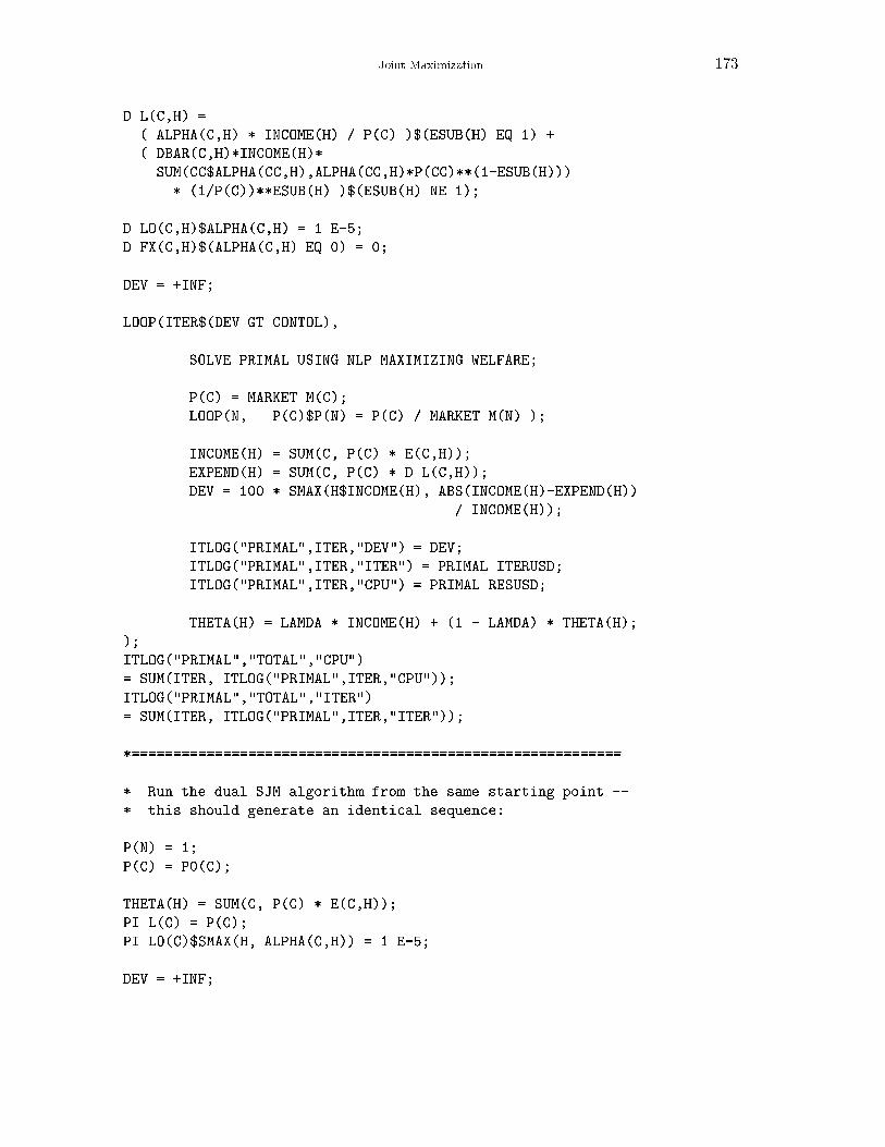
Joint Maximization 173
D.L(C,H) =
( ALPHA(C,H) * INCOME(H) / P(C) )$(ESUB(H) EQ 1) +
( DBAR(C,H)*INCOME(H)*
SUM(CC$ALPHA(CC,H),ALPHA(CC,H)*P(CC)**(1-ESUB(H)))
* (1/P(C))**ESUB(H) )$(ESUB(H) NE 1);
D.LO(C,H)$ALPHA(C,H) = 1.E-5;
D.FX(C,H)$(ALPHA(C,H) EQ 0) = 0;
DEV = +INF;
LOOP(ITER$(DEV GT CONTOL),
SOLVE PRIMAL USING NLP MAXIMIZING WELFARE;
P(C) = MARKET.M(C);
LOOP(N, P(C)$P(N) = P(C) / MARKET.M(N) );
INCOME(H) = SUM(C, P(C) * E(C,H));
EXPEND(H) = SUM(C, P(C) * D.L(C,H));
DEV = 100 * SMAX(H$INCOME(H), ABS(INCOME(H)-EXPEND(H))
/ INCOME(H));
ITLOG("PRIMAL",ITER,"DEV") = DEV;
ITLOG("PRIMAL",ITER,"ITER") = PRIMAL.ITERUSD;
ITLOG("PRIMAL",ITER,"CPU") = PRIMAL.RESUSD;
THETA(H) = LAMDA * INCOME(H) + (1 - LAMDA) * THETA(H);
);
ITLOG("PRIMAL","TOTAL","CPU")
= SUM(ITER, ITLOG("PRIMAL",ITER,"CPU"));
ITLOG("PRIMAL","TOTAL","ITER")
= SUM(ITER, ITLOG("PRIMAL",ITER,"ITER"));
*===========================================================
* Run the dual SJM algorithm from the same starting point --
* this should generate an identical sequence:
P(N) = 1;
P(C) = P0(C);
THETA(H) = SUM(C, P(C) * E(C,H));
PI.L(C) = P(C);
PI.LO(C)$SMAX(H, ALPHA(C,H)) = 1.E-5;
DEV = +INF;
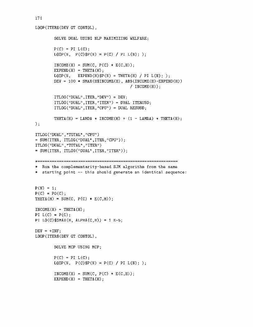
174
LOOP(ITER$(DEV GT CONTOL),
SOLVE DUAL USING NLP MAXIMIZING WELFARE;
P(C) = PI.L(C);
LOOP(N, P(C)$P(N) = P(C) / PI.L(N); );
INCOME(H) = SUM(C, P(C) * E(C,H));
EXPEND(H) = THETA(H);
LOOP(N, EXPEND(H)$P(N) = THETA(H) / PI.L(N); );
DEV = 100 * SMAX(H$INCOME(H), ABS(INCOME(H)-EXPEND(H))
/ INCOME(H));
ITLOG("DUAL",ITER,"DEV") = DEV;
ITLOG("DUAL",ITER,"ITER") = DUAL.ITERUSD;
ITLOG("DUAL",ITER,"CPU") = DUAL.RESUSD;
THETA(H) = LAMDA * INCOME(H) + (1 - LAMDA) * THETA(H);
);
ITLOG("DUAL","TOTAL","CPU")
= SUM(ITER, ITLOG("DUAL",ITER,"CPU"));
ITLOG("DUAL","TOTAL","ITER")
= SUM(ITER, ITLOG("DUAL",ITER,"ITER"));
*===========================================================
* Run the complementarity-based SJM algorithm from the same
* starting point -- this should generate an identical sequence:
P(N) = 1;
P(C) = P0(C);
THETA(H) = SUM(C, P(C) * E(C,H));
INCOME(H) = THETA(H);
PI.L(C) = P(C);
PI.LO(C)$SMAX(H, ALPHA(C,H)) = 1.E-5;
DEV = +INF;
LOOP(ITER$(DEV GT CONTOL),
SOLVE MCP USING MCP;
P(C) = PI.L(C);
LOOP(N, P(C)$P(N) = P(C) / PI.L(N); );
INCOME(H) = SUM(C, P(C) * E(C,H));
EXPEND(H) = THETA(H);
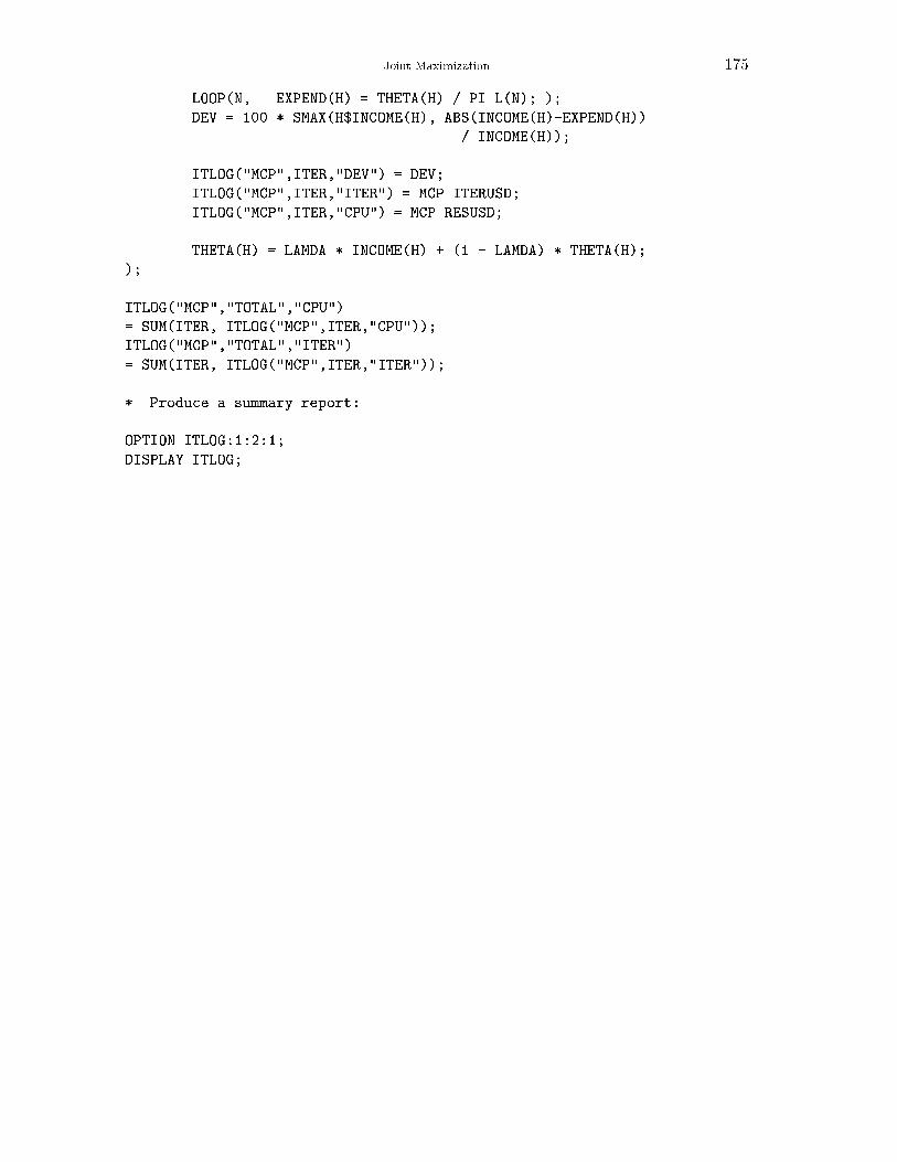
Joint Maximization 175
LOOP(N, EXPEND(H) = THETA(H) / PI.L(N); );
DEV = 100 * SMAX(H$INCOME(H), ABS(INCOME(H)-EXPEND(H))
/ INCOME(H));
ITLOG("MCP",ITER,"DEV") = DEV;
ITLOG("MCP",ITER,"ITER") = MCP.ITERUSD;
ITLOG("MCP",ITER,"CPU") = MCP.RESUSD;
THETA(H) = LAMDA * INCOME(H) + (1 - LAMDA) * THETA(H);
);
ITLOG("MCP","TOTAL","CPU")
= SUM(ITER, ITLOG("MCP",ITER,"CPU"));
ITLOG("MCP","TOTAL","ITER")
= SUM(ITER, ITLOG("MCP",ITER,"ITER"));
* Produce a summary report:
OPTION ITLOG:1:2:1;
DISPLAY ITLOG;