Embed Size (px)
Citation preview
.A 911 ARMY LOGISTICS MANAGEMENT CENTER FORT LEE VA F/ 15/5IMPACT OF INCREMENTAL CHANGES IN 7S FUNDING ON SUPPLY PEIRPORMAN-ETC(U)
UUNCL S AUG 79 V T CRADDOCK
l//l/uuuuuun..u..iCuuuIll/IML .!//I//ImmI
-EEEEEE--El-- U//-II/

t o,
UNITED STATES ARMYLOGISTICS MANAGEMENT CENTER
FORT LEE, VIRGINIA
IMPACT OF INCREMENTAL CHANGES
IN S~r'l,' 7~~S FUNDING F - .ee.
SUPPLY PERFORMANCE C
(DELTA 7S)
FINAL REPORT
1$ o Manage Our Resources Wisel
Approved for Public Release, Distribution Unlimited
August 197980 3 10 080
SECURITY CLASSIFICATION OF THIS PAGE (Whet Date Entered)
READ INSTRUCTIONSRPTDUMNAIO~NF~ PAGEBEFORE COMPLETING FORM
. RjEPORT NUMBER 2. GOVT ACCESSION NO. 3. RECIPIENT'S CATALOG NUMBER
4.tT I (and Subtitle) TYPE OF REPORT & PERIOD COVERED
TMPACT OF LNCREMENTAL QANGES IN 7S FUNDING ON ',Final t ISU.PPLY PER RMANCE; DELA 7S .. 6. PERFORMING ORG. REPORT NUMBER
TmOR(.) 8. CONTRACT OR GRANT NUMBER(e)
William T.Craddock9. PERFORMING ORGANIZATION NAME AND AOORESS 10. PROGRAM ELEMENT. PROJECT, TASK
US Army Logistics Management Center AREA&WORKUNIT NMOCRSSystems and Cost Analysis Department (DRXMC-C-SCAD , ,, /. ,'
Ft Lee, VA 23801"i ~ ~ ' ,CANTROL.,6 OFF'f' E..AMEAND ADORE"S 19VO41RT DA TE
rmy )a erie opment and Readiness Command
ATTN: DRCDRM-TG . AuqwE OFP79E
. 5001 Eisenhower Avenue 13.'NUMBEROFPAGESAlexandria, VA 22333 15614. MONITORING AGENCY NAME & ADRESS(Il different from Controlling Office) IS. SECURITY CLASS. (ot this report)
UNCLASSIFIEDIS. DECLASSIFICATIONiOOWNGRADING
SCHEDULE
16. DISTRIBUTION STATEMENT (of this Report)
Approved for public release; distribution unlimited
17. DISTRIBUTION STATEMENT (of the abstract entered In Block 20. If different from Report)
IS. SUPPLEMENTARY NOTES
IS. KEY WORDS (Continue on teverae side If nelessary and Identify by block number)
Goal ProgrammingResource Allocation
, I Program 7S
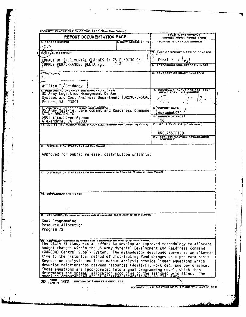
t Aft" ACT' C-Catde do reverse ebb It naeem md Identify7 by block nbr)he DELTA 7S Study was an effort to develop an improved methodology to allocatebudget changes within the US Army Materiel Development and Readiness Command(DARCOM) Central Supply System. The methodology developed serves as an alterna-tive to the historical method of distributing fund changes on a pro rata basis.Regression analysis and input-output analysis provide linear equations whichdescribe relationships between resources (dollars), workload, and performance.These equations are incorporated into a goal programming model, which thendetermines the optimal alQcation accordin5 to the assi ned priorities. Themodel is cnmnutpri~p rid1, ~~co 4nto rit~Ic v j a"-
DO 1473 EDI'oN OFI NOV S IS OsOLETE
SECURITY CLASSf! ICATON OF ?'MS PAGE 'Wen Date Entered)
o .*.

IMPACT OF INCREMENTAL CHANGES IN 7SFUNDING ON SUPPLY PERFORMANCE
(DELTA 7S)
by
William T. Craddock
August 1979
Approved for Public Release;Distribution Unlimited
US Army Logistics Management Center
Systems and Cost Analysis Department
-J Fort Lee, Virginia 23801
DISCLAIMER
Information and data contained in this report are based on input available
at the time of preparation. Because the results may be subject to change,
this report should not be construed to represent the official position of
the US Army Materiel Development and Readiness Command unless so stated by
that Command.
AV.
-
I
ABSTRACT
*. The DELTA 7S Study was an effort to develop an improved methodology to
allocate budget changes within the US Army Materiel Development and
Readiness Command (DARCOM) Central Supply System. The methodology developed
serves as an alternative to the historical method of distributing fund
changes on a pro rata basis. Regression analysis and input-output analysis
provide linear equations which describe relationships between resources
(dollars), workload, and performance. These equations are incorporated
into a goal programming model, which then determines the optimal allocation
according to the assigned priorities. The model is computerized and is
accessed interactively by the user.
-- I
ii
ACKNOWLEDGEMENTS
Various personnel within the Systems and Cost Analysis Department at
the US Army Logistics Management Center have participated in this study
effort. These include MAJ Daniel A. Ryan, CPT Richard W. DeMouy, Mr. J.
Allen Hill, Mr. 0. John Erickson, Mr. Joseph D. Brannon, CPT Lonnie B.
* Adams, LT Gary L. Martin, Mr. Thomas A. Miller, and Mr. Gerald A. Klopp.
Of these, special acknowledgement should be given to MAJ Ryan, who was
" responsible for the revamping of the Input-Output model and the Goal
Programming algorithm. He made changes which contributed to the success of
the DELTA 7S effort, and was the only member of the study team with
Mr. Craddock after September 1978. MAJ Ryan wrote Annexes H (User Instruc-
tion) and I (Computer Program) of this report. Also, acknowledgement is
due Mr. Hill for writing Annex B (Literature Survey).
Various other personnel assisted the study team in its endeavors.
They include Mr. David Hodges and Ms. Joan Tackett of HQ DARCOM, and
Mr. Don Ruth, Tim Sommons, and Ron Hulscher of DESCOM.
Last, but not least, a very special acknowledgement is due
Mrs. Debbie Thompson for superb administrative support. She never tired of
the countless drafts of briefing charts and reports.
iii
TABLE OF CONTENTS
Page
Disclaimer. .. ..... ....... ........ .......... i
Abstract .. ... ....... ....... ....... ....... ii
Acknowledgements .. ... ....... ....... ..........iii
Table of Contents .. ...... ....... ........ ..... iv
List of Tables. .. ..... ........ ....... ....... vi
List of Figures. ... ....... ........ ....... .. vii
Part I - Executive Summary
1. Problem Statement . . . . . . . . . . . . . . . . . . . . . . . . 1
2. Background. ...... ........ ....... ....... 2
3. Assumptions. .... ....... ....... ....... ... 3
4. Methodology .. ...... ....... ....... ....... 4
5. Model Output .. ... ....... ....... ....... ... 8
6. Conclusions and Recommendations. ... ........ ....... 8
Part II - Main Report
1. Problem Statement .. ...... ....... ....... ... 10
2. Background. ...... ....... ........ ....... 11
3. Study Approach. .. ..... ........ ....... ..... 12
4. Assumptions .. ...... ....... ....... ....... 14
5. Data Base. ... ....... ....... ........ ... 14
6. Model Description .. ...... ....... ....... ... 15
7. Model Application .. ...... ....... ....... ... 27
8. Conclusions and Recommiendations .. ...... ........ .. 34
iv
* I
TABLE OF CONTENTS (Cont'd)
Page
I Annexes
A. Administrative Documents ...... ..................... ... A-I
3. Literature Survey .......... ........................ B-1
C. Model Description .......... ........................ C-I
(1) Regression Analysis ......... ..................... C-2
(2) Input-Output Analysis ....... .................... .. C-7
(3) Goal Programming ....... ....................... .. C-30
D. Description of Program Elements ...... .................. D-1
E. Data .......... ............................... . E-I
F. Sensitivity Analysis ........ ...................... .. F-I
G. Validation ......... ............................ . G-I
H. User Instructions ........ ........................ . H-1
I. Computer Program ......... ......................... I-I
v
I.
LIST OF TABLES
TABLE TITLE PAGE
<I1 Sources of Data. .. ..... ........ ....... .. 15
2 Workload Equations .. ...... ....... ........ 16
3 Performance Equations .. ... ....... ........ .. 18
4 Support Sectors. .. ...... ....... ....... .. 21
5 Program Budget Guidance for FY 79 (dated 16 Jan 79) .. ... .. 28
6 General Priority Structure. ... ....... ........ 34
C-1 Workload and Performance Equations .. ...... ....... C-3
C-2 Independent Variables for Regression Equations .. ........C-s
C-3 AMS Code/Input-Output Sector Relationships .. ...... ... C-12
C-4 FY 79 COBE Requirements (CSCAB-205 Report, July 1978) .. ..... C-21
C-5 Linear Input-Output Analysis Equations. .... ......... C-29
C-6 Additional 1-0 Equations. ... ....... .......... C-31
C-7 Priority Structure Input File. .. ..... ........ .. C-34
C-8 Budget and Goal Input File. ... ....... ........ C-40E-1 Variables in Master Data File. .. ..... ........ .. E-5
E-2 Master Data File .. ..... ........ ....... .. E-6
E-3 Inflation Factors. .. ...... ....... ......... E-7
F-l Model Sensitivity. .. ..... ........ ......... F-3
LIST OF FIGURES
FIGURE PAGE
1 Allocation of a Hypothetical DA Budget ... ........... ... 19
2 Supply Economy Input-Output Relationships ..... .... 22
* 3 Input-Output Budget Allocation Table (FY 79 Funded and
Unfunded Requirements) ...... ................... ... 24
4 Model Output--Page 1 ....... ................... ... 30
5 Model Output--Page 2 ...... ................... ... 31
6 Model Output--Page 3 ...... ................... ... 33
C-1 Allocation of COBE Requirements in 1-0 Matrix . ....... .. C-22
vii
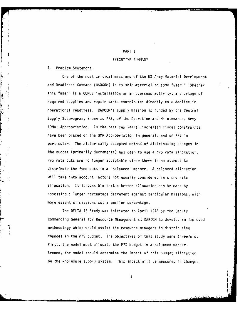
PART I
EXECUTIVE SUMMARY
. Problem Statement
One of the most critical missions of the US Army Materiel Development
and Readiness Command (DARCOM) is to ship materiel to some "user." Whether
this "user" is a CONUS installation or an overseas activity, a shortage of
required supplies and repair parts contributes directly to a decline in
operational readiness. DARCOM's supply mission is funded by the Central
Supply Subprogram, known as P7S, of the Operation and Maintenance, Army
(OMA) Appropriation. In the past few years, increased fiscal constraints
have been placed on the OMA Appropriation in general, and on P7S in
particular. The historically accepted method of distributing changes in
the budget (primarily decrements) has been to use a pro rata allocation.
Pro rata cuts are no longer acceptable since there is no attempt to
distribute the fund cuts in a "balanced" manner. A balanced allocation
will take into account factors not usually considered in a pro rata
allocation. It is possible that a better allocation can be made by
assessing a larger percentage decrement against particular missions, with
more essential missions cut a smaller percentage.
The DELTA 7S Study was initiated in April 1978 by the Deputy
Commanding General for Resource Management at DARCOM to develop an improved
methodology which would assist the resource managers in distributing
changes in the P7S budget. The objectives of this study were threefold;
First, the model must allocate the P7S budget in a balanced manner.
Second, the model should determine the impact of this budget allocation
on the wholesale supply system. This impact will be measured in changes
1 !
. . ... .... A

to workload and performance. Workload is broadly defined as how much
work the supply system must accomplish and is measured in such terms as
* procurement actions accomplished and requisitions processed. Performance
is broadly defined as how well the supply system accomplishes that work-
load, and is measured in such terms as stock availability and on-time
requisition processing. A balanced allocation will consider the impact
of fund changes on supply workload and performance. Third, the model
should be able to perform the functions of allocation and impact determi-
nation when the funding for some programs is fixed.
2. Background
The Department of the Army (DA) informs its major commands (such as
DARCOM) of their funding guidance periodically via the Program Budget
Guidance (PBG). Annually, each major command prepares and sends to DA a
budget which includes the budget estimate for the next two fiscal years as
well as an update on the execution status of the budget for the current
fiscal year. This budget, known as the Command Operating Budget Estimate
(COEE), contains estimates for money and personnel requirements based upon
both the previously received PBG and updated projections of workload.
Under Zero-Based Budgeting, this budget estimate is stratified into several
* "funding levels. These strata include projections of the workload possible
based upon the funding expected to be received, and estimates of the funds
required to accomplish the total workload projected. The difference
between these two funding levels is sometimes referred to as the unfinanced
requirement. The study team narrowly defined resources to imply funds
2
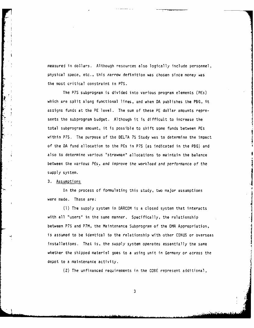
measured in dollars. Although resources also logically include personnel,
physical space, etc., this narrow definition was chosen since money was
the most critical constraint in P7S.
The P7S subprogram is divided into various program elements (PEs)
which are split along functional lines, and when DA publishes the PBG, it
assigns funds at the PE level. The sum of these PE dollar amounts repre-
- sents the subprogram budget. Although it is difficult to increase the
total subprogram amount, it is possible to shift some funds between PEs
within P7S. The purpose of the DELTA 7S Study was to determine the impact
of the DA fund allocation to the PEs in P7S (as indicated in the PBG) and
also to determine various "strawman" allocations to maintain the balance
between the various PEs, and improve the workload and performance of the
supply system.
3. Assumptions
In the process of formulating this study, two major assumptions
were made. These are:
(1) The supply system in DARCOM is a closed system that interacts
with all "users" in the same manner. Specifically, the relationship
between P7S and P7M, the Maintenance Subprogram of the OMA Appropriation,
is assumed to be identical to the relationship with other CONUS or overseas
installations. That is, the supply system operates essentially the same
whether the shipped materiel goes to a using unit in Germany or across the
depot to a maintenance activity.
(2) The unfinanced requirements in the COBE represent additional,
3
,
. . .. . .. . . . . . . . . . . . . . . . . . .
-
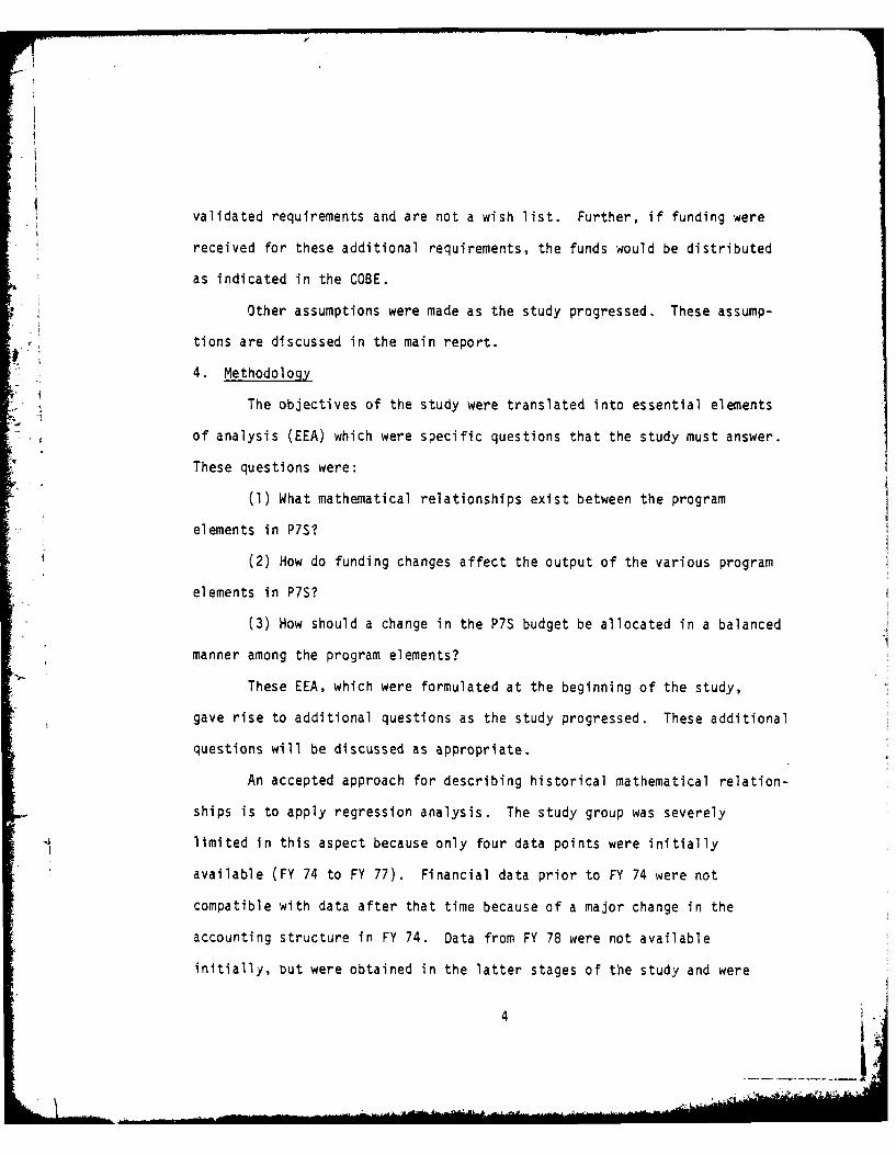
validated requirements and are not a wish list. Further, if funding were
-received for these additional requirements, the funds would be distributed
as indicated in the COBE.
Other assumptions were made as the study progressed. These assump-
tions are discussed in the main report.
4. Methodology
The objectives of the study were translated into essential elements
of analysis (EEA) which were specific questions that the study must answer.
These questions were:
(1) What mathematical relationships exist between the program
elements in P7S?
(2) How do funding changes affect the output of the various program
elements in P7S?
(3) How should a change in the P7S budget be allocated in a balanced
manner among the program elements?
These EEA, which were formulated at the beginning of the study,
gave rise to additional questions as the study progressed. These additional
questions will be discussed as appropriate.
An accepted approach for describing historical mathematical relation-
ships is to apply regression analysis. The study group was severely
limited in this aspect because only four data points were initially
available (FY 74 to FY 77). Financial data prior to FY 74 were not
compatible with data after that time because of a major change in the
accounting structure in FY 74. Data from FY 78 were not available
initially, but were obtained in the latter stages of the study and were
4
used for validation purposes. Regression equations were developed that
described both workload and performance as a function of resources (dollars).
A popular theory at DARCOM is that performance is logically a
function of both workload and resources. That is, how well one does
something depends upon not only how much one must do (workload) but also
how much is available with which to do it (resources). The exact relation-
ship between resources, workload, and performance is a complex one, but an
attempt was made to model performance as a function of both workload and
resources using multiple regression. This approach did not work because
of the small number of observations and the high correlation between work-
load and resources.
An attempt was made to base the final equation choices on both
logic and mathematical fit. Using the sets of equations that were developed
from four data points, the study group validated the equations with a fifth
data point (from FY 78 data which were then available). The resulting sets
of equations for workload and performance are the best equations available
given the constraints of logic, mathematical fit, and predictive ability.
The data for these equations came from various DARCOM cost and
performance reports, and from briefing charts (primarily on performance)
prepared by the Materiel Management Directorate at HQ DARCOM. All cost
data were adjusted to FY 78 constant dollars using inflation guidance
published by HQ DARCOM.
The study team used input-output analysis to model the balance
between the program elements in P7S. Input-Output (1-0) analysis is an
econometric technique that describes the interrelationships between
5
various sectors of an "economy." In order to apply input-output analysis
to the wholesale supply system, one must first consider it as a supply
economy and identify the various support sectors and the final product of
*the economy. In this case, the final product of the supply economy is
assumed to be the materiel that is shipped to some user. All other functions
that do not directly relate to the shipping function are considered to be
support functions. The Army Management Structure (AMS) codes provided a
natural break for the support sectors. After several iterations, the
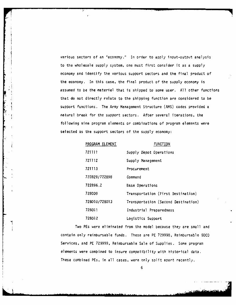
following nine program elements or combinations of program elements were
selected as the support sectors of the supply economy:
PROGRAM ELEMENT FUNCTION
721711 Supply Depot Operations
721112 Supply Management
721113 Procurement
722829/722898 Command
722896.Z Base Operations
728009 Transportation (First Destination)
728010/728013 Transportation (Second Destination)
728011 Industrial Preparedness
728012 Logistics Support
Two PEs were eliminated from the model because they are small and
contain only reimbursable funds. These are PE 729998, Reimbursable GOCO
Services, and PE 729999, Reimbursable Sale of Supplies. Some program
elements were combined to insure compatibility with historical data.
These combined PEs, in all cases, were only split apart recently.
6
To determine the relationships between the various support sectors
and the final product, the study group first identified which functional
relationships should exist between the various sectors. For example, what
actions does a depot perform that support a National Inventory ControlPoint? The study group examined AR-37-0OO-78, looking at each AMS code to
determine in which cell of the I-0 matrix its function belonged. These
relationships were quantified by using the dollars programmed for the
different functions. Both the FY 79 Funded and Unfunded requirements were
included to insure that the correct balance was modeled between the various
program elements. These I-0 relationships were formalized as equations
which were used to represent the balance relationships.
Since this model is primarily a fund allocation model, the classical
approach is to use a type of linear programming. Goal programming (GP) is
a relatively new and more flexible variation of linear programming. The
primary difference is that GP allows for several conflicting objectives or
goals, and attempts to satisfy these goals in order of priority. For
convenience, these goals are grouped into five areas. These areas are:
(1) Totally allocate the P7S budget.
(2) Assure that the funding levels for selected PEs are guaranteed
via the "fencing" option. These PEs will be allocated, as a minimum, the
amount of funds equal to their fence.
(3) Maintain a balanced relationship between the various program
elements.
(4) Meet the workload as stated in the COBE.
(5) Achieve the DARCOM numerical goals for various performance
indicators.7
5. Model Output
The goal programming model is computerized and is accessed inter-
actively. The output of the model comes in three pages. The first page of
output displays the latest program budget guidance by direct, funded, and
automatic reimbursable obligations for each of the PEs in the model. The
program determines all of the totals, and then asks two questions of the
operator. The first question is to identify any "fencing" that may be
required for selected PEs. The second question verifies the total 7S budget.
The second page shows the comparison of COBE and model allocations
for both direct and total obligations. The last page of the output shows
the impact of both the COBE and model allocations on the workload and
performance parameters. The predicted values are actually the expected
values obtained from the workload and performance reqression equations.
The difference column shows the difference between the predicted value and
the goal. A negative difference implies underachievement.
6. Conclusions and Recommendations
In summary, this model does what it was intended to do. It not only
provides the impact of DA funding guidance on supply workload and perform-
ance, but also provides an alternate or "strawman" allocation to improve
workload and performance. This strawman considers the proper balance
between program elements within P7S. The model also has the ability to
fence selected PEs, that is, to insure that the model allocates a pre-
determined dollar amount to those "fenced" PEs. A real advantage is that
the model can do these things with very short turn-around time.
The study team recommends that the Budget Operations Branch in the
Comptroller Directorate at HQ DARCOM use the DELTA 7S model to analyze
funding alternatives for FY 80 and FY 81. Further, someone at HQ DARCOM
should be designated as a Point-of-Contact for the model. This person
would be responsible for handling all questions on the operation and
maintenance of the model.
9
PART I I
MAIN REPORT
1. Problem Statement
One of the US Army Materiel Development and Readiness Command's
prime missions is to function as the Army's wholesale supply system. The
funds to operate this supply activity come from the Central Supply and
Maintenance (Program 7) portion of the Operations and Maintenance, Army
Appropriation. More specifically, the supply funds come from Subprogram 7S,
(P7S), Central Supply Activities. The P7S subprogram (like other programs)
* is divided into various Program Elements that are essentially split along
logical, functional lines. The PEs may also be furthey subdivided, and
this is the basis for the Army Management Structure. (A more comolete
description of the P7S subprogram and its PEs is contained in Annex D.)
The P7S subprogram has been a frequent target of budget changes (primarily
decrements), and the "traditional" way to allocate these changes among the
various program elements in P7S was based on pro rata shares. This
allocation assumes that all of the PEs are of equal importance, although
some PEs are clearly more critical than others.
This study was initiated to develop an improved methodology which
would distribute changes in the P7S budget in a balanced manner. A balanced
allocation will consider the contribution of each segment of the supply
, system. This methodology must also assess the impact of this balanced fund
allocation on the supply system workload and performance. Workload will
be defined, in general, as "how much work the supply system must accomplish."
Performance will be defined, in general, as "how well the supply system
accomplishes that workload." There are management indicators and goals for
10
both workload and performance variables. The methodology developed for this
study is able to allocate proposed P7S budget changes and assess the predicted
impact on supply workload and performance.
2. Background
As stated earlier, the traditional approach to budget decrements has
4 been to assess pro rata cuts. That is, the various program elements are
each decremented by the same fixed percentage. This implicitly assumes that
all PEs are of equal importance, which may not be the case. Some program
elements fund activities which deal with day-to-day operations (such as in
a supply depot). These PEs have clearly defined and measured management
indicators, and are sometimes referred to as the "hard" accounts. Other
PEs fund activities whose impacts are long range (such as Industrial
Preparedness Activities). These PEs tend to have less specific management
indicators, and are sometimes referred to as the "soft" accounts. The
descriptors "hard" and "soft" are not intended to be derogatory, but rather
to indicate the dilemma that management faces. It may be more feasible to
assess a lower percentage cut to those PEs where the impact will be felt
immediately, and assess a higher percentage cut to those PEs where the
impact will be delayed, perhaps for years. This should not be interpreted
as a management "cop out." It essentially attempts to minimize the known,
immediate impacts while delaying the less certain, long-range impacts.
However, to be able to do this in a defensible manner, one must be
able to assess those known, immediate impacts quantitatively. Qualitative
impact statements are becoming less useful in the current budget-strained
environment. Recognizing this, the Deputy Commanding General for Resource
11
Management at HQ DARCOM initiated a study in April 1978 to develop a metho-
dology which would assist managers with allocating the P7S budget changes
in a balanced manner. This study, known as the DELTA 7S Study, had the
following specific study objectives:
(1) Balanced allocation of changes in 7S funding.
(2) Effect of funding change on supply performance.
(3) Balance and effect when the funding for some elements is fixed.
These study objectives were then translated into Essential Elements of
Analysis (EEA), which are specific questions that the study must answer.
These are:
(1) What mathematical relationships exist between program elements
in P7S?
(2) How do funding changes affect the output of various program
elements in P7S?
(3) How should a change in the P7S budget be allocated in a balanced
manner among the program elements?
These EEA gave rise to other specific questions as the study progressed,
which will be discussed as appropriate.
3. Study Approach
Since this problem is basically a fund allocation model, the
classical approach is to use some form of mathematical programming. Linear
programming is the most common form of math programming, and there exists a
large number of computer algorithms for solving these problems. However,
the constraints that exist within the supply system would possibly lead to
an infeasible solution in linear programming. Goal Programming is a
12
relatively new variation of linear programming in which several conflicting
objectives or goals are possible. (In practice, GP problems are not
restricted to a linear form. However, whenever references to GP appear in
this report, they refer to a linear goal programming model.) The GP will
*satisfy as many of these goals as possible by looking at them each
separately in a predetermined order of priority.
This study used GP as the basic model structure, and developed the
linear objective equations using other techniques. Specifically, regression
analysis and input-output analysis were used to establish linear equations
which were later incorporated into the GP.
Since the model must determine the impact of the budget allocations
on the supply system workload and performance, the study team had to
develop the relationships between resources (R), workload (W), and
performance (P). W though resources logically include dollars, personnel,
space, time, equipment, etc., the study team restricted the meaning of
"resources" to imply only dollars, the most critical resource variable.
The relationships to be developed were:
W = f(R)
and P = f(W,R) or P = f(R).
Linear regression analysis was the technique used because of the linear
restriction of the GP chosen for the DELTA 7S model.
Input-Output analysis is an econometric technique which was used to
model the balance between the various PEs in P7S. Input-Output analysis
has traditionally been used to model the US economy. In order to apply
13
1-0 to the problem at hand, the study team had to describe the Army's
wholesale supply system as an economy. Once this was done, an I-0
budget allocation matrix was prepared. Sets of linear equations were
derived from this budget allocation matrix which describe the inter-
relationships of the various PEs in P7S. These linear equations were then
incorporated into the GP with the regression equations described above.
4. Assumptions
In the process of model development, the study team had to make
several assumptions. These assumptions include:
(1) The purpose of the supply system is to ship materiel to a user.
(2) The three main functions of a depot are to receive, store, and
ship. The receipt and storage functions are actions that a depot performs
in order to posture itself to ship.
(3) The unfunded requirement is a validated requirement, and does
not represent a wish list.
(4) If funds were received at the enhanced level, DARCOM would
distribute the funds as indicated in the Command Operating Budget Estimate
(COBE).
(5) The supply system functions essentially the same whether the
shipped materiel is going to some unit overseas or across the depot to a
maintenance facility.
5. Data Base
Initially, the study team attempted to obtain detailed quarterly
financial, workload, and performance data back to FY 74. Financial data
14
previous to FY 74 were not comparable because of a major change in the
accounting structure from FY 73 to FY 74. Accordingly, the study team
issued several data calls. The results of these data calls were either
no data provided at all, or data which could not be combined. Consequently,
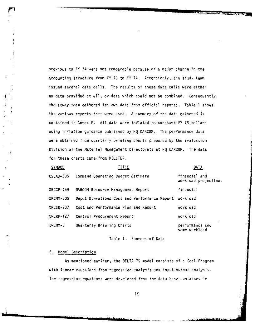
the study team gathered its own data from official reports. Table 1 shows
the various reports that were used. A summary of the data gathered is
contained in Annex E. All data were inflated to constant FY 78 dollars
using inflation guidance published by HQ DARCOM. The performance data
were obtained from quarterly briefing charts prepared by the Evaluation
Division of the Materiel Management Directorate at HQ DARCOM. The data
for these charts came- from MILSTEP.
SYMBOL TITLE DATA
CSCAB-205 Command Operating Budget Estimate financial andworkload projections
DRCCP-159 DARCOM Resource Management Report financial
DRCMM-305 Depot Operations Cost and Performance Report workload
DRCSU-207 Cost and Performance Plan and Report workload
DRCRP-127 Central Procurement Report workload
DRCMM-E Quarterly Briefing Charts performance andsome workload
Table 1. Sources of Data
6. Model Description
As mentioned earlier, the DELTA 7S model consists of a Goal Program
with linear equations from regression analysis and input-output analysis.
The regression equations were developed from the data base contained in
5 1:
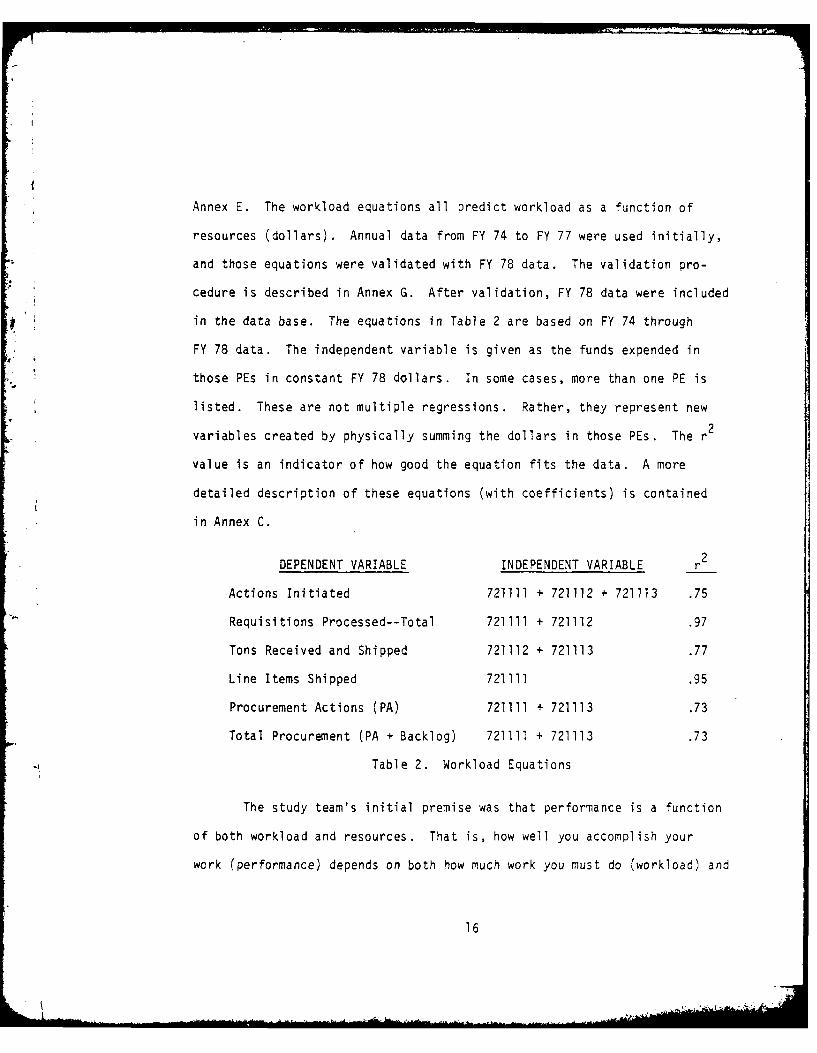
Annex E. The workload equations all predict workload as a function of
resources (dollars). Annual data from FY 74 to FY 77 were used initially,
and those equations were validated with FY 78 data. The validation pro-
cedure is described in Annex G. After validation, FY 78 data were included
in the data base. The equations in Table 2 are based on FY 74 through
FY 78 data. The independent variable is given as the funds expended in
those PEs in constant FY 78 dollars. In some cases, more than one PE is
listed. These are not multiple regressions. Rather, they represent new2
variables created by physically summing the dollars in those PEs. The r
value is an indicator of how good the equation fits the data. A more
detailed description of these equations (with coefficients) is contained
in Annex C.
DEPENDENT VARIABLE INDEPENDENT VARIABLE r2
Actions Initiated 721111 + 721112 + 721113 .75
Requisitions Processed--Total 721111 + 721112 .97
Tons Received and Shipped 721112 + 721113 .77
Line Items Shipped 721111 .95
Procurement Actions (PA) 721111 + 721113 .73
Total Procurement (PA + Backlog) 721111 + 721113 .73
Table 2. Workload Equations
The study team's initial premise was that performance is a function
of both workload and resources. That is, how well you accomplish your
work (performance) depends on both how much work you must do (workload) and
16
how much resources are available with which to do it (resources). To this
end, the study team attempted to develop multiple linear equations which
"predict" performance as a function of both workload and performance. The
problem was that there were only four annual data points initially.
Although this left only one degree of freedom, the equations were marginally
acceptable because of the extremely high experimental F values. In an
attempt to increase the number of data points, the study team investigated
quarterly data (1 Qtr FY 76 through 2 Qtr FY 78, including FY 7T).
However, the relationships that were developed using annual data could not
be reproduced when quarterly data were used. The quarterly data had much
too much variability/noise. In an attempt to decrease the variability,
the statistical technique of a three quarter moving average was used, but
this also did not produce satisfactory results. The data were also shifted
one or more quarters based on the premise that resources in Quarter I may
affect performance in Quarters 2 and 3. The data were also smoothed and
shifted at the same time. None of these attempts produced statistically
acceptable and logically explainable equations, so the study team decided
to not use the quarterly data.
The annual equation,- with workload and resources as the independent
variables were also not used, but not because of the degrees of freedom.
The high correlation between the two independent variables was unacceptable.
More specifically, the value for the workload "independent" variable was
itself derived from an equation with resources as the independent variable.
Logically, workload is a better predictor for performance than is resource.
17

However, the workload value is still based on resources. The use of work-
load to predict performance would constitute a two-step process with possibly
increased variability. Therefore, the final equations predict performance
as a function of resources. As with the workload equations, the performance
equations were initially based on annual data from FY 74 to FY 77, validated
with FY 78 data, and then revised to include the FY 78 data. The resulting
equations are shown in Table 3. The details of these equations are contained
in Annex C.
DEPENDENT VARIABLE INDEPENDENT VARIABLE r_2
NICP O-T Reqn Proc 721112 .87
Depot O-T Reqn Proc 721111 .71
O-T Receiving Rate--Reporting 721111 .78
O-T Receiving Rate--Stowing 721111 .86
Location Survey Accuracy 721111 .84
DARCOM O-T Trans Rate 721111 .76
Stock Availability Rate EXi except 728009 .66
Table 3. Performance Equations
As with any regression equation, the value "predicted" is really an
expected value. It is rare to observe the predicted value exactly.
Further, the variability between the predicted and the observed values is
directly related to the number of data points used in the regression.
Input-Output analysis is an econometric technique most commonly
used to measure the interrelationships between the various sectors of an
economy. As an example of 1-0 applied to a military situation, consider
the hypothetical DA budget that is shown in Figure 1. In this example,
18 1., t .
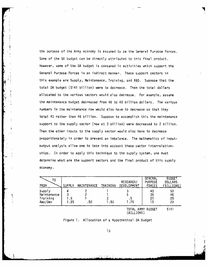
the purpose of the Army economy is assumed to be the General Purpose Forces.
Some of the DA budget can be directly attributed to this final product.
However, some of the DA budget is consumed in activities which support the
General Purpose Forces in an indirect manner. These support sectors in
this example are Supply, Maintenance, Training, and R&D. Suppose that the
total DA budget ($141 billion) were to decrease. Then the total dollars
allocated to the various sectors would also decrease. For example, assume
the maintenance budget decreased from 46 to 40 billion dollars. The various
numbers in the maintenance row would also have to decrease so that they
total 40 rather than 46 billion. Suppose to accomplish this the maintenance
support to the supply sector (now at 3 billion) were decreased to 2 billion.
Then the other inputs to the supply sector would also have to decrease
proportionately in order to prevent an imbalance. The mathematics of input-
*. output analysis allow one to take into account these sector interrelation-
ships. In order to apply this technique to the supply system, one must
determine what are the support sectors and the final product of this supply
economy.
TO o GENERAL BUDGET0 RESEARCH/ PURPOSE DOLLARS.
FROM SUPPLY MAINTENANCE TRAINING DEVELOPMENT FORCES (BILLIONS)
Supply 4 2 1 3 40 50Maintenance 3 2 1 5 35 46Training 1.5 1 2 .5 20 25Res/Dev 1.25 .50 1.50 1.75 15 20
TOTAL ARMY BUDGET $141(BILLIONS)
Figure 1. Allocation of a Hypothetical DA Budget
19
An assumption was made that the purpose of the supply economy is to
ship material to some user, and that all functions which directly relate
to the issue and shipping function are to be considered as the "final
product," analogous to the general purpose forces in the previous example.
The various PEs in P7S are split along functional lines, and represent a
convenient description of the support sectors for the supply economy. These
V alPEs are described in detail in AR-37-100-XX, The Army Management Structure.
The XX refers to the specific fiscal year under consideration. Since FY 78
is the base year for this study, AR-37-100-78 was used. Only the PEs
applicable to DARCOM (those contained in the COBE) were considered. Some
of these PEs were also eliminated because they were small, reimbursable
accounts. These include PE 729998, Reimbursable GOCO Services and
PE 729999, Reimbursable Sale of 3upplies. Some of the remaining PEs were
combined because they were only recently split apart. Specifically,
PE 722829, Logistics Administrative Support, was combined with PE 722898,
Management HQ (Logistics). Also, the DARCOM portion of PE 728013, Overseas
Port Units (Non-IF), was combined with PE 728010, Second Destination
Transportation. These combinations were necessary in order to be compatible
with previous data. One new PE was included: PE 728009, First Destination
Transportation. Although this program element was not established until
FY 79, it was included to be compatible with future budgets.
The resulting PEs and combinations of PEs form the support sectors
of the supply economy. These are shown in Table 4.
The next step was to determine how the various PEs support each
other and the final product. First, the study team identified the logical,
20
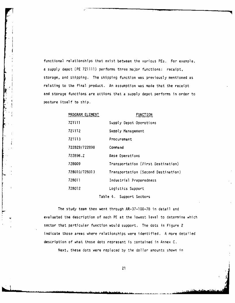
functional relationships that exist between the various PEs. For example,
a supply depot (PE 721111) performs three major functions: receipt,
storage, and shipping. The shipping function was previously mentioned as
relating to the final product. An assumption was made that the receipt
and storage functions are actions that a supply depot performs in order to
posture itself to ship.
PROGRAM ELEMENT FUNCTION
721111 Supply Depot Operations
721112 Supply Management
721113 Procurement
722829/722898 Command
722896.Z Base Operations
728009 Transportation (First Destination)
728010/728013 Transportation (Second Destination)
728011 Industrial Preparedness
728012 Logistics Support
Table 4. Support Sectors
The study team then went through AR-37-100-78 in detail and
evaluated the description of each PE at the lowest level to determine which
sector that particular function would support. The dots in Figure 2
indicate those areas where relationships were identified. A more detailed
description of what those dots represent is contained in Annex C.
Next, these dots were replaced by the dollar amounts shown in
21

0----
0000 0
CD
0 LAco 0 0
u CC -=4
,-ooz-0 0
ON W
00 0 0
I--
-C 4
rA.-
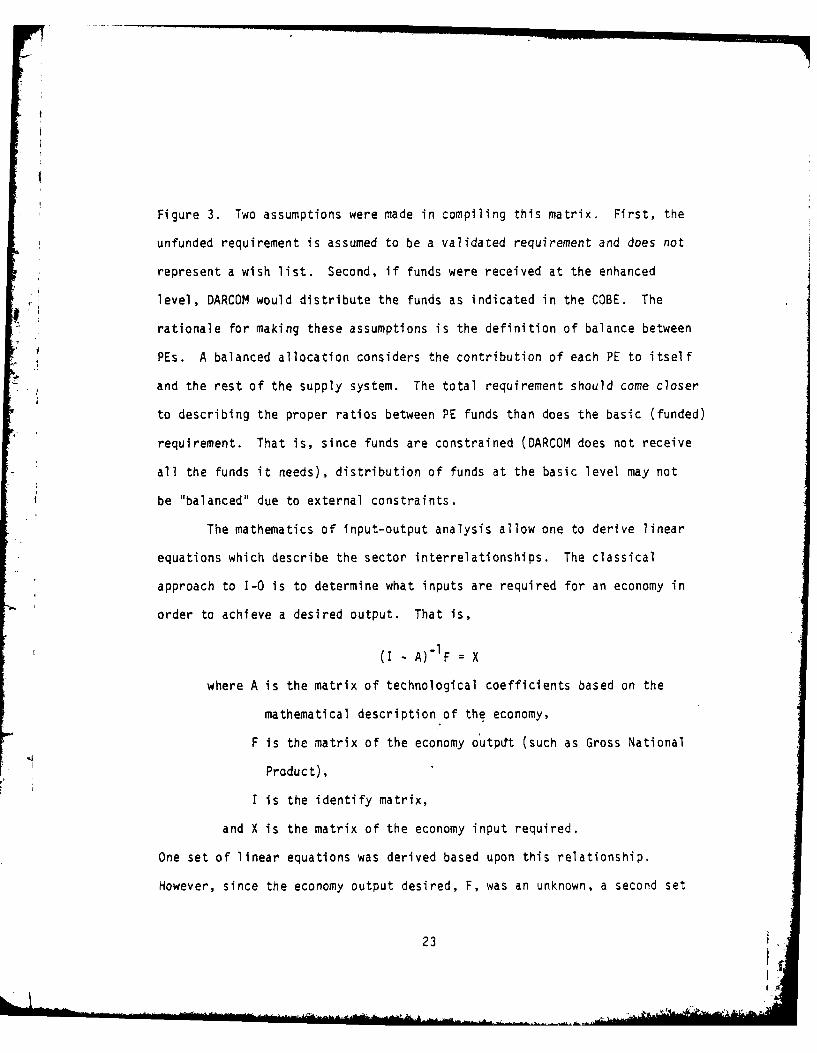
Figure 3. Two assumptions were made in compiling this matrix. First, the
unfunded requirement is assumed to be a validated requirement and does not
represent a wish list. Second, if funds were received at the enhanced
level, DARCOM would distribute the funds as indicated in the COBE. The
rationale for making these assumptions is the definition of balance between
PEs. A balanced allocation considers the contribution of each PE to itself
and the rest of the supply system. The total requirement should come closer
to describing the proper ratios between PE funds than does the basic (funded)
requirement. That is, since funds are constrained (DARCOM does not receive
all the funds it needs), distribution of funds at the basic level may not
be "balanced" due to external constraints.
The mathematics of input-output analysis allow one to derive linear
equations which describe the sector interrelationships. The classical
approach to 1-0 is to determine what inputs are required for an economy in
order to achieve a desired output. That is,
(I - A)'IF = X
where A is the matrix of technological coefficients based on the
mathematical description of the economy,
F is the matrix of the economy outpdt (such as Gross National
Product),
I is the identify matrix,
and X is the matrix of the economy input required.
One set of linear equations was derived based upon this relationship.
However, since the economy output desired, F, was an unknown, a second set
23

-LU
N0 C)
WN r-. 1ro -.
- co co a
X:: -- -- Z=C4 .
LAJ.
*C C O
CN I
LU L" -o C-- --CD 400
00 0'
_- C* L*q
- -
*~ C14 0" Co_-00~ ~ ~ 00( 140
-- C0 C\0 1
0 LLU
_-r C1 C4C4T Co- .n C C L
*I C1o
C- 0- CJ 00 wLIN -0 ( 0' Lo Lo c
c*-Jfl LIN o ~Co 0
-4 C1 C14 -4lCo -
- 0
C- - -l CD - -
00 00~N 0 co CDU- Co) C')
e..j C~ 00 0 00 1.-- N
-24
Iof linear equations was necessary. A more detailed description of these
equations is contained in Annex C.
As was mentioned previously, the overall model structure is based
upon goal programming. The linear equations developed using regression
analysis and 1-0 form the constraints in the GP. As an example of how the
individual goals are formulated, consider the following equation:
-3773.5 't .0327Xl = Line Items Shipped
where X I dollars in PE 721111.
This equation is one of the workload equations discussed previously.
The usual way to use this equation is to choose some value for X and then
"predict" the number of line items to be shipped. However, in GP this
would be formulated slightly different. The GP approach to this problem
is to predetermine a value desired for line items shipped (the goal), and
then allow the difference between the predicted value of line items shipped
and the goal to be absorbed in "deviations." Consider the following:
-+-3773.5 + .0327X1 + d" - d = GOAL for line items shipped
where X = dollars in PE 721111
d- = the negative (underachievement) deviation; i.e., the
number of line items below the GOAL
d = the positive (overachievement) deviation; i.e., the
number of line items above the GOAL
GOAL = the stated goal for the number of line items to be shipped
In this case, the goal was taken from the COBE, which stated this workload
requirement as 5646.9(10 3) line items shipped.
25
In GP, the value of X, will be chosen that will minimize the devia-
tions from the stated goal. In practice, there are many equations all of
which cannot be satisfied at the same time. The algorithm will then attempt
to minimize these various deviations in a prespecified order of priority.
For convenience, the goals for the DELTA 7S model are grouped into
five categories:
(1) Totally allocate the P7S budget. This goal consists of a single
equation that says that the summation of all of the PEs must equal the P7S
budget amount. Deviations above or below this budget amount are not
permitted.
(2) Assure that the funding levels for selected PEs are guaranteed
via the "fencing" option. This goal consists of an equation for each PE
to be "fenced" at a certain funding level. The GP will not permit devia-
tions below these specified funding levels. These equations are structured
so that "fencing" a PE will establish a minimum funding level permitted.
Otherwise, this minimum funding level is set at zero dollars.
(3) Maintain a balanced relationship between the various program
elements. This goal consists of two sets of linear equations derived from
the input-output model.
(41 Meet the workload as stated in the COBE. This goal consists of
a series of linear regression equations which predict workload as a function
of dollars.
(5) Achieve the DARCOM numerical goals for various performance
indicators. This goal consists of linear regression equations which predict
performance as a function of dollars.
26
Each goal equation must have priorities assigned to its deviational
variables (d- and d+). The two deviational variables may have different
priorities, if desired. For example, consider the equation for the
"totally allocate the P7S budget" goal described previously. This goal
consists of a summation of the funds expended in each of the PEs. The
overachievement deviational variable, d+ , represents the dollars spent
over the P7S budget total. The underachievement deviational variable, d-,
represents the underspending difference in dollars between the P7S budget
and the P7S projected expenses. It may be far more important to avoid an
overspending than an underspending, in which case the d+ would have a higher
priority than would d. A more detailed description of the priority
structure is contained in Annex C.
One important feature of the priority structure is the "fencing"
provision. This consists of a series of equations that establishes goals
of spending at least a minimum amount for each PE. In the absence of a
fence, this minimum amount is zero dollars. This minimum can easily be
changed to a positive amount for any PE at the beginning of the model
exercise. This is an important feature to insure compliance with external
or internal funding directives. For example, the Congress directed that a
certain amount be spent on Industrial Preparenesss Activities (PE 728011)
in FY 79. This is translated into an equation that states PE 728011 be
funded at a minimum equal to the Congressional directive. The under-
achievement deviational variable has a very high priority in this instance.
7. Model Application
DARCOM receives funding guidance in the form of the Program Budget
27
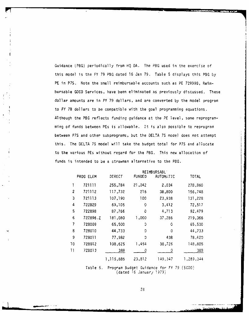
Guidance (PBG) periodically from HQ DA. The PBG used in the exercise of
this model is the FY 79 PBG dated 16 Jan 79. Table 5 displays this PBG by
PE in P7S. Note the small reimbursable accounts such as PE 729998, Reim-
bursable GOCO Services, have been eliminated as previously discussed. These
dollar amounts are in FY 79 dollars, and are converted by the model program
to FY 78 dollars to be compatible with the goal programming equations.
Although the PBG reflects funding guidance at the PE level, some reprogram-
ming of funds between PEs is allowable. It is also possible to reprogram
between P7S and other subprograms, but the DELTA 7S model does not attempt
this. The DELTA 7S model will take the budget total for P7S and allocate
to the various PEs without regard for the PSG. This new allocation of
funds is intended to be a strawman alternative to the PBG.
REIMBURSABL -
PROG ELEM DIRECT FUNDED AUTOMATIC TOTAL
1 721111 255,784 21,042 2,034 273,860
2 721112 117,732 216 38,800 156,748
3 721113 107,190 100 23,938 131,228
4 722829 69,105 0 3,412 72,517
5 722898 87,766 0 4,713 92,479
6 722896.Z 181,080 1,000 37,286 219,366
7 728009 65,500 0 0 65,500
8 728010 44,733 0 0 44,733
9 728011 77,982 0 438 78,420
10 728012 108,625 1,454 38,726 148,805
11 728013 388 0 0 388
1,115,885 23,812 149,347 1,289,3a4
Table 5. Program Budget Guidance for FY 79 (S000)(dated 16 January 1979)
28
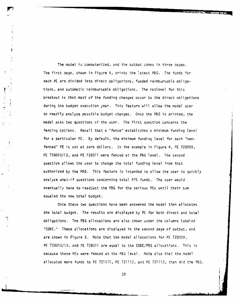
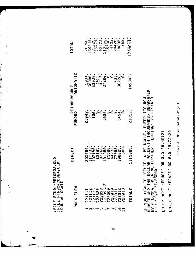
The model is computerized, and the output comes in three pages.
The first page, shown in Figure 4, prints the latest PBG. The funds for
each PE are divided into direct obligations, funded reimbursable obliga-
tions, and automatic reimbursable obligations. The rational for this
breakout is that most of the funding changes occur to the direct obligations
during the budget execution year. This feature will allow the model user
to readily analyze possible budget changes. Once the PBG is printed, the
model asks two questions of the user. The first question concerns the
fencing options. Recall that a "fence" establishes a minimum funding level
for a particular PE. By default, the minimum funding level for each "non-
fenced" PE is set at zero dollars. In the example in Figure 4, PE 728009,
PE 728010/13, and PE 728011 were fenced at the PBG level. The second
question allows the user to change the total funding level from that
authorized by the PBG. This feature is intended to allow the user to quickly
analyze what-if questions concerning total P7S funds. The user would
eventually have to readjust the PBG for the various PEs until their sum
equaled the new total budget.
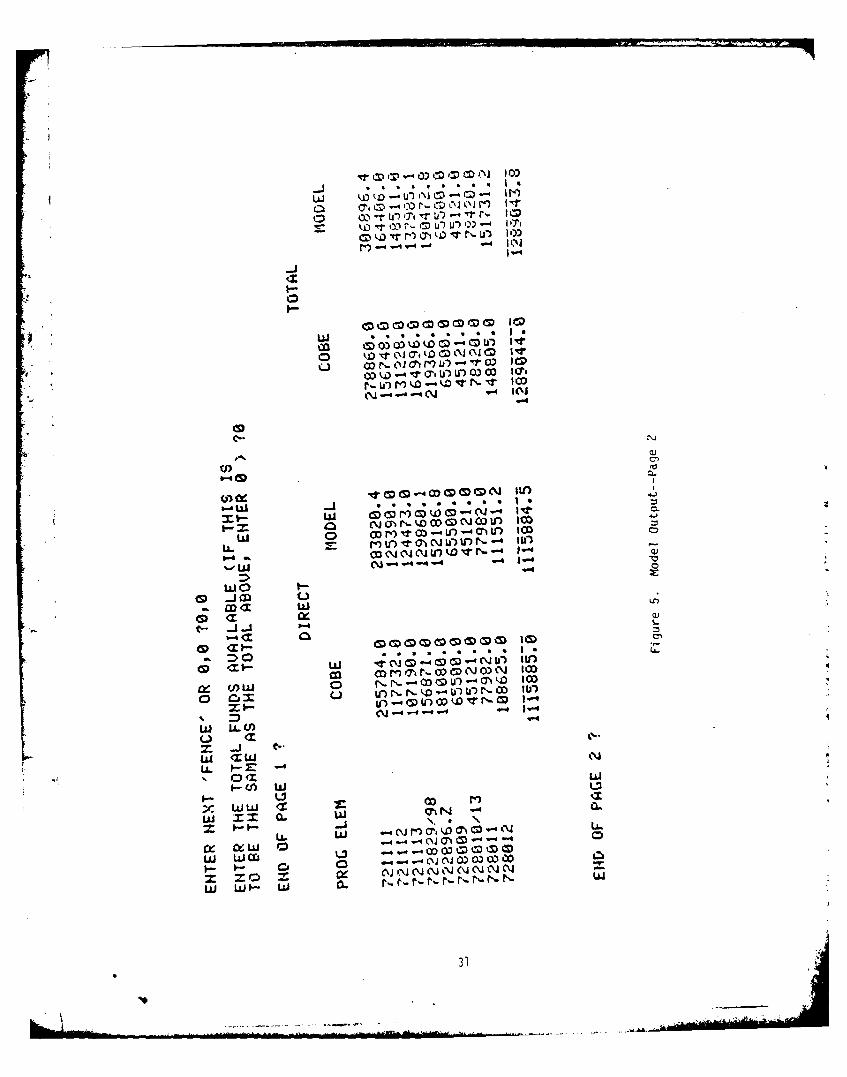
Once these two questions have been answered the model then allocates
the total budget. The results are displayed by PE for both direct and total
obligations. The PBG allocations are also shown uider the columns labeled
"COBE." These allocations are displayed in the second page of output, and
are shown in Figure 5. Note that the model allocations for PE 728009,
PE 728010/13, and PE 728011 are equal to the COBE/PBG allocations. This is
because these PEs were fenced at the PBG level. Note also that the model
allocated more funds to PE 721111, PE 721112, and PE 721113, than did the PBG.
29
. "T 17\ -- iS k m M 1\ CD CO I *
r- u) t- - 7 - , 0
o ~ ~ c rI,'-~r~wo j- m ' N .M4
1-4
c~) S S S S S S S Sn
(p IV-..
W V, CD 0 LO 1-
CDCM-~ ~ ~ ~ CD v lca n
Ni IN
WJ w U) 03*M =
4- -t
L) O J M 0' k 0 ()rq O- (Jr OD 103' I-- I
W LX LU
-4-('(J'J22000 m- W ' = kmrOefNN~-N v- Wo m
6-4IM u- =- ~-MO .* ,O2LAJ L LU
IOL L) Li-30
n *
S S V * I it
w Im
00
CC~
cD t CD D (M'M C IC
C-.j
p- ~ I,r. a kDw TN v IO
100
14 % . 0 0 4 a 1
C) c m CO -0'JU-)u--4 0' ' 10)
03' -4 04 N4- -) W-4w
wo I
15 CJ~ 5
-1-
-1-iw C4 a') CO -, Si U-' I U-
Imma r CDI CW ~ ~ N ) N 100
(j)0 w ,r . OCDU)- ) 100
o C.qw L - ( 1 )o
1 -
<W LLU
wL w masw-i x 4
N
w -l 14 M 14. 4
.141 -q (I ~j0 O )0
Z P-I JAI r, \-r Zr-r
31
- I
These three PEs fund the "hard" accounts, as discussed previously and these
PEs also are used most often as the independent variables in the workload
and performance equations. The funds for these increases came from some
of the "soft" accounts. Specifically, the model attempted to first
significantly reduce PE 728011, then PE 728009, and finally PE 728010/13.
p , These PEs were fenced at the PBG level to prevent this.
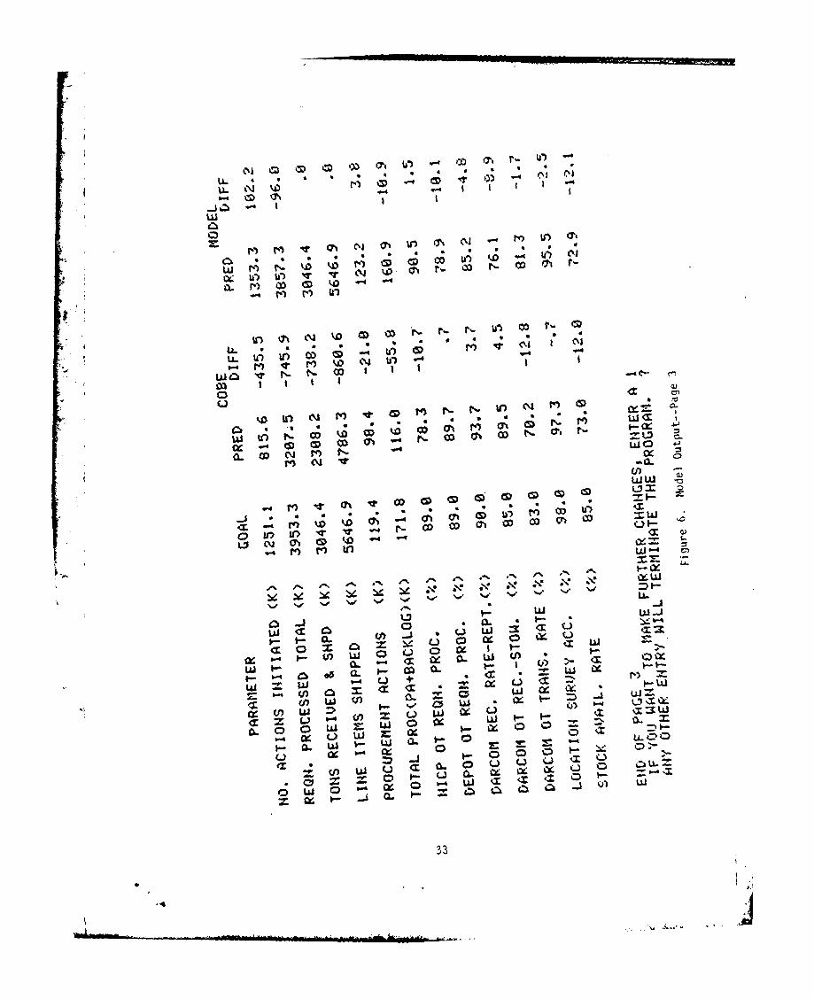
The third page of the output contains the impact of the COBE and
model allocations on the workload and perfcrmance variables. This is
displayed in Figure 6. The GOAL column contains the goals for the various
equations in the goal program. The goals for the workload equation came
from the COBE, and the goals for the performance equations came from the
DARCOM numerical goals for performance indicators. The "PRED" column is
the result of taking the dollar amounts from the various PEs and plugging
into the workload and performance equations previously discussed. The
"DIFF" column is the result of subtracting the goal from the predicted
value. A negative difference indicates an underachievement, and a positive
difference indicates an overachievement. Note in Figure 6 that the model
differences are in general better than the COBE differences. This is
because the model allocates more funds to PE 721111, PE 721112, and PE
-' 721113, than does the PBG. These PEs were used as the independent variables
in most of the equations. Not all negative workload differences are bad,
however. Some of the workload goals represent the enhanced level as
opposed to the basic (funded) level. All of the predicted workload and
performance variables are actually expected values since they are the
results of a regression equation. The actual, observed values in FY 79
32
..............................................................
IMV~ U') -*
LU*
w r~N
' ~o~- U
U. 00 coU'
N N 1I
C-)pw V- N co
C4X 44 CD c C
0 C M 0M ' ~
re M N Z :4
Ui <c
CL LyL3 a 0' ) '0 A. 1
I .4 F' ) C"W- + M
CaJ .J I- W
(n w o-n %X. * - *
I- fr- a ) ..J *r U Z Iw
UJ ~ ~ L w-0.C . L A
o w u a L ,;-k w
W. -S o.L
0. 0 0 LU~ ~0 ~ U 1-I33
will probably be different even though some of the funds may be the same
as programmed. Thus, it is dangerous to draw conclusions based on the
absolute differences between numbers. It is valid only to look at the
relative magnitude of differences.
The general priority structure that resulted in this allocation in
shown in Table 6. A more detailed discussion of the priority structure is
contained in Annex C. As the priority structures change, so do the model
results. In general, the major conflicts are between the 1-0 balance
equations and the workload/performance equations for reasons discussed
previously. Historical DARCOM allocations appear to resemble the alloca-
tions based on the balance equations rather than the workload/performance
equations. In fact, the model allocation is almost identical to the PBG
when only the balance equations are included. For these reasons, the
balance equations are placed at a higher priority than the workload/
performance equations in most priority structures.
PRIORITY GOAL
I Totally allocate the P7 Budget
2 Fencing
3 Balance
4 Balance
5 Workload/Performance
Table 6. General Priority Structure
8. Conclusions and Recommendations
The model has several limitations. First, the supply system is
treated as a "closed" economy, with the output of the economy being
34
materiel that is shipped to some user. The relationship between P7S and
P7M is treated explicitly by considering P7M as another "user" of items.
Some people feel that P7S cannot be separated from P7M. Second, the work-
load and performance equations are based on historical data (FY 74 to FY 78),
and assume that these relationships are valid for succeeding fiscal years.
- In other words, the model assumes that DARCOM will not make drastic changes
in its management philosophy for the wholesale supply system. Another
model limitation is the sensitivity of the model allocations to the
priority structure. This sensitivity is not bad, per se, given the user
is familiar enough with the model operation, to understand the effects of
changing the priority structure. In practice, this should not be a limi-
tation because the user should be very familiar with the model.
The model also has several advantages. First, it seeks to make an
optimal allocation of the budget for a given priority structure. In
essence, it allocates the funds to achieve as many priority goals as
possible. Second, the technique used to allocate the funds (goal program-
ming) is defensible as an accepted methodology. Third, the model is
interactive and operates in real time. Finally, the model gives the impact.
of the budget allocations on various workload and performance parameters.
In summary, the model not only satisfies the study requirements, but
also does it on an interactive terminal display. It not only provides the
impact of DA funding guidance on supply and performance, but also provides
an alternate or strawman allocation to improve workload and performance.
This strawman considers the proper balance between PEs within P7S. The
model also has the ability to fence selected PEs; i.e., to insure that the
35
model allocates a predetermined dollar amount to those fenced PEs. The
model has been transferred to the Supply Section of the Budget Operations
Branch in the Comptroller Directorate, HQ DARCOM. The program is opera-
tional, and is accessed via remote terminals.
The DELTA 7S model can be a very useful tool for assisting manage-
ment in analyzing budget alternatives. In fact, the model should be used
to analyze several different funding alternatives so that management has
several options from which to choose. The study team recommends that the
Budget Operations Branch in the Comptroller Directorate use the DELTA 7S
model to analyze funding alternatives for FY 80 and 81. Further, someone
at HQ DARCOM should be designated as a Point-of-Contact for the model.
This person would be responsible for handling all questions on the operation
and maintenance of the model.
-6
36
ANNEX A
ADMINISTRATIVE DOCUMENTS
A-i
ANNEX A
ADMINISTRATIVE DOCUMENTS
This annex contains the major documents that describe the adminis-
trative conduct of the study. A Study Directive was never prepared for this
study. Rather, the Proposed Study Concept on page A-3 was the response to
a verbal tasking by HQ DARCOM. This proposed study concept was briefed to
the Deputy Commanding General for Resource Management on 20 April 1979.
The result of this briefing was a decision to proceed with the study as
* outlined. Although the Proposed Study Concept was never formalized, it
nonetheless served as the Study Plan.
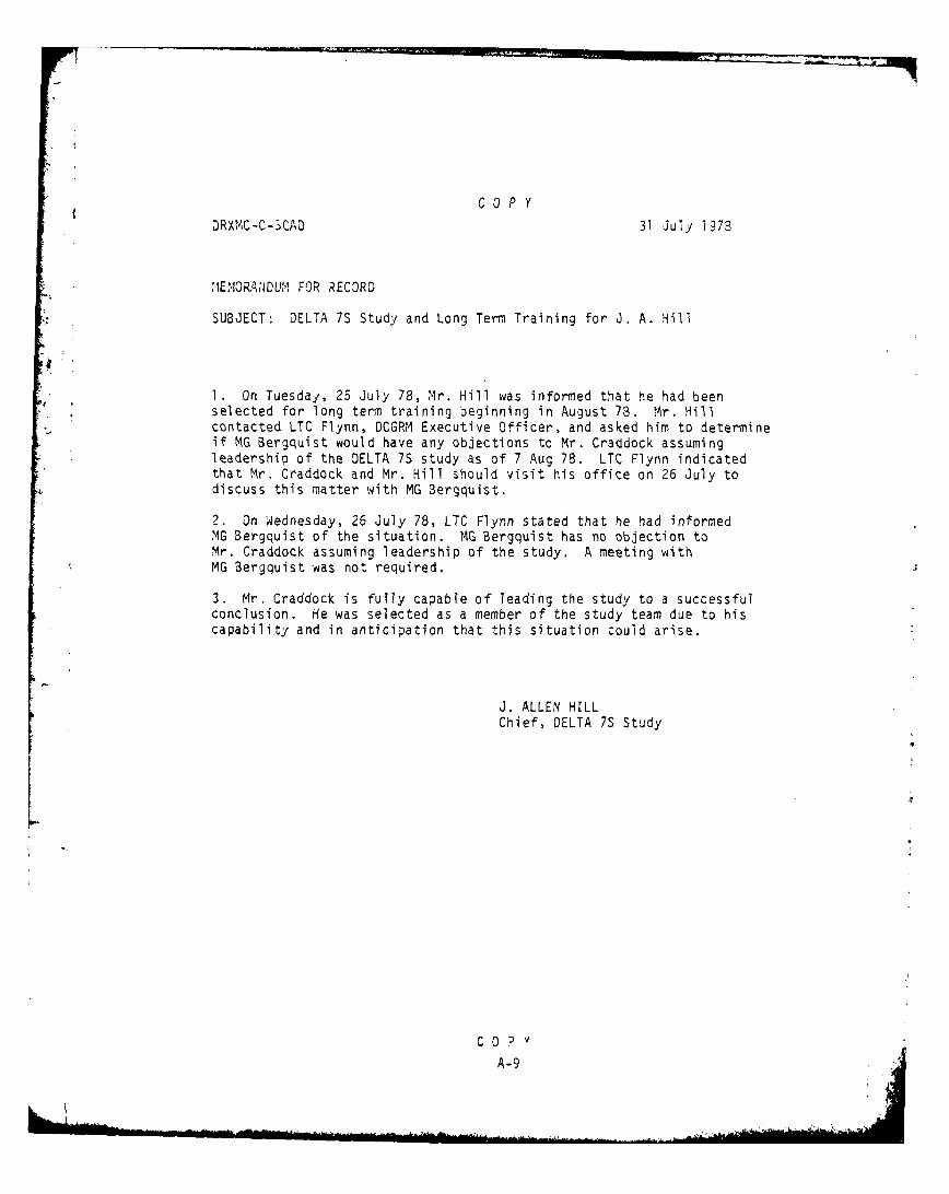
Mr. J. Allen Hill was the initial study team leader. However, he
was selected for Long Term Training early in the conduct of the study and
Mr. William T. Craddock was designated as the study team leader. A
Memorandum for Record describing this is on page A-9. Finally, a brief
chronology of the study conduct is on page A-l0.
A-2

PROPOSED STUDY CONCEPT
Title: Impact of Incremental Changes in 7S Funding on Suppily Performance(Delta 7S Impact: DELTA 7S)
Memorandum For: Deputy Commanding General for Resource Management, HQ DARCOM
1. References:
a. 7 Apr 78, DCGRM, MG Bergquist, discussed need and limits of thisstudy effort with US Army Logistics Management Center representatives.
b. 7 Apr 78, Director, PTFD, BG Forney, verbally tasked ALMC toinitiate this study effort.
c. Administrative and Procedural References:
(1) AR 5-5, The Army Study System
(2) DARCOMR il-i, Systems Analysis
d. AR 37-100-78, The Army Management Structure
e. AR 37-59 (Rescinded Dec 77), Command Analysis Of Operations andMaintenance, Army, Funding
f. AR 700-126, Logistics: Basic Functional Structure
g. Reports (See Annex A)
2. Purpose: There is a need to relate the many, diverse OMA funded functionsto performance indicators. The proposed study will relate the effects ofincremental changes in funding for supply functions to supply performance inorder to improve the capability to articulate requirements for resources.
3. Study Sponsor: Deputy Commanding General for Resource Management,HQ DARCOM
Points of Contact: Mr. Don Camp, DCGRMATTN: DRCDRM-TGAUTOVON: 284-9343/9388
Mr. Tony Haver, ANADATTN: SDSAN-PPAAUTOVON: 694-7575
4. Study Agency: US Army Logistics Management CenterSchool of Management ScienceSystems and Cost Analysis Department
A-3
a:
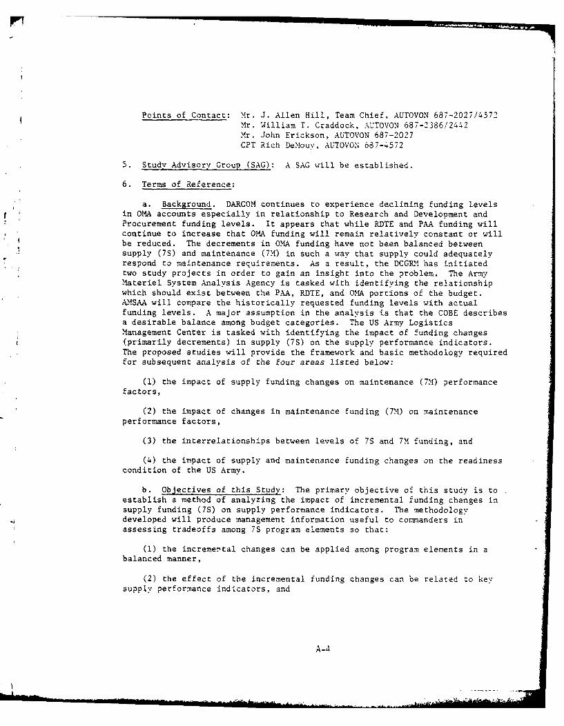
Points of Contact: Mr. J. Allen Hill, Team Chief, AUTOVON 687-2027/4572Mr. William T. Craddock, AUTOVON 687-2386/2442Mr. John Erickson, AUTOVON 687-2027CPT Rich DeMouv, AUTOVON 687-4572
5. Study Advisory Group (SAG): A SAG will be established.
6. Terms of Reference:
a. Background. DARCOM continues to experience declining funding levelsin OMA accounts especially in relationship to Research and Development andProcurement funding levels. It appears that while RDTE and PAA funding willcontinue to increase that OMA funding will remain relatively constant or willbe reduced. The decrements in OMA funding have not been balanced betweensupply (7S) and maintenance (7M) in such a way that supply could adequatelyrespond to maintenance requirements. As a result, the DCGPM has initiatedtwo study projects in order to gain an insight into the problem. The ArmyMateriel System Analysis Agency is tasked with identifying the relationshipwhich should exist between the PAA, RDTE, and OMA portions of the budget.AMSAA will compare the historically requested funding levels with actualfunding levels. A major assumption in the analysis is that the COBE describesa desirable balance among budget categories. The US Army LogisticsManagement Center is tasked with identifying the impact of funding changes(primarily decrements) in supply (7S) on the supply performance indicators.The proposed studies will provide the framework and basic methodology requiredfor subsequent analysis of the four areas listed below:
(1) the impact of supply funding changes on maintenance (7M) performancefactors,
(2) the impact of changes in maintenance funding (7M) on maintenanceperformance factors,
(3) the interrelationships between levels of 7S and 7M funding, and
(4) the impact of supply and maintenance funding changes on the readinesscondition of the US Army.
b. Objectives of this Study: The primary objective of this study is toestablish a method of analyzing the impact of incremental funding changes insupply funding (7S) on supply performance indicators. The methodologydeveloped will produce management information useful to commanders inassessing tradeoffs among 7S program elements so that:
(1) the incremental changes can be applied among program elements in abalanced manner,
(2) the effect of the incremental funding changes can be related to keysupply performance indicators, and
A-a~

(3) the above analyses can be performed when some program elements are"fenced" at a given level.
c. Scope. The study will address a one year funding horizon ratherthan a FYDP for DARCOM supply (7S) funding. The nethodology ill be yearindependent (however, the parameters in the model may be year dependent).
d. Limits. The study will be limited to changes in the level offunding for DARCOM supply functions.
e., Time Frame. The study will use the FY 77 or FY 78 time frame(dependent on data availability) for development of the methodology. Uponvalidation, the methodology will be used to address FY 80 funding levels.
f. Assumptions:
(i) The DARCOM FY 78 COBE describes a desirable balance among budgetcategories and within the program elements of supply (7S) funding.
(2) Computer programming and computer time required for data extraction,data analysis, and validation of the methodology will be made available byHQ DARCOM.
g. Essential Elements of Analysis.
(1) What relationships exist between program elements in 7S
(2) How do funding changes affect the output of various program elementsin 7S
(3) How should a change in the 7S budget be allocated in a balancedmanner among the program elements
h. Steps in the Analysis:
(1) A literature survey supplemented by visits to other analytical agencieswill be performed to determine the approaches and results of prior and ongoingstudies in related areas.
(2) Methodologies will be developed to:
(a) allocate funding changes among 7S program elements in a balancedmanner
(b) relate funding changes to changes in supply performance indicators, and
(c) to perform the above analysis when some program elements are fixed ata given level.
(3) Data suitable for exercise and validation of the methodology will becollected by FY 77 and FY 73 as appropriate.
A-5
(4) The methodology will be validated.
(5) Data for FY 80 will be collected and used to exercise the methodologyto provide command information for action.
i. Models/Techniques. Several types of analytical techniques will beevaluated for possible use in analyzing this problem. Anticipated usefulmethodologies are:
(1) Regression/correlation analysis to determine the empirical relation-ships between funding levels and performance indicators.
(2) Descriptive and/or inferential statistical models will be used to
determine sensitivity of data.
(3) Leontief's Input/Output Analysis model may be used to determinefirst and higher order relationships among funding levels within the supplybudget.
(4) Goal Programming may be used to determine optimal relationshipsamong funding levels for 7S program elements.
The above listed models/techniques represent the present assessment ofthose which hold promise for the solution of the problem; however, othermodels/techniques will be used if found to be efficacious.
7. Support and Resource Requirements:
a. Travel and per diem funds in the amount of $8,000 are required foraccomplishment of this study and will be obtained through normal budget
channels.
b. Representatives from the following organizations may be requiredto participate in the study on an ad hoc basis.
(1) Comptroller, HQ DARCOM
(2) Materiel Management, HQ DARCOM
(3) Procurement and Production, HQ DARCOM
(4) Development and Engineering, HQ DARCOM
(5) HQ DESCOM
c. Computer programming and computer time for data extraction andprocessing will be required. ALMC computer resources will be used to themaximum extent possible; however, some data extraction and attendantprogramming may be required of DARCOM agencies.
8. Administration:
a. Study Title. Impact of Incremental Changes in 7S Funding on SupplyPerformance.
Short Title. Delta 7S Funding
Acronym. DELTA7S
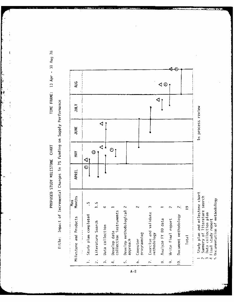
b. Study Schedule. The proposed study schedule and milestone chart areattached as Inclosure 1.
c. Control Procedures. A Study Advisory Group (SAG) should be establishedto monitor the study approach and emerging results. It is recommended thatjembers of the SAG also monitor the A.1SAA study for possible coordination ofideas and results.
d. Action Documents. The study will provide the following products:
(1) A final study report, and
(2) Documentation of recommended methodologies.
A-7
00
5 L
cncU
C
4-
C-I I C
O - M:
o e
I--
4- 43 'I C) a- Cd,& -)0 >
ra ad= = - r
fa LLJI~z: I r~LU .C - dC0A-8
COPY
DRXIC-C-3CAD 31 July 1973
1EMORANJDUM1 FOR RECORD
SUBJECT: DELTA 7S Study and Long Term Training for J. A. '-ill
1 . On Tuesday, 25 July 78, Mr. Hill was informed that he had beenselected for long term training beginning in August 73. Mr. Hillcontacted LTC Flynn, DCGRM Executive Officer, and asked him to determineif MG Bergquist would have any objections to Mr. Craddock assumingleadership of the DELTA 7S study as of 7 Aug 78. LTC Flynn indicatedthat Mr. Craddock and Mr. Hill should visit his office on 26 July todiscuss this matter with MG 3ergquist.
2. On Wednesday, 26 July 78, LTC Flynn stated that he had informedMG Bergquist of the situation. MG Bergquist has no objection toMr. Craddock assuming leadership of the study. A meeting withMG Bergquist was not required.
3. Mr. Craddock is fulTy capable of leading the study to a successfulconclusion. He was selected as a member of the study team due to hiscapability and in anticipation that this situation could arise.
J. ALLEN HILLChief, DELTA 7S Study
COPY
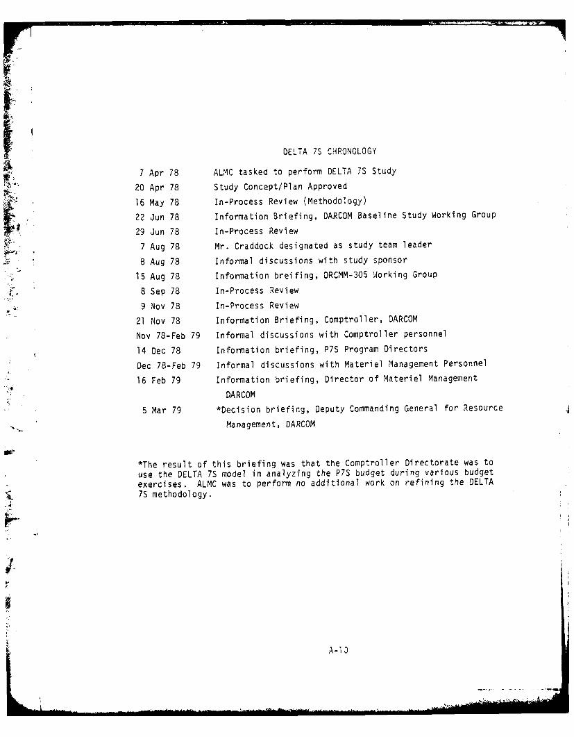
I' DELTA 7S CHRONOLOGY
7 Apr 78 AU4C tasked to perform DELTA 7S Study
20 Apr 78 Study Concept/Plan Approved
16 May 78 In-Process Review (Methodology)
22 Jun 78 Information Briefing, DARCOM Baseline Study Working Group
29 Jun 78 In-Process Review
7 Aug 78 Mr. Craddock designated as study team leader
8 Aug 78 Informal discussions with study sponsor
15 Aug 78 Information breifing, DRCMM-305 Working Group
8 Sep 78 In-Process Review
9 Nov 78 In-Process Review
21 Nov 78 Information Briefing, Comptroller, DARCOM
Nov 78-Feb 79 Informal discussions with Comptroller personnel
14 Dec 78 Information briefing, P7S Program Directors
Dec 78-Feb 79 Informal discussions with Materiel Management Personnel
16 Feb 79 Information briefing, Director of Materiel Management
DARCOM
5 Mar 79 *Decision briefing, Deputy Commanding General for Resource
Management, DARCOM
*The result of this briefing was that the Comptroller Directorate was to
use the DELTA 7S model in analyzing the P7S budget during various budgetexercises. ALMC was to perform no additional work on refining the DELTA7S methodology.
A-l 0

ANNEX B
LITERATURE SURVEY
B-i
1.
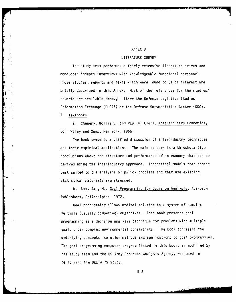
ANNEX B
LITERATURE SURVEY
The study team performed a fairly extensive literature search and
conducted indepth interviews with knowledgeable functional personnel.
Those studies, reports and texts which were found to be of interest are
briefly described in this Annex. Most of the references for the studies/
reports are available through either the Defense Logistics Studies
Information Exchange (DLSIE) or the Defense Documentation Center (DDC).
1. Textbooks.
a. Chenery, Hollis B. and Paul G. Clark, Interindustry Economics,
John Wiley and Sons, New York, 1966.
The book presents a unified discussion of interindustry techniques
and their empirical applications. The main concern is with substantive
conclusions about the structure and performance of an economy that can be
derived using the interindustry approach. Theoretical models that appear
best suited to the analysis of policy problems and that use existing
statistical materials are stressed.
b. Lee, Sang M., Goal Programming for Decision Analysis, Auerbach
Publishers, Philadelphia, 1972.
Goal programming allows ordinal solution to a system of complex
multiple (usually competing) objectives. This book presents goal
programming as a decision analysis technique for problems with multiple
goals under complex environmental constraints. The book addresses the
underlying concepts, solution methods and applications to goal programming.
The goal programming computer program listed in this book, as modified by
the study team and the US Army Concepts Analysis Agency, was used in
performing the DELTA 7S Study.
B-2
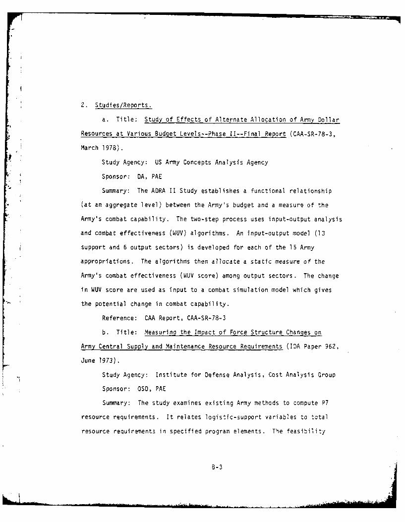
2. Studies/Reports.
a. Title: Study of Effects of Alternate Allocation of Army Dollar
Resources at Various Budget Levels--Phase Il--Final Report (CAA-SR-78-3,
March 1978).
Study Agency: US Army Concepts Analysis Agency
Sponsor: DA, PAE
Summary: The ADRA II Study establishes a functional relationship
(at an aggregate level) between the Army's budget and a measure of the
Army's combat capability. The two-step process uses input-output analysis
and combat effectiveness (WUV) algorithms. An input-output model (13
support and 6 output sectors) is developed for each of the 15 Army
appropriations. The algorithms then allocate a static measure of the
Army's combat effectiveness (WUV score) among output sectors. The change
in WUV score are used as input to a combat simulation model which gives
the potential change in combat capability.
Reference: CAA Report, CAA-SR-78-3
b. Title: Measuring the Impact of Force Structure Changes on
Army Central Supply and Maintenance Resource Requirements (IDA Paper 962,
June 1973).
Study Agency: Institute for Defense Analysis, Cost Analysis Group
Sponsor: OSO, PAE
Summary: The study examines existing Army methods to compute P7
resource requirements. It relates logistic-support variables to total
resource requirements in specified program elements. The feasibility
B-3
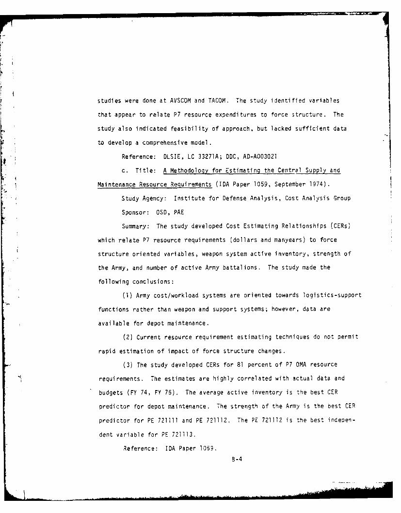
studies were done at AVSCOM and TACOM. The study identified variables
that appear to relate P7 resource expenditures to force structure. The
study also indicated feasibility of approach, but lacked sufficient data
to develop a comprehensive model.
Reference: DLSIE, LC 33271A; DDC, AD-AO03021
c. Title: A Methodology for Estimating the Central Supply and
Maintenance Resource Requirements (IDA Paper 1059, September 1974).
Study Agency: Institute for Defense Analysis, Cost Analysis Group
Sponsor: OSD, PAE
Summary: The study developed Cost Estimating Relationships (CERs)
which relate P7 resource requirements (dollars and manyears) to force
structure oriented variables, weapon system active inventory, strength of
the Army, and number of active Army battalions. The study made the
following conclusions:
(1) Army cost/workload systems are oriented towards logistics-support
functions rather than weapon and support systems; however, data are
available for depot maintenance.
(2) Current resource requirement estimating techniques do not permit
rapid estimation of impact of force structure changes.
(3) The study developed CERs for 81 percent of P7 0MA resource
requirements. The estimates are highly correlated with actual data and
budgets (FY 74, FY 75). The average active inventory is the best CER
predictor for depot maintenance. The strength of the Army is the best CER
predictor for PE 721111 and PE 721112. The PE 721112 is the best indepen-
dent variable for PE 721113.
Reference: IDA Paper 1059.
B-4
d. Title: An Army Logistics Support Information System (2A Paper
1110, March 1975).
Study Agency: Institute for Defense Analysis, Cost Analysis Group
Sponsor: OASD, PAE
Summary: The study provides an information system to be used by
*OASD/PAE in obtaining data on a regular basis from Army logistics cost
and reporting systems. These data will permit OASD/PAE to maintain
current the IDA developed methodology for estimating Army central supply
and maintenance resource requirements. The methodology was designed to
be used in studies of defense resource allocations related to proposed
alternative Army force structures. The information system must provide
forecasts of the appropriate resource sensitive force-structure-oriented
variables, as well as pertinent historical data. The identification of
organizations as sources for elements of data is based on the IDA
experience in developing the initial data base used to construct the P7
cost estimating methodology in IDA Paper 1059, "A Methodology for
Estimating Army Central Supply and Maintenance Requirements."
Reference: DLSIE, LD 35036A; DDC, AD-016272.
e. Title: Logistics Resources Data Base Structure (January 1977)
Study Agency: General Research Corp., McLean, VA
Sponsor: PA&E Directorate, Office of the Chief of Staff, US Army
Summary: The study was initiated to develop an improved Army
logistics data base structure for determining and displaying logistics
resources allocated to, consumed by, and projected for units, weapons
systems and logistics functions. The study made the following conclusions:
3-5

(1) Neither the FYDP program elements nor the AMS codes orovide a
meaningful or useful identification of logistics resources, otner than in
Program 7.
(2) The logistics resources structure is relatable to the FYOP
and the logistics output requirements.
(3) Automated data base gaps may necessitate additional reporting
requirements or other data acquisition techniques.
(4) An automated system is the most effective approach to the
establishment of the required data base.
Reference: OLSIE, LD 38524A
f. Title: An Initial Feasibility Demonstration of the Army's
Logistic Resource Annex (LRA) to the Five Year Defense Program (FYDP),
GRC Report CR-205, January 1978.
Study Agency: General Research Corporation, McLean, VA
Sponsor: Program Analysis and Evaluation Directorate, Office of
the Chief of Staff, US Army.
Summary: The Five Year Defense Program is not configured to
display the logistics resources in many of its program elements. For
example, in many cases, a single logistics function consists of resources
from several program elements, or conversely, the resources in one PE
can be applied to several logistics functions. The objective of the study
was to accomplish three major tasks: (1) design a Logistics Resource
Annex (LRA) to the FYDP, (2) develop the structure and methodology to
construct an LRA, and (3) demonstrate the feasibility of the LRA conceot.
3-6

The general methdology employed was to develop a two-dimensional matrix
with logistic related resources allocated to force units as the rows, and
specific combat battalion types as the columns. The method of filling
the matrix "cells" consisted of: (1) extraction of logistic function
totals from the FYDP using various factoring methods, (2) separation of
Force and Non-Force related resources, and (3) attribution of logistic
functional resources to force units or non-force units via appropriate
attribution factors. The development of the various factors employed in
steps (1) and (3) is contained in the body of the report. In many cases
it is simply the ratio of the size (or amount) of a particular force (or
program element dollar amount) to the total. In other cases, more complex
factoring techniques are used. The report concluded that:
(1) It is possible to prepare an LRA, either manually (6 to 8 weeks
of effort) or by automated mians provided that there exists simultaneous
availability of the FYDP and related documents.
(2) The factors for Supply Support, Maintenance, and Transportation
do not change. That is, no significant changes in division size units
occur in the force structure.
(3) The factors used can be validated using future FYDP data.
(4) Automation of the system is highly desirable.
Reference: DLSIE, LD 41188A.
g. Title: An Exploratory Input-Output Model for Support Cost
Estimates (September 1976)
Study Agency: None. Thesis by Clemente Pionilla Mariano
Sponsor: Naval Postgraduate School, Monterey, California
B-7
Summary: This thesis develops a cost model to estimate support
costs in the Phillipine Army. Leontief's input-output technique is
appraised for applicability and is related to cost analysis techniques.
The use and validation of proxy variables is presented. Correlation
analysis is discussed as a tool for choosing a valid proxy variable. The
matter of fixed costs and treatment in the cost model is addressed.
Using hypothetical data, an example of the use of the model in the
Phillipine Army setting is presented. Support units, tactical forces,
and budgetary programs comprise the major elements of the system in the
cost model.
Reference: DLSIE, LD 38136A; DDC, AD-A032254
h. Title: An Input-Output Analysis of the US Navy (May 1971)
Study Agency: US Naval Academy - Trident Scholar Project Report
Forrester William Isen.
Summary: This report sets forth the basic aspects of input-output
analysis and explores the problems involved in implementing input-output
analysis of the US Navy. The original work was done to formulate a method
for locating hotspots or bottlenecks in an economy using the basic input-
output matrices. Special emphasis was given to non-price oriented
economics, of which the military services are prime examples.
Reference: DLSIE, LD 27065
i. Title: Budget Justification Model (11 November 1975). "Response
Time Technical Memorandum 440."
Study Agency: US Naval Fleet Material Support )ffice, Supply System
Derformance Evaluation Office
B-S
.............................................. .. ........ "
Sponsor: Naval Supply Systems Command
Summary: The cost-benefit model documented in this technical
memurandum suggests an approach to related resources allocated to the
logistics system to combat readiness. The model presented related
operational availability and combat readiness to material and personnel
resources available to the supply system. Reliability, availability,
maintainability, and system response time and resource levels are the
primary inputs to the model. The model is conceptually valid; however,
attempts to derive data to support the model were unsuccessful.
Reference: DLSIE, LD 33353MA
B-9 i
ANNEX C
MODEL DESCRIPTION
c-1
ANNEX C
MODEL DESCRIPTION
The major analytical techniques used in the DELTA 7S Model are
regression analysis, input-output (I-0) analysis, and goal programming. As
discussed in the main report, the overall model structure is a goal program,
with most of the equations obtained from regression or 1-0 analysis. Each
of these three major analytical techniques are discussed in more detail
in the remainder of this annex.
Regression Analysis. Regression analysis is a technique which
allows one to develop the mathematical equation that best describes a
given set of data. This equation can then be used to make statements about
future observations of data. Since the equations developed for the DELTA
7S model were to be used in a linear goal program, the study team used
only linear regression analysis. As discussed in the main report, the
study team developed equations based on annual data from FY 74 to FY 78.
These workload and performance equations were initially developed based
on four annual data points (FY 74 to FY 77), validated based on a fifth
annua' data point (FY 78), and then revised to include all five data points.
The validation procedure is described in more detail in Annex G. The
final equations are shown in Table C-1.
The dependent variable in Table C-1 is identified by both a variable
number and name. The variable number is the number by which that variable
is identified in the master data file. Those variable numbers which begin
with a "5" are resource variables. The workload variables begin with a
"6", and the performance variables begin with a "7". The five annual points
(FY 74 to FY 78) for each of these variables are contained in Annex E.
C-2
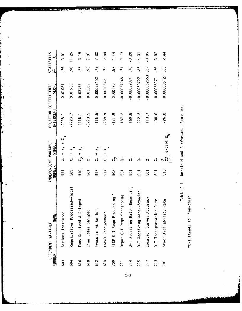
-Z2 cn a-o -O r. :r - m- ~ f -. a
cr C\J -0 r, LO r- C\0 kc-- l I- ON 1, I - rI c c o r
I L
LIn
r -rC'.j C Ir C\j C'J
LLJ -3 -' C'J aI w In C) t. M- C) k 00 0a- Cl) LO 0o r C) C\ In 0 U- 00 C
u0 0 1 C1 C0 CD- C : 0D 0) 0=-V) ,D CD 0D CD 0D 0D C0 0D C0 0) C
C) 0 ) C0 0 0 0 0) CD c0 0 0 c0 0 0LL.
LUJ
0
COLLJ -O LO M In In 0, C~j fnI~ r,- C) CD4
I1 In 14 ll 4m* _- r- 04, C\i M') C 10cL m C\a -z r- C"J M r. M k- I') C\J C7
rI - - Q. '- - ~ - - - -\ IL0 z - . 10 c'n I I I
LO E-S-.
LU 4- 4-.. J..J + . L-
cm C\D C" ')C)- < cc >iC~ n en mu 0
L/5 +I + + + +C
LU 0
Luj IO LO Lo In n Lo Ln IO U') LO LO U-) In
0- S- 2 =,0-' a 0 2: > to a)
I - 0 u C) cu I-a~ ) *- (A C) 4-' ea 4-' 4-)
(A 0. (AI C) m(A( ) UL = I =
-0 U LI C) 0 4-' 0 S- 4-1 I- 0 1-LU o) 0 Z C- S.. a. 10 '0
*- C 0C 0- U~ EAC U ~ > >L ~*
< C) a C) 0m 9- (A .0
C (A1 (3 -) c-. w S.. C)(
ci (A 0) U ' U . 0I 'V9-~~~~~~~3 0- -C C 04'5)0 -9 -09
U C) 0 *,- 06 0- -) C)I I) -LU 0 (u 1. -I 0- 9-800 C J
LUi
LU w
C-3
The independent variable in Table C-I is identified by a variable
number and a symbol. The variable number was discussed in the previousparagraph. The symbol X. represents the funds expended in a particular
1
Program Element. These symbols are explained in Table C-2. For some
equations the independent variable is shown as the sum of several different
resource variables. For example, the independent variable of the "Actions
Initiated" equation is X + X + X3. This is still a simple linear
regression equation in which a new variable is created by physically
summing the dollars expended in the PEs represented by X1 2 X2, and X3.
Although the independent variable number for this equation is 511 (which
Annex D shows is the sum of PEs 721111, 721112, and 721113), the actual
equation represents these as X1, X2, and X3. That is, the equation for
Actions Initiated (Y) is
Y = -4938.1 + O.01081(X 1 + X2 + X3 )
or Y = -4938.1 + O.01081X 1 + 0.01081X + 0.01081X 3These equations also assume the Xi are in the FY 78 dollars, since the data
used to develop equations were in constant FY 78 dollars. The computer
program automatically converts the Program Budget Guidance (which is now
in FY 79 dollars) to FY 78 dollars.
The intercept and slope coefficients are shown for each equation
in Table C-1. Also shown are the r2 and t statistics. The coefficient of
determination, r2 , is a measure of how good the equation fits the observed
data. A value of r2 = 1 would imply that all of the observed data lie on
the line described by the equation. The coefficient of correlation, r,
is the square root of r2 . The sign of r is the same as the t value, and
C-4
a negative r implies that the variables are inversely proportional. That
is, if X and Y have a negative r value, X increases as Y decreases, and
vice versa. Note that four of the performance equations (dependent
variable numbers 711, 714, 715, and 717) have negative correlation coeffi-
cients. This seems to imply, on the surface, that performance decreases
as resources increase. However, this phenomenon can be explained.
SYMBOL PROGRAM ELEMENT FUNCTION
X1 721111 Supply Depot Operations
X2 721112 Supply Management
X3 721113 Procurement
X4 722829/722898 Command
X5 722896.Z Base Operations
X6 728009 Transportation (First Destination)
X7 728010/728013 Transportation (Second Destination)
X 728011 Industrial Preparedness
X9 728012 Logistics Support
Table C-2. Independent Variables for Regression Equations
Suppose, as a means of explanation, that a depot's manpower standard
is 500 "filled orders" per worker per year, and that the depot has 10
workers. Thus, the depot is expected to produce 5,000 "filled orders"
annually. The fallacy here is that manpower standards are based solely on
workload, and do not consider performance. Suppose that this hypothetical
depot does produce the 5,000 "filled orders," but that the on-timeprocessing rate for these orders is 80,, whereas the management goal is
C-5
90% on-time processing. Further, suppose that this depot is authorized two
additional workers. If this depot is now expected to produce 5,D0O "filled
orders," the on-time processing rate will probably not improve, and may even
degrade a little. If the depot is expected to produce 6,500 or more
"filled orders" with only the two additional workers, its on-time processing
rate will probably decrease.
Although this hypothetical example is oversimplified, a similar
situation may have existed in DARCOM in the past few years. An investiga-
tion of the data in Annex E shows that both resources and workload, in
general, have increased in the past five years. However, workload may have
increased more than resources so that overall performance is declining. The
equations cannot capture this phenomenon mathematically because of the
small number of data points.
The t values in Table C-l are experimental statistics used to test
the hypothesis that the theoretical slope is equal to zero. There are
three degrees of freedom associated with these data, and at the 0.10 level
of significance, the critical value of t is 2.353. Another test of
hypothesis that can be performed is that the theoretical coefficient of
determination is equal to zero. The F statistic is used to test this
hypothesis, where F is approximately the square of the experimental t value.
As was discussed in the main report, an attempt was made to increase
the number of data points by using quarterly data from 1 Qtr FY 76 to
2 Qtr FY 78. Although this produced eleven data points (including FY 7T),
the study team could not duplicate many of the equations originally develooed
using annual data. Issiming that this was due to noise in the quarterly
C-6
data, the study team attempted to smooth the data using several methods.
These attempts included using a three-quarter moving average, shifting the
workload and performance data one or more quarters following the resource
data, and a combination of shifting the three-quarter moving averages. By
this time the data were extremely disguised, and the decision was made to
use only the annual data.
* The original premise of the study team is that performance is
logically a function of both workload and resources. Although these were
initially only four data points, the study team developed several performance
equations from multiple linear regression using workload and resources as
the independent variable. Although these equations had only one degree of
freedom, the experimental F values were extremely high. These equations
were discarded because of the high correlation between workload and
resources. In fact, the numerical value for the workload independent
variable would itself come from a simple linear regression equation with
resources as the independent variable. A decision was made to use only
resources or combination of resources, as the independent variable. The
resulting equations, shown in Table C-l, represent the best compromise
between mathematical fit and functional logic (based on discussions with
HQ DARCOM personnel).
Input-Output Analysis. Leontief's input-output analysis is a
classical technique used by economists to determine the interrelationships
between various "sectors" of an economy and the "final users." In
economic applications, the sectors might typically be various industries such
as agriculture, steel, and mining. The model assumes tnat tHe Droduc, o"
C-7
each sector is partially consumed by itself and the other sectors. The
remaining product is distributed to the final users. Examples of final
users are domestic consumption and export. The model information is
displayed by means of a matrix or tableau.
To use the 1-0 model, one first determines the "gross transactions"
between the various sectors and the final users. That is, the total output
from each sector is allocated to itself, the other sectors, and the final
users. When these data are displayed in a matrix, it is called the gross
transactions matrix. The model then "normalizes" this gross transactions
matrix by dividing each value in a particular column by the corresponding
row sum. The row sum is the result of adding the gross transaction in a
particular row, say the agriculture sector. Then each gross transactions
value in the agriculture column is divided by the agriculture row sum.
This procedure is repeated for all of the sectors.
The result of this normalizing effort is the "A" matrix. This A
matrix considers only the "first order" effects, and ignores any indirect
demand made on one sector by its consumption of the output of another
sector. These higher order effects are accounted for mathematically by
computing the (I - A)"1 matrix. This matrix accounts for the ripple effects
in an economy.
In order to apply input-output analysis to the Army's Wholesale
Supply System, the study team had to describe the supply system as an
economy. The product of this economy was assumed to be materiel shipped
to some user. All activities which relate to the issue and shipping
functions were considered as the final users of the economy. The program
C-3
element structure of the Army Management Structure provides a logical,
functional description of the sectors of this supply econorKy. The PEs
generally fund activities which are related. A more detailed description
of these PEs is contained in Annex D. The PEs that were chosen to represent
the sectors of the supply economy are listed in Table 4 of the main report.
Note that this list combines some PEs and completely omits others.
Specifically, PE 722829 (Logistics Administrative Support) and PE 722898
(Management HQ Logistics) were combined since they were only recently
split apart, and the historical data (FY 74 to FY 78) shows these PEs as
one account. Also, the DARCOM portions of PE 728010 (Second Destination
Transportation) and PE 728013 (Overseas Port Units--Non-IF) were only
recently split apart. In this case, PE 728013 funds a small group of
personnel at Tobyhanna Army Depot who monitor the world-wide movement of
containers. The PEs in P7S which are not shown in Table 4 were eliminated
from the model because they were either not applicable to DARCOM or
contain only small funds as compared to the other PEs. An example of a PE
not applicable to DARCOM is PE 728018 (Real Estate and Construction
Administration). The basis for this statement is the absence of this PE
from the DARCOM COBE. An example of a PE which contains only a small
amount of funds is PE 729998, Reimbursable Small Business Administration
(SBA) Development costs.
In order to determine the sector relationships, the study first
made several assumptions about the functional relationship between the
activities funded by a particular PE and the various sectors of the supoly
economy. For example, a supply depot (PE 72111V, performs several major
|_
functions, including the receipt, storage, and shipment of materiel. Since
the final product of this supply economy was assumed to be materiel shipped
to some user, the issue and shipping functions are activities that the
depot performs in support of the final user. The corollary to this is
that the receipt and storage functions are activities that a depot performs
* in order to posture itself to ship materiel , and would therefore be
functions that a supply depot performs in support of itself.
The study team then went through AR-37-100-78 in detail to determine
L" what similar relationships would hold for other PEs. Each PE was evaluated
based upon the smallest accounting subdivision of the PE. The study team
made assumptions about what each of the Program Element Activity Accounts
(PEAA) would support. The result was Figure 2 in the main report. The
dots in this matrix represent those sector combinations where a functional
relationship was found. The composition of each of these dots is explained
in Table C-3, which shows which sectors each PEAA supports. The data in
this table have been aggregated where possible. For example, the PEAA
721111.11 (Receipts) is not further subdivided in Table C-2, although the
accounting structure provides for further subdivisions. The 'x' for each
PEAA indicates its functional relationship. Occasionally, a particular
PEAA will support more than one sector. For example, PEAA 721111.123 (Bin
Issue) is assumed to support both PE 721111 and the final product or product
de;ivered. In this ca e, 25 percent of the output of PEAA 721111.123 will
support PE 721111, and 75 percent of the output oF PEAA 721111.123 will
support the product delivered. These percentages are based on discussions
C-1O
with Depot Systems Command (DESCOM) and HQ DARCOM personnel. Some of :he
PEAAs are prorated across several of the support sectors. This is identified
with a "P" under the appropriate support sectors. Also, some of the PEAAs
are further clarified with notes at the end of Table C-3.
C-lI
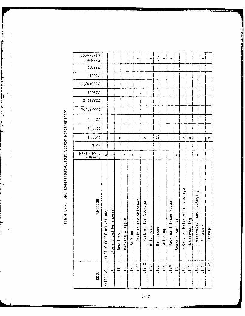
ELt08ZL .
6008 -L
Z*968Z II
C LL. 1L {j
ZLLLLZLfI
4-;
c M
0 CC..I
fuo 0 LM &--- a. i
m- - 0=
0 0CL-
C- vi
C-1 2
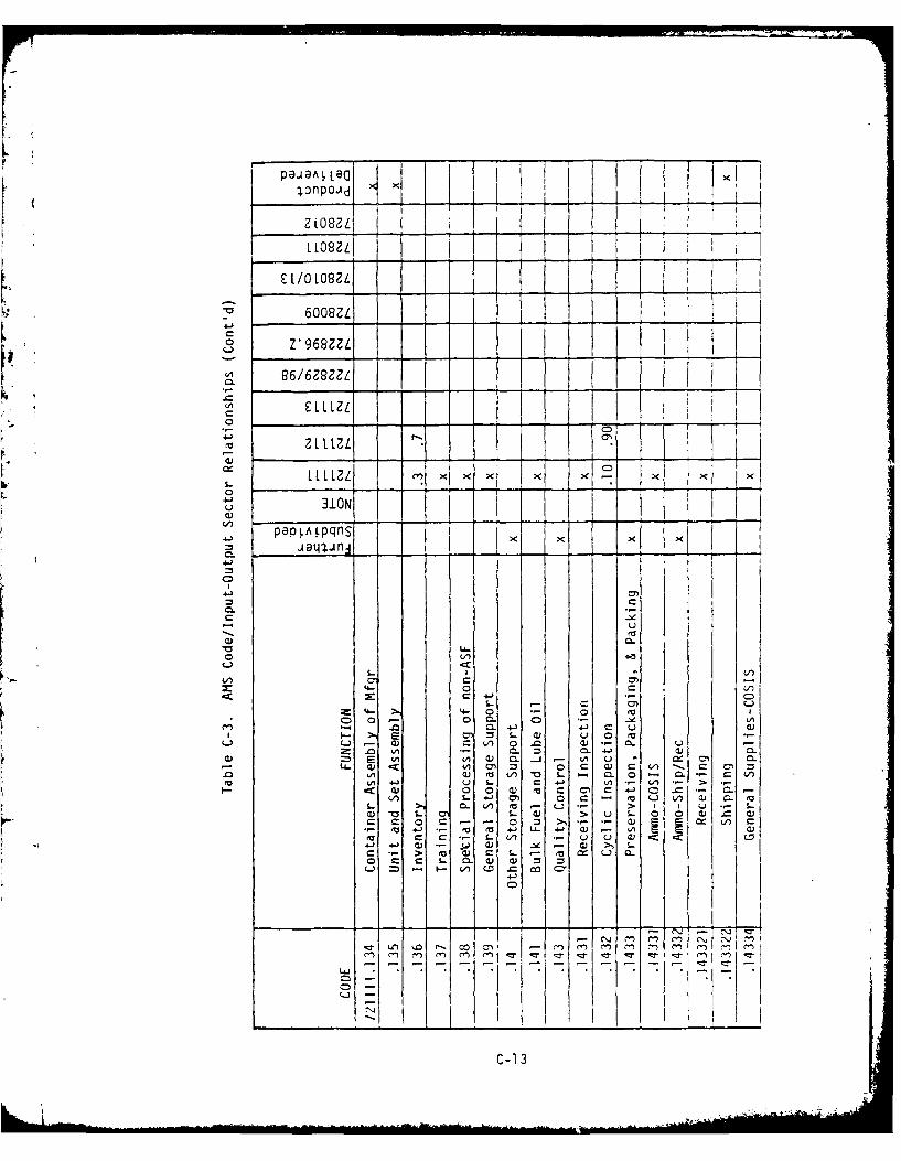
4 ~~ ~ floPOJdt--- jzZL08ZL
Lb LBZ~LL
0Z '968ZZLL~
LLLLZL I I -: 1 . 2 I
4- 0
~~~~~~~~~X I92;S[Z :. ~ . 0 .. ~0
- I
0--
C. 0-D 1
c K L CUcLI 0 __ ___a)
2E ~ ~ ~ - 3iC .a
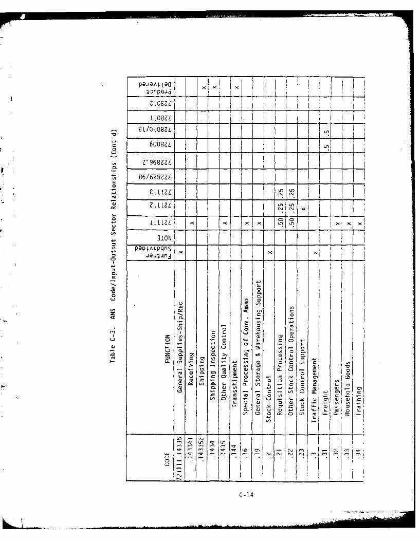
-. L
C LOLOIRZL I O
c60083ZL{TL
Ln )
LLL LnL. 9
JIONI
C
L0
0.
o. >,0.S(r) 0m V) -4J +
M C- 0
.2 0 a 0) c 0. c
S- 4- J 0 LM*.n m. L. V) S. o
CL CA 0' mA~UL l LA *.- rC .- (-) (-A X: 0 C) (
.( et3 0' vj 0
0) o 0' I--,U 0 0) 0
V) z o.. C C 0. 0 0 C D LL- CL0) 0 .C * U ~ -' 0 U ..4J..(C ~ ( 0. .C . S. 0 C C /)
p.- ) 0 0) ( ~ -' ~J 0 e~ 0 -Ocr .C (A - *X A 'fn4s r ~ 0 (AC C .
(Ac0rU U . ' 00
C-14 0 U(A(

LLOSZLI I
60082L 1Z*968ZZL1
966Z8ZZL~~I
Co 2LLL L x 0
31.ONq papLALpqlnI
CLccl~~ 0lC 0 0
CD.0
CLC
L)L03 0 1/) a 0
= O 4- j Cwc
0X 0 C W
4. l <j* l U
I ~ ~! _ ___
C<
t4-bd
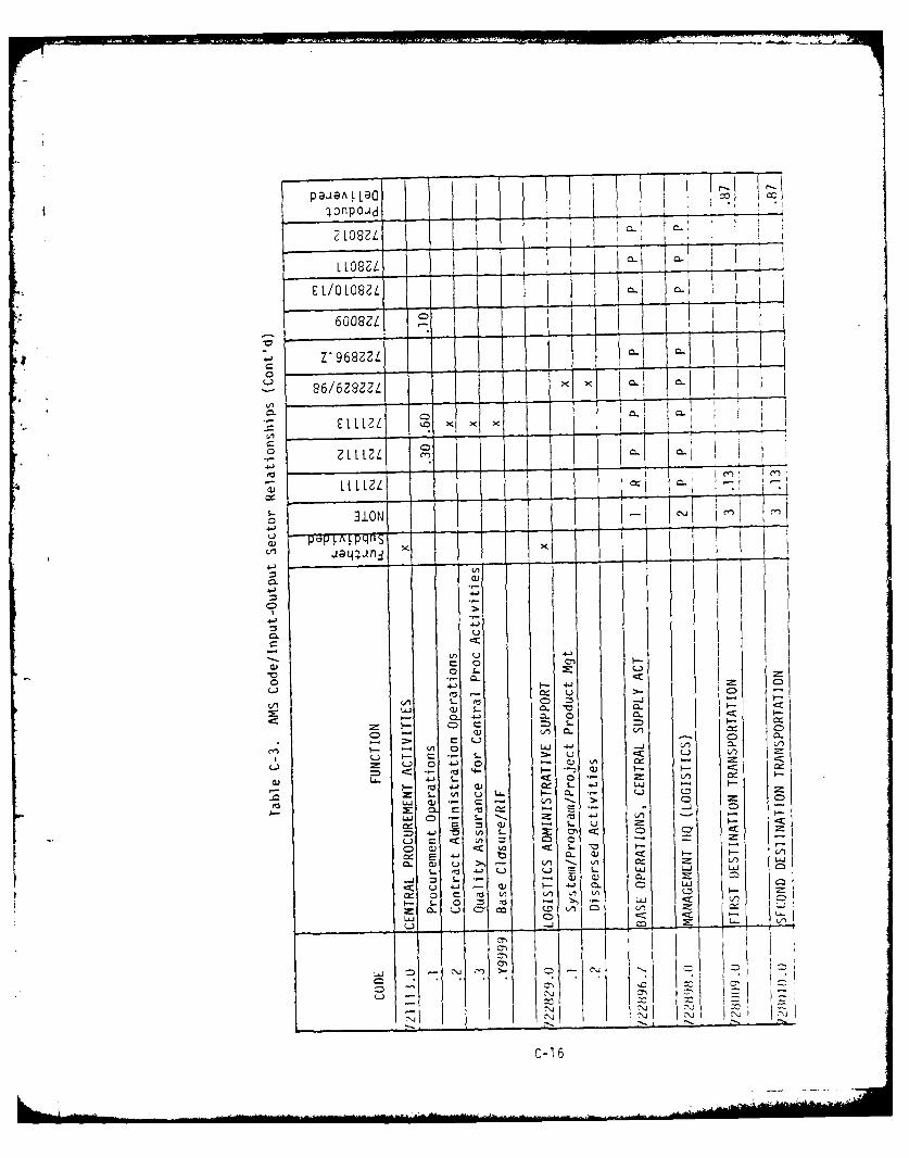
pJa L LQ
C L/O LOSZL' o-x. x
96/6z~zzzL-
V)t~
C LIL xx> ' I
ZLLLUL- -F
4-_ __ - - -) cW Lt.I
CA dLRON~--
4z
(-C4-.
-a 000 L
CL <
~ - C_ CC
I- C 0 LU 4. Cn
Z L) 0 ~ '-' di C C~
s- V) ui L- L -D
eo LW .' C
I-~S LU <* .. -V) C ~ C) C C7- <k z
C) c 4u s- -V - - I0: E 41' Q) < I-0. aw u Q,( . A A L
m.. ~ 4'C. LUJ LU LUW
S- G- G C LU
- S. C~ cc LiU
C..TN
-7
C-16
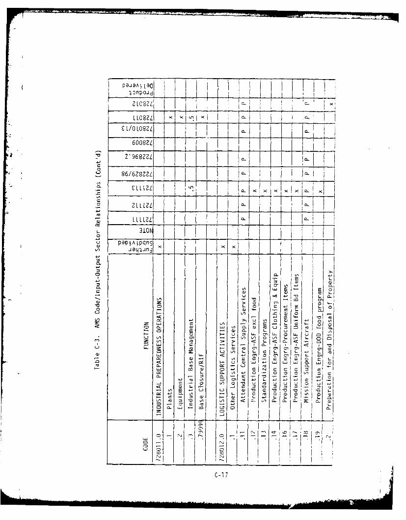
Pa@LLOL0 0.
£ 1.0 1O,L T d__ __ __ _ - -z 1
Z U6ZZ I I~ I .~XI
0 CLLLZLE -L t - xI x x x
p8pLALpqnS
LA CL
a, *> 0 n 0 a j 0 (LW X. 0 -)
E a - * CL 1
v ;:: (j =3 - o)L - U4-) m, 01 V 0 l L. ' 0) U. C
0 C7 cn =I( . a L ~ )U
i u.. L- a) LA 0- wA S. Lu S.. L
~~ LU C~ S - S. - 0. I II
4) LU Ue< -' 0 0 0 0' L 0 r
LA LU COI C- a- -)- C J
C- 7 1 )
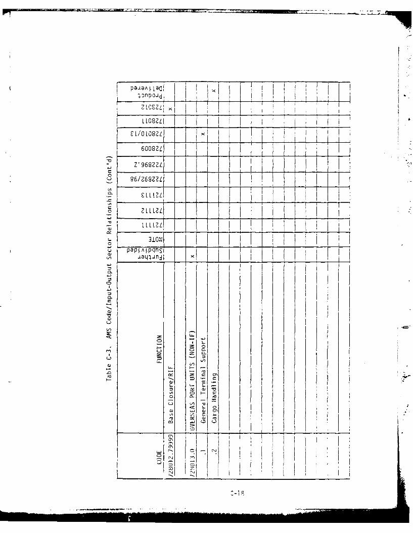
PaaaAL tj;onPOAdj L
LLZL ~ I
60082L
ZLL1LZ
- LLLI.ZL
310
jaq
0l 4
(-V)
co 0
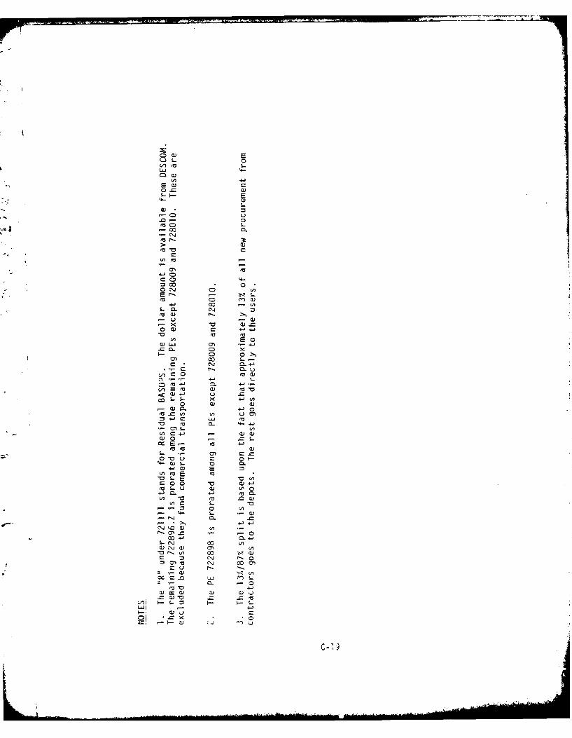
LAJ 4-
CD
co CL
-o
=-0 0.
41 000
0c' CL ciMC (U >
U
x
2 0
CD*
In. ~-)
x0 CLW
~4-) r LU '
ea CL C
-a 0Qj)
o 0.
4-J U E U
00 s- V
4-) 4-- U * --~ 0.
& -
*0 - J 4
C 0
C-1
The gross transactions matrix shows how the output of each sector
is consumed by itself, the other support sectors, and the final users. A
problem encountered in applying 1-0 analysis to the supply economy is the
difficulty in determining the economic output of each sector. For this
reason, dollars expended (or programmed) for the different PEs (support
sectors) were used as proxy variables in lieu of the economic output of
each PE. The result is a budget allocation matrix rather than a gross
transactions matrix. This budget allocation matrix, shown in Figure 3 of
the main report, is based upon both the funded and unfinanced requirements
for FY 79. The assumptions behind this inclusion of the unfinanced require-
ment are discussed in the main report. The COBE data for this matrix are
contained in Table C-4. Since neither the COBE nor the PBG provides
information at the AMS detail in Table C-3, various existing reports which
do have the detail necessary were employed to establish ratios for dividing
the PE totals. The actual allo'aton of the funds in Table C-4 is shown
in Figure C-1. The end result of these allocations is Input-Output Budget
Allocation Table, shown in Figure 3 in the main report. This budget
allocation table will be used as a proxy for the gross transactions matrix.
The budget allocation table is "normalized" by first determining the
sum of each row. In this case, each row sum should equal the total require-
ment for that PE in Table C-4. Each of the support sector columns is then
divided by its respective row sum. For example, the sum of the values in
the first row (PE 721111) of Figure 3 of the main report is 337607, and
each value in the first column (PE 721111) is divided by this amount. Thus,
C-20
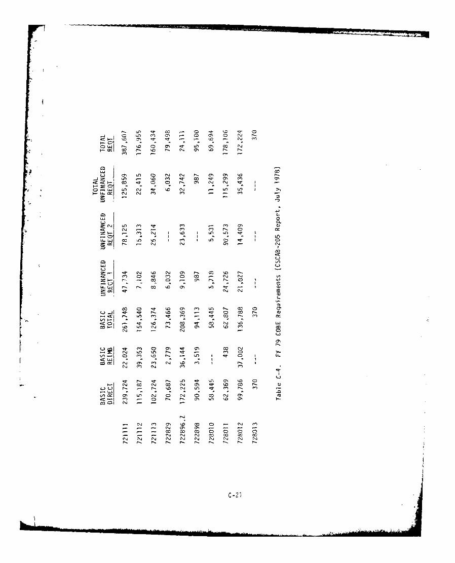
0i cnj Ln -l C - ON ON ~0U. co C- C0 0~j It I) 0
3' CL
(1) N ~ o IC NO LO I
I I LC
-- C') co nJ I 1.0 I LO ) -: I n
Li~Lj ~ U ) I C) I U
-9: N ~ ko N l m 0'. co N
00 CDd)
co N 10 NO 0m cn U) r-_ co C 0!* -r F 0 - 0'.= r-. N 0
- ~ C'j UO U-) r C' 'sz) "
~0 U N N 0 0' U) I) C,)0
v)- ~~ ~ L C0 C' ) N - U) I6C
0) j N 0' C') No 10 C') N: I. oq
CC-)
(A~ 0'. U) N 0 1 Ch ) N 0.C
cc No co - C-(
.. ' C) ' 11 C41 co cc N w- 'Ill -~ NI 0'. 0'. - ~ - - -
C -21
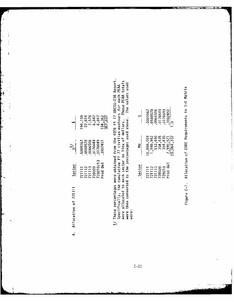
o <c~ et c)CL.3< 4-1 0W LLJ 0
CL 4 -Jvi 4-)
Q j.~a<.,
C*.J tv L&J-I a) O C)
I.>La --C
c-. 0 ui CU
0 *a) CLO k . -zl
cy) r- jr- Ur CL S.2o c oCLr oC) r r~ a)c k -c
kc - 0- )C OC
C-r~ a) 0
-~L I~~Cfl qa) m O O C CC
r- 00~r.t. 0. M n*- :*-:rIrL
a)J. LO C -O - 4CC La) 0 9C -f )r D 4
-- LLa00 --
L~~ .a >4-) Z;) ~0- ~.C)0i0O n 4-) Qa) 0 C)'J - uU CD-0 'a 0 (o Ln41 u C)-00 0a) --- c0 0 a) co -0
V) ~C~jC\J " C'j S a) . 0 V) C C\JNJ -l lir- r -o, lr a L U -u -r - -C
a)a ) 0 4 -)
- 43 * a)a
a- - 4- 0
S- 0C
d) u -) Q) a)
4- 41
C -22
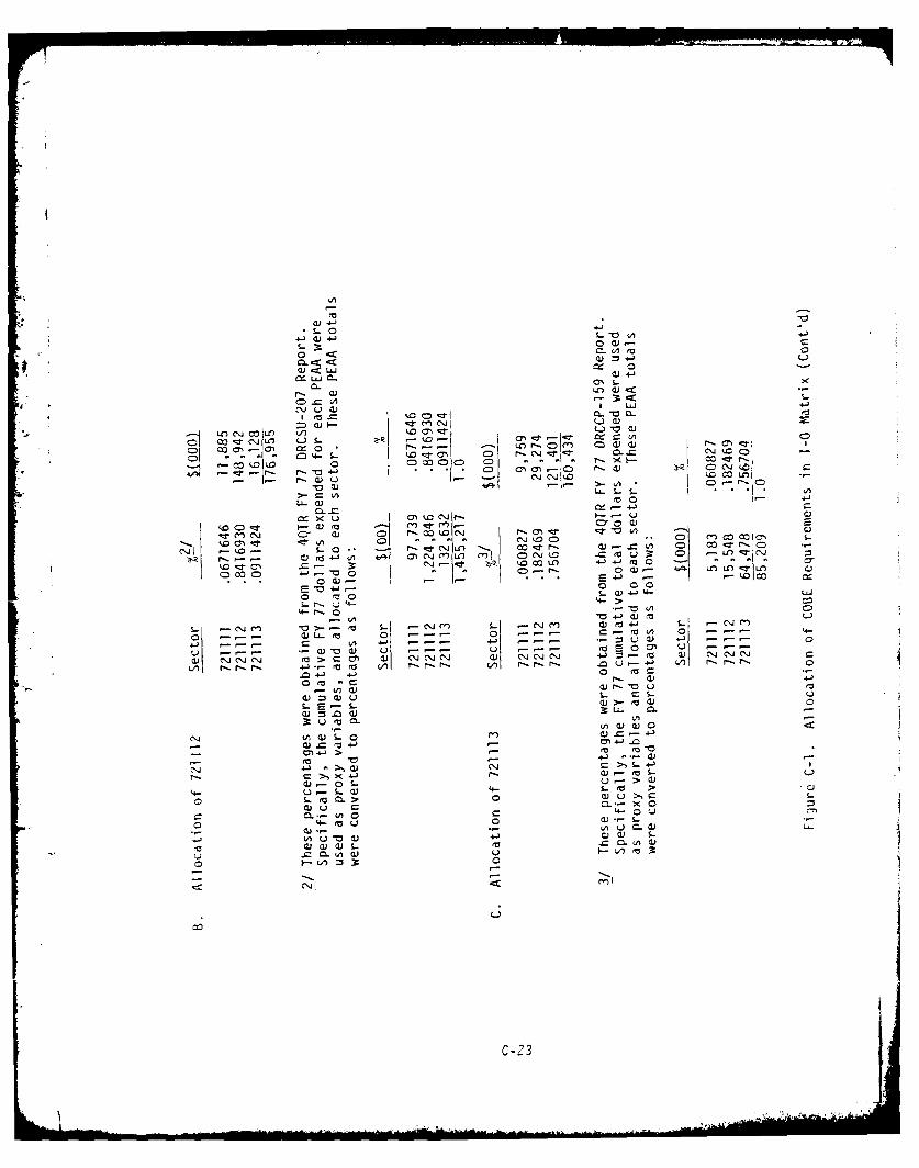
a) 4-'4-
S- 0
Q) 4J4-
Gi LO o) <C)0 = (A03<%
tio- =0r0 0 . 0.= e' 0 I -C
CO 0' -0 0J -
0-~U S- 0 S-~ 0 A -
0o -z c'a0j o ~)~I4- 0 -'l0 0-1CD0 cu Lf 0 1.0 CJ
ow-i . CD CD en .o0 n
C: 4-' -c 00 00rr- a C
o o 00 LO --'"4J MCD 0 U -> L
4-J - ~( 0I + >A c ow c
0 -- WLL'~ 0~ .- *0 -. C - 0 CA 0 :)'
4- 2 ra V) 0A 4- - ~ -U~~~~a -- -~ m - ~ 0
W \ C'J\j r >C c ) C'Ji-JC~j aW e~j 'C\JCI 4- 0 f M ) C'4CNC\j
LO r.r-f .r, 4-3 t* -rV r-vir- .OU - V) ~r -- 0
04) +j0 LL .-
C"J (V)L 0)C--
0)4-) M I
4- >!- -r ~
- 0 fu -> w rS
0 Lc-.> 0
4-ra U U, U0( 0(A L ' a 4-) W)) S
(- .CL () (3 o
co~
C-23
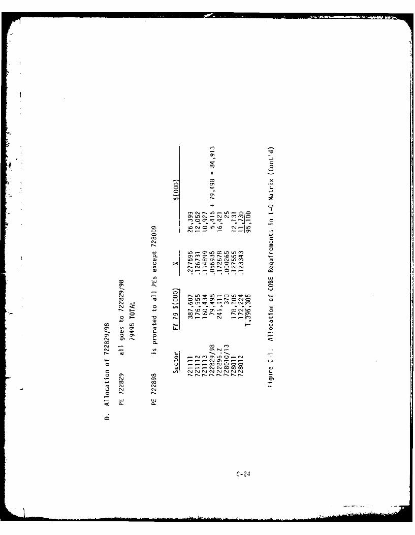
00
co xo: S..
+ C0
M*~jf OrLO ,LO~- -C
o. 4-' L o "
.4-' ~4-)
Un C NU r-C' 00C L-0-1 N m r- .0 U) N
aj N-)r 000 10 JLX
0a. . CD
cS, -- 0 l 0 C t0--oC : - C- a-, o'n -0 C..
r- .0 00C~0D m c - .c r -:: r-.r-Z
00 cc 4J~ ,-all mj 0CLLU. 0
0S, 0QS. 0
N - -c CJ
o -N CC)
4-o o 00N(o u~ ,--.ccco
Q C ~~N cccc
(/j JNNL.
o ar.
C- 24
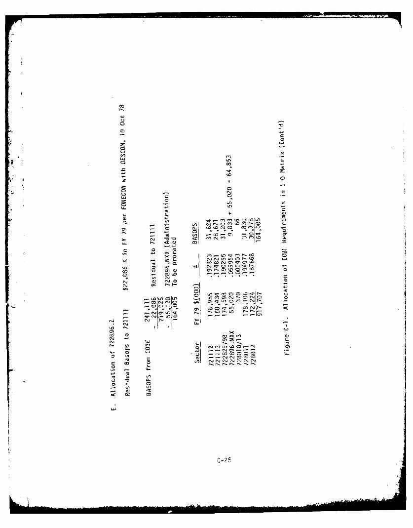
C-)
C)
CDC
004
44-'
0 L0
4-O 41'co +
4-3
ca. UI t.0 Lt CDW -)c/) 'c'.j J CDMk. r--OD S
I. -. co 0o -- C)
cc r'- Cci '-m m oc-4-
4'4-
0 Lk0
'j < 0.' m C t m r
S-J cii C'JO 0oL -
w . a, nCDC
00-
= 00.t
C-) C) CD C
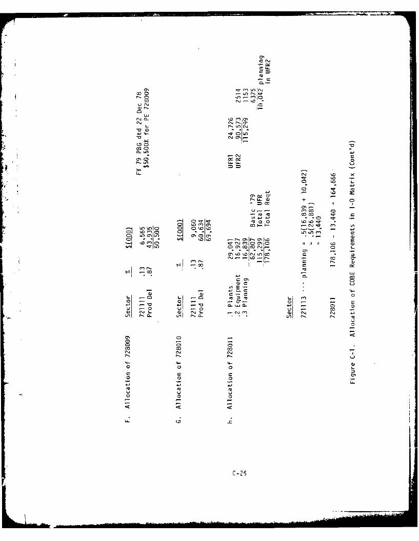
C LL
0- CD
0
cu r-
LJc'.J~" c,' -C~iC~r- C )C'
CD =J
co CDS.
?I, .6.JL-L
-- =4A. I
m' 00
m o o-0 qrm ~) C\4i C'-r
0 Cl'0 0n M~U 0C0 O
0! Is ~Iz- C1 C
C-,09JL CL
Low D
Le) r, CLC -a . . .V)
I DCCD
CD/ CD
W~ ~ C- Co - - r-0~
00
04-)
LL)
C-2-
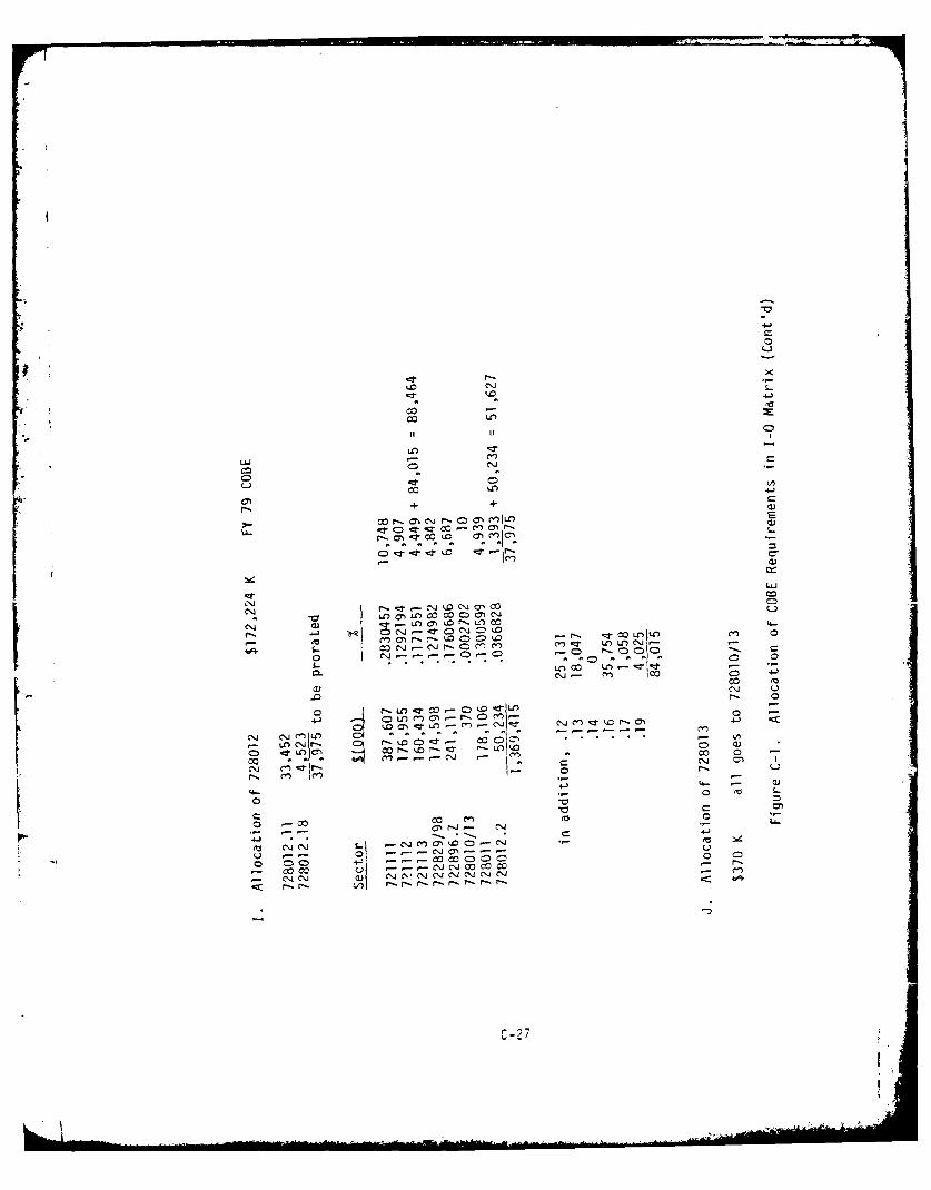
c-o
LnL0 tt tA
u co Lf.
C) + +
U- ,: Dc
r' i '3 O . ,iIl 7
CD - r r 1. -r-LI' C7
inO .Fr i 'r - e.J t.0 C~ a) cc C
olr- a~. 0
LO0 U)W )5-4 aj
0t 0 - I O0. . CCD j CCD CI
0D
ea~~'. c, U.000Id,
00
oo C 0-0 CD- "C
0
.r- -O- C r4 I')., j
C) -o M C - '
M -- -- c
(N an -* JCrC.J\C'C. C~
C-27
the value in the "from 721111/to 721112" cell is 11885 divided by 387607,
or 0.030663. This procedure is repeated for each of the support sectors;
the product delivered is disregarded after the row sums are calculated.
the result of this "normalization" is a square matrix. If this matrix is
referred to as the A matrix, then an element of the matrix, aij, represents
the proportional amount of the output of sector i consumed by sector j.
Since the output of each sector which is not consumed by itself or the
other sectors is consumed by the final users (F) the following matrix
equation is applicable:
AX + F : X
where X is a column matrix of the Total Requirements in the COBE. For
example, XI is the total requirement for PE 721111, X2 is the total
requirement for PE 721112, etc. The matrix AX is the amount of the total
requirement consumed by the support sectors. Thus, this equation is
partitioning the total requirement into that consumed by the support
sectors and that consumed by the final users:
(A - I)X + F = 0
where I is the identity matrix and 0 is a column matrix with all zeroes.
This equation results in a series of nine linear equations, which are
listed in Table C-5. The Xi are those defined in Table C-2.
1 The notation used here is based on that used by Dr. Harold E.Fassberg in his address to the Operations Research Systems AnalysisExecutive Course (ORSAEC) at the US Army Management School at FortBelvoir, VA. The transcript of his presentation, Input-Output Analysisand Linear Programming, was used at one time as a handout for the ORSAEC.
C.-C-23L t
..... .. -: i ......
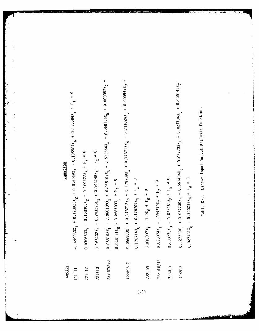
++ +- +
LO C-' 00 w
+ + +
co o n'U,) - 0 C
oO ( r-0
o + LI.
+ + +
U, -l '0C)C T C
U, 0 0n '.
- ~ ' ItI f.
CD - n 0
U- C). .4-'Lrl - A
'I >< C'j '.0 CjCjc Ci m L
r-. co c- lN + 0n
m
'.0!Z r- N 0 r 00
co C* 'V- -) CDo cc 0 0 U o 0 o U .. U.
+ + 4- + 4- +i4 4
00 ('j N - 0 . N C'
N~~. '.o '. C. N -
CD LA- 0- '.0 CQ , -m U, kV'. .0 LO cc- 0 .
c? * C' c
Cc 0 0 0 -r+
I + + + I I +D
- N 0 - -
0 ~ ~ I I') N 0 ~ ~ -~ .j
The "traditional" way to use input-output analysis is to use the
above equation to solve for X. That is,
X = (I A) F
where F is the known, desired output to the final users. In the case of
the supply economy, the F matrix is an unknown. Thus, the F. in Table C-5
are also unknowns. This necessitated an additional series of nine linear
equations. These additional equations were generated by assigning the
values of the FY 79 funded requirement to the above Xi values, and
solving for the Fi values. Thus,
F = (I - A)X
This is readily accomplished by assigning the Xi in the equations of
Table C-5 the values of the funded (Basic) requirements in Table C-4,
and solving for the Fi. The results of this are shown in Table C-6.
These equations are also included in the Goal Program. Note that the
equations for F3 and F8 will require the addition of artificial variables
in the Goal Program. (These artificial variables will also appear in
the equations in Table C-5 which contain F3 and F8 .)
The equations in Tables C-5 and C-6 are included in the goal
program to represent the balance between the various program elements.
Goal Programming. Goal programming is an extension of linear
programming which allows for more than one objective or goal. These
multiple objectives may be conflicting; i.e., not all of the objectives
can be fully satisfied it the same time. In linear programming, this
situation .aould result in an infeasille linsolvabie) scl ution ,
C-30
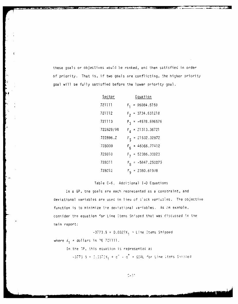
these goals or objectives would be ranked, and then satisfied in order
of priority. That is, if two goals are conflicting, the higher priority
goal will be fully satisfied before the lower priority goal.
Sector Equation
721111 F1 = 96084.51 59
721112 F2 = 3734.631218
721113 F3 = -4578.596576
722829/98 F4 = 21313.36721
722896.Z F5 = 21532.32872
728009 F6 = 46066.77412
728010 F7 = 52386.30023
728011 F8 = -5847.250075
728012 F9 = 2380.61938
Table C-6. Additional 1-0 Equations
In a GP, the goals are each represented as a constraint, and
deviational variables are used in lieu of slack variables. The objective
function is to minimize the deviational /ariables. As -n example,
consider the equation for Line Items ShiDped that was discussed in the
main report:
-3773.5 + 0.0327X- Line Items Shipped
where X = dollars in )E 721111.
In the 3P, this equation is represented as
+ Li-3773.5 >D 337X, + d -d = OAL cor Lne items SnT:ed
W AGG 914 ARMY LOGISTICS MANAGEMENT CENTER FORT LEE VA FIG 15/5IWACT OF INCREMENTAL CHANGES IN 7S FUNDING ON SUPFLY PEiWORMAN-ETC.(U)AUG 79 W T CRADDOCKNCLASSIFIED N
2,IiI/I/IlfliI
I iuuuuunnlnin!llIlllllm.iliiiiiiimi
!lllENDBCI
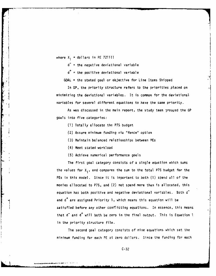
where X = dollars in PE 721111
d = the negative deviational variable
d the positive deviational variable
GOAL = the stated goal or objective for Line Items Shipped
In GP, the priority structure refers to the priorities placed on
minimizing the deviational variables. It is common for the deviational
"* variables for several different equations to have the same priority.
As was discussed in the main report, the study team grouped the GP
goals into five categories:
(1) Totally allocate the P7S budget
(2) Assure minimum funding via "fence" option
(3) Maintain balanced relationships between PEs
(4) Meet stated workload
(5) Achieve numerical performance goals
The first goal category consists of a single equation which sums
the values for Xi, and compares the sum to the total P7S budget for the
PEs in this model. Since it is important to both (1) spend all of the
monies allocated to P7S, and (2) not spend more than is allocated, this
equation has both positive and negative deviational variables. Both d-
* and d+ are assigned Priority 1, which means this equation will be
satisfied before any other conflicting equations. In essence, this means
that d- and d+ will both be zero in the final output. This is Equation 1
in the priority structure file.
The second goal category consists of nine equations which set the
minimum funding for each PE at zero dollars. Since the funding for each
C-32
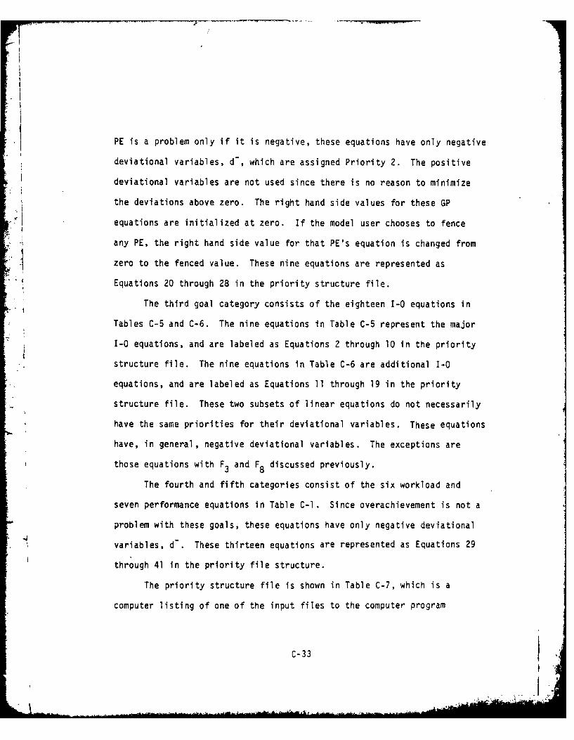
PE is a problem only if it is negative, these equations have only negative
deviational variables, d, which are assigned Priority 2. The positive
deviational variables are not used since there is no reason to minimize
the deviations above zero. The right hand side values for these GP
equations are initialized at zero. If the model user chooses to fence
any PE, the right hand side value for that PE's equation is changed from
zero to the fenced value. These nine equations are represented as
Equations 20 through 28 in the priority structure file.
The third goal category consists of the eighteen I-0 equations in
Tables C-5 and C-6. The nine equations in Table C-5 represent the major
I-0 equations, and are labeled as Equations 2 through 10 in the priority
structure file. The nine equations in Table C-6 are additional I-0
equations, and are labeled as Equations 11 through 19 in the priority
structure file. These two subsets of linear equations do not necessarily
have the same priorities for their deviational variables. These equations
have, in general, negative deviational variables. The exceptions are
those equations with F3 and F8 discussed previously.
The fourth and fifth categories consist of the six workload and
seven performance equations in Table C-l. Since overachievement is not a
problem with these goals, these equations have only negative deviational
variables, d-. These thirteen equations are represented as Equations 29
through 41 in the priority file structure.
The priority structure file is shown in Table C-7, which is a
computer listing of one of the input files to the computer program
C-33
I *'
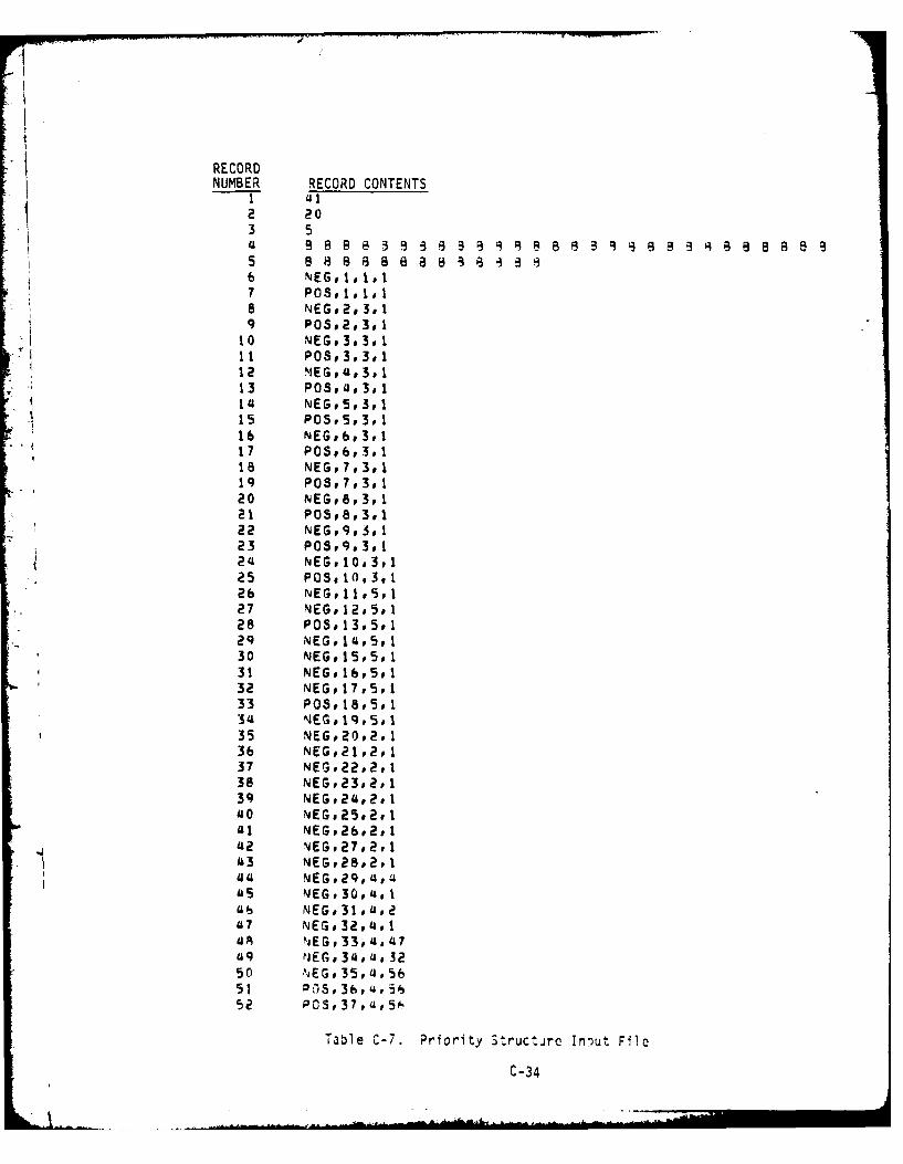
RECORDNUMBER RECORD CONTENTS
1 412 203 5
10 NEG.3.I 11 P05s3,311a NEGv,,3p 1
4 4 1 P05.4,3#11o NEG#533#
12 NEGo,3pl*13 POSo4#3#1
14 NEGPS,3pl15 P05.7,3.120 NEGv,,3, 117 P05,8,3.1Is2 NEG#7#3#113 P05#,3. 120 NEGr,Q3,125 POS#,3, I~22 NEGP,1,1
24 NEGv12.5,1
28 P05,v13.5,129 NEG , 14 , So30 NEG# 15#5# 1
*31 NEG.16,5o132 NEGv 17#5, 133 P03,I15#134 NEGo I .5,135 NEG#20*2* 136 NEG#21#2u137 NEG,22#2,138 NEGP23,2# I39 NEGP24#2#1'40 NEG*25,2#1at1 NEGP26*2#142 NEGP27@2*143 NEG*28#2#144 NEG*29p4'Las NEGP30*4tt
43 NEG,31,4,2447 NEG#32,LI.1
UANEG, 33, 4,47L19 NEGP34,44.3250 NEG3,35,4,5651 OP64i
P03,37.4,50.
Table C-7. Priority Structirc Iniut File
C-34
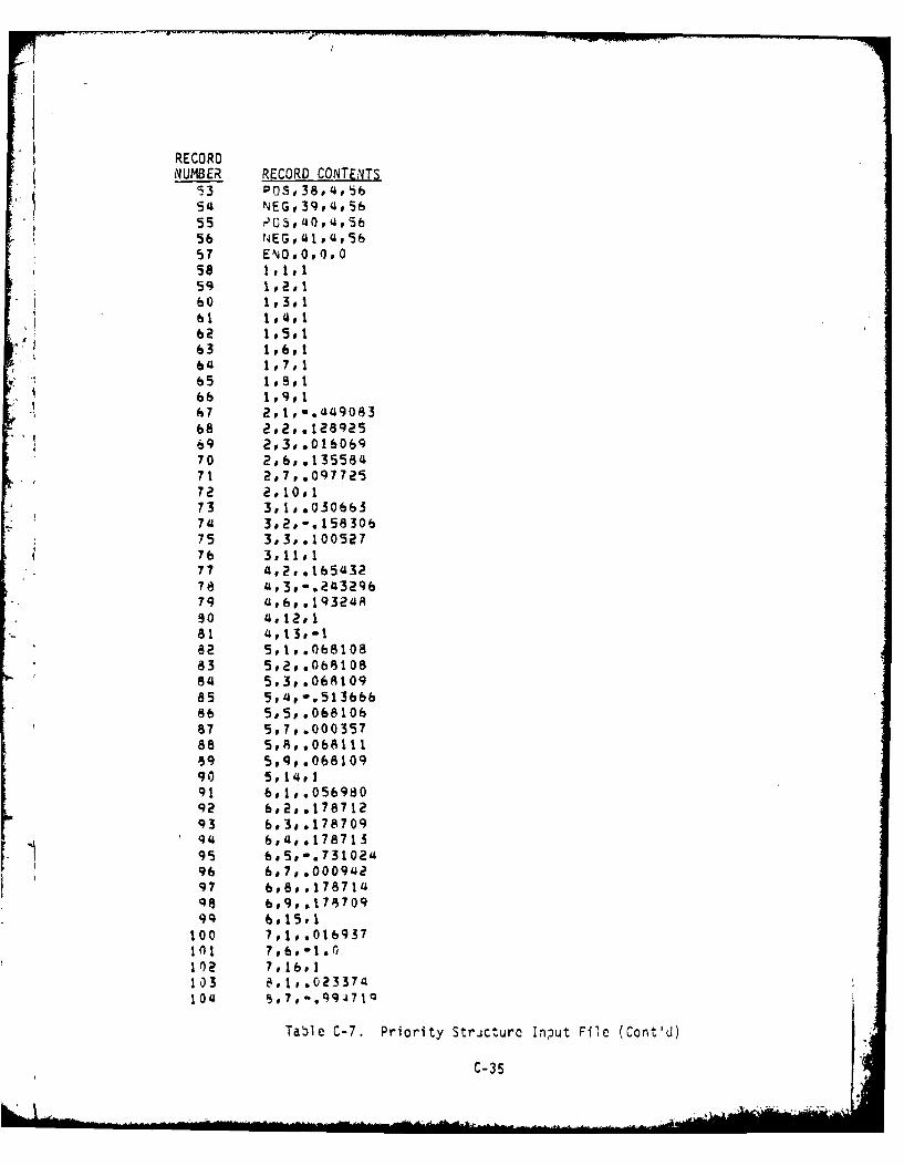
RECORDNUMBER RECORD CONTENTS
53 0OS,38,4,5b54 NEGP39,4 ,655 P . 4 ,4 556 14EG,4I#4,5657 EN0O,0,O58 1,1,159 1,2,160 1,3,161 1.4,162 I1so I63 1,6,1
I bu 1,7,1
65 1,8,166 1,09. 1h 7 2,1,-.44908368 2,2,.12892569 2,3,.01606970 2,6,.13558471 2,7,.0q772572 2 10s173 3,1,.03066374 3.2,-.15830675 3,3,.1005277b 3 11,177 4,2,.16543278 4,3,-.24329679 4L.6,.I1324A90 Up,12,181 4, 1 3,-I82 5,11.06810883 5.2,,06810884 5.3,.06810985 5,4-.5136668b 515,.06810687 5,7,.00035788 5,,.0b811139 5,9,.06810990 5,14,191 6,1,.056980q2 6,2,,17871293 b,3,.17870944 bo4 .17871395 6,5,-.73102496 6,7,.00094297 6,8,.17871498 bg,.11870q
99 6,15,1100 7,,1.016937
1(117)o- .102 7,16,1103 a,1,.023374IOU 5,?,-. l47l
Table C-7. Priority StrJcturc Input File (Cont'd)
C-35
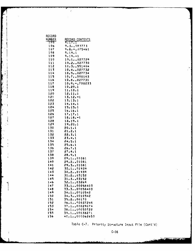
RECORDNUMBER RECORD CONTENTS
106 q,3,,083773107 9@8,-.075461108 9,F1I1109 q.1q,-lI10 10,1,.02772q111 10,2,,027730112 10,3,.551404113 10,4s,027732114 10,5,.027734115 10,7,.000143116 10,8.,027731117 10.9,-.700233118 10,20,1119 I 0I I01120 12 ,111121 13,12,-I122 13 13,1123 14v 14 1124 1s,15,1125 16 16v1126 17,17,1127 18.18.1128 18 19,1129 19,20,1130 20.,11131 21,2,1132 22,3o1133 23.4, 11314 24#5,1135 25,6,1136 26 7,1137 27,8,1138 28,9,1139 29,1#.01081140 29,2,.01081141 29,3,.01081142 30,1,.01939143 30,2*.0193q144 31,2,.03152145 31,3,.03152I ab 32,1 .032bq147 33,1,.0005840314I8 33o3,.00058403
349 34 # 10010542ISO 34p] .0010542
151 35,2t.00170152 36t1,.00037248153 37,1t.0002907415" 38,1,.00050722155 39,1,.00038271156 'Ip,1,.0002b53
Table C-7. Priority Structure Input File (Cont'd)
C-36
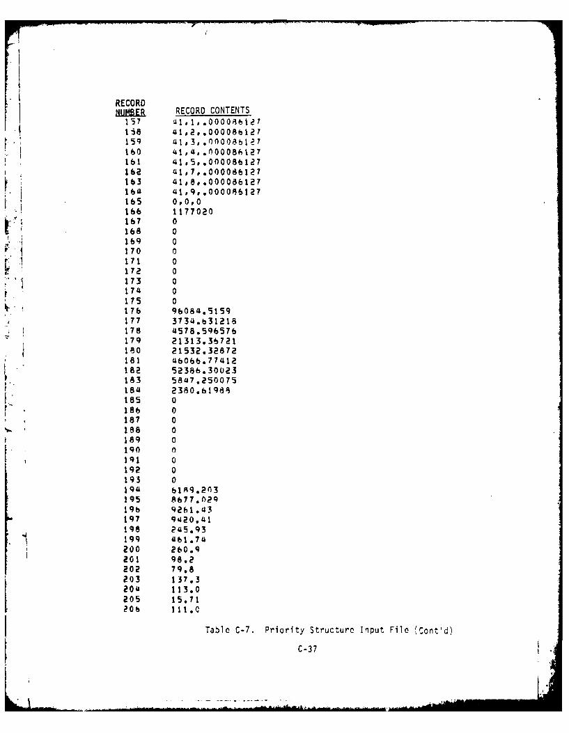
RECORDNUMBER RECORD CONTENTS
137 (1,1g.0000831271i8 41,2,.000086127159 4l.3,.00008b127160 41,G,.000086127161 l1,5,.00008bl27162 u17,.000086127163 41,8p.000086127164 a1,9,.000086127165 0,0,0166 1177020167 0
,-. 168 0
169 0170 0171 0172 0173 0
4 175 0
176 96084.5159177 3734.031218178 4578.596576179 21313.36721180 21532.32872181 4b0bb.77412182 52386.30023183 5847.250075184 2380.61988185 0186 0187 0188 0189 0190 0191 0192 0193 0lq 6189.2n3195 8677.02919b 9261,43l97 9420.41
198 245.93199 461,74200 260.9201 98.2202 79.8203 137.3204 113.0205 15.7120b 111.0
Table C-7. Priority Structure Input File (Cont'd)
C-37

discussed in Annex I. Record 1 in this file is the number of equations
in the GP. Record 2 is the number of decision variables, X. . In this
model, the additional decision variables are for the Fi discussed earlier.
Record 3 is the number of priority levels. Records 4 and 5 represent
the "sign" of the equations. In this case the "B" implies deviations in
both directions are possible (although we may wish to minimize some of
these deviations).
Records 6 through 57 contain information on the deviational variables.
Consider Record 9. The "POS" implies a positive deviational variable
(d+); the "2" refers to the equation number; the "3" refers to the
priority assigned to that deviational variable; and the "1" refers to the
weight assigned to that deviational variable. The "END, 0,0,0" in
Record 57 implies that this is the end of the deviational variable
information.
Records 58 through 165 contain information on the coefficients for
the various equations. For example, consider Record 67. The "2" refers
to the equation number (in this case, the equation at the top of Table C-5);
the "1" reFers to the variable number (in this case, the coefficient of
X0, and the "-.449083" is the coefficient. The "0,0,0" in Record 165
implies the end of the equation coefficients.
Records 166 through 206 represent the right-hand side values for
Equations 1 through 41, respectively. No'te that the right hand side values
for the workload and performance equations (Records 194 through 206) are
obtained by transposing the intercept constants of the equations in
C-38
-N W I.~ -h w-A, I
.1
Table C-1 and combining this value with the GOAL for that equation. For
example, the intercept for the first equation in Table C-1 is -4938.1
(Actions Initiated), and the GOAL is 1251.103. Thus, the right hand side
value is:
1251.103 - (-4938.1) = 6189.203
This value is shown in Record 194.
2The computer program requires a second data input file. This file,
shown in Table C-8, contains budget anJ goal information. Specifically,
Record 1 is the year basis for the dollars. In this case, the dollars
are in FY 79 dollars, and must be converted by the computer program to
FY 78 constant dollars to be compatible with the equations. Records 2
through 12 contain the direct, funded reimbursable, and automatic
reimbursable obligations for the PEs represented in this model. Note that
the PEs that are normally combined; e.g., PE 722829 and PE 722898, are
separate here. The order of the PEs is the same order as shown in
Figure 4 of the main report.
Records 13 through 25 are the numerical workload and performance
goals for the equations in Table C-l. The workload goals are taken from
the COBE, and the performance goals are taken from the Commander's Handbook
for Performance Indicators.
As discussed in the main report, the model output comes in three
pages. These are shown in Figures 4, 5, and 6 of the main report, and
will not be discussed further here. However, one should be able to see
certain parallels between the data in Table C-8 and Model Output Pages
I and 3.
C-39
Ai
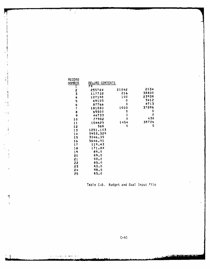
-RECORD
NUMBER RELJRD CONTENTS
1 192 255784 21002 203U
3 117732 216 3880041 1071q0 100 23938
5 69105 0 3412
6 877b6 0 47137 181080 1000 372868 65500 0 0
9 44733 0 0
10 77982 0 438
11 10a625 la5a 38726
12 388 0 0
13 1251.1031A 3953,32915 3046.3516 5646.q17 119.4318 171.8419 89.020 89.021 90.022 85.023 83.024 98.025 85.0
Table C-8. Budget and Goal Input File
C-40
It is important to note that the model output in the main report
was obtained using the input files in Tables C-7 and C-8. The priority
structure (Table C-7) could and should be changed to investigate the
effects of alternate priority structures. In practice, this file is
accessed interactively external to the goal program through the use of
the EDITOR or other computer file manipulation routines.
I
C -41
ANNEX 0
[DESCRIPTION OF PROGRAM ELEMENTS
D-1
ANNEX 0
DESCRIPTION OF SUPPLY PROGRAM ELE'E NTS
The Army Management Structure (AMS) is the official budgeting
framework for the Army. The AMS is described in detail in AR-37-100-XX,
where the "XX" refers to the applicable fiscal year. Since FY 78 was used
as a base for the model, AR-37-100-78 was the basic reference for the
program elements in this study. The PEs applicable to this study are
briefly described in the remainder of this annex. Note that PE 728009,
First Destination Transportation, is included in this list even though it
is not in AR-37-I00-78. This PE was first established in FY 79, and it
was included in the model to make it compatible with future budgets.
a. PE 721111, Supply Depot Operations, provides for internal
operations at Army depots and arsenals. It includes the receipt of
materiel into depots, care of supplies in storage (COSIS), the issue and
shipment of assigned stocks and all operations incident thereto. It also
includes stock control activities (processing of receipt documents,
maintaining order files, receiving, recording, and processing material
request documents and maintaining requisition files) when performed in
depots and administrative portions of traffic management performed within
depots.
b. PE 721112, Supply Management Operations, provides for the
-' operation of Inventory Control Points and other activities performing
supply management functions. It includes inventory management, provisioning,
requirements computations for all principal and secondary items, and direc-
tions initiated resulting from requirements computations; e.g., cataloging,
procurement, redistribution, rebuild, and disposal. It also includes the
D-2
control and processing of receipt documents and maintaining active and
complete order files; receiving, recording, and processing material
request documents; maintaining requisition files and providing status
* I information on requisitions and maintaining stock records.
c. PE 721113, Central Procurement Activities, includes operation
* of the Army's Central procurement offices and provides for contract
administration and quality assurance not assigned to the Defense Contract
Administration Service. Specifically, it provides for the actions following
the receipt of a procurement request including the preparation and issuance
of solicitations, evaluation of bids and proposals, and negotiation and
award of contractual documents; overall management of the procurement
function including policy formulation; planning actions designed to assure
that purchase requirements are fulfilled; and quality assurance actions in
support of Central Procurement Offices.
d. PE 722829, Logistics Administrative Support, includes the costs
of Central Supply Activities performed by system/program/project/product
managers and the cost of dispersed activities performing logistics control
and direction functions in support of Central Supply Activities.
e. PE 722896.Z, Base Operations, Central Supply Activities, provides
for those activities of an installation support nature. It includes those
support elements and services identified as indirect overhead by Headquarters,
Department of the Army. It includes audio-visual services, supply
operations, maintenance of materiel, transportation services, laundry and
drycleaning services, the Army Food Service program, personnel support,
D-3
|&
bachelor housing furnishings support, operation of utilities, maintenance
and repair of real property, minor construction, other engineering support,
administration, data processing activities, and installation restoration.
f. PE 722898, Management Headquarters, provides for the operations
of HQ DARCOM, HQ Staff Support Activities, and mid-management commodity
commands under HQ DARCOM.
g. PE 728009, First Destination Transportation, includes the
movement of Army supplies and equipment directly from the vendor to either
a CONUS depot, a CONUS user unit, or a CONUS port for shipment to an
overseas user.
h. PE 728010, Second Destination Transportation, includes movement
of Army supplies and equipment worldwide, after receipt from production
at either CONUS port, CONUS depot, or CONUS customer; and Army Industrial
Fund (AIF) water port operations.
i. PE 728011, Industrial Preparedness Operations, provides for
those operations which are performed to assure the production capability
required to support current and emergency procurement programs, including
actions taken by the Department of Defense to augment the production
ca;ability of the industrial base.
j. PE 728012, Logistics Support Activities, provides for central
supply logistics activities including: attendant central supply services;
production engineering, Defense Standardization Program, facilities
investigation and studies, and DARCOM mission support activities. It also
includes the preparation for and disposal of excess, surplus, and foreign
0-4
AL. Pr,
excess property. This includes the demilitarization of combat materiel
and other military supplies and equipment for the Property Disposal
Activities.
k. PE 728013, Overseas Port Units (Non-IF), provides for the non-
industrially funded overseas water ports pertaining to the receipt and
shipment of cargo and passengers.
D-5
• __ ...... j.. ~ ~ ~ ~ ~~- -... -..... -... -.... .. ., , .. ,, ...

ANNEX E
DATA
ANNEX E
DATA
This annex contains the raw data used in the DELTA 7S Study. These
data were arranged in a master data file, and were indexed by a unique
three digit number. These numbers are shown in Table E-l, and the master
data file is shown in Table E-2. The only transformation to these data
was inflation of the resource data to constant FY 78 dollars using inflation
1 guidance published by HQ DARCOM. The inflation indicies are shown in
Table E-3.
E-2
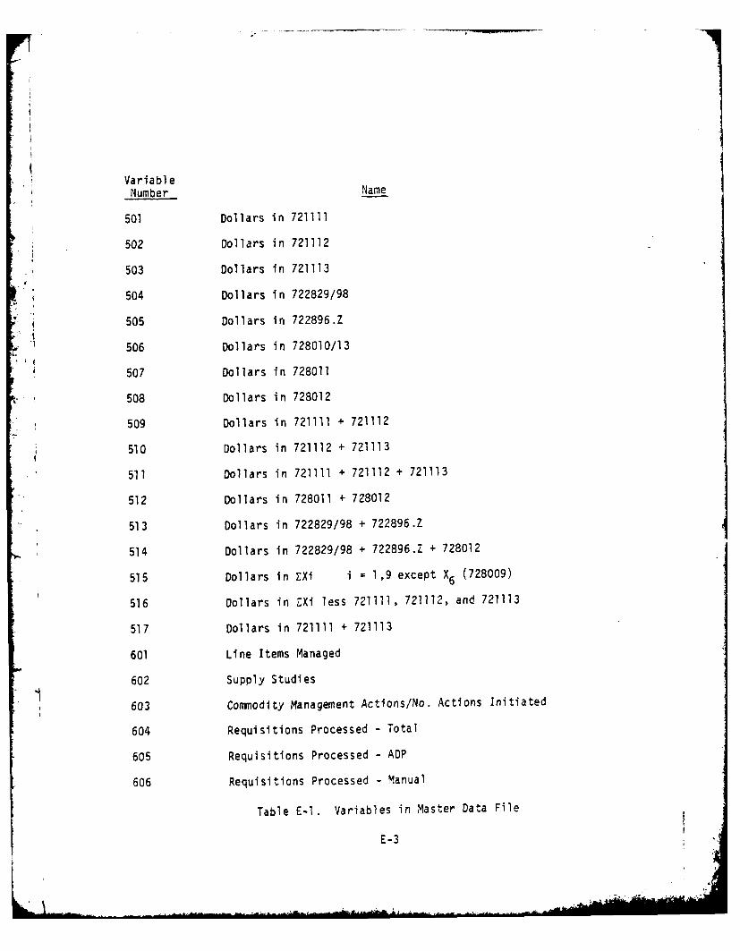
VariableNumber Name
501 Dollars in 721111
502 Dollars in 721112
503 Dollars in 721113
504 Dollars in 722829/98
505 Dollars in 722896.Z
506 Dollars in 728010/13
507 Dollars in 728011
508 Dollars in 728012
509 Dollars in 721111 + 721112
510 Dollars in 721112 + 721113
511 Dollars in 721111 + 721112 + 721113
512 Dollars in 728011 + 728012
513 Dollars in 722829/98 + 722896 Z
514 Dollars in 722829/98 + 722896.Z + 728012
515 Dollars in ZXi i = 1,9 except X6 (728009)
516 Dollars in ZXi less 721111, 721112, and 721113
517 Dollars in 721111 + 721113
601 Line Items Managed
602 Supply Studies
603 Commodity Management Actions/No. Actions Initiated
604 Requisitions Processed - Total
605 Requisitions Processed - ADP
606 Requisitions Processed - Manual
Table E-l. Variables in Master Data File
E-3
--A j"I i

VariableNumber Name
607 Requisitions Received
608 Line Items Received
609 Tons Received
610 Line Items Shipped
611 Tons Shipped
612 Procurement Actions
613 Backlog
614 Total Procurement (612 + 613)
615 FSN in Stock
616 Tons Received and Shipped (609 + 611)
701 DARCOM Stock Availability Rate
702 DARCOM Stock Availability Rate - NORS
703 DARCOM Backorders Outstanding
704 DARCOM Backorders Outstanding - NORS
705 Percent Backorders over 90 Days
706 Percent Backorders over 90 Days - NORS
707 DARCOM On-Time Requisition Processing
708 DARCOM On-Time Requisition Processing - NORS
* 709 NICP On-Time Requisition Processing
710 NICP On-Time Requisition Processing - NORS
711 Depot On-Time Requisition Processing
712 Depot On-Time Requisition Processing - NORS
Table E-l. Variables in Master Data File (Cont'd)
E-4
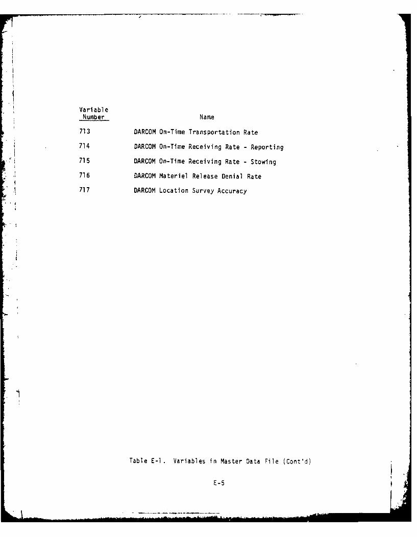
II
Variable
Number Name
713 DARCOM On-Time Transportation Rate
714 DARCOM On-Time Receiving Rate - Reporting
715 DARCOM On-Time Receiving Rate - Stowing
716 DARCOM Materiel Release Denial Rate
717 DARCOM Location Survey Accuracy
Table E-l. Variables in Master Data File (Cont'd)
E-5
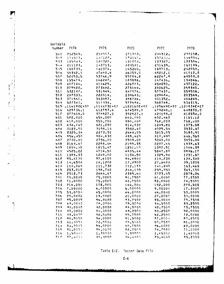
VariableNumber FY74 FY75 FY76 FY77 FY78
b~f ?2 5..5. 7b 7 1 qI . 2 4 As12.q 2 038.
r-1)3 1250,41. 120320. 12100-5. 123387. 12?39b.
5119 ls0 753 1-30374. 1 5&5. 1(Q713. 242050.5 )n 130342ol 4 7 2,4 46059.0 48212.1 41012.0507 52093.5 537h69 597418 62247.R 6950310
9 0 '(07144. 411629. a2b071. 454050. 437122.510 27q32. 273442. 2751hil. 280625. 249340511 53217. 931949. 547071. 577437. 554508.512 207133. 222014. 23Q6A3. 22Q0,Au. 2035h9.
*513 37 1500 . 3'I3OP7. 3A7S 140352.a4295114 52134'). 5111341 57hAU. 56878A. 538315.
515 ,11"Iq2E +07 .11!473E 07 .1221hOE 07 .125669E*07 .12034E+07bl '2973%.I b12783.4 O,7UL2F.0 6792u8.1 6f45830.051? 377b08.0 37827.0 392C27.1) 42(01q9.O a1554.o0b0l 522.000 65a.000 60.o00 602.460 111.12, 02 4 tn.oQo 555.000 990.00A 768.000 758.u00603 6d,740 321.290 A14.Q30 124q.8b IVS.38
6n 3182. 1 4198.14 3552.47 4025.54 3530.47h05 2325.5h 2273.51 2664.05 3215.05 31B3.91
ho07 2700.00 275b.00 PqOQ.00 3240.00 5450.00bOg 21b .47 22A8.4 2199.35 2207.hS 143,(330q 12014,0 1215.a7 1251.10 13q7.51 04 .3
hl( 425.22 4714.50 a935.cau 5847.80 5 96 L7hit 130. 35 t2a 9.0 1134.50 1329.94 1231.87(12 q5.qt1(o q7.6100 q4.A800 114.230 12a.340"IS 1 .6500 14.1200 17.2900 27,6h00 34.1200h1t 110.060 111.730 112.170 141.84n Ib3.abO615 253.010 148.740 244.136 25 .950 30.15C031 2512.7 3 246 .,17 2385.(-0 27P3 .145 2V 7 .216
701 70.0000 75.0000 91.750 n 61.0000 77.2500702 71.0000 75.0000 42.7500 92.0000 74.5000703 216.00') 178.600 14U.OOu 192.000 270.000704 1.00000 h.00000 S.00000 9.00000 17.3000
7 05 5S.000A 45.0000 46.0n0 46.00,()0 5 . 6q701 2.0000 13.0000 20.0000 27.0000 33.0000707 45.0000 86. 0000 A3.7500 55.0000 7 .75007 ~A ~0 02 7 A. 0o 7 9 , o o) 84.15 000 D 33. 2 9f701 1).00)0 42.0000 4.5non 2.7500 75.750071, 40.0000 8U.0000 Aq.25fr) 80.2506 9.(o00711 43.0010 92.0u00 '5.7500 b2.2500 7?.00007 q .0 0 9U,0000 91.5000 -7 .0j 0A .2s0011 5 )1.,01 " 72. 7o n7.590 'bn.7500 81.0(071 .. '0,0 Q3.0000 90.7500 46.u000 8 .Oo0o71S 1.061% .,)O00 2.A5 74.7500 71.00007? 1 . OCM I.30000 n I .e5000 1 .O000
Table E-2. [ astcr Data Filc
E-6
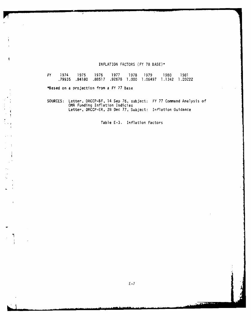
INFLATION FACTORS (FY 78 BASE)*
FY 1974 1975 1976 1977 1978 1979 1980 1981.79935 .84180 .88517 .92678 1.000 1.06497 1.1342 1.20222
*Based on a projection from a FY 77 Base
I. SOURCES: Letter, DRCCP-BF, 14 Sep 76, subject: FY 77 Command Analysis ofOMA Funding Inflation IndiciesLetter, DRCCP-ER, 28 Dec 77, Subject: Inflation Guidance
Table E-3. Inflation Factors
E-7
.1 ~~-~.~-----,- ~ -- .MAU-
ANNEX F
SENSITIVITY ANALYSIS
.F-
F-i i "
! ~
ANNEX F
SENSITIVITY ANALYSIS
The study team did not perform a formal sensitivity analysis in the
sense that each variable was investigated over a range of values to
determine its optimum value. However, the study team did investigate the
sensitivity of the model output to the priority structure. Table F-1
shows the model output for four different priority structures. Note that
this table excludes PE 728009. Although this analysis was performed prior
to the addition of this PE, the general results are still applicable. The
Roman numeral column headings refer to the four different priority structures
at the bottom. The "Spend Budget" priority is the sum of all the variables
equation. The "Balance" priority is the first series of 1-0 equations
derived. The "Output Level" priority is the second series of 1-0 equations
derived which determines the Fi values. The "workload" priority is the
series of workload equations. Performance equati)ns and the fence provision
were not included in this analysis.
Note that the workload and balance equations are conflicting.
Priority Structure I places the workload at the lowest priority, and the
model allocation is essentially the same as the COBE. However, as the
workload is placed at a priority higher than the balance equations (Priority
Structure III), the model allocations for PE 721111, PE 721112, and PE
721113 (the "hard" accounts) are considerably higher than are the COBE
allocations. The extra funds for these PEs come from the "soft" accounts
such as PE 728011. As noted previously, the descriptors "hard" and "soft"
are not intended to be derogatory, but refer to the degree to which the
impact of fund changes can be quantified.
F-2
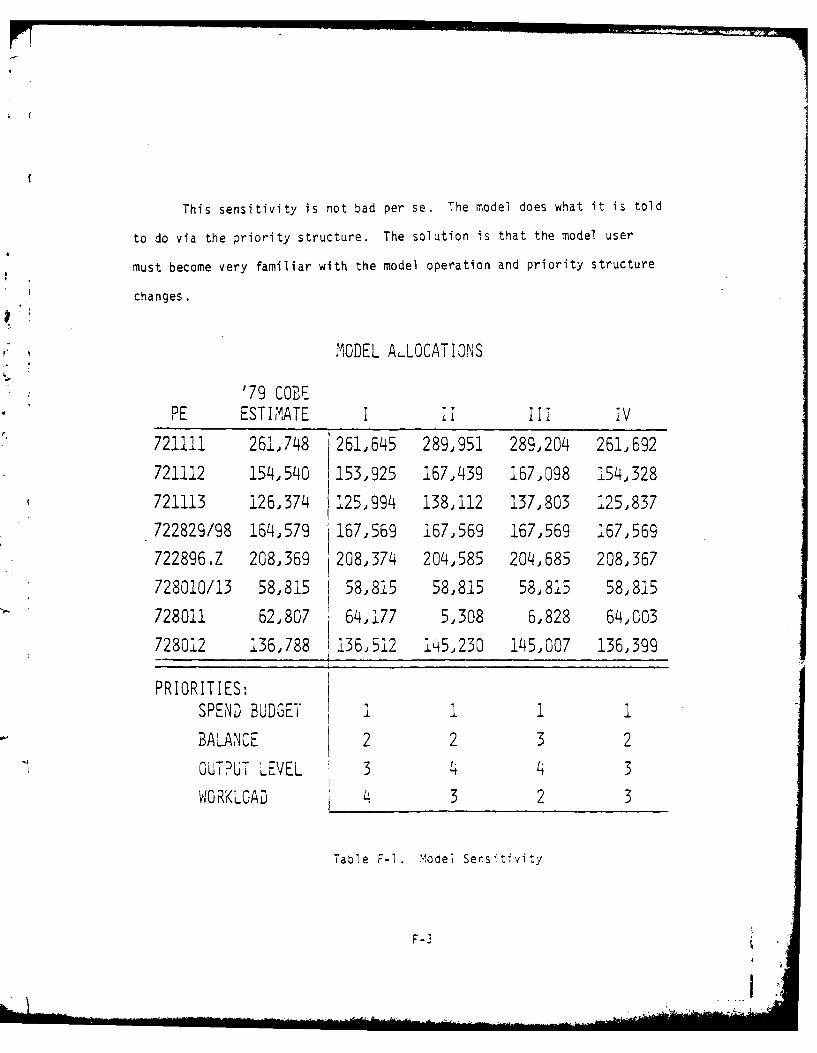
This sensitivity is not bad per se. The model does what it is told
to do via the priority structure. The solution is that the model user
must become very familiar with the model operation and priority structure
changes.
MODEL ALLOCATIONS
'79 COBE
PE ESTIMATE I II II IV
721111 261,748 1261,645 289,951 289,204 261,692
721112 154,540 153,925 167,439 167,098 154,328
721113 126,374 1125,994 138,112 137,803 125,837
722829/98 164,579 167,569 167,569 167,569 167,569
722896.Z 208,369 208,374 204,585 204,685 208,367
728010/13 58,815 58,815 58,815 58,815 58,815
728011 62,807 64,177 5,308 6,828 64,003
728012 136,788 136,512 1i5,230 145,007 136,399
PRIORITIES:SPEND BUDGET 1 1 1 1
BALANCE 2 2 3 2
OUTPUT LEVEL 3 4 4 3
WORKLOAD 4 3 2 3
Table F-i. Yodel Sensitivity
F-3 -
h6-
ANNEX G
VALIDATION
ANNEX G
VALIDATION
The regression equations for workload and performance described in
Annex C were initially developed using four data points: FY 74 through
FY 77. The equations chosen were based on mathematical fit and functional
logic. A 90 percent prediction interval was determined for each equation.Then the observed value for FY 78 (which was not included in the equation
calculations) was compared to the prediction interval limits. When the
observed value fell within these limits, the data base was augmented to
*include the FY 78 data. The equation coefficients were then reevaluated
based upon five data points. In those instances where the observed FY 78
data fell outside the prediction interval, the equation was scrapped, and
new equations were developed based again upon four data points (FY 74 to
FY 77). The above validation procedure was repeated until the FY 78
observed data fell within the prediction interval. The equations in
Table C-l were all validated using this procedure.
The validation of the input-output equations was less formal. The
I-0 budget allocation table was first based on information from the FY 78
COBE. When the FY 79 COBE became available, the study team reevaluated the
transfer coefficients (A matrix) based on the new data. When compared, the
two different sets of 1-0 coefficients were consistent. This procedure was
discussed in Reference 2-g of the Literature Survey (Annex B) as a method
of validation.
The validation of the goal programming model was even less formal.
Although the algorithm itself was checked against "textbook" examples, no
attempt was made to solve the DELTA 7S goal program by hand. However,
G-2
during one of the study briefings, new budget information was made
available. When this new information was reallocated by the model during
the briefing, the results were very similar to those obtained by the
Budget personnel working manually over the prior three-week period.
G-3

ANNEX H
USER I14STRUCTIONS
ANNEX H
USER INSTPUCTIONS
This annex contains the detail instructions that enable a user to
access and apply the DELTA 7S model. These instructions are divided into
three sections:
Section A Procedures for Operation of the DELTA 7S Model
Section B Description of the Input Files
Section C File Operations
These instructions are written based upon the timesharing use of the
Picatinny Arsenal computer. Although the program is written in FORTRAN and
should be executable on any computer with a FORTRAN capability, the user
instruction will change for different computers.
H-2
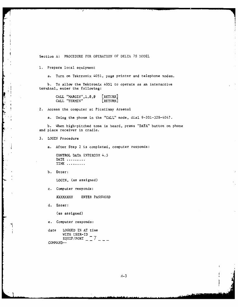
Section A: PROCEDURE FOR OPERATION OF DELTA 7S MODEL
1. Prepare local equipment
a. Turn on Tektronix 4051, page printer and telephone modem.
b. To allow the Tektronix 4051 to operate as an interactiveSI terminal, enter the following:
CALL "MARGIN",i,0,0 [RETURN]
CALL "TERMIN" [RETURN]
2. Access the computer at Picatinny Arsenal
a. Using the phone in the "CALL" mode, dial 9-201-328-4047.
b. When high-pitched tone is heard, press "DATA" button on phone* and place receiver in cradle.
3. LOGIN Procedure
a. After Step 2 is completed, computer responds:
CONTROL DATA INTERCOM 4.5DATE .........
TIME .........
b. Enter:
LOGIN, (as assigned)
c. Computer responds:
XXXXXXXX ENTER PASSWORD
d. Enter:
(as assigned)
e. Computer responds:
date LOGGED IN AT time
WITH USER-ID
EQUIP/PORT /
COKMAND--
H -3
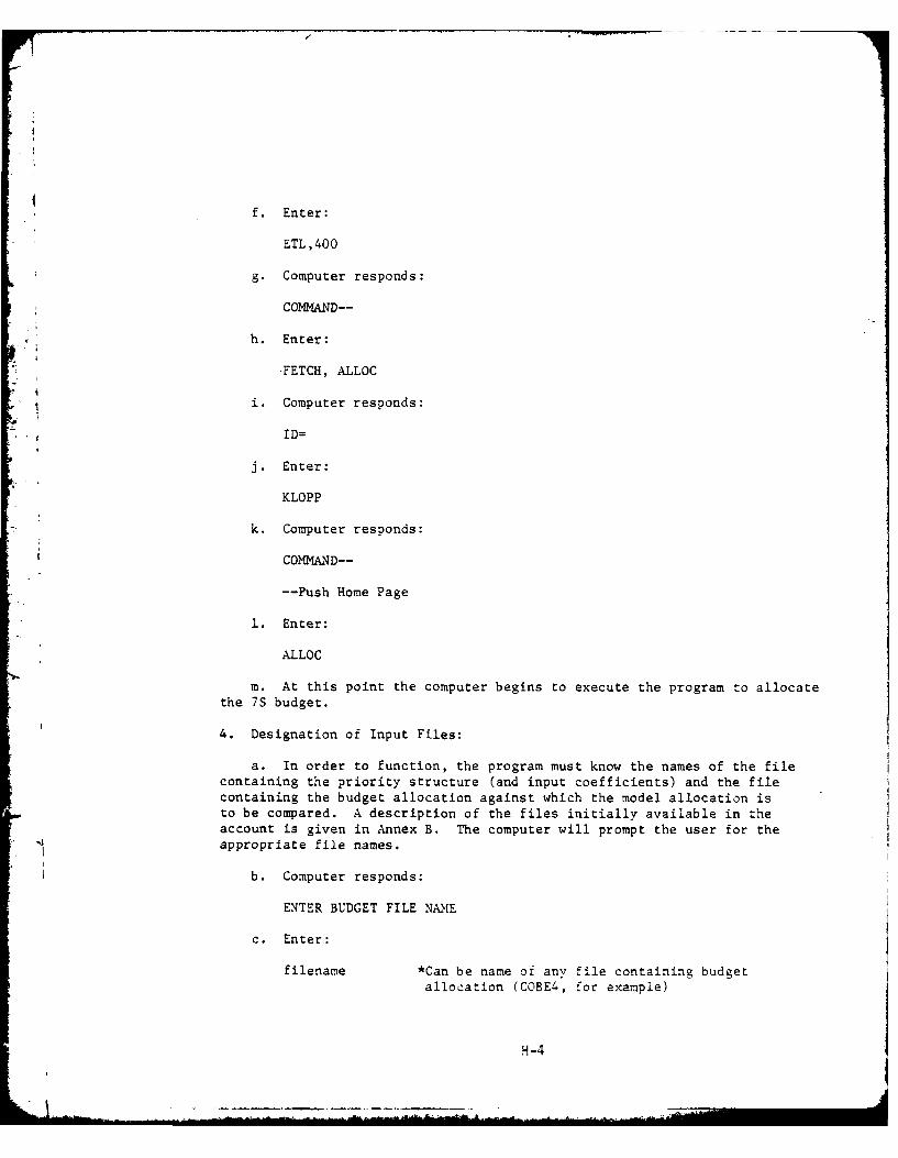
f. Enter:
ETL,400
g. Computer responds:
COMMAND--
h. Enter:
-FETCH, ALLOC
i. Computer responds:
ID=
j. Enter:
KLOPP
k. Computer responds:
COMMAND--
--Push Home Page
1. Enter:
ALLOC
m. At this point the computer begins to execute the program to allocatethe 7S budget.
4. Designation of Input Files:
a. In order to function, the program must know the names of the filecontaining the priority structure (and input coefficients) and the filecontaining the budget allocation against which the model allocation isto be compared. A description of the files initially available in theaccount is given in Annex B. The computer will prompt the user for the
_ appropriate file names.
b. Computer responds:
ENTER BUDGET FILE NAME
c. Enter:
filename *Can be name of any file containing budgetallocation (COBE4, for example)
H-4
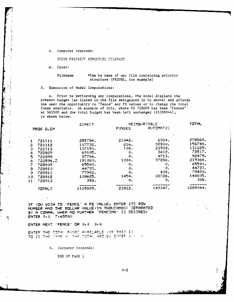
$ d. Computer responds:
ENTER PRIORI-7Y STRUCTU"RE FILENAYT
e. Enter:
filename *Can be name of any file containing prioritystructure (PRIORl, for example)
5. Execution of Model Computations:
a. Prior to performing any computations, the model displays thepresent budget (as listed in the file designated in 4c above) and affordsthe user the opportunity to "fence" any PE values or to change the totalfunds available. An example of this, where PE 728009 has been "fenced"at $65500 and the total budget has been left unchanged ($1289044),is shown below:
t'IPECT RE IMBLP'H-BLE rTTALPROG ELEM FUNDED FiUT:OMF4T I C
1 721111 255784. 21042. 2(134. 278860.2721112 117732. 216. 38*z801). 156749.
3 722111$ 107190. 100. '231:3-3. 131228.4 722829 69105. 0. '3412. 72517.5 72289 8766 1). 4713. 92479.
6 7228,9.' 181080:. 1000. 372806. 219*366.
*7 729009 65500. 0:. 0. 65''8 728010 44173:3. :'. 0. 473
9728011 77982. 0. 4:38. 79420.10 728012 1083625. 1454. 38726. 14880)5.
r11 728013 388. 0. 0. 3:38.
TOTALS: 1115885. 238312. 149:347. 1289044.
IF YOU WI&14 TO 'FENCE' Rt PE '-YF4LUEi, ENTER ITS ROWdNUMBER ANiD THE DOLLA$R VRLUE(IN THOUSANDSts) :3EPRtPTEDBle R COMMAt. WHEN NO FURTHER 'FENCING-' IS TIESIREtIENTER 090 7-65500
ENTER NEXT 'FENCE' OR 090 090
ENTE= T'-E TITzA fj4:*!~FE T;: TwU7 1-
T13 T-= -1 : T64 T:]T-;4 ciE.r:2 C:4T~r i
b. Ccrputcr responds:
END OF PAGE 1
H-5
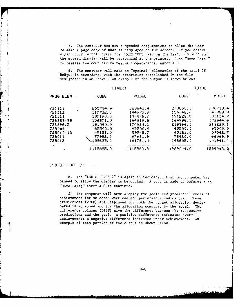
I
c. The computer has now suspended computations to allow the user
to make a page copy of what is displayed on the screen. If you desirea pagy copy, simply press the "MAUKE COPY" key on the Tektronix O5 .the screen display will be reproduced at the printer. Push "Home Page."
To release the computer to resume computations, enter a 0.
d. The computer will make an "optimal" allocation of the total 7Sbudget in accordance with the priorities established in the filedesignated in 4e above. An example of the output is shown below:
DIRECT TOT.L
PROG ELEM COBE MODEL COBE MODEL
'721111 255784. G- 269643.4 278860.0 22719. 421112 117732.0 104973.9 156748. 0 1439:9'. 91
07190. 0 107076.7 131228. 0 131114.772292S-'98 156871.0 1648 19.6 1649'N. 172944.6722896. Z 1811080.0 1749.34.1 -19:366. 1) 213220.1,28009 65500.0 65500.0 65500. 0 65500. 07280 to./ 13 45121.0 59542. 7 45121.0 59542.7728011 \ 77982.0 67631.9 78420.0 60')69.729012 0S :.6 2 5. 01 101761.4 148805.0 141941.4
1 1158:_35. 0 1 115883.8 128'?044.0l 1289,043.0
ENtD "7 P, .E 2
c. The "END OF PAGE 2" is again an indication that the computer haspaused to allow the display to be copied. A copy is made as before; push
"Home Page;" enter a 0 to continue.
f. The cor puter will next display the goals and predicted levels ofachievement for selected workload and performance indicators. Thesepredictions (PRED) are displayed for both the budget allocation desig-nated in 4c above and for the allocation computed by the model. Thedifference columns (DIFF) give the difference between the respectivepredictions and the goal. A positive difference indicates over-achievement; a negative difference indicates under-achievement. An
example of this portion of the output is shown below.
H-6
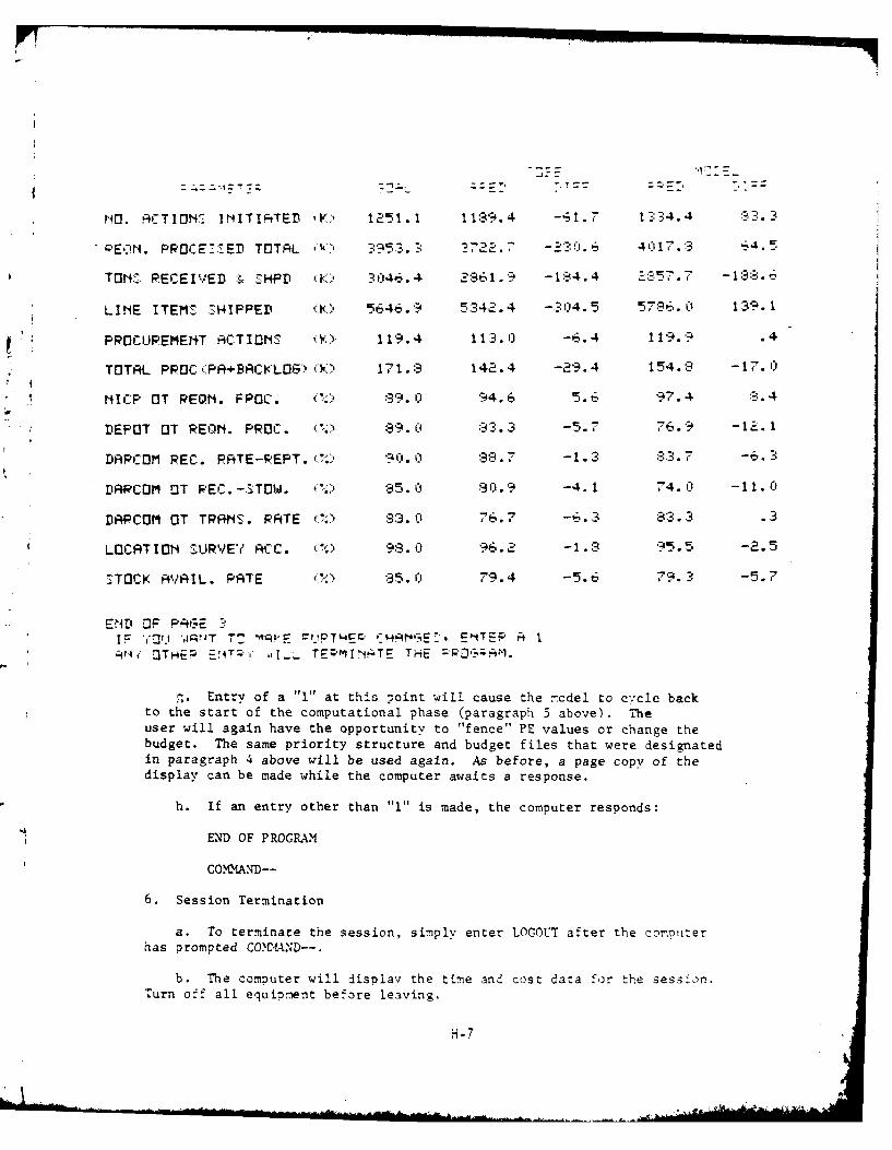
ri4. ACTION INITIF+TED K.' 1251.1 -119.4 -61.i , 1_34.4 3..
PEON.r. PPOCE _'ED TOTAL '. . . .3 " ''. -C ' .6 4017. . 5
TO: RECEIVED :- HPD .) 3046.4 28-_61.9 -1:94.4 S.57 -7 13.
LINE ITEMS N'HIPPED (10 5646.9 5342.4 -:4.5 57836.0 139.1
PROCUPEMENiT .CTIOti' ,'Ky 119.4 11:3.0 -6.4 119.? .4
TOTAL PROC'.PF+BACLOG >) 171.8 142.4 -29.4 154.8 -17. 0
NICP OT PEQN. FPOC. 39.0 94.6 5.6 97.4 ',.4
DEPOT OT REOM. PROC. '9.. :93. 3 -5.7 76.? -IQ.1
DAPCOM REC. PRTE-REPT. (.%) '4 Cf. 0 89.7 -1.3 3:3.7 -7. -
DACOM OT REC.-STOW. 85.0 90.9 -4.1 74. u -11. 0
DAPCOM OT TRPFH. RPTE (..- :93. 0 76.- -.. 3 3.3 3
LOCATION SURVE' AC. ,*', 98.'0 96.2 -1.8 95.5 -2.5
:TOCK FiVRIL. PATE :5.0 79.4 -5.6 . -5.7
END OP PRGE 3IF -f ',I NdT 7- " q'E r PnT- ' cHEir'3E.- E 4T 1* -JN OTHER I'iT -I. TEZ"MIN,"TE THE F'3'Al.
'. Entry of a "l" at this point will cause the -cdel to c.-cle backto the start of the computational phase (paragraph 5 above). Theuser will again have the opportunity to "fence" PE values or change thebudget. The same priority structure and budget files that were designatedin paragraph 4 above will be used again. As before, a page copy of thedisplay can be made while the computer awaits a response.
h. If an entry other than "1" is made, the computer responds:
END OF PROGRAM
COMMAND--
6. Session Termination
a. To terminate the session, simply enter LOGOUT after the comouter
has prompted COMMAND--.
b. The computer will display the time and cost data for the session.Turn off all equipent before leaving.
H-7
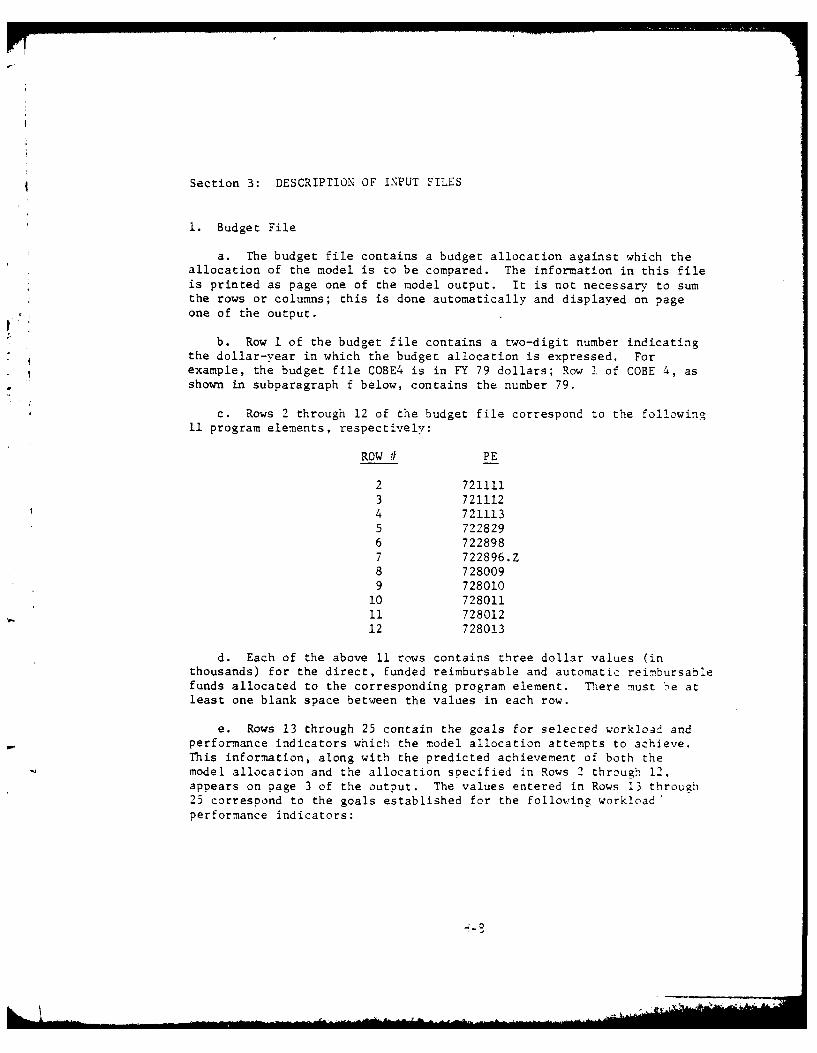
Section B: DESCRIPTION OF INPUT FILES
1. Budget File
a. The budget file contains a budget allocation against which theallocation of the model is to be compared. The information in this fileis printed as page one of the model output. It is not necessary to sumthe rows or columns; this is done automatically and displayed on page
one of the output.
b. Row 1 of the budget file contains a two-digit number indicating* the dollar-year in which the budget allocation is expressed. For
example, the budget file COBE4 is in FY 79 dollars; Row 1 of COBE 4, asshown in subparagraph f below, contains the number 79.
c. Rows 2 through 12 of the budget file correspond to the following11 program elements, respectively:
ROW # PE
2 7211113 7211124 721113
5 722829
6 7228987 722896.Z
8 7280099 728010
10 728011
11 728012
12 728013
d. Each of the above 11 rows contains three dollar values (inthousands) for the direct, funded reimbursable and automatic reimbursablefunds allocated to the corresponding program element. There must 'e atleast one blank space between the values in each row.
e. Rows 13 through 25 contain the goals for selected workload andperformance indicators which the model allocation attempts to achieve.This information, along with the predicted achievement of both themodel allocation and the allocation specified in Rows 2 through 12,appears on page 3 of the output. The values entered in Rows 13 through25 correspond to the goals established for the folloving workload'performance indicators:
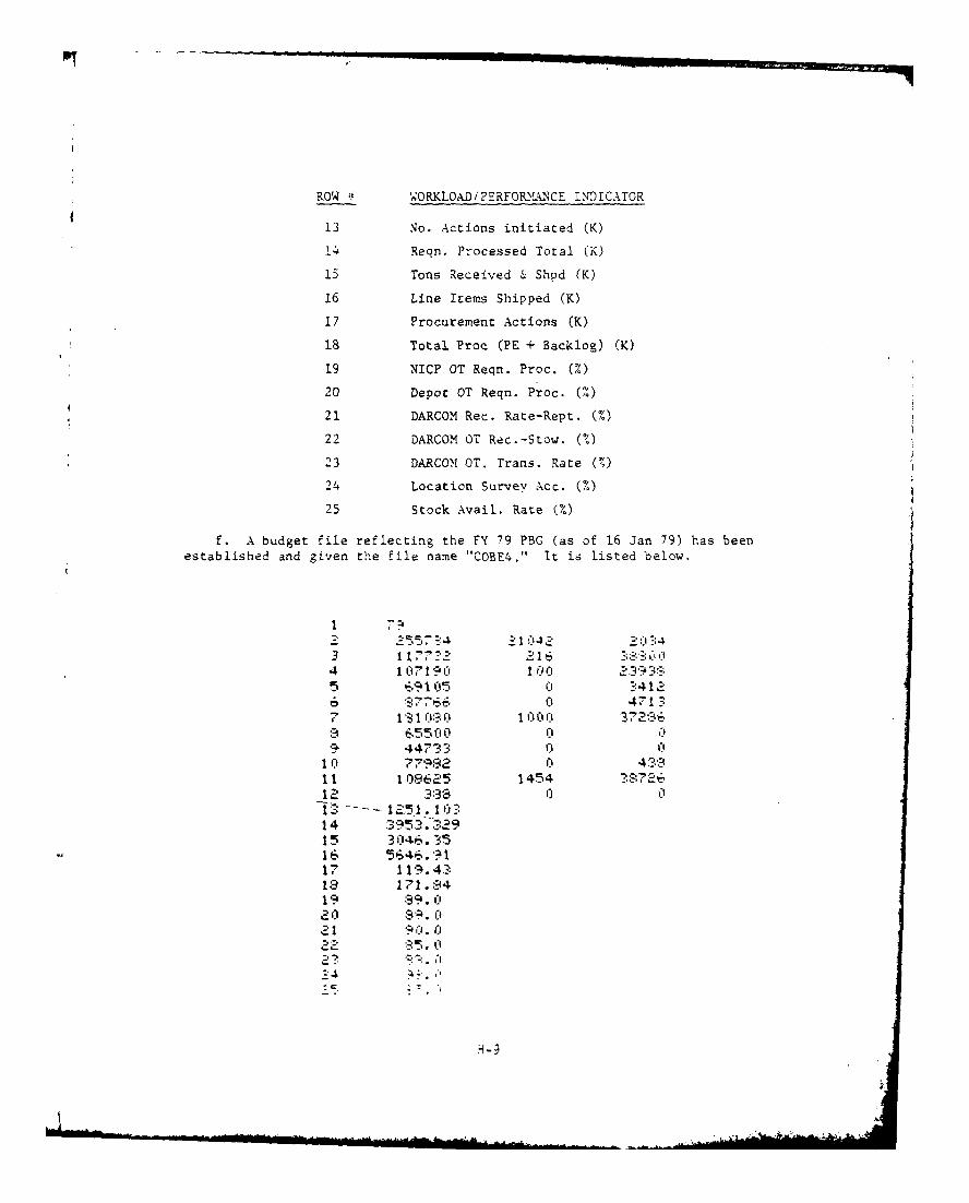
ROW 4 WORKLOAD/PERFOR2%WNCE INDICATOR
13 No. Actions initiated (K)
14 Reqn. Processed Total (K)
15 Tons Received & Shpd (K)
16 Line Items Shipped (K)
17 Procurement Actions (K)
18 Total Proc (PE + Backlog) (K)
19 NICP OT Reqn. Proc. (%)
20 Depot OT Reqn. Proc. (%)
21 DARCOM Rec. Rate-Rept. (%)
22 DARCOM OT Rec.-Stow. (%)
23 DARCOM OT. Trans. Rate (%)
24 Location Survey Acc. (%)
25 Stock Avail. Rate (%)
f. A budget file reflecting the FY 79 PBG (as of 16 Jan 79) has been
established and given the file name "COBE4." It is listed below.
-1 -,J -.,
11... :,n42-
4 107 19 C 100
: 7766 10 471
7Z1 'I O'S1 00Cro55 0 0 01
44733 C117492 0 4.,
11 108625 1454 872-612 33;B800
-1E- .10314 3953. 32915 30F6 . 3516 5O46.117 119.4?1 171. 419 8 9.0
d-. . C,
", ,. 2,'L,. I
H- ?
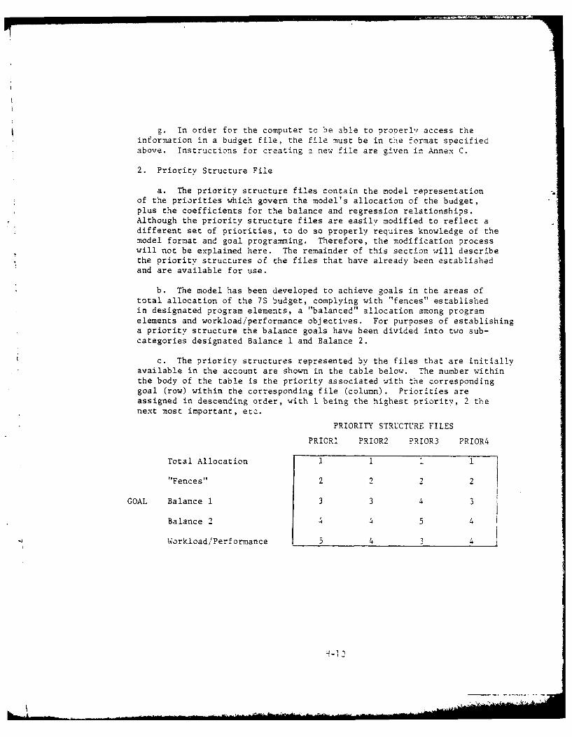
. In order for the computer to be able to properly access theinformation in a budget file, the file must be in the format specifiedabove. Instructions for creating a new file are given in Annex C.
2. Priority Structure File
a. The priority structure files contain the model representationof the priorities which govern the model's allocation of the budget,plus the coefficients for the balance and regression relationships.Although the priority structure files are easily modified to reflect adifferent set of priorities, to do so properly requires knowledge of themodel format and goal prograrmming. Therefore, the modification processwill not be explained here. The remainder of this section will describethe priority structures of the files that have already been establishedand are available for use.
b. The model has been developed to achieve goals in the areas oftotal allocation of the 7S budget, complying with "fences" establishedin designated program elements, a "balanced" allocation among programelements and workload/performance objectives. For purposes of establishinga priority structure the balance goals have been divided into two sub-categories designated Balance 1 and Balance 2.
c. The priority structures represented by the files that are initiallyavailable in the account are shown in the table below. The number withinthe body of the table is the priority associated with the correspondinggoal (row) within the corresponding file (column). Priorities areassigned in descending order, with I being the highest priority, 2 thenext most important, etc.
PRIORITY STRUCTURE FILES
PRIOR PRIOR2 PRIOR3 PRIOR4
Total Allocation 1 1 1 1
"Fences" 2 2 2 2
GOAL Balance 1 3 3 4 3
Balance 2 4 4 5 4
Workload/Performance 5 4 3 4
H-Ii
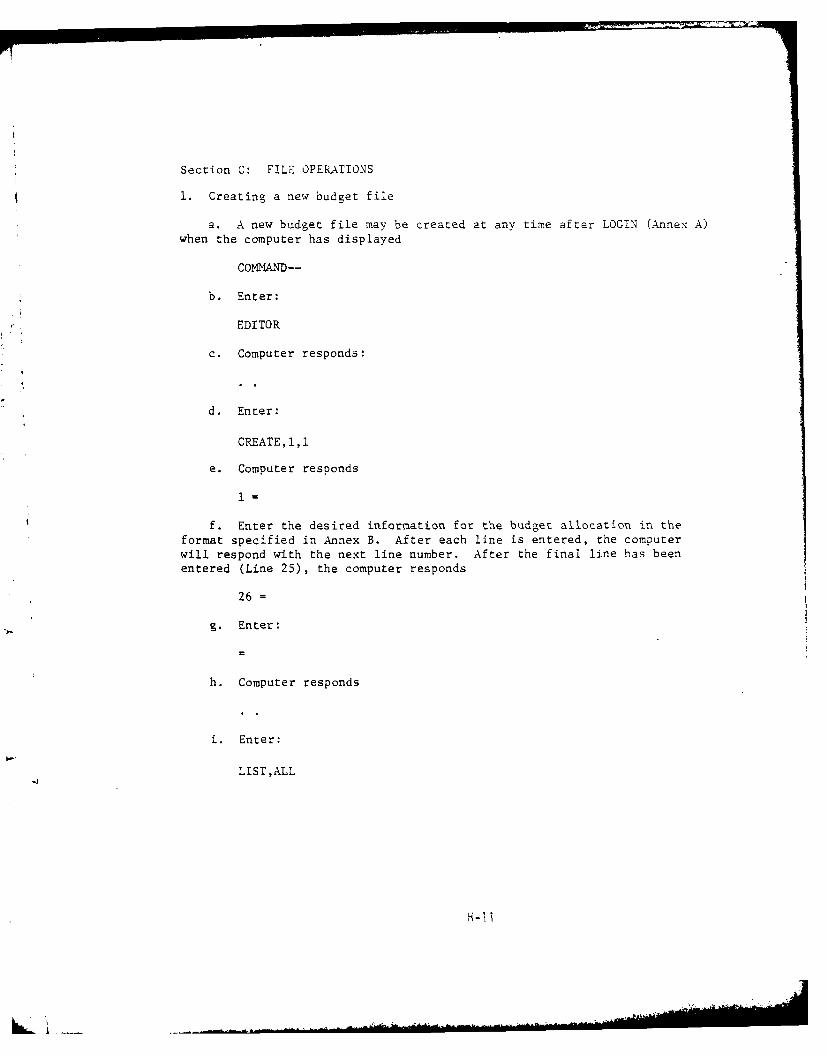
Section C: FILE OPERATIONS
1. Creating a new budget file
a. A new budget file may be created at any time after LOGIN (Annex A)
when the computer has displayed
COMMAND--
b. Enter:
EDITOR
c. Computer responds:
d. Enter:
CREATE,1,1
e. Computer responds
1=
f. Enter the desired information for the budget allocation in theformat specified in Annex B. After each line is entered, the computer
will respond with the next line number. After the final line has been
entered (Line 25), the computer responds
26=
g. Enter:
h. Computer responds
i. Enter:
LIST,ALL
MoA
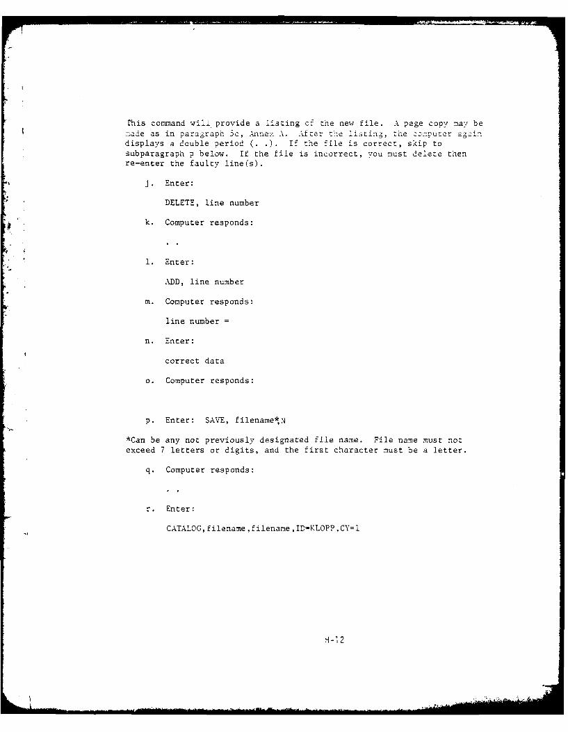
This command will provide a listing of the new file. A page copy may benade as in paragraph 5c, Annex A. After the listing, the co=puter agaiindisplays a double period (. .). If the file is correct, skip tosubparagraph p below. If the file is incorrect, you must delete thenre-enter the faulty line(s).
j. Enter:
DELETE, line number
k. Computer responds:
1. Enter:
ADD, line number
m. Computer responds:
line number =
n. Enter:
correct data
o. Computer responds:
p. Enter: SAVE, filename*N
*Can be any not previously designated file name. File name must notexceed 7 letters or digits, and the first character must be a letter.
q. Computer responds:
r. Enter:
CATALOG,filename ,filename,ID-KLOPP,CY=i
H-1 2
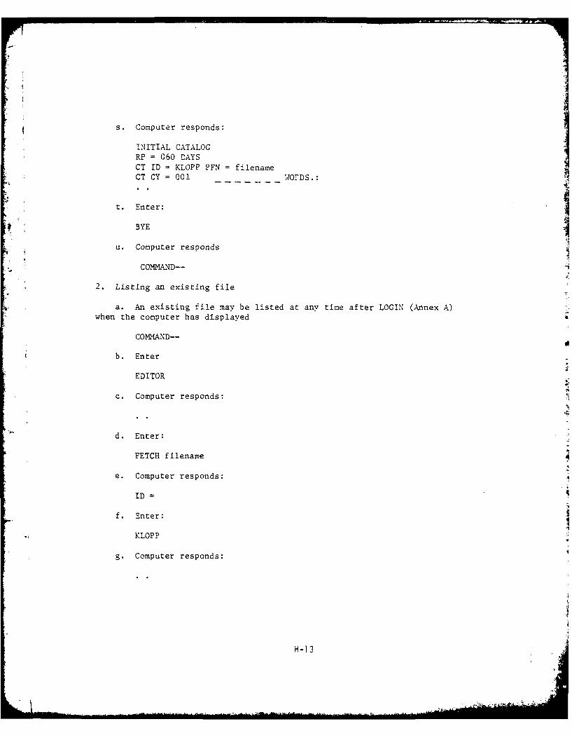
s. Computer responds:
INITIAL CATALOG
RP = 060 DAYS
CT ID = KLOPP PFN = filenameCT CY = 001 WO-DS.:
t. Enter:
* BYE
U. Computer responds
COMIAND--
2. Listing an existing file
a. An existing file may be listed at any time after LOGIN (Annex A)when the computer has displayed
COMMAND--
b. Enter
EDITOR
c. Computer responds:
d. Enter:
FETCH filename
e. Computer responds:
ID =
f. Enter:
KLOPP
g. Computer responds:
H-I 3
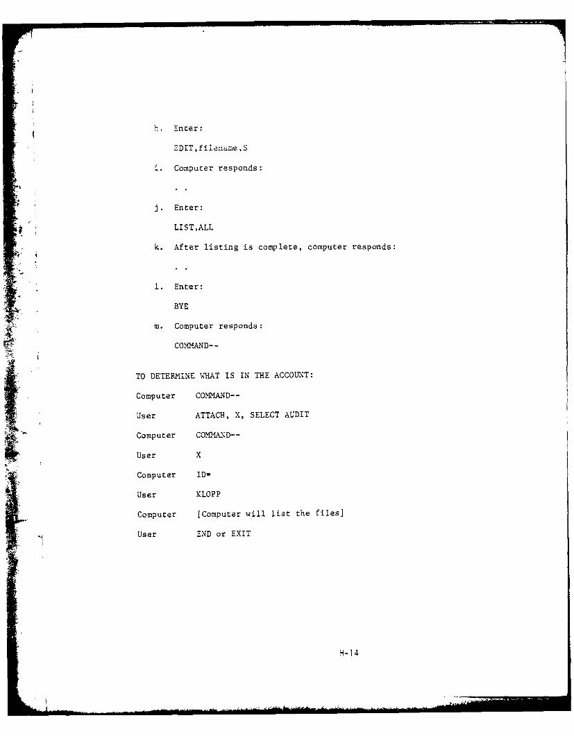
h. Enter:
EDIT,filename,S
i. Computer responds:
j. Enter:
LIST,ALL
k. After listing is complete, computer responds:
1. Enter:
BYE
m. Computer responds:
COMAND--
TO DETERMINE WHAT IS IN THE ACCOUNT:
Computer COMAND--
User ATTACH, X, SELECT AUDIT
Computer COM.MAND--
Lw User X
Computer ID=
User KLOPP
Computer [Computer will list the files]
User END or EXIT
H-14

ANNEX I
COMPUTER PROGRAM
ii
ANNEX I
COMPUTER PROGRAM
The remainder of this annex contains the documented computer program
for the DELTA 7S model. This FORTRAN program is based upon modifications
to the program listed in Goal Programming for Decision Analysis by Sang M.
Lee, and another modification to this program by the US Army Concepts
*. Analysis Agency. This particular listing is operational on the HP 3000
minicomputer at the US Army Logistics Management Center. The program
operational on the Picatinny Arsenal computer is essentially identical to
this one.
1-2
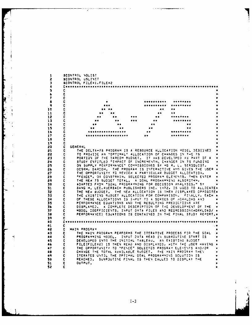
1 SCONTROL NOLIST2 SCONTROL USLINIT3 SCONTROL FILE:lFILE:24 COOOO*0000000000000000000*oOO**..ooooo.*oOOOOOOO*0000000000000*0000
40.4 5 C
b C 0-7 C 0
S C 0 0*00*00000 *00000009 C 000 *00 00 ****ooo
10 C *1 C *12 C 0 0000 000*
13 C 0T *R IS 0U TOOEo 014 C 0* "T L T N7 *15 C *0 r O 00 00 T16 C 3TU O O * IooooT N N 000000*00 U17 C N U Y oOooo E" CO 000*0*00 0
18 C 0
19 C020 C GENERAL e21 C THE DELTA-1S PROGRAM IS A RESOURCE ALLOCATION MODE DESINE *22 C TO PROVI)E AN "OPTIMAL" ALLOCATION OF CHANGES IN TmE Is23 C PORTION OF rHE DARCOM BUDGET. IT AS DEVELIPE AS PART OF A 0
24 C STUDY ENTITLED "IPACT OF INCREMENTAL C7ANES IN 75 FUNDING T25 C ON SUPPLY ORFOqRMANCE" COM'MISSIONED 3Y -AG q. L. SERS~uIST,26 C OCGRM DAR:O.. THE PROGRAM is INTERACTIVE A!'N GIVES TOE SER *27 C THE OPPORTUNITY TO EVIEo A PARTICULAR BUDGET ALLOCATIONJ, k
28 C "FeCNCE". OR CONSTRAIN, SELECTED PROGRAm ELE,4EATS. 'HEN ENTER *29 C THEE NEA IS Su0ET TOTAL. A GOAL PERIOAMMING ALGORITI'AO 0
30 C ADAPTED FR M "GOAL PROGRAMMING FOR DECISION ANALYSIS" Y31 C SANG M. LEEoAUERSACH PUBLISHERS INC. 1972, IS USED TO ALLOCATE*32 C THE NEvO 6UOGET. THE N~q ALLOCATION IS THEN O'ISPLAYED OPPOSITE*33 C TH4E ceXISTING RUOGET ALLOCATION FOR COMPARISONi. ZIALLY, EACH034 C OF THESE ALLOCATIONS4 IS I.,iPUT To A SERIES OF -4CR'(LOAO AN) 0
35 C PERFORMANCE E,)UATIONS AND THE RESULTING PREDICTIZ-v ARE036 C DISPLAYEO. A COMPLETE DESCRIPTION OF THE OEVELOP4ENT OF THE *37 C MODEL :OEFFICIENTS, INPUT DATA FILES AND REGRESSION(AORXLOAD/ 0
38 C PERFORMANCE) EOUATIONS Is CONTAINED IN THE FINAL STUDY REPORT.*39 C 040 C0000000000000000000000000000000000000000000000000000000000000000000
41 C .0
42 C MAIN PROGRAM 0
43 C THE MAIN PROGRAM PERFORMS THE ITERATIVE PROCESS FOR T'4E GOAL 0
44 C PROGRAMMING MODEL. INPUT DATA READ IN SUBROUTINE START IS 0
45 C DEVELOPED INTO THE INITIAL TABLEAU. AN EXISTING 3UDGET •46 C FILE(FILE:2) IS THEN REAO AND DISPLAYED, NITH THE JSER HAVING 0
47 C THE OPPORTUNITY TO "FENCE" SELECTED PROGRA'A ELE'.E'iTS AND/DR 0
48 C CHANGE THE TOTAL AVAILABLE 9UOGET. THE MAIN PROSRAM Tr4E' 0
49 C ITERATES UNTIL THE OPTIMAL GOAL PROGRAMMING SCLUTION IS50 C REACHED. SU4ROUTINE FINAL I THEN CALLED TO DISPLAY THE 0
51 C OUTPUT. 0
52 C
1-3

53 C VARIABLE DEFINITIONS IN THE MAIN PROGRAM54 C VARIABLE USAGE IN THE SUBROUTINES IS CONSISTENT aITo THE55 C DEF I fT InN5 LISTED 6ELDA. VARIABLE DEFINITIONS 0 R TH4E56 C SUBROUTINES NILL NOT REPEAT ANY OF TWE BELOd, LISTED57 C DEFINITIONS. *S C59 C NROv4S NUMBER OF ROAS(GOALS OR CONSTRAINTS)60 C NVAR READ IN AS NUMBER OF DECISION VAPIABLES. UPDATED .bi C IN SUBROUTINE START TO INCLUDE OEVIATIONAL AND *
62 C ARTIFICIAL VARIABLES ADDED. *63 C NPRT NUMbER OF PRIORITY LEVELS. SUBROUTIJE START ADDS*64 C AN ADDITIONAL LEVEL TO ACCOMMODATE ARTIFICIAL
: 65 C VARIABLES IF NECESSARY.b6 C C(IJ) TECHNOLOGICAL COEFFICIENTS OF THE SIMPLEX TABLEAU *
67 C RVLX(I,J) ZJ-CJ VALUES FOR TAE I TH PRIORITY, J T4 VARIABLE *68 C VALX(IJ) CJ COEFFICIENTS FOR THE I TH PRIORITY, J TH VAR. 0
69 C VALY(JI) CJ COEFFICIENTS FOR THE BASIS VARIABLES70 C RHS(I) RIGMT-HANO-SIDE VALUE FOR THE I TH RODA71 C RHSI(I) ORIGINAL RIGHT-HAND-SIDE VALUE FOR T4E I TH 0A *72 C NALPI NUMbER OF vORKLOAO/PERFORMANCE INDICATOR EQUATIONS*73 C INYR DOLLAR YEAR OF EXISTING BUDGET FILE(FILE=2)74 C FACTOR INFLATION AOJUSPmENT FACTOR *
75 C COBE(IJ) EXISTING BUDGET 5Y PROGRAM ELEET ANjO TYPE FUNDS o
7b C SUM(1) qOm TOTAL OF BUDGET FILE. iY PRUGRAM ELEMENT77 C TOTAL(I) COLUMN TOTAL OF BUDGET FILE. BY TYPE FUNnS *78 C BUDGET TOTAL DOLLARS AVAILAiLE IN EXISTING BUD;ET FILE79 C CORRE(I) PARTIAL PREDICTION OF vvORKLOAO/FERFORMANCE OF .80 C EXISTING BUDGET. COMPLETED IN SUBROUTINE FINAL 0
81 C WHEN REGRESSION CONSTANT IS INCLUDED.82 C FENCES(•,J) USER LIIT PLACED ON INDIVIDUAL PROGRAM ELEMENTS .
83 C X(j) VARIABLE NUMSER OF VARIABLE IN THE J T- COLUMN *64 C Y(I) VARIABLE NUMBEW OF THE I TX VARIABLE IN THE BASIS *85 C L1K3 USED TOGETHER DURING ITERATIONS TO CHE K ARRAYS *
86 C STARTING AT LAST ROW, MOVING TO FIRST qfl87 C SUMP ZJ VALUE COMPUTED DURING SIMPLEX ITERATIONS *88 C ZMAX MAXIMUM ZJ-CJ - COEFFICIENT OF ENTERINS VARIABLE ,89 C AMT(I) RHS(I)/C(I,J) -> DETERMINES LEAVING VARIABLE *
90 C ZMIN MINIMUM AMT(I) -) LI4ITING AMOUNT OF LEAVING VAR. *
91 C K2 COLUMN NUMBER TO ENTER BASIS92 C ITER ITERATION NUMBER93 C9495 DIMENSION C(lIO,2),RVLX(b6,O2).VALX(C*IO2),VALY9b *( ltS)#9-SI(41),Y(4I),RHS(4I],AMT(4I),CO6PRE(13),
97 *X(1O2),COBE(II,3),PECII),SUM(1I),TOTAL(3),FENCESCII,2)98 CHARACTER*q PE99 DATA PE(I),PE(2)PE(3)/9H721111 09H721112 ,9*721113
100 DATA PE(a),PE(b),PE(7)/qH722829 ,9H7228b.Z o9H723009 /101 OATA PE(8),PE(9),PE(1O)/9m72301O ,9H728011 ,H9-BO1e /102 DATA PE(5)ePE(ll)/9H722SS ,gM728013 /103 NwLPI 2 13104 9999 CALL START(NRCS,NVARNPRT,C,VALXVALY,RHSRVLX)
1-4
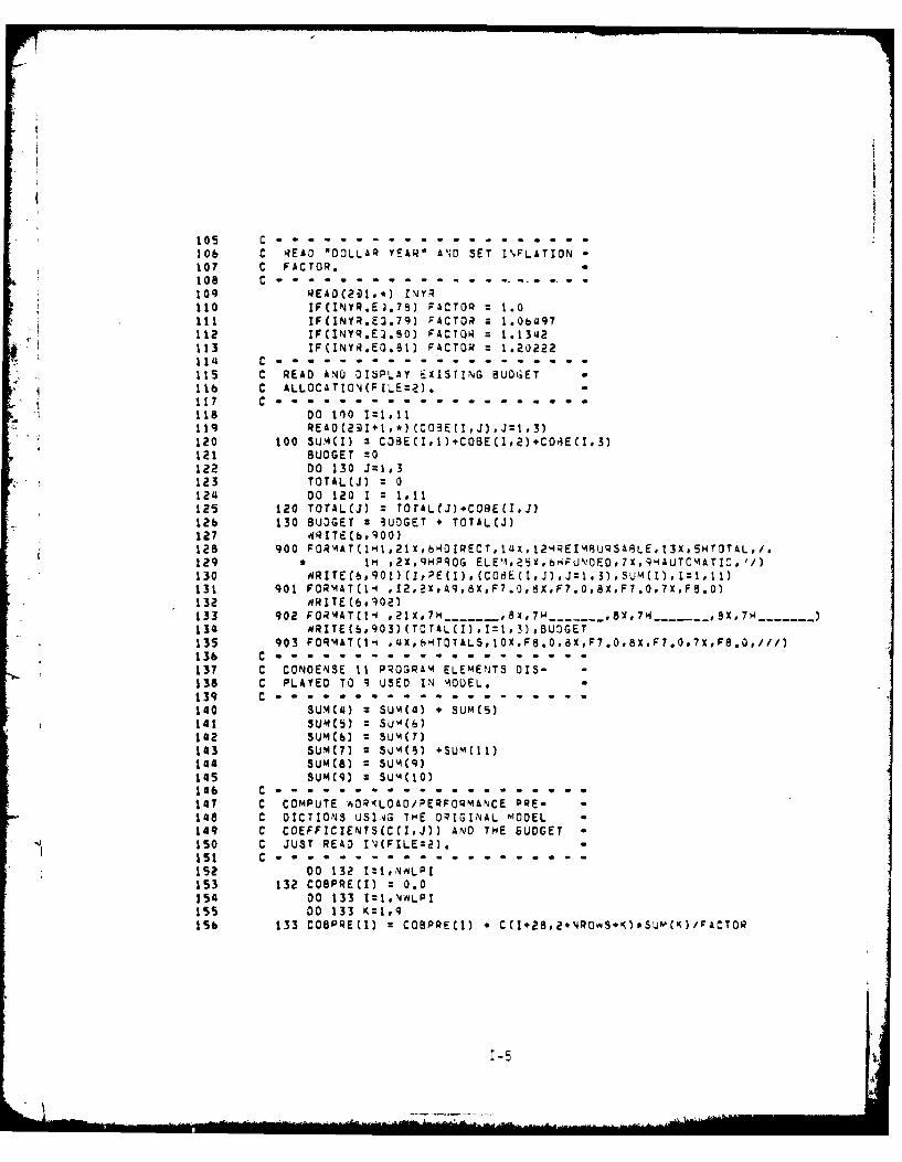
105 C .-
106 C READ "DOLLAR YEAR" A4D SET I'%FLATI0N107 C FACTOR.108 C .-- . . . . . . .. .
110 IF(IN'vR.E;9.78) FACTOR 1.0III IFCINYR.E3.79) FACTOR = 1.06497112 IFCINYR.E .90) FACTOR~ z 1.1342113 IFCINY'9.EG.812 FACTOR = 1.20222
14 C .- . . .*
115 C READ ANU DISPLAY wxisrING BUDGET
4116 C ALLOCATION(FILE:2) -
I1I7 C -.. .. .. .. .. .. .. .. ...
118 00 100 1:1.11l
120 100 SU.M(I) z COEII+OEIp)CrEI3121 BUDGET =0122 DO 130 1=1,3123 TOTALW = 0124& 00 120 1 = 1,11125 120 TorAL(J) z T0TAI..J)+COE(I.J)12b 130 BUDGET = 3UDGET + TOTALWJ127 IQ~ITE(b,900)128 900 FORMAT(Il1.21x,b-4OIQECT,14X, l2NREIMRUqSA6LE. 13X,5HTOTAL,/.129 *Im t2X#9HPROG ELEM,125X,bP-FiUE,7X~qAUTMATI:.,/)130 ARItEC6,90l) (IPE(I).(C~i3E(IJ) .31,3) ,$UM(1) .1:1,11)131 901 FOR'4AT(1-4 * I2,2X,A9,8X.F7.O,8XF7.0.8XF7.0.7X,F9.0)132 OVRITE(6,902)133 902 FOR4TMt *21X,7m E7-------- 8X,7H ----- r..,BX---S),7H ---134 ARITEC6.903) (TOTALU(I:1,~l3),BUDGET135 903 FORMAT(1I ,4X.bpTOTALS, 10X.F8.0,8X,F7.O,8XF7.0,7x,F8.0.///)136 C . . . . . .. .w. .. .. .. ..
137 C CONDENSE 11 PROGRA"' ELEMENTS 013- -
138 C PLAYED TO 9 USED IN MIOEL.139 C 0 . . .. . .. .. .. .. .. .
140 SU'4(0 z SU'i(4) + SUM(S)141 SUM C 5) z SUA(b)142 SUW SUM(7143 SUMM7 z Su"1(S) *SuM(11)144 SUMW8 z SUM(9)145 SUNC9 z SUM(10)106 C......... ..... . . ... . . . . .. .
147 C COMPUTE AOR LOAD/PERFORMANCE PRE-148 C DICTIONS USING TooE OqIGINAL HODEL149 C COEFFICIENTS(CUvJ)) AND THE SUDGET
ISO C JUST READ IN(FILEz2).151 C *..ft. .... ... .. .
152 00 132 :,jL153 132 COBPRE () 0.0154 00 133 lLP155 DO 133 K=10q156 133 COOPREMI) COBPREMI + C(I,28.2*NROAS.IK).Suw(K)/rACTOR
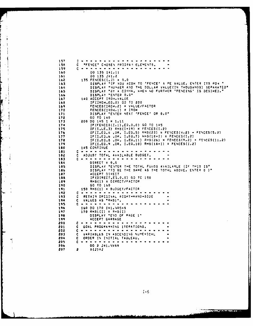
157 C . . . . . . . . . .
158 C "FE'CE" CAOSN PO;; A.' ELEmENTS. -
159 C .. ....... ..................160 00 135 1:1,11161 00 135 J=1,21b2 135 FENCES(1,J1 = 0.0163 DISPLAY "IF YOU AISH TO 'FENCE' A PE VALUE, ENTE4 ITS P04164 DISPLAY "NUMdER A DJ THE DOLLAR VALUE(IN THOUSANDS) SEPARATED"lbs DISPLAY "dY A C04MA. WHEN NO FURTHER 'FENCING' IS OESIRE ,"16b DISPLAY "ENTER 0,0"167 140 ACCEPT IROA.VALUE168 IF(IROO.ECI.O) 50 TO 200
169 FENCES(IROA,2) Z VALUE/FACTOR170 FENCE$S 0.R,] -- ICOW171 DISPLAY "ENTER NEXT 'FENCE' OR 0,0"r' i 72 GO TO 140
173 200 00 1 I5 I = P Hl A174 IF(FENCES(EQ.0.O) GO TO 145176 IF(I.LE.:) RHS(1+19) z FENCESCI,2)176 IF(I.E .4 .OR. I.EQ.5) PHS(23) = FENCE$C[ ,2) FE4CESC5o2)
177 IF(IE .b OR. I.EQ.7) kmS(1S I) I FENCES(I,21178 IF(IE. .OR. .EO. ) RHS(2) = FENCE(A*2) + 9ENCES(11,2)179 IF(IEQ OR IEOO) RHS(18 I) x FENCES(1,2)too 145 CONTINUE
l00 C ..................182 C ADJUST TOTAL AVAILATLE BUOGET.183 C. . . . . .........................164 DIRECT:= 0.0'185 DISPLAY "EN TER THE TOTAL FUNDS AVAILABLE (IF THIS IS"
186 DISPLAY "TO BE THE SAME AS THE TOTAL ABOVE, ETE; 0187 ACCEPT DIRECTtoo IF(OIRECT.gOO) GO TO 150189 RMS(1) z DIRECT/FACTOR190 GO TO 1b0191 150 RHMI z BUDGET/FACTOR192 C . .. .. .. .. .. .. .. .. .. .193 C RETAIN ORISINAL RIGHT-HAND-SIDE -194 C VALUES AS "RHSI",145 C . .. .%. .. .. .. .. .. .. ...196 160 DO 170 I:INRO^S197 170 RHSI(I) = RAS(I)198 D13PLAY "ENO OF PAGE I"199 ACCEPT GRgAGE
201 C GAL PROGRA;47N: iTT7 3:TO
203,o Cc "V;PT;L:5'1; ;S E;O7N: ZU:E4I ,A ""204 C ORDER IN INITIAL TA6LEAU,2 0 C .... . . .. .. .. .. ...20b DO0 2 Jz:NA207 2 x CJ):zJ
i \ . .. . ... . . ' ', 1-6
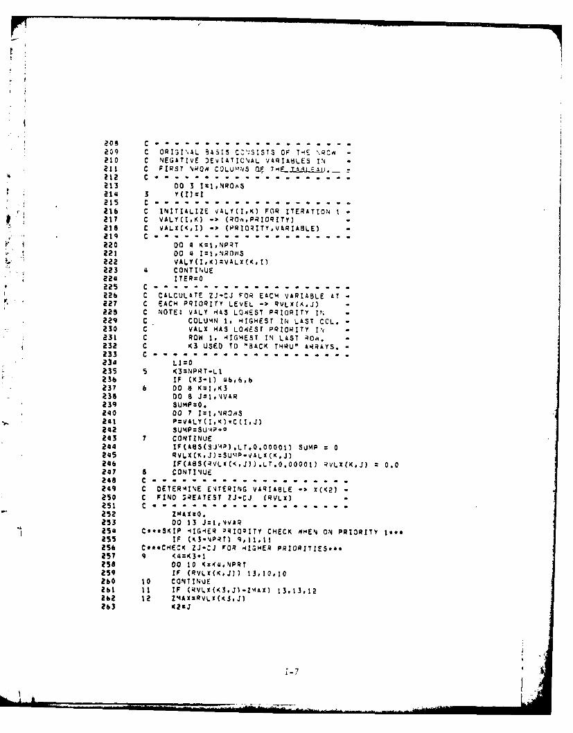
208 C------------------------------------------209 C ORI31'4 AL 3ASIS C 'SISTS OF T-E %W -
210 C NEGATIVE )EVtATIONAL VARIABLES IN211 C FIRST NkO COL.Uk!NS QF To4EL.L-3L_;__i__212 C .
213 ;0 3 Iml PNROAS21" 3 Y (I I c216 C INIILIZE V'ILY(I,11. ;0; ITERATION1
* a17 C VAL'(I,K) -M(Rs#PRIOqITY)-218 C VALX(I) - PRIORITy#V4RIA8LE)?19 C7220 00 a KcI,NP4RT
4221 00 ~a I21#,ROVIS222 VAL(I,K)=VALX(Ks1)
223 '1 CONTINUE224 C -Q=
226 C CALCULATE ZJ-CJ FOR EACH VARIABLE AT227 C EACH4 PRIORITY LEVEL -I PVLX(A*J)225 C NOTE: VALY HAS LOAEST PRIORITY IN229 c COLUMN Is HIGHiEST IN LAST COL.-230 C VALX HAS LOAEST PRIO'AITY IN -
231 C ROW 1, 4IGHEST IN LAST ROae. -
232 C K3 USED TO "BACK THRUM AR~RAYS.-233 C . sm e........................ . . .. .. .. ...234 LIzO235 5 K3=NPRT-LI236 IF (K3-1) 46,6,b237 6 DO 8 Xzt,K3238 00 8 J:1.NVAR239 3UMP=0.2410 00 7 I:1,NROAS
I.241 PZVALY(I,()*C(IJ)2412 3U4P=SU4P*P243 7 CONTINUE244 IF(A8S(SU'41P).L-T.0.0000I) SUJMP :0245 RVLXCKtj)=SUkIP-VALK (K.J)246 IF(A8SCRVLxK#(JU).LT.O.0000I) RVLX(K.J) :0.0247 a CONTINUE2418 C............................................?419 C DETER4iINE E\ITERING VARIABLE -1 X(K2)-250 C FIND SREATEST ZJ-CJ (RVLX)251 C--------------------------------------------252 ZpAk:0o.253 00 13 j:1,VVAR254 C*..SKIP -41G4IER PRI04ITY CH'ECK AHEN ON PRIORITY I***as5 IF (K3-'NPRT) q,11,1125% C*a.CH4ECK ZJ-OJ FOR .410xER PRIORITIES-.257 9 zK#as8 00 10 KgQ.NPRT259 IF (qVLX(K#J11 13,10,10260 10 CONTINUE261 it IF CiIVLX(K3.J)-ZMAX) 13,13,12a62 12 Z4AKUQvLx(KS.J)263 K23J
1-7
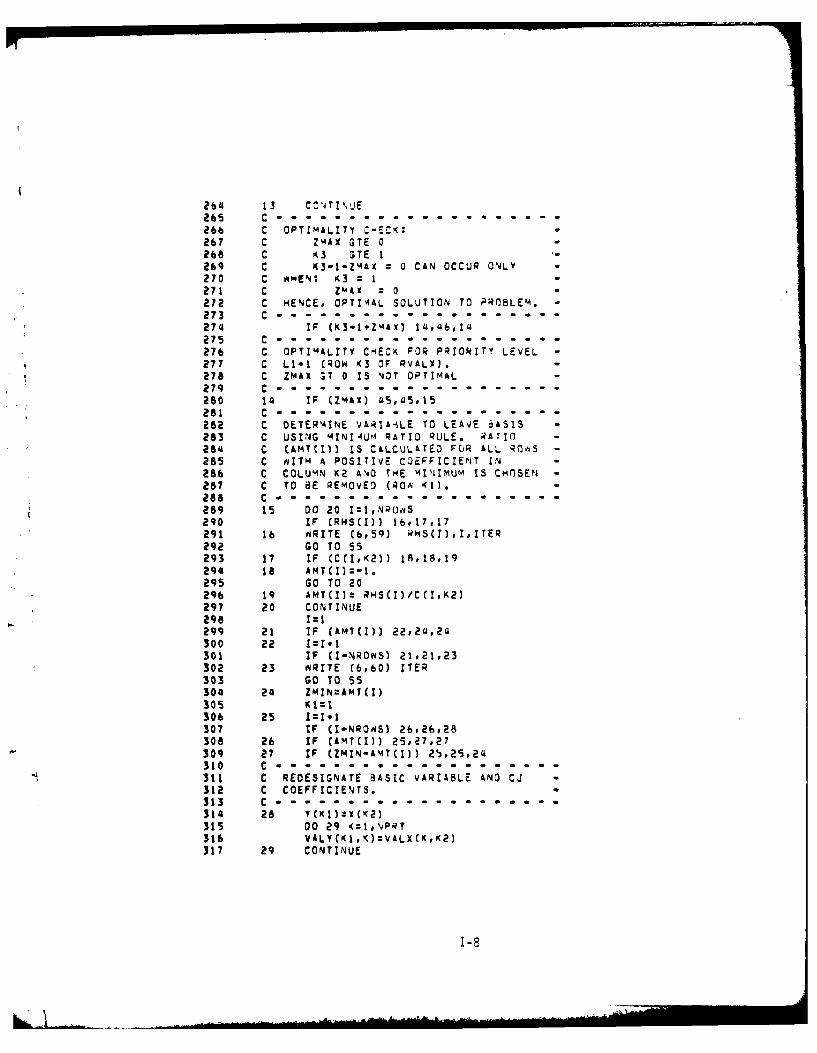
?64 13 CC'T!N'jE265 C .26b C OPTIMALITY 'CK267 C ZMAX GTE 02b8 C K.3 GTE I269 C K3-1-Z4AX 0 CAN OCCUR ONLY270 C AmEN: K3 1271 C ZMAX 0272 C HENCE, OPTIlAi. SOLUTION TO PROBLEM. -
273 C---------------------------m------274 IF (K3-1:Z:AX) 1:,a6,1a275 C.. .. ...................27b C OPT14AL;TY CIL; FO; PRIO;ITY LEVEL -
277 C L1.1 (ROW X3 OF QVALX).?78 C ZMAX GT 0 IS NOT OPTIM~AL279 C-----------------------------------280 14 IF (Zi4A1) o5.a5,15T281 C--------------------------------------282 C DETER4INE VARTAiLE TO LEAVE 8A515283 C USINJG 4INI4lUM QATIO RULE. 4ATIO -
284 C CAMTCI)) IS C&LCULATED FO~R ALL ROhS -
285 C OITH A POSITIVE COEPFICIENT IN286 C COLUM'N K2 ANO THE 41'JIMUCA IS CHOSEN -
287 C TO BE REmOVEO (QOni Kfl.288 C -- -----------------------------289 15 D0 20;:,~~290 IF (RHS(1)) 16#17,17291 16 ,iRITE (6,5q) iRNS(I).I,ITER292 GO TO 55293 17 IF (C(I,(2)) 18,18,19294 is AIT(I):-I.295 GO TO 20296 19 AMT(I)z RHSI)/C(IK2)297 20 CONTINUE298 121299 21 IF (AMT(I)) 22P24#.24300 22 I:Ii.1301 IF (I-NROwS) 21,21.23302 23 W~RITE (6o60) ITER303 GO TO 55304 24 ZMIN=AMTCI)305 Ka306 25 I=I~1307 IF (I-NROASI 26.2b,28308 26 IF (AMT(I)) 25,27o27
-309 27 IF (ZMIIN-&'iT(I)) 2bt2Sp24310 C . .. . . .... ..
311 C RECESIGNATE"BSSC VARIABLE ANOC;312 C COEFFICIENTS.313 C-------------------------------------
315 00 29 K=lNP4T316 VALYCK1,O:ZVALX(KK2)317 29 CONTINUE
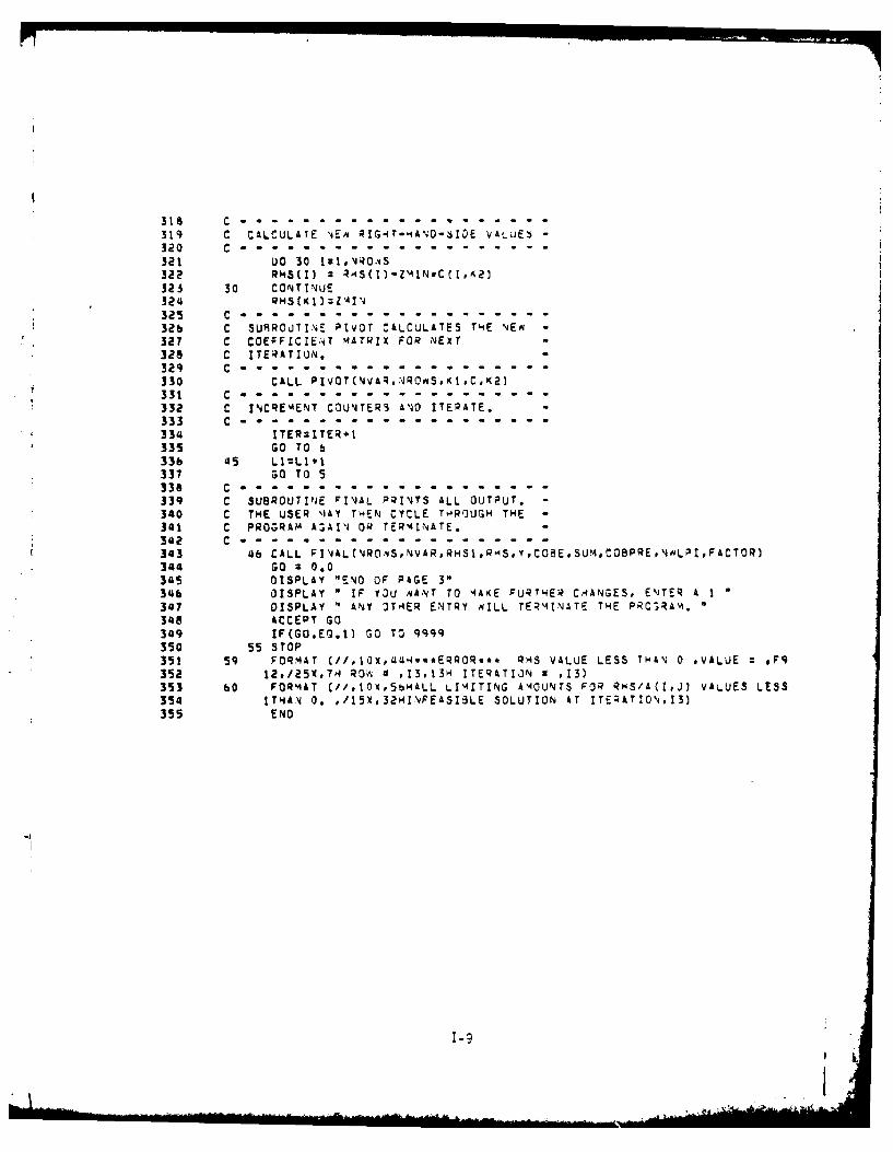
316 C .-.......319 C CALCULArE NEm RIGNTT-U-;;e VALUE; -
321 UO 30 3 l,RO.;S322 RHS(I) 2 4AS(l)-Z lN*C(I,K2)
323 30 CONTINUE324 QH5(K I) ZA I '325 C ....................32b C SURROUTINE PIVOT CALCULATES THE NEm -
327 C COEFFICIe' 4ATUIX FOR NExT -
328 C ITERATION. -
329 C . -
330 CALL PIVOT(NVAq.NROS,.,CK331 C . ............. . . . . ..-
332 C INCREmENT COUNTERS AND ITERATE. -
333 C . .--.-..... ...... . . . . . .
334 ITER=ITER l335 GO TO 633b as LI=L1.1337 GO TO 5338 C . ..-.. ....-.......339 C SUBROUTIJE FINAL PQINTS ALL OUTPUT. -
340 C THE USER %lAY THEN CYCLE THROUGH THE -
341 C PROGRAM A3AI'l OQ TERMINATE. -
342 C- - - ... . . . . . . . . ..-.-. ..
343 46 CALL FlN AL(4ROSNVARRHSt, HSYCOBESUCOBPRE,NALPI,FACTOR)344 GO 0.0345 DISPLAY "ENO OF PAGE 3"34b DISPLAY " IF YOU NANT TO 4AKE FURTHER CAANSES, ENTER A I "
347 DISPLAY 4 ANY OTHER ENTRY AILL TERMINATE THE PRORAM. "
348 ACCEPT GO
349 IF(GO.EQ.t) GO TO 9999350 55 STOP351 59 FORMAT (//,IOx,uaI4**ERROR*** qHS VALUE LESS THAN 0 -VALUE F9
352 12,/25X,7H RoD 4 13,13H ITERATION 9 ,13)353 60 FORMAT (//,tOX,5bHALL LINITING A4OUNTS FOR qHS/A(I#J) VALUES LESS354 IT4AN 0. ,/15X,32HINFEASI3LE SOLUTION AT ITErATION,I3)355 END
I-9
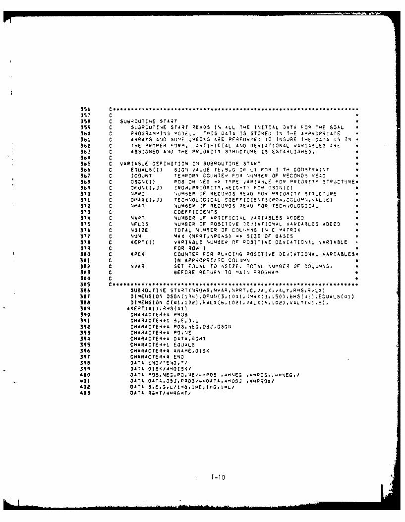
3157 C356 C SU6-OUTINE START359 C SU3RUuTI'qE START READS IN ALL T-4E INITIAL DATA FOP TmE GOAL360 C DWGPAM'AIN4 "CE. THIJS DATA IS STOkED IN THiE A2PROPRIATE f361 C ARRAYS ANJD SOM'E -14ECKS ARE PEPFOW"ED TO INSUPE ToE DATA IS IN*362 C T.4E PROPER POA AwTIFICIAL AND rIEVIATIONAL VAWIA4,LES ARE a363 C ASSIGNED A140 THE PRIORITY STWuCTURE IS ESTA3LISHED.364 C365 C VARIABLE DEFINITION IN SUBRUUTINE STAWT366 C EtnUALS(I) SIGNl VALJE (E9r OR L) FIR I Tr CONSTRAINT3b7 C ICOUNT TE4PORY CCLINTE- FOR *jJMHiEQ OF RECOkDS ;?EA0368 C OS3NCI) POS OR 'NEG -> TYPE VAPIAiLE 90 PRIORITY STQJ:-T1JqE369 C OFUN(I.J) (PRim,PRIOPITY,8Elr,-T) FOP~ ISGN(I)370 C NPRI 4um.3E.Q OF QECDqOS READ FO-? OqIORITY STRLJCTURE371 C DAEX(IoJ) TE^.HNOLDGICAL COEF -ICIENTSCRO'A,.-)LUMAN.ALjE)372 C NmAT NUMi.3ER OF RECO40S READ FOR T-ECM^40LDGI:AL373 C COEFFICIENTS374 C 4AW NUMBER UF ARTIFICIAL VARIABLES AODE-)375 C NFLOS NUMBSER OF POSITIVE JEI/IATIDNIAL VARIAiLE5 ADDED t376 C NSIZE TOTAL NIjM9ER OF COL MNA'S Ili C MAATRIX377 C NU4 MAX (NPRT,NRUAS) -3, SIZE OF BASISa378 C KEPT(I) VARIABLE NLJP46ER ng POSITIVE DEvIATIOAL vARIASLE379 C FOR RDA I380 C KPCK COUNTER FOR PLACING POSITIVE DEVIATIDNAL VARIABLES*381 C IN APPR~OPRIATE CD)LU-N382 C NVAR SET EJUAL TO NSIZE, TCT4L NJMBE4 OF :OLJMNVS, a383 C BEFORE RETURN TO MlAIN PROGkAM *
38a C385 aaaaaaaaaaaaaaaaaaaaaaaaaaaaaaaaaa386 SUBROUT1'JE START (J OwhS.NVAP.NPRTC,VALX, VALY,RHS, RvX)
387 DI4ENSION4 OSG,%(104) OFUr(3. IOU) ,M>AX(3, 150) bHS(JI) E^.UALS(ul)388 DIMENSION C(aI, 1D2),RVLX(b, IOa).IALE(O, 102),VALYI41,S),389 .KEPT(4I),4,4S(4I1)390 CHARACTEQaV PROS391 CHARACTE4*1 5###392 C'4ARACTE4a'4 POS.iEG,08J,DSGN393 CHARACTE4aQ POoNE394 CNARACTER*u OATA,QG,4T395 CHARACTE4*1 EaUALS39b C?4ARAC TE4*4 ANAMEDISK391 CHARACTER*4 ENO398 DATA ENO/"ENO,ff/399 DATA 0 ISK/040 I SK400 DATA P0SNE5,PON\E/u"POS #UHpNEG 44SPOS,,44HNEG./401 DATA OATA,O3J,PROS/ ODATA,uQBoJ .404PROd/402 DATA 8..,/-6Im~rGIL403 DATA q;HT/g4RG..T/
A-l
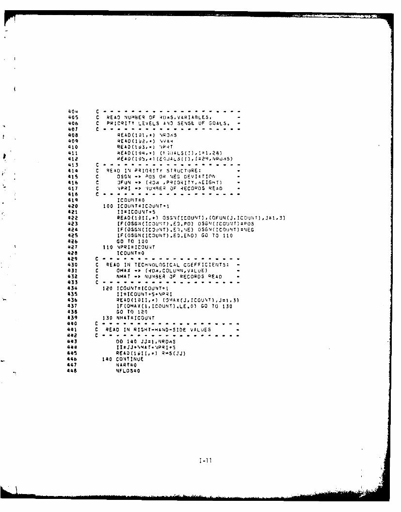
" C .-405 C R~EAD NUMBER OF 40odS,VARIABLES,
40b C PRIORITY L.EVELS AND SENSE OF GOALS.-'407 C .-
* 405 REAO(1i91,.) NR3e4S409 READ 1 ii , *) NVA -4
410 READ 1 :3 ,. * P ~T
'413 C .-4 1 C READ IN P;tO4ITY STRUCTURE:415 C OSGN -'J~OS OR NEG DEVIATION416 C JFUN (40A ,PRIORITY,AEIGH'T)417 C NPRI N~~UA1RE; OF RECORDS READ -
418 C .-419 ICOUNT=0020 100 ICOu.NT=ICOUNT.1021 II=ICOUNT.5022 REAO~lti~,*) OSG'NCICOUNIT),(OFUN(J,ICO~j\4T),Jzl,3)42~3 IF (0SG-NCICOUA; T) . EO.PO) OSGN ( COUN.T ) =OSaaa IF(OSGN(ICOUNT).E.'jE) OSG-N(ICOLJNT):NEG425 tF(OSGNU(COUNT).EO .END) GO TO 11042b GO TO 100#A2 7 110 NPRIMICOU;NT428 ICOUNT=0429 C--------------------------------------430 C READ IN TECHNO.nGICAL CGEFFIZIENJTS: -
431 C OMAX -x 40',CO"LUM~N,VALUE) -
032 C NMAT -oNU43ER OF RECORDS READ -
433 C--------------------------------------434 120 ICOU,%T=ICOUNT.1435 II=ICOUNT+S+NP4I4 3b READ(1@11,*) (OA(~CUN)JI3437 1F(0MAX(U,ICOUNT).LE.0) GO TO 130038 GO TO 120039 130 N4MATZICOUNT040 C............................041 C READ IN RIGH4T-'ANO-SIDE VALUES4402 C--------------------------------------003 00 14~0 JJ=1.NROAS000 1 I:JJ+N4A T+'PR .5445 READ~liIl,.) RSuJJ)
-. 44b 140 CONTINUE447 NART=0448 NFLDS:0
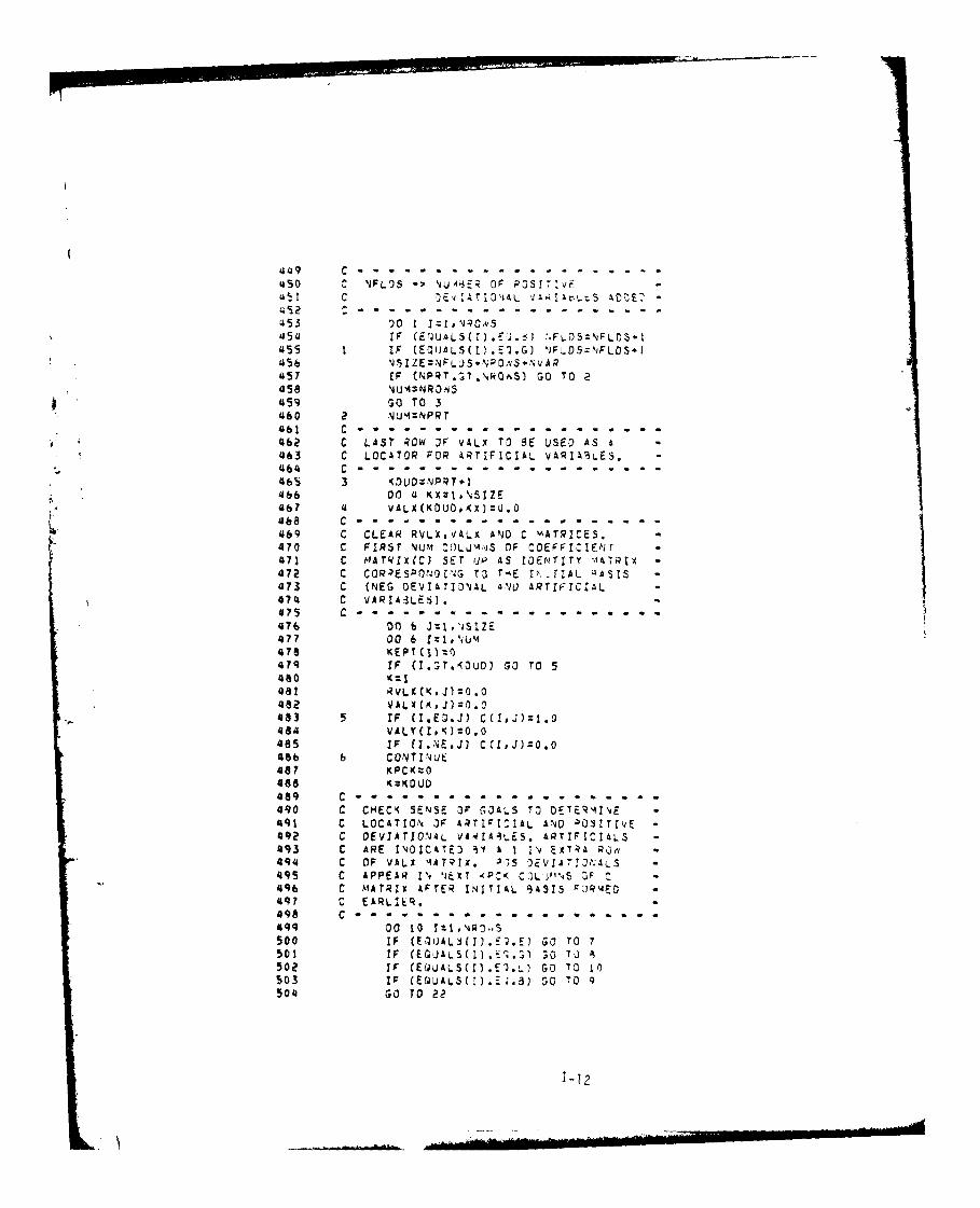
'149 C
~451 00 1 ) ~.",10'& ' ,;
454IF (EQUALS(I.E .. %FL.SNFL0S.1455 1 IF (EQUALS(I). EI. G) 'JFLS:,lFLOSI
457 IF (NP4T.4T.lqkoiS) GO TO 2
459 GO TO 3460 a NUIZNPRT461 C .462 C LAST P70 OF VALX TO 3E USEO AS a063 C LOCATOR FOR 4RTIFICIAL VARIABLES.464 C............................................
46i 3 K(DuO:-NPRT.1466 00 '4 KX1."JSIZ5467 '4 VALX(KDO.X)=O.OAlba C--------------------------------------------469 C CLEAR RVLX.'IALX AND C MATRICES.470 C FIRST NUPM OC1LJWMlS OF COEFFACIENr
c7 C MATRIX(C3 SET iUP AS IDEN~TITY M1ATRIX-472 C CORESPOA4Or'4G TO r-4E IP.. IAL 4ASIS473 C (NEG OEVIATIOYVAL AJL) ARTIFICIAL -
474 C VARIA3LE5).475 C--------------------------------------------476 00 b ;,'SZ477 00 6 1:1.ANU4478 KEP!(Ifl04?9 IF (1.3T.OUO) GO TO 54480 K:!j081 RVLX(I(.J)20.0482 AXAJ=.483 5 IF (I.EQ.J) C(I,J)1-.O484 VALY(IoK)20.0485 IF fl.NE.J) CCI,J)=0.O45b6 b CONTIN4UE087 KPCK-:0488 KKU489 C............................................490 C CHECX SENSE 3; GOALS TO DETE; '4!NE491 C LOCATION~ OF 4RTt:IAL ANO 005tTtr'E -
49? C DEVIATI0OWL V44JAiLS. ARTrFICIALS -
493 C ARE Ji'4OCkTE3 'f i I j E974A RC~e494 C OF VAL$ 'qATRIX. 2,15 )EVIA7TJ%4LS -
49S C APPEAR IN'J XT <P' C-IL''S OF C -
496 C MATRIx AFTER INITIAL iA315 FJR%4ED4q? C E&RLI~q.098 C............................................494 00 10 121090,-.sSoo IF GO rO 7
502 IF (E(JALS(l).Ebl..) GO TO 10503 IF (EQUALS!).J.a) GO TO 9500 GO TO 2?
kft~khA~b%1-A12
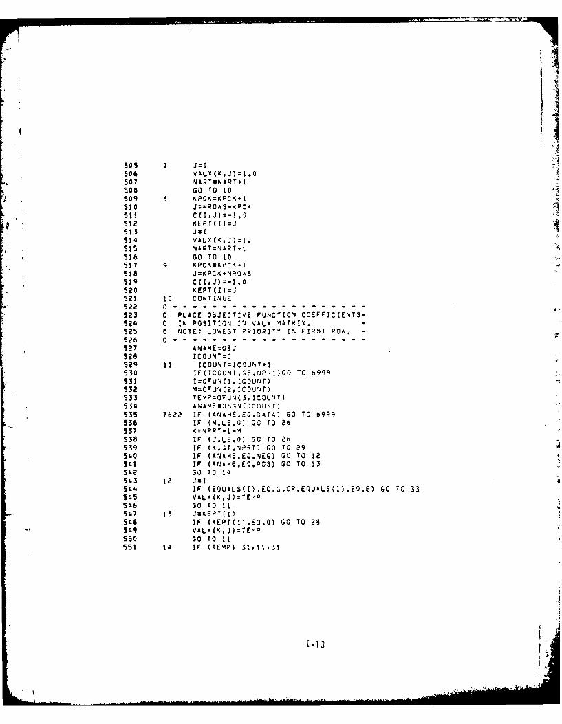
505 7 1:1 -
506 VALX(i(,J=j:.0507 NART=NART+i508 GO TO 10509 8 KPCI(KPCK~1510 J:NROAS.P(sit C(I,J)=-l.O512 K E P rIJ513 j=1
515 NART=NART+1516 GO TO 10
*517 9 XPCK:KPCK.1518 J=i(PCK+(.R4S519 C(IOJ)=-1.O520 PEPT(I):J521 10 CONT INUE522 C------------------------523 C PLACEOBJECTIVE"FUNCmTION OEFIIETS524 C IN POSITIO~i IN~ VAL% MtATWIX.525 C NOTE: LONEST PRIORITY IN FIRST ROh.-526 C----- ---- ------------------527 XN;ME=u33528 ICOUNT=O5214 11 ICOUNT:ICOUNT~l530 IF(ICOUNT.SE.NP41)GO TO b9q9531 I=OFUN(1,ICOUNT)532 '4OFUN(2pIC0UNT)S33 TEPO:'(,CUT534 ANA%4E=OSGN(ICO\IT)535 7622 IF (ANA4E.EQ.0ATA) GO TO 6999536 IF CM.LP.O) GO TO 26S 37 K=NPRT,1.'i538 IF CJ.LE.0) GO TO 26539 IF (K.;T.'4ORT) GO TO 29 J540 IF (ANANME.E0.NE-G) GO TO 12541 IF (ANA'4E.E'1.POS) GO TO 13542 GO TO 14543 12 J:Il544 IF (EOU&LS().EO.G.OR.EQUALS(l).Eg.E) GO TO 33545 VALX(K,J)--TE'4P54b GO TO 11547 13 JZKEPT(I)548 IF ('EPT(fl.E'2.0) GO TO 28549 VALXCK,J):TE%4P550 GO TO I11
551 4 IF (TEA) Si tleS
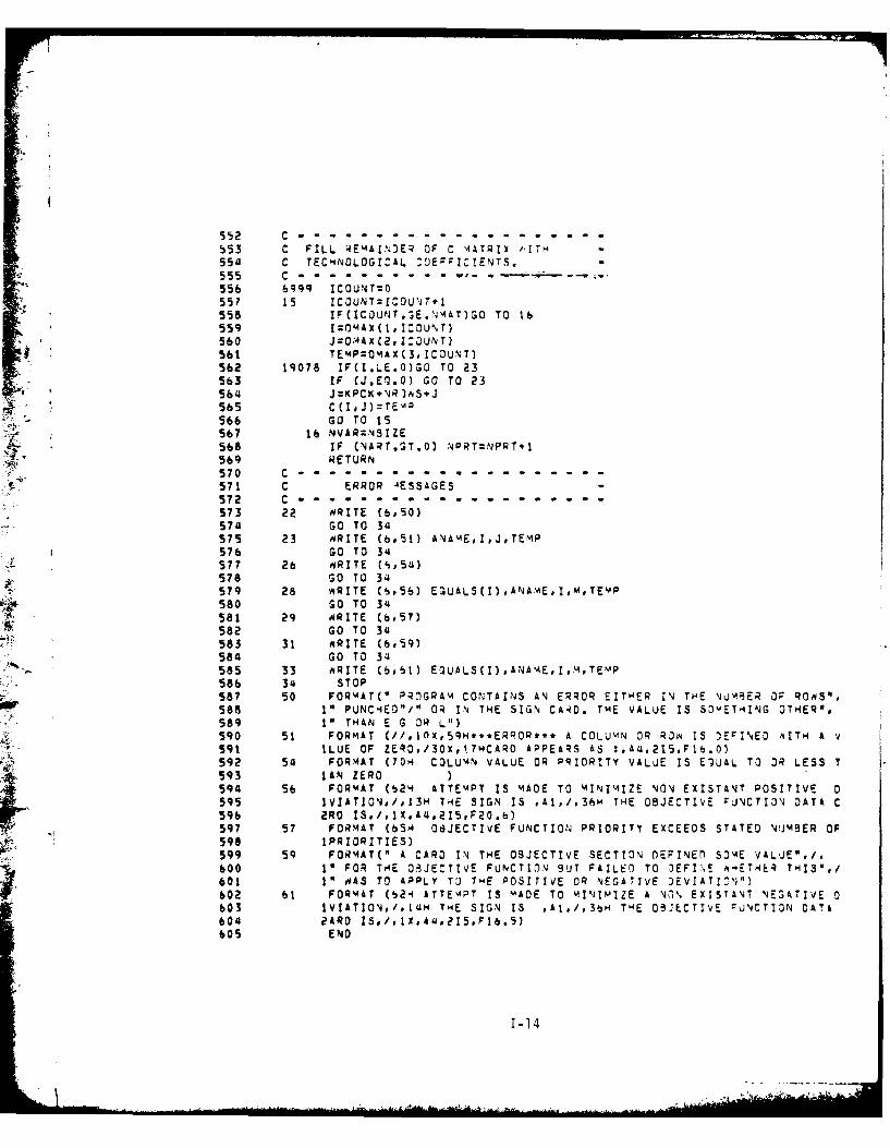
552 C .-
553 C FILL REMAINOER OF C AATRIX ,,ITH554 C TECNOLOGIA4 J0E=I:!ENTS.555 C . ...... .. .--- -
556 bgq ICOUNT=O557 15 ICOUNT=ICOU'aT I558 IF(ICOUNT.SE.IA4T)GO TO 1b
559 I=MOAX(t,ICOUNT)560 J=OMAAx,IaUNT)561 TEMP=OMAX(3,ICOUNT)562 19078 IF(I.LE.O)5O TO 23563 IF (J.E1.O) GO TO 23
564 J=XPCK NR)AS*J565 C(Ij)=rEM1-566 GO TO 15567 16 NVARMNSIZE568 IF (NART.GT.O) NPRTMNPRT.1
569 RETURN570 C ...-....-...-.-.-.-.-.-.-.-.-.-.571 C ERROR AESSAGES572 C . ......-........573 22 mRITE (b50)574 GO TO 34575 23 aRITE (b,51) ANAME,IJ,TEmP
57b GO TO 34577 26 RITE (S,54)578 GO TO 34579 28 mRITE (S.56) EQUALS(I),ANA.EI,m,TEmP580 GO TO 34581 29 aRITE (b,57)582 GO TO 34583 31 mRITE (6.59)584 GO TO 34585 33 ARITE (b6b1) EQUALS(I)#ANAME*I,MTEMP
358 34 STOP587 50 FORMAT(" PIGRAM CONTAINS AN ERROR EITWER IN THE NU iER OF ROAS",588 1" PUNC4ED"/" OR IN THE SIGN CAkD. THE VALUE IS SOmET.4ING OTHER*@589 10 THAN E G OR L")
590 51 FORMAT (//,IOX,59H***ERROR*** A COLUMN OR ROQN IS DEFINEO .ITP4 A V591 ILUE OF ZERO,/30X.I7HCARO APPEARS AS :,A4,215,Fb.O)592 54 FORMAT (70H COLUMN VALUE OR PRIORITY VALUE IS EIUAL TO OR LESS T593 JAN ZERO594 5b FORMAT (62H ATTEMPT IS MADE TO MINIMIZE NON EXISTANT POSITIVE 0595 IVIATIONs/13H TE SIGN IS Aj/,3hH THE OBJECTIVE rJNCTI3N DATA C59b 2RO IS,./tX,A4,215,F20.b)597 57 FORMAT (bS OdJECTIvE FUNCTION PRIORITY EXCEEOS STATED NUMBER OF598 1PRIORITIES)
599 59 FORMAT(" A CARD IN THE OBJECTIVE SECTION D-EFINEf SOE VALJE".I,600 I FOR Tr4E OJECTIvE FUNCTION BUT FAILE0 TO 3EFIN! m-ET'4EQ TMIOm,/601 1" OAS TO APPLY T: THE POSItIVE OR NEGATIVE OEVIATI:N")
602 61 FORMAT (S2 ATTEMPT IS MADE TO MINIMIZE A N!% EXISTANT NESATIVE 0bO3 IVIATION#/,t{ THE SIGN IS ,it,/,O6H TwE 03JECTIVE PUNCTION DATA604 2ARD 15#1#1X#A41#215,F~b.5)bO5 END
1-14
607 C a
b08 C SU8OUTINJE FINAL609 C SUBROUTI E FINAL.OENTJ-I.E-S-LL E -EVIATOAL AkO OE-:IS610 C VARIA6LES IN T'4E SOLUTION TO TmE GOAL P06bRAMNIN,, ;406LEi ibl C SOLVED IN T 4E MAIN PROGRAM. OUTPUT PREDICTIO.S FOR THE612 C EXISTING 3UOGET ALLOCATION(FILE=2) A,40 TPIE GOAL ROSRA1MING *b13 C SOLUTION ARE MADE. THE PREOICTION FOR THE EXISTINSbl C ALLOCATION IS qAIE BY ADJJSTING TmE VARIABLE CCbPE, ab15 C CALCULATED IN THE MAIN PROGRAM. 6Y THE REGRESSION CONSTA'4T. a616 C THE PwEDICTION FOR THE GOAL PROGAMMI'JG S'LUTION IS 'AOE 3Y ab17 C ADDING O SU8TqACTING THE APPROPNIATE OEVIATI[.AAL VAQIALE *618 C FROM T4E CORRESPONDING GOAL. ALL RESULTS ARE THEN PRINTED a619 C AS THE FINAL PAGE OF OUTPUT. 0
" 620 C621 C VARIABLE OEFINITIONS IN SUBROUTINE FINALb22 C BUOG(I) "OPTI'AL" ALLOCATION OF THE BUOGET COmPJTED 5Y ab23 C THE GOAL PROGRAM'ING ALGORITHM a624 C AIa, C, TEMPORY VARIAdLES FOR STORING COLUMN SUMS OF625 C BUDGET ALLOCATIONS a626 C PE(I) NUMERIC DESIGNATION OF PROGRAM ELE ENTS a627 C DEV(IJ) VALUE OF OEVIATIONAL VARIABLES FOR THE iOgKLOAO/ a628 C PERFORMANCE E UATIONS a
b29 C GOALICI) COBE GOALS FOR AORKLOAO/PERFOPMANCE EgUATIONS ab3O C GOALCI) PREDICTED AORKLOAO/PERFOR4ANCE OUTPUT FOR THE O631 C COMPUTED SOLUTION - BUDG(U *
632 C633634 SUBROUTINE FINAL (NRUAS,NVAk.HSI,RMS.Y,COBESUM,:CSPRE.N Pl,635 a FACTOR)636 DIMENSION RwSI(u1),RHS([I),YU1),BUDG(q),OEV(3,2),GOAL(13)637 DIMENSION GOALI(13),COBE(l1,3),OIFF(13),PE(9),SUM(Ill,CO3PRE(13)638 DIMENSION OIFFC(13)639 CHARACTER*9 PE640 DATA PE(1),7E(2),PE(3)/QH721111 ,9H721112 ,qH721113 /641 DATA PEC )SPE(5},PE()/9M722 2Q/RQH7224qh.Z ,947TSU I642 DATA PE(7),PE(4),PE(9)/9H728010/13o9M72q011 ,94728012 /643 O0 100 I:1,3644 C ........ ....................645 C ALL THREE PORTIONS OF THE EXISTING64b C CO6E(FILEz2) ARE :ONOENSED FROM THE -647 C 11 PROGRAM ELEMENTS READ IN TO THE648 C 9 USED IN T14E PROGRAM.649 C v . . ........... ....... .650 100 Co8E(0.I) : Co;E(4,I) * COBE(S.I)651 00 110 1=6,7652 DO 110 J:1,3653 110 COBE(I-1,J) - COBE(IJ)654 DO 120 I:I,3655 120 COBE(7,I) : COBE(8,!) * COBE(11,I)656 O0 130 1:9,10657 00 130 JfI,3658 130 COSE(I-l,J) : COBE(I,J)659 50 J:,1qOas.2+ I660 NRITE (be1)
1-15
61 71 FOR'4AT(I l.25i*b Il4ECT,21'Y.5aTOTAL,//,14 qNPROS El-E4'1)X.'C08E.662 * 1 1,#5HIOOEL# 1 5,.a'CJ,6E, 10X.S'AOEL,//)663 C . .
6 b 1 C INITIAL:ZE ijoG r; 0.665 C . 5bbb 00 521 ,
*667 52 8UDG(I1 0.0668 C....b69 C 10ENTI;,V T'V DECI iO A V LR;A5LE I N
0 60 C THE GOAL P40GA'AfING SOLUTION AND671 C STORE AS 3')G CI ).672 C-------------------------------------------673 KK J J674 DO 54 1 = .NRONSV75 00 54 4 J,NVAP676 IF (Y(I) - A) S'As53#54b 77 53 BUOCK - KK)= 4S(I)*FACTOR678 54 CONTINUE679 C .680 c compturE TiTALA.'.)00;4ECT COU1 U~i681 C FOR T4E SOLirioN AND EXISTING 3UOGET
682 C ANO PRINT RES:JLTS, INCLUDING T14E683 C AMOUNT ALLOCATED TO EACH PROGRAM684 C ELEM4ENT.68s C..................... . .. .. .. .. ....
686 A z0.0687 a 0.0&as C =0.0689 0, 0.0690 00 80 121,9691 A 2A+C33E(I,1)692 TE4iP a 3BuOG(I)-C33E(I,2)-C~dE(I*3)693 8 a .TE4P694 C a C+SU'A(I)695 0 = 0+UDGUI)696 80 NRITE(6, 72] EI C8C,1 ,)PSi3,uGI697 72 F0?R4AT(14 A.KF.7EF. RF.1,x92)b6 WRITE(6,7b)699 76 FORMATMh4 ..... o7,'-----qx,700 8* ------ X,9M-----------)701 OVRItE(6,77) 4,9,C,O702 77 FOqR1AT(1'4 * tEXF9.1 .6XF9.1 ,8V.F9 1 ,6XF9.1 Dill,703 DISPLAY "ENOQ OF PAGE 2"
-I704 ACCEPT GA49AGE705 C 0.................. .. . *.. .. ..
706 C INITIALIZE ;SV TO00:707 C 0. . ... . . . . .. .
708 00 55 ;,3S5709 00 55 J=1.2710 DEVIj) --0.0MI 55 CONTINUE
1-16
712 C.......................713 IDNTFY TmE OvIAIO.L ;AI~E
714 C IN T'mE GOAL P-1OGRAm1''!G SOLJTIoN715 C AHICM COR49-SPONI TO TiHE NO-LOAO/
716 C PERFOR4ANCE-IN-I1CATOR EUUATIGNS.717 C . . . . . . . . . . . . . . . . . . .
718 00 61 I1,%JRl~uws719 D0 60 4=29,NWOAS720 IF(Y(I) - '() 58,57,58721 57 0EVC'K-2A,8.=1] (I722 GO TO 61723 58 IF(Y(I)-NQOAS-K) 60,59.60724 59 DEV(K-25.2) zQmS(l)725 GO TO 61
*72b bO CONTINUE727 bI CONTINUE
-728 fIRITECb,73)729 73 FORMAT(1r~l,05X.0MC0OEI0X.5HmODEL,/. IH 8X,PARvETEQ,730 *I1X~bi GOAL ,OXbH PRED o3X,bH 01FF *4Xv6M PRED731 3X.64 01FF)732 C . .. .. .. .. .. .. .. .. ..
733 C READ THE EXISTING COBE GOALS(FILE=2).-734 C--------------------------------------------735 D0 200 I:1.NALPI736 200 REAO(2UI.I2,*) GOAL1IN)737 RENdINO 2
* 738 C-------------------------------------------739 C COMPUTE T-4E PqEOICTIONS FOR THE740 C EXISTING BUDGET ALLOCATlOkN(FILE:= -
741 C AINO T-4E GOAL P'#OGRAM'MING SOLUTION.742 C PERFORMANCE INDICATOR PREDICTIONS743 C /iMIC,4 EXCEEO 100% ARE LISTED AS 100%744 C . . .- . .- . .- . .- . .- . .- . .-. .-. .-
745 00 96 1=1,774b GOAL(IJ:G^OALI CI)-OEV(I,1).DEVCI.27
-747 96 COBPRE(I):C38PRE(I)+GOALIl)-RHSIC28+1)748 00 97 I:d. 12749 IFCX.EO.11) GO TO 250750 C08PRE(I)=4HS1 (28,r).GOALI tr)-CORPQEfl)751 GOAL(I):-GOALI CI)g0EV(I,1)-DEV(I,2)752 GO TO 977S3 250 COBPRE(11):CO9PRE(1l).GCALI(11).RNSI(3q)750 GOAL(IIJZGOAL1 (11)-OEV(11, 1j.OEV(11.2)755 q7 CONTINUE756 C08PRE(13)=:OPRE(13).GOALI13)-R,4S1(41)757 G0AL(13)=IOAL1 (13)-OEV(13. 1).0EV(13,2)758 00 98 121,NALPI
760 98 OIFFC(I)=C0iPAE(I).GOAL1 (I)761 00 63 I ,-AP762 IF(GOAL(t).LE.100.0) GO TO 63783 GOALCI) 2 100.0760 DIFF(I) --100.0 !. GOALICI)765 b3 CONTINUE
1-17
766 DO b~4 I 7,0JALPI707 IF(C0RPRE(I).LE.100.01 GO TO 6.4768 COSPRECI) 100.0?b9 OIFFC(I) 100.0 - GOALI(I)770 b a CON T I NLE771 C . . . . . . . . . . . . . . .?72 C %RITE ALL RESULTS.
7734-775 tARITE(b.TL) (GOAL1(I),CO6PRECI).!UFFC(I),GOALCI),)IF(I),1,7NILP
77b 74 FORMAT( I H,25NNO. ACT I US IP41T I ATEO (K) , 3,Fh..IhUX,F6. I,3Xv777 a Fb.1l#4kF6.1,3X,Fb.l./.778 * 1I40,?SME'N. PRUCESSEO TOTAL779 * Fb.1 1*4XoF.1,3x,Fh.l./.780 * 1N0,5HiTONS RECEIVED .; 5wpo (.).3XFb.1,QX*-b.l,3Xv781 F6 14af.12 , 7 j /782 * lHOP25MLINE ITEMS SHIPPEO (K 1".1x783 F 7.1,'UX,Fb.j,2X.F7.l,/,7 8a * l0*25HPOCtjREMENT ACTIONS (K78578b lm1x025HTOTAL PROC(PAtiACKL0G3CK1.3EF.1'Jx.06.13X,787 * F6.1.4XoFb.1 o3K,F6.t)788 75 FORMAT(1N0,25mNICP OT WEtON. PQ0C. (%,XF~~u,'~vX789 F* apF.vY,6j/
790 IHO*25HOEPOT OiT REO~j. PR0C. (%),3X,Fb.1,uLX.;.1,3X.791 * Fb.*lJXtFb.j,3X,F6.1,,792 a 41r02bHDARCOM REC. 44TE.REPT. (%) 3x#Pb.l,4xvv'j1t3yv
794 l m0#25m1DAACOm OT ;EC.-5TO.,i. (%).3X.Fb.I,~AX#Vb.1,3X#
795 a P6.1.4X.F6.l,3XF6.lv,
79b * P4.25HO4A'PCOM OT Ti4AS. RATE ()3,b1~KW..E797 FbP.1.'aXoF6.lr3x,Fb.1,/,798 a INQ2SHLDCATIOJ SORVEY ACC. (%),3X,F6.1,'Ax#Fb.1.3Xo799 * Fbsl*4KpFb.l.3X,Fb.1,/o
800 * 1NO25HSTOCIK AVAIL. RATE (%)@3XF6.lo4XoF6.l#3Xo
802 RETURN803 ENO
1-18
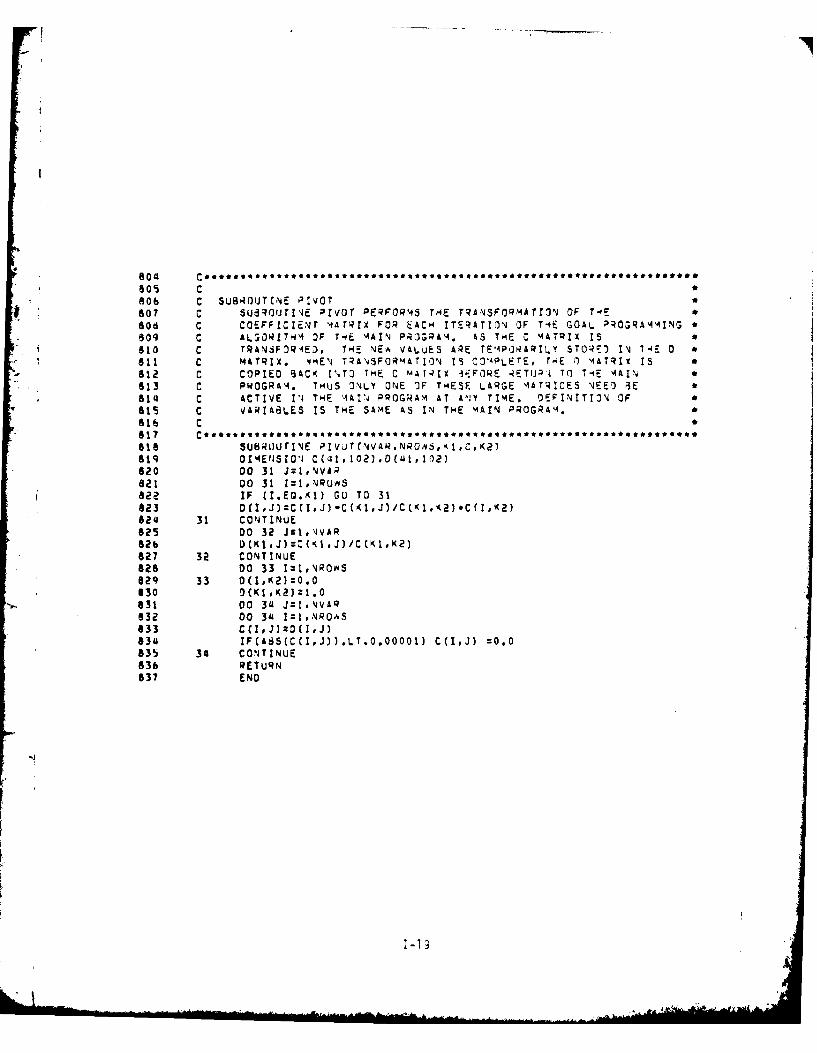
804505 C806 C SUBROUTINE PrvOT807 C SU3d7OU1T1'E mivoT PEQFOR45 TMlE TRANJSFORMATION OF TO~E606 C COEFF LCIENr 4A rQIX FOR EACH4 ITERATIONJ OF T-4E GOAL PROGRAA44ING909 C A~j4TH4O TOE 14AIN PROGRAM. AS THE C MATRIX 1s
st01 C TRANSF OR E), THE 14EA VALUES ARE TE, 2OARILY STOQ~l INi 14E 0
811 C MATRIX. 404E'j TRANSFORMATION 15 C3'APLETE, TH4E 0 4AiTRI'g IS-812 C COPIED 3ACK I'jT3 THE C kMAT4tX *IoFOWE QETlJRP4 TO T-qE A~AIN
$ 13 C PROGRA4. Tr4uS ONLY ONE O)F TH.ESE LARGE 4ATRICES NJEEI i a814 C ACTIVE 11~ THE AI' PROGRAM AT ANY TIME. DEFINITION OFat$ C VARIA13LES 1S THE SAME AS IN THE MAIN PROGRAM4.s1b C817618 SUBROUTINE ?IVUT(. VARNP0.vS,A.,C.K2)819 0IMENlSIO'J C(4l, lO2).D(4J1,102)I620 DO 31 J=1,NVAR021 00 31 I:1s,'JRUAS822 IF (I.EgDSU GU TO 31
824 31 CONTINUE825 DO 32 J:1j,\lVAR
827 32 CONTINUE828 DO 33 Iz,NQOYYS629 33 O(I,K21:O.0630 O(KI.K2J:1.O831 00 34 J=1,4VAQ632 00 34 1=1,,NROAS633 C(IIJ):0D(I,J)834 IF(AdS(CCI,j)).LT.O.O0Ol0) C(I,J) =0.0835 34 C0ONTINUE83b RETURN637 END

ANNEX J
DISTRIBUTION LIST
J-1
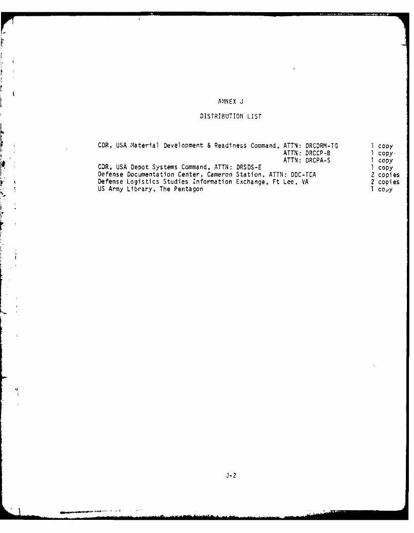
ANNEX J
DISTRIBUTION LIST
CDR, USA Material Development & Readiness Command, ATTN: DRCDRM-TG 1 copyATTN: DRCCP-B 1 copy-ATTN: DRCPA-S 1 copy
CDR, USA Depot Systems Command, ATTN: DRSDS-E 1 copyDefense Documentation Center, Cameron Station, ATTN: DDC-TCA 2 copiesDefense Logistics Studies Information Exchange, Ft Lee, VA 2 copiesUS Army Library, The Pentagon 1 copy
J-2


![eeeee)))))eeeee))eeeeee D re)€¦ · )eeeee)))))eeeee))eeeeee re)ee)rerrer D)))))AA)))r]) nnnnnnnnnnnnnnnnnnnnnnnnnnnnnnnnnnnnnnnnnnnnnnnnnnnnnnnnnnnnnnnnnnnnnnnnnnnnnnnnnnnnnnnnnnnnnnnnnnnnn](https://img.pdfslide.net/doc/110x75/5fb66d0eeb63566c5c6a5386/eeeeeeeeeeeeeeee-d-re-eeeeeeeeeeeeeeee-reeererrer-daar.jpg)