GEOGRAPHICAL PROXIMITY EFFECTS ON THE ADJUSTMENT PR OCESS IN THE

COMPANIES’ FINANCIAL STRUCTURE. DOES THE FIRM HETER OGENEITY

MATTER?

Fernando López Hernández

Departamento de Métodos Cuantitativos e Informáticos Facultad de Ciencias de la Empresa

Universidad Politécnica de Cartagena

Mariluz Maté Sánchez Val Departamento de Economía Financiera y Contabilidad

Facultad de Ciencias de la Empresa Universidad Politécnica de Cartagena

Jesús Mur Lacambra

Departamento de Análisis Económico Facultad de Economía y Empresa

Universidad de Zaragoza.

Área temática : b) Valoración y Finanzas

Keywords : Financial ratios, Partial Adjustment Model, geographical proximity, spatial

interactions, industrial companies.

Palabras clave : Ratios Financieros, Modelo de Ajuste Parcial, Proximidad Geográfica,

Interacciones espaciales, empresas industriales.

113b

GEOGRAPHICAL PROXIMITY EFFECTS ON THE ADJUSTMENT PR OCESS IN THE

COMPANIES’ FINANCIAL STRUCTURE. DOES THE FIRM HETER OGENEITY

MATTER?

Abstract

This paper examines the adjustment process in companies’ financial structure

highlighting the role of the geographical proximity in this context. Our findings show that

the traditional factors previously considered in the literature (distance to the objective,

technological intensity and the size of the company) have different effects on adjustment

coefficient, while the geographical proximity is always significant in the model. Moreover,

the spatial effect has different intensity depending on the size of the company. A spatial

panel data model on a sample of over 12000 Spanish industrial companies illustrates

these results.

EL EFECTO DE LA PROXIMIDAD GEOGRÁFICA EN EL PROCESO DE AJUSTE DE

LAESTRUCTURA FINANCIERA: ¿AFECTA LA HETEROGENEIDAD EMPRESARIAL?

Resumen

Este trabajo analiza el proceso de ajuste en la estructura financiera empresarial

destacando el papel de la proximidad geográfica en este contexto. Nuestros resultados

muestran que los factores explicativos tradicionalmente considerados en la literatura

(distancia al objetivo, intensidad tecnológica y el tamaño empresarial) producen

diferentes efectos sobre el coeficiente de ajuste mientras que la proximidad geográfica

es siempre significativa en el modelo. Además, el efecto de la proximidad varía en

función del tamaño empresarial. Un modelo de datos de panel espacial sobre una base

de 12000 empresas industriales españolas muestra estos resultados.

1. Introduction

Reppenhagen (2010) highlights the role of the geographical proximity among economic

agents to reduce the asymmetric information and overcome certain limitations from the

financial environments. He concludes that the accounting practices are affected by a

contagion effect and propose the following question “Are all accounting choices equally

susceptible to contagion effect?”. To answer this question in a corporate finance

scenario is the aim of this paper.

Financial ratios’ analytic capacity has promoted a fruitful research in finance which

analyses financial ratios’ dynamic in order to evaluate companies’ situation and predict

its short-term results. These studies part from the assumption that financial ratios follow

an adjustment process towards their target values which use to be represented by the

industrial averages (Lev, 1969). When an external shock happens, the economic

environment change and managers reconsider their financial objectives. The lack of

perfect information in the market provokes that companies tend to follow the average

value of their industry as a referenced value. The explanatory mechanism which

supports this result is based on the idea that financial ratios cannot deviate from the

referenced value. Companies with financial ratios far from the industrial averages incur

in costs of being out of equilibrium which use to be higher than the adjustment costs. So,

managers change the accounting practices (e.g. inventory evaluation methods) to

readjust their financial ratios (Lev, 1969). In addition, the own market forces tend to

readjust the financial magnitudes in the companies. For example, companies with high

return on assets ratios will attract additional companies to enter into the industry,

diminishing the return on assets ratios towards the average value (Peles and Schneller,

1988).

Adjustment mechanism in financial ratios may not be equal for all firms but they could be

conditioned upon internal or/and external factors to the company (Greeve, 2005).

Regarding previous literature, we find studies which have examined this topic taking into

account different factors such as the size of the firm and/or the industry in which the

company produces for (Lee and Wu, 1988; Lee, 1985; Fieldsend et al., 1987; Lev and

Sunder, 1979; Seay et al., 2004, Aybar-Arias et al., 2012). These studies find differences

in the adjustment process depending on the analysed characteristics.

In this context, we hypothesize that geographical proximity is also an important factor to

be considered in the adjustment of the financial ratios. In this sense, the proximity

among firms enables managers to gather more information about the other firms’

operations and practices and imitate them in order to guarantee their results (Kedia and

Rajgopal 2007; O’Brien and Tan, 2014). In order to test this hypothesis, we develop an

empirical application based on a sample of industrial Spanish companies. With this

information we estimate a spatial panel data model with spatial interaction effects. In

addition, we provide a methodological contribution to to contrast if the proximity effect is

conditioned by the companies’ size. This paper contributes to the accounting choice

research area which is an important issue in finance. The assumption that managers

adopt decisions based on external comparisons is important to understand how

managers make accounting decisions.

This paper is exposed according to the following structure. Second section explains the

mechanisms which cause interdependences in accounting practices. The third section

presents the Partial Adjustment Model (PAM) and theirspatial versions to analyse

financial ratios dynamic. Section four shows the empirical application. The last section

concludes.

2. Does geographical proximity matter in accounting practices?

Companies are interconnected with other companies (Granovetter, 1985). As

consequence, managers do not adopt financial decisions by themselves but they study

the reactions of other companies in the uncertain environments where they are

producing. Proximity among economic agents alleviates financial problems related with

asymmetric information and promotes the interaction effects (Rogers, 2003). Shorter

distances provoke the actions of each company more observable. This allows external

agents identify variables related with their performance (Pirinsky and Wand, 2010). The

proximity influences on corporate financing decisions. In this sense, firms located in

dense areas reduce limitations derived from the lack of information such as the agency

problems or/and informational asymmetries. This effect improves their external financial

choices and reduces financial costs.Regarding financial management practices,

geographical proximity among firms enables managers to gather more information about

the other firms’ operations and practices. This exchange of information favours the

mimetic tendency among companies in order to guarantee their future results (Kedia and

Rajgopal 2007; O’Brien and Tan, 2014).

Which factors propitiate the exchange of information among closer companies?.

According to previous studies, social interactions among managers in different media

foster the interconnection among companies. In this sense, local executive conferences,

local meetings or regional associations are scenarios in which executives exchange

ideas and learn from others’ experiences (Davis and Greve, 1997). In addition, the

exchange of information among near companies could be promoted by the share of

external agents, such as clienteles, suppliers or financial entities, which provide

information about the others companies (Greve, 2005).

Which firms are more susceptible to the proximity? The degree in which companies are

more susceptible to the exchange of information depends on their particular

characteristics. Companies in disadvantage situations, in comparison with their

environments, are more motivated to follow the other companies. Regarding companies’

size, we could think that reduced size companies tend to present an imitative behaviour

more intense than larger companies. In this sense, traditional management practices in

small and medium companies cause that managers face important asymmetries of

information decisive to adopt decisions (Carreira and Silva, 2010). This produces that

SMEs’ managers discard their own information and give relevance to companies’

external information from other companies which that they believe are able to make

more accurate predictions. Therefore, following this reasoning, it is expected that SMEs

are more motivated to imitate other firms’ financial methods in a search of improving

their performance. Nevertheless, we also can see that larger companies have more

resources to analyse practices and methods from other companies and, therefore, of

implementing other accounting methods in their organization (Reppenhagen, 2010,

Greve, 2005). In this sense, large companies appeal more attention and as

consequence are related with more imitation practices (Baum et al., 2000).

3. Geographical proximity in the financial ratios’ dynamic

According to previous studies accounting methods tend to be transferred among

companies. Therefore, we expect that in the financial dynamic context, the adjustment

process in the financial ratios is influenced by the interaction among companies and is

more intense as closer asthe distance is among companies. With this idea in our mind,

this section presents the specification to analyse the financial ratios’ dynamic and

contrast the significance of interactions among companies.

3.1 The Partial Adjustment model (PAM)

Dynamic analysis in financial ratios allows researchers to predict and evaluate

companies’ behaviour. The importance of financial ratios has caused a wide number of

contributions which have as main aim to model financial ratios’ dynamic. In this paper,

we use the PAM based on the studies of Lev (1969) and Chen and Ainina (1994). The

theory behind the PAM assumes that the observed changes in an output Yit of the agent

(i) in a temporal period (t) tend to adjust toward the difference between the desired

amount in the present moment Yit* and the amount produced Yit-1 in a previous temporal

period (t-1) at a constant rate.

In terms of equations it could be written as:

Yit

− Yit−1

= δ(Yit* − Y

it−1) + e

it (1)

where Yit is the output in the current temporal period corresponding to the agent i in t.

Yit* is the desired objective, δ is the speed of adjustment. The term eit corresponds with

the error of the estimation and it is assumed to be independent and normally distributed

with average zero and constant variance. According to the equation (1) the speed of

adjustment δ is the ratio between the effective produced change Yit − Yit−1and the desired

change Yit* −Yit−1. To conclude about an adjustment process, this coefficient may vary

between 0 and 1. The values of this coefficient reflect the adjustment limitations due to

technological and institutional restrictions. In the case that δ=0 then there is not a

dynamic and the output in t coincides with the output in t-1. In the other extreme, if δ=1

the output in t reaches the objective Yit = Yit* . In this case, the adjustment will be

complete (full). From a practical perspective this value is never reached and therefore,

the adjustment is uncompleted or only partial which provides the name to the model.

Under the PAM perspective, the objective Yit* is not observable. Several papers propose

different alternatives which allow to estimate the speed of adjustment These alternatives

are diverse such as the original Lev’s proposal (1969, note 2) which propose considering

as objective the output average value in the instant t-1.

3.2 Heterogeneity in financial ratios

The assumption about the stability in the speed of adjustment, such as is specified in the

equation (1) is a valid hypothesis when we are considering a homogeneous set of

companies. But when we are working with a heterogeneous group of firms this

hypothesis should be relaxed and adapted to the specific characteristics of each

company. The seminal paper of Lev (1969) highlights the relevance of this problem into

the model: “in such a large and heterogeneous sample there is no way to identify

specific techniques which probably differ from firm to firm” (p. 299). Having into account

this limitation, several authors have deal with the heterogeneity examining financial

ratios’ adjustment processes in function of companies’ characteristics (Lee and Wu,

1988; Lee, 1985; Fieldsend et al., 1987; Lev and Sunder, 1979; Seay et al., 2004,

Aybar-Arias et al., 2012). The size and the industry are the most usual factors which

have been included into these studies.

3.2.1 Size

The size may be an important factor in the speed of adjustment of the financial ratios

towards the objective. Researches have considered companies’ size as a heterogeneity

cause. This heterogeneity would be motivated by the particular characteristics in

reduced size companies in comparison with large companies. Managers in Small and

Medium Enterprises (SMEs) face rigid productive structures with severe restrictions to

get equity and debt (Brown et al., 2005). Besides, they have limited access to the

market’s information and their actions are restricted by the high dependence between

the company and their closer environments (Palacin et al., 2013). Under these

circumstances, it is difficult to think about the existence of general adjustment forces to

all the companies, independently of their size, which provoke the financial ratios’

adjustments towards similar target values. The expected result would be to get different

adjustment forces and intensities for the companies in function of their sizes.

Despite the undertaken efforts in this ambit, researchers do not find a clear relationship

size-adjustment process. From a theoretical point of view, this relationship is not

obvious. On the one hand, it is expected that large firms have more resources and better

access to capital markets and information. Therefore, their size allows them to adjust

their financial ratios at faster rates than reduced size companies. On the other hand,

smaller companies have more incentives of being in equilibrium because of the high

costs derived from the disequilibrium (Davis and Peles, 1993). From an empirical

perspective, Lee and Wu (1988) analyse six financial ratios including large and small

companies. Their results offer different speed of adjustment for the financial ratios equity

and turnover and find a positive relationship between the size of the company and

adjustment process’ rates. According to their results, larger firms adjust quicker their

financial ratios towards the objective than smaller companies. On the contrary, Davis

and Peles (1993) get that smaller firms adjust their ratios to the optimal target faster than

large firms. In the same line, Wu and Ho (1997) get that smaller firms are subject to

greater passive industry-wide effects. This implies that smaller firms’ financial ratios

have higher fluctuations. The results also suggest that smaller firms adjust their ratios to

the optimal target more quickly than large firms. Also Seay et al. (2004) propose the

hypothesis Ha1: The greater the size of the firm, the higher the ratio adjustment

coefficients (p. 29). For the specific case of the indebtedness ratio, Ayrbas-Arias et al.

(2012) argue that the size should be an important influence about the speed of

adjustment of the companies to their objective values. In this sense, large companies

tend to have less cost of restructuration and, therefore, we should expect a higher speed

of adjustment. Large companies have also a reputation in the financial markets1.

Therefore, there is not a theoretical nor an empirical agreed answer about the effect

derived from the company size on the adjustment process rate. A more profound

analysis is necessary to clarify the differences in the adjustment processes

distinguishing companies according to their sizes.

3.2.2Technological Intensity

Chen and Ainina (1994) reward the partial adjustment model (1) allowing differences in

the speed of adjustment depending on the sector. Lee and Wu (1988) show that there

are differences in the adjustments patterns of the financial ratios for industrial companies

of different sub-sectors. Gallizo and Salvador (2003) and Gallizo et al. (2008) examine

financial ratios’ adjustment splitting the sample according to the productive subsectors.

In general, all papers find significant differences in the adjustment processes when

different subsectors are considered.

3.2.3 Distance to the objective

1 In the specific case of the indebtedness dimension, Ayrbas-Arias et al (2012) argue that size is an important element to be considered. When large companies deviate from the target, they may be encouraged to restructure their capital structure to the extent that a significant part of the costs involved could be fixed costs, thus inducing scale economies. Hence, the larger the size, the smaller the cost of restructuring and, consequently, the higher the adjustment speed to be expected. In addition, it can be argued that larger firms can find more financial market opportunities and, obviously, more readily adjust. Hence, size and adjustment speed are expected to be positively related(Ayrbas-Arias et al.,2001). Large companies can achieve a better reputation on financial markets and accomplish higher optimal debt capacity. Nevertheless, large companies also face lower costs derived from informational asymmetries and monitoring and as a result, they may have fewer incentives to boost leverage (Rajan and Zingales 1995).

Another factor which could determine the behaviour in the speed of adjustment is the

own regressor variable of the PAM (distance to the objective). From a theoretical point of

view, we expect that further companies from the objective in one period will undertake, in

the next period, a biggest effort to get approach to the average value of their sector. On

the contrary, companies with financial ratios closed to the objective, will tend to keep in

similar positions in the next period. This idea encourages proposing a nonlinear structure

in the PAM which allows different speeds of adjustment depending on the distance from

the financial ratio to the general aim. Some authors have considered these effects in

their researches. Lee and Wu (1988) introduce a nonlinear model. Aybar-Arias et al.

(2012) specifically considers this factor when model the behaviour of the adjustment

parameter δ.

3.3 PAM model with discrete breakdowns

Previous studies find an asymmetric behaviour in the adjustment coefficients of some

companies’ financial dimensions which depends on firms characteristics (Drobezt et al.,

2014). These results highlight that this effect “should be incorporated in empirical studies

of corporate leverage” (Faulkender et al., 2012). With the aim of including into the PAM

the effects provoked by the factors presented in the section 3.2, we include nonlinear

instability in the adjustment speeds of the model (1) through the inclusion of dummy

variables which incorporate breakdowns in the adjustment coefficient δ in order to adapt

it to each company specific characteristics.

We can rewrite the equation (1) as:

Yit

− Yit−1

= δ(Yit* − Y

it−1) + δ

kf (Y

it* − Y

it −1)F

kif

k=2

f k

∑f =1

F

∑ + eit (2)

where Fkif (Rx1) is a dichotomy variable which takes the value of 1 if the company i

belongs to the category k (k=1,…,fk) in the specified classification by the factor f

(f=1,…,F). The coefficient δ estimates the adjustment speed of a specific typology which

is considered as the referenced category and which is modified (or not) by the coefficient

δkf if the company belongs to the category k in the factor f.

3.4 The inclusion of spatial effects in the PAM

Despite the important role of the spatial factor in current economic studies and the

availability of wide databases with spatial information (Anselin, 1988), the incorporation

of spatial effects in the PAM, referred as the influence exerted by the interaction effects

of closer companies on the adjustment process, has not eco in the literature.

Previous ideas suggest us that residuals in eq. (2) are not independent but they could be

including a spatial interaction structure. The existence of spatial interaction in the PAM

residuals causes important problems in the estimation results (Anselin, 1998). Spatial

econometric techniques develop models which include these effects. In order to specify

these models, we have to define a previous neighbourhood structure (connections

among companies) which is codified through a (RxR) weight matrix W in which the i-th

file indicates, with values different to zero, the companies which spatially interact with

the company i.

Based on the weight matrix W, the most applied models are the Spatial Lag Model

(SLM),the Spatial Error Models (SEM) and the Durbin model (SDM). We can extend the

equation (2) through these models:

The SLM model:

Yit

− Yit−1

= ρW(Yit

− Yit−1

) + δ(Yit* − Y

it−1) + δ

kf (Y

it* − Y

it−1) F

kif

k=2

fk

∑f =1

F

∑ + eit (3)

The SEM model:

itititit

F

f

f

k

fkiitititititit uWeeeFYYYYYY

k

+=+−+−=− ∑∑= =

−−− λδδ ;)()(1 2

1*

1*

1 (4)

And the SDM model:

;)()()()(1 2

1*

1 21

*1

*11 it

F

f

f

k

fkiitit

fk

F

f

f

k

fkiitit

fkitititititit eFYYWFYYYYYYWYY

kk

+−+−+−+−=− ∑∑∑∑= =

−= =

−−−− λδδρ

(5)

Before models are estimated by Maximum Likelihood (ML) (Anselin, 1988) and the

selection strategy between them follows Mur and Angulo (2009) strategy.

3.4.1Instability in the spatial dependence

As we proposed for the adjustment speed, the spatial interaction parameter (ρ/λ) could

be unstable over whole companies’ sample. Instability in spatial dependence has been

considered in Mur et al. (2008) and (2010) developing testing and estimation techniques

which include, in the models (3), (4) and (5), different intensity in the spatial interaction

In this paper, we consider the size of the company to test the instability in the spatial

dependence parameter (ρ/λ). Therefore, the research question is: Does the mimetic

behaviour among companies has the same intensity for large than for small companies?

The models which extend the equations (3), (4) and (5) are rewritten as follows:

For SLM model

Yit −Yit−1 = ρW(Yit −Yit−1)+ ρ*W* (Yit −Yit−1)+δ(Yit* −Yit−1)+ δk

f (Yit* −Yit−1) Fki

f

k=2

fk

∑f =1

F

∑ + eit (6)

for the SEM

Yit −Yit−1 = δ(Yit* −Yit−1)+ δk

f (Yit* −Yit−1) Fki

f

k=2

fk

∑f =1

F

∑ + eit

eit = λW(Yit −Yit−1)eit + λ *W* (Yit −Yit−1)eit + uit

(7)

And for the SDM:

;)(

)()()()(

1 21

*

1 21

*1

*1

**11

it

F

f

f

k

fkiitit

fk

F

f

f

k

fkiitit

fkitititititititit

eFYYW

FYYYYYYWYYWYY

k

k

+−

+−+−+−+−=−

∑∑

∑∑

= =−

= =−−−−−

λ

δδρρ (8)

Following Mur et al. (2008) the weight matrix W* coincides with the weight matrix W in

those rows and columns corresponding to the elements which belongs to the differential

group, being the rest of the elements of W equal to zero2.

4. Financial ratios and sample

4.1 Financial ratios

For each company, three ratios were chosen representing different companies’ financial

dimensions. According to Soboh et al. (2009), the financial dimensions are classified in

two categories. The first category includes the liquidity and indebtedness dimensions in

order to study the ability of a firm to pay its current obligations as they come due and the

nature of any financing equity. The second category is related to the profitability and

evaluates the ability of the company to generate earnings. The liquidity dimension is

measured the Current-ratio (CU) computed as Short Term Assets divided by Short Term

Liabilities. Indebtedness is evaluated by the Debt Equity ratio (DE) calculated as Total

2 Detailed information about the spatial stability tests are showed in the methodological section of this paper (4.3).

Liabilities over Total Assets. Finally, the Profitability dimension is evaluated by the

Profitability ratio (PR) which is Net Operating Income divided by Total Assets.

4.2 Sample

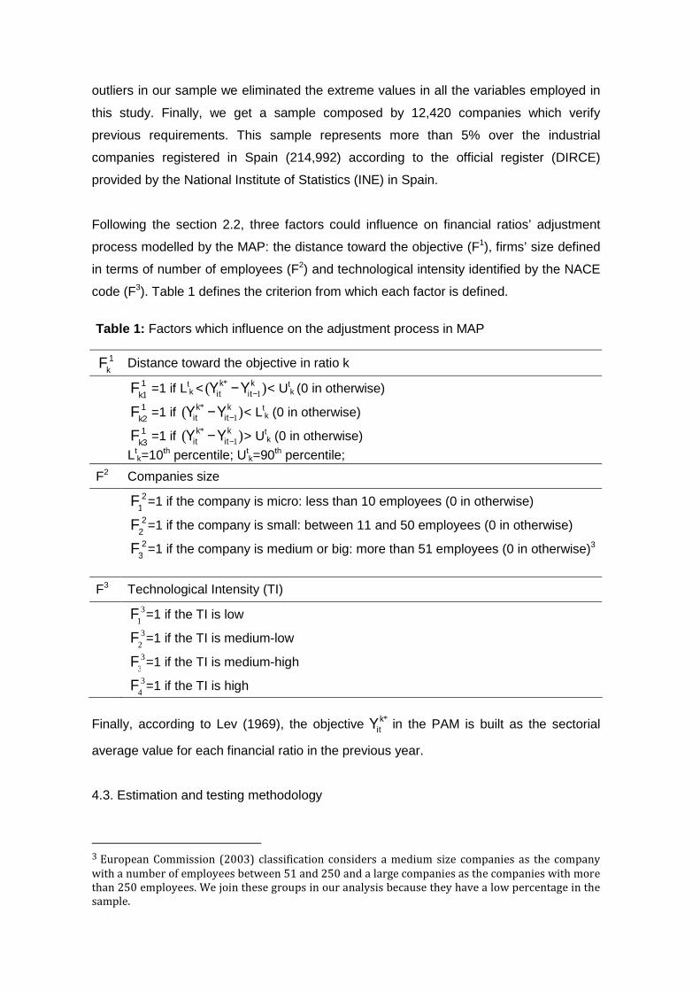
Our analysis is focused on a sample of Spanish industrial companies located in the

Mediterranean Axis. The Spanish Mediterranean axis is integrated by a dense network

of commercial and manufacturing activities and this region has been an area of strong

economic growth in recent decades (Boix, 2011). We select companies located in some

of the 12 provinces (Nuts III in Eurostat terminology) in the Spanish Mediterranean Axis

(Alicante, Almeria, Barcelona, Castellon, Cadiz, Gerona, Granada, Lerida, Murcia,

Malaga, Tarragona and Valencia) and which correspond with four different Autonomous

Communities (Nuts II in Eurostat terminology) Cataluña, Valencia, Region de Murcia and

Andalucía. The database is obtained from SABI (Sistema de Balances Ibéricos). SABI

database provides the accounting register of each company and also includes general

information of each company such as the geographical location, Statistical Classification

of Economic Activities (NACE) or number of employees. The initial sample is composed

by 38,323 industrial companies (NACE codes between 1000 and 4100) over the period

2006-2012. Figure 1 shows the analysed geographical area in provincial terms.

Figure 1: Sample area and firms

With the aim of undertaking a join analysis of the three financial ratios, we select those

companies for which we have available information for each variable of the considered

period (25,903 are excluded). Moreover, observations of firms with anomalies in their

financial statements were eliminated, for example negative values in their sales or

assets that distort the behaviour of the companies. In addition, to reduce the effect of

outliers in our sample we eliminated the extreme values in all the variables employed in

this study. Finally, we get a sample composed by 12,420 companies which verify

previous requirements. This sample represents more than 5% over the industrial

companies registered in Spain (214,992) according to the official register (DIRCE)

provided by the National Institute of Statistics (INE) in Spain.

Following the section 2.2, three factors could influence on financial ratios’ adjustment

process modelled by the MAP: the distance toward the objective (F1), firms’ size defined

in terms of number of employees (F2) and technological intensity identified by the NACE

code (F3). Table 1 defines the criterion from which each factor is defined.

Table 1: Factors which influence on the adjustment process in MAP

Fk1 Distance toward the objective in ratio k

Fk11 =1 if Lt

k < (Yitk* −Yit−1

k )< Utk (0 in otherwise)

Fk21 =1 if (Yit

k* −Yit−1k )< Lt

k (0 in otherwise) Fk3

1 =1 if (Yitk* −Yit−1

k )> Utk (0 in otherwise)

Ltk=10th percentile; Ut

k=90th percentile;

F2 Companies size

F12=1 if the company is micro: less than 10 employees (0 in otherwise)

F22=1 if the company is small: between 11 and 50 employees (0 in otherwise)

F32=1 if the company is medium or big: more than 51 employees (0 in otherwise)3

F3 Technological Intensity (TI)

F13=1 if the TI is low

F23=1 if the TI is medium-low

F33=1 if the TI is medium-high

F43=1 if the TI is high

Finally, according to Lev (1969), the objective Yit

k* in the PAM is built as the sectorial

average value for each financial ratio in the previous year.

4.3. Estimation and testing methodology

3 European Commission (2003) classification considers a medium size companies as the company

with a number of employees between 51 and 250 and a large companies as the companies with more

than 250 employees. We join these groups in our analysis because they have a low percentage in the

sample.

In order to estimate the proposed models in section 3 for the three ratios, we select a

panel data framework. First, a standard non-spatial panel data models are estimate by

maximum likelihood. The simpler non-spatial pooled OLS model is compared with spatial

fixed effect and spatial random effect using the likelihood ratio test. To select between

fixed effect or random effects model, the Hausman specification test can be used

(Baltagi, 2005, pp. 66-68). Next, we extended the standard model in order to include

spatial effects. The strategic to select the correct specification model in a panel data

framework is describe in Elhorst (2014) and we reproduce in this subsection in sort. To

test for spatial interaction effect we use the classical LM test (Anselin, 1988) extended

for a spatial panel (Baltagi et al., 2013; Anselin et al., 2006). In case of non-spatial model

is rejected, the spatial Durbin model (Elhorst, 2014) will be estimated and then we test

whether it can be simplified to the spatial lag or the spatial error model, following the

general-to-specific approach (Mur and Angulo, 2009). The LRcomfac test (Burridge,

1985) can be used for this propose. In case of reject the null, the select model will be a

spatial Durbin model with spatial lag.

Finally, in order to test the instability of spatial dependence describe in model (6-8) we

develop in this paper, extended in a framework of panel data, the test present by Mur et

al. 2010 for a simple cross-section. The final expression of the test is

)1(~*)~~*)('( 2

21

χ∼−⊗=−

lag

Tbreaklag e

WBTtruWIYLM (9)

where B=I-ρW; u is the ML vector of residuals from model, σ2 and ρ the ML estimation

of both parameters, also under the null hypothesis, and elag the ML estimated variance

corresponding to the linear restriction of the null hypothesis of the test.

4. Results

Table 2 shows companies’ distribution according to the previous referenced variables

and a descriptive analysis of the financial ratios. According with the information of the

official census of companies in Spain (INE, 2014), the industrial productive system is

characterized by a limited dimension. The 38.4% of the industrial companies have not

any employer, the 78.4% have five or less than five employees and only a seven per

cent of the industrial companies have more than twenty employees. These results are in

accordance with our sample from SABI.

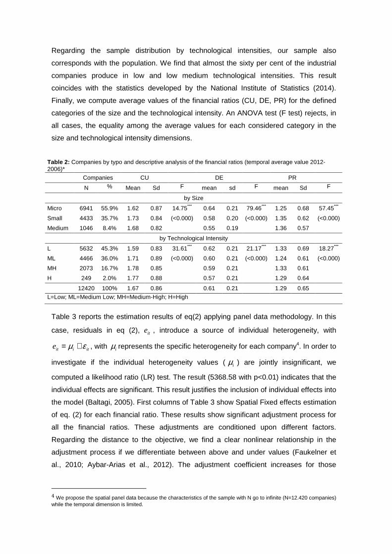
Regarding the sample distribution by technological intensities, our sample also

corresponds with the population. We find that almost the sixty per cent of the industrial

companies produce in low and low medium technological intensities. This result

coincides with the statistics developed by the National Institute of Statistics (2014).

Finally, we compute average values of the financial ratios (CU, DE, PR) for the defined

categories of the size and the technological intensity. An ANOVA test (F test) rejects, in

all cases, the equality among the average values for each considered category in the

size and technological intensity dimensions.

Table 2: Companies by typo and descriptive analysis of the financial ratios (temporal average value 2012-2006)*

Companies CU DE PR

N % Mean Sd F mean sd F mean Sd F

by Size

Micro 6941 55.9% 1.62 0.87 14.75*** 0.64 0.21 79.46*** 1.25 0.68 57.45***

Small 4433 35.7% 1.73 0.84 (<0.000) 0.58 0.20 (<0.000) 1.35 0.62 (<0.000)

Medium 1046 8.4% 1.68 0.82 0.55 0.19 1.36 0.57

by Technological Intensity

L 5632 45.3% 1.59 0.83 31.61*** 0.62 0.21 21.17*** 1.33 0.69 18.27***

ML 4466 36.0% 1.71 0.89 (<0.000) 0.60 0.21 (<0.000) 1.24 0.61 (<0.000)

MH 2073 16.7% 1.78 0.85 0.59 0.21 1.33 0.61

H 249 2.0% 1.77 0.88 0.57 0.21 1.29 0.64

12420 100% 1.67 0.86 0.61 0.21 1.29 0.65

L=Low; ML=Medium Low; MH=Medium-High; H=High

Table 3 reports the estimation results of eq(2) applying panel data methodology. In this

case, residuals in eq (2), ite , introduce a source of individual heterogeneity, with

itiite εµ += , with iµ represents the specific heterogeneity for each company4. In order to

investigate if the individual heterogeneity values ( iµ ) are jointly insignificant, we

computed a likelihood ratio (LR) test. The result (5368.58 with p<0.01) indicates that the

individual effects are significant. This result justifies the inclusion of individual effects into

the model (Baltagi, 2005). First columns of Table 3 show Spatial Fixed effects estimation

of eq. (2) for each financial ratio. These results show significant adjustment process for

all the financial ratios. These adjustments are conditioned upon different factors.

Regarding the distance to the objective, we find a clear nonlinear relationship in the

adjustment process if we differentiate between above and under values (Faukelner et

al., 2010; Aybar-Arias et al., 2012). The adjustment coefficient increases for those

4 We propose the spatial panel data because the characteristics of the sample with N go to infinite (N=12.420 companies) while the temporal dimension is limited.

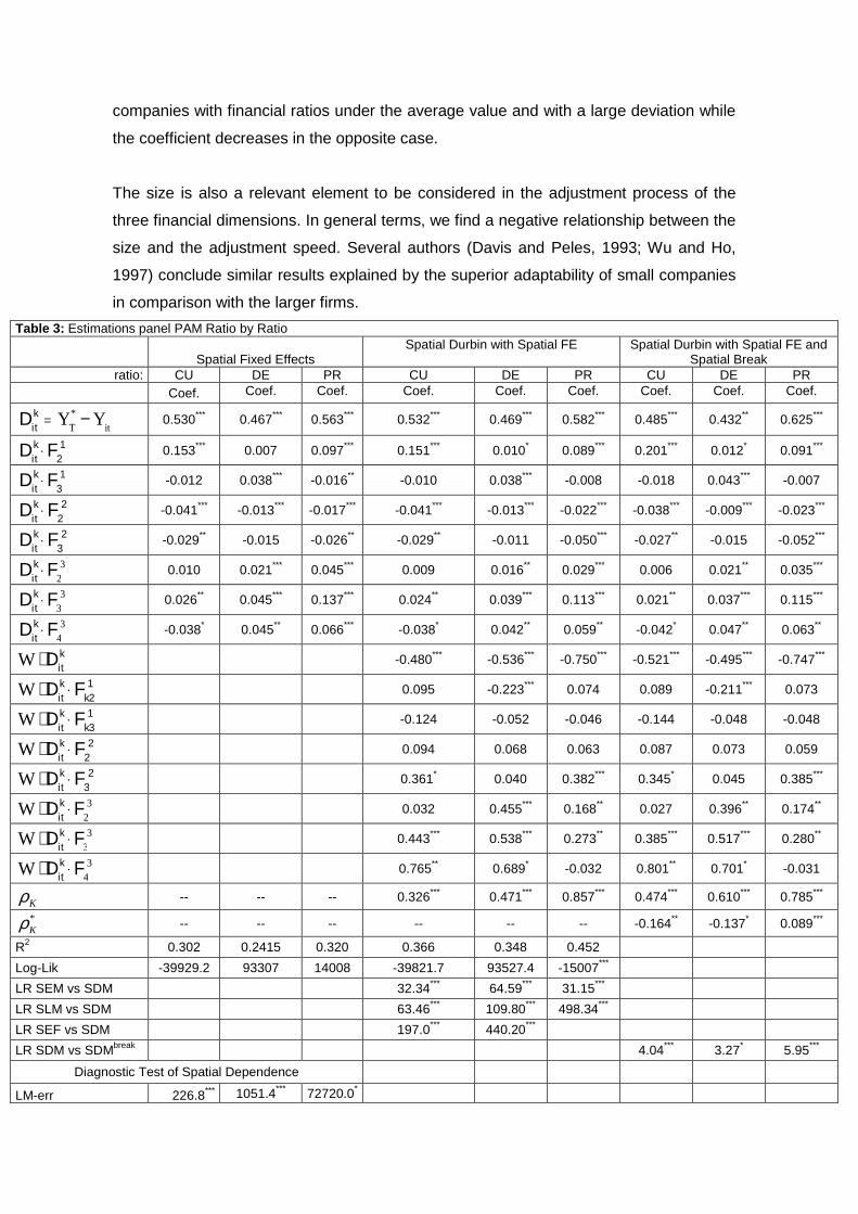
companies with financial ratios under the average value and with a large deviation while

the coefficient decreases in the opposite case.

The size is also a relevant element to be considered in the adjustment process of the

three financial dimensions. In general terms, we find a negative relationship between the

size and the adjustment speed. Several authors (Davis and Peles, 1993; Wu and Ho,

1997) conclude similar results explained by the superior adaptability of small companies

in comparison with the larger firms.

Table 3: Estimations panel PAM Ratio by Ratio

Spatial Fixed Effects Spatial Durbin with Spatial FE Spatial Durbin with Spatial FE and

Spatial Break ratio: CU DE PR CU DE PR CU DE PR

Coef. Coef. Coef. Coef. Coef. Coef. Coef. Coef. Coef.

Ditk = Y

T* − Y

it 0.530*** 0.467*** 0.563*** 0.532*** 0.469*** 0.582*** 0.485*** 0.432** 0.625***

Ditk· F2

1 0.153*** 0.007 0.097*** 0.151*** 0.010* 0.089*** 0.201*** 0.012* 0.091***

Ditk· F3

1 -0.012 0.038*** -0.016** -0.010 0.038*** -0.008 -0.018 0.043*** -0.007

Ditk· F2

2 -0.041*** -0.013*** -0.017*** -0.041*** -0.013*** -0.022*** -0.038*** -0.009*** -0.023***

Ditk· F3

2 -0.029** -0.015 -0.026** -0.029** -0.011 -0.050*** -0.027** -0.015 -0.052***

Ditk· F

23 0.010 0.021*** 0.045*** 0.009 0.016** 0.029*** 0.006 0.021** 0.035***

Ditk· F

33 0.026** 0.045*** 0.137*** 0.024** 0.039*** 0.113*** 0.021** 0.037*** 0.115***

Ditk· F

43 -0.038* 0.045** 0.066*** -0.038* 0.042** 0.059** -0.042* 0.047** 0.063**

W ⋅ Ditk

-0.480*** -0.536*** -0.750*** -0.521*** -0.495*** -0.747***

W ⋅ Ditk· Fk2

1 0.095 -0.223*** 0.074 0.089 -0.211*** 0.073

W ⋅ Ditk· Fk3

1 -0.124 -0.052 -0.046 -0.144 -0.048 -0.048

W ⋅ Ditk· F2

2 0.094 0.068 0.063 0.087 0.073 0.059

W ⋅ Ditk· F3

2 0.361* 0.040 0.382*** 0.345* 0.045 0.385***

W ⋅ Ditk· F

23 0.032 0.455*** 0.168** 0.027 0.396** 0.174**

W ⋅ Ditk· F

33 0.443*** 0.538*** 0.273** 0.385*** 0.517*** 0.280**

W ⋅ Ditk· F

43 0.765** 0.689* -0.032 0.801** 0.701* -0.031

Kρ -- -- -- 0.326*** 0.471*** 0.857*** 0.474*** 0.610*** 0.785***

*Kρ -- -- -- -- -- -- -0.164** -0.137* 0.089***

R2 0.302 0.2415 0.320 0.366 0.348 0.452

Log-Lik -39929.2 93307 14008 -39821.7 93527.4 -15007***

LR SEM vs SDM 32.34*** 64.59*** 31.15***

LR SLM vs SDM 63.46*** 109.80*** 498.34***

LR SEF vs SDM 197.0*** 440.20***

LR SDM vs SDMbreak 4.04*** 3.27* 5.95***

Diagnostic Test of Spatial Dependence

LM-err 226.8*** 1051.4*** 72720.0*

**

LM-EL 3.5* 5.3** 10.9***

LM-lag 338.0*** 1382.2*** 143997.4***

LM-LE 114.7*** 336.1*** 71287.7*

**

Break in function of the companies’ size

LMlagbreak Size<10

emp. 4.95** 4.79* 6.69***

LMlagbreak Size>50

emp. 0.25 2.69* 26.07

About the technological intensity, we find significant results depending on the considered

financial ratio. For the profitability dimension, we obtain that those companies producing

in high technological subsectors have higher adjustment speeds in the profitability ratios.

This result coincides with Gallizo et al. (2002) which get a significant relationship

between technological intensity and some financial ratios in different subsectors.

Last rows in Table 3, below spatial fixed effect estimation, show the results of spatial

dependence in the residuals of the PAM applying a weighed matrix W that is based on

the 120 closest neighbours5. W is row standardized as is usual in this literature. In all the

cases, the Moran-I test rejects the null hypothesis about independence in the residuals

of the PAM. In addition, LM test identify SLM and SEM structures in the residuals of the

model which encourage us to estimate the Spatial Durbin with Spatial Fixed Effects.

Next three columns in Table 3 show this estimation results (eq5). LR tests confirm that

SDM is better to estimate the PAM that the SLM(LR SLM vs SDM) or SEM(LR SEM vs

SDM) structures. The spatial interaction parameter ρk is significant for the three ratios.

This result confirms the importance of the interaction factor when the financial structure

of the company is analysed. What does it mean a spatial interaction structure in the

adjustment process? In general terms, we conclude that the adjustment process of

neighbour companies influences on the adjustment process of the analysed company.

Therefore, managers do not adopt financial decisions by themselves but their decisions

seem to be influenced by the reactions of closer companies in order to overcome the

limitations derived from uncertain environments where companies are producing (OBrien

and Tan, 2014).

5 Results are robust when we change the number of neighbors. The value 120 has been selected because we get more homogeneous results.

Additionally, we also test if the company’s size influences on the degree of the spatial

interaction. In equation term, this hypothesis can be proposed as a problem of spatial

dependence instability, testing in eq. (8):

0:

0:*

*0

≠

=

kA

k

H

H

ρρ

(10)

With this objective we compute LMSEMbreak tests for companies’ size. These results are

showed in last rows of the Table 3. According to them, financial ratios show instability in

the spatial dependence parameters. The size is the more representative factor rejecting

the null hypothesis about the spatial dependence stability in the three financial ratios.

Therefore a SEM break model is required to estimate. Last columns of Table 3 show the

estimation results for the model with the breakdown in the parameter ρ (eq. 8) related

with the size. The proposed hypothesis is confirmed and the estimated values of ρ in the

eq. (5) present important changes depending on the size of the company. In this sense,

we find that the spatial interaction value ρ=0.474***decreases to a value of 0.310

( *11 ρρ − =0.474-0.164=0.310) if the company is not a micro size firm. Similar results are

obtained for the indebtedness (DE). For profitability ratios (PR), the adjustment

coefficient increases if the company is not a micro-size company.

5. Conclusions This paper examines the dynamic in the financial ratios through a Partial Adjustment

model. With this purpose, we include in our estimation additional factors which have

been considered in previous studies. Apart from these elements, we also consider the

spatial interactions among companies as a fundamental variable to be considered. In

order to test the effect of these variables, we test the PAM model including spatial

interaction factors into the equation. We develop an empirical application on a sample of

Spanish companies located on the Mediterranean axis. Our results confirm the

adjustment process of financial ratios for the three considered dimensions. This

adjustment presents a nonlinear pattern for the three financial ratios. Apart from the

traditional explicative factors, we also conclude about the significance of the spatial

interaction which intensity is conditioned upon the size of the company.

References Acharya, V., Almeida, H., Campello, M., (2007). Is cash negative debt? A hedging

perspective on corporate. Financial policies. Journal of Financial Intermediation 16

(4), 515–554.

Anselin L. (1988) Spatial Econometrics: Methods and Models, Kluwer, Dordrecht.

Anselin L, Bera A, Florax R, Yoon M (1996). Simple diagnostic tests for spatial

dependence. Regional Science and Urban Economic 26(1):77–104

Anselin, L., Le Gallo, J, Jayet H (2006). Spatial panel econometrics. In: Matyas L,

Sevestre P (Eds) The econometrics of panel data, fundamentals and recent

developments in theory and practice, 3rd edn, Kluwer, Dordrecht, pp:901-969.

Aybar-Arias, C., Casino-Martínez, A., and López-Gracia, J. (2012). On the adjustment

speed of SMEs to their optimal capital structure. Small Business Economics, 39(4),

977-996.

Baltagi, BH. (2005). Econometric analysis of panel data, 3rd edn. Wiley, Chichester.

Baltagi, BH, Egger, P. and Pfaffermayr, M (2013). A Generalized Spatial Panel Data

Model with Random Effects. Econometric Reviews, 32, 5-6, 650-685.

Boissay, F., and R. Gropp (2007). Trade Credit Defaults and Liquidity Provision by

Firms, Working paper 753, European central Bank.

Boix, R., (2011). Facing globalization and increased trade: Catalonia's evolution from

industrial region to knowledge and creative economy. Regional Science Policy and

Practice. Available online

Brown, G., Lawrence, T. B., and Robinson, S. L. (2005). Territoriality in organizations.

Academy of Management Review, 30, 577–594.

Burridge, P., 1981. Testing for a common factor in a spatial autoregression model.

Environment and Planning A 13, 795–800

Chen, C. R., and F. Ainina (1994). Financial Ratio Adjustment Dynamics and Interest

Rate Expectations, Journal of Business Finance & Accounting, 21(8), 1111-1126.

Davis, H. and Y. Peles (1993). Measuring Equilibrating Forces of Financial Ratios, The

Accounting Review, 68, 725-747.

Drobetz, W. Schilling, D. and Schröder, H. (2014): Heterogeneity in the Speed of Capital

Structure Adjustment across Countries and over the Business Cycle. European

Financial Management, Online version

Faulkender, M., Flannery, M; WatsonHankins, K. and M.Smith, J (2012). Cash flows and

leverage adjustments. Journal of Financial Economics 103 (2012) 632–646

Fieldsend, S. N. Longford and S. McLeay (1987). Ratio analysis: A variance component

analysis. Journal of Business, Finance and Accounting, Winter, 497-517.

Frecka, J. and F. Lee (1983). Generalized Financial Ratio Adjustment Processes and

Their Implications, Journal of Accounting Research, 21 (1), pp. 308-316.

Gallizo, J. L., and M. Salvador (2003). What Factors Drive and which Act as a Brake on

the Convergence of Financial Statements in EMU Member Countries?, Review of

Accounting & Finance, 1(4), pp. 49-68.

Gallizo, J.L., P. Gargallo and M. Salvador (2008). Multivariate Partial Adjustment of

Financial Ratios: A Bayesian Hierarchical Approach, Journal of Applied

Econometrics, 23(1), pp. 46-64.

Lee, C. F., and Wu, C. (1988). Expectation formation and financial ratio adjustment

processes, Accounting Review, 292-306.

Lee, C.W. (1985). Stochastic properties of cross sectional financial data. Journal of

Accounting Research, Spring, 213-227.

Lehtinen J. (1996). Financial ratios in an international comparison: Validity and reliability.

Acta Wasaensia, 49. Universitas Wasaensis, Vaasa

Lev, B., (1969) Industry Averages as Targets for Financial Ratios, Journal of Accounting

Research, pp. 290-299.

Lev, B.B. and S. Sunder (1979). Methodological issues in the use of financial ratios.

Journal of Accounting and Economics, 1, 187-210.

Lieberman, M.B., and S. Asaba (2006). Why Do Firms Imitate Each Other?, Academy of

Management Review, 31(2), pp. 366-385.

Martínez-Sola, C, García-Teruel, P. J. and Martínez-Solano, P. (2013). Trade credit

policy and firm value, Accounting and Finance, 53 (3), 791–808

Mata, J. and P. Portugal, (2002), ‘The survival of new domestic and foreign-owned

firms’, Strategic Management Journal, 23, 323-343.

Maté, M.L, F.A. López and J. Mur (2012). Analysing Long Term Average Adjustment of

Financial Ratios with Spatial Interactions, Economic Modelling, 29, pp. 1370-1376.

Mur J., López F.A. and A. Angulo (2008). Symptoms of instability in models of spatial

dependence. An application to the European case. Geographical Analysis, 40, 189–

211.

Mur J. and A. Angulo (2009). Model selection strategies in a spatial setting: Some

additional results. Regional Science and Urban Economics, 39(2), 200–213.

Mur J., López F.A. and A. Angulo (2010). Instability in Spatial Error Models. An

Application to the Hypothesis of Convergence in the European Case. Journal of

Geographical Systems, 12, 259-280.

Mur, J., and Angulo, A. (2009). Model selection strategies in a spatial setting: Some

additional results. Regional Science and Urban Economics, 39(2), 200-213.

Palacín-Sánchez M.J., Ramírez-Herrera L.M. and Di Pietro F. (2013). Capital structure

of SMEs in Spanish regions. Small Business Economics, 41(2), pp.503–519.

Petersen, M. A., and R. G. Rajan (1994). The Benefits of Lending Relationships: Evi-

dence from Small Business Data, Journal of Finance, 49, pp. 3-37.

Rajan, R. G., and Zingales, L. (1995). What do we know about capital structure? Some

evidence from international data. The Journal of Finance, 50(5), 1421–1460.

Sankay, O., Clement, A., and Funke, A., (2013). Profitability and debt capital decision: a

reconsideration of the pecking order model. International Journal of Business and

Management 8 (13).

Seay, S. S., Pitts, S. T., and Kamery, R. H. (2004). The Contribution of Firm-specific

Factors: Theory Development of the Ratio Adjustment Process. Academy of

Strategic Management, 27.

Soboh, R.A., A.O. Lansink, G. Giesen, and G. Van Dijk. (2009). Performance

Measurement of the Agricultural Marketing Cooperatives: The Gap Between Theory

and Practice. Applied Economic Perspectives and Policy 31:446-469.

Wu, C. Ho, K. and Lee, C.F. (1997) Inter-Company Dynamics in the Financial Ratio

Adjustment.. Advances in Quantitative Finance and Accounting. 5, 17-31. Research

Collection Lee Kong Chian School of Business.

Wu, C., and S.K. Ho (1997). Financial Ratio Adjustment: Industry-Wide Effectson

Strategic Management, Review of Quantitative Finance and Accounting, 9, pp. 71-

88.

Zhang, Z. (2012). Strategic Interaction of Capital Structures: A Spatial Econometric

Approach, Pacific-Basin Finance Journal, 20, pp. 702-722.