© John M. Abowd and Lars Vilhuber 2005, all rights reserved Record Linking, II John M. Abowd and Lars Vilhuber March 2005

© John M. Abowd and Lars Vilhuber 2005, all rights reserved

Record Linking, II

John M. Abowd and Lars VilhuberMarch 2005


Need for automated record linkage

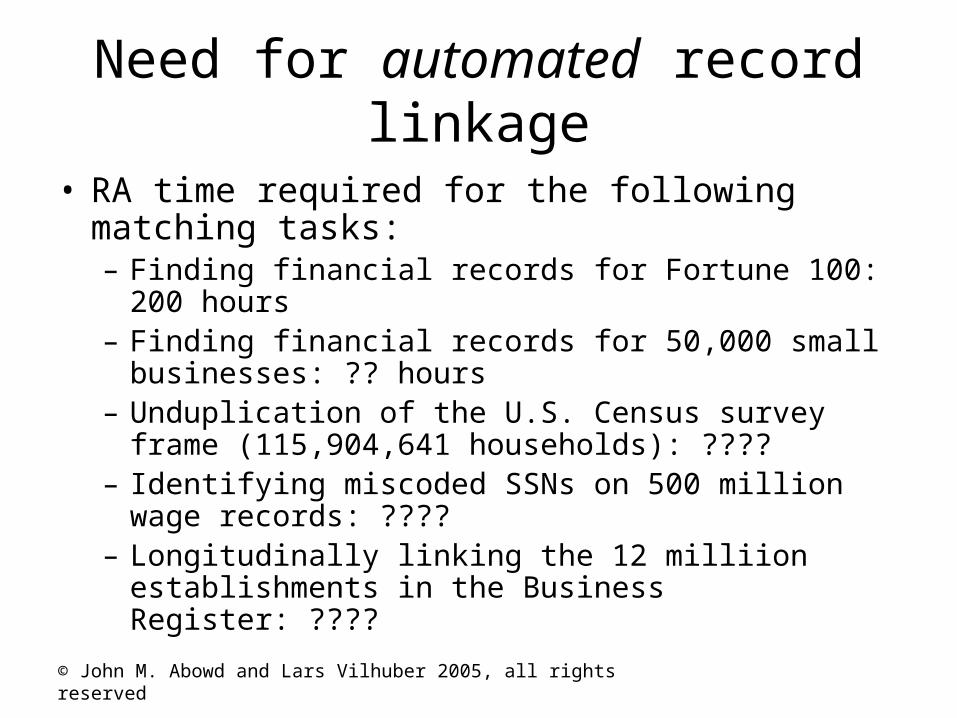
• RA time required for the following matching tasks:– Finding financial records for Fortune 100: 200 hours– Finding financial records for 50,000 small

businesses: ?? hours– Unduplication of the U.S. Census survey frame

(115,904,641 households): ????– Identifying miscoded SSNs on 500 million wage

records: ????– Longitudinally linking the 12 milliion establishments in

the Business Register: ????


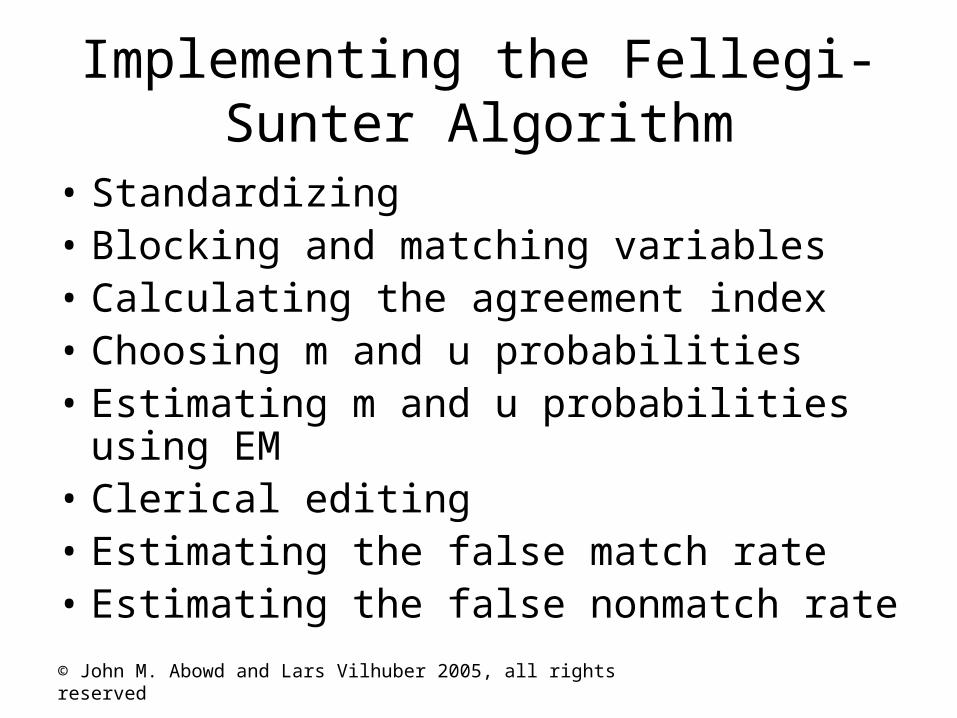
Implementing the Fellegi-Sunter Algorithm

• Standardizing• Blocking and matching variables• Calculating the agreement index• Choosing m and u probabilities• Estimating m and u probabilities using EM• Clerical editing• Estimating the false match rate• Estimating the false nonmatch rate


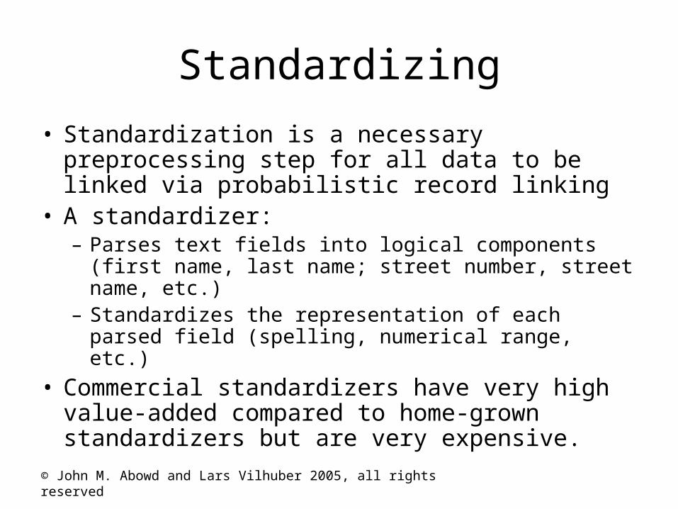
Standardizing

• Standardization is a necessary preprocessing step for all data to be linked via probabilistic record linking

• A standardizer:– Parses text fields into logical components (first name,

last name; street number, street name, etc.)– Standardizes the representation of each parsed field

(spelling, numerical range, etc.)

• Commercial standardizers have very high value-added compared to home-grown standardizers but are very expensive.


Blocking and Matching

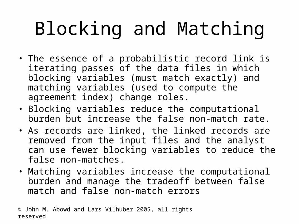
• The essence of a probabilistic record link is iterating passes of the data files in which blocking variables (must match exactly) and matching variables (used to compute the agreement index) change roles.

• Blocking variables reduce the computational burden but increase the false non-match rate.

• As records are linked, the linked records are removed from the input files and the analyst can use fewer blocking variables to reduce the false non-matches.

• Matching variables increase the computational burden and manage the tradeoff between false match and false non-match errors


Recall the Setup

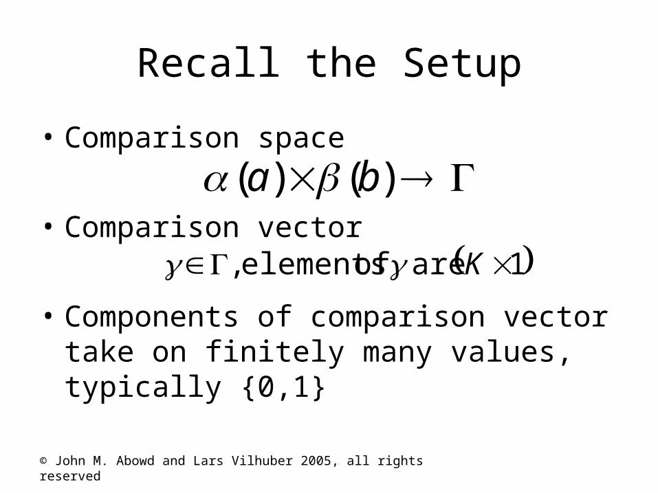
• Comparison space

• Comparison vector

• Components of comparison vector take on finitely many values, typically {0,1}

)()( ba

1 are of elements , K


Linkage rule

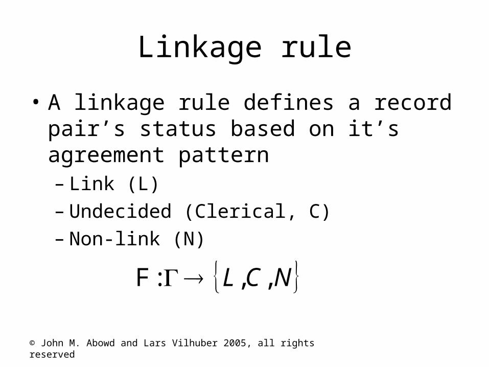
• A linkage rule defines a record pair’s status based on it’s agreement pattern– Link (L)– Undecided (Clerical, C)– Non-link (N)

NCL ,,:F


Calculating the Agreement Index

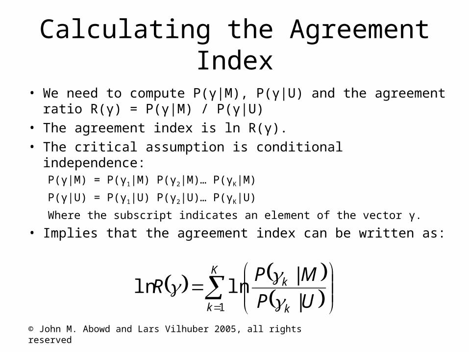
• We need to compute P(γ|M), P(γ|U) and the agreement ratio R(γ) = P(γ|M) / P(γ|U)

• The agreement index is ln R(γ).• The critical assumption is conditional independence:

P(γ|M) = P(γ1|M) P(γ2|M)… P(γK|M)

P(γ|U) = P(γ1|U) P(γ2|U)… P(γK|U)

Where the subscript indicates an element of the vector γ.

• Implies that the agreement index can be written as:

K

k k

k

UP

MPR

1 |

|lnln


Choosing m and u Probabilities

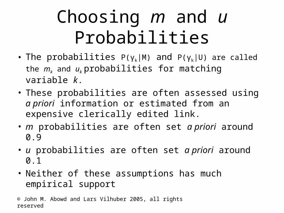
• The probabilities P(γk|M) and P(γk|U) are called the

mk and uk probabilities for matching variable k.

• These probabilities are often assessed using a priori information or estimated from an expensive clerically edited link.

• m probabilities are often set a priori around 0.9• u probabilities are often set a priori around 0.1• Neither of these assumptions has much

empirical support


Estimating m and u Using Matched Data

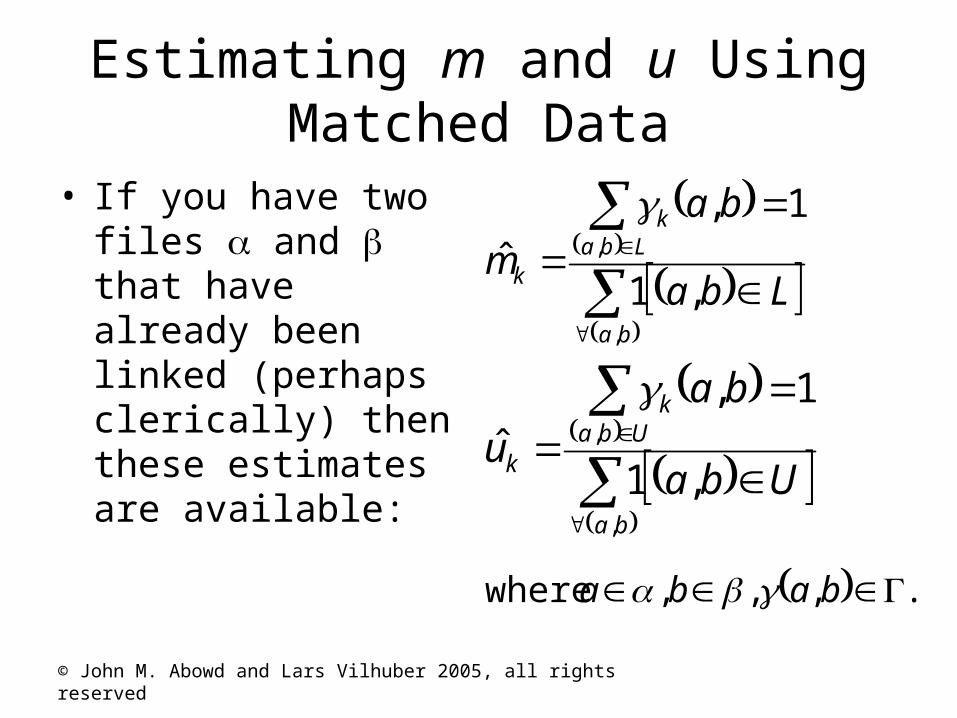
• If you have two files and that have already been linked (perhaps clerically) then these estimates are available:

ba

Lbak

k Lba

ba

m

,

,

,1

1,

ˆ

ba

Ubak

k Uba

ba

u

,

,

,1

1,

ˆ

.,,, where baba


Estimating m and u Probabilities Using EM

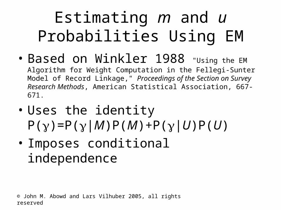
• Based on Winkler 1988 "Using the EM Algorithm for Weight Computation in the Fellegi-Sunter Model of Record Linkage," Proceedings of the Section on Survey Research Methods, American Statistical Association, 667-671.

• Uses the identityP()=P(|M)P(M)+P(|U)P(U)

• Imposes conditional independence


Estimating m and u Probabilities Using EM: Algorithm I

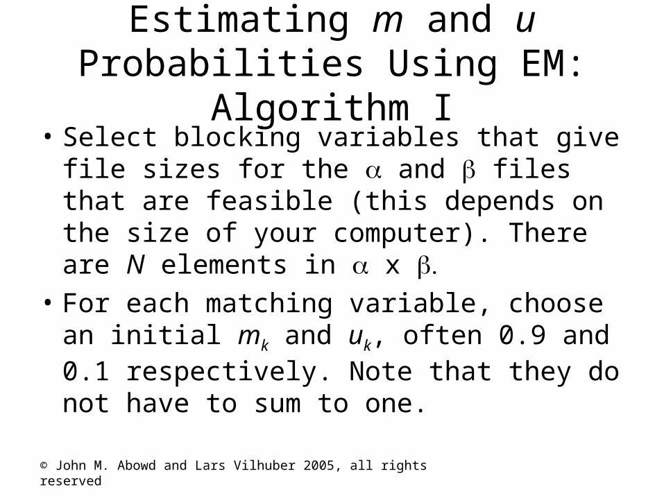
• Select blocking variables that give file sizes for the and files that are feasible (this depends on the size of your computer). There are N elements in x

• For each matching variable, choose an initial mk and uk, often 0.9 and 0.1 respectively. Note that they do not have to sum to one.


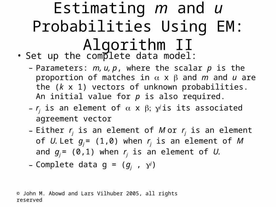
Estimating m and u Probabilities Using EM: Algorithm II

• Set up the complete data model:– Parameters: m, u, p, where the scalar p is the

proportion of matches in x and m and u are the (k x 1) vectors of unknown probabilities. An initial value for p is also required.

– rj is an element of x j is its associated agreement vector

– Either rj is an element of M or rj is an element of U. Let gj = (1,0) when rj is an element of M and gj = (0,1) when rj is an element of U.

– Complete data g = (gj , j)


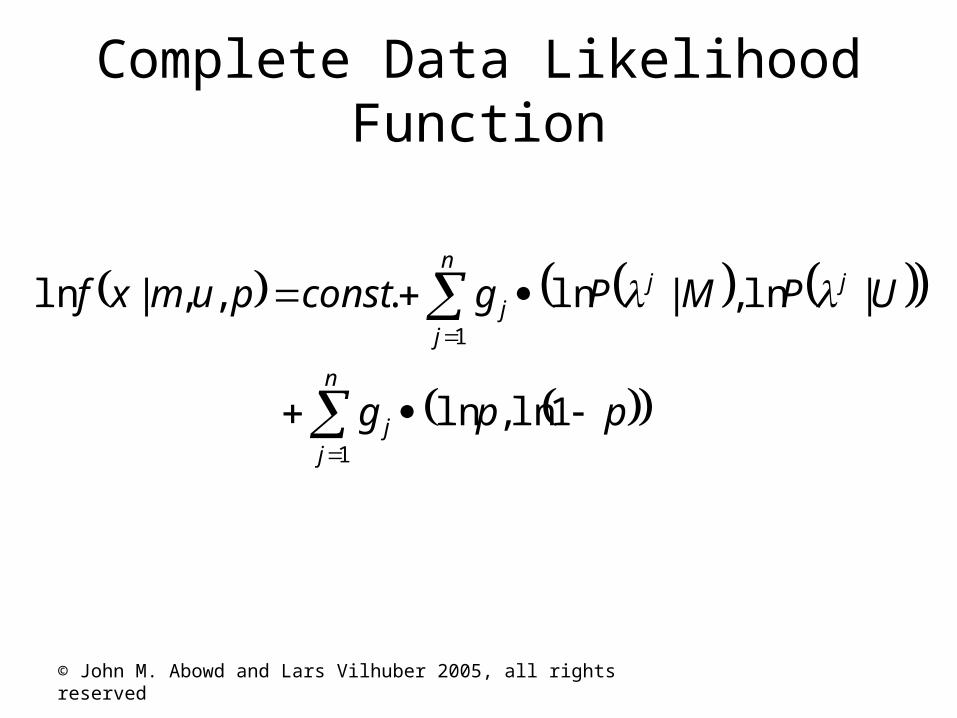
Complete Data Likelihood Function

n

jj

n

j

jjj

ppg

UPMPgconstpumxf

1

1

1ln,ln

|ln,|ln.,,|ln


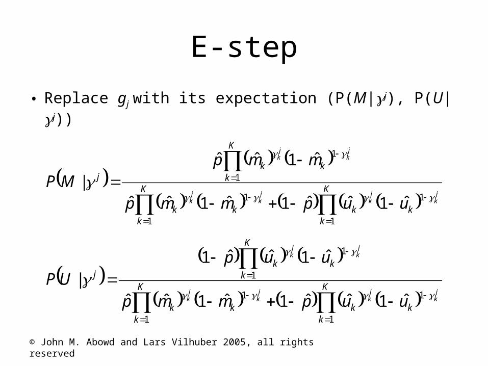
E-step

• Replace gj with its expectation (P(M|j), P(U|j))

K

kkk

K

kkk

K

kkk

j

jk

jk

jk

jk

jk

jk

uupmmp

mmpMP

1

1

1

1

1

1

ˆ1ˆˆ1ˆ1ˆˆ

ˆ1ˆˆ

|

K

kkk

K

kkk

K

kkk

j

jk

jk

jk

jk

jk

jk

uupmmp

uupUP

1

1

1

1

1

1

ˆ1ˆˆ1ˆ1ˆˆ

ˆ1ˆˆ1|


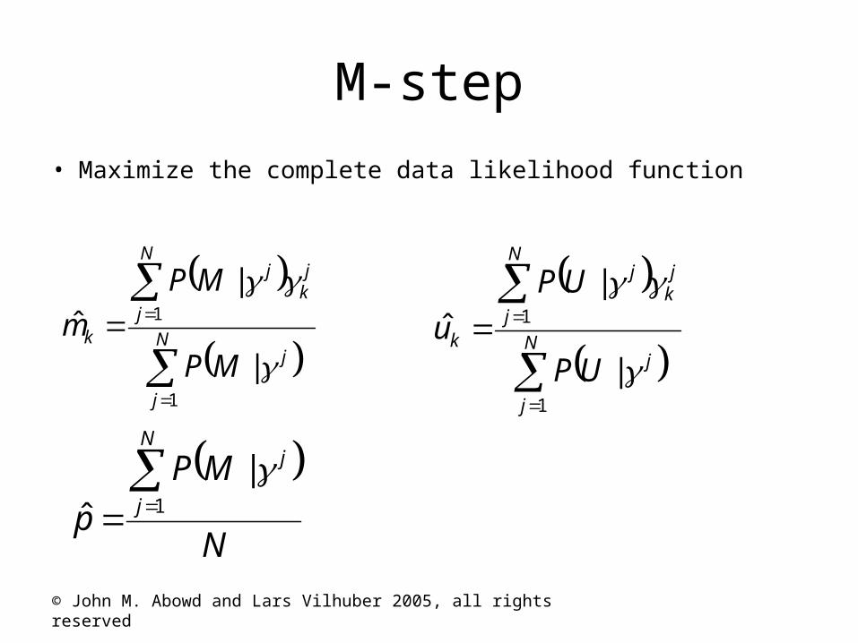
M-step

• Maximize the complete data likelihood function

N

j

j

N

j

jk

j

k

MP

MP

m

1

1

|

|

ˆ

N

j

j

N

j

jk

j

k

UP

UP

u

1

1

|

|

ˆ

N

MP

p

N

j

j 1

|

ˆ


Convergence

• Alternate E and M steps

• Compute the change in the complete data likelihood function

• Stop when the change in the complete data likelihood function is small


Clerical Editing

• Once the m and u probabilities have been estimated, cutoffs for the U, C, and L sets must be determined.

• This is usually done by setting preliminary cutoffs then clerically refining them.

• Often the m and u probabilities are tweaked as a part of this clerical review.


Estimating the False Match Rate

• This is usually done by clerical review of a run of the automated matcher.

• Some help is available from Belin, T. R., and Rubin, D. B. (1995), "A Method for Calibrating False- Match Rates in Record Linkage," Journal of the American Statistical Association, 90, 694-707.


Estimating the False Nonmatch Rate

• This is much harder.• Often done by a clerical review of a sample of

the non-match records.• Since false nonmatching is relatively rare among

the nonmatch pairs, this sample is often stratified by variables known to affect the match rate.

• Stratifying by the agreement index is a very effective way to estimate false nonmatch rates.


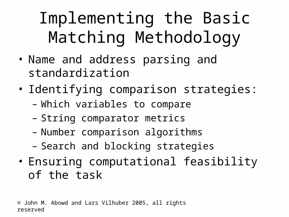
Implementing the Basic Matching Methodology

• Name and address parsing and standardization• Identifying comparison strategies:

– Which variables to compare– String comparator metrics– Number comparison algorithms– Search and blocking strategies

• Ensuring computational feasibility of the task


Generic workflow

• Standardize

• Match

• Revise and iterate through again


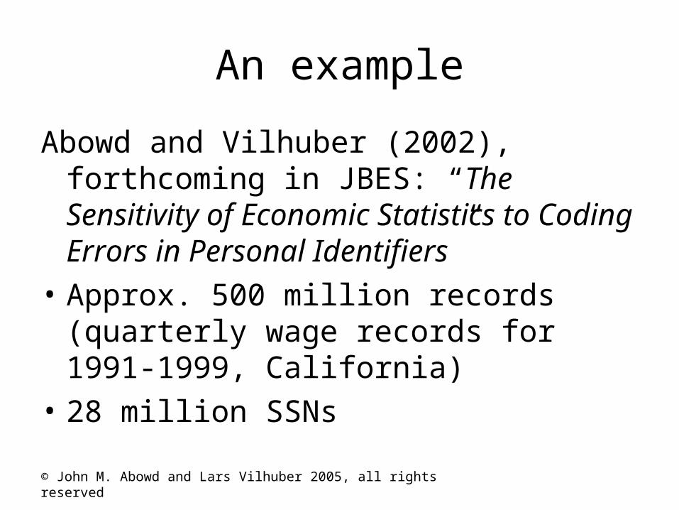
An example

Abowd and Vilhuber (2002), forthcoming in JBES: “The Sensitivity of Economic Statistics to Coding Errors in Personal Identifiers”

• Approx. 500 million records (quarterly wage records for 1991-1999, California)

• 28 million SSNs


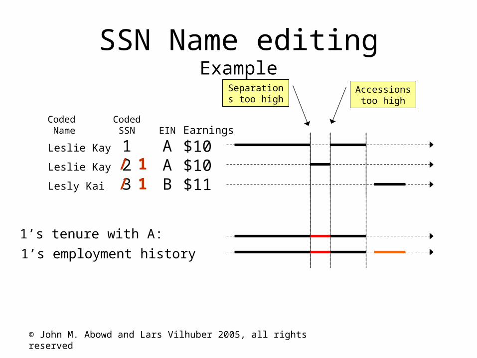
1’s tenure with A:

1’s employment history

Coded Coded Name SSN EIN

Leslie Kay 1 ALeslie Kay 2 ALesly Kai 3 B

Earnings

$10$10$11

Separations too high

Accessions too high

SSN Name editingExample

/ 1/ 1


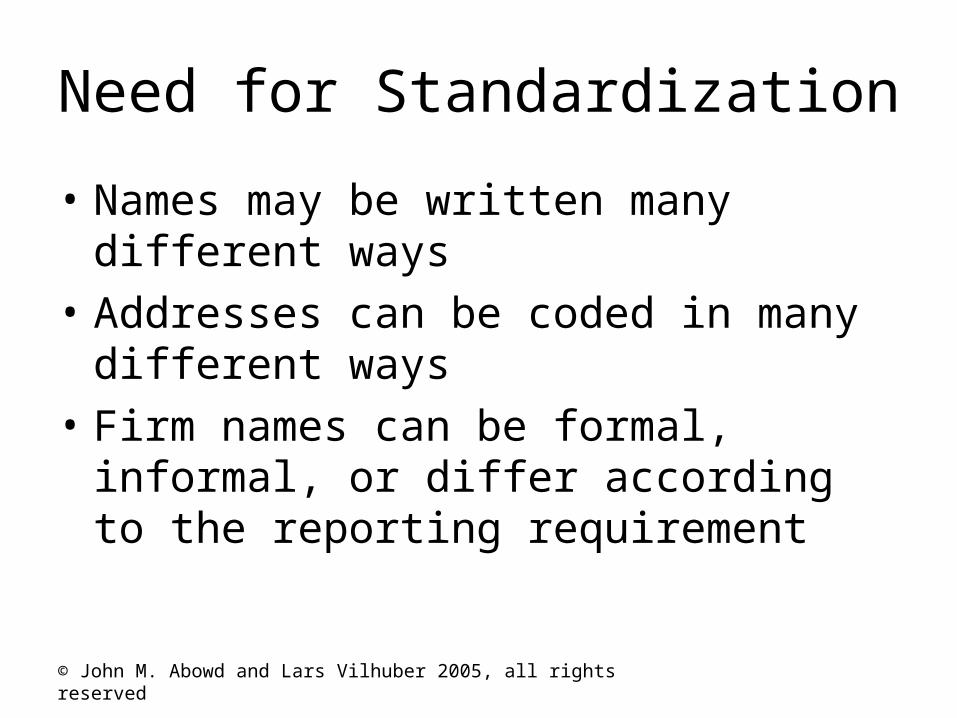
Need for Standardization

• Names may be written many different ways

• Addresses can be coded in many different ways

• Firm names can be formal, informal, or differ according to the reporting requirement


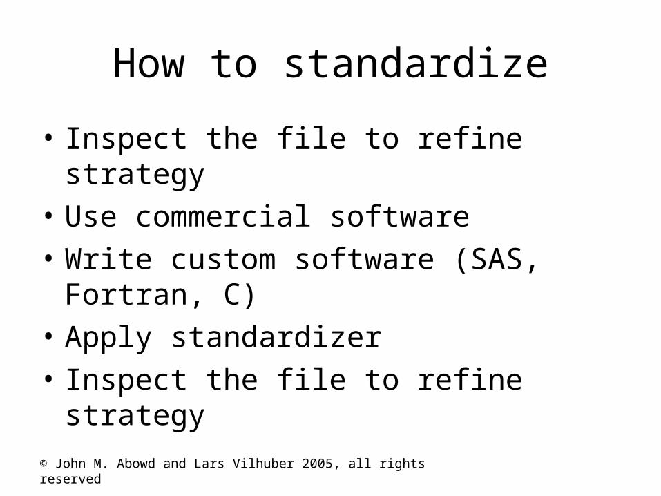
How to standardize

• Inspect the file to refine strategy

• Use commercial software

• Write custom software (SAS, Fortran, C)

• Apply standardizer

• Inspect the file to refine strategy


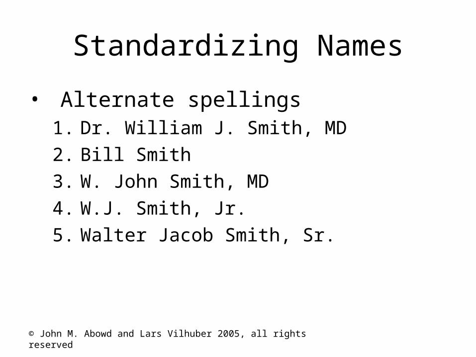
Standardizing Names

• Alternate spellings1. Dr. William J. Smith, MD

2. Bill Smith

3. W. John Smith, MD

4. W.J. Smith, Jr.

5. Walter Jacob Smith, Sr.


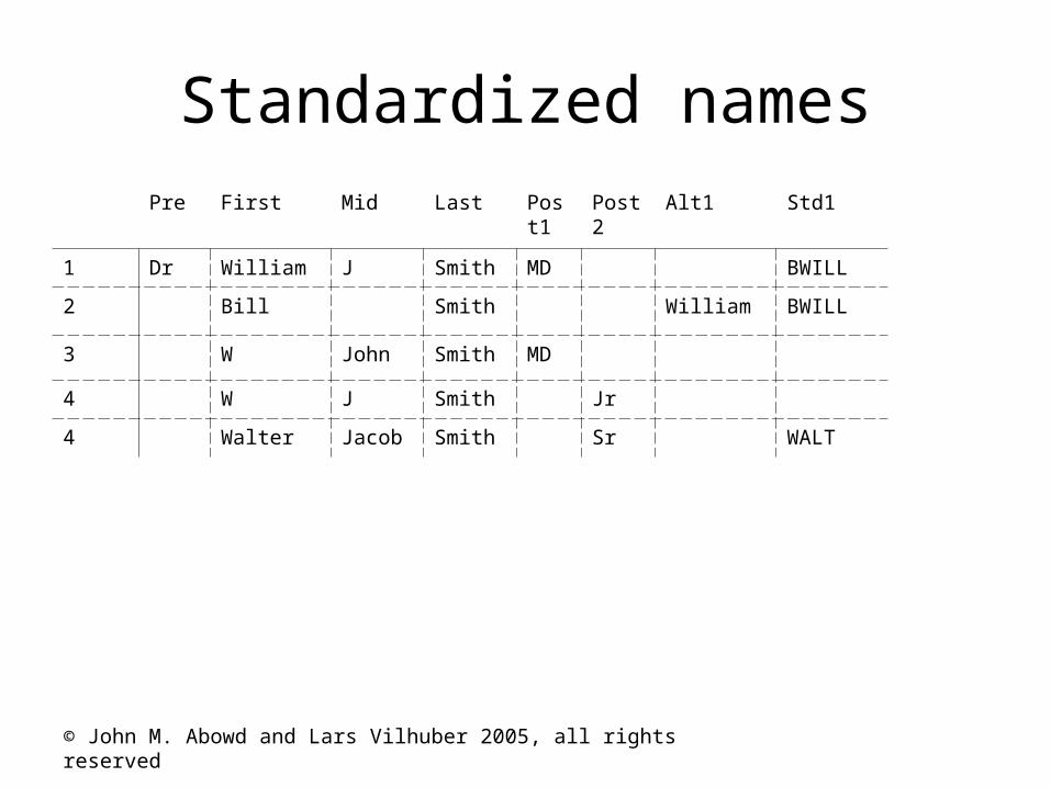
Standardized namesPre First Mid Last Pos

t1Post2

Alt1 Std1

1 Dr William J Smith MD BWILL

2 Bill Smith William BWILL

3 W John Smith MD

4 W J Smith Jr

4 Walter Jacob Smith Sr WALT


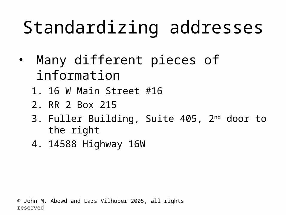
Standardizing addresses

• Many different pieces of information1. 16 W Main Street #16

2. RR 2 Box 215

3. Fuller Building, Suite 405, 2nd door to the right

4. 14588 Highway 16W


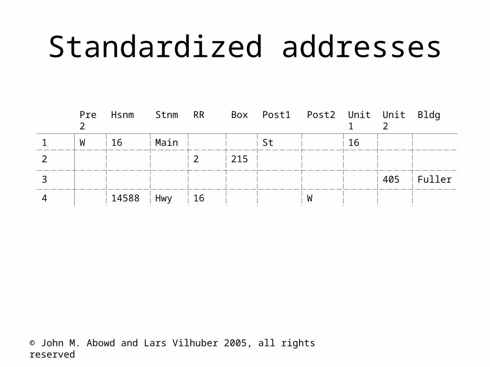
Standardized addresses

Pre2

Hsnm Stnm RR Box Post1 Post2 Unit1

Unit2

Bldg

1 W 16 Main St 16

2 2 215

3 405 Fuller

4 14588 Hwy 16 W


A&V: standardizing

• Knowledge of structure of the file: -> No standardizing

• Matching will be within records close in time -> assumed to be similar, no need for standardization

• BUT: possible false positives -> chose to do an weighted unduplication step (UNDUP) to eliminate wrongly associated SSNs


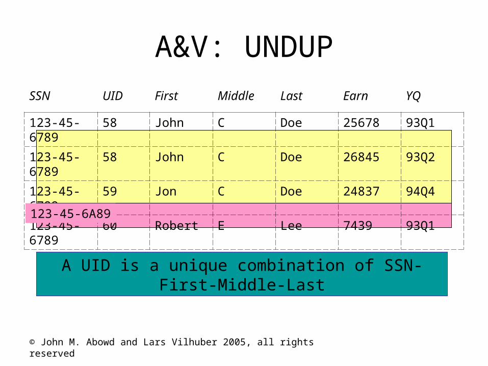
A&V: UNDUP

SSN UID First Middle Last Earn YQ

123-45-6789 58 John C Doe 25678 93Q1

123-45-6789 58 John C Doe 26845 93Q2

123-45-6789 59 Jon C Doe 24837 94Q4

123-45-6789 60 Robert E Lee 7439 93Q1

A UID is a unique combination of SSN-First-Middle-Last

123-45-6A89


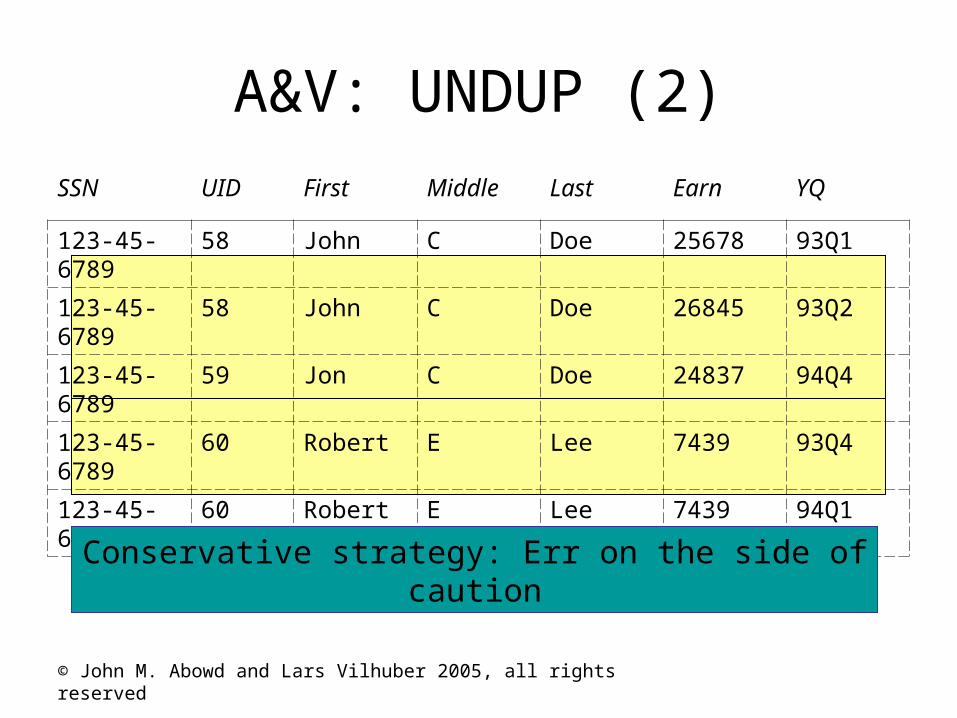
A&V: UNDUP (2)


123-45-6789 58 John C Doe 25678 93Q1

123-45-6789 58 John C Doe 26845 93Q2

123-45-6789 59 Jon C Doe 24837 94Q4

123-45-6789 60 Robert E Lee 7439 93Q4

123-45-6789 60 Robert E Lee 7439 94Q1

Conservative strategy: Err on the side of caution


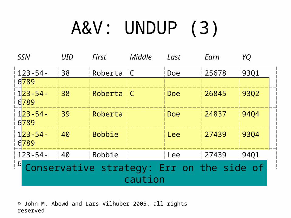
A&V: UNDUP (3)


123-54-6789 38 Roberta C Doe 25678 93Q1

123-54-6789 38 Roberta C Doe 26845 93Q2

123-54-6789 39 Roberta Doe 24837 94Q4

123-54-6789 40 Bobbie Lee 27439 93Q4

123-54-6789 40 Bobbie Lee 27439 94Q1

Conservative strategy: Err on the side of caution


Matching

• Define match blocks

• Define matching parameters: marginal probabilites

• Define upper Tu and lower Tl cutoff values


Record Blocking

• Computationally inefficient to compare all possible record pairs

• Solution: Bring together only record pairs that are LIKELY to match, based on chosen blocking criterion

• Analogy: SAS merge by-variables


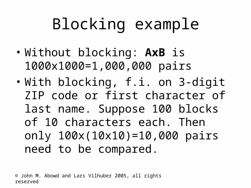
Blocking example

• Without blocking: AxB is 1000x1000=1,000,000 pairs

• With blocking, f.i. on 3-digit ZIP code or first character of last name. Suppose 100 blocks of 10 characters each. Then only 100x(10x10)=10,000 pairs need to be compared.


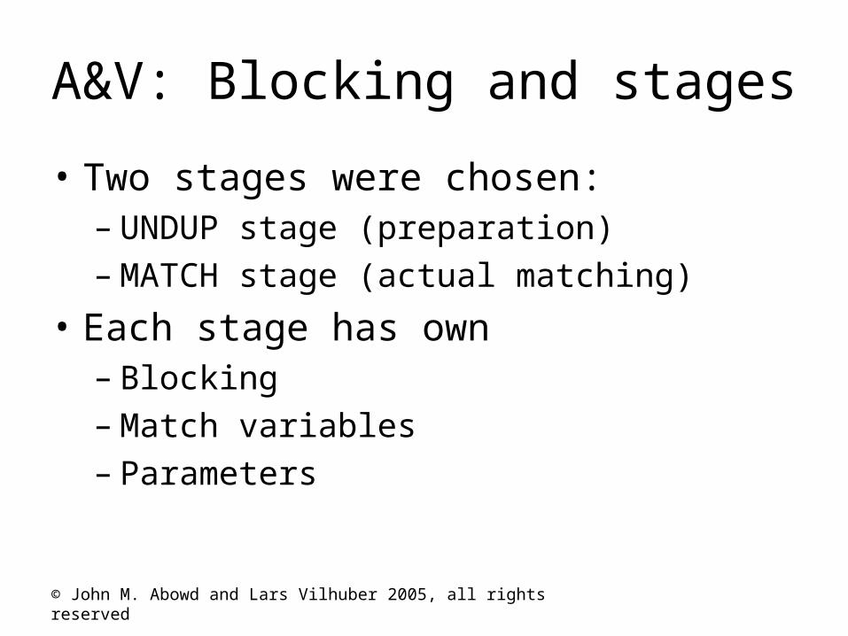
A&V: Blocking and stages

• Two stages were chosen:– UNDUP stage (preparation)– MATCH stage (actual matching)

• Each stage has own – Blocking– Match variables– Parameters


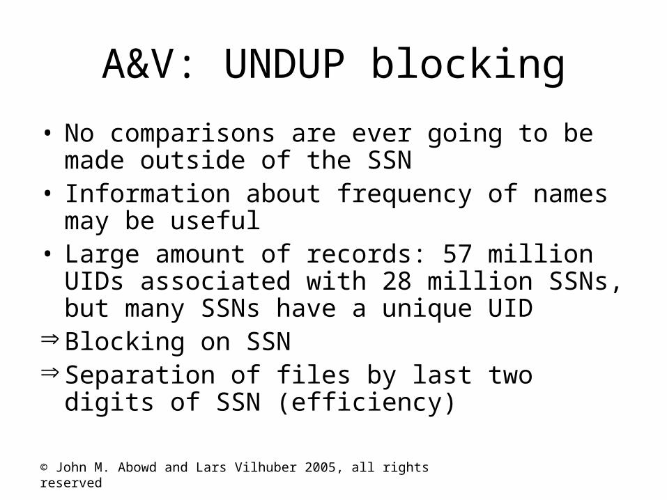
A&V: UNDUP blocking

• No comparisons are ever going to be made outside of the SSN

• Information about frequency of names may be useful

• Large amount of records: 57 million UIDs associated with 28 million SSNs, but many SSNs have a unique UID

Blocking on SSN Separation of files by last two digits of SSN

(efficiency)


A&V: MATCH blocking

• Idea is to fit 1-quarter records into work histories with a 1-quarter interruption at same employer

Block on Employer – QuarterPossibly block on Earnings deciles


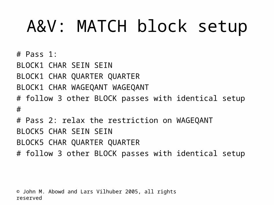
A&V: MATCH block setup

# Pass 1: BLOCK1 CHAR SEIN SEINBLOCK1 CHAR QUARTER QUARTERBLOCK1 CHAR WAGEQANT WAGEQANT# follow 3 other BLOCK passes with identical setup## Pass 2: relax the restriction on WAGEQANTBLOCK5 CHAR SEIN SEINBLOCK5 CHAR QUARTER QUARTER# follow 3 other BLOCK passes with identical setup


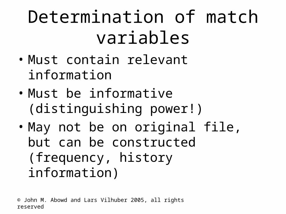
Determination of match variables

• Must contain relevant information

• Must be informative (distinguishing power!)

• May not be on original file, but can be constructed (frequency, history information)


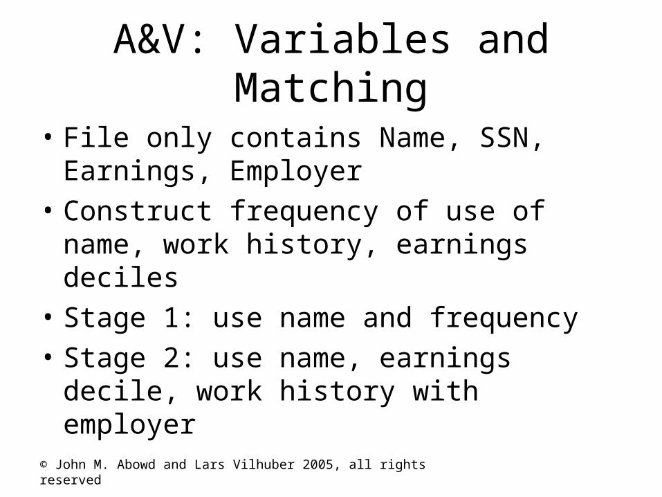
A&V: Variables and Matching

• File only contains Name, SSN, Earnings, Employer

• Construct frequency of use of name, work history, earnings deciles

• Stage 1: use name and frequency

• Stage 2: use name, earnings decile, work history with employer


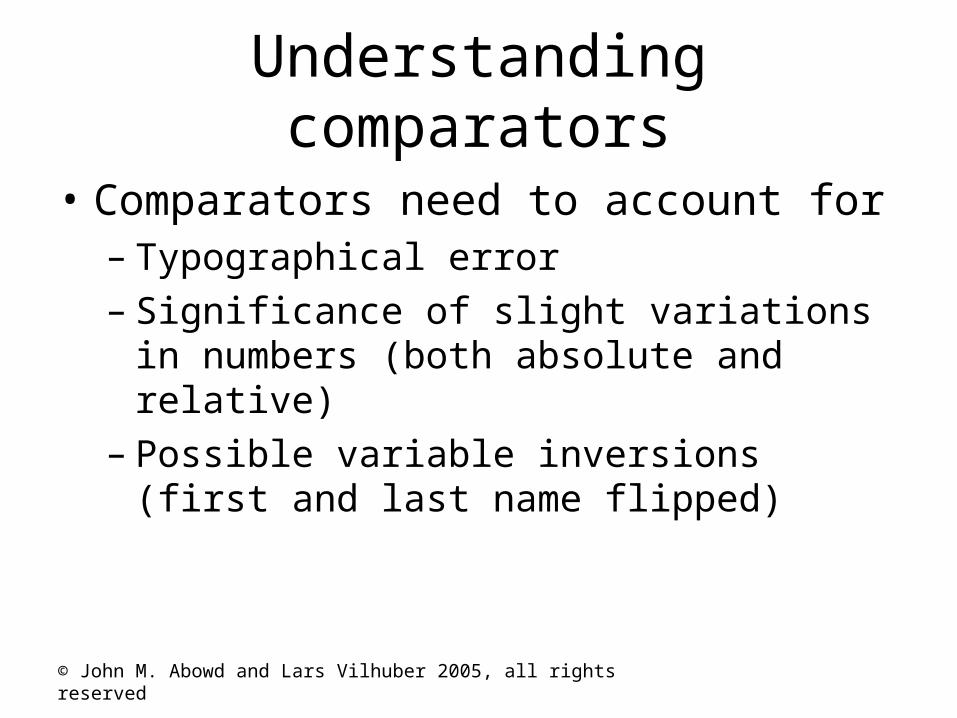
Understanding comparators

• Comparators need to account for– Typographical error– Significance of slight variations in numbers

(both absolute and relative)– Possible variable inversions (first and last

name flipped)


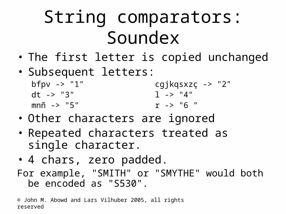
String comparators: Soundex

• The first letter is copied unchanged • Subsequent letters:

bfpv -> "1" cgjkqsxzç -> "2" dt -> "3" l -> "4" mnñ -> "5" r -> "6 "

• Other characters are ignored• Repeated characters treated as single character.• 4 chars, zero padded. For example, "SMITH" or "SMYTHE" would both be

encoded as "S530".


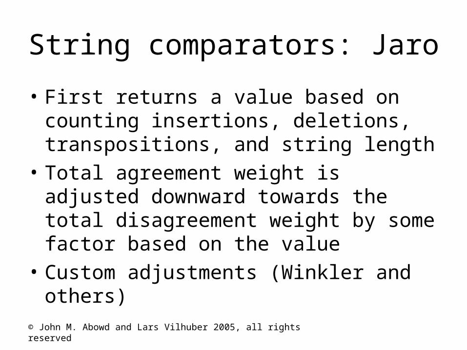
String comparators: Jaro

• First returns a value based on counting insertions, deletions, transpositions, and string length

• Total agreement weight is adjusted downward towards the total disagreement weight by some factor based on the value

• Custom adjustments (Winkler and others)


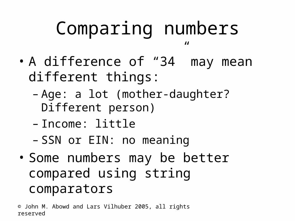
Comparing numbers

• A difference of “34” may mean different things:– Age: a lot (mother-daughter? Different person)– Income: little– SSN or EIN: no meaning

• Some numbers may be better compared using string comparators


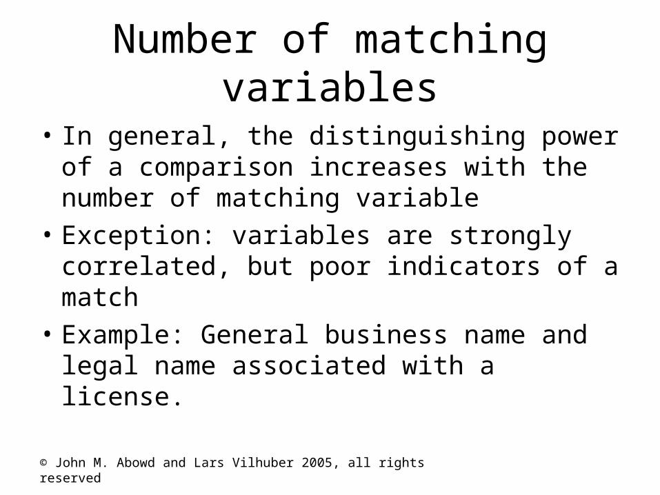
Number of matching variables

• In general, the distinguishing power of a comparison increases with the number of matching variable

• Exception: variables are strongly correlated, but poor indicators of a match

• Example: General business name and legal name associated with a license.


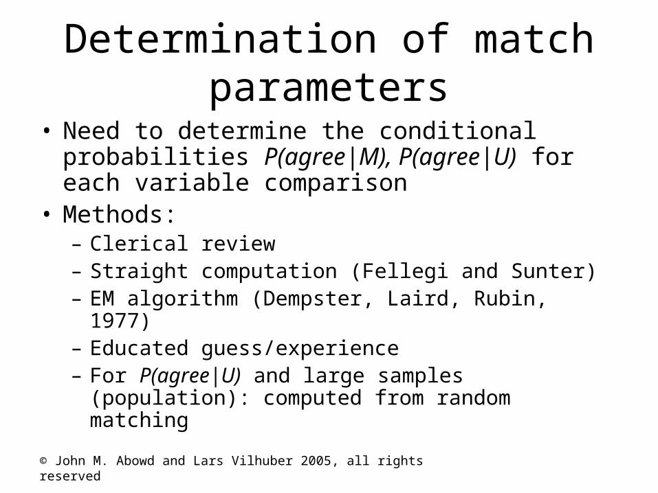
Determination of match parameters

• Need to determine the conditional probabilities P(agree|M), P(agree|U) for each variable comparison

• Methods:– Clerical review– Straight computation (Fellegi and Sunter)– EM algorithm (Dempster, Laird, Rubin, 1977)– Educated guess/experience– For P(agree|U) and large samples (population):

computed from random matching


Determination of match parameters (2)

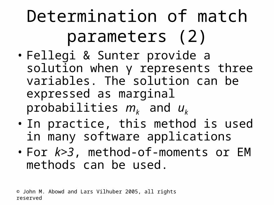
• Fellegi & Sunter provide a solution when γ represents three variables. The solution can be expressed as marginal probabilities mk and uk

• In practice, this method is used in many software applications

• For k>3, method-of-moments or EM methods can be used.


Marginal probabilities: educated guesses for starting values

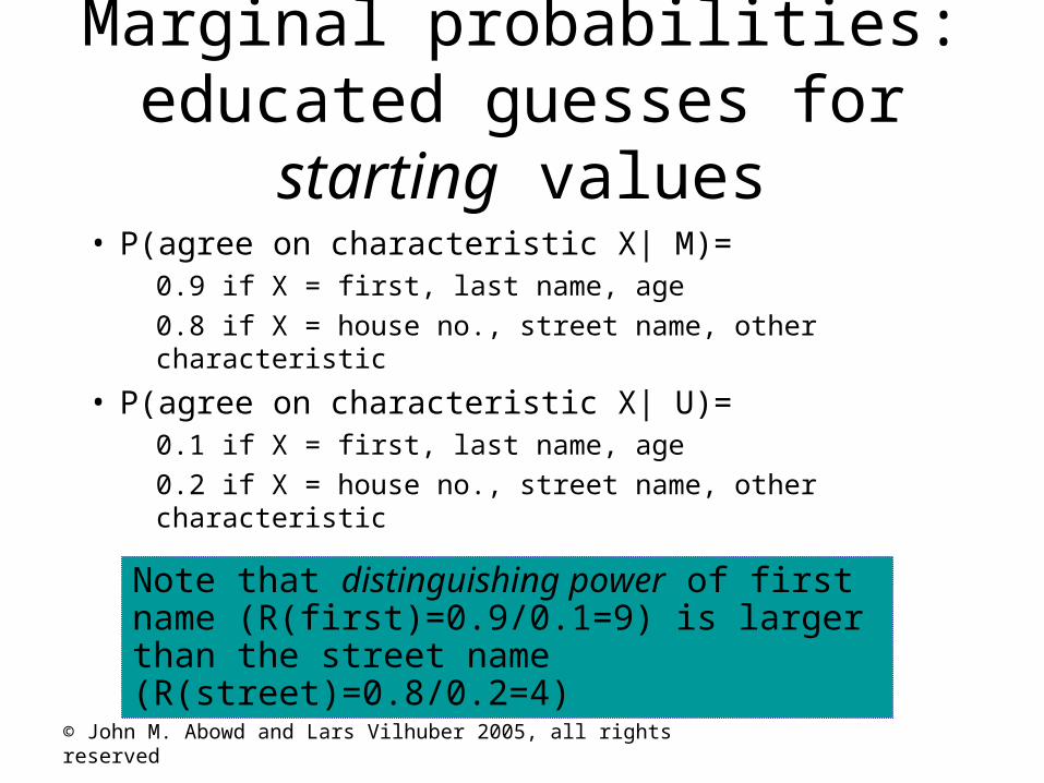
• P(agree on characteristic X| M)=0.9 if X = first, last name, age

0.8 if X = house no., street name, other characteristic

• P(agree on characteristic X| U)= 0.1 if X = first, last name, age

0.2 if X = house no., street name, other characteristic

Note that distinguishing power of first name (R(first)=0.9/0.1=9) is larger than the street name (R(street)=0.8/0.2=4)


Marginal probabilities: better estimates of P(agree|M)

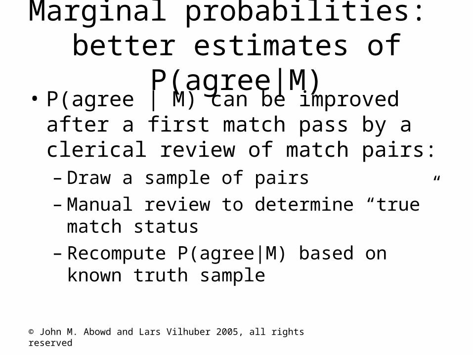
• P(agree | M) can be improved after a first match pass by a clerical review of match pairs: – Draw a sample of pairs– Manual review to determine “true” match

status– Recompute P(agree|M) based on known truth

sample


A&V: UNDUP match variables

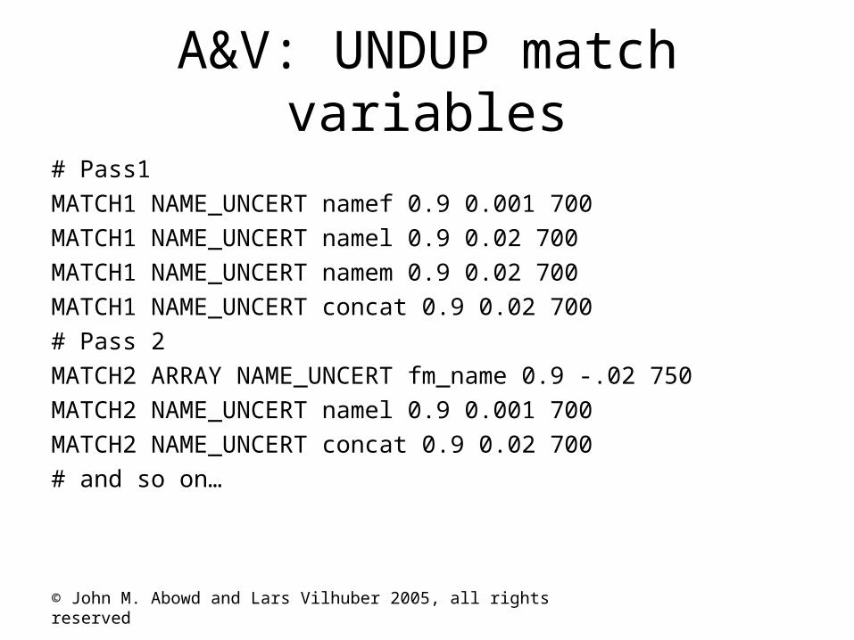
# Pass1MATCH1 NAME_UNCERT namef 0.9 0.001 700MATCH1 NAME_UNCERT namel 0.9 0.02 700MATCH1 NAME_UNCERT namem 0.9 0.02 700MATCH1 NAME_UNCERT concat 0.9 0.02 700# Pass 2MATCH2 ARRAY NAME_UNCERT fm_name 0.9 -.02 750MATCH2 NAME_UNCERT namel 0.9 0.001 700MATCH2 NAME_UNCERT concat 0.9 0.02 700# and so on…


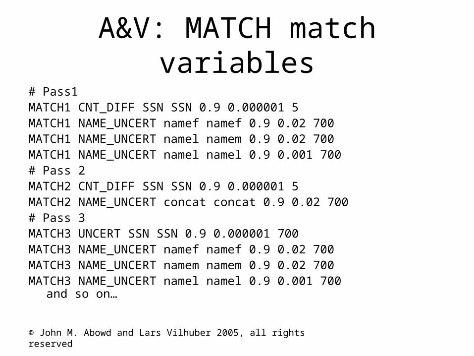
A&V: MATCH match variables# Pass1MATCH1 CNT_DIFF SSN SSN 0.9 0.000001 5MATCH1 NAME_UNCERT namef namef 0.9 0.02 700MATCH1 NAME_UNCERT namel namem 0.9 0.02 700MATCH1 NAME_UNCERT namel namel 0.9 0.001 700# Pass 2MATCH2 CNT_DIFF SSN SSN 0.9 0.000001 5MATCH2 NAME_UNCERT concat concat 0.9 0.02 700# Pass 3MATCH3 UNCERT SSN SSN 0.9 0.000001 700MATCH3 NAME_UNCERT namef namef 0.9 0.02 700MATCH3 NAME_UNCERT namem namem 0.9 0.02 700MATCH3 NAME_UNCERT namel namel 0.9 0.001 700 and so on…


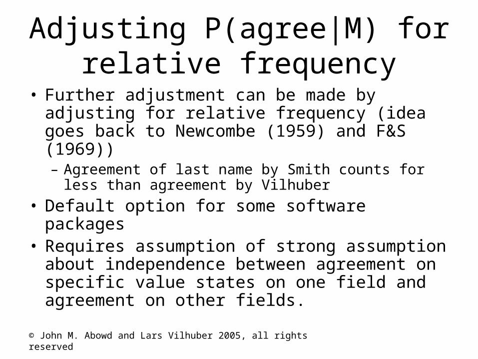
Adjusting P(agree|M) for relative frequency

• Further adjustment can be made by adjusting for relative frequency (idea goes back to Newcombe (1959) and F&S (1969))– Agreement of last name by Smith counts for less than

agreement by Vilhuber

• Default option for some software packages• Requires assumption of strong assumption

about independence between agreement on specific value states on one field and agreement on other fields.


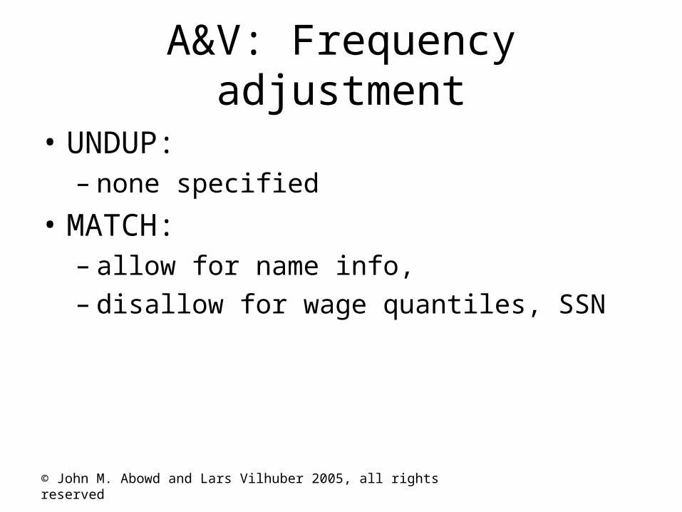
A&V: Frequency adjustment

• UNDUP: – none specified

• MATCH: – allow for name info, – disallow for wage quantiles, SSN


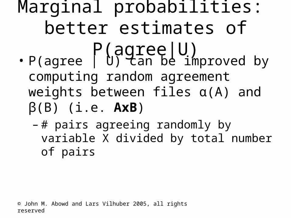
Marginal probabilities: better estimates of P(agree|U)

• P(agree | U) can be improved by computing random agreement weights between files α(A) and β(B) (i.e. AxB)– # pairs agreeing randomly by variable X

divided by total number of pairs


Error rate estimation methods

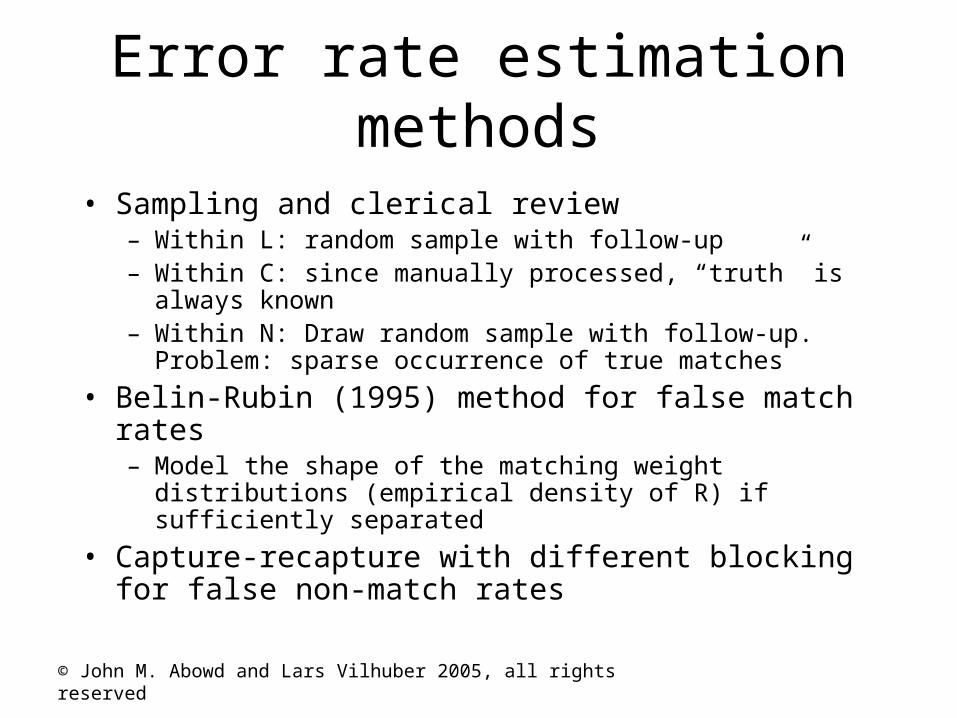
• Sampling and clerical review– Within L: random sample with follow-up– Within C: since manually processed, “truth” is always known– Within N: Draw random sample with follow-up. Problem:

sparse occurrence of true matches

• Belin-Rubin (1995) method for false match rates– Model the shape of the matching weight distributions

(empirical density of R) if sufficiently separated

• Capture-recapture with different blocking for false non-match rates


Analyst Review

• Matcher outputs file of matched pairs in decreasing weight order

• Examine list to determine cutoff weights and non-matches.


A&V: Finding cutoff values

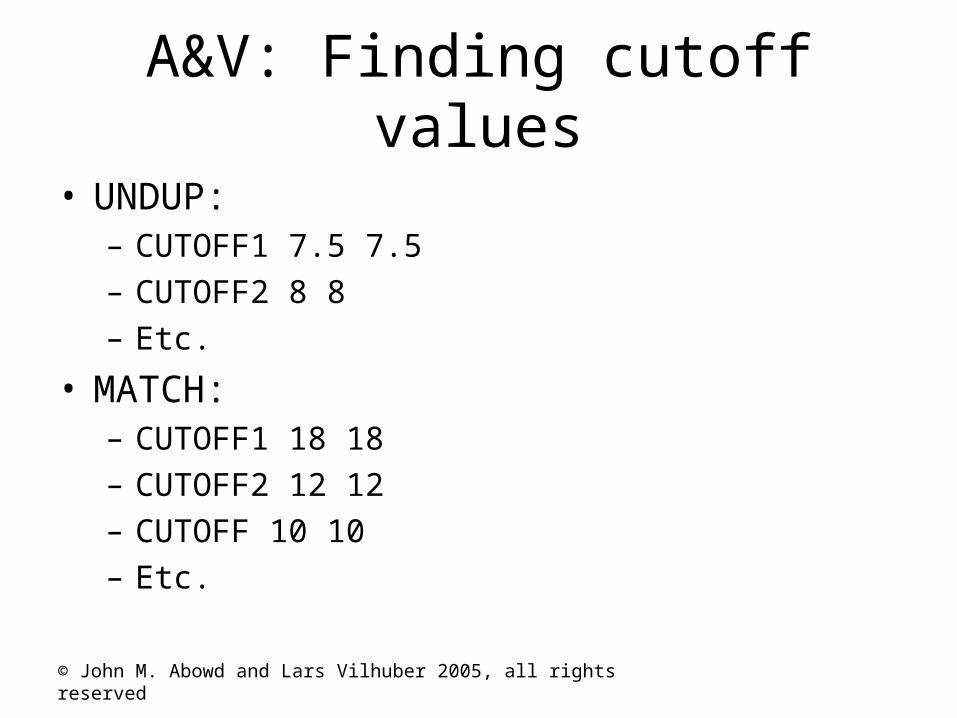
• UNDUP:– CUTOFF1 7.5 7.5– CUTOFF2 8 8– Etc.

• MATCH:– CUTOFF1 18 18– CUTOFF2 12 12– CUTOFF 10 10– Etc.


A&V: Sample matcher output

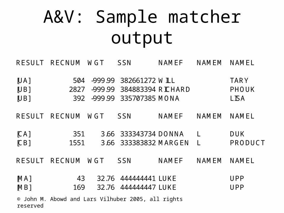
RESULT RECNUM WGT SSN NAMEF NAMEM NAMEL

[UA] 504 -999.99 382661272 WILL TARY[UB] 2827 -999.99 384883394 RICHARD PHOUK[UB] 392 -999.99 335707385 MONA LISA


[CA] 351 3.66 333343734 DONNA L DUK[CB] 1551 3.66 333383832 MARGEN L PRODUCT


[MA] 43 32.76 444444441 LUKE UPP[MB] 169 32.76 444444447 LUKE UPP


Post-processing

• Once matching software has identified matches, further processing may be needed:– Clean up– Carrying forward matching information– Reports on match rates


Generic workflow (2)

• Start with initial set of parameter values

• Run matching programs

• Review moderate sample of match results

• Modify parameter values (typically only mk) via ad hoc means


Acknowledgements

• This lecture is based in part on a 2000 lecture given by William Winkler, William Yancey and Edward Porter at the U.S. Census Bureau

• Some portions draw on Winkler (1995), “Matching and Record Linkage,” in B.G. Cox et. al. (ed.), Business Survey Methods, New York, J. Wiley, 355-384.

• Examples are all purely fictitious, but inspired from true cases presented in the above lecture, in Abowd & Vilhuber (2004).

Documents

© John M. Abowd and Lars Vilhuber 2005, all rights reserved Record Linking, II John M. Abowd and Lars Vilhuber March 2005