Embed Size (px)
Citation preview
GRUAN Technical Document
Technical characteristics and GRUAN data
processing for the Meisei RS-11G and iMS-100
radiosondes
Nobuhiko Kizu, Takuji Sugidachi, Eriko Kobayashi, Shunsuke Hoshino,Kensaku Shimizu, Ryota Maeda and Masatomo Fujiwara
Publisher
GRUAN Lead Centre
Number & Version
GRUAN-TD-5
Rev 1.0 (2018-02-21)

Kizu et al. GRUAN-TD-5 Rev 1.0 (2018-02-21)
Document info
Title: Technical characteristics and GRUAN data processing
for the Meisei RS-11G and iMS-100 radiosondes
Topic: Data productAuthors: Nobuhiko Kizu, Takuji Sugidachi, Eriko Kobayashi,
Shunsuke Hoshino, Kensaku Shimizu, Ryota Maeda andMasatomo Fujiwara
Publisher: GRUAN Lead Centre, DWDDocument type: Technical DocumentDocument number: GRUAN-TD-5Page count: 152Version: Rev 1.0 (2018-02-21)
Abstract
The GCOS (Global Climate Observing System) Reference Upper-Air Network (GRUAN) data pro-cessing for the Meisei RS-11G and iMS-100 radiosondes has been developed to meet the criteria forreference measurements. Since July 2013, the RS-11G radiosonde has been regularly launched atTateno (36.06!N, 140.13!E, 25.2 m; Aerological Observatory of the Japan Meteorological Agency),Japan. Also, a smaller version, the Meisei iMS-100 radiosonde has been developed, with the samesensors as those of the RS-11G radiosonde, and will be used at Tateno in the future. This techni-cal document describes the algorithms including the corrections to obtain pressure (or geopotentialheight), temperature, relative humidity (RH), and horizontal wind data from the RS-11G and iMS-100radiosonde raw data. It also discusses the uncertainty evaluation for each variable obtained from theseradiosondes. The corrections compensate various known systematic biases, which are mainly the so-lar radiation error, calibration error, and heat spike error for the temperature measurements, and thedry biases due to solar heating, time-lag error, and calibration error at low temperature conditions forthe RH measurements. The measurement uncertainty for each variable was evaluated by laboratoryexperiments and verified by comparison flights. The uncertainty for the temperature measurementsis mainly determined by that of the corrections for the solar radiation error and calibration error. Itsuncertainty increases with altitude, and reaches 0.8 K at 30 km. Up to "15 km, the calibration-errorcorrection is the dominant factor to the total uncertainty of the temperature measurements, while inthe stratosphere, the radiation correction is the dominant factor. Because the actual sounding con-ditions are different from the assumed condition (e.g., surface and cloud albedo), it is consideredthat additional information for each sounding, such as the cloud condition, is necessary to reducethe uncertainty. Also, the uncertainty due to heat spikes needs to be considered for particular flightconfigurations (e.g., the case with a shorter string of 15 m and a 600 g balloon). A large payload anda rig for multiple-payload sounding may introduce additional heat spikes and thus larger uncertainty.The uncertainty of the RH measurements is maximal around the tropopause because of the large andsudden change in RH between the wet troposphere and dry stratosphere and of the coldness there,leading to large time-lag correction component. The uncertainty from the calibration-error correctionis relatively large at low temperatures because the evaluation is difficult there. Solar heating on the RHsensor leads to dry bias; thus, this bias is corrected by considering the difference between the sensor
3 / 152
Kizu et al. GRUAN-TD-5 Rev 1.0 (2018-02-21)
temperature and air temperature. The uncertainty from the solar heating dry bias correction is derivedfrom the sensor temperature measurement uncertainty (±0.3 K). The sensor temperature is measuredwith the dedicated thermistor for the iMS-100, and is estimated by the solar radiation correction andthermal-lag for the RS-11G. There are other minor factors contributing to the total RH uncertainty,though they are currently not quantified. The hysteresis bias arises only when the RH changes fromwet to dry. The contamination error causes wet biases only under rainy conditions, though its quan-tification is currently not possible because the RH reference measurements do not exist under rainyconditions. The uncertainty for the geopotential height is determined by the accuracy of the GlobalPositioning System (GPS) antenna and module in use (as the RS-11G and iMS-100 radiosondes areusually not equipped with a pressure sensor). The 3 dimensional error of the GPS for the RS-11Gand iMS-100 is typically less than 10 m. The pressure is calculated from the GPS geopotential heightusing the relationship of the hydrostatic equation and thus using temperature and RH data. Therefore,the uncertainties in the GPS-based geopotential-height, temperature, and RH measurements propa-gate to the uncertainty of the pressure measurement. In addition, the uncertainty of surface pressuremeasurement affects the total pressure uncertainty. The geopotential-height uncertainty is the mainfactor for the pressure uncertainty at lower altitudes, while the temperature uncertainty is the mainfactor at higher altitudes. Also, the uncertainty of the surface pressure measurement contributes to thepressure uncertainty at all levels. The uncertainty (1! ) of the GPS Doppler speed measurements isless than 0.01 m s#1, and thus this is not the main factor of the uncertainty for the GPS-based horizon-tal wind measurements. The main factor comes from the radiosonde pendulum motions during theflight. Such oscillations are removed by a software filter (in particular for operational sounding data).Because of this filtering, smaller-scale variabilities with the periods less than the pendulum periodcannot be obtained. The period of the pendulum motion is 7.8 s for the string of 15 m length, and theuncertainty due to these oscillations are typically 1 – 3 m s#1, being larger at higher altitudes.
Revision history
Version Author / Editor Description
Rev 1.0 (2018-02-21) Nobuhiko Kizu, TakujiSugidachi, ErikoKobayashi, ShunsukeHoshino, KensakuShimizu, Ryota Maedaand Masatomo Fuji-wara
First published version as GRUAN TechnicalDocument 5 (GRUAN-TD-5)
4 / 152
Kizu et al. GRUAN-TD-5 Rev 1.0 (2018-02-21)
Table of Contents
1 Introduction . . . . . . . . . . . . . . . . . . . . . . . . . . . . . . . . . . . . . . . . . . 8
1.1 Motivation . . . . . . . . . . . . . . . . . . . . . . . . . . . . . . . . . . . . . . . . 8
1.2 Historical overview of the operational radiosonde soundings in Japan . . . . . . . . . 8
1.3 JMA’s contributions to the GRUAN . . . . . . . . . . . . . . . . . . . . . . . . . . . 12
2 Overview of the RS-11G and iMS-100 radiosondes . . . . . . . . . . . . . . . . . . . . . 20
2.1 RS-11G radiosonde . . . . . . . . . . . . . . . . . . . . . . . . . . . . . . . . . . . 20
2.2 iMS-100 radiosonde . . . . . . . . . . . . . . . . . . . . . . . . . . . . . . . . . . . 20
2.3 Specifications of the RS-11G and iMS-100 radiosondes . . . . . . . . . . . . . . . . 21
2.3.1 The configuration of the RS-11G and iMS-100 radiosondes . . . . . . . . . . . 21
2.3.2 Information on the connectivity of external sensors for the RS-11G radiosonde . 27
2.3.3 Manufacturer-provided measurement specifications . . . . . . . . . . . . . . . 28
2.3.4 Production of the radiosondes . . . . . . . . . . . . . . . . . . . . . . . . . . . 28
2.4 Ground checks . . . . . . . . . . . . . . . . . . . . . . . . . . . . . . . . . . . . . . 28
2.4.1 Ground check (baseline check) using the manufacturer’s Baseline Checker . . . 28
2.4.2 Ground check with the 0 %RH and 100 %RH Standard Humidity Chamber . . . 30
2.5 Launching method . . . . . . . . . . . . . . . . . . . . . . . . . . . . . . . . . . . . 31
3 Measurements from the RS-11G and iMS-100 radiosondes . . . . . . . . . . . . . . . . 33
3.1 Temperature measurements . . . . . . . . . . . . . . . . . . . . . . . . . . . . . . . 33
3.1.1 Sensor material . . . . . . . . . . . . . . . . . . . . . . . . . . . . . . . . . . 33
3.1.2 Sensor calibration . . . . . . . . . . . . . . . . . . . . . . . . . . . . . . . . . 33
3.1.3 Calculation and correction procedures . . . . . . . . . . . . . . . . . . . . . . 34
3.1.4 Uncertainty budget of the temperature measurements . . . . . . . . . . . . . . 39
3.2 Relative humidity measurements . . . . . . . . . . . . . . . . . . . . . . . . . . . . 50
3.2.1 Sensor material . . . . . . . . . . . . . . . . . . . . . . . . . . . . . . . . . . 50
3.2.2 Sensor calibration . . . . . . . . . . . . . . . . . . . . . . . . . . . . . . . . . 50
3.2.3 Calculation and correction procedures . . . . . . . . . . . . . . . . . . . . . . 51
3.2.4 Uncertainty budget of the relative humidity measurements . . . . . . . . . . . . 61
3.3 Geopotential height and pressure measurements . . . . . . . . . . . . . . . . . . . . 63
3.3.1 Geopotential height . . . . . . . . . . . . . . . . . . . . . . . . . . . . . . . . 63
3.3.2 Pressure . . . . . . . . . . . . . . . . . . . . . . . . . . . . . . . . . . . . . . 66
3.3.3 Uncertainty budget of the geopotential height and pressure measurements . . . . 67
3.4 GPS-based wind measurements . . . . . . . . . . . . . . . . . . . . . . . . . . . . . 68
3.4.1 Procedures to obtain the wind information . . . . . . . . . . . . . . . . . . . . 68
3.4.2 Uncertainty budget of the wind measurements . . . . . . . . . . . . . . . . . . 69
3.4.3 Better wind measurements with a lighter radiosonde . . . . . . . . . . . . . . . 71
4 Data product . . . . . . . . . . . . . . . . . . . . . . . . . . . . . . . . . . . . . . . . . . 76
4.1 Data processing software prepared by Meisei . . . . . . . . . . . . . . . . . . . . . . 76
4.1.1 JMAFMT/GRUAN files . . . . . . . . . . . . . . . . . . . . . . . . . . . . . . 77
4.1.2 Algorithm for the GRUAN data product for the RS-11G and iMS-100 radiosondes 77
5 / 152
Kizu et al. GRUAN-TD-5 Rev 1.0 (2018-02-21)
5 Traceability . . . . . . . . . . . . . . . . . . . . . . . . . . . . . . . . . . . . . . . . . . 79
5.1 RIC Tsukuba . . . . . . . . . . . . . . . . . . . . . . . . . . . . . . . . . . . . . . . 795.2 Traceability chain for the RS-11G and iMS-100 radiosondes . . . . . . . . . . . . . 80
6 Verification . . . . . . . . . . . . . . . . . . . . . . . . . . . . . . . . . . . . . . . . . . 81
6.1 Results from the pre-launch checks . . . . . . . . . . . . . . . . . . . . . . . . . . . 816.1.1 Temperature sensor checks using the Baseline Checker . . . . . . . . . . . . . 816.1.2 Relative humidity sensor checks using the Baseline Checker . . . . . . . . . . . 826.1.3 Relative humidity sensor checks using the Standard Humidity Chamber . . . . . 82
6.2 Results from the multiple-payload soundings . . . . . . . . . . . . . . . . . . . . . . 836.2.1 Comparison of two RS-11G radiosondes . . . . . . . . . . . . . . . . . . . . . 836.2.2 Comparison with the Vaisala RS92 radiosonde . . . . . . . . . . . . . . . . . . 866.2.3 Comparison with the Cryogenic Frostpoint Hygrometer . . . . . . . . . . . . . 87
7 Summary . . . . . . . . . . . . . . . . . . . . . . . . . . . . . . . . . . . . . . . . . . . 93
A Connection to external sensors for the RS-11G radiosonde . . . . . . . . . . . . . . . . 95
A.1 Meisei’s original protocol interfacing with external sensors . . . . . . . . . . . . . . 95A.2 Sensors with the GRUAN standard generic interface (the GRUAN sensors) . . . . . . 96
B Temperature calculation for the RS-11G and iMS-100 radiosondes . . . . . . . . . . . . 98
C Radiation correction for the RS-11G and iMS-100 temperature measurements . . . . . 99
C.1 Equation of radiation correction . . . . . . . . . . . . . . . . . . . . . . . . . . . . . 99C.2 Thermal conductivity . . . . . . . . . . . . . . . . . . . . . . . . . . . . . . . . . . 99C.3 Solar radiation energy absorbed by sensor parts . . . . . . . . . . . . . . . . . . . . 101C.4 Equation of radiation energy . . . . . . . . . . . . . . . . . . . . . . . . . . . . . . 102C.5 Effect of clouds . . . . . . . . . . . . . . . . . . . . . . . . . . . . . . . . . . . . . 104C.6 Amount of the radiation correction . . . . . . . . . . . . . . . . . . . . . . . . . . . 105
D RH calculation of the RS-11G and iMS-100 radiosondes . . . . . . . . . . . . . . . . . . 107
D.1 Calculation of the raw RH values . . . . . . . . . . . . . . . . . . . . . . . . . . . . 107D.2 Estimation of the RH sensor temperature (applicable only for RS-11G) . . . . . . . . 107
D.2.1 Thermal lag consideration . . . . . . . . . . . . . . . . . . . . . . . . . . . . 107D.2.2 Solar heating consideration . . . . . . . . . . . . . . . . . . . . . . . . . . . . 108D.2.3 Validation of the estimated RH sensor temperature with iMS-100 radiosonde . . 109
D.3 Adjustment of the RH sensor temperature for the iMS-100 and RS-11G radiosonde . 110
E Low-pass filtering for the wind measurement and RH correction . . . . . . . . . . . . 111
F Manufacturer-independent ground check for the RS-11G and iMS-100 radiosondes . . 113
F.1 The manufacturer-independent and manufacturer’s ground check systems . . . . . . . 113F.1.1 The SHC system (0 %RH and 100 %RH) for the RS-11G and iMS-100 radiosondes113F.1.2 The GC system (room environment) for the RS-11G radiosonde . . . . . . . . . 114F.1.3 The GC system (room environment) for the iMS-100 radiosonde . . . . . . . . 115
F.2 Details of the reference sensors in the SHC and GC systems and their calibration . . . 116F.3 The 0 %RH and 100 %RH ground check procedures using the SHC system . . . . . . 118F.4 Results from the SHC checks . . . . . . . . . . . . . . . . . . . . . . . . . . . . . . 118
6 / 152
Kizu et al. GRUAN-TD-5 Rev 1.0 (2018-02-21)
F.5 Uncertainty of the ground check measurements using the SHC system . . . . . . . . 119F.5.1 Uncertainty of the calibration of the reference instruments . . . . . . . . . . . . 120F.5.2 Uncertainty from repeatability of the measurements for a particular radiosonde . 121F.5.3 Uncertainty from the dispersion of measurement between individual radiosondes 121F.5.4 Uncertainty from inhomogeneity in the chambers . . . . . . . . . . . . . . . . 123F.5.5 Total uncertainty of the ground check measurements using the SHC system . . 126
G Description of the JMA data format . . . . . . . . . . . . . . . . . . . . . . . . . . . . . 128
H Actual procedures to create the GRUAN data product for the RS-11G and iMS-100 ra-
diosondes . . . . . . . . . . . . . . . . . . . . . . . . . . . . . . . . . . . . . . . . . . . 133
H.1 The data files . . . . . . . . . . . . . . . . . . . . . . . . . . . . . . . . . . . . . . 133H.2 Loading meta data . . . . . . . . . . . . . . . . . . . . . . . . . . . . . . . . . . . . 133H.3 Loading raw data . . . . . . . . . . . . . . . . . . . . . . . . . . . . . . . . . . . . 133H.4 Re-calibration of the RH coefficients using SHC data . . . . . . . . . . . . . . . . . 133H.5 Obtaining initial ascending data . . . . . . . . . . . . . . . . . . . . . . . . . . . . . 133H.6 Calculation of geopotential height and ascending rate . . . . . . . . . . . . . . . . . 134H.7 Calculation of temperature . . . . . . . . . . . . . . . . . . . . . . . . . . . . . . . 134H.8 Calculation of the temperature of the RH sensor . . . . . . . . . . . . . . . . . . . . 135H.9 Calculation of RH . . . . . . . . . . . . . . . . . . . . . . . . . . . . . . . . . . . . 135H.10 Calculation of pressure . . . . . . . . . . . . . . . . . . . . . . . . . . . . . . . . . 136H.11 Calculation of horizontal wind . . . . . . . . . . . . . . . . . . . . . . . . . . . . . 137H.12 Calculation of other derived data . . . . . . . . . . . . . . . . . . . . . . . . . . . . 137H.13 Output file . . . . . . . . . . . . . . . . . . . . . . . . . . . . . . . . . . . . . . . . 138H.14 The environments . . . . . . . . . . . . . . . . . . . . . . . . . . . . . . . . . . . . 138
I Acronym list . . . . . . . . . . . . . . . . . . . . . . . . . . . . . . . . . . . . . . . . . . 147
7 / 152
Kizu et al. GRUAN-TD-5 Rev 1.0 (2018-02-21)
1 Introduction
1.1 Motivation
Since the 1930s, routine radiosonde observations have been carried out in Japan, and it was 1957when the radiosonde network in Japan was established by the JMA (JMA, 1975). These radiosondedata provide the longest record of upper air temperature, relative humidity (RH), geopotential height,pressure, and horizontal winds. These data have a great potential for climate research. However, theoriginal radiosonde record contains various errors and biases because of changes in instrumentationand observational practices, which cause non-climate-related changes or inhomogeneities (e.g. Seidel
et al., 2009). This is because the original (and still current) motivation of the operational radiosondeobservations was to support weather forecast activities. Such inhomogeneities in the data record haveseverely hampered the application of radiosonde data in climate studies.
The Global Climate Observing System (GCOS) Reference Upper Air Network (GRUAN) was estab-lished in 2008 to provide long-term and high-quality climate data records from the surface, throughthe troposphere, and into the stratosphere (Seidel et al., 2009; Bodeker et al., 2016). The primarygoals of the GRUAN are to provide the GRUAN data product, that is, vertical profiles of referencemeasurements suitable for reliably detecting climate change on decadal time scales. To prevent the in-homogeneities by the instrumental change in the radiosonde record, the GRUAN data product must beopen, documented in peer-reviewed literatures, traceable to SI (International System of Units) stan-dards, and must contain best possible estimates of the measurement uncertainties. For operationalupper-air observations from radiosondes, metadata are often incomplete. The GRUAN data productis expected to be the processed data together with the complete metadata (including raw data, and theinformation on the sonde type, software version, payload configuration, etc.).
The RS-11G and iMS-100 radiosondes have been recently developed by a Japanese company MeiseiElectric Co. Ltd. The RS-11G radiosonde has been used at the Japan Meteorological Agency (JMA)operational stations including Tateno station which is a to-be-certified GRUAN site. The iMS-100 ra-diosonde is a smaller version of RS-11G, with the same sensors as those of RS-11G, and will be usedat some JMA sites in the future. In this technical document, the technical details, processing algo-rithms, and uncertainty evaluation of the Meisei RS-11G and iMS-100 radiosondes will be explained,so that their data product would meet the criteria for a GRUAN data product. The rest of this chapterdescribes the historical overview of the operational radiosonde soundings in Japan (Chapter 1.2) andthe JMA’s contributions to the GRUAN (Chapter 1.3).
1.2 Historical overview of the operational radiosonde soundings in Japan
The technologies used in the RS-11G and iMS-100 radiosondes is a compilation of the technologiesthat Meisei (in collaboration with the JMA for many cases) has developed in the past "80 years.The main motivations of the development of the latest two radiosonde models are to produce anenvironmentally friendly, light-weight, and high-precision radiosonde. This section briefly describesthe 80-year history of the technical development leading up to the latest two radiosonde models.
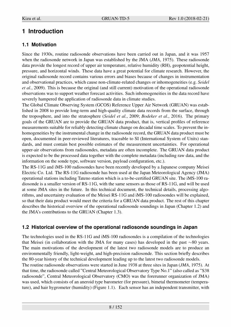
The routine radiosonde observations were started in June 1938 at three sites in Japan (JMA, 1975). Atthat time, the radiosonde called ”Central Meteorological Observatory Type No.1” (also called as ”S38radiosonde”, Central Meteorological Observatory (CMO) was the forerunner organization of JMA)was used, which consists of an aneroid type barometer (for pressure), bimetal thermometer (tempera-ture), and hair hygrometer (humidity) (Figure 1.1). Each sensor has an independent transmitter, with
8 / 152
Kizu et al. GRUAN-TD-5 Rev 1.0 (2018-02-21)
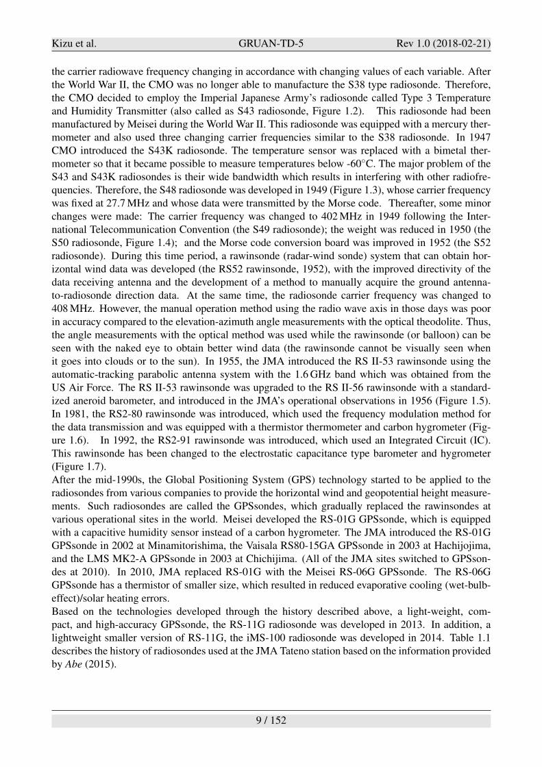
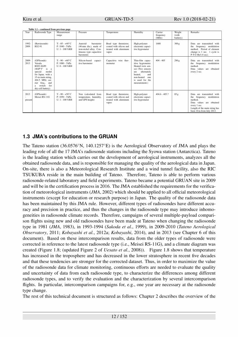
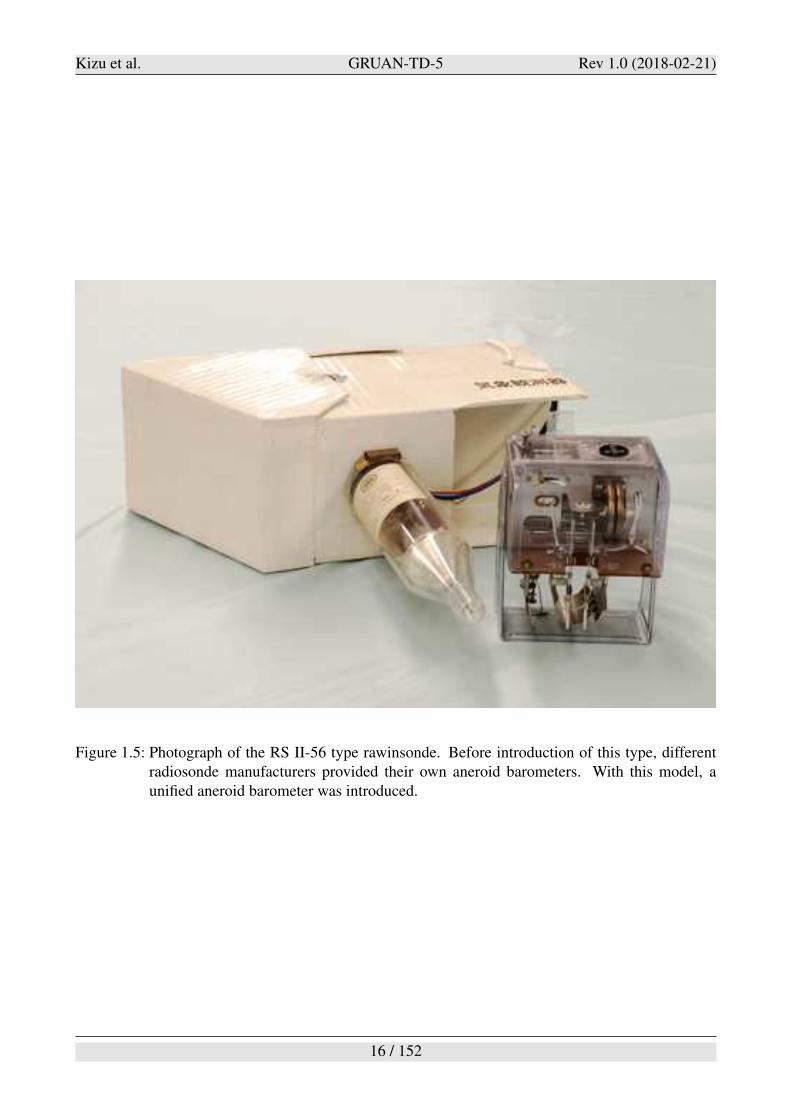
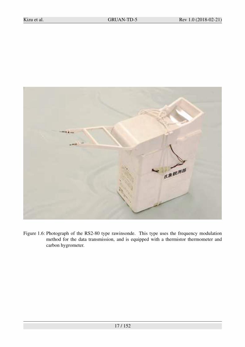
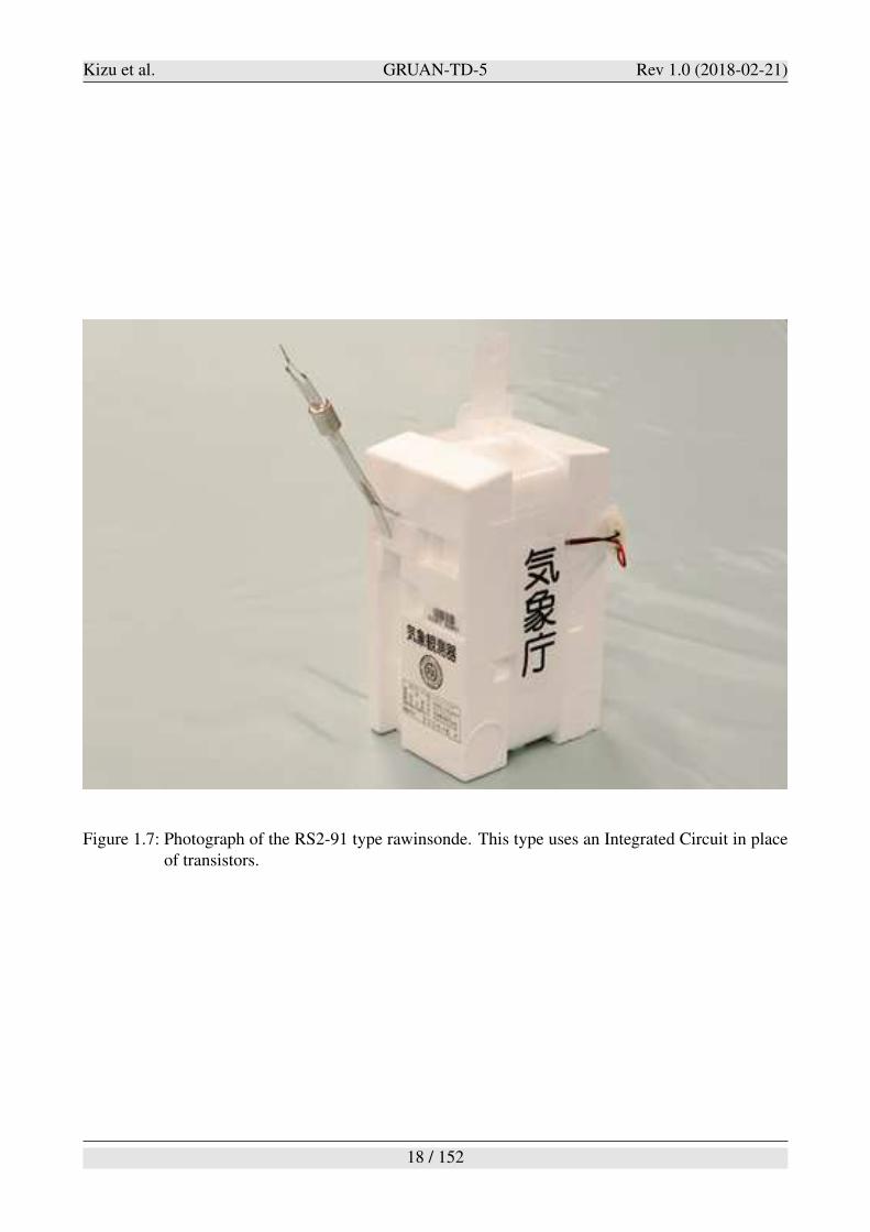
the carrier radiowave frequency changing in accordance with changing values of each variable. Afterthe World War II, the CMO was no longer able to manufacture the S38 type radiosonde. Therefore,the CMO decided to employ the Imperial Japanese Army’s radiosonde called Type 3 Temperatureand Humidity Transmitter (also called as S43 radiosonde, Figure 1.2). This radiosonde had beenmanufactured by Meisei during the World War II. This radiosonde was equipped with a mercury ther-mometer and also used three changing carrier frequencies similar to the S38 radiosonde. In 1947CMO introduced the S43K radiosonde. The temperature sensor was replaced with a bimetal ther-mometer so that it became possible to measure temperatures below -60!C. The major problem of theS43 and S43K radiosondes is their wide bandwidth which results in interfering with other radiofre-quencies. Therefore, the S48 radiosonde was developed in 1949 (Figure 1.3), whose carrier frequencywas fixed at 27.7 MHz and whose data were transmitted by the Morse code. Thereafter, some minorchanges were made: The carrier frequency was changed to 402 MHz in 1949 following the Inter-national Telecommunication Convention (the S49 radiosonde); the weight was reduced in 1950 (theS50 radiosonde, Figure 1.4); and the Morse code conversion board was improved in 1952 (the S52radiosonde). During this time period, a rawinsonde (radar-wind sonde) system that can obtain hor-izontal wind data was developed (the RS52 rawinsonde, 1952), with the improved directivity of thedata receiving antenna and the development of a method to manually acquire the ground antenna-to-radiosonde direction data. At the same time, the radiosonde carrier frequency was changed to408 MHz. However, the manual operation method using the radio wave axis in those days was poorin accuracy compared to the elevation-azimuth angle measurements with the optical theodolite. Thus,the angle measurements with the optical method was used while the rawinsonde (or balloon) can beseen with the naked eye to obtain better wind data (the rawinsonde cannot be visually seen whenit goes into clouds or to the sun). In 1955, the JMA introduced the RS II-53 rawinsonde using theautomatic-tracking parabolic antenna system with the 1.6 GHz band which was obtained from theUS Air Force. The RS II-53 rawinsonde was upgraded to the RS II-56 rawinsonde with a standard-ized aneroid barometer, and introduced in the JMA’s operational observations in 1956 (Figure 1.5).In 1981, the RS2-80 rawinsonde was introduced, which used the frequency modulation method forthe data transmission and was equipped with a thermistor thermometer and carbon hygrometer (Fig-ure 1.6). In 1992, the RS2-91 rawinsonde was introduced, which used an Integrated Circuit (IC).This rawinsonde has been changed to the electrostatic capacitance type barometer and hygrometer(Figure 1.7).After the mid-1990s, the Global Positioning System (GPS) technology started to be applied to theradiosondes from various companies to provide the horizontal wind and geopotential height measure-ments. Such radiosondes are called the GPSsondes, which gradually replaced the rawinsondes atvarious operational sites in the world. Meisei developed the RS-01G GPSsonde, which is equippedwith a capacitive humidity sensor instead of a carbon hygrometer. The JMA introduced the RS-01GGPSsonde in 2002 at Minamitorishima, the Vaisala RS80-15GA GPSsonde in 2003 at Hachijojima,and the LMS MK2-A GPSsonde in 2003 at Chichijima. (All of the JMA sites switched to GPSson-des at 2010). In 2010, JMA replaced RS-01G with the Meisei RS-06G GPSsonde. The RS-06GGPSsonde has a thermistor of smaller size, which resulted in reduced evaporative cooling (wet-bulb-effect)/solar heating errors.Based on the technologies developed through the history described above, a light-weight, com-pact, and high-accuracy GPSsonde, the RS-11G radiosonde was developed in 2013. In addition, alightweight smaller version of RS-11G, the iMS-100 radiosonde was developed in 2014. Table 1.1describes the history of radiosondes used at the JMA Tateno station based on the information providedby Abe (2015).
9 / 152
Kizu et al. GRUAN-TD-5 Rev 1.0 (2018-02-21)
Figure 1.1: Photograph of the Central Meteorological Observatory Type No.1 radiosonde (also calledas S38 type radiosonde). This radiosonde is composed of a pressure instrument part,temperature instrument part and humidity instrument part. Each part is composed of asensor and transmitter. This photograph shows a later version (1942- ) of the S38 typeradiosonde, for the paulownia wood was used for the radiosonde housing.
Table 1.1: History of radiosondes used at Tateno since 1944. Rawin and special radiosondes are excluded. Excerpt for Tateno from Abe (2015); JMA (1975).
sensor
Year Radiosonde Type Measurementrange
Pressure Temperature Humidity Carrierfrequency(MHz)
Weight(withbatttery)
Remarks
1944-1945
(Sonde)Central Meteoro-logical Observa-tory No. 1
T: –80 - +20!CP: 760 - 100 hPaU: 0 - 100 %RH
Aneroid barometer Bimetallic thermometer Hair hygrometer T: 10 - 12P: 6.2 - 7.4U: 7.5 - 10
400 g(for thetype withpaulow-nia woodhousing)
PTU data are transmitted sep-arately with different carrierfrequencies. Three Hartleyoscillators are used. Com-monly known as 38 type.
1944-1947
(Sonde)3-SHIKION-SHITSUHASSHINKI
T: –60 - +40!CP: 674 - 90 hPaU: 20 - 100 %RH
Aneroid barometer Mercury thermometer Hair hygrometer T: 9.5 - 11.5P:–U: 7.5 - 8.5
550 g TU data are transmitted sep-arately with different carrierfrequencies. P data are sentwith an altitude switch whichhas 12 contact points. Com-monly known as 43 type.
1947-1949
(Sonde)S43K
T: <–60 - +40!CP: 674 - 90 hPaU: 20 - 100 %RH
Aneroid barometer Bimetallic thermometer Hair hygrometer T: 9.5 - 11.5P: –U: 7.5 - 8.5
550 g TU data are transmitted sep-arately with different carrierfrequencies.T sensor has been changedfrom the S43 type, and is ableto measure also below –60! .
Continued on next page
10 / 152
Kizu et al. GRUAN-TD-5 Rev 1.0 (2018-02-21)
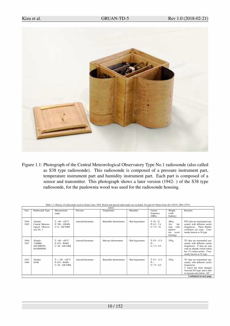
Table 1.1 – continued from previous page
Year Radiosonde Type Measurementrange
Pressure Temperature Humidity Carrierfrequency(MHz)
Weight(withbatttery)
Remarks
1949-1950
(Sonde)S48
T: –80 - +40!CP: 1040 - 5 hPaU: 0 - 100 %RH
Aneroid barometer Bimetallic thermometer Hair hygrometer 27.7 1250 g Data are transmitted with theMorse code method
1950-1950
(Sonde)S49AS49B
T: –80 - +40!CP: 1040 - 5 hPaU: 0 - 100 %RH
Two connected aneroidbarometers (53 mmdia.)
Type A:Made of nickel silver
Type B:Made of phosphorusbronze
Bimetallic thermometerwith nickel plating onboth sides
Type A:Length: 37 mm, Width:41 mm, Thickness:0.31-0.37 mm
Type B:Length: 38 mm, Width:35 mm, Thickness:0.21-0.27 mm
Hair hygrometer
Length: 80 mm,# hairs: 18
402 1400 g Changed to the frequency as-signed by the InternationalTelecommunication Conven-tion. Data are transmittedwith the Morse code method.
1950-1952
(Sonde)S50LS50M
T: –80 - +40!CP: 1040 - 5 hPaU: 0 - 100 %RH
Type L:Two connected aneroidbarometers (43 mmdia.), made of phospho-rus bronze
Type M:Two connected aneroidbarometers (42 mmdia.), “no wave” type,made of nickel silver
Bimetallic thermometerwith nickel plating onboth sides.
Type L:Length: 50 mm, Width:42 mm, Thickness:0.23-0.28 mm
Type M:Length: 37 mm, Width:27 mm, Thickness:0.25 mm
Two cutting-type(at –30!C and –50!C)mercury thermometersare also installed forin-flight calibrationand for terminationof humidity datatransmission.
Hair hygrometer
Type L:Length: 60 mm,# hairs: 16
Type M:Length: 55 mm,# hairs: 24
402 850 g Data are transmitted with theMorse code method.Length of the main string is7 m.
1952-1954
(Sonde)S52M(Rawinsonde)RS52M, RS52L
ditto ditto ditto ditto ditto 1300 g ditto (The Morse code boardhas been improved)
1954-1956
(Rawinsonde)RS53K, RS53M
T: –80 - +40!CP: 1040 - 5 hPaU: 0 - 100 %RH
Type K:Two connected aneroidbarometers (42 mmdia.), “no wave” type,made of nickel silver
Type M:Two connected aneroidbarometers (44 mmdia.), made of phospho-rus bronze
Bimetallic thermome-ter with nickel plating.Length: 50 mm, Width:42 mm, Thickness:0.25 mm
Two cutting-type(at –30!C and –50!C)mercury thermometersare also installed forin-flight calibrationand for terminationof humidity datatransmission.
Hair hygrometer,with rolling pro-cessing. Length:60 mm,# hairs: 20
408 970 g Data are transmitted with theMorse code method.Length of the main string is7 m.
1956-1957
(Rawinsonde)RS56
T: –85 - +40!CP: 1040 - 5 hPaU: 1 - 100 %RH
Two connected aneroidbarometers (44 mmdia.), “no wave” type,made of phosphorusbronze
ditto Hair hygrometer,with rolling pro-cessing.Length: 60 mm,# hairs: 20until Dec. 1956,10 from Jan.1957
408 950 g Data are transmitted with theMorse code method.
1957-1981
(Rawinsonde)RS II-56
ditto ditto ditto ditto 1680 1275 g Data are transmitted with theMorse code method. Transis-tors are used for the modula-tion and transmitter parts.Length of the main string waschanged from 7 m to 15 m inJune 1968.
1981-1992
(Rawinsonde)RS2-80
T: –90 - +45!CP: 1040 - 5 hPaU: 0 - 100 %RH
Aneroid barometer(60 mm dia.), made ofiron-nickel alloy, with78 contact points
Diode type thermistorthermometer, withwhite-painted
Carbon-filmhygrometer (anacrylic substratecoated withcarbon particles)
1680 600 g Data are transmitted withthe frequency modulationmethod. Period of elementchange is 3 sec for analogrecording and 1 sec for auto-mated processing. 1 cycle isP-T-P-U-P-T-P-Ref (8 or 24sec).
Continued on next page
11 / 152
Kizu et al. GRUAN-TD-5 Rev 1.0 (2018-02-21)
Table 1.1 – continued from previous page
Year Radiosonde Type Measurementrange
Pressure Temperature Humidity Carrierfrequency(MHz)
Weight(withbatttery)
Remarks
1992-2009
(Rawinsonde)RS2-91
T: –85 - +40!CP: 1040 - 5 hPaU: 1 - 100 %RH
Aneroid barometer(46 mm dia.), made ofiron-nickel alloy. Con-tinuous type capacitivebarometer.
Bead type thermistor,coated with silicon andtreated with aluminumvapor.
High-polymerelectronic capaci-tive hygrometer
1680 300 g Data are transmitted withthe frequency modulationmethod. Period of elementchange is 1 sec. 1 cycle isP-T-U-Ref (4 sec).
2009-2013
(GPSsonde)VaisalaRS92-SGPJ(SGP“J” is aspecial modelfor Japan, with a15-m main string,404.5 MHz car-rier freq., anda switch fordry-cell battery)
T: –90 - +60!CP: 1080 - 3 hPaU: 0 - 100 %RH
Silicon-based capaci-tive barometer
Capacitive wire ther-mometer
Thin-film capac-itive hygrometer.Heated twin sen-sor (Two sensorsare alternatelyheated, andnon-heated oneis used for themeasurement.)
404 - 405 290 g Data are transmitted withthe frequency modulationmethod.Data values are obtainedevery 2 sec.
2013-present
(GPSsonde)Meisei RS-11G
T: –90 - +50!CP: 1050 - 3 hPaU: 1 - 100 %RH
Non (calculated fromtemperature, humidity,and GPS height)
Bead type thermistor,coated with silicon andtreated with aluminumvapor.
High-polymerelectronic capaci-tive hygrometer
404.6 - 405.7 85 g Data are transmitted withthe frequency modulationmethod.Data values are obtainedevery 1 sec.Length of the main string hasbeen 10 m from July 2013.
1.3 JMA’s contributions to the GRUAN
The Tateno station (36.0576!N, 140.1257!E) is the Aerological Observatory of JMA and plays theleading role of all the 17 JMA’s radiosonde stations including the Syowa station (Antarctica). Tatenois the leading station which carries out the development of aerological instruments, analyzes all theobtained radiosonde data, and is responsible for managing the quality of the aerological data in Japan.On-site, there is also a Meteorological Research Institute and a wind tunnel facility, also the RICTSUKUBA reside in the main building of Tateno. Therefore, Tateno is able to perform variousradiosonde-related laboratory and field experiments. Tateno became a potential GRUAN site in 2009and will be in the certification process in 2016. The JMA established the requirements for the verifica-tion of meteorological instruments (JMA, 2002) which should be applied to all official meteorologicalinstruments (except for education or research purpose) in Japan. The quality of the radiosonde datahas been maintained by this JMA rule. However, different types of radiosondes have different accu-racy and precision in practice, and thus the changes in the radiosonde type may introduce inhomo-geneities in radiosonde climate records. Therefore, campaigns of several multiple-payload compari-son flights using new and old radiosondes have been made at Tateno when changing the radiosondetype in 1981 (JMA, 1983), in 1993-1994 (Sakoda et al., 1999), in 2009-2010 (Tateno Aerological
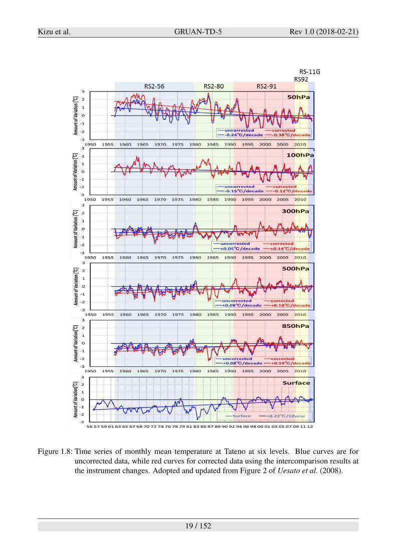
Observatory, 2011; Kobayashi et al., 2012a; Kobayashi, 2014), and in 2013 (see Chapter 6 of thisdocument). Based on these intercomparison results, data from the older types of radiosonde werecorrected in reference to the latest radiosonde type (i.e., Meisei RS-11G), and a climate diagram wascreated (Figure 1.8; (updated Figure 2 of Uesato et al., 2008)). Figure 1.8 shows that temperaturehas increased in the troposphere and has decreased in the lower stratosphere in recent five decadesand that these tendencies are stronger for the corrected dataset. Thus, in order to maximize the valueof the radiosonde data for climate monitoring, continuous efforts are needed to evaluate the qualityand uncertainty of data from each radiosonde type, to characterize the differences among differentradiosonde types, and to verify the evaluation and the characterization by several intercomparisonflights. In particular, intercomparison campaigns for, e.g., one year are necessary at the radiosondetype change.
The rest of this technical document is structured as follows: Chapter 2 describes the overview of the
12 / 152
Kizu et al. GRUAN-TD-5 Rev 1.0 (2018-02-21)
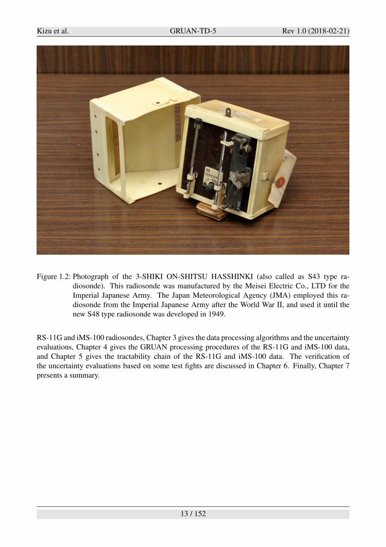
Figure 1.2: Photograph of the 3-SHIKI ON-SHITSU HASSHINKI (also called as S43 type ra-diosonde). This radiosonde was manufactured by the Meisei Electric Co., LTD for theImperial Japanese Army. The Japan Meteorological Agency (JMA) employed this ra-diosonde from the Imperial Japanese Army after the World War II, and used it until thenew S48 type radiosonde was developed in 1949.
RS-11G and iMS-100 radiosondes, Chapter 3 gives the data processing algorithms and the uncertaintyevaluations, Chapter 4 gives the GRUAN processing procedures of the RS-11G and iMS-100 data,and Chapter 5 gives the tractability chain of the RS-11G and iMS-100 data. The verification ofthe uncertainty evaluations based on some test fights are discussed in Chapter 6. Finally, Chapter 7presents a summary.
13 / 152
Kizu et al. GRUAN-TD-5 Rev 1.0 (2018-02-21)
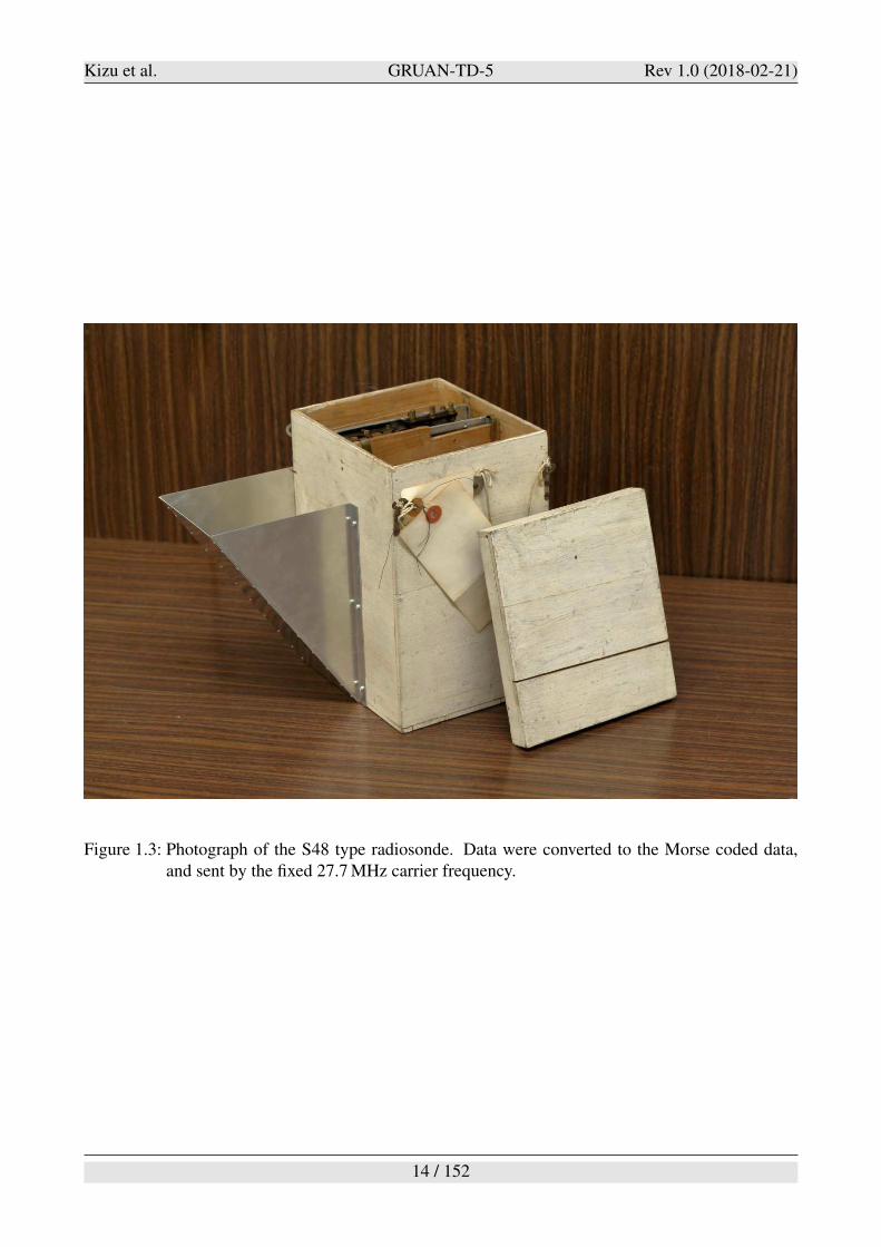
Figure 1.3: Photograph of the S48 type radiosonde. Data were converted to the Morse coded data,and sent by the fixed 27.7 MHz carrier frequency.
14 / 152
Kizu et al. GRUAN-TD-5 Rev 1.0 (2018-02-21)
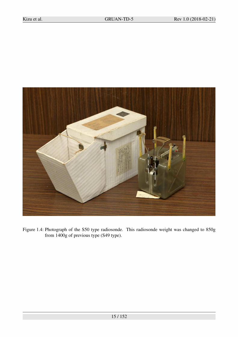
Figure 1.4: Photograph of the S50 type radiosonde. This radiosonde weight was changed to 850gfrom 1400g of previous type (S49 type).
15 / 152
Kizu et al. GRUAN-TD-5 Rev 1.0 (2018-02-21)
Figure 1.5: Photograph of the RS II-56 type rawinsonde. Before introduction of this type, differentradiosonde manufacturers provided their own aneroid barometers. With this model, aunified aneroid barometer was introduced.
16 / 152
Kizu et al. GRUAN-TD-5 Rev 1.0 (2018-02-21)
Figure 1.6: Photograph of the RS2-80 type rawinsonde. This type uses the frequency modulationmethod for the data transmission, and is equipped with a thermistor thermometer andcarbon hygrometer.
17 / 152
Kizu et al. GRUAN-TD-5 Rev 1.0 (2018-02-21)
Figure 1.7: Photograph of the RS2-91 type rawinsonde. This type uses an Integrated Circuit in placeof transistors.
18 / 152
Kizu et al. GRUAN-TD-5 Rev 1.0 (2018-02-21)
Figure 1.8: Time series of monthly mean temperature at Tateno at six levels. Blue curves are foruncorrected data, while red curves for corrected data using the intercomparison results atthe instrument changes. Adopted and updated from Figure 2 of Uesato et al. (2008).
19 / 152
Kizu et al. GRUAN-TD-5 Rev 1.0 (2018-02-21)
2 Overview of the RS-11G and iMS-100 radiosondes
2.1 RS-11G radiosonde
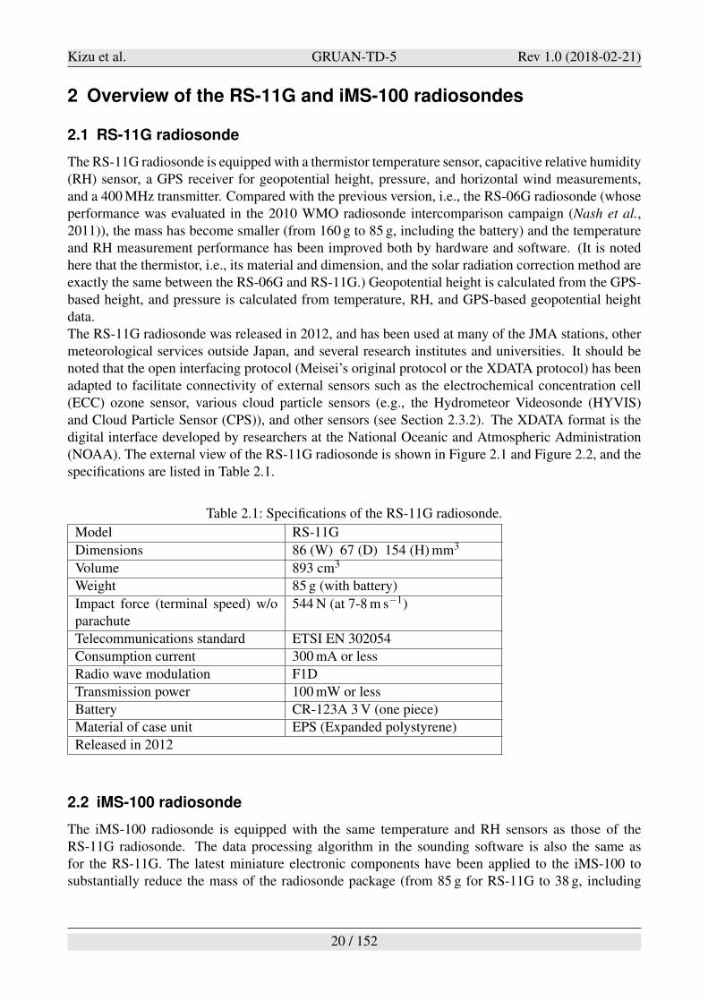
The RS-11G radiosonde is equipped with a thermistor temperature sensor, capacitive relative humidity(RH) sensor, a GPS receiver for geopotential height, pressure, and horizontal wind measurements,and a 400 MHz transmitter. Compared with the previous version, i.e., the RS-06G radiosonde (whoseperformance was evaluated in the 2010 WMO radiosonde intercomparison campaign (Nash et al.,2011)), the mass has become smaller (from 160 g to 85 g, including the battery) and the temperatureand RH measurement performance has been improved both by hardware and software. (It is notedhere that the thermistor, i.e., its material and dimension, and the solar radiation correction method areexactly the same between the RS-06G and RS-11G.) Geopotential height is calculated from the GPS-based height, and pressure is calculated from temperature, RH, and GPS-based geopotential heightdata.The RS-11G radiosonde was released in 2012, and has been used at many of the JMA stations, othermeteorological services outside Japan, and several research institutes and universities. It should benoted that the open interfacing protocol (Meisei’s original protocol or the XDATA protocol) has beenadapted to facilitate connectivity of external sensors such as the electrochemical concentration cell(ECC) ozone sensor, various cloud particle sensors (e.g., the Hydrometeor Videosonde (HYVIS)and Cloud Particle Sensor (CPS)), and other sensors (see Section 2.3.2). The XDATA format is thedigital interface developed by researchers at the National Oceanic and Atmospheric Administration(NOAA). The external view of the RS-11G radiosonde is shown in Figure 2.1 and Figure 2.2, and thespecifications are listed in Table 2.1.
Table 2.1: Specifications of the RS-11G radiosonde.
Model RS-11G
Dimensions 86 (W) 67 (D) 154 (H) mm3
Volume 893 cm3
Weight 85 g (with battery)
Impact force (terminal speed) w/oparachute
544 N (at 7-8 m s#1)
Telecommunications standard ETSI EN 302054
Consumption current 300 mA or less
Radio wave modulation F1D
Transmission power 100 mW or less
Battery CR-123A 3 V (one piece)
Material of case unit EPS (Expanded polystyrene)
Released in 2012
2.2 iMS-100 radiosonde
The iMS-100 radiosonde is equipped with the same temperature and RH sensors as those of theRS-11G radiosonde. The data processing algorithm in the sounding software is also the same asfor the RS-11G. The latest miniature electronic components have been applied to the iMS-100 tosubstantially reduce the mass of the radiosonde package (from 85 g for RS-11G to 38 g, including
20 / 152
Kizu et al. GRUAN-TD-5 Rev 1.0 (2018-02-21)
Figure 2.1: External view of the Meisei RS-11G radiosonde (unit: mm). 1: Processing unit and signalconverting unit; 2: Transmitter; 3: Antenna; 4: GPS module; 5: Temperature sensor; 6:Relative humidity sensor with a cap; 7: Battery; 8: Sensor boom; 9: Styrofoam (EPS)case; 10: Rope; 11: Label; and 12: Interface.
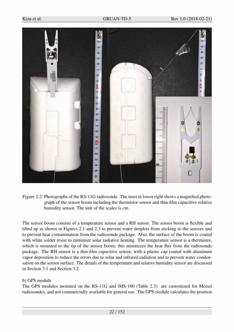
battery). This leads to a substantial reduction of the impact force when falling down to the ground,ensuring much safer operation. Besides, the downsizing has led to smaller pendulum motions, andimproved the horizontal wind measurements (see Section 3.4.3). The iMS-100 was released in late2014. The external view of the iMS-100 radiosonde is shown in Figure 2.3 and Figure 2.4, andspecifications are listed in Tables2.1 and 2.2.
2.3 Specifications of the RS-11G and iMS-100 radiosondes
This section describes the major parts used in the RS-11G and iMS-100 radiosondes, the connectivityof external sensors, and the production of these radiosondes.
2.3.1 The configuration of the RS-11G and iMS-100 radiosondes
(1) The components of the RS-11G and iMS-100 radiosondes
Figure 2.5 shows the system diagram of the RS-11G and iMS-100 radiosondes. All modules arebasically common. The operation and specifications of each module are discussed below.
a) Sensor boom
21 / 152
Kizu et al. GRUAN-TD-5 Rev 1.0 (2018-02-21)
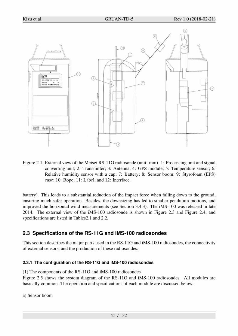
Figure 2.2: Photographs of the RS-11G radiosonde. The inset in lower right shows a magnified photo-graph of the sensor boom including the thermistor sensor and thin-film capacitive relativehumidity sensor. The unit of the scales is cm.
The sensor boom consists of a temperature sensor and a RH sensor. The sensor boom is flexible andtilted up as shown in Figures 2.1 and 2.3 to prevent water droplets from sticking to the sensors andto prevent heat contamination from the radiosonde package. Also, the surface of the boom is coatedwith white solder resist to minimize solar radiative heating. The temperature sensor is a thermistor,which is mounted to the tip of the sensor boom; this minimizes the heat flux from the radiosondepackage. The RH sensor is a thin-film capacitive sensor, with a plastic cap coated with aluminumvapor deposition to reduce the errors due to solar and infrared radiation and to prevent water conden-sation on the sensor surface. The details of the temperature and relative humidity sensor are discussedin Section 3.1 and Section 3.2.
b) GPS moduleThe GPS modules mounted on the RS-11G and iMS-100 (Table 2.3) are customized for Meiseiradiosondes, and not commercially available for general use. The GPS module calculates the position
22 / 152
Kizu et al. GRUAN-TD-5 Rev 1.0 (2018-02-21)
Figure 2.3: External view of the Meisei iMS-100 radiosonde (unit: mm). 1: Temperature sensor; 2:Relative humidity sensor with a cap; 3: Sensor boom; 4: Rope; 5: Styrofoam (EPS) case;and 6: Antenna.
and velocity of the radiosonde. The GPS module consists of the GPS antenna with a preamplifierand the GPS receiver supporting the Satellite-Based Augmentation System (SBAS). It should benoted that the SBAS is a method of improving the navigation system’s attributes, such as accuracy,reliability, and availability, through the external information from satellite and that the positioningaccuracy of the SBAS is at the same level as the Ground-based Augmentation System (GBAS). Thereceiving frequency is 1575.42 MHz. The module provides data with the National Marine ElectronicsAssociation (NMEA) format, including the GPS status (e.g., number of GPS satellites whose signalsare received), latitude, longitude, altitude, Doppler velocity, azimuth direction, GPS time, and theDilution of Precision (DOP) value. These data are sent to the Central Processing Unit (CPU) on theprocessing unit every second, and edited into the transmitted format.
c) Signal converting unitThe signal converting circuit works for the temperature and RH measurements. It consists of aresistor-capacitor (CR) oscillating circuit including the thermistor and the thin-film capacitive sen-sors with a Schmitt circuit and an analog switch. The temperature and RH signals are converted intofrequency data, which are switched by the analog switch with switching signals from the CPU in the
23 / 152
Kizu et al. GRUAN-TD-5 Rev 1.0 (2018-02-21)
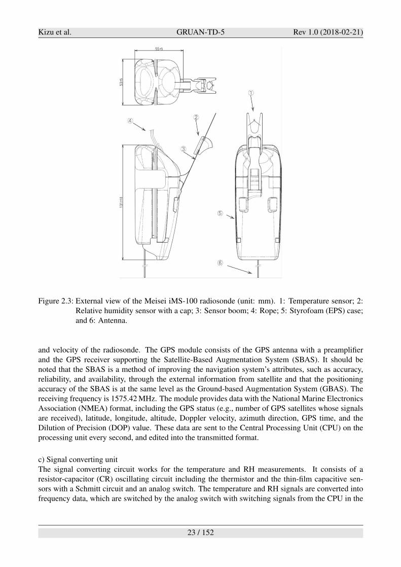
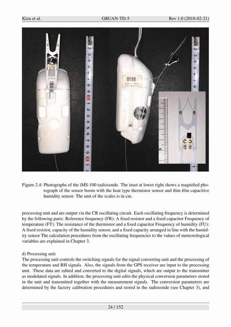
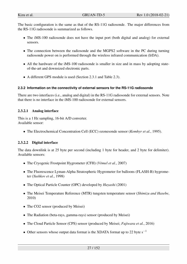
Figure 2.4: Photographs of the iMS-100 radiosonde. The inset at lower right shows a magnified pho-tograph of the sensor boom with the heat type thermistor sensor and thin-film capacitivehumidity sensor. The unit of the scales is in cm.
processing unit and are output via the CR oscillating circuit. Each oscillating frequency is determinedby the following parts: Reference frequency (FR): A fixed resistor and a fixed capacitor Frequency oftemperature (FT): The resistance of the thermistor and a fixed capacitor Frequency of humidity (FU):A fixed resistor, capacity of the humidity sensor, and a fixed capacity arranged in line with the humid-ity sensor The calculation procedures from the oscillating frequencies to the values of meteorologicalvariables are explained in Chapter 3.
d) Processing unitThe processing unit controls the switching signals for the signal converting unit and the processing ofthe temperature and RH signals. Also, the signals from the GPS receiver are input to the processingunit. These data are edited and converted to the digital signals, which are output to the transmitteras modulated signals. In addition, the processing unit edits the physical conversion parameters storedin the unit and transmitted together with the measurement signals. The conversion parameters aredetermined by the factory calibration procedures and stored in the radiosonde (see Chapter 3), and
24 / 152
Kizu et al. GRUAN-TD-5 Rev 1.0 (2018-02-21)
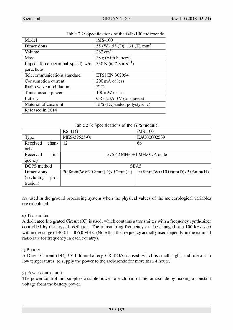
Table 2.2: Specifications of the iMS-100 radiosonde.
Model iMS-100
Dimensions 55 (W) 53 (D) 131 (H) mm3
Volume 262 cm3
Mass 38 g (with battery)
Impact force (terminal speed) w/oparachute
330 N (at 7-8 m s#1)
Telecommunications standard ETSI EN 302054
Consumption current 200 mA or less
Radio wave modulation F1D
Transmission power 100 mW or less
Battery CR-123A 3 V (one piece)
Material of case unit EPS (Expanded polystyrene)
Released in 2014
Table 2.3: Specifications of the GPS module.
RS-11G iMS-100
Type MES-39525-01 EAU00002539
Received chan-nels
12 66
Received fre-quency
1575.42 MHz ±1 MHz C/A code
DGPS method SBAS
Dimensions(excluding pro-trusion)
20.8mm(W)x20.8mm(D)x9.2mm(H) 10.8mm(W)x10.0mm(D)x2.05mm(H)
are used in the ground processing system when the physical values of the meteorological variablesare calculated.
e) TransmitterA dedicated Integrated Circuit (IC) is used, which contains a transmitter with a frequency synthesizercontrolled by the crystal oscillator. The transmitting frequency can be changed at a 100 kHz stepwithin the range of 400.1 – 406.0 MHz. (Note that the frequency actually used depends on the nationalradio law for frequency in each country).
f) BatteryA Direct Current (DC) 3 V lithium battery, CR-123A, is used, which is small, light, and tolerant tolow temperatures, to supply the power to the radiosonde for more than 4 hours.
g) Power control unitThe power control unit supplies a stable power to each part of the radiosonde by making a constantvoltage from the battery power.
25 / 152
Kizu et al. GRUAN-TD-5 Rev 1.0 (2018-02-21)
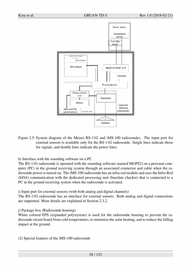
Figure 2.5: System diagram of the Meisei RS-11G and iMS-100 radiosondes. The input port forexternal sensors is available only for the RS-11G radiosonde. Single lines indicate thosefor signals, and double lines indicate the power lines.
h) Interface with the sounding software on a PCThe RS-11G radiosonde is operated with the sounding software (named MGPS2) on a personal com-puter (PC) in the ground receiving system through an associated connector and cable when the ra-diosonde power is turned on. The iMS-100 radiosonde has an infra-red module and uses the Infra-Red(IrDA) communication with the dedicated processing unit (baseline checker) that is connected to aPC in the ground receiving system when the radiosonde is activated.
i) Input port for external sensors (with both analog and digital channels)The RS-11G radiosonde has an interface for external sensors. Both analog and digital connectionsare supported. More details are explained in Section 2.3.2.
j) Package box (Radiosonde housing)White colored EPS (expanded polystyrene) is used for the radiosonde housing to prevent the ra-diosonde circuit board from cold temperatures, to minimize the solar heating, and to reduce the fallingimpact at the ground.
(2) Special features of the iMS-100 radiosonde
26 / 152
Kizu et al. GRUAN-TD-5 Rev 1.0 (2018-02-21)
The basic configuration is the same as that of the RS-11G radiosonde. The major differences fromthe RS-11G radiosonde is summarized as follows.
• The iMS-100 radiosonde does not have the input port (both digital and analog) for externalsensors.
• The connection between the radiosonde and the MGPS2 software in the PC during turningradiosonde power on is performed through the wireless infrared communication (IrDA).
• All the hardware of the iMS-100 radiosonde is smaller in size and in mass by adopting state-of-the-art and downsized electronic parts.
• A different GPS module is used (Section 2.3.1 and Table 2.3).
2.3.2 Information on the connectivity of external sensors for the RS-11G radiosonde
There are two interfaces (i.e., analog and digital) in the RS-11G radiosonde for external sensors. Notethat there is no interface in the iMS-100 radiosonde for external sensors.
2.3.2.1 Analog interface
This is a 1 Hz sampling, 16-bit A/D converter.Available sensor:
• The Electrochemical Concentration Cell (ECC) ozonesonde sensor (Komhyr et al., 1995).
2.3.2.2 Digital interface
The data downlink is at 25 byte per second (including 1 byte for header, and 2 byte for delimiter).Available sensors:
• The Cryogenic Frostpoint Hygrometer (CFH) (Vomel et al., 2007)
• The Fluorescence Lyman-Alpha Stratospheric Hygrometer for balloons (FLASH-B) hygrome-ter (Yushkov et al., 1998)
• The Optical Particle Counter (OPC) developed by Hayashi (2001)
• The Meisei Temperature Reference (MTR) tungsten temperature sensor (Shimizu and Hasebe,2010)
• The CO2 sensor (produced by Meisei)
• The Radiation (beta-rays, gamma-rays) sensor (produced by Meisei)
• The Cloud Particle Sensor (CPS) sensor (produced by Meisei; Fujiwara et al., 2016)
• Other sensors whose output data format is the XDATA format up to 22 byte s#1
27 / 152
Kizu et al. GRUAN-TD-5 Rev 1.0 (2018-02-21)
The communication between the RS-11G radiosonde and an external sensor is synchronized using the1 Hz pulse sent from the RS-11G radiosonde. The external sensor is to send the 25-byte data everysecond according to the ”1 Hz demand pulse” rule. The checksum is included in the 25-byte data, anddetecting errors which may have been introduced during its transmission every second. The externalsensor needs to send a full 25-byte data between the sequential 1 Hz demand pulses; otherwise all databecome missing at this particular 1-second time window.). When a sensor with the XDATA formatis used, a special communication interface board provided by Meisei is attached between the sensorand the RS-11G radiosonde, which converts the XDATA-formatted data into the RS-11G 25-byte dataformat. The detailed communication protocol for external sensors is described in Appendix A.
2.3.3 Manufacturer-provided measurement specifications
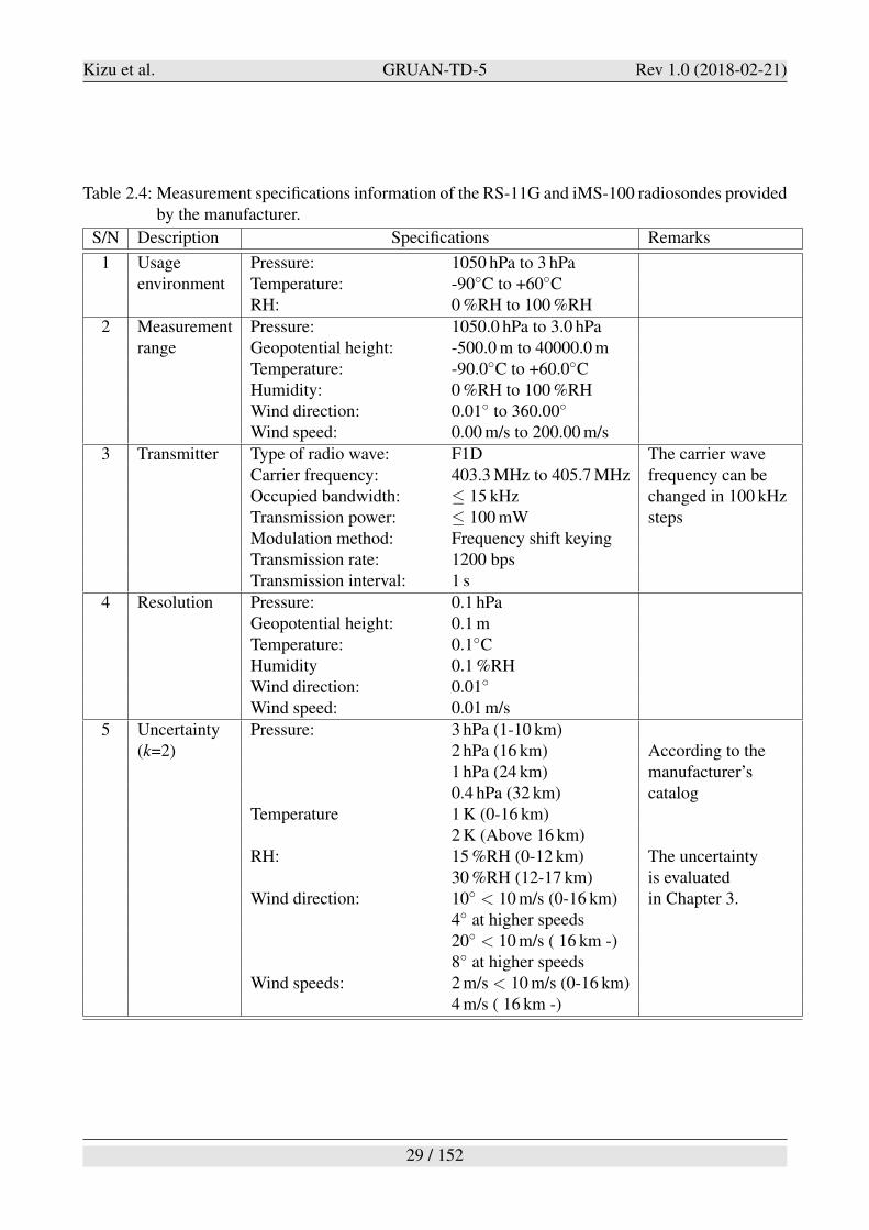
The list of measurement specifications of the RS-11G and iMS-100 radiosondes are shown in Ta-ble 2.4. The values in this table are provided by the manufacturer.
2.3.4 Production of the radiosondes
As of 2015, the RS-11G radiosonde is being used operationally at 8 of the JMA upper-air stations(Wakkanai, Sapporo, Akita, Tateno, Fukuoka, Kagoshima, Chichijima, Minamitorishima), some sta-tions in other countries, and is also used for research purposes by universities, research institutes, andprivate weather companies. The annual production is approximately 50,000 units of radiosondes forthe case of year 2014. It takes about 2.5 months between the order and the delivery of the RS-11G andiMS-100 radiosondes. Meisei has a production system that can produce 100,000 units of radiosondesper year.
2.4 Ground checks
The ground check is conducted on-site before the launch to confirm that the sensors calibrated at thefactory are not damaged nor deteriorated during the delivery and storage. The results of the groundcheck are used to judge whether the radiosonde can be flown.The ground check is made by using both the manufacturer’s instrument called Ground Checker (GC)and the Standard Humidity Chamber (SHC) which is independent of the manufacturer and has beendeveloped by the JMA. The manufacturer’s GC checks the temperature and RH measurements underroom conditions just before the launch. On the other hand, the SHC checks the RH measurementsat 100 %RH using distilled water and at 0 %RH using desiccant (molecular sieve), which are carriedout more than one day before the launch. The manufacturer-independent ground check is required bythe GRUAN (GCOS, 2013). The RH deviations obtained at 0 %RH, RH under a room condition, and100 %RH are used for the recalibration of the obtained data to produce the GRUAN data product.First, the ground check procedure using Meisei’s GC under room condition is carried out. The ra-diosondes that have passed the GC check precede to 0 %RH check using the SHC system. The sensorboom is placed in the SHC (0 %RH). Then, the sensor boom is placed in the SHC (100 %RH). Theradiosondes are then stored in a low humidity environment for more than one day, and are subject tothe room environment GC check again right before the launch.
2.4.1 Ground check (baseline check) using the manufacturer’s Baseline Checker
The manufacturer’s ”GC” equipment (baseline checker) has reference temperature and RH sensors.The radiosonde sensors are placed in a small chamber, and the readings are recorded with the software
28 / 152
Kizu et al. GRUAN-TD-5 Rev 1.0 (2018-02-21)
Table 2.4: Measurement specifications information of the RS-11G and iMS-100 radiosondes providedby the manufacturer.
S/N Description Specifications Remarks
1 Usage Pressure: 1050 hPa to 3 hPaenvironment Temperature: -90!C to +60!C
RH: 0 %RH to 100 %RH
2 Measurement Pressure: 1050.0 hPa to 3.0 hParange Geopotential height: -500.0 m to 40000.0 m
Temperature: -90.0!C to +60.0!CHumidity: 0 %RH to 100 %RHWind direction: 0.01! to 360.00!
Wind speed: 0.00 m/s to 200.00 m/s
3 Transmitter Type of radio wave: F1D The carrier waveCarrier frequency: 403.3 MHz to 405.7 MHz frequency can beOccupied bandwidth: $ 15 kHz changed in 100 kHzTransmission power: $ 100 mW stepsModulation method: Frequency shift keyingTransmission rate: 1200 bpsTransmission interval: 1 s
4 Resolution Pressure: 0.1 hPaGeopotential height: 0.1 mTemperature: 0.1!CHumidity 0.1 %RHWind direction: 0.01!
Wind speed: 0.01 m/s
5 Uncertainty Pressure: 3 hPa (1-10 km)(k=2) 2 hPa (16 km) According to the
1 hPa (24 km) manufacturer’s0.4 hPa (32 km) catalog
Temperature 1 K (0-16 km)2 K (Above 16 km)
RH: 15 %RH (0-12 km) The uncertainty30 %RH (12-17 km) is evaluated
Wind direction: 10! < 10 m/s (0-16 km) in Chapter 3.4! at higher speeds20! < 10 m/s ( 16 km -)8! at higher speeds
Wind speeds: 2 m/s < 10 m/s (0-16 km)4 m/s ( 16 km -)
29 / 152
Kizu et al. GRUAN-TD-5 Rev 1.0 (2018-02-21)
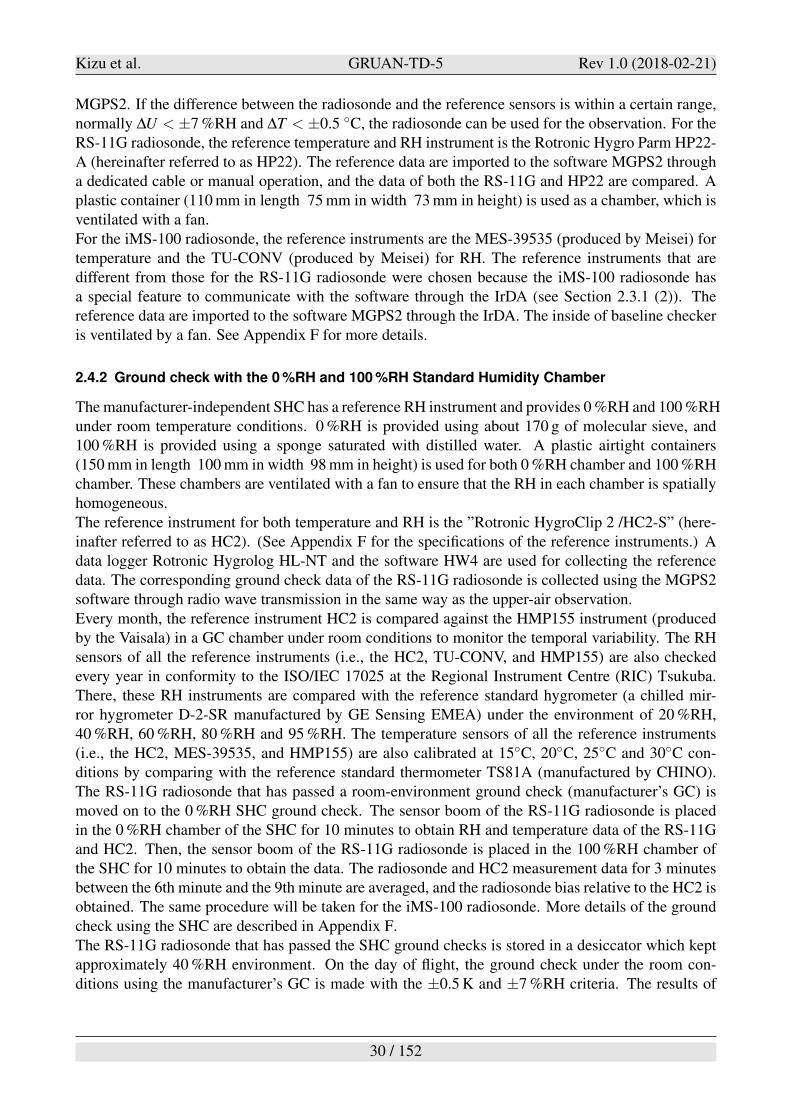
MGPS2. If the difference between the radiosonde and the reference sensors is within a certain range,normally !U < ±7 %RH and !T < ±0.5 !C, the radiosonde can be used for the observation. For theRS-11G radiosonde, the reference temperature and RH instrument is the Rotronic Hygro Parm HP22-A (hereinafter referred to as HP22). The reference data are imported to the software MGPS2 througha dedicated cable or manual operation, and the data of both the RS-11G and HP22 are compared. Aplastic container (110 mm in length 75 mm in width 73 mm in height) is used as a chamber, which isventilated with a fan.
For the iMS-100 radiosonde, the reference instruments are the MES-39535 (produced by Meisei) fortemperature and the TU-CONV (produced by Meisei) for RH. The reference instruments that aredifferent from those for the RS-11G radiosonde were chosen because the iMS-100 radiosonde hasa special feature to communicate with the software through the IrDA (see Section 2.3.1 (2)). Thereference data are imported to the software MGPS2 through the IrDA. The inside of baseline checkeris ventilated by a fan. See Appendix F for more details.
2.4.2 Ground check with the 0 %RH and 100 %RH Standard Humidity Chamber
The manufacturer-independent SHC has a reference RH instrument and provides 0 %RH and 100 %RHunder room temperature conditions. 0 %RH is provided using about 170 g of molecular sieve, and100 %RH is provided using a sponge saturated with distilled water. A plastic airtight containers(150 mm in length 100 mm in width 98 mm in height) is used for both 0 %RH chamber and 100 %RHchamber. These chambers are ventilated with a fan to ensure that the RH in each chamber is spatiallyhomogeneous.
The reference instrument for both temperature and RH is the ”Rotronic HygroClip 2 /HC2-S” (here-inafter referred to as HC2). (See Appendix F for the specifications of the reference instruments.) Adata logger Rotronic Hygrolog HL-NT and the software HW4 are used for collecting the referencedata. The corresponding ground check data of the RS-11G radiosonde is collected using the MGPS2software through radio wave transmission in the same way as the upper-air observation.
Every month, the reference instrument HC2 is compared against the HMP155 instrument (producedby the Vaisala) in a GC chamber under room conditions to monitor the temporal variability. The RHsensors of all the reference instruments (i.e., the HC2, TU-CONV, and HMP155) are also checkedevery year in conformity to the ISO/IEC 17025 at the Regional Instrument Centre (RIC) Tsukuba.There, these RH instruments are compared with the reference standard hygrometer (a chilled mir-ror hygrometer D-2-SR manufactured by GE Sensing EMEA) under the environment of 20 %RH,40 %RH, 60 %RH, 80 %RH and 95 %RH. The temperature sensors of all the reference instruments(i.e., the HC2, MES-39535, and HMP155) are also calibrated at 15!C, 20!C, 25!C and 30!C con-ditions by comparing with the reference standard thermometer TS81A (manufactured by CHINO).The RS-11G radiosonde that has passed a room-environment ground check (manufacturer’s GC) ismoved on to the 0 %RH SHC ground check. The sensor boom of the RS-11G radiosonde is placedin the 0 %RH chamber of the SHC for 10 minutes to obtain RH and temperature data of the RS-11Gand HC2. Then, the sensor boom of the RS-11G radiosonde is placed in the 100 %RH chamber ofthe SHC for 10 minutes to obtain the data. The radiosonde and HC2 measurement data for 3 minutesbetween the 6th minute and the 9th minute are averaged, and the radiosonde bias relative to the HC2 isobtained. The same procedure will be taken for the iMS-100 radiosonde. More details of the groundcheck using the SHC are described in Appendix F.
The RS-11G radiosonde that has passed the SHC ground checks is stored in a desiccator which keptapproximately 40 %RH environment. On the day of flight, the ground check under the room con-ditions using the manufacturer’s GC is made with the ±0.5 K and ±7 %RH criteria. The results of
30 / 152
Kizu et al. GRUAN-TD-5 Rev 1.0 (2018-02-21)
all these ground checks are reported to the GRUAN Lead Centre via the GRUAN RsLaunchClient.Regarding these transmission data by GRUAN RsLaunchClient, it is described in ”User Guide ofGRUAN RsLaunchClient” (Sommer, 2014).
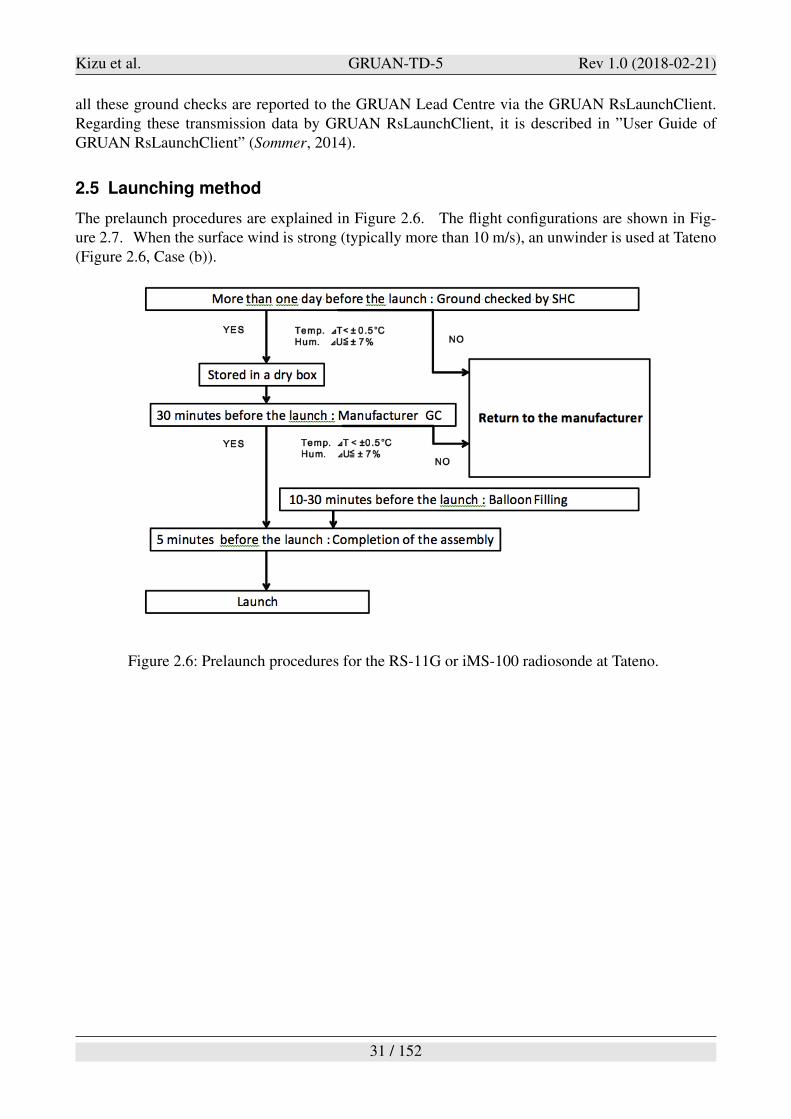
2.5 Launching method
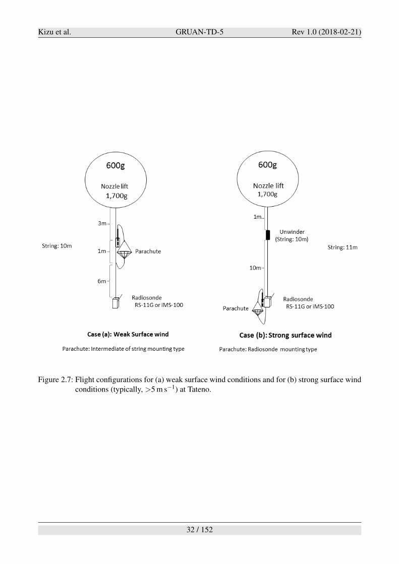
The prelaunch procedures are explained in Figure 2.6. The flight configurations are shown in Fig-ure 2.7. When the surface wind is strong (typically more than 10 m/s), an unwinder is used at Tateno(Figure 2.6, Case (b)).
Figure 2.6: Prelaunch procedures for the RS-11G or iMS-100 radiosonde at Tateno.
31 / 152
Kizu et al. GRUAN-TD-5 Rev 1.0 (2018-02-21)
Figure 2.7: Flight configurations for (a) weak surface wind conditions and for (b) strong surface windconditions (typically, >5 m s#1) at Tateno.
32 / 152
Kizu et al. GRUAN-TD-5 Rev 1.0 (2018-02-21)
3 Measurements from the RS-11G and iMS-100 radiosondes
In this chapter, we describe the calculation procedures of temperature, RH, geopotential height, pres-sure, and horizontal wind data from the RS-11G and iMS-100 radiosondes, and discuss the mea-surement uncertainty evaluations. We follow the approach outlined in the Guide to the expression ofuncertainty in measurement by the working group 1 of the Joint Committee for Guide in Metrology(JCGM/WG 1, 2008) (see also Immler et al., 2010; Dirksen et al., 2014). There are two types of mea-surement error quantities, that is, systematic and random errors. A systematic error (or a measurementbias) is associated with the fact that a measured quantity value contains an offset. A random error,on the other hand, is associated with the fact that when a measurement is repeated, it will generallyprovide a measured quantity value that is different from the previous value; it can be reduced by in-creasing the number of measurements. For the radiosonde measurements, there are many factors thatintroduce systematic biases such as the radiation error for the temperature measurement. If system-atic biases are properly characterized, they can be removed with confidence by correction procedures,which reduces the uncertainty of the measurement. The corrections described in the following are ap-plied to the original data to compensate for some known systematic effects that significantly influencethe measurement results. However, because the systematic errors are in general not completely char-acterized, all corrections involve uncertainty. We attempt to identify the likely sources of uncertaintyand to estimate the total uncertainty.
3.1 Temperature measurements
3.1.1 Sensor material
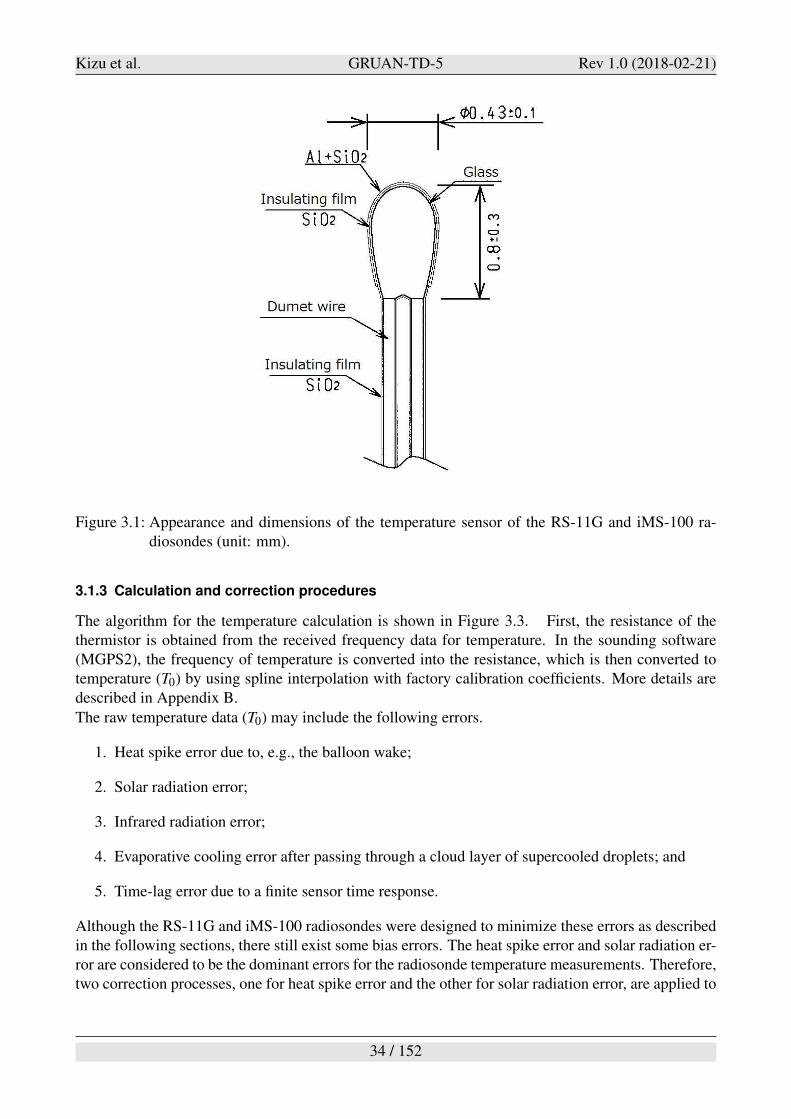
The temperature sensor of the RS-11G and iMS-100 radiosondes is a thermistor. Figure 3.1 showsthe external view of the sensor. The thermistor is coated with aluminum and silica dioxide to reducethe solar heating, and to minimize the correction amount for the solar heating. The reflectively isabout 89% at 500 nm wavelength. The thermistor has a spherical shape (the maximum diameter is"0.43 mm) for its cross section with length of "0.8 mm. This smallness in size leads to a small heatcapacity, and thus fast response even under low-air-pressure conditions.
3.1.2 Sensor calibration
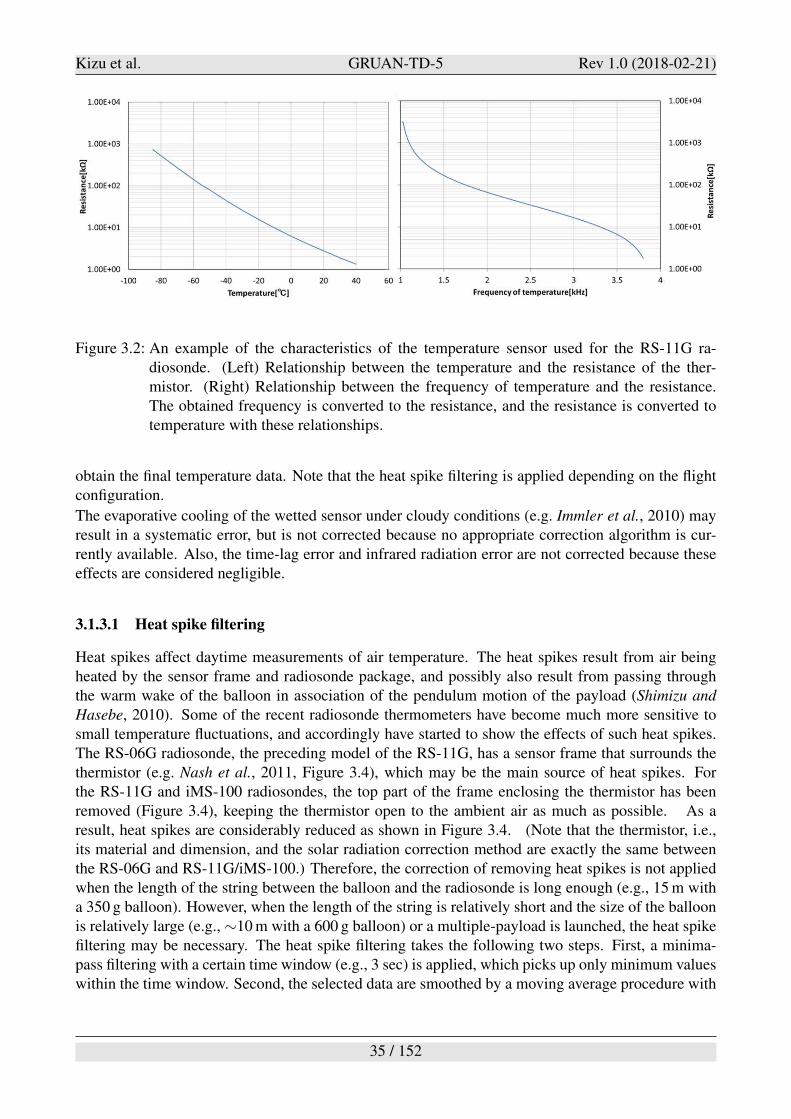
The thermistor is calibrated during the manufacturing process. The thermistors are immersed in liquidsolution in the calibration chamber together with a platinum resistance thermometer and are calibratedat 20 temperature points between -85!C to +40!C. From the 20 measurement points, 11 points includ-ing +40!C and -85!C are selected and used as the calibration points. The other 9 points are used tocheck the accuracy of the obtained calibration curve, by calculating the deviation. If the differencebetween the maximum deviation (positive) and minimum deviation (negative) is more than 0.3 K, thethermistor is rejected. Figure 3.2 shows an example of the relationship between the temperature andthe resistance for a particular thermistor used in the RS-11G and iMS-100 radiosondes.
For the RS-11G and iMS-100 radiosondes, the resistance of the thermistor is detected as the fre-quency of temperature through the CR oscillating circuit on the radiosonde board. The relationshipbetween the resistance and the frequency of temperature is obtained by the calibration using refer-ence resistances. Figure 3.2 (right panel) shows an example of relationship between the frequency oftemperature and the resistance for a particular thermistor – CR oscillating circuit system used in theRS-11G radiosonde.
33 / 152
Kizu et al. GRUAN-TD-5 Rev 1.0 (2018-02-21)
Figure 3.1: Appearance and dimensions of the temperature sensor of the RS-11G and iMS-100 ra-diosondes (unit: mm).
3.1.3 Calculation and correction procedures
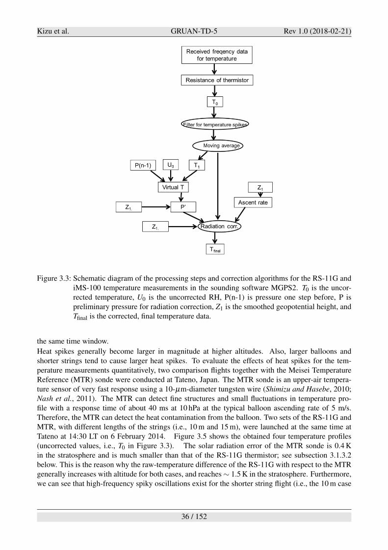
The algorithm for the temperature calculation is shown in Figure 3.3. First, the resistance of thethermistor is obtained from the received frequency data for temperature. In the sounding software(MGPS2), the frequency of temperature is converted into the resistance, which is then converted totemperature (T0) by using spline interpolation with factory calibration coefficients. More details aredescribed in Appendix B.
The raw temperature data (T0) may include the following errors.
1. Heat spike error due to, e.g., the balloon wake;
2. Solar radiation error;
3. Infrared radiation error;
4. Evaporative cooling error after passing through a cloud layer of supercooled droplets; and
5. Time-lag error due to a finite sensor time response.
Although the RS-11G and iMS-100 radiosondes were designed to minimize these errors as describedin the following sections, there still exist some bias errors. The heat spike error and solar radiation er-ror are considered to be the dominant errors for the radiosonde temperature measurements. Therefore,two correction processes, one for heat spike error and the other for solar radiation error, are applied to
34 / 152
Kizu et al. GRUAN-TD-5 Rev 1.0 (2018-02-21)
Figure 3.2: An example of the characteristics of the temperature sensor used for the RS-11G ra-diosonde. (Left) Relationship between the temperature and the resistance of the ther-mistor. (Right) Relationship between the frequency of temperature and the resistance.The obtained frequency is converted to the resistance, and the resistance is converted totemperature with these relationships.
obtain the final temperature data. Note that the heat spike filtering is applied depending on the flightconfiguration.
The evaporative cooling of the wetted sensor under cloudy conditions (e.g. Immler et al., 2010) mayresult in a systematic error, but is not corrected because no appropriate correction algorithm is cur-rently available. Also, the time-lag error and infrared radiation error are not corrected because theseeffects are considered negligible.
3.1.3.1 Heat spike filtering
Heat spikes affect daytime measurements of air temperature. The heat spikes result from air beingheated by the sensor frame and radiosonde package, and possibly also result from passing throughthe warm wake of the balloon in association of the pendulum motion of the payload (Shimizu and
Hasebe, 2010). Some of the recent radiosonde thermometers have become much more sensitive tosmall temperature fluctuations, and accordingly have started to show the effects of such heat spikes.The RS-06G radiosonde, the preceding model of the RS-11G, has a sensor frame that surrounds thethermistor (e.g. Nash et al., 2011, Figure 3.4), which may be the main source of heat spikes. Forthe RS-11G and iMS-100 radiosondes, the top part of the frame enclosing the thermistor has beenremoved (Figure 3.4), keeping the thermistor open to the ambient air as much as possible. As aresult, heat spikes are considerably reduced as shown in Figure 3.4. (Note that the thermistor, i.e.,its material and dimension, and the solar radiation correction method are exactly the same betweenthe RS-06G and RS-11G/iMS-100.) Therefore, the correction of removing heat spikes is not appliedwhen the length of the string between the balloon and the radiosonde is long enough (e.g., 15 m witha 350 g balloon). However, when the length of the string is relatively short and the size of the balloonis relatively large (e.g., "10 m with a 600 g balloon) or a multiple-payload is launched, the heat spikefiltering may be necessary. The heat spike filtering takes the following two steps. First, a minima-pass filtering with a certain time window (e.g., 3 sec) is applied, which picks up only minimum valueswithin the time window. Second, the selected data are smoothed by a moving average procedure with
35 / 152
Kizu et al. GRUAN-TD-5 Rev 1.0 (2018-02-21)
Figure 3.3: Schematic diagram of the processing steps and correction algorithms for the RS-11G andiMS-100 temperature measurements in the sounding software MGPS2. T0 is the uncor-rected temperature, U0 is the uncorrected RH, P(n-1) is pressure one step before, P ispreliminary pressure for radiation correction, Z1 is the smoothed geopotential height, andTfinal is the corrected, final temperature data.
the same time window.
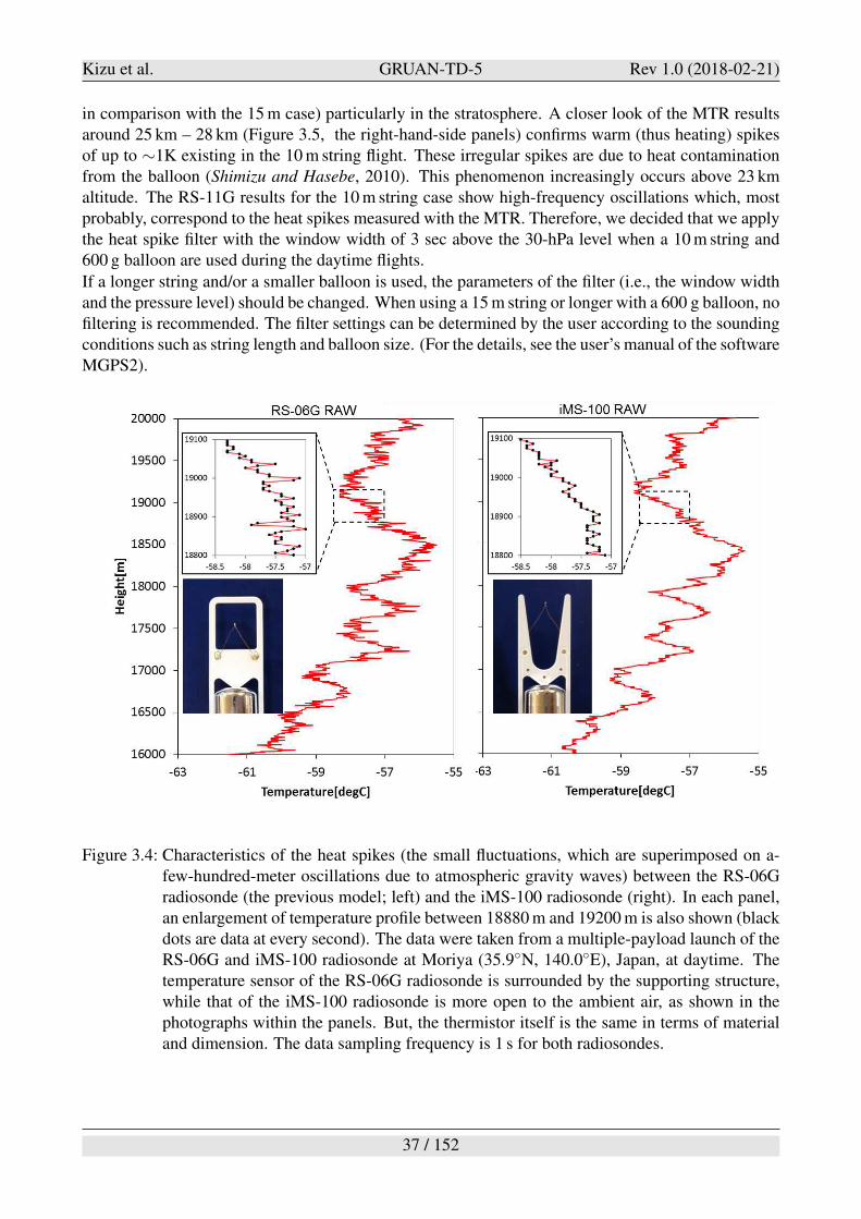
Heat spikes generally become larger in magnitude at higher altitudes. Also, larger balloons andshorter strings tend to cause larger heat spikes. To evaluate the effects of heat spikes for the tem-perature measurements quantitatively, two comparison flights together with the Meisei TemperatureReference (MTR) sonde were conducted at Tateno, Japan. The MTR sonde is an upper-air tempera-ture sensor of very fast response using a 10-µm-diameter tungsten wire (Shimizu and Hasebe, 2010;Nash et al., 2011). The MTR can detect fine structures and small fluctuations in temperature pro-file with a response time of about 40 ms at 10 hPa at the typical balloon ascending rate of 5 m/s.Therefore, the MTR can detect the heat contamination from the balloon. Two sets of the RS-11G andMTR, with different lengths of the strings (i.e., 10 m and 15 m), were launched at the same time atTateno at 14:30 LT on 6 February 2014. Figure 3.5 shows the obtained four temperature profiles(uncorrected values, i.e., T0 in Figure 3.3). The solar radiation error of the MTR sonde is 0.4 Kin the stratosphere and is much smaller than that of the RS-11G thermistor; see subsection 3.1.3.2below. This is the reason why the raw-temperature difference of the RS-11G with respect to the MTRgenerally increases with altitude for both cases, and reaches " 1.5 K in the stratosphere. Furthermore,we can see that high-frequency spiky oscillations exist for the shorter string flight (i.e., the 10 m case
36 / 152
Kizu et al. GRUAN-TD-5 Rev 1.0 (2018-02-21)
in comparison with the 15 m case) particularly in the stratosphere. A closer look of the MTR resultsaround 25 km – 28 km (Figure 3.5, the right-hand-side panels) confirms warm (thus heating) spikesof up to "1K existing in the 10 m string flight. These irregular spikes are due to heat contaminationfrom the balloon (Shimizu and Hasebe, 2010). This phenomenon increasingly occurs above 23 kmaltitude. The RS-11G results for the 10 m string case show high-frequency oscillations which, mostprobably, correspond to the heat spikes measured with the MTR. Therefore, we decided that we applythe heat spike filter with the window width of 3 sec above the 30-hPa level when a 10 m string and600 g balloon are used during the daytime flights.
If a longer string and/or a smaller balloon is used, the parameters of the filter (i.e., the window widthand the pressure level) should be changed. When using a 15 m string or longer with a 600 g balloon, nofiltering is recommended. The filter settings can be determined by the user according to the soundingconditions such as string length and balloon size. (For the details, see the user’s manual of the softwareMGPS2).
Figure 3.4: Characteristics of the heat spikes (the small fluctuations, which are superimposed on a-few-hundred-meter oscillations due to atmospheric gravity waves) between the RS-06Gradiosonde (the previous model; left) and the iMS-100 radiosonde (right). In each panel,an enlargement of temperature profile between 18880 m and 19200 m is also shown (blackdots are data at every second). The data were taken from a multiple-payload launch of theRS-06G and iMS-100 radiosonde at Moriya (35.9!N, 140.0!E), Japan, at daytime. Thetemperature sensor of the RS-06G radiosonde is surrounded by the supporting structure,while that of the iMS-100 radiosonde is more open to the ambient air, as shown in thephotographs within the panels. But, the thermistor itself is the same in terms of materialand dimension. The data sampling frequency is 1 s for both radiosondes.
37 / 152
Kizu et al. GRUAN-TD-5 Rev 1.0 (2018-02-21)
3.1.3.2 Solar radiation correction
Daytime radiosonde temperature measurements are affected by solar radiative heating particularly athigher altitudes (e.g. Nash et al., 2011; Dirksen et al., 2014). The amount of solar radiative heatingdepends on the amount of absorbed radiation into the sensor, heat transfer with the ambient air, andthe thermal conduction of the thermistor and lead wire. (Note that Meisei’s thermistor is quasi-spherical, and thus sensor orientation is not a significant issue compared with other thermistors withdifferent shapes.) The amount of solar radiative heating can theoretically be estimated by solving theheat-balance equation including these three factors (JMA, 1995, Appendix C), and the final solutionbecomes as follows:
!t =(K(Pst +Q2))
Q1(3.1)
where !t is the amount of temperature correction, Pst [kcal s#1 or J s#1] is the directly absorbedsolar radiative energy, Q2 [kcal s#1 or J s#1] is the heat conduction of radiation energy through thelead wire, Q1 [kcal s#1 K#1 or J s#1 K#1] is the heat conduction to the ambient air through thethermistor surface, and K is a parameter representing attenuation of solar radiation by clouds. Q1
and Q2 are determined according to the characteristics of the temperature sensor. More details of thesolar radiation correction are explained in Appendix C. To apply the solar radiation correction, thepressure, temperature, ventilation speed (estimated from the balloon ascent rate and pendulum motionspeed), and solar elevation angle at the time of measurement are needed. As shown in Figure 3.3,uncorrected temperature and RH values and tentative pressure and geopotential height values are usedfor this purpose. The correction model explained above (and in Appendix C) is called the JMA solarradiation correction model hereafter.
Figure 3.6 shows the correction amount calculated based on the JMA solar radiation correction modelwhich considers the effects of absorption of solar radiation, heat transfer between the ambient air andthe temperature sensor, and thermal conduction of the lead wire, with the assumed balloon ascent rateof 6 m/s. Figure 3.6 shows that the correction amount becomes "2.0 K at 10 hPa at all solar elevationangles during the daytime.
3.1.3.3 Infrared radiation error
For the RS-11G and iMS-100 radiosondes, the solar radiation error is naturally corrected for daytimeonly. This section discusses the infrared radiation error of the two radiosondes and shows that it isnegligible and not necessary to be corrected.
The budget of the infrared radiative energy for the case of a radiosonde temperature sensor is givenby the following equations (Nakamura et al., 1983).
Plt = At"1
!
1
2(!# 4
e1+!# 4
e2)#!# 4
t
"
(3.2)
!Tl =Plt
Q1(3.3)
where Plt [kcal s#1 or J s#1] is infrared radiation energy, At [m2] is surface area of the thermistor,"1 is the emissivity, ! is the Stefan-Boltzmann’s constant, #e1 is the radiative effective temperatureof downward longwave emission from the atmosphere, #e2 is the radiative effective temperature of
38 / 152
Kizu et al. GRUAN-TD-5 Rev 1.0 (2018-02-21)
upward longwave emission from the atmosphere and ground, #t is thermistor temperature, !Tl is theinfrared radiation error in temperature, and Q1 [kcal s#1 K#1 or J s#1 K#1] is the heat conductionfrom the thermistor to the ambient air. For simplicity, the radiative effective temperature is treated as12
4
#
# 4e1+# 4
e2= #e. The value of #e varies significantly depending on atmospheric conditions. With
the assumption that #e # #t = 10 K (Kobayashi et al., 2012b), the infrared error is estimated to be!Tl = 0.002 K. If the emissivity changes from 0.1 to 0.8 due to icing on the thermistor, the infrarederror can become as large as "0.02 K, which is still substantially small compared to, e.g., the solarradiation error. Therefore, the infrared radiation error is negligible and needs not to be corrected.
3.1.3.4 Evaporative cooling error
During the flights through liquid cloud layers, the thermistor may be coated with water or ice; thiswould introduce errors in the temperature measurement above those cloud layers due to evaporativecooling until water or ice completely evaporates. This effect may cause erroneous super-adiabaticlapse rates (e.g. Hodge, 1956; Dirksen et al., 2014; JMA, 1995). Note that, while the radiosonde isflying inside those cloud layers, the condensate on the thermistor would be close to the equilibriumwith the ambient air, so that it is unlikely that the temperature measurement is substantially affected.
It is difficult to quantitatively estimate the evaporative cooling error because the error depends on theunknown condensate amount attached to the thermistor, and the evaporating speed, temperature andRH above the cloud layer. Thus, currently, correction for the evaporating cooling is not applied forthe Meisei RS-11G and iMS-100 GRUAN data product.
For the TEMP message data sent through the GTS from the JMA stations, however, the process thatremoves super-adiabatic lapse rates is applied according to the JMA guideline (JMA, 1995).
3.1.3.5 Sensor response time
The response time of the temperature sensor is evaluated in the manufacturer’s laboratory as 0.374 s at1000 hPa with 5 m s#1 airflow. The response time depends on the air density and air flow (ventilationspeed) around the sensor, and becomes slower at lower pressure conditions. The response time t oftemperature sensors is calculated from the following equation,
t = t0($ · v)n (3.4)
where t0 is the response time at 1000 hPa, $ is air density, v is ventilation speed, and n is a constantranging from 0.4 and 0.8 depending on the shape of the sensor and on the nature of air flow (laminaror turbulent) (WMO, 2008). According to Eq. 3.4, typical response times are 0.94 s at 100 hPa and2.36 s at 10 hPa. The response of the temperature sensor is thus fast enough for balloon soundings sothat the correction is not applied for the Meisei RS-11G and iMS-100 GRUAN data product.
3.1.4 Uncertainty budget of the temperature measurements
Following JCGM/WG 1 (2008) and Dirksen et al. (2014), the uncertainties for the Meisei RS-11Gand iMS-100 temperature measurement have been estimated and are listed in Table 3.1. See belowfor the uncertainty calculation for each factor.
(1) Calibration error
39 / 152
Kizu et al. GRUAN-TD-5 Rev 1.0 (2018-02-21)
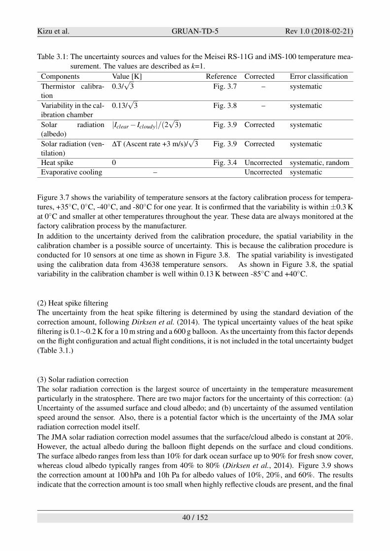
Table 3.1: The uncertainty sources and values for the Meisei RS-11G and iMS-100 temperature mea-surement. The values are described as k=1.
Components Value [K] Reference Corrected Error classification
Thermistor calibra-tion
0.3/%
3 Fig. 3.7 – systematic
Variability in the cal-ibration chamber
0.13/%
3 Fig. 3.8 – systematic
Solar radiation(albedo)
|Iclear # Icloudy|/(2%
3) Fig. 3.9 Corrected systematic
Solar radiation (ven-tilation)
!T (Ascent rate +3 m/s)/%
3 Fig. 3.9 Corrected systematic
Heat spike 0 Fig. 3.4 Uncorrected systematic, random
Evaporative cooling – Uncorrected systematic
Figure 3.7 shows the variability of temperature sensors at the factory calibration process for tempera-tures, +35!C, 0!C, -40!C, and -80!C for one year. It is confirmed that the variability is within ±0.3 Kat 0!C and smaller at other temperatures throughout the year. These data are always monitored at thefactory calibration process by the manufacturer.
In addition to the uncertainty derived from the calibration procedure, the spatial variability in thecalibration chamber is a possible source of uncertainty. This is because the calibration procedure isconducted for 10 sensors at one time as shown in Figure 3.8. The spatial variability is investigatedusing the calibration data from 43638 temperature sensors. As shown in Figure 3.8, the spatialvariability in the calibration chamber is well within 0.13 K between -85!C and +40!C.
(2) Heat spike filteringThe uncertainty from the heat spike filtering is determined by using the standard deviation of thecorrection amount, following Dirksen et al. (2014). The typical uncertainty values of the heat spikefiltering is 0.1"0.2 K for a 10 m string and a 600 g balloon. As the uncertainty from this factor dependson the flight configuration and actual flight conditions, it is not included in the total uncertainty budget(Table 3.1.)
(3) Solar radiation correctionThe solar radiation correction is the largest source of uncertainty in the temperature measurementparticularly in the stratosphere. There are two major factors for the uncertainty of this correction: (a)Uncertainty of the assumed surface and cloud albedo; and (b) uncertainty of the assumed ventilationspeed around the sensor. Also, there is a potential factor which is the uncertainty of the JMA solarradiation correction model itself.
The JMA solar radiation correction model assumes that the surface/cloud albedo is constant at 20%.However, the actual albedo during the balloon flight depends on the surface and cloud conditions.The surface albedo ranges from less than 10% for dark ocean surface up to 90% for fresh snow cover,whereas cloud albedo typically ranges from 40% to 80% (Dirksen et al., 2014). Figure 3.9 showsthe correction amount at 100 hPa and 10h Pa for albedo values of 10%, 20%, and 60%. The resultsindicate that the correction amount is too small when highly reflective clouds are present, and the final
40 / 152
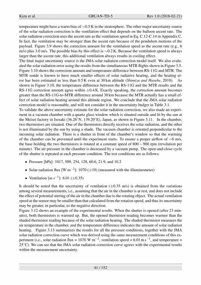
Kizu et al. GRUAN-TD-5 Rev 1.0 (2018-02-21)
temperature might have a warm bias of "0.5 K in the stratosphere. The other major uncertainty sourceof the solar radiation correction is the ventilation effect that depends on the balloon ascent rate. Thesolar radiation correction uses the ascent rate as the ventilation speed in Eq. C.12-C.14 in Appendix C.In fact, the ventilation may be stronger than the ascent rate because of the pendulum motions of thepayload. Figure 3.9 shows the correction amount for the ventilation speed as the ascent rate (e.g., 6m/s) plus 3.0 m/s. The possible bias by this effect is "0.2 K. Because the ventilation speed is alwayslarger than the ascent rate, this additional ventilation always results in cooling effect.The final major uncertainty source is the JMA solar radiation correction model itself. We also evalu-ated the solar radiation error using the results from the simultaneous MTR flights shown in Figure 3.5.Figure 3.10 shows the correction amount and temperature difference between RS-11G and MTR. TheMTR sonde is known to have much smaller effects of solar radiative heating, and the heating er-ror has been estimated as less than 0.5 K even at 30 km altitude (Shimizu and Hasebe, 2010). Asshown in Figure 3.10, the temperature difference between the RS-11G and the MTR results and theRS-11G correction amount agree within ±0.4 K. Exactly speaking, the correction amount becomesgreater than the RS-11G-to-MTR difference around 30 km because the MTR actually has a small ef-fect of solar radiation heating around this altitude region. We conclude that the JMA solar radiationcorrection model is reasonable, and will not consider it in the uncertainty budget in Table 3.1.To validate the above uncertainty estimate for the solar radiation correction, we also made an experi-ment in a vacuum chamber with a quartz glass window which is situated outside and lit by the sun atthe Meisei factory in Isesaki (36.26!N, 139.20!E), Japan, as shown in Figure 3.11. In the chamber,two thermistors are situated. One of the thermistors directly receives the solar radiation, and the otheris not illuminated by the sun by using a shade. The vacuum chamber is oriented perpendicular to theincoming solar radiation. There is a shutter in front of the chamber’s window so that the warmingof the chamber can be prevented until the experiment starts. To ensure a proper airflow of "6 m/s,the base holding the two thermistors is rotated at a constant speed of 800 – 900 rpm (revolution perminute). The air pressure in the chamber is decreased by a vacuum pump. The open-and-close cycleof the shutter is repeated at each pressure condition. The test conditions are as follows:
• Pressure [hPa]: 1017, 509, 254, 128, 60.6, 21.9, and 10.2
• Solar radiation flux [W m#2]: 1070 (±19) (measured with the illuminometer)
• Ventilation [m s#1]: 6.01 (±0.35)
It should be noted that the uncertainty of ventilation (±0.35 m/s) is obtained from the variationsamong several measurements, i.e., assuming that the air in the chamber is at rest, and does not includethe effect of potential stirring of the air in the chamber due to the rotating object. The actual ventilationspeed at the sensor may be smaller than that calculated from the rotation speed, and thus its uncertaintymay be greater, in particular, to the negative direction.Figure 3.12 shows an example of the experimental results. When the shutter is opened (after 23 min-utes), both thermistors is warmed up. But, the opened thermistor reading becomes warmer than theshaded thermistor reading because of the solar radiation heating. The shaded thermistor measures theair temperature in the chamber, and the temperature difference indicates the amount of solar radiationheating. Figure 3.13 summarizes the results for all the pressure conditions, together with the JMAsolar radiation correction curve which was derived using the same measurement conditions of this ex-periment (i.e., solar radiation flux = 1070 W m#2, ventilation speed = 6.01 m s#1, and temperature =25!C). We can see that the JMA solar radiation correction curve agrees with the experimental resultswithin the measurement uncertainty.
41 / 152
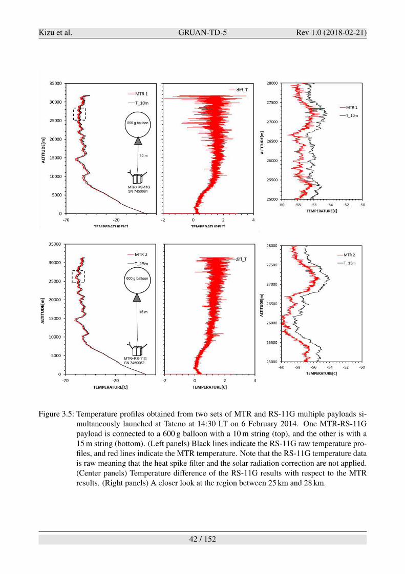
Kizu et al. GRUAN-TD-5 Rev 1.0 (2018-02-21)
Figure 3.5: Temperature profiles obtained from two sets of MTR and RS-11G multiple payloads si-multaneously launched at Tateno at 14:30 LT on 6 February 2014. One MTR-RS-11Gpayload is connected to a 600 g balloon with a 10 m string (top), and the other is with a15 m string (bottom). (Left panels) Black lines indicate the RS-11G raw temperature pro-files, and red lines indicate the MTR temperature. Note that the RS-11G temperature datais raw meaning that the heat spike filter and the solar radiation correction are not applied.(Center panels) Temperature difference of the RS-11G results with respect to the MTRresults. (Right panels) A closer look at the region between 25 km and 28 km.
42 / 152
Kizu et al. GRUAN-TD-5 Rev 1.0 (2018-02-21)
Figure 3.6: Amount of the solar radiation correction for the RS-11G and iMS-100 temperature mea-surements at different pressure levels. The correction amount is calculated with the JMAcorrection model (JMA 1995) which considers the effects of absorption of solar radiation,heat transfer between the ambient air and the temperature sensor, and thermal conductionof the lead wire. The balloon ascent rate is assumed to be 6 m s#1.
43 / 152
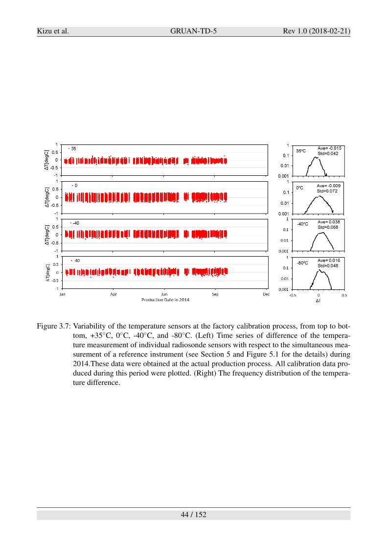
Kizu et al. GRUAN-TD-5 Rev 1.0 (2018-02-21)
Figure 3.7: Variability of the temperature sensors at the factory calibration process, from top to bot-tom, +35!C, 0!C, -40!C, and -80!C. (Left) Time series of difference of the tempera-ture measurement of individual radiosonde sensors with respect to the simultaneous mea-surement of a reference instrument (see Section 5 and Figure 5.1 for the details) during2014.These data were obtained at the actual production process. All calibration data pro-duced during this period were plotted. (Right) The frequency distribution of the tempera-ture difference.
44 / 152
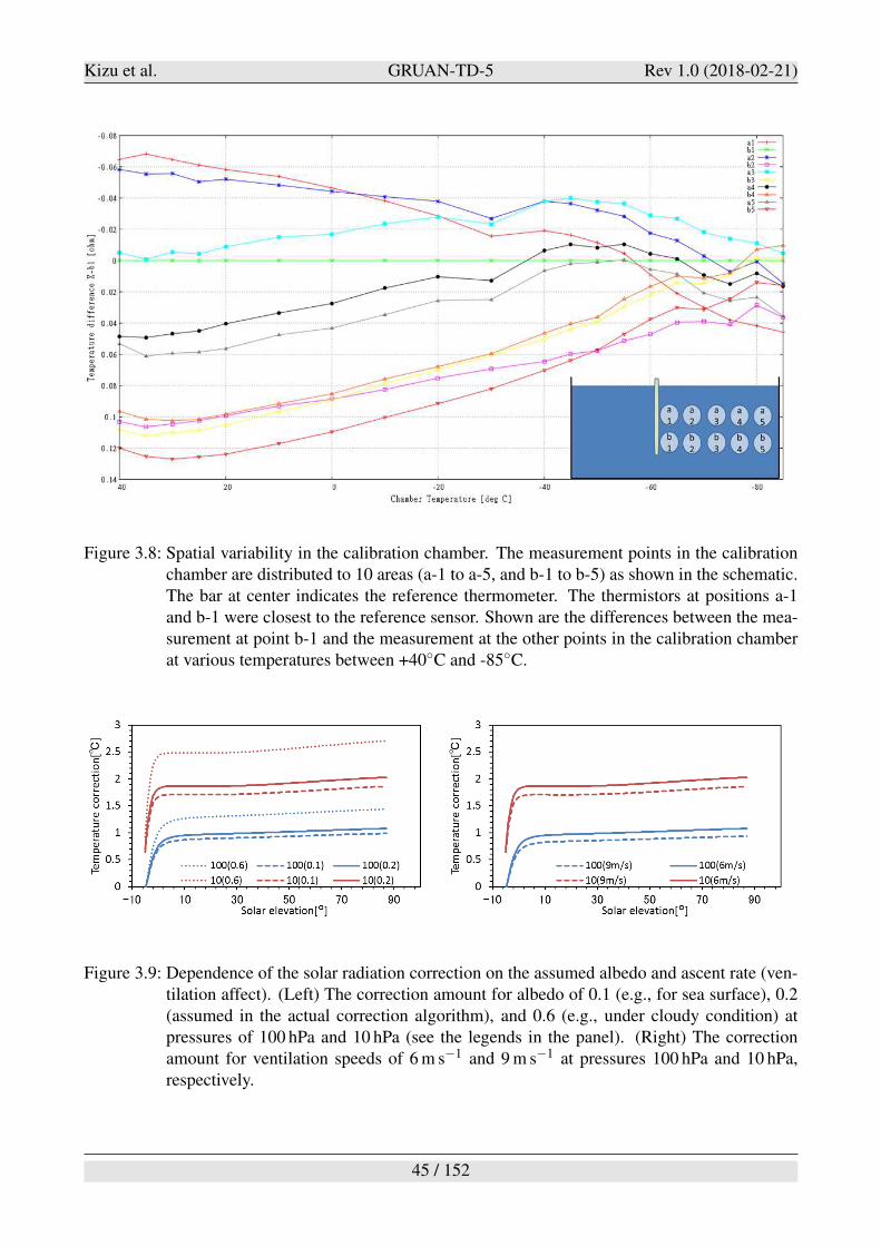
Kizu et al. GRUAN-TD-5 Rev 1.0 (2018-02-21)
Figure 3.8: Spatial variability in the calibration chamber. The measurement points in the calibrationchamber are distributed to 10 areas (a-1 to a-5, and b-1 to b-5) as shown in the schematic.The bar at center indicates the reference thermometer. The thermistors at positions a-1and b-1 were closest to the reference sensor. Shown are the differences between the mea-surement at point b-1 and the measurement at the other points in the calibration chamberat various temperatures between +40!C and -85!C.
Figure 3.9: Dependence of the solar radiation correction on the assumed albedo and ascent rate (ven-tilation affect). (Left) The correction amount for albedo of 0.1 (e.g., for sea surface), 0.2(assumed in the actual correction algorithm), and 0.6 (e.g., under cloudy condition) atpressures of 100 hPa and 10 hPa (see the legends in the panel). (Right) The correctionamount for ventilation speeds of 6 m s#1 and 9 m s#1 at pressures 100 hPa and 10 hPa,respectively.
45 / 152
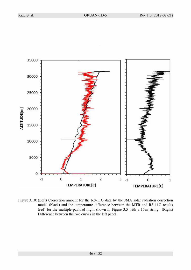
Kizu et al. GRUAN-TD-5 Rev 1.0 (2018-02-21)
Figure 3.10: (Left) Correction amount for the RS-11G data by the JMA solar radiation correctionmodel (black) and the temperature difference between the MTR and RS-11G results(red) for the multiple-payload flight shown in Figure 3.5 with a 15 m string. (Right)Difference between the two curves in the left panel.
46 / 152
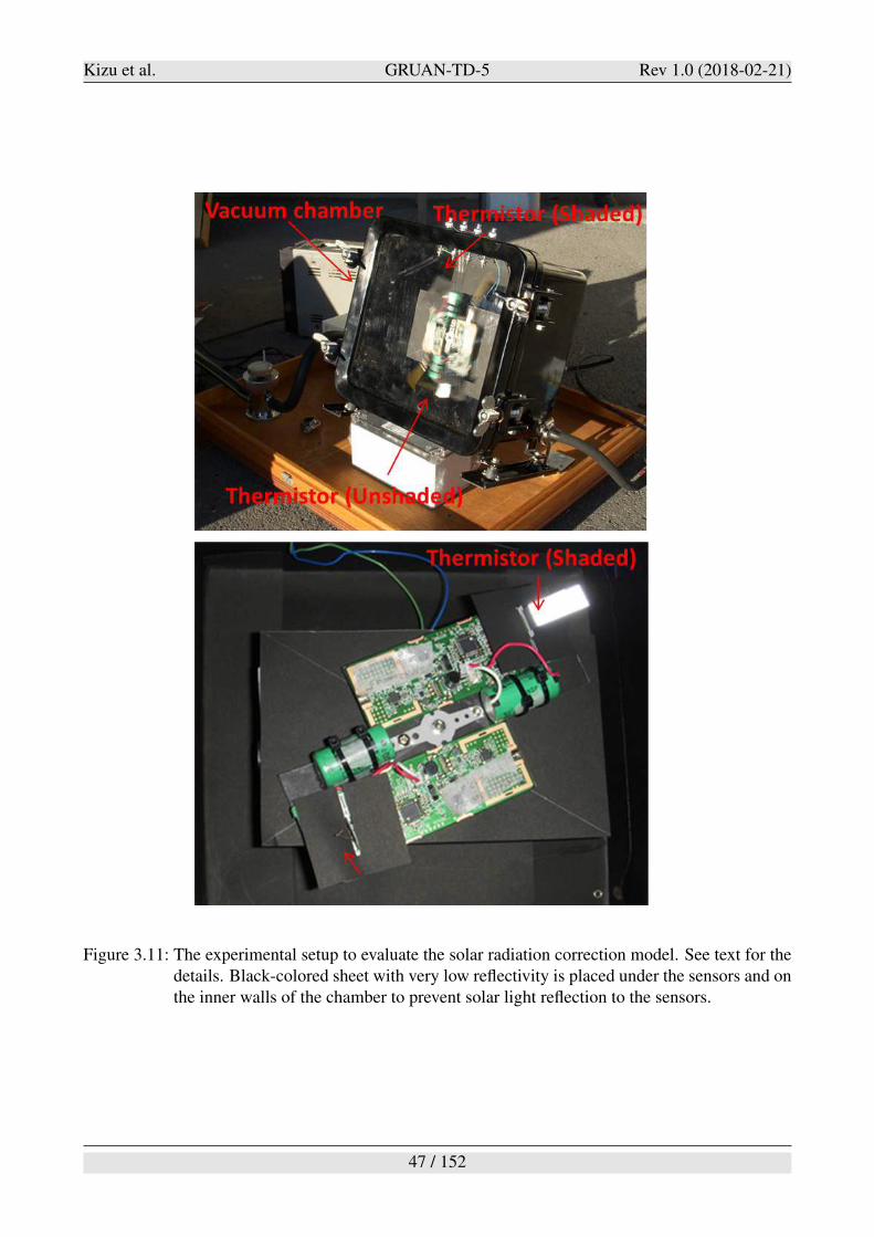
Kizu et al. GRUAN-TD-5 Rev 1.0 (2018-02-21)
Figure 3.11: The experimental setup to evaluate the solar radiation correction model. See text for thedetails. Black-colored sheet with very low reflectivity is placed under the sensors and onthe inner walls of the chamber to prevent solar light reflection to the sensors.
47 / 152
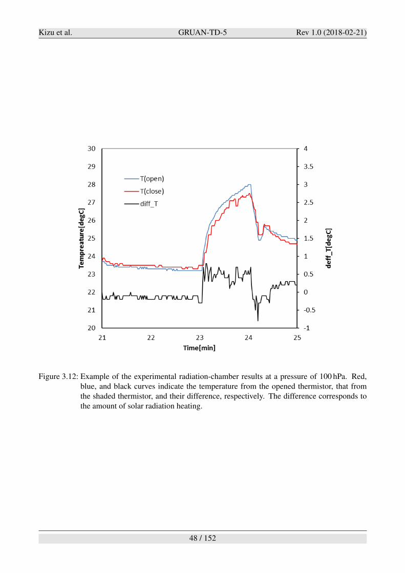
Kizu et al. GRUAN-TD-5 Rev 1.0 (2018-02-21)
Figure 3.12: Example of the experimental radiation-chamber results at a pressure of 100 hPa. Red,blue, and black curves indicate the temperature from the opened thermistor, that fromthe shaded thermistor, and their difference, respectively. The difference corresponds tothe amount of solar radiation heating.
48 / 152
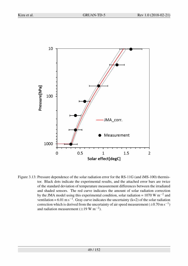
Kizu et al. GRUAN-TD-5 Rev 1.0 (2018-02-21)
Figure 3.13: Pressure dependence of the solar radiation error for the RS-11G (and iMS-100) thermis-tor. Black dots indicate the experimental results, and the attached error bars are twiceof the standard deviation of temperature measurement differences between the irradiatedand shaded sensors. The red curve indicates the amount of solar radiation correctionby the JMA model using this experimental condition, solar radiation = 1070 W m#2 andventilation = 6.01 m s#1. Gray curve indicates the uncertainty (k=2) of the solar radiationcorrection which is derived from the uncertainty of air speed measurement (±0.70 m s#1)and radiation measurement (±19 W m#2).
49 / 152
Kizu et al. GRUAN-TD-5 Rev 1.0 (2018-02-21)
(4) Total uncertainty of the RS-11G and iMS-100 temperature measurementThe total uncertainty depends on altitude and observation conditions, and its amount generally in-creases with altitude. Figure 3.14 shows an example of the measurement uncertainty profile of tem-perature for a daytime observation, launched at 14:00 LT on 07 October 2014 14:00 LT, at Lindenberg(52.21!N, 14.12!E), Germany. The uncertainty increases with altitude and reaches 0.8 K at 30 km.Up to "15 km, the uncertainty is dominated by the calibration uncertainty. In the stratosphere, theuncertainty from the solar radiation correction is the main source of uncertainty. Note that the sur-face/cloud albedo is assumed to be constant at 20%, which is not the case for actual surface and cloudconditions during the flight, and that the ventilation speed around the sensor is assumed to be equal tothe ascent rate, i.e., not including the additional ventilation by the pendulum motions of the payload.It is considered that these uncertain parameters, the albedo and the ventilation speed, cause large un-certainty in temperature measurements. It is noted that the uncertainty from the infrared radiationerror and time-lag error is negligible and not considered here. Also, the uncertainty from heat spikesis not considered because this flight was conducted with a long string of 30 m. If the payload configu-ration is different, e.g., with a much shorter string and/or with multiple payload with a rig, additionaluncertainty would arise.
3.2 Relative humidity measurements
3.2.1 Sensor material
The RS-11G and iMS-100 radiosondes are equipped with the same thin-film capacitive RH sensor.Figure 3.15 shows the external view of the RH sensor. This thin-film capacitive sensor consists of athin hydrophilic polymer layer on a glass substrate, which acts as the dielectric of a capacitor. Thecapacitance changes in response to the number of water molecules permeating from the ambient airinto the polymer layer. The capacitive sensor on the RS-11G and iMS-100 radiosondes measuresthe change of capacitance as electric frequency signals (frequency of humidity) by the CR oscillationcircuit described in Section 2.3. The relationship between the frequency of humidity and the RH of theambient air is determined by factory calibration procedures. The RH sensor of the RS-11G and iMS-100 radiosondes has a protective cap coated with aluminum vapor deposition to prevent the sensorfrom icing of supercooled droplets and heating by solar radiation (see Figures 2.1-2.4). Potentialnegative effects of having a protective cap include trapping of water droplets, whose impacts arereduced by applying a contamination removal filter (see Section 3.2.3). In addition, the iMS-100radiosonde is equipped with a dedicated thermistor on the RH sensor for the temperature correctionof the RH data.
3.2.2 Sensor calibration
The relationship between the frequency of humidity and the value of RH is approximated with acubic function. A set of four sensor-specific calibration coefficients of the cubic function is obtainedfor each sensor by a calibration procedure, which is conducted in the factory at 15 %RH, 30 %RH,50 %RH, 70 %RH, 90 %RH, and 95 %RH at a constant air temperature of +25!C. Figure 3.16 showsan example of the relationship between the frequency of humidity and the value of RH for a particularsensor. In this calibration process, the reference RH values are obtained from a reference platinumresistance thermometer (R900-F25 by CHINO) and a reference chilled mirror hygrometer (D-2-SR byGeneral Eastem for the RS-11G, or DewStar S-2 by SHINYEI for the iMS-100). For the D-2-SR (forRS-11G), the water vapor pressure equation by Buck (1981) is used, while for the DewStar S-2 (for
50 / 152
Kizu et al. GRUAN-TD-5 Rev 1.0 (2018-02-21)
iMS-100), the equation by Hyland and Wexler (1983) is used. For both equations, the enhancementfactor ”f” is set to be unity. Because the calibration is made only at 25!C, the difference due to theuse of different water vapor pressure equations is negligible (the difference among different watervapor pressure equations is non-negligible only at very low temperatures; see e.g., Nash et al. (2011),their section 8.2.5, and Murphy and Koop (2005)). As described later, for both RS-11G and iMS-100, the Hyland-Wexler equation is only used for all the data processing, i.e., for the Temperature-Humidity Dependence correction (Section 3.2.3 (3)), for the sensor versus air temperature correction(Section 3.2.3 (4)), for the pressure calculation (Section 3.3.2), and for creating the GRUAN dataproduct (Appendix H).
According to the WMO Commission for Instruments and Methods of Observation (CIMO) guide(WMO, 2008), by convention, RH should be calculated with respect to liquid water even at air tem-peratures below 0!C. In addition to normal manufacturer’s calibration as described above, at Tatenosite, new calibration coefficients are determined by using the data for 0 %RH and 100 %RH duringthe SHC checks. This process enables to improve the measurement accuracy around 0 % RH and100 %RH because these points are the extrapolated values for the original manufacture’s calibration.Note that all calibrations are conducted at +25!C or room temperatures. The temperature dependencecorrection procedure will be described in Section 3.2.3 (3).
3.2.3 Calculation and correction procedures
The algorithm to obtain the RH data is shown in Figure 3.17. The received frequency data for hu-midity is converted to the capacitance values and then to the raw RH values (U0) by using the sensor-specific factory calibration coefficients. More details to obtain the raw RH values are described inAppendix D. In general, thin-film capacitive RH sensors on radiosondes are subject to several sourcesof errors, including slow responses at low temperatures, contamination errors caused by supercooledcloud droplets, bias errors related to non-water molecules being absorbed into the hydrophilic poly-mer layer, and bias errors due to the temperature difference between the RH sensor and ambient air(e.g. Dirksen et al., 2014). Thus the raw radiosonde RH data (U0) may need the following correctionsor filtering.
1. Contamination removal filter for rain and cloud droplets (Contami corr)
2. Time-lag correction (TL corr.)
3. Temperature-Humidity Dependence correction (TUD corr.)
4. Sensor versus air temperature correction (Ts/Ta corr.)
5. Hysteresis consideration
6. Sensor aging consideration
For the RS-11G and iMS-100 radiosondes, the corrections (1), (2), (3), and (4) are considered neces-sary and thus are applied to obtain the final RH data. Note that for the former models of the Meiseiradiosonde, these corrections are not necessarily considered. For example, the RS-06G radiosondeapplies correction (3) only (e.g. Sugidachi and Fujiwara, 2013).
51 / 152
Kizu et al. GRUAN-TD-5 Rev 1.0 (2018-02-21)
3.2.3.1 Contamination removal filter for rain and cloud droplets (Contami corr)
During soundings under rainy conditions, water droplets or ice may attach to the RH-sensor capand/or the sensor arm. After the radiosonde passes through the cloud layer and enters a drier region,the RH sensor may quasi-periodically be affected by the air flow directly capturing additional watervapor from the wet structures surrounding the sensor, resulting in wet biases in its measurements.The RH profile affected by this wet contamination error shows spiky structures or small-vertical-scale oscillations, similar to the heat spikes in contaminated temperature measurements. Therefore,the following procedure is applied to remove contaminated RH measurements.
1. The raw humidity profile is separated into the high-frequency and low-frequency componentsby using the time response of RH sensor as the cut-off frequency with a window width of 60 s.
2. The time-lag correction (explained below) is applied to both the high-frequency and low-frequency components.
3. The RH offset by the contamination is determined by applying a minimum filter, which issimilar to heat spike filter for temperature measurements, with a window width of pendulumfrequency (depending on the string length: 6.3 s for the string of 10 m, 7.8 s for the string of 15m) to the high-frequency component.
4. The filtered high-frequency component is added to the low-frequency component to obtain thecontamination-corrected RH (U1).
3.2.3.2 Time-lag correction
Thin-film polymer RH sensors show slower responses at lower temperatures, which result in smooth-ing of the RH profile and a major error component in the upper troposphere and above (Miloshevich
et al., 2004). The response time of the RS-11G and iMS-100 RH sensor, defined as the time re-quired to respond by 63% to a sudden change, has been evaluated by laboratory experiments at sometemperature points in a thermostatic chamber. Figure 3.18 shows the response time measured at-60!C, -40!C, -20!C, and 0!C. The response time increases exponentially at lower temperatures. Theobtained relationship for the stepwise change from dry to wet condition can be expressed as
%(T ) = 0.1537e#0.087T (3.5)
where T is the sensor temperature. Although the response time is different by the condition (theresponse time from wet to dry is slower than that from dry to wet), we use the values from dry towet condition in any case to prevent from over correction (over-shooting). Also, the dashed lines inFigure 3.18 indicate the uncertainty derived from the standard deviation from the 69 measurements ateach temperature points, which can be approximately expressed as
u(%) = 0.25% (3.6)
Using the response time values, the time-lag error is corrected with the following equation (Miloshe-
vich et al., 2004).
U1(t) =U0(t)#U0(t #!t)e#!t/%(T )
1# e#!t/(%(T )(3.7)
52 / 152
Kizu et al. GRUAN-TD-5 Rev 1.0 (2018-02-21)
where U1(t) is the RH value after the time-lag correction, U0(t) is the RH value before the time-lagcorrection, !t is the time interval (sampling rate). 1 s for both RS-11G and iMS-100, and %(T ) is thee-folding (63%) response time of the RH sensor as a function of temperature.
Eq. 3.7 not only retrieves the actual large gradients in the RH profile but also tends to amplify noisesin the original U0. Therefore, a low-pass digital filter using the Kaiser window (Appendix E), withthe cutoff period of the RH sensor’s response time in Eq. 3.5, is applied to the original U0 before thetime-lag correction Eq. 3.7 is applied.
3.2.3.3 Temperature-Humidity Dependence correction (TUD corr.)
A thin-film polymer RH sensor has temperature dependence at lower temperatures, while the factorycalibration of the RS-11G and iMS-100 radiosondes is conducted at a constant temperature at 25!C.Therefore, the RH biases at lower temperatures need to be corrected during the correction procedure.The temperature dependence of the RS-11G and iMS-100 RH sensor was evaluated by comparisonwith the reference dew/frost-point by a chilled mirror hygrometer (FDW10, manufactured by the Az-bil; with the water vapor pressure equation by Hyland and Wexler (1983) and temperature by PT100instruments (RF-100, manufactured by the ETI) under various chamber conditions, at air tempera-tures from -80!C to +40!C. The experimental setup was the same as that described in Sugidachi and
Fujiwara (2013).
Figure 3.19 shows the measured biases of the RS-11G RH sensor with respect to the reference mea-surements under various chamber conditions. Results from these chamber experiments showed wetbiases between -60!C and 40!C, and dry biases below -60!C (down to -75!C). Also, these biaseshave a RH dependence, being larger at higher RH conditions. To correct these biases, the followingcorrection curve for the temperature-RH dependence is developed by least squares method based onthe experiment results.
!U = (K0 +K1Ts +K2T 2s +K3T 3
s )(K4 +K5U1 +K6U21 ) (3.8)
U2 = U1 #!U (3.9)
where !U (%) is the correction, U1 is the uncorrected RH, U2 is the corrected RH, K0 to K6 are con-stant coefficients, and Ts is the sensor temperature. Ts is measured with a dedicated thermistor attachedto the RH sensor for the case of iMS-100, while it is estimated from air temperature measurementsby considering the effect of solar heating and thermal lag for the case of RS-11G. Figure 3.19 alsoshows the correction curves at selected RH values.
3.2.3.4 Sensor versus air temperature correction (Ts/Ta corr)
During the sounding, temperature of the RH sensor does not necessarily equal to the ambient airtemperature because of the solar heating and the thermal lag of the RH sensor. Measurements withan RH sensor warmer (colder) than the ambient air would result in dry (wet) biases. Therefore, theRH values obtained from Eq. 3.8 need to be translated to the RH with respect to the saturation vaporpressure of the air temperature by using the following equation.
U3 =U2 &e(Ts)
e(Ta)(3.10)
where U3 is the corrected RH, U2 is the uncorrected RH, Ts is the temperature of the RH sensor, and Ta
53 / 152
Kizu et al. GRUAN-TD-5 Rev 1.0 (2018-02-21)
is the temperature of the ambient air. The water vapor pressure equation e(T ) by Hyland and Wexler
(1983) is used.For the iMS-100 radiosonde, Ts is measured with a dedicated thermistor attached to the surface ofthe RH sensor. On the other hand, the RS-11G radiosonde does not have the dedicated thermistorfor the RH sensor. Therefore, the temperature of the RH sensor is estimated on the assumption thatthe sensor becomes warmer (or colder) than the ambient air due to the thermal lag and solar radiationheating, using the following equation.
Ts = Ta +!Ts SR +!Ts T L (3.11)
where !Ts SR is the heating amount by solar radiation (see Appendices D and C for details), !Ts T L
is the warming by thermal lag (in the troposphere). The time constant of the thermal lag (the 63%response time) is estimated to be 22 s at surface pressure level from chamber experiments. The thermallag used in this correction was determined by considering the measurement results of the RH sensortemperature in some flight tests.The RH sensor temperature becomes generally warmer at higher altitudes (upper-troposphere andstratosphere). The difference between Ts and Ta reaches above 5 K in the upper troposphere, andabove 10 K in the stratosphere. In the lower troposphere, on the other hand, Ts is generally very closeto Ta because solar radiation is weak and air density is large. Therefore, Ts/Ta correction is appliedabove the 600 hPa level. More details of this correction is explained in Appendix D.
3.2.3.5 Hysteresis consideration
The RH sensor of the RS-11G and iMS-100 has a small hysteresis property, which causes smallwet biases when the sensor goes from a wetter condition to a drier condition. This wet bias of thehysteresis affects longer times than that of time-lag error. Note that this hysteresis error does notappear when measuring in a constant RH condition for a long period of time (such as in the calibrationprocedure).The hysteresis property was investigated by chamber experiments at the GRUAN Lead Center, Lin-denberg, Germany (Figure 3.20). Five chambers with different RH values are prepared by usingsaturated salt solutions, LiCl for 11 %RH, MgCl2 for 33 %RH, NaCl for 75 %RH, and pure water for100 %RH. RH was then measured with six RS-11G sensors for 3 minutes at each condition in thefollowing order, 0 %RH, 11 %RH, 33 %RH, 75 %RH, 100 %RH, 75 %RH, 33 %RH, 11 %RH, and0 %RH. The results (Figure 3.20) show that wet biases of "1.8 %RH appear when the RH conditionswere changed from 100 %RH to 0 %RH, while biases are much smaller when the RH conditions werechanged from 0 %RH to 100 %RH. The wet biases found here are considered to be due to the hys-teresis. Additional experiments using the thermostatic chamber and a chilled-mirror hygrometer atMeisei showed the following characteristics. These biases are always observed when the RH sensoris exposed to wet conditions (e.g. "80 %RH) as well as to the saturated (100 %RH) condition. Thesebiases do not disappear quickly and are only very slowly reduced at the rate of "0.5 %RH/hour. Itis difficult to create a correction procedure for this hysteresis error because the effect is consideredto be determined by the combination of the wet and dry RH values and the elapsed time from theRH-condition change. Therefore, the correction is not applied, and instead, this error (maximum1.8 %RH) will be considered as an uncertainty source in the uncertainty budget calculation.
54 / 152
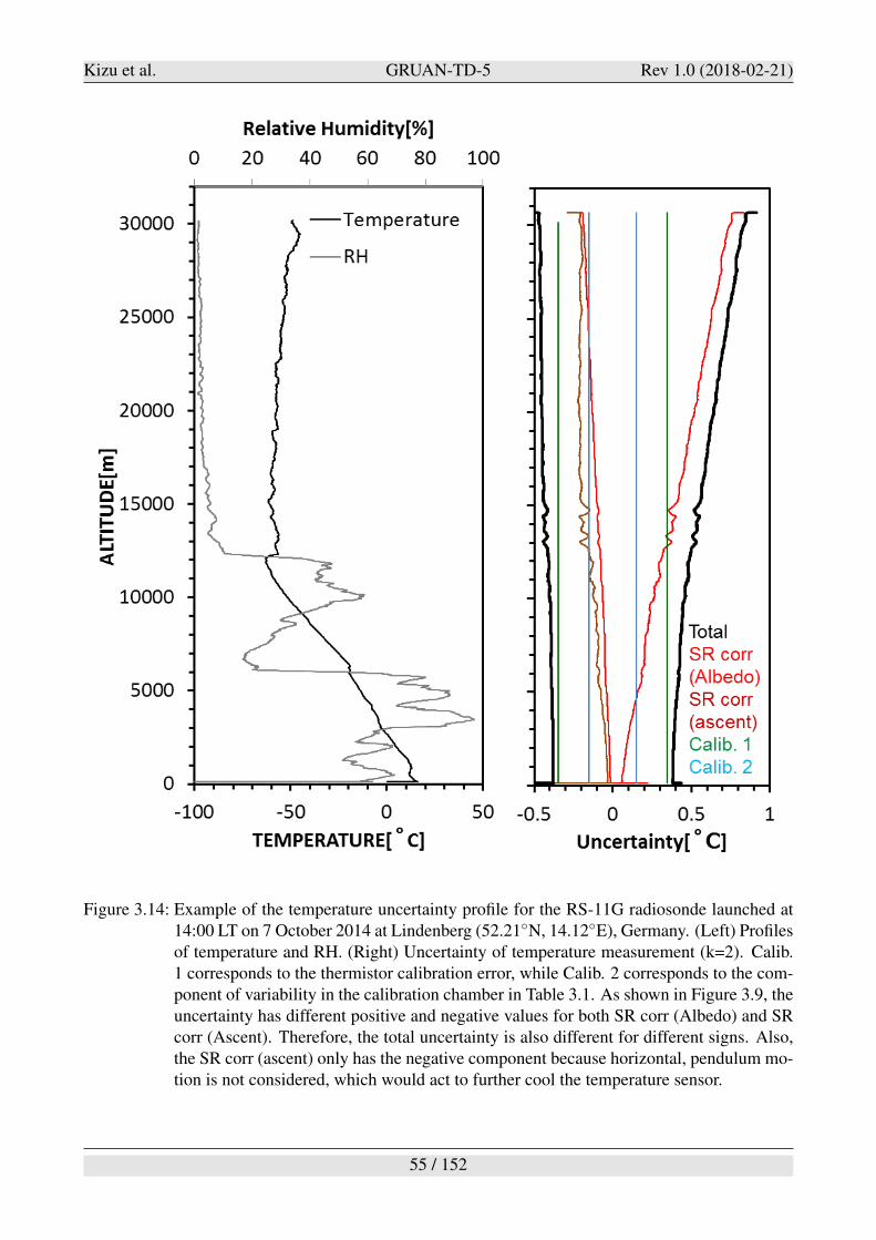
Kizu et al. GRUAN-TD-5 Rev 1.0 (2018-02-21)
Figure 3.14: Example of the temperature uncertainty profile for the RS-11G radiosonde launched at14:00 LT on 7 October 2014 at Lindenberg (52.21!N, 14.12!E), Germany. (Left) Profilesof temperature and RH. (Right) Uncertainty of temperature measurement (k=2). Calib.1 corresponds to the thermistor calibration error, while Calib. 2 corresponds to the com-ponent of variability in the calibration chamber in Table 3.1. As shown in Figure 3.9, theuncertainty has different positive and negative values for both SR corr (Albedo) and SRcorr (Ascent). Therefore, the total uncertainty is also different for different signs. Also,the SR corr (ascent) only has the negative component because horizontal, pendulum mo-tion is not considered, which would act to further cool the temperature sensor.
55 / 152
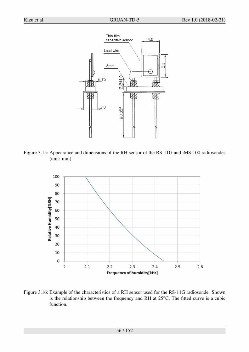
Kizu et al. GRUAN-TD-5 Rev 1.0 (2018-02-21)
Figure 3.15: Appearance and dimensions of the RH sensor of the RS-11G and iMS-100 radiosondes(unit: mm).
Figure 3.16: Example of the characteristics of a RH sensor used for the RS-11G radiosonde. Shownis the relationship between the frequency and RH at 25!C. The fitted curve is a cubicfunction.
56 / 152
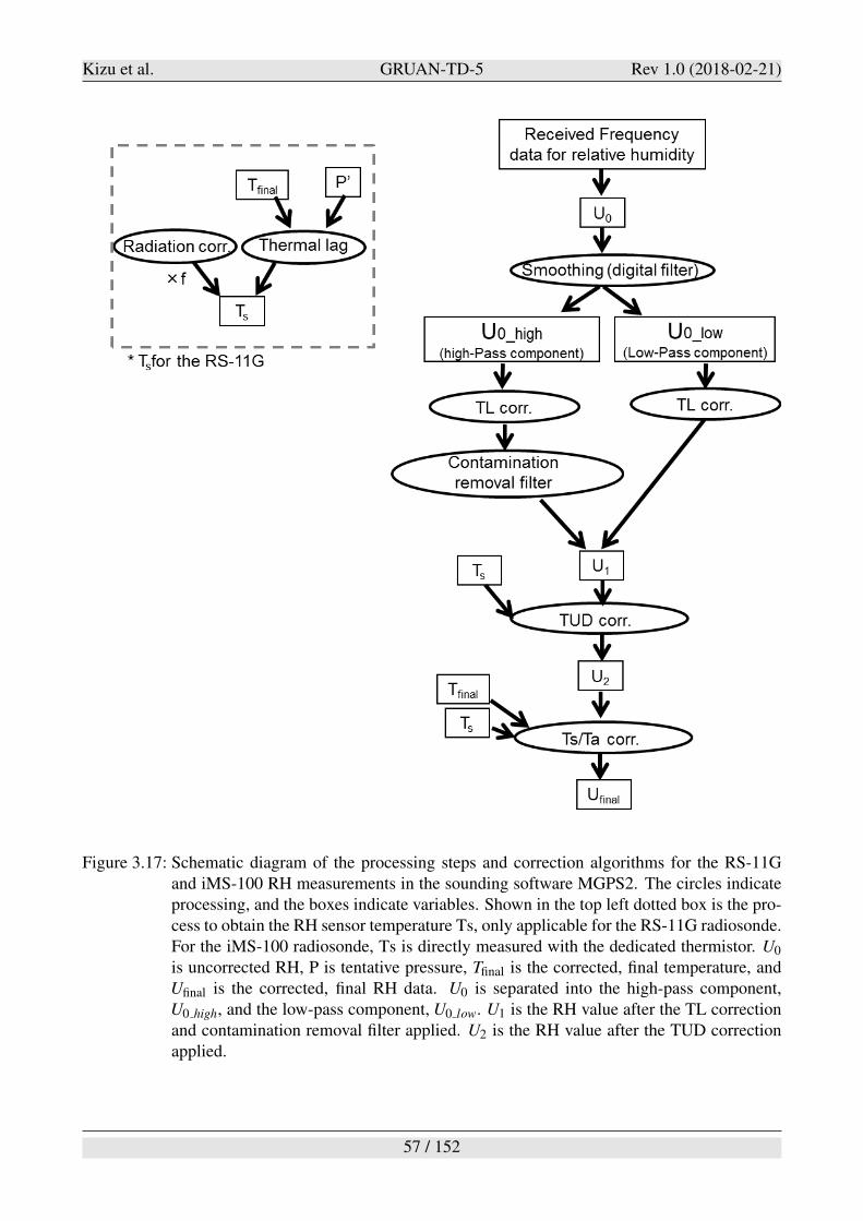
Kizu et al. GRUAN-TD-5 Rev 1.0 (2018-02-21)
Figure 3.17: Schematic diagram of the processing steps and correction algorithms for the RS-11Gand iMS-100 RH measurements in the sounding software MGPS2. The circles indicateprocessing, and the boxes indicate variables. Shown in the top left dotted box is the pro-cess to obtain the RH sensor temperature Ts, only applicable for the RS-11G radiosonde.For the iMS-100 radiosonde, Ts is directly measured with the dedicated thermistor. U0
is uncorrected RH, P is tentative pressure, Tfinal is the corrected, final temperature, andUfinal is the corrected, final RH data. U0 is separated into the high-pass component,U0 high, and the low-pass component, U0 low. U1 is the RH value after the TL correctionand contamination removal filter applied. U2 is the RH value after the TUD correctionapplied.
57 / 152
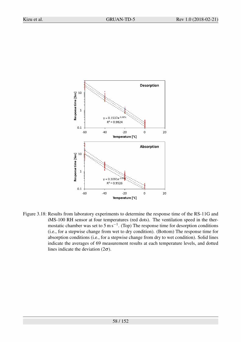
Kizu et al. GRUAN-TD-5 Rev 1.0 (2018-02-21)
Figure 3.18: Results from laboratory experiments to determine the response time of the RS-11G andiMS-100 RH sensor at four temperatures (red dots). The ventilation speed in the ther-mostatic chamber was set to 5 m s#1. (Top) The response time for desorption conditions(i.e., for a stepwise change from wet to dry condition). (Bottom) The response time forabsorption conditions (i.e., for a stepwise change from dry to wet condition). Solid linesindicate the averages of 69 measurement results at each temperature levels, and dottedlines indicate the deviation (2! ).
58 / 152
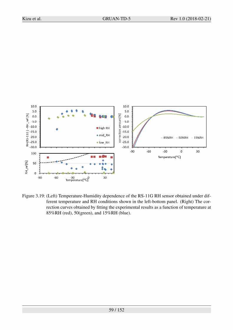
Kizu et al. GRUAN-TD-5 Rev 1.0 (2018-02-21)
Figure 3.19: (Left) Temperature-Humidity dependence of the RS-11G RH sensor obtained under dif-ferent temperature and RH conditions shown in the left-bottom panel. (Right) The cor-rection curves obtained by fitting the experimental results as a function of temperature at85%RH (red), 50(green), and 15%RH (blue).
59 / 152
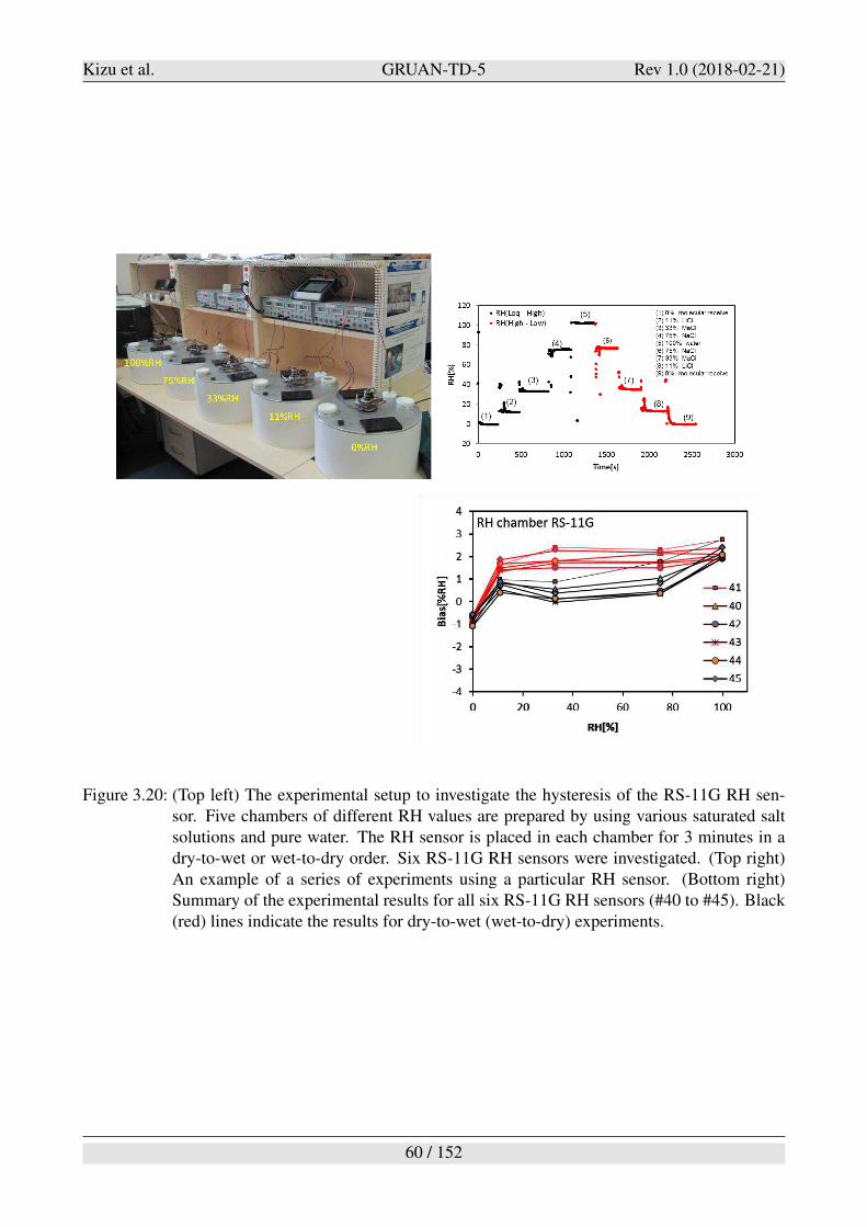
Kizu et al. GRUAN-TD-5 Rev 1.0 (2018-02-21)
Figure 3.20: (Top left) The experimental setup to investigate the hysteresis of the RS-11G RH sen-sor. Five chambers of different RH values are prepared by using various saturated saltsolutions and pure water. The RH sensor is placed in each chamber for 3 minutes in adry-to-wet or wet-to-dry order. Six RS-11G RH sensors were investigated. (Top right)An example of a series of experiments using a particular RH sensor. (Bottom right)Summary of the experimental results for all six RS-11G RH sensors (#40 to #45). Black(red) lines indicate the results for dry-to-wet (wet-to-dry) experiments.
60 / 152
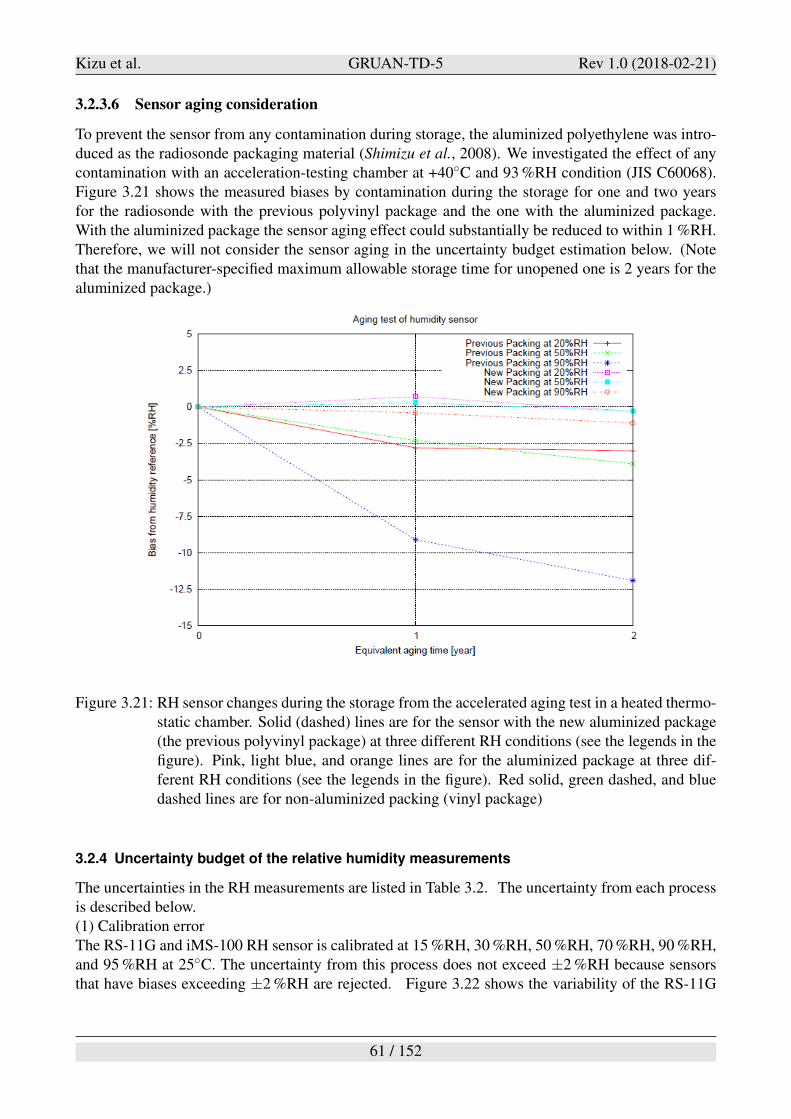
Kizu et al. GRUAN-TD-5 Rev 1.0 (2018-02-21)
3.2.3.6 Sensor aging consideration
To prevent the sensor from any contamination during storage, the aluminized polyethylene was intro-duced as the radiosonde packaging material (Shimizu et al., 2008). We investigated the effect of anycontamination with an acceleration-testing chamber at +40!C and 93 %RH condition (JIS C60068).Figure 3.21 shows the measured biases by contamination during the storage for one and two yearsfor the radiosonde with the previous polyvinyl package and the one with the aluminized package.With the aluminized package the sensor aging effect could substantially be reduced to within 1 %RH.Therefore, we will not consider the sensor aging in the uncertainty budget estimation below. (Notethat the manufacturer-specified maximum allowable storage time for unopened one is 2 years for thealuminized package.)
Figure 3.21: RH sensor changes during the storage from the accelerated aging test in a heated thermo-static chamber. Solid (dashed) lines are for the sensor with the new aluminized package(the previous polyvinyl package) at three different RH conditions (see the legends in thefigure). Pink, light blue, and orange lines are for the aluminized package at three dif-ferent RH conditions (see the legends in the figure). Red solid, green dashed, and bluedashed lines are for non-aluminized packing (vinyl package)
3.2.4 Uncertainty budget of the relative humidity measurements
The uncertainties in the RH measurements are listed in Table 3.2. The uncertainty from each processis described below.(1) Calibration errorThe RS-11G and iMS-100 RH sensor is calibrated at 15 %RH, 30 %RH, 50 %RH, 70 %RH, 90 %RH,and 95 %RH at 25!C. The uncertainty from this process does not exceed ±2 %RH because sensorsthat have biases exceeding ±2 %RH are rejected. Figure 3.22 shows the variability of the RS-11G
61 / 152
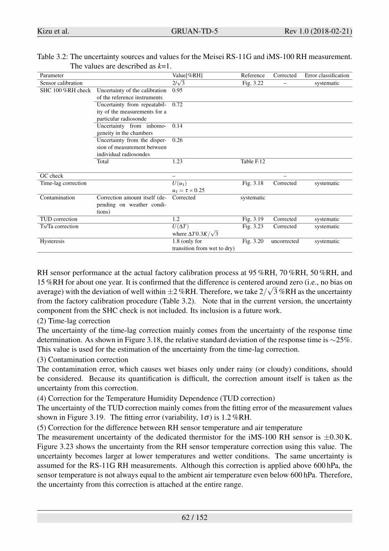
Kizu et al. GRUAN-TD-5 Rev 1.0 (2018-02-21)
Table 3.2: The uncertainty sources and values for the Meisei RS-11G and iMS-100 RH measurement.The values are described as k=1.
Parameter Value[%RH] Reference Corrected Error classification
Sensor calibration 2/%
3 Fig. 3.22 – systematic
SHC 100 %RH check Uncertainty of the calibrationof the reference instruments
0.95
Uncertainty from repeatabil-ity of the measurements for aparticular radiosonde
0.72
Uncertainty from inhomo-geneity in the chambers
0.14
Uncertainty from the disper-sion of measurement betweenindividual radiosondes
0.26
Total 1.23 Table F.12
GC check – –
Time-lag correction U(u%) Fig. 3.18 Corrected systematicu% = % &0.25
Contamination Correction amount itself (de-pending on weather condi-tions)
Corrected systematic
TUD correction 1.2 Fig. 3.19 Corrected systematic
Ts/Ta correction U(!T ) Fig. 3.23 Corrected systematic
where !T 0.3K/%
3
Hysteresis 1.8 (only for Fig. 3.20 uncorrected systematictransition from wet to dry)
RH sensor performance at the actual factory calibration process at 95 %RH, 70 %RH, 50 %RH, and15 %RH for about one year. It is confirmed that the difference is centered around zero (i.e., no bias onaverage) with the deviation of well within ±2 %RH. Therefore, we take 2/
%3 %RH as the uncertainty
from the factory calibration procedure (Table 3.2). Note that in the current version, the uncertaintycomponent from the SHC check is not included. Its inclusion is a future work.
(2) Time-lag correctionThe uncertainty of the time-lag correction mainly comes from the uncertainty of the response timedetermination. As shown in Figure 3.18, the relative standard deviation of the response time is "25%.This value is used for the estimation of the uncertainty from the time-lag correction.
(3) Contamination correctionThe contamination error, which causes wet biases only under rainy (or cloudy) conditions, shouldbe considered. Because its quantification is difficult, the correction amount itself is taken as theuncertainty from this correction.
(4) Correction for the Temperature Humidity Dependence (TUD correction)The uncertainty of the TUD correction mainly comes from the fitting error of the measurement valuesshown in Figure 3.19. The fitting error (variability, 1! ) is 1.2 %RH.
(5) Correction for the difference between RH sensor temperature and air temperatureThe measurement uncertainty of the dedicated thermistor for the iMS-100 RH sensor is ±0.30 K.Figure 3.23 shows the uncertainty from the RH sensor temperature correction using this value. Theuncertainty becomes larger at lower temperatures and wetter conditions. The same uncertainty isassumed for the RS-11G RH measurements. Although this correction is applied above 600 hPa, thesensor temperature is not always equal to the ambient air temperature even below 600 hPa. Therefore,the uncertainty from this correction is attached at the entire range.
62 / 152
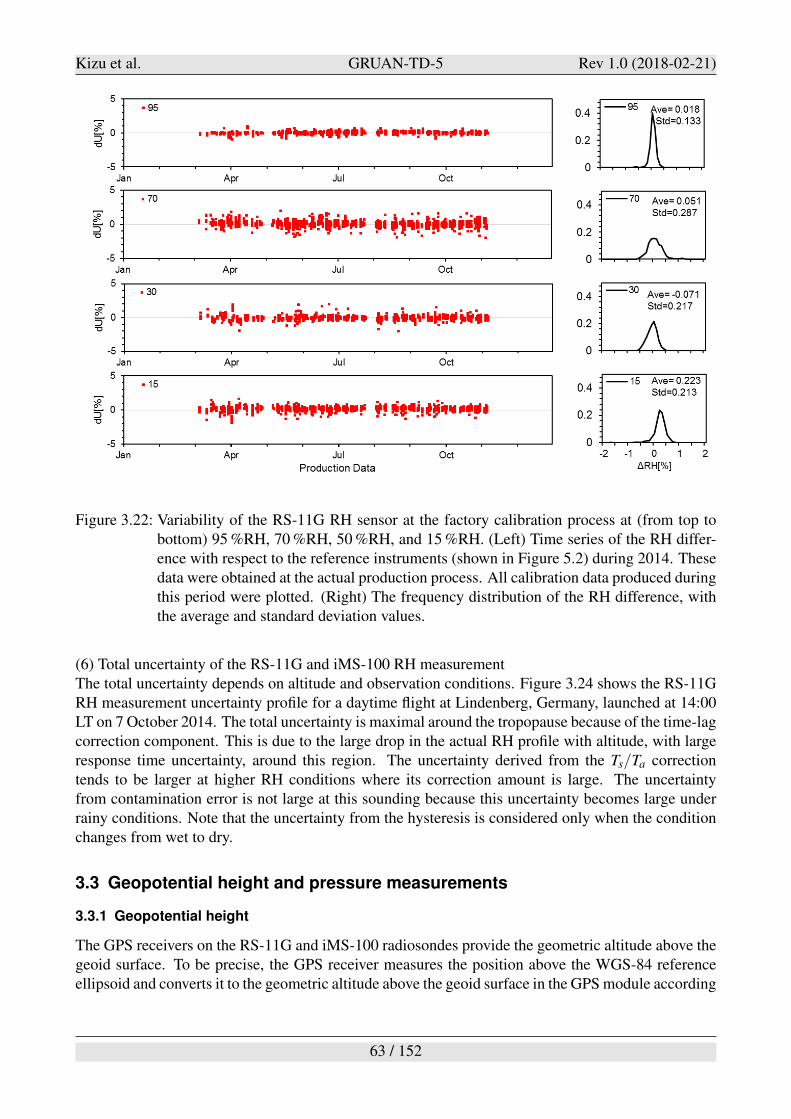
Kizu et al. GRUAN-TD-5 Rev 1.0 (2018-02-21)
Figure 3.22: Variability of the RS-11G RH sensor at the factory calibration process at (from top tobottom) 95 %RH, 70 %RH, 50 %RH, and 15 %RH. (Left) Time series of the RH differ-ence with respect to the reference instruments (shown in Figure 5.2) during 2014. Thesedata were obtained at the actual production process. All calibration data produced duringthis period were plotted. (Right) The frequency distribution of the RH difference, withthe average and standard deviation values.
(6) Total uncertainty of the RS-11G and iMS-100 RH measurementThe total uncertainty depends on altitude and observation conditions. Figure 3.24 shows the RS-11GRH measurement uncertainty profile for a daytime flight at Lindenberg, Germany, launched at 14:00LT on 7 October 2014. The total uncertainty is maximal around the tropopause because of the time-lagcorrection component. This is due to the large drop in the actual RH profile with altitude, with largeresponse time uncertainty, around this region. The uncertainty derived from the Ts/Ta correctiontends to be larger at higher RH conditions where its correction amount is large. The uncertaintyfrom contamination error is not large at this sounding because this uncertainty becomes large underrainy conditions. Note that the uncertainty from the hysteresis is considered only when the conditionchanges from wet to dry.
3.3 Geopotential height and pressure measurements
3.3.1 Geopotential height
The GPS receivers on the RS-11G and iMS-100 radiosondes provide the geometric altitude above thegeoid surface. To be precise, the GPS receiver measures the position above the WGS-84 referenceellipsoid and converts it to the geometric altitude above the geoid surface in the GPS module according
63 / 152
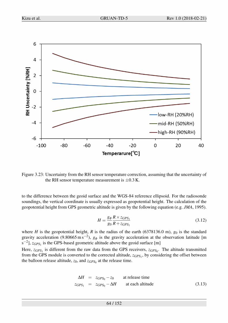
Kizu et al. GRUAN-TD-5 Rev 1.0 (2018-02-21)
Figure 3.23: Uncertainty from the RH sensor temperature correction, assuming that the uncertainty ofthe RH sensor temperature measurement is ±0.3 K.
to the difference between the geoid surface and the WGS-84 reference ellipsoid. For the radiosondesoundings, the vertical coordinate is usually expressed as geopotential height. The calculation of thegeopotential height from GPS geometric altitude is given by the following equation (e.g. JMA, 1995).
H =g&
g0
R& zGPS1
R+ zGPS1
(3.12)
where H is the geopotential height, R is the radius of the earth (6378136.0 m), g0 is the standardgravity acceleration (9.80665 m s#2), g& is the gravity acceleration at the observation latitude [ms#2], zGPS1
is the GPS-based geometric altitude above the geoid surface [m]
Here, zGPS1is different from the raw data from the GPS receivers, zGPS0
. The altitude transmittedfrom the GPS module is converted to the corrected altitude, zGPS1
, by considering the offset betweenthe balloon release altitude, z0, and zGPS0
at the release time.
!H = zGPS0# z0 at release time
zGPS1= zGPS0
#!H at each altitude (3.13)
64 / 152
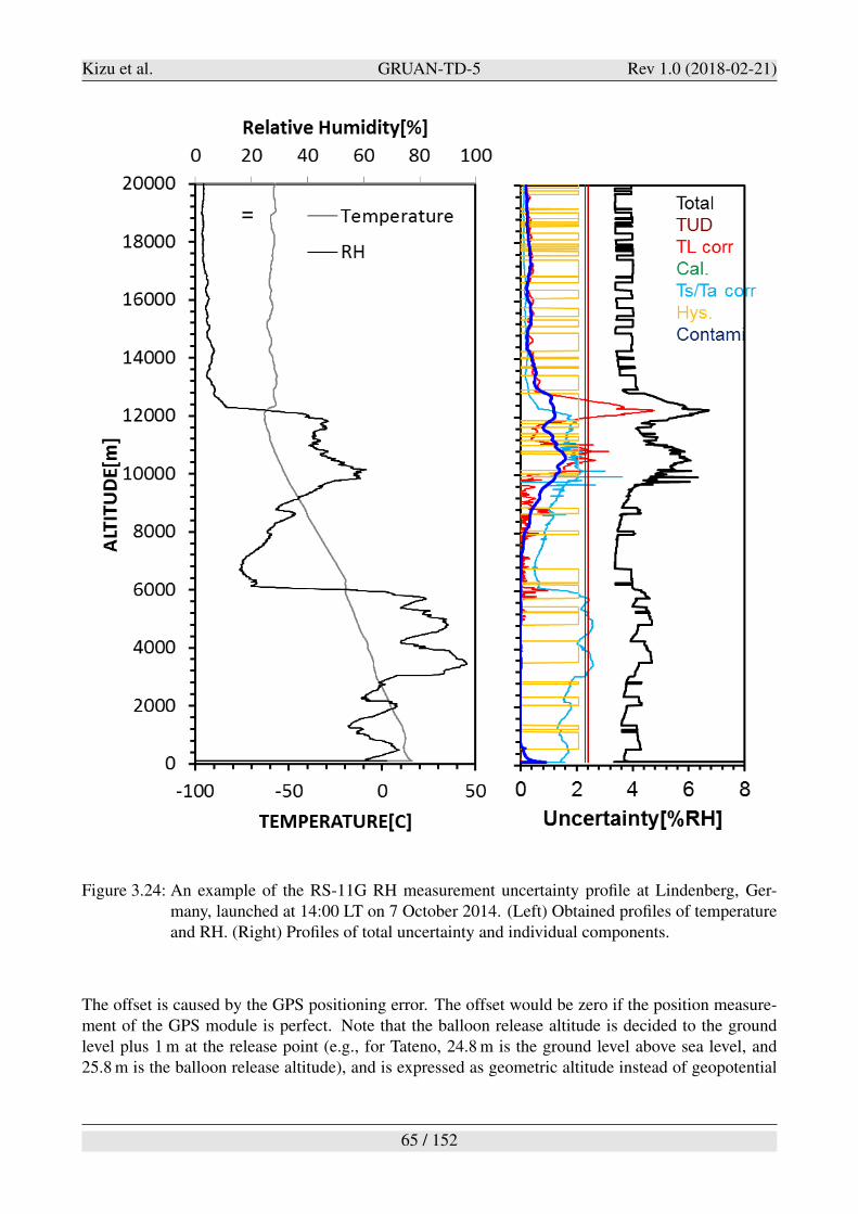
Kizu et al. GRUAN-TD-5 Rev 1.0 (2018-02-21)
Figure 3.24: An example of the RS-11G RH measurement uncertainty profile at Lindenberg, Ger-many, launched at 14:00 LT on 7 October 2014. (Left) Obtained profiles of temperatureand RH. (Right) Profiles of total uncertainty and individual components.
The offset is caused by the GPS positioning error. The offset would be zero if the position measure-ment of the GPS module is perfect. Note that the balloon release altitude is decided to the groundlevel plus 1 m at the release point (e.g., for Tateno, 24.8 m is the ground level above sea level, and25.8 m is the balloon release altitude), and is expressed as geometric altitude instead of geopotential
65 / 152
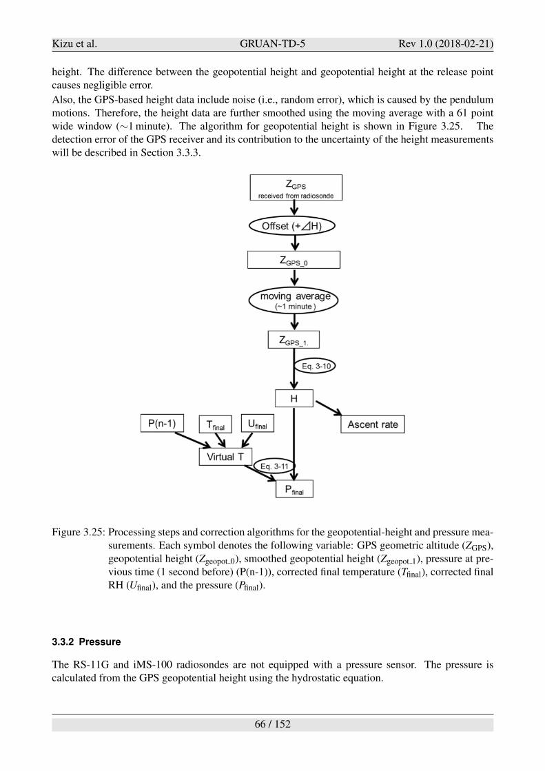
Kizu et al. GRUAN-TD-5 Rev 1.0 (2018-02-21)
height. The difference between the geopotential height and geopotential height at the release pointcauses negligible error.
Also, the GPS-based height data include noise (i.e., random error), which is caused by the pendulummotions. Therefore, the height data are further smoothed using the moving average with a 61 pointwide window ("1 minute). The algorithm for geopotential height is shown in Figure 3.25. Thedetection error of the GPS receiver and its contribution to the uncertainty of the height measurementswill be described in Section 3.3.3.
Figure 3.25: Processing steps and correction algorithms for the geopotential-height and pressure mea-surements. Each symbol denotes the following variable: GPS geometric altitude (ZGPS),geopotential height (Zgeopot 0), smoothed geopotential height (Zgeopot 1), pressure at pre-vious time (1 second before) (P(n-1)), corrected final temperature (Tfinal), corrected finalRH (Ufinal), and the pressure (Pfinal).
3.3.2 Pressure
The RS-11G and iMS-100 radiosondes are not equipped with a pressure sensor. The pressure iscalculated from the GPS geopotential height using the hydrostatic equation.
66 / 152
Kizu et al. GRUAN-TD-5 Rev 1.0 (2018-02-21)
Pi = Pi#1 exp
!
#g0
TvmRd(Hi #Hi#1)
"
(3.14)
where Pi is the calculated pressure (hPa) at geopotential height = Hi(m),Pi#1 is the pressure (hPa)at previous level (1 s before) at geopotential height= Hi#1(m),g0 is the standard gravity acceleration(9.80665m s#2), Tvm is the averaged virtual temperature between Pi and Pi#1 (K) (see below), and Rd
is the specific gas constant of dry air (287 J kg#1 K ). Note that g0 and Rd are used by following theJMA’s convention (JMA, 1995). The virtual temperature is calculated with the following equations.
Tv = T(1+ rv/")
1+ rv(3.15)
rv ="e
P# e(3.16)
where Tv is the virtual temperature (K), rv is the mixing ratio of water vapor (kg kg#1), " is the ratioof molecular weight between water vapor and dry air (0.622), P is the pressure (hPa), e is the watervapor pressure (hPa) which is calculated from temperature and RH using the Hyland and Wexler
(1983) water vapor pressure equation. The pressure value used in Eq. 3.15 is the one at previous time(1 s before).
The surface pressure at the release point is measured with an independent pressure sensor at theobservation station. The balloon release altitude is not necessarily equal to the altitude where thesurface pressure sensor is located. Thus, the surface pressure at the release point is obtained fromthe pressure sensor reading and the altitude difference between the pressure sensor and release pointusing Eqs. 3.14-3.16.
3.3.3 Uncertainty budget of the geopotential height and pressure measurements
(a) Geopotential heightThe uncertainty of the geopotential height depends strongly on the detection error of the GPS receiver.In this document, the GPS dimensional error is treated as the standard uncertainty. The sources ofthe GPS measurement error include the delay of radio propagation in the ionosphere and troposphere,multipath by the reflection from mountains and buildings, and noise of the receiver. The variabilityof the GPS position is indicated as the value of PDOP (Position Dilution of Position) which dependson the GPS signal receiving conditions (i.e., the geometric layout of between the radiosonde and theGPS satellites) and is outputted from the module every second. The 3-dimensional errors of GPS(1! ) eGPS are estimated with PDOP and UERE (User Equivalent Range Error). The UERE is thedistance error between the GPS receiver and the GPS satellite. The value of UERE (1! ) is 5.3 m forthe C/A (Coarse/Acquisition) code which is used in the GPS module of the RS-11G and iMS-100radiosondes. The 3-dimensional errors of GPS (1! ) eGPS are calculated by the following equation(Kobayashi, 2006).
eGPS = PDOP&UERE (3.17)
The GPS modules of the RS-11G and iMS-100 radiosondes use the Satellite-Based AugmentationSystem (SBAS) to improve the accuracy of position detection (i.e., making PDOP smaller). How-ever, at high latitudes, SBAS is not used for the radiosonde observation because the SBAS uses thestationary satellites which are not available at high latitudes. For example, SBAS is not available atSyowa, a Japanese Antarctic station (69.01!S, 39.59!E). Figure 3.26 shows the vertical profile of GPS
67 / 152
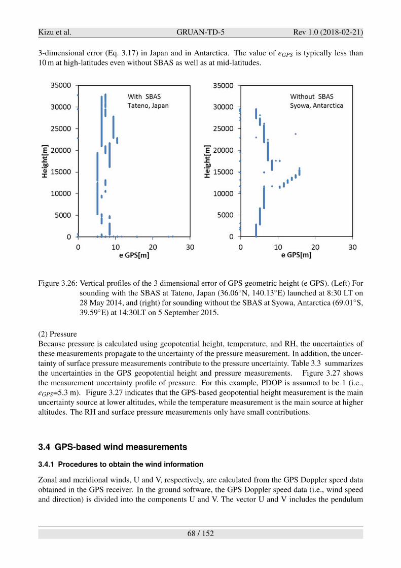
Kizu et al. GRUAN-TD-5 Rev 1.0 (2018-02-21)
3-dimensional error (Eq. 3.17) in Japan and in Antarctica. The value of eGPS is typically less than10 m at high-latitudes even without SBAS as well as at mid-latitudes.
Figure 3.26: Vertical profiles of the 3 dimensional error of GPS geometric height (e GPS). (Left) Forsounding with the SBAS at Tateno, Japan (36.06!N, 140.13!E) launched at 8:30 LT on28 May 2014, and (right) for sounding without the SBAS at Syowa, Antarctica (69.01!S,39.59!E) at 14:30LT on 5 September 2015.
(2) PressureBecause pressure is calculated using geopotential height, temperature, and RH, the uncertainties ofthese measurements propagate to the uncertainty of the pressure measurement. In addition, the uncer-tainty of surface pressure measurements contribute to the pressure uncertainty. Table 3.3 summarizesthe uncertainties in the GPS geopotential height and pressure measurements. Figure 3.27 showsthe measurement uncertainty profile of pressure. For this example, PDOP is assumed to be 1 (i.e.,eGPS=5.3 m). Figure 3.27 indicates that the GPS-based geopotential height measurement is the mainuncertainty source at lower altitudes, while the temperature measurement is the main source at higheraltitudes. The RH and surface pressure measurements only have small contributions.
3.4 GPS-based wind measurements
3.4.1 Procedures to obtain the wind information
Zonal and meridional winds, U and V, respectively, are calculated from the GPS Doppler speed dataobtained in the GPS receiver. In the ground software, the GPS Doppler speed data (i.e., wind speedand direction) is divided into the components U and V. The vector U and V includes the pendulum
68 / 152
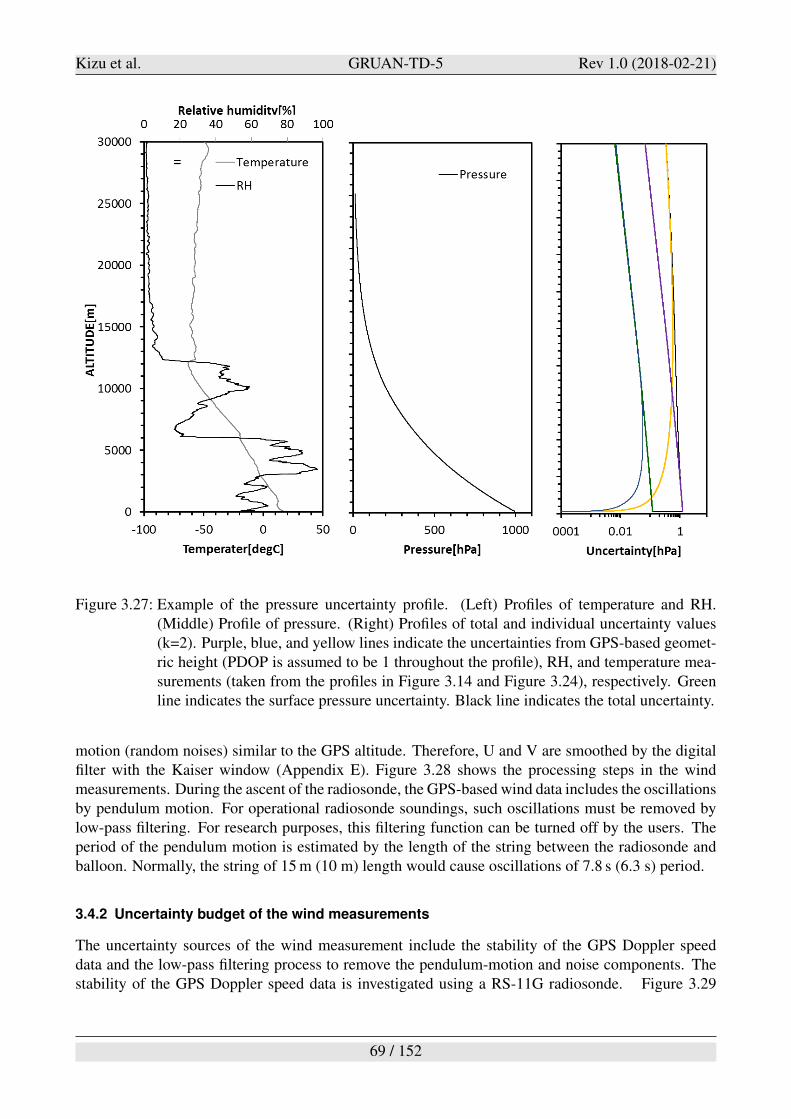
Kizu et al. GRUAN-TD-5 Rev 1.0 (2018-02-21)
Figure 3.27: Example of the pressure uncertainty profile. (Left) Profiles of temperature and RH.(Middle) Profile of pressure. (Right) Profiles of total and individual uncertainty values(k=2). Purple, blue, and yellow lines indicate the uncertainties from GPS-based geomet-ric height (PDOP is assumed to be 1 throughout the profile), RH, and temperature mea-surements (taken from the profiles in Figure 3.14 and Figure 3.24), respectively. Greenline indicates the surface pressure uncertainty. Black line indicates the total uncertainty.
motion (random noises) similar to the GPS altitude. Therefore, U and V are smoothed by the digitalfilter with the Kaiser window (Appendix E). Figure 3.28 shows the processing steps in the windmeasurements. During the ascent of the radiosonde, the GPS-based wind data includes the oscillationsby pendulum motion. For operational radiosonde soundings, such oscillations must be removed bylow-pass filtering. For research purposes, this filtering function can be turned off by the users. Theperiod of the pendulum motion is estimated by the length of the string between the radiosonde andballoon. Normally, the string of 15 m (10 m) length would cause oscillations of 7.8 s (6.3 s) period.
3.4.2 Uncertainty budget of the wind measurements
The uncertainty sources of the wind measurement include the stability of the GPS Doppler speeddata and the low-pass filtering process to remove the pendulum-motion and noise components. Thestability of the GPS Doppler speed data is investigated using a RS-11G radiosonde. Figure 3.29
69 / 152
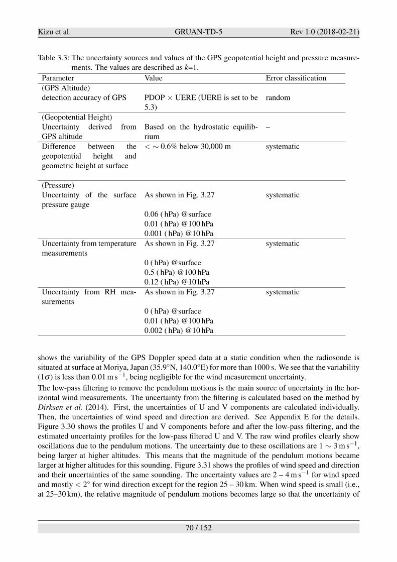
Kizu et al. GRUAN-TD-5 Rev 1.0 (2018-02-21)
Table 3.3: The uncertainty sources and values of the GPS geopotential height and pressure measure-ments. The values are described as k=1.
Parameter Value Error classification
(GPS Altitude)detection accuracy of GPS PDOP & UERE (UERE is set to be
5.3)random
(Geopotential Height)Uncertainty derived fromGPS altitude
Based on the hydrostatic equilib-rium
–
Difference between thegeopotential height andgeometric height at surface
< " 0.6% below 30,000 m systematic
(Pressure)Uncertainty of the surfacepressure gauge
As shown in Fig. 3.27 systematic
0.06 ( hPa) @surface0.01 ( hPa) @100 hPa0.001 ( hPa) @10 hPa
Uncertainty from temperaturemeasurements
As shown in Fig. 3.27 systematic
0 ( hPa) @surface0.5 ( hPa) @100 hPa0.12 ( hPa) @10 hPa
Uncertainty from RH mea-surements
As shown in Fig. 3.27 systematic
0 ( hPa) @surface0.01 ( hPa) @100 hPa0.002 ( hPa) @10 hPa
shows the variability of the GPS Doppler speed data at a static condition when the radiosonde issituated at surface at Moriya, Japan (35.9!N, 140.0!E) for more than 1000 s. We see that the variability(1! ) is less than 0.01 m s#1, being negligible for the wind measurement uncertainty.
The low-pass filtering to remove the pendulum motions is the main source of uncertainty in the hor-izontal wind measurements. The uncertainty from the filtering is calculated based on the method byDirksen et al. (2014). First, the uncertainties of U and V components are calculated individually.Then, the uncertainties of wind speed and direction are derived. See Appendix E for the details.Figure 3.30 shows the profiles U and V components before and after the low-pass filtering, and theestimated uncertainty profiles for the low-pass filtered U and V. The raw wind profiles clearly showoscillations due to the pendulum motions. The uncertainty due to these oscillations are 1 " 3 m s#1,being larger at higher altitudes. This means that the magnitude of the pendulum motions becamelarger at higher altitudes for this sounding. Figure 3.31 shows the profiles of wind speed and directionand their uncertainties of the same sounding. The uncertainty values are 2 – 4 m s#1 for wind speedand mostly < 2! for wind direction except for the region 25 – 30 km. When wind speed is small (i.e.,at 25–30 km), the relative magnitude of pendulum motions becomes large so that the uncertainty of
70 / 152
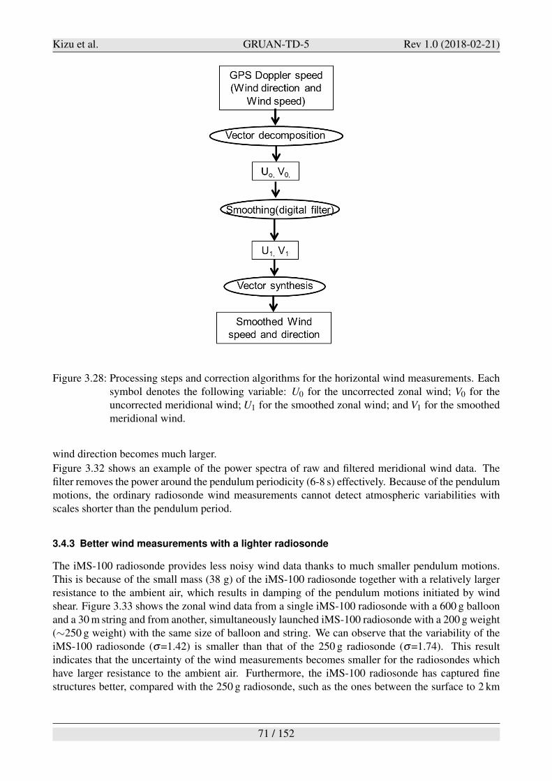
Kizu et al. GRUAN-TD-5 Rev 1.0 (2018-02-21)
Figure 3.28: Processing steps and correction algorithms for the horizontal wind measurements. Eachsymbol denotes the following variable: U0 for the uncorrected zonal wind; V0 for theuncorrected meridional wind; U1 for the smoothed zonal wind; and V1 for the smoothedmeridional wind.
wind direction becomes much larger.
Figure 3.32 shows an example of the power spectra of raw and filtered meridional wind data. Thefilter removes the power around the pendulum periodicity (6-8 s) effectively. Because of the pendulummotions, the ordinary radiosonde wind measurements cannot detect atmospheric variabilities withscales shorter than the pendulum period.
3.4.3 Better wind measurements with a lighter radiosonde
The iMS-100 radiosonde provides less noisy wind data thanks to much smaller pendulum motions.This is because of the small mass (38 g) of the iMS-100 radiosonde together with a relatively largerresistance to the ambient air, which results in damping of the pendulum motions initiated by windshear. Figure 3.33 shows the zonal wind data from a single iMS-100 radiosonde with a 600 g balloonand a 30 m string and from another, simultaneously launched iMS-100 radiosonde with a 200 g weight("250 g weight) with the same size of balloon and string. We can observe that the variability of theiMS-100 radiosonde (!=1.42) is smaller than that of the 250 g radiosonde (!=1.74). This resultindicates that the uncertainty of the wind measurements becomes smaller for the radiosondes whichhave larger resistance to the ambient air. Furthermore, the iMS-100 radiosonde has captured finestructures better, compared with the 250 g radiosonde, such as the ones between the surface to 2 km
71 / 152
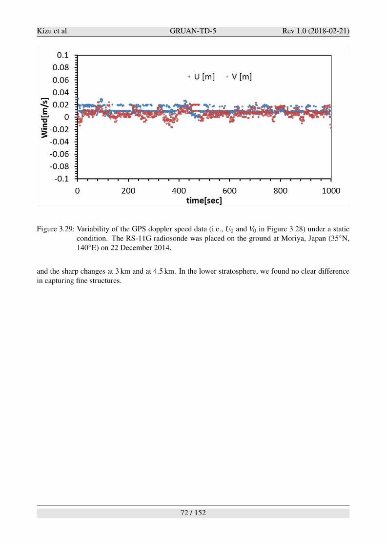
Kizu et al. GRUAN-TD-5 Rev 1.0 (2018-02-21)
Figure 3.29: Variability of the GPS doppler speed data (i.e., U0 and V0 in Figure 3.28) under a staticcondition. The RS-11G radiosonde was placed on the ground at Moriya, Japan (35!N,140!E) on 22 December 2014.
and the sharp changes at 3 km and at 4.5 km. In the lower stratosphere, we found no clear differencein capturing fine structures.
72 / 152
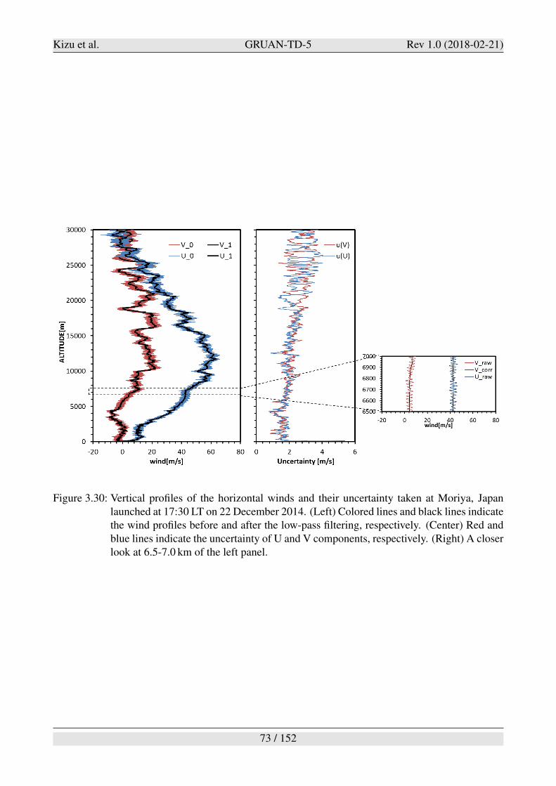
Kizu et al. GRUAN-TD-5 Rev 1.0 (2018-02-21)
Figure 3.30: Vertical profiles of the horizontal winds and their uncertainty taken at Moriya, Japanlaunched at 17:30 LT on 22 December 2014. (Left) Colored lines and black lines indicatethe wind profiles before and after the low-pass filtering, respectively. (Center) Red andblue lines indicate the uncertainty of U and V components, respectively. (Right) A closerlook at 6.5-7.0 km of the left panel.
73 / 152
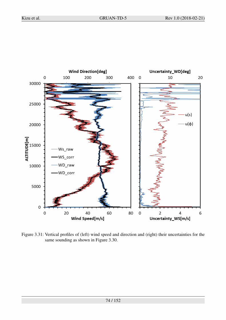
Kizu et al. GRUAN-TD-5 Rev 1.0 (2018-02-21)
Figure 3.31: Vertical profiles of (left) wind speed and direction and (right) their uncertainties for thesame sounding as shown in Figure 3.30.
74 / 152
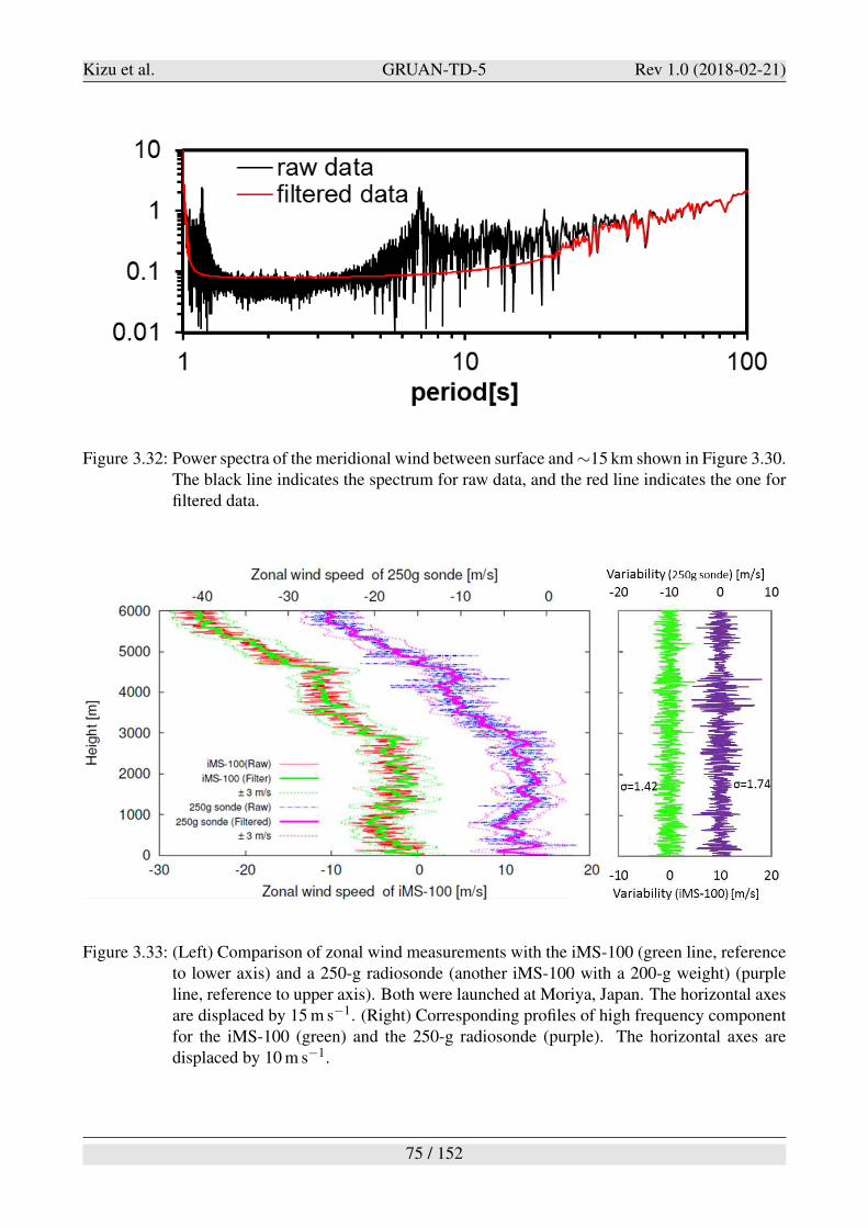
Kizu et al. GRUAN-TD-5 Rev 1.0 (2018-02-21)
Figure 3.32: Power spectra of the meridional wind between surface and "15 km shown in Figure 3.30.The black line indicates the spectrum for raw data, and the red line indicates the one forfiltered data.
Figure 3.33: (Left) Comparison of zonal wind measurements with the iMS-100 (green line, referenceto lower axis) and a 250-g radiosonde (another iMS-100 with a 200-g weight) (purpleline, reference to upper axis). Both were launched at Moriya, Japan. The horizontal axesare displaced by 15 m s#1. (Right) Corresponding profiles of high frequency componentfor the iMS-100 (green) and the 250-g radiosonde (purple). The horizontal axes aredisplaced by 10 m s#1.
75 / 152
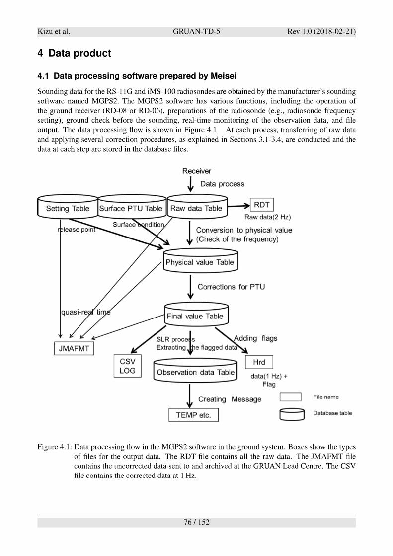
Kizu et al. GRUAN-TD-5 Rev 1.0 (2018-02-21)
4 Data product
4.1 Data processing software prepared by Meisei
Sounding data for the RS-11G and iMS-100 radiosondes are obtained by the manufacturer’s soundingsoftware named MGPS2. The MGPS2 software has various functions, including the operation ofthe ground receiver (RD-08 or RD-06), preparations of the radiosonde (e.g., radiosonde frequencysetting), ground check before the sounding, real-time monitoring of the observation data, and fileoutput. The data processing flow is shown in Figure 4.1. At each process, transferring of raw dataand applying several correction procedures, as explained in Sections 3.1-3.4, are conducted and thedata at each step are stored in the database files.
Figure 4.1: Data processing flow in the MGPS2 software in the ground system. Boxes show the typesof files for the output data. The RDT file contains all the raw data. The JMAFMT filecontains the uncorrected data sent to and archived at the GRUAN Lead Centre. The CSVfile contains the corrected data at 1 Hz.
76 / 152
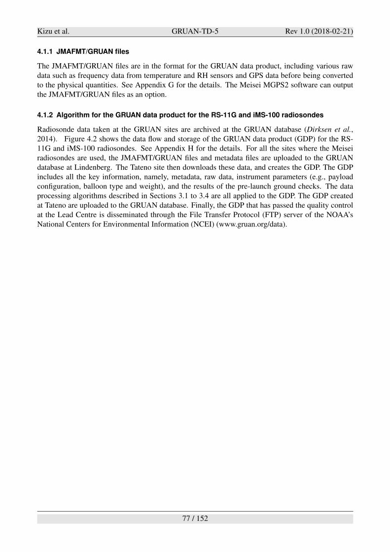
Kizu et al. GRUAN-TD-5 Rev 1.0 (2018-02-21)
4.1.1 JMAFMT/GRUAN files
The JMAFMT/GRUAN files are in the format for the GRUAN data product, including various rawdata such as frequency data from temperature and RH sensors and GPS data before being convertedto the physical quantities. See Appendix G for the details. The Meisei MGPS2 software can outputthe JMAFMT/GRUAN files as an option.
4.1.2 Algorithm for the GRUAN data product for the RS-11G and iMS-100 radiosondes
Radiosonde data taken at the GRUAN sites are archived at the GRUAN database (Dirksen et al.,2014). Figure 4.2 shows the data flow and storage of the GRUAN data product (GDP) for the RS-11G and iMS-100 radiosondes. See Appendix H for the details. For all the sites where the Meiseiradiosondes are used, the JMAFMT/GRUAN files and metadata files are uploaded to the GRUANdatabase at Lindenberg. The Tateno site then downloads these data, and creates the GDP. The GDPincludes all the key information, namely, metadata, raw data, instrument parameters (e.g., payloadconfiguration, balloon type and weight), and the results of the pre-launch ground checks. The dataprocessing algorithms described in Sections 3.1 to 3.4 are all applied to the GDP. The GDP createdat Tateno are uploaded to the GRUAN database. Finally, the GDP that has passed the quality controlat the Lead Centre is disseminated through the File Transfer Protocol (FTP) server of the NOAA’sNational Centers for Environmental Information (NCEI) (www.gruan.org/data).
77 / 152
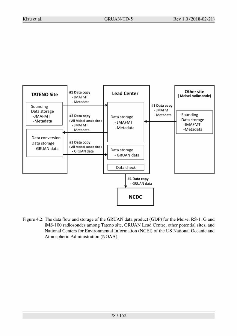
Kizu et al. GRUAN-TD-5 Rev 1.0 (2018-02-21)
Figure 4.2: The data flow and storage of the GRUAN data product (GDP) for the Meisei RS-11G andiMS-100 radiosondes among Tateno site, GRUAN Lead Centre, other potential sites, andNational Centers for Environmental Information (NCEI) of the US National Oceanic andAtmospheric Administration (NOAA).
78 / 152
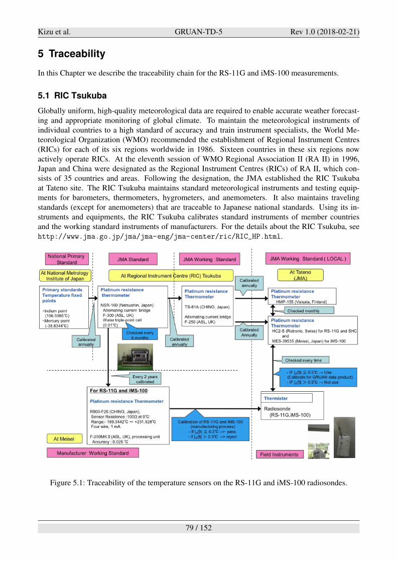
Kizu et al. GRUAN-TD-5 Rev 1.0 (2018-02-21)
5 Traceability
In this Chapter we describe the traceability chain for the RS-11G and iMS-100 measurements.
5.1 RIC Tsukuba
Globally uniform, high-quality meteorological data are required to enable accurate weather forecast-ing and appropriate monitoring of global climate. To maintain the meteorological instruments ofindividual countries to a high standard of accuracy and train instrument specialists, the World Me-teorological Organization (WMO) recommended the establishment of Regional Instrument Centres(RICs) for each of its six regions worldwide in 1986. Sixteen countries in these six regions nowactively operate RICs. At the eleventh session of WMO Regional Association II (RA II) in 1996,Japan and China were designated as the Regional Instrument Centres (RICs) of RA II, which con-sists of 35 countries and areas. Following the designation, the JMA established the RIC Tsukubaat Tateno site. The RIC Tsukuba maintains standard meteorological instruments and testing equip-ments for barometers, thermometers, hygrometers, and anemometers. It also maintains travelingstandards (except for anemometers) that are traceable to Japanese national standards. Using its in-struments and equipments, the RIC Tsukuba calibrates standard instruments of member countriesand the working standard instruments of manufacturers. For the details about the RIC Tsukuba, seehttp://www.jma.go.jp/jma/jma-eng/jma-center/ric/RIC_HP.html.
Figure 5.1: Traceability of the temperature sensors on the RS-11G and iMS-100 radiosondes.
79 / 152
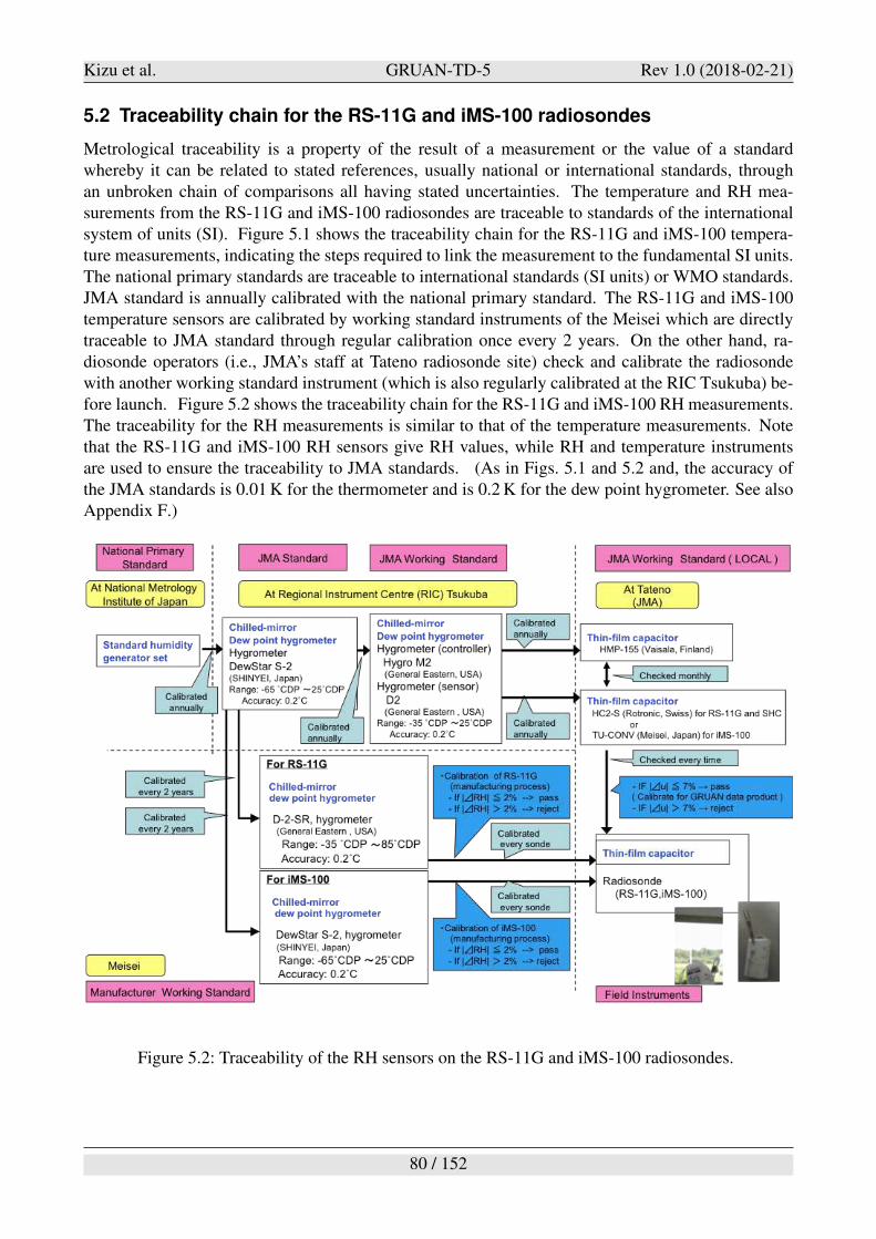
Kizu et al. GRUAN-TD-5 Rev 1.0 (2018-02-21)
5.2 Traceability chain for the RS-11G and iMS-100 radiosondes
Metrological traceability is a property of the result of a measurement or the value of a standardwhereby it can be related to stated references, usually national or international standards, throughan unbroken chain of comparisons all having stated uncertainties. The temperature and RH mea-surements from the RS-11G and iMS-100 radiosondes are traceable to standards of the internationalsystem of units (SI). Figure 5.1 shows the traceability chain for the RS-11G and iMS-100 tempera-ture measurements, indicating the steps required to link the measurement to the fundamental SI units.The national primary standards are traceable to international standards (SI units) or WMO standards.JMA standard is annually calibrated with the national primary standard. The RS-11G and iMS-100temperature sensors are calibrated by working standard instruments of the Meisei which are directlytraceable to JMA standard through regular calibration once every 2 years. On the other hand, ra-diosonde operators (i.e., JMA’s staff at Tateno radiosonde site) check and calibrate the radiosondewith another working standard instrument (which is also regularly calibrated at the RIC Tsukuba) be-fore launch. Figure 5.2 shows the traceability chain for the RS-11G and iMS-100 RH measurements.The traceability for the RH measurements is similar to that of the temperature measurements. Notethat the RS-11G and iMS-100 RH sensors give RH values, while RH and temperature instrumentsare used to ensure the traceability to JMA standards. (As in Figs. 5.1 and 5.2 and, the accuracy ofthe JMA standards is 0.01 K for the thermometer and is 0.2 K for the dew point hygrometer. See alsoAppendix F.)
Figure 5.2: Traceability of the RH sensors on the RS-11G and iMS-100 radiosondes.
80 / 152
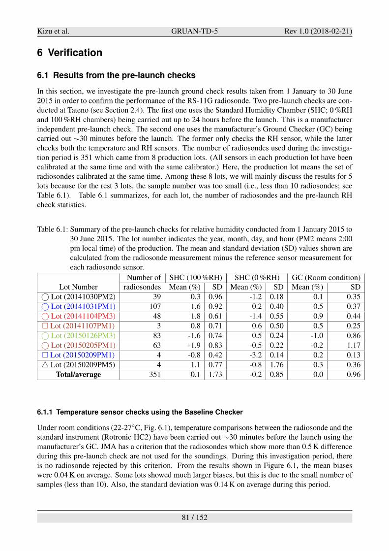
Kizu et al. GRUAN-TD-5 Rev 1.0 (2018-02-21)
6 Verification
6.1 Results from the pre-launch checks
In this section, we investigate the pre-launch ground check results taken from 1 January to 30 June2015 in order to confirm the performance of the RS-11G radiosonde. Two pre-launch checks are con-ducted at Tateno (see Section 2.4). The first one uses the Standard Humidity Chamber (SHC; 0 %RHand 100 %RH chambers) being carried out up to 24 hours before the launch. This is a manufacturerindependent pre-launch check. The second one uses the manufacturer’s Ground Checker (GC) beingcarried out "30 minutes before the launch. The former only checks the RH sensor, while the latterchecks both the temperature and RH sensors. The number of radiosondes used during the investiga-tion period is 351 which came from 8 production lots. (All sensors in each production lot have beencalibrated at the same time and with the same calibrator.) Here, the production lot means the set ofradiosondes calibrated at the same time. Among these 8 lots, we will mainly discuss the results for 5lots because for the rest 3 lots, the sample number was too small (i.e., less than 10 radiosondes; seeTable 6.1). Table 6.1 summarizes, for each lot, the number of radiosondes and the pre-launch RHcheck statistics.
Table 6.1: Summary of the pre-launch checks for relative humidity conducted from 1 January 2015 to30 June 2015. The lot number indicates the year, month, day, and hour (PM2 means 2:00pm local time) of the production. The mean and standard deviation (SD) values shown arecalculated from the radiosonde measurement minus the reference sensor measurement foreach radiosonde sensor.
Number of SHC (100 %RH) SHC (0 %RH) GC (Room condition)Lot Number radiosondes Mean (%) SD Mean (%) SD Mean (%) SD
' Lot (20141030PM2) 39 0.3 0.96 -1.2 0.18 0.1 0.35
' Lot (20141031PM1) 107 1.6 0.92 0.2 0.40 0.5 0.37
' Lot (20141104PM3) 48 1.8 0.61 -1.4 0.55 0.9 0.44
! Lot (20141107PM1) 3 0.8 0.71 0.6 0.50 0.5 0.25
' Lot (20150126PM3) 83 -1.6 0.74 0.5 0.24 -1.0 0.86
' Lot (20150205PM1) 63 -1.9 0.83 -0.5 0.22 -0.2 1.17
! Lot (20150209PM1) 4 -0.8 0.42 -3.2 0.14 0.2 0.13
( Lot (20150209PM5) 4 1.1 0.77 -0.8 1.76 0.3 0.36
Total/average 351 0.1 1.73 -0.2 0.85 0.0 0.96
6.1.1 Temperature sensor checks using the Baseline Checker
Under room conditions (22-27!C, Fig. 6.1), temperature comparisons between the radiosonde and thestandard instrument (Rotronic HC2) have been carried out "30 minutes before the launch using themanufacturer’s GC. JMA has a criterion that the radiosondes which show more than 0.5 K differenceduring this pre-launch check are not used for the soundings. During this investigation period, thereis no radiosonde rejected by this criterion. From the results shown in Figure 6.1, the mean biaseswere 0.04 K on average. Some lots showed much larger biases, but this is due to the small number ofsamples (less than 10). Also, the standard deviation was 0.14 K on average during this period.
81 / 152
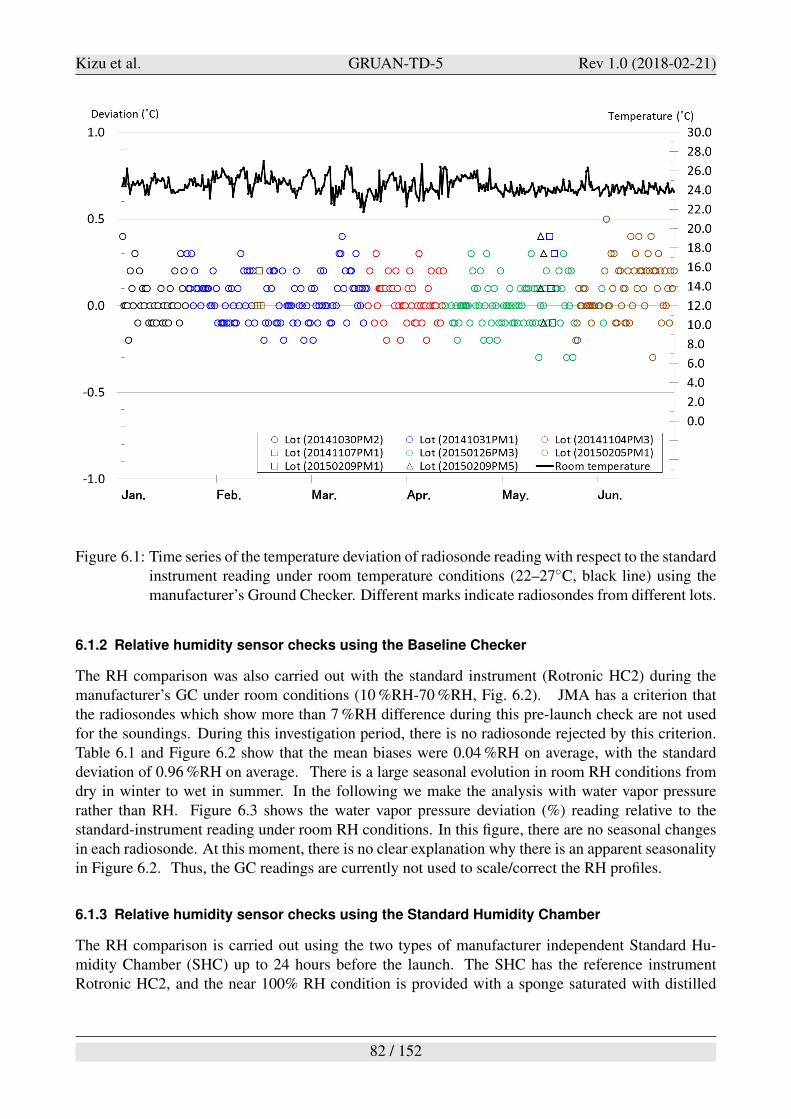
Kizu et al. GRUAN-TD-5 Rev 1.0 (2018-02-21)
Figure 6.1: Time series of the temperature deviation of radiosonde reading with respect to the standardinstrument reading under room temperature conditions (22–27!C, black line) using themanufacturer’s Ground Checker. Different marks indicate radiosondes from different lots.
6.1.2 Relative humidity sensor checks using the Baseline Checker
The RH comparison was also carried out with the standard instrument (Rotronic HC2) during themanufacturer’s GC under room conditions (10 %RH-70 %RH, Fig. 6.2). JMA has a criterion thatthe radiosondes which show more than 7 %RH difference during this pre-launch check are not usedfor the soundings. During this investigation period, there is no radiosonde rejected by this criterion.Table 6.1 and Figure 6.2 show that the mean biases were 0.04 %RH on average, with the standarddeviation of 0.96 %RH on average. There is a large seasonal evolution in room RH conditions fromdry in winter to wet in summer. In the following we make the analysis with water vapor pressurerather than RH. Figure 6.3 shows the water vapor pressure deviation (%) reading relative to thestandard-instrument reading under room RH conditions. In this figure, there are no seasonal changesin each radiosonde. At this moment, there is no clear explanation why there is an apparent seasonalityin Figure 6.2. Thus, the GC readings are currently not used to scale/correct the RH profiles.
6.1.3 Relative humidity sensor checks using the Standard Humidity Chamber
The RH comparison is carried out using the two types of manufacturer independent Standard Hu-midity Chamber (SHC) up to 24 hours before the launch. The SHC has the reference instrumentRotronic HC2, and the near 100% RH condition is provided with a sponge saturated with distilled
82 / 152
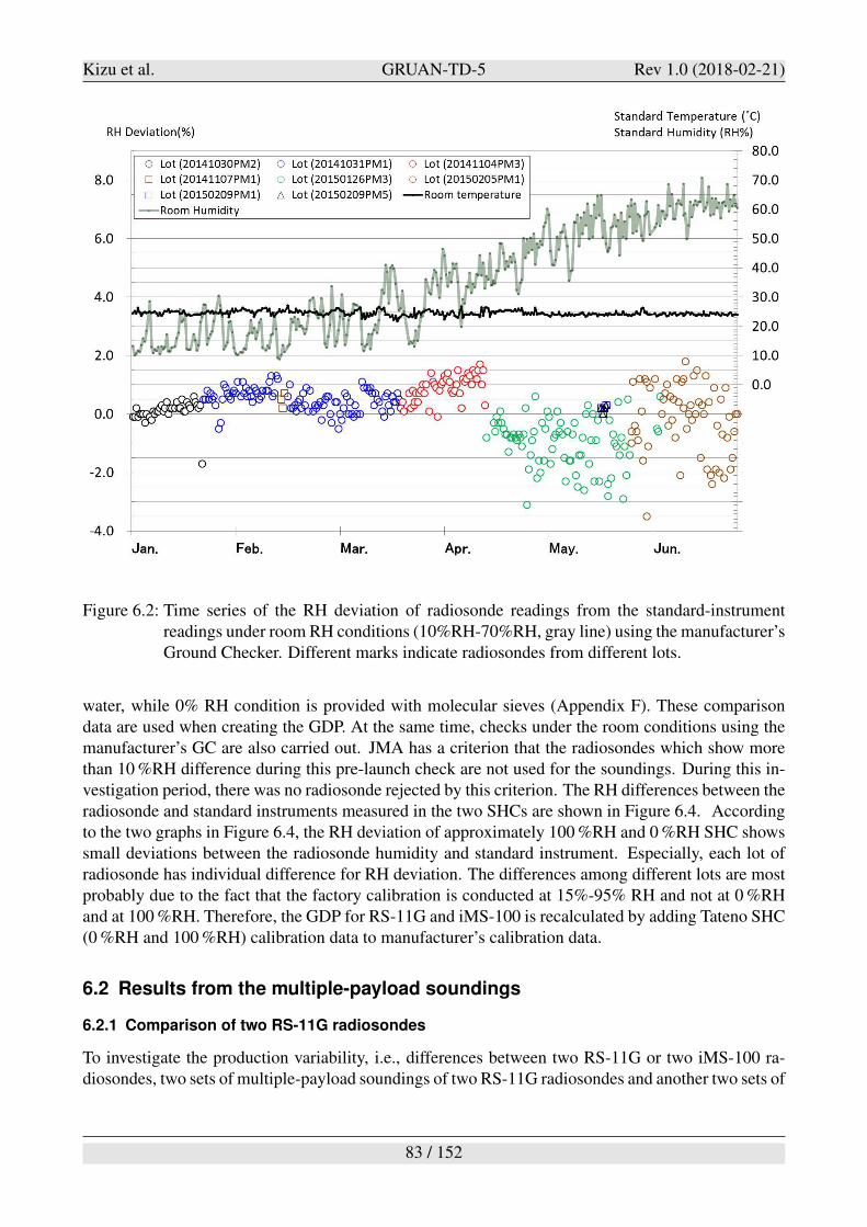
Kizu et al. GRUAN-TD-5 Rev 1.0 (2018-02-21)
Figure 6.2: Time series of the RH deviation of radiosonde readings from the standard-instrumentreadings under room RH conditions (10%RH-70%RH, gray line) using the manufacturer’sGround Checker. Different marks indicate radiosondes from different lots.
water, while 0% RH condition is provided with molecular sieves (Appendix F). These comparisondata are used when creating the GDP. At the same time, checks under the room conditions using themanufacturer’s GC are also carried out. JMA has a criterion that the radiosondes which show morethan 10 %RH difference during this pre-launch check are not used for the soundings. During this in-vestigation period, there was no radiosonde rejected by this criterion. The RH differences between theradiosonde and standard instruments measured in the two SHCs are shown in Figure 6.4. Accordingto the two graphs in Figure 6.4, the RH deviation of approximately 100 %RH and 0 %RH SHC showssmall deviations between the radiosonde humidity and standard instrument. Especially, each lot ofradiosonde has individual difference for RH deviation. The differences among different lots are mostprobably due to the fact that the factory calibration is conducted at 15%-95% RH and not at 0 %RHand at 100 %RH. Therefore, the GDP for RS-11G and iMS-100 is recalculated by adding Tateno SHC(0 %RH and 100 %RH) calibration data to manufacturer’s calibration data.
6.2 Results from the multiple-payload soundings
6.2.1 Comparison of two RS-11G radiosondes
To investigate the production variability, i.e., differences between two RS-11G or two iMS-100 ra-diosondes, two sets of multiple-payload soundings of two RS-11G radiosondes and another two sets of
83 / 152
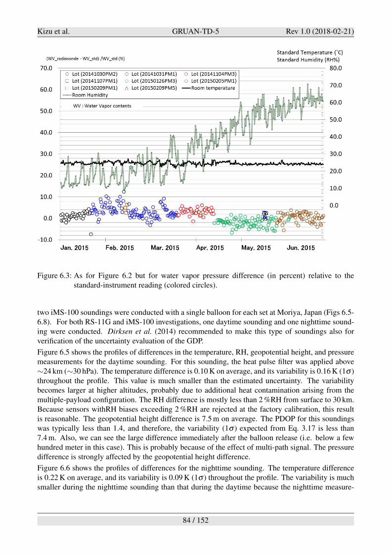
Kizu et al. GRUAN-TD-5 Rev 1.0 (2018-02-21)
Figure 6.3: As for Figure 6.2 but for water vapor pressure difference (in percent) relative to thestandard-instrument reading (colored circles).
two iMS-100 soundings were conducted with a single balloon for each set at Moriya, Japan (Figs 6.5-6.8). For both RS-11G and iMS-100 investigations, one daytime sounding and one nighttime sound-ing were conducted. Dirksen et al. (2014) recommended to make this type of soundings also forverification of the uncertainty evaluation of the GDP.
Figure 6.5 shows the profiles of differences in the temperature, RH, geopotential height, and pressuremeasurements for the daytime sounding. For this sounding, the heat pulse filter was applied above"24 km ("30 hPa). The temperature difference is 0.10 K on average, and its variability is 0.16 K (1! )throughout the profile. This value is much smaller than the estimated uncertainty. The variabilitybecomes larger at higher altitudes, probably due to additional heat contamination arising from themultiple-payload configuration. The RH difference is mostly less than 2 %RH from surface to 30 km.Because sensors withRH biases exceeding 2 %RH are rejected at the factory calibration, this resultis reasonable. The geopotential height difference is 7.5 m on average. The PDOP for this soundingswas typically less than 1.4, and therefore, the variability (1! ) expected from Eq. 3.17 is less than7.4 m. Also, we can see the large difference immediately after the balloon release (i.e. below a fewhundred meter in this case). This is probably because of the effect of multi-path signal. The pressuredifference is strongly affected by the geopotential height difference.
Figure 6.6 shows the profiles of differences for the nighttime sounding. The temperature differenceis 0.22 K on average, and its variability is 0.09 K (1! ) throughout the profile. The variability is muchsmaller during the nighttime sounding than that during the daytime because the nighttime measure-
84 / 152
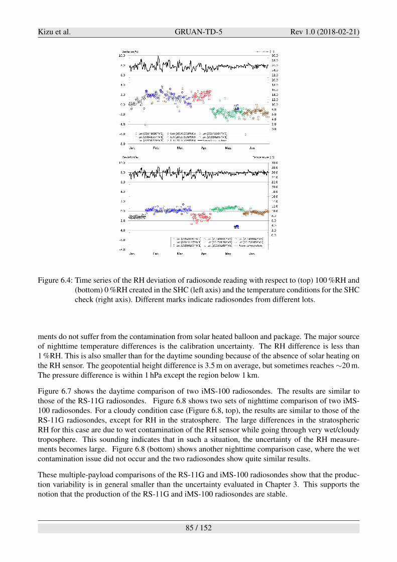
Kizu et al. GRUAN-TD-5 Rev 1.0 (2018-02-21)
Figure 6.4: Time series of the RH deviation of radiosonde reading with respect to (top) 100 %RH and(bottom) 0 %RH created in the SHC (left axis) and the temperature conditions for the SHCcheck (right axis). Different marks indicate radiosondes from different lots.
ments do not suffer from the contamination from solar heated balloon and package. The major sourceof nighttime temperature differences is the calibration uncertainty. The RH difference is less than1 %RH. This is also smaller than for the daytime sounding because of the absence of solar heating onthe RH sensor. The geopotential height difference is 3.5 m on average, but sometimes reaches "20 m.The pressure difference is within 1 hPa except the region below 1 km.
Figure 6.7 shows the daytime comparison of two iMS-100 radiosondes. The results are similar tothose of the RS-11G radiosondes. Figure 6.8 shows two sets of nighttime comparison of two iMS-100 radiosondes. For a cloudy condition case (Figure 6.8, top), the results are similar to those of theRS-11G radiosondes, except for RH in the stratosphere. The large differences in the stratosphericRH for this case are due to wet contamination of the RH sensor while going through very wet/cloudytroposphere. This sounding indicates that in such a situation, the uncertainty of the RH measure-ments becomes large. Figure 6.8 (bottom) shows another nighttime comparison case, where the wetcontamination issue did not occur and the two radiosondes show quite similar results.
These multiple-payload comparisons of the RS-11G and iMS-100 radiosondes show that the produc-tion variability is in general smaller than the uncertainty evaluated in Chapter 3. This supports thenotion that the production of the RS-11G and iMS-100 radiosondes are stable.
85 / 152
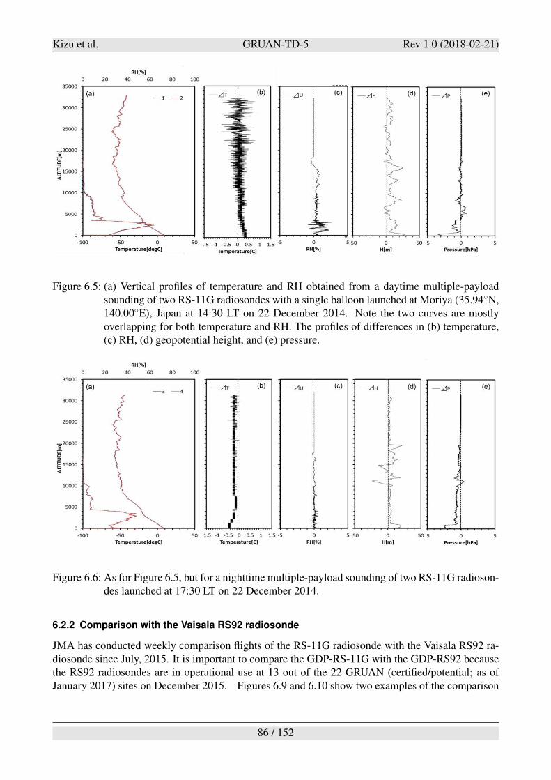
Kizu et al. GRUAN-TD-5 Rev 1.0 (2018-02-21)
Figure 6.5: (a) Vertical profiles of temperature and RH obtained from a daytime multiple-payloadsounding of two RS-11G radiosondes with a single balloon launched at Moriya (35.94!N,140.00!E), Japan at 14:30 LT on 22 December 2014. Note the two curves are mostlyoverlapping for both temperature and RH. The profiles of differences in (b) temperature,(c) RH, (d) geopotential height, and (e) pressure.
Figure 6.6: As for Figure 6.5, but for a nighttime multiple-payload sounding of two RS-11G radioson-des launched at 17:30 LT on 22 December 2014.
6.2.2 Comparison with the Vaisala RS92 radiosonde
JMA has conducted weekly comparison flights of the RS-11G radiosonde with the Vaisala RS92 ra-diosonde since July, 2015. It is important to compare the GDP-RS-11G with the GDP-RS92 becausethe RS92 radiosondes are in operational use at 13 out of the 22 GRUAN (certified/potential; as ofJanuary 2017) sites on December 2015. Figures 6.9 and 6.10 show two examples of the comparison
86 / 152
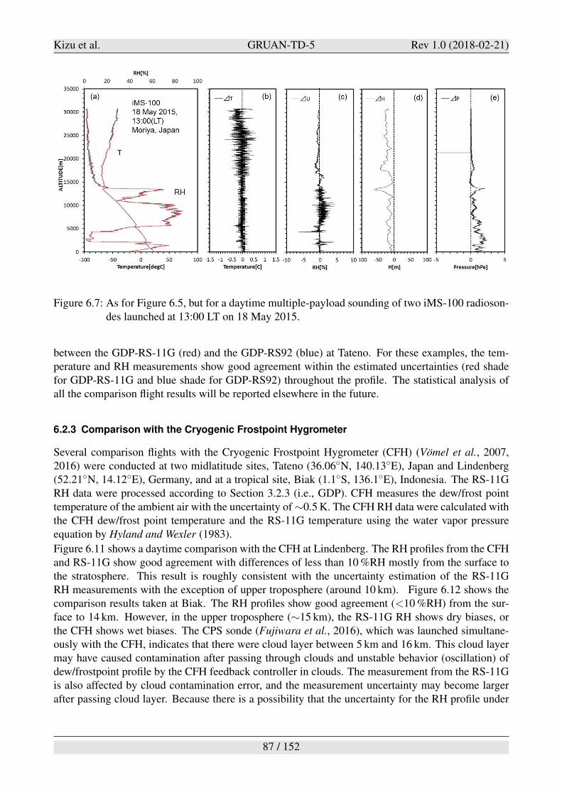
Kizu et al. GRUAN-TD-5 Rev 1.0 (2018-02-21)
Figure 6.7: As for Figure 6.5, but for a daytime multiple-payload sounding of two iMS-100 radioson-des launched at 13:00 LT on 18 May 2015.
between the GDP-RS-11G (red) and the GDP-RS92 (blue) at Tateno. For these examples, the tem-perature and RH measurements show good agreement within the estimated uncertainties (red shadefor GDP-RS-11G and blue shade for GDP-RS92) throughout the profile. The statistical analysis ofall the comparison flight results will be reported elsewhere in the future.
6.2.3 Comparison with the Cryogenic Frostpoint Hygrometer
Several comparison flights with the Cryogenic Frostpoint Hygrometer (CFH) (Vomel et al., 2007,2016) were conducted at two midlatitude sites, Tateno (36.06!N, 140.13!E), Japan and Lindenberg(52.21!N, 14.12!E), Germany, and at a tropical site, Biak (1.1!S, 136.1!E), Indonesia. The RS-11GRH data were processed according to Section 3.2.3 (i.e., GDP). CFH measures the dew/frost pointtemperature of the ambient air with the uncertainty of "0.5 K. The CFH RH data were calculated withthe CFH dew/frost point temperature and the RS-11G temperature using the water vapor pressureequation by Hyland and Wexler (1983).
Figure 6.11 shows a daytime comparison with the CFH at Lindenberg. The RH profiles from the CFHand RS-11G show good agreement with differences of less than 10 %RH mostly from the surface tothe stratosphere. This result is roughly consistent with the uncertainty estimation of the RS-11GRH measurements with the exception of upper troposphere (around 10 km). Figure 6.12 shows thecomparison results taken at Biak. The RH profiles show good agreement (<10 %RH) from the sur-face to 14 km. However, in the upper troposphere ("15 km), the RS-11G RH shows dry biases, orthe CFH shows wet biases. The CPS sonde (Fujiwara et al., 2016), which was launched simultane-ously with the CFH, indicates that there were cloud layer between 5 km and 16 km. This cloud layermay have caused contamination after passing through clouds and unstable behavior (oscillation) ofdew/frostpoint profile by the CFH feedback controller in clouds. The measurement from the RS-11Gis also affected by cloud contamination error, and the measurement uncertainty may become largerafter passing cloud layer. Because there is a possibility that the uncertainty for the RH profile under
87 / 152
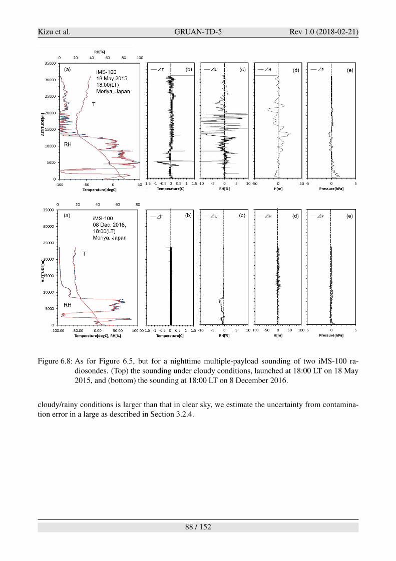
Kizu et al. GRUAN-TD-5 Rev 1.0 (2018-02-21)
Figure 6.8: As for Figure 6.5, but for a nighttime multiple-payload sounding of two iMS-100 ra-diosondes. (Top) the sounding under cloudy conditions, launched at 18:00 LT on 18 May2015, and (bottom) the sounding at 18:00 LT on 8 December 2016.
cloudy/rainy conditions is larger than that in clear sky, we estimate the uncertainty from contamina-tion error in a large as described in Section 3.2.4.
88 / 152

Kizu et al. GRUAN-TD-5 Rev 1.0 (2018-02-21)
Figure 6.9: Comparison of temperature (left) and RH (right), with uncertainty range, between theRS-11G GDP (red) and RS92 GDP (blue) at Tateno, both launched at 00:00 UTC on 19January 2015.
89 / 152
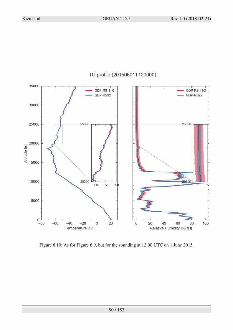
Kizu et al. GRUAN-TD-5 Rev 1.0 (2018-02-21)
Figure 6.10: As for Figure 6.9, but for the sounding at 12:00 UTC on 1 June 2015.
90 / 152
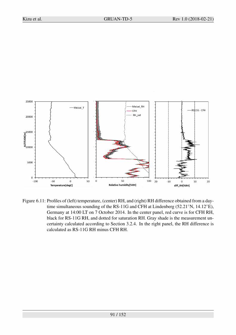
Kizu et al. GRUAN-TD-5 Rev 1.0 (2018-02-21)
Figure 6.11: Profiles of (left) temperature, (center) RH, and (right) RH difference obtained from a day-time simultaneous sounding of the RS-11G and CFH at Lindenberg (52.21!N, 14.12!E),Germany at 14:00 LT on 7 October 2014. In the center panel, red curve is for CFH RH,black for RS-11G RH, and dotted for saturation RH. Gray shade is the measurement un-certainty calculated according to Section 3.2.4. In the right panel, the RH difference iscalculated as RS-11G RH minus CFH RH.
91 / 152
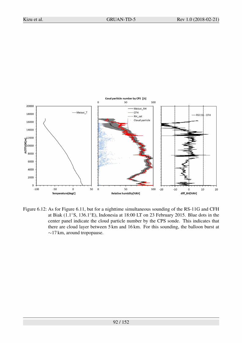
Kizu et al. GRUAN-TD-5 Rev 1.0 (2018-02-21)
Figure 6.12: As for Figure 6.11, but for a nighttime simultaneous sounding of the RS-11G and CFHat Biak (1.1!S, 136.1!E), Indonesia at 18:00 LT on 23 February 2015. Blue dots in thecenter panel indicate the cloud particle number by the CPS sonde. This indicates thatthere are cloud layer between 5 km and 16 km. For this sounding, the balloon burst at"17 km, around tropopause.
92 / 152
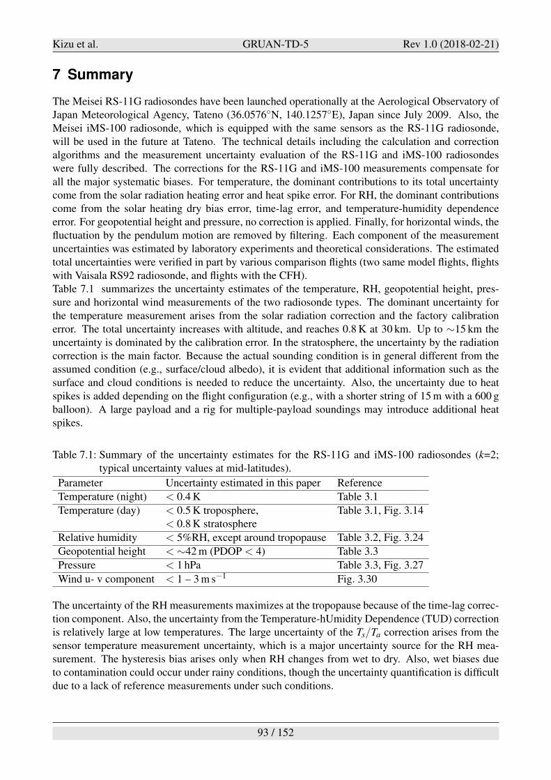
Kizu et al. GRUAN-TD-5 Rev 1.0 (2018-02-21)
7 Summary
The Meisei RS-11G radiosondes have been launched operationally at the Aerological Observatory ofJapan Meteorological Agency, Tateno (36.0576!N, 140.1257!E), Japan since July 2009. Also, theMeisei iMS-100 radiosonde, which is equipped with the same sensors as the RS-11G radiosonde,will be used in the future at Tateno. The technical details including the calculation and correctionalgorithms and the measurement uncertainty evaluation of the RS-11G and iMS-100 radiosondeswere fully described. The corrections for the RS-11G and iMS-100 measurements compensate forall the major systematic biases. For temperature, the dominant contributions to its total uncertaintycome from the solar radiation heating error and heat spike error. For RH, the dominant contributionscome from the solar heating dry bias error, time-lag error, and temperature-humidity dependenceerror. For geopotential height and pressure, no correction is applied. Finally, for horizontal winds, thefluctuation by the pendulum motion are removed by filtering. Each component of the measurementuncertainties was estimated by laboratory experiments and theoretical considerations. The estimatedtotal uncertainties were verified in part by various comparison flights (two same model flights, flightswith Vaisala RS92 radiosonde, and flights with the CFH).Table 7.1 summarizes the uncertainty estimates of the temperature, RH, geopotential height, pres-sure and horizontal wind measurements of the two radiosonde types. The dominant uncertainty forthe temperature measurement arises from the solar radiation correction and the factory calibrationerror. The total uncertainty increases with altitude, and reaches 0.8 K at 30 km. Up to "15 km theuncertainty is dominated by the calibration error. In the stratosphere, the uncertainty by the radiationcorrection is the main factor. Because the actual sounding condition is in general different from theassumed condition (e.g., surface/cloud albedo), it is evident that additional information such as thesurface and cloud conditions is needed to reduce the uncertainty. Also, the uncertainty due to heatspikes is added depending on the flight configuration (e.g., with a shorter string of 15 m with a 600 gballoon). A large payload and a rig for multiple-payload soundings may introduce additional heatspikes.
Table 7.1: Summary of the uncertainty estimates for the RS-11G and iMS-100 radiosondes (k=2;typical uncertainty values at mid-latitudes).
Parameter Uncertainty estimated in this paper Reference
Temperature (night) < 0.4 K Table 3.1
Temperature (day) < 0.5 K troposphere, Table 3.1, Fig. 3.14< 0.8 K stratosphere
Relative humidity < 5%RH, except around tropopause Table 3.2, Fig. 3.24
Geopotential height < "42 m (PDOP < 4) Table 3.3
Pressure < 1 hPa Table 3.3, Fig. 3.27
Wind u- v component < 1 – 3 m s#1 Fig. 3.30
The uncertainty of the RH measurements maximizes at the tropopause because of the time-lag correc-tion component. Also, the uncertainty from the Temperature-hUmidity Dependence (TUD) correctionis relatively large at low temperatures. The large uncertainty of the Ts/Ta correction arises from thesensor temperature measurement uncertainty, which is a major uncertainty source for the RH mea-surement. The hysteresis bias arises only when RH changes from wet to dry. Also, wet biases dueto contamination could occur under rainy conditions, though the uncertainty quantification is difficultdue to a lack of reference measurements under such conditions.
93 / 152
Kizu et al. GRUAN-TD-5 Rev 1.0 (2018-02-21)
The uncertainty of the geopotential height measurement is mainly determined by the GPS signalaccuracy. Pressure data from the RS-11G and iMS-100 radiosondes are calculated from GPS geopo-tential height using the hydrostatic equation. Therefore, the uncertainties of the temperature, RH, andgeopotential height measurements propagate to the pressure uncertainty. In addition, the uncertaintyof the surface pressure measurement at the launch affects the pressure uncertainty. The GPS-basedgeopotential height is the main uncertainty source for pressure at lower altitudes, while temperatureis the main source at high altitudes.GPS-based horizontal wind data include oscillations by pendulum motions of the radiosonde. Suchoscillations must be removed by a low-pass filter. This is the main source of the uncertainty of thewind measurements.
94 / 152
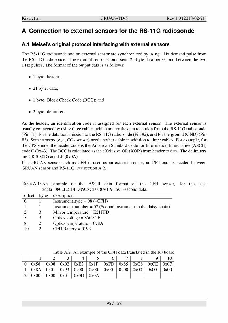
Kizu et al. GRUAN-TD-5 Rev 1.0 (2018-02-21)
A Connection to external sensors for the RS-11G radiosonde
A.1 Meisei’s original protocol interfacing with external sensors
The RS-11G radiosonde and an external sensor are synchronized by using 1 Hz demand pulse fromthe RS-11G radiosonde. The external sensor should send 25-byte data per second between the two1 Hz pulses. The format of the output data is as follows:
• 1 byte: header;
• 21 byte: data;
• 1 byte: Block Check Code (BCC); and
• 2 byte: delimiters.
As the header, an identification code is assigned for each external sensor. The external sensor isusually connected by using three cables, which are for the data reception from the RS-11G radiosonde(Pin #1), for the data transmission to the RS-11G radiosonde (Pin #2), and for the ground (GND) (Pin#3). Some sensors (e.g., CO2 sensor) need another cable in addition to three cables. For example, forthe CPS sonde, the header code is the American Standard Code for Information Interchange (ASCII)code C (0x43). The BCC is calculated as the eXclusive OR (XOR) from header to data. The delimitersare CR (0x0D) and LF (0x0A).
If a GRUAN sensor such as CFH is used as an external sensor, an I/F board is needed betweenGRUAN sensor and RS-11G (see section A.2).
Table A.1: An example of the ASCII data format of the CFH sensor, for the casexdata=0802E21FFD85C8CE078A0193 as 1-second data.
offset bytes description
0 1 Instrument type = 08 (=CFH)1 1 Instrument number = 02 (Second instrument in the daisy chain)2 3 Mirror temperature = E21FFD5 3 Optics voltage = 85C8CE8 2 Optics temperature = 078A10 2 CFH Battery = 0193
Table A.2: An example of the CFH data translated in the I/F board.
1 2 3 4 5 6 7 8 9 10
0 0x58 0x08 0x02 0xE2 0x1F 0xFD 0x85 0xC8 0xCE 0x07
1 0x8A 0x01 0x93 0x00 0x00 0x00 0x00 0x00 0x00 0x00
2 0x00 0x00 0x31 0x0D 0x0A
95 / 152
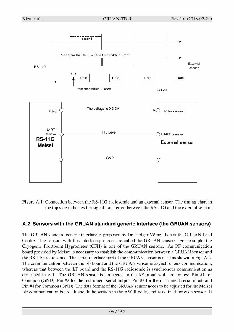
Kizu et al. GRUAN-TD-5 Rev 1.0 (2018-02-21)
RS-11G
Meisei
Data Data Data Data
RS-11G
TTL Level
GND
Figure A.1: Connection between the RS-11G radiosonde and an external sensor. The timing chart inthe top side indicates the signal transferred between the RS-11G and the external sensor.
A.2 Sensors with the GRUAN standard generic interface (the GRUAN sensors)
The GRUAN standard generic interface is proposed by Dr. Holger Vomel then at the GRUAN LeadCentre. The sensors with this interface protocol are called the GRUAN sensors. For example, theCryogenic Frostpoint Hygrometer (CFH) is one of the GRUAN sensors. An I/F communicationboard provided by Meisei is necessary to establish the communication between a GRUAN sensor andthe RS-11G radiosonde. The serial interface port of the GRUAN sensor is used as shown in Fig. A.2.The communication between the I/F board and the GRUAN sensor is asynchronous communication,whereas that between the I/F board and the RS-11G radiosonde is synchronous communication asdescribed in A.1. The GRUAN sensor is connected to the I/F broad with four wires: Pin #1 forCommon (GND), Pin #2 for the instrument serial output, Pin #3 for the instrument serial input, andPin #4 for Common (GND). The data format of the GRUAN sensor needs to be adjusted for the MeiseiI/F communication board. It should be written in the ASCII code, and is defined for each sensor. It
96 / 152
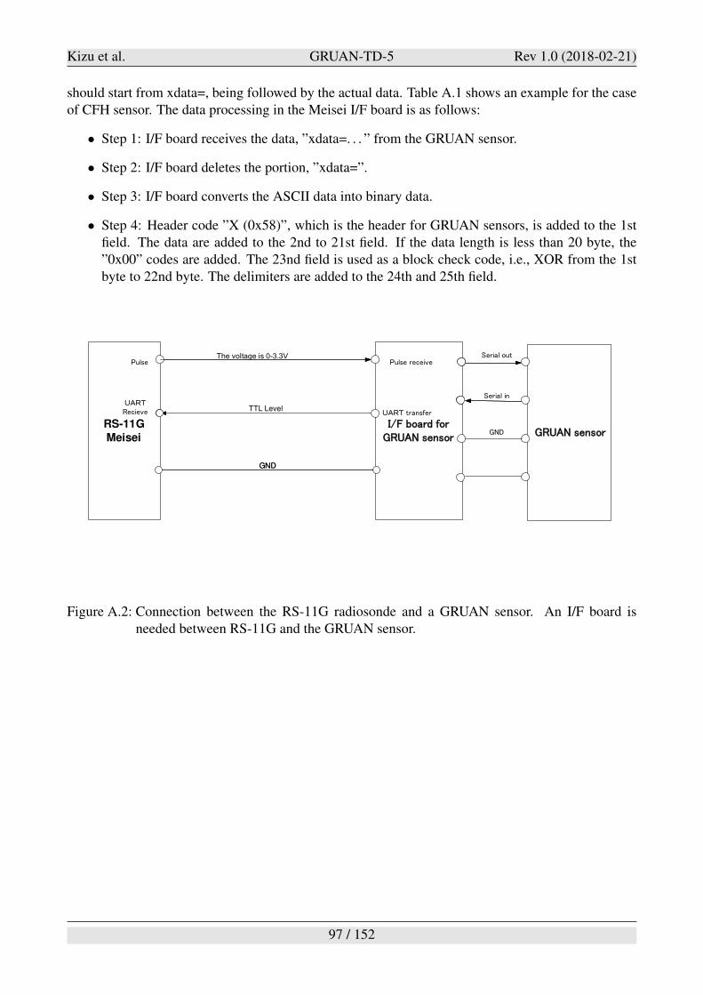
Kizu et al. GRUAN-TD-5 Rev 1.0 (2018-02-21)
should start from xdata=, being followed by the actual data. Table A.1 shows an example for the caseof CFH sensor. The data processing in the Meisei I/F board is as follows:
• Step 1: I/F board receives the data, ”xdata=. . . ” from the GRUAN sensor.
• Step 2: I/F board deletes the portion, ”xdata=”.
• Step 3: I/F board converts the ASCII data into binary data.
• Step 4: Header code ”X (0x58)”, which is the header for GRUAN sensors, is added to the 1stfield. The data are added to the 2nd to 21st field. If the data length is less than 20 byte, the”0x00” codes are added. The 23nd field is used as a block check code, i.e., XOR from the 1stbyte to 22nd byte. The delimiters are added to the 24th and 25th field.
RS-11G
Meisei
TTL Level
GND
GND
Figure A.2: Connection between the RS-11G radiosonde and a GRUAN sensor. An I/F board isneeded between RS-11G and the GRUAN sensor.
97 / 152
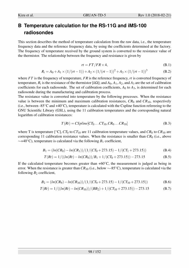
Kizu et al. GRUAN-TD-5 Rev 1.0 (2018-02-21)
B Temperature calculation for the RS-11G and iMS-100
radiosondes
This section describes the method of temperature calculation from the raw data, i.e., the temperaturefrequency data and the reference frequency data, by using the coefficients determined at the factory.The frequency of temperature received by the ground system is converted to the resistance value ofthe thermistor. The relationship between the frequency and resistance is given by
rt = FT/FR&4, (B.1)
Rt = A0 +A1 & (1/(rt #1))+A2 & (1/(rt #1))2 +A3 & (1/(rt #1))3 (B.2)
where FT is the frequency of temperature, FR is the reference frequency, rt is converted frequency oftemperature, Rt is the resistance of the thermistor [k"]; and A0, A1, A2, and A3 are the set of calibrationcoefficients for each radiosonde. The set of calibration coefficients, A0 to A3, is determined for eachradiosonde during the manufacturing and calibration process.The resistance value is converted into temperature by the following processes. When the resistancevalue is between the minimum and maximum calibration resistances, CR0 and CR10, respectively(i.e., between -85!C and +40!C), temperature is calculated with the Cspline function refereeing to theGNU Scientific Library (GSL), using the 11 calibration temperatures and the corresponding naturallogarithm of calibration resistances:
T (Rt) =CSpline[CT0 . . .CT10,CR0 . . .CR10] (B.3)
where T is temperature [!C], CT0 to CT10 are 11 calibration temperature values, and CR0 to CR10 arecorresponding 11 calibration resistance values. When the resistance is smaller than CR0 (i.e., above"+40!C), temperature is calculated via the following B1 coefficient,
B1 = (ln(CR0)# ln(CR1))/(1/(CT0 +273.15)#1/(CT1 +273.15)) (B.4)
T (Rt) = 1/((ln(Rt)# ln(CR0))/B1 +1/(CT0 +273.15))#273.15 (B.5)
If the calculated temperature becomes greater than +60!C, the measurement is judged as being inerror. When the resistance is greater than CR10 (i.e., below "-85!C), temperature is calculated via thefollowing B2 coefficient,
B2 = (ln(CR9)# ln(CR10))/(1/(CT9 +273.15)#1/(CT10 +273.15)) (B.6)
T (Rt) = 1/((ln(Rt)# ln(CR10))/(BB2)+1/(CT10 +273.15))#273.15 (B.7)
98 / 152
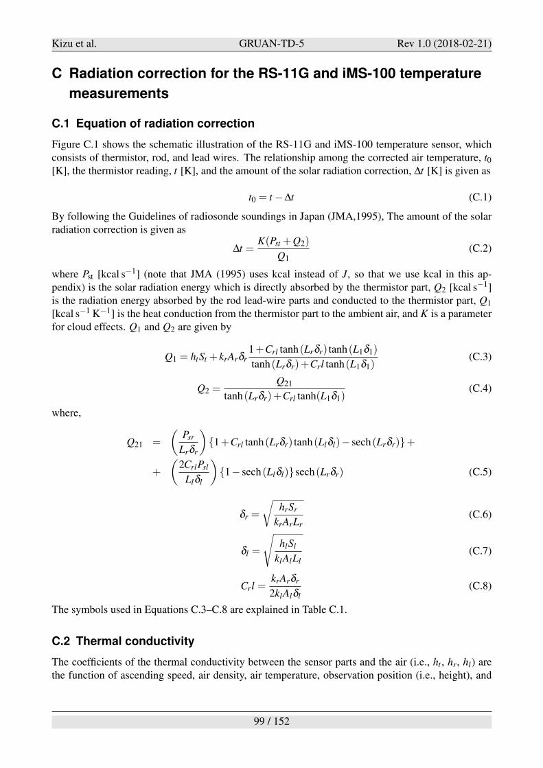
Kizu et al. GRUAN-TD-5 Rev 1.0 (2018-02-21)
C Radiation correction for the RS-11G and iMS-100 temperature
measurements
C.1 Equation of radiation correction
Figure C.1 shows the schematic illustration of the RS-11G and iMS-100 temperature sensor, whichconsists of thermistor, rod, and lead wires. The relationship among the corrected air temperature, t0[K], the thermistor reading, t [K], and the amount of the solar radiation correction, !t [K] is given as
t0 = t #!t (C.1)
By following the Guidelines of radiosonde soundings in Japan (JMA,1995), The amount of the solarradiation correction is given as
!t =K(Pst +Q2)
Q1(C.2)
where Pst [kcal s#1] (note that JMA (1995) uses kcal instead of J, so that we use kcal in this ap-pendix) is the solar radiation energy which is directly absorbed by the thermistor part, Q2 [kcal s#1]is the radiation energy absorbed by the rod lead-wire parts and conducted to the thermistor part, Q1
[kcal s#1 K#1] is the heat conduction from the thermistor part to the ambient air, and K is a parameterfor cloud effects. Q1 and Q2 are given by
Q1 = htSt + krAr'r1+Crl tanh(Lr'r) tanh(L1'1)
tanh(Lr'r)+Crl tanh(L1'1)(C.3)
Q2 =Q21
tanh(Lr'r)+Crl tanh(L1'1)(C.4)
where,
Q21 =
$
Psr
Lr'r
%
{1+Crl tanh(Lr'r) tanh(Ll'l)# sech(Lr'r)}+
+
$
2CrlPsl
Ll'l
%
{1# sech(Ll'l)}sech(Lr'r) (C.5)
'r =
&
hrSr
krArLr(C.6)
'l =
'
hlSl
klAlLl(C.7)
Crl =krAr'r
2klAl'l(C.8)
The symbols used in Equations C.3–C.8 are explained in Table C.1.
C.2 Thermal conductivity
The coefficients of the thermal conductivity between the sensor parts and the air (i.e., ht , hr, hl) arethe function of ascending speed, air density, air temperature, observation position (i.e., height), and
99 / 152
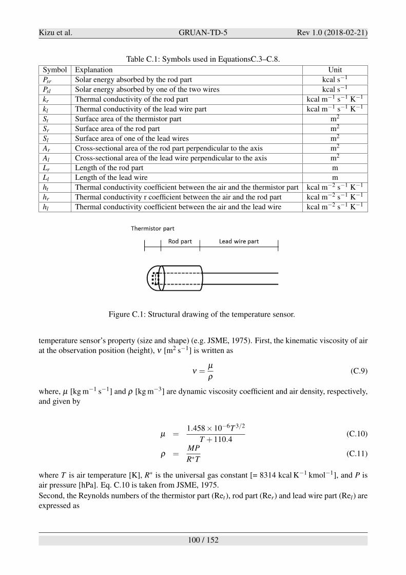
Kizu et al. GRUAN-TD-5 Rev 1.0 (2018-02-21)
Table C.1: Symbols used in EquationsC.3–C.8.
Symbol Explanation Unit
Psr Solar energy absorbed by the rod part kcal s#1
Psl Solar energy absorbed by one of the two wires kcal s#1
kr Thermal conductivity of the rod part kcal m#1 s#1 K#1
kl Thermal conductivity of the lead wire part kcal m#1 s#1 K#1
St Surface area of the thermistor part m2
Sr Surface area of the rod part m2
Sl Surface area of one of the lead wires m2
Ar Cross-sectional area of the rod part perpendicular to the axis m2
Al Cross-sectional area of the lead wire perpendicular to the axis m2
Lr Length of the rod part m
Ll Length of the lead wire m
ht Thermal conductivity coefficient between the air and the thermistor part kcal m#2 s#1 K#1
hr Thermal conductivity r coefficient between the air and the rod part kcal m#2 s#1 K#1
hl Thermal conductivity coefficient between the air and the lead wire kcal m#2 s#1 K#1
Figure C.1: Structural drawing of the temperature sensor.
temperature sensor’s property (size and shape) (e.g. JSME, 1975). First, the kinematic viscosity of airat the observation position (height), ( [m2 s#1] is written as
( =µ
$(C.9)
where, µ [kg m#1 s#1] and $ [kg m#3] are dynamic viscosity coefficient and air density, respectively,and given by
µ =1.458&10#6T 3/2
T +110.4(C.10)
$ =MP
R)T(C.11)
where T is air temperature [K], R) is the universal gas constant [= 8314 kcal K#1 kmol#1], and P isair pressure [hPa]. Eq. C.10 is taken from JSME, 1975.
Second, the Reynolds numbers of the thermistor part (Ret), rod part (Rer) and lead wire part (Rel) areexpressed as
100 / 152
Kizu et al. GRUAN-TD-5 Rev 1.0 (2018-02-21)
Ret =DtV
((C.12)
Rer =V Dr/cos(50!)
((C.13)
Rel =V Dl/cos(33!)
((C.14)
where Dt is the diameter of the thermistor part [m], Dr is the diameter of the rod part [m], Dl is thediameter of the lead wire part [m], V is the ascent rate of the radiosonde at observation position [ms#1]. The factor of cos(50!) in Eq. C.13 is considered because the rod part is tilted, on average, by 50!
with respect to the horizontal plane during the flight. The factor of cos(33!) in Eq. C.14 is consideredbecause the lead part is tilted by 33! with respect to the horizontal plane.
Third, the Nusselt number, Nu is a dimensionless number related to the thermal conductivity in afluid, which is related with the Reynolds number as
Nut = 2+0.50Re0.5t (C.15)
Nur = 0.445+0.499(Rer #0.189)0.492 (C.16)
Nul = 0.445+0.499(Rel #0.189)0.492 (C.17)
(Nakamura et al., 1983)
Assuming the thermistor part, rod part and lead wire part as columnar forms, the thermal conductivityfor each part can be expressed using the Nusselt number as
ht =Nut)
Dt(C.18)
hr =Nur)
Dr/cos(50!)(C.19)
hl =Nul)
Dl/cos(33!)(C.20)
where, ) [kcal m#1 s#1 K#1] is the thermal conductivity of air at the radiosonde position, which isexpressed as a function of temperature as
) =6.325&10#7T 3/2
T +245.4&10#(12/T )(C.21)
C.3 Solar radiation energy absorbed by sensor parts
The amounts of solar radiation energy absorbed by the sensor parts, i.e., Pst, Ptextrmsr, and Psl inEquations C.2 and C.5 are given as in Nakamura et al. (1983) as
101 / 152
Kizu et al. GRUAN-TD-5 Rev 1.0 (2018-02-21)
Pst = "stSst(1+*)I (C.22)
Psr = "srSsr(1+*)I (C.23)
Psl = "slSsl(1+*)I (C.24)
where "st , "sr, and "sl are the solar radiation absorption rate of the thermistor part (0.20), rod part(0.20), and lead wire part (0.70), respectively, Sst , Ssr, and Ssl are the effective cross-sectional area[m2] of the thermistor, rod, and one lead wire, respectively, to the direct solar radiation, * is a co-efficient representing the contribution of reflected light from the surface or scattered light from theatmosphere (0.20), and I is the direct solar radiation energy at the observation position [kcal m#2 s#1].
Radiosondes are generally ascending while rotating around the vertical axis as shown in Figure C.2.With this in mind, Sst , Ssr, and Ssl can be expressed as
Sst =+D2
t
4Fst(Z) (C.25)
Ssr = DrLrFsr(Z) (C.26)
Ssl = DlLlFsl(Z) (C.27)
where Z is the solar elevation angle, and Fst (Z), Fsr (Z), Fsl (Z) represent the angle between the solarenergy transfer and the sensor parts, being expressed as
Fst(Z) = 0.5(1+ cos, sinZ) (C.28)
Fsr(Z) = 1/+( +
0
#
1# (cos, sinZ + sin, cosZ cos&)2d& (C.29)
Fsl(Z) = 1/+( +
0
#
1# (cos, * sinZ + sin, * cosZ cos&)2d& (C.30)
where & is azimuth angle of the sun as seen from the radiosonde, , is the angle of the rod part withrespect to the vertical axis, and , * is the angle of the lead wire part with respect to the vertical axis.
The integration in Equations C.29 and C.30 cannot be obtained analytically. Therefore, Fsr (Z) andFsl (Z) are approximated by a cubic equation of Z as
Fsr(Z) = a3Z3 +a2Z2 +a1Z +a0 (C.31)
Fsl(Z) = b3Z3 +b2Z2 +b1Z +b0 (C.32)
The eight constant coefficients, a0 to a3 and b0 to b3 are obtained from a numerical integration andgiven in Table C.2.
C.4 Equation of radiation energy
The direct solar radiation energy (I) at the observation position is expressed as
I = I0(Tr #Aw) (C.33)
102 / 152
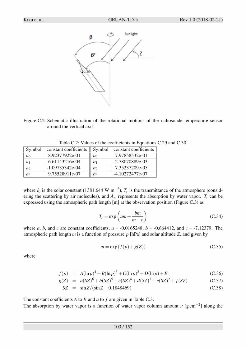
Kizu et al. GRUAN-TD-5 Rev 1.0 (2018-02-21)
Figure C.2: Schematic illustration of the rotational motions of the radiosonde temperature sensoraround the vertical axis.
Table C.2: Values of the coefficients in Equations C.29 and C.30.
Symbol constant coefficients Symbol constant coefficients
a0 8.92377922e-01 b0 7.97858532e-01
a1 -6.61143216e-04 b1 -2.78070889e-03
a2 -1.09735342e-04 b2 7.35237209e-05
a3 9.75528911e-07 b3 -4.10272477e-07
where I0 is the solar constant (1381.644 W m#2), Tr is the transmittance of the atmosphere (consid-ering the scattering by air molecules), and Aw represents the absorption by water vapor. Tr can beexpressed using the atmospheric path length [m] at the observation position (Figure C.3) as
Tr = exp
$
am+bm
m# c
%
(C.34)
where a, b, and c are constant coefficients, a = -0.0165248, b = -0.664412, and c = -7.12379. Theatmospheric path length m is a function of pressure p [hPa] and solar altitude Z, and given by
m = exp( f (p)+g(Z)) (C.35)
where
f (p) = A(ln p)4 +B(ln p)3 +C(ln p)2 +D(ln p)+E (C.36)
g(Z) = a(SZ)6 +b(SZ)5 + c(SZ)4 +d(SZ)3 + e(SZ)2 + f (SZ) (C.37)
SZ = sinZ/(sinZ +0.1848469) (C.38)
The constant coefficients A to E and a to f are given in Table C.3.
The absorption by water vapor is a function of water vapor column amount u [g cm#2] along the
103 / 152
Kizu et al. GRUAN-TD-5 Rev 1.0 (2018-02-21)
Table C.3: Values of the coefficients in Equations C.34 and C.35
Symbol constant coefficients Symbol constant coefficients Symbol constant coefficients
A 0.001521491 B -0.01631784 C 0.04158605
D 0.9578739 E -3.066776 – –
a -0.1263798 b -0.6810729 c -0.9013728
d 0.5597896 e 1.047277 f -4.465039
atmospheric path and is giving by
Aw = 0.0938exp)
0.7990logu#0.1289(logu)2 #0.01382(logu)3*
(C.39)
and
u = w0
$
p
p0
%4m(p,Z)
m(p,Z = 90)(C.40)
where w0 is the water vapor column amount averaged for January and July at 30!N (2.55 g cm#2
(Miller, 1977), p is air pressure at the observation position, and p0 is surface pressure. With theseequations, the maximum contribution of the solar radiation correction amount by the water vapor col-umn amount (W0) is estimated. For this estimate, a tropical water vapor condition (W0 = 10 g cm#2),with a low solar elevation angle (10!) and low GPSsonde altitude (1 km), is assumed. The result isthat the contribution of the solar radiation to the amount of correction of the W0 is 0.06 K. Thus, it isconcluded that variations in W0 would not significantly affect the solar radiation correction amount.
Figure C.3: Atmospheric path length for the solar radiation for a radiosonde located at pressure P.
C.5 Effect of clouds
Existence of clouds complicates the radiative transfer. Here, the reduction of direct solar radiation byclouds is only considered by setting the factor K in Eq. C.2 appropriately. As there is no measurementof cloud radiative property on the radiosonde, an average situation is assumed for all the soundings.Specifically, K is set as follows:
104 / 152
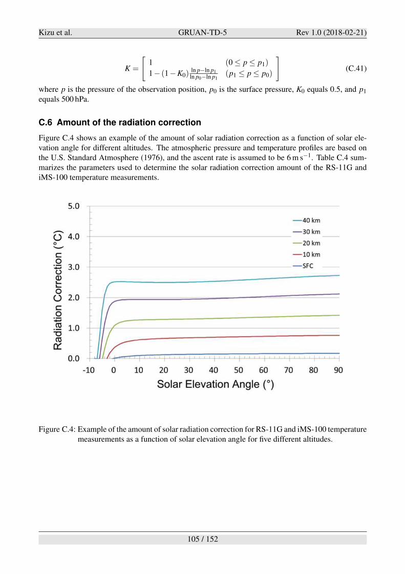
Kizu et al. GRUAN-TD-5 Rev 1.0 (2018-02-21)
K =
+
1 (0 $ p $ p1)
1# (1#K0)ln p#ln p1ln p0#ln p1
(p1 $ p $ p0)
,
(C.41)
where p is the pressure of the observation position, p0 is the surface pressure, K0 equals 0.5, and p1
equals 500 hPa.
C.6 Amount of the radiation correction
Figure C.4 shows an example of the amount of solar radiation correction as a function of solar ele-vation angle for different altitudes. The atmospheric pressure and temperature profiles are based onthe U.S. Standard Atmosphere (1976), and the ascent rate is assumed to be 6 m s#1. Table C.4 sum-marizes the parameters used to determine the solar radiation correction amount of the RS-11G andiMS-100 temperature measurements.
Figure C.4: Example of the amount of solar radiation correction for RS-11G and iMS-100 temperaturemeasurements as a function of solar elevation angle for five different altitudes.
105 / 152
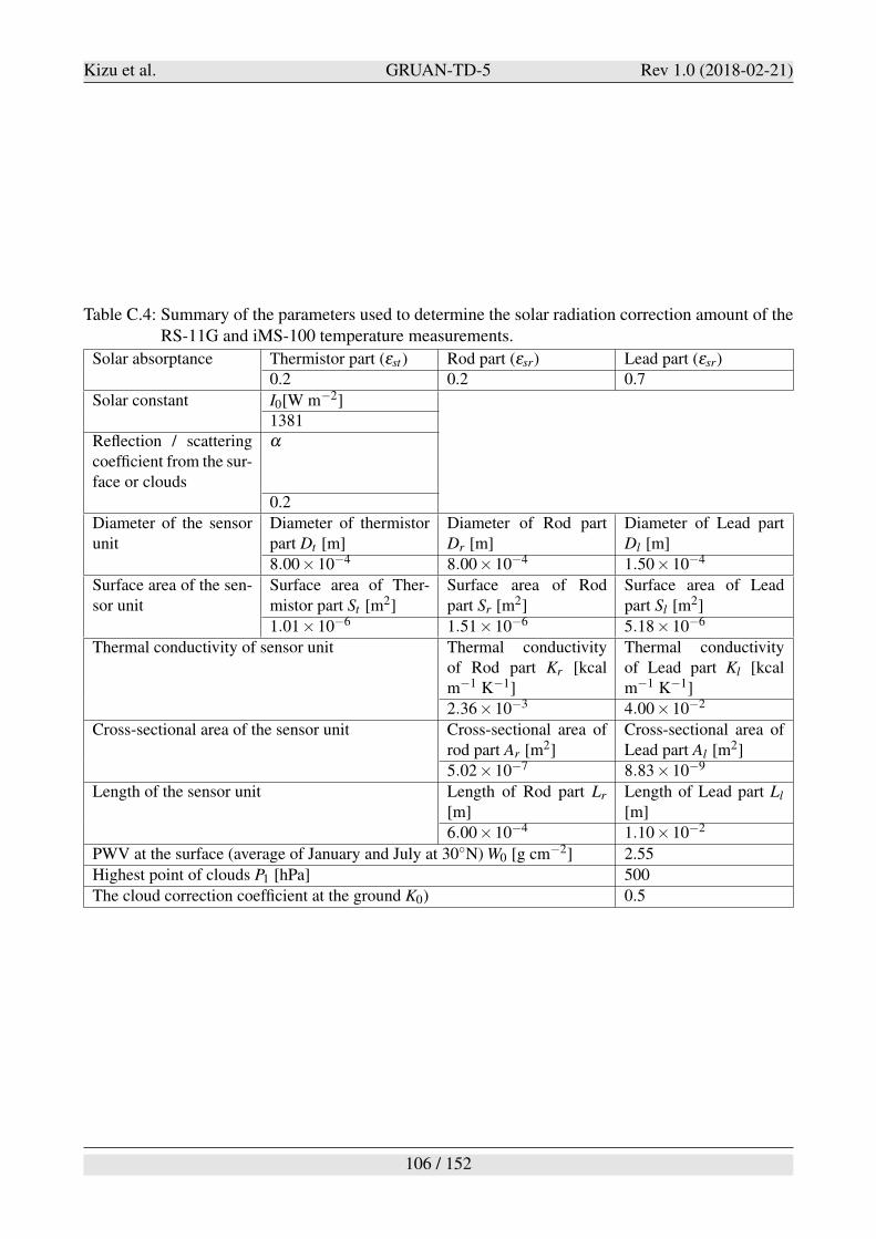
Kizu et al. GRUAN-TD-5 Rev 1.0 (2018-02-21)
Table C.4: Summary of the parameters used to determine the solar radiation correction amount of theRS-11G and iMS-100 temperature measurements.
Solar absorptance Thermistor part ("st) Rod part ("sr) Lead part ("sr)0.2 0.2 0.7
Solar constant I0[W m#2]1381
Reflection / scatteringcoefficient from the sur-face or clouds
*
0.2
Diameter of the sensorunit
Diameter of thermistorpart Dt [m]
Diameter of Rod partDr [m]
Diameter of Lead partDl [m]
8.00&10#4 8.00&10#4 1.50&10#4
Surface area of the sen-sor unit
Surface area of Ther-mistor part St [m2]
Surface area of Rodpart Sr [m2]
Surface area of Leadpart Sl [m2]
1.01&10#6 1.51&10#6 5.18&10#6
Thermal conductivity of sensor unit Thermal conductivityof Rod part Kr [kcalm#1 K#1]
Thermal conductivityof Lead part Kl [kcalm#1 K#1]
2.36&10#3 4.00&10#2
Cross-sectional area of the sensor unit Cross-sectional area ofrod part Ar [m2]
Cross-sectional area ofLead part Al [m2]
5.02&10#7 8.83&10#9
Length of the sensor unit Length of Rod part Lr
[m]Length of Lead part Ll
[m]
6.00&10#4 1.10&10#2
PWV at the surface (average of January and July at 30!N) W0 [g cm#2] 2.55
Highest point of clouds P1 [hPa] 500
The cloud correction coefficient at the ground K0) 0.5
106 / 152
Kizu et al. GRUAN-TD-5 Rev 1.0 (2018-02-21)
D RH calculation of the RS-11G and iMS-100 radiosondes
This section describes the method of relative humidity (RH) calculation from the raw data, i.e., the RHfrequency data and the reference frequency data, by using the coefficients determined at the factory.
D.1 Calculation of the raw RH values
The frequency of humidity received by the ground system is converted to the capacitance of the RHsensor. The relationship between the frequency and capacitance is given by
ru =FU
FR&4 (D.1)
U0 = B0 +B1 & ru+B2 & ru2 +B3 & ru3 (D.2)
where ru is converted frequency of humidity, FU is the frequency of humidity, FR is the reference fre-quency, U0 is the raw relative humidity value [%RH], and B0, B1, B2, and B3 are the set of calibrationcoefficients for each radiosonde.
The set of calibration coefficients, B0 to B3 is normally determined for each radiosonde during themanufacturing and calibration process (at RH levels of 15%, 30%, 50%, 70%, 90%, and 95%, andat a constant air temperature of +25!C). But, for the station where the SHC checks are conducted(e.g., Tateno), the set of coefficients is determined with the frequency data for the levels 0 %RH and100 %RH in addition to original calibration data in factory.
D.2 Estimation of the RH sensor temperature (applicable only for RS-11G)
The temperature of the RH sensor generally does not equal to the ambient air temperature becauseof the thermal lag of the RH sensor and the solar heating. During the balloon ascent through thetroposphere, the RH sensor temperature would usually become warmer than the ambient air temper-ature due to the thermal lag. The warmer RH sensor would result in giving RH measurements thatare biased dry, so that a correction procedure that considers the difference between the air and sensortemperatures is necessary. Because the RS-11G radiosonde is not equipped with a dedicated temper-ature sensor for the RH sensor, the temperature of the RS-11G RH sensor needs to be estimated usingthe air temperature measurement. On the other hand, the solar heating on the RH sensor occurs onlyduring daytime soundings. The amount of heating is estimated by following the same procedure asthat for the thermistor, as explained in Appendix C, with some special considerations.
D.2.1 Thermal lag consideration
On the basis of the Newton’s law of cooling, the relationship between the RH sensor temperature, Ts
and the air temperature, Ta (both in K) can be written as
Ts(t) =Ta' t + %Ts(t #' t)
% +' t(D.3)
where % is the time constant (or the thermal lag) of the sensor, and ' t is a finite time step.
The time constant depends on the heat transfer between the ambient air and the surface of the RHsensor and on the sensor property. Williams and Acheson (1976) give the time constant of a sensor in
107 / 152
Kizu et al. GRUAN-TD-5 Rev 1.0 (2018-02-21)
the air theoretically as
% =mc
hA(D.4)
where m is the mass of the sensor, c is the specific heat of the sensor, h is the convective heat-transfercoefficient, and A is the total surface area of the sensor. The convective heat transfer would decreasewith height primarily because air density decreases with height. Morrissey and Brousaides (1970)proposed that, assuming that the RH sensor is a flat plate with a zero angle of attack to airflow, h canbe calculated from
h =1
L
( L
00.332kPr1/3
'
$( *
µxdx (D.5)
where L is the width of the RH sensor, k is the thermal conductivity of air, Pr is the Prandtl number, $is the density of air, ( * is the flow rate on the RH sensor, and µ is the viscosity coefficient. The valuesof Pr, k, and µ depend on air temperature. Substituting Eq. D.5 into Eq. D.4, % can be rewritten as
% =Ck#1Pr#1/3
&
µ
$((D.6)
where C is a constant, in theory, determined by the RH sensor property.
The iMS-100 radiosonde has a dedicated temperature sensor for the RH sensor. Therefore, the iMS-100 sounding results can be used to validate Eq. D.6. The results show that the value of C actuallyhas a dependency on pressure. This is because the convective heat-transfer coefficient in Eq. D.5 wasassumed to be the one for laminar airflow. In reality, the airflow around the RH sensor during theflight is turbulent, and thus the ventilation depends on pressure particularly in the troposphere belowthe 200 hPa level. Therefore, C is modified empirically as
C =CT s &C(P) CT s = 150 (D.7)
where CT s is determined based on some RH sensor temperature profiles measured with iMS-100, andC(P) is
-
C(P) = 1# (1#0.2) lnP#ln200lnP0#ln200 (for P > 200 hPa)
C(P) = 1 (for P < 200 hPa)(D.8)
The pressure dependency above the 200 hPa level is negligible.
D.2.2 Solar heating consideration
The amount of the solar heating on the RH sensor is estimated by following the same procedure asthat for the thermistor (Appendix C). The surface area of the RH sensor and the sensor cap is muchgreater than that of the thermistor, and this factor needs to be considered. Also, the factor due tonon-laminar airflow (i.e., C(P) in Eq. D.8), which is not considered for the thermistor, needs to beconsidered. Therefore, the amount of solar heating, !Ts SR is estimated as
!Ts SR =C(P) f !TSR f = 3.3 (D.9)
where f is surface area factor and !Ts SR is the solar heating amount for the thermistor at the same timeof measurement. The value of f , 3.3 was determined by the comparison with some simultaneous iMS-100 sounding, which are conducted at mid-latitude, Tateno and Moriya, during September–October2014.
108 / 152
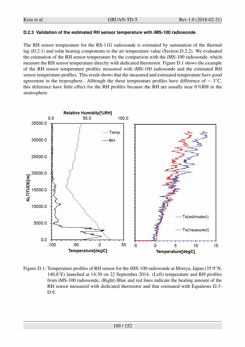
Kizu et al. GRUAN-TD-5 Rev 1.0 (2018-02-21)
D.2.3 Validation of the estimated RH sensor temperature with iMS-100 radiosonde
The RH sensor temperature for the RS-11G radiosonde is estimated by summation of the thermallag (D.2.1) and solar heating components to the air temperature value (Section D.2.2). We evaluatedthe estimation of the RH sensor temperature by the comparison with the iMS-100 radiosonde, whichmeasure the RH sensor temperature directly with dedicated thermistor. Figure D.1 shows the exampleof the RH sensor temperature profiles measured with iMS-100 radiosonde and the estimated RHsensor temperature profiles. This result shows that the measured and estimated temperature have goodagreement in the troposphere. Although the these temperature profiles have difference of " 3!C,this deference have little effect for the RH profiles because the RH are usually near 0 %RH in thestratosphere.
Figure D.1: Temperature profiles of RH sensor for the iMS-100 radiosonde at Moriya, Japan (35.9!N,140.0!E) launched at 14:30 on 22 September 2014. (Left) temperature and RH profilesfrom iMS-100 radiosonde, (Right) Blue and red lines indicate the heating amount of theRH sensor measured with dedicated thermistor and that estimated with Equations D.3-D.9.
109 / 152
Kizu et al. GRUAN-TD-5 Rev 1.0 (2018-02-21)
D.3 Adjustment of the RH sensor temperature for the iMS-100 and RS-11G
radiosonde
The iMS-100 has a dedicated temperature sensor (a thermistor) for the RH sensor. Its accuracy is 0.3K below 0!C, but worse above 0!C. Considering also that in the lower troposphere, the differencebetween the sensor temperature and the air temperature is very small because of very effective con-vective heat transfer, it would be reasonable that the iMS-100 RH sensor temperature is calculatedin combination with the air temperature and the measured RH sensor temperature by the followingequation:
Ts = KTa &Ts obs +(1#KTa)&Ta (D.10)
where Ts obs is the measured RH sensor temperature, Ta is air temperature, and KTa is the followingweighting parameter:
KTa =
.
/
0
0 (for P > 600 hPa)
1# lnP#ln400ln600#ln400 (for 400 < P < 600 hPa)
1 (for P < 400 hPa)
(D.11)
As in Eq. D.11, below the 600 hPa level, air temperature is used as the RH sensor temperature, andabove the 400 hPa level, the measured RH sensor temperature is used. Between 400 hPa and 600 hPa,both temperatures are combined according to the weighting parameter K to estimate the RH sensortemperature.It is noted here that the RH sensor temperature for the RS-11G radiosonde is also calculated withEq. D.11.
110 / 152
Kizu et al. GRUAN-TD-5 Rev 1.0 (2018-02-21)
E Low-pass filtering for the wind measurement and RH
correction
A low-pass digital filter with the Kaiser window (Kuo and Kaiser, 1966) is used to remove noises inthe wind and relative humidity (RH) measurements. The same formula are used for the two variablesexcept for the cut-off frequency value. The cut-off frequency for the wind measurements is deter-mined from the period of the pendulum motions, and that for the RH measurements is determinedfrom the response time of the RH sensor. The actual filtering calculations are performed with thefollowing four steps.
(1) Calculation of the Kaiser window
The Kaiser value * is defined as
* =
.
/
0
0 (for 21 dB $ A)0.5842(A#21)0.4 +0.07886(A#21) (for 21 dB < A < 50 dB)0.1102(A#8.7) (for A + 50 dB)
(E.1)
where A is the rate of decrease of the side lobe. When A is larger, the filter is closer to the stepfunction, being with better selectivity of frequency. The default value is 40 dB.
(2) Calculation of the window function
w(n) =I0(, )
I0(*), , = *
&
1#1 n
M
22(E.2)
and
I0(u) = 1+#$r=1
+
)
u2
*r
r!
,2
(E.3)
where M is window length, 30 (i.e., 60 / 2), I0 is the Bessel function of the first kind with the zerothorder, and r is set to 20 for this filtering.
(3) Calculation of the weighting function
First, the impulse response H(n) is calculated as
H(n) =
3
sin-cn+n w(n) for n ,= 0
2 fcfs
for n = 0(E.4)
and
-c =2+ fc
fs(E.5)
where fc is the cut-off frequency and fs is the sampling frequency (normally 1 Hz).
The cut-off frequency for the wind measurements is determined from the pendulum period, and thusfrom the length of the string between the balloon and the payload, by the following equation.
fc = 1. & 1
Tc
= 1. & 1
2+%
L/g
(E.6)
where . is an empirical coefficient, L is the length of string, and g is gravitational acceleration. Thecut-off frequency for the RH measurements is given in Section 3.2.
111 / 152
Kizu et al. GRUAN-TD-5 Rev 1.0 (2018-02-21)
The standardized impulse response h(n) is obtained by
h(n) =H(n)
#Mn=#MH(n)
(E.7)
(4) Obtaining low-pass filtered dataThe filtered data Vout is obtained from the original data Vin by the following equation.
Vout = h(0)&Vin(M)+#Mn=1[h(n)&Vin(M#n)+h(n)&Vin(M+n)] (E.8)
112 / 152
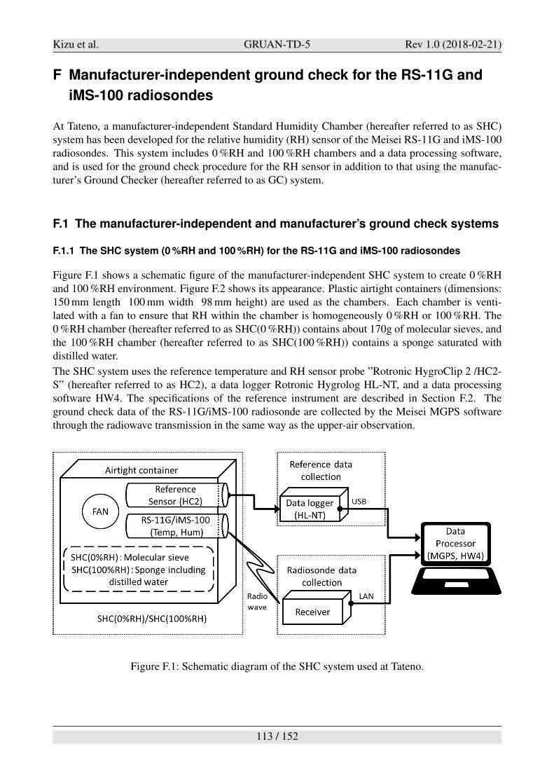
Kizu et al. GRUAN-TD-5 Rev 1.0 (2018-02-21)
F Manufacturer-independent ground check for the RS-11G and
iMS-100 radiosondes
At Tateno, a manufacturer-independent Standard Humidity Chamber (hereafter referred to as SHC)system has been developed for the relative humidity (RH) sensor of the Meisei RS-11G and iMS-100radiosondes. This system includes 0 %RH and 100 %RH chambers and a data processing software,and is used for the ground check procedure for the RH sensor in addition to that using the manufac-turer’s Ground Checker (hereafter referred to as GC) system.
F.1 The manufacturer-independent and manufacturer’s ground check systems
F.1.1 The SHC system (0 %RH and 100 %RH) for the RS-11G and iMS-100 radiosondes
Figure F.1 shows a schematic figure of the manufacturer-independent SHC system to create 0 %RHand 100 %RH environment. Figure F.2 shows its appearance. Plastic airtight containers (dimensions:150 mm length 100 mm width 98 mm height) are used as the chambers. Each chamber is venti-lated with a fan to ensure that RH within the chamber is homogeneously 0 %RH or 100 %RH. The0 %RH chamber (hereafter referred to as SHC(0 %RH)) contains about 170g of molecular sieves, andthe 100 %RH chamber (hereafter referred to as SHC(100 %RH)) contains a sponge saturated withdistilled water.
The SHC system uses the reference temperature and RH sensor probe ”Rotronic HygroClip 2 /HC2-S” (hereafter referred to as HC2), a data logger Rotronic Hygrolog HL-NT, and a data processingsoftware HW4. The specifications of the reference instrument are described in Section F.2. Theground check data of the RS-11G/iMS-100 radiosonde are collected by the Meisei MGPS softwarethrough the radiowave transmission in the same way as the upper-air observation.
Figure F.1: Schematic diagram of the SHC system used at Tateno.
113 / 152
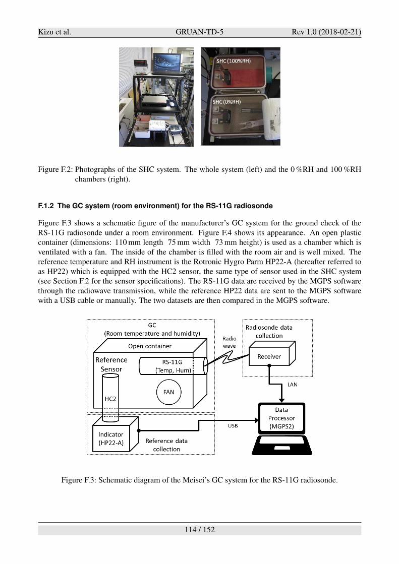
Kizu et al. GRUAN-TD-5 Rev 1.0 (2018-02-21)
Figure F.2: Photographs of the SHC system. The whole system (left) and the 0 %RH and 100 %RHchambers (right).
F.1.2 The GC system (room environment) for the RS-11G radiosonde
Figure F.3 shows a schematic figure of the manufacturer’s GC system for the ground check of theRS-11G radiosonde under a room environment. Figure F.4 shows its appearance. An open plasticcontainer (dimensions: 110 mm length 75 mm width 73 mm height) is used as a chamber which isventilated with a fan. The inside of the chamber is filled with the room air and is well mixed. Thereference temperature and RH instrument is the Rotronic Hygro Parm HP22-A (hereafter referred toas HP22) which is equipped with the HC2 sensor, the same type of sensor used in the SHC system(see Section F.2 for the sensor specifications). The RS-11G data are received by the MGPS softwarethrough the radiowave transmission, while the reference HP22 data are sent to the MGPS softwarewith a USB cable or manually. The two datasets are then compared in the MGPS software.
Figure F.3: Schematic diagram of the Meisei’s GC system for the RS-11G radiosonde.
114 / 152
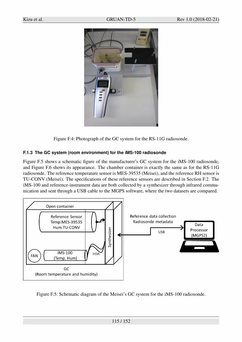
Kizu et al. GRUAN-TD-5 Rev 1.0 (2018-02-21)
Figure F.4: Photograph of the GC system for the RS-11G radiosonde.
F.1.3 The GC system (room environment) for the iMS-100 radiosonde
Figure F.5 shows a schematic figure of the manufacturer’s GC system for the iMS-100 radiosonde,and Figure F.6 shows its appearance. The chamber container is exactly the same as for the RS-11Gradiosonde. The reference temperature sensor is MES-39535 (Meisei), and the reference RH sensor isTU-CONV (Meisei). The specifications of these reference sensors are described in Section F.2. TheiMS-100 and reference-instrument data are both collected by a synthesizer through infrared commu-nication and sent through a USB cable to the MGPS software, where the two datasets are compared.
Figure F.5: Schematic diagram of the Meisei’s GC system for the iMS-100 radiosonde.
115 / 152
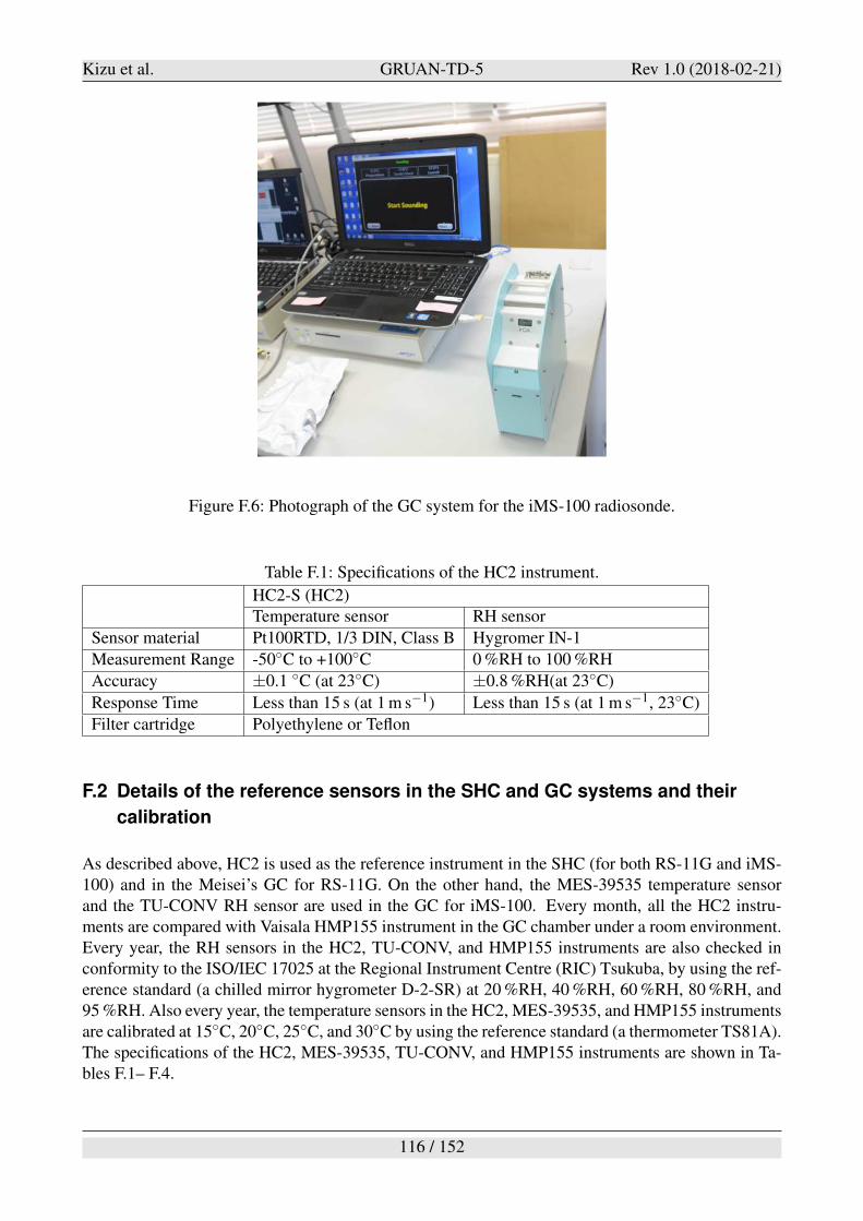
Kizu et al. GRUAN-TD-5 Rev 1.0 (2018-02-21)
Figure F.6: Photograph of the GC system for the iMS-100 radiosonde.
Table F.1: Specifications of the HC2 instrument.
HC2-S (HC2)Temperature sensor RH sensor
Sensor material Pt100RTD, 1/3 DIN, Class B Hygromer IN-1
Measurement Range -50!C to +100!C 0 %RH to 100 %RH
Accuracy ±0.1 !C (at 23!C) ±0.8 %RH(at 23!C)
Response Time Less than 15 s (at 1 m s#1) Less than 15 s (at 1 m s#1, 23!C)
Filter cartridge Polyethylene or Teflon
F.2 Details of the reference sensors in the SHC and GC systems and their
calibration
As described above, HC2 is used as the reference instrument in the SHC (for both RS-11G and iMS-100) and in the Meisei’s GC for RS-11G. On the other hand, the MES-39535 temperature sensorand the TU-CONV RH sensor are used in the GC for iMS-100. Every month, all the HC2 instru-ments are compared with Vaisala HMP155 instrument in the GC chamber under a room environment.Every year, the RH sensors in the HC2, TU-CONV, and HMP155 instruments are also checked inconformity to the ISO/IEC 17025 at the Regional Instrument Centre (RIC) Tsukuba, by using the ref-erence standard (a chilled mirror hygrometer D-2-SR) at 20 %RH, 40 %RH, 60 %RH, 80 %RH, and95 %RH. Also every year, the temperature sensors in the HC2, MES-39535, and HMP155 instrumentsare calibrated at 15!C, 20!C, 25!C, and 30!C by using the reference standard (a thermometer TS81A).The specifications of the HC2, MES-39535, TU-CONV, and HMP155 instruments are shown in Ta-bles F.1– F.4.
116 / 152
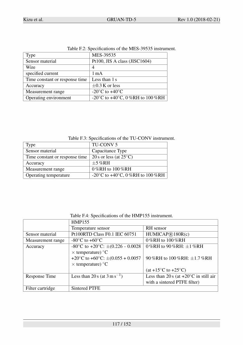
Kizu et al. GRUAN-TD-5 Rev 1.0 (2018-02-21)
Table F.2: Specifications of the MES-39535 instrument.
Type MES-39535
Sensor material Pt100, JIS A class (JISC1604)
Wire 4
specified current 1 mA
Time constant or response time Less than 1 s
Accuracy ±0.3 K or less
Measurement range -20!C to +40!C
Operating environment -20!C to +40!C, 0 %RH to 100 %RH
Table F.3: Specifications of the TU-CONV instrument.
Type TU-CONV 5
Sensor material Capacitance Type
Time constant or response time 20 s or less (at 25!C)
Accuracy ±5 %RH
Measurement range 0 %RH to 100 %RH
Operating temperature -20!C to +40!C, 0 %RH to 100 %RH
Table F.4: Specifications of the HMP155 instrument.
HMP155Temperature sensor RH sensor
Sensor material Pt100RTD Class F0.1 IEC 60751 HUMICAP R'180R(c)
Measurement range -80!C to +60!C 0 %RH to 100 %RH
Accuracy -80!C to +20!C: ±(0.226 - 0.0028& temperature) !C
0 %RH to 90 %RH: ±1 %RH
+20!C to +60!C: ±(0.055 + 0.0057& temperature) !C
90 %RH to 100 %RH: ±1.7 %RH
(at +15!C to +25!C)
Response Time Less than 20 s (at 3 m s#1) Less than 20 s (at +20!C in still airwith a sintered PTFE filter)
Filter cartridge Sintered PTFE
117 / 152
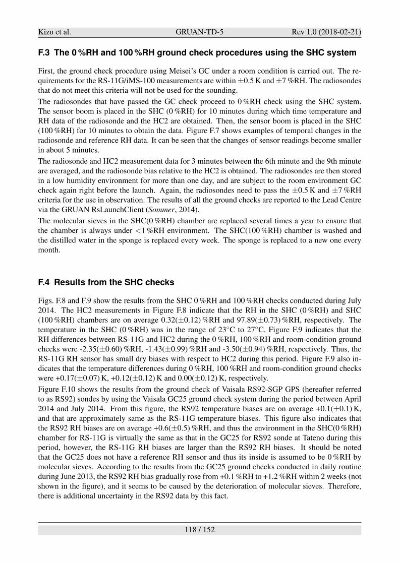
Kizu et al. GRUAN-TD-5 Rev 1.0 (2018-02-21)
F.3 The 0 %RH and 100 %RH ground check procedures using the SHC system
First, the ground check procedure using Meisei’s GC under a room condition is carried out. The re-quirements for the RS-11G/iMS-100 measurements are within ±0.5 K and ±7 %RH. The radiosondesthat do not meet this criteria will not be used for the sounding.
The radiosondes that have passed the GC check proceed to 0 %RH check using the SHC system.The sensor boom is placed in the SHC (0 %RH) for 10 minutes during which time temperature andRH data of the radiosonde and the HC2 are obtained. Then, the sensor boom is placed in the SHC(100 %RH) for 10 minutes to obtain the data. Figure F.7 shows examples of temporal changes in theradiosonde and reference RH data. It can be seen that the changes of sensor readings become smallerin about 5 minutes.
The radiosonde and HC2 measurement data for 3 minutes between the 6th minute and the 9th minuteare averaged, and the radiosonde bias relative to the HC2 is obtained. The radiosondes are then storedin a low humidity environment for more than one day, and are subject to the room environment GCcheck again right before the launch. Again, the radiosondes need to pass the ±0.5 K and ±7 %RHcriteria for the use in observation. The results of all the ground checks are reported to the Lead Centrevia the GRUAN RsLaunchClient (Sommer, 2014).
The molecular sieves in the SHC(0 %RH) chamber are replaced several times a year to ensure thatthe chamber is always under <1 %RH environment. The SHC(100 %RH) chamber is washed andthe distilled water in the sponge is replaced every week. The sponge is replaced to a new one everymonth.
F.4 Results from the SHC checks
Figs. F.8 and F.9 show the results from the SHC 0 %RH and 100 %RH checks conducted during July2014. The HC2 measurements in Figure F.8 indicate that the RH in the SHC (0 %RH) and SHC(100 %RH) chambers are on average 0.32(±0.12) %RH and 97.89(±0.73) %RH, respectively. Thetemperature in the SHC (0 %RH) was in the range of 23!C to 27!C. Figure F.9 indicates that theRH differences between RS-11G and HC2 during the 0 %RH, 100 %RH and room-condition groundchecks were -2.35(±0.60) %RH, -1.43(±0.99) %RH and -3.50(±0.94) %RH, respectively. Thus, theRS-11G RH sensor has small dry biases with respect to HC2 during this period. Figure F.9 also in-dicates that the temperature differences during 0 %RH, 100 %RH and room-condition ground checkswere +0.17(±0.07) K, +0.12(±0.12) K and 0.00(±0.12) K, respectively.
Figure F.10 shows the results from the ground check of Vaisala RS92-SGP GPS (hereafter referredto as RS92) sondes by using the Vaisala GC25 ground check system during the period between April2014 and July 2014. From this figure, the RS92 temperature biases are on average +0.1(±0.1) K,and that are approximately same as the RS-11G temperature biases. This figure also indicates thatthe RS92 RH biases are on average +0.6(±0.5) %RH, and thus the environment in the SHC(0 %RH)chamber for RS-11G is virtually the same as that in the GC25 for RS92 sonde at Tateno during thisperiod, however, the RS-11G RH biases are larger than the RS92 RH biases. It should be notedthat the GC25 does not have a reference RH sensor and thus its inside is assumed to be 0 %RH bymolecular sieves. According to the results from the GC25 ground checks conducted in daily routineduring June 2013, the RS92 RH bias gradually rose from +0.1 %RH to +1.2 %RH within 2 weeks (notshown in the figure), and it seems to be caused by the deterioration of molecular sieves. Therefore,there is additional uncertainty in the RS92 data by this fact.
118 / 152
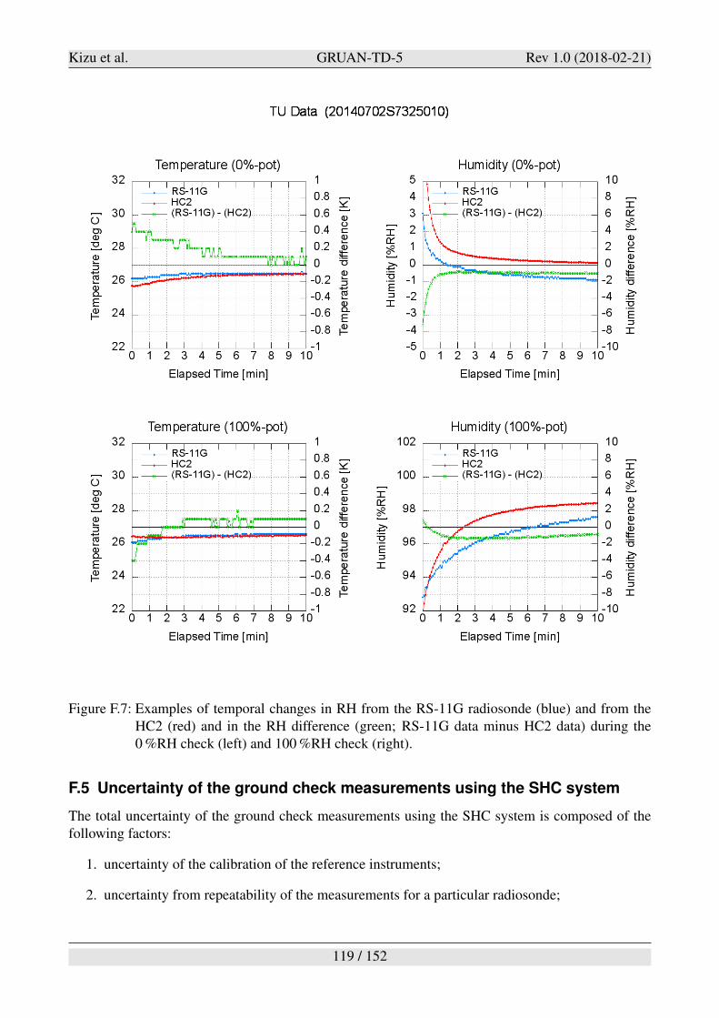
Kizu et al. GRUAN-TD-5 Rev 1.0 (2018-02-21)
Figure F.7: Examples of temporal changes in RH from the RS-11G radiosonde (blue) and from theHC2 (red) and in the RH difference (green; RS-11G data minus HC2 data) during the0 %RH check (left) and 100 %RH check (right).
F.5 Uncertainty of the ground check measurements using the SHC system
The total uncertainty of the ground check measurements using the SHC system is composed of thefollowing factors:
1. uncertainty of the calibration of the reference instruments;
2. uncertainty from repeatability of the measurements for a particular radiosonde;
119 / 152
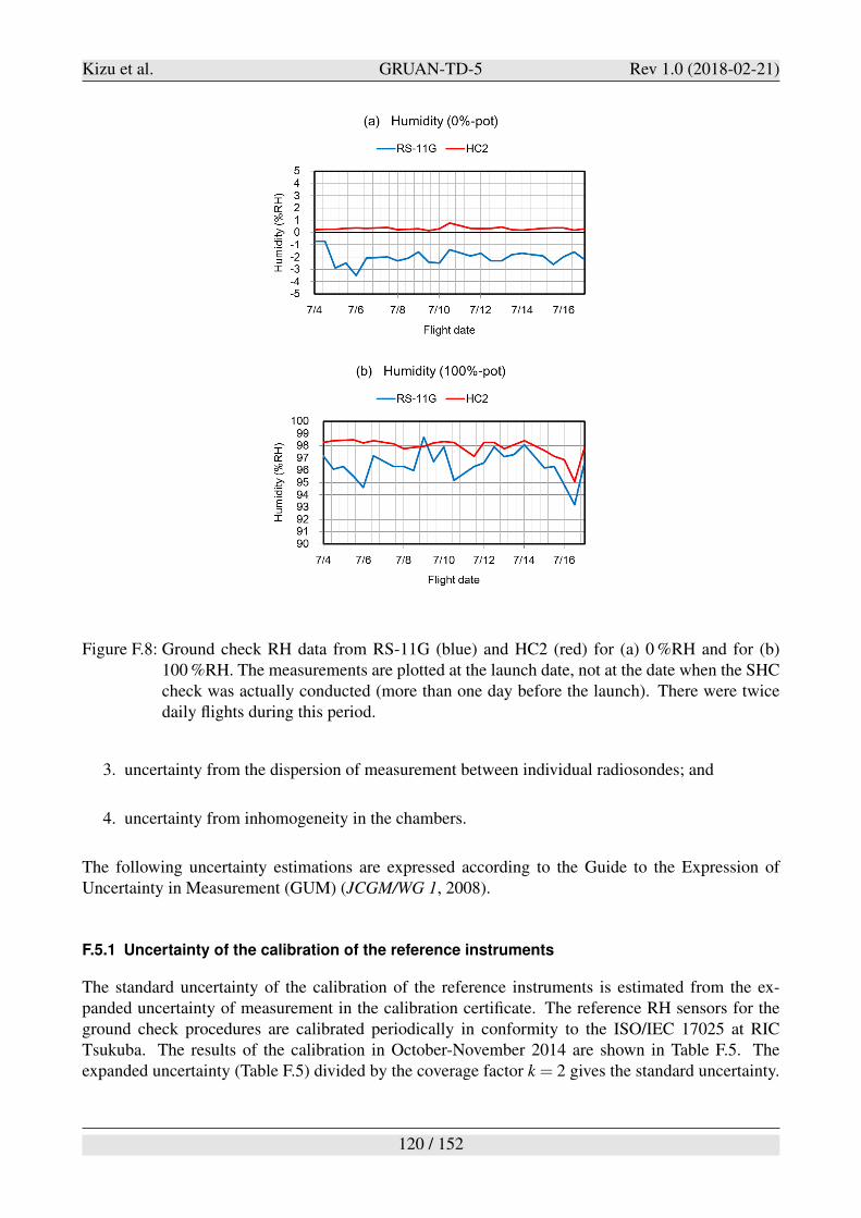
Kizu et al. GRUAN-TD-5 Rev 1.0 (2018-02-21)
Figure F.8: Ground check RH data from RS-11G (blue) and HC2 (red) for (a) 0 %RH and for (b)100 %RH. The measurements are plotted at the launch date, not at the date when the SHCcheck was actually conducted (more than one day before the launch). There were twicedaily flights during this period.
3. uncertainty from the dispersion of measurement between individual radiosondes; and
4. uncertainty from inhomogeneity in the chambers.
The following uncertainty estimations are expressed according to the Guide to the Expression ofUncertainty in Measurement (GUM) (JCGM/WG 1, 2008).
F.5.1 Uncertainty of the calibration of the reference instruments
The standard uncertainty of the calibration of the reference instruments is estimated from the ex-panded uncertainty of measurement in the calibration certificate. The reference RH sensors for theground check procedures are calibrated periodically in conformity to the ISO/IEC 17025 at RICTsukuba. The results of the calibration in October-November 2014 are shown in Table F.5. Theexpanded uncertainty (Table F.5) divided by the coverage factor k = 2 gives the standard uncertainty.
120 / 152
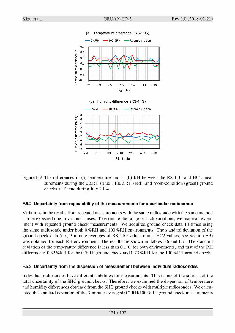
Kizu et al. GRUAN-TD-5 Rev 1.0 (2018-02-21)
Figure F.9: The differences in (a) temperature and in (b) RH between the RS-11G and HC2 mea-surements during the 0%RH (blue), 100%RH (red), and room-condition (green) groundchecks at Tateno during July 2014.
F.5.2 Uncertainty from repeatability of the measurements for a particular radiosonde
Variations in the results from repeated measurements with the same radiosonde with the same methodcan be expected due to various causes. To estimate the range of such variations, we made an exper-iment with repeated ground check measurements. We acquired ground check data 10 times usingthe same radiosonde under both 0 %RH and 100 %RH environments. The standard deviation of theground check data (i.e., 3-minute averages of RS-11G values minus HC2 values; see Section F.3)was obtained for each RH environment. The results are shown in Tables F.6 and F.7. The standarddeviation of the temperature difference is less than 0.1!C for both environments, and that of the RHdifference is 0.32 %RH for the 0 %RH ground check and 0.73 %RH for the 100 %RH ground check.
F.5.3 Uncertainty from the dispersion of measurement between individual radiosondes
Individual radiosondes have different stabilities for measurements. This is one of the sources of thetotal uncertainty of the SHC ground checks. Therefore, we examined the dispersion of temperatureand humidity differences obtained from the SHC ground checks with multiple radiosondes. We calcu-lated the standard deviation of the 3-minute-averaged 0 %RH/100 %RH ground check measurements
121 / 152
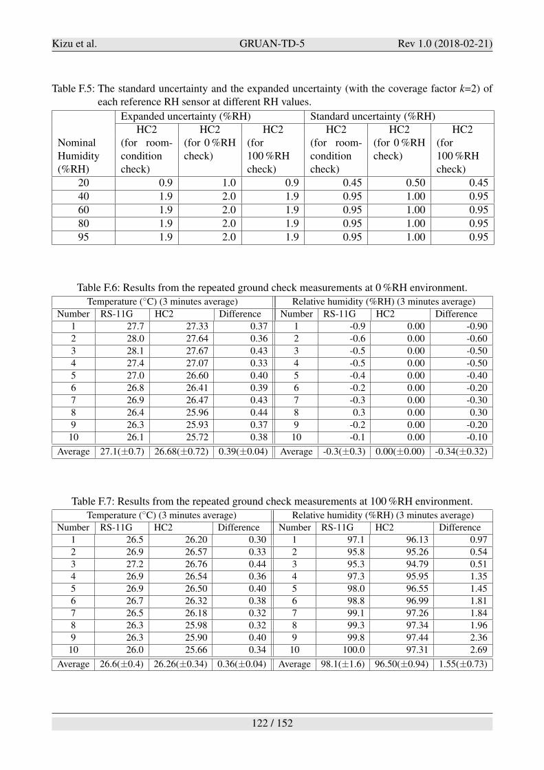
Kizu et al. GRUAN-TD-5 Rev 1.0 (2018-02-21)
Table F.5: The standard uncertainty and the expanded uncertainty (with the coverage factor k=2) ofeach reference RH sensor at different RH values.
Expanded uncertainty (%RH) Standard uncertainty (%RH)HC2 HC2 HC2 HC2 HC2 HC2
NominalHumidity(%RH)
(for room-conditioncheck)
(for 0 %RHcheck)
(for100 %RHcheck)
(for room-conditioncheck)
(for 0 %RHcheck)
(for100 %RHcheck)
20 0.9 1.0 0.9 0.45 0.50 0.45
40 1.9 2.0 1.9 0.95 1.00 0.95
60 1.9 2.0 1.9 0.95 1.00 0.95
80 1.9 2.0 1.9 0.95 1.00 0.95
95 1.9 2.0 1.9 0.95 1.00 0.95
Table F.6: Results from the repeated ground check measurements at 0 %RH environment.
Temperature (!C) (3 minutes average) Relative humidity (%RH) (3 minutes average)
Number RS-11G HC2 Difference Number RS-11G HC2 Difference
1 27.7 27.33 0.37 1 -0.9 0.00 -0.90
2 28.0 27.64 0.36 2 -0.6 0.00 -0.60
3 28.1 27.67 0.43 3 -0.5 0.00 -0.50
4 27.4 27.07 0.33 4 -0.5 0.00 -0.50
5 27.0 26.60 0.40 5 -0.4 0.00 -0.40
6 26.8 26.41 0.39 6 -0.2 0.00 -0.20
7 26.9 26.47 0.43 7 -0.3 0.00 -0.30
8 26.4 25.96 0.44 8 0.3 0.00 0.30
9 26.3 25.93 0.37 9 -0.2 0.00 -0.20
10 26.1 25.72 0.38 10 -0.1 0.00 -0.10
Average 27.1(±0.7) 26.68(±0.72) 0.39(±0.04) Average -0.3(±0.3) 0.00(±0.00) -0.34(±0.32)
Table F.7: Results from the repeated ground check measurements at 100 %RH environment.
Temperature (!C) (3 minutes average) Relative humidity (%RH) (3 minutes average)
Number RS-11G HC2 Difference Number RS-11G HC2 Difference
1 26.5 26.20 0.30 1 97.1 96.13 0.97
2 26.9 26.57 0.33 2 95.8 95.26 0.54
3 27.2 26.76 0.44 3 95.3 94.79 0.51
4 26.9 26.54 0.36 4 97.3 95.95 1.35
5 26.9 26.50 0.40 5 98.0 96.55 1.45
6 26.7 26.32 0.38 6 98.8 96.99 1.81
7 26.5 26.18 0.32 7 99.1 97.26 1.84
8 26.3 25.98 0.32 8 99.3 97.34 1.96
9 26.3 25.90 0.40 9 99.8 97.44 2.36
10 26.0 25.66 0.34 10 100.0 97.31 2.69
Average 26.6(±0.4) 26.26(±0.34) 0.36(±0.04) Average 98.1(±1.6) 96.50(±0.94) 1.55(±0.73)
122 / 152
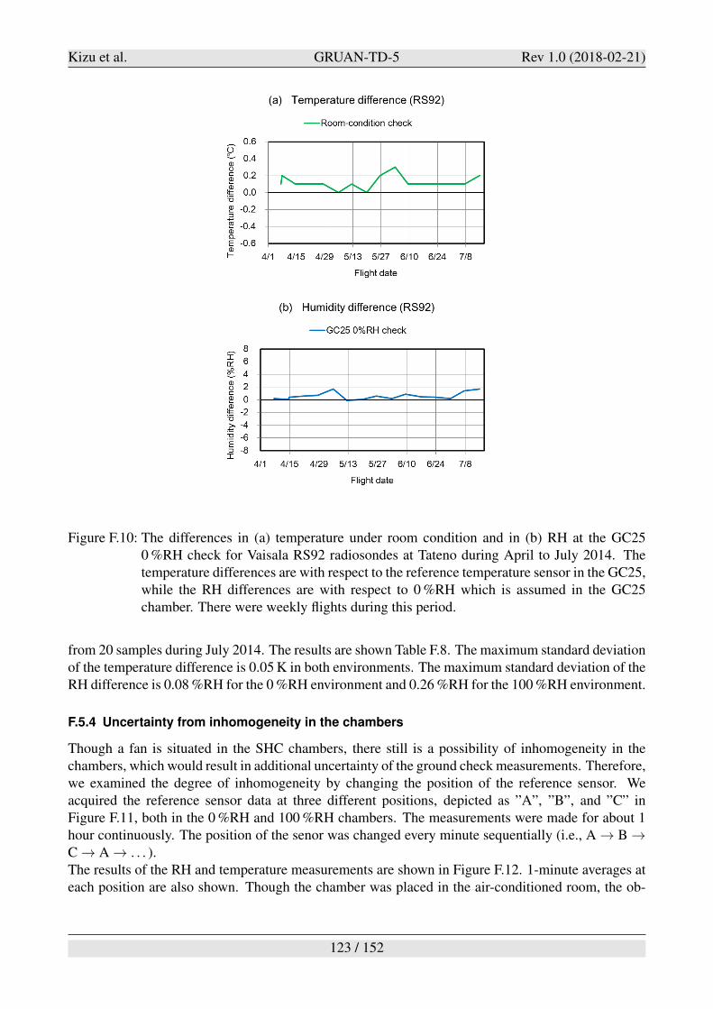
Kizu et al. GRUAN-TD-5 Rev 1.0 (2018-02-21)
Figure F.10: The differences in (a) temperature under room condition and in (b) RH at the GC250 %RH check for Vaisala RS92 radiosondes at Tateno during April to July 2014. Thetemperature differences are with respect to the reference temperature sensor in the GC25,while the RH differences are with respect to 0 %RH which is assumed in the GC25chamber. There were weekly flights during this period.
from 20 samples during July 2014. The results are shown Table F.8. The maximum standard deviationof the temperature difference is 0.05 K in both environments. The maximum standard deviation of theRH difference is 0.08 %RH for the 0 %RH environment and 0.26 %RH for the 100 %RH environment.
F.5.4 Uncertainty from inhomogeneity in the chambers
Though a fan is situated in the SHC chambers, there still is a possibility of inhomogeneity in thechambers, which would result in additional uncertainty of the ground check measurements. Therefore,we examined the degree of inhomogeneity by changing the position of the reference sensor. Weacquired the reference sensor data at three different positions, depicted as ”A”, ”B”, and ”C” inFigure F.11, both in the 0 %RH and 100 %RH chambers. The measurements were made for about 1hour continuously. The position of the senor was changed every minute sequentially (i.e., A - B -C - A - . . . ).The results of the RH and temperature measurements are shown in Figure F.12. 1-minute averages ateach position are also shown. Though the chamber was placed in the air-conditioned room, the ob-
123 / 152
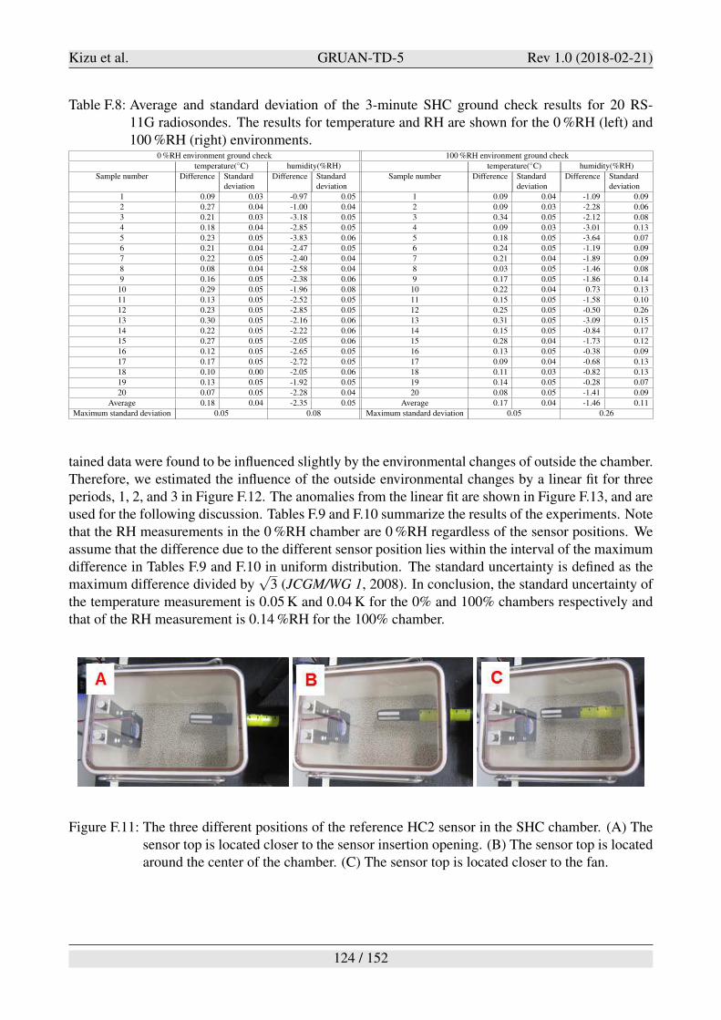
Kizu et al. GRUAN-TD-5 Rev 1.0 (2018-02-21)
Table F.8: Average and standard deviation of the 3-minute SHC ground check results for 20 RS-11G radiosondes. The results for temperature and RH are shown for the 0 %RH (left) and100 %RH (right) environments.
0 %RH environment ground check 100 %RH environment ground check
temperature(!C) humidity(%RH) temperature(!C) humidity(%RH)
Sample number Difference Standarddeviation
Difference Standarddeviation
Sample number Difference Standarddeviation
Difference Standarddeviation
1 0.09 0.03 -0.97 0.05 1 0.09 0.04 -1.09 0.09
2 0.27 0.04 -1.00 0.04 2 0.09 0.03 -2.28 0.06
3 0.21 0.03 -3.18 0.05 3 0.34 0.05 -2.12 0.08
4 0.18 0.04 -2.85 0.05 4 0.09 0.03 -3.01 0.13
5 0.23 0.05 -3.83 0.06 5 0.18 0.05 -3.64 0.07
6 0.21 0.04 -2.47 0.05 6 0.24 0.05 -1.19 0.09
7 0.22 0.05 -2.40 0.04 7 0.21 0.04 -1.89 0.09
8 0.08 0.04 -2.58 0.04 8 0.03 0.05 -1.46 0.08
9 0.16 0.05 -2.38 0.06 9 0.17 0.05 -1.86 0.14
10 0.29 0.05 -1.96 0.08 10 0.22 0.04 0.73 0.13
11 0.13 0.05 -2.52 0.05 11 0.15 0.05 -1.58 0.10
12 0.23 0.05 -2.85 0.05 12 0.25 0.05 -0.50 0.26
13 0.30 0.05 -2.16 0.06 13 0.31 0.05 -3.09 0.15
14 0.22 0.05 -2.22 0.06 14 0.15 0.05 -0.84 0.17
15 0.27 0.05 -2.05 0.06 15 0.28 0.04 -1.73 0.12
16 0.12 0.05 -2.65 0.05 16 0.13 0.05 -0.38 0.09
17 0.17 0.05 -2.72 0.05 17 0.09 0.04 -0.68 0.13
18 0.10 0.00 -2.05 0.06 18 0.11 0.03 -0.82 0.13
19 0.13 0.05 -1.92 0.05 19 0.14 0.05 -0.28 0.07
20 0.07 0.05 -2.28 0.04 20 0.08 0.05 -1.41 0.09
Average 0.18 0.04 -2.35 0.05 Average 0.17 0.04 -1.46 0.11
Maximum standard deviation 0.05 0.08 Maximum standard deviation 0.05 0.26
tained data were found to be influenced slightly by the environmental changes of outside the chamber.Therefore, we estimated the influence of the outside environmental changes by a linear fit for threeperiods, 1, 2, and 3 in Figure F.12. The anomalies from the linear fit are shown in Figure F.13, and areused for the following discussion. Tables F.9 and F.10 summarize the results of the experiments. Notethat the RH measurements in the 0 %RH chamber are 0 %RH regardless of the sensor positions. Weassume that the difference due to the different sensor position lies within the interval of the maximumdifference in Tables F.9 and F.10 in uniform distribution. The standard uncertainty is defined as themaximum difference divided by
%3 (JCGM/WG 1, 2008). In conclusion, the standard uncertainty of
the temperature measurement is 0.05 K and 0.04 K for the 0% and 100% chambers respectively andthat of the RH measurement is 0.14 %RH for the 100% chamber.
Figure F.11: The three different positions of the reference HC2 sensor in the SHC chamber. (A) Thesensor top is located closer to the sensor insertion opening. (B) The sensor top is locatedaround the center of the chamber. (C) The sensor top is located closer to the fan.
124 / 152
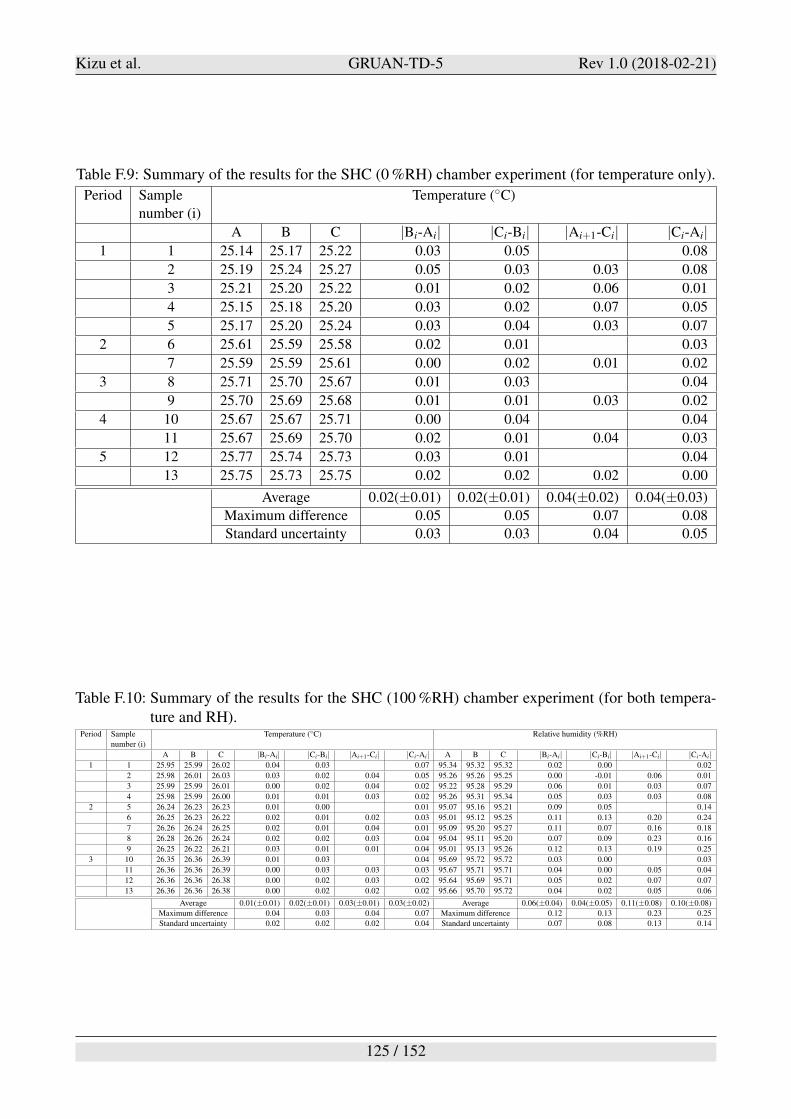
Kizu et al. GRUAN-TD-5 Rev 1.0 (2018-02-21)
Table F.9: Summary of the results for the SHC (0 %RH) chamber experiment (for temperature only).
Period Sample
number (i)
Temperature (!C)
A B C |Bi-Ai| |Ci-Bi| |Ai+1-Ci| |Ci-Ai|1 1 25.14 25.17 25.22 0.03 0.05 0.08
2 25.19 25.24 25.27 0.05 0.03 0.03 0.08
3 25.21 25.20 25.22 0.01 0.02 0.06 0.01
4 25.15 25.18 25.20 0.03 0.02 0.07 0.05
5 25.17 25.20 25.24 0.03 0.04 0.03 0.07
2 6 25.61 25.59 25.58 0.02 0.01 0.03
7 25.59 25.59 25.61 0.00 0.02 0.01 0.02
3 8 25.71 25.70 25.67 0.01 0.03 0.04
9 25.70 25.69 25.68 0.01 0.01 0.03 0.02
4 10 25.67 25.67 25.71 0.00 0.04 0.04
11 25.67 25.69 25.70 0.02 0.01 0.04 0.03
5 12 25.77 25.74 25.73 0.03 0.01 0.04
13 25.75 25.73 25.75 0.02 0.02 0.02 0.00
Average 0.02(±0.01) 0.02(±0.01) 0.04(±0.02) 0.04(±0.03)
Maximum difference 0.05 0.05 0.07 0.08
Standard uncertainty 0.03 0.03 0.04 0.05
Table F.10: Summary of the results for the SHC (100 %RH) chamber experiment (for both tempera-ture and RH).
Period Sample
number (i)
Temperature (!C) Relative humidity (%RH)
A B C |Bi-Ai| |Ci-Bi| |Ai+1-Ci| |Ci-Ai| A B C |Bi-Ai| |Ci-Bi| |Ai+1-Ci| |Ci-Ai|1 1 25.95 25.99 26.02 0.04 0.03 0.07 95.34 95.32 95.32 0.02 0.00 0.02
2 25.98 26.01 26.03 0.03 0.02 0.04 0.05 95.26 95.26 95.25 0.00 -0.01 0.06 0.01
3 25.99 25.99 26.01 0.00 0.02 0.04 0.02 95.22 95.28 95.29 0.06 0.01 0.03 0.07
4 25.98 25.99 26.00 0.01 0.01 0.03 0.02 95.26 95.31 95.34 0.05 0.03 0.03 0.08
2 5 26.24 26.23 26.23 0.01 0.00 0.01 95.07 95.16 95.21 0.09 0.05 0.14
6 26.25 26.23 26.22 0.02 0.01 0.02 0.03 95.01 95.12 95.25 0.11 0.13 0.20 0.24
7 26.26 26.24 26.25 0.02 0.01 0.04 0.01 95.09 95.20 95.27 0.11 0.07 0.16 0.18
8 26.28 26.26 26.24 0.02 0.02 0.03 0.04 95.04 95.11 95.20 0.07 0.09 0.23 0.16
9 26.25 26.22 26.21 0.03 0.01 0.01 0.04 95.01 95.13 95.26 0.12 0.13 0.19 0.25
3 10 26.35 26.36 26.39 0.01 0.03 0.04 95.69 95.72 95.72 0.03 0.00 0.03
11 26.36 26.36 26.39 0.00 0.03 0.03 0.03 95.67 95.71 95.71 0.04 0.00 0.05 0.04
12 26.36 26.36 26.38 0.00 0.02 0.03 0.02 95.64 95.69 95.71 0.05 0.02 0.07 0.07
13 26.36 26.36 26.38 0.00 0.02 0.02 0.02 95.66 95.70 95.72 0.04 0.02 0.05 0.06
Average 0.01(±0.01) 0.02(±0.01) 0.03(±0.01) 0.03(±0.02) Average 0.06(±0.04) 0.04(±0.05) 0.11(±0.08) 0.10(±0.08)
Maximum difference 0.04 0.03 0.04 0.07 Maximum difference 0.12 0.13 0.23 0.25
Standard uncertainty 0.02 0.02 0.02 0.04 Standard uncertainty 0.07 0.08 0.13 0.14
125 / 152
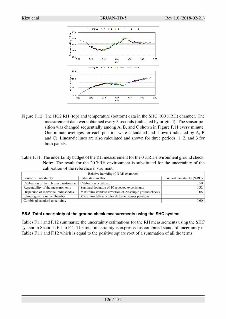
Kizu et al. GRUAN-TD-5 Rev 1.0 (2018-02-21)
Figure F.12: The HC2 RH (top) and temperature (bottom) data in the SHC(100 %RH) chamber. Themeasurement data were obtained every 5 seconds (indicated by original). The sensor po-sition was changed sequentially among A, B, and C shown in Figure F.11 every minute.One-minute averages for each position were calculated and shown (indicated by A, Band C). Linear-fit lines are also calculated and shown for three periods, 1, 2, and 3 forboth panels.
Table F.11: The uncertainty budget of the RH measurement for the 0 %RH environment ground check.Note: The result for the 20 %RH environment is substituted for the uncertainty of thecalibration of the reference instrument.
Relative humidity (0 %RH chamber)
Source of uncertainty Estimation method Standard uncertainty (%RH)
Calibration of the reference instrument Calibration certificate 0.50
Repeatability of the measurements Standard deviation of 10 repeated experiments 0.32
Dispersion of individual radiosondes Maximum standard deviation of 20 sample ground checks 0.08
Inhomogeneity in the chamber Maximum difference for different sensor positions
Combined standard uncertainty 0.60
F.5.5 Total uncertainty of the ground check measurements using the SHC system
Tables F.11 and F.12 summarize the uncertainty estimations for the RH measurements using the SHCsystem in Sections F.1 to F.4. The total uncertainty is expressed as combined standard uncertainty inTables F.11 and F.12 which is equal to the positive square root of a summation of all the terms.
126 / 152
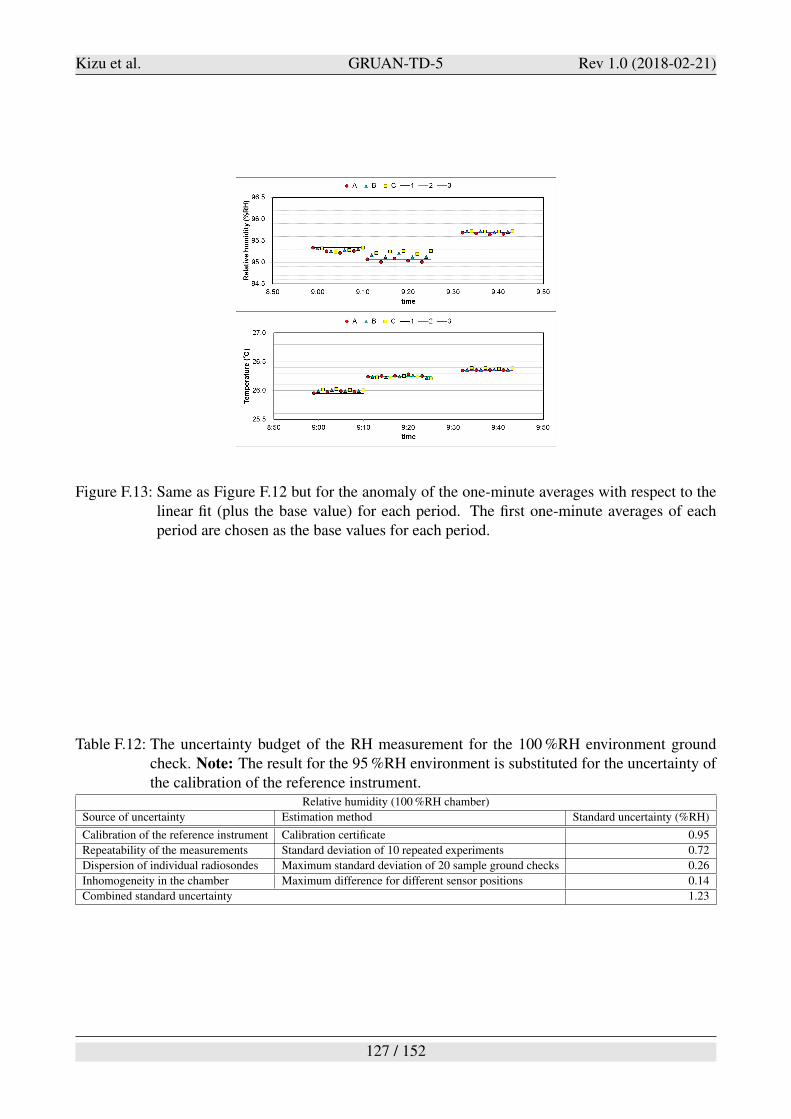
Kizu et al. GRUAN-TD-5 Rev 1.0 (2018-02-21)
Figure F.13: Same as Figure F.12 but for the anomaly of the one-minute averages with respect to thelinear fit (plus the base value) for each period. The first one-minute averages of eachperiod are chosen as the base values for each period.
Table F.12: The uncertainty budget of the RH measurement for the 100 %RH environment groundcheck. Note: The result for the 95 %RH environment is substituted for the uncertainty ofthe calibration of the reference instrument.
Relative humidity (100 %RH chamber)
Source of uncertainty Estimation method Standard uncertainty (%RH)
Calibration of the reference instrument Calibration certificate 0.95
Repeatability of the measurements Standard deviation of 10 repeated experiments 0.72
Dispersion of individual radiosondes Maximum standard deviation of 20 sample ground checks 0.26
Inhomogeneity in the chamber Maximum difference for different sensor positions 0.14
Combined standard uncertainty 1.23
127 / 152
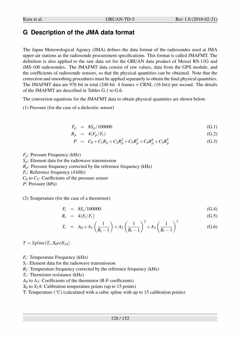
Kizu et al. GRUAN-TD-5 Rev 1.0 (2018-02-21)
G Description of the JMA data format
The Japan Meteorological Agency (JMA) defines the data format of the radiosondes used at JMAupper-air stations as the radiosonde procurement specifications. This format is called JMAFMT. Thedefinition is also applied to the raw data set for the GRUAN data product of Meisei RS-11G andiMS-100 radiosondes. The JMAFMT data consist of raw values, data from the GPS module, andthe coefficients of radiosonde sensors, so that the physical quantities can be obtained. Note that thecorrection and smoothing procedures must be applied separately to obtain the final physical quantities.The JMAFMT data are 976 bit in total (240 bit 4 frames + CRNL (16 bit)) per second. The detailsof the JMAFMT are described in Tables G.1 to G.6.
The conversion equations for the JMAFMT data to obtain physical quantities are shown below.
(1) Pressure (for the case of a dielectric sensor)
Fp = 8Sp/100000 (G.1)
Rp = 4(Fp/Fr) (G.2)
P = C0 +C1Rp +C2R2p +C3R3
p +C4R4p +C5R5
p (G.3)
Fp: Pressure Frequency (kHz)Sp: Element data for the radiowave transmissionRp: Pressure frequency corrected by the reference frequency (kHz)Fr: Reference frequency (4 kHz)C0 to C5: Coefficients of the pressure sensorP: Pressure (hPa)
(2) Temperature (for the case of a thermistor)
Ft = 8St/100000 (G.4)
Rt = 4(Ft/Fr) (G.5)
Tr = A0 +A1
$
1
Rt #1
%
+A2
$
1
Rt #1
%2
+A3
$
1
Rt #1
%3
(G.6)
T = Spline(Tr,X0toX14)
Ft : Temperature Frequency (kHz)St : Element data for the radiowave transmissionRt : Temperature frequency corrected by the reference frequency (kHz)Tr: Thermistor resistance (kHz)A0 to A3: Coefficients of the thermistor (R-F coefficients)X0 to X14: Calibration temperature points (up to 15 points)T: Temperature (!C) (calculated with a cubic spline with up to 15 calibration points)
128 / 152
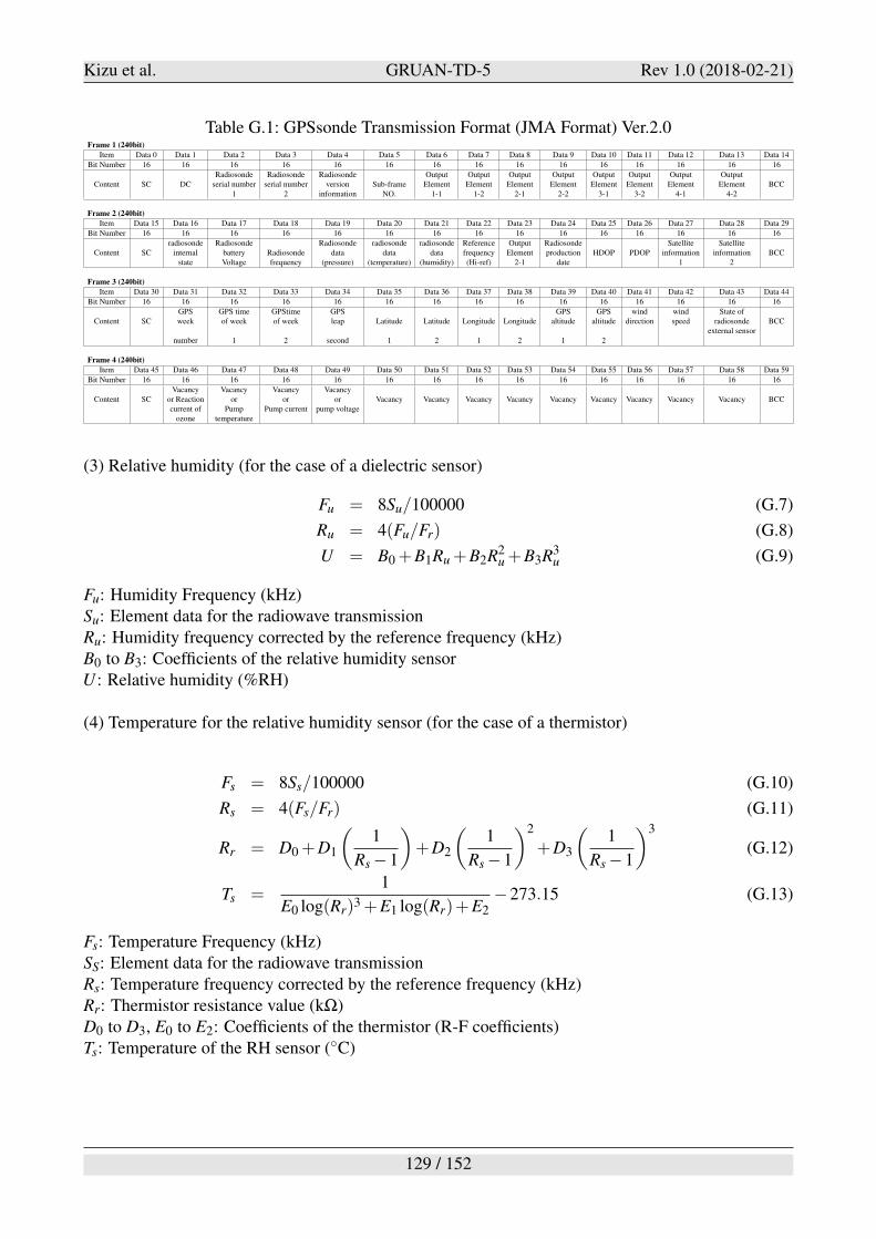
Kizu et al. GRUAN-TD-5 Rev 1.0 (2018-02-21)
Table G.1: GPSsonde Transmission Format (JMA Format) Ver.2.0Frame 1 (240bit)
Item Data 0 Data 1 Data 2 Data 3 Data 4 Data 5 Data 6 Data 7 Data 8 Data 9 Data 10 Data 11 Data 12 Data 13 Data 14
Bit Number 16 16 16 16 16 16 16 16 16 16 16 16 16 16 16
Radiosonde Radiosonde Radiosonde Output Output Output Output Output Output Output OutputContent SC DC serial number serial number version Sub-frame Element Element Element Element Element Element Element Element BCC
1 2 information NO. 1-1 1-2 2-1 2-2 3-1 3-2 4-1 4-2
Frame 2 (240bit)
Item Data 15 Data 16 Data 17 Data 18 Data 19 Data 20 Data 21 Data 22 Data 23 Data 24 Data 25 Data 26 Data 27 Data 28 Data 29
Bit Number 16 16 16 16 16 16 16 16 16 16 16 16 16 16 16
radiosonde Radiosonde Radiosonde radiosonde radiosonde Reference Output Radiosonde Satellite SatelliteContent SC internal battery Radiosonde data data data frequency Element production HDOP PDOP information information BCC
state Voltage frequency (pressure) (temperature) (humidity) (Hi-ref) 2-1 date 1 2
Frame 3 (240bit)
Item Data 30 Data 31 Data 32 Data 33 Data 34 Data 35 Data 36 Data 37 Data 38 Data 39 Data 40 Data 41 Data 42 Data 43 Data 44
Bit Number 16 16 16 16 16 16 16 16 16 16 16 16 16 16 16
GPS GPS time GPStime GPS GPS GPS wind wind State ofContent SC week of week of week leap Latitude Latitude Longitude Longitude altitude altitude direction speed radiosonde BCC
external sensornumber 1 2 second 1 2 1 2 1 2
Frame 4 (240bit)
Item Data 45 Data 46 Data 47 Data 48 Data 49 Data 50 Data 51 Data 52 Data 53 Data 54 Data 55 Data 56 Data 57 Data 58 Data 59
Bit Number 16 16 16 16 16 16 16 16 16 16 16 16 16 16 16
Vacancy Vacancy Vacancy VacancyContent SC or Reaction or or or Vacancy Vacancy Vacancy Vacancy Vacancy Vacancy Vacancy Vacancy Vacancy BCC
current of Pump Pump current pump voltageozone temperature
(3) Relative humidity (for the case of a dielectric sensor)
Fu = 8Su/100000 (G.7)
Ru = 4(Fu/Fr) (G.8)
U = B0 +B1Ru +B2R2u +B3R3
u (G.9)
Fu: Humidity Frequency (kHz)Su: Element data for the radiowave transmissionRu: Humidity frequency corrected by the reference frequency (kHz)B0 to B3: Coefficients of the relative humidity sensorU : Relative humidity (%RH)
(4) Temperature for the relative humidity sensor (for the case of a thermistor)
Fs = 8Ss/100000 (G.10)
Rs = 4(Fs/Fr) (G.11)
Rr = D0 +D1
$
1
Rs #1
%
+D2
$
1
Rs #1
%2
+D3
$
1
Rs #1
%3
(G.12)
Ts =1
E0 log(Rr)3 +E1 log(Rr)+E2#273.15 (G.13)
Fs: Temperature Frequency (kHz)SS: Element data for the radiowave transmissionRs: Temperature frequency corrected by the reference frequency (kHz)Rr: Thermistor resistance value (k")D0 to D3, E0 to E2: Coefficients of the thermistor (R-F coefficients)Ts: Temperature of the RH sensor (!C)
129 / 152
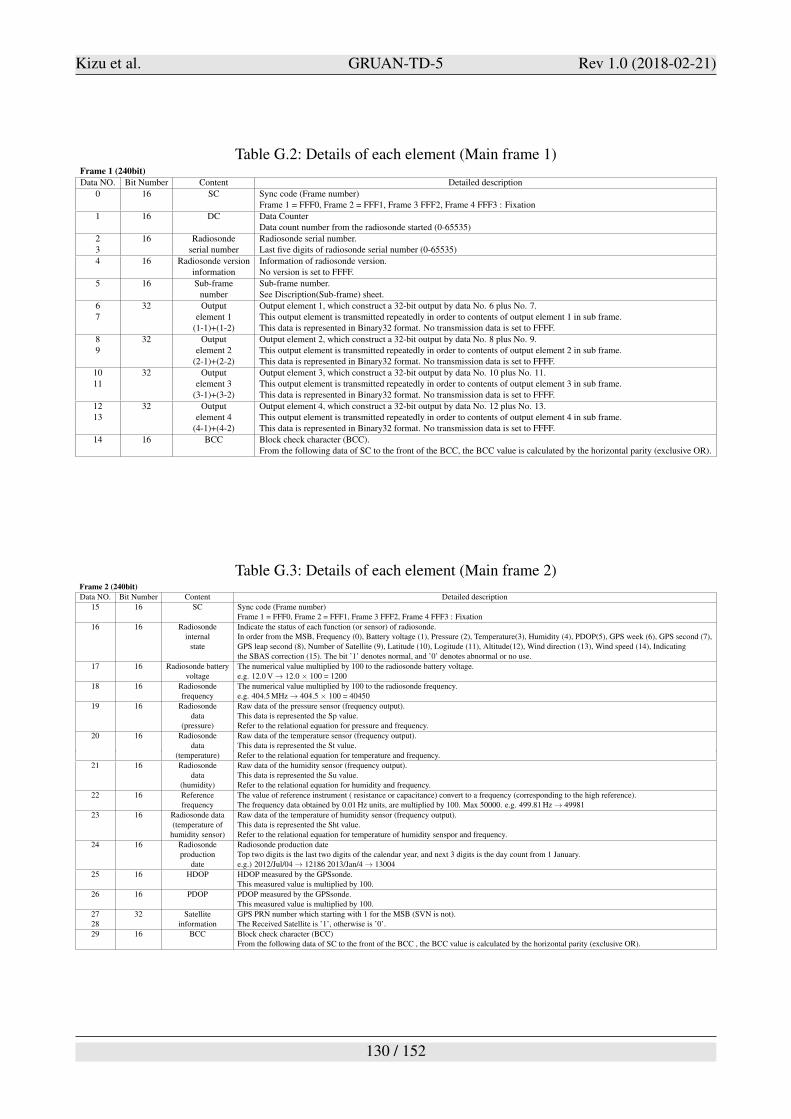
Kizu et al. GRUAN-TD-5 Rev 1.0 (2018-02-21)
Table G.2: Details of each element (Main frame 1)Frame 1 (240bit)
Data NO. Bit Number Content Detailed description
0 16 SC Sync code (Frame number)Frame 1 = FFF0, Frame 2 = FFF1, Frame 3 FFF2, Frame 4 FFF3 : Fixation
1 16 DC Data CounterData count number from the radiosonde started (0-65535)
2 16 Radiosonde Radiosonde serial number.3 serial number Last five digits of radiosonde serial number (0-65535)
4 16 Radiosonde version Information of radiosonde version.information No version is set to FFFF.
5 16 Sub-frame Sub-frame number.number See Discription(Sub-frame) sheet.
6 32 Output Output element 1, which construct a 32-bit output by data No. 6 plus No. 7.7 element 1 This output element is transmitted repeatedly in order to contents of output element 1 in sub frame.
(1-1)+(1-2) This data is represented in Binary32 format. No transmission data is set to FFFF.
8 32 Output Output element 2, which construct a 32-bit output by data No. 8 plus No. 9.9 element 2 This output element is transmitted repeatedly in order to contents of output element 2 in sub frame.
(2-1)+(2-2) This data is represented in Binary32 format. No transmission data is set to FFFF.
10 32 Output Output element 3, which construct a 32-bit output by data No. 10 plus No. 11.11 element 3 This output element is transmitted repeatedly in order to contents of output element 3 in sub frame.
(3-1)+(3-2) This data is represented in Binary32 format. No transmission data is set to FFFF.
12 32 Output Output element 4, which construct a 32-bit output by data No. 12 plus No. 13.13 element 4 This output element is transmitted repeatedly in order to contents of output element 4 in sub frame.
(4-1)+(4-2) This data is represented in Binary32 format. No transmission data is set to FFFF.
14 16 BCC Block check character (BCC).From the following data of SC to the front of the BCC, the BCC value is calculated by the horizontal parity (exclusive OR).
Table G.3: Details of each element (Main frame 2)Frame 2 (240bit)
Data NO. Bit Number Content Detailed description
15 16 SC Sync code (Frame number)Frame 1 = FFF0, Frame 2 = FFF1, Frame 3 FFF2, Frame 4 FFF3 : Fixation
16 16 Radiosonde Indicate the status of each function (or sensor) of radiosonde.internal In order from the MSB, Frequency (0), Battery voltage (1), Pressure (2), Temperature(3), Humidity (4), PDOP(5), GPS week (6), GPS second (7),
state GPS leap second (8), Number of Satellite (9), Latitude (10), Logitude (11), Altitude(12), Wind direction (13), Wind speed (14), Indicatingthe SBAS correction (15). The bit ’1’ denotes normal, and ’0’ denotes abnormal or no use.
17 16 Radiosonde battery The numerical value multiplied by 100 to the radiosonde battery voltage.voltage e.g. 12.0 V - 12.0 & 100 = 1200
18 16 Radiosonde The numerical value multiplied by 100 to the radiosonde frequency.frequency e.g. 404.5 MHz - 404.5 & 100 = 40450
19 16 Radiosonde Raw data of the pressure sensor (frequency output).data This data is represented the Sp value.
(pressure) Refer to the relational equation for pressure and frequency.
20 16 Radiosonde Raw data of the temperature sensor (frequency output).data This data is represented the St value.
(temperature) Refer to the relational equation for temperature and frequency.
21 16 Radiosonde Raw data of the humidity sensor (frequency output).data This data is represented the Su value.
(humidity) Refer to the relational equation for humidity and frequency.
22 16 Reference The value of reference instrument ( resistance or capacitance) convert to a frequency (corresponding to the high reference).frequency The frequency data obtained by 0.01 Hz units, are multiplied by 100. Max 50000. e.g. 499.81 Hz - 49981
23 16 Radiosonde data Raw data of the temperature of humidity sensor (frequency output).(temperature of This data is represented the Sht value.
humidity sensor) Refer to the relational equation for temperature of humidity senspor and frequency.
24 16 Radiosonde Radiosonde production dateproduction Top two digits is the last two digits of the calendar year, and next 3 digits is the day count from 1 January.
date e.g.) 2012/Jul/04 - 12186 2013/Jan/4 - 13004
25 16 HDOP HDOP measured by the GPSsonde.This measured value is multiplied by 100.
26 16 PDOP PDOP measured by the GPSsonde.This measured value is multiplied by 100.
27 32 Satellite GPS PRN number which starting with 1 for the MSB (SVN is not).28 information The Received Satellite is ’1’, otherwise is ’0’.
29 16 BCC Block check character (BCC)From the following data of SC to the front of the BCC , the BCC value is calculated by the horizontal parity (exclusive OR).
130 / 152
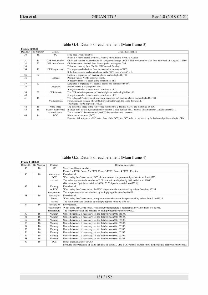
Kizu et al. GRUAN-TD-5 Rev 1.0 (2018-02-21)
Table G.4: Details of each element (Main frame 3)Frame 3 (240bit)
Data NO. Bit Number Content Detailed description
30 16 SC Sync code (Frame number)Frame 1 = FFF0, Frame 2 = FFF1, Frame 3 FFF2, Frame 4 FFF3 : Fixation
31 16 GPS week number GPS week number obtained from the navigation message of GPS. This week number start from zero week on August 22, 1999.
32 32 GPS time of week GPS time count obtained from the navigation message of GPS.33 This time count up from 00m00s UTC on each Sunday.
34 16 GPS leap second The leap seconds obtained from the navigation message of GPS.If the leap seconds has been included in the ”GPS time of week” is 0.
35 32 Latitude is expressed to 7 decimal places, and multiplied by 107.36 Latitude Positive values: North; negative: South.
A negative number is taken as the complement of 2.
37 32 Longitude is expressed to 7 decimal places, and multiplied by 107.38 Longitude Postive values: East; negative: West.
A negative number is taken as the complement of 2.
39 32 GPS altitude The GPS altitude expressed to 2 decimal places, and multiplied by 100.40 A negative number is taken as the complement of 2.
41 16 The radiosonde’s direction of movement expressed to 2 decimal places, and multiplied by 100.Wind direction For example, in the case of 360.00 degrees (north) wind, the sonde flows south.
This yields 180.00 degrees (=18000).
42 16 Wind speed The horizontal speed of the radiosonde expressed to 2 decimal places, and multiplied by 100.
43 16 State of Radiosonde In order from the MSB, external sensor number 0 (data number 46) ... external sensor number 12 (data number 58).external sensor The bit value ’1’ denotes normal, and ’0’ denotes abnormal or no use.
44 16 BCC Block check character (BCC)From the following data of SC to the front of the BCC , the BCC value is calculated by the horizontal parity (exclusive OR).
Table G.5: Details of each element (Main frame 4)Frame 4 (240bit)
Data NO. Bit Number Content Detailed description
45 16 SC Sync code (Frame number)Frame 1 = FFF0, Frame 2 = FFF1, Frame 3 FFF2, Frame 4 FFF3 : Fixation
46 16 Vacancy or Free channel.ECC When using the Ozone sonde, ECC electric current is represented by values from 0 to 65535.
current The value represents the number of 0.001µA units multiplied by 100, added with 10000.(For example: 0µA is encoded as 10000. 55.535 µA is encoded as 65535.).
47 16 Vacancy Free channel.or ECC When using the Ozone sonde, the ECC temperature is represented by values from 0 to 65535.
temperature The temperature data are obtained by multiplying this value by 0.01 K.
48 16 Vacancy or Free channel.Pump When using the Ozone sonde, pump motor electric current is represented by values from 0 to 65535.current The current data are obtained by multiplying this value by 0.01 mA.
49 16 Vacancy or Free channel.reaction tube When using the Ozone sonde, reaction tube temperature is represented by values from 0 to 65535.temperature The temperature data are obtained by multiplying this value by 0.01 K.
50 16 Vacancy Unused channel. If necessary, set the data between 0 to 65535.
51 16 Vacancy Unused channel. If necessary, set the data between 0 to 65535.
52 16 Vacancy Unused channel. If necessary, set the data between 0 to 65535.
53 16 Vacancy Unused channel. If necessary, set the data between 0 to 65535.
54 16 Vacancy Unused channel. If necessary, set the data between 0 to 65535.
55 16 Vacancy Unused channel. If necessary, set the data between 0 to 65535.
56 16 Vacancy Unused channel. If necessary, set the data between 0 to 65535.
57 16 Vacancy Unused channel. If necessary, set the data between 0 to 65535.
58 16 Vacancy Unused channel. If necessary, set the data between 0 to 65535.
59 16 BCC Block check character (BCC)From the following data of SC to the front of the BCC , the BCC value is calculated by the horizontal parity (exclusive OR).
131 / 152
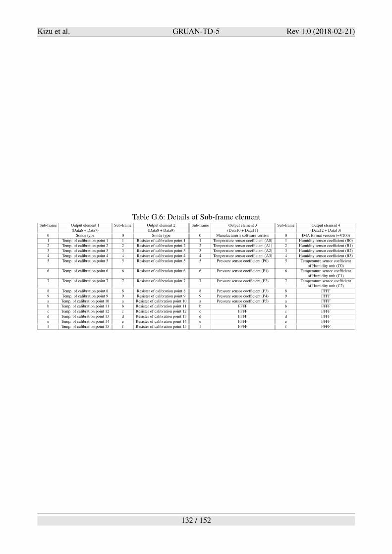
Kizu et al. GRUAN-TD-5 Rev 1.0 (2018-02-21)
Table G.6: Details of Sub-frame elementSub-frame Output element 1 Sub-frame Output element 2 Sub-frame Output element 3 Sub-frame Output element 4
(Data6 + Data7) (Data8 + Data9) (Data10 + Data11) (Data12 + Data13)
0 Sonde type 0 Sonde type 0 Manufacturer’s software version 0 JMA format version (=V200)
1 Temp. of calibration point 1 1 Resister of calibration point 1 1 Temperature sensor coefficient (A0) 1 Humidity sensor coefficient (B0)
2 Temp. of calibration point 2 2 Resister of calibration point 2 2 Temperature sensor coefficient (A1) 2 Humidity sensor coefficient (B1)
3 Temp. of calibration point 3 3 Resister of calibration point 3 3 Temperature sensor coefficient (A2) 3 Humidity sensor coefficient (B2)
4 Temp. of calibration point 4 4 Resister of calibration point 4 4 Temperature sensor coefficient (A3) 4 Humidity sensor coefficient (B3)
5 Temp. of calibration point 5 5 Resister of calibration point 5 5 Pressure sensor coefficient (P0) 5 Temperature sensor coefficientof Humidity unit (C0)
6 Temp. of calibration point 6 6 Resister of calibration point 6 6 Pressure sensor coefficient (P1) 6 Temperature sensor coefficientof Humidity unit (C1)
7 Temp. of calibration point 7 7 Resister of calibration point 7 7 Pressure sensor coefficient (P2) 7 Temperature sensor coefficientof Humidity unit (C2)
8 Temp. of calibration point 8 8 Resister of calibration point 8 8 Pressure sensor coefficient (P3) 8 FFFF
9 Temp. of calibration point 9 9 Resister of calibration point 9 9 Pressure sensor coefficient (P4) 9 FFFF
a Temp. of calibration point 10 a Resister of calibration point 10 a Pressure sensor coefficient (P5) a FFFF
b Temp. of calibration point 11 b Resister of calibration point 11 b FFFF b FFFF
c Temp. of calibration point 12 c Resister of calibration point 12 c FFFF c FFFF
d Temp. of calibration point 13 d Resister of calibration point 13 d FFFF d FFFF
e Temp. of calibration point 14 e Resister of calibration point 14 e FFFF e FFFF
f Temp. of calibration point 15 f Resister of calibration point 15 f FFFF f FFFF
132 / 152
Kizu et al. GRUAN-TD-5 Rev 1.0 (2018-02-21)
H Actual procedures to create the GRUAN data product for the
RS-11G and iMS-100 radiosondes
This section describes the workflow for creating the GRUAN data product (GDP). The overview ofthe workflow is illustrated in Figure H.1.
H.1 The data files
The JMAFMT data file (containing raw data and sensor-coefficient data) and the GRUAN Meta Datafile (GMD; containing the meta-data) for each sounding are submitted from a GRUAN site (e.g.,Tateno) to the GRAUN Lead Centre. The GRUAN Lead Centre publishes the GRUAN processingticket (GPT) file for each sounding, which contains the Product ID and Ascent ID of the sounding.Tateno downloads the JMAFMT, GMD, and GPT files that are used to create the GRUAN DataProduct (GDP).
H.2 Loading meta data
From the GMD file, the following information is loaded: The date and time of the launch; measuring-system information; serial number of the sonde; list of the instruments; results of the GC checks;results of the SHC check; surface data at the launch; and the site name. The list of the instruments con-tains the filling weight of the balloon and the length of the unwinder or of the string. The informationon latitude, longitude, altitude of the site is loaded from the meta-data file from the RSLaunchClientwhich is the software for submitting data to the GRUAN Lead Centre.
H.3 Loading raw data
From the JMAFMT file, the following information and data are loaded: The sonde type; version ofthe JMAFMT file; raw frequency data, GPS time data, GPS position data (latitude, longitude, andaltitude), GPS wind data, and the calibration coefficient data to calculate air temperature (An), RH(Bn), and the RH sensor temperature (Cn; for the case of iMS-100 radiosondes).
H.4 Re-calibration of the RH coefficients using SHC data
At the factory, the RH sensors were calibrated at 15 %RH, 30 %RH, 50 %RH, 70 %RH, 90 %RH,and 95 %RH, and the original calibration coefficients (Bn) were determined. The frequency data for0 %RH and 100 %RH during the SHC checks are calculated using the original coefficients, and byadding these SHC calibration information, a set of new calibration coefficients are obtained.
H.5 Obtaining initial ascending data
Raw frequency data are converted to raw air temperature data Traw (Appendix B), raw RH data Uraw
(Appendix C), and raw RH sensor temperature data T sraw for the case of iMS-100 (Appendix C).GPS wind (speed and direction) data are converted to zonal and meridional wind data, uraw and vraw,respectively. Raw geopotential height data, geopotraw are calculated using GPS height data, altraw
and GPS latitude data (Section 3.3). GPS latitude data, latraw and longitude data, lonraw are obtainedfrom GPS position data. Information on the launch time and the burst altitude is also obtained from
133 / 152
Kizu et al. GRUAN-TD-5 Rev 1.0 (2018-02-21)
GPS data. The time launched the balloon and the burst point are obtained from altraw. The ascendingdata set, between the launch and the balloon burst, is extracted from the raw data set. Finally, fillingmeasurement-missing fields by linear interpolation using adjacent measurements, the initial data set(T0, U0, T s0, u0, v0, geopot0, alt0, lat0, and lon0) is obtained.
H.6 Calculation of geopotential height and ascending rate
The interpolated GPS altitude alt0 is converted the corrected altitude alt1 in consideration the offsetbetween alt0 at the release time and the release altitude, ! alt.
alt1 = alt0 #!alt (H.1)
The moving averages of alt1 within ±30 seconds are calculated to obtain the final GPS altitude data,alt f in. The uncertainty of the GPS altitude u(alt) is calculated by the composition with the uncertaintyby the raw GPS altitude from PDOP, uGPS (alt), and the uncertainty by the moving average, uma (alt),(Section 3.3). The estimated standard uncertainty of smoothed (moving averaged or low-pass filtered)data are calculated using the method written in Appendix A of Dirksen et al. (2014) as
N* =
4
M
%j=#M
h2j
5#1
(H.2)
u(si) =
6
7
7
8
N*
N* #1
M
%j=#M
h2j(si+ j # si)2 (H.3)
where M is the half-width of the filter window (30 for the case of ±30 s moving average of 1-sec-resolution data), h is the normalized weight coefficient, and s is the value before filtering and s is thevalue filtered. N* is the parameter called as the effective sample size.
The final geopotential height data, geopot f in is derived from alt f in and lat0. The ascending rate data,asc, are derived from the time difference of geopot f in as
asc =
-
0 (t = 0)geopot f in(t)#geopot f in(t #1) (t > 0)
(H.4)
H.7 Calculation of temperature
If the length of the string or the unwinder is equal to or less than 10 m, the temperature spike filteringis applied when the pressure is below 30 hPa. For this filtering and the radiation correction (will bediscussed below), the provisional pressure P1 are derived using T0, U0, surface pressure data, Psur f ,and geopot f in (Section 3.1). T1, the temperature after spike filtering, equals to T0 if the filter is notneeded. The uncertainty with this filtering is uspike(T).
The moving averages of T1 within ±1 second are calculated to obtain the uncorrected temperaturedata, T2 and the standard uncertainty of temperature, uma (T). The amount of the radiation correction,Tcor is calculated using T2,P1,Psur f , asc, GPS time, lat0, and lon0. Tcor is subtracted from T2 to obtainthe final temperature data, Tf in.
The total uncertainty of the temperature u(T ) is also calculated (Section 3.1).
134 / 152
Kizu et al. GRUAN-TD-5 Rev 1.0 (2018-02-21)
The correlated uncertainty of the temperature ucor (T) is calculated from the uncertainties by albedoualbedo (T), by ventilation uventilation (T), and by calibration uT calib1 (T) and uT calib2 (T).
ualbedo (T) is derived from the difference between the radiation correction values with albedo of 0.1and with albedo of 0.6.
ualbedo(T ) =1
2%
3|Tcor(albedo = 0.6)#Tcor(albedo = 0.1)| (H.5)
uventilation (T) is derived from the difference between radiation correction values with ventilation ofasc + 3.0 m s#1 and with ventilation of asc.
uventilation(T ) =1%3|Tcor(v = asc+3)#Tcor(v = asc)| (H.6)
The total, correlated uncertainty becomes:
ucor(T ) =#
(u2T calib1 +u2
T calib2 +ualbedo(T )2 +uventilation(T )2 +uspike(T )2 (H.7)
Finally, the total uncertainty of the temperature u(T ) is derived as
u(T ) =#
(ucor(T )2 +ustd(T )2) (H.8)
H.8 Calculation of the temperature of the RH sensor
For the RS-11G radiosonde, the uncorrected RH sensor temperature data, T s0 is derived from Tf in,P1, Psur f , and asc (Appendix C). The corrected RH sensor temperature data, T s f in is obtained byconsidering the thermal lag and solar radiative heating from Tf in,P1, and T s0 (Appendix C). T s f in isused in the corrections of RH.
H.9 Calculation of RH
The response time %U is estimated from T s f in (Section 3.2). U0 are separated into low and high fre-quency components, U1low and U1high, respectively, by the digital filter (Appendix E) whose cutoffperiod is set as four times of Tpendulum. The statistical uncertainty for this step is written as ustd1(U).The time-lag correction is applied to the both components to obtain U2low and U2high. The contamina-tion correction is applied to U2high to obtain U3high, and the statistical uncertainty for this is ustd3 (U).Moving averages for ±90 seconds are taken for U3high to obtain U4high with the statistical uncertainty,ustd4(U). The corrected high frequency component U4high and the low frequency component U2low
are composed to obtain U4. The TUD correction using T s f in is applied to U4 to obtain U5. Finally, theTs/Ta correction is applied to U5 to obtain the final RH data, Uf in. If Uf in is less than 0% or greaterthan 100% RH, they are replaced with 0 %RH or 100 %RH, respectively.
The statistical uncertainty of RH, ustd (U) is calculated as
ustd(U) =#
ustd1(U)2 +ustd3(U)2 +ustd4(U)2 (H.9)
The correlated uncertainty of RH, ucor (U) is calculated from the uncertainties by the time-lag correc-tion, uT L (U), by TUD correction, uTUD (U), by the Ts/Ta correction, uT s (U), by the hysteresis of theRH sensor, uhysteresis (U), and by the calibration, uUcalib (U).
135 / 152
Kizu et al. GRUAN-TD-5 Rev 1.0 (2018-02-21)
uT L(U) is determined by the uncertainty of the response time, and is written as
uT L(U) =1
2%
3|U(% = %U +u(%U))#U(% = %U #u(%U))| (H.10)
uTUD(U) is a fixed value as uTUD(U) = 1.8 uT s(U) is determined by the uncertainty of the T s f in
whose uncertainty is assumed to be ±0.3 K, and thus is written as
uT s(U) =1
2%
3
9
9U(T s = T s f in +0.3)#U(T s = T s f in #0.3)9
9 (H.11)
Significant hysteresis appears only when RH is decreasing, so uhysteresis(U) is given as
uhystereis(U) =
3
0 (trend +#0.05%RHs#1)1.8%
3(trend <#0.05%RHs#1) (H.12)
where trend is a short-term trend in Uf in which is estimated as the slope of the tangent using theSavitzky-Golay method (Savitzky and Golay, 1964) with ±10 s values. The threshold value of -0.05 %RH s#1 (i.e., almost constant vertically) is determined empirically.
ucor(U) and the total uncertainty, u(U) are calculated as
ucor(U) =#
(uT L(U)2 +uTUD(U)2 +uT s(U)2 +uhysteresis(U)2 +u2Ucalib (H.13)
and
u(U) =#
ucor(U)2 +ustd(U)2 (H.14)
respectively.
H.10 Calculation of pressure
The final pressure data, Pf in are calculated from geopot f in, Tf in, Uf in, and Psur f (Section 3.3).
The correlated uncertainty of the pressure is calculated from the uncertainties by the surface pressure,upsur f (P), by GPS altitude, ualt (P), by temperature, utemp (P) and by RH uRH (P).
upsur f (P) is calculated in the consideration of Psur f with the error, u(Psur f ).
ualt(P),utemp(P),uRH(P), and the totally uncertainty u(P) as:
ualt(P) =1
2%
3|P(Tf in,Uf in,alt #u(alt))#P(Tf in,Uf in,alt +u(alt))| (H.15)
utemp(P) =1
2%
3|P(Tf in +u(T ),Uf in,alt)#P(Tf in #u(T ),Uf in,alt)| (H.16)
uRH(P) =1
2%
3|P(Tf in,Uf in +u(U),alt)#P(Tf in,Uf in #u(U),alt)| (H.17)
u(P) =#
u2psur f (P)+u2
alt(P)+u2temp(P)+u2
RH(P) (H.18)
respectively.
136 / 152
Kizu et al. GRUAN-TD-5 Rev 1.0 (2018-02-21)
H.11 Calculation of horizontal wind
The final zonal wind data, u f in and the final meridional wind data, v f in are derived from u0 andv0 using the low-pass filter with the cutoff frequency as 1/Tpendulum (Appendix E). The statisticaluncertainties, ustd(u) and ustd(v) are also calculated. The final wind speed data, wspeed f in and thefinal wind direction data, wdir f in are derived from u f in and v f in. The uncertainty of wind speed,u(wspeed) and the uncertainty of wind direction, u(wdir) are calculated using Equations 27 and 28 inDirksen et al. (2014) as
u(wspeed) =
'
(u ·ustd(u))2 +(v ·ustd(v))2
u2 + v2(H.19)
u(wdir) =180
+
:
(ustd(u)2 +ustd(v)2
(1+ uv
2) |v|(H.20)
H.12 Calculation of other derived data
In the GDP file, dewpoint/frostpoint temperature, FP, water vapor volume mixing ratio, WVMR, andprecipitable water vapor (or the column amount of water vapor), PWV are also stored as the deriveddata. The saturation vapor pressure for air temperature T [K], es(T ) [hPa], is calculated as (by Hyland
and Wexler (1983)):ln(100es(T )) = #0.58002206&104/T
+0.13914993 ·10
#0.48640239 ·10#1 &T
+0.41764768 ·10#4 &T 2
#0.14452093 ·10#7 &T 3
+0.65459673 ·10& lnT
(H.21)
FP is derived by solving the equation below:
es(FP) = es(Tf in)&0.01Uf in (H.22)
WVMR is derived from FP and Pf in as
WV MR =es(FP)
Pf in=
es(Tf in)&0.01Uf in
Pf in(H.23)
The mixing ratio by weight mr is derived from
mr = 0.622es(FP)
Pf in # es(FP)= 0.622
es(Tf in)&0.01Uf in
Pf in # es(Tf in)&0.01Uf in(H.24)
PWV is derived from the integration of mr as
PWV =1
g
( Pbp
Psur f
mrd p (H.25)
where Psur f and Pbp are the pressures at the surface and at the burst point, respectively. In practice,PWV is calculated as
137 / 152
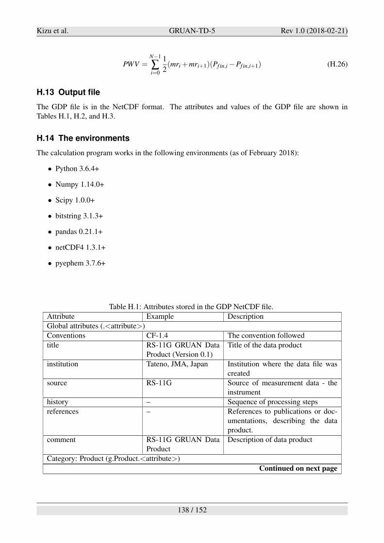
Kizu et al. GRUAN-TD-5 Rev 1.0 (2018-02-21)
PWV =N#1
%i=0
1
2(mri +mri+1)(Pf in,i #Pf in,i+1) (H.26)
H.13 Output file
The GDP file is in the NetCDF format. The attributes and values of the GDP file are shown inTables H.1, H.2, and H.3.
H.14 The environments
The calculation program works in the following environments (as of February 2018):
• Python 3.6.4+
• Numpy 1.14.0+
• Scipy 1.0.0+
• bitstring 3.1.3+
• pandas 0.21.1+
• netCDF4 1.3.1+
• pyephem 3.7.6+
Table H.1: Attributes stored in the GDP NetCDF file.
Attribute Example Description
Global attributes (.<attribute>)
Conventions CF-1.4 The convention followed
title RS-11G GRUAN DataProduct (Version 0.1)
Title of the data product
institution Tateno, JMA, Japan Institution where the data file wascreated
source RS-11G Source of measurement data - theinstrument
history – Sequence of processing steps
references – References to publications or doc-umentations, describing the dataproduct.
comment RS-11G GRUAN DataProduct
Description of data product
Category: Product (g.Product.<attribute>)
Continued on next page
138 / 152
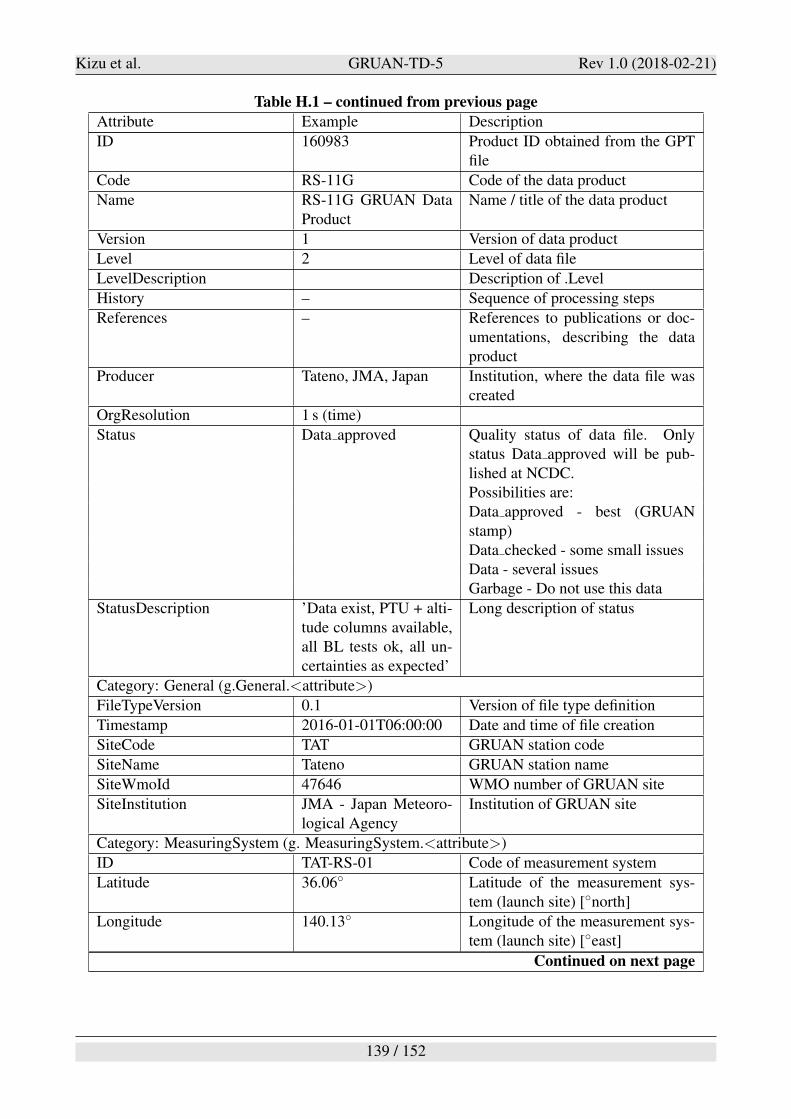
Kizu et al. GRUAN-TD-5 Rev 1.0 (2018-02-21)
Table H.1 – continued from previous page
Attribute Example Description
ID 160983 Product ID obtained from the GPTfile
Code RS-11G Code of the data product
Name RS-11G GRUAN DataProduct
Name / title of the data product
Version 1 Version of data product
Level 2 Level of data file
LevelDescription Description of .Level
History – Sequence of processing steps
References – References to publications or doc-umentations, describing the dataproduct
Producer Tateno, JMA, Japan Institution, where the data file wascreated
OrgResolution 1 s (time)
Status Data approved Quality status of data file. Onlystatus Data approved will be pub-lished at NCDC.Possibilities are:Data approved - best (GRUANstamp)Data checked - some small issuesData - several issuesGarbage - Do not use this data
StatusDescription ’Data exist, PTU + alti-tude columns available,all BL tests ok, all un-certainties as expected’
Long description of status
Category: General (g.General.<attribute>)
FileTypeVersion 0.1 Version of file type definition
Timestamp 2016-01-01T06:00:00 Date and time of file creation
SiteCode TAT GRUAN station code
SiteName Tateno GRUAN station name
SiteWmoId 47646 WMO number of GRUAN site
SiteInstitution JMA - Japan Meteoro-logical Agency
Institution of GRUAN site
Category: MeasuringSystem (g. MeasuringSystem.<attribute>)
ID TAT-RS-01 Code of measurement system
Latitude 36.06! Latitude of the measurement sys-tem (launch site) [!north]
Longitude 140.13! Longitude of the measurement sys-tem (launch site) [!east]
Continued on next page
139 / 152
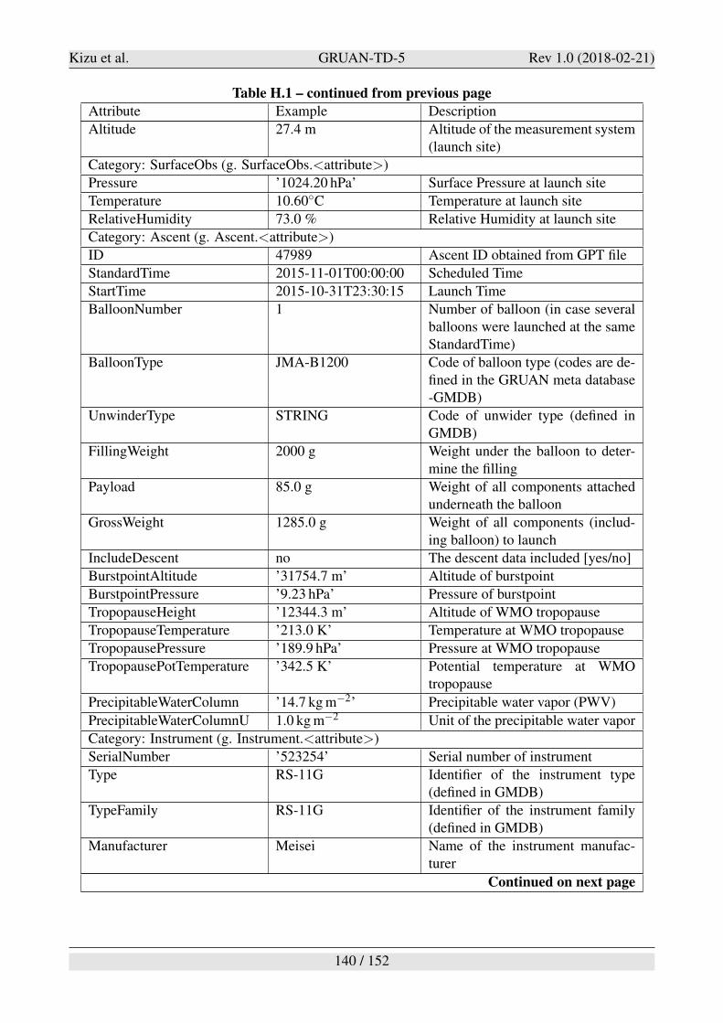
Kizu et al. GRUAN-TD-5 Rev 1.0 (2018-02-21)
Table H.1 – continued from previous page
Attribute Example Description
Altitude 27.4 m Altitude of the measurement system(launch site)
Category: SurfaceObs (g. SurfaceObs.<attribute>)
Pressure ’1024.20 hPa’ Surface Pressure at launch site
Temperature 10.60!C Temperature at launch site
RelativeHumidity 73.0 % Relative Humidity at launch site
Category: Ascent (g. Ascent.<attribute>)
ID 47989 Ascent ID obtained from GPT file
StandardTime 2015-11-01T00:00:00 Scheduled Time
StartTime 2015-10-31T23:30:15 Launch Time
BalloonNumber 1 Number of balloon (in case severalballoons were launched at the sameStandardTime)
BalloonType JMA-B1200 Code of balloon type (codes are de-fined in the GRUAN meta database-GMDB)
UnwinderType STRING Code of unwider type (defined inGMDB)
FillingWeight 2000 g Weight under the balloon to deter-mine the filling
Payload 85.0 g Weight of all components attachedunderneath the balloon
GrossWeight 1285.0 g Weight of all components (includ-ing balloon) to launch
IncludeDescent no The descent data included [yes/no]
BurstpointAltitude ’31754.7 m’ Altitude of burstpoint
BurstpointPressure ’9.23 hPa’ Pressure of burstpoint
TropopauseHeight ’12344.3 m’ Altitude of WMO tropopause
TropopauseTemperature ’213.0 K’ Temperature at WMO tropopause
TropopausePressure ’189.9 hPa’ Pressure at WMO tropopause
TropopausePotTemperature ’342.5 K’ Potential temperature at WMOtropopause
PrecipitableWaterColumn ’14.7 kg m#2’ Precipitable water vapor (PWV)
PrecipitableWaterColumnU 1.0 kg m#2 Unit of the precipitable water vapor
Category: Instrument (g. Instrument.<attribute>)
SerialNumber ’523254’ Serial number of instrument
Type RS-11G Identifier of the instrument type(defined in GMDB)
TypeFamily RS-11G Identifier of the instrument family(defined in GMDB)
Manufacturer Meisei Name of the instrument manufac-turer
Continued on next page
140 / 152
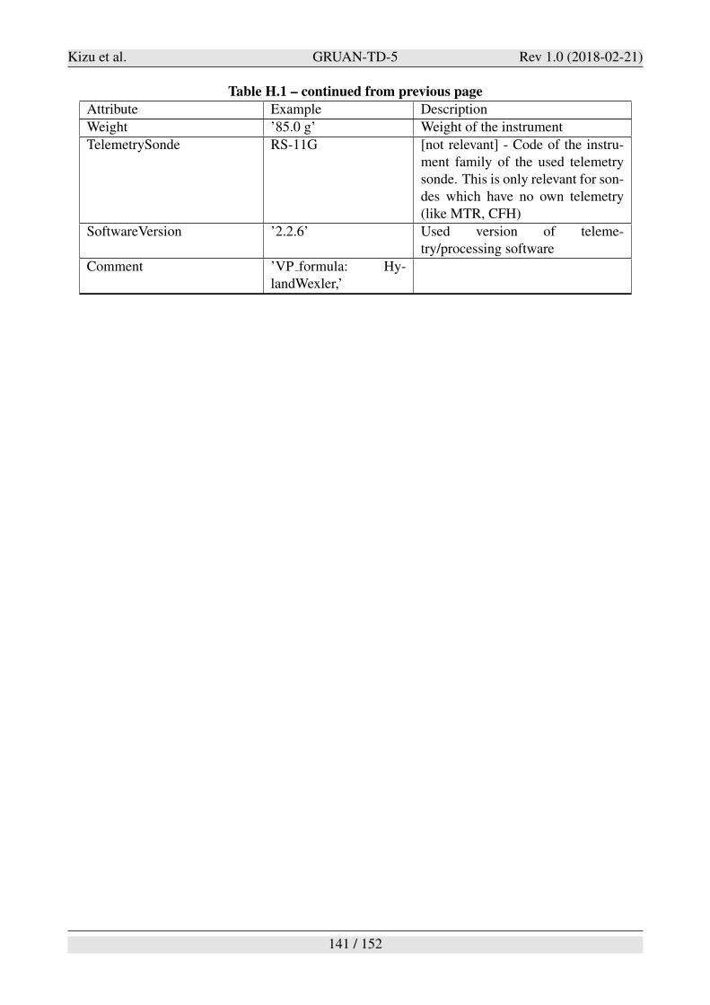
Kizu et al. GRUAN-TD-5 Rev 1.0 (2018-02-21)
Table H.1 – continued from previous page
Attribute Example Description
Weight ’85.0 g’ Weight of the instrument
TelemetrySonde RS-11G [not relevant] - Code of the instru-ment family of the used telemetrysonde. This is only relevant for son-des which have no own telemetry(like MTR, CFH)
SoftwareVersion ’2.2.6’ Used version of teleme-try/processing software
Comment ’VP formula: Hy-landWexler,’
141 / 152
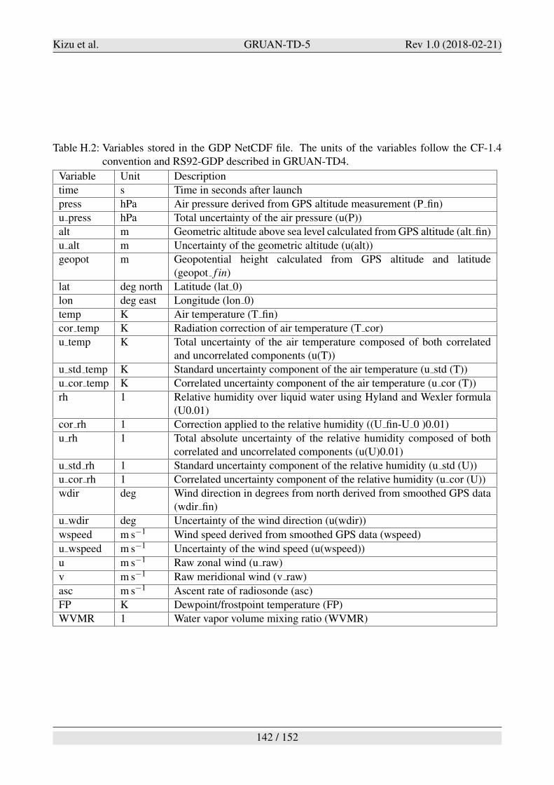
Kizu et al. GRUAN-TD-5 Rev 1.0 (2018-02-21)
Table H.2: Variables stored in the GDP NetCDF file. The units of the variables follow the CF-1.4convention and RS92-GDP described in GRUAN-TD4.
Variable Unit Description
time s Time in seconds after launch
press hPa Air pressure derived from GPS altitude measurement (P fin)
u press hPa Total uncertainty of the air pressure (u(P))
alt m Geometric altitude above sea level calculated from GPS altitude (alt fin)
u alt m Uncertainty of the geometric altitude (u(alt))
geopot m Geopotential height calculated from GPS altitude and latitude(geopot f in)
lat deg north Latitude (lat 0)
lon deg east Longitude (lon 0)
temp K Air temperature (T fin)
cor temp K Radiation correction of air temperature (T cor)
u temp K Total uncertainty of the air temperature composed of both correlatedand uncorrelated components (u(T))
u std temp K Standard uncertainty component of the air temperature (u std (T))
u cor temp K Correlated uncertainty component of the air temperature (u cor (T))
rh 1 Relative humidity over liquid water using Hyland and Wexler formula(U0.01)
cor rh 1 Correction applied to the relative humidity ((U fin-U 0 )0.01)
u rh 1 Total absolute uncertainty of the relative humidity composed of bothcorrelated and uncorrelated components (u(U)0.01)
u std rh 1 Standard uncertainty component of the relative humidity (u std (U))
u cor rh 1 Correlated uncertainty component of the relative humidity (u cor (U))
wdir deg Wind direction in degrees from north derived from smoothed GPS data(wdir fin)
u wdir deg Uncertainty of the wind direction (u(wdir))
wspeed m s#1 Wind speed derived from smoothed GPS data (wspeed)
u wspeed m s#1 Uncertainty of the wind speed (u(wspeed))
u m s#1 Raw zonal wind (u raw)
v m s#1 Raw meridional wind (v raw)
asc m s#1 Ascent rate of radiosonde (asc)
FP K Dewpoint/frostpoint temperature (FP)
WVMR 1 Water vapor volume mixing ratio (WVMR)
142 / 152
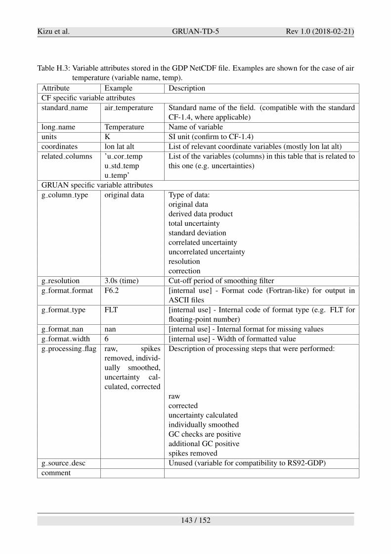
Kizu et al. GRUAN-TD-5 Rev 1.0 (2018-02-21)
Table H.3: Variable attributes stored in the GDP NetCDF file. Examples are shown for the case of airtemperature (variable name, temp).
Attribute Example Description
CF specific variable attributes
standard name air temperature Standard name of the field. (compatible with the standardCF-1.4, where applicable)
long name Temperature Name of variable
units K SI unit (confirm to CF-1.4)
coordinates lon lat alt List of relevant coordinate variables (mostly lon lat alt)
related columns ’u cor tempu std tempu temp’
List of the variables (columns) in this table that is related tothis one (e.g. uncertainties)
GRUAN specific variable attributes
g column type original data Type of data:original dataderived data producttotal uncertaintystandard deviationcorrelated uncertaintyuncorrelated uncertaintyresolutioncorrection
g resolution 3.0s (time) Cut-off period of smoothing filter
g format format F6.2 [internal use] - Format code (Fortran-like) for output inASCII files
g format type FLT [internal use] - Internal code of format type (e.g. FLT forfloating-point number)
g format nan nan [internal use] - Internal format for missing values
g format width 6 [internal use] - Width of formatted value
g processing flag raw, spikesremoved, individ-ually smoothed,uncertainty cal-culated, corrected
Description of processing steps that were performed:
rawcorrecteduncertainty calculatedindividually smoothedGC checks are positiveadditional GC positivespikes removed
g source desc Unused (variable for compatibility to RS92-GDP)
comment
143 / 152
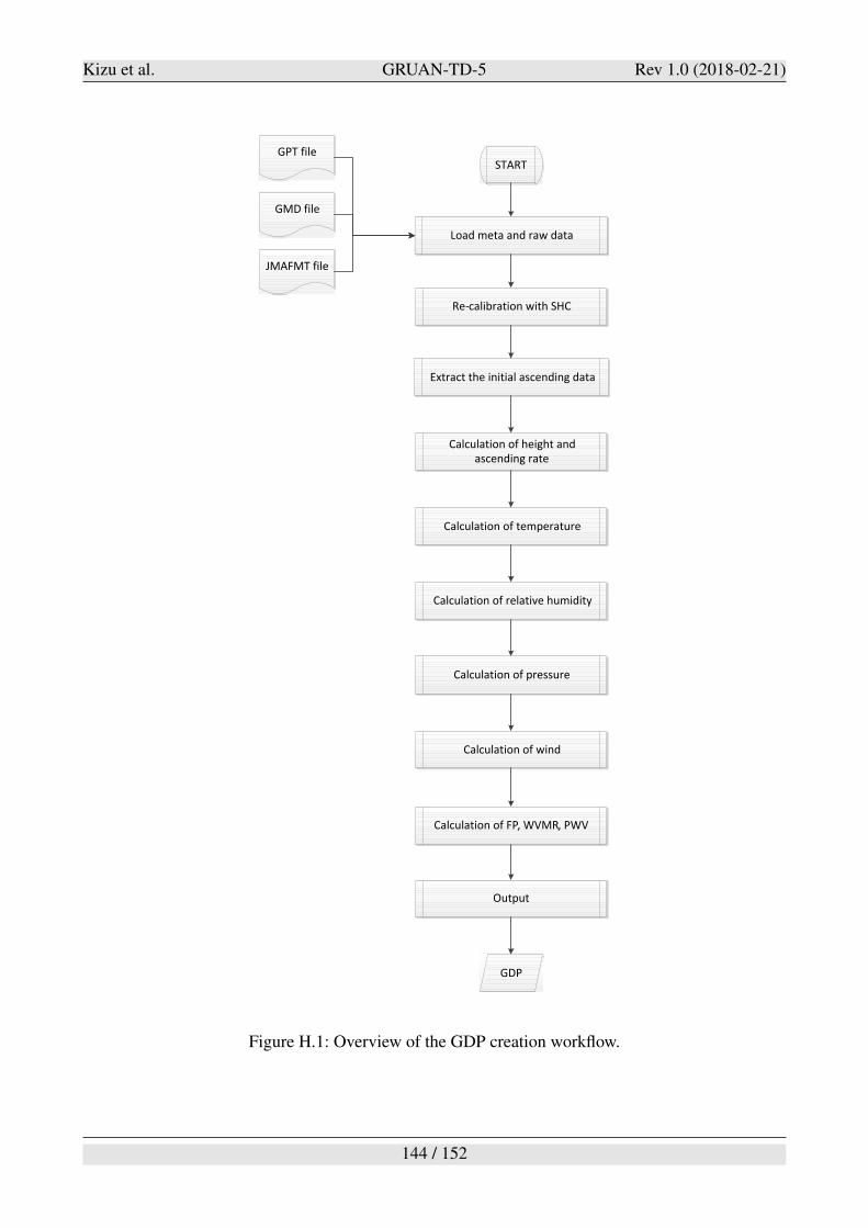
Kizu et al. GRUAN-TD-5 Rev 1.0 (2018-02-21)
Figure H.1: Overview of the GDP creation workflow.
144 / 152
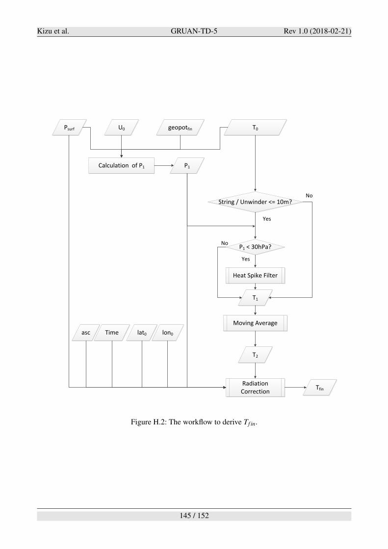
Kizu et al. GRUAN-TD-5 Rev 1.0 (2018-02-21)
Figure H.2: The workflow to derive Tf in.
145 / 152
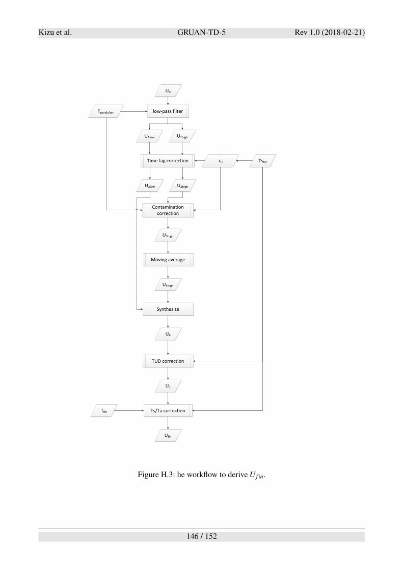
Kizu et al. GRUAN-TD-5 Rev 1.0 (2018-02-21)
Figure H.3: he workflow to derive Uf in.
146 / 152

Kizu et al. GRUAN-TD-5 Rev 1.0 (2018-02-21)
I Acronym list
BC Base line checkCFH Cryogenic Frostpoint HygrometerCIMO WMO Commission for Instruments and Methods of ObservationCMO Central Meteorological ObservatoryDGPS Differential GPSFLASH Fluorescent Advanced Stratospheric HygrometerGC Ground check or Ground checkerGCOS Global Climate Observing SystemGDP GRUAN Data processingGNSS Global Navigation Satellite SystemGOS Global Observing SystemGPS Global Positioning SystemGRUAN GCOS Reference Upper Air NetworkGUAN GCOS Upper Air NetworkGUM Guide to the Expression of Uncertainty in MeasurementICM Implementation and Coordination MeetingIrDA Infrared Data AssociationJMA Japan Meteorological AgencyJMAFMT JMA transmission FormatMeisei Meisei electric co., LTDMTR Meisei Temperature Reference (sensor)NCEI NOAA National Centers for Environmental InformationNOAA National Oceanic and Atmospheric AdministrationOPC Optical Particle CounterPDOP position dilution of precision (for GPS)PLL Phase-Locked LoopRMS Root Mean SquareSBAS Satellite-Based Augmentation SystemSHC Standard Humidity ChamberTUD Temperature-hUmidity DependenceUERE User Equivalent Range ErrorWG GRUAN Working Group on GRUANWMO World Meteorological Organization
147 / 152

Kizu et al. GRUAN-TD-5 Rev 1.0 (2018-02-21)
Acknowledgments
We would like to thank Dr. Holger Vomel, Dr. Ruud Dirksen, Dr. Michael Sommer, Ms. Mar-ion Fiedler, and Ms. Tatjana Naebert for their great support when we carried out several laboratoryexperiments and comparison flights at the GRUAN Lead Centre in the Lindenberg Aerological Ob-servatory, Deutscher Wetterdienst (DWD), Germany.We also deeply thank the colleagues of the JMA Aerological Observatory at Tateno, Japan and ofthe Meisei Electoric Co. Ltd. for their cooperation for the laboratory experiments and radiosondesoundings.We thank Drs. Ruud Dirksen, Christoph von Rohden, Rolf Philipona, and Martial Haefelin as well asHannu Jauhiainen for reviewing this document, and for their valuable comments and suggestions thatcontributed to its improvement.Finally, we thank Dr. Ruud Dirksen for editing the document.
148 / 152
Kizu et al. GRUAN-TD-5 Rev 1.0 (2018-02-21)
References
Abe, T., The historical changes of upper-air observation and the characteristics of aerological dataat Japan Meteorological Agency. Part 1: The historical changes of instruments and methods aboutupper-air observation, TENKI, 62, 161–185, 2015, in Japanese.
Bodeker, G. E., S. Bojinski, D. Cimini, R. J. Dirksen, M. Haeffelin, J. W. Hannigan, D. F. Hurst,T. Leblanc, F. Madonna, M. Maturilli, A. C. Mikalsen, R. Philipona, T. Reale, D. J. Seidel, D. G. H.Tan, P. W. Thorne, H. Vomel, and J. Wang, Reference upper-air observations for climate: Fromconcept to reality, Bull. Amer. Meteor. Soc., 97, 123–135, 10.1175/bams-d-14-00072.1, 2016.
Buck, A. L., New equations for computing vapor pressure and enhancement factor, J. Appl. Meteor.,20, 1527–1532, 1981.
Dirksen, R. J., M. Sommer, F. J. Immler, D. F. Hurst, R. Kivi, and H. Vomel, Reference quality upper-air measurements: GRUAN data processing for the Vaisala RS92 radiosonde, Atmos. Meas. Tech.,7(12), 4463–4490, 10.5194/amt-7-4463-2014, 2014, URL http://www.atmos-meas-tech.net/7/4463/2014/.
Fujiwara, M., T. Sugidachi, T. Arai, K. Shimizu, M. Hayashi, Y. Noma, H. Kawagita, K. Sagara,T. Nakagawa, S. Okumura, Y. Inai, T. Shibata, S. Iwasaki, and A. Shimizu, Development of a cloudparticle sensor for radiosonde sounding, Atmos. Meas. Tech., 9(12), 5911–5931, 10.5194/amt-9-5911-2016, 2016, URL http://www.atmos-meas-tech.net/9/5911/2016/.
Hayashi, M., Size Distribution of Aerosol in the Stratosphere and Troposphere Observed with Air-Borne 1765 Optical Particle Counter, Earozoru Kenkyu, 16, 118–124, 2001.
Hodge, M. W., Superadiabatic lapse rates of temperature in radiosonde observations, Monthly
Weather Review, 84(3), 103–106, http://dx.doi.org/10.1175/1520-0493(1956)084<0103:slroti>2.0.co;2, 1956.
Hyland, R. and A. Wexler, Formulations for the thermodynamic properties of the saturated phases ofH2O from 173.15 K to 473.15 K, ASHRAE Trans., 89, 500–519, 1983.
Immler, F. J., J. Dykema, T. Gardiner, D. N. Whiteman, P. W. Thorne, and H. Vomel, ReferenceQuality Upper-Air Measurements: guidance for developing GRUAN data products, Atmos. Meas.
Tech., 3(5), 1217–1231, 10.5194/amt-3-1217-2010, 2010, URL http://www.atmos-meas-tech.net/3/1217/2010/.
Japan Society of Mechanical Engineers (JSME), Heat transfer (1975), 3rd edition, in Japanese.
JCGM/WG 1, Evaluation of measurement data – Guide to the expression of uncertainty in mea-
surement, International Bureau of Weights and Measures / Bureau International des Poidset Mesures, 2008, URL http://www.bipm.org/utils/common/documents/jcgm/JCGM_100_2008_E.pdf.
JMA, A hundred years memorial magazine of japan meteorological agency, Technical report, JapanMeteorological Agency, 1975, in Japanese.
JMA, Comparison of the Meisei RS2-80 rawinsonde and Meisei RSII-56 rawinsonde, Meteorological
Research Note, 50, 373, 1983, in Japanese.
149 / 152
Kizu et al. GRUAN-TD-5 Rev 1.0 (2018-02-21)
JMA, Guidelines of radiosonde soundings, Technical report, Japan Meteorological Agency, 1995, inJapanese.
JMA, Verification provisions for meteorological instruments, Technical report, Japan MeteorologicalAgency, 2002, in Japanese.
Kobayashi, E., Result of comparison and verification with RS2-91 Rawinsonde and RS92-DGPGPSsonde, Kishou Kenkyuu Note, 229, 27–36, 2014, in Japanese.
Kobayashi, E., Y. Noto, S. Wakino, H. Yoshii, T. Ohyoshi, S. Saito, and Y. Baba, Comparison ofMeisei RS2-91 Rawinsondes and Vaisala RS92-SGP Radiosondes at Tateno for the Data Continuityfor Climatic Data Analysis, Journal of the Meteorological Society of Japan. Ser. II, 90(6), 923–945,10.2151/jmsj.2012-605, 2012a.
Kobayashi, E., H. Yoshii, T. Abe, and Y. Kaneko, Investigation of characteristic of temperature atcloud top and stratosphere in the rainy weather with comparison observation data of RS2-91 Raw-insonde and RS92-SGP GPSsonde, Journal of the Aerological Observatory, 70, 13–22, 2012b, inJapanese.
Kobayashi, K., GPS Wave Reception and Measurement of Position, KODEN TECH., 22, 1–11, 2006.
Komhyr, W. D., R. A. Barnes, G. B. Brothers, J. A. Lathrop, and D. P. Opperman, Electrochemi-cal concentration cell ozonesonde performance evaluation during STOIC 1989, J. Geophys. Res.,100(D5), 9231–9244, 10.1029/94JD02175, 1995, ISSN 2156-2202, URL http://dx.doi.org/10.1029/94JD02175.
Kuo, F. F. and J. F. Kaiser, System analysis by digital computer (John Wiley & Sons, New York,1966), 438 pp.
Miller, D., Water at the surface of the Earth (Academic Press, New York, USA, 1977).
Miloshevich, L. M., A. Paukkunen, H. Vomel, and S. J. Oltmans, Development and Validation of aTime-Lag Correction for Vaisala Radiosonde Humidity Measurements, J. Atmos. Ocean. Technol.,21(9), 1305–1327, http://dx.doi.org/10.1175/1520-0426(2004)021<1305:DAVOAT>2.0.CO;2, 2004.
Morrissey, J. F. and F. J. Brousaides, Temperature induced errors in the ML-476 humidity data, J.
Appl. Meteor., 8, 805–808, 1970.
Murphy, D. M. and T. Koop, Review of the vapour pressures of ice and supercooled water for atmo-spheric applications, Quart. J. Roy. Meteor. Soc., 131, 15391565, 10.1256/qj.04.94, 2005.
Nakamura, K., N. Hayashi, and K. Masuda, The estimation of some error in the RS2-80 temperaturemeasurements. -solar radiation correction-, Sokko Jiho, 50, 117–138, 1983, in Japanese.
Nash, J., T. Oakley, H. Vomel, and L. Wei, WMO Intercomparison of High Quality Ra-diosonde Systems Yangjiang, China, 12 July – 3 August 2010, Technical report, WMO, 2011,URL https://www.wmo.int/pages/prog/www/IMOP/publications/IOM-107%_Yangjiang/IOM-107_Yangjiang.zip, WMO/TD-No. 1580, Instruments And Observing Methods Report No.107.
150 / 152
Kizu et al. GRUAN-TD-5 Rev 1.0 (2018-02-21)
NOAA, NASA, and USAF, US Standard Atmosphere (US Government printing office, WashingtonDC, 1976), 241 pp.
Sakoda, Y., K. Naganuma, H. Ogihara, N. Inoue, and A. Mita, RS-91 Rawinsonde, Kishou Kenkyuu
Note, 194, 3–24, 1999, in Japanese.
Savitzky, A. and M. J. E. Golay, Smoothing and differentiation of data by simplified least squaresprocedures, Anal. Chem., 36, 16271639, 10.1021/ac60214a047, 1964.
Seidel, D. J., F. H. Berger, F. Immler, M. Sommer, H. Vomel, H. J. Diamond, J. Dykema, D. Goodrich,W. Murray, T. Peterson, D. Sisterson, P. Thorne, and J. Wang, Reference upper-air observa-tions for climate: Rationale, progress, and plans, Bull. Amer. Meteor. Soc., 90(3), 361–369,10.1175/2008bams2540.1, 2009.
Shimizu, K., T. Asanuma, K. Yamaguchi, and K. Yoshikawa, Upgraded thermistor for unbiased mea-surements evaluation of new gps radiosonde rs-06g, IOM 97, Papers presented at the WMO tech-
nical Conference on Instruments and Methods of observation (TECO 2008), 2008.
Shimizu, K. and F. Hasebe, Fast-response high-resolution temperature sonde aimed at contamination-free profile observations, Atmos. Meas. Tech., 3(6), 1673–1681, 10.5194/amt-3-1673-2010, 2010.
Sommer, M., GRUAN Technical document 3 - User Guide of GRUAN RsLaunchClient, Technicalreport, GRUAN Lead Centre, Lindenberg, 2014, version 1.0.
Sugidachi, T. and M. Fujiwara, Correction of the Stepwise Change Observed at 0!C in Meisei RS2-91, RS-01G, and RS-06G Radiosonde Relative Humidity Profiles, Journal of the Meteorological
Society of Japan. Ser. II, 91(3), 323–336, 10.2151/jmsj.2013-306, 2013.
Tateno Aerological Observatory, Intercomparison and verification of the Meisei RS2-91 rawinsondeand Vaisala RS92-SGP, Sokko Jiho, 50, 373–384, 2011, in Japanese.
Uesato, I., T. Ito, M. Kumamoto, R. Shigebayashi, and M. Nakamura, Temperature trend consideringhistrical changes of radiosonde (part 1), Journal of the Aerological Observatory, 68, 15–22, 2008,in Japanese.
Vomel, H., D. E. David, and K. Smith, Accuracy of tropospheric and stratospheric water vapor mea-surements by the cryogenic frost point hygrometer: Instrumental details and observations, J. of
Geophys. Res. Atmos., 112(D8), D08,305, 10.1029/2006jd007224, 2007.
Vomel, H., T. Naebert, R. Dirksen, and M. Sommer, An update on the uncertainties of water va-por measurements using cryogenic frost point hygrometers, Atmos. Meas. Tech., 9(8), 3755–3768,10.5194/amt-9-3755-2016, 2016, URL http://www.atmos-meas-tech.net/9/3755/2016/.
Williams, S. L. and D. T. Acheson, Thermal time constants of u. s radiosonde sensors used in gate,NOAA Tech. Memo. EDS CEDDA-7, 1976, (Available from U. S. Govt. Printing Office, Washing-ton, DC 20402.).
WMO, Guide to Meteorological Instruments and Methods of Observation, World MeteorologicalOrganization, Geneva, 7th edition, 2008, URL http://library.wmo.int/pmb_ged/wmo_8_en-2012.pdf, [Accessed 3 December 2014].
151 / 152
Kizu et al. GRUAN-TD-5 Rev 1.0 (2018-02-21)
Yushkov, V., V. Astakhov, and S. Merkulov, Optical balloon hygrometer for upper-troposphere andstratosphere water vapor measurements, in J. Wang, B. Wu, T. Ogawa, and Z.-H. Guan, eds., Op-
tical Remote Sensing of the Atmosphere and Clouds, Proc. Soc. Photo-Opt. Instrum. Eng., volume3501, pp. 439–445 (1998), 10.1117/12.317759.
152 / 152