-labeling of perfect elimination bipartite graphs

Discrete Applied Mathematics 159 (2011) 1878–1888

Contents lists available at ScienceDirect

Discrete Applied Mathematics

journal homepage: www.elsevier.com/locate/dam

L(2, 1)-labeling of perfect elimination bipartite graphsB.S. Panda ∗, Preeti GoelComputer Science and Application Group, Department of Mathematics, Indian Institute of Technology Delhi, Hauz Khas, New Delhi 110 016, India

a r t i c l e i n f o

Article history:Received 2 October 2009Received in revised form 30 June 2010Accepted 16 July 2010Available online 8 August 2010

Keywords:L(2, 1)-labelingPerfect elimination bipartite graphsGraph algorithmsNP-complete

a b s t r a c t

An L(2, 1)-labeling of a graph G is an assignment of nonnegative integers, called colors, tothe vertices of G such that the difference between the colors assigned to any two adjacentvertices is at least two and the difference between the colors assigned to any two verticeswhich are at distance two apart is at least one. The span of an L(2, 1)-labeling f is themaximum color number that has been assigned to a vertex of G by f . The L(2, 1)-labelingnumber of a graph G, denoted as λ(G), is the least integer k such that G has an L(2, 1)-labeling of span k. In this paper, we propose a linear time algorithm to L(2, 1)-label achain graph optimally. We present constant approximation L(2, 1)-labeling algorithmsfor various subclasses of chordal bipartite graphs. We show that λ(G) = O(∆(G)) for achordal bipartite graph G, where ∆(G) is the maximum degree of G. However, we showthat there are perfect elimination bipartite graphs having λ = Ω(∆2). Finally, we provethat computing λ(G) of a perfect elimination bipartite graph is NP-hard.

© 2010 Elsevier B.V. All rights reserved.

1. Introduction

The frequency assignment problem is to assign frequencies to radio transmitters such that nearby transmitters areassigned frequencies without causing interference. This problem was introduced by Hale [19] and can be modeled as agraph coloring problem where the vertices represent the transmitters and two vertices are adjacent if there is possibleinterference between the corresponding two transmitters.

L(2, 1)-labeling (coloring) problem was introduced by Griggs and Yeh [17], initially proposed by Roberts, as a variationof the frequency assignment problem. An L(2, 1)-labeling of a graph G(V , E) is a function f from V to the set of nonnegativeintegers (called colors) such that |f (x) − f (y)| ≥ 2 if xy ∈ E and |f (x) − f (y)| ≥ 1 if the distance between x and y is 2. Thespan of an L(2, 1)-labeling f of G is maxf (v)|v ∈ V (G). The L(2, 1)-labeling number of G, denoted by λ(G), is the smallestk such that G has an L(2, 1)-labeling of span k.

Griggs and Yeh [17] proved that λ(G) ≤ ∆2+ 2∆ for a graph G with maximum degree ∆. Chang and Kuo [11] later

improved this bound to∆2+∆. It was further improved to∆2

+∆−1 in [23] and the current best bound λ(G) ≤ ∆2+∆−2

is due to Gonçalves [16]. Griggs and Yeh [17] have proposed the following conjecture, which we shall call ‘‘Griggs and Yeh’’conjecture.

Conjecture 1. For any graph G with maximum degree ∆ ≥ 2, λ(G) ≤ ∆2.

Havet et al. [18] have proved this conjecture asymptotically. However, the conjecture is still open in general and has beenthe motivating factor for considerable research on L(2, 1)-labeling of graphs. The conjecture has been proved to be true forseveral special classes of graphs such aswheels, complete k-partite graphs [17], trees [17,11], cographs [11], regular tiling [4],chordal graphs [26,22], unit interval graphs [26], OSF-chordal, SF-chordal [11], outerplanar [10], split graphs, permutation

∗ Corresponding author. Tel.: +91 11 26591448; fax: +91 11 26581005.E-mail addresses: [email protected], [email protected] (B.S. Panda).

0166-218X/$ – see front matter© 2010 Elsevier B.V. All rights reserved.doi:10.1016/j.dam.2010.07.008

http://dx.doi.org/10.1016/j.dam.2010.07.008

http://www.elsevier.com/locate/dam

http://www.elsevier.com/locate/dam

mailto:[email protected]

mailto:[email protected]

http://dx.doi.org/10.1016/j.dam.2010.07.008

B.S. Panda, P. Goel / Discrete Applied Mathematics 159 (2011) 1878–1888 1879

Fig. 1. Inclusion relationship between some subclasses of bipartite graphs.

graphs [5], co-comparability graphs [9], and Hamiltonian cubic graphs [21]. For a comprehensive survey on this problemwerefer to [29,8].

The L(2, 1)-labeling problem, i.e., the problem of deciding whether λ(G) ≤ k given an integer k and a graph G, is NP-complete [17]. In fact, this problem remains NP-complete even for any fixed integer k ≥ 4 [14].

Since the L(2, 1)-labeling problem for general graphs is a known difficult problem and Conjecture 1 is still open forgeneral graphs, researchers have studied these two problems on various graph classes as has been summarized above.

The class of bipartite graphs is a wide and an important class of graphs both from practical as well as from theoreticalpoints of view. The class of bipartite graphs includemany interesting subclasses such as chain graphs, bipartite permutationgraphs, bipartite distance hereditary graphs, convex and biconvex graphs, chordal bipartite graphs, and perfect eliminationbipartite graphs (see the later sections for definition of these graph classes). The inclusion hierarchy of these subclassesis shown in Fig. 1. Studies of these subclasses are motivated by the fact that many NP-hard problems are efficiently solvedwhen restricted to these subclasses (see [7,15]). The L(2, 1)-labeling problem remains NP-complete even for planar bipartitegraphs [5]. However, the problem admits polynomial time solution for trees [11]. Similarly, Conjecture 1 is still open evenfor bipartite graphs and is true for trees [17]. Also it is known that there are bipartite graphs with λ(G) = Ω(∆2). In viewof these observations, it is worth studying the above two problems, i.e., the L(2, 1)-labeling problem and Conjecture 1, forvarious subclasses of bipartite graphs.

The aims of this paper are to study Conjecture 1 on various subclasses of bipartite graphs and to study the complexity ofthe problem of computing λ(G) for the various subclasses of bipartite graphs. On the positive side, we show that an L(2, 1)-labeling of span λ(G) for a chain graph can be computed in linear time. We propose constant approximation algorithms tocompute λ(G) for various subclasses of chordal bipartite graphs. We show that Conjecture 1 holds true for chain graphs andbiconvex graphs. We also show that Conjecture 1 holds true for all chordal bipartite graphs of maximum degree ∆, ∆ = 3.We show that there are perfect elimination bipartite graphs with λ = Ω(∆2). Finally, we show that computing λ(G) isNP-hard for perfect elimination bipartite graphs.

The rest of the paper is organized as follows. Section 2 contains some preliminary results and pertinent definitions.Section 3 presents L(2, 1)-labeling algorithms for various subclasses of chordal bipartite graphs. We present a linear timealgorithm to compute an optimal L(2, 1)-labeling of chain graphs. We show that λ(G) ≤ ∆1 +∆2, where ∆1 and ∆2 are themaximum degrees of a vertex in X and a vertex in Y , respectively, of a biconvex graph G = (X, Y , E), where X and Y are thevertex sets of the two parts of the bipartite graph. We show that λ(G) ≤ 4∆ − 2 for a bipartite distance hereditary graph.We prove that λ(G) ≤ 4∆ − 1 for a chordal bipartite graph. In Section 4, we show that there exists a perfect eliminationbipartite graphGwithλ(G) = Ω(∆2(G)). In Section 5,we prove that computingλ(G) of a perfect elimination bipartite graphis NP-hard. In fact, we prove that it is NP-complete to decide whether λ(G) ≤ 8 for a planar perfect elimination bipartitegraph of maximum degree seven.

2. Preliminaries

For a graph G = (V , E), the sets NG(v) = u ∈ V (G)|uv ∈ E and NG[v] = NG(v) ∪ v denote the neighborhood and theclosed neighborhood of a vertex v, respectively. The degree of a vertex v is |NG(v)| and is denoted by dG(v). When the contextis clear we omit the index G. The maximum degree of a graph G, denoted by ∆(G), is the maximum of the degrees of all its

1880 B.S. Panda, P. Goel / Discrete Applied Mathematics 159 (2011) 1878–1888

vertices. When the context is clear we use ∆ instead of ∆(G). A subset of pairwise adjacent vertices is called a clique. Letd(u, v) denote the distance between two vertices u, v ∈ V (G). Let n andm denote the number of vertices, and number edgesof G, respectively. Let G[S] denote the subgraph induced by G on S, S ⊂ V . A graph G = (V , E) is said to be bipartite if V (G)can be partitioned into two disjoint sets X and Y such that every edge joins a vertex in X to another vertex in Y . A partitionX, Y of V is called a bipartition. A bipartite graph with partition X, Y of V is denoted by G = (X, Y , E). A bipartite graphG = (X, Y , E) is said to be complete bipartite if each vertex in X is adjacent to all vertices in Y . A bipartite graph G is calledchordal bipartite if every cycle of G of length at least six has a chord, i.e. an edge joining two non-consecutive vertices ofthe cycle. For a bipartite graph, a subset of vertices is called biclique if it induces a complete bipartite subgraph. The bicliquenumber of a bipartite graph G is the maximum order of a biclique of G and is denoted by bc(G).

Throughout the paper we will denote ∆1 = maxd(x) : x ∈ X, ∆2 = maxd(y) : y ∈ Y and ∆ = max∆1, ∆2,n1 = |X |, n2 = |Y |, n1 ≤ n2, for a bipartite graph G = (X, Y , E) with n vertices and m edges.

Let α = v1, v2, . . . , vn be an ordering of V (G). The following algorithm always finds an L(2, 1)-labeling f of G.

Algorithm 1: Greedy-L(2, 1)-labeling(α)

S = ∅;1foreach i = 1 to n do2

Let j be the smallest nonnegative integer such that j /∈ f (v), f (v) − 1, f (v) + 1|v ∈ NG(vi) ∩ S ∪ f (w)|w ∈ S3and d(vi, w) = 2;f (vi) = j;4S = S ∪ vi;5

end6

Algorithm 1 can be implemented as follows. Each vertex maintains the colors that have been assigned to its neighbors.When a vertex is labeled with a color, this color is added to the color list of each of its neighbors. To select the least integerthat can be assigned to a vertex vi, one has to examine the color set maintained by vi and the color sets maintained by eachneighbor of vi. This takesO(di+(

∑v∈N(vi)

d(v))) timewhich is atmostO(di∆), where di = d(vi). Thuswe have the followingtheorem.

Theorem 2.1. Algorithm Greedy-L(2, 1)-labeling(α) can be implemented in O(∆(n + m)) time.

The following lemma gives a necessary condition for a graph Gwith λ(G) = ∆(G) + 1.

Lemma 2.2 ([17]). For a graph G with ∆(G) ≥ 1, λ(G) ≥ ∆(G) + 1. Furthermore, if λ(G) = ∆(G) + 1, then each vertex ofdegree ∆(G) is assigned color 0 or ∆(G) + 1 in any L(2, 1)-labeling of G of span λ(G).

3. L(2, 1)-labeling of subclasses of chordal bipartite graphs

In this section, we propose constant approximation L(2, 1)-labeling algorithms for various subclasses of chordal bipartitegraphs and show that Conjecture 1 holds true for several of these subclasses.

3.1. Computing λ(G) of chain graphs

A bipartite graph G = (X, Y , E), with |X | = n1 and |Y | = n2, is called a chain graph if there exists an ordering x1, . . . , xn1of X and an ordering y1, . . . , yn2 of Y such that N(x1) ⊆ N(x2) ⊆ · · · ⊆ N(xn1) and N(yn2) ⊆ · · · ⊆ N(y2) ⊆ N(y1). It isknown that such orderings of X and Y of a chain graph G = (X, Y , E) can be computed in linear time [28, Lemma 7].

The following theorem shows that Algorithm 2 produces an optimal L(2, 1)-labeling of G of span bc(G).

Theorem 3.1. Given a connected chain graph G, Algorithm 2 finds an optimal L(2, 1)-labeling f of G. Furthermore,λ(G) = bc(G)and Conjecture 1 holds true for chain graphs.

Proof. Clearly Algorithm 2 produces an L(2, 1)-labeling.Next we prove that the labeling f produced by Algorithm 2 is an optimal labeling of the connected chain graph G =

(X, Y , E) and λ(G) = bc(G).Let λ∗ be the span of f . So f (xi) = λ∗ for some 1 ≤ i ≤ n1. Let k be the largest index such that yk ∈ N(xi). Consider

G′= G[xi, . . . , xn1 , y1, . . . , yk]. Since G is a chain graph, G′

= G[xi, . . . , xn1 , y1, . . . , yk] is a complete bipartite graph withk+n1− i+1 vertices. So bc(G) ≥ k+n1− i+1. Since λ(G′) ≤ λ(G), λ(G) ≥ k+n1− i+1.We claim that k+n1− i+1 = λ∗.

Since f (xi) = λ∗, for each s ∈ k, k + 1, . . . , n2, there is exactly one vertex xt in X such that f (xt) = s for i < t ≤ n1.Otherwise, if there is some s which is not assigned to any xt for i < t ≤ n1, then s has been assigned to xi by Algorithm 2.Thus all the colors in the set k, k + 1, . . . , n2 are assigned to some xt for i < t ≤ n1.

Now consider colors in the set n2 + 1, n2 + 2, . . . , λ∗− 1. Clearly f (xn1) = n2 + 1. If some color in the set

n2 + 2, n2 + 3, . . . , λ∗− 1 has not been assigned to any xt for i < t ≤ n1 then it would have been assigned to xi by

Algorithm 2. Since every color in k+ 1, k+ 2, . . . , λ∗ has been assigned to some xt for i < t ≤ n1 and since every color in

k+ 1, k+ 2, . . . , λ∗ is used at most once, we have that n1 − i = λ∗

− (k+ 1) = λ∗− k− 1. Therefore λ∗

= n1 − i+ k+ 1and hence λ∗

= bc(G) = λ. Since bc(G) ≤ 2∆(G) ≤ ∆2(G) for ∆(G) ≥ 2, Conjecture 1 is true for chain graphs.


Algorithm 2: COLORING-CHAIN-GRAPH(G)Find an ordering x1, . . . , xn1 of X and an ordering y1, . . . , yn2 of Y such that N(x1) ⊆ N(x2) ⊆ · · · ⊆ N(xn1) and1N(yn2) ⊆ . . . ⊆ N(y2) ⊆ N(y1);Let α = v1, v2, . . . , vn2+n1 be such that vi = yi, 1 ≤ i ≤ n2, and vn2+j = xn1+1−j, 1 ≤ j ≤ n1;2foreach i = 1 to n2 do3

f (vi) = i − 1;4

end5f (vn2+1) = n2 + 1;6S = Y ∪ xn1;7foreach i = n2 + 2 to n2 + n1 do8

Let j be the smallest nonnegative integer such that j /∈ f (v), f (v) − 1, f (v) + 1|v ∈ NG(vi) ∩ S ∪ f (w)|w ∈ S9and d(vi, w) = 2;f (vi) = j;10S = S ∪ vi;11

end12

a b

Fig. 2. (a) An L(2, 1)-labeled bipartite chain graph given in [3], (b) L(2, 1)-labeling of bipartite chain graph (a) generated by Algorithm 2.

Observe that Algorithm 2 is nothing but Greedy-L(2, 1)-labeling(α), where α is the ordering produced in Algorithm 2.We used Algorithm 2 instead of Greedy-L(2, 1)-labeling(α) in order to achieve time complexity of O(n + m).

We now analyze the time complexity of Algorithm 2. Finding the ordering α takes O(n + m) time [28]. We need to findthe least admissible color available for vj such that n2 +2 ≤ j ≤ n2 +n1. Let l be the largest color that has been assigned to avertex so far. The vertex vj, n2 + 2 ≤ j ≤ n2 + n1, will be labeled with the smallest color from the set d(vj)+ 2, . . . , n2 − 1that has not been assigned to any vertex vk, n2 + 2 ≤ k ≤ j − 1 if such a color is available; otherwise with the color l + 1. Ifl+1 is used for vj, thenwe increment l by 1 so that l always represents the largest color that has been assigned to a vertex sofar. Note that no two vertices vj and vk, n2 +1 ≤ k ≤ j ≤ n2 +n1 will receive the same color as d(vj, vk) = 2. For j = n2 +2,we maintain a sorted linked list containing the integers 2, 3, . . . , n2 − 1. So, for vj, we need to delete the smallest integer rfrom the linked list such that r ≥ d(vj)+2 if such an integer exists and assign to vj. If no such integer is present in the linkedlist, then we assign l+1 to vj and increment l by 1. To find such an integer, we have to traverse exactly d(vj)−1 elements inthe linked list. So this operation takesO(d(vj)) time. Thus the total time taken to find the labels for all vj, n2+2 ≤ j ≤ n2+n1is O(n + m). Hence Algorithm 2 takes O(n + m) time.

So we have the following theorem.

Theorem 3.2. An L(2, 1)-labeling of span λ(G) of a chain graph G can be computed in linear time.

Araki [3] has proposed a linear time algorithm for L(2, 1)-labeling chain graphs. However, the algorithm by Araki [3] isdifferent from our algorithm. Our algorithm is a very simple one and is based on the greedy labeling and easily generalizedto other classes of graphs. Fig. 2(a) illustrates the labeling of Araki [3] and Fig. 2(b) illustrates the labeling produced by ouralgorithm. The algorithm in [3] first computes the biclique number bc(G) of G and then a label (function of bc(G)) is assignedto each vertex of G. However, we have considered special vertex ordering and then labels are assigned to vertices greedily.Note that the labeling given in Fig. 2(a) cannot be produced by Greedy-L(2, 1)-labeling.

3.2. Biconvex graphs

A graph G = (V , E) is called a permutation graph if there exists a one to one correspondence between V (G) and a set ofline segments between two parallel lines such that two vertices are adjacent if and only if their corresponding line segmentsintersect. If G = (V , E) is both a bipartite graph and a permutation graph, then it is called a bipartite permutation graph. Notethat λ(G) ≤ 5∆(G) − 2 for a permutation graph [5] and λ(G) ≤ bc(G) + 1 [3] for a bipartite permutation graph.


An ordering of X ∪ Y of a bipartite graph G = (X, Y , E) is called a strong ordering if xy′, x′y ∈ E with x < x′ and y < y′,then xy and x′y′ are also in E. It was introduced by Spinrad in [27].

Let α = y1, . . . , yn2 be some ordering of Y of a bipartite graph G = (X, Y , E). A subset of Y is called a segment of Y w.r.t.α if its elements are consecutive in α. The ordering α has the convex property if for each vertex x ∈ X , N(x) is a segment in Yw.r.t. α. An ordering of Y with the convex property is called a convex ordering. A bipartite graph G = (X, Y , E) is said to beconvex on Y if there exists a convex ordering of Y . The term convex on X is defined similarly. A bipartite graph G = (X, Y , E)is called a convex graph if it is convex either on X or on Y . Every convex graph is chordal bipartite.

Let α = x1, . . . , xn1 and β = y1, . . . , yn2 be some ordering of X and Y , respectively, of a bipartite graph G = (X, Y , E).For any segment S = sa, sa+1, . . . , sb in X (or Y ), define first (S) and last (S) respectively to be the smallest and greatestindices of an element in S with respective to the ordering induced on S. For two segments A and B in the same vertex set,define A ≼ B if first (A) ≤ first (B) and last (A) ≤ last (B). If G is convex on Y then G is said to have the forward property iffor every pair of vertices xi, xj ∈ X with i < j then N(xi) ≼ N(xj). G is said to be forward convex if there exists an ordering ofX ∪ Y such that G is convex on Y and also has the forward property. Such an ordering is called a forward convex ordering. Alinear time algorithm for computing forward convex ordering of a bipartite permutation graph is presented in [24].

The class of bipartite permutation graphs corresponds to the class of forward convex graphs as can be seen from thefollowing theorem.

Theorem 3.3 ([24]). The following statements are equivalent for a bipartite graph G = (X ∪ Y , E):

(i) G is a bipartite permutation graph.(ii) G has a strong ordering.(iii) G is forward convex.

A bipartite graph G = (X, Y , E) is called biconvex if G is convex on both X and on Y . In this case, we say that V (G) = X ∪Yhas a biconvex ordering. A linear time algorithm for computing a convex ordering is given by Booth and Lueker in [6]. Applyingthis algorithm twice, on X and Y , a bipartite graph G = (X, Y , E) can be tested whether it is a biconvex graph and if it is, abiconvex ordering can be obtained in O(n + m) time. A permutation graph Gw.r.t. a strong ordering α of its vertices is saidto be a strongly ordered bipartite permutation graph.

Lemma 3.4 ([1]). A connected biconvex graph G = (X, Y , E) with a biconvex ordering α = x1, x2, . . . , xn1 , y1, y2, . . . , yn2 is astrongly ordered bipartite permutation graph if x1y1 and xn1yn2 are edges in G.

Let G = (X, Y , E) be a connected biconvex graph with a biconvex ordering α = x1, x2, . . . , xn1 , y1, y2, . . . , yn2 . Define xL,xR, Xr , and Gr as follows. xL is the smallest index vertex in N(y1) such that there does not exist any xj ∈ X such that N(xL)is a proper subset of N(xj), and xR is the largest index vertex in N(yn2) such that there does not exist any xj ∈ X such thatN(xR) is a proper subset of N(xj). We may assume that xL ⩽ xR, because otherwise we can consider the biconvex ordering ofG = (X ′, Y , E), where X ′

= xn1 , . . . , x1. Let Xr = xi|xL ⩽ xi ⩽ xR. Let Gr = G[Xr ∪ Y ].

Lemma 3.5 ([30]). Gr is a connected strongly ordered bipartite permutation graph. For all xi and xj, where x1 ⩽ xi < xj ⩽ xL orxR ⩽ xj < xi ⩽ xn1 , it holds that N(xi) ⊆ N(xj).

Lemma 3.6. If G = (X, Y , E) is a bipartite permutation graph, then max∆1, ∆2 + 1 ≤ λ(G) ≤ ∆1 + ∆2. Furthermore, anL(2, 1)-labeling of span ∆1 + ∆2 of a bipartite permutation graph can be computed in O(m∆) time.

Proof. Let x1, x2, . . . , xn1 and y1, y2, . . . , yn2 be orderings ofX and Y , respectively, such that this is a forward convex orderingof G. Let β = v1, . . . , vn1+n2 be such that vi = yi, for 1 ≤ i ≤ n2 and vn2+j = xn1+1−j, for 1 ≤ j ≤ n1. Let f be the L(2, 1)-labeling of G produced by Greedy-L(2, 1)-labeling(β). Next we prove that the span of f is at most ∆1 + ∆2.

We first prove that AlgorithmGreedy-L(2, 1)-labeling(β) assigns labels from 0, 1, . . . , ∆1−1 to the vertices in Y . Sincevertices in Y are labeled before the vertices in X , only distance two constraint need to be verified for the vertices in Y . LetSi = N(xi) for 1 ≤ i ≤ n1. By forward convexity, S1 ≼ Si ≼ Sj ≼ Sn1 for 1 ≤ i < j ≤ n1.

Consider yi ∈ Y for 1 ≤ i ≤ n2. Let N(yi) = xi1 , xi2 , . . . , xik such that xi1 < xi2 < · · · < xik . By forward convexity,Si1 ≼ Si2 ≼ · · · ≼ Sik and |yj : yj ∈ Y , j < i, d(yi, yj) = 2| = |Si1 | − 1. Therefore the number of colors forbidden for yi is atmost d(xi1) − 1 ≤ ∆1 − 1. Thus there will be a color in the set 0, 1, . . . , ∆1 − 1 which can be used to color yi. Hence allthe vertices in Y can be colored with colors in 0, 1, . . . , ∆1 − 1.

Let xi ∈ X , for 1 ≤ i ≤ n1. Since G is symmetric w.r.t. forward convex ordering, by the above argument there will beat most |xj|d(xi, xj) = 2, j < i| ≤ ∆2 − 1 vertices at distance two from xi. Since all the vertices in Y require at most∆1 colors, the number of colors forbidden for xi will be at most ∆1 + ∆2 − 1. Hence λ(G) ≤ ∆1 + ∆2. The inequalitymax∆1, ∆2 + 1 ≤ λ(G) follows from Lemma 2.2.

A forward convex ordering of a bipartite permutation graph can be computed in O(n + m) time [24]. By Theorem 2.1,Greedy-L(2, 1)-labeling(β) takes O(∆(n + m)) time. Hence, an L(2, 1)-labeling of span at most ∆1 + ∆2 of a bipartitepermutation graph can be computed in O(m∆) time.


Next we present an algorithm to L(2, 1)-label a biconvex graph.

Algorithm 3: Coloring-Biconvex-Graph(G)

Find an ordering x1, x2, . . . , xn1 of X and an ordering y1, y2, . . . , yn2 of Y such that this is a biconvex ordering of G that1satisfies Lemma 3.5. Find xL, xR, and Gr as defined before;Find an ordering x∗

1, x∗

2, . . . , x∗

R−L+1 of Xr and an ordering y∗

1, y∗

2, . . . , y∗n2 of Y such that this is a forward convex2

ordering of Gr ;Let α = v1, . . . , vn2+n1 be such that vi = y∗

i , for 1 ≤ i ≤ n2, vn2+j = x∗

j , for 1 ≤ j ≤ R − L + 1, vn2+R−L+1+i = xL−i, for31 ≤ i < L, and vn2+R+i = xR+i, for 1 ≤ i ≤ n1 − R ;Greedy-L(2, 1)-labeling(α);4

Theorem 3.7. Algorithm 3 finds an L(2, 1)-labeling f of span at most ∆1 + ∆2 of a biconvex graph G.

Proof. Let G′= G[v1, v2, . . . , vn2+R−L+1]. By Lemma 3.5, G′ is a strongly ordered bipartite permutation graph. Note that

Algorithm 3 first colors the vertices of G′, and then colors the remaining vertices. So by Lemma 3.6, λ(G′) ≤ ∆1 + ∆2.Next we show that the remaining vertices of G are colored without using any extra color. Since G′ is a strongly ordered

bipartite permutation graph, xLy1, xRyn2 ∈ E. By Lemma 3.5, N(x1) ⊆ N(xi) ⊆ N(xj) ⊆ N(xL) for every xi and xj withx1 ≤ xi < xj ≤ xL.

Consider xi, 1 ≤ i < L and let G′′= G[v1, v2, . . . , vn2+R−L+1+i]. Since Algorithm 3 assigns labels in 0, 1, . . . , ∆1 − 1

to neighbors of xi, the number of colors forbidden for xi due to distance one constraint is at most ∆1 + 1. Next we countthe vertices that are at distance two from xi. Let yl, . . . , yp be the neighbors of xi. Since G′ is a strongly ordered bipartitepermutation graph and yj ∈ N(xi) ⊆ N(xL), NG′′(yj) ⊆ NG′′(yp) for 1 ≤ l ≤ j ≤ p. Thus there will be at mostd(yp) − 1 ≤ ∆2 − 1 vertices at distance two from xi. Therefore there will be at least one color available in the set0, 1, . . . , ∆1 + ∆2 which can be assigned to xi.

The case xR < xi ≤ xn1 is similar to the above case and so no extra color will be needed to label xi. Hence, λ(G) ≤

∆1 + ∆2.

In view of the above theorem, we have the following corollary.

Corollary 3.8. Conjecture 1 is true for biconvex graphs and λ(G) ≤ ∆1 + ∆2 for a biconvex graph G.

Note that finding x1, x2, . . . , xL and xR, xR+1, . . . , xn1 satisfying Lemma 3.5 for a biconvex graph takesO(n+m) time givena biconvex ordering of G = (X, Y , E). So Step 1 of Algorithm 3 takes O(n + m) time. Step 2 takes O(n + m) time [24]. Step 4takes O(m∆) time. So Algorithm 3 takes O(m∆) time. Thus we have the following theorem.

Theorem 3.9. An L(2, 1)-labeling f of a biconvex graph G with span(f ) ≤ ∆1 + ∆2 can be computed in O(m∆) time.

3.3. Bipartite distance hereditary graphs

A connected graph G is distance hereditary if for every connected induced subgraph H of G, dH(x, y) = dG(x, y) for everyx, y ∈ V (H). Distance hereditary graphs were introduced by Howorka in [20]. A graph, which is both a bipartite graphand a distance hereditary graph, is called a bipartite distance hereditary graph. A vertex v is called 2-simplicial if there is noinduced P4 in the graph induced on S = u : d(u, v) ≤ 2. An ordering v1, v2, . . . , vn of vertices is called a 2-simplicialelimination ordering if for all i, 1 ≤ i ≤ n, vi is 2-simplicial in G[v1, . . . , vi]. Every bipartite distance hereditary graphadmits a 2-simplicial elimination ordering. A 2-simplicial elimination ordering of a bipartite distance hereditary graph canbe computed in linear time [12].

Theorem 3.10. If G = (X, Y , E) is a bipartite distance hereditary graph, then λ(G) ≤ 4∆ − 2. Furthermore, an L(2, 1)-labelingof span at most 4∆ − 2 of a bipartite distance hereditary graph can be computed in O(∆m) time.

Proof. Let β = v1, . . . , vn be a 2-simplicial elimination ordering of G. Let f be the L(2, 1)-labeling of G produced by Greedy-L(2, 1)-labeling(β). We show that the largest color used by f is not greater than 4∆ − 2.

Color 0 is assigned to v1. Consider vertex vi, 1 < i ≤ n. We count the number of colors that are forbidden for vi. Since vi is2-simplicial in the graph G′

= G[v1, v2, . . . , vi], there is no induced P4 in the graph induced on vj : d(vj, vi) ≤ 2, j ≤ i. Letd(vi) = k. Let vj1 , vj2 , . . . , vjk be the neighbors of vi such that j1 < j2 < · · · < jk. Consider vjl , 1 < l ≤ k. Let vp ∈ N(vjl) besuch that p < i. Consider vp, vj1 , vi, vjl. As G is bipartite, neither vpvi ∈ E(G) nor vj1vjl ∈ E(G). So vp, vj1 , vi, vjl inducesa P4 in G[v1, v2, . . . , vr ] if vpvj1 ∈ E, where r is maximum of i and jl. Thus N(vjl) ∩ V (G′) = N(vj1) ∩ V (G′) for every l with1 < l ≤ k. Therefore the number of vertices at distance two from vi that have already been assigned a color is at most|N(vj1)| − 1 ≤ ∆ − 1.

Case 1. d′

G(vi) ≤ ∆ − 1.

So the number of colors forbidden for vi is at most 3(∆ − 1) + ∆ − 1 ≤ 4∆ − 4.


Case 2. d′

G(vi) = ∆.

Let vj and vs be any two neighbors of vi. So j, s < i. Let vp ∈ N(vj) be such that p < i. If vp ∈ N(vs), then vi, vj, vs, vp

induces a P4 in G′ contradicting the fact that vi is 2-simplicial in G′. So N(vj) ∩ V (G′) = N(vs) ∩ V (G′) for any two neighborsvj and vs of vi. If |N(vl) ∩ V (G′)| = ∆ for some vl ∈ N(vi), l < i, then G has a connected component isomorphic to thecomplete bipartite graph K∆,∆. In this case λ(G) = 2∆. Assume that |N(vj) ∩ V (G′)| ≤ ∆ − 1 for all vj ∈ N(vi). Thus thenumber of vertices which are at distance two from vi in G′ is at most ∆ − 2. Therefore the number of colors forbidden for viis at most 3∆ + (∆ − 2) ≤ 4∆ − 2.

If we have 4∆− 1 colors, then a color for vi is always available. So the span of f is at most 4∆− 2. Hence, λ(G) ≤ 4∆− 2for a bipartite distance hereditary graph G.

Since computing a 2-elimination ordering of a bipartite distance hereditary graph G takes O(n + m) time [12], andAlgorithm Greedy-L(2, 1)-labeling(β) takes O(∆(n + m)) time, f can be computed in O(∆m) time.

3.4. Chordal bipartite graphs

An ordering σ = v1, v2, . . . , vn of V (G) of a bipartite graph G is called a strong elimination ordering if for every fourvertices vi, vj, vk, vl with vivk, vivl, vjvk ∈ E, i < j and k < l, then vjvl ∈ E.

It is well known (see [2,13]) that chordal bipartite graphs are exactly those bipartite graphs which have a strongelimination ordering, and a strong elimination ordering of a chordal bipartite graph can be computed in O(minm log n, n2

)time (see [25]).

Theorem 3.11. λ(G) ≤ 4∆ − 1 for a chordal bipartite graph G. Furthermore, an L(2, 1)-labeling of span at most 4∆ − 1 of achordal bipartite graph G can be computed in O(∆m) time.

Proof. Let α = u1, u2, . . . , un be a strong elimination ordering of G. Let β = v1, v2, . . . , vn be such that vi = un+1−i, 1 ≤

i ≤ n. Let f be the L(2, 1)-labeling of G produced by Greedy-L(2, 1)-labeling(β). We show that the largest color used byf is not greater than 4∆ − 1. Consider vertex vi, 1 < i ≤ n. We count the number of colors that are forbidden for vi. Letvj1 , vj2 , . . . , vjk be the neighbors of vi such that 1 ≤ j1 < j2 < · · · < jk. Let S = v1, v2, . . . , vi.

Let vs ∈ (N(vjr ) ∩ S), 1 < r ≤ k. So s < i. Consider the four vertices vi, vs, vjr , vj1 . Now vivjr , vivj1 , vsvjr ∈ E, andi > s, jr > j1. Since α is a strong elimination ordering, vsvj1 ∈ E. This implies that (N(vjr )∩S) ⊆ (N(vj1)∩S). So the numberof vertices in S that are at distance two from vi is at most |N(vj1)| − 1. Therefore the number of colors forbidden for vi is3k + |N(vj1)| − 1 ≤ 3∆ + (∆ − 1) = 4∆ − 1.

Thus if we have 4∆ colors, then a color for vi is always available. Therefore the span of f is at most 4∆ − 1 and henceλ(G) ≤ 4∆ − 1.

Finding a strong elimination ordering α of a chordal bipartite graph takes O(minm log n, n2) time. By Theorem 2.1,

Greedy-L(2, 1)-labeling(β) takes O(∆(n + m)) time. So the L(2, 1)-labeling f of a chordal bipartite graph G having span atmost 4∆(G) − 1 can be computed in O(minm log n, n2

+ m∆) time.

As by Lemma 2.2, λ(G) ≥ ∆(G) + 1 for any graph, the L(2, 1)-labeling algorithm that produces an L(2, 1)-labeling ofspan 4∆(G) − 1 of a chordal bipartite graph is a 4-approximation algorithm. Note that similar observations hold good forthe L(2, 1)-labeling algorithms for other subclasses of chordal bipartite graphs discussed in previous subsections.

Note that 4∆ − 1 ≤ ∆2 if ∆ ≥ 4. If ∆(G) = 2 for a bipartite chordal graph, then Gmust be isomorphic to C4, the cycle oflength four. As Conjecture 1 is true for C4, we have the following corollary.

Corollary 3.12. Conjecture 1 is true for a chordal bipartite graph G with ∆(G) = 3.

4. Perfect elimination bipartite graphs with λ = Ω(∆2)

An edge e = xy is said to be a bisimplicial edge if N(x) ∪ N(y) induces a complete bipartite subgraph. Let σ =

x1y1, x2y2, . . . , xkyk be a sequence of pairwise nonadjacent edges of a bipartite graph G = (X, Y , E). Denote Sj =

x1, x2, . . . , xj ∪ y1, y2, . . . , yj and let S0 = ∅. Then σ is said to be a perfect edge elimination scheme for G if each edgexj+1yj+1 is bisimplicial in G[(X ∪ Y ) \ Sj] for j = 0, . . . , k− 1 and G[(X ∪ Y ) \ Sk] has no edge. A graph for which there existsa perfect edge elimination scheme is called a perfect elimination bipartite graph. Every chordal bipartite graph is a perfectelimination bipartite graph [15].

We have seen already in Section 3 that λ(G) = O(∆) for a chordal bipartite graph G. However, the same is not true forperfect elimination bipartite graphs. We first show that there are perfect elimination bipartite graphs with λ = Ω(∆2). LetG = (X, Y , E) be a bipartite graph. We construct a new bipartite graph G′

= (X, Y ∪ Y ′, E ′) from G as follows:Rule(R1): Let G = (X, Y , E) be a bipartite graph. Let X ′

= x ∈ X | there is no y ∈ NG(x) with dG(y) = 1, i.e., X ′ is the setof all those vertices in X which have no degree one neighbors. Without loss of generality assume that X ′

= x1, x2, . . . , xkfor some k ≥ 0. The graph G′ is obtained from G by adding a set Y ′

= z1, z2, . . . , zk of k new vertices and k new edgesxizi, 1 ≤ i ≤ k. So G′

= (X, Y ∪ Y ′, E ′), where E ′= E ∪ xizi, 1 ≤ i ≤ k.


Lemma 4.1. The graph G′= (X, Y ∪Y ′, E ′) obtained from a bipartite graph G = (X, Y , E) using Rule(R1) is a perfect elimination

bipartite graph. Furthermore, if λ(G) ≥ ∆(G) + 3 then λ(G) = λ(G′).

Proof. Let X ′= x1, x2, . . . , xk and Y ′

= z1, z2, . . . , zk as in Rule(R1). Let X \ X ′= xk+1, xk+2, . . . , xn1. For each

xk+i, there is a yk+i such that xk+iyk+i ∈ E andd(yk+i) = 1 for 1 ≤ i ≤ n1. Clearly x1y1, x2y2, . . . , xkyk, xk+1yk+1, xk+2yk+2, . . . ,xn1yn1 is a perfect edge elimination ordering ofG′ andG\(∪

n1i=1xi, yi) has no edge. HenceG′ is a perfect elimination bipartite

graph.Next assume that λ(G) ≥ ∆(G)+3. We will show that λ(G′) = λ(G). Since G is an induced subgraph of G′, λ(G) ≤ λ(G′).

Let f be an L(2, 1)-labeling of G with span(f ) = λ(G). We show that f can be extended to an L(2, 1)-labeling of G′ withoutusing any extra color. Note that ∆(G′) ≤ ∆(G) + 1. Let y ∈ Y ′. So dG′(y) = 1. Let NG′(y) = x. So there are at most3 + dG(x) ≤ 3 + ∆(G) colors that cannot be assigned to y. Thus there will be at least one color in 0, 1, . . . , ∆(G) + 3 thatcan be assigned to y. Therefore all the vertices in Y ′ can be labeled with a color from the set 0, 1, . . . , ∆(G) + 3. Sinceλ(G) ≥ ∆(G) + 3, span(f ) ≥ ∆(G) + 3. So λ(G′) ≤ λ(G). Hence λ(G′) = λ(G).

The idea behind constructing a perfect elimination bipartite graph G′ with λ(G′) = Ω(∆2(G′)) is to construct a bipartitegraph G with λ(G) = Ω(∆2(G)) and to construct a perfect elimination bipartite graph G′ from G using Rule(R1). The graphG′ will be the required graph by Lemma 4.1.

Griggs and Yeh [17] as well as Bodlaender et al. [5] have constructed bipartite graphs that require Ω(∆2) colors for anyL(2, 1)-labeling.

Theorem 4.2 ([17]). For any ∆ ≥ 2, there is a bipartite graph G with maximum degree ∆(G) with λ(G) = ∆2(G) − ∆(G).

Theorem 4.3 ([5]). For every ∆ ≥ 2, there is a bipartite graph G with maximum degree ∆(G) with λ(G) ≥∆2(G)

4 .

Let G′ be the graph obtained by applying Rule(R1) to the graph G obtained either by Theorem 4.2 or by Theorem 4.3. So,by Lemma 4.1, λ(G′) = Ω(∆(G′)). So we have the following theorem.

Theorem 4.4. For every ∆ ≥ 3, there is a perfect elimination bipartite graph with maximum degree ∆(G), with λ(G) =

Ω(∆2(G)).

5. Complexity of λ-labeling on perfect elimination bipartite graphs

In this section, we prove that computing λ(G) of a perfect elimination bipartite graph is NP-hard. We prove this byshowing that the problem of deciding whether λ(G) ≤ 8 for a given planar perfect elimination bipartite graph of maximumdegree seven is NP-complete. A graph G = (V , E) is said to be 3-colorable if there is a function f : V (G) −→ 1, 2, 3 suchthat f (u) = f (v) for all edges uv ∈ E. An edge 4-coloring of a graph G = (V , E) is a function g : E −→ 1, 2, 3, 4 such thatg(e) = g(e′) for each pair of adjacent edges e, e′

∈ E, e = e′. Bodlaender et al. [5] have shown that the problem of 3-coloringa planar graph with a given 4-edge coloring is NP-complete. They proved that the problem of deciding whether λ(G) ≤ 8for a given planar bipartite graph of maximum degree seven is NP-complete. Given a planar graph Gwith a 4-edge coloring,we obtain a planar bipartite graph G′ of maximum degree seven and then construct a planar perfect elimination bipartitegraph G′′ from G′ of maximum degree seven such that λ(G′) = λ(G′′). Since G is 3-colorable if and only if λ(G′) ≤ 8 andλ(G′) = λ(G′′), G is 3-colorable if and only if λ(G′′) ≤ 8. So the problem of deciding whether λ(G′′) ≤ 8 for a planar perfectelimination bipartite graph is NP-complete.

Given a planar graphG = (V , E), whereV (G) = v1, v2, . . . , vnwith a 4-edge coloring f : E −→ 1, 2, 3, 4, Bodlaenderet al. [5] constructed a planar bipartite graph G′ using the following construction rule.Construction Rule(R2):Step 1: Subdivide every edge of G and distinguish new vertices in following five types:

• original vertices: vertices belonging to V (G).• 0-vertices: vertices that resulted from subdividing an edge e with f (e) = 1.• 1-vertices: vertices that resulted from subdividing an edge e with f (e) = 2.• 7-vertices: vertices that resulted from subdividing an edge e with f (e) = 3.• 8-vertices: vertices that resulted from subdividing an edge e with f (e) = 4.

Let A0,8 = ai : ai is either a 0-vertex or a 8-vertex and A1,7 = ai : ai is either a 1-vertex or a 7-vertex.Step 2: To an original vertex vj for some 1 ≤ j ≤ n, which has no i-vertex as a neighbor for some i ∈ 0, 1, 7, 8, add anew vertex xi and make it adjacent to vj only and call it an extra i-vertex. So, at the end of this step, each original vertexhas exactly four neighbors and has exactly either an i-vertex or an extra i-vertex as a neighbor for each i ∈ 0, 1, 7, 8. LetB0,8 = xi : xi is an extra 0-vertex or an extra 8-vertex and B1,7 = xi : xi is an extra 1-vertex or an extra 7-vertex.Step 3: To each ai ∈ A0,8, add five new pendant vertices adjacent to ai only, and to each bi ∈ B0,8, add six new pendantvertices adjacent to bi only. Let P ′ be the set of all these new pendant vertices. Let H be the resulting graph obtained from Gafter applying the above three steps.


a b

c

Fig. 3. (a) Trees T , (b) T1 and (c) T2 .

a

b

Fig. 4. (a) Subtree added to 1-vertices and 7-vertices and (b) subtree added to extra 1-vertices and extra 7-vertices.

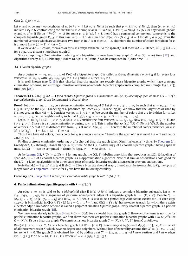
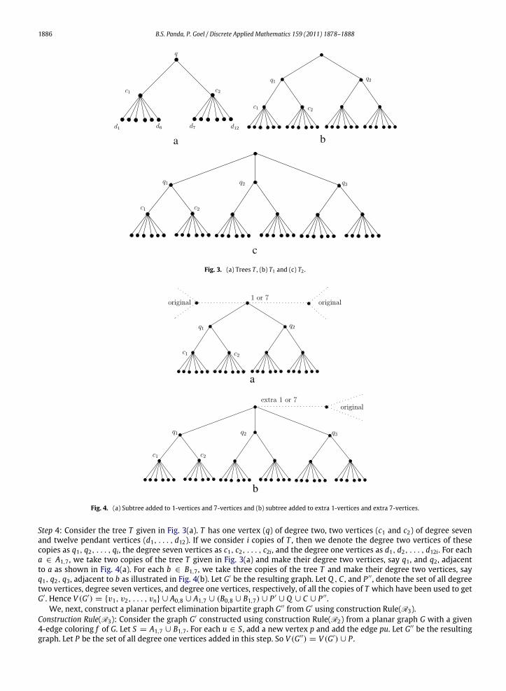
Step 4: Consider the tree T given in Fig. 3(a). T has one vertex (q) of degree two, two vertices (c1 and c2) of degree sevenand twelve pendant vertices (d1, . . . , d12). If we consider i copies of T , then we denote the degree two vertices of thesecopies as q1, q2, . . . , qi, the degree seven vertices as c1, c2, . . . , c2i, and the degree one vertices as d1, d2, . . . , d12i. For eacha ∈ A1,7, we take two copies of the tree T given in Fig. 3(a) and make their degree two vertices, say q1, and q2, adjacentto a as shown in Fig. 4(a). For each b ∈ B1,7, we take three copies of the tree T and make their degree two vertices, sayq1, q2, q3, adjacent to b as illustrated in Fig. 4(b). Let G′ be the resulting graph. Let Q , C , and P ′′, denote the set of all degreetwo vertices, degree seven vertices, and degree one vertices, respectively, of all the copies of T which have been used to getG′. Hence V (G′) = v1, v2, . . . , vn ∪ A0,8 ∪ A1,7 ∪ (B0,8 ∪ B1,7) ∪ P ′

∪ Q ∪ C ∪ P ′′.We, next, construct a planar perfect elimination bipartite graph G′′ from G′ using construction Rule(R3).

Construction Rule(R3): Consider the graph G′ constructed using construction Rule(R2) from a planar graph G with a given4-edge coloring f of G. Let S = A1,7 ∪ B1,7. For each u ∈ S, add a new vertex p and add the edge pu. Let G′′ be the resultinggraph. Let P be the set of all degree one vertices added in this step. So V (G′′) = V (G′) ∪ P .


a b

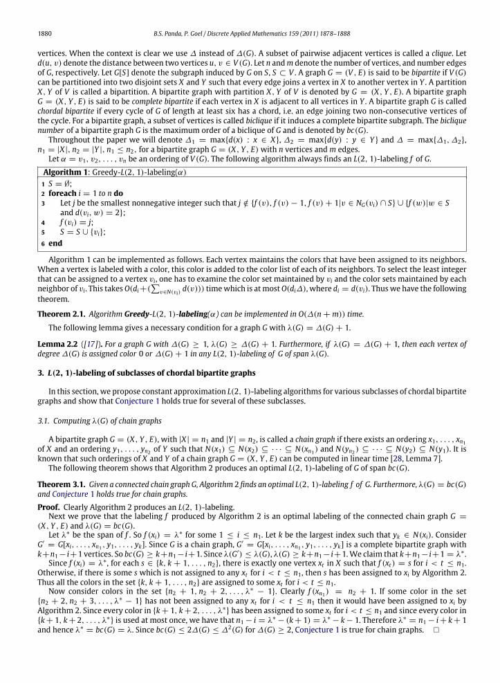
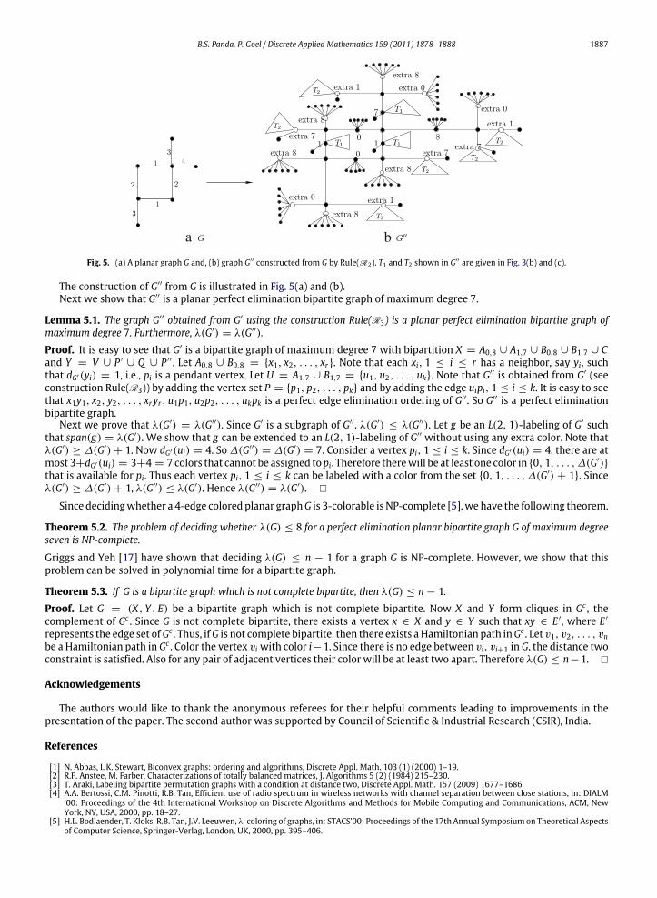
Fig. 5. (a) A planar graph G and, (b) graph G′′ constructed from G by Rule(R2). T1 and T2 shown in G′′ are given in Fig. 3(b) and (c).

The construction of G′′ from G is illustrated in Fig. 5(a) and (b).Next we show that G′′ is a planar perfect elimination bipartite graph of maximum degree 7.

Lemma 5.1. The graph G′′ obtained from G′ using the construction Rule(R3) is a planar perfect elimination bipartite graph ofmaximum degree 7. Furthermore, λ(G′) = λ(G′′).Proof. It is easy to see that G′ is a bipartite graph of maximum degree 7 with bipartition X = A0,8 ∪ A1,7 ∪ B0,8 ∪ B1,7 ∪ Cand Y = V ∪ P ′

∪ Q ∪ P ′′. Let A0,8 ∪ B0,8 = x1, x2, . . . , xr. Note that each xi, 1 ≤ i ≤ r has a neighbor, say yi, suchthat dG′(yi) = 1, i.e., pi is a pendant vertex. Let U = A1,7 ∪ B1,7 = u1, u2, . . . , uk. Note that G′′ is obtained from G′ (seeconstruction Rule(R3)) by adding the vertex set P = p1, p2, . . . , pk and by adding the edge uipi, 1 ≤ i ≤ k. It is easy to seethat x1y1, x2, y2, . . . , xryr , u1p1, u2p2, . . . , ukpk is a perfect edge elimination ordering of G′′. So G′′ is a perfect eliminationbipartite graph.

Next we prove that λ(G′) = λ(G′′). Since G′ is a subgraph of G′′, λ(G′) ≤ λ(G′′). Let g be an L(2, 1)-labeling of G′ suchthat span(g) = λ(G′). We show that g can be extended to an L(2, 1)-labeling of G′′ without using any extra color. Note thatλ(G′) ≥ ∆(G′) + 1. Now dG′(ui) = 4. So ∆(G′′) = ∆(G′) = 7. Consider a vertex pi, 1 ≤ i ≤ k. Since dG′(ui) = 4, there are atmost 3+dG′(ui) = 3+4 = 7 colors that cannot be assigned to pi. Therefore therewill be at least one color in 0, 1, . . . , ∆(G′)that is available for pi. Thus each vertex pi, 1 ≤ i ≤ k can be labeled with a color from the set 0, 1, . . . , ∆(G′) + 1. Sinceλ(G′) ≥ ∆(G′) + 1, λ(G′′) ≤ λ(G′). Hence λ(G′′) = λ(G′).

Since decidingwhether a 4-edge colored planar graphG is 3-colorable is NP-complete [5],we have the following theorem.

Theorem 5.2. The problem of deciding whether λ(G) ≤ 8 for a perfect elimination planar bipartite graph G of maximum degreeseven is NP-complete.

Griggs and Yeh [17] have shown that deciding λ(G) ≤ n − 1 for a graph G is NP-complete. However, we show that thisproblem can be solved in polynomial time for a bipartite graph.

Theorem 5.3. If G is a bipartite graph which is not complete bipartite, then λ(G) ≤ n − 1.Proof. Let G = (X, Y , E) be a bipartite graph which is not complete bipartite. Now X and Y form cliques in Gc , thecomplement of Gc . Since G is not complete bipartite, there exists a vertex x ∈ X and y ∈ Y such that xy ∈ E ′, where E ′

represents the edge set ofGc . Thus, ifG is not complete bipartite, then there exists a Hamiltonian path inGc . Let v1, v2, . . . , vnbe a Hamiltonian path in Gc . Color the vertex vi with color i−1. Since there is no edge between vi, vi+1 in G, the distance twoconstraint is satisfied. Also for any pair of adjacent vertices their color will be at least two apart. Therefore λ(G) ≤ n−1.

Acknowledgements

The authors would like to thank the anonymous referees for their helpful comments leading to improvements in thepresentation of the paper. The second author was supported by Council of Scientific & Industrial Research (CSIR), India.

References

[1] N. Abbas, L.K. Stewart, Biconvex graphs: ordering and algorithms, Discrete Appl. Math. 103 (1) (2000) 1–19.[2] R.P. Anstee, M. Farber, Characterizations of totally balanced matrices, J. Algorithms 5 (2) (1984) 215–230.[3] T. Araki, Labeling bipartite permutation graphs with a condition at distance two, Discrete Appl. Math. 157 (2009) 1677–1686.[4] A.A. Bertossi, C.M. Pinotti, R.B. Tan, Efficient use of radio spectrum in wireless networks with channel separation between close stations, in: DIALM

’00: Proceedings of the 4th International Workshop on Discrete Algorithms and Methods for Mobile Computing and Communications, ACM, NewYork, NY, USA, 2000, pp. 18–27.

[5] H.L. Bodlaender, T. Kloks, R.B. Tan, J.V. Leeuwen, λ-coloring of graphs, in: STACS’00: Proceedings of the 17th Annual Symposium on Theoretical Aspectsof Computer Science, Springer-Verlag, London, UK, 2000, pp. 395–406.


[6] K.S. Booth, G.S. Lueker, Linear-time algorithm for reduction of a pq-tree, J. Comput. System Sci. 3 (1976) 335–379.[7] A. Brandstädt, V.B. Lee, J. Spinrad, Graph Classes: A Survey, SIAM Monograph, 1999.[8] T. Calamoneri, The L(h, k)-labelling problem: a survey and annotated bibliography, Comput. J. 49 (2006) 585–608.[9] T. Calamoneri, S. Caminiti, S. Olariu, R. Petreschi, On the L(h, k)-labeling of co-comparability graphs and circular-arc graphs, Networks 53 (2009)

27–34.[10] T. Calamoneri, R. Petreschi, L(h, 1)-labeling subclasses of planar graphs, J. Parallel Distrib. Comput. 64 (3) (2004) 414–426.[11] G.J. Chang, D. Kuo, The L(2, 1)-labeling problem on graphs, SIAM J. Discrete Math. 9 (2) (1996) 309–316.[12] F.F. Dragan, F. Nicolai, Lexbfs-orderings of distance-hereditary graphs with application to the diametral pair problem, Discrete Appl. Math. 98 (2000)

191–207.[13] M. Farber, Characterizations of strongly chordal graphs, Discrete Math. 43 (1983) 173–189.[14] J. Fiala, T. Kloks, J. Kratochvil, Fixed parameter complexity of λ-labelings, Discrete Appl. Math. 113 (2001) 59–72.[15] M.C. Golumbic, C.F. Goss, Perfect elimination and chordal bipartite graphs, J. Graph Theory 2 (1978) 155–163.[16] D. Gonçalves, On the L(p, 1)-labelling of graphs, Discrete Math. 308 (2008) 1405–1414.[17] J.R. Griggs, R.K. Yeh, Labelling graphs with a condition at distance 2, SIAM J. Discrete Math. 5 (1992) 586–595.[18] F. Havet, B. Reed, J.S. Sereni, L(2, 1)-labeling of graphs, in: Proc. 19th annual ACM–SIAM Symposium on Discrete Algorithms, SODA 2008, SIAM, 2008,

pp. 621–630.[19] W.K. Hale, Frequency assignment: theory and applications, Proc. IEEE 68 (1980) 1497–1514.[20] E. Howorka, A characterization of distance-hereditary graphs, Quart. J. Math. Oxford Ser. 2 28 (1977) 417–420.[21] J.-H. Kang, L(2, 1)-labeling of Hamiltonian graphs with maximum degree 3, SIAM J. Discrete Math. 22 (2008) 213–230.[22] D. Král’, Coloring powers of chordal graphs, SIAM J. Discrete Math. 18 (3) (2005) 426–437.[23] D. Král’, R. Skrekovski, A theorem about the channel assignment problem, SIAM J. Discrete Math. 16 (2003) 426–437.[24] T.-H. Lai, S.S. Wei, Bipartite permutation graphs with application to the minimum buffer size problem, Discrete Appl. Math. 74 (1997) 33–55.[25] A. Lubiw, Doubly lexical orderings of matrices, in: STOC’85: Proceedings of the Seventeenth Annual ACM Symposium on Theory of Computing, ACM,

New York, NY, USA, 1985, pp. 396–404.[26] D. Sakai, Labeling chordal graphs: distance two condition, SIAM J. Discrete Math. 7 (1994) 133–140.[27] J. Spinrad, A. Brandstädt, L. Stewart, Bipartite permutation graphs, Discrete Appl. Math. 18 (1987) 279–292.[28] R. Uehara, Y. Uno, Efficient algorithms for the longest path problem, in: 15th Annual International Symposium on Algorithms and Computation,

in: Lecture Notes in Computer Science, vol. 3341, Springer Berlin, Heidelberg, December,2004, pp. 871–883.[29] R.K. Yeh, A survey on labeling graphs with a condition at distance two, Discrete Math. 306 (2006) 1217–1231.[30] C.-W. Yu, G.-H. Chen, Efficient parallel algorithms for doubly convex-bipartite graphs, Theoret. Comput. Sci. 147 (1995) 249–265.

Documents

-labeling of perfect elimination bipartite graphs