LEE'* and ALAN G. BARR' USA

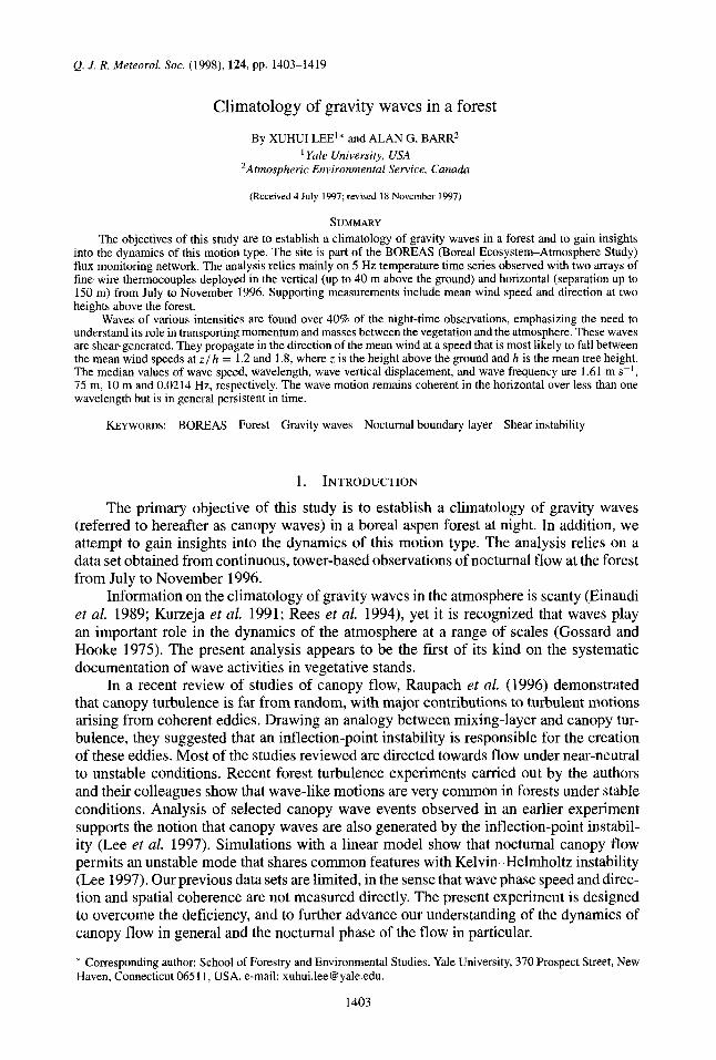
Q. J . R. Meteorol. SOC. (1998), 124, pp. 1403-1419

Climatology of gravity waves in a forest

By XUHUI LEE'* and ALAN G. BARR' ' Yale University, USA

'Atmospheric Environmental Service, Canada

(Received 4 July 1997; revised 18 November 1997)

SUMMARY

The objectives of this study are to establish a climatology of gravity waves in a forest and to gain insights into the dynamics of this motioil type. The site is part of the BOREAS (Boreal Ecosystem-Atmosphere Study) flux monitoring network. The analysis relies mainly on 5 Hz temperature time series observed with two arrays of fine-wire thermocouples deployed in the vertical (up to 40 m above the ground) and horizontal (separation up to 150 m) from July to November 1996. Supporting measurements include mean wind speed and direction at two heights above the forest.

Waves of various intensities are found over 40% of the night-time observations, emphasizing the need to understand its role in transporting momentum and masses between the vegetation and the atmosphere. These waves are shear-generated. They propagate in the direction of the mean wind at a speed that is most likely to fall between the mean wind speeds at z / h = 1.2 and 1.8, where z is the height above the ground and h is the mean tree height. The median values of wave specd, wavelength, wave vertical displacement, and wave frequency are 1.61 m s-', 75 m, 10 m and 0.0214 Hz, respectively. The wave motion remains coherent in the horizontal over less than one wavelength but is in general persistent in time.

KEYWORDS: BOREAS Forest Gravity waves Nocturnal boundary layer Shear instability

1. INTRODUCTION

The primary objective of this study is to establish a climatology of gravity waves (referred to hereafter as canopy waves) in a boreal aspen forest at night. In addition, we attempt to gain insights into the dynamics of this motion type. The analysis relies on a data set obtained from continuous, tower-based observations of nocturnal flow at the forest from July to November 1996.

Information on the climatology of gravity waves in the atmosphere is scanty (Einaudi et al. 1989; Kurzeja et al. 1991; Rees et al. 1994), yet it is recognized that waves play an important role in the dynamics of the atmosphere at a range of scales (Gossard and Hooke 1975). The present analysis appears to be the first of its kind on the systematic documentation of wave activities in vegetative stands.

In a recent review of studies of canopy flow, Raupach et al. (1996) demonstrated that canopy turbulence is far from random, with major contributions to turbulent motions arising from coherent eddies. Drawing an analogy between mixing-layer and canopy turbulence, they suggested that an inflection-point instability is responsible for the creation of these eddies. Most of the studies reviewed are directed towards flow under near-neutral to unstable conditions. Recent forest turbulence experiments carried out by the authors and their colleagues show that wave-like motions are very common in forests under stable conditions. Analysis of selected canopy wave events observed in an earlier experiment supports the notion that canopy waves are also generated by the inflection-point instability (Lee et al. 1997). Simulations with a linear model show that nocturnal canopy flow permits an unstable mode that shares common features with Kelvin-Helmholtz instability (Lee 1997). Our previous data sets are limited, in the sense that wave phase speed and direction and spatial coherence are not measured directly. The present experiment is designed to overcome the deficiency, and to further advance our understanding of the dynamics of canopy flow in general and the nocturnal phase of the flow in particular.

* Corresponding author: School of Forestry and Environmental Studies, Yale University, 370 Prospect Street, New Haven, Connecticut 065 11, USA. e-mail: [email protected].

1403

1404 X. LEE and A. G. BARR

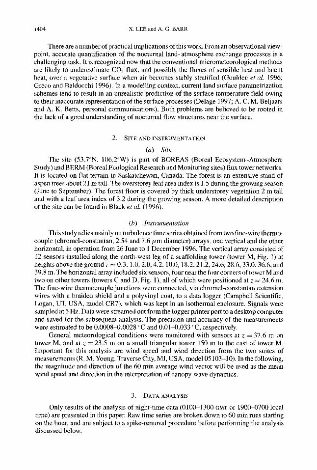
There are a number of practical implications of this work. From an observational view- point, accurate quantification of the nocturnal land-atmosphere exchange processes is a challenging task. It is recognized now that the conventional micrometeorological methods are likely to underestimate C02 flux, and possibly the fluxes of sensible heat and latent heat, over a vegetative surface when air becomes stably stratified (Goulden et al. 1996; Greco and Baldocchi 1996). In a modelling context, current land surface parametrization schemes tend to result in an unrealistic prediction of the surface temperature field owing to their inaccurate representation of the surface processes (Delage 1997; A. C. M. Beljaars and A. K. Betts, personal communications). Both problems are believed to be rooted in the lack of a good understanding of nocturnal flow structures near the surface.

2. SITE AND INSTRUMENTATION

(a) Site The site (53.7"N, 106.2"W) is part of BOREAS (Boreal Ecosystem-Atmosphere

Study) and BERM (Boreal Ecological Research and Monitoring sites) flux tower networks. It is located on flat terrain in Saskatchewan, Canada. The forest is an extensive stand of aspen trees about 21 m tall. The overstorey leaf area index is 1.5 during the growing season (June to September). The forest floor is covered by thick understorey vegetation 2 m tall and with a leaf area index of 3.2 during the growing season. A more detailed description of the site can be found in Black et al. (1996).

(b) Instrumentation This study relies mainly on turbulence time series obtained from two fine-wire thermo-

couple (chromel-constantan, 2.54 and 7.6 p m diameter) arrays, one vertical and the other horizontal, in operation from 26 June to 1 December 1996. The vertical array consisted of 12 sensors installed along the north-west leg of a scaffolding tower (tower M, Fig. 1) at heights above the ground z = 0.3, 1.0,2.0,4.2, 10.0, 18.2,21.2,24.6,28.6,33.0,36.6, and 39.8 m. The horizontal array included six sensors, four near the four corners of tower M and two on other towers (towers C and D, Fig. l), all of which were positioned at z = 24.6 m. The fine-wire thermocouple junctions were connected, via chromel-constantan extension wires with a braided shield and a polyvinyl coat, to a data logger (Campbell Scientific, Logan, UT, USA, model CR7), which was kept in an isothermal enclosure. Signals were sampled at 5 Hz. Data were streamed out from the logger printer port to a desktop computer and saved for the subsequent analysis. The precision and accuracy of the measurements were estimated to be 0.0008-0.0028 "C and 0.01-0.033 "C, respectively.

General meteorological conditions were monitored with sensors at z = 37.6 m on tower M, and at z = 23.5 m on a small triangular tower 150 m to the east of tower M. Important for this analysis are wind speed and wind direction from the two suites of measurements (R. M. Young, Traverse City, MI, USA, model 05103-10). In the following, the magnitude and direction of the 60 min average wind vector will be used as the mean wind speed and direction in the interpretation of canopy wave dynamics.

3. DATA ANALYSIS

Only results of the analysis of night-time data (0100-1300 GMT or 1900-0700 local time) are presented in this paper. Raw time series are broken down to 60 min runs starting on the hour, and are subject to a spike-removal procedure before performing the analysis discussed below.

CLIMATOLOGY O F GRAVITY WAVES IN A FOREST 1405 'VC 66m

M i

Figure 1 . Geometry of the horizontal thermocouple sensor array on towers M, C and D at height z = 24.6 m. Distances are measured from the sensor near the north-west corner of tower M.

(a) Waviness index and wave frequency Fourier transformation is applied to the full 60 min record. Prior to the transformation

the linear trend is removed from the signal, and a low-pass filter with a cut-off frequency of 0.5 Hz is applied. The filtering is necessary to avoid noise-related spectral peaks being interpreted as a result of wave motions at times when temperature fluctuations are weak. A waviness index (i,) is defined as

i w = (f sT)rnax/ 1 S T df,

where ,f is natural frequency and S, is the temperature power spectrum. The frequency of (,fST),,,ax is taken as the wave frequency (f,). The ambiguity in finding f, is minimized by the fact that there is a large sample size in the low frequency end of the spectrum.

In the following, the time series from the north-west sensor at z = 24.6 m on tower M is used to find the waviness index and wave frequency unless stated otherwise. This sensor is chosen for two reasons: (1) its records are least interrupted by problems; (2) the air layer near z = 24.6 m is most likely to undergo wave motions, as indicated by data from a previous experiment (Lee et al. 1997). It should be noted that i , values are dependent upon sampling frequency and the record length used in the Fourier transformation. The thresholds adopted for assessing percentage of wave occurrence (section 4(a)) are specific to this particular data set and analysis strategy.

The simple detection technique based on the waviness index implies a working defi- nition of what we regard as a wave: it is an event in which the time series of a tracer scalar


I I I I I I 0 10 20 30 40 50 60

Time (min)

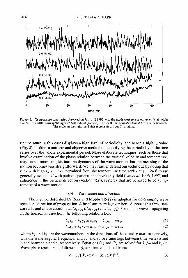
Figure 2. Temperature time series observed on July 1-2 1996 with the north-west sensor on tower M at height z = 24.6 m and the corresponding waviness indices (see text). The local time of observation is given in the brackets.

The scale on the right-hand side represents a 1 degC variation.

(temperature in this case) displays a high level of periodicity, and hence a high i, value (Fig. 2). It offers a uniform and objective method of quantifying the periodicity of the time series over the whole experimental period. More elaborate techniques, such as those that involve examination of the phase relation between the vertical velocity and temperature, may reveal more insights into the dynamics of the wave motion, but the meaning of the motion becomes less straightforward. We may further defend our technique by noting that runs with high i, values determined from the temperature time series at z = 24.6 m are generally associated with periodic patterns in the velocity field (Lee et al. 1996, 1997) and coherence in the vertical direction (section 4(a)), features that are believed to be symp- tomatic of a wave motion.

(b) Wave speed and direction The method described by Rees and Mobbs (1988) is adopted for determining wave

speed and direction of propagation. A brief summary is given here. Suppose that three sensors a, b, and c have coordinates (x,, y,), (xb, Yb) and (&, yc). For a plane wave propagating in the horizontal direction, the following relations hold:

where k, and k, are the wavenumbers in the directions of the x and y axes respectively, w is the wave angular frequency, and tab and ra, are time lags between time series a and b and between a and c, respectively. Equations (1) and (2) are solved for k x / o and k y / o . Wave phase speed, c, and direction, 4, are then calculated from:

c = 1/[(k,/o)2 + ( k , / ~ ) ~ l ” ~ , (3)

CLIMATOLOGY OF GRAVITY WAVES IN A FOREST I407

4 = tan-'((-kx/@)/(-ky/@)I. (4)

As with Rees and Mobbs (1988), 4 is specified in the meteorological convention such that 4 = 0" or 360" if waves propagate from the north, 4 = 90" if from the east, and so forth.

Temperature time series from the four sensors on towerM (Fig. 1) are used to find c and 4. Digital filtering with a second-order Butterworth filter (band-path 0.5fw - 2fw) is first applied to the time series. Time lags are then determined with a lagged cross-correlation procedure from the filtered data.

Rees and Mobbs' procedure requires three horizontally displaced sensors. The sensor array on tower M (Fig. 1) allows four possible combinations. The wavenumbers k, and k, are calculated for each combination and are averaged for every 60 min run. Estimates of c and 4 are based on the averaged k, and k, values.

(c) Spatial coherence The records from the north-west sensor on tower M and sensors on towers C and

D (Fig. 1, triangle), all located at z = 24.6 m, are used to assess the spatial coherence of the wave-like motions. Here spatial coherence is defined as the maximum value of the lagged correlation coefficient of two time series. Prior to the coherence calculation, the raw time series are filtered with the same band-path digital filter as above, to remove the low- frequency trend and the high-frequency noise. The lagged correlation procedure removes the dependence on phase, while the band-path filtering maximizes the contribution of the wave motion to the correlation value. Three coherence values are obtained from the three tower pairs for each 60 min run.

4. RESULTS AND DISCUSSION

(a) Waviness The plot of the temperature time series observed during a typical wave event brings

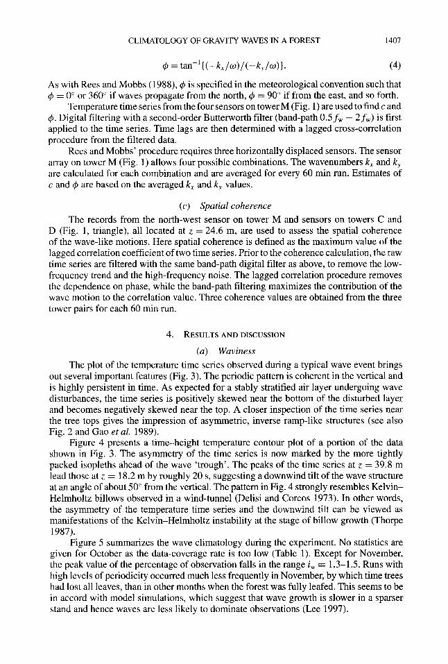
out several important features (Fig. 3). The periodic pattern is coherent in the vertical and is highly persistent in time. As expected for a stably stratified air layer undergoing wave disturbances, the time series is positively skewed near the bottom of the disturbed layer and becomes negatively skewed near the top. A closer inspection of the time series near the tree tops gives the impression of asymmetric, inverse ramp-like structures (see also Fig. 2 and Gao et al. 1989).

Figure 4 presents a time-height temperature contour plot of a portion of the data shown in Fig. 3. The asymmetry of the time series is now marked by the more tightly packed isopleths ahead of the wave 'trough'. The peaks of the time series at z = 39.8 m lead those at z = 18.2 m by roughly 20 s, suggesting a downwind tilt of the wave structure at an angle of about 50" from the vertical. The pattern in Fig. 4 strongly resembles Kelvin- Helmholtz billows observed in a wind-tunnel (Delisi and Corcos 1973). In other words, the asymmetry of the temperature time series and the downwind tilt can be viewed as manifestations of the Kelvin-Helmholtz instability at the stage of billow growth (Thorpe 1987).

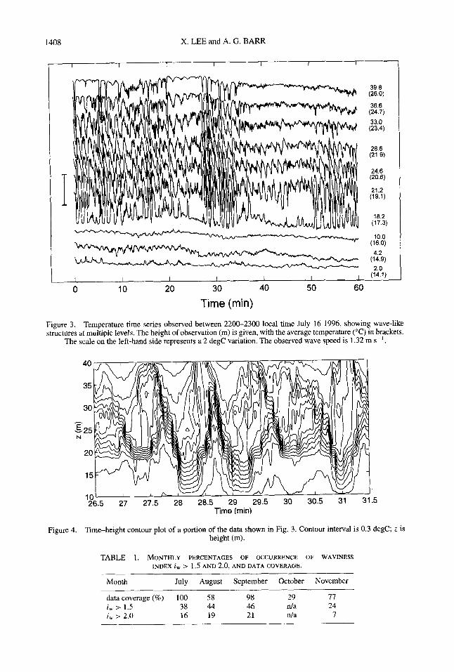
Figure 5 summarizes the wave climatology during the experiment. No statistics are given for October as the data-coverage rate is too low (Table 1). Except for November, the peak value of the percentage of observation falls in the range i , = 1.3-1.5. Runs with high levels of periodicity occurred much less frequently in November, by which time trees had lost all leaves, than in other months when the forest was fully leafed. This seems to be in accord with model simulations, which suggest that wave growth is slower in a sparser stand and hence waves are less likely to dominate observations (Lee 1997).


I I I I I I

0 10 20 30 40 50 60 Time (min)

Figure 3. Temperature time series observed between 2200-2300 local time July 16 1996, showing wave-like structures at multiple levels. The height of observation (m) is given, with the average temperature ("C) in brackets.

The scale on the left-hand side represents a 2 degC variation. The observed wave speed is 1.32 m s-l.

.5 Time (min)

Figure 4. Time-height contour plot of a portion of the data shown in Fig. 3. Contour interval is 0.3 degC; z is height (m).

TABLE 1. MONTHLY PERCENTAGES OF OCCURRENCE OF WAVINESS INDEX i, z 1.5 AND 2.0, AND DATA COVERAGE.

Month July August September October November

data coverage (%) 100 58 98 29 I1

i, t 2.0 16 19 21 n/a I i, > 1.5 38 44 46 n/a 24

CLIMATOLOGY OF GRAVITY WAVES IN A FOREST 1409

0 0 1 2 3 4 5

Figure 5 . Frequency distribution of wave occurrence by month (solid line July; dash line August; dash-dot line September; dot line November). Percentage of observation is for equal waviness index (iW, see text) intervals of

0.2.

Visual inspection of the time series from selected runs, shows that an i, value greater than 2.0 corresponds to clear and persistent wave-like patterns over the full hour, and that the time series with i, between 1.5-2.0 are periodic for at least 30% of the run. Summary statistics based on the threshold values are given in Table 1. As a reference, i, for the smooth-wall surface layer under statically stable conditions without wave activities is about 0.25 (see Fig. 20 of Kaimal et aE. 1972). The two wave events (events A and B) analysed by Lee et al. (1997) have i, values of 2.8 and 2.9, respectively. Choice of the thresholds is somewhat arbitrary, but it is clear from Table 1 and Fig. 5 that wave-like motions are a common form of air motion in the forest. It is also noted that statistics in Table 1 are biased low, because the Fourier method will exclude runs which experience only a few episodic wave cycles.

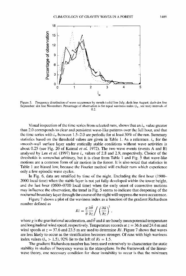
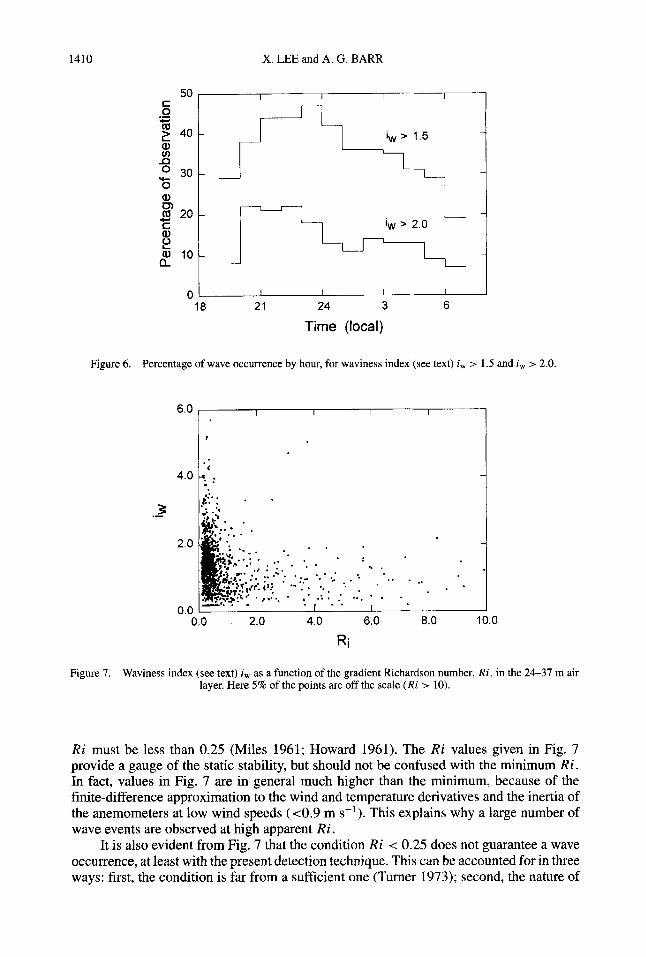
In Fig. 6, data are stratified by time of the night. Excluding the first hour (1900- 2000 local time) when the stable layer is not yet fully developed within the tower height, and the last hour (0600-0700 local time) when the early onset of convective motions may influence the observation, the trend in Fig. 5 seems to indicate that deepening of the nocturnal boundary layer through thecourse of the night will suppress the wave occurrence.

Figure 7 shows a plot of the waviness index as a function of the gradient Richardson number defined as

where g is the gravitational acceleration, and 6 and ii are hourly mean potential temperature and longitudinal wind speed, respectively. Temperature records at z = 36.6 and 24.6 m and wind speeds at z = 37.6 and 23.5 m are used to determine Ri. Figure 7 shows that waves are less likely to occur as the stratification becomes stronger. Of runs with high waviness index values (i, > lS ) , 92% lie to the left of Ri = 1.5.

The gradient Richardson number has been used extensively to characterize the static stability in studies of buoyancy waves in the atmosphere. In the framework of the linear- wave theory, one necessary condition for shear instability to occur is that the minimum


50 c 0 .- +

40

s a O Q)

30 Y-

- B 20 c Q)

Q) 10 a 2

0 I I I I

18 21 24 3 6

Time (local)

Figure 6 . Percentage of wave occurrence by hour, for waviness index (see text) i, > 1.5 and i, > 2.0.

.- 3

2.0

0.0

.\ .' . * * .

I I

0.0 2.0

. . . . . . 5 .

.. . . * . . . .. . .- . . . . .. . . . : . , ... . ... . . . . . I

4.0 6.0 I

8.0 10.0

Figure 7. Waviness index (see text) i, as a function of the gradient Richardson number, Ri, in the 24-37 m air layer. Here 5% of the points are off the scale ( R i > 10).

Ri must be less than 0.25 (Miles 1961; Howard 1961). The Ri values given in Fig. 7 provide a gauge of the static stability, but should not be confused with the minimum Ri. In fact, values in Fig. 7 are in general much higher than the minimum, because of the finite-difference approximation to the wind and temperature derivatives and the inertia of the anemometers at low wind speeds (<0.9 m s-l). This explains why a large number of wave events are observed at high apparent Ri.

It is also evident from Fig. 7 that the condition Ri < 0.25 does not guarantee a wave occurrence, at least with the present detection technique. This can be accounted for in three ways: first, the condition is far from a sufficient one (Turner 1973); second, the nature of

CLIMATOLOGY OF GRAVITY WAVES IN A FOREST 141 1

4

3

h

#

W 22 0

1

0 0 1 2 3 4

u (mls)

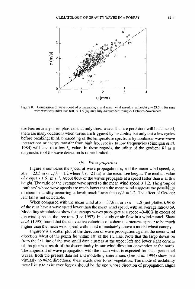
Figure 8. Comparison of wave speed of propagation, c, and mean wind speed, u, at height z = 23.5 m for runs with waviness index (see text) > 1.5 (squares July-September; triangles October-November).

the Fourier analysis emphasizes that only those waves that are persistent will be detected, there are many occasions when waves are triggered by instability but only last a few cycles before breaking; third, broadening of the temperature spectrum by nonlinear wave-wave interactions or energy transfer from high frequencies to low frequencies (Finnigan et al. 1984) will lead to a low i , value. In these regards, the utility of the gradient Ri as a diagnostic tool for wave detection is rather limited.

(b) Wave properties Figure 8 compares the speed of wave propagation, c, and the mean wind speed, u ,

at z = 23.5 m or z / h = 1.2 where h (= 21 m) is the mean tree height. The median value of c equals 1.61 m s-l. About 86% of the waves propagate at a speed faster than u at this height. The ratio of the average wave speed to the mean wind speed is 1.2. The group of 'outliers' whose wave speeds are much lower than the mean wind suggests the possibility of shear instability occurring at levels much lower than z / h = 1.2. The effect of October leaf fall is not detectable.

When compared with the mean wind at z = 37.6 m or z/ h = 1.8 (not plotted), 96% of the runs have a wave speed lower than the mean wind speed, with an average ratio 0.69. Modelling simulations show that canopy waves propagate at a speed 40-80% in excess of the wind speed at the tree tops (Lee 1997). In a study of air flow in a wind-tunnel, Shaw et al. (1995) found that the convective velocities of coherent structures appear to be much higher than the mean wind speed within and immediately above a model wheat canopy.

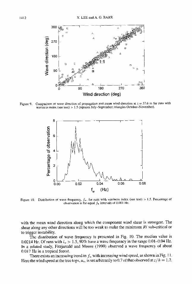
Figure 9 is a scatter plot of the direction of wave propagation against the mean wind direction. Most of the points lie within lo" of the 1 : 1 line. Note that the large deviation from the 1:l line of the two small data clusters at the upper left and lower right corners of the plot is a result of the discontinuity in our wind direction convention at the north. The alignment of wave propagation with the mean wind is expected for shear-generated waves. Both the present data set and modelling simulations (Lee et al. 1994) show that virtually no wind directional shear exists over forest vegetation. The mode of instability most likely to exist over forests should be the one whose direction of propagation aligns


360

h

8) 270

C 0

8 180

-0

;E!

.- 4

L .-

2 90 3

0

t - m A m P 1 - 0

A

I A

0 90 180 270 360

Wind direction (deg)

Figure 9. Comparison of wave direction of propagation and mean wind direction at z = 37.6 m for runs with waviness index (see text) z 1.5 (squares July-September; triangles October-November).

8 I I I

Figure 10. Distribution of wave frequency, fw, for runs with waviness index (see text) > 1.5. Percentage of observation is for equal f w intervals of 0.001 Hz.

with the mean wind direction along which the component wind shear is strongest. The shear along any other directions will be too weak to make the minimum Ri sub-critical or to trigger instability.

The distribution of wave frequency is presented in Fig. 10. The median value is 0.0214 Hz. Of runs with i, > 1.5,90% have a wave frequency in the range 0.01-0.04 Hz. In a related study, Fitzjarrald and Moore (1990) observed a wave frequency of about 0.017 Hz in a tropical forest.

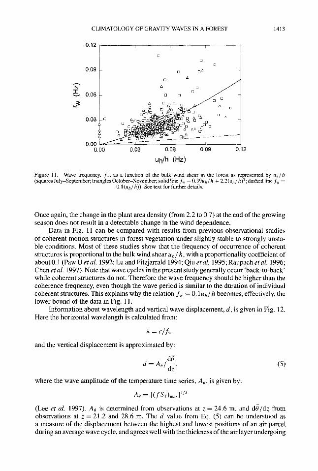
There exists an increasing trend in fw with increasing wind speed, as shown in Fig. 11. Here the wind speed at the tree tops, uh, is set arbitrarily to 0.7 of that observed at z / h = 1.2.


0.12

0.09

h

N

E 0.06 3 Y-

0.03

0.00 0.00 0.03 0.06 0.09 0.12

uh/h (Hz)

Figure 11. Wave frequency, f w , as a function of the bulk wind shear in the forest as represented by u h / h (squares July-September; triangles October-November; solid line fw = 0.39uhl h + 2 .2 (~h /h )* ; dashed line f w =

O.l (uh/h) ) . See text for further details.

Once again, the change in the plant area density (from 2.2 to 0.7) at the end of the growing season does not result in a detectable change in the wind dependence.

Data in Fig. 11 can be compared with results from previous observational studies of coherent motion structures in forest vegetation under slightly stable to strongly unstable conditions. Most of these studies show that the frequency of occurrence of coherent structures is proportional to the bulk wind shear u h / h , with a proportionality coefficient of about 0.1 (Paw U et al. 1992; Lu and Fitzjarrald 1994; Qiu etaf. 1995; Raupach et al. 1996; Chen et al. 1997). Note that wave cycles in the present study generally occur ‘back-to-back’ while coherent structures do not. Therefore the wave frequency should be higher than the coherence frequency, even though the wave period is similar to the duration of individual coherent structures. This explains why the relation fw = O.lu,,/ h becomes, effectively, the lower bound of the data in Fig. 1 1 .

Information about wavelength and vertical wave displacement, d, is given in Fig. 12. Here the horizontal wavelength is calculated from:

and the vertical displacement is approximated by:

d8 dz

d = Ae/--,

where the wave amplitude of the temperature time series, Ae, is given by:

A8 = { ( f % l a x P 2

(Lee et al. 1997). Ae is determined from observations at z = 24.6 m, and dg/dz from observations at z = 21.2 and 28.6 m. The d value from Eq. ( 5 ) can be understood as a measure of the displacement between the highest and lowest positions of an air parcel during an average wave cycle, and agrees well with the thickness of the air layer undergoing


d (m) 0 10 20 30

15 I I

d (m) 0 10 20 30

15 I I

0 50 100 150 200

(m)

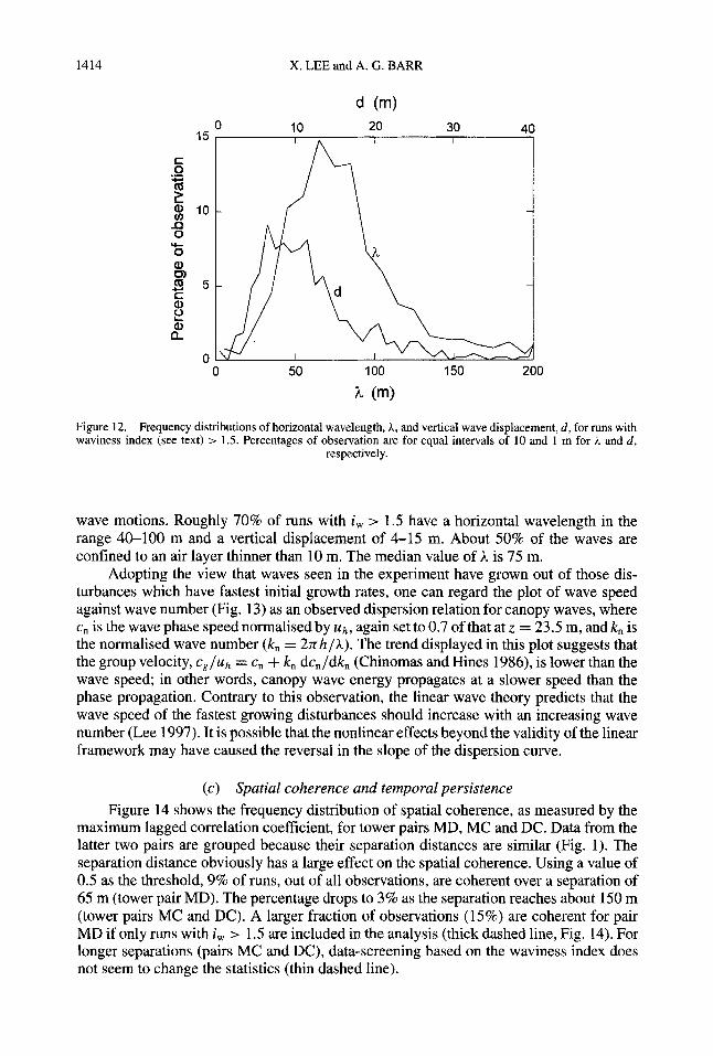
Figure 12. Frequency distributions of horizontal wavelength, h, and vertical wave displacement, d , for runs with waviness index (see text) > 1.5. Percentages of observation are for equal intervals of 10 and 1 m for A. and d ,

respectively.

wave motions. Roughly 70% of runs with i, > 1.5 have a horizontal wavelength in the range 40-100 m and a vertical displacement of 4-15 m. About 50% of the waves are confined to an air layer thinner than 10 m. The median value of h is 75 m.

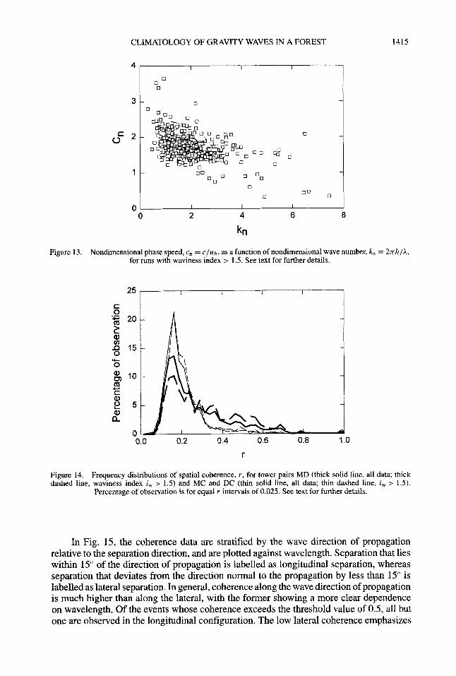
Adopting the view that waves seen in the experiment have grown out of those disturbances which have fastest initial growth rates, one can regard the plot of wave speed against wave number (Fig. 13) as an observed dispersion relation for canopy waves, where c, is the wave phase speed normalised by uh, again set to 0.7 of that at z = 23.5 m, and k, is the normalised wave number (k, = 2nh/h). The trend displayed in this plot suggests that the group velocity, cg/uh = c, + k, dc,/dk, (Chinomas and Hines 1986), is lower than the wave speed; in other words, canopy wave energy propagates at a slower speed than the phase propagation. Contrary to this observation, the linear wave theory predicts that the wave speed of the fastest growing disturbances should increase with an increasing wave number (Lee 1997). It is possible that the nonlinear effects beyond the validity of the linear framework may have caused the reversal in the slope of the dispersion curve.

(c) Spatial coherence and temporal persistence Figure 14 shows the frequency distribution of spatial coherence, as measured by the

maximum lagged correlation coefficient, for tower pairs MD, MC and DC. Data from the latter two pairs are grouped because their separation distances are similar (Fig. 1). The separation distance obviously has a large effect on the spatial coherence. Using a value of 0.5 as the threshold, 9% of runs, out of all observations, are coherent over a separation of 65 m (tower pair MD). The percentage drops to 3% as the separation reaches about 150 m (tower pairs MC and DC). A larger fraction of observations (15%) are coherent for pair MD if only runs with i , > 1.5 are included in the analysis (thick dashed line, Fig. 14). For longer separations (pairs MC and DC), data-screening based on the waviness index does not seem to change the statistics (thin dashed line).


4

3

G

1

0 0 2 4 6 8

kn

Figure 13. Nondimensional phase speed, c,, = C/Uh, as a function of nondimensional wave number, k, = 2 n h / l , for runs with waviness index z 1.5. See text for further details.

r

Figure 14. Frequency distributions of spatial coherence, r, for tower pairs MD (thick solid line, all data; thick dashed line, waviness index i, > 1.5) and MC and DC (thin solid line, all data; thin dashed line, i, > 1.5).

Percentage of observation is for equal r intervals of 0.025. See text for further details.

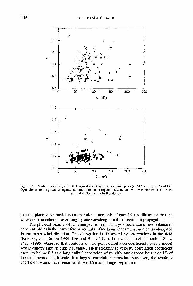
In Fig. 15, the coherence data are stratified by the wave direction of propagation relative to the separation direction, and are plotted against wavelength. Separation that lies within 15" of the direction of propagation is labelled as longitudinal separation, whereas separation that deviates from the direction normal to the propagation by less than 15" is labelled as lateral separation. In general, coherence along the wave direction of propagation is much higher than along the lateral, with the former showing a more clear dependence on wavelength. Of the events whose coherence exceeds the threshold value of 0.5, all but one are observed in the longitudinal configuration, The low lateral coherence emphasizes


1 .o

0.8

0.6

L

0.4

0.2

0.0

I I I I

a 0 0

03

00

I I I I

0 50 100 150 200 250

(m)

0.8 1 0.6 1 0

0

0 0 0

0

0.0 I I I I I I 0 50 100 150 200 250

(m>

Figure 15. Spatial coherence, r , plotted against wavelength, A, for tower pairs (a) MD and (b) MC and DC. Open circles are longitudinal separation; bullets are lateral separation. Only data with waviness index > 1.5 are

presented. See text for further details.

that the plane-wave model is an operational one only. Figure 15 also illustrates that the waves remain coherent over roughly one wavelength in the direction of propagation.

The physical picture which emerges from this analysis bears some resemblance to coherent eddies in the convective or neutral surface layer, in that those eddies are elongated in the mean wind direction. The elongation is illustrated by observations in the field (Panofsky and Dutton 1984; Lee and Black 1994). In a wind-tunnel simulation, Shaw et al. (1995) observed that contours of two-point correlation coefficients over a model wheat canopy take an elliptical shape. Their streamwise velocity correlation coefficient drops to below 0.5 at a longitudinal separation of roughly one canopy height or 1/3 of the streamwise length-scale. If a lagged correlation procedure was used, the resulting coefficient would have remained above 0.5 over a longer separation.


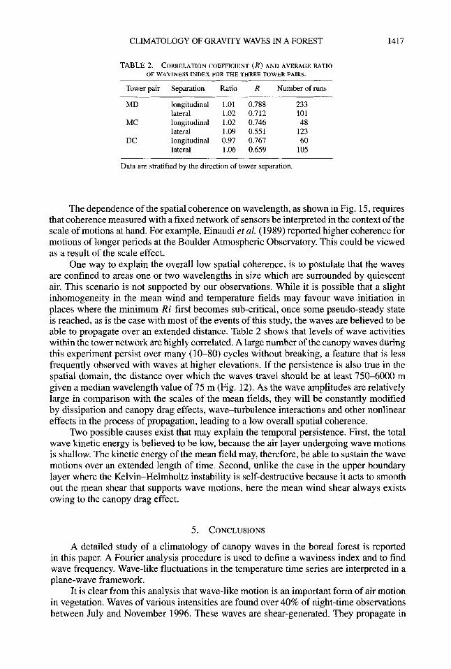
TABLE 2. CORRELATION COEFFICIENT (R) AND AVERAGE RATIO OF WAVINESS INDEX FOR THE THREE TOWER PAIRS.

~

Tower pair Separation Ratio

MD longitudinal 1.01 lateral 1.02

MC longitudinal 1.02 lateral 1.09

DC longitudinal 0.97 lateral 1.06

R Number of runs

0.788 233 0.712 101 0.746 48 0.551 123 0.767 60 0.659 105

Data are stratified by the direction of tower separation.

The dependence of the spatial coherence on wavelength, as shown in Fig. 15, requires that coherence measured with a fixed network of sensors be interpreted in the context of the scale of motions at hand. For example, Einaudi et al. (1989) reported higher coherence for motions of longer periods at the Boulder Atmospheric Observatory. This could be viewed as a result of the scale effect.

One way to explain the overall low spatial coherence, is to postulate that the waves are confined to areas one or two wavelengths in size which are surrounded by quiescent air. This scenario is not supported by our observations. While it is possible that a slight inhomogeneity in the mean wind and temperature fields may favour wave initiation in places where the minimum Ri first becomes sub-critical, once some pseudo-steady state is reached, as is the case with most of the events of this study, the waves are believed to be able to propagate over an extended distance. Table 2 shows that levels of wave activities within the tower network are highly correlated. A large number of the canopy waves during this experiment persist over many (10-80) cycles without breaking, a feature that is less frequently observed with waves at higher elevations. If the persistence is also true in the spatial domain, the distance over which the waves travel should be at least 750-6000 m given a median wavelength value of 75 m (Fig. 12). As the wave amplitudes are relatively large in comparison with the scales of the mean fields, they will be constantly modified by dissipation and canopy drag effects, wave-turbulence interactions and other nonlinear effects in the process of propagation, leading to a low overall spatial coherence.

Two possible causes exist that may explain the temporal persistence. First, the total wave kinetic energy is believed to be low, because the air layer undergoing wave motions is shallow. The kinetic energy of the mean field may, therefore, be able to sustain the wave motions over an extended length of time. Second, unlike the case in the upper boundary layer where the Kelvin-Helmholtz instability is self-destructive because it acts to smooth out the mean shear that supports wave motions, here the mean wind shear always exists owing to the canopy drag effect.

5. CONCLUSIONS

A detailed study of a climatology of canopy waves in the boreal forest is reported in this paper. A Fourier analysis procedure is used to define a waviness index and to find wave frequency. Wave-like fluctuations in the temperature time series are interpreted in a plane-wave framework.

It is clear from this analysis that wave-like motion is an important form of air motion in vegetation. Waves of various intensities are found over 40% of night-time observations between July and November 1996. These waves are shear-generated. They propagate in


the direction of the mean wind at a speed that is most likely to fall between the mean wind speeds at z / h = 1.2 and 1.8 ( z is height and h the mean tree height). The median values of wave speed, wavelength, vertical displacement, and wave frequency are 1.61 m s-l, 75 m, 10 m and 0.0214 Hz, respectively. The wave motion remains coherent in the horizontal over less than one wavelength, but is in general persistent in time. The temporal persistence is believed to be associated with the persistence of strong mean wind shear near the top of vegetation. In fact it is the temporal persistence that has made our Fourier waviness index a useful one.

ACKNOWLEDGEMENTS

XL is supported by the US National Science Foundation through grant ATM-9629497. AGB acknowledges the support of the Atmospheric Environment Service, Canada. We also acknowledge our fruitful discussions with Professor R. B. Smith on the wave dynamics. We thank Anu Awasthi for her skilful preparation of the figures.

Black, T. A., den Hartog, G., Neumann, H. H., Blanken, P. D., Yang, P. C., Russell, C., Nesic, Z., Lee, X., Chen, S. G., Staebler, R. and Novak, M. D.

Chen, W., Novak, M. D., Black, T. A. and Lee, X.

Chinomas, G. and Hines, C. 0.

Delage, Y.

Delisi, D. P. and Corcos, G.

Einaudi, F., Bedard, A. J. and Finnigan, J. J .

Finnigan, J. J., Einaudi, F. and Fua. D.

Fitzjarrald, D. R. and Moore, K. E.

Gao, W., Shaw, R. H. and Paw U, K. T.

Gossard, E. E. and Hooke, W. H. Goulden, M. L., Munger, J. W.,

Fan, S.-M., Daube, B. C. and Wofsy, s. c.

Greco, S. and Baldocchi, D.

Howard, L. N. Kaimal, J. C., Wyngaard, J. C. ,

Izumi, Y. and Cote, 0. R. Kurzeja, R. J., Berman, S . and

Weber, A. H. Lee, X.

Lee, X. and Black, T. A.

1996

1997

1986

1997

1973

1989

1984

1990

1989

1975 1996

1996

1961 1972

1991

1997

1994

REFERENCES Annual cycles of water vapour and carbon dioxide fluxes in and

above a boreal aspen forest. Global Change Biol., 2,219-229

Coherent eddies and temperature structure functions for three con- trasting surfaces. Part I: ramp model with finite microfront time. Boundary-Layer Meteorol., 84,99-123

Doppler ducting of atmospheric gravity waves. J. Geophys. Res.,

Parameterising sub-grid scale vertical transport in atmospheric models under statically stable conditions. Boundary-Layer Meteorol., 82,2348

A study of internal waves in a wind tunnel. Boundary-Layer Meteorol., 5, 121-137

A climatology of gravity waves and other coherent disturbances at the Boulder Atmospheric Observatory during March-Apnl 1984. J. Amos. Sci., 46,303-329

The interaction between an internal gravity wave and turbulence in the stably-stratified nocturnal boundary layer. J. Amos. Sci., 41,2409-2436

Mechanisms of nocturnal exchange between the rain forest and the atmosphere. J. Geophys. Rex, 95,16839-16850

Observation of organized structure in turbulent flow withm and above a forest canopy. Boundary-Layer Meteorol., 47,349- 377

91,1219-1230

Waves in the armosphere. Elsevier, New York Measurements of carbon sequestration by long-term eddy covari-

ance: methods and a critical evaluation of accuracy. Global Change Biol., 2,169-182

Seasonal variations of COz and water vapor exchange rates over a temperate deciduous forest. Global Change Biol., 2,183-197

Note on a paper by John W. Miles. J. Fluid Mech., 10,509-512 Spectral characteristics of surface layer turbulence. Q. 1. R.

A climatological study of the nocturnal planetary boundary layer.

Gravity waves in a forest: a linear analysis. J. Atmos. Sci., 54,

Relating eddy correlation sensible heat flux to horizontal sensor separation in the unstable atmospheric surface layer. J. Geo- phys. Rex, 99, 18545-18553

Meteorol. Soc., 98,563-589

Boundary-Layer MeteoroL, 54,105-128

2514-2585


Lee, X., Shaw, R. H. and Black, T. A.

Lee, X., Black, T. A., den Hartog, G., Neumann, H. H., Nesic, Z. and Olejnik, J.

den Hartog, G., Fuentes, J. D., Black, T. A., Mickle, R. E., Yang, P. C. and Blanken, P. D.

Lee, X., Neumann, H. H.,

Lu, C. H. and Fitzjarrald, D. R.

Miles, J. W.

Panofsky, H. A. and Dutton, J. A.

Paw U, K. T., Brunet, Y., Collineau, S., Shaw, R. H., Maitani, T., Qiu, J. and Hipps, L.

Oiu. J.. Paw U, K. T. and - . Shaw, R. H.

Brunet, Y. Raupach, M. R., Finnigan, J. J.

Rees, J. M. and Mobbs, S . D.

and

Rees, J. M., McConnell, I., Anderson, P. S. and King, J. C .

Shaw, R. H., Brunet, Y., Finnigan, J. J. and Raupach, M. R.

Thorpe, S. A.

Turner, J. S.

1994

1996

1997

1994

1961

1984

1992

1995

1996

1988

1994

1995

1987

1973

Modelling the effect of mean pressure gradient on the mean flow

Carbon dioxide exchange and nocturnal processes over a mixed within forests. Agric. Forest Meteorol., 68,201-212

deciduous forest. Agric. Forest Meteorol., 81,13-29

Observations of gravity waves in a boreal forest. Boundary-Layer Meteorol., 84,383-398

Seasonal and diurnal variations of coherent structures over a de-

On the stability of heterogeneous shear flows. J. Fluid Mech., 10,

Atmospheric turbulence: models and methods for engineering ap-

On coherent structures in turbulence above and within agricultural

ciduous forest. Boundary-Layer Meteorol., 69,43-69

496-508

plications. John Wiley, New York

plant canopies. Agric. Forest Meteorol., 61,55-68

Pseudo-wavelet analysis of turbulence patterns in three vegetation layers. Boundaly-Layer Meteorol., 72, 177-204

Coherent eddies and turbulence in vegetation canopies: the mixing layer analogy. Boundary-Layer Meteorol., 78,35 1-382

Studies of internal gravity waves at Halley Base, Antarctica, using wind observations. Q. J . R. Meteorol. Soc., 114,939-966

Observations of internal gravity waves over an Antarctic ice shelf using a microbaragraph array. Pp. 61-79 in Stably stratifed jlows:jlow and dispersion over topography. Eds. I. P. Castro and N. J. Rockliff. Oxford University Press, UK

A wind tunnel study of airflow in waving wheat: two-point velocity statistics. Boundary-Layer Meteorol., 76,349-376

Transitional phenomena and the development of turbulence in stratified fluids: a review. J. Geophys. Res., 92C, 523 1-5248

Buoyancy effects in fluids. Cambridge University Press, London

Documents

LEE'* and ALAN G. BARR' USA