- Linear Buckli

Linear Bucklin

This chapter includes material written by Markus Kriesch anas material from Matthias Goelke.

Introduction

The demand for automobiles with less fuel consumption andThe demand for automobiles with less fuel consumption andrising commodity prices. However, the quest for light weight de

to passive and active safety systems and the steadily increasing colightweight concepts in many industries, not only in aerospace an

Besides the lightweight design, the increasing usage of optimizattend to buckle under axial loading.

Thin structures subject to compression loads that haven’t achiebuckling. Buckling is characterized by a sudden failure of a struactual compressive stress at the point of failure is less than thwithstanding (may be helpful is the explanation on Wikipedia (if st

In other words, once a critical load is reached, the slender compits cross sectional area) draws aside instead of taking up addition

Force versus displacements of a slender beam; from Ihlenburg: Skrip

1

ng Analysis -

ng Analysis

nd André Wehr (Universität der Bundeswehr München) as well

less emissions has increased since the year 2000 because ofless emissions has increased since the year 2000 because ofsigns is (partly) counterbalanced by the additional weight relatedomfort level for passengers. This creates a demand for intelligentd automotive.

tion software leads to thin-walled and slender components which

eved the material strength limits can show a failure mode calledctural member subjected to high compressive stress, where thee ultimate compressive stresses that the material is capable oftill alive) http://en.wikipedia.org/wiki/Buckling)

ponent (for example a beam where its length is much larger thannal load.

t Technische Mechanik 2.7 Knicken. HAW Hamburg – FB MP; 2012

- Linear Buckli

This failure can be analyzed using a technique well known as lineabuckling load factor, λ, and the critical buckling load.

In OptiStruct, if the load factor λ is > 1, the component is considbuckling would occur).buckling would occur).

Elastic Buckling

Euler buckling cases; K=effective buckling len

(f Lä l V lk Ei füh g i di F ti(from Läppele, Volker: Einführung in die Festi

In 1757 Leonhard Euler derived the following equation:

F = π2 Ε Ι / (K crit

where

F = maximum or critical force (vertical load on column)

E d l f l i i I f i i ( d E = modulus of elasticity; I = area moment of inertia (second mom

L = unsupported length of column

K = column effective length factor, whose value depends on the c

• For both ends pinned (hinged, free to rotate), K = 1.0

F b th d fi d K 0 50• For both ends fixed, K = 0.50

• For one end fixed and the other end pinned, K = 0.707

• For one end fixed and the other end free to move laterally, K =

KL = the effective buckling length of the column

In other words, the critical force depends on:

• Length of column

• Cross-section (second moment of surface area)

• Material property (Young’s modulus, in case of elastic materia

• Boundary condition (The boundary conditions determine thethe deflected column. The closer together the inflection points

2

The strength of a column may therefore be increased by distributibe done without increasing the weight of the column by distributias possible, while keeping the material thick enough to preventsection is much more efficient than a solid section for column serv

Note: Real constructions often contain imperfections, such as pre

ng Analysis -

ar buckling analysis. The goal of this analysis is to determine the

dered to be safe (i.e. the actual load can be multiplied by λ until

ngth factor; L=unsupported length of column

igk it l h Vi g+T b V l g 2011)igkeitslehre; Vieweg+Teubner Verlag; 2011)

L)2 = π2 Ε Ι / s2

f ) ment of area)

onditions of the end support of the column, as follows:

= 2.0

al)

mode of bending and the distance between inflection points ons are, the higher the resulting capacity of the column.)

ng the material so as to increase the moment of inertia. This canng the material as far from the principal axis of the cross sectionlocal buckling. This bears out the well-known fact that a tubularvice.

e-deformations, due to which large displacements or failure may

- Linear Buckli

occur even if the loading is still below the ideally critical load. Thestability of the structure and leads to non-conservative results. Thbuckling analysis at least provides information about the expected

Looking at Euler’s equation and dividing it by the area Adefines thLooking at Euler s equation and dividing it by the area Adefines th

σ = F krit crit

where R is the elastic limit.e

σ = F / A = π2 E I /krit crit

λ = s / √ (I / Awith

Linear Buckling Analysis With OptiStruct

The problem of linear buckling in finite element analysis is solvedThis is ideally a unit load, F, that is applied. The unit load and ressubcase. A standard linear static analysis is then carried out to obmatrix K . The buckling loads are then calculated as part of the s

Gmatrix K . The buckling loads are then calculated as part of the s

G

(K-λKG

Κ is the stiffness matrix of the structure and λ is the multipliergenerally yields n eigenvalues λ, (buckling load factor) where n iseigenvalues is usually calculated). The vector x is the eigenvector

The eigenvalue problem is solved using a matrix method called thnumber of the lowest eigenvalues are normally calculated for bucg y

The lowest eigenvalue is associated with buckling. The critical or

F = λcrit

In other words,

λ = F crit c

thusthus

λ < 1 bc

λ > 1c

Note: The displacement results obtained with a buckling analysismeaningless. The same holds true for stress and strain results fro

From Theory To Practice: How To Set Up A Linear B

In order to run a linear buckling analysis, the following two steps a

Step 1

3 load collectors and 2 loadsteps/subcases must be specified:

• One Load collector for constraints (SPC = SinglePoint Constra

3

• One Load collector for loads (ideally unit load); no Card Image

• One load collector (with Card Image EIGRL) which defines thebelow)

ng Analysis -

e linear buckling analysis in general overestimates the strength/hus, it shouldn’t be used as the only measure. However, the lineard deformation shapes..

he critical stress at which buckling will occur:he critical stress at which buckling will occur:

/ A ≤ Rt e

/ A s2 = π2 E / λ2 ≤ Re

A)

t

by first applying a reference level of loading, F to the structure.ref

spective constraints, SPC, are referenced in the first load steps/btain stresses which are needed to form the geometric stiffnessecond loadsteps/subcase, by solving an eigenvalue problem:econd loadsteps/subcase, by solving an eigenvalue problem:

)x=0G

r to the reference load. The solution of the eigenvalue problems the number of degrees of freedom (in practice, only a subset ofcorresponding to the eigenvalue.

he Lanczos method. Not all eigenvalues are required. Only a smallkling analysis.g y

buckling load is:

λ Fcrit ref

/ Fcrit ref

uckling

1 safe

s depict the buckling mode shape. Any displacement values are om a buckling analysis.

Buckling Analysis

are required:

aints; no Card Image needed)

e needed

number of buckling modes to be determined (card image shown

- Linear Buckli

• ND = 1: This tells OptiStruct to extract the first buckling mode

Step 2

Defining of 2 loadsteps; one for static and for buckling. The loadsubcase. Notice that the type is set to linear static:

Then the buckling load step (which needs the results from the sta

As before SPC references the load collector which contains the msubcase/loadstep from before, and finally, METHOD references tof eigen (buckling) modes to be extracted (i.e. load collector withbuckling.

Note:

• STATSUB cannot refer to a subcase that uses inertia relief.

• The buckling analysis will ignore zero-dimensional elements,in buckling analysis, but they do not contribute to the geomet

• By default, the contribution from the rigid elements to thePARAM KGRGD YES to the bulk data section to include the cPARAM, KGRGD, YES to the bulk data section to include the c

• In addition, through the EXCLUDE subcase information entrto the geometric stiffness matrix, effectively allowing users tThe excluded properties are only removed from the geometboundary conditions. This means that the excluded propertie

4

ng Analysis -

e

d collectors with the SPCs and the unit load define a static load

atic loadstep) is defined:

model constraints. STATSUB(BUCKLING) is referencing the staticthe load collector which bears the information about the numberCard Image EIGRL). Also notice that the type is now set to= linear

MPC, RBE3, and CBUSH elements. These elements can be usedtric stiffness matrix, K .

G

e geometric stiffness matrix is not included. Users have to addcontribution of rigid elements to the geometric stiffness matrixcontribution of rigid elements to the geometric stiffness matrix.

ry, users may decide to omit the contribution of other elementsto control which parts of the structure are analyzed for buckling.tric stiffness matrix, resulting in a buckling analysis with elastics may still be showing movement in the buckling mode.

- Linear Bucklin

Example: Linear Buckling Analysis Of A B

Step 1

Launch HyperMesh, select the OptiStruct User Profile and retrieveLaunch HyperMesh, select the OptiStruct User Profile and retrieve

Imported model “BAR_Euler_1.hm”. The 1D elements

Model information:

b = 10 mmb 10 mm

h = 20 mm

l = 1000 mm

E = 210.000 N/mm2 , ν=0.3 (steel)

Area moment of inertia = 1.666,667 mm4

Analytical critical buckling force F = 863,59 N (Euler cacrit

The model is built on 1D elements (of type CBAR) with Property Ca1D elements, please see the corresponding chapter in this book).

In order to better understand the model details, please review the

Step 2Step 2

Create three load collectors.

• SPC (Single Point Constraints; no Card Image)

• Force (static unit load; no Card Image)

• Buckling (with Card Image EIGRL)

34

The load collectors can be easily created through right-click in theCollector.

ng Analysis -

Beam Structure

e the file BAR EULER 1.hm:e the file BAR_EULER_1.hm:

s are displayed via 3D Element Representation,

ase 1)

ard Image PBARL (in case you are interested to learn more about. The material parameters correspond to steel.

Card Images of the property and material collector, respectively.

40

e Model Browser window, and activate the option Create > Load

- Linear Buckli

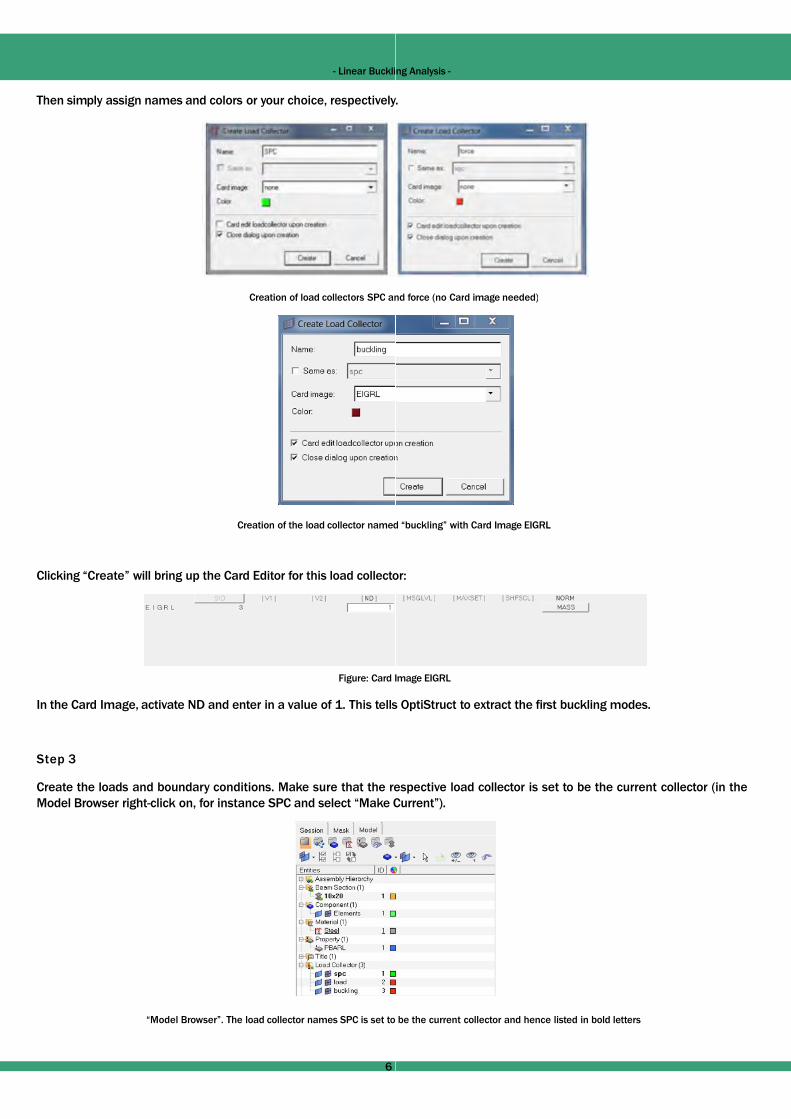
Then simply assign names and colors or your choice, respectively

Creation of load collectors SPC anCreation of load collectors SPC an

Creation of the load collector named

Clicking “Create” will bring up the Card Editor for this load collecto

Figure: Card I

In the Card Image, activate ND and enter in a value of 1. This tells

Step 3

Create the loads and boundary conditions. Make sure that the reModel Browser right-click on, for instance SPC and select “Make C

“Model Browser”. The load collector names SPC is set to

6

ng Analysis -

y.

nd force (no Card image needed)nd force (no Card image needed)

d “buckling” with Card Image EIGRL

or:

Image EIGRL

s OptiStruct to extract the first buckling modes.

espective load collector is set to be the current collector (in theCurrent”).

be the current collector and hence listed in bold letters

- Linear Buckli

In the constraints panel (BCs > Create > Constraints) select thebelow. All degrees of freedom dof are constraint (dof 1-6= 0).

Constraint panel. The node at the lower end of the

Next, set the load collector force as the current collector and create> Forces) the node at the top of the beam is selected, as shown in

Force Panel. A reference unit load in negative

Step 4

Create the loadsteps. For the linear buckling analysis, two loadste

• Linear static loading

• Linear buckling analysis

The subcases are created in the Loadsteps panel which can be

7

The subcases are created in the Loadsteps panel which can beLoadSteps.

ng Analysis -

node on the bottom face of the beam, as shown in the image

column is constraint with respect to all of its dof’s

e the reference load (unit load). In the forces panel (BCs > Createn the figure below:

x-direction is applied (magnitude= -1, x-axis)

eps/subcases are required.

e accessed from the menu bar by selecting Setup > Create > e accessed from the menu bar by selecting Setup > Create >

- Linear Buckli

Make sure the type is set to linear static. In here SPC references ththe load collector with the reference load (load):

Loadsteps panel (definition

In the second loadstep, the buckling loadstep, make sure the type

Loadstep panel (Definition of the linear buckling subcase) STATSUB references thbuckling modes t

Th t’ ll it t k ti t th l iThat’s all it takes – time to run the analysis.

Step 5

Start the computation run of OptiStruct. On the Analysis pagethen save the model as .*fem (the extension *.fem indicates incalculation.

With the start of the calculation, the Solver View appears. ThisMessage log area.

HyperWorks

Note: the *.out file includes information from the model check ruthe calculated results. Also, check this file error messages and wpresent. In general, always view this file, even if the analysis run w

Step 6Step 6

Postprocessing of the analysis. If the job is successful, you shodirectory is the directory where the model was saved.

8

ng Analysis -

he single point constraints load collector (named SPC), and LOAD

n of a linear static subcase)

e is set to linear buckling:

he static subcase and METHOD the load collector with the information about theto be determined

e, select the OptiStruct panel, chose the working directory andinput files for OptiStruct). Finally, click OptiStruct to execute the

s shows the steps of the calculation and possible errors in the

Solver View

n before the calculation as well as additional base information ofwarnings that will help you debug your input deck if any errors arewas successful.

ould see new results files in the working directory. The working

- Linear Buckli

The default files that will be written to your directory are:

File Explanation

*.h3d Binary HyperView res

*.res Includes all the resulcan be shown in the

*.out ACSII-based outputthe model check rubase information of c

*.stat Detailed breakdownimportant analysis st

Table: Standard

To view the results, start HyperView.

Make sure and pay attention to the loadstep/subcase selected fo

Subcase 2 “buckling” in HyperView. Re

The critical buckling load for the calculated bar (with unit load 1 Nwords, the model could be loaded 863 times the unit load until buan ideally linear buckling analysis and that real parts tend to buckl

9

ng Analysis -

sult file

ts of displacement through stress, which Post panel of HyperMesh

file, which includes information aboutun before the calculation and additionalcalculation results

n of the elapsed CPU-time for all teps

computed files

r display. This is controlled in the Results Browser.

eference (undeformed) model in blue

N) is F = 863,53 N (critical buckling factor λ = 863.53). In othercr

uckling would occur. Of course, we need to remember that this isle at lower loads than the theoretical value due to imperfections.

- Linear Buckli

Example: Wing Linear Buckling Analysis

This exercise runs a linear buckling analysis on a simple aircraneed to be very light and consequently become slender. Becausverification becomes necessary The objective of this project is toverification becomes necessary. The objective of this project is toit fail.

In this exercise, you will learn how to verify a wing baseline design

Model Information (Wing.hm):

Design Criteria:Design Criteria:

Buckling: first mode > (1.5 x).

(Static: U < 20 mm and Von Mises < 70 MPa)

Material Aluminum:

ρ = 2.1e-9 T/mm3 [RHO] Density

E = 70.000 MPa [E] Young’s modulus

ν = 0.33 - [nu] Poisson’s ratio

In the given model (Wing.hm), the load, constraints and loadcasesand load collectors before starting the baseline analysis.

Here, we focus on the load collectors:

Left: Applied constraints (green triangles) are in the load collector constraints

10

ng Analysis -

aft wing. This is a typical problem for aerospace structures thatse the structure has a high slenderness ratio, the buckling failureo verify if the 3 static load cases applied to the wing will not makeo verify if the 3 static load cases applied to the wing will not make

n for buckling criteria.

have already been created. Please review the property, material,

s. Right: Applied pressure (yellow arrows) are in the load collector pressure.

0

- Linear Bucklin

Tip load at the wing (purple arrows

In the load collector named SUM (with Card Image LOAD), the load

pressure (ID=2) and tip_load (ID=3) are combined. S, S1(1) ,and

The three static loadsteps are:

Note, the analysis type is set to linear static, respectively.

In order to define the buckling load step, another load collector is

We need to create a load collector with Card Image EIGRL (to defin

11

ng Analysis -

are in the load collector tip_load)

ds from the load collectors

S1(2) are weighting factors, respectively.

needed. Do you recall what the missing load collector is about?

ne the number of buckling modes we are interested in).

1

- Linear Buckli

It’s Card Image is

With respect to the loadsteps of interest,

we define the buckling loadsteps next.g

Please compare the ID’s of the referenced load collectors (SPC= a

Finally, run the analysis and view the buckling modes.

Example: Buckling With Gravitational Loa

Typically, the critical load factor is determined with respect to all loby STATSUB).by STATSUB).

In case the critical load factor should only be applied to variable(constant load), the two procedures/techniques described belconsidered in the model file: Prestressed_gravity.zip.

Working Procedure A

In case gravitational and variable loads are to be considered, the

• Load collector for variable loads (here named force; no Card I

• Load collector for gravity (Card Image GRAV; remind the syste

12

ng Analysis -

and METHOD =) and loadstep (STATSUB = )

ad

oads defined in the referenced linear static loadcase (referenced

e loads (e.g. pressure, forces) and NOT to the gravitational loadow may be employed. The below described working steps are

following load collectors are required:

mage needed)

m units)

2

- Linear Bucklin

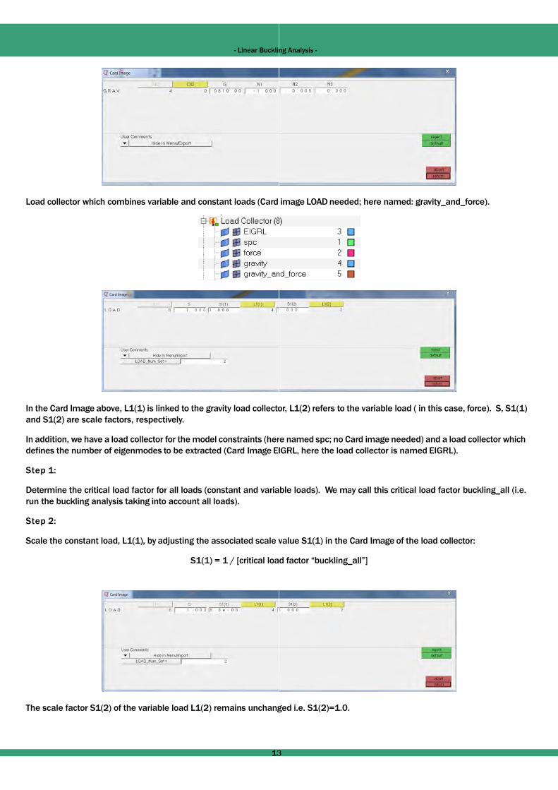
Load collector which combines variable and constant loads (Card

In the Card Image above, L1(1) is linked to the gravity load collectoand S1(2) are scale factors, respectively.

In addition, we have a load collector for the model constraints (herdefines the number of eigenmodes to be extracted (Card Image EI

Step 1:

D t i th iti l l d f t f ll l d ( t t d iDetermine the critical load factor for all loads (constant and variarun the buckling analysis taking into account all loads).

Step 2:

Scale the constant load, L1(1), by adjusting the associated scale v

S1(1) = 1 / [critical loa

The scale factor S1(2) of the variable load L1(2) remains unchang

13

ng Analysis -

image LOAD needed; here named: gravity_and_force).

or, L1(2) refers to the variable load ( in this case, force). S, S1(1)

re named spc; no Card image needed) and a load collector whichIGRL, here the load collector is named EIGRL).

bl l d ) W ll thi iti l l d f t b kli g ll (i able loads). We may call this critical load factor buckling_all (i.e.

value S1(1) in the Card Image of the load collector:

d factor “buckling_all”]

ged i.e. S1(2)=1.0.

3

- Linear Buckli

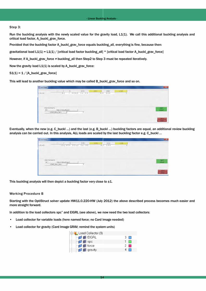
Step 3:

Run the buckling analysis with the newly scaled value for the grcritical load factor, A_buckl_grav_force.

Provided that the buckling factor A_buckl_grav_force equals buck

gravitational load L1(1) = L1(1) / [critical load factor buckling_all]

However, if A_buckl_grav_force ≠ buckling_all then Step2 to Step

Now the gravity load L1(1) is scaled by A_buckl_grav_force:

S1(1) = 1 / [A_buckl_grav_force]

This will lead to another buckling value which may be called B_bu

Eventually, when the new (e.g. C_buckl …) and the last (e.g. B_buanalysis can be carried out. In this analysis, ALL loads are scaled

This buckling analysis will then depict a buckling factor very close

Working Procedure B

Starting with the OptiStruct solver update HW11.0.220-HW (Julymore straight forward.

In addition to the load collectors spc” and EIGRL (see above), we np ( ),

• Load collector for variable loads (here named force; no Card I

• Load collector for gravity (Card Image GRAV; remind the syste

14

ng Analysis -

ravity load, L1(1). We call this additional buckling analysis and

kling_all, everything is fine, because then:

* [critical load factor A_buckl_grav_force]

3 must be repeated iteratively.

uckl_grav_force and so on.

uckl …) buckling factors are equal, an additional review buckling by the last buckling factor e.g. C_buckl …

e to ±1.

2012) the above described process becomes much easier and

now need the two load collectors:

mage needed)

m units)

4

- Linear Buckli

Based on these two load collectors, the two loadcases are defined

• Loadcase forces_only

• Loadcase gravity_only

Note: Currently (July 2012) the definition of a buckling loadstep inyou to select type: generic.

As before SPC references the model constraints, METHOD (STRUC

STATSUB (BUCKLING) references forces_only, and

eventually, the gravity loading gravity_only is applied as a pre-load

You can view the load collectors and loadsteps in the file: prestres

35

ng Analysis -

d:

n which the gravitational/constant loads are neglected requires

CT) references the load collector with the Card Image EIGRL,

d.

ssed_gravity.hm

50

- Linear Bucklin

Linear Buckling Analysis Tutorials And Vi

Recommended Tutorials:

The following tutorial is part of the HyperWorks Help Documentati

• OS-1040: 3D Buckling Analysis using OptiStruct

Demo Files:

• Buckling analysis of a bottle

• Buckling analysis of the central wing of aircraftg y g

• MBD Cable showing torsional buckling

Videos On Youtube

• HyperMesh 12 - Tower – Buckling (http://youtu.be/BueeQiwc

• Buckling of a Thin Column (http://youtu.be/wrdO8hPJGyg , 8

16

ng Analysis -

deos

ion:

c0JY, 15 minutes)

minutes)

6