Motivating Application: Patients with Metastatic Renal Cell Cancer (MRCC) who have not had previous systemic therapy Standard treatments are ineffective,

Motivating Application: Patients with Metastatic Renal Cell Cancer (MRCC) who have not had previous systemic therapy

Standard treatments are ineffective, with median(DFS) ≈ 8 months

Three “targeted” treatments will be studied in 240 MRCC patients, using a two-stage within-patient Dynamic Treatment Regime

Two-Stage Treatment Strategies Based On Sequential Failure Times

Outcome Example

Disease Worsening Cancer Progression Psychotic Episode

Alcoholic Relapse

Discontinuation

of Therapy

Death

SAE precluding further therapy

Physician stops rx due to futility

Dropout

Treatment Failure

Disease Worsening

or

Discontinuation of Therapy

A Within-Patient Two-Stage Treatment Assignment Algorithm

(Dynamic Treatment Regime)Stage1

At entry, randomize the patient among the stage 1 treatment pool {A1,…,Ak}

Stage 2

If the 1st failure is disease worsening

(progression of cancer) & not discontinuation,

re-randomize the patient among a set of treatments {B1,…,Bn} not received initially

“Switch-Away From a Loser”

B = (A, B)

C = (A, C)

A = (B, A)

C = (B, C)

A = (C, A)

B = (C, B)

Frontline Salvage Strategy

A

B

C

Select the two-stage strategy having the largest “average” time to second treatment failure (“overall failure time”)

In the “null” case where all 6 strategies give the same overall failure time, each strategy is selected with probability 1/6

Goal of the Renal Cancer Trial

Outcomes

T1 = Time to 1st treatment failure

T2 = Time from 1st disease worsening to 2nd treatment

failure

T1 + T2 = Time of 2nd treatment failure

Unavoidable Complications

1)Because disease is evaluated repeatedly (MRI, PET), either T1 or T1 + T2 may be interval censored

2)There may be a delay between 1st failure and start of stage 2 therapy

3)T1 may affect T2

4)The failure rates may change over time (they increase for MRC)

Discontinuation

Delay before start of 2nd stage rx

Start of stage 2 rx

T2,1 = Time from 1st progression to

2nd treatment failure if it occurs during the delay interval before stage 2 therapy is begun

T2,2 = Time from 1st progression to

2nd treatment failure if it occurs after stage 2 therapy has begun

A Parametric Model

Weib() = Weibull distribution with mean () = e(1+e), for real-valued and

[ T1 | A ] ~ Weib(AA)

[ T2,1 | A,B, T1] ~ Exp{ AA log(T1) }

[ T2,2 | A,B, T1] ~ Weib( A,BA log(T1), A,B)

has 28 elements, but the 6 subvectors are

A,B = (1,A, 2,A,B , A , A, A, A , A,B , A,B )

Pr(Dis. Worsening) Reg. of TReg. of T22 on T on T11

Weib pars of T1 Weib pars of T2

The A,B’s are exchangeable across the 6 strategies, so they have the same priors

Establishing Priors

1,A , 2,A,B ~ iid beta(0.80, 0.20) based on clinical experience

A , A, A, A , A,B , A,B ~ indep. normal priors

Prior means: We elicited percentiles of T1 and

[ T2 | T1 = 8 mos], & applied the Thall-Cook (2004) least squares method to determine means

Prior variances: We set

var{exp(A)} = var{exp(A)} = var{exp(A,B)} = 100

Assuming Pr(Disc. During delay period) = .02 E(A,B) = 7.0 mos & sd(A,B ) = 12.9

Establishing Priors

Mean Overall Failure Time

T = T1 + Y1,W T2

A,B() = E{ T | (A,B)}

= E(T1) + Pr(Y1,W =1) E(TE(T22))

Pr(1st failure is

Disease Worsening)

Mean time

to 2nd failure

Mean time

to 1st failure

Criteria for Choosing a Best Strategy

1. Mean{ A,B() | data }: B-Weib-Mean

2. Median{ A,B() | data }: B-Weib-Median

3. MLE of A,B() under simple Exponential:

F-Exp-MLE

4. MLE of A,B() under full Weibull:

F-Weib-MLE

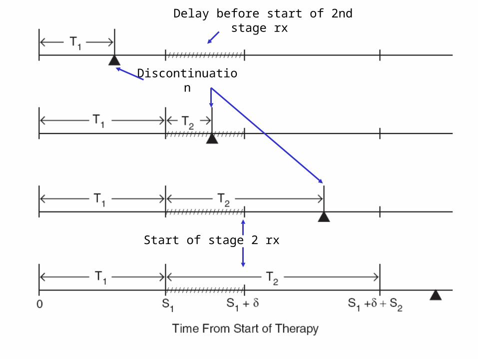
A Tale of Four Designs

Design 1 (February 21, 2006)

N=240, accrual rate a = 12/month

20 month accrual + 18 mos addt’l FU

Stage 1 pool = {A,B,C,D} 12 strategies

(A,B), (A,C), (A,D), (B,A), (B,C), (B,D),

(C,A), (C,B), (C,D), (D,A), (D,B), (D,C)

Drop-out rate .20 between stages

(240/12) x .80 = 16 patients per strategy


Design 2 (April 17, 2006)

Following “advice” from CTEP, NCI :

N = 240, a = 9/month (“more realistic”)

Stage 1 pool = {A,B}

(C, D not allowed as frontline)

Stage 2 pool = {A,B,C,D}

6 strategies :

(A,B), (A,C), (A,D), (B,A), (B,C), (B,D)



An Interesting Property of Design 2

Stage 1 may be thought of as a conventional phase III trial comparing A vs B with size .05 and power .80 to detect a 50% increase in median(T1), from 8 to 12 months, embedded in the two-stage design

However, the design does not aim to test hypotheses. It is a selection design.


Design 3 (January 3, 2007)

CTEP was no longer interested, but several Pharmas were VERY interested

N = 360, a = 12/month, 3 new treatments

Stage 1 rx pool = Stage 2 rx pool = {a,s,t}

6 strategies (different from Design 2) :

(a,s), (a,t), (s,a), (s,t), (t,a), (t,s)



Design 4 (May 15, 2007)

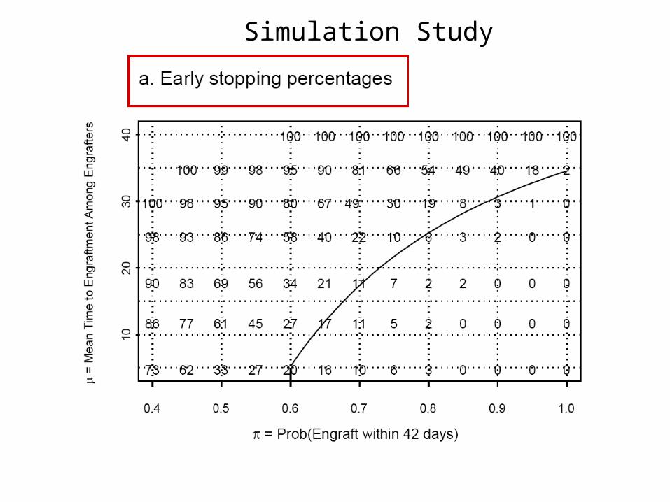
Question: Should a futility stopping rule be included, in case the accrual rate turns out to be lower than planned?

Answer: Yes!!

“Weeding” Rule: When 120 pats. are fully evaluated, stop accrual to strategy (a,b) if

Pr{ (a,b) < (best) – 3 mos | data} > .90


Applying the Weeding Rule when 120 patients have been fully evaluated

Accrual Rate (# Patients per month)

Expected # Future Patients Affected by

the Rule

12 24

9 78

6 132

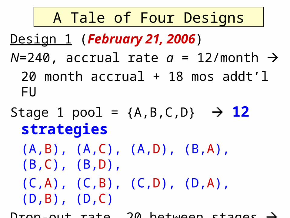
Simulation Scenarios specified in terms of 1(A) = median (T1 | A) and

2(A,B) = median { T2,2 | T1 = 8, (A,B) }

Null values 1 = 8 and 2 = 3

1 = 12 Good frontline

2 = 6 Good salvage

2 = 9 Very good salvage

Computer Simulations

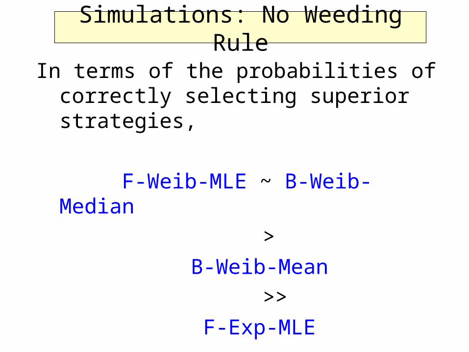
Simulations: No Weeding Rule

In terms of the probabilities of correctly selecting superior strategies,

F-Weib-MLE ~ B-Weib-Median

>

B-Weib-Mean

>>

F-Exp-MLE

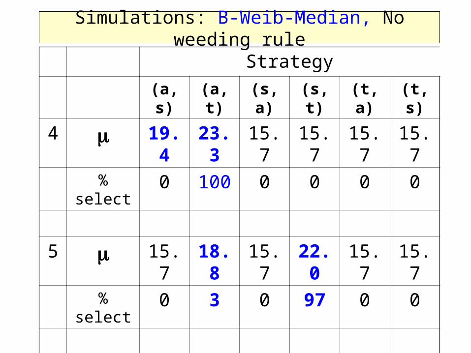
Simulations: B-Weib-Median, No weeding rule

Strategy

(a, s) (a, t) (s, a) (s, t) (t, a) (t, s)

1 15.7 15.7 15.7 15.7 15.7 15.7

% select 15 17 17 18 17 16

2 19.4 19.4 15.7 15.7 15.7 15.7

% select 52 48 0 0 0 0

3 15.7 18.8 15.7 18.8 15.7 15.7

% select 0 49 0 51 0 0

Strategy

(a, s) (a, t) (s, a) (s, t) (t, a) (t, s)

4 19.4 23.3 15.7 15.7 15.7 15.7

% select 0 100 0 0 0 0

5 15.7 18.8 15.7 22.0 15.7 15.7

% select 0 3 0 97 0 0

6 12.5 12.5 15.7 15.7 15.7 15.7

% select 0 0 28 25 25 23

Simulations: B-Weib-Median, No weeding rule

Sims With Weeding Rule

1)Correct selection probabilities are affected only very slightly

2)There is a shift of patients from inferior strategies to superior strategies – but this only becomes substantial with lower accrual rates

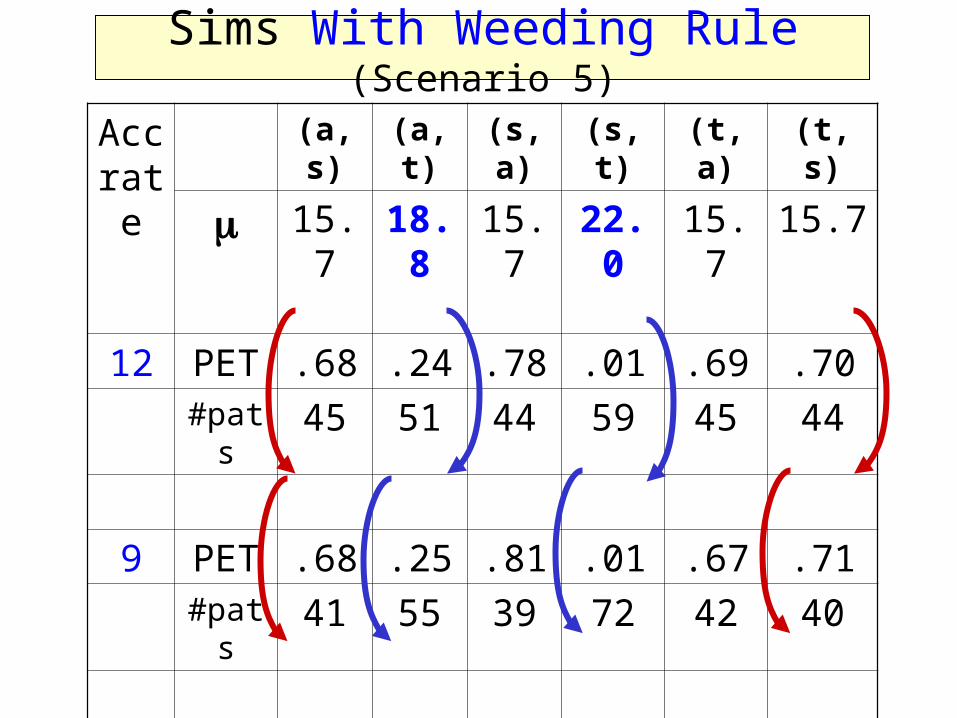
Acc rate

(a, s) (a, t) (s, a) (s, t) (t, a) (t, s)

15.7 18.8 15.7 22.0 15.7 15.7

12 PET .68 .24 .78 .01 .69 .70#pats 45 51 44 59 45 44

9 PET .68 .25 .81 .01 .67 .71#pats 41 55 39 72 42 40

6 PET .68 .22 .82 0 .68 .69#pats 37 59 34 84 37 36

Sims With Weeding Rule (Scenario 5)

An Acute Leukemia Trial Comparing Two-Stage Treatment Strategies

Thall, Sung and Estey, 2002

1) Each patient receives 1 or 2 courses of rx

2) Re-randomization for course 2 rx

3) Historical data are used to estimate non-

treatment (“baseline”) model parameters

4) Interimly, the design drops inferior

2-stage strategies within subgroups

Trial Conduct

Treatment Stage 1 : Randomize patients with probs. 1/3 each among the three course 1 treatments, balancing dynamically on patient covariates

Treatment Stage 2 : Re-randomize patients whose course 1 treatment fails (patient is alive but disease is resistant to this chemotherapy)

Weeding Out Inferior Strategies: Half-way through the trial, based on a trade-off-based utility of the probabilities of response and death, drop inferior treatment strategies within each prognostic subgroup

AML Trial Treatment Assignment Algorithm AML Trial Treatment Assignment Algorithm

Treatments and Outcomes

0 = Standard treatment (Idarubicin + ara-C)

1, 2 = indices of the two experimental treatments

Four two-course strategies were considered :

(0,1), (0,2), (1,0), (2,0)

Yk,c = I[Outcome k in course c] for k=R, D, F and c = 1,2

j = treatment assigned in course j

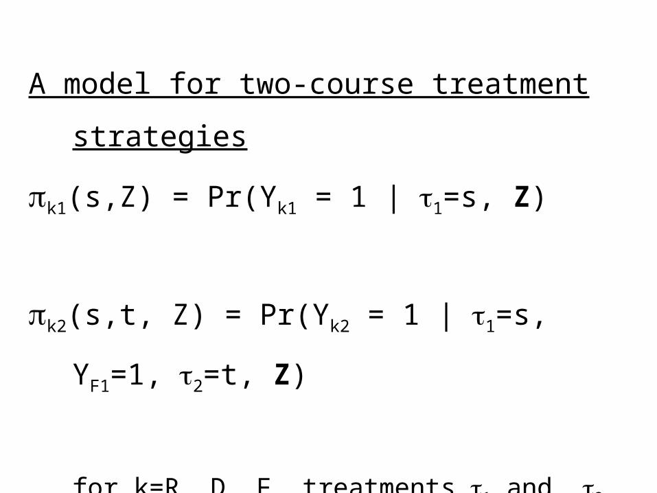
A model for two-course treatment strategies

k1(s,Z) = Pr(Yk1 = 1 | 1=s, Z)

k2(s,t, Z) = Pr(Yk2 = 1 | 1=s, YF1=1, 2=t, Z)

for k=R, D, F, treatments 1 and, 2 and baseline

prognostic covariates Z = (Z1, …, Zq)

A GENERALIZED LOGISTIC MODELA GENERALIZED LOGISTIC MODEL

Outcome k = R,D, strategy (s,t), covariates Z

Course 1

Course 2

A GENERALIZED LOGISTIC MODELA GENERALIZED LOGISTIC MODEL


Course 1

Course 2

TRT1 COV TRT1 x COV

STRATEGY COURSE 2

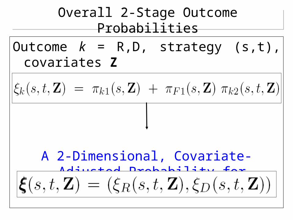
Overall 2-Stage Outcome ProbabilitiesOverall 2-Stage Outcome Probabilities


A 2-Dimensional, Covariate-Adjusted Probability for Evaluating 2-Stage Strategies

R

D

CR-Death Trade-Off Contours

Analysis of the Historical Data

All parameters assumed to follow N(0,10) priors

Covariates: [Age < 50 yrs], [1st CR Dur > 1 year]

A hierarchy of models was considered

BIC = Bayes Information Criterion used to assess fit

Simulation Study1. The same p(B| historical data) was used throughout

2. All others parameters assumed to follow N(0,10) priors

3. Maximum sample size = 96 patients, interim decisions to terminate subgroups made at 48 patients

4. 4000 replications for each of 4 clinical scenarios

Results:

In the presence of treatment-covariate interactions, the method reliably

terminated inferior strategies early

selected superior strategies

within patient prognostic subgroups

Bayesian Geometric Approach to Treatment Comparison in Rapidly Fatal Diseases

(Thall, Wooten and Shpall, 2005)

The ProblemIn treatment of rapidly fatal diseases,Response (R) and Death Without Response are Competing Risks

Example In cord blood transplantation (tx) for treatment of acute leukemia, Response = Engraftment = Recovery of neutrophil (white blood cell) count to a functional level (> 500 cells/mm3 blood)

TR + T2 if TR < T1 (Response Achieved)

TD = T1 if TR > T1 (Death w/o Response)

Response

Death

Treatment

TR

T1

T2

Given a initial time t* to achieve a

Response, two parameters matter :

= Pr{ Respond by time t* }

= Pr{ TR < min( t* ,TD )}

and

= E { TR | TR < TD }

Application: A randomized 60 patient trial to compare two double cord blood tx methods, currently ongoing at MDACC

“Expansion” = ex vivo selection and expansion of the cord blood cells

Rx1 = Two unexpanded grafts

Rx2 = One expanded + one unexpanded

Predictive covariate Z = Age, with 38 yrs. the physician’s reference value. For arm j = 1, 2,

j = Prj { Engraft by day 42 | Z = 38 }

= Prj { TR < min( 42 ,TD ) | Z = 38 }

j = mean time to engraftment

= Ej (T | TR < TD , Z = 38)

If 1 = 2 = .70 but 1 = 14 days while 2 = 28 days, then method 1 is greatly superior to method 2.

A statistical comparison based only on 1 and 2 , ignoring 1 and 2 , would be likely to conclude that 1 = 2 and make the false negative conclusion that the two methods do not differ.

Why two parameters?

Defining the parameters () under a Competing Risks Model

For k = R, D, 1 denote fk = pdf, Fk = cdf and = 1–Fk = survivor function of Tk

Technical Problem :How to compare the two treatments in terms of (11) versus (22) ? Solution : Talk to your Physician !Compared to the pair (00) of historical means with standard rx,elicit several equally desirable target pairs (1

*1*), . . . ,(M

*M*) that correspond

to a “reference patient” Z*

Each elicited (**) pair is represented by an "x"

Solution (continued)Use standard regression methods to fit a smooth, increasing curve D to the elicited pairs (1

*1*), . . . , (M

*M*), and

identify the region

D ={() : 'and < ' for some (',') on D}

= The set of () pairs at least as desirable as a pair on the target contour

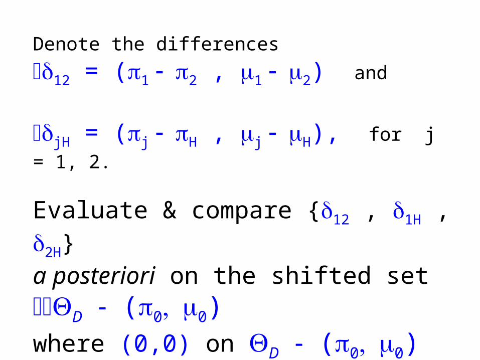
Denote the differences 12 = (1 2 , 1 2) and

jH = (j H , j H), for j = 1, 2.

Evaluate & compare {12 , 1H , 2H}a posteriori on the shifted set D (00) where (0,0) on D (00) corresponds to (0 0) on D.

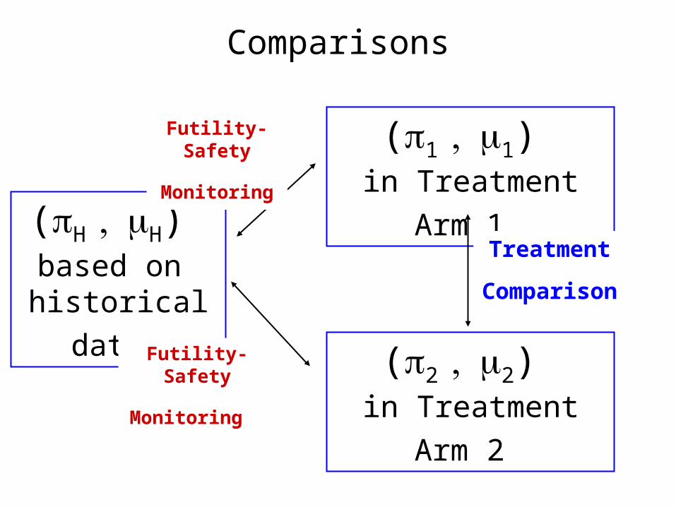
Comparisons

(1 1) in Treatment Arm 1

(2 2) in Treatment Arm 2

(H H) based on

historical data Futility-Safety

Monitoring

Treatment

Comparison

Futility-Safety

Monitoring

Safety Monitoring: Terminate arm j = 1 or 2 ifPr(jH D (00) | data) < pL

Treatment Selection : At the end of the trial, Select Treatment 1 if

Pr { 12 D (00) | dataN } >

Pr { 21 D (00) | dataN }

(use the symmetric rule for selecting treatment 2)

Analysis of historical data on 37 cord blood transplant patients

1) 28/37 (76%) engrafted within 42 days

2) Mean time to engraftment was 28 days

3) Goodness-of-fit analyses showed the event times TR, T1, and [ T2 | TR ] followed log normal distributions

Fit of the model to the historical data on 37 cord blood transplant patients

Posterior

1) Older age was predictive of smaller and larger

2) Longer TR was moderately predictive of shorter T2

3) For a 38-year old patient,

0= E{ | Z=38, dataH} = 0.69

0= E{| Z=38, dataH} = 30 days

Inferences from the historical data

Prob(Older Age Is Worse | data) = 0.86

0

0.05

0.1

0.15

0.4 0.5 0.6 0.7 0.8 0.9

Posterior of (Z=38) given historical data

Posterior mean = .69

0

0.05

0.1

0.15

0.2

20 25 30 35 40

Posterior mean = 30 days

Posterior of (Z=38) given historical data

Posterior median and 95% credible intervals for = Pr(Engraft) as a function of AGE based on

historical cord blood tx data (n=37)

Posterior median and 95% credible intervals for = E(Time to Engraft | Engraft) as a function of

AGE based on historical cord blood tx data (n=37)

Establishing Priors

The priors must yield a design with good operating characteristics – otherwise the design cannot be used in practice.

1) Use p(| dataH) as the prior on

2) Since () = ()(R1R, 1) assume (R1logR), log1) ) ~ 4-variate log normal with means = historical means but inflated variances.

Establishing Priors

We calibrated the prior hyperparameters and design cut-offs jointly to obtain

1) Good operating characteristics and 2) A reasonably uninformative prior

p(| dataH) = prior on covariate effects

Since () = ()(R1R, 1) assume (R1logR), log1) ) ~ 4-variate log normal with means = historical means but inflated variances.

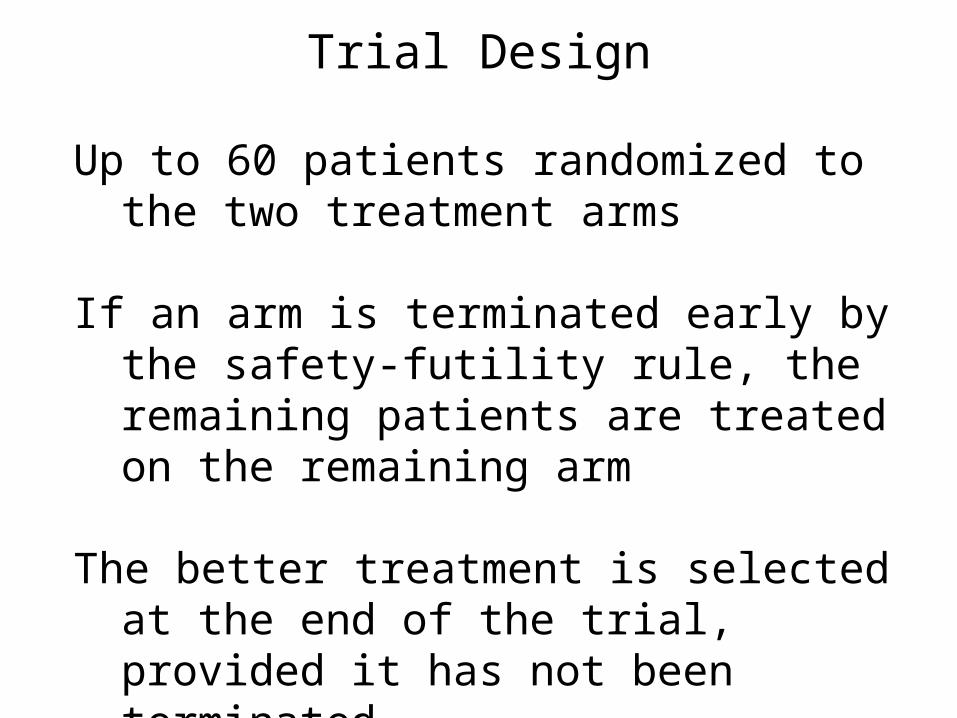
Trial Design

Up to 60 patients randomized to the two treatment arms

If an arm is terminated early by the safety-futility rule, the remaining patients are treated on the remaining arm

The better treatment is selected at the end of the trial, provided it has not been terminated

Simulation Study

Simulation Study

Robustness and Consistency

If the event times follow 1) a Weibull distribution, or2) a discrete mixture of 2 lognormalsthen the design still has good

operating characteristics

For N=60 to 150, correct decision probabilities all increase with N

A Hybrid Geometric Phase II-III Design

Disease: Pediatric Brain Tumors

Bivariate Primary Outcome: Event-Free Survival Time and Toxicity in 4 months (Yes/No)(An “Event” = Progression, 2nd Malignancy, or Death)

Patient Covariates:Age (Median = 3 years), Metastatic disease (Yes / No)Complete resection (Yes / No), Histology (CPC, vs other)

Treatments S = carboplatin + cyclophosphamide + etoposide + vincristine E1 = doxorubicin + cisplatinum + actinomycin + etoposide

E2 = high dose methotrexate

E3 = temozolomide + CPT-11.

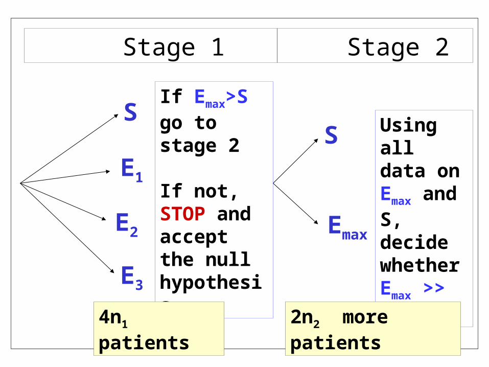
S

E1

E2

E3

S

Emax

If Emax>S go to stage 2

If not, STOP and accept the null hypothesis

Using all data on Emax and S, decide whether Emax >> S

4n1 patients 2n2 more patients

Stage 1 Stage 2

t1t1t2

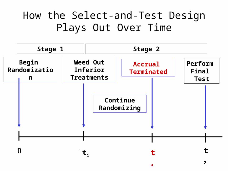
Perform Final Test

ta

How the Select-and-Test DesignPlays Out Over Time

Begin Randomization

Weed Out Inferior

Treatments

Accrual Terminated

ContinueRandomizing

Stage 1 Stage 2

Compared to What?

A conventional 2-arm design based on EFS :

Assuming null median EFS 43 months

A two-arm group sequential trial with type I error .05 and power .80 to detect target 56 months

(HR = 1.3), assuming accrual 4 pats/month, would require about

580 patients and 12 years

Setting Goals for the Trial

For a reference patient with (age=2 years, non-metastatic disease, complete resection, CPC),the historical mean

(Pr[EFS>24mos] , Pr[Toxicity]) = (.47, .11)

Elicited equally desirable target pairsElicited equally desirable target pairs:(.65, .01), (.70, .05), (.80, .20), (.99, .40), (.99, .99) The “reference patient” and “24 months” provide a

specific basis for comparison. All patients are accrued, and (EFS time, Toxicity) are recorded.

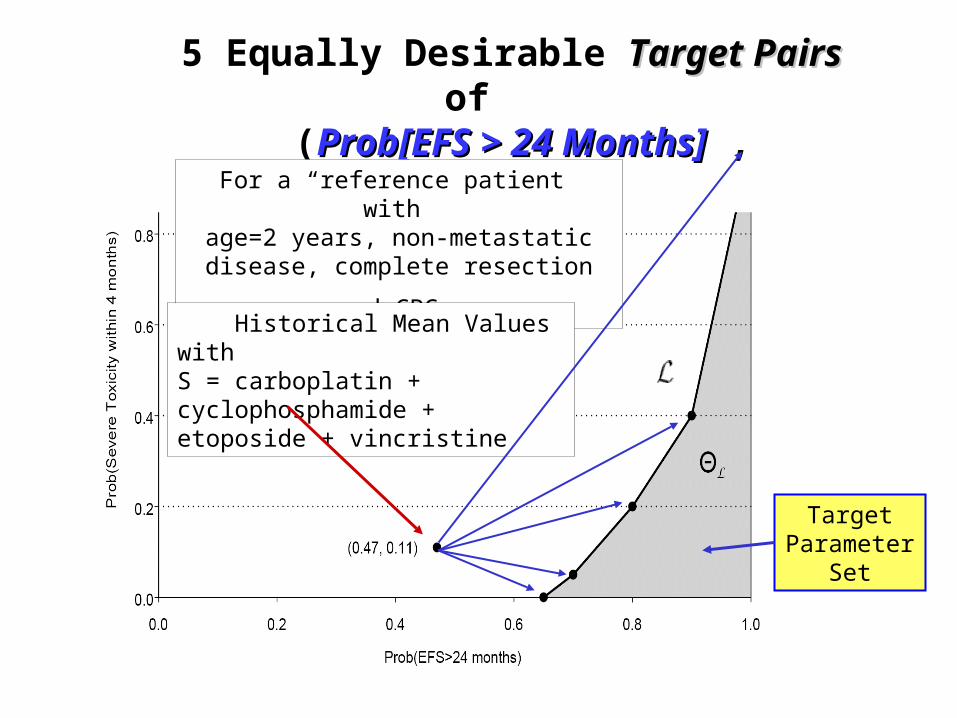
5 Equally Desirable Target PairsTarget Pairs of (Prob[EFS > 24 Months]Prob[EFS > 24 Months] , Prob[Toxicity) Prob[Toxicity) )

Target Parameter

Set

For a “reference patient” with age=2 years, non-metastatic disease,

complete resection and CPC

Historical Mean Values with S = carboplatin + cyclophosphamide + etoposide + vincristine

How the Bayesian Test Works

1) “Treatment effect” is 2-dimensional((EFS rateEFS rate , , Prob[Toxicity in 4 months]Prob[Toxicity in 4 months]))

2) Adjust for patient covariates:

(Age, CR, [metastatic disease], [histology=CPC])(Age, CR, [metastatic disease], [histology=CPC])

3) Transform the parameters by covariate-adjusting 3) Transform the parameters by covariate-adjusting

4) For each Ej, compute the ratio :

Prob(Ej-vs-S effect is in the target set | data)

Rj =

Prob(Ej-vs-S effect in null set | data)

E-vs-S Effect

On Pr(Toxicity)

E-vs-S Effect On EFS Time

Null Set where E < S

Target Setwhere E>>S

The Transformed E-vs-S Parameter Sets

Type I Error and Power

Type I Error

The probability of incorrectly concluding some Ej >> S

when in fact all Ej are clinically equivalent to S

Usual Power for comparing one E to S:

The probability of correctly concluding E>>S when in fact E>>S

What is the “power” for comparing several What is the “power” for comparing several EEjj’s ?’s ?

Generalized Power

The “Generalized Power” for comparing

E1, . . . , EK to S is the probability of :

1) correctly selecting Ej as Emax at stage 1, and 2) correctly continuing to stage 2, and 3) correctly concluding Ej >> S at the end of

stage 2 when in fact when in fact EEjj is the is the only only experimental experimental

treatment >> treatment >> SS all other all other EErr are clinically are clinically

equivalent to equivalent to SS

Optimal (minimum expected sample size) Design For 3 Experimental Treatment Arms

Stage 1: 30 events in the 4 arms E(# patients) = 84 to 96

Stage 2: 74 events in the 2 arms E(# patients) = 87 to 128

Expected trial duration = 4.7 to 6.7 years if accrual is 30 patients per year

Includes 2 year FU

E-vs-S Effect

On Pr(Toxicity)

E-vs-S Effect On EFS Time

Size and Generalized Power for K=3 Experimental Treatments

.05

Type I Error

Generalized Power

.84

.80

.92

.97

.99

1) Randomizing throughout No treatment-trial confounding and data are not wasted

2) Avoids bias of uncontrolled pre-test selection

3) The decision criteria reflect the trade-off between EFS Time and Toxicity

4) The model and method account for patient covariate effects

5) The overall false positive and false negative error rates both are controlled

Advantages of the Select-and-Test Design

Statistics and Medicine

“Mr. Jones, I have two possible treatments for your cancer,

A and B, but I don’t know

which is better.

So . . . I am going to to choose your treatment by flipping a coin.”

Also, looking at Your Data Can Cause Problems !!

What if you look at your data (sometimes prohibited by the trial protocol . . . ) and notice that you have

5 responses in 20 patients (25%) in arm A and 10 responses in 20 patients (50%) arm B ?

The posterior odds are 19-to-1 that B is superior to A

Do you still want to choose the next patient’s treatment by flipping a coin?

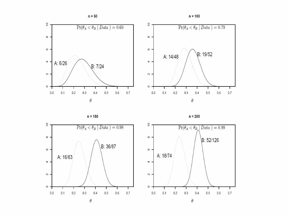
Posterior Distributions of P(Resp | A, 5/20) and P(Resp | B, 10/20)

Why not just “Play the Winner”?

1) Start by treating a small # patients, ½ with A and ½ with B

2) Keep track of the success rates

3) Thereafter, always treat the next patient with the treatment that has the larger success rate, that is, “play the winner”

Play-the-winner is a terrible strategy!

Suppose that A= .30 and B = .60

Suppose you start with 4 patients, observe 1 success in 2 with A, and 0 in 2 with B.

Since the success rate with B is 0, and the success rate with A is ½ and will always be > 0, you will treat all remaining patients with the inferior treatment A

Adaptive Randomization

Use the interim data to compute the probability that one treatment is “better” than the other

“Better” means it has a higher tumor shrinkage rate, lower toxicity rate, etc.

Unbalance the randomization in favor of the better treatment(s) based on the observed interim data

Repeatedly update the randomization probabilities to reflect the most recent data from the trial

Adaptive Randomization (AR) is more ethically appealing than conventional balanced “50:50” randomization because,

On Average AR assigns more patients to the

treatment or treatments that have higher interim success rates or lower interim adverse event rates

Randomize

50:50

Randomize

Adaptively

Play the Winner

A College Professor at Yale

Thompson (1933), considered two binomial probabilities, A and B , following beta priors, representing the success probabilities of two treatments, A and B

Based on binomial data, he proposed Adaptively Randomizing patients between A and B, as follows

Randomize each new patient to

A with probability pB<A = Pr(B < A | data)

B with probability pB>A = Pr(B > A | data) = 1 - pB<A

Generalizations: A and B can be probabilities, mean failure times, etc.

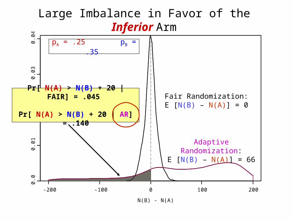
The Good News: For example, if the true success probabilities

are pA = .25 and pB = .35 then the expected imbalance in favor of the superior treatment, B, in a 200 patient trial is E[ N(B) – N(A) ] = 66 patients !!

The Bad News: The AR statistic Pr(B < A | data) is very

unstable (large variance)! It has a high probability of unbalancing the sample size in the wrong direction, giving the inferior treatment more often than the superior treatment !!

AR

N(B) - N(A)

-200 -100 0 100 200

0.0

0.0

10

.02

0.0

30

.04

Large Imbalance in Favor of the Inferior Arm

Fair Randomization:E [N(B) – N(A)] = 0

Adaptive Randomization:E [N(B) – N(A)] = 66

pA = .25 pB = .35

Pr[ N(A) > N(B) + 20 | FAIR] = .045

Pr[ N(A) > N(B) + 20 | AR] = .140

Randomize each new patient to

A with probability

{ pB<A }c

_____________________ { pB<A }c + { pB>A }c

A More Stable AR Procedure

Randomize each new patient to A with probability

{ pB<A }c / [ { pB<A }c + { pB>A }c ] ]

c = 1 gives the “usual” Bayesian AR c = ½ gives a much more stable ARc = n/2N gives a VERY stable AR

where n = current sample size and N = maximum sample size

A More Stable AR Procedure

BAR(n/2N)

N(B) - N(A)

-200 -100 0 100 200

0.0

0.0

10

.02

0.0

30

.04

Small Imbalance in Favor of the Superior Arm

Wathen’s Adaptive Randomization Method :

E [ N(B) - N(A) ] = 20

pA = .25 pB = .35

Pr[ N(A) > N(B) + 20 | FAIR] = .045

Pr[ N(A) > N(B) + 20 | Wathen AR] = .030

Treatment “Stop and Select” Rules

If Pr(B < A | data) > .99 Stop Early and select A

Pr(B > A | data) > .99 Stop Early and select B

Otherwise, select the better treatment at the end

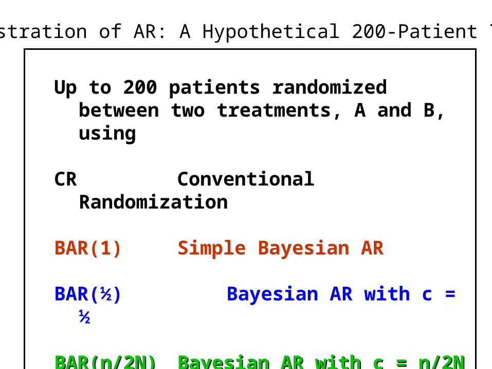
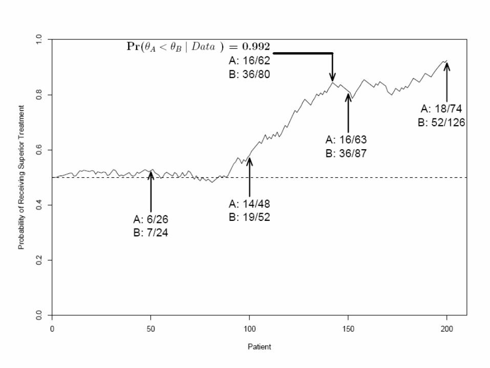
Illustration of AR: A Hypothetical 200-Patient Trial

Up to 200 patients randomized between two treatments, A and B, using

CR Conventional Randomization

BAR(1) Simple Bayesian AR

BAR(½) Bayesian AR with c = ½

BAR(n/2N)BAR(n/2N) Bayesian AR with c = n/2NBayesian AR with c = n/2N

0

0.05

0.1

0.15

0.2

0.25

0.3

0.35

0.4

0.45

0.25 0.3 0.35 0.4 0.45

CRBAR(1)BAR(1/2)BAR(n/2N)

Pr(NA > NB + 20) =

Probability of an imbalance > 20 patients in the WRONG direction when B > A = 0.25

True Value of B

0

10

20

30

40

50

60

70

80

90

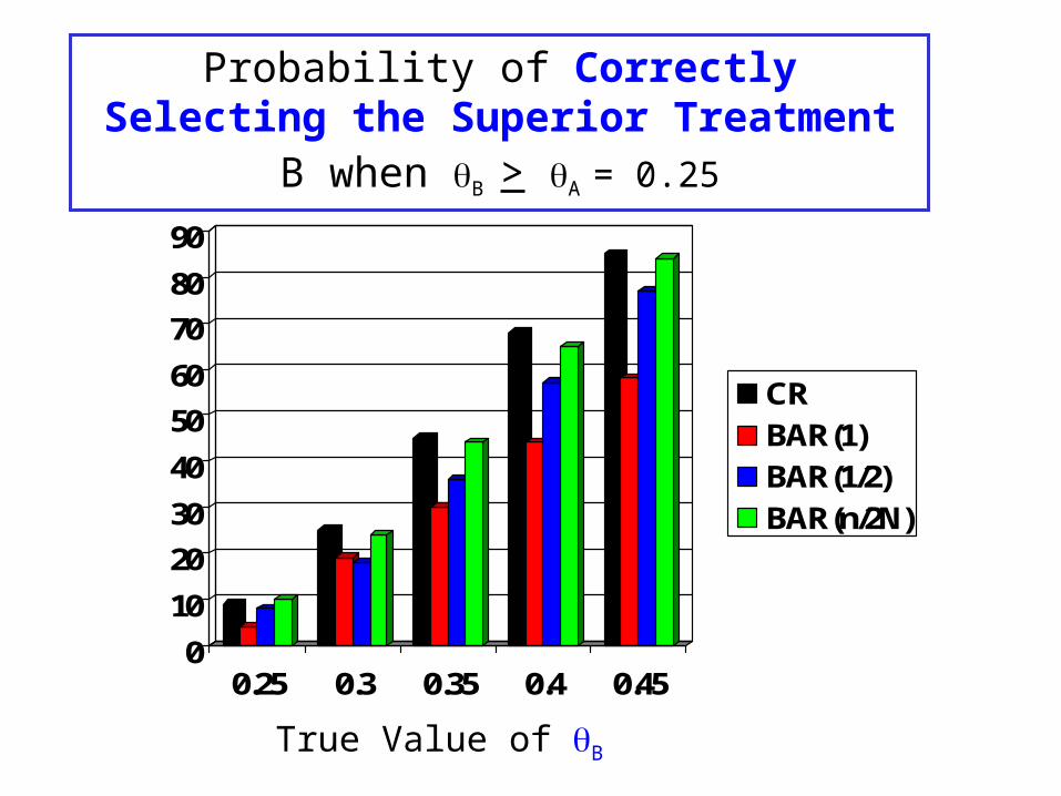
0.25 0.3 0.35 0.4 0.45


Probability of Correctly Selecting the Superior Treatment B when B > A = 0.25

True Value of B

020406080

100120140160180200

0.25 0.3 0.35 0.4 0.45


Mean Total Sample Size when B > A = 0.25

True Value of B

Modern Statistics and Medicine

“Mr. Jones, I have two possible treatments for your cancer, but I’m not sure which is better.

So, I can choose your treatment randomly, based on the data that we have so far on how well these two treatments have done with previous patients.”

Documents

Motivating Application: Patients with Metastatic Renal Cell Cancer (MRCC) who have not had previous systemic therapy Standard treatments are ineffective,