Embed Size (px)
Citation preview

AD-B 186 649 '
1.3
Research Summary No. 36-8for the period February 1, 7 961 to April I
ELECTEJUN 17 1994
~LI o
JULI
J ET PROPULSION LABORATORY
CALIFORNIAINSTITUTE OF TECHNOLOGY
C :vil PASADENA. CALIFORNIA
May 1, 1961
94-18021
1 94 6 t0 168z/
NATIONAL AERONAUTICS AND SPACE ADMINISTRATION
CONTRACT NO. NASw-6
Research Summary No. 36-8for the period February 1, 1961 to April 1, 1961
Accesion ForNTIS CRA&I
DTIC TABU:announcedJustification
By ...........................
Dist, ibution I
Availability CodesAvail and I or
Dist Special
JET PROPULSION LABORATORY
CALIFORNIA INSTITUTE OF TECHNOLOGY
PASADENA. CALIFORNIA
May 1, 1961
JPL RESEARCH SUMMARY NO. 36-8'-
Preface
The Research Summary is a report of supporting research and development activities
at the Jet Propulsion Laboratory, California Institute of Technology. This bimonthly peri-
odical is usually published in two volumes. However, for this issue, all the material hasbeen combined into one volume. To foster a more rapid interchange of original ideas
and information throughout the scientific and technical community, all authors' nameshave been added as bylines to the material they contributed.
W. H. Pickering, DirectorJet Propulsion Laboratory
Research Summary No. 36-8
Copyright @ 1961Jet Propulsion Laboratory
California Institute of Technology
II
7
, JPL RESEARCH SUMMARY NO. 36-8
Contents
SYSTEMS DIVISION
I. Systems Analysis ......... ................... 1A. Trajectory Analysis by V. C. Clarke ..... ........... 1B. Orbit Determination by D. L. Cain ...... ............ 2C. Space Fiight Studies by J. 0. Maloy ..... ........... 4D. Low-Thrust Trajectory Optimization by W. G. Melbourne . . . 6E. Powered Flight Studies by H. S. Gordon .... ......... 7
GUIDANCE AND CONTROL DIVISION
II. Guidance and Control Research ....... .............. 11A. Cryogenic Gyros by J. T. Harding .... ............ .11B. Gas-Supported Spinning Spheres by F. F. Batsch .. ....... .. 13C. Ferromagnetic Flux Reversal Mechanisms by F. B. Humphrey . . 15D. Closed-Cycle Gas Supply System by H. D. McGinness ...... .. 18
TELECOMMUNICATIONS DIVISION
III. Communications Elements Research .... ............ .21
A. Low-Noise Amplifiers by T. Sato .... ............ .21B. Antennas for Space Communications
by D. Schuster and C. T. Stelzried .... ............ .. 22C. Thin-Filn Techniques
by J. Maserjian and H. Erpenbach ... ........... . 31IV. Communications Systems Research ...... ............. 35
A. Communications Researchby W. V. Rusch, K. W. Linnes, S. Frankel, and A. J. Viterbi . . . 35
B. Information Processing by N. Zierler ... ........... .. 51C. Digital Communications Techniques
by M. F. Easterling, C. E. Gilchriest, and R. L. Choate ...... .. 52D. Venus Radar Experiment
by M. H. Brockman, L. R. Malling, and H. R. Buchanan . . . . 65
PHYSICAL SCIENCES DIVISION
V. Chemistry Research ....... .................. ... 74A. High-Resolution Nuclear Magnetic Resonance Spectroscopy
by D. D. Elleman and S. L. Manatt .... ............ . 74VI. Physics Research ....... ................... ... 80
A. Fission Electric Cells by W. F. Krieve ... .......... . 80VII. Gas Dynamics Research ...... ................. .. 82
A. Stability of a Shear Layer in a Magnetic Fieldby J. Menkes ....... ................... .. 82
B. Similarity Solution for Stagnation Point Heat Transferin Low-Density, High-Speed Flow by M. Chahine ........ .. 82
C. Hot-Wire Anemometer in Hypersonic Flow by T. Vrebalovich 84
III

JPL RESEARCH SUMMARY NO. 36-8
ENGINEERING MECHANICS DIVISION
VIII. Materials Research ...... ................... .. 86A. Graphite by W. V. Kotlensky and D. B. Fischbach ........ .. 86B. Endothermal Materials by W. V. Kotlensky and R. G. Nagler . . 91C. Behavior of Materials in Space by J. B. Rittenhouse ........ .. 94D. Structural Materials by W. W. Gerberich .. ......... ... 94
IX. Engineering Reseaich .. ............... ........ 98A. Liquid Surface Shapes by H. E. Williams, Consultant ...... .. 98B. Free-Fall Capsule to Study Weightless
Liquid Behavior by E. A. Zeiner .... ............ .99
ENGINEERING FACILITIES DIVISION
X. Wind Tunnel and Environmental Facilities ... .......... .102A. 20-Inch Supersonic Wind Tunnel by G. Goranson ........ .102
XI. Instrumentation ........ .................... 103A. Instrumentation Facilities by J. Z. Inskeep .. ......... .. 103B. Instrument Performance Studies by J. Earnest ... ........ .104
PROPULSION DIVISION
XII. Liquid Propellant Propulsion ..... ............... .108A. Combustion and Injection by G. I. Jaivin ... ......... .108B. Heat Transfer and Fluid Mechanics by A. B. Witte ........ .110
References .......... ........................ .112
IV
JPL RESEARCH SUMMARY NO. 36-8
SYSTEMS DIVISION
I. Systems Analysis
A. Trajectory Analysis energy dates) for Mars and Venus through 1971. In addi-tion, trajectories have been computed for Mercury from
V. C. Clarke October 1967 to January 1969.
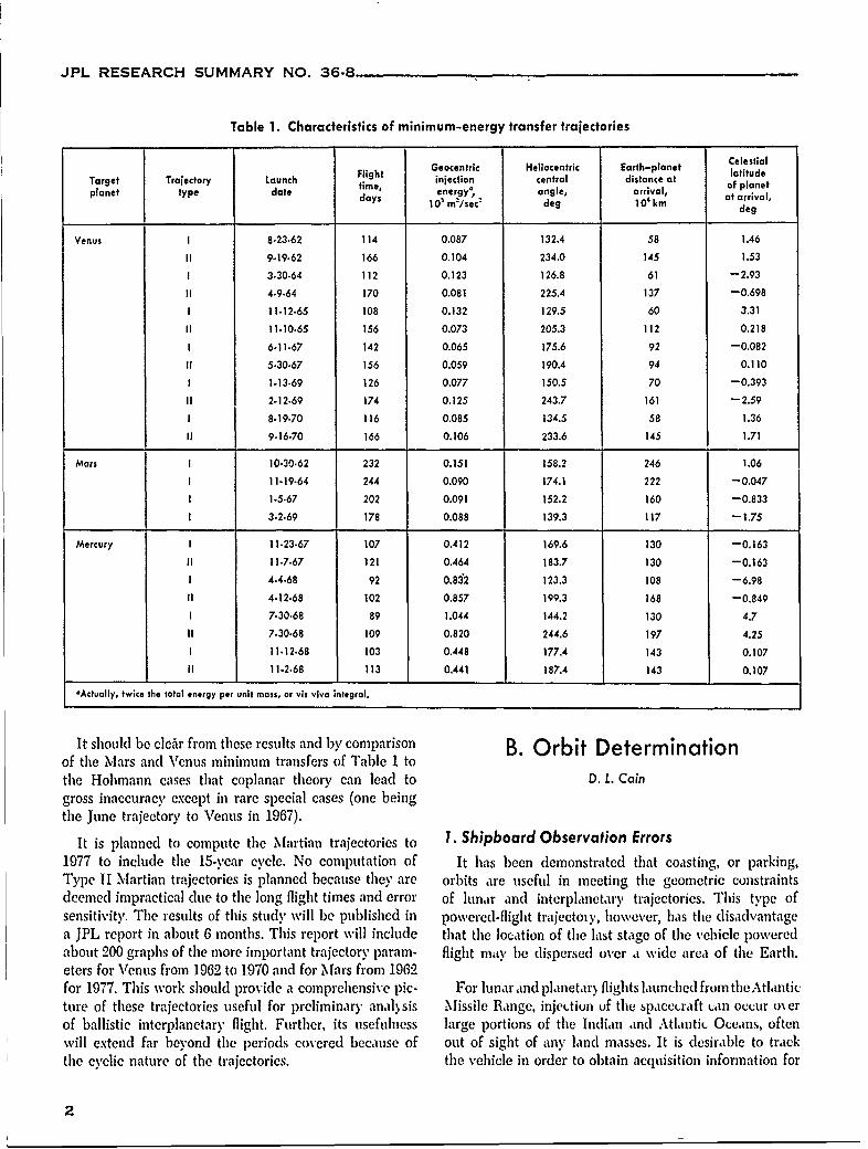
Partial preliminary results of this study are given in1. Interplanetary Trajectories Table 1, which lists pertinent parameters for the Type I
Minimum energy interplanetary trajectories are usually and II minimum energy transfers. Several interestingassociated with the Hohmann transfer orbit. But, in characteristics of these trajectories may be noted. Thereality, this type of orbit is rarely possible. In its place first is the 8-year cyclic behavior of the Venus trajectories.are two minimum-energy type trajectories, denoted Type The parameters for 1970 Venus trajectories are virtuallyI and Type II. Type I trajectories have heliocentric cen- the same as those for 1962. The reason for this is thattral angleso less than 180 degrees, and Type II trajec- approximately the same space-fixed geometry of Earthtories have heliocentric central angles greater than 180 and Venus recurs every 8 years, or after five Cythereandegrees. The two types of minimum are a result of the synodic periods (1.5987 years). A similar cyclic behaviorfact that the orbits of the launch and target planets are will occur for Mars trajectories every 15 years, or afternot coplanar. seven Martian synodic periods (2.1353 years). A second
interesting characteristic occurs for the Mercury trajec-A computer study is in progress to determine the char- tories. Here, based on coplanar theory it would be
acteristics of ballistic interplanetary trajectories launched expected that transfers requiring approximately equalfrom Earth to Mars, to Venus, to Mercury, and to Jupiter. energy would be possible about every 4 months (or everyThus far, trajectories have been obtained for each launch synodic period of 115.88 days). However, as noted fromperiod (approximately 3 months about the minimum Table 1, the energies required in April and July of 1968
are approximately twice those required in November of°Heliocentric central angle is defined as the angle subtended at the 1967 and 1968. The reason for this vast difference is two-Sun between the Sun-launch planet line at launch time and the fold; (1) Mercury is quite far out of the ecliptic, and(2) itsSun-target planet line at arrival time. orbit is closer to the Sun at arrival in April and July.
JPL RESEARCH SUMMARY NO. 36-8
Table 1. Characteristics of minimum-energy transfer trajectories
CelestialGeocentric Heliocentric Earth-planet latitude
Target Trajectory Launch Flight injection central distance at of planetplanet type date time, energy, angle, arrival, at arrival,
days p0n m^/sece deg 10' km dog
Venus I 8-23-62 114 0.087 132.4 58 1.46
II 9.19-62 166 0.104 234.0 145 1.53
1 3.30.64 112 0.123 126.8 61 -2.93
II 4.9.64 170 0.081 225.4 137 -0.698
I 11-12-65 108 0.132 129.5 60 3.31
II 11-10-65 156 0.073 205.3 112 0.218
I 6-11-67 142 0.065 175.6 92 -0.082
II 5.30.67 156 0.059 190.4 94 0.110
1 1.13-69 126 0.077 150.5 70 -0.393
II 2.12.69 174 0.125 243.7 161 -2.59
I 8.19-70 116 0.085 134.5 58 1.36
II 9.16-70 166 0.106 233.6 145 1.71
Mars I 10.30.62 232 0.151 158.2 246 1.06
1 11-19.64 244 0.090 174.1 222 -0.047
1 1.5.67 202 0.091 152.2 160 -0.833
1 3.2.69 178 0.088 139.3 117 -1.75
Mercury I 11.23.67 107 0.412 169.6 130 -0.163
II 11.7.67 121 0.464 183.7 130 -0.163
1 4.4.68 92 0.832 123.3 108 -6.98
li 4.12-68 102 0.857 199.3 168 -0.849
1 7.30.68 89 1.044 144.2 130 4.7
II 7.30.68 109 0.820 244.6 197 4.25
1 11.12.68 103 0.448 177.4 143 0.107
II 11.2.68 113 0.441 187.4 143 0.107
*Actually, twice the total energy per unit mass, or vis viva integral.
It should be cleir from these results and by comparison B. Orbit Determinationof the Mars and Venus minimum transfers of Table 1 tothe Hohmann cases that coplanar theory can lead to D, L. Caingross inaccuracy except in rare special cases (one beingthe June trajectory to Venus in 1967).
It is planned to compute the Martian trajectories to 1. Shipboard Observation Errors1977 to include tile 15-year cycle. No computation of It has been demonstrated that coasting, or parking,Type II Martian trajectories is planned because tile) are orbits are useful in meeting the geometric constraintsdeemed impractical due to the long flight times and error of lunar and interplanetary trajectories. This type ofsensitivity. The results of this study will be published in powered-flight trajectoiy, however, has the disadvantagea JPL report in about 6 months. This report will include that the location of the last stage of the vehicle poweredabout 200 graphs of the more important trajectory param- flight may be dispersed over a wide area of the Earth.eters for Venus from 1962 to 1970 and for Mars from 1962for 1977,. This work should provide a comprehensive pic- For lunar and planetarN flights launched from the Atlanticture of these trajectories useful for preliminary anal) sis Missile Range, injection of the spaceCraft can occur ox erof ballistic interplanetary flight. Further, its usefulness large portions of the Indian and Atlantic Oceans, oftenwill extend far beyond the periods covered because of out of sight of any, land masses. It is desirable to trackthe cyclic nature of the trajectories, the vehicle in order to obtain acquisition information for
2
JPL RESEARCH SUMMARY NO. 36-8
the Deep Space Instrumentation Facility (DSIF) and to The distance of the ship from the center of the Earthget preliminary estimates of the orbit path for the orbit was assumed to be perfectly known, but the latitude anddetermination iterative procedure. This tracking can longitude were assumed to be contaminated with noisepossibly be done by a ship at sea with tracking radars having an rms value of 0.017 degree (1 nn,). Data noiseaboard. The feasibility of this procedure has undergone was assumed to have the same variance for all times.a preliminary study in order to determine the errors in All data were assumed uncorrelated, with no biases.predicted spacecraft position angles that result fromuncertainties in a tracking ship's position at sea and other The orbit was determined from the observed data bydata errors. the method of least-squares. The uncertainty in the data
then was reflected as uncertainty in the orbital param-The orbit considered in this study, consisted of a typical eters. This uncertainty was then transformed, by a linear
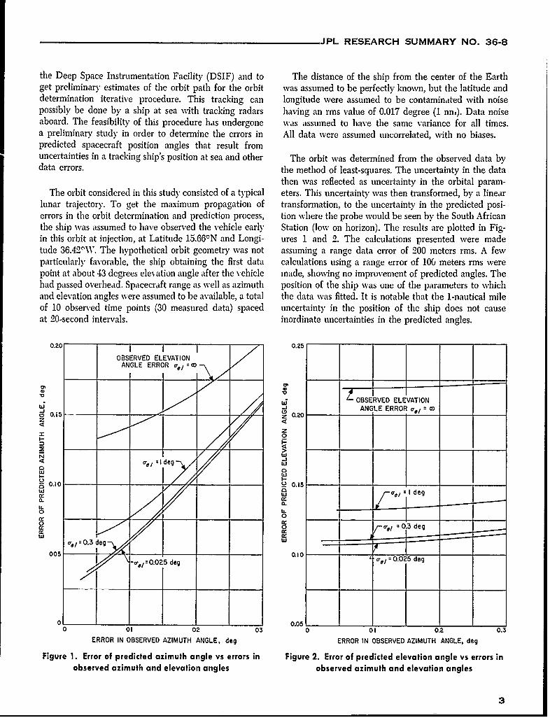
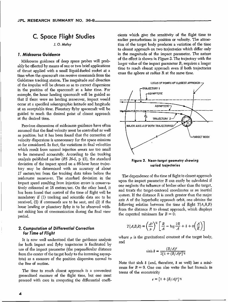
lunar trajectory. To get the maximum propagation of transformation, to the uncertainty in the predicted posi-errors in the orbit determination and prediction process, tion where the probe would be seen by the South Africanthle ship was assumed to have observed the vehicle early Station (low on horizon). The results are plotted in Fig-in this orbit at injection, at Latitude 15.66N and Longi- ures 1 and 2. The calculations presented were madetude 36.42OW. The hypothetical orbit geometry was not assuming a range data error of 200 meters rms. A fewparticularly favorable, the ship obtaining the first data calculations using a range error of 106 meters rms werepoint at about 43 degrees ele% ation angle after the vehicle made, showing no improvement of predicted angles. Thehad passed overhead. Spacecraft range as well as azimuth position of the ship was one of the parameters to whichand elevation angles were assumed to be available, a total the data was fitted. It is notable that the 1-nautical mileof 10 observed time points (30 measured data) spaced uncertainty in the position of the ship does not causeat 20-second intervals. inordinate uncertainties in the predicted angles.
0. 0.25
OBSERVED ELEVATIONANGLE ERROR =o,
',oi , OBSERVED ELEVATION
"_ _ ANGLE ERROR,(D 0.15 z 0.20
Z z0/7
N W0 o
0.10 20.15
a- a.Ld
o. I-
0 ___ __o 0
a: 0e/ 03 deg
0.-0.025 deg
0 - __L I I 1 0.050 01 02 03 0 01 0.2 0.3
ERROR IN OBSERVED AZIMUTH ANGLE, deg ERROR IN OBSERVED AZIMUTH ANGLE, deg
Figure 1. Error of predicted azimuth angle vs errors in Figure 2. Error of predicted elevation angle vs errors inobserved azimuth and elevation angles observed azimuth and elevation angles
3
JPL RESEARCH SUMMARY NO. 36-8
C. Space Flight Studies cients which give the sensitivity of the flight time toearlier perturbations in position or velocity. The attrac-
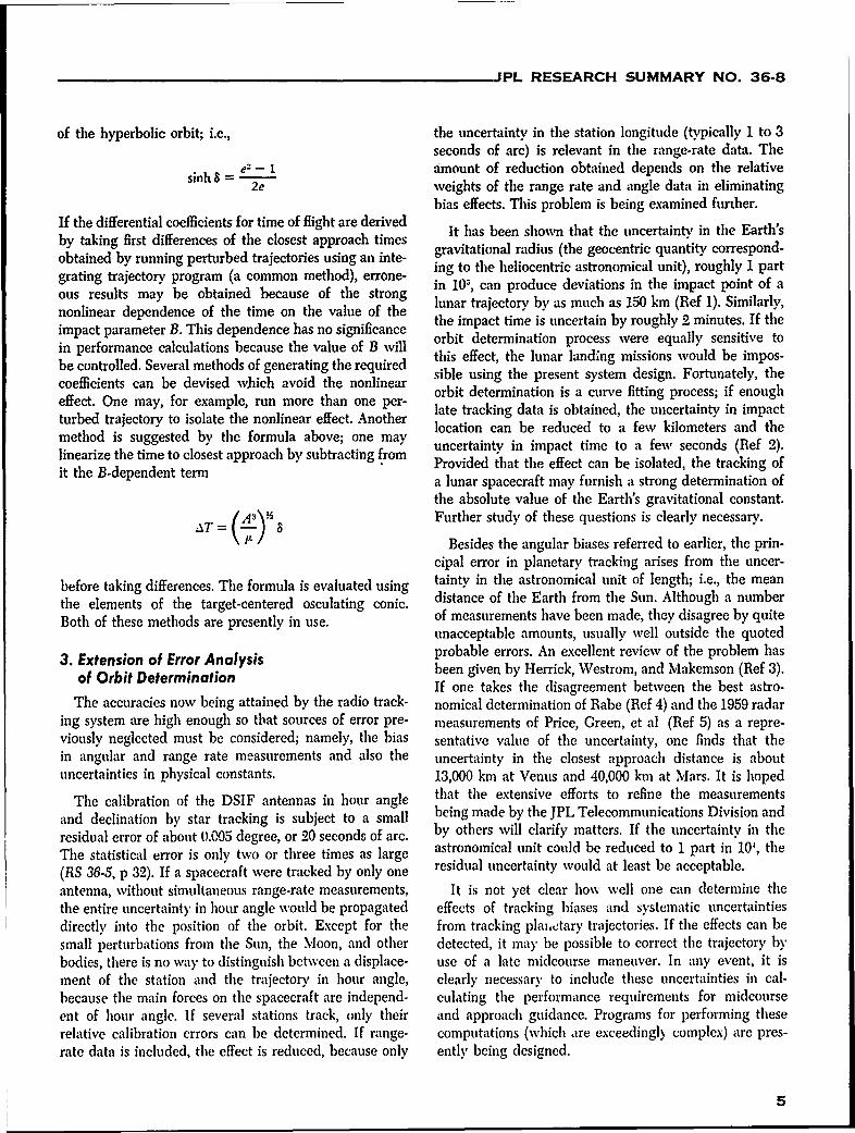
J. 0. Maloy tion of the target body produces a variation of the timeto closest approach on two trajectories which differ only
1. Midcourse Guidance in the magnitude of the impact parameter. The nature
Midcourse guidance of deep space probes will prob- of the effect is shown in Figure 3. The trajectory with thecof one or two brief applications larger value of the impact parameter B, requires a longer
ably be effected by means tim toe reac cloes approac evenaton if bohta ereof thrust applied with a small liquid-fueled rocket at a time to reach closest approach even if both trajectories
time when the spacecraft can receive commands from the cross the sphere at radius R at the same time.
Goldstone tracking station. The magnitude and directionof the impulse will be chosen so as to correct dispersions LcO I C T
in the position of the spacecraft at a later time. For TRAJECTORYI
example, the lunar landing spacecraft will be guided so /ASYMPTOTEthat if there were no landing maneuver, impact would -- --- --- -...........------ ---occur at a specified selenographic latitude and longitude YMPT'
at an acceptable time. Planetary flyby spacecraft will be ASYMPTOTE
guided to reach the desired point of closest approach - -- - ----at the desired time. TRAJECTORY 2
Previous discussions of midcourse guidance have often MAJOR AXIS A OF BOTH TRAJECTORIES/'
assumed that the final velocity must be controlled as well
as position; but it has been found that the correction of R'TARGET BODY
velocity dispersions is unnecessary for the space missionsso far considered. In fact, the variations in final velocitieswhich result from normal injection errors are too smallto be measured accurately. According to the trackinganalysis published earlier (RS 36-5, p 13), the standard Figure 3. Near-target geometry showingdeviation of the impact speed on a 66-hour lunar trajec- varied trajectoriestory may be determined with an accuracy of about17 meters/see from the tracking data taken before themidcourse maneuver. The standard deviation in the The dependence of the time of flight to closest approachimpact speed resulting from injection errors is conserva- upon the impact parameter B can easily be calculated iftively estimated at 18 meters/sec. On the other hand, it one neglects the influence of bodies other than the target,has been found that control of the time of flight will be and treats the target-centered coordinates as an inertialmandatory if (1) tracking and scientific data are to be system. If the distance H is much greater than the majorreceived, (2) if commands are to be sent, and (3) if the axis A of the hyperbolic approach orbit, one obtains thelureceived, (2dig o andare i to be observed with- following relation between the time of flight T(A,B,R)lunar landing or planetary flyby is to be observew from the distance R to closest approach, which displaysout risking loss of communication during the final view the expected minimum for B = 0:period.
2. Computation of Differential Correction T(A,B,R) = (- logA + +for Time of Flight where t is the gravitational constant of the target body,It is now well understood that the guidance analysis and
for both impact and flyby trajectories is facilitated byuse of the impact parameter (the perpendicular distance sinh 8 (B/A)-from the center of the target body to the incoming asymp- 2[ 1 + (B/A) -]
%
tote) as a measure of the position dispersion normal tothe line of motion. Note that sinh 8 (and, therefore, 8 as well) has a mini-
mum for B =0. One can also write the last formula inThe time to reach closest approach is a convenient term of the eccentricity
generalized measure of the flight time, but one must
proceed with care in computing the differential coeffi- e = [ + (B/A)'] %
4
JPL RESEARCH SUMMARY NO. 36-8
of the hyperbolic orbit; i.e., the uncertainty in the station longitude (typically 1 to 3seconds of arc) is relevant in the range-rate data. The
sinh -1 amount of reduction obtained depends on the relative2e weights of the range rate and angle data in eliminating
bias effects. This problem is being examined further.If the differential coefficients for time of flight are derived It has been shown that the uncertainty in the Earth'sby taking first differences of the closest approach times Ithation ra n (th gecer intit cor sobtained by running perturbed trajectories using an inte- gravitational radius (the geocentric quantity correspond-
gratng rajctoy pogrm (acomon ethd),errne- ing to the heliocentric astronomical unit), roughly I partgrating trajectory program (a common method), errone- in 107, can produce deviations in the impact point of aous results may be obtained because of the strong lunar trajectory by as much as 150 km (Ref 1). Similarlynonlinearthe impact time is uncertain by roughly 2 minutes. If the
impact parameter B. This dependence has no significance orbit te in cess byrully snte toin performance calculations because the value of B will orbit determination process were equally sensitive toieonromae ealulatos bfenease g the lueo ild this effect, the lunar landing missions would be impos-be controlled. Several methods of generating the required sible using the present system design. Fortunately, thecoefficients can be devised which avoid the nonlinear siluintepretsyemdig.Ftnalteeffect. One may, for example, run more than one per- orbit determination is a curve fitting process; if enoughturbed trajectory to isolate the nonlinear effect. Another late tracking data is obtained, the uncertainty in impact
e tlocation can be reduced to a few kilometers and themethod is suggested by the formula above; one may uncertainty in impact time to a few seconds (Ref 2).linearize the time to closest approach by subtracting fromit te B-epenent ermProvided that the effect can be isolated, the tracking of
a lunar spacecraft may furnish a strong determination ofthe absolute value of the Earth's gravitational constant.
AT [A3 Further study of these questions is clearly necessary.AT =k''
Besides the angular biases referred to earlier, the prin-cipal error in planetary tracking arises from the uncer-
before taking differences. The formula is evaluated using tainty in the astronomical unit of length; i.e., the mean
the elements of the target-centered osculating conic. distance of the Earth from the Sun. Although a number
Both of these methods are presently in use. of measurements have been made, they disagree by quiteunacceptable amounts, usually well outside the quoted
3. Extension of Error Analysis probable errors. An excellent review of the problem has
of Orbit Determination been given by Herrick, Westrom, and Makemson (Ref 3).If one takes the disagreement between the best astro-
The accuracies now being attained by the radio track- nomical determination of Rabe (Ref 4) and the 1959 radaring system are high enough so that sources of error pre- measurements of Price, Green, et al (Ref 5) as a repre-viously neglected must be considered; namely, the bias sentative value of the uncertainty, one finds that thein angular and range rate measurements and also the uncertainty in the closest approach distance is aboutuncertainties in physical constants. 13,000 km at Venus and 40,000 km at Mars. It is hoped
The calibration of the DSIF antennas in hour angle that the extensive efforts to refine the measurements
and declination by star tracking is subject to a small being made by the JPL Telecommunications Division and
residual error of about 0.005 degree, or 20 seconds of arc. by others will clarify matters. If the uncertainty in the
The statistical error is only two or three times as large astronomical unit could be reduced to 1 part in 10, the
(RS 36-5, p 32). If a spacecraft were tracked by only one residual uncertainty would at least be acceptable.antenna, without simultaneous range-rate measurements, It is not yet clear how well one can determine thethe entire uncertainty in hour angle would be propagated effects of tracking biases and systematic uncertaintiesdirectly into the position of the orbit. Except for the from tracking plai,ctary trajectories. If the effects can besmall perturbations from the Sun, the Moon, and other detected, it may be possible to correct the trajectory bybodies, there is no way to distinguish between a displace- use of a late midcourse maneuver. In any event, it isment of the station and the trajectory in hour angle, clearly necessary to include these uncertainties in cal-because the main forces on the spacecraft are independ- culating the performance requirements for midcourseent of hour angle. If several stations track, only their and approach guidance. Programs for performing theserelative calibration errors can be determined. If range- computations (which are exceedingly complex) are pres-rate data is included, the effect is reduced, because only ently being designed.
5
JPL RESEARCH SUMMARY NO. 36-8 -
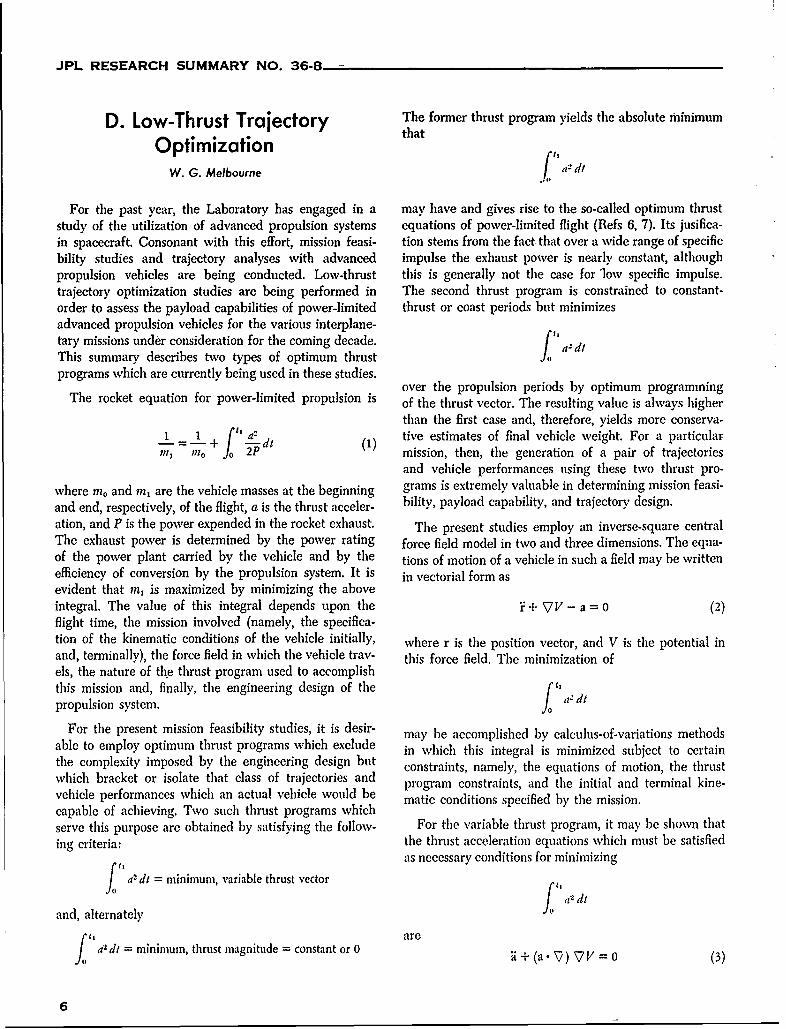
D. Low-Thrust Trajectory The former thrust program yields the absolute minimumD. L w-Thust rajetorythat
OptimizationW. G. Melbourne fa d
For the past year, the Laboratory has engaged in a may have and gives rise to the so-called optimum thruststudy of the utilization of advanced propulsion systems equations of power-limited flight (Refs 6, 7). Its jusifica-in spacecraft. Consonant with this effort, mission feasi- tion stems from the fact that over a wide range of specificbility studies and trajectory analyses with advanced impulse the exhaust power is nearly constant, althoughpropulsion vehicles are being conducted. Low-thrust this is generally not the case for low specific impulse.trajectory optimization studies are being performed in The second thrust program is constrained to constant-order to assess the payload capabilities of power-limited thrust or coast periods but minimizesadvanced propulsion vehicles for the various interplane-tary missions under consideration for the coming decade.This summary describes two types of optimum thrust, dt
programs which are currently being used in these studies.over the propulsion periods by optimum programming
The rocket equation for power-limited propulsion is of the thrust vector. The resulting value is always higherthan the first case and, therefore, yields more conserva-
(1) n"-tive estimates of final vehicle weight. For a particularS J2P mission, then, the generation of a pair of trajectories
and vehicle performances using these two thrust pro-
where mo and m, are the vehicle masses at the beginning grams is extremely valuable in determining mission feasi-
and end, respectively, of the flight, a is the thrust acceler- bility, payload capability, and trajectory design.
ation, and P is the power expended in the rocket exhaust. The present studies employ an inverse-square centralThe exhaust power is determined by the power rating force field model in two and three dimensions. The equa-of the power plant carried by the vehicle and by the tions of motion of a vehicle in such a field may be writtenefficiency of conversion by the propulsion system. It is in vectorial form asevident that m, is maximized by minimizing the aboveintegral. The value of this integral depends upon the Y + TV - a = 0 (2)
flight time, the mission involved (namely, the specifica-tion of the kinematic conditions of the vehicle initially, where r is the position vector, and V is the potential inand, terminally), the force field in which the vehicle tray- this force field. The minimization ofels, the nature of the thrust program used to accomplishthis mission and, finally, the engineering design of the fa,propulsion system. a, dt
For the present mission feasibility studies, it is desir- may he accomplished by calculus-of-variations methodsable to employ optimum thrust programs which exclude in which this integral is minimized subject to certainthe complexity imposed by the engineering design but constraints, namely, the equations of motion, the thrustwhich bracket or isolate that class of trajectories andvehile erfrmaceswhih anactal ehile oul be program constraints, and the initial and terminal kine-vehicle performances which an actual vehicle would be matic conditions specified by the mission.
capable of achieving. Two such thrust programs whichserve this purpose are obtained by satisfying the follow- For the variable thrust program, it may be shown thating criteria: the thrust acceleration equations which must be satisfied
as necessary conditions for minimizing
J a- dt = minimum, variable thrust vector
and, alternately
area-dt = minimum, thrust magnitude = constant or 0 i + (a. -) 7V = 0 (3)
6
JPL RESEARCH' SUMMARY NO. 36-8
These equations admit a first integral in scalar form been developed. This routine has been remarkably suc-which may be expressed as cessful in the large-scale production of interplanetary
flyby and rendezvous trajectories to nearly all the planetsa, r - a--' a • 71/= constant (4) with flight times ranging from 30 days to 3 years. Numer-
For the constant thrust program, the analogous expres- ical studies with the variable thrust program have beensions are reported elsewhere (Ref 7). Studies with the constant
thrust program are in progress and will be reported in a+ (." 7) VI' = o (5) later publication.
X.i - .(a - V V) + a (k - r,,L) = constant (6)
a t I (7)(7) E. Powered Flight Studies
a = ao -- (8) H. S. Gordon
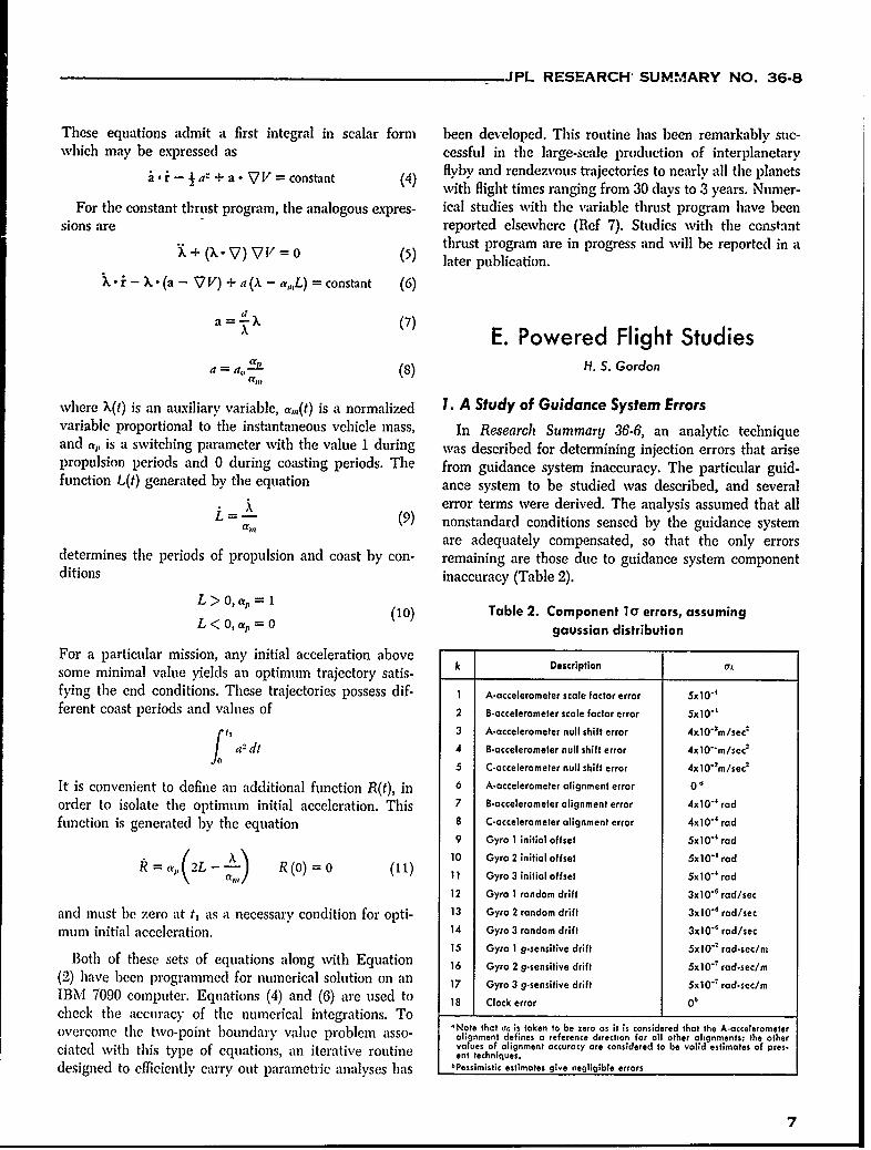
where X(t) is an auxiliary variable, a,,,(t) is a normalized 1. A Study of Guidance System Errorsvariable proportional to the instantaneous vehicle mass, In Research Summary 36-6, an analytic techniqueand a, is a switching parameter with the value 1 during was described for determining injection errors that arisepropulsion periods and 0 during coasting periods. The from guidance system inaccuracy. The particular guid-function L(t) generated by the equation ance system to be studied was described, and several
( error terms were derived. The analysis assumed that all,,, () nonstandard conditions sensed by the guidance system
are adequately compensated, so that the only errorsdetermines the periods of propulsion and coast by con- remaining are those due to guidance system componentditions inaccuracy (Table 2).
L> 0, a , = 1L<0, a= 1 (10) Table 2. Component 1o" errors, assumingL < 0, a, = 0 gaussian distribution
For a particular mission, any initial acceleration above -
some minimal value yields an optimum trajectory satis- k Description asfying the end conditions. These trajectories possess dif- I A.accelerometer scale factor error 5x10'ferent coast periods and values of 2 B.accelerometer scale factor error 5xiO"
ti 3 A-accelerometer null shift error 4xlO'm/sec
f" adi 4 B-accelerometer null shift error 4xl0"m/sec2
5 C-accelerometer null shift error 4xlO'm/sec*
It is convenient to define an additional function R(t), in 6 A-accelerometer alignment error 0O
order to isolate the optimum initial acceleration. This 7 B-accelerometer alignment error 4xl0' radfunction is generated by the equation 8 C-accelerometer alignment error 4x10" rod
9 Gyro 1 initial offset 5x10 " rod, R(0) = 0 1) 10 Gyro 2 initial offset 5xl0' rad
I-( 11 Gyro 3 initial offset 5x10"- rod
12 Gyro 1 random drift 3x10" rad/sec
and must be zero at t, as a necessary condition for opti- 13 Gyro 2 random drift 3x0 rod/secmum initial acceleration. 14 Gyro 3 random drift 3x10" rod/sec
15 Gyro 1 g-sensitive drift 5x10 " rad-sec/rnBoth of these sets of equations along with Equation 16 Gyro 2 g-sensitive drift 5xi0" rad-sec/m
(2) have been programmed for numerical solution on an 17 Gyro 3 g-sensitive drift 5xiO1r rad.sec/mIBM 7090 computer. Equations (4) and (6) are used to 18 Clock error 0bcheck the accuracy of the numerical integrations. To I I
oNote that s is token to be zero as it is considered that the A-accelerometerovercome the two-point boundary value problem asso- alignment defines a reference drecton for oil other alignments$; the other
values of alignment accuracy are considered to be valid estimates of pres-elated with this type of equations, an iterative routine en techniques.
designed to efficiently carry out parametric analyses has 'Pessimistic estimates give negligible errors
7
JPL RESEARCH SUMMARY NO. 36-8
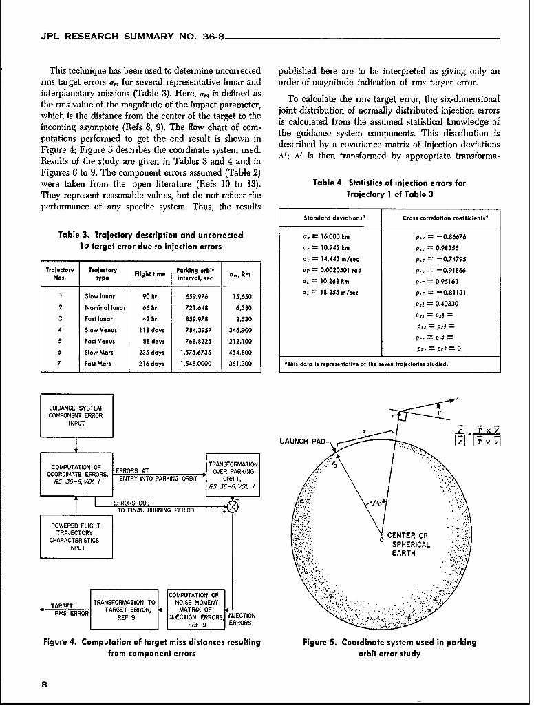
This technique has been used to determine uncorrected published here are to be interpreted as giving only anrms target errors a, for several representative lunar and order-of-magnitude indication of rms target error.interplanetary missions (Table 3). Here, a, is defined as To calculate the rms target error, the -six-dimensionalthe rms value of the magnitude of the impact parameter, joint distribution of normally distributed injection errorswhich is the distance from the center of the target to the is calculated from the assumed statistical knowledge ofincoming asymptote (Refs 8, 9). The flow chart of com- the guidance system components. This distribution isputations performed to get the end result is shown in described by a covariance matrix of injection deviationsFigure 4; Figure 5 describes the coordinate system used. Atdesed by ae roiet ansResults of the study are given in Tables 3 and 4 and in A'; is then transformed by appropriate transforma-Figures 6 to 9. The component errors assumed (Table 2)were taken from the open literature (Refs 10 to 13). Table 4. Statistics of injection errors forThey represent reasonable values, but do not reflect the Trajectory 1 of Table 3performance of any specific system. Thus, the results
Standard deviations" Cross correlation coefficients"
Table 3. Trajectory description and uncorrected a, = 16.000 km P, = -0.86676
1a target error due to injection errors a, = 10.942 km pr, = 0.98355cr" = 14.443 m/sec prr = -0.74795
Trajectory Trajectory Parking orbit ar = 0.0020501 rad pr = -0.91866Nos. type interval, sec o = 10.268 km p'r = 0.95163
1 Slow lunar 90 hr 659.976 15,650 aS 18.255ni/sec Prr = -0.81131
2 Nominal lunar 66 hr 721.648 6,380 p,, = 0.40330
3 Fast lunar 42 hr 859.978 2,530 P:.- = PC.-
4 Slow Venus 118 days 784.3957 346,900 P,: = p," -
5 Fast Venus 88 days 768.8225 212,100 Pr PC -
6 Slow Mars 235 days 1,575.6735 454,800 pr pr 0
7 Fast Mars 216 days 1,548.0000 351,300 *This data is representative of the seven trajectories studied.
GUIDANCE SYSTEMCOMPONENT ERROR r
INPUT x~ ~ x III V
LAUNCH PAD 7F 171
[COMPUTATION OF 1TRANSFORMATION rCOORDINATE ERRORS, ERRORS AT OVER PARKING
RS 36-6, VOL I ENTRY INTO PARKING ORBIT ORBIT,j RS 36-6, VOL I
XTI~ ERRORS DUETO FINAL BURNING PERIOD +
POWERED FLIGHTTRAJECTORY C OF
CHARACTERISTICS 0INPUT SPHERICALINPUT____"_________________ EARTH
COMPUTATION OFTRANSFORMATION TO NOISE MOMENT
RGERO I TARGET ERROR, 0- MATRIX OFREF 9 INJECTION ERRORS, INJECTION
REF 9 ERRORS
Figure 4. Computation of target miss distances resulting Figure 5. Coordinate system used in parkingfrom component errors orbit error study
8
JPL RESEARCH SUMMARY NO. 36-8
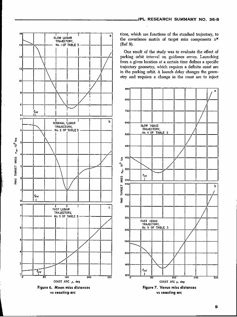
I tions, which are functions of the standard trajectory, toSLOW LUNAR the covariance matrix of target miss components Am
1TRAJECTORY,INo. 10 1F TABLE 3 (Ref 9).I I I One result of the study wvas to evaluate the effect ofparking orbit interval on guidance errors. Launchingfrom a given location at a certain time defines a specific.... trajectory geometry, which requires a definite coast arc
I in the parking orbit. A launch delay changes the geom-etry and requires a change in the coast arc to inject
I0
880
8O
&Id t 720
NOMINAL LUNAR 640TRAJECTORY, SLOW VENUS
6 No. 2 OF TABLE 3 TRAJECTORY,
560 No 4 OF TABLE 3
E5 -
2 480 - - - - - - - -
i/b I
W -2 -
- - - ~~~~ 2401 L.- -
X- 4C0 b
00a I I C 360
FAST LUNARTRAJECTORY,
7 No. 3 OF TABLE 3 - 32
FAST VENUSTRAJECTORY,
- -- -- -No 5 OF TABLE 3
-J 200-
-I 1206 -80 160 240 320 0 80 160 24
0 320
COAST ARC p, deg
Figure 6. Moon miss distances Figure 7. Venus miss distancesvs coasting arc vs coasting arc
9
JPL RESEARCH SUMMARY NO. 36-8
1600 I I I/ /36 j TSLOW,SLOW MARS TRAJECTORY I
TRAJECTORY,i~oo No. 6 OF TABLE 3l'._
0
S000b10
600 N-MNA, - -2 0
E 6- TRJCTR IT400 - - - -- - - - -
D~ 2001- j FAST, I2720 - - -__ 21 TRAJECTORY 31a
FAST MARS 20 40 60 80JTRAJECTORY, FLIGHT TIME T, hr
i.640 No.7 OF TABLE 3 Figure 9. Moon miss distances
vs flight time
560 tity affects guidance accuracy. It is clear that there is an
480C- \ - - optimum value of the coast arc. This is because correla-7tions between coordinate deviations change as a function
of the parking orbit interval, and certain errors may-o- ...- cancel each other.
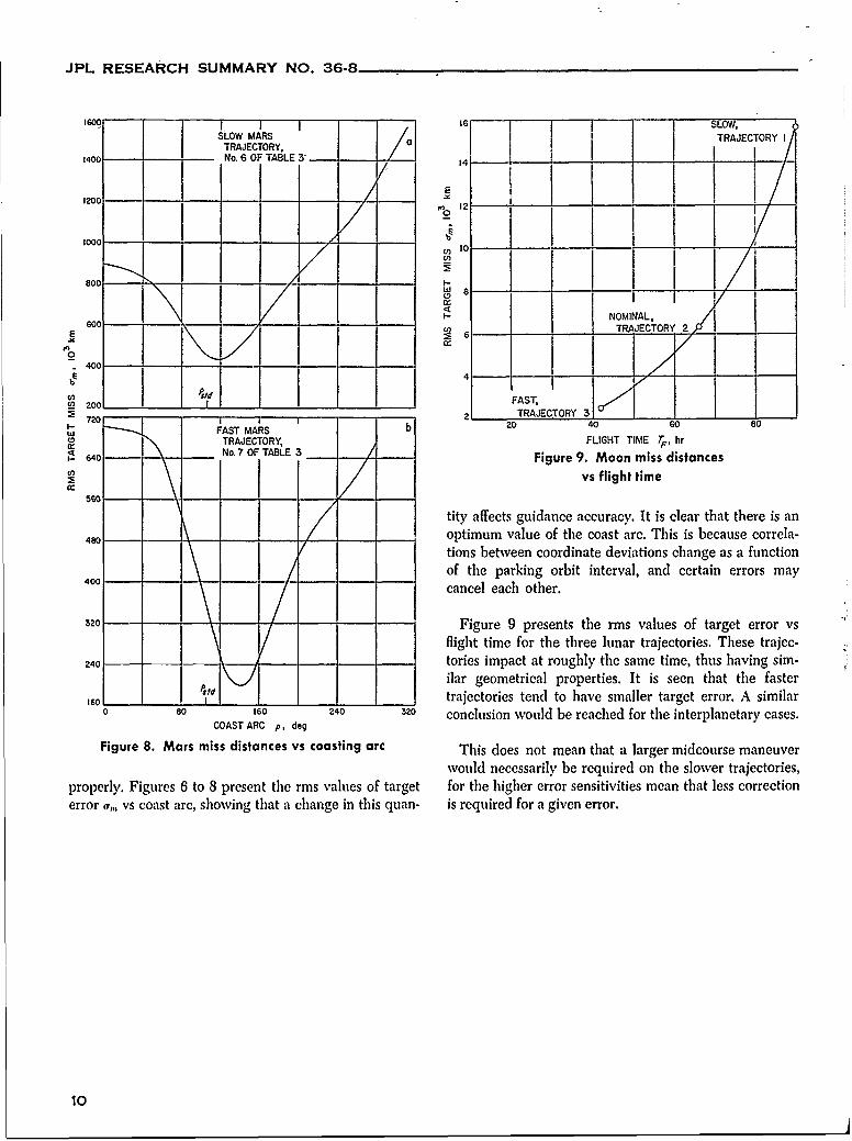
320 Figure 9 presents the rms values of target error vs
flight time for the three lunar trajectories. These trajec-240 - - tories impact at roughly the same time, thus having sim-
ilar geometrical properties. It is seen that the faster,0 8 - - - 1 trajectories tend to have smaller target error. A similar
o 80 160 240 320 conclusion would be reached for the interplanetary cases.COAST ARC p, deg
Figure 8. Mars miss distances vs coasting arc This does not mean that a larger midcourse maneuverwould necessarily be required on the slower trajectories,
properly. Figures 6 to 8 present the rms values of target for the higher error sensitivities mean that less correctionerror or,, vs coast arc, showing that a change in this quan- is required for a given error.
10
JPL RESEARCH SUMMARY NO. 36-8
GUIDANCE AND CONTROL DIVISION
II. Guidance and Control Research
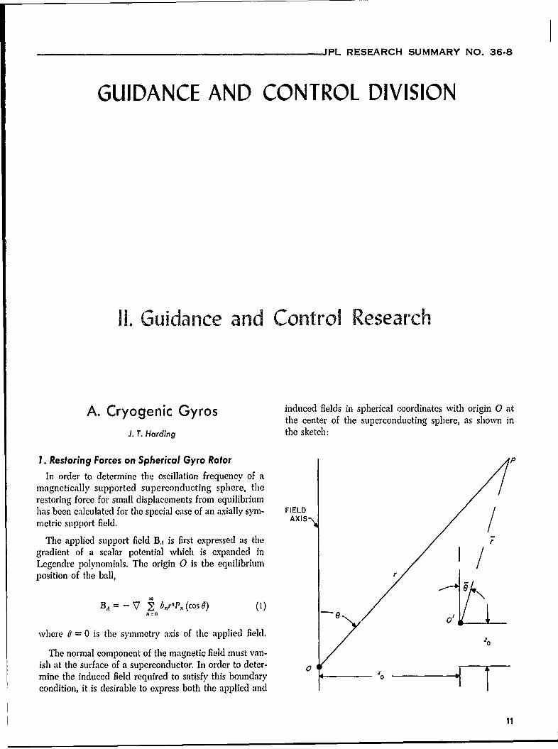
A. Cryogenic Gyros induced fields in spherical coordinates with origin 0 atthe center of the superconducting sphere, as shown in
J. T. Harding the sketch:
1. Restoring Forces on Spherical Gyro Rotor ,
In order to determine the oscillation frequency of amagnetically supported superconducting sphere, therestoring force for small displacements from equilibriumhas been calculated for the special case of an axially sym- FIELD
metric support field. AXIS /The applied support field Bj is first expressed as the
gradient of a scalar potential which is expanded inLegendre polynomials. The origin 0 is the equilibriumposition of the ball,
B., = - 7 b,,,.P,, (CoS) (1)
where 0 = 0 is the symmetry axis of the applied field.
The normal component of the magnetic field must van-ish at the surface of a superconductor. In order to deter-mine the induced field required to satisfy this boundary 0condition, it is desirable to express both the applied and
11
JPL RESEARCH SUMMARY NO. 36-8
The induced field B, must have the form The restoring force constants are- n (cos ) Cos ml (2) k. -R3b=4k:n=0 'n=0 rn/t IO 2
B, is transformed into barred coordinates by a Taylor 2. Damping of a Cryogenic Gyroseries in powers of xo, zo, the displacements from equi- A proposed cryogenic gyro consists of a superconduct-librium. If terms higher than linear are neglected, ing sphere supported by currents in superconducting coils
BA (, 0) = - V7 b [rP (cos 9) + zonTrn'1P. 1 (cos ) (RS 36-5). Such a system is lossless so that, once set inn=o motion, the sphere will bounce almost endlessly, limited
-Xorn-P'iPi (cos s + . • + only by radiation. To provide damping, the sphere maybe surrounded by a lossy shield. The ac magnetic fieldinduced by the motion of the sphere in the support field
The net field B BA + B, which satisfies the boundary will generate eddy currents in the resistive shield, whichcondition, is will dampen the oscillation. The magnitude of this effect
B , 2n+1 -. [b dP, . dP, has been calculated for the case of a thin spherical shellB,(, 2 + I R-'bd"+ o( + 1)b"BA (" 0 +ok - + z(n +) b,d+o when the oscillation is along the axis of an axially sym-
dpi ~ metric support field. The calculation consists of the fol-Xob,+, Cos _+ -L [x~b +,P,, sin ] lowing steps:
(1) Expressing the applied field B 1 as the gradient ofTo compute the force exerted on the sphere by this a scalar potential which is expanded in Legendre
field, the Maxwell stress tensor is integrated over the polynominals; the origin 0 is at the center of thesurface. resistive shell, which is assumed to be the equilib-
rium position of the ball;
= ). s =-BA 7-,=- b,"P, (cos 0) ()n=
since B r = 0. where 0 = 0 is the symmetry axis of the applied
Axial component of force: field.
F 2 ffB2 COS 2d cos 0 do (2) Transforming B to coordinates fixed with respect
21A= ffJBcs0~csd to the oscillating sphere.4 7 r b, [nRon ib, + z + 2)R°-.1b,+. (3) Determining the induced field produced by the1A, n=o sphere to satisfy the boundary condition for a
+ z (it - 1) nR2 -1b,] superconductor:
Bnormal = 0Radial component of force:
= I [ f(4) Calculating the power dissipated due to eddy cur-"2 = 2 oj, BZsin 8cos R2 d o 8"d$ rents induced in the resistive shell by the time-
varying field determined in (3); this is done by_ 2.x 0, - employing a formula developed by Smythe for
11o no " the dissipation rate in a thin spherical resistiveshell due to a sinusoidally time-varying magnetic
where terms quadratic in x,, zo have been neglected. field (Ref 14).
Example. If b, = 0 for n > 2 The damping has been worked out in detail for the fol-lowing special cases: (1) The spherical rotor is oscillat-
F.. = - L [R~b. + 2zoRfl ing sinusoidally with a small amplitude c,, at its resonant1 frequency. (2) The applied field involves only b, and b!,
., = - 2rx' 0 R3b2 all other coefficients being zero. (3) Values of b, and b:F A0 are determined by the two conditions that the magnetic
12
JPL RESEARCH SUMMARY NO. 36-8
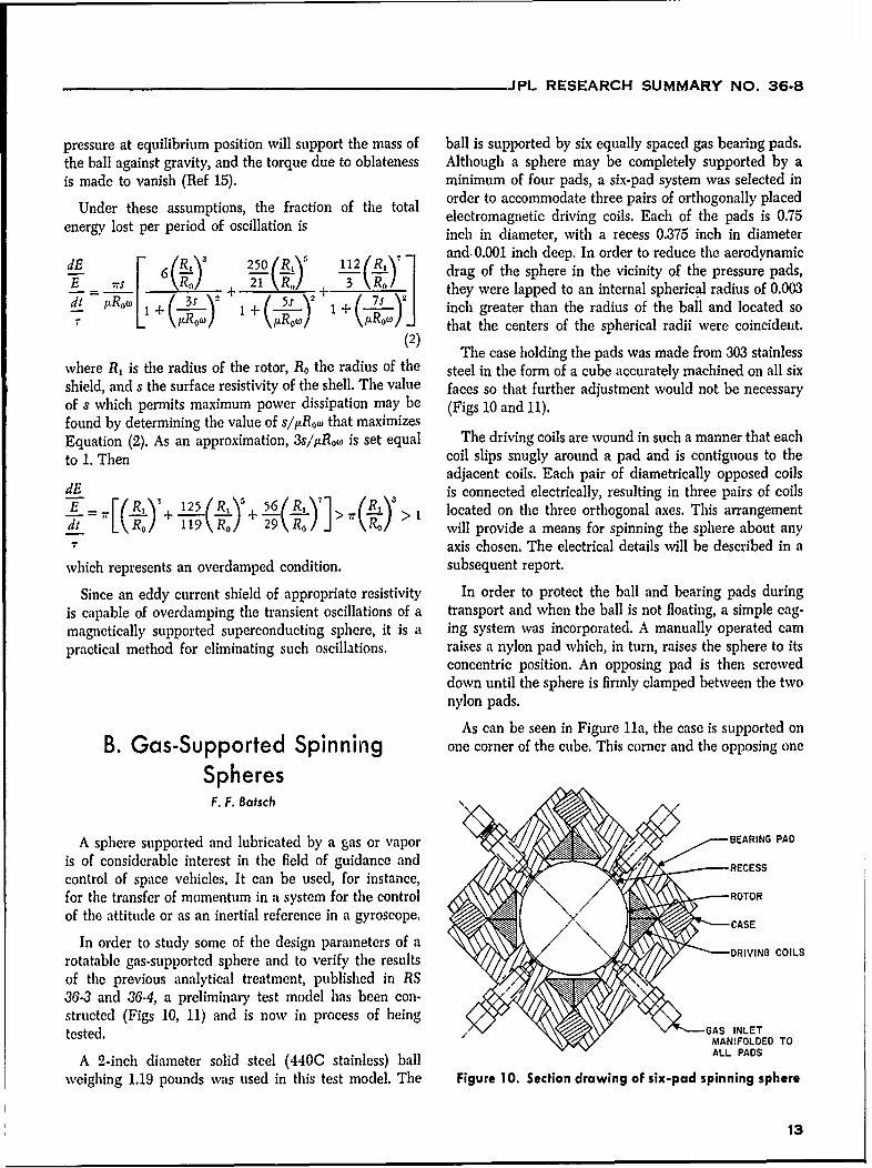
pressure at equilibrium position will support the mass of ball is supported by six equally spaced gas bearing pads.the ball against gravity, and the torque due to oblateness Although a sphere may be completely supported by ais made to vanish (Ref 15). minimum of four pads, a six-pad system was selected in
Under these assumptions, the fraction of the total order to accommodate three pairs of orthogonally placedner lsthee aptions, te caction electromagnetic driving coils. Each of the pads is 0.75
energy lost per period of oscillation is inch in diameter, with a recess 0.375 inch in diameter
dE R 25 112 and-0.001 inch deep. In order to reduce the aerodynamic6 250 R, -'(\'' 1 drag of the sphere in the vicinity of the pressure pads,
dt rs 0 + . + they were lapped to an internal spherical radius of 0.003di1( 3S 22 + (inch greater than the radius of the ball and located so+( o + Ro,) that the centers of the spherical radii were coincident.
(2) The case holding the pads was made from 303 stainless
where R, is the radius of the rotor, Ro the radius of the steel in the form of a cube accurately machined on all sixshield, and s the surface resistivity of the shell. The value faces so that further adjustment would not be necessaryof s which permits maximum power dissipation may be (Figs 10 and 11).found by determining the value of s/1tRow that maximizesEquation (2). As an approximation, 3s/ltRow is set equal The driving coils are wound in such a manner that eachto 1. Then coil slips snugly around a pad and is contiguous to the
adjacent coils. Each pair of diametrically opposed coilsdE is connected electrically, resulting in three pairs of coils-E' _ [('/_i 5 12(R s+ 6(L-r1> 7r(R > located on the three orthogonal axes. This arrangementT R 1 29 R, will provide a means for spinning the sphere about any
T axis chosen. The electrical details will be described in a
which represents an overdamped condition. subsequent report.
Since an eddy current shield of appropriate resistivity In order to protect the ball and bearing pads duringis capable of overdamping the transient oscillations of a transport and when the ball is not floating, a simple cag-magnetically supported superconducting sphere, it is a ing system was incorporated. A manually operated campractical method for eliminating such oscillations, raises a nylon pad which, in turn, raises the sphere to its
concentric position. An opposing pad is then screweddown until the sphere is firmly clamped between the twonylon pads.
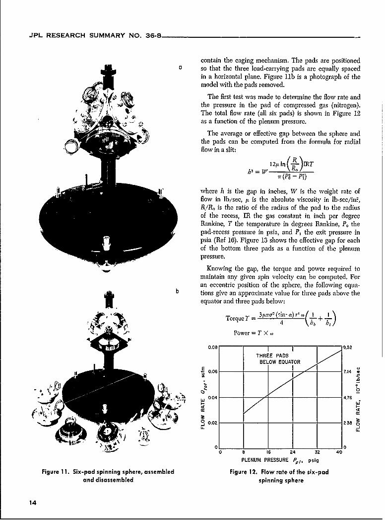
As can be seen in Figure 11a, the case is supported onB. Gas-Supported Spinning one corner of the cube. This corner and the opposing one
SpheresF. F. Batsch
A sphere supported and lubricated by a gas or vapor BEARING PAD
is of considerable interest in the field of guidance and ,E-EScontrol of space vehicles, It can be used, for instance,
for the transfer of momentum in a system for the control ROTORof the attitude or as an inertial reference in a gyroscope.
In order to study some of the design parameters of a DRIN C O
rotatable gas-supported sphere and to verify the results DRIVING COILSof the previous analytical treatment, published in RS36.3 and 36-4, a preliminary test model has been con-structed (Figs 10, 11) and is now in process of beingtested. GAS INLET
MANIFOLDED TO
A 2-inch diameter solid steel (440C stainless) ball ALL PADS
weighing 1.19 pounds was used in this test model. The Figure 10. Section drawing of six-pad spinning sphere
13
JPL RESEARCH SUMMARY NO. 36-8
contain the caging mechanism. The pads are positioneda so that the three load-carrying pads are equally spaced
in a horizontal plane. Figure llb is a photograph of themodel with the pads removed.
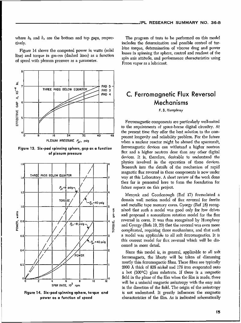
The first test was made to determine the flow rate andthe pressure in the pad of compressed gas (nitrogen).The total flow rate (all six pads) is shown in Figure 124 ,as a function of the plenum pressure.
The average or effective gap between the sphere andthe pads can be computed from the formula for radialflow in a slit:
12ttln R
(P2 - P2)
where h is the gap in inches, W is the weight rate offlow in lbisec, i is the absolute viscosity in lb-sec/in2-,R!R, is the ratio of the radius of the pad to the radiusof the recess, MR the gas constant in inch per degreeRankine, T the temperature in degrees Rankine, P. thepad-recess pressure in psia, and P, the exit pressure inpsia (Ref 16). Figure 13 shows the effective gap for eachof the bottom three pads as a function of the plenumpressure.
Knowing the gap, the torque and power required tomaintain any given spin velocity can be computed. Foran eccentric position of the sphere, the following equa-
b tions give an approximate value for three pads above theequator and three pads below:
Torque T = _3ttr-a2 (6an- a) P- w-L+_TorquT- 4h6 h),
Power = T w<4
0.08 1 9,52THREE PADS
BELOW EQUATOR
1 0.06 7.1
004 4.76
" 0.02 238
LL _jLL
"-0 8 16 24 32 40
PLENUM PRESSURE P/', psig
Figure 11. Six-pad spinning sphere, assembled Figure 12. Flow rate of the six-padand disassembled spinning sphere
14
JPL RESEARCH SUMMARY NO. 36-8
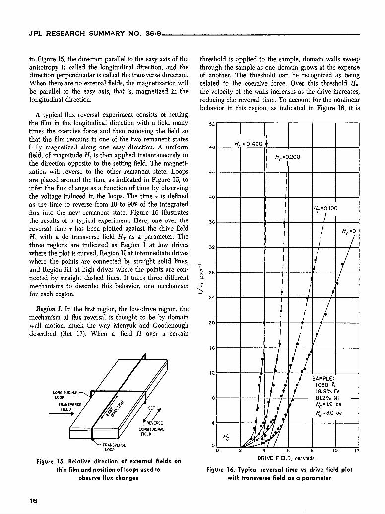
where hb and h, are the bottom and top gaps, respec- The program of tests to be performed on this modeltively. includes the determination and possible control of tur-
Figure 14 shows the computed power in watts (solid bine torque, determination of viscous drag and power
line) and torque in gm-cm (dashed lines) as a function losses in spinning the sphere, control and readout of the
of speed with plenum pressure as a parameter. spin axis attitude, and performance characteristics usingFreon vapor as a lubricant.
81
7 4-PAD 5THREE PADS BELOW EQUATOR PAD 30
- PAD 4 C. Ferromagnetic Flux Reversal6 Mechanisms
, F. B. Humphrey
I-
L- Ferromagnetic components are particularly well-suitedWa to the requirements of space-borne digital circuitry. At
4 the present time they offer the best solution to the com-0 8 16 24 32 40 48 ponent longevity and reliability problem. For the future
PLENUM PRESSURE P/, psig when a nuclear reactor might be aboard the spacecraft,
Figure 13. Six-pad spinning sphere, gap as a function ferromagnetic devices can withstand a higher neutronof plenum pressure flux and a higher neutron dose than any other digital
devices. It is, therefore, desirable to understand the.6 8 physics involved in the operation of these devices.
.Is Research into the details of the mechanism of rapid
/ magnetic flux reversal in these components is now under1.4 T7- 7 way at this Laboratory. A short review of the work done
TR BELO thus far is presented here to form the foundation for
1,=i"P 1/ future reports on this project.
/ Menyuk and Goodenough (Ref 17) formulated aTORQUE/ __ domain wall motion model of flux reversal for ferriteTOR./ / 40 psi and metallic tape memory cores. Gyorgy (Ref 18) recog-
S/ nized that such a model was good only for low drives/ / rand proposed a nonuniform rotation model for the flux
.o4 _ / reversal in cores. It was then recognized by Humphrey/ p0 and Gyorgy (Refs 19, 20) that the reversal was even more
0 0/ i complicated, requiring three mechanisms, and that sucho.6 // a model was applicable to all soft ferromagnetics. It is
// this current model for flux reversal which will be dis-/ / 1 .s cussed in more detail.
0.4 /OW Since this model is, in general, applicable to all soft/ POWER ferromagnets, the liberty will be taken of discussing
/ _____ ____ 1 ____ _____mostly thin ferromagnetic films. These films are typically
o 7 / I2000 A thick of 83% nickel and 17% iron evaporated onto_a hot (300 0 C) glass substrate. If there is a magnetic
0 10_ field in the plane of the film when the film is made, there0 2 4 6 8 to 12 will be a uniaxial magnetic anisotropy with the easy axis
SPIN RATE, 10 rpm in the direction of the field. The origin of the anisotropyFigure 14. Six-pad spinning sphere, torque and is not understood. It greatly influences the magnetic
power as a function of speed characteristics of the film. As is indicated schematically
15
JPL RESEARCH SUMMARY NO. 36-8
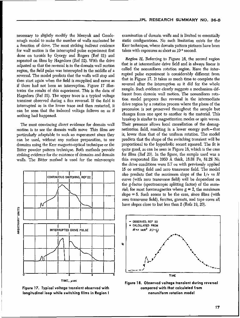
in Figure 15, the direction parallel to the easy axis of the threshold is applied to the sample, domain walls sweepanisotropy is called the longitudinal direction, and the through the sample as one domain grows at the expensedirection perpendicular is called the transverse direction. of another. The threshold can be recognized as beingWhen there are no external fields, the magnetization will related to the coercive force. Over this threshold H,be parallel to the easy axis, that is, magnetized in the the velocity of the walls increases as the drive increases,longitudinal direction. reducing the reversal time. To account for the nonlinear
behavior in this region, as indicated in Figure 16, it isA typical flux reversal experiment consists of setting
the film in the longitudinal direction with a field many 52
times the coercive force and then removing the field sothat the film remains in one of the two remanent states H 04fully magnetized along one easy direction. A uniform 48 Hr 0.400field, of magnitude H, is then applied instantaneously in Hr=.200the direction opposite to the setting field. The magneti- Ization will reverse to the other remanent state. Loops 44
are placed around the film, as indicated in Figure 15, toinfer the flux change as a function of time by observingthe voltage induced in the loops. The time r is defined 40 ___
as the time to reverse from 10 to 90% of the integrated Hr'-°.l°flux into the new remanent state. Figure 16 illustrates I Tthe results of a typical experiment. Here, one over the 36____
reversal time T has been plotted against the drive field H/0H, with a dc transverse field HT as a parameter. The I / T
three regions are indicated as Region I at low drives 32 ,-/
where the plot is curved, Region II at intermediate drives 32
where the points are connected by straight solid lines,and Region III at high drives where the points are con- 28nected by straight dashed lines. It takes three different .mechanisms to describe this behavior, one mechanism €for each region. 24 /
Region I. In the first region, the low-drive region, themechanism of flux reversal is thought to be by domain 2wall motion, much the way Menyuk and Goodenough -0described (Ref 17). When a field H over a certain I
16-
12SAMPLE;105o A
LONGITUDINAL 18.8% FeLOOP 8 - 81.2% Ni
TRANSVERSE Hc= .9 oeH,=3.0 oe
TRANSVERSE 0 ,LOOP 0 2 4 6 8 10 12
Figure 15. Relative direction of external fields on DRIVE FIELD, oersteds
thin film and position of loops used to Figure 16. Typical reversal time vs drive field plotobserve flux changes with transverse field as a parameter
16
JPL RESEARCH SUMMARY NO. 36-8
necessary to slightly modify the Menyuk and Goode- examination of domain walls and is limited to essentiallynough model to make the number of walls nucleated be static configurations. No such limitation exists for thea function of drive. The most striking indirect evidence Kerr technique, where domain pattern pictures have beenfor wall motion is the interrupted pulse experiment first taken with exposures as short as 10"1 second.done on toroids by Gyorgy and Rogers (Ref 21) andrepeated on films by Hagedorn (Ref 22). With the drive Region II. Referring to Figure 16, the second regionadjusted so that the reversal is in the domain wall motion that is at intermediate drive field and is always linear isadjste sotha th reersl i inthedomin allmoton called the nonuniform rotation region. Here thae inter-region, the field pulse was interrupted in the middle of a called the nonunim ion r io. eret ir-reversal. The model predicts that the wvalls wvill stop and rupted pulse experiment is considerably different from
revesal Th moel redctsthatthewals wll topand that in Figure 17. It takes as much time to complete thethen start again when the field is reapplied and move as re 17. t tes as c ti to te heif there had not been an interruption. Figure 17 illus- reversal after the interruption as it did for the wvholetrates the results of this experiment. This is the data of sample. Such evidence clearly suggests a mechanism dif-Hagedorn (Ref 22). The upper trace is a typical voltage ferent from domain wall motion. The nonuniform rota-transient observed during a flux reversal. If the field is tion model proposes flux reversal in the intermediateinterrupted as in the lower trace and then restarted, it drive region by a rotation process where the phase of thecan be seen that the induced voltage follows on as if precession is not preserved throughout the sample butnothing had happened. changes from one spot to another in the material. This
breakup is similar to magnetization modes or spin waves.The most convincing direct evidence for domain wall Their presence allows local cancellation of the demag-
motion is to see the domain walls move Thin films are netization field, resulting in a lower energy path-thatparticularly adaptable to such an experiment since they is, lower than that of the uniform rotation. The modelcan be used, without any surface preparation, to see predicts that the shape of the switching transient will bedomains using the Kerr magneto-optical technique or the proportional to the hyperbolic secant squared. The fit isBitter powder pattern technique. Both methods provide quite good, as can be seen in Figure 18, which is the casestriking evidence for the existence of domains and domain for films (Ref 20). In the figure, the sample used was awalls. The Bitter method is used for the microscopic thin evaporated film 1050 A thick, 18.8% Fe, 81.2% Ni;
the drive conditions were 5.7 oe with previously applied15 oe setting field and zero transverse field. The model
I I also predicts that the maximum slope of the 1/ vs HCONTINUOUS SWITCHING, REF22 curve (with zero transverse field) will be dependent on
the g-factor (spectroscopic splitting factor) of the mate-rial; for most ferromagnetics where g = 2, the maximumslope = 5. Such seems to be the case, since films (withzero transverse field), ferrites, garnets, and tape cores allhave slopes close to but less than 5 (Refs 19, 20).
I-
- - .- OBSERVED, REF 201 J 0 CALCULATED FROMM INTERRUPTED DRIVE PULSE M?-o sech 2 b(l-to)
- - - I ''
0 1 2 3 4 TIME
TIME, /sec Figure 18. Observed voltage transient during reversal
Figure 17. Typical voltage transient observed with compared with that calculated fromlongitudinal loop while switching films in Region I nonuniform rotation model
17
JPL RESEARCH SUMMARY NO. 36-8
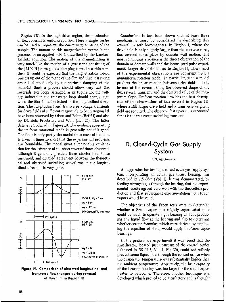
Region III. In the high-drive region, the mechanism Conclusion. It has been shown that at least threeof flux reversal is uniform rotation. Here a single vector mechanisms must be considered in describing fluxcan be used to represent the entire magnetization of the reversal in soft ferromagnets. In Region I, where thesample. The motion of this magnetization vector in the drive field is only slightly larger than the coercive force,presence of an applied field is described by the Landau- flux reversal takes place by domain wall motion. TheLifshitz equation. The motion of the magnetization is most convincing evidence is the direct observation of thevery much like the motion of a gyroscope consisting of domain or domain walls and the interrupted pulse experi-the [M X H] term plus a damping term. In a thin film, ment. Larger drive fields lead to Region II, where mostthen, it would be expected that the magnetization would of the experimental observations are consistent with aprecess up out of the plane of the film and then just swing nonuniform rotation model. In particular, such a modelaround, damped only by the intrinsic damping of the predicts the linear relation between drive field and thematerial. Such a process should allow very fast flux inverse of the reversal time, the observed shape of thereversals. For loops arranged as in Figure 15, the volt- flux reversal transient, and the observed value of the max-age induced in the transverse loop should change sign imum slope. Uniform rotation pro% ides the best descrip-when the film is half-switched in the longitudinal direc- tion of the observations of flux reversal in Region III,tion. The longitudinal and transverse voltage transients where a still larger drive field and a transverse magneticfor drive fields of sufficient magnitude to be in Region III field are required. The observed fast reversal is accountedhave been observed by Olson and Pohm (Ref 24) and also for as is the transverse switching transient.by Dietrich, Proebster, and Wolf (Ref 25). The latterdata is reproduced in Figure 19. The evidence supportingthe uniform rotational mode is generally not this good.The fault is only partly the model since most of the datais taken in times so short that the experimental problemsare formidable. The model gives a reasonable explana- D. Closed-Cycle Gas Supplytion for the existence of the short reversal times observed,although it generally predicts times shorter than those Systemmeasured, and detailed agreement between the theoreti- H. D. McGinnesscal and observed switching waveforms in the longitu-dinal direction is very poor. An apparatus for testing a closed-cycle gas supply sys-
a FILM 215 tem, incorporating an actual gas thrust bearing, wastREF 25 described in RS 36-7 (Vol 1). It was demonstrated, by
> ./ kT- -feeding nitrogen gas through the bearing, that the experi-W mental results agreed very well with the theoretical pro-o __ -,--..- diction and that subsequent experimentation with Freon
1500 A, Hio 3 we vapors would be valid.HS 5 6oe The objectives of the Freon tests vere to determineHr~ -1.25whether a Freon vapor in a slightly superheated state
1 04 msec LONITcould be made to operate a gas bearing without produc-
b0 - -sec FILM 215 ing any liquid flow at the bearing and also to determineREF 25 whether certain formulas, which were derived by employ-
S -- ing the equation of state, would apply to Freon vaporo> bearings.
In the preliminary experiments it was found that the
superheater, located just upstream of the control orifice'I. - H$=6oe (pictured in RS 36-7, Vol 1, Fig 30), could not reliably
I TRSVERSE PICKUP prevent some liquid flow through the control orifice when- TRANSVERSE the evaporator temperature was substantially higher than~-i 04msec the ambient temperature. Apparently, the heat capacity
Figure 19. Comparison of observed longitudinal and of the bearing housing was too large for the small super-transverse flux changes during reversal heater to overcome. Therefore, another technique was
of thin film in Region III developed which proved to be satisfactory and is thought
18
JPL RESEARCH SUMMARY NO. 36-8
to be more readily adaptable to spacecraft applications, whenThis method consists of maintaining the evaporator tem-perature below the ambient and letting the saturated _' 2 1_'i
vapor become superheated as it flows through the tubing - k + 1,(at room temperature) leading to the bearing.
Freon C318 was selected, because its pressure near [ \ - 1room temperature is suitable for many gas bearing appli- \2kgP P,.,k b)cations. At 45 0F its pressure is 10.5 psig, and increases For P(k- 1)I PAC
approximately linearly to 30 psig at 760F. The evaporator (P/may be cooled by blowing off some of the Freon; it maybe heated by applying electric current to heating coilsplaced within the container. Thus, the temperature is wheneasily adjusted to the desired value. Several tests weremade over this temperature range; in each case as the P> 2evaporator temperature approached ambient, the entrance P, (k + 1)to the pad bearing was visually observed in order to seewhen. there was liquid flow. In all instances where the - h (Po - P )temperature of the evaporator was very slowly raised, R =
liquid flow did not occur until the evaporator temperature 12!IRT log T(was approximately 0.50F more than the bearing temper-ature. When the evaporator temperature was rapidly whereincreased, a small amount of liquid flow would appearand then disappear, even at evaporator temperatures as l' weight flow through control orificemuch as 8F below the bearing temperature. A possible 1171, = weight flow through pad bearingexplanation for this is that, due to vigorous boiling, smalldroplets are thrown upward into the open end of the k = = ratio of specific heatsevaporator discharge pipe (RS 36-7, Vol I, Fig 30). When g = acceleration of gravitythe temperature difference between the evaporator and T = absolute temperaturethe bearing was not more than 80F, the droplets were notvaporized before entering the bearing, whereas for a R = gas constant in units of length per degree abso-greater temperature difference such droplets were vapor- lute temperatureized. P1,1 = absolute pressure upstream of control orifice
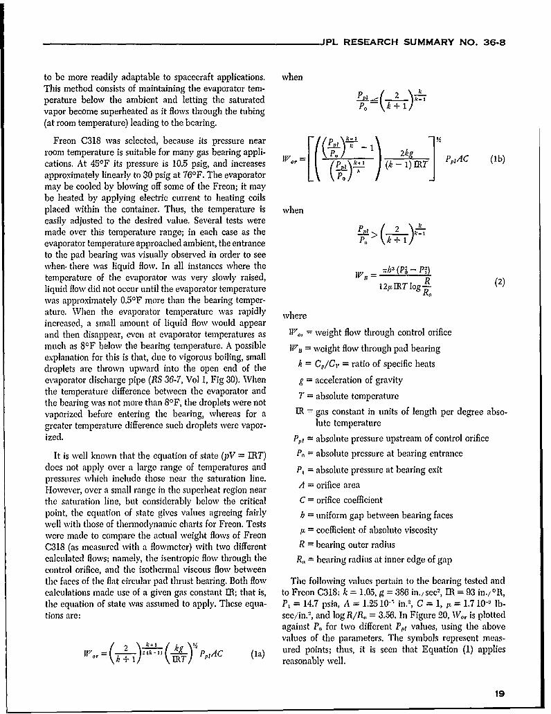
It is well known that the equation of state (pV = IRT) P, = absolute pressure at bearing entrancedoes not apply over a large range of temperatures and P, = absolute pressure at bearing exitpressures which include those near the saturation line. A = orifice areaHowever, over a small range in the superheat region nearthe saturation line, but considerably below the critical C = orifice coefficientpoint, the equation of state gives values agreeing fairly h = uniform gap between bearing faceswell vith those of thermodynamic charts for Freon. Testswere made to compare the actual weight flows of Freon = coefficient of absolute viscosityC318 (as measured with a flowmeter) with two different R = bearing outer radiuscalculated flows; namely, the isentropic flow through the R,, = bearing radius at inner edge of gapcontrol orifice, and the isothermal viscous flow betweenthe faces of the flat circular pad thrust bearing. Both flow The following values pertain to the bearing tested andcalculations made use of a given gas constant IlR; that is, to Freon C318: k = 1.05, g = 386 in./sec2 , M = 93 in./ 0 R,the equation of state was assumed to apply. These equa- P, = 14.7 psia, A = 1.25 10', in.', C = 1, it = 1.7 10-9 lb-tions are: see/in.", and log R/R,, = 3.56. In Figure 20, Wo is plotted
against P, for two different P,1 values, using the abovevalues of the parameters. The symbols represent meas-
IF,, = -_"" 1)-'R PpIAC ( ua) ured points; thus, it is seen that Equation (1) applies
k + 1 \ " reasonably well.
19
JPL RESEARCH SUMMARY NO. 36-8
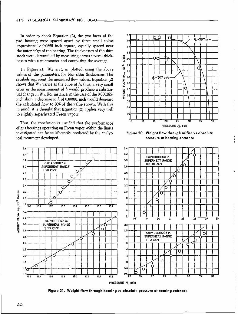
In order to check Equation (2), the two faces of the 2. - b,!1J I t1 I Fpad bearing were spaced apart by three small shims Z6 b iC-PJ,=38.7psia
approximately 0.0625 inch square, equally spaced near 24 _ __
the outer edge of the bearing. The thicknesses of the shim 22 _ I Istock were determined by measuring across several thick- 20 - - "
nesses with a micrometer and computing the average. *I YiIn Figure 21, W vs P0 is plotted, using the above 2 1 - I6 ]
values of the parameters, for four shim thicknesses. The C p 0s
symbols represent tht measured flow values. Equation (2) 3 1 , 1 1 1shows that 17B varies as the cube of h; thus, a very small U . -
error in the measurement of h would produce a substan- I -
tial change in WI. For instance, in the case of the 0.000285- A Rinch shim, a decrease in h of 0.00001 inch would decrease 1 . i6 1.1111in mind, it is thought that Equation (2) applies very well o ... ' II
to slightly superheated Freon vapors. 02 - 1 f + z5 0 15 20 210 5 4
Thus, the conclusion is justified that the performance RE5 20 R5 30 35 0
of gas bearings operating on Freon vapor within the limits PRESSURE Po, psio
investigated can be satisfactorily predicted by the analyt- Figure 20. Weight flow through orifice vs absoluteical treatment developed, pressure at bearing entrance
I GAP =0,00050 in.51 'FF1 Fo5- SUPERHEAT RANGE -
GAP=O.OOI13 in. 0.5 TO 360F30 SUPERHEAT RANGE
8TO 260F o.,6 /0
28 20-/
-zo - - i.- /j- C
b80 -1.8 - - --
150 1Sl 152 153 1, 15,5 156 15,74
3I " I-I - I - ! I A-o..... -- -
3 30 SUPRHEAT RnG 2 18 19 20 21 22 23 24 T5
2.0 I-30 -- SUPERHEAT RANGE .--2-
.a GAP=OQO00285 in. ol'. ! - - SUPERHEATRANGE
C - ~ I -o 50F-/"->-"_-
200
z2 1.Y/ '- C
162 16,A 166 168 170 172 17.4 176 23 25 27 29 31 33 35 37
PRESSURE P, psio
Figure 21. Weight flow through bearing vs absolute pressure at bearing entrance
20
JPL RESEARCH SUMMARY NO. 36-8
TELECOMMUNICATIONS DIVISION
1i1. Communications Elements Research
A. Low-Noise AmplifiersT. Sato
1. Solid State Maser L-.
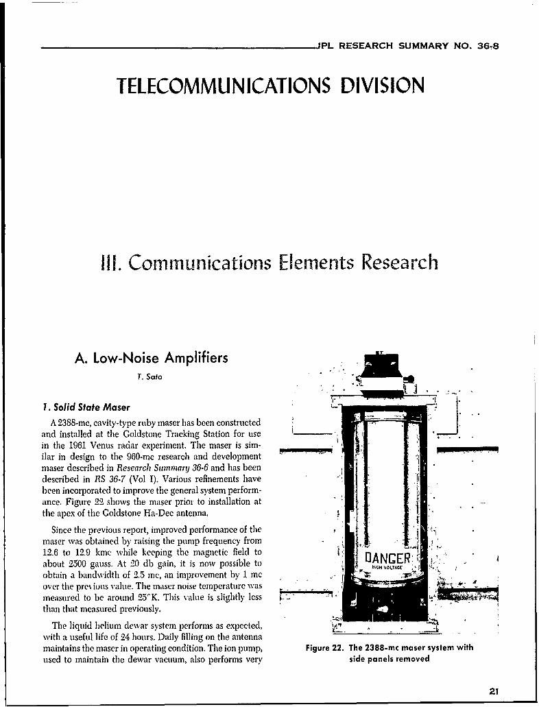
A 2388-mc, cavity-type ruby maser has been constructedand installed at the Goldstone Tracking Station for usein the 1961 Venus radar experiment. The maser is sim- _ _ ____I_____
ilar in design to the 960-mc research and development "'.. ...maser described in Research Summary 36-6 and has beendescribed in RS 36-7 (Vol I). Various refinements have -
been incorporated to improve the general system perform- iance. Figure 22 shows the maser prior to installation atthe apex of the Goldstone Ha-Dec antenna.
Since the previous report, improved performance of the ,maser was obtained by raising the pump frequency from12.6 to 12.9 kmc while keeping the magnetic field to IJANCERabout 2500 gauss. At 20 db gain, it is now possible to 4 VOL"AGE
obtain a bandwidth of 2.5 mc, an improvement by I mc -.
over the pre% iuus value. The maser noise temperature was "measured to be around 25'K. This value is slightly less ,.,"than that measured previously.
The liquid helium dewar system performs as expected, .with a useful life of 24 hours. Daily filling on the antennamaintains the maser in operating condition. The ion pump, Figure 22. The 2388-mc maser system withused to maintain the dewar vacuum, also performs very side panels removed
21
JPL RESEARCH SUMMARY NO. 36-8
well; it has maintained the vacuum to better than 10-7 mm tested. The initial ideas included the use of RF chokesHg after 1 month of continuous operation. The unique of various types around the horn mouth, a variation ofdesign of this pump enables it to outperform ion pumps the flange size in order to shape the pattern (Ref 26),twice the volume and four times the weight. the placing of obstacles and chokes in the horn mouth
The performance of the maser was checked after instal- to simulate multiple tilted horns, and the use of large
lation on the receiving antenna. The gain-bandwidth tilted ground planes at approximately the edge illumina-
product and noise temperature were substantially the tion angle of the dish. The idea of using a metallic lenssame as those measured in the laboratory. The presence in front of the horn was considered briefly. The use of
of gain variations with antenna position was detected. an array of horns was considered but was discarded
The source of this gain variation is believed to be small because of the required additional waveguide feedlines
changes in the magnetic field resulting from the mechan- which would contribute additional excess temperature.ical shifting of the magnet system relative to the ruby By late December, some progress had been achievedcrystal. Gain fluctuations observed are of the order of with the use of chokes around the horn mouth. Experi-__.2 db when the antenna is rapidly scanned across the mental data showed this to be a promising approach, butsky. When tracking a slowly moving object such as Venus, insufficient data war available to design the feed. Thea periodic adjustment of the magnet current allows the use of obstacles in a horn mouth was tried without prom-gain fluctuations to be kept under _0.5 db. ising results for this application. Next, an experiment was
carried out with a large wide-angle (120 deg) tiltedgroundplane, flaring out from the horn mouth, that pro-vided good results for linear polarization in the E-plane.Later, very good shaping of an H-plane pattern was
B. Antennas for Space obtained using a very large flat groundplane around the
Communication horn mouth. A combination of these two ideas was tested
D. Schuster and C. T. Stelzried a. COORDINATES 1I1FFEED HORN
I. Shaped Beam Feed Researchr GRUNDLLMNTi\GROUND ILLUMINATION
In November 1960, research in low-noise antenna sys- I ,,NGLE
tens was directed to aid development of a low-noise 0*temperature, high-gain, circularly polarized feed to be I
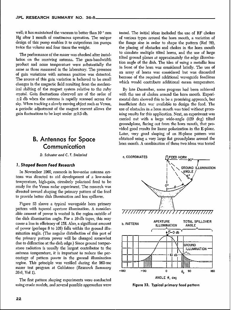
ready for the Venus radar experiment. The research wasdirected toward shaping the primary pattern of the feedto provide better dish illumination and less spillover.
Figure 23 shows a typical waveguide horn primarypattern with tapered aperture illumination. A consider-able amount of power is wasted in the region outside ofthe dish illumination angle. For a 10-db taper, this may APERTURE TOTAL SPILLOVERcause a loss in efficiency of 15%. Also, a significant amount b. PATTERN ILLUMINATION ANGLEof power (perhaps 8 to 10%) falls within the ground illu- yOd,
mination angle. (The angular distribution of this part of 0,--o db' _ _
the primary pattern power will be changed somewhatdue to diffraction at the dish edge.) Since ground temper-/ - l I GROUNDattire radiation is usually the largest contributor to the LLILLUMINATIONantenna temperature, it is important to reduce the per-centage of pattern power in the ground illumination - db
region. This principle was verified during the 960-me IIi'maser test program at Goldstone (Research Summary - -0 -90 0 90 ISO36-6, Vol I). -leo
The first pattern shaping experiments were conducted ANGLE , deg
using crude models, and several possible approaches were Figure 23. Typical primary feed pattern
22
JPL RESEARCH SUMMARY NO. 36-8
and provided a good technique for shaping the pattern antenna range. Some pieces of equipment were purchased,of a linearly polarized horn. and some were designed and built specifically for this
During January, numerous tests were carried out on purpose. By January, this range was operating with high
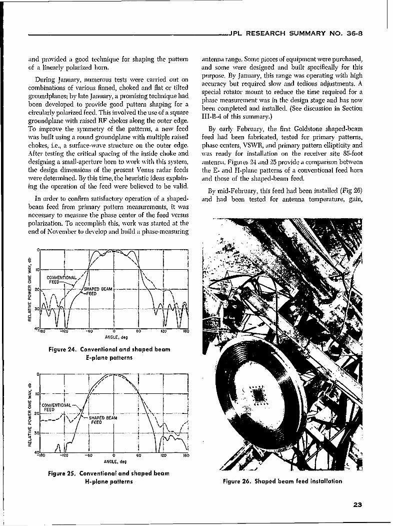
combinations of various finned, choked and flat or tilted accuracy but required slow and tedious adjustments. Agroundplanes; by late January, a promising technique had special rotator mount to reduce the time required for abeen phase measurement as in the design stage and has nowbioled atte use of aa been completed and installed. (See discussion in Sectioncircularly polarized feed. This involved the use of a squaresummary.)groundplane with raised RF chokes along the outer edge.To improve the symmetry of the patterns, a new feed By early' February, the first Goldstone shaped-beamwas built using a round groundplane with multiple raised feed had been fabricated, tested for primary patterns,chokes, i.e., a surface-wave structure on the outer edge. phase centers, VSWR, and primary pattern ellipticity andAfter testing the critical spacing of the inside choke and was ready for installation on the receiver site 85-footdesigning a small-aperture horn to work with this system, antenna. Figui s 24 and 25 provide a comparison betweenthe design dimensions of the present Venus radar feeds the E- and H-plane patterns of a conventional feed hornwere determined. By this time, the heuristic ideas explain- and those of the shaped-beam feed.ing the operation of the feed were believed to be valid. By mid-February, this feed had been installed (Fig 26)
In order to confirm satisfactory operation of a shaped- and had been tested for antenna temperature, gain,beam feed from primary pattern measurements, it wasnecessary to measure the phase center of the feed versuspolarization. To accomplish this, work was started at theend of November to develop and build a phase-measuring
0
CONVENTIONAL / "EEAo FEED /
20, 0 " 6APED
BEAM
4-180 -10 -0 0 60 120 I8O
ANGLE, deg
Figure 24. Conventional and shaped beam . i'
E-plane patterns , mCo .. ..
FEED __,1 ! _ __\'\
.. / I\ # /-SHAPED BEAMo FEED
0.W \
-I0 -120 -60 0 60 120 180
ANGLE, degFigure 25. Conventional and shaped beam
H-plane patterns Figure 26. Shaped beam feed installation
23
JPL RESEARCH SUMMARY NO. 36-8
ellipticity, and secondary patterns. The results of the the 85-foot receiving antenna. In order to achieve thisexperimental measurements are included in Section III- purpose, three horns were provided. Two of these wereB-2 on the Venus radar feeds. conventional horns to produce edge illuminations of 10
At the present time, research on shaped-beam feed and 14 db (and with fin loading to obtain equal E- and
design is continuing. The immediate aim is to see if fur- H-plane patterns). The third was a shaped-beam feedhorn which was developed at JPL. (See discussion in
ther improvements can be made in the gain and figure pof mritof prabloial atenas.Section 111-13-1 on research leading to this development.)
All three horns were designed to use the same waveguidephase shifter and transformer sections to achieve circular
2. Feed System for Venus Radar Experiment polarization.
Several proposed feed systems to provide a low-noise During the installation period, the three horns werelistening feed for the Venus radar experiment were tested for gain, ellipticity, antenna temperature, and sec-described in Research Summary 36-7 (Vol 1). The primary ondary patterns. The shaped-beam feed was found todesign objective was to obtain a circularly polarized have from 0.8 to 1.1 db more gain than the conventional2388-mc feed that would produce the highest figure of feeds. The axial ratio of the elliptical polarization wasmerit (the quotient of gain and system temperature) for 0.75 db for the shaped-beam feed. The measured antenna
PHASE SHIFTER, 90 deg
FEEDHORN
TRANSFORMER WAVEGUME COUPLER,
45 deg dbWAVEGUID E
rSt COAXIALMOTOR-DRIVEN ADAPTER
W AV EG U ID E SW ITC H C P F
CIRCULATOR COUPLER FORWAVEGUIDE GAIN CALIBRATION
7/8-in. COAXIAL SERVO-ADAPTER CONTROLLED
WAVEGUIDE MASERATTENUATOR 2 _ PLIFIER
I NOISE BOX
I (SIMPLIFIED)
LIQUID WAVEGUIDE IHELIUM COAXIAL I SWITCH] NEON GAS
ADAPTER 1 = " ' I TUBE
II AMBIENTTEMPERATURE ILOAD I
FOCAL POINT L.- --OF ANTENNA
CONTROL ROOM
FOLLOWUPRECEIVERSYSTEM
Figure 27. Feed system for Venus radar receiver
24
JPL RESEARCH SUMMARY NO. 36-8
temperatures with the antenna pointed at zenith (and cussion of the noise temperature measurement techniqueswith a quiet sky background) were as follows: in Section III-B-3 of this summary.)
Horn with 10-db taper, 30 0K. An alternate feed system design includes a bimodalcombiner and an additional waveguide switch to allowHorn with 14-db taper, 160K. rapid changing between right- and left-handed circular
Shaped-beam feed, 140K (absolute accuracy 40K). polarization. The bimodal combiner has not yet beeninstalled; it still remains as a possible modification laterThe best estimate of the far field gain, based on measure- i h eu aa xeiet
ments taken in the near field at 0.3D-/,\, is 53.5 db for a
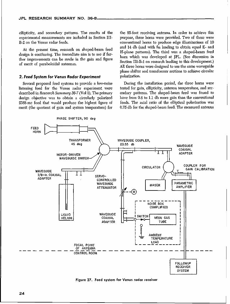
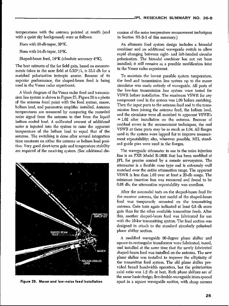
matched polarization isotropic source. Because of its To maintain the lowest possible system temperature,superior performance, the shaped-beam feed is being the feed and transmission line system up to the maserused in the Venus radar experiment, circulator was made entirely of waveguide. All parts of
A block diagram of the Venus radar feed and transmis- the low-loss transmission line system were tested forsion line system is shown in Figure 27; Figure 28 is a photo VSWR before installation. The maximum VSWR for an),of the antenna focal point with the feed system, maser, component used in the system was 1.09 before matching.helium load, and parametric amplifier installed. Antenna Then the input ports to the antenna feed and to the trans-temperatures are measured by comparing the recorded mission lines joining the antenna feed, the helium load,
noise signal from the antenna to that from the liquid and the circulator were all matched to apparent VSWR's
helium cooled load. A calibrated amount of additional = 1.02 after installation on the antenna. Because ofnoise is injected into the system to raise the apparent residual errors in the measurement techniques, the realtemperature of the helium load to equal that of the VSWR at these ports may be as much as 1.04. All flangesantenna. The switching is done after several integration used in the system were lapped flat to improve measure-
anent repeatability; also, wherever possible, MIL stand-time constants on either the antenna or helium load posi-tion. Very good short-term gain and temperature stability ard guide pins were used in the flanges.
are required of the receiving system. (See additional dis- The waveguide attenuator in use in the noise injectionline is an FXR Model R-160B that has been modified atJPL for precise control by a remote servosystem. Theattenuator is a flexible vane type and is extremely wellmatched over the entire attenuation range. The apparentVSWR is less than 1.03 over at least a 20-db range. Theminimum insertion loss was measured and found to be0.08 db; the attenuation repeatability was excellent.
After the successful tests on the shaped-beam feed forthe receiver antenna, the test model of the shaped-beamfeed was temporarily mounted on the transmittingantenna. Gain tests again indicated at least 0.8 db moregain than for the other available transmitter feeds. Afterthis, another shaped-beam feed was fabricated for useWith the 10-kw%' transmitting system. The feed section wasdesigned to attach to the standard circularly polarizedphase shifter section.
A modified waveguide 90-degree phase shifter andsquare-to-rectangular transformer were fabricated, tuned,and installed at the same time that the newly fabricated
- shaped-beam feed was installed on the antenna. The newphase shifter was installed to improve the ellipticity ofthe transmitter feed system. The old phase shifter pro-vided broad bandwidth operation, but the polarizationaxial ratio was 1.2 db at best. Both phase shifters are ofthe same basic design; five double-waveguide irises spaced
Figure 28. Maser and low-noise feed installation apart in a square waveguide section, with sharp corners
25
JPL RESEARCH SUMMARY NO. 36-8
rounded to prevent corona arcing. After installation 320
of the new shaped-beam feed, phase shifter, and trans-former, the ellipticity was measured for right-hand sec- 280--
ondary polarization and the axial ratio was less than 0.3db. The present best estimate of the far-field gain of the 240-
transmitter antenna, under the same conditions that apply 2-
to the receiving antenna, is 53.8 db. 0 2 0
160----------------
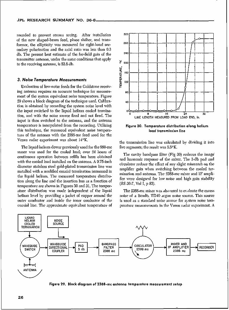
3. Noise Temperature Measurements W - -
ing antenna requires an accurate technique for measure- 80 -
ment of the system equivalent noise temperature. Figure29 shows a block diagram of the technique used. Calibra- 4 -
tion is obtained by recording the system noise level withthe input switched to the liquid helium cooled termina- 0tion, and with the noise source fired and not fired. The 0 8 S 24 32LINE LENGTH MEASURED FROM LOAD END, in.
input is then switched to the antenna, and the antennatemperature is interpolated from the recording. Utilizing Figure 30. Temperature distribution along heliumthis technique, the measured equivalent noise tempera- load transmission lineture of the antenna with the 2388-mo feed used for theVenus radar experiment wvas about 140K. the transmission line was calculated by dividing it into
The liquid helium dewar previously used for the 960-me five segments; the result was 5.50 K.maser was used for the cooled load; over 24 hours of The cavity bancpass filter (Fig 30) reduces the imagdcontinuous operation between refills has been obtained and harmonic response of the mixer. The 3-cb pad and
wvith the cooled load installed on the antenna. A 0.75-inch circulator reduce the effect of any slight mismatch on thediameter stainless steel gold-plated transmission line was amplifier gain when switching between tie cooled tr-installed with a modified coaxial termination immersed in aiiain nen Thi bewen h coole -muination and antenna. The 0388-mc mixer and IF ampli-the liquid helium. The measured temperature distribu- fier wre designl for low noise and high gain stabilitytion along the line and the insertion loss as a function of (RS 36-7, Vol I, p 83).temperature are shown in Figures 30 and 31. The temper-ature distribution was made independent of the liquid The 2388-mc mixer was also used to evaluate the excesshelium level by providing a jacket of copper around the noise of a Bendix TD,10 argon noise source. This sourceouter conductor and inside the inner conductor of the is used as a standard noise source for s)stem noise tern-coaxial line. The approximate equivalent temperature of perature measurements in the Venus radar experiment. A
LIQUID
HELIUM NOISECOOLED SOURCE
TERMINATIONL
DIRECTIONAL FILTER IF AMPLIFIER RECORDERCOUPLER 2388 mc
ANTE NNA
Figure 29. Block diagram of 2388-mc antenna temperature measurement setup
26
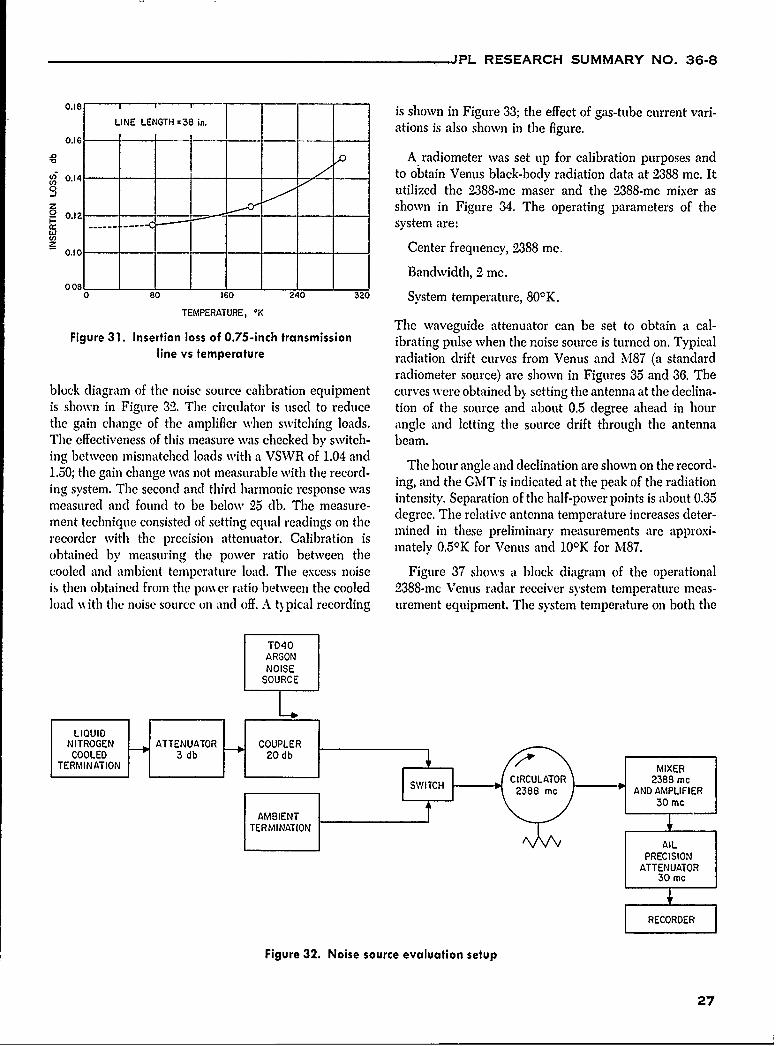
JPL RESEARCH SUMMARY NO. 36-8
0.18 ,F- I -is shown in Figure 33; the effect of gas-tube current vari-LINE LENGTH =38 in. ations is also shown in the figure.
0.16 - - IIo A radiometer was set up for calibration purposes and
. to obtain Venus black-body radiation data at 2388 me. It2,3 utilized the 2388-me maser and the 2388-me mixer asz - shown in Figure 34. The operating parameters of theP 0.12 -
- --- ...... .system are:z - Center frequency, 2388 me.
Bandwidth, 2 mc.008
0 80 160 240 30 System temperature, 80 0K.TEMPERATURE, -K
The waveguide attenuator can be set to obtain a cal-Figure 31. Insertion loss of 0.75-inch transmission ibrating pulse when the noise source is turned on. Typical
line vs temperature radiation drift curves from Venus and M87 (a standardradiometer source) are shown in Figures 35 and 36. The
block diagram of the noise source calibration equipment curves were obtained b> setting the antenna at the declina-is shown in Figure 32. The circulator is used to reduce tion of the source and about 0.5 degree ahead in hourthe gain change of the amplifier when switching loads, angle and letting the source drift through the antennaThe effectiveness of this measure was checked by switch- beam.ing between mismatched loads with a VSWR of 1.04 and1.0 bteegain mitched lnotasu with t ror nd The hour angle and declination are shown on the record-1.50; the gain change was not measurable with the record-
ig s m Ting, and the GMT is indicated at the peak of the radiationmeasurtem. ane fond adto ird bermonic bel 2e eas intensity. Separation of the half-power points is about 0.35m e asu red a n d fo u n d to b e b elo w 25 d b . T h e m e a su re - d e r e T e r l a i e nt n a e m r t u e n c as s e e -ment technique consisted of setting equal readings on the degree. The relative antenna temperature increases deter-recorder with the precision attenuator. Calibration is mined in these preliminary measurements are approxi-obtained by measuring the power ratio between the mately 0.50 K for Venus and 100K for M87.cooled and ambient temperature load. The excess noise Figure 37 shows a block diagram of the operationalis then obtained from the po\% er ratio between the cooled 2388-mc Venus radar receiver system temperature meas-load \% ith the noise source on and off. A t) pical recording urement equipment. The system temperature on both the
TD40ARGONNOISESOURCE
LIQUIDNITROGEN ATTENUATOR COUPLERCOOLED 3 db 20 db
TERMINATION MIXERSWITH CRCULTOR2388 me
2388 m AND AMPLIFIER
30 mc
AMBIENT _
TERMINATIONAIL
PRECISIONATTENUATOR
30 mc
F RECORDER
Figure 32. Noise source evaluation setup
27
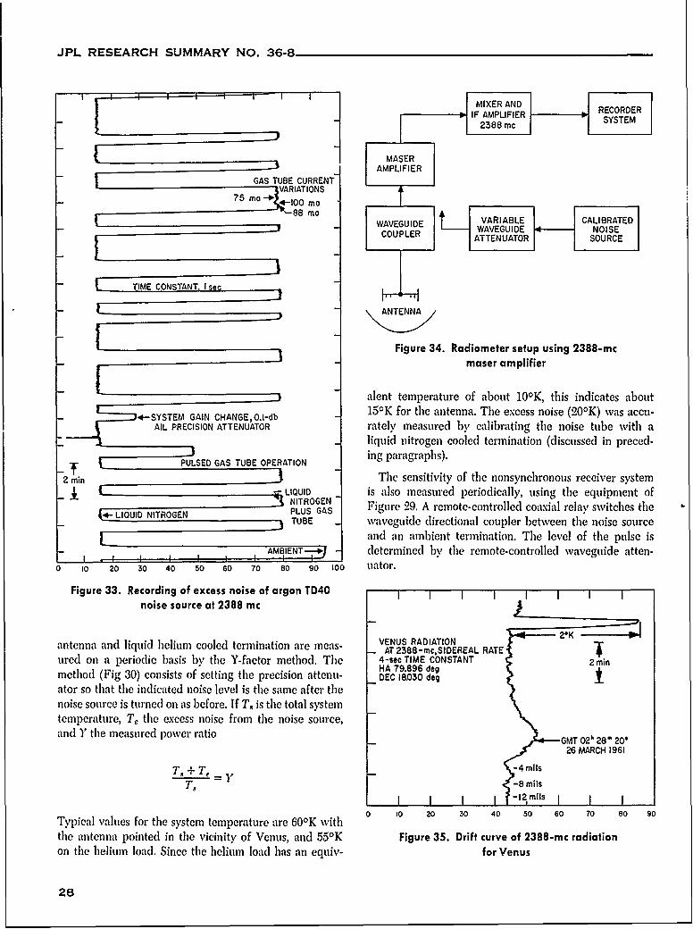
JPL RESEARCH SUMMARY NO. 36-8
MIXER AND RCREIF AMPLIFIER SYSTEM
2388 mc
MASERAMPLIFIER
GAS TUBE CURRENTVARIATIONS_7 5 m a --W .* 10 0 m o
WAVEGUIDE VARIABLE CALIBRATEDCUEWAVEGUIDE NOISECOUPLER ATTENUATOR SOURCE
-- L TIME CONSTANT, I s,,i
ANTENNA
Figure 34. Radiometer setup using 2388-mcmaser amplifier
alent temperature of about 100K, this indicates about
4-SYSTEM GAIN CHANGE,O.I-db - 150K for the antenna. The excess noise (20 0K) was accu-AIL PRECISION ATTENUATOR rately measured by calibrating the noise tube with a
-_ liquid nitrogen cooled termination (discussed in preced-
" PULSED GAS TUBE OPERATION ing paragraphs).
2 in - The sensitivity of the nonsynebronous receiver systemLIQUID is also measured periodically, using the equipment of
PLUS GAS Figure 29. A remote-controlled coaxial relay switches theLI RTUBE waveguide directional coupler between the noise source
and an ambient termination. The level of the pulse isAMBIENT- determined by the remote-controlled waveguide atten-
o 10 20 30 40 50 60 70 80 90 1oo uator.
Figure 33. Recording of excess noise of argon TD40noise source at 2388 mc
antenna and liquid helium cooled termination are ias- VENUS RADIATION 20K
AT 2388-mc,SIDEREAL RATEured on a periodic basis by the Y-factor method. The 4-sec TIME CONSTANT 2 mi" HA 79.896 degmethod (Fig 30) consists of setting the precision attenu- DEC 18.030 degator so that the indicated noise level is the same after thenoise source is turned on as before. If T, is the total systemtemperature, T, the excess noise from the noise source,and Y the measured power ratio GMT 0 2 h 28 20'
26 MARCH 1961
TA + T, -4rmils
T,-8 mils-120mils
Typical values for the system temperature are 600K with 0 10 20 30 40 50 60 70 80 90
the antenna pointed in the vicinity of Venus, and 55 0K Figure 35. Drift curve of 2388-mc radiationon the helium load. Since the helium load has an equiv- for Venus
28
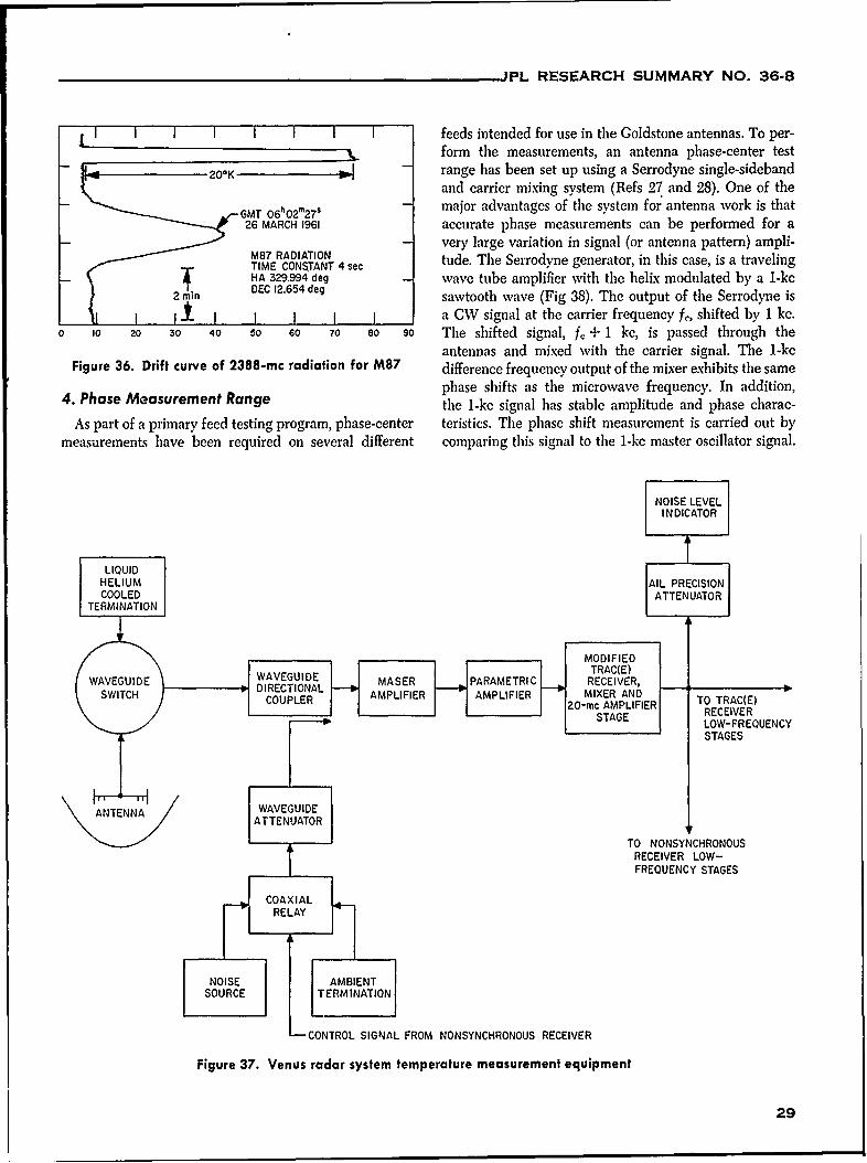
__ JPL RESEARCH SUMMARY NO. 36-8
feeds intended for use in the Goldstone antennas. To per-form the measurements, an antenna phase-center test
-11111- 200K range has been set up using a Serrodyne single-sidebandand carrier mixing system (Refs 27 and 28). One of the
GMT 060227 - major advantages of the system for antenna work is that26 MARCH 1961 accurate phase measurements can be performed for a
- very large variation in signal (or antenna pattern) ampli-
TIME CONSTANT 4 sec tude. The Serrodyne generator, in this case, is a travelingHA 329.994 deg - wave tube amplifier with the helix modulated by a 1-kc
2 mn DEC 12.654 deg sawtooth wave (Fig 38). The output of the Serrodyne isI I I I I I I a CW signal at the carrier frequency fJ, shifted by 1 kc.
0 10 20 30 40 50 60 70 80 90 The shifted signal, f, + 1 kc, is passed through theantennas and mixed with the carrier signal. The 1-kc
Figure 36. Drift curve of 2388-mc radiation for M87 difference frequency output of the mixer exhibits the samephase shifts as the microwave frequency. In addition,
4. Phase Measurement Range the 1-kc signal has stable amplitude and phase charac-As part of a primary feed testing program, phase-center teristics. The phase shift measurement is carried out by
measurements have been required on several different comparing this signal to the 1-kc master oscillator signal.
NOISE LEVELINDICATOR
LIQUIDHELIUM AIL PRECISIONCOOLED ATTENUATOR
TERMINATION
_ MODIFIED
WVGIEWAVEGUIDE MASER PARAMETRIC RECEIVER,SWTHDRCOAL AMPLIFIER 0 AMPLIFIER I IMIXER AND
20-mc AMPLIFIER TO TRAC(E)STAGE RECEIVER
LOW-FREQUENCYSTAGES
ANTENNAWAVEGUIDEATTENUATOR
TO NONSYNCHRONOUSRECEIVER LOW-FREQUENCY STAGES
RELAY
N O S A M I N
-CONTROL SIGNAL FROM NONSYNCHRONOUS RECEIVER
Figure 37. Venus radar system temperature measurement equipment
29
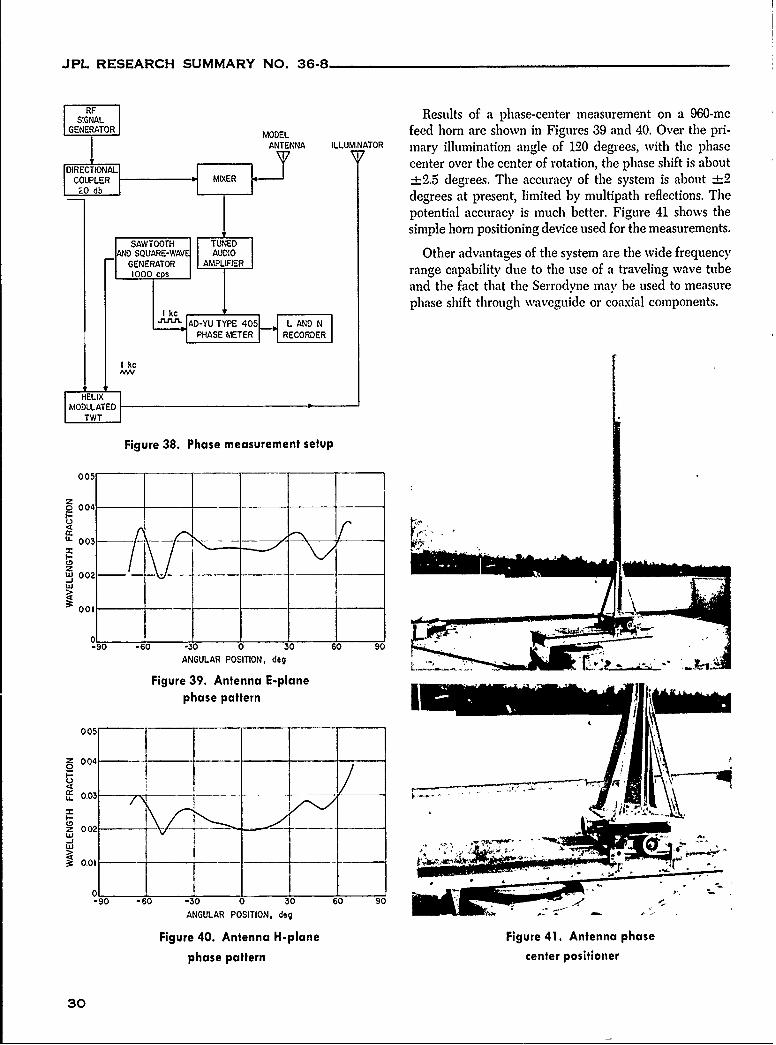
JPL RESEARCH SUMMARY NO. 36-8
RF
SIGNAL Results of a phase-center measurement on a 960-meGENERATOR MODEL feed horn are shown in Figures 39 and 40. Over the pri-
ANTENNA ILLUMINATOR mary illumination angle of 120 degrees, with the phaseDIRECTIONALI [center over the center of rotation, the phase shift is about
OUPLER MIX:ER -2.5 degrees. The accuracy of the system is about ±2__o db degrees at present, limited by multipath reflections. The
potential accuracy is much better. Figure 41 shows thesimple horn positioning device used for the measurements.
|SAWTOOTH T UNED I
AND Other advantages of the system are the wide frequencySGENERATOR AMLFE
1000O cps range capability due to the use of a traveling wave tubeand the fact that the Serrodyne may be used to measurephase shift through waveguide or coaxial components.
I kIf-AD-YU TYPE 405h L AND N
| PHSE ETERI IRECORDER
I kc
H ELIX
MODULATED
Figure 38. Phase measurement setup
005
004
U-003 ,
W 002-
-90 -60 -30 0 30 60 90
ANGULAR POSITION, deg
Figure 39. Antenna E-planephase pattern
005
Z 004-)
C-)I-o~w
.OI~I_ _ - _
I.-
1 0-" 00
-90 -60 -30 0 30 60 90ANGULAR POSITION, deg
Figure 40. Antenna H-plane Figure 41. Antenna phase
phase pattern center positioner
30
JPL RESEARCH SUMMARY NO. 36-8
C. Thin-Film Techniques porting material. Sapphire has proved to be a good matchfor germanium; however, no corresponding material has
J. Maserjian and H. Erpenbach yet been found for silicon. Attention was temporarilyturned to silicon because of the availability of excellent
1. Thin-Film Single Crystals preferential etches which can be used in the treatment of
The concept of microzone growing of single crystals the microzone melted specimens. Attempts to use either
from semiconductor film has been under investigation for sapphire or fused quartz with silicon have been unsuc-
several months (RS 36-4, 36-5, 36-7, and Ref 29). Recent cessful. Attempts at using an intermediate film of lead
efforts include incorporation into the experimental appa- (immiscible with silicon) as a means of relieving the
ratus of an improved electron-visual optical system. Prior strains were also unsuccessful. The choice of supporting
to this, experiments were conducted in a less satisfactory materials is very limited because of all the thermal, elec-system which did, however, provide some encouraging trical, and chemical requirements; the search is being
preliminary results. continued.Some germanium films evaporated wvith sapphire sub-
The experiment utilizes a finely focused electron beam Sae manined ear tempertu hve b
as a means of melting small areas or zones along a path successfully used in recent experiments without the occur-
on the film. The small dimensions (a few microns) require rencesf crack in rflkng Th e m icr on te regiona bih-prfomane elctrn-vsua optcalsysem.The rence of cracking or flaking. Tihe microzone melted region
a high-performance electron-visual optical system. The did not show the rippled texture observed previously thatoriginal system, designed inside an EMU 2 electron micro- seemed to relate to the grains of the adjacent film (RSscope, provided satisfactory electron optics but lacked 36-7). Figure 43a is a photomicrograph of a melted regiongood visual optics. which also reveals the very fine-grained or amorphous
Figure 42 shows a cutaway drawing of the new system texture of the adjacent germanium film. The crystallized
incorporated in th,. Jectron microscope. The water cooled path, about 27 microns wide, is quite smooth except for
heater anl specimen stage are the same as in the original the intermittent shrinkage crevices. Narrower paths were
apparattri. The major difference involves the use of light also melted, but the subsequent etching treatment makesoptics coaxial with the electron optics. In the original this wider path a convenient region to study.
system, the light was reflected from a mirror above and to A reasonably good preferential etch for germanium mayone side of the opening at the top of the heater jacket. have been found (Ref 30), as indicated by the resultsThe new system permits closer spacing of the electron seen t otniRogra ofigure by the etchin
seen in the photomnicrograph of Figure 43b. Thle etchingleris to the specimen for better beam focusing and allows action produced a glossy smooth surface on the crystal-a larger numerical aperture for the visual microscope lized path which is more characteristic of single crystals.objective. The objective also has the advantage of focus- The texture of the surrounding film is seen to becomeing in the plane of the specimen surface. Great care was increasingly rough with etching. The preferential actionnecessary in selecting a suitable objective lens and pre- is noted particularly at the sides of the path where deepserving its optical alignment in the system. Initial tests crevices have formed.on the new system have been highly satisfactory, butmelting experiments have not been conducted, as yet. If the path crystallized with a (111) orientation at the
surface, faster etching along the less dense planes atIt was suggested in RS 36-7 that the presence of suf- the sides would be expected. In addition, the surface
ficiently large crystal grains in the original semiconductor of the path is focused slightly above the surrounding film,film may have a detrimental influence on the single crystal indicating the preferential action originally hoped for.growth process. Efforts to evaporate films at lower sub-strate temperatures in order to obtain less grainy deposits Figure 43c shows that further etching removed somehave been complicated by poor adherence of the film of the crystalline path, indicating that the zone had not
to the substrate. melted through to the underlying sapphire support. Thisis not surprising in view of the rather thick film used (101t)
Improved adherence has been observed when the sub- and the minimum of heat which had been employed dur-strate is thoroughly baked out at high temperatures under ing the melting process. It may be a fortunate event ifhigh vacuum shortly before evaporation of the film. How- subsequent results indicate the sapphire support to inter-ever, cracking and flaking occur during subsequent heat fere with the growth process. This has been open to spec-cycling if there is any significant mismatch of the coeffi- ulation thus far. Comparison with the present resultscients of thermal expansion between the film and sup- should provide some answers.
31
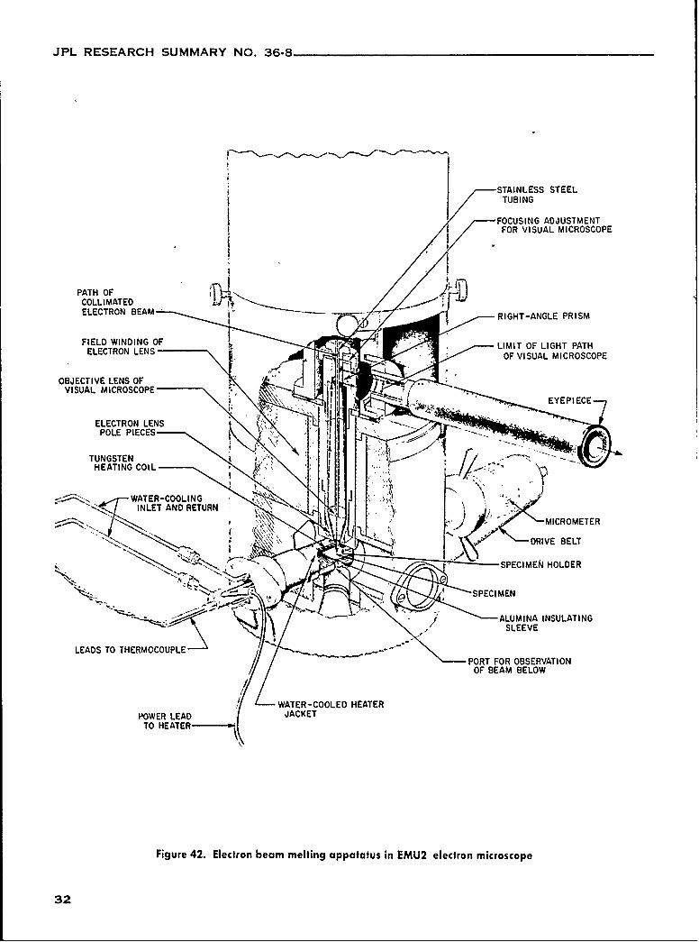
JPL RESEARCH SUMMARY NO. 36-8
STAINLESS STEELTUBING
FOCUSING ADJUSTMENTFOR VISUAL MICROSCOPE
PATH OFCOLLIMATEDELECTRON BEAM RIGHT-ANGLE PRISM
FIELD WINDING OF LELECTRON LENS O IULMCOCP
OBJECTIVE LENS OFVISUAL MICROSCOPE (,- , .EYEPIECE
m
ELECTRON LENSPOLE PIECES
HEATING COIL .
WATER-COOLINGINLET AND RETURN
F BM DRIVE BELT
-. .. ,. ... , ., SPECIMEN HOLDER
" ' :' " ' - /ALUMINA INSULATING/t
SLEEVE
LEADS TO THERMOCOUPLE POR FOR/ OBSERATIO
OF BEAM BELOW
WATER-COOLED HEATERPOWER LEAD JACKET
TO HEATER
Figure 42. Electron beam melting appatatus in EMU2 electron microscope
32

JPL RESEARCH SUMMARY NO. 36-8
= 7-- 2. Niobium Superconducting Thin Films
Work is continuing on the problem of depositing thinSfilms of niobium, which are superconducting. Since the
last report (RS 36-7), a film of niobium approximately 1.5 /thick has been deposited inside a cylindrical substrate.The deposition of the film was done in high vacuum by
," sublimation techniques, as shown in Figure 44. The filmhas been tested for superconductivity, and positive resultshave been obtained.
A cylindrical alumina (GE Lucalox) substrate was usedfor the following reasons: (1) The geometry of a cylinderis good for making experimental superconductivity tests.(2) The coaxial geometry and the resulting proximity of
BEFOREETCHING .... the niobium wire evaporant to the substrate wall will-' : - ," .... BEFORE ETCHING ," ""
. .heat it to approximately 10000C without external means.i $ (3) The coefficient of linear expansion of alumina approx-
imates that of niobium, and it may be heated to 10000Cin a vacuum.
i, Figure 44 shows the water cooled electrode terminalsand the cylindrical substrate in place with the 0.025-inch
- niobium wire inside the cylinder. The electrode terminalsare spring-loaded sufficiently to take up the linear expan-sion of the niobium wire.
! AFTER ETCHINd * * AE-COE: "¢ ,V NIOBIUM TERMINAL
- " ' WIRE 0025 in. - _
CERAMICSUBSTRATE
SUPPORT--
WATER-COOLEDTERMINAL---,-
SBELL JAR -- -.
TO I
WATERLI NES
Figure 43. Photomicrograph of microzone TO PUMPS
melted path on germanium film Figure 44. Vacuum chamber arrangement forbefore and after etching niobium thin-film deposition
33
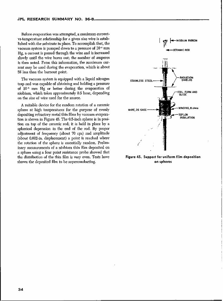
JPL RESEARCH SUMMARY NO. 36-8
Before evaporation was attempted, a maximum current-vs-temperature relationship for a given size wire is estab- [4 --NIOBIUM RIBBON
lished with the substrate in place. To accomplish that, thevacuum system is pumped down to a pressure of 10-1 mm -- CERAMIC ROD
Hg, a current is passed through the wire and is increasedslowly until the wire burns out; the number of amperesis then noted. From this information, the maximum cur-rent may be used during the evaporation, which is about ,JQt5% less than the burnout point.
The vacuum system is equipped with a liquid nitrogen STAINLESS RADIATION
trap and was capable of obtaining and holding a pressureof 10- ' mm Hg or better during the evaporation ofniobium, which takes approximately 0.5 hour, depending COILDFORM AND
on the size of wire used for the source.
A suitable device for the random rotation of a ceramic
sphere at high temperatures for the purpose of evenly WIRE, 26 GAGEohms
depositing refractory metal thin films by vacuum evapora- TEFLON
tion is shown in Figure 45. The 0.5-inch sphere is in posi- INSULATION
tion on top of the ceramic rod; it is held in place by a /spherical depression in the end of the rod. By properadjustment of frequency (about 70 cps) and amplitude(about 0.002-in. displacement) a point is reached wherethe rotation of the sphere is essentially random. Prelim-inary measurements of a niobium thin film deposited ona sphere using a four point resistance probe showed thatthe distribution of the thin film is very even. Tests have Figure 45. Support for uniform film depositionshown the deposited film to be superconducting. on spheres
34
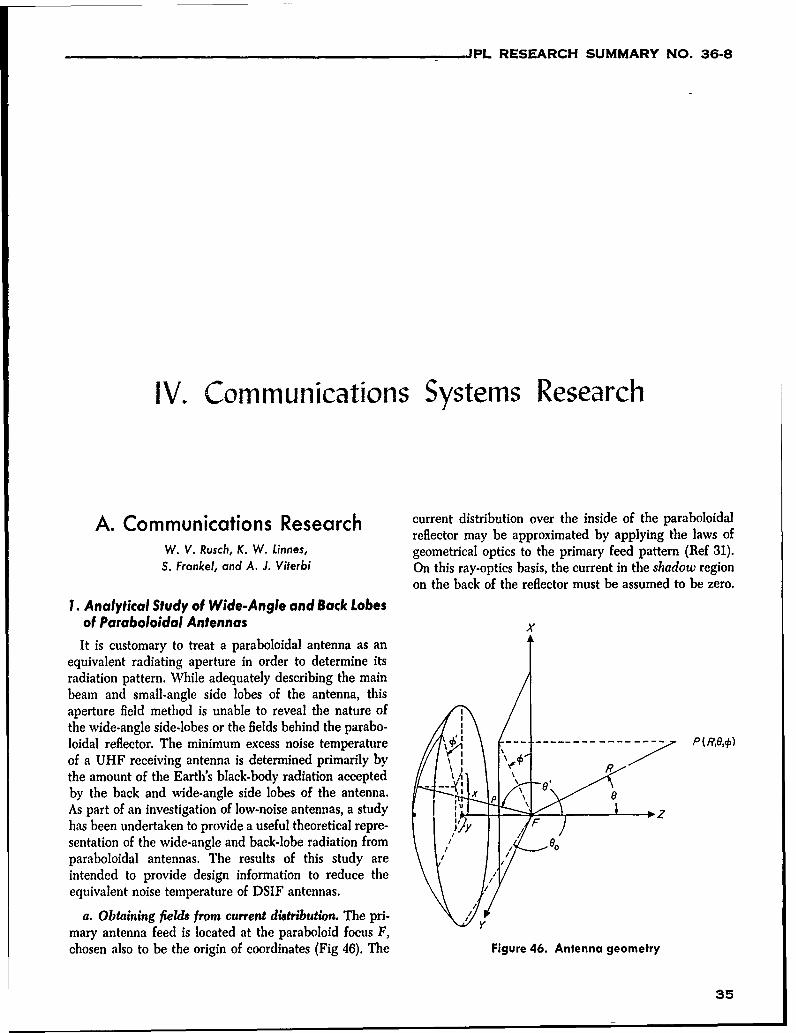
,PL RESEARCH SUMMARY NO. 36-8
IV. Communications Systems Research
A. Communications Research current distribution over the inside of the paraboloidalreflector may be approximated by applying the laws of
W. V. Rusch, K. W. Linnes, geometrical optics to the primary feed pattern (Ref 31).S. Frankel, and A. J. Viterbi On this ray-optics basis, the current in the shadow region
on the back of the reflector must be assumed to be zero.
1. Analytical Study of Wide-Angle and Back Lobesof Paraboloidal Antennas x
It is customary to treat a paraboloidal antenna as anequivalent radiating aperture in order to determine itsradiation pattern. While adequately describing the mainbeam and small-angle side lobes of the antenna, thisaperture field method is unable to reveal the nature ofthe wide-angle side-lobes or the fields behind the parabo-loidal reflector. The minimum excess noise temperature-"T P(R,0,4 )
of a UHF receiving antenna is determined primarily bythe amount of the Earth's black-body radiation accepted 'A
by the back and wide-angle side lobes of the antenna. XAs part of an investigation of low-noise antennas, a study P Zhas been undertaken to provide a useful theoretical repre- //F
sentation of the wide-angle and back-lobe radiation from 9_.0paraboloidal antennas. The results of this study areintended to provide design information to reduce theequivalent noise temperature of DSIF antennas.
a. Obtaining fields from current distribution. The pri- ymary antenna feed is located at the paraboloid focus F,chosen also to be the origin of coordinates (Fig 46). The Figure 46. Antenna geometry
35
JPL RESEARCH SUMMARY NO. 36-8
For a primary feed polarized along the x-axis, the vector The equivalent result for the aperture-field method is:surface current density is:
E0(= eL--k-- [(I +COS2sin. +,, (1) L COS 'cot-, T ( of)
-(5)where i, and i. are unit vectors in the x- and z-direc-
tions, p = f/sin" 0'/2, f is the focal length, and T (0, ") However, Equation (5) is valid only for small angles, inis the primary feed directivity pattern. No y-component which case (4) and (5) are in agreement. Equation (4)of the current is excited by this feed polarization, is valid for all values of 0, both in the directly illuminated
The radiation field is then obtained by integrating region and in the shadow region behind the reflectorEquation (1) over the inner surface of the reflector within the range of validity of the geometrical optics(Ref 32), approximation.
[r'kR1 -b. Evaluation of integrals. When the following aper-E= [.L"-'.-J eik2tc°67/2 ture field distribution is assumed:
X T (0," ) sin sig(r) = (1- r2)",, =0,1,2, (6)I p s the integral form of the field (4) becomes a Lommel
sJR function which can be expressed as an infinite power
R sseries of Bessel functions (Ref 32). Hnwever, since thiswhere series solution converges very slowly for large values of
D/X, Equation (4) has been integrated directly on the=-2- sin; - - sin 0 (xcos 0 + ysin 0) IBM 7090 computer. Results are presented in Figures 47
2/ and 48 where the absolute gain function G(O) is plottedfor n = 0 (uniform illumination), n = 1, and n = 2. When
Direct radiation from the primary feed is also included in axial symmetry is assumed, the gain function may beEquation (2). defined:
If the primary feed directivity pattern is axially sym. 2 E0(0) 1 1metric so that G(0) = 10log,,[ 1 E,() sin 0 J (7)
2[ . L ,,I ,(O'sin"- tnr (o 6 = (3)2sin I tan2 These theoretical results were calculated for the Gold-
stone DSIF antennas operating at 960 me (Fig 47) andwhere q = 1/tan 0o/2, then the field distribution in the 2-316 mc (Fig 48). The three aperture distributions g(r)reflector aperture is given by g(r)/2f, where considered were: uniform distribution, (1 - r2), and
r = (tan o /2)/(tan 01/2) (1 - 14) :% as shown in Figure 49. The primary feedpatterns completely filled the reflector and were zero
the normalized aperture radius. Then, in the plane elsewhere; consequently, spillover effects were not con-= -r/ 2, the total radiation field is: sidered. Local maxima in the gain were found at 0 = 0
eJ .lR ( (main beam), 6 = 0. (the shadow boundary), and 0 r.E() = [laq (r) /o (zr) I-''/2 r dr In addition to making the evaluation of radiation pat-
l) i~~1 terns for larger DIX ratios possible, direct numerical-14
g (4) integration of Equation (4) also facilitates the evaluationflZ f /3 /for primary feed aperture field distributions g(r), other
where than the idealized (1 - r2)n. The important problem ofprimary feed spillover can thus be evaluated with no(D/X) additional mathematical difficulties. The gain function is
D = diameter of antenna aperture presently being evaluated for various types of primaryfl = q tan (0/2) feed spillover. The results of this calculation will bez = a sin 0 translated into equivalent antenna noise temperature.
36
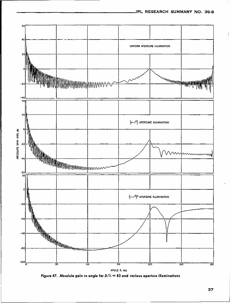
JPL RESEARCH SUMMARY NO. 36-8
UNIFORM APERTURE ILLUMINATION
-401
(,-,2) APERTURE ILLUMINATION
0V)
-60 ___________
(I - r2)2 APERTURE ILLUMINATION
-4C
-60
-8C
-1001__________ __________
0 3 09 2 5 8
ANGLE 0, deg
Figure 47. Absolute gain vs angle for DAX = 83 and various aperture illuminations
37
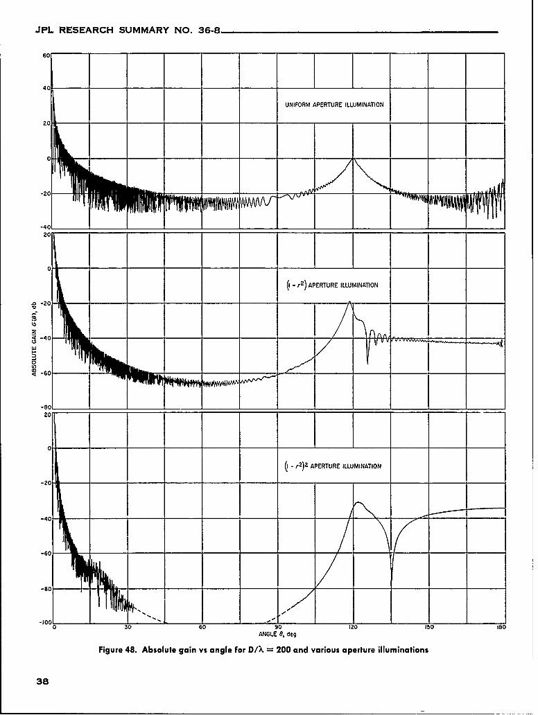
JPL RESEARCH SUMMARY NO. 36-8
60
40
UNIFORM APERTURE ILLUMINATION
20
-40
-20
0
(I - ,2) APERTURE ILLUMINATION
0
0
cn I
S-60 ___
- ( - 2)2 APERTURE ILLUMINATION
-40
-80
-100L I' I -II
0 30 60 90 120 15o 180ANGLE 8, deg
Figure 48. Absolute gain vs angle for D/. = 200 and various aperture illuminations
38
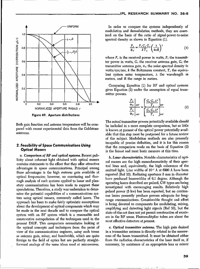
JPL RESEARCH SUMMARY NO. 36-8
UNIFORM In order to compare the systems independently ofmodulation and demodulation methods, they are exam-ined on the basis of the ratio of signal-power-to-noise
I-r2 spectral density as shown in Equation (1).
P_ PGtG, ( i '(10 08 -- =()
mwhere P,. is the received power in watts, Pt the transmit-
(n 0.6 ter power in watts, G, the receiver antenna gain, Gt thetransmitter antenna gain, 4)y the noise spectral density in
Dwatts/cyc/sec, k the Boltzmann constant, T, the equiva-Q: 0.A lent system noise temperature, k the wavelength in
meters, and R the range in meters.
_ _ _ _Comparing Equation (1) for RF and optical systemsN0.2Nj .gives Equation (2) under the assumption of equal trans-
mitter powers.0
0 0.2 0.4 0.6 0.8 1.0L -RR
NORMALIZED APERTURE RADIUS r P (2)
Figure 49. Aperture distributions lDo L T, ]opt
The actual transmitter powers potentially available shouldBoth gain function and antenna temperature will be com- be included in a more complete comparison, but so littlepared with recent experimental data from the Goldstone is known at present of the optical power potentially avail-antennas. able that this step must be postponed for a future review
of the subject. Modulation methods are also presentlyincapable of precise definition, and it is for this reason
2. Feasibility of Space Communications Using that the comparison made on the basis of Equation (2)Optical Masers is the fairest and most basic measure at this time.
a. Comparison of RF and optical systems. Recent pub- b. Laser characteristics. Notable characteristics of opti-licity about coherent light obtained with optical masers cal masers are the high monochromaticity of their spec-contains statements to the effect that they offer attractive tral lines and, equivalently, the high coherence of theadvantages in space communications. Principal among emitted light. Line widths of 10- A at 6900 A have beenthese advantages is the high antenna gain available at reported (Ref 33). Radiating apertures 5 mm in diameteroptical frequencies; however, no convincing and thor- have produced beamwidths of 0.1 degree. Although theough analysis of such systems applied to lunar and plan- operating lasers described are pulsed, CW types are beingetary communications has been made to support these investigated with encouraging results. Relatively highspeculations. Therefore, a study, was undertaken to deter- pulsed power (5 kw) has been reported, but no continu-mine the potential capabilities of a communications sys- os lasers presently produce powers adequate for long-tem using optical masers, commonly called lasers. The rae communtly od eraeuae ffortrange communications. Considerable thought and effortapproach has been to make fairly optimistic assumptions is being devoted to components for modulating, mixing,about the development of optical components which may amplifying and detecting light signals (Ref 33), but thebe made in the next decade and to compare the optical state-of-the-art does not yet permit construction of receiv-system with an HF system which is a reasonable andcosevtive witrpoan isthe chies asein the ers in the RF sense. Photomulitplier tubes are about theconservative extrapolation of the techniques used inte most effective detectors at~present.present DSIF. This comparison necessitates looking atthe optical concepts and techniques from the point of c. Optical transmitter antenna. The high gain desiredview of the communications engineer, using such terms in a transmitter antenna is directly related to the narrow-as antenna gain, mixer, and bandwidth, which are quite ness of the beam transmitted. It must be obtained eitherforeign to the field of optics but are perfectly straight- from the radiation characteristics of the laser itself or, ifforward analogs of the same ideas used at microwaves, necessary, by assistance of an appropriate lens or mirror
39
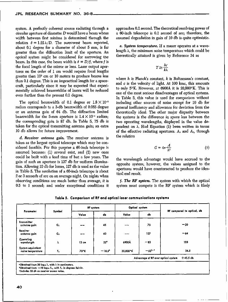
JPL RESEARCH SUMMARY NO. 36-8
system. A perfectly coherent source radiating through a approaches 0.2 second. The theoretical resolving power ofcircular aperture of diameter D would have a beam whose a 60-inch telescope is 0.1 second of arc; therefore, thewidth between first minima is determined through the assumed degradation in gain of 10 db is quite optimistic.relation 0 = 1.22 X/D. The narrowest beam reported,about 0.1 degree for a diameter of about 5 mm, is far e. System temperature. If a maser operates at a wave-
greater than the diffraction limit of the aperture. An length k, the minimum noise temperature which could be
optical system might be considered for narrowing the theoretically attained is given by Reference 34 as
beam. In this case, the beam width is 0 = D/f, where f isthe focal length of the mirror or lens. Laser output aper- T -
tures on the order of 1 cm would require focal lengths kXgreater than 101 cm or 10 meters to produce beams less where h is Planck's constant, k is Boltzmann's constant,than 0.1 degree. This is an impractical length for a space- and c is the velocity of light. At 100 kmc, this amountscraft, particularly since it may be expected that experi- an 5 H wvei o t At 100, This smentally achieved beamwidths of lasers will be reduced to only 5°K. Howvever, at 6900A it is 20,800°K. This is
one of the most serious disadvantages of optical systems.even further than the present 0.1 degree. In Table 5, this value is used for comparison without
The optical beamwidth of 0.1 degree or 1.8 X 10⁻¹ including other sources of noise except for 10 db forradian corresponds to a 3-db beamwidth of 0.085 degree general inefficiency and allowance for deviation from theor an antenna gain of 64 db. The diffraction limited theoretically ideal. The other major disparity betweenbeamwidth for the 5-mm aperture is 1.4 X 10⁻¹ radian; the systems is the difference in space loss between thethe corresponding gain is 87 db. In Table 5, 75 db is two operating wavelengths, displayed in the value de-taken for the optical transmitting antenna gain; an extra pendent on X. Had Equation (1) been written in terms10 db allows for future improvement, of the effective radiating apertures. A, and At, through
d. Receiver antenna gain. The receiver antenna is the relation
taken as the largest optical telescope which may be con- Asidered feasible. For this purpose a 60-inch telescope is G = 4r7- (3)assumed because: (1) several exist, and (2) new onescould be built with a lead time of but a few years. The the wavelength advantage would have accrued to thegain of such an aperture is 137 db for uniform illumina- opposite system; however, the values assigned to thetion. Allowing 10 db for losses, 127 db is used as the value apertures would have counteracted to produce the iden-in Table 5. The resolution of a 60-inch telescope is about tical end result.2 or 3 seconds of are on an average night. On nights whenobserving conditions are much better than average, it is f. The RF system. The system with which the optical0.5 to 1 second; and under exceptional conditions it system must compete is the RF system which is likely
Table 5. Comparison of RF and optical laser communications systems
IF system Optical systemParameter Symbol RF compared to optical, db
Value db Value db
Transmitterantenna gain G8 45 75 -30
Receiverantenna gain Gr 63 -- 127 -64
Operatingwavelength X 13 cm 22' 69OA -83 105
System equivalentnoise temperature T. 70*K -18.5' 20,800-K -5361 34.5
Advantage of RF over optical system + 45.5 db
dObtained from 20 logio X, with X in centimeters.$Obtained from -10 logto T., with T. in degrees Kelvin.'Includes 10 db as receiver excess noise.
40
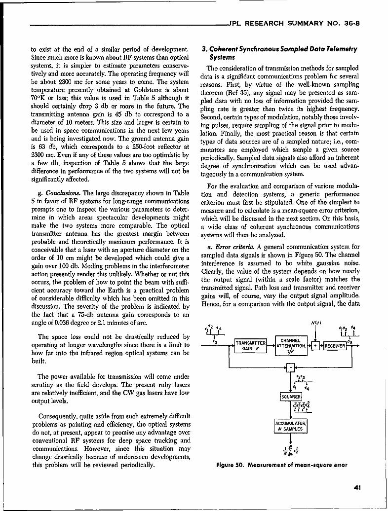
____JPL RESEARCH SUMMARY NO. 36-8
to exist at the end of a similar period of development. 3. Coherent Synchronous Sampled Data TelemetrySince much more is known about RF systems than optical Systemssystems, it is simpler to estimate parameters conserva- The consideration of transmission methods for sampledtively and more accurately. The operating frequency will data is a signifidant communications problem for severalbe about 2300 me for some years to come. The system reasons. First, by virtue of the well-known samplingtemperature presently obtained at Goldstone is about theorem (Ref 35), any signal may be presented as sam-70 0K or less; this value is used in Table 5 although it pled data with no loss of information provided the sam-should certainly drop 3 db or more in the future. The pling rate is greater than twice its highest frequency.transmitting antenna gain is 45 db to correspond to a Second, certain types of modulation, notably those involv-diameter of 10 meters. This size and larger is certain to ing pulses, require sampling of the signal prior to modu-be used in space communications in the next few years lation. Finally, the most practical reason is that certainand is being investigated now. The ground antenna gain types of data sources are of a sampled nature; i.e., com-is 63 db, which corresponds to a 250-foot reflector at mutators are employed which sample a given source2300 me. Even if any of these values are too optimistic by periodically. Sampled data signals also afford an inherenta few db, inspection of Table 5 shows that the large degree of synchronization which can be used advan-difference in performance of the two systems will not be tageously in a communication system.significantly affected.
For the evaluation and comparison of various modula-g. Conclusions. The large discrepancy shown in Table tion and detection systems, a generic performance
5 in favor of RF systems for long-range communications criterion must first be stipulated. One of the simplest toprompts one to inspect the various parameters to deter- measure and to calculate is a mean-square error criterion,mine in which areas spectacular developments might which will be discussed in the next section. On this basis,make the two systems more comparable. The optical a wide class of coherent synchronous communicationstransmitter antenna has the greatest margin between systems will then be analyzed.probable and theoretically maximum performance. It isconceivable that a laser with an aperture diameter on the a. Error criteria. A general communication system fororder of 10 cm might be developed which could give a sampled data signals is shown in Figure 50. The channelgain over 100 db. Moding problems in the interferometer interference is assumed to be white gaussian noise.action presently render this unlikely. Whether or not this Clearly, the value of the system depends on how nearly
occurs, the problem of how to point the beam with suffi- the output signal (within a scale factor) matches the
cient accuracy toward the Earth is a practical problem transmitted signal. Path loss and transmitter and receiverof considerable difficulty which has been omitted in this gains will, of course, vary the output signal amplitude.discussion. The severity of the problem is indicated by Hence, for a comparison with the output signal, the data
the fact that a 75-db antenna gain corresponds to anangle of 0.036 degree or 2.1 minutes of arc. N() 012 04
The space loss could not be drastically reduced by LLriLoperating at longer wavelengths since there is a limit to 43 TRANSMITTER CHANNEL 0
opertin at ATTENUATION, + RECEIVERhow far into the infrared region optical systems can be GNK
built.
The power available for transmission will come under E2 (3scrutiny as the field develops. The present ruby lasers ft 44
are relatively inefficient, and the CW gas lasers have low SQUARER
output levels.
Consequently, quite aside from such extremely difficultproblems as pointing and efficiency, the optical systems ACCUMULATOR,
do not, at present, appear to promise any advantage over N SAMPLES
conventional RF systems for deep space tracking andcommunications. However, since this situation may N 2
change drastically because of unforeseen developments,this problem will be reviewed periodically. Figure 50. Measurement of mean-square error
41
JPL RESEARCH SUMMARY NO. 36-8
signal must be amplified or attenuated by an appropriate (2) Phase modulation, or phase shift keying (PSK).factor K. Thus, the error in the nth sample will be (3) Frequency modulation, or frequency shift keyingE, = s,, - o,,, where s,, woud be the nth output sample in ()the absence of noise, and o,, is the actual nth output (FSK).sample. It may be assumed that both the data signal and (4) Pulse duration modulation (PDM).the output signal levels have been adjusted so that theirmeans are zero. Then the error mean will also be zero.
There are several measures of how nearly the output (6) Pulse code modulation (PCM).
resembles the data. The most common is the mean-square In this work, we shall be interested in coherent syn-error which, for stationary signal and noise, is given by chronous detection of the various forms of modulation;
I X that is, the detection process will involve locally gener-E= lim T En ated signals which are coherent to the transmitted carrier
N=1 and synchronous with the sampled data rate. In this
A simple method of measuring this is shown in Figure 50. context, it will be shown that the six types of modulation
A criterion which is more simply measured and generally may be detected coherently and synchronously by meansequaly vlidis te man-asolte erorof one of the followving detection techniques:equally valid is the mean-absolute error
s (1) Linear synchronous detection.
1 0 = l Z (2) Correlation detection, or matched filtering.
Although the mean-absolute error is precisely the same The next two sections will treat the detection of the sixas the mean-square error when both the signal and noise forms of modulation by these two methods.are gaussian, it is not readily calculated when one of the Linear synchronous detection. In this section it willtwo is not gaussian. Likewise, several other error criteria be shown that pulse amplitude, modulation (PAM), pulseare equivalent to the mean-square error for gaussian duration modulation (PDM), and phase shift keyingdistributions (Ref 36) but are hopeless to determine in (PSK), can all be detected by a pulsed integrator syn-general. Thus, for the sake of analytical feasibility, only chronous with the sample transmission time and that thethe mean-square error will be considered. Of course, the output signal-to-mean-square error ratio is a linear func-magnitude of this parameter will depend on the data tion of the channel signal-to-noise ratio.signal magnitude. For this reason it is necessary to nor-malize e, by some parameter of the signal. The most Pulse amplitude modulation consists simply of extend-significant such parameter is the data signal power or ing the sample amplitude to last over the allottedmean-square signal transmission time of T seconds and multiplying the carrier
1 V by this waveform. This is shown in Figure 51a. In pulse-.lim '.,i (s,)" duration modulation, a pulse is generated whose width
is proportional to the amplitude of the sample. For thisIt is evident that both , and e, have the dimension of purpose, the sample must be amplitude-limited, saypower. For the sake of similarity to the well-known between -A and +A. Then a sample of amplitude x,,signal-to-noise ratio, the ratio s or mean-square (where -A < x,, < A) will produce a pulse of durationsignal-to-error ratio, will be used here. [1 + (x./A)] (T/2) seconds. In order to keep the trans-
mitted power a constant, the pulse waveform is made tob. Classification of telemetry systems. A number of atraebtve n 1rte hnbten1ad0moduatin mthod ofthecontnuos wve ad plse alternate between I and - 1 rather than between 1 and 0.modulation methods of the continuous wave and pulse The waveform is then used to multiply the carrier
variety are in common use. Certain types (such as ampli- Thi 51b). i s the mpltue carrie
tude modulation) are basically for transmission of con- (rig 51ib). In phase shift keying, the amplitude of the
tinuous signals rather than sampled data. However, even sinusoidal carrier is not varied, but rather its phase is
tnuse havegneuivalseahermthansampled data. The varied from --. ,12 to r/2, depending on the amplitudethese hav e an equivalent form fordulatied data. are of the sample. Again, the data is assumed to befollowing is a list of the forms of modulation thich are amplitude-limited between + A and - A, and the phasegenerally accepted (Ref 37) and their sampled data of the carrier over a given sample transmission time isequivalents: sin -' x,/A when the sample is x,, (where -A !x, < A).
(1) Amplitude modulation, or pulse amplitude modula- Since the phase varies between -/2 and -,/2 it is,tion (PAM). therefore, unambiguous. The phase waveform is shown
42
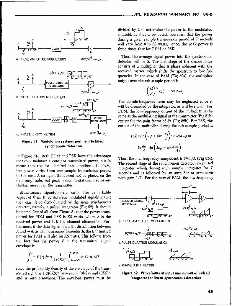
JPL RESEARCH SUMMARY NO. 36-8
x1 divided by 2 to determine the power in the modulatedsinusoid. It should be noted, however, that the power
X4 0 I1r " 3r 4r during a given sample transmission period of T secondsXl X2 will vary from 0 to 3S watts; hence, the peak power is
L A M3r three times that for PDM or PSK.X2 Thus, the average signal power into the synchronous
a. PULSE AMPLITUDE MODULATION (KSIA)sin woI detector will be S. The first stage of the demodulator
consists of a multiplier that is phase coherent with the
(r/2)+x,A)-rfI1I1 received carrier, which shifts the spectrum to low fre-X3 x4 o jU r 4r quencies. In the case of PAM (Fig 52a), the multiplier
x X X4 PULSE DURATION output over the nth sample period is+€ "1 MODULATORI(2KS) z sin wo 0) x, (1 - cos 2wot)
b. PULSE DURATION MODULATIONsinl x3,1 The double-frequency term may be neglected since it
x4 sin-'x/A __M will be discarded by the integrator, as will be shown. ForXj o r273T 4r PDM, the low-frequency output of the multiplier is the
sin-/ PHASE same as the modulating signal at the transmitter (Fig 51b)CLAM A _ MOULATOR except for the gain factor of S% (Fig 52b). For PSK, 'the
X2 output of the multiplier during the nth sample period is
c. PHASE SHIFT KEYING (2KS) 2sjn W0 1 (2S) sin (oot + sin-' -$). 2% cos wt =
Figure 51. Modulation systems pertinent to linear A
synchronous detection S%, AA sin(2wot + sin-'
in Figure 51c. Both PDM and PSK have the advantage Thus, the low-frequency component is Sx 5/A (Fig 52c).that they maintain a constant transmitted power, but in The second stage of the synchronous detector is a pulsedreturn they require a limited data amplitude. In PAM, integrator which during each sample integrates for Tthe power varies from one sample transmission period seconds and is followed by an amplifier or attenuatorto the next. A stringent limit need not be placed on the oith gain 1/T. For the case of PAM, the lov-frequencydata amplitude, but peak power limitations are, never-theless, present in the transmitter.
Mean-square signal-to-error ratio. The remarkableaspect of these three different modulated signals is that 'they can all be demodulated by the same synchronous RECEIVED SIGNAL ,• (POWER - ) , 22sinwo t
l
detector; namely, a pulsed integrator (Fig 52). It should (3s)-I,/A (3S)Fx1/Abe noted, first of all, from Figure 51 that the power trans- II Zmitted for PDM and PSK is KS watts, where S is the o r0r 37 4r o r"...2r 37 4r
received power and 1/K the channel attenuation. Fur- o.PULSE AMPLITUDE MODULATIONthermore, if the data signal has a flat distribution between I IA and -A, as will he assumed henceforth, the transmitted 31 (2s)EXI/A
( r/2I(I+ xA) _MM mm .r"31"- 1-1,,'-
power for PAM will also be KS watts. This follows from o.UrLJ2Tu3ru4T 0 T N2T 3r 4T
the fact that the power P in the transmitted signal b. PULSE DURATION MODULATION
envelope is
~ S2,4 SIX1/AX2 P (x) dx 2 (6Sx2 dx = 2KS r_ A3r 4
c. PHASE SHIFT KEYINGsince the probability density of the envelope of the trans-
mitted signal is 1,, 2(6KS)i - between - (6KS)4 and (6KS)% Figure 52. Waveforms at input and output of pulsedand is zero elsewhere. The envelope power must be integrator for linear synchronous detection
43
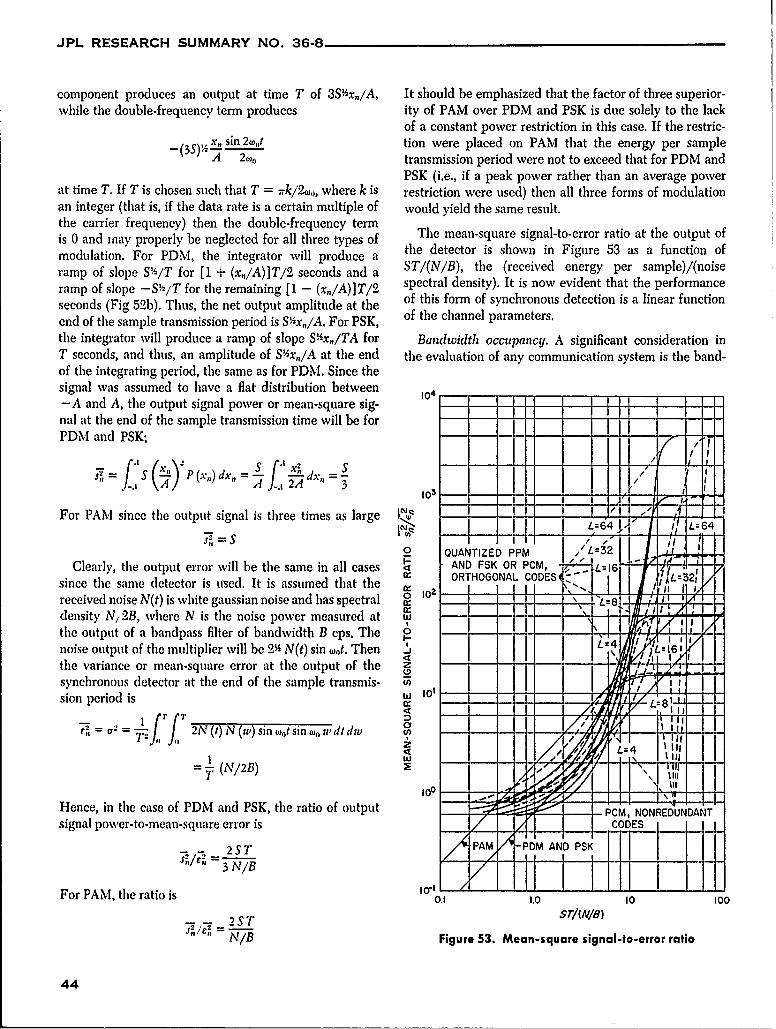
JPL RESEARCH SUMMARY NO. 36-8
component produces an output at time T of 3S~xiA, It should be emphasized that the factor of three superior-while the double-frequency term produces ity of PAM over PDM and PSK is due solely to the lack
of a constant power restriction in this case. If the restric-(3 x" sin 2wt tion were placed on PAM that the energy per sample
A) 2to transmission period were not to exceed that for PDM andPSK (i.e., if a peak power rather than an average power
at time T. If T is chosen such that T = ,k/2 0o, where k is restriction were used) then all three forms of modulationan integer (that is, if the data rate is a certain multiple of would yield the same result.the carrier frequency) then the double-frequency termis 0 and may properly be neglected for all three types of The mean-square signal-to-error ratio at the output of
modulation. For PDM, the integrator will produce aramp of slope S'h/T for [1 + (x,/A)]T/2 seconds and a ST/(N/B), the (received energy per sample)/(noise
ramp of slope -Sl T for the remaining [1 - (x,/A)]T/2 spectral density). It is now evident that the performance
seconds (Fig 52b). Thus, the net output amplitude at the of this form of synchronous detection is a linear functionend of the sample transmission period is Sx,/A. For PSK, of the channel parameters.the integrator will produce a ramp of slope Sx,,/TA for Bandwidth occupancy. A significant consideration inT seconds, and thus, an amplitude of Sxn/A at the end the evaluation of any communication system is the band-of the integrating period, the same as for PDM. Since thesignal was assumed to have a flat distribution between 104
-A and A, the output signal powver or mean-square sig-- --
nal at the end of the sample transmission time will be for - -1
PDM and PSK; IA/ 3
_s S f--x /.
For PAM since the output signal is three times as largesI=S - - / -/1L=64 JL=.64
S in , _t/0 QUANTIZED PPM ,'L=32
Clearly, the output error will be the same in all cases AND FSK OR PCM, - L=16 A 1 Tsince the same detector is used. It is assumed that the 0 ORTHOGONAL CODESreceived noise N(t) is white gaussian noise and has spectral W - I Ito. . M1density N/2B, where N is the noise power measured at - - h -the output of a bandpass filter of bandwidth B cps. The --
noise output of the multiplier will be 2% N(t) sin wt. Then L: Ithe variance or mean-square error at the output of the z -
synchronous detector at the end of the sample transmis- W I IW 10, _sion period is - - - :8
= = 2N (t) N (w) sin w0o1 sin o iw dt dw - -o /
= (N/2B) -
Hence, in the case of PDM and PSK, the ratio of output Z - - - PCM, NONREDUNDANTsignal power-to-mean-square error is ___ CODES
2STPAM -PDM AND PSKsVE. 3 11B lFor PAM, the ratio is 1011 100
2 S T ST/(N/B)
N/ B Figure 53. Mean-square signal-to-error ratio
44
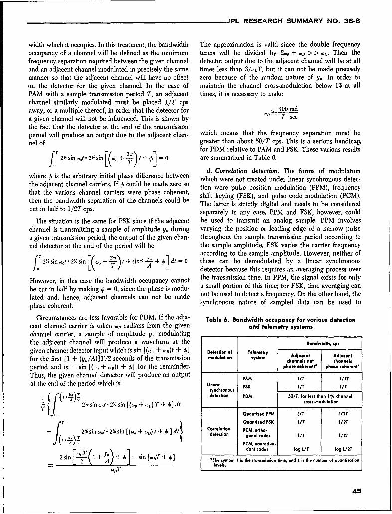
JPL RESEARCH SUMMARY NO. 36-8
width which it occupies. In this treatment, the bandwidth The approximation is valid since the double frequencyoccupancy of a channel will be defined as the minimum terms will be divided by 2wo + WD > > O)D. Then thefrequency separation required between the given channel detector output due to the adjacent channel will be at alland an adjacent channel modulated in precisely the same times less than 3/, gT, but it can not be made preciselymanner so that the adjacent channel will have no effect zero because of the random nature of Y,,. In order toon the detector for the given channel. In the case of maintain the channel cross-modulation below 1% at allPAM with a sample transmission period T, an adjacent times, it is necessary to makechannel similarly modulated must be placed 1/T cpsaway, or a multiple thereof, in order that the detector for W, 300 rada given channel will not be influenced. This is shown by T secthe fact that the detector at the end of the transmissionperiod will produce an output due to the adjacent chan- which means that the frequency separation must benel of greater than about 50/T cps. This is a serious handicaD
for PDM relative to PAM and PSK. These various results2% sin owt 2% sin Ria + i + ,1 = 0 are summarized in Table 6.
d. Correlation detection. The forms of modulationwhere tk is the arbitrary initial phase difference between which were not treated under linear synchronous detec-the adjacent channel carriers. If 4 could be made zeron0 tion were pulse position modulation (PPM), frequencythat the various channel carriers were phase coherent, shift keying (FSK), and pulse code modulation (PCM).then the bandwidth separation of the channels could be The latter is strictly digital and needs to be consideredcut in half to 1/2T cps. separately in any case. PPM and FSK, however, could
The situation is the same for PSK since if the adjacent be used to transmit an analog sample. PPM involveschannel is transmitting a sample of amplitude y. during varying the position or leading edge of a narrow pulsea given transmission period, the output of the given chan- throughout the sample transmission period according tonel detector at the end of the period will be the sample amplitude. FSK varies the carrier frequency
L _"according to the sample amplitude. However, neither off 2 sin wd 2% sin (O+ + sin-' -- + dt=0 these can be demodulated by a linear synchronous7, R A I detector because this requires an averaging process over
However, in this case the bandwidth occupancy cannot the transmission time. In PPM, the signal exists for only
be cut in half by making , = 0, since the phase is modu- a small portion of this time; for FSK, time averaging can
lated and, hence, adjacent channels can not be made not be used to detect a frequency. On the other hand, the
phase coherent. synchronous nature of sampled data can be used to
Circumstances are less favorable for PDM. If the adja- Table 6. Bandwidth occupancy for various detectioncent channel carrier is taken o),) radians from the given and telemetry systemschannel carrier, a sample of amplitude y. modulatingthe adjacent channel will produce a waveform at the Bandwidth, cpsgiven channel detector input which is sin [(o,, + WD)t + 0] Detection of Telemetryfor the first [1 + (y,/A)]T/2 seconds of the transmission modulation system Adiacent Adlacentchannels not channels
period and is - sin [(w,, + .,))t + q0] for the remainder, phase coherent' phase coherent'
Thus, the given channel detector will produce an output PlI/T 1/2Tat the end of the period which is Linear PSK /T lIT
synchronousdetection POM 501T, for less than 1 % channel
2 sin ,d 2%6 sin [(&,, + wJ,) T + 40] it cross.odulation
Quantized PPM LIT L/2T
Quantized FSK LIT L/2T-2 sin wilt. 234 sin [(Co,, + r) t + ]d Correlation FCM, ortho.
detection gonal codes LIT L/2Tu .) PM, nonredun.
2 sin si .\,, + dant codles lag LIT log LI2T2 sin I 1I + ) + 4, -"sin[wT + 4] "The symbol T is the transmission time, and L is the number of quantization
21 ( A levels.
45
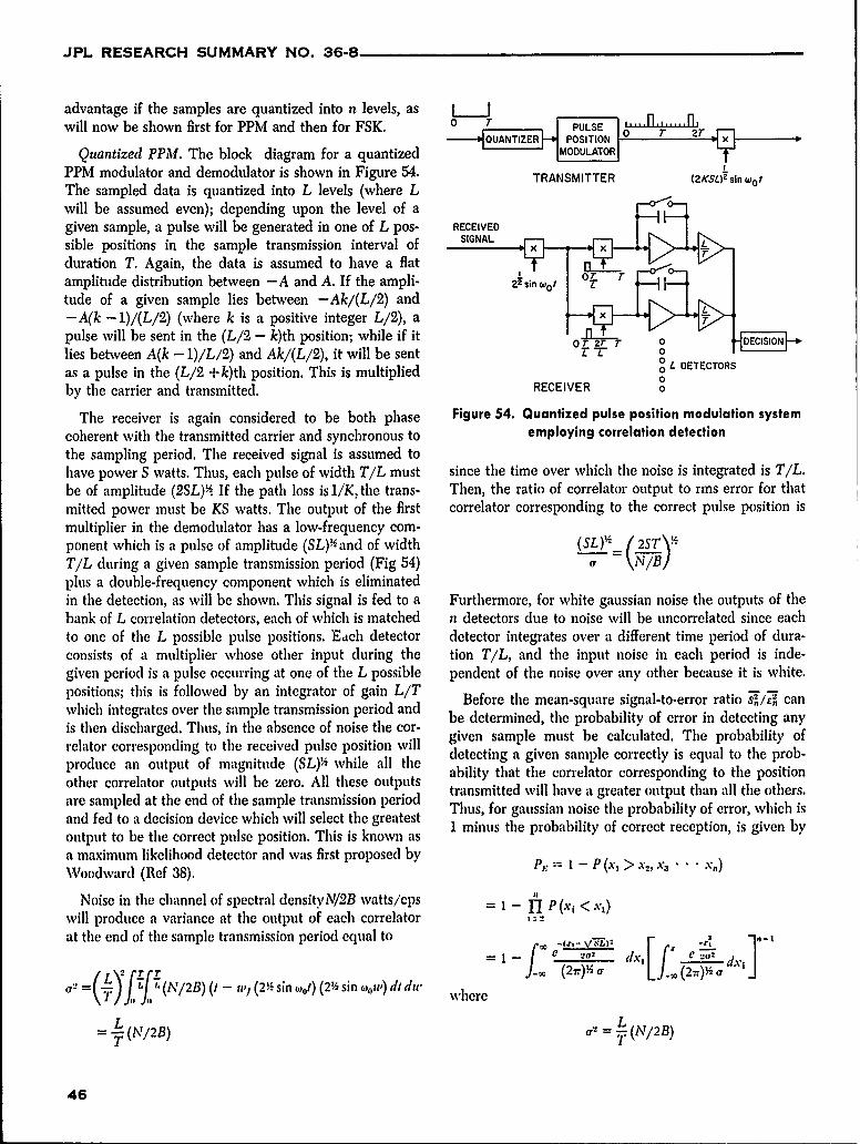
JPL RESEARCH SUMMARY NO. 36-8
advantage if the samples are quantized into n levels, as L.Jwill now be shown first for PPM and then for FSK. 0 r U
Quantized PPM. The block diagram for a quantized MODULATR
PPM modulator and demodulator is shown in Figure 54. TRANSMITTER (2KS_ sin tootThe sampled data is quantized into L levels (where L
will be assumed even); depending upon the level of agiven sample, a pulse will be generated in one of L pos- RECEIVED
sible positions in the sample transmission interval of SIGNAL L
duration T. Again, the data is assumed to have a flat Ramplitude distribution between -A and A. If the ampli-tude of a given sample lies between -Ak/(L/2) and-A(k -1)/(L/2) (where k is a positive integer L/2), apulse will be sent in the (L/2 - k)th position; while if it or 2r r E
lies between A(k - 1)/L/2) and Ak/(L/2), it will be sent 0DECRas a pulse in the (L/2 +k)th position. This is multiplied 0by the carrier and transmitted. RECEIVER 0
The receiver is again considered to be both phase Figure 54. Quantized pulse position modulation system
coherent with the transmitted carrier and synchronous to employing correlation detectionthe sampling period. The received signal is assumed tohave power S watts. Thus, each pulse of width T/L must since the time over which the noise is integrated is T/L.be of amplitude (2SL) . If the path loss is 1/K, the trans- Then, the ratio of correlator output to rms error for thatmitted power must be KS watts. The output of the first correlator corresponding to the correct pulse position ismultiplier in the demodulator has a low-frequency com-ponent which is a pulse of amplitude (SL)%and of width (SL),'_ 1ST 1
T/L during a given sample transmission period (Fig 54) (NI)plus a double-frequency component which is eliminatedin the detection, as will be shown. This signal is fed to a Furthermore, for white gaussian noise the outputs of thebank of L correlation detectors, each of which is matched n detectors due to noise will be uncorrelated since eachto one of the L possible pulse positions. Etch detector detector integrates over a different time period of dura-consists of a multiplier whose other input during the tion T/L, and the input noise in each period is inde-given period is a pulse occurring at one of the L possible pendent of the noise over any other because it is white.positions; this is followed by an integrator of gain L/T Before the mean-square signal-to-error ratio Z,/; canwhich integrates over the sample transmission period and be determined, the probability of error in detecting anyis then discharged. Thus, in the absence of noise the cor-relator corresponding to the received pulse position will given sample must be calculated. The probability ofproduce an output of magnitude (SL)'4 while all the detecting a given sample correctly is equal to the prob-
ability that tile correlator corresponding to the positionother correlator outputs will be zero. All these outputs transmitted will have a greater output than all the others.are sampled at the end of the sample transmission period Thus, for gaussian noise the probability of error, which isand fed to a decision device which will select the greatest 1 minus the probability of correct reception, is given byoutput to be the correct pulse position. This is known asa maximum likelihood detector and was first proposed by P 1 - P (X > X2 X3 x )Woodward (Ref 38).
Noise in the channel of spectral densityN/2B watts/cps = 1 - P (x1 <x1 )will produce a variance at the output of each correlator ,at the end of the sample transmission period equal to JF1
/L\2f~f1 -= - ,,,__ x1 L ../)
i: = 7)j (N/2B) (I - u,! (2.sin ot) (24 sin ,ou) didu where
LL= -(T v/2 ) N= 1\( /2B)
46
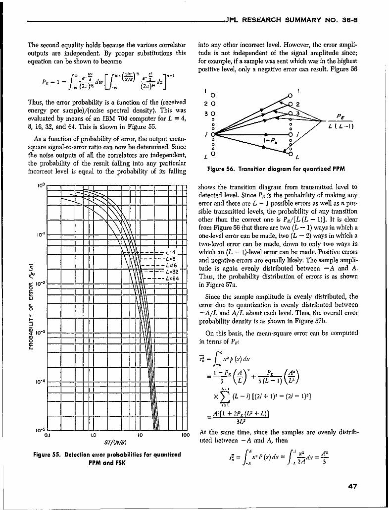
JPL RESEARCH SUMMARY NO. 36-8
The second equality holds because the various correlator into any other incorrect level. However, the error ampli-outputs are independent. By proper substitutions this tude is not independent of the signal amplitude since;equation can be shown to become for example, if a sample was sent which was in the highest
e- Z - IV~~ ~positive level, only a negative error can result. Figure 56
J_= (=) J- * (2r)s dz I, = I wUe
Thus, the error probability is a function of the (received 20 2energy per sample)/(noise spectral density). This was 3evaluated by means of an IBM 704 computer for L = 4, 4 __P__
8, 16, 32, and 64. This is shown in Figure 55. 0 0
As a function of probability of error, the output mean- 0square signal-to-error ratio can now be determined. Since othe noise outputs of all the correlators are independent, L Lthe probability of the result falling into any particularincorrect level is equal to the probability of its falling Figure 56. Transition diagram for quantized PPM
1°o ,- shows the transition diagram from transmitted level to-: - detected level. Since P, is the probability of making any-'- - - error and there are L - 1 possible errors as well as n pos-
sible transmitted levels, the probability of any transition-\' - other than the correct one is Pji[L (L - 1)]. It is clear
from Figure 56 that there are two (L - 1) ways in which a- I - - one-level error can be made, two (L - 2) ways in which a
- ii - - - two-level error can be made, down to only two ways in-- L:4 _ which an (L - 1)-level error can be made. Positive errors
-....- \ L-8 and negative errors are equally likely. The sample ampli-t -- -- L=""6 tude is again evenly distributed between -A and A.
--- L64 Thus, the probability distribution of errors is as shownX 10-2- il I I in Figure 57a.
- - -,- Since the sample amplitude is evenly distributed, the- - error due to quantization is evenly distributed between0! -A/L and A/L about each level. Thus, the overall error- l I probability density is as shown in Figure 57b.
< On this basis, the mean-square error can be computed0- in terms of P'::a.
1-4\L/ 3 (L -1) LBill I I I
IZI
I= A'[I + 2P,:(L + L)3L2
01 1O 10 100 At the same time, since the samples are evenly distrib-Sr/(NIB) uted between -A and A, then
Figure 55. Detection error probabilities for quantized f P (.,) = fx2 APPM and FSK .2A 3
47
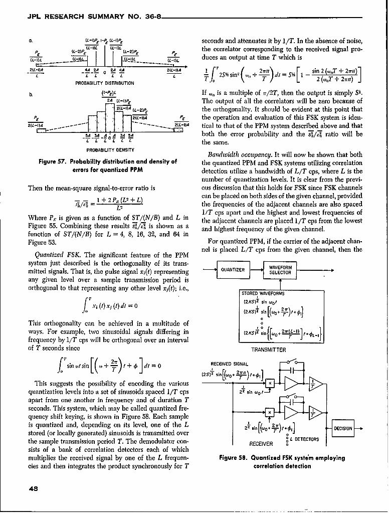
JPL RESEARCH SUMMARY NO. 36-8
. (L-PE I-P (L-P, seconds and attenuates it by 11T. In the absence of noise,(L2)P(L -IL 1 L (L-2)P, the correlator corresponding to the received signal pro-
(L-2)L ..... E . . - duces an output at time T which is
2(L-I)A 4A2A o A 4A 2(L-,)A (fsin 2 (wT+oT+ 2rn)jL ,. "' o/ L 2S% sin" ,+ dt = Sl 1 s 2 (oT + 2=r1) .
PROBABILITY DISTRIBUTION
b. (-PE). If n is a multiple of ./2T, then the output is simply Si.2A IL-)P- The output of all the correlators will be zero because of
2(,-I) the orthogonality. It should be evident at this point thatPr" - { 7J7 ' PE the operation and evaluation of this FSK system is iden-
Z. . . . 2.L- A tical to that of the PPM system described above and thatAi 3A A _' , both the error probability and the " e ratio will be" T"Z Z T L the same.PROBABILITY DENSITY Bandwidth occupancy. It will now be shown that both
Figure 57. Probability distribution and density of the quantized PPM and FSK systems utilizing correlationerrors for quantized PPM detection utilize a bandwidth of L/T cps, where L is the
number of quantization levels. It is clear from the previ-Then the mean-square signal-to-error ratio is ous discussion that this holds for FSK since FSK channels
I + 2 P, (L; + L) can be placed on both sides of the given channel, providedL2 the frequencies of the adjacent channels are also spacedr ii1T cps apart and the highest and lowest frequencies of
Where P5 is given as a function of ST/(N/B) and L in the adjacent channels are placed 1/T cps from the lowestFigure 55. Combining these results si/e is shown as a and highest frequency of the given channel.
function of ST/(N/B) for L = 4, 8, 16, 32, and 64 in
Figure 53. For quantized PPM, if the carrier of the adjacent chan-nel is placed LIT cps from the given channel, then theQuantized FSK. The significant feature of the PPM
system just described is the orthogonality of its trans- WAVEFORM
mitted signals. That is, the pulse signal x1(t) representing QUANTIZER SELECTOR
any given level over a sample transmission period isorthogonal to that representing any other level x,(t); i.e.,
STORED WAVEFORMS
7"(2 KS) 2 sin Wo/ _' () .x1 (i) di = oVS)
0This orthogonality can be achieved in a multitude of 0ways. For example, two sinusoidal signals differing in (2KS) 2 sin [c,0+2 2 Lt+#. 1frequency by 1/T cps will be orthogonal over an interval t J j
of T seconds since TRANSMITTER
sin o sin [o + L7 + ) ] dt=0 RECEIVED SIGNAL
(2S 2siR-+
This suggests the possibility of encoding the various _quantization levels into a set of sinusoids spaced lIT cps 22 sin cotapart from one another in frequency and of duration Tseconds. This system, which may be called quantized fre-quency shift keying, is shown in Figure 58. Each sampleis quantized and, depending on its level, one of the L 22
stored (or locally generated) sinusoids is transmitted over R- r 0the sample transmission period T. The demodulator con- RECEIVER o - DETECTORSsists of a bank of correlation detectors each of whichmultiplies the received signal by one of the L frequen- Figure 58. Quantized FSK system employingcies and then integrates the product synchronously for T correlation detection
48
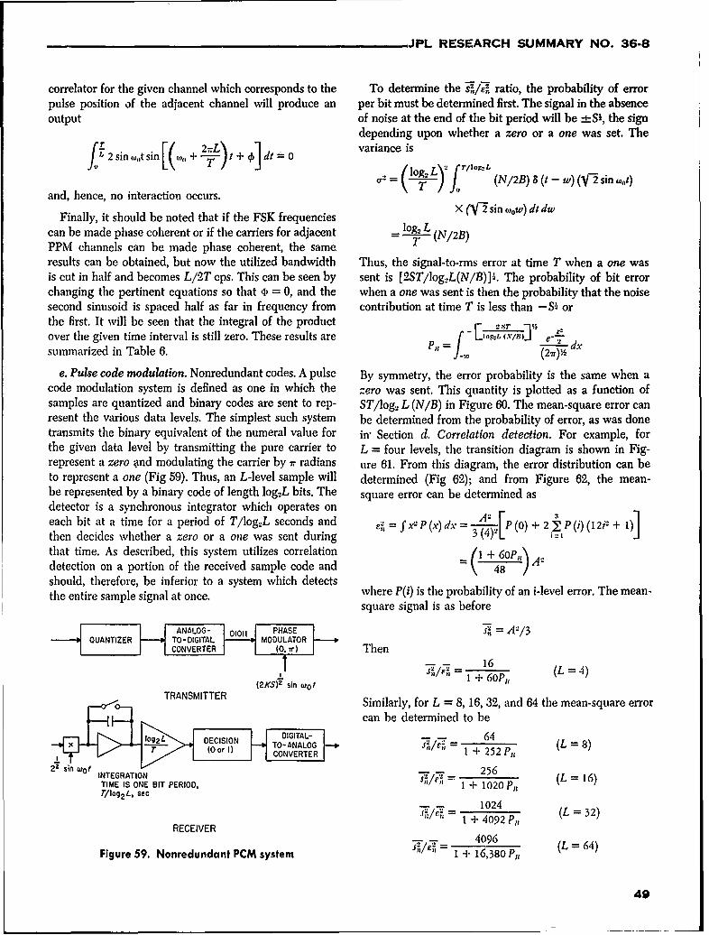
_JPL RESEARCH SUMMARY NO. 36-8
correlator for the given channel which corresponds to the To determine the , ratio, the probability of errorpulse position of the adjacent channel will produce an per bit must be determined first. The signal in the absenceoutput of noise at the end of the bit period will be -- S, the sign
depending upon whether a zero or a one was set. Thef 2in s I() 1 variance isfL2 sin woot sin I(., + 1T)t + 01 dt = o010:+ =l og2 z 1 r/iog7 L.
e L= T (N/2B) 8 (t - w) (V-2sinl ont)
and, hence, no interaction occurs.
Finally, it should be noted that if the FSK frequencies X (V2 sin wow) dt dw
can be made phase coherent or if the carriers for adjacent = T \(N/2B)PPM channels can be made phase coherent, the same Tresults can be obtained, but now the utilized bandwidth Thus, the signal-to-rms error at time T when a one wasis cut in half and becomes L/2T cps. This can be seen by sent is [2ST/log..L(N/B).. The probability of bit errorchanging the pertinent equations so that 4, = 0, and the when a one was sent is then the probability that the noisesecond sinusoid is spaced half as far in frequency from contribution at time T is less than -S-1 orthe first. It will be seen that the integral of the product _ ., 1 "over the given time interval is still zero. These results are f Liog:ia.v/i/ -s dsummarized in Table 6.
e. Pulse code modulation. Nonredundant codes. A pulse By symmetry, the error probability is the same when acode modulation system is defined as one in which the zero was sent. This quantity is plotted as a function ofsamples are quantized and binary codes are sent to rep- ST/log.. L (N/B) in Figure 60. The mean-square error canresent the various data levels. The simplest such system be determined from the probability of error, as was donetransmits the binary equivalent of the numeral value for in" Section d. Correlation detection. For example, forthe given data level by transmitting the pure carrier to L = four levels, the transition diagram is shown in Fig-represent a zero 4nd modulating the carrier by r radians ure 61. From this diagram, the error distribution can beto represent a one (Fig 59). Thus, an L-level sample will determined (Fig 62); and from Figure 62, the mean-be represented by a binary code of length log2L bits. The square error can be determined asdetector is a synchronous integrator which operates oneach bit at a time for a period of T/log.,L seconds and E= P (x) dx = 3'4 (0) + 2 P (i) (12i + 1)1then decides whether a zero or a one was sent during 3(4)21 (0that time. As described, this system utilizes correlation = + 60P,)4.detection on a portion of the received sample code and 480 Ashould, therefore, be inferior to a system which detectsthe entire sample signal at once. where P(i) is the probability of an i-level error. The mean-
square signal is as before
I'N 11, (:1PHAS s2= A2131UANIZ 1 TO'- DIGITAL001 MODULATORn
CONVERTER (0. 7r Then.= 16 (L=4)
1 1,/, + 60Pr(2KS)
z sin wol1
TRANSMITTER Similarly, for L = 8, 16, 32, and 64 the mean-square errorcan be determined to be
DI > CISJNGITAL- - 64
102. DECISION TO-ANALOG Jnt: = 64 8r(Oor I CONVERTER 1 + 252 Pi (L 8)
2? si W01256INTEGRATION S2 26 (L 16)TIME IS ONE BIT PERIOD, I+1020Pi1T/Iog 2 L, sec
1024
RECEIVER 1 + 4092 P,, (L 32)
4096Figure 59. Nonredundant PCM system 1 + 16,380 Pit
49
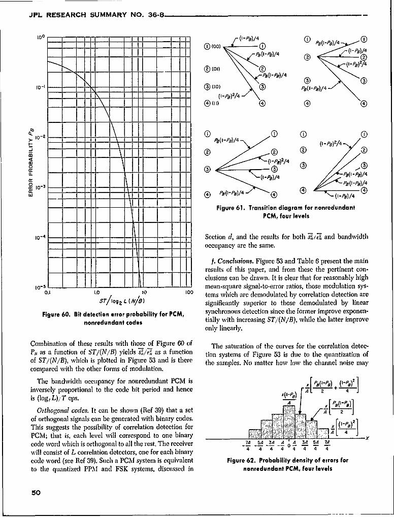
JPL RESEARCH SUMMARY NO. 36-8
100 I I-PB)/4 D(
D 1 (D,-0 P8 Q-P 8 )/4 0- ,, ®',,1 £-P)/4 @ (,P,(0_ @ (I po8 \ ) 2/4
P8 Q1-P)/4
10 - @ - (10) P8 (1-PB)/4
_ (I-Pe)2/4I - i -
-j --0 - -8 0- -- Pa/(Io P8)/4
o ,P(-I-)4)/4
-~~~P (I - PB) /4IP)/-
0~ 0 B
a: (I - p/ /40 P8 , ", (I -PS) /4
- -Figure 61. Transition diagram for nonredundantPCM, four levels
I0- 4 - - Section d, and the results for both / and bandwidth
S -occupancy are the same.
f. Conclusions. Figure 53 and Table 6 present tile mainresults of this paper, and from these the pertinent con-
io-5 i clusions can be drawn. It is clear that for reasonably highI - 1 -- mean-square signal-to-error ratios, those modulation sys-
0.1 1.0 100 tems which are demodulated by correlation detection aresr/log2 L (N/IB) significantly superior to those demodulated by linear
Figure 60. Bit detection error probability for PCM, synchronous detection since the former improve exponen-
nonredundant codes tially with increasing ST/(N/B), while the latter improveonly linearly.
Combination of these results with those of Figure 60 of The saturation of the curves for the correlation detec-P,, as a function of ST/(N/B) yields s--7,/ as a function tion systems of Figure 53 is due to the quantization ofof STi(N/B), which is plotted in Figure 53 and is there the samples. No matter how low the channel noise maycompared with the other forms of modulation.
The bandwidth occupancy for nonredundant PCM is XPS(IP 5) (I2P) 2
inversely proportional to the code bit period and hence "(IP 8'A 2 4' I
is (log L),T cps. A )
Oilhogonal codes. It can be shown (Ref 39) that a set 4 7 f~).1 I
of orthogonal signals can be generated with binary codes. t- ]This suggests the possibility of correlation detection for . ('PxPCM; that is, each level will correspond to one binary . .:..code word which is orthogonal to all the rest. The receiver LA A A 0will consist of L correlation detectors, one for each binary 4 4 4 4 4 4 4 4
code word (see Ref 39). Such a PCM system is equivalent Figure 62. Probability density of errors forto the quantized PPM and FSK systems, discussed in nonredundant PCM, four levels
50
JPL RESEARCH SUMMARY NO. 36-8
become, the quantization noise will always be present easier to instrument for that reason. Finally, the appli-and constant for a fixed number of levels, cation of the general method to specific codes may be
Nonredundant PGM, which requires roughly 1/Lth as expected to yield further insight into the method with
much demodulation equipment as the orthogonal systems particular regard to its feasibility.
employing correlation detection, requires only about twice The principal tool in the construction of a decodingas much received energy to achieve the same results for procedure by the method of References 40 and 41 is theL = 64 quantization levels, group G ot coordinate. permutations of the space V of
binary n-tuples which map the code subspace A on itselfPAM appears to be better than PDM and PSK by a (actually, a sufficiently transitive subgroup will serve as
factor of three among the modulation methods which may well). The groups G for the first-order Reed-Muller codesbe demodulated by linear synchronous detection, only of arbitrary block length 2" have been characterized bothbecause the average poer is the criterion. If a peak as linear transformations on the spaces on which they actpower criterion were used, the three systems ould and also with regard to their abstract group-theoreticalbehave equally well. structure. It should be noted that each such group is a
PAM and PSK occupy the least bandwidth of all the subgroup-and probably sufficiently transitive-of thesystems considered, 1/ T cps, where T is the sample trans- corresponding group for all higher order codes of themission time. The orthogonal systems, quantized PPM, same block length. These characterizations are sufficientFSK and PCM with orthogonal codes, occupy LIT cps, for the computation of specific decoding procedures, andwhere L is the number of quantization levels. Nonredun- are as follows.dant PCM occupies only (log, L)/T cps. All the systems Let V be the space of binary 2"-tuples, and let A bewith the exception of PSK occupy half as much band- the first-order Reed-Muller code in V; then A is the linearwidth if the adjacent channel carriers can be made phase span of the n + 1 vectorscoherent. Because it is impossible to make adjacent chan-nels of PDM orthogonal to one another by appropriate ( 10)frequency separation, PDM utilizes an excessive amount V1 = (1 0 1 0 1 0 i 0)of bandwidth (approx 501T cps) in order to maintain the v.= (1 1 0 0 1 1 0 0 .... 1 1 0 0)channel cross-modulation less than 1%. =(1 1 1 1 0 0 0 0 .... 0 0 0 0)
,=(I 1 .... 0 0.. 0)
Note that v,, is mapped on itself by ever), member gof G = G,,, and so g is completely determined by the
B. Information Processing specification of the images vig,. , vg of v,
N. Zierler V,, under g.
Theorem 1. Let u,, .. , be any linearly independ-ent members of A whose linear span does not include v,.1. Decoding Groups for Reed-Muller Codes Te hr sa(nqe ebro vtThen there is a (unique) member of G with
In References 40 and 41, a general method for decod-ing linear codes is described. In spite of the fact that l'g = uj * = 1, ,nthe Reed decoding procedure for the Reed-Muller codes and every member of G,, is obtained in this way.is quite efficient, it is of interest to apply the general Theorem 2. Group G,, is the direct product of subgroupsmethod to these codes for the following three reasons.First, the Reed decoding procedure for an rth order code ,, and L,,, where I,, is of the type (2, 2, , 2)
of block length 2" will correct all errors of norm less (n terms), and L,, is isomorphic to the general linear
than 21-r'- but almost no others, while the general group of n dimensional space over GF(2).
decoding procedure will correct all correctible errors. Corollary. The order of G,, isSecond, the Reed decoder computes first either the orig-inal message or its complement and resolves the ambig-uity by a further operation; the general procedure The proofs and further details will appear in a forth-computes the message directly and is probably somewhat coming article.
51
JPL RESEARCH SUMMARY NO. 36-8
2. Optimal Search Procedures for Acquisition ing that the Bi are pairwise disjoint and exactly cover A;of a Single Target thus, a = b, + • • - + bk and
In an optimal search procedure, it is known that a T = m (B,) cb, + m (B.) c (b, + b.) + m (B3) c (b, + b. + b3)radiating point P lies within a region A of the celestial + + n (Bk) c (b1 + + bk)sphere. The search objective is to locate Point P withina subregion having an area s and a regular convex shape. = -E (b2 + b. (b, + b.) + b, (b, + b2 + b3)The antenna can look at a fairly arbitrary subregion of A, + + bk(b, + + b )but the integration time, i.e., the time it takes to decidewhether or not the point lies in a given subregion, is = -L [(b, + • + b) + bi + + bi]proportional to the area of the subregion. Although the 2a
following assertion will be proved for only a rather spe- C
cial case', there seems little doubt that the assertion holds 2a (a + b + + bk.)with essentially the stated generality. Let m be the To minimize T, we must pick the partition b,,a-priori distribution of P in A; that is, if R is any (meas- bk of a that minimizes b + • • • + b.; but this is ob-urable) subset of A, then m(R) is the a-priori probability viously b, = ... = bk = 1 which corresponds preciselythat P lies in RI. Let A, , A, be subregions of A, alltha P iesin .Lt . . . . b sbreion ofA, ll to a procedure of the type described above, and we haveof area s and of the desired shape (i.e., the target hasbeen acquired when it has been determined in which T--t - (a2 + a)=- (a +of the regions Ai it lies) such that
with equality for an optimal procedure, whose average(1) A C A, U ...U A,,, and A is not contained in acquisition time is thus c (a+ 1)/2.
the union of any smaller number of subregions ofthe same area and shape as Ai.
(2) m(A,) - re(A2) t ' • • - m(A,,).
An optimal search procedure (one that minimizes theexpected acquisition time) then consists of looking insequence at the regions A,, A2, " until the target is C. Digital Communicationsacquired. Techniques
At first glance, one might expect that improvement M. F. Easterling, C. E. Gilchriest, and R. L. Choatecould result from covering A with a smaller numberof subregions B,, B., ''' of area larger than s, deter- 1. Ranging Subsystemmining in which Bi the point lies, then further locating a. History of ranging experiments. A series of radarP within that B1. That this is not the case is clearly ranging experiments was conducted at Goldstone duringindicated by the followving discussion, the period October 1960 through January 1961. The over-
Without loss of generality we take s = 1 as our unit all objective of these experiments was to combine the vari-
of distance. Suppose A is a square with integral side. Let ous parts into an operating system and to test the resultingBi be a subregion of A of integral area bi, i = 1, • • • , k, system in actual ranging operations using convenient
and such that A C B, U ...U BL. Suppose that m is Earth satellites. The Echo satellite was chosen for the
the uniform distribution over A; i.e., re(r) = area Ria first object to be ranged because it gave a large returnfor any (measurable) subset R of A, where a is the area signal and was often optically visible, making it easy toof A. We shall compute the average time T it takes to acquire. After some preliminary difficulties in getting the
determine to which of the sets Bi the point belongs (look- parts of the system to work properly together, the firsting in order at B,, B., • • • ) and show that it is at least successful ranging was performed on Echo Pass 1107 on
as large as the average total acquisition time for a proce- November 11. After 1 minute and 20 seconds of rangedure of the type described above, tracking, the range lock was deliberately broken and re-
established. After an additional 2 minutes and 40 secoidsNow the integration time for the region B, is cbi, where of range tracking, RF lock was lost.momentarily. When
c is a positive constant, and T is made no larger by assum- the RF lock was re-established, the ranging code was
52
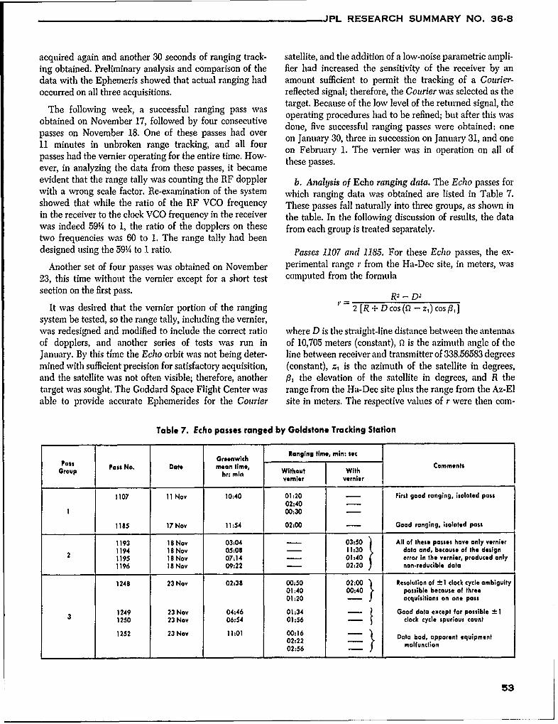
_JPL RESEARCH SUMMARY NO. 36-8
acquired again and another 30 seconds of ranging track- satellite, and the addition of a low-noise parametric ampli-ing obtained. Preliminary analysis and comparison of the fier had increased the sensitivity of the receiver by andata with the Ephemeris showed that actual ranging had amount sufficient to permit the tracking of a Courier-occurred on all three acquisitions. reflected signal; therefore, the Courier was selected as the
was target. Because of the low level of the returned signal, theThe following week, a successful ranging pass operating procedures had to be refined; but after this was
obtained on November 17, followed by four consecutive done, five successful ranging passes were obtained: onepasses on November 18. One of these passes had over
11 minutes in unbroken range tracking, and all four on January 30, three in succession on January 31, and one
passes had the vernier operating for the entire time. How- on February 1. The vernier was in operation on all of
ever, in analyzing the data from these passes, it became these passes.
evident that the range tally was counting the RF doppler b. Analysis of Echo ranging data. The Echo passes forwith a wrong scale factor. Re-examination of the system which ranging data was obtained are listed in Table 7.showed that while the ratio of the RF VCO frequency These passes fall naturally into three groups, as shown inin the receiver to the clock VCO frequency in the receiver the table. In the following discussion of results, the datawas indeed 59% to 1, the ratio of the dopplers on these from each group is treated separately.two frequencies was 60 to 1. The range tally had beendesigned using the 591/ to .1 ratio. Passes 1107 and 1185. For these Echo passes, the ex-
Another set of four passes was obtained on November perimental range r from the Ha-Dec site, in meters, was23, this time without the vernier except for a short test computed from the formulasection on the first pass. R2 - D2
It was desired that the vernier portion of the ranging 2 [R + D cos (0 - z,) cos P]system be tested, so the range tally, including the vernier,was redesigned and modified to include the correct ratio where D is the straight-line distance between the antennasof dopplers, and another series of tests was run in of 10,705 meters (constant), f2 is the azimuth angle of theJanuary. By this time the Echo orbit was not being deter- line between receiver and transmitter of 338.56583 degreesmined with sufficient precision for satisfactory acquisition, (constant), z, is the azimuth of the satellite in degrees,and the satellite was not often visible; therefore, another fi the elevation of the satellite in degrees, and R thetarget was sought. The Goddard Space Flight Center was range from the Ha-Dec site plus the range from the Az-Elable to provide accurate Ephemerides for the Courier site in meters. The respective values of r were then com-
Table 7. Echo passes ranged by Goldstone Tracking Station
Greenwich Ranging time, min: secPass Pass No. Dote mean time, Comments
Group hr: rain Without Withvernier vernier
1107 11 Nov 10:40 01:20 - First good ranging, isolated pass02:40 -
1 00:30 -
1185 17 Nov 11:54 02:00 - Good ranging, isolated pass
1193 18 Nov 03:04 - 03:50 All of these passes have only vernier1 194 18 Nov 05:08 - 11:30 data and, because of the design1195 18 Nov 07:14 - 01:40 error in the vernier, produced only
1196 18 Nov 09:22 - 02:20 non.reducible data
1248 23 Nov 02:38 00:50 02:00 Resolution of t I clock cycle ambiguity01:40 00:40 possible because of three01:20 - acquisitions on one pass
1249 23 Nov 04:46 01:34 - Good data except for possible ± I1250 23 Nov 06:54 01:56 - clock cycle spurious count
1252 23 Nov 11:01 00:16 - "I Data bad, apparent equipment02:22 malfunction02:56-
53
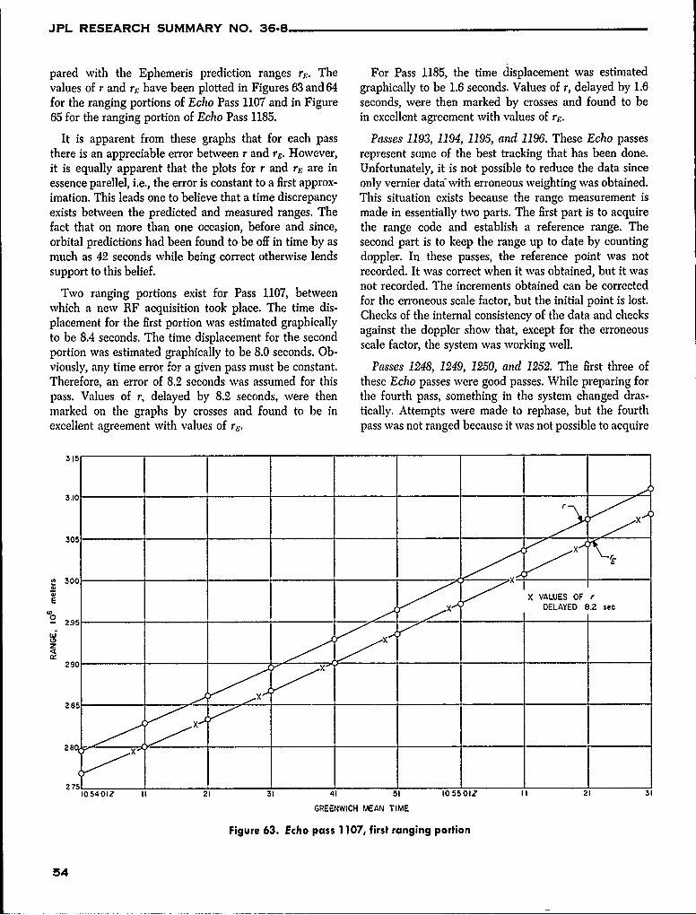
JPL RESEARCH SUMMARY NO. 36-8
pared with the Ephemeris prediction ranges rp5 . The For Pass 1185, the time displacement was estimatedvalues of r and ri: have been plotted in Figures 63 and 64 graphically to be 1.6 seconds. Values of r, delayed by 1.6for the ranging portions of Echo Pass 1107 and in Figure seconds, were then marked by crosses and found to be65 for the ranging portion of Echo Pass 1185. in excellent agreement with values of rF.
It is apparent from these graphs that for each pass Passes 1193, 1194, 1195, and 1196. These Echo passesthere is an appreciable error between r and rE. However, represent some of the best tracking that has been done.it is equally apparent that the plots for r and rE are in Unfortunately, it is not possible to reduce the data sinceessence parellel, i.e., the error is constant to a first approx- only vernier data with erroneous weighting was obtained.imation. This leads one to believe that a time discrepancy This situation exists because the range measurement isexists between the predicted and measured ranges. The made in essentially two parts. The first part is to acquirefact that on more than one occasion, before and since, the range code and establish a reference range. Theorbital predictions had been found to be off in time by as second part is to keep the range up to date by countingmuch as 42 seconds while being correct otherwise lends doppler. In these passes, the reference point was notsupport to this belief, recorded. It was correct when it was obtained, but it was
portions exist for Pass 1107, between not recorded. The increments obtained can be correctedwhich a new RF acquisition took place. The time dis- for the erroneous scale factor, but the initial point is lost.
placement for the first portion was estimated graphically Checks of tie internal consistency of tie data and checks
to be 8.4 seconds. The time displacement for the second against the dopplcr show that, except for the erroneous
portion was estimated graphically to be 8.0 seconds. Ob- scale factor, the system was working well.
viously, any time error for a given pass must be constant. Passes 1248, 1249, 1250, and 1252. The first three ofTherefore, an error of 8.2 seconds was assumed for this these Echo passes were good passes. While preparing forpass. Values of r, delayed by 8.2 seconds, were then the fourth pass, something in the system changed dras-marked on the graphs by crosses and found to be in tically. Attempts were made to rephase, but the fourthexcellent agreement with values of rk:. pass was not ranged because it was not possible to acquire
315
3.Ic
305
300
E VLE OFrDELAYED 8.2 sec
20 2950
z
,o54o1z I, 21 31 4 59 1o55o1z I, 21 3,GREENWICH MEAN TIME
Figure 63. Echo pass 1 107, first ranging portion
54
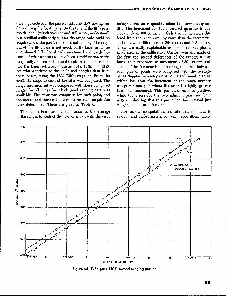
JPL RESEARCH SUMMARY NO. 36-8
the range code over the passive link; only RF tracking was being the measured quantity minus the computed quan-done during the fourth pass. By the time of the fifth pass, tity. The increment for the measured quantity is onethe situation (which was not and still is not, understood) clock cycle or 301.33 meters. Only two of the errors dif-was rectified sufficiently so that the range code could be fered from the mean error by more than the increment,acquired over the passive link, but not reliably. The rang- and they were differences of 304 meters and 303 meters.ing of the fifth pass is not good, partly because of the These are easily explainable as one increment plus aunexplained difficulty already mentioned and partly be- small error in the calibration. Checks were also made ofcause of what appears to have been a malfunction in the the first and second differences of the ranges; it wasrange tally. Because of these difficulties, the data reduc- found that they were in increments of 301 meters andtion has been restricted to Passes 1248, 1249, and 1250. smooth. The increments in the range number betweenAn orbit was fitted to the angle and doppler data from each pair of points were compared with the averagethese passes, using the IBM 7090 computer. From the of the doppler for each pair of points and found to agreeorbit, the range to each of the sites was computed. The within less than the increment of the range numberrange measurement was compared with these computed except for one pair where the error is slightly greaterranges for all times for which good ranging data was than one increment. This particular error is positive,available. The error was computed for each point, and while the errors for the two adjacent pairs are boththe means and standard deviations for each acquisition negative showing that this particular time interval justwere determined. These are given in Table 8. caught a count at either end.
The comparison was made in terms of the average The several computations indicate that the data isof the ranges to each of the two antennas, with the error smooth and self-consistent for each acquisition. How-
4.30
4 2C
r
4.10
X VALUES OFrX DELAYED 8.2 sec
40 C
SX
o 390
Idz,r'
380
3,70
10 57:21Z 41 1015801Z 21 41 10'59,01Z 21 41 IIO'OIZ 21
GREENWICH MEAN TIME
Figure 64. Echo pass 1107, second ranging portion
55
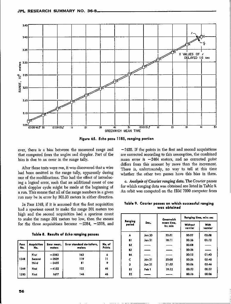
JPL RESEARCH SUMMARY NO. 36-8
3A5
r340 X
3.35 IX VALUES OF r
DELAYED 1.6 sec
2 330 - 1__
5)
E
w_ 325 -
Z 3.20 -
3.1
3.10C
12:08:41Z 51 12.09:01Z II 21 31 41 51 12:IO'01Z 11 21 31 41 51GREENWICH MEAN TIME
Figure 65. Echo pass 1185, ranging portion
ever, there is a bias between the measured range and -2455. If the points in the first and second acquisitionsthat computed from the angles and doppler. Part of the are corrected according to this assumption, the combinedbias is due to an error in the range tally, mean error is -2464 meters, and no corrected point
differs from this amount by more than the increment.After these tests were run, it was discovered that a wire There is, unfortunately, no way to tell at this time
had been omitted in the range tally, apparently during hether the other two passes have this bias in them.
one of the modifications. This had the effect of introduc-
ing a logical error, such that an additional count of one c. Analysis of Courier ranging data. The Courier passesclock doppler cycle might be made at the beginning of for which ranging data was obtained are listed in Table 9.
a run. This means that all of the range numbers in a given An orbit was computed on the IBM 7090 computer fromrun may be in error by 301.33 meters in either direction.
In Pass 1248, if it is assumed that the first acquisition Table 9. Courier passes on which successful ranginghad a spurious count to make the range 301 meters too was obtainedhigh and the second acquisition had a spurious countto make the range 301 meters too low, then the means Greenwich Ranging time, min: sec
Ranging Da1. mean time,for the three acquisitions became -2384, -2528, and period hr: min Without wtivernier vernier
Table 8. Results of Echo ranging passes A Jan 30 22:51 00:02 02158
BI Jan 31 18:11 00126 0112
Pass Acquisition Error mean, Error standard deviations, No. of 82 - - 00:08 -No. No. meters meters Points
3 - - 00:26 -
First -2083 163 6 94 - - 00:12 01:40
1248 Second -2829 119 11 C J6n 31 20:05 00:26 02:48
Third -2455 81 D Jan 31 21:55 00:06 03:46
1249 First -4152 122 46 El Feb 1 19:12 00:32 00:32
1250 First 1677 146 46 E2 - - 00:16 00;06
56
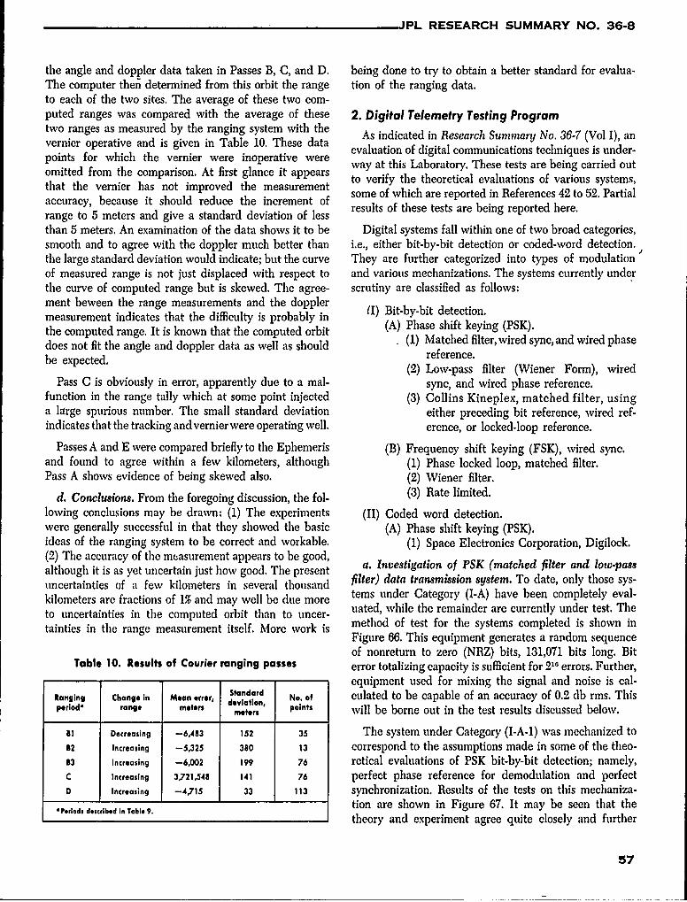
JPL RESEARCH SUMMARY NO. 36-8
the angle and doppler data taken in Passes B, C, and D. being done to try to obtain a better standard for evalua-The computer then determined from this orbit the range tion of the ranging data.to each of the two sites. The average of these two com-puted ranges was compared with the average of these 2. Digital Telemetry Testing Programtwo ranges as measured by the ranging system with the As indicated in Research Summary No. 36-7 (Vol I), anvernier operative and is given in Table 10. These data evaluation of digital communications techniques is under-points for which the vernier were inoperative were way at this Laboratory. These tests are being carried outomitted from the comparison. At first glance it appears to verify the theoretical evaluations of various systems,that the vernier has not improved the measurement some of which are reported in References 42 to 52. Partialaccuracy, because it should reduce the increment of results of these tests are being reported here.range to 5 meters and give a standard deviation of lessthan 5 meters. An examination of the data shows it to be Digital systems fall within one of two broad categories,smooth and to agree with the doppler much better than i.e., either bit-by-bit detection or coded-word detection.the large standard deviation would indicate; but the curve They are further categorized into types of modulationof measured range is not just displaced with respect to and various mechanizations. The systems currently underthe curve of computed range but is skewed. The agree- scrutiny are classified as follows:ment beween the range measurements and the doppler (I) Bit-by-bit detection.measurement indicates that the difficulty is probably in () t-by-bit einthe computed range. It is known that the computed orbit (A) Phase shift keying (PSK).does not fit the angle and doppler data as well as should (1) Matched filter, wired sync, and wired phasebe expcted.reference.be expected. (2) Low-pass filter (Wiener Form), wired
Pass C is obviously in error, apparently due to a mal- sync, and wired phase reference.function in the range tally which at some point injected (3) Collins Kineplex, matched filter, usinga large spurious number. The small standard deviation either preceding bit reference, wired ref-indicates that the tracking and vernier were operating well. erence, or locked-loop reference.
Passes A and E were compared briefly to the Ephemeris (B) Frequency shift keying (FSK), wired sync.and found to agree within a few kilometers, although (1) Phase locked loop, matched filter.Pass A shows evidence of being skewed also. (2) Wiener filter.
d. Conclusions. From the foregoing discussion, the fol- (3) Rate limited.
lowing conclusions may be drawn: (1) The experiments (II) Coded word detection.were generally successful in that they showed the basic (A) Phase shift keying (PSK).ideas of the ranging system to be correct and workable. (1) Space Electronics Corporation, Digilock.(2) The accuracy of the measurement appears to be good,although it is as yet uncertain just how good, The present a. Investigation of PSK (matched fiter and lowpassuncertainties of a fewv kilometers in several thousand flter) data transmission system. To date, only those sys-kilometers are fractions of 1 and may well be clue more ms nder Category (I-A) have been completely eval-kiloetes ae frctins f 1%andmaywellbe ue ore uated, while the remainder are currently under test. Theto uncertainties in the computed orbit than to uncer- utd hl h eane r urnl ne et htainties in the range measurement itself. More work is method of test for the systems completed is shown inFigure 66. This equipment generates a random sequence
of nonreturn to zero (NRZ) bits, 131,071 bits long. BitTable 10. Results of Courier ranging passes error totalizing capacity is sufficient for 21r errors. Further,
equipment used for mixing the signal and noise is cal-Ranging Change in Mean error Standard No. af culated to be capable of an accuracy of 0.2 db rms. Thisperiod' range meoers deviation, pointsmeters will be borne out in the test results discussed below.
SI Decreasing -6,483 152 35 The system under Category (I-A-i) was mechanized to82 Increasing -5,325 380 13 correspond to the assumptions made in some of the theo-83 Increasing -6,002 1" 76 retical evaluations of PSK bit-by-bit detection; namely,C Increasing 3,721,548 141 76 perfect phase reference for demodulation and perfectD Increasing -4,715 33 113 synchronization. Results of the tests on this mechaniza-
'Periods described in Table 9. tion are shown in Figure 67. It may be seen that thetheory and experiment agree quite closely and further
57
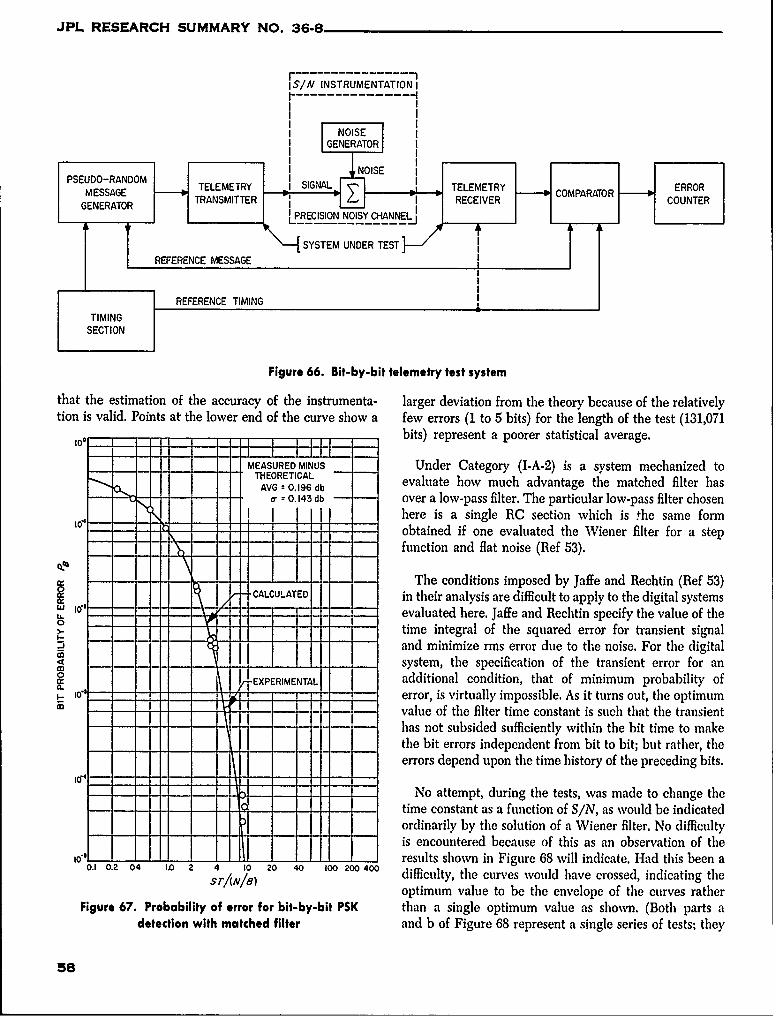
JPL RESEARCH SUMMARY NO. 36-8
S/ INSTRUMENTATION I
SNOISE
GENERATOR I
PSEUDO-RANDOM I SI-
GO
MESAGETELEMETRY I = SIGNAL I TELEMETRY ERROR
REFERENCE MESSAGE C
REFERENCE TIMING
TIMINGSECTION
Figure 66. Bit-by-bit telemetry test system
that the estimation of the accuracy of the instrumenta- larger deviation from the theory because of the relativelytion is valid. Points at the lower end of the curve show a few errors (1 to 5 bits) for the length of the test (131,071
-0 bits) represent a poorer statistical average.
MEASURED MINUS Under Category (I-A-2) is a system mechanized toTHEORETICAL evaluate how much advantage the matched filter has
AVG -0.196 dbadntg0.143 db over a low-pass filter. The particular low-pass filter chosen
here is a single RC section which is the same formobtained if one evaluated the Wiener filter for a stepfunction and flat noise (Ref 53).
,,- - - The conditions imposed by Jaffe and Rechtin (Ref 53)CALCULATED in their analysis are difficult to apply to the digital systems
,. -;- evaluated here. Jaffe and Rechtin specify the value of the0f time integral of the squared error for transient signal
- - and minimize rms error due to the noise. For the digital4 1 system, the specification of the transient error for an0 EXPERIMENTAL additional condition, that of minimum probability ofL. t' I Adt error, is virtually impossible. As it turns out, the optimumcc value of the filter time constant is such that the transient
- - has not subsided sufficiently within the bit time to makethe bit errors independent from bit to bit; but rather, theerrors depend upon the time history of the preceding bits.
- - No attempt, during the tests, was made to change the- time constant as a function of S/N, as would be indicated
ordinarily by the solution of a Wiener filter. No difficultyis encountered because of this as an observation of the
o"0 ~ results shown in Figure 68 will indicate. Had this been a0.1 0.2 04 10 2 4 difficulty, the curves would have crossed, indicating the
SrAN/8) optimum value to be the envelope of the curves rather
Figure 67. Probability of error for bit-by-bit PSK than a single optimum value as shown. (Both parts adetection with matched filter and b of Figure 68 represent a single series of tests; they
58
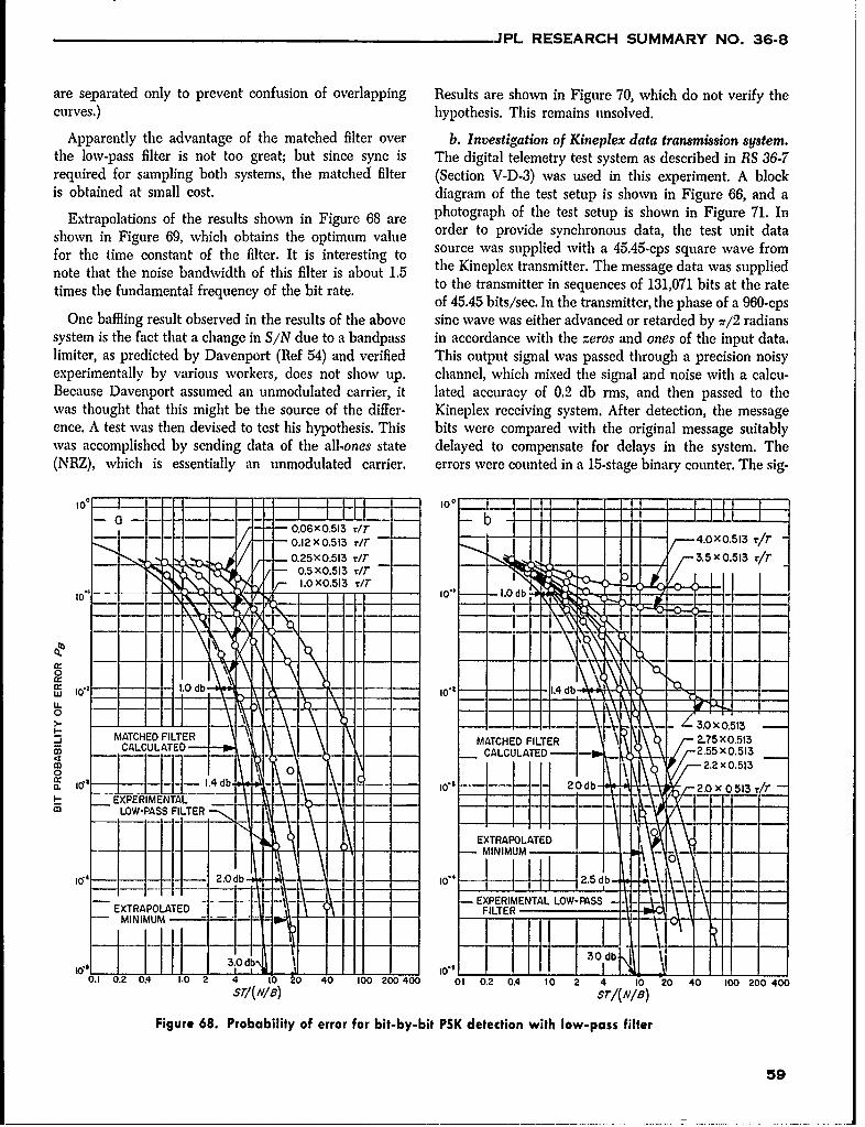
JPL RESEARCH SUMMARY NO. 36-8
are separated only to prevent confusion of overlapping Results are shown in Figure 70, which do not verify thecurves.) hypothesis. This remains unsolved.
Apparently the advantage of the matched filter over b. Investigation of Kineplex data transmission system.the low-pass filter is not too great; but since sync is The digital telemetry test system as described in RS 36-7required for sampling both systems, the matched filter (Section V-D-3) was used in this experiment. A blockis obtained at small cost. diagram of the test setup is shown in Figure 66, and a
Extrapolations of the results shown in Figure 68 are photograph of the test setup is shown in Figure 71. Inshown in Figure 69, which obtains the optimum value order to provide synchronous data, the test unit data
for the time constant of the filter. It is interesting to source was supplied with a 45.45-cps square wave from
note that the noise bandwidth of this filter is about 1.5 the Kineplex transmitter. The message data was suppliedtimes the fundamental frequency of the bit rate. to the transmitter in sequences of 131,071 bits at the rate
of 45.45 bits/see. In the transmitter, the phase of a 960-cpsOne baffling result observed in the results of the above sine wave was either advanced or retarded by ,r/2 radians
system is the fact that a change in S/N due to a bandpass in accordance with the zeros and ones of the input data.limiter, as predicted by Davenport (Ref 54) and verified This output signal was passed through a precision noisyexperimentally by various workers, does not show up. channel, which mixed the signal and noise with a calcu-Because Davenport assumed an unmodulated carrier, it lated accuracy of 0.2 db rms, and then passed to thewas thought that this might be the source of the differ- Kineplex receiving system. After detection, the messageence. A test was then devised to test his hypothesis. This bits were compared with the original message suitablywas accomplished by sending data of the allones state delayed to compensate for delays in the system. The(NRZ), which is essentially an unmodulated carrier, errors were counted in a 15-stage binary counter. The sig-
- 0.06x0,513 r/r r--.x.1 /
//T-0.12X0.513 rit -- X 51 r/
-0.25 X0513 r/r - 3.5 X0.513 r/r
- 0.5x0.513 r/r
10
1.0x .513 r/ 1 1
0
w 0 10- 14 _
MATCHE FILTER 3.0 x 0.513 -
MATCHEDMATCHED FILTER 2.75 x0513CALCULATED -- 2.55 x 0, 513
C T" CALCULATED - --imp
a: - -j1.4db - VI,
_- EXPERIMENTAL ---,.n LOW-PASS FILTER
I, iEXTRAPOLATED~:4 - 9MINIMUM1L
.. EXPERIMENTAL LOW-PASSEXTRAPOLATED FIL, i ,TER- MINIMUM -
3. 0 d - -\ 30 db 10.1 0.2 o.4 1.0 2 1 0 100 200400 01 0.2 0.4 to 2 4 10 20 40 100 200400
srl( ) srl(N/s)
Figure 68. Probability of error for bit-by-bit PSK detection with low-pass filter
59
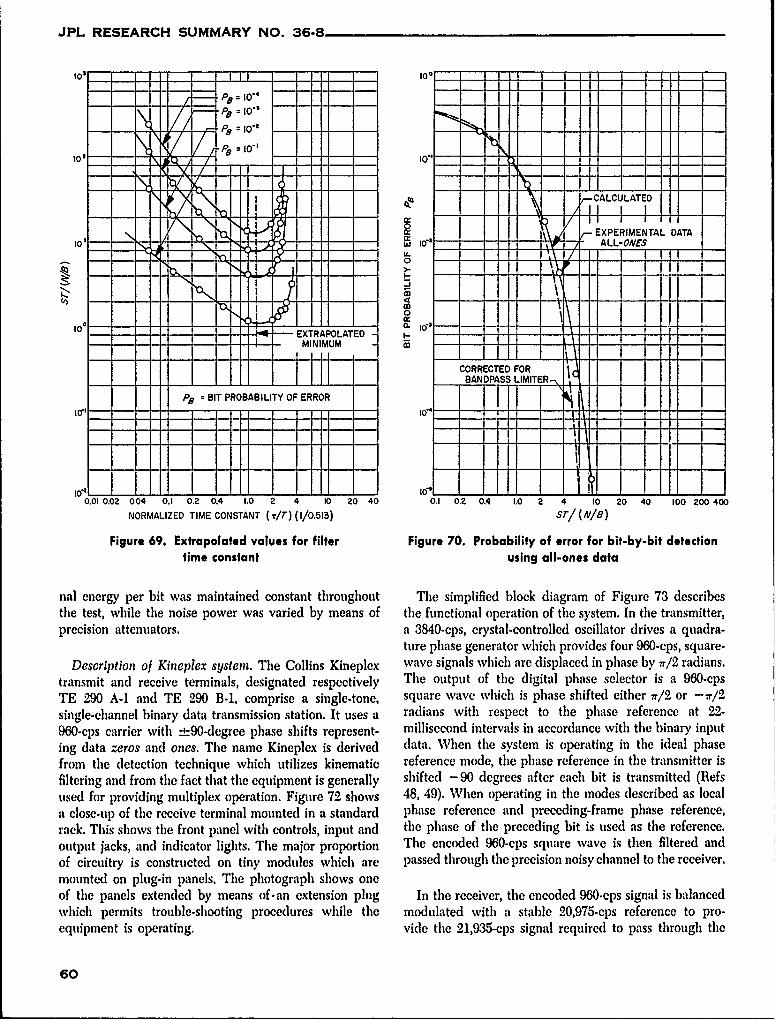
JPL RESEARCH SUMMARY NO. 36-8
-_p 11--
- - ~~p8 z 10' -----to - - 'P8= 10-5'm P 8 = 1 "
i
CALCULATED
r -EXPERIMENTAL DATA
1 ~ N, 0. i -
l0 - . EXTRAPOLATED - -
MINIMUM -
CORRECTED FOR 1 -
BANDPASS LIMITER- ,
P8 BIT PROBABILITY OF ERROR 074 -
Ililr IC/A -
0.01 0.02 004 0.1 0.2 0.4 1.0 2 4 10 20 40 0.1 0.2 0.4 1.0 2 4 10 20 40 100 200400
NORMALIZED TIME CONSTANT (T/T) (1/0.513) ST/(N/8)
Figure 69. Extrapolated values for filter Figure 70. Probability of error for bit-by-bit detectiontime constant using all-ones data
nal energy per bit was maintained constant throughout The simplified block diagram of Figure 73 describesthe test, while the noise power was varied by means of the functional operation of the system. In the transmitter,precision attenuators. a 3840-cps, crystal-controlled oscillator drives a quadra-
ture phase generator which provides four 960-cps, square-
Description of Kineplex system. The Collins Kineplex wave signals which are displaced in phase by 7r/2 radians.transmit and receive terminals, designated respectively The output of the digital phase selector is a 960-cpsTE 290 A-1 and TE 290 B-i, comprise a single-tone, square wave which is phase shifted either 7r/ 2 or -7r/ 2
single-channel binary data transmission station. It uses a radians with respect to the phase reference at 22-960-cps carrier with ±90-degree phase shifts represent- millisecond intervals in accordance with the binary inputing data zeros and ones. The name Kineplex is derived data. When the system is operating in the ideal phasefrom the detection technique which utilizes kinematic reference mode, the phase reference in the transmitter isfiltering and from the fact that the equipment is generally shifted -90 degrees after each bit is transmitted (Refsused for providing multiplex operation. Figure 72 shows 48, 49). When operating in the modes described as locala close-up of the receive terminal mounted in a standard phase reference and preceding-frame phase reference,rack. This shows the front panel with controls, input and the phase of the preceding bit is used as the reference.output jacks, and indicator lights. The major proportion The encoded 960-cps square wave is then filtered andof circuitry is constructed on tiny modules which are passed through the precision noisy channel to the receiver.mounted on plug-in panels. The photograph shows oneof the panels extended by means of-an extension plug In the receiver, the encoded 960.cps signal is balancedwhich permits trouble-shooting procedures while the modulated with a stable 20,975-cps reference to pro-equipment is operating. vide the 21,935-cps signal required to pass through the
60
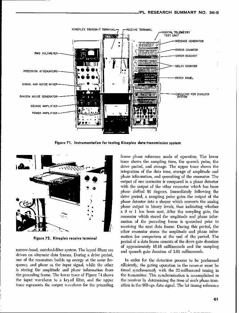
JPL RESEARCH SUMMARY NO. 36-8
KINEPLEX TRANSMIT TERMINAL 7 F RECEIVE TERMINAL DIGITAL TELEMTRY
TEST UNIT
* . ~,,iMESSAGE GENERATOR
, . ERROR COUNTERRMS VOLTMETER ERROR READOUT
T9 DELAY COUNTERPRECISION ATTENUATORSI i
-PATCH PANEL
SIGNAL AND NOISE MIXER
CIRCUITRY FOR DIGILOCKRANDOM NOISE GENERATOR SYSTEM
DECADE AMPLIFIER
POWER AMPLIFIER
Figure 71. Instrumentation for testing Kineplex data transmission system
frame phase reference mode of operation. The lowertrace shows the sampling time, the quench pulse, the
i drive period, and storage. The upper trace shows theintegration of the data tone, storage of amplitude and
aphase information, and quenching of the resonator. Theoutput of one resonator is compared in a phase detector
S with the output of the other resonator which has beenphase shifted 90 degrees. Immediately following thedrive period, a sampling pulse gates the output of thephase detector into a shaper which converts the analogphase output to binary levels, thus indicating whethera 0 or 1 has been sent. After the sampling gate, theresonator which stored the amplitude and phase infor-mation of the preceding frame is quenched prior toft receiving the next data frame. During this period, theother resonator stores the amplitude and phase infor-
Figure 72. Kineplex receive terminal mation for comparison at the end of the period. Theperiod of a data frame consists of the drive gate durationof approximately 18.18 milliseconds and the sampling
narrow-band, matched-filter system. The keyed filters are and quench gate duration of 3.82 milliseconds.driven on alternate data frames. During a drive period,one of the resonators builds up energy at the same fre- In order for the detection process to be performedquenc) and phase as the input signal, while the other efficiently, the gating operation in the recen~er must beis storing the amplitude and phase information from timed synchronously NN ith the 22-millisecond timing inthe preceding frame. The lower trace of Figure 74 shows the transmitter. This sy nchronization is accomplished inthe input waveform to a key ed filter, and the upper the receiver by determining the time of each phase tran-trace represents the output waveform for the preceding sition in the 960-cps data signal. The bit timing reference
61
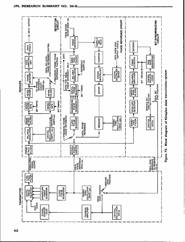
JPL RESEARCH SUMMARY NO. 36-8
w w
0-33 Imu uI-
LoL
Ir w
I (~ x !D (D(W 2bJ 2 u,
0~U 0, 0
fn LL i-
I( 1 i-I Id- *
m. Ia0040. i LL
ZU ; II a ,a1).Iw wbJ z~ Q
2 -.LL maw
0 0
I I.
4c 4
0 (10 z
IW n 0i U.-
aI Mo
L---------------------62 UcI
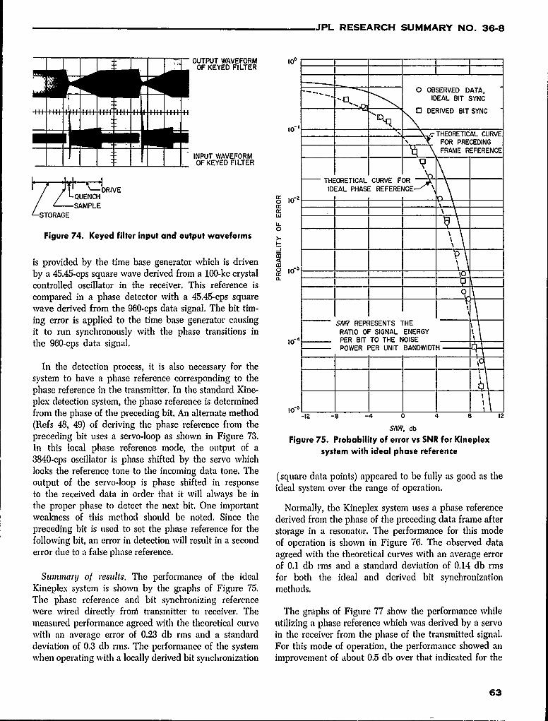
JPL RESEARCH SUMMARY NO. 36-8
OUTPUT WAVEFORM I0°
I IOF KEYED FILTER
OF KYEDFILTR 0 OBSERVED DATA,
" ... ""'-0,.... IDEAL BIT SYNC
• r'l DERIVED BIT SYNC
--L~LLL J 10 __r". 'THEORETICAL CURVE___m___ FOR PRECEDING
-- "- "[ \FRAME REFERENCEINPUT WAVEFORM FAE___
- OF KEYED FILTERI. _L JTHEORETICAL CURVE FOR
D-'DRIVE IDEAL PHASE REFERENCE- '%// QUENCH __ 16_2
/ '----SAMPLE ,O_"LSTORAGE W
IL
Figure 74. Keyed filter input and output waveforms >.
is provided by the time base generator which is drivenby a 45.45-cps square wave derived from a 100-ke crystal 0 16"30.
controlled oscillator in the receiver. This reference iscompared in a phase detector with a 45.45-cps square 0
wave derived from the 960-eps data signal. The bit tim-ing error is applied to the time base generator causing SNR REPRESENTS THE
it to run synchronously with the phase transitions in RATIO OF SIGNAL ENERGY
the 960-cps data signal. o- PER BIT TO THE NOISEPOWER PER UNIT BANDWIDTH
In the detection process, it is also necessary for thesystem to have a phase reference corresponding to thephase reference in the transmitter. In the standard Kine-plex detection system, the phase reference is determinedfrom the phase of the preceding bit. An alternate method IO'-12 -8 -4 0 4 8 12
(Refs 48, 49) of deriving the phase reference from the SNR, dbpreceding bit uses a servo-loop as shown in Figure 73. Figure 75. Probability of error vs SNR for KineplexIn this local phase reference mode, the output of a3840-cps oscillator is phase shifted by the servo whichlocks the reference tone to the incoming data tone. The (square data points) appeared to be fully as good as theoutput of the servo-loop is phase shifted in response ideal system over the range of operation.to the received data in order that it will always be in
the proper phase to detect the next bit. One important Normally, the Kineplex system uses a phase referenceweakness of this method should be noted. Since the derived from the phase of the preceding data frame afterpreceding bit is used to set the phase reference for the storage in a resonator. The performance for this modefollowing bit, an error in detection will result in a second of operation is shown in Figure 76. The observed dataerror due to a false phase reference. agreed with the theoretical curves with an average error
of 0.1 db rms and a standard deviation of 0.14 db rmsSummary of results. The performance of the ideal for both the ideal and derived bit synchronization
Kineplex system is shown by the graphs of Figure 75. methods.The phase reference and bit synchronizing referencewere wired directly frorM transmitter to receiver. The The graphs of Figure 77 show the performance whilemeasured performance agreed with the theoretical curve utilizing a phase reference which was derived by a servowith an average error of 0.23 db rms and a standard in the receiver from the phase of the transmitted signal.deviation of 0.3 db rms. The performance of the system For this mode of operation, the performance showed anwhen operating with a locally derived bit synchronization improvement of about 0.5 db over that indicated for the
63
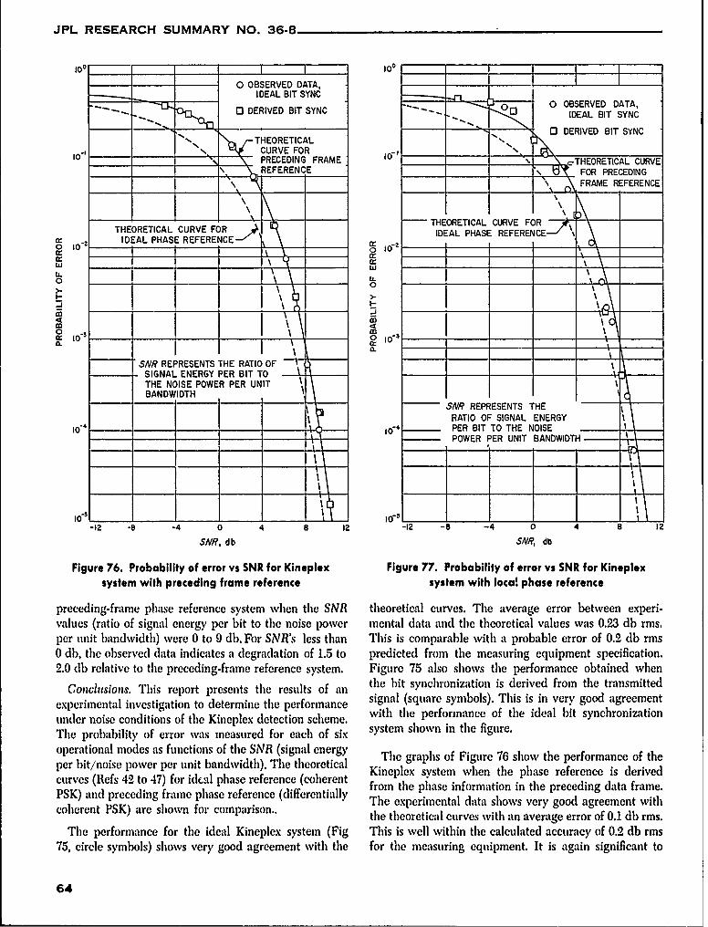
JPL RESEARCH SUMMARY NO. 36-8
10, 1__ _ _ __ _ _ 1 1_ _
0 OBSERVED DATA,IDEAL BIT SYNC
0 DERIVED BIT SYNC 0 OBSERVED DATA,"-__. DEIVEDBITSYNC.... ., j IDEAL BIT SYNC
"" .. . r DERIVED BIT SYNC
THEORETICAL
10" ",, PRECEDING FRAME _0_"___ - THEORETICAL CURVE\_ ' REFERENCE _ _FOR PRECEDING
- FRAME REFERENCE
THEORETICAL CURVE FORTHEORETICAL CURVE FOR IDEAL PHASE REFERENCE---'
0 102 IDEAL PHASE REFERENCE - " 0
o _ _ _ _ _ I°" _ _ _\
0
L. .
"'SNR REPRESENTS THE RATIO OF-- \,SIGNAL ENERGY PER BIT TO
THE NOISE POWER PER UNITBANDWIDTH
-- SNR REPRESENTS THEI RATIO OF SIGNAL ENERGY10 4 10 - PER BIT TO THE NOISE
POWER PER UNIT BANDWIDTH10. 5
0 -
*I 8 -4 0 4 8' I2 -12 -8 -4 0 4 8 12
SNR, db SNR, db
Figure 76. Probability of error vs SNR for Kineplex Figure 77. Probability of error vs SNR for Kineplexsystem with preceding frame reference system with local phase reference
preceding-frame phase reference system wvhen the SNR theoretical curves. The average error betwveen experi-valucs (ratio of signal energy per bit to the noise power mental data and the theoretical v'alues was 0.2,3 db rms.per unit bandwidth) wvere 0 to 9 db. For SNR's less than This is comparable wvith a probable error of 0.2 db rms0 db, the observed data indicates a dlegradlation of 1.5 to predicted fromn the measuring equipment specification.2.0 db relative to the preceding-frame reference system. Figure 75 also shows the performance obtained when
Concusins.Thisreprt resets he esuls o an the bit synchronization is derived from the transmittedexperimental investigation to determine the performance signal (square symbols). This is in very good agreementunder noise conditions of the Kineplex detection scheme. with the performance of the ideal bit synchronizationThe probability of error wvas measured for each of six system showvn in the figure.operational modes as functions of the SNR (signal energy The graphs of Figure 76 show the performance of theper bit/noise power per unit bandwvidth). The theoretical Kieexstmwhnhepaerfecesdrvdcurves (Refs 42 to 47) for idcal phase reference (coherent frome yse we the phase ifrtonnthprefecei derame.PSK) and preceding frame phase reference (differentially The experimental data shows very good agreement withcoherent PSK) are shown for comparison., the theoretical curves wvith an average error of 0.1 db rms.
The performance for the ideal Kineplex system (Fig This is wvell wvithin the calculated accuracy of 0.2 db rms75, circle symbols) showvs very good agreement wvith the for the measuring equipment. It is again significant to
64
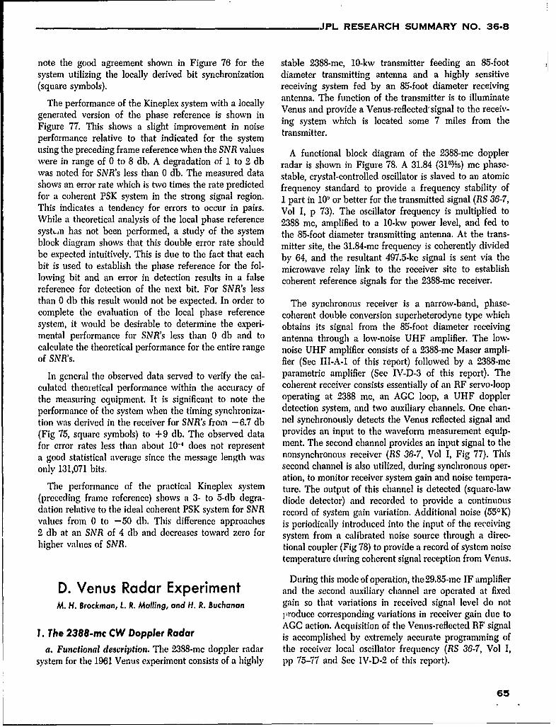
JPL RESEARCH SUMMARY NO. 36-8
note the good agreement shown in Figure 76 for the stable 2388-mc, 10-kw transmitter feeding an 85-footsystem utilizing the locally derived bit synchronization diameter transmitting antenna and a highly sensitive(square symbols). receiving system fed by an 85-foot diameter receiving
antenna. The function of the transmitter is to illuminateThe performance of the Kineplex system with a locally VeuanprvdaVnsreecesialtthrci-
generated version of the phase reference is shown in Venus and provide a Venus-reflectedsignal to the receiv-
Figure 77. This shows a slight improvement in noise ing system which is located some 7 miles from the
performance relative to that indicated for the system transmitter.
using the preceding frame reference when the SNR values A functional block diagram of the 2388-me dopplerwere in range of 0 to 8 db. A degradation of 1 to 2 db radar is shown in Figure 78. A 31.84 (31, 3A) me phase-was noted for SNR's less than 0 db. The measured data stable, crystal-controlled oscillator is slaved to an atomicshows an error rate which is two times the rate predicted frequency standard to provide a frequency stability offor a coherent PSK system in the strong signal region. 1 part in 109 or better for the transmitted signal (RS 36-7,This indicates a tendency for errors to occur in pairs. Vol 1, p 73). The oscillator frequency is multiplied toWhile a theoretical analysis of the local phase reference 2388 me, amplified to a 10-kw power level, and fed tosystn has not been performed, a study of the system the 85-foot diameter transmitting antenna. At the trans-block diagram shows that this double error rate should mitter site, the 31.84-mc frequency is coherently dividedbe expected intuitively. This is due to the fact that each by 64, and the resultant 497.5-ke signal is sent via thebit is used to establish the phase reference for the fol- microwave relay link to the receiver site to establishlowing bit and an error in detection results in a false coherent reference signals for the 2388-mc receiver.reference for detection of the next bit. For SNR's lessthan 0 db this result would not be expected. In order to The synchronous receiver is a narrow-band, phase-complete the evaluation of the local phase reference coherent double conversion superheterodyne type whichsystem, it would be desirable to determine the experi- obtains its signal from the 85-foot diameter receivingmental performance for SNR's less than 0 db and to antenna through a low-noise UHF amplifier. The low-calculate the theoretical performance for the entire range noise UHF amplifier consists of a 2388-me Maser ampli-of SNR's. fier (See III-A-1 of this report) followed by a 2388-me
In general the observed data served to verify the cal- parametric amplifier (See IV-D-3 of this report). Theculated theoretical performance within the accuracy of coherent receiver consists essentially of an RF servo-loopthe measuring equipment. It is significant to note the operating at 2388 me, an AGC loop, a UHF dopplerperformance of the system when the timing synchroniza- detection system, and two auxiliary channels. One chan-tion was derived in the receiver for SNR's from -6.7 db nel synchronously detects the Venus reflected signal and(Fig 75, square symbols) to +9 db. The observed data provides an input to the waveform measurement equip-for error rates less than about 10-4 does not represent ment. The second channel provides an input signal to thea good statistical average since the message length was nonsynchronous receiver (RS 36-7, Vol I, Fig 77). Thisonly 131,071 bits. second channel is also utilized, during synchronous oper-
ation, to monitor receiver system gain and noise tempera-The performance of the practical Kineplex system ture. The output of this channel is detected (square-law
(preceding frame reference) shows a 3- to 5-db degra- diode detector) and recorded to provide a continuousdation relative to the ideal coherent PSK system for SNR record of system gain variation. Additional noise (55 0K)values from 0 to -50 db. This difference approaches is periodically introduced into the input of the receiving2 db at an SNR of 4 db and decreases toward zero for system from a calibrated noise source through a direc-higher values of SNR. tional coupler (Fig 78) to provide a record of system noise
temperature during coherent signal reception from Venus.
During this mode of operation, the29.85-mc IF amplifierD. Venus Radar Experiment and the second auxiliary channel are operated at fixed
M. H. Brockman, t. R. Mailing, and H. R. Buchanan gain so that variations in received signal level do notproduce corresponding variations in receiver gain due toAGC action. Acquisition of the Venus-reflected RF signal
1. The 2388-inc CW Doppler Radar is accomplished by extremely accurate programming ofa. Functional description. The 2388-me doppler radar the receiver local oscillator frequency (RS 36-7, Vol I,
system for the 1961 Venus experiment consists of a highly pp 75-77 and See IV-D-2 of this report).
65
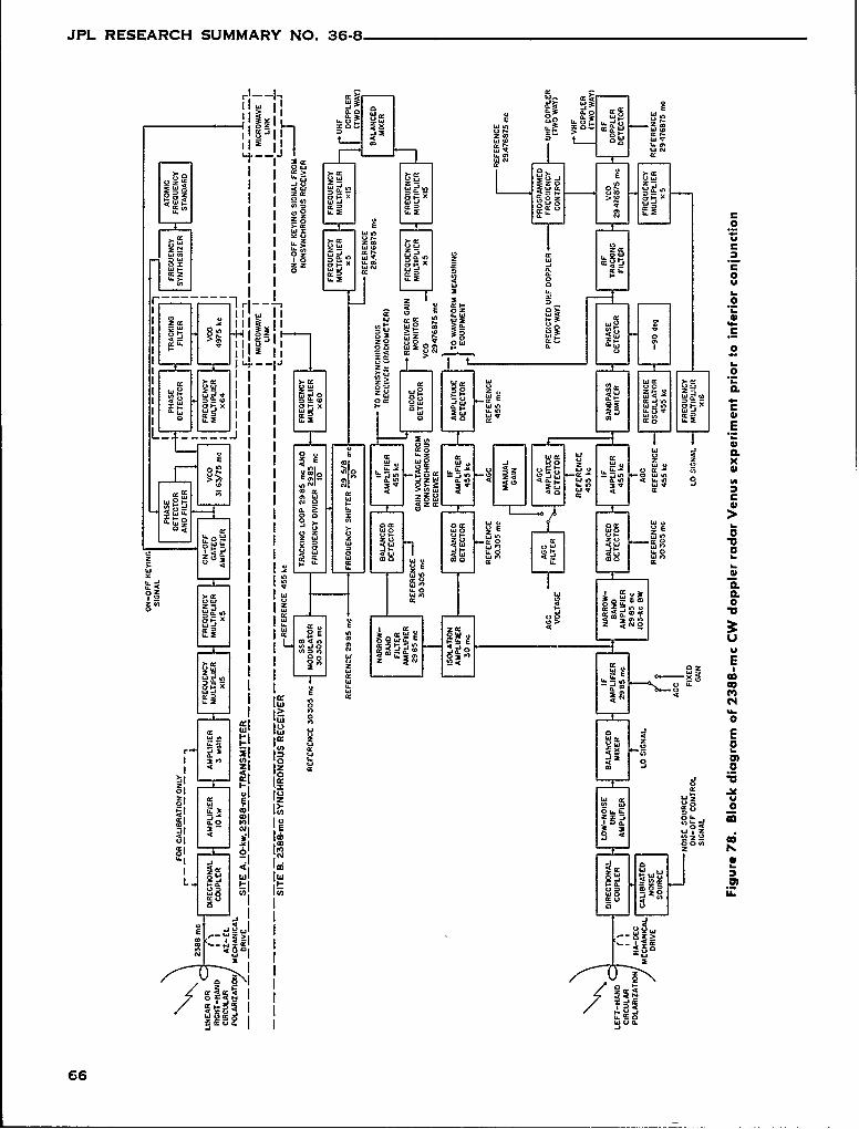
JPL RESEARCH SUMMARY NO. 36-8
I> >
t WN W- VaCCo 0) w 0
zI 0 0 00 Z
', 1~ .0 w
2 1
- - -- -0 I - 2.0I1 0z- SE =4~iiW
I~~ w0~ 0~Ii0 ~~ 4
4 ,I~., ZO 0~ C~t- * 0~ WC-X 44 4
0z 0 .0 ow U
L v 0 2
L w
00 ww. cc mW 400 n2
0E
-T--Oo)
w- 0
0e 0 H
w1 w
z 00 , w o N
N z Iz Z
-' wL0-i I co 0 m
I .0
0. m 40
66V
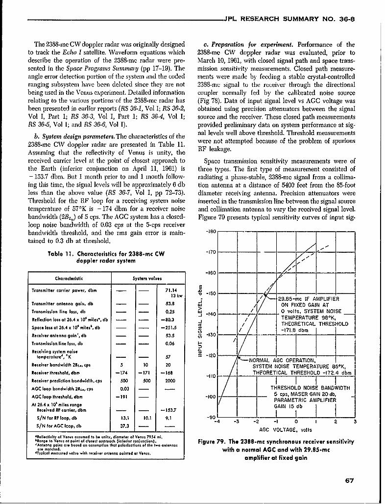
JPL RESEARCH SUMMARY NO. 36-8
The 2388-mo CW doppler radar was originally designed c. Preparation for experiment. Performance of theto track the Echo I satellite. Waveform equations which 2388-mc CW doppler radar was evaluated, prior todescribe the operation of the 2388-mc radar were pre- March 10, 1961, with closed signal path and space trans-sented in the Space Programs Sum may (pp 17-19). The mission sensitivity measurements. Closed path measure-angle error detection portion of the system and the coded ments were made by feeding a stable crystal-controlledranging subsystem have been deleted since they are not 2388-inc signal to the receiver through the directionalbeing used in the Venus experiment. Detailed information coupler normally fed by the calibrated noise sourcerelating to the various portions'of the 2388-mc radar has (Fig 78). Data of input signal level vs AGC voltage wasbeen presented in earlier reports (RS 36-1, Vol I; RS 36-2, obtained using precision attenuators between the signalVol I, Part 1; RS 36-3, Vol I, Part 1; RS 36-4, Vol I; source and the receiver. These closed path measurementsRS 36-5, Vol I; and RS 36-6, Vol I). provided preliminary data on system performance at sig-
b. System design parameters. The characteristics of the nal levels well above threshold. Threshold measurements
2388-mo GW doppler radar are presented in Table 11. were not attempted because of the problem of spurious
Assuming that the reflectivity of Venus is unity, the RF leakage.
received carrier level at the point of closest approach to Space transmission sensitivity measurements were ofthe Earth (inferior conjunction on April 11, 1961) is three types. The first type of measurement consisted of-153.7 dbm. But 1 month prior to and 1 month follow- radiating a phase-stable, 2388-mc signal from a collima-ing this time, the signal levels will be approximately 6 db tion antenna at a distance of 5400 feet from the 85-footless than the above value (RS 36-7, Vol 1, pp 72-73). diameter receiving antenna. Precision attenuators wereThreshold for the RF loop for a receiving system noise inserted in the transmission line between the signal sourcetemperature of 57 0K is - 174 dbm for a receiver noise and collimation antenna to vary the received signal level.bandwidth (2B,,,) of 5 cps. The ACC system has a closed- Figure 79 presents typical sensitivity curves of input sig-loop noise bandwidth of 0.03 cps at the 5-cps receiverbandwidth threshold, and the rms gain error is main- -180 Ttained to 0.3 db at threshold.
Table 11. Characteristics for 2388-mc CW -170 - -
doppler radar system / I-160 -
Characteristic System values 10 "
E /Transmitter carrier power, dbm - - 71.14 .0 -15 .
13 kw o -150 __
1n3. w / 29.85-mc IF AMPLIFIERTransmitter antenna gai, db - - 53.8 i / ON FIXED GAIN ATTransmission line loss, db - - 0.25 W -140 / 0 volts, SYSTEM NOISEReflection loss at 26.4 x 10' miles', db - - -80.3 J- TEMPERATURE 980K,
// THEORETICAL THRESHOLDSpace loss at 26.4 x 10' miles', db - - -251.5 / -171,8 dbm
Receiver antenna gain', db - - 53.5 -130
Transmission line loss, db - - 0.06 t /Receiving system noise t
temperature4, OK -7 - .120NORMAL AGC OPERATION,
Receiver bandwidth 2B.., cpS 5 10 20 SYSTEM NOISE TEMPERATURE 850 K,Receiver threshold, dbm -174 -171 -168 THORETICAL THRESHOLD -172.4 bm
Receiver prediction bandwidth, cps 500 500 2000 I 1AGC loop bandwidth 28L., cpS 0.03 - - THRESHOLD NOISE BANDWIDTHAGC loop threshold, dbm -191 -100 5 cps, MASER GAIN 20 db,
PARAMETRIC AMPLIFIERAt 26.4 x 10' miles range GAIN 15 db
Received RF carrier, dbmn - - -153.7SIN for RF loop, db 13.1 10.1 9.1 -90-
-4 -3 -2 -I 0 I 2 3SIN for AGC Icop, db 37.3 -AG VOLTAGE, volts
etfleclvily of Venus assumed to be unity, diameter of Venus 7954 mi.$Range to Venus at paint of closest approach (inferior conjunctlonl. Figure 79. The 2388-mc synchronous receiver sensitivitycAntenna gains are based on assumption that polarizations of the two antennas
are matched. with a normal AGC and with 29.85-mc4Typical measured value with receiver antenna pointed at Venus.amplifier at fixed gain
67
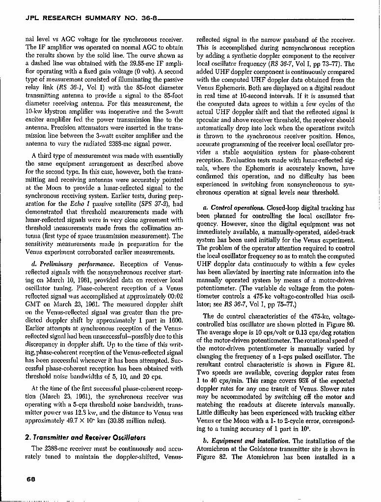
JPL RESEARCH SUMMARY NO. 36-8
nal level vs AGC voltage for the synchronous receiver, reflected signal in the narrow passband of the receiver.The IF amplifier was operated on normal AGC to obtain This is accomplished during nonsynchronous receptionthe results shown by the solid line. The curve shown as by adding a synthetic doppler component to the receivera dashed line was obtained with the 29.85-me IF ampli- local oscillator frequency (RS 36-7, Vol I, pp 73-77). Thefier operating with a fixed gain voltage (0 volt). A second added UHF doppler component is continuously comparedtype of measurement consisted of illuminating the passive with the computed UHF doppler data obtained from therelay link (RS 36-1, Vol I) with the 85-foot diameter Venus Ephemeris. Both are displayed on a digital readouttransmitting antenna to provide a signal to the 85-foot in real time at 10-second intervals. If it is assumed thatdiameter receiving antenna. For this measurement, the the computed data agrees to within a few cycles of the10-kw klystron amplifier was inoperative and the 3-watt actual UHF doppler shift and that the reflected signal isexciter amplifier fed the power transmission line to the specular and above receiver threshold, the receiver shouldantenna. Precision attenuators were inserted in the trans- automatically drop into lock when the operations switchmission line between the 3-watt exciter amplifier and the is thrown to the synchronous receiver position. Hence,antenna to vary the radiated 2388-mc signal power. accurate programming of the receiver local oscillator pro-
A third type of measurement was made with essentially vides a stable acquisition system for phase-coherentthe same equipment arrangement as described above reception. Evaluation tests made with lunar-reflected sig-
for the second type. In this case, however, both the trans- nals, where the Ephemeris is accurately known, havemitting and receiving antennas were accurately pointed confirmed this operation, and no difficulty has been
at the Moon to provide a lunar-reflected signal to the experienced in switching from nonsynehronous to syn-
synchronous receiving system. Earlier tests, during prep- chronous operation at signal levels near threshold.aration for the Echo I passive satellite (SPS 37-2), had a. Control operations. Closed-loop digital tracking hasdemonstrated that threshold measurements made with been planned for controlling the local oscillator fre-
lunar-reflected signals were in very close agreement with been p or s in the ocal scillt fre-thresholdquency. However, since the digital equipment was nottenna (first type of space transmission measurement). Te immediately available, a manually-operated, aided-trackteniivirstypea e nt p ac e prearansion u renthe system has been used initially for the Venus experiment.sensitivity erme ents made in preparation for the The problem of the operator attention required to controlVenus experiment corroborated earlier measurements. the local oscillator frequency so as to match the computed
d. Preliminary performance. Reception of Venus- UHF doppler data continuously to within a few cyclesreflected signals with the nonsynchronous receiver start- has been alleviated by inserting rate information into theing on March 10, 1961, provided data on receiver local manually operated system by means of a motor-drivenoscillator tuning. Phase-coherent reception of a Venus potentiometer. (The variable dc voltage from the poten-reflected signal was accomplished at approximately 00:02 tiometer controls a 475.kc voltage-controlled bias oscil-GMT on March 23, 1961. The measured doppler shift lator; see RS 36-7, Vol I, pp 75-77.)on the Venus-reflected signal was greater than the pre- The dc control characteristics of the 475-kc, voltage-dicted doppler shift by approximately 1 part in 1600. controlled bias oscillator are shown plotted in Figure 80.Earlier attempts at synchronous reception of the Venus- The average slope is 10 cps/volt or 0.13 cps/deg rotationreflected signal had been unsuccessful-possibly due to this of the motor-driven potentiometer. The rotational speed ofdiscrepancy in doppler shift. Up to the time of this writ- the motor-driven potentiometer is manually varied bying, phase-coherent reception of the Venus-reflected signal changing the frequency of a 1-cps pulsed oscillator. Thehas been successful whenever it has been attempted. Sue- resultant control characteristic is shown in Figure 81.cessful phase-coherent reception has been obtained with Two speeds are available, covering doppler rates fromthreshold noise bandwidths of 5, 10, and 20 cps. 1 to 40 eps/min. This range covers 95% of the expected
At the time of the first successful phase-coherent recep- doppler rates for any one transit of Venus. Slower ratestion (March 23, 1961), the synchronous receiver was may be accommodated by switching off the motor andoperating with a 5-cps threshold noise bandwidth, trans- matching the readouts at discrete intervals manually.mitter power was 12.8 kw, and the distance to Venus was Little difficulty has been experienced with tracking eitherapproximately 49.7 X 10" km (30.88 million miles). Venus or the Moon with a 1- to 2-cycle error, correspond-
ing to a tuning accuracy of 1 part in 109.2. Transmitter and Receiver Oscillators b. Equipment and installation. The installation of the
The 2388-mc receiver must be continuously and accu- Atomichron at the Goldstone transmitter site is shown inrately tuned to maintain the doppler-shifted, Venus- Figure 82. The Atomichron has been installed in a
68
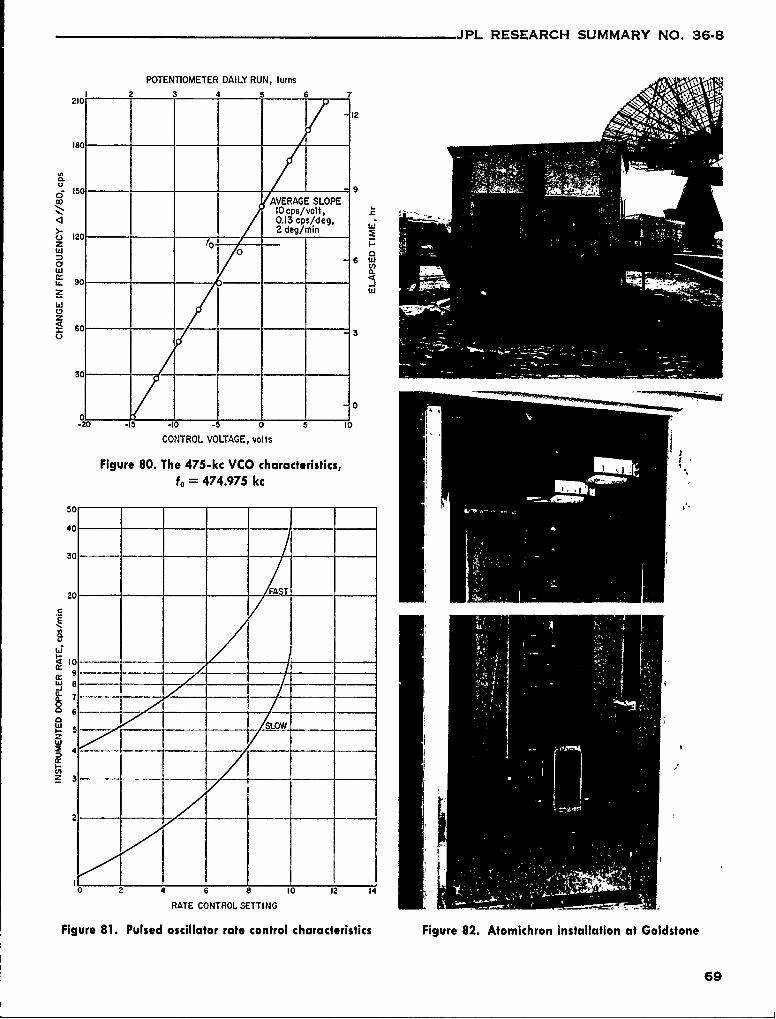
JPL RESEARCH SUMMARY NO. 36-8
POTENTIOMETER DAILY RUN, turns
2 3 4 ___5 6 7210
12
0
Cr150AVERAGE SLOPE
10 cps/volt,0.13 cps/deg,
o 12 2 deg/min0 020 -
z
C-a)
00
.20 -15 -10 -5 0 5 10
CONTROL VOLTAGE, volts
Figure 80. The 475-kc VCO characteristics,=o 474.975 kc
- FASJ T _I20I
-
__ __ _ SLOW
2
0 4 6 8 to 12
RATE CONTROL SETTING
Figure 81. Pulsed oscillator rate control characteristics Figure 82. Atomnichron installation at Goldstone
69
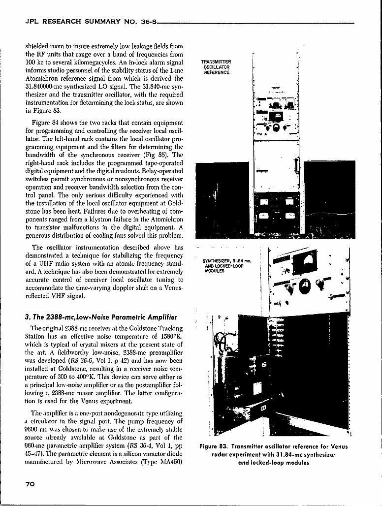
JPL RESEARCH SUMMARY NO. 36-8
shielded room to insure extremely low-leakage fields fromthe RF units that range over a band of frequencies from100 kc to several kilomegacycles. An in-lock alarm signal TRANSMITTER i
OSCILLATORinforms studio personnel of the stability status of the 1-mc REFERENCE
Atomichron reference signal from which is derived the31.840000-in synthesized LO signal. The 31.840-mc syn-instrumentation for determining the lock status, are shown
in Figure 83.
Figure 84 shows the two racks that contain equipmentfor programming and controlling the receiver local oscil-lator. The left-hand rack contains the local oscillator pro-gramming equipment and the filters for determining thebandwidth of the synchronous receiver (Fig 85). Theright-hand rack includes the programmed tape-operateddigital equipment and the digital readouts. Relay-operatedswitches permit synchronous or nonsynchronous receiveroperation and receiver bandwidth selection from the con-trol panel. The only serious difficulty experienced withthe installation of the local oscillator equipment at Cold-stone has been heat. Failures due to overheating of com-ponents ranged from a klystron failure in the Atomichronto transistor malfunctions in the digital equipment. Agenerous distribution of cooling fans solved this problem.
The oscillator instrumentation described above hasdemonstrated a technique for stabilizing the frequencyof a UHF radio system with an atomic frequency stand- AN D LCE L
ard. A technique has also been demonstrated for extremely MODULES
accurate control of receiver local oscillator tuning toaccommnodate the time-varying doppler shift on a Venus-reflected VHF signal.
3. The 2388-mc, Low-Noise Parametric AmplifierThe original 2388-inc receiver at the Golcstone Tracking
Station has an effective noise temperature of 1580 0K,which is typical of crystal mixers at the present state ofthe art. A fieldworthy low-noise, 2388-mc preamplifierwas developed (RS 36-6, Vol I, p 42) and has now beeninstalled at Goldstone, resulting in a receiver noise tem-perature of 300 to 400 0K. This device can serve either asa principal low-noise amplifier or as the postamplifier fol-lowing a 2388-inc maser amplifier. The latter configura-tion is used for the Venus experiment.
The amplifier is a one-port nondegenerate type utilizinga circulator in the signal port. The pump frequency of96W( mc Ns chosen to make use of the extremel) stablesource already available at Goldstone as part of the960-me parametric amplifier systen (RS 36-4, Vol 1, pp Figure 83. Transmitter oscillator reference for Venus45-47). The parametric element is a silicon varactor diode radar experiment with 31.84-mc synthesizermanufactured by Microwave Associates (Type MA450) and locked-loop modules
70
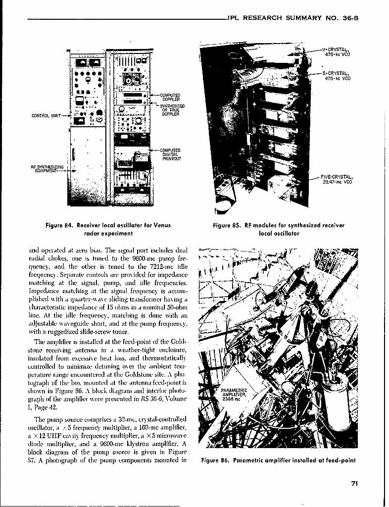
JPL RESEARCH SUMMARY NO. 36.8
V-CRYSTAL,
(- S-CRYSTAL,
-)COMPUJTED
OR TRUE
CONTROL UNIT--. DOPPLER
- DIGITALPRINTOUT
- FIVE-CRYSTAL,29.47-inc VCO
Figure 84. Receiver local oscillator for Venus Figure 85. RF modules for synthesized receiverradar experiment local oscillator
radial chokes, one is tuned to the 9600-mc pump fre- i"
any oratcd te oer bis tur n to pte 72inde idle~--.:
frequency. Separate controls are provided for impedance Vmnatching at the signal, pump, and idle frequencies. ~ ~Impedance matching at the signal frequency is accom-plished with it quarter-N~ aN c sliding transformer hia% ing acharacteristic impedance of 15 ohmis in at nominal 50-ohm rnfline. At the idle frequency, matching is clone with anladjustable waveguide short, and at the pump frequency,with a ruggedized slide-screw tuncr.
The amplifier is installed at the feed-point of the Gold-stone rccei\ ing antenna in a weather-tight enclosure,insulated from excessi~ e hecat loss, and thermostaticallycntrolled to minfimize detuning o~ ci the ambient teml-perature range encountered at the Goldstone site. A 1)110-tograph of the box. mounted at the antenna feed-point isshown in Figure 86. A hlock diagram and interior photo- PARMFER
graph of the amplifier wvere p~resented in R1 S 36-6, Volume 2388 mc
1, Page '42.
The pump source comprises at 32-mnc, cr stal-controlledoscillator, a -,5 frequency multiplier, a 160-inc amplifier,aI X 12 UIIF caN its' frequency imiltiplier, a X5 microwavediode multiplier, and a 9600-mec klystron amplifier. A jblock diagram of the pump source is giv'en in Figure87. A photograph of tile pump components mounted in Figure 86. Parametric amplifier installed at feed-point
71
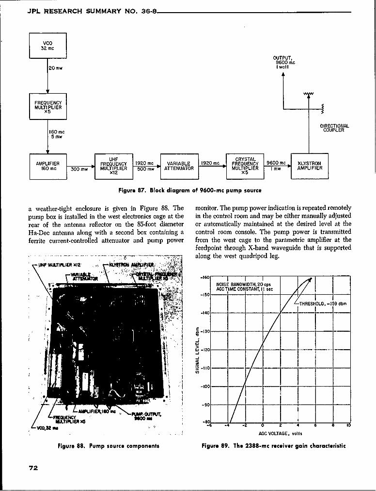
JPL RESEARCH SUMMARY NO. 36-8
vCo32 mc
OUTPUT,9600 mc
20 mw I watt
FREQUENCYMULTIPLIER
X5
DIRECTIONAL160 Mc7 COUPLER5 mw
SUHF CRYSTAL
APIFIER FREQUENCY 1920 MC VARIABLE 1920 MC FREQUENCY 9600 MC KLYSTRON1Mc 300 MW MULTIPLIER 500 mw "
ATTENUATOR MULTIPLIER I mw AMPLIFIER
EmpLx12 x5
Figure 87. Block diagram of 9600-mc pump source
a weather-tight enclosure is given in Figure 88. The monitor. The pump power indication is repeated remotelypump box is installed in the west electronics cage at the in the control room and may be either manually adjustedrear of the antenna reflector on the 85-foot diameter or automatically maintained at the desired level at theHa-Dec antenna along with a second box containing a control room console. The pump power is transmittedferrite current-controlled attenuator and pump power from the west cage to the parametric amplifier at the
feedpoint through X-band waveguide that is supportedalong the west quadripod leg.
':-160 I
NOISE BANDWIDTH, 20 cpsAGC TIME CONSTANT, II sec
. , , -150
THRESHOLD, -159 dbm
iiJ~ ~' -140'
W'-120-- -
,J-I0 .-1
z
-100-
• "" J -90-
,FIF. I se t"Kt T
-2 0 2 4 6 8 10
- - AGC VOLTAGE, volts
Figure 88. Pump source components Figure 89. The 2388-mc receiver gain characteristic
72
JPL RESEARCH SUMMARY NO. 36-8
The measured noise figure of the Goldstone parametric reasonable agreement with theoretical performance hasamplifier and following system was 3.25 db at 20-db gain, been obtained.referenced to the parametric amplifier input terminal. Preliminary gain stability checks have been made onThis indicates a noise temperature of 3220K. The band- the parametric amplifier. The gain drift measured 0.2 db
width is 5 mc. A space path receiver sensitivity curve teprmti mlfe.Tegi rf esrd02dover a 15-minute period while the antenna was orientedwas made using the parametric amplifier as the principal in various positions. Less than 0.5-db gain drift waslow-noise amplifier. The results are given in Figure 89. observed over a 45-minute period. It is anticipated that
periodic checks of gain and noise figure will be madeIt is noted that threshold of -159 dbm was obtained, during the Venus experiment as frequently as operational
Assuming an antenna temperature of 150K, an input experience proves to be desirable. The noise figure testcable loss of 0.5 db, and a RF loop noise bandwidth of equipment installed for the maser amplifier will be used20 cps, the theoretical threshold is -160 dbm; therefore, for this purpose.
73

JPL RESEARCH SUMMARY NO. 36-8
PHYSICAL SCIENCES DIVISION
\V. Chemistry Research
A. Hgh-esoltio Nucearelectron-couipled nuclear spin-spin interactions arc trans-A. Hgh-R soltiontiucearmittedi by the b~onding electrons in molecules in such aM~agnetic Resonance manner that they are not averaged to zero by the tutu-
Spectrocopy hung of the molecuiles in a liquid, gas, or solution. ThisS pecrosc ~)Ispin-spin coupling is thc mnain cause of the great coin-
D. D. Elleman and S. L. Manatt plexity of the NNM1I spcctra of molecuiles containing asfew as three or four magnetic nuclei. TIhis coupling isdescribed in terms of coup~ling constants andl is field
The theory of nuclear mnagnetic resonance (NM B) is independent. The termn Iigh-rcsoluiion NMII spect roscopywvell known (llefs 55 to 57). Since no previous stuioi Ol is generally applied to nuclear resonance e~perimentshigh-resolution NNMII spectroscopy have been given i'n which permit resolution ain( measurement of the chemini-these suimmaries, a, brief outline of the imp~ortant effects cal shifts and spin-spin coupling constants in a miolecule.is given hiere. InI a magnetic field there are three lprin-Cipall factor's Which determine the magnetic em~ironinent The hligh-resolution NMR1 invest igat ions niow in prog-of it nucleus ha' ing a nom-izero nuclear magnetic ress are concerned Nvitli (1) the (letcrmnination of struc-mloment. These are (1) the magnetic dipole interactions, tural formulas, (2) the interpretation in (detail of tlhe(2) the imagnetic shielding b) the orbital elctron01s, and spectra, including numerical e~ aluation of chemical(3) thle CILetron-coulpled nutclear spill-spin interactions. shifts and coupling constants and the relation of theseInI liquids and gases, \ hlure thle mlolecuiles are undergoing to molecular structure and s> mnnetr) , (T) thme (eterifi-verN rapid i aidom motion, tile magnetic (dipole interac- nation of thle theoretical significance of thme chemicaltions. are nearl% a~ ciaged to zero in most cases so that shifts and coupling constants as related to electronicthle latter t%%o effects need o111% be considered. Ile mflag- structure of miolecules, (I) the influence of intra- andnletic shielding b% thle electrons manifests itself as an in termlolecullar interactions onl thle appeiaranlce of spectra,attenuation of thle applied mnagnetk, field, anmd tile m elati~ e (5) the use of double-resonanI ce techniquelIs fol thle Clenii-magnitudle of this attenuiation is referred to as thme cmenmi- nation of pioton spill-spin couipling, (6) thme NNIR spectracal shift. Chemical shift is directl\ proportional to field of elements othemr than hydrogeni, anmd (7) thme improve-strength. Thle dhie al shift can be rela ted to local nient of NM 11 instrumentation. Some resuilts front wv-chemilical em~ ironmilent and to local electron denlsit% . The eral of these inmcstigattions are briefly (described lure.
74
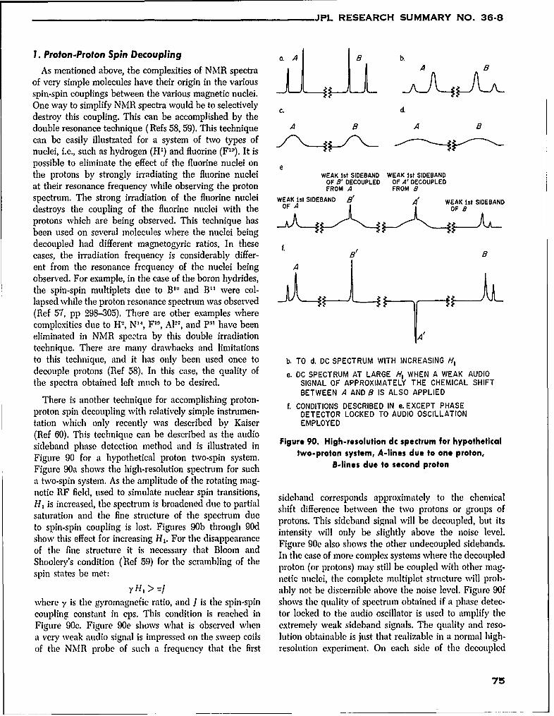
JPL RESEARCH SUMMARY NO. 36-8
1. Proton-Proton Spin Decoupling ~.A 8 b.
As mentioned above, the complexities of NMR spectra A B
of very simple molecules have their origin in the variousspin-spin couplings between the various magnetic nuclei.
One way to simplify NMR spectra would be to selectivelydestroy this coupling. This can be accomplished by thedouble resonance technique (Refs 58, 59). This technique A B A B
can be easily illustrated for a system of two types of ,"._,::/Nnuclei, i.e., such as hydrogen (H') and fluorine (F19). It is .
possible to eliminate the effect of the fluorine nuclei onthe protons by strongly irradiating the fluorine nuclei WEAK 1st SIDEBAND WEAK 1st SIDEBAND
OF 8' DECOUPLED OF A' DECOUPLEDat their resonance frequency while observing the proton FROM A FROM Bspectrum. The strong irradiation of the fluorine nuclei WEAK 1st SIDEBAND 8' A' WEAK 1st SIDEBAND
destroys the coupling of the fluorine nuclei with the OF A OF B
protons which are being observed. This technique hasbeen used on several molecules where the nuclei beingdecoupled had different magnetogyric ratios. In these tcases, the irradiation frequency is considerably differ- B Bent from the resonance frequency of the nuclei being Aobserved. For example, in the case of the boron hydrides,the spin-spin multiplets due to B1 and B1 were col-lapsed while the proton resonance spectrum was observed
(Ref 57, pp 298-305). There are other examples wherecomplexities due to H:, N14, F19, A1
27 , and P31 have beeneliminated in NMR spectra by this double irradiation Atechnique. There are many drawbacks and limitationsto this technique, and it has only been used once to b. TO d. DC SPECTRUM WITH INCREASING HI
decouple protons (Ref 58). In this case, the quality of e. DC SPECTRUM AT LARGE H, WHEN A WEAK AUDIOthe spectra obtained left much to be desired. SIGNAL OF APPROXIMATELY THE CHEMICAL SHIFT
BETWEEN A AND B IS ALSO APPLIEDThere is another technique for accomplishing proton- f. CONDITIONS DESCRIBED IN e. EXCEPT PHASE
proton spin decoupling with relatively simple instrumen- DETECTOR LOCKED TO AUDIO OSCILLATIONtation which only recently was described by Kaiser EMPLOYED(Ref 60). This technique can be described as the audiosideband phase detection method and is illustrated in Figure 90. High-resolution dc spectrum for hypotheticolFigure 90 for a hypothetical proton two-spin system. two-proton system, A-lines due to one proton,Figure 90a shows the high-resolution spectrum for such B-lines due to second protona two-spin system. As the amplitude of the rotating mag-netic RF field, used to simulate nuclear spin transitions, sideband corresponds approximately to the chemicalH, is increased, the spectrum is broadened due to partial shift difference between the two protons or groups ofsaturation and the fine structure of the spectrum due protons. This sideband signal will be decoupled, but itsto spin-spin coupling is lost. Figures 90b through 90d intensi will be de o ele vel.show this effect for increasing H,. For the disappearance intensity will only be slightly above the noise level.of the fine structure it is necessary that Bloom and Figure 90e also shows the other undecoupled sidebands.
Shoolery's condition (Ref 59) for the scrambling of the In the case of more complex systems where the decoupled
states be met: proton (or protons) may still be coupled with other mag-netic nuclei, the complete multiplet structure will prob-
, H, > v] ably not be discernible above the noise level. Figure 90fwhere -y is the gyromagnefic ratio, and J is the spin-spin shows the quality of spectrum obtained if a phase detec-coupling constant in cps. This condition is reached in tor locked to the audio oscillator is used to amplify theFigure 90c. Figure 90e shows what is observed when extremely weak sideband signals. The quality and reso-a very weak audio signal is impressed on the sweep coils lution obtainable is just that realizable in a normal high-of the NMR probe of such a frequency that the first resolution experiment. On each side of the decoupled
75
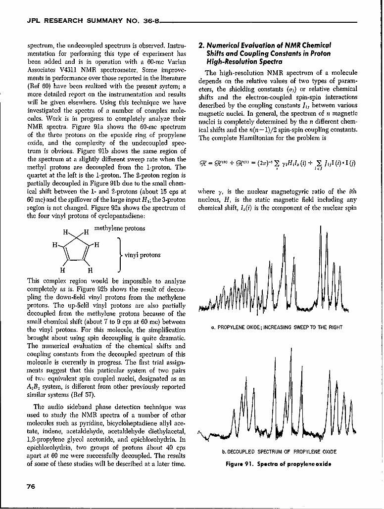
JPL RESEARCH SUMMARY NO. 36-8
spectrum, the undecoupled spectrum is observed. Instru- 2. Numerical Evaluation of NMR Chemicalmentation for performing this type of experiment has Shifts and Coupling Constants in Protonbeen added and is in operation with a 60-me Varian High-Resolution SpectraAssociates V4311 NMR spectrometer. Some improve- The high-resolution NMR spectrum of a moleculements in performance over those reported in the literature depends on the relative values of two types of param-(Ref 60) have been realized with the present system; a eters, the shielding constants (aj) or relative chemicalmore detailed report on the instrumentation and results shifts and the electron-coupled spin-spin interactionswill be given elsewhere. Using this technique we have described by the coupling constants 1, between variousinvestigated the spectra of a number of complex mole- magnetic nuclei. In general, the spectrum of n magneticcules. Work is in progress to completely analyze their nuclei is completely determined by the n different chem-NMR spectra. Figure 91a shows the 60-me spectrum ical shifts and the n(n- 1)/2 spin-spin coupling constants.of the three protons on the epoxide ring of propylene The complete Hamiltonian for the problem isoxide, and the complexity of the undecoupled spec-trum is obvious. Figure 91b shows the same region ofthe spectrum at a slightly different sweep rate when the 9? = go) + = ()-7,H yHjL (i) + .. JjI (i) 1(Imethyl protons are decoupled from the 1-proton. Thequartet at the left is the 1-proton. The 2-proton region ispartially decoupled in Figure 91b due to the small chem-ical shift between the 1- and 2-protons (about 15 cps at where 7, is the nuclear magnetogyric ratio of the ith60 mc) and the spillover of the large input HI; the 3-proton nucleus, H, is the static magnetic field including anyregion is not changed. Figure 92a shows the spectrum of chemical shift, 1.(i) is the component of the nuclear spinthe four vinyl protons of cyclopentadiene:
H H methylene protons
H H 1I vinyl protons
H H JThis complex region would be impossible to analyzecompletely as is. Figure 92b shows the result of decou-pling the down-field vinyl protons from the methyleneprotons. The up-fiel vinyl protons are also partially L )decoupled from the methylene protons because of thesmall chemical shift (about 7 to 9 cps at 60 me) betweenthe vinyl protons. For this molecule, the simplification a. PROPYLENE OXIDE;INCREASING SWEEPTO THE RIGHTbrought about using spin decoupling is quite dramatic.The numerical evaluation of the chemical shifts andcoupling constants from the decoupled spectrum of thismolecule is currently in progress. The first trial assign-ments suggest that this particular system of two pairsof tw', equivalent spin coupled nuclei, designated as anA.B.. system, is different from other previously reportedsimilar systems (Ref 57).
The audio sideband phase detection technique wasused to study the NMR spectra of a number of othermolecules such as pyridine, bicycloheptadiene allyl ace-tate, indene, acetaldehyde, acetaldehyde diethylacetal,1,2-propylene glycol acetonide, and epichlorohydrin. Inepichlorohydrin, two groups of protons dbout 40 cps b. DECOUPLED SPECTRUM OF PROPYLENE OXIDEapart at 60 me were successfully decoupled. The resultsof some of these studies will be described at a later time. Figure 91. Spectra of propyleneoxide
76
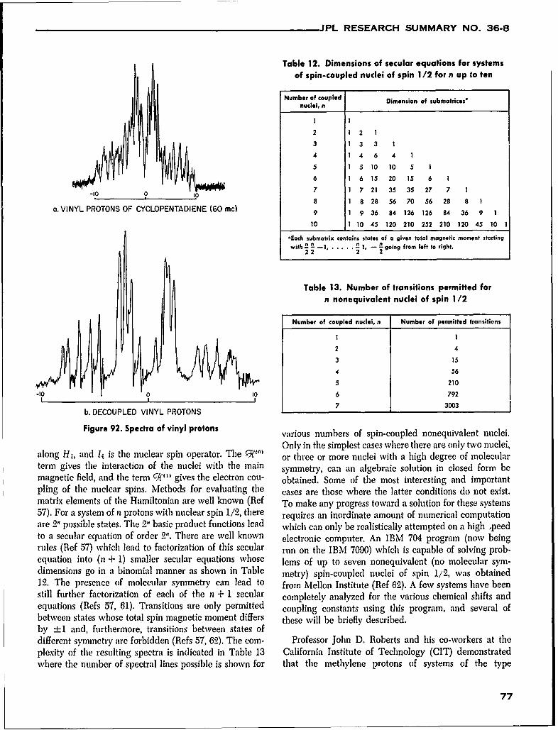
JPL RESEARCH SUMMARY NO. 36-8
Table 12. Dimensions of secular equations for systemsof spin-coupled nuclei of spin 1/2 for n up to ten
Number of coupled Dimension of submatrices'nuclei, n
2 12 1
3 1 33 1
4 1 4 6 4 1
5 1 5 10 10 5 1
6 1 6 15 20 15 6 1
-10 0 7 1 7 21 35 35 27 7 1
8 1 8 28 56 70 56 28 8 1a. VINYL PROTONS OF CYCLOPENTADIENE (60 mc) 9 1 9 36 84 126 126 84 36 9 1
10 1 10 45 120 210 252 210 120 45 10 1
-Each submatrix contains states of a given total magnetic moment starting
with 2 !L-i. 1, - n going from left to right.22 2 2
Table 13. Number of transitions permitted forn nonequivalent nuclei of spin 1/2
Number of coupled nuclei, n Number of permitted transitions
2 4
3 15
4 56
5 210
-10 0 0 6 7927 3003
b. DECOUPLED VINYL PROTONS
Figure 92. Spectra of vinyl protons various numbers of spin-coupled nonequivalent nuclei.
Only in the simplest cases where there are only two nuclei,along HI, and Ij is the nuclear spin operator. The ¢Rf') or three or more nuclei with a high degree of molecularterm gives the interaction of the nuclei with the main symmetry, can an algebraic solution in closed form bemagnetic field, and the term C- ) gives the electron cou- obtained. Some of the most interesting and importantpling of the nuclear spins. Methods for evaluating the cases are those where the latter conditions do not exist.matrix elements of the Hamiltonian are well known (Ref To make any progress toward a solution for these systems57). For a system of n protons with nuclear spin 1/2, there requires an inordinate amount of numerical computationare 2n possible states. The 2" basic product functions lead which can only be realistically attempted on a high ,peedto a secular equation of order 2". There are well known electronic computer. An IBM 704 program (now beingrules (Ref 57) which lead to factorization of this secular run on the IBM 7090) which is capable of solving prob-equation into (n + 1) smaller secular equations whose lems of up to seven nonequivalent (no molecular sym-dimensions go in a binomial manner as shown in Table metry) spin-coupled nuclei of spin 1/2, was obtained12. The presence of molecular symmetry can lead to from Mellon Institute (Ref 62). A few systems have beenstill further factorization of each of the n + 1 secular completely analyzed for the various chemical shifts andequations (Refs 57, 61). Transitions are only permitted coupling constants using this program, and several ofbetween states whose total spin magnetic moment differs these will be briefly described.by -. 1 and, furthermore, transitions between states ofdifferent symmetry are forbidden (Refs 57, 62). The corn- Professor John D. Roberts and his co-workers at theplexity of the resulting spectra is indicated in Table 13 California Institute of Technology (CIT) demonstratedwhere the number of spectral lines possible is shown for that the methylene protons of systems of the type
77
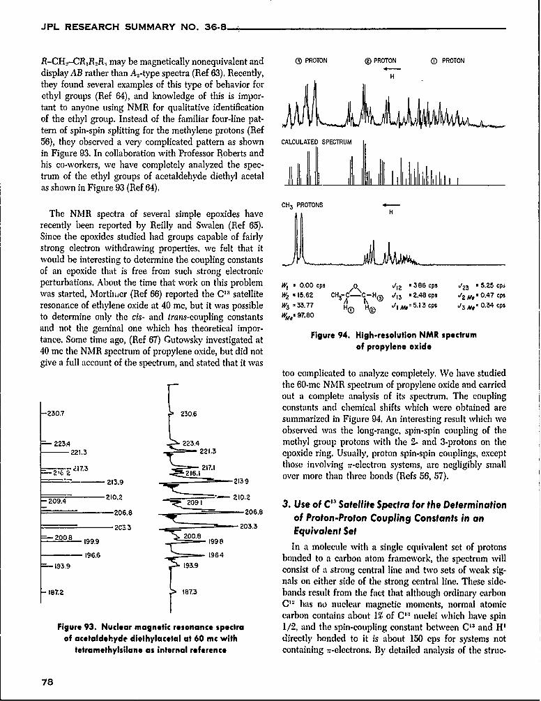
JPL RESEARCH SUMMARY NO. 36-8
R-CH.-CR&R., may be magnetically nonequivalent and (® PROTON ( PROTON ® PROTON
display AB rather than A2-type spectra (Ref 63). Recently, Hthey found several examples of this type of behavior forethyl groups (Ref 64), and knowledge of this is impor-tant to anyone using NMR for qualitative identificationof the ethyl group. Instead of the familiar four-line pat-tern of spin-spin splitting for the methylene protons (Ref56), they observed a very complicated pattern as shown CALCULATED SPECTRUM
in Figure 93. In collaboration with Professor Roberts andhis co-workers, we have completely analyzed the spec-trum of the ethyl groups of acetaldehyde diethyl acetalas shown in Figure 93 (Ref 64).
CH3 PROTONS 4
The NMR spectra of several simple epoxides have CH P
recently been reported by Reilly and Swalen (Ref 65).Since the epoxides studied had groups capable of fairlystrong electron withdrawing properties, we felt that itwould be interesting to determine the coupling constantsof an epoxide that is free from such strong electronicperturbations. About the time that work on this problem w, 0.00 cps "0 /12 386 cps "23 - 5.25 cpswas started, Mortinier (Ref 66) reported the C"' satellite w2 - 15.62 CHS-,?C jH® j3 " 2,48 cps W2 M, 0.47 cps
resonance of ethylene oxide at 40 mc, but it was possible W3 - 33.77 Ho H /I Me' 5.13 cps '3 Me' 0.34 cps
to determine only the cis- and trans-coupling constants Wf 97.80
and not the geminal one which has theoretical impor- Figure 94. High-resolution NMR spectrumtance. Some time ago, (Ref 67) Cutowsky investigated at of prolen oxide40 me the NMR spectrum of propylene oxide, but did not of propylene oxidegive a full account of the spectrum, and stated that it was
too complicated to analyze completely. We have studiedthe 60-mc NMR spectrum of propylene oxide and carriedout a complete analysis of its spectrum. The couplingconstants and chemical shifts which were obtained are
230,7 230,6 summarized in Figure 94. An interesting result which weobserved was the long-range, spin-spin coupling of the
2234 223.4 methyl group protons with the 2- and 3-protons on the22L,3 221,3 epoxide ring. Usually, proton spin-spin couplings, except
2 .271 those involving r-electron systems, are negligibly small26_i213.9 2161 2139 over more than three bonds (Refs 56, 57).
2102 '- ,,, 210.2
-209.4 2 3. Use of C'3 Satellite Spectra for the Determination206.8 206.8 of Proton-Proton Coupling Constants in an2C33 200.8 - 203.3 Equivalent Set
2008 199.9 1998 In a molecule with a single equivalent set of protons196,6 1964 bonded to a carbon atom framework, the spectrum will
-- 193.9 I 19.9 consist of a strong central line and two sets of weak sig-
nals on either side of the strong central line. These side-187.2 187.3 bands result from the fact that although ordinary carbon
C' has no nuclear magnetic moments, normal atomiccarbon contains al)out 1% of Ca:3 nuclei which have spin
Figure 93. Nuclear magnetic resonance spectra 1/2, and the spin-coupling constant between C13 and H'of acetaldehyde diethylacetal at 60 mc with directly bonded to it is about 150 cps for systems not
tetramethylsilane as internal reference containing --electrons. By detailed analysis of the struc-
78
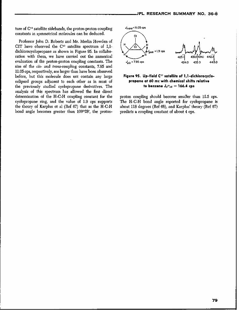
,JPL RESEARCH SUMMARY NO. 36-8
ture of C13 satellite sidebands, the proton-proton coupling rt, ons 0 = 11o5 cps
constants in symmetrical molecules can be deduced.
Professor John D. Roberts and Mr. Merlin Howden of H,CIT have observed the C13 satellite spectrum of 1,1- H H 4dichlorocyclopropane as shown in Figure 95. In collabo- H/ -- H gem 1.9 cps
ration with them, we have carried out the numerical P...A423.11 431.014.1 442.11evaluation of the proton-proton coupling constants. The Ji, 7.95 cps 424.0 4333 443.0size of the cis- and trans-coupling constants, 7.95 and11.05 cps, respectively, are larger than have been observedbefore, but this molecule does not contain any large Figure 95. Up-field C13 satellite of 1,1-dichlorocyclo-eclipsed groups adjacent to each other as in most of propane at 60 mc with chemical shifts relativethe previously studied cyclopropane derivatives. The to benzene JC'l.H = 166.4 cpsanalysis of this spectrum has allowed the first directdetermination of the H-C-H coupling constant for the proton coupling should become smaller than 12.5 cps.cyclopropane ring, and the value of 1.9 cps supports The H-C-H bond angle reported for cyclopropane isthe theory of Karplus et al (Ref 67) that as the H-CJ-I about 118 degrees (Ref 68), and Karplus' theory (Ref 67)bond angle becomes greater than 1090281, the proton- predicts a coupling constant of about 4 cps.
79
JPL RESEARCH SUMMARY NO. 36-8
Vi. Physics Research
A. Fission Electric Cells section supported by quartz rods from the outer cylinder.A portion of the inner cylinder supports the fissionable
W. F. Krieve material and serves as the cathode. A solenoid surroundsthe capsule and will be the source of the magnetic fieldfor suppression of the 8- or follow-out electrons that
1. Capsule Irradiation accompany the fission fragments. The shape of the anode,An experiment has been designed to determine the cathode, and magnetic field has been contoured so that
acceptability of fission electric cell fuel elements (RS 36-4) fragments that do not reach the anode will be interceptedthat have been fabricated. / various techniques. Accept- by the cathode in regions where the magnetic field isability of sample fuel elements, which are essentially perpendicular to the electrostatic field and the magneticthin layers (3.0 to 10.0 mg/cm-) of fissionable material field is of sufficient magnitude to suppress the secondaryon suitable base materials, will be determined by follow- electrons produced.ing their operating characteristics during irradiation in a The outer shell of the capsule has a 2.00-inch diameter,high-density neutron flux, and by post-irradiation analy- and the inner cylinder has a 0.50-inch diameter except insis. Maximum neutron flux intensities that can be toler- regions that are expanded for fragment interception.ated in a typical experiment of this type are available Total capsule length is 9.0 inches. The fuel layer is depos-in the pool region of a pool research reactor of the MTR ited in the central 3-inch section of the inner cylindercategory. Space limitations and environmental conditions and has a surface area of 30.4 cm 2. Nominal wall thick-in the pool irradiation area have determined the size, nesses are 0.025 inch, and the material, 6061-T6 alumi.shape, and structural material of the fuel element or num. The anode is 1.50 inches in diameter (except incapsule and, consequently, the magnitude of the cur- contracted regions), is 6.10 inches long, and is 0.002 inchrents that are to be measured. thick. Anode material is nickel. Aluminum wire is used
a. Capsule structure. The capsule is formed by a pair for the coil which is canned in an aluminum containerof concentric cylinders with the inner space hermetically that has an ID of 2.16 inches, an ODof 2.685 inches, andsealed and evacuated; it contains a cylindrical anode a length of 9.5 inches.
80
JPL RESEARCH SUMMARY NO. 36-8
An ion pump will be attached to the first capsule, at will be: fission fragment current, i.e., current with mag-least, to help maintain the vacuum and to determine if netic field, +10 to +20 jtamp; 8-electron current, i.e.,an ion pump will function when located in an intense current without electron suppression, -100 to -200field of ionizing radiation. The pump and electrical ter- 1xamp; background current due to Compton electronsminals are sealed in a container that is attached to the and beta rays, -0.1 to -0.5 jamp; and leakage current,capsule and coil housing. Electrical leads are strung -0.5 to +0.5 juamp. The maximum design potential ofthrough an aluminum tube that extends from the pump the capsule is 5 kv.housing to the pool surface. This distance is approxi- Following the irradiation and a cooling period, themately 26 feet. capsules will be transferred to a hot cell where they will
An attempt has been made to minimize the net current be machined open to allow visual and analytical inspec-
loss through lead wire insulation and terminal insulators. tion. Spatial distribution of several of the fragment
Materials and mass ratios between conductors, ground- species typifying both the heavy and light group willing shield, and insulation have been selected so that the be determined on the anode and cathode by gammacurrent flow o l electrons produced by Compton inter- count analysis. The ratio of the number of several species
actions will be reverse to and of the same magnitude of fragments betoeen the anode and cathode will beas the current flow due to the conductance of the insu- determined via both gamma spectroscopy and chemicallation in the ionizing radiation. Background currents have analysis. The amount of fissionable material transferredbeen minimized by the use of low-density, low-radiative- from the cathode to anode will be measured by chemical
capture neutron cross section material that is compatible analysis. Results of these examinations will not only give
with the environment, and by the use of the thin anode. information about the operating characteristics of a fuel
This gives a low production rate of high-energy electrons element, but also energy, charge, and range distribution
and beta rays in the structural material and a low prob- of fission fragments.
ability that these particles will be stopped in the anode. A capsule utilizing an electrostatic grid to suppressthe 8-electrons is being designed. This capsule will be
b. Experimental procedure. Expected currents from used to determine the feasibility of 8-electron suppressionthe capsules with various amounts of fissionable material via a grid as well as fuel element analysis.
81
JPL RESEARCH SUMMARY NO. 36-8
Vii. Gas Dynamics Research
A. Stability of a Shear Layer When a sphere travels at supersonic speeds, a shockwave is formed close to the front surface, and by con-
in a Magnetic Field fining ourselves to the region close to the stagnationpoint, the shock wave can be taken to a good approxi-
J. Menkes mation as spherical and concentric with the sphere.We will assume that close to the stagnation point, con-
It is demonstrated that a uniform magnetic field in a ditions at the outer edge of the boundary layer cor-direction normal to the mean flow has a stabilizing influ- respond to those immediately behind the shock. Also,ence. A disturbance which propagates with fixed maxi- the temperature of the surface T,, is assumed to bemum amplitude in the absence of a magnetic field is constant.shown to be damped once the field is applied. The degree A similarity type solution is obtained for the compres-of damping is proportional to the Alfv6n speed. This sible boundary layer with heat transfer and pressureconfirms a result obtained earlier by Stuart (Ref 69) for sralenboundaryelayer w it e tima s aressethe case where the magnetic field is aligned with the gradient, and the order of magnitude estimates are thosemean flow. For the case of infinite conductivity, the flow appropriate to the stagnation region of a sphere ofis absolutely stable for arbitrarily small magnetic fields. radius a.
1. Basic EquationsThe equation of state for a perfect gas is
B. Similarity Solution for Stagna- P=pRT ()
tion Point Heat Transfer in Low- where P is the pressure, p is the density, R is the gas
Density, High-Speed Flow constant, and T is the temperature. The Prandtl number,= ttC 1./K, is taken to be a constant. A spherical system
M. Chahine of coordinates (r, 0, ,) is used as shown in Figure 96;
however, since the body is axisymmetric, the velocityThe problem considered is that of estimating skin component in the 0, direction is equal to zero, and sub-
friction and heat transfer to a spherical body at super- scripts oo and 1 denote conditions ahead of and behindsonic speeds and under rarefied gas conditions. the shock wave. In accordance with the oblique shock
82

JPL RESEARCH SUMMARY NO. 36-8
relation, the tangential velocity behind the shock v, is and the effect of compressibility is made less marked byrelated to conditions ahead of the shock by the relation choosing a Howarth variable
v,= U sin0 (2) (2U .)3 pds (6)
Subject to the conditions stated above, we now seeka solution for the steady axisymmetric compressible lam- Substituting Equations (2), (3), (4), and (5) into theinar boundary layer equation for perfect fluids. We momentum and energy equations and reducing the resultsassume that the dependent variables have the forms to the stagnation region, taking into account that the tem-
perature T (r, 6) is an even function symmetric withv=v (r) cos 6 respect to 0 = 0, the final results read
tV0 = u (r) sin 6 8 j~-g10 U i 0 3PP, (3) g= o+fgf (7)
:u =p (r) cos 0 where
P, = constantT =P_.
with the pressure variation behind the shock given by g = p
y = ,UL sin 0 cos 0 (4) Since f and g are not a function of the standoff distance
of the shock wave, the boundary conditions at the outer
and edge of the boundary layer, i.e., conditions at the shock,
2 =P will be taken at infinity, or
ao ao f () = N(O) 0 g(o)=-
The continuity equation P,(oo)1 g(oo)= 1
a 1 + (sin 6) This equation was first given by V. M. Falkner and S. W."r a sin' 0 = Skan, and its solutions were studied in detail by C. B.
Cohen and E. Reshotko (Ref 70). From these solutions,the variations of the shear function at the wall f' (0) with
and the boundary condition at the shock are satisfied by respect to the heat transfer function g can easily becomputed.
P= - (,AU-)j (n!) (5) The shear function f" (0) is related to the shear stressof the wall T through the expression
SHOCK- WAV - I diA___ ..
SHOCK WAVE 7 '7/,=- = a /" (0) sin* 8 cos 0 (8)
V The value of the skin friction drag coefficient is thenobtained by integrating the axial projection of T over thefront surface of the sphere. The resulting relation is
c, 8 Re P , (0) sin 0 cos 0 dO (9)
' ER where the upper limit of integration 6, is determined.. .... experimentally from the unheated case T, = T, by match-
ing the theoretical curve with the experimental points,as shown in Figure 97, and by taking the experimental
__ value of the pressure drag coefficient to be 1, or
Figure 96. Coordinate system on sphere in + 9 (P,/P.)% P ( (10)hypersonic flow 8 Re e
83
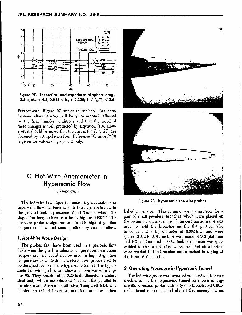
JPL RESEARCH SUMMARY NO. 36-8
2.4 T
_ _ __ __
22 0 =26EXPERIMENTAL A =22
RESULTS 0= 1620 [ * 1 0
THEORETICAL {714I5
1..0
Re,
Figure 97. Theoretical and experimental sphere drag,3.8 < M.o < 4.3; 0.013 < K, < 0.200; 1 < T,ITI < 2.6 ,
Furthermore, Figure 97 serves to indicate that aero-dynamic characteristics will be quite seriously affectedby the heat transfer conditions and that the trend ofthese changes is well predicted by Equation (10). How-ever, it should be noted that the curves for T,, > 2T, are
obtained by extrapolation from Reference 70, since " (0)is given for values of gup to 2 only.
C. Hot-Wire Anemometer inHypersonic Flow
T. Vrebalovich
The hot-wire technique for measuring fluctuations in Figure 98. Hypersonic hot-wire probessupersonic flow has been extended to hypersonic flow inthe JPL 21-inch Hypersonic Wind Tunnel where the baked in an oven. This ceramic was an insulator for astagnation temperatures can be as high as 1400 0F. The pair of small jewelers' broaches which were placed onhot-wire probe design for use in this high stagnation the ceramic coat, and more of the ceramic adhesive wastemperature flow and some preliminary results follov. used to hold the broaches on the flat portion. The
broaches had a tip diameter of 0.002 inch and were
1. Hot-Wire Probe Design spaced 0.012 to 0.015 inch. A wire made of 90% platinumand 10% rhodium and 0.00005 inch in diameter was spot-
The probes that have been used in supersonic flow welded to the broach tips. Glass insulated nickel wiresfields were designed to tolerate temperatures near room were welded to the broaches and attached to a plug attemperature and could not be used in high stagnation the base of the probe.temperature flow fields. Therefore, new probes had tobe designed for use in the hypersonic tunnel. The hyper-sonic hot-wire probes are shown in two views in Fig- 2. Operating Procedure in Hypersonic Tunnelure 98. They consist of a 0.25-inch diameter stainless The hot-wire probe was mounted on a vertical traversesteel body with a nosepiece which has a flat parallel to mechanism in the hypersonic tunnel as shown in Fig-the air stream. A ceramic adhesive, Temporell 1604, was ore 99. A second probe with only one broach had 0.001-painted on this flat portion, and the probe was then inch diameter chromel and alumel thermocouple wires
84
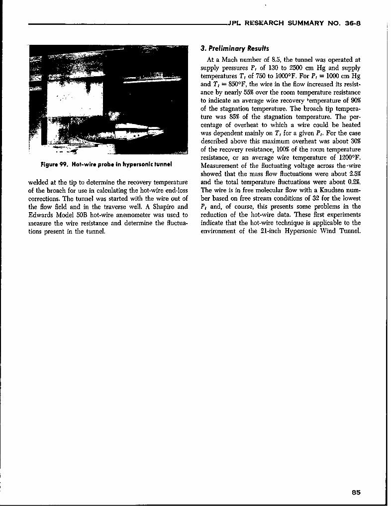
JPL RESEARCH SUMMARY NO. 36-8
3. Preliminary ResultsAt a Mach number of 8.5, the tunnel was operated at
supply pressures P, of 130 to 2500 cm Hg and supplytemperatures Tt of 750 to 10000F. For Pt = 1000 cm Hgand Tt = 8500F, the wire in the flow increased its resist-ance by nearly 55% over the room temperature resistanceto indicate an average wire recovery temperature of 90%of the stagnation temperature. The broach tip tempera-ture was 85% of the stagnation temperature. The per-centage of overheat to which a wire could be heatedwas dependent mainly on Tt for a given Pt. For the casedescribed above this maximum overheat was about 30%of the recovery resistance, 100% of the room temperatureresistance, or an average wire temperature of 12000F.
Figure 99. Hot-wire probe in hypersonic tunnel Measurement of the fluctuating voltage across the -wireshowed that the mass flow fluctuations were about 2.5%
welded at the tip to determine the recovery temperature and the total temperature fluctuations were about 0.2%.of the broach for use in calculating the hot-wire end-loss The wire is in free molecular flow with a Knudsen num-corrections. The tunnel was started with the wire out of ber based on free stream conditions of 32 for the lowestthe flow field and in the traverse well. A Shapiro and Pt and, of course, this presents some problems in theEdwards Model 50B hot-wire anemometer was used to reduction of the hot-wire data. These first experimentsmeasure the wire resistance and determine the fluctua- indicate that the hot-wire technique is applicable to thetions present in the tunnel. environment of the 21-inch Hypersonic Wind Tunnel.
85
JPL RESEARCH SUMMARY NO. 36-8
ENGINEERING MECHANICS DIVISION
ViI. Materials Research
Also presented in Table 14 are elongations for roomA. Graphite temperature tests which were obtained from a dial indi-
W. V. Kotlensky and D. B. Fischbach cator clamped to the specimen holders. Elongations ofapproximately 0.5% would be expected (assuming a mod-ulus of 3 million psi) if the strain were entirely elastic.
1. Graphite Tension Testing The difference between the expected and measured strain
Determination of tensile properties of pyrolytic graph- suggests that about 1% of the measured strain may be dueite supplied by Lockheed Missile and Space Division for to specimen seating.the purpose of noting lot-to-lot variations has been con- Reduction in area data for 5000F tensile tests for lotstinued. These tests were made in the manner previously shown in Figure 100 are given in Table 15. It is noteddescribed (RS 36-3, 36-7). that there is a greater reduction in thickness (perpendicu-
Tensile data from five lots of pyrolytic graphite pro- lar to the basal planes) than in width (parallel to the basaldue'd by three different manufacturers are presented in planes) and that the greater the recorded elongation, theTable 14. The ultimate tensile strengths and elongations greater the reduction in area.for these lots are not markedly different from the datafor Lots 158, 159, and 160 previously given (RS 36-7). A study of the effect of hot-working pyrolytic graphiteThe relatively low strengths for Specimens 3003, 3006, on its tensile strength (reported in RS 36.7) has also con-3017, 3028,and 3200 may be attributed to either a notch tinued. These data, which are presented in Table 16,effect caused by nicks along the edges of the gage section show that prestraining at 5000i F and testing at loweror fracture at large growth cones. Because of the limited temperatures definitely increases the tensile strength ofnumber of tests, no definite conclusions on the variations pyrolytic graphite and that the amount of increase inin tensile poperties from lot-to-lot are apparent. strength is dependent upon the amount of hot-working.
An examination of the microstructures (Fig 100) reveals A typical engineering stress-strain curve recorded dur-
little difference, except for Lot 175 which shows a more ing the straining at 5000 0F, as well as during the testingregenerative structure. The relationship between the at 40000F, is shown in Figure 101.
microstructure and tensile properties for these eight lots Earlier data (RS 36-3, 36-4, 36-5) showed changes(Table 14 and RS 36-7) is being studied. in X-ray structure and microstructure when pyrolytic
86
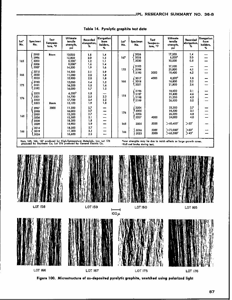
JPL RESEARCH SUMMARY NO. 36-8
Table 14. Pyrolytic graphite test data
Ultimate Elongation Ultimate Recordd ElongationLot Specimen t ensile Recorded o Lot' Specimen tensile fromTempera- elongation, Tempera- elongation,
strength, % holders, No. No. tue, F strength, % holders,No. No. ture, %F
2995 Room 10,000 1.8 1.4 (3026 17,200 1.4 -
2996 12,800 2.0 1.5 167 3028 8,500' 2.0 -
165 3003 5,200' 1.2 1.1 , 3030 10,500 0.5 -
3006 9 ,00 0b 1.6 1.4 3193 17,100 - -
3007 14,300 1.9 1.6 175 13194 21,000 4.1 -
(3015 14,100 2.1 1.9 (3195 3000 19,400 4.2 -
166 3020 11,000 2.0 1.83025 10,900 2.0 1.8 (3017 4000 8,200' 1.8 -
3190 15,000 1.4 1.2 166 3018 16,800 3.2 -
175 3 91 16,300 1.8 1.6 13021 21,800 2.6 -
3192 16,000 1.7 1.5 3196 18,900 3.1 -(3200 6 ,300' 1.8 - 3197 21,800 4.6 -
17 3201 14,700 2.5 2.3 175 3198 21,200 4.5 -176 3202 17,700 2.4 2.2 j3 1 9 9 26,100 5.0 -
(3203 Room 12,100 1.9 1.8
2997 3000 11,200 2.7 - (3204 22,300 3.7 -
2998 16,000 3.7 - 7 3205 18,500 3.1 -
2999 13,300 2.7 - 176 3206 26,300 4.8 -165 3004 12,500 2.1 - (3207 4000 24,000 4.0 -
3008 18,200 1.8 -
3009 14,900 1.9 - 165 3005 5000 >60,400' >32' -
(3014 18,200 2.7 -
166 (3019 11,300 2.1 - 166 3016 5000 >72,000 >50 -
f3024 16,600 2.3 13023 5000 >63,500t > 4 3r
'Lots 165, 166, 167 produced by High.Temperature Materials, Inc; Lot 175 bLow strengths may be due to notch effects or large growth cones.produced by Raytheon Ca; Lot 176 produced by General Electric Co. 'Pull rod broke during test.
LOT 158 LOT 159 LOT 160 LOT 165
tOO f L
LOT 166 LOT 167 LOT 175 LOT 176
Figure 100. Microstructure of as-deposited pyrolytic graphite, unetched using polarized light
87
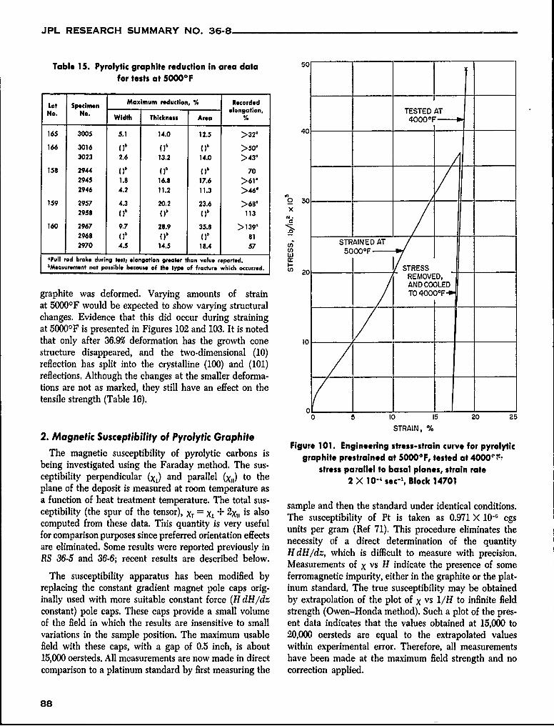
JPL RESEARCH SUMMARY NO. 36-8
Table 15. Pyrolytic graphite reduction in area data 50
for tests at 5000°F
Maximum reduction, % RecordedNo. No. elongation, TESTED ATWidth Thickness Area % 4000
0FL
165 3005 5.1 14.0 12.5 >32' 40
166 3016 () >50*3023 2.6 13.2 14.0 >43/
158 2944 )( )' ( 702945 1.8 16.8 17.6 >61'2946 4.2 11.2 11.3 >46'
159 2957 4.3 20.2 23.6 >68' 5? 30
2958 (( )' ( 113 XIV.
C160 2967 9.7 28.9 35.8 > 139*
2968 ( ( 81 -STRAINED AT2970 4.5 14.5 18.4 57 50SS 0 F
Jcn 5000OFPull rod broke during test; elongation greater than value reported. 0,I-
SMeasurement not possible because of the type of fracture which occurred. ti 20 _ STRESSU) 20REMOVED,
AND COOLED
graphite was deformed. Varying amounts of strain TO 4000OFat 5000OF would be expected to show varying structuralchanges. Evidence that this did occur during strainingat 5000F is presented in Figures 102 and 103. It is notedthat only after 36.9% deformation has the growth cone icstructure disappeared, and the two.dimensional (10)reflection has split into the crystalline (100) and (101)reflections. Although the changes at the smaller deforma-tions are not as marked, they still have an effect on thetensile strength (Table 16).
0 5 10 15 20 25
STRAIN, %2. Magnetic Susceptibility of Pyrolytic Graphite Figure 101. Engineering stress-strain curve for pyrolyticThe magnetic susceptibility of pyrolytic carbons is graphite prestralned at 5000OF, tested at 4000'F!
being investigated using the Faraday method. The sus- stress parallel to basal planes, strain rateceptibility perpendicular (X1) and parallel (X,) to the 2 X 10⁻⁴ sec-', Block 14701plane of the deposit is measured at room temperature asa function of heat treatment temperature. The total sus- sample and then the standard under identical conditions.ceptibility (the spur of the tensor), XT = x, + 2x11 is also The susceptibility of Pt is taken as 0.971 X 10⁻⁶ cgscomputed from these data. This quantity is very usefulfor comparison purposes since preferred orientation effects units per gram (Ref 71). This procedure eliminates theareeliinaed.Soe rsuls wre eprte prvioslyin necessity of a direct determination of the quantityare eliminated. Some results were reported previously in H dH/dz, which is difficult to measure with precision.RS 36-5 and 366; recent results are described below. Measurements of X vs H indicate the presence of some
The susceptibility apparatus has been modified by ferromagnetic impurity, either in the graphite or the plat-replacing the constant gradient magnet pole caps orig- inum standard. The true susceptibility may be obtainedinally used with more suitable constant force (H dH/dz by extrapolation of the plot of X vs 1/H to infinite fieldconstant) pole caps. These caps provide a small volume strength (Owen-Honda method). Such a plot of the pres-of the field in which the results are insensitive to small ent data indicates that the values obtained at 15,000 tovariations in the sample position. The maximum usable 20,000 oersteds are equal to the extrapolated valuesfield with these caps, with a gap of 0.5 inch, is about within experimental error. Therefore, all measurements15,000 oersteds. All measurements are now made in direct have been made at the maximum field strength and nocomparison to a platinum standard by first measuring the correction applied.
88
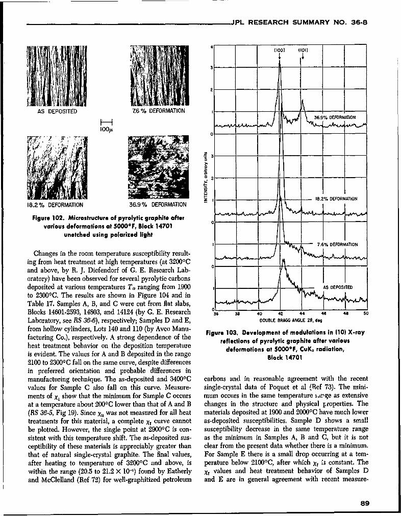
JPL RESEARCH SUMMARY NO. 36-8
S(100) (101)
1 1 I _ _
AS DEPOSITED 76 %, DEFORMATION
18.2% DEFORMATION 36.9% DEFORMATION
Figure 102. Microstructure of pyrolytic graphite after 0 -J vv
various deformations at 50000F, Block 14701unetched using polarized light
0.,. DEFORMATIONChanges in the room temperature susceptibility result-
ing from heat treatment at high temperatures (at 3200C 0and above, by R. J. Diefendorf of G. E. Research Lab-\oratory) have been observed for several pyrolytic carbons
pJ
deposited at various temperatures TL, ranging from 1900 1 AS Ds EPOSITrEDto 23000C. The results are shown in Figure 104 and inTable 17. Samples A, B, and C were cut from flat slabs,Blocks 14601-2593, 14803, and 14124 (by G. E. Research 36 30 40 42 44 46 48 50
Laboratory, see RS 36-6), respectively; Samples D and E, DOUBLE BRAGG ANGLE 28,. dog
from hollow cylinders, Lots 140 and 110 (by Avco M anu- Fg r 0 .D vl p e t o o u ai n n( 0 -afacturing Co.), respectively. A strong dependence of the Fgreflcin of3 Developet graphitelatern vious0 Xrheat treatment behavior on the deposition temperature deformations at 50000F, CuKa radiation,is evident. The values for A and B deposited in the range Block 147012100 to 23000C fall on the same curve, despite differencesin preferred orientation and probable differences inmanufacturing technique. The as-deposited and 34000C carbons and in reasonable agreement with the recentvalues for Sample C also fall on this curve. Measure- single-crystal data of Poquet et al 1(Ref 73). The mini-ments of X, show that the minimum for Sample C occurs mum occurs in the same temperature iarge as extensiveat a temperature about 2000C lower than that of A and B changes in the structure and physical p.roperties. The(RS 36-5, Fig 19). Since X,1 was not measured for all beat materials deposited at 1900 and 20000C have much lowertreatments for this material, a complete X, curve cannot as-deposited susceptibilities, Sample D shows a st-allsbe plotted. However, the single point at 29000C is con- susceptibility decrease in the same temperature rangesistent with this temperature shift. The as-deposited sus- as the minimum in Samples A, B and C, but it is notceptibility of these materials is appreciably greater than clear from the present data whether there is a minimum.that of natural single-crystal graphite. The final values, For Sample E there is a small drop occurring at a tern-after heating to temperature of 32000C and above, is perature below 21000C, after which XT is constant. Thewithin the range (20.5 to 21.2 X 10-"1) found by Eatherly XT values and heat treatment behavior of Samples Dand McClelland (Ref '7) for well-graphitized petroleum and E are in general agreement with recent measure-
89
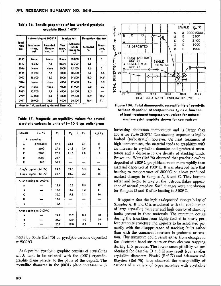
JPL RESEARCH SUMMARY NO. 36-8
Table 16. Tensile properties of hot-worked pyrolytic E SAMPLE r .Cgraphite Block 14701a 0
428_- 0 A 2200-2300J " I - I --. o A B 2100
Hot-working at 5000*F Tension test Elongation after test
Speci-. Ultimate A D 200men Maximum Recorded Test tensile Recorded, Meas- L AS DEPOSITEDNo. stress, Elonga- temp, si R ured, A
psi tion, % O strength, % % 24I X3045 None None Room 10,000 2.8 0 >* + GUHA AND ROY
2993 18,080 7.6 Room 22,700 8.8 - + POQUET et al CRYSTAL2990 .6 Rom 22700 I 8.8 - F0 REF 73 I r3046 None None 3000 15,500 1.6 0 I. -2985 15,200 7.6 3000 20,400 8.2 6.5 20 0
2993 35,500 18.2 3000 34,500 18.0 14.5
3044 None None 4000 12,600 2.4 0.3 _j._l
2992 None None 4000 14.90 2.0 0.72983 13,700 7.7 4000 24,100 8.5 - I-16 _
298 1,70 I 7. 4ao 4,oo I 8. IRT 1800 2200 2600 3000 3400
2989 37,000 18.2 4000 49,100 18.9 12.7 H A 1E0N 2200 20HEAT TREATMENT TEMPERATURE, -C2991 59,000 1 36.9 4000 56,100 36.4 41.1
-From Lot 147, produced by General Electric Co. Figure 104. Total diamagnetic susceptibility of pyrolyticcarbons deposited at temperatures TD as a function
of heat treatment temperature, values for naturalTable 17. Magnetic susceptibility values for several single-crystal graphite shown for comparisonpyrolytic carbons in units of (-10-6) cgs units/gram
increasing deposition temperature and is larger thanSample TD, *C XT X_ X, x_/x, 100 A for To i 21000C. The stacking sequence is highly
As deposited faulted (turbostratic), however. On heat treatment atA 2200.2300 27.6 23.4 2.1 11 high temperatures, the material tends to graphitize with8 2100 27.6 21.8 2.9 7 an increase in crystallite diameter and preferred orien-C 2100 27.3 21.6 2.8 8 tation and a decrease in the density of stacking faults.D 2000 20.7 - - - Brown and Watt (Ref 76) observed that pyrolytic carbonE 1900 20.2 - - - deposited at 21000C graphitized much more rapidly than
Single crystal (Ret 74) 23.0 22.0 0.5 44 material deposited at 19000C. It was observed here that
Single crystal (Ref 73) 21.7 21.0 0.3 65 heating to temperatures of 30000C or above producedmarked changes in Samples A, B and C. They became
After heating to 2900"C softer wad began to take on the lustrous, flakey appear-A - 18.1 16.2 0.9 17 ance of natural graphite. Such changes were not obviousI - 18.3 15.7 1.3 11 for Samples D and E after heating to 3100OC.C - 20.0 17.8 1.1 16
O - 18.7 - - - It appears that the high as-deposited susceptibility ofE - 19.4 - - - Samples A, B and C is associated with the combination
After heating to 3400*C of large crystallite diameter and high density of stackingA - 21.2 20.2 0.5 40 faults present in these materials. The minimum occursB - 21.0 19.0 1.0 19 during the transition from highly faulted to nearly per-C - 20.7 19.0 0.8 24 fect graphite structure and appears to be associated pri-
marily with the disappearance of stacking faults ratherthan with the concurrent increase in preferred orienta-
ments by Soule (Ref 75) on pyrolytic carbons deposited tiQn. This minimum could result either from changes inat 2000C. the electronic band structure or from electron trapping
during this process. The lower susceptibility valuesAs-deposited pyrolytic graphite consists of crystallites obtained for Samples D and E may result from smaller
which tend to be oriented with the (0001) crystallo- crystallite diameters. Pinnick (Ref 77) and Adamson andgraphic plane parellel to the plane of the deposit. The Blayden (Ref 78) have observed the susceptibility ofcrystallite diameter in the (0001) plane increases with carbons of a variety of types increases with crystallite
90
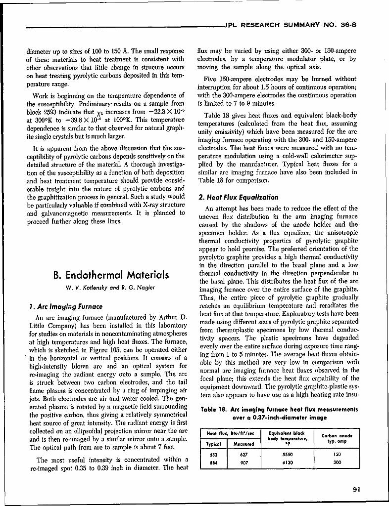
JPL RESEARCH SUMMARY NO. 36-8
diameter up to sizes of 100 to 150 A. The small response flux may be varied by using either 300- or 150-ampereof these materials to heat treatment is consistent with electrodes, by a temperature modulator plate, or byother observations that little change in strucure occurs moving the sample along the optical axis.on heat treating pyrolytic carbons deposited in this tem-peratre rnge.Five 150-ampere electrodes may be burned withoutperature range. interruption for about 1.5 hours of continuous operation;
Work is beginning on the temperature dependence of with the 300-ampere electrodes the continuous operationthe susceptibility. Preliminary- results on a sample from is limited to 7 to 9 minutes.block 2593 indicate that X1 increases from -22.3 X 10⁻⁶ Table 18 gives heat fluxes and equivalent black-bodyat 3000K to -39.8 X 10⁻⁶ at 1000K. This temperature temperatures (calculated from the heat flux, assumingdependence is similar to that observed for natural graph- unity emissivity) which have been measured for the arcite single crystals but is much larger. imaging urnace operating with the 300- and 150-ampere
It is apparent from the above discussion that the sus- electrodes. The heat fluxes were measured with no tem-ceptibility of pyrolytic carbons depends sensitively on the perature modulation using a cold-wall calorimeter sup-detailed structure of the material. A thorough investiga- plied by the manufacturer. Typical heat fluxes for ation of the susceptibility as a function of both deposition similar are imaging furnace have also been included inand heat treatment temperature should provide consid- Table 18 for comparison.erable insight into the nature of pyrolytic carbons andthe graphitization process in general. Such a study would 2. Heat Flux Equalizationbe particularly valuable if combined with X-ray structure An attempt has been made to reduce the effect of theand galvanomagnetic measurements. It is planned to uneven flux distribution in the arm imaging furnaceproceed further along these lines, caused by the shadows of the anode holder and the
specimen holder. As a flux equalizer, the anisotropicthermal conductivity properties of pyrolytic graphiteappear to hold promise. The preferred orientation of thepyrolytic graphite provides a high thermal conductivityin the direction parallel to the basal plane and a low
B. Endothermal Materials thermal conductivity in the direction perpendicular tothe basal plane. This distributes the heat flux of the are
W. V. Kotlensky and R. G. Nagler imaging furnace over the entire surface of the graphite.Thus, the entire piece of pyrolytic graphite gradually
1. Arc Imaging Furnace reaches an equilibrium temperature and reradiates the
An arc imaging furnace (manufactured by Arthur D. heat flux at that temperature. Exploratory tests have been
Little Company) has been installed in this laboratory made using different sizes of pyrolytic graphite separated
for studies on materials in noncontaminating atmospheres from thermoplastic specimens by low thermal conduc-
at high temperatures and high heat fluxes. The furnace, tivity spacers. The plastic specimens have degraded
which is sketched in Figure 105, can be operated either evenly over the entire surface during exposure time rang-
in the horizontal or vertical positions. It consists of a ing from 1 to 5 minutes. The average heat fluxes obtaii-
high-intensity blown arc and an optical system for able by this method are very low in comparison with
re-imaging the radiant energy onto a sample. The arc normal arc imaging furnace heat fluxes observed in the
is struck between two carbon electrodes, and the tail focal plane; this extends the heat flux capability of the
flame plasma is concentrated by a ring of impinging air equipment downward. The pyrolytic graphite-plastic sys-
jets. Both electrodes are air and water cooled. The gen- tem also appears to have use as a high heating rate insu-
erated plasma is rotated by a magnetic field surrounding Table 18. Arc imaging furnace heat flux measurements
the positive carbon, thus giving a relatively symmetrical over a 0.37-inch-diameter imageheat source of great intensity. The radiant energy is firstcollected on an ellipsoidal projection mirror near the arc Heat flux, Btu/lftsec Equivalent black Crbon.ande
and is then re-imaged by a similar mirror onto a sample, body temperature, Cabo and
The optical path from arc to sample is about 7 feet. Typical Measured Ftyp amp553 627 5550 i150
The most useful intensity is concentrated within a 884 97 610 I00884 907 6130 300
re-imaged spot 0.35 to 0.39 inch in diameter. The heat
91
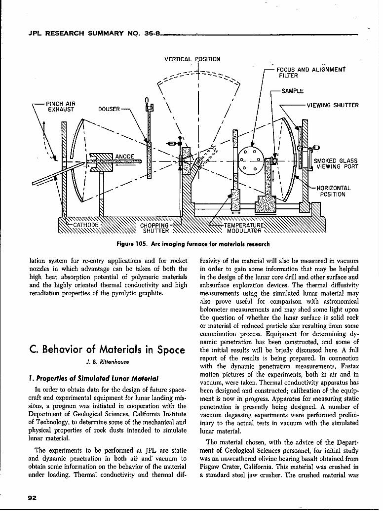
JPL RESEARCH SUMMARY NO. 36-8
VERTICAL POSITION
FOCUS AND ALIGNMENTFILTER
S-SAMPLE
EXNH ASIOUER VIEWING SHUTTER
I '
/ - -7 i0 -
IANODE Al"' 0" - SMOKED GLASS0 VIEWING PORT
,. HORIZONTAL. ,: POSITION
-CATHODETEMPERATURSHUTTER MODULATR
Figure 105. Arc imaging furnace for materials research
lation system for re-entry applications and for rocket fusivity'of the material will also be measured in vacuumnozzles in which advantage can be taken of both the in order to gain some information that may be helpfulhigh heat absorption potential of polymeric materials in the design of the lunar core drill and other surface andand the highly oriented thermal conductivity and high subsurface exploration devices. The thermal diffusivityreradiation properties of the pyrolytic graphite. measurements using the simulated lunar material may
also prove useful for comparison with astronomicalbolometer measurements and may shed some light uponthe question of whether the lunar surface is solid rockor material of reduced particle size resulting from somecomminution process. Equipment for determining dy-namic penetration has been constructed, and some of
C. Behavior of Materials in Space the initial results will be briefly discussed here. A fullJ B. Rittenhouse report of the results is being prepared. In connection
with the dynamic penetration measurements, Fastax1. Properties of Simulated Lunar Material motion pictures of the experiments, both in air and in
vacuum, were taken. Thermal conductivity apparatus hasIn order to obtain data for the design of future space- been designed and constructed; calibration of the equip-
craft and experimental equipment for lunar landing mis- ment is now in progress. Apparatus for measuring staticsions, a program was initiated in cooperation with the penetration is presently being designed. A number ofDepartment of Geological Sciences, California Institute vacuum degassing experiments were performed prelim-of Technology, to determine some of the mechanical and inary to the actual tests in vacuum with the simulatedphysical properties of rock dusts intended to simulate lunar material.lunar material. The material chosen, with the advice of the Depart-
The experiments to be performed at JPL are static ment of Geological Sciences personnel, for initial studyand dynamic penetration in both air and* vacuum to was an unweathered olivine bearing basalt obtained fromobtain some information on the behavior of the material Pisgaw Crater, California. This mateiial was crushed inunder loading. Thermal conductivity and thermal dif- a standard steel jaw crusher. The crushed material was
92
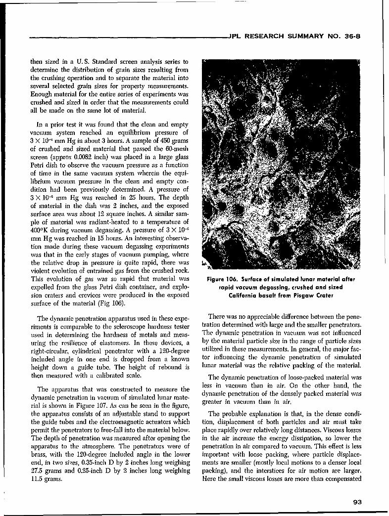
JPL RESEARCH SUMMARY NO. 36-8
then sized in a U.S. Standard screen analysis series todetermine the distribution of grain sizes resulting fromthe crushing operation and to separate the material intoseveral selected grain sizes for property measurements.Enough material for the entire series of experiments wascrushed and sized in order that the measurements couldall be made on the same lot of material.
In a prior test it was found that the clean and emptyvacuum system reached an equilibrium pressure of3 X 10- mm Hg in about 3 hours. A sample of 450 gramsof crushed and sized material that passed the 60-meshscreen (approx 0.0082 inch) was placed in a large glassPetri dish to observe the vacuum pressure as a functionof time in the same vacuum system wherein the equi-librium vacuum pressure in the clean and empty con-dition had been previously determined. A pressure of3 X 10-1 mm Hg was reached in 25 hours. The depthof material in the dish was 2 inches, and the exposedsurface area was about 12 square inches. A similar sam-ple of material was radiant-heated to a temperature of4000K during vacuum degassing. A pressure of 3 X 10⁻¹'
mm Hg was reached in 15 hours. An interesting observa-tion made during these vacuum degassing experimentswas that in the early stages of vacuum pumping, wherethe relative drop in pressure is quite rapid, there was .violent evolution of entrained gas from the crushed rock.This evolution of gas was so rapid that material was Figure 106. Surface of simulated lunar material afterexpelled from the glass Petri dish container, and explo- rapid vacuum degassing, crushed and sizedsion craters and crevices were produced in the exposed California basalt from Pisgaw Cratersurface of the material (Fig 106).
The dynamic penetration apparatus used in these expe- There was no appreciable difference between the pene-riments is comparable to the scleroscope hardness tester tration determined with large and the smaller penetrators.used in determining the hardness of metals and meas- The dynamic penetration in vacuum was not influenceduring the resilience of elastomers. In these devices, a by the material particle size in the range of particle sizesright-circular, cylindrical penetrator with a 120-degree utilized in these measurements. In general, the major fac-included angle in one end is dropped from a known tor influencing the dynamic penetration of simulatedheight down a guide tube. The height of rebound is lunar material was the relative packing of the material.then measured with a calibrated scale. The dynamic penetration of loose-packed material was
The apparatus that was constructed to measure the less in vacuum than in air. On the other hand, the
dynamic penetration in vacuum of simulated lunar mate- dynamic penetration of the densely packed material was
rial is shown in Figure 107. As can be seen in the figure, greater in vacuum than in air.
the apparatus consists of an adjustable stand to support The probable explanation is that, in the dense condi-the guide tubes and the electromagnetic actuators which tion, displacement of both particles and air must takepermit the penetrators to free-fall into the material below. place rapidly over relatively long distances. Viscous lossesThe depth of penetration was measured after opening the in the air increase the energy dissipation, so lower theapparatus to the atmosphere. The penetrators were of penetration in air compared to vacuum. This effect is lessbrass, with the 120-degree included angle in the lower important with loose packing, where particle displace-end, in two si'es, 0.35-inch D by 2 inches long weighing ments are smaller (mostly local motions to a denser local27.5 grams and 0.25-inch D by 2 inches long weighing packing), and the interstices for air motion are larger.11.5 grams. Here the small viscous losses are more than compensated
93
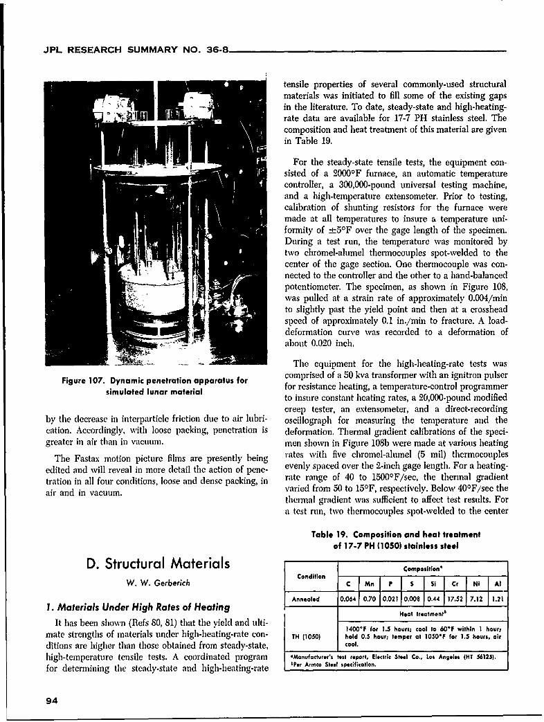
JPL RESEARCH SUMMARY NO. 36-8
tensile properties of several commonly-used structuralmaterials was initiated to fill some of the existing gapsin the literature. To date, steady-state and high-heating-rate data are available for 17-7 PH stainless steel. Thecomposition and heat treatment of this material are givenin Table 19.
For the steady-state tensile tests, the equipment con-sisted of a 2000OF furnace, an automatic temperaturecontroller, a 300,000-pound universal testing machine,and a high-temperature extensometer. Prior to testing,calibration of shunting resistors for the furnace weremade at all temperatures to insure a temperature uni-formity of ±t50F over the gage length of the specimen.During a test run, the temperature was monitorea bytwo chromel-alumel thermocouples spot-welded to thecenter of the gage section. One thermocouple was con-nected to the controller and the other to a hand-balancedpotentiometer. The specimen, as shown in Figure 108,was pulled at a strain rate of approximately 0.004/minto slightly past the yield point and then at a crossheadspeed of approximately 0.1 in./min to fracture. A load-deformation curve was recorded to a deformation of
T 6- about 0.020 inch.
.- The equipment for the high-heating-rate tests was
Figure 107. Dynamic penetration apparatus for comprised of a 50 kva transformer with an ignitron pulser
simulated lunar material for resistance heating, a temperature-control programmerto insure constant heating rates, a 20,000-pound modifiedcreep tester, an extensometer, and a direct-recording
by the decrease in interparticle friction due to air lubri- oscillograph for measuring the temperature and thecation. Accordingly, with loose packing, penetration is deformation. Thermal gradient calibrations of the speci-greater in air than in vacuum, men shown in Figure 108b were made at various heating
The Fastax motion picture films are presently being rates with five chromel-alumel (5 mil) thermocouples
edited and will reveal in more detail the action of pene- evenly spaced over the 2-inch gage length. For a heating-
tration in all four conditions, loose and dense packing, in rate range of 40 to 1500 0F/sec, the thermal gradient
air and in vacuum, varied from 50 to 150F, respectively. Below 400F/sec thethermal gradient was sufficient to affect test results. Fora test run, two thermocouples spot-welded to the center
Table 19. Composition and heat treatmentof 17-7 PH (1050) stainless steel
D. Structural Materials Composition*Condition I I I I
W. W. Gerberich CC Mn P $ Si Cr Ni Al
Annealed 0.064 0.70 0.021 0.008 0.44 17.52 7.12 1.21. Materials Under High Rates of HeatingtreatmentIt has been shown (Refs 80, 81) that the yield and ulti- i400F fr 1.5 hours; cool to 60 F within I hour;
mate strengths of materials under high-heating-rate con- TH (1050) hold 0.5 hour; temper at 1050'F for 1.5 hours, air
ditions are higher than those obtained from steady-state, cool.high-temperature tensile tests. A coordinated program *Manufacturer's test report, Electric Steel Co., Los Angeles (HT 56125).
for determining the steady-state and high-heating-rate *Per Armco Steel specification.
94
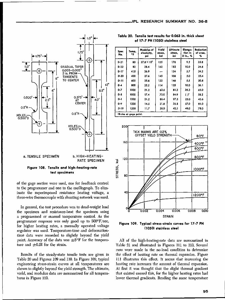
JPL RESEARCH SUMMARY NO. 36-8
,.0" -Table 20. Tensile test results for 0.063 in. thick sheetof 17-7 PH (1050) stainless steel
1.75" S-e Modulus of Yield Ultimate Elonga- Reduction75. OF elasticity, stress, stress, tion in of area,
I l41 175-- _J[_ .-- '/ o. °F psi ksi ksi 2 in., % %
D-21 80 27.8 X 10' 155 178 9.5 33.8-. oo GRADUAL TAPER D-22 80 28.4 162 183 10.0 34.6
2in. FROM"- D-17 415 26.9 - 154 5.7 34.2
TANGENTS D-20 400 27.6 145 156 5.0 25.4TO CENTER D-11 600 25.6 133 146 5.5 20.8
12 D-4 800 23.2 114 125 10.0 36.1
6. 8.5" D-7 1000 21.2 63.6 81.3 35.3 65.0
0.Id- 0.70*4 -8 1000 17.4 73.0 84.9 ( ), 58.2
2.5" AT 4.0 D-1 1000 21.2 86.4 97.5 25.0 45.6CENTER D-9 1200 14.5 21.8 35.8 57.0 81.0
0.5"R 0.19 1 200 11.7 26.0 40.1 49. 78.0HOLES 0.5" Broke of gage point.
0.5000D
-. HOLES. 200.500D O IO
TICK MARKS ARE 0.2%OFFSET YIELD STRENGTH 80 0 F
160 400OF
600OF
a. TENSILE SPECIMEN b. HIGH-HEATING- 120 800OFRATE SPECIMEN
Figure 108. Tensile and high-heating-rate c10
test specimens Xu 80
of the gage section were used, one for feedback controlto the programmer and one to the oscillograph. To elim-inate the superimposed resistance heating voltage, a 40three-wire thermocouple with shunting network was used.
in general, the test procedure was to dead-weight load 0the specimen and resistance-heat the specimen using 0 0.002 0.004 0.006 0.008 0.010
a programmed or manual temperature control. As the STRAINprogrammer response was only good up to 500 0F/sec, Figure 109. Typical stress-strain curves for 17-7 PHfor higher heating rates, a manually operated voltage (1050) stainless steelregulator was used. Temperature-time and deformation-time data were recorded to slightly beyond the yieldpoint. Accuracy of the data was ±5 0F for the tempera- All of the high.heating-rate data are summaarized inture and ±0.2% for tie strain. Table 21 and illustrated in Figures 111 to 113. Several
runs were made in tie no-load condition to determineResults of the steady-state tensile tests are given in the effect of heating rate on thermal expansion. Figure
Table 20 and Figures 109 and 110. In Figure 109, typical 111 illustrates this effect. It seems that increasing theengineering stress-strain curves at all temperatures are heating rate increases the amount of thermal expansion.shown to slightly beyond the yield strength. The ultimate, At first it was thought that the slight thermal gradientvield, and modulus data are summarized for all tempera- that existed caused this, for the higher heating rates hadlures in Figure 110. lower thermal gradients. Reading the same temperature
95
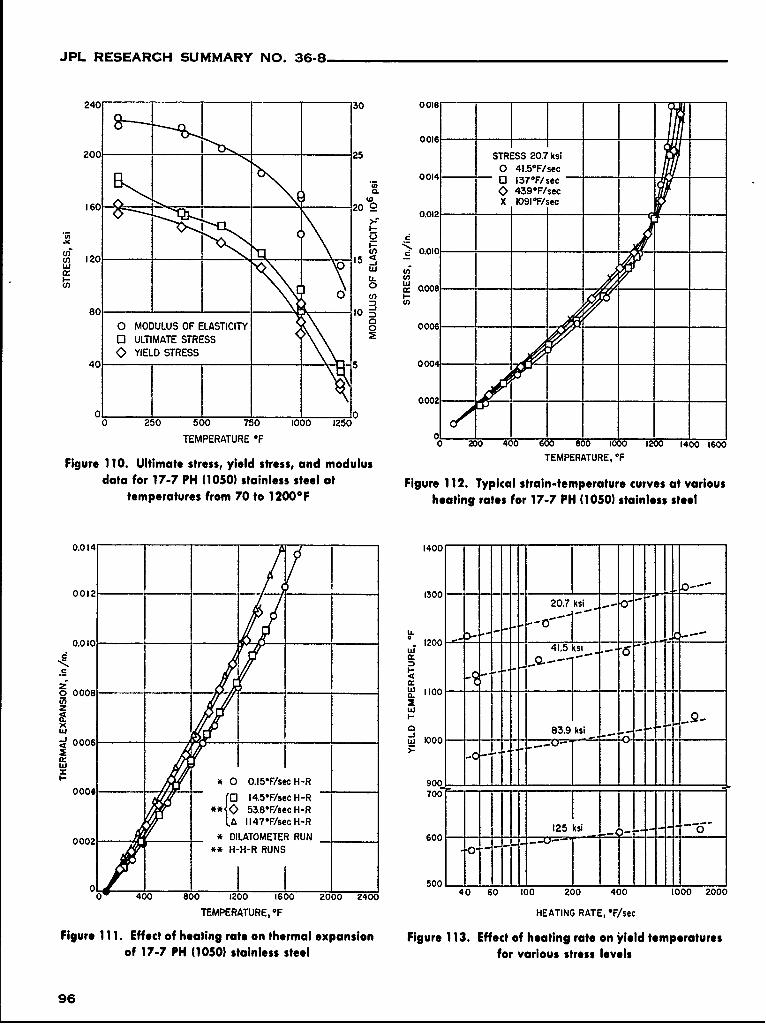
JPL RESEARCH SUMMARY NO. 36.8
0016c20 25 STRESS 20.7 ksi
0 41.5*F/sec.7 0014 - 03 1370F/sec
CL 0 439*F/secwD X 1091 F/sec1020 5?--------------------- -
C-
w
0 )Cn
0MODULUS OF ELASTICITY 0 000- -- -
o3 ULTIMATE STRESS '
1 00--
0 250 500 750 1000 1250j
TEPRTR F0 200 400) 600 Boo) 1000 1206 4010
Figure 1 10. Ultimate stress, yield stress, and modulus TEMPERATURE, OF
data for 17-7 PH (1050) stainless steel at Figure 112. Typical strain-temperature curves at varioustemperatures from 70 to 12000 F heating rates for 17-7 PH (1050) stainless steel
0.014. 1400--
0012 - 1300 20. -s
0.010 1200 ~w 1*
2F000 oou 1100
z wx w _j83.9 ks!-j 0006 - __ 00
< OOOC -
*0 0.I5*F/sec H-R 900-000~r 14.5,F/sec H-R 700
**~5WF/sec H-RLA 1147*F/sec H-R12 s0
0002 *DILATOMETER RUN 600 -
**H-H-R RUNS
0 500__0 0 00 10 10 00 4040 60 100 200 400 1000 2000
TEMPERATURE, OF HEATING RATE, *F/sec
Figure 111. Effect of heating rate on thermal expansion Figure 113. Effect of heating rate on yieldl temperaturesof 17-7 PH (1050) stainless steel for various stress levels
96
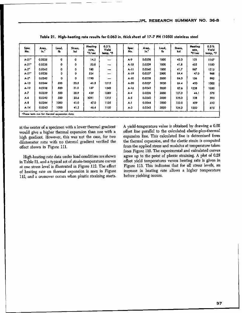
_ ___ _JPL RESEARCH SUMMARY NO. 36-8
Table 21. High-heating rate results for 0.063 in. thick sheet of 17-7 PH (1050) stainless steel
Spec Area, Load, Stress, Heating 0.2 % Spec Area, Load, Stress, Heating 0.2 %rate, Yield No. in.' Ib ksi rate, Yield
No. In. lb ksi F/sec temp, OF .F/sec temp, OF
A-21 0.0235 0 0 14.5 - A-9 0.0238 1000 42.0 121 1167
A-21' 0.0235 0 0 53.8 - A-15 0.0239 1000 41.8 455 1180
A.2* 0.0242 0 0 190 - A-11 0.0240 1000 41.7 967 1215A-21' 0.0235 0 0 524 - A-19 0.0237 2000 84.4 47.0 968
A-24 0.0242 0 0 1190 - A-10 0.0238 2000 84.0 156 995
A-13 0.0244 500 20.5 41.5 1215 A-20 0.0237 2000 84.4 450 1000
A-12 0.0238 500 21.0 137 1240 A-16 0.0242 2000 82.6 1238 1050
A-7 0.0239 500 20.9 439 1280 A-4 0.0236 3000 127.0 44.1 575
A.6 0.0243 500 20.6 1091 1315 A-5 0.0240 3000 125.0 138 595
A.8 0.0244 1000 41.0 47.0 1135 A-I 0.0244 3000 123.0 409 610
A.14 0.0243 1000 41.2 48.4 1120 A-3 0.0242 3000 124.0 1350 615
'These tests run for thermal expansion data.
at the center of a specimen with a lower thermal gradient A yield-temperature value is obtained by drawing a 0.24
would give a higher thermal expansion than one with a offset line parallel to the calculated elastic-plus-thermal
high gradient. However, this was not the case, for two expansion line. This calculated line is determined from
dilatometer runs with no thermal gradient verified the the thermal expansion, and the elastic strain is computed
effect shown in Figure 111. from the applied stress and modulus at temperature takenfrom Figure 110. The experimental and calculated curves
High-heating-rate data under load conditions are shown agree up to the point of plastic straining. A plot of 0.2%
in Table 21, and a typical set of strain-temperature curves offset yield temperatures versus heating rate is given in
at one stress level is illustrated in Figure 112. The effect Figure 113. This indicates that for all stress levels, an
of heating rate on thermal expansion is seen in Figure increase in heating rate allows a higher temperature
112, and a crossover occurs when plastic straining starts. before yielding occurs.
97
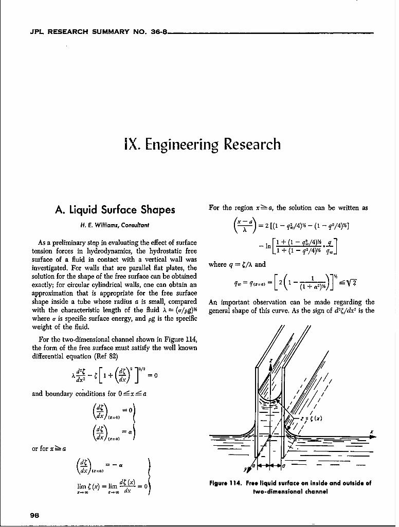
JPL RESEARCH SUMMARY NO. 36-8
IX. Engineering Research
A. Liquid Surface Shapes For the region xi--a, the solution can be written as
(L-:-a) = - q2/. -( - q2/4)"]H. E. Williams, Consultant 2 [(1 /4)-
As a preliminary step in evaluating the effect of surface _i1+ (1 - q2/4tension forces in hydrodynamics, the hydrostatic free L+ (1 q/4)A q-1surface of a fluid in contact with a vertical wall wasinvestigated. For walls that are parallel flat plates, the where q = C/A andsolution for the shape of the free surface can be obtained F _______
exactly; for circular cylindrical walls, one can obtain an qo = q(za) = L2k (1 +'___-_
approximation that is appropriate for the free surfaceshape inside a tube whose radius a is small, compared An important observation can be made regarding thewith the characteristic length of the fluid A = (o/pg)% general shape of this curve. As the sign of d2C/dx2 is thewhere a is specific surface energy, and pg is the specificweight of the fluid.
For the two-dimensional channel shown in Figure 114,the form of the free surface must satisfy the well knowndifferential equation (Ref 82)
- - 2+ ]3/ =o ///_C F (dCY3/
Ld+I = J //x
/ /-d~/'
z=C) 0
or for x a . ..
- -
\dx/ (z~a)
lir td(x) = lir dC (x) 0 Figure 114. Free liquid surface on inside and outside ofX. dx two-dimensional channel
98
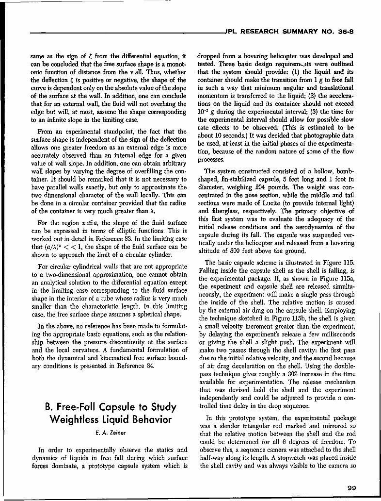
'PL RESEARCH SUMMARY NO. 36-8
same as the sign of C from the differential equation, it dropped from a hovering helicopter was developed andcan be concluded that the free surface shape is a monot- tested. Three basic design requiremriats were outlinedonic function of distance from the v all. Thus, whether that the system should provide: (1) the liquid and itsthe deflection C is positive or negative, the shape of the container should make the transition from 1 g to free fallcurve is dependent only on the absolute value of the slope in such a way that minimum angular and translationalof the surface at the wall. In addition, one can conclude momentum is transferred to the liquid; (2) the accelera-that for an external wall, the fluid will not overhang the tions on the liquid and its container should not exceededge but will, at most, assume the shape corresponding 10-
3 g during the experimental interval; (3) the time forto an infinite slope in the limiting case. the experimental interval should allow for possible slow
rate effects to be observed. (This is estimated to beFrom an experimental standpoint, the fact that the about 10 seconds.) It was decided that photographic data
surface shape is independent of the sign of the deflection bou t est w ecided hat otogrpimeta
allows one greater freedom as an external edge is more be used, at least in the initial phases of the experimenta-
accurately observed than an internal edge for a given tion, because of the random nature of some of the flow
value of wall slope. In addition, one can obtain arbitrary processes.
wall slopes by varying the degree of overfilling the con- The system constructed consisted of a hollow, bomb-tainer. It should be remarked that it is not necessary to shaped, fin-stabilized capsule, 5 feet long and 1 foot inhave parallel walls exactly, but only to approximate the diameter, weighing 204 pounds. The weight was con-two dimensional character of the wall locally. This can centrated in the nose section, while the middle and tailbe done in a circular container provided that the radius sections were made of Lucite (to provide internal light)of the container is very much greater than X. and fiberglass, respectively. The primary objective of
For the region x g a, the shape of the fluid surface this first system was to evaluate the adequacy of the
can be expressed in terms of elliptic functions. This is initial release conditions and the aerodynamics of the
worked out in detail in Reference 83. In the limiting case capsule during its fall. The capsule was suspended ver-
that (a/) 2 < < 1, the shape of the fluid surface can be tically under the helicopter and released from a hovering
shown to approach the limit of a circular cylinder, altitude of 800 feet above the ground.
For circular cylindrical walls that are not appropriate The basic capsule scheme is illustrated in Figure 115.
to a two-dimensional approximation, one cannot obtain Falling inside the capsule shell as the shell is falling, isthe experimental package. If, as shown in Figure 115a,
an analytical solution to the differential equation except the experiment acap s sh ar relea e sula-
in the limiting case corresponding to the fluid surface the experiment and capsule shell are released simulta-
shape in the interior of a tube whose radius is very much the inside of the shell. The relative motion is caused
smaller than the characteristic length. In this limiting the ete air The capsue shell. Employingcase, the free surface shape assumes a spherical shape. by the external air drag on the capsule shell. Employing
the technique sketched in Figure 115b, the shell is given
In the above, no reference has been made to formulat- a small velocity increment greater than the experiment,ing the appropriate basic equations, such as the relation- by delaying the experiment's release a few millisecondsship between the pressure discontinuity at the surface or giving the shell a slight push. The experiment willand the local curvature. A fundamental formulation of make two passes through the shell cavity: the first passboth the dynamical and kinematical free surface bound- due to the initial relative velocity, and the second becauseary conditions is presented in Reference 84. of air drag deceleration on the shell. Using the double-
pass technique gives roughly a 30% increase in the timeavailable for experimentation. The release mechanismthat was devised held the shell and the experimentindependently and could be adjusted to provide a con-
B. Free-Fall Capsule to Study trolled time delay in the drop sequence.
Weightless Liquid Behavior In this prototype system, the experimental packagewas a slender triangular rod marked and mirrored so
E. A. Zeiner that the relative motion between the shell and the rodcould be determined for all 6 degrees of freedom. To
In order to experimentally observe the statics and observe this, a sequence camera was attached to the shelldynamics of liquids in free fall during which surface half-way along its length. A stopwatch was placed insideforces dominate, a prototype capsule system which is the shell cavity and was always visible to the camera so
99
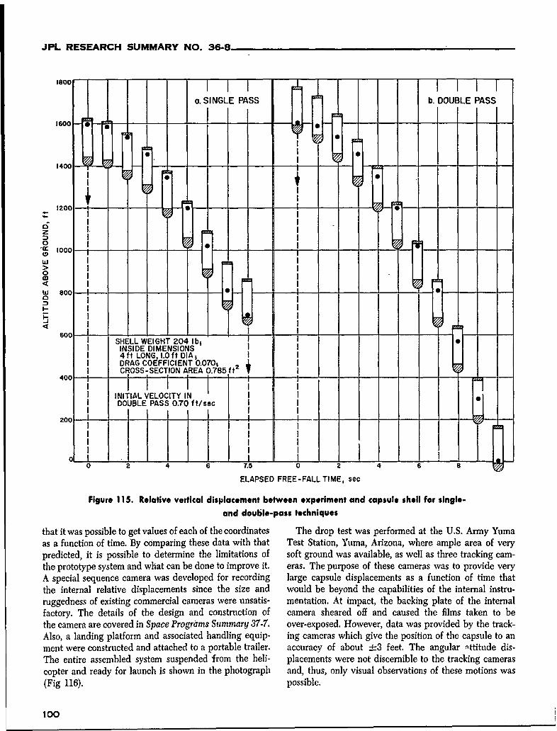
JPL RESEARCH SUMMARY NO. 36-8
-o-I, i- I1 1 Fa. SINGLE PASS b. DOUBLE PASS
1600 !4 -
IEl000 1 I
1400
I I
I;17.100 -I. I
0
hi II III
o II- Ito
6, -00 I600 SHELL WEIGHT 204 Ib, I
INSIDE DIMENSIONS I I4ft LONG, I.0ft DIA, I IDRAG COEFFICIENT 0.0701 2CROSS-SECTION AREA 0.785 ft V
400 j i II I i
INITIAL VELOCITY IN I IDOUBLE PASS 0.70 ft/sec I I
I I
S-j III I 4,6 8
0 2.45 0 2 46 8
ELAPSED FREE-FALL TIME, sec
Figure 115. Relative vertical displacement between experiment and capsule shell for single-
and double-pass techniques
that it was possible to get values of each of the coordinates The drop test was performed at the U.S. Army Yumaas a function of time. By comparing these data with that Test Station, Yuma, Arizona, where ample area of verypredicted, it is possible to determine the limitations of soft ground was available, as well as three tracking cam-the prototype system and what can be done to improve it. eras. The purpose of these cameras was to provide veryA special sequence camera was developed for recording large capsule displacements as a function of time thatthe internal relative displacements since the size and would be beyond the capabilities of the internal instru-ruggedness of existing commercial cameras were unsatis- mentation. At impact, the backing plate of the internalfactory. The details of the design and construction of camera sheared off and caused the films taken to bethe camera are covered in Space Programs Summary 37-7. over-exposed. However, data was provided by the track-Also, a landing platform and associated handling equip- ing cameras which give the position of the capsule to anment were constructed and attached to a portable trailer. accuracy of about ±3 feet. The angular -ttitude dis-The entire assembled system suspended from the heli- placements were not discernible to the tracking camerascopter and ready for launch is shown in the photograph and, thus, only visual observations of these motions was(Fig 116). possible.
too
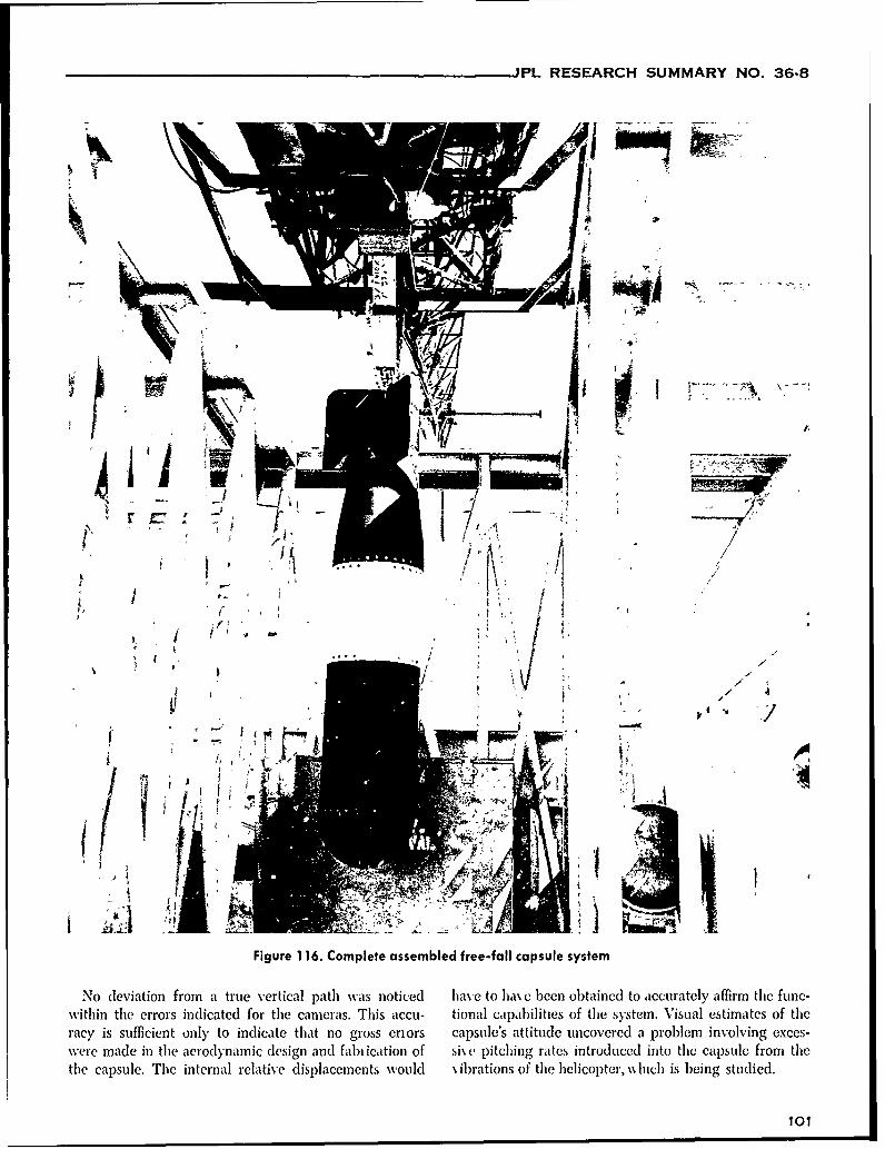
JPL RESEARCH SUMMARY NO. 36-8
Figur 11 .C m lt se be/fe -alc p uesse
Ni
/ ,
No deito rmatu etl pat %va noieaet j~ enotiedt cuaeyafr h u
w t e il -t, ! /
~i __
Figure 1 16. Complete assembled free-fall capsule system
No deviation from a true vertical path wxas noticed have to hax e been ob~tained to accurately affirm thec fune-
within the errors indicated for the cameras. This accu- tional capab~ilities of the system. Visual estimates of the
racy is sufficient only to indicate that no gross criors capsule's attitude uncovered a problem involving exces-
were made in the aerodynamic design and fabiication of si\t, pitching rates introduced into the capsule from the
the capsule. The internal relative displacements would \ibrations of the helicopter, xx hich is being studied.
101

JPL RESEARCH SUMMARY NO. 36-8
ENGINEERING FACILITIES DIVISION
X. Wind Tunnel and EnvironmentalFacilities
A. 20-Inch Supersonic Wind Tunnel configuration studies which constitute a large share ofthe wind tunnel testing time. Operation at Al = 6 was
G. Goranson attempted, but the resulting supersonic air flow in thetest section was unsatisfactory due to insufficient diffuserthroat adjustment. Design work has been completed for a
Test20.36Bwas ompete duing arc inthe modification of thle diffuser throat which will permit the20-inch supersonic wind tunnel in order to determine the
maximum practical Mach number for this tunnel. It was necessary additional adjustment.
found that M = 5.6 can be run satisfactorily if the effects After completion of the high Mach number work, aof air condensation are neglected. Because the supply few runs were made at Il = 2.21 and 4.54 to obtain flowtemperature of the air in the 20-inch tunnel is limited to field and wake information for a mockup of a typical blunt1500F, air condensation starts occurring at about l = 5.2. body dynamic stability model and its supporting struc-However, information gained from the 21-inch hypersonic ture. The tunnel started and operated satisfactorily with-tunnel indicates that air condensation effects can be out any adverse interactions between the tunnel sidewallsneglected in some types of test N ork such as coarse and the model.
102
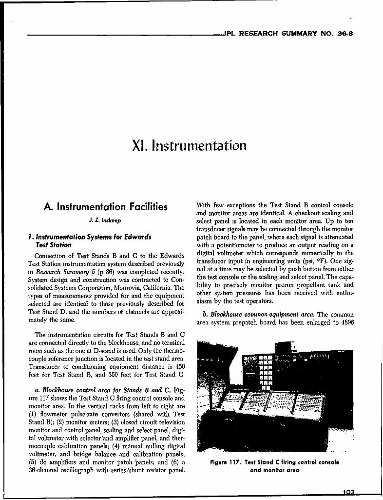
'PL RESEARCH SUMMARY NO. 36-8
XI. Instrumentation
A. Instrumentation Facilities With few exceptions the Test Stand B control consoleand monitor areas are identical. A checkout scaling and
J. Z. Inskeep select panel is located in each monitor area. Up to tentransducer signals may be connected through the monitor
1. Instrumentation Systems for Edwards patch board to the panel, where each signal is attenuatedTest Station with a potentiometer to produce an output reading on a
Connection of Test Stands B and C to the Edwards digital voltmeter which corresponds numerically to the
Test Station instrumentation system described previously transducer input in engineering units (psi, OF). One sig-
in Research Summary 5 (p 86) was completed recently. nal at a time may be selected by push button from either
System design and construction was contracted to Con- the test console or the scaling and select panel. The capa-
solidated Systems Corporation, Monrovia, California. The bility to precisely monitor prerun propellant tank and
types of measurements provided for and the equipment other system pressures has been received with enthu-
selected are identical to those previously described for siasm by the test operators.
Test Stand D, and the numbers of channels are approxi- b. Blockhouse common-equipment area. The commonmately the same. area system prepatch board has been enlarged to 4896
The instrumentation circuits for Test Stands B and Care connected directly to the blockhouse, and no terminalroom such as the one at D-stand is used. Only the thermo-couple reference junction is located in the test stand area.Transducer to conditioning equipment distance is 450feet for Test Stand B, and 350 feet for Test Stand C.
a. Blockhouse control area for Stands B and C. Fig- 1, . .ure 117 shows the Test Stand C firing control console and P)monitor area. In the vertical racks from left to right are -- ' I(1) flowmeter pulse-rate converters (shared with TestStand B); (2) monitor meters; (3) closed circuit televisionmonitor and control panel, scaling and select panel, digi-tal voltmeter with selector'and amplifier panel, and ther-mocouple calibration panels; (4) manual nulling digitalvoltmeter, and bridge balance and calibration panels;(5) dc amplifiers and monitor patch anels; and (6) a Figure 117. Test Stand C firing control console36-channel oscillograph with series/shunt resistor panel. and monitor area
~na
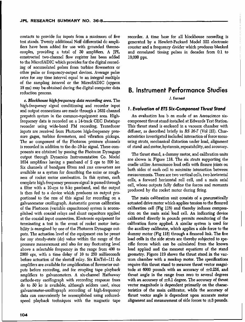
JPL RESEARCH SUMMARY NO. 36-8
contacts to provide for inputs from a maximum of five recorder. A time base for all blockhouse recording istest stands. Twenty additional Neff differential de ampli- generated by a Hewlett-Packard Model 522 electronicfiers have been added for use with grounded thermo- counter and a frequency divider which produces blankedcouples, providing a total of 30 amplifiers. A JPL and correlated timing pulses in decades from 0.1 toconstructed two-channel flow register has been added 10,000 pps.to the MicroSADIC which provides for the digital record-ing of accumulated pulses from turbine flowmeters orother pulse or frequency-output devices. Average pulserates for any time interval equal to an integral multipleof the sampling interval or the MicroSADIC (approx18 ms) may be obtained during the digital computer data B. Instrument Performance Studiesreduction process.
c. Blockhouse high.frequency data recording area. The J. Earnest
high-frequency signal conditioning and recorder input 1. Evaluation of ETS Six-Component Thrust Standand output connections are made through a 1632 channelprepatch system in the common-equipment area. High- An evaluation has b .en made of an Aeroscience six-frequency data is recorded on a 14-track CEC Datatape component thrust stand installed at Edwards Test Station.recorder using wide-band FM recording. Transducer This thrust stand is enclosed in a vacuum chamber withinputs are received from Photocon high-frequency pres- diffuser, as described briefly in RS 36-7 (Vol III). Char-sure gages, turbine flowmeters, and vibration pickups. acteristics investigated included interaction of force meas-The ac component of the Photocon pressure channels uring struts, mechanical distortion under load, alignmentis recorded in addition to the dc-10-kc signal. These com- of stand and motor, hysteresis, repeatability, and accuracy.ponents are obtained by passing the Photocon Dynagage The thrust stand, a dummy motor, and calibration unitsoutput through Dynamics Instrumentation Co. Model are shown in Figure 118. The six struts supporting the1634 amplifiers having a passband of 2 cps to 200 kc. cradle utilize Aeroscience load cells with flexure joints onSix channels of bandpass filters and rms converters are both sides of each cell to minimize interaction betweenavailable as a system for describing the noise or rough- measurements. There are two vertical cells, two horizontalness of rocket motor combustion. In this system, each cells, a forward horizontal roll cell, and a main axialcomplete high-frequency pressure signal is passed through cell, whose outputs fully define the forces and momentsa filter with a 10-cps to 8-kc passband, and the output produced by the rocket motor during firing.is then fed to a device which produces an output pro-portional to the rms of this signal for recording on a The main calibration unit consists of a pneumaticallygalvanometer oscillograph. Automatic prerun calibration actuated drive motor which applies tension to the flexuredof the Photocon (variable capacitance) system is accom- calibration cell (Fig 118) and thereby induces compres-plished with coaxial relays and shunt capacitors applied sion on the main axial load cell. An indicating deviceat the coaxial input connection. Electronic equipment for calibrated directly in pounds permits monitoring of theterminating a test in the event of rocket motor insta- calibration force applied. A similar system is used forbility is energized by one of the Photocon Dynagage out- the auxiliary calibrator, which applies a side force to theputs. The actuation level of the equipment can be preset dummy motor (Fig 118) through a flexured link. The fivefor any steady-state (de) value within the range of the load cells in the side struts are thereby subjected to spe-pressure measurement and also for any fluctuating level cific forces which can be calculated from the knownabove a selectable frequency in the range from 400 to load applied and the moment equations of the stand2000 cps, with a time delay of 10 to 250 milliseconds geometry. Figure 119 shows the thrust stand in the vac-before actuation of the shutoff relay. Six KinTel-lll dc uum chamber with a mockup motor. The specificationsamplifiers are available for amplification of flowmeter out- require this thrust stand to measure thrust vector magni-puts before recording, and for coupling tape playback tude at 6000 pounds with an accuracy of ±0.25%, andamplifiers to galvanometers. A six-channel Hathaway thrust angle in the range from zero to several degreescathode-ray oscillograph with recording response from with an accuracy of ±0.1 degree. The accuracy of thrustdc to 50 kc is available, although seldom used, since vector magnitude is dependent primarily on the charac-galvanometer-oscillograph recording of high-frequency teristics of the main calibrator, while the accuracy ofdata can conveniently be accomplished using reduced- thrust vector angle is dependent upon accurate motorspeed playback techniques with the magnetic tape alignment and measurement of side forces to ±3 pounds.
104
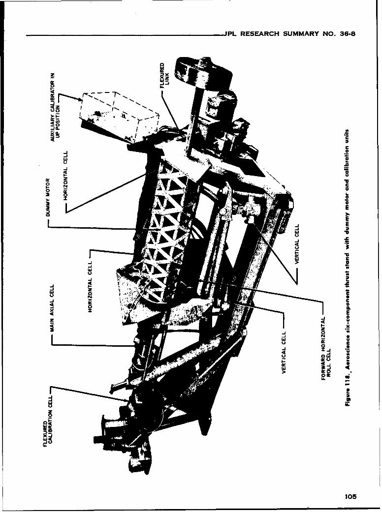
-JPL RESEARCH SUMMARY NO. 36-8
-i
00
: Jl. Ia,
0
zU
CwU
0
0
C~o 801
LL.
X
105
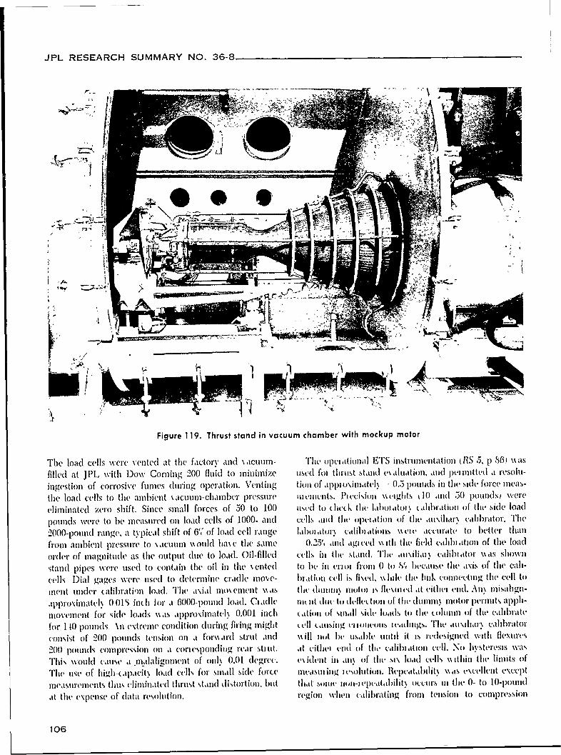
JPL RESEARCH SUMMARY NO. 36-8
Figure 119. Thrust stand in vacuum chamber with mockup motor
The load cells were vented at the factory andl \ aCuulf- The opei ational "I'S instrumentation uIS .5. p 86) Nwas
filled at JPL with D~ow Corning 200 fluid to mriinize used fol tlhrust stanld cluat61 aiodd pci ited a resolu-
ingestion of Corrosive fumiles dluring operation. Veniting ton of appi o\iiflatcl\ 0.5 pouinds in hesd force ineas-
the load cells to the ambient \actuum-chamnbci pressure 1m emenrts. Pi ecisiol \%eighits 00 and .0 pounds) w ere
elimrinated zero shift. Since small forces of 50 to 100 uised to ( lwedk the labow1 tol\ talilbratioii of tlhe side load
pounds were to be mevasurled onl load Cells of 1000. and cells and the opel at ion of the .iuxillaryN calibrator. The
2000-pound range, a typical shift of 6'( of load cell range la)oi ator\ (.dliiatiouis eiv accutrate to b)etter thanl
froml amb~ient pressulre to N~aeni s \oulci hax e thle samle 0.2151t and agi eed NwI ithile field cahlbiationl of thle load
order of magnitudle as the output due to load. Oil-filled cells inl tIt Stand. 'lThe liiit\ Calibi ator \% as shown
Stand Pipes were used to contain the oil inl thle \ ented to I)e inl er oi froml 0 to S" because the axis of the call-
cells D~ial gages were used to determine cradle move- brat ionl cell is iecd. \01 (bie hllk connecting tile Cell to
mnent under calibration load. The aLsial mlox emenIt Nw s the, duminiy niotoi is flexuied at eitliei end. AnN isalingn-
appro'imatel\ 0 01S~ inch for a 6000-polund load. Ci adle nlik ut doei to delleL t1io1 of tl(11Cm Motor permlits 01)1)1-
Movement for side loads \%aSaprimtl 0.001 inch d atioii of small side loads to th e .olumrn oif the calibrate
for 110 pounds, \n extreme condlit ion diiiring firing imigl t .(I e tl asing eli ollcis i ead ings. Ille at li calibrator
(10risist of 200) pokindl5 tension onl a forx\ arc1 strut and \\ ill not be usable 1tuitil it is redesigned withi flexures
200 pounds compression onl a con esponidiiig rearl stilit, at eitliei enid of the calibi ation cell. No hysteresis wvas
Th'lis would cautse a mal1,1aligniment of oly 0.01 degree. ux idenlt ill ali\ of the six load Cells x itljin thle limiits of
The uise of uih Iat\load (els for smrall side force mleasmn iig i esoluition. Repeatabilit\ \\,IaS excellent ex\cept
mea(%sturemlents thuls (liminlatcd thrust stand distortion. but that sollc nionl-iepeattabilit\ occurs inl tile 0- to 10-pounld
at thle expense of data resoluition, region xvhien calib~rating froml tension to compression
106
JPL RESEARCH SUMMARY NO. 36-8
through the zero point of a load cell. This uncertainty cradle. This is unimportant so long as the real motor iswas of the order of ± 1 pound for the front vertical-strut, aligned within the cradle to be parallel to the axis of thewhich permitted this type of test. main load cell. The dummy motor was optically aligned
for initial tests and scribe marks transferred to the cham-Initially, it was believed that the too calibrators would ber wall for prefiring alignment of the operational motor.
permit interaction studies and the setup of a calibration Itiesmadththsmtodfalg enmybenmatix or atacorelaion Fr~n prctial tanpoit, It is estimated that this method of alignment may be in
matrix for data correlation. Fr.n a practical standpoint, error by as much as ±0.5 degree. At present, the accuracyseveral features prohibited this procedure. As mentioned, with which the true thrust vector angle may be deter-
the auxiliary calibrator is incorrectly designed. Also, the mine wvich dee pral upone a y of motorreadut evies or othcaliraton ell ar sevo- mined will depend primarily upon tihe accuracy of motor
readout devices for both calibration cells are servo- alignment during firing. The final accuracy with whichmechanisms utilizing mechanical counters, repeatable to axial thrust can be measured is estimated to be ±0.5%.
only ±1 count, which corresponds to ±10 pounds on
the main calibration cell and ±1 pound on the auxiliary After completion of the evaluation, a 6000-pound thrustcalibration cell. This resolution combined with the reso- N2O4-N:H, liquid-rocket engine was tested in the thrustlution inherent in the six operational load cells is of the stand and vacuum chamber. All thrust parameters weresame magnitude as the interactions to be determined, recorded during this run with no apparent instrumenta-especially in the low side-force region expected for nor- tion failures. Several days after the run, however, twomal operation. Further, the auxiliary calibrator yields load cells were found to be inoperative due to openonly sets of conditions instead of permitting force to be circuits in the strain gage bridge. A second firing resultedapplied to one or two cells at a time. By the use of in two more inoperative load cells. A current investigationweights, pulleys and wires, 50-pound forces were applied indicates severe internal corrosion of the metallic strainover the axes of each of the five side struts with no indi- gage elements. Apparently moisture of high acid contentcation of cross coupling to any other cell. The more has entered the load cells through the vented standpipes,important interaction of main thrust to any specific side either in the form of water or fumes. The thrust standforce was minimized by proper alignment of the thrust is currently being used only with an unvented main axialstand. The alignment procedure used insures minimum load cell whose output is corrected for zero shift due tothrust to side force interaction but does not align the ambient pressure conditions.
107
JPL RESEARCH SUMMARY NO. 36-8
PROPULSION DIVISION
Xll. Liquid Propellant Propulsion
A. Combustion and Injection located behind the hole in the plate. The pressure distri-bution resulting from the jet impingement is determined
G. I. Jaivin by moving the plate in a plane perpendicular to thestream centerline. Relative to the stream diameter, the
1. Atomnization and Injection Hydraulics hole should be small and the plate large, in order toassure that the flow configuration produced by the
In RS 36-4 (Vol II), it was noted that sheet velocity and impingement of the stream on the plate does not changevelocity profile were pertinent variables which may be as the probe is moved from point to point in the pressuresignificant in determining the breakup of liquid sheets, field. In that initial set of experiments, the diameter ofA ballistic trajectory method for evaluating sheet veloci- the probe hole ranged from 0.013 to 0.022 inch.ties was discussed in RS 36-5 (Vol II). The utilization of a In the course of some current vork. it became evidentflat plate probe for the determination of velocity profile that certain anomalies existed in the data obtained within the sheet is currently being planned. the flat plate probe. In particular it was noted that ineas-
The pressure distributions produced by the perpendic- tired pressure distributions were inconsistent with otherular impingement of free liquid jets upon a flat plate have experimental results; the empirical data obtained withbeen previously evaluated for three reference streams the probe lead to results which indicate that the observed(CBS 43, 44, 47, and 52). These reference conditions were pressures are too high.obtained from jets produced by known flow conditions, In order to explain this effect it was reasoned that, ini.e., fully developed laminar flow and fully developed the presence of a large pressure gradient, the streamlineturbulent flow, as well as the jet produced by a sharp- the e of r e ese gan the stremledgd oifie.These data have proved useful in categoriz- pattern in the region of the hole can become sufficientlyedged orifice, Tdisturbed to significantly affect the measured pressure.ing jets of unknown dynamic characteristics. This phenomenon can be understood when it is realized
The dynamic-head probe used in the investigation that any finite hole in the retaining surface will produce(Ref 85) essentially consists of a small hole in the center some curvature of the streamlines due to removal of theof a flat plate. The pressure is measured by a pressure- constraining boundary. The streamlines will dip into thesensing element bounding one side of a small cavity hole producing a centripetal force field which tends to
108
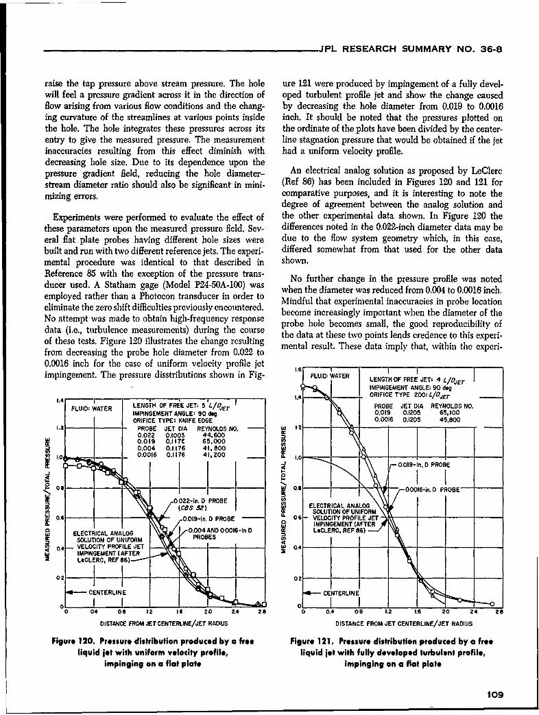
JPL RESEARCH SUMMARY NO. 36-8
raise the tap pressure above stream pressure. The hole ure 121 were produced by impingement of a fully devel-will feel a pressure gradient across it in the direction of oped turbulent profile jet and show the change causedflow arising from various flow conditions and the chang- by decreasing the hole diameter from 0.019 to 0.0016ing curvature of the streamlines at various points inside inch. It should be noted that the pressures plotted onthe hole. The hole integrates these pressures across its the ordinate of the plots have been divided by the center-entry to give the measured pressure. The measurement line stagnation pressure that would be obtained if the jetinaccuracies resulting from this effect diminish with had a uniform velocity profile.decreasing hole size. Due to its dependence upon thepressure gradient field, reducing the hole diameter- An electrical analog solution as proposed by LeClercstream diameter ratio should also be significant in mini- (Ref 86) has been included in Figures 120 and 121 formizing errors. comparative purposes, and it is interesting to note the
degree of agreement between the analog solution andExperiments were performed to evaluate the effect of the other experimental data shown. In Figure 120 the
these parameters upon the measured pressure field. Sev- differences noted in the 0.022-inch diameter data may beeral flat plate probes having different hole sizes were due to the flow system geometry which, in this case,built and run with two different reference jets. The experi- differed somewhat from that used for the other datamental procedure was identical to that described in shown.Reference 85 with the exception of the pressure trans- No further change in the pressure profile was notedducer used. A Statham gage (Model P24-50A-100) was when the diameter was reduced from 0.004 to 0.0016 inch.employed rather than a Photocon transducer in order to Mindful that experimental inaccuracies in probe locationeliminate the zero shift difficulties previously encountered. become increasingly important when the diameter of theNo attempt was made to obtain high-frequency response probe hole becomes small, the good reproducibility ofdata (i.e., turbulence measurements) during the course the data at these two points lends credence to this experi-of these tests. Figure 120 illustrates the change resulting mental result. These data imply that, within the experi-from decreasing the probe hole diameter from 0.022 to0.0016 inch for the case of uniform velocity profile jet 16 ___
impingement. The pressure disstributions shown in Fig- FLUID: WATER LENGTH OF FREE JET: 4 L/OsrIMPINGEMENT ANGLE: 90 deg
1.4 _ _L4 ORIFICE TYPE 200L:4/D4r
FLUID: WATER LENGTH OF FRiE JET: L/5, r PROBE JET DIA REYNOLDS NO.IMPINGEMENT ANGLE: 90 deg 0.019 0.1205 65,100ORIFICE TYPE: KNIFE EDGE 0.0016 0.1205 45,800
1.2 PROBE JET DIA REYNOLDS NO. W --
0.022 0.1003 44,600 c0.019 0.1ITC 65,0000.004 0.1176 41,800
)1.0 0.0016 0.1176 41,200 - - -. - --
1 O
0 .0 1 9 - I n .D P R O B E
12 0
08 - 02-n Dh PROBEE- -(CBS 5P) ELECTRICAL ANALOG(B )SOLUTION OF UNIFORM
0., -6- 0.019-In. D PROBE 06- VELOCITY PROFILE JET -
MNMIMPINGEMENT (AFTER0.004 AND 00016-In D LCLERC, REF 86)
SUTION OF UNIFORM PRBE
U,
0A 0. VELOCITY PROFILE JET - 0A ~4 -MINGEMENT (AFTER
LOCLERC, RF8)--
C1RLN CENTERLINE 0[4- CCCENTERLINEI I I I :!I IIo_0 04 0 12 I, 20 2.4 20 0 0.4 08 1.2 1.6 20 24 28
DISTANCE FROM JET CENTERLINE/JET RADIUS DISTANCE FROM JET CENTERLINE/JET RADIUS
Figure 120. Pressure distribution produced by a free Figure 121. Pressure distribution produced by a freeliquid jet with uniform velocity profile, liquid jet with fully developed turbulent profile,
impinging on a flat plate impinging on a flat plate
109
JPL RESEARCH SUMMARY NO. 36-8
mental accuracy of the measurements, a minimal error is tus, the thrust chamber assembly, the injector, and theintroduced if the hole size is kept below a critical value, operating procedure is given in Reference 87. The resultsIn the case of an impinging jet, this critical size would of six tests have been tabulated in Table 22 in terms ofbe a function of the jet diameter and the type of jet chamber pressure pc, mixture ratio r, characteristic veloc-(since different jets produce different pressure gradient ity c, characteristic combustion chamber length L*, maxi-fields). mum experimental heat flux qntaxexpt, and the ratio of
The use of the flat plate probe seems feasible for use q,naxezpt to calculated maximum analytical heat flux
in the liquid sheet investigation if the diameter of the qmzana. The results indicate that,-s expected, c in-creases-with-increaeof L* i rvedprobe hole can be reduced to 0.001 inch and the mini- k
mum sheet thickness is approximately 0.025 inch. This also for a 4-to-1 and an 8-to-1 nozzle reported in Ref 87).
sheet thickness is considerably larger than the thickness The experimental heat flux maxima, which occurred
obtained in the uniform, reproducible sheets produced slightly upstream of the nozzle throat, also increased
to date (RS 36-5, Vol II), but it is expected that a modi- with increasing c and L*. The qmaxanat was based on
fication of the present hardware will result in the desired experimental c* since both the heat transfer coefficient
sheet configuration. determined by the method of Reference 88 and theenthalpy difference between the stagnation and wall con-dition as determined by the method used in Reference 87are given as a function of c. Consequently, to determinethe sole effect of these changes of L* and qtnaerpt, the heatflux ratio q,nmazpt/qnanawas calculated. The last column
in Table 22 shows that the qmept/q, aanaz values for
B. Heat Transfer and Fluid 17.0 and 23.6-inch V indicate random scatter of approxi-mately4% with no apparent effect of L* on q,,,ta ezpt/qaz analMechanics at these conditions. The tests at 30.1-inch L* show values
A. B. Witte of this ratio about 8% above the average value of the firstfour tests. An increase of heat flux ratio with an increase
1. Heat Transfer in Rocket Motors in L* of this magnitude has not been observed previouslywith other nozzles, and no apparent explanation can be
An experimental investigation of heat transfer in rocket given for this result. Furthermore, the chamber pressuresengines is being conducted to determine the effect of for all tests were within 2% of the average value.injector configuration, thrust-chamber geometry, andoperating conditions on the axial heat flux distribution. Results of an 8-to-i and 4-to-i nozzle operating atThese tests are being made at chamber pressures between 38- and 62.8-inch and 23.7- and 39-7-inch L*, respectively,100 and 300 psia, with hydrazine (NH,) and nitrogen wvere compared in a similar way (Ref 87) to this investi-tetroxide (NO,) as bipropellants at a nominal mixture gation. The 8-to-i nozzle showed a decrease of 10 to 20%rati of1.0 Stedy-tat exerimnta vaaes f hat lux of the heat flux ratio as L* was increased from 38.0 to 62.8ratio of 1.0. Steady-state experimental values of heat flux inches; however, the 4-to-1 nozzle showed no change ofare measured calorimetrically by passing cooling wvater heat flux ratio when L* was increased from 23.7 to 39.7through axially short, circumferential coolant passages inches.which form the thrust-chamber walls. Comparisons be-tween the analytical and experimental values of local A comparison of all these results seems to indicate thatheat flux have been made with 1.64-to-1, 4-to-i, and for the particular thrust-chamber geometries tested, the8-to-1 contraction-area-ratio nozzles and reported inReference 87. Table 22. Experimental heat transfer in rocket engines
Recently, calorimetric heat transfer measurementswere made on a 1.64-to-1 contraction-area-ratio nozzle Test No. Pt C . . .pIpsi. ft/sec n. Btu/in. set c ,.
(throat dia = 3.9 inches) to determine the effect of change 6 -1 .3 3 .0 9.
in characteristic combustion chamber length L* near 200 6031A 198 1.03 5300 17.0 6.91 1.23
psia chamber pressure on semi-local values of heat flux. 6031 199 1.02 5280 17.0 7.00 1.26
Tests were made at 17.0, 23.6 and 30.1-inch L* which was 6103 201 1.06 540 23.6 7.28 1.23
accomplished by changing combustion chamber length. 6103 201 1.06 5420 23.6 7.28 1.23
An eight-orifice-pair, splash-plate type injector was used. 6106 203 1.04 5460 30.1 8.01 1.346106 203 1.04 5450 30.1 8.00 1.35A description of the thrust-chamber operational appara-
110

JPL RESEARCH SUMMARY NO. 36-8
effect of changes in L (aside from the changes in c* with uniform flow at the entrance to the 8-to-1 nozzle. It alsoL*) had little or no effect on heat flux maxima for the seems reasonable to hypothesize that increasing L* (fur-1.64-to-i and 4-to-1 contraction-area-ratio nozzles; how- ther separating the injector from the nozzle entrance at aever, with the 8-to-1 contraction-area-ratio nozzle, changes given contraction area ratio) would improve the uni-in L* significantly affected the heat flux maxima. Since formity of flow at the entrance to the nozzle. This effectthe Mach number at the entrance to the 8-to-1 nozzle is would account for the decreasing heat flux maxima with0.08 compared to 0.24 and 0.4 for the 4-to-1 and 1.64-to-i increasing L* as was observed for the 8-to-1 nozzle butnozzles, one may speculate that combustion nonuniformi- does not explain the reverse trend that apparentlyties may well significantly perturb the one-dimensional, occurred for the 1.64-to-i nozzle.
111

JPL RESEARCH SUMMARY NO. 36-8
References
1. Tross, C., "Astronomical Constants and Their Importance in Lunar Tra- 24. Olson, C. D., and Pohm, A. V., "Flux Reversal in Thin Films of 82% Ni.jectory Determination," Journal of the American Rocket Society, 30: 18% Fe," Journal of Applied Physics, 29: 274-282, 1958.938-941, 1960. 25. Dietrich, W., Proebster, W. E., and Wolf, P., IBM Journal of Research,
2. Magness, T., Space Technology Laboratories, work performed under 4: 189, 1960.Space Systems Analysis Study Contract No. 950045, 1961. 26. Silver, S., Microwave Antenna Theory and Design, p 383, McGraw-Hill
3. Herrick, S., Westrom, G., and Makemson, M. W., Astrodynamical Report Book Co., New York, 1949.No. 5, University of California, Los Angeles, 1959. 27. Measurement of Relativ7 Phase Shift at Microwave Frequencies, Engi-
4. Rabe, E., "Derivation of Fundamental Astronomical Constants front the nearing Notes, Vol II, No. 1, Huggins Laboratories, Sunnyvale, 1961.Observations of Eros," Astronomical Journal, 55: 112, 1949. 28. Cumming, R. C., "The Serrodyne Frequency Translator," Proceedings
5. Price, R., et al, "Radar Echoes from Venus," Science, 129: 751, 1959. of the IRE, 45: 175-186, February 1957.
6. Irving, J., Space Technology, Chap 10, ed. H. Seifert, John Wiley and 29. Maseriian, J., A Semiconductor Approach to Microelectronics, TechnicalSons, Inc., New York, 1959. Release No. 34-206, Jet Propulsion Laboratory, Pasadena, December 2,
7. Melbourne, W., Interplanetary Trajectories and Payload Capabilities of 1960.Advanced Propulsion Vehicles, Technical Report No. 32-68, Jet Pro- 30. Robbins, H., Hughes Aircraft Co., personal communication, 1961.pulsion Laboratory, Pasadena, March 31, 1961. 31. Silver, S., Microwave Antenna Theory and Design, p 145, McGraw-Hill
8. Kizner, W., A Method of Describing Miss Distances For Lunar and Inter. Book Co., New York, 1949.planetary Trajectories, External Publication No, 674, Jet Propulsion 32. Tartakovskii, L. B., "Side Radiation from Ideal Paraboloid with CircularLaboratory, Pasadena, August 1, 1959. Aperture," Radiotekhnika i elektronika, 4(No. 6): 920-929, 1959.
9. Noton, A. R. M., Statistical Analysis of Space Guidance Systems, Tech- 33. Singer, J. R., Chairman, Second International Conference on Quantumnical Memorandum No. 33-15, Jet Propulsion Laboratory, Pasadena, Electronics, University of California at Berkeley, March 23-25, 1961,June 15, 1960. to be published.
10. Meisenholder, G. W., An Introduction to the Operation and Testing of 3 Schawlow, A. L., and Townes, C. H., "Infrared and Optical Masers,"Accelerometers, Technical Memorandum No. 33-2, Jet Propulsion Lab- Physical Review, 112: 1940-1949, December 15, 1958.roary, Pasadena, October 3, 1960.PhsclRie,1219094,Demr1,19.
35. Shannon, C. E., and Weaver, W., The Mathematical Theory of Com.11. Jensen, L. K., Evans, B. H., Clark, R. B., Evaluation of Precision Gyros munication, University of Illinois Press, Urbana, 1949.
for Space Boost Guidance Applications, presented as ARS 1175.0 at
American Rocket Society Semi-Annual Meeting, May 9-12, 1960. 36. Lorens, C. S., and Viterbi, A. J., Optimum Filtering, External Publica-
12. Preliminary Descriptive Material on the GG80078 Miniature Integrating tion No. 633. May 15, 1959.
Gyro, U-ED 9841, Minneapolis Honeywell Aeronautical Division, March 37. Black, H. S., Modulation Theory, Van Nostrand Co., New York, 1953.
28, 1960. 38. Woodward, P. M., and Davies, I. L., "Information Theory and Inverse
13. Preliminary Description Document, GG177 Hinged Pendulous Acceler. Probability in Telecommunications," Proceedings of the lEE, 99(Part Ill):ometer, U.ED 9870, Minneapolis Honeywell Aeronautical Division, Octo- 37, 1952.ber 6, 1960. 39. Viterbi, A. J., On Coded Phase.Coherent Communications, Technical
14. Smythe, W., Static and Dynamic Electricity, Second Edition, Section Release No. 32-25, Aug. 15, 1960, to be published In IRE Transactions11.14, pp 408-411, McGraw.Hill, New York, 1950. on Space Electronics and Telemetry, March 1961.
15. Harding, J. T., Force and Torque on a Superconducting Ellipsoid in an 40. Zierler, N., "On Decoding Linear Errar-Correcling Codes. I." IRE Trans.Axially Symmetric Magnetic Field, Technical Release No. 34-242, Jet actions of PGIT, 1T6(No. 4)z 450-459, September 1960.Propulsion Laboratory, Pasadena, February 6, 1961.
41. Zierler, N., "On Decoding Linear Error-Correcting Codes. II," to appear16. Laub, J. H., Hdrostatic Gas Bearings, Progress eprt No. 20-353, Jet in Proceedings of the Fourth London Symposium on Information Theory,
Propulsion Laboratory, Pasadena, October 3, 1958.19.1961.
17. Menyvk, N., and Goodenough, J. B., "Magnetic Materials for Digital.
Computer Components. I. A Theory of Flux Reversal in Polycrystalline 42. Viterbi, A. J., "On Coedd Phase-Coherent Communications,' Technical
Feromagnetics," Journal of Applied Physics, 26: 8-18, 1955. Report No. 32.25, Jet Propulsion Laboratory, Pasadena, August 15, 1960.
18. Gyorgy, F. M., "Rotational Model of Flux Reversal in Square-Loop For. 43. Lawton, J. G., "Theoretical Error Rates of Differentially Coherent Binary
rites," Journal of Applied Physics, 28. 1011-1015, 1957. and Kineplex Data Transmission Systems," Proceedings of the IRE,47: 333-334, February 1959.
19. Humphrey, F. B., Journal of Applied Physics, 281 284, 1956.
20. Humphrey, F. B., and Gyorgy, E. M., Journal of Applied Physics, 30: 44. Cohn, C. R., "Comparison of Coherent and Phase Comparison Detection
935, 1959. of a Four.Phase Digital Signal," Proceedings of the IRE, 47: 1662,
21. Gyorgy, E. M., and Rogers, J. L., Proceedings of Magnetism Conference, September 1959.
Boston, AIEE T-91, p 637, 1959., 45. Glenn, A. B., "Comparison of PSK.AM Versus FSK-AM and PSK Versus
22. Hagedorn, F. B., "Partial Switching at Thin Fermalloy Films,' Journal FSK Binary Coded Transmissions,' IRE Transactions on Communicationsof Applied Physics, 30: 254S, 1959. Systems, CS-8(No. 2): 87, June 1960.
23. Sarles, F. W., Jr., A Magneto.Optic Apparatus fpr the Dynamic Study 46. Doelz, M. L., Heald, E. T., and Marlin, D. L., "Binary Data Transmissionof Ferromagnetic Surface Domains, PhD Thesis, Massachusetts Institute Techniques for Linear Systems," Proceedings of the IRE, 45(No. 5):of Technology, EE Dept, January 9, 1961. 656-661, May 1957.
112

JPL RESEARCH SUMMARY NO. 36-8
47. Barry, G., and Garobedian, A., Performance of Predicted Wave Systems 70. Cohen, C. B., and Reshotko, E., Similar Solutions for the Compressiblein the Presence of Additive, White Gaussian Noise, Engineering Report Boundary Layer with Heat Transfer and Pressure Gradient, NACA ReportNo. CER-W592, Collins Radio Co., Newport Beach, Calif., January 29, No. 1293(TN3325), National Aeronautics and Space Administration,1958. Washington, 1956.
48. Landee, R. W., A Method of Generating an Unambiguous Local Phase 71. Hoare, F. E., and Walling, J. C., "An Absolute Measurement of theReference for Data Detection Applications, Technical Memorandum, Susceptibility of Tantalum and Other Metals," Proceedings of PhysicalCollins Radio Company, December 19, 1960. Society, (London), 64B: 337-341, 1951.
49. Coggshall, J. C., and Nybo, R., Technical Report on the TE.290 Data 72. Eatherly, W. P., and McClelland, J. D., "Anisotropic Susceptibility ofTerminal Set, Collins Radio Company, Newport Beach, Calif., 1960. Polycrystalline Graphite," Physical Reviews, 89: 661(L), 1953.
50. Performance of Predicted Wave Systems in the Presence of Additive, 73. Poquet, E., et al, "Etude du diamagn6tisme de mono cristaux deWhite Gaussian Noise, Collins Radio Company, Cedar Rapids, Iowa, graphite"' Journal de Chimie Physique, 57: 866, 1960.January 29, 1958.
74. Guha, B. C., and Roy, B. P., "The Principle of Magnetic Susceptibility51. Theoretical Comparison of Binary Data Transmission Systems, Report o rpie"Ida ora fPyis :35 94
No. CA-1172.5-1, Cornell Aeronautical Laboratory, Inc., May 1958.
75. Soule, D. E., Resecrch Laboratories, Notional Carbon Company, private52. Study and Development Program for an Advanced Telemetry System, cmuiain
Final Report SEC-4R-1, Space Electronics Corp., Glendale, May 19, 1959.
53. Jaffee, R., and Rechlin, E., "Design and Performance of Phase-Locked 76. Bown, A. R. 0., and Wat, W., "The Preparation and Properties of
Circuits of Near Optimum Performance over a Wide Range of Input High-Temperature Pyrolytic Carbon," Industrial Carbon and Graphite
Signal and Noise Levels," IRE Transactions on Information Theory, (Society of Chemical Industry, London), p. 86, 1958.
IT-1: 66-76, March 1955. 77. Pinnick, H. T., "The Magnetic Susceptibility of Carbons and Polycrys-
54. Davenport, W. B., "Signal.to-Noise Ratios in Bnd.Pass Limiters," talline Graphites, I," Physical Review, 94: 319-326, 1954.
Journal of Applied Physics, 24(No. 6): 720-727, June 1953. 78. Adamson, A. F., and Blayden, D. H., "The Magnetic Susceptibility of
55. Andrew, E. R., Nuclear Magnetic Resonance, Cambridge University Press, Mesomorphous Carbons and Graphites," Industrial Carbon and GraphiteNew York, 1955. (Soc. of Chem. Industry, London), p. 28, 1958.
56. Roberts, J. D, Nuclear Magnetic Resonance, Applications to Organic 79. Kirshman, K. S., and Ganguli, N., "The Temperature Variation of theChemistry, McGraw-Hill, New York, 199S. Abnormal Unidirectional Diamagnetism of Graphite Crystals,' Nature,
57. Pople, J. A., Schneider, W. G,, and Bernstein, H. J., High.Resoltion 139: 155, 1937.Nuclear Magnetic Resonance, McGraw-Hill, New York, 1959. c0. Helmed, G. J., Kurg, 1. M., and Inge, J. E., Tensile Properties of Inconel
58. Anderson, W. A., "Nuclear Magnetic Resonance Spectra of Some Hydro- and RS.120 Titanium-Alloy Sheet under Rapid.Heating and Constant.carbons," Physical Review, 102;151-167, 1956. Temperature Conditions, NACA TN3731, National Aeronautics and Space
59. Bloom, A. L., and Shoolery, J. N., "Effects of Perturbing RF Fields on Admlnlstratien, July 1956.Nuclear Spin Coupling," Physical Review, 97: 1261-1265, 1955. 31. Kurg, h. M., Tensile Properties of AZ31A.O Magnesium-Altoy Sheet
60. Kaiser, R., "Double Resonance Technique for Elimination of Prton under RpidHaing and Constant Temperature Conditions, NACA'Spin-Spin Splitting," Review of Scientific Instruments, 31: 963--%5, TN3752, National Aeronautics and Space Administration, August 1956.1960.
61. Carlo, P. L., "The Analysis of Nuclear Magnetic Resonance Spectra," 82. Champion, F. C., and Davy, N., Properties of Matter, Philosophical
Chemical Reviews, 60: 363-429, 1960. Library, New York, 1959.
62. Grateful acknowledgement to Dr. Aksol A. Bothner.By, Assistant Director 83. Williams, H. E., On Hydrostatics with Surface Tension, Technical Report
of Research, Mellon Institute. No. 32.89, Jet Propulsion Laboratory, Pasadena, May 15, 1961.
63. Nair, P. M., and Roberts, J. D., "Nuclear Magnetic Resonance Spectra," 14. Rupe, J. H., A Dynamic.Head Probe for Evaluating the Properties ofJournal of American Chemical Society, 79s 4565, 1957. Free Liquid Jets, Progress Report No. 20-299, Jet Propulsion Laboratory,
64. Shafer, P. R., Davis, D. R., Vogel, Martin, Nagarajan, K., and Roberts, Pasadena, May 23, 1956.
J. D., Journal of American Chemical Society, in press. 86. LeClerc, A., Deflection of a Liquid Jet by a Perpendicular Boundary,
65. Reilly, C. A., and Swalen, J. D., Journal of Chemical Physics, 32: 1378- Thesis, Department of Mechanics and Hydraulics, State University of1385, 1960. Iowa, Iowa City, 1948.
66. Mortimer, F. S., Molecular Spectroscopy, 5: 199-205, 1960. 87. Welsh, W. E., Jr., ard Witte, A. B., Comparison of Analytical and
67. Gutowsky, H. S., Karplus, M., and Grant, D. M., Journal of Chemical Experimental Local Heat Fluxes in Liquid.Propellant Rocket ThrustPhysics, 31t 1278-1289, 1959. Chambers. Technical Report No. 32-43, Jet Propulsion Laboratory, Pasa.
68. Goldish, E., Journal of Chemical Education, 36: 408-416, 1959. dena, February 1, 1961.
69. Stuart, J. T., "On the Stability of Viscous Flow Between Parallel Planes 88. Bartz, D. R., "A Simple Equation for Rapid Estimation of Rocket Nozzlein the Presence of a Coplanar Magnetic Field., Proceedings of the Convective Heat Transfer Coefficients," Jet Propulsion, 27(No. 1):Royal Society of London, A, 221: 189-205, 1954. 49.51, January 1957.
113