INSTITUT FUR INFORMATIK

On optimality of exact and approximation

algorithms for scheduling problems

Lin Chen, Klaus Jansen, Guochuan Zhang

Bericht Nr. 1303

June 5, 2013

CHRISTIAN-ALBRECHTS-UNIVERSITAT

KIEL

Institut fur Informatik derChristian-Albrechts-Universitat zu Kiel

Olshausenstr. 40D – 24098 Kiel

On optimality of exact and approximation

algorithms for scheduling problems

Lin Chen, Klaus Jansen, Guochuan Zhang

Bericht Nr. 1303

June 5, 2013

e-mail: chenlin198662@zju.edu.cn, kj@informatik.uni-kiel.de,zgc@zju.edu.cn

Dieser Bericht ist als personliche Mitteilung aufzufassen.

On optimality of exact and approximationalgorithms for scheduling problems∗

Lin Chen1 Klaus Jansen2 Guochuan Zhang1

1College of Computer Science, Zhejiang University, Hangzhou, 310027, China

chenlin198662@zju.edu.cn, zgc@zju.edu.cn

2 Department of Computer Science, Kiel University, 24098 Kiel, Germany

kj@informatik.uni-kiel.de

Abstract

We consider the classical scheduling problem on parallel identical machinesto minimize the makespan. Under the exponential time hypothesis (ETH), lowerbounds on the running times of exact and approximation algorithms are character-ized. We achieve the following results: (1) For scheduling on a constant number mof identical machines, denoted by Pm||Cmax, a fully polynomial time approxima-

tion scheme (FPTAS) of running time (1/ε)O(m1−δ)|I|O(1) for any constant δ > 0implies that ETH fails (where |I| is the length of the input). It follows that thebest-known FPTAS of running time O(n) + (m/ε)O(m) for the more general prob-lem with a constant number m of unrelated machines Rm||Cmax is essentially thebest possible. (2) For scheduling on an arbitrary number of identical machines,denoted by P ||Cmax, a polynomial time approximation scheme (PTAS) of running

time 2O((1/ε)1−δ)|I|O(1) for any δ > 0 also implies that ETH fails. Thus the best-

known PTAS of running time 2O(1/ε2 log3(1/ε)) + O(n log n) is almost best possiblein terms of running time. (3) For P ||Cmax, even if we restrict that there are njobs and the processing time of each job is bounded by O(n), an exact algorithm

of running time 2O(n1−δ) for any δ > 0 implies that ETH fails. Thus the tradi-tional dynamic programming algorithm of running time 2O(n) is essentially thebest possible.

Keywords: Approximation schemes; Lower bounds; Exponential time hypothesis

∗Part of the work was done when the first author was visiting Kiel University. Research was supportedin part by Chinese Scholarship Council and NSFC (11271325).

1

1 Introduction

The theory of NP-hardness allows us to rule out polynomial time algorithms for manyfundamental optimization problems under the complexity assumption P 6= NP . On theother hand, however, this does not give us (non-polynomial) lower bounds on the runningtime for such algorithms. For example, under the assumption P 6= NP , there couldstill be an algorithm with running time nO(logn) for 3-SAT or bin packing. A strongerassumption, the Exponential Time Hypothesis (ETH), was introduced by Impagliazzo,Paturi, and Zane [10]:

Exponential Time Hypothesis (ETH): There is a positive real δ such that 3-SATwith n variables and m clauses cannot be solved in time 2δn(n+m)O(1).

Using the Sparsification Lemma by Impagliazzo et al. [10], the ETH assumptionimplies that there is no algorithm for 3-SAT with n variables and m clauses that runs intime 2δm(n+m)O(1) for a real δ > 0 as well. Under the ETH assumption, lower bounds onthe running time for several graph theoretical problems have been obtained via reductionsbetween decision problems. For example, there is no 2δn time algorithm for 3-Coloring,Independent Set, Vertex Cover, and Hamiltonian Path unless the ETH assumption fails.An essential property of the underlying strong reductions to show these lower boundsis that the main parameter, the number of vertices, is increased only linearly. Theselower bounds together with matching optimal algorithms of running time 2O(n) givesus some evidence that the ETH is true, i.e. that a subexponential time algorithm for3-SAT is unlikely to exist. For a nice survey about lower bounds via the ETH we refer toLokshtanov, Marx, and Saurabh [20]. Interestingly, using the ETH assumption one canalso prove lower bounds on the running time of approximation schemes. For example,Marx [21] proved that there is no PTAS of running time 2O((1/ε)1−δ)nO(1) for MaximumIndependent Set on planar graphs, unless the ETH fails.

There are only few lower bounds known for scheduling and packing problems. Chenet al. [3] showed that precedence constrained scheduling on m machines cannot be solvedin time f(m)|I|o(m) (where |I| is the length of the instance), unless the parameterizedcomplexity class W [1] = FPT . Kulik and Shachnai [16] proved that there is no PTAS

for the 2D knapsack problem with running time f(ε)|I|o(√

1/ε), unless all problems inSNP are solvable in sub-exponential time. Patrascu and Williams [25] proved using theETH assumption a lower bound of no(k) for sized subset sum with n items and cardinalityvalue k. Recently, Jansen et al. [12] showed a lower bound of 2o(n)|I|O(1) for the subsetsum and partition problem and proved that there is no PTAS for the multiple knapsackand 2D knapsack problem with running time 2o(1/ε)|I|O(1) and no(1/ε)|I|O(1), respectively.

In this paper, we consider the classical scheduling problem of jobs on identical ma-chines with the objective of minimizing the makespan, i.e., the largest completion time.Formally, an instance I is given by a setM of m identical machines and a set J of n jobswith processing times pj. The objective is to compute a non-preemptive schedule or anassignment a : J →M such that each job is executed by exactly one machine and the

2

maximum load maxi=1,...,m

∑j:a(j)=i pj among all machines is minimized. In scheduling

theory, this problem is denoted by Pm||Cmax if m is a constant or P ||Cmax if m is anarbitrary input.

This problem is NP-hard even if m = 2, and is strongly NP-hard if m is an input. Onthe other hand, for any ε > 0 there is a (1 + ε)-approximation algorithm for Pm||Cmax[9] and the more general problem P ||Cmax [7]. Furthermore, there is a long history ofimprovements on the running time of such algorithms. We give a brief introduction asfollows.

In 1976, Horowitz and Sahni [9] presented a fully polynomial-time approximationscheme (FPTAS) for a more generalized scheduling model Rm||Cmax on unrelated ma-chines, where each job j could have different execution times pij on different machines.The running time of the algorithm in [9] is O(nm(nm/ε)m−1). Lenstra, Shmoys andTardos [17] presented an alternative approximation scheme for the problem with run-ning time (n + 1)m/ε|I|O(1). In 2001, Jansen and Porkolab [14] presented an FPTASwith running time O(n(m/ε)O(m)). This has been improved by Fishkin et al. [4]to O(n) + (logm/ε)O(m2) and by Jansen and Mastrolilli [13] to O(n) + (m/ε)O(m) =O(n) + (logm/ε)O(m logm). If ε is small enough (e.g. ε < 1/m), the running time can bebounded by O(n) + (1/ε)O(m) [13]. All the above mentioned algorithms are based on acombination of linear and dynamic programming and have a running time that dependsexponentially on m. The running time increases drastically as m increases, which is alsoknown as the curse of dimensionality. It is not yet known whether there is an FPTASof running time (1/ε)o(m)|I|O(1) for Pm||Cmax.

For P ||Cmax, where the number of machines is a part of input, Hochbaum and Shmoys[7] gave a polynomial-time approximation scheme (PTAS) of running time (n/ε)O(1/ε2).It has been improved by Leung [19] to a running time of (n/ε)O(1/ε log(1/ε)). In 1998, Alonet al. [1] and Hochbaum and Shmoys [8] presented an efficient polynomial-time approxi-mation scheme (EPTAS) with running time f(1/ε)+O(n), where f is doubly exponentialin 1/ε. Jansen [11] gave an EPTAS for the scheduling problem on identical machinesP ||Cmax and uniform machines Q||Cmax with running time 2O(1/ε2 log3(1/ε)) + nO(1). Thealgorithm is based on solving a mixed integer linear program (MILP). Recently, Jansenand Robenek [15] showed how to avoid the MILP and presented an algorithm with thesame running time 2O(1/ε2 log3(1/ε)) + nO(1). Here the approximation scheme uses a com-bination of a linear program relaxation and a dynamic program. Interestingly, if themaximum distance ‖y∗ − x∗‖∞ between any optimum linear solution x∗ and the closestoptimum integer linear solution y∗ is bounded by a polynomial in 1/ε, the running timecan be bounded by 2O(1/ε log2(1/ε)) + nO(1) [15].

As seen above there are a plenty of approximation schemes for both Pm||Cmax andP ||Cmax. A natural and important question is to find lower bounds on the running timefor approximation schemes to solve the scheduling problem with the help of ETH.

Exact algorithms for the scheduling problem are also under extensive research. Re-cently Lente et al. [18] provided algorithms of running time 2n/2 and 3n/2 for P2||Cmaxand P3||Cmax, respectively. O’Neil [23, 24] gave a sub-exponential time algorithm of

3

running time 2O(k√|I|) for the related bin packing problem where |I| is the length of the

input and k is the number of bins. Such an algorithm also works for the schedulingproblem, and thus it is again natural to ask whether the sub-exponential time is the bestpossible.

The main contribution of this paper is to characterize lower bounds on the runningtimes of exact and approximation algorithms for the classical scheduling problem. Weprove the following theorems.

Theorem 1 For any δ > 0, there is no 2O((1/ε)1−δ) |I|O(1) time PTAS for P ||Cmax, unlessETH fails.

Theorem 2 For any δ > 0, there is no 2O(n1−δ) time exact algorithm for P ||Cmax withn jobs even if we restrict that the processing time of each job is bounded by O(n), unlessETH fails.

Theorem 3 For any δ > 0, there is no (1/ε)O(m1−δ) |I|O(1) time FPTAS for Pm||Cmax,unless ETH fails.

Theorem 4 For any δ > 0, there is no 2O(m1/2−δ√|I|) time exact algorithm for Pm||Cmax,

unless ETH fails.

We also prove the traditional dynamic programming algorithm for the scheduling

problem actually runs in 2O(√m|I| logm+m log |I|) time, and it is thus essentially the best

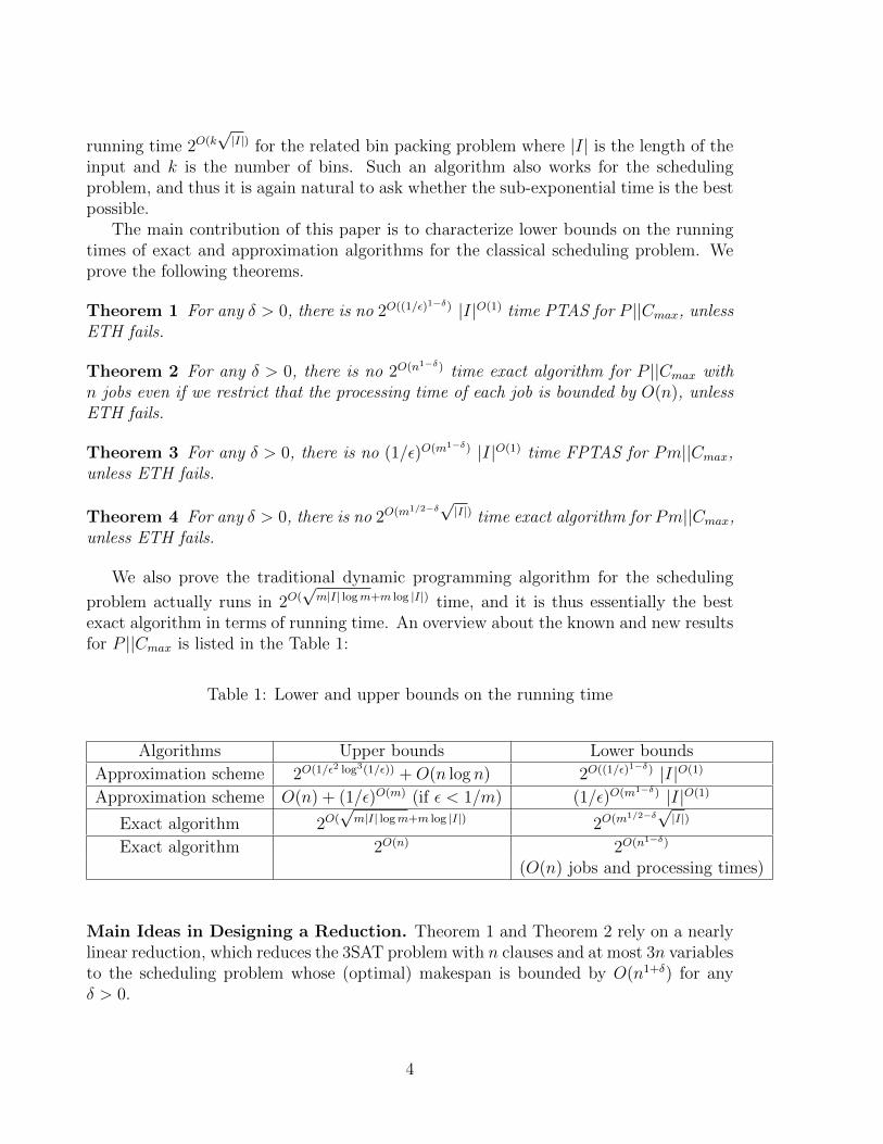
exact algorithm in terms of running time. An overview about the known and new resultsfor P ||Cmax is listed in the Table 1:

Table 1: Lower and upper bounds on the running time

Algorithms Upper bounds Lower bounds

Approximation scheme 2O(1/ε2 log3(1/ε)) +O(n log n) 2O((1/ε)1−δ) |I|O(1)

Approximation scheme O(n) + (1/ε)O(m) (if ε < 1/m) (1/ε)O(m1−δ) |I|O(1)

Exact algorithm 2O(√m|I| logm+m log |I|) 2O(m1/2−δ

√|I|)

Exact algorithm 2O(n) 2O(n1−δ)

(O(n) jobs and processing times)

Main Ideas in Designing a Reduction. Theorem 1 and Theorem 2 rely on a nearlylinear reduction, which reduces the 3SAT problem with n clauses and at most 3n variablesto the scheduling problem whose (optimal) makespan is bounded by O(n1+δ) for anyδ > 0.

4

The traditional reduction constructs a scheduling problem whose makespan is boundedby O(n16) [5], and thus yields a lower bound of 2(1/ε)1/16 . To improve it, the followingidea is used. We construct jobs for variables and clauses, and try to represent the in-formation ’variable zi is in clause cj’ with the form of ’the two jobs corresponding tozi and cj are on the same machine’. We can assume that there is a huge job on eachmachine, leaving a gap if the load of each machine is required to be a specified value. Ifwe define the processing times of the jobs corresponding to zi and cj to be i (i ≤ 3n)and 4nj (j ≤ n), and generate a gap of 4nj + i = O(n2) (through a huge job), then thisgap has to be filled up by the two jobs. To make the job processing times smaller, say,to O(n3/2), the following two ideas are applied. One is that, if every clause cj containszi, zi+1 and zi+2 such that 0 ≤ i − j ≤ O(1), then the two jobs for zi and cj could bedefined to have processing times of i and 4n(i− j) + i = O(n), respectively. We createa gap of 4n(i − j) + 2i. There are multiple ways of filling up such a gap by a variableand a clause job. However, we can prove that there is a unique way of filling up all suchkind of gaps, in which a gap of 4n(i− j) + 2i is filled up by i and 4n(i− j) + i.

The second idea assumes that there is a “proper partition” of the clauses so thatthey can be divided into O(

√n) groups where each group contains O(

√n) clauses, and

every variable only appears in clauses of one group. Then if cj is in group k, we re-index it as j′ ≤ O(

√n) and re-index variable zi ∈ cj as i′ ≤ O(

√n). Let x = O(

√n).

The processing times of the jobs for zi and cj are defined as kx2 + i′ = O(n3/2) andkx2 + j′x = O(n3/2). Again we can create a gap of 2kx2 + j′x + i′ and prove that itcould only be filled up by the two jobs. Both ideas rely on a certain structure of thegiven 3SAT instance. However, we can use Tovey’s method [26] to alter the instanceso that its clauses could be divided into two subsets and we can apply one idea for onesubset. It is possible to generalize the second idea to get even lower processing times bypartitioning the set of clauses recursively, i.e., we first equally partition the clauses intonδ groups, and then partition each group equally into nδ subgroups, and so on, untileach subgroup contains only nδ clauses eventually. Basically, the partition process forms1/δ − 1 levels from nδ groups to n1−δ groups each containing nδ clauses, where the toplevel is denoted as level 1/δ and the bottom level is level 2. For each clause cj, it appearsin a (unique) group at each level. Suppose it is in the ki-th group for each level i, andit is the k1-th element in the group at the bottom level. Then the job corresponding tocj has a processing time of k1/δx

1/δ + · · ·+ k2x2 + k1x = O(n1+δ) where x = O(nδ). The

job for zi is defined similarly as k1/δx1/δ + · · ·+ k2x

2 + k1.Theorem 3 and Theorem 4 rely on a different reduction, which reduces the 3SAT

problem with O(n) variables and clauses to the scheduling problem on m machines

whose makespan is bounded by 2O(n/m logO(1)m).The traditional reduction reduces 3SAT to 3DM (the 3-dimensional matching prob-

lem) with q = O(n2) elements, and then further reduces 3DM to the 2-machine schedulingproblem with the makespan of 2O(q log q) [5]. To get a lower makespan, we generalize 3DMa bit to allow one-element and two-element matches (i.e., matches of the form (wi) and(wi, xj)). We are able to reduce 3SAT to the generalized 3DM with q = O(n) elements

5

and matches. From 3DM to 2-machine scheduling, the traditional reduction lists allthe elements. Suppose wi is the f(wi)-th element in the list. Then a job of processingtime αf(wi) + αf(xj) + αf(yk) where α = q + 1 is constructed for a match (wi, xj, yk),and f is a sort of function to determine the index of an element. We create a gap of∑q

i=1 αi = (111 · · · 11)α (through some huge job) on one machine, where this gap has to

be filled up by a subset of jobs where every αi term appears once, and they correspondto the 3-dimensional matching in which every element appears once. Let |f | be thelargest value returned by f . The makespan of the above reduction (from the generalized3DM) is 2O(|f | logn) = 2O(n logn). To reduce the exponential term O(|f | log n) by utiliz-ing the m-machine environment, we may allow m − 1 elements to share one ’bit’, e.g.,f(wil) = λ for 1 ≤ l ≤ m − 1, and construct a job for (wi, xj, yk) with processing timeg(wi)α

f(wi) + g(xj)αf(xj) + g(yk)α

f(yk) where α = mO(1) and g(wi), g(xj), g(yk) < α. Wecreate a gap similar as (111 · · · 11)α on m − 1 machines, and each gap should be filledup by a subset of jobs where every αi term appears once. A 3-dimensional matchingcould thus be determined through the matches corresponding to the jobs on the m − 1machines. The main difficulty of this idea is from (the generalized) 3DM to scheduling:f should be defined without the knowledge of the 3-dimensional matching, meanwhileit should ensure that given any 3-dimensional matching (if it exists), jobs correspondingto the matching admits a “proper partition”, i.e., they could be partitioned and putonto m − 1 machines so that any two jobs sharing the same αi term are on differentmachines. To handle this, we design f in a way such that the following partition isalways a proper partition: given any 3-dimensional matching we always partition theminto m− 1 groups such that matches containing the element wkn/(m−1)+l are in the samegroup for 0 ≤ l ≤ n/(m − 1) − 1, and jobs corresponding to the matching are dividedaccordingly. We formulate the problem of designing the f satisfying the above propertyinto a graph coloring problem and provide a greedy algorithm to solve it. The functionf computed by the greedy algorithm satisfies |f | = O(n/m logm).

2 Scheduling on Arbitrary Number of Machines

We prove the following theorem in this section.

Theorem 5 Assuming ETH, there is no 2O(K1−δ)|Ische|O(1) time algorithm which deter-mines whether there is a feasible schedule of makespan no more than K for any δ > 0.

Given the above theorem, Theorem 1 follows directly. To see why, suppose Theorem 1fails, then for some δ0 > 0 there exists a 2O((1/ε)1−δ0 ) |I|O(1) time PTAS. We use thisalgorithm to test if there is a feasible schedule of makespan no more than K for thescheduling problem by taking ε = 1/(K + 1). If there exists a feasible schedule ofmakespan no more than K, then the PTAS returns a solution with makespan no morethan K(1 + ε) < K + 1. Otherwise, the makespan of the optimal solution is larger thanor equal to K + 1, and the PTAS thus returns a solution at least K + 1. In a word, the

6

PTAS determines whether there is a feasible schedule of makespan no more than K in2O((K+1)1−δ0 ) |I|O(1) time, which is a contradiction to Theorem 5.

To prove Theorem 5, we start with a modified version of the 3SAT problem, say,3SAT’ problem, in which the set of clauses could be divided into sets C1 and C2 suchthat

• Every clause of C1 contains three variables; every variable appears once in clausesof C1

• Every clause of C2 is of the form (zi∨¬zk); every positive (negative) literal appearsonce in C2

• If a 3SAT’ instance is satisfiable, every clause of C2 is satisfied by exactly one literal

There is a reduction from 3SAT (with m clauses) to 3SAT’ via Tovey’s method [26]which only increases the number of clauses and variables by O(m), and thus ensures thefollowing lemma.

Lemma 1 Assuming ETH, there exists some s > 0 such that there is no 2sn timealgorithm for the 3SAT’ problem with n variables.

Proof. Given any instance Isat (with m clauses) of the 3SAT problem, we may transformIsat into a 3SAT’ instance I ′sat in which every variable appears exactly three times. Sucha transformation is due to Tovey and we describe it as follows for the completeness.

Let z be any variable in Isat and suppose it appears d times in clauses. If d = 1 thenwe add a dummy clause (z ∨ ¬z). Otherwise d ≥ 2 and we introduce d new variablesz1, z2, · · · , zd and d new clauses (z1 ∨ ¬z2), (z2 ∨ ¬z3), · · · , (zd ∨ ¬z1). Meanwhile wereplace the d occurrences of z by z1, z2, · · · , zd in turn and remove z. By doing so wetransform Isat into I ′sat by introducing at most 3m new variables and 3m new clauses.Notice that each new clause we add is of the form (zi ∨ ¬zk). We let C2 be the set ofthem and let C1 be the set of other clauses. It is not difficult to verify that I ′sat is aninstance of 3SAT’, and is satisfiable if and only if Isat is satisfiable. According to ETH,the lemma follows directly. 2

From now on we use Isat to denote a 3SAT’ instance with n variables. Notice that thespecial structure of a 3SAT’ instance implies that n could be divided by 3, and clausescould be divided into C1 and C2 such that |C1| = n/3, |C2| = n, and every variableappears once in clauses of C1. We can re-index all the variables so that every clauseci ∈ C1 contains variables zi, zi+1 and zi+2 for i ∈ R = {1, 4, 7, · · · , n− 2}.

Given any δ > 0 (where 1/δ ≥ 2 is a constant integer), we may further assume thatn is sufficiently large (e.g., n ≥ 23/δ2+7/δ) and nδ is an integer. (Indeed, if nδ is not aninteger, we can simply choose σ ∈ {0, 1, 2} such that dnδe+ σ could be divided by 3 andadd (dnδe + σ)1/δ − n = 3ρ dummy variables into I ′sat. Let z1 to z3ρ be these dummyvariables. We add ρ dummy clauses (z1∨z2∨z3), · · · , (z3ρ−2∨z3ρ−1∨z3ρ) into C1 and 3ρ

7

dummy clauses (z1 ∨ ¬z1), · · · , (z3ρ ∨ ¬z3ρ) into C2. Obviously these dummy variablesand clauses do not change the satisfiability of I ′3sat. Furthermore, given the fact thateδ ≥ 1 + δ, dnδe + σ ≤ nδ + δnδ ≤ (en)δ, thus 3ρ ≤ (e− 1)n, which means that we addat most 2n dummy variables and clauses.)

In the following part of this section, we will construct a scheduling instance withO(n/δ) jobs and O(n/δ) machines such that it admits a feasible solution with makespanno more than K = O(23/δn1+δ) if and only if Isat is satisfiable. This would be enoughto prove Theorem 5, to see why, suppose the theorem fails, then an exact algorithm ofrunning time 2O(K1−δ0 )|Ische|O(1) exists for some δ0 > 0. We take δ = δ0 in the reduction,

and we can determine in 2O(n1−δ20 )|I|O(1) = 2o(n) time whether the constructed schedulinginstance admits a schedule of makespan K, and thus determine whether the given 3SAT’instance is satisfiable, which is a contradiction.

To provide an overview of the whole construction and the proof, we give a simplifiedreduction where δ = 1/2 in the next subsection. We give the reduction for arbitrary δafter the simplified reduction.

2.1 The reduction for δ = 1/2

We give a brief overview. For each positive (negative) literal, say, zi (or ¬zi), two pairsof jobs vγi,1 and vγi,2 (vγi,3 and vγi,4) are constructed where γ ∈ {T, F}. For each clause ofC1, say, cj, one job uTj and two copies of job uFj are constructed.

As we have mentioned, we create huge jobs so as to make a gap on every machine.There are five kinds of huge jobs (gaps).

[1.] Variable-assignment gaps. To fill up these gaps either vFi,1, vFi,2, v

Ti,3, v

Ti,4 (meaning

variable zi is true), or vTi,1, vTi,2, v

Fi,3, v

Fi,4 (meaning variable zi is false) are used. Jobs aγi ,

bγi , cγi and dγi are created as ’assistant jobs’ to help achieve the above requirement.

[2.] Variable-clause gaps. If the positive (or negative) literal zi (or ¬zi) is in cj ∈ C1,then a variable-clause gap is created so that it could only be filled up by uj and vi,1 (orvi,3). Notice that i = j, j + 1, j + 2, the first idea in the introduction is used to ensurethat the gap can only be filled up in this way. Furthermore, for the superscripts of ujand vi,1 (or vi,3), the gap enforces that only three combinations are valid: (T,T), (F,F)and (F,T). Recall that there is one uTj , it is thus always scheduled with a true variablejob, say, vTi′,1 (or vTi′,3), indicating that the clause is satisfied by zi′ (or ¬zi′).[3.] Variable-agent and agent-agent gaps. We want to create a gap for (zi∨¬zk) ∈ C2 sothat it could only be filled up by vTi,2 and vFk,4 (or vFi,2 and vTk,4), indicating that (zi∨¬zk) issatisfied by zi (or ¬zk). However, such a gap could not be constructed directly since thethe size of a gap should be O(n3/2). We use the following idea to achieve this. We createa pair of agent jobs for vi,2 (or vk,4), namely ηγi,+ (or ηγi,−). We create one variable-agentgap which could only be filled up by vi,2 and its agent ηi,+, and they should be one trueand one false (i.e., their superscripts are T and F ). Similarly another variable-agent gapis created which could only be filled up by vk,4 and ηk,− that are one true and one false.

8

We further create an agent-agent gap which could only be filled up by ηi,+ and ηk,− thatare one true and one false. Combining the three gaps, we can conclude that the vi,2 andvk,4 used in these gaps are one true and one false. The second idea in the introductionis used to construct these gaps.

[4.] Variable-dummy gaps. Recall that we construct 8 jobs for a variable and only use7 of them (either vi,1 or vi,3 is left), the remaining one will be used to fill these gaps.

2.1.1 Partition Clauses

Given a 3SAT’ instance Isat with n variables, we know that C1 = n/3 and C2 = n. Wemay further assume that n is sufficiently large (i.e., n ≥ 226) and

√n is an integer.

Recall that there are n clauses in C2 and every positive (negative) literal appears oncein them. We partition clauses of C2 equally into

√n groups. Let Sn = {1, 2, · · · , n}. We

define the function f : Sn → S√n such that the positive literal zi is in group f(i), andwe define the function f : Sn → S√n such that the negative literal ¬zi is in group f(i).

In each group, say, group i, there are√n different positive literals. Let their indices

be i1 < i2 < · · · < i√n, then we define g : Sn → S√n such that g(ik) = k. Similarlythe indices of negative literals could be listed as i1 < i2 < · · · < i√n and we defineg : Sn → S√n such that g(ik) = k.

Our definition of g and g implies the following lemma.

Lemma 2 For any i, i′ ∈ Sn and i < i′, if f(i) = f(i′), then g(i) < g(i′). Similarly iff(i) = f(i′), then g(i) < g(i′).

Furthermore, if (zi ∨ ¬zk) ∈ C2, then f(i) = f(k) according to our definition.

2.1.2 Construction of the Scheduling Instance

Given Isat, we construct an instance of scheduling problem with 30n jobs and 9n ma-chines, and prove that Isat is satisfiable if and only if there exists a feasible solutionfor the constructed scheduling instance with makespan no more than K = 105r, wherer = 215n3/2. Throughout this section we set x = 4

√n and use s(j) to denote the

processing time of job j. γ ∈ {T, F}.20n jobs are constructed for variables, among them there are 8n variable jobs, 4n

agent jobs and 8n truth assignment jobs. n jobs are constructed for clauses of C1. 9nhuge jobs are constructed so that there is one on each machine.

Variable jobs: vγi,1 and vγi,2 are constructed for zi, vγi,3 and vγi,4 are for ¬zi.

s(vTi,k) = r + 29(f(i)x2 + i) + 28 + k, k = 1, 2

s(vTi,k) = r + 29(f(i)x2 + i) + 28 + k, k = 3, 4

s(vFi,k) = s(vTi,k) + 2r, k = 1, 2, 3, 4

9

Agent jobs: ηγi,+ and ηγi,−.

s(ηTi,+) = r + 29(f(i)x2 + g(i)) + 27 + 8,

s(ηTi,−) = r + 29(f(i)x2 + g(i)x) + 27 + 16,

s(ηFi,σ) = s(ηTi,σ) + 2r, σ = +,−

Truth assignment jobs: aγi , bγi , c

γi and dγi .

s(aFi ) = 11r + (27i+ 8), s(bFi ) = 11r + (27i+ 32),

s(cFi ) = 101r + (27i+ 16), s(dFi ) = 101r + (27i+ 64),

s(kTi ) = s(kFi ) + r, k = a, b, c, d.

Clause jobs: 3 clause jobs are constructed for every cj ∈ C1 where j ∈ R, with oneuTj and two copies of uFj :

s(uTj ) = 10004r + 211j, s(uFj ) = 10002r + 211j.

Dummy jobs: n + n/3 jobs with processing time 1000r, and n − n/3 jobs withprocessing time 1002r.

Let V and Va be the set of variable jobs and agent jobs. Let A, B, C, D be the setof aγi , b

γi , c

γi and dγi respectively. Sometimes we may drop the superscript for simplicity,

e.g., we use ai to represent aTi or aFi .We construct huge jobs. There are five kinds of huge jobs corresponding to the five

kinds of gaps we mention before.Two huge jobs (variable-agent jobs) θη,i,+ and θη,i,− are constructed for each variable

zi:

s(θη,i,+) = 105r − 4r − 29[2f(i)x2 + g(i) + i]− (28 + 27 + 10)

s(θη,i,−) = 105r − 4r − 29[2f(i)x2 + g(i)x+ i]− (28 + 27 + 20)

One huge job (agent-agent job) θi,k,C2 is constructed for (zi ∨ ¬zk) ∈ C2:

s(θi,k,C2) = 105r − 4r − 29[f(i)x2 + f(k)x2 + g(k)x+ g(i)] + 28 + 24].

Notice that f(i) = f(k) according to our definition of f and f .Three huge jobs (variable-clause jobs) are constructed for each cj ∈ C1 (j ∈ R), one

for each literal: for i = j, j + 1, j + 2, if zi ∈ cj, we construct θj,i,+,C1 , otherwise ¬zi ∈ cj,and we construct θj,i,−,C1 .

s(θj,i,+,C1) = 105r − 11005r − (29f(i)x2 + 211j + 29i+ 28 + 1),

s(θj,i,−,C1) = 105r − 11005r − (29f(i)x2 + 211j + 29i+ 28 + 3).

10

One huge job (variable-dummy job) is constructed for each variable. Notice that eachvariable appears exactly three times in clauses, if zi appears twice while ¬zi appears once,we construct θi,−. Otherwise, we construct θi,+ instead.

s(θi,+) = 105r − 1003r − (29f(i)x2 + 29i+ 28 + 1),

s(θi,−) = 105r − 1003r − (29f(i)x2 + 29i+ 28 + 3).

Thus, for each clause cj (j ∈ R) and i = j, j + 1, j + 2, either θi,+ and θj,i,−,C1 exist,or θi,− and θj,i,+,C1 exist.

Four huge jobs (variable-assignment jobs) are constructed for each variable zi, namelyθi,a,c, θi,b,d, θi,a,d and θi,b,c:

s(θi,a,c) = 105r − 115r − 29(f(i)x2 + i)− (28 + 28i+ 25),

s(θi,b,d) = 105r − 115r − 29(f(i)x2 + i)− (28 + 28i+ 98),

s(θi,a,d) = 105r − 115r − 29(f(i)x2 + i)− (28 + 28i+ 75),

s(θi,b,c) = 105r − 115r − 29(f(i)x2 + i)− (28 + 28i+ 52).

It is not difficult to verify that the total processing time of all the jobs is 9n · 105r.Furthermore, if the given 3SAT’ instance Isat is satisfiable, then the constructed schedul-ing instance Ische admits a feasible schedule whose makespan is 105r (the reader mayrefer to Subsection 2.2.3 for a similar proof).

2.1.3 Scheduling to 3SAT

We prove that if there is a schedule whose makespan is no more than 105r (which impliesthat the load of each machine is exactly 105r), then Isat is satisfiable.

The input of a scheduling instance is a set of integers with 9n identical machines, weprove that we can determine the symbol (e.g., aTi , uFj ) of a job based on its processingtime. Recall that we define the processing time of a job in the form of a polynomial,which could be partitioned into four terms, the r-term, x2-term, x-term and constantterm (the summation of all terms without r or x). The sum of the x-term and constantterm is called small-x2-term, and the sum of x2-term, x-term and constant term is calledsmall-r-term. Since x = 4

√n and r = 215n3/2, there are gaps between terms.

Lemma 3 The small-r-term and small-x2-term of a huge job are negative with theirabsolute values bounded by 1/2r and 29 · 3/4x2 respectively. The small-r-term of anyother job is positive and bounded by 1/4r. The small-x2-term of a variable or agent jobis positive and bounded by 29 · 3/8x2.

The reader may refer to Lemma 8 for a similar proof. The above lemma allows usto determine the r-term and x2-term of a job, and the symbol of it could be determinedeasily if it is a variable, agent, truth assignment, clause or dummy job. If it is a huge job,

11

we observe that, the function g is defined in the way that if f(i1) = f(i2) for i1 < i2, theng(i1) < g(i2) (Lemma 2), which implies that i1 + g(i1) < i2 + g(i2), thus the processingtime of a huge job is unique and we can also determine its symbol.

Let Sol∗ be an optimal solution, it can be easily seen that there is a huge job on eachmachine, creating a gap. The following lemmas follows by considering the r-terms andthe residuals of dividing each job by 27 (the reader may refer to Lemma 10 for a similarproof).

Lemma 4 The following statements hold.

• A variable-agent gap is filled up with a variable job and an agent job.

• An agent-agent gap is filled up with two agent jobs.

• A variable-clause gap is filled up with a clause job, a variable job and a dummyjob.

• A variable-dummy gap is filled up with a variable job and a dummy job.

• A variable-assignment gap is filled up with a variable job and two truth-assignmentjobs, one in A ∪B, the other in C ∪D.

Combining Lemmas 3 and 4, we have the following lemma.

Lemma 5 For jobs on each machine, their r-terms add up to 105r, x2-terms and small-x2-terms add up to 0.

Consider the x2-terms of gaps. An agent-agent gap or variable-agent gap is called aregular gap, since their x2-terms are 29 · 2ζx2 where 1 ≤ ζ ≤

√n. Other gaps are called

singular gaps with the x2-terms being 29ζx2.A singular gap is called well-canceled, if it is filled up by jobs (other than huge jobs)

whose x2-terms are 29ζx2 and 0. A regular gap is called well-canceled, if it is filled upby two jobs whose x2-terms are both 29ζx2.

Lemma 6 Every singular gap is well-canceled, and every regular gap is well-canceled.

Proof. We briefly argue why it is the case. The first part follows directly from Lemma 4and Lemma 5. We show the second part.

Consider the regular gap with the term 29 ·2x2. Since it is filled up by two variable oragent jobs (Lemma 4), whose x2-term is at least 29x2, thus it is obviously well-canceled.

According to the construction of f and f , there are√n indices such that f(i) = 1 and√

n indices such that f(i) = 1, thus in all there are 12√n variable and agent jobs with

the term 29x2. There are√n variable-clause gaps,

√n variable-dummy gaps and 4

√n

variable-assignment gaps with the term 29x2, meanwhile there are 2√n variable-agent

gaps and√n agent-agent gaps with the term 29 ·2x2. All of these gaps are well-canceled,

12

implying that all the variable and agent jobs with 29x2 are used to fill up these gaps.Thus to fill up a regular gap with the term of 29 · 4x2, we have to use variable or agentjobs with the term of at least 29 ·2x2, implying that this regular gap is also well-canceled.Iteratively applying the above arguments, every regular gap is well-canceled. 2

A huge job (gap) is called satisfied, if the indices of other jobs on the same machinewith it coincide with its index. For example, the variable-clause job θj,i,−,C1 is satisfied ifit is on the same machine with the variable job vi,k and clause job uj where k ∈ {1, 2, 3, 4},and θi,a,c is satisfied if it is with vi,k, ai and ci.

Lemma 7 Every huge job (gap) is satisfied.

Proof. We give the sketch of proof. It is easy to see that every variable-dummy job issatisfied. According to the definition of f and g (f ′ and g′), an index i is determineduniquely by the pair (f(i), g(i)) (or (f(i), g(i))). Combining this fact with Lemma 6, itis not difficult to verify that every agent-agent job θi,k,C2 is scheduled with ηi,σ and ηk,σ′where σ, σ′ ∈ {+,−}, and is thus satisfied.

Consider the variable-agent job θη,1,+. According to Lemma 4 and Lemma 6, the gapof 4r + 29(2f(1)x2 + g(1) + 1) + 28 + 27 + 10 should be filled up by a variable job vi′,kand an agent job ηi′′,σ where k ∈ {1, 2, 3, 4} and σ ∈ {+,−}, such that f(i′) = f(i′′) = 1.Simple calculations show that g(i′′) + i′ = g(1) + 1. Since i, i′ ≥ 1, Lemma 2 implies thati′ = i′′ = 1, and θη,1,+ is thus satisfied. Similarly we can prove that θη,1,− is satisfied.

Using similar arguments, it is not difficult to verify that the three variable-clause jobθ1,i,σi,C1 (σi ∈ {+,−} for i = 1, 2, 3) and the four variable-assignment jobs θ1,a,c, θ1,b,d,θ1,a,d, θ1,b,c are satisfied. We call vi,k (k ∈ {1, 2, 3, 4}) and ηi,σ (σ ∈ {+,−}) as jobsof index-level i, then all the jobs of index-level 1 are used to fill up the the previousmentioned gaps so that when we consider θη,2,+, it should be scheduled together withvi′,k and ηi′′,σ with i′, i′′ ≥ 2, and we can carry on the previous arguments. 2

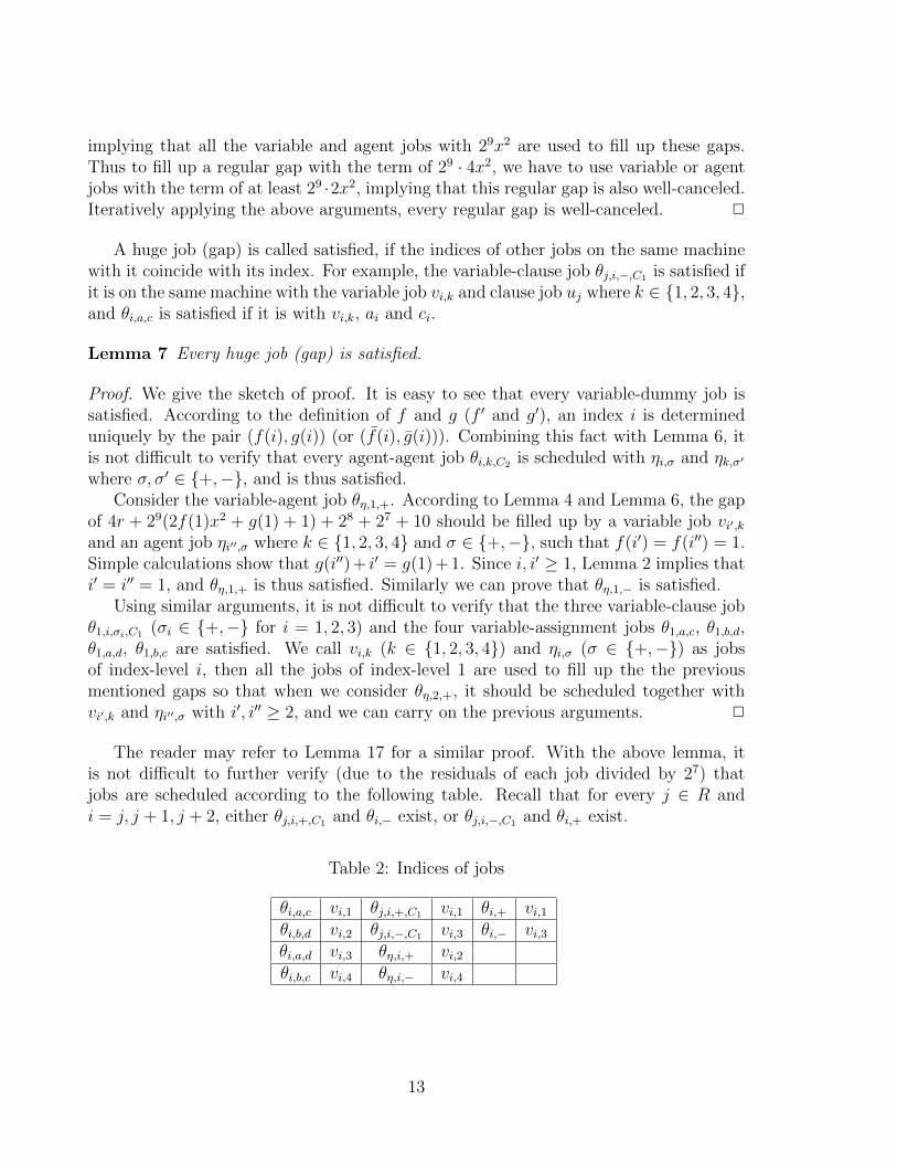
The reader may refer to Lemma 17 for a similar proof. With the above lemma, itis not difficult to further verify (due to the residuals of each job divided by 27) thatjobs are scheduled according to the following table. Recall that for every j ∈ R andi = j, j + 1, j + 2, either θj,i,+,C1 and θi,− exist, or θj,i,−,C1 and θi,+ exist.

Table 2: Indices of jobs

θi,a,c vi,1 θj,i,+,C1 vi,1 θi,+ vi,1θi,b,d vi,2 θj,i,−,C1 vi,3 θi,− vi,3θi,a,d vi,3 θη,i,+ vi,2θi,b,c vi,4 θη,i,− vi,4

13

The previous discussion determines the indices of jobs on each machine, and we needto further determine their superscripts. We have the following simple observations (byconsidering the r-terms of jobs).

• The two jobs with an agent-agent or variable-agent job are one true and one false.

• The three jobs with a variable-assignment job are either (T,T,T) or (F,F,F).

• The clause job and variable job with a variable-clause job are (T,T), (F,F) or (F,T),i.e., the variable job must be true if the clause job is true.

According to the superscripts of jobs on each machine, we give a truth assignment ofvariables in the following way. Notice that according to the analysis above, there are twoway of scheduling truth-assignment jobs, either (vTi,1, a

Ti , c

Ti ), (vTi,2, b

Ti , d

Ti ), (vFi,3, a

Fi , d

Fi ),

(vFi,4, bFi , c

Fi ) or (vFi,1, a

Fi , c

Fi ), (vFi,2, b

Fi , d

Fi ), (vTi,3, a

Ti , d

Ti ), (vTi,4, b

Ti , c

Ti ). We let variable zi be

false if aTi is with vTi,1, otherwise it is true. We prove that Isat is satisfied.Consider any cj ∈ C1, u

Tj should be scheduled with a true variable job and it is either

vTi,1 or vTi,3. If it is vTi,1, then obviously the variable zi is true (for otherwise vTi,1 is with aTi ,rather than uTj ). Furthermore, uTj and vTi,1 must be scheduled with θj,i,+,C1 . Recall thatwe construct the job θj,i,+,C1 if the positive literal zi ∈ cj. Thus cj is satisfied. Otherwiseit is vTi,3, and vFi,3 is with aFi , meaning that aTi is with vTi,1 and the variable zi is false.Similar arguments show that ¬zi ∈ cj and cj is also satisfied.

Consider any (zi ∨ ¬zk) ∈ C2. θi,k,C2 is scheduled with two agent jobs, one true andone false. If it is with ηTi,+, then ηFi,+ is with vTi,2, implying that vFi,2 is with bFi and dFi .Hence the variable zi is true, meaning that (zi ∨ ¬zk) is satisfied. Otherwise θi,k,C2 iswith ηFi,+, and using similar arguments we can show that (zi ∨ ¬zk) is also satisfied.

Remark The reader can see that, the x2-terms of variable jobs are only used whenwe try to prove that variable-agent and agent-agent jobs are satisfied. Indeed, thesatisfaction of (zi ∨ ¬zk) ∈ C2 follows from vi,2 and vk,4 should be one true and onefalse (meaning that the positive literal zi and negative literal ¬zk should be one true andone false), and this is ensured by the following two facts.

• vi,2 (vk,4) has two agents, one true and one false. vi,2 (vk,4) is scheduled with oneof its agents, and they are one true and one false.

• One agent of vi,2 is scheduled together with one agent of vk,4, and they are one trueand one false.

The processing time of an agent job should be defined in a proper way so that we candetermine from the gaps that a variable job is scheduled with its corresponding agentjob, and two specific agent jobs are scheduled together, and this requires a processingtime of O(n3/2). To reduce it to O(n1+δ) for δ > 0, we create 1/δ − 1 pairs of agentjobs (from layer-1 to layer-(1/δ − 1)) for a variable. A variable job is scheduled with its

14

layer-(1/δ − 1) agent job, its layer-(1/δ − 1) agent job is with its layer-(1/δ − 2) agentjob, · · · , its layer-2 agent job is with its layer-1 agent job, and two specific layer-1 agentjobs are scheduled together. Detailed description is in the next subsection.

2.2 Reduction for arbitrary δ

We give a brief overview. We create jobs vγi,1, vγi,2, v

γi,3, v

γi,4 for variable zi and jobs uγj

for cj ∈ C1 where γ ∈ {T, F}, just as what we do when δ = 1/2. Recall that in theprevious subsection we create 2 pairs of agent jobs ηγi,+ and ηγi,− for every variable zi,in this subsection we create 2(1/δ − 1) pairs of agent jobs, namely ηγi,j,+ and ηγi,j,− for1 ≤ j ≤ 1/δ − 1. For simplicity, ηγi,j,+ and ηγi,j,− are called layer-j agent jobs. Again wecreate huge jobs so as to make a gap on every machine. There are six kinds of huge jobs(gaps).

[1.] Variable-assignment gaps. Similar as the previous subsection, to fill up these gapseither vFi,1, v

Fi,2, v

Ti,3, v

Ti,4 (meaning variable zi is true), or vTi,1, v

Ti,2, v

Fi,3, v

Fi,4 (meaning

variable zi is false) are used. Jobs aγi , bγi , c

γi and dγi also serve as ’assistant jobs’.

[2.] Variable-clause gaps. Similar as the previous subsection, if the positive (or negative)literal zi (or ¬zi) is in cj ∈ C1, then a variable-clause gap is created so that it could onlybe filled up by uj and vi,1 (or vi,3), and their superscripts can only be (T,T), (F,F) or(F,T).

[3.] Variable-agent, layer-decreasing and agent-agent gaps. Similar as what we do in theprevious subsection, we try to construct several gaps so as to enforce that either vTi,2, v

Fk,4

or vFi,2, vTk,4 are are used to fill up these gaps. We create 1/δ − 1 pairs of agent jobs for

vi,2 (or vk,4), namely ηγi,j,+ (or ηγi,j,−) for 1 ≤ j ≤ 1/δ − 1. We create one variable-agentgap which could only be filled up by vi,2 and the corresponding layer-(1/δ− 1) agent jobηi,1/δ−1,+, and they should be one true and one false (i.e., their superscripts are T and F ).We then create 1/δ − 2 layer-decreasing gaps such that the j-th gap could only be filledup by ηi,j+1,− and ηi,j,− that are one true and one false. Similarly another variable-agentgap is created which could only be filled up by vk,4 and ηk,1/δ−1,− that are one true andone false, and another 1/δ − 2 layer-decreasing gaps are created such that the j-th gapcould only be filled up by ηi,j+1,+ and ηi,j,+ that are one true and one false. Finally wecreate an agent-agent gap which could only be filled up by ηi,1,+ and ηk,1,− that are onetrue and one false. It is not difficult to verify that if all these gaps are filled up, theneither vTi,2, v

Fk,4 or vFi,2, v

Tk,4 are are used together with all the agent jobs.

[4.] Variable-dummy gaps. Again we construct 8 jobs for a variable and only use 7 ofthem (either vi,1 or vi,3 is left), the remaining one will be used to fill these gaps.

2.2.1 Partition Clauses

Recall that nδ is an integer. We first partition all the clauses (of C2) equally into nδ

groups. Let these groups be S1,k1 for 1 ≤ k1 ≤ nδ. We call them as layer-1 groups.

15

It can be easily seen that each layer-1 group contains exactly n1 = n1−δ clauses, as aconsequence, clauses of S1,k1 contain n1 positive literals and n1 negative literals.

For simplicity, let S+1,k1

be the indices of all the positive literals of S1,k1 and S−1,k1 bethe indices of all the negative literals of S1,k1 .

Suppose i(1,k1)1 < i

(1,k1)2 < · · · < i

(1,k1)n1 are all the indices in S+

1,k1, we then define

f1/δ(i(1,k1)l ) = k1, g1/δ−1(i

(1,k1)l ) = l.

Similarly let i(1,k1)1 < i

(1,k1)2 < · · · < i

(1,k1)n1 be all the indices in S−1,k1 , we then define

f1/δ (i(1,k1)l ) = k1, g1/δ−1(i

(1,k1)l ) = l.

Each group S1,k1 is then further partitioned equally into nδ subgroups and let thesegroups be S2,k1,k2 for 1 ≤ k2 ≤ n1/δ. In general, suppose we have already derived n(j−1)δ

layer-(j− 1) groups for 2 ≤ j ≤ 1/δ− 1. Each layer-(j− 1) group, say, Sj−1,k1,k2,··· ,kj−1is

then further partitioned equally into nδ subgroups. Let them be Sj,k1,k2,··· ,kj for 1 ≤ kj ≤nδ. It can be easily seen that each layer-j group contains nj = n1−jδ clauses. Again letS+j,k1,k2,··· ,kj and S−j,k1,k2,··· ,kj be the sets of indices of all the positive literals and negative

literals in Sj,k1,k2,··· ,kj respectively. Let i(j,k1,k2,··· ,kj)1 < i

(j,k1,k2,··· ,kj)2 < · · · < i

(j,k1,k2,··· ,kj)nj be

the indices in S+j,k1,k2,··· ,kj , we then define

f1/δ−j+1(i(j,k1,k2,··· ,kj)l ) = kj, g1/δ−j(i

(j,k1,k2,··· ,kj)l ) = l.

Similarly let i(j,k1,k2,··· ,kj)1 < i

(j,k1,k2,··· ,kj)2 < · · · < i

(j,k1,k2,··· ,kj)nj be all the indices in

S−j,k1,k2,··· ,kj , we then define

f1/δ−j+1(i(j,k1,k2,··· ,kj)l ) = kj, g1/δ−j (i

(j,k1,k2,··· ,kj)l ) = l.

The above procedure stops when we derive layer-(1/δ− 1) groups with each of themcontaining nδ clauses. We have the following simple observations.

Observation

1. For any 1 ≤ i ≤ n, 1 ≤ fk(i) ≤ nδ for 2 ≤ k ≤ 1/δ, and 1 ≤ gk(i), gk(i) ≤ nkδ for1 ≤ k ≤ 1/δ − 1.

2. If (zi ∨ ¬zh) ∈ C2, then fk(i) = fk(h) for 2 ≤ k ≤ 1/δ.

3. For any 0 ≤ k ≤ 1/δ − 2 and i < i′

– If f1/δ(i) = f1/δ(i′), f1/δ−1(i) = f1/δ−2(i

′), · · · , f1/δ−k(i) = f1/δ−k(i′),

then g1/δ−k−1(i) < g1/δ−k−1(i′).

– If f1/δ(i) = f1/δ(i′), f1/δ−1(i) = f1/δ−2(i

′), · · · , f1/δ−k(i) = f1/δ−k(i′),

then g1/δ−k−1(i) < g1/δ−k−1(i′).

4. For any 1 ≤ τ ≤ nδ and 2 ≤ k ≤ 1/δ, |{i|fk(i) = τ}| = |{i|fk(i) = τ}| = n1−δ.

16

2.2.2 Construction of the Scheduling Instance

We construct the scheduling instance based on Isat. Throughout this section we setx = 4nδ, r = 23/δ+9n1+δ and use s(j) to denote the processing time of job j. We willshow that the constructed scheduling instance admits a feasible schedule of makespanK = 105r if and only if the given 3SAT’ instance is satisfiable. Similar to the special casewhen δ = 1/2, we construct 8n variable jobs, 8n truth assignment jobs, n clause jobs,2n dummy jobs. The only difference is that we construct more agent jobs, indeed, wewill construct 4(1/δ − 1)n agent jobs, divided from layer-1 agent jobs to layer-(1/δ − 1)agent jobs.Variable jobs: vγi,1 and vγi,2 are constructed for zi, v

γi,3 and vγi,4 are for ¬zi.

s(vTi,k) = r + 21/δ+7[f1/δ(i)x1/δ + i] + 21/δ+6 + k, k = 1, 2

s(vTi,k) = r + 21/δ+7[f1/δ(i)x1/δ + i] + 21/δ+6 + k, k = 3, 4

s(vFi,k) = s(vTi,k) + 2r, k = 1, 2, 3, 4

Agent jobs: layer-j agent jobs ηγi,j,+ and ηγi,j,− are constructed for 1 ≤ i ≤ n and 1 ≤ j ≤1/δ − 1.

s(ηTi,j,+) = r + 21/δ+7[

1/δ∑k=j+1

fk(i)xk + gj(i)] + 2j+6 + 8, j = 1, 2, · · · , 1/δ − 1

s(ηTi,j,−) = r + 21/δ+7[

1/δ∑k=j+1

fk(i)xk + gj(i)] + 2j+6 + 16, j = 2, 3, · · · , 1/δ − 1

Specifically, s(ηTi,1,−) = r + 21/δ+7[∑1/δ

k=2 fk(i)xk + g1(i)x] + 27 + 16,

s(ηFi,j,σ) = s(ηTi,σ) + 2r, σ = +,−

Truth assignment jobs: aγi , bγi , c

γi and dγi .

s(aFi ) = 11r + (27i+ 8), s(bFi ) = 11r + (27i+ 32),

s(cFi ) = 101r + (27i+ 16), s(dFi ) = 101r + (27i+ 64),

s(ζTi ) = s(ζFi ) + r, ζ = a, b, c, d.

Clause jobs: 3 clause jobs are constructed for every cj ∈ C1 where j ∈ R, with one uTjand two copies of uFj :

s(uTj ) = 10004r + 21/δ+9j, s(uFj ) = 10002r + 21/δ+9j.

Dummy jobs: n+n/3 jobs with processing time 1000r, and n−n/3 jobs with processingtime 1002r.

17

Let V and Va be the set of variable jobs and agent jobs. Let A, B, C, D be theset of aγi , b

γi , c

γi and dγi respectively. Let G0 = V ∪ Va, G1 = A ∪ B, G2 = C ∪ D, G3

be the set of dummy jobs and G4 = U be the set of clause jobs. Again we may dropthe superscript for simplicity. We construct huge jobs. They create gaps on machines.According to which jobs are needed to fill up the gap, they are divided into six groups.

Two huge jobs (variable-agent jobs) θη,i,+ and θη,i,− are constructed for each variablezi:

s(θη,i,+) = 105r − [4r + 21/δ+7(2f1/δ(i)x1/δ + i+ g1/δ−1(i)) + 21/δ+6 + 21/δ+5 + 10]

s(θη,i,−) = 105r − [4r + 21/δ+7(2f1/δ(i)x1/δ + i+ g1/δ−1(i)) + 21/δ+6 + 21/δ+5 + 20]

2/δ − 4 huge jobs (layer-decreasing jobs) θi,j,+ and θi,j,− are constructed for j =1, · · · , 1/δ − 2. For j = 2, 3, · · · , 1/δ − 2, their processing times are

s(θi,j,+) = 105r − [4r + 21/δ+7(2

1/δ∑k=j+2

fk(i)xk + fj+1(i)x

j+1 + gj+1(i) + gj(i)) + 2j+7 + 2j+6 + 16]

s(θi,j,−) = 105r − [4r + 21/δ+7(2

1/δ∑k=j+2

fk(i)xk + fj−1(i)x

j+1 + gj+1(i) + gj(i)) + 2j+7 + 2j+6 + 32].

For j = 1, their processing times are

s(θi,1,+) = 105r − [4r + 21/δ+7(2

1/δ∑l=3

fl(i)xl + f2(i)x

2 + g2(i) + g1(i)) + 28 + 27 + 16]

s(θi,1,−) = 105r − [4r + 21/δ+7(2

1/δ∑l=3

fl(i)xl + f2(i)x

2 + g2(i) + g1(i)x) + 28 + 27 + 32].

One huge job (agent-agent job) θi,k,C2 is constructed for (zi ∨ ¬zk) ∈ C2:

s(θi,k,C2) = 105r − [4r + 21/δ+7(2

1/δ∑l=2

fl(i)xl + g1(k)x+ g1(i)) + 28 + 24].

Three huge jobs (variable-clause jobs) are constructed for each cj ∈ C1 (j ∈ R), onefor each literal: for i = j, j + 1, j + 2, if zi ∈ cj, we construct θj,i,+,C1 , otherwise ¬zi ∈ cj,and we construct θj,i,−,C1 .

s(θj,i,+,C1) = 105r − 11005r − (21/δ+7f1/δ(k)x1/δ + 21/δ+9i+ 21/δ+7k + 21/δ+6 + 1),

s(θj,i,−,C1) = 105r − 11005r − (21/δ+7f1/δ(k)x1/δ + 21/δ+9i+ 21/δ+7k + 21/δ+6 + 3).

One huge job (variable-dummy job) is constructed for each variable. Notice that eachvariable appears exactly three times in clauses, if zi appears twice while ¬zi appears once,we construct θi,−. Otherwise, we construct θi,+ instead.

s(θi,+) = 105r − 1003r − (21/δ+7f1/δ(i)x1/δ + 21/δ+7i+ 21/δ+6 + 1),

18

s(θi,−) = 105r − 1003r − (21/δ+7f1/δ(i)x1/δ + 21/δ+7i+ 21/δ+6 + 3).

Thus, for each clause ci (i ∈ R) and k = i, i + 1, i + 2, either θi,+ and θj,i,−,C1 exist,or θi,− and θj,i,+,C1 exist.

Four huge jobs (variable-assignment jobs) are constructed for each variable zi, namelyθi,a,c, θi,b,d, θi,a,d and θi,b,c:

s(θi,a,c) = 105r − 115r − 21/δ+7(f1/δ(i)x1/δ + i)− (21/δ+6 + 28i+ 25),

s(θi,b,d) = 105r − 115r − 21/δ+7(f1/δ(i)x1/δ + i)− (21/δ+6 + 28i+ 98),

s(θi,a,d) = 105r − 115r − 21/δ+7(f1/δ(i)x1/δ + i)− (21/δ+6 + 28i+ 75),

s(θi,b,c) = 105r − 115r − 21/δ+7(f1/δ(i)x1/δ + i)− (21/δ+6 + 28i+ 52).

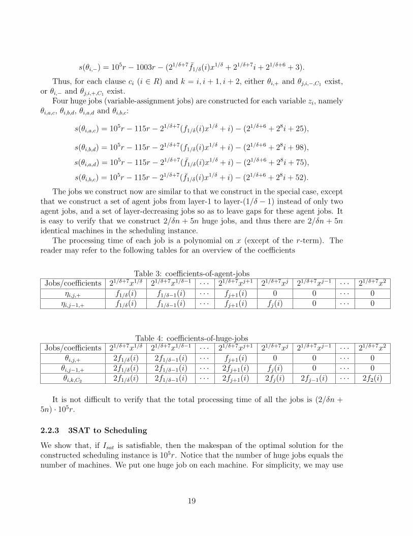
The jobs we construct now are similar to that we construct in the special case, exceptthat we construct a set of agent jobs from layer-1 to layer-(1/δ − 1) instead of only twoagent jobs, and a set of layer-decreasing jobs so as to leave gaps for these agent jobs. Itis easy to verify that we construct 2/δn + 5n huge jobs, and thus there are 2/δn + 5nidentical machines in the scheduling instance.

The processing time of each job is a polynomial on x (except of the r-term). Thereader may refer to the following tables for an overview of the coefficients

Table 3: coefficients-of-agent-jobsJobs/coefficients 21/δ+7x1/δ 21/δ+7x1/δ−1 · · · 21/δ+7xj+1 21/δ+7xj 21/δ+7xj−1 · · · 21/δ+7x2

ηi,j,+ f1/δ(i) f1/δ−1(i) · · · fj+1(i) 0 0 · · · 0ηi,j−1,+ f1/δ(i) f1/δ−1(i) · · · fj+1(i) fj(i) 0 · · · 0

Table 4: coefficients-of-huge-jobsJobs/coefficients 21/δ+7x1/δ 21/δ+7x1/δ−1 · · · 21/δ+7xj+1 21/δ+7xj 21/δ+7xj−1 · · · 21/δ+7x2

θi,j,+ 2f1/δ(i) 2f1/δ−1(i) · · · fj+1(i) 0 0 · · · 0θi,j−1,+ 2f1/δ(i) 2f1/δ−1(i) · · · 2fj+1(i) fj(i) 0 · · · 0θi,k,C2 2f1/δ(i) 2f1/δ−1(i) · · · 2fj+1(i) 2fj(i) 2fj−1(i) · · · 2f2(i)

It is not difficult to verify that the total processing time of all the jobs is (2/δn +5n) · 105r.

2.2.3 3SAT to Scheduling

We show that, if Isat is satisfiable, then the makespan of the optimal solution for theconstructed scheduling instance is 105r. Notice that the number of huge jobs equals thenumber of machines. We put one huge job on each machine. For simplicity, we may use

19

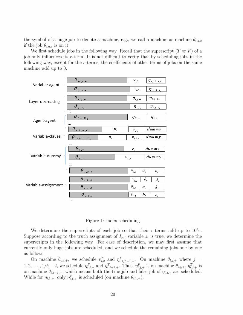
the symbol of a huge job to denote a machine, e.g., we call a machine as machine θi,a,cif the job θi,a,c is on it.

We first schedule jobs in the following way. Recall that the superscript (T or F ) of ajob only influences its r-term. It is not difficult to verify that by scheduling jobs in thefollowing way, except for the r-terms, the coefficients of other terms of jobs on the samemachine add up to 0.

Figure 1: index-scheduling

We determine the superscripts of each job so that their r-terms add up to 105r.Suppose according to the truth assignment of Isat variable zi is true, we determine thesuperscripts in the following way. For ease of description, we may first assume thatcurrently only huge jobs are scheduled, and we schedule the remaining jobs one by oneas follows.

On machine θη,i,+, we schedule vTi,2 and ηFi,1/δ−1,+. On machine θi,j,+ where j =

1, 2, · · · , 1/δ − 2, we schedule ηFi,j,+ and ηTi,j+1,+. Thus, ηFi,j,+ is on machine θi,j,+, ηTi,j,+ ison machine θi,j−1,+, which means both the true job and false job of ηi,j,+ are scheduled.While for ηi,1,+, only ηFi,1,+ is scheduled (on machine θi,1,+).

20

Similarly on machine θη,i,−, we schedule vFi,4 and ηTi,1/δ−1,−. On machine θi,j,− where

j = 1, 2, · · · , 1/δ − 2, we schedule ηTi,j,− and ηFi,j+1,−. Thus, ηTi,j,− is on machine θi,j,−,ηFi,j,− is on machine θi,j−1,−, which means both the true job and false job is scheduled.While for ηi,1,−, only ηTi,1,− is scheduled (on machine θi,1,−).

Consider agent-agent machines. For the variable zi, there is a clause (zi ∨ ¬zk) ∈ C2

for some k, and we need to schedule ηi,1,+ and ηk,1,− on machine θi,k,C2 . Since Isat issatisfiable, variables zi and zk should be both true or both false. Thus, given that zi istrue, zk is also true. This implies that ηTi,1,+ and ηFk,1,− are not scheduled before, and weschedule these two jobs.

Meanwhile in C2 there is also a clause (zk′∨¬zi) for some k′, and we need to scheduleηi,1,− and ηk′,1,+ on machine θk′,i,C2 . Since Isat is satisfiable, variables zk′ and zi shouldbe both true or both false. Thus, given that zi is true, zk is also true. This implies thatηTk′,1,+ and ηFi,1,− are not unscheduled before, and we schedule them on machine θk′,i,C2 .

Consider variable-assignment jobs. We put vFi,1, aFi , cFi on machine θi,a,c, put vFi,2, b

Fi , d

Fi

on machine θi,b,d, put vTi,3, aTi , d

Ti on machine θi,a,d, and put vTi,4, b

Ti , c

Ti on machine θi,b,c.

Thus, both the true copy and false copy of ai, bi, ci and di are scheduled. It can beeasily seen that the r-terms of three true jobs or three false jobs both add up to 115r.Otherwise, zi is false, and we schedule jobs just in the opposite way, i.e., we replace eachtrue job with its corresponding false job, and each false job with its corresponding truejob in the previous scheduling.

We consider the remaining jobs. If zi is true, then vTi,1 and vFi,3 are left. If zi is false,then vFi,1 and vTi,3 are left. These jobs should be scheduled with clause jobs and dummyjobs on variable-clause machines or variable-dummy machines. Notice that for any i ∈ Rand k ∈ {i, i+ 1, i+ 2}, either θi,k,+,C1 and θk,− exist, or θi,k,−,C1 and θk,+ exist.

Suppose the variable zk is true. If θi,k,+,C1 and θk,− exist, we put vTk,1 on machineθi,k,+,C1 , and vFk,3 on machine θk,−. Otherwise θi,k,−,C1 and θk,+ exist, and we put vFk,3 onmachine θi,k,−,C1 , and vTk,1 on machine θk,+. In both cases, the remaining jobs vTk,1 andvFk,3 are scheduled.

Otherwise zk is false. If θi,k,+,C1 and θk,− exist, put vFk,1 on machine θi,k,+,C1 , and vTk,3on machine θk,−. Otherwise θi,k,−,C1 and θk,+ exist. We put vTk,3 on machine θi,k,−,C1 , andvFk,1 on machine θk,+. Again in both cases, the remaining jobs vFk,1 and vTk,3 are scheduled.

From now on we drop the symbol + or − and just use θi,k,C1 to denote either θi,k,+,C1

or θi,k,−,C1 , and use θk to denote either θk,+ or θk,−. It is easy to verify that the abovescheduling has the following property.

Property If ci is satisfied by variable zk (i.e., zk ∈ ci and zk is true or ¬zk ∈ ci and zkis false), then a true variable job is on machine θi,k,C1 ; if ci is not satisfied by zk, then afalse variable job is on machine θi,k,C1 .

Consider variable-dummy machines. For each k = 1, 2, · · · , n, there is one machineθk. If a true variable job is on it, we then put additionally a dummy job of size 1002r.Otherwise a false variable job is on it, and we put additionally a dummy job of size 1000ron it. Thus, in both cases the r-terms of variable job and dummy job add up to 1003r.

21

Consider variable-clause machines. For each clause ci ∈ C1 (i.e., i ∈ R), there arethree copies of ui, one true and two false. There are three machines, θi,i,C1 , θi,i+1,C1 andθi,i+2,C1 .

Notice that according to the truth assignment, ci is satisfied by at least one variable.Suppose ci is satisfied by zk1 , and let zk2 and zk3 be the remaining two variables in thisclause, i.e., k1, k2, k3 is some permutation of the three indices i, i + 1, i + 2. We put uTion machine θi,k1,C1 . Additionally, we put a dummy job of size 1000r on this machine.According to the property we have mentioned above, since ci is satisfied by zk1 , thevariable job on machine θi,k1,C1 is a true job. Thus, the r-terms of the true clause job,true variable job and a dummy job on θi,k1,C1 add up to 11005r.

Consider machine θi,k2,C1 and θi,k3,C1 . We put one of the remaining two false jobs uFion them respectively. We add dummy jobs according to the following criteria. If thevariable job is true, we add a dummy job of size 1002r. If the variable job is false, weadd a dummy job of size 1000r.

Thus in both cases, the r-terms of the variable job and dummy job add up to 1003r.And if we further add the r-terms of the false clause job and the relation job, the sumis 105r. Finally we check the number of dummy jobs that are used.

For simplicity we use (T/F, T/F, 1000r/1002r) to denote the truth-type of a variable-clause machine, i.e., the first coordinate is T is the variable job is true, and F if it isfalse, similarly the second coordinate is T (or F ) if the clause job is T (or F ), the thirdcoordinate is 1000r (or 1002r) if the dummy job is of size 1000r (or 1002r). We alsodenote the truth-type of a variable-dummy machine in the form of (T/F, 1000r/1002r).

A dummy job of size 1000r is always scheduled on a machine of truth-type (T, T, 1000r),(F, F, 1000r) and (F, 1000r), while a dummy job of 1002r is scheduled on a machine oftruth-type (T, F, 1002r) and (T, 1002r). Notice that on these machines, there are n truevariable jobs and n false variable jobs, and there are |C1| = n/3 true clause jobs, thussimple calculations show that n+n/3 dummy jobs of 1000r and n−n/3 dummy jobs of1002r are scheduled, which coincides with the dummy jobs we construct.

2.2.4 Scheduling to 3SAT

We show that, if the constructed scheduling instance admits a feasible schedule withmakespan 105r, then Isat is satisfiable. Notice that in a scheduling problem, jobs arerepresented by their processing times rather than symbols, we first show that we can theprocessing time of each job we construct is distinct (except that two copies of uFi areconstructed for every clause in C1), this would be enough to determine the symbol of ajob from its processing time.

Distinguishing Jobs from Their Processing Times Recall that we define theprocessing time of a job in the form of a polynomial, we use the notion xj-term or r-term in their direct meaning. Meanwhile, we call the sum of all except the r-term of ajob as the small-r-term. For any 2 ≤ j ≤ 1/δ, we delete the r-term and xk-term with

22

k ≥ j from the processing time of a job, and call the sum of all the remaining terms asthe small-xj-term.

For example, the relation job θi,3,+ is of processing time 105r−[4r+21/δ+7(2∑1/δ

k=5 fk(i)xk+

f4(i)x4 + g4(i) + g3(i)) + 210 + 29 + 16], and thus for 5 ≤ k ≤ 1/δ, its xk-term is

21/δ+7 · 2f(i)xk. Its x4-term is f(4)(i)x4. Its x3-term and x2-term are 0. Its small-x5-term is 21/δ+7(f4(i)x

4 + g4(i) + g3(i)) + 210 + 29 + 16. Meanwhile, for a clause job, say,ui, its xj-term is 0 for 1 ≤ j ≤ 1/δ, and its small-xj-term for any j is 21/δ+9i.

Consider the small-r-term of any job. If it is a huge job, this value is negativeand its absolute value is bounded by 21/δ+7(2

∑1/δk=2 n

1/δxk + 2n) + 21/δ+7 + 32 < 1/2r(notice that nδxk = 1/4xk+1). Otherwise it is a variable, or agent, or clause, or truthassignment, or dummy job, and the sum is positive with its absolute value also boundedby 21/δ+7(

∑1/δk=2 n

1/δxk + n) + 21/δ+6 + 64 < 1/4r.For the small-xj-terms of jobs, we have the following lemma.

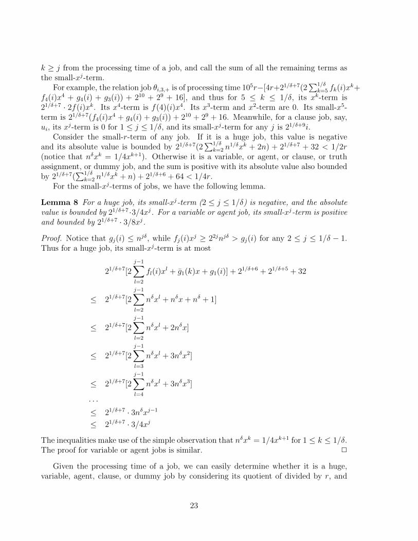
Lemma 8 For a huge job, its small-xj-term (2 ≤ j ≤ 1/δ) is negative, and the absolutevalue is bounded by 21/δ+7 ·3/4xj. For a variable or agent job, its small-xj-term is positiveand bounded by 21/δ+7 · 3/8xj.

Proof. Notice that gj(i) ≤ njδ, while fj(i)xj ≥ 22jnjδ > gj(i) for any 2 ≤ j ≤ 1/δ − 1.

Thus for a huge job, its small-xj-term is at most

21/δ+7[2

j−1∑l=2

fl(i)xl + g1(k)x+ g1(i)] + 21/δ+6 + 21/δ+5 + 32

≤ 21/δ+7[2

j−1∑l=2

nδxl + nδx+ nδ + 1]

≤ 21/δ+7[2

j−1∑l=2

nδxl + 2nδx]

≤ 21/δ+7[2

j−1∑l=3

nδxl + 3nδx2]

≤ 21/δ+7[2

j−1∑l=4

nδxl + 3nδx3]

· · ·≤ 21/δ+7 · 3nδxj−1

≤ 21/δ+7 · 3/4xj

The inequalities make use of the simple observation that nδxk = 1/4xk+1 for 1 ≤ k ≤ 1/δ.The proof for variable or agent jobs is similar. 2

Given the processing time of a job, we can easily determine whether it is a huge,variable, agent, clause, or dummy job by considering its quotient of divided by r, and

23

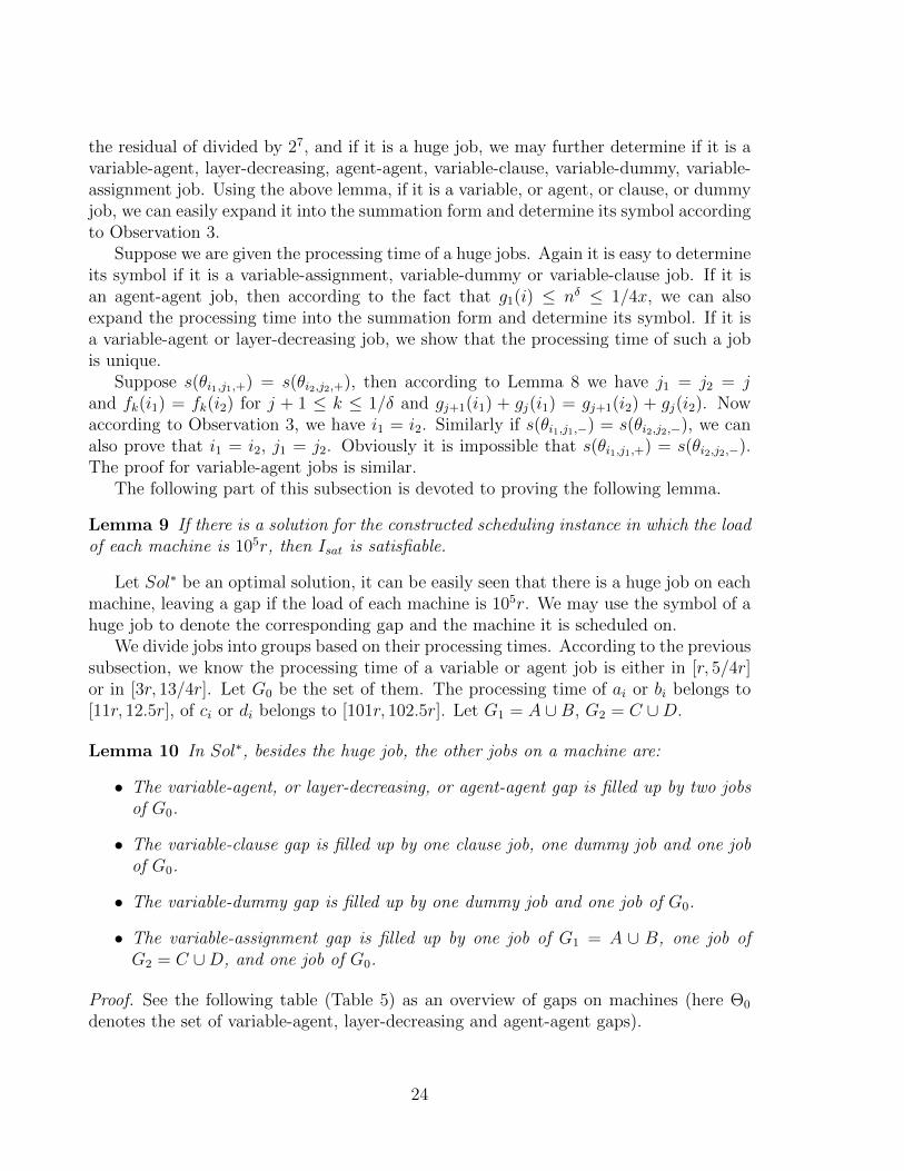
the residual of divided by 27, and if it is a huge job, we may further determine if it is avariable-agent, layer-decreasing, agent-agent, variable-clause, variable-dummy, variable-assignment job. Using the above lemma, if it is a variable, or agent, or clause, or dummyjob, we can easily expand it into the summation form and determine its symbol accordingto Observation 3.

Suppose we are given the processing time of a huge jobs. Again it is easy to determineits symbol if it is a variable-assignment, variable-dummy or variable-clause job. If it isan agent-agent job, then according to the fact that g1(i) ≤ nδ ≤ 1/4x, we can alsoexpand the processing time into the summation form and determine its symbol. If it isa variable-agent or layer-decreasing job, we show that the processing time of such a jobis unique.

Suppose s(θi1,j1,+) = s(θi2,j2,+), then according to Lemma 8 we have j1 = j2 = jand fk(i1) = fk(i2) for j + 1 ≤ k ≤ 1/δ and gj+1(i1) + gj(i1) = gj+1(i2) + gj(i2). Nowaccording to Observation 3, we have i1 = i2. Similarly if s(θi1,j1,−) = s(θi2,j2,−), we canalso prove that i1 = i2, j1 = j2. Obviously it is impossible that s(θi1,j1,+) = s(θi2,j2,−).The proof for variable-agent jobs is similar.

The following part of this subsection is devoted to proving the following lemma.

Lemma 9 If there is a solution for the constructed scheduling instance in which the loadof each machine is 105r, then Isat is satisfiable.

Let Sol∗ be an optimal solution, it can be easily seen that there is a huge job on eachmachine, leaving a gap if the load of each machine is 105r. We may use the symbol of ahuge job to denote the corresponding gap and the machine it is scheduled on.

We divide jobs into groups based on their processing times. According to the previoussubsection, we know the processing time of a variable or agent job is either in [r, 5/4r]or in [3r, 13/4r]. Let G0 be the set of them. The processing time of ai or bi belongs to[11r, 12.5r], of ci or di belongs to [101r, 102.5r]. Let G1 = A ∪B, G2 = C ∪D.

Lemma 10 In Sol∗, besides the huge job, the other jobs on a machine are:

• The variable-agent, or layer-decreasing, or agent-agent gap is filled up by two jobsof G0.

• The variable-clause gap is filled up by one clause job, one dummy job and one jobof G0.

• The variable-dummy gap is filled up by one dummy job and one job of G0.

• The variable-assignment gap is filled up by one job of G1 = A ∪ B, one job ofG2 = C ∪D, and one job of G0.

Proof. See the following table (Table 5) as an overview of gaps on machines (here Θ0

denotes the set of variable-agent, layer-decreasing and agent-agent gaps).

24

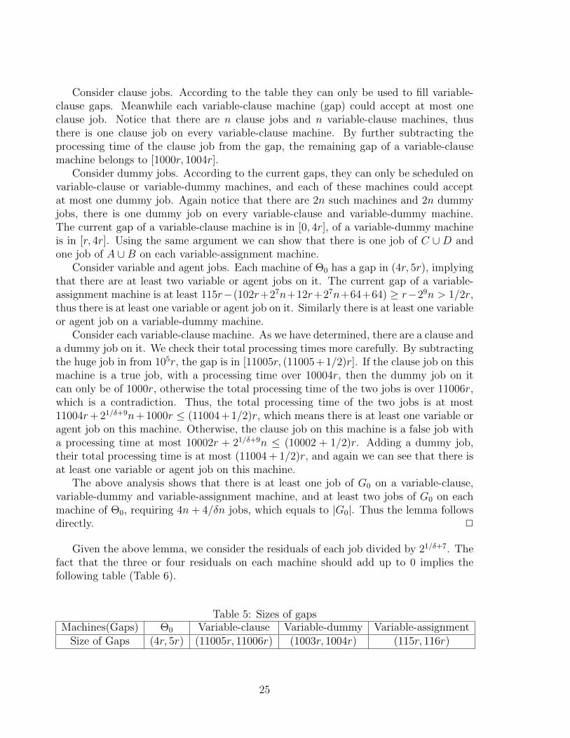
Consider clause jobs. According to the table they can only be used to fill variable-clause gaps. Meanwhile each variable-clause machine (gap) could accept at most oneclause job. Notice that there are n clause jobs and n variable-clause machines, thusthere is one clause job on every variable-clause machine. By further subtracting theprocessing time of the clause job from the gap, the remaining gap of a variable-clausemachine belongs to [1000r, 1004r].

Consider dummy jobs. According to the current gaps, they can only be scheduled onvariable-clause or variable-dummy machines, and each of these machines could acceptat most one dummy job. Again notice that there are 2n such machines and 2n dummyjobs, there is one dummy job on every variable-clause and variable-dummy machine.The current gap of a variable-clause machine is in [0, 4r], of a variable-dummy machineis in [r, 4r]. Using the same argument we can show that there is one job of C ∪D andone job of A ∪B on each variable-assignment machine.

Consider variable and agent jobs. Each machine of Θ0 has a gap in (4r, 5r), implyingthat there are at least two variable or agent jobs on it. The current gap of a variable-assignment machine is at least 115r−(102r+27n+12r+27n+64+64) ≥ r−29n > 1/2r,thus there is at least one variable or agent job on it. Similarly there is at least one variableor agent job on a variable-dummy machine.

Consider each variable-clause machine. As we have determined, there are a clause anda dummy job on it. We check their total processing times more carefully. By subtractingthe huge job in from 105r, the gap is in [11005r, (11005+1/2)r]. If the clause job on thismachine is a true job, with a processing time over 10004r, then the dummy job on itcan only be of 1000r, otherwise the total processing time of the two jobs is over 11006r,which is a contradiction. Thus, the total processing time of the two jobs is at most11004r+ 21/δ+9n+ 1000r ≤ (11004 + 1/2)r, which means there is at least one variable oragent job on this machine. Otherwise, the clause job on this machine is a false job witha processing time at most 10002r + 21/δ+9n ≤ (10002 + 1/2)r. Adding a dummy job,their total processing time is at most (11004 + 1/2)r, and again we can see that there isat least one variable or agent job on this machine.

The above analysis shows that there is at least one job of G0 on a variable-clause,variable-dummy and variable-assignment machine, and at least two jobs of G0 on eachmachine of Θ0, requiring 4n+ 4/δn jobs, which equals to |G0|. Thus the lemma followsdirectly. 2

Given the above lemma, we consider the residuals of each job divided by 21/δ+7. Thefact that the three or four residuals on each machine should add up to 0 implies thefollowing table (Table 6).

Table 5: Sizes of gapsMachines(Gaps) Θ0 Variable-clause Variable-dummy Variable-assignment

Size of Gaps (4r, 5r) (11005r, 11006r) (1003r, 1004r) (115r, 116r)

25

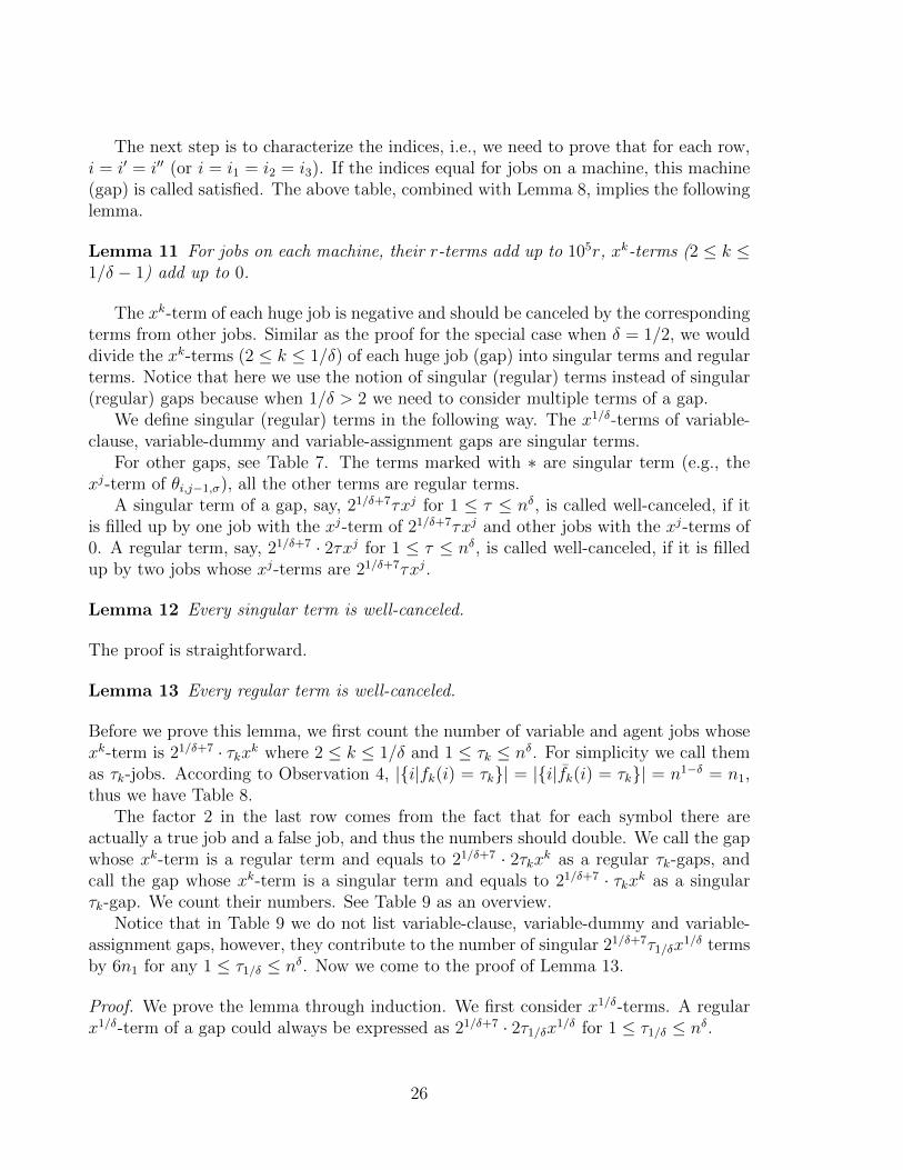
The next step is to characterize the indices, i.e., we need to prove that for each row,i = i′ = i′′ (or i = i1 = i2 = i3). If the indices equal for jobs on a machine, this machine(gap) is called satisfied. The above table, combined with Lemma 8, implies the followinglemma.

Lemma 11 For jobs on each machine, their r-terms add up to 105r, xk-terms (2 ≤ k ≤1/δ − 1) add up to 0.

The xk-term of each huge job is negative and should be canceled by the correspondingterms from other jobs. Similar as the proof for the special case when δ = 1/2, we woulddivide the xk-terms (2 ≤ k ≤ 1/δ) of each huge job (gap) into singular terms and regularterms. Notice that here we use the notion of singular (regular) terms instead of singular(regular) gaps because when 1/δ > 2 we need to consider multiple terms of a gap.

We define singular (regular) terms in the following way. The x1/δ-terms of variable-clause, variable-dummy and variable-assignment gaps are singular terms.

For other gaps, see Table 7. The terms marked with ∗ are singular term (e.g., thexj-term of θi,j−1,σ), all the other terms are regular terms.

A singular term of a gap, say, 21/δ+7τxj for 1 ≤ τ ≤ nδ, is called well-canceled, if itis filled up by one job with the xj-term of 21/δ+7τxj and other jobs with the xj-terms of0. A regular term, say, 21/δ+7 · 2τxj for 1 ≤ τ ≤ nδ, is called well-canceled, if it is filledup by two jobs whose xj-terms are 21/δ+7τxj.

Lemma 12 Every singular term is well-canceled.

The proof is straightforward.

Lemma 13 Every regular term is well-canceled.

Before we prove this lemma, we first count the number of variable and agent jobs whosexk-term is 21/δ+7 · τkxk where 2 ≤ k ≤ 1/δ and 1 ≤ τk ≤ nδ. For simplicity we call themas τk-jobs. According to Observation 4, |{i|fk(i) = τk}| = |{i|fk(i) = τk}| = n1−δ = n1,thus we have Table 8.

The factor 2 in the last row comes from the fact that for each symbol there areactually a true job and a false job, and thus the numbers should double. We call the gapwhose xk-term is a regular term and equals to 21/δ+7 · 2τkxk as a regular τk-gaps, andcall the gap whose xk-term is a singular term and equals to 21/δ+7 · τkxk as a singularτk-gap. We count their numbers. See Table 9 as an overview.

Notice that in Table 9 we do not list variable-clause, variable-dummy and variable-assignment gaps, however, they contribute to the number of singular 21/δ+7τ1/δx

1/δ termsby 6n1 for any 1 ≤ τ1/δ ≤ nδ. Now we come to the proof of Lemma 13.

Proof. We prove the lemma through induction. We first consider x1/δ-terms. A regularx1/δ-term of a gap could always be expressed as 21/δ+7 · 2τ1/δx1/δ for 1 ≤ τ1/δ ≤ nδ.

26

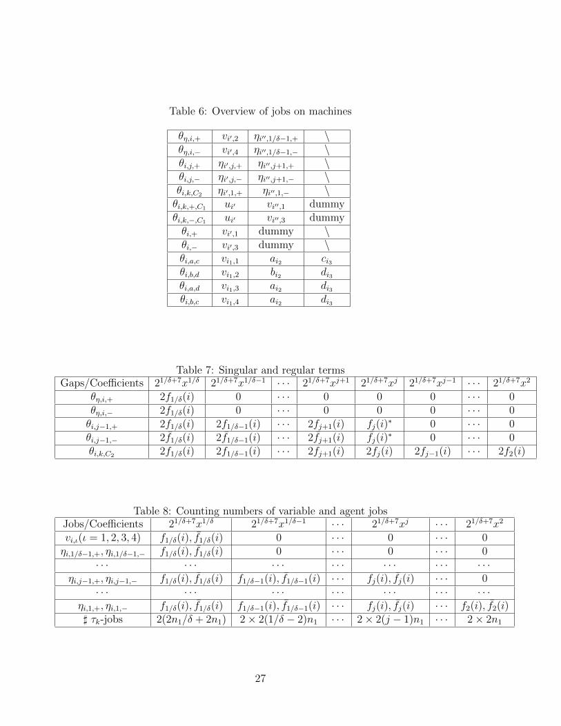
Table 6: Overview of jobs on machines

θη,i,+ vi′,2 ηi′′,1/δ−1,+ \θη,i,− vi′,4 ηi′′,1/δ−1,− \θi,j,+ ηi′,j,+ ηi′′,j+1,+ \θi,j,− ηi′,j,− ηi′′,j+1,− \θi,k,C2 ηi′,1,+ ηi′′,1,− \θi,k,+,C1 ui′ vi′′,1 dummyθi,k,−,C1 ui′ vi′′,3 dummyθi,+ vi′,1 dummy \θi,− vi′,3 dummy \θi,a,c vi1,1 ai2 ci3θi,b,d vi1,2 bi2 di3θi,a,d vi1,3 ai2 di3θi,b,c vi1,4 ai2 di3

Table 7: Singular and regular termsGaps/Coefficients 21/δ+7x1/δ 21/δ+7x1/δ−1 · · · 21/δ+7xj+1 21/δ+7xj 21/δ+7xj−1 · · · 21/δ+7x2

θη,i,+ 2f1/δ(i) 0 · · · 0 0 0 · · · 0θη,i,− 2f1/δ(i) 0 · · · 0 0 0 · · · 0θi,j−1,+ 2f1/δ(i) 2f1/δ−1(i) · · · 2fj+1(i) fj(i)

∗ 0 · · · 0θi,j−1,− 2f1/δ(i) 2f1/δ−1(i) · · · 2fj+1(i) fj(i)

∗ 0 · · · 0θi,k,C2 2f1/δ(i) 2f1/δ−1(i) · · · 2fj+1(i) 2fj(i) 2fj−1(i) · · · 2f2(i)

Table 8: Counting numbers of variable and agent jobsJobs/Coefficients 21/δ+7x1/δ 21/δ+7x1/δ−1 · · · 21/δ+7xj · · · 21/δ+7x2

vi,ι(ι = 1, 2, 3, 4) f1/δ(i), f1/δ(i) 0 · · · 0 · · · 0ηi,1/δ−1,+, ηi,1/δ−1,− f1/δ(i), f1/δ(i) 0 · · · 0 · · · 0

· · · · · · · · · · · · · · · · · · · · ·ηi,j−1,+, ηi,j−1,− f1/δ(i), f1/δ(i) f1/δ−1(i), f1/δ−1(i) · · · fj(i), fj(i) · · · 0

· · · · · · · · · · · · · · · · · · · · ·ηi,1,+, ηi,1,− f1/δ(i), f1/δ(i) f1/δ−1(i), f1/δ−1(i) · · · fj(i), fj(i) · · · f2(i), f2(i)] τk-jobs 2(2n1/δ + 2n1) 2× 2(1/δ − 2)n1 · · · 2× 2(j − 1)n1 · · · 2× 2n1

27

We start with τ1/δ = 1. Notice that a regular x1/δ-term comes from a variable-agent,layer-decreasing or agent-agent gap. According to Table 5, the x1/δ-term of the other twojobs (variable or agent jobs) used to fill up such a gap are nonzero and at least 21/δ+7x1/δ,thus the regular term 21/δ+7 ·2x1/δ is well canceled. Suppose for any τ1/δ < h0 ≤ nδ, eachregular term 21/δ+7τ1/δx

1/δ is well-canceled.We consider the case that τ1/δ = h0. For any τ1/δ such that 1 ≤ τ1/δ < h0, there are

in all 4n1(1/δ + 1) variable or agent jobs whose x1/δ-term is 21/δ+7τ1/δx1/δ (see Table 8).

We determine the scheduling of these jobs.Among them 6n1 jobs are on used to cancel singular terms according to Lemma

12. Meanwhile since there are 2n1/δ − n1 gaps with regular terms 21/δ+7 · 2τ1/δx1/δ (seeTable 9), the induction hypothesis implies that 4n1/δ − 2n1 of these variable and agentjobs are used to cancel these regular terms.

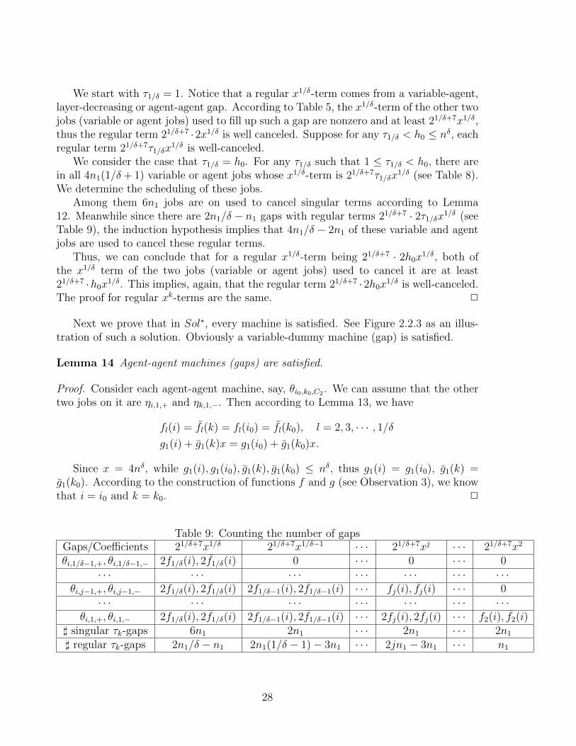
Thus, we can conclude that for a regular x1/δ-term being 21/δ+7 · 2h0x1/δ, both ofthe x1/δ term of the two jobs (variable or agent jobs) used to cancel it are at least21/δ+7 ·h0x1/δ. This implies, again, that the regular term 21/δ+7 ·2h0x1/δ is well-canceled.The proof for regular xk-terms are the same. 2

Next we prove that in Sol∗, every machine is satisfied. See Figure 2.2.3 as an illus-tration of such a solution. Obviously a variable-dummy machine (gap) is satisfied.

Lemma 14 Agent-agent machines (gaps) are satisfied.

Proof. Consider each agent-agent machine, say, θi0,k0,C2 . We can assume that the othertwo jobs on it are ηi,1,+ and ηk,1,−. Then according to Lemma 13, we have

fl(i) = fl(k) = fl(i0) = fl(k0), l = 2, 3, · · · , 1/δg1(i) + g1(k)x = g1(i0) + g1(k0)x.

Since x = 4nδ, while g1(i), g1(i0), g1(k), g1(k0) ≤ nδ, thus g1(i) = g1(i0), g1(k) =g1(k0). According to the construction of functions f and g (see Observation 3), we knowthat i = i0 and k = k0. 2

Table 9: Counting the number of gapsGaps/Coefficients 21/δ+7x1/δ 21/δ+7x1/δ−1 · · · 21/δ+7xj · · · 21/δ+7x2

θi,1/δ−1,+, θi,1/δ−1,− 2f1/δ(i), 2f1/δ(i) 0 · · · 0 · · · 0· · · · · · · · · · · · · · · · · · · · ·

θi,j−1,+, θi,j−1,− 2f1/δ(i), 2f1/δ(i) 2f1/δ−1(i), 2f1/δ−1(i) · · · fj(i), fj(i) · · · 0· · · · · · · · · · · · · · · · · · · · ·

θi,1,+, θi,1,− 2f1/δ(i), 2f1/δ(i) 2f1/δ−1(i), 2f1/δ−1(i) · · · 2fj(i), 2fj(i) · · · f2(i), f2(i)] singular τk-gaps 6n1 2n1 · · · 2n1 · · · 2n1

] regular τk-gaps 2n1/δ − n1 2n1(1/δ − 1)− 3n1 · · · 2jn1 − 3n1 · · · n1

28

We consider variable-clause machines. Notice that for each i0 and k0 ∈ {i0, i0+1, i0+2}, either θi0,k0,+,C1 or θi0,k0,−,C1 exists.

Lemma 15 Machine θ1,k,+,C1 or θ1,k,−,C1 (k = 1, 2, 3) is satisfied. The machine θi0,k0,+,C1

or θi0,k0,−,C1 for i0 ≥ 2 and k0 ∈ {i0, i0 + 1, i0 + 2} is satisfied if:

• For i < i0, each machine θi,k,+,C1 or θi,k,−,C1 is satisfied.

• All variable jobs vk′,ι with k′ < i0 and ι = 1, 2, 3, 4 are not scheduled on thismachine.

Proof. We consider clause c1 ∈ C1. As c1 contains three variables z1, z2 and z3, thereare three huge jobs θ1,1,σ1,C1 , θ1,2,σ2,C1 and θ1,3,σ3,C1 where σ1, σ2, σ3 ∈ {+,−}. Meanwhilethere are three clause jobs of u1.

For i0 = 1 and any k0 ∈ {1, 2, 3}, suppose θ1,k0,+,C1 exists, and the two jobs togetherwith it are a clause job ui and a variable job vk,ι with ι ∈ {1, 2, 3, 4}. Since s(θ1,k0,+,C1) =105r− 11005r− (21/δ+7f1/δ(1) + 21/δ+9 + 21/δ+7k0 + 21/δ+6 + 1), according to Lemma 11,we have 21/δ+9i + 21/δ+7k + 1 = 21/δ+9 + 21/δ+7k0 + ι. If i ≥ 2, then the left side is atleast 21/δ+10, while the right side is at most 21/δ+9 + 21/δ+7 × 3 + 4 < 21/δ+10, which is acontradiction. Thus i = 1 and it follows directly that k = k0, ι = 1. Otherwise θ1,k0,−,C1

exists, and the proof is just similar. Thus, machine θ1,k0,+,C1 or θ1,k0,−,C1 (k0 = 1, 2, 3) issatisfied.

When i0 ≥ 2 and k0 ∈ {i0 + 1, i0 + 2, i0 + 3}, again we suppose that θi0,k0,+,C1

exists. Notice that for any i ≤ i0 − 1, ci contains three variables. According to thehypothesis, the three clause jobs ui are scheduled on three machines, they are θi,i,+,C1

or θi,i,−,C1 , θi,i+1,+,C1 or θi,i+1,−,C1 and θi,i+2,+,C1 or θi,i+2,−,C1 . Thus when we considermachine θi0,k0,+,C1 , all clause jobs ui with i ≤ i0 − 1 could not be scheduled on thismachine.

Again suppose that the two jobs scheduled together with θi0,k0,+,C1 are ui′ and vk′,ι,then 21/δ+9i0 + 21/δ+7k0 + 1 = 21/δ+9i′ + 21/δ+7k′ + ι. Since i′ ≥ i0 − 1 and k′ ≥ i′,if i′ ≥ i0 + 1, then we have 21/δ+9i′ + 21/δ+7k′ + σ > 21/δ+9(i0 + 1) + 21/δ+7(i0 + 1) ≥21/δ+9i0 + 21/δ+7(i0 + 3) + 1, which is a contradiction. Thus i′ = i0, k

′ = k0 and ι = 1,which means machine θi0,k0,+,C1 is satisfied.

Similarly if θi0,k0,−,C1 exists, this machine is also satisfied. 2

Lemma 16 Machines θ1,a,c, θ1,b,d, θ1,a,d and θ1,b,c are satisfied. Moreover, machinesθi0,a,c, θi0,b,d, θi0,a,d and θi0,b,c for i0 ≥ 2 are satisfied if:

• Machines θi,a,c, θi,b,d, θi,a,d and θi,b,c are satisfied for i ≤ i0 − 1.

• All variable jobs vi′,ι with i′ < i0 and ι ∈ {1, 2, 3, 4} are not scheduled on thesemachines.

29

Proof. Consider machine θ1,a,c. Except the huge job, let the other three jobs be vi1,ι(ι ∈ {1, 2, 3, 4}), ai2 and ci3 . Then we have

21/δ+7i1 + 21/δ+6 + ι1 + 27i2 + 8 + 27i3 + 16 = 21/δ+7 + 21/δ+6 + 28 + 25.

It can be easily seen that i1 = i2 = i3 = 1 and ι = 1. Thus, machine θ1,a,c is satisfied.Using similar arguments we can show that machines θ1,b,c, θ1,a,d and θ1,b,d are satisfied.

The proof that machines θi0,a,c, θi0,b,d, θi0,a,d and θi0,b,c are satisfied for i0 ≥ 2 if twoconditions of the lemma hold is the same. 2

For simplicity, we call variable jobs vi,ι1 with ι1 ∈ {1, 2, 3, 4} and agent jobs ηi,j,ι2with ι2 ∈ {+,−} as jobs of index-level i.

In contrast, let σ ∈ {+,−}, we call machine θη,i,σ, θi,j,σ, machine θi′,i,σ,C1 , machineθi,σ, machines θi,a,c, θi,a,d, θi,b,c, θi,b,d as machines of index-level i.

Specifically, machine θi,k,C2 is of index-level i and also of index-level k, i.e., thismachine would appear in the set of machines with index-level of i as well as the set ofmachines with index-level of k. Notice that according to Lemma 14 these machines arealready satisfied.

Lemma 17 In Sol∗, every machine (gap) is satisfied.

Proof. We prove it through induction on the index-level of machines. We start withi = 1.

Consider machine θη,1,+. We assume jobs vi,2 and ηi′,1/δ−1,+ are on it. Then simplecalculations show that

2f1/δ(1)x1/δ + 1 + g1/δ−1(1) = f1/δ(i)x1/δ + i+ f1/δ(i

′)x1/δ + g1/δ−1(i′).

According to Lemma 13, f1/δ(1) = f1/δ(i) = f1/δ(i′).

Since i′ ≥ 1, according to Observation 3 we have g1/δ−1(i′) ≥ g1/δ−1(1). Meanwhile

i ≥ 1, thus g1/δ−1(i′) = g1/δ−1(1) and i = 1. Again, due to Observation 3 we have

i = i′ = 1. Thus v1,2 and η1,1/δ−1,+ are on machine θη,1,+, i.e., this machine is satisfied.Similarly we can prove that v1,4 and η1,1/δ−1,− are on machine θη,1,−.

Consider machine θ1,j,+ for 1 ≤ j ≤ 1/δ − 2. We assume jobs ηi,j,+ and ηi′,j+1,+ areon it. Then simple calculations show that

2

1/δ∑l=j+2

fl(1)xl+fj+1(1)xj+1+gj+1(1)+gj(1) =

1/δ∑l=j+1

fl(i)xl+

1/δ∑l=j+2

fl(i′)xl+gj+1(i

′)+gj(i).

According to Lemma 13, we have

fl(i) = fl(1), l = j + 1, j + 2, · · · , 1/δ,

fl(i′) = fl(1), l = j + 2, j + 3, · · · , 1/δ.

30

Thus gj+1(1) + gj(1) = gj+1(i′) + gj(i).

According to Observation 3, we have gj(i) ≥ gj(1) and gj+1(i′) ≥ gj+1(1). Thus

gj(i) = gj(1), gj+1(i′) = gj+1(1). Again due to Observation 3 we have i = i′ = 1, i.e.,

machine θ1,j,+ is satisfied.Similarly we can prove that machine θ1,j,− for 2 ≤ j ≤ 1/δ − 2 is also satisfied. For

j = 1, recall that there is a slight difference between θ1,1,− and θ1,1,+, we prove thatmachine θ1,1,− is satisfied separately.

Consider θ1,1,− and assume jobs ηi,1,− and ηi′,2,− are on it. Then

2

1/δ∑l=3

fl(1)xl + f2(1)x2 + g2(1) + g1(1)x =

1/δ∑l=2

fl(i)xl +

1/δ∑l=3

fl(i′)xl + g2(i

′) + g1(i)x.

According to Lemma 13, we have

fl(i) = fl(1), l = 2, 3, · · · , 1/δ,

fl(i′) = fl(1), l = 3, 4, · · · , 1/δ.

Thus g2(1)+g1(1)x = g2(i′)+g1(i)x. Similarly due to observation 3 we have g2(i

′) ≥ g2(1),and g1(i) ≥ g1(1). Thus again we can prove i = i′ = 1, which implies that machine θ1,1,−is also satisfied.

Combining Lemma 15, Lemma 16 and Lemma 14, we have proved so far that eachmachine of index-level 1 is satisfied. We further show that indeed, all the variable andagent jobs of index-level 1 are on machines of index-level 1. To see why, see Figure 2 foran overview of the scheduling of jobs of index-level 1 (here Case 1 means z1 ∈ C1, whileCase 2 means ¬z1 ∈ C1).

Suppose that for any i < i0 ≤ n, each machine of index-level i is satisfied and allthe variable or agent jobs of index-level i are on machines of index-level i. We consideri = i0.

According to Lemma 15 and Lemma 16, we know that machines θi0,k,+,C1 (or θi0,k,−,C1)for k ∈ {i0, i0 + 1, i0 + 2} and machines θi0,a,c, θi0,b,d, θi0,a,d, θi0,b,c are satisfied.

Consider machine θη,i0,+ which is of index-level i0. Again we may assume jobs vi,2and ηi′,1/δ−1,+ are on it, and the induction hypothesis implies that i ≥ i0, i

′ ≥ i0. Simplecalculations show that

2f1/δ(i0)x1/δ + i0 + g1/δ−1(i0) = f1/δ(i)x

1/δ + i+ f1/δ(i′)x1/δ + g1/δ−1(i

′).

According to Lemma 13, f1/δ(i0) = f1/δ(i) = f1/δ(i′). Since i′ ≥ i0, according to

Observation 3 we have g1/δ−1(i′) ≥ g1/δ−1(i0). Meanwhile i ≥ i0, thus g1/δ−1(i

′) =g1/δ−1(i0) and i = i0. We can conclude that i = i′ = i0. So, vi0,2 and ηi0,1/δ−1,+ areon machine θη,i0,+, i.e., this machine is satisfied. Similarly we can prove that vi0,4 andηi0,1/δ−1,− are on machine θη,i0,−.

31

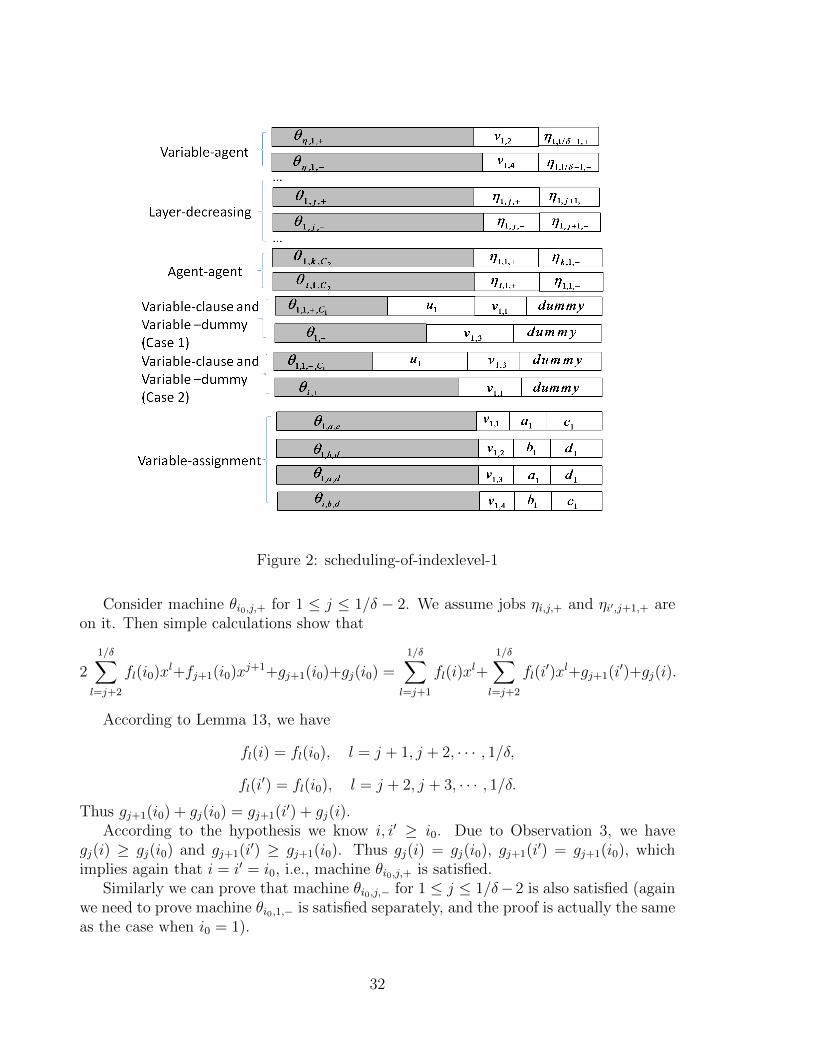
Figure 2: scheduling-of-indexlevel-1

Consider machine θi0,j,+ for 1 ≤ j ≤ 1/δ − 2. We assume jobs ηi,j,+ and ηi′,j+1,+ areon it. Then simple calculations show that

2

1/δ∑l=j+2

fl(i0)xl+fj+1(i0)x

j+1+gj+1(i0)+gj(i0) =

1/δ∑l=j+1

fl(i)xl+

1/δ∑l=j+2

fl(i′)xl+gj+1(i

′)+gj(i).

According to Lemma 13, we have

fl(i) = fl(i0), l = j + 1, j + 2, · · · , 1/δ,

fl(i′) = fl(i0), l = j + 2, j + 3, · · · , 1/δ.

Thus gj+1(i0) + gj(i0) = gj+1(i′) + gj(i).

According to the hypothesis we know i, i′ ≥ i0. Due to Observation 3, we havegj(i) ≥ gj(i0) and gj+1(i

′) ≥ gj+1(i0). Thus gj(i) = gj(i0), gj+1(i′) = gj+1(i0), which

implies again that i = i′ = i0, i.e., machine θi0,j,+ is satisfied.Similarly we can prove that machine θi0,j,− for 1 ≤ j ≤ 1/δ−2 is also satisfied (again

we need to prove machine θi0,1,− is satisfied separately, and the proof is actually the sameas the case when i0 = 1).

32

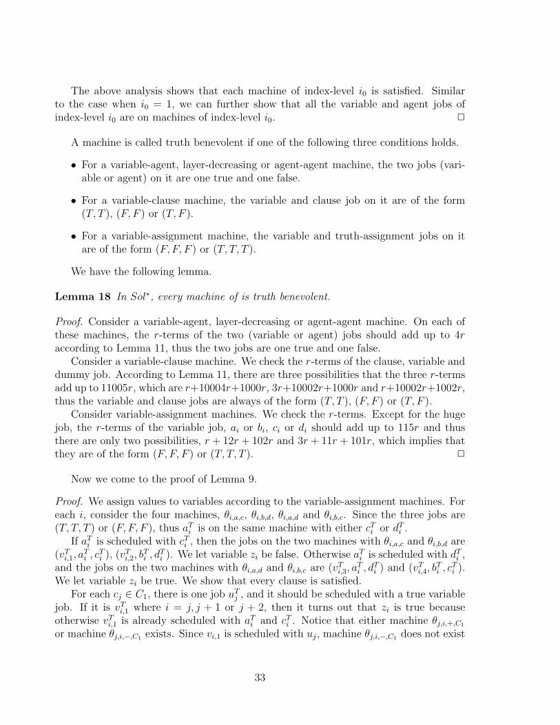
The above analysis shows that each machine of index-level i0 is satisfied. Similarto the case when i0 = 1, we can further show that all the variable and agent jobs ofindex-level i0 are on machines of index-level i0. 2

A machine is called truth benevolent if one of the following three conditions holds.

• For a variable-agent, layer-decreasing or agent-agent machine, the two jobs (vari-able or agent) on it are one true and one false.

• For a variable-clause machine, the variable and clause job on it are of the form(T, T ), (F, F ) or (T, F ).

• For a variable-assignment machine, the variable and truth-assignment jobs on itare of the form (F, F, F ) or (T, T, T ).

We have the following lemma.

Lemma 18 In Sol∗, every machine of is truth benevolent.

Proof. Consider a variable-agent, layer-decreasing or agent-agent machine. On each ofthese machines, the r-terms of the two (variable or agent) jobs should add up to 4raccording to Lemma 11, thus the two jobs are one true and one false.

Consider a variable-clause machine. We check the r-terms of the clause, variable anddummy job. According to Lemma 11, there are three possibilities that the three r-termsadd up to 11005r, which are r+10004r+1000r, 3r+10002r+1000r and r+10002r+1002r,thus the variable and clause jobs are always of the form (T, T ), (F, F ) or (T, F ).

Consider variable-assignment machines. We check the r-terms. Except for the hugejob, the r-terms of the variable job, ai or bi, ci or di should add up to 115r and thusthere are only two possibilities, r + 12r + 102r and 3r + 11r + 101r, which implies thatthey are of the form (F, F, F ) or (T, T, T ). 2

Now we come to the proof of Lemma 9.

Proof. We assign values to variables according to the variable-assignment machines. Foreach i, consider the four machines, θi,a,c, θi,b,d, θi,a,d and θi,b,c. Since the three jobs are(T, T, T ) or (F, F, F ), thus aTi is on the same machine with either cTi or dTi .

If aTi is scheduled with cTi , then the jobs on the two machines with θi,a,c and θi,b,d are(vTi,1, a

Ti , c

Ti ), (vTi,2, b

Ti , d

Ti ). We let variable zi be false. Otherwise aTi is scheduled with dTi ,

and the jobs on the two machines with θi,a,d and θi,b,c are (vTi,3, aTi , d

Ti ) and (vTi,4, b

Ti , c

Ti ).

We let variable zi be true. We show that every clause is satisfied.For each cj ∈ C1, there is one job uTj , and it should be scheduled with a true variable

job. If it is vTi,1 where i = j, j + 1 or j + 2, then it turns out that zi is true becauseotherwise vTi,1 is already scheduled with aTi and cTi . Notice that either machine θj,i,+,C1

or machine θj,i,−,C1 exists. Since vi,1 is scheduled with uj, machine θj,i,−,C1 does not exist

33

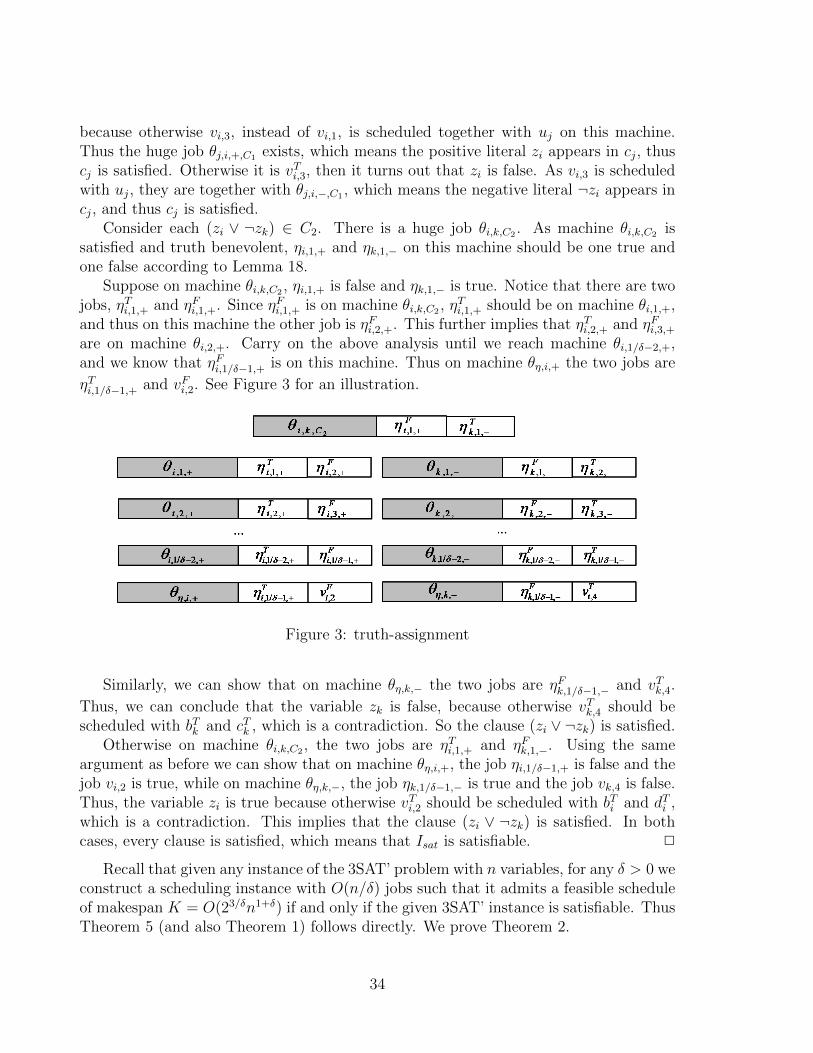
because otherwise vi,3, instead of vi,1, is scheduled together with uj on this machine.Thus the huge job θj,i,+,C1 exists, which means the positive literal zi appears in cj, thuscj is satisfied. Otherwise it is vTi,3, then it turns out that zi is false. As vi,3 is scheduledwith uj, they are together with θj,i,−,C1 , which means the negative literal ¬zi appears incj, and thus cj is satisfied.

Consider each (zi ∨ ¬zk) ∈ C2. There is a huge job θi,k,C2 . As machine θi,k,C2 issatisfied and truth benevolent, ηi,1,+ and ηk,1,− on this machine should be one true andone false according to Lemma 18.

Suppose on machine θi,k,C2 , ηi,1,+ is false and ηk,1,− is true. Notice that there are twojobs, ηTi,1,+ and ηFi,1,+. Since ηFi,1,+ is on machine θi,k,C2 , η

Ti,1,+ should be on machine θi,1,+,

and thus on this machine the other job is ηFi,2,+. This further implies that ηTi,2,+ and ηFi,3,+are on machine θi,2,+. Carry on the above analysis until we reach machine θi,1/δ−2,+,and we know that ηFi,1/δ−1,+ is on this machine. Thus on machine θη,i,+ the two jobs are

ηTi,1/δ−1,+ and vFi,2. See Figure 3 for an illustration.

Figure 3: truth-assignment

Similarly, we can show that on machine θη,k,− the two jobs are ηFk,1/δ−1,− and vTk,4.

Thus, we can conclude that the variable zk is false, because otherwise vTk,4 should bescheduled with bTk and cTk , which is a contradiction. So the clause (zi ∨ ¬zk) is satisfied.

Otherwise on machine θi,k,C2 , the two jobs are ηTi,1,+ and ηFk,1,−. Using the sameargument as before we can show that on machine θη,i,+, the job ηi,1/δ−1,+ is false and thejob vi,2 is true, while on machine θη,k,−, the job ηk,1/δ−1,− is true and the job vk,4 is false.Thus, the variable zi is true because otherwise vTi,2 should be scheduled with bTi and dTi ,which is a contradiction. This implies that the clause (zi ∨ ¬zk) is satisfied. In bothcases, every clause is satisfied, which means that Isat is satisfiable. 2

Recall that given any instance of the 3SAT’ problem with n variables, for any δ > 0 weconstruct a scheduling instance with O(n/δ) jobs such that it admits a feasible scheduleof makespan K = O(23/δn1+δ) if and only if the given 3SAT’ instance is satisfiable. ThusTheorem 5 (and also Theorem 1) follows directly. We prove Theorem 2.

34

Proof. Suppose the theorem fails, then there exists an exact algorithm for the restrictedscheduling problem that runs in 2O(n1−δ0 ) time for some δ0 > 0, then we may simplychoose δ = δ0 in our reduction. Since δ0 is some fixed constant, the scheduling problem weconstruct contains O(n) jobs with the processing time of each job bounded by O(n1+δ0).Then we apply the scheduling algorithm to get an optimum solution, and it runs in

2O(n(1−δ0)(1+δ0)), i.e., 2O(n1−δ20 ) time. Through the makespan of this optimum solution, we

can determine whether the given 3SAT’ instance is satisfiable in 2O(n1−δ20 ) time for somefixed δ0 > 0, resulting a contradiction. 2

3 Scheduling on m Machines

We consider the scheduling problem on m (m ≥ 2) identical machines and prove thefollowing theorem.

Theorem 6 Assuming ETH, there is no (1/ε)o( m

log2m)|Ische|O(1) time FPTAS for Pm||Cmax.

Given the above theorem, Theorem 3 follows since otherwise, there exists a (1/ε)O(m1−δ0 ) |I|O(1)

time FPTAS for some δ0 > 0, and it runs in (1/ε)o( m

log2m)|Ische|O(1) time, which is a con-

tradiction.To prove Theorem 6, given any 3SAT’ instance Isat with n variables, we construct

a scheduling instance Ische such that it admits an optimal solution with makespan2O( n

mlog2m) if and only if Isat is satisfiable, then if the above theorem fails, we may apply

the (1/ε)o( m

log2m)|Ische|O(1) time PTAS for Ische by setting 1/ε = 2O( n

mlog2m) + 1. Simple

calculations show that the optimal solution could be computed in 2δmn time where δmgoes to 0 as m increases, and thus the satisfiability of the given 3SAT’ instance couldalso be determined in 2δmn time, which is a contradiction.

We give an overview of the whole reduction. For simplicity throughout the remainingpart of this section we assume the number of machines is m + 1 with m ≥ 1. Given a3SAT’ instance Isat, we would transform it into an instance of the 3DM’ problem, whichis formally defined as follows:

• There are three disjoint sets of elements W = {wi, wi|i = 1, · · · , 3n}, X ={sj, ai|j = 1, · · · , n′, i = 1, · · · , 3n} and Y = {bi|i = 1, · · · , 3n} where n′ ≤ 3n.

• There are three sets of matches T1 = {(wi), (wi)|i = 1, · · · , 3n}, T2 ⊆ {(wi, sj), (wi, sj)|wi ∈W, sj ∈ X}, T3 = {(wi, ai, bi), (wi, ai, bζ(i))|i = 1, · · · , 3n} where ζ is defined asζ(3k + 1) = 3k + 2, ζ(3k + 2) = 3k + 3 and ζ(3k + 3) = 3k + 1 for k = 1, · · · , n

• Either wi or wi appears in T2, and it appears once. Every sj appears at most threetimes in T2.

35

A subset of T = T1 ∪ T2 ∪ T3 is called an exact cover if every element of W ∪ X ∪ Yappears exactly once in its matches.

We first show that, if Isat contains n variables, then a 3DM’ instance I3dm in whichthere are O(n) elements (indeed, |W |=6n) and O(n) matches could be constructed suchthat I3dm admits an exact cover if and only if Isat is satisfiable. We then construct ascheduling instance Ische which admits a feasible schedule of makespan K = 2O( n

mlog2m)

if and only if I3dm admits an exact cover, and thus if and only if Isat is satisfiable.We give a brief description of Ische. Every match of T has a corresponding job (called

as a match job) in Ische. Recall that there are m+ 1 machines. If there is an exact cover,then Ische admits a schedule of makespan K in which all the jobs corresponding to thematches of the exact cover are on the first m machines while other match jobs are onthe last machine. Meanwhile, if Ische admits a schedule of makespan K, then in thisschedule there are m machines such that the matches correspond to the match jobs onthem form an exact cover.

3.1 Modification of the 3SAT’ Instance

Given a 3SAT’ instance Isat, we transform it into a 3DM’ instance I3dm, as we mentionbefore..

Transforming Isat to I ′sat Given a 3SAT’ instance Isat (with n variables), we canapply Tovey’s method [26] to alter it into I ′sat by adding O(n) variables and clauses suchthat the following properties are satisfied:

• Clauses of I ′sat could be divided into C1 and C2

– Every variable appears once in C1

– Every (positive or negative) literal appears once in C2

– All the clauses of C2 could be listed as (z3k+1 ∨ ¬z3k+2), (z3k+2 ∨ ¬z3k+3),(z3k+3 ∨ ¬z3k+1) for k = 0, 1, · · · , n− 1

• I ′sat is satisfiable if and only if Isat is satisfiable

To see why, given Isat, we replace each occurrence of a variable in Isat with a newvariable. Since every variable, say, zi, appears three times, we can replace its threeoccurrences with z3i−1, z3i−1 and z3i and meanwhile add (z3i−2 ∨ ¬z3i−1), (z3i−1 ∨ ¬z3i),(z3i ∨¬z3i−2). Let C2 be the set of all the newly added clauses and C1 be the remainingclauses, then it is not difficult to verify that the modified instance I ′sat satisfies all theproperties above.

Notice that there are 3n variables in I ′sat. For simplicity, we may further assume thatn could be divided by m and let n = qm. (Indeed, if n = qm + r with 0 < r < mwith q ≥ 1, we could add additionally 3(m − r) dummy variables, say, zd3i+1, z

d3i+2 and

zd3i+3 for 0 ≤ i ≤ m − r − 1, and meanwhile introduce m − r dummy clauses in C1 as

36

(zd3i+1 ∨ zd3i+2 ∨ zd3i+3), and 3(m − r) clauses in C2 as (zd3i+1 ∨ ¬zd3i+1), (zd3i+2 ∨ ¬zd3i+3),(zd3i+3 ∨¬zd3i+1). It is not difficult to verify that these newly added variables and clausesdo not change the satisfiability of the original instance.)

Transforming I ′sat to I3dm We prove that, given I ′sat that contains 3n variables, a3DM’ instance I3dm could be constructed such that I3dm admits an exact cover if andonly if I ′sat is satisfiable.Construction of I3dm. We construct two variable elements for each variable zi, i.e.,we construct wi corresponding to zi and wi corresponding to ¬zi. Let W be the set ofthem. It can be easily seen that |W | = 6n. We construct a clause element sj ∈ X foreach cj ∈ C1.

Recall that all the clauses of C2 could be listed as (z3i+1 ∨ ¬z3i+1), (z3i+2 ∨ ¬z3i+3),(z3i+3 ∨ ¬z3i+1) for i = 0, 1, · · · , n − 1. For every i, we construct a3i+1, a3i+2, a3i+3 ∈ Xand b3i+1, b3i+2, b3i+3 ∈ Y .

This completes the construction of elements and it can be easily seen that |X| =3n+m, and |Y | = 3n. We construct matchings. For each variable zi, we construct twomatchings of T1, namely (wi) and (wi).

For each clause cj ∈ C1, if the positive literal zi ∈ cj, then we construct (wi, sj) ∈T2. Else if the negative literal ¬zi ∈ cj, then we construct (wi, sj). Notice that cjmight contain two or three literals, thus two or three matchings of T2 are constructedcorresponding to it.

For each 0 ≤ i ≤ n−1, 6 matchings of T3 are constructed for the three clauses (z3i+1∨¬z3i+1), (z3i+2∨¬z3i+3) and (z3i+3∨¬z3i+1), namely (w3i+1, a3i+1, b3i+1), (w3i+2, a3i+2, b3i+2),(w3i+3, a3i+3, b3i+3) and (w3i+1, a3i+1, b3i+2), (w3i+2, a3i+2, b3i+3), (w3i+3, a3i+3, b3i+1).

It can be easily seen that |T1| = 6n, |T2| = 3n, |T3| = 6n. Thus in all, I3dm containsO(n) elements and matches.

The following part of this subsection is devoted to proving the following lemma. Weremark that the proof is similar to the traditional proof showing that 3DM is NP-hard [5].

Lemma 19 I ′sat is satisfiable if and only if I3dm admits an exact cover.

Proof. Suppose I ′sat is satisfiable, we choose matchings out of T to form an exact cover.We know that for each 0 ≤ i ≤ n − 1, z3i+1, z3i+2 and z3i+3 are either all true

or all false. If they are all true, then we choose (w3i+1, a3i+1, b3i+2), (w3i+2, a3i+2, b3i+3),(w3i+3, a3i+3, b3i+1). Otherwise they are all false, and (w3i+1, a3i+1, b3i+1), (w3i+2, a3i+2, b3i+2),(w3i+3, a3i+3, b3i+3) are chosen instead.

Now every element of Y appears exactly once in the matches we choose currently.Since each clause cj ∈ C1 is satisfied, it is satisfied by at least one variable. We choosethe variable that leads to the satisfaction of cj (if there are multiple such variables, wechoose arbitrarily one). Suppose this variable is zi. If zi is true, then we know thepositive literal zi ∈ cj. According to our construction (wi, sj) ∈ T2 and we choose it.Otherwise zi is false, and the negative literal ¬zi ∈ cj. Again it follows that (wi, sj) ∈ T2and we choose it.

37

Consider the matches we have chosen so far. Every element of X and Y appearsexactly once in these matchings. Moreover, each element of W appears at most once inthese matchings. To see why, notice that if we choose (wi, sj) ∈ T2, for example, thenzi is true and we do not choose matchings of T3 that contain wi. Finally, we choosematchings of T1 to enforce that every element of W appears exactly once.

On the contrary, suppose there exists an exact cover of I3dm, we prove that I ′sat issatisfiable. Consider elements of X and Y . For each 0 ≤ i ≤ n − 1, to ensure thata3i+1, b3i+1, a3i+2, b3i+2 and a3i+3, b3i+3 appear once respectively, in the exact cover T ′

we have to choose either (w3i+1, a3i+1, b3i+2), (w3i+2, a3i+2, b3i+3), (w3i+3, a3i+3, b3i+1), orchoose (w3i+1, a3i+1, b3i+1), (w3i+2, a3i+2, b3i+2), (w3i+3, a3i+3, b3i+3).

If (w3i+1, a3i+1, b3i+2), (w3i+2, a3i+2, b3i+3), (w3i+3, a3i+3, b3i+1) are in T ′, we set z3i+1,z3i+2 and z3i+3 to be true. Otherwise we set z3i+1, z3i+2 and z3i+3 to be false. It can beeasily seen that every clause of C2 is satisfied.

We consider cj ∈ C1. Notice that sj ∈ X appears once in T ′. Suppose the matchcontaining sj is (sj, wi) for some i, then it follows that the positive literal zi ∈ cj. Thefact that wi also appears once implies that wi appears in T ′ ∩ T3, and thus variable zi istrue and cj is satisfied.

Otherwise the matching containing sj is (sj, wi) for some i, then similar argumentsshow that the negative literal ¬zi ∈ cj and variable zi is false. Again cj is satisfied. 2

3.2 Defining the Functions f and g Based on Partitioning Matches

Notice that there are one-element, two-element and three-element matches in I3dm,throughout this section we may use (wi, xj, yk) to represent any match of T = T1∪T2∪T3,where xj = yk = ∅ if it represents a one-element match, and yk = ∅ if it represents atwo-element match.

Recall that n = qm for some integer q. We divide the set W equally into m subsets,with Wk = {wi, wi|3kq + 1 ≤ i ≤ 3kq + 3q} for 0 ≤ k ≤ m − 1. We aim to constructa scheduling instance in which there is one job for every match, and the goal of thissubsection is to construct the functions f and g through which the processing time of thejob corresponding to (wi, xj, yk) is defined as g(wi)α

f(wi)+g(xj)αf(xj)+g(yk)α

f(yk) whereα = mO(1) and g(wi), g(xj), g(yk) < α. Given any exact cover (if it exists), a schedule forthe constructed scheduling instance is called a natural schedule (corresponding to theexact cover) if jobs corresponding to matches of this exact cover that contain wi ∈ Wk orwi ∈ Wk are on machine k. We try to design f and g such that the following propertieshold for a natural schedule,

1. f(∅) = g(∅) = 0, otherwise f(xj), g(xj), f(yk), g(yk) ∈ Z+.

2. For any (wi, xj, yk) and (wi′ , xj′ , yk′) from the exact cover, if f(wi) = f(wi′) 6= 0(or f(xj) = f(xj′) 6= 0 or f(yk) = f(yk′) 6= 0), then the two corresponding jobsshould be on different machines in the natural schedule.

38

3. The largest value returned by f (denoted as |f |) is as small as possible.

The second property above actually ensures that if jobs corresponding to matches ofan exact cover are on the same machine according to the corresponding natural schedule,then their processing times contain different αi terms, and it is a key property throughwhich a natural schedule of makespan K could be constructed from the given exact coverfor I3dm.

The following part of this subsection is devoted to designing the functions f andg satisfying the properties above. Obviously we can simply define f so that it takes adistinct value for every element, and then |f | = O(n), which is too large. In the followingpart, we will define f such that |f | = O(n/m logm).

We construct a bipartite graph G = (V w ∪ V s, E) in the following way. There are mvertices in V w, with a slight abuse of notations we denote them as Wk for 0 ≤ k ≤ m−1.There are |C1| ≤ 3n vertices in V s, and we denote them as sj for 1 ≤ j ≤ |C1|. There isan edge between Wk and sj if (wi, sj) ∈ T2 or (wi, sj) ∈ T2 where wi, wi ∈ Wk.

It can be easily verified that the degree of every Wk is at most 3q, while the degreeof every sj is at most 3.

We define f in the following way. According to the special structure of T1 and T3, wefirst let f(b3kq+i) = i, f(a3kq+i) = 3q + i, f(w3kq+i) = 6q + i and f(w3kq+i) = 9q + i. Itcan be easily seen that jobs corresponding to one-element and three-element matches ofthe exact cover do not share the same αi term for 1 ≤ i ≤ 12q if they are on machine k(according to the natural schedule). For jobs corresponding to two-element matches, thefollowing property can ensure that they do not share the same αi term if they are on thesame machine: for any sj and sj′ which are both connected to some Wk, f(sj) 6= f(sj′).We associate the value of each distinct f(sj) with a specific color. The problem becomesthat, can we draw each vertex of V s with a color so that for any 0 ≤ k ≤ m− 1, all thesj connected to Wk are drawn with different colors.

Obviously we can draw every sj with a distinct color and this yields a solution withO(n) colors. We provide a natural greedy algorithm which uses O(n/m logm) colors,and the function f is defined accordingly.

Consider the following method of coloring. We sequence sj in an arbitrary order.Suppose we have used t different colors and currently we pick a new color t+ 1. We takethe first uncolored sj in the sequence and color it with t+ 1. Then we delete vertices inthe sequence sharing the same neighbors with sj (since they could not be colored witht+ 1). Now we pick the first remaining vertex in the sequence and color it. We carry onthis procedure until we can not color any more, then we pick a new color t+ 2.

To analyze the number of colors used by the above algorithm, we have the followinglemma.

Lemma 20 If currently there are h ≤ |C1| vertices uncolored, then using a new colorwe could color at least d h

9qe vertices.

Proof. Suppose sj is colored with color t. Then according to the greedy algorithm,vertices sharing the same neighbors with it should be deleted. Recall that the degree of

39

sj is at most 3, while the degree of Wk (0 ≤ k ≤ m − 1) is at most 3q. Thus we deleteat most 9q − 1 vertices and the lemma follows directly. 2

Let φk be the number of vertices that are not colored when k different colors areused, then φ0 = |C1| ≤ 3n and it follows directly that φk+1 ≤ φk − dφk9q e.

Thus φk+1 ≤ φk(1 − 19q

). Meanwhile φk+1 ≤ φk − 1, so the integer sequence goes to

0. We assume |C1| ≥ 9q, otherwise we use at most 9q = O(n/m) colors. Let k0 be thelargest index such that φk0 ≥ 9q, then it follows that |C1|(1 − 1

9q)k0 ≥ 9q, and simple

calculations show that k0 ≤ dlog1− 19q

9qm1e ≤ 9q lnm. Thus in all the greedy algorithm

uses τ ≤ 9q lnm+ 9q different colors.Let χ(j) ≤ τ be the color of sj. We define the function f in the following way.

• f(b3kq+i) = i, f(a3kq+i) = 3q + i.

• f(w3kq+i) = 6q + i, f(w3kq+i) = 9q + i.

• f(sj) = 12q + χ(j).

As we mention before, a job corresponding to a match, say, (wi, xj, yk) has a pro-cessing time of g(wi)α

wi + g(xj)αf(xj) + g(yk)α

f(yk) where α = mO(1). The function findicates the index of the exponential, while the function g indicates the coefficient. Ac-cording to our previous discussion if we put jobs corresponding to matches that containw3kq+i or w3kq+i onto machine k (as the natural schedule indicates), then all the jobs onmachine k have different αi terms.

We provide the definition of g now.

• g(w3kq+i) = g(w3kq+i) = g(a3kq+i) = g(b3kq+i) = m+ k.

• Sort vertices with the same color in an arbitrary way. Suppose sj is colored withcolor t and is the l-th vertex in the sequence, then g(sj) = m+ l − 1.

We have the following simple observation on g.

Lemma 21 g(sj) < 2m for 1 ≤ j ≤ |C1|.

Proof. Suppose the lemma fails, then there are at least m+ 1 vertices coloring with thesame color. Notice that every sj is connected with some Wk for some 0 ≤ k ≤ m − 1,among these m+ 1 vertices there are two of them connecting to the same Wk, implyingthat they should be colored with different colors, which is a contradiction. 2

40

3.3 Construction of the Scheduling Instance

Let α = 6m4 + 6m3 + 6m2 be the base. Recall that n = qm, τ = O(n/m logm).With a slight abuse of notation we let |f | = 12q + τ = O(n/m logm). We con-struct a scheduling instance Ische such that it admits an optimal solution of makespan6m3

∑|f |i=1 α

i = 2O(n/m log2m) if and only if I3dm admits an exact cover.We construct three kinds of jobs, a match job for every match, a cover job for every

element and dummy jobs.For every match (w, x, y), we construct a job with processing time g(w)αf(w) +

g(x)αf(x) + g(y)αf(y) where (w, x, y) may represent (wi) or (wi) (in this case we takeg(x) = g(y) = 0), or represent (wi, sj) or (wi, sj) (in this case we take g(y) = 0), orrepresent (wi, ai, bi) or (wi, ai, bζ(i)).

For every element η, we construct a job with processing time (6m3−g(η))αf(η) whereη may represent wi, wi, sj, ai or bi.

We construct dummy jobs. For each color we would construct several dummy jobs,and we also construct a huge dummy job.

According to Lemma 21, we suppose there are lt ≤ m vertices colored with color t.If lt < m, we then construct m− lt dummy jobs, each of which has a processing time of6m3α12q+t. We call these dummy jobs as dummy jobs of color t.

Recall that there are m+1 machines, we construct a huge dummy job whose process-ing time equals to 6m3(m + 1)

∑9q+τi=1 αi minus the total processing time of all the jobs

we construct before. It follows directly that if there exists a feasible solution for Ischewhose makespan is no more than 6m3

∑|f |i=1 α

i, the load of every machine is 6m3∑|f |

i=1 αi.

3.4 From 3DM’ to Scheduling

For simplicity we index the m + 1 machines as machine 0 to machine m. We provide afeasible solution of Ische with makespan 6m3

∑|f |i=1 α

i.Given the exact cover of I3dm, we take out the jobs corresponding to the matches of

the exact cover. We put jobs corresponding to the matches that contain w3kq+i or w3kq+i

onto machine k for 0 ≤ k ≤ m−1. According to our definition of f , each job on machinek contains distinct αi terms.

Let Lk be total processing time of jobs on machine k. It is not difficult to verify thatfor 1 ≤ i ≤ 12q, the coefficient of αi term is g(k) = m+ k. By adding the correspondingcover job (with processing time (6m3 − g(k))αi), it becomes 6m3αi.

For the αi term with 12q + 1 ≤ i ≤ 12q + τ , the coefficient is either g(sj) or 0. If itis g(sj), we add a corresponding cover job, otherwise we add a dummy job of processingtime 6m3αi. In both cases the it becomes 6m3αi. Recall that for color t, there are ltcover jobs and m− lt dummy jobs, so we can always add jobs in the above way.

Now the loads of machine 0 to machine m − 1 are all 6m3∑|f |

i=1 αi, implying that if

we put all the remaining jobs to machine m, its load is also 6m3∑|f |

i=1 αi.

41

3.5 From Scheduling to 3DM’

Given a solution for Ische in which the load of each machine is 6m3∑|f |

i=1 αi, we construct

a an exact cover. We assume that the huge job is on machine m, and the followinglemma follows.

Lemma 22 For jobs on machine 0 to machine m− 1, the coefficients of their αi terms(1 ≤ i ≤ |f |) add up to 6m3αi.

Proof. Notice that the huge job is on machine m, we prove that, except for this job, thesum of all the coefficients of αi term is bounded by α − 1. This would be enough toensure that there is no “carry-over”from αi to αi+1 when we compute the sum of theprocessing times of the jobs on machine k for 0 ≤ k ≤ m − 1, and the lemma followsdirectly.

Consider the αi term for 1 ≤ i ≤ 3q. For each 0 ≤ k ≤ m − 1, since b3kq+iappear twice in matches, hence the sum of all the coefficients of αi terms is bounded by∑m−1

k=0 [6m3 − (m+ k)] + 2∑m−1

k=0 (m+ k) ≤ 6m4 + 3m2 < α.The sum of coefficients of αi term for i > 3q could be verified in the same way. 2

Lemma 23 For machine 0 to machine m−1, the term 6m3αi in the sum is contributedby either a dummy job, or a cover and match job.

Proof. If the coefficient 6m3 of the αi term is contributed by only one job, then obviouslyit is a dummy job. Otherwise it is contributed by two or more jobs, and among thesejobs there could be at most one cover job since the coefficient of a cover job is at least6m3 − (m + k) > 5m3. Meanwhile there should be at least one cover job, otherwise allthe coefficients of match jobs add up to 3

∑m−1k=0 (m + k) < 6m3 (every element appear

at most three times in matches), which is a contradiction.Given that the coefficient 6m3 is contributed by exactly one cover job, the coefficients

of the remaining jobs add up to a value in (m, 2m), implying that it is a match job. 2

Lemma 24 All the cover jobs are on machine 0 to machine m− 1.

Proof. Consider jobs with nonzero αi terms for 1 ≤ i ≤ 12q. There are m cover jobswhose coefficients are 6m3 − m, 6m3 − (m + 1), · · · , 6m3 − (2m − 1), and no dummyjobs. According to Lemma 23 these cover jobs must be on machine 0 to machine m− 1,one for each.

Consider jobs with nonzero α12q+t terms for 1 ≤ t ≤ τ . There are lt cover jobs whosecoefficients are 6m3 −m, · · · , 6m3 − (m+ lt − 1), and m− lt dummy jobs, again due toLemma 23 we know they are on machine 0 to machine m− 1, one for each. 2

For any i ≤ |f |, if the coefficient 6m3 of the αi term is contributed by a coverand a match job, then the match corresponding to the match job contains the elementcorresponding to the cover job. Furthermore, there is a cover job for every element, thus

42

if we take the matches corresponding to the match jobs on machine 0 to machine m− 1,they form an exact cover of I3dm.

This completes the proof of Theorem 6. Simple calculations show that the input

length of the scheduling instance we construct is |Ische| ≤ O(n log3mm

), and from thesame reduction Theorem 4 also follows. On the other hand, the traditional dynamic

programming algorithm for Pm||Cmax runs in 2O(√m|I| logm+m log |I|) time, as is shown in

the next section.

4 Dynamic Programming for Pm||CmaxWe show in this section that the traditional dynamic programming algorithm for the

scheduling problem runs in 2O(√m|I| logm+m log |I|) time.

Consider the dynamic programming algorithm for the scheduling problem. Supposejobs are sorted beforehand as p1 ≤ p2 ≤ · · · ≤ pn. We use a vector (k, t1, t2, · · · , tm) torepresent a schedule for the first k jobs where the load of machine i (i.e., total processingtimes of jobs on machine i) is ti. Let STk be the set of all these vectors that correspondto some schedules. We could determine STk iteratively in the following way.

Let ST0 = (0, 0, 0, · · · , 0). For k ≥ 1, (k, t1, t2, · · · , tm) ∈ STk if there exists some(k − 1, t′1, t

′2, · · · , t′m) ∈ STk−1 such that for some 1 ≤ i ≤ m, ti = t′i + pk, and tj = t′j for

j 6= i. Since each vector of STk−1 can give rise to at most m different vectors of STk,the computation of the set STk thus takes O(m|STk−1|) time. Meanwhile, once STn isdetermined, we check each vector of it and select the one whose makespan is minimized,which also takes O(m|STn|) time. After the desired vector is chosen, we may need tobacktrack to determine how jobs are scheduled on each machine, and this would takeO(n) time.

Thus, the overall running time of the dynamic programming algorithm mainly de-pends on the size of the set |STk| for 1 ≤ k ≤ n. We have the following lemma.

Lemma 25|STk| ≤ 2O(

√m|I| logm+m log |I|).

Proof. Notice that each vector of STk corresponds to some schedule. Let J1, J2 · · · , Jkbe the first k jobs with processing times 1 ≤ p1 ≤ p2 ≤ · · · ≤ pk and λk = log2

∏ki=1 pi.

Notice that such an indexing of jobs is only used in the proof, while in the dynamicprogramming jobs are in arbitrary order. There are three possibilities.

Case 1: log2 p1 ≥√λk log2m/m. Since each vector in STk corresponds to a schedule,

we consider all possible assignments of the k jobs. Each job could be assigned to mmachines, thus there are at most mk = 2k log2m different assignments for k different jobs.

Since 1 ≤ p1 ≤ p2 ≤ · · · ≤ pk, we have

λk =k∑i=1

log2 pi ≥ k√λk log2m/m,

43

thus k log2(m+ 1) ≤√λkm log2m, which implies that

|STk| ≤ 2k log2m ≤ 2√λkm log2m.

Case 2: log2 pk ≤√λk log2m/m. Consider any vector of STk, say, (k, t1, t2, · · · , tm).

As ti ≤ kpk, there are at most (kpk)m = 2m(log2 k+log2 pk) different vectors. It can be easily

seen that|STk| ≤ 2m(log2 k+log2 pk) ≤ 2

√λkm log2m+m log2 k.

Case 3: There exists some 1 ≤ k0 ≤ k − 1 such that log2 pk0 ≤√λk log2m/m and

log2 pk0+1 ≥√λk log2m/m.

Notice that each vector of STk corresponds to some schedule. Given (k, t1, t2, · · · , tm) ∈STk, we may let Gi be the set of jobs on machine i. Group Gi can be split into two sub-groups, i.e., jobs belonging to the set {J1, J2, · · · , Jk0}∩Gi and the set {Jk0+1, Jk0+2, · · · , Jk}∩Gi. Let t

(1)i be the total processing time of jobs in the former subgroup and t

(2)i be the

total processing time of jobs in the latter subgroup. Then the vector (t1, t2, · · · , tm) canbe expressed as the sum of two vectors

(t1, t2, · · · , tm) = (t(1)1 , t

(1)2 , · · · , t(1)m ) + (t

(2)1 , t

(2)2 , · · · , t(2)m ).

Let ST(1)k and ST

(2)k be the sets of all possible vectors (t

(1)1 , t

(1)2 , · · · , t(1)m ) and (t

(2)1 , t

(2)2 , · · · , t(2)m )

respectively, then we know |STk| ≤ |ST (1)k | × |ST

(2)k |. Consider each vector of ST

(1)k , it

corresponds to some feasible schedule of jobs 1 to k0 over machines. Since t(1)i ≤ k0pk0

and log2 pk0 ≤√λk log2m/m, we have

|ST (1)k | ≤ (k0pk0)

m ≤ 2m log2 k0+√λkm log2m.

Consider each vector of ST(2)k , it corresponds to some feasible schedule of jobs k0 + 1

to k over machines. To assign k − k0 different jobs to m machines, there are at mostmk−k0 = 2(k−k0) log2m different assignments. Since log2 pk0+1 ≥

√λk log2m/m, we have

λk ≥k∑

i=k0+1

log2 pi ≥ (k − k0)√λk log2m/m,

thus (k − k0) log2m ≤√λkm log2m, which implies that

|ST (2)k | ≤ 2(k−k0) log2m ≤ 2

√λkm log2m.

Thus,

|STk| ≤ |ST (1)k | × |ST

(2)k | ≤ 2m log2 k0+2

√λkm log2m.

In any of the above three cases, we always have

|STk| ≤ 2O(√m|I| logm+m log |I|).

2

44

5 Conclusion

We provide lower bounds for exact and approximation algorithms of scheduling prob-lems under the Exponential Time Hypothesis. We show that, the traditional dynamicprogramming for P ||Cmax and the best known FPTAS for Pm||Cmax are essentially thebest possible, while the lower bound of 2O((1/ε)1−δ) |I|O(1) for any δ > 0 and upper boundof 2O(1/ε2 log3(1/ε)) +O(n log n) for the running time of the PTAS for P ||Cmax leave someroom for improvement. Furthermore, we conjecture that there is an EPTAS with run-ning time 2O(1/ε logc(1/ε))|I|O(1) for P ||Cmax where c is some constant. Finally, we believethat the techniques could be useful also for other scheduling and packing problems.

References

[1] N. Alon, Y. Azar, G.J. Woeginger, and T. Yadid: Approximation schemes forscheduling on parallel machines, Journal on Scheduling, 1, 1998, 55–66.

[2] C. Calabro, R. Impagliazzo, and R. Paturi: A duality between clause width andclause density for sat. IEEE Conference on Computational Complexity (CCC 2006),252–260.

[3] J. Chen, X. Huang, I. Kanj, and G. Xia: On the computational hardness based onlinear FPT-reductions. Journal of Combinatorial Optimization, 11, 2006, 231-247.

[4] A. Fishkin, K. Jansen, and M. Mastrolilli: Grouping techniques for scheduling prob-lems: simpler and faster, Algorithmica, 51, 2008, 183–199.

[5] M.R. Garey, and D.S. Johnson: Computers and Intractability: A Guide to theTheory of NP-Completeness, chapter 34. W. H. Freeman and Company, 1979.

[6] T. Hertli: 3-Sat faster and simpler - unique-Sat bounds for PPSZ hold in general,52th IEEE Symposium on Foundations of Computer Science (FOCS 2011), 277–284.

[7] D.S. Hochbaum and D.B. Shmoys: Using dual approximation algorithms forscheduling problems: practical and theoretical results, Journal of the ACM, 34,1987, 144–162.

[8] D.S. Hochbaum: Various notions of approximations: good, better, best, and more,in: Approximation Algorithms for NP-Hard Problems, D.S. Hochbaum, ed., PrenticeHall, 1977, 346–398.

[9] E. Horowitz and S. Sahni: Exact and approximate algorithms for scheduling non-identical processors. Journal of the ACM, 23, 1976, 317–327.

[10] R. Impagliazzo, R. Paturi, and F. Zane: Which problems have strongly exponentialcomplexity? Journal of Computer and System Science, 63.4, 2001, 512–530.

45

[11] K. Jansen: An EPTAS for Scheduling Jobs on Uniform Processors: Using an MILPRelaxation with a Constant Number of Integral Variables. SIAM Journal on Dis-crete Mathematics 24(2), 2010, 457–485.

[12] K. Jansen, F. Lang, and K. Lang: Bounding the running time of algorithms forscheduling and packing problems. University of Kiel, Technical Report 1302 (2013).

[13] K. Jansen and M. Mastrolilli: Scheduling unrelated parallel machines: linear pro-gramming strikes back. University of Kiel, Technical Report 1004 (2010).

[14] K. Jansen and L. Porkolab: Improved approximation schemes for scheduling unre-lated parallel machines. Mathematics of Operations Research 26(2), 2001, 324–338.

[15] K. Jansen and C. Robenek: Scheduling jobs on identical and uniform processorsrevisited. Workshop on Approximation and Online Algorithms (WAOA 2011), 109–122.

[16] A. Kulik and H. Shachnai: There is no EPTAS for two-dimensional knapsack. In-formation Processing Letters, 110, 2010, 707–710.

[17] J. K. Lenstra, D. B. Shmoys, and Eva Tardos: Approximation algorithms forscheduling unrelated parallel machines. Mathematical Programing, 46, 1980, 259–271.

[18] C. Lente, M. Liedloff, A. Soukhal, and V. T’Kindt: On an extension of the sortand search method with application to scheduling theory. submitted to TheoreticalComputer Science.

[19] J. Leung: Bin packing with restricted piece sizes, Information Processing Letters,31, 1989, 145–149.

[20] D. Lokshtanov, D. Marx, and S. Saurabh: Lower bounds based on the ExponentialTime Hypothesis. Bulletin of the EATCS 105, 2011, 41–72.

[21] D. Marx: On the optimality of planar and geometric approximation schemes. IEEESymposium on Foundations of Computer Science (FOCS 2007), 338–348.

[22] D. Marx: Parameterized complexity and approximation algorithms. The ComputerJournal, 51(1), 2008, 60–78.

[23] T. O’Neil: Sub-exponential algorithms for 0/1 knapsack and bin packing. Unpub-lished Manuscript.

[24] T. O’Neil and S. Kerlin: A simple 2O(√x) algorithm for partition and subset sum.

International Conference on Foundations of Computer Science (FCS 2010), 55–58.

46

[25] M. Patrascu and R. Williams: On the possibility of faster SAT algorithms. ACM-SIAM Symposium on Discrete Algorithms (SODA 2010), 1065–1075.

[26] C.A. Tovey: A simplified satisfiability problem, Discrete Applied Mathematics, 8,1984, 85–89.

[27] G. Woeginger: Exact algorithms for NP-hard problems: A survey, in M. Junger,G. Reinelt, G. Rinaldi (Eds): Combinatorial Optimization–Eureka! You shrink!,LNCS 2570 (2003), 185–207.

47