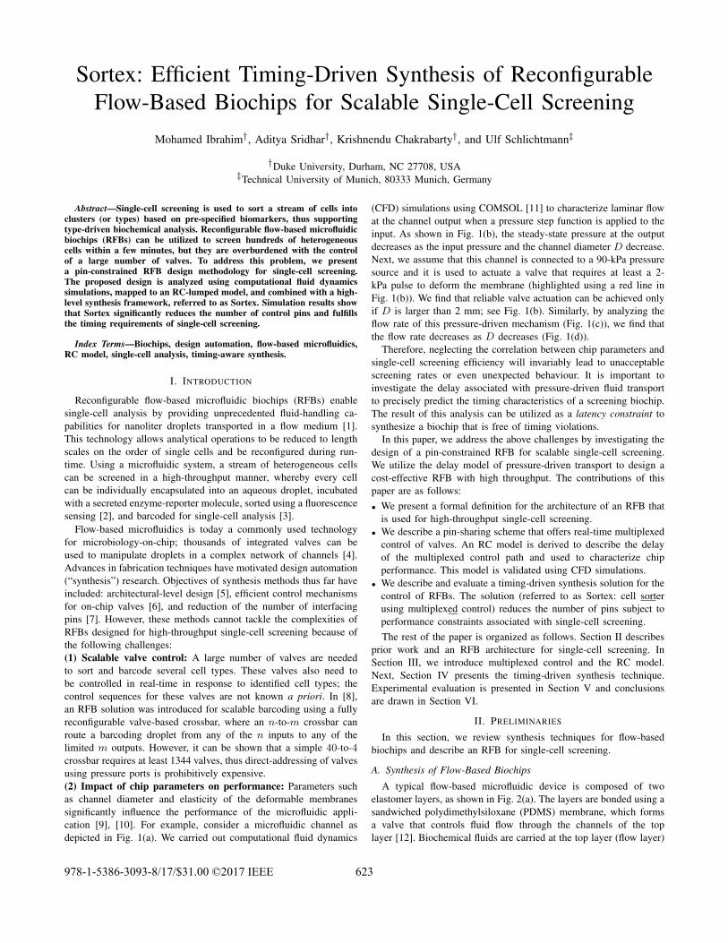
Sortex: Efficient Timing-Driven Synthesis of Reconfigurable

Flow-Based Biochips for Scalable Single-Cell Screening

Mohamed Ibrahim†, Aditya Sridhar†, Krishnendu Chakrabarty†, and Ulf Schlichtmann‡

†Duke University, Durham, NC 27708, USA‡Technical University of Munich, 80333 Munich, Germany

Abstract—Single-cell screening is used to sort a stream of cells intoclusters (or types) based on pre-specified biomarkers, thus supporting

type-driven biochemical analysis. Reconfigurable flow-based microfluidicbiochips (RFBs) can be utilized to screen hundreds of heterogeneouscells within a few minutes, but they are overburdened with the control

of a large number of valves. To address this problem, we presenta pin-constrained RFB design methodology for single-cell screening.

The proposed design is analyzed using computational fluid dynamicssimulations, mapped to an RC-lumped model, and combined with a high-level synthesis framework, referred to as Sortex. Simulation results show

that Sortex significantly reduces the number of control pins and fulfillsthe timing requirements of single-cell screening.

Index Terms—Biochips, design automation, flow-based microfluidics,

RC model, single-cell analysis, timing-aware synthesis.

I. INTRODUCTION

Reconfigurable flow-based microfluidic biochips (RFBs) enable

single-cell analysis by providing unprecedented fluid-handling ca-

pabilities for nanoliter droplets transported in a flow medium [1].

This technology allows analytical operations to be reduced to length

scales on the order of single cells and be reconfigured during run-

time. Using a microfluidic system, a stream of heterogeneous cells

can be screened in a high-throughput manner, whereby every cell

can be individually encapsulated into an aqueous droplet, incubated

with a secreted enzyme-reporter molecule, sorted using a fluorescence

sensing [2], and barcoded for single-cell analysis [3].

Flow-based microfluidics is today a commonly used technology

for microbiology-on-chip; thousands of integrated valves can be

used to manipulate droplets in a complex network of channels [4].

Advances in fabrication techniques have motivated design automation

(“synthesis”) research. Objectives of synthesis methods thus far have

included: architectural-level design [5], efficient control mechanisms

for on-chip valves [6], and reduction of the number of interfacing

pins [7]. However, these methods cannot tackle the complexities of

RFBs designed for high-throughput single-cell screening because of

the following challenges:

(1) Scalable valve control: A large number of valves are needed

to sort and barcode several cell types. These valves also need to

be controlled in real-time in response to identified cell types; the

control sequences for these valves are not known a priori. In [8],

an RFB solution was introduced for scalable barcoding using a fully

reconfigurable valve-based crossbar, where an n-to-m crossbar can

route a barcoding droplet from any of the n inputs to any of the

limited m outputs. However, it can be shown that a simple 40-to-4crossbar requires at least 1344 valves, thus direct-addressing of valves

using pressure ports is prohibitively expensive.

(2) Impact of chip parameters on performance: Parameters such

as channel diameter and elasticity of the deformable membranes

significantly influence the performance of the microfluidic appli-

cation [9], [10]. For example, consider a microfluidic channel as

depicted in Fig. 1(a). We carried out computational fluid dynamics

(CFD) simulations using COMSOL [11] to characterize laminar flow

at the channel output when a pressure step function is applied to the

input. As shown in Fig. 1(b), the steady-state pressure at the output

decreases as the input pressure and the channel diameter D decrease.

Next, we assume that this channel is connected to a 90-kPa pressure

source and it is used to actuate a valve that requires at least a 2-

kPa pulse to deform the membrane (highlighted using a red line in

Fig. 1(b)). We find that reliable valve actuation can be achieved only

if D is larger than 2 mm; see Fig. 1(b). Similarly, by analyzing the

flow rate of this pressure-driven mechanism (Fig. 1(c)), we find that

the flow rate decreases as D decreases (Fig. 1(d)).

Therefore, neglecting the correlation between chip parameters and

single-cell screening efficiency will invariably lead to unacceptable

screening rates or even unexpected behaviour. It is important to

investigate the delay associated with pressure-driven fluid transport

to precisely predict the timing characteristics of a screening biochip.

The result of this analysis can be utilized as a latency constraint to

synthesize a biochip that is free of timing violations.

In this paper, we address the above challenges by investigating the

design of a pin-constrained RFB for scalable single-cell screening.

We utilize the delay model of pressure-driven transport to design a

cost-effective RFB with high throughput. The contributions of this

paper are as follows:

• We present a formal definition for the architecture of an RFB that

is used for high-throughput single-cell screening.

• We describe a pin-sharing scheme that offers real-time multiplexed

control of valves. An RC model is derived to describe the delay

of the multiplexed control path and used to characterize chip

performance. This model is validated using CFD simulations.

• We describe and evaluate a timing-driven synthesis solution for the

control of RFBs. The solution (referred to as Sortex: cell sorter

using multiplexed control) reduces the number of pins subject to

performance constraints associated with single-cell screening.

The rest of the paper is organized as follows. Section II describes

prior work and an RFB architecture for single-cell screening. In

Section III, we introduce multiplexed control and the RC model.

Next, Section IV presents the timing-driven synthesis technique.

Experimental evaluation is presented in Section V and conclusions

are drawn in Section VI.

II. PRELIMINARIES

In this section, we review synthesis techniques for flow-based

biochips and describe an RFB for single-cell screening.

A. Synthesis of Flow-Based Biochips

A typical flow-based microfluidic device is composed of two

elastomer layers, as shown in Fig. 2(a). The layers are bonded using a

sandwiched polydimethylsiloxane (PDMS) membrane, which forms

a valve that controls fluid flow through the channels of the top

layer [12]. Biochemical fluids are carried at the top layer (flow layer)

978-1-5386-3093-8/17/$31.00 ©2017 IEEE 623

0

0.5

1

1.5

2

2.5

3

3.5

4

1.6 1.8 2 2.2

Mea

sure

d o

utp

ut

pre

ssu

re (

kP

a)

Channel diameter “D” (mm)

70 kPa input pressure 90 kPa input pressure

110 kPa input pressure

(b)(a)

19

0 m

m

Input

pressure

step

Output

pressure

DW

ater

0.01s 0.05s 0.1s 0.2s0.15s

Vel

oci

ty

hea

t m

apL

ow

Hig

h

(c)

0

5

10

15

20

25

0 0.25 0.5 0.75 1Time (s)

Vo

l. f

low

rat

e p

er

un

it a

rea

(m3/s

)

D = 1.8 mm D = 2.2 mm

(d)

Fig. 1: The correlation between the parameters of a microfluidic channel

and system performance: (a) geometric specifications, (b) evaluation of

output pressure, (c) velocity profile of pressure-driven mechanisms, (d)

dependence of flow rate on D.

Top layer channel

(flow channel)

Bottom layer channel

(control channel)Applying vacuum

PDMS

membrane

Valve seat

Displacement chamber

(a)

Elastomer layers

Closed OpenFlow

blocked

Atmospheric

pressureVacuum

applied

(b)

Flow

allowed

Fig. 2: (a) The components, and (b) the operation of a normally closed

valve [12].

and the other layer (control layer) provides the vacuum to deflect

the PDMS membrane “outside” the flow channel to permit fluid

flow–this valve is characterized as “normally closed” (Fig. 2(b)).

Synthesis techniques have been developed for channel placement

and routing in each layer separately [5], [13], [14]. These methods,

however, overlooked the interaction between the control and flow

layers, thus they may lead to infeasible solutions. The interaction

between the control and flow layers was highlighted in [15], and

solutions for pin-count reduction were presented in [6], [7]. These

methods, however, are inadequate for high-throughput screening for

the following reasons:

(i) For control-pin minimization, [7] relies on activation-based

compatibility; valve-actuation patterns of a protocol are mapped to

a pin-count minimization strategy. A more flexible approach in [6]

Cells

Cells

Dyes

Dyes

Fluor. Detector

Fluor. DetectorN

1

N

1

Barcoding

crossbar

K

1

“Cel

l stre

ams”

1

WBar

cod

ing

lib

rary

1

W

Dro

ple

ts t

o

do

wn-s

trea

m

W << K

Fluorescence detection

Sorting

network

(a)

(b)

K = 4; W = 2

Step (1)

Step (2)

N = 2; W = 2

(c)

B1

B2

B1

B2

Normally

closed valve

I1

I2

I3

I4

B1

B2

Closed valve

Open valve

Route of barcode 1

Route of barcode 2

Route of sample 1

Route of sample 2

S1

S1

S2

S2

Valve/Mixer

O1

O1

O2

O2

Fig. 3: An RFB for single-cell screening: (a) platform modules, (b) a

4-to-2 barcoding module [8], (c) a 2-by-2 sorting network [1].

explores compatibility among basic control actions of individual flu-

idic operations. However, both techniques assume that “compatible”

valves can be simultaneously addressed using the same pressure

source—this assumption is valid only with a small number of com-

patible valves due to fan-out limits. Moreover, these approaches do

not enable independent actuation of valves, limiting reconfigurability

for single-cell screening.

(ii) The work in [6] considered pressure-propagation delay within

fluidic-channel routing using a path-length model. However, this

model does not capture the correlation between fluid dynamics

and biochip parameters (e.g., channel width and elasticity). Further-

more, [6] uses only the longest pressure-propagation delay of a pin-

sharing valve group to assess performance. This approach cannot be

used with multiplexed control of independently addressable valves.

B. An RFB for Single-Cell Screening

Fig. 3(a) shows an RFB architecture that screens N streams

of cells, classifies cells into K types, and barcodes the cells via

W ports (W << K). This platform consists of three modules:

valve-less fluorescence detection, barcoding crossbar, and sorting

network. Adaptation is achieved via the detection of samples in the

fluorescence-detection module, whereas reconfiguration is carried out

in response at both the barcoding crossbar and the sorting network.

A reconfigurable valve-based crossbar is employed to barcode

droplets and route them towards the sorting network. A barcoding

droplet is routed from an input port Ik ∈ {I1, I2, ..., IK} to an output

port Bw ∈ {B1, B2, ..., BW } through channels, and the routing path

is configured online using a set of valves Vp = {V1, V2, ..., VP }; P

is the number of crossbar valves. Fig. 3(b) shows a 4-to-2 crossbar

that routes two different barcoding droplets concurrently.

Connected to the crossbar is a sorting module that mixes a sample

droplet from a stream Sn ∈ {S1, S2, ..., SN} with a barcoding

droplet generated from Bw. This function can be implemented

624

using N × W independent mixers. However, this approach makes

channel network design overly complex for large N and W . Scalable

single-cell sorting requires a programmable microfluidic platform

that performs biochemical operations at functional units on-the-fly.

We exploit the programmable microfluidic network proposed in [1],

where an N -by-W network can dynamically process any pair of

N × W input droplets. A set of valves Vq = {V1, V2, ..., VQ},

where Q is the number of network valves, are used to mix barcodes

with cells and route mixed droplets to output ports in the set

{O1, O2, ..., OW }. Fig 3(c) illustrates a 2-by-2 network.

While this RFB design offers reconfigurability, the efficiency of

single-cell screening depends on the topology of the flow channels

and how fast the flow valves in the set V = Vp ∪ Vq can be

actuated. Since we consider a fixed topology for the flow channels, we

focus on delays associated with valve actuation (pressurization or de-

pressurization). We demonstrate in the next section that an effective

pin-constrained control methodology for an RFB must consider the

timing overhead of valve actuation. Therefore, we consider valve-

based modules (the barcoding crossbar and the sorting network) to

investigate the sequence and delay of valve controls required to route

a barcode from Ik : {k ∈ N, k ≤ K} to Ow : {w ∈ N, w ≤ W}and to route the barcoded cell from Sn : {n ∈ N, n ≤ N} to

Ow : {w ∈ N, w ≤ W}. This sequence is referred to as a control

sequence and is denoted by Ht : {Ht ∈ {0, 1}X , t ∈ N, t ≤ T},

where X is the number of chip valves (X = P+Q) and T is the total

number of possible control sequences. The parameter T can also be

interpreted as the number of possible flow paths that can be utilized

by a single-cell sample of any type. In addition, we use θ(X,Y ) to

denote a screening biochip that contains X valves and is actuated

using Y control pins.

Our goal in this paper is to provide an architectural-level synthesis

scheme that allows the control of X valves by Y pins (Y << X),

while the latency of every control sequence Ht is less than a

threshold. A solution to this problem leads to a biochip that provides

a desired screening throughput.

III. MULTIPLEXED CONTROL AND DELAY

In this section, we explain the pin-constrained design methodology

and the associated delay model.

A. Multiplexed Control

To reduce the number of control pins, we allow several valves in a

screening biochip to share a few pins using time-division multiplexing

(TDM) [12]. Fig. 4(b) shows an example of multiplexed control for

an 8-valve flow channel (shown in Fig. 4(a)); i.e., T = 1. As shown

in Fig. 4(b), the circles in blue and orange represent the control pins

of the biochip whereas the circles in white represent the valves.

To implement TDM, two types of control pins are needed: (1) A

set of primary pins Ca (blue circles), used to provide the pressure

(or vacuum) through primary control channels to actuate valves

in the flow channel; (2) a set of demultiplexing pins Cg (orange

circles), used to direct the pressure-driven flow from a primary pin

to a particular valve in the flow channel through demultiplexing

control channels, thereby allowing flow valves to be independently

addressable. The pins in Cg , configured as two-way sources [12], can

pressurize and de-pressurize a set of valves, referred to as control

valves L (Fig. 4(b)) to avoid confusion with the flow valves in

Fig. 4(a). A control valve li ∈ L acts as a two-way switch to direct

a control pulse in one of two directions.

For example, to actuate flow valve V2 in Fig. 4(a), demultiplexing

pins Cg1 , C

g2 , and C

g3 (shown in Fig. 4(b)) are first activated to switch

Flow valves

1 2 3 4 5 6 7 8

(b)

Primary pinDemultiplexing pin

i

Control valve

Flow valvePrimary control channel Demultiplexing control channel

(a)

l1 l2 l3 l4

l5 l6l7 l8��������

������

Fig. 4: (a) An 8-valve channel; (b) Mutliplexed control of the channel

using 4 control pins.

1 2 3 4 5 6 7 8

1 2 3 4 5 6 7 8

(a)

(b)

Primary pinDemultiplexing pin

i

Control valve

Flow valvePrimary control channel Demultiplexing control channel����������

����

������

��

�� ��

Control path associated with �� Control path associated with ��Fig. 5: Multiplexed control of an 8-valve channel using (a) 4 control pins

and (b) 6 control pins.

the control valves l7, l1, and l5, respectively. By switching these

control valves, a control path is now opened between the primary

pin Ca1 and the desired flow valve V2. Next, Ca

1 is actuated to open

or close V2, which in turn is a latching valve that can maintain its

open or closed state while disconnected from the controller [12].

Note that we can route a fluid through the flow channel in Fig. 4(a)

from A to B or vice versa only after all the 8 valves are actuated. In

addition, the flow circuitry in Fig. 4(a) and the multiplexed control

circuitry in Fig. 4(b) are located on different layers.

By using multiplexed control and by considering the valve-control

signal as a binary signal, X flow valves can be independently actuated

using only a single primary pin and ⌈log2 X⌉ demultiplexing pins;

i.e., Y = ⌈log2 X⌉ + 1 provides a lower bound on the number of

control pins needed to actuate X valves. For example, the 8 valves

in Fig. 4(a) can be addressed using only 4 control pins. Similarly,

the valves of an 1024-valve biochip can be addressed using 11 pins.

Note however that the addressing of a single flow valve requires

a sequence of pin actuations, which imposes timing overhead. For

the 8-valve channel in Fig. 4(a), Fig. 5(a-b) illustrates multiplexed

control for actuating all the channel valves using 4 pins and 6

pins, respectively. Although Fig. 5 does not show the delays of

control pulses through the control circuitry (the delays are expected

to be larger for the 4-pin design), it is evident that the multiplexed

control procedure is less complicated with 6 control pins. Hence,

there is a tradeoff between pin-count reduction and the complexity

of multiplexed control, and therefore the performance of single-cell

screening.

625

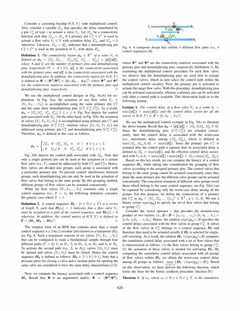
Consider a screening biochip θ(X,Y ) with multiplexed control.

Also, consider a variable dixy that specifies the delay contributed by

a pin Ciy of type i to actuate a valve Vx. Let λa

xy be a connectivity

function such that λaxy = daxy if a primary pin Ca

y ∈ Ca is used to

actuate a flow valve Vx ∈ V with actuation delay daxy , and λaxy = 0

otherwise. Likewise, λgxy = dgxy indicates that a demultiplexing pin

Cgy ∈ Cg is used in the actuation of Vx with delay dgxy .

Definition 1. The connectivity vector φx ∈ RY of a valve Vx is

defined as φx = [λax1 λa

x2 ... λaxA|λ

gx1 λ

gx2 ... λ

gxG] = [φa

x|φgx],

where A and G are the number of primary pins and demultiplexing

pins, respectively (Y = A + G), φax is the connectivity associated

with the primary pins, and φgx is the connectivity associated with the

demultiplexing pins. In addition, the connectivity matrix for θ(X,Y )is defined as Φ = [Φa|Φg] = [φ1 φ2 ... φX ]⊺; where Φa and Φg

are the connectivity matrices associated with the primary pins and

demultiplexing pins, respectively. ✷

We use the multiplexed control designs in Fig. 5(a-b) for ex-

planation. In Fig. 5(a), the actuation of any flow valve Vx ∈{V1, V2, ..., V8} is accomplished using the same primary pin Ca

1

and the same three demultiplexing pins {Cg1 , C

g2 , C

g3}. As a result,

φx = [λax1|λ

gx1 λ

gx2 λ

gx3], 1 ≤ x ≤ 8. Fig. 5(a) depicts the control

path associated with λa21. On the other hand, in Fig. 5(b), the actuation

of valves {V1, V2, V3, V4} is accomplished using primary pin Ca1 and

demultiplexing pins {Cg1 , C

g2}, whereas valves {V5, V6, V7, V8} are

addressed using primary pin Ca2 and demultiplexing pins {Cg

3 , Cg4}.

Therefore, φx is defined in this case as follows:

φx =

{

[λax1 0 |λg

x1 λgx2 0 0 ] if 1 ≤ x < 5

[ 0 λax2| 0 0 λ

gx3 λ

gx4] if 5 ≤ x ≤ 8

Fig. 5(b) depicts the control path associated with λg22. Note that

only a single primary pin can be used in the actuation of a certain

flow valve (i.e., Vx cannot be addressed by both Ca1 and Ca

2 ). Hence,

flow valves are divided into groups; each group is associated with

a particular primary pin. To prevent control interference between

groups, each demultiplexing pin can only be used in the actuation of

flow valves that belong to the same group. By this grouping method,

different groups of flow valves can be actuated concurrently.

While the flow valves {V1, V2, ..., V8} construct only a single

control sequence (i.e., T = 1), the following definition considers

the generic case where T > 1.

Definition 2. A control sequence Ht : {t ∈ N, t ≤ T} is a vector

of length X such that Ht[x] = 1 indicates that a flow valve Vx

must be actuated as a part of the control sequence, and Ht[x] = 0otherwise. In addition, the control matrix of θ(X,Y ) is defined as

Γ = [H1 H2 ... HT ]⊺. ✷

The simplest form of an RFB that contains more than a single

control sequence is a 2-by-2 crossbar (also known as a transposer [8]);

see Fig. 6. Such a transposer consists of six valves {V1, V2, ..., V6}that can be configured to route a biochemical sample through four

different paths (T = 4): I1 to B1, I1 to B2, I2 to B1, and I2 to B2.

To activate the second path (i.e., I1 to B2), valves {V2, V4} must

be opened and valves {V1, V6} must be closed. Hence the control

sequence H2 is defined as follows: H2 = [1 1 0 1 0 1]. Note that a

pressure pulse for closing a valve and a vacuum pulse for opening the

same valve are considered to have the same delay characteristics [12].

Next, we compute the latency associated with a control sequence

Ht. Recall that Φ is an augmented matrix; Φ = (Φa|Φg),

V1I1

I2

B1

B2

V3V2

V4V5

V6

Fig. 6: A transposer design that exhibits 4 different flow paths (i.e., 4

control sequences) [8].

where Φa and Φg are the connectivity matrices associated with the

primary pins and demultiplexing pins, respectively (Definition 1). By

examining the multiplexed control procedure for each flow valve,

we observe that the demultiplexing pins are used first to actuate

the control valves, which in turn select the control path within the

multiplexed control circuitry. Next, the primary pin is activated to

actuate the target flow valve. With this procedure, demultiplexing pins

can be activated concurrently, whereas a primary pin can be activated

only after a control path is available. This observation leads us to the

following lemma.

Lemma 1. The control delay of a flow valve Vx is a value bx =max{φa

x} + max{φgx}, and the control delay vector for all the

valves in θ(X,Y ) is β = [b1 b2 ... bX ]⊺.

We use the multiplexed control example in Fig. 5(b) to illustrate

the above lemma. Recall that φ2 = [φa2 |φ

g2] = [λa

21 0|λg21 λ

g22 0 0].

Since the demultiplexing pins {Cg1 , C

g2} are actuated concur-

rently, then the control delay is associated with the worst-case

(i.e., maximum) delay among {λg21, λ

g22}, which is defined as

max{λg21, λ

g22, 0, 0} = max{φg

2}. Since the primary pin Ca

1 is

actuated after the control path is opened, then its associated delay is

defined as λa21 = max{φa

2}, and the effective control delay associ-

ated with V2 is b2 = max{φa2}+max{φg

2} = λa

21+max{λg21, λ

g22}.

Based on this key result, we can compute the latency of a control

sequence Ht, while taking into consideration the grouping of flow

valves according to the assigned primary pins. The control valves that

belong to the same group cannot be actuated concurrently since they

share the same primary pin, but different valve groups can be actuated

concurrently. The concurrent actuation of different valve groups (even

those which belong to the same control sequence; see Fig. 5(b)) can

be captured by considering only the worst-case delay among all the

groups. For this purpose, we define the connectivity of a primary

pin Cay as ρy = [λa

1y λa2y ... λa

Xy]⊺ ∈ R

X , y ∈ [1, A]. We use a

binary vector sign(ρy) to specify the set of flow valves that belong

to group Cay .

Consider the vector operator ◦ that provides the element-wise

product of two vectors, i.e., E ◦B = [e1 e2 ... en] ◦ [b1 b2 ... bn] =[e1b1 e2b2 ... enbn]. Hence, the relation sign(ρy) ◦ β specifies the

control delays associated with the flow valves in group Cay . A subset

of the flow valves in Cay belongs to a control sequence Ht and

therefore they need to be actuated serially if Ht is selected for single-

cell screening. As a result, the relation Ht ·(sign(ρy)◦β) computes

the cumulative control delay associated with a set of flow valves that

is characterized as follows: (1) the flow valves belong to group Cay ;

(2) the actuation of these valves is needed for activating Ht. By

computing the cumulative control delays associated with all groups

of flow valves within Ht, we obtain the worst-case control delay

among all groups as follows: max1≤y≤A

{Ht · (sign(ρy) ◦ β)}. Based

on this observation, we have derived the following theorem, which

forms the basis for the Sortex synthesis procedure (Section IV).

Theorem 1. If αt, where αt ∈ R, t ∈ N, t ≤ T , is the cumulative

626

control latency value associated with a control sequence Ht in a

chip θ(X,Y ), then αt = max1≤y≤A

{Ht · (sign(ρy) ◦ β)}, where ◦ is

the element-wise product. In addition, the cumulative control latency

vector for all control sequences in θ(X,Y ) is Θ = max1≤y≤A

{Γ ·

(sign(ρy) ◦ β)}.

Fig. 6 illustrates Theorem 1. Recall that the second control

sequence is H2 = [1 1 0 1 0 1]. First, assume that all six

valves belong to the same group, i.e., they are actuated using the

same primary pin Ca1 . In this case, sign(ρ1) = [1 1 ... 1]. To

activate H2, V1, V2, V4, V6 need to be actuated serially; therefore the

cumulative control latency is the sum of the control delays associated

with these valves. In other words, α2 = H2 · (sign(ρ1) ◦ β) =[1 1 0 1 0 1] · [b1 b2 ...]⊺ = b1 + b2 + b4 + b6. Second, if two

primary pins {Ca1 , C

a2 } are used, where sign(ρ1) = [1 1 1 0 0 0]

and sign(ρ2) = [0 0 0 1 1 1], the cumulative control latency α2

is computed as α2 = max1≤y≤2

{[1 1 0 1 0 1] · (sign(ρy) ◦ β)} =

max{b1 + b2, b4 + b6}.

The above discussion is focused on the latency of multiplexed

control in an RFB. Since the topology of flow channels in the

proposed RFB is fixed, we can easily estimate the flow latency of

samples through these channels and therefore obtain an accurate

estimate of biochip throughout. Note that a sample can be routed

through a flow path only after the associated control sequence is

activated. Therefore, if the flow latency vector associated with the

biochip control sequences is defined as ω ∈ RT , then the effective

latency vector of θ(X,Y ) is Θ+ω and the worst-case latency is τ =max{Θ + ω}. To optimize the throughput of single-cell screening,

our synthesis method in Section IV optimizes the multiplexed control

scheme in an RFB such that Y is minimized and τ ≤ η, where η is

a predefined value.

B. Delay of Pressure-Driven Fluid Transport

In electrical circuits, the delay of an electrical signal through a wire

can be characterized using a delay model [16]; a widely used delay

model, especially with wires characterized as RC trees or ladders, is

the Elmore delay model [16].

In analogy with electrical circuits, the delay of laminar flow

through a long elastic channel can be approximated using an equiva-

lent Elmore delay model, which is a practical alternative to complex

CFD simulations. For this purpose, there is a need to define the

model components, i.e., the hydraulic resistance R and the hydraulic

compliance M [10].

A laminar flow of a fluid through a long channel can be described

using the Hagen-Poiseuille equation: QH = πs4·∆Pr8µ·b

, where QH is

the flow rate, s is the channel radius, ∆Pr = Prin − Prout is the

pressure drop across the channel, µ is the dynamic viscosity of the

fluid, and b is the length of the channel. The analog of this law in

electrical circuits is Ohm’s law. We use this analogy to estimate the

hydraulic resistance R, which is defined as R = ∆Pr

QH= 8µ·b

πs4.

The above model makes the assumption that a microfluidic channel

is rigid. However, RFBs are fabricated using elastic material (e.g.,

PDMS) hence pressure can cause the cross-sectional area of a channel

to change; see Fig. 7(a). The capability of an elastic channel to store

fluid when pressurized is known as hydraulic compliance (similar

to capacitance in electrical circuits). To verify this behavior, we

conducted transient CFD simulation using COMSOL for laminar flow

in a PDMS channel. Fig. 7(b) shows channel deformation at different

time steps when a pressure step Pr1 is applied to the input. This

deformation can be interpreted as the potential of a channel to store

(a)

25

15

5

Velocity

(cm/s)

(b)

10

0 µ

m

300 µm

Pr1 Pr1Pr2

Pr1 Pr2

Pr2

(c) (d)

0.5*(Pr1-Pr2)

0.5*R 0.5*R

M M1 M2

0.5*R1 0.5*R1 0.5*R2 0.5*R2

Mn

0.5*Rn 0.5*Rn

Fig. 7: (a) A PDMS microfluidic channel expands when pressurized. (b)

Result of transient CFD simulation for an elastic channel under pressure.

(c) Lumped-RC model. (d) Distributed-RC model.

fluid when pressurized; this is referred to as hydraulic compliance

M . We also observe that the deformation distance and therefore M

are correlated with the material elasticity (i.e., channel dilatability

γ). This observation corroborates an analytic expression that spec-

ifies the hydraulic compliance for an elastic circular channel [17]:

M = γ · πs2 · b, where γ is the channel dilatability, s is the channel

radius, and b is the channel length.

The closed-form equations for R and M can be used to estimate

fluidic delay. Furthermore, since the values of R and M are specified

based on the channel geometry and material elasticity, the fluidic

delay, and therefore the screening throughput, can be tuned based

on these parameters. According to [18], a straightforward approach

for modeling an elastic channel is by using a lumped-RC model,

as shown in Fig. 7(c). For this model, the fluidic delay of the

channel is simply R · M . However, this lumped model does not

take into account the significant change in pressure across the

channel. To capture the variation in pressure and its impact on fluidic

delay, we use a distributed-RC ladder, as shown in Fig. 7(d). This

model offers three advantages: (1) increasing the number of model

segments n enhances model accuracy since every segment exhibits

an infinitesimal change in pressure; (2) similar to the models of

electrical interconnects [16], modeling various segments of a channel

provides the opportunity to design a width-varying channel—this

design method can be employed to minimize both the fluidic delay

and the channel area; (3) the delay associated with a distributed-RC

ladder (containing n segments) can be estimated using the Elmore

model [16]: del =∑n

i=1

(

Mi ·(∑i

j=1Rj)

)

, where del is the Elmore

delay, Rj and Mj are the resistance and compliance of segment j,

respectively. Hence, we adopt this model in our synthesis framework

to estimate the delay associated with flow and multiplexed-control

paths.

IV. SORTEX: SYNTHESIS SOLUTION

In this section, we discuss the problem formulation and the

proposed synthesis framework (Sortex).

A. Problem Formulation

We consider the following problem formulation in this work.

Input: (1) The specifications of a screening biochip θ(X,Y ), which

includes: (i) the locations of all the valves V and L; (ii) the channels

connecting the flow valves V; (iii) the maximum number of control

pins (Ca and Cg) and their locations; (iv) possible values of the

channel width D = {D1, D2, ...}.

(2) A fluidic delay model based on a distributed RC ladder.

(3) A threshold η ∈ R that represents the maximum latency.

627

(4) An upper bound Armax on the channel area.

Output: (1) The screening matrix Γ. (2) The connectivity matrix

Φ. (3) The worst-case latency τ . (4) The dimensions of the control

channels: lengths U = {u1, u2, ...} and widths F = {f1, f2, ...}.

Constraints: (1) Screening latency constraint (τ ≤ η). (2) Area

constraint (∑

i(ui × fi) ≤ Armax).

Objective: Minimize the number of control pins Y used for multi-

plexed control of biochip valves.

Note that efficient channel routing is beyond the scope of this

paper. Sortex calculates control delays by using Manhattan distances

between different entities. This work can be extended further by

incorporating routing as in [6].

B. Sortex Algorithm

Recall that flow valves are assigned to groups; each group is

actuated using a dedicated primary pin. To reduce the number of

control pins, synthesis for multiplexed control must increase the

number of flow valves assigned to a group.

We use a heuristic method based on divide-and-conquer (Algo-

rithm. 1). Initially, the proposed method selects a primary pin (Line

13) and iterates over the flow valves in a pairwise manner (Line

10) trying to connect every pair to the current primary pin (Line 16).

When the multiplexed-control scheme is expanded, timing analysis is

performed using the Elmore delay model from Section III-B and the

relation from Theorem 1 to ensure that the latency constraint is not

violated (Line 17). If no constraint violation is detected, the expanded

multiplexed control is accepted and the associated valve/pin variables

are updated (Lines 18-21). However, if a violation is detected, the

proposed connection to the current primary pin is declined and a new

primary pin is selected for connection (Lines 23-24). In this case,

the flow valves are divided into two groups; one group combines

the valves that have already been connected to the first primary pin

and the second group combines the remaining valves (including the

current pair)—we call this scheme divide-and-conquer. When the

remaining flow valves are connected to a second primary pin, we

further divide the set of valves into two groups according to the

latency constraint. This process continues until all the flow valves

are addressed.

The order of selection of the valves impacts computational per-

formance. Random selection of valves may lead to high CPU time

because distant valves can be combined in a single group, causing

divide-and-conquer to be invoked frequently; i.e., unnecessarily in-

creasing the number of control pins. To address this issue, we create a

priority queue of the unaddressed flow valves (Line 2). The priority of

valve selection is decided according to the following policy: (1) select

a valve Vf randomly and place it at the head of the queue; (2) select a

set of flow valves that does not belong to the same control sequences

as Vf and sort these valves in an increasing order according to their

Manhattan distance from Vf ; (3) sort the remaining valves according

to their Manhattan distance from Vf . This priority scheme (worst-

case time complexity O(T ·X +X · logX)) is invoked whenever a

divide-and-conquer action takes place (Line 25).

We next connect a new pair of flow valves to a primary pin (i.e.,

TestMC function in Algorithm 1). To expand the multiplexed control,

control paths are designed to manage the actuation of the new flow

valves. The synthesis of a control path is governed by two aspects:

(1) the selection of control valves L = {l1, l2, ...} through which the

control path is designed; (2) the selection of a new demultiplexing

pin (if needed) in order to actuate the control valve. Consider the

design of the control paths for the RFB in Fig. 8(a). To simplify

the selection of control valves at each iteration, we initially split L

Algorithm 1 Sortex Procedure

1: Γ← ConstructScreeningMatrix(V);

2: VQ ← ConstructValvesPriorityQueue(V);

3: AssignControlValvesToLevels(L);

4: SortDecrChannelWidthsRange(D);

5: j ← 0; // Iterator

6: repeat

7: CCa ← ∅; CCg ← ∅; // Connected pins so far

8: U ← ∅; F ← ∅; Φ← [0]; τ ← 0; A← 0;

9: Dj ← ConsiderChannelWidth(D);

10: for (Vi, Vi+1) ∈ VQ do

11: X ← ∅; Y ← ∅; // Connected pins to the pair

12: if CCa = ∅ then

13: X ← selectNearestPrimaryPinLocation();

14: Y ← BuildMC(Vi, Vi+1,X ,“2-Pin”);

15: else

16: {Φ,Conf} ← TestMC(Vi, Vi+1);

17: τ ← CalculateLatencyUsingElmore(Φ, Dj );

18: if τ ≤ η and Conf = “1-Pin” then

19: Y ← BuildMC(Vi, Vi+1, “1-Pin”);

20: else if τ ≤ η and Conf = “0-Pin” then

21: BuildMC(Vi, Vi+1, “0-Pin”);

22: else

23: X ← selectNearestPrimaryPinLocation();

24: {X ,Y} ← BuildMC(Vi, Vi+1,X , “2-Pin”);

25: UpdatePriorityQueue(VQ);

26: UpdateVariables(U ,F ,Φ, τ );

27: CCa ← CCa ∪ X ; CCg ← CCg ∪ Y;

28: Ar ← CalculateChannelsArea(U ,F);

29: if Ar > Armax then break;

30: j ← j + 1;

31: until Ar ≤ Armax

32: return {U ,F , CCa, CCg , τ,Φ};

into logical levels (Line 3), where the first level contains control

valves that will be directly connected to the flow valves, e.g., l1 in

Fig. 8(b) and {l1, l2} in Fig. 8(c). Such an organization is performed

in advance and it enforces two conditions: (1) two control valves

cannot be connected using primary control channels if they belong

to the same logical level; (2) a single demultiplexing pin can only

be used to actuate the control valves that belong to the same level

and are used in the actuation of a single group of flow valves. For

example, in Fig. 8(c), {l1, l2} can be actuated using only Cg1 , which

cannot be used to actuate l3.

Based on the above hierarchy of control valves, the synthesis

of control paths associated with a new pair of flow valves can be

performed based on three different configurations (associated with

the variable Conf in Line 16), as shown in Fig. 8(b-d). The first

(2-Pin) configuration is applied when a new primary pin is needed.

This configuration is adopted either at the first iteration (Line 12-

14) or when there is a need for a new primary pin in order to

prevent violation of the screening-latency constraint (Lines 23-24).

In addition, a new demultiplexing pin is also needed. For example,

in Fig. 8(b), a new primary pin Ca1 is connected to {V1, V2} using

a control valve l1 that belongs to Level 1. Since l1 is the first valve

to be used in Level 1, a new demultiplexing pin Cg1 is connected.

The second and third configurations address the case where a new

primary pin is not needed. These configurations, however, differ in

how control valves are selected, and therefore, whether a demulti-

plexing pin is needed. To demonstrate the difference between the

two configurations, we map the control valves and their connectivity

into a binary tree, referred to as control-valves (CV) tree. Each

node represents a connected control valve, and the root represents

628

H1

H2

1 2

3

5 6 7 8

4

1 2

3 4

5 6 7 8

Root

l1l2

l3

l4

l5

l6

l7

l5

2 1

CV Tree

“Imbalanced”

l3

l4l1 l2

1 1�� �� �� ��

l1 l2

l3

l1

0 0

3 4

1 2RootCV Tree

“Balanced”

�� �� ��

l1

1 2

�� ��

(a)

(b) (c)

(d)

Flow valve

Control valve Demultiplexing pin

Primary pin Control channels

Level 1

Level 2

Level 1

Previous channel connection

Level 2

Level 3

Fig. 8: Multiplexed control configurations used to connect a pair of

flow valves. (a) An 8-valve RFB with two control sequences. (b) 2-Pin

configuration. (c) 1-Pin configuration. (d) 0-Pin configuration.

the control valve at the highest level that is directly connected to

the primary pin; see Fig. 8(c-d). Each node has two interfaces (left

and right) which are connected to two sub-trees. Each interface is

characterized by the maximum height of the associated sub-tree. A

CV tree is balanced only if the interfaces of every node in the tree

exhibit equal heights.

The CV tree evolves at every iteration whenever a new pair of flow

valves is selected; the tree evolves in a bottom-up fashion; the root of

the tree may change when new nodes are added. The second (1-Pin)

configuration is selected if the CV tree is currently balanced. Fig. 8(c)

shows an example for 1-Pin. Before the multiplexed-control scheme

is expanded for connecting the pair {V3, V4}, we observe that the

CV tree contains only one node l1 and it is balanced. For connecting

{V3, V4} to the same primary pin Ca1 , two new control valves {l2, l3}

are connected. Since l3 is the first valve to be connected at Level 2, a

new demultiplexing pin Cg2 is selected and l3 becomes the new root.

On the other hand, the third (0-Pin) configuration is applied if either

the CV tree or any sub-tree within the CV tree is imbalanced. For

example, in Fig. 8(d), we investigate the multiplexed-control paths

when a new pair {V7, V8} is selected. The CV tree is imbalanced,

because the difference between the heights of l5 interfaces is 1; this

difference is called the imbalance factor. Valve l5 is therefore called

the source of imbalance and its level (Level 3) is called the level of

imbalance. To connect {V7, V8} to the primary pin Ca1 , two control

valves {l6, l7} are connected. The valve l6 connects the pair {V7, V8}and therefore it is located at Level 1. However, l7 is located at Level z

which is determined as follows: z = level of imbalance − imbalance

factor. The control valve l7 is used to connect the source of imbalance

l5, the new control valve L6, and the previously connected valve l4. This configuration does not allocate new control pins. By using

this balancing scheme, we reduce the height of the tree and hence

decrease the number of demultiplexing pins.

The worst-case time complexity of this algorithm is O(X · |L| ·A ·G).

V. EXPERIMENTAL RESULTS

We implemented Sortex in a software simulation environment. All

evaluations were carried out using a 3.4 GHz Intel i7 CPU with 12 GB

RAM. The architecture of single-cell screening biochip (Section II-B)

was used as a benchmark, and two biochip configurations were

adopted; see Table I (# FV: number of flow valves; Max. # CV:

maximum number of control valves; Max. # CP: maximum number

of control pins). During simulation, we set an upper bound on the

number of control entities (i.e., control pins and valves); locations of

these entities were specified in advance.

We evaluate the performance of Sortex using two metrics: (1) the

worst-case screening latency, measured in seconds (s); (2) the number

of used control pins. In all evaluations, we consider air as a channel

medium (µ = 1.983 ∗ 10−5Pa · s), and the channel dilatability is set

to γ = 10−5Pa−1 (PDMS).

A. Comparison with Direct-Addressing

We compare Sortex with the direct-addressing (DA) method, in

which every valve is addressed by a dedicated control pin. We

evaluate DA and Sortex in terms of the screening latency and we

study the convergence of latency for Sortex by varying the number

of control pins. Fig. 9(a-b) show the screening-latency results for CF1

and CF2, respectively.

Based on Fig. 9, we observe that the latency decreases when the

number of control pins is increased. With more control pins, the

complexity of multiplexed control decreases, therefore the latency

decreases. Moreover, the latency for Sortex converges to that for DA,

despite the significant gap in the number of control pins between these

methods.

B. Impact of Chip Parameters and Constraints

We next evaluate the impact of chip parameters and design

constraints on screening performance. We focus only on the channel-

width parameter and the worst-case latency.

TABLE I: Biochip configurations used in evaluation

Conf. K,W,N # FV Max. # CV Max. # CP

CF1 4,2,1 28 140 28

CF2 8,4,1 80 400 80

Lower-bound delay Upper-bound delay

0

10

20

30

40

50

60

70

80

6 8 9 10 12 13 28

Scr

een

ing

lat

ency

(s)

Number of control pins

DA

(28 c

ontr

ol

pin

s)

(a)

0

50

100

150

200

250

8 13 18 19 22 23 26 80

Number of control pins

Scr

een

ing

lat

ency

(s)

(b)

DA

(80 c

ontr

ol

pin

s)

Fig. 9: Comparison between Sortex and DA: (a) screening latency (τ )

for CF1, (b) τ for CF2.

629

Channel width (μm)

Y1 Y

2

Channel width (μm) Channel width (μm) Channel width (μm)

Y1

Y1

Y1

Y2

Y2

Y2

(a) (b) (c) (d)

Number of demultiplexing pins Screening latencyNumber of primary pins Y1: Number of pins Y

2: Screening latency (s)

0

2

4

6

8

10

12

14

16

18

20

0

5

10

15

20

25

2 3 4 5 6 7

0

5

10

15

20

25

30

35

40

0

2

4

6

8

10

12

14

2 3 4 5 6 7

0

10

20

30

40

50

60

70

80

0

5

10

15

20

25

30

35

40

2 3 4 5 6 7

0

20

40

60

80

100

120

140

160

0

5

10

15

20

25

2 3 4 5 6 7

Fig. 10: Impact of channel width and latency constraint η on performance: (a) CF1, η = 19 s; (b) CF1, η = 38 s; (c) CF2, η = 70 s; (d) CF2, η =

140 s.

For each biochip configuration, we carried out two sets of synthesis

simulations. In each set, we consider a specific latency constraint and

report the number of control pins and the worst-case screening latency

while varying the channel width. The latency constraints considered

for CF1 are 19 s and 38 s, and their associated results are shown in

Fig. 10(a) and Fig. 10(b), respectively. Also, the latency constraints

for CF2 are 70 s and 140 s, and their associated results are depicted

in Fig. 10(c) and Fig. 10(d), respectively.

We first investigate the number of control pins in Fig. 10. In all

four cases, we observe that fewer control pins are needed (to satisfy

the latency constraint) when the channel width is increased. This

result is intuitive because using a wider channel causes the Elmore

delay for fluid transport to be minimized, thus reducing the number

divide-and-conquer procedures in Sortex (Section IV-B).

Second, we investigate the screening latency reported in Fig. 10.

We observe that in Fig. 10(b) the latency first increases when the

channel width is increased from 2 µm to 3 µm. Since the increase

in the channel width leads to pin-count reduction, the impact of pin-

count reduction on increasing the latency surpasses the impact of

increasing the channel width on reducing the latency. We also observe

that the latency is decreased in Fig. 10(b) when the channel width is

larger than 3 µm as no further pin-count reduction can be achieved,

i.e., the minimum number of control pins is reached (⌈log2 X⌉+1).

The same argument also applies to all other cases in Fig. 10. These

results show the impact of the channel width, particularly narrow

channels, on the screening performance.

We finally investigate the impact of changing the latency constraint

on the number of control pins. As expected, by relaxing the latency

constraint (i.e., increasing its value), the number of control pins is

reduced. For example, by comparing Fig. 10(c) with Fig. 10(d), the

number of control pins is decreased from 38 to 22 for a design with a

2 µm-channel width. While pin-constrained design has been studied

earlier [6], [7], the trade-off analysis presented in this section cannot

be applied to these prior methods; therefore a meaningful comparison

is not applicable in this case.

VI. CONCLUSION

We have introduced a timing-driven design method for a pin-

constrained RFB that performs single-cell screening. The proposed

design synthesizes multiplexed control and employs a delay model of

pressure-driven transport to satisfy a screening-delay constraint. The

proposed method has been evaluated based on the screening delay

and the pin count.

ACKNOWLEDGMENT

M. Ibrahim and K. Chakrabarty were supported in part by the

US National Science Foundation under grants CCF-1702596 and

CCF-1135853. In addition, K. Chakrabarty was supported by the

Technische Universitat Munchen – Institute for Advanced Study,

funded by the German Excellence Initiative and the European Union

Seventh Framework Programme under grant agreement N◦ 291763.

REFERENCES[1] J. Kim et al., “Pneumatically actuated microvalve circuits for pro-

grammable automation of chemical and biochemical analysis,” Lab on

a Chip, vol. 16, no. 5, pp. 812–819, 2016.[2] J. Baret et al., “Fluorescence-activated droplet sorting (FADS): efficient

microfluidic cell sorting based on enzymatic activity,” Lab on a Chip,vol. 9, no. 13, pp. 1850–1858, 2009.

[3] R. Zilionis et al., “Single-cell barcoding and sequencing using dropletmicrofluidics,” Nature Protocols, vol. 12, no. 1, pp. 44–73, 2017.

[4] I. Araci et al., “Microfluidic very large scale integration (mVLSI) withintegrated micromechanical valves,” Lab on a Chip, vol. 12, no. 16, pp.2803–2806, 2012.

[5] W. Minhass et al., “Architectural synthesis of flow-based microfluidiclarge-scale integration biochips,” CASES, 2012.

[6] K. Hu et al., “Control-layer routing and control-pin minimization forflow-based microfluidic biochips,” IEEE Trans. TCAD, vol. 36, no. 1,pp. 55–68, 2017.

[7] T. Tseng et al., “Columba: co-layout synthesis for continuous-flowmicrofluidic biochips,” in DAC, 2016.

[8] M. Ibrahim et al., “Cosyn: Efficient single-cell analysis using a hybridmicrofluidic platform,” in DATE, 2017.

[9] D. Kim et al., “A method for dynamic system characterization usinghydraulic series resistance,” Lab on a Chip, vol. 6, no. 5, pp. 639–644,2006.

[10] B. Kirby, Micro-and Nanoscale Fluid Mechanics: Transport in Microflu-

idic Devices. Cambridge University Press, 2010.[11] “COMSOL Multiphysics Modeling Software,” http://www.comsol.com/.[12] W. Grover et al., “Development and multiplexed control of latching

pneumatic valves using microfluidic logical structures,” Lab on a Chip,vol. 6, no. 5, pp. 623–631, 2006.

[13] N. Amin et al., “Computer-aided design for microfluidic chips based onmultilayer soft lithography,” in ICCD, 2009.

[14] W. Minhass et al., “Control synthesis for the flow-based microfluidiclarge-scale integration biochips,” ASPDAC, 2013.

[15] H. Yao et al., “Integrated flow-control codesign methodology for flow-based microfluidic biochips,” IEEE Des. Test., 2015.

[16] J. Cong et al., “Performance optimization of VLSI interconnect layout,”Integ., VLSI J., 1996.

[17] F. Perdigones et al., “Correspondence between electronics and fluids inMEMS: Designing microfluidic systems using electronics,” IEEE Trans.

Ind. Electron., vol. 8, no. 4, pp. 6–17, 2014.[18] P. Tabeling, Introduction to Microfluidics. Oxford University Press,

2005.

630