Embed Size (px)
Citation preview

The role of metabolic trade-offs inthe establishment of biodiversityStochastic Models in Ecology and Evolutionary Biology - Venice
Leonardo Pacciani5th April 2018

IntroductionOpen questions
1 What is the relationship between an ecosystem’s biodiversity and itsstability? → May’s stability criterion
2 How many species can compete for the same resources? →Competitive exclusion principle
1 of 18

IntroductionOpen questions
1 What is the relationship between an ecosystem’s biodiversity and itsstability? → May’s stability criterion
2 How many species can compete for the same resources? →Competitive exclusion principle
1 of 18

IntroductionOpen questions
1 What is the relationship between an ecosystem’s biodiversity and itsstability? → May’s stability criterion
2 How many species can compete for the same resources? →Competitive exclusion principle
1 of 18

IntroductionMay’s stability criterion
The first theoretical criterion for ecosystem stability was introduced byMay in 1972.Main resultBuilding a very simple model of ecosystem governed only by stochasticityand characterized by its biodiversity, i.e. the number m of speciespresent, the system will be stable only if
Σ√mC < d (1)
with Σ, C and d parameters of the model that describe the inter-specificinteractions (contained in the community matrix).
ProblemBiodiversity brings instability, but observations suggest the opposite!
2 of 18

IntroductionMay’s stability criterion
The first theoretical criterion for ecosystem stability was introduced byMay in 19721.
Main resultBuilding a very simple model of ecosystem governed only by stochasticityand characterized by its biodiversity, i.e. the number m of speciespresent, the system will be stable only if
Σ√mC < d (1)
with Σ, C and d parameters of the model that describe the inter-specificinteractions (contained in the community matrix).
ProblemBiodiversity brings instability, but observations suggest the opposite!
1Robert May. “Will a Large Complex System be Stable?” In: Nature 238 (1972).
2 of 18
IntroductionMay’s stability criterion
The first theoretical criterion for ecosystem stability was introduced byMay in 19721.Main resultBuilding a very simple model of ecosystem governed only by stochasticityand characterized by its biodiversity, i.e. the number m of speciespresent, the system will be stable only if
Σ√mC < d (1)
with Σ, C and d parameters of the model that describe the inter-specificinteractions (contained in the community matrix).
ProblemBiodiversity brings instability, but observations suggest the opposite!
1Robert May. “Will a Large Complex System be Stable?” In: Nature 238 (1972).
2 of 18

IntroductionMay’s stability criterion
A more general formulationIt is possible to generalize May’s simple model in order to make it morerealistic. In the end the stability criterion can be written as
max{√
mV (1 + ρ)− E , (m − 1)E}< d , (2)
where again V , E , ρ and d are again parameters of the communitymatrix.
3 of 18
IntroductionMay’s stability criterion
A more general formulation2
It is possible to generalize May’s simple model in order to make it morerealistic. In the end the stability criterion can be written as
max{√
mV (1 + ρ)− E , (m − 1)E}< d , (2)
where again V , E , ρ and d are again parameters of the communitymatrix.
2Stefano Allesina and Si Tang. “The stability–complexity relationship at age 40: arandom matrix perspective”. In: Population Ecology 57.1 (2015).
3 of 18

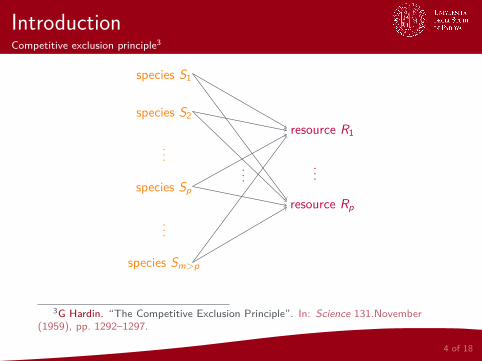
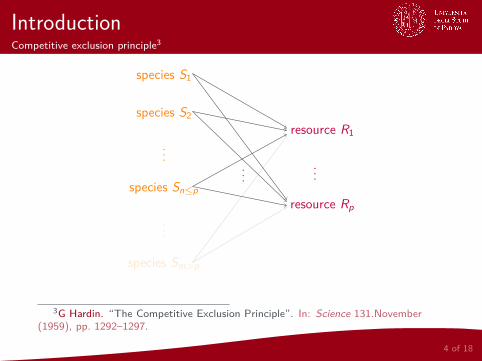
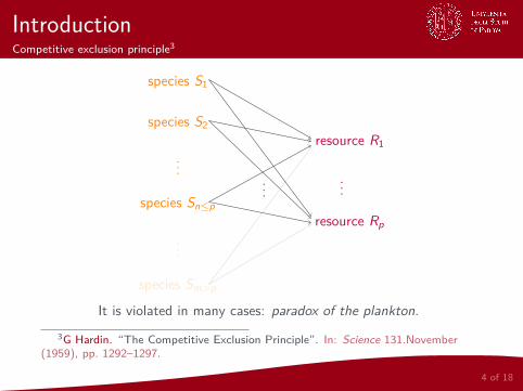
IntroductionCompetitive exclusion principle3
species Sm>p
...
species Sp
...
species S2
species S1
resource Rp
...
resource R1
...
species Sm>p
...
species Sn≤p
...
species S2
species S1
resource Rp
...
resource R1
...
3G Hardin. “The Competitive Exclusion Principle”. In: Science 131.November(1959), pp. 1292–1297.
4 of 18
It is violated in many cases: paradox of the plankton.

The PTW model
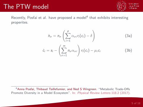
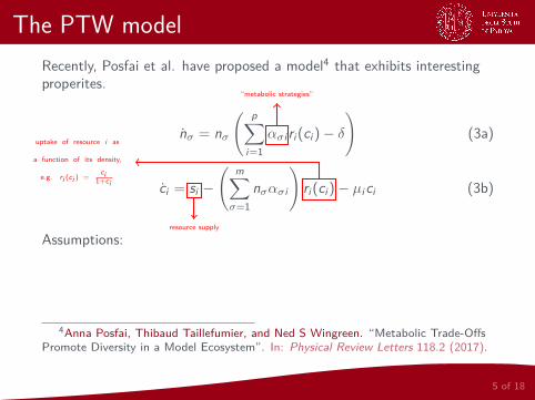
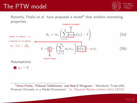
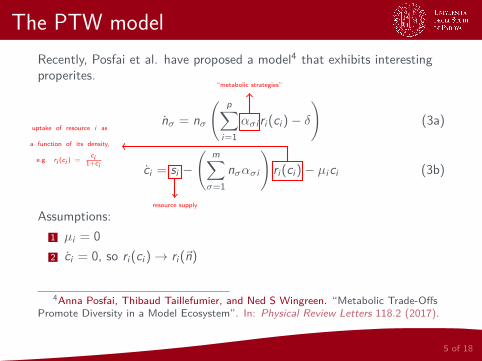
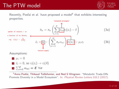
Recently, Posfai et al. have proposed a model that exhibits interestingproperites.
nσ = nσ
( p∑i=1
ασi ri (ci )− δ)
(3a)
ci = si −
( m∑σ=1
nσασi
)ri (ci )− µici (3b)
Assumptions:1 µi = 02 ci = 0, so ri (ci )→ ri (~n)3∑p
i=1 ασi = E ∀σ
5 of 18

The PTW modelRecently, Posfai et al. have proposed a model4 that exhibits interestingproperites.
nσ = nσ
( p∑i=1
ασi ri (ci )− δ)
(3a)
ci = si −
( m∑σ=1
nσασi
)ri (ci )− µici (3b)
Assumptions:1 µi = 02 ci = 0, so ri (ci )→ ri (~n)3∑p
i=1 ασi = E ∀σ
4Anna Posfai, Thibaud Taillefumier, and Ned S Wingreen. “Metabolic Trade-OffsPromote Diversity in a Model Ecosystem”. In: Physical Review Letters 118.2 (2017).
5 of 18
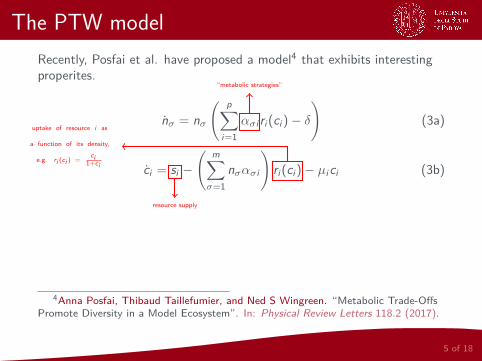
“metabolic strategies”
resource supply
uptake of resource i as
a function of its density,
e.g. ri (ci ) = ci1+ci
The PTW modelRecently, Posfai et al. have proposed a model4 that exhibits interestingproperites.
nσ = nσ
( p∑i=1
ασi ri (ci )− δ)
(3a)
ci = si −
( m∑σ=1
nσασi
)ri (ci )− µici (3b)
Assumptions:
1 µi = 02 ci = 0, so ri (ci )→ ri (~n)3∑p
i=1 ασi = E ∀σ
4Anna Posfai, Thibaud Taillefumier, and Ned S Wingreen. “Metabolic Trade-OffsPromote Diversity in a Model Ecosystem”. In: Physical Review Letters 118.2 (2017).
5 of 18
“metabolic strategies”
resource supply
uptake of resource i as
a function of its density,
e.g. ri (ci ) = ci1+ci
The PTW modelRecently, Posfai et al. have proposed a model4 that exhibits interestingproperites.
nσ = nσ
( p∑i=1
ασi ri (ci )− δ)
(3a)
ci = si −
( m∑σ=1
nσασi
)ri (ci )− µici (3b)
Assumptions:1 µi = 0
2 ci = 0, so ri (ci )→ ri (~n)3∑p
i=1 ασi = E ∀σ
4Anna Posfai, Thibaud Taillefumier, and Ned S Wingreen. “Metabolic Trade-OffsPromote Diversity in a Model Ecosystem”. In: Physical Review Letters 118.2 (2017).
5 of 18
“metabolic strategies”
resource supply
uptake of resource i as
a function of its density,
e.g. ri (ci ) = ci1+ci
The PTW modelRecently, Posfai et al. have proposed a model4 that exhibits interestingproperites.
nσ = nσ
( p∑i=1
ασi ri (ci )− δ)
(3a)
ci = si −
( m∑σ=1
nσασi
)ri (ci )− µici (3b)
Assumptions:1 µi = 02 ci = 0, so ri (ci )→ ri (~n)
3∑p
i=1 ασi = E ∀σ
4Anna Posfai, Thibaud Taillefumier, and Ned S Wingreen. “Metabolic Trade-OffsPromote Diversity in a Model Ecosystem”. In: Physical Review Letters 118.2 (2017).
5 of 18
“metabolic strategies”
resource supply
uptake of resource i as
a function of its density,
e.g. ri (ci ) = ci1+ci
The PTW modelRecently, Posfai et al. have proposed a model4 that exhibits interestingproperites.
nσ = nσ
( p∑i=1
ασi ri (ci )− δ)
(3a)
ci = si −
( m∑σ=1
nσασi
)ri (ci )− µici (3b)
Assumptions:1 µi = 02 ci = 0, so ri (ci )→ ri (~n)3∑p
i=1 ασi = E ∀σ4Anna Posfai, Thibaud Taillefumier, and Ned S Wingreen. “Metabolic Trade-Offs
Promote Diversity in a Model Ecosystem”. In: Physical Review Letters 118.2 (2017).
5 of 18
“metabolic strategies”
resource supply
uptake of resource i as
a function of its density,
e.g. ri (ci ) = ci1+ci
ασ1
ασ2ασ3

The PTW model
Main resultThe system will reach a stationary state where an arbitrary number ofspecies can coexist if
ES~s =
m∑σ=1
n∗σ~ασ withm∑σ=1
n∗σ = 1, S =p∑
i=1si , (4)
has a positive solution n∗σ > 0. This means that coexistence is possible if~sE/S belongs to the convex hull of the metabolic strategies.
Important remarkThe number of coexisting species is arbitrary, so we can also have m > p:the competitive exclusion principle can be violated.
6 of 18

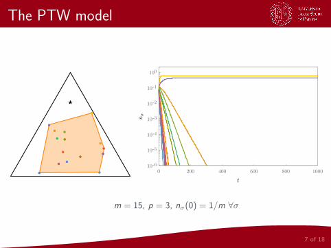
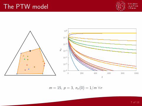
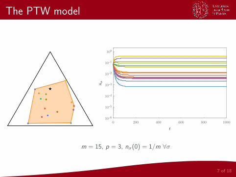
The PTW model
7 of 18
The PTW model
7 of 18
●●
●● ●●
●●
●●
●●
●●
●●
●●
●●
●●
●●
●●
●●
●●
★★
0 200 400 600 800 1000
10-6
10-5
10-4
10-3
10-2
10-1
100
m = 15, p = 3, nσ(0) = 1/m ∀σ
The PTW model
7 of 18
●●
●● ●●
●●
●●
●●
●●
●●
●●
●●
●●
●●
●●
●●
●●
★★
0 200 400 600 800 1000
10-6
10-5
10-4
10-3
10-2
10-1
100
m = 15, p = 3, nσ(0) = 1/m ∀σ
The PTW model
7 of 18
●●
●● ●●
●●
●●
●●
●●
●●
●●
●●
●●
●●
●●
●●
●●
★★
0 200 400 600 800 1000
10-6
10-5
10-4
10-3
10-2
10-1
100
m = 15, p = 3, nσ(0) = 1/m ∀σ

The PTW modelLimitations
No complete information on the stability of the steady state
The metabolic strategies are fixed in time
All species have the same death rate δ and energy budget E
8 of 18

The PTW modelLimitations
No complete information on the stability of the steady state
The metabolic strategies are fixed in time
All species have the same death rate δ and energy budget E
8 of 18

The PTW modelLimitations
No complete information on the stability of the steady state
The metabolic strategies are fixed in time
All species have the same death rate δ and energy budget E
8 of 18

The PTW modelLimitations
No complete information on the stability of the steady state
The metabolic strategies are fixed in time
All species have the same death rate δ and energy budget E
8 of 18

The PTW modelLimitations
No complete information on the stability of the steady state
The metabolic strategies are fixed in time
All species have the same death rate δ and energy budget E
8 of 18

Advancements on the PTW modelStability of the steady state
Is May’s stability criterion satisfied when all species coexist?
1d max
{√mV (1 + ρ)− E , (m − 1)E
}< 1 (5)
1 Let the system evolve until a steady state is reached2 Compute the community matrix at stationarity:
M = −DASAT (6)
withD = diag(n∗1 , . . . , n∗m) A = (ασi )σ∈{1,...,m}
i∈{1,...,p}S = diag(1/s1, . . . , 1/sp)
(7)
3 Compute max{√mV (1 + ρ)− E , (m − 1)E}/d and compare with 1
9 of 18
Advancements on the PTW modelStability of the steady state
Is May’s stability criterion satisfied when all species coexist?
1d max
{√mV (1 + ρ)− E , (m − 1)E
}< 1 (5)
1 Let the system evolve until a steady state is reached
2 Compute the community matrix at stationarity:
M = −DASAT (6)
withD = diag(n∗1 , . . . , n∗m) A = (ασi )σ∈{1,...,m}
i∈{1,...,p}S = diag(1/s1, . . . , 1/sp)
(7)
3 Compute max{√mV (1 + ρ)− E , (m − 1)E}/d and compare with 1
9 of 18
Advancements on the PTW modelStability of the steady state
Is May’s stability criterion satisfied when all species coexist?
1d max
{√mV (1 + ρ)− E , (m − 1)E
}< 1 (5)
1 Let the system evolve until a steady state is reached2 Compute the community matrix at stationarity:
M = −DASAT (6)
withD = diag(n∗1 , . . . , n∗m) A = (ασi )σ∈{1,...,m}
i∈{1,...,p}S = diag(1/s1, . . . , 1/sp)
(7)
3 Compute max{√mV (1 + ρ)− E , (m − 1)E}/d and compare with 1
9 of 18
Advancements on the PTW modelStability of the steady state
Is May’s stability criterion satisfied when all species coexist?
1d max
{√mV (1 + ρ)− E , (m − 1)E
}< 1 (5)
1 Let the system evolve until a steady state is reached2 Compute the community matrix at stationarity:
M = −DASAT (6)
withD = diag(n∗1 , . . . , n∗m) A = (ασi )σ∈{1,...,m}
i∈{1,...,p}S = diag(1/s1, . . . , 1/sp)
(7)
3 Compute max{√mV (1 + ρ)− E , (m − 1)E}/d and compare with 1
9 of 18
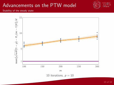
Advancements on the PTW modelStability of the steady state
10 of 18
10 iterations, p = 10
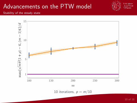
Advancements on the PTW modelStability of the steady state
10 of 18
10 iterations, p = m/10

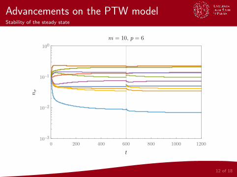
Advancements on the PTW modelStability of the steady state
HypothesisIs the steady state marginally stable?
ResultM is negative semidefiniterkM = min{m, p} ⇒ when m > p there are m− p null eigenvalues
11 of 18

Advancements on the PTW modelStability of the steady state
HypothesisIs the steady state marginally stable?
ResultM is negative semidefiniterkM = min{m, p} ⇒ when m > p there are m− p null eigenvalues
11 of 18

Advancements on the PTW modelStability of the steady state
HypothesisIs the steady state marginally stable?
ResultM is negative semidefiniterkM = min{m, p} ⇒ when m > p there are m− p null eigenvalues
11 of 18
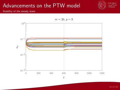
Advancements on the PTW modelStability of the steady state
12 of 18
0 200 400 600 800 1000 1200
10-3
10-2
10-1
100
Advancements on the PTW modelStability of the steady state
12 of 18
0 200 400 600 800 1000 1200
10-3
10-2
10-1
100

Advancements on the PTW modelStability of the steady state
12 of 18
0 200 400 600 800 1000 1200
10-3
10-2
10-1
100

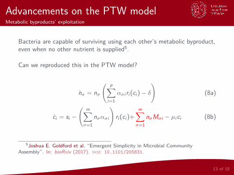
Advancements on the PTW modelMetabolic byproducts’ exploitation
Bacteria are capable of surviving using each other’s metabolic byproduct,even when no other nutrient is supplied.
Can we reproduced this in the PTW model?
nσ = nσ
( p∑i=1
ασi ri (ci )− δ)
(8a)
ci = si −
( m∑σ=1
nσασi
)ri (ci )+
m∑σ=1
nσMσi − µici (8b)
13 of 18

Advancements on the PTW modelMetabolic byproducts’ exploitation
Bacteria are capable of surviving using each other’s metabolic byproduct,even when no other nutrient is supplied5.
Can we reproduced this in the PTW model?
nσ = nσ
( p∑i=1
ασi ri (ci )− δ)
(8a)
ci = si −
( m∑σ=1
nσασi
)ri (ci )+
m∑σ=1
nσMσi − µici (8b)
5Joshua E. Goldford et al. “Emergent Simplicity in Microbial CommunityAssembly”. In: bioRxiv (2017). doi: 10.1101/205831.
13 of 18

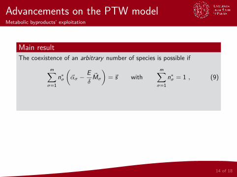
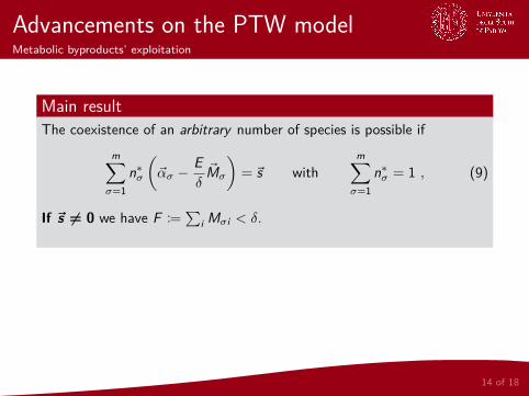
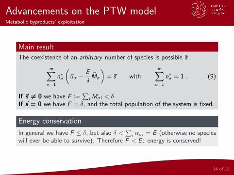
Advancements on the PTW modelMetabolic byproducts’ exploitation
Main resultThe coexistence of an arbitrary number of species is possible if
m∑σ=1
n∗σ(~ασ −
Eδ~Mσ
)= ~s with
m∑σ=1
n∗σ = 1 , (9)
If ~s 6= 0 we have F :=∑
i Mσi < δ.If ~s = 0 we have F = δ, and the total population of the system is fixed.
Energy conservationIn general we have F ≤ δ, but also δ <
∑i ασi = E (otherwise no species
will ever be able to survive). Therefore F < E : energy is conserved!
14 of 18
Advancements on the PTW modelMetabolic byproducts’ exploitation
Main resultThe coexistence of an arbitrary number of species is possible if
m∑σ=1
n∗σ(~ασ −
Eδ~Mσ
)= ~s with
m∑σ=1
n∗σ = 1 , (9)
If ~s 6= 0 we have F :=∑
i Mσi < δ.
If ~s = 0 we have F = δ, and the total population of the system is fixed.
Energy conservationIn general we have F ≤ δ, but also δ <
∑i ασi = E (otherwise no species
will ever be able to survive). Therefore F < E : energy is conserved!
14 of 18
Advancements on the PTW modelMetabolic byproducts’ exploitation
Main resultThe coexistence of an arbitrary number of species is possible if
m∑σ=1
n∗σ(~ασ −
Eδ~Mσ
)= ~s with
m∑σ=1
n∗σ = 1 , (9)
If ~s 6= 0 we have F :=∑
i Mσi < δ.If ~s = 0 we have F = δ, and the total population of the system is fixed.
Energy conservationIn general we have F ≤ δ, but also δ <
∑i ασi = E (otherwise no species
will ever be able to survive). Therefore F < E : energy is conserved!
14 of 18
Advancements on the PTW modelMetabolic byproducts’ exploitation
Main resultThe coexistence of an arbitrary number of species is possible if
m∑σ=1
n∗σ(~ασ −
Eδ~Mσ
)= ~s with
m∑σ=1
n∗σ = 1 , (9)
If ~s 6= 0 we have F :=∑
i Mσi < δ.If ~s = 0 we have F = δ, and the total population of the system is fixed.
Energy conservationIn general we have F ≤ δ, but also δ <
∑i ασi = E (otherwise no species
will ever be able to survive). Therefore F < E : energy is conserved!
14 of 18
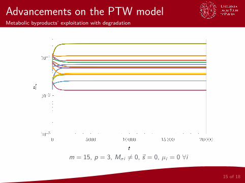
Advancements on the PTW modelMetabolic byproducts’ exploitation with degradation
15 of 18
m = 15, p = 3, Mσi 6= 0, ~s = 0, µi = 0 ∀i
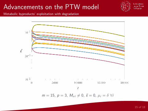
Advancements on the PTW modelMetabolic byproducts’ exploitation with degradation
15 of 18
m = 15, p = 3, Mσi 6= 0, ~s = 0, µi = δ ∀i
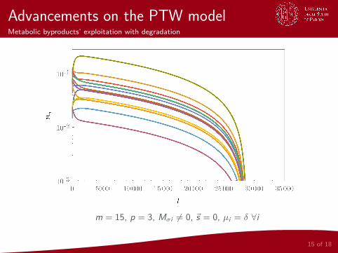
Advancements on the PTW modelMetabolic byproducts’ exploitation with degradation
15 of 18
m = 15, p = 3, Mσi 6= 0, ~s = 0, µi = δ ∀i
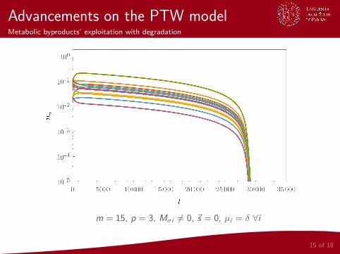
Advancements on the PTW modelMetabolic byproducts’ exploitation with degradation
15 of 18
m = 15, p = 3, Mσi 6= 0, ~s = 0, µi = δ ∀i

Conclusions
The competitive exclusion principle can be violated, but the price topay is that the resulting steady state is only marginally stable
Introducing metabolic byproducts’ exploitation, coexistence canoccur also without externally supplied resources
16 of 18

Conclusions
The competitive exclusion principle can be violated, but the price topay is that the resulting steady state is only marginally stable
Introducing metabolic byproducts’ exploitation, coexistence canoccur also without externally supplied resources
16 of 18

Conclusions
The competitive exclusion principle can be violated, but the price topay is that the resulting steady state is only marginally stable
Introducing metabolic byproducts’ exploitation, coexistence canoccur also without externally supplied resources
16 of 18

Future perspectivesWork in progress
Dynamic metabolic strategies
Dynamic metabolic strategies and Mσi
Generalization to δσ, Eσ
Emergence of patterns (taxonomic families)
Relax the metabolic trade-off to the weaker requirement∑
i ασi ≤ E
17 of 18

Future perspectivesWork in progress
Dynamic metabolic strategies
Dynamic metabolic strategies and Mσi
Generalization to δσ, Eσ
Emergence of patterns (taxonomic families)
Relax the metabolic trade-off to the weaker requirement∑
i ασi ≤ E
17 of 18

Future perspectivesWork in progress
Dynamic metabolic strategies
Dynamic metabolic strategies and Mσi
Generalization to δσ, Eσ
Emergence of patterns (taxonomic families)
Relax the metabolic trade-off to the weaker requirement∑
i ασi ≤ E
17 of 18

Future perspectivesWork in progress
Dynamic metabolic strategies
Dynamic metabolic strategies and Mσi
Generalization to δσ, Eσ
Emergence of patterns (taxonomic families)
Relax the metabolic trade-off to the weaker requirement∑
i ασi ≤ E
17 of 18

Future perspectivesWork in progress
Dynamic metabolic strategies
Dynamic metabolic strategies and Mσi
Generalization to δσ, Eσ
Emergence of patterns (taxonomic families)
Relax the metabolic trade-off to the weaker requirement∑
i ασi ≤ E
17 of 18

Future perspectivesWork in progress
Dynamic metabolic strategies
Dynamic metabolic strategies and Mσi
Generalization to δσ, Eσ
Emergence of patterns (taxonomic families)
Relax the metabolic trade-off to the weaker requirement∑
i ασi ≤ E
17 of 18

Bibliography
Stefano Allesina and Si Tang. “The stability–complexityrelationship at age 40: a random matrix perspective”. In: PopulationEcology 57.1 (2015).
Joshua E. Goldford et al. “Emergent Simplicity in MicrobialCommunity Assembly”. In: bioRxiv (2017). doi: 10.1101/205831.
G Hardin. “The Competitive Exclusion Principle”. In: Science131.November (1959), pp. 1292–1297.
Robert May. “Will a Large Complex System be Stable?” In: Nature238 (1972).
Anna Posfai, Thibaud Taillefumier, and Ned S Wingreen.“Metabolic Trade-Offs Promote Diversity in a Model Ecosystem”.In: Physical Review Letters 118.2 (2017).
18 of 18

Backup slides
May’s stability criterion
In general we can model an ecosystem of m species as a system of mcoupled differential equations:
nσ = fσ(~n(t)) . (1)
Obviously at equilibrium we have
nσ(~n∗) = fσ(~n∗) = 0 , (2)
and the properties of the equilibrium are given by the spectral distributionof the jacobian matrixM:
Mρσ = ∂fρ∂nσ |~n∗
. (3)
Of course, the system is stable if all the eigenvalues ofM have negativereal part.
1 of 27
May’s stability criterion
ProblemDepending on the chosen fσ, i.e. depending on the particular modelchosen, the properties of the equilibrium can change.
May’s solutionWe completely skip the derivation ofM from fσ, and we directly buildM as a properly defined random matrix: we are thus assuming thatinteractions between species at stationarity are random, so the ecosystemwill be characterized only by its biodiversity, i.e. the number m of speciesthat are living in it.
2 of 27
May’s stability criterion
The community matrixM must have the following properties:The elements on the diagonal must be negative, i.e.Mσσ = −d < 0 (every species goes to extinction if “left by itself”)Since experimentally we observe that interactions between speciesare not numerous, the off-diagonal elements are set to zero withprobability 1− C and drawn from any distribution with null meanand variance Σ2 with probability C
ProblemWhat is the spectral distribution of such a matrix? When does it haveonly eigenvalues with negative real part?
3 of 27

May’s stability criterionWe have to use a slightly modified version of the
Circular lawLetM be an m ×m matrix whose entries (included the diagonal ones)are iid random variables whose distribution has null mean and unitvariance. Then the empirical spectral distribution
µm(x , y) = #{σ ≤ m : Re(λσ) ≤ x , Im(λσ) ≤ y} (4)
of the eigenvalues λ1, . . . , λm ofM/√m tends in the limit m→∞ to a
uniform distribution on the unit disk centered at the origin of thecomplex plane.
ImportantNote that this is a universal result: the limit of the spectral distributiondoes not depend on the particular distribution from which we have drawnthe entries ofM, as long as it has null mean and unit variance.
4 of 27

May’s stability criterion
5 of 27
-1.0 -0.5 0.0 0.5 1.0
-1.0
-0.5
0.0
0.5
1.0
-1.0 -0.5 0.0 0.5 1.0
-1.0
-0.5
0.0
0.5
1.0
-1.0 -0.5 0.0 0.5 1.0
-1.0
-0.5
0.0
0.5
1.0
Normal distribution N (0, 1)
May’s stability criterion
5 of 27
-1.0 -0.5 0.0 0.5 1.0
-1.0
-0.5
0.0
0.5
1.0
-1.0 -0.5 0.0 0.5 1.0
-1.0
-0.5
0.0
0.5
1.0
-1.0 -0.5 0.0 0.5 1.0
-1.0
-0.5
0.0
0.5
1.0
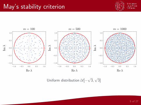
Uniform distribution U [−√3,√3]

May’s stability criterion
In our case of interest we draw all the off-diagonal elements from adistribution with null mean and variance Σ2, and all the diagonalelements are set to −d < 0. What does this change?
1 The spectral radius ofM tends to√m as m→∞
2 A matrix with Σ 6= 1 can be obtained from one with Σ = 1multiplying its entry by Σ; this way the spectral radius in the limitm→∞ tends to Σ
√m
3 The introduction of the probability C reduces the variance from Σ2
to CΣ2, so the spectral radius tends to Σ√mC when m→∞
4 Setting the diagonal entries equal to −d < 0 moves the disk to theleft, so that it is centered in (−d , 0):
A ∈ Mn, B = A− dI ⇒
{det(λAI−A) = 0 λAidet(λBI− B) = 0 λBi
⇒
⇒ det[(λBi + d)I−A] = 0 ⇒ λBi = λAi (5)
6 of 27
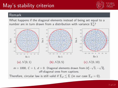
May’s stability criterionRemarkWhat happens if the diagonal elements instead of being set equal to anumber are in turn drawn from a distribution with variance Σ2
d?
-30 -20 -10 0 10 20 30
-30
-20
-10
0
10
20
30
(a) N (0, 1)
-30 -20 -10 0 10 20 30
-30
-20
-10
0
10
20
30
(b) N (0, 5)
-30 -20 -10 0 10 20 30
-30
-20
-10
0
10
20
30
(c) N (0, 10)
m = 1000, C = 1, d = 0. Diagonal elements drawn from U [−√3,−√3],
off-diagonal ones from captions.Therefore, circular law is still valid if Σd . Σ (in our case Σd = 0).
7 of 27
May’s stability criterion
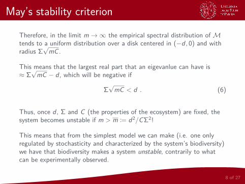
Therefore, in the limit m→∞ the empirical spectral distribution ofMtends to a uniform distribution over a disk centered in (−d , 0) and withradius Σ
√mC .
This means that the largest real part that an eigevanlue can have is≈ Σ√mC − d , which will be negative if
Σ√mC < d . (6)
Thus, once d , Σ and C (the properties of the ecosystem) are fixed, thesystem becomes unstable if m > m := d2/CΣ2!
This means that from the simplest model we can make (i.e. one onlyregulated by stochasticity and characterized by the system’s biodiversity)we have that biodiversity makes a system unstable, contrarily to whatcan be experimentally observed.
8 of 27
May’s stability criterion
9 of 27
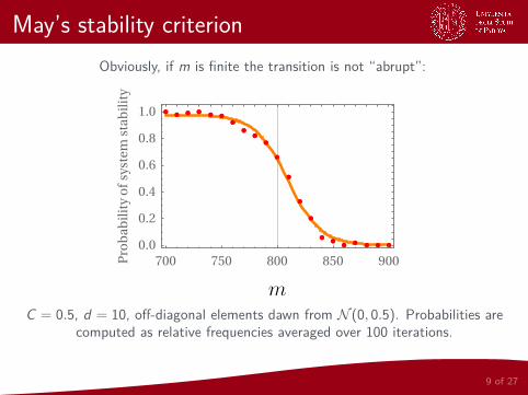
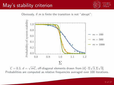
Obviously, if m is finite the transition is not “abrupt”:
700 750 800 850 9000.0
0.2
0.4
0.6
0.8
1.0P
rob
ab
ilit
yo
fsy
ste
mst
ab
ilit
y
C = 0.5, d = 10, off-diagonal elements dawn from N (0, 0.5). Probabilities arecomputed as relative frequencies averaged over 100 iterations.
May’s stability criterion
9 of 27
Obviously, if m is finite the transition is not “abrupt”:
C = 0.3, d =√mC , off-diagonal elements drawn from U [−Σ
√3,Σ√3].
Probabilities are computed as relative frequencies averaged over 100 iterations.
Generalization of May’s stability criterion
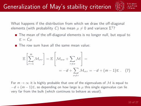
What happens if the distribution from which we draw the off-diagonalelements (with probability C) has mean µ 6= 0 and variance Σ2?
The mean of the off-diagonal elements is no longer null, but equal toE = CµThe row sum have all the same mean value:
E
[ m∑τ=1Mστ
]= E
Mσσ +∑τ 6=σM
=
= −d +∑σ 6=τMστ = −d + (m − 1)E . (7)
For m→∞ it is highly probable that one of the eigenvalues ofM is equal to−d + (m − 1)E , so depending on how large is µ this single eigenvalue can lievery far from the bulk (which continues to behave as usual).
10 of 27

Generalization of May’s stability criterion
The center of the disk is further translated. In fact, calling D thenew real part of the center of the disk, requiring that the average ofall the real parts is still −d we have
(m − 1)D− d + (m − 1)Em = −d ⇒ D = −d − E . (8)
The variance of the off-diagonal elements is now
V = Var[Mστ ] = C [Σ2 + (1− C)µ] (9)
If µ is sufficiently large the eigenvalue −d + (m − 1)E can lie outside ofthe disk, so in this case the larges real part for an eigenvalue is−dè(m − 1)E ; if µ is sufficiently large, on the other hand, the maximumreal part is −(d + E) +
√mV . The stability criterion can therefore be
written as:max{
√mV − E , (m − 1)E} < d . (10)
11 of 27

Generalization of May’s stability criterionFurther problemIn general it is not true thatMστ andMτσ are uncorrelated: if σ is aprey and τ a predator,Mστ < 0 andMτσ > 0. What happens then ifthe off-diagonal elements, and in particular the symmetric couples(Mστ ,Mτσ) have a non-null correlation ρ?
We have to use a slightly modified version of the
Elliptic lawLetM be an m ×m whose off-diagonal coefficients are sampledindependently in pairs from a bivariate distribution with zero marginalmean, unit marginal variance and correlation ρ. Then, the empiricalspectral distribution of the eigenvalues λ1, . . . , λm ofM/
√m converges
in the limit m→∞ to the uniform distribution on an ellipse in thecomplex plane centered at (0, 0), with horizontal semi-axis of length1 + ρ and vertical semi-axis of length 1− ρ.
12 of 27
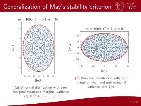
Generalization of May’s stability criterion
-40 -30 -20 -10 0 10 20
-40
-20
0
20
40
(a) Binormal distribution with zeromarginal mean and marginal variance
equal to 4, ρ = −1/5.
-40 -20 0 20 40
-20
-10
0
10
20
(b) Binormal distribution with zeromarginal mean and unit marginal
variance, ρ = 1/4.
13 of 27

Generalization of May’s stability criterion
In our case, setting:the diagonal elements equal to −d < 0the pairs (Mστ ,Mτσ) with σ 6= τ equal to (0, 0) with probability1− C and drawing them with probability C from a bivariatedistribution with mean and covariance matrix
~µ =(µµ
)Σ =
(Σ2 ρΣ2
ρΣ2 Σ2
), (11)
we find the same results as before, with the difference that now the largesreal part of the bulk is ≈ −(d + E) +
√mV (1 + ρ). Therefore May’s
stability criterion can now be written as:
max{√
mV (1 + ρ)− E , (m − 1)E}< d . (12)
14 of 27
The PTW model
The original equations of the system are
nσ = nσ (gσ(c1, . . . , cp)− δ) gσ(c1, . . . , cp) =p∑
i=1viασi ri (ci ) (13a)
ci = si −
( m∑σ=1
nσασi
)ri (ci )− µici (13b)
with vi the “value” of resource i , and the fundamental assumptions thatwe make are:
µi = 0 ∀i , i.e. there is no degradationci = 0 ∀i , i.e. the resource concentration immediately reach theirsteady-state values (metabolic processes are generally much fasterthen reproductive ones).∑p
i=1 wiασi = E , with wi the “cost” of resource i
15 of 27
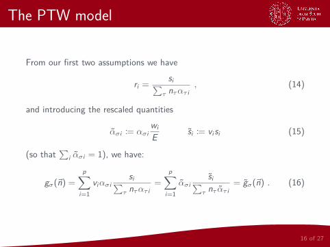
The PTW model
From our first two assumptions we have
ri = si∑τ nτατ i
, (14)
and introducing the rescaled quantities
ασi := ασiwiE si := visi (15)
(so that∑
i ασi = 1), we have:
gσ(~n) =p∑
i=1viασi
si∑τ nτατ i
=p∑
i=1ασi
si∑τ nτ ατ i
= gσ(~n) . (16)
16 of 27
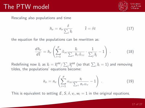
The PTW modelRescaling also populations and time
nσ = nσδ∑i si
t = δt (17)
the equation for the populations can be rewritten as:
dnσdt = nσ
( p∑i=1
ασisi∑
τ nτ ατ i· 1∑
j sj− 1). (18)
Redefining now si as si = soldi /∑
j soldj (so that∑
i si = 1) and removingtildes, the populations’ equations become:
nσ = nσ
( p∑i=1
ασisi∑
τ nτατ− 1). (19)
This is equivalent to setting E ,S, δ, vi ,wi = 1 in the original equations.
17 of 27
Coexistence of speices
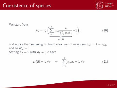
We start from
nσ = nσ( p∑
i=1ασi
si∑τ nτατ︸ ︷︷ ︸
gσ(~n)
−1), (20)
and notice that summing on both sides over σ we obtain ntot = 1− ntot,and so n∗tot = 1.Setting nσ = 0 with nσ 6= 0 e have
gσ(~n) = 1 ∀σ ⇒p∑
i=1ασi ri = 1 ∀σ (21)
18 of 27
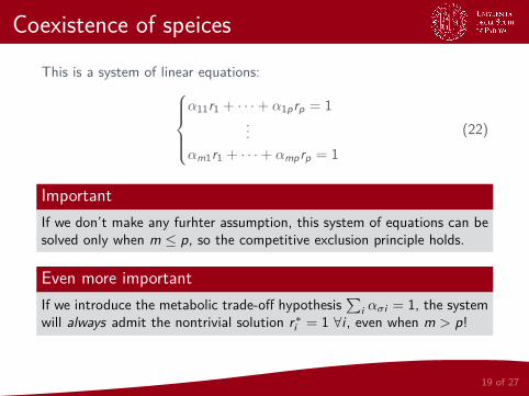
Coexistence of speicesThis is a system of linear equations:
α11r1 + · · ·+ α1prp = 1...
αm1r1 + · · ·+ αmprp = 1(22)
ImportantIf we don’t make any furhter assumption, this system of equations can besolved only when m ≤ p, so the competitive exclusion principle holds.
Even more importantIf we introduce the metabolic trade-off hypothesis
∑i ασi = 1, the system
will always admit the nontrivial solution r∗i = 1 ∀i , even when m > p!
19 of 27
Coexistence of species
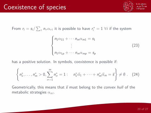
From ri = si/∑τ nτατ i it is possible to have r∗i = 1 ∀i if the system
n1α11 + · · · nmαm1 = s1...
n1α1p + · · · nmαmp = sp
(23)
has a positive solution. In symbols, coexistence is possible if:{n∗1 , . . . , n∗m > 0,
m∑σ=1
n∗σ = 1 : n∗1~α1 + · · ·+ n∗m~αm = ~s}6= ∅ . (24)
Geometrically, this means that ~s must belong to the convex hull of themetabolic strategies ασi .
20 of 27

Stability of the steady stateStarting from the equations of the system
nσ = nσ(gσ(~n)− 1) gσ(~n) =p∑
i=1ασi ri (25)
and writing ~n = ~n∗ + ∆~n with ~n∗ steay state, performing a Taylorexpansion to the first order we get:
ddt ∆nσ = n∗σ
( m∑τ=1
∂gσ∂nτ
(~n∗)∆nτ
), (26)
where
∂gσ∂nτ
(~n∗) = −p∑
i=1ασi
si(∑ρ nραρi
)2ατ i = −p∑
i=1ασiατ i
r∗i2
si= −
p∑i=1
ασiατ isi
(27)
21 of 27

Stability of the steady state
We can therefore writeddt ∆~n =M∆~n , (28)
where
M = −DM D =
n∗1 0 · · · 00 n∗2 · · · 0...
.... . .
...0 · · · 0 n∗m
Mστ = −p∑
i=1
ασiατ isi
.
(29)
22 of 27

Stability of the steady state
In order to show that ~n∗ is an equilibrium, we need to show thatM isnegative definite, i.e. DM is positive definite.In order to do that we first notice that since D is invertible we canperform the following similarity transformation:
DM −→ D−1/2(DM )D1/2 = D1/2MD1/2 , (30)
which of course does not alter the eigenvalue of the matrix.Now, given any non-null vector ~v we have:
~v ·D1/2MD1/2~v =p∑
j,k=1
m∑σ,τ=1
vjD1/2jσ MστD1/2
τk vk =p∑
i=1
m∑σ,τ=1
vσ√
n∗σασiατ i
sivτ√
n∗τ =
=p∑
i=1
1si
( m∑σ=1
vσ√n∗σασi
)( m∑τ=1
vτ√n∗τατ i
)=
p∑i=1
( m∑σ=1
vσ√n∗σασi√si
)2
≥ 0 .
(31)
23 of 27
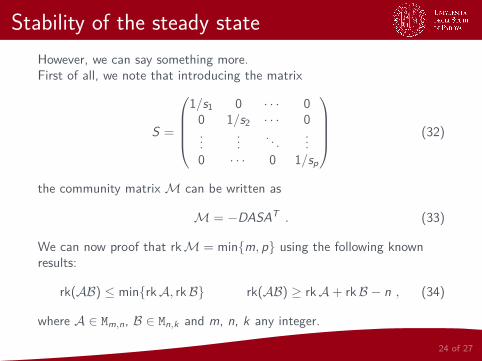
Stability of the steady stateHowever, we can say something more.First of all, we note that introducing the matrix
S =
1/s1 0 · · · 00 1/s2 · · · 0...
.... . .
...0 · · · 0 1/sp
(32)
the community matrixM can be written as
M = −DASAT . (33)
We can now proof that rkM = min{m, p} using the following knownresults:
rk(AB) ≤ min{rkA, rkB} rk(AB) ≥ rkA+ rkB − n , (34)
where A ∈ Mm,n, B ∈ Mn,k and m, n, k any integer.
24 of 27

Stability of the steady state
Let us suppose m > p; considering that
D ∈ Mm A ∈ Mm,p S ∈ Mp (35)
then:{rk(DA) ≤ min {rk D, rk A} = min {m, p} = prk(DA) ≥ rk D + rk A−m = m + p −m = p
⇒ rk(DA) = p , (36){rk(SAT ) ≤ min {rk S, rk A} = min {p, p} = prk(SAT ) ≥ rk S + rk A− p = p + p − p = p
⇒ rk(SAT ) = p , (37)
and so:{rkM≤ min
{rk(DA), rk(SAT )
}= min {p, p} = p
rkM≥ rk(DA) + rk(SAT )− p = p + p − p = p⇒ rkM = p . (38)
In the same way we can proof that rkM = m when m < p.
25 of 27

Stability of the steady state
Since for m > p we have rkM = p, the community matrix is rankdeficient and has m − p null eigenvalues. This means that the steadystate of the system is only marginally stable.
In fact, we have seen that coexistence is possible if
~s = n∗1~α1 + · · ·+ n∗m~αm (39)
admits a positive solution with∑σ n∗σ = 1. However, this is a system of
p equations in m unknowns, so when m > p it’s underdetermined and assuch there are infinite solutions. Therefore, if the system is in a steadystate and is perturbed, it will relax to one of these infinitely manypossible equilibriums.
If m ≤ p the community matrixM has full rank, so there are no nulleigenvalues and the equilibrium is asymptotically stable.
26 of 27

Relationship with May’s stability criterion
The most general form of May’s stability criterion can be rewritten as:
1d max
{√mV (1 + ρ)− E , (m − 1)E
}< 1 . (40)
In order to see if the PTW model satisfies it, we have:1 Set a system in the condition for coexistence and let it evolve until
stationarity is reached2 Computed the community matrix asM = −DASAT
3 Computed d = E[Mσσ]4 Computed E = E[Mστ ] and V = Var[Mστ ] with σ 6= τ
5 Computed ρ = (E[MστMτσ]− E2)/V6 Computed the left hand side of (40) and compared it with one
27 of 27