Embed Size (px)
Citation preview

Received ; Revised ; Accepted
DOI: xxx/xxxx
ARTICLE TYPE
Recognizing a Spatial Extreme dependence structure: A Deep
Learning approach
Manaf AHMED1,2 | Véronique MAUME-DESCHAMPS2 | Pierre RIBEREAU2
1Department of statistics and Informatics,University of Mosul, Mosul, Iraq
2Institut Camille Jordan, ICJ, Univ Lyon,Université Claude Bernard Lyon 1, CNRSUMR 5208, Villeurbanne, F-69622, France
CorrespondenceManaf AHMED,Email: [email protected]
Summary
Understanding the behaviour of environmental extreme events is crucial for evalu-ating economic losses, assessing risks, health care and many other aspects. In thespatial context, relevant for environmental events, the dependence structure playsa central rule, as it influence joined extreme events and extrapolation on them. Sothat, recognising or at least having preliminary informations on patterns of thesedependence structures is a valuable knowledge for understanding extreme events.In this study, we address the question of automatic recognition of spatial Asymp-totic Dependence (AD) versus Asymptotic independence (AI), using ConvolutionalNeural Network (CNN). We have designed an architecture of Convolutional NeuralNetwork to be an efficient classifier of the dependence structure. Upper and lowertail dependence measures are used to train the CNN. We have tested our methodol-ogy on simulated and real data sets: air temperature data at two meter over Iraq landand Rainfall data in the east cost of Australia.
1 INTRODUCTION
Understanding extreme environmental events such as heat waves or heavy rains is still challenging. The dependence structure
is one important element in this field. Multivariate extreme value theory (MEVT) is a good mathematical framework for mod-
elling the dependence structure of extremes events (see for instance De Haan and Ferreira (2007) and Embrechts, Klüppelberg,
and Mikosch (2013)). Max-stable processes consist in an extension of multivariate extreme value distributions to spatial pro-
cesses and provide models for spatial extremes (see De Haan, Pereira, et al. (2006) and De Haan et al. (1984)). These max-stable
processes are asymptotically dependent (AD). This may not be realistic in practice. Wadsworth and Tawn (2012) introduced
inverted max-stable processes which are asymptotically independent (AI). Using AD versus AI models has important implica-
tions on the extrapolation of joined extreme events (see Bortot, Coles, and Tawn (2000) and Coles and Pauli (2002)). So that,
arX
iv:2
103.
1073
9v1
[st
at.M
E]
19
Mar
202
1
2 Manaf AHMED ET AL
recognising the class of dependence structure is an important task when building models for environmental data. One of the
main challenges is how to recognise the dependence structure pattern of a spatial process. Despite various studies dealt with
spatial extremes models, we have not found works focused on the question of the automatic determination of AI versus AD for
a spatial process. The usual approach is to use Partial Maximum Likelihood estimations after having chosen (from exploratory
graph studies) a class of models. We propose a first deep learning approach to deal with this question. Many works using deep
learning for spatial and spatio-temporal processes have been developed but none concerned with AD versus AI (see Wang, Cao,
and Yu (2019)).
Artificial Intelligence techniques have demonstrated a significant efficiency in many applications, such as environment, risk
management, image analysis and many others. We will focus on Convolutional Neural Network (CNN) which have ability in
automatic extracting the spatial features hierarchically. It has been used e.g. on spatial dependencies from raw datasets. For
instance, Zhu, Chen, Zhu, Duan, and Liu (2018) proposed a predictive deep convolutional neural network to predict the wind
speed in a spatio-temporal context, where the spatial dependence between locations is captured. Liu et al. (2016) developed a
CNN model to predict extremes of climate events, such as tropical cyclones, atmospheric rivers and weather fronts. Lin et al.
(2018) presented an approach to forecast air quality (PM2.5 construction) in a Spatio-temporal framework. While Zuo et al.
(2015) improved the power of recognising objects in images by learning the spatial dependencies of these regions via CNN. In
the spatial extreme context, Yu, Uy, and Dauwels (2016) tried to model the spatial extremes by bridging the cape between the
traditional statistical method and Graph methods via decision Trees.
Our objective is to employ deep learning concepts in order to recognise patterns of spatial extremes dependence structures
and distinguish between AI and AD. Upper and Lower tail dependence measures � and � are used as a summary of the extreme
dependence structure. These dependence measures have been introduced by Coles, Heffernan, and Tawn (1999) in order to
quantify the pairwise dependence of extremes events between two locations. Definitions and properties of these measures will
be given in Section 2. The pairwise empirical versions of these measures are used as a summary dataset. The CNN will be
trained to recognise the pattern of dependence structures via this summary dataset.
Due to the influence of the air temperature at 2 meters above the surface on assessing climate changes and on all biotic
processes, especially in extreme, we will apply our methods to this case study, data come from the European Center for Medium-
Range Weather Forecasts ECMWF. The second case study is the rainfall amount recorded in the east coast of Australia.
The paper is organised as follows. Section 2 is devoted to the theoretical tools used in paper. An overview of Convolutional
Neural Networks concepts is exposed in Section 3. Section 4 is devoted to configure the architecture of the CNN for classifi-
cation of dependence structures. Section 5 shows the performance of our designed CNN on simulated data. Applications to
environmental data: Air temperature and Rainfall events are presented in Section 6. Finally, a discussion and main conclusions
of this study are given in Section 7.
Manaf AHMED ET AL 3
2 THEORETICAL TOOLS
Let us give a survey on spatial extreme models ad tail dependence functions, see Coles et al. (1999) for more details.
2.1 Spatial extreme models
Let {X′i (s)}s∈ , ∈ ℝd , d ≥ 1 be i.i.d replications of a stationary process. Let an(s) > 0 and bn(s), n ∈ ℕ be two sequences of
continues functions. If
{max∀i∈n
(
X′i (s) − bn(s)∕an(s)
)
}s∈d→ {X(s)}s∈ (1)
as n → ∞, with non-degenerated marginals, then {X(s)}s∈ is a max-stable process. Its marginals are Generalized Extreme
Value (GEV). If for all n ∈ ℕ, an(s) = 1 and bn(s) = 0, then {X(s)}s∈ is called a simple max-stable process. It has unite
Fréchet marginal, which means: ℙr{X(s) ≤ x} = exp(−1∕x), x > 0, (see De Haan et al. (2006)). In De Haan et al. (1984), it
is proved that any simple max-stable process defined on a compact set ⊂ ℝd , d ≥ 1 with continuous sample path admits a
spectral representation as follows.
Let {�i, i ≥ 1} be an i.i.d Poisson point process on (0,∞), with intensity d�∕�2 and let {W +i (s)}i≥1 be a i.i.d replicates of a
positive random filed W ∶= {W (s)}s∈ , such that E[W (s)] = 1. Then
X(s) ∶= maxi≥1{�iWi(s)+}, s ∈ , ∈ ℝd , d ≥ 1 (2)
is a simple max-stable process. The multivariate distribution function is given by
ℙr{X(s1) ≤ x1,⋯ , X(sd) ≤ xd} = exp(−Vd(x1, ..., xd)), (3)
where s1,⋯ , sd ⊂ and V is called the exponent measure. It is homogenous of order −1 and has the expression:
Vd(x1, ..., xd) = E[
maxj=1,⋯,d
{W (sj)∕xj}]
, (4)
The extremal dependence coefficient is given by Θd = Vd(1,⋯ , 1) ∈ [1, d]. It has been shown by Schlather and Tawn (2003)
that for max-stable processes, either Θd = 1 which means that the process is asymptotically dependent (AD) or Θd = d which
is the independent case. If Θ ≠ 1, the process is said to be asymptotically independent (AI). For max-stable processes, AI
implies independence. Wadsworth and Tawn (2012) introduced inverted max-stable processes which may be AI without being
independent. Let {X(s)}s∈ be a simple max-stable process, an inverted max-stable process Y is defined as
Y (s) = −1∕ log{1 − exp(−1∕X(s))}, s ∈ . (5)
4 Manaf AHMED ET AL
It has unit Fréchet marginal laws and its multivariate survivor function is
ℙr{Y (s1) > y1,⋯ , Y (sd) > yj} = exp(−Vd(y1,⋯ , yd)). (6)
In the definition of max-stable processes, different models for W lead to different simple max-stable models, as well as
inverted max-stable models. For instance, the Brown-Resnick model is constructed with Wi(s) = {�i(s) − (s)}i≥1, where �i(s)
are i.i.d replicates of a stationary Gaussian process with zero mean and variogram (s) (see Brown and Resnick (1977) and
Kabluchko, Schlather, De Haan, et al. (2009). Many other models have been introduced, such as Smith, Schlather and Extremal-
t introduced respectively by Smith (1990), Schlather (2002) and Opitz (2013).
In what follows, we shall consider extreme Gaussian processes which are Gaussian processes whose marginals have been
turned to a unite Fréchet distribution. We shall also consider max-mixture processes which are max(aX(s), (1 − a)Y (s)) where
a ∈ [0, 1], X(s) is a max-stable process and Y (s) is an invertible max-stable process or an extreme Gaussian process.
2.2 Extremal dependence measures
Consider a stationary spatial process X ∶= {X(s)}s∈ , ⊂ ℝd , d ≥ 2. The upper and lower tail dependence functions
have been constructed in order to quantify the strength of AD and AI respectively. The upper tail dependence coefficient � is
introduced in Ledford and Tawn (1996) and defined by
�(ℎ) = limu→1
ℙ(
F (X(s)) > u|F (X(s + ℎ)) > u)
, (7)
where F is the marginal distribution function of X. If �(ℎ) = 0, the pair (X(s + ℎ), X(s)) is asymptotically independent (AI).
If �(ℎ) ≠ 0, the pair (X(s + ℎ), X(s)) is asymptotically dependent (AD). The process is AI (resp. AD) if ∃ℎ ∈ such that
�(ℎ) = 0 (resp. ∀ℎ ∈ , �(ℎ) ≠ 0). In Coles et al. (1999), the lower tail dependence coefficient �(ℎ) is proposed in order to
study the strength of dependence in AI cases. It is defined as:
�(ℎ) = limu→1
[
2 logℙ(
F (X(s)) > u)
logℙ(
F (X(s)) > u, F (X(s + ℎ)) > u) − 1
]
, 0 ≤ u ≤ 1. (8)
We have −1 ≤ �(ℎ) ≤ 1 and the spatial process is AD if ∃ℎ ∈ such that �(ℎ) = 1. Otherwise, it is a AI.
Of course, working on data require to have empirical versions of these extreme dependence measures. We denote them respec-
tively by � and � , they have been defined in Wadsworth and Tawn (2012), see also Bacro, Gaetan, and Toulemonde (2016).
Consider Xi, i = 1, 2,⋯ , N the copies of a spatial process X, the corresponding empirical versions of �(ℎ) and �(ℎ) are
respectively
�(s, t) = 2 −log
(
N−1∑Ni=1 1{Ui(s)<u,Ui(t)<u}
)
log(
N−1∑Ni=1 1{Ui(s)<u}
), (9)
Manaf AHMED ET AL 5
and
�(s, t) =2 log
(
N−1∑Ni=1 1{Ui(s)>u}
)
log(
N−1∑Ni=1 1{Ui(s)>u,Ui(t)>u}
)− 1, (10)
where Ui ∶= F (xi) = N−1∑Ni=1 1{X≤xi}, for |s − t| = ℎ.
3 CONVOLUTIONAL NEURAL NETWORK (CNN)
A Convolutional Neural Network CNN is an algorithm constructed and perfected to be one of the primary branches in deep
learning. We shall use this method in order to recognise the dependence structure in spatial patterns. It stems from two stud-
ies introduced by Hubel and Wiesel (1968) and Fukushima (1980). CNN are used in many domains, one of the common use
is for image analysis. It appears to be relevant in order to identify the dependencies between nearby pixels (locations). It may
recognise spatial features (see Wang et al. (2019)). Mainly, a convolutional neural network consists in three basic layers: Convo-
lutional, pooling, and fully connected. The first two layers are dedicated to feature learning and the latter one for classification.
Many researches present the CNN architecture, see e.g. Yamashita, Nishio, Do, and Togashi (2018) or Caterini and Chang
(2018) for a mathematical framework . We shall not provide the details of the CNN architecture, as it exists in many articles
and books, we refer the interested reader to the above references. Let us just recall that, reconsidering spatial data, a convolu-
tion step is requiered. It is helpfull to make the procedure invariant by translation.
Once the CNN is build, the kernel values of the convolutional layers and the weights of the fully connected layers are learned
during a training process.
Training is the process of adjusting values of the kernels and weights using known categorical datasets. The process has two
steps, the first one is the forward propagation and the second step is the backpropagation. In forward propagation, the network
performance is evaluated by a loss function according to the kernels and weights updated in the previous step. From the value
of the loss, the kernel and weights is updated by a gradient descent optimisation algorithm. If the difference between the true
and predicted class of the dataset is acceptable, the process of training stops. So that, selecting the suitable loss function and
gradient descent optimisation algorithm is decisive for the quality of the constructed network performance. Determining the
loss function (objective function) should be done according to the network task. Since our goal consists in classification, we
shall use the cross-entropy as an objective function to minimize. Let ya, a = 1,⋯A be the true class (label) of the dataset and
let �a be the estimated probability of the a-th class, the cross-entropy loss function can formulated as
L = −A∑
a=1ya log(�a).
Minimizing the loss means updating the parameters, i.e. kernels and weights until the CNN predicts the correct class. This
update will be done by the gradient descent optimization algorithm in the back propagation step. Many gradient algorithms
6 Manaf AHMED ET AL
are proposed. The most commonly used in CNN are stochastic gradient descent (SGD) and Adam algorithm Kingma and Ba
(2014). This algorithm is also an hyper-parameter in the network. To begin the training process, the data is divided into three
parts. The first part is devoted to training CNN. Monitoring the model performance, hyperparameter tuning and model selection
are done with the second part. This part is called validation dataset. This third part is used for the evaluation of the final model
performance. This latter part of data has never been seen before by the CNN.
4 CONFIGURE CNN TO CLASSIFY THE TYPES OF DEPENDENCE STRUCTURES
We shall now explain how we used the CNN technology for our purpose to distinguish extreme dependence structures in spatial
data.
4.1 Constructing the dependence structures of the event
Spatial extreme models may have different dependence structures, such as asymptotic dependence or asymptotic independence.
These structures may be identified by many measures. The well known measures able to capture these structures are e.g. upper
and lower dependence measures � and � in Equations (7) and (8), respectively. Upper tail is able to capture the dependence
structure for asymptotic dependence models, but it fails with asymptotically independent models. The lower tail measure treats
this problem by providing the dependence strength for asymptotically independent models. We propose to consider these two
measures � and � as learning data for the CNN, because each of them provide information on each type of dependence
structure. The empirical counterparts �(ℎ) and �(ℎ) in Equations (9) and (10) respectively, computed above a threshold u will
be used on the raw data to construct raster dataset with a symmetric array in two tensors, the first one for � and the second for
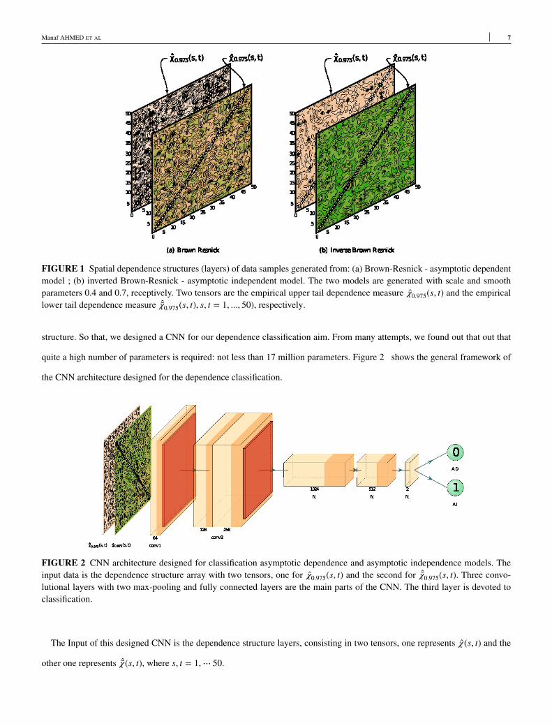
� . This array will present the dependence structure of the corresponding data. Figure 1 shows of an array constructed from
Brown-Resnick and inverse Brown-Resnick models.
4.2 Building CNN architecture
It is essential in the convolutional neural network design to take into account the kind of data and the task to be done: clas-
sification, representations, or anomaly detection. Practically, designing a CNN for classification of complex patterns remains
challenging. First of all, one has to determine the number of convolutional and fully connected layers that shoud be used. Sec-
ondly, tuning a high number of parameters (kernel, weights) is required. Many articles are devoted to build and improve CNN
architectures to have good performance: LeCun et al. (1990), Alex, Sutskever, and Hinton (2012), He, Zhang, Ren, and Sun
(2016) and Xie, Girshick, Dollár, Tu, and He (2017).
These CNN architectures are appropriate for image classifications but not for our goal because we need to keep the dependence
Manaf AHMED ET AL 7
FIGURE 1 Spatial dependence structures (layers) of data samples generated from: (a) Brown-Resnick - asymptotic dependentmodel ; (b) inverted Brown-Resnick - asymptotic independent model. The two models are generated with scale and smoothparameters 0.4 and 0.7, receptively. Two tensors are the empirical upper tail dependence measure �0.975(s, t) and the empiricallower tail dependence measure �0.975(s, t), s, t = 1, ..., 50), respectively.
structure. So that, we designed a CNN for our dependence classification aim. From many attempts, we found out that out that
quite a high number of parameters is required: not less than 17 million parameters. Figure 2 shows the general framework of
the CNN architecture designed for the dependence classification.
FIGURE 2 CNN architecture designed for classification asymptotic dependence and asymptotic independence models. Theinput data is the dependence structure array with two tensors, one for �0.975(s, t) and the second for �0.975(s, t). Three convo-lutional layers with two max-pooling and fully connected layers are the main parts of the CNN. The third layer is devoted toclassification.
The Input of this designed CNN is the dependence structure layers, consisting in two tensors, one represents �(s, t) and the
other one represents �(s, t), where s, t = 1,⋯ 50.
8 Manaf AHMED ET AL
Two networks are constructed, one has two classes output called 2-class, for recognizing asymptotic dependence vs asymp-
totic independence dependence structure. The second CNN has a third ouput class in order to detect if a spatial process is neither
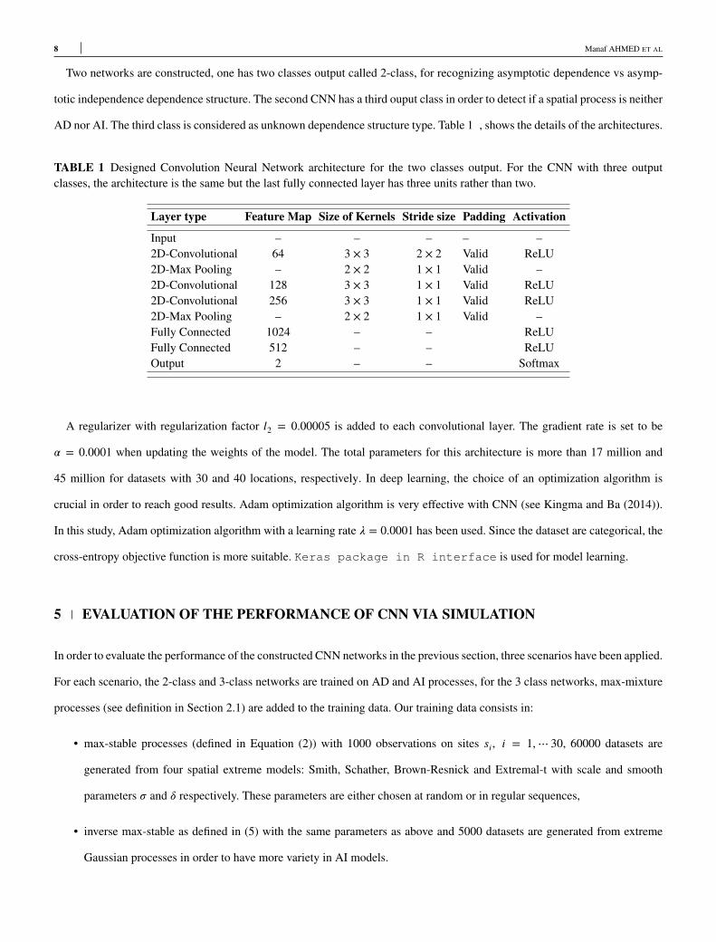
AD nor AI. The third class is considered as unknown dependence structure type. Table 1 , shows the details of the architectures.
TABLE 1 Designed Convolution Neural Network architecture for the two classes output. For the CNN with three outputclasses, the architecture is the same but the last fully connected layer has three units rather than two.
Layer type Feature Map Size of Kernels Stride size Padding Activation
Input – – – – –2D-Convolutional 64 3 × 3 2 × 2 Valid ReLU2D-Max Pooling – 2 × 2 1 × 1 Valid –2D-Convolutional 128 3 × 3 1 × 1 Valid ReLU2D-Convolutional 256 3 × 3 1 × 1 Valid ReLU2D-Max Pooling – 2 × 2 1 × 1 Valid –Fully Connected 1024 – – ReLUFully Connected 512 – – ReLUOutput 2 – – Softmax
A regularizer with regularization factor l2 = 0.00005 is added to each convolutional layer. The gradient rate is set to be
� = 0.0001 when updating the weights of the model. The total parameters for this architecture is more than 17 million and
45 million for datasets with 30 and 40 locations, respectively. In deep learning, the choice of an optimization algorithm is
crucial in order to reach good results. Adam optimization algorithm is very effective with CNN (see Kingma and Ba (2014)).
In this study, Adam optimization algorithm with a learning rate � = 0.0001 has been used. Since the dataset are categorical, the
cross-entropy objective function is more suitable. Keras package in R interface is used for model learning.
5 EVALUATION OF THE PERFORMANCE OF CNN VIA SIMULATION
In order to evaluate the performance of the constructed CNN networks in the previous section, three scenarios have been applied.
For each scenario, the 2-class and 3-class networks are trained on AD and AI processes, for the 3 class networks, max-mixture
processes (see definition in Section 2.1) are added to the training data. Our training data consists in:
• max-stable processes (defined in Equation (2)) with 1000 observations on sites si, i = 1,⋯ 30, 60000 datasets are
generated from four spatial extreme models: Smith, Schather, Brown-Resnick and Extremal-t with scale and smooth
parameters � and � respectively. These parameters are either chosen at random or in regular sequences,
• inverse max-stable as defined in (5) with the same parameters as above and 5000 datasets are generated from extreme
Gaussian processes in order to have more variety in AI models.
Manaf AHMED ET AL 9
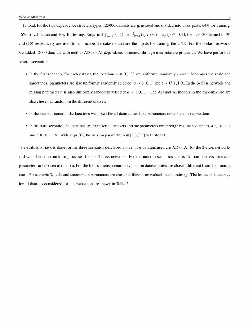
In total, for the two dependence structure types 125000 datasets are generated and divided into three parts, 64% for training,
16% for validation and 20% for testing. Empirical �0.975(si, ti) and �0.975(si, ti) with (si, ti) ∈ [0, 1], i = 1,⋯ 30 defined in (9)
and (10) respectively are used to summarize the datasets and are the inputs for training the CNN. For the 3-class network,
we added 12000 datasets with neither AD nor AI dependence structure, through max-mixture processes. We have performed
several scenarios.
• In the first scenario, for each dataset, the locations s ∈ [0, 1]2 are uniformly randomly chosen. Moreover the scale and
smoothness parameters are also uniformly randomly selected: � ∼ U (0, 1) and � ∼ U (1, 1.9). In the 3-class network, the
mixing parameter a is also uniformly randomly selected: a ∼ U (0, 1). The AD and AI models in the max-mixture are
also chosen at random in the different classes.
• In the second scenario, the locations was fixed for all datasets, and the parameters remain chosen at random.
• In the third scenario, the locations are fixed for all datasets and the parameters ran through regular sequences, � ∈ [0.1, 1]
and � ∈ [0.1, 1.9], with steps 0.2, the mixing parameter a ∈ [0.3, 0.7] with steps 0.1.
The evaluation task is done for the three scenarios described above. The datasets used are AD or AI for the 2-class networks
and we added max-mixture processes for the 3-class networks. For the random scenarios, the evaluation datasets sites and
parameters are chosen at random. For the fix locations scenario, evaluation datasets sites are chosen different from the training
ones. For scenario 3, scale and smoothness parameters are chosen different for evaluation and training. The losses and accuracy
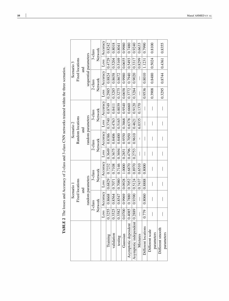
for all datasets considered for the evaluation are shown in Table 2 .
10 Manaf AHMED ET AL
TAB
LE
2T
helo
sses
and
Acc
urac
yof
2-cl
ass
and
3-cl
ass
CN
Nne
twor
kstr
aine
dw
ithin
the
thre
esc
enar
ios.
Scen
ario
1Fi
xed
loca
tions
and
rand
ompa
ram
eter
s
Scen
ario
2R
ando
mlo
catio
nsan
dra
ndom
para
met
ers
Scen
ario
3Fi
xed
loca
tions
and
sequ
entia
lpar
amet
ers
2-cl
ass
Net
wor
k3-
clas
sN
etw
ork
2-cl
ass
Net
wor
k3-
clas
sN
etw
ork
2-cl
ass
Net
wor
k3-
clas
sN
etw
ork
Los
sA
ccur
acy
Los
sA
ccur
acy
Los
sA
ccur
acy
Los
sA
ccur
acy
Los
sA
ccur
acy
Los
sA
ccur
acy
Trai
ning
0.32
550.
8668
0.68
290.
7232
0.36
490.
8386
0.37
400.
8749
0.29
850.
8824
0.47
290.
8242
valid
atio
n0.
3525
0.85
640.
7071
0.71
080.
3675
0.84
060.
4763
0.84
110.
3285
0.86
580.
5204
0.80
18te
stin
g0.
3582
0.85
470.
7080
0.71
460.
3694
0.84
000.
5165
0.80
390.
3275
0.86
720.
5169
0.80
41G
auss
ian
0.07
000.
9969
0.09
281.
0000
0.28
510.
9550
0.38
680.
9540
0.06
580.
9980
0.06
550.
9980
Asy
mpt
otic
depe
nden
t0.
4085
0.78
800.
7052
0.68
700.
4796
0.70
500.
6378
0.66
600.
3772
0.79
400.
5493
0.74
80A
sym
ptot
icin
depe
nden
t0.
2889
0.93
900.
5124
0.89
700.
2753
0.96
100.
4621
0.91
200.
3284
0.90
200.
3317
0.92
40M
ixtu
res
——
0.74
370.
6510
—–
6.03
350.
1370
——
0.82
990.
6633
Diff
eren
tloc
atio
ns0.
779
0.80
600.
8888
0.80
00—
——
—0.
9536
0.80
101.
1231
0.79
90D
iffer
ents
cale
para
met
ers
——
——
——
——
0.39
080.
8480
0.50
240.
8100
Diff
eren
tsm
ooth
para
met
ers
——
——
——
——
0.32
950.
8744
0.43
610.
8355
Manaf AHMED ET AL 11
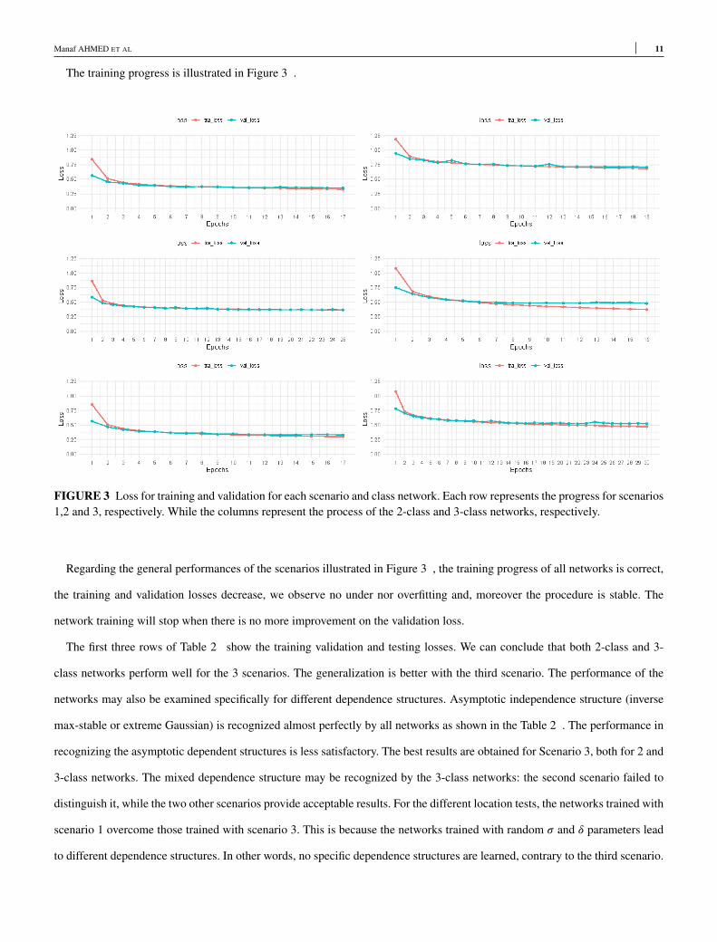
The training progress is illustrated in Figure 3 .
FIGURE 3 Loss for training and validation for each scenario and class network. Each row represents the progress for scenarios1,2 and 3, respectively. While the columns represent the process of the 2-class and 3-class networks, respectively.
Regarding the general performances of the scenarios illustrated in Figure 3 , the training progress of all networks is correct,
the training and validation losses decrease, we observe no under nor overfitting and, moreover the procedure is stable. The
network training will stop when there is no more improvement on the validation loss.
The first three rows of Table 2 show the training validation and testing losses. We can conclude that both 2-class and 3-
class networks perform well for the 3 scenarios. The generalization is better with the third scenario. The performance of the
networks may also be examined specifically for different dependence structures. Asymptotic independence structure (inverse
max-stable or extreme Gaussian) is recognized almost perfectly by all networks as shown in the Table 2 . The performance in
recognizing the asymptotic dependent structures is less satisfactory. The best results are obtained for Scenario 3, both for 2 and
3-class networks. The mixed dependence structure may be recognized by the 3-class networks: the second scenario failed to
distinguish it, while the two other scenarios provide acceptable results. For the different location tests, the networks trained with
scenario 1 overcome those trained with scenario 3. This is because the networks trained with random � and � parameters lead
to different dependence structures. In other words, no specific dependence structures are learned, contrary to the third scenario.
12 Manaf AHMED ET AL
The performances are much improved by training the networks with datasets whose parameters cover sequences of parameters.
Finally, scenario 3 has good performances, even for datasets with untrained scale and smooth parameters. These observations
lead us to use the third scenario in our application studies: 2-meters air temperature over Iraq and the rainfall over the East coast
of Australia.
6 APPLICATION TO THE ENVIRONMENTAL CASE STUDIES
Modeling spatial extreme dependence structure on environmental data is our initial purpose in this work. We finish this paper
wtih two specific studies on Iraqi air temperature and East Austrian rainfall.
6.1 Spatial dependence pattern of the air temperature at two meter above Iraq land
Temperature of the air at two meters above the surface has a major influence on assessing climate changes as well as on all
biotic processes. This data is inherently a spatio-temporal process (see Hooker, Duveiller, and Cescatti (2018)).
6.1.1 The data
We used data produced by the meteorological reanalysis ERA5 and achieved by the European Center for Medium-Range
Weather Forecasts ECMWF. An overview and quality assessment of this data may be found in http://dx.doi.org/
10.24381/cds.adbb2d47. Our objective is to study the spatial dependence structure pattern of this data recorded from a
high temperature region in Iraq. Let {Xk(s)}s∈ ,k∈, ⊂ ℝ2, k ∈ ⊂ ℝ+, be the daily average of the 2 meter air temperature
process computed at the peak hours from 11H to 17H for the period 1979-2019 along of the summer (June, July and August ).
This collection of data results in || = 3772 temporal replications and || = 1845 grid cells. The data has naturally a spatio-
temporal nature. Nevertheless, a preliminary preprocessing suggests us to treat them as independent replications of a stationary
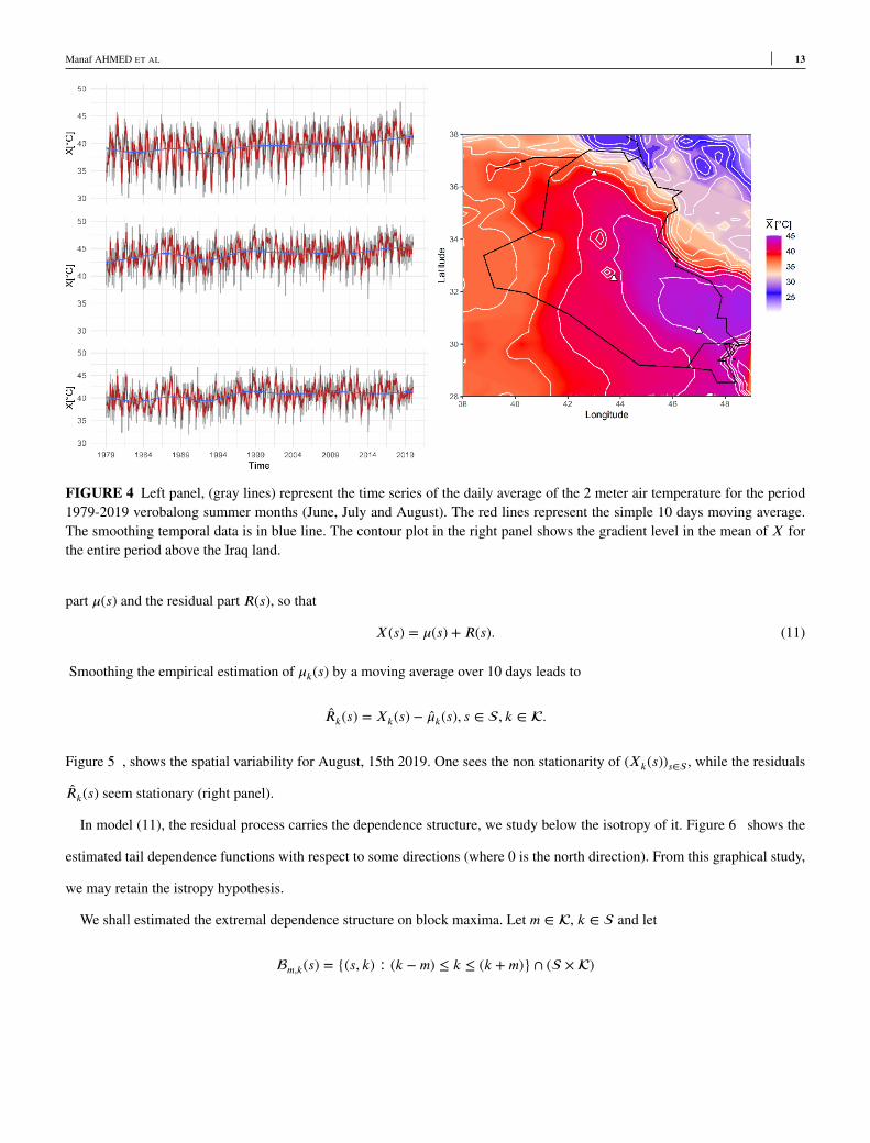
spatial process. The left panel in Figure 4 shows the time series of the X for three locations located in the north, middle and
south of Iraq (white triangles on the right panel). The right panel, shows the temporal mean.
Regarding the time series in the left panel, the data in three locations may be considered as stationary in time. In order to
remove the spatial non stationarity, we shall aply a simple moving average, as used in Huser (2020), see Section 6.1.2.
6.1.2 Preprocessing of 2 meter air temperature data.
As mentioned above, the 2meter summer air temperature data in Iraq look spatially non stationary. We propose to follow Huser
(2020), in order to remove the non stationarity. We shall decompose the spatial process {X(s)}s∈ into two terms, the average
Manaf AHMED ET AL 13
FIGURE 4 Left panel, (gray lines) represent the time series of the daily average of the 2 meter air temperature for the period1979-2019 verobalong summer months (June, July and August). The red lines represent the simple 10 days moving average.The smoothing temporal data is in blue line. The contour plot in the right panel shows the gradient level in the mean of X forthe entire period above the Iraq land.
part �(s) and the residual part R(s), so that
X(s) = �(s) + R(s). (11)
Smoothing the empirical estimation of �k(s) by a moving average over 10 days leads to
Rk(s) = Xk(s) − �k(s), s ∈ , k ∈ .
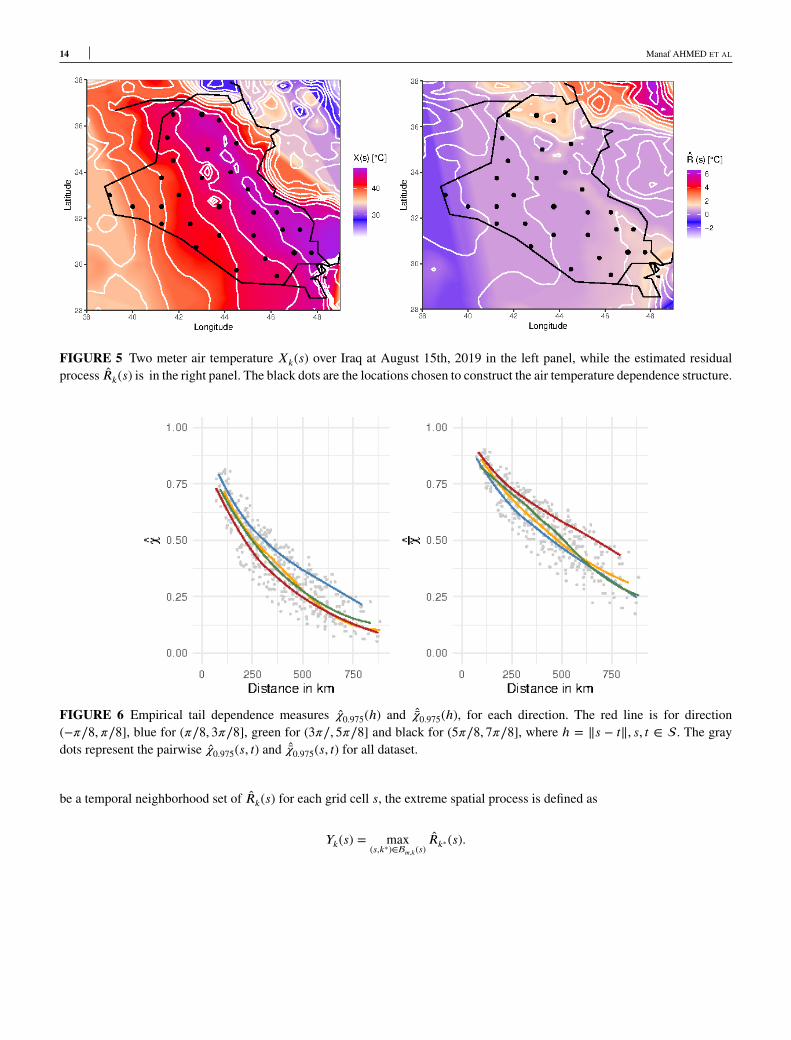
Figure 5 , shows the spatial variability for August, 15th 2019. One sees the non stationarity of (Xk(s))s∈ , while the residuals
Rk(s) seem stationary (right panel).
In model (11), the residual process carries the dependence structure, we study below the isotropy of it. Figure 6 shows the
estimated tail dependence functions with respect to some directions (where 0 is the north direction). From this graphical study,
we may retain the istropy hypothesis.
We shall estimated the extremal dependence structure on block maxima. Let m ∈ , k ∈ and let
m,k(s) = {(s, k) ∶ (k − m) ≤ k ≤ (k + m)} ∩ ( ×)
14 Manaf AHMED ET AL
FIGURE 5 Two meter air temperature Xk(s) over Iraq at August 15th, 2019 in the left panel, while the estimated residualprocess Rk(s) is in the right panel. The black dots are the locations chosen to construct the air temperature dependence structure.
FIGURE 6 Empirical tail dependence measures �0.975(ℎ) and �0.975(ℎ), for each direction. The red line is for direction(−�∕8, �∕8], blue for (�∕8, 3�∕8], green for (3�∕, 5�∕8] and black for (5�∕8, 7�∕8], where ℎ = ‖s − t‖, s, t ∈ . The graydots represent the pairwise �0.975(s, t) and �0.975(s, t) for all dataset.
be a temporal neighborhood set of Rk(s) for each grid cell s, the extreme spatial process is defined as
Yk(s) = max(s,k∗)∈m,k(s)
Rk∗(s).
Manaf AHMED ET AL 15
Then, dependence structure of the air temperature will be estimated using �0.975(s, t) and �0.975(s, t), s, t = 1, ..., 30, (s, t) ∈ .
We shall consider the rank transformation applied on Y , in order to transform the margin to unite Fréchet:
Yk(s) =
⎧
⎪
⎪
⎨
⎪
⎪
⎩
−1∕ log(Rank(Yk(s))∕(|m,k(s)| + 1))
ifRank(Yk(s)) > 0
0 if Rank(Yk(s)) = 0,
where k = 1, ..., |m,k(s)|, s = 1, ..., 30 and | ⋅ | is the cardinality, we get a [30 × 30 × 2] table which will consists in the CNN
inputs.
6.1.3 Training the designed Convolutional Neural Network
We shall now use the CNN procedure described in Sections 4 and 5, we consider the locations of the data, according to scenario
3. We resize the data into [0, 1]2. The training datasets are generated as in scenario 3, for parameters, we use regular sequences
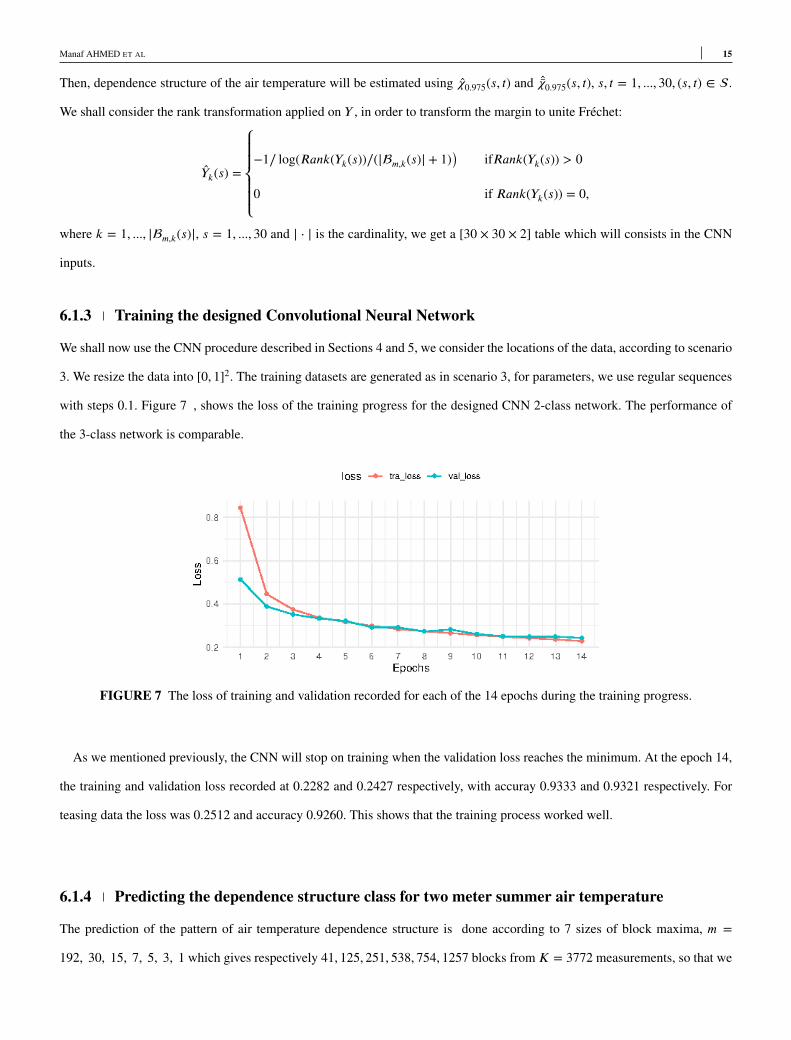
with steps 0.1. Figure 7 , shows the loss of the training progress for the designed CNN 2-class network. The performance of
the 3-class network is comparable.
FIGURE 7 The loss of training and validation recorded for each of the 14 epochs during the training progress.
As we mentioned previously, the CNN will stop on training when the validation loss reaches the minimum. At the epoch 14,
the training and validation loss recorded at 0.2282 and 0.2427 respectively, with accuray 0.9333 and 0.9321 respectively. For
teasing data the loss was 0.2512 and accuracy 0.9260. This shows that the training process worked well.
6.1.4 Predicting the dependence structure class for two meter summer air temperature
The prediction of the pattern of air temperature dependence structure is done according to 7 sizes of block maxima, m =
192, 30, 15, 7, 5, 3, 1 which gives respectively 41, 125, 251, 538, 754, 1257 blocks from K = 3772 measurements, so that we
16 Manaf AHMED ET AL
shall see the influence of block size on the predicted class. Table 3 shows the predicted pattern of the dependence structure
of 2 meter air temperature corresponding to each block maxima size proposed. For all block sizes, the predicted pattern was
asymptotic dependence, with no significant effect of block size on the probability of prediction for both 2-class and 3-class
CNN. So, we may conclude that the 2 meter air summer temperature has an asymptotic dependent spatial structure.
TABLE 3 Predicted class and its probability for the 2 meter air temperature data for each block maxima size proposed. Thedependence structure is validated by the two CNN. AD and AI refer to asymptotic dependence and asymptotic independence,respectively.
2 classes CNN 3 Classes CNNBlock Maxima size Probability of AD Probability of AI Probability of AD Probability of AI Probability of mix
m = 92 days 1.000 0.000 1.000 0.000 0.000m = 30 days 1.000 0.000 1.000 0.000 0.000m = 15 days 0.990 0.001 0.645 0.355 0.000m = 7 days 0.860 0.140 0.791 0.199 0.010m = 5 days 0.929 0.071 0.686 0.013 0.301m = 3 days 0.864 0.136 0.702 0.085 0.213m = 1 day 0.995 0.005 0.950 0.037 0.013
6.2 Rainfall dataset: case study in Australia
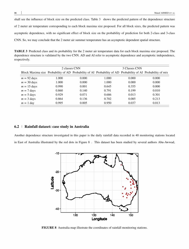
Another dependence structure investigated in this paper is the daily rainfall data recorded in 40 monitoring stations located
in East of Australia illustrated by the red dots in Figure 8 . This dataset has been studied by several authors Abu-Awwad,
FIGURE 8 Australia map illustrate the coordinates of rainfall monitoring stations.
Manaf AHMED ET AL 17
Maume-Deschamps, and Ribereau (2019); Ahmed, Maume-Deschamps, Ribereau, and Vial (2017); Bacro et al. (2016).
6.2.1 The data
For each location, the cumulative rainfall amount (in millimeters) over 24 hours is recorded, during the period 1972-2019
along the extended rainfall season (April-September). It results || = 8784 observations. The locations have been selected
among many monitoring locations (red points on Figure 8 ), keeping the elevations above mean sea level between 2 to 540
meters, in order to ensure the spatial stationarity. The data is available freely on the website of Australian meteorology Bureau
http://www.bom.gov.au. The spatial stationarity and isotropy properties have been investigated for the this data in many
papers, for instance see e.g., Bacro et al. (2016), Ahmed et al. (2017) and Abu-Awwad et al. (2019). We shall consider that the
data is stationary and isotropic. That leads to construct the corresponding dependence structure directly form the data itself
without having to estimate the residuals as in the previous section. Let {Xk(s)}s∈ ,k∈, s = 1, ..., 40, k = 1, ..., 8784 be the
spatial process representing the rainfall in the East cost of Australia. Adopting the block maxima size as in the previous section,
we consider the extreme process:
Yk(s) = max(s,k∗)∈m,k(s)
Xk∗(s)
and transform Y into a unite Fréchet marginals process. The dependence structure of this data will be summarized in a 40×40×2
array. The first and second tensor are �0.975(s, t) and �0.975(s, t), s, t = 1, ..., 40, respectively with threshold u = 0.975.
6.2.2 Predicting the pattern of the dependence structure of rainfall amount in East Austria.
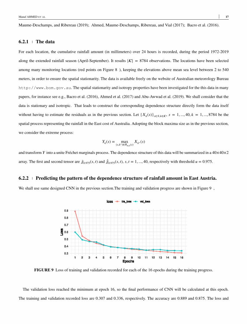
We shall use same designed CNN in the previous section.The training and validation progress are shown in Figure 9 ,
FIGURE 9 Loss of training and validation recorded for each of the 16 epochs during the training progress.
The validation loss reached the minimum at epoch 16, so the final performance of CNN will be calculated at this epoch.
The training and validation recorded loss are 0.307 and 0.336, respectively. The accuracy are 0.889 and 0.875. The loss and
18 Manaf AHMED ET AL
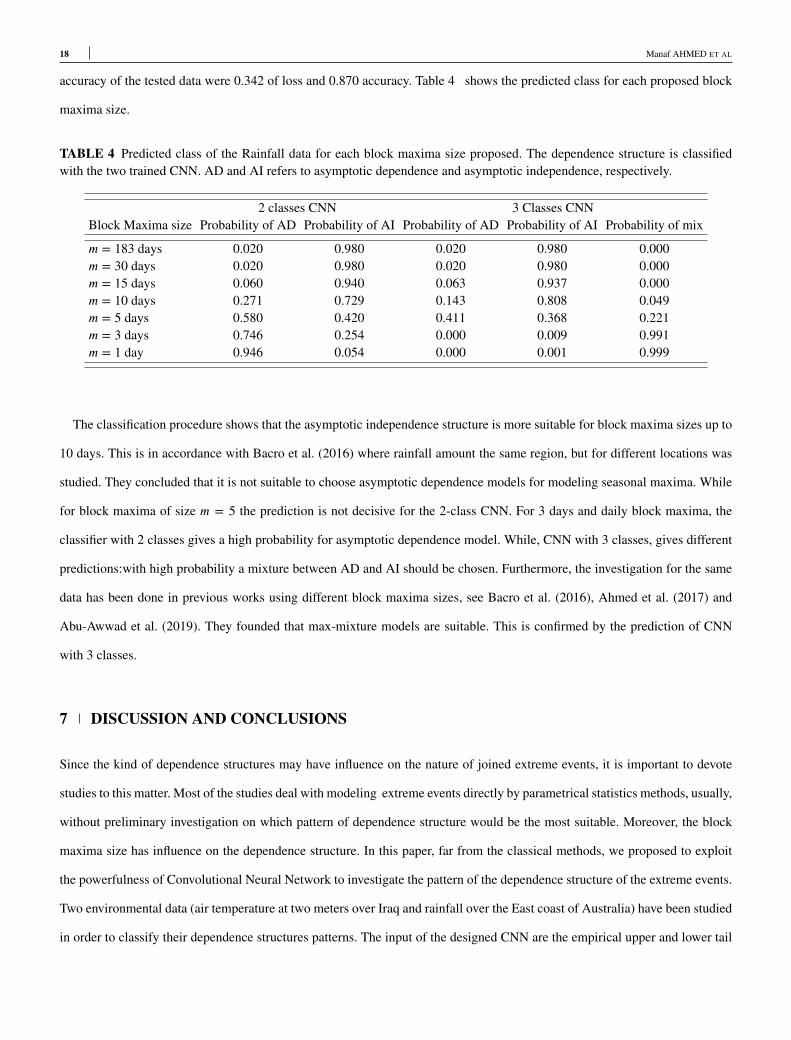
accuracy of the tested data were 0.342 of loss and 0.870 accuracy. Table 4 shows the predicted class for each proposed block
maxima size.
TABLE 4 Predicted class of the Rainfall data for each block maxima size proposed. The dependence structure is classifiedwith the two trained CNN. AD and AI refers to asymptotic dependence and asymptotic independence, respectively.
2 classes CNN 3 Classes CNNBlock Maxima size Probability of AD Probability of AI Probability of AD Probability of AI Probability of mix
m = 183 days 0.020 0.980 0.020 0.980 0.000m = 30 days 0.020 0.980 0.020 0.980 0.000m = 15 days 0.060 0.940 0.063 0.937 0.000m = 10 days 0.271 0.729 0.143 0.808 0.049m = 5 days 0.580 0.420 0.411 0.368 0.221m = 3 days 0.746 0.254 0.000 0.009 0.991m = 1 day 0.946 0.054 0.000 0.001 0.999
The classification procedure shows that the asymptotic independence structure is more suitable for block maxima sizes up to
10 days. This is in accordance with Bacro et al. (2016) where rainfall amount the same region, but for different locations was
studied. They concluded that it is not suitable to choose asymptotic dependence models for modeling seasonal maxima. While
for block maxima of size m = 5 the prediction is not decisive for the 2-class CNN. For 3 days and daily block maxima, the
classifier with 2 classes gives a high probability for asymptotic dependence model. While, CNN with 3 classes, gives different
predictions:with high probability a mixture between AD and AI should be chosen. Furthermore, the investigation for the same
data has been done in previous works using different block maxima sizes, see Bacro et al. (2016), Ahmed et al. (2017) and
Abu-Awwad et al. (2019). They founded that max-mixture models are suitable. This is confirmed by the prediction of CNN
with 3 classes.
7 DISCUSSION AND CONCLUSIONS
Since the kind of dependence structures may have influence on the nature of joined extreme events, it is important to devote
studies to this matter. Most of the studies deal with modeling extreme events directly by parametrical statistics methods, usually,
without preliminary investigation on which pattern of dependence structure would be the most suitable. Moreover, the block
maxima size has influence on the dependence structure. In this paper, far from the classical methods, we proposed to exploit
the powerfulness of Convolutional Neural Network to investigate the pattern of the dependence structure of the extreme events.
Two environmental data (air temperature at two meters over Iraq and rainfall over the East coast of Australia) have been studied
in order to classify their dependence structures patterns. The input of the designed CNN are the empirical upper and lower tail
Manaf AHMED ET AL 19
dependence measures �0.975(s, t) and �0.975(s, t). The training process has been done on generated data from max-stable stable
models, inverse max-stable processes and extreme Gaussian processes, in order to get asymptotic independent models. The data
are generated according to fixed coordinates rescaled in [0, 1]2. The ability of this model to recognize the pattern of dependence
structure has been emphasized in training, validation, testing loss and accuracy.
It is worth mentioning that the sensitivity of the dependence structure class by considering the size of block maxima should
be taking into account in the models. Adopting this classification procedure may advise for choosing a reasonable size of block
maxima such that the data has a good representation. For instance, for the air temperature event, whatever the block maxima
size is chosen, the dependence structure is asymptotic independence. While, for rainfall data, the dependence structure class
changed across block size.
ACKNOWLEDGMENTS
This work was supported by PAUSE operated by Collège de France, and the LABEX MILYON (ANR-10-LABX-0070) of
Université de Lyon, within the program “Investissements d’Avenir” (ANR-11-IDEX-0007) operated by the French National
Research Agency (ANR).
References
Abu-Awwad, A., Maume-Deschamps, V., & Ribereau, P. (2019). Fitting spatial max-mixture processes with unknown extremal
dependence class: an exploratory analysis tool. Test, 1–44.
Ahmed, M., Maume-Deschamps, V., Ribereau, P., & Vial, C. (2017). A semi-parametric estimation for max-mixture spatial
processes. arXiv preprint arXiv:1710.08120.
Alex, K., Sutskever, L., & Hinton, G. (2012). Imagenet classification with deep convolutional neural networks. In F. Pereira,
C. J. C. Burges, L. Bottou, & K. Q. Weinberger (Eds.), Advances in neural information processing systems 25 (pp.
1097–1105). Curran Associates, Inc. Retrieved from http://papers.nips.cc/paper/4824-imagenet-\
classification-with-deep-convolutional-neural-\networks.pdf
Bacro, J., Gaetan, C., & Toulemonde, G. (2016). A flexible dependence model for spatial extremes. Journal of Statistical
Planning and Inference, 172, 36–52.
Bortot, P., Coles, S., & Tawn, J. (2000). The multivariate gaussian tail model: An application to oceanographic data. Journal
of the Royal Statistical Society: Series C (Applied Statistics), 49(1), 31–049.
Brown, B. M., & Resnick, S. I. (1977). Extreme values of independent stochastic processes. Journal of Applied Probability,
20 Manaf AHMED ET AL
14(4), 732–739.
Caterini, A. L., & Chang, D. E. (2018). Deep neural networks in a mathematical framework. Springer.
Coles, S., Heffernan, J., & Tawn, J. (1999). Dependence measures for extreme value analyses. Extremes, 2(4), 339–365.
Coles, S., & Pauli, F. (2002). Models and inference for uncertainty in extremal dependence. Biometrika, 89(1), 183–196.
De Haan, L., & Ferreira, A. (2007). Extreme value theory: an introduction. Springer Science & Business Media.
De Haan, L., et al. (1984). A spectral representation for max-stable processes. The annals of probability, 12(4), 1194–1204.
De Haan, L., Pereira, T. T., et al. (2006). Spatial extremes: Models for the stationary case. The annals of statistics, 34(1),
146–168.
Embrechts, P., Klüppelberg, C., & Mikosch, T. (2013). Modelling extremal events: for insurance and finance (Vol. 33). Springer
Science & Business Media.
Fukushima, K. (1980). Neocognitron: A self-organizing neural network model for a mechanism of pattern recognition
unaffected by shift in position. Biological cybernetics, 36(4), 193–202.
He, K., Zhang, X., Ren, S., & Sun, J. (2016). Deep residual learning for image recognition. In Proceedings of the ieee
conference on computer vision and pattern recognition (pp. 770–778).
Hooker, J., Duveiller, G., & Cescatti, A. (2018). A global dataset of air temperature derived from satellite remote sensing and
weather stations. Scientific data, 5(1), 1–11.
Hubel, D. H., & Wiesel, T. N. (1968). Receptive fields and functional architecture of monkey striate cortex. The Journal of
physiology, 195(1), 215–243.
Huser, R. (2020). Eva 2019 data competition on spatio-temporal prediction of red sea surface temperature extremes. Extremes,
1–14.
Kabluchko, Z., Schlather, M., De Haan, L., et al. (2009). Stationary max-stable fields associated to negative definite functions.
The Annals of Probability, 37(5), 2042–2065.
Kingma, D., & Ba, J. (2014). Adam: A method for stochastic optimization. arXiv preprint arXiv:1412.6980.
LeCun, Y., Boser, B. E., Denker, J. S., Henderson, D., Howard, R. E., Hubbard, W. E., & Jackel, L. D. (1990). Handwritten digit
recognition with a back-propagation network. In Advances in neural information processing systems (pp. 396–404).
Ledford, A., & Tawn, J. A. (1996). Statistics for near independence in multivariate extreme values. Biometrika, 83(1), 169–187.
Lin, Y., Mago, N., Gao, Y., Li, Y., Chiang, Y., Shahabi, C., & Ambite, J. L. (2018). Exploiting spatiotemporal patterns for
accurate air quality forecasting using deep learning. In Proceedings of the 26th acm sigspatial international conference
on advances in geographic information systems (pp. 359–368).
Liu, Y., Racah, E., Correa, J., Khosrowshahi, A., Lavers, D., Kunkel, K., . . . others (2016). Application of deep convolutional
neural networks for detecting extreme weather in climate datasets. arXiv preprint arXiv:1605.01156.
Manaf AHMED ET AL 21
Opitz, T. (2013). Extremal t processes: Elliptical domain of attraction and a spectral representation. Journal of Multivariate
Analysis, 122, 409–413.
Schlather, M. (2002). Models for stationary max-stable random fields. Extremes, 5(1), 33–44.
Schlather, M., & Tawn, J. A. (2003). A dependence measure for multivariate and spatial extreme values: Properties and
inference. Biometrika, 90(1), 139–156.
Smith, R. L. (1990). Max-stable processes and spatial extremes. Unpublished manuscript, 205.
Wadsworth, J. L., & Tawn, J. A. (2012). Dependence modelling for spatial extremes. Biometrika, 99(2), 253–272.
Wang, S., Cao, J., & Yu, P. S. (2019). Deep learning for spatio-temporal data mining: A survey. arXiv preprint
arXiv:1906.04928.
Xie, S., Girshick, R., Dollár, P., Tu, Z., & He, K. (2017). Aggregated residual transformations for deep neural networks. In
Proceedings of the ieee conference on computer vision and pattern recognition (pp. 1492–1500).
Yamashita, R., Nishio, M., Do, R., & Togashi, K. (2018). Convolutional neural networks: an overview and application in
radiology. Insights into imaging, 9(4), 611–629.
Yu, H., Uy, W. I. T., & Dauwels, J. (2016). Modeling spatial extremes via ensemble-of-trees of pairwise copulas. IEEE
Transactions on Signal Processing, 65(3), 571–586.
Zhu, Q., Chen, J., Zhu, L., Duan, X., & Liu, Y. (2018). Wind speed prediction with spatio–temporal correlation: A deep
learning approach. Energies, 11(4), 705.
Zuo, Z., Shuai, B., Wang, G., Liu, X., Wang, X., Wang, B., & Chen, Y. (2015). Convolutional recurrent neural networks:
Learning spatial dependencies for image representation. In Proceedings of the ieee conference on computer vision and
pattern recognition workshops (pp. 18–26).