Embed Size (px)
Citation preview
1
08 Sample Size and Power
Topics 1. Review Hypothesis Testing Concepts2. Effect Size d3. Sample Size with d4. Effect Size r; Sample Size with r5. A Priori Power (Sensitivity Analysis)6. Effect Size f; Sample Size with f7. Effect Size f and ANCOVASample size with categorical variables (to be added)
1. Review of Hypothesis Testing Concepts
1.1 Typical Null and Alternative Hypotheses
Group Comparisons (IV is Categorical, DV is Quantitative)Null Hypothesis
Written There is no difference in mean achievement between female and male students.
SymbolicHo: μf=μm
Alternative HypothesisWritten
There is a difference in mean achievement between female and male students.Symbolic
Ha: μf ≠ μm
Relationships (IV is Quantitative, DV is Quantitative) Null Hypothesis
Written There is no correlation between hours studied and achievement.
SymbolicHo: ρ=0.00
Alternative HypothesisWritten
There is a correlation between hours studied and achievement.Symbolic
Ha: ρ≠0.00
2
1.2 Types 1 and 2 Errors
Type 1 error incorrectly rejecting a true null hypothesis; claiming there is an effect based upon sample results when there is not an effect in the
population; a false positive
ExampleUsing sample data, one concludes a new teaching strategy produces higher achievement than traditional practices when, in fact, it does not show this difference in the population
Type 2 error failure to reject a false null hypothesis; failure to identify an effect in the sample when there is an effect in the population; a false negative
ExampleBased upon a sample one claims a new teaching strategy does not produce higher achievement than traditional practices when, in fact, it does in the population
Type 1 and 2 Errors IllustratedAssume the following null hypothesis:
Ho: patient is not pregnant.
Question 1Which of the following diagnoses would be Type 1 and Type 2 errors?
Image sourcehttp://effectsizefaq.com/2010/05/31/i-always-get-confused-about-type-i-and-ii-errors-can-you-show-me-something-to-help-me-remember-the-difference/

3
Question 1 Answer
1.2 Alpha, Beta, Power, and Others
alpha (α) probability of a Type 1 error; normally .05 or .01, values .10 and .001 occasionally used; also called significance level
ExampleThere’s a 5% chance we will find a relationship between hours studied and achievement in our sample when there isn’t a relationship in the population
Based upon our sample evidence, there’s a 1% chance we will claim our new teaching strategy is more effective when it is not more effective in the population
beta (β) probability of a Type 2 error; researchers often strive to set this rate .20 or less
ExampleThere’s a 20% chance we will claim there is no relationship between hours studied and achievement when there is a relationship in the population
There’s a 10% chance we will claim our new teaching strategy is not more effective when it is more effective in the population
4
power (1−β) probability of identifying an effect if one exists; probability of rejecting a false null hypothesis; complement of beta (1−β) so it is the probability of not committing a Type 2 error
ExampleThere’s an 80% chance we will detect a relationship between hours studied and achievement in our sample if there is a relationship in the population
With this small sample there is only a 40% chance we will correctly claim our new teaching strategy is more effective when it is more effective
n is study sample size Example
In our pregnancy study we tested 15 doctors to determine if they could correctly identify pregnancy status of patients
To test our new teaching strategy, we sampled 108,637 students; 46,714 students received the new teaching strategy and 61,923 received current standard instructional approaches
effect size effect size denotes the magnitude of difference if comparing means or magnitude of
relationship between variables may be unstandardized or standardized four commonly used ESs
d: mean difference of two groupsES d is defined as the mean difference between two groups divided by a standard deviation which is commonly the pooled SD, but could be other SDs, so ES d is the standardized mean difference between two groups. ES d is suitable for any situations in which two groups are compared by a mean difference.
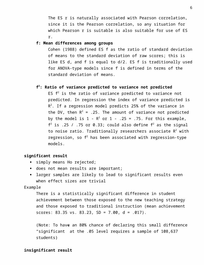
r: Pearson correlationThe ES r is naturally associated with Pearson correlation, since it is the Pearson correlation, so any situation for which Pearson r is suitable is also suitable for use of ES r.
f: Mean differences among groupsCohen (1988) defined ES f as the ratio of standard deviation of means to the standard deviation of raw scores; this is like ES d, and f is equal to d/2. ES f is traditionally used for ANOVA-type models since f is defined in terms of the standard deviation of means.
f2: Ratio of variance predicted to variance not predictedES f2 is the ratio of variance predicted to variance not predicted. In regression the index of variance predicted is R2. If a regression model predicts 25% of the variance in the DV, then R2 = .25. The amount of variance not predicted by the model is 1 - R2
5
or 1 - .25 = .75. For this example, f2 is .25 / .75 or 0.33; could also define f2 as the signal to noise ratio. Traditionally researchers associate R2 with regression, so f2 has been associated with regression-type models.
significant result
simply means Ho rejected; does not mean results are important; larger samples are likely to lead to significant results even when effect sizes are trivial
ExampleThere is a statistically significant difference in student achievement between those exposed to the new teaching strategy and those exposed to traditional instruction (mean achievement scores: 83.35 vs. 83.23, SD = 7.00, d = .017).
(Note: To have an 80% chance of declaring this small difference “significant” at the .05 level requires a sample of 108,637 students)
insignificant result simply means Ho was not rejected; does not mean results are unimportant
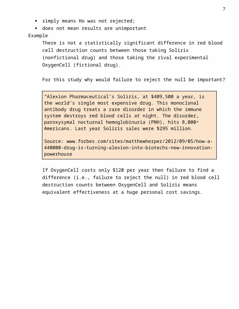
ExampleThere is not a statistically significant difference in red blood cell destruction counts between those taking Soliris (nonfictional drug) and those taking the rival experimental OxygenCell (fictional drug).
For this study why would failure to reject the null be important?
“Alexion Pharmaceutical’s Soliris, at $409,500 a year, is the world’s single most expensive drug. This monoclonal antibody drug treats a rare disorder in which the immune system destroys red blood cells at night. The disorder, paroxysymal nocturnal hemoglobinuria (PNH), hits 8,000 Americans. Last year Soliris sales were $295 million.”
Source: www.forbes.com/sites/matthewherper/2012/09/05/how-a-440000-drug-is-turning-alexion-into-biotechs-new-innovation-powerhouse
If OxygenCell costs only $120 per year then failure to find a difference (i.e., failure to reject the null) in red blood cell destruction counts between OxygenCell and Soliris means equivalent effectiveness at a huge personal cost savings.
6
2. Effect Size d
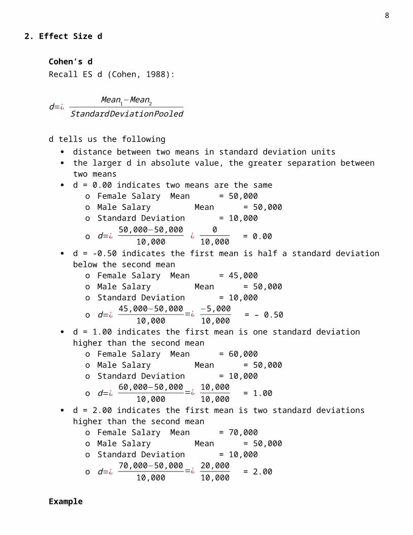
Cohen’s d Recall ES d (Cohen, 1988):
d=¿ Mean1−Mean2
Standard DeviationPooled
d tells us the following distance between two means in standard deviation units the larger d in absolute value, the greater separation between two means d = 0.00 indicates two means are the same
o Female Salary Mean = 50,000o Male Salary Mean = 50,000o Standard Deviation = 10,000
o d=¿ 50,000−50,000
10,000 ¿ 0
10,000 = 0.00
d = -0.50 indicates the first mean is half a standard deviation below the second meano Female Salary Mean = 45,000o Male Salary Mean = 50,000o Standard Deviation = 10,000
o d=¿ 45,000−50,000
10,000=¿
−5,00010,000 = – 0.50
d = 1.00 indicates the first mean is one standard deviation higher than the second meano Female Salary Mean = 60,000o Male Salary Mean = 50,000o Standard Deviation = 10,000
o d=¿ 60,000−50,000
10,000=¿
10,00010,000 = 1.00
d = 2.00 indicates the first mean is two standard deviations higher than the second meano Female Salary Mean = 70,000o Male Salary Mean = 50,000o Standard Deviation = 10,000
o d=¿ 70,000−50,000
10,000=¿
20,00010,000 = 2.00
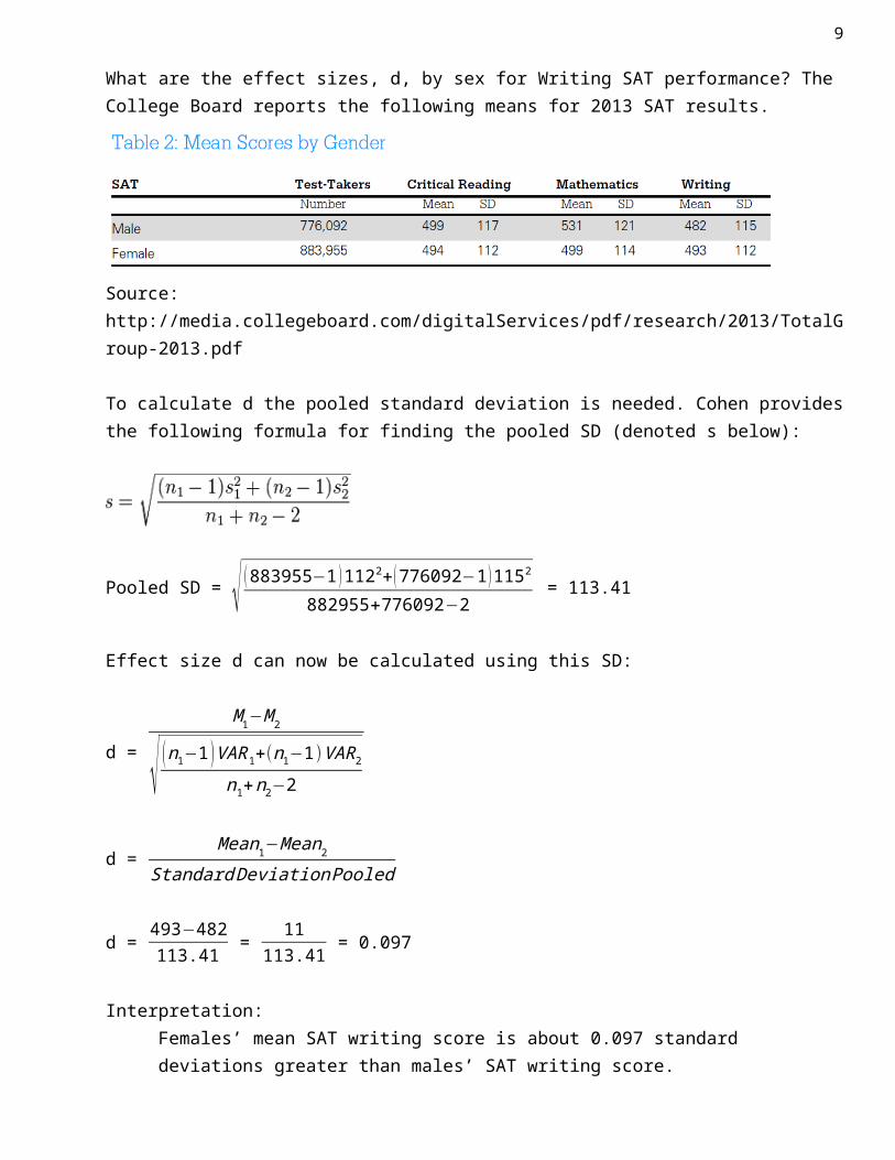
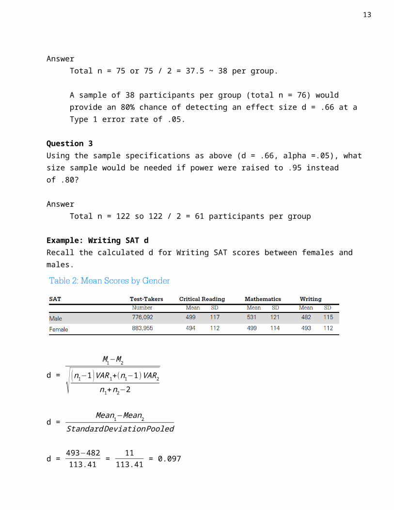
Example What are the effect sizes, d, by sex for Writing SAT performance? The College Board reports the following means for 2013 SAT results.
Source: http://media.collegeboard.com/digitalServices/pdf/research/2013/TotalGroup-2013.pdf
7
To calculate d the pooled standard deviation is needed. Cohen provides the following formula for finding the pooled SD (denoted s below):
Pooled SD = √ (883955−1 )1122+ (776092−1 )1152
882955+776092−2 = 113.41
Effect size d can now be calculated using this SD:
d =
M 1−M 2
√ (n1−1 )VAR1+(n1−1)VAR2n1+n2−2
d = Mean1−Mean2
Standard DeviationPooled
d = 493−482113.41 =
11113.41 = 0.097
Interpretation:Females’ mean SAT writing score is about 0.097 standard deviations greater than males’ SAT writing score.
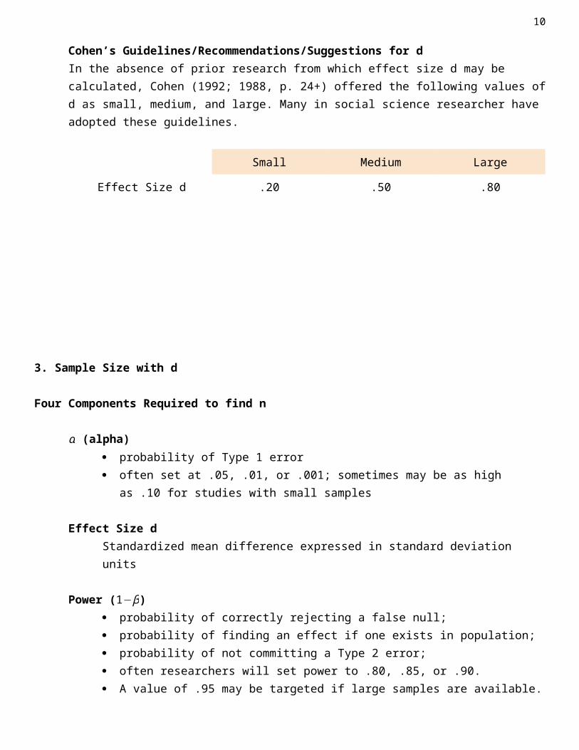
Cohen’s Guidelines/Recommendations/Suggestions for dIn the absence of prior research from which effect size d may be calculated, Cohen (1992; 1988, p. 24+) offered the following values of d as small, medium, and large. Many in social science researcher have adopted these guidelines.
Small Medium Large
Effect Size d .20 .50 .80
8
3. Sample Size with d
Four Components Required to find n
α (alpha) probability of Type 1 error often set at .05, .01, or .001; sometimes may be as high as .10 for studies with small
samples
Effect Size dStandardized mean difference expressed in standard deviation units
Power (1−β) probability of correctly rejecting a false null; probability of finding an effect if one exists in population; probability of not committing a Type 2 error; often researchers will set power to .80, .85, or .90. A value of .95 may be targeted if large samples are available.
degrees of freedom (df) number of parameters estimated in general linear model excluding the intercept df for common statistical tests
o df = 1 for two-group t-testo df = 1 Pearson correlationo df = 2 if comparing 3 groups with ANOVAo df = 3 if comparing 4 groups with ANOVAo df = 4 if comparing 5 groups with ANOVA, etc.
Which Statistical Tests with d?Any group comparison in which the
independent or predictor variable is categorical with two groups (e.g., sex, experimental study of treatment vs. control)
dependent or outcome variable is quantitative (e.g., test scores in percent correct, anxiety scale score, weight in lbs, distance in feet, etc.)
While effect size d can be associated with a variety of statistical tests, the focus of here will be d for an independent samples t-test.
Finding n with Excel An Excel file designed to calculate sample sizes:
http://www.bwgriffin.com/samplesize/samplesize.htmor http://www.bwgriffin.com (follow link to Excel Sample Size)
9
Note – be sure to enable content with the Excel file after downloading, otherwise it will be unable to assess iterative program to find solutions.
Important Limitations This calculator is suitable only for designs with balanced data (equal or approximately equal sample sizes per group), non-directional alternative hypotheses, linear models with fixed predictors (although random predictors are discussed below), and for non-correlated linear models. For studies with large imbalances in sample size, directional tests, or correlated data, use the free software G*Power: http://www.gpower.hhu.de/en.html
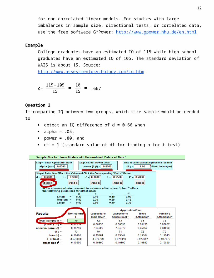
Example College graduates have an estimated IQ of 115 while high school graduates have an estimated IQ of 105. The standard deviation of WAIS is about 15. Source: http://www.assessmentpsychology.com/iq.htm
d= 115−10515 = 1015 = .667
Question 2If comparing IQ between two groups, which size sample would be needed to
detect an IQ difference of d = 0.66 when alpha = .05, power = .80, and df = 1 (standard value of df for finding n for t-test)
10
AnswerTotal n = 75 or 75 / 2 = 37.5 ~ 38 per group.
A sample of 38 participants per group (total n = 76) would provide an 80% chance of detecting an effect size d = .66 at a Type 1 error rate of .05.
Question 3Using the sample specifications as above (d = .66, alpha =.05), what size sample would be needed if power were raised to .95 instead of .80?
AnswerTotal n = 122 so 122 / 2 = 61 participants per group
Example: Writing SAT d Recall the calculated d for Writing SAT scores between females and males.
d =
M 1−M 2
√ (n1−1 )VAR1+(n1−1)VAR2n1+n2−2
d = Mean1−Mean2
Standard DeviationPooled
d = 493−482113.41 =
11113.41 = 0.097
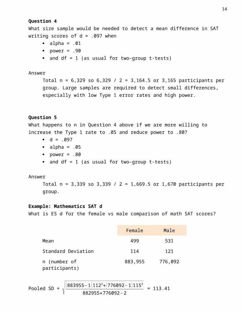
Question 4What size sample would be needed to detect a mean difference in SAT writing scores of d = .097 when
alpha = .01 power = .90 and df = 1 (as usual for two-group t-tests)
Answer
11
Total n = 6,329 so 6,329 / 2 = 3,164.5 or 3,165 participants per group. Large samples are required to detect small differences, especially with low Type 1 error rates and high power.
Question 5What happens to n in Question 4 above if we are more willing to increase the Type 1 rate to .05 and reduce power to .80?
d = .097 alpha = .05 power = .80 and df = 1 (as usual for two-group t-tests)
AnswerTotal n = 3,339 so 3,339 / 2 = 1,669.5 or 1,670 participants per group.
Example: Mathematics SAT dWhat is ES d for the female vs male comparison of math SAT scores?
Female Male
Mean 499 531
Standard Deviation 114 121
n (number of participants) 883,955 776,092
Pooled SD = √ (883955−1 )1122+ (776092−1 )1152
882955+776092−2 = 113.41
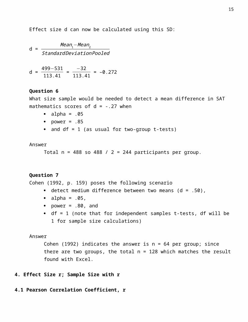
Effect size d can now be calculated using this SD:
d = Mean1−Mean2
Standard DeviationPooled
d = 499−531113.41 =
−32113.41 = –0.272
Question 6What size sample would be needed to detect a mean difference in SAT mathematics scores of d = -.27 when
alpha = .05 power = .85 and df = 1 (as usual for two-group t-tests)
Answer
12
Total n = 488 so 488 / 2 = 244 participants per group.
Question 7Cohen (1992, p. 159) poses the following scenario
detect medium difference between two means (d = .50), alpha = .05, power = .80, and df = 1 (note that for independent samples t-tests, df will be 1 for sample size
calculations)
AnswerCohen (1992) indicates the answer is n = 64 per group; since there are two groups, the total n = 128 which matches the result found with Excel.
4. Effect Size r; Sample Size with r
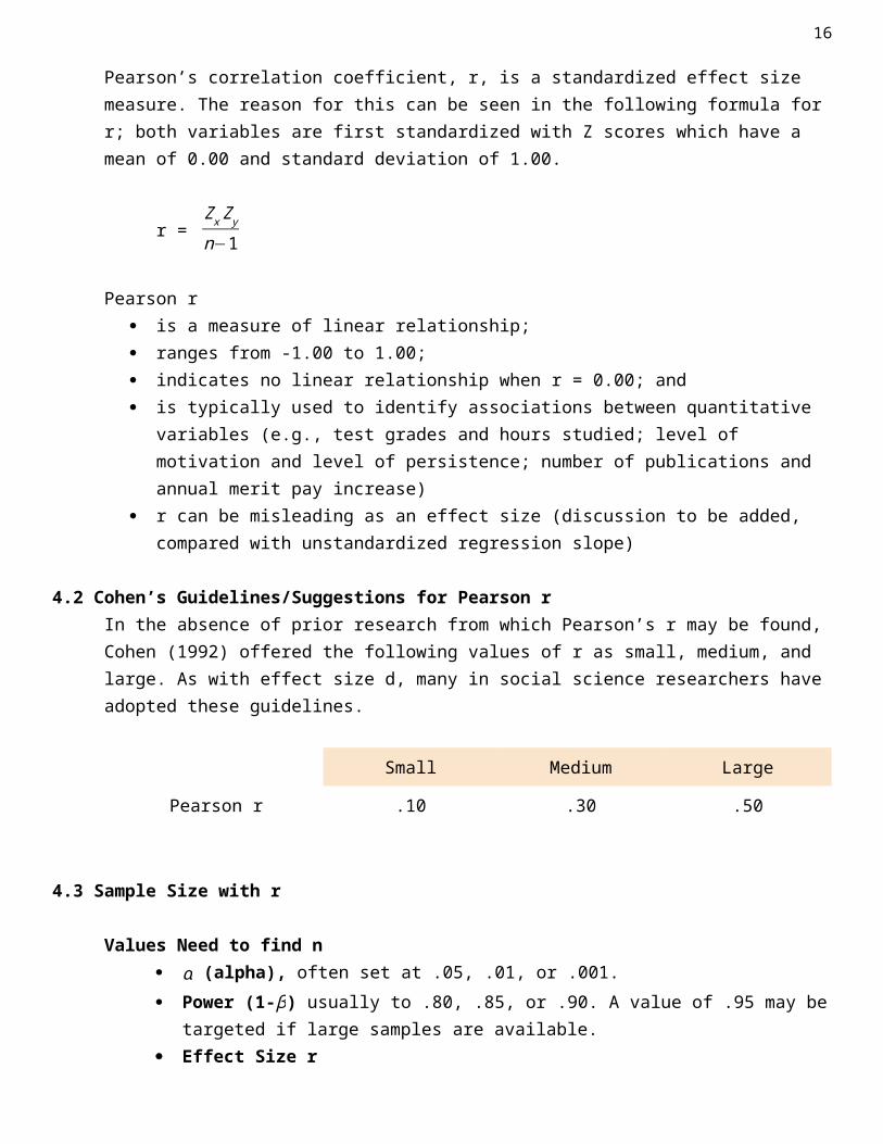
4.1 Pearson Correlation Coefficient, rPearson’s correlation coefficient, r, is a standardized effect size measure. The reason for this can be seen in the following formula for r; both variables are first standardized with Z scores which have a mean of 0.00 and standard deviation of 1.00.
r = Z xZ y
n−1
Pearson r is a measure of linear relationship; ranges from -1.00 to 1.00; indicates no linear relationship when r = 0.00; and is typically used to identify associations between quantitative variables (e.g., test grades
and hours studied; level of motivation and level of persistence; number of publications and annual merit pay increase)
r can be misleading as an effect size (discussion to be added, compared with unstandardized regression slope)
4.2 Cohen’s Guidelines/Suggestions for Pearson rIn the absence of prior research from which Pearson’s r may be found, Cohen (1992) offered the following values of r as small, medium, and large. As with effect size d, many in social science researchers have adopted these guidelines.
Small Medium Large
Pearson r .10 .30 .50
13
4.3 Sample Size with r
Values Need to find n α (alpha), often set at .05, .01, or .001. Power (1-β) usually to .80, .85, or .90. A value of .95 may be targeted if large samples
are available. Effect Size r Degrees of Freedom (df) which defaults to 1 for zero-order correlations.
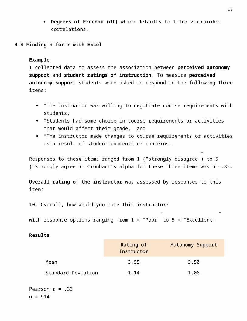
4.4 Finding n for r with Excel
ExampleI collected data to assess the association between perceived autonomy support and student ratings of instruction. To measure perceived autonomy support students were asked to respond to the following three items:
“The instructor was willing to negotiate course requirements with students,” “Students had some choice in course requirements or activities that would affect their
grade,” and “The instructor made changes to course requirements or activities as a result of student
comments or concerns.”
Responses to these items ranged from 1 (“strongly disagree”) to 5 (“Strongly agree”). Cronbach’s alpha for these three items was =.85. α
Overall rating of the instructor was assessed by responses to this item:
10. Overall, how would you rate this instructor?
with response options ranging from 1 = “Poor” to 5 = “Excellent.”
Results
Rating of Instructor Autonomy Support
Mean 3.95 3.50
Standard Deviation 1.14 1.06
Pearson r = .33 n = 914
14
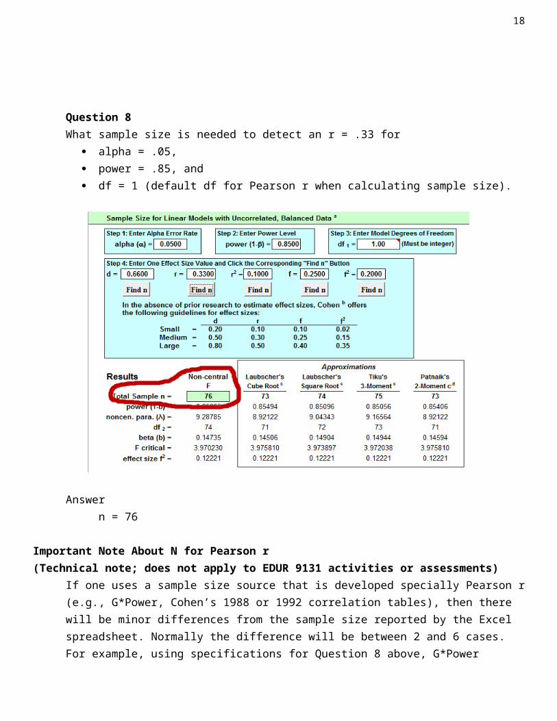
Question 8What sample size is needed to detect an r = .33 for
alpha = .05, power = .85, and df = 1 (default df for Pearson r when calculating sample size).
Answern = 76
Important Note About N for Pearson r (Technical note; does not apply to EDUR 9131 activities or assessments)
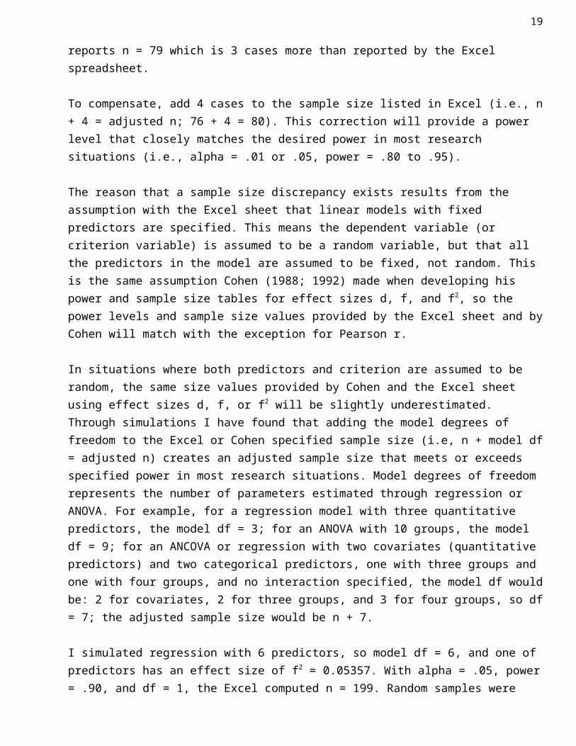
If one uses a sample size source that is developed specially Pearson r (e.g., G*Power, Cohen’s 1988 or 1992 correlation tables), then there will be minor differences from the sample size reported by the Excel spreadsheet. Normally the difference will be between 2 and 6 cases. For example, using specifications for Question 8 above, G*Power reports n = 79 which is 3 cases more than reported by the Excel spreadsheet.
To compensate, add 4 cases to the sample size listed in Excel (i.e., n + 4 = adjusted n; 76 + 4 = 80). This correction will provide a power level that closely matches the desired power in most research situations (i.e., alpha = .01 or .05, power = .80 to .95).
The reason that a sample size discrepancy exists results from the assumption with the Excel sheet that linear models with fixed predictors are specified. This means the dependent variable (or criterion variable) is assumed to be a random variable, but that all the predictors in the model are assumed to be fixed, not random. This is the same assumption Cohen (1988; 1992) made when
15
developing his power and sample size tables for effect sizes d, f, and f2, so the power levels and sample size values provided by the Excel sheet and by Cohen will match with the exception for Pearson r.
In situations where both predictors and criterion are assumed to be random, the same size values provided by Cohen and the Excel sheet using effect sizes d, f, or f2 will be slightly underestimated. Through simulations I have found that adding the model degrees of freedom to the Excel or Cohen specified sample size (i.e, n + model df = adjusted n) creates an adjusted sample size that meets or exceeds specified power in most research situations. Model degrees of freedom represents the number of parameters estimated through regression or ANOVA. For example, for a regression model with three quantitative predictors, the model df = 3; for an ANOVA with 10 groups, the model df = 9; for an ANCOVA or regression with two covariates (quantitative predictors) and two categorical predictors, one with three groups and one with four groups, and no interaction specified, the model df would be: 2 for covariates, 2 for three groups, and 3 for four groups, so df = 7; the adjusted sample size would be n + 7.
I simulated regression with 6 predictors, so model df = 6, and one of predictors has an effect size of f2 = 0.05357. With alpha = .05, power = .90, and df = 1, the Excel computed n = 199. Random samples were taken from these data 250,000 times and the calculated power (number times Ho was rejected) was .8925 (close to the specified value of .90). This was repeated a second time and the empirical power level obtained was .8901 (again, close to the specified value of .90).
The simulations were performed again, but this time with model df added to the sample size, so the adjusted sample size was 199 + 6 = 205. The first run of 250,000 samples produced a power level of .9017 and the second run of 250,000 produced a power level of .8989, both closer to the targeted power level of .90 than the previous estimates. This shows that adding model df to the Excel sample size estimate for models with random predictors provides an easy way to determine sample size for random variate models.
Question 9Sridevi (2013) reports a correlation of -.22 between test anxiety and midterm examination scores among secondary education students in Pakistan. Source: Sridevi, K. V. (2013). A Study of Relationship among General Anxiety, Test Anxiety and Academic Achievement of Higher Secondary Students. Journal of Education and Practice, 4(1).
What sample size is needed to detect an r = -.22 for alpha = .01, power = .90, and df = 1 (default df for Pearson r when calculating sample size).
Answern = 296
16
Question 10Cohen (1992, p. 159) poses the following scenario, what n is needed?
large r, so r = .50, alpha = .01, power = .80, and df = 1 (note that for independent samples t-tests, df will be 1 for sample size
calculations)
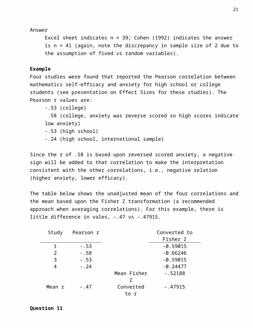
AnswerExcel sheet indicates n = 39; Cohen (1992) indicates the answer is n = 41 (again, note the discrepancy in sample size of 2 due to the assumption of fixed vs random variables).
ExampleFour studies were found that reported the Pearson correlation between mathematics self-efficacy and anxiety for high school or college students (see presentation on Effect Sizes for these studies). The Pearson r values are:
-.53 (college) .58 (college, anxiety was reverse scored so high scores indicate low anxiety)-.53 (high school)-.24 (high school, international sample)
Since the r of .58 is based upon reversed scored anxiety, a negative sign will be added to that correlation to make the interpretation consistent with the other correlations, i.e., negative relation (higher anxiety, lower efficacy).
The table below shows the unadjusted mean of the four correlations and the mean based upon the Fisher Z transformation (a recommended approach when averaging correlations). For this example, there is little difference in vales, -.47 vs -.47915.
Study Pearson r Converted to Fisher Z1 -.53 -0.590152 -.58 -0.662463 -.53 -0.590154 -.24 -0.24477
Mean Fisher Z -.52188Mean r -.47 Converted to r -.47915
Question 11What size sample of college students is needed to have 90% chance to detect a correlation of -.47 with alpha at .01?
AnswerExcel sheet reports n = 56.
17
5. A Priori Power Analysis (Sensitivity Analysis)A priori power analysis can be used to determine whether a study will be sensitive enough to detect a given sized effect.
ExampleAn EdS student wishes to investigate which of two instructional strategies may result in greater student motivation to learn science. Results can be analyzed via a two-group t-test.
The EdS student has access to two classes for this proposed study. The first class has 23 students and the second has 25 students for total sample size of 48.
The EdS student also expects a standardized mean difference of about d = .35 given prior published research.
Question 12What would be the expected power level for this study?
d = .35 alpha = .05 n = 48 df = 1
Note on the Excel sheet the bottom tab named “Power” – select that tab to access the power calculator.
18
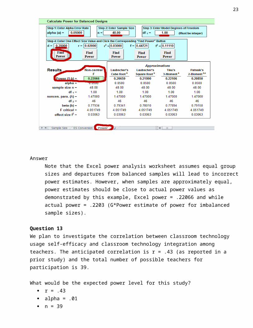
AnswerNote that the Excel power analysis worksheet assumes equal group sizes and departures from balanced samples will lead to incorrect power estimates. However, when samples are approximately equal, power estimates should be close to actual power values as demonstrated by this example, Excel power = .22066 and while actual power = .2203 (G*Power estimate of power for imbalanced sample sizes).
Question 13We plan to investigate the correlation between classroom technology usage self-efficacy and classroom technology integration among teachers. The anticipated correlation is r = .43 (as reported in a prior study) and the total number of possible teachers for participation is 39.
What would be the expected power level for this study? r = .43 alpha = .01 n = 39 df = 1
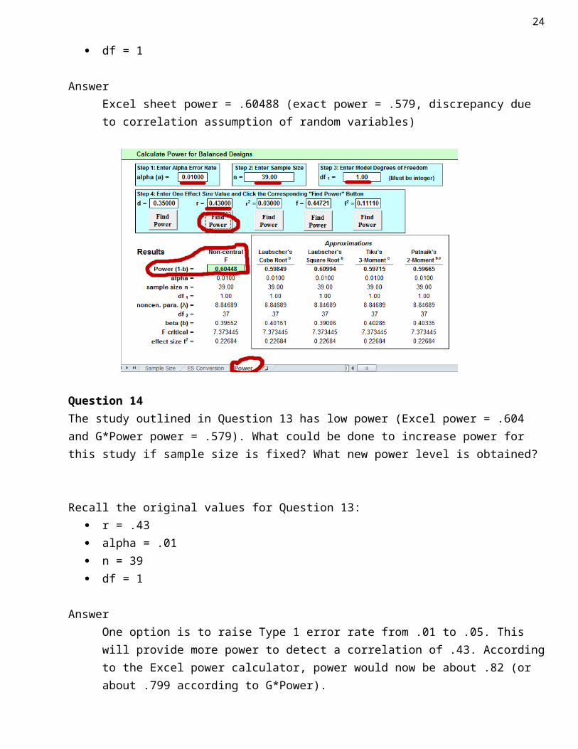
AnswerExcel sheet power = .60488 (exact power = .579, discrepancy due to correlation assumption of random variables)
Question 14The study outlined in Question 13 has low power (Excel power = .604 and G*Power power = .579). What could be done to increase power for this study if sample size is fixed? What new power level is obtained?
19
Recall the original values for Question 13: r = .43 alpha = .01 n = 39 df = 1
AnswerOne option is to raise Type 1 error rate from .01 to .05. This will provide more power to detect a correlation of .43. According to the Excel power calculator, power would now be about .82 (or about .799 according to G*Power).
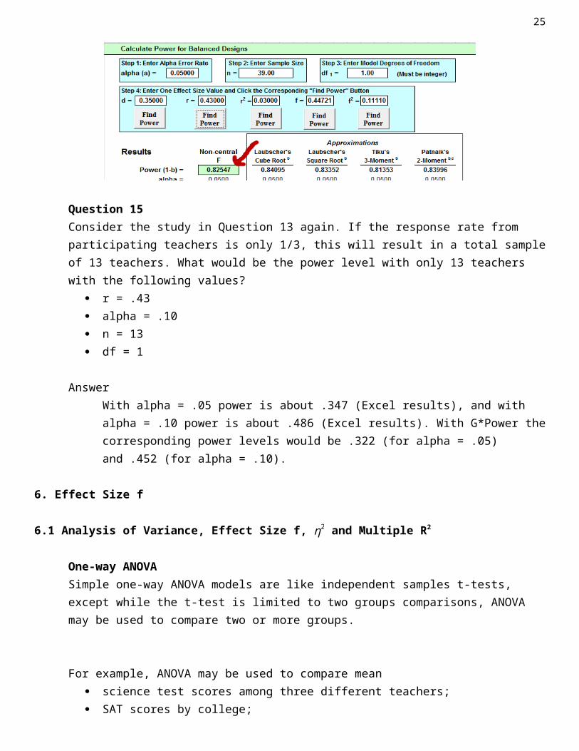
Question 15Consider the study in Question 13 again. If the response rate from participating teachers is only 1/3, this will result in a total sample of 13 teachers. What would be the power level with only 13 teachers with the following values?
r = .43 alpha = .10 n = 13 df = 1
AnswerWith alpha = .05 power is about .347 (Excel results), and with alpha = .10 power is about .486 (Excel results). With G*Power the corresponding power levels would be .322 (for alpha = .05) and .452 (for alpha = .10).
6. Effect Size f
6.1 Analysis of Variance, Effect Size f, η2 and Multiple R2
One-way ANOVASimple one-way ANOVA models are like independent samples t-tests, except while the t-test is limited to two groups comparisons, ANOVA may be used to compare two or more groups.
20
For example, ANOVA may be used to compare mean science test scores among three different teachers; SAT scores by college; motivation scores between treatment and control groups; or salary between females and males.
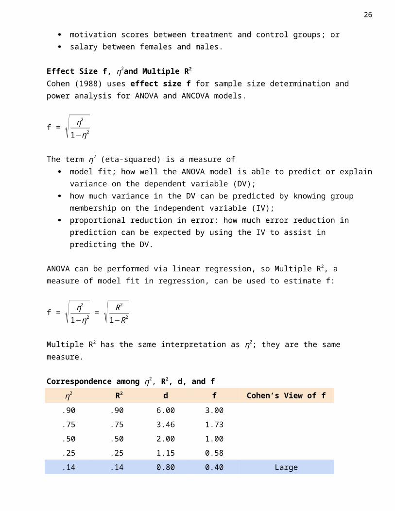
Effect Size f, η2and Multiple R2 Cohen (1988) uses effect size f for sample size determination and power analysis for ANOVA and ANCOVA models.
f = √ η2
1−η2
The term η2 (eta-squared) is a measure of model fit; how well the ANOVA model is able to predict or explain variance on the
dependent variable (DV); how much variance in the DV can be predicted by knowing group membership on the
independent variable (IV); proportional reduction in error: how much error reduction in prediction can be expected
by using the IV to assist in predicting the DV.
ANOVA can be performed via linear regression, so Multiple R2, a measure of model fit in regression, can be used to estimate f:
f = √ η2
1−η2 = √ R2
1−R2
Multiple R2 has the same interpretation as η2; they are the same measure.
Correspondence among η2, R2, d, and f
η2 R2 d f Cohen’s View of f
.90 .90 6.00 3.00
.75 .75 3.46 1.73
.50 .50 2.00 1.00
.25 .25 1.15 0.58
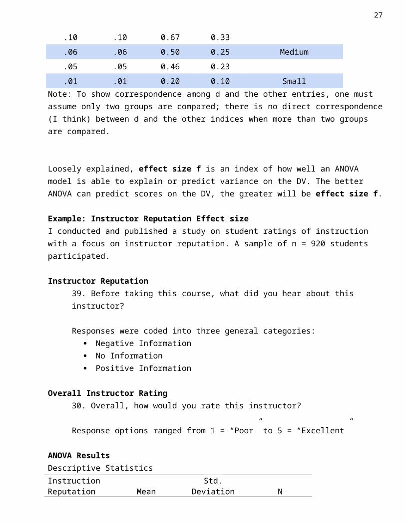
.14 .14 0.80 0.40 Large
.10 .10 0.67 0.33
.06 .06 0.50 0.25 Medium
.05 .05 0.46 0.23
.01 .01 0.20 0.10 Small
21
Note: To show correspondence among d and the other entries, one must assume only two groups are compared; there is no direct correspondence (I think) between d and the other indices when more than two groups are compared.
Loosely explained, effect size f is an index of how well an ANOVA model is able to explain or predict variance on the DV. The better ANOVA can predict scores on the DV, the greater will be effect size f.
Example: Instructor Reputation Effect size I conducted and published a study on student ratings of instruction with a focus on instructor reputation. A sample of n = 920 students participated.
Instructor Reputation39. Before taking this course, what did you hear about this instructor?
Responses were coded into three general categories: Negative Information No Information Positive Information
Overall Instructor Rating30. Overall, how would you rate this instructor?
Response options ranged from 1 = “Poor” to 5 = “Excellent”
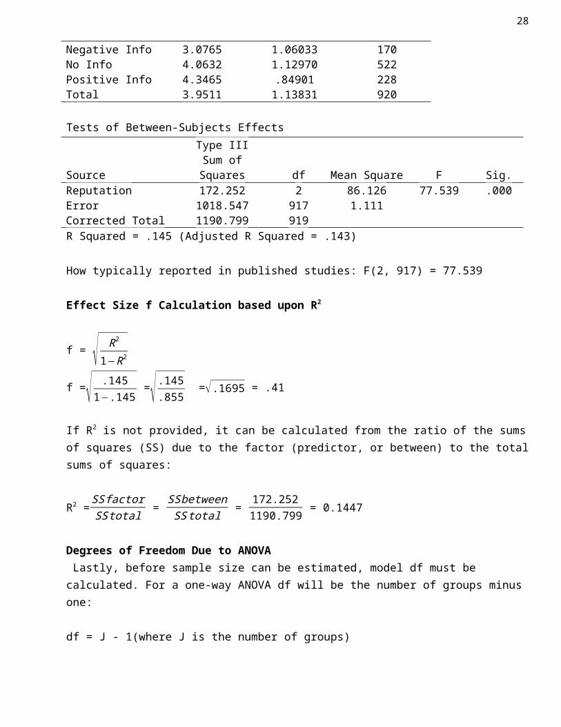
ANOVA ResultsDescriptive Statistics Instruction Reputation Mean Std. Deviation NNegative Info 3.0765 1.06033 170No Info 4.0632 1.12970 522Positive Info 4.3465 .84901 228Total 3.9511 1.13831 920
Tests of Between-Subjects Effects
SourceType III
Sum of Squares df Mean Square F Sig.Reputation 172.252 2 86.126 77.539 .000Error 1018.547 917 1.111Corrected Total 1190.799 919R Squared = .145 (Adjusted R Squared = .143)
How typically reported in published studies: F(2, 917) = 77.539
22
Effect Size f Calculation based upon R2
f = √ R2
1−R2
f =√ .1451−.145
=√ .145.855 =√ .1695 = .41
If R2 is not provided, it can be calculated from the ratio of the sums of squares (SS) due to the factor (predictor, or between) to the total sums of squares:
R2 =SS factorSS total =
SSbetweenSS total =
172.2521190.799 = 0.1447
Degrees of Freedom Due to ANOVA Lastly, before sample size can be estimated, model df must be calculated. For a one-way ANOVA df will be the number of groups minus one:
df = J - 1(where J is the number of groups)
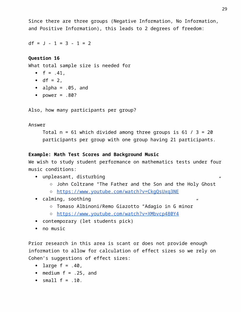
Since there are three groups (Negative Information, No Information, and Positive Information), this leads to 2 degrees of freedom:
df = J - 1 = 3 - 1 = 2
Question 16What total sample size is needed for
f = .41, df = 2, alpha = .05, and power = .80?
Also, how many participants per group?
Answer Total n = 61 which divided among three groups is 61 / 3 = 20 participants per group with one group having 21 participants.
Example: Math Test Scores and Background MusicWe wish to study student performance on mathematics tests under four music conditions:
unpleasant, disturbing ○ John Coltrane “The Father and the Son and the Holy Ghost” ○ https://www.youtube.com/watch?v=CkgQsUxq3NE
calming, soothing○ Tomaso Albinoni/Remo Giazotto “Adagio in G minor”
23
○ https://www.youtube.com/watch?v=XMbvcp480Y4 contemporary (let students pick) no music
Prior research in this area is scant or does not provide enough information to allow for calculation of effect sizes so we rely on Cohen’s suggestions of effect sizes:
large f = .40, medium f = .25, and small f = .10.
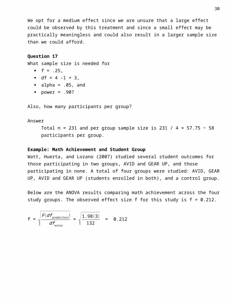
We opt for a medium effect since we are unsure that a large effect could be observed by this treatment and since a small effect may be practically meaningless and could also result in a larger sample size than we could afford.
Question 17What sample size is needed for
f = .25, df = 4 -1 = 3, alpha = .05, and power = .90?
Also, how many participants per group?
AnswerTotal n = 231 and per group sample size is 231 / 4 = 57.75 ~ 58 participants per group.
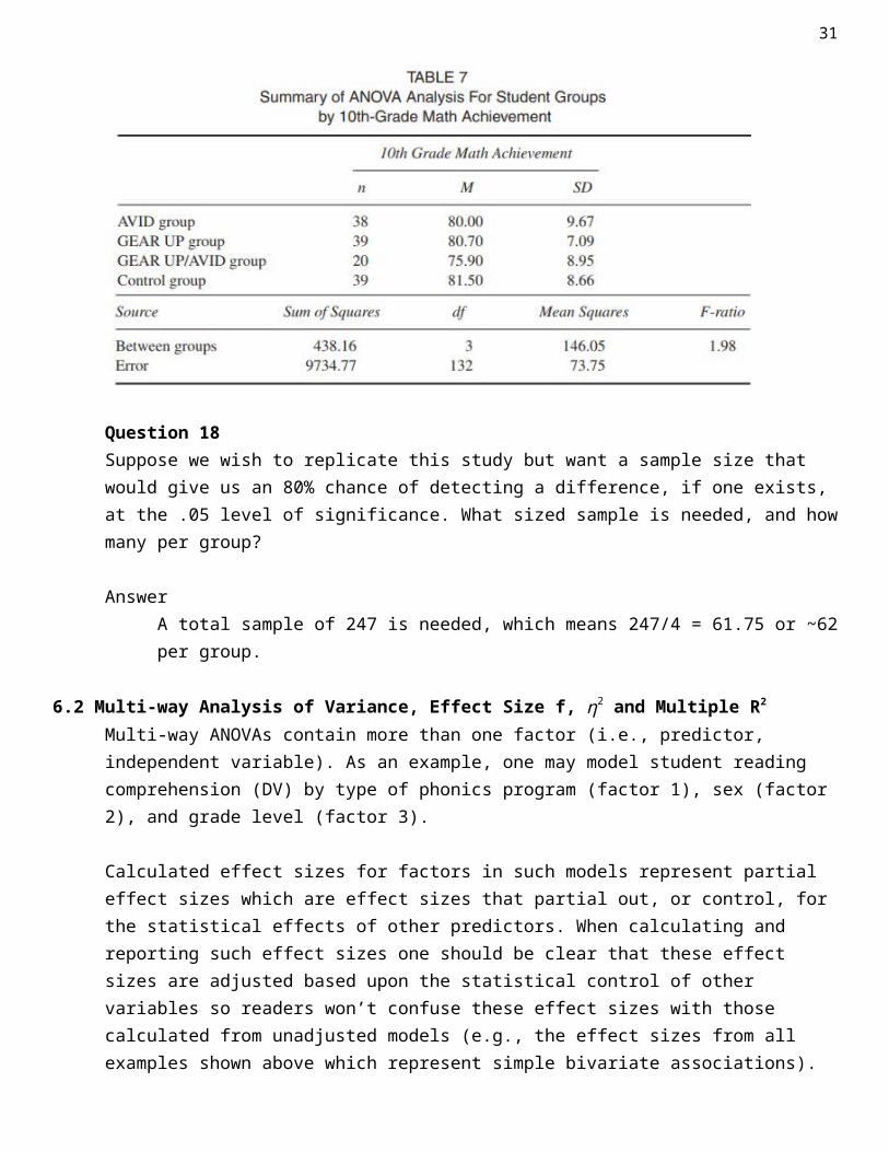
Example: Math Achievement and Student Group Watt, Huerta, and Lozano (2007) studied several student outcomes for those participating in two groups, AVID and GEAR UP, and those participating in none. A total of four groups were studied: AVID, GEAR UP, AVID and GEAR UP (students enrolled in both), and a control group.
Below are the ANOVA results comparing math achievement across the four study groups. The observed effect size f for this study is f = 0.212.
f = √ F (df predictors)df error
= √ 1.98 (3)132 = 0.212
24
Question 18Suppose we wish to replicate this study but want a sample size that would give us an 80% chance of detecting a difference, if one exists, at the .05 level of significance. What sized sample is needed, and how many per group?
AnswerA total sample of 247 is needed, which means 247/4 = 61.75 or ~62 per group.
6.2 Multi-way Analysis of Variance, Effect Size f, η2 and Multiple R2 Multi-way ANOVAs contain more than one factor (i.e., predictor, independent variable). As an example, one may model student reading comprehension (DV) by type of phonics program (factor 1), sex (factor 2), and grade level (factor 3).
Calculated effect sizes for factors in such models represent partial effect sizes which are effect sizes that partial out, or control, for the statistical effects of other predictors. When calculating and reporting such effect sizes one should be clear that these effect sizes are adjusted based upon the statistical control of other variables so readers won’t confuse these effect sizes with those calculated from unadjusted models (e.g., the effect sizes from all examples shown above which represent simple bivariate associations).
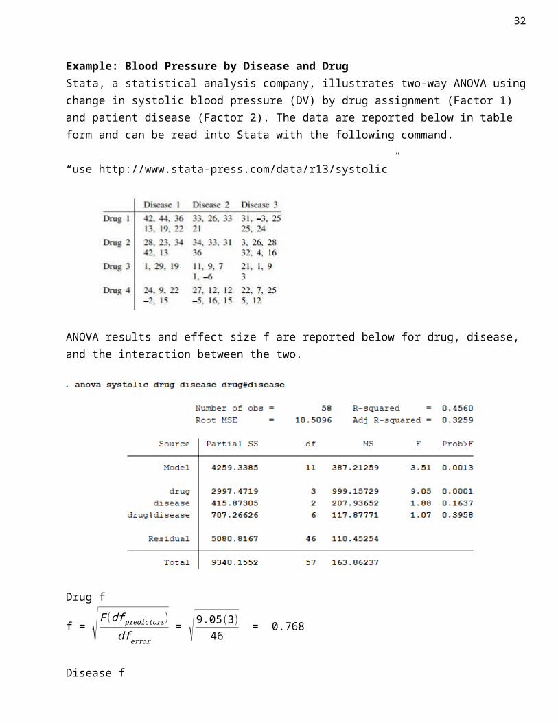
Example: Blood Pressure by Disease and Drug Stata, a statistical analysis company, illustrates two-way ANOVA using change in systolic blood pressure (DV) by drug assignment (Factor 1) and patient disease (Factor 2). The data are reported below in table form and can be read into Stata with the following command.
“use http://www.stata-press.com/data/r13/systolic”
25
ANOVA results and effect size f are reported below for drug, disease, and the interaction between the two.
Drug f
f = √ F (df predictors)df error
= √ 9.05(3)46 = 0.768
Disease f
f = √ F (df predictors)df error
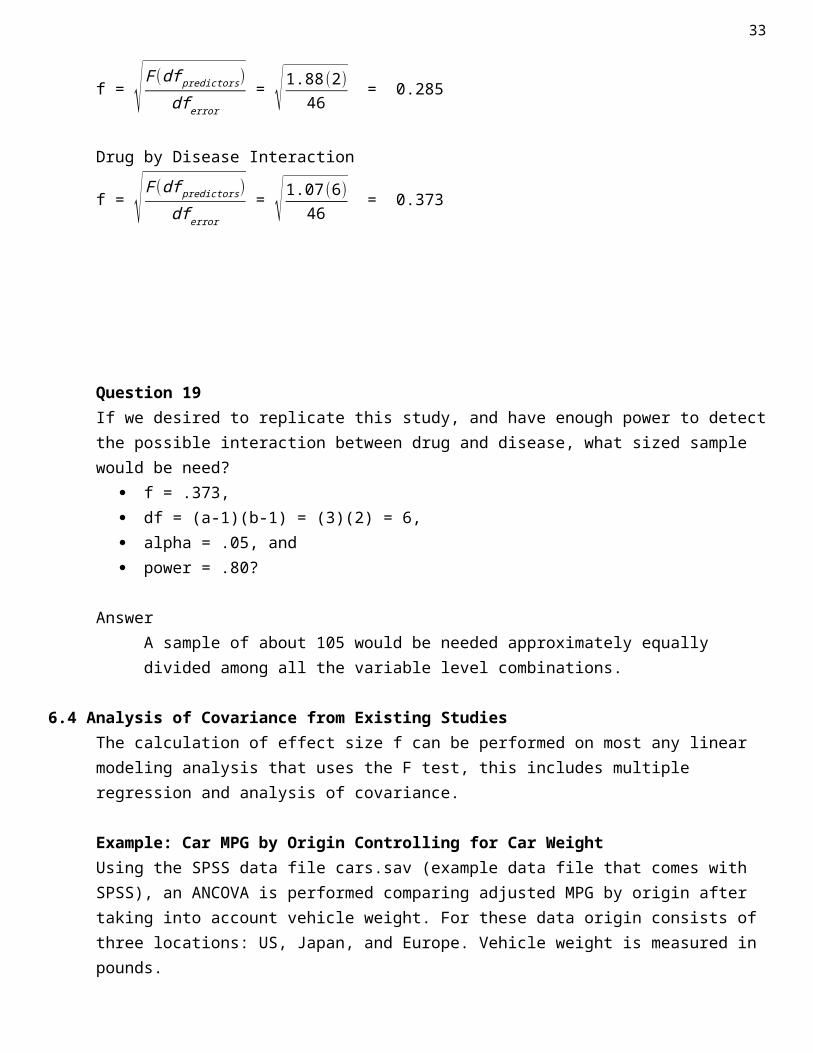
= √ 1.88 (2)46 = 0.285
Drug by Disease Interaction
f = √ F (df predictors)df error
= √ 1.07 (6)46 = 0.373
26
Question 19If we desired to replicate this study, and have enough power to detect the possible interaction between drug and disease, what sized sample would be need?
f = .373, df = (a-1)(b-1) = (3)(2) = 6, alpha = .05, and power = .80?
AnswerA sample of about 105 would be needed approximately equally divided among all the variable level combinations.
6.4 Analysis of Covariance from Existing Studies The calculation of effect size f can be performed on most any linear modeling analysis that uses the F test, this includes multiple regression and analysis of covariance.
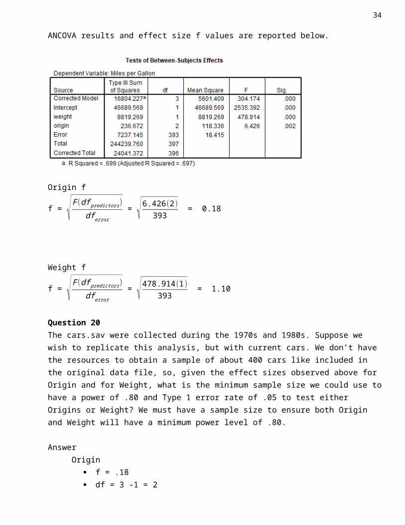
Example: Car MPG by Origin Controlling for Car Weight Using the SPSS data file cars.sav (example data file that comes with SPSS), an ANCOVA is performed comparing adjusted MPG by origin after taking into account vehicle weight. For these data origin consists of three locations: US, Japan, and Europe. Vehicle weight is measured in pounds.
ANCOVA results and effect size f values are reported below.
Origin f
f = √ F (df predictors)df error
= √ 6.426 (2)393 = 0.18
Weight f
27
f = √ F (df predictors)df error
= √ 478.914(1)393 = 1.10
Question 20The cars.sav were collected during the 1970s and 1980s. Suppose we wish to replicate this analysis, but with current cars. We don’t have the resources to obtain a sample of about 400 cars like included in the original data file, so, given the effect sizes observed above for Origin and for Weight, what is the minimum sample size we could use to have a power of .80 and Type 1 error rate of .05 to test either Origins or Weight? We must have a sample size to ensure both Origin and Weight will have a minimum power level of .80.
AnswerOrigin
f = .18 df = 3 -1 = 2 alpha = .05 power = .80 n = 301
Weight f = 1.10 df = 1 alpha = .05 power = .80 n = 9
The relation between Weight and MPG is so strong that a sample of only 9 cars is needed to detect that relationship. However, Origin requires a sample of 301 once Weight is considered, so a sample of only 9 would not provide adequate power to detect the Origin effect, the minimum sample needed is 301.
6.5 Multiple RegressionRegression and ANOVA are part of the general linear model and therefore share the same underlying linear model, so the effect sizes learned above with ANOVA also apply to regression. One differences is that ANOVA traditionally uses F-tests while regression incorporates t-tests of parameter estimates. If the degrees of freedom for the predictor is 1.00, the t-test is equivalent to an F-test, i.e., F = t2. In situations where predictor degrees of freedom do not equal 1.00 (e.g., sets of predictors are tested, or a factor with more than two categories is modeled), one uses an F-test in regression.
Given this equivalence, formulas posted above continue to work for regression, and the t-test can be converted to f by squaring t and using formula F6.
f = √ F (df predictors)df error
28
f = √ t 2
df error
Example: Car MPG Regression on Weight, Horsepower, and Engine DisplacementUsing the SPSS data file cars.sav, and MPG was regressed upon three predictors: vehicle weight, horsepower, and engine displacement in cubic inches.
SPSS results and ES f are presented below. Two tables of information are needed, the ANOVA summary so df error can be found (df2 = 388), and the coefficient table so t-ratios can be obtained.
Horsepower
f = √ t 2
df error = √−4.1532
388 = .21
Weight
f = √ t 2
df error = √−6.1862
388 = .31
Displacement
f = √ t 2
df error = √−0.7862
388 = .039
Question 21
29
If we wished to replicate this study with current production cars, what sized sample would be needed to detect the smallest effect size observed in the above regression with power = .90 and alpha = .01?
AnswerThe smallest effect size is associated with Displacement with f = 0.039. Keep in mind this is a partialed effect size that represents statistical control that takes into account both Weight and Horsepower. The replication study must also include these predictors otherwise the effect size observed for Displacement may be invalid without the presence of these two predictors.
f = .039 df = 1 alpha = .01 power = .90 n = 9,786
This result show that a very large sample (n = 9,786) is required to detect the small contribution that Displacement added to the model over the effects of Horsepower and Weight. Given the small effect of Displacement once Horsepower and Weight are controlled, I probably would not replicate this study and instead would focus on just Horsepower and Weight if I could see similar results from a second data file or study.
7. Effect Size f2 Discussion to be added and expanded. In short, f2 is just effect size f squared, so little new information is obtained from f2. All examples shown above with f also work with f2 and provide the same answer. Cohen introduced f2 in discussion of power and sample size with regression since f was defined as a measure of group mean variability which is more common in ANOVA models than regression models.
8. Effect Size f and ANCOVA for Prospective, Experimental Studies (Not covered in EDUR 9131 spring 2018)
(Note that this approach assumes variable targeted for adjustment is uncorrelated with added covariates or predictors, so this approach works well for true experimental studies, but not for studies in which groups are not randomly formed since covariates are likely to be correlated with targeted variable and resultant adjustment is difficult to predict – better to find existing study with same predictors and obtain ES from existing study.)
An ANCOVA is formed when covariates are added to an ANOVA model. The addition of covariates leads to increased power and precision of model estimates due to a reduction in the model error term. The addition of covariates may also result in adjusted group means on the dependent variable (DV) to reflect statistical control, or partialing effect, of added covariates.
30
Cohen (1988) writes that sample size and power analysis procedures for ANCOVA proceeds like that for ANOVA except that the adjusted means --- adjusted for the covariates --- are used for calculating effect sizes of interest.
One approach to incorporating covariate influence on the ANOVA model for determining n or power is to adjust effect size estimates based upon anticipated explanatory power added by covariates.
For example, if one believes that a covariate, or set of covariates, will correlate with the DV at the r = .30 level (or multiple R = .30 in case of multiple covariates), then this correlation can be employed to adjust the effect size used in determining sample size for an ANOVA model. The formula for adjustment follows:
adjusted effect size = effect ¿¿√(1−r2)¿ = effect ¿¿√(1−R2)¿
where effect size refers to d or f; neither squared effect sizes such as f2 or r2, nor Pearson r, should be adjusted using the above formula since the adjustment for these values is nonlinear.
Below are two illustrations of this process.
Illustration ASample size for an ANOVA model with four groups is estimated using the following criteria
alpha = .05 power = .80 df = 3 f = .20
Resulting ANOVA total n = 277 so the per-group n would be 277 / 4 = 69.25 or about 70 per group.
A covariate will be added to this ANOVA model and prior research suggests the correlation between this covariate and the DV is r = .35. With this value of r, the ANCOVA adjusted effect size, f, would be:
adjusted f ¿ f
√(1−r 2)= .20
√(1−.352)= .20
√(1−.1225)
¿ .20√.8775
= .20.9367
=¿.2135
One would then use this adjusted f of .2135 as the effect size for determining sample size. There will be no need to adjust degrees of freedom from the original ANOVA model sample size calculation; only the effect size estimate must be adjusted.
Entering the following criteria
31
alpha = .05 power = .80 df = 3 adjusted f = .20 .2135
results in a total n of 244 or about 61 participants per group. Adding the covariate has reduced the required sample size from 277 to 244.
Illustration BWe wish to compare mathematics SAT means between females and males. Given College Board results cited earlier, the anticipated effect size d is -0.27.
Using these criteria alpha = .05 power = .85 df = 1 d = -0.27
the sample size for this t-test is n = 495 or about 248 per group.
We wish to add three covariates to this study: mathematics self-efficacy, mathematics anxiety, and IQ scores. While it is difficult to know how much predictive power these three measures will bring to the model of mathematics SAT scores, we know from prior research that each variable correlates between .20 and .40, in absolute value, with various academic assessments. Together we anticipate these three variables would contribute to a total model R2 of about .25.
The resulting adjusted d value can be found as follows:
adjusted d¿ d
√(1−R2)= −.27
√(1−.25)=−.27
√.75
¿ −.27.866
=¿-.3118
What sample size is needed to detect SAT mean differences once these covariates are taken into account?
Using these criteria alpha = .05 power = .85 df = 1 adjusted d = -.27 -0.3118
the required sample size for this ANCOVA is n = 372 or about 186 females and 186 males. This sample size estimate agrees (within rounding error) with that obtained from Stata (version 12), a statistical software program that can be used to estimate n for a two-group ANCOVA study.
32
Stata Sample Size Estimate
. sampsi 0 -.27, pre(1) post(1) p(0.85) r01(.5) sd1(1) sd2(1) m(ancova)
Estimated sample size for two samples with repeated measuresAssumptions:
alpha = 0.0500 (two-sided)power = 0.8500m1 = 0m2 = -.27sd1 = 1sd2 = 1n2/n1 = 1.00
number of follow-up measurements = 1number of baseline measurements = 1correlation between baseline & follow-up = 0.500
Method: ANCOVArelative efficiency = 1.333adjustment to sd = 0.866adjusted sd1 = 0.866adjusted sd2 = 0.866
Estimated required sample sizes:n1 = 185n2 = 185
Question 22 (Problematic example, for adjustment to work as modeled, covariates must be uncorrelated with instructor reputation, otherwise very difficult to predict how the adjustment will affect the original effect size)
Recall the instructor reputation and overall rating of instruction example. Suppose we include three covariates in this study:
student intrinsic motivation in the course subject, student GPA, and student rating of course difficulty.
In the original analysis R2 = .145 for the sole predictor of instructor reputation, which computes to an effect size f = .412.
We believe these three predictors will uniquely account for about 6% of the variance in student ratings, so their R2 contribution is estimated to be .06.
33
The adjusted effect size f after adding this predictor is:
adjusted f¿f
√(1−R2)= .412
√(1−.06)= .412
√.94
¿ .412.9695
=¿ 0.425
What would be the sample size needed now that these covariates are taken into account? adjusted f = .425, df = 2, alpha = .05, and power = .80?
Also, how many participants per group?
AnswerTotal n = 57Per group sample size is 57 / 3 = 19 per group
Question 23The music experiment in Question 17 required a total sample of 231. Suppose a pretest of mathematics is administered to students and used as a covariate to help equate groups and reduce model error.
Often pretest measures of achievement correlate well with posttest achievement scores, so anticipate a correlation of .40 between pretest and posttest. Converting this correlation to r2 = .4x.4 = .16.
In the original study we expected f = .25; the adjusted effect size f would be
adjusted f¿f
√(1−r 2)= .25
√(1−.16)= .25
√.84
¿ .25.9165
=¿ 0.273
What sample size is needed for adjusted f = .273, df = 3, alpha = .05, and power = .90?
34
Also, how many participants per group? Lastly, how does this sample size compare with the original of 231?
AnswerTotal n = 195Sample size per group is 195 / 4 = 48.75 or 49 per group.Original study n = 231, but addition of covariate reduced this number to 195, a potential savings in resources and effort.
CautionsThe procedures outlined above assume no correlation between covariates and group membership, i.e., no differences in covariate means among groups of the factor/independent variable of interest.
If group membership is correlated with covariate scores (e.g., group A has a lower covariate mean than group B), then the correlation employed to adjust the effect size will likely be overlarge.
In most cases the result of a correlation between covariate and group membership is a reduction of power for detecting mean differences on the DV; thus estimated sample sizes for the ANCOVA will be too small.
The ANCOVA steps explained above work best for experimental designs in which groups are randomly formed since this likely produces no correlation between group membership and covariates. Stated differently, random formation of groups from a common population of participants assures that groups, over the long run, are equivalent on possible confounding variables. This equivalence results in no differences, or only trivial differences, in covariate means between groups. In this situation there is no correlation, or only a trivially small correlation, between group membership and covariate scores.
In studies with intact, pre-existing groups that were not randomly formed, it is very likely that covariates will correlate, perhaps substantially, with group membership variables. For sample size determination, partial correlations to identify the unique contribution of covariates partialed from group membership variables are needed for effect size adjustment.
Sources for ANCOVA adjustment approach outlined above: Lipsey, M. (1990). Design sensitivity: Statistical Power for Experimental Research. p 131. (2
group comparison) Cohen (1988) p. 432. (4 groups) Maxwell, S. E., & Delaney, H. D. (2004). Designing experiments and analyzing data: A model
comparison perspective (2nd ed.). Belmont, CA: Wadsworth. p. 442. (3 group comparison) Shan G, Ma C (2014) A Comment on Sample Size Calculation for Analysis of Covariance in
Parallel Arm Studies. J Biomet Biostat 5: 184. Beyene, N. & Lui, K. (2001). Sample Size Determination for Analysis of Covariance.
Proceedings of the Annual Meeting of the American Statistical Association, August 5-9.
35
PASS Sample Size Software, Chapter 551 Analysis of Covariance, NCSS.com (note their ES is f, not d, for output; p. 10)
References
Cohen, J. (1988). Statistical power analysis for the behavioral sciences (2nd). Erlbaum: Hillsdale, NJ.
Cohen, J. (1992). A power primer. Psychological Bulletin, 112, 155-159.