Figure S1. Illustration of measuring the slip face advance on a barchan sand dune. The yellow shaded region is the area covered by the slip face between the two co-registered HiRISE images. The black curve is the length of the active region of the slip face. These two values’ ratios reveal the characteristic dune migration distance during the images’ time interval, giving dune speed. Multiplying the speed by the crest height gives the volumetric sand flux at the crest. The estimated uncertainty is 10 pixels in both the overlap area (± 0.6 m2) and the arc length (± 2.5 m) measurement, and ± 1 m height from the DEM, giving an estimated flux uncertainty of ~10% for similar measurements. The scale bar is 50 m long and north is up. The co-registered HiRISE images are PSP_002728_1645 and ESP_037948_1645.

Text S1. Study Site: Herschel Crater Herschel crater (14.4˚S, 130˚E) is a degraded Noachian peak-ring basin almost 300 km in diameter located in the southern highlands [Tanaka et al., 2014; Cardinale et al., 2016]. It features multiple aeolian landforms: barchan, barchanoid, and dome dune fields; numerous sand sheets; sand ripples; and indurated transverse aeolian ridges (TARs). It thus serves as a natural laboratory for studying dune and ripple migration rates and direction, sediment flux, deposition and erosion rates, sediment sources and sinks, bedform induration, bedform morphology changes, and generally the evolution of a landscape as caused by wind-mobilized sediment over most of Mars’ geologic history.

Nili Patera and HiRISEThe Nili Patera dune field has been studied extensively [Bridges et al., 2012; Ayoub et al., 2014] at 25 cm/px resolution from HiRISE’s (High Resolution Imaging Science Experiment) orbital altitude and has shown to be quite active and to vary in activity seasonally and annually. We extended the use of HiRISE to monitor several portions of the Herschel Crater dune field.

In the manner of Bridges et al. [2012], we used three HiRISE images per location: two images taken close together in time (a few months) allowed digital elevation model (DEM) construction, and one of those images compared against a later orthoimage allowed for tracking dune migration.

Repeat HiRISE coverage at Nili Patera did not extend as far downwind as needed to measure crest fluxes on distal dunes. Thus we can only compare the central and upwind portions of the Nili dune field to the Herschel dune fields.

Text S2. Mobility Intermittency EstimationOur numeric atmospheric circulation models allowed us to investigate the fraction of time the wind was above the critical shear stress threshold 𝜏c. First we integrated under the histogrammed data using Matlab’s trapezoid approximation method with the command “trapz” (blue and red data points in Figure S2). Then, we selected the shear stresses at and above threshold and integrated under those data (red in Figure S2). Then we took the ratio of above-threshold to all data (red/(red+blue) data points). In this case, illustrated in Figure S2 for East Herschel, the critical threshold value was 𝜏c = 0.01 N m-2, and the ratioed integrands are 0.035521/0.38661 = 0.092 ~ 9%. So, sediment should be mobile 9% of the time. Corresponding values of u*, I, and U for 𝜏c = 0.01 N m-2 are given in Table S2.

Text S3. IBL Flux Equation CoefficientOur usage of the 0.055 coefficient, by coincidence, is ten times greater than that used by Jerolmack et al. (2012) (see their Supplementary sections 4-5) and is a phenomenological friction factor. The coefficient they use of 0.0055 is partly derived from Glauert's (1956) formulation of Blasius' (1913) boundary layer shear stress equation τ=0.0225 ρatmoU

2( νUδ )14 , where 𝛿 is the

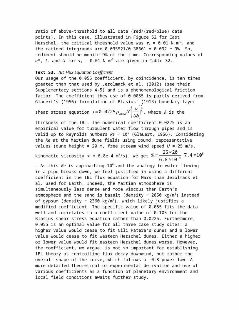
thickness of the IBL. The numerical coefficient 0.0225 is an empirical value for turbulent water flow through pipes and is valid up to Reynolds numbers Re ~ 105 (Glauert, 1956). Considering the Re at the Martian dune fields using round, representative values (dune height = 20 m, free stream wind speed U = 25 m/s, kinematic viscosity 𝜈 = 6.8e-4 m2/s), we get ℜ= 25×20

6.8×10−4 7.4×105. As this Re is approaching 106 and the analogy to water flowing in a pipe breaks down, we feel justified in using a different coefficient in the IBL flux equation for Mars than Jerolmack et al. used for Earth. Indeed, the Martian atmosphere is simultaneously less dense and more viscous than Earth’s atmosphere and the sand is basalt (density ~ 2850 kg/m3) instead of gypsum (density ~ 2360 kg/m3), which likely justifies a modified coefficient. The specific value of 0.055 fits the data well and correlates to a coefficient value of 0.105 for the Blasius shear stress equation rather than 0.0225. Furthermore, 0.055 is an optimal value for all three case study sites: a higher value would cease to fit Nili Patera's dunes and a lower value would cease to fit western Herschel dunes. Either a higher or lower value would fit eastern Herschel dunes worse. However, the coefficient, we argue, is not so important for establishing IBL theory as controlling flux decay downwind, but rather the overall shape of the curve, which follows a -0.3 power law. A more detailed theoretical or experimental derivation and use of various coefficients as a function of planetary environment and local field conditions awaits further study.

Table S1. Values used in calculating <qs> in the main text.

Variable Value & Units Description

C 3.88 Friction coefficient for sand at Mars’ Reynolds number < 10

D 250 µm Characteristic grain size, µm

D0 100 µm Reference grain size (standard), µm

g 3.7 m/s2 Mars gravity, m/s2

u*a Typically ~1.1 m/s Critical threshold friction speed, m/s (not a physical speed)

U Typically 24-27 m/s

Free stream air velocity, m/s

x (Independent Variable)

Distance downwind from the upwind margin, m

h 17 m22 m28 m

W Herschel dune heightsE HerschelNili Patera

s 3009 m2

2167 m2

3136 m2

Western Herschel frontal dune area (characteristic cross-sectional area per dune that the wind “sees”)Eastern Herschel frontal dune areaNili Patera frontal dune area

n/A 9.5 × 10-6 dunes m-2

1.38 × 10-5 dunes m-2

6.8 × 10-6 dunes m-2

W Herschel spatial dune densityE Herschel spatial dune densityNili Patera spatial dune density

ν 6.8831 x 10-4 m2/s Kinematic viscosity of the atmosphere

H, z 10000 m Top of atmospheric boundary layer

ρatmo 0.013-0.015 kg/m3 Air density

ρsolid 2850 kg/m3 Density of basaltic sand grains

Figure S2. The predicted wind shear stress histogram for Nili Patera from our model. The ratio of the integrands of the above-threshold shear stresses (here, 0.01 N m-2, red) to the total histogram (blue and red points) yields the mobility intermittency value I. Here, I = 0.09 (Table S2).

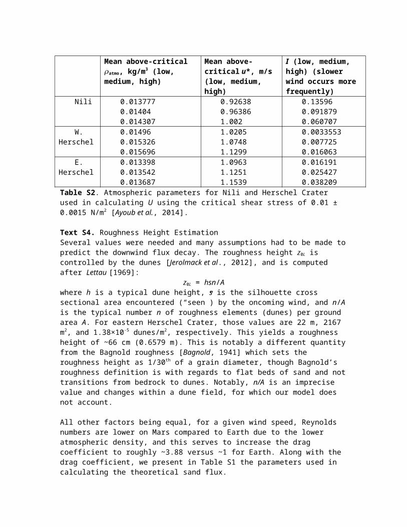
Table S2. Atmospheric parameters for Nili and Herschel Crater used in calculating U using the critical shear stress of 0.01 ± 0.0015 N/m2 [Ayoub et al., 2014].

Text S4. Roughness Height EstimationSeveral values were needed and many assumptions had to be made to predict the downwind flux decay. The roughness height z0L is controlled by the dunes [Jerolmack et al., 2012], and is computed after Lettau [1969]:

z0L = hsn/Awhere h is a typical dune height, s is the silhouette cross sectional area encountered (“seen”) by the oncoming wind, and n/A is the typical number n of roughness elements (dunes) per ground area A. For eastern Herschel Crater, those values are 22 m, 2167 m2, and 1.38×10-5 dunes/m2, respectively. This yields a roughness height of ~66 cm (0.6579 m). This is notably a different quantity from the Bagnold roughness [Bagnold, 1941] which sets the roughness height as 1/30th of a grain diameter, though Bagnold’s roughness definition is with regards to flat beds of sand and not transitions from bedrock to dunes. Notably, n/A is an imprecise value and changes within a dune field, for which our model does not account.

All other factors being equal, for a given wind speed, Reynolds numbers are lower on Mars compared to Earth due to the lower atmospheric density, and this serves to increase the drag coefficient to roughly ~3.88 versus ~1 for Earth. Along with the drag coefficient, we present in Table S1 the parameters used in calculating the theoretical sand flux.

Mean above-critical 𝜌atmo, kg/m3 (low, medium, high)

Mean above-critical u*, m/s (low, medium, high)

I (low, medium, high) (slower wind occurs more frequently)

Nili 0.0137770.014040.014307

0.926380.963861.002

0.135960.0918790.060707

W. Herschel

0.014960.0153260.015696

1.02051.07481.1299

0.00335530.0077250.016063

E. Herschel

0.0133980.0135420.013687

1.09631.12511.1539

0.0161910.0254270.038209

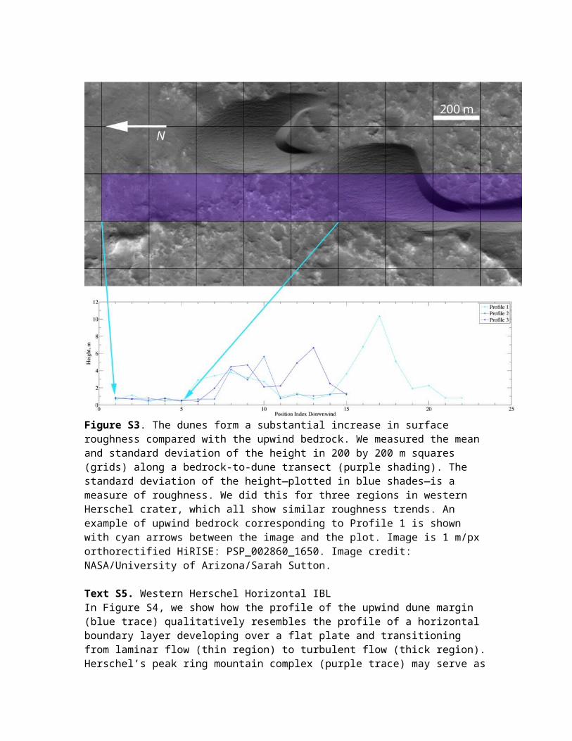
Figure S3. The dunes form a substantial increase in surface roughness compared with the upwind bedrock. We measured the mean and standard deviation of the height in 200 by 200 m squares (grids) along a bedrock-to-dune transect (purple shading). The standard deviation of the height—plotted in blue shades—is a measure of roughness. We did this for three regions in western Herschel crater, which all show similar roughness trends. An example of upwind bedrock corresponding to Profile 1 is shown with cyan arrows between the image and the plot. Image is 1 m/px orthorectified HiRISE: PSP_002860_1650. Image credit: NASA/University of Arizona/Sarah Sutton.

Text S5. Western Herschel Horizontal IBLIn Figure S4, we show how the profile of the upwind dune margin (blue trace) qualitatively resembles the profile of a horizontal boundary layer developing over a flat plate and transitioning from laminar flow (thin region) to turbulent flow (thick region). Herschel’s peak ring mountain complex (purple trace) may serve as a “plate,” creating a boundary layer which controls the location of the dune field. However, no obvious corresponding relationship exists on the eastern side of the peak ring complex.

Figure S4. Putative “sideways IBL” highlighted in blue from the peak-ring complex highlighted in purple which possibly may control the shape of the western Herschel dune field margin. The red outlines denote the location of HiRISE “footprints.” Context Camera image mosaic from GoogleMars.