Embed Size (px)
DESCRIPTION
Metodo taguchi
Citation preview

GRPS 2012-2013 - Maria Caridi
Qualità robusta
Maria Caridi
1
GRPS 2012-2013 - Maria Caridi
La qualità è una proprietà dei prodotti (e dei processi utilizzati) misurabile attraverso il costo indotto alla società.
Tale costo include• costi di rilavorazione• costi per garanzia e interventi di assistenza• costi di inefficienza per scarsa qualità del prodotto.
La qualità secondo Taguchi
Overall loss = quality loss (after shipping) + factory loss
GRPS 2012-2013 - Maria Caridi
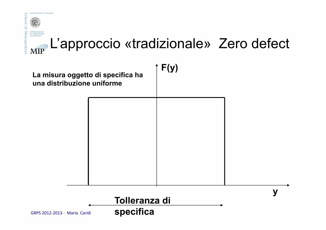
F(y)
yTolleranza di specifica
L’approccio «tradizionale» Zero defect
La misura oggetto di specifica ha una distribuzione uniforme
GRPS 2012-2013 - Maria Caridi
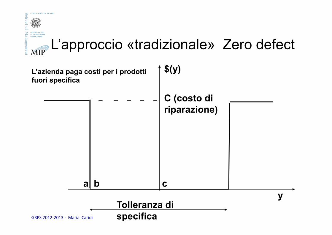
$(y)
yTolleranza di specifica
C (costo diriparazione)
L’approccio «tradizionale» Zero defect
L’azienda paga costi per i prodotti fuori specifica
a b c
GRPS 2012-2013 - Maria Caridi
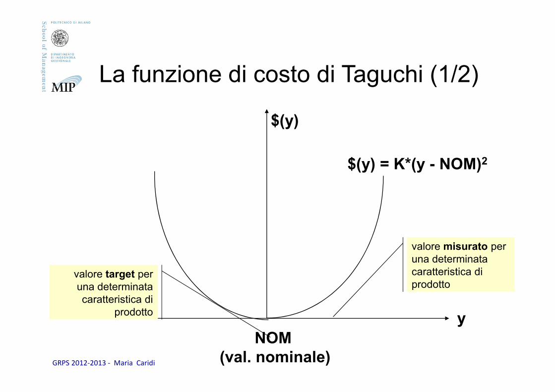
$(y) = K*(y - NOM)2
$(y)
NOM(val. nominale)
y
La funzione di costo di Taguchi (1/2)
valore target per una determinata caratteristica di
prodotto
valore misurato per una determinata caratteristica di prodotto
GRPS 2012-2013 - Maria Caridi
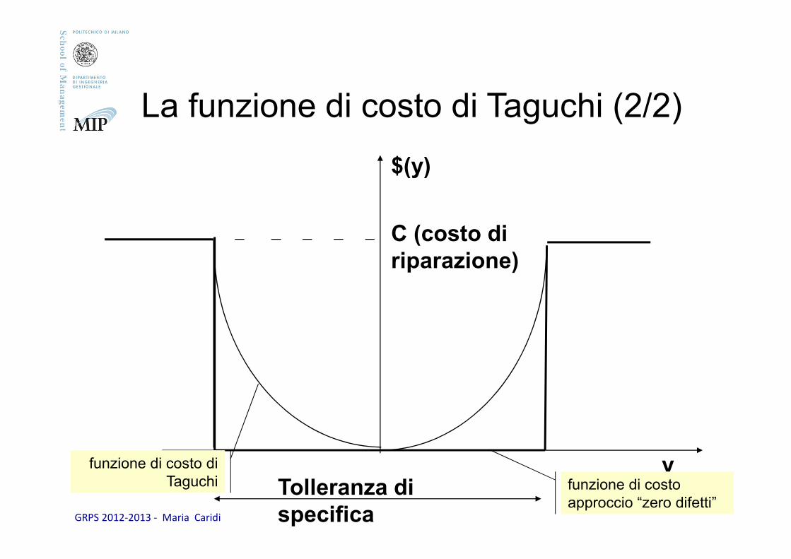
$(y)
yTolleranza di specifica
C (costo diriparazione)
La funzione di costo di Taguchi (2/2)
funzione di costo di Taguchi funzione di costo
approccio “zero difetti”
GRPS 2012-2013 - Maria Caridi
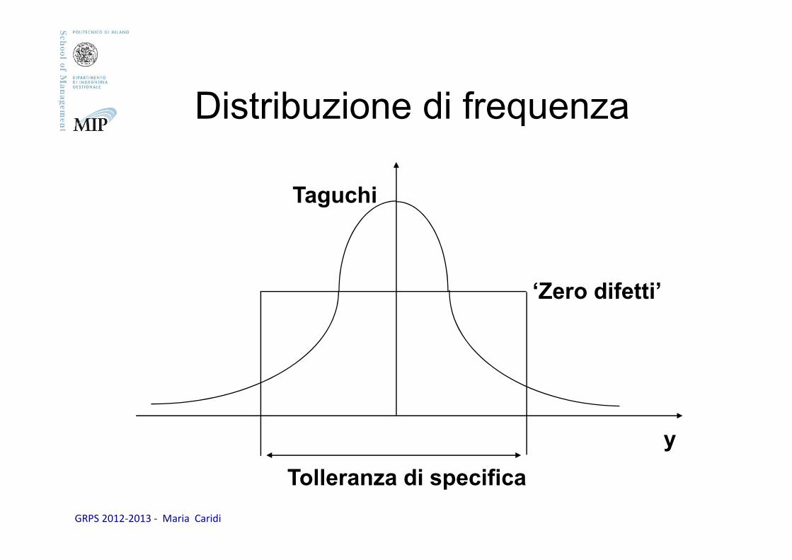
Tolleranza di specifica
Taguchi
‘Zero difetti’
y
Distribuzione di frequenza
GRPS 2012-2013 - Maria Caridi
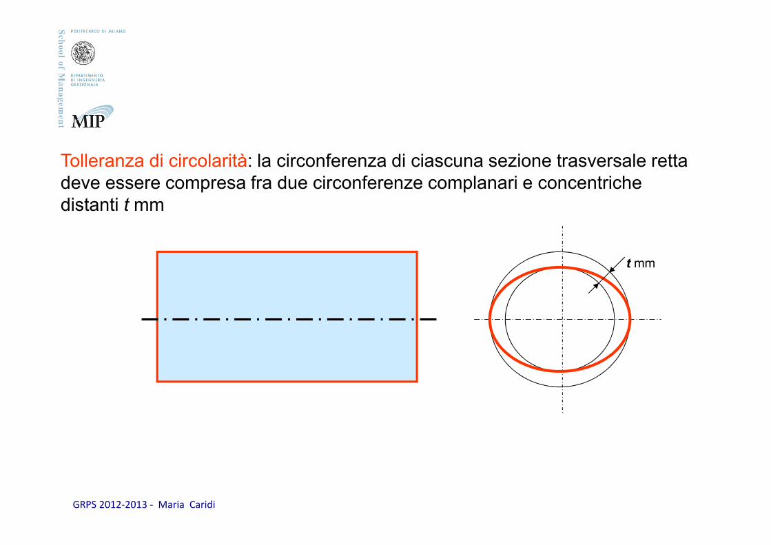
Tolleranza di circolarità: la circonferenza di ciascuna sezione trasversale rettadeve essere compresa fra due circonferenze complanari e concentrichedistanti t mm
t mm
GRPS 2012-2013 - Maria Caridi
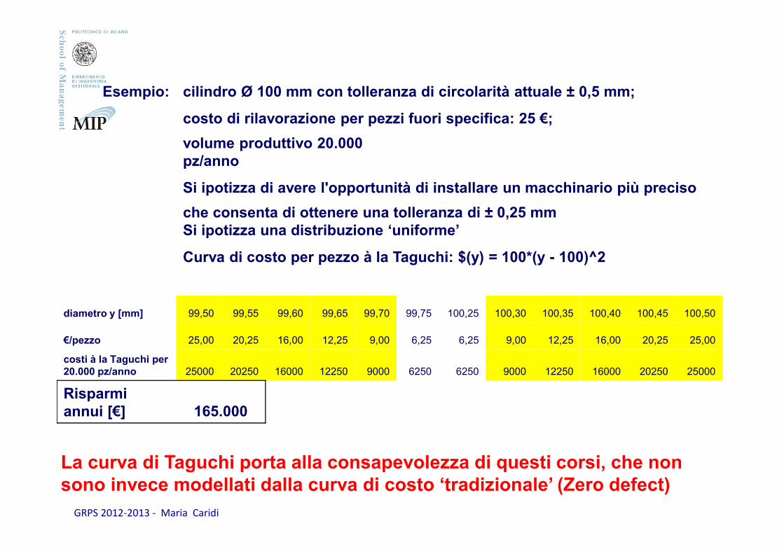
Esempio: cilindro Ø 100 mm con tolleranza di circolarità attuale ± 0,5 mm;
costo di rilavorazione per pezzi fuori specifica: 25 €;
volume produttivo 20.000 pz/anno
Si ipotizza di avere l'opportunità di installare un macchinario più preciso
che consenta di ottenere una tolleranza di ± 0,25 mmSi ipotizza una distribuzione ‘uniforme’
Curva di costo per pezzo à la Taguchi: $(y) = 100*(y - 100)^2
diametro y [mm] 99,50 99,55 99,60 99,65 99,70 99,75 100,25 100,30 100,35 100,40 100,45 100,50
€/pezzo 25,00 20,25 16,00 12,25 9,00 6,25 6,25 9,00 12,25 16,00 20,25 25,00
costi à la Taguchi per 20.000 pz/anno 25000 20250 16000 12250 9000 6250 6250 9000 12250 16000 20250 25000
Risparmi annui [€] 165.000
La curva di Taguchi porta alla consapevolezza di questi corsi, che non sono invece modellati dalla curva di costo ‘tradizionale’ (Zero defect)
GRPS 2012-2013 - Maria Caridi
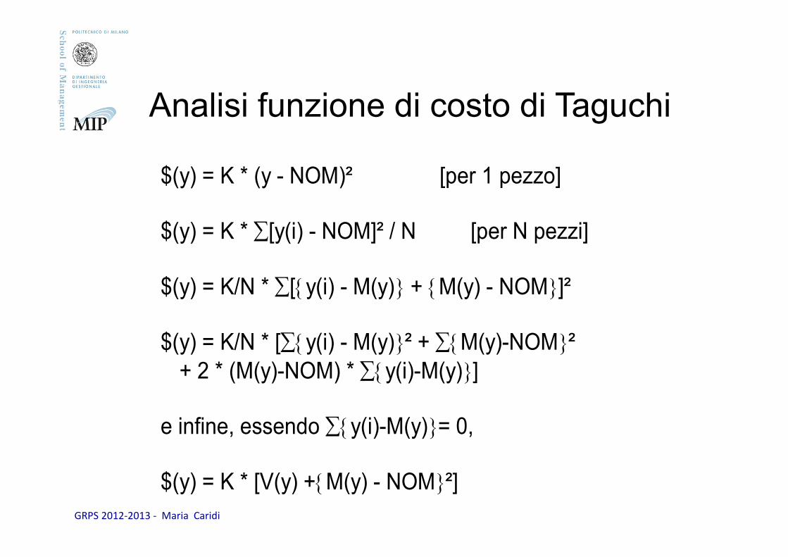
$(y) = K * (y - NOM)² [per 1 pezzo] $(y) = K * ∑[y(i) - NOM]² / N [per N pezzi] $(y) = K/N * ∑[{y(i) - M(y)} + {M(y) - NOM}]² $(y) = K/N * [∑{y(i) - M(y)}² + ∑{M(y)-NOM}² + 2 * (M(y)-NOM) * ∑{y(i)-M(y)}] e infine, essendo ∑{y(i)-M(y)}= 0, $(y) = K * [V(y) +{M(y) - NOM}²]
Analisi funzione di costo di Taguchi
GRPS 2012-2013 - Maria Caridi
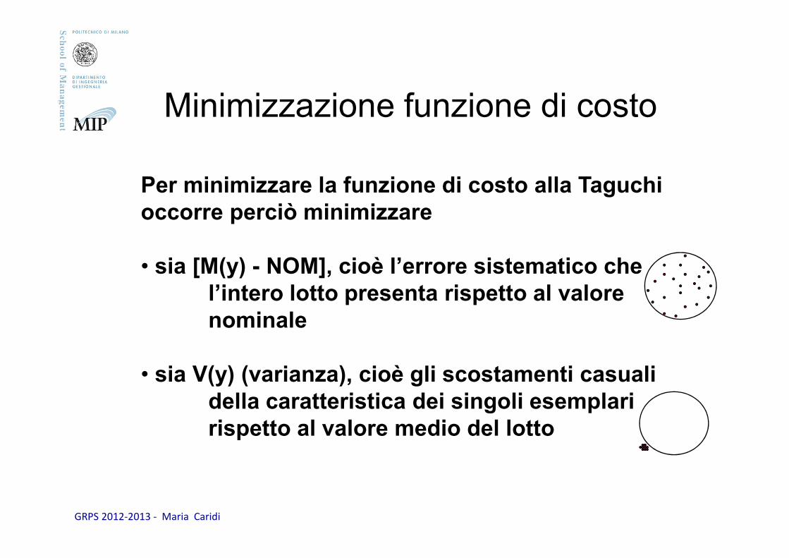
Per minimizzare la funzione di costo alla Taguchi occorre perciò minimizzare
• sia [M(y) - NOM], cioè l’errore sistematico che l’intero lotto presenta rispetto al valorenominale
• sia V(y) (varianza), cioè gli scostamenti casualidella caratteristica dei singoli esemplaririspetto al valore medio del lotto
Minimizzazione funzione di costo
GRPS 2012-2013 - Maria Caridi
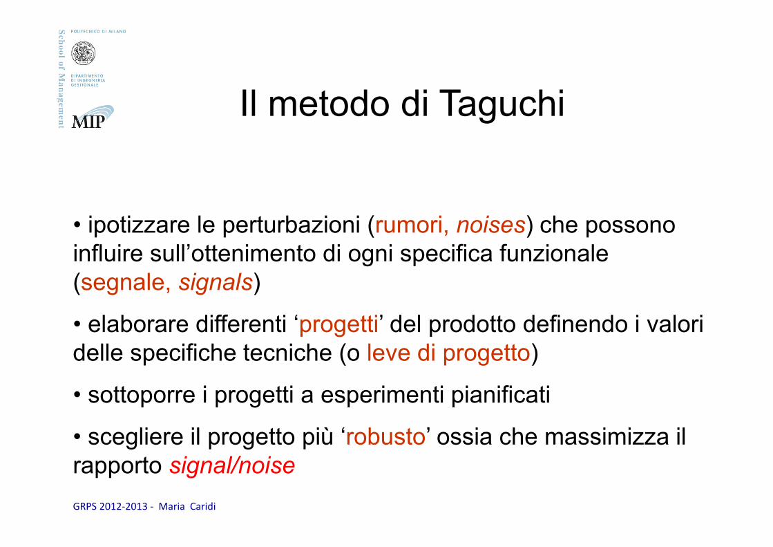
• ipotizzare le perturbazioni (rumori, noises) che possono influire sull’ottenimento di ogni specifica funzionale (segnale, signals)
• elaborare differenti ‘progetti’ del prodotto definendo i valori delle specifiche tecniche (o leve di progetto)
• sottoporre i progetti a esperimenti pianificati
• scegliere il progetto più ‘robusto’ ossia che massimizza il rapporto signal/noise
Il metodo di Taguchi
GRPS 2012-2013 - Maria Caridi
Tipi di fattori in relazione all’effetto
13
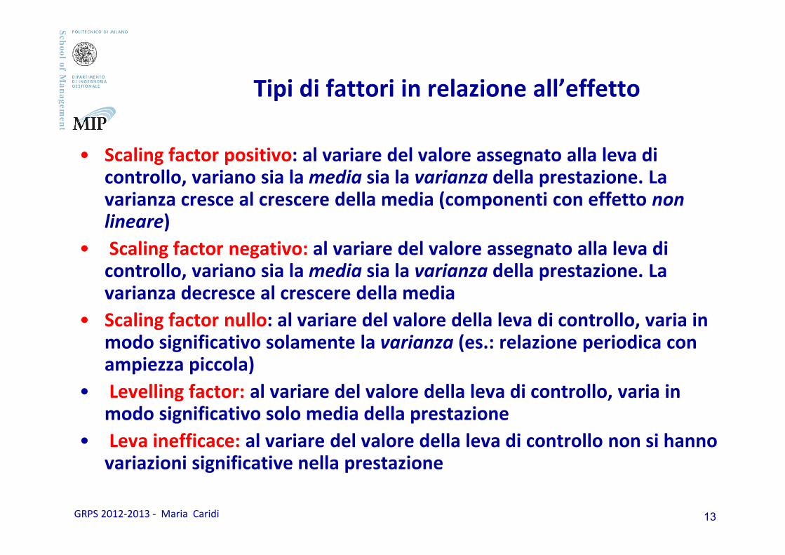
• Scaling factor positivo: al variare del valore assegnato alla leva di controllo, variano sia la media sia la varianza della prestazione. La varianza cresce al crescere della media (componenti con effetto non
lineare)
• Scaling factor negativo: al variare del valore assegnato alla leva di controllo, variano sia la media sia la varianza della prestazione. La varianza decresce al crescere della media
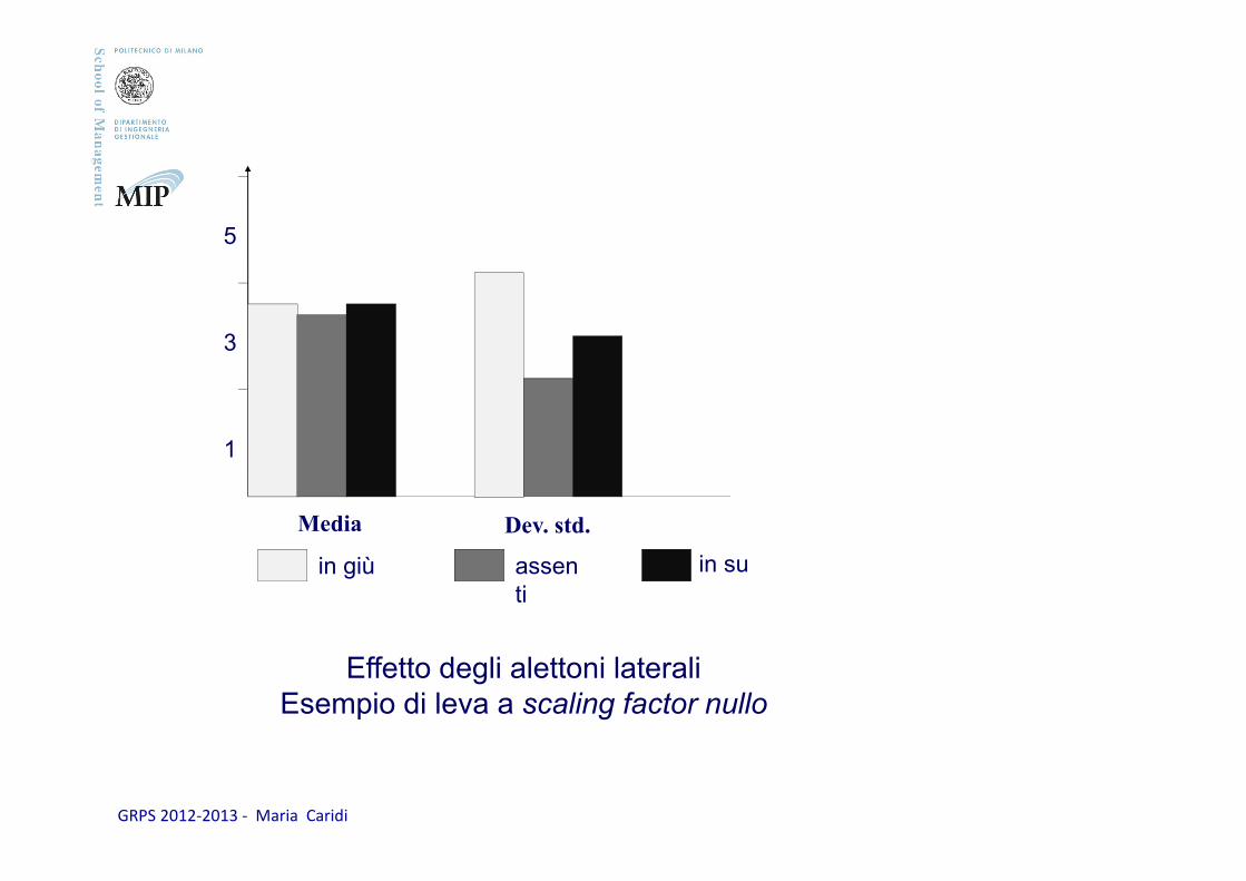
• Scaling factor nullo: al variare del valore della leva di controllo, varia in modo significativo solamente la varianza (es.: relazione periodica con ampiezza piccola)
• Levelling factor: al variare del valore della leva di controllo, varia in modo significativo solo media della prestazione
• Leva inefficace: al variare del valore della leva di controllo non si hanno variazioni significative nella prestazione
GRPS 2012-2013 - Maria Caridi
Tipi di fattori in relazione all’effetto
Gli Scaling factors vengono utilizzati per minimizzare la dispersione della risposta attorno alla media (per ottenere cioè un progetto ‘robusto’ rispetto ai disturbi). Gli Scaling factors nulli permettono di minimizzare la dispersione senza modificare significativamente la media. Se si utilizzano anche Scaling factors positivi o negativi, il progetto con dispersione minima avrà una prestazione media generalmente non coincidente con il valore nominale: occorrerà in tal caso qualche Leveling factor.
GRPS 2012-2013 - Maria Caridi
I Leveling factors - che influiscono poco sulla dispersione - vengono utilizzati per far collimare la prestazione media con il valore nominale. Se non si individua nessun Leveling factor, le alternative sono: • trovare un compromesso tra riduzione della dispersione e raggiungimento
del valore nominale; • riesaminare il progetto per introdurre un Leveling factor (ad esempio un
controllo lineare). L’utilizzo combinato degli Scaling factors e dei Leveling factorsrappresenta l’essenza della progettazione parametrica (parameter design), che è uno dei momenti fondamentali della progettazione.
Tipi di fattori in relazione all’effetto
GRPS 2012-2013 - Maria Caridi
1
3
5
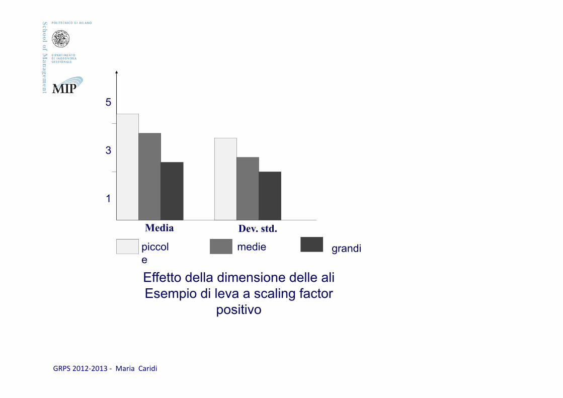
piccole
medie grandi
Effetto della dimensione delle aliEsempio di leva a scaling factor
positivo
Media Dev. std.
GRPS 2012-2013 - Maria Caridi
m
5
1
3
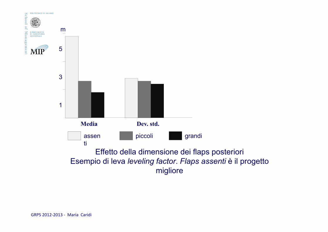
assenti
piccoli grandi
Effetto della dimensione dei flaps posterioriEsempio di leva leveling factor. Flaps assenti è il progetto
migliore
Media Dev. std.
GRPS 2012-2013 - Maria Caridi
5
1
3
in giù assenti
in su
Effetto degli alettoni lateraliEsempio di leva a scaling factor nullo
Media Dev. std.

GRPS 2012-2013 - Maria Caridi
Design of Experiments (DOE)

GRPS 2012-2013 - Maria Caridi
AGENDA
Introduction and origin
Basic concepts
Experiment with one factor
22 factorial design
23 factorial design
Fractional designs/half fraction design
GRPS 2012-2013 - Maria Caridi
�Design of Experiment is a statistics technique to improve industrialprocesses
�DOE is a test or series of tests that enable us to compare two or moremethods to determine which is better, or determine levels of controllablefactors to optimize the yield of a process or minimize the variability of theoutput
�In particular DOE help us to improve the processes by:
1) screening the factors to determine which are important to explainprocess variations and to try to understand how factors interact and drivethe process (Characterization Experiments)
2) finding the factor settings that produce optimal process performance(Optimization Experiments)
INTRODUCTION

GRPS 2012-2013 - Maria Caridi
For example:
Let’s suppose that two machine produce the same part.
The material used in processing can be loaded onto themachines either manually or with an automatic device.
The experimenter might wish to determine whether the type ofmachine and the type of loading process affect the number ofdefects, and then to select the machine type and loadingprocess combination that minimizes these defects.
INTRODUCTION

GRPS 2012-2013 - Maria Caridi
ORIGIN AND HISTORIC EVOLUTION
DOE was developed by R. A. Fisher in England, and dates back to the1920s.
Historically, experimental design was not widely used in industrial qualityimprovement studies because engineers had trouble working with thelarge number of variables and their interactions on many different levelsof the industrial processes
Improvement in computer software has recently allowed DOE to becomean important tool for quality.
GRPS 2012-2013 - Maria Caridi
AGENDA
Introduction and origin
Basic concepts
Experiment with one factor
22 factorial design
23 factorial design
Fractional designs/half fraction design
GRPS 2012-2013 - Maria Caridi
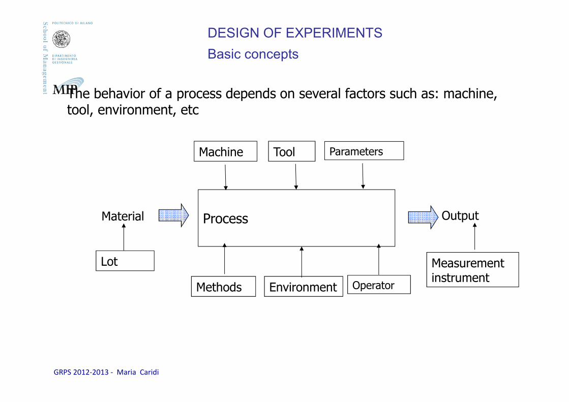
DESIGN OF EXPERIMENTS
Basic concepts
Process
Methods
OutputMaterial
Operator
Machine Tool
Environment
Measurement instrument
Lot
Parameters
The behavior of a process depends on several factors such as: machine, tool, environment, etc
GRPS 2012-2013 - Maria Caridi
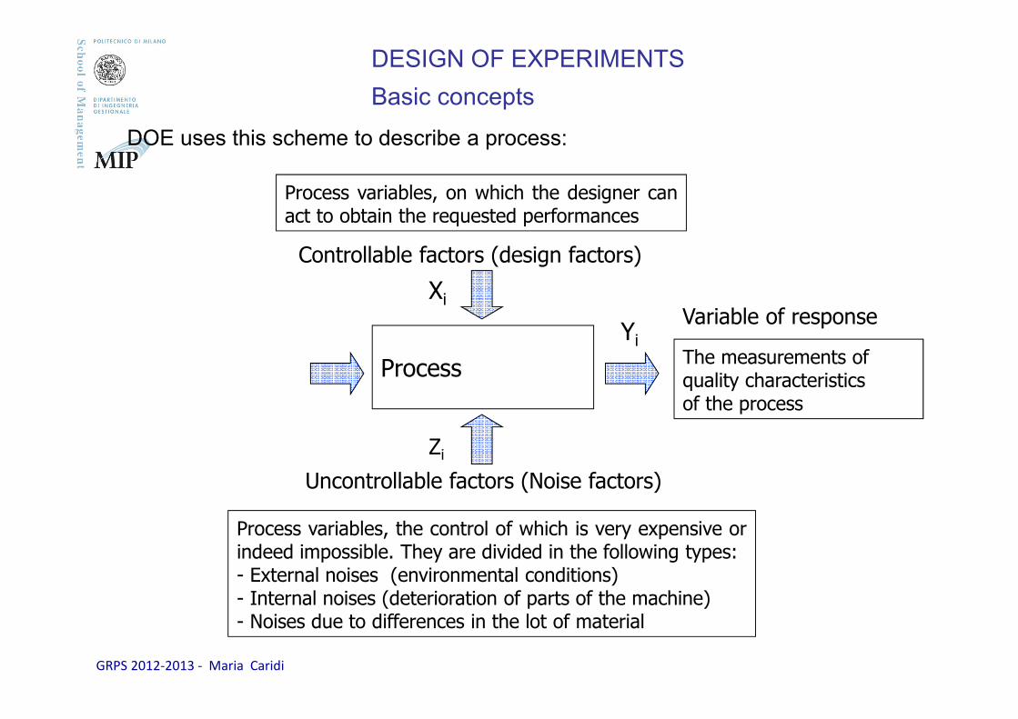
Process
Uncontrollable factors (Noise factors)
Controllable factors (design factors)
Variable of response
Process variables, on which the designer canact to obtain the requested performances
Process variables, the control of which is very expensive orindeed impossible. They are divided in the following types:- External noises (environmental conditions)- Internal noises (deterioration of parts of the machine)- Noises due to differences in the lot of material
Zi
Xi
YiThe measurements of quality characteristics of the process
DOE uses this scheme to describe a process:
DESIGN OF EXPERIMENTS
Basic concepts
GRPS 2012-2013 - Maria Caridi
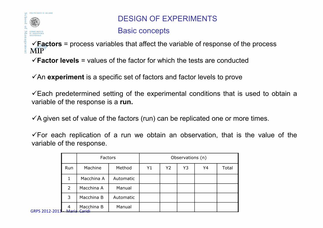
Factors Observations (n)
Run Machine Method Y1 Y2 Y3 Y4 Total
1 Macchina A Automatic
2 Macchina A Manual
3 Macchina B Automatic
4 Macchina B Manual
�Factors = process variables that affect the variable of response of the process
�Factor levels = values of the factor for which the tests are conducted
�An experiment is a specific set of factors and factor levels to prove
�Each predetermined setting of the experimental conditions that is used to obtain avariable of the response is a run.
�A given set of value of the factors (run) can be replicated one or more times.
�For each replication of a run we obtain an observation, that is the value of thevariable of the response.
DESIGN OF EXPERIMENTS
Basic concepts
GRPS 2012-2013 - Maria Caridi
In an experiment with m factors in which each factor can assume k levels we have km runs
With the growth of m the number of runs drastically increases
For example if m = 6 and k1 = k2 =…= km = 10 we have N =106 tests
DESIGN OF EXPERIMENTS
Basic concepts
GRPS 2012-2013 - Maria Caridi
�The number of experiments depends on the number of factors. Sometimes it istoo large.
�There doesn’t make sense to include all factors in an experiment programbecause usually only some of them are important, while the effects of the otherscan be considered as random variation.
�To select the “vital ones” and to discard “the trial ones” we can use well knownmethods of brainstorming or cause-and-effect diagrams.
�The factors which are neglected can be:- kept constant during the experiment. In this case the obtained results will be true for the chosen constant values of these factors- left to vary during the experiment. In this case their effects are considered as random and this increases the response variance.
DESIGN OF EXPERIMENTS
Basic concepts
GRPS 2012-2013 - Maria Caridi
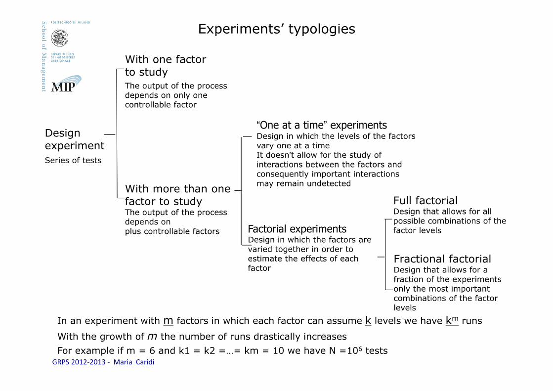
Factorial experimentsDesign in which the factors are varied together in order to estimate the effects of each factor
Full factorial Design that allows for all possible combinations of the factor levels
With more than one factor to studyThe output of the process depends on plus controllable factors
With one factor to study
The output of the process depends on only one controllable factor
Design experiment
Series of tests
“One at a time” experimentsDesign in which the levels of the factors vary one at a timeIt doesn’t allow for the study of interactions between the factors and consequently important interactions may remain undetected
Fractional factorial Design that allows for a fraction of the experiments only the most important combinations of the factor levels
In an experiment with m factors in which each factor can assume k levels we have km runs
With the growth of m the number of runs drastically increases
For example if m = 6 and k1 = k2 =…= km = 10 we have N =106 tests
Experiments’ typologies

GRPS 2012-2013 - Maria Caridi
AGENDA
Introduction and origin
Basic concepts
Experiment with one factor
22 factorial design
23 factorial design
Fractional designs/half fraction design
GRPS 2012-2013 - Maria Caridi
�It is the simplest experiment.
�The output of the process depends on only one controllable factor.
�In this case we study the response of the process for different levels ofthe factor.
EXPERIMENT WITH ONE FACTOR TO STUDY
GRPS 2012-2013 - Maria Caridi
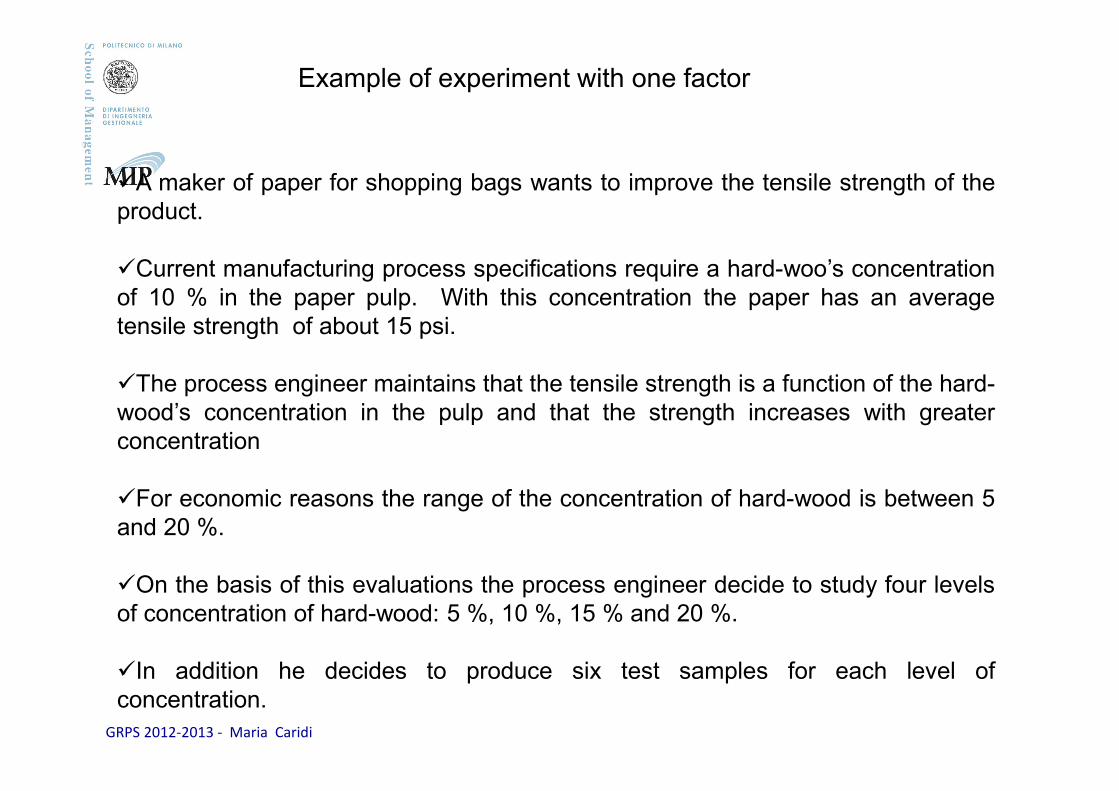
Example of experiment with one factor
�A maker of paper for shopping bags wants to improve the tensile strength of theproduct.
�Current manufacturing process specifications require a hard-woo’s concentrationof 10 % in the paper pulp. With this concentration the paper has an averagetensile strength of about 15 psi.
�The process engineer maintains that the tensile strength is a function of the hard-wood’s concentration in the pulp and that the strength increases with greaterconcentration
�For economic reasons the range of the concentration of hard-wood is between 5and 20 %.
�On the basis of this evaluations the process engineer decide to study four levelsof concentration of hard-wood: 5 %, 10 %, 15 % and 20 %.
�In addition he decides to produce six test samples for each level ofconcentration.
GRPS 2012-2013 - Maria Caridi
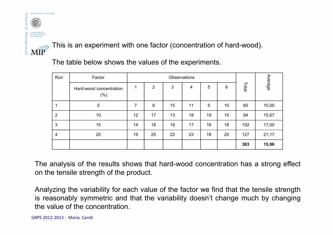
This is an experiment with one factor (concentration of hard-wood).
The table below shows the values of the experiments.
Run Factor Observations
Tota
l
Ave
rag
eHard-wood concentration
(%)
1 2 3 4 5 6
1 5 7 8 15 11 9 10 60 10,00
2 10 12 17 13 18 19 15 94 15,67
3 15 14 18 19 17 16 18 102 17,00
4 20 19 25 22 23 18 20 127 21,17
383 15,96
The analysis of the results shows that hard-wood concentration has a strong effecton the tensile strength of the product.
Analyzing the variability for each value of the factor we find that the tensile strengthis reasonably symmetric and that the variability doesn’t change much by changingthe value of the concentration.

GRPS 2012-2013 - Maria Caridi
AGENDA
Introduction and origin
Basic concepts
Experiment with one factor
22 factorial design
23 factorial design
Fractional designs/half-fraction design
GRPS 2012-2013 - Maria Caridi
�Experiments in which the factors are varied together
�The purpose of a factorial experiment is to estimate the effects of eachfactor
�Full factorial: experiment in which all possible combinations of the factorlevels are fulfilled
�Fractional factorial: experiment in which only a fraction of theexperiments are conducted
FACTORIAL EXPERIMENTS
GRPS 2012-2013 - Maria Caridi
FULL FACTORIAL DESIGN
�In a full factorial design all possible combinations of factor levels are fulfilled
�That is, in a full factorial experiment, responses (observations) are measured atall combinations of the experimental factor levels (run).
�The number of all possible factor level combinations in a full factorial design is N = k1, k2, …, km, where ki is the number of the levels of the i-th factor while m is the number of factors.
�In general an experiment with m factors at k levels have km combinations
�With the growth of m the number of runs drastically increases.
�For example if m = 6 and k1 = k2 =…= km = 10 we have N=106 runs.
GRPS 2012-2013 - Maria Caridi
�In a two-level full factorial design, each experimental factor has only two levels
�The experimental runs are 4
�These include all combinations of the factor levels.
TWO-LEVEL FULL FACTORIAL DESIGN (22)
GRPS 2012-2013 - Maria Caridi
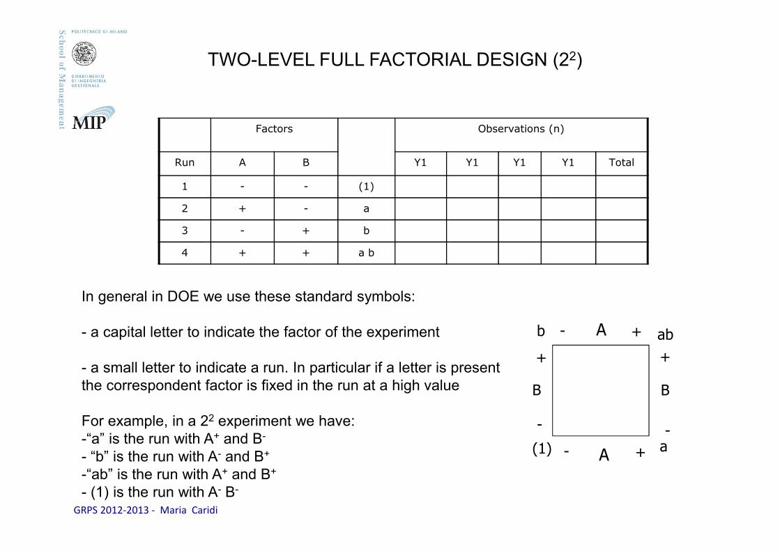
In general in DOE we use these standard symbols:
- a capital letter to indicate the factor of the experiment
- a small letter to indicate a run. In particular if a letter is present the correspondent factor is fixed in the run at a high value
For example, in a 22 experiment we have: -“a” is the run with A+ and B-
- “b” is the run with A- and B+
-“ab” is the run with A+ and B+
- (1) is the run with A- B-
Factors Observations (n)
Run A B Y1 Y1 Y1 Y1 Total
1 - - (1)
2 + - a
3 - + b
4 + + a b
TWO-LEVEL FULL FACTORIAL DESIGN (22)
A
B
+
-
A
B
- +
b
(1)
ab
a
- +
+
-
GRPS 2012-2013 - Maria Caridi
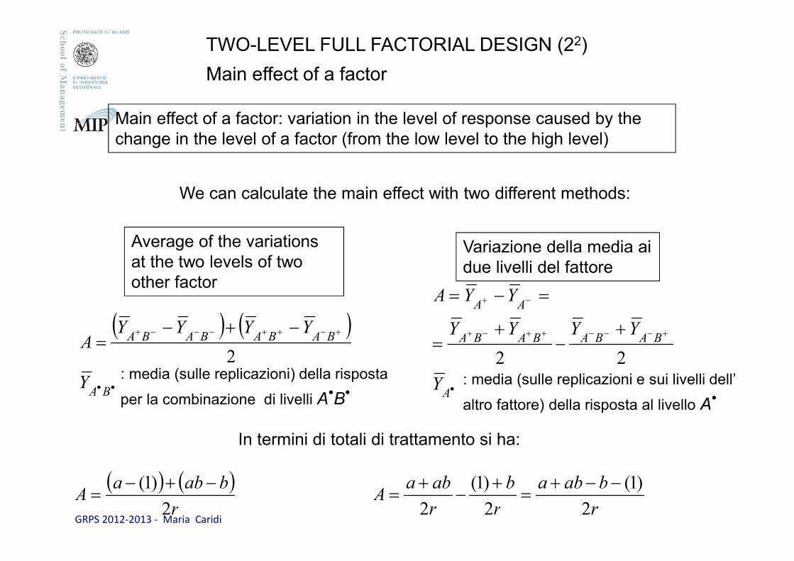
Main effect of a factor: variation in the level of response caused by the change in the level of a factor (from the low level to the high level)
( ) ( )
••
+−++−−−+ −+−=
BA
BABABABA
Y
YYYYA
2: media (sulle replicazioni) della risposta
per la combinazione di livelli A•B•
In termini di totali di trattamento si ha:
( ) ( )r
babaA
2
)1( −+−=
We can calculate the main effect with two different methods:
Average of the variations at the two levels of two other factor
Variazione della media ai due livelli del fattore
•
+−−−++−+
−+
+−
+=
=−=
A
BABABABA
AA
Y
YYYY
YYA
22
r
baba
r
b
r
abaA
2
)1(
2
)1(
2
−−+=
+−
+=
: media (sulle replicazioni e sui livelli dell’
altro fattore) della risposta al livello A•
TWO-LEVEL FULL FACTORIAL DESIGN (22)
Main effect of a factor
GRPS 2012-2013 - Maria Caridi
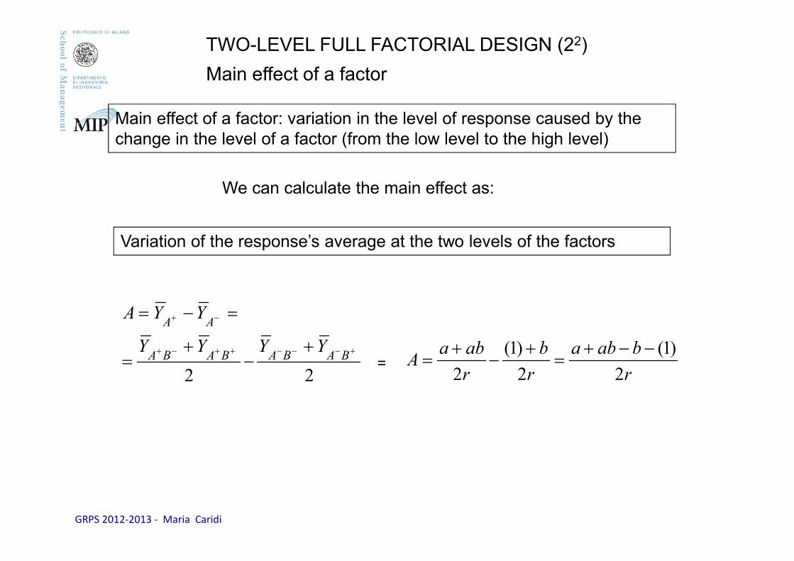
Main effect of a factor: variation in the level of response caused by the change in the level of a factor (from the low level to the high level)
We can calculate the main effect as:
Variation of the response’s average at the two levels of the factors
•
+−−−++−+
−+
+−
+=
=−=
A
BABABABA
AA
Y
YYYY
YYA
22 r
baba
r
b
r
abaA
2
)1(
2
)1(
2
−−+=
+−
+=
TWO-LEVEL FULL FACTORIAL DESIGN (22)
Main effect of a factor
=
GRPS 2012-2013 - Maria Caridi
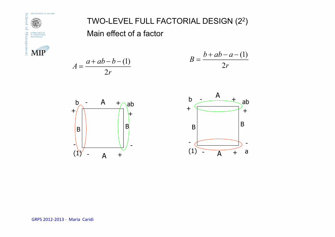
r
aabbB
2
)1(−−+=
r
babaA
2
)1(−−+=
TWO-LEVEL FULL FACTORIAL DESIGN (22)
Main effect of a factor
B
A
+
-
A
B
- +
b
(1)
ab- +
+
-
B
A
+
-
A
B
- +
b
(1)
ab- +
+
-
a
GRPS 2012-2013 - Maria Caridi
A─ +
−AY
+AY
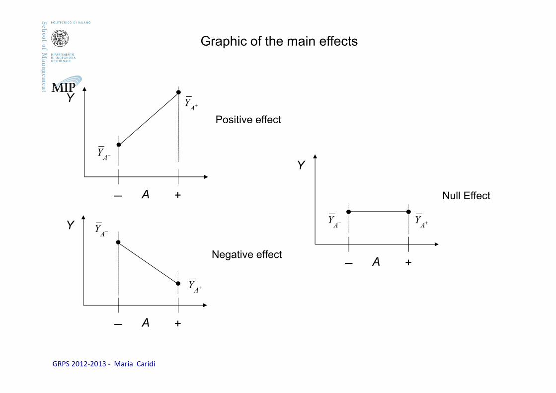
Graphic of the main effects
Y
Positive effect
A─ +
Y−AY
+AY
A─ +
−AY +
AY
Y
Null Effect
Negative effect
GRPS 2012-2013 - Maria Caridi
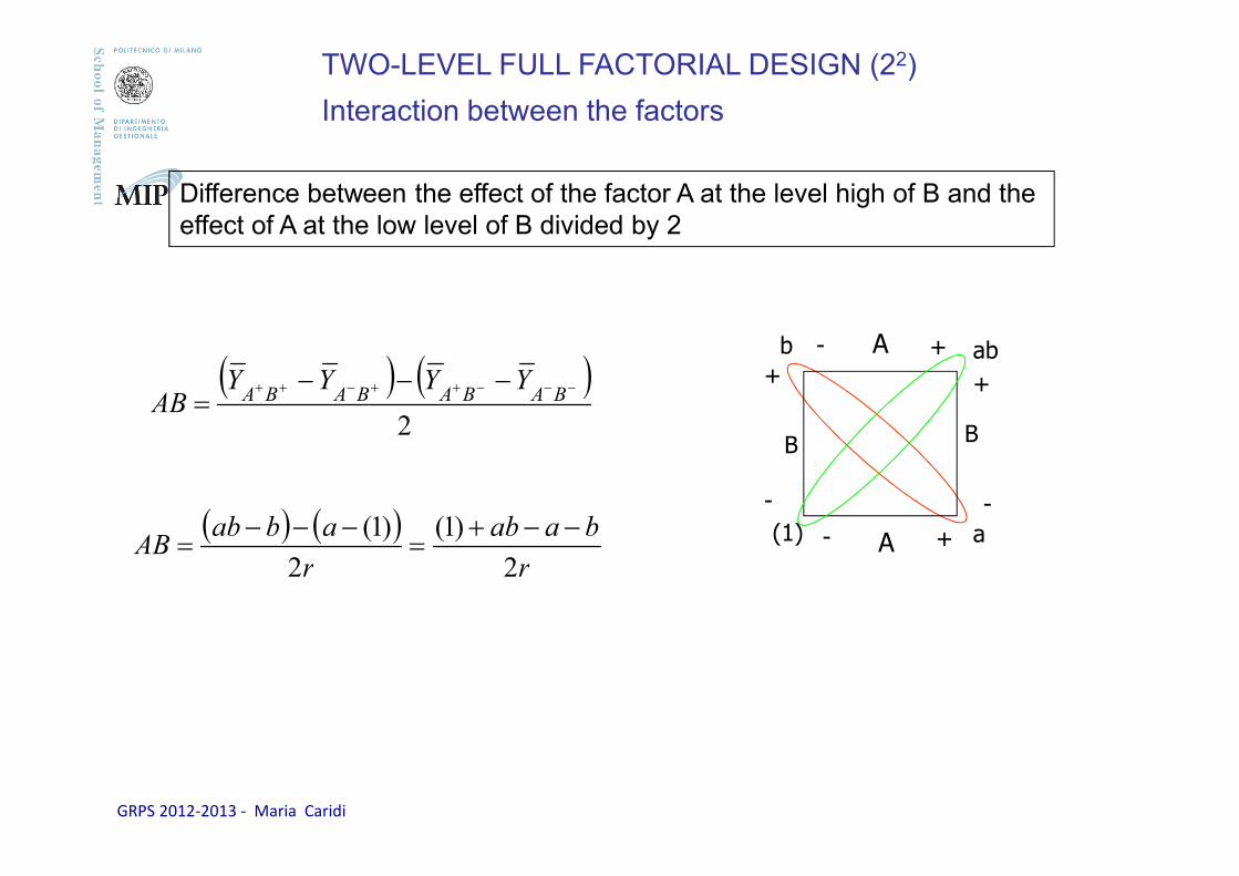
Difference between the effect of the factor A at the level high of B and the effect of A at the low level of B divided by 2
( ) ( )2
−−−++−++ −−−= BABABABA
YYYYAB
( ) ( )r
baab
r
ababAB
2
)1(
2
)1( −−+=
−−−=
TWO-LEVEL FULL FACTORIAL DESIGN (22)
Interaction between the factors
B
A
+
-
A
B
- +
b
(1)
ab- +
+
-
a
GRPS 2012-2013 - Maria Caridi
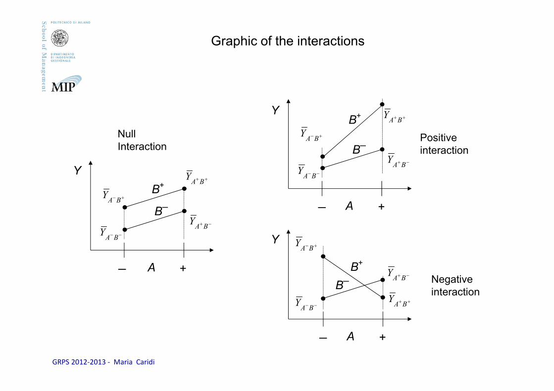
Graphic of the interactions
A─ +
B─
B+
Y
−−BA
Y
−+BA
Y
+−BA
Y
++BA
Y
NullInteraction
A─ +
B─
B+Y
−−BA
Y
−+BA
Y
+−BA
Y
++BA
Y
Positive interaction
A─ +
B─
B+
Y
−−BA
Y
−+BA
Y
+−BA
Y
++BA
Y
Negative interaction
GRPS 2012-2013 - Maria Caridi
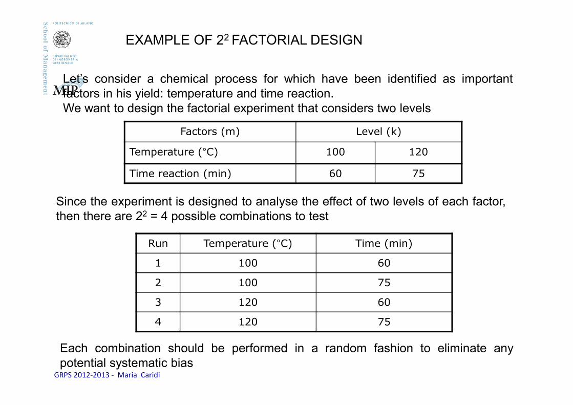
Run Temperature (°C) Time (min)
1 100 60
2 100 75
3 120 60
4 120 75
Let’s consider a chemical process for which have been identified as importantfactors in his yield: temperature and time reaction.We want to design the factorial experiment that considers two levels
Factors (m) Level (k)
Temperature (°C) 100 120
Time reaction (min) 60 75
EXAMPLE OF 22 FACTORIAL DESIGN
Since the experiment is designed to analyse the effect of two levels of each factor,then there are 22 = 4 possible combinations to test
Each combination should be performed in a random fashion to eliminate anypotential systematic bias
GRPS 2012-2013 - Maria Caridi
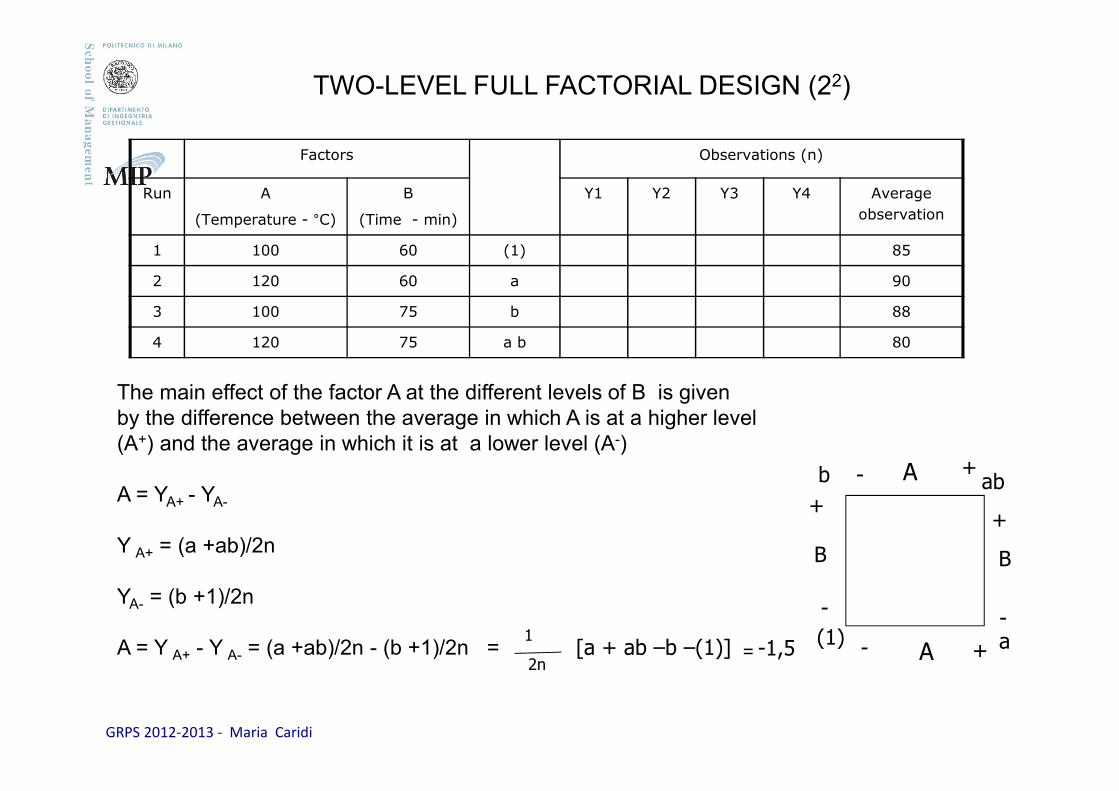
The main effect of the factor A at the different levels of B is given by the difference between the average in which A is at a higher level (A+) and the average in which it is at a lower level (A-)
A = YA+ - YA-
Y A+ = (a +ab)/2n
YA- = (b +1)/2n
A = Y A+ - Y A- = (a +ab)/2n - (b +1)/2n =
Factors Observations (n)
Run A
(Temperature - °C)
B
(Time - min)
Y1 Y2 Y3 Y4 Average
observation
1 100 60 (1) 85
2 120 60 a 90
3 100 75 b 88
4 120 75 a b 80
A
B
+
-
A
B
- +
b
(1)
ab
a1
2n[a + ab –b –(1)]
TWO-LEVEL FULL FACTORIAL DESIGN (22)
+-
-
+
-1,5=
GRPS 2012-2013 - Maria Caridi
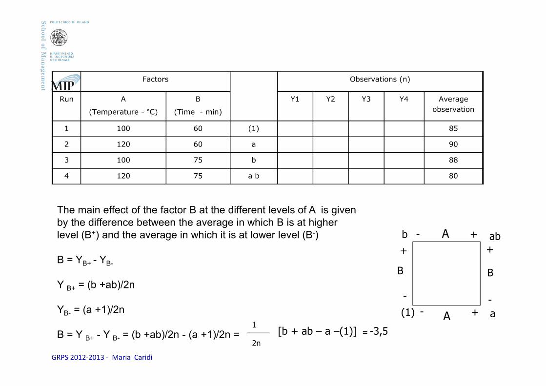
The main effect of the factor B at the different levels of A is given by the difference between the average in which B is at higher level (B+) and the average in which it is at lower level (B-)
B = YB+ - YB-
Y B+ = (b +ab)/2n
YB- = (a +1)/2n
B = Y B+ - Y B- = (b +ab)/2n - (a +1)/2n =
A
B
+
-
A
B
- +
b
(1)
ab
a1
2n
[b + ab – a –(1)]
+
+
-
-
Factors Observations (n)
Run A
(Temperature - °C)
B
(Time - min)
Y1 Y2 Y3 Y4 Average
observation
1 100 60 (1) 85
2 120 60 a 90
3 100 75 b 88
4 120 75 a b 80
-3,5=
GRPS 2012-2013 - Maria Caridi
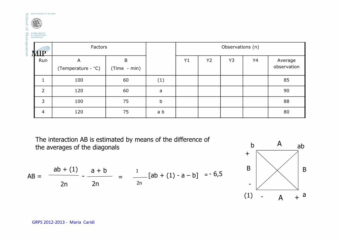
The interaction AB is estimated by means of the difference of the averages of the diagonals
A
B
+
-
A
B
- +
b
(1)
ab
a
1
2n
[ab + (1) - a – b]AB =ab + (1)
2n
-a + b
2n=
Factors Observations (n)
Run A
(Temperature - °C)
B
(Time - min)
Y1 Y2 Y3 Y4 Average
observation
1 100 60 (1) 85
2 120 60 a 90
3 100 75 b 88
4 120 75 a b 80
- 6,5=
GRPS 2012-2013 - Maria Caridi
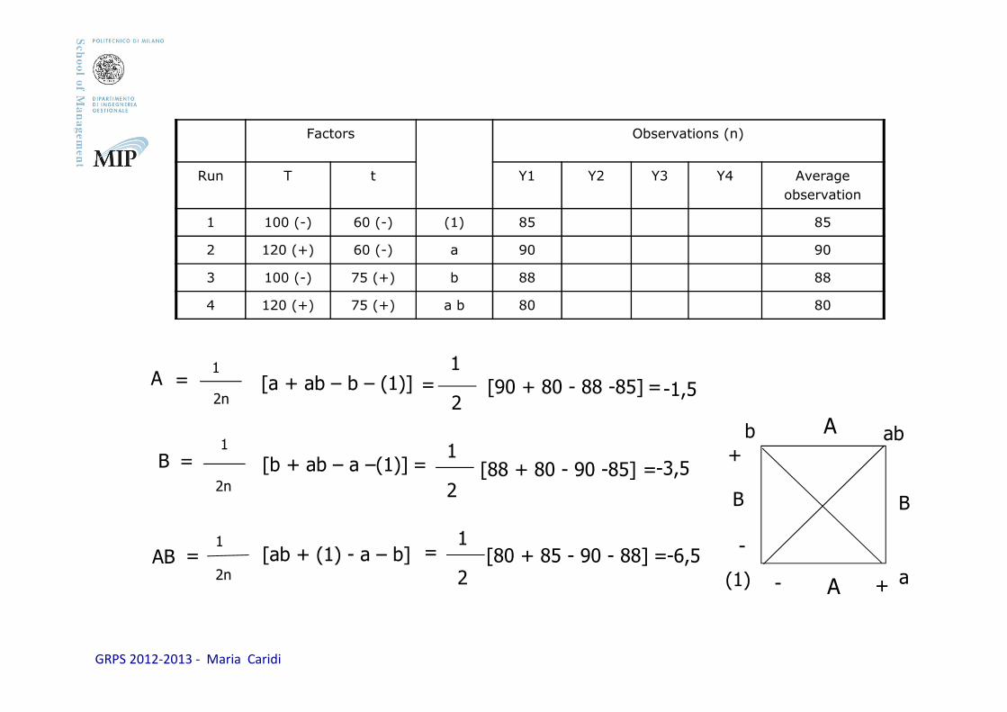
Factors Observations (n)
Run T t Y1 Y2 Y3 Y4 Average
observation
1 100 (-) 60 (-) (1) 85 85
2 120 (+) 60 (-) a 90 90
3 100 (-) 75 (+) b 88 88
4 120 (+) 75 (+) a b 80 80
A
B
+
-
A
B
- +
b
(1)
ab
a
1
2n[a + ab – b – (1)]A =
1
2n
[b + ab – a –(1)]B =
1
2n
[ab + (1) - a – b]AB =
=
=
1
2[90 + 80 - 88 -85]
1
2[88 + 80 - 90 -85]
=1
2[80 + 85 - 90 - 88] =
=
=
-6,5
-3,5
-1,5
GRPS 2012-2013 - Maria Caridi
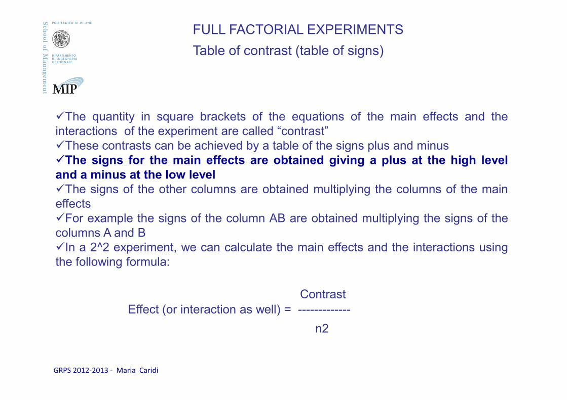
�The quantity in square brackets of the equations of the main effects and theinteractions of the experiment are called “contrast”�These contrasts can be achieved by a table of the signs plus and minus�The signs for the main effects are obtained giving a plus at the high leveland a minus at the low level�The signs of the other columns are obtained multiplying the columns of the maineffects�For example the signs of the column AB are obtained multiplying the signs of thecolumns A and B�In a 2^2 experiment, we can calculate the main effects and the interactions usingthe following formula:
FULL FACTORIAL EXPERIMENTS
Table of contrast (table of signs)
Effect (or interaction as well) = -------------
Contrast
n2
GRPS 2012-2013 - Maria Caridi
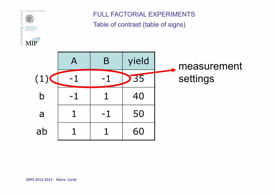
A B yield
(1) -1 -1 35
b -1 1 40
a 1 -1 50
ab 1 1 60
measurement settings
FULL FACTORIAL EXPERIMENTS
Table of contrast (table of signs)
GRPS 2012-2013 - Maria Caridi
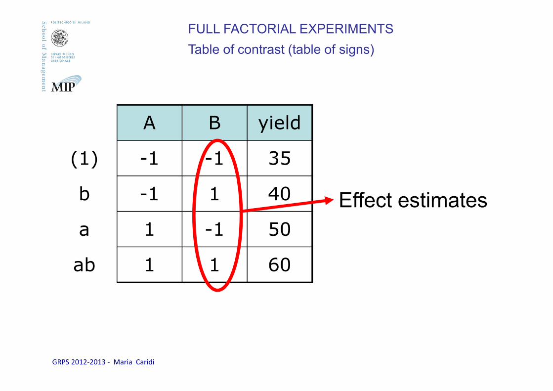
A B yield
(1) -1 -1 35
b -1 1 40
a 1 -1 50
ab 1 1 60
Effect estimates
FULL FACTORIAL EXPERIMENTS
Table of contrast (table of signs)
GRPS 2012-2013 - Maria Caridi
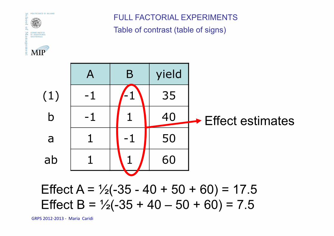
A B yield
(1) -1 -1 35
b -1 1 40
a 1 -1 50
ab 1 1 60
Effect estimates
Effect A = ½(-35 - 40 + 50 + 60) = 17.5Effect B = ½(-35 + 40 – 50 + 60) = 7.5
FULL FACTORIAL EXPERIMENTS
Table of contrast (table of signs)
GRPS 2012-2013 - Maria Caridi
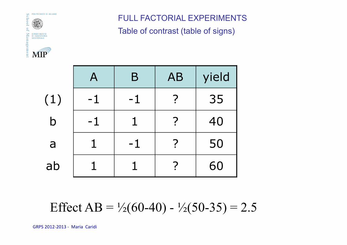
A B AB yield
(1) -1 -1 ? 35
b -1 1 ? 40
a 1 -1 ? 50
ab 1 1 ? 60
Effect AB = ½(60-40) - ½(50-35) = 2.5
FULL FACTORIAL EXPERIMENTS
Table of contrast (table of signs)
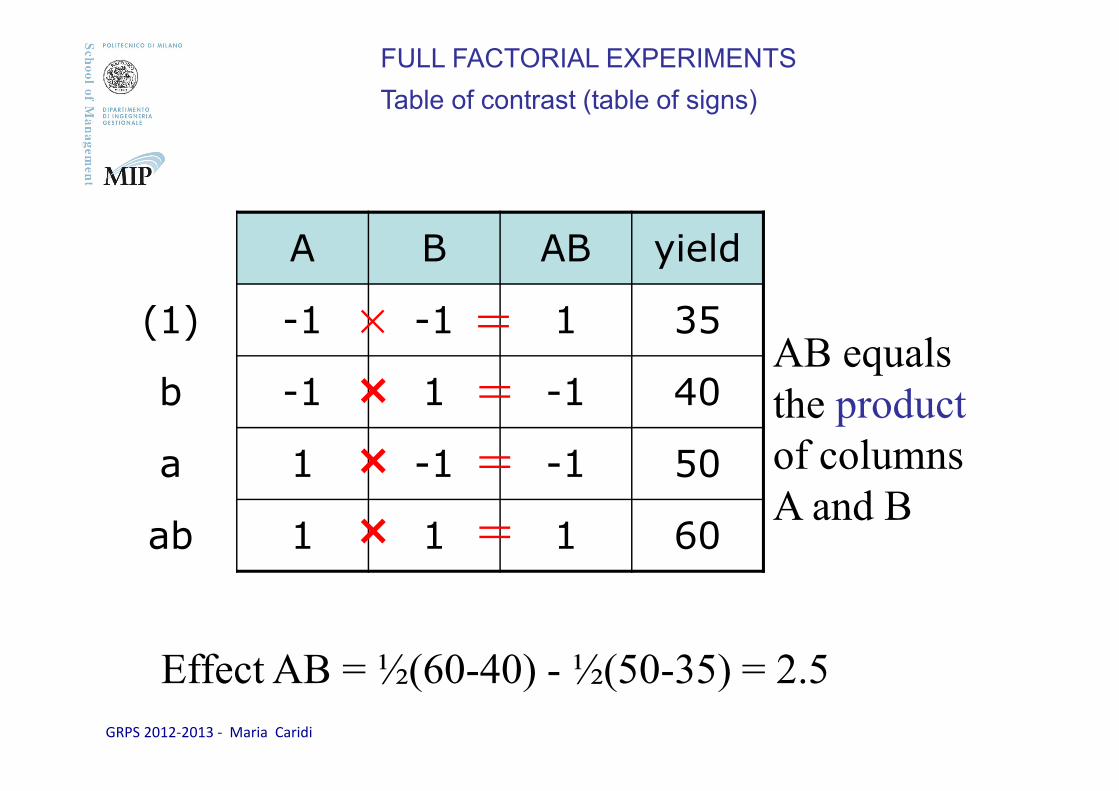
GRPS 2012-2013 - Maria Caridi
A B AB yield
(1) -1 -1 1 35
b -1 1 -1 40
a 1 -1 -1 50
ab 1 1 1 60
Effect AB = ½(60-40) - ½(50-35) = 2.5
× =
× =
× =
× =
AB equals
the product
of columns
A and B
FULL FACTORIAL EXPERIMENTS
Table of contrast (table of signs)

GRPS 2012-2013 - Maria Caridi
AGENDA
Introduction and origin
Basic concepts
Experiment with one factor
22 factorial design
23 factorial design
Fractional designs/half fraction design
GRPS 2012-2013 - Maria Caridi
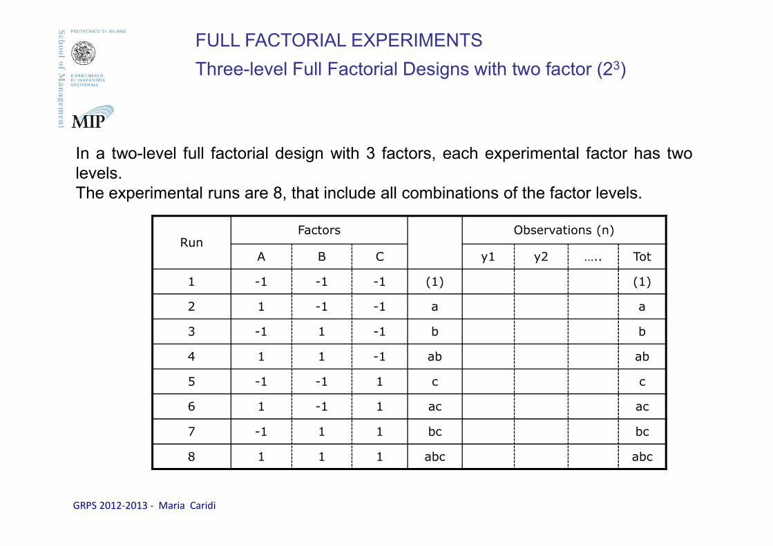
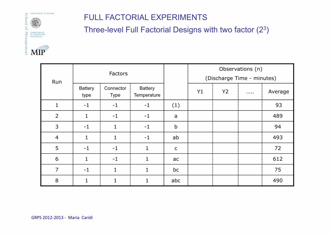
In a two-level full factorial design with 3 factors, each experimental factor has twolevels.The experimental runs are 8, that include all combinations of the factor levels.
RunFactors Observations (n)
A B C y1 y2 ….. Tot
1 -1 -1 -1 (1) (1)
2 1 -1 -1 a a
3 -1 1 -1 b b
4 1 1 -1 ab ab
5 -1 -1 1 c c
6 1 -1 1 ac ac
7 -1 1 1 bc bc
8 1 1 1 abc abc
FULL FACTORIAL EXPERIMENTS
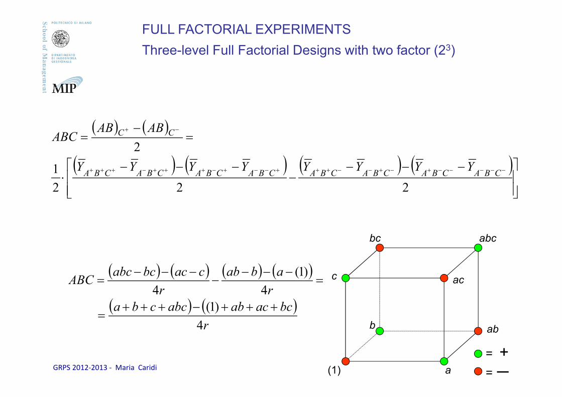
Three-level Full Factorial Designs with two factor (23)
GRPS 2012-2013 - Maria Caridi
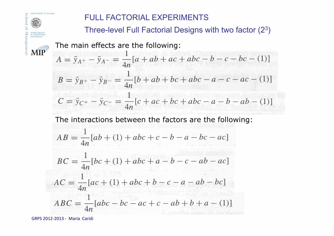
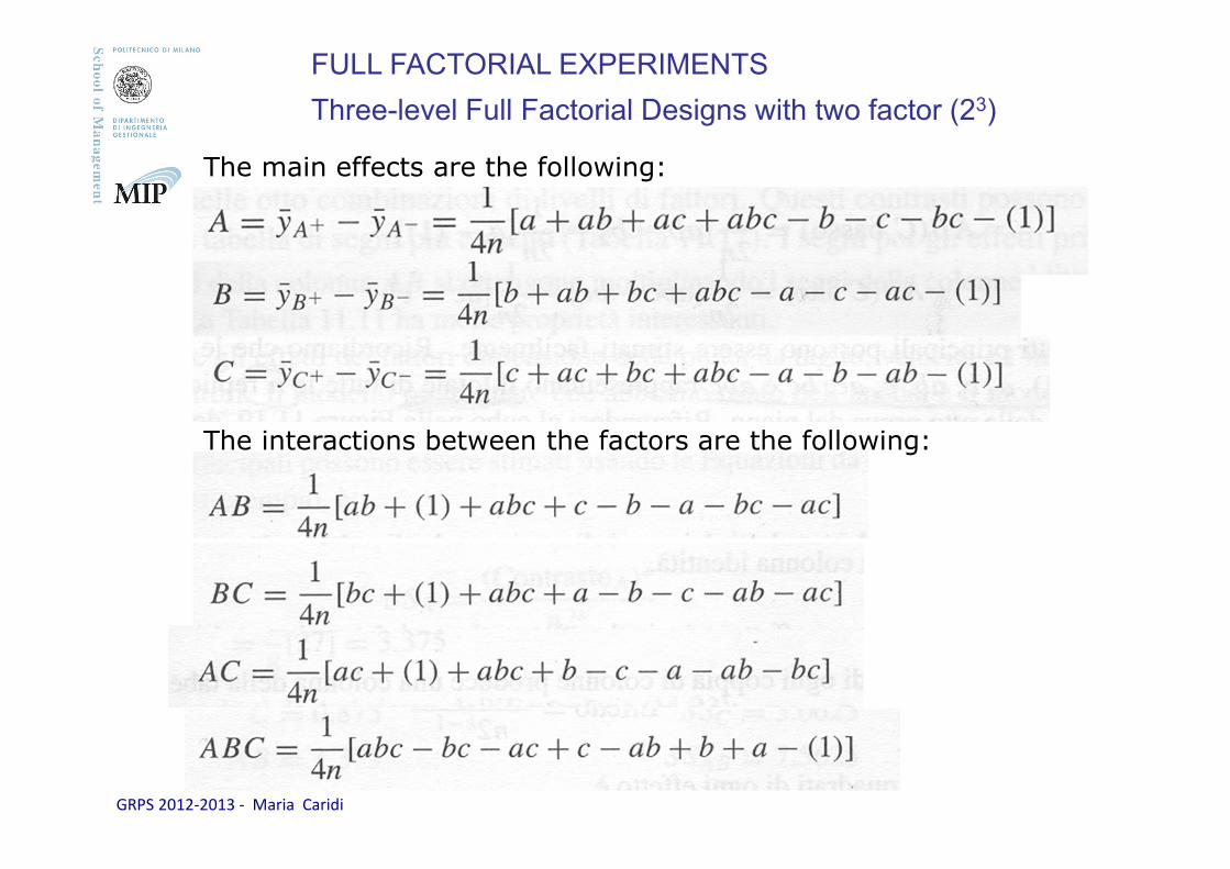
The main effects are the following:
The interactions between the factors are the following:
FULL FACTORIAL EXPERIMENTS
Three-level Full Factorial Designs with two factor (23)
GRPS 2012-2013 - Maria Caridi
(1) a
b
cac
abc
ab
bc
(1) a
b
cac
abc
ab
bc
(1) a
b
cac
abc
ab
bc
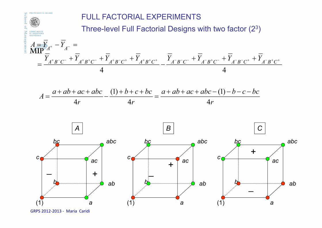
44
++−+−−−+−−−−++++−+−++−−+
−+
+++−
+++=
=−=
CBACBACBACBACBACBACBACBA
AA
YYYYYYYY
YYA
+─ ─
─
+
+
A B C
r
bccbabcacaba
r
bccb
r
abcacabaA
4
)1(
4
)1(
4
−−−−+++=
+++−
+++=
FULL FACTORIAL EXPERIMENTS
Three-level Full Factorial Designs with two factor (23)
GRPS 2012-2013 - Maria Caridi
( ) ( )
( ) ( ) ( ) ( )
−−−−
−−−⋅
=−
=
−−−−−+−+−−+++−−+−+++−+++
−+
222
1
2
CBACBACBACBACBACBACBACBA
CC
YYYYYYYY
ABABABC
( ) ( ) ( ) ( )
( ) ( )r
bcacababccba
r
abab
r
cacbcabcABC
4
)1(
4
)1(
4
+++−+++=
=−−−
−−−−
=
(1) a
b
c ac
abc
ab
bc
= += ─
FULL FACTORIAL EXPERIMENTS
Three-level Full Factorial Designs with two factor (23)
GRPS 2012-2013 - Maria Caridi
The main effects are the following:
The interactions between the factors are the following:
FULL FACTORIAL EXPERIMENTS
Three-level Full Factorial Designs with two factor (23)
GRPS 2012-2013 - Maria Caridi
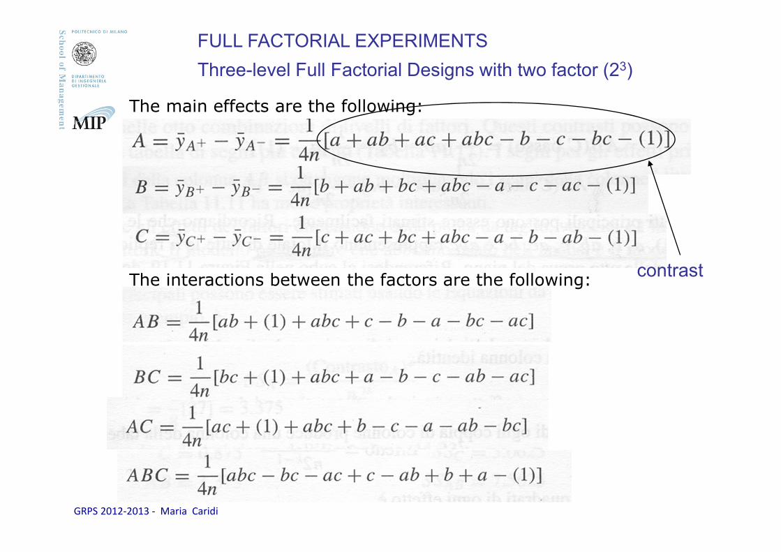
The main effects are the following:
The interactions between the factors are the following:contrast
FULL FACTORIAL EXPERIMENTS
Three-level Full Factorial Designs with two factor (23)
GRPS 2012-2013 - Maria Caridi
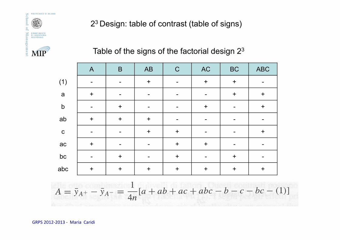
A B AB C AC BC ABC
(1) - - + - + + -
a + - - - - + +
b - + - - + - +
ab + + + - - - -
c - - + + - - +
ac + - - + + - -
bc - + - + - + -
abc + + + + + + +
Table of the signs of the factorial design 23
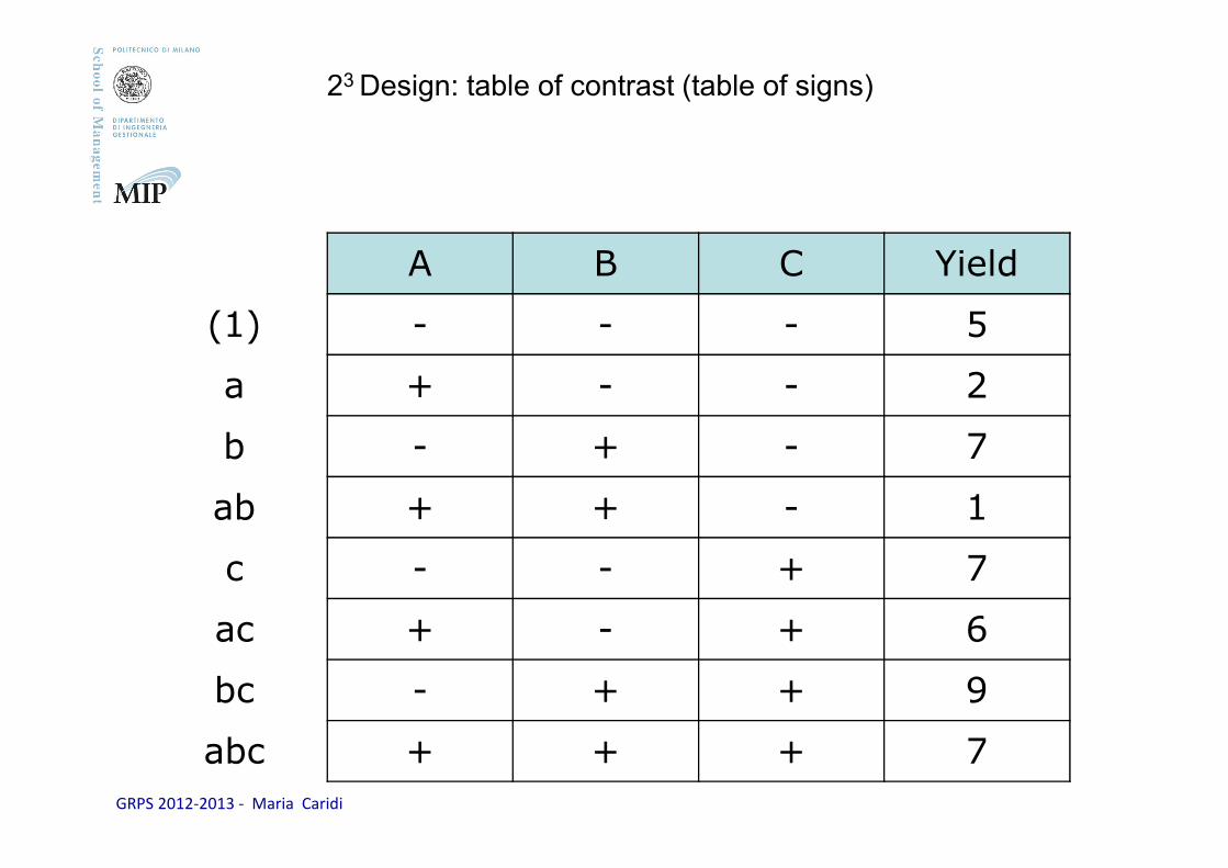
23 Design: table of contrast (table of signs)
GRPS 2012-2013 - Maria Caridi
A B C Yield
(1) - - - 5
a + - - 2
b - + - 7
ab + + - 1
c - - + 7
ac + - + 6
bc - + + 9
abc + + + 7
23 Design: table of contrast (table of signs)
GRPS 2012-2013 - Maria Caridi
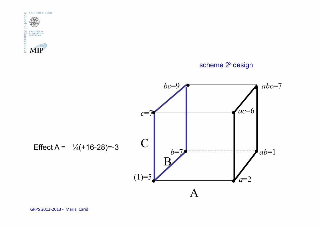
(1)=5 a=2
ab=1b=7
ac=6
abc=7bc=9
c=7
• •
• •
• •
• •
Effect A = ¼(+16-28)=-3
A
B
C
scheme 23 design
GRPS 2012-2013 - Maria Caridi
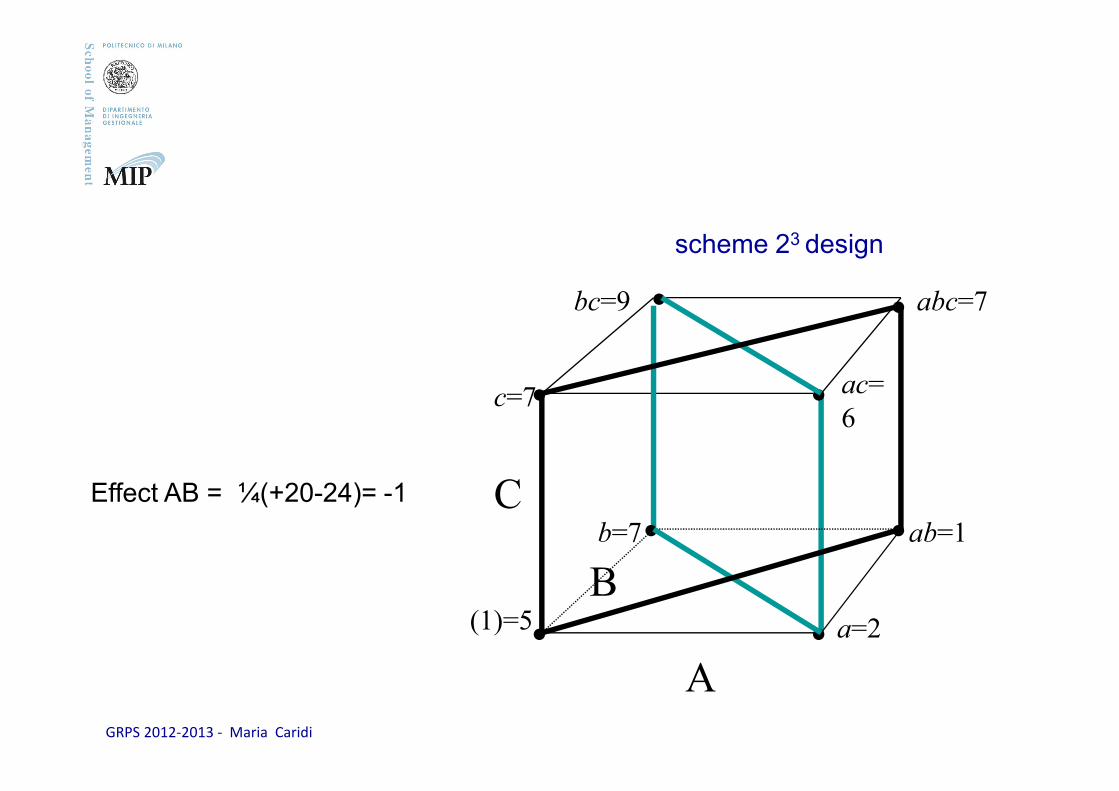
Effect AB = ¼(+20-24)= -1
scheme 23 design
(1)=5 a=2
ab=1b=7
ac=
6
abc=7bc=9
c=7
• •
• •
• •
• •
A
B
C

GRPS 2012-2013 - Maria Caridi
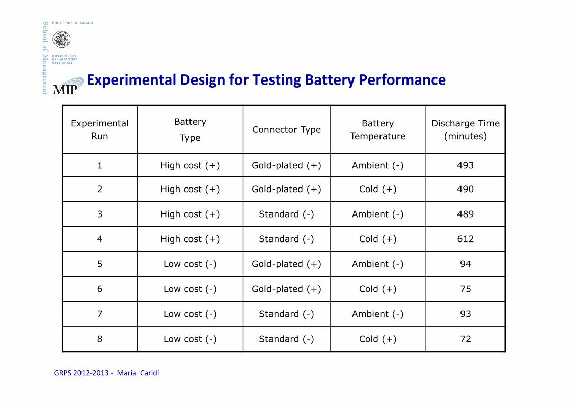
A lot of enthusiasts of remote control (RC) model car racing believe thatspending more money on high-quality batteries, using expensive gold-plated connectors, and storing batteries at low temperatures will improvebattery life performance in a race.
To test this hypothesis, an electrical test circuit was constructed tomeasure battery discharge under different configurations.
Each factor (battery type, connector type, and temperature) was evaluatedat two levels, resulting in
23 = 8 experimental conditions shown in the table below:
EXAMPLE OF 23 FACTORIAL EXPERIMENTAL DESIGN
Experimental Design for Testing Battery Performance

GRPS 2012-2013 - Maria Caridi
Experimental Design for Testing Battery Performance
Experimental
Run
Battery
TypeConnector Type
Battery
Temperature
Discharge Time
(minutes)
1 High cost Gold-plated Ambient 493
2 High cost Gold-plated Cold 490
3 High cost Standard Ambient 489
4 High cost Standard Cold 612
5 Low cost Gold-plated Ambient 94
6 Low cost Gold-plated Cold 75
7 Low cost Standard Ambient 93
8 Low cost Standard Cold 72
GRPS 2012-2013 - Maria Caridi
Experimental Design for Testing Battery Performance
Experimental
Run
Battery
TypeConnector Type
Battery
Temperature
Discharge Time
(minutes)
1 High cost (+) Gold-plated (+) Ambient (-) 493
2 High cost (+) Gold-plated (+) Cold (+) 490
3 High cost (+) Standard (-) Ambient (-) 489
4 High cost (+) Standard (-) Cold (+) 612
5 Low cost (-) Gold-plated (+) Ambient (-) 94
6 Low cost (-) Gold-plated (+) Cold (+) 75
7 Low cost (-) Standard (-) Ambient (-) 93
8 Low cost (-) Standard (-) Cold (+) 72
GRPS 2012-2013 - Maria Caridi
Run
FactorsObservations (n)
(Discharge Time - minutes)
Battery
type
Connector
Type
Battery
TemperatureY1 Y2 ….. Average
1 -1 -1 -1 (1) 93
2 1 -1 -1 a 489
3 -1 1 -1 b 94
4 1 1 -1 ab 493
5 -1 -1 1 c 72
6 1 -1 1 ac 612
7 -1 1 1 bc 75
8 1 1 1 abc 490
FULL FACTORIAL EXPERIMENTS
Three-level Full Factorial Designs with two factor (23)
GRPS 2012-2013 - Maria Caridi
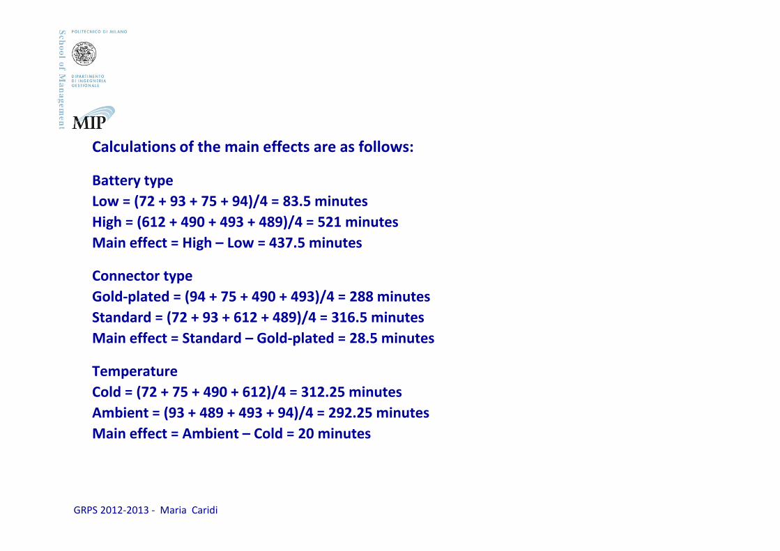
Calculations of the main effects are as follows:
Battery type
Low = (72 + 93 + 75 + 94)/4 = 83.5 minutes
High = (612 + 490 + 493 + 489)/4 = 521 minutes
Main effect = High – Low = 437.5 minutes
Connector type
Gold-plated = (94 + 75 + 490 + 493)/4 = 288 minutes
Standard = (72 + 93 + 612 + 489)/4 = 316.5 minutes
Main effect = Standard – Gold-plated = 28.5 minutes
Temperature
Cold = (72 + 75 + 490 + 612)/4 = 312.25 minutes
Ambient = (93 + 489 + 493 + 94)/4 = 292.25 minutes
Main effect = Ambient – Cold = 20 minutes
GRPS 2012-2013 - Maria Caridi
These results suggest that high cost batteries do have a longer life, butthat the impacts of gold plating or battery temperature do not appear tobe significant.
Because only one factor appears to be significant, calculation ofinteraction effects are not required.
Experimental Design for Testing Battery Performance

GRPS 2012-2013 - Maria Caridi
AGENDA
Introduction and origin
Basic concepts
Experiment with one factor
22 factorial design
23 factorial design
Fractional designs/half fraction design
GRPS 2012-2013 - Maria Caridi
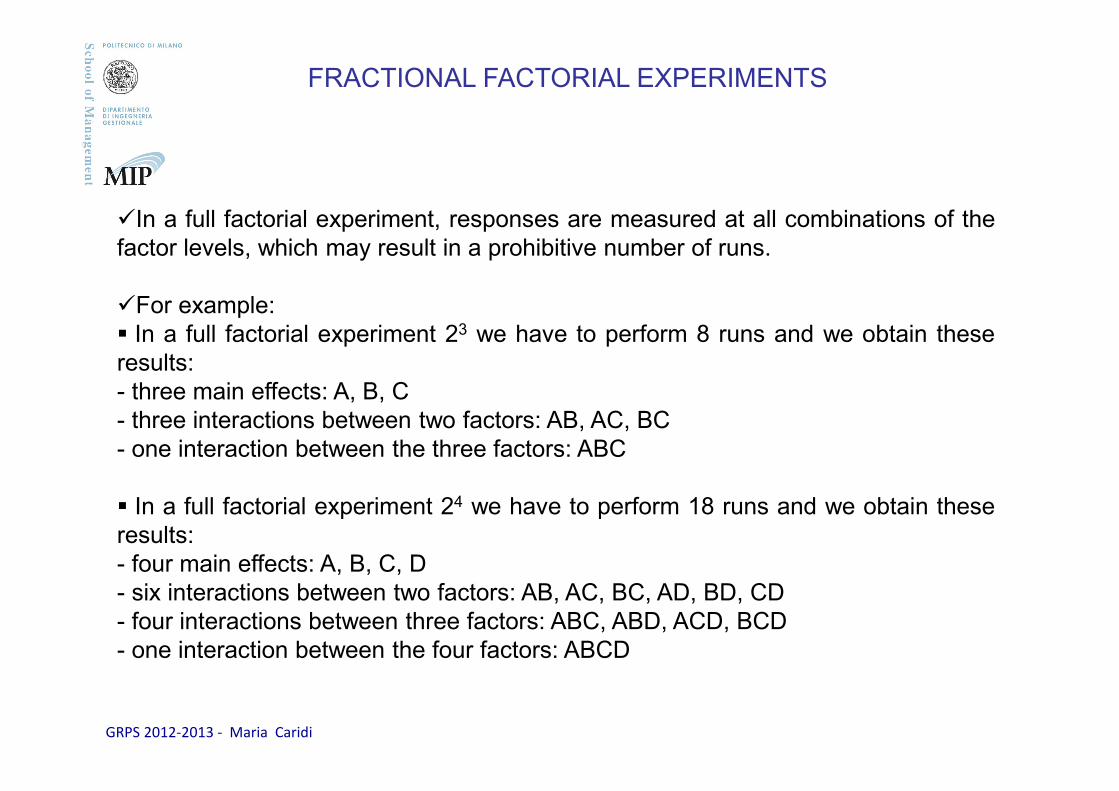
�In a full factorial experiment, responses are measured at all combinations of thefactor levels, which may result in a prohibitive number of runs.
�For example:� In a full factorial experiment 23 we have to perform 8 runs and we obtain theseresults:- three main effects: A, B, C- three interactions between two factors: AB, AC, BC- one interaction between the three factors: ABC
� In a full factorial experiment 24 we have to perform 18 runs and we obtain theseresults:- four main effects: A, B, C, D- six interactions between two factors: AB, AC, BC, AD, BD, CD- four interactions between three factors: ABC, ABD, ACD, BCD- one interaction between the four factors: ABCD
FRACTIONAL FACTORIAL EXPERIMENTS
GRPS 2012-2013 - Maria Caridi
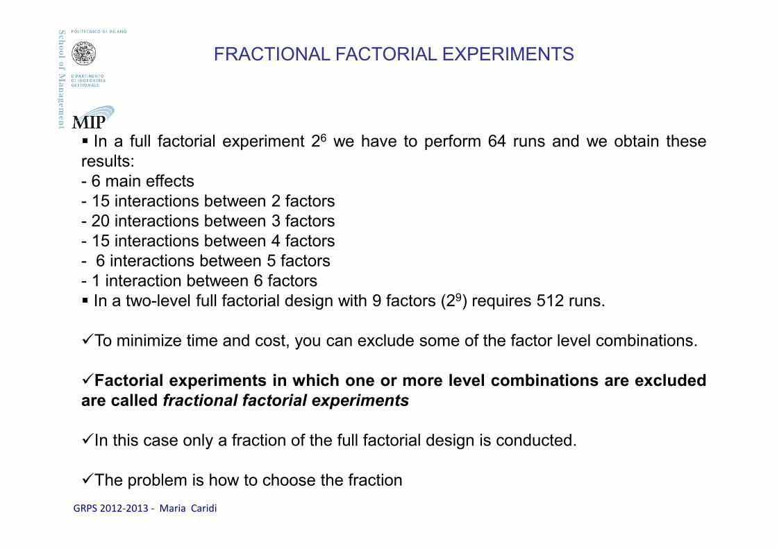
� In a full factorial experiment 26 we have to perform 64 runs and we obtain theseresults:- 6 main effects- 15 interactions between 2 factors- 20 interactions between 3 factors- 15 interactions between 4 factors- 6 interactions between 5 factors- 1 interaction between 6 factors� In a two-level full factorial design with 9 factors (29) requires 512 runs.
�To minimize time and cost, you can exclude some of the factor level combinations.
�Factorial experiments in which one or more level combinations are excludedare called fractional factorial experiments
�In this case only a fraction of the full factorial design is conducted.
�The problem is how to choose the fraction
FRACTIONAL FACTORIAL EXPERIMENTS
GRPS 2012-2013 - Maria Caridi
�The main effects postulate states that systems are controlled by the main effectsand by the interactions of low order (that is interactions of only a few factors)whereas the interactions between three or more factors are normally negligible
�Fractional design makes use of this postulate by sacrificing high orderinteractions to reduce the number of the runs
�The high order interaction which is sacrificed is called generator of the
fraction
FRACTIONAL FACTORIAL EXPERIMENTS
GRPS 2012-2013 - Maria Caridi
FRACTIONAL EXPERIMENTS
Half-Fraction Factorial Design
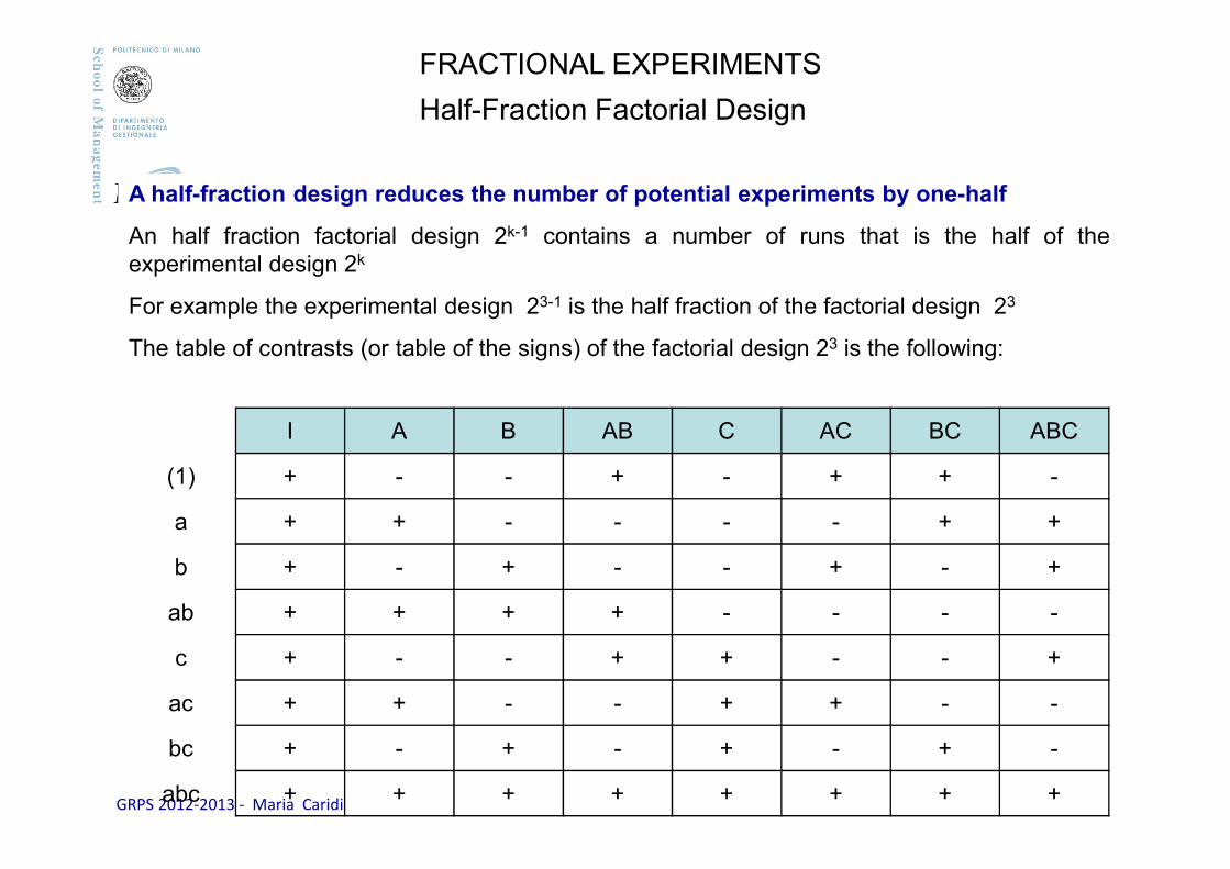
A half-fraction design reduces the number of potential experiments by one-half
An half fraction factorial design 2k-1 contains a number of runs that is the half of theexperimental design 2k
For example the experimental design 23-1 is the half fraction of the factorial design 23
The table of contrasts (or table of the signs) of the factorial design 23 is the following:
I A B AB C AC BC ABC
(1) + - - + - + + -
a + + - - - - + +
b + - + - - + - +
ab + + + + - - - -
c + - - + + - - +
ac + + - - + + - -
bc + - + - + - + -
abc + + + + + + + +
GRPS 2012-2013 - Maria Caridi
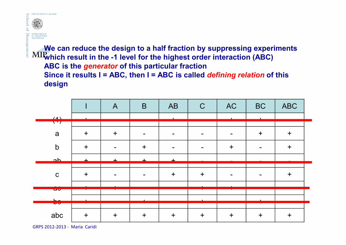
We can reduce the design to a half fraction by suppressing experiments which result in the -1 level for the highest order interaction (ABC)ABC is the generator of this particular fractionSince it results I = ABC, then I = ABC is called defining relation of this design
I A B AB C AC BC ABC
(1) + - - + - + + -
a + + - - - - + +
b + - + - - + - +
ab + + + + - - - -
c + - - + + - - +
ac + + - - + + - -
bc + - + - + - + -
abc + + + + + + + +
GRPS 2012-2013 - Maria Caridi
I A B AB C AC BC ABC
a + + - - - - + +
b + - + - - + - +
c + - - + + - - +
abc + + + + + + + +
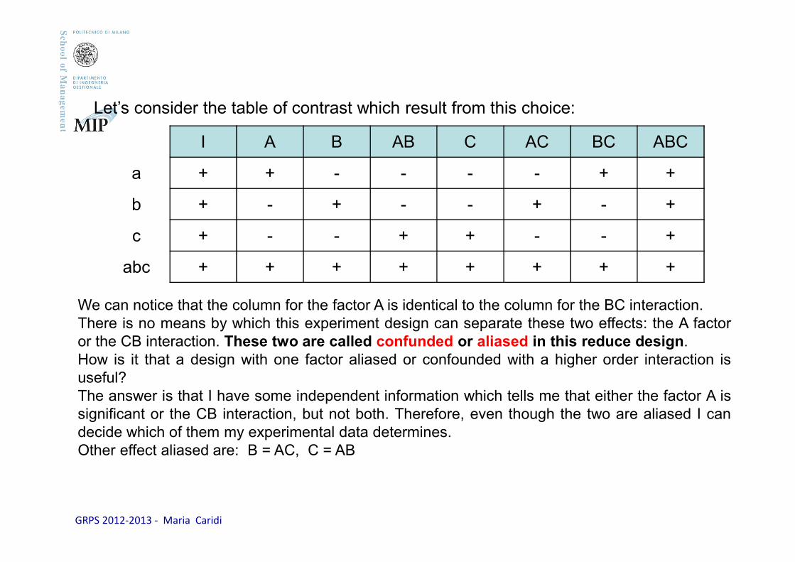
Let’s consider the table of contrast which result from this choice:
We can notice that the column for the factor A is identical to the column for the BC interaction.There is no means by which this experiment design can separate these two effects: the A factoror the CB interaction. These two are called confunded or aliased in this reduce design.How is it that a design with one factor aliased or confounded with a higher order interaction isuseful?The answer is that I have some independent information which tells me that either the factor A issignificant or the CB interaction, but not both. Therefore, even though the two are aliased I candecide which of them my experimental data determines.Other effect aliased are: B = AC, C = AB
GRPS 2012-2013 - Maria Caridi
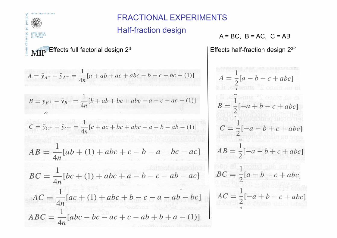
FRACTIONAL EXPERIMENTS
Half-fraction designA = BC, B = AC, C = AB
Effects full factorial design 23 Effects half-fraction design 23-1