0444 - E306 - Nondestructive Examination (NDE) Technology ...ANSI/ASNT CP-189 (2006 Edition), or ACCP Qualification in accordance with a prior ... A person may be qualified directly

Nondestructive Examination (NDE) Technology and Codes

Student Manual

Chapter 9.0

Volume 2

Introduction to Eddy Current Testing Examination

NDE Technology and Codes Student Manual Table of Contents

USNRC Technical Training Center Rev 0103 9−i

TABLE OF CONTENTS

9.0 INTRODUCTION TO EDDY CURRENT TESTING EXAMINATION ...................................... 1

Learning Objectives

9.1 History . . . . . . . . . . . . . . . . . . . . . . . . . . . . . . . . . . . . . . . . . . . . . . . . . . . . . . . . . . . . . . . . . . . .1

9.2 Personnel Qualification and Certification ................................................................................. 2

9.3 Principles. . . . . . . . . . . . . . . . . . . . . . . . . . . . . . . . . . . . . . . . . . . . . . . . . . . . . . . . . . . . . . . . . . 3

9.3.1 Electromagnetic Induction ....................................................................................... 4

9.3.2 Eddy Current Characteristics ................................................................................... 4

9.3.2.1 Material Properties ...................................................................................... 5

9.3.2.1.1 Conductivity .......................................................................................... 5

9.3.2.1.2 Permeability ........................................................................................... 6

9.3.2.1.3 Test Display of Material Property Variations ........................................ 6

9.3.2.2 Frequency .................................................................................................... 6

9.3.2.3 Test Specimen Geometry ............................................................................. 7

9.3.2.4 Coil Design .................................................................................................. 7

9.3.2.4.1 Coil Coupling (Lift-Off) ........................................................................ 7

9.3.2.4.2 Edge Effect ............................................................................................ 8

9.4 Equipment. . . . . . . . . . . . . . . . . . . . . . . . . . . . . . . . . . . . . . . . . . . . . . . . . . . . . . . . . . . . . . . . . .8

9.4.1 System Components ................................................................................................ 8

9.4.2 Data/Displays......................................................................................................... 10

9.4.2.1 Lift-Off Curves .......................................................................................... 10

9.4.2.2 Conductivity Curve.................................................................................... 10

9.4.2.3 Thickness Curves ....................................................................................... 10

9.4.2.4 Discontinuity Signal Display ..................................................................... 11

9.4.3 Basic Coils ............................................................................................................. 12

9.4.3.1 Surface Coils.............................................................................................. 12


USNRC Technical Training Center Rev 0103 9−ii

9.4.3.2 Encircling Coils ......................................................................................... 12

9.4.3.3 Internal Coils ............................................................................................. 13

9.5 Techniques. . . . . . . . . . . . . . . . . . . . . . . . . . . . . . . . . . . . . . . . . . . . . . . . . . . . . . . . . . . . . . . . 13

9.5.1 Impedance Plane Fundamentals ............................................................................ 13

9.5.2 Impedance Plane Response to Conductivity Variations ........................................ 13

9.5.3 Sorting. . . ............................................................................................................. 14

9.5.4 Discontinuities ....................................................................................................... 14

9.5.4.1 Discontinuity Location in Installed Nonferrous Steam Generator

Heat Exchanger Tubing ....................................................................... 14

9.5.4.2 Calibration Procedure ................................................................................ 15

9.5.4.3 Probe Speed ............................................................................................... 16

9.5.5 Thickness ............................................................................................................. 16

9.5.5.1 Location of Secondary Layer Corrosion or Cracking ............................... 16

9.5.6 Coatings ............................................................................................................. 17

9.5.6.1 Variations in Thickness of Plating or Cladding......................................... 17

9.6 Interpretation and Code Requirements .................................................................................... 17

9.6.1 Written Procedure .................................................................................................. 17

9.6.2 Description of Method ........................................................................................... 17

9.6.3 Reference Specimen .............................................................................................. 18

9.6.4 Equipment Qualification ........................................................................................ 18

9.6.5 Procedure Requirements ........................................................................................ 18

9.7 Advantages and Limitations of ET Examinations ................................................................... 18

9.7.1 Advantages ............................................................................................................ 19


USNRC Technical Training Center Rev 0103 9−iii

9.7.2 Limitations ............................................................................................................. 19

LIST OF FIGURES

9-1 Alternating Current Flowing Through Test Coil ........................................................................... 20

9-2 Primary Magnetic Field Develops ................................................................................................. 21

9-3 Inductive Reactance Occurs .......................................................................................................... 22

9-4 Eddy Currents Develop…………………………………………………………………………..23

9-5 Secondary Field Develops ............................................................................................................. 24

9-6 Eddy Currents Develop Parallel to the Coil’s Turns ..................................................................... 25

9-7 Effect of Variation in Discontinuity Orientation on Eddy Current Flow Paths ............................ 26

9-8 Compression of Eddy Current Flow Paths by Material Edge ....................................................... 27

9-9 Attenuation and Phase Lag of Eddy Currents Penetrating into a Conductive Material ................ 28

9-10 Reduction in Eddy Current Strength with Lift-Off Results in Positive Meter

Movement Unless Lift-Off is Compensated ............................................................................ 29

9-11 Block Diagram of Eddy Current Instrument ........................................................................... 30

9-12 Typical Eddy Current Instrument with Storage Monitor ......................................................... 31

9-13 Conductivity Curve ............................................................................................................. 32

9-14a Low Frequency (20 kHz) ......................................................................................................... 33

9-14b Medium Frequency (100 kHz) ................................................................................................ 33

9-14c High Frequency (1 MHZ) ........................................................................................................ 33

9-15 Direction of Surface and Subsurface Cracks in Aluminum on the Impedance Plane ............. 34

9-16 Various High Frequency Surface Probes................................................................................. 35

9-17 Typical Low Frequency Probes ............................................................................................... 36

9-18 Encircling Coil ……………………………………………………………………………37

9-19 Internal Coil (Bobbin Probe) ................................................................................................... 38

9-20 Internal (Insertion, Bobbin) Differential Probe ....................................................................... 39

9-21 Eddy Current Test System ....................................................................................................... 40

9-22 Impedance Plane ............................................................................................................. 41

9-23 Conductivity Measurement...................................................................................................... 42

9-24 Frequency Selection for Crack Resolution .............................................................................. 43

9-25 Tube Calibration Standards ..................................................................................................... 44

9-26 Internal Bobbin Probe. ............................................................................................................. 45

9-27 Typical Signal Response from a Properly Calibrated Differential Bobbin Coil Probe

System………………. ............................................................................................................ 46


USNRC Technical Training Center Rev 0103 9−iv

9-28 Typical Signal Response from a Properly Calibrated Absolute Bobbin Coil Probe

System ………………………………………………………………………………………..47

9-29 Changes in Thickness (Example 1) ......................................................................................... 48

9-30 Changes in Thickness (Example 2) ......................................................................................... 49

9-31 Changing Signal Phase and Signal Amplitude with Depth ..................................................... 50

9-32 Changes in Conductivity, Lift-off, Probe and Thickness ........................................................ 51

9-33 Coating Thickness Measurement............................................................................................. 52

NDE Technology and Codes Chapter 9.0 Introduction to ET Examination Student Manual

USNRC Technical Training Center Rev 0103 9−1

9.0 INTRODUCTION TO EDDY CUR-

RENT TESTING EXAMINATION

Learning Objectives:

To enable the student to:

1. Understand the theory and principles upon

which eddy current testing (ET) examination

is based.

2. Recognize the variables associated with ET.

3. Become familiar with basic instrument types

used.

4. Understand the principles of the presentation

of ET data on impedance plane displays.

5. Become familiar with the basics of heat

exchanger tubing examination using ET.

6. Understand typical reference standards used.

7. Become familiar with code requirements.

8. Recognize the advantages and limitations of

ET.

9.1 History

Evolution of the ET method resulted from

various discoveries about the relationship

between electricity and magnetism. In 1820

Hans Oerstead discovered electromagnetism

resulting from electrical current flow through a

conductor creating a magnetic field around that

conductor.

In 1823 Michael Faraday discovered electro-

magnetic induction (Faraday’s Law), the basic

principle of eddy currents: relative motion be-

tween a magnetic field and conductor causes a

voltage to be induced in that conductor. During

an ET examination, alternating magnetic fields

indirectly develop circulating electrical currents

in an electrically conductive object. The manner

in which these currents flow provides data that

can be displayed and interpreted.

Eddy currents were identified by James

Maxwell in 1864. The term “eddy currents”

resulted from the similarity in movement of these

circulating electrical currents to the whirlpool

activity of so-called “eddies” in liquids. Eddy

currents are defined as circulating electrical

currents indirectly induced in an isolated

conductor by an alternating magnetic field. The

alternating magnetic field is developed through

and around a coil connected to the AC generator

output of an eddy current instrument. When the

alternating magnetic field is brought near a

metallic material, its flux lines affect the atoms

of the material in such a way that electrons are

passed from one atom to the next. However, in

contrast to electricity conducted along the length

of a wire, the electricity generated by the test

coil’s lines of force has a circular eddy-like

pattern.

The extensive use of ET results from the

method’s sensitivity to the following variables:

• Conductivity variations,

• Presence of surface and subsurface

discontinuities,



• Spacing between coil and specimen (lift-off

distance),

• Material thickness,

• Thickness of plating or cladding on a base

metal,

• Spacing between conductive layers, and

• Permeability variations.

Major application areas include the

following:

• In-service examination of tubing at nuclear

and fossil fuel power utilities, at petrochemi-

cal plants, on nuclear submarines, and in air

conditioning systems;

• Aircraft structures and engines;

• Production examination of tubing, pipe, wire,

rod and bar stock; and

• Rapid sorting for a wide range of parts.

9.2 Personnel Qualification and Certifica-

tion

ET is an essential and important NDE

method and requires a high degree of expertise,

formalized training and significant experience.

ET examiners must be highly qualified if ET is to

be effective for nuclear power plant

examinations.

The 2007 Edition with 2008 Addenda of the

ASME Code Section V requires that NDE

personnel be qualified in accordance with either:

SNT-TC–1A (2006)

ANSI/ASNT CP-189 (2006 Edition), or

ACCP

Qualification in accordance with a prior

edition of either SNT-TC–1A or CP-189 is con-

sidered valid until recertification. Recertific-

ation must be in accordance with SNT-TC-1A

(2006 Edition), CP-189 (2006 Edition), or

ACCP.

Section XI requires that personnel

performing NDE be qualified and certified using

a written practice prepared in accordance with

ANSI/ANST CP-189 as amended by Section XI.

IWA 2314 states that the possession of an ASNT

Level III Certificate, which is required by

CP-189, is not required by Section XI. Section

XI also states that certifications to SNT-TC-1A

or earlier editions of CP-189 will remain valid

until recertification at which time CP-189 (1995

Edition) must be met.

A Level II Eddy Current examiner, who is a high

school graduate, must complete one of the

following for Section V and only the CP-189

requirements for Section XI.

The SNT-TC-1A requirements are:

Training

Experience

Level I 40 hrs 210* hrs / 400**hrs

Level II 40 hours 630* hrs / 1200**hrs

NOTES:

1. To certify to Level II directly with no

time at Level I, the training and

experience for Level I and II shall be

combined.



2. Training hours may be reduced with

additional engineering or science study

beyond high school. Refer to Chapter 2

and SNT-TC-1A.

3. There are no additional training require-

ments for Level III. Refer to Chapter 2

of this manual for Level III requirements.

The CP-189 requirements are:

Training

Experience

Level I

40 hours

200*/400**

Level II

40 hours

600*/1200**

* Hours in ET/** Total Hours in NDE

NOTES:

Experience is based on the actual hours

worked in the specific method.

A person may be qualified directly to NDT

Level II with no time as certified Level I

providing the required training and

experience consists of the sum of the

hours required for NDT Level I and NDT

Level II.

The required minimum experience must be

documented by method and by hour with

supervisor or NDT Level III approval.

While fulfilling total NDT experience

requirement, experience may be gained

in more than one (1) method. Minimum

experience hours must be met for each

method.

In addition, Section XI Appendix IV

specifies performance demonstration

requirements for ET examination procedures,

equipment, and personnel used to detect and size

flaws in piping and components not including

steam generator heat exchanger tubing

examination. Appendix IV specifically applies

to the acquisition process and not to personnel

involved in the acquisition process. Such

personnel are covered under the employer’s

program.

This appendix includes Scope, General Sys-

tem, and Personnel Requirements, Qualification

Requirements, Essential Variable Tolerances and

Record of Qualification.

There is also a supplement to Appendix IV

that addresses the essential variables associated

with ET data acquisition instrumentation and

establishes a methodology for variable measure-

ments.

9.3 Principles

In ET examination, the instrument and coil

assembly function together. The instrument’s

AC generator applies an alternating voltage of a

certain frequency to the coil (illustrated in Figure

9-1), which causes an alternating current to flow

through the coil.

9.3.1 Electromagnetic Induction

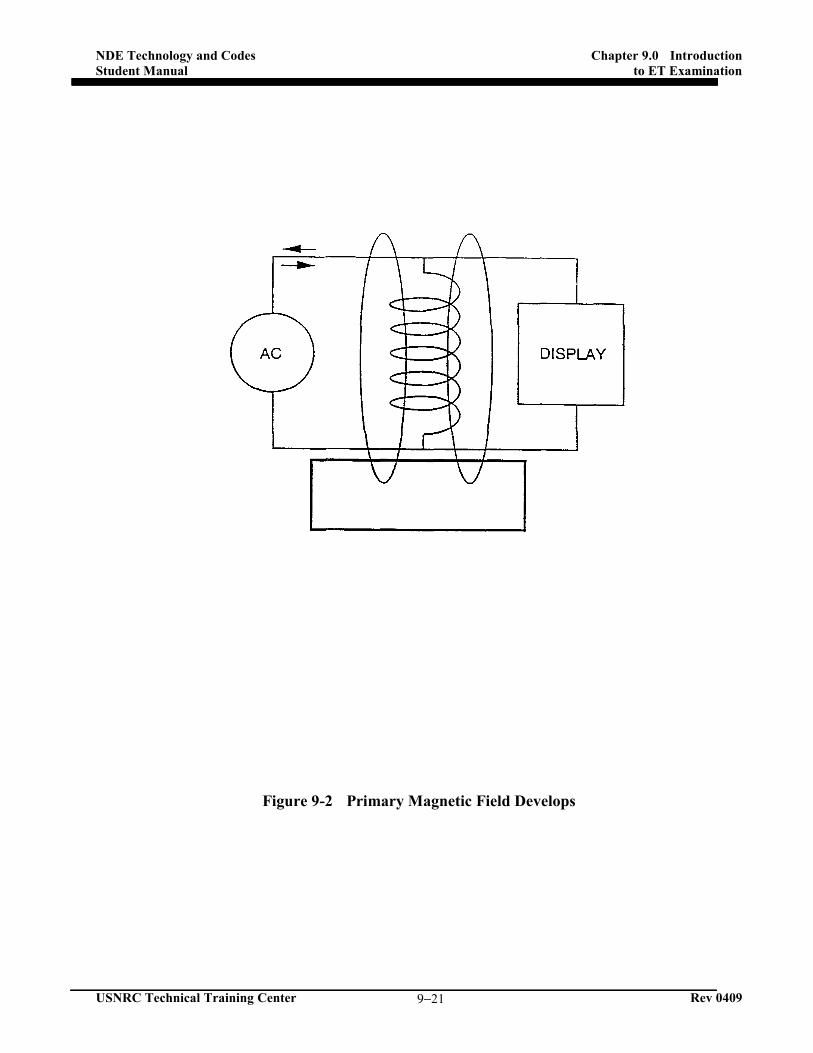
The current in the coil develops a magnetic

field, called the primary field, around the coil as

illustrated in Figure 9-2. This field becomes the

source of two induction processes induced by the



coil’s flux: (1) back voltage into the coil that

causes inductive reactance (Indicated by XL on

Figure 9-3) and (2) voltage into the specimen that

causes eddy currents to circulate (Figure 9-4).

The eddy currents cause friction when they

circulate, resulting in generation of heat in the

test material. Thus, there is a conversion of

electrical energy into thermal energy causing an

effective resistive load on the test coil. Both

types of induction show on the display.

The eddy currents generate a magnetic field

of their own, called the secondary field, which

reacts with the primary field that the coil is

generating (Figure 9-5).

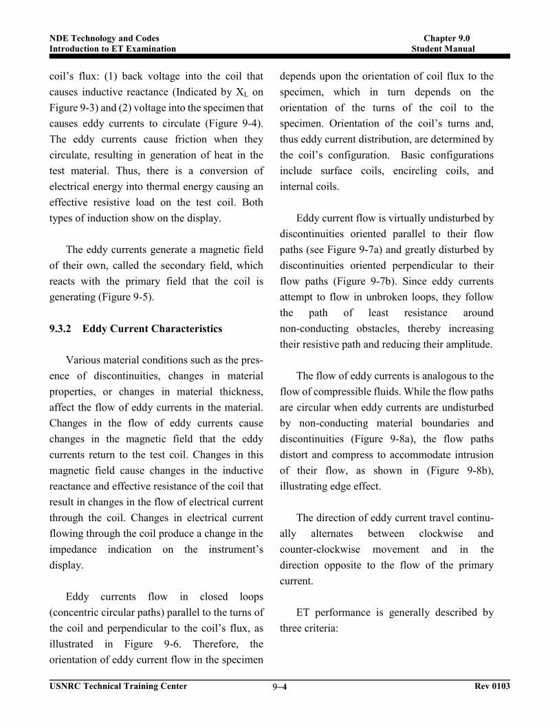
9.3.2 Eddy Current Characteristics

Various material conditions such as the pres-

ence of discontinuities, changes in material

properties, or changes in material thickness,

affect the flow of eddy currents in the material.

Changes in the flow of eddy currents cause

changes in the magnetic field that the eddy

currents return to the test coil. Changes in this

magnetic field cause changes in the inductive

reactance and effective resistance of the coil that

result in changes in the flow of electrical current

through the coil. Changes in electrical current

flowing through the coil produce a change in the

impedance indication on the instrument’s

display.

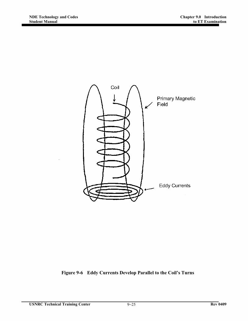
Eddy currents flow in closed loops

(concentric circular paths) parallel to the turns of

the coil and perpendicular to the coil’s flux, as

illustrated in Figure 9-6. Therefore, the

orientation of eddy current flow in the specimen

depends upon the orientation of coil flux to the

specimen, which in turn depends on the

orientation of the turns of the coil to the

specimen. Orientation of the coil’s turns and,

thus eddy current distribution, are determined by

the coil’s configuration. Basic configurations

include surface coils, encircling coils, and

internal coils.

Eddy current flow is virtually undisturbed by

discontinuities oriented parallel to their flow

paths (see Figure 9-7a) and greatly disturbed by

discontinuities oriented perpendicular to their

flow paths (Figure 9-7b). Since eddy currents

attempt to flow in unbroken loops, they follow

the path of least resistance around

non-conducting obstacles, thereby increasing

their resistive path and reducing their amplitude.

The flow of eddy currents is analogous to the

flow of compressible fluids. While the flow paths

are circular when eddy currents are undisturbed

by non-conducting material boundaries and

discontinuities (Figure 9-8a), the flow paths

distort and compress to accommodate intrusion

of their flow, as shown in (Figure 9-8b),

illustrating edge effect.

The direction of eddy current travel continu-

ally alternates between clockwise and

counter-clockwise movement and in the

direction opposite to the flow of the primary

current.

ET performance is generally described by

three criteria:



Sensitivity - This is the minimum size of

discontinuity that can be displayed from a given

depth distance in the material,

Penetration - Penetration is the maximum

depth from which a useful signal can be

displayed for a particular application, and

Resolution - Resolution is the degree to

which separation between signals can be

displayed.

ET performance depends primarily on test

material properties, test frequency, and coil

design. Because only frequency and coil design

are selectable, they are the primary controls over

performance. The following sections discuss in

more detail the important variables and their

effect on ET performance.

9.3.2.1 Material Properties

9.3.2.1.1 Conductivity

Conductivity is a material characteristic that

describes the ease with which electrons pass

through a given material. Each metal is

assigned a conductivity value on a scale called

the International Annealed Copper Standard

(IACS). According to the IACS, conductivity

values are rated in percent, with the conductivity

of pure copper being 100 percent.

An increase in conductivity of the test

material causes an increase in sensitivity to

discontinuities, but a decrease in penetration of

eddy currents into the material. As the coil’s

flux field expands, voltage is induced first on the

surface and then at increasing depths in the

material. In high conductivity materials, a

considerable eddy current flow (and thus a strong

secondary flux field) is developed at the surface.

This results in a substantial cancellation of

primary flux. Because the primary flux has been

greatly weakened, less primary flux is available

to develop eddy currents at greater depth.

The following factors can cause changes in

conductivity within a material:

Material Hardness - Variations in material

hardness affect conductivity. As hardness in-

creases, conductivity decreases and penetration

increases. As a matter of interest, greatest

conductivity is apparent in the annealed state of

nonferrous alloys.

Chemical Composition - Variations in

chemical composition within an alloy affect

conductivity.

Mechanical Processing - Material

processing, such as cold working, affects lattice

structure, which causes minor conductivity

changes.

Thermal Processing - Thermal processing,

such as heat treatment, causes hardness changes

that are detectable as conductivity changes.

Residual Stresses - Residual stress in a

material causes unpredictable conductivity

changes. This is an undesirable condition.

Temperature - Variations in material

temperature causes conductivity to change. As

material temperature increases, conductivity



decreases. This is an undesirable condition. As

a result, care must be taken that material

temperature does not vary during an examination

and that reference standards are the same

temperature as the test specimen.

9.3.2.1.2 Permeability

Permeability is the relative ability of a mate-

rial to become magnetized when subjected to a

magnetizing force, that is, when placed in a

magnetic field. Ferromagnetic metals (including

iron, carbon steels, 400-series stainless steel,

nickel, and cobalt) have high permeability. The

alternating magnetic field of an eddy current coil

becomes highly concentrated in such materials

and overpowers the eddy current response, caus-

ing the system to display permeability rather than

conductivity variations. However, since essen-

tially the same factors that influence conductivity

also influence permeability, the permeability

signals can provide useful information.

As material permeability increases, signals

resulting from permeability variations

increasingly mask eddy current signal variations.

This effect becomes more pronounced with

increased depth. Permeability thus limits the

effective penetration of eddy currents.

9.3.2.1.3 Test Display of Material Property

Variations

Care must be taken during examination to

ensure separation of variables on the display.

Since meter instruments can display only

up-scale or down-scale deflections, the

instruments must be operated so that only one

material variable is displayed. However, with

impedance plane display cathode ray tube (CRT)

instruments, each type of material condition

presents data in a characteristic manner, which

results in the separation of variables and

facilitates the interpretation of signals.

9.3.2.2 Frequency

As test frequency is increased, the density of

eddy currents on the surface increases and sensi-

tivity to surface discontinuities also increases,

permitting increasingly smaller surface disconti-

nuities to be detected. As frequency is decreased,

material penetration depth increases, and the

eddy current density decreases on the surface.

Eddy currents are subject to “skin effect”, in

which current density is maximum at the

material surface and decreases rapidly

(exponentially) with depth. The material depth at

which current density decreases to 36.8 percent

of surface current density is called the standard

depth of penetration.

In addition, eddy currents experience a linear

phase lag with depth. As depth increases, eddy

current activity is progressively delayed. Phase

lag in the specimen proceeds at the rate of one

radian (57.3 percent) per standard depth of

penetration. However, phase lag is displayed at

approximately twice that amount (Figure 9-9).

This is discussed in more detail in Section 9.5.5.

9.3.2.3 Test Specimen Geometry



Test specimen geometry restricts eddy

current flow due to physical differences such as

size or thickness.

Material Thickness - Thickness can be

measured because changes in thickness affect

eddy current flow in the test material. As the

material becomes thinner, eddy current flow

becomes restricted.

Material Discontinuities - These

discontinuities cause indications relative to the

extent that the size and depth of the

discontinuities disturb eddy current flow. Thus,

discontinuities whose major dimensions are

perpendicular to eddy current flow paths and

which are located near the test surface provide

the strongest indications. Additionally, since

eddy currents attain peak amplitude

progressively later as depth increases, display of

this “phase lag” information can indicate

discontinuity depth.

Material Boundaries - Restriction of eddy

current flow called “edge effect” occurs when a

surface coil approaches the edge of a plate, as

shown in Figure 9-8. Similarly, a current flow

restriction called “end effect” occurs when an

encircling or internal coil approaches the end of a

tube or pipe. Both conditions produce strong

signals. The effects are intensified by the wider

eddy current fields developed by large diameter

coils and lower test frequencies.

9.3.2.4 Coil Design

Penetration and sensitivity are affected by

coil geometry. As a rule of thumb, eddy current

penetration is limited to coil diameter. However,

since a small surface discontinuity causes a

proportionally greater disturbance in the field of

a smaller coil, smaller coils are preferred for

detection and localization of small surface

discontinuities.

9.3.2.4.1 Coil Coupling (Lift-Off)

When distance between the coil and

specimen varies, the intensity of the induced flux

field likewise varies. The spacing between a

surface coil and the specimen is called “lift-off”

(Figure 9-10).

The spacing between either an internal coil or

encircling coil and concentrically positioned

specimen is called “fill factor”. Sensitivity to

lift-off and fill factor depends on flux density and

thus decreases as distance between coil and

specimen increases.

The decrease in sensitivity is nonlinear due to

the decrease in flux density according to the

Inverse Square Law. Lift-off is useful for

measuring the thickness of paint or other

nonconductive coatings on the surface of a metal.

It can also be used to measure the thickness of

nonconductive materials, as long as such

materials are placed on a conductive object. Fill

factor deflections can indicate material variations

such as wall thickness changes or ovality

conditions.

9.3.2.4.2 Edge Effect

Restriction of current flow called “edge

effect” occurs when an eddy current surface coil



approaches the edge of a geometric change

(Figure 9-8). Similarly, as mentioned above, a

current flow restriction called “end effect”

occurs when an encircling or internal coil

approaches the end of a tube or pipe. Both

effects produce strong signals. The effects are

intensified by the wide eddy current fields

developed by large diameter coils and lower test

frequencies.

Edge effect can be eliminated by scanning

the coil parallel to the material edge at a constant

distance from the edge; simple fixtures to

accomplish this can be easily fabricated. This

technique maintains edge effect at a constant

value. Interception of a discontinuity then causes

a signal change. The use of smaller diameter

coils reduces edge effect and the use of shielded

coils virtually eliminates it.

9.4 Equipment

A variety of ET instruments are available for

use, from simple to complex. Although these

instruments vary greatly in applications

flexibility as well as size, most of them operate

on similar principles.

Multifrequency instruments offer potential

for substantial enhancement of performance. Use

of more than one test frequency has three advan-

tages:

• Signals generated by the various frequencies

can be “mixed” to prevent display of

undesirable signals; suppression of signals

from steel supports during examination of

nonferro-magnetic tubes is an example. Each

additional frequency enables an additional

variable to be isolated.

• Use of multiple frequencies allows more than

one frequency to be used simultaneously. For

example, during in-service tube examination,

a higher frequency provides sensitivity to

inner diameter discontinuities and a lower

frequency provides sensitivity for responding

to outer diameter discontinuities.

• Use of multiple frequencies aids signal

analysis. The various conditions that can be

detected by ET exhibit different responses as

frequency is varied.

9.4.1 System Components

All ET instruments require at least three

circuit components: alternating current

generator, coil, and processing/display circuitry.

The level of flexibility designed into each of

these elements generally determines how ET

instruments differ from each other. ET coils can

be classified according to both basic

configuration and mode of operation. Coil

design, as well as magnitude and frequency of

the applied current, all affect the electromagnetic

field developed by the coil.

Basic ET equipment consists of an

alternating current source (oscillator), voltmeter,

and probe. When the probe is brought close to a

conductor or moved past a discontinuity, the

voltage across the coil changes and this is read

off the voltmeter. The oscillator sets the test

frequency and the probe governs coupling and

sensitivity to discontinuities.



Most ET instruments use an alternating cur-

rent bridge for balancing but use various

methods for lift-off compensation. Send-receive

instruments should be used for accurate absolute

measurements in the presence of temperature

fluctuations. Multi-frequency instruments can be

used to simplify discontinuity signals in the

presence of extraneous signals.

ET instruments and recording equipment

have a finite frequency response which limits the

examination speed.

The main functions of an ET instrument are

illustrated in the block diagram in Figure 9-11.

A sine wave oscillator generates sinusoidal

current, at a specified frequency, that passes

through the test coils. Since the impedance of

two coils is never exactly equal, balancing is

required to eliminate the voltage difference

between them. Most ET instruments achieve this

through an alternating current bridge or by

subtracting a voltage equal to the unbalance

voltage. In general they can tolerate an

impedance mismatch of 5 percent. Once

balanced, the presence of a discontinuity in the

vicinity of one coil creates a small unbalanced

signal, which is then amplified.

The most troublesome parameter in ET is

lift-off (probe-to-specimen spacing). A small

change in lift-off creates a large output signal.

Figure 9-12 shows a typical eddy current

instrument with various control functions. The

frequency selector sets the desired test

frequency. Frequency is selected by continuous

control or in discrete steps from about 1 kHz to 2

MHz.

The balancing controls, labeled X and R are

potentiometers. They match coil impedance to

achieve a null when the probe is in a

discontinuity free location on the test sample.

Most instruments have automatic balancing.

The bridge output signal amplitude is con-

trolled by the GAIN control. In some instruments

it is labeled as sensitivity. GAIN controls the

amplifier of the bridge output signal and does not

affect current going through the probe.

Following amplification of the bridge unbal-

ance signal, the signal is converted to direct

current signals. Since the alternating current’s

signal has both amplitude and phase, it is con-

verted into quadrature X and Y components.

ET instruments do not have a phase reference. To

compensate for this they have a phase shift.

Crack Detection Instruments - Crack

detector instruments contain only one coil, with a

fixed value capacitor in parallel with the coil to

form a resonant circuit. At this condition the

output voltage for a given change in coil

impedance is maximum. The coil’s inductive

reactance, XL, must be close to the capacitive

reactance, XC.

Crack detectors that operate at or close to

resonance do not have selectable test

frequencies. Crack detectors for

non-ferromagnetic, high electrical resistivity

materials such as Type 304 stainless steel

typically operate between 1 and 3 MHz; those for



low resistivity materials (aluminum alloys,

brasses) operate at a lower frequency, normally

in the 10 to 100 kHz range. Some crack detectors

for high resistivity materials can also be used to

examine ferromagnetic materials, such as carbon

steel, for surface discontinuities. Normally a

different probe is required; however, coil

impedance and test frequency change very little.

Crack detectors have a meter output and

three basic controls: balance, lift-off, and

sensitivity. Balancing is performed by adjusting

the potentiometer on the adjacent bridge arm,

until bridge output is zero (or close to zero).

GAIN (sensitivity) adjustment occurs at the

bridge output. The signal is then rectified and

displayed on a meter. Because the signal is

filtered, in addition to the mechanical inertia of

the pointer, the frequency response of a meter is

very low (less than 10 Hz). LIFT-OFF control

adjusts the test frequency (by less than 25

percent) to operate slightly off resonance. In

crack detectors the test frequency is chosen to

minimize the effect of probe wobble (lift-off),

not to change the skin depth or phase lag.

9.4.2 Data/Displays

Since the impedance plane is a graphic plot

of ET information, resistance values are shown

on the X axis; inductive reactance values, on the

Y axis. Impedance plane display instruments

thus present both impedance amplitude and

impedance phase angle simultaneously on a CRT

screen.

Data on an impedance plane instrument is

interpreted by observing the movement of the

display dot on a CRT screen while the coil inter-

acts with the specimen. Each type of condition

that ET can detect is characterized by a certain

pattern of display dot movement. Variables are,

in fact, arranged along curves or “loci” on the im-

pedance plane. Generally there are separate

curves for each variable. Distribution of

information on the impedance plane can be

altered by changing frequency. Redistribution of

information on the impedance plane by

adjustment of frequency is a key technique in

optimizing performance.

Sections 9.4.2.1 through 9.4.2.4 describe

several types of curves displayed on the CRT.

9.4.2.1 Lift-Off Curves

The zero conductivity point, also called the

coil in air or empty coil point, is typically located

at a position of low resistance, but of moderately

high inductive reactance. This is the impedance

point for a coil whose flux is not near any

conductive material. However, as a coil is moved

toward a conductor, secondary flux changes the

coil’s impedance and the display dot moves. The

position where movement terminates depends on

the conductivity of the test material. The more

conductive the test material, the greater the

cancellation of primary flux, which causes a

greater drop in inductive reactance and

movement further downward by the dot. Because

the coil and specimen are coupled, the specimen

acts as a load on the coil and the effective

resistance of the coil also changes. The

movement of the display dot is, therefore, a

combination of variations in both inductive

reactance and effective resistance.



9.4.2.2 Conductivity Curve

Originating at the zero conductivity point is

the conductivity curve, sometimes called the

comma curve, because of its shape. Different

positions along this curve represent

non-ferromagnetic materials of different

conductivities, whose thicknesses are infinite

relative to electromagnetic penetration. That is,

the flux lines entering the material, as well as the

eddy currents that they generate, are not

perceptibly affected by the bottom surface of the

material. The counterclockwise extreme of the

conductivity curve represents zero conductivity,

whereas the clockwise extreme of the curve

represents infinite conductivity.

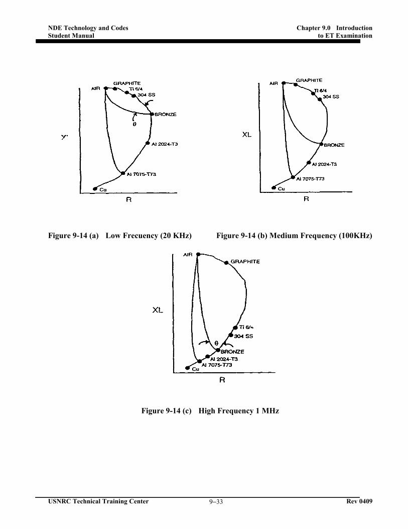
As the frequency is increased, the impedance

points for the various conductivities move

clockwise along the curve; the lower

conductivity materials spread apart along the

curve while the higher conductivity materials

become compressed at the bottom end of the

curve (Figure 9-13). Higher frequencies provide

greater separation for conductivity tests on lower

conductivity materials (Figure 9-14a). As the

frequency is decreased, the impedance points for

the various conductivities move

counterclockwise along the curve (Figure

9-14b); the higher conductivity materials spread

apart while the lower conductivity materials

become compressed at the top end of the curve.

Lower frequencies provide greater separation for

conductivity tests for high conductivity materials

(Figure 9-14c). Frequency adjustment also

helps separate the lift-off and conductivity

variables during conductivity tests. At low

frequencies, lift-off curves for low conductivity

materials are almost parallel to the conductivity

curve.

As frequency is increased, the operating

point moves clockwise along the conductivity

curve, increasing the angle between the lift-off

curve and conductivity curve. Maximum

separation is achieved at the so called “knee” of

conductivity curve, where the lift-off curve

approaches it almost perpendicularly.

9.4.2.3 Thickness Curves

As previously stated, the conductivity curve

consists of impedance points for materials whose

thicknesses are infinite, relative to electromag-

netic penetration. At lesser thicknesses, eddy

current flow in the material becomes restricted

and the impedance point moves

counterclockwise, spiraling away from the

conductivity curve. As thickness approaches

zero, the impedance point necessarily

approaches the zero conductivity point.

A standard depth of penetration is indicated

by the δ symbol. It is approximately located on

thickness curve at a point slightly to the right of

the intersection with the conductivity curve.

Again, frequency adjustment optimizes perfor-

mance. As frequency is decreased, material

penetration increases, but thickness resolution on

thinner materials decreases. As frequency is

increased, material penetration decreases, but

thickness resolution on thinner materials in-

creases.

9.4.2.4 Discontinuity Signal Display



In an ET examination, a discontinuity is an

interruption of conductivity. The magnitude of

an ET discontinuity signal depends on the

quantity of interrupted current flow. Length,

width, and depth of a discontinuity all affect

signal magnitude to the extent that discontinuity,

volume, and shape obstruct the greatest amount

of electron flow. Because ET density decreases

exponentially with depth, a given discontinuity

volume disturbs increasingly fewer electrons

with depth. The depth of the disturbance,

however, causes a linear phase lag of the signal

(Figure 9-15).

9.4.3 Basic Coils

The basic coil configuration determines how

the coil is packaged to “fit” the object being

examined. There are three basic configurations,

described in sections 9.4.3.1 through 9.4.3.3.

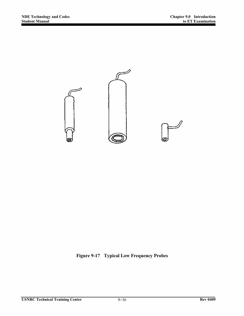
9.4.3.1 Surface Coils

Surface coils are built into probe type hous-

ings for scanning material surfaces. The coil axis

is usually perpendicular to the specimen’s

surface. Surface coils are available in different

shapes and sizes to meet different application

needs (Figure 9-16). Larger surface probes

permit faster scanning and deeper penetration,

but cannot pinpoint the location of small

discontinuities (Figure 9-17). They are useful for

conductivity examination because they tend to

average out localized conductivity variations

along material surfaces. Conversely, narrow

coils are preferred for detecting and pinpointing

the location of small surface discontinuities.

Because of their smaller diameter

electromagnetic fields, narrow coils are less

susceptible to edge effect.

9.4.3.2 Encircling Coils

Encircling coils (Figure 9-18) completely

surround the specimen, thus they are normally

used for production examination of rods, wire,

bar stock, pipes, and tubing. Because of “center

effect”, eddy currents oppose and therefore

cancel themselves at the center of solid

cylindrical materials examined with encircling

coils. Thus, discontinuities located at the center

of rods and bar stock cannot be detected with

encircling coils. Encircling coils examine the

entire circumference of the specimen; however,

they cannot pinpoint the exact location of a

discontinuity along the circumference.

9.4.3.3 Internal Coils

Internal coils (Figures 9-19 and 9-20) pass

though the cores of pipes and tubes; thus, they

are normally employed for in-service

examinations. Like encircling coils, standard

bobbin-wound internal coils examine the entire

circumference of the specimen at one time but

cannot pinpoint the exact location of a

discontinuity along the circumference.

Both manual and automatic means are used

to propel internal coils down the length of a long

tube. Flexible “u-bend” assemblies are available

for navigating extreme curvature of tubing.



9.5 Techniques

During examination, ET instruments and

recording equipment are typically connected as

in Figure 9-21. The eddy current signal is

monitored on a storage CRT and recorded on

X-Y and two-channel recorders. Recording on a

magnetic tape recorder for subsequent playback

is also common.

9.5.1 Impedance Plane Fundamentals

The essential features of impedance plane

analysis are:

• The separation of the voltage drop across the

eddy current probe coil(s) into voltage drop

due to pure resistance and the voltage drop

due to inductive reactance.

• The presentation of the impedance vector due

to resistance changes and inductive reactance

changes as a “spot” on an oscilloscope

(Figure 9-22).

• The movement of the impedance spot in

different directions is caused by the

following different factors:

- A change in conductivity (or resistivity),

- A change in lift-off (separation of the

probe from the test surface),

- A change in probe frequency,

- A change in geometry,

- A change in probe, or

- A change in permeability (or reluctance).

9.5.2 Impedance Plane Response to

Conductivity Variations

Presentation of conductivity changes on the

impedance plane are shown in Figure 9-22. The

point where the probe is balanced (nulled) is

known as the operating point. It is from this point

that all movement of the “spot” is originated.

Measurement of conductivity can be made:

• By setting an intermediate operating

frequency that will not exceed 30 percent

thickness of the test material for one standard

depth of penetration.

• By balancing (nulling) the equipment and

calibrating the CRT display as shown in

Figure 9-23 to display two known

conductivities bracketing the unknown

conductivity.

NOTE: The use of reference calibration

samples is essential for this task. Reference

calibration samples should both bracket and

approximate the unknown conductivity for

higher accuracy.

9.5.3 Sorting

In the same way that conductivity can be

measured, materials can be sorted. Different heat

treatments or different alloys, even different

permeabilities, are easily discriminated

permitting material sorting.

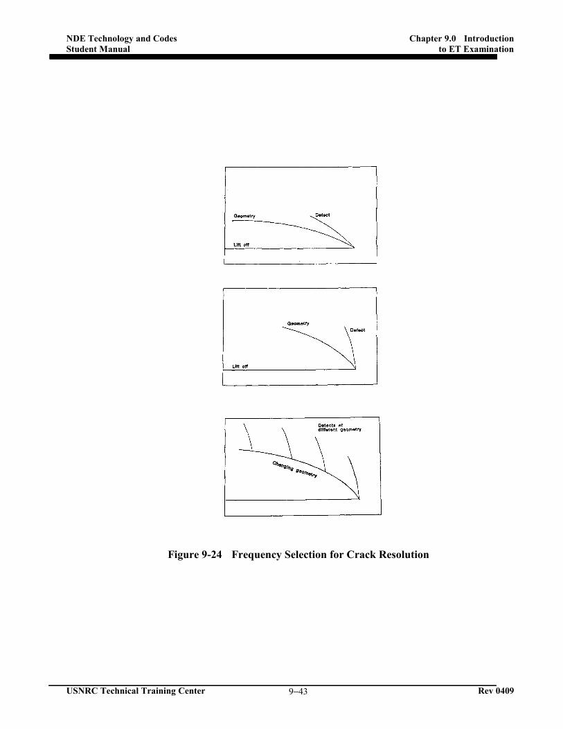
9.5.4 Discontinuities



Location of surface breaking discontinuities

is dependent on frequency. Presentation of fre-

quency changes on the impedance plane are

shown in Figure 9-24.

Calibration is formally defined as

comparison of the instrument to a reference

standard. During an actual ET examination,

calibration is the process of adjusting the

instrument display to represent a known

reference standard so that the examination can be

a comparison between the specimen and the

reference standard. The validity of the

examination thus depends upon the validity of

the reference standard.

Since there is an infinite variety of a

discontinuity condition, it is neither possible nor

practical to have a set of reference standards so

complete as to replicate every possible condition

that could be detected during an examination.

Therefore, it is not practical to match each signal

with an identical reference signal. Instead, one

obtains practical reference standards that contain

a manageable number of representative

discontinuity conditions. Signals that vary from

these must then be interpreted through

techniques such as impedance plane analysis.

9.5.4.1 Discontinuity Location in Installed

Nonferrous Steam Generator Heat

Exchanger Tubing

ET equipment capable of operation in the

differential mode or the absolute mode, or both,

should be used for this examination. A device

for recording data, real time, in a format suitable

for evaluation and for archival storage, should be

provided when required by the referencing Code

Section.

Electronic instrumentation of the ET system

should be calibrated at least once a year or

whenever the equipment has been overhauled or

repaired as a result of malfunction or damage.

Single frequency or multiple frequency tech-

niques are permitted for this examination. Upon

selection of the test frequency(s) and after com-

pletion of calibration, the probe should be

inserted into the tube where it is extended or

positioned to the region of interest. Resulting

ET signals at each of the individual frequencies

should be recorded for review, analysis, and final

disposition.

The calibration tube standard (Figure 9-25)

should be manufactured from a length of tubing

of the same nominal size and material type

(chemical composition and product form) as that

to be examined in the steam generator. The

intent of this reference standard is to establish

and verify system response. The standard

should contain calibration discontinuities as

follows:

• A single hole drilled 100 percent through the

wall;

• A flat bottom hole 0.109” in diameter and

60%throuigh the tube wall from the outer

surface.

• Four flat bottom holes, 3/16 inch diameter,

spaced 90° around the circumference at 20%

through wall from the outside surface;



• A 1/16-inch wide, 360° circumferential

groove, 10 percent through from the inner

tube surface (optional);

Other requirements for the standard include:

• All calibration discontinuities should be

spaced so that they can be identified from

each other and from the end of the tube.

• Each standard should be identified by a serial

number.

• The dimensions of the calibration

discontinuities and the applicable ET

response should become part of the

permanent record of the standard.

9.5.4.2 Calibration Procedure

The examination system should be calibrated

utilizing the standard. A summary of the

calibration steps follows:

Calibration Using Differential Bobbin

Coil Technique (Figure 9-26):

1. The ET instrument is adjusted for the fre-

quency chosen so that the phase angle of a

signal from the four 20 percent flat bottom

holes is between 50° and 120° rotated clock-

wise from the signal of the through-the-wall

hole (Figure 9-27).

2. The trace display for the four 20 percent flat

bottom holes should be generated, when

pulling the probe, in the directions illustrated

in Figure 9-27, down and to the left first,

followed by an upward motion to the right,

followed by a downward motion returning to

the point of origin.

3. The sensitivity should be adjusted to produce

a minimum peak-to-peak signal from the four

20 percent flat bottom holes of 30 percent of

the full scale horizontal presentation with the

oscilloscope sensitivity set at 1 volt per divi-

sion.

4. It is common to then adjust the phase or

rotation control so that the signal response

due to probe motion, or the 10 percent deep

circumferential inside diameter groove, or

both, is positioned along the horizontal axis

of the display.

Calibration Using Absolute Bobbin Coil

Technique:

1. The ET instrument should be adjusted for a

frequency so that the phase angle between a

line drawn from the origin to the tip of the

response from the through-the-wall hole and

the horizontal axis is approximately 40°.

The phase angle formed by a line drawn from

the origin to the tip of the response of the four

20 percent flat bottom holes and the

through-the-wall response line is between

50° and 120°. (Figure 9-28).

2. The sensitivity should be adjusted to produce

a minimum origin-to-peak signal from the

four 20 percent flat bottom holes of 30

percent of the full scale horizontal

presentation with the oscilloscope sensitivity

set at 1 volt per division.

3. It is common to adjust the phase or rotation

control so that the signal response due to

probe rotation, or the 10 percent deep cir-



cumferential inside diameter groove, or both,

is positioned along the horizontal axis of the

display 5°.

4. The response may be rotated to the upper

quadrants of the display at the option and

convenience of the operator.

5. Withdrawing the probe through the

calibration tube standard at the probe speed

selected for the examination should be

repeated. The responses should be recorded

for the applicable calibration discontinuities

and verified that they are clearly indicated by

the instrument and are distinguishable from

each other, as well as from probe motion

signals.

9.5.4.3 Probe Speed

The typical probe speed during examination

should not exceed 14 inch/second. Higher probe

speeds may be used if system frequency response

and sensitivity to the applicable calibration stan-

dards.

9.5.5 Thickness

The effects of edge effect have already been

described and edge effect should be clearly dis-

cernible from other factors effecting eddy cur-

rents. Geometry is different from edge effect

and can also be described by reduction in

thickness (Figure 9-29).

Phase indications on CRTs are related to the

phase change as the eddy currents penetrate the

material under test. As the phase change occurs

into the material by 57° per standard depth of

penetration, it should be quite acceptable that the

same phase change occurs again when sensed by

a probe on the surface (sensed at 114° total indi-

cated phase change). This phenomenon can be

proven. A discontinuity at exactly one standard

depth of penetration will give an indication of 2 x

57° = 114° out of phase with lift-off (Figure

9-30).

9.5.5.1 Location of Secondary Layer Cor-

rosion or Cracking

The frequency should be selected to give 90°

phase separation between lift-off and material

loss. As one standard depth of penetration gives

114° phase angle, if multiplied by 0.7895, the

answer will be 90°. So, for 90° phase separation

of subsurface discontinuities, the standard depth

of penetration frequency should be multiplied by

approximately 0.80.

The equipment should be balanced (nulled),

and the lift-off set horizontally from the operat-

ing point which should be to the lower right hand

quadrant of the CRT.

Thinning is represented by a move of the spot

up the calibrated thinning line. Similar results

will be seen for subsurface cracks except the

move of the spot from the operating point on the

conductivity curve will be quicker, and include

an integration of the phase change through the

depth of the crack. If the material thickens from

the balance point, the spot will move down the

CRT from the lift-off.

The final result of the variations in thickness

on the eddy currents is shown in Figure 9-31.



Note the small “comma” shaped curve is the

material thickening from the balance (operating)

point.

9.5.6 Coatings

9.5.6.1 Variations in Thickness of Plating

or Cladding

These variations combine both conductivity

and dimensional variables.

Presentation of lift-off changes on the

impedance plane is shown in Figure 9-32. The

point where the probe is in the balanced condi-

tion (nulled) is known as the operating point. It

is from this point that all movement of the spot is

originated.

Measurement of non-conducting coating

thickness (lift-off) can be made using the

following procedure:

- The highest frequency should be chosen

to give maximum sensitivity to lift-off (and

hence accuracy). The equipment should be

balanced. This will bring the operating point to

the bottom of the conductivity curve.

- - The CRT display should be calibrated as

shown in Figure 9-33 to display two known

non-conducting thickness (plastic foil or shim

calibration samples are used) bracketing the

unknown coating thickness.

NOTE: The use of reference calibration

shims is essential to this task. Reference

calibration shims should approximate the

unknown for higher accuracy.

9.6 Interpretation and Code

Requirements

9.6.1 Written Procedure

All ET examinations should be performed to

detailed written procedures, unless otherwise

stated in the reference code.

9.6.2 Description of Method

The procedure for eddy current should

provide a sensitivity which will consistently

detect discontinuity indications equal to or

greater than those conditions in the reference

specimen. Parts with discontinuities that

produce indications in excess of the reference

standards should be evaluated in accordance with

the procedure that meets code requirements.

9.6.3 Reference Specimen

The reference specimen should be a part of

and be processed in the same manner as the

product being examined. It should be of the

same dimensions and the same nominal

composition as the product being examined.

Unless otherwise specified in the referencing

Code, the reference discontinuities should be

transverse notches, drilled holes, or should

simulate as near as possible the conditions to be

detected.

The reference specimen should be long or

large enough to simulate the handling of the

product being examined through the examination

equipment. The separation between reference

discontinuities placed in the same reference



specimen should be not less than twice the length

or diameter of the sensing unit of the

examination equipment.

9.6.4 Equipment Qualification

The proper functioning of the examination

equipment should be checked and calibrated by

the use of the reference specimens as follows:

• At the beginning of each production run of

given dimensions of a given material,

• After each hour during the production run,

• At the end of the production run, and

• At any time that malfunctioning is suspected.

Acceptance requirements shall be as

specified in the referenced code.

9.6.5 Procedure Requirements

The written procedure should include at least

the following:

• Frequency,

• Type of coil or probe (e.g., differential coil),

• Type of material and sizes to which applica-

ble,

• Reference specimen notch or hole size, and

• Additional information as necessary to

permit retesting.

9.7 Advantages and Limitations of ET

Examinations

ET can provide a variety of useful

information about an object. In addition, an

extensive selection of equipment is available to

fit the examination to the application. Frequency

adjustment and coil selection are the examiner’s

primary controls over performance.

Information is obtained by monitoring changes

in coil impedance caused by variations in the

specimen. However, because the process is

complex, examiner skill is a critical variable

especially for the examination of heat exchanger

tubing.

9.7.1 Advantages

The following are advantages of ET:

• This method is sensitive to numerous

material variables. Consequently, any of

several material properties can be measured

providing the other variables are either

separately identifiable or suppressed.

• Much of the equipment is portable, light-

weight, and battery powered.

• This method is nondestructive. No couplant,

powders, or other physical substances are

applied to the specimen. The only link be-

tween the probe and specimen is a magnetic

field.

• Results are instantaneous. As soon as the test

coil is applied to the specimen, a qualified

examiner can interpret the results. An excep-

tion, however, is computer analysis of tape

recorded multichannel test data.

• ET testing is ideal for “go/no-go” examina-

tions. Audible and visual alarms, triggered by

threshold gates or box gates, are available for

high-speed examination.

• There is no danger from radiation or other

such hazards.



• Material preparation is usually unnecessary;

cleanup is not required.

9.7.2 Limitations

ET also has several limitations:

• The material must be electrically conductive.

It is possible to measure the thickness of

nonconductive coating on conductive

materials.

• ET normally cannot penetrate ferromagnetic

materials. Consequently, examination of

ferromagnetic material is limited to surface

discontinuities only, unless the material has

been magnetically saturated using direct

current field coils. Magnetic saturation is

limited to certain geometries only. In

addition, magnetically saturated objects may

have to be demagnetized after testing is

completed.

• Even for non-ferromagnetic materials, the

ET method has limited penetration.

NDE Technology and Codes Student Manual

USNRC Technical Training Center

Figure 9-1 Alternat

Chapter 9.0 to ET

9−20

ting Current Flowing Through Test Coil

Introduction T Examination

Rev 0409

NDE Technology and CodesStudent Manual


Figure 9-2

Chapter to

9−21

2 Primary Magnetic Field Develops

9.0 Introduction o ET Examination

Rev 0409



Figure 9-3

Chapter 9.0 to ET

9−22

Inductive Reactance Occurs


Rev 0409



Figu

Chapter to

9−23

re 9-4 Eddy Currents Develop


Rev 0409



Figure 9-

Chapter 9.0 to ET

9−24

5 Secondary Field Develops


Rev 0409



Figure 9-6 Eddy C

Chapter to

9−25

Currents Develop Parallel to the Coil’s Turns


Rev 0409



Figure 9-7 Effect o on

Chapter 9.0 to ET

9−26

f Variation in Discontinuity Orientation Eddy Current Flow Paths


Rev 0409



Figure 9-8 Compressi

Chapter to

9−27

ion of Eddy Current Flow Paths by Material E


Rev 0409

Edge



Figure 9-9 Attenu Penetra

Chapter 9.0 to ET

9−28

uation and Phase Lag of Eddy Currents ating into a Conductive Material


Rev 0409



Figure 9-10 ReduResults i

Chapter to

9−29

uction in Eddy Current Strength with Lift-Off in Positive Meter Movement Unless

Lift-Off is Compensated


Rev 0409



Figure 9-11 Block

Chapter 9.0 to ET

9−30

k Diagram of Eddy Current Instrument


Rev 0409



Figure 9-12 Typical

Chapter to

9−31

Eddy Current Instrument with Storage Monit


Rev 0409

tor



Figure 9

Chapter 9.0 to ET

9−32

9-13 Conductivity Curve


Rev 0409



Figure 9-14 (a) Low Frecuency (2

Figure

Chapter to

9−33

20 KHz) Figure 9-14 (b) Medium Frequ

9-14 (c) High Frequency 1 MHz


Rev 0409

ency (100KHz)



Figure 9-15 Direcin Alumin

Chapter 9.0 to ET

9−34

ction of Surface and Subsurface Cracks num on the Impedance Plane


Rev 0409



Figure 9-16

Chapter to

9−35

Various High Frequency Surface Probes


Rev 0409



Figure 9-17

Chapter 9.0 to ET

9−36

7 Typical Low Frequency Probes


Rev 0409



Chapter to

9−37

Figure 9-18 Encircling Coil


Rev 0409



Figure 9-1

Chapter 9.0 to ET

9−38

19 Internal Coil (Bobbin Probe)


Rev 0409



Figure 9-20 In

Chapter to

9−39

nternal (Insertion, Bobbin) Differential Probe


Rev 0409



Figure 9-2

Chapter 9.0 to ET

9−40

1 Eddy Current Test System


Rev 0409



F

Chapter to

9−41

Figure 9-22 Impedance Plane


Rev 0409



Figure 9-

Chapter 9.0 to ET

9−42

-23 Conductivity Measurement


Rev 0409



Figure 9-24

Chapter to

9−43

Frequency Selection for Crack Resolution


Rev 0409



Figure 9-25

Chapter 9.0 to ET

9−44

5 Tube Calibration Standards


Rev 0409



Fig

Chapter to

9−45

gure 9-26 Internal Bobbin Probe


Rev 0409



Figure 9-27 TypCalibrated Diff

Chapter 9.0 to ET

9−46

pical Signal Response from a Properly ferential Bobbin Coil Probe System


Rev 0409



Figure 9-28 TCalibrated

Chapter to

9−47

Typical Signal Response from a Properly d Absolute Bobbin Coil Probe System


Rev 0409



Figure 9-29

Chapter 9.0 to ET

9−48

Changes in Thickness (Example 1)


Rev 0409



Figure 9

Chapter to

9−49

-30 Change in Thickness (Example 2)


Rev 0409



Figure 9-31 Changing

Chapter 9.0 to ET

9−50

Signal Phase and Signal Amplitude with Depth


Rev 0409

h



Figure 9-32 Changes

Chapter to

9−51

s in Conductivity, Lift-Off, Probe, and Thickne


Rev 0409

ess



Figure 9-33

Chapter 9.0 to ET

9−52

Coating Thickness Measurement


Rev 0409

Documents

0444 - E306 - Nondestructive Examination (NDE) Technology ...ANSI/ASNT CP-189 (2006 Edition), or ACCP Qualification in accordance with a prior ... A person may be qualified directly