Embed Size (px)
Citation preview
J. Elder CSE 6390/PSYC 6225 Computational Modeling of Visual Perception
LINEAR MODELS FOR CLASSIFICATION

Linear Models for Classification
J. Elder CSE 6390/PSYC 6225 Computational Modeling of Visual Perception
2
Classification: Problem Statement
In regression, we are modeling the relationship between a continuous input variable x and a continuous target variable t.
In classification, the input variable x is still continuous, but the target variable is discrete.
In the simplest case, t can have only 2 values.

Linear Models for Classification
J. Elder CSE 6390/PSYC 6225 Computational Modeling of Visual Perception
3
Example Problem
Animal or Vegetable?

Linear Models for Classification
J. Elder CSE 6390/PSYC 6225 Computational Modeling of Visual Perception
4
Linear Models for Classification
Linear models for classification separate input vectors into classes using linear decision boundaries. Example:
!4 !2 0 2 4 6 8
!8
!6
!4
!2
0
2
4
Input vector x
Two discrete classes C1 and C2
Linear Models for Classification
J. Elder CSE 6390/PSYC 6225 Computational Modeling of Visual Perception
5
Discriminant Functions
A linear discriminant function y(x) = f w tx +w0( )
maps a real input vector x to a scalar value y(x).
f (⋅) is called an activation function.
Linear Models for Classification
J. Elder CSE 6390/PSYC 6225 Computational Modeling of Visual Perception
6
Outline
Linear activation functions Least-squares formulation Fisher’s linear discriminant
Nonlinear activation functions Probabilistic generative models Probabilistic discriminative models
Logistic regression Bayesian logistic regression
Linear Models for Classification
J. Elder CSE 6390/PSYC 6225 Computational Modeling of Visual Perception
7
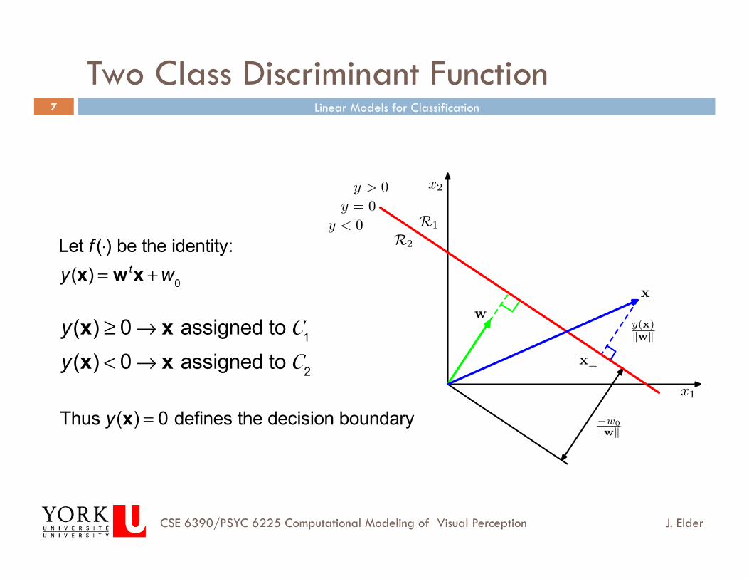
Two Class Discriminant Function
Let f (⋅) be the identity:y(x) = w tx +w0
y(x) ≥ 0→ x assigned to C1
y(x) < 0→ x assigned to C2
Thus y(x) = 0 defines the decision boundary
x2
x1
wx
y(x)�w�
x⊥
−w0�w�
y = 0y < 0
y > 0
R2
R1

Linear Models for Classification
J. Elder CSE 6390/PSYC 6225 Computational Modeling of Visual Perception
8
K>2 Classes
Idea #1: Just use K-1 discriminant functions, each of which separates one class Ck from the rest. (One-versus-the-rest classifier.)
Problem: Ambiguous regions
R1
R2
R3
?
C1
not C1
C2
not C2
Linear Models for Classification
J. Elder CSE 6390/PSYC 6225 Computational Modeling of Visual Perception
9
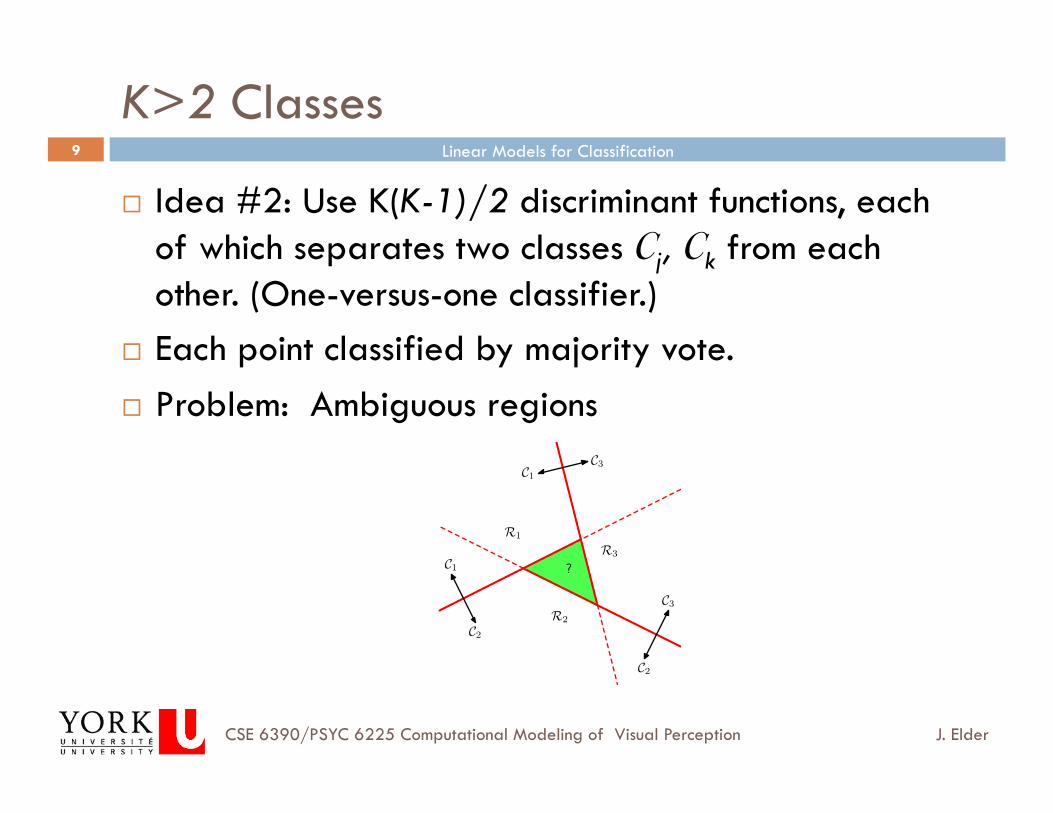
K>2 Classes
Idea #2: Use K(K-1)/2 discriminant functions, each of which separates two classes Cj, Ck from each other. (One-versus-one classifier.)
Each point classified by majority vote. Problem: Ambiguous regions
R1
R2
R3
?C1
C2
C1
C3
C2
C3
Linear Models for Classification
J. Elder CSE 6390/PSYC 6225 Computational Modeling of Visual Perception
10
K>2 Classes
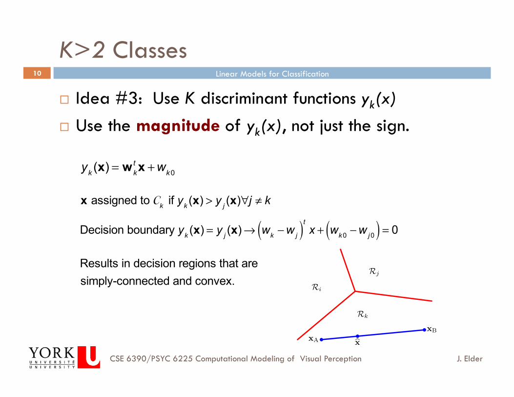
Idea #3: Use K discriminant functions yk(x) Use the magnitude of yk(x), not just the sign.
yk (x) = w kt x +wk0
x assigned to Ck if yk (x) > y j (x)∀j ≠ k
Decision boundary yk (x) = y j (x)→ wk −w j( )t x + wk0 −w j 0( ) = 0
Results in decision regions that are simply-connected and convex. Ri
Rj
Rk
xA
xB
�x

Linear Models for Classification
J. Elder CSE 6390/PSYC 6225 Computational Modeling of Visual Perception
11
Learning the Parameters
Method #1: Least Squares
yk (x) = w kt x +wk0
→ y(x) = Wt x
where x = (1,xt )t
W is a (D +1) × K matrix whose kth column is w k = w0,w kt( )t

Linear Models for Classification
J. Elder CSE 6390/PSYC 6225 Computational Modeling of Visual Perception
12
Learning the Parameters
Method #1: Least Squares y(x) = Wt x
Training dataset xn,tn( ), n = 1,…,N
Let T be the N × K matrix whose nth row is tnt
where we use the 1-of-K coding scheme for tn
Let X be the N × (D +1) matrix whose nth row is xnt
We define the error as ED
W( ) = 12
Tr X W − T( )t X W − T( ){ }
Setting derivative wrt W yields:W = Xt X( )−1 XtT = X†T
Linear Models for Classification
J. Elder CSE 6390/PSYC 6225 Computational Modeling of Visual Perception
13
Fisher’s Linear Discriminant
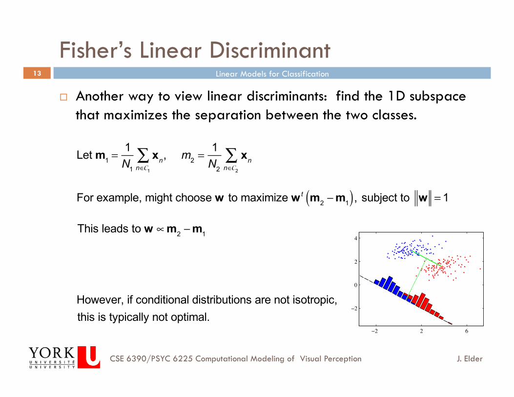
Another way to view linear discriminants: find the 1D subspace that maximizes the separation between the two classes.
!2 2 6
!2
0
2
4
Let m1 =
1N1
xnn∈C1
∑ , m2 =1
N2
xnn∈C2
∑
For example, might choose w to maximize w t m2 −m1( ), subject to w = 1
This leads to w ∝m2 −m1
However, if conditional distributions are not isotropic, this is typically not optimal.
Linear Models for Classification
J. Elder CSE 6390/PSYC 6225 Computational Modeling of Visual Perception
14
Fisher’s Linear Discriminant
!2 2 6
!2
0
2
4
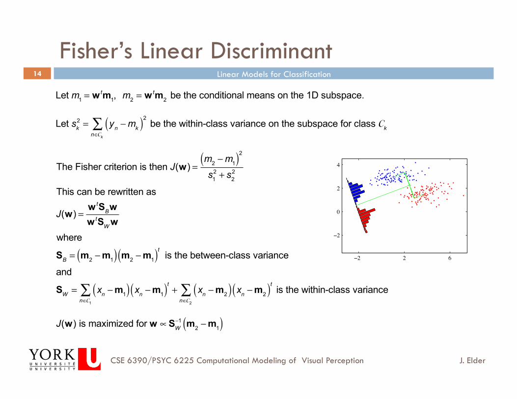
Let m1 = w tm1, m2 = w tm2 be the conditional means on the 1D subspace.
Let sk
2 = yn − mk( )2
n∈Ck
∑ be the within-class variance on the subspace for class Ck
The Fisher criterion is then J(w) =
m2 − m1( )2
s12 + s2
2
This can be rewritten as
J(w) =w tSBww tSW w
where
SB = m2 −m1( ) m2 −m1( )t is the between-class variance
and
SW = xn −m1( ) xn −m1( )tn∈C1
∑ + xn −m2( ) xn −m2( )tn∈C2
∑ is the within-class variance
J(w) is maximized for w ∝SW−1 m2 −m1( )
Linear Models for Classification
J. Elder CSE 6390/PSYC 6225 Computational Modeling of Visual Perception
15
Connection between Least-Squares and FLD
Change coding scheme to
tn =NN1
for C1
tn = −NN2
for C2
Then one can show that the ML w satisfiesw ∝SW
−1 m2 −m1( )

Linear Models for Classification
J. Elder CSE 6390/PSYC 6225 Computational Modeling of Visual Perception
16
Least Squares Classifier
Problem #1: Sensitivity to outliers
!4 !2 0 2 4 6 8
!8
!6
!4
!2
0
2
4
!4 !2 0 2 4 6 8
!8
!6
!4
!2
0
2
4

Linear Models for Classification
J. Elder CSE 6390/PSYC 6225 Computational Modeling of Visual Perception
17
Least Squares Classifier
Problem #2: Linear activation function is not a good fit to binary data. This can lead to problems.
!6 !4 !2 0 2 4 6!6
!4
!2
0
2
4
6

Linear Models for Classification
J. Elder CSE 6390/PSYC 6225 Computational Modeling of Visual Perception
18
Outline
Linear activation functions Least-squares formulation Fisher’s linear discriminant
Nonlinear activation functions Probabilistic generative models Probabilistic discriminative models
Logistic regression Bayesian logistic regression

Linear Models for Classification
J. Elder CSE 6390/PSYC 6225 Computational Modeling of Visual Perception
19
Probabilistic Generative Models
Consider first K=2:
By Bayes' equation, the posterior for class C1 can be written :
p C1 | x( ) = p x | C1( )p C1( )p x | C1( )p C1( ) + p x | C2( )p C2( )
=1
1+ exp(−a)= σ (a)
where
a = logp x | C1( )p C1( )p x | C2( )p C2( )
and σ (a) is the logistic sigmoid function
!5 0 50
0.5
1
a
σ (a)

Linear Models for Classification
J. Elder CSE 6390/PSYC 6225 Computational Modeling of Visual Perception
20
Probabilistic Generative Models
Let's assume that the input vector x is multivariate normal, when conditioned upon the class Ck ,and that the covariance is the same for all classes :
p x | Ck( ) = 1
2π( )D / 2Σ
1/2 exp −12
x − µk( )t Σ−1 x − µk( )⎧⎨⎩
⎫⎬⎭
Then we have that p C1 | x( ) = σ w tx +w0( )wherew = Σ−1 µ1 − µ2( )w0 = −
12µ t
1Σ−1µ1 +
12µ t
2Σ−1µ2 + log
p C1( )p C2( )
Thus we have a generalized linear model, and the decision surfaces will be hyperplanes in the input space.
Linear Models for Classification
J. Elder CSE 6390/PSYC 6225 Computational Modeling of Visual Perception
21
Probabilistic Generative Models
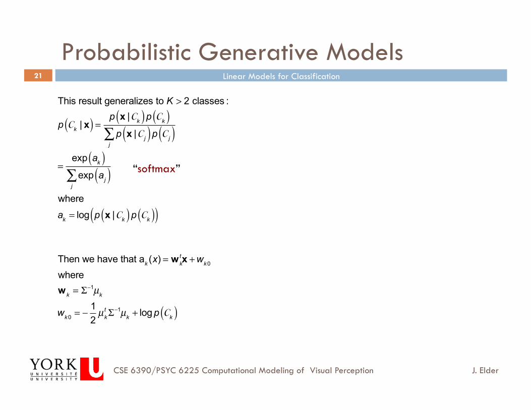
Then we have that ak (x) = w ktx +wk0
wherew k = Σ−1µk
wk0 = −12µ t
kΣ−1µk + log p Ck( )
This result generalizes to K > 2 classes :
p Ck | x( ) = p x | Ck( )p Ck( )p x | C j( )p C j( )
j∑
=exp ak( )
exp aj( )j∑
where
ak = log p x | Ck( )p Ck( )( )
“softmax”
Linear Models for Classification
J. Elder CSE 6390/PSYC 6225 Computational Modeling of Visual Perception
22
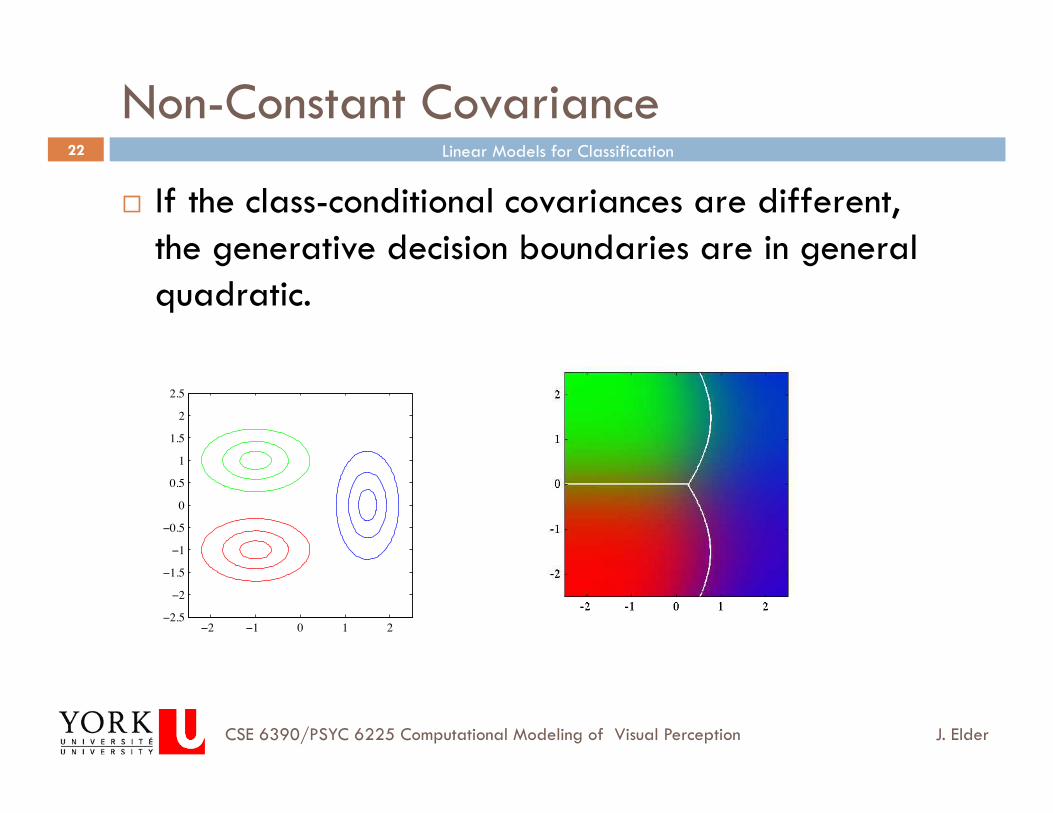
Non-Constant Covariance
If the class-conditional covariances are different, the generative decision boundaries are in general quadratic.
!2 !1 0 1 2!2.5
!2
!1.5
!1
!0.5
0
0.5
1
1.5
2
2.5
Linear Models for Classification
J. Elder CSE 6390/PSYC 6225 Computational Modeling of Visual Perception
23
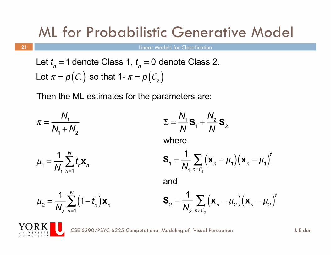
ML for Probabilistic Generative Model
µ1 =
1N1
tnxnn=1
N
∑
µ2 =
1N2
1− tn( )xnn=1
N
∑
Σ =N1
NS1 +
N2
NS2
where
S1 =1N1
xn − µ1( ) xn − µ1( )tn∈C1
∑and
S2 =1
N2
xn − µ2( ) xn − µ2( )tn∈C2
∑
Let tn = 1 denote Class 1, tn = 0 denote Class 2.
Then the ML estimates for the parameters are: Let π = p C1( ) so that 1- π = p C2( )
π =
N1
N1 + N2

Linear Models for Classification
J. Elder CSE 6390/PSYC 6225 Computational Modeling of Visual Perception
24
Probabilistic Discriminative Models
An alternative to the generative approach is to model the dependence of the target variable t on the input vector x directly, using the activation function f.
One big advantage is that there will typically be fewer parameters to determine.
Linear Models for Classification
J. Elder CSE 6390/PSYC 6225 Computational Modeling of Visual Perception
25
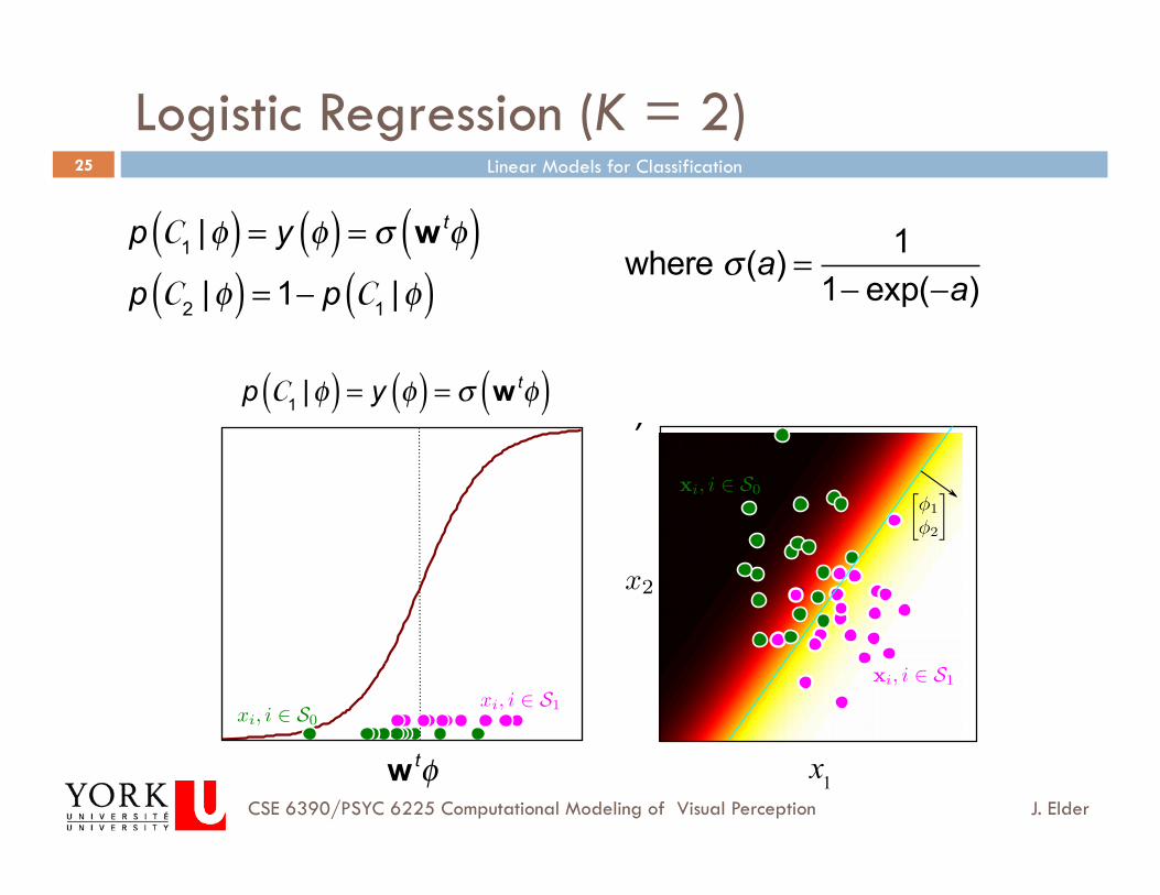
Logistic Regression (K = 2)
p C1 |φ( ) = y φ( ) = σ w tφ( )p C2 |φ( ) = 1− p C1 |φ( )
where σ (a) = 11− exp(−a)
140 8 Classification models
#"%
Figure 8.3 Logistic regression model in 1D and 2D. a) One dimensional fit.Green points denote set of examples S0 where y = 0. Pink points denoteset of examples S1 where y = 1. Note that in this (and all future figuresin this chapter) we have only plotted the probability Pr(y = 1|x) (compareto figure 8.2c). The probability Pr(y = 0|x) can be trivially computed as1 − Pr(y = 1|x). b) Two dimensional fit. Here, the model has a sigmoidprofile in the direction of the gradient φ and is constant in the orthogonaldirections. The decision boundary (blue line) is linear.
As usual, however, it is simpler to maximize the logarithm L of this expression.
Since the logarithm is a monotonic transformation, it does not change the position
of the maximum with respect to φ. However, applying the logarithm the product
and replaces it with a sum so that
L =
I�
i=1
yi log
�1
1 + exp[−φTxi]
�+
I�
i=1
(1− yi) log
�exp[−φTxi]
1 + exp[−φTxi]
�. (8.6)
The derivative of the log likelihood L with respect to the parameters φ is
∂L
∂φ=
I�
i=1
�1
1 + exp[−φTxi]− yi
�xi =
I�
i=1
(sig[ai]− yi)xi. (8.7)
Unfortunately, when we equate this expression to zero, there is no way to re-
arrange to get a closed form solution for the parameters φ. Instead we must
rely on a non-linear optimization technique to find the maximum of this function.
We’ll now sketch the main ideas behind non-linear optimization. We defer a more
detailed discussion until section 8.10.
In non-linear optimization, we start with an initial estimate of the solution
φ and iteratively improve it. The methods we will discuss rely on computing
wtφ
p C1 |φ( ) = y φ( ) = σ w tφ( )
x1
Linear Models for Classification
J. Elder CSE 6390/PSYC 6225 Computational Modeling of Visual Perception
26
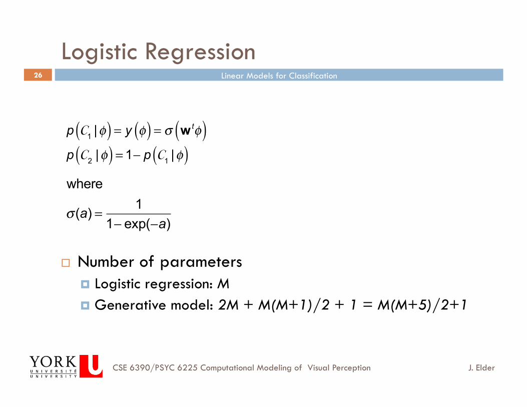
Logistic Regression
Number of parameters Logistic regression: M Generative model: 2M + M(M+1)/2 + 1 = M(M+5)/2+1
p C1 |φ( ) = y φ( ) = σ w tφ( )p C2 |φ( ) = 1− p C1 |φ( )
where
σ (a) = 11− exp(−a)

Linear Models for Classification
J. Elder CSE 6390/PSYC 6225 Computational Modeling of Visual Perception
27
ML for Logistic Regression
p t |w( ) = yn
tn 1− yn{ }1− tn
n=1
N
∏ where t = t1,…,tN( )t and yn = p C1 |φn( )
We define the error function to be E(w) = − log p t | w( )
Given yn = σ an( ) and an = w tφn, one can show that
∇E(w) = yn − tn( )φn
n=1
N
∑
Unfortunately, there is no closed form solution for w.

Linear Models for Classification
J. Elder CSE 6390/PSYC 6225 Computational Modeling of Visual Perception
28
ML for Logistic Regression:
Iterative Reweighted Least Squares Although there is no closed form solution for the ML
estimate of w, fortunately, the error function is convex. Thus an appropriate iterative method is guaranteed to
find the exact solution. A good method is to use a local quadratic
approximation to the log likelihood function (Newton-Raphson update):
w (new ) = w (old ) −H−1∇E(w)where H is the Hessian matrix of E(w)
Linear Models for Classification
J. Elder CSE 6390/PSYC 6225 Computational Modeling of Visual Perception
29
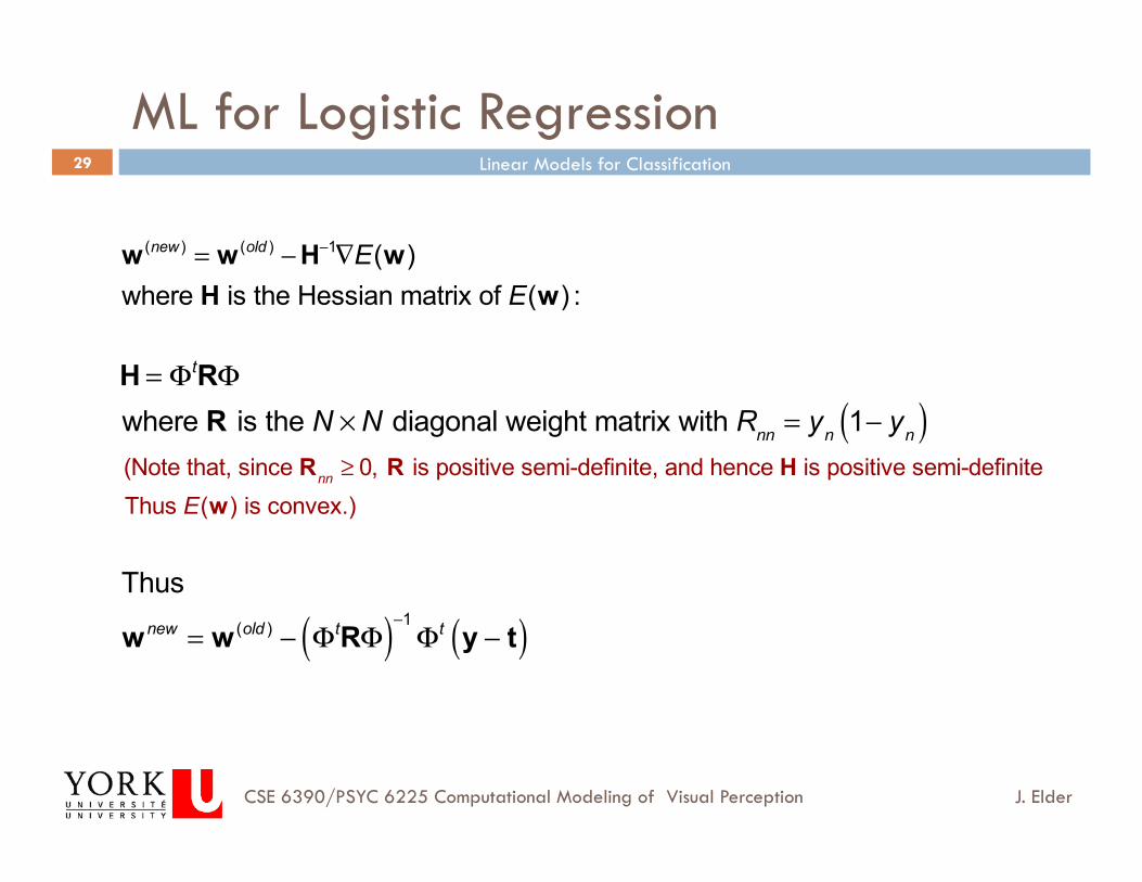
ML for Logistic Regression
w (new ) = w (old ) −H−1∇E(w)where H is the Hessian matrix of E(w) :
Thus
wnew = w (old ) − ΦtRΦ( )−1Φt y − t( )
H = ΦtRΦwhere R is the N × N diagonal weight matrix with Rnn = yn 1− yn( )
(Note that, since Rnn ≥ 0, R is positive semi-definite, and hence H is positive semi-definiteThus E(w) is convex.)

Linear Models for Classification
J. Elder CSE 6390/PSYC 6225 Computational Modeling of Visual Perception
30
ML for Logistic Regression
Iterative Reweighted Least Squares
142 8 Classification models
!
"
#
Figure 8.4 Parameter estimation for logistic regression with 1D data. a)In maximum likelihood learning, we seek the maximum of Pr(y|X,φ) withrespect to φ. b) In practice, we instead maximize log likelihood: noticethat the peak is in the same place. Crosses show results of 2 iterations ofoptimization using Newton’s method. c) The logistic sigmoid functions asso-ciated with the parameters at each optimization step. As the log likelihoodincreases, the model fits the data more closely: the green points representdata where y = 0 and the purple points represent data where y = 1 and sowe expect the chosen model to increase from right to left just like curve 3.
For general functions, gradient ascent and Newton approaches only find localmaxima: we cannot be certain that there is not a taller peak in the likelihood
function elsewhere. However the log likelihood for logistic regression has a special
property: it is a convex function of the parameters φ. For convex functions there
are never multiple maxima and gradient based approaches are guaranteed to find
the global maximum. It is possible to establish whether a function is convex or
not by examining the Hessian matrix. If this is positive definite for all φ then the
function is convex. This is obviously the case for logistic regression as the Hessian
(equation 8.10) consists of a positive weighted sum of outer products.
The logistic regression model as described has a number of problems:
1. It is overconfident as it was learnt using maximum likelihood
2. It can only describe linear decision boundaries
3. It is computationally innefficient and may overlearn the data in high dimen-
sions.
In the remaining part of this chapter we will extend this model to cope with
these problems (figure 8.5)
142 8 Classification models
$
$
%
&
Figure 8.4 Parameter estimation for logistic regression with 1D data. a)In maximum likelihood learning, we seek the maximum of Pr(y|X,φ) withrespect to φ. b) In practice, we instead maximize log likelihood: noticethat the peak is in the same place. Crosses show results of 2 iterations ofoptimization using Newton’s method. c) The logistic sigmoid functions asso-ciated with the parameters at each optimization step. As the log likelihoodincreases, the model fits the data more closely: the green points representdata where y = 0 and the purple points represent data where y = 1 and sowe expect the chosen model to increase from right to left just like curve 3.
For general functions, gradient ascent and Newton approaches only find localmaxima: we cannot be certain that there is not a taller peak in the likelihood
function elsewhere. However the log likelihood for logistic regression has a special
property: it is a convex function of the parameters φ. For convex functions there
are never multiple maxima and gradient based approaches are guaranteed to find
the global maximum. It is possible to establish whether a function is convex or
not by examining the Hessian matrix. If this is positive definite for all φ then the
function is convex. This is obviously the case for logistic regression as the Hessian
(equation 8.10) consists of a positive weighted sum of outer products.
The logistic regression model as described has a number of problems:
1. It is overconfident as it was learnt using maximum likelihood
2. It can only describe linear decision boundaries
3. It is computationally innefficient and may overlearn the data in high dimen-
sions.
In the remaining part of this chapter we will extend this model to cope with
these problems (figure 8.5)
w1
w2 wtφ
p C1 |φ( ) = y φ( ) = σ w tφ( )

Linear Models for Classification
J. Elder CSE 6390/PSYC 6225 Computational Modeling of Visual Perception
31
Bayesian Logistic Regression
Unfortunately, the posterior over w will not be normal for logistic regression, and hence we cannot integrate over it analytically.
This means that we cannot do Bayesian prediction analytically.
However, there are methods for approximating the posterior that allow us to do approximate Bayesian prediction.
We can make logistic regression Bayesian by applying a prior over w:
p(w) = N(w |m0,S0)

Linear Models for Classification
J. Elder CSE 6390/PSYC 6225 Computational Modeling of Visual Perception
32
The Laplace Approximation In the Laplace approximation, we approximate the log of a
distribution by a local, second order (quadratic) form, centred at the mode.
This corresponds to a normal approximation to the distribution, with mean given by the mode of the original distribution precision matrix given by the Hessian of the negative log of the
distribution
!2 !1 0 1 2 3 40
0.2
0.4
0.6
0.8 p(z)
!2 !1 0 1 2 3 40
10
20
30
40 − log p(z)

Linear Models for Classification
J. Elder CSE 6390/PSYC 6225 Computational Modeling of Visual Perception
33
Bayesian Logistic Regression
When applied to the posterior over w in logistic regression, this yields
p(w) q(w) = N w | wMAP ,SN( )where
S−1N = S−1
0 + yn 1− yn( )φnφtn
n=1
N
∑

Linear Models for Classification
J. Elder CSE 6390/PSYC 6225 Computational Modeling of Visual Perception
34
Prediction
Bayesian prediction requires that we integrate out this posterior over w:
p C1 |φ,t( ) = p C1 |φ,w( )∫ p(w | t)dw σ w tφ( )∫ q(w)dw
This integral is not tractable analytically. However, approximation of the sigmoid function σ (⋅) by the inverse probit (cumulative normal) functionyields an analytical solution:
p C1 |φ,t( ) σ κ σa2( ) µa( ),
where µa = wMAPt φ, σa
2 = φ tSNφ and κ σa2( ) = 1+ πσa
2 / 8( )−1/2

Linear Models for Classification
J. Elder CSE 6390/PSYC 6225 Computational Modeling of Visual Perception
35
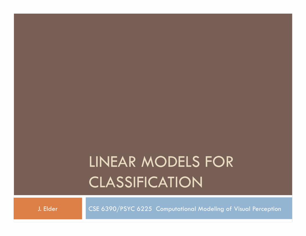
Bayesian Logistic Regression
This last approximation is excellent!
8.3 Non-Linear Logistic Regression 147
!"!#
$!"!
%& & %& & %& &!
$
!
$
!
!"!&
'( )( *(
Figure 8.8 Approximation of activation integral (equation 8.17). a) Actualresult of integral as a function of µa and σ2
a. b) Approximation (equation8.18). c) The absolute difference between the actual result and the approx-imation is very small over a large range of reasonable values.
Figure 8.9 Bayesian logistic regression predictions. a) The Bayesian predic-tion for the class y is more moderate than the maximum likelihood estimate.b) In two dimensions (compare to figure 8.3c) this effect is greatest as wemove farther from the mean. In practice this means that although the deci-sion boundary (blue line) is still linear, iso-probability curves at levels otherthan 0.5 are curved.
• Heaviside Step functions of projections: zk = Heaviside[αTk x]
• Arc tan functions of projections: zk = arctan[αTk x]
• Radial basis functions: zk = exp
�− 1
λ0(x−αk)
T(x−αk)
�
where zk denotes the kth element of the transformed vector z. As usual we have
σ κ σa
2( ) µa( ) Residual σ w tφ( )∫ q(w)dw