08-13791_P1323_covI-IV.indd 1 2008-09-24 13:03:53

ON-LINE MONITORINGFOR IMPROVING PERFORMANCE

OF NUCLEAR POWER PLANTSPART 2: PROCESS AND COMPONENT

CONDITION MONITORING ANDDIAGNOSTICS

AFGHANISTANALBANIAALGERIAANGOLAARGENTINAARMENIAAUSTRALIAAUSTRIAAZERBAIJANBANGLADESHBELARUSBELGIUMBELIZEBENINBOLIVIABOSNIA AND HERZEGOVINABOTSWANABRAZILBULGARIABURKINA FASOCAMEROONCANADACENTRAL AFRICAN REPUBLICCHADCHILECHINACOLOMBIACOSTA RICACÔTE D’IVOIRECROATIACUBACYPRUSCZECH REPUBLICDEMOCRATIC REPUBLIC OF THE CONGODENMARKDOMINICAN REPUBLICECUADOREGYPTEL SALVADORERITREAESTONIAETHIOPIAFINLANDFRANCEGABONGEORGIAGERMANYGHANAGREECE

GUATEMALAHAITIHOLY SEEHONDURASHUNGARYICELANDINDIAINDONESIAIRAN, ISLAMIC REPUBLIC OF IRAQIRELANDISRAELITALYJAMAICAJAPANJORDANKAZAKHSTANKENYAKOREA, REPUBLIC OFKUWAITKYRGYZSTANLATVIALEBANONLIBERIALIBYAN ARAB JAMAHIRIYALIECHTENSTEINLITHUANIALUXEMBOURGMADAGASCARMALAWIMALAYSIAMALIMALTAMARSHALL ISLANDSMAURITANIAMAURITIUSMEXICOMONACOMONGOLIAMONTENEGROMOROCCOMOZAMBIQUEMYANMARNAMIBIANEPALNETHERLANDSNEW ZEALANDNICARAGUANIGERNIGERIANORWAY

PAKISTANPALAUPANAMAPARAGUAYPERUPHILIPPINESPOLANDPORTUGALQATARREPUBLIC OF MOLDOVAROMANIARUSSIAN FEDERATIONSAUDI ARABIASENEGALSERBIASEYCHELLESSIERRA LEONESINGAPORESLOVAKIASLOVENIASOUTH AFRICASPAINSRI LANKASUDANSWEDENSWITZERLANDSYRIAN ARAB REPUBLICTAJIKISTANTHAILANDTHE FORMER YUGOSLAV REPUBLIC OF MACEDONIATUNISIATURKEYUGANDAUKRAINEUNITED ARAB EMIRATESUNITED KINGDOM OF GREAT BRITAIN AND NORTHERN IRELANDUNITED REPUBLIC OF TANZANIAUNITED STATES OF AMERICAURUGUAYUZBEKISTANVENEZUELAVIETNAMYEMENZAMBIAZIMBABWE

The Agency’s Statute was approved on 23 October 1956 by the Conference on the Statute of the IAEAheld at United Nations Headquarters, New York; it entered into force on 29 July 1957. The Headquarters of theAgency are situated in Vienna. Its principal objective is “to accelerate and enlarge the contribution of atomicenergy to peace, health and prosperity throughout the world’’.

The following States are Members of the International Atomic Energy Agency:

ON-LINE MONITORING FOR IMPROVING PERFORMANCE

OF NUCLEAR POWER PLANTSPART 2: PROCESS AND COMPONENT

CONDITION MONITORING AND DIAGNOSTICS

IAEA NUCLEAR ENERGY SERIES No. NP-T-1.2

INTERNATIONAL ATOMIC ENERGY AGENCYVIENNA, 2008

COPYRIGHT NOTICE

All IAEA scientific and technical publications are protected by the termsof the Universal Copyright Convention as adopted in 1952 (Berne) and asrevised in 1972 (Paris). The copyright has since been extended by the WorldIntellectual Property Organization (Geneva) to include electronic and virtualintellectual property. Permission to use whole or parts of texts contained inIAEA publications in printed or electronic form must be obtained and isusually subject to royalty agreements. Proposals for non-commercialreproductions and translations are welcomed and considered on a case-by-casebasis. Enquiries should be addressed to the IAEA Publishing Section at:

Sales and Promotion, Publishing SectionInternational Atomic Energy AgencyWagramer Strasse 5P.O. Box 1001400 Vienna, Austriafax: +43 1 2600 29302tel.: +43 1 2600 22417email: sales.publications@iaea.org http://www.iaea.org/books

© IAEA, 2008

Printed by the IAEA in AustriaSeptember 2008STI/PUB/1323

IAEA Library Cataloguing in Publication Data

On-line monitoring for improving performance of nuclear power plants.Part 2, Process and component condition monitoring and diagnostics.— Vienna : International Atomic Energy Agency, 2008.

p. ; 29 cm. — (IAEA nuclear energy series, ISSN 1995–7807 ;no. NP-T-1.2)

STI/PUB/1323ISBN 978–92–0–101208–1Includes bibliographical references.

1. Nuclear power plants — Safety measures. 2. Nuclear power plants— Management. I. International Atomic Energy Agency. II. Series.

IAEAL 08–00538

FOREWORD

The IAEA’s work in the area of nuclear power plant operating performance and life cycle management is aimed at enhancing the capability of Member States to utilize good engineering and management practices developed and transferred by the IAEA. In particular, the IAEA supports activities such as improving nuclear power plant performance, plant life management, training, power uprating, operational licence renewal, and modernization of the instrumentation and control systems of nuclear power plants in Member States.

The subject of improving the performance of nuclear power plants by utilizing on-line condition monitoring of instrumentation and control systems in plants was suggested by the Technical Working Group on Nuclear Power Plant Control and Instrumentation (TWG-NPPCI) in 2003. It was then approved by the IAEA and included in its work programmes for 2004–2007.

This is the second report on the use of on-line monitoring (OLM) in nuclear power plants. The first report, On-Line Monitoring for Improving Performance of Nuclear Power Plants, Part 1: Instrument Channel Monitoring (IAEA Nuclear Energy Series No. NP-T-1.1), focused on application of OLM to verify the static (calibration) and dynamic (response time) performance of process instruments in nuclear power plants. This second report extends the application of OLM to equipment and process condition monitoring encompassing an array of technologies, including vibration monitoring, acoustic monitoring, loose parts monitoring, motor current signature analysis and noise diagnostics, as well as vibration analysis of the reactor core and the primary circuit.

Furthermore, this report includes the application of modelling technologies for equipment and process condition monitoring. A majority of these technologies depend on existing data from existing sensors and first principles models to estimate equipment and process behaviour using empirical and physical modelling techniques. In doing so, pattern recognition tools such as neural networks, fuzzy classification of data, multivariate state estimation and other means are used. These means are described in this report, and examples of their application and implementation are provided.

It should be pointed out that OLM data are routinely collected in nuclear power plants for a variety of purposes, but that these data are not often trended or used for long term predictive maintenance purposes. This report promotes the idea of trending such data and provides guidance on how this trending may be performed to yield a new maintenance tool for nuclear power plants.

This report was produced by experts and advisors from numerous IAEA Member States. Particular appreciation is due to H.M. Hashemian (United States of America), who served as Chair of the drafting committee and the IAEA committee meetings for this report. J. Eiler (Hungary) was Chair of the consultants meeting where the report was completed in May 2007. The IAEA officer responsible for this publication was O. Glöckler of the Division of Nuclear Power.

EDITORIAL NOTE

This report has been edited by the editorial staff of the IAEA to the extent considered necessary for the reader’s assistance.Although great care has been taken to maintain the accuracy of information contained in this publication, neither the

IAEA nor its Member States assume any responsibility for consequences which may arise from its use.The use of particular designations of countries or territories does not imply any judgement by the publisher, the IAEA, as

to the legal status of such countries or territories, of their authorities and institutions or of the delimitation of their boundaries.The mention of names of specific companies or products (whether or not indicated as registered) does not imply any

intention to infringe proprietary rights, nor should it be construed as an endorsement or recommendation on the part of theIAEA.

CONTENTS

1. INTRODUCTION . . . . . . . . . . . . . . . . . . . . . . . . . . . . . . . . . . . . . . . . . . . . . . . . . . . . . . . . . . . . . . . . . . . . . 1

1.1. Objective . . . . . . . . . . . . . . . . . . . . . . . . . . . . . . . . . . . . . . . . . . . . . . . . . . . . . . . . . . . . . . . . . . . . . . . . . 11.2. Historical background . . . . . . . . . . . . . . . . . . . . . . . . . . . . . . . . . . . . . . . . . . . . . . . . . . . . . . . . . . . . . . 11.3. Description of on-line condition monitoring . . . . . . . . . . . . . . . . . . . . . . . . . . . . . . . . . . . . . . . . . . . 11.4. Examples of on-line condition monitoring techniques . . . . . . . . . . . . . . . . . . . . . . . . . . . . . . . . . . . 2

1.4.1. Vibration monitoring . . . . . . . . . . . . . . . . . . . . . . . . . . . . . . . . . . . . . . . . . . . . . . . . . . . . . . . . 21.4.2. Acoustic monitoring . . . . . . . . . . . . . . . . . . . . . . . . . . . . . . . . . . . . . . . . . . . . . . . . . . . . . . . . . 21.4.3. Loose parts monitoring . . . . . . . . . . . . . . . . . . . . . . . . . . . . . . . . . . . . . . . . . . . . . . . . . . . . . . 21.4.4. Reactor noise analysis . . . . . . . . . . . . . . . . . . . . . . . . . . . . . . . . . . . . . . . . . . . . . . . . . . . . . . . 31.4.5. Motor electrical signature analysis . . . . . . . . . . . . . . . . . . . . . . . . . . . . . . . . . . . . . . . . . . . . . 31.4.6. Modelling techniques . . . . . . . . . . . . . . . . . . . . . . . . . . . . . . . . . . . . . . . . . . . . . . . . . . . . . . . . 3

2. BENEFITS OF ON-LINE CONDITION MONITORING . . . . . . . . . . . . . . . . . . . . . . . . . . . . . . . . . . . 4

2.1. Plant safety . . . . . . . . . . . . . . . . . . . . . . . . . . . . . . . . . . . . . . . . . . . . . . . . . . . . . . . . . . . . . . . . . . . . . . . 42.2. Plant ageing management . . . . . . . . . . . . . . . . . . . . . . . . . . . . . . . . . . . . . . . . . . . . . . . . . . . . . . . . . . . 52.3. Economic . . . . . . . . . . . . . . . . . . . . . . . . . . . . . . . . . . . . . . . . . . . . . . . . . . . . . . . . . . . . . . . . . . . . . . . . 52.4. Plant availability and performance . . . . . . . . . . . . . . . . . . . . . . . . . . . . . . . . . . . . . . . . . . . . . . . . . . . 62.5. Maintenance . . . . . . . . . . . . . . . . . . . . . . . . . . . . . . . . . . . . . . . . . . . . . . . . . . . . . . . . . . . . . . . . . . . . . . 62.6. Knowledge identification and capture . . . . . . . . . . . . . . . . . . . . . . . . . . . . . . . . . . . . . . . . . . . . . . . . 6

3. DESCRIPTION OF CONDITION MONITORING TECHNIQUES . . . . . . . . . . . . . . . . . . . . . . . . . 7

3.1. Vibration monitoring . . . . . . . . . . . . . . . . . . . . . . . . . . . . . . . . . . . . . . . . . . . . . . . . . . . . . . . . . . . . . . 73.2. Acoustic monitoring . . . . . . . . . . . . . . . . . . . . . . . . . . . . . . . . . . . . . . . . . . . . . . . . . . . . . . . . . . . . . . . 10

3.2.1. Acoustic monitoring of processes . . . . . . . . . . . . . . . . . . . . . . . . . . . . . . . . . . . . . . . . . . . . . 103.2.2. Acoustic monitoring of components . . . . . . . . . . . . . . . . . . . . . . . . . . . . . . . . . . . . . . . . . . . . 103.2.3. Acoustic emission monitoring . . . . . . . . . . . . . . . . . . . . . . . . . . . . . . . . . . . . . . . . . . . . . . . . . 113.2.4. Acoustic leakage monitoring . . . . . . . . . . . . . . . . . . . . . . . . . . . . . . . . . . . . . . . . . . . . . . . . . . 11

3.3. Loose parts monitoring . . . . . . . . . . . . . . . . . . . . . . . . . . . . . . . . . . . . . . . . . . . . . . . . . . . . . . . . . . . . . 133.3.1. Definitions . . . . . . . . . . . . . . . . . . . . . . . . . . . . . . . . . . . . . . . . . . . . . . . . . . . . . . . . . . . . . . . . . 133.3.2. Discrimination algorithms . . . . . . . . . . . . . . . . . . . . . . . . . . . . . . . . . . . . . . . . . . . . . . . . . . . . 143.3.3. Source localization and mass estimation . . . . . . . . . . . . . . . . . . . . . . . . . . . . . . . . . . . . . . . . 153.3.4. Utilization of results . . . . . . . . . . . . . . . . . . . . . . . . . . . . . . . . . . . . . . . . . . . . . . . . . . . . . . . . . 16

3.4. Reactor noise analysis technology . . . . . . . . . . . . . . . . . . . . . . . . . . . . . . . . . . . . . . . . . . . . . . . . . . . . 173.4.1. Spectral methods . . . . . . . . . . . . . . . . . . . . . . . . . . . . . . . . . . . . . . . . . . . . . . . . . . . . . . . . . . . . 173.4.2. Surveillance or monitoring . . . . . . . . . . . . . . . . . . . . . . . . . . . . . . . . . . . . . . . . . . . . . . . . . . . . 183.4.3. Direct diagnostics . . . . . . . . . . . . . . . . . . . . . . . . . . . . . . . . . . . . . . . . . . . . . . . . . . . . . . . . . . . 183.4.4. Implementation of reactor noise analysis applications . . . . . . . . . . . . . . . . . . . . . . . . . . . . 183.4.5. Required data acquisition systems . . . . . . . . . . . . . . . . . . . . . . . . . . . . . . . . . . . . . . . . . . . . . 19

3.4.5.1. Isolation requirements . . . . . . . . . . . . . . . . . . . . . . . . . . . . . . . . . . . . . . . . . . . . . . . . 193.4.5.2. Analogue signal conditioning . . . . . . . . . . . . . . . . . . . . . . . . . . . . . . . . . . . . . . . . . . 193.4.5.3. Plant conditions for data acquisition . . . . . . . . . . . . . . . . . . . . . . . . . . . . . . . . . . . . 20

3.4.6. Core barrel vibration diagnostics in PWRs . . . . . . . . . . . . . . . . . . . . . . . . . . . . . . . . . . . . . . 203.4.7. Control rod vibrations in PWRs . . . . . . . . . . . . . . . . . . . . . . . . . . . . . . . . . . . . . . . . . . . . . . . 223.4.8. Core flow measurements with neutron noise in PWRs . . . . . . . . . . . . . . . . . . . . . . . . . . . . 233.4.9. Measurements of the moderator temperature coefficient in PWRs . . . . . . . . . . . . . . . . . . 233.4.10. Flow measurements in PWRs . . . . . . . . . . . . . . . . . . . . . . . . . . . . . . . . . . . . . . . . . . . . . . . . . 243.4.11. Data acquisition for noise analysis in PHWRs . . . . . . . . . . . . . . . . . . . . . . . . . . . . . . . . . . . 243.4.12. Vibration of fuel channels detected by ICFD noise analysis . . . . . . . . . . . . . . . . . . . . . . . . 24

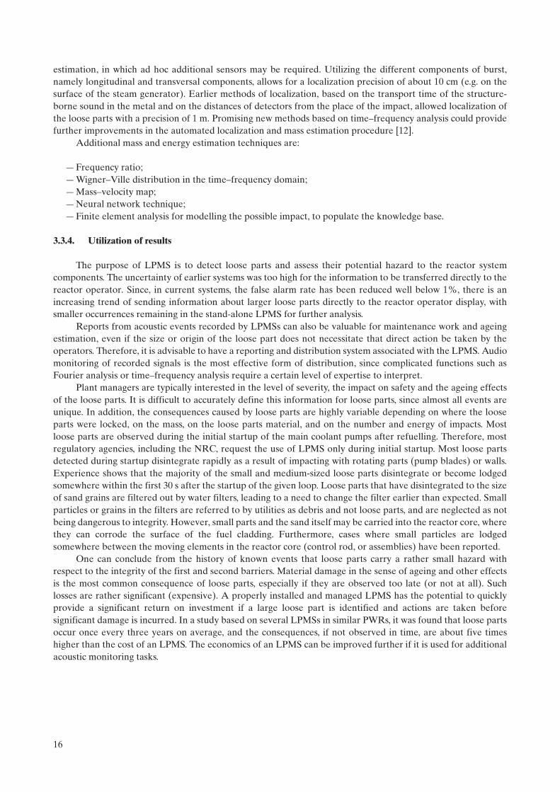
3.4.13. Vibration of detector tubes detected by ICFD noise analysis . . . . . . . . . . . . . . . . . . . . . . . 273.4.14. Two-phase flow diagnostics and the local component in BWRs . . . . . . . . . . . . . . . . . . . . . 283.4.15. BWR instability . . . . . . . . . . . . . . . . . . . . . . . . . . . . . . . . . . . . . . . . . . . . . . . . . . . . . . . . . . . . . 283.4.16. Impacting of detector tubes in BWRs . . . . . . . . . . . . . . . . . . . . . . . . . . . . . . . . . . . . . . . . . . 29

3.5. Motor electrical signature analysis . . . . . . . . . . . . . . . . . . . . . . . . . . . . . . . . . . . . . . . . . . . . . . . . . . . 303.5.1. Motor current signature analysis . . . . . . . . . . . . . . . . . . . . . . . . . . . . . . . . . . . . . . . . . . . . . . . 303.5.2. Motor power signature analysis . . . . . . . . . . . . . . . . . . . . . . . . . . . . . . . . . . . . . . . . . . . . . . . 31

4. MODELLING TECHNIQUES . . . . . . . . . . . . . . . . . . . . . . . . . . . . . . . . . . . . . . . . . . . . . . . . . . . . . . . . . . 32

4.1. Empirical modelling . . . . . . . . . . . . . . . . . . . . . . . . . . . . . . . . . . . . . . . . . . . . . . . . . . . . . . . . . . . . . . . 344.1.1. Requirements . . . . . . . . . . . . . . . . . . . . . . . . . . . . . . . . . . . . . . . . . . . . . . . . . . . . . . . . . . . . . . 344.1.2. Neural networks . . . . . . . . . . . . . . . . . . . . . . . . . . . . . . . . . . . . . . . . . . . . . . . . . . . . . . . . . . . . 36

4.1.2.1. Strengths and weaknesses . . . . . . . . . . . . . . . . . . . . . . . . . . . . . . . . . . . . . . . . . . . . . 374.1.2.2. Applications . . . . . . . . . . . . . . . . . . . . . . . . . . . . . . . . . . . . . . . . . . . . . . . . . . . . . . . . 37

4.1.3. Local polynomial regression . . . . . . . . . . . . . . . . . . . . . . . . . . . . . . . . . . . . . . . . . . . . . . . . . . 374.1.3.1. Strengths and weaknesses . . . . . . . . . . . . . . . . . . . . . . . . . . . . . . . . . . . . . . . . . . . . . 384.1.3.2. Current applications . . . . . . . . . . . . . . . . . . . . . . . . . . . . . . . . . . . . . . . . . . . . . . . . . . 38

4.1.4. Transformation based techniques . . . . . . . . . . . . . . . . . . . . . . . . . . . . . . . . . . . . . . . . . . . . . . 384.1.4.1. Strengths and weaknesses . . . . . . . . . . . . . . . . . . . . . . . . . . . . . . . . . . . . . . . . . . . . . 394.1.4.2. Applications . . . . . . . . . . . . . . . . . . . . . . . . . . . . . . . . . . . . . . . . . . . . . . . . . . . . . . . . . 39

4.2. Physical modelling . . . . . . . . . . . . . . . . . . . . . . . . . . . . . . . . . . . . . . . . . . . . . . . . . . . . . . . . . . . . . . . . . 394.2.1. Requirements . . . . . . . . . . . . . . . . . . . . . . . . . . . . . . . . . . . . . . . . . . . . . . . . . . . . . . . . . . . . . . 40

4.2.1.1. Strengths and weaknesses . . . . . . . . . . . . . . . . . . . . . . . . . . . . . . . . . . . . . . . . . . . . . 414.2.2. Applications . . . . . . . . . . . . . . . . . . . . . . . . . . . . . . . . . . . . . . . . . . . . . . . . . . . . . . . . . . . . . . . . 41

4.3. Related techniques . . . . . . . . . . . . . . . . . . . . . . . . . . . . . . . . . . . . . . . . . . . . . . . . . . . . . . . . . . . . . . . . 414.3.1. Fuzzy logic . . . . . . . . . . . . . . . . . . . . . . . . . . . . . . . . . . . . . . . . . . . . . . . . . . . . . . . . . . . . . . . . . 424.3.2. Multilevel flow modelling . . . . . . . . . . . . . . . . . . . . . . . . . . . . . . . . . . . . . . . . . . . . . . . . . . . . 42

5. ON-LINE MONITORING IMPLEMENTATION STRATEGY . . . . . . . . . . . . . . . . . . . . . . . . . . . . . . 44

5.1. Collecting plant data . . . . . . . . . . . . . . . . . . . . . . . . . . . . . . . . . . . . . . . . . . . . . . . . . . . . . . . . . . . . . . . 455.2. Storing plant data . . . . . . . . . . . . . . . . . . . . . . . . . . . . . . . . . . . . . . . . . . . . . . . . . . . . . . . . . . . . . . . . . 465.3. Performing analysis and presenting results . . . . . . . . . . . . . . . . . . . . . . . . . . . . . . . . . . . . . . . . . . . . 475.4. On-line monitoring software issues . . . . . . . . . . . . . . . . . . . . . . . . . . . . . . . . . . . . . . . . . . . . . . . . . . . 475.5. Acceptance testing . . . . . . . . . . . . . . . . . . . . . . . . . . . . . . . . . . . . . . . . . . . . . . . . . . . . . . . . . . . . . . . . . 485.6. Life cycle management . . . . . . . . . . . . . . . . . . . . . . . . . . . . . . . . . . . . . . . . . . . . . . . . . . . . . . . . . . . . . 495.7. Establishment and maintenance of OLM expertise . . . . . . . . . . . . . . . . . . . . . . . . . . . . . . . . . . . . . 49

6. ENABLING TECHNOLOGIES . . . . . . . . . . . . . . . . . . . . . . . . . . . . . . . . . . . . . . . . . . . . . . . . . . . . . . . . . 50

6.1. Introduction . . . . . . . . . . . . . . . . . . . . . . . . . . . . . . . . . . . . . . . . . . . . . . . . . . . . . . . . . . . . . . . . . . . . . . 506.2. Sensors . . . . . . . . . . . . . . . . . . . . . . . . . . . . . . . . . . . . . . . . . . . . . . . . . . . . . . . . . . . . . . . . . . . . . . . . . . 506.3. Data collection systems . . . . . . . . . . . . . . . . . . . . . . . . . . . . . . . . . . . . . . . . . . . . . . . . . . . . . . . . . . . . . 51

6.3.1. Industrial networks . . . . . . . . . . . . . . . . . . . . . . . . . . . . . . . . . . . . . . . . . . . . . . . . . . . . . . . . . . 526.3.1.1. Initial protocols . . . . . . . . . . . . . . . . . . . . . . . . . . . . . . . . . . . . . . . . . . . . . . . . . . . . . . 526.3.1.2. Area networking protocols . . . . . . . . . . . . . . . . . . . . . . . . . . . . . . . . . . . . . . . . . . . . 536.3.1.3. OPC communication protocol . . . . . . . . . . . . . . . . . . . . . . . . . . . . . . . . . . . . . . . . . 536.3.1.4. Internet and Web networks . . . . . . . . . . . . . . . . . . . . . . . . . . . . . . . . . . . . . . . . . . . 55

6.3.2. Communication equipment . . . . . . . . . . . . . . . . . . . . . . . . . . . . . . . . . . . . . . . . . . . . . . . . . . . 556.4. Data analysis systems . . . . . . . . . . . . . . . . . . . . . . . . . . . . . . . . . . . . . . . . . . . . . . . . . . . . . . . . . . . . . . 55

6.4.1. Analysis algorithms . . . . . . . . . . . . . . . . . . . . . . . . . . . . . . . . . . . . . . . . . . . . . . . . . . . . . . . . . . 556.4.2. Computer platform/operating systems . . . . . . . . . . . . . . . . . . . . . . . . . . . . . . . . . . . . . . . . . . 55

6.4.3. Programming languages . . . . . . . . . . . . . . . . . . . . . . . . . . . . . . . . . . . . . . . . . . . . . . . . . . . . . . 566.4.4. Software packages . . . . . . . . . . . . . . . . . . . . . . . . . . . . . . . . . . . . . . . . . . . . . . . . . . . . . . . . . . . 56

6.5. Higher level integration . . . . . . . . . . . . . . . . . . . . . . . . . . . . . . . . . . . . . . . . . . . . . . . . . . . . . . . . . . . . 56

7. FUTURE TRENDS . . . . . . . . . . . . . . . . . . . . . . . . . . . . . . . . . . . . . . . . . . . . . . . . . . . . . . . . . . . . . . . . . . . . 57

7.1. Hybrid condition monitoring and diagnostics . . . . . . . . . . . . . . . . . . . . . . . . . . . . . . . . . . . . . . . . . . 577.1.1. Requirements . . . . . . . . . . . . . . . . . . . . . . . . . . . . . . . . . . . . . . . . . . . . . . . . . . . . . . . . . . . . . . 587.1.2. Strengths and weaknesses . . . . . . . . . . . . . . . . . . . . . . . . . . . . . . . . . . . . . . . . . . . . . . . . . . . . 58

7.2. Advanced data communication . . . . . . . . . . . . . . . . . . . . . . . . . . . . . . . . . . . . . . . . . . . . . . . . . . . . . . 597.2.1. Wireless networks . . . . . . . . . . . . . . . . . . . . . . . . . . . . . . . . . . . . . . . . . . . . . . . . . . . . . . . . . . . 597.2.2. Mesh networks . . . . . . . . . . . . . . . . . . . . . . . . . . . . . . . . . . . . . . . . . . . . . . . . . . . . . . . . . . . . . 60

7.3. Functional level integration . . . . . . . . . . . . . . . . . . . . . . . . . . . . . . . . . . . . . . . . . . . . . . . . . . . . . . . . . 617.3.1. Integrating signal validation and alarm processing . . . . . . . . . . . . . . . . . . . . . . . . . . . . . . . . 617.3.2. Integrating condition monitoring with on-line risk assessment . . . . . . . . . . . . . . . . . . . . . . 627.3.3. General integration principles . . . . . . . . . . . . . . . . . . . . . . . . . . . . . . . . . . . . . . . . . . . . . . . . . 62

7.3.3.1. Encapsulation . . . . . . . . . . . . . . . . . . . . . . . . . . . . . . . . . . . . . . . . . . . . . . . . . . . . . . . 627.3.3.2. Synergism . . . . . . . . . . . . . . . . . . . . . . . . . . . . . . . . . . . . . . . . . . . . . . . . . . . . . . . . . . 637.3.3.3. Infrastructure . . . . . . . . . . . . . . . . . . . . . . . . . . . . . . . . . . . . . . . . . . . . . . . . . . . . . . . 637.3.3.4. Standards . . . . . . . . . . . . . . . . . . . . . . . . . . . . . . . . . . . . . . . . . . . . . . . . . . . . . . . . . . . 63

7.4. Fleetwide monitoring . . . . . . . . . . . . . . . . . . . . . . . . . . . . . . . . . . . . . . . . . . . . . . . . . . . . . . . . . . . . . . 637.5. Condition monitoring of electrical cables using the line resonance analysis method . . . . . . . . . . 64

8. CONCLUSIONS AND RECOMMENDATIONS . . . . . . . . . . . . . . . . . . . . . . . . . . . . . . . . . . . . . . . . . . 65

REFERENCES . . . . . . . . . . . . . . . . . . . . . . . . . . . . . . . . . . . . . . . . . . . . . . . . . . . . . . . . . . . . . . . . . . . . . . . . . . . . 67CONTRIBUTORS TO DRAFTING AND REVIEW . . . . . . . . . . . . . . . . . . . . . . . . . . . . . . . . . . . . . . . . . . . 69

1

1. INTRODUCTION

1.1. OBJECTIVE

A number of well established techniques are available for on-line monitoring (OLM) of the condition of equipment and systems in nuclear power plants. This report presents a general review of these techniques. Furthermore, it provides an assessment of other emerging or promising technologies that have been conceived or are being developed for on-line condition monitoring but are not in widespread use in nuclear power plants.

1.2. HISTORICAL BACKGROUND

In the early 1970s, numerous efforts were initiated to develop on-line diagnostics to identify problems — specifically, to detect and identify anomalies, and to provide an alternative way of measuring certain operating and process parameters in nuclear power plants. In particular, the reactor noise analysis technique was developed to use existing signals from existing sensors in nuclear power plants to provide incipient failure detection, measure sensor response time, monitor primary coolant flow behaviour through the reactor system, identify blockages in pressure sensing lines, measure the vibration of reactor internals, etc. These developments spread beyond research and development and found their way into the nuclear industry. For example, the noise analysis technique is now routinely used in many plants for response time testing of pressure, level and flow transmitters, and for detection of pressure sensing line blockages. However, the use of these techniques in nuclear power plants for diagnostics and surveillance of processes and components was not yet widespread at that time.

In the early 1980s, in the aftermath of the Three Mile Island accident, the use of signal validation techniques found its way into the nuclear power industry in some specific applications such as the safety parameter display system (SPDS). The work continued into the 1990s, leading to applications of data-driven empirical and physical modelling techniques for sensor and process performance monitoring. In particular, methods were developed for on-line calibration monitoring of pressure transmitters and detection of equipment anomalies [1, 2]. These methods are now used to extend the calibration intervals of sensors and have been approved by the regulatory authorities of the United States of America and the United Kingdom. While the US Nuclear Regulatory Commission (NRC) has granted generic approval, there are numerous requirements that must be met in a request for a licence amendment to change the calibration schedule of safety related transmitters.

Since the 1990s, OLM techniques have been explored by the nuclear industry for equipment condition monitoring beyond sensors. For example, OLM data are used to track the vibration of reactor internals, measure core stability margins, verify plant thermal performance, detect leaks, anticipate failures of rotating equipment, verify proper operation of valves, and identify and locate loose parts within the reactor system.

1.3. DESCRIPTION OF ON-LINE CONDITION MONITORING

On-line condition monitoring of plant equipment, systems and processes includes the detection and diagnosis of abnormalities via long term surveillance of process signals while the plant is in operation. The term ‘on-line condition monitoring’ of nuclear power plants refers to the following:

— The equipment or system being monitored is in service, active and available (on-line).— The plant is operating, including startup, normal steady-state operation and shutdown transient.— Testing is done in situ in a non-intrusive, passive way.

As the above description shows, in this respect ‘on-line’ is not synonymous with ‘real-time’, i.e. the processing of the measurement data is not necessarily performed simultaneously with the measurement. Real-time methods are an important class of OLM methods, but some OLM applications involve off-line signal

2

processing, modelling, interpretation and decision making. Figure 1 illustrates the essence of what this reportintends to convey.

1.4. EXAMPLES OF ON-LINE CONDITION MONITORING TECHNIQUES

A summary of representative on-line condition monitoring technologies and some of their applications ispresented here briefly. More details are given in the body of this report.

1.4.1. Vibration monitoring

In the past 20 years, predictive maintenance through vibration analysis has become one of the mostprevalent practices in industrial processes. Using accelerometers and similar sensors, the vibration of operatingmachinery is measured and trended to identify deviations from expected, normal or historical behaviour. Thispractice has been proved to successfully identify the onset of many problems with industrial equipment,especially rotating machinery.

1.4.2. Acoustic monitoring

Acoustic monitoring is a form of noise analysis whereby signals from listening sensors (accelerometers) aremonitored for amplitude and frequency content to provide diagnostics through comparison with userestablished baseline signatures. Acoustic monitoring for leak detection and valve monitoring is used in nuclearpower plants on a routine basis, and extensive experience exists in this area that can be integrated into aplantwide monitoring programme.

1.4.3. Loose parts monitoring

Loose parts monitoring is performed in many nuclear power plants on a continuous basis. This workinvolves accelerometers installed at several locations in the plant such as the reactor vessel (top and bottom),steam generators and reactor coolant pumps.

Both audio signals and noise data records are used in loose parts monitoring. The audio signals are used toproduce alarms if any part of the system is significantly loose. The alarm set points are selected on the basis ofthe plant and the sensitivity of the loose parts monitoring equipment. If a loose parts alarm is activated, acceler-ometer output data are analysed to confirm the loose part and identify its size and location. The size of a loosepart is estimated using baseline measurements that are made with known masses on calibrated hammers used to

Purpose:

On-Line

Condition

Monitoring

&

Diagnostics

Applications/Tools:

• Vibration Monitoring

• Acoustic Monitoring

• Loose Parts Monitoring

• Reactor Noise Analysis

• Motor Electrical Signature Analysis

• Modelling Techniques

FIG. 1. On-line condition monitoring of equipment, systems and processes in nuclear power plants.

3

intentionally hit the plant piping and vessel from the outside to calibrate the loose parts monitoring system.Localization of a loose part is achieved by comparing signals from accelerometers in various locations byidentifying signal transmission times.

1.4.4. Reactor noise analysis

Power reactors are equipped with both in-core flux detectors (self-powered neutron detectors (SPNDs))and ex-core ionization chambers, as well as a number of other sensors (e.g. thermocouples, pressure and flowsensors, ex-vessel accelerometers). The primary purpose of in-core flux detectors is to measure the neutron fluxdistribution and reactor power. The detectors are used for flux mapping for in-core fuel management (ICFM)purposes, for control actions and for initiating reactor protection (trip) functions in the case of an abnormalevent. To accomplish this, the direct current (DC) output of the detectors’ current signal is measured andcalibrated to indicate the neutron flux or the reactor power. The same output also contains small fluctuations(noise) that can be analysed to collect information on the various processes taking place in the core. Forexample, the noise components of ex-core neutron detectors in pressurized water reactors (PWRs) can measurethe vibration of the reactor vessel and the reactor vessel internals. Furthermore, through cross-correlation ofneutron signals and other existing sensors such as the core exit thermocouples or the reactor vessel level sensors,the flow through the reactor can be characterized to detect flow anomalies. In boiling water reactors (BWRs),average power range monitors (APRMs) and local power range monitors (LPRMs) are used to perform reactordiagnostics and to estimate the flow through the core. The APRM and LPRM signals are also used to measurethe stability margin for the core in terms of a decay ratio.

There are other applications based on reactor noise analysis. For example, the response times of safetysystem flow transmitters and their sensing lines can be estimated using in situ signal noise measurements at full-power operating conditions. The response time estimation involves the measurement based calculations of thedynamic transfer function of the flow transmitter and the auto power spectral density (APSD) function of thetransmitter’s output noise signal [3]. A more detailed description of this method can be found in Ref. [4].

1.4.5. Motor electrical signature analysis

Motor current signature analysis (MCSA) was conceived more than 20 years ago and quickly found its wayinto nuclear power plants. As its name implies, MCSA uses the signals from clamp-on current sensors to monitorthe electrical currents going to a motor. Analysis of the current signals may result in the identification of avariety of problems (e.g. a stuck valve). The techniques of MCSA are used in numerous nuclear power plants formany types of equipment. A similar technique based on power signals and called motor power signature analysis(MPSA) is also available. Motor current changes at reduced load levels (50% of total load or below) are noteasily detectable by routine techniques. MPSA has been found to be more responsive to load variations such asduring valve cycling; as such, it may be a possible replacement for valve stroke testing.

1.4.6. Modelling techniques

OLM modelling techniques have the capability of providing early warning of impending failure ordegradation of plant equipment, in addition to indications of changes in expected process performance andefficiency. This capability results from the identification of unusual or unexpected behaviour (anomalies) in theprocess model outputs.

OLM techniques are based on qualitative interpretation of measured process signals and on quantitativeconclusions drawn from the evaluation of the signal content. Neither part is possible without some basic, a prioriknowledge of the processes associated with the measured signals. For instance, in order to evaluate reactivitycoefficients of temperature, void, etc., one has to build a functional relationship between these parameters andthe neutron flux variations on the basis of the physics of the process. The reactivity can then be determined byparameter fitting from the measured temperature/void and neutron flux values. This is the case of physicalmodelling. In some other cases, a physical model can give quantitative relationships between signal values indifferent parts of the core (amplitude ratios, phase delays) that would prevail in normal conditions. Deviationsfrom these relationships can indicate an incipient failure. Other types of modelling (empirical modelling) are not

4

based on an actual physical description of the process. Empirical models establish baseline relationships (through statistical descriptors) by characterizing the normal state of the process (on the basis of historical measurement data) and then monitor for deviations from these established relationships in order to indicate incipient failures. A related approach is to utilize empirical models to classify observed patterns into one of a series of fault signatures.

While the use of physical models for monitoring process and equipment performance is well established in the nuclear industry, the use of empirical models to monitor the condition of plant systems and equipment is a recent development. A number of organizations have had direct involvement in bringing this about. These organizations include research institutes and utilities that have developed and/or introduced the application of model based monitoring techniques. Examples of such organizations are the Electric Power Research Institute (EPRI) in the United States of America, the Halden Reactor Project (HRP) in Norway, the Korea Atomic Energy Research Institute (KAERI) in the Republic of Korea, Analysis and Measurement Services (AMS) Corporation in the United States of America, and Ontario Power Generation (OPG) in Canada. In particular, a variety of equipment and process modelling techniques have been adapted to provide a baseline for detection of equipment and process anomalies. Both empirical and physical modelling techniques are used in this endeavour. The physical modelling techniques are mostly based on first principle equations, while the empirical modelling techniques are mostly data driven and involve such tools as neural networks, pattern recognition, and fuzzy logic for data classification and preprocessing.

2. BENEFITS OF ON-LINE CONDITION MONITORING

The purpose of on-line condition monitoring is to monitor and assess the status of plant equipment and processes while the plant is in operation. In doing so, OLM allows timely repair and maintenance to be planned and undertaken so as not to compromise the safety and production of the plant.

The implementation of OLM also provides a framework to enable the optimization of plant maintenance intervals, using reliability information from operational history such that more targeted maintenance can be introduced.

This targeted maintenance regime will yield additional benefits such as more efficient use of the maintenance staff, reduction of unnecessary radiation dose and reduction of maintenance induced errors. Subsequent benefits, such as reduction of spurious control room alarm activity and reduced need for health physics support, are much more difficult to quantify but do exist.

2.1. PLANT SAFETY

The use of OLM can contribute significantly to overall plant safety by enabling maintenance activities to be condition based rather than relying on time dependent schedules, which often result in intrusive maintenance of equipment that is in proper condition.

OLM can be used to identify equipment degradation between the standard maintenance periods, which allows the rectification to occur at the earliest opportunity and hence ensures that the plant remains within the safety analysis assumptions.

In some instances, early identification of the onset of equipment degradation will prevent potentially catastrophic failures. Typically, such failures result in potential or actual loss of generation and present a potential threat to personnel safety. In addition, recovery plans used to resolve the situation often place undue time pressure on staff, which is not conducive to safety. Moreover, the plant impact is not limited to the actual incident, since recovery plans often threaten the work planned for the period, delaying and/or prolonging these activities.

Reduction of radiation exposure of plant staff may also be achievable, since the required maintenance can be forecast such that an efficient plan for repair can be carried out, minimizing the repair time. Elimination of

5

unnecessary maintenance will also reduce radiation exposure of staff, and prior knowledge of a future failureevent may allow for maintenance to be scheduled during an outage period.

2.2. PLANT AGEING MANAGEMENT

The need for ageing management is twofold: first, to ensure that the assumptions for plant safety are notcompromised by age related degradation, and, second, to support long term maintenance strategies to addressequipment replacement and plant life extension.

Equipment qualification is a good example of both of the above. Equipment in nuclear power plants isqualified or rated to operate for a certain length of time on the basis of the environment to which the equipmentis exposed; that is, information such as ambient temperature, pressure, humidity, radiation and other effects isused to identify the qualified life of equipment. Often, equipment is rated on the basis of conservative values ofenvironmental parameters (e.g. high environmental temperatures are assumed in arriving at the qualified life ofequipment). Demonstrable evidence that the equipment has been operated in milder conditions than assumedwill often allow its life to be extended significantly. On the other hand, evidence that the operating environmentis harsher than expected may lead to a reduction in the recommended life, or appropriate modifications to theenvironment can be made such that the assumed operating environment is established and maintained.

With OLM, one can measure and monitor the environment around the equipment and establish the actualconditions to which it is exposed, as opposed to making conservative assumptions. This is an importantapplication of OLM in nuclear power plants, as equipment often is prematurely replaced on the basis of assumedconditions instead of actual and objective assessments of the environmental conditions.

As plants begin to move into their extended lifetime periods, additional monitoring and diagnostics willincrease the likelihood of continuous safe and efficient operation. Degradation may become more common as asubstantial number of nuclear units move into this extended period. Having additional tools for equipmentcondition monitoring may reduce the risk of increased plant downtime in the future as the plants continue toage. Similar arguments can be made for plants that have completed power uprates, as many systems and piecesof equipment operate closer to the margins of their design specifications.

A different example of the use of OLM for extension of equipment life is safety category pressure anddifferential pressure sensors used in PWRs, where the lifetime of qualified equipment is typically 20 years. Whilethe safety analysis may allow extension beyond 20 years, this typically requires the calibration frequency to beincreased, which may not be an option if the sensor is only accessible during an outage. The increase incalibration frequency is based on the assumption that as a sensor ages it tends to drift more. However, studiesshow that modern sensors do not suffer from systematic drift. With recent advances in OLM techniques thatallow the drift to be monitored by alternative means, the need to change the sensor just because it has reachedthe end of its 20 year lifetime will be diminished.

Such applications have indeed been used successfully in nuclear power plants, providing substantialsavings to utilities by reducing equipment replacement costs.

2.3. ECONOMIC

It is often difficult to justify the use of OLM on economic grounds, as many of the benefits are indirect andin many respects are viewed only as insurance against an event that may or may not happen, i.e. it would bedifficult to prove whether or not the incident would have occurred if OLM tools and techniques had beenavailable.

It is likely, therefore, that the introduction of OLM at a nuclear power plant will require significanteducation of the staff about the techniques available and the long term and hidden benefits. A gradual imple-mentation is likely to be the most effective methodology to adopt. For example, prior to making significantfinancial investments in new data acquisition systems, one should consider what can be done with data thatalready exist. Many nuclear power plants already have a plant computer holding significant amounts of data,much of which may never have been examined from the OLM point of view. Many of the techniques describedin this report can be applied using existing plant data systems.

6

The primary economic benefits from the implementation of OLM techniques are a reduction of unplannedoutages or downtime and a reduction of operations and maintenance expenses.

2.4. PLANT AVAILABILITY AND PERFORMANCE

The addition of OLM tools for monitoring and diagnosis may increase the performance and availability ofa power plant by forewarning of failure events and identifying deviations from expected behaviour that reducethe performance and efficiency of the plant. Forewarning of a degradation or failure may lead to the planning ofadditional maintenance activities during an upcoming outage to reduce the chance that the forewarned failureevent will occur during the subsequent fuel cycle.

2.5. MAINTENANCE

OLM techniques can provide various types of information that can be used to better plan and schedulemaintenance activities. Planned activities can be carried out in a much more efficient and safe manner thanactivities carried out in response to an unknown failure event. Unforeseen failures and their unscheduled repairplace significant stress on plant staff and have the potential to adversely affect related plant equipment and plantsafety.

Knowledge of poor equipment condition may be used to reduce the load on that equipment such that therisk of further damage is minimized until the next maintenance opportunity, and the consequent maintenancetime and direct costs are reduced.

While OLM techniques are generally promoted for identifying degradation or failures, it is equallyimportant to identify normal conditions. Indications of the proper equipment condition can be combined withother information to plan maintenance activities only when they are necessary. Thus, indications of propercondition can reduce the possibility of performing unnecessary maintenance.

Improved knowledge of equipment, system and plant condition can be exploited to reduce maintenancecosts by:

— Eliminating unnecessary maintenance or replacement of equipment;— Reducing the damage to equipment by reducing its load when a problem is identified;— Reducing the possibility of damage to related equipment through remediation of a failure event, as

opposed to operating at full load until failure;— Properly planning and scheduling maintenance activities (during outages, when possible).

2.6. KNOWLEDGE IDENTIFICATION AND CAPTURE

After an instance of component degradation or failure, a review of the available data, either measured orprocessed through a monitoring application, frequently reveals that an early warning indicator was available. Insome cases, the precursor event identified results from monitoring system output that was not previouslyavailable, and hence the information was not properly utilized. In such cases, the precursor knowledge has beenidentified, and, assuming the degradation mechanism is consistent and repeatable, this new knowledge can beembedded in a logic scheme associated with the OLM system, effectively capturing and updating knowledge.Additionally, there is the potential to capture existing knowledge from the operations and maintenance staff bycreating new, logic based interpretations using as inputs direct measurements or data processed through OLMapplications, or a combination of both. Once the appropriate knowledge is captured and embedded in the OLMsystem, automatic identification of the degradation or failure should be available.

7

3. DESCRIPTION OF CONDITION MONITORING TECHNIQUES

This section presents current technologies for condition monitoring, with a brief description of theirprinciples and examples of applications.

3.1. VIBRATION MONITORING

Modern maintenance methods (e.g. predictive maintenance) are based on the determination of amachine’s condition while in operation. The technique is dependent on the fact that most machine componentsexhibit symptoms prior to a failure event. Identification of these symptoms requires several types of non-destructive testing such as oil analysis, wear particle analysis, thermography and vibration analysis. The last ofthese is applied most frequently to rotating machinery.

The collection of vibration measurements is an essential part of the commissioning period for a nuclearpower plant. Vibration characteristics of the main components are collected during the initial startup period,typically by the vendor [5]. Accelerometers mounted on different components usually remain installed after thestartup period; therefore, it is typical for the utilities to continue to monitor the vibration modes and eigenfre-quencies of the main components. A typical distribution of sensor locations in the primary loop is shown inFig. 2.

Off-line measurements have been replaced by OLM systems, as computer systems and digital signalprocessing techniques have improved. Databases of resonance frequencies have been established for individualreactors and reactor types.

Accelerometers mounted on main components, such as main coolant pumps (MCPs), have characteristicautospectra (see Fig. 3), where peaks can be identified by different methods on the basis of monitoringexperience, design information and model calculations (e.g. finite element modelling). Abnormal vibration

FIG. 2. Typical arrangement of vibration sensors in a WWER-1000 unit [6].

8

modes are identified when the locations of vibration peaks deviate from their baseline locations. Newlyemerging vibration peaks can also be identified.

Databases and libraries of vibration spectra, as well as of typical signatures for the malfunction of bearings,misalignment and similar problems, have been compiled for rotating machinery. This information has beenincluded in ready-made expert systems for several power plant and reactor types. Both German and FrenchPWRs have developed and continue to use such systems. Over the past two decades, these plant specificdatabases have been gradually replaced with general purpose rotating machinery expert systems adjusted to agiven task. The typical diagnostic features of an abnormal vibration spectrum are very similar for all rotatingmachinery, i.e. bearing problems, shaft problems, misalignments. They are recognizable by today’s expertsystems. In some cases, OLM systems have been extended to portable devices, which are used to periodicallycollect data and either analyse them directly or download them to a database for later analysis. Portable systemshave been used in cases where the cost of cabling was prohibitive. With the continuous advances in wireless datatransfer, it may soon be cost effective to replace these portable periodic analysis routes with permanent wirelessenabled sensors for automatic data collection and analysis.

FIG. 3. Vibration spectra of an MCP of a WWER-1000 reactor in the original normal condition (a) and with bearing degra-dation (b) [7].

9

In the past two decades, advanced expert systems have become available — mainly for rotating machinery— that can automatically provide diagnostic information on common malfunctions. For example, the Paksnuclear power plant in Hungary has been using a rule based, automated vibration diagnostic system since 1996,which provides critical information on machinery condition by rapidly screening and analysing vibrationmeasurements. The system applies over 4500 unique rules to identify individual faults in a wide variety ofmachine types. The measurement points on the monitored machines are typically located at the top of thebearing housing or on some mechanically rigid surface (e.g. cooling flange of the electric motor). Figure 4provides the locations of the vibration transducers for a typical configuration.

In such an expert system, the rotating machines are modelled in terms of their characteristics important tovibration diagnostics. Typical features are:

— Bearing class and type (journal bearing or rolling element bearing);— Number of rotating vanes or blades;— Coupling type, number of coupling elements;— Gearing (number of teeth, stages);— Number of electrical motor rotor bars, poles, vanes of the motor cooling fan;— Turbine stage blade numbers, etc.

These features (representing possible fault frequencies) establish the basis of the frequency analysis. Theexpert system measures and stores baseline vibration spectra for each machine type, representing normaloperating conditions. In the test period, the expert system compares the actual spectrum with the baselinevibration spectrum, providing an assessment of the machine’s condition. Based on predetermined inferencerules, a test report is prepared on the nature and severity of possible anomalies (see Fig. 5).

When a moderate, serious or extreme fault is detected, human experts analyse the data with conventionalfrequency analysis methods and decide on follow-up actions. The long term measurement trends are utilized inboth predictive maintenance programmes and lifetime management of the plant.

FIG. 4. The orientation of the vibration transducers.

10

3.2. ACOUSTIC MONITORING

The term ‘acoustic monitoring’ in nuclear installations covers a collection of methods that measure theacoustic emissions and/or reflections of different processes and components. Leakage monitoring is also a typeof acoustic monitoring, since most of the applied leakage monitoring systems identify leakage through changesin the measured response from audible and ultrasonic sensors. More recently, other techniques have emergedthat detect leakage through measuring an increase in moisture resulting from evaporation from the leakage.

Acoustic monitoring can be roughly divided into three categories:

— Simple observation of acoustic signals in order to monitor the functioning of the main components of theprimary and secondary loops;

— Acoustic emission (mainly in the ultra-high-frequency range);— Acoustic leakage monitoring.

Loose parts monitoring by acoustic methods is discussed separately in Section 3.3 of this report.

3.2.1. Acoustic monitoring of processes

The audible spectra obtained through acoustic monitoring of reactor components can be utilized directly,without any signal processing. Observed changes in the audible spectra indicate a potential problem in themonitored system. An example is the monitoring of motor operated valves (MOVs), where the concern is todetect a valve that is nearly, but not completely, closed (or not completely open). If a valve is completely open orclosed, or half open, there is no observable acoustic signal above the background noise. In a nearly closed ornearly open state, the valve blade vibrates with impacting on the valve house. This condition generates anacoustic signal above the background that can be easily detected. The vibration and impacting of the bladesleads to material degradation and ageing of the valve.

Cavitation noise can also be observed with acoustic methods. Cavitation typically occurs in pumps but mayalso occur in long sections of pipes with rather high flow rates. Observation of the acoustic signal to detectcavitation may prevent eventual ruptures due to fatigue.

3.2.2. Acoustic monitoring of components

Most components that possess some dynamics (movement, vibrations, etc.) emit sound that is uniquelycharacteristic of the given equipment and its environment. This fact is used in everyday life, e.g. assessing thecondition of an automobile engine from its sound. One particular and well developed application area foracoustic monitoring is rotating machinery. The principle of noise diagnostics is based on establishing a baselinesignature for the normal condition as well as signatures for each of the different anomalous states. Thesesignatures are collected into a library and used to classify later measurements as normal or as falling into one ofthe anomalous categories using some suitable expert system or algorithm. Such classification can also be madeby a noise analysis expert. Automatic recognition is based, in most cases, on power spectra estimated using fast

FIG. 5. Expert system report with indication of problem severity.

11

flux testing techniques; however, other techniques are also available, such as autoregressive analysis, waveletdecomposition, calculations of various moments estimated from the recorded noise, or a combination of these.For larger components in nuclear power plants, permanently installed, on-line and sometimes real-time acousticmonitoring systems are common. For smaller components (e.g. small pumps, secondary rotating equipment),manual data collection with portable devices is completed on a periodic basis, for example, once a week. Thecollected data are then transferred to a computer for further analysis.

Acoustic monitoring based condition assessment seeks to identify changes in the acoustic response at thecomponent’s eigenfrequencies, rotating frequency and higher harmonic frequency. The responses at the rotatingand higher harmonic frequencies usually appear in the measured spectrum as narrow band, high amplitudepeaks. Deviations of these peaks from their baseline location, shape or magnitude give a warning of changingconditions. These changes are well classified. For example, one of the classes consists of the shifting of standingwave frequencies due to temperature changes; another class for rotating machines is due to changes in therotation speed. In the latter case, all higher harmonics will also be shifted. There is a considerable amount ofexperience regarding bearing failures, depending on the bearing type, lubrication, material of the axes, etc. Thisknowledge is built into typical expert systems (e.g. Pulse from B&K, DLI) widely used in many plants today. Theuse of the eigenfrequencies for monitoring requires structural calculation (by finite element methods) of thevibration eigenmodes that define the mechanical behaviour of the system.

3.2.3. Acoustic emission monitoring

Traditionally, the term ‘acoustic emission’ was used to describe the process of sound emission due tochanging pressure or stress applied to metallic components. Transient elastic waves can be generated in a regionof a material that experiences abrupt changes in stress or strain. This phenomenon is known as acoustic emissionand is generally detected by means of ultrasonic transducers coupled to the material. Growth of microcracks,interfacial bond failure in materials and delamination of layers are typical examples of events that produceacoustic emission. When crystal domains are moving in relation to each other and their surfaces are worn, orwhen dislocation or microcracks occur in a material, a sound is emitted.

Acoustic emission frequencies are usually in the range of 50–300 kHz, which is well above the frequency ofaudible sound, such that ambient noise can be easily filtered out.

Acoustic emission techniques have been successfully applied in nuclear power plants on:

— Reactor vessels;— Primary main coolant pipes (PWRs) or main steam lines (BWRs);— Control rod housings.

The final goal of such measurements is to prevent material degradation. Microcracks can lead to largerruptures or at least to fatigue of the material. The acoustic emission technique can give information on thisprocess at an early stage of its progression. Typically, data are recorded when stress changes occur, such as inperiods of heating up and cooling down of the reactor system (vessel), or in the event of changing pressure in theprimary system. Acoustic emission pulses are counted; their number and dynamics are then evaluated usingstatistical methods. This gives some qualitative indication of material degradation. Finite element modelling orexperimental observation of test samples or materials of similar structures is carried out to create a reference forcomparison of the recorded data. However, there is no universal solution or procedure for accuratelydetermining the severity of the condition on the basis of the statistics of the acoustic emission pulses. Each caseand method has its own history and its own unique advantages and disadvantages.

3.2.4. Acoustic leakage monitoring

Compressed gas or high pressure fluid leaking from a crack or the improper fitting of components (e.g.pipes) produces a very strong ultrasonic noise (in some cases, even an audible noise). Today, several inexpensiveportable devices exist to measure such noise signals. Although in some cases it is possible to calibrate theequipment in order to quantify the size of the leak (or the mass flow from the leakage), the most important

12

result from the use of these devices is detection of the leak. Acoustic leakage monitoring is primarily used in thesecondary side of nuclear power plants, where it is easier to detect and localize a leak.

Historically, leakage monitoring in nuclear power plants was developed using acoustic emission sensors;hence, it was also performed by specialists dealing with acoustic emission. Acoustic emission sensors make useof the resonance frequency in accelerometers, thus the weak noise produced due to a leak is amplified in thesensors. This allows for the observance of the amplified signal above the acoustic background (sufficient signalto noise ratio), which exists over the entire frequency range in nuclear power plants, but is predominant at lowfrequencies.

The leakage monitoring methods described above are typically deployed on-line with specially designeddetectors and amplifiers. One issue to consider is that acoustic emission sensors of the ultrasound region cannotwithstand the radiation and heat in the vicinity of the reactor vessel where leakage detection is most important.In the vicinity of the reactor vessel, waveguides are applied to attach the sensors (see Fig. 6). The signals areusually integrated, and in most cases only short time root mean square (RMS) values are used for data analysis.The quality of the waveguides and the attachment methods of the guides and sensors have a significant effect onthe sensitivity and accuracy of the leak detection system.

In general, the leakage monitoring technique is rather straightforward. The detectors are placed in thevicinity of anticipated leakages. The RMS of the total signal of the acoustic emission detector is typicallygenerated by the hardware and is recorded continuously. If the recorded value becomes larger than thepreviously established RMS background level, a warning or an alarm is issued. In several cases, small leakages(less than 5 kg/s) have been identified and reported using the technology. An example of a leakage monitoringsystem interface is shown in Fig. 7.

Leakage monitoring has been successfully applied to:

— Reactor vessel heads, a typical leakage place at the intrusion of control rods;— Steam generator inlet/outlet pipes and fittings of closing holes;— Feedwater heater tubes;— Valves and fittings of valves.

FIG. 6. Acoustic leakage detector with waveguide.

13

3.3. LOOSE PARTS MONITORING

3.3.1. Definitions

‘Loose parts’ is a common term for loosened, detached and drifting objects, found mainly in the primarycoolant loop of the nuclear steam supply system. Owing to high coolant mass flow rate, loose parts can be carriedaway and have an impact on the inner walls of the primary system (the fuel boxes, fuel pin cladding and primarypiping walls). Loose parts and their impacts can cause material damage and malfunction of safety components,and can lead to leakage. If the loose part becomes stuck or disintegrates, it is referred to as being disarmed.Disarmed loose parts no longer constitute a direct hazard from impacting, but may still have secondary effects.

The purpose of a loose parts monitoring system (LPMS) is to detect (i.e. discriminate against thebackground) and localize the moving loose parts and to estimate their size and damage potential. Loose partsconstitute a hazard to safety and integrity, can result in material ageing and may lead to significant economicconsequences.

Most PWRs have an LPMS installed, and according to US regulations [8] it is required that the LPMS beused during the startup period of the PWR. The German KTA standard and the European IEC standard [9] alsorecommend the use of an LPMS as a standard procedure during startup.

Monitoring of impacts caused by loose parts is based on the detection of acoustic events. Both the audiblefrequency range and the ultrasonic frequency range can be monitored for detection. Today, almost all systemsapply accelerometers (in the audible range) and so-called acoustic emission detectors (in the ultrasonic range).Impacts on the wall are manifested as bursts in the time signal embedded in the background noise, whenmeasured in the vicinity of the impact (Fig. 8). They appear with different time delays depending on the distanceof the sensor from the location of the impacting. However, if the structureborne sound has travelled a long

FIG. 7. A leakage detection display showing positions of the sensors on the head of the reactor vessel in the vicinity of thecontrol rods, and leakage noises (RMS) from the sensors.

14

distance owing to the large spatial separation between the impact location and the detector, then the shape ofthe burst, due to different group velocities, will be smeared out and its amplitude will attenuate rapidly withincreasing distance. Hence, considering also the high acoustic background noise present in the primary loop of anuclear power plant, the detection, identification and localization of loose parts is a difficult task.

A typical LPMS consists of the following components:

— Detectors and preamplifiers;— Signal conditioning and automated data acquisition module;— Main evaluation computer for discrimination, mass estimation event localization algorithms;— Reporting or Web server module.

To reduce costs and maintenance burdens, detectors and preamplifiers are typically shared between theLPMS and the vibration detection system in the primary loops. There are typically at least three sensors perloop, and additional sensors are needed for the reactor pressure vessel. For startup measurements of the MCPs,it is also recommended that phase sensors mounted on the shaft of the MCPs be used.

Signal conditioning modules should ensure the undistorted transmission of the signal over relatively longdistances, with minimal electrical interference, in the frequency range of interest (typically up to 20 kHz). Dataacquisition should ensure simultaneous sampling for all channels in the same frequency range. For optimalperformance, data should be continuously sampled and buffered in a local memory, and only the regions ofsignals that have been preselected by different triggering methods should be transferred. Research is currentlyunder way to establish robust preselection methods to minimize false alarms. Only loose parts that impactrepeatedly on the inner wall of the primary system are typically analysed, since it is only these parts thatrepresent a hazard and can be detected with minimum uncertainty.

3.3.2. Discrimination algorithms

The most significant problems of traditional LPMSs are the high missed alarm and false alarm rates. In thecase of high false alarm rates, operators tend to neglect the warnings given by LPMSs. In early applications, themain cause of high false alarm rates was that event recognition was based mainly on the RMS value or on theamplitudes of the signals of loose part sensors. In these applications, only the RMS value of the signal with ashorter or longer time constant was used. This value was then compared with the previously estimatedbackground RMS. Experimentally estimated alarm levels were used for signalization. In such systems, evenlocalization was based on the principle of descending intensity with increased distance.

The most developed systems today use significantly more sophisticated methods for event identification.Autoregressive (AR) modelling and the sequential probability ratio test (SPRT) are two of the most sensitive

FIG. 8. Burst in time signals from sensors in two different time scales.

15

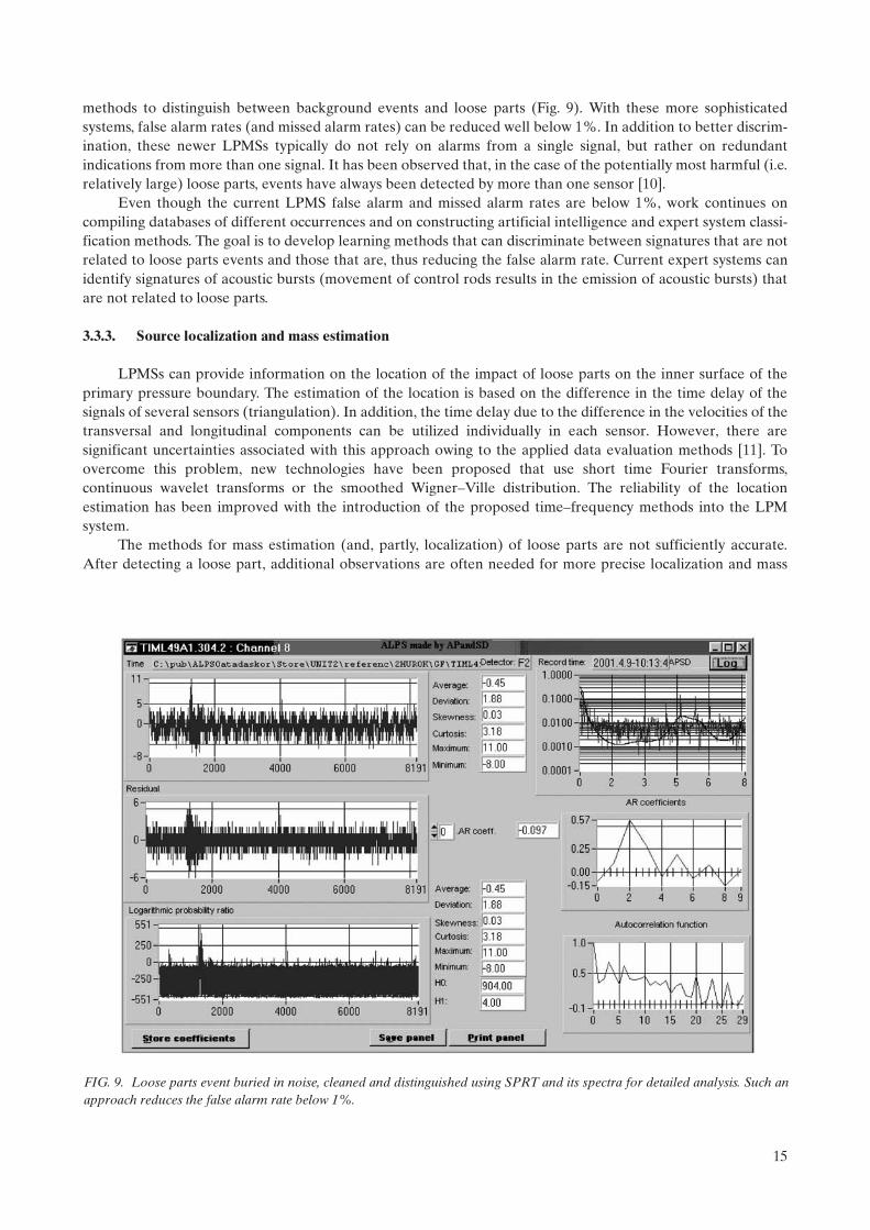
methods to distinguish between background events and loose parts (Fig. 9). With these more sophisticatedsystems, false alarm rates (and missed alarm rates) can be reduced well below 1%. In addition to better discrim-ination, these newer LPMSs typically do not rely on alarms from a single signal, but rather on redundantindications from more than one signal. It has been observed that, in the case of the potentially most harmful (i.e.relatively large) loose parts, events have always been detected by more than one sensor [10].

Even though the current LPMS false alarm and missed alarm rates are below 1%, work continues oncompiling databases of different occurrences and on constructing artificial intelligence and expert system classi-fication methods. The goal is to develop learning methods that can discriminate between signatures that are notrelated to loose parts events and those that are, thus reducing the false alarm rate. Current expert systems canidentify signatures of acoustic bursts (movement of control rods results in the emission of acoustic bursts) thatare not related to loose parts.

3.3.3. Source localization and mass estimation

LPMSs can provide information on the location of the impact of loose parts on the inner surface of theprimary pressure boundary. The estimation of the location is based on the difference in the time delay of thesignals of several sensors (triangulation). In addition, the time delay due to the difference in the velocities of thetransversal and longitudinal components can be utilized individually in each sensor. However, there aresignificant uncertainties associated with this approach owing to the applied data evaluation methods [11]. Toovercome this problem, new technologies have been proposed that use short time Fourier transforms,continuous wavelet transforms or the smoothed Wigner–Ville distribution. The reliability of the locationestimation has been improved with the introduction of the proposed time–frequency methods into the LPMsystem.

The methods for mass estimation (and, partly, localization) of loose parts are not sufficiently accurate.After detecting a loose part, additional observations are often needed for more precise localization and mass

FIG. 9. Loose parts event buried in noise, cleaned and distinguished using SPRT and its spectra for detailed analysis. Such anapproach reduces the false alarm rate below 1%.

16

estimation, in which ad hoc additional sensors may be required. Utilizing the different components of burst,namely longitudinal and transversal components, allows for a localization precision of about 10 cm (e.g. on thesurface of the steam generator). Earlier methods of localization, based on the transport time of the structure-borne sound in the metal and on the distances of detectors from the place of the impact, allowed localization ofthe loose parts with a precision of 1 m. Promising new methods based on time–frequency analysis could providefurther improvements in the automated localization and mass estimation procedure [12].

Additional mass and energy estimation techniques are:

— Frequency ratio;— Wigner–Ville distribution in the time–frequency domain;— Mass–velocity map;— Neural network technique;— Finite element analysis for modelling the possible impact, to populate the knowledge base.

3.3.4. Utilization of results

The purpose of LPMS is to detect loose parts and assess their potential hazard to the reactor systemcomponents. The uncertainty of earlier systems was too high for the information to be transferred directly to thereactor operator. Since, in current systems, the false alarm rate has been reduced well below 1%, there is anincreasing trend of sending information about larger loose parts directly to the reactor operator display, withsmaller occurrences remaining in the stand-alone LPMS for further analysis.

Reports from acoustic events recorded by LPMSs can also be valuable for maintenance work and ageingestimation, even if the size or origin of the loose part does not necessitate that direct action be taken by theoperators. Therefore, it is advisable to have a reporting and distribution system associated with the LPMS. Audiomonitoring of recorded signals is the most effective form of distribution, since complicated functions such asFourier analysis or time–frequency analysis require a certain level of expertise to interpret.

Plant managers are typically interested in the level of severity, the impact on safety and the ageing effectsof the loose parts. It is difficult to accurately define this information for loose parts, since almost all events areunique. In addition, the consequences caused by loose parts are highly variable depending on where the looseparts were locked, on the mass, on the loose parts material, and on the number and energy of impacts. Mostloose parts are observed during the initial startup of the main coolant pumps after refuelling. Therefore, mostregulatory agencies, including the NRC, request the use of LPMS only during initial startup. Most loose partsdetected during startup disintegrate rapidly as a result of impacting with rotating parts (pump blades) or walls.Experience shows that the majority of the small and medium-sized loose parts disintegrate or become lodgedsomewhere within the first 30 s after the startup of the given loop. Loose parts that have disintegrated to the sizeof sand grains are filtered out by water filters, leading to a need to change the filter earlier than expected. Smallparticles or grains in the filters are referred to by utilities as debris and not loose parts, and are neglected as notbeing dangerous to integrity. However, small parts and the sand itself may be carried into the reactor core, wherethey can corrode the surface of the fuel cladding. Furthermore, cases where small particles are lodgedsomewhere between the moving elements in the reactor core (control rod, or assemblies) have been reported.

One can conclude from the history of known events that loose parts carry a rather small hazard withrespect to the integrity of the first and second barriers. Material damage in the sense of ageing and other effectsis the most common consequence of loose parts, especially if they are observed too late (or not at all). Suchlosses are rather significant (expensive). A properly installed and managed LPMS has the potential to quicklyprovide a significant return on investment if a large loose part is identified and actions are taken beforesignificant damage is incurred. In a study based on several LPMSs in similar PWRs, it was found that loose partsoccur once every three years on average, and the consequences, if not observed in time, are about five timeshigher than the cost of an LPMS. The economics of an LPMS can be improved further if it is used for additionalacoustic monitoring tasks.

17

3.4. REACTOR NOISE ANALYSIS TECHNOLOGY

Noise analysis refers to methods that utilize the fluctuations in process signals to extract importantinformation concerning the system [13–15]. Examples of such process signals are neutron detector signals,temperature, pressure, flow and accelerometer signals. The application of such techniques in nuclear powerplants started with neutron noise analysis in zero power systems and research reactors. The objective was todetermine nuclear parameters, primarily the reactivity, or the effective delayed neutron fraction. These methodsuse some second moment of the neutron detector count, either the variance-to-mean (Feynman alpha) or thecorrelations (Rossi alpha), or some related method. It is interesting to note that these methods have recentlyreceived some renewed interest in connection with plans for developing subcritical, accelerator driven systems.Later applications concerned detecting structural vibrations, such as control rod vibrations, in research reactorssuch as that at the Oak Ridge National Laboratory (ORNL) and the High Flux Isotope Reactor. Gradually,neutron noise methods found applications in commercial power reactors as well. At the same time, theinformation content in the fluctuating part of other signals (temperature, pressure, etc.) was utilized, either aloneor in combination with neutron detectors or other signals. The field of power reactor noise diagnostics is, by now,a very broad field with many applications. A description of the principles and a list of the main applicationsfollows.

3.4.1. Spectral methods

In noise applications, usually the auto- and cross-spectra (APSD and CPSD, respectively) or auto- andcross-correlation functions (ACF and CCF, respectively) of the fluctuating part (alternating current (AC)component) of the measured process signals are generated and used in the analysis. Apart from a few cases, suchas BWR instability, which is discussed later in this report, it is assumed that the fluctuating signals are small(typically less than 0.1% of the signal’s DC component) and the linear systems theory can be used. In thisexample, the fluctuations in the measured signal (noise) are caused by the fluctuations of another signal (noisesource or perturbation) whose effect on the noise is exerted through a physical process, described by the transferof the unperturbed system. Often, but not exclusively, the perturbations in the noise spectra (peak in the powerspectra) can be identified as anomalies (excessive vibrations, boiling, flow irregularities, etc.). However, allprocess signals have inherent fluctuations in the normal state, which influence the fluctuations of many othersignals with which they have a cause and effect relationship. The relationship between the various processes andparameters is shown schematically in Fig. 10.

Two of the three ingredients in process noise generation — i.e. noise source, transfer function and, particu-larly, induced noise (neutron noise) — must be known (measured or calculated) such that the third can bedetermined by the physical relationship among the three, which is known from theory. In practice, there are twomain categories: surveillance (monitoring) and direct diagnostics.

Reactor core,

as a dynamic

transfer function

Measured process

signals

(neutron noise)

Noise source

(Driving force)

Vibrations

Boiling

Coolant flow

Temperature noise

Static cross sections

Reactivity coefficients

Neutron noise

FIG. 10. Schematic of the generation of neutron noise.

18

3.4.2. Surveillance or monitoring

Surveillance or monitoring consists of measuring the induced (output) noise, typically the neutron noise,and identifying anomalies in the measured data. To detect an anomaly and to identify its type, it is sufficient toknow the signature of the anomaly in the affected spectra (broadband, sink structure, peaks, etc.). For quantifi-cation, such as locating the position or determining the strength (e.g. vibration amplitude), one needs to measurethe output noise and know the corresponding transfer function (e.g. by dynamic core calculations or frommodels).

Parameter estimation refers mostly to the determination of some parameter of the core, such as reactivitycoefficients, heat capacity or core flow transit time. Such parameters are therefore included in the transferfunction of the core; thus, both the input (noise source) and the output (induced noise) signals need to bemeasured. In addition, a physical model needs to be established that describes the transfer between the two.Often this physical model is in the form of a frequency dependent complex transfer function with unknownparameters that need to be determined.

3.4.3. Direct diagnostics

Direct diagnostics is a third type of noise analysis technique where a process signal (time series) ismeasured directly, with the aim being simply to classify whether it reflects normal or abnormal behaviour,without trying to identify the cause of the anomaly or the underlying physical process. Relevant examples areimpacting of detector tubes, BWR instability and, to some extent, core barrel vibration diagnostics.

3.4.4. Implementation of reactor noise analysis applications

The implementation of reactor noise analysis applications in an operating nuclear power plant fordiagnostic and inspection purposes may require careful planning and gradual introduction. Most of the requireddata acquisition systems, connection points, electronics, measurement procedures, licensing requirements andanalysis/interpretation procedures are not part of the original nuclear power plant design or the operatinginstructions delivered by the vendor. Large-scale applications of reactor noise analysis require the developmentof the following essential components:

— Multichannel data acquisition systems for digitizing and storing detector signals. These systems can beeither general purpose portable data acquisition systems, or permanently installed systems dedicated tomonitoring a fixed set of signals.

— Multichannel optical isolation amplifiers separating the data acquisition systems from the station hardware(e.g. shutdown system test points).

— Maintenance procedures to connect and disconnect the data acquisition hardware systems to/from stationhardware without disturbing the normal operation of the reactor.

— Dedicated station engineers responsible for the planning, preparation and execution of the fieldwork forrecording measurement signal data.

— Digital signal processing techniques to operate off-line on the recorded detector signals (multichannel,digitized and prescreened) to produce multichannel statistical functions in the frequency and time domainsfor noise analysis.

— Physical models of processes in the reactor to be used in the interpretation of noise signatures measured inspecific applications (e.g. fuel channel vibration, coolant boiling, moderator circulation, water level oscilla-tions).

— Dedicated experts to plan and execute field measurements, to process and interpret measurements, toanalyse patterns, to develop models and software tools for new applications, and to solve previouslyunseen problems.

— Involvement of the nuclear regulator (i) to license and approve the data acquisition systems thattemporarily become part of the station’s safety system hardware during the measurements, and (ii) to havethe validity of the analysis techniques and their results accepted.

19

In the initial development phase, management approval is likely to be given only for a limited and well-defined application of noise analysis. Applications from the early startup phase of noise analysis projects mayexpand rapidly to other applications if the results of the measurements can be used in (i) meeting licensingrequirements, (ii) justifying continued operation of ageing instrumentation, (iii) successfully trouble-shootingunusual conditions and (iv) satisfying required inspection and testing activities.

3.4.5. Required data acquisition systems

In practical applications of reactor noise analysis, computer based data acquisition systems are needed toobtain high quality high frequency data. Usually, the requirements for sampling rates, amplitude resolution,signal conditioning, system isolation, simultaneous sampling and synchronization are more stringent than thosein a typical plant computer; therefore, digital data provided by plant computers (data loggers, plant historian,etc.) cannot be used for noise analysis purposes.

In many applications, portable multipurpose data acquisition systems are applied to collect measurementdata (multichannel time series). There are some disadvantages to using these systems. First, isolation from theplant equipment is required. Second, hardware access to plant analogue signals (‘hook-up points’) is oftendifficult in existing nuclear power plants where provisions for these measurements were not designed. Third, itcan be expensive to design, build, operate and maintain a sufficiently large fleet of portable multipurposeacquisition systems. In a new plant, where the use of an OLM system can be designed as part of the plant instru-mentation systems, the measurements can be carried out readily in a more systematic and routine way.

3.4.5.1. Isolation requirements

If analogue process signals are to be accessed by directly connecting the noise data acquisition systems tostation systems (control systems, reactor protection systems), the isolation is critical and must be accomplishedthrough applying special isolation hardware, which needs to be connected without affecting the plant instrumen-tation and safety related functions. There are varieties of isolators or buffer amplifiers, such as high impedanceoptical isolators, that can be used for this purpose. The isolation specification (e.g. input impedance, low-passfilter cut-off frequencies) is an important part of planning, and it must be selected on the basis of the character-istics of the plant equipment or system that is being monitored.

The isolation amplifiers separate the station instrument from the data acquisition hardware by preventingany feedback from the isolation amplifier’s output to its input side. The isolation amplifiers usually have a gainof one and a low-pass cut-off frequency in the 10–100 kHz range. Their function is only to isolate the signals, notto filter or amplify them. Depending on the level of required independence, the isolation amplifiers may bephysically separated from the rest of the data acquisition system.

The independence and separation of multichannel isolation amplifiers must be tested and demonstratedbefore the signal connections are made. Similarly, the input impedance of the isolation amplifiers must bechecked in both power-on and power-off conditions. An additional requirement is the measurement of theisolation amplifier output with zero (or shorted) input. These zero-offset values are also used in the calibrationcorrection calculations when the recorded voltage signals are converted into physical units.

3.4.5.2. Analogue signal conditioning

For dedicated data acquisition systems, the station instrument signals to be accessed may be in thefollowing forms:

— Analogue current signal as a direct output of the measurement sensor (e.g. a self-powered flux detector asa current generator in the µA range, or a flow transmitter in a 4–20 mA current loop);

— Analogue voltage signal already transformed into a standard voltage range (e.g. 1.0–5.0 V).

In the case of current signals, an additional component is needed to convert the current signals intomeasurable voltage signals. This component could be as simple as a sampling resistor in a 4–20 mA current loop,or a current-to-voltage converter in the flux detector’s amplifier. If the station signals are available in an

20

analogue voltage form, they can be directly connected to the isolation amplifiers of the noise data acquisitionsystems.

The actual filtering and amplification of analogue signals are performed after the isolation by separatesignal conditioning units including the following functions:

— Anti-aliasing low-pass filtering, usually needed to remove the high frequency components. The low-passfrequency is typically set below 40% of the sampling frequency for all recording channels. If anti-aliasingfiltering is not performed before sampling, the user must make sure that the sampling rate is at least twicethe maximum frequency contained in the analogue noise signals to be recorded.

— Removal of the mean value or the DC component of the signal by subtracting a constant voltage valuefrom the analogue signal, or by applying an analogue high-pass filter to the signal. The DC compensationis performed either automatically or by the user individually for all recording channels.

— Amplification of the signal or the DC compensated signal. The signal amplification is performed eitherautomatically or by the user individually for all recording channels.

— After the analogue signal conditioning steps, the signals are fed into the multichannel analogue-to-digitalconverter (ADC) where the simultaneous sampling for all channels takes place.

3.4.5.3. Plant conditions for data acquisition

Depending on the purpose of the signal noise measurement, certain conditions and restrictions may beplaced on the plant for the duration of the data collection. Most of the measurements have to be made at steady-state high-power operation, with no operator-induced changes in the reactor system (such as testing, or on-linefuelling in CANDU reactors). The duration of noise signal recording sessions may vary from half an hour totwelve hours. The actual length depends on the sampling rate and the purpose of the noise measurement (e.g.establishing accurate noise signature baselines, or anomaly detection), and on the type of signal monitored.Noise measurements of slowly changing temperature signals require long recording times, while measurementsof high frequency vibration signals need short ‘snapshots’ of time series data.

Other measurements may take advantage of specific changes in the plant operating mode (e.g. pump tripor startup, reactor trip or startup, power step-back, pump changeover). Although these transient responsemeasurements can be recorded by the noise data acquisition systems, they are not noise measurements in thetraditional sense.

3.4.6. Core barrel vibration diagnostics in PWRs

Diagnostics of the motion of the core barrel and the core barrel support assembly are one of the earliestapplications of noise analysis in nuclear power plants. Core barrel motion is a significant safety related issue,since if the core barrel undergoes a pendulum type movement it may touch the reactor vessel, leading to fatigueand wear. Another possible point of concern is the presence of instrument tubes inserted from the bottom of thereactor vessel. Even a small amplitude of core barrel motion is sufficient to damage such tubes.

In addition, increased vibration amplitudes are a sign of fatigue in the mechanical structure of the coreinternals. Fatigue of the secondary core barrel support resulted in increased vibration amplitudes in the Stadenuclear power plant in Germany; loosening of the hold-down spring resulted in increased vibration amplitudesin several reactors, including Russian-made reactors such as Energiewerke Nord in the former GermanDemocratic Republic, as well as several Westinghouse type PWRs.

Vibrations of the core barrel with respect to the core barrel secondary support and the vibrations of thepressure vessel can be detected from in-core pressure fluctuations and external displacement sensors (piezo-electric accelerometers), and from ex-core neutron noise. The pressure and displacement sensors have beenused during startup tests at many reactors. At most plants, the analysis is based on ex-core neutron noise signals.The methodology is based on spectral analysis of the neutron noise. Usually, ex-core neutron detectors are used(see Fig. 11), which are part of the safety channels, though other sensors may also be involved (such as in-coreneutron detectors or accelerometers positioned on the reactor vessel). The main purpose of the ex-core neutronnoise analysis is to monitor the incipient changes of the mechanical conditions of the components and to helpjudge the integrity of the system.

21

The noise signals are measured and processed in different combinations of the signals simultaneouslythrough a data acquisition system. For OLM of reactor internals, the fast Fourier transform (FFT) technique isapplied and averaged to calculate the auto-power spectral density (APSD), cross-power spectral density(CPSD), coherence function and phase. The APSD represents the relatively strong periodic components withinthe stochastic time domain signal, and the coherence function of two simultaneously measured signals revealsthe degree of commonality between the periodic components of the two signals. An example of noise spectra isshown in Fig. 12.

Such measurements can reveal material degradation (such as loosening of the core barrel secondarysupport, or wear of the hold-down springs) through increasing amplitudes and decreasing frequencies. Bothbeam mode (pendulum) and shell mode vibrations are monitored. The analysis methods have been developed inorder to make the method suitable for a consistent trend analysis. Core barrel vibration analysis and monitoringis performed in many countries, and it constitutes a basis for judging the material integrity and for planningmaintenance (such as change of the hold-down springs) [16].

FIG. 11. Typical locations of ex-core neutron detectors in a PWR.

FIG. 12. Noise signal analysis using two ex-core neutron detectors at opposite positions.

22

The performance of the analysis of core barrel vibrations is greatly enhanced if a mechanical model of thevibration modes of the whole internal structure of the pressure vessel, core barrel and core barrel support isavailable. Such a model serves partly to identify the eigenmodes and eigenfrequencies of the system, and partlyto perform a sensitivity analysis of how the degradation of various components affects the vibration amplitudesand frequencies. This helps the interpretation of any changes in the vibration parameters determined by noiseanalysis [17]. Such calculations are performed by finite element methods. Figure 13 shows a typical reactorinternal structure and the finite element model for the vibration analysis.

The simulated vibration characteristics are illustrated in Fig. 14.

3.4.7. Control rod vibrations in PWRs

After the first pioneering measurements in the ORNL research reactors, excessive control rod vibrationswere observed in several PWRs. These vibrations are due to material degradation problems. Owing to obviousstructural differences, control rods are more vulnerable to flow induced vibrations than are fuel assemblies.Usually, excessive vibrations can occur and lead to serious consequences only in reactor constructions with largemassive control rods that replace a whole fuel assembly. The result of excessive vibrations can be damage to thecontrol rod and/or to the neighbouring fuel assembly; in the worst case, the control rod can break and drop intothe core.

Both detection of excessive control rod vibrations and identification of the excessively vibrating rod (local-ization) are possible from the signals of a few (at least three) in-core neutron detectors at different radial

FIG. 13. Reactor internal structure and its simplified model for a finite element analysis in a PWR.

FIG. 14. Typical vibration modes of reactor internal structures in a PWR.

23

(horizontal) locations. The localization is based on knowledge of the spatial attenuation of the neutron noise outfrom the vibrating control rod and an inversion method to unfold the source position from the measured signals.

A methodology for locating excessively vibrating rods from in-core neutron noise measurements has beenrefined over the years [18]. A theory describing the induced neutron noise as a function of the vibrationproperties and the core transfer properties was elaborated first. Then an inversion method was necessary, whichdetermined the vibration properties and the position of the vibrating rod from the measured neutron noise andthe core transfer properties. Both parametric (localization curves) and empirical (neural networks) inversion orunfolding methods were used. A notable case of control rod vibrations occurred in a WWER-440 type PWR inHungary in 1985, where the localization was performed successfully during operation [19]. It is interesting tonote that the methodology of localization was developed further to determine the position of local (channeltype) thermohydraulic instabilities in BWRs.

The most extensive work with monitoring and identifying core internal vibrations was performed by EDFin France, in collaboration with the University of Tennessee. On-line control rod vibration monitoring isperformed today in several countries.

3.4.8. Core flow measurements with neutron noise in PWRs

In-core LPRMs of fission chambers can detect the effect of propagating temperature fluctuations on theneutron field. By cross-correlating detectors from two different axial levels in the same channel, and applyingadvanced signal analysis techniques, the local coolant velocity in a PWR can be determined. In the Paks-2 PWRin Hungary, such measurements clarified that the reason for core power asymmetry lay in the asymmetric flowvelocities in the core due to crud buildup on the surface of the fuel pins. A graphical representation of thevelocity distribution over a horizontal cross-section of the core of Paks-2 is shown in Fig. 15. Such measurementsare occasionally performed at other plants.

3.4.9. Measurements of the moderator temperature coefficient in PWRs

The moderator temperature coefficient (MTC) is an important safety parameter whose measurement withtraditional methods is slow and costly. It has long been suggested that it could be measured by noise methods ina non-intrusive way, by cross-correlating the inlet (or outlet) temperature fluctuations with in-core neutron

FIG. 15. Asymmetric velocity profile in the core of Paks-2 (from Ref. [20]).

24

noise. In its originally proposed form, the method used local temperature and neutron signals and resulted in, asan absolute method without calibrations, quantitatively very inaccurate results with a systematic underesti-mation by a factor of 2–5. It could therefore only be used as a relative method, after calibration. Some recentwork, however, pointed out that using a radial weighted average of the temperature noise instead of a localthermocouple signal yields much more accurate results that agree with predicted or calculated MTC values verywell. The method has been demonstrated in the Swedish Ringhals-2 PWR [21].

This method requires the measurement of the in-core temperature noise at several radial positions. In theRinghals-2 plant, this was achieved by using so-called gamma thermometers at nine different radial positionsinside the core. These gamma thermometers are installed for measuring the local static gamma flux (as analternative to the neutron flux), but in the frequency range of interest for the determination of the MTC, i.e.between 0.5 and 1 Hz, the gamma thermometers act as thermocouples. In some other plants, core exit thermo-couples can be used for the same purpose.

3.4.10. Flow measurements in PWRs

Several correlation based flow measurement methods were developed in the early 1970s to measure flow,i.e. mass flow of water in a pipe in nuclear power plants. Feedwater flow measurements are part of the thermalpower calibration methods, which use calorimetric principles. One early method was based on the cross-correlation between axially displaced thermocouples, measuring the temperature fluctuations propagating withthe flow. Later, in primary circuits the fluctuations of the generated 16N activity were used in cross-correlationflow meters. There exist permanent installations of this type. Yet another method is the cross-correlation ofultrasonic signals, transmitted diagonally in the flow. The periodic signals are randomly modulated by theturbulent eddies travelling with the flow.

3.4.11. Data acquisition for noise analysis in PHWRs

The CANDU reactors’ two independent shutdown systems (SDS1 and SDS2) and the reactor regulatingsystem (RRS) are equipped with:

— Fast responding in-core flux detectors (ICFDs) and ex-core ion chambers;— Flow, level and pressure transmitters;— Resistance temperature detectors (RTDs).

These safety and regulating signals are divided into six safety channels (D, E, F for SDS1 and G, H, J forSDS2) and three regulating channels (A, B, C), and are available for multichannel noise signal recording in ananalogue format at the output of the station amplifiers. Temporary connections to the noise data acquisitionsystems are made through optically isolated buffer amplifiers. The analogue multichannel signal conditioning(low-pass anti-aliasing filtering, DC removal and amplification) and the analogue-to-digital conversion of signalsare carried out in the computer controlled data acquisition systems. The digital recording of the separate dataacquisition systems assigned to the above nine independent safety/regulating channels may be synchronizedthrough sending data acquisition computer clock signals via isolated wire connections. Typically, noise signalrecording is carried out for a duration of 30 min–12 h at steady-state high-power operation. The recorded noisesignals may be analysed off-line in the frequency and time domain [22, 23].

3.4.12. Vibration of fuel channels detected by ICFD noise analysis

The noise signals of the horizontal and vertical in-core flux detectors contain information on the character-istics of flow-induced vibration of fuel channels and detector tubes. Experience has shown that abnormalities inthe integrity of these structures can be detected and diagnosed at an early stage by analysing the frequencyspectra of the ICFD noise signals.

Reactor noise analysis was introduced as a powerful inspection technique in the early 1990s at theCANDU units of Ontario Hydro [24]. Several applications have been developed and are applied on a routinebasis. The analysis of regularly performed ICFD noise measurements showed the effect of flow-induced

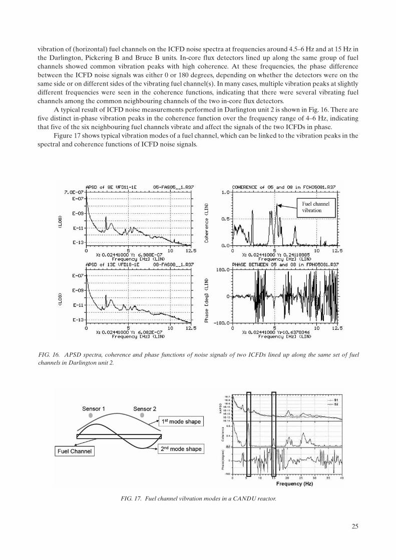
25

vibration of (horizontal) fuel channels on the ICFD noise spectra at frequencies around 4.5–6 Hz and at 15 Hz inthe Darlington, Pickering B and Bruce B units. In-core flux detectors lined up along the same group of fuelchannels showed common vibration peaks with high coherence. At these frequencies, the phase differencebetween the ICFD noise signals was either 0 or 180 degrees, depending on whether the detectors were on thesame side or on different sides of the vibrating fuel channel(s). In many cases, multiple vibration peaks at slightlydifferent frequencies were seen in the coherence functions, indicating that there were several vibrating fuelchannels among the common neighbouring channels of the two in-core flux detectors.

A typical result of ICFD noise measurements performed in Darlington unit 2 is shown in Fig. 16. There arefive distinct in-phase vibration peaks in the coherence function over the frequency range of 4–6 Hz, indicatingthat five of the six neighbouring fuel channels vibrate and affect the signals of the two ICFDs in phase.

Figure 17 shows typical vibration modes of a fuel channel, which can be linked to the vibration peaks in thespectral and coherence functions of ICFD noise signals.

FIG. 16. APSD spectra, coherence and phase functions of noise signals of two ICFDs lined up along the same set of fuelchannels in Darlington unit 2.

FIG. 17. Fuel channel vibration modes in a CANDU reactor.

26

The primary and secondary bending modes of the fuel channel vibration affect the ICFD noise spectra atthe same frequencies. The major components of the fuel channel assembly are the calandria tube, pressure tube,fuel bundles, two end fittings and four garter springs, as shown in Fig. 18. Figure 19 shows an example of thecomparison between normal and abnormal vibration (displacement) spectra of a fuel channel obtained from thefinite element modelling.

Finite element vibration analyses of CANDU fuel channels have been used to create a database ofvibration modes and frequencies for various abnormal conditions of the end fitting support and the gartersprings.

FIG. 18. A typical CANDU fuel channel and its simplified model used in finite element analysis.

FIG. 19. An example of the simulated vibration spectra of a CANDU fuel channel based on finite element analysis.

27

3.4.13. Vibration of detector tubes detected by ICFD noise analysis

Evidence of flow-induced mechanical vibrations of both horizontal and vertical detector guide tubes inCANDU reactors has been found in the spectral functions of ICFD noise signals. A detector vibrating in aninhomogeneous static flux senses virtual flux changes and produces a small oscillating current component at thevibration frequency via its prompt response channel. In this way, the movement of the detector in a non-zeroflux gradient is directly mapped into detector current fluctuations. An increase in the vibration amplitude orpossible impacting with surrounding structures can be detected indirectly by ICFD noise analysis.

The vibration of detector tubes induced by the moderator flow results in strong peaks in the spectra andcoherence functions of noise signals of ICFDs in the frequency range of 2–5 Hz. Noise signals of detectorslocated in the same vibrating detector tube have high coherence and zero phase differences at the fundamentalfrequency of tube vibration. Depending on the locations of the ICFDs inside the guide tube, the detectors mayhave zero or 180 degree phase differences at the frequencies of the higher harmonics, with high coherence.

A typical pattern, measured between ICFDs located in the same horizontal detector tube in Pickering Bunit 5, can be seen in Fig. 20. It shows the APSD, coherence and phase functions between the signal fluctuationswith a detector vibration frequency of 3.8 Hz.

The strong and sharp vibration peak in the coherence function and the zero phase difference at thevibration frequency indicate that the oscillation is monochromatic and stationary; that is, the detectors in thehorizontal tubes vibrate freely at a constant frequency.

By monitoring the trend of vibration peaks in the noise spectral functions of the measured ICFD signals,the mechanical condition of the detector tube can be assessed on the basis of the following simple principles:

— An increase in the magnitude of the peak in the noise spectra of the ICFD indicates detector tube vibrationwith increasing amplitude.

— A shift in the frequency location of the spectral peak indicates changes in the mechanical conditions/support of the detector tube.

— A widening of the spectral peak and the occurrence of higher harmonics in the ICFD noise spectra indicateincreasing impacting with the surrounding reactor internals.

FIG. 20. APSD spectra, coherence and phase functions of noise signals of two SDS2-G ICFDs located in the same horizontaldetector tube, HFD8, measured in Pickering B unit 5.

28

The long term trend monitoring of these vibration peaks is useful for early detection of mechanicaldegradation in the reactor core caused by vibrations. Also, excessive detector tube vibration may lead tomechanical failures compromising the integrity of the ICFD signals (e.g. fatigue of lead cable and detectorjunction, and loss of cover helium pressure).

3.4.14. Two-phase flow diagnostics and the local component in BWRs

It was observed in the mid-1980s that the cross-correlation between in-core neutron detectors in the sameinstrument tube could indicate the bubble transit time, and hence give an indication of flow velocity. Thephysical reason for this was explained by the existence of a so-called local component of the two-group neutronnoise, which had already been observed in early measurements at the Oak Ridge Graphite Reactor (X-10 or the‘Clinton Pile’). Methods were developed to assess steam velocity and void fraction from in-core BWR noisemeasurements. Even a so-called second transit time (co-existence of two distinct velocities in one channel) wasobserved in several measurements. Despite convincing results and a sufficient methodology, surveillance of two-phase flow properties by neutron noise methods has not found routine application. Measurements of the localsteam velocity at several plants have been conducted.

3.4.15. BWR instability

It is well known that during startup conditions, i.e. medium/high power level and low/moderate core flow,BWRs can experience unstable power oscillations and regional (out-of-phase) or local neutron flux oscillations.The possibility of such power oscillations, which are to some extent analogous to xenon oscillations in a PWR,was predicted theoretically [15]. Calculations are thus performed before startup via coupled neutronic–thermohydraulic codes to verify the conditions under which the reactor becomes unstable. This defines anexclusion zone, i.e. a set of operating conditions that the reactor operator should avoid.

During the startup tests of the reactor, measurements of the in-core neutron noise are usually performed.This is achieved by the use of in-core detectors. For instance, in the Swedish ABB BWRs there are 36 in-coredetector strings with 4 detectors in each. The individual detectors are called local power range monitors(LPRMs). There are also four groups, each consisting of the arithmetic mean or the sum of nine detector stringsdistributed over the core, which are called average power range monitors (APRMs). Both the LPRMs and theAPRMs are used for stability monitoring, although the latter cannot detect regional or local instabilities.

There exist three different types of unstable oscillation: global or core-wide (in-phase), regional or out-of-phase, and local or channel type (pure density wave oscillation (DWO) type) oscillations. The first two arecoupled core physics–thermohydraulics phenomena, whereas the channel type instability is purelythermohydraulic.

For the global or in-phase instability, the flux oscillates over the whole core at a typical frequency of 0.5 Hz,and the space dependence of the flux follows the first neutronic mode, i.e. the fundamental mode. Since theeigenvalue of the fundamental mode is the only one that might be larger than unity, the neutronics might amplifyany perturbation of the core. The mechanism driving this kind of oscillation is mainly the time delay between agiven power perturbation and the corresponding reactivity response due to the void/pressure coefficient. Insome cases, the initial perturbation can be reinforced by the void/pressure feedback if the phase of this delayedresponse coincides with the phase of the power perturbation. Although the thermohydraulics also plays somerole in this kind of instability, it is a stabilizing effect, i.e. the flow oscillations induced by the void/pressure oscil-lations are damped by the friction in the recirculation loop.

For the out-of-phase oscillation, there is a positive flow rate perturbation in one half of the core and anegative flow rate perturbation in the other half of the core. The recirculation loop does not play a role in thiscase, since the core-averaged flow rate perturbation is roughly equal to zero. The mechanism driving theoscillation is thermohydraulic, whereas the neutron kinetics has a damping effect. This behaviour is precisely theopposite of the case of global or in-phase oscillations. Namely, a power perturbation will induce a change of void/pressure, which itself will create a perturbation of the flow rate. Depending on the operating conditions, the timedelay between the power perturbation and the corresponding flow rate response can either reinforce or dampthe initial perturbation. One characteristic of the regional oscillation is that several higher modes can be excited,compared with the in-phase oscillation. Typically, the second and third modes, i.e. first and second azimuthal

29

modes, respectively, are excited. Even if these modes are subcritical, the thermohydraulics might self-sustain theoscillations. The oscillation frequency of these two modes, although typically close to 0.5 Hz, might be slightlydifferent from each other. Thus, the resulting oscillation, which is the sum of these two modes, might exhibit arotating neutral line, with the neutral line being defined as the line separating the positive and the negative lobesof the oscillation. Very often, a fourth mode, i.e. the first axial mode, can also be excited. The regional or out-of-phase oscillation is thus a complicated oscillation owing to its spatial intermittence, i.e. the neutral line might bestable in some cases or might rotate. Clearly, conventional frequency-domain analysis methods will fail torecognize this type of oscillation if it is non-stationary (time- and frequency-domain analysis methods, such aswavelets, should be used instead).

The last type of possible instability in a forced convection BWR is a local oscillation or DWO. This type ofoscillation typically occurs when a fuel assembly is unseated, i.e. does not sit properly on the lower fuel tie plateof the core. Since each fuel assembly in a BWR is contained in a fuel box, the fuel channels are independent ofeach other. If there is an unseated fuel assembly, some of the coolant bypasses the fuel channel. The inlet flowperturbation will create a modification of the single-phase pressure drop in the single-phase region of the heatedchannel. This perturbation will travel upward with the flow and generate a modification of the two-phasepressure drop in the two-phase region of the heated channel. Since the perturbation only affects one fuelchannel, and since the core is large, the total pressure drop between the core upper plenum and the core lowerplenum remains constant. Owing to this imposed boundary condition, the two-phase pressure drop in theperturbed fuel channel will create a feedback pressure perturbation of the opposite sign in the single-phaseregion, either reinforcing or damping the initial perturbation.

In addition to the above described ‘pure’ (single type) instabilities, there have been cases where two of theabove described modes have occurred simultaneously, such as global and regional (Ringhals Plant (Sweden),1992) and global and local (Forsmark Plant (Sweden), 1997/1998). Since the two oscillations occur at the samefrequency (inverse of the core flow transit time), they cannot be separated in the power spectra. The problemwith the mixed modes is that the less stable component may have smaller oscillation amplitudes, and hence asimple determination of the decay ratio (DR) using a detector signal that contains the sum of the two oscillationswill be dominated by the more stable component, leading to an overly optimistic estimation of the stabilitymargin. However, methods have been elaborated to eliminate the various modes such that the stabilityproperties of each mode can be determined separately and hence a margin of instability can be re-established.

Despite the awareness of BWR instability and the preparatory measures, unexpected instabilities haveoccurred in the past in different BWRs. In Sweden, one of the most spectacular events was the Oskarshamn 3 in-phase instability event in February 1998, where very large power oscillations (more than 40% of the nominalpower from peak to peak) were undetected by the reactor operator before the plant protection system automat-ically shut the reactor down.

3.4.16. Impacting of detector tubes in BWRs

Flow induced vibrations of the detector tubes have in several instances led to impacting, which in somecases caused significant damage to both the detectors and the fuel assembly walls. The vibrations of the detectorin a flux gradient can be identified from the detector signal itself through the peaks of the detector signalAPSDs. To determine whether or not impacting is occurring is straightforward; however, to quantify theseverity of the impacting is much more difficult, and there is no significantly reliable method. There are manyqualitative indicators, including increased amplitude or width of the peak (requiring access to baseline datafrom before impacting); distortion of the linear phase between two detectors at different axial positions in thesame tube; and occurrence of higher harmonics (peaks at double or triple frequencies). Recently, moreobjective methods have been developed that do not require comparison with baseline data (non-impactingconditions). These methods are based on wavelet analysis and detecting short transients in the signals thatfollow each detector impact.

30

3.5. MOTOR ELECTRICAL SIGNATURE ANALYSIS

Condition monitoring of electrical systems includes both stationary components (such as cables,instrument channels, electric circuits) and rotating or more dynamic components (such as motors, generators,actuators). Short term operational as well as long term ageing of electrical components and their maintenanceare very important issues in both power and process industries. Some of these are addressed by the NRC’sNuclear Plant Aging Research (NPAR) programme. The sections below address only those monitoring methodsbased on electrical signature analysis of motors that operate pumps or valves in a power plant.

3.5.1. Motor current signature analysis

As the mechanical load on an induction motor varies, the current drawn by the motor changes, increasingwith increasing load. Thus, a motor acts as a transducer, and the variations in the mechanical loads are reflectedin the variations of motor current. Motor current can be measured non-intrusively using a clamp-on currentprobe. The technology of drawing diagnostic information from the analysis of such measurements is calledmotor current signature analysis (MCSA). MCSA systems can also include a signal conditioning device, whichmakes a sensitive and selective analysis of the current variations possible. The output of this device is processedfurther using standard signal processing techniques. Various anomalies can be seen as changes in the pattern ofthe motor current during e.g. a valve stroke [25–27].

The change in the mechanical load (apart from a normal variation of the external load) can also be due toa malfunction of either the motor itself or of the component operated by the valve (MOV). These two cases areconsidered below.

Motor current variations corresponding to motor malfunctions are generally due to:

— Rotor imbalance, eccentricity with respect to the stator;— Thermal bowing of the rotor;— Broken or cracked rotor bars;— Shaft or stator resonances;— Mechanical and electrical misalignment;— Loose rotor on the rotor shaft.

Information about these anomalies is obtained by monitoring various frequencies of an induction motoroperation, which are defined as follows:

fL = line frequency (Hz);

fSN = synchronous frequency of the motor = , P = No. of poles;

fR = rotational frequency (rotational speed) of the motor (Hz);

Slip frequency, fSL = fSN – fR;

fSB = sideband frequency = slip frequency × No. of poles = fSL × P (Hz).

Both the sideband frequency location and spectral magnitudes are indicative of rotor bar problems.Continuous monitoring of motor current spectra at various frequency bands provides predictive maintenanceinformation during normal operation. The changes in the spectral magnitudes of the motor current, at slipfrequency sidebands of the line frequency, are indicative of rotor related anomalies.

MOVs are subjected to loads and stresses from the control systems and power systems that serve them, aswell as from the fluid systems in which they operate. They may be subjected to partial damage or degradationthat will leave them operable for normal or no-load situations, but may cause failure at design basis demandpressure or flows.

2 ¥ fL HzR

( )

31

The following basic failure modes of MOVs were identified by the NPAR programme: failure to open;failure to close; failure to operate as required; plugging (failure to remain open); internal leakage; externalleakage. Various anomalies can be seen as changes in the pattern of the motor current during the valve stroke.

The diagnostic information that can be extracted from the motor current spectrum is:

— Identified spectral peaks, such as worm gear teeth meshing frequency, stem nut rotation, shaft speed andmotor slip frequency;

— Unidentified peaks that may be related to loads resulting from bearings, imbalance, etc.;— Harmonics of fundamental peaks and sidebands (usually indicative of wear and/or eccentricity).

The following abnormalities could be detected by MCSA:

— Valve stem taper;— Stem nut wear;— Degraded voltage;— Degraded valve stem lubrication;— Worm gear tooth wear;— Obstruction in the valve seat area;— Motor pinion disengagement;— Degraded worm and worm gear lubrication;— Changes in stem packing adjustments;— Improper torque switch settings.

MCSA was developed at ORNL. An expert system using the pattern recognition technique anddiagnostics rules for a given motor operator was developed at the University of Tennessee.

3.5.2. Motor power signature analysis

Motor power signature analysis (MPSA), such as that developed by Duke Power Company [28], consists ofmonitoring the three phase induction motor power during valve operation (open-to-close and close-to-openstrokes). For a balanced Y – Δ connected motor, the power is given by:

Motor power =

where:

cosF = power factor;Vphase = voltage across each phase;Iphase = current across each phase.

In actual MPSA tests, the three phase voltages and the three phase currents are measured, and the totalpower is calculated as:

Power =

Changes in the power signature are sensitive to operation anomalies and can be effectively diagnosed bythis signature analysis.

3 3 V Iphase phase cosF

3 1 1 2 2 3 3( )cosV I V I V I+ + F

32

4. MODELLING TECHNIQUES

This chapter describes common modelling techniques that have been applied for equipment conditionmonitoring in nuclear power plants. Modelling techniques applied to equipment condition monitoring aredistinctly different from the measurement based techniques described in the previous chapter. Two generalcategories of modelling types are described in the following sections, namely empirical and physical:

— Empirical modelling techniques construct models from historical operating data or simulated data.— Physical modelling techniques, on the other hand, construct models based on sets of equations grounded

on first principles and physical laws.

A final section describes some less common but related techniques such as fuzzy logic and multilevel flowmonitoring. Before going into details, the discussion that follows describes a generalized development andimplementation process for a modelling technique.

In general, the modelling techniques described here are applied to the components and systems that arecritical to continuous, safe operation of the plant. Modelling of noise sources and other processes, as well astransfer functions, is also used in reactor noise analysis, but is not described here. A list of the primary equipmentand subsystems that modelling techniques would address in an OLM system for a nuclear power plant isprovided below. Depending on the needs of a specific plant, this list could be modified:

— Main steam turbine: High pressure, intermediate pressure and low pressure turbine, thrust bearing, glandsteam;

— Reactor coolant system: Flow, pump motor and pump seal;— Feedwater system: Flow, pump and turbine performance and mechanics, heaters;— Condenser (performance): Pump, turbine;— Generator: Rotor cooling, stator cooling, exciter, transformer.

The application of modelling techniques to nuclear power plant equipment and systems can typically becompleted without the need for additional instrumentation and data acquisition systems. Most nuclear powerplants have a dedicated data historian, which is a suitable interface for modelling system software. Datahistorians typically store data whenever the difference between the current measured value and the previouslystored value exceeds a predefined threshold. In most cases these thresholds, or deadbands, are set such thatchanges of significant magnitude are recorded. Furthermore, in cases where the deadband may be set too large,it is a simple task to reduce this value such that the data historian archives data on a more regular basis. Whilemodelling techniques can be applied to existing equipment using the available instrumentation, in some casesthe instrumentation may be too limited for the modelling technique to produce sufficiently accurate results.Most critical plant equipment is instrumented well enough to develop and deploy modelling techniques. Theaddition of new instrumentation can assist in cases where more instrumentation is necessary, but the need foradditional instrumentation would be determined on a case-by-case basis.

In developing an empirical model, the preliminary tasks are to identify the component of interest and toselect an initial set of input variables. The initial set of variables usually consists of those parameters that directlymeasure the physical conditions of the equipment, as well as other, more global parameters and parametersfrom related equipment:

— A set of variables;— A historical period of time (beginning and end date);— A sampling rate.

This historical data set can then be imported into the modelling software either automatically, if a directcommunications link is available with the plant historian, or manually. Additional information on data andsignal selection is provided in Section 4.1.1.

33

After the data are imported, a variety of steps are required to build an empirical model. The first stepreduces the data set to a much smaller set of representative samples of data that fully characterize the model. Asa rule of thumb, the set of historical data will contain 1–5 min samples of data for a 12 month period, resulting ina tremendous volume of data. These data will often be reduced initially through a manual selection process. Thismanual process is based on engineering judgement that seeks to identify expected operating conditions in thedata set, while removing outliers and abnormal conditions. The data included in this reduced data set will definethe empirical model’s knowledge of the system or equipment, and thus any included operating conditions(normal or abnormal) in the data will be recognized as normal in the future. A further reduction is then achievedusing automated data selection algorithms, which are designed to select samples of data that are equally spacedacross the region of interest, or some other sampling criterion. A typical final set of representative data samplesto be used to train or develop the final model will contain no more than ~1000 data samples. The remainder ofthe model development steps will vary from one modelling architecture or software product to the next, but ingeneral will require the setting and adjustment of model parameters to optimize model performance. Once anempirical model has been developed, it will be directly linked to the data historian so that the data can besampled on a regular basis from the historian without user intervention or the need for manual batch processing.Common sampling rates are 5 or 15 min. Typically, model outputs are written back to the plant historian, or insome cases dedicated servers are set up to record modelling system outputs.

In developing a physical model, the requirements for collection of a large quantity of historical data, andthe subsequent reduction of the historical data set into a smaller training data set, would be omitted. In somecases, the collection of some data to verify the performance of the physical model will be necessary. As was thecase for the empirical model, there will most likely be some adjustable parameters necessary within the physicalmodelling framework that must be defined. Note that in this discussion it is assumed that a complete physicalmodel of the plant is already available.

The output of a model (empirical or physical) is typically a set of calculated or predicted values that can becompared with either measured values or expected values to identify deviations from normal or expectedconditions. The process of automatic comparison of observed deviations to threshold (user specified) values isreferred to as anomaly detection. Both physical and empirical models are capable of performing anomalydetection. When considering the goal of identifying the onset of equipment degradation or failure, there isanother higher level of analysis that attempts to automate the process of interpreting the anomalies output frommodelling systems. Most modelling software systems include a framework for embedding anomaly interpre-tation logic into a model; however, the knowledge required to interpret all anomaly patterns is not commonlyavailable.

The developer and end user of modelling systems are typically the same person, or group of persons.Usually the engineering staff would be responsible for modelling systems and, owing to the significant level ofoversight and maintenance required to keep a full modelling system operational, staff resources should bededicated to this effort. During use, when an engineer or system analyst detects a potential degradation based ona modelling system, it is his or her responsibility to contact the appropriate person at the site who is responsiblefor the maintenance of that particular system or component. Most modelling systems implemented in nuclearpower plants are stand-alone systems that require manual expertise and intervention by the end user to initiateactions based on the information provided from the modelling system.

The primary feature of model based equipment and process condition monitoring implementation is thepotential for early warning of equipment degradation and failure. Properly developed models can be highlyaccurate in producing estimations and highly sensitive to process variable changes. Unexpected process variablechanges can be identified as anomalies, and experience has shown that early onset of equipment degradation canoften be observed in the process variable measurements. Thus, the identification of anomalies acts as an earlywarning system for equipment degradation if these anomalies are properly interpreted.

Current implementations often rely on manual interpretation by equipment specialists or other end usersof the empirical equipment condition monitoring system. While this is a valid approach, the interpretation is atedious and time consuming task that may be automated if it is a repeatable process. In other words, if a failure’sdiagnosis consistently has the same precursor indications, then to automatically link the occurrence of thisprecursor to the event diagnosis is a logical next step.

34

4.1. EMPIRICAL MODELLING

As early onset of equipment degradation can often be observed in the process variable measurements, theidentification of anomalies acts as an early warning system for equipment degradation, provided theseanomalies are properly interpreted. Current implementations rely on manual interpretation by equipmentspecialists or other end users of the empirical equipment condition monitoring system.

When a nuclear power plant is operating normally, the readings of the instruments form a pattern (orunique set) of readings that represents a normal state of the plant or system. When a disturbance occurs, theinstrument readings undergo a transition to a different pattern, representing a different state that may be normalor abnormal, depending upon the nature of the disturbance. The fact that the pattern of instrument readingsundergoes a transition to a different state may be sufficient to provide a basis for identifying the transient or thechange of state of the system. When a transient occurs starting from steady state operation, instrument readingsdevelop a time dependent pattern. These patterns are unique with respect to the type of accident, severity ofaccident and initial conditions. A technique particularly suited to the task of recognizing patterns in instrumentreadings is empirical modelling.

Empirical modelling, also known as data based modelling, is a popular technique to analyse the conditionand predict the evolution of the process from operational data that does not require a detailed physical under-standing of the process or knowledge of the material properties, geometry and other characteristics of the plantand its components, both of which are often lacking in real, practical cases.

The underlying process model is identified by fitting the measured or simulated plant data to a genericlinear or non-linear model through a procedure that is often referred to as ‘learning’. This learning process maybe active or passive, and involves the identification and embedding of the relationships between the processvariables into the model. An active learning process involves an iterative process of minimizing an error functionthrough gradient based parameter adjustments. A passive learning process does not require mathematicaliterations and consists only of compiling representative data vectors into a training matrix.

One way that empirical models can be constructed is around a set of input process variables to produceestimations for all or some of the input process variables based on the embedded relationships learned from thetraining data (see Fig. 21). Residual values are computed as the numerical differences between the measuredprocess variables and their estimations. These residual values are analysed to identify deviations from expectedbehaviour, i.e. anomalies. Expected behaviour of residual values is nominally a zero mean value with some fixedvariance; however, other characteristic nominal residual distributions may also be used.

Another way empirical models can be constructed is around a set of input process variables to directlydetect anomalies and make diagnostic hypotheses (see Fig. 22). In this case, a set of input process measurementsis analysed by the model and related to predefined fault hypotheses in an inverse mapping process. This scenariois a typical classification problem for which artificial neural networks, among other techniques, are well suited[29, 30].

4.1.1. Requirements

An extremely important consideration in designing empirical models is that the training data must provideexamples of all conditions for which accurate predictions will be queried. This is not to say that all possibleconditions must exist in the training data, but rather that the training data should provide adequate coverage ofthese conditions. Empirical models will provide interpolative predictions, but the training data must provideadequate coverage above and below the interpolation site for this prediction to be sufficiently accurate.Accurate extrapolation, i.e. providing estimations for data residing outside the training data, is either notpossible or not reliable for most empirical models.

Empirical models are reliably accurate only when applied to the same, or similar, operating conditionsunder which the data used to develop the model were collected. When plant conditions or operations changesignificantly, the model is forced to extrapolate outside the learned space, and the results will be of lowreliability. This observation is particularly true for non-linear empirical models, since, unlike linear models,which extrapolate in a known linear fashion, non-linear models extrapolate in an unknown manner. Artificial

35

FIG. 21. Information flow and interpretation of equipment condition monitoring system based on empirical variableestimation models.

FIG. 22. Information flow and interpretation of equipment condition monitoring system based on empirical diagnosticmodels.

36

neural network (ANN) and local polynomial regression models are both non-linear, whereas the transformationbased techniques discussed herein are linear techniques. Extrapolation, even if using a linear model, is notrecommended for empirical models, since the existence of pure linear relationships between measured processvariables is not expected. Furthermore, the linear approximations to the process are less valid during extrapo-lation because the density of training data in these extreme regions is either very low or non-existent.

The choice of input process variables to include in an empirical model can significantly affect the fidelity ofthe model. The fidelity and accuracy of a model may be compromised when irrelevant variables are included inthe overall model. A similar effect will occur if not all of the necessary signals are included in a given model. Thetask of input variable selection and grouping is typically based on engineering decisions, correlation analyses andphysical reasoning. In-depth studies of optimal channel groupings based on uncertainty analyses and/or modelperformance will provide parsimonious and efficient models, though the standard procedure is a more loosemethodology based on engineering judgement and physical or mathematical correlations.

One of the major obstacles to the implementation of empirical modelling techniques for equipmentcondition monitoring is that of data availability with respect to past examples of failures. While there is typicallyan ample number of instrument channel measurements to construct and employ an empirical model for anomalydetection, the automated interpretation of the observed anomaly patterns is much more difficult. There arenormally not enough data available to train models to recognize the sensor patterns for a wide range of failures.Also, not all possible faults can be simulated or even pre-enumerated. Most applications of empirical modellingwill therefore focus on a limited number of faults and/or components that are of particular interest.

Other scenarios for the implementation of empirical modelling for equipment condition monitoring on alarger scale include the case where the empirical system would only be used to detect the failures with humanexperts performing the diagnostics, and the case where a database of fault signatures obtained from past failuresas well as from simulations is gradually built to form a growing platform that supports empirical modelling.Currently, the latter approach is being implemented fleetwide in fossil fuel power plants, resulting in a fastergrowing fault signature database.

4.1.2. Neural networks

ANN models contain layers of simple computing nodes that operate as non-linear summing devices. Thesenodes are highly interconnected with weighted connection lines, and these weights are adjusted when trainingdata are presented to the ANN during the training process. Successfully trained ANNs can perform a variety oftasks [31], the most common of which are: prediction of an output value, classification, function approximationand pattern recognition.

Only those layers of a neural network that have an associated set of connection weights will be recognizedas legitimate processing layers. The input layer of a neural network is not a true processing layer because it doesnot have an associated set of weights. The output layer, on the other hand, does have a set of associated weights.Thus, the most efficient terminology for describing the number of layers in a neural network uses the term‘hidden layer’. A hidden layer is a legitimate layer exclusive of the output layer.

A neural network structure consists of a number of hidden layers and an output layer, as depicted inFig. 23. The computational capabilities of neural networks were proven by the general function approximationtheorem, which states that a neural network, with a single non-linear hidden layer, can approximate anyarbitrary non-linear function given a sufficient number of hidden nodes.

The neural network training process begins with the initialization of its weights to small random numbers.The network is then presented with the training data, which consist of a set of input vectors and correspondingdesired outputs, often referred to as targets. The neural network training process is an iterative adjustment of theinternal weights to bring the network’s outputs closer to the desired values, given a specified set of input vector/target pairs. Weights are adjusted to increase the likelihood that the network will compute the desired output.The training process attempts to minimize the mean squared error (MSE) between the network’s output valuesand the desired output values. While minimization of the MSE function is by far the most common approach,other error functions are available.

37

4.1.2.1. Strengths and weaknesses

ANNs are powerful tools that can be applied to pattern recognition problems for monitoring process datafrom power plant equipment. They are well suited for monitoring non-linear systems and for recognizing faultpatterns in complex data sets. Owing to the iterative training process, the computational effort required todevelop ANN models is greater than that for other types of empirical model. Accordingly, the computationalrequirements lead to an upper limit on model size that is typically more limiting than that for other empiricalmodel types.

4.1.2.2. Applications

ANNs have been applied successfully in prediction, classification, function estimation, pattern recognitionand pattern completion problems in many disciplines. Many applications have been presented for signalvalidation in the power industry [32–36], though the number of applications currently operating in commercialnuclear power plants is very limited. ANNs have also been applied for transient identification and foroptimization.

4.1.3. Local polynomial regression

Nonparametric regression using data in a neighbourhood of the present query point is generally referredto as a local model, and the general class of techniques is referred to as local polynomial regression (LPR). Localfitting in the context of regression analysis was introduced by Watson [37], Stone [38] and Cleveland [39].

LPR models are often referred to as ‘lazy learning’ methods, since they are a set of methods in which dataprocessing is deferred until a prediction at a query point needs to be made. They are also known as memorybased methods owing to the approach of storing the training data and recalling relevant training data when aquery is made.

A training data set comprises a set of input vectors and a corresponding set of output values. A query pointis an input vector for which an output is to be determined. An output value is calculated as a weighted estimateof relevant points in the training data set. Relevance is quantified through the use of a kernel function centred atthe query point. A kernel function will assign maximum relevance when a query point matches a point in thetraining set and diminishing relevance from this maximum as the distance between a query point and thetraining point increases. The kernel’s influence can be adjusted via the so-called kernel bandwidth.

Kernel regression and local polynomial regression are covered extensively in various textbooks [40, 41].

FIG. 23. A typical ANN structure.

38

4.1.3.1. Strengths and weaknesses

One of the major benefits of local polynomial regression is that it does not require a formal learningalgorithm whereby the model iteratively converges to its final form. Local polynomial regression models areprimarily defined by the data comprising the training data set and therefore require a limited modelling effort.

4.1.3.2. Current applications

In the nuclear power industry, the primary form of local polynomial regression applied is a zero-orderpolynomial regression — fitting a local region of data with a constant value. A variant of this methodology wasdeveloped at Argonne National Laboratory (multivariate state estimation technique) [42] and is one of the mostcommonly tested and applied algorithms in the US nuclear power industry.

4.1.4. Transformation based techniques

Transformation based techniques are more traditional statistical models. The most often appliedtechniques of this type for equipment condition monitoring in nuclear power plants are principal componentanalysis (PCA) [43] and partial least squares (PLS) [44, 45].

In general, transformation based techniques decompose a data matrix X (m samples, n variables) as thesum of the outer product of vectors ti and pi plus a residual matrix:

X = t1p1T

+ t2p2T

+ ... + tkpkT

+ E = TkPkT + E

The vectors pi are orthonormal, and the vectors ti are orthogonal, that is:

piTpj = 1, if i = j

piTpj = 0, if i ≠ j

tiTtj = 0, if i ≠ j

A set of transformed variables can be computed from:

ti = Xpi

The primary computational difference between PCA and PLS, with respect to matrix decomposition, is indetermining the vector p (the loading or weight vector). In PCA the weight vectors are determined to maximizethe variance of X contained in the first transformed vector t1. On the other hand, PLS is designed primarily forprediction of a response variable y, such that the weight vectors are determined to maximize the covariancebetween X and y contained in the first transformed vector, t1. PLS can also accommodate multiple responsevariables in a matrix Y, and there exists a complimentary transformation for the response variable matrix;however, applications of this type are rare in power plant monitoring. For both PCA and PLS, the subsequenttransformed vectors are defined to be orthogonal to the first and capture the maximum remaining variance(PCA) or covariance (PLS).

One of the primary features of transformation based techniques is dimensionality reduction. If variance(or covariance) is considered to be the information in the data, then the first few transformed variables willcontain most of the information in the data set. If the remaining information is considered uninformative, thenthe dimensionality reduction can be significant. Another feature of transformation based techniques is that theyare well suited to large sets of collinear variables, which are extremely common in designing power plant modelsowing to the large number of instrument channels and the strong relationships between their measurements.

Transformation based techniques can be applied to OLM in a variety of ways; however, there will alwaysbe the need to gather historical data to establish a baseline model for comparison with the future computationsbased on new data. The transformed variables can be regressed onto a response variable to form a predicted

39

variable. The regression parameters can then be applied to new data and the predicted values monitored fordeviation from the measured or expected value. In addition, the statistical properties of the transformed vectorscan be monitored by applying the established weight vectors and monitoring the distance of the transformedpoint from the previously established transformation vector.

Typically, transformation based techniques utilize numerous input variables and output a single responsevariable or deviation parameter, which represents the closeness of fit of the established transformation basedmodel to the currently observed (measured) conditions. This architecture is different from the more commonapproach utilizing an auto-associative architecture, which provides predicted values for each input variable.There are no theoretical limitations for PCA and PLS that prohibit establishing an auto-associative regressionmodel using these techniques, though in practice it is not done. The single output feature changes the way inwhich diagnostics are performed with a transformation based technique. In an auto-associative framework,when a pattern of anomalies is identified, it is clear from a review of the residual differences between themeasurements and estimations which input signals are deviating from their measured values. For the case of atransformation based model, the single output will exceed its threshold value, indicating an anomaly. The drivingforce behind that anomaly must then be extracted by reviewing the transformation scores to identify the leadingcontributing signals, which were the root cause of the anomaly.

4.1.4.1. Strengths and weaknesses

The transformation based techniques eliminate numerical issues related to collinear data. In addition,these techniques allow for dimensionality reduction, resulting in compact and efficient models. However, bothPCA and PLS are linear modelling techniques generally applied globally, that is across the entire operatingspace for the given equipment model. It is important to note that even though these are linear models, localizedversions of these methods can be devised, which will effectively result in a non-linear global model.

4.1.4.2. Applications

Transformation based techniques have been embedded in several commercial empirical modellingsoftware packages. Very few examples of applications to nuclear power plants are available; however, the use ofthese empirical models for anomaly detection in the power industry is increasing, and it is likely that additionalapplications will arise in nuclear power plants.

4.2. PHYSICAL MODELLING

Provided that the structure and design of a system are known, modelling techniques can be used that startfrom a set of well-defined model components and connect them in a network structure to build a completephysical model. This is similar to the design of a process simulator, the primary difference being the application.For a simulator, a set of process variable values is defined on the basis of a prescribed operating point for theprocess. For the case of physical modelling of a process, the physical relationships between parameters aredefined and specific output variables are calculated on the basis of measured input variables to the physicalmodel. Thus, for the case of the simulator, calculated values are determined on the basis of the expectedoperation of the process, whereas for physical modelling, calculated values are determined on the basis ofprocess variables measured directly. Comparing the calculated values with the expected results provides a meansfor monitoring the system’s deviation from normal.

The complexity of a physical model, in terms of both the level of detail of the component models and theirinterconnections, depends on the final purpose of the modelling. Two broad classes of models can be identifiedwhich account for different degrees of required detail and accuracy:

— Qualitative models;— Quantitative models.

40

Qualitative models are reasonably straightforward to derive from the physical principles governing thesystem of interest. The simplicity of the modelling is, however, often associated with difficulties in processing andreasoning in qualitative terms owing to the insurgence of possible ambiguities in the results. When the modelresolution required for system monitoring is relatively low, qualitative models can be very well suited for faultdetection and diagnosis. One of the biggest advantages of qualitative modelling applied to condition monitoringis the facilitated human–system interaction deriving from the fact that qualitative representations oftencorrespond to the natural descriptions and mental models of operators and designers. Owing to the limitedapplication to date of this type of a physical model, the rest of this section will focus on quantitative physicalmodels.

Quantitative physical models are also based on component models and a network structure that describestheir interconnection. Quantitative models use mathematical models constructed from first principles such asphysical balance equations for the conservation of mass, energy and momentum, and phenomenological laws fordescribing potentials, gradients and flows. The resultant model behaviour can be determined in detail by solvingthe balance equations that are associated with the network structure and model components. The balanceequations normally take the form of algebraic or differential equations and generally can be solved eitheranalytically or by simulation.

The most common way of using physical models for equipment condition monitoring and diagnosis isthrough the implementation of some form of analytical redundancy and the generation of residuals, which arethen analysed to detect anomalies, as shown in Fig. 24.

The residuals are the outcomes of consistency checks between the plant observations and the mathe-matical models used. The residuals will be non-zero when in the presence of faults, disturbances, noise andmodelling errors.

4.2.1. Requirements

The main requirement for physical modelling is that the structure, design and function of the modelledprocess or component are well known and can be accurately described in rigorous mathematical terms. Theavailability of efficient computational methods for solving the particular type of equation employed in themodelling is also a primary requirement for the applicability of this class of modelling techniques.

FIG. 24. Information flow and interpretation of the equipment condition monitoring system based on physical models.

41

4.2.1.1. Strengths and weaknesses

The strength of applying quantitative physical modelling for condition monitoring is the ability to calculatethe ‘as-built’ reference plant behaviour without degradation or failures. Once a physical model exists, it can beapplied for various purposes, e.g. for studying effects of different degradation mechanisms and performing‘what if’ analysis by varying parameters or simulating changes made in the process or equipment. In addition toproviding analytical redundancy to measurements, non-measured quantities about the process state can beprovided when needed.

The main weakness of these techniques is that the analytical approach involved in physical modellingrequires accurate quantitative mathematical models in order to be effective. For large-scale systems, suchinformation may not be available or may be too costly and time consuming to compile. Also, if changes are madeto the plant, engineering work is needed to update and modify the physical models. Although modelling toolsare available to support such model building and maintenance activities, process experts are needed for keepingplant models up-to-date.

4.2.2. Applications

Quantitative physical models can be applied to a range of condition monitoring and diagnostic tasks,including the following:

— Thermal performance optimization. Monitoring and optimization of the thermal efficiency of nuclearpower plants is becoming increasingly important as liberalization of the energy market exposes plants toincreasing availability requirements and fiercer competition. The general goal in thermal performancemonitoring is to maximize the production to cost under the constraints of safe operation. This goal is to bepursued in two ways, one oriented toward fault detection and cost-optimal predictive maintenance, and theother toward optimizing target values of plant parameters in response to any component degradationdetected, changes in ambient conditions, or the like. A number of computer systems for thermalperformance monitoring exist, either as prototypes or commercially available. The system characteristicsand needs of power plants may vary widely. However, several power plants look for enhancements of theirthermal performance management systems, providing extended functionality, higher accuracy andintegration with other decision support tools.

— Data reconciliation. Process measurement errors inevitably occur during the measurement, processing andtransmission of the measured signal, and hinder process improvement activities such as processmonitoring, fault detection and optimization. Typically, process measurements are related to each otherthrough physical constraints such as mass and energy conservation laws. However, owing to theomnipresent instrument errors, the process measurements are in general in conflict with mass and energybalances. Data reconciliation resolves this conflict by correcting each process measurement so that thetotal set is consistent with the balance equations.

— Fault detection and identification. Typical problems are fouling and leakages in heat exchangers, leakingvalves, degradation of pumps and compressors, and drift in sensors, in particular flow meters. These faultsmay not be severe enough to cause major operational problems, but will affect the economic performanceof the plant if not identified and rectified at an early stage. Using a reference physical model to comparenormal fault-free calculated behaviour with actual plant measurements can reveal failures at an early stage.Various techniques exist for using the physical model to isolate and diagnose types of failure, and toevaluate the magnitude and severity of different failures.

4.3. RELATED TECHNIQUES

Outside the primary categories of empirical and physical modelling, there are related techniques thateither contribute to an overall modelling system or can independently conduct monitoring and diagnostic tasks.In this section, discussions will be limited to two selected techniques that have recently found application in thenuclear industry, namely fuzzy logic and multilevel flow modelling. A discussion of more ‘historical’ techniques,

42

such as expert systems, which have seen a constant decrease of interest and actual applications in recent years, isnot included.

4.3.1. Fuzzy logic

Fuzzy modelling covers a range of modelling techniques in which model variables take on quantitativevalues that correspond to continuous grades of membership to categorical or qualitative values such as cold–normal–hot, or very low–low–normal–high–very high. Fuzzy models partition the input/output (I/O) spaces intoseveral, typically overlapping regions, whose shapes are established by so-called membership functions andwhose mapping relationships are governed by simple if-then rules. Fuzzy models are therefore usually coded inthe form of a knowledge base of fuzzy rules.

On the basis of the principles of fuzzy set theory, fuzzy modelling provides a formal mathematicalframework for dealing with the vagueness of everyday reasoning. In contrast to binary reasoning based onordinary set theory, fuzzy modelling allows for classification into multiple classes with different degrees ofmembership. Further, measurement uncertainty and estimation imprecision can be properly accommodatedwithin the fuzzy modelling framework.

Fuzzy models deal primarily with linguistic variables (e.g. temperature or pressure) whose values arewords, also called fuzzy values (e.g. negative, approximately zero, positive, low, high). Each of these words refersto a subset of the variable range, and the degree of membership of actual values within the subset is analyticallyspecified by the defined membership function. While membership functions of classical set theory can bethought of as being rectangular in shape and disjoint (i.e. either a value is a member of a set or it is not), themembership functions associated with fuzzy sets have subjective shapes (typically triangular or bell shaped) thatmay overlap to describe a continuous transition from one set to another, thus providing for the possibility that agiven observed value simultaneously belongs to several sets with different degrees of membership.

A fuzzy model aims at reproducing the knowledge and experience supporting the actions or reasoning ofskilled human operators using fuzzy rules. The set of fuzzy rules constitutes the heart of the I/O mapping systemprovided by the fuzzy model. When the experience of the skilled human operators is unavailable or insufficient(e.g. because of the complexity of the system), empirical I/O data can be used to generate automatically a set offuzzy rules representative of the mapping from the input space into the output one. This phase of ruleconstruction is often referred to as ‘learning’, analogous with the procedure for determining the weights ofneural network models.

The largest proportion of fuzzy modelling applications in the nuclear industry has undoubtedly been in thearea of process control. Current trends point in the direction of more integration of fuzzy modelling conceptswith other modelling techniques, especially with neural networks. Various so-called neuro-fuzzy techniques havebeen proposed [46], and will possibly be applied in the area of process and component condition monitoring innuclear power plants.

4.3.2. Multilevel flow modelling

Multilevel flow models (MFMs) use a formal modelling language in which the intentional properties of atechnical system are described [47]. MFMs are graphical models of technical systems goals (typically productiongoals, safety goals or economy goals) and functions. The goals describe the purpose of a system or component,while the functions describe the capabilities of the system in terms of mass flows, energy flows and informationflows. MFMs also describe the relations between the goals and the functions to achieve those goals, and areorganized into functional networks. The main functions are sources, transports, storages, balances, barriers andsinks. Additionally, the manager function describes control systems.

Flow networks can be connected to one or several goals via achieve relations, meaning that the functions inthe network achieve the goal. A goal can be connected to one or several functions via condition relations,meaning that the goal is a precondition for the function. An overview of the symbols used to graphicallyconstruct MFMs is given in Fig. 25.

A simple example of an MFM for a combustion engine is shown in Fig. 26. In the example, the engine runson gasoline and oxygen. The cooling system consists of two heat exchangers, one internal (connected to theengine) and one external (connected to the outside environment). A circulation pump moves water through the

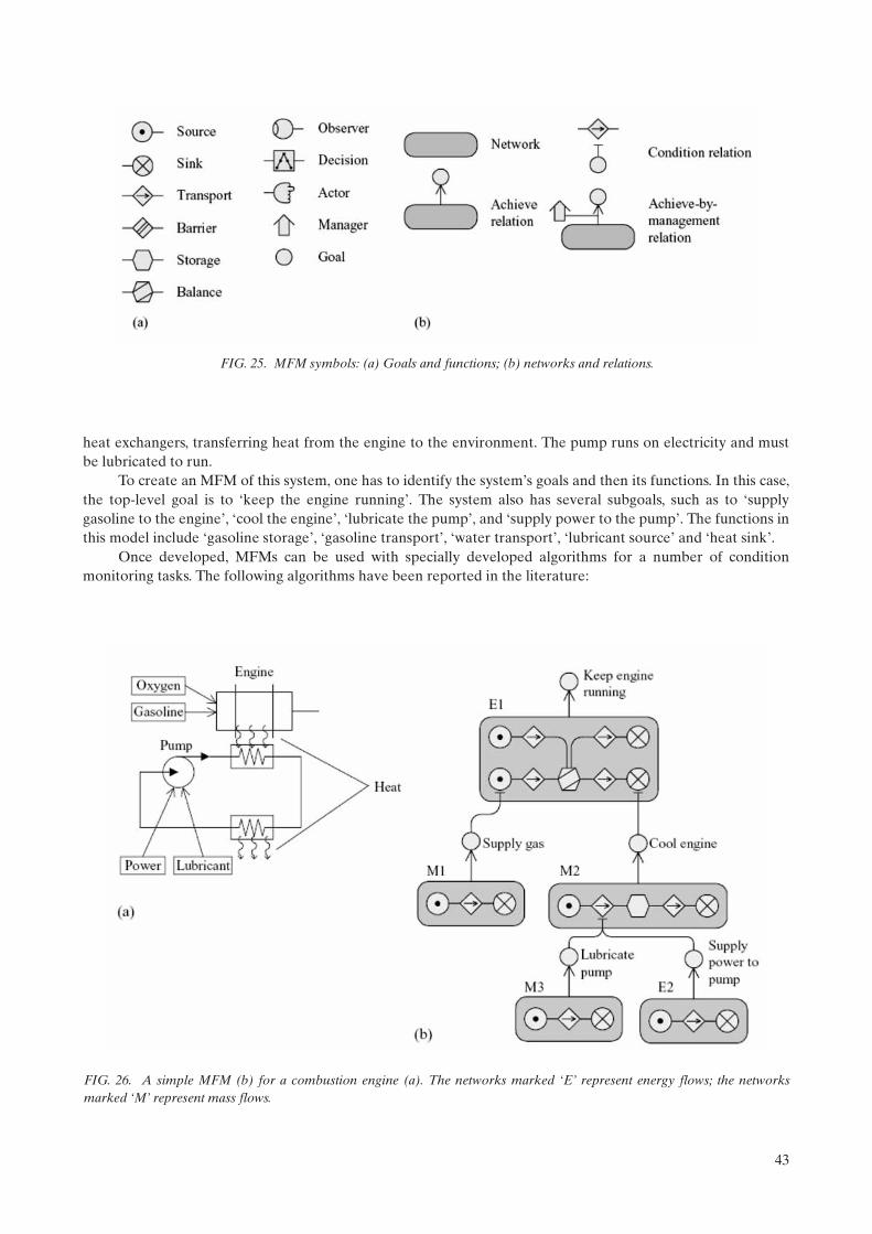
43

heat exchangers, transferring heat from the engine to the environment. The pump runs on electricity and mustbe lubricated to run.

To create an MFM of this system, one has to identify the system’s goals and then its functions. In this case,the top-level goal is to ‘keep the engine running’. The system also has several subgoals, such as to ‘supplygasoline to the engine’, ‘cool the engine’, ‘lubricate the pump’, and ‘supply power to the pump’. The functions inthis model include ‘gasoline storage’, ‘gasoline transport’, ‘water transport’, ‘lubricant source’ and ‘heat sink’.

Once developed, MFMs can be used with specially developed algorithms for a number of conditionmonitoring tasks. The following algorithms have been reported in the literature:

FIG. 25. MFM symbols: (a) Goals and functions; (b) networks and relations.

FIG. 26. A simple MFM (b) for a combustion engine (a). The networks marked ‘E’ represent energy flows; the networksmarked ‘M’ represent mass flows.

44

— Signal validation checks the consistency between redundant sensor values and can detect flow leaks, sensorfailures and other measurement errors.

— Alarm analysis identifies which faults are primary and which faults may be consequences of the primaryones.

— Fault diagnosis uses sensor values and queries to the operator to discover the faults of the target system.— Explanation generation uses the states discovered by the fault diagnosis algorithm to produce explanations

and remedies in pseudo-natural language.— Failure mode analysis uses MFM with added timing information to predict the consequences of failures. It

can be used during both design and operation.— Fuzzy alarm analysis similar to the alarm analysis algorithm but uses fuzzy concepts to achieve a more

robust behaviour when faced with noisy signals close to decision boundaries.

All the described algorithms are based on discrete logic (with the exception of the fuzzy alarm analysisalgorithm) where the sensor values are low, normal or high, and the resulting values are consistent or incon-sistent, working or failed, primary or consequential, etc. Multilevel flow modelling uses a linguistic interpre-tation of variables, and MFM algorithms work by operating searches in the defined MFM graphs.

Known applications in the nuclear industry include alarm analysis for the realization of a decision supporttool for operators to be used in complex fault situations. Other reported applications are in failure mode analysisand fault diagnosis in industrial processes.

The MFM technology has recently been commercialized, and additional practical applications areexpected.

5. ON-LINE MONITORING IMPLEMENTATION STRATEGY

The options for the implementation of an OLM strategy will vary considerably from plant to plant and willdepend very much on the user’s specific end requirements, the existing data extraction capability and theprevailing monetary restraints.

The following are typical examples of where an OLM implementation should be considered:

— To predict onset of failure (detection of off-normal plant operation);— To reduce maintenance activities (extension of sensor and equipment calibration period);— To extend EQ life (environmental monitoring of temperature, humidity, etc.);— For plant optimization (thermal performance monitoring of turbo-generators);— To reduce radiological dose (move from time dependent to condition based maintenance);— To shorten outage time (extended maintenance periods) to move from time dependent to condition based

maintenance.

Plant instrumentation and control (I&C) and/or digital upgrades are an ideal opportunity for the consider-ation of OLM, since a key issue in the determination of the feasibility is the availability and suitability of data.For example, the additional overhead for obtaining data extraction/capture facilities to support an OLM imple-mentation is relatively low at the design stage compared with that required as a retro-fit.

Where an upgrade is not an option, it will be necessary to conduct a review of the data already available (orarchived) to ascertain whether they are suitable for the intended OLM application. For example, vibration oracoustic noise based applications require a fast sample rate (up to 100 kHz) and historically have been restrictedto dedicated stand-alone data acquisition and analysis systems. In contrast, trend applications such as themonitoring of sensor drift only require a sample every few seconds, and the installed plant data processingsystems may already provide sufficient resolution, hence the problems of implementation of OLM may berestricted to that of extracting the data without compromising the plant data processing systems.

45

On the basis of data availability, the following issues need to be considered as part of the OLM implemen-tation strategy:

— Provision of additional sensors to supplement existing data.— Methods of extracting the data, e.g. isolation, hardware, storage.— Suitability of existing data, e.g. accuracy, ‘historizing’ limitations of archived data.— OLM application, e.g. commercial off the shelf (COTS) versus custom built packages.— Data users, e.g. maintenance engineers, plant managers, operations engineers.— What the analysis results will be used for, e.g. maintenance scheduling, determination of plant compliance

with technical specifications (i.e. safety versus non-safety application).— Acceptance testing, e.g. determining whether the application meets the functional design specification and/

or fulfils the requirements of any activity it may replace (e.g. accuracy (uncertainty) and reliability wouldbe particular concerns for safety related applications).

— Life cycle management, e.g. configuration and security control of the OLM application and maintenance ofsupport systems (i.e. management of hardware and operating system obsolescence).

— Establishment and maintenance of OLM expertise. Although OLM applications may reduce intrusiveplant based activities, there will be a need to establish an office based expert(s) who can perform the roleof ‘intelligent operator’, in particular, for the final determination of how the OLM analysis and resultsshould be used to determine changes to plant operation/configuration and maintenance activities.

As already indicated, in an ideal situation, the implementation of an OLM application would be part of theinstalled data processing capability, and this should be the intent for new build or I&C upgrade. However, at thepresent time, most OLM applications are a backfit, and there will be some significant issues with respect to theintroduction and integration of new software and hardware to facilitate interfaces with the installed plant.

All OLM applications will involve the following key processes:

— Collecting plant data;— Storing plant data;— Performing analysis;— Outputting results.

In addition to the key processes identified above, the initial implementation of an OLM application willrequire acceptance testing to ensure that the analysis techniques are sound.

Once installed, the OLM system will then require maintenance and support by an ‘expert’ operator whounderstands the operation of the plant being monitored and the intent and limitations of the OLM application.

5.1. COLLECTING PLANT DATA

All OLM applications require significant amounts of plant data, and the success of the implementation willbe highly dependent on the quality, accuracy and resolution of those data.

The significance of the data properties will vary with respect to OLM application and will need to beconsidered on a case-by-case basis.

For example, noise analysis based applications are highly dependent on sampling rate but are not signifi-cantly affected by loop accuracy. However, for sensor calibration monitoring, the loop accuracy is the mostimportant property.

The installed plant data processing systems will need to be considered with respect to their influence ondata collection (see Fig. 27). For example, in an analogue based system, it is normal to use isolation amplifiersbetween the protection/control circuits and the data processing computer. These isolation amplifiers willintroduce a scaling uncertainty between the signals presented to the operator/OLM and the protection/controlcircuits. In a digital system, the data will typically be passed by optical data link and are identical in value tothose presented to the protection/control circuits, but are likely to have a time skew owing to differingprocessing times.

46

Where it is not possible to collect plant data via existing isolated interfaces, or where the isolationintroduces unacceptable uncertainties, it will be necessary to connect a dedicated data acquisition system toexisting sensors or to provide additional OLM application specific sensors. Where connection to existing sensorsis used, appropriate isolation precautions will be required to ensure that the plant signal is not degraded by theOLM hardware application and that the signal is not interrupted during connections or reconnection.

5.2. STORING PLANT DATA

All OLM applications require significant amounts of data. Although media storage is now relativelyinexpensive and is unlikely to be a problem for the introduction of new stand-alone systems, it may presentproblems where the OLM is reliant on existing data processing hardware.

The issue of storage capacity is easy to understand and should be relatively easy to resolve. Moresignificant is the issue of how the data have been archived and/or saved. In order to maximize storage, the plantdata processing system often ‘historizes’ the data either by reducing the sample rate (e.g. only stores every tenthrecord), or by reducing the resolution (e.g. only stores a new data point if a change of signal greater than 1% isdetected). Both these techniques will have the effect of filtering the original signal and important characteristicsmay be lost. Although these ‘historizing’ techniques may render old data unusable, it is normally possible tohave the properties switched off or reduced to a limit that does not impact the data.

FIG. 27. OLM data collection.

47

5.3. PERFORMING ANALYSIS AND PRESENTING RESULTS

Having captured and stored the data, the next stage of implementation is identifying where the analysis will be performed, and how and to whom the results will be presented. While use of the installed data processing systems is the preferred option, this will pose several problems.

— The installed data processing systems software and/or hardware may not support the new application;— New applications may pose a threat to existing data processing systems either from interaction with

existing applications or from a cyber security standpoint;— The end user of the results of the OLM application may not have access to the plant computer.

Consideration could be given to transferring the data to a ‘business’ computer environment such as a corporate local area network (LAN) and performing the analysis on a more easily accessible system. The disad-vantage of this approach is that the threat from loss of configuration control and cyber security will be signifi-cantly increased. It is therefore unlikely that an OLM application that might ultimately impact decisions about safety equipment could be justified.

The alternative currently adopted for many OLM applications is that the analysis is performed on a stand-alone computer. The main problem with this approach is the lack of consistency between the various applica-tions and multiple databases of plant data that cannot be shared.

The preferred solution therefore is to establish a secure ‘engineering’ computer environment to act as a depository for both OLM data and OLM applications. The Sizewell B plant in the United Kingdom has implemented this by providing an ‘engineering’ LAN (ELAN) using an OSI plant information data historian. This ELAN runs in parallel but is not connected to either the ‘business’ LAN or the Internet. ELAN is treated as a plant system, and is maintained and operated by dedicated plant engineers rather than the site IT group. Hence ELAN is subject to the same stringent configuration and cyber security controls that are used on other plant computer systems, i.e. the emphasis is on system integrity rather than on confidentiality usually employed by IT practitioners (e.g. it does not matter who can see the data, provided that the data cannot be changed).

Some 20 000 signals are continuously downloaded at fixed scan rates (1, 2, 10 or 30 s) via a unidirectional datalink from the plant data processing system. Additional plant signals can be transferred via an ELAN dedicated data logging system at variable scan rates from 100 ms upward. These inputs are hardwired as either a temporary or a permanent measure. Other data can be transferred to the system via OLE for process control (OPC) protocol or a dedicated link.

An applications server is available and may be used for running OLM packages directly, or the data can be exported for running on stand-alone machines. An off-line test environment is also available that has access to real plant data.

Access to ELAN is via dedicated client personal computers, which are primarily used by engineering support staff but may be made available to any section.

5.4. ON-LINE MONITORING SOFTWARE ISSUES

The techniques and applications presented in this document are already in widespread use and are demanded by several nuclear power regulatory bodies around the world. One example is monitoring of loose parts, which is implemented in many plants, especially those sites with PWR and WWER designs. Increased interest in OLM for safety related equipment is anticipated, partly because of developments in sensor technology, but most importantly because of the development of computer based signal analysis tools and data acquisition techniques.

Licensees around the world are continually trying to improve their profitability and management of resources, and often prolong the original licensed operational lifetime. OLM provides a very powerful tool in all these areas. However, the issues surrounding reliability, uncertainty and the use of COTS and general purpose operating systems software are not well defined, and hence there is a natural resistance from regulatory bodies regarding their use in safety related applications. A graded and pragmatic approach is needed to the use of OLM and commensurate with its intended use and safety significance by both the licensee and the regulatory body.

48

Generally, the requirements for safety class equipment are well defined by the various regulatory author-ities, and agreed processes by the licensee are based on diverse factors, such as design bases faults and post faults,and on whether the equipment is required to operate during normal power operation. These requirements andprocesses apply to permanently installed and well established equipment (e.g. pumps, motors, protectionsystems). However, the introduction of OLM typically introduces the use of non-safety equipment and processeson which diagnosis of the condition and operability of safety equipment depends.

Most of the techniques presented in this document have only a minor or no influence on the plantprocesses, although this would have to be proved as part of any implementation. The validity of the signals andanalysis techniques poses a significant problem, especially if the licensee wishes to replace well established andproven methods. This situation is exacerbated when the proposed OLM makes use of techniques that requiresignificant expert knowledge.

Where OLM is to be applied to safety class equipment or processes, it is likely that a change to the planttech specifications or operating rules will be required for its use, and hence a submittal to the regulator will berequired. Even though the OLM equipment may not itself be safety category classified, if the output and/orresults of the proposed OLM processes are used for the determination of the operability of safety classequipment, then it may present a significant risk if ill-conceived. In some instances, the additional validation andverification burden may be cost prohibitive for the benefits realized in the mitigation of such a risk. For example,an OLM proposal that replaces an existing surveillance method with a method that is totally reliant on the use ofa COTS software application is unlikely to be realizable, as it would be difficult to perform sufficient validationand verification owing to the unavailability of source code for third party verification.

Therefore, the decision of whether to use COTS software or a custom-built package will very much dependon the equipment the OLM application is intended to be used on, who will use the application and what plantdecisions will be made on the basis of the OLM results.

Table 1 is intended to provide a guide to the potential impact on safety documentation and/or regulatoryimpact on the basis of the intended use of the OLM application.

5.5. ACCEPTANCE TESTING

The assessment of software presents unique difficulties, mainly because of its peculiar characteristics andcomplexities. For example, software failure usually arises from design and/or specification errors rather than

TABLE 1. QUESTIONS TO BE CONSIDERED IN THE DETERMINATION OF SAFETY IMPLICATIONS

Question Potential impact

Does the proposed OLM support existing maintenance processes or is it a replacement?

Low — if support, since the existing system becomes the ‘fallback’ and failure of OLM is not significantMedium — if replacement, since it may result in unnecessary or delayed maintenance, or, in the worst case, a loss of safe plant availability

Will the proposed OLM be used in the determination of plant operability as required by the technical specification/operating rules governing compliance with the site licence?

Medium — since failure of the system may cause an inability to determine operability and subsequent entry into controlled shutdown

Could failure of the proposed OLM cause failure of a safety system?

High — since OLM could be a threat to installed safety equipment and will incur higher levels of verification and validation

Is there a reliability claim for the proposed OLM? High — since OLM is moving toward safety classification, which will incur formal verification and validation commensurate with modern standards for the use of software on safety critical systems (Ref IEC 601508 & 60880)

49

from software ageing. Another unique characteristic is software’s vulnerability to accidental/inadvertentchanges and/or malevolent attacks, both of which could remain undetected. The impact of this latter pointdepends on the nature of the accidental/malevolent change and the process to which the OLM is applied. Anexample would be a change in acceptance criteria used to determine the operability status of equipment, whichcould cause it to operate beyond its safety limits and, in the worst case, fail to perform its safety duty whenrequired.

When a software fault does exist, it will most probably manifest itself in a predictable manner when aparticular set of conditions presents itself. Thus, in a software system composed of redundant but identicalcomponents, all components will fail at once. In contrast, the parts of a hardware system comprising identicalcomponents rarely will fail all at once due to ageing.

Validation of the complete system should be performed to confirm that it is compliant with the specifi-cation and that no extraneous functionality has been introduced. Evidence of commissioning tests should bepreserved with sufficient detail to permit a check on functionality at a later date. Where modifications have beenundertaken and subsequent tests were not completely rerun, the justification for limited testing should bepreserved.

Verification of the software code will be dependent on the specific OLM application but, as indicatedabove, will be primarily governed by practicality, i.e. the availability of the source code and the impact that anyresultant decision making will have on plant configuration. At its highest level, it may be necessary todemonstrate that the software performs with a particular reliability by the use of statistical testing. While it mayappear very onerous, it is unlikely that reliability figures greater than that claimed for ‘operator action’ in safetyanalysis reports would be necessary. This is typically between 10–1 and 10–2, and hence a relatively small numberof statistical tests could be used to gain that confidence.

5.6. LIFE CYCLE MANAGEMENT

There should be effective, documented and approved procedures to cover use, maintenance, securitydefect analysis and change control. In addition, there should be a defined method of ensuring that the functionalintegrity of the software is maintained. This requirement should include the following characteristics:

— The system (and spares) should be stored and used in conditions that limit physical, accidental andmalevolent damage.

— Adequate means to ensure that the hardware configuration is correct.— Adequate means to ensure that the installed software is the correct version (including operating systems)

and has not been accidentally or malevolently damaged; e.g. routine examination of check sums andstandard tests (a subset of the commissioning tests for example) prior to use.

— Adequate means to ensure that the end users of the software are suitably qualified and trained.— Adequate means to ensure that security measures are in place commensurate with the functionality, claim

and use of the software.

5.7. ESTABLISHMENT AND MAINTENANCE OF OLM EXPERTISE

OLM applications are clearly intended to reduce intrusive and unnecessary plant based activities, andhence maintenance and operator workload; however, there will be an ‘expert operator’ burden to establish andmaintain an OLM service.

It is unlikely that any OLM application will produce a simple pass/fail result. Especially during itsinception, it will be highly reliant on the user’s understanding of the normal plant processes, typical degradationand failure mechanisms. Also, the results of many OLM applications are not absolute; hence their first use maybe of limited value. It will be the historical trends and the early detection of off-normal operation that will yieldfuture success. It is therefore paramount that baseline measurements are accurately documented (e.g.calibration records, amplifier gain settings, reactor power levels, acceptance criteria) to ensure that, when OLMapplications are run at a later date, true comparisons are possible.

50

Historical plant data just prior to plant failure are very useful for training or seeing how an OLMapplication will flag off-normal conditions; however, care should be exercised when such data are retrieved froma plant historian, as important data may have already been lost during archiving, or falsely created due to extrap-olation when retrieved (see also Section 5.2).

The use of an ‘expert operator’ is also imperative when the OLM is to be used to judge or support thejudgement of safety equipment performance. In effect this is a ‘sanity check’ to ensure that the OLM results donot just meet acceptance criteria, but are also realistic; e.g. the time response of a pressure level sensor given byan OLM application as 2 ms may easily pass the technical specification acceptance criterion of faster than 250ms, but if the norm is 200 ms, then it is necessary to establish what changed. In this case, it is unlikely that thesensor became faster, but more likely the OLM was presented with the wrong data, either through plant orsoftware misconfiguration, or, in the worst case, a software error.

Since it is very difficult to develop an OLM application with a human–system interface (HSI) that issuitable for all interested users of the results, the ‘expert operator’ is also the obvious candidate to act as theinterface with the less familiar, i.e. to assist in the presentation of results tables, performance graphs, etc., to, say,the plant manager.

6. ENABLING TECHNOLOGIES

6.1. INTRODUCTION

To optimize OLM and its potential derivatives at nuclear power plants, an IT infrastructure needs to bedeveloped that can support data acquisition, central data storage and analysis tools. While such optimizationmay not be realizable at nuclear power plants that are currently operating, it is useful to examine the variousenabling technologies that could be used should the opportunity arise, e.g. a digital upgrade.

This section briefly discusses a number of these enabling technologies. In particular, the followingdiscussion is divided into three categories: sensors, data collection systems and data analysis systems. Sensors arethose devices used to generate information about the monitored process. This process information is thencollected and communicated to the data analysis systems by the data collection systems. Finally, data analysissystems represent those methods used to interpret the collected process information and possibly provideoperational suggestions and issue actions. Information about the monitored system/plant flows from the sensorsto the data collection systems and then to the data analysis systems, as illustrated in Fig. 28.

6.2. SENSORS

New sensor technologies are constantly being developed and deployed, providing an enormous range ofoptions for process monitoring under broad environmental conditions. While the generation of sensory data isfairly direct (assuming that an appropriate sensor is available to measure the variable of interest), transmissionof these data to a monitoring system is still a challenge owing to the cost, security, reliability and complexityusually associated with the operation of communication networks. As a result, besides ongoing advances inmeasuring technology, sensor devices are being provided with network capabilities in order to significantly

Sensors Data Collection

Systems

Data Analysis

Systems

Monitored

System

FIG. 28. Key elements for implementing on-line condition monitoring.

51

improve their deployment within modern industrial IT infrastructures. These capabilities often lead to, forexample, the reduction of wiring, the minimization of communication complexity, the promotion of systemmodularity and the facilitation of interconnecting multiple devices. In addition, networked devices can be moreeasily monitored for anomalies and promptly reconfigured (in software as opposed to being physically changed),and their information can be made more broadly accessible. Owing to their increased networking capabilities,sensors are experiencing a paradigm shift from being information devices to communication devices. The impactof such a shift for the management of security and configuration control should not be underestimated, and theapplication of these new technologies to safety equipment or decisions that affect safety equipment or processeswill require significant justification.

Information can be passed from the instrumentation to the data collection systems using different media,including wireless media, UTP/wire media and fibre media. While ‘wireless’ reduces the expense of physicalwiring (local power supplies are still required), it is also the least secure of the physical layers. Limiting power,implementing built-in wireless security and utilizing a hybrid wireless/wired solution can in theory minimizemost security issues. In practice, this may be difficult to prove in a running nuclear power plant, although theutilization of previously tested frequencies does mitigate this concern somewhat. However, this may be a verylimited resource, as most new technologies operate a long way from those that may have been tested duringinitial plant startup. In addition, the range and fidelity of the signals can be influenced by implementation issuessuch as multipath and signal attenuation due to proximity to metallic structures, which can limit deployment. Onthe other hand, wired media utilizing traditional IT Ethernet provides good performance while enabling the useof inexpensive, state of the art networking equipment. Finally, using fibre for communication has the advantagesof speed (gigabit or better), bandwidth (ability to use multiple colours in a single fibre) and electrical isolation(ability to co-locate fibre with high voltage cables).

6.3. DATA COLLECTION SYSTEMS

The most basic level of integration, and a prerequisite for the realization of actual ‘on-line’ monitoring, asopposed to ‘off-line’ or batch monitoring, is integration at the data level. This involves, as a minimum, the abilityof an OLM system to communicate with the plant process computers in order to acquire the live plant datanecessary for the particular condition monitoring function implemented. Additionally, communication withother support systems, such as control systems, alarm systems, computerized procedure systems and diagnosticsystems, might be required.

Modern data collection systems often consist of several subsystems, starting with the actual collection ofinformation from the instrumentation to the delivery of that data to the end business user. Typically, datacollection systems may consist of four subsystems: the supervisory, control, and data acquisition (SCADA), thedemilitarized zone (DMZ), the Intranet or business network, and the Internet or external network. In particular,the SCADA is the portion of the system that physically interfaces with the equipment via sensors and actuators,and has the capability to securely deliver that information to HSIs and data collection equipment.

While the above layered approach may be acceptable for non-safety critical applications, the use of abusiness network, Internet and external networks will pose significant security challenges when applied to safetyequipment or decisions that affect safety equipment, in particular with respect to data and application integrity(i.e. configuration control together with protection against accidental or malevolent attack). It may therefore benecessary to consider the use of a secure engineering network.

The layered nature of the information collection network discussed above provides the desired on-lineinformation needed to operate a facility while providing a safe method of delivering data to make businessdecisions for maximizing productivity and reducing downtime for maintenance and/or breakdown. Properconfiguration control of computer systems, such as desktops, servers, firewalls and routers, is vital to thecontinued health of the entire system. In addition to the initial costs of installation, testing and operation, anannual maintenance budget and resources to implement that maintenance is required to repair IT equipment,replace ageing obsolete equipment and respond to changing cyber security threats that may not have beenanticipated during the initial design.

52

6.3.1. Industrial networks

An industrial network, or fieldbus, links sensors, actuators, discrete/analogue I/O and smart devices. Forexample, networking allows multiple devices to communicate over a single trunk line instead of using numerousindividual wires. Depending on the types of devices that are interconnected, four hierarchical levels of function-ality and associated buses may be present in a typical installation, namely, the sensor bus, device bus, control busand enterprise bus. When interconnecting these levels, industrial networks can thus exhibit different topologiesand utilize numerous protocols and communication media (e.g. fibre optics or wireless). A network topology isthe logical configuration of a network, defining how the nodes are logically connected to one another and howthey communicate. Numerous topologies exist to interconnect devices, including the star, ring, mesh, cluster tree,trunk/drop and daisy chain. In a star topology, for example, all nodes are connected to a network host or coordi-nator. This topology is appropriate for relatively simple and low-power applications. Instrumentation topologiescan also be classified as point-to-point, point-to-multipoint and multipoint-to-multipoint networks. A point-to-point network is the simplest configuration, establishing a dedicated session or connection between twonetworked devices using their own direct communication link. The connection is symmetrical and provides thesame bandwidth performance for sending or receiving. Point-to-point networks often exhibit high reliabilitybecause there is only one potential single point of failure in the topology, i.e. the host. However, they suffer fromhigh cost and low adaptability, as they do not scale adequately to accommodate more than one pair of endpoints. Point-to-point links are ideally suited for high performance, dedicated connections, high speed Internetlinks or backup applications. On the other hand, point-to-multipoint networks provide a path from one locationto two or more specified locations (from one to many). These networks are often connected in a star topology,often consisting of a base station or access point at a central or hub site and multiple clients located at distributedsites. Multipoint-to-multipoint services are provided to interconnect multiple locations. While point-to-multipoint networks can accommodate more end points, they exhibit low adaptability and reliability, asreliability is highly determined by the placement of the access and end points. Multidrop networks reduce wiringrequirements but also introduce a single point of failure (i.e. the cable).

Besides a given topology, it is also necessary to define how devices communicate. A network protocol is aformal set of rules, conventions and data structure that governs how networked devices may exchange infor-mation. There are numerous methods for sending data over communication media. Transport control protocol(TCP) and IP (Internet protocol) are the most important protocols for industrial automation today. TCP isinherently peer-to-peer and full duplex, which means that bidirectional communication between two devices canoccur concurrently. Based on their communication scheme, they can be classified as either serial data trans-mission or local area networking. There are several serial data communication hardware standards, such asRS-232 and RS-485. RS-232 is a single-ended (unbalanced) interconnection scheme for serial data communi-cation and transmission between modules. Similarly, RS-485 is a robust scheme for serial communication amongmultiple devices, sharing a common set of serial data communication lines. RS-485 allows multidrop networkingon a single line. On the other hand, there are several LAN protocols, within which Ethernet is one of the mostcommon wiring and networking scheme. A brief discussion on LAN and traditional protocols is provided in thesubsections that follow.

6.3.1.1. Initial protocols

Early industrial networks used shielded twisted pair implementations for each I/O device. Data subse-quently were transmitted over serial buses using proprietary, layered protocols. Numerous protocols wereintroduced for industrial automation, including Modbus, Profibus, and ControlNet. Most of these industrialprotocols are vendor specific, lacking interoperability and limited in the number of nodes, topology, distancesand data rates that they can accommodate. Among these protocols, Modbus is the oldest network communi-cation standard and probably the most popular serial protocol in process monitoring and control. While veryuseful with serial devices, Modbus does not adequately accommodate complex devices such as mass flow andmotion controllers. On the other hand, Profibus is probably the most widely accepted international networkingstandard. Similar to Ethernet, this standard has a high overhead-to-message ratio for small amounts of data andcarries no power on the bus. Supporting several topologies, ControlNet, a precursor to DeviceNet, is a peer-to-peer highly deterministic and repeatable controller-to-controller network. DeviceNet is an application layer

53

protocol, emphasizing connection as opposed to being message oriented. Both of these protocols are objectbased, meaning that every device on the network is represented as a series of objects with attributes and values.

6.3.1.2. Area networking protocols

Traditionally, there has been no single, universal open networking architecture. In fact, protocols used ateach of the common four levels of functionality (i.e., sensor, device, control and enterprise) often differ. Typicalprotocol choices are: (i) CAN, ASI and Seriplex for the sensor bus; (ii) H1 Fieldbus, Profibus PA and DeviceNetfor the device bus; (iii) Foundation Fieldbus High Speed Ethernet (HSE), Profinet, Profibus DP and ControlNetfor the control bus; (iv) Ethernet for the enterprise bus. However, the automation industry is actively engaged inimplementing more open networking architectures. Supporting all four of the above network levels, Ethernetbased protocols are expected to dominate industrial applications, offering also Web server capabilities at noadditional cost. Ethernet is a full duplex connection and LAN protocol/standard for hardware, communicationand wiring, being the most common physical layer in distributed process control systems and with a packetswitching technology inherently superior in cost and complexity to circuit switching. In fact, Ethernet may be thebest compromise between cost and performance, providing the most flexibility when compared with traditionalprotocols such as Modbus and DeviceNet. Benefits of Ethernet include the following:

— Easily scalable from 10 and 100 Mbps to 1 and 10 Gbps;— Cost effective with multiple vendors;— Fully standards based with product interoperability among vendors;— One of the most widely used networking architectures;— Easy integration among plant instrumentation and control, business and IT systems.

Numerous companies are already embracing Ethernet over traditional, proprietary bus topologies, asFieldbus, Interbus and Profibus. A significant characteristic of this protocol is that it is free. However, Ethernet’sdrawbacks include a high overhead-to-message ratio for small amounts of data and an industrial weak (non-industrial-strength) connector (i.e. RJ-45), in addition to carrying no power on the bus. Ethernet typicallyrequires a star or a bus (daisy chain) topology. Popular industrial Ethernet protocols/standards includeEtherNet/IP, Foundation Fieldbus HSE and Profinet. Based on the TCP/IP suite, the peer-to-peer capabilitiesprovided by these standards make them very effective networks for linking local clusters of sensors, transducers,controllers, actuators and DA systems. Among current Ethernet based protocols, EtherNet/IP FoundationFieldbus is expected to become the future standard for process industry networking.

6.3.1.3. OPC communication protocol

OPC communication protocol is a set of standard specifications, created with the collaboration of anumber of leading worldwide automation hardware and software suppliers working in cooperation withMicrosoft to support open connectivity in industrial automation. The organization that manages this standard isthe OPC Foundation, which has over 150 members from around the world, including nearly all of the world’smajor providers of instrumentation and process control systems. The objective of the OPC Foundation is todevelop an open, flexible, plug-and-play standard that allows end users to enjoy a greater choice of solutions, aswell as sharply reducing development and maintenance costs for hardware and software suppliers.

In the absence of any standard, vendors have developed proprietary hardware and software solutions. Allprocess control and information systems on the market today have proprietary techniques, interfaces and APIsin order to access the information that they contain. The cost of integrating the different systems and the longterm maintenance and support of an integrated environment can be significant. This situation is clearly depictedin Fig. 29.

Custom drivers and interfaces can be written, but the variety increases rapidly because of the thousands ofdifferent types of control devices and software packages that need to communicate. This proliferation of driversexacerbates certain problems, such as inconsistencies among different vendors’ drivers, hardware features thatare not universally supported, hardware upgrades that can wreck an existing driver and access conflicts. OPCstandards offer an open platform solution that provides real plug-and-play software technology for process

54

control and factory automation where every system, every device, and every driver can freely connect andcommunicate, as shown in Fig. 30.

There currently are seven standard specifications completed or in development, as follows:

— OPC Data Access. Used to move real-time data from PLCs, DCSs and other control devices to HSIs andother display clients.

— OPC Alarms and Events. Provides alarm and event notifications on demand (in contrast to the continuousdata flow of Data Access). These include process alarms, operator actions, informational messages andtracking/auditing messages.

— OPC Batch. This specification carries the OPC philosophy to the specialized needs of batch processes. Itprovides interfaces for the exchange of equipment capabilities (corresponding to the S88.01 PhysicalModel) and current operating conditions.

— OPC Data eXchange. This specification extends from client/server to server-to-server with communicationacross Ethernet Fieldbus networks providing multivendor interoperability.

— OPC Historical Data Access. While OPC Data Access provides access to real-time, continually changingdata, OPC Historical Data Access provides access to data already stored. From a simple serial data loggingsystem to a complex SCADA system, historical archives can be retrieved in a uniform manner.

FIG. 29. Complexity of integration in the absence of standards.

FIG. 30. OPC supported connectivity.

55

— OPC Security. All the OPC servers provide information that is valuable to the enterprise and that, ifimproperly updated, could have significant consequences to plant processes. OPC Security specifies how tocontrol client access to these servers in order to protect this sensitive information and to guard againstunauthorized modification of process parameters.

— OPC XML-DA. Provides flexible, consistent rules and formats for exposing plant floor data using XML(eXtensible Markup Language), leveraging the work done by Microsoft and others on SOAP and Webservices.

6.3.1.4. Internet and Web networks

The Internet has become a ubiquitous force that is redefining industrial automation. In a web topology, allnodes can in principle be connected to each other at all times. This massive interconnectivity feature facilitatesthe migration of intelligence to lower devices such as sensors. Decision making tasks may more easily beconducted locally at the sensors and actuators. However, network security and routing may be serious concerns.

6.3.2. Communication equipment

In traditional wireline networks, hardwired sensors are connected to multiplexers, which often arenetworked to main computer hosts. As industrial networks become more complex and greater capabilities arerequired, this approach is losing favour among practitioners. To reduce connection needs and implementcomplex communication networks, a variety of communication equipment is now available including hubs,switches, routers, bridges and gateways. For example, a hub distributes/broadcasts each packet to all directions(i.e. one packet in is forwarded to every port). Therefore, it shares its bandwidth over all its ports. On the otherhand, switches, routers and bridges pass packets only to their intended destinations (i.e. one packet in isforwarded only to the appropriate port). These latter devices can then be used to segment a given network andcreate deterministic segments within it. Similarly, gateways can be used to link devices that have limited commu-nication capabilities (e.g. having only RS-232 and RS-485 ports) to a modern industrial network.

6.4. DATA ANALYSIS SYSTEMS

6.4.1. Analysis algorithms

Given that sensor data have been collected, the task is to analyse these data to determine the condition ofthe monitored machine, process or system. The analysis can be conducted locally or centrally, or in acombination of the two, and can be completed in the time or frequency domain, for example. On-line conditionmonitoring algorithms, which include those described in this report, are conducted at the monitoring computersystems and used to monitor different machine conditions such as vibration, structural damage, processanomalies (e.g. cavitations), and wear and frictional behaviours. For example, a vibration analysis monitorsystem may measure and record all forms of machine vibrations, bearing conditions, as well as process andinspection data. For the diagnosis of complex vibrational behaviours, these systems may provide comprehensiveanalysis functions such as order spectrum, orbit, phase, cross-phase analysis and coast down measurement. Inaddition to spectral and frequency analysis (e.g. FFT and wavelet transform), a monitor system may providetime series and finite elements based interpretations. Different techniques can also be combined to derive morecomprehensive diagnostics. For example, vibration and acoustic emission techniques can be integrated to detectearly stage damage of bearings. Numerous hardware and software capabilities are available for realizing thespecified on-line condition monitoring tasks, with some briefly mentioned below.

6.4.2. Computer platform/operating systems

Numerous operating systems (OS) are available for DA and OLM applications, including MicrosoftWindows, VxWorks and Linux. Windows based OS include Windows 95, 98, 2000, NT and XP. Similarly,Windows CE.NET is a popular embedded hard real-time OS often built in internal non-volatile memory to

56

provide fast boot up, determinism and system crash avoidance. This OS provides not only stable, recoverableand robust features of an embedded real time OS, but also powerful OS capabilities, rich functionality anddiversified application development support.

6.4.3. Programming languages

Numerous programming languages are available to develop or improve on-line DA and OLM capabilities.The most popular programming languages for these purposes include Basic, Pascal, C/C++, Java and Delphi.Programming tools such as editors, debuggers, ActiveX controls, Common Object Model (COM) objects, VisualComponent Libraries (VCL), Application Programming Interfaces (API) and WebMasters are also available tofacilitate product development. Under object based open architecture models, objects not only avoid the need towrite drivers for a variety of hardware, but also allow the replacement of many lines of code for commonfunctions. Advanced Windows programming languages such as Visual C++, Visual Basic .NET and Visual C.NET are also available for complex applications.

6.4.4. Software packages

A large number of DA and OLM software packages are available from numerous vendors. Prior to theintroduction of the Windows environment, DA and OLM software was either open or closed. Open packageswere supplied with drivers and libraries, allowing the user to access, modify and/or expand them in order toinclude or develop new capabilities and tools. On the other hand, closed packages had limited programming andcontrol options available to the user and were intended to be configured through fixed mechanisms, such as pull-down menus and fill-in-the-blank forms. Currently, the majority of software packages are Windows applications,providing significant programming options for the user. These packages include not only freeware but alsoproprietary packages (e.g. LabView and Windows CVI from National Instruments, TestPoint from CapitalEquipment, and VEE from Agilent). There are also diversified software supports such as ATL, ActiveX,DCOM, ADO .NET and Win32 SDK that can greatly increase the maintainability and productivity ofapplication software development. For enabling connectivity with legacy and business systems, and imple-menting Web enabled applications, numerous tools are available such as XML, TCP/IP sockets, wed, FTP andTelnet servers. Ample SCADA software, such as InduSoft, is also available.

6.5. HIGHER LEVEL INTEGRATION

The importance of integration becomes evident when one analyses the shortcomings associated with thelack of integration that is typical of a large portion of condition monitoring applications to date. Control roomstaff often report condition monitoring systems being brought into the control room as an add-on to theirexisting set of support systems. Introduction of these systems often fails to take into account how the use of thesystems could be fitted to whatever tasks, working procedures or other support systems the operators areactually using. One typical mistake is that the condition monitoring system is located in the wrong place in thecontrol room (often relegated to some corner of the room). Another possible mistake is that it might requireconsiderable extra input from the operator due to a lack of communication with other systems alreadypossessing this information. A third potential mistake is that the HSI of the auxiliary system is not fitted to thetasks of the operator, resulting, for example, in excessive navigation and unnecessary focus on secondary tasks.Even though the system itself is well designed and implemented, the lack of integration often results in interfaceproliferation, workspace clutter, low usability, gradual fading of interest on the part of the operators, and higheroperation and maintenance costs.

Once data level integration has been implemented, integration of condition monitoring systems at theoperational level must be considered. The access to the functionality provided by condition monitoring systems,control systems, alarm systems, computerized procedure systems and diagnostic support systems should beintegrated in a unified HSI to better support, from a human factors perspective, the operator while performinghis or her surveillance and control tasks.

57

The proliferation of interfaces that is often associated with the introduction of additional support systems,such as condition monitoring systems, in the control room can have negative effects on the performance of theoperator. The possible negative effects include information overload, navigation problems, increased HSIcomplexity and increased cognitive workload.

A unified HSI limits information overload by minimizing duplication of information. Furthermore, itfacilitates navigation among the different information displays and permits HSI complexity to be kept to aminimum. Cognitive workload is also reduced thanks to the minimization of secondary tasks, i.e. tasks thatoperators perform when interacting with the HSI that are not directed to the primary task. Typical examples ofsecondary tasks include interface management, navigation through displays and retrieval of information.

7. FUTURE TRENDS

7.1. HYBRID CONDITION MONITORING AND DIAGNOSTICS

This report describes a wide variety of condition monitoring techniques that perform diagnostics on thebasis of direct measurements or through a model based approach. To satisfy the requirements for each of thesetechniques, the appropriate data sources must be available. Assuming that the appropriate sources are available,one could deploy all of the diagnostic techniques described herein. This would result in a new challenge ofmanaging the multitude of new models, monitoring tools and diagnostic results. Undoubtedly, some of thediagnostics from one application (or technique) will overlap with those from other applications. This situationpoints to the need for integrated, hybrid condition monitoring systems.

There are two approaches to this problem that can assist in reducing the burden on the end user and havethe potential to present better, more precise diagnostic information. The first approach is to combine datasources and transform them into a common sampling basis without reducing the information content relevant tothe end goal of diagnostics. To achieve this, signal processing methods may be required to extract theappropriate information from the high frequency signals.

The second approach is a hybrid condition monitoring technique, which essentially combines two or morecondition monitoring methods. Some hybrid modelling applications have been described in the literature [48];however, there are no commonly known hybrid condition monitoring applications in the nuclear power industry.The most typical approach to hybrid modelling is to combine some form of physical modelling with empiricalmodelling for capturing un-modelled physics. In these designs, first principles models are developed andimproved with empirical models as data become available. These methods provide the robustness of firstprinciples models with the sensitivity of data based models. A statistical estimation procedure is often used incombination for quantifying and addressing any remaining process uncertainty.

Other approaches to hybrid modelling focus on creating decision logic to combine the diagnostic outputsfrom multiple systems into a single diagnostic result that has the potential to be more informative than theindependent diagnostics from the contributing systems. As an example, one may consider combining anempirical model with a first principles model. It may be assumed that a kernel based regression method is usedand that prior (functional relationship) knowledge of the monitored process is available (derived from expertknowledge and first principles). Given this function, a memory matrix is constructed, which stores the input andthe output correction (residual) information (i.e. measured minus computed output values). The mathematicalframework is then composed of three basic steps. First, the distance between a query vector (of input and outputcorrection measurements) and each of the memory vectors is computed, which results in a matrix of distances(typically Euclidean). Second, these distances are transformed into similarity measures used to determineweights by evaluating the Gaussian kernel. Finally, these weights are combined with the memory vectors tomake estimations. The output correction is computed, which is then used to compute the corrected output.Figure 31 illustrates the procedure described above.

After determining the difference between the true plant and the physical model, stochastic parametersrepresenting remaining model uncertainty need to be estimated by a statistical method, as errors and

58

uncertainties enter the model in different ways. For example, process dynamics may have been excited duringdata collection, and there may be un-modelled process state variables. Likewise, input and output signals areoften measured with some additive measurement noises. A stochastic model is then formulated and used todetect when the process is no longer consistent with the model (incipient failure detection); to estimate the valueof an unmeasured process state (process monitoring); and to predict with a given confidence how closelyoperating limits will be approached for a proposed control action (process control and prediction). Finally, toimplement the decision module, a test statistic, such as the sequential probability ratio test (SPRT), may be used.The SPRT procedure consists of testing whether the monitored system is more likely to be in a normal mode orin a degraded mode. The general procedure for the SPRT is to first calculate the likelihood ratio of the observa-tions collected. The likelihood ratio is then compared with the lower and upper bound defined by the false alarmprobability and missed alarm probability. A normal condition is declared if the likelihood ratio is less than thelower bound. An abnormal condition is declared if the likelihood ratio is greater than the upper bound.Otherwise, no conclusion is made regarding the condition of the system. Basically, SPRT determines whether theresidual sequence is more probably generated from the normal or the faulted distributions.

Several useful overview papers on hybrid modelling include Thompson and Kramer [49], Wilson andZorsetto [50], ter Braake and van Can [51], and Garcia and Vilim [52].

7.1.1. Requirements

When considering a hybrid physical–empirical model, prior knowledge is required to establish the firstprinciple or expert based relationships, which may include mass and energy balances and enforce physicalconstraints. The approach assumes that the contribution of the un-modelled physics to the process behaviour isobservable in the I/O measurements. If so, then one discovers a fitted function that takes as its inputs the systemforcing functions and state vector and returns a value that, when added to the known model equations,reproduces the measured behaviour of the system.

Considering other alternate hybrid structures, the general requirement is that the integrated approach cansuccessfully complete the diagnostic tasks of the individual techniques. Furthermore, there is an assumption thathaving a greater level of information upon which to base a decision provides the potential for improved decisionmaking.

Depending on the approach taken, some additional signal processing may be required to manipulatemultiple data types into the appropriate reference for the applied model or condition monitoring tool.

7.1.2. Strengths and weaknesses

This hybrid framework, although more complicated, has a very important advantage. Purely data basedsystems are not reliable when the system moves into new operating conditions that may result from configu-ration changes, new operating practices or external factors such as unusually cold cooling water temperatures in

Measured

input

Measured

output

Physical or/and knowledge based model

(e.g. first principle, expert system)

Empirical model

(e.g. neural networks, kernel regression)

Expected

output

Correction Residual

+

+

+

-

FIG. 31. Output estimation with hybrid monitoring.

59

condensers. Through proper application of hybrid systems, the predictions can be forced to revert to the firstprinciples model when new operating conditions are encountered and will use the data based models when infamiliar operating conditions.

In physical and knowledge based modelling, a complete model consists of a set of relationships thatdescribe, for example, the transfer of mass, energy and momentum, and may also include correlated data fromexpert knowledge. Often, however, obtaining a good model is complicated by non-linearities and systemparameter variations related to manufacturing tolerances. It is also possible that a complete model is notavailable because the complexity of the system does not allow for timely and cost effective model development.Hybrid model methods may be used to obtain a model when a complete set of equations is not available. Whilethe first principles or knowledge based models control the extrapolation of the hybrid model in the regions ofthe input space that lack training data, the instance based learning techniques compensate for inaccuracy in thefirst principles or knowledge based models. In addition, the inclusion of un-modelled physics and a statisticalrepresentation of uncertainties results in lower false alarm and missed detection rates than other methods.

The expected benefits include:

— Improved generalization capabilities.— Fewer data to produce accurate estimations and more reliable extrapolation.— Quicker detection of system anomaly with comparable decision quality.— As more information is used, uncertainty in the estimation is reduced.

The main drawback of hybrid modelling might reside in the increased complexity of the approach and inthe fact that some of the drawbacks of the techniques that are integrated in a hybrid model might transfer to theintegrated solution. Care should be taken to avoid these pitfalls and instead maximize the benefits that comefrom the integration.

7.2. ADVANCED DATA COMMUNICATION

7.2.1. Wireless networks

Wireline protocols such as Modbus, Profibus, DeviceNet, Foundation Fieldbus HSE and Profinet typicallyprovide adequate levels of reliability and security for integrating I&C devices within a monitored and controlledprocess. These networks are most suitable whenever time or mission critical data and closed-loop control arerequired. However, wireline networks usually impose high cabling and installation costs, which can exceed $1000per linear foot in regulated environments such as typical nuclear power plants. Recently, wireless solutions haveincreasingly been considered and implemented in actual industrial installations owing to their cost and flexibilityadvantages. In fact, on-line condition monitoring is emerging as the first opportunity for wireless technology toprove itself in industry.

Currently, the largest installation of wireless sensors in the world is at the TXU Comanche Peak nuclearpower plant, where a $14 million wireless network continues to be deployed. Even though the original justifi-cation for the network was voice communications, the benefit seen from condition monitoring is inspiringdeployments in other sites in the nuclear power industry. The cost, however, of $1000 per point per year is wellabove the level where application to less than the most critical assets is viable. This installation has otherwiseshown that the wireless sensor networks can be cost efficient, reliable and secure. In general, a wireless systemprovides the lowest overall cost for large scale condition monitoring applications, without the need of requiringsophisticated planning and site mapping to achieve reliable communications. Wireless is also immediatelyavailable, with no right-of-way limitations, and can often be installed and operational within a short time period.These systems often offer a return on investment of several months, versus the years it may take for wiredsolutions. However, reliability is an issue in wireless communication. In industrial applications, most interferenceresults from intermittent bursts of narrow-band signals, random electromagnetic interference (EMI) (e.g.background noise) and deterministic EMI (e.g. radio stations).

On the other hand, security in wireless is no different from security in wired infrastructure. Wireless can bemade more secure than wired by including security in the physical layer, thus providing no access to record or

60

tap into the bit stream. With condition monitoring as an economic driver, ubiquitous deployment will follow asissues of reliability and security arise. Current requirements are being addressed, for example, through theassurance that all measured telemetry over wireless links is independently verified before active deployment. Asconfidence grows, this assurance will no longer be necessary. In this regard, condition monitoring has thesignificant advantage of being fault tolerant and latency tolerant, since independent verification of faultyequipment can be included in the strategy without undue costs, and delays in reporting as long as several minutesare not significant to these applications, as most of this equipment previously was monitored daily at best.Emerging technologies detailed in this document hold promise for extending the applicability of wireless to lessfault tolerant scenarios and reducing the cost to the point where equipment monitoring with wireless sensorsbecomes the standard without further justification.

Similarly, non-nuclear industries, including heavy industrial markets, are moving torward wirelessdeployment spearheaded by a programme at DOE prompted by the NRC study theorizing a 10% improvementin energy efficiency and a 15% reduction in emissions. DOE generated a document titled “Industrial WirelessTechnology for the 21st Century”, December 2002, which highlights the hurdles that need to be overcome fordeployment of wireless technology in an industrial environment. Companies involved in that programmeinclude the industrial instrumentation leaders Eaton, Honeywell and General Electric. Their first generationproducts for condition monitoring, commercially available in 2007, will establish a new standard for reliabilityand security in industrial wireless applications. These mesh networked sensors rely on redundant signal paths,ultra-low-power electronics and emerging standards (IEEE 802.15.4, SP100) to set the stage for requirementsassociated with interoperability and coexistence. The current justification in the nuclear industry includes theassertion that no data will be acted upon unless independently verified by human intervention. This appears tobe an artefact of perceived weaknesses in security in identification and privacy. The new wireless sensors fromEaton, Honeywell, General Electric and others are expected to demonstrate in other industries their reliability,robustness and security in real-time or near-real-time condition monitoring. Ultimately, these demonstrationswill open applications for true real-time monitoring and perhaps even control. Wireless sensors for these appli-cations are already available, with costs dropping from thousands to tens of dollars. Applying these sensors in anuclear environment is at least feasible, so future deployments in the nuclear industries will likely focus on themore ubiquitous sensing models embraced by DOE and NRC. Future applications of wireless technologies willinclude more than just replacing the wire. Clearly, distributed intelligence available in the network will reducethe need for high data rates over the wireless links. Reductions in size and power requirements associated withemerging technologies will further drive down costs as well. The convergence of sensing, computation andcommunication currently driving the consumer market will ultimately impact the industrial markets as well. Thisnew infrastructure will allow the development of intelligent agents, application driven architecture and real-timeresource allocation, further improving performance and enhancing security.

7.2.2. Mesh networks

Recently, there has been an increasing interest in mesh networks owing to their scalable, self-configuringand self-healing characteristics. Mesh networks use a decentralized, multihop architecture with each node indirect communication with its neighbours. Each networked device may be a communication node (i.e. it canresend and receive messages), assisting other devices in transmitting packets through the network andcooperating to relay a message to its destination. Data packets find their ways to their destinations followingcommunication links that are identified on-line as reliable instead of following a pre-established topology orbeing forced through predetermined control points. Messages can thus be automatically routed along one ormore alternate paths. If one link is identified as inadequate, the network automatically routes packets throughalternate links. In this manner, mesh networks offer multiple redundant communication paths throughout thenetwork, while simplifying routing and network deployment. This automatic reconfiguration feature makesmesh networks self-healing, as human intervention is not necessary for maintaining a desired quality of service.Network reliability is essentially a function of node density due to the duality of nodes and its ‘ad hoc’ executingtopology. Thus, increasing node density would in general increase network reliability. Mesh networks have foundmany applications, such as in the area of modular and distributed control systems. The highly unstructureddynamic topology with powerful nodes and self-configuring capabilities facilitates the implementation ofdistributed intelligence and localized decision making, as information does not need to be sent to central points.

61

Clusters of devices, such as sensors and actuators, can more easily communicate directly with each other,effectively implement local decisions and promptly isolate problems. Using wireless technologies, wireless meshnetworks can also be deployed to connect devices distributed around the plant.

7.3. FUNCTIONAL LEVEL INTEGRATION

The highest level of condition monitoring integration considered here is integration at the functional level.The functionality offered by condition monitoring systems should be integrated with the functionality offered byother support systems, with the aim of exploiting synergistic effects and achieving new functions.

Taking the example of condition monitoring systems for signal validation, their functionality becomes mostvaluable when integrated in the overall process control system. The control system itself and additional operatorsupport systems, such as the alarm system, can be improved by applying the sensor validation system as a front-end to resolve their vulnerability to corrupted or missing input data. One example that is discussed in thefollowing is the use of signal validation to improve the alarm suppression logic of a computerized alarm system.

7.3.1. Integrating signal validation and alarm processing

One of the main characteristics of an effective alarm system is the alarm suppression capability, which isthe possibility to suppress all non-important alarms from the overview display, so that at all times the displayedalarms are only those that carry the necessary information concerning an ongoing disturbance.

The suppression logic is usually a function of:

— Other alarms previously triggered;— Related systems or component status;— Related process variables value (in relation to predefined thresholds).

This mechanism relies heavily on the plant instrumentation: a failed or out of calibration sensor can have anegative impact on the suppression logic, because of the possibility of unwanted and dangerous suppression ofalarms. Integration of signal validation can help to build more robust and functional alarm systems.

An advanced alarm system can, for example, generate new alarms and logics according to the followingrules:

— Generate a low reliability alarm whenever the confidence value is negative and the validation module isenabled. This is a low priority alarm which, however, indicates that either the process is currently experi-encing an event that was not anticipated or that the sensor validation module is not correctly tuned.

— Generate a sensor drift or failure alarm whenever the sensor mismatch exceeds the tolerance value for thatsensor, the confidence value is positive and the validation module is enabled.

— Whenever the previous condition is true (sensor drift alarm), any alarm suppression conditioned by thealarmed sensor is disabled.

Utilizing a signal validation module before alarm processing leads to the following additional functionality,which is not present when considering each system in isolation:

— Generation of sensor fault alarms;— Suppression of alarms raised by faulty sensor readings;— Avoided suppression of alarms where the suppression logic is based on faulty readings;— Avoided oscillating alarms generated by noisy sensors.

The suppression logics in the alarm system therefore become more reliable and conservative, problemscaused by noisy signals are reduced, and new alarms warning about incorrect measurements may be issued.

62

7.3.2. Integrating condition monitoring with on-line risk assessment

Another example of functional level integration is the development of a methodology to use conditionmonitoring data and information to improve probability of failure (POF) calculations. POF data can then beintegrated into a probabilistic risk assessment (PRA) for improved risk based decisions and can also be used tooptimize condition based maintenance decisions.

PRAs have been increasingly incorporated into risk monitors, which are used to assist decision making inthe control room. The term risk monitor is defined in the IAEA Safety Glossary as follows:

“A plant specific real time analysis tool used to determine the instantaneous risk based on the actual statusof the systems and components. At any given time, the risk monitor reflects the current plant configurationin terms of the known status of the various systems and/or components, e.g. whether there are anycomponents out of service for maintenance or tests.”

The risk monitor is used by the plant staff in support of operational decisions.A basic PRA uses initiating event frequencies and basic event probabilities to calculate risk. In a basic

PRA, these frequencies and probabilities are constant values. In a living PRA, these values can change due toconfiguration changes, or other environmental factors such as a strong storm could change the probability of aloss of off-site power. It is known that the probabilities of the basic events are not constant. They are currentlyallowed to change in limited instances, which include the following cases:

— The common cause failure probability of a safety system would change if the level of redundancy werereduced.

— The human error probability for a specific human action would change if associated instrumentationchannels were removed from service.

— The probability of an undeveloped event would change as a result of activities being carried out on thatsystem.

Current risk monitors do not take into consideration the normal, and sometimes abnormal, degradation ofplant equipment. The risk monitor considers plant equipment to have a failure probability that is equal to one ifthe equipment has been taken out of service or to its nominal failure probability if it is in service. In reality, thefailure probability of a piece of equipment changes over time as the component degrades through usage. Futureresearch should develop techniques to calculate equipment failure probabilities using equipment conditionassessment data gathered through plantwide OLM systems.

Many different types of risk monitor exist, and their usage varies from plant to plant. Some can be accessedthroughout a plant’s distributed computer network, allowing access by the operations department (shift super-visors, control room operators), the nuclear safety department and the maintenance planning department.Therefore, decisions made with incomplete or incorrect data can affect reactor operations, safety and mainte-nance. The economic consequences of these ill-conceived decisions could be devastating to the industry.

7.3.3. General integration principles

In this section, four general guiding principles for the integration of condition monitoring systems innuclear power plants are presented. These principles are largely applicable to and facilitate the realization of allthree levels of integration previously discussed, namely the data, operational and functional levels. Theidentified integration principles are encapsulation, synergism, infrastructure and standards.

7.3.3.1. Encapsulation

The principle of encapsulation, largely adopted in object oriented programming, consists in the ability toprovide a well defined interface to a set of functions in a way that hides their internal workings. This principlecan be effectively used to facilitate integration, since it keeps the implementation of the condition monitoringtechnology separate from the implementation of its interface.

63

Through encapsulation, one can preserve a healthy degree of independence between the technologyemployed and the specific means of delivery that might be chosen, i.e. its deployment. To achieve this, oneshould avoid mixing the implementation of the technology with the implementation of its interfaces, and makethe basic shift from thinking in terms of application to thinking in terms of component.

7.3.3.2. Synergism

Synergism is the coming together of two or more systems or functionalities to create an effect that isgreater than the sum of the effects each is able to create independently. By its nature, synergism applies mostlyat the functional level, and the case described in Section 7.3.1 is a good example of new functionality emergingfrom the combination of the functionalities of independent systems. In the case of condition monitoring systems,other synergistic effects could be envisioned in the integration of condition monitoring systems for calibrationreduction or equipment condition monitoring with computerized maintenance management systems (CMMSs).

7.3.3.3. Infrastructure

Infrastructure is the set of interconnected structural elements that provide the framework for supportingintegration. The typical example is the data communication infrastructure that has to be present before any kindof integration can take place. While being fundamentally applied at the data level of integration, the repercus-sions of infrastructure are also significant at the operational and functional levels owing to its fundamentalenabling property.

The initial investment costs of designing and implementing an integration infrastructure have been faroutweighed by the obtained benefits, which include:

— Fast prototyping of integration solutions;— Reduced costs of integration of new support systems;— Reduced system maintenance costs (due to the absence of ad hoc interfaces between communicating

systems);— Flexibility for implementing new system configurations.

7.3.3.4. Standards

Standards have an important role to play in integration projects, especially if the ability to integratesystems and solutions from different vendors is considered a strategic advantage. The adoption of standards isparticularly relevant in the implementation of a data communication infrastructure, as described inSection 7.3.3.3, with strong repercussions also at the operational and functional levels of integration owing to theinherent facilitation properties of standards. In this respect, the most relevant is perhaps the OPC standardssuite described in Section 6.3.1.3.

7.4. FLEETWIDE MONITORING

As a result of mergers and acquisitions within the nuclear power industry, utilities are becoming owners ofmultiple plants — sometimes more than 15 plant units. Therefore, there is substantial incentive for the utilities totake advantage of OLM technologies, applying them throughout their fleet of plants. Essentially the same set oftechnologies can be used over a wide spectrum of plants (potentially including not only nuclear plants, but alsofossil plants). This will provide substantial savings to the plants in the implementation of OLM and in thereduction of maintenance costs. Another advantage of the fleetwide approach is the relative ease with whichinformation may be shared between plants. This allows condition monitoring databases to be constructed, fromwhich the collective condition monitoring knowledge of all the plants in the fleet can be stored and retrieved.

From a centralized location, the expertise of particular individuals can be applied across all plants in thefleet. In addition, having many systems of the same type allows for monitoring results to be compared withsimilar results from other plants in the fleet. The interpretive abilities of the analysts (OLM system users) will

64

improve with a greater number of examples. Similarly, a potential repository of indicative patterns andsignatures can be compiled and easily recalled when a similar condition is observed in the future for the same ora different plant. The benefits of OLM of equipment condition are scalable across a fleet of plants, and througha centralized facility additional comparative and benchmarking benefits become available.

EPRI is at the forefront of the fleetwide monitoring effort and is keeping the power generation industryabreast of the latest information in the area. In fact, EPRI has established a fleetwide monitoring interest groupwith nearly twenty active utilities.

7.5. CONDITION MONITORING OF ELECTRICAL CABLES USING THE LINE RESONANCE ANALYSIS METHOD

On-line techniques can also be used to monitor the condition of the jacket, insulation and conductor ofI&C cables and power supply cables. Condition monitoring of cable systems installed in nuclear power plants isan important part of ageing monitoring and licence renewal programmes.

A new on-line technique for cable ageing in nuclear power plants, named line resonance analysis (LIRA)has recently been developed [53, 54] and is being tested in field experiments [55]. The technique is based ontransmission line theory, like the time domain reflectometry (TDR) method. However, LIRA enhances thediagnosis performance by including a proprietary algorithm to evaluate an accurate line impedance spectrumfrom noise measurements. The technique detects global and localized changes in the cable electrical parametersas a consequence of insulation faults or degradation.

Noise based estimation of line impedance is the basis for local and global degradation assessment. Testsperformed with LIRA show that thermal degradation of the wire insulation and mechanical damage on thejacket and/or the insulation do have an impact on the insulation capacitance C and, to a lesser degree, on theconductor inductance L. LIRA monitors variations in insulation capacitance C through its impact on thecomplex line impedance.

Hot spots due to localized high temperature conditions and local mechanical damage to the insulation aredetectable by LIRA through an algorithm starting from the line impedance spectra (see Fig. 32).

The LIRA system is composed of several software and hardware modules, as depicted in Fig. 33.

FIG. 32. Hot spot detection in LIRA.

65

The hardware modules are:

— The LIRA modulator, where the cable under test is connected.— The LIRA generator, which controls the arbitrary waveform generator (AWG), currently a National

Instruments PXI-5422, 200 Ms/s. It supplies a low voltage (1–3 V) white noise signal or signal sweep as testinput to the system.

— The LIRA DSO (Digital Storage Oscilloscope), currently a National Instruments PXI-5124, 200 Ms/sdigitizer. It is a two channel digitizer for the two signals coming from the modulator, i.e. the referencesignal (CH0 — input) and the signal modulated by the cable impedance (CH1 — output).

8. CONCLUSIONS AND RECOMMENDATIONS

This report provides an overview of techniques for on-line equipment and process condition monitoring,focusing on monitoring techniques to ascertain the current and future condition of plant equipment. Inparticular, it focuses only on techniques that can be performed while the plant is operating (on-line). Twogeneral categories of techniques are presented herein. The first is a set of techniques using direct measurementto infer the current and future condition of plant equipment. The second category is model based techniques.These are not traditional condition based maintenance activities, but rather are used more for future assessmentthan for current assessments and can be generally classified as prognostic indicators.

The equipment condition monitoring techniques discussed in this report should be used to augmentexisting plant maintenance programmes. In some cases, experience with these equipment monitoring techniqueswill prove to be accurate and consistent with equipment condition indicators such that changes to the traditionalpreventative maintenance intervals can be made; however, this is a secondary effect. The primary goal is toprovide additional benefits with respect to the existing maintenance strategies. These benefits are increasedsafety and reduced maintenance expenditure due to reduced likelihood of catastrophic failures. Additionalsavings can be obtained through planning maintenance for identified degradations during the most cost effectiveperiods and cost savings due to better planning for maintenance activities when equipment condition isaccurately known.

NOISE/SWEEP

GENERATORMODULATOR DIGITIZER

IMPEDANCE

SPECTRUM

ON-LINE

LOCAL DEGR

ANALYSIS

POST-

ANALYSIS

TOOL

.ref files

SIMULATOR

RECORD

&

PLAYBACK

.pbk files

CH0

CH1

ON-LINE

GLOBAL DEGR

ANALYSIS

CABLE INPUT

STORAGE

FIG. 33. LIRA block diagram.

66

Optimal maintenance strategies are based on a holistic approach whereby proper management, stafftraining, appropriate technologies, and a positive work culture are established to support the maintenanceprogramme. This report focuses on describing the types of technology available and omits discussions of theestablishment and management of an overall maintenance programme. It is expected that an overallmaintenance programme is in place, and that the addition of some of the technologies discussed in this report isintended to increase the gains of the programme overall.

There are two groups of tests for equipment and process condition monitoring:

(1) Classic tests such as vibration measurements, reactor noise analysis, and acoustic and loose partsmonitoring that have been developed, validated and used in nuclear power plants.

(2) New tests based on empirical and physical modelling and new analysis methods based on intelligentcomputing algorithms to predict process behaviour, which are then used to identify the onset of anomaliesin the process or equipment.

While there is considerable experience with the former, the latter are still evolving and are still in theresearch and development stage for nuclear power plants, although they have been used with success in otherindustries.

The use of classic methods for anomaly detection and parameter estimation has not yet reached its fullpotential. In many cases, such methods are only used for troubleshooting rather than for routine predictivemaintenance. For example, neutron noise analysis has been used for monitoring of core internals vibration, bothcontrol rods and the core barrel structure, and for one- and two-phase flow characteristics in PWRs and BWRs,respectively.

One area where there has been a recent increase in the use of monitoring is post-power-uprateprogrammes, which have been carried out in several countries. Experience so far indicates that vibration andflow anomalies and BWR instability problems are aggravated by these power uprates. However, the applicationof these monitoring techniques is only effective if baseline signatures are taken before the power uprates. Thistherefore provides an incentive for the installation and use of OLM techniques before any planned poweruprates.

Therefore, this report recommends the use of classic diagnostic techniques as a valuable tool to assist withpredictive maintenance activities in the first instance, and, as confidence is established, to consider their use insupporting surveillance programmes of nuclear power plants. As for the new techniques, such as empirical andphysical modelling, nuclear utilities are advised to allow pilot projects to be implemented in their plants so thatexperience in the techniques can be obtained and their effectiveness judged.

This report recognizes that a great body of knowledge exists in the areas that this report has covered and thatthis inventory of knowledge is readily available from a variety of sources, including the IAEA. In particular, theIAEA has sponsored the development of numerous Technical Documents (TECDOCs) and correspondingworkshops on the use of diagnostic technologies and automated testing. For example, Implementation Strategiesand Tools for Condition Based Monitoring at Nuclear Power Plants (IAEA TECDOC-1551), has been developedconcurrently with this report and complements the material covered herein [56]. More specifically, it emphasizesreliability centred maintenance (RCM) and risk based maintenance topics, whereas in this report, modellingtechniques are emphasized. In this vein, TECDOC-1551 and Part 1 of this report [4] may be used along with thematerial here to provide a more comprehensive review of on-line condition monitoring technologies for nuclearpower plants.

67

REFERENCES

[1] HASHEMIAN, H.M., Sensor Performance and Reliability, Instrumentation, Systems, and Automation Society,Research Triangle Park, NC (2005).

[2] HASHEMIAN, H.M., On-line Testing of Calibration of Process Instrumentation Channels in Nuclear Power Plants,NUREG/CR-6343, US Nuclear Regulatory Commission, Rockville (1995).

[3] GLÖCKLER, O., “Measurement-based estimation of response time parameters used in safety analysis of CANDUreactors”, Proc. Conf. on Nuclear Mathematical and Computational Sciences, Gatlinburg, 6–11 April 2003, AmericanNuclear Society, La Grange Park, IL (2003).

[4] INTERNATIONAL ATOMIC ENERGY AGENCY, On-Line Monitoring for Improving Performance of NuclearPower Plants, Part 1: Instrument Channel Monitoring, IAEA Nuclear Energy Series No. NP-T-1.1, IAEA, Vienna(2008).

[5] NUCLEAR REGULATORY COMMISSION, Comprehensive Vibration Assessment Program for Reactor Internalsduring Preoperational and Initial Startup Testing, Reg. Guide 1.20, NRC, Washington DC (1976).

[6] KUNZE, U., BECHTOLD, B., New generation of monitoring systems with on-line diagnostics, Prog. Nucl. Energy 29(1995) 215.

[7] POR, G., KANTOR, P.A., SOKOLOV, L.A., “Experiences with a reactor noise Diagnostics System for WWER-1000Type Russian Reactors”, Proc. OECD Specialists Meeting on Reactor Noise, Avignon, June 1992, OECD, Paris (1992).

[8] AMERICAN SOCIETY OF MECHANICAL ENGINEERS, Loose Parts Monitoring in Light Water Reactor PowerPlants, OMa-S/G-1991, Addendum to ASME OMA-S/G-1990 Standards and Guides for Operation and Maintenanceof Nuclear Power Plants, ASME, New York (1991).

[9] INTERNATIONAL ELECTROTECHNICAL COMMISSION, Acoustic Monitoring Systems for Loose PartsDetection — Characteristics, Designs Criteria and Operational Procedures, IEC-988 Standard, IEC, Geneva (1999).

[10] POR, G., KISS, J., SOROSÁNSZKY, J., SZAPPANOS, G., Development of a false alarm free advanced loose partsmonitoring system, Prog. Nucl. Energy 43 (2003) 243.

[11] OLMA, B.J., Experience with identification of loose parts by acoustic monitoring of primary system, Prog. Nucl.Energy 43 (2003) 225.

[12] PARK, G.Y., CHEON, S.W., LEE, C.K., KWON, K.C., An estimation method for impact location of loose parts, Prog.Nucl. Energy 48 (2006) 360.

[13] THIE, J.A., Reactor Noise, Rowman & Littlefield, Lanham, MD (1963).[14] WILLIAMS, M.M.R., Random Processes in Nuclear Reactors, Pergamon Press, Oxford (1974).[15] THIE, J.A., Power Reactor Noise, American Nuclear Society, La Grange Park, IL (1981).[16] AMERICAN NATIONAL STANDARDS INSTITUTE/AMERICAN SOCIETY OF MECHANICAL

ENGINEERS, OMb Part 5, In-service Monitoring of Core Support Barrel Axial Preload in Pressurized WaterReactors, ASME, New York (1989).

[17] PARK, J., et al., Identification of reactor internals’ vibration modelling and neutron noise analysis, Prog. Nucl. Energy43 (2003) 177.

[18] PÁZSIT, I., GLÖCKLER, O., On the neutron noise diagnostics of PWR control rod vibrations II. Stochasticvibrations, Nucl. Sci. Eng. 88 (1984) 77.

[19] PÁZSIT, I., GLÖCKLER, O., On the neutron noise diagnostics of PWR control rod vibrations III. Application atpower plant, Nucl. Sci. Eng. 99 (1988) 313.

[20] CZIBÓK, T., KISS, G., KISS, S., KRINIZS, K., VÉGH, J., Regular neutron noise diagnostics measurements at theHungarian Paks NPP, Prog. Nucl. Energy 43(2003) 67.

[21] DEMAZIÉRE, C., PÁZSIT, I., Development of a method for measuring the MTC by noise analysis and itsexperimental verification in Ringhals-2, Nucl. Sci. Eng. 148 (2004) 1.

[22] GLÖCKLER, O., Reactor noise measurements in the safety and regulating systems of CANDU stations, Prog. Nucl.Energy 43 (2003) 75.

[23] GLÖCKLER, O., “Reactor noise analysis applications in NPP I&C systems”, Proc. 5th ANS Nuclear PlantInstrumentation, Control and Human Machine Interface Technology (NPIC & HMIT), Albuquerque, 12–16November 2006, American Nuclear Society, La Grange Park, IL (2006).

[24] GLÖCKLER, O., TULETT, M.V., Application of reactor noise analysis in the CANDU reactors of Ontario Hydro,Prog. Nucl. Energy 29 (1995) 171.

[25] NICHOLAS, J.R., Analyzing electrical imbalance in motors, Maintenance Technol. (1993) 24.[26] HAYNES, H.D., Aging and Service Wear of Electric Motor-Operated Valves Used in Engineered Safety-Feature

Systems of Nuclear Power Plants, Rep. NUREG/CR-4234, ORNL-6170/V2, Vol. 2, NRC, Washington DC (1989).[27] KRYTER, R.C., HAYNES, H.D., Condition Monitoring of Machinery Using Motor Current Signature Analysis,

Sound Vib., September (1989).

68

[28] DUKE POWER COMPANY, Motor Power Signature Analysis, DPC, Charlotte, NC (1993).[29] ROVERSO, D., On-Line Early Fault Detection & Diagnosis with the Aladdin Transient Classifier, Proc.

NPIC&HMIT-2004, Columbus, 19–22 September, ANS, La Grange Park, IL (2004).[30] ROVERSO, D., “Dynamic empirical modelling techniques for equipment and process diagnostics in nuclear power

plants”, Proc. Conf. on On-Line Conditioning Monitoring of Equipment and Processes in Nuclear Power Plants UsingAdvanced Diagnostic Systems, Knoxville, TN (2005).

[31] WHITE, H., Artificial Neural Networks: Approximation and Learning Theory, Blackwell, Oxford (1992).[32] PÁZSIT, I., KITAMURA, M., The role of neural networks in reactor diagnostics and control, Adv. Nucl. Sci. Technol.

24 (1996) 95.[33] HOFFMANN, M., “On-line calibration monitoring with PEANO”, Proc. of NPIC&HMIT-2004, Columbus, OH,

19–22 September, ANS, La Grange Park, IL (2004).[34] FANTONI, P.F., HOFFMANN, M., SHANKAR, R., DAVIS, E., “On-line monitoring of instrument channel

performance in nuclear power plants using PEANO”, Proc. of 10th Int. Conf. on Nuclear Engineering, 14–18 April2002, Arlington, VA (2002).

[35] FANTONI, P.F., MAZZOLA, A., A pattern recognition-srtificial neural networks based model for signal validation innuclear power plants, Ann. Nucl. Energy 23 (1996) 1069.

[36] UPADHYAYA, B.R., EVREN, E., Application of neural networks for sensor validation and plant monitoring, Nucl.Technol. 97 (1992) 170.

[37] WATSON, G.S., Smooth regression analysis, Sankhya– Ser. A, 26 (1964) 359.[38] STONE, C.J., Consistent nonparametric regression, Ann. Stat. 5 (1977) 595.[39] CLEVELAND, W.S., Robust locally weighted regression and smoothing scatterplots, J. Am. Stat. Assoc. 74 (1979) 829.[40] WAND, M.P., JONES, M.C., Kernel Smoothing, Monographs on Statistics and Applied Probability, Chapman & Hall,

London (1995).[41] FAN, J., GIJBELS, I., Local Polynomial Modelling and its Applications, Chapman & Hall, London (1996).[42] ZAVALJIEVSKI, N., MIRON, A., YU, C., DAVIS, E., Uncertainty analysis for the multivariate state estimation

technique (MSET) based on Latin hypercube sampling and wavelet de-noising, Trans. Amer. Nucl. Soc. 89 (2003) 19.[43] JOLLIFFE, I.T., Principal Component Analysis, Springer, New York (2002).[44] GELADI, P., KOWALSKI, B.R., Partial least squares regression: A tutorial, Analytica Chimica Acta 185 (1986) 1.[45] HÖSKULDSSON, A., A combined theory for PCA and PLS, J. Chemometrics 9 (1995) 91.[46] FANTONI, P., A neuro-fuzzy model applied to full range signal validation of PWR nuclear power plant data, Int. J.

Gen. Syst. 29 (2000) 305.[47] LARSSON, J.E., Diagnostic reasoning based on explicit means-ends models, Artif. Intell. 80 (1996) 29.[48] ALPAY, B., GARCIA, H.E., YOO, T., A Hybrid Model Combining First-principles and Data-driven Models for On-

line Condition Monitoring, Proc. American Nuclear Society NPIC&HMIT Top. Mtg, Albuquerque, NM, November,ANS, La Grange Park, IL (2006).

[49] THOMPSON, M.L., KRAMER, M.A., Modelling chemical processes using prior knowledge and neural networks,AIChE J. 4 (1994) 1328.

[50] WILSON, J.A., ZORSETTO, L.F.M., A generalized approach to process state estimation using hybrid artificial neuralnetwork mechanistic models, Comp. Chem. Eng. 21 (1997) 951.

[51] TER BRAAKE, H.A.B., VAN CAN, H.J.L.V., VERBRUGGEN, H.B., Semi-mechanistic modelling of chemicalprocesses with neural networks, Eng. Appl. Artif. Intell. 11 (1998) 507.

[52] GARCIA, H.E., VILIM, R., Integrating physical modelling, neural computing, and statistical analysis for on-lineprocess monitoring, Nucl. Technol. 141 (2003) 69.

[53] FANTONI, P.F., NPP Wire System Aging Assessment and Condition Monitoring: State-Of-the-Art Report, OECDHalden Reactor Project (HWR-746), Halden (2004).

[54] FANTONI, P.F., Wire System Aging Assessment and Condition Monitoring: The Line Resonance Analysis Method(LIRA), OECD Halden Reactor Project (HWR-788), Halden (2005).

[55] FANTONI, P.F., TOMAN, G.J., Wire System Aging Assessment and Condition Monitoring Using Line ResonanceAnalysis (LIRA), Proc. NPIC&HMIT 2006 Conf., Albuquerque, 12–16 November (2006).

[56] INTERNATIONAL ATOMIC ENERGY AGENCY, Implementation Strategies and Tools for Condition BasedMaintenance at Nuclear Power Plants, IAEA-TECDOC-1551, IAEA, Vienna (2007).

69

CONTRIBUTORS TO DRAFTING AND REVIEW

Berg, Ø. OECD Halden Reactor Project, Norway

Eiler, J. Paks nuclear power plant, Hungary

Garcia, H. E. Idaho National Laboratory, United States of America

Glöckler, O. International Atomic Energy Agency

Hashemian, H.M. Analysis and Measurement Services Corporation, United States of America

Hines, W. University of Tennessee, United States of America

Lillis, D. Sizewell B nuclear power plant, United Kingdom

Park, J. Korea Atomic Energy Research Institute, Republic of Korea

Pázsit, I. Chalmers University of Technology, Sweden

Pór, G. Technical University of Budapest, Hungary

Rasmussen, B. Electric Power Research Institute, United States of America

Roverso, D. OECD Halden Reactor Project, Norway

Shumaker, B.D. Analysis and Measurement Services Corporation, United States of America

Consultants Meetings

Vienna, Austria: 3–7 April 2006; Balatonfüred, Hungary: 7–11 May 2007

Technical Meeting

Knoxville, United States of America: 27–30 June 2005

IAEA NUCLEAR ENERGY SERIES PUBLICATIONS

STRUCTURE OF THE IAEA NUCLEAR ENERGY SERIES

Under the terms of Article III.A. and VIII.C. of its Statute, the IAEA is authorized to foster the exchange of scientific and technical information on the peaceful uses of atomic energy. The publications in the IAEA Nuclear Energy Series provide information in the areas of nuclear power, nuclear fuel cycle, radioactive waste management and decommissioning, and on general issues that are relevant to all of the above mentioned areas. The structure of the IAEA Nuclear Energy Series comprises three levels: 1 — Basic Principles and Objectives; 2 — Guides; and 3 — Technical Reports.

The Nuclear Energy Basic Principles publication describes the rationale and vision for the peaceful uses of nuclear energy.

Nuclear Energy Series Objectives publications explain the expectations to be met in various areas at different stages of implementation.

Nuclear Energy Series Guides provide high level guidance on how to achieve the objectives related to the various topics and areas involving the peaceful uses of nuclear energy.

Nuclear Energy Series Technical Reports provide additional, more detailed, information on activities related to the various areas dealt with in the IAEA Nuclear Energy Series.

The IAEA Nuclear Energy Series publications are coded as follows: NG — general; NP — nuclear power; NF — nuclear fuel; NW — radioactive waste management and decommissioning. In addition, the publications are available in English on the IAEA’s Internet site:

http://www.iaea.org/Publications/index.html

For further information, please contact the IAEA at P.O. Box 100, Wagramer Strasse 5, 1400 Vienna, Austria.

All users of the IAEA Nuclear Energy Series publications are invited to inform the IAEA of experience in their use for the purpose of ensuring that they continue to meet user needs. Information may be provided via the IAEA Internet site, by post, at the address given above, or by email to Official.Mail@iaea.org.

08-13791_P1323_covI-IV.indd 2 2008-09-24 13:03:53

08-13791_P1323_covI-IV.indd 1 2008-09-24 13:03:53